Monsoon-2010:

Performance of T254L64 and T382L64 Global Assimilation – Forecast System

May, 2011

NMRF/MR/01/2011

M

ON

SOO

N R

EPO

RT

National Centre for Medium Range Weather Forecasting Ministry of Earth Sciences, Government of India

A-50, Sector-62, NOIDA - 201 309 INDIA

Please cite this report as given below: NCMRWF, Ministry of Earth Sciences (MoES), Government of India, (May 2011): 'MONSOON-2010: Performance of the T254L64 and T382L64 Global Assimilation Forecast System', Report no. NMRF/MR/01/2011, with 177 pages, Published by NCMRWF (MoES), A- 50 Institutional Area. Disclaimer: The geographical boundaries shown in this report do not necessarily correspond to political boundaries. The contents published in this report have been checked and authenticity assured within limitations of human errors. Short extracts may be reproduced, however the source should be clearly indicated. Front Cover: Geographical distribution of mean wind field (a) and anomaly (b) at 850 hPa; for July 2010. The anomalies are departures from the 1979-95 base period monthly means of NCEP reanalysis. [Units: m/s, Contour interval: 5m/s for analyses and 2m/s for anomalies] This report was compiled by: D. Rajan and G.R. Iyengar NCMRWF/MoES Acknowledgements: Acknowledgement is also due to NCEP/NOAA for providing the GFS assimilation- forecast system codes and their support for its implementation in 2007 and 2010. Observed rainfall data was provided by India Meteorological Department. For other details about NCMRWF see the website www.ncmrwf.gov.in

FdFrd nFtd

d. #cr qrq-6DR. SHAILESH NAYAK

qfusqrtf, tt{iFft

tzqI lq$ln +l?l<' l <.1

rrdnrFf{ q-Fr. <nq;-1 2. €-d-3i. oiqdw,dA ds. Tg ffi i1o oo3

SECRETARYGOVERNMENT OF INDIA

MINISTRY OF EARTH SCIENCESIMAHASAGAR B HAVAN' B LOCK.12, C.G,O. COMPLEX,

LODHI ROAD, NEW OELHI-110 OO3

FOREWORD

The primary mandate of the Earth System Science Organisation, l/inistry of EarthSciences (MoES) is to provide the nation with best possible services in forecasting themonsoons. various weather/climate parameters, ocean state, earthquakes, tsunamls andother phenomena related to the earth system. Public/private/government demand foraccuraie prediction of weather and climate at short, seasonal and local scales areincreasingiy becoming a routine atfair, more so due to the increased awareness of possibleimpacts of global climate change on e*reme weather events. lmproved and reliable forecastof weather and climate requiring foutine integrations as well as research and developmentusing very high resolution dynamical models with high complexity (e.g. coupled ocean-atmosphere-biosphere-cryosphere models) are thus becoming increasingly important

The impact of meteorological services on society in general, and on safety of life andproperty in particular, is profound in terms of f'nancial and social value. Weather servicescurrently engage the India Meteorological Department (lMD), National Centre for lvlediumnange Weainer Forecasting (NCMRWF), and the Indian Institute of Tropical Meteorology(llTM) in an integrated manner. While IMD is the National Weather Service, llTM is thespecialized centre for basic research in meteorology and climate NCMRWF is a specializedientre undertaking developmental work in the field of numerical weather and climatemodeling for improved weather and climate services of the country, with special emphas,s onmonsoon,

The science pertaining to monsoon has progressed substantially in the last twodecades due to enhanced observations available from ground, ocean and space-basedinstruments along with the availability of necessary computing power for running numencalmodels in various spatial and temporal ranges. NcMRWF has vast experience in global andregional modeling and data-assimilation. The centre is making efforts to constantly imbibethe latest technologies in terms of data assimilation, improved resolution, better physics, andmodeling techniques to capture the monsoon system in a most realistic manner' Towardsthis end. detailed performance of the models along with inter-comparison studies with majorleading international NWP centres become important

I am happy that NCMRWF has brought out this performance verificalion report titled"Monsoon.2010: Performance ot T254L64 and T382L64 Global Assimilation-ForecastSysiem". lam sure that this report wil l beofuseto meteorological community at large, andfoiecast centres and researchers in particular. I wish NCMRWF scientists all success intheir endeavor towards attaining skillful forecasts for the benefit of the society

nffi"T€1. : 00-91-11-24360874, 24352548 O E mail : secretary@moes.gov.in O Fax No. : 00-9!11"24352644/24360336

Earth System Science Organisation

National Centre for Medium Range Weather Forecasting (NCMRWF) Document Control Data Sheet

S. No.

1 Name of the Institute

National Centre for Medium Range Weather Forecasting (NCMRWF)

2 Document Number

NMRF/MR/01/2011

3 Date of publication May, 2011 4 Title of the

document Monsoon - 2010: Performance of T254L64 and T382L64 Global Assimilation - Forecast System

5 Type of Document Monsoon Report (MR), Scientific

6 No. of pages & figures

Pages 177 & Figures 82

7 Number of References

References 113

8 Author (S)

G.R Iyengar, E.N. Rajagopal, Saji Mohandas, A.K. Mitra, M. Das Gupta, R. Ashrit, D. Rajan, Ashok Kumar, Aditi, J.P. George, V.S. Prasad, J.V. Singh, Ranjeet Singh, M. Chourasia and T. Patnaik

9 Originating Unit

National Centre for Medium Range Weather Forecasting (NCMRWF), Ministry of Earth Sciences (MoES), Government of India, Noida

10 Abstract(100 words)

The Asian summer monsoon affects the lives and the economies of countries in the region. The primary mission of NCMRWF is to make available accurate and reliable weather forecasts over India using deterministic dynamical techniques. Prediction and simulation of Indian monsoon with NWP models still remains a very challenging scientific problem for the professionals engaged in the field. This report is to evaluate the performance of NCMRWF global models with the resolutions T254L64 and T382L64 to predict various components of the monsoon during the year 2010. Results of an in-house examination of the performance of the above analysis-forecasts system during the year 2010 are documented . This detailed report will provide useful information to the researchers, scientists, academicians and operational forecasters engaged in monsoon prediction and research studies.

11 Security classification

Unclassified

12 Distribution Unrestricted 13 Key Words Southwest Monsoon, Moisture Rainfall, Onset, Satellite, Boundary

layer, Anomaly correlation, Errors, etc

i

EXECUTIVE SUMMARY

The most important rainy period for an agro-economically driven country like India is the ‘southwest monsoon season’. The variability of the Indian summer monsoon rainfall affects the economy of the country significantly. The science pertaining to monsoon has progressed significantly in the last two decades due to an increase in the observations, improvement in understanding of underlying physical and dynamical processes and the availability of enhanced computing power. NCMRWF constantly strives to imbibe the latest technologies in terms of data assimilation and modeling techniques to capture the monsoon system in a more realistic way. The global high-resolution assimilation-forecast system based on Global Forecast System (GFS) of National Centers for Environmental Prediction (NCEP), USA was implemented in 2007 at NCMRWF. Since then real time runs of that system are being carried out at T254L64 resolution and forecasts are generated up to 168 hours. An upgraded data assimilation and forecast model version of the NCEP GFS at T382L64 resolution was implemented in 2010. Experimental runs in real time mode were carried out during June-September 2010 period. Verification/diagnostics of the analysis - forecast products is a crucial component of research and development activity in NCMRWF. A comprehensive set of diagnostics not only provides a summary of the model's prediction, but also indicates the suitability of the model for a variety of applications. Performance evaluation reports are being generated for comparing the skill of the NCMRWF analysis - forecast system vis-à-vis those of other major global NWP centres. This report evaluates the performance of NCMRWF global analysis forecast systems with the resolutions T254L64 and T382L64 in predicting the various components of the monsoon during the year 2010. Chapter 1 describes the various components of global data assimilation - forecast system like Data pre-processing and quality control, Global Data Assimilation Scheme (Gridpoint Statistical Interpolation (GSI) scheme), types and amount of observation assimilated, physics and dynamics used in the global forecast model. Chapter 2 explains the mean circulation characteristics of this summer monsoon season along with their anomalies. Chapter 3(a) summarizes the nature and distribution of systematic error in the global T254L64 and T382L64 model forecasts and some verification scores. The T382 model forecasts feature relatively smaller RMSE as compared to the T254 model. Chapter 3(b) provides the verification statistics of the model rainfall forecasts. Both the models indicate higher forecast skill along the west coast, north-eastern states and along the foothills of Himalayas. The T382 model forecasts show marginally higher skill compared to the T254 model forecasts The onset, advancement and withdrawal phases of the monsoon are addressed in Chapter 4. In 2010, the monsoon set in over Kerala on 31 May and covered the entire country by 6 July, earlier than its normal date of 15 July. Subsequently advancement of the monsoon across west coast was delayed by about a week time due to the formation of a very severe cyclonic storm. There was a

ii

prolonged hiatus in the advancement of monsoon till the end of June due to the weakening of monsoon current. However, the withdrawal of monsoon from west Rajasthan was delayed and it commenced only on 27 September as compared to its normal date 1 September. Monitoring and prediction of the position and intensity of the monsoon trough is important for assessment of monsoon activity. The characteristics of the two semi-permanent features namely Heat low and Monsoon trough as seen in the two global models analyses forecasts are examined in the Chapter 5. In general, the model forecasts tend to intensify the heat lows, compared to analysis. The performance of the two versions of the global model's assimilation-forecasts system during the monsoon 2010 is respect of the Mascarene high, cross-equatorial flow, the low level westerly jet and the north-south pressure gradient along west coast are described briefly in Chapter 6. In general in a mean sense, the T382L64 system is seen to be slightly better than the T254L64 system in representing the monsoon low-level circulation features. Chapter 7 documents the significant features like tropical easterly jet, location of the Tibetan anticyclone of the monsoon circulation over the Indian region at 200 hPa level and its interactions with mid-latitude disturbances as seen from model analysis and forecast during this season. The parameterization of planetary boundary layer in atmospheric models is one of the most important aspects and needs special attention. These boundary layer height variations over a site are largely driven by the diurnal and seasonal changes in thermal instability and turbulence. The comparison of the boundary layer height in the above two models analysis-forecasts systems are discussed in the Chapter 8 of this report. At the end of this report the skills of the location specific weather forecast for major cities and districts of India and customized forecasts based upon T254L64 and T382L64 are described in the Chapter 9 in detail. In general in a mean sense, the T382L64 system is seen to be slightly better than the T254L64 system in representing the monsoon circulation features, rainfall prediction and other diagnostics undertaken.

i

Contents S.No Title Page

No

1 Overview of Global T254, and T382 Data Assimilation-Forecast Systems E.N.Rajagopal, M.Das Gupta, V.S.Prasad, Saji Mohandas

1

2 Mean Circulation Characteristics of the Summer Monsoon G.R.Iyengar

10

3 (a) Systematic Errors in the Medium Range Prediction of the Summer Monsoon G.R.Iyengar

29

3 (b) Verification of Model Rainfall Forecasts R. Ashrit, A.K.Mitra, G.R.Iyengar, Saji Mohandas, M.Chourasia

56

4 (a) Onset and Advancement of Monsoon M. Das Gupta

66

4 (b) Monsoon Indices: Onset, Strength and Withdrawal D. Rajan, G.R. Iyengar

74

5 Heat Low, Monsoon Trough, Lows and Depressions R.Ashrit, J.P.George, M.Chourasia

90

6 Mascarene High, Cross-Equatorial Flow, Low-Level Jet and North- South Pressure Gradient A.K.Mitra, M.Das Gupta, G.R.Iyengar

96

ii

7 Tropical Easterly Jet, Tibetan High and Mid-Latitude Interaction Saji Mohandas

115

8 Comparison of Planetary Boundary Layer (PBL) Height in T382L64 and T254L64 Analysis-Forecast Systems Aditi, E.N. Rajagopal

126

9 Location Specific and Customized Weather Forecast for Cities and Districts: Evaluation of Forecast Skills Ashok Kumar, E.N.Rajagopal, J.V.Singh, Ranjeet Singh, Trilochan Patnaik

148

1

1. Overview of Global Data Assimilation - Forecast System E. N. Rajagopal, M. Das Gupta, V.S. Prasad and Saji Mohandas

1. Introduction:

The global high-resolution assimilation-forecast system based on Global Forecast

System (GFS) of National Centers for Environmental Prediction (NCEP), USA was

implemented on CRAY-X1E and Param Padma (IBM P5 cluster) in 2007 at NCMRWF.

Since then real time runs of that system are being carried out at T254L64 resolution and

forecasts are prepared up to 168 hours. The complete detail of the system was documented

by Rajagopal et al. (2007).

In March 2010 a High Performance Computing (HPC) system based on IBM-p6

processor was installed at the centre. An upgraded data assimilation and forecast model

package of GFS at T382L64 resolution was implemented on this system. Using this new

T382L64 system, experimental runs in real time mode was carried out during June-

September 2010 period.

In this report an attempt is made to verify and compare the evolutions of various

weather systems and semi-permanent monsoon features during June-September 2010, in

both T254L64 and T382L64 analysis-forecast systems.

2. Data Pre-Processing and Quality Control :

The meteorological observations from all over the globe and from various

observing platforms are received at Regional Telecommunication Hub (RTH), New Delhi

through Global Telecommunication System (GTS) and the same is made available to

NCMRWF through a dedicated link at half hourly interval.

In decoding step, all the GTS bulletins are decoded from their native format and

encoded into NCEP BUFR format using the various decoders. Global data assimilation

system (GDAS) access the observational database at a set time each day (i.e., the data cut-

off time, presently set as 6 hour), four times a day. Observations of a similar type [e.g.,

satellite-derived winds ("satwnd"), surface land reports ("adpsfc")] are dumped into

3

2

individual BUFR files in which, duplicate reports are removed, and upper-air report parts

(i.e. AA,BB,CC,DD ) are merged.

Last step of conventional data processing is the generation of "prebufr" files. This

step involves the execution of series of programs designed to assemble observations

dumped from a number of decoder databases, encode information about the observational

error for each data type as well the background (first guess) interpolated to each data

location, perform both rudimentary multi-platform quality control and more complex

platform-specific quality control. Quality control of satellite radiance data is done within

the global analysis scheme.

3. Global Data Assimilation Scheme:

The Gridpoint Statistical Interpolation (GSI) [Wu et al. 2002] replaced Spectral

Statistical Interpolation (SSI) in the operational global suite with effect from 1 January

2009. Some positive impacts of GSI were seen in the parallel analysis system experiment

conducted in August 2008 using NCMRWF's T254L64 model (Rajagopal et al., 2008) and

hence it was decided to make GSI operational from January 2009.

GSI replaces spectral definition for background errors with grid point version based

on recursive filters. Diagonal background error covariance in spectral space allows little

control over the spatial variation of the error statistics as the structure function is limited to

being geographically homogeneous and isotropic about its center (Parrish and Derber

1992; Courtier et al. 1998). GSI allows greater flexibility in terms of inhomogeneity and

anisotropy for background error statistics. The major improvement of GSI over SSI

analysis scheme is its latitude-dependent structure functions and has more appropriate

background errors in the tropics. The background error covariances are isotropic and

homogenous in the zonal direction. It has the advantage of being capable of use with

forecast systems in both global and regional scale. It also has capability to assimilate

newer satellite, radar, profiler and surface data. Assimilation capability of cosmic GPS –

Radio Occultation, Doppler radial velocities and reflectivity, precipitation, cloud and

ozone observations are the scientific advancement in GSI over SSI. A detailed description

of GSI code and its usage can be found in GSI User’s Guide (DTC, 2009)

3

The analysis variables in GSI are stream function, surface pressure, unbalanced

velocity potential, unbalanced virtual temperature, unbalanced surface pressure, relative

humidity, surface skin temperature, ozone mixing ratio and cloud condensate mixing ratio.

Horizontal resolution of the analysis system is quadratic T254 Gaussian grid

(approximately 0.5 x 0.5 degree). The analysis is performed directly in the model's

vertical coordinate system. This sigma ( spp=σ ) coordinate system extends over 64

levels from the surface (~997.3 hPa) to top of the atmosphere at about 0.27hPa. This

domain is divided into 64 layers with enhanced resolution near the bottom and the top,

with 15 levels is below 800 hPa, and 24 levels are above 100 hPa.

Meteorological observations from various types of observing platforms that were

assimilated into both T254L64 and T382L64 global analysis schemes at NCMRWF are

shown Table 3.

Satellite Radiance Data Processing The NOAA level 1b radiance data sets obtained from NESDIS/NOAA contain raw

instrument counts, calibration coefficients and navigation parameters. The data is in a

packed format and all the band data exists in a 10 bit format. The data product, in addition

to video data, contains ancillary information like Earth Location Points (ELPs), solar

zenith angle and calibration. The raw counts in the level 1b files are transformed using the

calibration coefficients in the data file to antenna temperatures and then to brightness

temperatures (for AMSU-A data) using the algorithm of Mo (1999). The geometrical and

channel brightness temperature data extracted from orbital data are then binned in 6 hour

periods (+/-3hrs) of the analysis time for use in the assimilation system. The use of the

level 1b data requires the application of quality control, bias correction, and the

appropriate radiative transfer model (Derber & Wu, 1998; McNally et al., 1999). The

radiative transfer model (CRTM) uses the OPTRAN transmittance model to calculate

instrument radiances and brightness temperatures and their Jacobians.

In the case of T254, satellite radiances (level 1b) from AMSU-A, AMSU-B/MHS &

HIRS on board NOAA-15, 16, 18, Metop-A and SBUV ozone profiles from NOAA-16 &

17 were downloaded from NOAA/NESDIS ftp server. The same are processed and

encoded in NCEP BUFR. As NCMRWF does not have access to the radiance (level 1b)

data of NOAA-19 and other latest satellites (namely, GPSRO, AIRS, AMSRE,

Precipitation rates from SSM/I and TRMM), all the processed radiance data of NCEP’s

4

GFS system were downloaded and used in T382 system. As a consequence more satellite

radiance data were assimilated into T382 system in comparison to T254.

Table 3: Observations used in T254L64 and T383L64 systems

Observation type Variables

Radiosonde u, v, T, q, p

Pibal winds

s

u, v

Wind profilers u, v

Surface land observations p

Surface ship and buoy observations

s

u, v, T, q, p

Conventional Aircraft observations (AIREP)

s

u, v, T

AMDAR Aircraft observations u, v, T

ACARS Aircraft observations u, v, T

GMS/MTSAT AMV (BUFR) u, v, T

INSAT AMV (SATOB) u, v, T

METEOSAT AMV (BUFR) u, v, T

GOES (BUFR) u, v, T

SSM/I Surface wind speed

AMSU-A radiance Bright. Temp.

AMSU-B radiance Bright. Temp.

HIRS radiance Bright. Tem

SBUV ozone Total Ozone

Upgrades to GSI from T254 to T382

o Upgraded to NCEP’s latest version of GSI. Incremental improvement due to addition of new data types.

o Inclusion of AIRS data; Use of variational qc; Addition of background error covariance input file; Reduction of number of airs water vapor angels used

o Change in land/snow/ice skin temperature variance o Flow dependent re-weighting of background error variances

5

o Use of new version and coefficients for community radiative transfer model o Modification of height assignment for height based wind observations;

Modification of surface land use file to remove a few permanent (~12) glacial points to improve surface temperature forecasts over those points.

4. Global Forecast Model:

The forecast model is a primitive equation spectral global model with state of art

dynamics and physics (Kanamitsu 1989, Kanamitsu et al. 1991, Kalnay et al. 1990,

Moorthi et al., 2001, EMC, 2003). Model horizontal and vertical resolution &

representation are same as described in analysis scheme. The main time integration is

leapfrog for nonlinear advection terms. Semi-implicit method is used for gravity waves

and for zonal advection of vorticity and moisture. An Asselin (1972) time filter is used to

reduce computational modes. With a spectral truncation of T254 waves in the zonal

direction the size of Gaussian grid is 768x384 which is approximately 50 km near the

equator. The model time step for T254 is 7.5 minutes for computation of dynamics and

physics. The full calculation of longwave radiation is done once every 3 hours and

shortwave radiation every hour (but with corrections made at every time step for diurnal

variations in the shortwave fluxes and in the surface upward longwave flux). Mean

orographic heights on the Gaussian grid are used. Negative atmospheric moisture values

are not filled for moisture conservation, except for a ‘temporary moisture filling’ that is

applied in the radiation calculation. The T254 model outputs were post-processed at 0.5

degree horizontal resolution at NCMRWF.

Various physical parameterization schemes used in both the models are

summarized briefly in Table 4.

6

Table 4: Physical Parameterization schemes in T254L64 and T382L64 Physics Scheme

Surface Fluxes Monin-Obukhov similarity Turbulent Diffusion Non-local Closure scheme (Hong and Pan (1996)) SW Radiation Based on Hou et al. 2002 –invoked hourly LW Radiation Rapid Radiative Transfer Model (RRTM) (Mlawer et al. 1997). –

invoked 3 hourly Deep Convection SAS convection (Pan and Wu (1994)) Shallow Convection Shallow convection Following Tiedtke (1983) Large Scale Condensation

Large Scale Precipitation based on Zhao and Carr (1997)

Cloud Generation Based on Xu and Randall (1996) Rainfall Evaporation Kessler's scheme Land Surface Processes NOAH LSM with 4 soil levels for temperature & moisture

Soil soisture values are updated every model time step in response to forecasted land-surface forcing (precipitation, surface solar radiation, and near-surface parameters: temperature, humidity, and wind speed).

Air-Sea Interaction Roughness length determined from the surface wind stress (Charnock (1955)) Observed SST, Thermal roughness over the ocean is based on a formulation derived from TOGA COARE (Zeng et al., 1998).

Gravity Wave Drag Based on Alpert et al. (1988)

Upgrades to forecast model from T254 to T382

• Inclusion of new ESMF library version 3.1.0rp2)

• Hybrid sigma-pressure vertical coordinate system. In vertical 64 hybrid sigma-p

levels are used. Model’s lower levels are terrain following and transforming to

pure pressure levels in the upper troposphere (Sela, 2009).

• Some modifications in radiation and clouds. It includes the definition of low

clouds which was changed to combine the previously separately defined

boundary-layer cloud and low cloud. High, Medium and Low clouds domain

boundaries are adjusted for better agreement with the observations.

• With a spectral truncation of 382 waves in the zonal direction the size of

Gaussian grid is 1152x576 which is approximately 35 km near the equator.

• The time step is 3 minutes and it is run for 10 days daily.

• The T382 model outputs are post-processed at 0.32 degree horizontal

resolution at NCMRWF

7

5. Computational Performance:

In the case of T254, one cycle of analysis (GSI) took about 70 minutes of

computing time on 27 MSPs (Multi-Streaming Processors) Cray X1E and the forecast

model took about 120 minutes of computation time in 27 MSPs of Cray X1E for a 168-hr

model forecast. T382 model takes around 30 minutes for a ten-day forecast on IBM HPC

with a combination of 24 nodes and 8 processors.

References

Alpert, J.C., S-Y Hong and Y-J Kim, 1996: Sensitivity of cyclogenesis to lower

troposphere enhancement of gravity wave drag using the Environmental Modeling Center medium range model. Proc. 11th

Conference. on NWP, Norfolk, 322-323.

Asselin, R., 1972: Frequency filter for time integrations. Mon. Wea. Rev., 100, 487-490. Charnock, H., 1955: Wind stress on a water surface. Quart. J. Roy. Meteor. Soc., 81, 639-

640. Courtier, P., and Coauthors, 1998: “The ECMWF implementation of the three-

dimensional variational assimilation (3D-Var). I: Formulation, Quarterly Journal of Royal Meteorological Society, 124, pp. 1783-1807.

Derber, J. C. and W.-S. Wu, 1998: The use of TOVS cloud-cleared radiances in the NCEP SSI analysis system. Mon. Wea. Rev., 126, 2287 - 2299

Derber, J. C., D.F. Parrish and S. J. Lord, 1991: The new global operational analysis

system at the National Meteorological Center. Weather and Forecasting, 6, 538-547.

DTC, 2009: Gridpoint Statistical Interpolation (GSI) Version 1.0 User’s Guide,

NCAR/NCEP, NOAA/GSD, ESRL, NOAA, 77 p. (http://www.dtcenter.org/com-

GSI/users/docs/users_guide/GSIUserGuide_V1.0.pdf)/. Environmental Modeling Centre, 2003: The GFS Atmospheric Model, NCEP Office Note

442, 12pp.

Hong, S.-Y. and H.-L. Pan, 1996: Nonlocal boundary layer vertical diffusion in a medium-

range forecast model. Mon. Wea. Rev., 124, 2322-2339. Hou, Y-T, K. A. Campana and S-K Yang, 1996: Shortwave radiation calculations in the

NCEP’s global model. International Radiation Symposium, IRS-96, August 19-24, Fairbanks, AL.

8

Kalnay, M. Kanamitsu, and W.E. Baker, 1990: Global numerical weather prediction at the National Meteorological Center. Bull. Amer. Meteor. Soc., 71, 1410-1428.

Kanamitsu, M., 1989: Description of the NMC global data assimilation and forecast

system. Weather and Forecasting, 4, 335-342. Kanamitsu, M., J.C. Alpert, K.A. Campana, P.M. Caplan, D.G. Deaven, M. Iredell, B.

Katz, H.-L. Pan, J. Sela, and G.H. White, 1991: Recent changes implemented into the global forecast system at NMC. Weather and Forecasting, 6, 425-435.

McNally, A. P., J. C. Derber, W.-S. Wu and B.B. Katz, 2000: The use of TOVS level-1

radiances in the NCEP SSI analysis system. Quart.J.Roy. Metorol. Soc. , 129

, 689-724

Mlawer, E.J., S.J. Taubman, P.D. Brown, M.J. Iacono, and S.A. Clough, 1997: Radiative transfer for inhomogeneous atmospheres: RRTM, a validated correlated-k model for the longwave. J. Geophys. Res., 102, 16663-16682.

Moorthi, S., H. L. Pan and P. Caplan, 2001: Changes to the 2001 NCEP operational

MRF/AVN global analysis/forecast system. NWS Technical Procedures Bulletin,

484, pp14.

[Available at http://www.nws.noaa.gov/om/tpb/484.htm].

Parrish, D.E. and J.C. Derber, 1992. The National Meteorological Center's spectral

statistical-interpolation analysis system. Mon. Wea. Rev., 120, 1747-1763. Pan, H.-L. and W.-S. Wu, 1995: Implementing a Mass Flux Convection Parameterization

Package for the NMC Medium-Range Forecast Model. NMC Office Note, No. 409, 40 pp.

Rajagopal, E.N., M. Das Gupta, Saji Mohandas, V.S. Prasad, John P. George, G.R.

Iyengar and D. Preveen Kumar, 2007: Implementation of T254L64 Global Forecast System at NCMRWF, NMRF/TR/1/2007, 42 p.

Rajagopal, E.N., Surya K. Dutta, V.S. Prasad, Gopal R. Iyengar and M. Das Gupta, 2008:

Impact of Gridpoint Statistical Interpolation Scheme over Indian Region, Extended Abstracts - Int'l Conf. on Progress in Weather and Climate Modelling over Indian Region, 9-12 December 2008, NCMRWF, NOIDA, 202-205.

Sela, J., 2009, Implementation of the sigma pressure hybrid coordinate into GFS, NCEP

Office Note # 461 [Available at http://www.emc.ncep.noaa.gov/officenotes/FullTOC.html#2000]. Tiedtke, M., 1983: The sensitivity of the time-mean large-scale flow to cumulus

convection in the ECMWF model. ECMWF Workshop on Convection in Large-Scale Models, 28 November-1 December 1983, Reading, England, pp. 297-316.

9

Wan-Shu Wu, R. James Purser, and David F. Parrish, 2002: Three-Dimensional Variational Analysis with Spatially Inhomogeneous Covariances. Monthly Weather Review, 130, 2905–2916.

Xu, K. M., and D. A. Randall, 1996: A semiempirical cloudiness parameterization for use

in climate models. J. Atmos. Sci., 53, 3084-3102. Zeng, X., M. Zhao, and R.E. Dickinson, 1998: Intercomparison of bulk aerodynamical

algorithms for the computation of sea surface fluxes using TOGA COARE and TAO data. J. Climate, 11, 2628-2644.

Zhao, Q. Y., and F. H. Carr, 1997: A prognostic cloud scheme for operational NWP

models. Mon. Wea. Rev., 125, 1931-1953.

10

2. Mean Circulation Characteristics of the Summer Monsoon

G. R. Iyengar

1 Introduction

In this chapter, mean circulation characteristics of the summer monsoon season of

2010 and their anomalies are examined. The anomalies are departures of the mean analyses of

the T254L64 Global Forecast system (GFS) from the 1979–95 base period monthly means of

NCEP reanalysis. For brevity, the anomalies of the mean analyses of the T382L64 GFS are

not discussed as the large scale circulation features in both these systems are similar.

2. Wind Fields

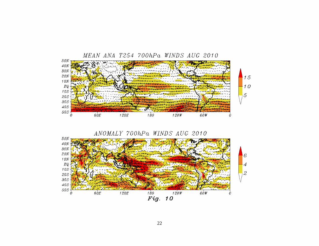
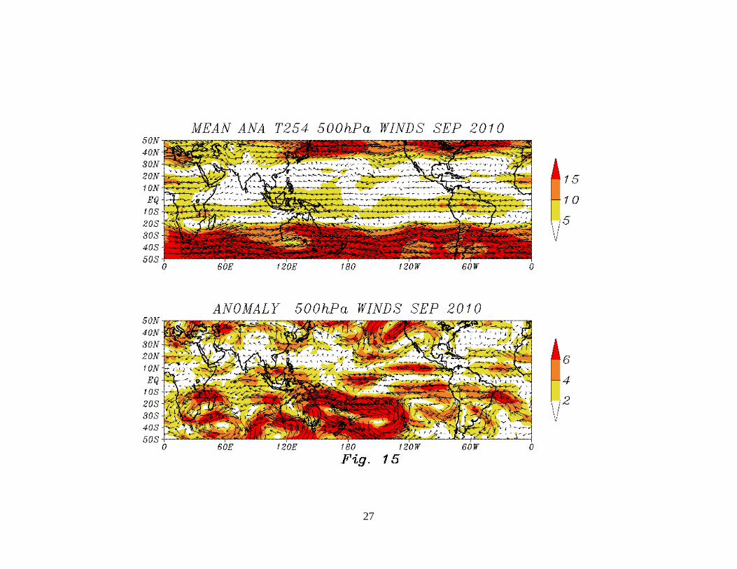
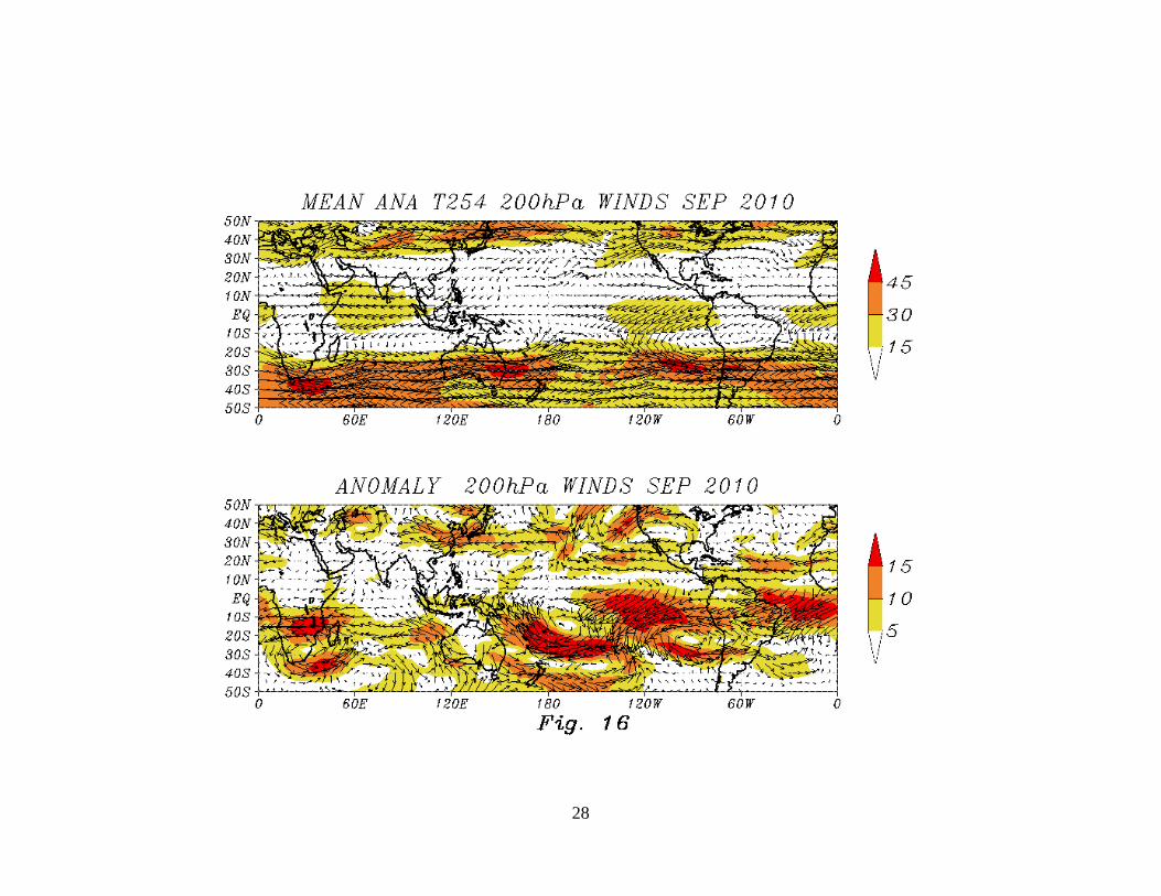
The geographical distribution of the mean analysed wind fields for the months of June,

July, August and September at 850, 700, 500 and 200hPa from the T254L64 GFS and their

monthly anomalies are shown in Fig. 1(a-b) to Fig. 16(a-b) respectively. The anomalous

features identified from the mean circulation of each month of monsoon-2010 are listed

below.

2.1 June

At 850 and 700 hPa levels, anomalous easterlies were seen over the peninsula and

adjoining Arabian Sea. Anomalous westerlies prevailed over the northern plains in the lower

levels, indicating weak monsoon conditions. This anomalous circulation feature was

associated with the prolonged hiatus in the advancement of monsoon over India during the

third and fourth weeks of June. At 500 hPa level, anomalous easterlies were seen over the

peninsula and an anomalous cyclonic circulation was seen over the northwestern parts of

India. At 200 hPa level, an anomalous cyclonic circulation was seen over the northern parts of

India

11

2.2 July In the lower tropospheric levels (850 - 500hPa ) anomalous easterlies were seen over the

northern parts of India, indicating active monsoon conditions. At 850 and 700 hPa levels,

anomalous south-easterlies and southerlies were seen over peninsula and Arabian Sea. At 200

hPa level, anomalous westerlies were seen over the southern peninsular India, indicating that

the Tropical Easterly Jet was weaker than normal.

2.3 August In the lower tropospheric levels (850 and 700hPa) anomalous easterlies were seen over the

entire country. Anomalous southerlies were also seen over the Arabian Sea in the lower

tropospheric levels. At 200 hPa level, anomalous westerlies were seen over the southern

peninsular India.

2.4 September In the lower tropospheric levels (850 and 700hPa ) anomalous southerlies were seen over the

Arabian Sea and adjoining north-western parts of the country. At 500 and 200 hPa levels an

anomalous cyclonic circulation was seen over the regions adjoining the north-western parts of

India. The rainfall activity was considerably above normal over the north-west homogeneous

region of India. At 200 hPa level, anomalous westerlies were seen over the peninsular India

12

Legends for figures: Figure 1: Geographical distribution of mean wind field (a) and anomaly (b) at 850hPa; for

June 2010. The anomalies are departures from the 1979–95 base period monthly means of

NCEP reanalysis. [Units: m/s, Contour interval: 5m/s for analyses and 3m/s for anomalies ]

Figure 2: Same as in Figure 1, but for 700hPa. Figure 3: Same as in Figure 1, but for 500hPa. Figure 4: Same as in Figure 1, but for 200hPa. [Units: m/s, Contour interval: 10m/s for analyses and 5m/s for anomalies ] Figure 5: Same as in Figure 1, but for July 2010. Figure 6: Same as in Figure 2, but for July 2010. Figure 7: Same as in Figure 3, but for July 2010. Figure 8: Same as in Figure 4, but for July 2010. Figure 9: Same as in Figure 1, but for August 2010. Figure 10: Same as in Figure 2, but for August 2010. Figure 11: Same as in Figure 3, but for August 2010. Figure 12: Same as in Figure 4, but for August 2010. Figure 13: Same as in Figure 1, but for September 2010. Figure 14: Same as in Figure 2, but for September 2010. Figure 15: Same as in Figure 3, but for September 2010. Figure 16: Same as in Figure 4, but for September 2010.

13

14

15

16

17

18

19

20

21

22

23

24

25

26

27

28

29

3 (a). Systematic Errors in the Medium Range Prediction of the Summer Monsoon

G. R. Iyengar

1 Introduction

The nature and distribution of systematic errors seen in the NCMRWF global

T254L64 and T382L64 model forecasts are discussed in this chapter using the seasonal

(June-September) means of analyses and medium range (Day-1 through Day-5) forecasts.

2 Circulation Features:

Geographical distribution of the mean analysed wind field and the systematic

forecast errors for the T254 and T832 model at 850hPa, 700hPa, 500hPa and 200hPa are

shown in figures 1(a-d) - 4(a-d) and 11(a-d) - 14(a-d) respectively.

The notable features seen in the systematic errors of the 850hPa flow pattern of

the T254 model are the anomalous southerlies over eastern parts of India and an anti-

cyclonic circulation is seen over the Bay of Bengal. This feature is also seen at 700hPa

level. Anomalous south-westerlies and a cyclonic circulation is also seen over the north-

west parts of India and adjoining areas at 850hPa level. A westerly bias is seen over

Central India extending to Southeast Asia. An easterly bias is seen over the central and

eastern equatorial Indian Ocean region. An anomalous cyclonic circulation is also seen

over the extreme southern peninsula and adjoining Arabian Sea. This feature is also seen

at 700 and 500hPa levels. At 200hPa, the most significant feature in the systematic errors

is the reduction of the return flow into the southern hemisphere. The T382 model

forecasts show an increased magnitude of the anomalous south-westerlies over the north-

west parts of India and adjoining areas at 850hPa level. However the magnitude of the

easterly bias seen over the central and eastern equatorial Indian Ocean region in the lower

levels is comparatively less in the T382 model forecasts. The reduction of the return flow

into the southern hemisphere is also comparatively less in the T382 model forecasts.

30

The strong crossequatorial low level jet stream with its core around 850 hPa is

found to have large intraseasonal variability. Figures 5 and 15 show the Hovmoller

diagram of zonal wind (U) of 850 hPa averaged over the longitude band 60–70E for the

period 1 June–30 September 2010 for the T254 and T382 models respectively. The top

panel in each figure shows the analysis and the middle and the lower panel depict the

Day3 and Day5 forecasts respectively. The active monsoon spells are characterized by

strong cores of zonal wind. The monsoon had set in over Kerala on 31st May. Subsequent

advancement of the monsoon across west coast was delayed by about one week due to

the formation of a very severe cyclonic Storm (PHET, 31st May–2nd June). Thereafter,

the monsoon covered nearly half of the country by the middle of June. There was a

prolonged hiatus in the advancement of monsoon till the end of June due to weakening of

monsoon current. The southwest monsoon covered the entire country by 6th July. As seen

from the analysis panel of the Fig 5 the zonal wind flow was quite weak during most

parts of June and in the first fortnight of July. The low level westerly flow picked up

strength with a core of zonal wind of about 20 m/s in the second fortnight of July and

remained so till the end of the month. This was followed by a spell of weak core of zonal

wind for a period of two weeks. Another spell of strong core of zonal wind of about 15

m/s was seen in the first fortnight of September. The Day3 and Day5 forecasts of the

T254 model agree reasonably well with the analysis and are able to depict the active and

weak spells of the monsoon flow. However the wind strength is weaker (stronger) during

the active (weak) spells in the Day5 forecasts. The T382 analyses and forecasts show

similar features The active spell in the first fortnight of September is better predicted in

the T382 model.

Figures 6 and 16 show the Hovmoller diagram of zonal wind (U) of 850 hPa

averaged over the longitude band 75–80E for the period 1 June–30 September 2010 for

the T254 and T382 models respectively. The top panel in each figure shows the analysis

and the middle and the lower panel depict the Day3 and Day5 forecasts respectively.

Both the T254 and T382 analyses show a prominent northward movement of the core of

zonal wind during the second fortnight of July. Two weak spells are seen in the second

and third weak of June and from the fourth week of August to the second week of

September. The Day3 forecasts compare well with the analysis. However, the Day5

31

forecasts are not able to depict the northward movement of the core of zonal wind as seen

in the analysis. The T382 model forecasts depict this feature comparatively better than

the T254 model.

3 Temperature:

Geographical distribution of the mean systematic forecast temperature errors for

the T254 (T382) models at 850hPa and 200hPa level are shown in figures 7 (17) and 8

(18) respectively. The T254 model forecasts show a warm bias in the lower troposphere

over the northwest parts of India and adjoining regions which is less as compared to the

T382 model. In the upper troposphere, the T254 model also shows a cold bias over the

northern parts of India. The magnitude of the cold bias is much less in the T382 model.

4 Humidity:

Geographical distribution of the mean systematic forecast specific humidity errors

for the T254 and T382 models at 850hPa level are shown in figures 9 and 19 respectively

The T254 and T382 model forecasts show a dry bias over the entire country, with the

magnitude of the bias being comparatively more in the latter.

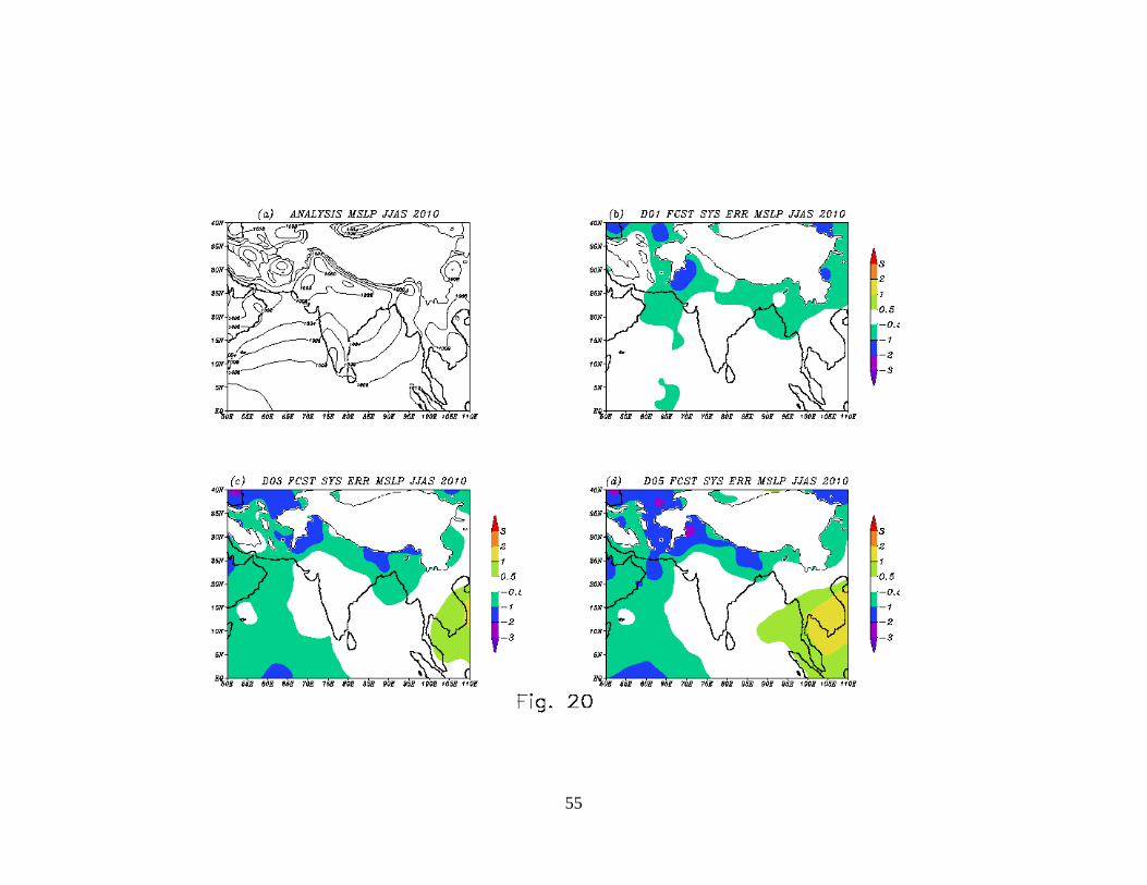
5 Mean Sea Level Pressure

Geographical distribution of the mean systematic forecast mean sea level pressure

errors for the T254 and T382 models at 850hPa level are shown in figures 10 and 20

respectively. The T382 model forecasts show an intensification of the heat low as

compared to the analyses. The T382 model forecasts also show a reduction in MSLP over

the northern plains.The bias in T382 model forecasts is comparatively more as compared

to the T254 model forecasts.

6. Verification of wind and temperature forecasts against analyses:

The RMSE of zonal wind, meridional wind and temperature at 850 and 200Pa

levels of Day1, Day3 and Day5 forecasts from T254 and T382 models for each day have

32

been computed for the Indian domain of 5-38 N and 68-94 E against their respective

analyses. Table 1 gives the average RMSE values corresponding for the season as a

whole. The T382 model forecasts feature relatively smaller RMSE as compared to the

T254 model.

7. Verification scores for wind and temperature against observations over India

Objective verification scores for the T254 and T382 model forecasts of winds and

temperature against the observations valid for 00UTC at standard pressure levels (850

and 250 hPa levels) as recommended by the WMO were computed for the Indian region

for the monsoon season of 2010.

Table 2 gives the average RMSE values corresponding for the season as a whole. The

T382 model forecasts show marginally smaller RMSE for both winds and temperature at

both 850 and 250 hPa levels

33

Legends for figures: Figure 1. Mean T254 analysed wind field (a) and systematic forecast errors for Day-1 (b), Day-3 (c) and Day-5 (d) at 850 hPa. [Units: m/s, Contour interval: 5m/s for analyses and 2m/s for forecast errors] Figure 2. Mean T254 analysed wind field (a) and systematic forecast errors for Day-1 (b), Day-3 (c) and Day-5 (d) at 700 hPa. . [Units: m/s, Contour interval: 10m/s for analyses and 5m/s for forecast errors] Figure 3. Mean T254 analysed wind field (a) and systematic forecast errors for Day-1 (b), Day-3 (c) and Day-5 (d) at 500 hPa. [Units: m/s, Contour interval: 5m/s for analyses and 2m/s for forecast errors] Figure 4. Mean T254 analysed wind field (a) and systematic forecast errors for Day-1 (b), Day-3 (c) and Day-5 (d) at 200 hPa. . [Units: m/s, Contour interval: 10m/s for analyses and 5m/s for forecast errors] Figure 5. Hovmoller diagram of T254 analyses and forecast zonal wind (U) of 850 hPa averaged over the longitude band 60–70E and smoothed by a 5-day moving average for the period 1 June–30 September 2009. Figure 6. Hovmoller diagram of T254 analyses and forecast zonal wind (U) of 850 hPa averaged over the longitude band 75–80E and smoothed by a 5-day moving average for the period 1 June–30 September 2009. Figure 7. Mean T254 analysed temperature field (a) and systematic forecast errors for Day-1 (b), Day-3(c) and Day-5 (d) of temperature at 850 hPa.: [Units: K, Contour interval: 2 K for analyses and 1 K for forecast errors] Figure 8. Mean T254 analysed temperature field (a) and systematic forecast errors for Day-1 (b), Day-3(c) and Day-5 (d) of temperature at 200 hPa.: [Units: K, Contour interval: 2 K for analyses and 1 K for forecast errors] Figure 9. Mean T254 analysed specific humiduty field (a) and systematic forecast errors for Day-1 (b), Day-3(c) and Day-5 (d) of specific humidity at 850 hPa.: [Units: gm/kg, Contour interval: 2 for analyses and 1 for forecast errors] Figure 10. Mean T254 analysed MSLP field (a) and systematic forecast errors for Day-1 (b), Day-3(c) and Day-5 (d) of MSLP: [Units: hPa, Contour interval: 2 for analyses and 1 for forecast errors] Figure 11. Mean T382 analysed wind field (a) and systematic forecast errors for Day-1 (b), Day-3 (c) and Day-5 (d) at 850 hPa. [Units: m/s, Contour interval: 5m/s for analyses and 2m/s for forecast errors] Figure 12. Mean T382 analysed wind field (a) and systematic forecast errors for Day-1 (b), Day-3 (c) and Day-5 (d) at 700 hPa. . [Units: m/s, Contour interval: 10m/s for analyses and 5m/s for forecast errors]

34

Figure 13. Mean T382 analysed wind field (a) and systematic forecast errors for Day-1 (b), Day-3 (c) and Day-5 (d) at 500 hPa. [Units: m/s, Contour interval: 5m/s for analyses and 2m/s for forecast errors] Figure 14. Mean T382 analysed wind field (a) and systematic forecast errors for Day-1 (b), Day-3 (c) and Day-5 (d) at 200 hPa. . [Units: m/s, Contour interval: 10m/s for analyses and 5m/s for forecast errors] Figure 15. Hovmoller diagram of T382 analyses and forecast zonal wind (U) of 850 hPa averaged over the longitude band 60–70E and smoothed by a 5-day moving average for the period 1 June–30 September 2009. Figure 16. Hovmoller diagram of T382 analyses and forecast zonal wind (U) of 850 hPa averaged over the longitude band 75–80E and smoothed by a 5-day moving average for the period 1 June–30 September 2009. Figure 17. Mean T382 analysed temperature field (a) and systematic forecast errors for Day-1 (b), Day-3(c) and Day-5 (d) of temperature at 850 hPa.: [Units: K, Contour interval: 2 K for analyses and 1 K for forecast errors] Figure 18. Mean T382 analysed temperature field (a) and systematic forecast errors for Day-1 (b), Day-3(c) and Day-5 (d) of temperature at 200 hPa.: [Units: K, Contour interval: 2 K for analyses and 1 K for forecast errors] Figure 19. Mean T382 analysed specific humiduty field (a) and systematic forecast errors for Day-1 (b), Day-3(c) and Day-5 (d) of specific humidity at 850 hPa.: [Units: gm/kg, Contour interval: 2 for analyses and 1 for forecast errors] Figure 20. Mean T382 analysed MSLP field (a) and systematic forecast errors for Day-1 (b), Day-3(c) and Day-5 (d) of MSLP: [Units: hPa, Contour interval: 2 for analyses and 1 for forecast errors]

35

Table 1: Day1-Day5 Root Mean Square Error (RMSE) of Wind(Zonal, Meridional) and Temperature over the Indian region (68-94E,5-38N) of T254 and T382 models

T382 Day1 Day2 Day3 Day4 Day5 850hPa 200hPa 850hPa 200hPa 850hPa 200hPa 850hPa 200hPa 850hPa 200hPa

u(m/s) 2.8 4.2 2.6 5.3 3.9 5.8 4.2 6.1 4.6 6.5 v(m/s) 2.5 3.9 3.0 4.6 3.3 4.9 3.5 5.4 3.7 5.7 Temp(0K) 0.7 0.6 0.8 0.8 0.9 0.9 1.0 1.0 1.1 1.1

T254 Day1 Day2 Day3 Day4 Day5 850hPa 200hPa 850hPa 200hPa 850hPa 200hPa 850hPa 200hPa 850hPa 200hPa

u(m/s) 2.9 4.6 3.6 5.45 4.0 5.8 4.4 6.2 4.8 6.6 v(m/s) 2.5 4.1 3.0 4.8 3.4 5.2 3.7 5.5 3.9 5.8 Temp(0K) 0.7 0.7 0.8 0.9 0.9 1.0 1.0 1.0 1.1 1.1

Table 2: Day1-Day5 Root Mean Square Error (RMSE) of Wind and Temperature against observations over India of T254 and T382 models

T254 Day1 Day3 Day5

850hPa 250hPa 850hPa 250hPa 850hPa 250hPa

Wind(m/s) 5.08 6.20 5.95 6.85 6.63 7.20

Temp(0K) 1.93 3.18 1.97 3.22 2.02 3.22

T382 Day1 Day3 Day5

850hPa 250hPa 850hPa 250hPa 850hPa 250hPa

Wind(m/s) 5.11 6.06 5.88 6.69 6.51 7.22

Temp(0K) 1.92 3.14 1.97 3.10 2.00 3.10

36

37

38

39

40

41

42

43

44

45

46

47

48

49

50

51

52

53

54

55

56

3(b). Verification of Model Rainfall Forecasts

R. Ashrit, A. K. Mitra, G. R. Iyengar, Saji Mohandas and Manjusha Chourasia

For India as a whole, nearly 78% of the annual rainfall occurs during the summer

monsoon season. However, the rainfall in the monsoon season over the homogenous

southern peninsular of India contributes about 60% of the annual mean, and a significant

amount (nearly 40% of the annual) also occurs in the post monsoon season or the north-

east monsoon season. For annual as well as monsoon season rainfall, the three prominent

high rainfall belts due to orographic effects are: (i) along the west coast of India and (ii)

along north-east India and (iii) the foothills of the sub-Himalayan ranges. There is a

general decrease of rainfall from east to west in central India and along the Gangetic

plains. The rainfall over the arid regions of west Rajasthan, Saurashtra, and Kutch is less

than one-third of its magnitude over the Gangetic West Bengal in the east. The monsoon

season features intraseasonal variations in rainfall amount and distribution. These are

mainly dictated by the active and weak cycles in the monsoon and the Bay of Bengal low

pressure systems that move inland causing heavy rainfall over land regions.

1 Mean Monsoon Rainfall during JJAS 2010:

The models with high spatial resolution are expected to resolve the mesoscale

processes in monsoon flow and the high resolution orography to give better rainfall

prediction compared to the coarse resolution global models. In this section the

performance of the two models (T254L64 and T382L64) for medium range rainfall

forecasting has been examined during monsoon (JJAS) 2010. For a detailed and

quantitative rainfall forecast verification, the IMD's 0.5 degree daily rainfall analysis

(Rajeevan and Bhate 2008, Rajeevan et. al, 2005) is used. This is the high resolution

daily gridded rainfall data set suitable for the high resolution regional evaluation. The

daily rainfall data from the two models is gridded on to the observed rainfall grids over

Indian land regions for the 122 days from 1st June through 30th September 2010.

The panels in Figure 1 present observed and forecast mean rainfall (cm/day) for

JJAS obtained from the two models. The observed distribution of rainfall indicates the

highest rainfall of up to 2 cm/day along the west coast of India surrounded by rainfall in

57

the range of 1-2 cm/day. Similar rainfall amounts in the range of 1-2 cm/day can be

prominently seen over parts of North-east India, Gangetic plains and a large region

covering West Bengal and Orissa. Over the west coast the day-1 forecasts show mean

rainfall in excess of 2 cm/day at many locations surrounded by rainfall in the range on 1-

2 cm/day. However, in the day-3 and day-5 forecasts the west coast features reduced

rainfall amounts. Over the north east India, forecasts show high rainfall amounts

comparable to the observations. The day-3 forecasts of both models show reduced

rainfall amounts compared to day-1 forecasts particularly over eastern India (Orissa and

surrounding areas). Over the Gangetic plains both models is over estimated rainfall

particularly in Day-5 forecasts.

2 Rainfall Forecast Verification:

A detailed and quantitative rainfall forecast verification is presented in this section

using the IMD's 0.5 degree daily rainfall data (Rajeevan and Bhate 2008) for the entire

period of JJAS 2010. Table 1 shows the contingency table for categorical forecasts of a

binary event using which the following statistics are computed. The computations take

into account only the rainy days i.e., days with rainfall >= 0.5 cm at each grid point over

land regions. The rainfall forecast verification is expressed in terms of three different

scores discussed below.

2.1 Mean Error: The difference between the observed and forecast mean rainfall (Figure

2) is presented to bring out the areas of overestimated and underestimated rainfall over

India. Models consistently overestimate the rainfall over the Gangetic plains. Rainfall

over the dry regions of NW India is under predicted in all the forecasts. Due to reduced

rainfall amounts over eastern India as well as Gangetic plains in the day-3 forecasts of

both models, the mean error over these two regions is lower compared to the day1 and

day-5 forecasts. In general both T254 and T382 show similar pattern and magnitude of

mean error.

2.2 Equitable threat score (Gilbert skill score)-

58

where

This is a standard skill score that is being used by various weather services to

evaluate their precipitation forecasts. It is frequently used to assess skill of rainfall

forecasts above certain predefined thresholds of intensity of rain.

2.3 False Alarm Ratio

ETS tells us how well

did the forecast "yes" events correspond to the observed "yes" events (accounting for hits

due to chance)? ETS ranges from -1/3 to 1, 0 indicates no skill and 1 meaning perfect

score. Figure 3 shows the ETS computed on the forecast rainfall from both the models.

Both models T254 and T382 show very similar pattern of skill in day-1, day-3 and day-5

forecasts. The gray shading in the plots indicates no skill. Large parts of peninsula shows

no skill and this is true in all the forecasts. Day-1 and day-3 forecasts of both models over

the central India including NW India show skill in predicting the rainy day. Similar

computations for different rainfall threshold is shown in Figure 4. For lower thresholds

(0.0, 0.1 and 0.6) the scores are high in the two models and there is no clear and

consistent higher skill for any model. For higher rainfall amounts, the scores are low. For

higher rainfall thresholds (>9cm/day) the ETS values are very small and the number of

occurrences are also very low. For some of the intermediate thresholds, the T382 model

forecasts show marginally higher skill compared to the T254 model forecasts.

False Alarm ratio (FAR) is a measure of fraction of the predicted "yes" events that

actually did not occur (i.e., were false alarms). This score ranges from 0 to 1 and a score

of 0 implies perfect forecast. This score is sensitive to false alarms, but ignores misses.

Figure 5 shows the FAR computed for the forecast rainfall for both the models. Both the

models indicate higher forecast skill (lower FAR) along the west coast, north-eastern

59

states and along the foothills of Himalayas. Both the models show very similar patterns

over dry regions with higher FAR values over the northwestern region and south-eastern

tip of the peninsula.

3 All India Rainfall Verification:

The all India rainfall (AIR) variability from model (compared to observations) in

time scales like daily, weekly, monthly and also in a season are useful model diagnostics,

which depicts important aspects of the model skill to capture the monsoon over the Indian

region in a broad sense. Several forecasters at IMD also seek (monitor) this AIR figures

from the model to infer about the monsoon strength in medium range time-scale. We now

examine the variability of AIR from observations and models. Figures (6-7) show the All

India daily rainfall in millimeters for JJAS 2010, Seasonal rainfall, Monthly rainfall and

weekly rainfall predicted by T254L64 model and figures (8-9), the corresponding charts

as predicted by T382L64 model, against the observed rainfall provided by India

Meteorological Department (IMD). The seasonal, monthly and weekly rainfall figures

also show the long period averages (Climatology) and the weekly rainfall is the 7 days

prediction from the single initial condition every week. Day-1 and Day-3 forecasts are

much similar to the observations for both T254L64 and T382L64 models and there are

only very minor differences between the models. However in the case of Day-5 forecasts,

there is a marginal improvement in T382L64 with the intraseasonal variability better

reflected by T382L64 model. The rainfall amount is over predicted by both models in

Day-1. This is better observed in the seasonal total rainfall bar diagrams with Day-5 also

slightly over predicting and Day-3 more comparable to the observed in both models.

However, when compared between T254L64 and T382L64 systems the Day-3 rainfall is

clearly closer to the observed for T382L64 compared to T254L64 model.

The monthly rainfall values suggest that July rainfall is highest followed by

August, September and June, This variability is more or less reflected by the model

predictions but show differences in the case of different forecast lead periods. For August

and September months, generally there is more over prediction compared to the first two

months. For a lead time of 3 days the predictions by T382L64 model is marginally better

60

than T254L64 model. In the weekly rainfall figures, the curves of observed and predicted

weekly rainfall more or less coincide except for some divergences during August and

September and the difference in the initial week for T254L64. T382L64 does not show

the large rainfall in the first week of June and is marginally better compared to T254L64

during the rest of the period in predicting the intraseasonal variability. These weekly

forecasts are made from a single initial condition once a week. The trends in AIR rainfall

(changes from one week to the next during the progression of season) from global model

matches well with the observed trend. However, there are some biases in values during

few weeks which are obvious and consistent with the skills examined in daily scores for

all India region.

4 Conclusions:

The observed distribution of JJAS mean rainfall indicates a highest rainfall of up to 2

cm/day along the west coast of India surrounded by rainfall in the range of 1-2

cm/day. Similar rainfall amounts in the range of 1-2 cm/day can be prominently seen

over parts of North-east India, Gangetic plains and a large region covering West

Bengal and Orissa. Over the west coast and parts of north-eastern India the model

forecasts show mean rainfall in excess of 2 cm/day surrounded by rainfall in the range

on 1-2 cm/day. The forecasts clearly overestimate the observed rainfall over these two

regions. Clearly the rainfall over the Gangetic plains is over estimated in both the

models particularly in Day-5 forecasts. However, this overestimation is subdued in the

day-3 forecasts.

While the dry conditions of June are well captured in all forecasts of all models, the

wet conditions (particularly Gangetic plains) of July, August and September are

overestimated in all the forecasts.

Both the models indicate higher forecast skill along the west coast, north-eastern states

and along the foothills of Himalayas. Both the models show very similar patterns over

dry regions with higher FAR values over the northwestern region and south-eastern tip

of the peninsula.

For all India rainfall, the higher resolution T382 system is marginally better compared

to coarse resolution T254 system.

61

Table 1. Contingency table for categorical forecasts of a binary event. Event Forecasts

Event Observed Yes No

Yes hit false alarm No miss correct rejection

Figure 1. Observed and forecast mean rainfall during JJAS 2010.

62

Figure 2. Mean error in the forecast rainfall during JJAS 2010.

Figure 3. Equitable Threat Score for forecast of rainy day during JJAS 2010.

63

Figure 4. Equitable Threat Score for predicted rainfall exceeding different thresholds.

Figure 5. False Alarm ratio for forecast of rainy day during JJAS 2010

64

Fig. 6 All India daily rainfall (mm) for JJAS 2010; (a) observed (b) Day-1 forecast (c) Day-3 forecast and (d) Day-5 forecast by T254L64 model.

Fig. 7 Seasonal (a), Monthly (b) and weekly (c) rainfall (mm) predicted by T254L64 model for Monsoon-2010 against observed and long period average (climatology). Weekly rainfall is accumulated 7-day forecast from single initial conditions of every week.

65

Fig. 8 All India daily rainfall (mm) for JJAS 2010; (a) observed (b) Day-1 forecast (c) Day-3 forecast and (d) Day-5 forecast by T382L64 model.

Fig. 9 Seasonal (a), Monthly (b) and weekly (c) rainfall (mm) predicted by T382L64 model for Monsoon-2010 against observed and long period average (climatology). Weekly rainfall is accumulated 7-day forecast from single initial conditions of every week.

4a. Onset and Advancement of MonsoonM. Das Gupta

Introduction:  

Southwest monsoon activity of  2010 over Indian region was  normal and  rainfall

received was  102% of its long period average (LPA) during June to September .  During

monsoon 2010, the onset over Kerala was declared on 31st May (one day prior to normal

date   is   1st  June)   by   India   Meteorological   Department(IMD).     There   after   rapid

advancement of southwest monsoon was seen and half of the country covered by middle

of June. Then there was a hiatus in the advance of the monsoon during 19th  to 30th June

with resulting rainfall  only 84% of LPA in June 2010. Rainfall  activity  subsequently

increased in first week of July and monsoon covered the entire country by 6th of July . 

The onset of Monsoon is recognized as a rapid, substantial and sustained increase

in rainfall over land. However significant transitions of tropospheric circulation pattern,

humidity and temperature fields are also observed.   An objective method for predicting

monsoon onset,  advancement and withdrawal date using dynamic and thermodynamic

precursors from NCMRWF T80L18 analysis­forecast system was developed (Ramesh et

al.  1996,  Swati  et  al.  1999.)  and used since 1995 at NCMRWF. The same has been

extended for NCMRWF T254L64 analysis­forecast system  during monsoon 2008 (Das

Gupta and Mitra, 2009) and subsequently to T382L64 system in 2010. The onset and

advancement   of   monsoon,   based   on   the   above   mentioned   objective   method   from

NCMRWF T382L64 and  T254L64 analysis­forecast system during monsoon 2010 will

be discussed here. 

66

1. Onset over Bay of Bengal:

The   advancement   summer   monsoon   over   southwest   Bay   of   Bengal   (BOB)

normally takes place prior to that over Arabian Sea (ARB) around 2nd­3rd week of May.

The evolution of monsoon onset was monitored routinely from the first week of May  by

monitoring the daily variations of the analysed and predicted value of 850 hPa kinetic

energy(KE), net tropospheric (1000hPa­300hPa) moisture (NTM) and mean tropospheric

(1000hPa­100hPa)   temperature   (MTT)  computed  over  BOB(0°N ­19.5°N,78°E­96°E).

Figure 1   depict the daily variations of KE, NTM and MTT over BOB form 1st May to

21st  June 2010 for 0000UTC T254L64 analysis (black line) and subsequent day­1(24hr.)

to day­7(168 hr.) predictions respectively.  As daily run of T382L64  at NCMRWF was

started from 21st May ,  the plot corresponding  to onset over BOB for T382L64 was not

shown here. As seen from the plots the substantial increase in KE was seen on 17th May,

associated with   formation of tropical cyclone Laila. IMD also declared the onset over

BOB on 17th May.

67

68

Fig.1    Daily variation of (a) Kinetic energy, (b) Net Tropospheric Moisture and   (c)Mean Tropospheric Temperature over Bay of Bengal  as simulated inT254L64 system during 1st May­21st June 2010

2.   Onset over Kerala (Arabian Sea Branch):

The Arabian Sea branch of monsoon generally first hits the Western Ghats of the

coastal state of Kerala around 1st June with standard deviation of 8 days. Figure 2 depicts

the daily variations of analysed and predicted KE at 850 hPa, NTM and MTT computed

over Arabian Sea (ARB) (0­19.5° N; 55.5°E­75°E) from 25th May 2010 onwards.  

As seen from the plot that though KE was more than the threshold value 60m2s­2

around 1st   June but  NTM was below 40 mm till 12th June.  IMD declared the monsoon

69

Fig.2    Daily variation of (a) Kinetic energy, (b) Net Tropospheric Moisture and   (c)Mean Tropospheric Temperature over Bay Arabian Sea  as simulated inT254L64  and T382L64 system during 1st May­21st June 2010

onset over Kerala on 31st May, but NCMRWF predictions showed the onset over Kerala

on  12th  June   (T264L64)  and  14th  June   (T382L64)   respectively,  based  on  above   said

objective criterion.  

3.  Advancement of Monsoon:  

According to objective criteria the advancement of monsoon over main land of

India is determined by examining changes in NTM together with the flow characteristics

at 850hPa in analyses and subsequent predictions.  The criteria adopted for determining

the progress of monsoon over a particular location are as follows:  

(i) Steady increase of NTM under the influence of expected wind regime at 850 hPa

(ii) Sharp fall in the net moisture content and subsequent rise there after under the

influence of same wind regime 

(iii) Date for advancing the  northern  limit of monsoon over a location is fixed on the

day of   fall   in   the  net  moisture  content,  which   is  believed   to  be    utilized   for

producing   the   rainfall  associated  with   the  advancement  of  monsoon  over   that

region

For determining the advancement of monsoon over different locations over Indian

main   land,   NTM   MTT   and   wind   direction   and   speed   at   850hPa   in   analysis   and

predictions are examined over 43 locations over India. 

In 2010 the advancement of monsoon along the west coast was seen during 1st to

15th  June. After that there was a prolonged hiatus period until 31st  June and thereafter

rapid advancement was seen over Gangetic plane, covering whole country within 6 days

i.e. by 6th July.  Figure 3 depicts the same for Mumbai during 31st May to 22nd June 2010

both for T254L64 and T382L64 system. As seen from the plot, the first occurrence of70

south­westerly  winds  are   seen  around 5th  June  and at   the  same  time  NTM was  also

showing an increasing trend. But by that time the monsoon was not covered the southern

part of west coast. Around 10th  June   wind regime   changed form westerly to   easterly

over Mumbai   indicating presence of   cyclonic vorticity   around 10th June.   During this

period NTM was also increasing and shown sudden  fall on 11th June both for T254L64

and T382L64. So according to objective criterion 11th June could be fixed as onset date

over   Mumbai   but   by   that   time   onset   over   Kerela   was   not   captured   in   NCMRWF

predictions. However, IMD declared onset over Mumbai on 11th June.

Since the advancement over Gangetic plane was very rapid during 2010 monsoon,

it was not possible to predict the onset over Gangetic plane and northern parts of country

using the objective criterion

71

Fig.3     Daily variation of (a) NTM, (b) Net MTT (c) Wind Speed at 850 hPa and (d)

Wind direction  at  Mumbai   (   IC:  31st  May­  22th  June  2010)  for  T254L64 and

T382L64 respectively 

 

4.  Summary:  

The objective  criteria   for  onset/progress of  monsoon was developed based on

analysis and forecast data from a coarser resolution global model (T80L/18) was tested

with data from a higher resolution global model (T254L64) for monsoon 2008. It was

concluded that the parameters related to the objective criteria of onset and progress of

monsoon   over   India   were   also   well   captured   by   analysis   and   the   medium   range

predictions from higher resolution model. But during 2009, it is seen that some of these72

features were not captured well by T254L64 system for southern peninsular stations.  In

2010 it  is seen that though onset over BOB was captured well but the onset of ARB

though captured but was delayed by almost two weeks. Advancement of monsoon over

land   was   also   not   captured   by   this   technique.   Mechanism   for   incorporating   rainfall

predictions from high resolution models, in the objective method could be explored in

future.  

References: 

Das   Gupta   M   2010:    Onset   and   Advancement   of   Monsoon,   “MONSOON­2008:

Performance   of   the   T254L64   Global   Assimilation   Forecast  System“,   Report   no.

NMRF/MR/01/2010, 131 pages, Published by NCMRWF (MoES), A­50 Institute Area,

Sector­ 62, NOIDA, UP, INDIA 201 307

Das Gupta M., A. K. Mitra 2009:   Onset and Advancement of Monsoon, “MONSOON­

2008: Performance of the T254L64 Global Assimilation Forecast  System“, Report no.

NMRF/MR/01/2009, 117 pages, Published by NCMRWF (MoES), A­50 Institute Area,

Sector­ 62, NOIDA, UP, INDIA 201 307

Ramesh,  K.J,  Swati  Basu,  and  Z.N.  Begum,  1996:  Objective  determination  of  onset,

Advancement and Withdrawal of the summer monsoon using large scale forecast fields

of a global spectral model over India, Meteor. and atmospheric Physics,61, 137­151. 

Swati Basu, K.J. Ramesh and Z.N. Begum,1999: Medium Range Prediction of summer

monsoon activities over India vis­avis their correspondence with observational features,

Adv. in Atmos. Sci.,16,1,133­146.

73

74

4(b). Monsoon Indices: Onset, Strength and Withdrawal

D. Rajan and G. R. Iyengar 1. Introduction:

The annual reversal of wind and rainfall regimes in monsoon is spectacular. An

objective manner of declaring the onset of the south west monsoon over Indian main land is

discussed in this chapter. Precipitation in India has clear seasonal variation and the onset of

the Indian summer monsoon is of great interest as not only a research target but also a socio-

economic factor for water resources in India. Due to distinct spatial features of monsoon and

the diverse ways of representing monsoon, it is difficult to derive 'universal index' to measure

the variability of the monsoon over all of Asia. The onset date of the monsoon has been

defined by various methods in past research studies.

The variability of the continental tropical convergence zone and the large-scale

monsoon rainfall is linked to the variability of convection over the equatorial Indian Ocean

and the surrounding seas ie Arabian Sea and the Bay of Bengal. The onset and withdrawal of

the broad scale Asian monsoon occur in many stages and represent significant transitions in

the large-scale atmospheric and ocean circulations (Fasullo and Webster 2003), which can be

examined by analyzing various monsoon indices. Useful indices provide a simple

characterization of the state of the monsoon during different epochs and also the inter-annual

variability. While there is no widely accepted definition of these monsoon transitions at the

surface, the onset is recognized as a rapid, substantial increase in rainfall within a large scale.

1(a). Background

In 1943 for the first time the India Meteorological Department (IMD) determined the

normal onset and withdrawal dates of summer monsoon with 180 rain-gauges stations across

British India (present India, Pakistan, Bangladesh, Myanmar and Sri-Lanka) from

'characteristic monsoon rise/fall in pentad rainfall', and prepared charts showing normal

onset and withdrawal dates across the Indian sub-continent.

The arrival of the summer monsoon over the Kerala coast is found to be reasonably

regular either towards the end of May or beginning of June (Ramesh et al. 1996; Prasad and

Hayashi 2005; Taniguchi and Koike 2006, Goswami and Gouda 2010). The monitoring and

forecasting of the summer monsoon onset over the Indian subcontinent is very important for

75

the guidelines for the operational forecaster reference. This migration and location of the heat

source associated with summer monsoon has important implications for the withdrawal of

monsoon over South Asia. Many studies show the declaration is best when the occurrence of

the onset withdrawal is abrupt and declaration is worst when it is feeble. However, to date

there has been no systematic investigation of the retreat of the monsoon system despite its key

contribution to total rainfall variability. But it is known that, in terms of rainfall, the onset is

better defined than the withdrawal. In this section of the report NCMRWF T254L64 &

T382L64 global analysis and forecast products have been used to compute various monsoon

indices to monitor onset, strength and the withdrawal of the monsoon during 2010 season.

2. Monsoon circulation indices for onset, strength and withdrawal:

Kerala state, situated in the southwest part of the Indian sub-continent is the gateway

for the Indian summer monsoon. Based on Kerala rainfall, the mean onset date occurs around

01 Jun and varies with a standard deviation of 8-9 days from year to year. Given the relatively

small scale of Kerala that is less than 200 km in breadth, sensitivity of the declaration of onset

based solely on the district’s rainfall (narrow area) only; but the monsoon transitions is also

likely to be large. In India at IMD the onset date is declared based on rainfall, wind,

temperature, moisture, cloud pattern, and the state of the sea, etc In addition to recently re-

determination of dates of onsets by taking rainfall data base from 1971- 2000 also taken place.

For a forecaster it is a difficult job to declare the date of onset because all the above

parameters are highly variable in space and time. It is difficult to quantify these parameters

precisely and so the experience of the forecaster plays a key role in declaring the date of

monsoon onset subjectively for individual years (Wang et al ., 2009).

The India Meteorological Department (IMD) has been using the qualitative method

over a long period using rainfall to declare the onset date for the monsoon forecast. As per

IMD’s daily weather bulletins for the year 2010, the southwest monsoon set in over Andaman

Sea around on 17 May, three days prior to its normal date in association with severe cyclonic

storm. As per the daily bulletins it set over Kerala on 31 May, about a day earlier than the

normal onset date.

Ramesh (1996) et al., suggested the following characteristics for the evolution of the

onset over the Arabian Sea covering the area of 0° – 19.5° N and 55.5°E – 75°E: (i) the net

tropospheric (1000 – 300 hPa) moisture build-up, (ii) the mean tropospheric (1000 – 100 hPa)

76

temperature increase, (iii) sharp rise of the kinetic energy at 850 hPa. It is read that the above

objective study most of the time computed the onset date delayed by few (8 -10) days than the

declared actual date. In the pervious section of this report, onset and progress have been

described with the above said criteria for monsoon 2010, which also shows onset over Kerala

around 10 Jun. As per that study this year also it is noted that the onset date is seen to be

around 10 Jun.

In this chapter four monsoon dynamical indices are computed using data from

NCMRWF high resolution T254L64 & T382L64 analyses and forecast systems. These widely

used monsoon dynamical indices of the South Asian summer monsoon are listed in the table

(I) with their corresponding brief definition. These monsoon indices are based on circulation

features associated with convection centers related with rainfall during the summer monsoon

for the Indian region.

In 1999 Goswami et al ., defined the index based on the meridional wind (V) shear

between 850 hPa and 200 hPa over the south Asian region 10°N – 30°N, 70°E – 110°E

which is related to the Hadley cell features. This index can be used to study the onset and

advancement phases of the monsoon.

Wang et al., (2001) introduced a dynamical index based on horizontal wind (U) shear

at 850 hPa called the circulation index. They recommend that the circulation index computed

with the mean difference of the zonal winds (U) between the two boxes; one for southern

region and the other for the northern region, i.e. 5°N – 15°N, 40°E – 80°E and 20°N – 30°N,

70°E – 90°E can be used as the criteria for identifying the onset date. The southern region box

is taken over South Arabian Sea and the northern region box is taken over northern land

region. This circulation index describes the variability of the low-level vorticity over the

Indian monsoon trough, thus realistically reflecting the large scale circulation. After that

Fasullo and Webster (2003) defined the onset date in terms of vertically integrated moisture

transport derived from reanalysis data sets. As per their discussions the inter-annual variation

in the onset date modestly agreed with reality.

Taniguchi and Koike (2006) first time emphasized the relationship between the Indian

monsoon onset and abrupt strengthening of low-level wind over the Arabian sea (7.5°N –

20°N, 62.5°E – 75°E). They have used three variables (i) vertically integrated water vapor (ii)

moisture transport (iii) low-level wind in an objective manner to determine the onset date.

This is a measure of the strength of the low-level jet over South Arabian Sea and indicates the

77

strength of the monsoon over India. They showed that Indian summer monsoon onset is

brought mainly by enhancement of low-level wind over the Arabian Sea.

Wang et al., (2009) found that the onset date can be objectively determined by

examining of the sustained 850 hPa zonal wind (U) averaged over the southern Arabian Sea

(5°N – 15°N, 40°E – 80°E). In the recent studies Wang et al., (2009) this criterion is referred

as objective circulation index. The rapid establishment of steady westerly is excellent

parameters to correlate with the abrupt commencement of the rainy season over the southern

tip of the Indian peninsula. In this index, the onset date is defined as a sustained zonal westerly

exceeding 6.2 m/s and persists for more than six days. This definition depends on large scale

circulation feature. This circulation index clearly omits the bogus onset or multiple onset

dates. The bogus or double/multiple monsoon onset develops when the strong convection in

the Bay of Bengal is accompanied by the monsoon like circulation and appears in the Indian

Ocean.

Syroka and Toumi (2002, 2004) also defined a similar type of circulation index by

taking the box slightly towards east of Wang’s (2001) case. However, to date there has been

no systematic investigation of the retreat of the monsoon system despite its key contribution to

total rainfall variability. A daily circulation index was defined as the difference in average 850

hPa zonal winds between a southern region 5°N – 15°N, 50°E –80°E and a northern region

20°N – 30°N, 60°E – 90°E. This daily circulation index is a physically sensible and practical

tool to study the withdrawal of the monsoon also. According to them the date of withdrawal of

the monsoon is defined as the first of seven consecutive days for which the index becomes

negative. This daily circulation index can be used to define both the dates of onset and

withdrawal of the Indian summer monsoon from these regions. The index changes sign,

reflecting both the changing intensity of the low-level westerly monsoon flow and the vorticity

associated with the monsoon trough and synoptic activity. The above index suggests that the

average date of withdrawal is 16 October with a standard deviation of 7 days. In this section

we have computed the above described computation for circulation indices based upon the

various definitions that are tabulated in table (I).

3. Results and discussions:

We use the daily NCMRWF high resolution NCEP version of T254L64 & T382L64

analyses and forecasts (up to 120 hrs) data sets for the period May to September 2010. Details

78

of the NCMRWF assimilation and forecast systems are described in chapter 1 of this report.

The IMD Climate Diagnostics Bulletin of India (2010) daily/seasonal reports have been

referred for the observation of rainfall, flow patterns, the dates for the declaration of onsets

monsoon strength and withdrawal etc during the entire period of this study.

Figures (1a1), (1a2) shows the objective circulation indices calculated by Wang et al .,

(2009) for the analyses and forecasts for the length of 24 hr, 72 hr and 120 hr. From these

figures it is seen that the apparent onset date (bogus onset) is noticed as 31 May, by the

sustained westerly (U) exceeding 6.2 m/sec and could not persist for more than four days i.e.

up to 04 Jun. This high value of U did persist beyond 05 Jun also; up-course there was a slight

less westerly have been noticed during 03 - 05 Jun. From these figures T254L64 & T382L64

it is seen that the actual onset date is noticed around 05 Jun, by the sustained westerly (U)

exceeding 6.2 m/sec and persisting for more than six days. Hence it is appropriate to say that

the real dynamical onset occurred on 05 Jun only. The bogus onset date 31 May can be

omitted safely by saying these monsoon onset criteria. In the predicted indices also broadly

these features are captured well. Although in the 72 hr and 120 hr forecasts able to capture

the transition of the onset. The bogus onset occurred on 31 May over Kerala coast is clearly

due to the system association with the very severe cyclonic storm called 'PHET' over the

Arabian Sea whose life history was 31 May - 02 Jun. In this case cooler air is brought by the

strong winds having intensity more than 6.2 m/sec at 850 hPa around the vicinity of the

cyclone over the Arabian Sea. The above theory has been brought out clearly by Taniguchi et

al., (2010).

Figures (1b1) and (1b2) show the circulation indices calculated by Syroka and Toumi

(2002, 2004) for the onset phase. From these figures of T254L64 & T382L64 we infer that the

onset date around 03 -05 Jun 2010, because on that day onwards the daily index is changing

it's sign from negative to positive and maintained there after. In this case also the bogus onset

seen around 28-30 May; as daily index is changing its sign from negative to positive but not

maintained thereafter. The analyses and the 24 hr forecasts, 72hr forecasts, 120hr forecasts of

both the resolutions show the change of sign, but with a lag of few days. Syroka and Toumi

index also shown that 28- 30 May is not the actual date of onset over Kerala during this year

2010.

Figures (1c1) & (1c2) show the circulation indices/vertical shear suggested by

Goswami et al., (1999) for the onset phase. This is popularly known as Goswami Hadley cell

79

circulation index. From these figures we infer that the onset date is seen around 03 - 05 Jun

only but not on the day 31 May, because on that day onwards the daily index is changing its

sign from negative to positive and maintained the positive sign there after. The analyses and

the 24 hr forecasts, 72 hr forecasts, 120 hr forecasts of both the resolutions are having the

same trend and are able to capture the change of sign from negative to positive with a lag of 2-

3 days. Among the resolutions the T254 have clear representation than T382 in this regard.

Figures (2a1), (2a2) and (2a3) show the Wang (2001) circulation index for the 122

days of the monsoon 2010. From the IMD source it is seen that in association with monsoon

onset the advance of monsoon over the northeastern states including West Bengal & Sikkim

occurred earlier than normal. This year it is observed that the advance of monsoon over the

northeastern states was earlier than normal. A prolonged hiatus in the advance of monsoon

occurred during 19 – 30 Jun, which is clearly seen in the figures having circulation index

about 5 m/sec only.

The further advance of monsoon occurred in association with the formation of a low

pressure area over the North Bay of Bengal and neighborhood on 02 Jul. The monsoon

covered most parts of the country except Rajasthan, on 05 Jul 2010. A prolonged hiatus

occurred during 10 - 20 Jul which is clearly reflected in the index curve having minimum

westerly strength as measured by Wang & Ding circulation indices.

On daily scale, rainfall for the country as a whole was generally normal to above

normal on most of the days during the season, except for some days, during the end of June,

middle of July, first week of August and last week of September. The seasonal rainfall was

above normal over most parts of the country except parts of northeastern/eastern and adjoining

central region and parts of Kerala. The above period can be very well correlated with the dates

as seen from the figures (2a1), (2a2) and (2a3) as well.

As per observation, apart from the cyclonic storm ‘PHET’, fourteen low pressure

areas (2 in the month of June and 4 each in July, August and September) were also formed

during the season. Of these, 12 low pressure areas formed over the Bay of Bengal. These low

pressure areas persisted for 4 to 5 days and generally moved Westward rabidly from Bay of

Bengal to western parts of the country and dissipated over the central/northern region. These

low pressure areas caused good amount of rainfall over the concerned region.

As shown in the figure (2a3) there are more than six peaks with the strength of more

than 10 m/sec wind speed, which can be correlated with the peaks rainfall observed Figure (2

80

b) during this season with some time lag. The break monsoon conditions also prevailed over

the country during the middle of July. It has affected the rainfall (- 0.39 %) over the central

and South peninsular India during July. The cross equatorial flow was weaker than normal

during major parts of the season except for a brief period from last week of June to third week

of July; which can be correlated with the rainfall observation shown in figure (2b).

The weak cross equatorial flow prevailed during most parts of June and in the first

fortnight of July. Two low pressure areas formed in June over the northwest Bay of Bengal

and neighborhood, one during the period 9-13 Jun and the other during 24-26 Jun. The first

one dissipated in-situ and the other one was short lived and dissipated over Gangetic west

Bengal and neighborhood. The observed rainfall during 21-27 Jun indicated very large

negative anomaly in rainfall.

In the year 2010 the less amount of rainfall distribution was mainly due to the break

monsoon condition that developed during 12 – 20 September, which can be easily correlated

with the circulation index shown in figures (2a1, 2a2, 2a3).

The figures (3a1) and (3a2) show the wind circulation index as per Syroka & Toumi

(2002) for the period of August – September 2010. From the IMD's climate diagnostics

bulletin of India (2010) it is seen that in there was delay in the withdrawal of southwest

monsoon due to rainfall activity over north India in associated with mid latitude westerly

activities. In this year 2010 there is considerable delay in the withdrawal of southwest

monsoon from west Rajasthan. This delay is due to the prevalence of moisture in the lower

levels and favorable conditions for rainfall created by the presence of mid-latitude westerlies

in the upper levels over the north western parts of the country.

From the figure it is seen that the circulation index values reduced sharply but it does

not changes its positive slope to negative (dip) up to the date 27 September. So the

withdrawal date can not be consider as the above date. From 22 – 30 September the index

curve is near to the vicinity of the axis. It is clear that the intensity gets the minimum value

around the 22 and 30 of September. Hence 27 September can be taken as withdrawal date of

the southwest monsoon 2010. This date can be commented as the real withdrawal date. Thus

the withdrawal of monsoon from west Rajasthan started only on 27- 28 September which is

delay of more than 2 weeks time from the normal date (1 September), of withdrawal from

extreme western parts of Rajasthan. In the second occasion circulation index changes its slope

from positive to negative on 27 -28 September onwards; subsequently it persists for more than

81

5 days. This increase in the circulation index brought rainfall to the country as shown in the

figure (2b). Thus the day 27 September can be regarded as the withdrawal date of southwest

monsoon for the year 2010. When we consider the IMD official information on withdrawal

dates it is closer to 27 September as seen in the above systems with the resolutions T254 &

T382. It is reported that the withdrawal started on 27-28 September over the Rajasthan. In

reality also the southwest monsoon withdrew from the entire country on 29 October 2010

(figure not shown).

4. Summary:

Several popular monsoon indices have been used to study the onset, strength and

withdrawal of monsoon during 2010 season. In general, the indices are able to represent the

onset, variability in strength of monsoon and the withdrawal in a reasonable way. This year

bogus onset occurred on 31 May has been clearly brought out by these indices programmers.

As per these indices studies, the actual date of monsoon onset over the main land is 05 Jun

only. The indices when used with medium range forecast data from the global models with

resolutions T254L64 & T382L64 indicate that the same could be used to forecast the changes

in phases of the monsoon system within this season. The monsoon withdrew from the entire

country, Bay of Bengal and Arabian Sea on 29 October and simultaneously the northeast

monsoon rains commenced over the south peninsula. These indices have to be refined with

more years of data from such a higher resolution system. In future use of thermodynamic

parameters from the model will add value to the monitoring of monsoon by such indices.

Acknowledgement: Thanks are due to the observed rain information of IMD made available via IITM web site.

References

Climate Diagnostic Bulletin of India 2010: Special Issue No. 58. Issued by National Climate Center office of the Additional Director General of Meteorology (Research) India Meteorological Department, Pune. Fasullo. J. and P. J. Webster, 2003: A hydrological definition of Indian monsoon onset and withdrawal. J. climate, 16(14), 3200-3211.

82

Goswami. B.N., V. Krishnamurthy and H. Annamalai 1999: A broad scale circulation index for interannual variability of the Indian summer monsoon. Quart. J. Roy. Meteor. Soc., 125, 611-633. Goswami. P. and K.C. Gouda 2010: Evaluation of a dynamical basis for advanced forecasting of date of onset of monsoon rainfall over India. Monthly Weather Review., (online version, February 2010) Prasad. V S and Hayashi.T. 2005: Onset and withdrawal of Indian summer monsoon. Geophy. Res. Lett., 32 L20715. Ramesh. K J., Swati Basu and Z N Begam 1996: Objective determination of onset, advancement and withdrawal of the summer monsoon using large-scale forecast fields of a global spectral model over India. Meteo. and Atmospheric physics, 61, 137-151. Syroka, J., and R. Toumi 2002: Recent lengthening of the south Asian summer monsoon season. Geophy. Res. Lett., 29, (DOI: 10.1029/2002/ GL015053). Syroka, J., and R. Toumi 2004: On the withdrawal of the Indian summer monsoon. Quart. J. Roy. Meteor. Soc., 130, 989-1008. Taniguchi. K., and T. Koike 2006: Comparison of definitions of Indian summer monsoon onset: better representation of rapid transitions of atmospheric conditions. Geo. Res. Lett., 33, L02709, 5 pages. Taniguchi. K., D. Rajan and T. Koike 2010: Effect of the variation in the lower tropospheric temperature on the wind onset of the Indian summer monsoon. Meteorology and Atmospheric Physics, 106, 75-94. Wang, B., Q. Ding and V. Joseph 2009: Objective definition of the Indian summer monsoon onset using large-scale winds. J. Climate 22, 3303–3316. Wang. B., R.Wu and K.M. Lau 2001: Interannual variability of the Asian summer monsoon: Contrasts between the Indian and Western North Pacific-East Asian monsoons. J. Climate, 14, 4073-4090.

83

Name of the

Index

Type of

Index

Domain of

application

Definition in terms of

regions

Reference

Goswami

Meridianal

wind

South Asia V850 – V200 over

(10°N – 30°N, 70°E –

110°E)

Goswami et al.,

(1999)

Wang and Wu

Circulation

index

Tropical

Asia

U850 (5°N – 15°N,

40°E – 80°E) – U850

(20° N – 30°N, 70°E –

90°E)

Wang et al .,

2001

Wang and Ding

Circulation

zonal wind

Tropical

South Asia

U850 averaged over

(5°N – 15°N, 40°E–

80°E)

Wang et al

.,2009

Syroka and

Toumi

Circulation

zonal wind

Tropical

Asia

U850 (5°N – 15°N,

50°E –80°E) –

U850 (20°N – 30°N,

60°E –90°E)

Syroka and

Toumi (2002,

2004)

Table I

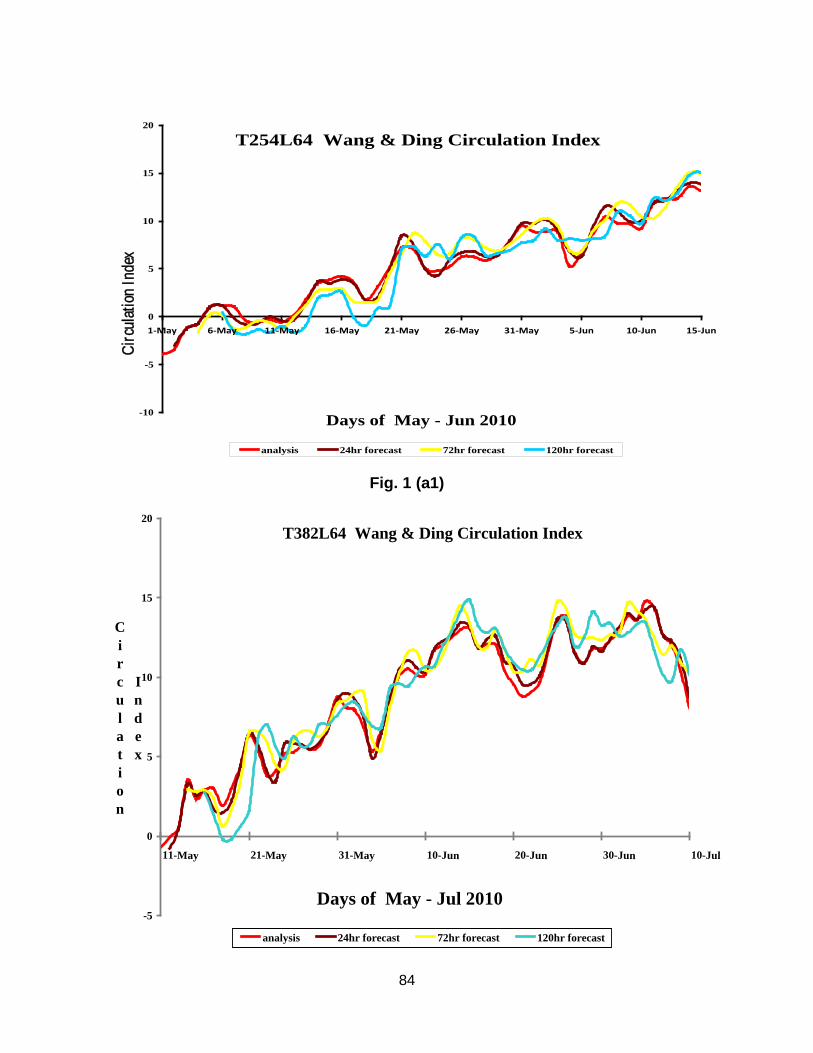
84

T254L64 Wang & Ding Circulation Index

-10

-5

0

5

10

15

20

1-May 6-May 11-May 16-May 21-May 26-May 31-May 5-Jun 10-Jun 15-Jun

Days of May - Jun 2010

Circ

ulat

ion In

dex

analysis 24hr forecast 72hr forecast 120hr forecast

Fig. 1 (a1)

T382L64 Wang & Ding Circulation Index

-5

0

5

10

15

20

11-May 21-May 31-May 10-Jun 20-Jun 30-Jun 10-Jul

Days of May - Jul 2010

Circulation

Index

analysis 24hr forecast 72hr forecast 120hr forecast

85

Fig. 1 (a2)

T254L64 Syroka & Toumi Circulation Index

-15

-10

-5

0

5

10

15

20

1-May 6-May 11-May 16-May 21-May 26-May 31-May 5-Jun 10-Jun

Days of May - Jun 2010

Cir

cula

tion

Inde

x

analysis 24hr forecast 72hr forecast 120hr forecast

Fig 1 (b1)

T382L64 Syroka & Toumi Circulation Index

-10

-5

0

5

10

15

20

11-May 16-May 21-May 26-May 31-May 5-Jun 10-Jun

Days of May - Jun 2010

Circu

lation

Inde

x

analysis 24hr forecast 72hr forecast 120hr forecast

Fig 1 (b2)

86

T254L64 Goswami Hadley cell Index

-10

-5

0

5

10

15

1-May 6-May 11-May 16-May 21-May 26-May 31-May 5-Jun 10-Jun 15-Jun

Days of May - Jun 2010

Veric

al S

hear

analysis 24hr forecast 72hr forecast 120hr forecast

Fig. 1(c1)

T382L64 Goswami Hadley cell Index

-10

-5

0

5

10

15

11-May 16-May 21-May 26-May 31-May 5-Jun 10-Jun 15-Jun

Days of May - Jun 2010

Vertical Shear

analysis 24hr forecast 72hr forecast 120hr forecast

Fig. 1(c2)

87

T254L64 Wang & Ding Circulation Index

-5

0

5

10

15

20

1-Jun 11-Jun 21-Jun 1-Jul 11-Jul 21-Jul 31-Jul 10-Aug 20-Aug 30-Aug 9-Sep 19-Sep 29-Sep

Days of Jun - Sep 2010

Circ

ulatio

n Ind

ex

analysis

Fig. 2 (a1)

T382L64 Wang & Ding Circulation Index

-5

0

5

10

15

20

11-Jun 21-Jun 1-Jul 11-Jul 21-Jul 31-Jul 10-Aug 20-Aug 30-Aug 9-Sep 19-Sep 29-Sep

Days of Jun - Sep 2010

Circ

ulat

ion

Inde

x

analysis

Fig. 2 (a2)

88

T382L64 Wang & Ding Circulation Index

-5

0

5

10

15

20

11-May 31-May 20-Jun 10-Jul 30-Jul 19-Aug 8-Sep 28-Sep

Days of May- Sep 2010

Circulation

Index

analysis 24hr forecast 72hr forecast 120hr forecast

Fig. 2(a3)

Fig. 2 (b)

89

T254L64 Syroka & Toumi Circulation Index

-10

-5

0

5

10

15

20

1-Aug 6-Aug 11-Aug 16-Aug 21-Aug 26-Aug 31-Aug 5-Sep 10-Sep 15-Sep 20-Sep 25-Sep 30-Sep

Days of Aug - Sep 2010

Circu

lation

Inde

x

analysis

Fig. 3 (a1)

Fig. 3 (a2)

5. Heat Low and Monsoon TroughR. Ashrit, J.P. George and Manjusha Chourasia

1.  Introduction:The Heat low over northwest of India and monsoon trough over the Gangetic plains

are the two most prominent quasi­permanent near surface features of monsoon circulation

and are closely related to the large scale monsoon activity over the Indian sub­continent.

Due to the intense heating in summer months a low pressure belt develops over the Afro­

Asian continent running from North Africa to North­West (NW) India through Arabia and

Pakistan. The deepest low pressure area over Pakistan and adjoining NW India is known as

the heat low.   The intensity of heat low is a good indicator of the continental heating and

land­sea   contrast   which   drives   the   monsoon.   Deep  (shallow)  heat   low   will   usually   be

associated with stronger  (weaker)  North­South pressure gradient and enhanced  (subdued)

monsoon activity.  The large scale monsoon activity is closely associated with the position

of the monsoon trough. During the established phase of the monsoon season, the monsoon

trough normally   runs   from Sriganganagar   in  NW India   to   the  Head  Bay  of  Bengal.  A

northward   shift  (towards   the   foothills  of  Himalayas   in   the  extreme cases)  of   trough   is

usually associated with weak monsoon activity over major parts of the country except over

the Sub­Himalayan regions and South­East peninsula. A  southward  location of monsoon

trough is favorable for strong monsoon activity over large parts of the country.  Monitoring

and   prediction   of   the   position   and   the   intensity   of   the   monsoon   trough   is   thus   very

important   for   assessment   of   monsoon   activity.   The   characteristics   of   these   two   semi­

permanent features, viz. Heat low and monsoon trough in the two global model (T382 and

T254) analysis and day­1 forecasts, day­3 forecasts and day­5 forecasts during JJAS 2010

are examined in this chapter. 

90

2. Heat Low:The intensity of the heat low is represented in this study by the magnitude of the

innermost closed isobaric contour on a mean sea level pressure chart. By this terminology,

a higher value of innermost closed isobar will mean shallow or less intense heat low. The

average heat  low centre pressure of  the NCMRWF T382 and T254 model  analyses and

forecasts  for different months during the monsoon season (Figure.  1) were examined to

understand   the  behavior   of   the  heat   low  during   June­September  2010.  The   time­series

presented in Figure 1 are computed over the region 24­34°N/65­75°E.   During June and

July, the minimum MSLP values are well below 1000 hPa in the analysis and forecasts of

the models. In the month of August the lowest MSLP values over this location were well

closer to 1000 hPa and in the month of September 2010 the minimum MSLP values over

this location were well closer to 1000 hPa. The Day­1, Day­3 and Day­5 forecast position

of the heat low for all months, except September, are close to its analysis position. In June,

the lowest MSLP contour in the analysis is 993 hPa whereas in the forecasts it is lower than

990 hPa.  In the month of August, the heat low becomes weak in both analysis and forecast;

particularly in the second half of August. In September no heat low is seen in both analysis

and forecast.  It   is  seen that the heat  low is  generally more intense in  model  forecast as

compared to the analysis. Also the Day­1 and Day­3 forecast intensity is more than that of

Day­5 forecast. In general, the model forecast tends to intensify the heat lows, compared to

analysis. 

 

3. Monsoon Trough:Monsoon   trough   is   the   most   prominent   semi­permanent   feature   of   the   Indian

summer monsoon. Intensity and location of the monsoon trough is  indicative of general

monsoon  condition  over   India   and  neighborhood.  During  JJAS of  2010  the  north­south

surface pressure gradient across the country was mostly weak throughout the season. The

91

vertical extent of monsoon trough was also very shallow and during many occasions was

situated north of its normal position. 

To identify the strength and position of the monsoon trough at surface level in the

T382 and T254 analysis and forecast, the MSLP field is used in this study (Figure. 2 and 3).

In the month of June, compared to the mean analysis, Day­1, Day­3 and Day­5 forecasts

show lower MSLP values over the monsoon trough region. This feature is seen in both the

models. The mean June position of the monsoon trough is the same in the analysis and the

forecast, up to day­5 forecast and is over the Indo­Gangetic plains close to foot hills. The

Day­5 forecast of T382 shows the monsoon trough extending to head Bay of Bengal (1000

hPa contour) which is not seen in T254 model. In July the mean analysis and forecasts of

both models indicate weaker monsoon trough in terms east­west spread compared to the

features in June. However both models show very similar patterns and intensity during July

in the analysis and forecasts. In the month of August, the monsoon trough was weak. Both

T382 and T254 forecasts also clearly show the dramatic change from July to August  in

terms of spatial extent. In September the monsoon trough is further weak both in analysis

and in the corresponding forecasts.

92

Figure 1. Time-series of the lowest SLP values in the heat low region (24-34N/65-75E)

during JJAS 2010 in the analysis and forecasts of T382 and T254 models.

93

94

Figu

re 2

. The

 mon

thly

 mea

n SL

P (h

Pa) i

n th

e T3

82 m

odel

 ana

lysis

 and

 fore

casts

. The

 pan

els 

in th

e fo

ur ro

ws 

corr

espo

nd to

 the 

four

 mon

ths 

June

­Sep

t 201

0. 

Mea

n an

alys

is pl

ots a

re in

 firs

t col

umn 

and 

the 

Day

­1, D

ay­3

 and

 Day

­5 fo

reca

sts a

re sh

own 

in se

conf

, thi

rd a

nd fo

urth

 col

umns

 resp

ectiv

ely.

95

Figu

re 3

. The

 mon

thly

 mea

n SL

P (h

Pa) i

n th

e T2

54 m

odel

 ana

lysis

 and

 fore

casts

. The

 pan

els 

in th

e fo

ur ro

ws 

corr

espo

nd to

 the 

four

 mon

ths 

June

­Sep

t 201

0. 

Mea

n an

alys

is pl

ots a

re in

 firs

t col

umn 

and 

the 

Day

­1, D

ay­3

 and

 Day

­5 fo

reca

sts a

re sh

own 

in se

conf

, thi

rd a

nd fo

urth

 col

umns

 resp

ectiv

ely.

96

6. Mascarene High, Cross-Equatorial Flow, Low-Level Westerly Jet and North-South Pressure Gradient During Monsoon 2010

A. K. Mitra, M. Das Gupta and G.R.Iyengar

1. Introduction

Low-level westerly jet is one of the most important feature of the south Asian summer

monsoon system. Various features of this low level jet and associated inter-hemispheric moisture

transport were documented four decades ago (Bunker, 1965; Tucker 1965; Findlatter, 1966;

Joseph and Raman, 1966; Saha and Bavedkar, 1973). Through the cross-equatorial flow, southern

hemisphere’s Mascarene High influences the low level jet in the Arabian Sea. As this is associated

with strong wind maxima offshore from Somalia, this jet is also known as Somali Jet. Indian

monsoon rainfall and its active/break phases are linked to the weather systems in the southern

hemisphere midlatitudes (Rodwell, 1997; Fukutomi and Yasunari, 2005). The low-level flow from

the southern hemisphere interacts with the cross equatorial flow and the low level westerly jet in

the Arabian Sea to shape the rainfall pattern (Anderson, 1976). Heating pattern over the southern

Indian Ocean is linked to the strength/position of the East African jet, which modulates the flow

over Indian monsoon region (Hoskins and Rodwell, 1995). In the southern Indian ocean

significant high frequency (periods 2-6 days) transient eddy activity are seen associated with

northern summer monsoon. This tropical-extratropical connection in the Indian Ocean region has

to be simulated correctly by the model to represent the monsoon precipitation in the medium range

time scale. The final strength of the monsoon flow is manifested in the north-south pressure

gradient along the west coast of India. Arabian Sea and the Bay of Bengal are among the few

regions of earth, where the low-level jets (LLJ) are seen with some regularity in the annual cycle.

These jets are related to the synoptic-scale forcing and have narrow zones of high-speed flow that

extend for hundreds of kilometers. These LLJs have appreciable horizontal and vertical shear.

These are also important for the fluxes of temperature and moisture (both horizontal and vertical)

and are generally associated with the development and evolution of deep convection over the

Indian sub-continent and the neighboring regions of south Asia. The proper representation of the

development and the evolution of these LLJs in a global numerical model, the physical

mechanisms like the shallow baroclinicity (in PBL) interacting with other factors like the strong

geostrophic forcing, the horizontal SST gradients, terrain effects are to be taken care of adequately

(Stensrud, 1996; Krishnamurti et al., 1976). Surface winds, SST over Arabian Sea and other

associated parameters are related to the rainfall over Indian sub-continent during monsoon

97

(Shukla and Misra, 1977; Raghavan et al., 1978). Similar relation of SST and low-level winds for

the tropics in general was also shown in relation to the tropical deep convection (Lindzen and

Nigam, 1987).

Oscillations in the strength of the components of monsoon flow have been linked to

variability of monsoon rainfall. This low level jet is found to have large intraseasonal variability,

affecting the moisture transport and finally the active/break conditions in convection over India

and Bay of Bengal region (Joseph and Sijikumar, 2004). The splitting of the Somali Jet depends

on the variable synoptic conditions, mean flow strength (dynamical feature of jet width and

wavelength) and the evolving transients in the region (Thompson et al., 2008). Features of the

large-scale monsoon circulation are related to the interaction of diabatic heating, orography

(mountains) and their non-linear interactions with flow itself (Hoskins and Rodwell, 1995).

Representations of these interactions in a model are essential to numerically simulate the low-level

monsoon flow realistically (Krishnamurti et al., 1976; krishnamurti and Wong, 1979;

Krishnamurti et al., 1983). The global model has to be realistic to capture the jet split. The model

vertical and horizontal resolution should also be fine enough to represent adequately the forces

responsible for maintenance and day-to-day variations in the strength of the low level westerly jet

over the Arabian Sea. A higher resolution model is highly desirable for capturing the meso-scale

convective structures in the monsoon system adequately and the associated details of monsoon

rainfall distribution (Sperber et al., 1994; Martin, 1999; Teixeira, 1999). Since the low-level jet is

very important in monsoon dynamics, monsoon modellers have to take adequate care to see that

the low level flow and the associated deep convection and their variability are properly captured in

model. This low level jet is intimately related to the cross-equatorial flow (inter hemispheric flow)

deciding the moisture transport and hence the fate of the rainfall associated with Indian monsoon

(Ramesh Kumar et al., 1999).

The performance of the two versions of (at different horizontal resolution and some other

aspects described in chapter 1) global model (T254L64 and T382L64) assimilation-forecast

system running in real-time during the monsoon 2010 in respect of the Mascarene High (MH),

Cross-equatorial flow (CEF), the low level westerly jet (LLWJ) and the north-south pressure

gradient along west coast is described briefly in this chapter. Description of the global modeling

system with its assimilation aspects are described in chapter one of this report. These modelling

systems were adapted at NCMRWF from NCEP's GFS system.

98

2. Performance of Model

2.1 Mascarene High (MH)

During monsoon 2010 season, the analyzed mean intensity of the Mascarene High (MH)

was 1032.1 hPa and it's position was approximately at 70.80 E and 35.4O S, as seen from the

T254L64 system (Figure 1). From T382L64 system, the analyzed mean intensity of the MH was

1031.8 hPa and it's position was approximately at 69.30 E and 35.6O S. Being a large-scale feature

of the monsoon over the oceanic region, a good agreement in the intensity and position is seen

between both the modeling system. The observed analysed positions from both T254L64 and

T382L64 systems are slightly to the south of the long-term (80 years mean data) observed mean

location of 690 E, 270 S with an intensity of 1024 hPa (Gorshkov, 1977). Intensity of MH also

generally varies with time and also associated with monsoon activity over Indian region. Daily

variation of MH intensity (central pressure) for analysed (lines with square marks), Day-1 and

Day-5 predictions for T254L64 and T382L64 are seen in Fig. 1. The intensities predicted in Day-1

forecasts are generally in good agreement with the analyses for both T254L64 and T382L64

systems. However, in day-5 forecasts larger disagreements with respect to analyses have been

noticed. Mean Analysed and predicted intensity of MH along with RMSE of predictions computed

against analyses are presented in Table I. The centre of MH exhibits northeast ward propagation

associated with the passage of southern hemisphere's westerly waves in day to day basis. This is

clearly seen in both the system. Figure 2 and 3 depicts the analysed (lines with square marks) and

Day-1 and Day-5 predicted longitudinal and latitudinal variation of MH during 1st June-30th

September, 2010. For both T254L64 and T382L64 analyses, day-1 and day-5 predictions showed

similar type of variation in longitude/latitude position, however the exact positions of those on a

typical day are different amongst analyses from both the modeling system. Table II and III

compare the mean of analyses and predictions (Day-1, Day-3 and Day-5) for longitude and latitude

positions of the centre of MH respectively for both T382L64 and T254L64 systems during JJAS

2010. They also compare the root mean square error (RMSE) of predictions against respective

analyses for and latitude and longitude positions of the centre of MH for both the systems. RMSEs

of prediction for latitude, longitude and intensity of MH grow with prediction time, but RMSEs

for T382L64 system are always less compared to T254L64 system.

99

2.2 Cross-Equatorial Flow (CEF)

The time mean analyzed, Day-1, Day-3 and Day-5 forecasts of the meridional wind at

equator over the sector 300 E-1000 E with mean taken over the entire monsoon period (June to

September 2010) are shown in figures 4(a) and 4(b) in the form of longitude-height cross-sections

from T254L64 and T382L64 modelling systems respectively. In T254L64 model, the analyzed

field shows prominent maxima of 15 mps around 400 E at 875 hPa representing the core of the

Arabian Sea branch of the cross-equatorial flow and a secondary maxima of 4 mps between 80 0 E

- 90 0 E, representing the Bay of Bengal branch. The dual core of cross-equatorial flow in the

Arabian Sea is not seen in this year's analysis, which was observed during monsoon season of

1995 and 1998. This dual core was also absent in recent monsoons of 2005, 2006, 2007, 2008 and

2009 (NCMRWF Report 2006a; NCMRWF Report 2006b; NCMRWF Report 2008; NCMRWF

Report 2009; NCMRWF Report 2010 ). Mean analysis from T382L64 system shows similar

features, except the maxima of Bay of Bengal showing 3 mps. In forecasts in both the models, the

core of the Arabian Sea branch of CEF is well maintained at 15 mps in a very consistent way

(except day-3, where a slight intensification is seen in both models). The Bay of Bengal branch of

the cross-equatorial flow is also maintained well. In T254L64 system the 3 mps contour over bay

of Bengal(BoB) region is seen to descend to lower levels further, indicating a slight weakening of

the BoB branch of low-level jet in terms of its vertical extent. In T382L64 system this aspect is

slightly better. Overall, the skill of the models are very good during monsoon 2010, in terms of

capturing and maintaining the low-level cross equatorial flow both in the Arabian Sea and the Bay

of Bengal.

The mean (June to September 2010) vertical profiles of meridional wind averaged over the

domain 2.50 S - 2.50 N; 39 0 E - 51 0 E from the analysed, Day-1, Day-3, and Day-5 prediction fields

from T254L64 and T382L64 are shown in figures 5(a) and 5(b) respectively. It is seen that the

maxima of the cross-equatorial flow occurs at around 875 hPa in the mean analysis. The intensity

and location forecasts of CEF from the both models agree very well with the observations

(analysis), indicating that the CEF is well maintained in the models. In both models, only marginal

weakening is noticed in forecasts between 900 and 800 hPa.

2.3 Low-Level Westerly Jet (LLWJ)

The mean analyzed and predicted positions and strength of the low-level westerly jet

(LLWJ) in the Arabian Sea at 850 hPa from T254L64 and T382L64 are shown in different panels

100

of figure 6(a) and 6(b) respectively for the whole monsoon season. This diagram brings out

clearly the well maintenance of the strength and location of LLWJ during monsoon 2010 in the

Arabian Sea throughout the forecast length (day-1 through day-5) in this high-resolution model,

particularly in T254L64 system. The contour of 20 mps adjacent to Somalia coast in the Arabian

Sea is very consistent in analysis and the forecasts in T254L64. In T382L64 system the small

region covering 20 mps contour is not seen in day-1 and day-5 forecasts, however the 15 mps

region is well maintained. The winds in the Bay of Bengal and peninsular India are also very well

maintained in the forecasts compared to the analysis. As a result the monsoon trough over the

central India is also well maintained in the forecasts.

The north-south cross-sections of seasonal mean analyzed and predicted (Day-1, Day-3 and

Day-5) zonal component of wind along 540 E, a longitude which falls within the climatological

location of LLWJ, from T254L64 and T382L64 models are given in figure 7(a) and 7(b)

respectively. The observed core of the jet matches with the climatological location. The jet core is

observed to be at 17 mps in both models. Here the second core (dual core) of 11 to 12 mps at

around 140 N is also seen during 2010 monsoon. The model forecasts (Day –1 through Day –5) are

matching very well with the observed jet strength and position. T382L64 system maintains this

better than the T254L64 system. In T254L64 system a slight intensification ( 17 mps to 18 mps) is

seen in day-1 and day-3 forecasts. The dual core system is very well maintained in both the

models. Throughout the forecast length the LLWJ is seen to be very consistent in structure among

each other and also with the observed analysis. In general, the representation and maintenance of

LLWJ is very good in the high resolution model.

The latitude-height cross-sections of seasonal mean analyzed and predicted zonal wind along

750 E (a longitude where the low-level westerlies interact with the west coast orography leading to

heavy rainfall) from T254L64 and T382L64 systems are given in figures 8(a) and 8(b)

respectively. The maximum zonal wind at 70 N in analysis is seen to be around 9 mps in both

modelling systems. The second core at 160 N represents the monsoon trough region (a very

important feature of monsoon system) which is seen to be quite strong at 9 to 10 mps. During the

forecast in general the strength is well maintained in T382L64 system. A slight intensification to

10/11 mps are seen in T254L64 system. The position and intensity of the monsoon trough is also

well maintained in both models. This season in both T254L64 and T382L64 modelling systems

the monsoon trough is seen to spread southwards slightly during the forecasts.

101

2.4 North-South Pressure Gradient

The daily variations of analyzed (line with square marks) and predicted (Day1 and Day5

predictions - line with diamond marks) values of north-south pressure gradient along the west

coast of India, during JJAS 2010 for models T382L64 and T254L64 systems are shown in figure

9. The difference of mean sea-level surface pressure between regions 210 N;700 E and 90 N;770 E

is considered to note the daily north-south pressure gradient near west coast of India. In T382L64

model, the day-1 predictions match very well with the corresponding analyzed values, whereas the

same for T254L64 system has shown some mismatch in the beginning and end of the season. Day-

5 predictions in both the system did not match very well with the corresponding analysed values

during the 1st week of August, 2010. Table IV compares the mean analysed, Day-1, Day-3 and

Day-5 predicted values of North-south pressure gradient along west coast of India and RMSE of

predictions computed against analyses for both T382L64 and T254L64 systems during JJAS 2010.

It is seen that, the errors in T382L64 system are always less than that of T254l64 system.

3. Summary

In this chapter the low-level circulation pattern and associated features seen in sea-level

pressures are discussed for both T254L64 and T382L64 global modelling systems. Both these

models are able to represent the low level monsoon circulation realistically. Wind pattern and their

intensities associated with cross-equatorial flows, low-level westerly jet over the Arabian sea and

the Bay of Bengal branch of jet are well maintained in forecasts up to day-5. The intensity of

Mascarene High, and its latitude and longitude positions are well represented in both the models.

However, by day-5, the errors are seen to be more compared to day-1, indicating possible impact

on rainfall forecasts on Indian sub-continent in the medium range. Particularly the longitude

position error of the Mascarene High by day-5 is high and needs attention. In general in a mean

sense, the T382L64 system is seen to be slightly better than the T254L64 system in representing

the monsoon low-level circulation features.

102

Legends for Figures

Fig. 1. Intensity of the Mascarene high in the analysis against Day-1 and Day-5 forecasts during monsoon 2010, from T254L64 and T382L64 global modelling systems

Fig. 2. Longitudinal position of Mascarene high in the analysis against Day-1 and Day-5 forecasts during monsoon 2010, from T254L64 and T382L64 global modelling systems

Fig. 3. Latitudinal position of Mascarene high in the analysis against Day-1 and Day-5 forecasts during monsoon 2010, from T254L64 and T382L64 global modelling systems

Fig. 4. Time mean analyzed, Day-1, Day-3 and Day-5 forecasts of meridional wind at equator over the sector 30 0 E-100 0 E, during monsoon 2010; (a) from T254L64 (b) from T383L64

Fig. 5. Time mean vertical profiles of meridional wind averaged over the domain 2.5 0 S-2.5 0 N and 39 0 E-51 0 E, during monsoon 2010; (a) from T254L64 (b) from T383L64

Fig. 6. Mean analyzed, Day-1, Day-3 and Day-5 forecasts of 850 hPa flow pattern and wind speeds, during monsoon 2010; (a) from T254L64 (b) from T383L64

Fig. 7. North-south cross-section of seasonal mean analyzed, Day-1, Day-3 and Day-5 forecasts for Zonal component of wind along 54 0 E, during monsoon 2010; (a) from T254L64 (b) from T383L64

Fig. 8. North-south cross-section of seasonal mean analyzed, Day-1, Day-3 and Day-5 forecasts for Zonal component of wind along 75 0 E, during monsoon 2010; (a) from T254L64 (b) from T383L64

Fig. 9. Analyzed, Day-1 and Day-5 forecasts of North-South Pressure Gradient along west coast during monsoon 2010, from T254L64 and T382L64 global modelling systems

103

Reference Anderson,D.L.T., 1976: The low level jet as a western boundary current , MWR, 104 , 907 - 921 Bunker,A.F., 1965: 'Interaction of the Summer Monsoon air with the Arabian Sea (preliminary analysis)', Proceedings of Symp. Meteor. Results from IIOE, July 1965, Bombay, India, 3-16 Findlatter,J., 1966 “Cross-equatorial jet streams at low level over Kenya “, Met. Mag., 95, 353-364 Fukutomi, Y., and Tetsuzo Yasunari, 2005, Southerly Surges on Submonthly Time Scales over the Eastern Indian Ocean during the Southern Hemisphere Winter, MWR, 133(6), 1637-1654 Gorshkov, S.G., (Ed.), 1977: World Ocean Atlas - Atlantic and Indian Oceans, Chief Directorate of Navigation and Oceanography, Former USSR Hoskins, B. J., and M.J.Rodwell 1995: A model of the Asian summer Monsoon. part I : The global scale , JAS , 52 , 1329 - 1340 Joseph P.V., and S. Sijikumar, 2004, Intraseasonal Variability of the Low-Level Jet Stream of the Asian Summer Monsoon , J Clim., 17(7), 1449–1458 Joseph,P.V. and P.L.Raman 1966: Existence of LLWJ stream over Peninsular India during July, Ind. J. Meteor. Geophys., 17 , 407-410 Krishnamurti, T.N.K. , V. Wong , H. L. Pan , R. Pasch , J. Molinari and P. Ardanuy 1983 : A three dimensional planetary boundary layer model for the Somali Jet , JAS , 40 , 894 - 908 Krishnamurti, T.N.K., and V. Wong 1979: A simulation of cross-equatorial flow over the Arabian Sea, JAS, 36, 1895-1907 Krishnamurti,T.N.K., J.Molinari and H.L.Pan 1976: Numerical Simulation of the Somali Jet, JAS, 33, 2350-2362 Lindzen, R.S. and R.S. Nigam 1987: On the role of SST gradients in forcing low-level winds and convergence in tropics, JAS, 44, 2418-2436 Martin, G.M., 1999: Simulation of the Asian summer monsoon, and its sensitivity to horizontal resolution, in UK Met. Office UM, QJRMS, part A, 125(557), 1499-1525 NCMRWF, DST(GOI), January 2006a: ‘Monsoon 2005: Performance of the NCMRWF Global Assimilation Forecast System’, Report no. NMRF/MR/01/2006, 139 pages, Published by NCMRWF(DST), A-50, Institute Area, Sector – 62, UP, India 201307, chapter 5, pages 71–88 NCMRWF, MoES(GOI), December 2006b: ‘Monsoon 2006: Performance of the NCMRWF Global Assimilation-Forecast System’, Report no. NMRF/MR/02/2006, 114 pages, Published by NCMRWF(MoES), A-50, Institute Area, Sector–62, UP, India 201307, Chapter 4, pages 51–66

104

NCMRWF, MoES(GOI), January 2008: ‘Monsoon 2007: Performance of T254L64 Global Assimilation-Forecast System’, Report no. NMRF/MR/01/2008, 143 pages, Published by NCMRWF(MoES), A-50, Institute Area, Sector–62, UP, India 201307, Chapter 5, pages 67–93 NCMRWF, MoES(GOI), February 2009: ‘Monsoon 2008: Performance of T254L64 Global Assimilation-Forecast System’, Report no. NMRF/MR/01/2009, 117 pages, Published by NCMRWF(MoES), A-50, Institute Area, Sector–62, UP, India 201307, Chapter 6, pages 81–97 NCMRWF, MoES(GOI), March 2010: ‘Monsoon 2009: Performance of T254L64 Global Assimilation-Forecast System’, Report no. NMRF/MR/01/2010, 131 pages, Published by NCMRWF(MoES), A-50, Institute Area, Sector–62, UP, India 201309, Chapter 6, pages 85–102 Raghavan,K., P.V.Puranik and V.R.Majumdar , P.Ismail and D.K.Paul 1978: Interaction between the west Arabian Sea and the Indian Monsoon, MWR , 106 , 719 - 724 Ramesh Kumar M. R., S. S. C. Shenoi and P. Schluessel, 1999: On the role of the cross equatorial flow on summer monsoon rainfall over India using NCEP/NCAR reanalysis data, MAP, 70(3-4), 201-213 Rodwell, M,J., 1997: Breaks in the Asian Monsoon: The influence of southern hemisphere weather systems, JAS, 54(22), 2597-2611 Saha,K.R. and S.N.Bavedkar 1973: Water vapour budget and precipitation over the Arabian Sea during the northern summer,QJRMS,99,273-278 Shukla,J., and B.M.Mishra 1977: Relationships between SST and wind speed over the central Arabian Sea and monsoon rainfall over India, MWR , 105 , 998-1002 Sperber,K.R., S.Hameed, G.L.Potter and J.S.Boyle 1994: "Simulation of the norther summer monsoon in the ECMWF Model: Sensitivity to horizontal resolution",MWR,122(11),2461-2441 Stensrud, D.J., 1996: Importance of Low-Level Jets to Climate: A Review, J. of Climate,8(9), 1698-1711 Teixeira, J., 1999: The impact of increased boundary layer vertical resolution on the ECMWF forecast system. ECMWF Tec. Mem. No268. Feb. 1999, ECMWF, Reading, UK, pp. 55 Thompson A, L. Stefanova and T.N. Krishnamurti, 2008, Baroclinic splitting of jets, MAP, 100, 257-274 Tucker,G.B. ,1965: "The equatorial tropospheric wind regime", QJRMS,91,140-150

105

Table - I Mean central pressure of MH (Intensity) for Analysis, Day-1, Day-3 and Day-5 Predictions along with RMSE of predictions computed against analyses for both T382L64 and T254L64 systems (JJAS 2010) Central Pressure

of MH (hpa)

Analysis

Mean

D1-FCST

Mean RMSE

D3-FCST

Mean RMSE

D5-FCST

Mean RMSE

T382L64 1031.83 1032.04 0.64 1031.68 1.46 1031.46 2.72

T254L64 1032.18 1031.94 0.80 1031.75 1.97 1031.37 3.51

Table - II Mean longitude position of the centre of MH for Analysis, Day-1, Day-3 and Day-5 Predictions along with RMSE of predictions computed against analyses for both T382L64 and T254L64 systems (JJAS 2010) Longitude of the

centre of MH (°)

Analysis

Mean

D1-FCST

Mean RMSE

D3-FCST

Mean RMSE

D5-FCST

Mean RMSE

T382L64 69.31 69.54 8.18 69.76 12.19 71.61 19.75

T254L64 70.85 70.18 9.09 71.35 16.40 71.50 20.28

Table - III Mean latitude position of the centre of MH for Analysis, Day-1, Day-3 and Day-5 Predictions along with RMSE of predictions computed against analyses for both T382L64 and T254L64 systems (JJAS 2010) Latitude of the

centre of MH (°)

Analysis

Mean

D1-FCST

Mean RMSE

D3-FCST

Mean RMSE

D5-FCST

Mean RMSE

T382L64 -35.64 -35.48 1.51 -35.34 1.82 -35.44 2.96

T254L64 -35.43 -35.70 1.64 -35.47 2.49 -35.57 3.55

Table - IV Mean Analysed, Day-1, Day-3 and Day-5 Predictied values of North-south pressure gradient and RMSE of predictions computed against analyses for both T382L64 and T254L64 systems (JJAS 2010) North-south

Pressure gradient

(hpa)

Analysis

Mean

D1-FCST

Mean RMSE

D3-FCST

Mean RMSE

D5-FCST

Mean RMSE

T382L64 4.87 5.12 0.92 4.45 1.32 4.54 1.82

T254L64 5.13 5.24 1.34 4.88 1.76 5.23 2.01

106

Intensity (Mascarane High) T254L64

1015

1020

1025

1030

1035

1040

1045

1-Jun-10 16-Jun-10 1-Jul-10 16-Jul-10 31-Jul-10 15-Aug-10 30-Aug-10 14-Sep-10 29-Sep-10Days

Pres

sure

(hPa

)

ANA

D1

Intensity (Mascarane High) T254L64

1015

1020

1025

1030

1035

1040

1045

1-Jun-10 16-Jun-10 1-Jul-10 16-Jul-10 31-Jul-10 15-Aug-10 30-Aug-10 14-Sep-10 29-Sep-10Days

Pres

sure

(hPa

)

ANA

D5

Intensity (Mascarane High) T382L64

1015

1020

1025

1030

1035

1040

1045

1-Jun-10 16-Jun-10 1-Jul-10 16-Jul-10 31-Jul-10 15-Aug-10 30-Aug-10 14-Sep-10 29-Sep-10Days

Pres

sure

(hPa

)

ANA

D1

Intensity (Mascarane High) T382L64

1015

1020

1025

1030

1035

1040

1045

1-Jun-10 16-Jun-10 1-Jul-10 16-Jul-10 31-Jul-10 15-Aug-10 30-Aug-10 14-Sep-10 29-Sep-10Days

Pres

sure

(hPa

)

ANA

D5

(a)

(b)

(c)

(d)

Fig 1. Daily variation of Analysed and predicted (Day-1 and Day-5) Intensity of Mascarene High during JJAS 2010 (a) T254L64, D-1 (b) T254L64, D-5 (c) T382L64, D-1 (d) T382L64, D-5

107

Longitude (Mascarane High) T254L64

20

40

60

80

100

120

1-Jun-10 16-Jun-10 1-Jul-10 16-Jul-10 31-Jul-10 15-Aug-10 30-Aug-10 14-Sep-10 29-Sep-10Days

Long

itud

e ( o E)

ANA

D1

Longitude (Mascarane High) T382L64

20

40

60

80

100

120

1-Jun-10 16-Jun-10 1-Jul-10 16-Jul-10 31-Jul-10 15-Aug-10 30-Aug-10 14-Sep-10 29-Sep-10Days

Long

itude

( oE

)

ANA

D1

Longitude (Mascarane High) T254L64

20

40

60

80

100

120

1-Jun-10 16-Jun-10 1-Jul-10 16-Jul-10 31-Jul-10 15-Aug-10 30-Aug-10 14-Sep-10 29-Sep-10Days

Long

itude

( oE

)

ANA

D5

RMSE D5=20.28o

Longitude (Mascarane High) T382L64

2030405060708090

100110120

1-Jun-10 16-Jun-10 1-Jul-10 16-Jul-10 31-Jul-10 15-Aug-10 30-Aug-10 14-Sep-10 29-Sep-10Days

Long

itude

( oE

)

ANA

D5

Fig 2. Daily Variation of Analysed and Predicted Longitude Position of the centre of Mascarene High during JJAS 2010 (a) T254L64, D-1 (b) T254L64, D-5 (c) T382L64, D-1 (d) T382L64, D-5

(a)

(b)

(c)

(d)

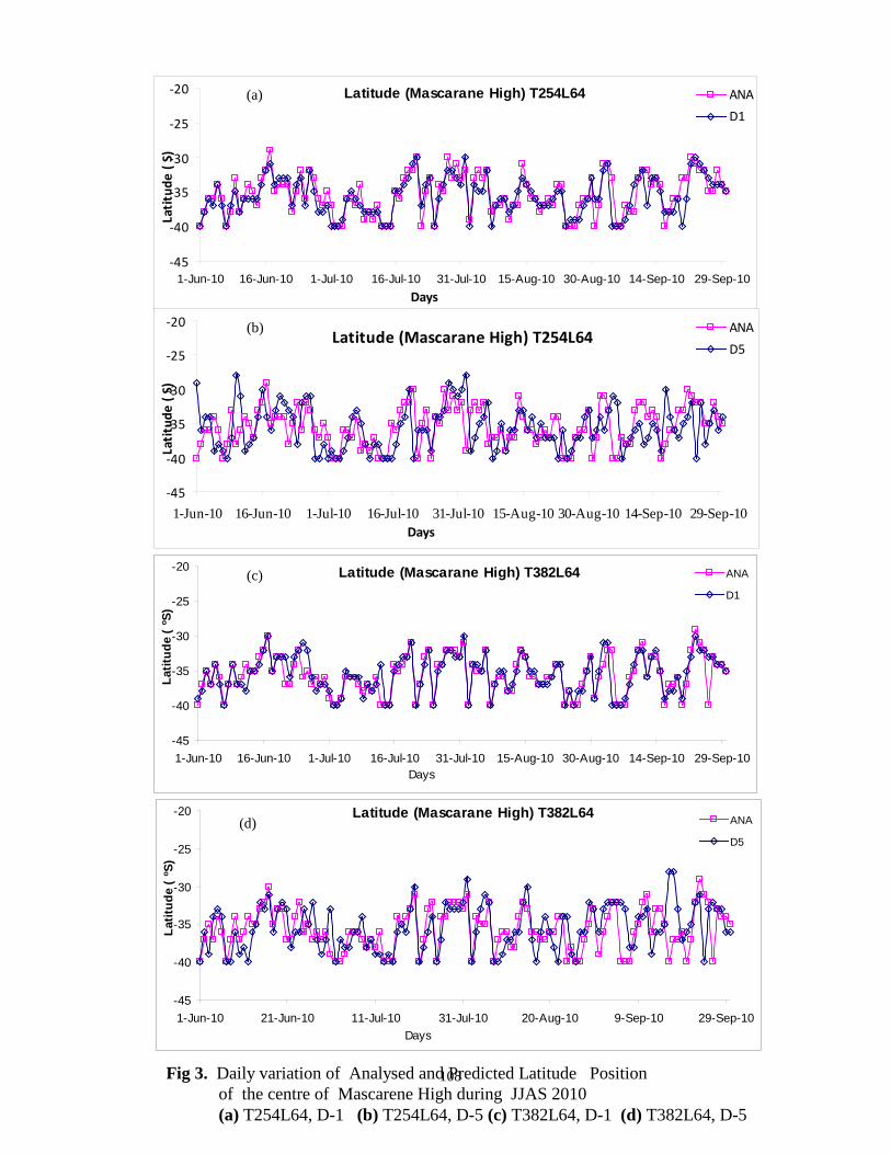
108

Latitude (Mascarane High) T382L64

-45

-40

-35

-30

-25

-20

1-Jun-10 16-Jun-10 1-Jul-10 16-Jul-10 31-Jul-10 15-Aug-10 30-Aug-10 14-Sep-10 29-Sep-10Days

Latit

ude

( o S

)

ANA

D1

Latitude (Mascarane High) T254L64

-45

-40

-35

-30

-25

-20

1-Jun-10 16-Jun-10 1-Jul-10 16-Jul-10 31-Jul-10 15-Aug-10 30-Aug-10 14-Sep-10 29-Sep-10Days

Lati

tude

( S)

ANA

D1

Latitude (Mascarane High) T254L64

-45

-40

-35

-30

-25

-20

1-Jun-10 16-Jun-10 1-Jul-10 16-Jul-10 31-Jul-10 15-Aug-10 30-Aug-10 14-Sep-10 29-Sep-10Days

Lati

tude

( S)

ANA

D5

Latitude (Mascarane High) T382L64

-45

-40

-35

-30

-25

-20

1-Jun-10 21-Jun-10 11-Jul-10 31-Jul-10 20-Aug-10 9-Sep-10 29-Sep-10Days

Latit

ude

( o S

)

ANA

D5

Fig 3. Daily variation of Analysed and Predicted Latitude Position of the centre of Mascarene High during JJAS 2010 (a) T254L64, D-1 (b) T254L64, D-5 (c) T382L64, D-1 (d) T382L64, D-5

(a)

(b)

(c)

(d)

109

110

111

112

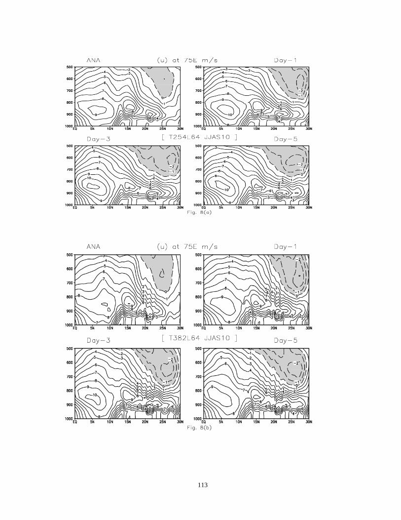
113

114

N/S Pressure Grad. T254L64

-5

0

5

10

15

01-Jun-10 16-Jun-10 01-Jul-10 16-Jul-10 31-Jul-10 15-Aug-10 30-Aug-10 14-Sep-10 29-Sep-10Days

Pre

ssur

e (h

Pa)

ANA

D1

N/S Pressure Grad. T254L64

-5

0

5

10

15

01-Jun-10 16-Jun-10 01-Jul-10 16-Jul-10 31-Jul-10 15-Aug-10 30-Aug-10 14-Sep-10 29-Sep-10Days

Pre

ssur

e (h

Pa)

ANA

D5

N/S Pressure Grad. T382L64

-5

0

5

10

15

01-Jun-10 16-Jun-10 01-Jul-10 16-Jul-10 31-Jul-10 15-Aug-10 30-Aug-10 14-Sep-10 29-Sep-10Days

Pre

ssur

e (h

Pa)

ANA

D1

N/S Pressure Grad. T382L64

-5

0

5

10

15

01-Jun-10 16-Jun-10 01-Jul-10 16-Jul-10 31-Jul-10 15-Aug-10 30-Aug-10 14-Sep-10 29-Sep-10Days

Pre

ssur

e (h

Pa)

ANA

D5

(a)

(b)

(c)

(d)

Fig 9. Daily variation of Analysed and predicted (Day-1 and Day-5) of North-South Pressure Gradient during JJAS 2010 (a) T254L64, D-1 (b) T254L64 , D-1 (c) T382L64, D-5 (d) T382L64, D-5

115

7. Tropical Easterly Jet, Tibetan High and Mid-Latitude Interaction

Saji Mohandas

1. Introduction:

Tropical Easterly Jet (TEJ) and Tibetan High are two prominent semi-permanent flow

structures that exist during the Indian summer monsoon season (Koteswaram, 1958, Rao,

1976). The easterly jet is found to the south of subtropical ridge over Asia, which runs from

the east coast of Vietnam to the west coast of Africa. Normally, the jet is at an accelerating

stage from South China Sea to South India and decelerates thereafter, with latitudinal

positions and speed fluctuating from day to day.

Tibetan High is a warm anticyclone, which gets established much later, after the onset

of monsoon. Tibetan high prominently appears with its center being most marked at 300hPa

level, approximately at 30 °N, 90 °E. It usually extends from 70 °E to 110 °E. There is also a

ridge normally found at 700hPa level, with its axis along 40 °N, between 75 °E and 95 °E,

just north of the Tibetan massif (Rao, 1976). In July another ridge also is normally observed

to lie at about 700hPa and aloft, over Pakistan and northwest India to the west of 75 °E, with

its axis along 30 °N. The high over Tibet from 500hPa upward, centred near Tibet at 500hPa

and over Tibet at 300hPa and 200hPa levels is normally termed as Tibetan High. In June the

axis of anticyclonic belt is at about 25 °N at 300hPa and 200hPa levels. In August, the

anticyclone is more or less similar to July, but is shifted to more north and is slightly more

intense. In September, the anticyclonic belt is near about 26°N upto 200hPa level.

Ramaswamy (1965) associates well-distributed rainfall over India with well-pronounced and

east-to-west oriented anticyclone over Tibet at 500hPa and 300hPa levels.

During the onset period, the position of sub-tropical high is to the south and even

middle latitude westerlies may be prevailing in northern India in the upper troposphere.

When the southwest monsoon is fully established over India, middle latitude westerlies

prevail mostly to the north of 30 °N. However, these westerlies appear to affect the monsoon

weather over north India to a considerable extend (Rao et al., 1970, Chakravorty and Basu,

1957, Mooley, 1957). Weather produced by monsoon depressions could be accentuated by

extra-tropical eastward moving disturbances at a higher latitude (Malurkar, 1958). The

116

weather on the southern side of the high latitude disturbance may be further increased by

orography near Himalayas. In this section, the significant features of the monsoon circulation over the Indian

region at 200hPa level and its interactions with mid-latitude disturbances as seen from the

model analysis and forecast during southwest monsoon season of 2010 are documented.

Tibetan High extends over the domain from 20°E to 140°E, with its axis along 28°N and the

tropical easterly jet (TEJ) forms to the south of this anticyclone. The Tibetan anticyclone may

break into two distinct cells, one close to 65°E and the other close to 85°E and oscillates about

its axis. This breaking up and oscillation of the anticyclone at 200hPa may be due to the

intrusion of transient mid-latitude westerly troughs over to the Indian region. In this report,

the time series of the fluctuations in the location of Tibetan Anticyclone along 65°E and 85°E,

the location of strong easterlies (along 75°E) and passage of westerly troughs between 65°E

and 95°E as seen at 200 hPa level are documented for the monsoon season of 2010. Comparison of two global model systems is made, namely, T254L64 and T382L64. The

charts give a concise record of the variations of the features mentioned above and form the

result of this work. The discussion therefore is brief.

2. Axis of the 200 hPa Anticyclone:

During the onset phase of Monsoon, seasonal anticyclone cell generally moves

northwards accompanied by the northward shift of upper level westerly flow over to its

northward fringes. Latitudinal positions of this 200hPa anticyclone along 65°E and 85°E are

shown in the panels a & b for Day-1 (Fig. 1 & 2), Day-3 (Fig. 3 & 4) and Day-5 (Fig. 5 & 6)

predictions respectively by T254L64 and T382L64 models.

It is seen that the general features of all the three forecast leading times are grossly

matching. The 200 hPa ridge axis analysed by T254L64 model gradually migrated from

around 20°N during the beginning of June to around 30°N by the end of June. Its position

fluctuated around 30°N till the last week of August. Thereafter, it stayed between 25-28°N till

the last week of September, when it migrated below 20°N. At 85°E, it is seen just below 30°N

from middle of June to middle of July and then fluctuated between 30°N and 40°N till the last

117

week of August. After that it stayed near around 20°N till the last week of September before

coming southward to 20°N. T254L64 day-1 forecast curve shows more or less good match

with the analysis curve. But there are more deviations between the curves at 85°E compared

to 65°E.

The T382L64 analysis shows more or less similar characteristics of intra-seasonal

fluctuations of the 200 hPa ridge axes at 65 °N and 85 °N. But the corresponding curves are

much smoother for both analysis and forecasts compared to T254L64 curves. The day-1

forecasts show very good agreement with the analysis. At day-3 and day-5, the

correspondence diminishes and the curves are showing more deviations throughout the

period. However, T382L64 shows better match between the forecasts and analysis in general,

compared with the respective panels of T254L64 model at all forecast lead times. 3. Tropical Easterly Jet:

Strength of tropical easterlies at 200hPa along 75°E was monitored throughout the

season as the strongest wind with speed exceeding 20 m/s (meter per second). Panels c & d of

the respective figures show the latitudinal positions and strength of easterlies in the analyses

and Day-1 (Figs. 1 & 2), Day-3 (Figs. 3 & 4) and Day-5 (Figs. 5 & 6) forecasts from

T254L64 and T382L64 models respectively. In the figures, latitudinal positions (where the

strength of easterly is maximum along 75°E) have been marked by crosses and vertical lines

show the strength of easterly in m/s for the day at that position. For simplifying the plot, 20

m/s has been subtracted from the strength of easterly and in the figures, 1 m/s represents one-

degree latitude of the vertical axis.

During beginning of June, the 200 hPa easterly jet at 75°E is weak and rarely attaining

20m/s at about 10°E in T254L64 analyses. With a spontaneous development of strong TEJ by

the second week, it fluctuates between equator and 10°N during the rest of June. By middle of

June, the easterlies of the order of 30 m/s are observed continuously for many days. By the

end of June, TEJ reduced in intensity and frequency. During the first week of July, it again

strengthened between equator and 5°N. However, during the second week of July, there is

seen a drastic shift of easterlies towards north, fluctuating between 10°N and 20°N. By the

third week of July, TEJ is again restricted mostly below 10°N. Again during the middle of

118

August, another episode of northward migration of TEJ is observed. By the last week of

August, TEJ again shifted southward with the strongest easterly winds occurring during the

last fortnight of September. By the last week of September, the activity again subsided and

restricted below 10°N. T254L64 day-1 forecast predicts intra-seasonal variability fairly well

in strength and position of TEJ. Day-5 forecast is also matching reasonably well with the

analyses while day-3 forecast shows somewhat reduced activity compared to the analysis.

T382L64 analysis shows similar features like T254L64, but apparently with slightly

higher intensity. Day-1 forecast is the best match with the analysis here also and day-3

forecast showing slightly lesser activity compared to day-1 or day-5. 4. Troughs in Upper Level Westerlies:

Panels e & f show the north south extension of the westerly troughs that passed

through Indian region between 65°E and 85°E in the analyses and day-1 (Figs. 1 & 2), day-3

(Figs. 3 & 4) and day-5 (Figs. 5 & 6) forecasts respectively by T254L64 and T382L64

models. It may be noted that these figures do not show any other characteristics of the trough

such as its orientation and strength. Also in these figures almost all long and smaller wave

activities seen even up to 50°N are presented whereas the major activities affecting the Indian

region may be related to those extending southward of 40°N. Still these may give some

indication of the variations in zonal index.

200 hPa trough in T254L64 analysis is found far north at the beginning of the season.

By the first week of June the troughs extend to its southernmost latitudinal positions (~20°N).

During the middle of July, the activity is somewhat subdued for about two weeks. Thereafter

in the last week of July, a couple of strong westerly activities are observed. August month

experienced a lull in the westerly activities during most of the period. By the last week of

August there is a revival of strong westerly activity. There is another lull in the activity during

the first fortnight of September. By around 15th

of September, a rejuvenated westerly activity

with a series of episodes in quick succession till the last week of September contributed to

many rainy days over north India. Day-1 forecast by T254L64 is in fair agreement with the

analysis, compared to day-3 and day-5.

119

T382L64 analysis and forecasts show similar patterns as T254L64 but apparently with

slightly less intensity and frequency.

Figure Legends

Fig. 1 Latitudinal positions of ridge axis at 200hPa level along 65 °E (a) and 85 °E (b) for both T254L64 analysis (dotted curve) and corresponding T254L64 forecasts (solid curve) for day-1. Latitudinal positions of maximum easterly wind along 75 °E at 200hPa level (marked by crosses) and the wind speed in knots above 20 knots denoted by the length of the vertical lines in terms of degrees of latitude, for analysis (c) and day-1 forecasts (d). Meridional extend in terms of degrees of latitude of the prominent trough(s) in westerlies at 200 hPa level over north India and the neighbouring parts to the north of India denoted as vertical lines for analysis (e) and day-1 forecasts (f). The x-axis is the number of days starting from 1 June, 2010 through 30 September and y-axis is latitude in degrees.

Fig. 2 Same as Fig. 1, but for day-1 forecast of T382L64. Fig. 3 Same as Fig. 1, but for day-3 forecast of T254L64. Fig. 4 Same as Fig. 1, but for day-3 forecast of T382L64. Fig. 5 Same as Fig. 1, but for day-5 forecast of T254L64. Fig. 6 Same as Fig. 1, but for day-5 forecast of T382L64.

References Chakravorty , KC and SC Basu, 1957, The influence of western disturbances on the

weather over north-east India in monsoon months, Indian J. Met. Geophys., 8, 261 – 272.

Koteswaram, P, 1958, The Easterly Jet Stream in the Tropics, Tellus, 10, 43 – 57.

Malurkar, SL, 1958, “Monsoons of the world – India Monsoon”, Monsoons of the

World, 92 – 100.

Mooley, DA, 1957, The role of western disturbances in the production of weather over

India during different seasons, Indian J. Met. Geophys., 8, 253 – 260.

Ramaswamy, C, 1965, “On synoptic methods of forecasting the vagaries of southwest

monsoon over India and neighbouring countries”, Proc. Symp., IIOE, 317 – 326.

Rao, YP, 1976, “Southwest Monsoon”, Meteorological Monograph, Synoptic

Meteorology No. 1/1976, India Meteorological Department, June 1976, 367pp.

Rao, YP, V Srinivasan and S Raman, 1970, “Effect of middle latitude westerly

systems on Indian monsoon”, Symp. Trop. Met., Hawaii, N IV 1 – 4.

120

121

122

123

124

125

126

8. Comparison of Planetary Boundary Layer (PBL) Height in T382L64 and T254L64 Analysis-Forecast Systems

Aditi and E.N. Rajagopal

1. Introduction:

The planetary boundary layer (PBL) is a critical component of earth’s climate

system. PBL has important role in both the atmospheric radiative and heat budgets as

boundary layer processes are responsible for low clouds like stratocumulus and are of

fundamental importance for cumulus convection. Thus, the parameterization of PBL in

atmospheric models is one of the most important aspects and need special attention.

Turbulence in the PBL is responsible for mixing of heat, moisture and

momentum. Due to extensive turbulent mixing, the concentration of water vapor and

trace gases remain reasonably steady within the layer whose vertical thickness is referred

to as the PBL/mixed layer height (Subrahamanyam et al. 2003, Alappatu et al. 2008). The

height of PBL is one of the fundamental parameters that are used to characterize its

structure (Gryning et al. 1987, Stull 1988, Garratt 1992). The PBL height variations over

a site are largely driven by the diurnal and seasonal changes in thermal instability and

turbulence (Stull 1988, Garratt 1992).

Remote sensing techniques like Lidar, Sodar and other direct measurement

techniques like dropsonde and radiosonde have been used to analyze the spatial and

temporal variations of PBL height in continental and marine regions (Holt and Raman

1986, Zeng et al. 1998, Subrahamanyam et al. 2003). Few long term extensive

investigations were focused on the seasonal changes of PBL heights and its structure

(Gamo 1984, Lee 1986, Dayan and Rodnizki 1998, Chen et al. 2001). Seasonal variation

of PBL height has been studied over many places in India (Vittalmurti et al. 1980,

Krishnan and Kunhikrishnan 2004). The marine PBL and its spatio-temporal variability

has been analyzed during INDOEX (Indian ocean Experiment) over the Indian ocean and

the Arabian sea (Subrahamanyam et al. 2003,Ramana et al. 2004).

In the present study, the performance of T254L64 and T382L64 analysis-forecast

systems in respect of the prediction of PBL height is examined over Indian region during

127

June-September 2010. The study investigates the difference between mean analysis and

mean 36 hr, 60 hr, and 108 hr forecast for PBL height for the month of June, July, August

and September 2010.

2. PBL Parameterization in Atmospheric Models:

In global models, the large-scale atmospheric flow determines to a large extent

the properties of the PBL and the PBL in turn reacts to these external forcings and

modifies the large scale flow. Generally, the vertical diffusion scheme based on local

gradients of wind and potential temperature, the so-called local K-approach, is used in

atmospheric numerical models. In this scheme, the eddy diffusivities coefficients are

parameterized as functions of local Richardson number. However, this scheme has

certain limitations such as the transport of mass and momentum in the PBL is

accomplished by largest eddies and such eddies should be modeled by bulk properties of

PBL instead of local properties. Also, such a scheme is unable to represent realistically

mixing in the convective boundary layer because of the counter gradient fluxes

(Deardroff 1972, Troen and Mahrt 1986, Stull 1991). This may affect profiles of mean

quantities especially in locations where dry convection is of importance in the PBL. One

of the ways to overcome these limitations is to use higher order closure approaches

developed by Mellor and Yamada (1974). The higher order closure approach was capable

of representing a well mixed boundary layer structure but was computationally more

expensive.

On the other hand, another type of simple diffusion scheme, the so-called

nonlocal-K approach is used in weather prediction and climate models. This scheme

utilizes the results of large eddy simulation research (Wyngaard and Brost 1984) and is

computationally efficient. The nonlocal turbulent mixing within the PBL in atmospheric

models is pioneered by the work of Troen and Mahrt (1986). The turbulent diffusivity

coefficients are calculated from a prescribed profile shape as a function of boundary layer

heights and scale parameters derived from similarity requirements. In addition to the

advantage in matching condition between the surface-layer top and the Ekman layer

bottom, it gives the ideal turbulent diffusivity profile proposed by O’Brien (1970), which

is based on the physical coupling that the profile and its first derivative be continuous

with height and matches the similarity requirement at the surface layer. Holtslag et. al

128

(1990) showed that this scheme is useful for predicting short-range weather phenomena

of temperature and humidity profiles in the lower atmosphere, the structure of boundary

layer, the boundary layer height and the amount of boundary layer clouds. Giorgi et al.

(1993) implemented this scheme in a second generation regional climate model

(RegCM2) and showed the impact on the simulated regional climate over Europe for

January and June 1979. Their results showed that this scheme induced an overall increase

in total precipitation amounts. Basu et. al. (2002) studied the impact of the non-local K-

closure scheme for the atmospheric boundary layer using the Global Spectral Model in

predicting monsoon circulation over Indian region. Their results showed a systematic

improvement in the precipitation distribution over the Indian region.

Both T254L64 and T382L64 models use non-local scheme of PBL

parameterization following Hong and Pan (1996). A brief description of the scheme is

given in the next section.

3. Non-local Vertical Diffusion Scheme in T254L64 and T382L64 Models:

According to Deardorff (1972), Troen and Mahrt (1986), Holtslag and Moeng

(1991), and Holtslag and Boville (1993), the turbulent diffusion equations for prognostic

variables (C; u, v, θ, q) can be expressed by

−∂∂

∂∂

=∂∂

cc zCK

ztC γ (1)

Where Kc is the eddy diffusivity coefficient and γc is a correction to the local gradient that

incorporates the contribution of the large-scale eddies to the total flux. This correction

applies to potential temperature (θ) and specific humidity (q) within the mixed boundary

layer. This nonlocal diffusion approach is applied only for the mixed layer diffusion. The

momentum diffusivity coefficient is formulated as

p

szm hzzkwK

−= 1 (2)

where p is the profile shape exponent taken to be 2, k is the von Karman constant (=0.4),

z is the height from the surface, and h is the height of the PBL. The mixed-layer velocity

scale is represented as

129

1*

−= ms uw φ (3)

where u* is the surface frictional velocity scale and φm is the wind profile function

evaluated at the top of the surface layer. The counter gradient terms for θ and q are given

by

( )s

c wcwb ''

=γ (4)

where ( )''cw is the corresponding surface flux for θ and q, and b is a coefficient of

proportionality. To satisfy the compatibility between the surface layer top and the bottom

of the PBL, the identical profile functions to those in surface-layer physics are used. For

unstable and neutral conditions ( )[ ],0'' 0 ≤vw θ

411.0161−

−=

Lh

mφ , for u and v (5)

211.0161

−

−=

Lh

tφ , for θ and q

while for the stable regime ( )[ ]0'' >vw θ ,

,1.051

+==

Lh

tm φφ (6)

where h is the boundary layer height and L is the Monin-Obukhov length scale. The top

of the surface layer is estimated as 0.1h. To determine the b factor in (4), the exponent of

-1/3 is chosen to ensure the free-convection limit. Therefore, the following approximation

is used: 3141 1.01211.0161

−−

−≈

−=

Lh

Lh

mφ (7)

Following the derivation of Troen and Mahrt (1986) and Holtslag et al. (1990),

the right hand side of (7) leads to b=7.8. The boundary layer height is given by

( ) ,)()( 2

sv

vacr hg

hURibh

θθθ

−= (8)

130

where Ribcr is the critical bulk Richardson number, U(h) is the horizontal wind speed at h,

θva is the virtual potential temperature at the lowest model level, θv(h) is the virtual

potential temperature at h, and θs is the appropriate temperature near the surface defined

as

( ),

' 0'

=+=

hww

bs

vTvas

θθθθ (9)

where θT is the scaled virtual temperature near the surface with a maximum limit of 3 K

(Hong and Pan 1996).

The eddy diffusivity for temperature and moisture (Kzt) is computed from Kzm in

(2) by using the relationship of the Prandtl number, which is given by

,1.0Pr

+=

hhbk

m

t

φφ

(10)

where Pr is a constant within whole mixed boundary layer.

Numerically, the boundary layer height, h, is obtained iteratively. First h is

estimated by (8) without considering the thermal excess, θT. This estimated h is utilized

to compute the profile functions in (5)-(7), and to compute the mixed-layer velocity ws in

(3). Using ws and θT in (9) h is enhanced. With the enhanced h and ws, Kzm is obtained by

(2), and Kzt by (10). The counter gradient correction terms for θ and q in (1) are also

obtained by (4).

4. Data and Methodology:

In this study, model outputs of T382L64 and T254L64 for the period of June-

September 2010 are used. The monthly mean PBL height of 12 UTC analyses is

compared with the model’s mean 36, 84 and 108 hr forecasts for June-September 2010.

The PBL height at 12 UTC is much more developed as compared to 00 UTC, thus

monthly mean PBL height of 12 UTC is utilized in the present study.

5. Results and Discussions:

5.1 Variation of mean PBL height in model analysis

131

Figs. 1 and 2 show the mean analysis of PBL height (meters, m) for June, July,

August and September 2010 for T382L64 and T254L64 respectively. Mean analysis

reveals that the PBL heights are highest (in north west part of India) in the month of June

and it decreases from July to September for both the models. In T382L64 the mean PBL

height ranges from 500-4500 m in June, 500- 3000 m in July, 500- 2000 m in August and

September (Fig. 1). Similar variations in magnitude of PBL height are observed in

T254L64 from June to September (Fig. 2).

The maximum value of mean PBL height is reported in June, mainly due to

summer conditions. The mean PBL heights reach their maximum values in June and July,

ignoring the subsiding effect of rain and loss of insolation by existing cloud cover,

because of intense mixing and inability of the heat to escape beyond the cloud layer. The

variations in mean PBL height are clearly seen during summer monsoon (June, July and

August). A decreasing trend in the PBL height is seen in September (Figs. 1d and 2d).

This can be attributed to weakening of convective activities during this month. This

month also happens to be a transition period from wet south-westerly wind to drier north

easterly wind.

Several attempts have been made to understand the seasonal variation of PBL

height over different locations in India using the observational data. Vittalmurti et al.

(1980) had shown the seasonal variation of PBL height over some urban locations in

India and found that maximum PBL height is observed during April (pre-monsoon) as

well as during October and January at several sites in India. Minimum values of MLH

were observed during August (summer/monsoon) and October (Post-monsoon). Gamo et

al. (1994) reported the day time maximum PBL height variation over Delhi and their

study revealed that PBL attained highest altitude during pre-monsoon (~3000 m), low

during monsoon (<2000 m), moderate during post monsoon (~2000 m) and lowest during

winter (< 1000 m). Similar variation is also reported by Krishnan and Kunhikrishnan

(2004) over Gadanki, a rural site in South-east India. They reported reasonably higher

values of PBL height for pre-monsoon (~2200 m) and post monsoon (~1770 m) months

as against slightly lower values in summer-monsoon (~1650 m) and winter months

(~1500 m). Srivastava et al. (2010) investigated the seasonal variation in PBL height over

Ahmedabad and found that PBL height is at maximum during summer monsoon and it is

132

at minimum during winter months. The differences in the estimated PBL height may be

due to prevailing meteorological conditions at different location. Nonetheless, the range

of PBL height is found to be somewhat similar to that obtained from mean analysis of

both T382L64 and T254L64 models. In Delhi, the mean PBL height is of the order of

4000 m in June, 1500 m in July, 1000 m in August and 500 m in September as per the

mean model analyses (Figs.1-2).

The changes in mean PBL height in the analysis of T382L64 and T254L64 (Figs.

1-2) are also evident in the marine boundary layer. The mean PBL height over Arabian

sea is found to be of the order of 1000-1500 in June, July, August and 1000 m in

September. However, over Bay of Bengal the mean PBL height is 1000 m during June

and July and 500 m in August and September which is slightly lower than that over

Arabian Sea. Over Indian Ocean the mean PBL height is found to be 1000-1500 m in

June, July and 500-1500 m in August and 500 m in September. The values are found to

be of the similar order in both the models. The model analysed values are somewhat

similar to those obtained in the other observational studies. The PBL height over Indian

Ocean was observed to a range of 400-1100 m (Ramana et al., 2004) during the first two

campaigns (Pre-INDOEX, 1997) and First Field Phase (FFP, 1998) of the INDOEX.

During the Intensive Field Phase (IFP-99) of the INDOEX campaign, Subrahamanyam et

al.(2003) reported the PBL height in the range 200-900 m. Holt and Raman (1986)

reported the PBL height over Bay of Bengal during monsoon about 400-500 in contrast to

about 800-1500 m over Arabian Sea (Holt and Raman, 1985).

In general, the mean analysis show somewhat higher values of PBL height in all

the months. This may be attributed to the fact that these values are valid for mid-

afternoon hours when the PBL becomes highly convective and turbulent thereby attaining

maximum values in afternoon hours. Further the height of the PBL may be really high for

the year 2010.

5.2 Comparison of mean PBL height in model forecasts

The mean analysis of T382L64 for the month of June (Fig. 3a) depicts the PBL

height of the order of 3000-4500 m in northwest parts of India whereas the minimum

PBL height (1000-1500 m) is seen along the Western Ghats. The difference between

(a) (a) (a)

133

mean analysis and mean 36 hr, 60 hr and 108 hr forecasts designated as A-F (where A

stands for analysis and F stands for forecast) are shown in Figs. 3b, 3c and 3d

respectively. The difference between mean analysis and mean 36 hr forecast is positive in

northern and central parts with forecast over predicting the PBL height. The difference is

negative in Southern peninsular region where the 36 hr forecast is under-predicting the

PBL height. The differences are found to be increasing in 60 hr and 108 hr forecasts over

north and central parts whereas in peninsular region significant changes are not observed.

In northwest parts the forecast is over-predicting the PBL height in 36 and 60 hr

forecasts, while 108 hr forecast the under-predicts the PBL height.

The mean analysis of T254L64 for the month of June (Fig. 4a) reveals similar

pattern for PBL height as in T382L64 system. The difference between mean analysis and

mean 36 hr forecast (Fig. 4b) is found to be positive with the forecast over-predicting in

northern and eastern parts. An under-prediction is observed in forecast in northwest and

central parts. The differences are found to be increasing with 60 hr (Fig. 4c) and 108 hr

forecast (Fig. 4d) over eastern parts and northwestern parts. In general, the differences are

found to be smaller in T254L64 compared to T382L64.

In the month of July, the mean analysis of T382L64 (Fig. 5a) shows a decrease in

magnitude of PBL height in all the parts as compared to that observed during June, with

maximum (2000-3000 m) observed in north west parts and minimum 500 m over

Western Ghats. The 36, 60 and 108 hr forecasts (Figs. 5b, 5c, 5d) over-predicts the PBL

height in north region with magnitude increasing with forecast lead time. However,

under-prediction is seen over east, west and peninsular region with highest under-

prediction in 108 hr forecast.

The mean analysis of T254L64 (Fig. 6a) for July 2010 show similar PBL heights

as in T382L64. The 36, 60 and 108 hr forecasts (Figs. 6b, 6c, 6d) over-predicts the PBL

height in northwest parts with magnitude increasing with forecast lead time However,

under-prediction is observed in western parts. The magnitudes of differences are found to

be smaller in comparison to T382L64.

The mean analysis of T382L64 for August 2010 (Fig. 7a) shows further decrease

in magnitude of PBL height all over India. For most of the parts the PBL height is found

to be of the order of 1000 m. PBL height is over-predicted in north, west and some parts

134

of east with nearly same magnitude in all the mean forecasts (Figs. 7b, 7c, 7d), however,

there is an increase in the area with the forecast lead time.

The mean analysis (Fig. 8a) of T254L64 is similar to that observed for T382L64.

The differences between mean analysis and mean forecasts (Figs. 8b, 8c, 8d) are not

much and there is also not much difference with forecast lead time.

The PBL height is found to decrease further to 500 m in most of the parts in mean

analysis of September 2010 (Fig. 9a) for T382L64. The magnitude of over-prediction in

the PBL height as compared to analysis is not increasing much with forecast lead time

(Figs. 9b, 9c, 9d)

The PBL height is found to show the same trend in T254L64 analysis for

September (Fig.10a) as in T382L64. PBL height is over-predicted in the forecasts over

west Rajasthan with magnitude not increasing much with forecast lead time (Figs. 10b,

10c, 10d)

6. Conclusions:

The high resolution T382L64 and T254L64 global models are used to analyze the

variation in the PBL height over Indian region during monsoon season (JJAS) 2010. The

mean analysis PBL height of the T382L64 and T254L64 forecast system at different

locations over India is somewhat in agreement with those obtained from different

observational studies carried over Indian continent. The differences between mean

analysis and predicted PBL height are found to be decreasing from June to September

with maximum in June and minimum in September. Also the differences are found to be

increasing with forecast lead time in all the months from both the models.

135

References

Alappattu, D.P., Subhrahamanyam, D.B., Kunhikrishnan, P.K., Somayaji, K.M., Bhat,

G.S., Venkateshan, R., Dutt, C.B.S., Singh, A.B., Soni, V.K., Tripathi, A.S.,

2008: On the marine atmospheric boundary layer characteristics over Bay of

Bengal and Arabian Sea during the Integrated Campaign for Aerosol gases and

Radiation Budget (ICARB), Journal of Earth System Science, 117, 281-291.

Basu, S., G.R. Iyengar. A.K. Mitra, 2002 : Impact of a nonlocal closure scheme in a

simulation of a monsoon system over India, Monthly Weather Review, 130, 161-

170.

Chen, W., Kuze, H., Uchiyama, A., Suzuki, Y., Takeuchi, N., 2001: One year observation

of urban mixed layer characteristics at Tsukuba, Japan using a micro pulse lidar.

Atmospheric Environment, 35, 4273-4280.

Dayan, U., Rodnizki, J., 1998: The temporal behavior of the atmospheric boundary layer

in Israel. Journal of Applied Meteorology, 38, 4273-4280.

Deardorff, J.W., 1972: Theoretical expression for the countergradient vertical heat flux.

J. Geophysical Research, 77, 5900-5904.

Gamo, M., 1984: Seasonal change of mixed layer structure at Tsukuba. Journal of

Meteorological Society of Japan, 63, 60-74.

Garratt, J.R., 1992: The Atmospheric Boundary Layer. Cambridge University Press,

Cambridge.

Giorgi, F., M. R. Marinucci, G.T. Bates, 1993: Development of a second-generation

regional climate model (RegCM2). Part 1: Boundary layer and radiative transfer

processes. Monthly Weather Review, 121, 2794-2813.

136

Gryning, S.E., Holtslag, A.A.M., Irwin, J.S., Sivertsen, B., 1987: Applied dispersion

modelling based on meteorological scaling parameters. Atmospheric

Environment, 21, 79-89.

Holt, T., Raman, S., 1986: Observations of the mean and turbulence structure of the

marine boundary layer over the Bay of Bengal during MONEX-79, Monthly

Weather Review, 114, 2176-2190.

Holtslag, A.A.M., I.F. Bruijin and H.L. Pan, 1990: A high resolution air mass

transformation model for short-range weather forecasting. Monthly Weather

Review, 118, 1561-1575.

Holtslag, A.A.M., C.H. Moeng, 1991: Eddy diffusivity and countergradient transport in

the convective atmospheric boundary layer. Journal of Atmospheric Sciences, 48,

1690-1698.

Holtslag, A.A.M., B.A. Boville, 1993: Local versus nonlocal boundary layer diffusion in

a global climate model. Journal of Climate, 6, 1825-1842.

Krishnan, P., Kunhikrishnan, P.K., 2004: Temporal variations of ventilation coefficient at

a tropical Indian station using UHF wind profiler. Current Science, 86, 447-451.

Lee, C.B., 1986: Simple model and climatological aspects of structure of the convective

boundary layer. Atmospheric Environment, 20, 705-714.

Mellor, G.L. and T. Yamada, 1974: A hierarchy of turbulence closure models for

planetary boundary layers. Journal of Atmospheric Sciences, 31, 1792-1806.

Naja, M., Lal, S., 2002: Surface ozone and precursor gases at Gadanki (13.50 N, 79.20 E),

a tropical rural site in India. Journal of Geophysical Research, 107 (D14), 4197.

137

O’Brien, J.J., 1970: A note on the vertical structure of the eddy exchange coefficient in

the planetary boundary layer. Journal of Atmospheric Science, 27, 1213-1215.

Ramana, M.V., Krishnan, P., Nair, S.M. Kunhikrishnan, P.K., 2004: Thermodynamic

structure of the atmospheric boundary layer over the Arabian sea and the Indian

ocean during pre-INDOEXand INDOEX-FFP campaigns, Annales Geophysicae

22, 2679-2691.

Stull, R. B., 1988: An Introduction to Boundary Layer Meteorology. Kluwer Academic

Publishers, UK, pp.666.

Stull, R. B., 1991: Static stability: An update. Bulletin of American Meteorological

Society, 72, 1521-1529.

Subhrahamanyam, D.B., Ramchandran, R., Sen Gupta, K., Mandal, T.K., 2003:

Variability of mixed layer heights over the Indian Ocean and central Arabian Sea

during INDOEX, IFP-99, Boundary Layer Meteorology, 107, 683-695.

Troen, I., Mahrt, L., 1986: A simple model of the atmospheric boundary layer: Sensitivity

to surface evaporation. Boundary Layer Meteorology, 37, 129-148.

Vittalmurti, K.P.R., Viswanadham, D.V., Sadhuram, Y., 1980: Mixing heights and

ventilation coefficients for urban centres in India. Boundary Layer Meteorology,

19, 441-451.

Zeng, X., Zhao, M., Dickinson, R. E., 1998: Intercomparison of bulk aerodynamic

algorthims for the computation of sea surface fluxes using the TOGA COARE

and TAO data. Journal of Climate, 11, 2628-2644.

138

Fig 1: Mean analysis of PBL height in T382L64 for (a) June (b) July (c) August and (d) September 2010

139

Fig 2: Mean Analysis of PBL height in T254L64 for (a) June (b) July (c) August and (d) September 2010

140

Fig. 3: Mean analysis (a) and difference between mean analysis and (b) 36 hr (c) 60 hr and (d) 108 hr mean forecasts for June 2010 for T382L64.

141

Fig. 4: Mean analysis (a) and difference between mean analysis and (b) 36 hr (c) 60 hr and (d) 108 hr mean forecasts for June 2010 for T254L64.

142

Fig. 5: Mean analysis (a) and difference between mean analysis and (b) 36 hr (c) 60 hr and (d) 108 hr mean forecasts for July 2010 for T382L64

143

Fig. 6: Mean analysis (a) and difference between mean analysis and (b) 36 hr (c) 60 hr and (d) 108 hr mean forecasts for July 2010 for T254L64

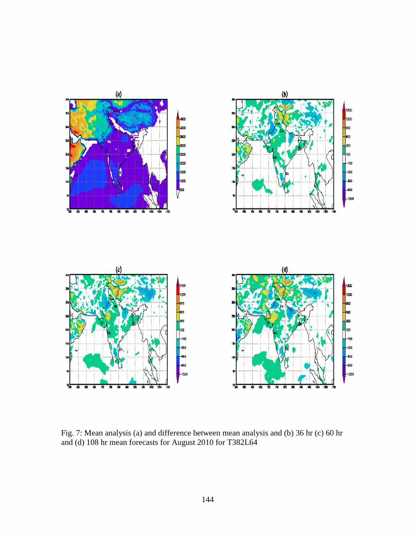
144

Fig. 7: Mean analysis (a) and difference between mean analysis and (b) 36 hr (c) 60 hr and (d) 108 hr mean forecasts for August 2010 for T382L64

145

Fig. 8: Mean analysis (a) and difference between mean analysis and (b) 36 hr (c) 60 hr and (d) 108 hr mean forecasts for August 2010 for T254L64.

146

Fig 9: Mean analysis (a) and difference between mean analysis and (b) 36 hr (c) 60 hr and (d) 108 hr mean forecasts for September 2010 for T382L64.

147

Fig 10: Mean analysis (a) and difference between mean analysis and (b) 36 hr (c) 60 hr and (d) 108 hr mean forecasts for September 2010 for T254L64.

148

9. Location specific weather forecast for major cities and distrcits of India and customized forecasts based upon T-254 and T-382 models and evaluation of forecast skills

Ashok Kumar, E.N.Rajagopal, J.V.Singh, Ranjeet Singh and Trilochan Patnaik

1. Introduction:

Location specific weather forecasts in medium range are extremely useful,

as 3-5 days lead time is very essential for taking precautionary measures to save crops

from bad weather in agriculture and managing other agriculture related activities.

The location specific weather forecast products are generated regularly based

upon the NWP models operational at NCMRWF. Initially these products were based

upon R-40, T-80 and T-170 models and now these forecasts are based upon T-254

general circulation model installed in January-2007. and T-382 general circulation

installed in July-2010.

Over the years a fully operational location specific forecast system for

agriculture was successfully developed on the basis of the T80L18 medium range

weather forecasts. (Kumar et.al.,1996)Later on location specific weather forecast

system was also developed based upon T-254 model and by monsoon 2008 it was

operational for all the 127 agro advisory service units in India. The location specific

weather forecasting for agriculture sector was transferred to the India Meteorological

Department in 2008.

Besides this, two main location specific weather forecast products are

generated every day, one is for major cities of India and other is for all the 602

districts of India and are put on NCMRWF website every day. These forecasts are

easily accessible for media, general public, district authorities and farmers for

planning their activities. These forecasts are obtained based upon T-254 and T-382

models. A detailed verification study for these forecasts is conducted at the end of

each monsoon season and is found up to the mark almost every year. The forecast

performance in monsoon 2010 is presented in the following sections.

Location specific forecasts also play an important role in managing different

activities and resources in other sectors like mountain expeditions, sea expeditions ,

organizing games, resources in power sector, aviation and satellite launching. These

forecasts are used for civil and military operations both. These special customized

forecasts are issued as and when demanded by the various user departments. These

forecasts had always been found matching well with the prevailing weather at the

149

place of work as per the information received at NCMRWF. The customized forecasts

are demanded and well appreciated.

2 General circulation models(GCMs) used

A R-40 general circulation model with a resolution of 2.8°x1.8° was installed

and made experimentally operational in 1989. The NCEP T80/L18 general

circulation model is made operational in 1993 at NCMRWF. The horizontal

resolution is spectral triangular truncation with 80 waves (T80). In physical space

the horizontal resolution is of 256 x 128 grid size. This is roughly equivalent to 1.5° x

1.5° latitude/longitude grid spacing. Forecast values are available at each time step

which is 15 minutes. Hence for a particular day 96 forecast values are obtained and

model is run for 7days starting from 0000UTC initial conditions (Kumar et. al.1999)

The NCMRWF T170/L28 Global Spectral Model was developed in-house,

(Kar,2002) and was made experimentally operational in 2002. It is based on the

NCEP T80/L18 Model, (Kanamitsu,1989), ( Kanamitsu et. al. 1991), (Kalnay et al.

1990) and subsequent changes were made to the T80/L18 model at NCMRWF.

Atmospheric dynamics are based on primitive equations with vorticity, divergence,

logarithm of surface pressure, specific humidity and virtual temperature as dependent

variables. In this model horizontal representation is spectral (spherical harmonic basis

functions) with transformation to a Gaussian grid for calculation of nonlinear

quantities and physics. The horizontal resolution is spectral triangular truncation with

170 waves (T170). In physical space the horizontal resolution is of 512 x 256 grid

size. This is roughly equivalent to 0.7° x 0.7° latitude/longitude grid spacing. The

model has a comprehensive physics package which includes parameterisation

schemes for cumulus convection, shallow convection, radiation, planetary boundary

layer, surface processes and gravity wave drag due to mountains. The time

integration scheme is semi-implicit. The time step is 7.5 minutes for computation of

the dynamics and physics terms.

The NCMRWF T254/L64 Global Spectral Model is obtained from NCEP and is

made operational at NCMRWF in January 2007, (Rajagopal et. al. 2007). The

horizontal resolution is spectral triangular truncation with 254 waves (T254). In

physical space the horizontal resolution is of 768 x 384 grid size. This is roughly

equivalent to 0.5° x 0.5° latitude/longitude grid spacing. The time step is 7.5 minutes

for computation of dynamics and physics terms. The model has comprehensive

parameterised physics package. T382/L64 Global Spectral Model is made operational

150

at NCMRWF in July 2010. The horizontal resolution is of 1152x576 grid size. This is

roughly equivalent to 0.3125 x 0.3125 latitude/longitude grid spacing.

3. Direct model output(DMO) forecast

3.1 Nearest grid and interpolated forecast values

As the forecasts are obtained at gaussian grids and not at a particular location,

hence the simplest way to get forecast at a specific location is to use the interpolated

value from the four grid points surrounding it. But if the location is very near to a grid

point, then the forecast at that grid point can also be taken as the forecast for the

location. In order to decide as to which forecast among the two should be given more

weightage for a location, it is necessary to know the distance of the location from the

four grid points surrounding it. If the distance of the location from the nearest grid is

less than one-fourth of the diagonal distance between any two grid points, then more

importance is given to the nearest grid forecast values otherwise the interpolated

value is considered, Fig 1(Kumar et.al.,1999).

Fig. 1 Area considered around a grid point for deciding the relative importance

of nearest grid and the interpolated DMO forecast values for a particular

location.

3.2 DMO Forecast

DMO forecast values of both types i.e. nearest grid and interpolated, for each

location of interest are obtained. Five day forecast for the following parameters is

obtained by using every hour forecast values obtained from each time step values of

7.5 minutes for T-254 and T-382 models.

• Average Mean Sea Level Pressure (hPa)

• Cloud Amount (Morning and Evening) (okta)

151

• Rainfall (24 hours accumulated) (mm)

• Maximum Temperature(oc)

• Minimum Temperature(oc)

• Average Wind Speed (kmph)

• Predominant Wind Direction (deg)

• Maximum Relative Humidity (%)

• Minimum Relative Humidity (%)

Here, the validity of the forecast values for a particular day is for the

subsequent 24 hours starting from 0003UTC(0830 hrs IST) of that day. As at

NCMRWF earlier T-80 model and later on T-254 and T-382 models are run only for

7 days based on 0000UTC analysis, hence only the 24,48,72 ,96,120 hours forecasts

are obtained.

The forecast thus obtained are biased and bias free forecasts are obtained for 70

major cities of India and all the districts of India, as explained in the following

sections. The bias free forecasts are obtained fro the following weather parameters

every day

● Rainfall (24 hours accumulated)(mm)

● Maximum Temperature (oc)

● Minimum Temperature (oc)

The meteograms are also obtained for the metropolitan cities, other important

major cities every day and as and when required for the customized forecasts. In

meteograms every six hourly accumulated rainfall values and six hourly wind speed

and wind direction values are shown , besides this every time step or every hour

values are also plotted for mean sea level pressure, maximum temperature and

minimum temperature(Fig.2)

4. Bias free rainfall and Kalman filtered temperature forecast

The systematic error(bias) free forecast is obtained by using the direct model

output obtained from the T-254 and T-382 general circulation models during

monsoon 2010.

4.1. Bias free rainfall forecast

An optimal rainfall threshold value is set to maximise the skill score. The optimal

threshold value means that if the forecasted rainfall amount is less than the threshold

then the forecasted value is taken as a zero otherwise it is taken as the forecasted

rainfall amount(Maini.. et. al. 2002). The optimal threshold is calculated as follows:

152

Fig 2. The meteogram for Delhi showing seven day forecast based upon initial condition of 0000UTC of 29 Jul. 2010.

153

Let the forecasted rainfall series during the seasons considered is denoted as Rfi , i

= 1,2, …….n. and Th be the threshold up to which the rainfall is taken as zero and

beyond the Th value rainfall is taken as the actual value .

Then using the Th value forecasted YES/NO rainfall series is derived from the

forecasted rainfall series as

if Rfi ≤ Th then no rain case i.e. 0(or N) case

and if Rfi > Th then rainfall case i.e. 1(or Y) case

i.e value of 1(or Y) is taken for rainfall case and value of 0(or N) for no-rain case.

Similarly let the observed rainfall series during the seasons under consideration is

denoted by Roi , i = 1,2, …..,n ; and threshold value as 0.1 mm and the observed

YES/NO rainfall series is derived from the observed rainfall series using the similar

logic.

As scores used for verification of the rainfall forecast are the ratio score and

Hanssen and Copiers(H.K) skill score. Hence HK skill score is calculated by using the

observed and forecasted YES/NO rainfall series based upon the data from the

previous 2 to 3 seasons. Then HK skill score is maximized by varying the

threshold(Th) value used for deriving forecasted YES/NO rainfall series. This

threshold value which maximizes the HK skill score during previous seasons is

applied for deriving YES/NO rainfall forecast from the DMO rainfall forecast during

the current season. In the present study the thresholds correction factors are calculated

based upon monsoon season (June, July, August and September) of 2003 for T-80

model. These thresholds correction factors are also calibrated and verified further

using the monsoon 2005 and 2006 data for T-80 and T-170 models and these are

further calibrated using monsoon 2007 and 2008 data and are used for T-254 and T-

382 models. These threshold correction factors are explained further in section 5.

4.2. Basis of Kalman filtered temperature forecast (Anders o.Persson,1991)

It is a common fact that NWP models exhibit systematic errors in the forecasts of

the near surface weather parameters. The 2m-temperatures for example are often

systematically biased , though the magnitude of the bias varies with geographical

location and time of the season. Such systematic errors may not only be due to short

comings in the model but also depend on the sub-grid location of the station.

Individual mountains or different parts of a large city with their specific climate can

hardly be fully resolved in any NWP model.

154

Mathematically a correction formula for a given station and for the specific lead

time can be formulated as

Y = X1 + X2* Temp. forc.

If X1 and X2 were constant over the seasons they could be computed with good

accuracy by linear regression techniques. To avoid storage of old data a recursive

regression technique could be used applying weights to make more recent data have a

larger impact. X1 and X2 would then reflect more recent conditions. However , in a

pure statistical sense this method is only a way to smooth the data, the weights

pushing the emphasis towards a more recent time. In contrast to smoothing, filtering

techniques actually tries to estimate today’s value, in light of historical data. Thus a

simple one parameter Kalman filter can be applied for removing the systematic errors

in the temperature forecasts(Rashmi et.al. 2009).

4.3. Kalman filter equations

The Kalman filter consists of two sets of equations, the observation equations and

the system(or prognostic) equations.

The observation equation:-

Let TFC(tau) be the forecasted value and the verifying observation TOBS(tau) at a

certain location and time of the year tau.

The observed forecast error is then

TFC(tau) – TOBS(tau) = Y(tau) -----------(1)

Where Y(tau) is the time varying bias and can be assumed to be a stochastic variable,

which contains noise, i.e. factors that we can not describe: errors in synoptic part of

the forecast, deficiencies in the physical parametrization and unexplained small scale

disturbances.

Y(tau) = X1(tau) + v(tau) -----------(2)

Where X1(tau) is the applied correction and v(tau) is the unexplained , non-

systematic noise. A part of this noise might be explained by another statistical model

e.g. containing more predictors. For example the bias might seem to be dependent on

the forecasted parameter, TFC(tau) or function of it:

Y(tau) = X1(tau) + X2(tau)*TFC(tau) + v(tau) -------(3)

(2) and (3) are examples of observation equations, since they relate the observed

errors to the statistical error model. If there is only a bias in the forecasts , then X2 =

0. If there are only non-systematic errors both X1 and X2 will be = 0.

The System (or prognostic ) equation:

155

So far we have only considered the static part of the Kalman filter. The “clue” of

the Kalman filter is a second stochastic and dynamic model that tries to describe the

time evolution of the model coefficients X(tau) in the form

X(tau+1) = A(tau)*X(tau) + u(tau) -------------------(4)

Where A (tau) is a time dependent transition matrix, known a priori, describing

how X involves from one time period to the next during the season and u(tau) is a

stochastic variable describing the “model noise”, i.e. those part of the model

development we do not know a priori.

Since we do not know the “ideal” coefficients X(tau) and u(tau) , we have to make

estimates: X(tau/tau) and e(tau/tau) is the corresponding co-variance of X.

In our applications A(tau) = 1 for all times tau, because we lack any theory (or

even empirical formulas) describing how the coefficients develop over time. In other

words, we will apply estimates valid “today” as a forecast some days ahead.

All changes in X will in our examples be due to random /unexplained variations

due to the noise u(tau). Both v(tau) and u(tau) as well as e(tau/tau) are supposed to be

normally distributed and uncorrelated with means 0(white noise) and standard

deviations D(tau), C(tau) and Q(tau) respectively.

4.4. Kalman filter forecast

The estimates for the standard deviations is obtained based upon the data for past

30-40 days and in turn the estimates for X1(tau) and X2(tau) are obtained and the

same estimates are used for getting the prediction for forecast error in the temperature

for the next day as per the following equation;

Y(tau) = X1(tau) + X2(tau)*TFC(tau)

and the systematic error free temperature is forecasted.

5. Bias free rainfall and trend based temperature forecast

The direct model output forecast used for this was the forecast obtained T-170

earlier and T-254 model presently..

5.1. Bias free rainfall forecast

The technique used for getting bias free rainfall forecast is explained in section 4

The threshold values obtained here are for the forecasts obtained from T-254 and T-

382 models and these are given in Table 1. These thresholds values are representative

of a region and are obtained as the most probable value for the stations in a particular

region(Rashmi et.al. 2007).

5.2. Trend based temperature forecast

156

Let Tf(I) and To(I) be the forecasted and observed temperatures(°C) respectively

on day I (I = 1,…….,n),where n is the number of observations considered during the

season. Let Tf(I) and To(I) for I = 1,......n, are having positive correlations. Forecasted

temperature values are for 24,48,72 and 96 hour forecast from T-170 & T-254

models.

If Tdf(I) and Tdo(I) are the forecasted and observed temperature trends

respectively on day I (I = 1, ……..,n).

Then

Tdf(I) = Tf(I) – Tf(I-1) --------(1)

Tdo(I) = To(I) – To(I-1) ---------(2)

Let Tbf and Tbo is the minimum value of the forecasted and observed

temperatures considered respectively and Tb is the minimum of Tbf and Tbo. Then

considering Tb as base value we can represent the forecasted and observed

temperatures in terms of the new series of positive values as;

Tf(I) = Tb + c(I) --------(3)

To(I) = Tb + d(I) --------(4)

where c(I) and d(I) are positive for all I, I = 1,….,n and are having positive

correlations.

Then as;

∑=

n

I 2(Tdf(I) - Tdo(I))2 = ∑

=

n

I 2 ((Tf(I) – Tf(I-1)) – (To(I) – To(I-1))) 2 (from 1 &2)

= ∑=

n

I 2 ((c(I) – c(I-1)) – (d(I) – d(I-1))) 2 (from 3&4)

As c(I) and d(I) are +ve and having positive correlations, I=1 ,…..

,n. Hence it is expected that per unit rate of change in c(I) and in d(I)

is expected to be same. Hence (c(I)-c(I-1)) and (d(I) - d(I-1) are

expected to be of same order and thus ((c(I)-c(I-1)) – (d(I) – d(I-1))) 2

is expected to be less than or equal to (c(I) - d(I)) 2, for I=1,………,n.

Hence, ∑=

n

I 2(Tdf(I) - Tdo(I))2 ≤ ∑

=

n

I 1 (c(I) – d(I)) 2

= ∑=

n

I 1

((c(I) + Tb)– (d(I) + Tb)) 2

157

=∑=

n

I 1

(Tf(I) – To(I)) 2 ---------(5) (from 3 & 4)

Hence from relation (5) it is clear that root mean square error for the observed and

forecasted temperature trends is less than the root mean square error for the observed

and forecasted temperatures having significant positive correlation (for samples of

moderately large size from nearly-normal populations having significant positive

correlation at a given level of confidence). This simple relation is due to the NWP model’s bias i.e. the tendency of the

model to over predict or under predict the temperatures always. Hence if we use the

temperature trends, such biases will get removed and will not contribute to the root

mean square error.”

Hence the temperature trend forecast is obtained for maximum and minimum

temperature for all the 602 districts of India based upon T-254 and T-382 models..

The user can add the present day temperature to the trends in order to get the

temperature forecasts for the future days.

6. Customized forecast for user departments;

The customized forecasts had been continuously issued as and when demanded

by the various user departments as per their requirements. In this direction following

are worth mentioning.

- Forecast bulletins containing the forecast for rainfall, temperature, wind speed

and direction had been issued along with the meteograms to various teams mainly

from Army adventure wing, ITBP, National Institute of Mountaineering who had

carried out expeditions to various peaks ranging from lower ranges to Mount Everest.

(Fig. 3). This forecast had been issued since over last decade.

- Forecast bulletins containing the forecast for cloud, rainfall, temperature, wind

speed and wind direction had been issued along with the vertical wind profile and

meteograms to SHAR centre for satellite launching missions of ISRO like PSLV and

GSLV. These forecasts had been issued for almost all such missions starting from the

beginning.

- Forecast bulletins for location specific weather forecasts for India’s first ever

scientific expedition to South Pole were issued during November and December

2010.

158

- A forecast bulletin containing the general statements on weather systems and

rainfall situation in general for Indian region and also for the different zones of the

country along with the forecast table containing the objective forecast for cloud/rain,

maximum and minimum temperature for 20 major cities had been continuously

issued to media everyday including holidays, Saturdays and Sundays.

- Presentations during the map discussion or the statements by e.mail. in regard to

forecasts from the NWP models operational NCMRWF, presently T-254 model,

during the monsoon season, STORM project during pre-monsoon season and FDP-

Cyclone during post-monsoon had been continuously made or sent to IMD.

- Last but not least is the district wise forecast for rainfall , maximum/minimum

temperature , which is available on NCMRWF website and can be utilised by the

district authorities and farmers for managing different activities at their end.

FFiigg.. 33.. NNCCMMRRWWFF’’ss CCuussttoommiizzeedd FFoorreeccaasstt ffoorr MMoouunnttaaiinneeeerriinngg EExxppeeddiittiioonnss

MMtt.. DDhhaauullaaggiirrii--22000099,, AArrmmyy

MMtt.. KKaammeett && MMtt.. AAbbiiggaammiinn--22000099,, IITTBBPP

MMtt.. EEvveerreesstt--22000099,, NNIIMM

MMtt.. SSaasseerr KKaannggrrii--22001100,, AAAAWW

MMtt.. NNaannddaa DDeevvii--22001100,, AAAAWW

MMtt.. BBuunnddeerrppuucchh--22001100,, AAAAWW

MMtt.. GGyyaa--22001100,, AAAAWW

MMtt.. JJooggiinn--22001100,, AAAAWW

MMtt.. TTrriisshhuull--22001100,, AAAAWW

MMtt.. JJooggiinn--IIIIII--22001100;; NNIIMM

159

7. Verification of the forecast 7.1 Skill scores used for verification. The scores used for verification of rainfall forecast are the ratio score and

Hanssen and Kuipers(H.K) skill scores. The ratio score (RS) measures the percentage

of correct forecasts out of total forecasts issued. The Hanssen and Kuipers'

discriminant (HK) is the ratio of economic saving over climatology. H.K Score can

be explained by the following contingency table.

Observed

Forecasted Rain No Rain

____________

Rain YY YN

No Rain NY NN

Ratio Score = (YY+NN) / N

H.K.Score = (YY*NN-YN*NY)/(YY+YN)*(NY+NN)

If the H.K Score is closer to 1 then the forecasts are the best and when the H.K Score

is near 0 or less than 0 then the forecasts are bad. In the case of MAX/MIN

temperatures, cloud amount, wind speed and wind direction the correlation and

RMSE values are calculated for evaluating the skill of the forecast.

7.2 Verification results(monson-2010)

For rainfall, minimum temperature and maximum temperature, the skill

scores are calculated for bias free rainfall and Kalman filtered temperature forecast for

selected major cities and for bias free rainfall and trend based temperature forecast for

selected districts of India for which more data are easily available , these are a good

sample representative of major cities and districts of India.

The skill scores for the 24,72 and 120 hr forecast using T-254 model output are

given in Table 2 to Table 4 for major cities and for the 72,120 and 168 hr forecast

using T-254 model output are given in Table 5 to Table 7 for selected districts of

India.

The skill scores for the 24,72 and 120 hr forecast using T-382 model output

are given in Table 8 to Table 10 for major cities and for the 72,120 and 168 hr

forecast using T-382 model output are given in Table 11 to Table 13 for selected

160

districts of India.

The skill scores for day-3 forecasts using T-254 & T-382 models output for bias

free rainfall and Kalman filtered minimum/maximum temperature are shown in Fig.

4. and that for bias free rainfall and trend based minimum/maximum temperature are

shown in Fig. 5.

The skill scores are good in general. The skill for all the above mentioned

forecasts decreases with prognosis hour. The skill of the forecast based upon T-254 is

marginally better than that based upon T-382 model. As for maximum and minimum

temperature, the correlations are comparatively less and root mean square error are

comparatively more for T-382 model as compared to T-254 model for many stations.

The skill scores for the forecasts for day-5 and more are giving high RMSE values

especially for T-382 model as compared to T-254 model., this may be due to the

problems of predicting the temperature in the tropics by using a high resolution

model.

As per the information provided by the various user departments about the

validity of the customized forecast issued from NCMRWF, the forecast has been

reported as matching well with the prevailing weather and has been quite useful in

taking strategic decisions by these departments.

8. Prospects and Future Plans:-

The forecast skill during monsoon 2010 is good in general.

There are some of the points which needs to be considered as the basis for future

plans.

- District wise forecast is made operational for 602 districts, using the temperature

trend and area wise estimates of the threshold value for rainfall starting from monsoon

2008 based upon T-254 model.

- Bias free forecast using kalman filter and threshold values for rainfall is obtained

on operational basis for 70 major cities of India, using GTS data and T-80 initially

and T-254 models output later respectively. Only last forty day data is being

considered for every day run. This forecast gives the direct forecast value on a

particular day, for next five days.

- The customized forecasts issued from NCMRWF had always been widely

demanded and appreciated and reported to be quite useful in taking various strategic

decisions by various user departments.

Following are some of the future plans;

161

(i). MME forecast based upon different models for rainfall and cloud amount using

Canonical variates and previous 2-3 seasons data.

(ii) Kalman filter models based upon single best model for Max/Min Temp and

Wind speed( or U & V),using online data for last 30 to 40 days for every day

forecast.

(iii) Kalman filter prediction models for rainfall based upon single best model using

observed values of rainfall and forecasted values of directly related parametrical

functions from NWP model using online data for last 30 to 40 days for every day

forecast.

(iv) SI forecast models based upon single best model for PoP and PoPT using

previous five to six seasons data and Logistic Regression and Discriminent Analysis.

162

References

1. Anders O. Persson., 1991, “Kalman Filtering --- A new approach to adaptive statistical interpretation of Numerical Meteorological Forecasts” PSMP report series no. 34, pp. XX-27 TO XX-30. 2. Ashok Kumar & Parvinder Maini 1996: Statistical interpretation of general

circulation model: A prospect for automation of medium range local weather forecast in India. Mausam (formerly Indian Journal of Meteorology, Hydrology & Geophysics)., 47(3):229-236. 3. Ashok Kumar, Parvinder Maini & Singh, S. V., 1999: An operational model for forecasting probability of precipitation and YES/NO forecast. Wea. and Forecasting, 14: 38-48. 4. Kalney E, Kanamitsu M, Baker WE. 1990. Global numerical weather prediction at the National Meteorological Centre. Bull.Amer.Meteor.Soc.,71,1410-1428. 5. Kanamitsu M. 1989. Description of the NMC global data assimilation and forecast system. Weather and Forecasting,4,335-342. 6. Kanamitsu M, Alpert JC, Campana KA, Caplan PM, Deaven DG, Iredell M, Katz B, Pan HL, Sela J,White GH. 1991. Recent changes implemented into the global forecast system at NMC. Weather and Forecasting, 6, 425-435. 7. Kar SC. 2002. Description of a high-resolution Global Model(T170/L28) developed at NCMRWF. Research report, NMRF/RR/1/2002. 8. Maini, Parvinder, Ashok Kumar, Singh S V and L S Rathore, 2002: Statistical interpretation of NWP products in India. Meteorl. Appl., 9 : 21-31. 9. Rajagopal, E.N., Munmun Das Gupta, Saji Mohandas, V.S. Prasad, John P. George, G.R. Iyengar and D. Preveen Kumar. 2007: Implementation of T254L64 Global Forecast System at NCMRWF, NCMRWF Technical Report No. NMRF/TR/1/2007. 10. Rashmi Bhardwaj, Ashok Kumar, Parvinder Maini, S.C. Kar and L.S. Rathore, 2007, ‘Bias free rainfall forecast and temperature trend based temperature forecast based upon T-170 model during monsoon season’ Meteorolgical Applications 14(4) ,pp 351-360. 11. Rashmi Bhardwaj , Ashok Kumar and Parvinder Maini, 2009, 'Evaluation of bias free rainfall forecasts and Kalman filtered temperature forecasts of T-80 model over Indian monsoon region, Mausam,60(2),pp 147-166.

163

Table 1

State specific threshold values for T-254/T-382 model rainfall forecasts

SN States/UT Threshold rainfall values(mm) (T-254/T-382 model)

1 Andhra pradesh 5.0 2 Assam 2.0 3 Arunachal pradesh 2.0 4 Bihar 1.0 5 Chhatisgarh 2.0

Gujarat 0.5 7 Haryana 1.0 8 Himachal pradesh 0.5 9 Jammu & Kashmir 0.0 10 Jharkhand 2.0 11 Karnataka 7.0 12 Kerala 7.0 13 Madhya pradesh 1.0 14 Maharashtra 2.0 15 Manipur 2.0 16 Meghalaya 2.0 17 Mizoram 2.0 18 Nagaland 2.0 19 Orissa 0.0 20 Punjab 1.0 21 Rajasthan 0.5 22 Sikkim 2.0 23 Tamil nadu 5.0 24 Tripura 2.0 25 Uttaranchal 0.5 26 Uttar pradesh 0.0 27 West Bengal 0.0 28 Delhi 1.0 29 Goa 2.0 30 Pondichery 2.0 31 Lakshdweep 7.0 32 Daman & Diu 2.0 33 Dadra & nagar 2.0 34 Chandigarh 1.0 35 Andaman & Nicobar 7.0

164

Table 2

Skill score for biasfree rainfall and Kalman filtered maximum and minimum temperature; 24hr forecast; based upon T-254 model for major cities during

Monsoon (Jun.-Sep)-2010

Sn. Station Rain Min Max Ratio HK RMSE Corr RMSE Corr

1. Ahmadabad 75 0.43 1.50 0.68 2.78 0.80 2. Akola 73 0.48 1.88 0.68 3.20 0.73

3. Allahabad 57 0.26 2.13 0.44 2.93 0.74

4. Bangalore 63 0.26 1.11 0.22 2.51 0.56

5. Bhopal 68 0.33 1.74 0.75 2.38 0.86

6. Bhubaneshwar 67 0.19 1.36 0.49 3.40 0.45

7. Coimbatore 75 0.16 1.17 0.54 2.24 0.62

8. Dehradun 86 0.74 2.45 0.21 3.22 0.80

9. Delhi 72 0.42 2.33 0.55 2.60 0.82

10. Hisar 72 0.53 2.58 0.46 2.77 0.81

11. Indore 69 0.38 1.57 0.71 2.79 0.76

12. Jabalpur 61 0.22 1.87 0.62 3.12 0.77

13. Jodhpur 77 0.55 1.79 0.70 3.54 0.67

14. Jaipur 75 0.49 1.99 0.71 2.90 0.81

15. Lucknow 68 0.36 2.25 0.32 3.43 0.60

16. Mumbai 84 -0.08 1.81 0.23 1.84 0.56

17. Nagpur 76 0.36 1.50 0.80 3.12 0.78 18. Raipur 68 0.22 1.79 0.79 3.58 0.74 19. Ranchi 68 0.27 1.25 0.75 2.18 0.80 20. Udaipur 68 0.39 1.59 0.79 2.40 0.85 21. Varanasi 59 0.27 2.19 0.58 3.02 0.66

165

Table 3

Skill score for biasfree rainfall and Kalman filtered maximum and minimum temperature ; 72 hr forecast; based upon T-254 model for major cities during

Monsoon (Jun.-Sep)-2010

Sn. Station Rain Min Max Ratio HK RMSE Corr RMSE Corr

1. Ahmadabad 80 0.56 1.71 0.67 3.09 0.71 2. Akola 68 0.37 1.86 0.67 4.07 0.56

3. Allahabad 63 0.35 2.73 0.39 3.25 0.61

4. Bangalore 64 0.27 1.11 0.26 3.04 0.48

5. Bhopal 70 0.37 2.32 0.60 3.54 0.73

6. Bhubaneshwar 66 0.17 1.74 0.44 3.43 0.32

7. Coimbatore 76 0.14 1.07 0.44 2.20 0.59

8. Dehradun 84 0.56 2.69 0.15 3.42 0.73

9. Delhi 71 0.39 3.58 0.34 3.89 0.70

10. Hisar 68 0.38 2.91 0.31 5.04 0.57

11. Indore 66 0.31 1.41 0.72 2.71 0.78

12. Jabalpur 69 0.38 1.57 0.71 2.96 0.76

13. Jodhpur 73 0.48 2.23 0.57 4.74 0.52

14. Jaipur 73 0.45 2.83 0.62 3.11 0.82

15. Lucknow 65 0.28 2.35 0.28 3.16 0.65

16. Mumbai 89 0.23 1.97 0.14 1.88 0.53

17. Nagpur 65 0.14 1.97 0.60 3.58 0.64 18. Raipur 66 0.19 2.42 0.53 3.58 0.68 19. Ranchi 67 0.24 1.71 0.62 3.02 0.64 20. Udaipur 66 0.35 1.79 0.74 2.95 0.77 21. Varanasi 63 0.33 1.76 0.55 2.93 0.76

166

Table 4

Skill score for biasfree rainfall and Kalman filtered maximum and minimum temperature ; 120 hr forecast; based upon T-254 model for major cities during

Monsoon (Jun.-Sep)-2010

Sn. Station Rain Min Max Ratio HK RMSE Corr RMSE Corr

1. Ahmadabad 73 0.44 1.92 0.62 4.01 0.67 2. Akola 66 0.33 2.81 0.41 4.66 0.45

3. Allahabad 59 0.29 2.29 0.52 4.73 0.35

4. Bangalore 60 0.19 1.10 0.24 2.78 0.33

5. Bhopal 65 0.25 2.14 0.62 3.40 0.70

6. Bhubaneshwar 63 0.12 1.82 -0.04 3.87 0.00

7. Coimbatore 75 0.10 1.22 0.21 2.73 0.31

8. Dehradun 78 0.33 2.67 -0.02 3.43 0.68

9. Delhi 71 0.39 3.38 0.31 5.81 0.57

10. Hisar 60 0.24 2.76 0.23 5.93 0.52

11. Indore 65 0.29 2.04 0.50 3.68 0.63

12. Jabalpur 65 0.30 2.37 0.57 3.74 0.60

13. Jodhpur 70 0.32 2.21 0.63 4.82 0.50

14. Jaipur 69 0.38 2.08 0.70 2.70 0.83

15. Lucknow 70 0.40 4.10 -0.09 3.62 0.50

16. Mumbai 87 0.35 2.00 0.03 2.29 0.30

17. Nagpur 75 0.32 2.69 0.42 4.27 0.55 18. Raipur 70 0.27 2.51 0.59 3.38 0.64 19. Ranchi 62 0.12 1.74 0.49 3.08 0.46 20. Udaipur 61 0.24 1.84 0.73 3.28 0.74 21. Varanasi 58 0.27 2.08 0.56 3.71 0.56

167

Table 5

Skill score for biasfree rainfall and trend based maximum and minimum temperature; 72hr forecast; based upon T-254 model for selected districts during

Monsoon (Jun.-Sep)-2010

Sn. Station Rain Min Max Ratio HK RMSE Corr RMSE Corr

1. Akola 64 0.32 1.40 0.79 2.85 0.80

2. Allahabad 60 0.31 1.88 0.69 2.77 0.77

3. Bhopal 65 0.26 1.68 0.71 2.86 0.82

4. Chennai 54 0.08 1.52 0.35 3.48 0.30

5. Delhi 72 0.41 1.69 0.74 3.39 0.74

6. Hisar 62 0.32 2.06 0.69 3.70 0.73

7. Hyderabad 69 0.19 1.33 0.69 2.91 0.67

8. Gwalior 62 0.28 2.09 0.60 2.96 0.82

9. Jabalpur 65 0.30 1.60 0.72 2.91 0.80

10. Jammu 73 0.47 2.64 0.46 3.88 0.58

11. Jaipur 68 0.35 2.06 0.72 2.96 0.83

12.. Lucknow 65 0.29 1.65 0.58 2.90 0.74

13 Ludhiana 67 0.39 1.97 0.62 4.19 0.55

14. Madurai 53 0.07 1.22 0.48 2.50 0.48

15. Mumbai 88 0.13 1.58 0.34 1.75 0.61

16. Nagpur 77 0.38 1.55 0.79 3.36 0.74

17. Pune 68 0.10 0.97 0.66 1.93 0.72

18. Raipur 67 0.22 1.35 0.83 3.03 0.75

19. Ranchi 65 0.20 1.11 0.76 2.30 0.79

20. Udaipur 65 0.34 1.43 0.84 2.79 0.83

21. Vishakhapatnam 62 0.17 1.28 0.54 2.30 0.47

168

Table 6

Skill score for biasfree rainfall and trend based maximum and minimum temperature; 120hr forecast; based upon T-254 model for selected districts during

Monsoon (Jun.-Sep)-2010

Sn. Station Rain Min Max Ratio HK RMSE Corr RMSE Corr

1. Akola 62 0.27 1.72 0.70 3.91 0.61

2. Allahabad 59 0.29 2.09 0.57 3.44 0.67

3. Bhopal 68 0.32 2.20 0.58 3.93 0.69

4. Chennai 53 0.05 1.92 0.00 4.36 0.12

5. Delhi 73 0.42 2.15 0.51 3.92 0.63

6. Hisar 63 0.35 2.33 0.54 4.73 0.54

7. Hyderabad 67 0.14 1.79 0.48 4.03 0.43

8. Gwalior 61 0.28 2.63 0.41 3.49 0.76

9. Jabalpur 65 0.30 2.20 0.54 3.88 0.65

10. Jammu 63 0.26 3.10 0.31 4.15 0.51

11. Jaipur 71 0.41 2.37 0.64 3.82 0.70

12.. Lucknow 65 0.29 1.94 0.39 3.50 0.66

13 Ludhiana 70 0.44 2.45 0.46 4.58 0.50

14. Madurai 52 0.07 1.64 0.10 3.14 0.23

15. Mumbai 88 0.33 1.96 -0.07 2.30 0.32

16. Nagpur 70 0.23 1.65 0.76 3.74 0.65

17. Pune 64 0.02 1.43 0.35 2.57 0.56

18. Ranchi 65 0.18 1.34 0.68 3.13 0.56

19. Raipur 71 0.30 1.74 0.72 3.45 0.69

20. Udaipur 63 0.31 2.47 0.56 4.04 0.64

21. Vishakhapatnam 61 0.14 1.63 0.22 2.96 0.21

169

Table 7

Skill score for biasfree rainfall and trend based maximum and minimum temperature; 168hr forecast; based upon T-254 model for selected districts during

Monsoon (Jun.-Sep)-2010

Sn. Station Rain Min Max Ratio HK RMSE Corr RMSE Corr

1. Akola 59 0.20 1.67 0.72 4.47 0.43

2. Allahabad 58 0.29 2.19 0.53 3.43 0.67

3. Bhopal 63 0.22 2.19 0.57 3.64 0.71

4. Chennai 49 -0.01 1.90 0.07 3.99 0.12

5. Delhi 68 0.32 2.43 0.46 4.45 0.57

6. Hisar 61 0.29 2.80 0.30 5.27 0.41

7. Hyderabad 66 0.15 1.89 0.37 3.75 0.45

8. Gwalior 59 0.24 2.48 0.49 3.47 0.75

9. Jabalpur 63 0.28 2.24 0.57 3.78 0.66

10. Jammu 67 0.34 2.95 0.36 4.07 0.54

11. Jaipur 62 0.24 2.73 0.53 4.41 0.59

12.. Lucknow 65 0.30 1.91 0.46 3.40 0.69

13 Ludhiana 62 0.30 2.74 0.30 5.20 0.27

14. Madurai 58 0.19 1.43 0.22 3.54 0.17

15. Mumbai 90 0.35 2.03 -0.13 2.39 0.24

16. Nagpur 70 0.20 2.06 0.62 3.80 0.62

17. Pune 66 -0.01 1.52 0.30 2.70 0.46

18. Raipur 69 0.25 2.02 0.61 4.04 0.50

19. Ranchi 65 0.17 1.42 0.59 2.79 0.61

20. Udaipur 59 0.23 2.47 0.57 3.95 0.58

21. Vishakhapatnam 54 0.01 1.58 0.24 2.82 0.13

170

Table 8 Skill score for biasfree rainfall and Kalman filtered maximum and minimum temperature; 24hr forecast; based upon T-382 model for major cities during

Monsoon (Jul.-Sep)-2010

Sn. Station Rain Min Max Ratio HK RMSE Corr RMSE Corr

1. Ahmadabad 79 0.17 1.79 0.12 3.06 0.47 2. Akola 71 0.34 1.06 0.44 2.27 0.63

3. Allahabad 56 0.08 2.92 0.17 4.49 0.33

4. Bangalore 65 0.37 1.05 0.25 2.15 0.38

5. Bhopal 65 0.05 1.46 0.26 2.27 0.54

6. Bhubaneshwar 66 0.00 1.02 0.30 2.00 0.51

7. Coimbatore 73 0.04 0.94 0.18 2.18 0.40

8. Dehradun 90 0.15 1.97 0.50 3.63 0.52

9. Delhi 74 0.30 1.67 0.61 4.01 0.40

10. Hisar 68 0.38 1.70 0.56 3.34 0.56

11. Indore 64 0.12 1.10 0.63 2.23 0.57

12. Jabalpur 63 0.04 1.35 0.39 2.05 0.61

13. Jodhpur 78 0.59 1.42 0.73 2.46 0.75

14. Jaipur 72 0.27 1.65 0.65 2.95 0.62

15. Lucknow 68 0.13 2.54 0.10 2.92 0.42

16. Mumbai 95 -0.01 1.33 0.12 1.87 0.03

17. Nagpur 79 0.06 1.73 0.14 2.60 0.47 18. Raipur 73 0.00 1.37 0.45 2.20 0.56 19. Ranchi 65 0.03 1.11 0.39 2.46 0.36 20. Udaipur 67 0.26 1.30 0.59 2.31 0.64 21. Varanasi 60 0.18 1.92 0.43 4.13 0.13

171

Table 9 Skill score for biasfree rainfall and Kalman filtered maximum and minimum temperature; 72hr forecast; based upon T-382 model for major cities during

Monsoon (Jul.-Sep)-2010

Sn. Station

Rain Min Max Ratio HK RMSE Corr RMSE Corr

1. Ahmadabad 80 0.23 1.41 0.16 2.52 0.30 2. Akola 65 0.28 1.30 0.28 2.35 0.54

3. Allahabad 61 0.18 2.68 -0.02 3.90 0.18

4. Bangalore 61 0.26 1.14 0.15 2.86 0.47

5. Bhopal 65 0.12 2.31 0.22 2.46 0.51

6. Bhubaneshwar 64 0.03 1.62 0.01 3.00 0.16

7. Coimbatore 77 0.16 0.80 0.26 4.04 0.10

8. Dehradun 89 0.65 2.45 0.28 3.51 0.42

9. Delhi 73 0.28 2.32 0.35 3.56 0.41

10. Hisar 70 0.41 2.25 0.40 3.73 0.46

11. Indore 67 0.21 1.23 0.47 2.05 0.62

12. Jabalpur 66 0.15 1.36 0.41 2.47 0.40

13. Jodhpur 70 0.41 1.54 0.75 2.87 0.62

14. Jaipur 65 0.16 1.71 0.57 2.40 0.67

15. Lucknow 66 0.07 2.04 0.16 5.39 0.27

16. Mumbai 95 0.57 1.56 -0.14 1.94 0.06

17. Nagpur 75 0.09 1.61 0.30 3.07 0.30 18. Raipur 70 0.02 1.52 0.17 2.74 0.38 19. Ranchi 68 0.18 1.38 0.24 2.24 0.19 20. Udaipur 71 0.37 1.79 0.21 1.93 0.59 21. Varanasi 59 0.15 1.93 0.41 3.54 0.27

172

Table 10 Skill score for biasfree rainfall and Kalman filtered maximum and minimum

temperature; 120hr forecast; based upon T-382 model for major cities during Monsoon (Jul.-Sep)-2010

Sn. Station Rain Min Max Ratio HK RMSE Corr RMSE Corr

1. Ahmadabad 79 0.38 1.63 0.11 2.44 0.44 2. Akola 60 0.18 1.86 0.08 4.45 -0.11

3. Allahabad 54 0.05 1.65 0.34 2.99 0.23

4. Bangalore 52 0.10 1.35 0.11 3.31 0.23

5. Bhopal 70 0.26 1.83 0.27 2.49 0.45

6. Bhubaneshwar 63 0.01 1.35 0.17 3.25 -0.19

7. Coimbatore 80 0.23 1.01 -0.03 3.36 0.16

8. Dehradun 79 -0.16 1.68 0.62 4.19 0.15

9. Delhi 66 0.21 3.85 0.06 6.47 0.16

10. Hisar 65 0.28 2.40 0.38 3.74 0.43

11. Indore 63 0.18 1.31 0.58 3.07 0.03

12. Jabalpur 67 0.18 1.54 0.41 3.04 -0.12

13. Jodhpur 62 0.20 1.75 0.61 2.82 0.52

14. Jaipur 67 0.28 1.67 0.60 3.52 0.49

15. Lucknow 61 -0.04 1.71 0.36 4.11 0.12

16. Mumbai 95 0.69 1.44 -0.01 1.89 0.07

17. Nagpur 77 0.12 1.91 -0.04 4.21 0.13 18. Raipur 74 0.17 1.75 0.11 3.44 0.09 19. Ranchi 63 0.01 1.90 0.17 3.37 0.02 20. Udaipur 65 0.27 2.31 0.08 2.79 0.40 21. Varanasi 55 0.10 2.46 0.21 3.37 0.21

173

Table 11

Skill score for biasfree rainfall and trend based maximum and minimum temperature; 72hr forecast; based upon T-382 model for selected districts during

Monsoon (Jun.-Sep)-2010

Sn. Station Rain Min Max Ratio HK RMSE Corr RMSE Corr

1. Akola 54 0.14 1.31 0.83 2.73 0.83

2. Allahabad 59 0.29 2.09 0.61 3.04 0.78

3. Bhopal 68 0.31 1.60 0.73 2.63 0.85

4. Chennai 54 0.10 1.56 0.37 2.80 0.40

5. Delhi 73 0.43 1.86 0.71 3.50 0.74

6. Hisar 53 0.12 2.55 0.49 4.45 0.56

7. Hyderabad 68 0.11 1.63 0.52 3.75 0.44

8. Gwalior 58 0.22 2.31 0.58 3.12 0.81

9. Jabalpur 61 0.21 1.84 0.70 3.53 0.73

10. Jammu 59 0.18 2.62 0.52 3.67 0.55

11. Jaipur 60 0.19 2.58 0.61 3.76 0.71

12.. Lucknow 68 0.35 1.79 0.54 3.58 0.58

13 Ludhiana 64 0.34 2.15 0.60 4.13 0.57

14. Madurai 61 0.21 1.30 0.45 3.01 0.39

15. Mumbai 89 0.15 1.62 0.31 2.21 0.43

16. Nagpur 74 0.22 2.00 0.69 3.44 0.71

17. Pune 65 0.00 1.05 0.60 2.25 0.66

19. Raipur 69 0.18 2.85 0.55 3.34 0.70

19. Ranchi 65 0.16 1.24 0.73 3.25 0.62

20. Udaipur 64 0.33 2.75 0.64 3.26 0.73

21. Vishakhapatnam 58 0.03 1.34 0.51 2.71 0.39

174

Table 12

Skill score for biasfree rainfall and trend based maximum and minimum temperature; 120hr forecast; based upon T-382 model for selected districts during

Monsoon (Jun.-Sep)-2010

Sn. Station Rain Min Max Ratio HK RMSE Corr RMSE Corr

1. Akola 50 0.04 1.81 0.71 4.22 0.64

2. Allahabad 59 0.30 2.21 0.61 3.85 0.71

3. Bhopal 68 0.31 2.19 0.62 3.97 0.68

4. Chennai 47 -0.05 1.81 0.05 3.29 0.18

5. Delhi 75 0.46 2.54 0.58 4.13 0.65

6. Hisar 59 0.33 2.45 0.58 4.62 0.66

7. Hyderabad 67 0.04 1.30 0.71 3.76 0.57

8. Gwalior 56 0.20 2.68 0.46 3.47 0.72

9. Jabalpur 57 0.14 2.24 0.70 4.24 0.69

10. Jammu 64 0.30 3.32 0.38 4.55 0.53

11. Jaipur 71 0.43 2.59 0.69 3.70 0.76

12.. Lucknow 69 0.36 2.04 0.59 3.40 0.77

13 Ludhiana 69 0.43 2.33 0.51 4.47 0.53

14. Madurai 61 0.17 1.65 0.10 3.61 0.11

15. Mumbai 90 0.15 1.41 0.47 1.60 0.72

16. Nagpur 67 0.08 1.99 0.75 3.63 0.74

17. Pune 65 0.00 1.44 0.35 2.88 0.46

18. Raipur 63 0.04 2.72 0.59 3.76 0.72

19. Ranchi 65 0.16 1.40 0.73 3.72 0.56

20. Udaipur 64 0.33 2.69 0.66 3.33 0.75

21. Vishakhapatnam 57 0.02 1.65 0.22 3.26 0.33

175

Table 13

Skill score for biasfree rainfall and trend based maximum and minimum temperature; 168hr forecast; based upon T-382 model for selected districts during

Monsoon (Jun.-Sep)-2010

Sn. Station Rain Min Max Ratio HK RMSE Corr RMSE Corr

1. Akola 50 0.05 1.64 0.74 4.21 0.52

2. Allahabad 57 0.27 2.67 0.59 3.95 0.67

3. Bhopal 63 0.21 2.36 0.57 3.80 0.70

4. Chennai 46 -0.08 1.91 -0.05 3.16 0.10

5. Delhi 71 0.39 2.91 0.50 4.37 0.62

6. Hisar 60 0.28 3.60 0.29 6.19 0.45

7. Hyderabad 66 -0.01 2.08 0.24 5.18 0.30

8. Gwalior 59 0.25 2.83 0.57 3.50 0.75

9. Jabalpur 58 0.17 2.91 0.48 4.56 0.67

10. Jammu 65 0.31 3.18 0.41 4.52 0.57

11. Jaipur 65 0.31 3.12 0.58 5.08 0.59

12.. Lucknow 65 0.36 2.65 0.43 4.96 0.49

13 Ludhiana 65 0.36 3.17 0.32 5.05 0.40

14. Madurai 59 0.07 1.62 0.10 4.06 0.00

15. Mumbai 92 0.31 2.07 -0.15 2.46 0.32

16. Nagpur 69 0.10 2.80 0.47 5.22 0.52

17. Pune 66 -0.01 1.54 0.31 3.00 0.33

18. Raipur 64 0.08 3.26 0.41 5.38 0.42

19. Ranchi 58 0.01 3.00 0.33 4.91 0.35

20. Udaipur 60 0.26 2.86 0.65 4.69 0.57

21. Vishakhapatnam 59 0.07 1.55 0.27 3.30 0.12

176

0102030405060708090

100A

hmad

abad

Ban

galo

re

Bhu

bane

shw

ar

Coi

mba

tore

Del

hi

Jodh

pur

Jaip

ur

Luck

now

Mum

bai

Nag

pur

Uda

ipur

Rat

io S

core

Rai

nfal

l (%

)

T254T382

0

0.1

0.2

0.3

0.4

0.5

0.6

Ahm

adab

ad

Ban

galo

re

Bhu

bane

shw

ar

Coi

mba

tore

Del

hi

Jaba

lpur

Jaip

ur

Luck

now

Mum

bai

Nag

pur

Uda

ipur

HK

Sco

re R

ainf

all

T254T382

00.5

11.5

22.5

33.5

4

Ahm

adab

ad

Bang

alor

e

Bhub

anes

hwar

Coim

bato

re

Delh

i

Jaba

lpur

Jaip

ur

Luck

now

Mum

bai

Nagp

ur

Udai

pur

RMSE

Min

Tem

p(° C

)

T254T382

-0.2-0.1

00.10.20.30.40.50.60.70.8

Ahm

adab

ad

Bang

alor

e

Bhub

anes

hwar

Coim

bato

re

Delh

i

Jodh

pur

Jaip

ur

Luck

now

Mum

bai

Nagp

ur

Udai

pur

Cor

r. M

in T

emp.

(° C)

T254

T382

0

1

2

3

4

5

6

Ahm

adab

ad

Ban

galo

re

Bhu

bane

shw

ar

Coi

mba

tore

Del

hi

Jaba

lpur

Jaip

ur

Luck

now

Mum

bai

Nag

pur

Uda

ipur

RM

SE M

ax T

emp(

° C

)

T254T382

00.10.20.30.40.50.60.70.80.9

Ah

mad

abad

Ban

gal

ore

Bh

ub

anes

hw

ar

Co

imb

ato

re

Del

hi

Jab

alp

ur

Jaip

ur

Lu

ckn

ow

Mu

mb

ai

Nag

pu

r

Ud

aip

ur

Cor

r. M

ax T

emp

(° C

)

T254T382

Fig-4. Skill scores for bias free rainfall and Kalman filtered minimum /maximum temperature for Day-3 forecast selected major cities of India.

177

0102030405060708090

100

Ako

la

Ch

en

nai

Delh

i

Hyd

era

bad

Jab

alp

ur

Jaip

ur

Lu

ckn

ow

Mu

mb

ai

Nag

pu

r

Ran

ch

i

Ud

aip

urRat

io S

core

Rai

nfa

ll (%

)

T254T382

00.050.1

0.150.2

0.250.3

0.350.4

0.450.5

Ako

la

Ch

enn

ai

Del

hi

Hyd

erab

ad

Jab

alp

ur

Jaip

ur

Lu

ckn

ow

Mu

mb

ai

Nag

pu

r

Ran

chi

Ud

aip

ur

HK

Sco

re R

ain

fall

T254T382

00.5

11.5

22.5

3

Ako

la

Che

nnai

Del

hi

Hyd

erab

ad

Jaba

lpur

Jam

mu

Jaip

ur

Luck

now

Mum

bai

Nag

pur

Ran

chi

Uda

ipurR

MS

E M

in T

emp

(°

C)

T254T382

00.10.20.30.40.50.60.70.80.9

Ak

ola

Ch

en

na

i

De

lhi

Hy

de

rab

ad

Ja

ba

lpu

r

Ja

ipu

r

Lu

ck

no

w

Mu

mb

ai

Na

gp

ur

Ra

nc

hi

Ud

aip

urC

orr

. Min

Tem

p (

°C)

T254T382

00.5

11.5

22.5

33.5

4

Ako

la

Che

nnai

Del

hi

Hyd

erab

ad

Jaba

lpur

Jaip

ur

Luck

now

Mum

bai

Nag

pur

Ran

chi

Uda

ipurR

MS

E M

ax T

emp

(° C

)

T254T382

00.10.20.30.40.50.60.70.80.9

Ako

la

Che

nnai

Del

hi

Hyd

erab

ad

Jaba

lpur

Jaip

ur

Luck

now

Ludh

iana

Mum

bai

Nag

pur

Ran

chi

Uda

ipur

Cor

r. M

ax T

emp

(° C

)

T254T382

Fig-5: Skill scores for bias free rainfall and Trend based minimum/maximum temperature for Day-3 forecast of selected districts of India