CHAPTER I

INTRODUCTION

1.1 GENERAL

The term digital image refers to processing of a

two dimensional picture by a digital computer. In

a broader context, it implies digital processing

of any two dimensional data. A digital image is an

array of real or complex numbers represented by a

finite number of bits. An image given in the form

of a transparency, slide, photograph or an X-ray

is first digitized and stored as a matrix of

binary digits in computer memory. This digitized

image can then be processed and/or displayed on a

high-resolution television monitor. For display,

the image is stored in a rapid-access buffer

memory, which refreshes the monitor at a rate of

25 frames per second to produce a visually

continuous display.

1

1.1.1 THE IMAGE PROCESSING SYSTEM

2

DIGITIZER:

A Digitizer converts an image into a numerical

representation suitable for input into a digital

computer. Some common digitizers are

1.Microdensitometer

2.Flying spot scanner

3.Image dissector

4.Videocon camera

5.Photosensitive solid- state arrays.

IMAGE PROCESSOR:

An image processor does the functions of image

acquisition, storage, preprocessing, segmentation,

representation, recognition and interpretation and

finally displays or records the resulting image.

The following block diagram gives the fundamental

sequence involved in an image processing system.

3

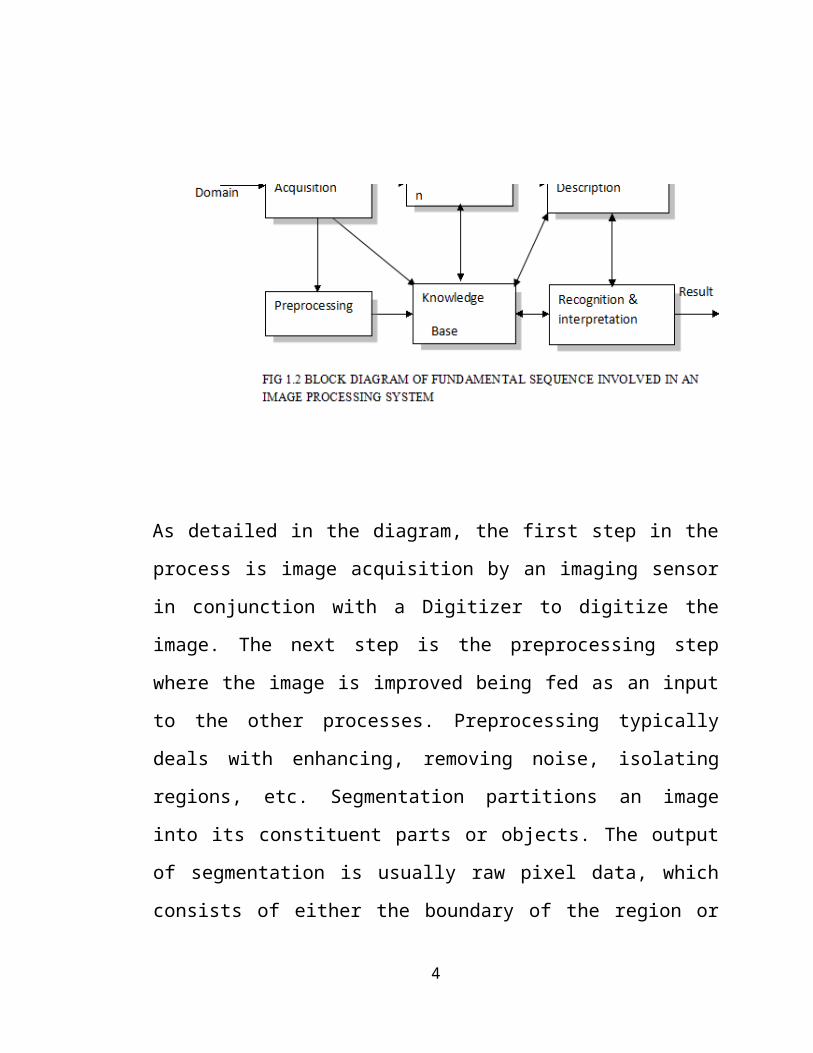
As detailed in the diagram, the first step in the

process is image acquisition by an imaging sensor

in conjunction with a Digitizer to digitize the

image. The next step is the preprocessing step

where the image is improved being fed as an input

to the other processes. Preprocessing typically

deals with enhancing, removing noise, isolating

regions, etc. Segmentation partitions an image

into its constituent parts or objects. The output

of segmentation is usually raw pixel data, which

consists of either the boundary of the region or

4

the pixels in the region themselves.

Representation is the process of transforming the

raw pixel data into a form useful for subsequent

processing by the computer. Description deals with

extracting features that are basic in

differentiating one class of objects from another.

Recognition assigns a label to an object based on

the information provided by its descriptors.

Interpretation involves assigning meaning to an

ensemble of recognized objects. The knowledge

about a problem domain is incorporated into the

knowledge base. The knowledge base guides the

operation of each processing module and also

controls the interaction between the modules. Not

all modules need be necessarily present for a

specific function. The composition of the image

processing system depends on its application. The

frame rate of the image processor is normally

around 25 frames per second.

DIGITAL COMPUTER:

5

Mathematical processing of the digitized image

such as convolution, averaging, addition,

subtraction, etc. are done by the computer.

MASS STORAGE:

The secondary storage devices normally used

are floppy disks, CD ROMs etc.

HARD COPY DEVICE:

The hard copy device is used to produce a

permanent copy of the image and for the storage of

the software involved.

OPERATOR CONSOLE:

The operator console consists of equipment and

arrangements for verification of intermediate

results and for alterations in the software as and

when require. The operator is also capable of

checking for any resulting errors and for the

entry of requisite data.

6

1.1.2 IMAGE PROCESSING FUNDAMENTAL:

Digital image processing refers processing of

the image in digital form. Modern cameras may

directly take the image in digital form but

generally images are originated in optical form.

They are captured by video cameras and

digitalized. The digitalization process includes

sampling, quantization. Then these images are

processed by the five fundamental processes, at

least any one of them, not necessarily all of

them.

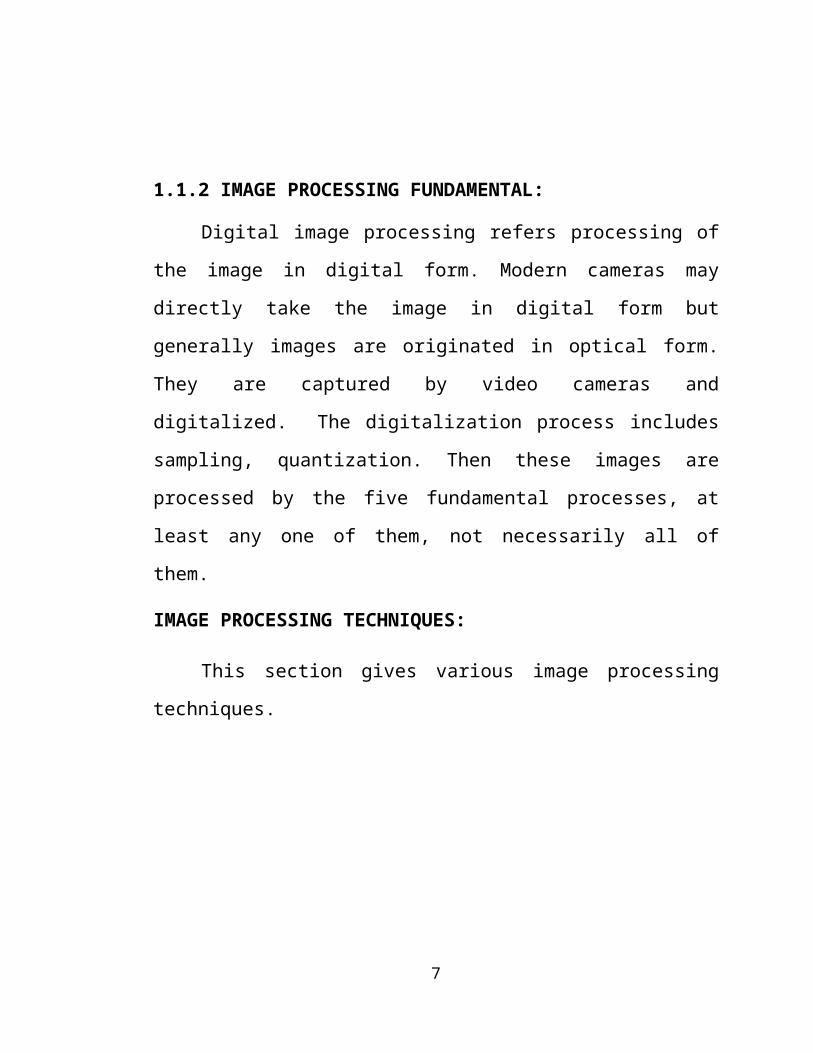
IMAGE PROCESSING TECHNIQUES:

This section gives various image processing

techniques.

7

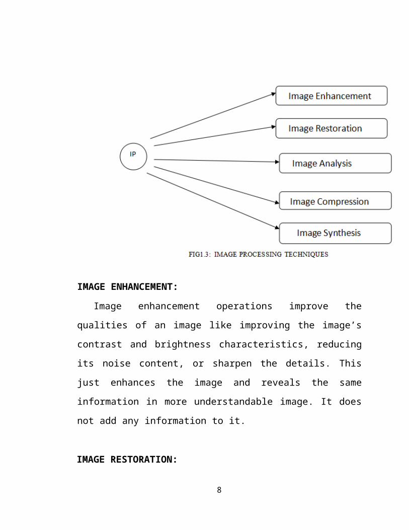
IMAGE ENHANCEMENT:

Image enhancement operations improve the

qualities of an image like improving the image’s

contrast and brightness characteristics, reducing

its noise content, or sharpen the details. This

just enhances the image and reveals the same

information in more understandable image. It does

not add any information to it.

IMAGE RESTORATION:

8

Image restoration like enhancement improves the

qualities of image but all the operations are

mainly based on known, measured, or degradation of

the original image. Image restorations are used to

restore images with problems such as geometric

distortion, improper focus, repetitive noise, and

camera motion. It is used to correct images for

known degradations.

IMAGE ANALYSIS:

Image analysis operations produce numerical or

graphical information based on characteristics of

the original image. They break into objects and

then classify them. They depend on the image

statistics. Common operations are extraction and

description of scene and image features, automated

measurements, and object classification. Image

analyze are mainly used in machine vision

applications.

IMAGE COMPRESSION:

9

Image compression and decompression reduce the

data content necessary to describe the image. Most

of the images contain lot of redundant

information, compression removes all the

redundancies. Because of the compression the size

is reduced, so efficiently stored or transported.

The compressed image is decompressed when

displayed. Lossless compression preserves the

exact data in the original

Image, but Loss compression do not represent the

original image but provide excellent

compression.

IMAGE SYNTHESIS:

Image synthesis operations create images from

other images or non-image data. Image synthesis

operations generally create images that are either

physically impossible or impractical to acquire.

APPLICATIONS OF DIGITAL IMAGE PROCESSING:

10

Digital image processing has a broad spectrum of

applications, such as remote sensing via

satellites and other spacecrafts, image

transmission and storage for business

applications, medical processing, radar, sonar and

acoustic image processing, robotics and automated

inspection of industrial parts.

MEDICAL APPLICATIONS:

In medical applications, one is concerned with

processing of chest X-rays,

cineangiograms, projection images of trans-axial

tomography and other medical images that occur in

radiology, nuclear magnetic resonance (NMR) and

ultrasonic scanning. These images may be used for

patient screening and monitoring or for detection

of tumors’ or other disease in patients.

SATELLITE IMAGING:

Images acquired by satellites are useful in

tracking of earth resources; geographical mapping;

11

prediction of agricultural crops, urban growth and

weather; flood and fire control; and many other

environmental applications. Space image

applications include recognition and analysis of

objects contained in image obtained from deep

space-probe missions.

COMMUNICATION:

Image transmission and storage applications occur

in broadcast television, teleconferencing, and

transmission of facsimile images for office

automation communication of computer networks,

closed-circuit television based security

monitoring systems and in military communications.

RADAR IMAGING SYSTEMS:

Radar and sonar images are used for detection and

recognition of various types of targets or in

guidance and maneuvering of aircraft or missile

systems.

DOCUMENT PROCESSING:

12

It is used in scanning, and transmission for

converting paper documents to a digital image

form, compressing the image, and storing it on

magnetic tape. It is also used in document reading

for automatically detecting and recognizing

printed characteristics.

DEFENSE/INTELLIGENCE:

It is used in reconnaissance photo-interpretation

for automatic interpretation of earth satellite

imagery to look for sensitive targets or military

threats and target acquisition and guidance for

recognizing and tracking targets in real-time

smart-bomb and missile-guidance systems.

1.2 OBJECTIVE AND SCOPE OF THE PROJECT:

A supervised classifier was designed through

combining level-nodule probability and level

context probability. The results from the

experiments on the ELCAP dataset showed promising

performance of our method. We also suggest that

13

the proposed method can be generally applicable to

other medical or general imaging domains.

1.3 EXISTING SYSTEM

In the existing system, we present our preliminary

study on the development of an advanced multiple

thresholding method for the automated detection of

small lung nodules. The method uses a three-step

approach. The first step is to automatically

extract the lungs from MSCT images by analyzing

the volumetric density histogram, thresholding the

original images, and subsequently applying a

morphological operation to the resultant images.

The second step is to identify higher density

structures e.g., nodules, vessels spread

throughout the extracted lungs using a local

density maximum LDM algorithm. The last step is to

reduce false-positive results from the detected

nodule candidates using a priorknowledge of the

lung nodules. The detection method has been

14

validated with computer simulated small lung

nodules.

1.3.1 DISADVANTAGES OF EXISTING SYSTEM

Direct classification from these would still be

problematic.

Contextual information surrounding the lung

nodules could be incorporated to improve nodule

classification is complicated segmentation

process.

Image segmentation is quite hard because of

noise interference.

Overlapped or over placed lung nodules are

difficult to find.

1.3.2 LITERATURE SURVEY

1. AUTOMATIC DETECTION OF SMALL LUNG NODULES ON CT

UTILIZING A LOCAL DENSITY MAXIMUM ALGORITHM,

15

BINSHENG ZHAO*, GORDON GAMSU, MICHELLE S.

GINSBERG, LI JIANG, AND LAWRENCE H. SCHWARTZ-2003

Increasingly, computed tomography (CT) offers

higher resolution and faster acquisition times.

This has resulted in the opportunity to detect

small lung nodules, which may represent lung

cancers at earlier and potentially more curable

stages. However, in the current clinical practice,

hundreds of such thin-sectional CT images are

generated for each patient and are evaluated by a

radiologist in the traditional sense of looking at

each image in the axial mode. This results in the

potential to miss small nodules and thus

potentially miss a cancer. In this paper, we

present a computerized method for automated

identification of small lung nodules on multi

slice CT (MSCT) images. The method consists of

three steps: (i) separation of the lungs from the

other anatomic structures, (ii) detection of

nodule candidates in the extracted lungs, and

16

~iii! Reduction of false-positives among the

detected nodule candidates. A three-dimensional

lung mask can be extracted by analyzing density

histogram of volumetric chest images followed by a

morphological operation. Higher density structures

including nodules scattered throughout the lungs

can be identified by using a local density maximum

algorithm. Information about nodules such as size

and compact shape are then incorporated into the

algorithm to reduce the detected nodule candidates

which are not likely to be nodules. The method was

applied to the detection of computer simulated

small lung nodules (2 to 7 mm in diameter) and

achieved a sensitivity of 84.2% with, on average,

five false-positive results per scan. The

preliminary results demonstrate the potential of

this technique for assisting the detection of

small nodules from chest MSCT images.

2. QUANTIFICATION OF NODULE DETECTION IN CHEST CT:

A CLINICAL INVESTIGATION BASED ON THE ELCAP STUDY

17

AMAL A. FARAG, SHIREEN Y. ELHABIAN, SALWA A.

ELSHAZLY AND ALY A. FARAG– 2008

This paper examines the detection step in

automatic detection and classification of lung

nodules from low-dose CT (LDCT) scans. Two issues

are studied in detail: nodule modeling and

simulation, and the effect of these models on the

detection process. From an ensemble of nodules,

specified by radiologists, we devise an approach

to estimate the gray level intensity distribution

(Hounsfield Units) and a figure of merit of the

size of appropriate templates. Hence, a data-

driven approach is used to design the templates.

The paper presents an extensive study of the

sensitivity and specificity of the nodule

detection step, in which the quality of the nodule

model is the driving factor. Finally, validation

of the detection approach on labeled clinical data

set from the Early Lung Cancer Action Project

(ELCAP) screening study is conducted. Overall,

18

this paper shows a relationship between the

spatial support of the nodule templates and the

resolution of the LDCT, which can be used to

automatically select the template size. The paper

also shows that isotropic templates do not provide

adequate detection rate (in terms of sensitivity

and specificity) of vascularized nodules. The

nodule models in this paper can be used in various

machine learning approaches for automatic nodule

detection and

classification.

3. PARAMETRIC AND NON-PARAMETRIC NODULE MODELS:

DESIGN AND EVALUATION AMAL A. FARAG, JAMES GRAHAM,

ALY A. FARAG, SALWA ELSHAZLY AND ROBERT FALK*-

2007

Lung nodule modeling quality defines the success

of lung nodule detection. This paper presents a

novel method for generating lung nodules using

19

variational level sets to obtain the shape

properties of real nodules to form an average

model template per nodule type. The texture

information used for filling the nodules is based

on a devised approach that uses the probability

density of the radial distance of each nodule to

obtain the maximum and minimum Hounsfield density

(HU). There are two main categories that lung

nodule models fall within; parametric and non-

parametric. The performance of the new nodule

templates will be evaluated during the detection

step and compared with the use of parametric

templates and another non-parametric Active

Appearance model to explain the advantages and/or

disadvantages of using parametric vs. non-

parametric models as well as which variation of

non-parametric template design, i.e., shape based

or shape-texture based yields better results in

the overall detection process.

20

4. COMPUTER ANALYSIS OF COMPUTED TOMOGRAPHY SCANS

OF THE LUNG: A SURVEY INGRID SLUIMER, ARNOLD

SCHILHAM, MATHIAS PROKOP, AND BRAM VAN GINNEKEN *,

MEMBER, IEEE– 2005

In this paper, Current computed tomography (CT)

technology allows for near isotropic, sub

millimeter resolution acquisition of the complete

chest in a single breath hold. These thin-slice

chest scans have become indispensable in thoracic

radiology, but have also substantially increased

the data load for radiologists. Automating the

analysis of such data is, therefore, a necessity

and this has created a rapidly developing research

area in medical imaging. This paper presents a

review of the literature on computer analysis of

the lungs in CT scans and addresses segmentation

of various pulmonary structures, registration of

chest scans, and applications aimed at detection,

classification and quantification of chest

abnormalities. In addition, research trends and

21

challenges are identified and directions for

future research are discussed.

5. EVALUATION OF GEOMETRIC FEATURE DESCRIPTORS FOR

DETECTION AND CLASSIFICATION OF LUNG NODULES IN

LOW DOSE CT SCANS OF THE CHEST AMAL FARAG, ASEM

ALI, JAMES GRAHAM, ALY FARAG, SALWA ELSHAZLY AND

ROBERT FALK*– 2011

This paper examines the effectiveness of geometric

feature descriptors, common in computer vision,

for false positive reduction and for

classification of lung nodules in low dose CT

(LDCT) scans. A data-driven lung nodule modeling

approach creates templates for common nodule

types, using active appearance models (AAM); which

are then used to detect candidate nodules based on

optimum similarity measured by the normalized

cross-correlation (NCC). Geometric feature

descriptors (e.g., SIFT, LBP and SURF) are applied

to the output of the detection step, in order to

22

extract features from the nodule candidates, for

further enhancement of output and possible

reduction of false positives. Results on the

clinical ELCAP database showed that the

descriptors provide 2% enhancements in the

specificity of the detected nodule above the NCC

results when used in a k-NN classifier. Thus

quantitative measures of enhancements of the

performance of CAD models based on LDCT are now

possible and are entirely model-based most

importantly; our approach is applicable for

classification of nodules into categories and

pathologies.

1.4 PROPOSED SYSTEM

This paper presents a novel image classification

method for the four common types of lung nodules.

We suggest that the major contributions of our

work are as follows: i) a patch-based image

representation with multilevel concentric

partition, ii) a feature set design for image

patch description, and iii) a contextual latent

23

semantic analysis-based classifier to calculate

the probabilistic estimations for each lung nodule

image. More specifically, a concentric level

partition of the image is designed in an adaptive

manner with: (1) an improved super pixel

clustering method based on quick shift is designed

to generate the patch division; (2) multilevel

partition of the derived patches is used to

construct level-nodule (i.e., -patches containing

the nodules), and level-context (i.e., patches

containing the contextual structures).A concentric

level partition is thus constructed to tackle the

rigid partitioning problem.

Second, a feature set of three components is

extracted for each patch of the image that are as

follows: (1) a SIFT descriptor, depicting the

overall intensity, texture, and gradient

information; (2) a MR8+LBP descriptor,

representing a richer texture feature

incorporating MR8 filters before calculating LBP

histograms; (3) a multi orientation HOG

24

descriptor, describing the gradients and

accommodating rotation variance in a multi

coordinate system.

Third, the category of the lung nodule image is

finally determined with a probabilistic estimation

based on the combination of the nodule structure

and surrounding anatomical context: (1) SVM is

used to compute the classification probability

based on level-nodule; (2) pLSA with contextual

voting is employed to calculate the classification

probability based on level-context. The designed

classifier can obtain better classification

accuracy, with SVM capturing the differences from

various nodules, and pLSA further revising the

decision by analyzing the context.

25

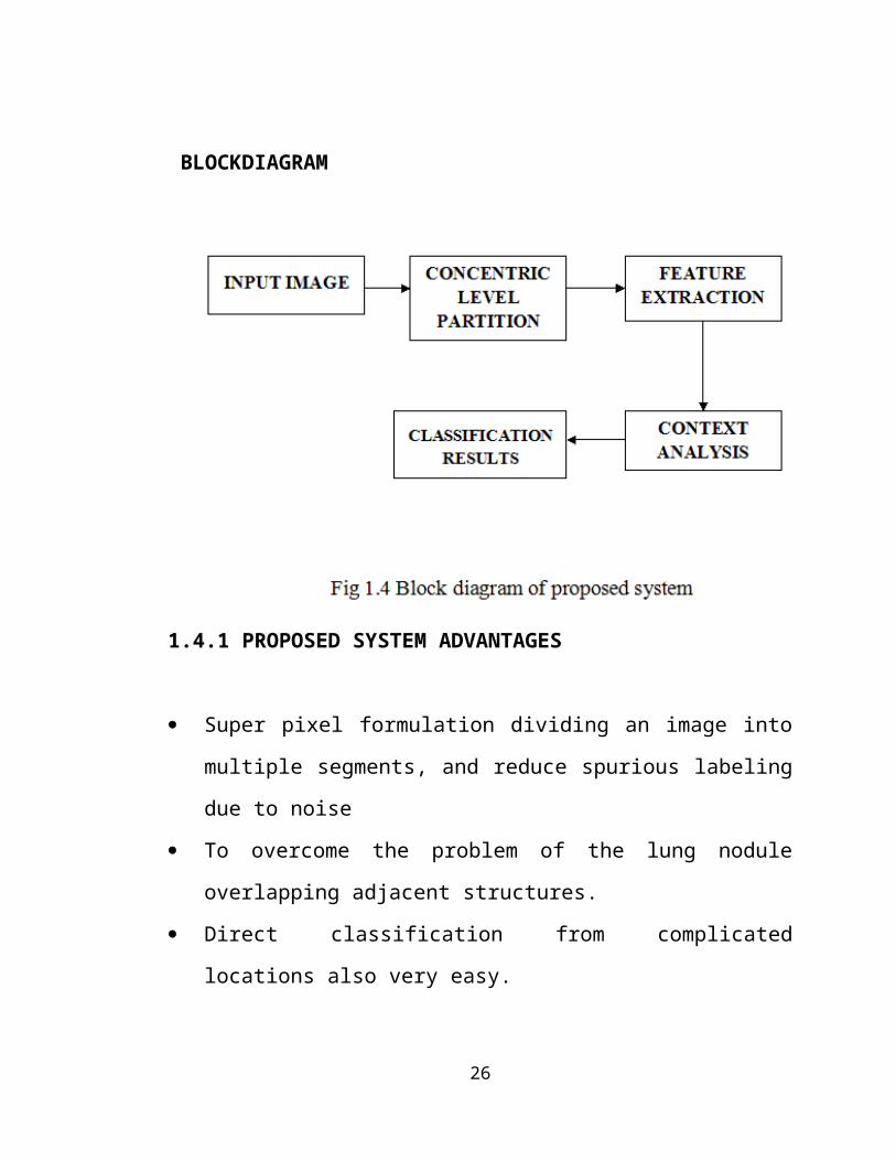
BLOCKDIAGRAM

1.4.1 PROPOSED SYSTEM ADVANTAGES

Super pixel formulation dividing an image into

multiple segments, and reduce spurious labeling

due to noise

To overcome the problem of the lung nodule

overlapping adjacent structures.

Direct classification from complicated

locations also very easy.

26

Contextual information surrounding the lung

nodules will be more useful to improve nodule

classification in segmentation process.

27

CHAPTER 2

PROJECT DESCRIPTION

2.1 INTRODUCTION:

LUNG cancer is a major cause of cancer-related

deaths in humans worldwide. Approximately 20% of

cases with lung nodules represent lung cancers;

therefore, the identification of potentially

malignant lung nodules is essential for the

screening and diagnosis of lung cancer. Lung

nodules are small masses in the human lung, and

are usually spherical; however, they can be

distorted by surrounding anatomical structures,

such as vessels and the adjacent pleura.

Intraparenchymal lung nodules are more likely to

be malignant than those connected with the

surrounding structures, and thus lung nodules are

divided into different types according to their

relative positions. At present, the classification

from Diciotti et al. is the most popular approach and

it d

28

vides nodules into four types: well-circumscribed

(W) with the nodule located centrally in the lung

without any connection to vasculature;

vascularized (V) with the nodule located centrally

in the lung but closely connected to neighboring

vessels; juxta-pleural (J) with a large portion of

the nodule connected to the pleural surface; and

pleural-tail (P) with the nodule near the pleural

surface connected by a thin tail.

Computed tomography (CT) is the most accurate

imaging modality to obtain anatomical information

about lung nodules and the surrounding structures.

In current clinical practice, however,

interpretation of CT images is challenging for

radiologists due to the large number of cases.

This manual reading can be error-prone and the

reader may miss nodules and thus a potential

cancer. Computer-aided diagnosis (CAD) systems

would be helpful for radiologists by offering

initial screening or second opinions to classify

lung nodules. CAD s provide depiction by

29

automatically computing quantitative measures, and

are capable of analyzing the large number of small

nodules identified by CT scans.

Increasingly, computed tomography (CT) offers

higher resolution and faster acquisition times.

This has resulted in the opportunity to detect

small lung nodules, which may represent lung

cancers at earlier and potentially more curable

stages. However, in the current clinical practice,

hundreds of such thin-sectional CT images are

generated for each patient and are evaluated by a

radiologist in the traditional sense of looking at

each image in the axial mode. This results in the

potential to miss small nodules and thus

potentially miss a cancer. In this paper, we

present a computerized method for automated

identification of small lung nodules on multi

slice images.

2.2 BASIC OPERATORS:

The basic operations are shift-invariant

(translation invariant) operators strongly related

30

to Minkowski addition. Let E be a Euclidean space

or an integer grid, and A binary image in E.

EROSION:

The erosion of the dark-blue square by a disk,

resulting in the light-blue square. The erosion of

the binary image A by the structuring element B is

defined by: where Bz is the translation of B by the

vector z, i.e., ,.When the structuring element B

has a center (e.g., B is a disk or a square), and

this center is located on the origin of E, then

the erosion of A by B can be understood as the

locus of points reached by the center of B when B

moves inside A. For example, the erosion of a

square of side 10, centered at the origin, by a

disc of radius 2, also centered at the origin, is

a square of side 6 centered at the origin. The

erosion of A by B is also given by the expression:

Example application: Assume we have received a fax

of a dark photocopy. Everything looks like it was

written with a pen that is bleeding. Erosion

31

process will allow thicker lines to get skinny and

detect the hole inside the letter "o".

DILATION:

The dilation of the dark-blue square by a disk,

resulting in the light-blue square with rounded

corners. The dilation of A by the structuring

element B is defined by: The dilation is

commutative, also given by: If B has a center on

the origin, as before, and then the dilation of A

by B can be understood as the locus of the points

covered by B when the center of B moves inside A.

In the above example, the dilation of the square

of side 10 by the disk of radius 2 is a square of

side 14, with rounded corners, centered at the

origin. The radius of the rounded corners is 2.The

dilation can also be obtained by, where Bs denotes

the symmetric of B, that.

Example application: Dilation is the dual

operation of the erosion. Figures that are very

lightly drawn get thick when "dilated". Easiest

32

way to describe it is to imagine the same fax/text

is written with a thicker pen.

OPENING:

The opening of the dark-blue square by a disk,

resulting in the light-blue square with round

corners. The opening of A by B is obtained by the

erosion of A by B, followed by dilation of the

resulting image by B:

The opening is also given by, which means that

it is the locus of translations of the structuring

element B inside the image A. In the case of the

square of side 10, and a disc of radius 2 as the

structuring element, the opening is a square of

side 10 with rounded corners, where the corner

radius is 2.

Example application: Let's assume someone has

written a note on a non-soaking paper and that the

writing looks as if it is growing tiny hairy roots

all over. Opening essentially removes the outer

33

tiny "hairline" leaks and restores the text. The

side effect is that it rounds off things. The

sharp edges start to disappear.

CLOSING:

The closing of the dark-blue shape (union of two

squares) by a disk, resulting in the union of the

dark-blue shape and the light-blue areas. The

closing of A by B is obtained by the dilation of A

by B, followed by erosion of the resulting

structure by B:

The closing can also be obtained by, where Xc

denotes the complement of X relative to E (that

is,). The above means that the closing is the

complement of the locus of translations of the

symmetric of the structuring element outside the

image A.

34

PROPERTIES OF THE BASIC OPERATORS:

Here are some properties of the basic binary

morphological operators (dilation, erosion,

opening and closing):

They are translation invariant.

They are increasing, that is, if, then, and,

etc.

The dilation is commutative.

If the origin of E belongs to the structuring

element B, then.

The dilation is associative, i.e. moreover,

the erosion satisfies.

Erosion and dilation satisfy the duality.

Opening and closing satisfy the duality.

The dilation is distributive over set union

The erosion is distributive over set

intersection

The dilation is a pseudo-inverse of the

erosion, and vice-versa, in the following

sense: if and only if.

35

Opening and closing are idempotent. Opening is

anti-extensive, i.e., , whereas the closing is

extensive, i.e.,.

GRAYSCALE MORPHOLOGY:

Watershed of the gradient of the cardiac image In

gray scale morphology, images are functions

mapping a Euclidean space or grid E into, where is

the set of reals, is an element larger than any

real number, and is an element smaller than any

real number. Gray scale structuring elements are

also functions of the same format, called

"structuring functions". Denoting an image by f(x)

and the structuring function by b(x), the gray

scale dilation of f by b is given by where "sup"

denotes the supremum. Similarly, the erosion of f

by b is given by, where "inf" denotes the

Infamous. Just like in binary morphology; the

opening and closing are given

respectively.

36

FLAT STRUCTURING FUNCTIONS:

It is common to use flat structuring elements in

morphological applications. Flat structuring

functions are functions b(x) in the form where. In

this case, the dilation and erosion are greatly

simplified, and given respectively by in the

bounded, discrete case (E is a grid and B is

bounded), the supremum and infimum operators can

be replaced by the maximum and minimum. Thus,

dilation and erosion are particular cases of order

statistics filters, with dilation returning the

maximum value within a moving window (the

symmetric of the structuring function support B),

and the erosion returning the minimum value within

the moving window B.

In the case of flat structuring element, the

morphological operators depend only on the

relative ordering of pixel values, regardless

their numerical values, and therefore are

especially suited to the processing of binary

37

images and gray scale images whose light transfer

function is not known.

By combining these operators one can obtain

algorithms for many image processing tasks, such

as feature detection, image segmentation, image

sharpening, image filtering, and classification.

Along this line one should also look into

Continuous Morphology.

MATHEMATICAL MORPHOLOGY ON COMPLETE LATTICES:

Complete lattices are partially ordered sets,

where every subset has an infimum and a supremum.

In particular, it contains a least element and a

greatest element (also denoted "universe").

ADJUNCTIONS (DILATION AND EROSION):

Let be a complete lattice, with infimum and

supremum symbolized by and, respectively. Its

universe and least element are symbolized by U

38

and, respectively. Moreover, let be a collection

of elements from L. Dilation is any operator that

distributes over the supremum, and preserves the

least element. I.e. Erosion is any operator that

distributes over the infimum, and preserves the

universe. I.e. Dilations and erosions form Galois

connections. That is,for every dilation there is

one and only one erosion that satisfies for all.

Similarly, for every erosion there is one and only

one dilation satisfying the above connection.

Furthermore, if two operators satisfy the

connection, then must be dilation, and erosion.

Pairs of erosions and dilations satisfying the

above connection are called "adjunctions", and the

erosion is said to be the ad joint erosion of the

dilation, and vice-versa.

OPENING AND CLOSING:

For every adjunction, the morphological opening

and morphological closing are defined as follows:

39

The morphological opening and closing are

particular cases of algebraic opening (or simply

opening) and algebraic closing (or simply

closing). Algebraic openings are operators in L

that are idempotent, increasing, and anti-

extensive. Algebraic closings are operators in L

that are idempotent, increasing, and extensive.

PARTICULAR CASES:

Binary morphology is a particular case of lattice

morphology, where L is the power set of E

(Euclidean space or grid), that is, L is the set

of all subsets of E, and is the set inclusion. In

this case, the infimum is set intersection, and

the supremum is set union.

2.3 IMAGE SEGMENTATION BY CLUSTERING PIXELS

Clustering is a process whereby a data set is

replaced by clusters, which are collections of

data points that “belong together”. It is natural

to think of image segmentation as clustering; we

40

would like to represent an image in terms of

clusters of pixels that “belong together”. The

specific criterion to be used depends on the

application. Pixels may belong together because

they have the same colour and/or they have the

same texture and/or they are nearby, etc.

2.3.1 SIMPLE CLUSTERING METHODS:

It is relatively easy to take a clustering method

and build an image segmenter from it. Much of the

literature on image segmentation consists of

papers that are, in essence, papers about

clustering (though this isn’t always

acknowledged). The distance used depends entirely

on the application, but measures of color

difference and of texture are commonly used as

clustering distances. It is often desirable to

have clusters that are “blobby”; this can be

achieved by using difference in position in the

clustering distance. The main difficulty in using

41

either agglomerative or divisive clustering

methods directly is that there are an awful lot of

pixels in an image. There is no reasonable

prospect of examining a dendrogram, because the

quantity of data means that it will be too big.

Furthermore, the mechanism is suspect; we don’t

really want to look at a dendrogram for each

image, but would rather have the segmenter produce

useful regions for an application on a long

sequence of images without any help. In practice,

this means that the segmenters decide when to stop

splitting or merging by using a set of threshold

tests — for example, an agglomerative segmenter

may stop merging when the distance between

clusters is sufficiently low, or when the number

of clusters reaches some value. The choice of

thresholds is usually made by observing the

behavior of the segmenter on a variety of images,

and choosing the best setting. The technique has

largely fallen into disuse except in specialized

applications, because in most cases it is very

42

difficult to predict the future performance of the

segmenter tuned in this way.

Another difficulty created by the number of pixels

is that it is impractical to look for the best

split of a cluster (for a divisive method) or the

best merge (for an agglomerative method). The

variety of tricks that have been adopted to

address this problem is far too large to survey

here, but we can give an outline of the main

strategies.

2.3.1.1 K-MEANS CLUSTERING METHOD

Simple clustering methods use greedy interactions

with existing clusters to come up with a good

overall representation. For example, in

agglomerative clustering we repeatedly make the

best available merge. However, the methods are not

explicit about the objective function that the

methods are attempting to optimize. An alternative

approach is to write down an objective function

that expresses how good a representation is, and

43

then build an algorithm for obtaining the best

representation. A natural objective function can

be obtained by assuming that we know there are k

clusters, where k is known. Each cluster is

assumed to have a center; we write the center of

the i’th cluster as ci. The j’th element to be

clustered is described by a feature vector xj .

For example, if we were segmenting scattered

points, then x would be the coordinates of the

points; if we were segmenting an intensity image,

x might be the intensity at a pixel.

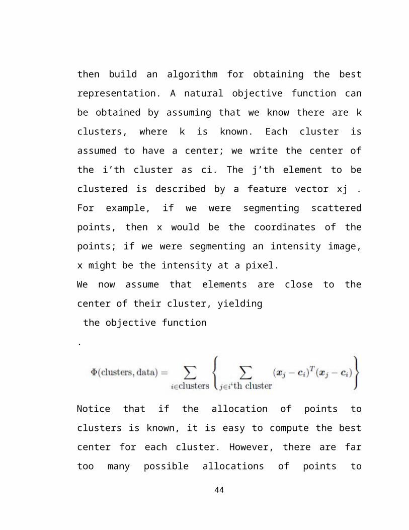
We now assume that elements are close to the

center of their cluster, yielding

the objective function

.

Notice that if the allocation of points to

clusters is known, it is easy to compute the best

center for each cluster. However, there are far

too many possible allocations of points to

44

clusters to search this space for a minimum.

Instead, we define an algorithm which iterates

through two activities:

Assume the cluster centers are known, and

allocate each point to the closest cluster

center.

Assume the allocation is known, and choose a

new set of cluster centers. Each center is the

mean of the points allocated to that cluster.

2.3.1.2 GRAPH-THEORETIC CLUSTERING METHOD

Clustering can be seen as a problem of cutting

graphs into “good” pieces. In effect, we associate

each data item with a vertex in a weighted graph,

where the weights on the edges between elements

are large if the elements are “similar” and small

if they are not. We then attempt to cut the graph

into connected components with relatively large

interior weights — which correspond to clusters —

by cutting edges with relatively low weights. This

view leads to a series of different, quite

successful, segmentation algorithms.

45

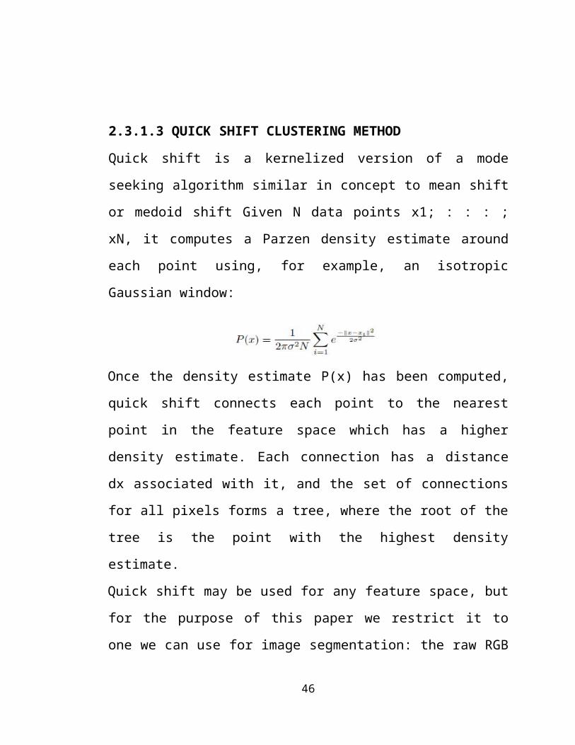
2.3.1.3 QUICK SHIFT CLUSTERING METHOD

Quick shift is a kernelized version of a mode

seeking algorithm similar in concept to mean shift

or medoid shift Given N data points x1; : : : ;

xN, it computes a Parzen density estimate around

each point using, for example, an isotropic

Gaussian window:

Once the density estimate P(x) has been computed,

quick shift connects each point to the nearest

point in the feature space which has a higher

density estimate. Each connection has a distance

dx associated with it, and the set of connections

for all pixels forms a tree, where the root of the

tree is the point with the highest density

estimate.

Quick shift may be used for any feature space, but

for the purpose of this paper we restrict it to

one we can use for image segmentation: the raw RGB

46

values augmented with the (x; y) position in the

image. So, the feature space is -ve dimensional:

(r; g; b; x; y).

To adjust the trade-o_ between the importance of

the color and spatial components of the feature

space, we simply pre-scale the (r; g; b) values by

a parameter, which for these experiments we x at =

0:5. To obtain segmentation from a tree of links

formed by quick shift, we choose a threshold and

break all links in the tree with dx. The pixels

which are a member of each resulting disconnected

tree form each segment.

47

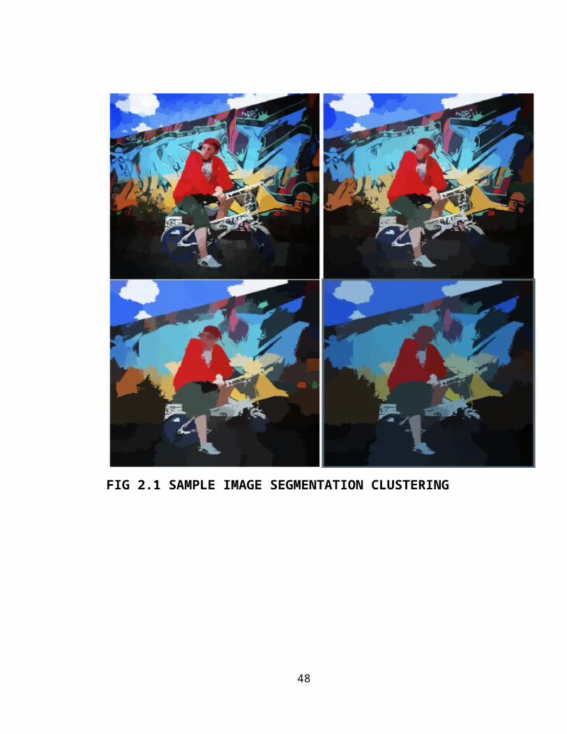
FIG 2.1 SAMPLE IMAGE SEGMENTATION CLUSTERING

48

2.4 FEATURE EXTRACTION

In pattern recognition and in image

processing, feature extraction is a special

form of dimensionality reduction. When the input

data to an algorithm is too large to be processed

and it is suspected to be very redundant (e.g. the

same measurement in both feet and meters, or the

repetitiveness of images presented as pixels),

then the input data will be transformed into a

reduced representation set of features (also named

features vector). Transforming the input data into

the set of features is called feature extraction.

If the features extracted are carefully chosen it

is expected that the features set will extract the

relevant information from the input data in order

to perform the desired task using this reduced

representation instead of the full size input.

2.4.1 SCALE-INVARIANT FEATURE TRANSFORM

49

For any object in an image, interesting points on

the object can be extracted to provide a "feature

description" of the object. This description,

extracted from a training image, can then be used

to identify the object when attempting to locate

the object in a test image containing many other

objects. To perform reliable recognition, it is

important that the features extracted from the

training image be detectable even under changes in

image scale, noise and illumination. Such points

usually lie on high-contrast regions of the image,

such as object edges.

Another important characteristic of these features

is that the relative positions between them in the

original scene shouldn't change from one image to

another. For example, if only the four corners of

a door were used as features, they would work

regardless of the door's position; but if points

in the frame were also used, the recognition would

fail if the door is opened or closed. Similarly,

features located in articulated or flexible

50

objects would typically not work if any change in

their internal geometry happens between two images

in the set being processed. However, in practice

SIFT detects and uses a much larger number of

features from the images, which reduces the

contribution of the errors caused by these local

variations in the average error of all feature

matching errors.

SIFT can robustly identify objects even among

clutter and under partial occlusion, because the

SIFT feature descriptor is invariant to uniform

scaling, orientation, and partially invariant

to affine distortion and illumination changes.

This section summarizes Lowe's object recognition

method and mentions a few competing techniques

available for object recognition under clutter and

partial occlusion.

SIFT key points

SIFT key points of objects are first extracted

from a set of reference images and stored in a

51

database. An object is recognized in a new image

by individually comparing each feature from the

new image to this database and finding candidate

matching features based on Euclidean distance of

their feature vectors. From the full set of

matches, subsets of key points that agree on the

object and its location, scale, and orientation in

the new image are identified to filter out good

matches. The determination of consistent clusters

is performed rapidly by using an efficient hash

table implementation of the generalized Hough

transform. Each cluster of 3 or more features that

agree on an object and its pose is then subject to

further detailed model verification and

subsequently outliers are discarded. Finally the

probability that a particular set of features

indicates the presence of an object is computed,

given the accuracy of fit and number of probable

false matches. Object matches that pass all these

tests can be identified as correct with high

confidence.

52

Scale-invariant feature detection

Lowe's method for image feature generation

transforms an image into a large collection of

feature vectors, each of which is invariant to

image translation, scaling, and rotation,

partially invariant to illumination changes and

robust to local geometric distortion. These

features share similar properties with neurons in

inferior temporal cortex that are used for object

recognition in primate vision. Key locations are

defined as maxima and minima of the result

of difference of Gaussians function applied

in scale space to a series of smoothed and

resampled images. Low contrast candidate points

and edge response points along an edge are

discarded. Dominant orientations are assigned to

localized keypoints. These steps ensure that the

keypoints are more stable for matching and

recognition. SIFT descriptors robust to local

affine distortion are then obtained by considering

pixels around a radius of the key location,

53

blurring and resampling of local image orientation

planes.

Comparison of SIFT features with other local

features

There has been an extensive study done on the

performance evaluation of different local

descriptors, including SIFT, using a range of

detectors. The main results are summarized below:

SIFT and SIFT-like GLOH features exhibit the

highest matching accuracies (recall rates) for

an affine transformation of 50 degrees. After

this transformation limit, results start to

become unreliable.

Distinctiveness of descriptors is measured by

summing the eigenvalues of the descriptors,

obtained by the Principal components

analysis of the descriptors normalized by

their variance. This corresponds to the amount

of variance captured by different descriptors,

54

therefore, to their distinctiveness. PCA-SIFT

(Principal Components Analysis applied to SIFT

descriptors), GLOH and SIFT features give the

highest values.

SIFT-based descriptors outperform other

contemporary local descriptors on both

textured and structured scenes, with the

difference in performance larger on the

textured scene.

For scale changes in the range 2-2.5 and image

rotations in the range 30 to 45 degrees, SIFT

and SIFT-based descriptors again outperform

other contemporary local descriptors with both

textured and structured scene content.

Introduction of blur affects all local

descriptors, especially those based on edges,

like shape context, because edges disappear in

the case of a strong blur. But GLOH, PCA-SIFT

and SIFT still performed better than the

55

others. This is also true for evaluation in

the case of illumination changes.

The evaluations carried out suggests strongly that

SIFT-based descriptors, which are region-based,

are the most robust and distinctive, and are

therefore best suited for feature matching.

However, most recent feature descriptors such

as SURF have not been evaluated in this study.

SURF has later been shown to have similar

performance to SIFT, while at the same time being

much faster. Another study concludes that when

speed is not critical, SIFT outperforms SURF.

Recently, a slight variation of the descriptor

employing an irregular histogram grid has been

proposed that significantly improves its

performance. Instead of using a 4x4 grid of

histogram bins, all bins extend to the center of

the feature. This improves the descriptor's

robustness to scale changes.

56

The SIFT-Rank descriptor was shown to improve the

performance of the standard SIFT descriptor for

affine feature matching. A SIFT-Rank descriptor is

generated from a standard SIFT descriptor, by

setting each histogram bin to its rank in a sorted

array of bins. The Euclidean distance between

SIFT-Rank descriptors is invariant to arbitrary

monotonic changes in histogram bin values, and is

related to Spearman's rank correlation

coefficient.

2.5 FILTER BANKS

We describe the rotationally invariant MR filter

sets that are used in the algorithm

for classifying textures with filter banks. We

also describe two other filter sets (LM and S)

that will be used in classification comparisons.

The aspects of interest are the dimension of the

filter space, and whether the filter set is

rotationally invariant or not.

57

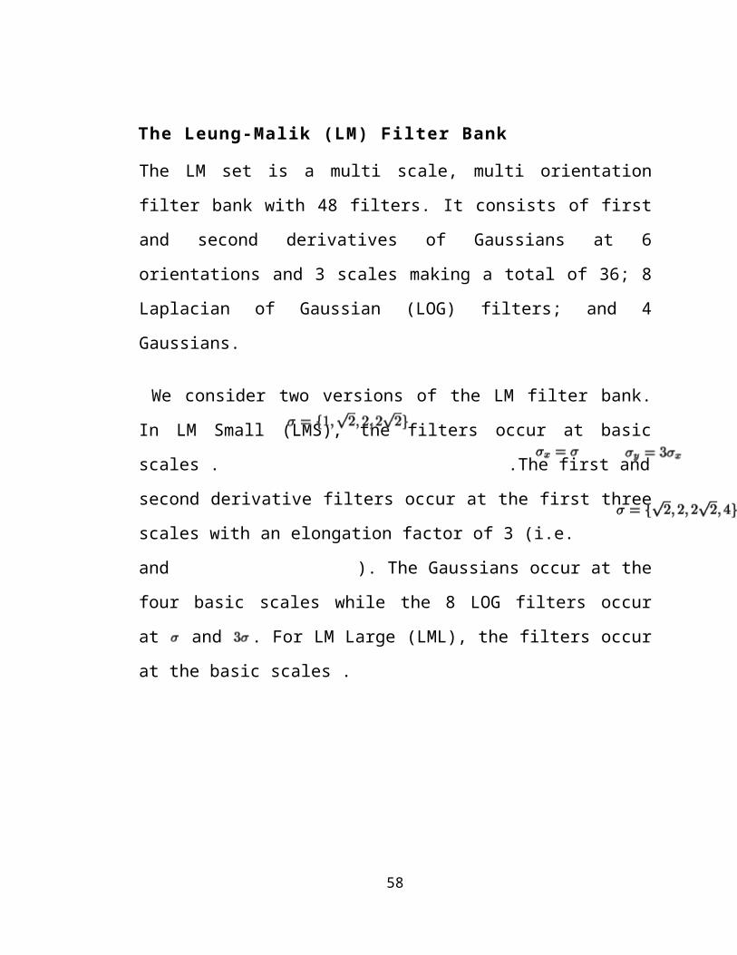
The Leung-Malik (LM) Filter Bank

The LM set is a multi scale, multi orientation

filter bank with 48 filters. It consists of first

and second derivatives of Gaussians at 6

orientations and 3 scales making a total of 36; 8

Laplacian of Gaussian (LOG) filters; and 4

Gaussians.

We consider two versions of the LM filter bank.

In LM Small (LMS), the filters occur at basic

scales . .The first and

second derivative filters occur at the first three

scales with an elongation factor of 3 (i.e.  

and  ). The Gaussians occur at the

four basic scales while the 8 LOG filters occur

at   and  . For LM Large (LML), the filters occur

at the basic scales .

58

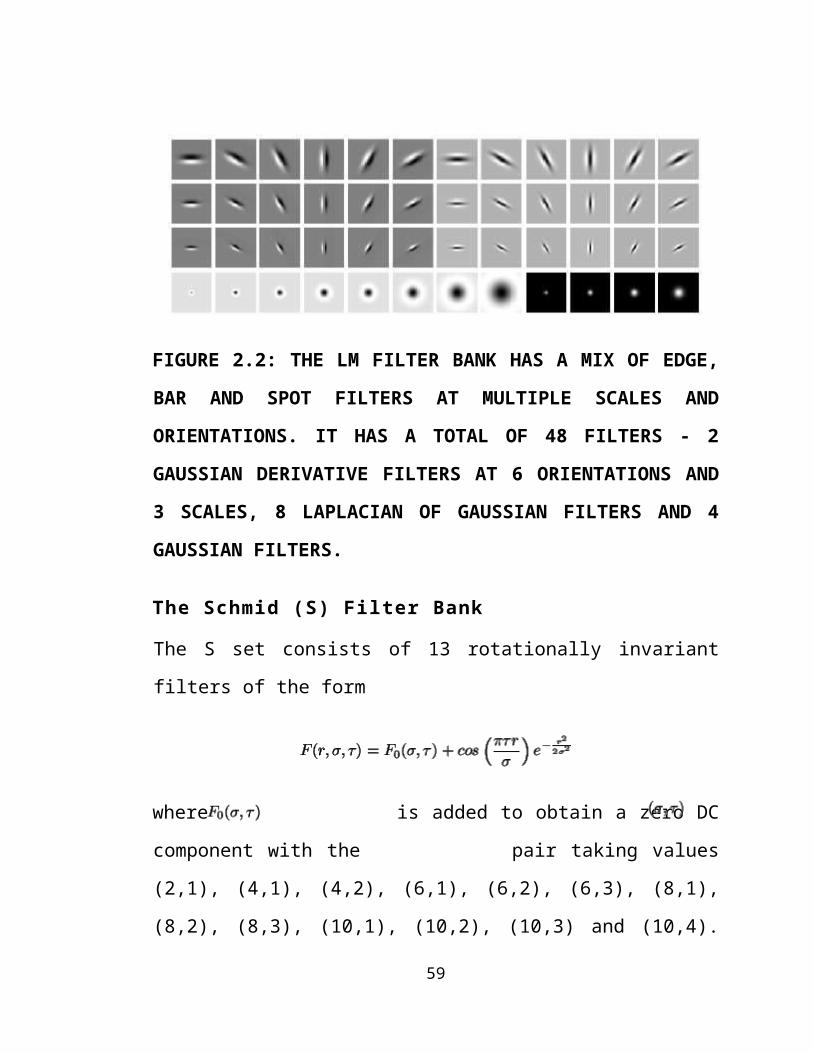
FIGURE 2.2: THE LM FILTER BANK HAS A MIX OF EDGE,

BAR AND SPOT FILTERS AT MULTIPLE SCALES AND

ORIENTATIONS. IT HAS A TOTAL OF 48 FILTERS - 2

GAUSSIAN DERIVATIVE FILTERS AT 6 ORIENTATIONS AND

3 SCALES, 8 LAPLACIAN OF GAUSSIAN FILTERS AND 4

GAUSSIAN FILTERS.

The Schmid (S) Filter Bank

The S set consists of 13 rotationally invariant

filters of the form

where    is added to obtain a zero DC

component with the   pair taking values

(2,1), (4,1), (4,2), (6,1), (6,2), (6,3), (8,1),

(8,2), (8,3), (10,1), (10,2), (10,3) and (10,4).

59

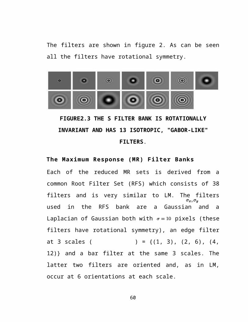
The filters are shown in figure 2. As can be seen

all the filters have rotational symmetry.

FIGURE2.3 THE S FILTER BANK IS ROTATIONALLY

INVARIANT AND HAS 13 ISOTROPIC, "GABOR-LIKE"

FILTERS.

The Maximum Response (MR) Filter Banks

Each of the reduced MR sets is derived from a

common Root Filter Set (RFS) which consists of 38

filters and is very similar to LM. The filters

used in the RFS bank are a Gaussian and a

Laplacian of Gaussian both with   pixels (these

filters have rotational symmetry), an edge filter

at 3 scales ( ) = {(1, 3), (2, 6), (4,

12)} and a bar filter at the same 3 scales. The

latter two filters are oriented and, as in LM,

occur at 6 orientations at each scale.

60

To achieve rotational invariance, we derive the

Maximum Response 8 (MR8) filter bank from RFS by

recording only the maximum filter response across

all orientations for the two anisotropic filters.

Measuring only the maximum response across

orientations reduces the number of responses from

38 (6 orientations at 3 scales for 2 oriented

filters, plus 2 isotropic) to 8 (3 scales for 2

filters, plus 2 isotropic). Thus, the MR8 filter

bank consists of 38 filters but only 8 filter

responses.

61

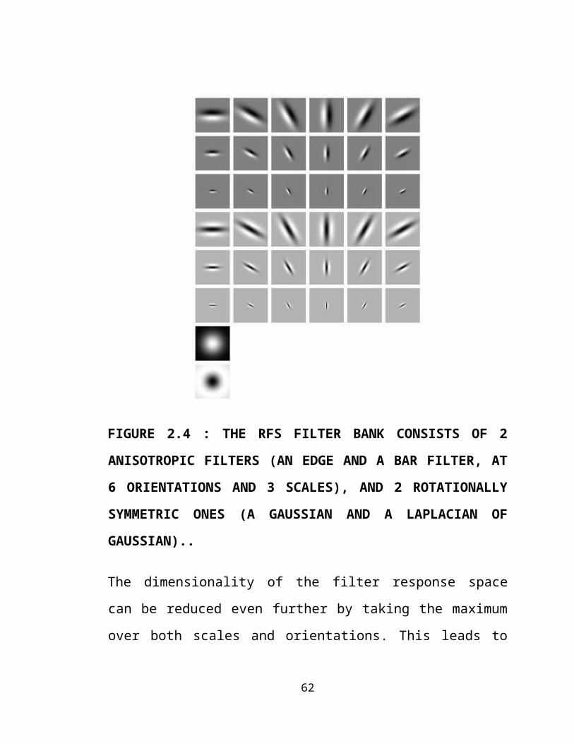
FIGURE 2.4 : THE RFS FILTER BANK CONSISTS OF 2

ANISOTROPIC FILTERS (AN EDGE AND A BAR FILTER, AT

6 ORIENTATIONS AND 3 SCALES), AND 2 ROTATIONALLY

SYMMETRIC ONES (A GAUSSIAN AND A LAPLACIAN OF

GAUSSIAN)..

The dimensionality of the filter response space

can be reduced even further by taking the maximum

over both scales and orientations. This leads to

62

the MRS4 filter bank. In it, each of the 4

different types of filters contributes only a

single response. As in MR8, the responses of the

two isotropic filters (Gaussian and LOG) are

recorded directly. However, for each of the

anisotropic filters, the maximum response is taken

over both orientations and scale again giving a

single response per filter type. With proper

normalization, MRS4 is both rotation and scale

invariant.

Finally, we also consider the MR4 filter bank

where we only look at filters at a single scale.

Thus, the MR4 filter bank is a subset of the MR8

filter bank where the oriented edge and bar

filters occur at a single fixed scale

( ) = (4, 1 2).

The motivation for introducing these MR filters

sets is twofold. The first is to overcome the

limitations of traditional rotationally invariant

filters which do not respond strongly to oriented

63

image patches and thus do not provide good

features for anisotropic textures. However, since

the MR sets contain both isotropic filters as well

as anisotropic filters at multiple orientations

they are expected to generate good features for

all types of textures. Additionally, unlike

traditional rotationally invariant filters, the MR

sets are also able to record the angle of maximum

response. This enables us to compute higher order

co-occurrence statistics on orientation and such

statistics may prove useful in discriminating

textures which appear to be very similar.

The second motivation arises out of a concern

about the dimensionality of the filter response

space. Quite apart from the extra processing and

computational costs involved, the higher the

dimensionality, the harder the clustering problem.

In general, not only does the number of cluster

centers needed to cover the space rise

dramatically, so does the amount of training data

64

required to reliably estimate each cluster centre.

This is mitigated to some extent by the fact that

texture features are sparse and can lie in lower

dimensional sub spaces. However, the presence of

noise and the difficulty in finding and projecting

onto these lower dimensional sub spaces can

counter these factors. Therefore, it is expected

that the MR filter banks should generate more

significant textons not only because of improved

clustering in a lower dimensional space but also

because rotated features are correctly mapped to

the same textons.

Histogram of oriented gradients

The essential thought behind the Histogram of

Oriented Gradient descriptors is that local object

appearance and shape within an image can be

described by the distribution of intensity

gradients or edge directions. The implementation

of these descriptors can be achieved by dividing

the image into small connected regions, called

65

cells, and for each cell compiling a histogram of

gradient directions or edge orientations for the

pixels within the cell. The combination of these

histograms then represents the descriptor. For

improved accuracy, the local histograms can be

contrast-normalized by calculating a measure of

the intensity across a larger region of the image,

called a block, and then using this value to

normalize all cells within the block. This

normalization results in better invariance to

changes in illumination or shadowing.

The HOG descriptor maintains a few key advantages

over other descriptor methods. Since the HOG

descriptor operates on localized cells, the method

upholds invariance to geometric and photo metric

transformations, except for object orientation.

Such changes would only appear in larger spatial

regions. Moreover, as Dalal and Triggs discovered,

coarse spatial sampling, fine orientation

sampling, and strong local photo metric

normalization permits the individual body movement

66

of pedestrians to be ignored so long as they

maintain a roughly upright position. The HOG

descriptor is thus particularly suited for human

detection in images.

Gradient computation

The first step of calculation in many feature

detectors in image pre-processing is to ensure

normalized color and gamma values. As Dalal and

Triggs point out, however, this step can be

omitted in HOG descriptor computation, as the

ensuing descriptor normalization essentially

achieves the same result. Image pre-processing

thus provides little impact on performance.

Instead, the first step of calculation is the

computation of the gradient values. The most

common method is to simply apply the 1-D centered,

point discrete derivative mask in one or both of

the horizontal and vertical directions.

Specifically, this method requires filtering the

color or intensity data of the image with the

following filter kernels:

67

[-1; 0; 1] and [-1; 0; 1]T

Dalal and Triggs tested other, more complex masks,

such as 3x3 Sobel masks (Sobel operator) or

diagonal masks, but these masks generally

exhibited poorer performance in human image

detection experiments. They also experimented with

Gaussian smoothing before applying the derivative

mask, but similarly found that omission of any

smoothing performed better in practice.

Orientation binning

The second step of calculation involves creating

the cell histograms. Each pixel within the cell

casts a weighted vote for an orientation-based

histogram channel based on the values found in the

gradient computation. The cells themselves can

either be rectangular or radial in shape, and the

histogram channels are evenly spread over 0 to 180

degrees or 0 to 360 degrees, depending on whether

the gradient is “unsigned” or “signed”. Dalal and

Triggs found that unsigned gradients used in

68

conjunction with 9 histogram channels performed

best in their human detection experiments. As for

the vote weight, pixel contribution can either be

the gradient magnitude itself, or some function of

the magnitude; in actual tests the gradient

magnitude itself generally produces the best

results.

Descriptor blocks

In order to account for changes in illumination

and contrast, the gradient strengths must be

locally normalized, which requires grouping the

cells together into larger, spatially connected

blocks. The HOG descriptor is then the vector of

the components of the normalized cell histograms

from all of the block regions. These blocks

typically overlap, meaning that each cell

contributes more than once to the final

69

descriptor. Two main block geometries exist:

rectangular R-HOG blocks and circular CHOG blocks.

R-HOG blocks are generally square grids,

represented by three parameters: the number of

cells per block, the number of pixels per cell,

and the number of channels per cell histogram. In

the Dalal and Triggs human detection experiment,

the optimal parameters were found to be 3x3 cell

blocks of 6x6 pixel cells with 9 histogram

channels. Moreover, they found that some minor

improvement in performance could be gained by

applying a Gaussian spatial window within each

block before tabulating histogram votes in order

to weight pixels around the edge of the blocks

less. The R-HOG blocks appear quite similar to the

scale-invariant feature transform descriptors;

however, despite their similar formation, R-HOG

blocks are computed in dense grids at some single

scale without orientation alignment, whereas SIFT

descriptors are computed at sparse, scale-

invariant key image points and are rotated to

70

align orientation. In addition, the RHOG blocks

are used in conjunction to encode spatial form

information, while SIFT descriptors are used

singly C-HOG blocks can be found in two variants:

those with a single, central cell and those with

an angularly divided central cell. In addition,

these C-HOG blocks can be described with four

parameters: the number of angular and radial bins,

the radius of the center bin, and the expansion

factor for the radius of additional radial bins.

Dalal and Triggs found that the two main variants

provided equal performance, and that two radial

bins with four angular bins, a center radius of 4

pixels, and an expansion factor of 2 provided the

best performance in their experimentation.

Also, Gaussian weighting provided no benefit when

used in conjunction with the C-HOG blocks. CHOG

blocks appear similar to Shape Contexts, but

differ strongly in that C-HOG blocks contain cells

with several orientation channels, while Shape

71

Contexts only make use of a single edge presence

count in their formulation.

APPLICATION:

1. Computed Tomography and Dicom:

Computed Tomography, also known as computed axial

tomography or CAT scan is a medical technology

that uses X - rays and computers to produce three-

dimensional images of the human body. Unlike

traditional X rays, which highlight dense body

parts, such as bones, CT provides detailed views

of the body’s soft tissues, including blood

vessels, muscle tissue, and organs, such as the

lungs. While conventional X-rays provide flat two-

dimensional images, CT images depict a cross-

section of the body. A patient undergoing a CT

scan rests on a movable table at the center of a

Donut-shaped scanner, which is about 2.4 m (8ft)

tall. The CT scanner contains an X-ray source,

which radiates X- rays; an X-ray detector, that

72

monitors the number of X rays striking various

parts of its surface; and a computer. The source

and detector face each other on the inside of the

scanner ring and are mounted so that they can

rotate around the rim of the scanner. Beams from

the X-ray source pass through the patient's body

and are recorded on the other side by the

detector. As the source and detector can rotate in

a 360° circle around the patient's body, X-ray

emissions are recorded from many angles. The

resulting data are sent to the computer, which

interprets the information and translates it into

images that pear as cross-sections on a monitor.

By moving the patient within the scanner area,

doctors can obtain a series of such parallel

images, called slices. This series of slices is

then analyzed to understand the 3D structure of

the body.

Digital Imaging and communications in Medicine

(DICOM) is a standard procedure for handling,

storing, printing, and transmitting information in

73

medical imaging. It includes a file format and a

network communication protocol. DICOM enables

integration of scanners, printers, servers,

workstations, and network hardware from various

manufacturers into a picture archiving and

communication systems (PACS).

2. Needle Biopsy

A lung nodule is relatively round lesion, or area

of abnormal tissue located within the lung. Lung

nodules are most often detected on a chest x-

ray and do not typically cause pain or other

symptoms. Nodules or abnormalities in the body are

often detected by imaging examinations. However,

it is not always possible to tell from these

imaging tests whether a nodule is benign (non-

cancerous) or cancerous. A needle biopsy, also

called a needle aspiration, involves removing some

cells—in a less invasive procedure involving a

hollow needle—from a suspicious area within the

body and examining them under a microscope to

74

determine a diagnosis. In a needle biopsy of lung

nodules, imaging techniques such as computed

tomography (CT), fluoroscopy, and sometimes

ultrasound or MRI are often used to help guide the

interventional radiologist's instruments to the

site of the abnormal growth. In a pleural biopsy,

the pleural membrane, the layer of tissue that

lines the pleural cavity is sampled.

2.6 MATERIALS AND METHODS

The work presented in this study consists of three

major modules:

1.CONCENTRIC LEVEL PARTITION

2.FEATURE EXTRACTION

3.CONTEXT ANALYSIS CLASSIFICATION

2.6.1 MODULE DESCRIPTION:

MODULE 1: CONCENTRIC LEVEL PARTITION:

75

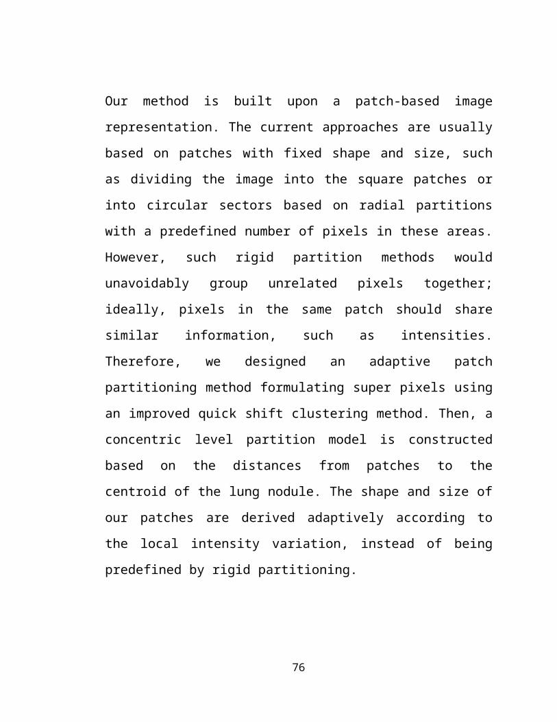
Our method is built upon a patch-based image

representation. The current approaches are usually

based on patches with fixed shape and size, such

as dividing the image into the square patches or

into circular sectors based on radial partitions

with a predefined number of pixels in these areas.

However, such rigid partition methods would

unavoidably group unrelated pixels together;

ideally, pixels in the same patch should share

similar information, such as intensities.

Therefore, we designed an adaptive patch

partitioning method formulating super pixels using

an improved quick shift clustering method. Then, a

concentric level partition model is constructed

based on the distances from patches to the

centroid of the lung nodule. The shape and size of

our patches are derived adaptively according to

the local intensity variation, instead of being

predefined by rigid partitioning.

76

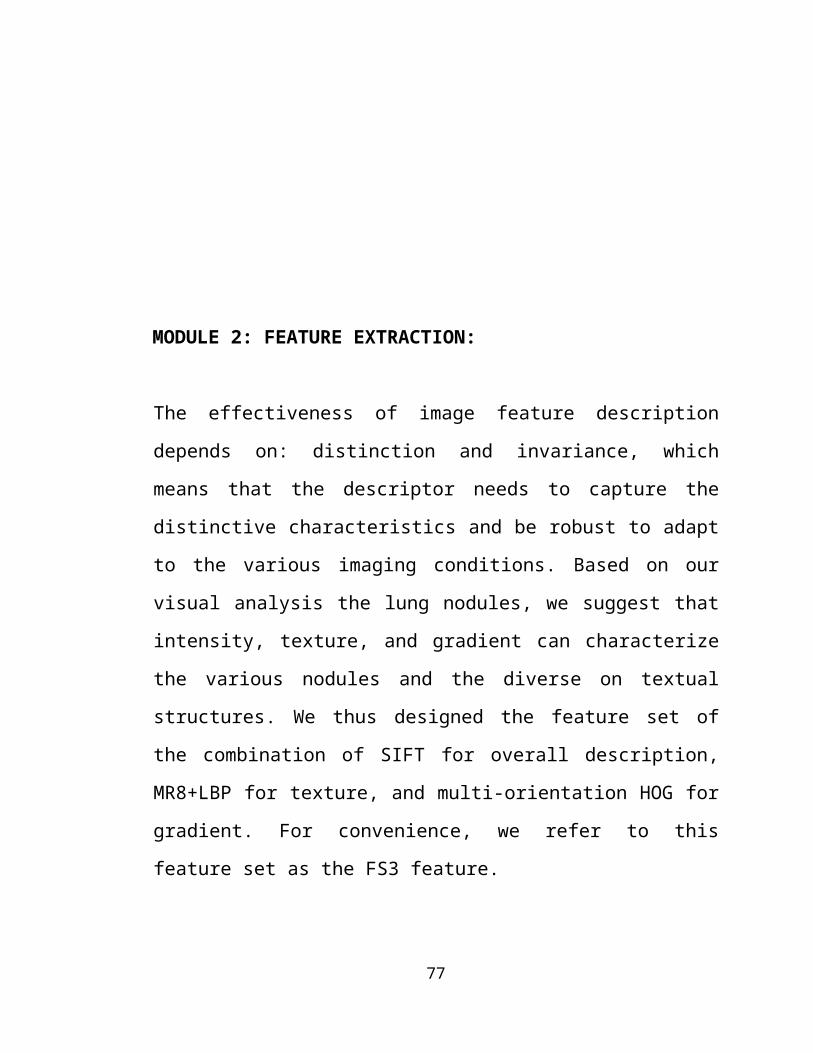
MODULE 2: FEATURE EXTRACTION:

The effectiveness of image feature description

depends on: distinction and invariance, which

means that the descriptor needs to capture the

distinctive characteristics and be robust to adapt

to the various imaging conditions. Based on our

visual analysis the lung nodules, we suggest that

intensity, texture, and gradient can characterize

the various nodules and the diverse on textual

structures. We thus designed the feature set of

the combination of SIFT for overall description,

MR8+LBP for texture, and multi-orientation HOG for

gradient. For convenience, we refer to this

feature set as the FS3 feature.

77

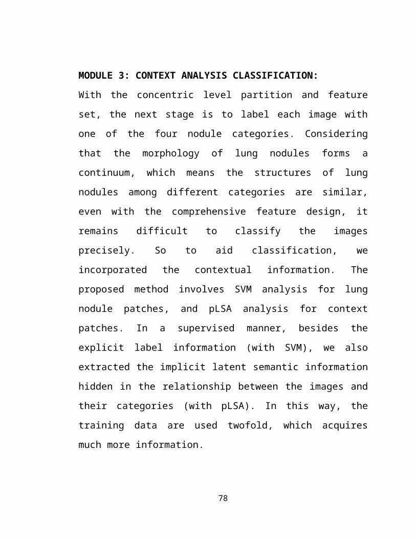
MODULE 3: CONTEXT ANALYSIS CLASSIFICATION:

With the concentric level partition and feature

set, the next stage is to label each image with

one of the four nodule categories. Considering

that the morphology of lung nodules forms a

continuum, which means the structures of lung

nodules among different categories are similar,

even with the comprehensive feature design, it

remains difficult to classify the images

precisely. So to aid classification, we

incorporated the contextual information. The

proposed method involves SVM analysis for lung

nodule patches, and pLSA analysis for context

patches. In a supervised manner, besides the

explicit label information (with SVM), we also

extracted the implicit latent semantic information

hidden in the relationship between the images and

their categories (with pLSA). In this way, the

training data are used twofold, which acquires

much more information.

78

GIVEN INPUT AND EXPECTED OUTPUT

MODULE-1:

Input image is CT scan image and the output is

context patch images.

MODULE-2:

Input image is context patch images and output

image is feature extracted keypoints.

MODULE-3:

Input image is fusion image and output is latent

semantic topics discovery by using pLSA

79

CHAPTER 3

SOFTWARE SPECIFICATION

3.1 GENERAL

MATLAB (matrix laboratory) is a numerical

computing environment and fourth-generation

programming language. Developed by Math Works,

MATLAB allows matrix manipulations, plotting

of functions and data, implementation

of algorithms, creation of user interfaces, and

80

interfacing with programs written in other

languages, including C, C++, Java, and Fortran.

Although MATLAB is intended

primarily for numerical computing, an optional

toolbox uses the MuPAD symbolic engine , allowing

access to symbolic computing capabilities. An

additional package, Simulink, adds graphical

multi-domain simulation and Model-Based

Design for dynamic and embedded systems.

In 2004, MATLAB had around one

million users across industry and academia. MATLAB

users come from various backgrounds

of engineering, science, and economics. MATLAB is

widely used in academic and research institutions

as well as industrial enterprises.

MATLAB was first adopted by

researchers and practitioners in control

engineering, Little's specialty, but quickly

spread to many other domains. It is now also used

in education, in particular the teaching of linear

algebra and numerical analysis, and is popular

81

amongst scientists involved in image processing.

The MATLAB application is built around the MATLAB

language. The simplest way to execute MATLAB code

is to type it in the Command Window, which is one

of the elements of the MATLAB Desktop. When code

is entered in the Command Window, MATLAB can be

used as an interactive mathematical shell.

Sequences of commands can be saved in a text file,

typically using the MATLAB Editor, as a script or

encapsulated into a function, extending the

commands available.

MATLAB provides a number of features

for documenting and sharing your work. You can

integrate your MATLAB code with other languages

and applications, and distribute your MATLAB

algorithms and applications.

3.2 FEATURES OF MATLAB

High-level language for technical computing.

82

Development environment for managing code,

files, and data.

Interactive tools for iterative exploration,

design, and problem solving.

Mathematical functions for linear algebra,

statistics, Fourier analysis,

filtering, optimization, and numerical

integration.

2-D and 3-D graphics functions for

visualizing data.

Tools for building custom graphical user

interfaces.

Functions for integrating MATLAB based

algorithms with external applications and

languages, such as C, C++, FORTRAN, Java™,

COM, and Microsoft Excel.

MATLAB is used in vast area, including signal and

image processing, communications, control

design, test and measurement, financial modeling

and analysis, and computational. Add-on toolboxes

(collections of special-purpose MATLAB functions)

83

extend the MATLAB environment to solve particular

classes of problems in these application areas.

MATLAB can be used on personal

computers and powerful server systems, including

the Cheaha compute cluster. With the addition of

the Parallel Computing Toolbox, the language can

be extended with parallel implementations for

common computational functions, including for-loop

unrolling. Additionally this toolbox supports

offloading computationally intensive workloads

to Cheaha the campus compute cluster.MATLAB is one

of a few languages in which each variable is a

matrix (broadly construed) and "knows" how big it

is. Moreover, the fundamental operators (e.g.

addition, multiplication) are programmed to deal

with matrices when required. And the MATLAB

environment handles much of the bothersome

housekeeping that makes all this possible. Since

so many of the procedures required for Macro-

Investment Analysis involves matrices, MATLAB

84

proves to be an extremely efficient language for

both communication and implementation.

3.2.1 INTERFACING WITH OTHER LANGUAGES

MATLAB can call functions and subroutines written

in the C programming language or FORTRAN. A

wrapper function is created allowing MATLAB data

types to be passed and returned. The dynamically

loadable object files created by compiling such

functions are termed "MEX-files"

(for MATLAB executable).

Libraries written

in Java, ActiveX or .NET can be directly called

from MATLAB and many MATLAB libraries (for

example XML or SQL support) are implemented as

wrappers around Java or Active X libraries.

Calling MATLAB from Java is more complicated, but

can be done with MATLAB extension, which is sold

separately by Math Works, or using an undocumented

mechanism called JMI (Java-to-Mat lab

85

Interface), which should not be confused with the

unrelated Java that is also called JMI.

As alternatives to the MuPAD based

Symbolic Math Toolbox available from Math Works,

MATLAB can be connected to Maple or Mathematica.

Libraries also exist to import and export MathML.

Development Environment

Start up Accelerator for faster MATLAB

start up on Windows, especially on Windows

XP, and for network installations.

Spreadsheet Import Tool that provides more

options for selecting and loading mixed

textual and numeric data.

Readability and navigation improvements to

warning and error messages in the MATLAB

command window.

86

Automatic variable and function renaming in

the MATLAB Editor.

Developing Algorithms and Applications

MATLAB provides a high-level language and

development tools that let you quickly develop and

analyze your algorithms and applications.

The MATLAB Language

The MATLAB language supports the vector and matrix

operations that are fundamental to engineering and

scientific problems. It enables fast development

and execution. With the MATLAB language, you can

program and develop algorithms faster than with

traditional languages because you do not need to

perform low-level administrative tasks, such as

declaring variables, specifying data types, and

allocating memory. In many cases, MATLAB

eliminates the need for ‘for’ loops. As a result,

one line of MATLAB code can often replace several

lines of C or C++ code.

87

At the same time, MATLAB provides all

the features of a traditional programming

language, including arithmetic operators, flow

control, data structures, data types, object-

oriented programming (OOP), and debugging

features.

MATLAB lets you execute commands or

groups of commands one at a time, without

compiling and linking, enabling you to quickly

iterate to the optimal solution. For fast

execution of heavy matrix and vector computations,

MATLAB uses processor-optimized libraries. For

general-purpose scalar computations, MATLAB

generates machine-code instructions using its JIT

(Just-In-Time) compilation technology.

This technology, which is available

on most platforms, provides execution speeds that

rival those of traditional programming languages.

Development Tools

88

MATLAB includes development tools

that help you implement your algorithm

efficiently. These include the following:

MATLAB Editor 

Provides standard editing and debugging features,

such as setting breakpoints and single stepping

Code Analyzer 

Checks your code for problems and recommends

modifications to maximize performance and

maintainability

MATLAB Profiler 

Records the time spent executing each line of code

Directory Reports 

Scan all the files in a directory and report on

code efficiency, file differences, file

dependencies, and code coverage

89

Designing Graphical User Interfaces

By using the interactive tool GUIDE (Graphical

User Interface Development Environment) to layout,

design, and edit user interfaces. GUIDE lets you

include list boxes, pull-down menus, push buttons,

radio buttons, and sliders, as well as MATLAB

plots and Microsoft Active X® controls.

Alternatively, you can create GUIs pro-

grammatically using MATLAB functions.

3.2.2 ANALYZING AND ACCESSING DATA

MATLAB supports the entire data analysis process,

from acquiring data from external devices and

databases, through preprocessing, visualization,

and numerical analysis, to producing presentation-

quality output.

Data Analysis

MATLAB provides interactive tools and command-line

functions for data analysis operations, including:

90

Interpolating and decimating

Extracting sections of data, scaling, and

averaging

Thresholding and smoothing

Correlation, Fourier analysis, and filtering

1-D peak, valley, and zero finding

Basic statistics and curve fitting

Matrix analysis

Data Access

MATLAB is an efficient platform for accessing

data from files, other applications, databases,

and external devices. You can read data from

popular file formats, such as Microsoft Excel;

ASCII text or binary files; image, sound, and

video files; and scientific files, such as HDF and

HDF5. Low-level binary file I/O functions let you

work with data files in any format. Additional

91

functions let you read data from Web pages and

XML.

Visualizing Data

All the graphics features that are required to

visualize engineering and scientific data are

available in MATLAB. These include 2-D and 3-D

plotting functions, 3-D volume visualization

functions, tools for interactively creating plots,

and the ability to export results to all popular

graphics formats. You can customize plots by

adding multiple axes; changing line colors and

markers; adding annotation, Latex equations, and

legends; and drawing shapes.

2-D Plotting

Visualizing vectors of data with 2-D plotting

functions that create:

Line, area, bar, and pie charts.

Direction and velocity plots.

Histograms.

92

Polygons and surfaces.

Scatter/bubble plots.

Animations.

3-D Plotting and Volume Visualization

MATLAB provides functions for visualizing 2-D

matrices, 3-D scalar, and 3-D vector data. You can

use these functions to visualize and understand

large, often complex, multidimensional data.

Specifying plot characteristics, such as camera

viewing angle, perspective, lighting effect, light

source locations, and transparency.

3-D plotting functions include:

Surface, contour, and mesh.

Image plots.

Cone, slice, stream, and isosurface.

3.2.3 PERFORMING NUMERIC COMPUTATION

MATLAB contains mathematical, statistical, and

engineering functions to support all common

93

engineering and science operations. These

functions, developed by experts in mathematics,

are the foundation of the MATLAB language. The

core math functions use the LAPACK and BLAS linear

algebra subroutine libraries and the FFTW Discrete

Fourier Transform library. Because these

processor-dependent libraries are optimized to the

different platforms that MATLAB supports, they

execute faster than the equivalent C or C++ code.

MATLAB provides the following types of

functions for performing mathematical operations

and analyzing data:

Matrix manipulation and linear algebra.

Polynomials and interpolation.

Fourier analysis and filtering.

Data analysis and statistics.

Optimization and numerical integration.

CHAPTER 4

IMPLEMENTATION

4.1 GENERAL

94

Matlab is a program that was originally designed

to simplify the implementation of numerical linear

algebra routines. It has since grown into

something much bigger, and it is used to implement

numerical algorithms for a wide range of

applications. The basic language used is very

similar to standard linear algebra notation, but

there are a few extensions that will likely cause

you some problems at first.

95

4.3 SNAP SHOTS:

ORIGINAL IMAGE

96

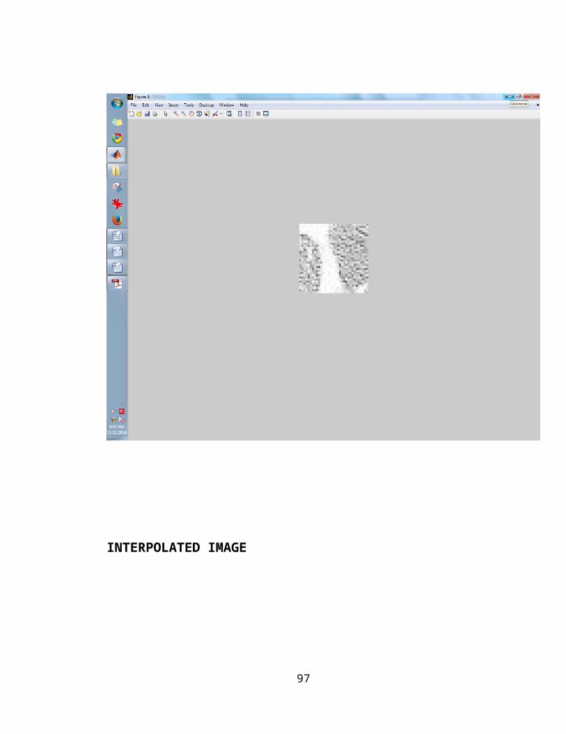
INTERPOLATED IMAGE

97

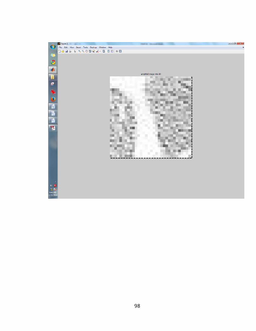
98

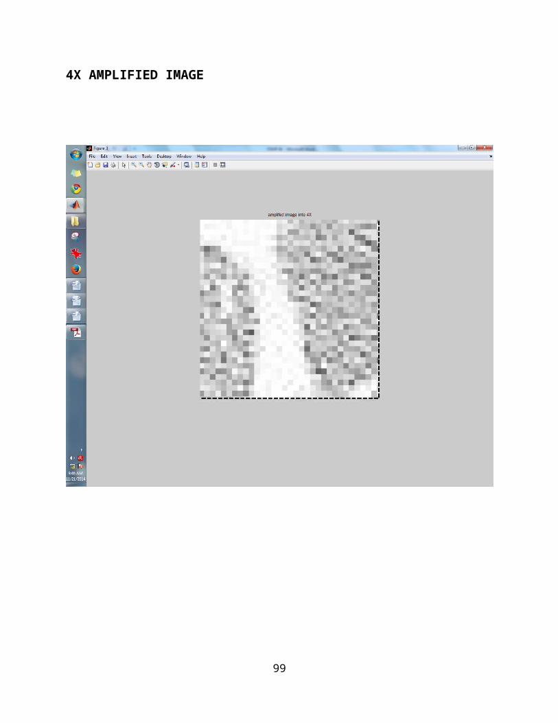
4X AMPLIFIED IMAGE

99

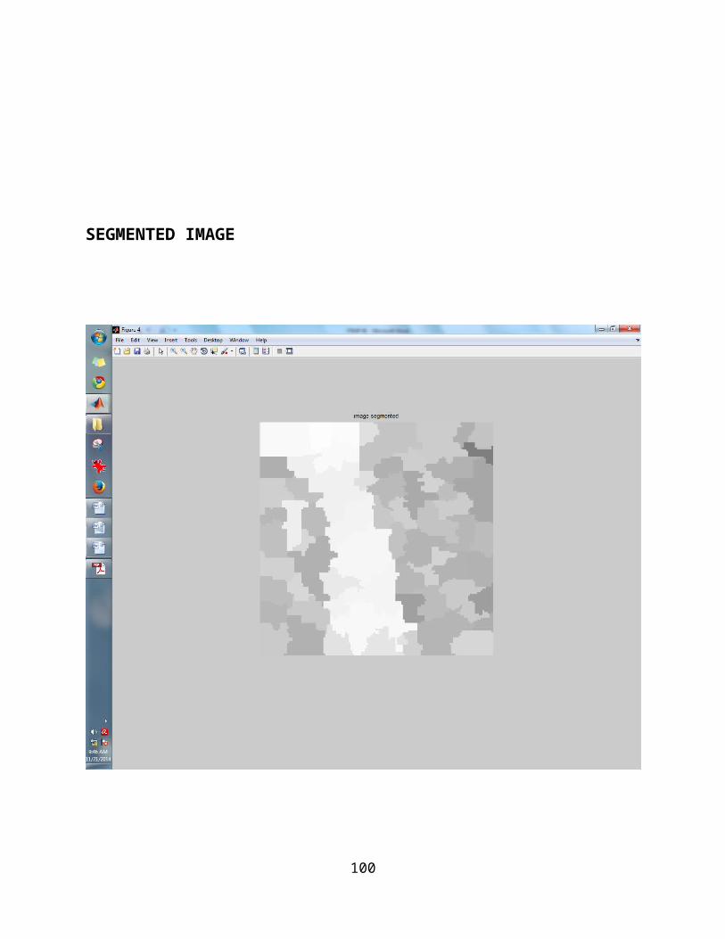
SEGMENTED IMAGE

100

DOWNSAMPLED IMAGE

101

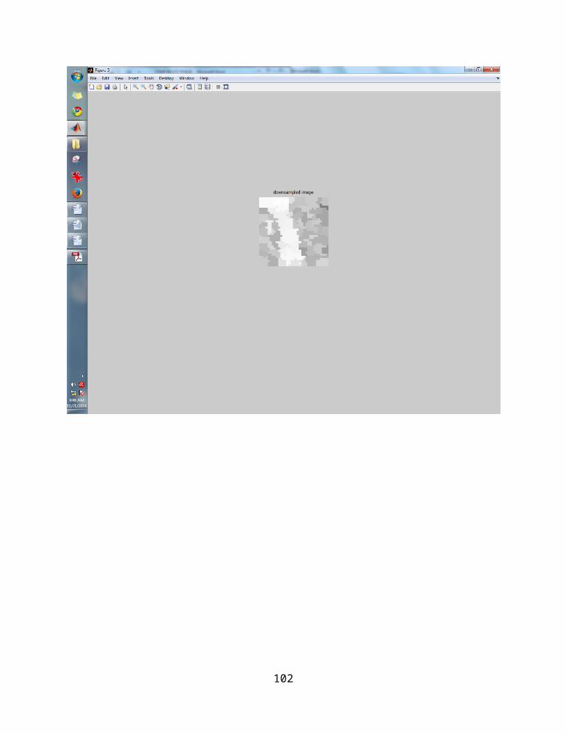
102

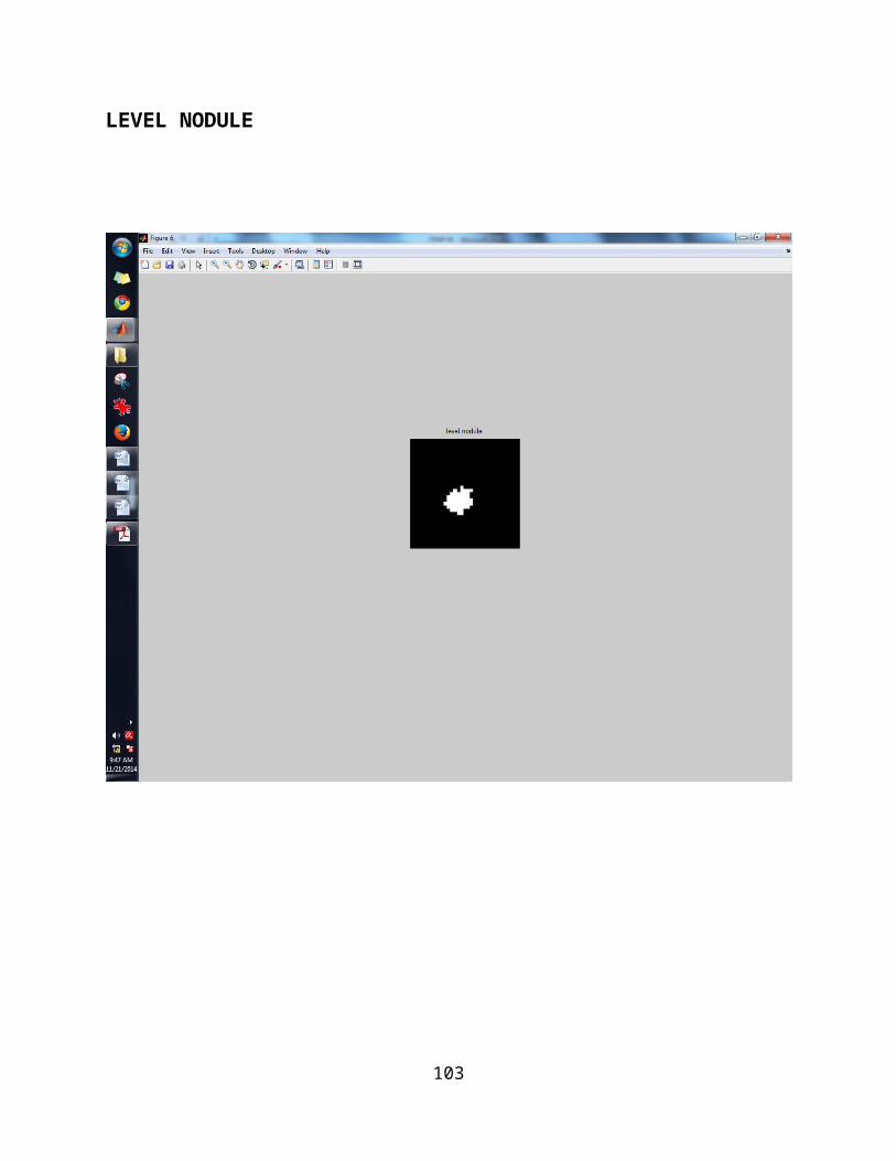
LEVEL NODULE

103

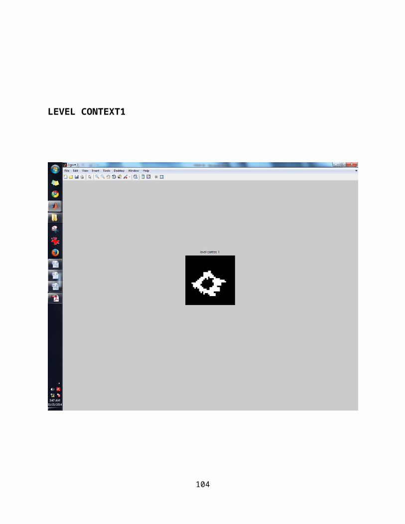
LEVEL CONTEXT1

104

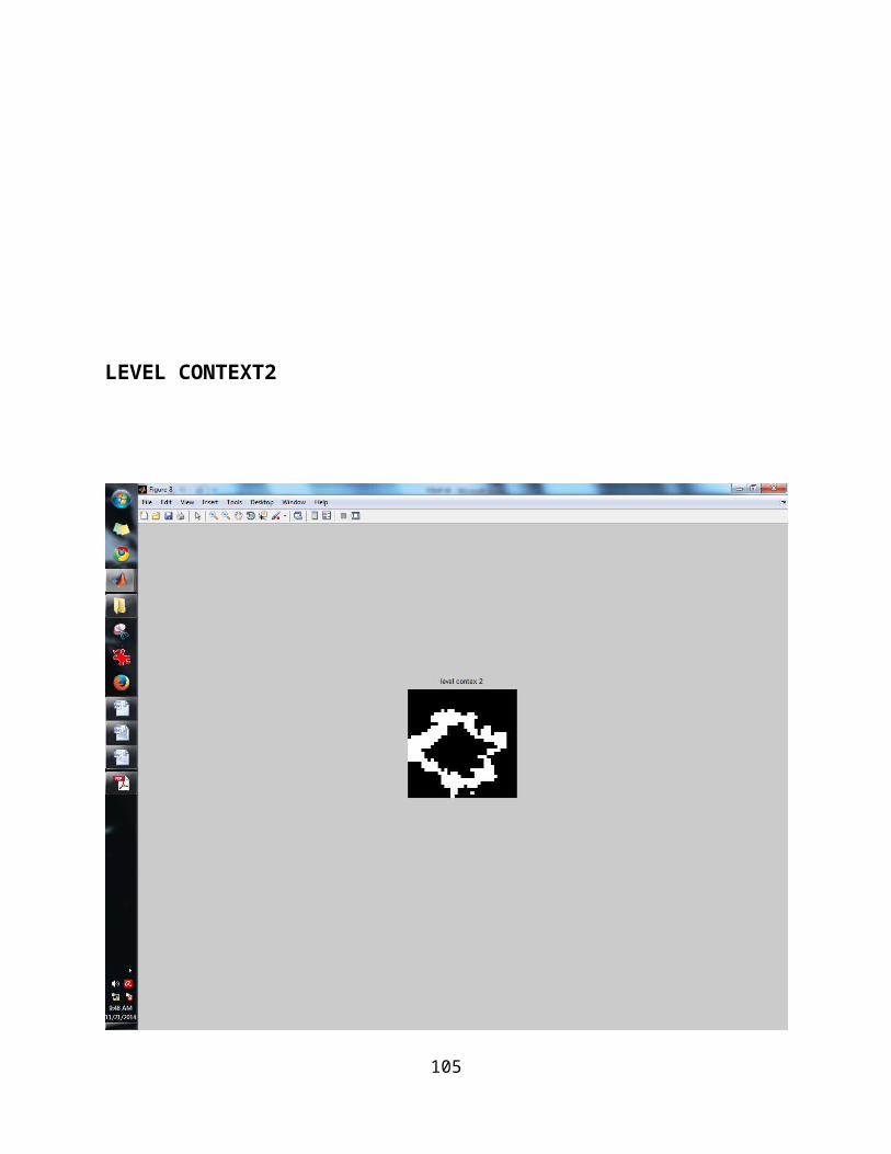
LEVEL CONTEXT2

105

SIFT DISCRIPTOR IMAGE

106

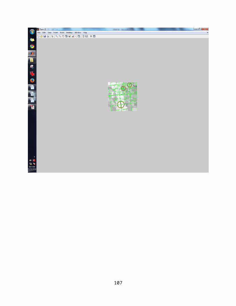
107

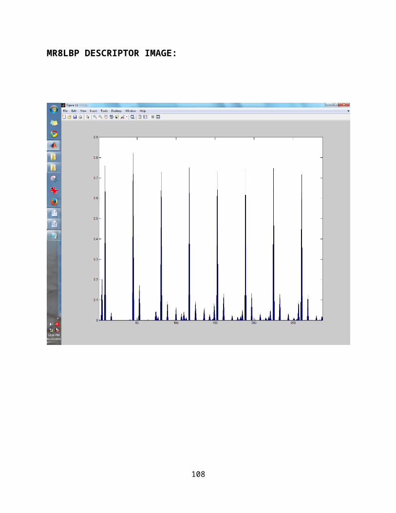
MR8LBP DESCRIPTOR IMAGE:

108

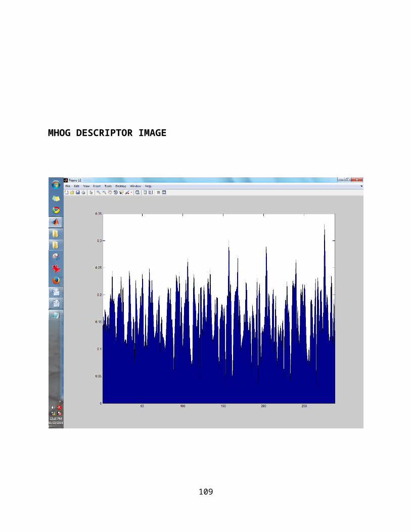
MHOG DESCRIPTOR IMAGE

109

OUTPUT

110

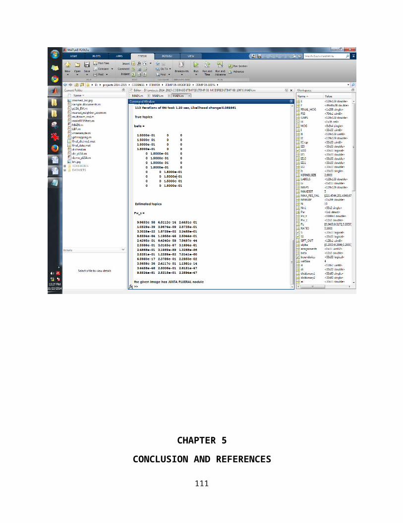
CHAPTER 5

CONCLUSION AND REFERENCES

111

5.1 CONCLUSION

To conclude, we present a supervised classification

method for lung nodule LDCT images in this paper. The

four main categories of lung nodules well-

circumscribed, vascularized, juxta-pleural, and

pleural-tail were the objects to be differentiated. We

designed a novel method to overcome the problem of the

lung nodule overlapping adjacent structures. Our method

had three components: concentric level partition,

feature extraction, and context analysis

classification. A concentric level partition was

constructed by an improved quick shift super pixel

formulation. Then, a FS3 feature set including SIFT,

MR8+LBP, and multi orientation HOG was generated to

describe the image patch from various perspectives.

Finally, a supervised classifier was designed through

combining level-nodule probability and level context

probability. The results from the experiments on the

ELCAP dataset showed promising performance of our

method. We also suggest that the proposed method can be

generally applicable to other medical or general

imaging domains. For instance, the improved quick shift

formulation process could be applied as the112

preprocessing stage for patch-based imaging analysis;

the extracted feature set could be employed as a

feature descriptor for other kinds of images; and the

latent semantic analysis with the voting process could

be used for analyzing hierarchical image patches.

5.2 REFERENCES

[1] J. J. Erasmus, J. E. Connolly, H. P. McAdams, and

V. L. Roggli, “Solitary pulmonary nodules: Part I.

morphologic evaluation for differentiation of benign

and malignant lesions,” Radiographics, vol. 20, no. 1,

pp. 43–58, 2000.

[2] D. Wu, L. Lu, J. Bi, Y. Shinagawa, K. Boyer, A.

Krishnan, and M. Salganicoff, “Stratified learning of

local anatomical context for lung nodules in CT

113

images,” in Proc. Comput. Vis. Pattern Recog., 2010,

pp. 2791–2798.

[3] R.A. Ochs, J.G. Goldin, F. Abtin, H. J. Kim, K.

Brown, P. Batra, D. Roback, M. F. McNitt-Gray, and M.

S. Brown, “Automated classification of lung

bronchovascular anatomy in CT using adaboost,” Med.

Image Anal., vol. 11, no. 3, pp. 315–324, 2007.

[4] A. Farag, S. Elhabian, J. Graham, A. Farag, and R.

Falk, “Toward precise pulmonary nodule descriptors for

nodule type classification,” in Proc. Med. Image

Comput. Comput.-Assisted Intervention Conf. Lecture

Notes Comput. Sci., 2010, vol. 13, no. 3, pp. 626–633.

[5] A. A. Farag, “A variational approach for small-size

lung nodule segmentation,” in Proc. Int. Symp. Biomed.

Imag., 2013, pp. 81–84.

[6] D. Xu, H. J. van der Zaag-Loonen, M. Oudkerk,

Y.Wang, R. Vliegenthart,E. T. Scholten, J.

Verschakelen,M. Prokop, H. J. de Koning, and R. J. van

Klaveren, “Smooth or attached solid indeterminate114

nodules detected at baseline CT screening in the NELSON

study: Cancer risk during 1 year of follow-up,”

Radiology, vol. 250, no. 1, pp. 264–272, 2009.

[7] S. Diciotti, G. Picozzi, M. Falchini, M. Mascalchi,

N. Villari, and G. Valli “3-D segmentation algorithm

of small lung nodules in spiral CT images,” IEEE Trans.

Inf. Technol. Biomed., vol. 12, no. 1, pp. 7–19, Jan.

2008.

[8] B. Zhao, “Automatic detection of small lung nodules

on CT utilizing alocal density maximum algorithm,” J.

Appl. Clin.Med. Phys., vol. 4, no. 3,pp. 248–260, 2003.

[9] Y. Lee, T. Hara,H. Fujita, S. Itoh, and T.

Ishigaki, “Automated detection of pulmonary nodules in

helical CT images based on an improved template

matching technique,” IEEE Trans.Med. Imag., vol. 20,

no. 7, pp. 595–604,Jul. 2001.

[10] A. A. Farag, S. Y. Elhabian, S. A. Elshazly, and

A. A. Farag, “Quantificationof nodule detection in

chest CT: A clinical investigation based onthe ELCAP115

study,” in Proc. 2nd Int. Workshop Pulmon. Image

Process.,2010, pp. 149–160.

[11] S. G. Armato III, M. L. Giger, and H. MacMahon,

“Automated detection of lung nodules in CT scans:

Preliminary results,” Med. Phys., vol. 28,no. 8, pp.

1552–1561, 2001.

[12] L. Fan, C. L. Novak, J. Qian, G. Kohl, and D.

Naidich, “Automatic detection of lung nodules from

multislice low-dose CT images,” in Proc. SPIE, Med.

Imag., 2001, vol. 4322, pp. 1828–1835.

[13] A. A. Farag, J. Graham, A. A. Farag, S. Elshazly,

and R. Falk, “Parametric and non-parametric nodule

models: Design and evaluation,” in Proc. 3rd Int.

Workshop Pulmon. Image Process., 2010, pp. 151–162.

[14] I. Sluimer, A. Schilham, M. Prokop, and B. van

Ginneken, “Computer analysis of computed tomography

scans of the lung: A survey,” IEEE Trans. Med. Imag.,

vol. 25, no. 4, pp. 385–405, Apr. 2006.

116

117