The Open Spectroscopy Journal, 2009, 3, 31-42 31 1874-3838/09 2009 Bentham Open Open Access The...
12
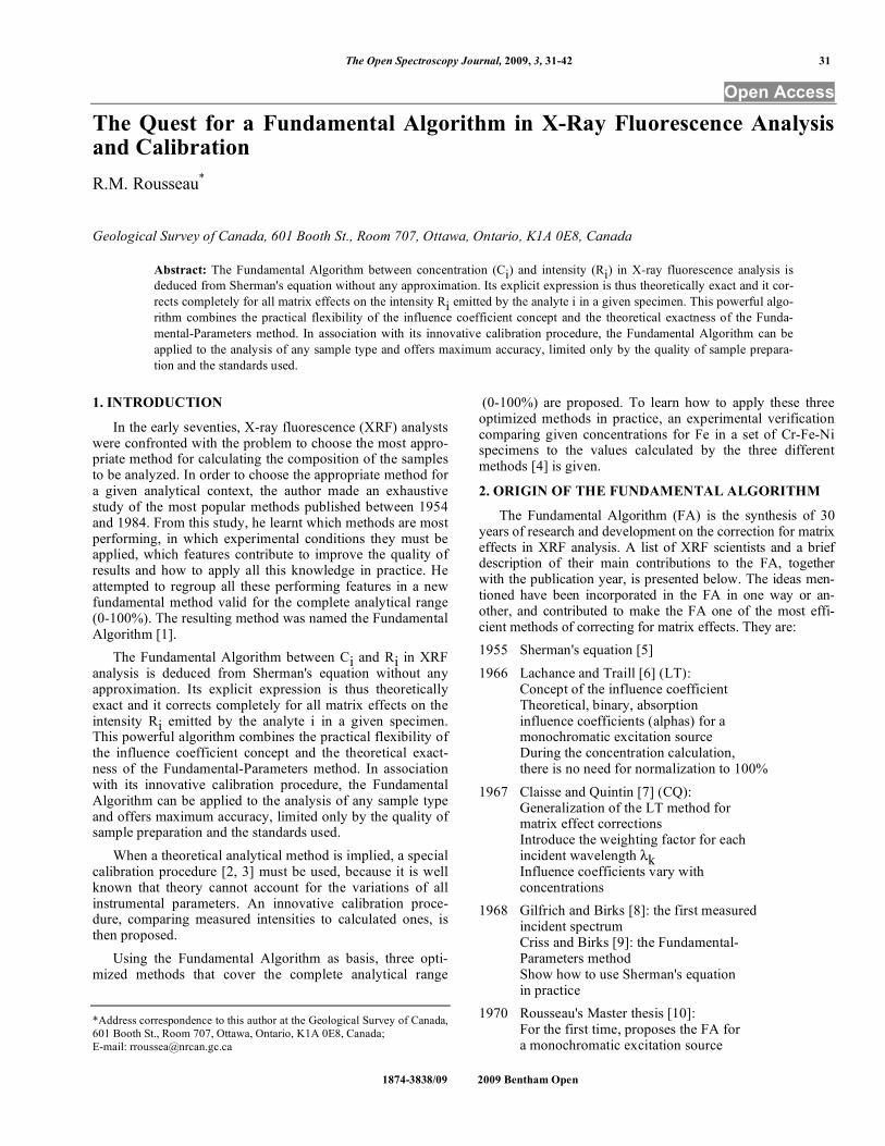
The Open Spectroscopy Journal, 2009, 3, 31-42 31 1874-3838/09 2009 Bentham Open Open Access The Quest for a Fundamental Algorithm in X-Ray Fluorescence Analysis and Calibration R.M. Rousseau * Geological Survey of Canada, 601 Booth St., Room 707, Ottawa, Ontario, K1A 0E8, Canada Abstract: The Fundamental Algorithm between concentration (C i ) and intensity (R i ) in X-ray fluorescence analysis is deduced from Sherman's equation without any approximation. Its explicit expression is thus theoretically exact and it cor- rects completely for all matrix effects on the intensity R i emitted by the analyte i in a given specimen. This powerful algo- rithm combines the practical flexibility of the influence coefficient concept and the theoretical exactness of the Funda- mental-Parameters method. In association with its innovative calibration procedure, the Fundamental Algorithm can be applied to the analysis of any sample type and offers maximum accuracy, limited only by the quality of sample prepara- tion and the standards used. 1. INTRODUCTION In the early seventies, X-ray fluorescence (XRF) analysts were confronted with the problem to choose the most appro- priate method for calculating the composition of the samples to be analyzed. In order to choose the appropriate method for a given analytical context, the author made an exhaustive study of the most popular methods published between 1954 and 1984. From this study, he learnt which methods are most performing, in which experimental conditions they must be applied, which features contribute to improve the quality of results and how to apply all this knowledge in practice. He attempted to regroup all these performing features in a new fundamental method valid for the complete analytical range (0-100%). The resulting method was named the Fundamental Algorithm [1]. The Fundamental Algorithm between C i and R i in XRF analysis is deduced from Sherman's equation without any approximation. Its explicit expression is thus theoretically exact and it corrects completely for all matrix effects on the intensity R i emitted by the analyte i in a given specimen. This powerful algorithm combines the practical flexibility of the influence coefficient concept and the theoretical exact- ness of the Fundamental-Parameters method. In association with its innovative calibration procedure, the Fundamental Algorithm can be applied to the analysis of any sample type and offers maximum accuracy, limited only by the quality of sample preparation and the standards used. When a theoretical analytical method is implied, a special calibration procedure [2, 3] must be used, because it is well known that theory cannot account for the variations of all instrumental parameters. An innovative calibration proce- dure, comparing measured intensities to calculated ones, is then proposed. Using the Fundamental Algorithm as basis, three opti- mized methods that cover the complete analytical range *Address correspondence to this author at the Geological Survey of Canada, 601 Booth St., Room 707, Ottawa, Ontario, K1A 0E8, Canada; E-mail: [email protected] (0-100%) are proposed. To learn how to apply these three optimized methods in practice, an experimental verification comparing given concentrations for Fe in a set of Cr-Fe-Ni specimens to the values calculated by the three different methods [4] is given. 2. ORIGIN OF THE FUNDAMENTAL ALGORITHM The Fundamental Algorithm (FA) is the synthesis of 30 years of research and development on the correction for matrix effects in XRF analysis. A list of XRF scientists and a brief description of their main contributions to the FA, together with the publication year, is presented below. The ideas men- tioned have been incorporated in the FA in one way or an- other, and contributed to make the FA one of the most effi- cient methods of correcting for matrix effects. They are: 1955 Sherman's equation [5] 1966 Lachance and Traill [6] (LT): Concept of the influence coefficient Theoretical, binary, absorption influence coefficients (alphas) for a monochromatic excitation source During the concentration calculation, there is no need for normalization to 100% 1967 Claisse and Quintin [7] (CQ): Generalization of the LT method for matrix effect corrections Introduce the weighting factor for each incident wavelength k Influence coefficients vary with concentrations 1968 Gilfrich and Birks [8]: the first measured incident spectrum Criss and Birks [9]: the Fundamental- Parameters method Show how to use Sherman's equation in practice 1970 Rousseau's Master thesis [10]: For the first time, proposes the FA for a monochromatic excitation source
-
Upload
independent -
Category
Documents
-
view
16 -
download
0
Transcript of The Open Spectroscopy Journal, 2009, 3, 31-42 31 1874-3838/09 2009 Bentham Open Open Access The...
The Open Spectroscopy Journal, 2009, 3, 31-42 31
1874-3838/09 2009 Bentham Open
Open Access
The Quest for a Fundamental Algorithm in X-Ray Fluorescence Analysis and Calibration
R.M. Rousseau*
Geological Survey of Canada, 601 Booth St., Room 707, Ottawa, Ontario, K1A 0E8, Canada
Abstract: The Fundamental Algorithm between concentration (Ci) and intensity (Ri) in X-ray fluorescence analysis is
deduced from Sherman's equation without any approximation. Its explicit expression is thus theoretically exact and it cor-
rects completely for all matrix effects on the intensity Ri emitted by the analyte i in a given specimen. This powerful algo-
rithm combines the practical flexibility of the influence coefficient concept and the theoretical exactness of the Funda-
mental-Parameters method. In association with its innovative calibration procedure, the Fundamental Algorithm can be
applied to the analysis of any sample type and offers maximum accuracy, limited only by the quality of sample prepara-
tion and the standards used.
1. INTRODUCTION
In the early seventies, X-ray fluorescence (XRF) analysts were confronted with the problem to choose the most appro-priate method for calculating the composition of the samples to be analyzed. In order to choose the appropriate method for a given analytical context, the author made an exhaustive study of the most popular methods published between 1954 and 1984. From this study, he learnt which methods are most performing, in which experimental conditions they must be applied, which features contribute to improve the quality of results and how to apply all this knowledge in practice. He attempted to regroup all these performing features in a new fundamental method valid for the complete analytical range (0-100%). The resulting method was named the Fundamental Algorithm [1].
The Fundamental Algorithm between Ci and Ri in XRF analysis is deduced from Sherman's equation without any approximation. Its explicit expression is thus theoretically exact and it corrects completely for all matrix effects on the intensity Ri emitted by the analyte i in a given specimen. This powerful algorithm combines the practical flexibility of the influence coefficient concept and the theoretical exact-ness of the Fundamental-Parameters method. In association with its innovative calibration procedure, the Fundamental Algorithm can be applied to the analysis of any sample type and offers maximum accuracy, limited only by the quality of sample preparation and the standards used.
When a theoretical analytical method is implied, a special calibration procedure [2, 3] must be used, because it is well known that theory cannot account for the variations of all instrumental parameters. An innovative calibration proce-dure, comparing measured intensities to calculated ones, is then proposed.
Using the Fundamental Algorithm as basis, three opti-mized methods that cover the complete analytical range
*Address correspondence to this author at the Geological Survey of Canada,
601 Booth St., Room 707, Ottawa, Ontario, K1A 0E8, Canada;
E-mail: [email protected]
(0-100%) are proposed. To learn how to apply these three optimized methods in practice, an experimental verification comparing given concentrations for Fe in a set of Cr-Fe-Ni specimens to the values calculated by the three different methods [4] is given.
2. ORIGIN OF THE FUNDAMENTAL ALGORITHM
The Fundamental Algorithm (FA) is the synthesis of 30 years of research and development on the correction for matrix effects in XRF analysis. A list of XRF scientists and a brief description of their main contributions to the FA, together with the publication year, is presented below. The ideas men-tioned have been incorporated in the FA in one way or an-other, and contributed to make the FA one of the most effi-cient methods of correcting for matrix effects. They are:
1955 Sherman's equation [5]
1966 Lachance and Traill [6] (LT): Concept of the influence coefficient Theoretical, binary, absorption influence coefficients (alphas) for a monochromatic excitation source During the concentration calculation, there is no need for normalization to 100%
1967 Claisse and Quintin [7] (CQ): Generalization of the LT method for matrix effect corrections Introduce the weighting factor for each incident wavelength k Influence coefficients vary with concentrations
1968 Gilfrich and Birks [8]: the first measured incident spectrum Criss and Birks [9]: the Fundamental- Parameters method Show how to use Sherman's equation in practice
1970 Rousseau's Master thesis [10]: For the first time, proposes the FA for a monochromatic excitation source
32 The Open Spectroscopy Journal, 2009, Volume 3 R.M. Rousseau
1973 de Jongh [11]: Theoretical multi-element influence coefficients can be calculated from the Sherman equation Calibration lines of measured intensities versus calculated intensities (or apparent concentration)
1974 Rasberry and Heinrich [12]: Absorption and enhancement effects obey to different mathematical rules and they must be treated separately
1974 Rousseau and Claisse [13]: Propose a new method to calculate theoretical binary influence coefficients in the CQ algorithm
1976 Tertian [14]: Introduces the CM factor in the CQ algorithm
1980 Criss [15]: Proposes calculation of an initial estimate of the sample composition for calculating the ij and ij coefficients once
1982 Rousseau: First public presentation of the FA at the 31
st Annual Denver X-Ray Conference
1984 Rousseau [16]: First publication on the Fundamental Algorithm
1985 Pella, Feng and Small [17]: Calculate intensity for each wavelength of the incident spectrum
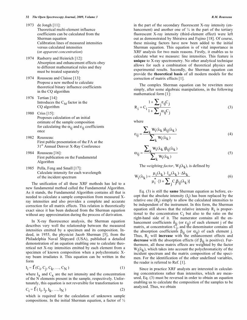
The unification of all these XRF methods has led to a new fundamental method called the Fundamental Algorithm. As it stands, the Fundamental Algorithm contains all that is needed to calculate a sample composition from measured X-ray intensities and also provides a complete and accurate correction for all matrix effects. This relation is theoretically exact since it has been deduced from the Sherman equation without any approximation during the process of derivation.
In X-ray fluorescence analysis, the Sherman equation describes very well the relationship between the measured intensities emitted by a specimen and its composition. In-deed, in 1955, the physicist Jacob Sherman [5], from the Philadelphia Naval Shipyard (USA), published a detailed demonstration of an equation enabling one to calculate theo-retical net X-ray intensities emitted by each element from a specimen of known composition when a polychromatic X-ray beam irradiates it. This equation can be written in the form
Ii = f (Ci, Cj, Ck, …, CN ) (1)
where Ix and Cx are the net intensity and the concentration of the N elements present in the sample, respectively. Unfor-tunately, this equation is not reversible for transformation to
Ci = f ( Ii, Ij, Ik, …, IN ) (2)
which is required for the calculation of unknown sample compositions. In the initial Sherman equation, a factor of
in the part of the secondary fluorescent X-ray intensity (en-hancement) and another one of in the part of the tertiary fluorescent X-ray intensity (third-element effect) were left out as demonstrated by Shiraiwa and Fujino [18]. Of course, these missing factors have now been added to the initial Sherman equation. This equation is of vital importance in XRF analysis for two main reasons. Firstly, it enables us to calculate what we measure: line intensities. This feature is unique to X-ray spectrometry. No other analytical technique allows for such a combination of theoretical physics and experimental results. Secondly, the Sherman equation can provide the theoretical basis of all modern models for the correction of matrix effects [1].
The complex Sherman equation can be rewritten more simply, after some algebraic manipulations, in the following mathematical form [1]:
Ri = Ci
1+ ijC jj
1+ ijC jj
(3)
where
ij =Wi( k ) ij( k )k
Wi( k )k
(4)
ij =Wi( k ) ij( k )k
Wi( k )k
(5)
The weighting factor, Wi( k), is defined by
Wi( k ) =μi( k ) Io( k ) k
μi* [1+ Cj ij( k )]
j
(6)
Eq. (3) is still the same Sherman equation as before, ex-cept that the absolute intensity (Ii) has been replaced by the relative one (Ri) simply to allow the calculated intensities to be independent of the instrument. In this form, the Sherman equation still shows that the relative intensity Ri is propor-tional to the concentration Ci but also to the ratio on the right-hand side of it. The numerator contains all the en-hancement coefficients ij (or ij) of each element j of the matrix, at concentration Cj, and the denominator contains all the absorption coefficients ij (or ij) of each element j. Thus, Ri will increase with the enhancement effects and decrease with the absorption effects (if ij is positive). Fur-thermore, all these matrix effects are weighted by the factor Wi( k), which takes into account the polychromaticity of the incident spectrum and the matrix composition of the speci-men. For the identification of the other undefined variables, the reader is referred to Ref. [1].
Since in practice XRF analysts are interested in calculat-ing concentrations rather than intensities, which are meas-ured, Eq. (3) must be reversed in order to obtain an equation enabling us to calculate the composition of the samples to be analyzed. Thus, we obtain
Fundamental Algorithm in X-Ray Fluorescence Analysis and Calibration The Open Spectroscopy Journal, 2009, Volume 3 33
Ci = Ri
1+ ijC jj
1+ ijC jj
(7)
or
C
i= R
iM
is (8)
with
Mis =
1+ ijC jj
1+ ijC jj
(9)
where the Mis factor is the correction factor for the matrix effects of specimen "s" on analyte i. In practice, the Ri inten-sities are measured and the Mis factor is calculated from the Sherman equation or any theoretically valid algorithm [4] selected by the analyst for a given analytical context. For the calculation of concentrations from the measured intensities, an accurate value of Mis is needed for each unknown sam-ple. However, Mis is strongly dependent on the sample com-position, which is obviously unknown prior to the analysis. Consequently, we are trapped in a vicious circle… We will see later the different solutions proposed to solve this prob-lem in practice.
3. PHYSICAL INTERPRETATION
The physical interpretation of the Fundamental Algo-rithm (Eq. 7) is quite simple and elegant. To a first approxi-mation, equation (7) reveals that the concentration of the analyte i, Ci, is proportional to its measured relative inten-sity, Ri, which is multiplied by a ratio correcting for all ma-trix effects.
The numerator contains all the absorption coefficients ij of each element j of the matrix. Thus, the numerator corrects for all absorption effects of the matrix on the analyte i, each element j bringing its contribution to the total correction in a proportion Cj. If the numerator is greater than unity (it could be lower if the matrix is less absorbent than the analyte), the intensity Ri will be increased by a quantity equivalent to that absorbed by the matrix.
The denominator contains all the enhancement coeffi-cients ij of each element j of the matrix. If some elements j are able to enhance the analyte i, the corresponding coeffi-cient ij will be different from zero and always positive. Thus, the denominator corrects for all enhancement effects of the matrix on the analyte i, each element j bringing its contribution to the total correction in a proportion Cj. In the case of enhancement, the denominator will be greater than unity and the intensity Ri will be reduced by a quantity equivalent to that caused by the enhancement. Thus, the in-tensity Ri in the equation (7) will increase with the absorp-tion effects (if the term j ijCj is positive) and decrease with the enhancement effects.
Since the numerator of the Fundamental Algorithm cor-rects for all absorption effects of the matrix on the analyte and since the denominator corrects for all enhancement ef-fects, the form of this equation makes it easier to understand the physical principles behind the complex equation of Sherman.
In physics, the validity of a new theory is confirmed if it reveals new facts. Regarding the FA, it reveals that the coef-ficients ij and ij are the weighted means of all absorption and enhancement effects, respectively, caused by element j on analyte i, where to each incident wavelength k is given a weight Wi, which takes into account the polychromaticity of the incident spectrum [1].
The knowledgeable reader may ask why I have not re-tained the canonical form of the algorithm proposed by Broll-Tertian [19] or Lachance-Claisse [20] rather than the one of the FA? These two algorithms have in common the fact that they merge in one new coefficient the coefficients for the correction of absorption and enhancement effects. By doing it, the above algorithms do not describe properly, or distort, physical reality as described by the Sherman equa-tion [21, 22]. Such is not the case with the FA, which com-pletely respects the Sherman equation.
4. A PHYSICAL DEMONSTRATION OF THE FUN-DAMENTAL ALGORITHM
A more "physical" demonstration of the Fundamental Algorithm is as follows. In 1966, Lachance and Traill [6] proposed the following definition of the absorption influence coefficient for a monochromatic incident source of wave-length k:
ij( k ) =μ j*
μi*
1 (10)
where
μ j*= μ j( k ) cosec ' + μ j( i ) cosec " (11)
μi*= μi( k ) cosec ' + μi( i ) cosec " (12)
The ij( k) coefficient corrects for the absorption effect of the matrix element j on the analyte i when the incident X-ray source is monochromatic [1]. In 1984, Rousseau [16] generalized this definition for a polychromatic incident source:
ij =Wi( k )k ij( k )
Wi( k )k
(13)
where
Wi( k ) =μi( k )
μi*
Io ( k ) k1+ Cj ij( k )j
(14)
is the weighting factor of each wavelength k of the incident X-ray spectrum. The ij coefficient is the weighted mean of all the absorption effects caused by matrix element j on ana-lyte i in a given specimen when it is bombarded by a poly-chromatic incident spectrum. The value of the ij coefficient is unique and fundamental for a given set of experimental conditions and for a given specimen composition. Note that the coefficient ij( k) is a binary coefficient depending only on elements i and j. On the other hand, the coefficient ij is a multi-element coefficient depending on the full matrix com-position including element j.
34 The Open Spectroscopy Journal, 2009, Volume 3 R.M. Rousseau
If there is no enhancement, the concentration Ci is cal-culated by the following algorithm:
Ci = Ri(1+ ijC j)j (15)
which has the same form as the Lachance-Traill algorithm [6]. In the general case where both matrix effects, absorption and enhancement, are present, this latter algorithm becomes
Ci = Ri
1+ ijC jj
1+ ijC jj
(16)
which is the Fundamental Algorithm where
ij =
Wi( k )k ij( k )
Wi( k )k
(17)
The ij coefficient is the weighted mean of all the en-hancement effects caused by matrix element j on analyte i in a given specimen when it is bombarded by a polychromatic incident spectrum. The value of the ij coefficient is unique and fundamental for a given set of experimental conditions and for a given specimen composition.
As demonstrated, the Fundamental Algorithm is the gen-eralization of the Lachance-Traill algorithm when the speci-men is bombarded by a polychromatic incident spectrum and where both matrix effects, absorption and enhancement, are present. The ij and ij coefficients are multi-element coef-ficients depending on the full matrix composition of each specimen. We will see now how to calculate them for each sample to be analyzed.
5. THE PRACTICAL APPLICATION OF THE FUN-DAMENTAL ALGORITHM
When a series of values of the ij and ij coefficients is calculated for a given specimen, these values are valid only for this specific specimen since they depend on the full ma-trix composition. Any other specimen with the same series of elements, but in different proportions, will need a new set of coefficient values to correct accurately for matrix effects.
Since the ij and ij coefficients depend on the total ma-trix composition, the composition of each sample must be first calculated from an initial estimate of the composition. It is calculated using the Claisse-Quintin algorithm [7]:
Ci = Ri[1+ aij + aijjCM( ) Cjj
+ aijkCjk> j
jCk]
(18)
where CM is the concentration of the total matrix, aij and aijj are binary, and aijk, ternary influence coefficients. Then, from this estimated composition, all ij and ij coefficients, the complex part of Sherman's equation, are calculated once only. With these calculated coefficients now used as con-
stants, the final (and more accurate) composition of the sample is calculated by applying an iteration process to the Fundamental Algorithm.
To apply this method in practice, a commercial WIN-DOWS software package known as CiROU is available [23].
The Fundamental Algorithm method has the following clear advantages:
1. Since the numerator of equation (7) corrects for all the absorption effects of the matrix on the analyte and since the denominator corrects for all the enhance-ment effects, the form of equation (7) makes it much easier to understand the physical principles behind the complex equation of Sherman. Consequently, its great beauty lies in its perfect symmetry.
2. For the first time, it enabled to deduce the concept of influence coefficients directly from the Sherman equation without any approximation. It proposes the fundamental, unique and explicit equations for calcu-lating the ij, ij coefficients, only in terms of fun-damental parameters.
3. The equations of the ij, ij coefficients reveal that they are the weighted means of all absorption and en-hancement effects, respectively, caused by element j on analyte i in a given specimen. They also introduce a weighting factor, Wi, for each incident wavelength
k of the incident spectrum.
4. Empirical coefficients are no longer required. The Fundamental Algorithm uses only theoretical influ-ence coefficients that are in full agreement with the treatment of physics as proposed by Sherman. They are calculated for each sample composition, increas-ing the accuracy in so doing.
5. This method also uses a fully theoretical approach to calculate all the required parameters. For example, the method uses equations proposed by Pella et al. [17] to calculate up to 350 different intensities of the incident spectrum emitted by the X-ray tube. It uses data from Heinrich [24] to calculate mass absorption coeffi-cients by a method proposed by Springer and Nolan [25]. It also uses modern values of X-ray fluorescence yields [26, 27] and Coster-Kronig transition prob-abilities [28].
6. The method can be used in practice to calculate the composition of any sample type, of any composition, i.e., for concentration ranges varying from 0 to 100%. It introduces a theoretical mean relative error of 0.05% only [4]. An experimental verification of this method done by Rousseau and Bouchard [29] on dif-ferent types of alloy has confirmed its accuracy and versatility.
7. In contrast to the Fundamental-Parameters method, it directly calculates concentrations rather than intensi-ties, and the calculation technique has been opti-mized.
8. Normalization of calculated concentrations is no longer required. Since the complex part of Sherman's equation is calculated once only, the calculation time is greatly reduced.
9. It allows deduction of other theoretically valid algo-rithms, such as the Lachance-Traill or the Claisse-
Fundamental Algorithm in X-Ray Fluorescence Analysis and Calibration The Open Spectroscopy Journal, 2009, Volume 3 35
Quintin algorithm [1]. In other words, it can be the source of all modern methods to correct for matrix ef-fects.
10. It takes advantage of 30 years of research and devel-opment on mathematical models for matrix effect cor-rections (see Section 2).
However, this theoretical approach needs to be adapted to the experimental data of each spectrometer, since theory cannot account for all the instrumental parameters. It is done through a smart calibration procedure that compares the measured intensities to the calculated ones [2].
6. THEORETICAL BINARY INFLUENCE COEFFI-CIENTS
In quantitative XRF analysis, one of the major problems is the correction for matrix effects (absorption and enhance-ment). The Fundamental Algorithm uses theoretical multi-element influence coefficients, which are numerical coeffi-cients that correct for the effect of each matrix element on the element to be determined (or analyte) in a given speci-men. However, these coefficients depend on the full sample composition to be analyzed (see Eqns 4 and 5), which in practice is unknown prior to analysis and they must be calcu-lated for each sample as already explained. One of the solu-tions proposed to solve this problem was the concept of theoretical binary influence coefficients.
These binary coefficients are based on the hypothesis that the total matrix effect on the analyte i is equal to the sum of the effects of each element j of the matrix, each of these ef-fects being calculated independently of each other. In other words, from a practical point of view, it is easier to consider a sample as a sum of binary mixtures rather than as a multi-element mixture. Of course, this approach is an approxima-tion because one cannot isolate the matrix effect of each element j on the analyte i from the effect of the rest of the matrix. But this approach allows one to correct for matrix effects with accuracy as long as the composition range of samples to analyze is fairly limited. With this approach it was then possible to calculate a set of theoretical binary in-fluence coefficients valid for a given composition range rather than for a given sample. In other words, with binary coefficients it is assumed that the binary coefficient aij is a constant for a given range of Ci and Cj rather than being a variable dependent on the whole matrix composition of each sample.
Theoretical binary influence coefficients can be calculated by using the Fundamental Algorithm. With this equation, the intensities emitted by representative binary standards are cal-culated rather than being measured. With this approach, one assumes that the composition of a complex sample is made up of a series of binary elements or compounds where one con-siders the effect of one matrix element at a time on each ana-lyte, independently of the rest of the matrix composition. Thus, a series of influence coefficients is calculated from hy-pothetical compositions for the binary series of elements or compounds that are present in the samples.
Two different algorithms can use the modern concept of theoretical binary influence coefficients. These two algorithms, among all the proposed ones, have been chosen because of their accuracy and their sound theoretical basis. They are:
First, the Lachance-Traill (LT) algorithm [6]:
Ci = Ri(1+ aijC j)j (19)
where Ri is the ratio of the measured net intensity Ii to the measured net intensity of the pure analyte i. The binary coef-ficient aij is calculated using the following equation [1]:
aij =ij ij
1+ ijC jm (20)
where ij and ij, defined by equations (5) and (4), are cal-culated for the special case of a binary standard having a composition (Cim, Cjm), where Cim is the mid-value of the calibration range of the analyte i and where
Cjm = 1 Cim (21)
Nowadays, the alpha coefficients as proposed by Lachance and Traill [6] are no longer used in practice be-cause of their lack of accuracy. They have been replaced by the theoretical binary influence coefficients aij, which, as opposed to the alpha coefficients, take into account the en-hancement effect as well as the polychromaticity of the inci-dent radiation [1].
This approach assumes that the coefficient aij is a con-
stant (it is an approximation!) when it is applied to speci-mens with a limited concentration range (0-10%), such as, for example, oxides in rock samples diluted in fused discs. In this case, the calculation method by itself (Eqns 19, 20 and 21) introduces a theoretical mean relative error of only 0.02% on the calculated concentrations. On the other hand, for concentration variations greater than 10%, the concentra-tions calculated by this algorithm associated to the aij coeffi-cients are unacceptable [4]. See the experimental verification at the end of this paper.
In the case of diluted samples such as fused discs or pressed powder pellets, the theoretical binary influence coef-ficient (aij) defined above can be modified by incorporating a constant term. For example, when a sample is fused in a fixed sample/flux ratio to produce a fused disc, or when a pulverized sample is mixed in a fixed sample/binder ratio and pressed, the aij coefficient can be modified by including the weight fraction and the composition of the flux or the binder, which are essentially constant for every specimen. In this case, the aij coefficient is referred to as a modified coef-ficient. The coefficients aij can also be modified to express them in terms of oxides rather than elements themselves.
Two different aij coefficients, calculated for the correc-tion of matrix effects of two different matrix elements on the analyte, can be combined to form only one coefficient. In this case, the new coefficient is referred to as a hybrid coef-ficient. It is an elegant way to eliminate the measurement of one analyte and to correct for its matrix effects even if it has not been measured or its concentration is not known. How-ever, this approach introduces more approximations and must be used with caution and applied with great care. The terminology “modified” and “hybrid” influence coefficients has been proposed by Lachance [30] in 1979 but his methods of calculation have not been retained.
36 The Open Spectroscopy Journal, 2009, Volume 3 R.M. Rousseau
When samples are prepared as fused discs, volatile prod-ucts (e.g. CO2, H2O, SO2, Cl, F, etc.) can be lost during the fusion and/or it can be accompanied with a gain in weight due to oxidation (e.g. FeO Fe2O3). In this case, there are three different ways to calculate the sample composition:
1. A conventional Loss On Ignition (LOI) is done on the pulverized sample BEFORE the fusion and the ig-nited powder is used to prepare the fused disc. In this case, there is usually NO further loss of volatile or gain in weight during the fusion and all the calculated concentrations in the fused disc are adjusted to take into account the LOI and get the analyte concentra-tions in the sample [31]. This approach generates ac-curate results except it is time consuming.
2. A conventional LOI is done on the pulverized sample, but the original sample is used to prepare the fused disc. In this case, there is loss of volatile and/or gain in weight during the fusion. It changes the sam-ple/flux ratio and may severely both affects the accu-racy of results. The method developed by us takes this phenomenon into account by using a theoretical ap-proach based on the famous Sherman equation [31]. The coefficient thus calculated for the loss of volatile products and/or gain in weight is included in the term [1 + …] correcting for matrix effects, even if it is not an influence coefficient. This approach generates ac-curate results and it is less time consuming than the previous one because the LOI and the fused disc can be done at the same time.
3. No conventional LOI is done on the pulverized sam-ple. In this case, there is loss of volatile and/or gain in weight during the fusion and the LOI value is un-known. The LOI value is calculated by difference be-tween 100% and the sum of calculated concentrations in the sample [31]. Knowing the LOI value, the sam-ple composition is recalculated as in the previous case. This approach introduces more approximations in the calculation method and is sensitive to any ex-perimental errors. Since the accuracy of this approach is more “unpredictable”, it must be applied with cau-tion and great care.
Second, the Claisse-Quintin (CQ) algorithm [7,13,14,29]:
The Claisse-Quintin algorithm (CQ) can be described as an extension of the Lachance-Traill algorithm (LT) taking into account the fact that the LT coefficient, aij
LT (see Eq.
22), is not a constant but varies with the concentration of the matrix elements. According to Claisse and Quintin the LT coefficient aij
LT varies linearly with the concentration Cj, i.e.
aijLT
= aij + aijjC j (22)
Thus, the general form of the Claisse-Quintin algorithm for a multicomponent sample can be written as:
Ci = Ri.[1+ (aij + aijjCM )j
Cj
+ aijkCjCkk> j
j]
(23)
where the matrix concentration CM is the sum of all ele-ments in the sample except i, i.e.
CM = 1 Ci = Cj + Ck + ...+ CN (24)
and where the “crossed” ternary coefficient aijk has been added to compensate for the fact that the total matrix correc-tion cannot be strictly represented by a weighted sum of bi-nary corrections. The binary coefficients aij and aijj are cal-culated from theory at hypothetical binary compositions of (Ci, Cj) = (0.2, 0.8) and (0.8, 0.2), respectively. The cross-product coefficient, aijk, is calculated at the ternary composi-tion of (Ci, Cj, Ck) = (0.30, 0.35, 0.35). To be more explicit [32], if for a ternary system (Ci, Cj, Ck), the variable Fi(Ci, Cj, Ck) is defined by
Fi(Ci,C j,Ck ) =1
Cj
CiRi
1 (25)
Note that: if Cj = 0, then
Fi(Ci, 0, Ck ) =1
Ck
CiRi
1 (26)
where the ratio Ci/Ri is calculated by the Fundamental Algo-rithm (Eq. 7) for a ternary system:
CiRi
=
1+ ijC j + ikCk1+ ijC j + ikCk
(27)
The three coefficients of the CQ algorithm are calculated by means of:
aij =13
Fi(0.2, 0.8, 0) + 4Fi(0.8, 0.2, 0)[ ] (28)
aijj =53Fi(0.2, 0.8, 0) Fi(0.8, 0.2, 0)[ ] (29)
aijk =20
7
Fi(0.3,0.35,0.35)
Fi(0.3,0.7,0)
Fi(0.3,0,0.7)
(30)
The influence coefficients of the CQ algorithm are con-sidered as constants when they are applied to specimens with a medium concentration range (0-40%), such as, for exam-ple, oxides in cement samples in pressed pellets. In this case, the calculation method by itself introduces a theoretical mean relative error of 0.04% on the calculated concentra-tions [4].
As with the LT algorithm, when a pulverized sample is mixed in a fixed sample/binder ratio and pressed, the influ-ence coefficients of the CQ algorithm can be modified by including the weight fraction and the composition of the binder, which are essentially constant for every specimen. The influence coefficients of this algorithm can also be modified to express them in terms of oxides rather than ele-ments themselves. The hybrid coefficients are not calculated for the CQ algorithm because there is no LOI (or gain in weight) during the preparation of pressed pellets.
Fundamental Algorithm in X-Ray Fluorescence Analysis and Calibration The Open Spectroscopy Journal, 2009, Volume 3 37
The experimental verification of these two algorithms (see Section 10) confirms the expected theoretical accuracy. Consequently, XRF analysts should consider the theoretical binary coefficient approach within the LT and CQ algo-rithms as a valuable alternative to the Fundamental-Parameters approach, especially when the variations of ma-trix effects or composition of samples to analyze are small. For the calibration and calculation of sample compositions using the two presented algorithms with their associated theoretical influence coefficients, some commercial WIN-DOWS software packages, such as CiLT and CiROU, run-ning only on PC, are available [23].
7. CALIBRATION
Calibration is a very important part of any solution to any FP method because it takes into account the imperfections of theory and experimental errors. Indeed, as pointed out by Criss [33], many assumptions are made in order to be able to use the Sherman equation in practice. For example, the ge-ometry of the specimen excitation is oversimplified: The exit angle from the tube target and the incident angle of the pri-mary radiation over the surface of the specimen vary widely; nevertheless, both parameters are represented by a single number. One also assumes that the primary radiation is par-allel, and that the X-rays travel effectively in a straight line within the specimen until they are absorbed. Moreover, only one level of enhancement is taken into account, and it is as-sumed that there is no scattering of X-ray fluorescence inten-sities and that all measured fluorescence X-rays exit the specimen at the same angle. There are many reasons to doubt the accuracy of the absorption and enhancement corrections: Mass absorption coefficients are only known to about 1%; in calculating the corrections, and the total attenuation coeffi-cient is often used as an approximation for the photoelectric coefficient.
Finally, there are many effects that the model does not address at all. For example, it does not account for the X-ray tube current, various solid angles, the reflectivity of the ana-lyzing crystal and the detector efficiency. The 1/r2 depend-ence of intensity on distance from the target is also ignored. In conclusion, the Sherman equation neglects several types of interactions. Clearly, the mathematical model proposed by Sherman is imperfect, but no model can account totally for all the subtleties of instrument response and X-ray interac-tions within the specimen. Nevertheless, experience shows that the model performs very well in practice [29] if all of these approximations are compensated by using an appropri-ate calibration procedure [3], as illustrated below. Willy de Jongh [11] was the first in 1973 to propose the philosophy of this calibration procedure that compares measured intensities to calculated intensities (he called them unrealistically "ap-parent concentrations"). However, the author proposes the same thing today from a completely new approach.
8. CALIBRATION AND DRIFT MONITORS
Although in many cases the analysis of samples with a limited composition range may allow the use of empirical calibration curves comparing uncorrected (for matrix effects) net intensities to concentrations, it is usually preferable to work with a general-purpose calibration procedure that is applicable to a larger variety of matrix types covering wide concentration ranges. Furthermore, with theoretical FP mod-
els (such as the FA), a special calibration procedure must be used, because it is well known that any theory cannot ac-count for the variations of all instrumental parameters. To reach these two objectives, the following calibration proce-dure is proposed.
Recalling that the relative intensity Ri is defined as the ratio of the net intensity Ii of the analyte i to the net intensity I(i) of the pure analyte i:
Ri =Ii
I(i)
(31)
This simple equation can be rewritten in the following form:
Ii = I(i)Ri (32)
Dividing both sides of this equation by IiM, the measured gross intensity of the analyte i in any drift monitor, leads to
Ii
IiM
=
I(i)
IiM
Ri (33)
This simple mathematical operation allows to correct any measured intensity for the instrumental drift. Indeed, even if the absolute value of intensities Ii and IiM vary because of the instrumental drift, their ratio remains constant [3].
The drift monitor is any type of stable specimen contain-ing a statistically significant concentration of one or several analytes. The drift monitor intensities for the various ana-lytes must be in the linear range of the counting electronics and high enough so that counting errors are minimized within reasonable counting times for each element (e.g. 60 s). In practice, it is recommended that the drift monitor in-tensity of each analyte is slightly higher than the highest in-tensity of the analyte concentration range. When a single drift monitor specimen does not contain all the elements to be determined in the samples, or when it is not possible to measure statistically significant intensity values for all ana-lytes from a single drift monitor specimen, the use of several drift monitor specimens is required. The matrix composition of a drift monitor may be completely different from that of the samples to be analyzed. For example, for the analysis of rock samples, a good drift monitor can be a vitrified syn-thetic specimen, a glass, an alloy, a selected standard or any other sample that is completely different physically from the samples to be analyzed. If available, pure element specimens can be used for every high-concentration analyte. Otherwise, for each analyte, a selected unknown sample containing the highest concentration of the considered analyte is used. A drift monitor does not need to be (but preferably should be) homogeneous and infinitely thick. However, it must have a flat and polished (without grooves) surface for high repro-ducibility. Since it is used solely as an intensity reference to evaluate the instrumental drift, its exact composition does not need to be known, provided that it remains stable with time. Finally, the measured intensity IiM of the analyte i in the drift monitor does not need to be corrected for back-ground, line overlaps, blank, etc., since it is always measured under the same experimental conditions.
38 The Open Spectroscopy Journal, 2009, Volume 3 R.M. Rousseau
Eq. (33) has the general form of a straight-line equation, i.e.
Y
i= m
iX
i (34)
where mi is the slope of the line. If we plot a calibration line of the measured relative intensity Ii/IiM (Y-axis) as a func-tion of the calculated (or theoretical) relative intensity Ri (X-axis), the slope mi of the line is equal to
mi =I(i)
IiM
(35)
The theoretical relative intensity Ri can be calculated from Eq. (8) rewritten in the following form:
Ri=
Ci
Mis
(36)
The Mis factor, that corrects for matrix effects, can be calculated from the Sherman equation or any theoretically valid algorithm between Ci and Ri [4], for example, the one of Lachance-Traill or Claisse-Quintin or the Fundamental Algorithm, selected by the analyst for the given type of sam-ples to be analyzed. The Ri intensities are calculated for the composition of all the standards at hand and their Ii intensi-ties, and also the IiM intensities, are measured.
The combination of (33), (35) and (36) leads to
Ii
IiM
= mi
Ci
Mis
(37)
This linear equation does not contain an intercept value because it is assumed that the true net intensity Ii is equal to zero when Ci is equal to zero. However, for many reasons (incorrect background, interference or blank subtraction, etc.), it may happen that Ii is different from zero even if Ci is zero. In that case, the introduction of an intercept can allow avoiding important systematic errors, especially for low con-centration values. Allowing then for the presence of an inter-cept bi, Eq. (37) becomes
Ii
IiM
= mi
Ci
Mis
+ bi (38)
which is the equation used to plot any calibration line in as-sociation with any FP model. Here, the intercept bi is theo-retically zero, unless Ii has not been perfectly corrected for background, line overlaps, etc. When calibrating for an ana-lyte, it must always be kept in mind that a significant inter-cept value indicates the presence of systematic errors and therefore should not be tolerated unless one knows the rea-son for it and is ready to accept it.
Thus, we can plot a calibration line of measured net in-tensity of the analyte i (Ii), corrected for the instrumental drift by IiM, as a function of the calculated ratio Ci/Mis. Ci is the concentration of the analyte i in a standard and the term Mis is calculated from the Sherman equation [1] or any theoretically valid algorithm [4]. The slope of the line repre-sents the net intensity of the pure element i (see Eq. 35). Thus, this calibration procedure represents very well the physical reality because we are consistently comparing
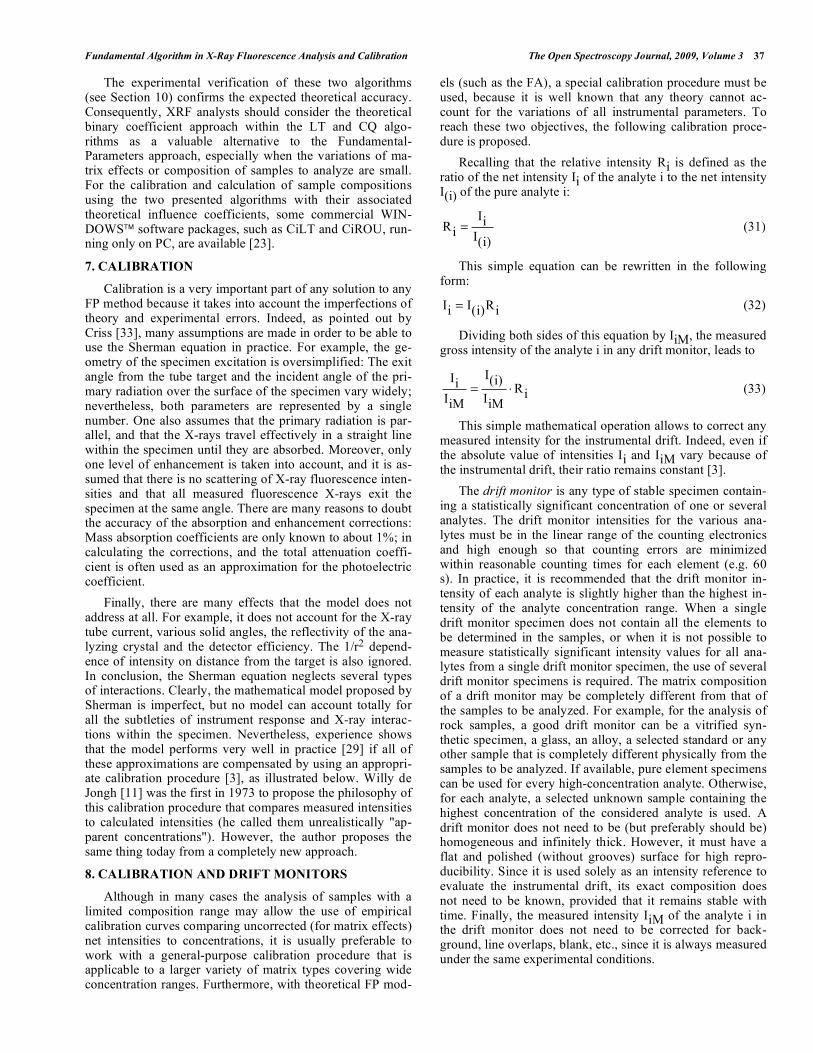
measured relative intensities (Ii/IiM) to calculated relative intensities (Ri=Ci/Mis). It is the best way to get a true cali-bration straight-line. This feature makes the calibration lines robust, i.e., they can be extrapolated by a factor of two or three, thus protecting the analyst from errors when the con-centrations of samples to be analyzed exceed the calibration range. In addition, incorrect standards will be shown clearly as outliers in the calibration line. Fig. (1) shows an example of the type of calibration straight line represented by equa-tion (38).
Fig. (1). Fe calibration graph using NIST alloy standards. The
graph of measured relative intensities as a function of the concen-
tration CFe gives scattered points (o). On the other hand, the plot of
the same measured relative intensities as a function of the theoreti-
cal relative intensities calculated by the Fundamental Algorithm
(Eq. 7) lines up each point (•) on the calibration line.
The calibration slope mi allows the theory to be adapted to the experimental data for each spectrometer. If the pure analyte specimen is used as a drift monitor, Eq. (35) gives a slope mi=1.0. If the experimental value of mi 1.0, the devia-tion results from the imperfections of the theoretical model that cannot account for all of the experimental parameters of a given spectrometer. The slope of the calibration line repre-sents the experimental average intensity of the pure analyte determined from a set of multi-element standards. Depend-ing on the analytical context, this measured value might be substantially different from the theoretical value. It is this difference that compensates to a large extent for all the theo-retical limitations mentioned above. The observed slope value is the required factor allowing adapting theory to a particular set of experimental data and makes truly meaning-ful the equal sign in Eq. (38) or Eq. (39).
The above described calibration procedure is truly matrix independent because it can put on a straight line any type of matrix compositions containing the analyte. Thus, its great advantage is that it can include on the same calibration line a large variety of matrix compositions, limited only by the physical effects (particle or grain size, mineralogy, heteroge-neity, surface, thickness, etc.). However, the preparation of standards must in all aspects be absolutely identical to that of the unknowns.
If empirical coefficients are used rather than theoretical ones, they are calculated during the calibration procedure by regression analysis, at the same time that the mi and bi val-ues of all analytes. Because of the large number of unknown
Fundamental Algorithm in X-Ray Fluorescence Analysis and Calibration The Open Spectroscopy Journal, 2009, Volume 3 39
values to determine, a corresponding large number of stan-dard specimens is needed. On the other hand, if theoretical coefficients are used, they are calculated before the calibra-tion procedure from theory [4]. Knowing them, each calibra-tion line requires only a minimum of two points for calculat-ing the mi and bi values. Therefore, the great advantage of theoretical coefficients, in addition to be accurate, is that only a few standards are needed to calibrate.
This calibration procedure enables each analyte to be calibrated over wide concentration ranges and requires only a few good standards. However, for getting accuracy, it must be stressed that the complete composition of each standard is needed because the analyte line intensity is affected by the concentration of all the elements present in the specimen. If only 98% or 99% of the composition of a standard is certi-fied, it will have limited capability for accurately calculating all the corrections for matrix effects, because the matrix composition is not well known.
Finally, one should recall that any theoretically valid model corrects only for variations in the chemical composi-tion of the samples or standards, i.e., for elemental interac-tions. It does not correct for instrumental (background, line overlaps and dead time) and physical effects (variations of particle size, mineralogical, thickness and surface effects). Both must be reduced to a minimum by careful selection of measurement conditions and sample preparation procedure.
9. ROUTINE ANALYSIS
To apply the calibration procedure explained above in practice, rearranging Eq. (38) for Ci leads to
Ci=
1
mi
Ii
IiM
bi
Mis
(39)
The interpretation of Eq. (39) makes physical sense. Firstly, if there are some errors in the background calcula-tion, bi is different from zero and subtracted from the meas-ured net intensity Ii before being corrected for matrix effects by the Mis factor. Secondly, the concentration is propor-tional to the true net intensity, corrected for the instrumental drift (by IiM), so that only the true net intensity is corrected for matrix effects by the Mis factor. Thirdly, the measured relative intensities
Ri=
1
mi
Ii
IiM
bi
(40)
used with any FP model for calculating the concentrations must be corrected absolutely for the imperfections of theory by the calibration slope mi before being corrected for matrix effects.
As stressed before, the values of the slope (mi) and the intercept (bi) of the calibration line remain valid even after the drift of the instrument. Indeed, the slope is equal to the intensity of the pure analyte, I(i), divided by the monitor intensity IiM (see Eq. 35). The intercept bi is the interception of the calibration line with the Y-axis and is equal to the re-sidual background intensity divided by the monitor intensity. Thus, if the absolute values of the intensities change further to an instrumental drift, their ratio remains constant [34].
Thus, Eq. (39) is in perfect agreement with the basic physical rules of XRF spectrometry. For accurate results, it is imperative that any theoretically valid model respects the underlying physics in XRF analysis.
In routine analysis, Eq. (39) is used to calculate concen-trations. A practical application of this analytical method is given in Ref. [29], where 15 different analytes were deter-mined in many different types of alloys, covering large con-centration ranges. However, the analyst must be aware of some precautions to take before using this equation:
1. When possible, and especially for trace elements, peak and background(s) should be measured for each analyte.
2. All the peak intensities should be corrected for back-ground, line overlaps and blank, an essential step. Without effective background subtraction strategies, the accuracy of the results may be severely compro-mised, especially for trace elements. Background and line overlaps must be subtracted before the calibration procedure, since the concentration is proportional only to the net intensity.
3. Drift correction should be applied to the net intensity of every analyte. Only one high-point drift monitor per analyte should be used where the intensity of the analyte in the drift monitor is slightly higher than the highest measured intensity of the analyte calibration range [34]. At the same time, this procedure for drift monitors guarantees low counting statistical errors.
4. Matrix effects (by calculating the Mis factor) can be corrected using any theoretically valid model, such as the Lachance-Traill, or Claisse-Quintin or Fundamen-tal Algorithm, in association with theoretical influ-ence coefficients. The choice of a particular algorithm depends on the analytical context [4].
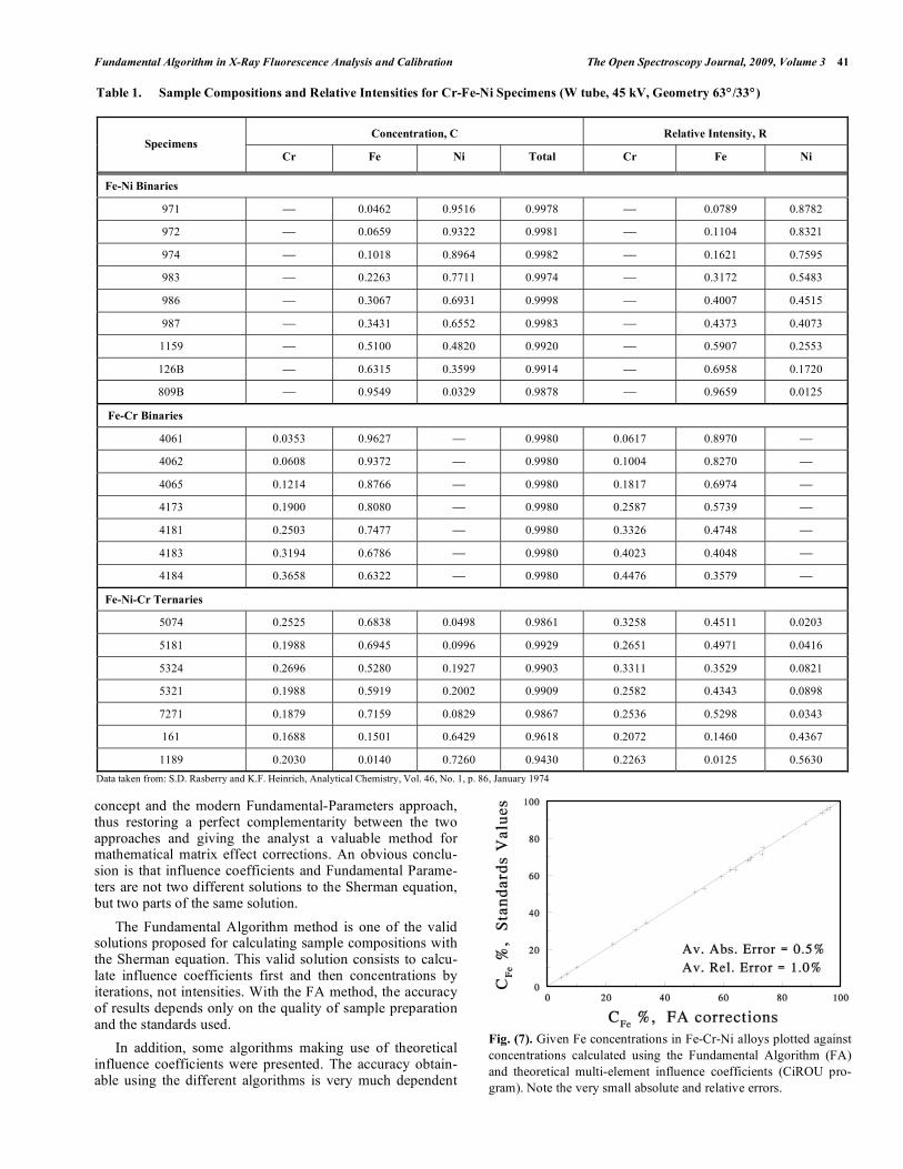
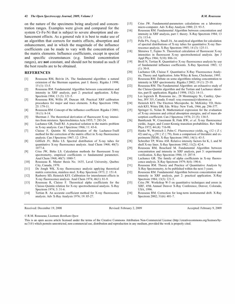
10. EXPERIMENTAL VERIFICATION
An application example [31] of the Fundamental Algo-rithm is given at Fig. (7). The concentration and the meas-ured relative intensity data of a set of Cr-Fe-Ni specimens are given in Table 1. Figs. (3-7) compare given concentra-tions for Fe in a set of Cr-Fe-Ni specimens to the values cal-culated by different algorithms [4] in Fig. (2). In these fig-ures the measured intensities are shown, respectively, uncor-rected, and corrected using the Lachance-Traill (LT) algo-rithm (used in association with empirical and binary constant influence coefficients), the Claisse-Quintin (CQ) algorithm and the Fundamental Algorithm (FA). It can be observed that there is a progressive improvement in the fit of the data in Figs. (3-7). The data fit for the LT algorithm is not as good as the CQ or Fundamental algorithm because the Fe concen-tration range is too large (1-96%). Here, the LT algorithm is used beyond its application range. Otherwise, it should give excellent results in specific contexts, such as limited concen-tration range (0-10%). On the other hand, there is little im-provement between the results from the CQ algorithm and the FA, which is normal. Remember that the CQ algorithm is used in association with the FA for calculating the composi-tion of a sample. The CQ algorithm calculates an accurate first estimate of the sample composition, while the FA calculates from it the final composition. In order to make the
40 The Open Spectroscopy Journal, 2009, Volume 3 R.M. Rousseau
FA method viable and valid, the first composition estimation must be very close to the final result. This is what we ob-serve for these samples.
Linear Algorithm
Ci = Ki Ii =1
I(i)Ii = Ri
Lachance-Traill Algorithm
Ci = Ri 1+ aijC jj
Claisse-Quintin Algorithm
Ci = Ri[1+ aij + aijjCM( )jC j
+ aijkCjCkk> j
j]
Fundamental Algorithm (Proposed by Rousseau)
Ci = Ri
1+ ijC jj
1+ ijC jj
Fig. (2). A comparison of some algorithms using influence coeffi-
cients.
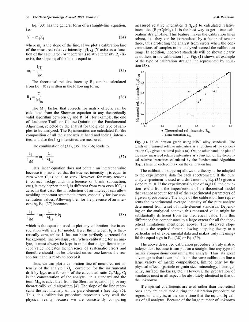
The two last ternary specimens of Table 1, i.e. numbers 161 and 1189, have a low total of 96.18% and 94.30%, re-spectively, which means that we cannot correct for matrix effects of 3.82% and 5.70%, respectively, of missing ele-ments. Therefore, the data points of these two specimens has been omitted from Figs. (4-7) because the low totals would distort the average errors introduced by the different algo-rithms for the calculation of matrix effect corrections. On the other hand, Fig. (3) represents the plot of the Fe concentra-tion (in %) as a function of the Fe relative intensity (in %). The data of the two low total specimens have been included in this figure to illustrate the effects of the matrix on the Fe peak intensities. In this case, the missing elements do not introduce any additional errors.
Fig. (3). Given Fe concentrations in Fe-Cr-Ni alloys plotted against
concentrations calculated from uncorrected Fe intensities. Note the
large absolute and relative errors.
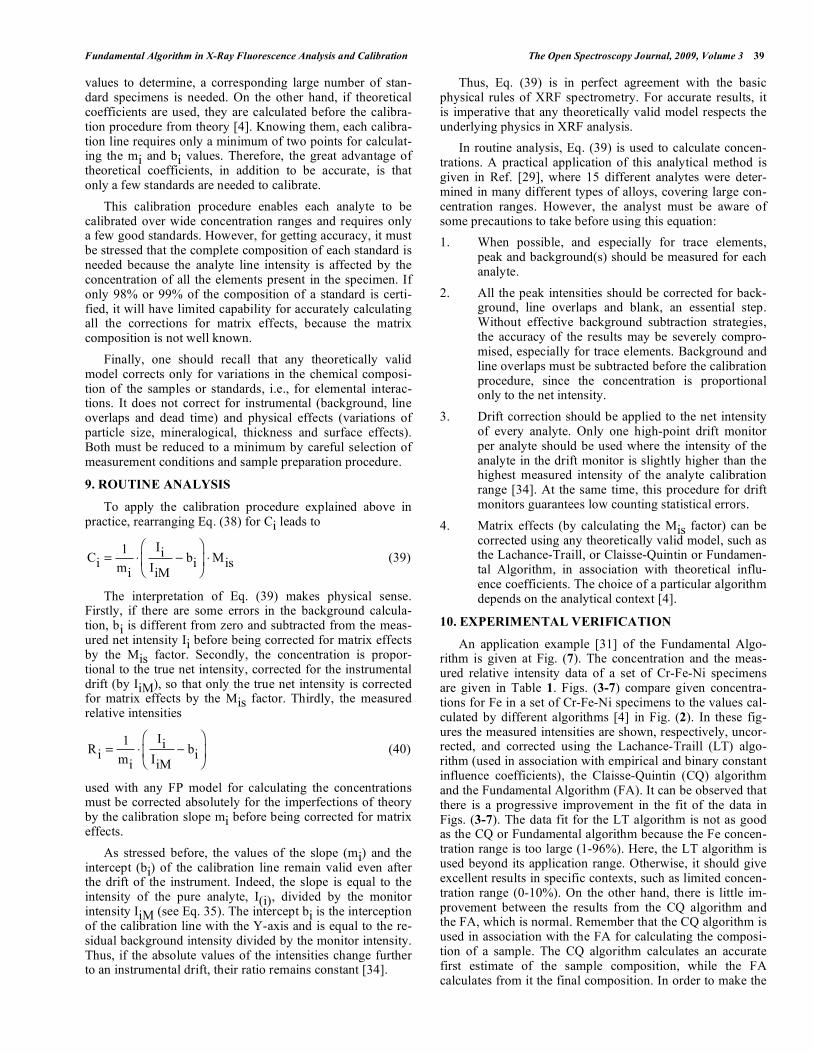
Fig. (4). Given Fe concentrations in Fe-Cr-Ni alloys plotted against
concentrations calculated using the Lachance-Traill algorithm (LT)
and empirical influence coefficients calculated by multiple regres-
sion analysis (CiREG program). Note that absolute and relative
errors are still unacceptably large.
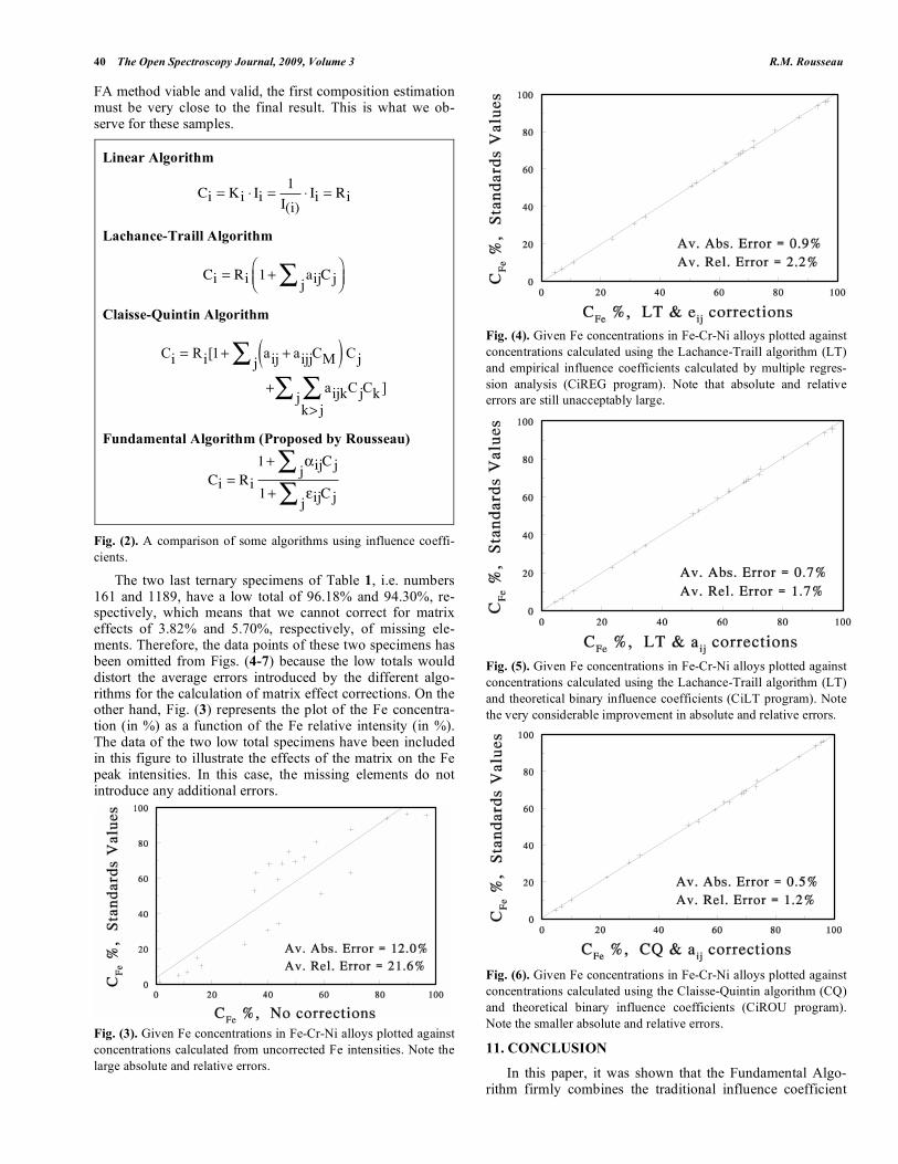
Fig. (5). Given Fe concentrations in Fe-Cr-Ni alloys plotted against
concentrations calculated using the Lachance-Traill algorithm (LT)
and theoretical binary influence coefficients (CiLT program). Note
the very considerable improvement in absolute and relative errors.
Fig. (6). Given Fe concentrations in Fe-Cr-Ni alloys plotted against
concentrations calculated using the Claisse-Quintin algorithm (CQ)
and theoretical binary influence coefficients (CiROU program).
Note the smaller absolute and relative errors.
11. CONCLUSION
In this paper, it was shown that the Fundamental Algo-rithm firmly combines the traditional influence coefficient
Fundamental Algorithm in X-Ray Fluorescence Analysis and Calibration The Open Spectroscopy Journal, 2009, Volume 3 41
concept and the modern Fundamental-Parameters approach, thus restoring a perfect complementarity between the two approaches and giving the analyst a valuable method for mathematical matrix effect corrections. An obvious conclu-sion is that influence coefficients and Fundamental Parame-ters are not two different solutions to the Sherman equation, but two parts of the same solution.
The Fundamental Algorithm method is one of the valid solutions proposed for calculating sample compositions with the Sherman equation. This valid solution consists to calcu-late influence coefficients first and then concentrations by iterations, not intensities. With the FA method, the accuracy of results depends only on the quality of sample preparation and the standards used.
In addition, some algorithms making use of theoretical influence coefficients were presented. The accuracy obtain-able using the different algorithms is very much dependent
Fig. (7). Given Fe concentrations in Fe-Cr-Ni alloys plotted against
concentrations calculated using the Fundamental Algorithm (FA)
and theoretical multi-element influence coefficients (CiROU pro-
gram). Note the very small absolute and relative errors.
Table 1. Sample Compositions and Relative Intensities for Cr-Fe-Ni Specimens (W tube, 45 kV, Geometry 63° /33°)
Concentration, C Relative Intensity, R Specimens
Cr Fe Ni Total Cr Fe Ni
Fe-Ni Binaries
971 0.0462 0.9516 0.9978 0.0789 0.8782
972 0.0659 0.9322 0.9981 0.1104 0.8321
974 0.1018 0.8964 0.9982 0.1621 0.7595
983 0.2263 0.7711 0.9974 0.3172 0.5483
986 0.3067 0.6931 0.9998 0.4007 0.4515
987 0.3431 0.6552 0.9983 0.4373 0.4073
1159 0.5100 0.4820 0.9920 0.5907 0.2553
126B 0.6315 0.3599 0.9914 0.6958 0.1720
809B 0.9549 0.0329 0.9878 0.9659 0.0125
Fe-Cr Binaries
4061 0.0353 0.9627 0.9980 0.0617 0.8970
4062 0.0608 0.9372 0.9980 0.1004 0.8270
4065 0.1214 0.8766 0.9980 0.1817 0.6974
4173 0.1900 0.8080 0.9980 0.2587 0.5739
4181 0.2503 0.7477 0.9980 0.3326 0.4748
4183 0.3194 0.6786 0.9980 0.4023 0.4048
4184 0.3658 0.6322 0.9980 0.4476 0.3579
Fe-Ni-Cr Ternaries
5074 0.2525 0.6838 0.0498 0.9861 0.3258 0.4511 0.0203
5181 0.1988 0.6945 0.0996 0.9929 0.2651 0.4971 0.0416
5324 0.2696 0.5280 0.1927 0.9903 0.3311 0.3529 0.0821
5321 0.1988 0.5919 0.2002 0.9909 0.2582 0.4343 0.0898
7271 0.1879 0.7159 0.0829 0.9867 0.2536 0.5298 0.0343
161 0.1688 0.1501 0.6429 0.9618 0.2072 0.1460 0.4367
1189 0.2030 0.0140 0.7260 0.9430 0.2263 0.0125 0.5630
Data taken from: S.D. Rasberry and K.F. Heinrich, Analytical Chemistry, Vol. 46, No. 1, p. 86, January 1974
42 The Open Spectroscopy Journal, 2009, Volume 3 R.M. Rousseau
on the nature of the specimens being analyzed and concen-tration ranges. Examples were given and compared for the system Cr-Fe-Ni that is subject to severe absorption and en-hancement effects. As a general rule it is best to make use of an algorithm that corrects for matrix effects, absorption and enhancement, and in which the magnitude of the influence coefficients can be made to vary with the concentration of the matrix elements. Influence coefficients, except in special and specific circumstances (e.g. limited concentration ranges), are not constant, and should not be treated as such if the best results are to be obtained.
REFERENCES
[1] Rousseau RM, Boivin JA. The fundamental algorithm: a natural
extension of the Sherman equation, part I: theory. Rigaku J 1998; 15 (1): 13-5.
[2] Rousseau RM. Fundamental Algorithm between concentration and intensity in XRF analysis, part 2: practical application. X-Ray
Spectrom 1984; 13 (3): 121-5. [3] Rousseau RM, Willis JP, Duncan AR. Practical XRF calibration
procedures for major and trace elements. X-Ray Spectrom 1996; 25: 179-11.
[4] Rousseau RM. Concept of the influence coefficient. Rigaku J 2001; 18 (1): 8-14.
[5] Sherman J. The theoretical derivation of fluorescent X-ray intensi-ties from mixtures. Spectrochimica Acta 1955; 7: 283-24.
[6] Lachance GR, Traill RJ. A practical solution to the matrix problem in X-ray analysis. Can J Spectrosc 1966; 11: 43-6.
[7] Claisse F, Quintin M. Generalization of the Lachance-Traill method for the correction of the matrix effect in X-ray fluorescence
analysis. Can J Spectrosc 1967; 12: 129-6. [8] Gilfrich JV, Birks LS. Spectral distribution of X-ray tubes for
quantitative X-ray fluorescence analysis. Anal Chem 1968; 40(7): 1077-4.
[9] Criss JW, Birks LS. Calculation methods for fluorescent X-ray spectrometry, empirical coefficients vs fundamental parameters.
Anal Chem 1968; 40(7): 1080-7. [10] Rousseau R. Master thesis No. 1635, Laval University, Quebec
City, Canada, 1970. [11] De Jongh WK. X-ray fluorescence analysis applying theoretical
matrix correction, stainless steel. X-Ray Spectrom 1973; 2: 151-8. [12] Rasberry SD, Heinrich KFJ. Calibration for interelement effects in
X-ray fluorescence analysis. Anal Chem 1974; 46(1): 81-9. [13] Rousseau R, Claisse F. Theoretical alpha coefficients for the
Claisse-Quintin relation for X-ray spectrochemical analysis. X-Ray Spectrom 1974; 3: 31-6.
[14] Tertian R. An accurate coefficient method for X-ray fluorescence analysis. Adv X-Ray Analysis 1976; 19: 85-27.
[15] Criss JW. Fundamental-parameters calculations on a laboratory
micro-computer. Adv X-Ray Analysis 1980; 23: 93-5. [16] Rousseau RM. Fundamental Algorithm between concentration and
intensity in XRF analysis, part 1: theory. X-Ray Spectrom 1984; 13 (3): 115-6.
[17] Pella PA, Feng L, Small JA. An analytical algorithm for calculation of spectral distributions of X-ray tubes for quantitative X-ray fluo-
rescence analysis. X-Ray Spectrom 1985; 14 (3): 125-11. [18] Shiraiwa T, Fujino N. Theoretical calculation of fluorescent X-ray
intensities in fluorescent X-ray spectrochemical analysis. Jpn J Appl Phys 1966; 5(10): 886-14.
[19] Broll N, Tertian R. Quantitative X-ray fluorescence analysis by use of fundamental influence coefficients. X-Ray Spectrom 1983; 12
(1): 30-8. [20] Lachance GR, Claisse F. Quantitative X-Ray Fluorescence Analy-
sis, Theory and Application. John Wiley & Sons, Chichester, 1995. [21] Rousseau RM. Debate on some algorithms relating concentration to
intensity in XRF spectrometry. Rigaku J 2002; 19 (1): 25-10. [22] Rousseau RM. The Fundamental Algorithm: an exhaustive study of
the Claisse-Quintin algorithm and the Tertian and Lachance identi-ties, part II: application. Rigaku J 1998; 15(2): 14-11.
[23] Les logiciels R. Rousseau inc., 28 Montmagny St., Cantley, Que-bec, J8V 3J1, Canada. E-mail: [email protected]
[24] Heinrich KFJ. The Electron Microprobe. In: McKinley TD, Hein-rich KFJ, Wittry DB, Eds. Wiley: New York, 1966, pp. 296-377.
[25] Springer G, Nolan B. Mathematical expression for the evaluation of X-ray emission and critical absorption energies, and of mass ab-
sorption coefficient. Can J Spectrosc 1976; 21 (5): 134-5. [26] Bambynek W, Crasemann B, Fink RW, et al. X-ray fluorescence
yields, Auger, and Coster-Kronig transition probabilities. Rev Mod Phys 1972; 44 (4): 716-98.
[27] Hanke W, Wernisch J, Pohn C. Fluorescence yields, K (12 Z 42) and L3 (38 Z 79), from a comparison of literature and ex-
periments (SEM). X-Ray Spectrom 1985; 14(1): 43-5. [28] Schreiber TP, Wims AM. Relative intensity factors for K, L and M
shell X-ray lines. X-Ray Spectrom 1982; 11(2): 42-4. [29] Rousseau RM, Bouchard M. Fundamental Algorithm between
concentration and intensity in XRF analysis, part 3: experimental verification. X-Ray Spectrom 1986; 15: 207-9.
[30] Lachance GR. The family of alpha coefficients in X-ray fluores-cence analysis. X-Ray Spectrom 1979; 8(4): 190-6.
[31] Rousseau RM. Theory and Practice of Quantitative Analysis by X-Ray Spectrometry, to be published within the next 3 years.
[32] Rousseau RM. Fundamental Algorithm between concentration and intensity in XRF analysis, part 2: practical application. X-Ray
Spectrom 1984; 13(3): 121-5. [33] Criss JW. Workshop W-5 on quantitative techniques and errors in
XRF, 45th Annual Denver X-Ray Conference, Denver, Colorado, USA, 1996.
[34] Rousseau RM. Correction for long-term instrumental drift. X-Ray Spectrom 2002; 31(6): 401-7.
Received: December 19, 2008 Revised: February 2, 2009 Accepted: February 9, 2009
© R.M. Rousseau; Licensee Bentham Open
This is an open access article licensed under the terms of the Creative Commons Attribution Non-Commercial License (http://creativecommons.org/licenses/by-nc/3.0/) which permits unrestricted, non-commercial use, distribution and reproduction in any medium, provided the work is properly cited.