Long-term patterns of mass loss during the decomposition of leaf and fine root litter: an intersite...

Long-term patterns of mass loss during thedecomposition of leaf and fine root litter:an intersite comparison

M A R K E . H A R M O N *, W H E N D E E L . S I LV E R w , B E C K Y F A S T H *, H U A C H E N *, I N G R I D C .

B U R K E z, W I L L I A M J . PA R T O N § , S T E P H E N C . H A R T } , W I L L I A M S . C U R R I E k and L I D E T 1

*Department of Forest Science, Oregon State University, 321 Richardson Hall, Corvallis, OR 97331, USA, wDepartment of

Environmental Science, Policy, and Management, Ecosystem Sciences Division, University of California, Berkeley, CA 94720, USA,

zDepartment of Forest, Rangeland, and Watershed Stewardship, Colorado State University, Fort Collins, CO 80523, USA, §Natural

Resource Ecology Laboratory, Colorado State University, Fort Collins, CO 80523, USA, }School of Forestry and Merriam-Powell

Center for Environmental Research, Northern Arizona University, PO Box 15018, Flagstaff, AZ 86011-5018, USA, kSchool of

Natural Resources & Environment, Dana Bldg., 430 E. University, University of Michigan, Ann Arbor, MI 48109-1115, USA

Abstract

Decomposition is a critical process in global carbon cycling. During decomposition, leaf

and fine root litter may undergo a later, relatively slow phase; past long-term experiments

indicate this phase occurs, but whether it is a general phenomenon has not been

examined. Data from Long-term Intersite Decomposition Experiment Team, representing

27 sites and nine litter types (for a total of 234 cases) was used to test the frequency of this

later, slow phase of decomposition. Litter mass remaining after up to 10 years of

decomposition was fit to models that included (dual exponential and asymptotic) or

excluded (single exponential) a slow phase. The resultant regression equations were

evaluated for goodness of fit as well as biological realism. Regression analysis indicated

that while the dual exponential and asymptotic models statistically and biologically fit

more of the litter type–site combinations than the single exponential model, the latter

was biologically reasonable for 27–65% of the cases depending on the test used. This

implies that a slow phase is common, but not universal. Moreover, estimates of the

decomposition rate of the slowly decomposing component averaged 0.139–0.221 year�1

(depending on method), higher than generally observed for mineral soil organic matter,

but one-third of the faster phase of litter decomposition. Thus, this material may be

slower than the earlier phases of litter decomposition, but not as slow as mineral soil

organic matter. Comparison of the long-term integrated decomposition rate (which

included all phases of decomposition) to that for the first year of decomposition

indicated the former was on average 75% that of the latter, consistent with the presence

of a slow phase of decomposition. These results indicate that the global store of litter

estimated using short-term decomposition rates would be underestimated by at least

one-third.

Keywords: decay, decomposition, fine roots, leaves, litter, long-term study, rate constant, stable fraction

Received 23 May 2008; revised version received 18 September 2008 and accepted 1 October 2008

Introduction

Plant litter in the form of dead leaves and roots is a

source of soil organic matter, the largest terrestrial store

of carbon (Post et al., 1982). The current size of this store

and its fate under global environmental change requires

insight into the long-term temporal pattern of litter

decomposition (Kirschbaum, 2000). Little is known

about long-term patterns of decomposition, in part,

because few experiments have tracked the process from

fresh litter to the formation of highly decomposed

material. Nearly 4000 papers have been published on

the topic of litter decomposition (Institute of Scientific

Information Web of Science), but few extend beyond a

Correspondence: Mark E. Harmon, fax 1 1 541 737 1393,

e-mail: [email protected]

1See Table 1 for the list of 27 LIDET team members

Global Change Biology (2009) 15, 1320–1338, doi: 10.1111/j.1365-2486.2008.01837.x

r 2009 The Authors1320 Journal compilation r 2009 Blackwell Publishing Ltd

given ecosystem type for more than several years (e.g.

Gholz et al., 2000; Trofymow et al., 2002). The vast

majority of experiments have lasted 1–2 years (Swift

et al., 1979; Melillo et al., 1984; Vogt et al., 1986; Silver &

Miya, 2001) yielding many insights into the temporal

pattern early in decomposition (Olson, 1963; Howard &

Howard, 1974) as well as the controls on initial mass

loss such as initial litter quality (Minderman, 1968;

Bunnell & Tait, 1977; Fogel & Cromack, 1977; Melillo

et al., 1982), invertebrates (Kurcheva, 1960; Witkamp &

Olson, 1963; Witkamp & Crossley, 1966), and environ-

mental variables such as temperature and moisture

(Bunnell et al., 1977; Meentemeyer, 1978; Jansson & Berg,

1985; Yahdjian et al., 2006). However, 2 years is not

enough time in most environments to reveal dynamics

in the later phases of this key ecosystem process.

Previous investigators have proposed conceptual

models of decomposition with at least two distinct

phases, although ideas have differed on the mechan-

isms distinguishing the phases and the degree of re-

calcitrance or stability of material in the later phases.

Couteaux et al. (1995) proposed a two-phase conceptual

model in which Phase I was dominated by the loss of

soluble and relatively labile compounds from litter,

including some of the cellulose present. In Phase II,

decomposition continued, but with a strong control

exerted by lignin. In contrast, Melillo et al. (1989) and

Aber et al. (1990) proposed a two-phase conceptual

model in which the material in Phase II was similar, if

not identical to soil organic matter and was termed

‘stable’ over a time-span of approximately a decade.

The gradually slowing absolute rate of mass loss from

decaying litter over time can be captured by a first-

order or exponential decay function [Eqn (1)] where Mt

is litter mass at time t, M0 is initial litter mass, and k is

the rate constant of loss

Mt ¼M0e�kt; ð1Þ

However, the long-term studies (e.g. Aber et al., 1990;

Magill & Aber, 1998; Berg et al., 2001; Trofymow et al.,

2002; Moore et al., 2005) that have been conducted

suggest that in later stages rates of decomposition slow

to a degree beyond that captured by a single-exponen-

tial decomposition curve. For litters high in soluble and

labile fractions, a very rapid phase of decomposition

may also occur within days to weeks of litter formation

(Harmon et al., 1990; Currie & Aber, 1997). Exponential

rate constants of mass loss (i.e. the proportion lost per

unit time) of the soluble and labile fractions during this

phase may exceed 10 year�1, indicating this material is

lost within a few months. During the following phase,

which dominates the first few years for many litter

types in temperate environments, structural polymers

are degraded. While there is considerable range in the

speed at which these materials are degraded, exponen-

tial rate constants of 0.1–5 year�1 are typical (Singh &

Gupta, 1977; Swift et al., 1979; Vogt et al., 1986). As these

polymers are degraded, residual and newly formed

recalcitrant materials begin to dominate the decomposi-

tion process. The size and rate this late phase pool

decomposes are not well established and may have a

great deal of variability (Berg & McClaugherty, 2003). In

some cases, slow phase decomposition rates appear to

be very low (Berg et al., 1984). Carbon isotope studies

suggest that rate constants for highly decomposed soil

organic matter, i.e. material that is generally complexed

with mineral material, are typically below 0.01 year�1

(Gaudinski et al., 2000; Trumbore, 2000). Modeling

analysis of the forest floor in northern hardwoods

forests of the northeastern United States suggests that

if Phase II sensu Aber et al. (1990), starts when 20% of the

original litter mass remained, then a rate constant of

0.017 year�1 would be needed to match the measured

forest floor mass (Currie & Aber, 1997).

A major gap to studying decomposition is the lack of

a careful assessment of the philosophy supporting and

consequences of choosing certain mathematical models

describing the course of decomposition. The single

negative exponential model [Eqn (1)] has been most

commonly used to determine the decomposition rate of

litter. This model often does not capture the initial very

rapid loss phase adequately (Blair et al., 1990; Chen

et al., 2002), but has worked remarkably well for the

majority of data from short-term experiments. If decom-

position follows this simple exponential pattern, then

predicting temporal patterns in the later stages of

decomposition by extrapolation is possible. However,

the long-term data that exist indicate a relatively slow

phase of decomposition is eventually reached (Lousier

& Parkinson, 1978, 1979; Berg et al., 1984; Edmonds,

1984; McClaugherty et al., 1985; Chen et al., 2002) and

sometimes an asymptote in mass being reached imply-

ing extremely slow decomposition (Wardle et al., 1997;

Berg et al., 2001).

There are two alternatives to the single negative

exponential equation: the multiple (or in the most

simple case the dual) exponential; and the negative

exponential with an asymptote (Howard & Howard,

1974; Wieder & Lang, 1982). Both equations capture the

transition from rapid to slow decomposition, although

the asymptotic equation implies a steady accumulation

of partially decomposed litter (because the litter repre-

sented by the asymptote does not decompose). In addi-

tion to deriving separate decomposition rates for each

of the multiple fractions (e.g. the ‘fast’ and ‘slow’

fractions), these equations require estimating the initial

proportions of these fractions. Previous studies on hard-

wood species in the northeastern United States indi-

M A S S L O S S D U R I N G L E A F A N D F I N E R O O T L I T T E R D E C O M P O S I T I O N 1321

r 2009 The AuthorsJournal compilation r 2009 Blackwell Publishing Ltd, Global Change Biology, 15, 1320–1338

cated that approximately 20% of the initial litter was

formed of slowly decomposing material (Aber et al.,

1990). Berg (2000a, b) found that it varied from 6% to

47% of initial forest litter mass, depending on the

amount of nitrogen present. The degree this slowly

decomposing fraction is initially present or created by

the many biological and chemical reactions that we

term ‘decomposition’ is still under debate. While some

litter types apparently enter a phase in which decom-

position rates are relatively low, it is unclear whether

this is a general pattern; if so, the degree that it is

influenced by substrate quality, environment, and their

interactions needs to be elucidated.

This paper provides a general overview of Long-term

Intersite Decomposition Experiment Team (LIDET), a

study that generated a dataset that we use to test the

generality of a late, slow phase of decomposition (Moor-

head et al., 1999; Gholz et al., 2000). Our specific objec-

tives in this paper are: (1) to examine a series of

mathematical models to test how well they statistically

fit observations and how well they conformed to biolo-

gical expectations; (2) to evaluate the generality of a

slow phase and the fraction of the litter involved; and

(3) to provide estimates of how fast this material de-

composed.

The LIDET study

Background

The data used in this study were from the LIDET, a

project which carried out a 10-year field study with the

primary objective of testing the degree to which sub-

strate quality and climate control the long-term carbon

and nitrogen dynamics of decomposing leaf and fine

root litter (Table 1). LIDET employed a standardized

methodology at a large number of sites (27) to examine

decomposition patterns within the first decade of de-

composition of 30 species of litter. In addition to char-

acterizing the climate during the course of the

experiments, the chemical nature of the material used

in the experiment was described using a wide range of

carbon fractions and nutrient elements. LIDET therefore

represents one of the few comprehensive, long-term or

large-scale datasets from which to develop generaliz-

able patterns.

General experimental design

Three experiments were conducted by LIDET: (1) a

comparison of long-term leaf and fine root decomposi-

tion to examine the effect of substrate quality and

climate on patterns of long-term decomposition and

nitrogen accumulation in above- and below-ground fine

litter, (2) a comparison of leaf decomposition with and

without macroinvertebrates, and (3) a comparison of

environmental influences on wood decomposition

above- and below-ground using wooden dowels as a

common substrate. The major factors considered in the

leaf and fine root experiment, the focus of this paper,

were site, species of litter, and time. There were 27 sites,

representing a wide array of moisture and temperature

conditions, at which the experiments were installed

(Table 1, Fig. 1). Each site was characterized in terms

of location (i.e. latitude and longitude), elevation, cli-

mate [precipitation, temperature, Actual Evapotran-

spiration (AET), potential evapotranspiration, Climate

Decomposition Index (CDI); see Adair et al., 2008], and

vegetation (biome type and specific vegetation cover).

The sites span a wide array of ecosystem types from

tundra to warm desert to shortgrass steppe to moist

tropical forest. Climate data were taken from measure-

ments at the site or from nearby climatic stations.

Precipitation ranged from 24 to 409 cm yr�1 and mean

annual air temperature ranged from �7 to 26 1C (Fig. 2).

Nine types of ‘standard’ litters were sent to each of the

27 sites including: three types of fine roots (graminoid,

hardwood, and conifer) and six types of leaf litter that

ranged in AUF/nitrogen ratio from 5 to 50 (Table 2, Fig.

3). Samples were collected 10 times and there were four

replicates for each species, site, and time. In addition to

the standard litters, each site is represented by a ‘wild-

card’ litter that appeared at one site for each sample

collection. The purpose of the wildcard species was to

verify the predictions from the standard species. There

were also four replicates for each wildcard species, site,

and time.

Materials and methods

Field and laboratory

Fresh leaf and fine roots for the standard litters was

gathered from five of the 27 LIDET sites. The leaves

were collected by a range of methods, ranging from

collection of senescent leaves from trees (the primary

method), to collecting freshly fallen litter from the

ground, to removing green foliage (used at one of the

tropical sites). Fine roots (o2 mm diameter) were col-

lected by either excavating surface roots and washing or

collecting material exposed along stream banks. All

litter was air dried at room temperature before ship-

ment to Oregon State University except materials those

from Luquillo which were oven-dried at 50 1C to halt

decomposition.

All the litterbags used were 20 cm� 20 cm and filled

with an air-dried mass of 10 g leaves and 5–7 g of fine

roots. Each bag was identified with a unique number

1322 M . E . H A R M O N et al.


Table 1 General characteristics of sites used in the LIDET study and the list of LIDET team members

Site Code Latitude Longitude Biome type MAP MAT AET PET Elev

LIDET team

member

*H. J Andrews

Experimental Forest,

Oregon

AND 441140N 1221110W Temperate Conifer

Forest

230.9 8.6 76.4 98.2 500 M. Harmon

*Arctic Lakes, Alaska ARC 681380N 1491340W Tundra 32.7 �7.0 28.4 42.3 760 J Laundre

Barro Colorado

Island, Panama

BCI 91100N 791510W Humid Tropical

Seasonal Forest

269.2 25.6 136.8 151.7 30 J. Wright

*Bonanza Creek


Alaska

BNZ 641450N 1481000W Boreal Forest 40.3 �5.0 36.0 57.6 300 J. Yarie

Blodgett Research

Forest, California

BSF 381520N 1051380W Temperate Conifer

Forest

124.4 14.4 75.3 109.7 1300 S. Hart

*Cedar Creek

Natural History

Area,Minnesota

CDR 451240N 931120W Temperate

Woodland/Humid

Grassland

82.3 5.5 73.3 102.6 230 D. Wedin

*Central Plains

Experimental Range,

Colorado

CPR 401490N 1041460W Temperate

Shortgrass

44.0 8.9 43.0 120.2 1650 I. Burke

*Coweeta

Hydrological

Laboratory, North

Carolina

CWT 351000N 831300W Temperate

Deciduous Forest

190.6 12.5 117.3 135.3 700 B. Clinton

Guanica State Forest,

Puerto Rico

GSF 171570N 651520W Dry Tropical Forest 50.8 26.3 50.2 142.2 80 A. Lugo

*Hubbard Brook


New Hampshire

HBR 431560N 711450W Temperate

Deciduous Forest

139.6 5.0 71.2 81.7 300 T. Fahey

*Harvard Forest,

Massachusetts

HFR 421400N 721150W Temperate

Deciduous Forest

115.2 7.1 85.1 104.1 335 J. Melillo

*Jornada

Experimental Range,

New Mexico

JRN 321300N 1061450W Warm Semi-desert 29.8 14.6 29.2 166.6 1410 J. Anderson

Juneau, Alaska JUN 581000N 1341000W Temperate Conifer

Forest

287.8 4.4 49.5 54.4 100 M. McClellan

*Kellogg Biological

Station, Michigan

KBS 421240N 851240W Agro Ecosystem 81.1 9.0 70.6 100.7 288 S. Halstead

*Konza Prairie

Research Natural

Area, Kansas

KNZ 391050N 961350W Temperate Tallgrass 79.1 12.8 74.7 125.0 366 J. Blair

La Selva Biological

Station, Costa Rica

LBS 101000N 831000W Humid Tropical

Forest

409.9 25.0 169.9 177.3 35 P. Sollins

*Luquillo


Puerto Rico

LUQ 181190N 651490W Humid Tropical

Forest

336.3 23.0 123.4 125.9 350 J. Lodge

Loch Vale Watershed,

Colorado

LVW 401170N 1051390W Boreal Forest 109.6 1.6 85.1 108.3 3160 J. Baron

Monte Verde,

Costa Rica

MTV 101180N 841480W Tropical Elfin Cloud

Forest

268.5 17.7 108.4 116.6 1550 N. Nadkarni

North Inlet (Hobcaw

Barony), South

Carolina

NIN 331300N 791130W Wetland 149.1 18.1 120.6 145.6 2 J. Morris

*North Temperate

Lakes, Trout Lake

Station, Wisconsin

NLK 461000N 891400W Temperate

Deciduous Forest

67.7 4.4 64.9 88.4 500 T. Gower

Continued



embossed on an aluminum tag. The bag openings were

sealed with six Monel staples. The initial air-dry weight,

calculated oven-dry weight, species, site, and replicate

number for each litterbag were recorded before place-

ment in the field. Subsamples of litter material were

taken to determine the air-dry to oven-dry conversion

factor and the initial chemistry of the litter. These were

taken at the start and end of each weighing session,

with an additional sample taken in the middle of longer

sessions. The standard deviation of the air dried litter

moisture content for all 120 samples was 2%, with a

standard error of 0.002%. Two types of bags were used

Site Code Latitude Longitude Biome type MAP MAT AET PET Elev

LIDET team

member

*Niwot Ridge/Green

Lakes Valley,

Colorado

NWT 401030N 1051370W Tundra 124.9 �3.7 64.7 75.6 3650 J. Baron

Olympic National

Park, Washington

OLY 471500N 1221530W Temperate Conifer

Forest

153.1 10.0 79.4 104.4 150 R. Edmonds

*Sevilleta National

Wildlife Refuge, New

Mexico

SEV 341290N 1061400W Warm Semi-desert 25.4 16.0 25.2 160.2 1572 C. White

Santa Margarita

Ecological Reserve,

California

SMR 331300N 1171450W Annual Grassland 24.0 16.4 23.6 186.0 500 P. Zedler

University of Florida,

Florida

UFL 291450N 821300W Temperate Conifer

Forest

123.8 21.0 116.6 162.1 35 H. Gholz

*Virginia Coast

Reserve, Virginia

VCR 371300N 751400W Wetland 113.8 15.0 99.3 121.5 0 L. Blum

LIDET, Long-term Intersite Decomposition Experiment Team; MAP, mean annual precipitation (cm); MAT, mean annual tempera-

ture ( 1C); AET, actual evapotranspiration (cm); PET, potential evapotranspiration (cm); elev, elevation (m). Climatic data are for the

duration of the experiment. Asterisks denote that the site is a member of the Long Term Ecological Research (LTER) network.

Table 1 Continued

Fig. 1 Location of the Long-term Intersite Decomposition Experiment Team (LIDET) study sites.

1324 M . E . H A R M O N et al.


in this experiment. For the long-term leaf litter experi-

ment, the bags had a top mesh of 1 mm nylon and a

bottom of 55 mm Dacron. The bags used for fine roots

were made entirely of 55mm Dacron mesh.

Samples were placed in the field during fall of 1990 or

1991 by each of the participating sites. Four separate

locations at each site were selected to represent the

range of typical conditions. At each of these locations,

10 sets of litter bags were placed. Each set of 10 bags to

be collected at a given time and location were tethered

to a cord; these sets of bags were laid out in parallel

lines in a random order. Leaf litter bags were placed

on the ground surface. Fine root bags were placed

within the top 20 cm of the soil by cutting into the soil

with a shovel at a 451 angle, sliding the root bag into the

cut, and then firmly pressing the overlying soil onto the

bag.

All sites, other than the tropical ones, collected the

fine litter on an annual basis for a 10-year period. For

tropical sites (Barro Colorado Island, La Selva, Luquillo,

and Monteverde) sampling was conducted every 3–6

months. Once the litter or dowels were collected, the

fresh and oven-dry weight was determined and re-

corded. Samples were oven dried in paper bags at

55 1C until the mass was stable. The samples were then

sent to Oregon State University for preparation for

chemical analysis as well as reweighing of selected

samples for data quality checks. The contents of each

litterbag were ground separately and stored in plastic

vials labeled to identify the species, site, and time the

sample was taken. Samples were also pooled by species,

site, and time to provide samples for wet chemical and

near infrared (NIR) analysis.

Nitrogen and carbon concentration was determined

on a Leco C/N/S-2000 Macro Analyzer (Leco Inc, St

Joseph, MI, USA). Ash concentration was determined

by heating in a muffle furnace at 450 1C for 8 h. Analysis

of carbon fractions for undecomposed litter followed

the methods of McClaugherty et al. (1985) and Ryan

et al. (1990). Nonpolar extractives, (i.e. soluble fats,

waxes, and oils) were removed using dichloromethane

(Tappi, 1976; Bridson, 1985). Simple sugars and water

soluble phenolics were removed with hot water (Tappi,

1981). Simple sugars were determined with the phenol–

sulfuric acid assay (DuBois et al., 1956). Water soluble

phenolics were determined using the Folin–Denis pro-

cedure (Hagerman, 1988; Haslam, 1989). The acid un-

hydrolysable fraction, traditionally called lignin, was

determined by hydrolyzing extractive-free material

with sulfuric acid and weighing the residue (Effland,

1977; Obst & Kirk, 1988). Hydrolysates were analyzed

for carbohydrate content using the phenol–sulfuric acid

assay (DuBois et al., 1956).

Mathematical models

The data used for this analysis were derived from the

LIDET study (Moorhead et al., 1999, Gholz et al., 2000)

and we only analyzed data for the ‘standard litters’

that were placed at all of the 27 sites for each sample

time (the raw data and detailed results of the analysis

can be found at http://www.fsl.orst.edu/lter/research/

intersite/lidet.htm). We examined how well the data

from all sites fit simple mathematical models and the

question of whether a ‘slow’ fraction formed during

long-term decomposition by comparing three types of

regression models: (1) a simple negative exponential, (2)

a negative exponential with an asymptote, and (3) a

dual negative exponential model (Wieder & Lang,

1982). Our intent was not to find the single ‘best’

equation to use or test the best simulation model.

Rather, we compared the predictions of these regression

models to the observed data and to each other to find

cases where a model would apply and if the models

predicted similar patterns. Each model is based on

different assumptions about the decomposition pro-

cesses, and because of this, the cases where each model

did not apply implies the assumptions were not valid.

Both the negative exponential with an asymptote, and

dual negative exponential model imply a later, slower

decomposition phase, although the asymptotic model

implies a rate constant equal to zero is eventually

reached.

The first regression model used (Model 1) was a

simple negative exponential

Mt1 ¼M01 � expð�k1 � tÞ; ð2Þ

where Mt1 is the percent ash-free mass remaining, M01

is the initial ash-free mass, t is time in years, and k1 is

the decomposition rate constant in year�1. This model is

the one most commonly used to determine the decom-

Fig. 2 Range of mean climate conditions for the sites used in

Long-term Intersite Decomposition Experiment Team (LIDET).



Tab

le2

Init

ial

litt

ersu

bst

rate

qu

alit

yin

dic

esfo

rL

IDE

Tst

ud

y

Sp

ecie

s*

Sam

ple

sA

sh(%

)

No

np

ola

rex

trac

tiv

esW

ater

So

lub

leA

cid

Hy

dro

lysa

ble

Aci

du

nh

yd

roly

sab

lew

Tan

nin

Wat

erso

lub

leca

rbo

hy

dra

tes

Aci

dh

yd

roly

sab

leca

rbo

hy

dra

tes

C(%

)N

C/

Nra

tio

sA

UF

/Nz

Lea

ves

*%

ash

-fre

e%

ash

-fre

e%

ash

-fre

e%

ash

-fre

e%

ash

-fre

e%

ash

-fre

e%

ash

-fre

e%

ash

-fre

e

AB

CO

35.

917

.839

.435

.77.

16.

012

.79.

351

.30.

6678

.310

.9A

BL

A3

4.3

19.4

32.0

30.6

18.0

6.2

15.9

15.6

54.0

0.71

76.1

25.3

AC

SA

54.

78.

248

.227

.616

.07.

711

.112

.749

.80.

8161

.819

.8A

MB

R5

3.6

6.4

21.7

57.3

14.5

4.7

15.2

36.7

48.6

0.67

73.5

21.7

AN

GE

67.

75.

914

.960

.318

.81.

84.

030

.844

.60.

6273

.130

.5A

NS

C5

3.8

3.9

12.0

71.5

12.7

3.7

6.9

41.1

47.3

0.56

86.1

22.5

BE

LU

55.

78.

018

.746

.327

.02.

65.

715

.149

.91.

6031

.216

.9B

OE

R5

9.2

5.1

13.4

65.7

15.8

1.2

5.3

34.3

44.9

0.86

52.9

18.3

BO

GR

510

.27.

614

.270

.12

8.1

1.9

7.5

44.3

43.0

0.96

45.0

8.4

CE

GR

54.

610

.849

.627

.112

.58.

117

.46.

752

.61.

3339

.79.

4C

ON

U5

11.7

9.2

52.5

37.6

0.8

9.4

14.5

14.5

44.1

0.81

55.8

1.0

DR

GL

87.

88.

040

.740

.311

.08.

013

.318

.147

.81.

9724

.25.

6FA

GR

56.

47.

416

.349

.826

.45.

36.

721

.349

.40.

8558

.431

.0G

YL

U3

9.0

9.87

40.5

42.9

6.8

5.2

7.4

19.9

43.0

1.37

31.5

5.0

KO

MY

55.

55.

423

.062

.39.

32.

48.

634

.846

.31.

0743

.98.

8L

AT

R5

8.0

18.7

32.0

41.1

8.1

5.9

8.6

10.4

50.9

2.14

23.8

3.8

LIT

U5

12.3

14.2

44.8

32.2

8.8

5.2

7.2

16.2

46.4

0.72

65.1

12.2

MY

CE

53.

813

.029

.630

.426

.96.

211

.412

.152

.02.

1124

.612

.8P

IEL

51.

517

.419

.741

.521

.54.

56.

820

.354

.30.

3616

3.8

59.7

PIR

E5

1.7

15.3

20.7

44.7

19.3

7.4

9.8

20.1

53.4

0.59

92.7

32.8

PIS

T5

3.9

18.9

20.3

40.0

20.8

4.8

7.9

19.6

52.8

0.62

85.9

33.3

PO

TR

57.

710

.628

.941

.419

.04.

69.

818

.549

.20.

7467

.225

.9P

SM

E9

11.9

13.7

17.2

41.0

28.1

2.9

7.6

24.2

48.8

0.82

59.4

34.2

QU

PR

84.

49.

427

.439

.623

.66.

97.

118

.051

.51.

0350

.523

.0R

HM

A5

4.6

9.0

36.6

37.3

17.1

6.3

17.2

19.6

50.8

0.42

126.

341

.0R

OP

S6

5.6

7.2

34.1

40.8

17.9

5.3

10.0

11.1

50.2

2.45

20.5

7.3

SP

AL

1012

.24.

927

.460

.46

7.4

4.1

4.7

28.3

42.7

0.71

62.6

10.2

TH

PL

77.

814

.626

.337

.621

.54.

49.

0316

.48

51.1

0.62

83.1

34.5

TR

AE

52.

83.

46.

873

.616

.32.

95.

041

.147

.30.

3813

3.3

43.2

VO

FE

65.

56.

731

.442

.819

.14.

99.

013

.049

.21.

9325

.69.

9R

oo

tsA

NG

E8

27.6

6.0

14.0

69.1

10.9

1.1

5.3

33.2

37.0

0.63

59.4

17.3

DR

GL

67.

010

.720

.252

.816

.32.

46.

715

.348

.20.

7664

.621

.5P

IEL

96.

38.

919

.836

.135

.23.

38.

519

.749

.40.

8261

.543

.0P

IRE

38.

66.

19.

456

.328

.22.

32.

213

.348

.41.

2239

.923

.2

Bo

ld-f

aced

spec

ies

are

for

the

stan

dar

dli

tter

s.

* AB

CO

,A

bies

con

colo

r,W

hit

efi

r;A

BL

A,

Abi

esla

sioc

arpa

,su

bal

pin

efi

r;A

CS

A,

Ace

rsa

ccha

rum

,su

gar

map

le;

AM

BR

-Am

moh

iabr

evil

gula

ta,

bea

chg

rass

;A

NG

E,

Sch

izac

hyri

um

(aka

An

drop

ogon

)ge

rard

i,b

igb

lue

stem

AN

SC

,S

chiz

achy

riu

m(a

kaA

ndr

opog

on)

scop

ariu

m,

litt

leb

lue

stem

;B

EL

U,B

etu

lalu

tea,

yel

low

bir

ch;

BO

ER

,B

outl

oua

erip

oda,

bla

ckg

ram

ma

gra

ss;

BO

GR

,B

outl

oua

grac

ilis

,b

lue

gra

mm

ag

rass

;C

EG

R,

Cea

not

hus

greg

gii;

CO

NU

-Cor

nu

sn

utt

alii

,P

acifi

cd

og

wo

od

;D

RG

L,

Dry

pete

sgl

auca

;FA

GR

,F

agu

sgr

andi

foli

a,b

eech

;G

YL

U,

Gym

nan

thes

luci

da;

KO

MY

,K

obre

sia

myo

suro

ides

;L

AT

R,

Lar

rea

trid

enta

ta,

creo

sote

bu

sh;

LIT

U,

Lir

iode

ndr

ontu

lipi

fera

,y

ello

wp

op

lar;

MY

CE

,M

yric

ace

rfer

,w

axm

yrt

le;

PIE

L,

Pin

us

elli

otii

,sla

shp

ine;

PIR

E,P

inu

sre

sin

osa,

red

pin

e;P

IST

,Pin

us

stro

bus,

east

ern

wh

ite

pin

e;P

OT

R,P

opu

lus

trem

ulo

ides

,asp

en;P

SM

E,P

seu

dots

uga

men

zies

ii,D

ou

gla

s-fi

r;Q

UP

R,Q

uer

cus

prin

us,

ches

tnu

to

ak;

RH

MA

,R

hodo

den

dron

mac

roph

yllu

m,

Pac

ific

rho

do

den

dro

n;

RO

PS

,R

obin

eaps

eudo

acac

ia,

bla

cklo

cust

;S

PA

L,

Spa

rtin

aal

tern

ifol

ia,

salt

wat

erco

rdg

rass

;T

HP

L,

Thu

japl

icat

a,w

este

rnre

dce

dar

;T

RA

E,

Trit

icu

mae

stiv

um

,w

hea

t;V

OF

E-V

ochy

sia

ferr

agen

ea.

wTh

isfr

acti

on

,tr

adit

ion

ally

call

edli

gn

in,

ism

ore

pro

per

lyte

rmed

the

acid

un

hy

dro

lysa

ble

frac

tio

n(A

UF

).

zTra

dit

ion

ally

call

edth

eli

gn

in:N

rati

o.

1326 M . E . H A R M O N et al.


position rate (Olson, 1963; Wieder & Lang, 1982; Har-

mon et al., 1999), particularly for short-term studies.

The second regression model used (Model 2) was also

a simple negative exponential, but the solution was

constrained so that M02 (the y-intercept) ranged be-

tween 95% and 105%. Its form was exactly the same

as Model 1

Mt2 ¼M02 � expð�k2 � tÞ; ð3Þ

We used this formulation because Model 1 will esti-

mate an initial mass below 100% if there is an initial

rapid drop in mass (Harmon et al., 1990, 1999). Con-

versely, if there is a lag before the onset of decomposi-

tion, Model 1 will estimate an initial mass above 100%.

Because we know that the mass started at 100%, Model

2 is constrained by that knowledge.

The third regression model used (Model 3) was a

simple negative exponential with an asymptote

Mt3 ¼M03 � expð�k3 � tÞ þ S03; ð4Þ

where Mt3 is the percent ash-free mass remaining, M03

is the initial ash-free mass of material subject to loss, S03

is the asymptote, t is time in years, and k3 is the

decomposition rate constant. This model represents a

two-phase decomposition process in which the second

phase is completely stable. It implies that there is a

fraction of the initial litter that either does not decom-

pose or that new material is formed in the decomposi-

tion process that cannot decompose over the time

period of observation. Although the model appears to

contain three parameters, it has in fact two, because M03

and S03 sum to 100% and an estimate of one can be used

to derive the other.

The fourth regression model used (Model 4) was also

a simple negative exponential with an asymptote, but

with M04 and S04 constrained to be within the range of

95–105% of original mass

Mt4 ¼M04 � expð�k4 � tÞ þ S04; ð5Þ

This model has the same biological meaning as Model

3 and although Model 3 should constrain the initial

mass to be 100%, we used Model 4 to assure that this

was the case.

The fifth regression model used (Model 5) was a dual

negative exponential

Mt5 ¼Mf05 � expð�kf5 � tÞ þMs05 � expð�ks5 � tÞ; ð6Þ

where Mt5 is the percent ash-free mass remaining, Mf05

is the initial ash-free mass of fast material, kf5 is the

decomposition rate constant of this fast material, Ms05

is the initial ash-free mass of slow material, ks5 is the

decomposition rate constant of this slow material, and

t is time in years. This model has been used to capture

decomposition dynamics in which two different frac-

tions of organic matter are conceived to exist simul-

taneously, one that decays quickly and the other

more slowly, each of which is controlled by its own

rate constant. This model has previously been shown

to capture the initial rapid loss of material followed

by a transition to a slower rate observed in some

short-term studies (Blair et al., 1990; Harmon et al.,

1990, 1999).

We used nonlinear regression (SAS PROC NLIN with the

DUD method) to estimate the parameters of the models

(SAS Institute, 1999, SAS Companion for the Microsoft

Windows Environment, Version 8, Cary, NC). We

avoided removing all except the most obvious outliers

from the raw dataset. Means of the percent ash-free

mass remaining were calculated for each combination

of standard litter and site for a total of 234 cases. Note

that although theoretically there could be 243 cases (27

sites�nine litters), some of the cases were compro-

mised by extreme outliers and/or missing data and

were not analyzed. While it was possible to use linear

regression models with logarithmic transformation to

estimate parameters for Models 1 and 2, this was not

possible for the remaining models. We therefore chose

to use a uniform method of parameter estimation. In

cases where we constrained the initial mass-related

parameters, we set bounds for the total initial mass to

95–105% given that variation in replicate samples was

approximately 5%. For all the other parameters, we

started the ‘search grid’ of possible parameter values

used by the DUD iterative process based on the range of

decomposition rate constants observed by earlier ana-

lysis of the first 5 years of data (Gholz et al., 2000). If the

convergence criteria of the iterative analysis procedure

were not met, we readjusted the search grid in terms

upper and lower limits and the initial search interval.

Fig. 3 Range of initial litter nitrogen and acid unhydrolysable

fraction (traditionally referred to as lignin) concentrations of the

litters used in Long-term Intersite Decomposition Experiment

Team (LIDET). Standard leaves indicated by triangles and stan-

dard fine roots indicated by diamonds.



This usually resulted in convergence, and in the cases

where parameters were estimated using both searches,

the parameters were extremely close (i.e. within 1%).

We estimated the r2 of the nonlinear regressions

by subtracting the residual sum of squares divided by

the corrected total sum of squares from (1). Given the

degrees of freedom of our analysis, we determined the

number of equations that were significant at the Po0.05

level, which corresponds to an r2 of 0.85 or greater.

Evaluating the biological realism of models

Once the parameters were estimated, we compared the

model predictions to the observed data for each species

and site. Rather than use r2 as the sole index of how well

the model fit the observed data, we compared the

model predictions to the key biological performance

criteria that the initial mass must start at 100% (Fig. 4).

Our intent was to determine in how many cases each

model matched or was biologically appropriate; one

might think of this as a biologically vs. a statistically

determined evaluation. In the case of Model 1, if the

initial mass estimated by a regression of mass trans-

formed to natural logarithms was statistically less than

o100% based on a one-tailed t-test, then a two-compo-

nent loss pattern was indicated, and the model was

scored as not matching. We also counted the number of

cases in which the initial mass was predicted to be

o95%, a value based on the typical level of variation

expected in the mass remaining. In the case of Model 2,

we expected that if a slow fraction exists, this model

would tend to over estimate mass in the early stages

and underestimate the mass in the later stages of

decomposition. This model was scored as not matching

if there was a significant and positive time-related trend

in the nonlinear regression residuals as indicated by a

significant negative y-intercept and a positive slope. In

the cases of Models 3 and 4, we also used a regression of

the residuals vs. time to test biological realism. The

biological realism of the model would be questionable if

Fig. 4 Examples that matched and mismatched biological performance criteria of models. The criteria differed for the models. For

example, for Model 1 we examined the initial mass estimate, but for Model 2 we looked for consistent underestimates in the later stages

of decomposition. The arrows indicate the mismatches with observations.

1328 M . E . H A R M O N et al.


the regression of residuals was significant with a posi-

tive y-intercept and a negative slope. This would in-

dicate mass continued to decline, but Models 3 or 4

predicted an asymptote. For Model 5, we considered

two possible types of biological mismatches using the

regression of the residuals vs. time. If the mass loss data

actually indicated an asymptote, then Model 5 should

tend to underestimate remaining mass in the later

observations. This would be indicated by a negative y-

intercept and a positive slope of the residual regression.

If the mass loss data followed a simple negative ex-

ponential pattern, then Model 5 should overestimate

remaining mass in the later observations. This would be

indicated by a positive y-intercept and a negative slope

to the residual regression.

Estimating long-term integrated decomposition rates

A disadvantage of using models with two components

(i.e. Models 3–5) is the difficulty in directly estimating a

long-term, average rate of decomposition. This is be-

cause the decomposition rate continuously changes

over time. We derived a long-term integrated, weighted

average decomposition rate by using the predicted

mass remaining for Model 5 at time steps of 0.1 years.

The sum of these masses over time represents the

theoretical accumulation of litter that one would expect

given a constant input and the modeled decomposition

curve. By then assuming that this represented the

steady-state mass (where the input and output fluxes

are equal) and that the input was 100 units of mass (i.e.

our models were expressed in percent mass remaining),

we calculated the time integrated average decomposi-

tion rate kI using the method of (Olson, 1963)

kI ¼ 100=Mss; ð7Þ

where kI is the time integrated average decomposition

rate constant, and Mss is the estimated steady-state

mass of litter. We used various times of up to 200 years

to check if the estimate of kI had become time invariant

(i.e. an indication the predicted steady-state mass had

been reached). We did not use Models 3 or 4 for this

estimate because the integral of this function linearly

increases once the asymptotic phase is reached; hence

there is no steady-state solution.

Evaluating the late, slow phase

In addition to fitting regressions to match the temporal

trends in decomposition, we approximated the amount

and rate of decomposition of the kinetically defined

slow phase. We used two methods to estimate the

amount of slowly decomposing material that the mod-

els identified. In the first, we used the asymptote

estimated by nonlinear regression. In our second test,

we averaged the last four data points for each site/litter

combination based on the assumption that this repre-

sented the midpoint of material in the later phases of

decomposition. This method is likely to overestimate

the amount of slow phase material if this phase is not

completely reached within the time period covered by

the last four data points.

We used two methods to estimate the decomposition

rate of the slow phase material. The first was to use the

mass specific decay rate (k05) for the slow fraction of

Model 5. The second was to use the rate of decomposi-

tion estimated by Model 1 (k01) for the last four data

points, after removing all the cases in which a simple

negative exponential model biologically fit the data

because these provided no evidence for a slow fraction.

Results

Final mass remaining

Despite the decade long duration, considerable litter

mass remained in some cases after the experiment

concluded. The minimum (0.3%) and maximum

(79.7%) mass remaining were found at North Inlet

and Arctic Lakes, respectively (Table 3). However, there

was considerable range within these two sites. For

example, Arctic Lakes had a minimum of 32.3%, while

North Inlet had a maximum of 58% mass remaining at

the last measurement. The degree species differed was

indicated in the differences between the maximum and

minimum final remaining mass; this ranged between

18% at LaSelva Biological Station and 65% at Jornada.

Evaluating the models

Model 1: the negative exponential. For all litter types and

sites, estimates of k1 for the negative exponential (Model

1) ranged from 0 to 3.471 year�1 and averaged

0.238 year�1. Values of 0 for k1 did not indicate that

there was no decomposition at all; in this particular

case, M01 was 57% of initial mass, indicating a rapid

initial loss followed by minimal decomposition. This

reveals a shortcoming in Model 1 for representing such

a wide range of litter� site combinations. Nonlinear

regressions using this model produced r2-values that

ranged from o0.01 to 0.99, with a mean of 0.78. The

model developed from nonlinear regression predicted

over 85% of the variation in 48% of the cases (indicating

they were significant), and therefore this model appears

to be able to predict decomposition dynamics of many

cases adequately. For the natural logarithm transformed

regression, the single exponential model was significant

(Po0.05) for 87% of the cases, indicating that our



nonlinear significance test was conservative. A

comparison to the observations with respect to our

‘biological criteria’ indicated that Model 1 had an

initial mass o95% for 73% of the total cases examined

(N 5 234), indicating the possibility of a biologically

unrealistic model. A one-tailed t-test indicated that in

35% of the cases the y-intercept was significantly

(Po0.05) lower than 100%; given our degrees of

freedom for the regressions, this is likely to be a

conservative estimate.

The degree to which cases matched our criterion for

Model 1 depended on the litter species and type

incubated. Analyzed at the level of species and type

of litter only Pinus resinosa roots did not have an initial

mass that was significantly lower than 100%. To

illustrate how well the models matched the data we

graphed two contrasting litter types: Pinus and Drypetes

leaves; see Fig. 5. For P. resinosa leaves, the major

mismatch between predictions and observations was

that the initial mass was predicted to be o100%,

although there were also cases in which a lag was

evident. For Drypetes leaves, the simple negative

exponential best fit the middle stages of

decomposition and generally underestimated the

initial mass as well as overestimated losses in the later

stages of decomposition. Analysis at the level of sites

indicated that for 13 of the 27 sites, the initial mass was

not significantly different than 100%; these were

typically drier sites (Central Plain-Short Grass Steppe,

Jornada, and Sevilleta) or those with a dry season at the

start of the experiment (Barro Colorado Island).

Model 2: constrained negative exponential. For all litter

types and sites, estimates of k2 for the negative

exponential constrained to have an initial mass of

100% (Model 2) ranged from 0 to 3.159 year�1 and

averaged 0.400 year�1. The k2 of 0 year�1 was for Pinus

elliottii roots at Niwot Ridge, a site that generally had

Table 3 The mean final percent mass remaining at the end of the experiment for sites and species

Site code

Species and litter type

Acer

saccharum

Andropogon

gerardi

Drypetes

glauca

Drypetes

glauca

Quercus

prinus

Thuja

plicata

Triticum

aestivum Pinus spp.*

Pinus

spp.*

Leaf Root Leaf Root Leaf Root Leaf Leaf Root

AND 19.98 19.04 5.89 15.60 20.28 25.99 20.59 21.92 44.13

ARC 32.33 50.03 36.47 64.82 36.11 45.89 46.00 63.83 79.71

BCI 6.92 12.58 2.88 17.52 9.09 15.83 8.38 46.35 55.66

BNZ 30.87 35.92 32.62 44.91 34.23 45.24 27.09 47.71 65.09

BSF 50.32 40.18 24.00 49.27 49.00 50.87 34.00 64.77 55.64

CDR 35.38 14.60 13.28 4.78 29.02 21.87 3.77 23.48 31.79

CPR 41.29 21.00 27.17 25.04 31.09 73.45 34.97 44.26 66.00

CWT 11.04 11.60 2.64 11.81 4.86 20.42 7.98 9.47 42.60

GSF 52.16 18.33 35.40 10.71 41.17 57.11 15.18 64.87 45.63

HBR 23.14 10.88 9.49 21.77 14.94 23.48 8.78 13.04 44.54

HFR 10.42 16.42 11.14 19.83 12.03 18.57 13.19 26.00 47.59

JRN 0.11 25.07 30.06 28.22 37.05 27.72 6.33 7.69 65.03

JUN 30.59 27.44 18.14 46.26 28.17 43.41 30.79 40.46 60.56

KBS 7.29 5.51 5.19 37.41 9.03 30.61 2.64 44.63 25.91

KNZ 31.57 10.13 5.37 21.96 54.36 47.14 19.04 26.85 33.18

LBS 13.20 5.15 9.97 11.58 18.35 15.36 16.20 19.26 23.47

LUQ 15.97 9.39 7.16 17.93 12.11 22.10 9.58 28.34 40.28

LVW 52.10 36.69 31.04 37.29 49.23 53.12 29.47 64.51 63.06

MTV 16.25 8.10 9.24 8.06 17.20 27.21 10.65 35.60 18.31

NIN 9.44 53.66 0.59 58.32 4.49 10.87 0.03 8.20 52.11

NLK 50.99 55.66 45.69 63.96 68.45 68.49 65.46 75.22 78.47

NWT 36.06 46.89 37.59 39.44 47.89 69.88 43.90 56.39 70.52

OLY 19.48 18.32 8.29 22.99 15.22 16.11 6.36 27.01 37.57

SEV 35.74 33.52 58.76 36.00 64.61 66.17 50.89 52.36 70.23

SMR 63.60 9.42 30.83 15.76 49.25 50.87 32.51 48.53 32.41

UFL 16.55 3.29 2.76 8.36 8.89 21.50 6.28 28.24 34.81

VCR 20.63 50.25 4.67 50.09 8.63 41.19 0.07 47.08 62.26

*The species of Pinus used varied by site and root vs. leaf.

1330 M . E . H A R M O N et al.


k240.10 year�1. Nonlinear regressions using this model

produced r2-values that ranged from o0.01 to 0.99, with

0.67 as the mean.

This model predicted over 85% of the variation in

30% of the cases, a lower proportion than for the simple

negative exponential model. However, we selected this

model because of its diagnostic potential; it should

deviate from the observations in a predictable manner

by underestimating mass in later stage of

decomposition if there was a slow phase of

decomposition. An analysis of the residuals from the

nonlinear regressions indicated that in 52.4% of the

cases that there was a significant relationship between

the residual and time, with 43.6% having a negative y-

intercept and a positive slope. This would indicate

Model 2 tended to underpredict mass in the later

stages of decomposition for many cases.

As with Model 1, the degree to which this model

biologically matched depended on the species, with P.

resinosa roots being the only litter type that did not have

a significant residual regression. In the case of P. resinosa

leaves, adding the constraint to the negative

exponential removed the mismatch between

predictions and observations for initial mass (Fig. 6).

For Drypetes leaves, Model 2 generally underestimated

the mass in the later stages of decomposition, but the

initial mass constraint imposed allowed this model to

match the earlier stages of decomposition better. Also as

with Model 1, there was a pattern of variation in the

adequacy of Model 2 among sites, with drier sites more

likely to conform to Model 2 than wetter sites.

Models 3 and 4: negative exponential model with an

asymptote. For all litter types and sites, estimates of k3

for the negative exponential with an asymptote (Model

3) ranged from 0.072 to 4.98 year�1 and averaged

0.721 year�1. Nonlinear regressions using this model

produced r2-values that ranged from o0.01 to 0.99

with a mean of 0.77. This model was statistically

significant and predicted over 85% of the variation in

46% of the cases, thus predicting decomposition

dynamics about as well as Model 1. A striking result

was that regression of residuals was significant in 11.9%

of the cases examined and that a positive y-intercept

and negative slope occurred in only 4% of the cases.

This would indicate this model matched our biological

criteria for � 95% of the total cases examined

(N 5 234).

Fig. 5 Remaining mass predicted by the simple negative ex-

ponential regression (Model 1) vs. the observed data for two

representative litter types. PMR is percent mass remaining; the

1 : 1 line is shown.

Fig. 6 Remaining mass predicted by the simple negative ex-

ponential regression with initial mass constrained to 100%

(Model 2) vs. the observed data for two representative litter

types. PMR is percent mass remaining; the 1 : 1 line is shown.



In the case of both P. resinosa and Drypetes leaves, the

major mismatch between predictions and observations

was that there was a tendency for mass in the later

phases of decomposition at first to be underestimated

and then to be overestimated as decomposition

progressed (Fig. 7). This pattern would be expected if

some decomposition occurred during the slow phase,

because the asymptote represents an average of these

two time periods.

The results for Model 4 were very similar to those of

Model 3 and therefore a detailed description of that

analysis is omitted (Fig. 8).

Fig. 7 Remaining mass predicted by the negative exponential

and asymptotic regression (Model 3) vs. the observed data for

two representative litter types. PMR is percent mass remaining;

the 1 : 1 line is shown.

Fig. 8 Relationship between predictions of Models 3 and 4.

Both models are negative exponential and asymptotic regres-

sions, but Model 4 has the initial mass constrained to 100%. PMR

is percent mass remaining; the 1 : 1 line is shown.

Fig. 9 Remaining mass predicted by the dual negative expo-

nential regression (Model 5) vs. the observed data for two

representative litter types. PMR is percent mass remaining; the

1 : 1 line is shown.

Fig. 10 Relationship between predictions of Model 4 (with

asymptote) and Model 5 (dual exponential) for all species and

sites. PMR is percent mass remaining; the 1 : 1 line is shown.

1332 M . E . H A R M O N et al.


Model 5: the dual exponential regression model. The dual

exponential regression (Model 5) produced r2-values

that ranged from 0.14 to 0.999 with a mean of 0.77 for

all litter types and sites. This model was statistically

significant and predicted over 85% of the variation in

59% of the cases. Based on purely statistical criterion

this model predicts decomposition dynamics best

across the range of litter types and sites we analyzed.

Consistent with this finding, the regression of residuals

against time indicated significant regressions in 10.2%

of the cases. For 0.4% of the cases, a negative y-intercept

and positive slope was found, indicating an

underestimation of mass remaining in the later stages

of decomposition. This would indicate an asymptotic

phase. For 2% of the cases, the regression had a

significant positive y-intercept and a negative slope,

indicating the mass remaining was overestimated as

would be expected if the mass loss pattern was a

negative exponential. This would indicate that Model

5 matched biological criteria for �97% of the 234 cases

examined.

For both P. resinosa and Drypetes leaves, the major

mismatch between predictions and observations was

that there was a tendency for mass in the later phases of

decomposition to be overestimated by the model (Fig.

9). We expected this to occur if decomposition in the

later phases was faster than indicated by ks5 (i.e. the rate

constant controlling the slow fraction) during this

period. Despite slight differences, the predictions of

Models 4 and 5 were very similar (Fig. 10). Based on

r2-values and the degree they biologically match with

the cases examined, it would be difficult to objectively

select between the two models. In other words, we

found that overall patterns of decay over the 10-year

period could be characterized equally well if late-stage

decay were represented by an asymptote or by a second

component, with a lower rate constant.

Estimates of long-term integrated decomposition rate

The estimates of the long-term average or integrated

decomposition rate (kI) ranged from 0.017 to

4.653 year�1 and averaged 0.353 year�1. These values

are considerably lower than the first-year decomposi-

tion rate constant, which ranged from 0.034 to

4.766 year�1 and averaged 0.51 year�1. Thus while not

all cases exhibited a slow phase of decomposition, it

was prominent enough that, on average long-term

integrated decomposition rate constant was roughly

70% of the short-term decomposition rate constant.

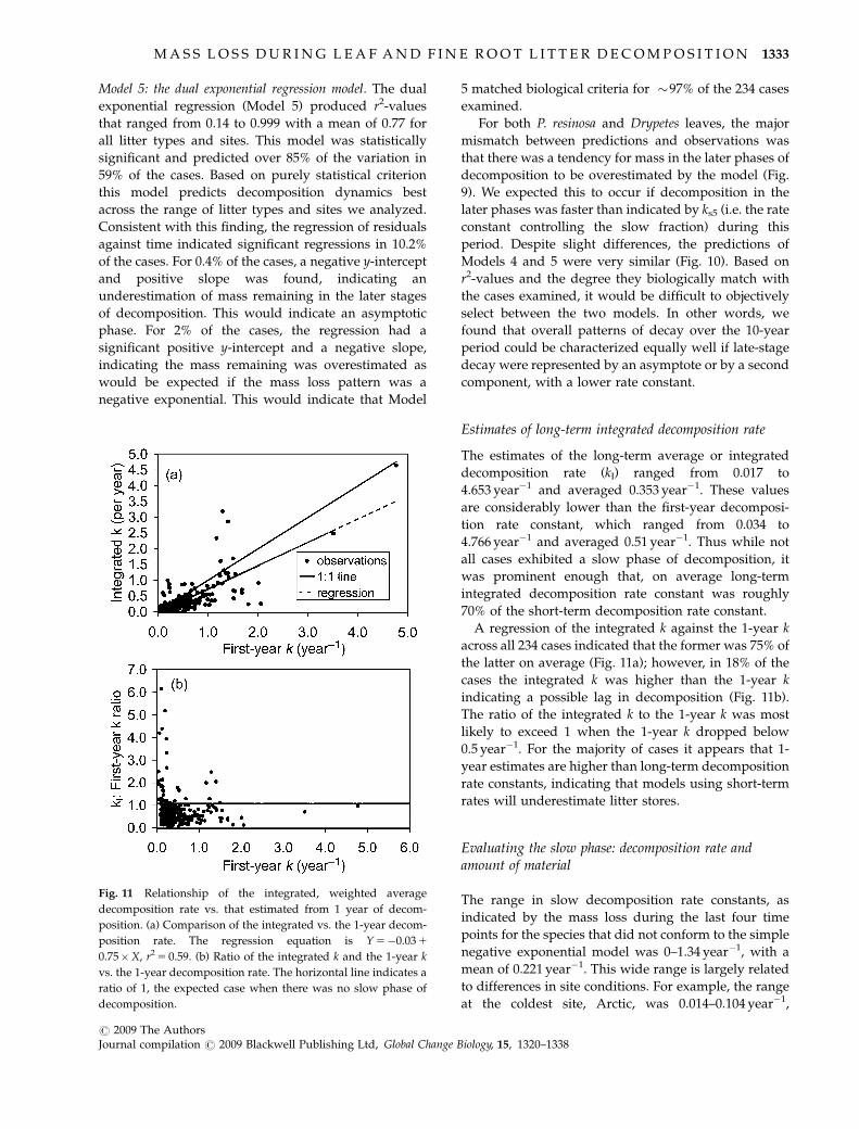
A regression of the integrated k against the 1-year k

across all 234 cases indicated that the former was 75% of

the latter on average (Fig. 11a); however, in 18% of the

cases the integrated k was higher than the 1-year k

indicating a possible lag in decomposition (Fig. 11b).

The ratio of the integrated k to the 1-year k was most

likely to exceed 1 when the 1-year k dropped below

0.5 year�1. For the majority of cases it appears that 1-

year estimates are higher than long-term decomposition

rate constants, indicating that models using short-term

rates will underestimate litter stores.

Evaluating the slow phase: decomposition rate andamount of material

The range in slow decomposition rate constants, as

indicated by the mass loss during the last four time

points for the species that did not conform to the simple

negative exponential model was 0–1.34 year�1, with a

mean of 0.221 year�1. This wide range is largely related

to differences in site conditions. For example, the range

at the coldest site, Arctic, was 0.014–0.104 year�1,

Fig. 11 Relationship of the integrated, weighted average

decomposition rate vs. that estimated from 1 year of decom-

position. (a) Comparison of the integrated vs. the 1-year decom-

position rate. The regression equation is Y 5�0.03 1

0.75�X, r2 5 0.59. (b) Ratio of the integrated k and the 1-year k

vs. the 1-year decomposition rate. The horizontal line indicates a

ratio of 1, the expected case when there was no slow phase of

decomposition.



whereas the range at one of the warmest sites (LaSelva)

was 0.23–0.80 year�1. There were also differences

among species, but the range of averages among species

was smaller than sites: 0.059 year�1 for P. elliottii fine

roots to 0.47 year�1 for Triticum aestivum as compared

with a site range of 0.057–1.073 year�1 (at Arctic and

Luquillo, respectively).

Across all sites and litter types the range of slow

fraction decomposition rates [ks5 in Eqn (6)] estimated

from Model 5 indicated that the decomposition rate

constant of the slow material ranged from 0 to

1.46 year�1 and averaged 0.139 year�1. These rates were

lower than that estimated for the last four data points,

which is consistent with our finding that, in inspecting

the curve fits of Model 5 for biological realism, we noted

that Model 5 tended to overestimate mass remaining in

the latest stage of decomposition. The slow fraction

decay-constants from Model 5 were also considerably

lower than the estimates of decomposition rate con-

stants for the ‘fast’ fraction, which ranged from 0.06 to

76 year�1 and averaged 9.73 year�1. This result indicates

that in many cases the fast phase of decomposition was

completed within a year. The species averages of the

decomposition rate of the slow fraction of litter (ks5)

ranged from 0.06 year�1 for P. elliottii fine roots to

0.178 year�1 for Quercus prinus leaves. The site averages

of ks5 ranged from 0.042 year�1 for Loch Vale to

0.687 year�1 for Luquillo.

Although the values of kf5 and ks5 [Eqn (6)] provide

no direct information about the amount of slow-decay-

ing substrate, our method of fitting regressions did fit

the constants Mf05 and Ms05 [Eqn (6)] representing the

portions of initial mass subject to decomposition at each

of the two rate constants. The amount of slow material

(Ms05) appeared to be a function of both site character-

istics and substrate quality. Similarly, Models 3 and 4

provided estimates of slow fraction masses S03 [Eqn (4)]

and S04 [Eqn (5)], respectively. Based on these estimates

of asymptotic mass, the slow fraction was equivalent to

0–73% of the initial mass across our range in litter types

and sites. Those regression estimates with little to no

slow fraction material were cases where a simple nega-

tive exponential model closely matched the temporal

pattern (e.g. P. resinosa leaves). The average of the

asymptotic mass was 32% of the initial mass, with the

species average ranging from a low of 15% for T.

aestivum to a high of 45% for P. elliottii fine roots. The

range among site averages was even wider, ranging

from 3.8% at Luquillo to 51% at Loch Vale. In general,

as the climatic favorability for decomposition of a site

increased, the amount of slow material decreased.

Similar patterns were revealed by the average of the

last four observations of mass remaining, which ranged

among all the cases from 2.8% to 80% of ash-free mass.

The range in averages for species was from 17% for

Drypetes leaves to 52% for P. elliottii fine roots. The range

among site averages was somewhat wider with 13% at

LaSelva and up to 56% at Loch Vale.

Discussion

Evaluating models of decomposition

We selected a range of regression models that had

meaningful biological interpretations and that have

been applied in the past. Our primary purpose of using

these models was not to find the ‘best’ model, as that is

likely to depend on the type of litter, the environment,

and the length of time of the measurements. For some

species and substrates (e.g. Pinus leaves) a simple

negative exponential model appears to match biological

criteria particularly well. For others (e.g. Drypetes

leaves), a simple negative exponential model does not

often match the reasonable biological expectation that

the initial mass start at 100%. For short-term studies that

end before the slow fraction becomes evident, a single

negative exponential model will most likely fit observa-

tions (although not if there are large initial rapid losses

of very labile fractions).

It is tempting to use the single negative exponential

model as it has the most convenient equation for simple

parameterization. However, our analysis shows that a

more complex model (Model 5) provides the most

generally acceptable set of curve fits to data across a

wide range of litters and sites. Moreover, Model 5, the

dual exponential, is the most general case and simplifies

to the other models. When a slow fraction is not present,

it simplifies to Models 1 or 2. Alternatively, when the

slow fraction has an undetectable rate of decomposi-

tion, it simplifies to Models 3 or 4 which includes an

asymptote representing a stable fraction. On this basis,

we recommend that a dual exponential model is the

logical starting place for any analysis of long-term

decomposition patterns. Models 3, 4, and 5 appear to

fit the data equally well in terms of statistical measures

of fit such as r2, P-values, or mean square error. Infor-

mation not present in the LIDET dataset, such as direct

measures of the rate of decomposition of the slow

fraction would be needed to distinguish among them.

Other models, particularly simulation models, might

be even better than those considered here. Given our

sample size for each litter type and site combination, we

could not use linear regression methods to estimate

parameters for a three-component model. However,

using a simulation modeling framework, this is possible

and there are indications that this improves the match

with observed data (Couteaux et al., 1998; Adair et al.,

2008). Biologically this probably does provide increased

1334 M . E . H A R M O N et al.


realism because it could capture a rapid loss of labile

material, an intermediate stage dominated by structural

compounds but still undergoing significant decomposi-

tion (Couteaux et al., 1995), and a slow phase or limit

value (Aber et al., 1990; Berg, 2000a, b). It may also be

advantageous to consider a continuous range of sub-

strate quality (Agren & Bosatta, 1987) or the generation

of slower decomposing secondary material by decom-

posers in more mechanistic models.

Estimating long-term decomposition rates

The observation that in many cases a simple negative

exponential model cannot be used has implications for

how species are compared and how decomposition data

are used. With a simple negative exponential model the

relative ranking of species is time invariant. However,

with either an asymptote or a dual exponential model it

is possible that the relative ranking is a function of time,

making one-time comparisons of species problematic.

Our integrated, weighted average rate constant (kI)

provides a time invariant ranking of species and sites.

This integrated rate is also most useful for aggregated

ecosystem models that consider a single overall pool of

litter vs. models that track cohorts of litter (Pastor &

Post, 1986), or ones that track fast and slow fractions

separately (Parton et al., 1987, 1994; Currie & Aber,

1997).

In 18% of the cases the integrated k was higher than

the 1-year k: six sites (Central Plains-Shortgrass Steppe,

Jornada, Juneau, North Temperate Lakes, Santa Mar-

garita, and Sevilleta) accounted for the majority (i.e.

82%) of these cases. With the exception of Juneau and

North Temperate Lakes, these were dry sites in which

colonization by decomposers might have been slow or

dependent on the arrival of a wet year. Alternatively,

these are sites where photodegradation is highly likely

and slow initial biological decomposition might be

followed by more rapid physical degradation (Parton

et al., 2007). In the case of North Temperate Lakes, the

shorter timeframe of the experiments at that site have

might have precluded the development of a slower

phase of decomposition. For Juneau, the incorporation

of the litterbags into the deep moss layers at that site

might have caused decomposition rates to increase over

time by increasing litter moisture content.

In addition to being slower than short-term decom-

position rate constants, it is possible that long-term

decomposition processes are under a different set of

controls than those of initial decomposition. W.S. Currie

et al. (unpublished data) examined the degree climate

and substrate quality indices correlated with long-term

decomposition rate constants. While climatic indices,

such as CDI and AET, and substrate quality indices,

such as, lignin, N, acid-hydrolysable fraction, and tan-

nin content, were correlated to kI, these correlations

were much weaker than for short-term decomposition

rate constants. This implies that as decomposition ad-

vances, differences in litter types and places tend to

decrease.

Evaluating the presence of a slow phase

The inter-relationship of the mathematical models we

analyzed yields insight into when and where there is a

slow fraction. It must be borne in mind that the slow

phase is operationally defined. One cannot actually

measure it directly because chemically it represents a

poorly understood, complex mixture of materials (Swift

et al., 1979; Melillo et al., 1989; Kogel-Knabner, 2002). If

we define the slow phase as causing a deviation from

the simple negative exponential model, then we can

conclude that in many cases, some slow material influ-

enced the temporal trend in mass remaining. However,

there are also many cases in which a slow fraction need

not be invoked to explain the temporal pattern of mass

loss. While it would be ideal if deviations from the

single exponential model could be predicted from sub-

strate quality or site conditions, we did not find any

obvious relationships that could be used in a predictive

model. As suggested in W.S. Currie et al. (unpublished

data) there may be interactions between the litter in the

bags and the surrounding litter that may influence the

pattern and rate of decomposition.

We observed a wide range in the amount of slow

material that is estimated across the LIDET experiment.

It appears to be lower at sites with environments more

conducive to rapid decomposition, but the differences

among species remain relatively constant. This may

indicate that the rate at which slow material is decom-

posed is a function of the site environment, while the

amount of slow-material precursor compounds initially

present is a property of the species of litter. W.S. Currie

et al. (unpublished data) found that climate indices,

such as CDI and AET, and substrate quality indices,

such as lignin, acid-hydrolysable fraction, and tannin,

were correlated to the size of the slow pool. However,

the coefficients of determination for these regressions

was o21%, supporting the lack of clear trends found in

our preliminary analysis.

Although the latter stages of decomposition have

been referred to as a stable phase (Melillo et al., 1989;

Aber et al., 1990), decomposition appears to be detect-

able over the time-span of a decade. Our analysis

indicates a decomposition rate of the slow fraction of

40.01 year�1, with most of the estimates being an order

of magnitude higher. This is in contrast to the decom-

position rates of mineral soil organic matter, which



tends to have decomposition rate constants of

o0.01 year�1 (Gaudinski et al., 2000; Trumbore, 2000).

Therefore, one might conceive of the slow litter material

as being the precursor to soil organic matter that is

complexed with mineral material, with the slow com-

ponent of litter having a faster rate of mass loss than soil

organic matter.

Our estimates of decomposition rates of the slowly

decomposing material are relatively crude. A more con-

trolled study, starting with a known quantity of this

material and examining its dynamics using stable isotope

enrichment would greatly improve understanding of the

factors controlling the degradation of this complex mate-

rial. Better chemical and kinetic characterization of the

nature of the slow material might also provide insights

into how this material is formed during decomposition. If

on one hand, the slow material is simply a residual

recalcitrant fraction initially present in the litter (e.g. as

proposed by Couteaux et al., 1995), one would predict

that the input is controlled by the type of litter and its rate

of decomposition controlled by the site physical environ-

ment and biota. If on the other hand, this material is

formed by decomposers from the original material (as

proposed by Kogel-Knabner, 2002), then both the input

and decomposition of this material are likely to be con-

trolled by the site physical environment and biota.

There is an important global-scale implication of the

presence or absence of a later, slowly decomposing

fraction in plant litter. Global estimates of litter stores

have rarely been directly estimated as in the case of

mineral soil carbon (Post et al., 1982; Jobbagy & Jackson,

2000), although the work of Matthews (1997) is an

exception. Estimates of pool sizes are typically derived

from litterfall rates combined with estimates of decom-

position rate constants. Our study indicates that short-

and long-term decomposition rates are not similar, and

in the majority of cases (82%) the average, long-term

decomposition-rate constant is lower than the 1-year

decomposition rate constant. A rough global impact on

the difference in estimates of litter stores can be derived

by dividing the input flux by the decomposition rate

constant (Olson, 1963). This indicates that if 1-year

decomposition rate constants are used in these esti-

mates, litter pool sizes are likely to be underestimated

by at least 34% relative to those using long-term rate

constants. Our analysis indicates that the negative ex-

ponential model is appropriate for the many species

and site combinations examined (27–65% depending on

the test used). Further, our estimates of an integrated

decomposition rate constant, representing a weighted

average, are on average 75% that of 1-year decomposi-

tion rate constants, an observation consistent with the

presence of a slower phase of decomposition. While our

study has focused on the biological degradation of litter,

there are many systems where fire removes a large

fraction of organic material added to the system. Sites

and litter types that exhibited an asymptotic pattern of

litter decomposition, may accumulate considerably less

litter than our equations indicate if fires are frequent. A

more detailed analysis of the degree to which litter stores

have been underestimated and relative balance of biotic

vs. abiotic (i.e. fire) losses is therefore warranted.

Acknowledgements

This study would not have been possible without the dedicatedefforts of many people. We are indebted to their efforts to collectand process samples, as well as to provide background informa-tion on their site characteristics and climate. Dr Richard Reevesof NCEAS (the National Center for Ecological Analysis andSynthesis) assisted with the programming for the nonlinearregression analysis. We also wish to thank Drs John Aber, JerryM. Melillo, and Knute Nadelhoffer for organizing the 1989workshop at Woods Hole that developed the original plan forLIDET. In addition to the numerous grants that supportedpersonnel at the individual sites, this study was supported bygrants from the National Science Foundation (DEB-9108329,DEB-9806493). These synthesis efforts were supported by fundsfrom the LTER Network Office, the Kaye and Ward RichardsonEndowment and the Bullard Fellowship Program of HarvardUniversity. This work was conducted as part of the Decomposi-tion working Group supported by NCEAS, a Center funded bythe NSF (DEB-0072909), the University of California at SantaBarbara, and the State of California. Dr John Pastor and twoother reviewers are thanked for their helpful comments on thedrafts of this manuscript.

References

Aber JD, Melillo JM, McClaugherty CA (1990) Predicting long-

term patterns of mass loss, nitrogen dynamics, and soil

organic matter formation from initial fine litter chemistry in

temperate forest ecosystems. Canadian Journal of Botany, 68,

2201–2208.

Adair EC, Parton WJ, DelGrosso SJ, Silver WL, Hall SA, Harmon

ME, Hart SC (2008) A simple three pool model accurately

describes patterns of long term, global decomposition in the

Long Term Intersite Decomposition Experiment Team (LIDET)

data set. Global Change Biology, 14, 2636–2660.

Agren GI, Bosatta N (1987) Theoretical analysis of the long-

term dynamics of carbon and nitrogen in soils. Ecology, 68,

181–1189.

Berg B (2000a) Initial rates and limit values for decomposition of

Scots pine and Norway spruce needle litter: a synthesis for

N-fertilized forest stands. Canadian Journal of Forest Research,

30, 122–135.

Berg B (2000b) Litter decomposition and organic matter turnover

in northern forest soils. Forest Ecology and Management, 133,

13–22.

Berg B, Ekbohm G, McClaugherty CA (1984) Lignin and hollo-

cellulose relations during long-term decomposition of some

forest litters: long-term decomposition in a Scots pine forest IV.

Canadian Journal of Botany, 62, 2540–2550.

1336 M . E . H A R M O N et al.


Berg B, McClaugherty CA (2003) Plant Litter: Decomposition,

Humus Formation, Carbon Sequestration. Springer-Verlag, New

York.

Berg B, McClaugherty CA, Virzo De Santo A, Johnson D (2001)

Humus buildup in boreal forests effects of litterfall and its

N concentration. Canadian Journal of Forest Research, 31,

988–998.

Blair JM, Parmelee RW, Beare MH (1990) Decay rates, nitrogen

fluxes, and decomposer communities of single- and mixed-

species foliar litter. Ecology, 71, 1976–1985.

Bridson JN (1985) Lipid fraction in forest litter: early stages of

decomposition. Soil Biology and Biochemistry, 17, 285–290.

Bunnell FL, Tait DEN (1977) Microbial respiration and substrate

loss. II. A model of the influences of chemical composition. Soil

Biology and Biochemistry, 9, 41–47.

Bunnell FL, Tait DEN, Flanagan PW, Van Cleve K (1977) Micro-

bial respiration and substrate loss. I. A general model of the

influences of abiotic factors. Soil Biology and Biochemistry, 9,

33–40.

Chen H, Harmon ME, Sexton J, Fasth B (2002) Fine root decom-

position and N dynamics in coniferous forests of the Pacific

Northwest of USA. Canadian Journal of Forest Research, 32,

320–331.

Couteaux MM, Bottner P, Berg B (1995) Litter decomposition,

climate and litter quality. Trends in Ecology and Evolution, 10,

63–66.

Couteaux MM, McTiernan KB, Berg B, Szuberla D, Dardenne P,

Bottner P (1998) Chemical composition and carbon minerali-

zation potential of Scots pine needles at different stages of

decomposition. Soil Biology and Biochemistry, 30, 583–595.

Currie WS, Aber JD (1997) Modeling leaching as a decom-

position process in humid montane forests. Ecology, 78,

1844–1860.

Dubois MK, Gilles KA, Hamilton JR, Rebers PA, Smith F (1956)

Colorimetric method for determination of sugars and related

substances. Annals of Chemistry, 28, 350–356.

Edmonds RL (1984) Long-term decomposition and nutrient

dynamics in Pacific silver fir needles in western Washington.

Canadian Journal of Forest Research, 14, 395–400.

Effland MJ (1977) Modified procedure to determine acid-insolu-

ble lignin in wood and pulp. Tappi, 60, 143–144.

Fogel R, Cromack K Jr (1977) Effect of habitat and substrate

quality on Douglas-fir litter decomposition in western Oregon.

Canadian Journal of Botany, 55, 1632–1640.

Gaudinski JB, Trumbore SE, Davidson EA, Zheng S (2000) Soil

carbon cycling in a temperate forest: radiocarbon-based esti-

mates of residence times, sequestration rates and partitioning

of fluxes. Biogeochemistry, 51, 33–69.

Gholz HL, Wedin D, Smitherman S, Harmon ME, Parton WJ

(2000) Long-term dynamics of pine and hardwood litter in

contrasting environments: toward a global model of decom-

position. Global Change Biology, 6, 751–765.

Hagerman AE (1988) Extraction of tannin from fresh and

preserved leaves. Journal of Chemical Ecology, 14, 453–462.

Harmon ME, Baker GA, Greene SE, Spycher G (1990) Early

decomposition of leaf litter in a Picea–Tsuga forest, Olympic

National Park, Washington, USA. Forest Ecology and Manage-

ment, 31, 55–66.

Harmon ME, Nadelhoffer KJ, Blair JM (1999) Measuring decom-

position, nutrient turnover, and stores in plant litter. In:

Standard Soil Methods for Long Term Ecological Research (eds

Robertson GP, Bledsoe CS, Coleman DC, Sollins P), pp. 202–

240. Oxford University Press, New York.

Haslam E (1989) Plant Polyphenols: Vegetable Tannins Revisited.

Cambridge University Press, Cambridge, MA.

Howard PJA, Howard DM (1974) Microbial decomposition of

tree and shrub litter. I. Weight loss and chemical composition

of decomposing litter. Okios, 25, 314–352.

Jansson PE, Berg B (1985) Temporal variation of litter decom-

position in relation to simulated soil climate: long-term de-

composition in a Scots pine forest. Canadian Journal of Botany,

63, 1008–1016.

Jobbagy EB, Jackson RB (2000) The vertical distribution of soil

organic carbon and its relation to climate and vegetation.

Ecological Applications, 10, 423–436.

Kirschbaum MUF (2000) Will changes in soil organic carbon act

as a positive or negative feedback on global warming? Bio-

geochemistry, 48, 21–51.

Kogel-Knabner I (2002) The macromolecular organic composi-

tion of plant and microbial residues as inputs to soil organic

matter. Soil Biology and Biochemistry, 34, 139–162.

Kurcheva GF (1960) The role of invertebrates in the decomposi-

tion of oak litter. Pedology (Leningrad), 4, 16–23.

Lousier JD, Parkinson D (1978) Chemical element dynamics in

decomposing leaf litter. Canadian Journal of Botany, 56, 2795–

2812.

Lousier JD, Parkinson D (1979) Organic matter and chemical

element dynamics in a aspen woodland soil. Canadian Journal

of Forest Research, 9, 449–463.

Magill AH, Aber JD (1998) Long-term effects of experimental

nitrogen additions on foliar litter decay and humus formation

in forest ecosystems. Plant and Soil, 203, 301–311.

Matthews E (1997) Global litter production, pools, and

turnover times: estimates from measurement data and regres-

sion models. Journal of Geophysical Research, 102D, 18,771–

18,800.

McClaugherty CA, Pastor J, Aber JD, Melillo JM (1985) Forest

litter decomposition in relation to soil nitrogen dynamics and

litter quality. Ecology, 66, 266–275.

Meentemeyer V (1978) Macroclimate and lignin control of litter

decomposition rates. Ecology, 59, 465–472.

Melillo JM, Aber JD, Linkins AE, Ricca A, Fry B, Naddelhoffer K

(1989) Carbon and nitrogen dynamics along the decay con-

tinuum: plant litter to soil organic matter. In: Ecology of Arable

Land (eds Clarholm M, Bergstrom L), pp. 53–62. Kluwer

Academic Publishers, Dordrecht.

Melillo JM, Aber JD, Murtore JF (1982) Nitrogen and lignin

control of hardwood leaf litter decomposition dynamics. Ecol-

ogy, 63, 621–626.

Melillo JM, Naiman RJ, Aber JD, Linkins AE (1984) Factors

controlling mass loss and nitrogen dynamics of plant litter

decaying in northern streams. Bulletin of Marine Science, 35,

341–356.

Minderman G (1968) Addition, decomposition, and accumula-

tion of organic matter in forests. Journal of Ecology, 56,

355–362.



Moore TR, Trofymow JA, Siltanen M, Prescott CCIDET Working

Group (2005) Patterns of decomposition and carbon, nitro-

gen,and phosphorus dynamics of litter in upland forest and

peatland sites in central Canada. Canadian Journal of Forest

Research, 35, 133–142.

Moorhead DL, Currie WS, Rastetter EB, Parton WJ, Harmon ME

(1999) Climate and litter quality controls on decomposition: an

analysis of modeling approaches. Global Climate Change, 13,

575–589.

Obst JR, Kirk KT (1988) Isolation of Lignin. Advances in Enzymol-

ogy, 161, 3–12.

Olson JS (1963) Energy stores and the balance of producers and

decomposers in ecological systems. Ecology, 44, 322–331.

Parton WJ, Ojima DS, Cole CV, Schimel DS (1994) A general

model for soil organic matter dynamics: sensitivity to litter

chemistry, texture, and management. Soil Science Society of

America Special Publication, 39, 147–167.

Parton WJ, Schimel DS, Cole CV, Ojima DS (1987) Analysis of

factors controlling soil organic matter levels in Great Plains

Grasslands. Soil Science Society of America Journal, 51, 1173–1179.

Parton WJ, Silver WL, Burke IC et al. (2007) Global-scale simila-

rities in nitrogen release patterns during long-term decom-

position. Science, 315, 361–364.

Pastor J, Post WM (1986) Influence of climate, soil moisture, and

succession on forest carbon and nitrogen cycles. Biogeochem-

istry, 2, 3–27.

Post WM, Emanuel W, Zinke PJ, Stangenberger AG (1982) Soil

carbon pools and world life zones. Nature, 298, 156–159.

Ryan MG, Melillo JM, Ricca A (1990) A comparison of methods

for determining proximate carbon fractions of forest litter.

Canadian Journal of Forest Research, 20, 166–171.

Silver WL, Miya RK (2001) Global patterns in root decom-

position: comparisons of climate and litter quality effects.

Oecologia, 129, 407–419.

Singh JS, Gupta SR (1977) Plant decomposition and soil

respiration in terrestrial ecosystems. Botanical Review, 43,

449–528.

Swift MJ, Heal OW, Anderson JM (1979) Decomposition in Terres-

trial Ecosystems. University of California Press, Berkeley.

Tappi (1976) Alcohol–benzene and dichloromethane solubles in wood

and pulp. Tappi Official Standard T204.

Tappi (1981) Water solubility of wood and pulp. Tappi Official

Standard T207.

Trofymow JA, Moore TR, Titus B et al. (2002) Rates of litter

decomposition over 6 years in Canadian forests: influence of

litter quality and climate. Canadian Journal of Forest Research, 32,

789–804.

Trumbore S (2000) Age of soil organic matter and soil respiration:

radiocarbon constraints on belowground C dynamics. Ecologi-

cal Applications, 10, 399–411.

Vogt KA, Grier CC, Vogt DJ (1986) Production, turnover,

and nutrient dynamics of above- and belowground

detritus of world forests. Advances in Ecological Research, 15,

303–377.

Wardle DA, Zachrisson O, Hornberg G, Gallet C (1997) The

influence of island area on ecosystem properties. Science, 277,

1296–1299.

Wieder RK, Lang GE (1982) A critique of the analytical methods

used in examining decomposition data obtained from litter

bags. Ecology, 63, 1636–1642.

Witkamp M, Crossley DA Jr (1966) The role of arthropods and

microflora in breakdown of white oak litter. Pedobiologia, 6,

292–303.

Witkamp M, Olson JS (1963) Breakdown of confined and non-

confined oak litter. Oikos, 14, 138–147.

Yahdjian LO, Sala E, Austin A (2006) Differential controls of

water input on litter decomposition and nitrogen dynamics in

the Patagonian Steppe. Ecosystems, 9, 128–141.

1338 M . E . H A R M O N et al.


Long-term patterns of mass loss during the decomposition of leaf and fine root litter: an intersite...

Documents

Transcript of Long-term patterns of mass loss during the decomposition of leaf and fine root litter: an intersite...