Lo

FKa

b

Dc

a

ARR1A

KCMTUM

1

btKbr(hl

i

h0

Agricultural and Forest Meteorology 200 (2015) 313–321

Contents lists available at ScienceDirect

Agricultural and Forest Meteorology

j our na l ho me page: www.elsev ier .com/ locate /agr formet

ong term carbon storage potential and CO2 sink strengthf a restored salt marsh in New Jersey

rancisco Artigasa, Jin Young Shina, Christine Hobblea, Alejandro Marti-Donatib,arina V.R. Schäferc, Ildiko Pechmanna,∗

New Jersey Meadowlands Commission, Meadowlands Environmental Research Institute, Lyndhurst, NJ, United StatesBarcelona Supercomputing Center—Centro Nacional de Supercomputación (BSC-CNS),epartment of Computer Applications in Science and Engineering (CASE), Barcelona, SpainRutgers University—Newark, Department of Biological Sciences, New Brunswick, NJ, United States

r t i c l e i n f o

rticle history:eceived 6 December 2013eceived in revised form6 September 2014ccepted 22 September 2014

eywords:O2 fluxixed high marsh-low marsh vegetation

idal effectrban tidal salt marsharsh coring

a b s t r a c t

The study compares the amounts of carbon fixed via photosynthesis of a restored tidal marsh to thetotal organic carbon remaining in sediments of a natural tidal marsh and arrives at preliminary baselinesfor carbon sequestration and storage over time. The Eddy-covariance method (indirect method) wasused to estimate marsh canopy net ecosystem exchange (NEE) and measured an annual gross primaryproduction of 979 g C m−2, while the loss through respiration was 766 g C m−2, resulting in a net uptakeof 213 g C m−2 yr−1. Time of the day, solar irradiation, air temperature, humidity and wind direction alltogether explained 66% of the variation in NEE. The high marsh community of Spartina patens showedNEE to be significantly higher than the low marsh community. The net ecosystem carbon balance (NECB)over long time scales was estimated by measuring the actual amount of total organic carbon contained indated sediment cores from a natural marsh (direct method), which resulted in a carbon accumulation rateof 192.2 g m−2 yr−1. Changes in total organic carbon content over time in the core sample showed that 78%of organic carbon remained stored in the sediments after 130 years and only the most recalcitrant carbon(50%) remained under storage beyond 645 years. Overall the study showed that temperate macrotidalsalt marshes are net sinks of carbon with potential for long term carbon storage. The marsh turned

into a carbon sink at the beginning of May and switched back to being a source in late November. Theaverage sedimentation rate estimated from the 137 CS dating (1950s to present) was 1.4 mm yr−1 whichis similar to accretion rates of comparable S. patens patches in the east coast. Accretion rates derived fromour study are slightly lower than the 60+ year rate of sea level rise (2.6 mm yr−1) recorded by tide gaugemeasurements in the Northeast.

. Introduction

Tidal wetlands actively remove carbon from the atmosphere byurying sediments rich in organic matter and represent an impor-ant component of the terrestrial biological carbon pool (Dixon andrankina, 1995; Duarte et al., 2005; Kathilankal et al., 2008). Thisiophysical control over carbon assimilation, sequestration andelease strongly influences the dynamics of global climate systems

Chapin et al., 2006). The presence of sulfate in tidal salt marshesinders methane production and emissions of N2O to almost neg-

igible levels and as such, tidal wetlands have a greater net positive

∗ Corresponding author. Tel.: +1 2014602808; fax: +1 2014602804.E-mail addresses: ildiko.pechmann@njmeadowlands.gov,

ldiko.pechmann@gmail.com (I. Pechmann).

ttp://dx.doi.org/10.1016/j.agrformet.2014.09.012168-1923/© 2014 Elsevier B.V. All rights reserved.

© 2014 Elsevier B.V. All rights reserved.

effect in terms of global warming potential than fresh water sys-tems (Peteet et al., 2006; Smith and Patrick, 1983; DeLaune et al.,1990).

According to Howes et al. (1985), less than 10% of the carbonfixed through photosynthesis in salt marshes is buried (case study:Great Sippewissett Salt Marsh, Cape Cod, Massachusetts), however,since the rate of primary production is exceptionally high, thesesystems contribute significantly to carbon sequestration comparedto other ecosystems (Chumra et al., 2003; Duarte et al., 2005).Salt marshes are considered outwelling systems that export car-bon (Mitsch and Gosselink, 2000). The “outwelling hypothesis”states that marshes are “primary production pumps” that feed

the surrounding area by exporting organic material in the formof detritus (Odum, 1968; Teal, 1962) yet significant amounts ofthe carbon buried in marsh sediments is of autochthonous origin(Ember et al., 1987; Allen, 2000). Studies of carbon sequestration

3 orest

rfetw

nBiwleBdva(i1mmcd

cbslchilscR(laCatew(i(mtat(

sTcakC2o∼vmt1a

14 F. Artigas et al. / Agricultural and F

ates and carbon storage potential as well as accretion are criticalor two reasons: First, to determine if tidal wetlands provide anffective long term carbon storage alternative to terrestrial vege-ation and second, to determine if accretion rates are keeping upith sea level rise.

Tidal marshes in glaciated northern New Jersey are con-ected with the retreat of the Wisconsin Ice sheet (15,000 yr..P), the creation of a post glacial lake Hackensack, the rise

n sea level and entry of tidewater into the Hackensack valleyhich resulted in deposition of peat and muck over the glacier

ake sediments (Heusser, 1949; Rind et al., 1989). An appar-nt reduction in the rate of sea level rise from 3000 to 2000 yr.P. (Stuiver and Daddario, 1963) is now linked to the earliestevelopment of coastal peats (3.8 m deep) in the Hackensackalley. Evidence of this early colonization are the Alnus seedsnd associated fresh water species dated to 2060 ± 120 yr B.P.Peteet, 1980) and basal peat formation over the same lake sed-ment dated to 2025 ± 300 yr B.P. only a few km away (Heusser,949, 1963). Palynology and peat stratigraphy evidence suggestsarine transgressions and regressions, where established tidalarsh areas became sufficiently fresh water to support swamps

ontaining alder and birch that later reverted back to marshlanduring marine transgressions (Heusser, 1949, 1963).

Tidal wetlands will most likely play a role as a source of carbonredits for a global carbon market so estimating their long term car-on storage potential (i.e. greater than 100 years) is a necessary firsttep (Freedman et al., 2009; Hansen, 2009). Moreover, solid base-ines for accretion rates and quantifiable carbon flows would also beritical to any future CO2 emission reduction program. On the otherand, if accretion rates are not keeping up with rising sea level there

s danger that these ecosystems could be completely inundated andose their ability to capture carbon. There is therefore a need fortandardized methods for quantifying carbon sequestration andarbon storage baselines as concluded by Chumra et al. (2003),ocha and Goulden (2009), Crooks et al. (2010), and Moffett et al.2010), To arrive at preliminary sequestration and storage base-ines for macrotidal wetlands we used an indirect approach thatssesses net ecosystem exchange (NEE) through measurements ofO2 fluxes on one hand, and a direct approach that looks at thectual carbon content in sediment profiles, which is an indication ofhe actual net ecosystem carbon balance (NECB) over time (Chapint al., 2006). Because of recent developments in software and hard-are, it is now possible using methods conceived in the early 1950s

Swinbank, 1951) to make reliable indirect measurement of NEEn the field using the eddy covariance method at annual scalesAubinet et al., 2001). This method records high frequency (20 Hz)

easurements of upward and downward CO2 fluxes to arrive athe rate of carbon exchanged at the canopy–atmosphere bound-ry. The direct approach on the other hand involves measuringhe amount of carbon actually contained in dated sediment coresCallaway et al., 2012).

Historical carbon accumulation rates are preserved in thetratigraphy of temperate macrotidal salt marshes (Allen, 2000).he rates of vertical accumulation depend on the type of plantommunity, sediment inputs, flooding regime, micro topographynd autocompaction of the peat (Pethick, 1979; Stumpf, 1983). Wenow from studies in Delaware Bay, the lower Hudson Valley andonnecticut (Bloom, 1964; Fletcher et al., 1993; Pederson et al.,005, respectively) that around 6000 yr ago palustrine wetlandsccupied the coastal valleys of the north eastern shore and that by3000–2000 yr B.P., the ongoing Holocene transgression created aariety of mud flats and sub-tidal environments and eventually the

odern marsh, which is only a few hundred years old and holds

he record of carbon sequestration rates (Pizzuto and Schwendt,997). The direct approach not only accounts for carbon lost to thetmosphere through decomposition in the form of methane (CH4),

Meteorology 200 (2015) 313–321

carbon monoxide (CO) and volatile organic carbon (VOC) but alsoaccounts for leaching of dissolved inorganic and organic carbon andlateral particulate carbon transfers. The indirect approach assumesconstant sedimentation and the absence of sedimentary gaps pro-duced by periods of non-deposition or loss of previously depositedsediment for the upper 250 cm.

The overall aim of our study is to compare the yearly carbonaccumulation rate from a restored wetland (indirect methods),with the yearly carbon accumulation rate of a corresponding nearbynatural wetland using sediment core measurements (direct meth-ods). More specific objectives include developing empirical modelswith easy to measure environmental factors that are sufficientlygood predictors of carbon sequestration and may be useful in futurecarbon accounting efforts. Finally to establish if the indirect eddycovariance method is sensitive to changes in water elevation andto differences in plant compositions.

2. Methods

2.1. Site description

The Secaucus High School Wetlands Enhancement Site (SHSsite) is a 16.2 ha restored tidal salt marsh in the town of Secau-cus, New Jersey, USA (Fig. 1A). The site used to be Phragmitesaustralis monoculture which was reconstructed in to a high diver-sity temporal emergent marsh. The restoration involved removingapproximately 0.5 m of surface sediments and replacing themwith clean sediments that contained no P. australis rhizomes. Therestoration included the construction of two high-marsh areas (ele-vation 0.9–1.2 m NADV88) totaling approximately 1.6 ha, plantedwith high marsh species, Spartina patens (saltmeadow hay), Dis-tichlis spicata (saltgrass), Spartina cynosuroides (big cordgrass) andJuncus gerardii (salt meadow rush). The remaining area was left aslow marsh (elevation less than 0.8 m NADV88) and planted withSpartina alterniflora (salt meadow cordgrass). The high marsh areafloods only under tides that exceed the mean–higher–high–watermark (MHHW). The low marsh on the other hand was designed toflood at every tidal cycle. High resolution balloon imagery (Artigasand Pechmann, 2010) was used to measure the area of each plantassociation within the 3.3 ha-footprint of the Eddy Covariancesampling tower (Fig. 1B). Six km downriver from the SHS site isthe mainly undisturbed 22 ha Riverbend Wetland Preserve (RWP)tidal salt marsh (N 400 45′ 11.37′′; W740 05′ 36.62′′) (Fig. 1C). Thismarsh is at the same elevation and contains the same high andlow marsh plant association present where the eddy flux tower islocated (Artigas and Pechmann, 2010). Low marsh areas of the nat-ural RWP site flood twice a day and high marsh habitats are onlyinundated under tides that exceed the MHHW, same as SHS. Thepredominant winds at both sites are from the north-west (NW) andthe terrain is flat.

2.2. Eddy covariance measurements

The sensor cluster of the eddy covariance sampling tower ismounted 3 m above the ground. The tower’s 3.3 ha footprint wascalculated following Kljun et al. (2004) simple footprint parame-terization method and includes high and low marsh areas (Fig. 2).The set of sensors consists of a 3-dimensional ultrasonic anemome-ter (CSAT-3, Campbell Scientific Inc., Logan, UT, USA), an open-pathinfra-red CO2 gas analyzer (IRGA; LI-7500, LI-COR, Lincoln, NE),

a HMP45C probe by Vaisala, (Helsinki, Finland) distributed byCampbell Scientific, which measures air temperature and relativehumidity and a fast response data logger (CR3000, Campbell Scien-tific Inc, Logan, UT). CO2 concentration, wind direction and speed,

F. Artigas et al. / Agricultural and Forest Meteorology 200 (2015) 313–321 315

Fig. 1. (A) Location of SHS site and RWP within the Hackensack Meadowlands, New Jersey, USA. (B) Location of the eddy covariance tower (triangle) at the SHS site;coordinates: (WGS84): W74◦2′44.48′′ , N40◦48′18.44. (C) Core sampling locations indicateCoordinates (WGS84): RB4 (N40◦45′11.37′′; W74◦05′36.62′′) and RB5 (N40◦45′11.51′′; W

Fig. 2. Eddy tower location and footprint area showing the dominant plant associa-tion types and discretized wind directions. Coordinates of tower location (WGS84):W74◦2′44.48′′ , N40◦48′18.44′′ .

d by triangles and 3.3 ha buffer area showing the channel locations at the RWP site.74◦05′34.55′′). Circles in (B) and (C) denote 3.3 ha tower footprint.

air pressure and temperature as well as relative humidity wererecorded at 20 Hz for a 13 month period.

Recordings of CO2 concentrations within the footprint beganin June of 2011 and are still ongoing. This study discusses theresults of CO2 flux measurements from June 7, 2011 through June30, 2012. A two point CO2 field calibration method was appliedmonthly during the growing season. A portable dew point genera-tor (LICOR–610, LiCor Inc, Lincoln, NE) was used to reach a desiredhumidity and temperature during calibration. Very few measure-ments were made in November and December of 2011 due to asnowstorm on Oct 29th. Overall 38% of potential measurementsof a 13 month sampling period were lost due to weather relatedreasons or equipment malfunction.

An automatic water level measuring station equipped with aCampbell Scientific (CS455) pressure transducer provided hourlyinformation of changes in water elevation. The 30 min solar irradia-tion measurements were captured by a LI-COR Silicon Pyranometer(LI200X-L).

The raw 20 Hz data from the sampling tower was recomputedusing Eddy Pro 3.0 (LI-COR, Lincoln, NE). The effects due to fluctua-tions in air density were removed according to Webb et al. (1980).Fluctuations due to turbulence were removed by block averagingaccording to Gash and Culf (1996) and errors due to misalignmentof the sonic anemometer were addressed by the double rotationmethod according to Wilczak et al. (2001). Finally, sensible heatfluxes were corrected according to Burba et al. (2008). The storageflux (Fs) i.e. the rate of change in storage of CO2 in the column ofair below the sensors height was calculated based on the followingequation (LI-COR, 2012):

Fs =∫ z

0

ıCO2

ıtdz (1)

3 orest Meteorology 200 (2015) 313–321

wNi

N

atf

N

(

N

p

2

a1bta0t(fi0N

22tmtsotstair

2wdrtda4tawoio

2wm

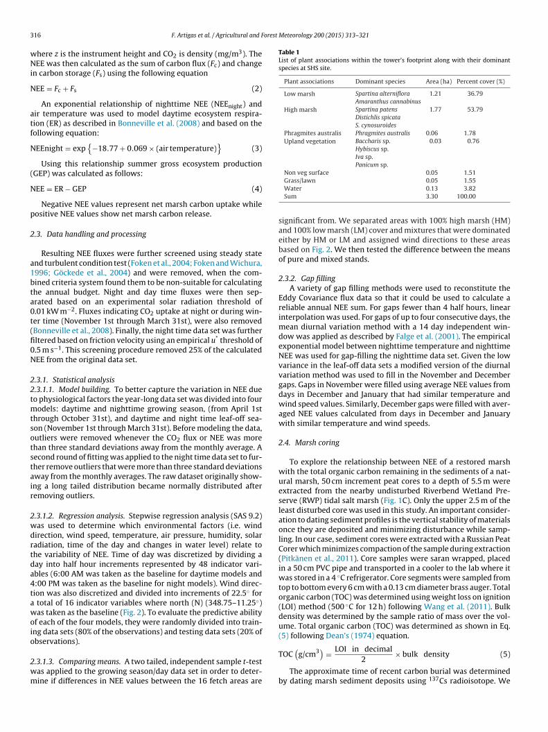
Table 1List of plant associations within the tower’s footprint along with their dominantspecies at SHS site.

Plant associations Dominant species Area (ha) Percent cover (%)

Low marsh Spartina alterniflora 1.21 36.79Amaranthus cannabinus

High marsh Spartina patens 1.77 53.79Distichlis spicataS. cynosuroides

Phragmites australis Phragmites australis 0.06 1.78Upland vegetation Baccharis sp. 0.03 0.76

Hybiscus sp.Iva sp.Panicum sp.

Non veg surface 0.05 1.51

16 F. Artigas et al. / Agricultural and F

here z is the instrument height and CO2 is density (mg/m3). TheEE was then calculated as the sum of carbon flux (Fc) and change

n carbon storage (Fs) using the following equation

EE = Fc + Fs (2)

An exponential relationship of nighttime NEE (NEEnight) andir temperature was used to model daytime ecosystem respira-ion (ER) as described in Bonneville et al. (2008) and based on theollowing equation:

EEnight = exp{

−18.77 + 0.069 × (air temperature)}

(3)

Using this relationship summer gross ecosystem productionGEP) was calculated as follows:

EE = ER − GEP (4)

Negative NEE values represent net marsh carbon uptake whileositive NEE values show net marsh carbon release.

.3. Data handling and processing

Resulting NEE fluxes were further screened using steady statend turbulent condition test (Foken et al., 2004; Foken and Wichura,996; Göckede et al., 2004) and were removed, when the com-ined criteria system found them to be non-suitable for calculatinghe annual budget. Night and day time fluxes were then sep-rated based on an experimental solar radiation threshold of.01 kW m−2. Fluxes indicating CO2 uptake at night or during win-er time (November 1st through March 31st), were also removedBonneville et al., 2008). Finally, the night time data set was furtherltered based on friction velocity using an empirical u* threshold of.5 m s−1. This screening procedure removed 25% of the calculatedEE from the original data set.

.3.1. Statistical analysis

.3.1.1. Model building. To better capture the variation in NEE dueo physiological factors the year-long data set was divided into four

odels: daytime and nighttime growing season, (from April 1sthrough October 31st), and daytime and night time leaf-off sea-on (November 1st through March 31st). Before modeling the data,utliers were removed whenever the CO2 flux or NEE was morehan three standard deviations away from the monthly average. Aecond round of fitting was applied to the night time data set to fur-her remove outliers that were more than three standard deviationsway from the monthly averages. The raw dataset originally show-ng a long tailed distribution became normally distributed afteremoving outliers.

.3.1.2. Regression analysis. Stepwise regression analysis (SAS 9.2)as used to determine which environmental factors (i.e. windirection, wind speed, temperature, air pressure, humidity, solaradiation, time of the day and changes in water level) relate tohe variability of NEE. Time of day was discretized by dividing aay into half hour increments represented by 48 indicator vari-bles (6:00 AM was taken as the baseline for daytime models and:00 PM was taken as the baseline for night models). Wind direc-ion was also discretized and divided into increments of 22.5◦ for

total of 16 indicator variables where north (N) (348.75–11.25◦)as taken as the baseline (Fig. 2). To evaluate the predictive ability

f each of the four models, they were randomly divided into train-ng data sets (80% of the observations) and testing data sets (20% ofbservations).

.3.1.3. Comparing means. A two tailed, independent sample t-testas applied to the growing season/day data set in order to deter-ine if differences in NEE values between the 16 fetch areas are

Grass/lawn 0.05 1.55Water 0.13 3.82Sum 3.30 100.00

significant from. We separated areas with 100% high marsh (HM)and 100% low marsh (LM) cover and mixtures that were dominatedeither by HM or LM and assigned wind directions to these areasbased on Fig. 2. We then tested the difference between the meansof pure and mixed stands.

2.3.2. Gap fillingA variety of gap filling methods were used to reconstitute the

Eddy Covariance flux data so that it could be used to calculate areliable annual NEE sum. For gaps fewer than 4 half hours, linearinterpolation was used. For gaps of up to four consecutive days, themean diurnal variation method with a 14 day independent win-dow was applied as described by Falge et al. (2001). The empiricalexponential model between nighttime temperature and nighttimeNEE was used for gap-filling the nighttime data set. Given the lowvariance in the leaf-off data sets a modified version of the diurnalvariation method was used to fill in the November and Decembergaps. Gaps in November were filled using average NEE values fromdays in December and January that had similar temperature andwind speed values. Similarly, December gaps were filled with aver-aged NEE values calculated from days in December and Januarywith similar temperature and wind speeds.

2.4. Marsh coring

To explore the relationship between NEE of a restored marshwith the total organic carbon remaining in the sediments of a nat-ural marsh, 50 cm increment peat cores to a depth of 5.5 m wereextracted from the nearby undisturbed Riverbend Wetland Pre-serve (RWP) tidal salt marsh (Fig. 1C). Only the upper 2.5 m of theleast disturbed core was used in this study. An important consider-ation to dating sediment profiles is the vertical stability of materialsonce they are deposited and minimizing disturbance while samp-ling. In our case, sediment cores were extracted with a Russian PeatCorer which minimizes compaction of the sample during extraction(Pitkänen et al., 2011). Core samples were saran wrapped, placedin a 50 cm PVC pipe and transported in a cooler to the lab where itwas stored in a 4 ◦C refrigerator. Core segments were sampled fromtop to bottom every 6 cm with a 0.13 cm diameter brass auger. Totalorganic carbon (TOC) was determined using weight loss on ignition(LOI) method (500 ◦C for 12 h) following Wang et al. (2011). Bulkdensity was determined by the sample ratio of mass over the vol-ume. Total organic carbon (TOC) was determined as shown in Eq.(5) following Dean’s (1974) equation.

TOC(

g/cm3) = LOI in decimal2

× bulk density (5)

The approximate time of recent carbon burial was determinedby dating marsh sediment deposits using 137Cs radioisotope. We

orest Meteorology 200 (2015) 313–321 317

af1hpnHf3attostppo

wwDdad

3

3

saSintttTshflwssOD

3

tTBatsciawsC

Table 2Regression coefficient table for the day time growing season model showing thedifferences from the baseline wind direction (N). Only wind directions significantlydifferent from the baseline at p < 0.05 are shown in the table.

Wind direction Plant community Regression coefficient

NE High marsh 1.05SSW High marsh 1.31W High marsh 1.62S High marsh 1.84WSW Low marsh 2.12SSE Low marsh 2.12SW Low marsh 2.34ENE High marsh 3.15ESE Low marsh 4.37

F. Artigas et al. / Agricultural and F

pplied this method, since 137Cs has proven to be a reliable methodor dating recent peat deposits in current studies (Orson et al.,998; Jetter, 2000). Deeper stratigraphic sequences on the otherand are distorted due to compaction involving a combination ofhysical and biochemical process that reduces the vertical thick-ess of the sediment column (Allen, 2000; Brain et al., 2012).ence our age model is based on a combination of 137Cs method

or the most recent peat deposits, and for sediments deeper than0 cm Heusser’s (1963) and Heusser et al., 1985 age models weredopted. Tidal waters that inundated the Hackensack valley afterhe retreat of the Wisconsin ice sheet created the conditions forhe first deposits of peat and muck on top on what was the bottomf glacial Lake Hackensack (Antevs, 1922). According to 14C mea-urements these first peat deposits (3.5 to 3.8 m deep) are datedo approximately 3000 BP. Therefore those studies provide a com-lete and applicable chronology based on 14C measurements andalynological observations of core samples for sediments depositedn top of glacial Lake Hackensack.

After being sampled for TOC analysis the first 30 cm of the coreas cut into ten 3 cm segments, stored in air tight containers andas shipped to a radioactive testing lab (University of Delaware,epartment of Oceanography, Newark, DE) where 137Cs isotopeating was performed according to Robbins and Edgington (1975)nd Arnaud et al. (2006) using a high-purity Germanium well-typeetector (Canberra Model GCW2523).

. Results

.1. Vegetation composition and growth characteristics

The vegetation within the sampling tower’s footprint at SHSite is predominantly a mixture of high marsh vegetation (54%)nd low marsh vegetation (37%). The high marsh is dominated by. patens, D. spicata and S. cynosuroides (Fig. 2). The low marshs mainly composed of S. alterniflora and Amaranthus cannabi-us. The rest of the tower’s footprint area (9%) is vegetationransition zones between low and high marsh and upland vege-ation along with water and non-vegetated areas. A summary ofhe plant association types and species composition is shown inable 1. First shoots of P. australis (common reed) and the Spartinapecies started to emerge at the end of March 2011, reached peakeight in mid-June and remained stable through August. S. alterni-ora was the earliest to start senescing in mid-September andas fully senesced by the end of October. S. patens and S. cyno-

uroides followed by beginning to senesce in October and were fullyenesced by mid-November. P. australis stayed green throughoutctober and was fully senescent by the end of November and earlyecember.

.2. Results of eddy flux measurements and GEP

The first true day of net CO2 uptake occurred on April 4, 2012 andhe highest uptake occurred in mid-July as 13.45 �mol C m−2 s−1.he marsh switched from net source to net sink in early May (Fig. 3).ecause of the long green period of S. patens, S. cynosuroides and P.ustralis the marsh did not switch back to net CO2 source most likelyill early November 2011. However, due to data loss as result of thenow storm on the eve of October 29, 2011 the exact turning pointannot be established (Fig. 3). GEP was calculated for the grow-ng season as described in Eq. (4), approximately 979 g C m−2 was

ccumulated as GEP during the growing season, and 766 g C m−2

as released as net ER throughout the year. Therefore during ourtudy period the SHS site was a net sink of 213 g C m−2 (C asO2).

E Low marsh 4.48SE Low marsh 4.70

3.3. Effects of environmental factors and tidal variation on NEE

NEE for the night time growing season dataset tended to showa non-random residual pattern when using a linear relationshipwith temperature; hence an exponential relationship was appliedfor this model (Eq. (3)). Time of the day was the most significantfactor and accounted for 49% of the variability in NEE values inthe growing season daytime model only. Air temperature, relativehumidity and solar radiation accounted for an additional 15% of thevariability, while wind direction accounted for the additional 2% ofthe variability in NEE. Together, these variables accounted for 66%of the variability in NEE during the growing season. In the growingseason night time model, air temperature was the most signifi-cant factor explaining 25% of the variance in NEE, while changesin water level accounted for an additional 5%. This relationship wasused when gap-filling the night time dataset. To test the predictiveability of the model, the root-mean-square error (RMSE) and pre-dicted squared error (PSE) were calculated. The degree of closenessthe values showed indicates that the fitted models perform well inpredicting NEE values, and are suitable for modeling the relation-ship between the environmental parameters and NEE. Time-of-dayis clearly an important variable and was included in the day timemodels even though in a few cases, the time-of-day was not sig-nificant at p < 0.05. Finally, linear regression analysis showed thatchanges in the water level were not an important factor in explain-ing NEE.

3.4. Wind direction as surrogate for vegetation composition

The effect of wind direction was analyzed to see if NEE wascorrelated to specific fetch areas representing plant associationsin the footprint (Fig. 2). As described in the methods, wind direc-tion was discretized into 16 segments of 22.5◦ with the northdirection selected (arbitrarily) as the base line to which all otherwind directions were compared. Stepwise regression was used todetermine which wind directions and consequently what plantassociations related to a particular wind direction were signifi-cantly different from the north direction. Fetch areas that weresignificantly different from the baseline direction are shown inTable 2. Results show that areas between west–north–west (WNW)and north–north–east (NNE) were not significantly different fromthe baseline (N) and together represent areas dominated by highmarsh vegetation (Fig. 2). Compared to the baseline, the coefficientfor SE is 4.7, which indicates that when all variables such as air tem-perature and time of day remain the same, the wind direction of SEyields a NEE value that is 4.7 units higher than the baseline. In other

words low coefficient values indicate similarity with the baseline(i.e. areas dominated by S. patens), whereas fetch areas with highcoefficient values (i.e. E, ESE, SE, SW and WSW) correspond to areasdominated by low marsh vegetation (S. alterniflora).

318 F. Artigas et al. / Agricultural and Forest Meteorology 200 (2015) 313–321

tive N

erb(bSdr

3

ridt2asdtstsBmmrp

aits

site (213 g m−3 yr−1 NEE calculated as the difference between GEPand ER).

Fig. 3. Daily averages of NEE from June 2011 through June 2012 with nega

Further comparison of means of NEE values between the differ-nt vegetation types using wind direction as a surrogate (Fig. 2)evealed that there are significant differences (p < 0.01) in car-on uptake between pure high marsh (WNW) and low marshSE), (16.79 and 9.14 �mol CO2 m−2 s−1, respectively). Differencesetween means of NEE measured in high marsh mixtures (W, NW,, SSW) and low marsh mixtures (ESE, SW) showed significantifference (p < 0.01) as well (12.67 and 10.79 �mol CO2 m−2 s−1,espectively).

.5. Marsh coring

The variations in 137Cs concentrations with depth show a wellesolved peak at 5.5 cm depth (Fig. 4), that coincides with max-mum atmospheric fallout due to the testing of thermonuclearevices that started in 1954 and peaked in 1963/1964. We can inferhat roughly 8 cm of sediments accumulated between 1954 and012, therefore – without accounting for compaction – on aver-ge, 1.4 mm of sediments accumulated per year since 1954. Fig. 5Bhows the total organic carbon (TOC) content in the sediment byepth. The analysis of TOC from the first 20 cm of the core showshat approximately 78% of carbon found in the surface layer remainstored 15 cm deep or beyond 134 years (137Cs dating) and 50% ofhe carbon remains buried beyond 122 cm or 645 years B.P. Fig. 5Chows a sharp increase in LOI values starting at 125 cm (∼660 yrP) indicating a shift from subtidal environments dominated byudflats to palustrine peats and finally to the modern emergentarsh (Holocene transgression in Allen, 2000). This change is cor-

oborated by the marked decrease in bulk density for the same timeeriod (Fig. 5A).

Fig. 5D shows a sharp increase in carbon accumulation rate

round 600 years ago that reaches a maximum of 192.2 g m−2 yr−1

n the most recent layers. These data confirm the generalizationhat short-term (0–150 yr) rates of carbon accumulation are con-istently larger than long-term (>1000 yr) rates (Glaser et al., 2012).

EE values showing CO2 uptake, positive NEE values showing CO2 release.

The carbon accumulation rate derived from the first 20 cm ofthe core (192.2 g m−2 yr−1) is similar to the net carbon uptake ofthe vegetation (measured by the eddy covariance technique) at the

Fig. 4. 137Cs profile in sediment core of the Hackensack Meadowlands.

F. Artigas et al. / Agricultural and Forest Meteorology 200 (2015) 313–321 319

F cumula

(s

4

ttf

taitavitot(0NfdflhwLegr2mrpuas

flMFfpint

ig. 5. Bulk density (A), total organic carbon (B), loss on ignition (C) and carbon acpproximately 1400 years.

The results suggest that approximately 22% of the carbon fixedas per the indirect method) in any given year remains stored in theediment (as per the direct method).

. Discussion

This study compared the CO2 exchange above the marsh canopyo what is buried in the sediments as total organic carbon and foundhat these habitats are net sinks of carbon and have a great potentialor becoming long term carbon storage.

Time of the day alone explained 49% of the NEE and when airemperature, humidity, solar radiation and wind direction weredded, altogether these variables explained 66% of the variationn NEE. The CO2 exchange measurements showed a net sink of CO2hrough the growing season from April through late October, and

net source over the course of the winter months. Field obser-ations showed S. patens and S. cynosuroides beginning to senescen October and dying back by mid-November followed by P. aus-ralis senescing into December. These assemblages make up 55%f the vegetation cover within the tower’s footprint. Consequentlyhe marsh turned into a net source at about the end of November2011). During the growing season the CO2 flux rates ranged from.2 to 13.51 �mol m2 s−1 of CO2 and the highest daily average ofEE was 10.81 �mol CO2 m−2 s−1. This compares well to studies

rom natural salt marshes. Guo et al. (2009) reported an averageaily carbon uptake between 3.3 and 12 �mol m2 s−1 for S. alterni-ora and P. australis stands in the estuary of the Yangtze River. Theighest daily NEE average at the SHS site was 13.45 g m−2 day−1,hich is similar to the concentration reported for P. australis by

issner et al. (1999) – 11.39 g m−2 day−1 – in Spain, or by Zhout al. (2009) – 13.58 g m−2 day−1 – in Northeast China. The annualross primary production was 979 g C m−1, while the loss throughespiration was 766 g C m−2, resulting in an annual net uptake of13 g C m−2. Annual net uptakes of 302 g C m−2 yr−1 (24 h) wereeasured by Houghton and Woodwell’s (1980) from a 57 ha natu-

al temperate macrotidal salt marsh dominated by S. alterniflora, S.atens, D. spicata in Long Island, NY. Results also show that NEE val-es of the restored tidal salt marsh are similar to the annual carbonccumulation rate (192.2 g m−1 yr−1) derived from the analysis ofediment cores from the natural RWP site.

Our analysis further showed that water elevation due to tideuctuations did not have a meaningful effect on NEE and GEP.offett et al. (2010) found that NEE during flooding in a San

rancisco marsh was negatively correlated with flood depth. Theact that our plant community was less submerged at high tide com-

ared to the San Francisco marsh site may explain the differences

n NEE between the two studies, although possible differences inutrient loadings and different climatic conditions can contributeo alterations in NEE as well.

ation rate (D) in the sediment of the Hackensack Meadowlands over the course of

We assumed that by discretizing the different wind directionsthat correspond to the various plant communities we could test ifthere were significant differences in terms of CO2 uptake betweenhigh marsh and low marsh (Fig. 2 and Tables 2 and 3). The resultsindicate that the Eddy Covariance method is able to detect sig-nificant difference in CO2 uptake between pure high marsh andlow marsh stands as well as between the mixtures dominated by asingle species.

Comparing net carbon uptake rates from CO2 fluxes with totalorganic carbon stored in sediment show that during any givengrowing season, 22% of the total fixed carbon remains as stand-ing biomass and/or is stored in the sediments. Over time, only themost recalcitrant carbon remains buried as organic carbon is lostdue to microbial respiration, inorganic and organic carbon leachateand lateral particulate carbon movements. Our total organic carboncontent analysis showed that, over a period of approximately 130years, 78% of the fixed and buried organic carbon remains stored inthe sediments and assuming earlier ecosystems had similar assim-ilation rates, about 50% of the assimilated carbon remains storedin the sediments beyond 645 years. Our sediment age model fordepths greater than 10 cm was derived from four dated sedimentcores from elsewhere in the estuary and is corroborated by thecarbon dated and pollen influx cross-referenced Piermont Marshcore, (NY, 41◦00′N, 73◦55′W) which shows that 120 cm in depthcorresponds to approximately 600 years B.P. (Pederson et al., 2005).

Based on the 137Cs dating we estimated an annual rate ofaccretion of 1.4 mm for the last 130 years. Sedimentation ratesof 1.8 mm yr−1 have been reported for comparable S. patenscommunities in Connecticut (Orson et al., 1998). Differences in sed-imentation rates can be attributed to the age of the marsh (Pethick,1979), distances from tidal creeks and shallow subsidence (Cahoonet al., 1995). The global rise in sea level from 1900 to 2009 hasbeen estimated to be 1.7 ± 0.3 mm yr−1 (Church and White, 2011).On the other hand, the 60 + year rate of sea level rise establishedthrough tide gauge measurements from New York, Connecticut andRhode Island (which is more representative for the HackensackMeadowlands estuary) averages 2.6 mm yr−1. Sediments sourcesto the estuary come from storm water outflows as a result of soilmovement from construction sites and from high capacity sewagetreatment plants. It would take further studies to effectively deter-mine if the estuary is sediment limited and if these macrotidalmarshes are keeping up sea level rise.

5. Conclusions

The presented study aimed to link the amounts of carbon fixedvia photosynthesis of a restored tidal marsh to the total organiccarbon remaining in sediments of a natural tidal marsh and arriveat preliminary baselines for carbon sequestration in restored and

3 orest

nadbmrcolt(

gatotatl(

A

R

f

LsGwm

R

A

A

A

A

A

B

B

B

B

C

C

C

C

C

C

20 F. Artigas et al. / Agricultural and F

atural marshes. The indirect Eddy Covariance method measured net uptake of 213 g C m−2 yr−1 for a restored marsh, while theirect method of marsh coring measured 192.2 g m−2 yr−1 net car-on accumulation from a natural marsh measured with the 137Csethod indicating similar carbon accumulation rates between a

estored and natural marsh. Results also showed that 22% of thearbon fixed through photosynthesis remains as standing biomassr is fixed and buried in any given growing season making tidal wet-ands net carbon sinks. Of the buried carbon pool, 78% remained inhe sediments 130 years later and only the most recalcitrant carbon50%) remains buried in the sediments beyond 645 years.

The Eddy Covariance method using wind direction as a surro-ate was able to detect significant differences in NEE between highnd low marsh communities. Time of day, air temperature, rela-ive humidity, solar radiation and wind direction accounted for 66%f the variability in NEE and water elevation due to tide fluctua-ions did not have a meaningful effect on NEE and GEP. Finally, theverage sedimentation rate determined from 137Cs dating suggestshat marshlands in the Meadowlands are accreting to levels slightlyower (1.4 mm yr−1) as compared to the regional sea level rise rate2.6 mm yr−1).

cknowledgments

This project was funded by Meadowlands Environmentalesearch Institute of New Jersey Meadowlands Commission.

Instrumentation was funded through Rutgers University startupunds to KVR Schäfer.

The authors wish to thank Dr. Aridaman K. Jain and Mr. Gavinynch of New Jersey Institute of Technology for their help in thetatistical analysis. We are grateful for the field assistance of Joerzyb of MERI and Rajan Tripathee of Rutgers University. Weish to thank Sandy Speers and Ishan Patel for proof reading theanuscript.

eferences

llen, J.R.L., 2000. Morphodynamics of Holocene salt marshes: a review sketch fromthe Atlantic and Southern North Sea coasts of Europe. Q. Sci. Rev. 19, 1155–1231.

ntevs, E., 1922. The Recession of the Last Ice Sheet in New England. Am. Geogr. Soc.Res. Ser. 11, Am. Geogr. Soc., New York, NY.

rnaud, F., et al., 2006. Radionuclide dating (210Pb, 137Cs, 241Am) of recent lake sedi-ments in a highly active geodynamic setting (Lakes Puyehue and Icalma-ChileanLake District). Sci. Total Environ. 366 (2–3), 837–850.

rtigas, F., Pechmann, I., 2010. Balloon imagery verification of remotely sensedPhragmites australis expansion in an Urban Estuary of New Jersey, USA. Land-scape Urban Plann. 95 (3), 105–112.

ubinet, M., et al., 2001. Long term carbon dioxide exchange above a mixed forestin the Belgian Ardennes. Agric. For. Meteorol. 108 (4), 293–315.

loom, A.L., 1964. Peat accumulation and compaction in a Connecticut salt mars. J.Sediment. Petrol. 34, 599–603.

onneville, M.C., et al., 2008. Net ecosystem CO2 exchange in a temperate cattailmarsh in relation to biophysical properties. Agric. For. Meteorol. 148, 69–81.

rain, M.J., et al., 2012. Modelling the effects of sediment compaction on saltmarsh reconstructions of recent sea-level rise. Earth Planet. Sci. Lett. 345–348,180–193.

urba, G., et al., 2008. Addressing the influence of instrument surface heat exchangeon the measurements of CO2 flux from open-path gas analyzers. Global ChangeBiol. 14, 1854–1876.

ahoon, D.R., et al., 1995. Estimating shallow subsidence in microtidal salt marshesof the southeastern United States: Kaye and Barghoorn revisited. Mar. Geol. 128,1–9.

allaway, J., et al., 2012. Carbon sequestration and sediment accretion in SanFrancisco Bay Tidal Wetlands. Estuaries Coasts 35 (5), 1163–1181.

hapin III, F.S., et al., 2006. Reconciling carbon-cycle concepts. Terminology andmethods. Ecosystems 9, 1041–1050.

humra, G.L., et al., 2003. Global carbon sequestration in tidal, saline wetland soils.Global Biogeochem. Cycles vol. 17 (4), 22–31.

hurch, J.A., White, N.J., 2011. Sea level rise from the late 19th. to early 21st century.Surv. Geophys. 32, 585–602.

rooks, S., et al., 2010. Findings of the National Blue Ribbon Panel on the devel-opment of a greenhouse gas offset protocol for Tidal Wetlands restoration andmanagement: action plan to guide protocol development. In: Restore America’sEstuaries. Philip Williams & Associates, Ltd., and Science Applications Interna-tional Corporation, Arlington, VA.

Meteorology 200 (2015) 313–321

Dean, W.E., 1974. Determination of carbonate and organic matter in calcareoussediments and sedimentary rocks by loss on ignition: comparison with othermethods. J. Sediment. Petrol. 44, 242–248.

DeLaune, R.D., et al., 1990. Nitrous oxide and methane emission from Gulf Coastwetlands. In: Bouwman, A.F. (Ed.), Soils and the Greenhouse Effect. John Wiley,New York, NY, pp. 497–502.

Dixon, R.K., Krankina, O.N., 1995. Can the terrestrial biosphere be managed to con-serve and sequester carbon? Carbon sequestration in the biosphere: processesand products. NATO ASI Ser. Ser. I 33, 153–179.

Duarte, C.M., et al., 2005. Major role of marine vegetation on the oceanic cycle.Biogeosciences 2, 1–8.

Ember, L.M., et al., 1987. Processes that influence carbon isotope variations in saltmarsh sediments. Mar. Ecol.-Prog. Ser. 36, 33–42.

Falge, E., et al., 2001. Gap filling strategies for defensible annual sums of net ecocys-tem exchange. Agric. For. Meteorol. 107, 43–69.

Fletcher III, C.H., et al., 1993. Tidal wetland record of Holocene sea-level move-ments and climate history. Palaeogeogr. Palaeoclimatol. Palaeoecol. 102, 177–213.

Freedman, B., et al., 2009. Carbon credits and the conservation of natural areas.Environ. Rev. 17, 1–19.

Foken, T., Wichura, B., 1996. Tools for quality assessment of surface-based flux mea-surements. Agric. For. Meteorol. 78, 83–105.

Foken, T., et al., 2004. Post-field quality control. In: Lee, X., et, al. (Eds.), Handbook ofMicrometeorology: A Guide for Surface Flux Measurements. Kluwer Academic,Dordrecht, pp. 81–108.

Gash, J.H.C., Culf, A.D., 1996. Applying linear de-trend to eddy correlation data inreal time. Boundary Layer Meteorol. 79, 301–306.

Glaser, P.H., et al., 2012. Carbon and sediment accumulation in the Everglades (USA)during the past 4000 years: rates, drivers and sources of error. J. Geophys. Res.117, G03026.

Göckede, M., et al., 2004. A combination of quality assessment tools for eddy covari-ance measurements with footprint modeling for the characterization of complexsites. Agric. For. Meteorol. 127, 175–188.

Guo, H., et al., 2009. Tidal effects on net ecosystem exchange of carbon in an estuarinewetland. Agric. For. Meteorol. 149, 1820–1828.

Hansen, L.T., 2009. The viability of creating wetlands for the sale of carbon offsets. J.Agric. Resour. Econ. 34, 350–365.

Heusser, C.J., 1949. History of an estuarine bog at Secaucus, New Jersey. Bull. TorreyBot. Soc. 76 (6), 385–406.

Heusser, C.J., 1963. Pollen diagrams from three former cedar bogs in the Hackensacktidal marsh, Northeastern New Jersey. Bull. Torrey Bot. Soc. 90 (1), 16–28.

Heusser, C.J., Heusser, L.E., Peteet, D.M., 1985. Late-Quaternary climatic change onthe American North Pacific Coast. Nature 315, 485–487.

Houghton, R.A., Woodwell, G.M., 1980. The flax pond ecosystem study: exchangesof CO2 between a salt marsh and the atmosphere. Ecology 61 (6),1434–1445.

Howes, B.L., et al., 1985. Annual carbon mineralization and belowground productionof Spartina alterniflora in a New England salt marsh. Ecology 66, 595–605.

Jetter, H.W., 2000. Determining the ages of recent sediments using measurementsof trace radioactivity. Terra Aqua 78, 21–28.

Kathilankal, C.J., et al., 2008. Tidal influences on carbon assimilation by a salt marsh.Environ. Res. Lett. 3, 044010.

Kljun, N., et al., 2004. A simple parameterisation for flux footprint predictions.Boundary Layer Meteorol. 112, 503–523.

LI-COR, Inc., 2012. EddyPro 4. 0 Help and User’s Guide. LI-COR, Inc., Lincoln, NE.Lissner, J., et al., 1999. Effect of climate on the salt tolerance of two Phragmites aus-

tralis populations. II. Diurnal CO2 exchange and transpiration. Aquat. Bot. 64,335–350.

Mitsch, W.J., Gosselink, J.G., 2000. Wetlands. John Wiley, New York, NY.Moffett, K.B., et al., 2010. Salt marsh—atmosphere exchange of energy, water vapor,

and carbon dioxide: effects of tidal flooding and biophysical controls. WaterResour. Res. 46 (10), W10525.

Odum, E.P., 1968. A research challenge: evaluating the productivity of coastal andestuarine water. In: Proceeding of Second Sea Grant Conference, Univ. of RhodeIsland, pp. 63–64.

Orson, R.A., Warren, R.S., Niering, W.A., 1998. Interpreting sea level rise and rates ofvertical marsh accretion in a southern New England tidal salt marsh. EstuarineCoastal Shelf Sci. 47, 419–429.

Pederson, D.C., et al., 2005. Medieval warming, little ice age, and European impact onthe environment during the last millennium in the lower Hudson Valley, NewYork, USA. Q. Res. 63, 238–249.

Peteet, D., 1980. A Record of Environmental Change During Recent Millennia in theHackensack Tidal Marsh, New Jersey. Bulletin of the Torrey Botanical Club 107(4), 512–524.

Peteet, D.M., et al., 2006. Hudson River paleoecology from marshes. In: Waldman,J (Ed.), Hudson River Fishes and Their Environment. American Fisheries SocietyMonograph (Chapter 11).

Pethick, J.S., 1979. Long-term accretion rates on tidal marshes. J. Sediment. Petrol.51 (2), 571–577.

Pitkänen, A., et al., 2011. Comparison of different types of peat corers in volumetricsampling. SUO 62 (2), 51–57.

Pizzuto, J.E., Schwendt, A.E., 1997. Mathematical modelling of a Holocene transgres-sive valley-fill deposit, Wolfe Glade, Delaware. Geology 258, 57–60.

Rind, D., Peteet, D., Kukla, G., 1989. Can Milankovitch orbital variations initiatethe growth of ice sheets in a general circulation model? J. Geophys. Res. 94,12851–12871.

orest

R

R

S

S

S

F. Artigas et al. / Agricultural and F

obbins, J.A., Edgington, D.N., 1975. Determination of recent sedimentation ratesin Lake Michigan using Pb-210 and Cs-137. Geochim. Cosmochim. Acta 39,285–304.

ocha, A.V., Goulden, M.L., 2009. Why is marsh productivity so high? New insightsfrom eddy covariance and biomass measurements in a Typha marsh. Agric. For.Meteorol. 149, 159–168.

mith, C.J., Patrick, W.H., 1983. Nitrous oxide emission as affected by alternate anaer-obic and aerobic conditions from soil suspensions enriched with ammonium

sulfate. Soil Biol. Biochem. 15, 693–697.

tuiver, M., Daddario, J.J., 1963. Submergence of the New Jersey Coast. Science 142(3594), 951.

tumpf, R.P., 1983. The process of sedimentation on the surface of a salt marsh.Estuarine Coastal Shelf Sci. 17, 495–508.

Meteorology 200 (2015) 313–321 321

Swinbank, W.C., 1951. The measurement of vertical transfer of heat and water vaporby Eddies in the lower atmosphere. J. Meteorol. 8, 135–145.

Teal, J.M., 1962. Energy flow in the salt marsh ecosystem of Georgia. Ecology 43,614–624.

Wang, et al., 2011. Optimizing the weight loss on-ignition methodology to quantifyorganic and carbonate carbon of sediments from diverse sources. Environ. Monit.Assess. 174, 241–257.

Webb, E.K., et al., 1980. Correction of flux measurements for density effects due to

heat and water vapour transfer. Q. J. R. Meteorolog. Soc. 106, 85–100.

Wilczak, J.M., et al., 2001. Sonic anemometer tilt correction algorithms. Boundary-Layer Meteorol. 99, 127–150.

Zhou, L., Zhou, G., Jia, Q., 2009. Annual cycle of CO2 exchange over a reed (Phragmitesaustralis) wetland in Northeast China. Aquat. Bot. 91, 91–98.