Article

Location of Faults in Power Transmission Lines Usingthe ARIMA Method

Danilo Pinto Moreira de Souza 1, Eliane da Silva Christo 1,∗ ID and Aryfrance Rocha Almeida 2

1 Computational Modeling in Science and Technology (MCCT), Fluminense Federal University (UFF),Volta Redonda 21941-916, Brazil; danilopms@id.uff.br

2 Technology Center, Federal University of Piauí (UFPI), Teresina 60455-760, Brazil; aryfrance@ufpi.edu.br* Correspondence: elianechristo@id.uff.br; Tel.: +55-24-2107-3510

Received: 11 August 2017; Accepted: 6 October 2017; Published: 13 October 2017

Abstract: One of the major problems in transmission lines is the occurrence of failures that affectthe quality of the electric power supplied, as the exact localization of the fault must be known forcorrection. In order to streamline the work of maintenance teams and standardize services, thispaper proposes a method of locating faults in power transmission lines by analyzing the voltageoscillographic signals extracted at the line monitoring terminals. The developed method relates timeseries models obtained specifically for each failure pattern. The parameters of the autoregressiveintegrated moving average (ARIMA) model are estimated in order to adjust the voltage curvesand calculate the distance from the initial fault localization to the terminals. Simulations of thefailures are performed through the ATPDraw R© (5.5) software and the analyses were completed usingthe RStudio R© (1.0.143) software. The results obtained with respect to the failures, which did notinvolve earth return, were satisfactory when compared with widely used techniques in the literature,particularly when the fault distance became larger in relation to the beginning of the transmission line.

Keywords: transmission line; fault localization; time series; ARIMA; discrete wavelet transformer

1. Introduction

The behavior of the electricity sector is directly related to economic factors such as Gross DomesticProduct (GDP). In this manner, the demand for electricity can be seen as a “thermometer” of themarket. As such, growth of the economy as well as increases in purchasing power and quality of lifemust be accompanied by improvements in the power system, with the objective being compliancewith current and future situations. The transportation of electric energy is carried out by means oftransmission lines (TLs) which, because they span long distances and are present in great quantity,make the electric power system (EPS) more susceptible to perturbations which are caused mainly bynatural phenomena, in particular atmospheric discharges. In the EPS , faults may occur in variouscomponents, among which TLs may be the most susceptible elements, especially considering theirphysical dimensions, functional complexity and the environment they are in, thus presenting greaterdifficulties in terms of maintenance and monitoring [1].

Keeping in mind the importance of having an electrical system where continuity, compliance,flexibility, and maintainability are observed and guaranteed, we have sought to improve and innovatewith respect to techniques used in the protection and supervision equipment of the EPS, while alsoproviding for the expansion of the electric sector and maintenance of system operation quality [2].The development and improvement of algorithms that allow the analysis and diagnosis of failures inpower systems can have an important economic impact, both for power utilities and consumers, asthey enable the continuity and reliability of the electric sector. Intelligent, autonomous, online systemshave been developed and applied to a significant degree to deal with this type of problem, since theyenable fast and accurate diagnosis without the need for human intervention.

Energies 2017, 10, 1596; doi:10.3390/en10101596 www.mdpi.com/journal/energies

Energies 2017, 10, 1596 2 of 12

The transient voltage and current components are based on the charge of the capacitances ofthe faultless phases and the discharges of the fault phases. Transients can be detected in almost alloccurrences of failures that require the functioning of the circuit breaker. The characteristics of transientphenomenon can be used in relay protection systems and in the location of faults. This technique issatisfactory when compared to techniques already used, such as the theory of traveling wave [3,4],and techniques that use the calculation of fault impedance [5–7]. The comparison is accomplishedthrough the application of these two methods to several transient signals of various situations ofsimulated faults in a computational environment. The discrete wavelet transform (DWT) is used todecouple sinusoidal signals from the network and transient signals from faults. The technique iswidely used for this purpose and has been demonstrated in the literature, with proven efficacy. Forthe decoupling of Fourier series, signals can be used very simply, although better results are obtainedwith more sophisticated methods such as DWT [8,9]. Unlike the Fourier analysis, which provides aglobal representation of the signal, the wavelet transform provides a local representation (in time andfrequency) of a particular signal. This "location" in time allows disturbances in signals to be detectedas soon as they begin [10].

The objective of this study is, through time series techniques, to model fault voltage data andthereby locate faults in transmission lines. The coefficients of autoregressive integrated movingaverage (ARIMA) models have different values depending on where the faults occur on the lines.When traveling waves are used, the main problem is to find the second reverse traveler wave fromdifferent disturbance signals [11]. Thus, with a database with different simulated situations, it ispossible to adjust curves according to models and calculate fault distances for various situations.

2. Simulated Transmission Line

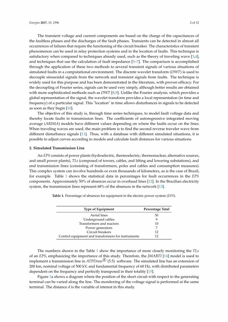
An EPS consists of power plants (hydroelectric, thermoelectric, thermonuclear, alternative sources,and small power plants), TLs (composed of towers, cables, and lifting and lowering substations), andend transmission lines (consisting of transformers, poles and cables and consumption measures).This complex system can involve hundreds or even thousands of kilometers, as is the case of Brazil,for example. Table 1 shows the statistical data in percentages for fault occurrences in the EPScomponents. Approximately 50% of absences occur in overhead lines [12]. In the Brazilian electricitysystem, the transmission lines represent 68% of the absences in the network [13].

Table 1. Percentage of absences for equipment in the electric power system (EPS).

Type of Equipment Percentage Total

Aerial lines 50Underground cables 9

Transformers and reactors 10Power generators 7Circuit breakers 12

Control equipment and transformers for instruments 12

The numbers shown in the Table 1 show the importance of more closely monitoring the TLsof an EPS, emphasizing the importance of this study. Therefore, the JMARTI [14] model is used toimplement a transmission line in ATPDraw R© (5.5) software. The simulated line has an extension of200 km, nominal voltage of 500 kV, and fundamental frequency of 60 Hz, with distributed parametersdependent on the frequency and perfectly transposed in their totality [15].

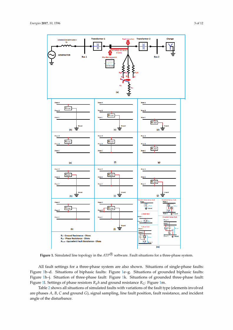
Figure 1a shows a diagram where the position of the short circuit with respect to the generatingterminal can be varied along the line. The monitoring of the voltage signal is performed at the sameterminal. The distance d is the variable of interest in this study.

Energies 2017, 10, 1596 3 of 12

Figure 1. Simulated line topology in the ATP R© software. Fault situations for a three-phase system.

All fault settings for a three-phase system are also shown. Situations of single-phase faults:Figure 1b–d. Situations of biphasic faults: Figure 1e–g. Situations of grounded biphasic faults:Figure 1h–j. Situation of three-phase fault: Figure 1k. Situations of grounded three-phase fault:Figure 1l. Settings of phase resistors Rph and ground resistance RG: Figure 1m.

Table 2 shows all situations of simulated faults with variations of the fault type (elements involvedare phases A, B, C and ground G), signal sampling, line fault position, fault resistance, and incidentangle of the disturbance.

Energies 2017, 10, 1596 4 of 12

Table 2. Situations of simulated faults.

Fault Data Sampling Location Failure Resistance (Ω) Angle of Incidence θ () Fault(kHz) d (km) Situations

A− G 200 10; 45; 84; 155 20; 50; 80; 120; 150; 180; 200; 240 0; 45; 90; 135; 180; 225; 270; 315 256B− G 200 10; 45; 84; 155 20; 50; 80; 120; 150; 180; 200; 240 0; 45; 90; 135; 180; 225; 270; 315 256C− G 200 10; 45; 84; 155 20; 50; 80; 120; 150; 180; 200; 240 0; 45; 90; 135; 180; 225; 270; 315 256A− B 200 10; 45; 84; 155 20; 50; 80; 120; 150; 180; 200; 240 0; 45; 90; 135; 180; 225; 270; 315 256A− C 200 10; 45; 84; 155 20; 50; 80; 120; 150; 180; 200; 240 0; 45; 90; 135; 180; 225; 270; 315 256B− C 200 10; 45; 84; 155 20; 50; 80; 120; 150; 180; 200; 240 0; 45; 90; 135; 180; 225; 270; 315 256

A− B− G 200 10; 45; 84; 155 20; 50; 80; 120; 150; 180; 200; 240 0; 45; 90; 135; 180; 225; 270; 315 256A− C− G 200 10; 45; 84; 155 20; 50; 80; 120; 150; 180; 200; 240 0; 45; 90; 135; 180; 225; 270; 315 256B− C− G 200 10; 45; 84; 155 20; 50; 80; 120; 150; 180; 200; 240 0; 45; 90; 135; 180; 225; 270; 315 256A− B− C 200 10; 45; 84; 155 20; 50; 80; 120; 150; 180; 200; 240 0; 45; 90; 135; 180; 225; 270; 315 256

3. Theory of Traveling Waves

Disturbances occur in the transmission line of electric power, and are caused by a variety ofelectromagnetic phenomena such as atmospheric discharges. Sudden changes occur in the conditionsof the electrical circuits that make up the transmission system, causing a redistribution of energy withthe purpose of finding a new break-even point. Thus, traveling waves refer to the propagation ofenergy over a system. This energy is distributed by the system in its circuit elements, capacitors andinductors [16].

The propagation of traveling waves always occurs in the direction of all the terminals of thetransmission line and causes the electrical transients perceived by the protection relays and otherautomation and control devices located in the operating centers of the system [16]. If any variationoccurs on one terminal of a power transmission line, the other terminal will only feel the variationoccurring when the wave travels the entire length of the line [17].

The remote terminal of the transmission line cannot influence the decisions about the system untilthe wave has traveled from the source of the local terminal to the remote terminal where, throughits interaction with the transmission line, a response is produced that travels from back to the localsource. In this way, electrical signals tend to propagate back and forth, like traveling waves, usuallydissipating energy with losses in the material [17].

The traveling wave theory allows for definition of the reflection and refraction coefficients ofthe traveling wave in discontinuities as well as the wave propagation velocity and the transmissionline surge impedance. It is noteworthy that during propagation along the line, traveling waves areattenuated mainly by resistive and leakage losses and may still suffer distortions in their waveform [18].

In order for the transient behavior of an electromagnetic wave on a transmission line to beadequately represented, it is necessary that the line parameters be evenly distributed over its length,since only this representation allows the theory of the traveling waves to be used to analyze thepropagation of these electromagnetic phenomena in it [19].

It is important to note that transmission line models in which the parameters are constant are notadequate for simulation of the transmission line response over a large range of frequencies that arepresent in the signals during transient conditions [14]. Despite this, in practice, constant frequencydistributed line models provide satisfactory results and are used in several transient studies in powersystems, according to the Alternative Transient Program Rule Book [16].

The reflections and refractions of the waves that travel on the transmission lines are the resultof discontinuities in the course of the wave. These discontinuities can not be caused by terminalimpedances, short circuits, or circuit breakers.

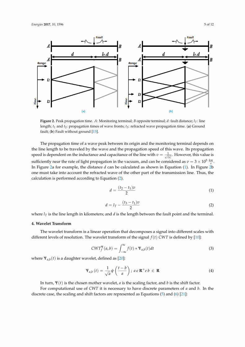
In order to monitor the propagation time of the generated wave fronts, only the peaks of thesewaves are followed. This restriction to only a few points greatly facilitates the monitoring of thisdata. The lattice diagram shown in Figure 2 is a summary of the above because it focuses only on thepropagation times between the point of origin of the fault and the terminals of the line.

Energies 2017, 10, 1596 5 of 12

Figure 2. Peak propagation time. A: Monitoring terminal; B opposite terminal; d: fault distance; lT : linelength; t1 and t2: propagation times of wave fronts; t3: refracted wave propagation time. (a) Groundfault; (b) Fault without ground [15].

The propagation time of a wave peak between its origin and the monitoring terminal depends onthe line length to be traveled by the wave and the propagation speed of this wave. Its propagationspeed is dependent on the inductance and capacitance of the line with v = 1√

LC. However, this value is

sufficiently near the rate of light propagation in the vacuum, and can be considered as v = 3× 105 kms .

In Figure 2a for example, the distance d can be calculated as shown in Equation (1). In Figure 2bone must take into account the refracted wave of the other part of the transmission line. Thus, thecalculation is performed according to Equation (2).

d =(t2 − t1)v

2(1)

d = lT −(t3 − t1)v

2(2)

where lT is the line length in kilometers; and d is the length between the fault point and the terminal.

4. Wavelet Transform

The wavelet transform is a linear operation that decomposes a signal into different scales withdifferent levels of resolution. The wavelet transform of the signal f (t) CWT is defined by [10]:

CWTΨf (a, b) =

∫ ∞

−∞f (t) ∗Ψa,b(t)dt (3)

where Ψa,b(t) is a daughter wavelet, defined as [20]:

Ψa,b (t) =1√a

ψ

(t− b

a

); a ε R+e b ∈ R (4)

In turn, Ψ(t) is the chosen mother wavelet, a is the scaling factor, and b is the shift factor.For computational use of CWT it is necessary to have discrete parameters of a and b. In the

discrete case, the scaling and shift factors are represented as Equations (5) and (6) [21]:

Energies 2017, 10, 1596 6 of 12

a = am0 (5)

b = nb0am0 (6)

m, n ∈ Z; a0 ≥ 1; b0 6= 0

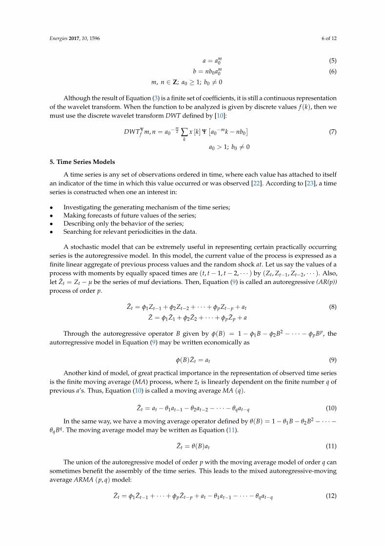
Although the result of Equation (3) is a finite set of coefficients, it is still a continuous representationof the wavelet transform. When the function to be analyzed is given by discrete values f (k), then wemust use the discrete wavelet transform DWT defined by [10]:

DWTΨf m, n = a0

−m2 ∑

kx [k]Ψ

[a0−mk− nb0

](7)

a0 > 1; b0 6= 0

5. Time Series Models

A time series is any set of observations ordered in time, where each value has attached to itselfan indicator of the time in which this value occurred or was observed [22]. According to [23], a timeseries is constructed when one an interest in:

• Investigating the generating mechanism of the time series;• Making forecasts of future values of the series;• Describing only the behavior of the series;• Searching for relevant periodicities in the data.

A stochastic model that can be extremely useful in representing certain practically occurringseries is the autoregressive model. In this model, the current value of the process is expressed as afinite linear aggregate of previous process values and the random shock at. Let us say the values of aprocess with moments by equally spaced times are (t, t− 1, t− 2, · · · ) by (Zt, Zt−1, Zt−2, · · · ). Also,let Zt = Zt − µ be the series of muf deviations. Then, Equation (9) is called an autoregressive (AR(p))process of order p.

Zt = φ1Zt−1 + φ2Zt−2 + · · ·+ φpZt−p + at (8)

Z = φ1Z1 + φ2Z2 + · · ·+ φpZp + a

Through the autoregressive operator B given by φ(B) = 1 − φ1B − φ2B2 − · · · − φpBp, theautorregressive model in Equation (9) may be written economically as

φ(B)Zt = at (9)

Another kind of model, of great practical importance in the representation of observed time seriesis the finite moving average (MA) process, where zt is linearly dependent on the finite number q ofprevious a’s. Thus, Equation (10) is called a moving average MA (q).

Zt = at − θ1at−1 − θ2at−2 − · · · − θqat−q (10)

In the same way, we have a moving average operator defined by θ(B) = 1− θ1B− θ2B2 − · · · −θqBq. The moving average model may be written as Equation (11).

Zt = θ(B)at (11)

The union of the autoregressive model of order p with the moving average model of order q cansometimes benefit the assembly of the time series. This leads to the mixed autoregressive-movingaverage ARMA (p, q) model:

Zt = φ1Zt−1 + · · ·+ φpZt−p + at − θ1at−1 − · · · − θqat−q (12)

Energies 2017, 10, 1596 7 of 12

Equation (12) can be written with the B operator.

φ(B)Zt = θ(B)at (13)

In some cases, it is necessary to make a distinction between the terms of the series to excludetrends, in accordance with Equation (14). The result is an ARIMA (p, d, q) model, where the term Iexpresses a differentiation of order d.

φ(B)Wdt = θ(B)at (14)

where Wdt are differentiations on the terms of series Z shown in Equation (15).

Wt = ∆Zt = Zt − Zt−1 (15)

Wdt = ∆dZt

When Wt presents deterministic seasonal behavior of period s, a model that can be used is shownin Equation (16).

φ(B)Φ(Bs)(∆s)D(∆)dZt = θ(B)Θ(Bs)at (16)

where Φ(Bs) = 1 − Φ1Bs − · · · − ΦPBsP is the seasonal autoregressive operator of P order;Θ(Bs) = 1 − Θ1Bs − · · · − ΘQBsQ is the seasonal moving-averages operator of Q order;φ(B) = 1− φ1B− · · · − φpBp is the autoregressive operator of p order; θ(B) = 1− θ1B− · · · − θqBq;is the moving-averages operator of q order; and ∆s = (1− Bs) is the seasonal difference operator.In ∆D

s = (1− Bs)D, D indicates the number of seasonal differences. The Equation (16) is denoted byseasonal autoregressive integrated moving average (SARIMA) (p, d, q)(P, D, Q)s

Model Evaluation Criteria

For the process ARMA (k, l), the Bayesian information criterion (BIC) is given by Equation (17) [24].

BIC(k, l) = lnσ2k,l + (k + l)

lnNN

(17)

where σ2k,l is a maximum likelihood estimate of the residual variance of the model with N observations.

It seeks to minimize BIC through the adjustments of k and l.For the estimation of the error, Equation (18) is used, where the absolute error module committed

in the extermination of the fault location is divided by the total length of the line.

Error(%) = 100∣∣∣∣Rt − Ct

Tt

∣∣∣∣ (18)

where R is the actual distance value of the fault, C is the value calculated for this distance, and T is thetotal length of the line. This calculation is performed for all calculated fault distances.

6. Results

The proposed method, illustrated by Figure 3, consists of using a discrete wavelet transform DWTin order to decouple the transient signal from the sinusoidal signal characteristic of the transmissionline. These decoupled signals are used in ARIMA models to establish mathematical relationshipsbetween fault distances and calculated coefficients. The RStudio R© (1.0.143) software is used for thecomputational implementation of DWT [25] and ARIMA models.

Energies 2017, 10, 1596 8 of 12

Figure 3. Schematic diagram for fault location with the proposed model. ARIMA: autoregressiveintegrated moving average; DWT: discrete wavelet transform.

Figure 4 illustrates a fault situation showing the behavior of the disturbance in the three phasesthat make up the system. Although the fault does not involve phase C, it is affected because there is acoupling between the three phases. However, the highest voltage values in the involved phases areevident. The figure further illustrates the decoupled disturbance signal of the characteristic sinusoidalsignal of the transmission line.

Figure 4. (a) Voltage signals with incident angle of 90 and fault resistance of 240 Ω at a distance of10 km from the monitoring terminal; (b) Disconnected disturbance signal.

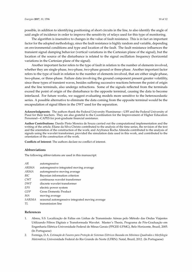
As mentioned, the objective of this work is to relate the distances of occurrences of faults with thecurves of ARIMA models. The Table 3 shows some results obtained, showing the distance–coefficientrelationship. All cases are two-phase faults with an incidence angle of 90.

It can be seen from Table 3 that the coefficients of the obtained SARIMA models are equalfor the same fault distances. For example, for faults occurring at 10 km, the obtained models areSARIMA(2, 0, 2)(2, 0, 4)19 where φ1 = 1.283, φ2 = −0.349, θ1 = −0.344, θ2 = 0.028, Φ19 = −1.460,Φ38 = −0.918, Θ19 = −1.333, Θ38 = −0.736, Θ57 = 0.044, and Θ76 = 0.073 in all faults whose angle ofincidence is 90, regardless of the fault resistance values

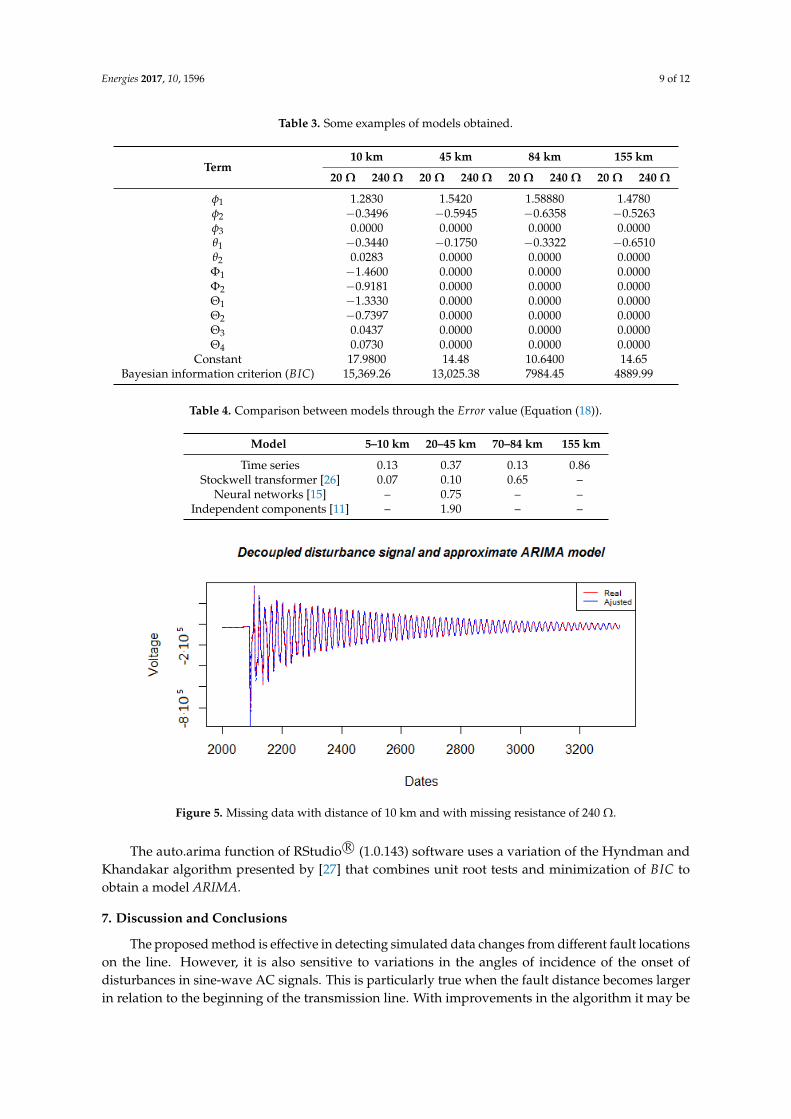
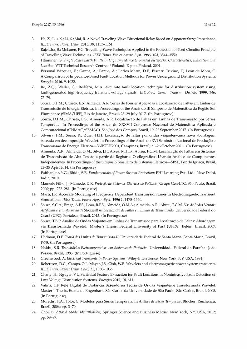
In Table 4 it should be noted that the traveler wave method presents a smaller error than the othermethods when it is at the beginning of the line. According to [26], when traveling waves are used, themain problem is to find the second reverse traveler wave from different disturbance signals. In thiscase, the proposed model presented a satisfactory result, because as the distance of the fault increases,the relative error becomes smaller than for the other methods. Fault resistances do not influence thebehavior of the model, and therefore results are shown for only two resistance values. Figure 5 showsa example of the a fault situation.

Energies 2017, 10, 1596 9 of 12

Table 3. Some examples of models obtained.

Term10 km 45 km 84 km 155 km

20 Ω 240 Ω 20 Ω 240 Ω 20 Ω 240 Ω 20 Ω 240 Ω

φ1 1.2830 1.5420 1.58880 1.4780φ2 −0.3496 −0.5945 −0.6358 −0.5263φ3 0.0000 0.0000 0.0000 0.0000θ1 −0.3440 −0.1750 −0.3322 −0.6510θ2 0.0283 0.0000 0.0000 0.0000Φ1 −1.4600 0.0000 0.0000 0.0000Φ2 −0.9181 0.0000 0.0000 0.0000Θ1 −1.3330 0.0000 0.0000 0.0000Θ2 −0.7397 0.0000 0.0000 0.0000Θ3 0.0437 0.0000 0.0000 0.0000Θ4 0.0730 0.0000 0.0000 0.0000

Constant 17.9800 14.48 10.6400 14.65Bayesian information criterion (BIC) 15,369.26 13,025.38 7984.45 4889.99

Table 4. Comparison between models through the Error value (Equation (18)).

Model 5–10 km 20–45 km 70–84 km 155 km

Time series 0.13 0.37 0.13 0.86Stockwell transformer [26] 0.07 0.10 0.65 –

Neural networks [15] – 0.75 – –Independent components [11] – 1.90 – –

Figure 5. Missing data with distance of 10 km and with missing resistance of 240 Ω.

The auto.arima function of RStudio R© (1.0.143) software uses a variation of the Hyndman andKhandakar algorithm presented by [27] that combines unit root tests and minimization of BIC toobtain a model ARIMA.

7. Discussion and Conclusions

The proposed method is effective in detecting simulated data changes from different fault locationson the line. However, it is also sensitive to variations in the angles of incidence of the onset ofdisturbances in sine-wave AC signals. This is particularly true when the fault distance becomes largerin relation to the beginning of the transmission line. With improvements in the algorithm it may be

Energies 2017, 10, 1596 10 of 12

possible, in addition to identifying positioning of short circuits in the line, to also identify the angle ofsaid angle of incidence in order to improve the sensitivity of relays used for this type of monitoring.

The algorithm is insensitive to changes in the value of fault resistance. This is in fact an importantfactor for the adopted methodology, since the fault resistance is highly random and variable, dependingon environmental conditions and type and location of the fault. The fault resistance influences thetransient signal damping behavior (vertical variations in the Cartesian plane of the signal), but thelocation of the source of the disturbance is related to the signal oscillation frequency (horizontalvariations in the Cartesian plane of the signal).

Another important factor refers to the type of fault in relation to the number of elements involved,whether they are single-phase, two-phase, two-phase ground or three-phase. Another important factorrefers to the type of fault in relation to the number of elements involved, that are either single-phase,two-phase, or three-phase. Failure data involving the ground component present greater volatility,since these types of transient waves, besides suffering successive reactions between the point of originand the line terminals, also undergo refractions. Some of the signals reflected from the terminalsexceed the point of origin of the disturbance to the opposite terminal, causing the data to becomeinterlaced. For future works, we suggest evaluating models more sensitive to the heteroscedasticseries. A possible alternative to eliminate the data coming from the opposite terminal would be theencapsulation of signal filters in the DWT used for the separation.

Acknowledgments: The authors thank the Federal University Fluminense—UFF and the Federal University ofPiauí for their teachers. They are also grateful to the Coordination for the Improvement of Higher EducationPersonnel—CAPES for post-graduate financial assistance.

Author Contributions: Danilo Pinto Moreira de Souza carried out the computational implementation and thewriting of the article; Eliane da Silva Christo contributed to the analysis of the time series, the revision of the textand the orientation of the construction of the work; and Aryfrance Rocha Almeida contributed to the analysis ofsignals using the wavelet transformer, provided the simulation data used in this work, and contributed to theorientation of the construction of the work.

Conflicts of Interest: The authors declare no conflict of interest.

Abbreviations

The following abbreviations are used in this manuscript:

AR autoregressiveARIMA autoregressive integrated moving averageARMA autoregressive moving averageBIC Bayesian information criterionCWT continuous wavelet transformerDWT discrete wavelet transformerEPS electric power systemGDP Gross Domestic ProductMA moving averageSARIMA seasonal autoregressive integrated moving averageTL transmission line

References

1. Abreu, S.S. Localização de Faltas em Linhas de Transmissão Aéreas pelo Método das Ondas ViajantesUtilizando Filtros Digitais e Transformada Wavelet. Master’s Thesis, Programa de Pós-Graduação emEngenharia Elétrica-Universidade Federal de Minas Gerais (PPGEE-UFMG), Belo Horizonte, Brazil, 2005.(In Portuguese)

2. Formiga, D.A. Estimação de Fasores para Proteção de Sistemas Elétricos Baseada em Mínimos Quadrados e MorfologiaMatemática; Universidade Federal do Rio Grande do Norte (UFRN): Natal, Brazil, 2012. (In Portuguese)

Energies 2017, 10, 1596 11 of 12

3. He, Z.; Liu, X.; Li, X.; Mai, R. A Novel Traveling-Wave Directional Relay Based on Apparent Surge Impedance.IEEE Trans. Power Deliv. 2015, 30, 1153–1161.

4. Rajendra, S.; McLaren, P.G. Travelling-Wave Techniques Applied to the Protection of Teed Circuits: Principleof Travelling Wave Techniques. IEEE Trans. Power Appar. Syst. 1985, 104, 3544–3550.

5. Hänninen, S. Single Phase Earth Faults in High Impedance Grounded Networks: Characteristics, Indication andLocation; VTT Technical Research Centre of Finland: Espoo, Finland, 2001.

6. Personal Vázquez, E.; García, A.; Parejo, A.; Larios Marín, D.F.; Biscarri Triviño, F.; León de Mora, C.A Comparison of Impedance-Based Fault Location Methods for Power Underground Distribution Systems.Energies 2016, 9, 1022.

7. Bo, Z.Q.; Weller, G.; Redfern, M.A. Accurate fault location technique for distribution system usingfault-generated high-frequency transient voltage signals. IEE Proc. Gener. Transm. Distrib. 1999, 146,73–79.

8. Souza, D.P.M.; Christo, E.S.; Almeida, A.R. Séries de Fourier Aplicadas à Localizaçao de Faltas em Linhas deTransmissão de Energia Elétrica. In Proceedings of the Anais do III Simpósio de Matemática da Região SulFluminense (SIMA/UFF), Rio de Janeiro, Brazil, 23–29 July 2017. (In Portuguese)

9. Souza, D.P.M.; Christo, E.S.; Almeida, A.R. Localização de Faltas em Linhas de Transmissão por SériesTemporais. In Proceedings of the Anais do XXXVII Congresso Nacional de Matemática Aplicada eComputacional (CNMAC/SBMAC), São José dos Campos, Brazil, 19–22 September 2017. (In Portuguese)

10. Silveira, P.M.; Seara, R.; Zürn, H.H. Localização de faltas por ondas viajantes–uma nova abordagembaseada em decomposição Wavelet. In Proceedings of the Anais do XVI Seminário Nacional de Produção eTransmissão de Energia Elétrica—SNPTEE’2001, Campinas, Brazil, 21–26 October 2001. (In Portuguese)

11. Almeida, A.R.; Almeida, O.M.; Silva, J.P.; Alves, M.H.S.; Abreu, F.C.M. Localização de Faltas em Sistemasde Transmissão de Alta Tensão a partir de Registros Oscilográficos Usando Análise de ComponentesIndependentes. In Proceedings of the Simpósio Brasileiro de Sistemas Elétricos—SBSE, Foz do Iguaçu, Brasil,22–25 Apirl 2014. (In Portuguese)

12. Paithankar, Y.G.; Bhide, S.R. Fundamentals of Power System Protection; PHI Learning Pvt. Ltd.: New Delhi,India, 2010.

13. Mamede Filho, J.; Mamede, D.R. Proteção de Sistemas Elétricos de Potência; Grupo Gen-LTC: São Paulo, Brasil,2000; pp. 272–281. (In Portuguese)

14. Marti, J.R. Accurate Modeling of Frequency Dependent Transmission Lines in Electromagnetic TransientSimulations. IEEE Trans. Power Appar. Syst. 1996 1, 1475–1550.

15. Souza, S.C.A.; Braga, A.P.S.; Leão, R.P.S.; Almeida, O.M.A.; Almeida, A.R.; Abreu, F.C.M. Uso de Redes NeuraisArtificiais e Transformada de Stockwell na Localização de Faltas em Linhas de Transmissão; Universidade Federal doCeará (UFC): Fortaleza, Brazil, 2015. (In Portuguese)

16. Souza, T.B.P. Análise de Ondas Viajantes em Linhas de Transmissão para Localização de Faltas: Abordagemvia Transformada Wavelet. Master’s Thesis, Federal University of Pará (UFPA): Belém, Brazil, 2007.(In Portuguese)

17. Hedman, D.E. Teoria das Linhas de Transmissão-II; Universidade Federal de Santa Maria: Santa Maria, Brazil,1978. (In Portuguese)

18. Naidu, S.R. Transitórios Eletromagnéticos em Sistemas de Potência. Universidade Federal da Paraíba: JoãoPessoa, Brazil, 1985. (In Portuguese)

19. Greenwood, A. Electrical Transients in Power Systems; Wiley-Interscience: New York, NY, USA, 1991.20. Robertson, D.C.; Camps, O.I.; Mayer, J.S.; Gish, W.B. Wavelets and electromagnetic power system transients.

IEEE Trans. Power Deliv. 1996, 11, 1050–1056.21. Chang, H.; Nguyen V.L. Statistical Feature Extraction for Fault Locations in Nonintrusive Fault Detection of

Low Voltage Distribution Systems. Energies 2017, 10, 611.22. Valins, T.F. Relé Digital de Distância Baseado na Teoria de Ondas Viajantes e Transformada Wavelet.

Master’s Thesis, Escola de Engenharia São Carlos da Universidade de São Paulo, São Carlos, Brazil, 2005.(In Portuguese)

23. Morettin, P.A.; Toloi, C. Modelos para Séries Temporais. In Análise de Séries Temporais; Blucher: Reichenau,Brazil, 2006; pp. 3–70.

24. Choi, B. ARMA Model Identification; Springer Science and Business Media: New York, NY, USA, 2012;pp. 58–87.

Energies 2017, 10, 1596 12 of 12

25. Aldrich, E. Wavelets: A Package of Functions for Computing Wavelet Filters, Wavelet Transforms and MultiresolutionAnalyses; R Package Version 0.3-0; University of Washington: Seattle, WA, USA, 2013.

26. Souza, S.C.A.; Braga, A.P.S.; Almeida, A.R.; Abreu, F.C.M.; Almeida, O.M. Uso da Transformada de Stockwelle ondas Viajantes na Localização de Faltas em Linhas de Transmissão; Universidade Federal do Ceará (UFC):Fortaleza, Brazil, 2014. (In Portuguese)

27. Hyndman, R.J.; Khandakar, Y. Automatic time series for forecasting: The forecast package for R. J. Stat. Softw.2008, 27, 5–22.

c© 2017 by the authors. Licensee MDPI, Basel, Switzerland. This article is an open accessarticle distributed under the terms and conditions of the Creative Commons Attribution(CC BY) license (http://creativecommons.org/licenses/by/4.0/).