sensors

Article

Load Resistance Optimization of a Magnetically CoupledTwo-Degree-of-Freedom Bistable Energy Harvester ConsideringThird-Harmonic Distortion in Forced Oscillation

Jinhong Noh 1, Pilkee Kim 2,3,* and Yong-Jin Yoon 1,4,*

Citation: Noh, J.; Kim, P.; Yoon, Y.-J.

Load Resistance Optimization of a

Magnetically Coupled

Two-Degree-of-Freedom Bistable

Energy Harvester Considering

Third-Harmonic Distortion in Forced

Oscillation. Sensors 2021, 21, 2668.

https://doi.org/10.3390/s21082668

Academic Editor: Fabio Viola

Received: 9 March 2021

Accepted: 7 April 2021

Published: 10 April 2021

Publisher’s Note: MDPI stays neutral

with regard to jurisdictional claims in

published maps and institutional affil-

iations.

Copyright: © 2021 by the authors.

Licensee MDPI, Basel, Switzerland.

This article is an open access article

distributed under the terms and

conditions of the Creative Commons

Attribution (CC BY) license (https://

creativecommons.org/licenses/by/

4.0/).

1 Department of Mechanical Engineering, Korea Advanced Institute of Science and Technology,Daejeon 34141, Korea; jinhongnoh@kaist.ac.kr

2 School of Mechanical Design Engineering, College of Engineering, Jeonbuk National University,567 Baekje-daero, Deokjin-gu, Jeonju-si 54896, Korea

3 Eco-Friendly Machine Parts Design Research Center, Jeonbuk National University, 567 Baekje-daero,Deokjin-gu, Jeonju-si 54896, Korea

4 School of Mechanical and Aerospace Engineering, Nanyang Technological University,Singapore 639798, Singapore

* Correspondence: pkim@jbnu.ac.kr (P.K.); yongjiny@kaist.ac.kr (Y.-J.Y.)

Abstract: In this study, the external load resistance of a magnetically coupled two-degree-of-freedombistable energy harvester (2-DOF MCBEH) was optimized to maximize the harvested power output,considering the third-harmonic distortion in forced response. First, the nonlinear dynamic analysiswas performed to investigate the characteristics of the large-amplitude interwell motions of the2-DOF MCBEH. From the analysis results, it was found that the third-harmonic distortion occurs inthe interwell motion of the 2-DOF MCBEH system due to the nonlinear magnetic coupling betweenthe beams. Thus, in this study, the third-harmonic distortion was considered in the optimizationprocess of the external load resistance of the 2-DOF MCBEH, which is different from the processof conventional impedance matching techniques suitable for linear systems. The optimal loadresistances were estimated for harmonic and swept-sine excitations by using the proposed method,and all the results of the power outputs were in excellent agreements with the numerically optimizedresults. Furthermore, the associated power outputs were compared with the power outputs obtainedby using the conventional impedance matching technique. The results of the power outputs arediscussed in terms of the improvement in energy harvesting performance.

Keywords: bistable energy harvester; optimal resistance; harmonic distortion; broadband performance

1. Introduction1.1. Introduction to Bistable Energy Harvesters

Energy harvesting, which draws useful electrical energy from environmental energysources [1–7], remains an active research area for various promising applications such assmart environments and wireless sensor networks [8]. Energy harvesting has been consid-ered as a possible alternative powering technology to chemical batteries [9]. When wirelesssensor networks are powered by energy harvesting technology, maintenance cost for bat-tery replacement in places like buildings, bridges, or tires would be unnecessary [10,11]. Inaddition, many researchers have been trying to apply energy harvesting technology to avariety of emerging applications, such as electrochemical cycles [12], energy-autonomouselectronic skins [13], or wireless power transfer for implantable devices [14].

Nonlinear vibration-based energy harvesters (VEHs) have gained intensive attentionover the past decade for broadband energy harvesting applications [15,16]. A bistableenergy harvester (BEH) is the fundamental design of a nonlinear VEH [17]. The energyharvester in this study utilizes the bistable configuration in which the potential energy,as a function of displacement, has two local minima. Figure 1a shows the behavior of

Sensors 2021, 21, 2668. https://doi.org/10.3390/s21082668 https://www.mdpi.com/journal/sensors

Sensors 2021, 21, 2668 2 of 15

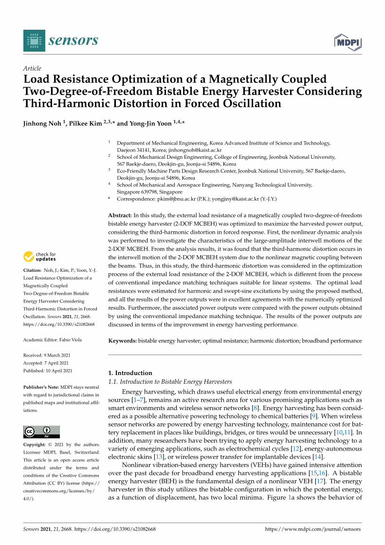
the monostable system, which has the single-well potential energy function. Path A inFigure 1a represents the single-well oscillation. Figure 1b depicts the double-well potentialenergy of the bistable system. The intrawell, interwell, and chaotic motions of the bistablesystem appear, depending on the initial conditions and the excitation [18]. When theintrawell motion appears, the system vibrates along path B in Figure 1b. Because theoscillation occurs within one of the two potential wells, the amplitude of the oscillation isinsufficient for energy harvesting [19]. In contrast, bistable energy harvesters are capable ofextracting adequate power when oscillating along path C in Figure 1b. The system vibratesacross the wells when the state overcomes the saddle barrier, which is the local maximumpoint between the wells. The output power harvested from this large-amplitude interwellmotion is bigger than that from the intrawell motion [20]. Thus, the main research effort inthis study was focused on the dynamical behavior in interwell motion in order to optimizethe energy harvesting performance.

Sensors 2021, 21, x FOR PEER REVIEW 2 of 15

Nonlinear vibration-based energy harvesters (VEHs) have gained intensive attention over the past decade for broadband energy harvesting applications [15,16]. A bistable energy harvester (BEH) is the fundamental design of a nonlinear VEH [17]. The energy harvester in this study utilizes the bistable configuration in which the potential energy, as a function of displacement, has two local minima. Figure 1a shows the behavior of the monostable system, which has the single-well potential energy function. Path A in Figure 1a represents the single-well oscillation. Figure 1b depicts the double-well potential energy of the bistable system. The intrawell, interwell, and chaotic motions of the bistable system appear, depending on the initial conditions and the excitation [18]. When the intrawell motion appears, the system vibrates along path B in Figure 1b. Because the oscillation occurs within one of the two potential wells, the amplitude of the oscillation is insufficient for energy harvesting [19]. In contrast, bistable energy harvesters are capable of extracting adequate power when oscillating along path C in Figure 1b. The system vibrates across the wells when the state overcomes the saddle barrier, which is the local maximum point between the wells. The output power harvested from this large-amplitude interwell motion is bigger than that from the intrawell motion [20]. Thus, the main research effort in this study was focused on the dynamical behavior in interwell motion in order to optimize the energy harvesting performance.

Figure 1. Schematics of the potential energy functions of (a) the monostable system and (b) the bistable system. In (a), the monostable system has only a single-well oscillation plotted by A. In contrast, in (b), the bistable system has not only the intrawell motion but also the interwell motion, depicted by B and C, respectively. An attractor for complex chaotic motion might coexist with regular behavior, but the chaotic motion is not investigated in this research.

1.2. Contribution of This Study Figure 2 shows the schematic of a magnetically coupled two-degree-of-freedom

bistable energy harvester (2-DOF MCBEH) considered in this study. As shown in Figure 2, the two piezoelectric bimorph beams are cantilevered into the base structure at the same height on the opposite side. The two identical neodymium magnets are attached to the free ends of the cantilevered beams, so that they are forced oppositely by repulsive magnetic forces. The piezoelectric layers of the bimorph beams are poled in the thickness direction and connected to the external load resistances in series. Such a 2-DOF MCBEH is known to have superior broadband performance to conventional 1-DOF BEHs [21]. In this study, the nonlinear dynamical behaviors of the 2-DOF MCBEH were investigated. From the results of the dynamic analyses, the third-harmonic distortion in the interwell motion of the 2-DOF MCBEH was observed and considered important in the optimization process of the external load resistances to maximize the energy harvesting performance.

Figure 1. Schematics of the potential energy functions of (a) the monostable system and (b) thebistable system. In (a), the monostable system has only a single-well oscillation plotted by A. Incontrast, in (b), the bistable system has not only the intrawell motion but also the interwell motion,depicted by B and C, respectively. An attractor for complex chaotic motion might coexist with regularbehavior, but the chaotic motion is not investigated in this research.

1.2. Contribution of This Study

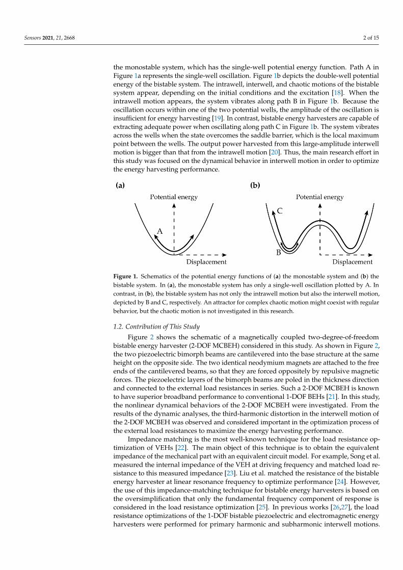
Figure 2 shows the schematic of a magnetically coupled two-degree-of-freedombistable energy harvester (2-DOF MCBEH) considered in this study. As shown in Figure 2,the two piezoelectric bimorph beams are cantilevered into the base structure at the sameheight on the opposite side. The two identical neodymium magnets are attached to the freeends of the cantilevered beams, so that they are forced oppositely by repulsive magneticforces. The piezoelectric layers of the bimorph beams are poled in the thickness directionand connected to the external load resistances in series. Such a 2-DOF MCBEH is knownto have superior broadband performance to conventional 1-DOF BEHs [21]. In this study,the nonlinear dynamical behaviors of the 2-DOF MCBEH were investigated. From theresults of the dynamic analyses, the third-harmonic distortion in the interwell motion ofthe 2-DOF MCBEH was observed and considered important in the optimization process ofthe external load resistances to maximize the energy harvesting performance.

Impedance matching is the most well-known technique for the load resistance op-timization of VEHs [22]. The main object of this technique is to obtain the equivalentimpedance of the mechanical part with an equivalent circuit model. For example, Song et al.measured the internal impedance of the VEH at driving frequency and matched load re-sistance to this measured impedance [23]. Liu et al. matched the resistance of the bistableenergy harvester at linear resonance frequency to optimize performance [24]. However,the use of this impedance-matching technique for bistable energy harvesters is based onthe oversimplification that only the fundamental frequency component of response isconsidered in the load resistance optimization [25]. In previous works [26,27], the loadresistance optimizations of the 1-DOF bistable piezoelectric and electromagnetic energyharvesters were performed for primary harmonic and subharmonic interwell motions.

Sensors 2021, 21, 2668 3 of 15

It was demonstrated that the optimal load resistance strongly depended on the oscilla-tion frequency of the interwell motion rather than on the forcing frequency of excitation.Although harmonic distortions in the interwell motions of the 1-DOF systems were notsignificant [26,27], it can be readily deduced that high-order frequency components are im-portant in the optimization of the external load resistance. Thus, the impedance matchingtechnique is possibly undesirable and inappropriate for the load resistance optimization ofthe 2-DOF MCBEH when certain high-order harmonics are significant in response (e.g., thethird-harmonic distortion of beam 2 presented later in this study).

Sensors 2021, 21, x FOR PEER REVIEW 3 of 15

Figure 2. Three-dimensional view of the two-degree-of-freedom bistable energy harvester (2-DOF MCBEH). A longer beam located on the left is the bimorph beam 1, and a shorter beam located on the right is the bimorph beam 2. The identical permanent magnets are attached to the tips of the beams. The base, considered as a rigid body, excites the beams. The harmonic motion of the base is confined to upward and downward movement. The energy harvester scavenges this vibrational energy to extract electrical power.

Impedance matching is the most well-known technique for the load resistance optimization of VEHs [22]. The main object of this technique is to obtain the equivalent impedance of the mechanical part with an equivalent circuit model. For example, Song et al. measured the internal impedance of the VEH at driving frequency and matched load resistance to this measured impedance [23]. Liu et al. matched the resistance of the bistable energy harvester at linear resonance frequency to optimize performance [24]. However, the use of this impedance-matching technique for bistable energy harvesters is based on the oversimplification that only the fundamental frequency component of response is considered in the load resistance optimization [25]. In previous works [26,27], the load resistance optimizations of the 1-DOF bistable piezoelectric and electromagnetic energy harvesters were performed for primary harmonic and subharmonic interwell motions. It was demonstrated that the optimal load resistance strongly depended on the oscillation frequency of the interwell motion rather than on the forcing frequency of excitation. Although harmonic distortions in the interwell motions of the 1-DOF systems were not significant [26,27], it can be readily deduced that high-order frequency components are important in the optimization of the external load resistance. Thus, the impedance matching technique is possibly undesirable and inappropriate for the load resistance optimization of the 2-DOF MCBEH when certain high-order harmonics are significant in response (e.g., the third-harmonic distortion of beam 2 presented later in this study).

The nonlinear dynamic analyses and load resistance optimization were performed in this study to maximize the energy harvesting performance of the 2-DOF MCBEH. First, frequency response analysis was conducted to find the operating frequency range of the 2-DOF MCBEH, where the large-amplitude interwell motion occurs. Second, to investigate the effects of high-order harmonics on the dynamic response, the interwell motions were analyzed in the frequency domain by the fast Fourier transform. It was found that for beam 2, the third-order harmonic component as well as the fundamental harmonic component plays an important role in the interwell oscillation of the 2-DOF MCBEH, which leads to the third-harmonic distortion. Therefore, in this study, an optimization process for the load resistance was established with consideration of the third-harmonic distortion. The optimal load resistances estimated by the proposed optimization method were compared with those evaluated by the numerical optimization process and the conventional impedance matching technique. The results of this study imply that the proposed optimization process, in which the third-harmonic distortion is considered, can be extended to various fields [28,29].

Figure 2. Three-dimensional view of the two-degree-of-freedom bistable energy harvester (2-DOFMCBEH). A longer beam located on the left is the bimorph beam 1, and a shorter beam located onthe right is the bimorph beam 2. The identical permanent magnets are attached to the tips of thebeams. The base, considered as a rigid body, excites the beams. The harmonic motion of the baseis confined to upward and downward movement. The energy harvester scavenges this vibrationalenergy to extract electrical power.

The nonlinear dynamic analyses and load resistance optimization were performed inthis study to maximize the energy harvesting performance of the 2-DOF MCBEH. First,frequency response analysis was conducted to find the operating frequency range of the2-DOF MCBEH, where the large-amplitude interwell motion occurs. Second, to investigatethe effects of high-order harmonics on the dynamic response, the interwell motions wereanalyzed in the frequency domain by the fast Fourier transform. It was found that for beam2, the third-order harmonic component as well as the fundamental harmonic componentplays an important role in the interwell oscillation of the 2-DOF MCBEH, which leads tothe third-harmonic distortion. Therefore, in this study, an optimization process for the loadresistance was established with consideration of the third-harmonic distortion. The optimalload resistances estimated by the proposed optimization method were compared with thoseevaluated by the numerical optimization process and the conventional impedance matchingtechnique. The results of this study imply that the proposed optimization process, in whichthe third-harmonic distortion is considered, can be extended to various fields [28,29].

2. Model Description2.1. Geometric Dimensions and Material Properties

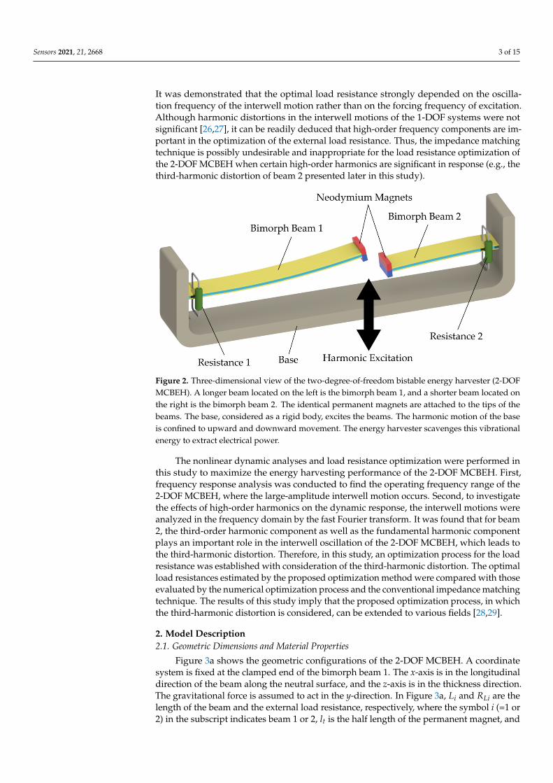
Figure 3a shows the geometric configurations of the 2-DOF MCBEH. A coordinatesystem is fixed at the clamped end of the bimorph beam 1. The x-axis is in the longitudinaldirection of the beam along the neutral surface, and the z-axis is in the thickness direction.The gravitational force is assumed to act in the y-direction. In Figure 3a, Li and RLi are thelength of the beam and the external load resistance, respectively, where the symbol i (=1 or2) in the subscript indicates beam 1 or 2, lt is the half length of the permanent magnet, and

Sensors 2021, 21, 2668 4 of 15

d is the separation distance between the centers of mass of two magnets when the beamsare undeformed. Figure 3b shows a schematic of the motion of the 2-DOF MCBEH. In thisfigure, zb is the displacement of the base structure excited harmonically in the z-directionand wi (i = 1 or 2) is the transverse deflection of the tip. The sign of w1 is positive forupward motion and opposite to the sign of w2, as depicted in Figure 3b. Figure 3c showsa cross-sectional view of the bimorph beam. In this figure, b is the width of the beam, hsand hp are the thicknesses of the metal substrate and piezoelectric layers, respectively, andthe thickness of the electrode is neglected. The dimensions of the permanent magnet aredepicted in Figure 3d, where 2ht and 2bt are the thickness and width of the two identicalneodymium magnets, respectively. The values of the geometric dimensions and materialproperties used in this study are listed in Table 1.

Sensors 2021, 21, x FOR PEER REVIEW 4 of 15

2. Model Description 2.1. Geometric Dimensions and Material Properties

Figure 3a shows the geometric configurations of the 2-DOF MCBEH. A coordinate system is fixed at the clamped end of the bimorph beam 1. The x-axis is in the longitudinal direction of the beam along the neutral surface, and the z-axis is in the thickness direction. The gravitational force is assumed to act in the y-direction. In Figure 3a, iL and LiR are the length of the beam and the external load resistance, respectively, where the symbol i (=1 or 2) in the subscript indicates beam 1 or 2, tl is the half length of the permanent magnet, and d is the separation distance between the centers of mass of two magnets when the beams are undeformed. Figure 3b shows a schematic of the motion of the 2-DOF MCBEH. In this figure, bz is the displacement of the base structure excited harmonically in the z-direction and iw (i = 1 or 2) is the transverse deflection of the tip. The sign of 1w is positive for upward motion and opposite to the sign of 2w , as depicted in Figure 3b. Figure 3c shows a cross-sectional view of the bimorph beam. In this figure, b is the width of the beam, sh and

ph are the thicknesses of the metal substrate and piezoelectric

layers, respectively, and the thickness of the electrode is neglected. The dimensions of the permanent magnet are depicted in Figure 3d, where 2 th and 2 tb are the thickness and width of the two identical neodymium magnets, respectively. The values of the geometric dimensions and material properties used in this study are listed in Table 1.

Figure 3. Geometric configurations and a schematic of motion of the 2-DOF MCBEH. Notations for geometric dimensions and coordinate system are depicted in (a). (a) shows that the external resistances are connected to the bimorph beam in series. (b) is a schematic of motion of the 2-DOF MCBEH in the x-z plane. The system is excited by the harmonic base displacement. The sign conventions of the tip deflections of the beams are opposite to each other. The out-of-phase motion

Figure 3. Geometric configurations and a schematic of motion of the 2-DOF MCBEH. Notationsfor geometric dimensions and coordinate system are depicted in (a). (a) shows that the externalresistances are connected to the bimorph beam in series. (b) is a schematic of motion of the 2-DOFMCBEH in the x-z plane. The system is excited by the harmonic base displacement. The signconventions of the tip deflections of the beams are opposite to each other. The out-of-phase motion ofthe beams is depicted in (b). (c) gives the magnified cross-sectional view of the bimorph beams. Eachbeam has the same dimensions except for the length. The thickness of the electrodes is neglectedbecause it is too thin. The geometry of two identical neodymium magnets is shown in (d). The centerof the magnet is considered to coincide with the centroid of the bimorph beam.

Sensors 2021, 21, 2668 5 of 15

Table 1. Geometric dimensions and material properties of the 2-DOF MCBEH. The values in theparentheses are the values for beam 2.

Metal Substrate Piezoelectric Layer Magnet

Length 73 mm (44 mm) 73 mm (44 mm) 2 mmThickness 0.3 mm 0.052 mm 6 mm

Width 10 mm 10 mm 10 mmDensity 7850 kg/m3 1780 kg/m3 -

Young’s modulus 200 GPa 3 GPa -Piezoelectric strain constant - −23 pm/V -

Permittivity - 110 pF/m -Mass - - 1 g

Mass moment of inertia - - 4 g·mm2

Magnetization - - 900 kA/mSeparation distance - - 11.6 mm

2.2. Mathematical Model of the 2-DOF MCBEH

For the curvatures of the beams, the Euler–Bernoulli beam theory for perfectly bondedcomposite structures was employed. For the constitutive relation, the linear elastic materialmodel was utilized. The permanent magnets (or tip masses) were approximated to beperfectly constrained at the tips of each beam and have the same rotational angle asthe that of the tips. The magnetic charge model was applied to describe the magneticrepulsive force acting on the tip in free space. Using Hamilton’s principle, the governingfield equations were derived and, subsequently, the modal analysis was performed toobtain the linear natural frequencies and mode shapes [30]. After imposing the singlemode approximation and discretization assumption on the governing equations in modalcoordinates, the oscillator model of the 2-DOF MCBEH can be derived as follows [31]:

..wi + 2ζiωi

.wi + ω2

i wi − βiVi − Fmi = −αi..zb, i = 1, 2, (1)

.Vi + ηiVi + γi

.wi = 0, i = 1, 2, (2)

where Vi is the voltage response, ζi is the damping ratio, ωi is the linear natural frequency,βi is the modal electromechanical coupling coefficient for motion, Fmi is the modal magneticforce, αi is the modal excitation coefficient, ηi is the modal resistance, and γi is the modalelectromechanical coupling coefficient for circuit. Herein, the modal resistance and baseexcitation are expressed by

ηi =2

CpiRLi, (3)

..zb = Fb cos(Ωt) (4)

where Cpi is the equivalent capacitance for the piezoelectric layer, and Fb and Ω are theamplitude and frequency of the base excitation, respectively.

For the geometric dimensions and material properties listed in Table 1, the valuesof the parameters were obtained as follows: ω1 = 1.5461× 102 rad/s, ω2 = 3.4785×102 rad/s, β1 = −1.6474× 10−3 C/kg·m, β2 = −3.0738× 10−3 C/kg·m, α1 = 1.1597,α2 = −1.0870, η1 = 1.3141× 103/s, η2 = 2.1802× 103/s, γ1 = −3.2167× 103 V/m, andγ2 = −8.9713× 103 V/m. In addition, both of the damping ratios, ζ1 and ζ2, were chosenas 0.007.

3. Methods: Dynamic Simulation and Optimization3.1. Dynamical Characterization Method

For numerical dynamic simulation, the second-order ordinary differential equations(ODEs) given by Equation (1,2) were converted by introducing the following state vector,

→x =

[x1 x2 x3 x4 x5 x6

]T=[ .

w1 w1 V1.

w2 w2 V2]T , (5)

Sensors 2021, 21, 2668 6 of 15

into a system of the first-order ODEs:

.→x =

−2ζ1ω1x1 −ω21x2 + β1x3 + Fm1 − α1

..zb

x1−γ1x1 − η1x3

−2ζ2ω2x4 −ω22x5 + β2x6 + Fm2 − α2

..zb

x4−γ2x4 − η2x6

. (6)

The direct numerical integration of Equation (6) was performed by implementingthe Runge–Kutta method. The frequency responses for the beam deflections and outputvoltages were evaluated by means of sine sweep technique with zero initial conditions.To analyze the nonlinear behaviors of the 2-DOF MCBEH, the excitation frequency wasincreased from 11.9 Hz to 17.5 Hz, where the third-harmonic distortion in the interwellmotion of beam 2 occurs. The amplitude of the base excitation was set to be 6 m/s2.

3.2. Analytical Optimization Method for Load Resistance

Frequency-domain analysis was performed by the fast Fourier transform of the timeresponses obtained by the numerical simulation. Based on the frequency-domain results,the tip deflection and voltage across the external load resistance can be expressed by

wi =∞

∑n=1

WineinΩt + W∗ine−inΩt

, (7)

Vi =∞

∑n=1

ΨineinΩt + Ψ∗ine−inΩt

(8)

where n indicates the order of the harmonic term and Ω is the angular excitation frequency.Substituting Equations (7) and (8) into Equation (2) and performing mathematical

manipulation lead to

Ψin =−inΩγiinΩ + ηi

Win, (9)

and the resulting root mean square (RMS) output power becomes

PRMSi =V2

RMSiRLi

= 2∞

∑n=1

(nΩγi)2

RLi

(nΩ)2 + η2

i

|Win|2. (10)

An equation for maximizing the RMS power, ∂PRMSi/∂RLi

∣∣∣RLi=Ropti = 0 , where Ropt

represents the optimal load resistance, takes the form:

∞

∑n=1

n2

η2opti − (nΩ)2

|Win|2

η2opti + (nΩ)2

2 = 0. (11)

Solving Equation (11) for ηopti gives the optimal load resistance as follows:

Ropti =2

ηoptiCpi. (12)

4. Results and Discussion4.1. Frequency Response near the First Primary Resonance

Figure 4 shows the frequency responses of the piezoelectric bimorph beams of the2-DOF MCBEH near the first primary resonance under the harmonic base excitation, ofwhich the amplitude is set to be 6 m/s2. The bifurcation structure of the 2-DOF MCBEH

Sensors 2021, 21, 2668 7 of 15

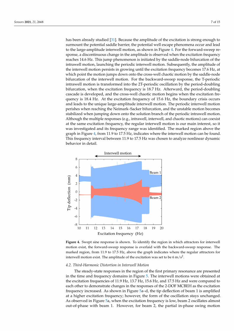
has been already studied [31]. Because the amplitude of the excitation is strong enough tosurmount the potential saddle barrier, the potential well escape phenomena occur and leadto the large-amplitude interwell motion, as shown in Figure 4. For the forward-sweep re-sponse, a discontinuous change in the amplitude is observed when the excitation frequencyreaches 14.6 Hz. This jump phenomenon is initiated by the saddle-node bifurcation of theintrawell motion, launching the periodic interwell motion. Subsequently, the amplitude ofthe interwell motion persists in growing until the excitation frequency becomes 17.6 Hz, atwhich point the motion jumps down onto the cross-well chaotic motion by the saddle-nodebifurcation of the interwell motion. For the backward-sweep response, the T-periodicintrawell motion is transformed into the 2T-periodic oscillation by the period-doublingbifurcation, when the excitation frequency is 18.7 Hz. Afterward, the period-doublingcascade is developed, and the cross-well chaotic motion begins when the excitation fre-quency is 18.4 Hz. At the excitation frequency of 15.6 Hz, the boundary crisis occursand leads to the unique large-amplitude interwell motion. The periodic interwell motionperishes when reaching the Neimark–Sacker bifurcation, and the unstable motion becomesstabilized when jumping down onto the solution branch of the periodic intrawell motion.Although the multiple responses (e.g., intrawell, interwell, and chaotic motions) can coexistat the same excitation frequency, the regular interwell motion is our main interest, so itwas investigated and its frequency range was identified. The marked region above thegraph in Figure 4, from 11.9 to 17.5 Hz, indicates where the interwell motion can be found.This frequency interval between 11.9 to 17.5 Hz was chosen to analyze nonlinear dynamicbehavior in detail.

Sensors 2021, 21, x FOR PEER REVIEW 8 of 15

Figure 4. Swept sine response is shown. To identify the region in which attractors for interwell motion exist, the forward-sweep response is overlaid with the backward-sweep response. The marked region, from 11.9 to 17.5 Hz, above the graph indicates where the regular attractors for interwell motion exist. The amplitude of the excitation was set to be 6 m/s2.

4.2. Third-Harmonic Distortion in Interwell Motion The steady-state responses in the region of the first primary resonance are presented

in the time and frequency domains in Figure 5. The interwell motions were obtained at the excitation frequencies of 11.9 Hz, 13.7 Hz, 15.6 Hz, and 17.5 Hz and were compared to each other to demonstrate changes in the responses of the 2-DOF MCBEH as the excitation frequency increased. As shown in Figure 5a–d, the tip deflection of beam 1 is amplified at a higher excitation frequency; however, the form of the oscillation stays unchanged. As observed in Figure 5a, when the excitation frequency is low, beam 2 oscillates almost out-of-phase with beam 1. However, for beam 2, the partial in-phase swing motion becomes more notable as the excitation frequency approaches 17.5 Hz. Figure 5e–h shows the results of applying the fast Fourier transform to Figure 5a–d. For both beams, the fundamental and third-order harmonic components are observed and compared. For beam 1, the third-harmonic component is always much smaller than the fundamental-harmonic component and tends to be more suppressed as the excitation frequency increases. This means that the distortion of the primary harmonic response produced by the third-harmonic component is negligible. On the other hand, for beam 2, the effect of the third-harmonic component (and thus the third-harmonic distortion) is more significant with the increase of the excitation frequency. The third-harmonic component in the response of beam 2 is relatively small at the lowest excitation frequency (Figure 5e), but it continues to increase with the excitation frequency (Figure 5f), and finally, it becomes larger than the fundamental-harmonic component (Figure 5g–h). Figure 5d,h clearly demonstrates that for beam 2, the third-harmonic distortion in the response is remarkable, while negligible for beam 1. The rapid growth in the third-harmonic distortion of beam 2 results in the amplification of the in-phase swing of beam 2 in Figure 5a–d.

Figure 4. Swept sine response is shown. To identify the region in which attractors for interwellmotion exist, the forward-sweep response is overlaid with the backward-sweep response. Themarked region, from 11.9 to 17.5 Hz, above the graph indicates where the regular attractors forinterwell motion exist. The amplitude of the excitation was set to be 6 m/s2.

4.2. Third-Harmonic Distortion in Interwell Motion

The steady-state responses in the region of the first primary resonance are presentedin the time and frequency domains in Figure 5. The interwell motions were obtained atthe excitation frequencies of 11.9 Hz, 13.7 Hz, 15.6 Hz, and 17.5 Hz and were compared toeach other to demonstrate changes in the responses of the 2-DOF MCBEH as the excitationfrequency increased. As shown in Figure 5a–d, the tip deflection of beam 1 is amplifiedat a higher excitation frequency; however, the form of the oscillation stays unchanged.As observed in Figure 5a, when the excitation frequency is low, beam 2 oscillates almostout-of-phase with beam 1. However, for beam 2, the partial in-phase swing motion

Sensors 2021, 21, 2668 8 of 15

becomes more notable as the excitation frequency approaches 17.5 Hz. Figure 5e–h showsthe results of applying the fast Fourier transform to Figure 5a–d. For both beams, thefundamental and third-order harmonic components are observed and compared. Forbeam 1, the third-harmonic component is always much smaller than the fundamental-harmonic component and tends to be more suppressed as the excitation frequency increases.This means that the distortion of the primary harmonic response produced by the third-harmonic component is negligible. On the other hand, for beam 2, the effect of the third-harmonic component (and thus the third-harmonic distortion) is more significant with theincrease of the excitation frequency. The third-harmonic component in the response ofbeam 2 is relatively small at the lowest excitation frequency (Figure 5e), but it continues toincrease with the excitation frequency (Figure 5f), and finally, it becomes larger than thefundamental-harmonic component (Figure 5g–h). Figure 5d,h clearly demonstrates thatfor beam 2, the third-harmonic distortion in the response is remarkable, while negligiblefor beam 1. The rapid growth in the third-harmonic distortion of beam 2 results in theamplification of the in-phase swing of beam 2 in Figure 5a–d.

Sensors 2021, 21, x FOR PEER REVIEW 9 of 15

Figure 5. The steady-state interwell responses of the two piezoelectric bimorph beams are shown. (a–d) are the time responses obtained when the excitation frequencies are 11.9 Hz, 13.7 Hz, 15.6 Hz, and 17.5 Hz, respectively, which belong to the frequency region of the first primary resonance. The amplitude of the excitation is 6 m/s2. The magnitudes of the harmonic components in the time responses (a–d) are plotted in (e–h). It is observed that the magnitudes of the fifth harmonic terms are negligible for all the cases (e–h).

According to the results of the fast Fourier transform, total harmonic distortion denoted by iK reduces to the third-harmonic distortion as follows:

+ +≈

+

2 2 232 3 4

1 1

ii i ii

i i

WW W WK

W W. (13)

Thus, the third-harmonic distortion measures the relative contribution of the third-harmonic component to the fundamental-harmonic component towards the interwell motion. Referring to Figure 6, as the excitation frequency approaches 17.5 Hz, the quantitative third-harmonic distortion of beam 1, evaluated by using Equation (13), tends to slightly decrease, and its absolute value remains small in the entire frequency band; on the other hand, the third-harmonic distortion of beam 2 soars dramatically, which means that the third-harmonic distortion has a significant effect on the nonlinear interwell motion of the 2-DOF MCBEH.

Figure 5. The steady-state interwell responses of the two piezoelectric bimorph beams are shown. (a–d) are the timeresponses obtained when the excitation frequencies are 11.9 Hz, 13.7 Hz, 15.6 Hz, and 17.5 Hz, respectively, which belongto the frequency region of the first primary resonance. The amplitude of the excitation is 6 m/s2. The magnitudes ofthe harmonic components in the time responses (a–d) are plotted in (e–h). It is observed that the magnitudes of the fifthharmonic terms are negligible for all the cases (e–h).

Sensors 2021, 21, 2668 9 of 15

According to the results of the fast Fourier transform, total harmonic distortion de-noted by Ki reduces to the third-harmonic distortion as follows:

Ki ,

√W2

i2 + W2i3 + W2

i4 + · · ·|Wi1|

≈ |Wi3||Wi1|

. (13)

Thus, the third-harmonic distortion measures the relative contribution of the third-harmonic component to the fundamental-harmonic component towards the interwellmotion. Referring to Figure 6, as the excitation frequency approaches 17.5 Hz, the quan-titative third-harmonic distortion of beam 1, evaluated by using Equation (13), tends toslightly decrease, and its absolute value remains small in the entire frequency band; on theother hand, the third-harmonic distortion of beam 2 soars dramatically, which means thatthe third-harmonic distortion has a significant effect on the nonlinear interwell motion ofthe 2-DOF MCBEH.

Sensors 2021, 21, x FOR PEER REVIEW 10 of 15

Figure 6. The quantitative third-harmonic distortions, the ratios of the magnitude of the third sinusoidal component to the magnitude of the fundamental component, of the steady-state response in interwell motion. In the calculations, the amplitude of the excitation was set to be 6 m/s2.

4.3. Optimization of the External Load Resistance of the 2-DOF MCBEH The load resistance optimization is proposed in this section, considering third-

harmonic distortion. As shown in the previous section, the interwell motion of beam 2 can be assumed to have the fundamental- and third-harmonic components, and accordingly the optimization problem given by Equation (11) reduces to the form:

η

η=

−=

+

Ω

Ω

22 2 2

22 21,3

(0

(

)

)

opti in

n opti

n n W

n. (14)

Rearranging Equation (14) gives a polynomial equation in the following vector form:

( )( )

( )

η

η

η

+ − + + − = − + + − − −

Ω

Ω

Ω

2 2 6

4 2 2 2 2 2

4 2 4 2 2 2 4 2

4 2 4 6

4

1

2 2 10

2 2

1

Ti opti

i iopti

i i opti

i

N K

N K N K N

N K N N K N

N K N

. (15)

The optimal load resistance optiR considering the third-harmonic distortion can be

obtained by solving Equation (15). For the case of the conventional impedance matching technique commonly used for

linear systems, only the fundamental-harmonic component of the response is considered in the optimization process. In this case, the optimization problem further reduces to η =Ω−2 2 0opti by taking =1n only in Equation (14), and the matched load resistance

matR can be obtained in the closed form:

Ω= = 2

opti matipi

R RC for =1n only. (16)

Figure 6. The quantitative third-harmonic distortions, the ratios of the magnitude of the thirdsinusoidal component to the magnitude of the fundamental component, of the steady-state responsein interwell motion. In the calculations, the amplitude of the excitation was set to be 6 m/s2.

4.3. Optimization of the External Load Resistance of the 2-DOF MCBEH

The load resistance optimization is proposed in this section, considering third-harmonicdistortion. As shown in the previous section, the interwell motion of beam 2 can be as-sumed to have the fundamental- and third-harmonic components, and accordingly theoptimization problem given by Equation (11) reduces to the form:

∑n=1,3

n2

η2opti − (nΩ)2

|Win|2

η2opti + (nΩ)2

2 = 0. (14)

Rearranging Equation (14) gives a polynomial equation in the following vector form:N2K2

i + 1(−N4K2

i + 2N2K2i + 2N2 − 1

)Ω2(

−2N4K2i + N4 + N2K2

i − 2N2)Ω4(−N4K2

i − N4)Ω6

T

η6opti

η4opti

η2opti1

= 0. (15)

Sensors 2021, 21, 2668 10 of 15

The optimal load resistance Ropti considering the third-harmonic distortion can beobtained by solving Equation (15).

For the case of the conventional impedance matching technique commonly used forlinear systems, only the fundamental-harmonic component of the response is consideredin the optimization process. In this case, the optimization problem further reduces toη2

opti −Ω2 = 0 by taking n = 1 only in Equation (14), and the matched load resistance Rmat

can be obtained in the closed form:

Ropti = Rmati =2

ΩCpifor n = 1 only. (16)

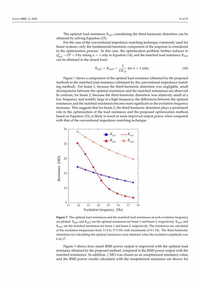
Figure 7 shows a comparison of the optimal load resistance (obtained by the proposedmethod) to the matched load resistance (obtained by the conventional impedance match-ing method). For beam 1, because the third-harmonic distortion was negligible, smalldiscrepancies between the optimal resistances and the matched resistances are observed.In contrast, for beam 2, because the third-harmonic distortion was relatively small at alow frequency and notably large at a high frequency, the differences between the optimalresistances and the matched resistances become more significant as the excitation frequencyincreases. This suggests that for beam 2, the third-harmonic distortion plays a prominentrole in the optimization of the load resistance and the proposed optimization method,based on Equation (15), is likely to result in more improved output power when comparedwith that of the conventional impedance matching technique.

Sensors 2021, 21, x FOR PEER REVIEW 11 of 15

Figure 7 shows a comparison of the optimal load resistance (obtained by the proposed method) to the matched load resistance (obtained by the conventional impedance matching method). For beam 1, because the third-harmonic distortion was negligible, small discrepancies between the optimal resistances and the matched resistances are observed. In contrast, for beam 2, because the third-harmonic distortion was relatively small at a low frequency and notably large at a high frequency, the differences between the optimal resistances and the matched resistances become more significant as the excitation frequency increases. This suggests that for beam 2, the third-harmonic distortion plays a prominent role in the optimization of the load resistance and the proposed optimization method, based on Equation (15), is likely to result in more improved output power when compared with that of the conventional impedance matching technique.

Figure 7. The optimal load resistances and the matched load resistances at each excitation frequency are plotted. Ropt1 and Ropt2 are the optimal resistances for beam 1 and beam 2, respectively. Rmat1 and Rmat2 are the matched resistances for beam 1 and beam 2, respectively. The resistances are calculated at the excitation frequencies from 11.9 to 17.5 Hz with increments of 0.1 Hz. The third-harmonic distortions for calculating the optimal resistances were obtained when the excitation amplitude was 6 m/s2.

Figure 8 shows how much RMS power output is improved with the optimal load resistance obtained by the proposed method, compared to the RMS power output with the matched resistances. In addition, 1 MΩ was chosen as an unoptimized resistance value, and the RMS power results calculated with the unoptimized resistance are shown for comparisons. In Figure 8, rms

optP , rmsmatP , and rms

unoptP denote the RMS power outputs

evaluated with the optimal, matched, and unoptimized resistances, respectively. The subscripts 1 and 2 indicate the results for beam 1 and beam 2, respectively. The RMS power output produced by beam 1 is shown in Figure 8a. For beam 1, the RMS power graphs with the optimized and matched resistances overlap because as shown in Figure 7, those resistances had ineffective differences. At the highest excitation frequency, 17.5 Hz, both the RMS power results with the optimized and matched resistances are improved by 5.93 times when compared to the RMS power with the unoptimized resistance. On the other hand, for beam 2, the RMS power output is more improved with the optimal resistances than with the matched resistances, as shown in Figure

Figure 7. The optimal load resistances and the matched load resistances at each excitation frequencyare plotted. Ropt1 and Ropt2 are the optimal resistances for beam 1 and beam 2, respectively. Rmat1 andRmat2 are the matched resistances for beam 1 and beam 2, respectively. The resistances are calculatedat the excitation frequencies from 11.9 to 17.5 Hz with increments of 0.1 Hz. The third-harmonicdistortions for calculating the optimal resistances were obtained when the excitation amplitude was6 m/s2.

Figure 8 shows how much RMS power output is improved with the optimal loadresistance obtained by the proposed method, compared to the RMS power output with thematched resistances. In addition, 1 MΩ was chosen as an unoptimized resistance value,and the RMS power results calculated with the unoptimized resistance are shown for

Sensors 2021, 21, 2668 11 of 15

comparisons. In Figure 8, Prmsopt , Prms

mat , and Prmsunopt denote the RMS power outputs evaluated

with the optimal, matched, and unoptimized resistances, respectively. The subscripts 1and 2 indicate the results for beam 1 and beam 2, respectively. The RMS power outputproduced by beam 1 is shown in Figure 8a. For beam 1, the RMS power graphs with theoptimized and matched resistances overlap because as shown in Figure 7, those resistanceshad ineffective differences. At the highest excitation frequency, 17.5 Hz, both the RMSpower results with the optimized and matched resistances are improved by 5.93 timeswhen compared to the RMS power with the unoptimized resistance. On the other hand,for beam 2, the RMS power output is more improved with the optimal resistances thanwith the matched resistances, as shown in Figure 8b. This is more obvious as the excitationfrequency increases owing to the differences between the optimal and matched resistancesin Figure 7. Particularly, at the excitation frequency of 17.5 Hz, the RMS power outputwith the optimal resistances is enhanced by 3.40 times relative to the RMS power outputwith the unoptimized resistances, whereas the matched resistances achieve a 2.13 timesenhancement. The total RMS power output produced by both of the two piezoelectricbeams are shown in Figure 8c. Because for beam 1 the optimized and matched resistancesshowed no difference in the RMS power outputs, the difference between the total poweroutput with the optimized resistances and the total power output with the matchedresistances originates mainly from beam 2. Resultantly, at the excitation frequency of17.5 Hz, the total RMS power outputs with the optimized and matched resistances areimproved by 4.06 times and 3.13 times, respectively, relative to the total RMS power withthe unoptimized resistance.

Sensors 2021, 21, x FOR PEER REVIEW 12 of 15

8b. This is more obvious as the excitation frequency increases owing to the differences between the optimal and matched resistances in Figure 7. Particularly, at the excitation frequency of 17.5 Hz, the RMS power output with the optimal resistances is enhanced by 3.40 times relative to the RMS power output with the unoptimized resistances, whereas the matched resistances achieve a 2.13 times enhancement. The total RMS power output produced by both of the two piezoelectric beams are shown in Figure 8c. Because for beam 1 the optimized and matched resistances showed no difference in the RMS power outputs, the difference between the total power output with the optimized resistances and the total power output with the matched resistances originates mainly from beam 2. Resultantly, at the excitation frequency of 17.5 Hz, the total RMS power outputs with the optimized and matched resistances are improved by 4.06 times and 3.13 times, respectively, relative to the total RMS power with the unoptimized resistance.

Figure 8. Root mean square (RMS) power output results of (a) beam 1 and (b) beam 2, and (c) total RMS output power results of the two beams. The red lines with the stars are the results obtained with the optimal load resistances considering the third-harmonic distortion. The blue dotted lines are the results obtained by applying the impedance matching technique considering the fundamental component only. The green lines with the circles are the RMS power output evaluated with the resistance of 1 MΩ without load resistance optimization. The excitation frequencies are increased from 11.9 Hz to 17.5 Hz with increments of 0.1 Hz, and the base acceleration was set to be 6 m/s2.

4.4. Improvements in Broadband Performance Enhancing broadband performance is of importance when designing VEHs [32].

Herein, for quantitative comparisons of broadband performance, average RMS power, denoted by iE , is introduced. The average RMS power is evaluated by dividing the area under the RMS power curve by the excitation frequency range in which interwell motion occurs. The average RMS power obtained when the resistances are optimized at 17.5 Hz is denoted by

optE . Likewise, m atE represents the average RMS power obtained when the

resistances are matched at 17.5 Hz. In addition, for comparison, unoptE denotes the average

RMS power obtained with the unoptimized resistances of 1 MΩ. The area under an RMS power curve is numerically integrated by utilizing Simpson’s 1/3 rule. To investigate the broadband performance of the 2-DOF MCBEH with respect to changes of load resistances, the values of the average RMS power were evaluated with variations in the load resistances of both the beams from 1 to 35 MΩ with increments of 0.5 MΩ.

Figure 9 depicts the simulation results for the broadband performance estimated by the average RMS power. First of all, it is noted that the average RMS power of beam 1 is practically independent of the variations of the resistance connected to beam 2, and vice versa. In this regard, for simplification, Figure 9a plots the average RMS power of beam 1 when the load resistance of beam 2 is set arbitrarily to be 8 MΩ. Likewise, the load

Figure 8. Root mean square (RMS) power output results of (a) beam 1 and (b) beam 2, and (c) total RMS output powerresults of the two beams. The red lines with the stars are the results obtained with the optimal load resistances consideringthe third-harmonic distortion. The blue dotted lines are the results obtained by applying the impedance matching techniqueconsidering the fundamental component only. The green lines with the circles are the RMS power output evaluated with theresistance of 1 MΩ without load resistance optimization. The excitation frequencies are increased from 11.9 Hz to 17.5 Hzwith increments of 0.1 Hz, and the base acceleration was set to be 6 m/s2.

4.4. Improvements in Broadband Performance

Enhancing broadband performance is of importance when designing VEHs [32].Herein, for quantitative comparisons of broadband performance, average RMS power,denoted by Ei, is introduced. The average RMS power is evaluated by dividing the areaunder the RMS power curve by the excitation frequency range in which interwell motionoccurs. The average RMS power obtained when the resistances are optimized at 17.5 Hzis denoted by Eopt. Likewise, Emat represents the average RMS power obtained when theresistances are matched at 17.5 Hz. In addition, for comparison, Eunopt denotes the average

Sensors 2021, 21, 2668 12 of 15

RMS power obtained with the unoptimized resistances of 1 MΩ. The area under an RMSpower curve is numerically integrated by utilizing Simpson’s 1/3 rule. To investigate thebroadband performance of the 2-DOF MCBEH with respect to changes of load resistances,the values of the average RMS power were evaluated with variations in the load resistancesof both the beams from 1 to 35 MΩ with increments of 0.5 MΩ.

Figure 9 depicts the simulation results for the broadband performance estimated bythe average RMS power. First of all, it is noted that the average RMS power of beam 1is practically independent of the variations of the resistance connected to beam 2, andvice versa. In this regard, for simplification, Figure 9a plots the average RMS power ofbeam 1 when the load resistance of beam 2 is set arbitrarily to be 8 MΩ. Likewise, the loadresistance for beam 1 is chosen arbitrarily as 13.5 MΩ in Figure 9b. For the purpose of thefollowing comparisons, the maximum average RMS power is numerically obtained anddenoted by Emax in Figure 9. As shown in Figure 9a, when the load resistance of beam 1 is13.5 MΩ, the average RMS power of beam 1 becomes maximized (6.62 times larger thanthe unoptimized case with the load resistances of 1 MΩ). In addition, it is observed thatthe average RMS power outputs evaluated with the optimized and matched resistancesare almost the same as shown in the inset of Figure 9a. Both the results are in an excellentagreement with the maximum average RMS result. The optimized average RMS power isimproved by 6.56 times relative to the unoptimized case.

Sensors 2021, 21, x FOR PEER REVIEW 13 of 15

resistance for beam 1 is chosen arbitrarily as 13.5 MΩ in Figure 9b. For the purpose of the following comparisons, the maximum average RMS power is numerically obtained and denoted by m axE in Figure 9. As shown in Figure 9a, when the load resistance of beam 1 is 13.5 MΩ, the average RMS power of beam 1 becomes maximized (6.62 times larger than the unoptimized case with the load resistances of 1 MΩ). In addition, it is observed that the average RMS power outputs evaluated with the optimized and matched resistances are almost the same as shown in the inset of Figure 9a. Both the results are in an excellent agreement with the maximum average RMS result. The optimized average RMS power is improved by 6.56 times relative to the unoptimized case.

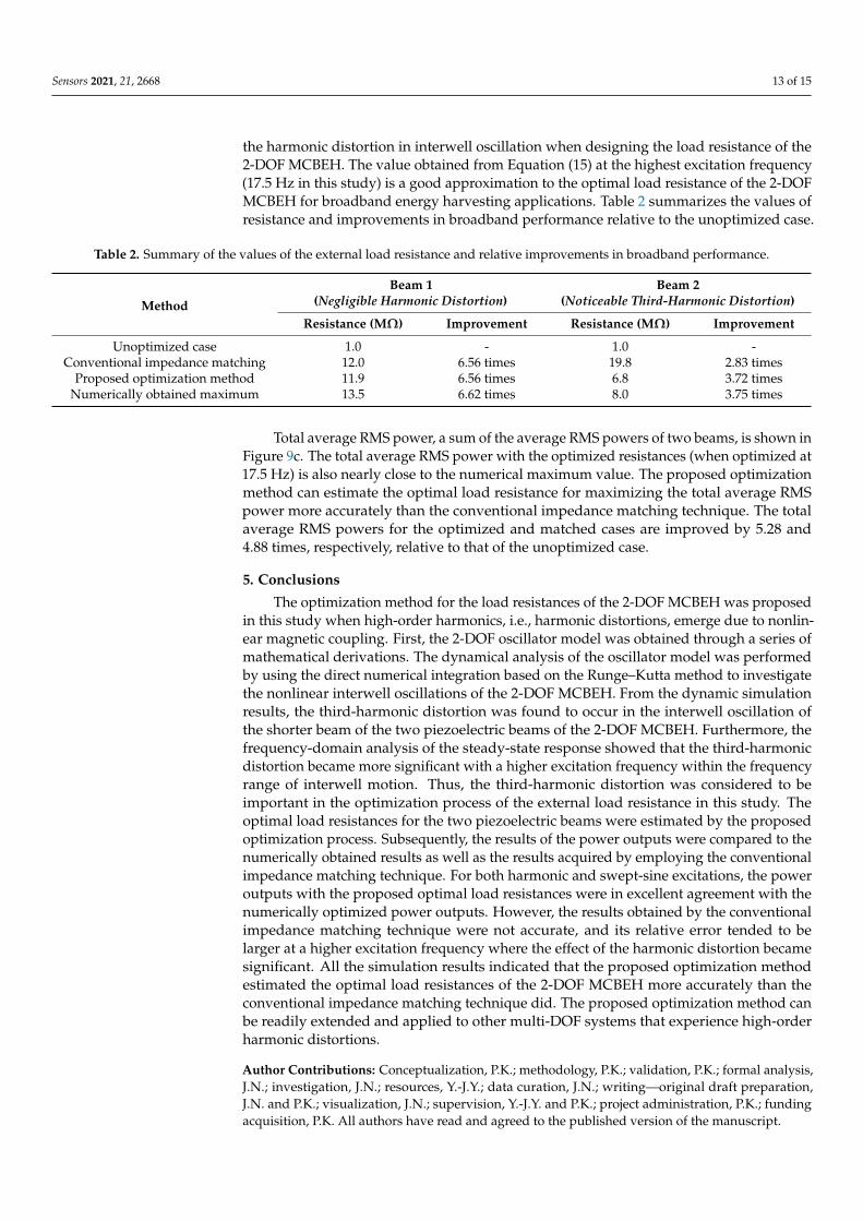
In Figure 9b for beam 2, when the load resistance of beam 2 is 8 MΩ, the average RMS power of beam 2 is maximized (3.75 times larger than the unoptimized case). It is noticeable that the average RMS power estimated with the proposed optimization method is still in excellent agreement with the numerically obtained one; on the other hand, the average RMS power estimated with the conventional impedance matching method shows a poor agreement. The average RMS power outputs with the optimized and matched resistances are improved by 3.72 times and 2.83 times, respectively, when compared to the output with the unoptimized resistances. This indicates that it is very important to consider the harmonic distortion in interwell oscillation when designing the load resistance of the 2-DOF MCBEH. The value obtained from Equation (15) at the highest excitation frequency (17.5 Hz in this study) is a good approximation to the optimal load resistance of the 2-DOF MCBEH for broadband energy harvesting applications. Table 2 summarizes the values of resistance and improvements in broadband performance relative to the unoptimized case.

Total average RMS power, a sum of the average RMS powers of two beams, is shown in Figure 9c. The total average RMS power with the optimized resistances (when optimized at 17.5 Hz) is also nearly close to the numerical maximum value. The proposed optimization method can estimate the optimal load resistance for maximizing the total average RMS power more accurately than the conventional impedance matching technique. The total average RMS powers for the optimized and matched cases are improved by 5.28 and 4.88 times, respectively, relative to that of the unoptimized case.

Figure 9. Average RMS power results for beam 1 and beam 2 are shown in (a,b), respectively, with changing external load resistances. (c) shows the summation of (a,b). Each resistance varies from 1 MΩ to 35 MΩ with increments of 0.5 MΩ for the simulations. The average RMS power of beam 1 is assumed to be independent of the load resistance of beam 2, and vice versa. The load resistance of beam 2 is set to be 8 MΩ for (a), and the load resistance of beam 1 is chosen as 13.5 MΩ for (b). The magenta triangle marker denotes the maximum average RMS power. The red star marker indicates the average RMS power obtained when the resistance is optimized at the excitation frequency of 17.5 Hz; on the other hand, the blue square is obtained with the matched resistances at the same excitation frequency. For comparisons, the average RMS power with the resistances of 1 MΩ is denoted by the green circle marker.

Figure 9. Average RMS power results for beam 1 and beam 2 are shown in (a,b), respectively, with changing external loadresistances. (c) shows the summation of (a,b). Each resistance varies from 1 MΩ to 35 MΩ with increments of 0.5 MΩ forthe simulations. The average RMS power of beam 1 is assumed to be independent of the load resistance of beam 2, and viceversa. The load resistance of beam 2 is set to be 8 MΩ for (a), and the load resistance of beam 1 is chosen as 13.5 MΩ for (b).The magenta triangle marker denotes the maximum average RMS power. The red star marker indicates the average RMSpower obtained when the resistance is optimized at the excitation frequency of 17.5 Hz; on the other hand, the blue squareis obtained with the matched resistances at the same excitation frequency. For comparisons, the average RMS power withthe resistances of 1 MΩ is denoted by the green circle marker.

In Figure 9b for beam 2, when the load resistance of beam 2 is 8 MΩ, the averageRMS power of beam 2 is maximized (3.75 times larger than the unoptimized case). It isnoticeable that the average RMS power estimated with the proposed optimization methodis still in excellent agreement with the numerically obtained one; on the other hand, theaverage RMS power estimated with the conventional impedance matching method showsa poor agreement. The average RMS power outputs with the optimized and matchedresistances are improved by 3.72 times and 2.83 times, respectively, when compared to theoutput with the unoptimized resistances. This indicates that it is very important to consider

Sensors 2021, 21, 2668 13 of 15

the harmonic distortion in interwell oscillation when designing the load resistance of the2-DOF MCBEH. The value obtained from Equation (15) at the highest excitation frequency(17.5 Hz in this study) is a good approximation to the optimal load resistance of the 2-DOFMCBEH for broadband energy harvesting applications. Table 2 summarizes the values ofresistance and improvements in broadband performance relative to the unoptimized case.

Table 2. Summary of the values of the external load resistance and relative improvements in broadband performance.

Method

Beam 1(Negligible Harmonic Distortion)

Beam 2(Noticeable Third-Harmonic Distortion)

Resistance (MΩ) Improvement Resistance (MΩ) Improvement

Unoptimized case 1.0 - 1.0 -Conventional impedance matching 12.0 6.56 times 19.8 2.83 times

Proposed optimization method 11.9 6.56 times 6.8 3.72 timesNumerically obtained maximum 13.5 6.62 times 8.0 3.75 times

Total average RMS power, a sum of the average RMS powers of two beams, is shown inFigure 9c. The total average RMS power with the optimized resistances (when optimized at17.5 Hz) is also nearly close to the numerical maximum value. The proposed optimizationmethod can estimate the optimal load resistance for maximizing the total average RMSpower more accurately than the conventional impedance matching technique. The totalaverage RMS powers for the optimized and matched cases are improved by 5.28 and4.88 times, respectively, relative to that of the unoptimized case.

5. Conclusions

The optimization method for the load resistances of the 2-DOF MCBEH was proposedin this study when high-order harmonics, i.e., harmonic distortions, emerge due to nonlin-ear magnetic coupling. First, the 2-DOF oscillator model was obtained through a series ofmathematical derivations. The dynamical analysis of the oscillator model was performedby using the direct numerical integration based on the Runge–Kutta method to investigatethe nonlinear interwell oscillations of the 2-DOF MCBEH. From the dynamic simulationresults, the third-harmonic distortion was found to occur in the interwell oscillation ofthe shorter beam of the two piezoelectric beams of the 2-DOF MCBEH. Furthermore, thefrequency-domain analysis of the steady-state response showed that the third-harmonicdistortion became more significant with a higher excitation frequency within the frequencyrange of interwell motion. Thus, the third-harmonic distortion was considered to beimportant in the optimization process of the external load resistance in this study. Theoptimal load resistances for the two piezoelectric beams were estimated by the proposedoptimization process. Subsequently, the results of the power outputs were compared to thenumerically obtained results as well as the results acquired by employing the conventionalimpedance matching technique. For both harmonic and swept-sine excitations, the poweroutputs with the proposed optimal load resistances were in excellent agreement with thenumerically optimized power outputs. However, the results obtained by the conventionalimpedance matching technique were not accurate, and its relative error tended to belarger at a higher excitation frequency where the effect of the harmonic distortion becamesignificant. All the simulation results indicated that the proposed optimization methodestimated the optimal load resistances of the 2-DOF MCBEH more accurately than theconventional impedance matching technique did. The proposed optimization method canbe readily extended and applied to other multi-DOF systems that experience high-orderharmonic distortions.

Author Contributions: Conceptualization, P.K.; methodology, P.K.; validation, P.K.; formal analysis,J.N.; investigation, J.N.; resources, Y.-J.Y.; data curation, J.N.; writing—original draft preparation,J.N. and P.K.; visualization, J.N.; supervision, Y.-J.Y. and P.K.; project administration, P.K.; fundingacquisition, P.K. All authors have read and agreed to the published version of the manuscript.

Sensors 2021, 21, 2668 14 of 15

Funding: This work was supported by the National Research Foundation of Korea (NRF) grantfunded by the Korean Government (MSIT) (No. NRF-2019R1C1C1009732). This work was alsosupported by the BK21+ Program of the National Research Foundation of Korea (NRF) grant fundedby the Ministry of Education (MOE).

Conflicts of Interest: The authors declare no conflict of interest.

References1. Chen, X.; Xu, S.; Yao, N.; Shi, Y. 1.6 V Nanogenerator for Mechanical Energy Harvesting Using PZT Nanofibers. Nano Lett. 2010,

10, 2133–2137. [CrossRef]2. Bakytbekov, A.; Nguyen, T.Q.; Huynh, C.; Salama, K.N.; Shamim, A. Fully printed 3D cube-shaped multiband fractal rectenna for

ambient RF energy harvesting. Nano Energy 2018, 53, 587–595. [CrossRef]3. Kishore, R.A.; Priya, S. A review on low-grade thermal energy harvesting: Materials, methods and devices. Materials 2018,

11, 1433. [CrossRef] [PubMed]4. Wang, J.; Geng, L.; Ding, L.; Zhu, H.; Yurchenko, D. The state-of-the-art review on energy harvesting from flow-induced vibrations.

Appl. Energy 2020, 267, 114902. [CrossRef]5. Lechêne, B.P.; Cowell, M.; Pierre, A.; Evans, J.W.; Wright, P.K.; Arias, A.C. Organic solar cells and fully printed super-capacitors

optimized for indoor light energy harvesting. Nano Energy 2016, 26, 631–640. [CrossRef]6. Lv, J.; Jeerapan, I.; Tehrani, F.; Yin, L.; Silva-Lopez, C.A.; Jang, J.-H.; Joshuia, D.; Shah, R.; Liang, Y.; Xie, L. Sweat-based wearable

energy harvesting-storage hybrid textile devices. Energy Environ. Sci. 2018, 11, 3431–3442. [CrossRef]7. Harb, A. Energy harvesting: State-of-the-art. Renew. Energy 2011, 36, 2641–2654. [CrossRef]8. Tan, T.; Yan, Z.; Zou, H.; Ma, K.; Liu, F.; Zhao, L.; Peng, Z.; Zhang, W. Renewable energy harvesting and absorbing via multi-scale

metamaterial systems for Internet of things. Appl. Energy 2019, 254, 113717. [CrossRef]9. Yang, Z.; Zhou, S.; Zu, J.; Inman, D. High-performance piezoelectric energy harvesters and their applications. Joule 2018,

2, 642–697. [CrossRef]10. Vullers, R.J.; Van Schaijk, R.R.; Visser, H.J.; Penders, J.; Van Hoof, C. Energy Harvesting for Autonomous Wireless Sensor

Networks. IEEE Solid-State Circuits Mag. 2010, 2, 29–38. [CrossRef]11. Liu, X.; Zhang, X. Rate and energy efficiency improvements for 5G-based IoT with simultaneous transfer. IEEE Internet Things J.

2018, 6, 5971–5980. [CrossRef]12. Zhang, Y.; Xie, M.; Adamaki, V.; Khanbareh, H.; Bowen, C.R. Control of electro-chemical processes using energy harvesting

materials and devices. Chem. Soc. Rev. 2017, 46, 7757–7786. [CrossRef]13. Núñez, C.G.; Manjakkal, L.; Dahiya, R. Energy autonomous electronic skin. npj Flex. Electron. 2019, 3, 1–24. [CrossRef]14. Jiang, D.; Shi, B.; Ouyang, H.; Fan, Y.; Wang, Z.L.; Li, Z. Emerging Implantable Energy Harvesters and Self-Powered Implantable

Medical Electronics. ACS Nano 2020, 14, 6436–6448. [CrossRef]15. Cook-Chennault, K.A.; Thambi, N.; Sastry, A.M. Powering MEMS portable devices—A review of non-regenerative and regen-

erative power supply systems with special emphasis on piezoelectric energy harvesting systems. Smart Mater. Struct. 2008,17, 043001. [CrossRef]

16. Tran, N.; Ghayesh, M.H.; Arjomandi, M. Ambient vibration energy harvesters: A review on nonlinear techniques for performanceenhancement. Int. J. Eng. Sci. 2018, 127, 162–185. [CrossRef]

17. Daqaq, M.F.; Masana, R.; Erturk, A.; Dane Quinn, D. On the role of nonlinearities in vibratory energy harvesting: A critical reviewand discussion. Appl. Mech. Rev. 2014, 66, 040801. [CrossRef]

18. Szemplinska-Stupnicka, W.; Rudowski, J. Steady states in the twin-well potential oscillator: Computer simulations and approxi-mate analytical studies. Chaos 1993, 3, 375–385. [CrossRef] [PubMed]

19. Fu, H.; Yeatman, E.M. Broadband rotational energy harvesting using bistable mechanism and frequency up-conversion. InProceedings of the 2017 IEEE 30th International Conference on Micro Electro Mechanical Systems (MEMS), Las Vegas, NV, USA,22–26 January 2017; pp. 853–856.

20. Nguyen, M.S.; Yoon, Y.-J.; Kwon, O.; Kim, P. Lowering the potential barrier of a bistable energy harvester with mechanicallyrectified motion of an auxiliary magnet oscillator. Appl. Phys. Lett. 2017, 111, 253905. [CrossRef]

21. Nguyen, M.S.; Yoon, Y.-J.; Kim, P. Enhanced broadband performance of magnetically coupled 2-DOF bistable energy harvesterwith secondary intrawell resonances. Int. J. Precis. Eng. Man. Technol. 2019, 6, 521–530. [CrossRef]

22. Kim, H.; Priya, S.; Stephanou, H.; Uchino, K. Consideration of impedance matching techniques for efficient piezoelectric energyharvesting. IEEE Trans. Ultrason. Ferroelectr. Freq. Control 2007, 54, 1851–1859. [CrossRef]

23. Song, H.-C.; Kumar, P.; Sriramdas, R.; Lee, H.; Sharpes, N.; Kang, M.-G.; Maurya, D.; Sanghadasa, M.; Kang, H.-W.; Ryu, J.Broadband dual phase energy harvester: Vibration and magnetic field. Appl. Energy 2018, 225, 1132–1142. [CrossRef]

24. Liu, W.; Badel, A.; Formosa, F.; Wu, Y.; Agbossou, A. Novel piezoelectric bistable oscillator architecture for wideband vibrationenergy harvesting. Smart Mater. Struct. 2013, 22, 035013. [CrossRef]

25. Liang, J.; Liao, W.-H. Impedance matching for improving piezoelectric energy harvesting systems. Proc. Act. Passiv. Smart Struct.Integr. Syst. 2010, 7643, 76430K.

26. Bae, S.; Kim, P. Load Resistance Optimization of a Broadband Bistable Piezoelectric Energy Harvester for Primary Harmonic andSubharmonic Behaviors. Sustainability 2021, 13, 2865. [CrossRef]

Sensors 2021, 21, 2668 15 of 15

27. Bae, S.; Kim, P. Load Resistance Optimization of Bi-Stable Electromagnetic Energy Harvester Based on Harmonic Balance. Sensors2021, 21, 1505. [CrossRef] [PubMed]

28. Allane, D.; Vera, G.A.; Duroc, Y.; Touhami, R.; Tedjini, S. Harmonic power harvesting system for passive RFID sensor tags. IEEETrans. Microw. Theory Tech. 2016, 64, 2347–2356. [CrossRef]

29. Vera, G.A.; Duroc, Y.; Tedjini, S. Third harmonic exploitation in passive UHF RFID. IEEE Trans. Microw. Theory Tech. 2015,63, 2991–3004. [CrossRef]

30. Erturk, A.; Inman, D.J. Piezoelectric Energy Harvesting; John Wiley & Sons: Chichester, West Sussex, UK, 2011.31. Kim, P.; Nguyen, M.S.; Kwon, O.; Kim, Y.-J.; Yoon, Y.-J. Phase-dependent dynamic potential of magnetically coupled two-degree-

of-freedom bistable energy harvester. Sci. Rep. 2016, 6, 34411. [CrossRef] [PubMed]32. Deng, H.; Du, Y.; Wang, Z.; Ye, J.; Zhang, J.; Ma, M.; Zhong, X. Poly-stable energy harvesting based on synergetic multistable

vibration. Commun. Phys. 2019, 2, 1–10. [CrossRef]