
Leveraged Buyout Bankruptcies, the Problem of Hindsight Bias, and the Credit Default Swap Solution
104
Electronic copy available at: http://ssrn.com/abstract=1632084 Electronic copy available at: http://ssrn.com/abstract=1632084 LEVERAGED BUYOUT BANKRUPTCIES, THE PROBLEM OF HINDSIGHT BIAS, AND THE CREDIT DEFAULT SWAP SOLUTION Michael Simkovic Benjamin S. Kaminetzky∗ I. Introduction and Background ......................................... 121 II. Hundreds of Billions of Dollars are at Stake in the Coming Wave of Fraudulent Transfer Litigation..... 126 III. Recent Judicial Decisions Can Make Fraudulent Transfer Law Fairer and More Efficient Through the Use of Financial Market Prices........................... 132 A. As Fraudulent Transfer Law Developed, It Became a Tool Used by Courts to Limit Risk Taking .................................................................. 135 B. The Badges of Fraud System Was Plagued by Inconsistency and Uncertainty ........................... 137 C. Constructive Fraud Reformed Badges of Fraud by Emphasizing Economics over Intent ............. 139 D. Dependence on Financial Experts Increased Costs and Arbitrariness ...................................... 141 ∗ Michael Simkovic is a professor of law at Seton Hall Law School. Benjamin S. Kaminetzky is a partner at Davis Polk & Wardwell LLP. The authors thank Professors Douglas G. Baird, Jeffrey N. Gordon, Michael A. Helfand, John Hull, Edward Janger, Kristin Johnson, Robert Lawless, Stephen Lubben, Chrystin Ondersma, and Mark Roe for commenting on drafts, and Professor René M. Stulz, Donald S. Bernstein, and Marshall S. Huebner for general discussion. We also thank the many financial professionals who generously agreed to speak with us, including Jaime d’Almeida, Allen Pfeiffer, and Anshul Shekhon at Duff & Phelps; James Brennan, Gareth Moody, and Jasmit Sandhu at Credit Market Associates; Otis Casey at Markit; and Beth Philips and Sonali Theisen at Bloomberg. We thank our research assistants, Karen Benton, Jonathan Brenner, Wolfgang Robinson, Michael J. Berkovits, Ashley M. Bryant, Deryn Darcy, Brad Ehrlichman, Scott Eisman, Natasha Tsiouris, Sabrina L. Ursaner, and Matthew Weinberg for outstanding research support.
Transcript of Leveraged Buyout Bankruptcies, the Problem of Hindsight Bias, and the Credit Default Swap Solution
Electronic copy available at: http://ssrn.com/abstract=1632084Electronic copy available at: http://ssrn.com/abstract=1632084
LEVERAGED BUYOUT BANKRUPTCIES, THE PROBLEM OF HINDSIGHT BIAS, AND THE CREDIT DEFAULT SWAP SOLUTION
Michael Simkovic Benjamin S. Kaminetzky∗
I. Introduction and Background......................................... 121 II. Hundreds of Billions of Dollars are at Stake in the
Coming Wave of Fraudulent Transfer Litigation..... 126 III. Recent Judicial Decisions Can Make Fraudulent
Transfer Law Fairer and More Efficient Through the Use of Financial Market Prices........................... 132 A. As Fraudulent Transfer Law Developed, It
Became a Tool Used by Courts to Limit Risk Taking .................................................................. 135
B. The Badges of Fraud System Was Plagued by Inconsistency and Uncertainty ........................... 137
C. Constructive Fraud Reformed Badges of Fraud by Emphasizing Economics over Intent ............. 139
D. Dependence on Financial Experts Increased Costs and Arbitrariness ...................................... 141
∗ Michael Simkovic is a professor of law at Seton Hall Law School. Benjamin S. Kaminetzky is a partner at Davis Polk & Wardwell LLP. The authors thank Professors Douglas G. Baird, Jeffrey N. Gordon, Michael A. Helfand, John Hull, Edward Janger, Kristin Johnson, Robert Lawless, Stephen Lubben, Chrystin Ondersma, and Mark Roe for commenting on drafts, and Professor René M. Stulz, Donald S. Bernstein, and Marshall S. Huebner for general discussion. We also thank the many financial professionals who generously agreed to speak with us, including Jaime d’Almeida, Allen Pfeiffer, and Anshul Shekhon at Duff & Phelps; James Brennan, Gareth Moody, and Jasmit Sandhu at Credit Market Associates; Otis Casey at Markit; and Beth Philips and Sonali Theisen at Bloomberg. We thank our research assistants, Karen Benton, Jonathan Brenner, Wolfgang Robinson, Michael J. Berkovits, Ashley M. Bryant, Deryn Darcy, Brad Ehrlichman, Scott Eisman, Natasha Tsiouris, Sabrina L. Ursaner, and Matthew Weinberg for outstanding research support.
Electronic copy available at: http://ssrn.com/abstract=1632084Electronic copy available at: http://ssrn.com/abstract=1632084
No. 1:118] LEVERAGED BUYOUT BANKRUPTCIES 119
1. Cash Flow Projections Are Inherently Subjective and Prone to Hindsight Bias ....... 144
2. Discount Rates Can Be Manipulated Because They Depend on Complicated Math Masking Subjective Assumptions........ 147
3. Multiples Methods Can Easily Be Manipulated Unless the Judge Is an Expert on Several Industries ..................................... 148
4. Experts Can Exploit Judges’ Natural Tendency to Avoid Extremes ......................... 149
5. Traditional Methods Assume That Capital Markets Are Efficient..................................... 150
E. Hindsight Bias Gives Plaintiffs an Advantage That the Law Does Not Permit........................... 151 1. Studies Demonstrate That Hindsight Bias
Affects Judges................................................. 153 2. Studies Show That Current Legal
Safeguards Against Hindsight Bias Are Ineffective ....................................................... 156
F. Delaware and New York Courts Have Started to Use Market Prices Instead of Experts ........... 157 1. VFB LLC v. Campbell Soup Co...................... 158 2. In re Iridium Operating LLC ......................... 160
IV. Benefits of Incorporation of Additional Insights from Finance into the Law ................................................. 163 A. Equity Market Prices Provide a Noisy Signal
of Default Probability Because They Reflect Option Value ........................................................ 164
B. Credit Spreads Should Be Used to Measure Credit Market Implied Probabilities of Default. 166 1. Market Implied Probabilities of Default
Facilitate Continuous Solvency Analysis...... 171 2. CDS Markets May Often Provide the Best
Information About Default Risk .................... 174 a. CDS Markets May Be More Efficient
Because They Are a Haven for Insider Trading...................................................... 174
b. CDS Markets Are Probably More “Complete” Than Bond Markets
Electronic copy available at: http://ssrn.com/abstract=1632084Electronic copy available at: http://ssrn.com/abstract=1632084
120 COLUMBIA BUSINESS LAW REVIEW [Vol. 2011
Because Credit Default Swaps Facilitate Shorting.................................... 177
c. CDS Markets May Be More Efficient Because They Are Anonymous and Reduce the Risk of Retaliation for Shorting..................................................... 178
d. Courts Can Reduce the Risk of Market Manipulation ............................................ 180
e. Counterparty Risk Has Been Minimized by Government and Regulatory Policy.... 183
3. High Quality Market Data Can Be Obtained Within the Context of Litigation ... 184 a. Corporate Bond Markets Are Generally
Transparent .............................................. 184 b. Although CDS Markets Are Generally
Not Transparent, Litigation Can Shed New Light on Their Inner Workings ....... 185
4. Simple, Robust, Manipulation-Resistant Equations Can Be Used to Calculate Market-Implied Probabilities of Default Based on Credit Market Prices...................... 188 a. How to Calculate Credit Spreads from
Bond Yields or CDS Fees ......................... 188 b. How to Extract the One-Year Market
Implied Probability of Default from Credit Spreads .......................................... 192
c. Credit Spreads Based on Treasuries May Overestimate Default Risk ...................... 194
d. How to Calculate the Multiyear Cumulative Probability of Default .......... 199
V. Our Original Empirical Analysis Confirms That Credit Default Swaps and Equity Prices Are Usually Inversely Correlated as Debtors Approach Bankruptcy ................................................................. 202 A. Descriptive Statistics............................................ 203 B. Results................................................................... 206
VI. Conclusion: A Shift to Market-Based Measures of Solvency Can Empower Risk Managers at Banks to Block Destabilizing Transactions.......................... 206
No. 1:118] LEVERAGED BUYOUT BANKRUPTCIES 121
VII. Appendix I: Explanation of Traditional Methods of Solvency Analysis....................................................... 208 A. Liquidity Analysis ................................................ 208 B. Discounted Cash Flow (DCF)............................... 209
1. Projections....................................................... 209 2. Discount Rates ................................................ 210 3. Terminal Value ............................................... 210
C. Multiples Analysis: Guideline (Comparable) Companies and Transactions.............................. 211
VIII. Appendix II: Explanation and Evidence for Equity as Option Value.......................................................... 214 A. Opposing Interests of Equity and Debt: A
Simple Mathematical Example........................... 214 B. Opposing Interests of Equity and Debt:
Empirical Evidence.............................................. 216 C. Opposing Interests of Equity and Debt: Real
World Strategic Implications .............................. 217 IX. Appendix III: Derivation and Illustration of
Equation 3 .................................................................. 218
I. INTRODUCTION AND BACKGROUND
In the wake of recent financial crises, credit default swaps (“CDS”) have become the financial instrument that scholars,1
1 Michael Simkovic, Secret Liens and the Financial Crisis of 2008, 83 AM. BANKR. L.J. 253, 253 (2009) (arguing that the preferential treatment of credit default swaps in bankruptcy, combined with a lack of disclosure, contributed to the financial crisis of 2008); Patricia A. McCoy, Andrey D. Pavlov & Susan M. Wachter, Systemic Risk Through Securitization: The Result of Deregulation and Regulatory Failure, 41 CONN. L. REV. 1327, 1343–44 (2009) (arguing that a lack of minimum capital regulation for CDS issuers contributed to the financial crisis); Stephen J. Lubben, The Bankruptcy Code Without Safe Harbors, 84 AM. BANKR. L.J. 123, 123–24 (2010) (arguing for the repeal of the bankruptcy safe harbors for derivatives because they may contribute to systemic risk); Jennifer S. Taub, Enablers of Exuberance: Legal Acts and Omissions that Facilitated the Global Financial Crisis (Sept. 4, 2009) (unpublished manuscript), available at http://ssrn.com/paper=1472190; J. Austin Murphy, An Analysis of the Financial Crisis of 2008: Causes and Solutions (Nov. 4,
122 COLUMBIA BUSINESS LAW REVIEW [Vol. 2011
journalists,2 government officials,3 and even some prominent financiers4 love to hate. However, even some of the CDS market’s harshest critics have acknowledged its power to draw attention to hidden financial risk.5 As credit default swaps mature from cutting edge financial innovations into transparent, standardized, and regulated instruments, they may provide valuable insights to regulators and courts tasked with preventing and managing insolvency. In particular, credit default swaps may help bankruptcy courts solve one of the most challenging problems of fraudulent transfer law: determining whether a corporate debtor who has filed for bankruptcy was solvent at a particular point in the past.
2008) (unpublished manuscript), available at http://ssrn.com/ paper=1295344 (arguing that mispricings in the CDS market amplified risk of mortgage defaults); J. Austin Murphy, The Largest Pyramid Scheme of All Time: The Effect of Allowing Unregulated Credit Default Swaps (Apr. 12, 2010) (unpublished manuscript), available at http://ssrn.com/paper=1588089.
2 Nelson D. Schwartz & Eric Dash, Banks Bet Greece Defaults on Debt They Helped Hide, N.Y. TIMES, Feb. 25, 2010, at A1 (arguing that the CDS markets may be pushing Greece “closer to the brink of financial ruin”).
3 Anupam Chander & Randall Costa, Clearing Credit Default Swaps: A Case Study in Global Legal Convergence, 10 CHI. J. INT’L L. 639, 639 (2010); Schwartz & Dash, supra note 2 (“[W]hile some European leaders have blamed financial speculators in general for worsening the crisis, the French finance minister, Christine Lagarde, last week singled out credit-default swaps. Ms. Lagarde said a few players dominated this arena, which she said needed tighter regulation.”); Emily Barrett, ‘Naked’ Swaps Targeted, WALL ST. J., Jan. 30, 2009, at C4 (“Rep. Collin Peterson . . . released a draft ‘Derivatives Markets Transparency and Accountability Act,’ in which he called for a ban on entering a so-called naked credit-default swap.”).
4 René M. Stulz, Credit Default Swaps and the Credit Crisis, 24 J. ECON. PERSP. 73, 73–74 (2010) (“George Soros, the prominent hedge fund manager . . . want[s] most or all trading in credit default swaps to be banned.”). Professor Stulz suggests that credit default swaps, particularly those of the straight-forward, single-name corporate nature that we discuss in this article, may have been unfairly blamed for problems that originated in the far more complex mortgage derivatives market.
5 See Tony Barber, Markets Over-reacted to Crisis in Eurozone, Says EU President, FIN. TIMES, June 14, 2010, at 3.
No. 1:118] LEVERAGED BUYOUT BANKRUPTCIES 123
Fraudulent transfer law enables bankruptcy courts to void certain pre-petition transfers that depleted a debtor’s estate. The standard of liability for constructive fraudulent transfer is that (1) the transfer was made for less than “reasonably equivalent value,” and (2) the debtor either (i) was insolvent at the time of the transfer or was rendered insolvent by the transfer; (ii) was inadequately capitalized; or (iii) believed it would be unable to pay its debts as they matured.6
Fraudulent transfer law fills an important gap in U.S. regulations of corporations. Although corporate law makes limited liability widely available and inexpensive for businesses,7 it has relatively few mechanisms to prevent excessive and socially destructive risk taking. Although it may seem sensible to enforce minimum capital requirements before granting limited liability, such prospective minimum capital regulation is generally only applied to firms in the
6 11 U.S.C. § 548(a)(1)(B)(ii). For the sake of economy, we sometimes
use the words “insolvent” or “insolvency” in this article to refer to any financial condition that is sufficient to satisfy the requirements for fraudulent transfer liability under the Bankruptcy Code or liability under similar state law fraudulent transfer or fraudulent conveyance statutes. Our meaning may therefore be broader than the definition of “insolvency” under the Bankruptcy Code.
7 Basic incorporation services can be purchased on the internet for less than $200. See, e.g., Incorporate or Organize Your LLC Online or Over the Phone, AMERILAWYER.COM, http://www.amerilawyer.com/index_ny.htm (last visited Mar. 4, 2011) (“Every Corporation or LLC is priced at just $29.95 above the lowest possible state filing fee for the particular state in which you are forming your Company.”). The website lists an all-inclusive price of $118.95 to incorporate a Delaware for-profit corporation. Delaware For Profit Corporation Fact Sheet, AMERI-LAWYER.COM, https://www.amerilawyerorders.com/lawyer/factsheet_forprofit.aspx (last visited Mar. 4, 2011). Tax burdens historically associated with limited liability have also declined because of changes to the tax code and newer structures, such as limited liability companies. See Rebecca J. Huss, Revamping Veil Piercing For All Limited Liability Entities: Forcing the Common Law Doctrine into the Statutory Age, 70 U. CIN. L. REV. 95, 97–98 (2001).
124 COLUMBIA BUSINESS LAW REVIEW [Vol. 2011
financial sector.8 For most other firms, fraudulent transfer law is the closest thing to a minimum capital requirement.
Important counterparties can pressure the debtor corporation to raise capital in order to resume business if they determine that the risk of fraudulent transfer liability is too high. Fraudulent transfer law9 forces parties who deal with financially vulnerable institutions to tread cautiously.10
There has recently been a surge in fraudulent transfer litigation.11 During the credit boom that started in 2003 and peaked in 2007, banks issued a remarkable volume of loans and bonds, and an astounding volume of highly leveraged transactions were financed.12 As these debts become due and financially strapped businesses struggle to refinance, the result will almost certainly be a wave of defaults,
8 Douglas G. Baird, Legal Approaches to Restricting Distributions to
Shareholders: The Role of Fraudulent Transfer Law, 7 EUR. BUS. ORG. L. REV. 201, 205 (2006); see generally Bruce A. Markell, Toward True and Plain Dealing: A Theory of Fraudulent Transfers Involving Unreasonably Small Capital, 21 IND. L. REV. 469, 497–98 (1988).
9 At various points in this article, we use “fraudulent transfer” to mean both “fraudulent transfer” and “fraudulent conveyance” because the standards of liability and the available remedies are similar.
10 HENRY F. OWSLEY & PETER S. KAUFMAN, DISTRESSED INVESTMENT
BANKING: TO THE ABYSS AND BACK 100 (2005) (illustrating the importance for counterparties who deal with financially distressed institutions to be cognizant of fraudulent transfer law’s impacts and noting the risks to counterparties of a highly leveraged business’s potential insolvency); Corinne Ball, Asset Dispositions in Chapter 11: Whether to Sell Through Section 363 or a Plan of Reorganization, in NAVIGATING TODAY’S
ENVIRONMENT: THE DIRECTORS’ AND OFFICERS’ GUIDE TO RESTRUCTURING 251, 251 (John Wm. Butler, Jr. & Nigel Page eds., 2010) (noting that transactions with financially troubled firms should be “closely scrutinized” because of potential fraudulent transfer risk).
11 There have already been several major cases brought and the data suggest that there are far more in store. See, e.g., In re Tribune Co., 418 B.R. 116 (Bankr. D. Del. 2009); In re TOUSA, Inc., Nos. 10-60017-CIV/GOLD, 10-61478, 10-62032, 10-62035, 10-62037, 2011 WL 522008 (S.D. Fla. Feb. 11, 2011); and Complaint of the Official Committee of Unsecured Creditors of Lyondell Chemical Co., In re Lyondell Chemical Co., No. 09-10023 (REG), 2009 WL 2350776 (Bankr. S.D.N.Y. July 22, 2009).
12 See infra Figure 1 and accompanying text.
No. 1:118] LEVERAGED BUYOUT BANKRUPTCIES 125
bankruptcies, and intercreditor disputes—including fraudulent transfer litigation.
The decisions of bankruptcy courts in adjudicating these disputes will cause tens, if not hundreds, of billions of dollars to change hands over the next few years.13 If bankruptcy courts make prudent decisions, they can help shape credit policy at U.S. banks for a generation. Unfortunately, the methods that bankruptcy courts have traditionally used to adjudicate fraudulent transfer claims have at times led to inconsistent, unpredictable, and inadvertently biased outcomes for two reasons. First, courts’ reliance on experts introduces tremendous subjectivity and complexity into the process. Second, well-established features of human psychology—which cannot be overcome, despite the good intentions of bankruptcy judges—taint the decision-making process with legally impermissible hindsight bias.
This article discusses recent legal and financial innovations that may aid bankruptcy courts in assessing fraudulent transfer claims in large business bankruptcies. These innovations have the potential to diminish the importance of experts, increase consistency and predictability in fraudulent transfer law, de-bias and simplify judicial decision-making, and ultimately help stabilize the economy by deterring imprudent business decisions. Part II of this article discusses the dramatic increase in financial leverage throughout the economy during the last decade of prosperity, the recession that began in 2008, and why fraudulent transfer law may determine who will bear billions of dollars in losses. Part III of this article describes the historical and intellectual development of fraudulent transfer law, the expert-centered paradigm that prevailed during the last twenty years, experimental and real-world evidence of the problem of hindsight bias, and two recent decisions that suggest the emergence of a new market-centered paradigm. Part IV of this article explains how this new market-centered paradigm—coupled with
13 More precisely, the decisions will allocate losses in addition to
transferring money.

126 COLUMBIA BUSINESS LAW REVIEW [Vol. 2011
recent innovations in the financial markets and finance theory—can enable fraudulent transfer law to more effectively achieve its historical policy objectives. Part V of this article includes original empirical analysis of the relationship between equity and CDS prices as debtors approach bankruptcy. Part VI explains how judicial adoption of the methods we suggest would improve credit decisions at banks and prevent destabilizing transactions.
Although this article focuses on fraudulent transfer law and CDS markets, its potential applications are much broader. Market-implied probabilities of default can assist courts in deciding any controversy that requires a judicial determination of corporate solvency, whether the controversy pertains to fraudulent transfer, preference, or corporate directors’ duties.14 Market-implied probabilities of default can be calculated from any debt instrument that is traded in a liquid and reasonably informed market and for which a yield to maturity can be calculated, whether the instrument is a credit default swap, a corporate bond, or a bank loan. The applications are diverse and the ramifications are potentially vast.
II. HUNDREDS OF BILLIONS OF DOLLARS ARE AT STAKE IN THE COMING WAVE OF FRAUDULENT
TRANSFER LITIGATION
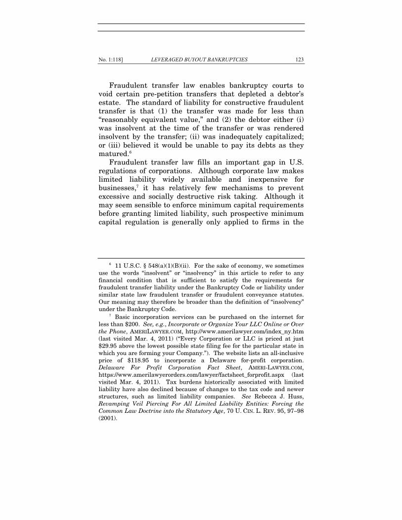
The volume of borrowing during the credit boom that started in 2003 and peaked in 2007 is astounding, as is the plunge in liquidity in 2008 and beyond. Figure 1 shows the
14 Under Delaware corporate law, the directors of an insolvent
corporation owe fiduciary duties to the corporation for the benefit of its creditors, while continuing to owe a duty to maximize the value of the firm as a whole for the benefit of shareholders. N. Am. Catholic Educ. Programming Found., Inc. v. Gheewalla, 930 A.2d 92, 101–03 (Del. 2007); cf. Akande v. Transamerica Airlines, Inc. (In re Transamerica Airlines, Inc.), No. Civ. A. 1039-N, 2006 WL 587846, at *7 (Del. Ch. Feb. 28, 2006) (“When a company becomes insolvent, its directors owe fiduciary duties to the company’s creditors, as well as its stockholders.”). Creditors of an insolvent corporation may therefore bring a derivative suit on behalf of the corporation against its directors. Gheewalla, 930 A.2d at 101–02.

No. 1:118] LEVERAGED BUYOUT BANKRUPTCIES 127
total volume of syndicated bank loans to U.S. borrowers from 1983 to 2009.15 High-yield (or “leveraged”) loans appear on top, while presumably less risky loans appear below.16
Figure 1: U.S. syndicated bank lending peaked in 2007, led by high-yield loans
As can be seen from Figure 1, bank lending grew
dramatically from 2003 to 2007 and then precipitously declined in 2008 and 2009. Much of the lending in the 2003
15 Volume is defined as the total principal amount of all new
syndicated loans issued and reported by Thomson Financial. Principal amount of borrowing includes both the actual proceeds that were received by the borrower and fees that the borrower paid to the banks that arranged and syndicated the loan. Dollars are nominal (not inflation-adjusted).
16 Thomson defines syndicated loans as high-yield by the interest rate rather than by the views of credit rating agencies; higher interest rate loans were presumably viewed as riskier when made. After January 1, 2006, loans were defined as high-yield if the interest rate was 2.5% or more plus a base rate. Before 2006, loans were defined as high-yield if the interest rate was between 1.25% and 1.75% above a base rate. Even though the cutoff for high-yield status was higher in 2006 and 2007 than in previous years, a larger proportion of loans qualified as high-yield.
128 COLUMBIA BUSINESS LAW REVIEW [Vol. 2011
to 2007 boom period was leveraged—higher interest rate loans that were likely considered to involve greater risk than traditional bank lending when made. In 2007, the peak year, more than $4.1 trillion in new loans were made, nearly $2.7 trillion of which were leveraged. From 2004 to 2008, there were a total of over $15.5 trillion in new loans, $8.4 trillion of which were leveraged.
Although many of these loans were for ordinary purposes that are rarely challenged under a theory of fraudulent transfer—for example, refinancing existing debt or financing working capital—some of these loans were at least in part used to finance leveraged transactions. These transactions, including leveraged buyouts (“LBOs”), dividend recapitalizations, and corporate spin-offs, are frequently challenged under fraudulent transfer law. Bank loan volumes and certain deal volumes during the previous four to six years are good leading indicators of potential future fraudulent transfer claims because the statute of limitations on constructive fraudulent transfer claims is typically four to six years.
LBO transactions became popular in the 1980s as a method of facilitating acquisitions.17 They are credited with creating a market for corporate control by funding many potential owners who would not otherwise have access to sufficient capital. By introducing competition for control, the prospect of an LBO can put performance pressure on existing management and benefit investors.18 Changes in a firm’s capital structure and ownership can also potentially increase the value of the firm by improving corporate governance and reducing taxes.19 Most empirical studies suggest that on
17 Steven L. Schwarcz, Rethinking a Corporation’s Obligations to
Creditors, 17 CARDOZO L. REV. 647, 649 (1996). 18 Id. 19 Douglas G. Baird, Fraudulent Conveyances, Agency Costs and
Leveraged Buyouts, 20 J. LEGAL STUD. 1, 5–7 (1991) (providing a general discussion of the potential benefits of LBOs); Michael C. Jensen, Agency Costs of Free Cash Flow, Corporate Finance, and Takeovers, 76 AM. ECON. REV. 323 (1986).
No. 1:118] LEVERAGED BUYOUT BANKRUPTCIES 129
average, LBOs create value for the firm as a whole but also transfer value from creditors to equity holders.20
An LBO resembles a nonrecourse mortgage, in which an acquirer buys an asset by borrowing funds against that asset.21 In a typical LBO transaction, the acquirer creates a merger subsidiary. At the closing, the merger subsidiary borrows funds to purchase the equity of the target from the target’s stockholders, often at a significant premium to market prices. Immediately after closing, the acquisition debt is secured by the target’s assets (and often its equity). After the LBO, the target’s capital structure includes more debt and fewer unencumbered assets.22 This change in capital structure may reduce the recovery of unsecured creditors if the company becomes insolvent.23
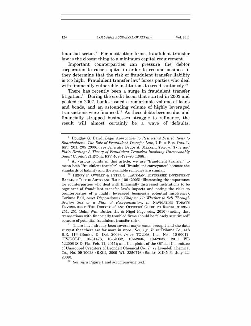
Figure 2 shows the volume of LBOs of U.S. companies from 1981 to 2009. The pattern of LBO activity resembles the pattern for syndicated bank loans, but the run-up that started in 2003 and peaked in 2007, and the subsequent crash in 2008 and 2009, is more pronounced.
20 Shourun Guo, Edith S. Hotchkiss & Weihong Song, Do Buyouts
(Still) Create Value? 1–5 (Aug. 9, 2009), http://ssrn.com/paper=1009281 (forthcoming, J. FIN.); Arthur Warga & Ivo Welch, Bondholder Losses in Leveraged Buyouts, 6 REV. FIN. STUD. 960 (1993) (finding large stockholder gains and small bondholder losses shortly after LBO announcements); Matthew T. Billett, Zhan Jiang & Erik Lie, The Role of Bondholder Wealth Expropriation in LBO Transactions (Mar. 27, 2008), http://ssrn.com/ abstract=1107448.
21 See Barry L. Zaretsky, Fraudulent Transfer Law as the Arbiter of Unreasonable Risk, 46 S.C. L. REV. 1165, 1178–79 (1995).
22 See, e.g., Mellon Bank, N.A. v. Metro Commc’ns, Inc., 945 F.2d 635, 645–46 (3d Cir. 1991).
23 Id.
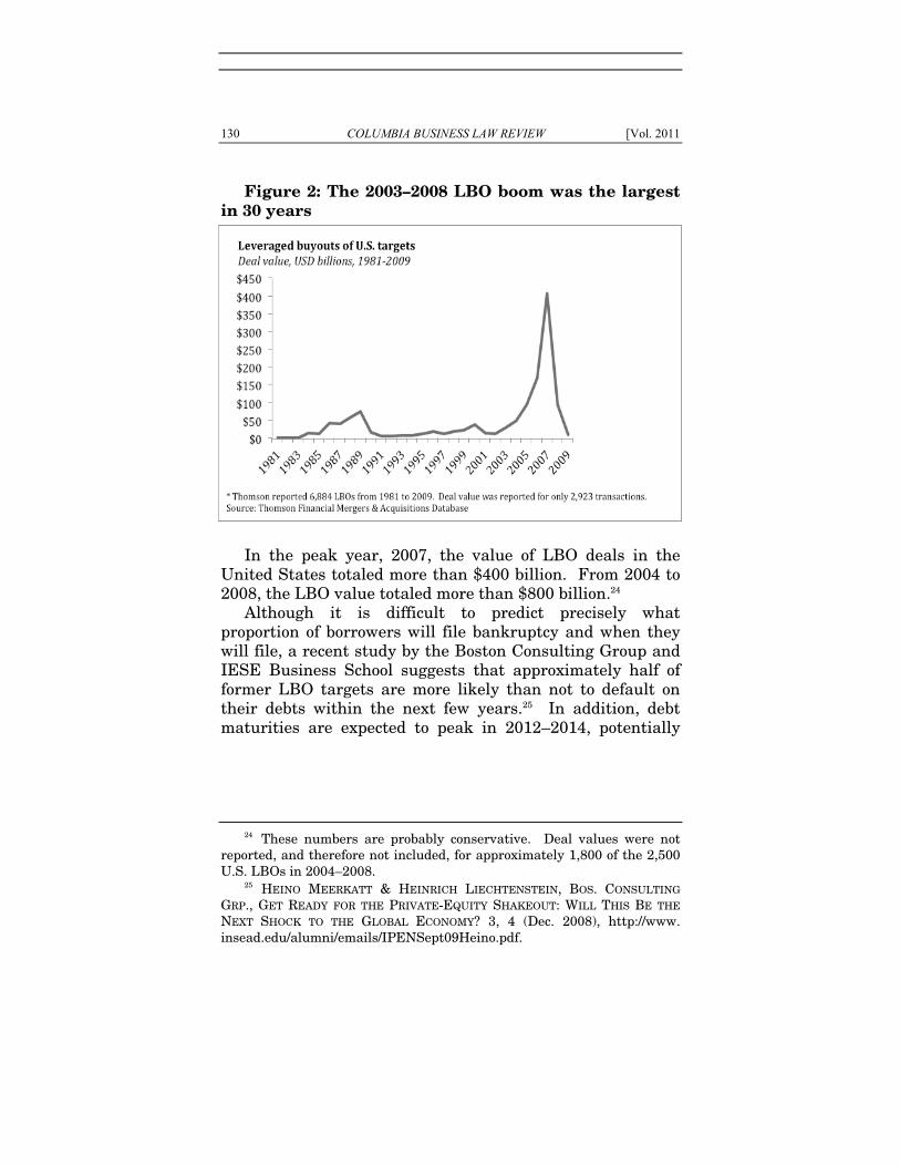
130 COLUMBIA BUSINESS LAW REVIEW [Vol. 2011
Figure 2: The 2003–2008 LBO boom was the largest in 30 years
In the peak year, 2007, the value of LBO deals in the
United States totaled more than $400 billion. From 2004 to 2008, the LBO value totaled more than $800 billion.24
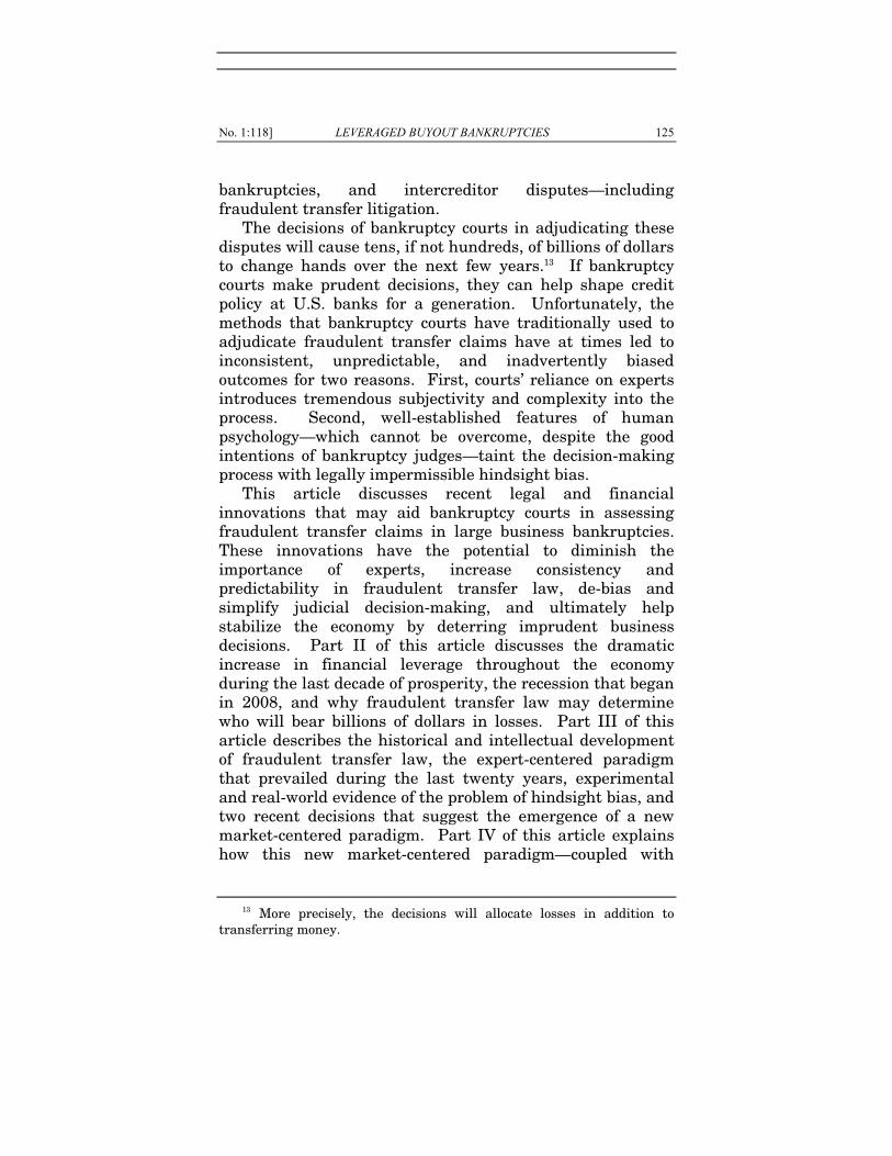
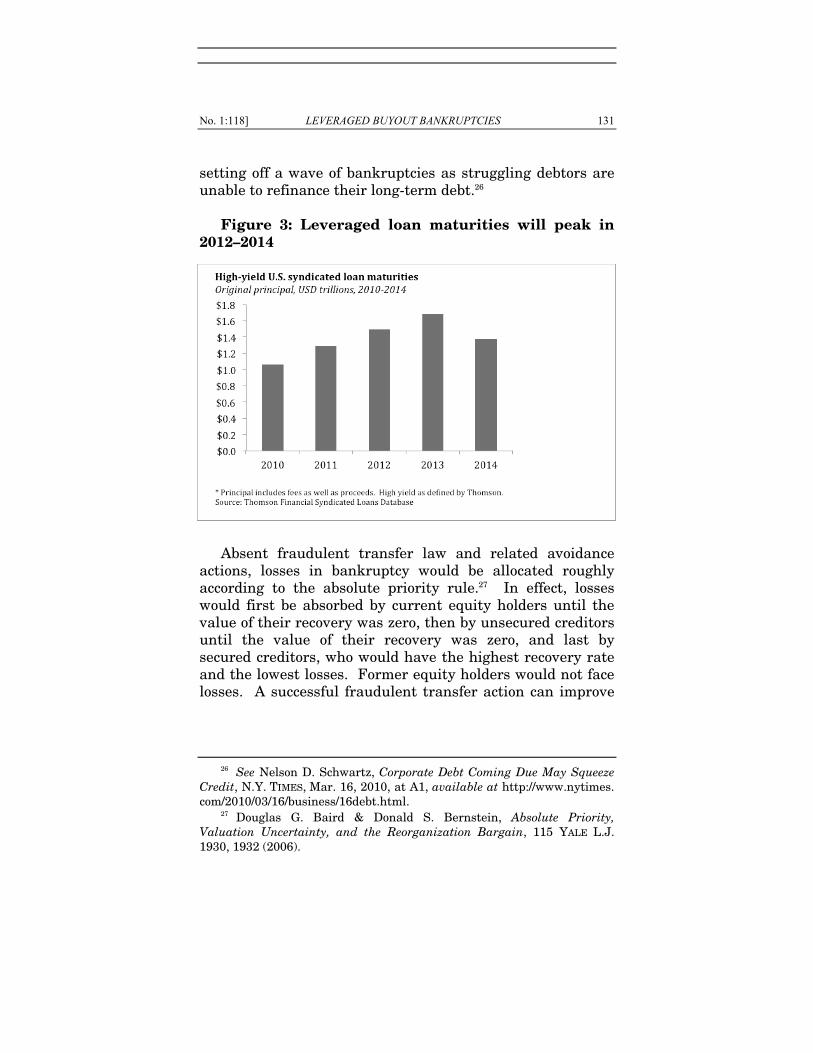
Although it is difficult to predict precisely what proportion of borrowers will file bankruptcy and when they will file, a recent study by the Boston Consulting Group and IESE Business School suggests that approximately half of former LBO targets are more likely than not to default on their debts within the next few years.25 In addition, debt maturities are expected to peak in 2012–2014, potentially
24 These numbers are probably conservative. Deal values were not
reported, and therefore not included, for approximately 1,800 of the 2,500 U.S. LBOs in 2004–2008.
25 HEINO MEERKATT & HEINRICH LIECHTENSTEIN, BOS. CONSULTING
GRP., GET READY FOR THE PRIVATE-EQUITY SHAKEOUT: WILL THIS BE THE
NEXT SHOCK TO THE GLOBAL ECONOMY? 3, 4 (Dec. 2008), http://www. insead.edu/alumni/emails/IPENSept09Heino.pdf.
No. 1:118] LEVERAGED BUYOUT BANKRUPTCIES 131
setting off a wave of bankruptcies as struggling debtors are unable to refinance their long-term debt.26
Figure 3: Leveraged loan maturities will peak in
2012–2014
Absent fraudulent transfer law and related avoidance
actions, losses in bankruptcy would be allocated roughly according to the absolute priority rule.27 In effect, losses would first be absorbed by current equity holders until the value of their recovery was zero, then by unsecured creditors until the value of their recovery was zero, and last by secured creditors, who would have the highest recovery rate and the lowest losses. Former equity holders would not face losses. A successful fraudulent transfer action can improve
26 See Nelson D. Schwartz, Corporate Debt Coming Due May Squeeze
Credit, N.Y. TIMES, Mar. 16, 2010, at A1, available at http://www.nytimes. com/2010/03/16/business/16debt.html.
27 Douglas G. Baird & Donald S. Bernstein, Absolute Priority, Valuation Uncertainty, and the Reorganization Bargain, 115 YALE L.J. 1930, 1932 (2006).
132 COLUMBIA BUSINESS LAW REVIEW [Vol. 2011
the recovery of unsecured creditors by shifting losses to former equity holders and secured creditors.28
During the next three to five years, bankruptcy courts will be entrusted with the power to allocate hundreds of billions of dollars in losses between different classes of creditors. It is crucial that bankruptcy courts wield their power in a way that is predictable, fair, and consistent.
III. RECENT JUDICIAL DECISIONS CAN MAKE FRAUDULENT TRANSFER LAW FAIRER AND
MORE EFFICIENT THROUGH THE USE OF FINANCIAL MARKET PRICES
LBOs and other complex leveraging transactions are routinely challenged under fraudulent transfer law if the debtor files bankruptcy.29 Plaintiffs allege that these transactions imprudently reduce the debtor’s liquidity and capital adequacy, and that the borrowed funds cannot provide reasonably equivalent value because they merely pass through the debtor to former shareholders. According to plaintiffs, the debtor is saddled with obligations while the lender effectively delivers the cash proceeds directly to equity holders.
Early debates about the propriety of the application of constructive fraudulent transfer law to LBOs and similar complex modern transactions30 led to a somewhat peculiar
28 The proceeds of a fraudulent transfer action can only benefit creditors, not equity holders. See Official Comm. of Unsecured Creditors of Cybergenics Corp. v. Chinery (In re Cybergenics Corp.), 226 F.3d 237, 244 (3d Cir. 2000); In re Best Prods. Co., 168 B.R. 35, 57–58 (Bankr. S.D.N.Y. 1994).
29 See, e.g., In re Tribune Co., 418 B.R. 116 (Bankr. D. Del. 2009); In re TOUSA, Inc., Nos. 10-60017-CIV/GOLD, 10-61478, 10-62032, 10-62035, 10-62037, 2011 WL 522008 (S.D. Fla. Feb. 11, 2011); and Complaint of the Official Committee of Unsecured Creditors of Lyondell Chemical Co., In re Lyondell Chemical Co., No. 09-10023 (REG), 2009 WL 2350776 (Bankr. S.D.N.Y. July 22, 2009).
30 Douglas G. Baird & Thomas H. Jackson, Fraudulent Conveyance Law and Its Proper Domain, 38 VAND. L. REV. 829, 852 (1985) (“A firm that incurs obligations in the course of a buyout does not seem at all like the Elizabethan deadbeat who sells his sheep to his brother for a pittance.”);
No. 1:118] LEVERAGED BUYOUT BANKRUPTCIES 133
development of the law. A number of courts have established threshold knowledge or intent requirements31 that excuse some stakeholders,32 thereby effectively blending
see also Bruce A. Markell, supra note 8, at 489–92 (arguing that a broader application of fraudulent transfer law to transactions such as LBOs is consistent with the historic policy objectives of the statute); Zaretsky, supra note 21, at 1181 (same).
31 See Kupetz v. Wolf, 845 F.2d 842, 848 (9th Cir. 1988) (“[W]e hesitate to utilize constructive intent to frustrate the purposes intended to be served by what appears to us to be a legitimate LBO. Nor do we think it appropriate to utilize constructive intent to brand most, if not all, LBOs as illegitimate. We cannot believe that virtually all LBOs are designed to ‘hinder, delay or defraud creditors.’”) (citing Baird & Jackson, supra note 30); see also Credit Managers Ass’n of S. Cal. v. Fed. Co., 629 F. Supp. 175, 181 (C.D. Cal. 1985) (holding that California’s Uniform Fraudulent Conveyance Act “clearly did not intend to cover leveraged buyouts . . . . The legislature was addressing, instead[,] transactions that have the earmarks of fraud.”); In re Ohio Corrugating Co., 91 B.R. 430, 440 (Bankr. N.D. Ohio 1988) (“[T]here appears to be a requirement of a small degree of scienter or awareness of fraud in cases brought under [section] 548(a)(2) for the purpose of avoiding LBOs . . . . [T]he Court believes that the constructive fraud provisions ought to be construed as requiring some degree of scienter . . . .”). Some more recent decisions have continued to require knowledge or intent. See, e.g., In re Plassein Int’l Corp., 388 B.R. 46, 49 (D. Del. 2008), aff’g In re Plassein Int’l Corp., 366 B.R. 318 (Bankr. D. Del. 2007) (stating that courts in the Third Circuit have typically required some proof of bad faith or fraudulent intent to justify collapsing an LBO); In re Sunbeam Corp., 284 B.R. 355, 373 (Bankr. S.D.N.Y. 2002) (refusing to collapse a transaction where the lenders had no knowledge that the debtor was or would be rendered insolvent by the acquisitions).
32 The specific mechanism is that the transaction is only “collapsed”—viewed in substantive economic terms rather than formal terms—with respect to some investors. This was perhaps most dramatically demonstrated in Wieboldt Stores, Inc. v. Schottenstein, 94 B.R. 488 (N.D. Ill. 1988), where the transaction was collapsed with respect to bank lenders and inside shareholders who understood and helped structure the transaction, but not with respect to passive shareholders. Id. at 503–04. Section 546(e) of the Bankruptcy Code has similarly been used to shield shareholders from fraudulent transfer liability, and 2006 amendments may extend this protection more broadly. See Lowenschuss v. Resorts Int’l, Inc. (In re Resorts Int’l, Inc.), 181 F.3d 505, 515–16 (3d Cir. 1999); Quality Stores, Inc. v. Alford (In re QSI Holdings, Inc.), 571 F.3d 545 (6th Cir. 2009), cert. denied, 130 S. Ct. 1141 (2010).
134 COLUMBIA BUSINESS LAW REVIEW [Vol. 2011
constructive and actual fraud standards, while others have limited the remedies available to successful plaintiffs.33
Once the threshold knowledge or intent requirement is met,34 liability generally turns on the financial condition of the debtor at the time of the challenged transaction.35 Although the financial condition determination must be made without the benefit of hindsight,36 the methods
33 Best Products, 168 B.R. at 57 (“[O]ne of the murkiest areas of
fraudulent transfer law as applied to LBOs is what remedy to apply when the plaintiff prevails.”); id. at 57–59 (reasoning that “[t]here is respectable commentary to the effect that LBO lenders should have a claim for all the consideration with which they have parted,” and concluding that LBO lenders whose loans had been voided should retain an unsecured claim against the estate).
34 Not all courts require knowledge or intent. See MFS/Sun Life Trust-High Yield Series v. Van Dusen Airport Servs. Co., 910 F. Supp. 913, 936 (S.D.N.Y. 1995) (explicitly stating that fraudulent intent is not required to collapse a transaction); Liquidation Trust of Hechinger Inv. Co. of Del. v. Fleet Retail Fin. Grp. (In re Hechinger Inv. Co. of Del.), 327 B.R. 537, 546–47, 551 (D. Del. 2005), aff’d, 278 F. App’x 125 (3d Cir. 2008) (collapsing an LBO with respect to lenders, even though the court found that there was no fraudulent intent). These courts move directly to an analysis of reasonably equivalent value and solvency.
35 Although plaintiffs must also prove that the debtor received “less than a reasonably equivalent value” in the challenged transfer, they can generally do so if the court is willing to “collapse” multiple steps of a leveraging transaction. See, e.g., Mellon Bank, N.A. v. Metro Commc’ns, Inc., 945 F.2d 635, 645–46 (3d Cir. 1991). However, where borrowed funds are used to repay previous debts or retained as working capital, or where the transaction creates very substantial synergies, defendants may have a stronger defense independent of the financial condition of the debtor. See Best Products, 168 B.R. at 58; Mellon Bank, 945 F.2d at 635 (finding that synergies could provide reasonably equivalent value); MFS/Sun Life, 910 F. Supp. at 937 (holding that tax savings, new management, and the availability of additional credit may qualify as indirect benefits).
36 Murphy v. Meritor Sav. Bank (In re O’Day Corp.), 126 B.R. 370, 404 (Bankr. D. Mass. 1991) (finding that the court’s task is “not to examine what happened to the company but whether the projections employed prior the LBO were prudent. . . . [A] decision should not be made using hindsight.”) (citing Credit Managers, 629 F. Supp. at 187); see also MFS/Sun Life, 910 F. Supp. at 943–44 (“We know, with hindsight, that the forecasts were not realized. But ‘[t]he question the court must decide is not whether [the] projection was correct, for it clearly was not, but
No. 1:118] LEVERAGED BUYOUT BANKRUPTCIES 135
traditionally used by the courts to evaluate the financial condition of the debtor inevitably introduce legally impermissible hindsight bias. Recent case law and financial market innovations suggest an approach that could reduce hindsight bias and improve judicial decision-making.
This section traces the evolution of fraudulent transfer law into a form of capital adequacy regulation, first through the emergence of constructive fraud, and later through the application of constructive fraud to modern leveraging transactions, primarily LBOs. The section explains how reliance on expert opinions led to subjectivity and arbitrariness, how human psychology gave plaintiffs an unfair and legally impermissible advantage, and how courts have recently turned to financial market data to try to alleviate these problems.
A. As Fraudulent Transfer Law Developed, It Became a Tool Used by Courts to Limit Risk Taking
Fraudulent transfer law originally developed in response to a very specific problem: debtors on the verge of insolvency would sometimes transfer their assets to friends or relatives for nominal consideration, leaving little or no value in their estates to satisfy the claims of other creditors.37 The English legal system responded to this problem by allowing creditors to petition a court to void the transfer as a “fraudulent conveyance” or a “fraudulent transfer.” The standard under which a fraudulent transfer could be voided was first codified in England in 1570, in the Statute of Elizabeth, 13 Eliz., c.5, § 1, which permitted creditors to set aside transfers made
whether it was reasonable and prudent when made.’ . . . ‘Because projections tend to be optimistic, their reasonableness must be tested by an objective standard anchored in the company’s actual performance.’”) (quoting Credit Managers, 629 F. Supp. at 184; Moody v. Sec. Pac. Bus. Credit, 971 F.2d 1056, 1073 (3d Cir. 1992)).
37 See Robert C. Clark, The Duties of the Corporate Debtor to Its Creditors, 90 HARV. L. REV. 505, 544–60 (1977); Baird & Jackson, supra note 30, at 829–30.

136 COLUMBIA BUSINESS LAW REVIEW [Vol. 2011
with intent to delay, hinder, or defraud creditors.38 The principal features of the Statute of Elizabeth are codified in modern U.S. law at both the federal level—in the Bankruptcy Code—and the state level—in state Uniform Fraudulent Conveyance Acts (“UFCA”) and Uniform Fraudulent Transfer Acts (“UFTA”).39 These statutes recapitulate the historic purpose of fraudulent transfer law: avoiding transactions involving actual intent to hinder, delay, or defraud creditors.40
However, in the United States, fraudulent transfer law developed from a remedy for a specific type of intentional fraud into a robust regulatory mechanism through which courts establish capital adequacy standards for numerous financial transactions.41 Expanding upon the common law tradition of “badges of fraud”—observable indicia of intent to defraud articulated by bankruptcy judges42—the Bankruptcy Code, UFTA, and UFCA established an independent cause of action called “constructive fraud” that enables courts to void certain transfers that were not necessarily made with
38 See Eberhard v. Marcu, 530 F.3d 122, 130 (2d Cir. 2008) (quoting
Statute of Elizabeth, 1570, 13 Eliz., c. 5, § 1 (Eng.)); Markell, supra note 8, at 472–73.
39 See 11 U.S.C. § 548 (2006); Unif. Fraudulent Conveyance Act § 4–6, 7A U.L.A. 205 (2007) [hereinafter “UFCA”]; Unif. Fraudulent Transfer Act § 4(a)(2) [hereinafter “UFTA”] (permitting creditors to set aside as fraudulent a conveyance for which the debtor receives less than “reasonably equivalent value”); 11 U.S.C. § 548(a)(1)(A); UFCA § 7, 7A; UFTA § 4(a)(1) (allowing the avoidance of transactions involving actual intent to defraud creditors).
40 See 11 U.S.C. § 548(a)(1)(A) (permitting trustee to avoid any transfer made “with actual intent to hinder, delay or defraud”); UFTA § 4(a)(1) (declaring transfers made or obligations incurred to be fraudulent if made “with actual intent to hinder, delay, or defraud”); UFCA § 7, 7A (“[Conveying] with actual intent . . . to hinder, delay, or defraud either present or future creditors . . . is fraudulent as to both present and future creditors.”).
41 See Baird, supra note 8, at 201–02; Markell, supra note 8, at 469–70; Zaretsky, supra note 21, at 1166.
42 See Baird, supra note 8, at 201; Bruce A. Markell, Following Zaretsky: Fraudulent Transfers and Unfair Risk, 75 AM. BANKR. L.J. 317, 322–23 (2001); Zaretsky, supra note 21, at 1172.
No. 1:118] LEVERAGED BUYOUT BANKRUPTCIES 137
fraudulent intent, but nevertheless depleted the debtor’s estate to the detriment of its creditors.43
B. The Badges of Fraud System Was Plagued by Inconsistency and Uncertainty
Prior to codification through constructive fraud statutes, fraudulent conveyance jurisprudence based on “badges of fraud” suffered from two major defects. The first defect was the considerable uncertainty regarding the precise combination of badges of fraud that constituted fraudulent intent.44 The second defect was the uncertainty concerning the extent to which the owner of a business could legitimately limit his risk of loss in the event that the business failed by shifting risk to creditors. Many badges of fraud related to efforts by an owner to shield his assets from loss.45 In applying these badges of fraud, the courts struggled with drawing a line between permissible business
43 Zaretsky, supra note 21, at 1166. 44 3 COLLIER ON BANKRUPTCY ¶ 548.04[2][b] (Alan N. Resnick & Henry
J. Sommer eds., 15th ed. rev.) [hereinafter COLLIER ON BANKRUPTCY] (citing Brown v. Third Nat’l Bank (In re Sherman), 67 F.3d 1348, 1254 (8th Cir. 1995)); Williamson v. Bender, 147 A. 858 (N.J. Ch. 1929), aff’d, 153 A. 376 (N.J. 1931); Unger v. Mayer, 147 A. 509 (N.J. Ch. 1929), aff’d, 151 A. 907 (N.J. 1930); Vail v. Diamond, 135 A. 791 (N.J. Ch. 1927); Horton v. Bamford, 81 A. 761 (N.J. Ch. 1911)); Markell, supra note 8, at 474–78, 482; Markell, supra note 42, at 324; see also Peter A. Alces & Luther M. Dorr, Jr., A Critical Analysis of the New Uniform Fraudulent Transfer Act, 1985 U. ILL. L. REV. 527, 527 (1985) (noting that there were fundamental differences between states as to the proper effect and conclusiveness of the insolvency badge).
45 See, e.g., Hagerman v. Buchanan, 17 A. 946 (N.J. 1889); Mackay v. Douglas, 14 L.R. Eq. 106; John E. Sullivan III, Future Creditors and Fraudulent Transfers: When a Claimant Doesn’t Have a Claim, When a Transfer Isn’t a Transfer, When Fraud Doesn’t Stay Fraudulent, and Other Important Limits to Fraudulent Transfers Law for the Asset Protection Planner, 22 DEL. J. CORP. L. 1015 (1997); Markell, supra note 8, at 476–78 (noting that badges of fraud included shifting onto creditors the risk of liquidating assets into cash, or depending on “stability of the market” for post-transfer solvency of the business); Markell, supra note 42, at 323.
138 COLUMBIA BUSINESS LAW REVIEW [Vol. 2011
planning and the imposition of unacceptably high risks on creditors.46
For example, in two cases with similar facts, the courts reached opposite results.47 In both Mackay48 and Hagerman,49 a businessman transferred his assets to a trust before entering a partnership that exposed him to personal liability. In both cases, although the transferor had no intent to defraud his creditors,50 the partnership failed, and subsequent creditors sought to avoid the transfer to the trust. The court in Mackay invalidated the transfer while the court in Hagerman upheld it.
Courts seemed to be grappling with a concern that too broad an application of fraudulent transfer law to these transactions would discourage useful business ventures. Business creditors expect debtors to take some risks.51 The question courts applying fraudulent transfer law sought to answer, on behalf of passive creditors, was how much risk should be allowed, and how much was imprudent and dangerous.52 Courts steeped in moralistic concepts of intent in effect took upon themselves the difficult task of establishing minimal capital requirements53—a task that
46 See Markell, supra note 8, at 478; Zaretsky, supra note 21, at 1173–
74. 47 See Markell, supra note 8, at 478–79. 48 Mackay, 14 L.R. Eq. at 109. 49 Hagerman, 17 A. at 946. 50 Id.; Mackay, 14 L.R. Eq. at 120. 51 Baird & Jackson, supra note 30, at 834; see also John C. McCoid II,
Constructively Fraudulent Conveyances: Transfers for Inadequate Consideration, 62 TEX. L. REV. 639, 657 (1983) (“[I]f gambling with another’s money is wrong, then it would be logical to outlaw credit transactions.”).
52 Zaretsky, supra note 21, at 1161, 1174 (arguing that “[b]y addressing unreasonable risks, fraudulent transfer law can be viewed as providing credit transactions and agreements with an off-the-rack term requiring the debtor to limit itself to reasonable business or financial risks”); Markell, supra note 42, at 321.
53 Schreyer v. Platt, 134 U.S. 405, 410 (1890) (stating that it was inappropriate to knowingly “throw the hazards of business in which the [transferor] is about to engage upon others, instead of honestly holding his
No. 1:118] LEVERAGED BUYOUT BANKRUPTCIES 139
challenges even modern day regulators and financial professionals using sophisticated quantitative analysis.
C. Constructive Fraud Reformed Badges of Fraud by Emphasizing Economics over Intent
The drafters of the UFCA attempted to ameliorate some of the uncertainty surrounding the uses of the badges of fraud by introducing the concept of constructive fraud.54 Constructive fraud was later incorporated into the UFTA and Section 548 of the Bankruptcy Code. Instead of attempting to divine the intent of the parties, constructive fraud focuses on the economics of the transaction. Section 548(a)(1)(B) of the Bankruptcy Code states that a debtor-in-possession or creditor can demonstrate constructive fraud when the debtor received “less than a reasonably equivalent value in exchange for such transfer or obligation,” while the debtor was either: (1) insolvent or about to become insolvent; (2) engaged in a business with unreasonably small capital; or (3) incurring debts that the debtor did not believe it could pay.55 Only the third of these three prongs implicates
means subject to the chance of those adverse results to which all business enterprises are liable,” but holding the transfer not voidable because the court could not find actual fraudulent intent and the debtor reasonably believed he would be able to pay his creditors).
54 See Alces & Dorr, supra note 44, at 533 (stating that the drafters were attempting to address (1) the uneven application of the insolvency concept, (2) the inconsistent specification of the proper parties and procedural steps necessary to challenge a conveyance, and (3) the fact that courts extended fraudulent conveyance laws to transactions not involving actual fraudulent intent); Markell, supra note 42, at 324–25.
55 Bankruptcy Code § 548(a)(1)(B). Similarly, section 4(a)(2) of the UFTA provides for constructive fraud if the debtor made the transfer or incurred the obligation without receiving reasonably equivalent value in exchange for the transfer or obligation, and the debtor: (1) was engaged or was about to engage in a business or a transaction for which the remaining assets of the debtor were unreasonably small in relation to the business; or (2) intended to incur, believed that he would incur, or reasonably should have believed that he would incur debts beyond his ability to pay as they became due. UFTA § 4(a)(2). Sections 4–6 of the UFCA state that a conveyance made or an obligation incurred may be voidable if it is made without fair consideration and: (1) by a person who is
140 COLUMBIA BUSINESS LAW REVIEW [Vol. 2011
knowledge or intent, and the knowledge or intent regards the financial condition of the debtor.56
Although constructive fraud represents a marked improvement over the badges of fraud system, constructive fraud only partially succeeds in reducing uncertainty and inconsistency. Constructive fraud statutes leave it to bankruptcy courts to develop methodologies for measuring “solvency” and “capital” and to determine what is “adequate.”
The methodologies that bankruptcy courts developed drew on the methods of solvency analysis and valuation that were used by financial professionals.57 These methods can roughly be divided into two categories: those used to measure cash-flow solvency (liquidity) and those used to measure balance sheet solvency (value).58
thereby rendered insolvent without regard to his actual intent; (2) when the person making it is engaged or is about to engage in a business or transaction for which the property remaining in his hands after the conveyance is an unreasonably small capital, without regard to actual intent; and (3) when the person making the conveyance or entering into the obligation intends to incur or believes that he will incur debts beyond his ability to pay as they mature. UFCA § 4–6, 7A.
56 See In re Taubman, 160 B.R. 964, 986–87 (Bank. S.D. Ohio 1993) (inferring intent to incur debts beyond ability to repay based in part on debtor’s insolvency).
57 Stan Bernstein, Susan H. Seabury & Jack F. Williams, Squaring Bankruptcy Valuation Practice with Daubert Demands, 16 AM. BANKR. INST. L. REV. 161, 175 n.56 (2008) (noting that the many courts have adopted the standards prescribed by the Association of Insolvency and Restructuring Advisors).
58 See Moody v. Sec. Pac. Bus. Credit, 971 F.2d 1056, 1066 (3d Cir. 1992) (holding that “insolvency has two components under [the Pennsylvania UFCA]: a deficit net worth immediately after the conveyance [and] an inability to pay debts as they mature” and noting that solvency in both senses is required); Murphy v. Meritor Sav. Bank (In re O’Day Corp.), 126 B.R. 370, 397–403 (Bankr. D. Mass. 1991) (noting that courts have used either or both tests, while itself using both tests to find that the debtor was insolvent at the time of the LBO). This article focuses on the value of the debtor as a going concern, which is usually at issue in large Chapter 11 cases. Courts will occasionally consider the liquidation value of the debtor, particularly in Chapter 7 cases. Liquidation value depends on an appraisal of the salable assets of the debtor. See Bernstein, Seabury & Williams, supra note 57, at 197.

No. 1:118] LEVERAGED BUYOUT BANKRUPTCIES 141
Unfortunately, however, there were several different methods by which financial professionals measured liquidity and valued companies,59 and new questions emerged about the relative weight that should be assigned to each of these methodologies. In effect, uncertainty regarding the weighting and combination of badges of fraud that collectively suggested fraudulent intent was replaced with uncertainty regarding the weighting and combination of financial measurements that collectively suggested insolvency or inadequate capitalization.60
D. Dependence on Financial Experts Increased Costs and Arbitrariness
In addition, the methods of financial analysis themselves, though quantitative, largely depend on subjective judgments.61 Although investors can legitimately disagree
59 See Bernstein, Seabury & Williams, supra note 57, at 172–74. 60 Compare Lippe v. Bairnco Corp., 288 B.R. 678, 689–90, 710
(S.D.N.Y. 2003) (finding that DCF is a significant component of the industry standard for valuation and rejecting expert testimony that included guideline company analysis but not DCF analysis), CNB Int’l, Inc. v. Kelleher (In re CNB Int’l, Inc.), 393 B.R. 306, 323 (Bankr. W.D.N.Y. 2008) (noting that courts should “rely primarily on the discounted cash flow method”), and In re Med Diversified, Inc., 346 B.R. 621 (Bankr. E.D.N.Y. 2006) (rejecting expert testimony that did not include DCF analysis), with In re Morris Commc’ns NC, Inc., 914 F.2d 458, 469 (4th Cir. 1990) (“It has been often declared by the courts that the method of ‘comparable sales’ in the relevant time frame is more appropriate than any other method in determining market value of the property taken.”) (internal quotations omitted), Peltz v. Hatten (In re USN Commc’ns, Inc.), 279 B.R. 710, 737–38 (D. Del. 2002) (finding that DCF was far less reliable than the similar transaction method of valuation because DCF depended on too many subjective adjustments), and VFB v. Campbell Soup Co., 482 F.3d 624, 633 (3d Cir. 2007) (rejecting DCF and finding that “[t]o the extent that the experts purport to measure actual post-[transaction] performance, as by, for example, discounted cash flow analysis, they are measuring the wrong thing. To the extent they purport to reconstruct a reasonable valuation of the company in light of uncertain future performance, they are using inapt tools.”).
61 TIM KOLLER, MARK GOEDHART & DAVID WESSELS, VALUATION
MEASURING AND MANAGING THE VALUE OF COMPANIES 355 (4th ed. 2005);
142 COLUMBIA BUSINESS LAW REVIEW [Vol. 2011
with each other about questions of value,62 in the context of high stakes litigation, experts who are motivated to serve the interest of the parties who pay their fees63 often come to starkly different and blatantly self-serving conclusions.64
Iridium Capital Corp. v. Motorola, Inc. (In re Iridium Operating LLC), 373 B.R. 283, 347–48 (Bankr. S.D.N.Y. 2007); Peltz, 279 B.R. at 737–38 (discussing subjectivity of DCF analysis); Global GT LP v. Golden Telecom, Inc., 993 A.2d 497, 497 (Del. Ch. 2010) (“[T]he outcome of [an] appraisal proceeding largely depends on [the court’s] acceptance, rejection, or modification of the views of the parties’ valuation experts.”); JPMorgan Chase Bank, N.A. v. Charter Commc’ns Operating, LLC (In re Charter Commc’ns), 419 B.R. 221, 236 (Bankr. S.D.N.Y. 2009) (“[V]aluation is a malleable concept, tough to measure and tougher to pin down without a host of explanations, sensitivities and qualifiers. Because point of view is an important part of the process, outcomes are also highly dependent on the perspectives and biases of those doing the measuring. When it comes to valuation, there is no revealed, objectively verifiable truth. Values can and do vary, and consistency among valuation experts is rare, especially in the context of high stakes litigation.”). Bernstein, Seabury & Williams, supra note 57, at 171.
62 Basic v. Levinson, 485 U.S. 224, 246 (1988) (“The idea of a free and open public market is built upon the theory that competing judgments of buyers and sellers as to the fair price of a security brings . . . about a situation where the market price reflects as nearly as possible a just price.”) (quoting H.R. Rep. No. 73-1383, at 11 (1934)).
63 As financial experts have become more influential, they have also become increasingly expensive. See Lynn M. LoPucki & Joseph W. Doherty, Rise of the Financial Advisors: An Empirical Study of the Division of Professional Fees in Large Bankruptcies, 82 AM. BANKR. L.J. 141, 142 (2008) (reporting that from 1998 to 2003, fees of financial advisers grew at the rate of about 25% per year, whereas professional fees and expenses as a whole grew only about 9% per year). As the number of financial advisers working on a case increases, so do their fees. Id. at 162–63.
64 In re Iridium Operating, 373 B.R. at 291, 293; Fidelity Bond & Mortg. Co. v. Brand (In re Fidelity Mortgage and Bond Corp.), 340 B.R. 266, 289 (Bankr. E.D. Pa. 2006), aff’d, 371 B.R. 708 (E.D. Pa. 2007) (finding that “both [parties’] experts made various adjustments to the balance sheet line items to arrive at their starkly different conclusions regarding . . . solvency . . . .”); In re Charter Commc’ns, 419 B.R. at 236 n.11; In re Nellson Nutraceutical, Inc., 356 B.R. 364, 367 (Bankr. D. Del. 2006) (where expert’s metric of value for determining the terminal value utilized a methodology not generally accepted by experts in the field of valuation and was, in fact, invented by the expert for use in the case).
No. 1:118] LEVERAGED BUYOUT BANKRUPTCIES 143
The “hired gun” approach of many experts, and the difficulty courts face evaluating their testimony, have produced substantial injustice for litigants and embarrassment for courts.65 In In re Exide Technologies, dueling experts for the debtor and the creditors’ committee both used the three standard valuation methodologies—comparable company analysis, comparable transaction analysis, and discounted cash flow—yet arrived at very different results.66 The Court sided with the creditors’ committee expert,67 but almost immediately after the debtor exited bankruptcy, the market showed that the Court was dead wrong.68 Exide exemplifies why judges should not be placed in a situation where experts can mislead them.
The sections that follow highlight ways in which the most commonly used traditional measures of solvency and adequate capital—liquidity, discounted cash flow, comparable company multiples, and comparable transactions multiples—can be manipulated. The discussion also describes inconsistent application of these methods by different courts and assumes reader familiarity with solvency analysis. Readers who are not familiar with these methods of analysis should consult Part VII of this article, Appendix I: Explanation of Traditional Methods of Solvency Analysis.
65 See Harvey R. Miller & Shai Y. Waisman, Is Chapter 11 Bankrupt?,
47 B.C. L. REV. 129, 174 n.259 (2005). 66 In re Exide Techs., 303 B.R. 48, 59 (Bankr. D. Del. 2003). The
expert financial adviser to the debtor submitted a valuation range of $950 million to $1.05 billion, while the expert financial adviser to the creditors’ committee submitted a valuation range of $1.478 billion to $1.711 billion. Exide involved valuation for plan confirmation, not for fraudulent transfer.
67 Id. at 66. Judge Carey determined the debtor’s valuation to be in the range of $1.4 billion to $1.6 billion.
68 When Exide emerged from bankruptcy in May 2004, the market set an enterprise value of $1.03 billion. By November 16, 2005, Exide’s enterprise value had declined to $788 million. See Miller & Waisman, supra note 65.
144 COLUMBIA BUSINESS LAW REVIEW [Vol. 2011
1. Cash Flow Projections Are Inherently Subjective and Prone to Hindsight Bias
Projected cash flows are probably the single most important component of solvency analysis because they are relevant to both a dynamic, cash-flow concept of solvency (can the company pay its debts as they become due?) and to a static, balance sheet approach to solvency (is the company currently worth more than it owes?). To wit, projections are used both in liquidity analysis and in discounted cash-flow (“DCF”) analysis.
Projecting future cash flows involves making a subjective judgment about the future based on imperfect and limited information about the past and the present.69 Although projections are generally based on a financial model, even a highly sophisticated financial model cannot by itself tell anyone whether the assumptions on which it depends are reasonable, as that requires subjective judgment.70
DCF is a method of valuation that has three components: (1) projections of future cash flows of the debtor; (2) a discount rate that is used to convert future cash flows into their present value; and (3) a terminal value used to limit the necessary projection period.71 Experts can manipulate
69 KOLLER, GOEDHART & WESSELS, supra note 61, at 159. 70 Prescott Group Small Cap v. Coleman Co., No. 17802, 2004 WL
2059515, at *31 (Del. Ch. Sept. 8, 2004) (“[T]he task of enterprise valuation, even for a finance expert, is fraught with uncertainty. For a layperson, even one who wears judicial robes, it is even more so. No formula exists that can invest with scientific precision a process that is inherently judgmental.”); Cede & Co. v. Technicolor, Inc., No. Civ. A. 7129, 2003 WL 23700218, at *2 (Del. Ch. Dec. 31, 2003) (noting that “valuation decisions are impossible to make with anything approaching complete confidence. Valuing an entity is a difficult intellectual exercise, especially when business and financial experts are able to organize data in support of wildly divergent valuations for the same entity. For a judge who is not an expert in corporate finance, one can do little more than try to detect gross distortions in the experts’ opinions.”).
71 RICHARD A. BREALEY, STEWART C. MYERS & FRANKLIN ALLEN, PRINCIPLES OF CORPORATE FINANCE 65 (8th ed. 2006); Doft & Co. v. Travelocity.com, Inc., No. 19734, 2004 WL 1152338, at *5 (Del. Ch. May 20, 2004).
No. 1:118] LEVERAGED BUYOUT BANKRUPTCIES 145
the outcome of a DCF analysis,72 either by constructing their own post hoc cash-flow projections or by selectively emphasizing certain projections that were created at the time of the allegedly fraudulent transaction.73 Terminal value can similarly be manipulated because it depends on the last year of cash-flow projections and on a perpetual growth rate for the company. Experts can manipulate terminal value by choosing a growth rate that is similar to the historical growth rate of either the company, the industry, or the broader economy (U.S. or global)—whichever leads to the outcome they prefer.
In the fraudulent transfer context, where experts retroactively select cash-flow “projections” for the period between the challenged transaction and the bankruptcy, the credibility of cash-flow projections and growth rates depends on the apparent foreseeability of the business setbacks that derailed the debtor.
Foreseeability is determined on a case-by-case basis, but such an ad hoc approach to justice provides little guidance to counterparties structuring transactions. In many cases, courts have reached seemingly inconsistent determinations about whether a particular type of business setback is foreseeable. Low-cost competition is apparently foreseeable in the automotive industry,74 but not in the mobile
72 See To-Am Equip. Co. v. Mitsubishi Caterpillar Forklift Am., Inc.,
953 F. Supp. 987, 996–997 (N.D. Ill. 1997), aff’d, 152 F.3d 658 (7th Cir. 1998); Iridium Capital Corp. v. Motorola, Inc. (In re Iridium Operating), 373 B.R. 283, 351 (Bankr. S.D.N.Y. 2007).
73 To-Am Equip., 953 F. Supp. at 996 (“[A] skilled practitioner can come up with just about any [projected future cash-flow] value he wants . . . .”); see also Bernstein, Seabury & Williams, supra note 57, at 187–88 (noting that experts may use projections prepared by management or investors, or develop their own projections). Management, lending banks, investors, and Wall Street research analysts will typically all have prepared projections for large companies, often under several different scenarios and at several different points in time. Baird & Bernstein, supra note 27, at 1942–43.
74 See CNB Int’l, Inc. v. Kelleher (In re CNB Int’l, Inc.), 393 B.R. 306, 321 (Bankr. W.D.N.Y. 2008) (finding that competition from low-cost Asian labor was foreseeable).

146 COLUMBIA BUSINESS LAW REVIEW [Vol. 2011
communications industry.75 Loss of revenue is apparently foreseeable if it is due to the loss of a key customer,76 but not if it is due to the loss of a key employee.77 Financial crises are apparently not foreseeable if they are due to defaults by poor formerly communist countries,78 but they are foreseeable if they are due to defaults by poor subprime mortgage borrowers.79 The failure to achieve post-merger synergies may or may not be foreseeable, but the manner in which the judiciary will resolve these matters certainly is not.80
In addition to contending with manipulations by expert witnesses and inconsistent precedent, judges must also contend with innate and universal psychological biases that affect all decision makers. An overwhelming amount of psychological research suggests that a judge will tend to believe that projections that closely match what actually happened are more reasonable than would a decision maker
75 See In re Iridium Operating, 373 B.R. at 298 (noting that
competition from the rapid build out of a rival mobile technology was unexpected).
76 See In re CNB Int’l., 393 B.R. at 321 (finding that subsequent inability to meet sales projections after reliance on a single customer was foreseeable).
77 See MFS/Sun Life Trust-High Yield Series v. Van Dusen Airport Servs. Co., 910 F. Supp. 913, 944 (S.D.N.Y. 1995).
78 See Peltz v. Hatten, 279 B.R. 710, 734–47 (D. Del. 2002) (finding that collapse of the high-yield bond market following the Russian debt default in the late 1990s was not foreseeable).
79 See Official Comm. of Unsecured Creditors of Tousa, Inc. v. Citicorp N. Am., Inc. (In re TOUSA, Inc.), 422 B.R. 783, 813–14 (Bankr. S.D. Fla. 2009) (finding that the sharp decline in the housing market in August 2007 was foreseeable at least several months prior), rev’d on other grounds, In re TOUSA, Inc., Nos. 10-60017-CIV/GOLD, 10-61478, 10-62032, 10-62035, 10-62037, 2011 WL 522008 (S.D. Fla. Feb. 11, 2011).
80 Compare In re CNB Int’l, 393 B.R. at 320–21 (finding that the failure of synergistic benefits to materialize is foreseeable and should be recognized as a risk factor in financial projections), with In re Sunbeam Corp., 284 B.R. 355, 372–73 (Bankr. S.D.N.Y. 2002) (finding that insolvency after acquisitions was not foreseeable when synergistic benefits in financial projections did not materialize).
No. 1:118] LEVERAGED BUYOUT BANKRUPTCIES 147
who did not have the benefit of hindsight.81 In other words, the court will generally tend to believe that more negative projections are more reasonable because the debtor did in fact file for bankruptcy. Instructions to the contrary, and legal prohibitions against hindsight, are an ineffective prophylactic against such hindsight bias.
2. Discount Rates Can Be Manipulated Because They Depend on Complicated Math Masking Subjective Assumptions
Discount rates are important for static balance sheet solvency analysis.82 Experts can manipulate the discount rate by choosing from several methods of calculation.83 In addition, within each method, experts can manipulate assumptions about financial arcana84 such as equity risk premiums85 and systemic risk (beta).86
81 See discussion infra Part III.E. 82 See BREALEY, MYERS & ALLEN, supra note 71, at 16, 37, 222–24;
KOLLER, GOEDHART & WESSELS, supra note 61, at 292–94; Bernstein, Seabury & Williams, supra note 57, at 190 (“Often the key determinant and cause of variance among experts in their valuation opinions is the selection of the appropriate discount rate.”).
83 BREALEY, MYERS & ALLEN, supra note 71, at 66–67, 222–26 (recognizing that judgment calls need to be made in calculating the appropriate discount rate); Bernstein, Seabury & Williams, supra note 57, at 191 n.102.
84 See Del. Open MRI Radiology Assocs. v. Kessler, 898 A.2d 290, 338 (Del. Ch. 2006) (noting that “[t]estimonial feuds about discount rates often have the quality of a debate about the relative merits of competing alchemists” and that “[o]nce the experts’ techniques for coming up with their discount rates are closely analyzed, the court finds itself in an intellectual position more religious than empirical in nature, insofar as the court’s decision to prefer one position over the other is more a matter of faith than reason.”).
85 See BREALEY, MYERS & ALLEN, supra note 71, at 217 (noting that “[m]easuring differences in risk is difficult to do objectively”); KOLLER, GOEDHART & WESSELS, supra note 61, at 297–98 (“Sizing the market risk premium . . . is arguably the most debated issue in finance.”); Bernstein, Seabury & Williams, supra note 57, at 190–93.
86 See BREALEY, MYERS & ALLEN, supra note 71, at 219–21 (discussing the difficulties of measuring beta); KOLLER, GOEDHART & WESSELS, supra
148 COLUMBIA BUSINESS LAW REVIEW [Vol. 2011
All else being equal, more extreme projections should be accompanied by a higher discount rate because more extreme projections are less likely to materialize. In practice, however, plaintiffs’ experts will typically use a high discount rate and low projections, while defense experts will typically use a low discount rate and high projections.87
3. Multiples Methods Can Easily Be Manipulated Unless the Judge Is an Expert on Several Industries
Multiples analysis embraces market value as a reality check on DCF analysis.88 However, rather than using market prices of the debtor, this approach instead uses market prices of similar firms.89
The problem with the multiples approach is that no two companies are ever perfectly comparable.90 Some are more cost-efficient, some have better growth prospects, some have stronger brands, and some enjoy better relationships with the government. They may have a different mix of business lines, or they may operate in different markets.
note 61, at 307–08; Bernstein, Seabury & Williams, supra note 57, at 190–93.
87 See CNB Int’l, Inc. v. Kelleher (In re CNB Int’l, Inc.), 393 B.R. 306, 320 (Bankr. W.D.N.Y. 2008).
88 KOLLER, GOEDHART & WESSELS, supra note 61, at 361 (“A careful multiples analysis . . . [p]roperly executed . . . can help test the plausibility of cash flow forecasts . . . .”).
89 Id. 90 Id. at 366–68, 380; BREALEY, MYERS & ALLEN, supra note 71, at 511;
Bernstein, Seabury & Williams, supra note 57, at 196; Prescott Group Small Cap, L.P. v. Coleman Co., No. 17802, 2004 WL 2059515, at *22 (Del. Ch. Sept. 8, 2004) (“[A] comparable company analysis is only as valid as the ‘comparable’ firms upon which the analysis is based, are truly comparable . . . .”); In re Radiology Assocs., Inc., 611 A.2d 485, 490 (Del. Ch. 1991) (noting that “[t]he utility of the comparable company approach depends on the similarity between the company the court is valuing and the companies used for comparison” and warning that “[a]t some point, the differences become so large that the use of the comparable company method becomes meaningless for valuation purposes”).
No. 1:118] LEVERAGED BUYOUT BANKRUPTCIES 149
The selection of comparable companies is an art, not a science, with considerable room for manipulation by experts.91 Defense experts tend to select guideline companies or transactions that will yield a high multiple, and therefore a high valuation of the debtor, while plaintiffs’ experts tend to select guideline companies or transactions that will yield a low multiple.92 Without extensive knowledge of many companies (and industries, given that large debtors often have multiple business lines), courts cannot easily evaluate which comparables are more appropriate than others.93
4. Experts Can Exploit Judges’ Natural Tendency to Avoid Extremes
Experts often provide a “sensitivity analysis” displayed as a table containing a range of possible assumptions and projections.94 Such an analysis enhances the apparent sophistication of the projections and the credibility of the
91 KOLLER, GOEDHART & WESSELS, supra note 61, at 362–63, 366–67. 92 Peltz, 279 B.R. at 737–38 (“[I]t is clear that experts and industry
analysts often disagree on the appropriate valuation of corporate properties, even when employing the same analytical tools such as . . . a comparable sales method . . . reasonable minds can and often do disagree. This is because the output of financial valuation models are driven by their inputs, many of which are subjective in nature. . . . [T]he comparable sales method involves making subjective judgments as to what transactions are ‘comparable’ to the property being valued.”) (internal citations omitted); see, e.g., Lippe v. Bairnco Corp., 99 F. App’x 274, 279 (2d Cir. 2004); In re Oneida Ltd., 351 B.R. 79, 91 n.18 (Bankr. S.D.N.Y. 2006) (experts introduced different multiples to achieve different values); see also Bernstein, Seabury & Williams, supra note 57, at 198–99.
93 See, e.g., Global GT LP v. Golden Telecom, Inc., 993 A.2d 497, 510 (Del. Ch. 2010) (where the court recognized that “I am also not going to pretend that I am personally qualified or have the time to engage in a from-scratch construction of comparable companies and transactions analyses using such public resources as I could obtain.”).
94 BREALEY, MYERS & ALLEN, supra note 71, at 248 (“Sensitivity analysis boils down to expressing cash flows in terms of key . . . variables and then calculating the consequences of misestimating the variables. . . . One drawback to sensitivity analysis is that it always gives somewhat ambiguous results.”).
150 COLUMBIA BUSINESS LAW REVIEW [Vol. 2011
expert.95 However, because judges, like most decision makers, tend to prefer to avoid extremes, courts will be inclined to believe that the most likely outcome is one that is in the middle.96 By manipulating the endpoints of the range, and thereby moving the middle, the expert can guide the court toward a decision that is favorable to his client.97 Judges may also want to split the difference between experts, which encourages experts to take extreme positions.
5. Traditional Methods Assume That Capital Markets Are Efficient
For all of their subjectivity and complexity, the traditional methods of solvency analysis still depend on the assumption that capital markets are efficient. The discount rate used in DCF analysis is almost always calculated using mathematical methods that require an assumption that capital markets are efficient.98 Multiples methods rely on the capital markets to value comparable firms. If financial markets can be trusted to discount cash flows or value comparable firms, then one wonders why they cannot be trusted to value the debtor, thereby eliminating the need to determine which projections are appropriate or which firms are comparable. As discussed below, a number of recent decisions have suggested that not only can financial markets
95 See, e.g., Lippe, 288 B.R at 686–87, 689–90. 96 Cass R. Sunstein, Social Norms and Social Roles, 96 COLUM. L. REV.
903, 933 (1996) (citing Itamar Simonson & Amos Tversky, Choice in Context: Tradeoff Contrast and Extremeness Aversion, 29 J. MARKETING
RES. 281, 289–92 (1992)); Bernstein, Seabury & Williams, supra note 57, at 198–99.
97 Bernstein, Seabury & Williams, supra note 57, at 198–99. 98 KOLLER, GOEDHART & WESSELS, supra note 61, at 294–318; Del.
Open MRI Radiology Assocs. v. Kessler, 898 A.2d 290, 338 (Del. Ch. 2006) (“[T]here is much dispute about how to calculate the discount rate to use in valuing their future cash flows, even when one tries to stick as closely as possible to the principles undergirding the capital asset pricing model and the semi-strong form of the efficient capital markets hypothesis.”); Bernstein, Seabury & Williams, supra note 57, at 190–92.
No. 1:118] LEVERAGED BUYOUT BANKRUPTCIES 151
frequently be trusted, they are in fact usually more trustworthy than litigation experts.
E. Hindsight Bias Gives Plaintiffs an Advantage That the Law Does Not Permit
In addition to the challenge of evaluating subjective judgments by dueling experts, judges face another serious challenge: innate human psychology. Judges are legally required to evaluate the financial condition of the debtor at the time of the allegedly fraudulent transfer without the use of hindsight.99 “Hindsight bias” is a term used by psychologists and behavioral economists to describe the widely observed human tendency to overestimate, after the fact, the foreseeability of events that have occurred.100 Hindsight bias can lead evaluators who have the benefit of present knowledge to believe that past decision makers were negligent or reckless.101 Empirical research conclusively demonstrates the existence of hindsight bias. As of 2003, hindsight bias was demonstrated in over 150 published
99 See supra note 36. 100 Blank et al., Hindsight Bias: On Being Wise After the Event, 25
SOC. COGNITION 1, 2 (2007); see also Marianne M. Jennings et al., Causality as an Influence on Hindsight Bias: An Empirical Examination of Judges’ Evaluation of Professional Audit Judgment, 21 J. ACCT. & PUB. POL’Y 143, 147 (1998) (“Hindsight bias has been operationalized as the difference between probability assessments of an event estimated with and without knowledge of the event outcome.”) (citation omitted). Hindsight bias operates through a variety of cognitive processes, including “anchoring,” “focusing,” and “availability.” See Ulrich Hoffrage & Rudiger F. Pohl, Research on Hindsight Bias: A Rich Past, A Productive Present, and A Challenging Future, 11 MEMORY 329, 331 (2003) (discussing hindsight bias and anchoring); Daniel Kahneman et al., Would You be Happier if You Were Richer? A Focusing Illusion, 312 SCIENCE 1908, 1908–09 (2006) (describing the “focusing” phenomenon and noting that “[n]othing in life is quite as important as you think it is while you are thinking about it”); Robert P. Agans & Leigh S. Shaffer, The Hindsight Bias: The Role of the Availability Heuristic and Perceived Risk, 15 BASIC &
APPLIED SOC. PSYCHOL. 439 (1994) (discussing hindsight bias and availability).
101 See generally Erin M. Harley, Hindsight Bias in Legal Decision Making, 25 SOC. COGNITION 48 (2007).

152 COLUMBIA BUSINESS LAW REVIEW [Vol. 2011
articles, many of which reported multiple empirical studies.102 Many of these studies specifically focus on determinations of legal liability in contexts analogous to fraudulent transfer litigation.103
In the prototypical study of hindsight bias in the litigation context, evaluators are randomly divided into two groups, a foresight group and a hindsight group. Evaluators from both groups are asked to independently evaluate the prudence of a defendant’s decision.104 However, each group of evaluators has access to different information. Evaluators in the foresight group are presented with all of the information that was available to the defendant at the time of the decision, but do not know the outcome of the decision. Evaluators in the hindsight group are presented with all of the information shown to the foresight group, plus the ultimate outcome. In other words, evaluators in the hindsight group share the role of real world decision makers—such as bankruptcy judges—who attempt to judge without utilizing hindsight, but nevertheless have access to information that may lead them to inadvertently judge with hindsight.
The studies consistently find that evaluators in the hindsight group view the actual outcome as far more likely,
102 Hoffrage & Pohl, supra note 100, at 329. 103 See Jennings et al., supra note 100 (discussing auditor liability for
audit opinion with respect to a company that subsequently went bankrupt); see generally Merrie Jo Stallard & Debra L. Worthington, Reducing the Hindsight Bias Utilizing Attorney Closing Arguments, 22 L. & HUM. BEHAV. 671 (1998) (noting director liability in the case of a failed savings and loan institution); John C. Anderson et al., The Mitigation of Hindsight Bias in Judges’ Evaluation of Auditor Decisions, 16 AUDITING: J. PRAC. & THEORY 20 (1997) (discussing auditor liability with respect to a company that experienced a precipitous drop in profits); D. Jordan Lowe & Philip M.J. Reckers, The Effects of Hindsight Bias on Jurors’ Evaluations of Auditor Decisions, 25 DECISION SCI. 401 (1994) (discussing auditor liability for audit opinion with respect to a company that subsequently went bankrupt).
104 See generally Harley, supra note 101; see also Susan J. LaBine & Gary LaBine, Determinations of Negligence and the Hindsight Bias, 20 L. & HUM. BEHAV. 501 (1996).
No. 1:118] LEVERAGED BUYOUT BANKRUPTCIES 153
and the defendant as far more culpable, than do evaluators in the foresight group.105 Worse yet, the more severe the negative outcome, the stronger the hindsight bias.106 In the fraudulent transfer context, this suggests that the more severe the losses—and therefore the higher the stakes of fraudulent transfer litigation between secured lenders and unsecured creditors—the greater the danger of hindsight bias.
1. Studies Demonstrate That Hindsight Bias Affects Judges
There are strong reasons to believe that the results of these controlled experiments are applicable to legal decision making in the real world. Several studies set in a context resembling the circumstances of bankruptcy judges in fraudulent transfer cases against LBO lenders have found evidence of hindsight bias.
In one study, 193 actual judges were divided into foresight and hindsight groups.107 The judges in each group were not aware of the existence of the other group. The judges were presented with information relevant to a determination under accounting rules of whether or not a merger target should immediately book losses because its inventory could become obsolete.108 The judges also learned that an auditing firm retained by the target recommended that it not book the losses.109 The judges in the hindsight group received additional information: they learned that after the audit opinion, the merger target’s market share declined, the target was forced to book inventory losses, and
105 For a recent review, see Blank et al., supra note 100. For a review
focusing on hindsight bias in the litigation context, see Harley, supra note 101.
106 See Harley, supra note 101, at 51 (“The severity of a negative outcome can have dramatic effects on the size of hindsight bias, with larger bias resulting from more severe negative outcomes.”).
107 See Anderson et al., supra note 103. 108 Id. at 25. 109 Id.
154 COLUMBIA BUSINESS LAW REVIEW [Vol. 2011
the acquiring corporation sued the auditor based on its audit opinion.110
Both groups of judges read a disclaimer stating that they had all of the information that was available to the auditors at the time of the audit.111 Finally, both groups of judges were asked to evaluate the propriety of the auditing firm’s decision not to recommend immediate booking of losses.112 The study found significant hindsight bias among judges in the hindsight group: judges in the hindsight group were far more likely to rate the auditor’s decision as “inappropriate.”113
In a similar study involving 96 actual judges, judges in the foresight group read detailed information about the business and financials of a manufacturing company facing potential obsolescence of its major product.114 The judges learned that a retained auditor had opined that the company would continue as a going concern for at least one additional year.115 Judges in the hindsight group received the same information but learned that soon after the audit opinion the company was forced to take a significant inventory write-
110 Id. at 26. 111 The disclaimer read: “Beyond the background information
summarized on the previous page (regarding past and current operations and environment, up to and including 1989), ONLY the additional information provided below was available as a basis for the audit partner’s decision. PLEASE REMEMBER THAT THIS BACKGROUND AND ADDITIONAL INFORMATION WAS ALL THE PERTINENT INFORMATION THE AUDIT PARTNER HAD AVAILABLE IN EARLY 1990.” Id. at 28 (uppercase in original).
112 Id. at 27. 113 Id. at 28–29. The study also included a second hindsight group
that learned, contrary to the first hindsight group, that the merger target’s profits increased and that no inventory write-down ever occurred. Id. at 26. While the traditional level of statistical significance was not reached, this group exhibited hindsight bias in the opposite direction: judges who heard the “good news” rated the auditor’s decision not to book inventory losses as more appropriate than did judges in the foresight group. Id. at 28–29.
114 Jennings et al., Causality as an Influence on Hindsight Bias, supra note 100, at 151, 153, 160.
115 Id. at 153.
No. 1:118] LEVERAGED BUYOUT BANKRUPTCIES 155
down and was driven into bankruptcy.116 Finally, both groups of judges were asked to evaluate the propriety of the auditing firm’s opinion.117
The study found significant hindsight bias among judges in the hindsight group.118 While this study did find evidence that more experienced judges were less likely to exhibit hindsight bias in the litigation context, there was no evidence that experience could entirely eliminate hindsight bias in judges.119 The researchers specifically noted that audit trails may be particularly conducive to hindsight bias, because “evidence can be reconstructed to reveal arguable deficiencies in audit procedures and decisions.”120 Similarly, in the fraudulent transfer context, historical cash-flow analyses can be picked apart years later, providing a convenient means to reconstruct the evidence with the benefit of hindsight.
116 Id. at 154–55. 117 Id. at 153. As in the prior study, both groups of judges read a
disclaimer: “This updated information on the audit client, in addition to the background information, represent ALL OF THE PERTINENT INFORMATION AVAILABLE in early 1992.” Id. at 156 (uppercase in original). Later in the study, the judges also read a warning to “[a]nswer the following questions based on the information that was available at the time of [the public accounting firm] audit.” Id. at 157. Judges in the hindsight group read the same warning, except that it explicitly cautioned to use the information available at the time of audit, “before you were told of the audit client’s bankruptcy.” Id.
118 Id. at 159, 161 (discussing table of results at 160). In addition to having a standard hindsight group, the study also included some judge-subjects in an “unforeseeable outcome” group. These judges learned the negative outcome but were informed that the bankruptcy was entirely due to unforeseeable environmental issues unrelated to the audit opinion; the study found no hindsight bias in this group of judges. Id. at 155, 161. While this result is interesting as a theoretical matter, it has limited practical significance. In the real world, the negative outcome (bankruptcy) will always have been arguably foreseeable. After all, if both parties agreed that the bankruptcy was entirely unforeseeable, the litigation would not have been brought.
119 Id. at 161. 120 Id. at 151.
156 COLUMBIA BUSINESS LAW REVIEW [Vol. 2011
2. Studies Show That Current Legal Safeguards Against Hindsight Bias Are Ineffective
In addition to demonstrating existence of hindsight bias, studies also show that techniques currently used by the legal system to “de-bias” judges and counter the effects of hindsight bias are largely ineffective.121 Instructions to act without hindsight, such as those within the fraudulent transfer case law, do not reduce hindsight bias.122 Review of an evaluator’s decision by a higher authority, a mechanism analogous to judicial review, also does not reduce hindsight bias because of deference to the first evaluator’s conclusions.123
The tendency to defer to a prior evaluator, however, suggests a potential route for reducing hindsight. If bankruptcy judges, instead of acting as first-time evaluators,
121 See generally Stallard & Worthington, supra note 103, at 673
(summarizing failed experimental attempts to reduce hindsight bias). Anderson et al. found some evidence that forcing judges to enumerate the different interest groups, such as shareholders, that an auditor must serve when issuing a contemporaneous opinion mitigated hindsight bias. Anderson et al., supra note 103, at 30. However, there is reason to believe that this de-biasing method is unique to the audit opinion context. A negative audit opinion is a red flag with immediate accounting effects that will have a direct and immediate impact on the company and its shareholders. In contrast, a conveyance later challenged as fraudulent is a simple market transaction whose consummation—or lack thereof—would ordinarily not be noticed contemporaneously, thereby dampening the relevance of other “stakeholders.” Moreover, Anderson et al. themselves found that directing judge-subjects’ attention to possible outcomes other than the actual outcome (bankruptcy) completely failed to mitigate hindsight bias. Id. at 28–30.
122 See generally Stallard & Worthington, supra note 103, at 673 (jury instructions warning against the use of hindsight proved ineffective); see also Jennings et al., supra note 100, at 156–57 (judge-subjects showed hindsight bias despite being instructed that the pre-outcome information represented “ALL OF THE PERTINENT INFORMATION AVAILABLE” to the auditors); Anderson et al., supra note 103, at 28 (employing similar instructions and nevertheless finding hindsight bias). But see Stallard & Worthington, supra note 103 (reporting some success in mitigating hindsight bias through the use of warning instructions).
123 See Hoffrage & Pohl, supra note 100, at 331.
No. 1:118] LEVERAGED BUYOUT BANKRUPTCIES 157
served as higher-level evaluators deferentially reviewing the opinions of contemporaneous decision makers who lack information about outcomes, like the foresight group in the reported studies, then hindsight bias may be reduced or eliminated.
For fraudulent transfer cases involving large-business bankruptcies, there is often a ready-made foresight group: the collective judgment of informed financial market participants at the time of the alleged fraudulent transfer, as reflected in historical market prices.
F. Delaware and New York Courts Have Started to Use Market Prices Instead of Experts
The Supreme Court has long embraced the belief, widely shared by many Anglo-American economists, that well-regulated financial markets effectively process available information and thereby fairly and appropriately value securities.124 The Court suggested that the main sources of defects in market prices are inaccurate or incomplete information, or other concerted attempts to manipulate market prices, which market regulation seeks to prevent.125
124 Basic v. Levinson, 485 U.S. 224, 244 (1988) (“[T]he market . . .
ideally transmits information to the investor in the processed form of a market price. Thus the market is performing a substantial part of the valuation process performed by the investor in a face-to-face transaction. The market is acting as the unpaid agent of the investor, informing him that given all the information available to it, the value of the stock is worth the market price.” (quoting, In re LVT Securities Litigation, 88 F.R.D. 134, 143 (N.D. Tex. 1980))); id. (“In an open and developed market . . . purchasers generally rely on the price of the stock as a reflection of its value.”); see also Bank of Am. Nat’l Trust & Sav. Ass’n v. 203 N. LaSalle St. P’ship, 526 U.S. 434, 456–57 (1999) (finding that “the best way to determine value is exposure to a market,” not through a “determination . . . made by a judge in bankruptcy court.”). In the parlance of economists, the Supreme Court has accepted the semi-strong form of the Efficient Market Hypothesis.
125 Basic, 485 U.S. at 245–46 (“Just as artificial manipulation tends to upset the true function of an open market, so the hiding and secreting of important information obstructs the operation of the markets as indices of real value.”) (quoting H.R. Rep. No. 1383, at 11); cf. Robert P. Bartlett III,
158 COLUMBIA BUSINESS LAW REVIEW [Vol. 2011
The Supreme Court’s insight about the use of market prices to perform valuation analysis has influenced fraudulent transfer analysis. The first judicial use of market prices as a substitute for, rather than as a supplement to, expert opinion was by the Delaware District Court in VFB LLC v. Campbell Soup Co. in 2005, affirmed by the Third Circuit in 2007.126 The propriety of using financial market prices for fraudulent transfer analysis was further reinforced by Judge Peck of the U.S. Bankruptcy Court for the Southern District of New York in In re Iridium Operating LLC, 373 B.R. 283 (Bankr. S.D.N.Y. 2007).
1. VFB LLC v. Campbell Soup Co.
VFB is noteworthy for three reasons: first, the Delaware District Court relied heavily on market prices and essentially ignored the opinions of expert witnesses who used traditional methods of valuation and solvency analysis.127 The district court attributed differences between the implicit judgment of the market and the opinion of plaintiffs’ experts to the experts’ “hindsight bias.”128 The Third Circuit went further, questioning the basic worth of expert opinion when market prices are available and trading is open, liquid, and informed.129
Second, the Third Circuit did not use the market prices of securities to simply value those securities, as the Supreme
Inefficiencies in the Information Thicket: A Case Study of Derivative Disclosures During the Financial Crisis (Apr. 2010), http://ssrn.com/ abstract=1585953 (arguing that the complexity of derivatives and the inconvenient form in which they are disclosed may limit the financial markets’ ability to rapidly incorporate all available information into securities pricing).
126 No. Civ. A. 02-137, 2005 WL 2234606, at *22 (D. Del. Sept. 13, 2005), aff’d, 482 F.3d 624 (3d Cir. 2007).
127 VFB, 482 F.3d at 629 (“[B]asically, the district court regarded the hired expert valuations as a side-show to the disinterested evidence of VFI’s capitalization in one of the most efficient capital markets in the world.”) (internal quotations omitted).
128 Id. at 629. 129 See id. at 629–30, 633.
No. 1:118] LEVERAGED BUYOUT BANKRUPTCIES 159
Court did in Basic v. Levinson, but instead used the price of securities to value and evaluate the solvency of a firm as a whole.130
Third, VFB is noteworthy because the Court developed a clever solution to the problem of imperfect public disclosure of relevant financial information. Rather than use contemporaneous market prices that were based on manipulated accounting information, the court used delayed market prices from a time period after the correct financial information had been disclosed to the market.131
In VFB, Campbell Soup Company (“Campbell”) spun off underperforming product lines through a leveraged transaction.132 Campbell received $500 million in cash, while the new company, Vlasic Foods International (“VFI”), took on debt obligations.133 About three years later, VFI filed bankruptcy.134
The spin-off transaction resembled an LBO with Campbell as the pre-LBO equity holder, receiving cash for its equity stake, and the new company replacing equity with bank debt. However, unlike most LBOs, the spin-off was not a going private transaction. The equity markets therefore continued to process and display information about the financial state of VFI after the transaction.
For two years before the spin-off, Campbell used a variety of dubious accounting techniques to improve the reported finances of the division that would become VFI without actually improving its long-term prospects.135 These manipulations appear to have successfully misled both the securities markets and the banks that extended credit to finance the spin-off transaction.136
130 As discussed below, there are important differences between
changes in the value of an equity investment and changes in the value of a firm as a whole.
131 VFB, 482 F.3d at 632. 132 Id. at 626–27. 133 Id. at 627, 629. 134 Id. at 628. 135 Id. at 627. 136 Id. at 627–28.
160 COLUMBIA BUSINESS LAW REVIEW [Vol. 2011
However, shortly after the spin-off, VFI’s “inflated sales and earnings figures quickly corrected themselves.”137 The market presumably processed this new, more accurate information about VFI’s past performance and future prospects, but VFI’s market capitalization remained above $1.1 billion, and the company was able to raise $200 million in new unsecured debt.138 The court interpreted equity market prices and bond market receptivity as a judgment by the capital markets that VFI was solvent as of the date of the spin-off, and therefore concluded the spin-off could not be avoided as a fraudulent transfer.
The court suggested that the point at which the debtor became insolvent could be determined based on the time when the debtor’s bonds began trading below par value.139 Note that at the time VFI filed for bankruptcy, bonds were generally traded on over-the-counter markets with very little public disclosure of transaction pricing or trade volumes140—unlike the liquid, transparent, exchange-traded stock markets discussed by the Supreme Court in Basic v. Levinson. The court nevertheless deferred to bond market prices.
2. In re Iridium Operating LLC
The Third Circuit’s reasoning in VFB, that market prices are the best indicator of valuation and solvency, was accepted and extended by the bankruptcy court in In re
137 Id. at 628. 138 Id. at 628–29. 139 Id. at 633. 140 Bond markets became far more transparent in the mid 2000s due
to mandatory disclosure through the Trade Reporting And Compliance Engine (TRACE). TRACE initially covered 500 bonds in July 2002, expanded to cover 4,600 bonds in April 2003, then expanded to 17,000 bonds in October 2004, and finally expanded to full coverage of virtually all corporate bonds—approximately 29,000 bonds—in February 2005. See News Release, NASD’s Fully Implemented “TRACE” Brings Unprecedented Transparency to Corporate Bond Market (Feb. 7, 2005), http://www.finra. org/Newsroom/NewsReleases/2005/P013274.
No. 1:118] LEVERAGED BUYOUT BANKRUPTCIES 161
Iridium Operating LLC.141 Iridium is noteworthy because Judge Peck resisted the temptation to second-guess market participants’ contemporaneous judgments, even though the market was so bad at predicting the future performance of the debtor that the market’s valuation in this instance seems almost absurd—at least with the benefit of hindsight.142 The court focused not on whether the market was a good predictor of the future in this particular instance, but on whether the market was “reasonably well informed as to [the debtor’s] operating characteristics and constraints. . . .”143
The key facts of Iridium, as described in the opinion, are as follows:
In 1990, Motorola established a Satellite Communications Division to design, develop, and implement a commercially viable satellite-based phone system that would provide worldwide coverage using a handheld, portable device.144 In the early 1990s, Motorola transferred ownership of the Iridium system to Iridium, Inc. (later Iridium LLC), and ultimately to a group of private investors who bought shares in Iridium, Inc. through private placements of equity.145 Motorola retained a significant equity stake, seats on the board, and, through a series of contracts, the rights to design, develop, and sell critical parts of the Iridium system.146 In the late 1990s, an Iridium entity raised hundreds of millions in equity through an initial public offering (IPO) and subsequent sales to the public.147
Pursuant to Iridium’s contracts with Motorola, Iridium paid Motorola more than $3.7 billion.148 To help finance the development of the Iridium System, Iridium borrowed
141 In re Iridium Capital Corp. v. Motorola, Inc. (In re Iridium
Operating), 373 B.R. 283, 291, 352 (Bankr. S.D.N.Y. 2007). 142 Id. at 292–93. 143 Id. at 293. 144 Id. at 305. 145 Id. at 305. 146 Id. at 305–06. 147 Id. at 329–30. 148 Id. at 290.
162 COLUMBIA BUSINESS LAW REVIEW [Vol. 2011
billions of dollars.149 Some, but not all, of these debts were guaranteed by Motorola. Throughout this period, stock market valuations and access to credit (including secured bank debt) suggested that Iridium was solvent and had a reasonably bright future.150
Iridium entered bankruptcy in 1999, less than a year after the commercial launch of the system. Subscriptions were far below projections. The disappointing results may have been due to technical limitations of the system, such as very large and heavy handsets and the need for a direct line of sight to the satellite (and therefore the inability to use the system reliably in urban environments).151 The failure may also have been due to the high cost of subscriptions and rapid improvement in competing cellular telephone technology.152
To anyone who has used a mobile telephone in the last few years, it seems obvious that a large, heavy, and expensive device that does not work reliably inside buildings or moving cars would not be a serious contender. However, in the 1990s when the system was developed and competing technologies were in their infancy, this was far from obvious to many highly intelligent and well-informed market participants. As Judge Peck explained:
The fact that Iridium failed in such a spectacular fashion stands out as a disturbing counterpoint to the market’s optimistic predictions of present and future value for Iridium, but in the end, the market evidence could not be denied. The capital markets synthesized and distilled what all the smart people of the era knew or believed to be true about Iridium. Given the overwhelming weight of that market evidence, it may be that the burden of proving insolvency and unreasonably small capital simply could not be met under any circumstances,
149 Id. at 320–22. 150 Id. at 346–49. 151 Id. at 296–301. 152 Id. at 296–301.
No. 1:118] LEVERAGED BUYOUT BANKRUPTCIES 163
regardless of the evidence adduced, in the wake of the Third Circuit’s VFB decision . . . .153
The court suggested that the debtor “may have been in the zone of insolvency or may have actually slipped into insolvency at some point between the date of commercial activation and the petition date.”154 The court pointed out that plaintiffs might have been able to prove insolvency after the launch, given the “inexorable and increasingly sharp decline” in the debtor’s stock price if they had analyzed the market data. However, the court did not discuss how a court would or could use a debtor’s stock price to distinguish between a solvent debtor with declining fortunes and a debtor that had actually become insolvent.155
IV. BENEFITS OF INCORPORATION OF ADDITIONAL INSIGHTS FROM FINANCE INTO
THE LAW
The VFB and Iridium decisions represent major advances in how courts approach fraudulent transfer. It is important for courts to use market prices to assess solvency, not only to combat the dangers of expert manipulation and hindsight bias, but also because accounting-based measures of default probability have become less informative over time as off-balance-sheet debt and derivatives have proliferated.156 Although accounting measures have become less predictive,
153 Id. at 352. 154 Id. at 302. 155 Id. at 302–03. 156 See William H. Beaver, Maureen F. McNichols & Jung-Wu Rhie,
Have Financial Statements Become Less Informative? Evidence from the Ability of Financial Ratios to Predict Bankruptcy, 10 REV. ACCT. STUD. 93, 122 (2005) (finding that market-based variables compensate for the decline in predictive power of financial statement variables that has occurred since the early 1990s); Stephen A. Hillegeist et al., Assessing the Probability of Bankruptcy, 9 REV. ACCT. STUD. 5, 6–8 (2004) (noting that accounting-based measures produce static and inconsistent results, whereas market price analyses can generate an intertemporal and more accurate estimate); Simkovic, supra note 1, at 253 (explaining the use of derivatives and off-balance sheet securitizations to hide debt).
164 COLUMBIA BUSINESS LAW REVIEW [Vol. 2011
market-based measures have come to provide additional predictive power.157
Nevertheless, important questions remain unanswered. For example, how should courts decide close cases such as when a debtor’s equity price is declining but still positive, when bonds are trading slightly below par, or when the debtor has access to credit but on unfavorable terms? What about cases in which equity prices may reflect volatility instead of adequate capitalization? When equity prices cease to be available, such as in going-private transactions? How can courts evaluate whether market prices in relatively lightly regulated, nontransparent markets reflect informed analysis or market manipulation? How can courts articulate clear standards that are applicable across time and across debtors?
The discussion that follows will try to answer some of these questions by explaining the methods that financial professionals and economists use to calculate the probability and severity of default implied by financial market prices. The discussion will also suggest relatively simple equations and rules of thumb to guide courts as they use market prices to evaluate solvency and adequate capitalization. The discussion will emphasize clarity and ease of use over technical precision, with the goal of providing courts with a practical tool they can readily use. The techniques are generally applicable, but particular emphasis will be placed on the fraudulent transfer and LBO contexts.
A. Equity Market Prices Provide a Noisy Signal of Default Probability Because They Reflect Option Value
For purposes of predicting default, equity market capitalization is not directly comparable to balance sheet equity158 or to adequate liquidity. Instead, economists and financial professionals view equity as a call option on the
157 See Beaver, McNichols & Rhie, supra note 156, at 118; Hillegeist et al., supra note 156, at 6.
158 Assets minus liabilities, also called “net worth.”
No. 1:118] LEVERAGED BUYOUT BANKRUPTCIES 165
assets and future cash flows of a firm.159 The most important implication of this realization is that a firm can have a positive equity value even though it is highly likely that debt holders will incur steep losses, i.e., that the firm will become insolvent. Equity value in isolation is therefore an unreliable measure of solvency.160
However, equity market prices can provide a more robust measure of solvency when coupled with measures of volatility, capital structure, and debt market prices.161 We do not describe in detail how such techniques for extracting probability of default from equity prices work because the mathematics are complex, equity prices generally cease to be available after an LBO, and the models can easily be incorrectly calibrated or applied to situations in which the assumptions on which they depend do not hold true.162
159 See Fischer Black & Myron Scholes, The Pricing of Options and
Corporate Liabilities, 81 J. POL. ECON. 637 (1973); Robert C. Merton, On The Pricing of Corporate Debt: The Risk Structure of Interest Rates, 29 J. FIN. 449 (1974); Maria Vassalou & Yuhang Xing, Default Risk in Equity Returns, 59 J. FIN. 831 (2004); Antje Berndt et al., Measuring Default Risk Premia from Default Swap Rates and EDFs (Bank for Int’l Settlements, Working Paper No. 173, 2005), available at http://ssrn.com/abstract= 556080. If equity is a call option, then the strike price equals the firm’s liabilities. If the firm is only worth as much as its debt, then equity is worth zero. If the firm is worth far less than its debt, equity is still worth zero—the downside is capped. If the firm is worth more than its debt, the option is in the money and equity is positive. Like all options, equity expires, but the expiration is not on a set date. Instead, equity expires when the firm runs out of cash and is forced to enter bankruptcy, at which point equity is wiped out.
160 Although the opinions in VFB and Iridium may reflect a misunderstanding of the relationship between equity prices and the likelihood of insolvency, the courts probably came to the correct conclusion regarding solvency of the debtor because they also considered indicators of solvency from the debt markets.
161 See Berndt et al., supra note 159, at 7–8. 162 See Sreedhar T. Bharath & Tyler Shumway, Forecasting Default
with the KMV-Merton Model, 1–3, 23 (AFA 2006 Boston Meetings Paper, 2004), available at http://ssrn.com/abstract=637342 (finding that the most widely applied equity-based model of implied probability of default, KMV-Merton, performs poorly as a predictor of default, possibly because of unrealistic assumptions and unnecessary mathematic complexity); Vineet
166 COLUMBIA BUSINESS LAW REVIEW [Vol. 2011
For a more detailed explanation of why equity prices provide a very noisy and difficult-to-interpret signal of probability of default, see Part VIII, Appendix II: Explanation and Evidence for Equity as Option Value. Instead of equity, courts should use credit spreads.
B. Credit Spreads Should Be Used to Measure Credit Market Implied Probabilities of Default
When courts apply fraudulent transfer law, they engage in a similar analysis to fixed income investors163 who buy or sell corporate debt (bonds) or insurance on corporate debt (credit default swaps). Courts must determine whether, at the time of the alleged fraudulent transfer, the debtor was inadequately capitalized and likely to become unable to pay its debts based on reasonable projected future cash flows. Fixed income investors must similarly determine the likelihood that the bond issuer (debtor) will default on its obligations and the likely severity of any default.
Courts face a more challenging task than fixed income investors, however, because by law, courts must act without hindsight, even though they are fully aware that the debtor ultimately filed for bankruptcy. By contrast, investors need only act in the moment based on the best information available to them at the time.
When bond market and CDS participants trade, they leave a record of the conclusions of their analysis. This record is prospective because market participants always act in the moment, without the benefit of hindsight. This record is also likely to reflect a reasonably good assessment of the probability of default because large fixed income market participants—such as investment managers at mutual
Agarwal & Richard J. Taffler, Comparing the Performance of Market-Based and Accounting-Based Bankruptcy Prediction Models, 3–4 (Sept. 18, 2006) (unpublished manuscript), http://ssrn.com/paper=968252 (describing the unrealistic assumptions that underlie structural models such as KMV-Merton).
163 The phrases “traders” and “investors” are used interchangeably in this article.
No. 1:118] LEVERAGED BUYOUT BANKRUPTCIES 167
funds, insurance companies, and pension funds and traders at hedge funds and investment banks—are generally sophisticated, well-informed, and data-driven.
Bond prices should not be used because bonds can trade above or below par because of factors that are unrelated to the probability or severity of default. These factors include current and expected fluctuations in prevailing interest rates, which affect yields and therefore prices.164 Bond price movements can be dramatic if there is a sufficiently large change in the interest rate environment and if most of the payments on the bond are due far in the future (i.e., the bond has a high duration).
Instead of bond prices or yields, courts should focus on credit spreads. Credit spreads can be the difference between the yield on a bond with some risk of default and the yield on a risk-free instrument. Credit spreads can also be the fees paid by protection buyers who enter into contracts known as credit default swaps.
Credit default swaps are derivatives that economically resemble bond insurance but can be used to speculate (or place a “naked” bet) as well as to hedge (or place a “covered” bet).165 Credit default swaps are designed specifically to permit bets on the likelihood of default of a particular
164 “Yield” is a measure of the effective interest rate to an investor who
buys a bond at a certain price, which may be above or below par (100 cents on the dollar), assuming no default. Most corporate bonds are coupon bonds initially issued at par and scheduled to pay a fixed coupon (or interest payment) periodically. Bonds may trade in the secondary market above or below par. An investor who buys a bond below par will receive a yield higher than the coupon rate, while an investor who buys a bond above par will receive a yield below the coupon rate. Secondary market yields inform pricing of new debt issuances.
165 See Frank Partnoy & David Skeel, Jr., The Promise and Perils of Credit Derivatives, 75 U. CIN. L. REV. 1019, 1022, 1050 n.79 (2007); Stephen J. Lubben, Credit Derivatives and the Future of Chapter 11, 81 AM. BANKR. L.J. 405, 411–12 & n.49 (2007); Simkovic, supra note 1, at 273–74. Unlike an insurance contract, a credit default swap does not require that the protection buyer have an “insurable interest” or provide proof of actual loss. Credit default swaps likely make bond markets more complete by facilitating short positions.
168 COLUMBIA BUSINESS LAW REVIEW [Vol. 2011
company, and therefore, arguably provide an even clearer market-based indicator of the likelihood of default than bond spreads. Several perceived limitations in the bond markets—such as limited liquidity and the difficulty of establishing a short position—are believed to have contributed to the growth of the market for credit default swaps.166 It is also likely that increasing transparency in the bond market made the CDS market more attractive to market participants who preferred to keep their transactions secret.167
Figure 4 below shows the growth of the CDS market. Notional amount is on the left axis, while gross market value is on the right.
166 See Robert F. Schwartz, Risk Distribution in the Capital Markets:
Credit Default Swaps, Insurance and a Theory of Demarcation, 12 FORDHAM J. CORP. & FIN. L. 167, 169 (2007) (suggesting that growth of CDS market was due in part to lenders’ desire to not be “stuck with bundles of indivisible, illiquid risks”); Lubben, supra note 165, at 411 (“In addition, the growth of credit markets has allowed for ‘shorting’ of bonds, something that was often impossible before-hand due to the limited liquidity of the corporate bond markets.”); Robert S. Neal & Douglas S. Rolph, An Introduction to Credit Derivatives, in THE HANDBOOK OF CREDIT
DERIVATIVES 10–21 (Jack Clark Francis et al. eds., 1999) (describing credit markets as illiquid because of the limited ability to offset exposure to debtor during the life of loan or debt).
167 Simkovic, supra note 1, at 273–74.
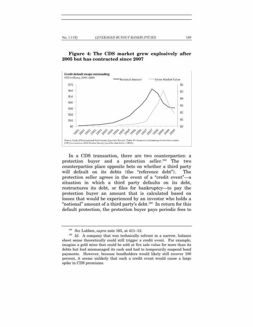
No. 1:118] LEVERAGED BUYOUT BANKRUPTCIES 169
Figure 4: The CDS market grew explosively after 2005 but has contracted since 2007
In a CDS transaction, there are two counterparties: a
protection buyer and a protection seller.168 The two counterparties place opposite bets on whether a third party will default on its debts (the “reference debt”). The protection seller agrees in the event of a “credit event”—a situation in which a third party defaults on its debt, restructures its debt, or files for bankruptcy—to pay the protection buyer an amount that is calculated based on losses that would be experienced by an investor who holds a “notional” amount of a third party’s debt.169 In return for this default protection, the protection buyer pays periodic fees to
168 See Lubben, supra note 165, at 411–12. 169 Id. A company that was technically solvent in a narrow, balance
sheet sense theoretically could still trigger a credit event. For example, imagine a gold mine that could be sold at fire sale value for more than its debts but had mismanaged its cash and had to temporarily suspend bond payments. However, because bondholders would likely still recover 100 percent, it seems unlikely that such a credit event would cause a large spike in CDS premiums.
170 COLUMBIA BUSINESS LAW REVIEW [Vol. 2011
the protection seller.170 The fees are quoted in basis points (“bps”; 100 bps = one percent) of the notional value.
When interpreting credit spreads, the most important concept to understand is that bankruptcies and defaults can involve different degrees of loss to bondholders. The probability of default and the severity of the default—the loss given default—are what drive credit spreads.171 For a given spread, the probability of default and the loss given default are inversely related. In other words, if two investors both agree that a certain credit spread is appropriate, but the first investor believes that the probability of default is higher than the second investor, then the first investor must believe that the loss given default, will be lower than the second investor.
The discussion that follows explains the relative advantages and disadvantages of bond market data and CDS data, and why courts should ideally consider data from both markets in their analyses. It also explains how courts (or those seeking to persuade them) can extract the probability of default and the expected loss given default that are implicit in bond credit spreads and CDS fees (also called spreads). The techniques we develop and present here are designed to be simple. Although professional fixed income traders—whose profits depend on fractions of a percent on every trade172 and who may wish to make surgical bets about
170 Although some contracts also require upfront fees, it is possible to
calculate what periodic fees would be for such a contract if there were no upfront fee.
171 See Merton, supra note 159, at 449 (arguing that the risk of default is reflected in interest rates and noting that the value of a particular issue of corporate debt depends on three things: (1) the default-risk-free rate of return; (2) the term structure and seniority; and (3) the probability of default); Lawrence Fisher, Determinants of Risk Premiums on Corporate Bonds, 67 J. POL. ECON. 217, 217 (1959) (hypothesizing that the difference between the market yield on the bond and the risk-free rate “depends first on the risk that the firm will default on its bonds and second on their marketability”).
172 See MICHAEL LEWIS, THE BIG SHORT: INSIDE THE DOOMSDAY
MACHINE 208 (2010) (“On a $2 billion trade . . . the traders were arguing
No. 1:118] LEVERAGED BUYOUT BANKRUPTCIES 171
the timing of a default—may use more sophisticated techniques,173 extracting market implied probabilities of default for our purposes does not require the same degree of precision. More complex techniques are more assumption-laden and therefore easier for experts to manipulate. In the legal context, simplicity is a virtue. The discussion also explains important caveats and precautions that should be taken when using the described approaches.
1. Market Implied Probabilities of Default Facilitate Continuous Solvency Analysis
Bankruptcy courts sometimes conceived of insolvency as a state into which a debtor moved on some date before filing bankruptcy, and that once insolvent, a debtor remained insolvent until filing bankruptcy. This view was convenient because it was historically expensive and time-consuming for a court to determine a debtor’s financial condition at each point in time, and a single bankruptcy might involve numerous alleged fraudulent transfers on different dates.
However, the truth is that a debtor can shift back and forth between being insolvent and being solvent several times before filing bankruptcy. The Bankruptcy Code explicitly contemplates this possibility because it refers to the financial condition of the debtor on “the date” of the alleged fraudulent transfer.
over interest payments amounting to $800,000 per year. Over that sum, the deal fell apart.”).
173 Trading models are proprietary. See GILLIAN TETT, FOOL’S GOLD
132–33 (2009). However, several economists have published sophisticated valuation models that influence many trading models. See John Hull & Alan White, Valuing Credit Default Swaps I: No Counterparty Default Risk, J. DERIVATIVES, Fall 2000, at 29; John Hull & Alan White, Valuing Credit Default Swaps II: Modeling Default Correlations, J. DERIVATIVES, Spring 2001, at 12; John Hull & Alan White, The Valuation of Credit Default Swap Options, J. DERIVATIVES, Spring 2003, at 40; Darell Duffie, Credit Swap Valuation, 55 FIN. ANALYSTS J. 73 (1999); Darrell Duffie, Jun Pan & Kenneth Singleton, Transforming Analysis and Asset Pricing for Affine Jump-Diffusions, 68 ECONOMETRICA 1343 (2000).
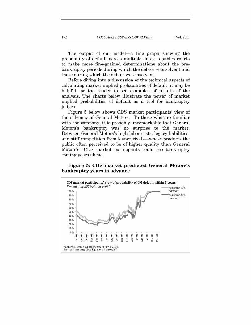
172 COLUMBIA BUSINESS LAW REVIEW [Vol. 2011
The output of our model—a line graph showing the probability of default across multiple dates—enables courts to make more fine-grained determinations about the pre-bankruptcy periods during which the debtor was solvent and those during which the debtor was insolvent.
Before diving into a discussion of the technical aspects of calculating market implied probabilities of default, it may be helpful for the reader to see examples of results of the analysis. The charts below illustrate the power of market implied probabilities of default as a tool for bankruptcy judges.
Figure 5 below shows CDS market participants’ view of the solvency of General Motors. To those who are familiar with the company, it is probably unremarkable that General Motors’s bankruptcy was no surprise to the market. Between General Motors’s high labor costs, legacy liabilities, and stiff competition from leaner rivals—whose products the public often perceived to be of higher quality than General Motors’s—CDS market participants could see bankruptcy coming years ahead.
Figure 5: CDS market predicted General Motors’s
bankruptcy years in advance
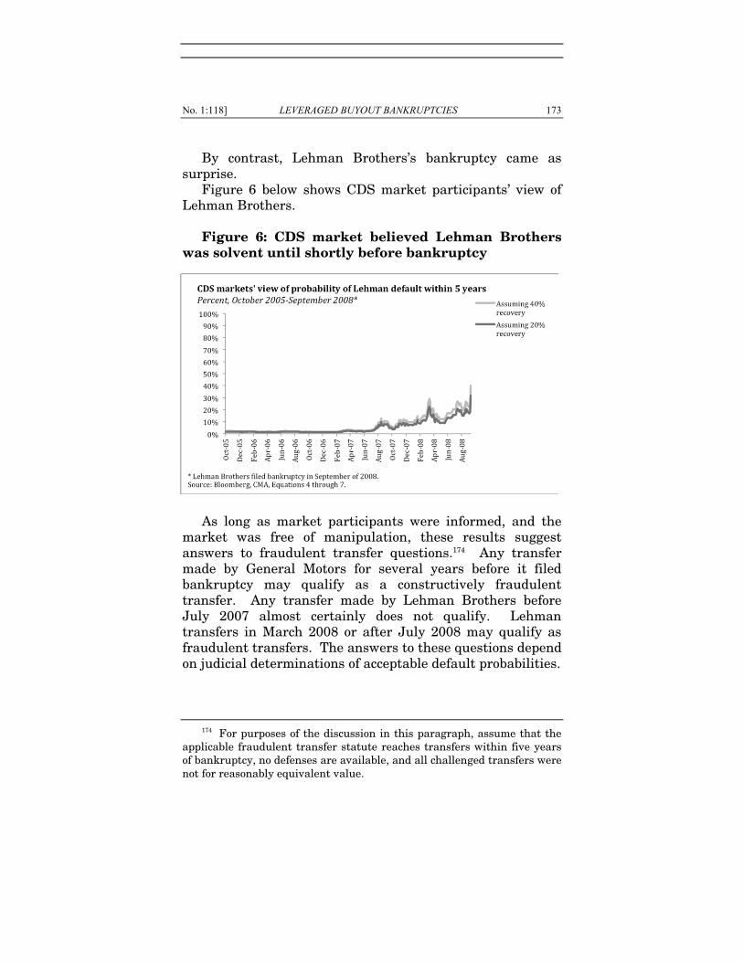
No. 1:118] LEVERAGED BUYOUT BANKRUPTCIES 173
By contrast, Lehman Brothers’s bankruptcy came as surprise.
Figure 6 below shows CDS market participants’ view of Lehman Brothers.
Figure 6: CDS market believed Lehman Brothers
was solvent until shortly before bankruptcy
As long as market participants were informed, and the
market was free of manipulation, these results suggest answers to fraudulent transfer questions.174 Any transfer made by General Motors for several years before it filed bankruptcy may qualify as a constructively fraudulent transfer. Any transfer made by Lehman Brothers before July 2007 almost certainly does not qualify. Lehman transfers in March 2008 or after July 2008 may qualify as fraudulent transfers. The answers to these questions depend on judicial determinations of acceptable default probabilities.
174 For purposes of the discussion in this paragraph, assume that the
applicable fraudulent transfer statute reaches transfers within five years of bankruptcy, no defenses are available, and all challenged transfers were not for reasonably equivalent value.
174 COLUMBIA BUSINESS LAW REVIEW [Vol. 2011
2. CDS Markets May Often Provide the Best Information About Default Risk
a. CDS Markets May Be More Efficient Because They Are a Haven for Insider Trading
The smaller the information gap between management and market participants at the time of the allegedly fraudulent transfer, the more reliable market prices are as a gauge of the risk of default.
The information available to market participants at the time of an allegedly fraudulent transaction may not include all of the information that courts wish to consider in evaluating whether the company was insolvent. For example, management and banks conducting due diligence may have non-public information. In such situations, courts have considered market prices after the public disclosure of pertinent information rather than solely at the time of the alleged fraudulent transfer.175
However, if insider trading or sophisticated due diligence by investors are prevalent in a particular market, prices at the time of the fraudulent transfer may at least in part reflect information that is not generally available to the public.
The data suggests that CDS markets anticipate negative credit rating agency actions, including reviews for downgrade, negative outlooks, and downgrades.176 Although
175 See VFB LLC v. Campbell Soup Co., 482 F. 3d 624, 632 (3d Cir.
2007). 176 John Hull, Mirela Predescu & Alan White, The Relationship
Between Credit Default Swap Spreads, Bond Yields, and Credit Rating Announcements, 28 J. BANKING FIN. 2789, 2801–03 (2004) (reporting that CDS markets anticipate rating agency reviews for downgrade, downgrades, and negative outlooks); Lars Norden & Martin Weber, Informational Efficiency of Credit Default Swap and Stock Markets: The Impact of Credit Rating Announcements, 28 J. BANKING & FIN. 2813, 2837 (2004) (“[B]oth [CDS and stock] markets anticipate rating downgrades by
No. 1:118] LEVERAGED BUYOUT BANKRUPTCIES 175
equities markets and bond markets also anticipate negative credit rating agency actions, CDS markets move sooner than either bond or equities markets.177 Empirical evidence strongly suggests the presence of insider trading in the CDS market: the CDS market anticipates the public release of negative news.178
There are strong reasons to believe that prices in the CDS market reflect insider information. The CDS market was historically lightly policed by regulators, and was therefore an attractive venue for insider trading.179 Market participants are overwhelmingly large, sophisticated financial institutions180 such as banks, securities firms,
all three agencies. Anticipation starts approximately 90–60 days before the announcement day.”).
177 Roberto Blanco, Simon Brennan & Ian W. Marsh, An Empirical Analysis of the Dynamic Relationship Between Investment Grade Bonds and Credit Default Swaps, 60 J. FIN. 2255, 2279 (2005) (finding that the CDS market leads the bond market, indicating that more price discovery occurs in the CDS market than the bond market); Norden & Weber, supra note 176, at 2838 (“[T]he CDS market tends to react earlier than the stock market [to reviews for downgrade].”).
178 See Viral V. Acharya & Timothy C. Johnson, Insider Trading in Credit Derivatives, 84 J. FIN. ECON. 110 (2007); see also LEWIS, supra note 172, at 197.
179 The SEC has acknowledged serious gaps in its ability to enforce insider trading and anti-manipulation regulations in derivatives markets. See Over-the-Counter Derivatives Markets Act of 2009: Hearing Before the H. Comm. on Fin. Servs., 111th Cong. (Oct. 7, 2009) (statement of Henry T. C. Hu, Director of the SEC Division of Risk, Strategy, and Financial Innovation), available at http://www.sec.gov/news/testimony/2009/ts1007 09hh.htm. The SEC brought its first insider trading case involving credit default swaps only recently. See Press Release, Sec. Exch. Comm’n, SEC Charges Hedge Fund Manager and Bond Salesman in First Insider Trading Case Involving Credit Default Swaps (May 5, 2009), available at http://www.sec.gov/news/press/2009/2009-102.htm; Press Release, Sec. Exch. Comm’n, SEC v. Jon-Paul Rorech, et. al., Lit. Release. No. 21023 (May 5, 2009), available at www.sec.gov/litigation/litreleases/2009/ lr21023.htm.
180 There is a substantial and growing body of empirical research supporting the notion that institutions are well-informed investors who convey private information to the market through their trading activities, particularly in the equities markets. See Ashiq Ali et al., Changes in
176 COLUMBIA BUSINESS LAW REVIEW [Vol. 2011
hedge funds, and insurance companies.181 Many of these institutions may also be secured creditors or financiers of inventory or receivables, and therefore have access to critical information about the debtor that is not widely known.182
Institutional Ownership and Subsequent Earnings Announcement Abnormal Returns, 19 J. ACCT. AUDITING & FIN. 221, 222 (2004) (finding that changes in institutional ownership in one quarter are positively related to the abnormal returns recorded when quarterly earnings are announced in the following periods and supporting the notion that institutions have private information on future earnings surprises and that they trade on this information); Ekkehart Boehmer & Eric K. Kelley, Institutional Investors and the Informational Efficiency of Prices, 22 REV. FIN. STUD. 3563, 3565 (2009) (analyzing the relation between informational efficiency and institutional ownership, and documenting that prices of stocks with greater institutional ownership more closely follow a random walk process); Hsiu-Lang Chen, Narasimhan Jegadeesh & Russ Wermers, The Value of Active Mutual Fund Management: An Examination of the Stockholdings and Trades of Fund Managers, 35 J. FIN. & QUANTITATIVE ANALYSIS 343, 345 (2000) (showing that stocks that have been recently bought by mutual funds outperform stocks that have been recently sold by mutual funds); Joseph D. Piotroski & Darren T. Roulstone, The Influence of Analysts, Institutional Investors, and Insiders on the Incorporation of Market, Industry, and Firm-Specific Information into Stock Prices, 79 ACCT. REV. 1119, 1121–22 (2004) (showing that trades by institutions facilitate the incorporation of the firm-specific component of future earnings into the market and other stock prices generally); Richard W. Sias, Laura T. Starks & Sheridan Titman, Changes in Institutional Ownership and Stock Returns: Assessment and Methodology, 79 J. BUS. 2869, 2870 (2006) (documenting a permanent effect of institutional trading on stock prices owing to the information conveyed by institutional trading); Xuemin Yan & Zhe Zhang, Institutional Investors and Equity Returns: Are Short-term Institutions Better Informed?, 22 REV. FIN. STUD. 893, 895 (2009) (finding that trades by institutions with short-term investment horizons predict future stock returns and earnings).
181 Francis A. Longstaff, Sanjay Mithal & Eric Neis, Corporate Yield Spreads: Default Risk or Liquidity? New Evidence from the Credit Default Swap Market, 60 J. FIN. 2213, 2217 (2005). Banks account for a large proportion of net protection buyers while insurance companies account for a large proportion of net protection sellers. Id.; see also BRITISH BANKERS’ ASS’N, CREDIT DERIVATIVES REPORT 2003/2004 (2004).
182 See Norden & Weber, supra note 176, at 2818.
No. 1:118] LEVERAGED BUYOUT BANKRUPTCIES 177
b. CDS Markets Are Probably More “Complete” Than Bond Markets Because Credit Default Swaps Facilitate Shorting
The outcome of an election can be changed, without persuading a single voter to change his or her mind, by simply shifting polling stations from one neighborhood to another.183 Similarly, the market price can be skewed if technical features of the market make it easier for investors with certain opinions to “vote” than others. A market is complete if it is possible to enter a trading position placing any bet with regard to the future state of the market.184 Bond markets may be less than perfectly complete in part because it may be difficult and costly to bet that a bond will fall in value.185 If an investor who does not already own a bond wishes to bet that the bond will fall in value, the investor may source the bond from a current bondholder who is willing to lend it, borrow the bond, sell it, and repurchase the bond later after the price has (hopefully) fallen. Transactions costs may in some cases be prohibitive, particularly where trading volumes are low and the bonds are difficult to source.186
If that is the case, then the bond market might reflect a somewhat more optimistic view than the prevailing view among sophisticated investors because of the technical
183 Moshe Haspel & H. Gibbs Knotts, Location, Location, Location:
Precincts Placement and the Costs of Voting, 67 J. POL. 560, 560 (2005). 184 See Mark D. Flood, An Introduction to Complete Markets, 7 FED.
RES. BANK ST. LOUIS REV. 32, 34 (1991), available at http://research. stlouisfed.org/publications/review/91/03/Markets_Mar_Apr1991.pdf.
185 See id. at 48–50 (discussing the difficulties of shorting physical commodities).
186 See LEWIS, supra note 172, at 107. In addition, short sellers may face risks of a short-squeeze—the temporary unavailability of the underlying security at a time when short sellers must repurchase the security to complete their contracts—driving up the price and imposing high costs on short sellers. A short-squeeze in Volkswagen shares temporarily made Volkswagen the most valuable company on earth as measured by (thinly traded) market price of its stock. See Vikas Bajaj, Even as Dow Soars 11%, Skeptics Lurk, N.Y. TIMES, Oct. 29, 2008, at B1.
178 COLUMBIA BUSINESS LAW REVIEW [Vol. 2011
difficulties such investors face in placing bets that the value of the bonds will fall.
Unlike the bond market, the CDS market likely reflects a neutral or perhaps even a pessimistic view. It is not necessary to source bonds to bet against them using credit default swaps. Rather, it is only necessary to find a sufficiently well-capitalized counterparty that is willing to make the opposite bet.
Considering probabilities of default implied by both bond spreads and CDS spreads should mitigate any problems caused by incompleteness in the bond market.
c. CDS Markets May Be More Efficient Because They Are Anonymous and Reduce the Risk of Retaliation for Shorting
In addition to the technical difficulties and risks inherent in short-selling debt, there is an additional challenge facing would-be-shorts: retribution. Corporations that disclose sensitive information to financial advisers and vendors—and who pay hefty fees to those advisers and vendors—tend to be displeased when their financial advisers and vendors bet against their success.187 In fact, firms that issue debt
187 See TETT, supra note 173, at 57 (“The European banks were usually
reluctant to reveal the names of the companies whose loans were included in CDS deals; they feared they would lose customers if companies found out their bank was buying insurance against its loan book risk.”); see also Jenny Strasburg, Aaron Lucchette & Liz Rappaport, New Law Fuels a Shake-Up at Morgan Stanley, WALL ST. J., Aug. 5, 2010, at C1 (reporting that for-profit education companies that were clients of Morgan Stanley complained to Morgan Stanley investment bankers after Steve Eisman, an investment manager at a hedge fund owned by Morgan Stanley, shorted them and “lambasted” them at an investor conference). Morgan Stanley is reportedly planning to sell Eisman’s fund at a loss. Regulators are also frequently hostile toward short sellers. See Nelson D. Schwartz & Eric Dash, Banks Bet Greece Defaults on Debt They Helped Hide, N.Y. TIMES, Feb. 25, 2010, at A1 (“[W]hile some European leaders have blamed financial speculators in general for worsening the crisis, the French finance minister, Christine Lagarde, last week singled out credit-default swaps. Ms. Lagarde said a few players dominated this arena, which she said needed tighter regulation.”); see also Matt Taibbi, Wall Street’s Naked
No. 1:118] LEVERAGED BUYOUT BANKRUPTCIES 179
typically require underwriters to agree to retain a portion of that debt on their balance sheets as a sign of support and confidence in the debtor.
Credit default swaps can enable financial institutions or other market participants to in effect offload all risk (or go further and actually bet against the debtor), while simultaneously holding a significant portion of the debt on their balance sheets.188 In so doing, the financial institution appears to their client—and the outside world—to believe in the client’s success, while its true opinion may be considerably less sanguine.189
Because credit default swaps are not disclosed on a balance sheet, through U.C.C. filings, through an exchange, or pursuant to any mandatory regulation, CDS trades are generally less transparent than bond trades.190 In other words, whereas selling a large amount of bonds or bank debt may be the equivalent of stating one’s vote during a roll call, buying credit default swap protection can more closely resemble casting a secret ballot.
However, the secrecy and anonymity of the CDS market could also make it an attractive vehicle for market manipulation.191
Swindle, ROLLING STONE, Apr. 5, 2010, available at http://www. rollingstone.com/politics/news/12697/64824 (suggesting that regulators should be suspicious of significant naked short selling activity).
188 See TETT, supra note 173, at 57 (calling credit default swaps “a way to maintain ‘client confidentiality’ even while reshaping a bank’s balance sheet”).
189 See Simkovic, supra note 1, at 270 (noting that banks offloaded mortgage risk prior to the subprime crisis while appearing to hold mortgage-backed bonds on their balance sheet).
190 See id. at 271–79. 191 See LEWIS, supra note 172, at 164–66, 184–86, 194–96, 219, 221
(describing an alleged pattern of market manipulation by dealers in the illiquid market for credit default swaps on mortgage bonds).
180 COLUMBIA BUSINESS LAW REVIEW [Vol. 2011
d. Courts Can Reduce the Risk of Market Manipulation
If courts or regulators rely heavily on a single indicator of the probability of default, such reliance will increase market participants’ incentive to manipulate that indicator. For example, an activist hedge fund with a large position in an individual debtor’s bonds might attempt to push down the price of those bonds (and thereby increase the bond spread) around the time of a leveraging transaction in order to establish a future claim for fraudulent transfer. Similarly, equity holders or banks that stand to benefit from such a transaction might attempt to temporarily support the price of the bonds in order to minimize the risk of a claim for fraudulent transfer. Market manipulation is generally prohibited by sections 9 and 10 of the Securities and Exchange Act of 1934, as well as the U.S. Commodity Futures Trading Commission’s rules and regulations, but it is probably safe to assume that enforcement is less than completely effective.192
Market prices of illiquid assets are less reliable than market prices of liquid assets because a relatively small transaction in an illiquid market can lead to a large change in the volume-weighted average price. To give a concrete example, if $10 million worth of bonds typically trade hands each day and an investor suddenly attempts to sell $50 million of bonds in one day, there will likely be an insufficient number of buyers at the most recent market price and the investor will have to accept a price significantly lower than the last market price. On the other hand, if $1 billion worth of bonds trade hands each day, the market can likely absorb the same $50 million transaction without a significant movement in price.
Higher trading volumes make market manipulation more difficult and more expensive because more capital must be
192 See, e.g., Franklin Allen, Lubomir Litov & Jianping Mei, Large Investors, Price Manipulation, and the Limits to Arbitrage: An Anatomy of Market Corners, at 2 (Wharton Fin. Inst. Ctr., Working Paper No. 06-02, 2006), available at http://fic.wharton.upenn.edu/fic/papers/06/0602.pdf.
No. 1:118] LEVERAGED BUYOUT BANKRUPTCIES 181
deployed to move the market price. Financial market prices are also generally more reliable when trading volume is robust. Prices generated through low-volume trades are unlikely to represent the collective wisdom of market participants for the same reasons that election results with low voter turnouts are unlikely to reflect the will of the people—the results only reveal the opinions of a small minority of potential decision makers who participated. Higher trading volumes suggest that more firms put more capital at stake and expended more resources evaluating the price at which the debt should trade. Higher trading volumes also tend to reduce transactions costs and make markets more efficient.
Because price disclosure in the CDS market is voluntary, and volume-weighted average price data is generally not available, CDS markets are probably vulnerable to manipulation, even with higher volume. Regulation in OTC derivatives markets is also notoriously lax.
To avoid the problems of low volume trades, it may be advisable to consider the volume-weighted average price over a period one to two weeks before or after the allegedly fraudulent transfer,193 because the total trading volume will be higher than on the day of the alleged fraudulent transfer.
193 One would examine the period before the alleged fraudulent transfer to assess claims that the transfer was made at a time when the debtor was already insolvent, while one would examine the period after the alleged fraudulent transfer to assess claims that the debtor, though financially healthy before the alleged fraudulent transfer, was rendered insolvent as a result of the allegedly fraudulent transfer. The distinction could have significant consequences for the outcome of the case. Courts generally view transfers at a time when a debtor is already insolvent as involving a much more severe degree of fraud—requiring a more severe remedy—than transfers that merely render a debtor insolvent. Compare United States v. Tabor Court Realty Corp., 803 F.2d 1288, 1307 (3d Cir. 1986), cert. denied, McClellan Realty Co. v. United States, 483 U.S. 1005 (1987) (largely voiding both the liens and the underlying obligations of the LBO lenders’ assignees and property sales by those assignees where debtor was insolvent before the LBO), with In re O’Day Corp., 126 B.R. 370, 410–13 (Bankr. D. Mass. 1991) (noting that the fact that the debtor in O’Day was healthy before the LBO “alone provides a sufficient reason for this Court to reject an application of the ruling in Gleneagles [Tabor] to
182 COLUMBIA BUSINESS LAW REVIEW [Vol. 2011
The dangers of market manipulation can also be reduced by considering market-based indicators of default suggested by multiple markets: different bonds or secured debt instruments of the same issuers, equity prices, and derivatives. The larger the universe, the more difficult it will be to manipulate.
Finally, courts can directly police and monitor manipulation by permitting discovery of trading records, emails, and other communications that might reveal the motives of large creditors—banks and hedge funds—who were trading bonds and credit default swaps around the time of the allegedly fraudulent transfer.194
the facts of this case,” preserving the obligations to the LBO lenders, and only avoiding the LBO lenders’ liens to the extent necessary to satisfy unsecured claims). Although Tabor involved clear indicia of fraud above and beyond insolvency of the debtor before the transaction, a recent fraudulent transfer case confirms that harsh penalties are more likely to be imposed when the debtor is insolvent before the transaction. See Official Comm. of Unsecured Creditors of TOUSA, Inc., v. Citicorp North America, Inc. (In re TOUSA, Inc.), 422 B.R. 783, 875 (Bankr. S.D. Fla. 2009), rev’d on other grounds, In re TOUSA, Inc., Nos. 10-60017-CIV/GOLD, 10-61478, 10-62032, 10-62035, 10-62037, 2011 WL 522008 (S.D. Fla. Feb. 11, 2011). The court imposed a remedy that involved avoidance of liens, obligations, and various financing and professional fees, but that in many respects was more similar to equitable subordination than the full claim avoidance seen in Tabor. Id. at 885 (“After all requisite payments to the Conveying Subsidiaries have been accomplished, the remainder of the funds shall be distributed to the First and Second Lien Lenders in accordance with the First and Second Lien Term Loan Agreements.”).
194 Recently-proposed amendments to Bankruptcy Rule 2019 may require many groups, committees, and entities to provide enhanced disclosures of their economic interests in the debtor, including derivatives, in order to participate actively in a bankruptcy case. See Insolvency and Restructuring Update: Standing Committee Approves Major Changes to Bankruptcy Disclosure Rule, DAVIS POLK CLIENT NEWSL. (Davis Polk & Wardwell LLP, New York, N.Y.), June 16, 2010.
No. 1:118] LEVERAGED BUYOUT BANKRUPTCIES 183
e. Counterparty Risk Has Been Minimized by Government and Regulatory Policy
Unlike a bond, which depends only on the creditworthiness of the debtor, the value of a credit default swap depends not only on the creditworthiness of the reference entity (the debtor), but also on the creditworthiness of the protection seller, much as the value of an insurance contract depends on the solvency of the insurance company.195 CDS market participants attempt to address counterparty risk through nonprice terms such as collateral posting requirements, but this approach is not completely effective. During the financial crisis of 2008, the Federal Government ensured that the counterparties to whom AIG had sold credit default swap protection were made whole (100 cents on the dollar recovery).196 It now appears likely that the Federal Deposit Insurance Corporation (“FDIC”) will protect derivatives counterparties against loss, thereby institutionalizing minimal counterparty risk for derivatives dealers and customers.197 Whatever the broader merit of this policy, it does have the beneficial effect
195 See Simkovic, supra note 1, at 272. 196 Louise Story & Gretchen Morgenson, In U.S. Bailout of A.I.G.,
Forgiveness for Big Banks, N.Y. TIMES, June 29, 2010, at A1. 197 Id. The provisions relating to the “Orderly Liquidation Authority”
under the Dodd-Frank Wall Street Reform and Consumer Protection Act, Pub. L. No. 111-203, 124 Stat. 1376, § 210(n) enable the FDIC to borrow funds from the Treasury when resolving a systemically important financial institution. During an FDIC-administered “orderly liquidation,” special protections for derivatives (“qualified financial contracts”) virtually guarantee that derivatives counterparties will recover in full, particularly if the swap is traded through a clearing organization. Id. § 210(c)(8); 11 U.S.C. §§ 555, 556, 559, 560 & 561; 12 U.S.C. § 1821(e)(8). Although any borrowed Treasury funds are supposed to be recovered through gradual assessments on large financial institutions, it seems unlikely that the FDIC will aggressively collect shortly after a financial crisis or that the Treasury will demand a market rate of return. Dodd-Frank Act §§ 210(b), 210(o)(1)(A), 210(o)(1)(B), 210(o)(1)(D), 210(o)(2), 210(o)(4). The Swaps Bank “Push-Out” provision includes exemptions for many cleared credit default swaps. Id. § 716.
184 COLUMBIA BUSINESS LAW REVIEW [Vol. 2011
of making CDS pricing a purer signal of default risk of the reference entity.
Prior to the financial crisis, the extent to which even sophisticated parties were caught off-guard by the inability of AIG to meet its obligations suggests that counterparty risk of protection sellers did not affect the CDS market as much as it should have.198 In other words, even before the recent regulatory reforms, CDS pricing was probably relatively unaffected by counterparty risk, and was therefore more purely driven by default risk of the reference entity.
3. High Quality Market Data Can Be Obtained Within the Context of Litigation
a. Corporate Bond Markets Are Generally Transparent
Detailed corporate bond trade data—including price, volume, date, and time—is available through TRACE, the Trade Reporting and Compliance Engine. Limited data is available as far back as 2002, but coverage greatly expanded from 2003 through 2005.199 Corporate bond trades must be disclosed within fifteen minutes of the trade under Financial Industry Regulatory Authority (“FINRA”) rules.200 TRACE data may be downloaded free of charge for personal use from the FINRA website, but it is also available in a more user-friendly format from financial data providers such as Bloomberg Professional Service and Markit.
198 See Simkovic, supra note 1, at 274 n.109. 199 See FINRA NEWS RELEASE, supra note 140. 200 FINRA MANUAL §6739(a) (2010), available at http://finra.
complinet.com/en/display/display_main.html?rbid=2403&element_id=4402 (last visited Mar. 4, 2011). Until July 2005, dealers were required to disclose trades within thirty minutes. See FINRA News Release, supra note 140.

No. 1:118] LEVERAGED BUYOUT BANKRUPTCIES 185
b. Although CDS Markets Are Generally Not Transparent, Litigation Can Shed New Light on Their Inner Workings
Historically, the CDS market was largely unregulated, and, as a result, detailed and reliable data about pricing and volume is hard to obtain.201 However, several private entities currently aggregate, validate, and sell pricing information provided to them by private market participants.202 The CDS market will likely become more transparent in the near future because the Dodd-Frank Wall Street Reform and Consumer Protection Act requires the Securities and Exchange Commission and the Commodities Futures Trading Commission to promulgate rules for real-time public reporting of swap transaction price and volume data.203
Two of the leading data providers of historical CDS pricing are Markit, which is affiliated with CDS dealers (large investment banks),204 and CME Group’s CMA Datavision, which is affiliated with large derivatives buyers (hedge funds, mutual funds, insurance companies, pension funds, etc.).205 Markit calculates its daily closing prices
201 See Simkovic, supra note 1, at 274. 202 The discussion of private data providers that follows is based on a
combination of those providers’ marketing materials and conversations with employees and customers of those data providers.
203 Dodd-Frank Wall Street Reform and Consumer Protection Act, § 753(i) (to be codified at 15 U.S.C. § 78a).
204 Markit was initially backed by Goldman Sachs, J.P. Morgan, and several other banks that are leading derivatives dealers. See Nelson D. Schwartz & Eric Dash, Banks Bet Greece Defaults on Debt They Helped Hide, N.Y. TIMES, Feb. 25, 2010, at A1. However, Markit describes itself as an “independent source of credit derivative pricing.” See About Markit, MARKIT, http://www.markit.com/en/about/about-Markit.page (last visited Mar. 4, 2011).
205 CDS pricing data providers other than Markit and CMA include Moody’s CreditQuotes and Fitch Pricing Services. Moody’s CreditQuotes appears to be similar to CMA in that its pricing data comes from quotes observed by buy-side institutions. Fitch appears to be similar to Markit in that pricing data comes from dealers’ books (brochures, on file with author).
186 COLUMBIA BUSINESS LAW REVIEW [Vol. 2011
based on the prices dealers record in their books,206 while CMA calculates daily prices based on intraday trading quotes sent to large derivatives users.207 Markit’s coverage is broader—Markit covers approximately 3,000 entities208 while CMA only covers about 1,500.209 But, CMA’s data is richer because CMA includes bid-ask spreads while Markit only provides a single price.210
Daily CDS trading volume is generally not publicly or commercially available, but limited weekly data has been published by the Depository Trust & Clearing Corporation (“DTCC”) since November 2008.211 The DTCC clears the overwhelming majority of CDS transactions and probably has the best aggregate market data.212
206 Because Markit depends on accounting by dealers rather than
individual trades or market quotes, it uses an algorithm to detect and remove prices that are “stale,” outliers, or otherwise seem inaccurate or suspicious. See Markit CDS Pricing, MARKIT, http://www.markit.com/ en/products/data/cds-pricing/cds-pricing.page (last visited Mar. 4, 2011).
207 CMA claims that its prices are more reliable because they are “observed market prices” seen by “front office” traders. See CMA Data Vision: CDS Pricing from the best vantage point: the buy-side front office, CMA, http://web.archive.org/web/20080622183745/www.cmavision.com/ Products_And_Services/DataVision/ (last visited Mar. 4, 2011). However, it should be noted that CMA’s prices are not necessarily prices at which transactions took place, only prices at which dealers offered to transact.
208 See Markit CDS Pricing, MARKIT, http://www.markit.com/en/ products/data/cds-pricing/cds-pricing.page? (last visited Mar. 4, 2011).
209 See CMA Historical CDS Prices, CMA, http://www.cmavision.com/ products-solutions/cma-datavision-historical-cds-prices (last visited Mar. 4, 2011).
210 The bid-ask spread is the difference between the price at which dealers are willing to buy CDS protection and the price at which they are willing to sell it. This spread is the dealer’s profit margin on each pair of offsetting trades.
211 Press Release, Depository Trust and Clearing Corporation, DTCC to Provide CDS Data from Trade Information Warehouse (Oct. 31, 2008), available at http://www.dtcc.com/news/press/releases/2008/warehouse_ data_values.php, (last visited Mar. 4, 2011).
212 Products & Services, DTCC Deriv/SERV LLC, Global Repository for OTC Credit Derivatives, THE DEPOSITORY TRUST & CLEARING CORP., http://www.dtcc.com/products/derivserv/suite/trade_reporting_repository. php (last visited Mar. 4, 2011) (“DTCC's Trade Information Warehouse’s
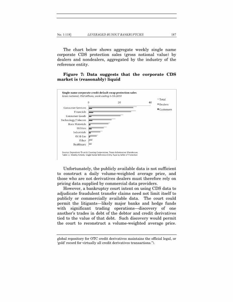
No. 1:118] LEVERAGED BUYOUT BANKRUPTCIES 187
The chart below shows aggregate weekly single name corporate CDS protection sales (gross notional value) by dealers and nondealers, aggregated by the industry of the reference entity. Figure 7: Data suggests that the corporate CDS market is (reasonably) liquid
Unfortunately, the publicly available data is not sufficient
to construct a daily volume-weighted average price, and those who are not derivatives dealers must therefore rely on pricing data supplied by commercial data providers.
However, a bankruptcy court intent on using CDS data to adjudicate fraudulent transfer claims need not limit itself to publicly or commercially available data. The court could permit the litigants—likely major banks and hedge funds with significant trading operations—discovery of one another’s trades in debt of the debtor and credit derivatives tied to the value of that debt. Such discovery would permit the court to reconstruct a volume-weighted average price.
global repository for OTC credit derivatives maintains the official legal, or ‘gold’ record for virtually all credit derivatives transactions.”).
188 COLUMBIA BUSINESS LAW REVIEW [Vol. 2011
The court might even be able to encourage the limited disclosure of DTCC CDS price and volume data, because the DTCC’s owners and customers are large banks that are frequently defendants in fraudulent transfer actions.
4. Simple, Robust, Manipulation-Resistant Equations Can Be Used to Calculate Market-Implied Probabilities of Default Based on Credit Market Prices
a. How to Calculate Credit Spreads from Bond Yields or CDS Fees
One relatively simple technique that helps to isolate default risk from other factors that affect bond yields is to subtract from the corporate bond yield the risk-free interest rate.213 The risk-free rate is an interest rate paid by a hypothetical borrower who has zero chance of defaulting.214 Although no such borrower exists, there are borrowers with extremely low probabilities of default. For example, the U.S. government is perceived to have an extremely low
213 See Jerome S. Fons, The Default Premium and Corporate Bond
Experience, 42 J. FIN. 81, 81 (1987) (developing a risk-neutral model of the expected probability of default for low-grade corporate bonds based on the additional required rate of return on these instruments over default-free bonds); Longstaff et al., supra note 181, at 2214–18 (finding that the majority of the corporate bond yield spread and CDS spread is due to default risk); Michael Simkovic, The Effect of BAPCPA on Credit Card Industry Profits and Prices, 83 AM. BANKR. L.J. 1, 5 (2009) (“The risk free interest rate reflects broad macroeconomic factors that affect economy-wide costs of credit. The spread between the risk free rate and [the yield on private debt] reflects the risk-adjusted price of [private debt]” if the debt market is efficient.).
214 Even in the absence of default risk, a borrower will pay interest because of the time value of money and inflation. The time value of money is the idea that money (or money’s worth in goods or services) is more valuable in the present than it is in the future because people generally prefer immediate consumption to delayed consumption and because money can be invested profitably.
No. 1:118] LEVERAGED BUYOUT BANKRUPTCIES 189
probability of default.215 Academic economists generally use yields on U.S. Treasuries as a benchmark risk-free rate for U.S. dollar denominated debts.216 Finance professionals tend to use the London Interbank Offered Rate (“LIBOR”), the rate at which banks rated AA (or better) can borrow from other banks.217 Although LIBOR is not as low risk as U.S. Treasuries (except during periods of distress in the financial system), LIBOR may be only slightly higher than Treasury yields.218
The difference between the corporate bond and the risk-free rate is called the “spread,” “bond spread,” or “credit spread.” Credit spreads should be calculated using a risk-free instrument with a term structure that matches the corporate bond as closely as possible.219 The term structure
215 Merton, supra note 159, at 449 (noting that government bonds are
essentially default-risk-free); Joost Driessen, Is Default Event Risk Priced in Corporate Bonds?, 18 REV. FIN. STUD. 165, 169 (2005) (assuming that U.S. Treasuries are default-risk-free). In truth, sovereign debt defaults do happen, but given governments’ powers to raise taxes, print money, or nationalize industries, a government is generally more capable of paying its debts than the private entities subject to its authority. Government defaults are usually strategic decisions rather than acts of necessity, particularly when a government borrows in its own currency. See CARMEN
M. REINHART & KENNETH ROGOFF, THIS TIME IS DIFFERENT: EIGHT
CENTURIES OF FINANCIAL FOLLY 59 (2009). However, Moody’s Investors Service recently warned that the United States could conceivably lose its triple-A rating. David Jolly & Catherine Rampell, Moody’s Says U.S. Debt Could Test Triple-A Rating, N.Y. TIMES, Mar. 16, 2010, at B1.
216 See Longstaff et al., supra note 181, at 2223 (“[T]he Treasury curve . . . is the standard benchmark riskless curve in most empirical tests in finance.”). Finance professionals will sometimes use swap curves rather than Treasuries. Id.; John Hull et al., Bond Prices, Default Probabilities and Risk Premiums, J. CREDIT RISK, Spring 2005, at 53.
217 See MOHAMED BOUZOUBAA & ADEL OSSEIRAN, EXOTIC OPTIONS &
HYBRIDS: A GUIDE TO STRUCTURING, PRICING AND TRADING 4 (2010). 218 The spread between Treasuries and LIBOR, known as the TED
spread, serves as a measure of credit risk in the interbank market. Id. 219 See, e.g., Fons, supra note 213, at 81–82 (“[M]odern approaches [to
extracting default risk from bond yields] acknowledge the influences on required returns that result from call provisions, the tax effect for deep discount bonds (due to the different tax treatment of ordinary income vs. capital gains), and sinking fund payments (which reduce the average
190 COLUMBIA BUSINESS LAW REVIEW [Vol. 2011
refers to the timing of interest and principal payments. Equation 1 below shows a simple technique to calculate a bond spread.
Equation 1 (Credit spread) = (Corporate bond yield) – (risk-free rate) It is important to match the duration and term structure
of the corporate bond and the risk-free instrument because yields vary by duration and term structure.220 In practice, it may not always be possible to perfectly match the term structures.
There are more sophisticated techniques available that try to account for differences in the term structure of the corporate bond and the risk-free rate by constructing a yield curve, but in most cases in the judicial context, the marginal improvement in accuracy presented by these techniques is unlikely to justify the added complexity and potential for manipulation.
Credit default swaps have the advantage of not requiring any math to calculate a credit spread—the market has
maturity of a firm's debt). Isolating the influence of default likelihood on interest rate differentials involves controlling for these other effects.”); Longstaff et al., supra note 181, at 2218 (“[C]orporate bond yield spreads will always be calculated as the yield on a corporate bond minus the yield on a riskless bond with the identical coupon rate and maturity date.”) (emphasis added); Merton, supra note 159, at 449; Gregory R. Duffee, The Relation Between Treasury Yields and Corporate Bond Yield Spreads, 53 J. FIN. 2225, 2225–26 (1998) (demonstrating that the spread between a corporate bond yield and Treasury yields depends on whether the corporate bond is callable, and thus supporting the notion that callable bonds should therefore only be compared to other callable bonds when evaluating implied default risk).
220 In general, long-term debt carries a higher yield than short-term debt from the same issuer, and zero-coupon debt carries a higher yield than coupon debt with the same maturity. This positive correlation between yield and maturity is known as the “upward sloping yield curve,” although yield curves are occasionally kinked, flat, or downward sloping. Historical yields for U.S. Treasuries of different maturities are freely available from the U.S. Treasury Department’s website and from Federal Reserve statistical releases.
No. 1:118] LEVERAGED BUYOUT BANKRUPTCIES 191
already done the math.221 CDS annual fees are themselves a credit spread. The fees paid by CDS protection buyers to protection sellers—under ideal market conditions in which there are no transactions costs, taxes, counterparty risks among derivatives counterparties, or arbitrage opportunities—should be equivalent to the spread between the yield of the reference corporate bond and the risk-free interest rate.222
To understand why this is true, consider the following example. Investor A holds $100 million worth of five-year corporate bonds yielding eight percent. Investor B holds $100 million worth of five-year Treasuries yielding five percent. If Investor A wishes to eliminate the risk of default from his portfolio, he may do so either by purchasing a five-year credit default swap or by selling his corporate bonds yielding eight percent and purchasing Investor B’s Treasuries yielding five percent. In selling his corporate bonds for default-risk-free Treasuries, Investor A will sacrifice 300 basis points, or three percent. Therefore, if a five-year credit default swap would successfully eliminate all default risk, it should also cost 300 basis points.223 Because
221 See Hull et al., supra note 176, at 2792 (“CDS spreads . . . are
already credit spreads.”). 222 See id. at 2790–91 (“[T]he N-year CDS spread should be close to the
excess of the yield on an N-year bond issued by the reference entity over the risk free rate. This is because a portfolio consisting of a CDS and a par yield bond issued by the reference entity is very similar to a par yield risk free bond.”); Duffie et al., supra note 173, at 74–76 (demonstrating that the CDS spread should equal the spread between corporate and riskless floating rates). Floating rate notes are far less common than fixed rate notes, and there are some differences in spreads between the two, reportedly five to ten basis points. See Longstaff et al., supra note 181, at 2218. However, this difference in bond spreads calculated based on floating rate notes and fixed rate notes is probably not significant for our purposes and likely does not justify the added complexity of adjusting data that is readily observable on the market.
223 Similarly, if Investor B wanted a higher yield, he could achieve a higher yield by selling his Treasuries and buying corporate bonds from Investor A. In so doing, Investor B would accept default risk in return for 300 basis points of extra yield. Investor B could replicate this payoff by
192 COLUMBIA BUSINESS LAW REVIEW [Vol. 2011
of this theoretical equivalence between CDS fees and bond spreads, the fees on credit default swaps are frequently referred to as the “CDS spread” or simply “the spread.”224
b. How to Extract the One-Year Market Implied Probability of Default from Credit Spreads
The relationship between a credit spread and the perceived risk of default may be approximated by the following simplified equation:
Equation 2 (perceived probability of default in year 1) = (credit
spread) / (expected loss rate given default)225 This simple equation is useful for illustrative purposes.
As this equation demonstrates, an increase in the bond spread suggests either an increase in the perceived probability of default or an increase in the expected loss rate given default.
These relationships are directionally correct, but Equation 2 is mathematically only a rough approximation. Even under ideal conditions—a credit market that is rational, risk-neutral, transparent, liquid, and free of transactions costs, taxes, or market manipulation—a more complex equation is needed to precisely describe the relationship between perceived probability of default,
retaining his Treasuries but instead selling CDS protection on the corporate bond for 300 basis points.
224 The difference between the price at which dealers are willing to sell CDS protection and the price at which they are willing to buy CDS protection is also sometimes referred to as the “bid-ask spread,” or simply the “spread.”
225 The expected loss rate given default will almost always be less than 100 percent because even when a debtor defaults, creditors generally recover some portion of the amount owed to them. The expected recovery rate and the expected loss rate given default sum to 100 percent. In mathematical notation, (expected loss rate given default) = 1 – (expected recovery rate).
No. 1:118] LEVERAGED BUYOUT BANKRUPTCIES 193
expected recovery rate, corporate bond yields, and the risk-free rate. The following formula provides a more precise description of the relationship under idealized conditions:
Equation 3 (probability of default in year 1) = [1 – (1 + risk-free
rate)/(1 + corporate bond yield)] / (expected loss rate given default)
If CDS spreads are used instead of bond spreads,
Equation 3 may be rewritten as: Equation 4 (probability of default in year 1) = [1 – (1 + risk-free
rate)/(1 + CDS spread + risk-free rate)] / (expected loss rate given default)
An algebraic derivation of Equation 3, alternate versions
of this equation, and an illustrative example of its superior precision compared to Equation 2 are presented in Part IX, Appendix III: Derivation and Illustration of Equation 3.
Equation 2, Equation 3, and Equation 4 all include the expected loss rate given default as a variable. The expected loss rate given default presents a challenge because unlike the corporate bond yield, CDS spread, and the risk-free rate, the expected loss rate given default cannot be directly observed in the market. By convention, financial professionals will sometimes assume a sixty percent expected loss rate given default (a forty percent expected recovery rate) when calculating the implied probability of default for senior unsecured bonds. However, it is possible to make a more well-informed assumption by using historical recovery rates.226 Furthermore, recent finance research
226 Moody’s Investors Service publishes historical recovery rates of
corporate bonds and loans from 1920 to the present, broken down by year, level of seniority, and letter rating, as well as recovery outlooks for the coming year. See, e.g., KENNETH EMERY et al., MOODY’S INVESTORS
SERVICE, CORPORATE DEFAULT AND RECOVERY RATES, 1920–2008 (Feb. 2009), available at http://www.moodys.com/cust/content/content.ashx?

194 COLUMBIA BUSINESS LAW REVIEW [Vol. 2011
suggests that it may be possible to calculate recovery rates based on prices and rates that are observable in the CDS and equities markets.227
c. Credit Spreads Based on Treasuries May Overestimate Default Risk
A recent empirical study suggests that, although the majority of the credit spread is due to default risk, other factors still play a role.228 The credit spread is therefore a good first approximation of default risk, but the analysis can be improved by taking other factors into account.
Finance professionals routinely use credit spreads as a measure of the market perception of the creditworthiness of the debtor,229 but a number of academic studies have suggested that Treasury-to-corporate bond spreads tend to be wider than can be justified by the real-world historical probability of default alone.230 In fact, a few studies have
source=StaticContent/Free%20Pages/Credit%20Policy%20Research/documents/current/2007400000578875.pdf.
227 See Sanjiv R. Das & Paul Hanouna, Implied Recovery, 33 J. ECON. DYNAMICS & CONTROL 1837 (2009).
228 Longstaff et al., supra note 181, at 2215 (reporting that the nondefault component ranges from 0.2% to 1%, and is present in at least three-quarters of firms sampled).
229 See Robert L. Geske & Gordon Delianedis, The Components of Corporate Credit Spreads: Default, Recovery, Tax, Jumps, Liquidity, and Market Factors 2 (The Anderson Sch. at UCLA, Working Paper No. 22-01, 2001), available at http://ssrn.com/abstract=306479 (“In the United States market for corporate bonds, credit spreads are generally measured and quoted as the yield difference between a government bond and a corporate bond properly adjusted for coupon and maturity. This yield difference is often attributed solely to default risk.”).
230 See, e.g., Edwin J. Elton, Martin K. Gruber, Deepak Agrawal & Christopher Mann, Explaining the Rate Spread on Corporate Bonds, 56 J. FIN. 247, 272–73 (2001) (concluding that taxes and a premium for bearing systemic risk account for a larger portion of the bond spread over Treasuries than the probability of default predicted by bonds ratings); Fons, supra note 213, at 96 (“We find that the default rates implied in corporate bond returns exceed those experienced in recent years . . . . We conclude either that there is systematic mispricing of low-rated corporate bonds by investors or that the risk neutral model derived herein cannot
No. 1:118] LEVERAGED BUYOUT BANKRUPTCIES 195
even suggested that default risk may account for only a minority of the yield spread.231 However, this counterintuitive finding is doubtful for two methodological reasons. First, these studies generally rely on complex models that are highly sensitive to assumptions made by the authors, and varying those assumptions increases the proportion of the yield spread that is due to default risk.232 Second, these studies generally rely on data from a subset of bonds over a very limited number of years, and it is therefore likely that during the years measured, the particular bonds that were tracked simply turned out to perform better than the market expected.233 Defaults are generally concentrated
fully capture the market’s assessment of the probability of default on these securities.”); Geske & Delianedis, supra note 229, at 3 (“[I]t seems likely that the credit spread between corporate and government bonds may be only partly attributed to default risk.”); id. at 26 (“The major components [of credit spreads] include taxes, jumps, liquidity, market risk factors, and to a small extent interest rate factors.”); Hull et al., supra note 216, at 53.
231 See, e.g., Geske & Delianedis, supra note 229, at 26–27; Jing-zhi Huang & Ming Huang, How Much of the Corporate-Treasury Yield Spread Is Due to Credit Risk? A New Calibration Approach, 3 (14th Annual Conference on Fin. Econ.& Accounting (FEA); Tex. Fin. Festival, Working Paper Series, 2003), available at http://ssrn.com/abstract=307360 (arguing that default risk accounts for a small fraction of the spread for investment grade bonds, but for a much larger fraction of the spread for junk bonds).
232 See Georges Dionne et al., Default Risk, Default Risk Premiums, and Corporate Yield Spreads 19 (EFA 2006 Zurich Meetings, Working Paper Series, 2006), available at http://ssrn.com/abstract=887380 (reporting that under modified model assumptions, up to sixty-four percent of the ten-year corporate yield spread for debt rated BAA is explained by default risk); Longstaff et al., supra note 181, at 2214–15 (finding that if CDS fees reflect the risk of default, “the default component [of corporate bond spreads] represents . . . 71% for BBB-rated bonds, and . . . 83% for BB-rated bonds.”). Longstaff et al. also note that “under some parameterizations, results paralleling ours can be obtained from a structural model” and that “some structural models can actually overestimate corporate spreads” and therefore underestimate the component that is due to default risk. Id. at 2215.
233 Fons considered defaults of only publicly held debt with a speculative rating or no rating from January 1980 through December 1985. Fons, supra note 213, at 83. The early 1980s was a period of relatively low default rates. Speculative grade default rates jumped in the late 1980s and early 1990s. See EMERY ET AL., supra note 226, at 5, exhibit
196 COLUMBIA BUSINESS LAW REVIEW [Vol. 2011
during intense but brief economic depressions or financial crises.234 If the timing of these depressions or crises is difficult to predict, then this systemic risk may be priced into bonds in all periods even though during the periods
3. Fons acknowledged that “the accumulation of a longer sample period would improve the ability of researchers to identify the underlying relationships determining corporate bond yields.” Fons, supra note 213, at 96–97. Elton et al. estimated default probabilities based on the historical defaults of bonds within certain ratings categories tracked by Moody’s and Standard & Poor’s. Elton, et al., supra note 230, at 257–63. However, this method of estimating the future probability of default assumes that ratings are consistent over time and that bond market participants are in agreement with the opinions of ratings agencies regarding the probability of future default. These may be dubious assumptions. Ratings may not be consistent over time because default rates within ratings categories vary widely from year to year, especially for speculative grade debt. See EMERY
ET AL., supra note 226, at 5; see also RICHARD CANTOR & CHRISTOPHER
MANN, MOODY’S INVESTORS SERVICE, Measuring the Performance of Corporate Bond Ratings 3 (2003), available at http://ssrn.com/abstract= 996025 (acknowledging that “the accuracy and stability of Moody’s ratings has fluctuated over time” and that accuracy was “low in the early 1980s.”). Different yields for debt within the same rating category and evidence that bond markets anticipate rating agency moves suggest that bond market participants do not passively accept the opinions of ratings agencies whole cloth. See CHRISTOPHER MANN & RICHARD CANTOR, MOODY’S INVESTORS
SERVICE, The Performance of Moody’s Corporate Bond Ratings: December 2006 Quarterly Update 13 (2007) (“Bond-implied ratings continue to demonstrate greater one-year accuracy than Moody’s ratings.”). Geske and Dilianedis considered credit spreads of bonds between November 1991 and December 1998, but partially relied on estimated bond prices. Geske & Delianedis, supra note 229, at 14–15. They also estimate default probabilities based on an options model that requires an unrealistic assumption about companies’ capital structures. Id. at 17–18 (“The Merton model assumes a single debt structure while most firms’ debt structure is more complicated.”).
234 Speculative grade default rates peaked in the early- to mid-1930s during the Great Depression, in the early 1970s during the oil shock, in the late 1980s to early 1990s during a recession, and in the early 2000s during another recession. See EMERY ET AL., supra note 226, at 29 exhibit 36.
No. 1:118] LEVERAGED BUYOUT BANKRUPTCIES 197
measured, default rates were much lower than the spread suggests.235
Nevertheless, it is likely that at least some of the bond spread is due to factors other than the probability of default, such as taxes236 and liquidity.237 Naïve use of bond spreads to
235 See Hull et al., supra note 216, at 59 (“In practice traders may [allow for] depression scenarios that are much worse than any seen since 1970 . . . . [T]raders [may] not regard the last 35 years as a good indicator of the future.”); REINHART & ROGOFF, supra note 215, at xxvii–xxviii (“A large fraction of the academic and policy literature on debt and default draws conclusions based on data collected since 1980. . . . [F]inancial crises have much longer cycles . . . . An event that was rare in that twenty-five-year span may not be all that rare when placed in a longer historical context. . . . To even begin to think about such events, one needs to compile data for several centuries.”).
236 Part of the credit spread is likely due to taxes because U.S. Treasuries are tax advantaged compared to corporate bonds. Interest on U.S. Treasuries is exempt from state and local taxes, whereas corporate bonds are taxed at the state and local (as well as federal) level. Because of this tax advantage, U.S. Treasuries pay a lower yield than they would if the interest were fully taxable. As a result, the spread between Treasuries and corporate bonds is higher than it would be if the spread were due entirely to default risk. Unless the effect of taxes is somehow taken into account, the bond market implied probability of default formulas will overestimate the probability of default when Treasury yields are used as the risk-free rate. The effect of taxes on bond spreads depends on the proportion of fixed income investors who are subject to state and local income taxes in each state or municipality and the applicable tax rate in each state or municipality. The higher the proportion of investors who are subject to taxes, and the higher the effective tax rate, the bigger the effect of the tax advantage. However, the proportion of investors who are subject to state taxes may be very low if corporate bonds are primarily held by tax exempt investors and in tax-protected accounts such as 401(k)s. Economists have estimated the implicit state tax rate reflected in corporate bond spreads may be as low as one-to-two percent, a tax rate that is unlikely to make a significant difference for our purposes. See Longstaff et al., supra note 181, at 2242. At the time, the top marginal tax rates were 9.3% in California and 10.4% in New York. Id. at 2242 n.28. But see Elton, et al., supra note 230, at 273 (concluding that taxes account for a very large portion of the spread between Treasuries and corporate bonds, in some cases more than one-third).
237 Economists have found that liquidity effects account for a substantial proportion of the non-default-related part of credit spreads.
198 COLUMBIA BUSINESS LAW REVIEW [Vol. 2011
calculate the probability of default will therefore tend, at least on the margin, to overestimate the implied probability of default.
Three approaches may be taken to account for the possibility that bond spreads may overestimate the probability of default.
One approach, frequently used by financial professionals, is to use LIBOR as a risk-free rate instead of Treasuries.238 Because LIBOR is higher than Treasury yields, the calculated spread will be lower, and the probability of default will also be lower. At least one academic economist strongly favors this approach.239 However, the use of LIBOR as a risk-free rate is inappropriate during times of distress in the financial system. When banks are perceived to be at risk of default, the spread between LIBOR and Treasuries widens and the impact of using LIBOR instead of Treasuries becomes large because banks are not risk-free.240
Another approach is to consider bond spreads, not only in isolation, but also relative to other bond spreads. For example, courts could consider bond spreads of both the debtor and comparable companies. Although an implied
See Longstaff et al., supra note 183, at 2246–47 (finding that “the nondefault component of corporate bond spreads is strongly related to a number of liquidity measures” such as the bid-ask spread and the outstanding principal amount of the corporate bond). Many corporate bonds are illiquid in that they trade relatively infrequently or in relatively small amounts. Investors are believed to demand a liquidity premium for holding such illiquid assets because it is more difficult and more costly to convert them into cash and perhaps also because of the greater difficulty of pricing such assets without reference to an up-to-date market price. Some bonds are more liquid than others, and the same bond may be more liquidly traded at certain points in time. Bond pricing, and therefore market-implied probabilities of default based on bond yields, are more reliable to the extent that the bond is more liquidly traded. Fortunately, highly detailed bond trading information is now available to the general public for free through TRACE.
238 See supra note 217 and accompanying text. 239 See Hull et al., supra note 176, at 2795–800. 240 See Lorenzo Naranjo, Implied Interest Rates in a Market with
Frictions 1–4, 8 (Feb. 2009) (unpublished manuscript), available at http://ssrn.com/abstract=1308908; supra note 218 and accompanying text.
No. 1:118] LEVERAGED BUYOUT BANKRUPTCIES 199
probability of default of twenty-five or thirty percent within five years may sound shockingly high in isolation, a comparison may reveal that it is in fact fairly typical for companies within a particular industry. Changes in bond spreads may also be considered over time, for example, shortly before and shortly after the allegedly fraudulent transfer. If the yield on a debtor’s bonds increased relative to both the risk-free rate and to comparable companies that did not engage in a similar allegedly fraudulent transfer, then the increase in the spread over comparable companies suggests the extent to which the allegedly fraudulent transfer increased the debtor’s risk of default.
Approaches similar to this are frequently used by finance professionals. Major benefits of this approach are that the math is straightforward and the analysis can be understood by viewing a simple line graph showing credit spreads of several companies over time and the timing of the allegedly fraudulent transfer. Although this approach entails subjectivity in the selection of “comparable” companies, it is no more subjective than the comparable companies multiples analysis currently used by the courts for valuation in the fraudulent transfer context.
A third approach, favored by academic economists, is to use mathematically complex models to attempt to isolate the portion of the bond spread that is due to default risk and the portions that are due to other factors. This approach is far more challenging, and probably no less subjective, given the sensitivity of the outcome to the selection of a model and the calibration of that model. Because of the mathematical complexity involved, and the way such complexity can hide subjective judgments of financial experts, we do not recommend that courts adopt this latter approach, but instead simply recognize that the true probability of default is likely somewhat lower than suggested by credit spreads.
d. How to Calculate the Multiyear Cumulative Probability of Default
Equation 2, Equation 3, and Equation 4 express the market-implied probability of default over one year.

200 COLUMBIA BUSINESS LAW REVIEW [Vol. 2011
However, bankruptcy courts deciding fraudulent transfer cases will generally be concerned with the cumulative probability of default over a multi-year period. Under section 548 of the Bankruptcy Code, the clawback period for fraudulent transfer claims is two years. Under section 544, which incorporates state fraudulent transfer and fraudulent conveyance statutes, the clawback depends on state law but will often be four to six years. It therefore makes sense for courts deciding fraudulent transfer cases to consider the implied cumulative probability of default over the time period during which transferees may be liable under the relevant fraudulent transfer statute.
Thus, for a claim under section 548, the courts should consider the cumulative probability of default from the date of the alleged fraudulent transfer to two years after the alleged fraudulent transfer. For a claim under section 544 and New York fraudulent conveyance law, the courts should consider the cumulative probability of default from the date of the alleged fraudulent transfer to six years after the alleged fraudulent transfer.
The ideal way to calculate the market implied probability of default over such a multi-year period is to calculate the credit spread from corporate bonds or credit default swaps whose maturity date, at the date of the alleged fraudulent transfer, matched the relevant fraudulent transfer period. For example, suppose the alleged fraudulent transfer took place on January 1, 2009 and the applicable fraudulent transfer statute extended fraudulent transfer liability for two years. The court would ideally calculate the spread between the historical yield, on January 1, 2009, of a non-callable bond of the debtor set to mature on January 1, 2011 and an appropriate historical risk-free rate, such as a Treasury bond whose term structure matched the corporate bond and which was set to mature on January 1, 2011. Alternatively, the court could try to look at the spread on a two-year credit default swap set to mature on January 1, 2011.
To calculate the cumulative probability of default over a multi-year period based on a single year probability of
No. 1:118] LEVERAGED BUYOUT BANKRUPTCIES 201
default equation—such as Equation 2, Equation 3, or Equation 4—the following equations may be used:
Equation 5 D2 cum= D1 + (1 - D1) * D2
D2 cum= Cumulative probability of default within two years after the transaction, i.e., a default in either year 1 or year 2.
D1 = Probability of default in year 1 after the transaction D2 = Probability of default in year 2 after the transaction Equation 6 D3 cum= D2 cum + (1 - D2 cum) * D3 D3 cum= Cumulative probability of default within three
years after the transaction, i.e., a default in either year 1, year 2, or year 3.
The formula may be extended over as many years as
necessary, with t as the number of years, as follows: Equation 7 Dt cum= Dt - 1 cum + (1 - Dt - 1 cum) * Dt
Using Equation 5, Equation 6, or Equation 7, as long as
the probability of default in each individual year is greater than zero but less than 100%, the cumulative probability of default will increase with additional years, approaching but never reaching 100%.
Caution should be exercised when extrapolating a cumulative probability of default over many years from a spread based on bonds or credit default swaps of a single, relatively short term. Caution is advised because the probability of default may be higher in some years than in others.
For example, if a debtor corporation has a large term loan principal payment due in year 3, market participants may believe that the probability that the debtor will default on its unsecured bonds in year 3 is high even though the probability of default in year 1 or year 2—before the large payment is due—is low. The market may also believe that
202 COLUMBIA BUSINESS LAW REVIEW [Vol. 2011
the probability of default after years 4 and 5 is low, because if the debtor survives year 3 without defaulting, it will likely do so by obtaining long term financing. Under this example, a cumulative six-year probability of default calculated by extrapolating the bond spread for bonds maturing in year 1 would tend to understate the implied probability of default over six years, while a cumulative probability of default calculated by extrapolating the probability of default in year 3 would tend to overstate the probability of default over six years.
When it is necessary to extrapolate because bonds or credit default swaps of the desired term are not trading, the bankruptcy judge or financial analyst should consider bond spreads across multiple maturities and the timing of large, predictable future cash inflows and outflows.
The most liquid and frequently traded CDS contract is typically the five-year CDS contract for senior unsecured debt.241 The five-year CDS contract is therefore the contract used most frequently by finance professionals as a benchmark for creditworthiness and default risk.242 The one-year CDS contract is generally the second most frequently traded. CDS pricing on contracts of other terms is less likely to be available.
V. OUR ORIGINAL EMPIRICAL ANALYSIS CONFIRMS THAT CREDIT DEFAULT SWAPS AND
EQUITY PRICES ARE USUALLY INVERSELY CORRELATED AS DEBTORS APPROACH
BANKRUPTCY
We conducted an independent empirical analysis to confirm that as large firms approach bankruptcy, credit default swaps behave in a way that is consistent with theory. We found that, as expected, during the two years prior to bankruptcy, CDS pricing and equity pricing were highly inversely correlated, and were moderately inversely
241 See Longstaff, supra note 181, at 2217. 242 The five-year CDS contract is also frequently used by researchers.
See id. (using five-year CDS contract data).
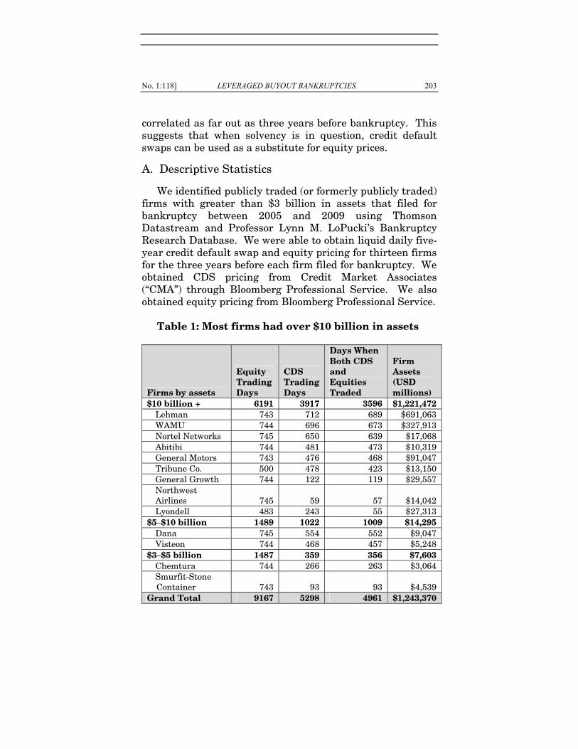
No. 1:118] LEVERAGED BUYOUT BANKRUPTCIES 203
correlated as far out as three years before bankruptcy. This suggests that when solvency is in question, credit default swaps can be used as a substitute for equity prices.
A. Descriptive Statistics
We identified publicly traded (or formerly publicly traded) firms with greater than $3 billion in assets that filed for bankruptcy between 2005 and 2009 using Thomson Datastream and Professor Lynn M. LoPucki’s Bankruptcy Research Database. We were able to obtain liquid daily five-year credit default swap and equity pricing for thirteen firms for the three years before each firm filed for bankruptcy. We obtained CDS pricing from Credit Market Associates (“CMA”) through Bloomberg Professional Service. We also obtained equity pricing from Bloomberg Professional Service.
Table 1: Most firms had over $10 billion in assets
Firms by assets
Equity Trading Days
CDS Trading Days
Days When Both CDS and Equities Traded
Firm Assets (USD millions)
$10 billion + 6191 3917 3596 $1,221,472 Lehman 743 712 689 $691,063 WAMU 744 696 673 $327,913 Nortel Networks 745 650 639 $17,068 Abitibi 744 481 473 $10,319 General Motors 743 476 468 $91,047 Tribune Co. 500 478 423 $13,150 General Growth 744 122 119 $29,557 Northwest Airlines 745 59 57 $14,042 Lyondell 483 243 55 $27,313
$5–$10 billion 1489 1022 1009 $14,295 Dana 745 554 552 $9,047 Visteon 744 468 457 $5,248
$3–$5 billion 1487 359 356 $7,603 Chemtura 744 266 263 $3,064 Smurfit-Stone
Container 743 93 93 $4,539 Grand Total 9167 5298 4961 $1,243,370
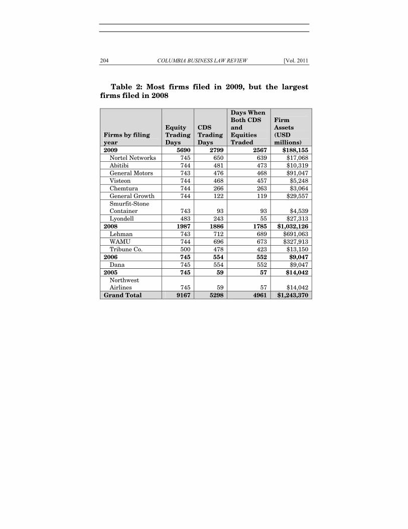
204 COLUMBIA BUSINESS LAW REVIEW [Vol. 2011
Table 2: Most firms filed in 2009, but the largest firms filed in 2008
Firms by filing year
Equity Trading Days
CDS Trading Days
Days When Both CDS and Equities Traded
Firm Assets (USD millions)
2009 5690 2799 2567 $188,155 Nortel Networks 745 650 639 $17,068 Abitibi 744 481 473 $10,319 General Motors 743 476 468 $91,047 Visteon 744 468 457 $5,248 Chemtura 744 266 263 $3,064 General Growth 744 122 119 $29,557 Smurfit-Stone Container 743 93 93 $4,539 Lyondell 483 243 55 $27,313
2008 1987 1886 1785 $1,032,126 Lehman 743 712 689 $691,063 WAMU 744 696 673 $327,913 Tribune Co. 500 478 423 $13,150
2006 745 554 552 $9,047 Dana 745 554 552 $9,047
2005 745 59 57 $14,042 Northwest Airlines 745 59 57 $14,042
Grand Total 9167 5298 4961 $1,243,370

No. 1:118] LEVERAGED BUYOUT BANKRUPTCIES 205
Table 3: Most firms were in manufacturing, but the largest were in finance and real estate
Firms by industry
Equity Trading Days
CDS Trading Days
Days When Both CDS and Equities Traded
Firm Assets (USD millions)
Manufacturing 5446 3059 2784 $163,727 Dana 745 554 552 $9,047 Abitibi 744 481 473 $10,319 General Motors 743 476 468 $91,047 Visteon 744 468 457 $5,248 Tribune Co. 500 478 423 $13,150 Chemtura 744 266 263 $3,064 Smurfit-Stone Container 743 93 93 $4,539 Lyondell 483 243 55 $27,313
Transportation, Communications, Electric, Gas 1490 709 696 $31,110
Nortel Networks 745 650 639 $17,068 Northwest Airlines 745 59 57 $14,042
Finance, Insurance, and Real Estate 2231 1530 1481 $1,048,533
Lehman 743 712 689 $691,063 WAMU 744 696 673 $327,913 General Growth 744 122 119 $29,557
Grand Total 9167 5298 4961 $1,243,370
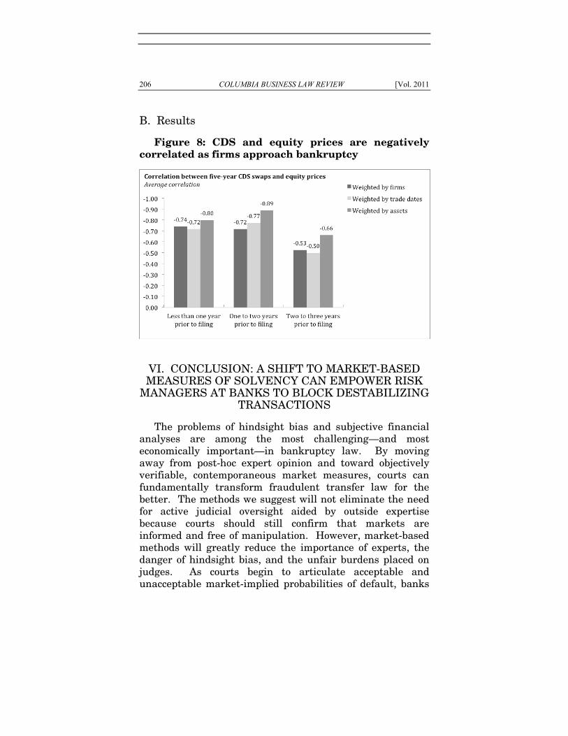
206 COLUMBIA BUSINESS LAW REVIEW [Vol. 2011
B. Results
Figure 8: CDS and equity prices are negatively correlated as firms approach bankruptcy
VI. CONCLUSION: A SHIFT TO MARKET-BASED MEASURES OF SOLVENCY CAN EMPOWER RISK
MANAGERS AT BANKS TO BLOCK DESTABILIZING TRANSACTIONS
The problems of hindsight bias and subjective financial analyses are among the most challenging—and most economically important—in bankruptcy law. By moving away from post-hoc expert opinion and toward objectively verifiable, contemporaneous market measures, courts can fundamentally transform fraudulent transfer law for the better. The methods we suggest will not eliminate the need for active judicial oversight aided by outside expertise because courts should still confirm that markets are informed and free of manipulation. However, market-based methods will greatly reduce the importance of experts, the danger of hindsight bias, and the unfair burdens placed on judges. As courts begin to articulate acceptable and unacceptable market-implied probabilities of default, banks
No. 1:118] LEVERAGED BUYOUT BANKRUPTCIES 207
and other creditors will be able to plan and adjust their behavior before problems arise. Banks can choose to forego funding LBOs or other transactions that would create liability.
Clear, predictable judicial guidance will empower risk managers at banks to block imprudent transactions. When times are good, default rates are low, and leveraged deals are plentiful, risk management is at the nadir of its power. Front office bankers who source deals and generate revenue outrank back office risk managers who appear to generate nothing but costs.243 People of lower rank rarely triumph in a bureaucracy. Their best chance of prevailing comes not when the situation is ambiguous—and charisma and entrenched power win the day—but when the data is clear as day.
When market prices become the best predictor of fraudulent transfer liability, banks can build contractual releases into their funding commitments that are tied to the relevant prices. With releases in place, if the condition of the debtor deteriorates between signing and closing, the bank need not face the Hobson’s choice of either walking away empty handed and being sued immediately by the LBO sponsor for breach of contract,244 or staying the course, collecting fees, and being sued later by bondholders under a theory of fraudulent transfer. In effect, bankruptcy courts and financial markets will jointly set minimum capital adequacy and liquidity standards for all non-financial firms,245 and large banks and other creditors will enforce
243 See TETT, supra note 173, at 112, 114–15, 134–35, 138. 244 The vagueness of currently used materially adverse change clauses
is an invitation to litigate. A contractual release tied to specific market indicators reaching specific levels would prevent litigation. Banks already use CDS spreads to adjust pricing on revolving credit facilities for risk. See Serena Ng, Banks Get Tougher on Credit Line Provisions, WALL ST. J., May 4, 2009, at A1.
245 Depository institutions and insurance companies are subject to special administrative insolvency regimes. Under the Dodd-Frank Wall Street Reform and Consumer Protection Act, almost any financial institution that the Secretary of the Treasury believes to be systemically important and “in default or in danger of default” may also be placed into

208 COLUMBIA BUSINESS LAW REVIEW [Vol. 2011
those standards. As a result of their gate-keeping activities, the law will be more fair, predictable, and administratively efficient. With fewer ill-conceived leveraged transactions and fewer resulting business bankruptcies, the economy will be more stable.
VII. APPENDIX I: EXPLANATION OF TRADITIONAL METHODS OF SOLVENCY
ANALYSIS
A. Liquidity Analysis
Liquidity analysis focuses on whether a debtor has sufficient cash to repay debt and continue as a going concern. It focuses on cash on hand and predictable future sources and uses of cash. The analysis often includes expected future ability to borrow as a source of cash.246 In addition, courts will often consider a debtor’s value independently of its liquidity.247 A debtor could theoretically have a high net worth, yet be unable to pay its debts as they become due or continue operations because the debtor has limited access to cash. The courts require a liquidity cushion capable of withstanding reasonably foreseeable setbacks, but not any and all setbacks.248 While this standard may seem prudent
an FDIC-administered “orderly liquidation” proceeding. H.R. 4173 § 202(b)(1)(A). Orderly liquidation authority requires either agreement by the board of directors of the financial institution or expedited court approval. Id. § 202(b)(2). For Broker-Dealers and Insurance companies, additional regulatory approvals are required. Id. § 205.
246 Peltz v. Hatten, 279 B.R. 710, 747 (D. Del. 2002) (finding that debtor would likely have been able to finance itself through, inter alia, the high-yield bond markets during two years of negative projected EBITDA).
247 See, e.g., MFS/Sun Life Trust-High Yield Series v. Van Dusen Airport Servs. Co., 910 F. Supp. 913, 944 (S.D.N.Y. 1995); Peltz, 279 B.R. at 742–43; Official Comm. of Former Partners v. Brennan (In re LaBrum & Doak, LLP), 227 B.R. 383, 387–88 (Bankr. E.D. Pa. 1998); Liebersohn v. Zisholtz (In re Martin’s Aquarium, Inc.), 225 B.R. 868, 876–77 (Bankr. E.D. Pa. 1998).
248 See, e.g., Van Dusen Airport Servs., 910 F. Supp. at 944 (“No doubt, [the debtor] could have weathered even these setbacks if it had unlimited
No. 1:118] LEVERAGED BUYOUT BANKRUPTCIES 209
on the surface, in practice it introduces tremendous uncertainty and potential for hindsight bias.249
B. Discounted Cash Flow (DCF)
Discounted cash flow (“DCF”) analysis has three primary components: (1) projections (or forecasts) of future cash flows of the debtor for a given period; (2) a terminal value used to limit the necessary projection period; and (3) a discount rate that is used to convert future cash flows and the terminal value into their present value.250 Cash flows are normally projected for a limited number of years.251 Cash flows beyond the explicit projection period are accounted for through a more loosely estimated “terminal value,” based either on an assumed constant perpetual growth rate or some form of multiples analysis (discussed infra).252
1. Projections
Projections are generally based on a financial model. The financial model can be thought of as a machine for synthesizing a series of small guesses (“assumptions”) about the future of components of the debtor’s business into a larger guess (“projections” or “forecasts”) about the future of the debtor’s business as a whole. The model is usually built
working capital, but that is not the proper legal standard. [The debtor] did retain sufficient capital to sustain its operation for a substantial period after the LBO.”).
249 See BREALEY, MYERS & ALLEN, supra note 71, at 309 (warning that accounting earnings and rates of return can be severely biased measures of true profitability); see generally In re Taxman Clothing Co., Inc., 905 F.2d 166, 170 (7th Cir. 1990) (warning courts that “[c]aution should be taken not to consider property as ‘dead’ merely because hindsight teaches that the debtor was traveling on the road to financial ruin”) (quoting 2 COLLIER ON BANKRUPTCY ¶101.31[5], at 101–94 (King 15 ed. 1989)).
250 See BREALEY, MYERS & ALLEN, supra note 71, at 65; Bernstein, Seabury & Williams, supra note 57, at 187; Doft & Co. v. Travelocity.com, Inc., 2004 WL 1152338, at *5 (Del. Ch. May 20, 2004, revised May 21, 2004).
251 See Bernstein, Seabury & Williams, supra note 57, at 188. 252 See id. at 188–89.
210 COLUMBIA BUSINESS LAW REVIEW [Vol. 2011
on spreadsheet software such as Microsoft Excel and is calibrated to a few years of the debtor’s historical performance.253 The projections are generated by making assumptions about how future conditions will differ from the recent past—changes in the price of raw materials or labor, synergies from a merger, demand for the debtor’s products or services, pricing, and margins. Sophisticated models may have granular detail about business units or even individual product lines.
2. Discount Rates
Discount rates are used to convert future cash flows into their present values.254 Future cash must be discounted because cash today is worth more than cash in the future. This is because cash today can be invested and will grow over time.255 Furthermore, although cash today is an indisputable fact, cash in the future is an uncertain prediction involving risk.256 Discounting attempts to take into account the riskiness of future cash flows by reducing the present value of those cash flows.257
3. Terminal Value
Terminal value is relevant to a static, balance sheet view of solvency, but not to a dynamic cash-flow view. As projections move further into the future, they become less and less certain. Rather than provide detailed but dubious projections into eternity, DCF models explicitly project a few years into the future and estimate the value of remaining cash flows through a “terminal value.” The terminal value
253 The number of years of past performance that should be considered
remains a source of controversy, and probably depends on the cyclicality of the debtor’s business, because both peak and trough conditions should be modeled. See KOLLER, GOEDHART & WESSELS, supra note 61, at 230, 659.
254 See BREALEY, MYERS & ALLEN, supra note 71, at 16; Bernstein, Seabury & Williams, supra note 57, at 189.
255 See BREALEY, MYERS & ALLEN, supra note 71, at 37. 256 See id. at 222–24. 257 See Bernstein, Seabury & Williams, supra note 57, at 189.
No. 1:118] LEVERAGED BUYOUT BANKRUPTCIES 211
generally depends on the discount rate, the cash flows projected in the last period of the explicit forecast, and the perpetual growth rate.
C. Multiples Analysis: Guideline (Comparable) Companies and Transactions
Multiples analysis is more relevant to the balance sheet concept of solvency than the cash-flow method. It values the debtor based on a ratio of market prices to some accounting metric.258 However, rather than use market prices of the debtor, this approach uses market prices of similar firms.259 Multiples can be either for equity alone (with the value of debt added later), or for the total value of the company including debt.
Performance metrics that are typically used include revenue, net income, and earnings before interest, taxes, depreciation, and amortization (“EBITDA”).260 EBITDA may be used instead of earnings because EBITDA strips away much of the effect of capital structure and accounting, leaving a proxy for cash flow from operations.261
Prices can either be trading prices of minority interests (i.e., the price at which the equity normally trades in the stock market) or prices paid for a controlling stake during an acquisition.262 When trading prices of minority interests are used, this method is referred to as “comparable company” or “guideline company” analysis. When the price of a controlling stake is used, this method is referred to as “similar transaction” analysis. Acquisition prices are generally higher than minority interest trading prices. This is widely believed to be because acquirers pay a control
258 See id. at 194. Commonly used metrics include revenue, EBIT, and
EBITDA. 259 See id.; KOLLER, GOEDHART & WESSELS, supra note 61, at 361. 260 See BREALEY, MYERS & ALLEN, supra note 71, at 511; KOLLER,
GOEDHART & WESSELS, supra note 61, at 361–80; Bernstein, Seabury & Williams, supra note 57, at 194.
261 See Bernstein, Seabury & Williams, supra note 57, at 188 n.95. 262 See id. at 194–95.
212 COLUMBIA BUSINESS LAW REVIEW [Vol. 2011
premium (or alternatively, because minority interests trade at a discount). All else being equal, the use of similar transactions will tend to yield higher multiples, and therefore higher valuations, than the use of guideline companies.
Guideline company and similar transactions analyses will suggest that “comparable” companies are worth a certain multiple of the relevant accounting metric—for example, one to two times the revenue or four to five times EBITDA. The value of the debtor is therefore inferred to also be within the range suggested by the multiples, or possibly near the mean or median of the multiples.
An example of a similar transaction analysis using equity multiples is provided below. The example analyzes the acquisition of Lyondell Chemical Company and was generated automatically using Bloomberg Professional Service.

No. 1:118] LEVERAGED BUYOUT BANKRUPTCIES 213
Table 4: An example of multiples analysis from the chemicals industry
Target Name Announced Date
Announced Value ($M) EBITDA EBIT
Lyondell Chemical Co 07/17/07 20,010.92 4.67 6.77 Comp Deals Median 9.48 13.94 Comp Deals Avg 10.7 16.6 Rohm and Haas Co 07/10/08 18,862.28 10.38 15.24 Imperial Chemical Industries PLC 06/18/07 16,059.40 11.92 15.48 SKW Trostberg 05/17/00 2,510.29 3.56 6.79 Celanese GmbH 12/16/03 2,216.09 11.53 Nova Chemicals Corp 02/23/09 2,076.97 2.11 Petkim Petrokimya Holding AS 10/16/07 1,873.57 22.36 39.69 BorsodChem NyRt 07/07/06 1,339.62 11.43 Vita Group/The 03/22/05 1,328.46 7.24 13.94 Foseco Ltd 10/11/07 1,198.95 8.59 10.63 DuPont Canada Inc 03/19/03 983.05 19.45 24.65
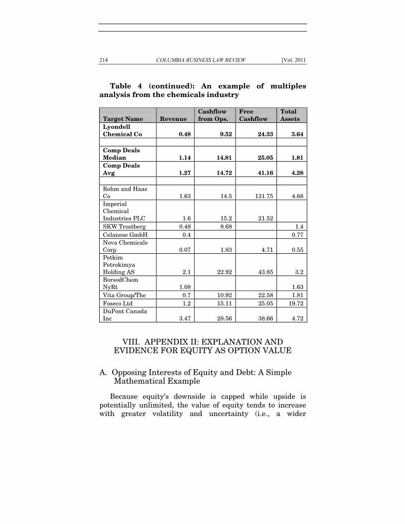
214 COLUMBIA BUSINESS LAW REVIEW [Vol. 2011
Table 4 (continued): An example of multiples analysis from the chemicals industry
Target Name Revenue Cashflow from Ops.
Free Cashflow
Total Assets
Lyondell Chemical Co 0.48 9.52 24.33 3.64 Comp Deals Median 1.14 14.81 25.05 1.81 Comp Deals Avg 1.27 14.72 41.16 4.28 Rohm and Haas Co 1.63 14.5 131.75 4.68 Imperial Chemical Industries PLC 1.6 15.2 21.52 SKW Trostberg 0.48 8.68 1.4 Celanese GmbH 0.4 0.77 Nova Chemicals Corp 0.07 1.83 4.71 0.55 Petkim Petrokimya Holding AS 2.1 22.92 43.85 3.2 BorsodChem NyRt 1.08 1.63 Vita Group/The 0.7 10.92 22.58 1.81 Foseco Ltd 1.2 15.11 25.05 19.72 DuPont Canada Inc 3.47 28.56 38.66 4.72
VIII. APPENDIX II: EXPLANATION AND EVIDENCE FOR EQUITY AS OPTION VALUE
A. Opposing Interests of Equity and Debt: A Simple Mathematical Example
Because equity’s downside is capped while upside is potentially unlimited, the value of equity tends to increase with greater volatility and uncertainty (i.e., a wider
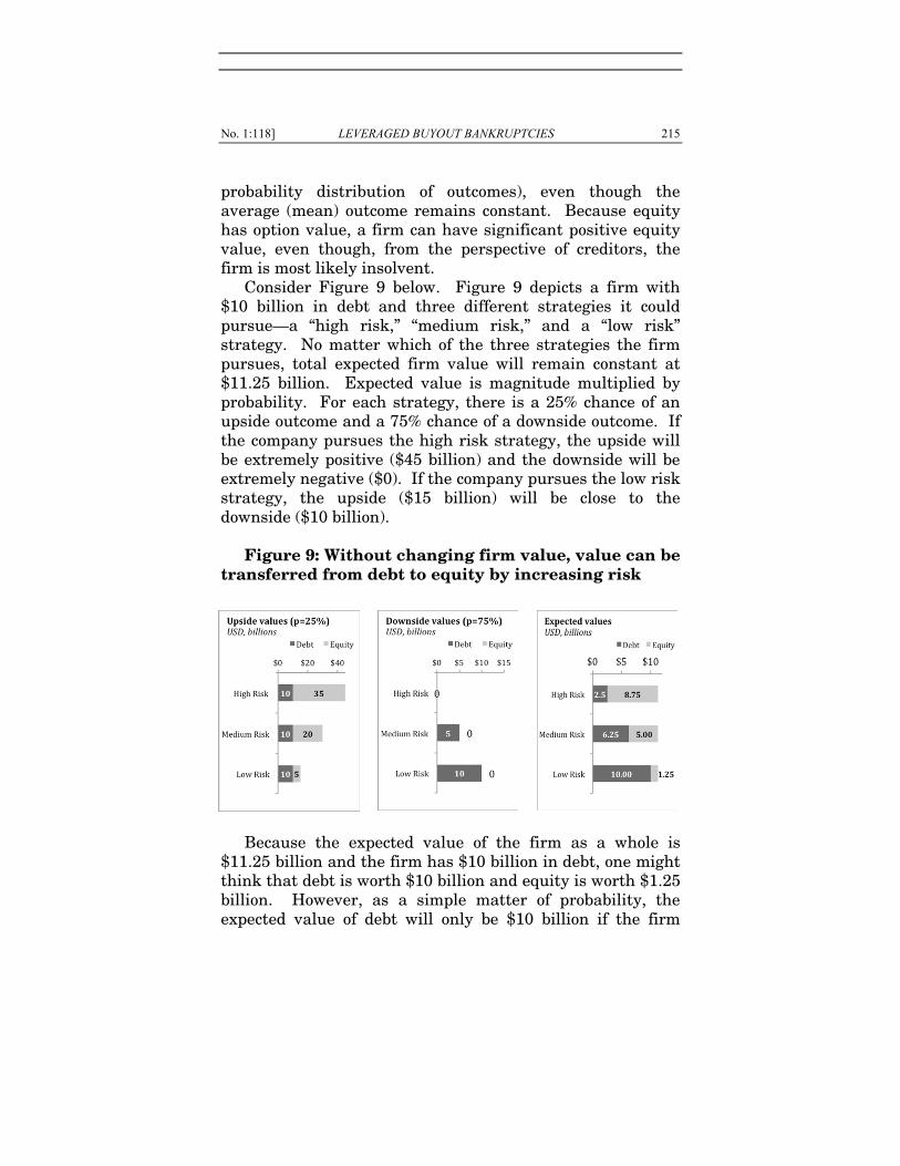
No. 1:118] LEVERAGED BUYOUT BANKRUPTCIES 215
probability distribution of outcomes), even though the average (mean) outcome remains constant. Because equity has option value, a firm can have significant positive equity value, even though, from the perspective of creditors, the firm is most likely insolvent.
Consider Figure 9 below. Figure 9 depicts a firm with $10 billion in debt and three different strategies it could pursue—a “high risk,” “medium risk,” and a “low risk” strategy. No matter which of the three strategies the firm pursues, total expected firm value will remain constant at $11.25 billion. Expected value is magnitude multiplied by probability. For each strategy, there is a 25% chance of an upside outcome and a 75% chance of a downside outcome. If the company pursues the high risk strategy, the upside will be extremely positive ($45 billion) and the downside will be extremely negative ($0). If the company pursues the low risk strategy, the upside ($15 billion) will be close to the downside ($10 billion).
Figure 9: Without changing firm value, value can be
transferred from debt to equity by increasing risk
Because the expected value of the firm as a whole is
$11.25 billion and the firm has $10 billion in debt, one might think that debt is worth $10 billion and equity is worth $1.25 billion. However, as a simple matter of probability, the expected value of debt will only be $10 billion if the firm
216 COLUMBIA BUSINESS LAW REVIEW [Vol. 2011
pursues the low risk strategy. If the firm pursues either the high risk or medium risk strategy, equity will benefit while debt will experience steep losses. By shifting from the low risk strategy to the high risk strategy, the firm can slash the expected value of debt to one fourth of par value, while increasing the expected value of equity to seven times book value.
B. Opposing Interests of Equity and Debt: Empirical Evidence
That existing shareholders can benefit while existing bondholders are harmed has been well documented in the empirical finance literature. Examples of events that have been found to benefit stockholders and harm debt holders include: hedge fund activism,263 LBOs,264 and dividend payments.265 Of course, other transactions, such as seasoned equity offerings, benefit existing bondholders at the expense of existing equity holders.266
Although some actions may benefit both equity holders and debt holders by increasing the value of the firm as a whole, it is sometimes harder to grow the pie than to use financial engineering to slice it to the advantage of one class of investors. Some transactions, including many LBOs, may simultaneously increase the value of the firm as a whole
263 See April Klein & Emanuel Zur, The Impact of Hedge Fund
Activism on the Target Firm’s Existing Bondholders 2 (May 2010) (unpublished manuscript), available at http://papers.ssrn.com/sol3/ papers.cfm?abstract_id=1572594 (finding positive returns to shareholders and negative returns to bondholders following hedge fund activism and evidence of expropriation of wealth from bondholders to shareholders).
264 See Warga & Welch, supra note 18; Matthew T. Billett, Zhan Jiang & Erik Lie, The Role of Bondholder Wealth Expropriation in LBO Transactions (March 2008) (unpublished manuscript), available at http://papers.ssrn.com/sol3/papers.cfm?abstract_id=1107448.
265 See Upinder S. Dhillon & Herb Johnson, The Effect of Dividend Changes on Stock and Bond Prices, 49 J. FIN. 281 (1994).
266 See Allan C. Eberhart & Akhtar Siddique, The Long-Term Performance of Corporate Bonds (and Stocks) Following Seasoned Equity Offerings, 15 REV. FIN. STUD. 1385 (2002).
No. 1:118] LEVERAGED BUYOUT BANKRUPTCIES 217
while expropriating wealth from one class of creditor to another.267
C. Opposing Interests of Equity and Debt: Real World Strategic Implications
The figures above are far more than an exercise in probability. They illustrate the strategic dynamic that animates every negotiation between debt holders and equity holders. Equityholders tend to favor high risk operational and financing decisions while debt holders, whose upside is capped, tend to favor conservative operational and financing decisions. Debt holders try to constrain equity holders’ freedom to take risks through covenants, change-of-control provisions, and other mechanisms designed to protect them from a risky shift in management strategy.
Fraudulent transfer law provides creditors with an additional measure of protection above and beyond contractual negotiations. The policy goal is presumably to encourage LBOs that are likely to increase the value of firms as a whole rather than to simply transfer value from debt holders to equity.
One of the mechanisms courts have used to try to identify “bad” LBOs is to consider how much of its own money the sponsor leaves inside the firm.268 Like all options, equity usually has a cost—the cash that the equity holder pays to the firm and that remains inside the firm. The less cash the equity holder leaves inside the firm, the lower the equity holder’s risk of loss, the cheaper the option, and greater the net value.
The appeal of LBO transactions is that they give the sponsor (the private equity firm that becomes the new owner) a very cheap or sometimes free option. If the buyout
267 See Klein & Zur, supra note 263; supra note 20 and accompanying
text. 268 See Official Comm. of Unsecured Creditors of Grand Eagle Cos. v.
Asea Brown Boveri, Inc., 313 B.R. 219, 230 (N.D. Ohio 2004); In re C-T of Va, Inc., 124 B.R. 694, 698–99 (W.D. Va. 1990), aff’d, 958 F.2d 606 (4th Cir. 1992).
218 COLUMBIA BUSINESS LAW REVIEW [Vol. 2011
is entirely funded by debt, or if the sponsor is able to extract its cash shortly after the close of the transaction through dividends, management fees, or some other device, then the sponsor can only experience upside and has no downside risk of loss. The sponsor therefore has strong incentives to pursue risky strategies such as mergers, roll-ups, divestitures, or drastic cost cutting that could either succeed spectacularly or fail miserably. If the sponsor stands to lose some of its own money, it might be somewhat more cognizant of downside risk.
By contrast, normal corporate managers, who are generally not significant equity owners, might pursue overly conservative strategies to preserve their jobs or to protect the interests of stakeholders other than equity. How much risk taking is optimal remains open to debate, and fraudulent transfer law strives to find a happy medium.
IX. APPENDIX III: DERIVATION AND ILLUSTRATION OF EQUATION 3
The relationship between the risk-free rate, the yield on a corporate bond, the probability of default, and the expected loss rate given default under idealized conditions was previously summarized by Equation 3:
(probability of default in year 1) = [1 - (1 + risk-free rate) /
(1 + corporate bond yield)] / (expected loss rate given default) This equation can be rewritten in mathematical notation
as: D = [1 - (1 + G) / (1 + X)] / (L) or D = (1 / L)*(1- (1 + G) / (1 + X)) where: G = risk-free rate X = corporate bond rate D = perceived probability of default in year 1; (1 - D) =
perceived probability of no default in year 1 L = loss rate given default; (1 - L) = recovery rate
No. 1:118] LEVERAGED BUYOUT BANKRUPTCIES 219
For the derivation of this formula, we will also use the following notation:
I = principal investment Consider a rational risk-neutral investor who represents
the aggregate views of all investors in an idealized perfect credit market. Our investor can either invest his principal (I) in a one-year government bond that yields (G) or in a one-year corporate bond that yields (X). If neither bond defaults, then the payoff from the government bond in one year will be (I) * (1 + G), while the payoff from the corporate bond will be (I) * (1 + X).
The investor believes that the government bond carries zero risk of default but that the corporate bond carries a risk of default, (D). The investor believes that if the corporate bond issuer defaults, his loss rate will be (L), his total losses will be (L) * (I) * (1 + X), and his total recovery will be (1 - L) * (I) * (1 + X). Assume that both bonds pay at the end of the year, and that a default can only occur at the end of the year.
Because we are assuming idealized market conditions, competition between the government and corporate issuers—or simply between different corporate issuers—will lead prices and yields to adjust until rational risk-neutral investors perceive the payoff of both investments to be equal.
Our investor believes there is only one possible outcome for investment in the government bond. He expects the future value of the government bond to be his principal investment (I) plus interest (G) * (I), for a payoff of (I) * (1 + G).
By contrast, the investor expects two possible outcomes for the investment in the corporate bond. There is a probability of no default (1 - D), in which case his payoff will be his principal investment (I) plus interest (I) * (X), for a payoff of (I) * (1 + X). The expected value of this payoff is its probability times its magnitude, or (1 - D) * (I) * (1 + X). There is also a probability of default (D), in which case his payoff will be his recovery rate (1 - L) times his expected payoff under the no-default condition, for a total payoff of (1 -

220 COLUMBIA BUSINESS LAW REVIEW [Vol. 2011
L) * (I) * (1 + X). The expected value of the payoff under the no default condition is (D) * (1 - L) * (1 + X) * (I).
The expected value of the corporate bond investment is the sum of the expected values of the default condition and no-default condition, which is:
(1 - D) * (1 + X) * (I) + (D) * (1 - L) * (1 + X) * (I) The expected value of the corporate bond investment can
be rewritten as: (I) * (1 + X) * [(1 - D) + (D) * (1 - L)] = (I) * (1 + X) * [(1 - D + D - (D * L)] = (I) * (1 + X) * (1 - D * L). When we set the corporate and government bond
expected values equal to one another, we get: (I)*(1 + G) = (I)*(1 + X)*(1 - D * L) = (1 + G)/(1 + X) = 1 - D * L = 1 - (1 + G) / (1 + X) = D*L Solving for the perceived probability of default in year 1
(D), we get: D = (1/L)*(1- (1 + G)/(1 + X)) which is Equation 3. This equation can also be rewritten to solve for expected
loss rate given default, corporate bond yield, or risk-free rate: L = (1/D)*(1- (1 + G)/(1 + X)) X = (1 + G)/(1 - D*L) -1 G = (1+ X)(1 - D*L) - 1 The following is an example of the rough precision of
Equation 2 compared to the more precise, but more complex, Equation 3.
A rational, risk-neutral investor has $100 that he can invest in either a one-year corporate bond or in a one-year government bond that yields 3%. The investor believes that the government bond carries zero risk of default but that the corporate bond carries a 6% risk of default. The investor
No. 1:118] LEVERAGED BUYOUT BANKRUPTCIES 221
believes that if the corporate bond issuer defaults, he will likely lose 50% of his money.
The investor believes there is only one possible outcome for investment in the government bond. He expects the future value of the government bond to be his principal investment plus 3% interest, or $103.
By contrast, the investor expects two possible outcomes for the investment in the corporate bond. There is a 94% probability of no default, in which case his payoff will be $100 plus interest. However, there is also a 6% probability of default, in which case his payoff will be $50 plus half of the interest.
Equation 2 suggests that the corporate bond should yield 6%.269 This is only approximately right—when the corporate bond yields 6%, the expected value of both bonds is roughly, but not precisely equal.
The expected value of the corporate bond investment is the sum of the expected values of the default and no-default condition. The expected value of the no-default condition is 6% probability * $106 payoff = $99.64. The expected value of the default condition is 6% probability * $53 payoff = $3.18. The sum of $99.64 and $3.18 is $102.82, just shy of $103. As discussed above, Equation 2 is an approximation; a more precise answer requires a more complex equation.
The corporate bond yield must be 6.19%, slightly higher than the 6% suggested by our simple Equation 2, to make both investments equally attractive to a risk neutral investor. If we use Equation 3 and rewrite it to solve for the corporate yield, we get:
corporate yield = [(1 + risk-free rate) / (1 - probability of default * Loss given default)] - 1
corporate yield = [(1 + 0.03)/(1 - (0.06)*(0.5)] -1 = [(1.03)/(1 - 0.03)] – 1
= (1.03)/(0.97) - 1 = 0.061856 = 6.19%.
269 6% probability of default * 50% loss given default = 3% spread; 3%
risk-free yield + 3% spread = 6% corporate yield.