


Lee Seshia Digital V1 08
519
Transcript of Lee Seshia Digital V1 08

Copyright c©2011-2012Edward Ashford Lee & Sanjit Arunkumar Seshia
All rights reserved
First Edition, Version 1.08
ISBN 978-0-557-70857-4
Please cite this book as:
E. A. Lee and S. A. Seshia,Introduction to Embedded Systems - A Cyber-Physical Systems Approach,
LeeSeshia.org, 2011.

This book is dedicated to our families.


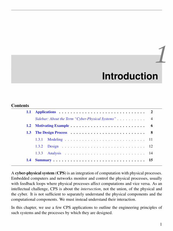
Contents
Preface . . . . . . . . . . . . . . . . . . . . . . . . . . . . . . . . . . . . . . xi
1 Introduction 11.1 Applications . . . . . . . . . . . . . . . . . . . . . . . . . . . . . . . . . 2
1.2 Motivating Example . . . . . . . . . . . . . . . . . . . . . . . . . . . . 6
1.3 The Design Process . . . . . . . . . . . . . . . . . . . . . . . . . . . . . 8
1.4 Summary . . . . . . . . . . . . . . . . . . . . . . . . . . . . . . . . . . 15
I Modeling Dynamic Behaviors 17
2 Continuous Dynamics 19
2.1 Newtonian Mechanics . . . . . . . . . . . . . . . . . . . . . . . . . . . . 202.2 Actor Models . . . . . . . . . . . . . . . . . . . . . . . . . . . . . . . . 252.3 Properties of Systems . . . . . . . . . . . . . . . . . . . . . . . . . . . . 29
2.4 Feedback Control . . . . . . . . . . . . . . . . . . . . . . . . . . . . . . 322.5 Summary . . . . . . . . . . . . . . . . . . . . . . . . . . . . . . . . . . 37
Exercises . . . . . . . . . . . . . . . . . . . . . . . . . . . . . . . . . . . . . 38
v

3 Discrete Dynamics 41
3.1 Discrete Systems . . . . . . . . . . . . . . . . . . . . . . . . . . . . . . 42
3.2 The Notion of State . . . . . . . . . . . . . . . . . . . . . . . . . . . . . 46
3.3 Finite-State Machines . . . . . . . . . . . . . . . . . . . . . . . . . . . . 47
3.4 Extended State Machines . . . . . . . . . . . . . . . . . . . . . . . . . . 57
3.5 Nondeterminism . . . . . . . . . . . . . . . . . . . . . . . . . . . . . . 63
3.6 Behaviors and Traces . . . . . . . . . . . . . . . . . . . . . . . . . . . . 66
3.7 Summary . . . . . . . . . . . . . . . . . . . . . . . . . . . . . . . . . . 70
Exercises . . . . . . . . . . . . . . . . . . . . . . . . . . . . . . . . . . . . . 71
4 Hybrid Systems 77
4.1 Modal Models . . . . . . . . . . . . . . . . . . . . . . . . . . . . . . . . 78
4.2 Classes of Hybrid Systems . . . . . . . . . . . . . . . . . . . . . . . . . 82
4.3 Summary . . . . . . . . . . . . . . . . . . . . . . . . . . . . . . . . . . 98
Exercises . . . . . . . . . . . . . . . . . . . . . . . . . . . . . . . . . . . . . 100
5 Composition of State Machines 107
5.1 Concurrent Composition . . . . . . . . . . . . . . . . . . . . . . . . . . 109
5.2 Hierarchical State Machines . . . . . . . . . . . . . . . . . . . . . . . . 124
5.3 Summary . . . . . . . . . . . . . . . . . . . . . . . . . . . . . . . . . . 128
Exercises . . . . . . . . . . . . . . . . . . . . . . . . . . . . . . . . . . . . . 130
6 Concurrent Models of Computation 133
6.1 Structure of Models . . . . . . . . . . . . . . . . . . . . . . . . . . . . . 135
6.2 Synchronous-Reactive Models . . . . . . . . . . . . . . . . . . . . . . . 136
6.3 Dataflow Models of Computation . . . . . . . . . . . . . . . . . . . . . . 146
6.4 Timed Models of Computation . . . . . . . . . . . . . . . . . . . . . . . 160
6.5 Summary . . . . . . . . . . . . . . . . . . . . . . . . . . . . . . . . . . 168
Exercises . . . . . . . . . . . . . . . . . . . . . . . . . . . . . . . . . . . . . 169
vi Lee & Seshia, Introduction to Embedded Systems

II Design of Embedded Systems 175
7 Embedded Processors 1777.1 Types of Processors . . . . . . . . . . . . . . . . . . . . . . . . . . . . . 179
7.2 Parallelism . . . . . . . . . . . . . . . . . . . . . . . . . . . . . . . . . 1877.3 Summary . . . . . . . . . . . . . . . . . . . . . . . . . . . . . . . . . . 204
Exercises . . . . . . . . . . . . . . . . . . . . . . . . . . . . . . . . . . . . . 205
8 Memory Architectures 207
8.1 Memory Technologies . . . . . . . . . . . . . . . . . . . . . . . . . . . 208
8.2 Memory Hierarchy . . . . . . . . . . . . . . . . . . . . . . . . . . . . . 210
8.3 Memory Models . . . . . . . . . . . . . . . . . . . . . . . . . . . . . . . 219
8.4 Summary . . . . . . . . . . . . . . . . . . . . . . . . . . . . . . . . . . 224
Exercises . . . . . . . . . . . . . . . . . . . . . . . . . . . . . . . . . . . . . 225
9 Input and Output 227
9.1 I/O Hardware . . . . . . . . . . . . . . . . . . . . . . . . . . . . . . . . 2289.2 Sequential Software in a Concurrent World . . . . . . . . . . . . . . . . 240
9.3 The Analog/Digital Interface . . . . . . . . . . . . . . . . . . . . . . . . 250
9.4 Summary . . . . . . . . . . . . . . . . . . . . . . . . . . . . . . . . . . 259
Exercises . . . . . . . . . . . . . . . . . . . . . . . . . . . . . . . . . . . . . 260
10 Multitasking 269
10.1 Imperative Programs . . . . . . . . . . . . . . . . . . . . . . . . . . . . 272
10.2 Threads . . . . . . . . . . . . . . . . . . . . . . . . . . . . . . . . . . . 27610.3 Processes and Message Passing . . . . . . . . . . . . . . . . . . . . . . . 289
10.4 Summary . . . . . . . . . . . . . . . . . . . . . . . . . . . . . . . . . . 294
Exercises . . . . . . . . . . . . . . . . . . . . . . . . . . . . . . . . . . . . . 295
11 Scheduling 297
11.1 Basics of Scheduling . . . . . . . . . . . . . . . . . . . . . . . . . . . . 298
Lee & Seshia, Introduction to Embedded Systems vii

11.2 Rate Monotonic Scheduling . . . . . . . . . . . . . . . . . . . . . . . . 304
11.3 Earliest Deadline First . . . . . . . . . . . . . . . . . . . . . . . . . . . 30911.4 Scheduling and Mutual Exclusion . . . . . . . . . . . . . . . . . . . . . 314
11.5 Multiprocessor Scheduling . . . . . . . . . . . . . . . . . . . . . . . . . 319
11.6 Summary . . . . . . . . . . . . . . . . . . . . . . . . . . . . . . . . . . 323
Exercises . . . . . . . . . . . . . . . . . . . . . . . . . . . . . . . . . . . . . 325
III Analysis and Verification 331
12 Invariants and Temporal Logic 333
12.1 Invariants . . . . . . . . . . . . . . . . . . . . . . . . . . . . . . . . . . 33512.2 Linear Temporal Logic . . . . . . . . . . . . . . . . . . . . . . . . . . . 337
12.3 Summary . . . . . . . . . . . . . . . . . . . . . . . . . . . . . . . . . . 345
Exercises . . . . . . . . . . . . . . . . . . . . . . . . . . . . . . . . . . . . . 347
13 Equivalence and Refinement 351
13.1 Models as Specifications . . . . . . . . . . . . . . . . . . . . . . . . . . 352
13.2 Type Equivalence and Refinement . . . . . . . . . . . . . . . . . . . . . 354
13.3 Language Equivalence and Containment . . . . . . . . . . . . . . . . . . 356
13.4 Simulation . . . . . . . . . . . . . . . . . . . . . . . . . . . . . . . . . . 36213.5 Bisimulation . . . . . . . . . . . . . . . . . . . . . . . . . . . . . . . . . 37013.6 Summary . . . . . . . . . . . . . . . . . . . . . . . . . . . . . . . . . . 372
Exercises . . . . . . . . . . . . . . . . . . . . . . . . . . . . . . . . . . . . . 373
14 Reachability Analysis and Model Checking 379
14.1 Open and Closed Systems . . . . . . . . . . . . . . . . . . . . . . . . . 380
14.2 Reachability Analysis . . . . . . . . . . . . . . . . . . . . . . . . . . . . 382
14.3 Abstraction in Model Checking . . . . . . . . . . . . . . . . . . . . . . . 389
14.4 Model Checking Liveness Properties . . . . . . . . . . . . . . . . . . . . 392
14.5 Summary . . . . . . . . . . . . . . . . . . . . . . . . . . . . . . . . . . 397
viii Lee & Seshia, Introduction to Embedded Systems

Exercises . . . . . . . . . . . . . . . . . . . . . . . . . . . . . . . . . . . . . 400
15 Quantitative Analysis 401
15.1 Problems of Interest . . . . . . . . . . . . . . . . . . . . . . . . . . . . . 40315.2 Programs as Graphs . . . . . . . . . . . . . . . . . . . . . . . . . . . . . 405
15.3 Factors Determining Execution Time . . . . . . . . . . . . . . . . . . . . 410
15.4 Basics of Execution Time Analysis . . . . . . . . . . . . . . . . . . . . . 416
15.5 Other Quantitative Analysis Problems . . . . . . . . . . . . . . . . . . . 425
15.6 Summary . . . . . . . . . . . . . . . . . . . . . . . . . . . . . . . . . . 427
Exercises . . . . . . . . . . . . . . . . . . . . . . . . . . . . . . . . . . . . . 429
IV Appendices 431
A Sets and Functions 433A.1 Sets . . . . . . . . . . . . . . . . . . . . . . . . . . . . . . . . . . . . . 433A.2 Relations and Functions . . . . . . . . . . . . . . . . . . . . . . . . . . . 434A.3 Sequences . . . . . . . . . . . . . . . . . . . . . . . . . . . . . . . . . . 438
Exercises . . . . . . . . . . . . . . . . . . . . . . . . . . . . . . . . . . . . . 441
B Complexity and Computability 443
B.1 Effectiveness and Complexity of Algorithms . . . . . . . . . . . . . . . . 444
B.2 Problems, Algorithms, and Programs . . . . . . . . . . . . . . . . . . . . 447
B.3 Turing Machines and Undecidability . . . . . . . . . . . . . . . . . . . . 449
B.4 Intractability: P and NP . . . . . . . . . . . . . . . . . . . . . . . . . . . 455
B.5 Summary . . . . . . . . . . . . . . . . . . . . . . . . . . . . . . . . . . 459
Exercises . . . . . . . . . . . . . . . . . . . . . . . . . . . . . . . . . . . . . 460
Bibliography 461
Notation Index 477
Index 479
Lee & Seshia, Introduction to Embedded Systems ix

Preface
What this Book is About
The most visible use of computers and software is processing information for humanconsumption. We use them to write books (like this one), search for information onthe web, communicate via email, and keep track of financial data. The vast majority ofcomputers in use, however, are much less visible. They run the engine, brakes, seatbelts,airbag, and audio system in your car. They digitally encode your voice and construct aradio signal to send it from your cell phone to a base station. They control your microwaveoven, refrigerator, and dishwasher. They run printers ranging from desktop inkjet printersto large industrial high-volume printers. They command robots on a factory floor, powergeneration in a power plant, processes in a chemical plant, and traffic lights in a city. Theysearch for microbes in biological samples, construct images of the inside of a human body,and measure vital signs. They process radio signals from space looking for supernovaeand for extraterrestrial intelligence. They bring toys to life, enabling them to react tohuman touch and to sounds. They control aircraft and trains. These less visible computersare called embedded systems, and the software they run is called embedded software.
Despite this widespread prevalence of embedded systems, computer science has, through-out its relatively short history, focused primarily on information processing. Only recentlyhave embedded systems received much attention from researchers. And only recently has
xi

PREFACE
the community recognized that the engineering techniques required to design and ana-lyze these systems are distinct. Although embedded systems have been in use since the1970s, for most of their history they were seen simply as small computers. The principalengineering problem was understood to be one of coping with limited resources (limitedprocessing power, limited energy sources, small memories, etc.). As such, the engineer-ing challenge was to optimize the designs. Since all designs benefit from optimization,the discipline was not distinct from anything else in computer science. It just had to bemore aggressive about applying the same optimization techniques.
Recently, the community has come to understand that the principal challenges in em-bedded systems stem from their interaction with physical processes, and not from theirlimited resources. The term cyber-physical systems (CPS) was coined by Helen Gill at theNational Science Foundation in the U.S. to refer to the integration of computation withphysical processes. In CPS, embedded computers and networks monitor and control thephysical processes, usually with feedback loops where physical processes affect compu-tations and vice versa. The design of such systems, therefore, requires understanding thejoint dynamics of computers, software, networks, and physical processes. It is this studyof joint dynamics that sets this discipline apart.
When studying CPS, certain key problems emerge that are rare in so-called general-purpose computing. For example, in general-purpose software, the time it takes to per-form a task is an issue of performance, not correctness. It is not incorrect to take longerto perform a task. It is merely less convenient and therefore less valuable. In CPS, thetime it takes to perform a task may be critical to correct functioning of the system. In thephysical world, as opposed to the cyber world, the passage of time is inexorable.
In CPS, moreover, many things happen at once. Physical processes are compositionsof many things going on at once, unlike software processes, which are deeply rootedin sequential steps. Abelson and Sussman (1996) describe computer science as “proce-dural epistemology,” knowledge through procedure. In the physical world, by contrast,processes are rarely procedural. Physical processes are compositions of many parallelprocesses. Measuring and controlling the dynamics of these processes by orchestratingactions that influence the processes are the main tasks of embedded systems. Conse-quently, concurrency is intrinsic in CPS. Many of the technical challenges in designingand analyzing embedded software stem from the need to bridge an inherently sequentialsemantics with an intrinsically concurrent physical world.
xii Lee & Seshia, Introduction to Embedded Systems
PREFACE
Why We Wrote this Book
Today, getting computers to work together with physical processes requires technicallyintricate, low-level design. Embedded software designers are forced to struggle with inter-rupt controllers, memory architectures, assembly-level programming (to exploit special-ized instructions or to precisely control timing), device driver design, network interfaces,and scheduling strategies, rather than focusing on specifying desired behavior. The sheermass and complexity of these technologies tempts us to focus an introductory course onmastering them. But a better introductory course would focus on how to model and designthe joint dynamics of software, networks, and physical processes. Such a course wouldpresent the technologies only as today’s (rather primitive) means of accomplishing thosejoint dynamics. This book is our attempt at a textbook for such a course.
Most texts on embedded systems focus on the collection of technologies needed to getcomputers to interact with physical systems (Barr and Massa, 2006; Berger, 2002; Burnsand Wellings, 2001; Kamal, 2008; Noergaard, 2005; Parab et al., 2007; Simon, 2006; Val-vano, 2007; Wolf, 2000). Others focus on adaptations of computer-science techniques(like programming languages, operating systems, networking, etc.) to deal with techni-cal problems in embedded systems (Buttazzo, 2005a; Edwards, 2000; Pottie and Kaiser,2005). While these implementation technologies are (today) necessary for system de-signers to get embedded systems working, they do not form the intellectual core of thediscipline. The intellectual core is instead in models and abstractions that conjoin com-putation and physical dynamics.
A few textbooks offer efforts in this direction. Jantsch (2003) focuses on concurrent mod-els of computation, Marwedel (2011) focuses on models of software and hardware behav-ior, and Sriram and Bhattacharyya (2009) focus on dataflow models of signal processingbehavior and their mapping onto programmable DSPs. These are excellent starting points.Models of concurrency (such as dataflow) and abstract models of software (such as Stat-echarts) provide a better starting point than imperative programming languages (like C),interrupts and threads, and architectural annoyances that a designer must work around(like caches). These texts, however, are not suitable for an introductory course. They areeither too specialized or too advanced or both. This book is our attempt to provide anintroductory text that follows the spirit of focusing on models and their relationship torealizations of systems.
The major theme of this book is on models and their relationship to realizations of sys-tems. The models we study are primarily about dynamics, the evolution of a system state
Lee & Seshia, Introduction to Embedded Systems xiii

PREFACE
in time. We do not address structural models, which represent static information about theconstruction of a system, although these too are important to embedded system design.
Working with models has a major advantage. Models can have formal properties. We cansay definitive things about models. For example, we can assert that a model is determinate,meaning that given the same inputs it will always produce the same outputs. No suchabsolute assertion is possible with any physical realization of a system. If our model isa good abstraction of the physical system (here, “good abstraction” means that it omitsonly inessential details), then the definitive assertion about the model gives us confidencein the physical realization of the system. Such confidence is hugely valuable, particularlyfor embedded systems where malfunctions can threaten human lives. Studying models ofsystems gives us insight into how those systems will behave in the physical world.
Our focus is on the interplay of software and hardware with the physical environment inwhich they operate. This requires explicit modeling of the temporal dynamics of soft-ware and networks and explicit specification of concurrency properties intrinsic to theapplication. The fact that the implementation technologies have not yet caught up withthis perspective should not cause us to teach the wrong engineering approach. We shouldteach design and modeling as it should be, and enrich this with a critical presentation ofhow to (partially) accomplish our objectives with today’s technology. Embedded systemstechnologies today, therefore, should not be presented dispassionately as a collection offacts and tricks, as they are in many of the above cited books, but rather as stepping stonestowards a sound design practice. The focus should be on what that sound design practiceis, and on how today’s technologies both impede and achieve it.
Stankovic et al. (2005) support this view, stating that “existing technology for RTES [real-time embedded systems] design does not effectively support the development of reliableand robust embedded systems.” They cite a need to “raise the level of programmingabstraction.” We argue that raising the level of abstraction is insufficient. We have alsoto fundamentally change the abstractions that are used. Timing properties of software,for example, cannot be effectively introduced at higher levels of abstraction if they areentirely absent from the lower levels of abstraction on which these are built.
We require robust and predictable designs with repeatable temporal dynamics (Lee, 2009a).We must do this by building abstractions that appropriately reflect the realities of cyber-physical systems. The result will be CPS designs that can be much more sophisticated,including more adaptive control logic, evolvability over time, and improved safety and re-liability, all without suffering from the brittleness of today’s designs, where small changeshave big consequences.
xiv Lee & Seshia, Introduction to Embedded Systems

PREFACE
In addition to dealing with temporal dynamics, CPS designs invariably face challengingconcurrency issues. Because software is so deeply rooted in sequential abstractions, con-currency mechanisms such as interrupts and multitasking, using semaphores and mutualexclusion, loom large. We therefore devote considerable effort in this book to developinga critical understanding of threads, message passing, deadlock avoidance, race conditions,and data determinism.
What is Missing
This version of the book is not complete. It is arguable, in fact, that complete coverage ofembedded systems in the context of CPS is impossible. Specific topics that we cover inthe undergraduate Embedded Systems course at Berkeley (see http://LeeSeshia.org) andhope to include in future versions of this book include sensors and actuators, networking,fault tolerance, security, simulation techniques, control systems, and hardware/softwarecodesign.
How to Use this Book
This book is divided into three major parts, focused on modeling, design, and analysis, asshown in Figure 1. The three parts of the book are relatively independent of one anotherand are largely meant to be read concurrently. A systematic reading of the text can beaccomplished in seven segments, shown with dashed outlines. Each segment includes twochapters, so complete coverage of the text is possible in a 15 week semester, assumingeach of the seven modules takes two weeks, and one week is allowed for introduction andclosing.
The appendices provide background material that is well covered in other textbooks, butwhich can be quite helpful in reading this text. Appendix A reviews the notation ofsets and functions. This notation enables a higher level of precision that is commonin the study of embedded systems. Appendix B reviews basic results in the theory ofcomputability and complexity. This facilitates a deeper understanding of the challengesin modeling and analysis of systems. Note that Appendix B relies on the formalism ofstate machines covered in Chapter 3, and hence should be read after reading Chapter 3.
In recognition of recent advances in technology that are fundamentally changing the tech-nical publishing industry, this book is published in a non-traditional way. At least thepresent version is available free in the form of PDF file designed specifically for on-line
Lee & Seshia, Introduction to Embedded Systems xv

PREFACE
reading. It can be obtained from the website http://LeeSeshia.org. The layout is optimizedfor medium-sized screens, particularly laptop computers and the iPad and other tablets.Extensive use of hyperlinks and color enhance the online reading experience.
Figure 1: Map of the book with strong and weak dependencies between chapters.Strong dependencies between chapters are shown with arrows in black. Weakdependencies are shown in grey. When there is a weak dependency from chapteri to chapter j, then j may mostly be read without reading i, at most requiringskipping some examples or specialized analysis techniques.
xvi Lee & Seshia, Introduction to Embedded Systems

PREFACE
We attempted to adapt the book to e-book formats, which, in theory, enable reading onvarious sized screens, attempting to take best advantage of the available screen. However,like HTML documents, e-book formats use a reflow technology, where page layout isrecomputed on the fly. The results are highly dependent on the screen size and proveludicrous on many screens and suboptimal on all. As a consequence, we have optedfor controlling the layout, and we do not recommend attempting to read the book on aniPhone.
Although the electronic form is convenient, we recognize that there is real value in atangible manifestation on paper, something you can thumb through, something that canlive on a bookshelf to remind you of its existence. Hence, the book is also available in printform from a print-on-demand service. This has the advantages of dramatically reducedcost to the reader (compared with traditional publishers) and the ability to quickly andfrequently update the version of the book to correct errors and discuss new technologies.See the website http://LeeSeshia.org for instructions on obtaining the printed version.
Two disadvantages of print media compared to electronic media are the lack of hyperlinksand the lack of text search. We have attempted to compensate for those limitations byproviding page number references in the margin of the print version whenever a term isused that is defined elsewhere. The term that is defined elsewhere is underlined with adiscrete light gray line. In addition, we have provided an extensive index, with more than2,000 entries.
There are typographic conventions worth noting. When a term is being defined, it will ap-pear in bold face, and the corresponding index entry will also be in bold face. Hyperlinksare shown in blue in the electronic version. The notation used in diagrams, such as thosefor finite-state machines, is intended to be familiar, but not to conform with any particularprogramming or modeling language.
Intended Audience
This book is intended for students at the advanced undergraduate level or introductorygraduate level, and for practicing engineers and computer scientists who wish to under-stand the engineering principles of embedded systems. We assume that the reader hassome exposure to machine structures (e.g., should know what an ALU is), computer pro-gramming (we use C throughout the text), basic discrete mathematics and algorithms, andat least an appreciation for signals and systems (what it means to sample a continuous-time signal, for example).
Lee & Seshia, Introduction to Embedded Systems xvii

PREFACE
Acknowledgements
The authors gratefully acknowledge contributions and helpful suggestions from MuratArcak, Dai Bui, Janette Cardoso, Gage Eads, Stephen Edwards, Suhaib Fahmy, Shanna-Shaye Forbes, Jeff C. Jensen, Jonathan Kotker, Wenchao Li, Isaac Liu, Slobodan Matic,Mayeul Marcadella, Le Ngoc Minh, Christian Motika, Steve Neuendorffer, David Olsen,Minxue Pan, Hiren Patel, Jan Reineke, Rhonda Righter, Chris Shaver, Shih-Kai Su (to-gether with students in CSE 522, lectured by Dr. Georgios E. Fainekos at Arizona StateUniversity), Stavros Tripakis, Pravin Varaiya, Reinhard von Hanxleden, Kevin Weekly,Maarten Wiggers, Qi Zhu, and the students in UC Berkeley’s EECS 149 class over thepast three years, particularly Ned Bass and Dan Lynch. The authors are especially gratefulto Elaine Cheong, who carefully read most chapters and offered helpful editorial sugges-tions. We give special thanks to our families for their patience and support, particularlyto Helen, Katalina, and Rhonda (from Edward), and Appa, Amma, Ashwin, and Bharathi(from Sanjit).
This book is almost entirely constructed using open-source software. The typesetting isdone using LaTeX, and many of the figures are created using Ptolemy II. See:
http://Ptolemy.org
Reporting Errors
If you find errors or typos in this book, or if you have suggestions for improvements orother comments, please send email to:
Please include the version number of the book, whether it is the electronic or the hardcopydistribution, and the relevant page numbers. Thank you!
xviii Lee & Seshia, Introduction to Embedded Systems

PREFACE
Further Reading
Many textbooks on embedded systems have appeared in recent years. These books ap-proach the subject in surprisingly diverse ways, often reflecting the perspective of a moreestablished discipline that has migrated into embedded systems, such as VLSI design,control systems, signal processing, robotics, real-time systems, or software engineering.Some of these books complement the present one nicely. We strongly recommend themto the reader who wishes to broaden his or her understanding of the subject.
Specifically, Patterson and Hennessy (1996), although not focused on embedded pro-cessors, is the canonical reference for computer architecture, and a must-read for any-one interested embedded processor architectures. Sriram and Bhattacharyya (2009) fo-cus on signal processing applications, such as wireless communications and digital me-dia, and give particularly thorough coverage to dataflow programming methodologies.Wolf (2000) gives an excellent overview of hardware design techniques and microproces-sor architectures and their implications for embedded software design. Mishra and Dutt(2005) give a view of embedded architectures based on architecture description languages(ADLs). Oshana (2006) specializes in DSP processors from Texas Instruments, giving anoverview of architectural approaches and a sense of assembly-level programming.
Focused more on software, Buttazzo (2005a) is an excellent overview of schedulingtechniques for real-time software. Liu (2000) gives one of the best treatments yet oftechniques for handling sporadic real-time events in software. Edwards (2000) givesa good overview of domain-specific higher-level programming languages used in someembedded system designs. Pottie and Kaiser (2005) give a good overview of network-ing technologies, particularly wireless, for embedded systems. Koopman (2010) focuseson design process for embedded software, including requirements management, projectmanagement, testing plans, and security plans.
No single textbook can comprehensively cover the breadth of technologies available tothe embedded systems engineer. We have found useful information in many of the booksthat focus primarily on today’s design techniques (Barr and Massa, 2006; Berger, 2002;Burns and Wellings, 2001; Gajski et al., 2009; Kamal, 2008; Noergaard, 2005; Parab et al.,2007; Simon, 2006; Schaumont, 2010; Vahid and Givargis, 2010).
Lee & Seshia, Introduction to Embedded Systems xix

PREFACE
Notes for Instructors
At Berkeley, we use this text for an advanced undergraduate course called Introductionto Embedded Systems. A great deal of material for lectures and labs can be found via themain web page for this text:
http://LeeSeshia.org
In addition, a solutions manual and other instructional material are available to qualifiedinstructors at bona fide teaching institutions. See
http://chess.eecs.berkeley.edu/instructors/
or contact [email protected].
xx Lee & Seshia, Introduction to Embedded Systems
1Introduction
Contents1.1 Applications . . . . . . . . . . . . . . . . . . . . . . . . . . . . . . 2
Sidebar: About the Term “Cyber-Physical Systems” . . . . . . . . . . 4
1.2 Motivating Example . . . . . . . . . . . . . . . . . . . . . . . . . . 6
1.3 The Design Process . . . . . . . . . . . . . . . . . . . . . . . . . . 8
1.3.1 Modeling . . . . . . . . . . . . . . . . . . . . . . . . . . . . 11
1.3.2 Design . . . . . . . . . . . . . . . . . . . . . . . . . . . . . 12
1.3.3 Analysis . . . . . . . . . . . . . . . . . . . . . . . . . . . . 14
1.4 Summary . . . . . . . . . . . . . . . . . . . . . . . . . . . . . . . . 15
A cyber-physical system (CPS) is an integration of computation with physical processes.Embedded computers and networks monitor and control the physical processes, usuallywith feedback loops where physical processes affect computations and vice versa. As anintellectual challenge, CPS is about the intersection, not the union, of the physical andthe cyber. It is not sufficient to separately understand the physical components and thecomputational components. We must instead understand their interaction.
In this chapter, we use a few CPS applications to outline the engineering principles ofsuch systems and the processes by which they are designed.
1

1.1. APPLICATIONS
1.1 Applications
CPS applications arguably have the potential to eclipse the 20th century information tech-nology (IT) revolution. Consider the following examples.
Example 1.1: Heart surgery often requires stopping the heart, performing thesurgery, and then restarting the heart. Such surgery is extremely risky and carriesmany detrimental side effects. A number of research teams have been working onan alternative where a surgeon can operate on a beating heart rather than stoppingthe heart. There are two key ideas that make this possible. First, surgical tools canbe robotically controlled so that they move with the motion of the heart (Kremen,2008). A surgeon can therefore use a tool to apply constant pressure to a point onthe heart while the heart continues to beat. Second, a stereoscopic video system canpresent to the surgeon a video illusion of a still heart (Rice, 2008). To the surgeon,it looks as if the heart has been stopped, while in reality, the heart continues tobeat. To realize such a surgical system requires extensive modeling of the heart,the tools, the computational hardware, and the software. It requires careful designof the software that ensures precise timing and safe fallback behaviors to handlemalfunctions. And it requires detailed analysis of the models and the designs toprovide high confidence.
Example 1.2: Consider a city where traffic lights and cars cooperate to ensureefficient flow of traffic. In particular, imagine never having to stop at a red lightunless there is actual cross traffic. Such a system could be realized with expensiveinfrastructure that detects cars on the road. But a better approach might be to havethe cars themselves cooperate. They track their position and communicate to coop-eratively use shared resources such as intersections. Making such a system reliable,of course, is essential to its viability. Failures could be disastrous.
Example 1.3: Imagine an airplane that refuses to crash. While preventing allpossible causes of a crash is not possible, a well-designed flight control system
2 Lee & Seshia, Introduction to Embedded Systems

1. INTRODUCTION
can prevent certain causes. The systems that do this are good examples of cyber-physical systems.
In traditional aircraft, a pilot controls the aircraft through mechanical and hydrauliclinkages between controls in the cockpit and movable surfaces on the wings andtail of the aircraft. In a fly-by-wire aircraft, the pilot commands are mediated by aflight computer and sent electronically over a network to actuators in the wings andtail. Fly-by-wire aircraft are much lighter than traditional aircraft, and thereforemore fuel efficient. They have also proven to be more reliable. Virtually all newaircraft designs are fly-by-wire systems.
In a fly-by-wire aircraft, since a computer mediates the commands from the pilot,the computer can modify the commands. Many modern flight control systems mod-ify pilot commands in certain circumstances. For example, commercial airplanesmade by Airbus use a technique called flight envelope protection to prevent anairplane from going outside its safe operating range. They can prevent a pilot fromcausing a stall, for example.
The concept of flight envelope protection could be extended to help prevent cer-tain other causes of crashes. For example, the soft walls system proposed by Lee(2001), if implemented, would track the location of the aircraft on which it is in-stalled and prevent it from flying into obstacles such as mountains and buildings.In Lee’s proposal, as an aircraft approaches the boundary of an obstacle, the fly-by-wire flight control system creates a virtual pushing force that forces the aircraftaway. The pilot feels as if the aircraft has hit a soft wall that diverts it. Thereare many challenges, both technical and non-technical, to designing and deployingsuch a system. See Lee (2003) for a discussion of some of these issues.
Although the soft walls system of the previous example is rather futuristic, there are mod-est versions in automotive safety that have been deployed or are in advanced stages ofresearch and development. For example, many cars today detect inadvertent lane changesand warn the driver. Consider the much more challenging problem of automatically cor-recting the driver’s actions. This is clearly much harder than just warning the driver.How can you ensure that the system will react and take over only when needed, and onlyexactly to the extent to which intervention is needed?
It is easy to imagine many other applications, such as systems that assist the elderly;telesurgery systems that allow a surgeon to perform an operation at a remote location;
Lee & Seshia, Introduction to Embedded Systems 3

1.1. APPLICATIONS
and home appliances that cooperate to smooth demand for electricity on the power grid.Moreover, it is easy to envision using CPS to improve many existing systems, such asrobotic manufacturing systems; electric power generation and distribution; process con-trol in chemical factories; distributed computer games; transportation of manufacturedgoods; heating, cooling, and lighting in buildings; people movers such as elevators; and
About the Term “Cyber-Physical Systems”
The term “cyber-physical systems” emerged around 2006, when it was coined by HelenGill at the National Science Foundation in the United States. While we are all familiarwith the term “cyberspace,” and may be tempted to associate it with CPS, the roots of theterm CPS are older and deeper. It would be more accurate to view the terms “cyberspace”and “cyber-physical systems” as stemming from the same root, “cybernetics,” rather thanviewing one as being derived from the other.
The term “cybernetics” was coined by Norbert Wiener (Wiener, 1948), an Americanmathematician who had a huge impact on the development of control systems theory.During World War II, Wiener pioneered technology for the automatic aiming and firing ofanti-aircraft guns. Although the mechanisms he used did not involve digital computers,the principles involved are similar to those used today in a huge variety of computer-based feedback control systems. Wiener derived the term from the Greek κυβερνητης(kybernetes), meaning helmsman, governor, pilot, or rudder. The metaphor is apt forcontrol systems.
Wiener described his vision of cybernetics as the conjunction of control and communi-cation. His notion of control was deeply rooted in closed-loop feedback, where the con-trol logic is driven by measurements of physical processes, and in turn drives the physicalprocesses. Even though Wiener did not use digital computers, the control logic is effec-tively a computation, and therefore cybernetics is the conjunction of physical processes,computation, and communication.
Wiener could not have anticipated the powerful effects of digital computation and net-works. The fact that the term “cyber-physical systems” may be ambiguously interpretedas the conjunction of cyberspace with physical processes, therefore, helps to underscorethe enormous impact that CPS will have. CPS leverages a phenomenal information tech-nology that far outstrips even the wildest dreams of Wiener’s era.
4 Lee & Seshia, Introduction to Embedded Systems

1. INTRODUCTION
Figure 1.1: Example structure of a cyber-physical system.
bridges that monitor their own state of health. The impact of such improvements on safety,energy consumption, and the economy is potentially enormous.
Many of the above examples will be deployed using a structure like that sketched inFigure 1.1. There are three main parts in this sketch. First, the physical plant is the“physical” part of a cyber-physical system. It is simply that part of the system that is notrealized with computers or digital networks. It can include mechanical parts, biologicalor chemical processes, or human operators. Second, there are one or more computationalplatforms, which consist of sensors, actuators, one or more computers, and (possibly)one or more operating systems. Third, there is a network fabric, which provides themechanisms for the computers to communicate. Together, the platforms and the networkfabric form the “cyber” part of the cyber-physical system.
Figure 1.1 shows two networked platforms each with its own sensors and/or actuators.The action taken by the actuators affects the data provided by the sensors through thephysical plant. In the figure, Platform 2 controls the physical plant via Actuator 1. It mea-sures the processes in the physical plant using Sensor 2. The box labeled Computation 2implements a control law, which determines based on the sensor data what commands toissue to the actuator. Such a loop is called a feedback control loop. Platform 1 makesadditional measurements using Sensor 1, and sends messages to Platform 2 via the net-
Lee & Seshia, Introduction to Embedded Systems 5

1.2. MOTIVATING EXAMPLE
work fabric. Computation 3 realizes an additional control law, which is merged with thatof Computation 2, possibly preempting it.
Example 1.4: Consider a high-speed printing press for a print-on-demand service.This might be structured similarly to Figure 1.1, but with many more platforms,sensors, and actuators. The actuators may control motors that drive paper throughthe press and ink onto the paper. The control laws may include a strategy for com-pensating for paper stretch, which will typically depend on the type of paper, thetemperature, and the humidity. A networked structure like that in Figure 1.1 mightbe used to induce rapid shutdown to prevent damage to the equipment in case ofpaper jams. Such shutdowns need to be tightly orchestrated across the entire sys-tem to prevent disasters. Similar situations are found in high-end instrumentationsystems and in energy production and distribution (Eidson et al., 2009).
1.2 Motivating Example
In this section, we describe a motivating example of a cyber-physical system. Our goal isto use this example to illustrate the importance of the breadth of topics covered in this text.The specific application is the Stanford testbed of autonomous rotorcraft for multi agentcontrol (STARMAC), developed by Claire Tomlin and colleagues as a cooperative effortat Stanford and Berkeley (Hoffmann et al., 2004). The STARMAC is a small quadrotoraircraft; it is shown in flight in Figure 1.2. Its primary purpose is to serve as a testbed forexperimenting with multi-vehicle autonomous control techniques. The objective is to beable to have multiple vehicles cooperate on a common task.
There are considerable challenges in making such a system work. First, controlling thevehicle is not trivial. The main actuators are the four rotors, which produce a variableamount of downward thrust. By balancing the thrust from the four rotors, the vehicle cantake off, land, turn, and even flip in the air. How do we determine what thrust to apply?Sophisticated control algorithms are required.
Second, the weight of the vehicle is a major consideration. The heavier it is, the morestored energy it needs to carry, which of course makes it even heavier. The heavier itis, the more thrust it needs to fly, which implies bigger and more powerful motors androtors. The design crosses a major threshold when the vehicle is heavy enough that the
6 Lee & Seshia, Introduction to Embedded Systems

1. INTRODUCTION
Figure 1.2: The STARMAC quadrotor aircraft in flight (reproduced with permis-sion).
rotors become dangerous to humans. Even with a relatively light vehicle, safety is aconsiderable concern, and the system needs to be designed with fault handling.
Third, the vehicle needs to operate in a context, interacting with its environment. It might,for example, be under the continuous control of a watchful human who operates it by re-mote control. Or it might be expected to operate autonomously, to take off, perform somemission, return, and land. Autonomous operation is enormously complex and challeng-ing because it cannot benefit from the watchful human. Autonomous operation demandsmore sophisticated sensors. The vehicle needs to keep track of where it is (it needs toperform localization). It needs to sense obstacles, and it needs to know where the groundis. With good design, it is even possible for such vehicles to autonomously land on thepitching deck of a ship. The vehicle also needs to continuously monitor its own health, todetect malfunctions and react to them so as to contain the damage.
It is not hard to imagine many other applications that share features with the quadrotorproblem. The problem of landing a quadrotor vehicle on the deck of a pitching ship is sim-ilar to the problem of operating on a beating heart (see Example 1.1). It requires detailedmodeling of the dynamics of the environment (the ship, the heart), and a clear understand-
Lee & Seshia, Introduction to Embedded Systems 7

1.3. THE DESIGN PROCESS
ing of the interaction between the dynamics of the embedded system (the quadrotor, therobot) and its environment.
The rest of this chapter will explain the various parts of this book, using the quadrotorexample to illustrate how the various parts contribute to the design of such a system.
1.3 The Design Process
The goal of this book is to understand how to go about designing and implementingcyber-physical systems. Figure 1.3 shows the three major parts of the process, modeling,design, and analysis. Modeling is the process of gaining a deeper understanding of asystem through imitation. Models imitate the system and reflect properties of the system.Models specify what a system does. Design is the structured creation of artifacts. Itspecifies how a system does what it does. Analysis is the process of gaining a deeperunderstanding of a system through dissection. It specifies why a system does what it does(or fails to do what a model says it should do).
Figure 1.3: Creating embedded systems requires an iterative process of model-ing, design, and analysis.
8 Lee & Seshia, Introduction to Embedded Systems

1. INTRODUCTION
As suggested in Figure 1.3, these three parts of the process overlap, and the design processiteratively moves among the three parts. Normally, the process will begin with modeling,where the goal is to understand the problem and to develop solution strategies.
Example 1.5: For the quadrotor problem of Section 1.2, we might begin by con-structing models that translate commands from a human to move vertically or lat-erally into commands to the four motors to produce thrust. A model will reveal thatif the thrust is not the same on the four rotors, then the vehicle will tilt and movelaterally.
Such a model might use techniques like those in Chapter 2 (Continuous Dynam-ics), constructing differential equations to describe the dynamics of the vehicle. Itwould then use techniques like those in Chapter 3 (Discrete Dynamics) to buildstate machines that model the modes of operation such as takeoff, landing, hov-ering, and lateral flight. It could then use the techniques of Chapter 4 (HybridSystems) to blend these two types of models, creating hybrid system models ofthe system to study the transitions between modes of operation. The techniques ofChapters 5 (Composition of State Machines) and 6 (Concurrent Models of Compu-tation) would then provide mechanisms for composing models of multiple vehicles,models of the interactions between a vehicle and its environment, and models of theinteractions of components within a vehicle.
The process may progress quickly to the design phase, where we begin selecting com-ponents and putting them together (motors, batteries, sensors, microprocessors, memorysystems, operating systems, wireless networks, etc.). An initial prototype may revealflaws in the models, causing a return to the modeling phase and revision of the models.
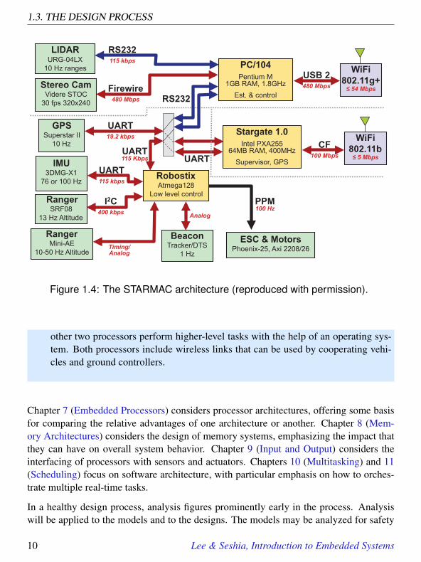
Example 1.6: The hardware architecture of the first generation STARMACquadrotor is shown in Figure 1.4. At the left and bottom of the figure are a numberof sensors used by the vehicle to determine where it is (localization) and what isaround it. In the middle are three boxes showing three distinct microprocessors.The Robostix is an Atmel AVR 8-bit microcontroller that runs with no operatingsystem and performs the low-level control algorithms to keep the craft flying. The
Lee & Seshia, Introduction to Embedded Systems 9
1.3. THE DESIGN PROCESS
WiFi
802.11b 5 Mbps
ESC & Motors Phoenix-25, Axi 2208/26
IMU 3DMG-X1
76 or 100 Hz
Ranger SRF08
13 Hz Altitude
GPS Superstar II
10 Hz
I2C 400 kbps
PPM 100 Hz
UART 19.2 kbps
Robostix Atmega128
Low level control
UART 115 kbps
CF 100 Mbps
Stereo Cam Videre STOC
30 fps 320x240
Firewire 480 Mbps
UART 115 Kbps
LIDAR URG-04LX
10 Hz ranges
Ranger Mini-AE
10-50 Hz Altitude
Beacon Tracker/DTS
1 Hz
WiFi
802.11g+ 54 Mbps
USB 2 480 Mbps
RS232 115 kbps
Timing/ Analog
Analog
RS232
UART
Stargate 1.0
Intel PXA255 64MB RAM, 400MHz
Supervisor, GPS
PC/104
Pentium M 1GB RAM, 1.8GHz
Est. & control
Figure 1.4: The STARMAC architecture (reproduced with permission).
other two processors perform higher-level tasks with the help of an operating sys-tem. Both processors include wireless links that can be used by cooperating vehi-cles and ground controllers.
Chapter 7 (Embedded Processors) considers processor architectures, offering some basisfor comparing the relative advantages of one architecture or another. Chapter 8 (Mem-ory Architectures) considers the design of memory systems, emphasizing the impact thatthey can have on overall system behavior. Chapter 9 (Input and Output) considers theinterfacing of processors with sensors and actuators. Chapters 10 (Multitasking) and 11(Scheduling) focus on software architecture, with particular emphasis on how to orches-trate multiple real-time tasks.
In a healthy design process, analysis figures prominently early in the process. Analysiswill be applied to the models and to the designs. The models may be analyzed for safety
10 Lee & Seshia, Introduction to Embedded Systems

1. INTRODUCTION
conditions, for example to ensure an invariant that asserts that if the vehicle is within onemeter of the ground, then its vertical speed is no greater than 0.1 meter/sec. The designsmay be analyzed for the timing behavior of software, for example to determine how longit takes the system to respond to an emergency shutdown command. Certain analysisproblems will involve details of both models and designs. For the quadrotor example, itis important to understand how the system will behave if network connectivity is lost andit becomes impossible to communicate with the vehicle. How can the vehicle detect thatcommunication has been lost? This will require accurate modeling of the network and thesoftware.
Example 1.7: For the quadrotor problem, we use the techniques of Chapter 12(Invariants and Temporal Logic) to specify key safety requirements for operationof the vehicles. We would then use the techniques of Chapters 13 (Equivalenceand Refinement) and 14 (Reachability Analysis and Model Checking) to verify thatthese safety properties are satisfied by implementations of the software. We wouldthen use the techniques of Chapter 15 (Quantitative Analysis) to determine whetherreal-time constraints are met by the software.
Corresponding to a design process structured as in Figure 1.3, this book is divided intothree major parts, focused on modeling, design, and analysis (see Figure 1 on page xvi).We now describe the approach taken in the three parts.
1.3.1 Modeling
The modeling part of the book, which is the first part, focuses on models of dynamicbehavior. It begins with a light coverage of the big subject of modeling of physical dy-namics in Chapter 2, specifically focusing on continuous dynamics in time. It then talksabout discrete dynamics in Chapter 3, using state machines as the principal formalism.It then combines the two, continuous and discrete dynamics, with a discussion of hybridsystems in Chapter 4. Chapter 5 (Composition of State Machines) focuses on concurrentcomposition of state machines, emphasizing that the semantics of composition is a criticalissue with which designers must grapple. Chapter 6 (Concurrent Models of Computation)gives an overview of concurrent models of computation, including many of those used indesign tools that practitioners frequently leverage, such as Simulink and LabVIEW.
Lee & Seshia, Introduction to Embedded Systems 11

1.3. THE DESIGN PROCESS
In the modeling part of the book, we define a system to be simply a combination of partsthat is considered as a whole. A physical system is one realized in matter, in contrastto a conceptual or logical system such as software and algorithms. The dynamics of asystem is its evolution in time: how its state changes. A model of a physical system is adescription of certain aspects of the system that is intended to yield insight into propertiesof the system. In this text, models have mathematical properties that enable systematicanalysis. The model imitates properties of the system, and hence yields insight into thatsystem.
A model is itself a system. It is important to avoid confusing a model and the system that itmodels. These are two distinct artifacts. A model of a system is said to have high fidelityif it accurately describes properties of the system. It is said to abstract the system if itomits details. Models of physical systems inevitably do omit details, so they are alwaysabstractions of the system. A major goal of this text is to develop an understanding ofhow to use models, of how to leverage their strengths and respect their weaknesses.
A cyber-physical system (CPS) is a system composed of physical subsystems togetherwith computing and networking. Models of cyber-physical systems normally includeall three parts. The models will typically need to represent both dynamics and staticproperties (those that do not change during the operation of the system).
Each of the modeling techniques described in this part of the book is an enormous subject,much bigger than one chapter, or even one book. In fact, such models are the focus ofmany branches of engineering, physics, chemistry, and biology. Our approach is aimed atengineers. We assume some background in mathematical modeling of dynamics (calculuscourses that give some examples from physics are sufficient), and then focus on how tocompose diverse models. This will form the core of the cyber-physical system problem,since joint modeling of the cyber side, which is logical and conceptual, with the physicalside, which is embodied in matter, is the core of the problem. We therefore make noattempt to be comprehensive, but rather pick a few modeling techniques that are widelyused by engineers and well understood, review them, and then compose them to form acyber-physical whole.
1.3.2 Design
The second part of the book has a very different flavor, reflecting the intrinsic heterogene-ity of the subject. This part focuses on the design of embedded systems, with emphasison the role they play within a CPS. Chapter 7 (Embedded Processors) discusses pro-
12 Lee & Seshia, Introduction to Embedded Systems

1. INTRODUCTION
cessor architectures, with emphasis on specialized properties most suited to embeddedsystems. Chapter 8 (Memory Architectures) describes memory architectures, includingabstractions such as memory models in programming languages, physical properties suchas memory technologies, and architectural properties such as memory hierarchy (caches,scratchpads, etc.). The emphasis is on how memory architecture affects dynamics. Chap-ter 9 (Input and Output) is about the interface between the software world and the physicalworld. It discusses input/output mechanisms in software and computer architectures, andthe digital/analog interface, including sampling. Chapter 10 (Multitasking) introduces thenotions that underlie operating systems, with particular emphasis on multitasking. Theemphasis is on the pitfalls of using low-level mechanisms such as threads, with a hope ofconvincing the reader that there is real value in using the modeling techniques covered inthe first part of the book. Those modeling techniques help designers build confidence insystem designs. Chapter 11 (Scheduling) introduces real-time scheduling, covering manyof the classic results in the area.
In all chapters in the design part, we particularly focus on the mechanisms that provideconcurrency and control over timing, because these issues loom large in the design ofcyber-physical systems. When deployed in a product, embedded processors typicallyhave a dedicated function. They control an automotive engine or measure ice thicknessin the Arctic. They are not asked to perform arbitrary functions with user-defined soft-ware. Consequently, the processors, memory architectures, I/O mechanisms, and operat-ing systems can be more specialized. Making them more specialized can bring enormousbenefits. For example, they may consume far less energy, and consequently be usablewith small batteries for long periods of time. Or they may include specialized hardwareto perform operations that would be costly to perform on general-purpose hardware, suchas image analysis. Our goal in this part is to enable the reader to critically evaluate thenumerous available technology offerings.
One of the goals in this part of the book is to teach students to implement systems whilethinking across traditional abstraction layers — e.g., hardware and software, computa-tion and physical processes. While such cross-layer thinking is valuable in implementingsystems in general, it is particularly essential in embedded systems given their heteroge-neous nature. For example, a programmer implementing a control algorithm expressedin terms of real-valued quantities must have a solid understanding of computer arithmetic(e.g., of fixed-point numbers) in order to create a reliable implementation. Similarly, animplementor of automotive software that must satisfy real-time constraints must be awareof processor features – such as pipelines and caches – that can affect the execution timeof tasks and hence the real-time behavior of the system. Likewise, an implementor of
Lee & Seshia, Introduction to Embedded Systems 13

1.3. THE DESIGN PROCESS
interrupt-driven or multi-threaded software must understand the atomic operations pro-vided by the underlying software-hardware platform and use appropriate synchronizationconstructs to ensure correctness. Rather than doing an exhaustive survey of different im-plementation methods and platforms, this part of the book seeks to give the reader an ap-preciation for such cross-layer topics, and uses homework exercises to facilitate a deeperunderstanding of them.
1.3.3 Analysis
Every system must be designed to meet certain requirements. For embedded systems,which are often intended for use in safety-critical, everyday applications, it is essentialto certify that the system meets its requirements. Such system requirements are alsocalled properties or specifications. The need for specifications is aptly captured by thefollowing quotation, paraphrased from Young et al. (1985):
“A design without specifications cannot be right or wrong, it can only besurprising!”
The analysis part of the book focuses on precise specifications of properties, on tech-niques for comparing specifications, and on techniques for analyzing specifications andthe resulting designs. Reflecting the emphasis on dynamics in the text, Chapter 12 (Invari-ants and Temporal Logic) focuses on temporal logics, which provide precise descriptionsof dynamic properties of systems. These descriptions are treated as models. Chapter13 (Equivalence and Refinement) focuses on the relationships between models. Is onemodel an abstraction of another? Is it equivalent in some sense? Specifically, that chap-ter introduces type systems as a way of comparing static properties of models, and lan-guage containment and simulation relations as a way of comparing dynamic properties ofmodels. Chapter 14 (Reachability Analysis and Model Checking) focuses on techniquesfor analyzing the large number of possible dynamic behaviors that a model may exhibit,with particular emphasis on model checking as a technique for exploring such behaviors.Chapter 15 (Quantitative Analysis) is about analyzing quantitative properties of embeddedsoftware, such as finding bounds on resources consumed by programs. It focuses partic-ularly on execution time analysis, with some introduction to other quantitative propertiessuch as energy and memory usage.
In present engineering practice, it is common to have system requirements stated in anatural language such as English. It is important to precisely state requirements to avoid
14 Lee & Seshia, Introduction to Embedded Systems

1. INTRODUCTION
ambiguities inherent in natural languages. The goal of this part of the book is to helpreplace descriptive techniques with formal ones, which we believe are less error prone.
Importantly, formal specifications also enable the use of automatic techniques for formalverification of both models and implementations. The analysis part of the book introducesreaders to the basics of formal verification, including notions of equivalence and refine-ment checking, as well as reachability analysis and model checking. In discussing theseverification methods, we attempt to give users of verification tools an appreciation of whatis “under the hood” so that they may derive the most benefit from them. This user’s viewis supported by examples discussing, for example, how model checking can be appliedto find subtle errors in concurrent software, or how reachability analysis can be used incomputing a control strategy for a robot to achieve a particular task.
1.4 Summary
Cyber-physical systems are heterogeneous blends by nature. They combine computation,communication, and physical dynamics. They are harder to model, harder to design,and harder to analyze than homogeneous systems. This chapter gives an overview of theengineering principles addressed in this book for modeling, designing, and analyzing suchsystems.
Lee & Seshia, Introduction to Embedded Systems 15

Part I
Modeling Dynamic Behaviors
This part of this text studies modeling of embedded systems, with emphasis on jointmodeling of software and physical dynamics. We begin in Chapter 2 with a discussionof established techniques for modeling the dynamics of physical systems, with emphasison their continuous behaviors. In Chapter 3, we discuss techniques for modeling discretebehaviors, which reflect better the behavior of software. In Chapter 4, we bring these twoclasses of models together and show how discrete and continuous behaviors are jointlymodeled by hybrid systems. Chapters 5 and 6 are devoted to reconciling the inherentlyconcurrent nature of the physical world with the inherently sequential world of software.Chapter 5 shows how state machine models, which are fundamentally sequential, can becomposed concurrently. That chapter specifically introduces the notion of synchronouscomposition. Chapter 6 shows that synchronous composition is but one of the ways toachieve concurrent composition.


2Continuous Dynamics
Contents2.1 Newtonian Mechanics . . . . . . . . . . . . . . . . . . . . . . . . . 202.2 Actor Models . . . . . . . . . . . . . . . . . . . . . . . . . . . . . . 252.3 Properties of Systems . . . . . . . . . . . . . . . . . . . . . . . . . 29
2.3.1 Causal Systems . . . . . . . . . . . . . . . . . . . . . . . . . 292.3.2 Memoryless Systems . . . . . . . . . . . . . . . . . . . . . . 292.3.3 Linearity and Time Invariance . . . . . . . . . . . . . . . . . 302.3.4 Stability . . . . . . . . . . . . . . . . . . . . . . . . . . . . . 31
2.4 Feedback Control . . . . . . . . . . . . . . . . . . . . . . . . . . . 322.5 Summary . . . . . . . . . . . . . . . . . . . . . . . . . . . . . . . . 37Exercises . . . . . . . . . . . . . . . . . . . . . . . . . . . . . . . . . . . 38
This chapter reviews a few of the many modeling techniques for studying dynamics ofa physical system. We begin by studying mechanical parts that move (this problem isknown as classical mechanics). The techniques used to study the dynamics of such partsextend broadly to many other physical systems, including circuits, chemical processes,and biological processes. But mechanical parts are easiest for most people to visualize, sothey make our example concrete. Motion of mechanical parts can often be modeled us-ing differential equations, or equivalently, integral equations. Such models really onlywork well for “smooth” motion (a concept that we can make more precise using notions
19

2.1. NEWTONIAN MECHANICS
of linearity, time invariance, and continuity). For motions that are not smooth, such asthose modeling collisions of mechanical parts, we can use modal models that representdistinct modes of operation with abrupt (conceptually instantaneous) transitions betweenmodes. Collisions of mechanical objects can be usefully modeled as discrete, instanta-neous events. The problem of jointly modeling smooth motion and such discrete eventsis known as hybrid systems modeling and is studied in Chapter 4. Such combinations ofdiscrete and continuous behaviors bring us one step closer to joint modeling of cyber andphysical processes.
We begin with simple equations of motion, which provide a model of a system in theform of ordinary differential equations (ODEs). We then show how these ODEs canbe represented in actor models, which include the class of models in popular model-ing languages such as LabVIEW (from National Instruments) and Simulink (from TheMathWorks, Inc.). We then consider properties of such models such as linearity, time in-variance, and stability, and consider consequences of these properties when manipulatingmodels. We develop a simple example of a feedback control system that stabilizes anunstable system. Controllers for such systems are often realized using software, so suchsystems can serve as a canonical example of a cyber-physical system. The properties ofthe overall system emerge from properties of the cyber and physical parts.
2.1 Newtonian Mechanics
In this section, we give a brief working review of some principles of classical mechanics.This is intended to be just enough to be able to construct interesting models, but is byno means comprehensive. The interested reader is referred to many excellent texts onclassical mechanics, including Goldstein (1980); Landau and Lifshitz (1976); Marion andThornton (1995).
Motion in space of physical objects can be represented with six degrees of freedom,illustrated in Figure 2.1. Three of these represent position in three dimensional space,and three represent orientation in space. We assume three axes, x, y, and z, where byconvention x is drawn increasing to the right, y is drawn increasing upwards, and z isdrawn increasing out of the page. Roll θx is an angle of rotation around the x axis, whereby convention an angle of 0 radians represents horizontally flat along the z axis (i.e., theangle is given relative to the z axis). Yaw θy is the rotation around the y axis, whereby convention 0 radians represents pointing directly to the right (i.e., the angle is given
20 Lee & Seshia, Introduction to Embedded Systems

2. CONTINUOUS DYNAMICS
z y
x
Roll
YawPitch
Figure 2.1: Modeling position with six degrees of freedom requires including pitch,roll, and yaw, in addition to position.
relative to the x axis). Pitch θz is rotation around the z axis, where by convention 0 radiansrepresents pointing horizontally (i.e., the angle is given relative to the x axis).
The position of an object in space, therefore, is represented by six functions of the formf : R→ R, where the domain represents time and the codomain represents either dis-tance along an axis or angle relative to an axis.1 Functions of this form are knownas continuous-time signals.2 These are often collected into vector-valued functionsx : R→ R3 and θ : R→ R3, where x represents position, and θ represents orientation.
Changes in position or orientation are governed by Newton’s second law, relating forcewith acceleration. Acceleration is the second derivative of position. Our first equationhandles the position information,
F(t) = Mx(t), (2.1)
where F is the force vector in three directions, M is the mass of the object, and x is thesecond derivative of x with respect to time (i.e., the acceleration). Velocity is the integral
1If the notation is unfamiliar, see Appendix A.2The domain of a continuous-time signal may be restricted to a connected subset of R, such as R+, the
non-negative reals, or [0,1], the interval between zero and one, inclusive. The codomain may be an arbitraryset, though when representing physical quantities, real numbers are most useful.
Lee & Seshia, Introduction to Embedded Systems 21

2.1. NEWTONIAN MECHANICS
of acceleration, given by
∀ t > 0, x(t) = x(0)+t∫
0
x(τ)dτ
where x(0) is the initial velocity in three directions. Using (2.1), this becomes
∀ t > 0, x(t) = x(0)+1M
t∫0
F(τ)dτ,
Position is the integral of velocity,
x(t) = x(0)+t∫
0
x(τ)dτ
= x(0)+ tx(0)+1M
t∫0
τ∫0
F(α)dαdτ,
where x(0) is the initial position. Using these equations, if you know the initial positionand initial velocity of an object and the forces on the object in all three directions as afunction of time, you can determine the acceleration, velocity, and position of the objectat any time.
The versions of these equations of motion that affect orientation use torque, the rotationalversion of force. It is again a three-element vector as a function of time, representing thenet rotational force on an object. It can be related to angular velocity in a manner similarto (2.1),
T(t) =ddt
(I(t)θ(t)
), (2.2)
where T is the torque vector in three axes and I(t) is the moment of inertia tensor ofthe object. The moment of inertia is a 3× 3 matrix that depends on the geometry andorientation of the object. Intuitively, it represents the reluctance that an object has tospin around any axis as a function of its orientation along the three axes. If the objectis spherical, for example, this reluctance is the same around all axes, so it reduces to aconstant scalar I (or equivalently, to a diagonal matrix I with equal diagonal elements I).The equation then looks much more like (2.1),
T(t) = Iθ(t). (2.3)
22 Lee & Seshia, Introduction to Embedded Systems

2. CONTINUOUS DYNAMICS
To be explicit about the three dimensions, we might write (2.2) as Tx(t)Ty(t)Tz(t)
=ddt
Ixx(t) Ixy(t) Ixz(t)Iyx(t) Iyy(t) Iyz(t)Izx(t) Izy(t) Izz(t)
θx(t)θy(t)θz(t)
.
Here, for example, Ty(t) is the net torque around the y axis (which would cause changesin yaw), Iyx(t) is the inertia that determines how acceleration around the x axis is relatedto torque around the y axis.
Rotational velocity is the integral of acceleration,
θ(t) = θ(0)+t∫
0
θ(τ)dτ,
where θ(0) is the initial rotational velocity in three axes. For a spherical object, using(2.3), this becomes
θ(t) = θ(0)+1I
t∫0
T(τ)dτ.
Orientation is the integral of rotational velocity,
θ(t) = θ(0)+∫ t
0θ(τ)dτ
= θ(0)+ tθ(0)+1I
t∫0
τ∫0
T(α)dαdτ
where θ(0) is the initial orientation. Using these equations, if you know the initial orien-tation and initial rotational velocity of an object and the torques on the object in all threeaxes as a function of time, you can determine the rotational acceleration, velocity, andorientation of the object at any time.
Often, as we have done for a spherical object, we can simplify by reducing the number ofdimensions that are considered. In general, such a simplification is called a model-orderreduction. For example, if an object is a moving vehicle on a flat surface, there may belittle reason to consider the y axis movement or the pitch or roll of the object.
Lee & Seshia, Introduction to Embedded Systems 23

2.1. NEWTONIAN MECHANICS
Mbody
tail
main rotor shaft
Figure 2.2: Simplified model of a helicopter.
Example 2.1: Consider a simple control problem that admits such reduction ofdimensionality. A helicopter has two rotors, one above, which provides lift, andone on the tail. Without the rotor on the tail, the body of the helicopter would spin.The rotor on the tail counteracts that spin. Specifically, the force produced by thetail rotor must counter the torque produced by the main rotor. Here we considerthis role of the tail rotor independently from all other motion of the helicopter.
A simplified model of the helicopter is shown in Figure 2.2. Here, we assume thatthe helicopter position is fixed at the origin, so there is no need to consider equationsdescribing position. Moreover, we assume that the helicopter remains vertical, sopitch and roll are fixed at zero. These assumptions are not as unrealistic as theymay seem since we can define the coordinate system to be fixed to the helicopter.
With these assumptions, the moment of inertia reduces to a scalar that representsa torque that resists changes in yaw. The changes in yaw will be due to Newton’sthird law, the action-reaction law, which states that every action has an equal andopposite reaction. This will tend to cause the helicopter to rotate in the oppositedirection from the rotor rotation. The tail rotor has the job of countering that torqueto keep the body of the helicopter from spinning.
We model the simplified helicopter by a system that takes as input a continuous-time signal Ty, the torque around the y axis (which causes changes in yaw). Thistorque is the sum of the torque caused by the main rotor and that caused by thetail rotor. When these are perfectly balanced, that sum is zero. The output of our
24 Lee & Seshia, Introduction to Embedded Systems

2. CONTINUOUS DYNAMICS
system will be the angular velocity θy around the y axis. The dimensionally-reducedversion of (2.2) can be written as
θy(t) = Ty(t)/Iyy.
Integrating both sides, we get the output θ as a function of the input Ty,
θy(t) = θy(0)+1
Iyy
t∫0
Ty(τ)dτ. (2.4)
The critical observation about this example is that if we were to choose to model thehelicopter by, say, letting x : R→ R3 represent the absolute position in space of the tailof the helicopter, we would end up with a far more complicated model. Designing thecontrol system would also be much more difficult.
2.2 Actor Models
In the previous section, a model of a physical system is given by a differential or anintegral equation that relates input signals (force or torque) to output signals (position,orientation, velocity, or rotational velocity). Such a physical system can be viewed as acomponent in a larger system. In particular, a continuous-time system (one that operateson continuous-time signals) may be modeled by a box with an input port and an outputport as follows:
parameters:
where the input signal x and the output signal y are functions of the form
x : R→ R, y : R→ R.
Here the domain represents time and the codomain represents the value of the signal at aparticular time. The domain R may be replaced by R+, the non-negative reals, if we wish
Lee & Seshia, Introduction to Embedded Systems 25

2.2. ACTOR MODELS
to explicitly model a system that comes into existence and starts operating at a particularpoint in time.
The model of the system is a function of the form
S : X → Y, (2.5)
where X = Y = RR, the set of functions that map the reals into the reals, like x andy above.3 The function S may depend on parameters of the system, in which case theparameters may be optionally shown in the box, and may be optionally included in thefunction notation. For example, in the above figure, if there are parameters p and q,we might write the system function as Sp,q or even S(p,q), keeping in mind that bothnotations represent functions of the form in 2.5. A box like that above, where the inputsare functions and the outputs are functions, is called an actor.
Example 2.2: The actor model for the helicopter of example 2.1 can be depictedas follows:
The input and output are both continuous-time functions. The parameters of the ac-tor are the initial angular velocity θy(0) and the moment of inertia Iyy. The functionof the actor is defined by (2.4).
Actor models are composable. In particular, given two actors S1 and S2, we can form acascade composition as follows:
3As explained in Appendix A, the notation RR (which can also be written (R→ R)) represents the set ofall functions with domain R and codomain R.
26 Lee & Seshia, Introduction to Embedded Systems

2. CONTINUOUS DYNAMICS
In the diagram, the “wire” between the output of S1 and the input of S2 means preciselythat y1 = x2, or more pedantically,
∀ t ∈ R, y1(t) = x2(t).
Example 2.3: The actor model for the helicopter can be represented as a cascadecomposition of two actors as follows:
The left actor represents a Scale actor parameterized by the constant a defined by
∀ t ∈ R, y1(t) = ax1(t). (2.6)
More compactly, we can write y1 = ax1, where it is understood that the product ofa scalar a and a function x1 is interpreted as in (2.6). The right actor represents anintegrator parameterized by the initial value i defined by
∀ t ∈ R, y2(t) = i+t∫
0
x2(τ)dτ.
If we give the parameter values a = 1/Iyy and i = θy(0), we see that this systemrepresents (2.4) where the input x1 = Ty is torque and the output y2 = θy is angularvelocity.
In the above figure, we have customized the icons, which are the boxes representingthe actors. These particular actors (scaler and integrator) are particularly useful build-ing blocks for building up models of physical dynamics, so assigning them recognizablevisual notations is useful.
Lee & Seshia, Introduction to Embedded Systems 27

2.2. ACTOR MODELS
We can have actors that have multiple input signals and/or multiple output signals. Theseare represented similarly, as in the following example, which has two input signals andone output signal:
A particularly useful building block with this form is a signal adder, defined by
∀ t ∈ R, y(t) = x1(t)+ x2(t).
This will often be represented by a custom icon as follows:
Sometimes, one of the inputs will be subtracted rather than added, in which case the iconis further customized with minus sign near that input, as below:
This actor represents a function S : (R→ R)2→ (R→ R) given by
∀ t ∈ R, ∀ x1,x2 ∈ (R→ R), (S(x1,x2))(t) = y(t) = x1(t)− x2(t).
Notice the careful notation. S(x1,x2) is a function in RR. Hence, it can be evaluated at at ∈ R.
In the rest of this chapter, we will not make a distinction between a system and its actormodel, unless the distinction is essential to the argument. We will assume that the actormodel captures everything of interest about the system. This is an admittedly bold as-sumption. Generally the properties of the actor model are only approximate descriptionsof the actual system.
28 Lee & Seshia, Introduction to Embedded Systems

2. CONTINUOUS DYNAMICS
2.3 Properties of Systems
In this section, we consider a number of properties that actors and the systems they com-pose may have, including causality, memorylessness, linearity, time invariance, and sta-bility.
2.3.1 Causal Systems
Intuitively, a system is causal if its output depends only on current and past inputs. Mak-ing this notion precise is a bit tricky, however. We do this by first giving a notation for“current and past inputs.” Consider a continuous-time signal x : R→ A, for some set A.Let x|t≤τ represent a function called the restriction in time that is only defined for timest ≤ τ, and where it is defined, x|t≤τ(t) = x(t). Hence if x is an input to a system, then x|t≤τis the “current and past inputs” at time τ.
Consider a continuous-time system S : X → Y , where X = AR and Y = BR for some setsA and B. This system is causal if for all x1,x2 ∈ X and τ ∈ R,
x1|t≤τ = x2|t≤τ⇒ S(x1)|t≤τ = S(x2)|t≤τ
That is, the system is causal if for two possible inputs x1 and x2 that are identical up to(and including) time τ, the outputs are identical up to (and including) time τ. All systemswe have considered so far are causal.
A system is strictly causal if for all x1,x2 ∈ X and τ ∈ R,
x1|t<τ = x2|t<τ⇒ S(x1)|t≤τ = S(x2)|t≤τ
That is, the system is strictly causal if for two possible inputs x1 and x2 that are identicalup to (and not including) time τ, the outputs are identical up to (and including) time τ.The output at time t of a strictly causal system does not depend on its input at time t.It only depends on past inputs. A strictly causal system, of course, is also causal. TheIntegrator actor is strictly causal. The adder is not strictly causal, but it is causal. Strictlycausal actors are useful for constructing feedback systems.
2.3.2 Memoryless Systems
Intuitively, a system has memory if the output depends not only on the current inputs, butalso on past inputs (or future inputs, if the system is not causal). Consider a continuous-
Lee & Seshia, Introduction to Embedded Systems 29

2.3. PROPERTIES OF SYSTEMS
time system S : X → Y , where X = AR and Y = BR for some sets A and B. Formally, thissystem is memoryless if there exists a function f : A→ B such that for all x ∈ X ,
(S(x))(t) = f (x(t))
for all t ∈ R. That is, the output (S(x))(t) at time t depends only on the input x(t) at timet.
The Integrator considered above is not memoryless, but the adder is. Exercise 2 showsthat if a system is strictly causal and memoryless then its output is constant for all inputs.
2.3.3 Linearity and Time Invariance
Systems that are linear and time invariant (LTI) have particularly nice mathematical prop-erties. Much of the theory of control systems depends on these properties. These proper-ties form the main body of courses on signals and systems, and are beyond the scope ofthis text. But we will occasionally exploit simple versions of the properties, so it is usefulto determine when a system is LTI.
A system S : X → Y , where X and Y are sets of signals, is linear if it satisfies the super-position property:
∀ x1,x2 ∈ X and ∀ a,b ∈ R, S(ax1 +bx2) = aS(x1)+bS(x2).
It is easy to see that the helicopter system defined in Example 2.1 is linear if and only ifthe initial angular velocity θy(0) = 0 (see Exercise 3).
More generally, it is easy to see that an integrator as defined in Example 2.3 is linear if andonly if the initial value i = 0, that the Scale actor is always linear, and that the cascade ofany two linear actors is linear. We can trivially extend the definition of linearity to actorswith more than one input or output signal and then determine that the adder is also linear.
To define time invariance, we first define a specialized continuous-time actor called adelay. Let Dτ : X → Y , where X and Y are sets of continuous-time signals, be defined by
∀ x ∈ X and ∀ t ∈ R, (Dτ(x))(t) = x(t− τ). (2.7)
Here, τ is a parameter of the delay actor. A system S : X → Y is time invariant if
∀ x ∈ X and ∀ τ ∈ R, S(Dτ(x)) = Dτ(S(x)).
30 Lee & Seshia, Introduction to Embedded Systems

2. CONTINUOUS DYNAMICS
The helicopter system defined in Example 2.1 and (2.4) is not time invariant. A minorvariant, however, is time invariant:
θy(t) =1
Iyy
t∫−∞
Ty(τ)dτ.
This version does not allow for an initial angular rotation.
A linear time-invariant system (LTI) is a system that is both linear and time invariant.A major objective in modeling physical dynamics is to choose an LTI model wheneverpossible. If a reasonable approximation results in an LTI model, it is worth making thisapproximation. It is not always easy to determine whether the approximation is reason-able, or to find models for which the approximation is reasonable. It is often easy toconstruct models that are more complicated than they need to be (see Exercise 4).
2.3.4 Stability
A system is said to be bounded-input bounded-output stable (BIBO stable or juststable) if the output signal is bounded for all input signals that are bounded.
Consider a continuous-time system with input w and output v. The input is bounded ifthere is a real number A < ∞ such that |w(t)| ≤ A for all t ∈ R. The output is bounded ifthere is a real number B < ∞ such that |v(t)| ≤ B for all t ∈ R. The system is stable if forany input bounded by some A, there is some bound B on the output.
Example 2.4: It is now easy to see that the helicopter system developed in Ex-ample 2.1 is unstable. Let the input be Ty = u, where u is the unit step, givenby
∀ t ∈ R, u(t) =
0, t < 01, t ≥ 0
. (2.8)
This means that prior to time zero, there is no torque applied to the system, andstarting at time zero, we apply a torque of unit magnitude. This input is clearlybounded. It never exceeds one in magnitude. However, the output grows withoutbound. In practice, a helicopter uses a feedback system to determine how muchtorque to apply at the tail rotor to keep the body of the helicopter straight. We studyhow to do that next.
Lee & Seshia, Introduction to Embedded Systems 31

2.4. FEEDBACK CONTROL
eK
ψ
Figure 2.3: Proportional control system that stabilizes the helicopter.
2.4 Feedback Control
A system with feedback has directed cycles, where an output from an actor is fed backto affect an input of the same actor. An example of such a system is shown in Figure2.3. Most control systems use feedback. They make measurements of an error (e inthe figure), which is a discrepancy between desired behavior (ψ in the figure) and actualbehavior (θy in the figure), and use that measurement to correct the behavior. The errormeasurement is feedback, and the corresponding correction signal (Ty in the figure) shouldcompensate to reduce future error. Note that the correction signal normally can only affectfuture errors, so a feedback system must normally include at least one strictly causal actor(the Helicopter in the figure) in every directed cycle.
Feedback control is a sophisticated topic, easily occupying multiple texts and completecourses. Here, we only barely touch on the subject, just enough to motivate the interac-tions between software and physical systems. Feedback control systems are often imple-mented using embedded software, and the overall physical dynamics is a composition ofthe software and physical dynamics. More detail can be found in Chapters 12-14 of Leeand Varaiya (2011).
Example 2.5: Recall that the helicopter model of Example 2.1 is not stable. Wecan stabilize it with a simple feedback control system, as shown in Figure 2.3. Theinput ψ to this system is a continuous-time system specifying the desired angularvelocity. The error signal e represents the difference between the actual and thedesired angular velocity. In the figure, the controller simply scales the error signal
32 Lee & Seshia, Introduction to Embedded Systems
2. CONTINUOUS DYNAMICS
by a constant K, providing a control input to the helicopter. We use (2.4) to write
θy(t) = θy(0)+1
Iyy
t∫0
Ty(τ)dτ (2.9)
= θy(0)+KIyy
t∫0
(ψ(τ)− θy(τ))dτ, (2.10)
where we have used the facts (from the figure),
e(t) = ψ(t)− θy(t), and
Ty(t) = Ke(t).
Equation (2.10) has θy(t) on both sides, and therefore is not trivial to solve. Theeasiest solution technique uses Laplace transforms (see Lee and Varaiya (2011)Chapter 14). However, for our purposes here, we can use a more brute-force tech-nique from calculus. To make this as simple as possible, we assume that ψ(t) = 0for all t; i.e., we wish to control the helicopter simply to keep it from rotating at all.The desired angular velocity is zero. In this case, (2.10) simplifies to
θy(t) = θy(0)−KIyy
t∫0
θy(τ)dτ. (2.11)
Using the fact from calculus that, for t ≥ 0,t∫
0
aeaτdτ = eatu(t)−1,
where u is given by (2.8), we can infer that the solution to (2.11) is
θy(t) = θy(0)e−Kt/Iyyu(t). (2.12)
(Note that although it is easy to verify that this solution is correct, deriving thesolution is not so easy. For this purpose, Laplace transforms provide a far bettermechanism.)
We can see from (2.12) that the angular velocity approaches the desired angularvelocity (zero) as t gets large as long as K is positive. For larger K, it will approachmore quickly. For negative K, the system is unstable, and angular velocity willgrow without bound.
Lee & Seshia, Introduction to Embedded Systems 33

2.4. FEEDBACK CONTROL
The previous example illustrates a proportional control feedback loop. It is called thisbecause the control signal is proportional to the error. We assumed a desired signal ofzero. It is equally easy to assume that the helicopter is initially at rest (the angular velocityis zero) and then determine the behavior for a particular non-zero desired signal, as we doin the following example.
Example 2.6: Assume that helicopter is initially at rest, meaning that
θ(0) = 0,
and that the desired signal isψ(t) = au(t)
for some constant a. That is, we wish to control the helicopter to get it to rotate ata fixed rate.
We use (2.4) to write
θy(t) =1
Iyy
t∫0
Ty(τ)dτ
=KIyy
t∫0
(ψ(τ)− θy(τ))dτ
=KIyy
t∫0
adτ− KIyy
t∫0
θy(τ)dτ
=KatIyy− K
Iyy
t∫0
θy(τ)dτ.
Using the same (black magic) technique of inferring and then verifying the solution,we can see that the solution is
θy(t) = au(t)(1− e−Kt/Iyy). (2.13)
Again, the angular velocity approaches the desired angular velocity as t gets largeas long as K is positive. For larger K, it will approach more quickly. For negativeK, the system is unstable, and angular velocity will grow without bound.
34 Lee & Seshia, Introduction to Embedded Systems

2. CONTINUOUS DYNAMICS
Note that the first term in the above solution is exactly the desired angular veloc-ity. The second term is an error called the tracking error, that for this exampleasymptotically approaches zero.
The above example is somewhat unrealistic because we cannot independently control thenet torque of the helicopter. In particular, the net torque Ty is the sum of the torque Tt dueto the top rotor and the torque Tr due to the tail rotor,
∀ t ∈ R, Ty(t) = Tt(t)+Tr(t) .
Tt will be determined by the rotation required to maintain or achieve a desired altitude,quite independent of the rotation of the helicopter. Thus, we will actually need to design acontrol system that controls Tr and stabilizes the helicopter for any Tt (or, more precisely,any Tt within operating parameters). In the next example, we study how this changes theperformance of the control system.
Example 2.7: In Figure 2.4(a), we have modified the helicopter model so that ithas two inputs, Tt and Tr, the torque due to the top rotor and tail rotor respectively.The feedback control system is now controlling only Tr, and Tt is treated as anexternal (uncontrolled) input signal. How well will this control system behave?
Again, a full treatment of the subject is beyond the scope of this text, but we willstudy a specific example. Suppose that the torque due to the top rotor is given by
Tt = bu(t)
for some constant b. That is, at time zero, the top rotor starts spinning a constantvelocity, and then holds that velocity. Suppose further that the helicopter is initiallyat rest. We can use the results of Example 2.6 to find the behavior of the system.
First, we transform the model into the equivalent model shown in Figure 2.4(b).This transformation simply relies on the algebraic fact that for any real numbersa1,a2,K,
Ka1 +a2 = K(a1 +a2/K).
We further transform the model to get the equivalent model shown in Figure 2.4(c),which has used the fact that addition is commutative. In Figure 2.4(c), we see that
Lee & Seshia, Introduction to Embedded Systems 35

2.4. FEEDBACK CONTROL
(c)
(a)
(b)
Figure 2.4: (a) Helicopter model with separately controlled torques for the topand tail rotors. (b) Transformation to an equivalent model (assuming K > 0). (c)Further transformation to an equivalent model that we can use to understand thebehavior of the controller.
36 Lee & Seshia, Introduction to Embedded Systems

2. CONTINUOUS DYNAMICS
the portion of the model enclosed in the box is exactly the same as the controlsystem analyzed in Example 2.6, shown in Figure 2.3. Thus, the same analysis asin Example 2.6 still applies. Suppose that desired angular rotation is
ψ(t) = 0.
Then the input to the original control system will be
x(t) = ψ(t)+Tt(t)/K = (b/K)u(t).
From (2.13), we see that the solution is
θy(t) = (b/K)u(t)(1− e−Kt/Iyy). (2.14)
The desired angular rotation is zero, but the control system asymptotically ap-proaches a non-zero angular rotation of b/K. This tracking error can be madearbitrarily small by increasing the control system feedback gain K, but with thiscontroller design, it cannot be made to go to zero. An alternative controller designthat yields an asymptotic tracking error of zero is studied in Exercise 6.
2.5 Summary
This chapter has described two distinct modeling techniques that describe physical dy-namics. The first is ordinary differential equations, a venerable toolkit for engineers, andthe second is actor models, a newer technique driven by software modeling and simu-lation tools. The two are closely related. This chapter has emphasized the relationshipbetween these models, and the relationship of those models to the systems being modeled.These relationships, however, are quite a deep subject that we have barely touched upon.Our objective is to focus the attention of the reader on the fact that we may use multiplemodels for a system, and that models are distinct from the systems being modeled. Thefidelity of a model (how well it approximates the system being modeled) is a strong factorin the success or failure of any engineering effort.
Lee & Seshia, Introduction to Embedded Systems 37

EXERCISES
Exercises
1. A tuning fork, shown in Figure 2.5, consists of a metal finger (called a tine) thatis displaced by striking it with a hammer. After being displaced, it vibrates. If thetine has no friction, it will vibrate forever. We can denote the displacement of thetine after being struck at time zero as a function y : R+ → Reals. If we assumethat the initial displacement introduced by the hammer is one unit, then using ourknowledge of physics we can determine that for all t ∈ Reals+, the displacementsatisfies the differential equation
y(t) =−ω20y(t)
where ω20 is constant that depends on the mass and stiffness of the tine, and and
where y(t) denotes the second derivative with respect to time of y. It is easy toverify that y given by
∀ t ∈ Reals+, y(t) = cos(ω0t)
is a solution to the differential equation (just take its second derivative). Thus, thedisplacement of the tuning fork is sinusoidal. If we choose materials for the tuningfork so that ω0 = 2π× 440 radians/second, then the tuning fork will produce thetone of A-440 on the musical scale.
(a) Is y(t) = cos(ω0t) the only solution? If not, give some others.
(b) Assuming the solution is y(t) = cos(ω0t), what is the initial displacement?
(c) Construct a model of the tuning fork that produces y as an output using genericactors like Integrator, adder, scaler, or similarly simple actors. Treat the initialdisplacement as a parameter. Carefully label your diagram.
2. Show that if a system S : AR→ BR is strictly causal and memoryless then its outputis constant. Constant means that the output (S(x))(t) at time t does not depend ont.
3. This exercise studies linearity.
(a) Show that the helicopter model defined in Example 2.1 is linear if and only ifthe initial angular velocity θy(0) = 0.
(b) Show that the cascade of any two linear actors is linear.
38 Lee & Seshia, Introduction to Embedded Systems

2. CONTINUOUS DYNAMICS
(c) Augment the definition of linearity so that it applies to actors with two inputsignals and one output signal. Show that the adder actor is linear.
4. Consider the helicopter of Example 2.1, but with a slightly different definition ofthe input and output. Suppose that, as in the example, the input is Ty : R→R, as inthe example, but the output is the position of the tail relative to the main rotor shaft.Specifically, let the x-y plane be the plane orthogonal to the rotor shaft, and let theposition of the tail at time t be given by a tuple ((x(t),y(t)). Is this model LTI? Is itBIBO stable?
5. Consider a rotating robot where you can control the angular velocity around a fixedaxis.
(a) Model this as a system where the input is angular velocity θ and the outputis angle θ. Give your model as an equation relating the input and output asfunctions of time.
(b) Is this model BIBO stable?
(c) Design a proportional controller to set the robot onto a desired angle. That is,assume that the initial angle is θ(0) = 0, and let the desired angle be ψ(t) =au(t), where u is the unit step function. Find the actual angle as a function of
displacement restorative force
tine
Figure 2.5: A tuning fork.
Lee & Seshia, Introduction to Embedded Systems 39

EXERCISES
K1
K2KK
Figure 2.6: A PI controller for the helicopter.
time and the proportional controller feedback gain K. What is your output att = 0? What does it approach as t gets large?
6. (a) Using your favorite continuous-time modeling software (such as LabVIEW,Simulink, or Ptolemy II), construct a model of the helicopter control systemshown in Figure 2.4. Choose some reasonable parameters and plot the actualangular velocity as a function of time, assuming that the desired angular veloc-ity is zero, ψ(t) = 0, and that the top-rotor torque is non-zero, Tt(t) = bu(t).Give your plot for several values of K and discuss how the behavior varieswith K.
(b) Modify the model of part (a) to replace the Controller of Figure 2.4 (the simplescale-by-K actor) with the alternative controller shown in Figure 2.6. Thisalternative controller is called a proportional-integrator (PI) controller. Ithas two parameter K1 and K2. Experiment with the values of these parameters,give some plots of the behavior with the same inputs as in part (a), and discussthe behavior of this controller in contrast to the one of part (a).
40 Lee & Seshia, Introduction to Embedded Systems

3Discrete Dynamics
Contents3.1 Discrete Systems . . . . . . . . . . . . . . . . . . . . . . . . . . . . 42
Sidebar: Probing Further: Discrete Signals . . . . . . . . . . . . . . 44Sidebar: Probing Further: Modeling Actors as Functions . . . . . . . 45
3.2 The Notion of State . . . . . . . . . . . . . . . . . . . . . . . . . . 463.3 Finite-State Machines . . . . . . . . . . . . . . . . . . . . . . . . . 47
3.3.1 Transitions . . . . . . . . . . . . . . . . . . . . . . . . . . . 483.3.2 When a Reaction Occurs . . . . . . . . . . . . . . . . . . . . 51Sidebar: Probing Further: Hysteresis . . . . . . . . . . . . . . . . . 523.3.3 Update Functions . . . . . . . . . . . . . . . . . . . . . . . . 54Sidebar: Software Tools Supporting FSMs . . . . . . . . . . . . . . . 543.3.4 Determinacy and Receptiveness . . . . . . . . . . . . . . . . 56
3.4 Extended State Machines . . . . . . . . . . . . . . . . . . . . . . . 57Sidebar: Moore Machines and Mealy Machines . . . . . . . . . . . . 58
3.5 Nondeterminism . . . . . . . . . . . . . . . . . . . . . . . . . . . . 633.5.1 Formal Model . . . . . . . . . . . . . . . . . . . . . . . . . . 643.5.2 Uses of Non-Determinism . . . . . . . . . . . . . . . . . . . 66
3.6 Behaviors and Traces . . . . . . . . . . . . . . . . . . . . . . . . . 663.7 Summary . . . . . . . . . . . . . . . . . . . . . . . . . . . . . . . . 70Exercises . . . . . . . . . . . . . . . . . . . . . . . . . . . . . . . . . . . 71
41

3.1. DISCRETE SYSTEMS
Models of embedded systems include both discrete and continuous components. Looselyspeaking, continuous components evolve smoothly, while discrete components evolveabruptly. The previous chapter considered continuous components, and showed that thephysical dynamics of the system can often be modeled with ordinary differential or in-tegral equations, or equivalently with actor models that mirror these equations. Discretecomponents, on the other hand, are not conveniently modeled by ODEs. In this chapter,we study how state machines can be used to model discrete dynamics. In the next chap-ter, we will show how these state machines can be combined with models of continuousdynamics to get hybrid system models.
3.1 Discrete Systems
A discrete system operates in a sequence of discrete steps and is said to have discretedynamics. Some systems are inherently discrete.
Example 3.1: Consider a system that counts the number of cars that enter andleave a parking garage in order to keep track of how many cars are in the garageat any time. It could be modeled as shown in Figure 3.1. We ignore for nowhow to design the sensors that detect the entry or departure of cars. We simplyassume that the ArrivalDetector actor produces an event when a car arrives, andthe DepartureDetector actor produces an event when a car departs. The Counter
Figure 3.1: Model of a system that keeps track of the number of cars in a parkinggarage.
42 Lee & Seshia, Introduction to Embedded Systems

3. DISCRETE DYNAMICS
Figure 3.2: Icon for the Integrator actor used in the previous chapter.
actor keeps a running count, starting from an initial value i. Each time the countchanges, it produces an output event that updates a display.
In the above example, each entry or departure is modeled as a discrete event. A discreteevent occurs at an instant of time rather than over time. The Counter actor in Figure 3.1is analogous to the Integrator actor used in the previous chapter, shown here in Figure3.2. Like the Counter actor, the Integrator accumulates input values. However, it doesso very differently. The input of an Integrator is a function of the form x : R→ R orx : R+ → R, a continuous-time signal. The signal u going into the up input port of theCounter, on the other hand, is a function of the form
u : R→absent,present.
This means that at any time t ∈ R, the input u(t) is either absent, meaning that there isno event at that time, or present, meaning that there is. A signal of this form is known asa pure signal. It carries no value, but instead provides all its information by being eitherpresent or absent at any given time. The signal d in Figure 3.1 is also a pure signal.
Assume our Counter operates as follows. When an event is present at the up input port,it increments its count and produces on the output the new value of the count. When anevent is present at the down input, it decrements its count and produces on the output thenew value of the count.1 At all other times (when both inputs are absent), it produces nooutput (the count output is absent). Hence, the signal c in Figure 3.1 can be modeled by afunction of the form
c : R→absent∪Z .
(See Appendix A for notation.) This signal is not pure, but like u and d, it is either absentor present. Unlike u and d, when it is present, it has a value (an integer).
1It would be wise to design this system with a fault handler that does something reasonable if the countdrops below zero, but we ignore this for now.
Lee & Seshia, Introduction to Embedded Systems 43

3.1. DISCRETE SYSTEMS
Assume further that the inputs are absent most of the time, or more technically, that theinputs are discrete (see the sidebar on page 44). Then the Counter reacts in sequenceto each of a sequence of input events. This is very different from the Integrator, whichreacts continuously to a continuum of inputs.
The input to the Counter is a pair of discrete signals that at certain times have an event(are present), and at other times have no event (are absent). The output also is a discretesignal that, when an input is present, has a value that is a natural number, and at othertimes is absent.2 Clearly, there is no need for this Counter to do anything when theinput is absent. It only needs to operate when inputs are present. Hence, it has discretedynamics.
2As shown in Exercise 6, the fact that input signals are discrete does not necessarily imply that the outputsignal is discrete. However, for this application, there are physical limitations on the rates at which cars canarrive and depart that ensure that these signals are discrete. So it is safe to assume that they are discrete.
Probing Further: Discrete Signals
Discrete signals consist of a sequence of instantaneous events in time. Here, we make thisintuitive concept precise.
Consider a signal of the form e : R→absent∪X , where X is any set of values. Thissignal is a discrete signal if, intuitively, it is absent most of the time and we can count,in order, the times at which it is present (not absent). Each time it is present, we have adiscrete event.
This ability to count the events in order is important. For example, if e is present at allrational numbers t, then we do not call this signal discrete. The times at which it is presentcannot be counted in order. It is not, intuitively, a sequence of instantaneous events in time(it is a set of instantaneous events in time, but not a sequence).
To define this formally, let T ⊆ R be the set of times where e is present. Specifically,
T = t ∈ R : e(t) 6= absent.
Then e is discrete if there exists a one-to-one function f : T →N that is order preserving.Order preserving simply means that for all t1, t2 ∈ T where t1 ≤ t2, we have that f (t1) ≤f (t2). The existence of such a one-to-one function ensures that we can count off the eventsin temporal order. Some properties of discrete signals are studied in Exercise 6.
44 Lee & Seshia, Introduction to Embedded Systems

3. DISCRETE DYNAMICS
The dynamics of a discrete system can be described as a sequence of steps that we callreactions, each of which we assume to be instantaneous. Reactions of a discrete systemare triggered by the environment in which the discrete system operates. In the case of theexample of Figure 3.1, reactions of the Counter actor are triggered when one or moreinput events are present. That is, in this example, reactions are event triggered. Whenboth inputs to the Counter are absent, no reaction occurs.
A particular reaction will observe the values of the inputs at a particular time t and calcu-late output values for that same time t. Suppose an actor has input ports P= p1, · · · , pN,
Probing Further: Modeling Actors as Functions
As in Section 2.2, the Integrator actor of Figure 3.2 can be modeled by a function of theform
Ii : RR+ → RR+ ,
which can also be written
Ii : (R+→ R)→ (R+→ R).
(See Appendix A if the notation is unfamiliar.) In the figure,
y = Ii(x) ,
where i is the initial value of the integration and x and y are continuous-time signals. Forexample, if i = 0 and for all t ∈ R+, x(t) = 1, then
y(t) = i+∫ t
0x(τ)dτ = t .
Similarly, the Counter in Figure 3.1 can be modeled by a function of the form
Ci : (R+→absent,present)P→ (R+→absent∪Z),
where Z is the integers and P is the set of input ports, P = up,down. Recall thatthe notation AB denotes the set of all functions from B to A. Hence, the input to thefunction C is a function whose domain is P that for each port p ∈ P yields a function in(R+→absent,present). That latter function, in turn, for each time t ∈R+ yields eitherabsent or present.
Lee & Seshia, Introduction to Embedded Systems 45

3.2. THE NOTION OF STATE
where pi is the name of the i-th input port. Assume further that for each input port p ∈ P,a set Vp denotes the values that may be received on port p when the input is present. Vp iscalled the type of port p. At a reaction we treat each p ∈ P as a variable that takes on avalue p ∈Vp∪absent. A valuation of the inputs P is an assignment of a value in Vp toeach variable p ∈ P or an assertion that p is absent.
If port p receives a pure signal, then Vp = present, a singleton set (set with only oneelement). The only possible value when the signal is not absent is present. Hence, at areaction, the variable p will have a value in the set present,absent.
Example 3.2: For the garage counter, the set of input ports is P = up,down.Both receive pure signals, so the types are Vup = Vdown = present. If a car isarriving at time t and none is departing, then at that reaction, up = present anddown = absent. If a car is arriving and another is departing at the same time, thenup = down = present. If neither is true, then both are absent.
Outputs are similarly designated. Consider a discrete system with output ports Q =q1, · · · ,qM with types Vq1 , · · · ,VqM . At each reaction, the system assigns a value q ∈Vq∪absent to each q ∈Q, producing a valuation of the outputs. In this chapter, we willassume that the output is absent at times t where a reaction does not occur. Thus, outputsof a discrete system are discrete signals. Chapter 4 describes systems whose outputs arenot constrained to be discrete (see also box on page 58).
Example 3.3: The Counter actor of Figure 3.1 has one output port named count,so Q = count. Its type is Vcount = Z. At a reaction, count is assigned the count ofcars in the garage.
3.2 The Notion of State
Intuitively, the state of a system is its condition at a particular point in time. In general,the state affects how the system reacts to inputs. Formally, we define the state to be an
46 Lee & Seshia, Introduction to Embedded Systems

3. DISCRETE DYNAMICS
encoding of everything about the past that has an effect on the system’s reaction to currentor future inputs. The state is a summary of the past.
Consider the Integrator actor shown in Figure 3.2. This actor has state, which in this casehappens to have the same value as the output at any time t. The state of the actor at a timet is the value of the integral of the input signal up to time t. In order to know how thesubsystem will react to inputs at and beyond time t, we have to know what this value is attime t. We do not need to know anything more about the past inputs. Their effect on thefuture is entirely captured by the current value at t. The icon in Figure 3.2 includes i, aninitial state value, which is needed to get things started at some starting time.
An Integrator operates in a time continuum. It integrates a continuous-time input signal,generating as output at each time the cumulative area under the curve given by the inputplus the initial state. Its state at any given time is that accumulated area plus the initialstate. The Counter actor in the previous section also has state, and that state is also anaccumulation of past input values, but it operates discretely.
The state y(t) of the Integrator at time t is a real number. Hence, we say that the statespace of the Integrator is States =R. For the Counter used in Figure 3.1, the state s(t) attime t is an integer, so States⊂Z. A practical parking garage has a finite and non-negativenumber M of spaces, so the state space for the Counter actor used in this way will be
States = 0,1,2, · · · ,M .
(This assumes the garage does not let in more cars than there are spaces.) The state spacefor the Integrator is infinite (uncountably infinite, in fact). The state space for the garagecounter is finite. Discrete models with finite state spaces are called finite-state machines(FSMs). There are powerful analysis techniques available for such models, so we considerthem next.
3.3 Finite-State Machines
A state machine is a model of a system with discrete dynamics that at each reactionmaps valuations of the inputs to valuations of the outputs, where the map may depend onits current state. A finite-state machine (FSM) is a state machine where the set States ofpossible states is finite.
If the number of states is reasonably small, then FSMs can be conveniently drawn using agraphical notation like that in Figure 3.3. Here, each state is represented by a bubble, so
Lee & Seshia, Introduction to Embedded Systems 47

3.3. FINITE-STATE MACHINES
for this diagram, the set of states is given by
States = State1,State2,State3.
At the beginning of each sequence of reactions, there is an initial state, State1, indicatedin the diagram by a dangling arrow into it.
3.3.1 Transitions
Transitions between states govern the discrete dynamics of the state machine and themapping of input valuations to output valuations. A transition is represented as a curvedarrow, as shown in Figure 3.3, going from one state to another. A transition may alsostart and end at the same state, as illustrated with State3 in the figure. In this case, thetransition is called a self transition.
In Figure 3.3, the transition from State1 to State2 is labeled with “guard / action.” Theguard determines whether the transition may be taken on a reaction. The action specifieswhat outputs are produced on each reaction.
A guard is a predicate (a boolean-valued expression) that evaluates to true when thetransition should be taken, changing the state from that at the beginning of the transitionto that at the end. When a guard evaluates to true we say that the transition is enabled.An action is an assignment of values (or absent) to the output ports. Any output port notmentioned in a transition that is taken is implicitly absent. If no action at all is given, thenall outputs are implicitly absent.
Figure 3.3: Visual notation for a finite state machine.
48 Lee & Seshia, Introduction to Embedded Systems

3. DISCRETE DYNAMICS
Example 3.4: Figure 3.4 shows an FSM model for the garage counter. The inputsand outputs are shown using the notation name : type. The set of states is States =0,1,2, · · · ,M. The transition from state 0 to 1 has a guard written as up∧¬down.This is a predicate that evaluates to true when up is present and down is absent. If ata reaction the current state is 0 and this guard evaluates to true, then the transitionwill be taken and the next state will be 1. Moreover, the action indicates that theoutput should be assigned the value 1. The output port count is not explicitly namedbecause there is only one output port, and hence there is no ambiguity.
If the guard expression on the transition from 0 to 1 had been simply up, then thiscould evaluate to true when down is also present, which would incorrectly countcars when a car was arriving at the same time that another was departing.
If p1 and p2 are pure inputs to a discrete system, then the following are examples of validguards:
true Transition is always enabled.p1 Transition is enabled if p1 is present.¬p1 Transition is enabled if p1 is absent.
p1∧ p2 Transition is enabled if both p1 and p2 are present.p1∨ p2 Transition is enabled if either p1 or p2 is present.
p1∧¬p2 Transition is enabled if p1 is present and p2 is absent.
Figure 3.4: FSM model for the garage counter of Figure 3.1.
Lee & Seshia, Introduction to Embedded Systems 49

3.3. FINITE-STATE MACHINES
These are standard logical operators where present is taken as a synonym for true andabsent as a synonym for false. The symbol ¬ represents logical negation. The operator∧ is logical conjunction (logical AND), and ∨ is logical disjunction (logical OR).
Suppose that in addition the discrete system has a third input port p3 with type Vp3 = N.Then the following are examples of valid guards:
p3 Transition is enabled if p3 is present (not absent).p3 = 1 Transition is enabled if p3 is present and has value 1.
p3 = 1∧ p1 Transition is enabled if p3 has value 1 and p1 is present.p3 > 5 Transition is enabled if p3 is present with value greater than 5.
Example 3.5: A major use of energy worldwide is in heating, ventilation, andair conditioning (HVAC) systems. Accurate models of temperature dynamics andtemperature control systems can significantly improve energy conservation. Suchmodeling begins with a modest thermostat, which regulates temperature to main-tain a setpoint, or target temperature. The word “thermostat” comes from Greekwords for “hot” and “to make stand.”
Consider a thermostat modeled by an FSM with States = heating, cooling asshown in Figure 3.5. Suppose the setpoint is 20 degrees Celsius. If the heateris on, then the thermostat allows the temperature to rise past the setpoint to 22degrees. If the heater is off, then it allows the temperature to drop past the setpointto 18 degrees. This strategy is called hysteresis (see box on page 52). It avoidschattering, where the heater would turn on and off rapidly when the temperatureis close to the setpoint temperature.
Figure 3.5: A model of a thermostat with hysteresis.
50 Lee & Seshia, Introduction to Embedded Systems

3. DISCRETE DYNAMICS
There is a single input temperature with type R and two pure outputs heatOn andheatOff. These outputs will be present only when a change in the status of theheater is needed (i.e., when it is on and needs to be turned off, or when it is off andneeds to be turned on).
The FSM in Figure 3.5 could be event triggered, like the garage counter, in which caseit will react whenever a temperature input is provided. Alternatively, it could be timetriggered, meaning that it reacts at regular time intervals. The definition of the FSM doesnot change in these two cases. It is up to the environment in which an FSM operates whenit should react.
On a transition, the action (which is the portion after the slash) specifies the resultingvaluation on the output ports when a transition is taken. If q1 and q2 are pure outputs andq3 has type N, then the following are examples of valid actions:
q1 q1 is present and q2 and q3 are absent.q1,q2 q1 and q2 are both present and q3 is absent.
q3 := 1 q1 and q2 are absent and q3 is present with value 1.q3 := 1, q1 q1 is present, q2 is absent, and q3 is present with value 1.
(nothing) q1, q2, and q3 are all absent.
Any output port that is not mentioned in a transition that is taken is implicitly absent.When assigning a value to an output port, we use the notation name := value to distinguishthe assignment from a predicate, which would be written name = value. As in Figure3.4, if there is only one output, then the assignment need not mention the port name.
3.3.2 When a Reaction Occurs
Nothing in the definition of a state machine constrains when it reacts. The environmentdetermines when the machine reacts. Chapters 5 and 6 describe a variety of mechanismsand give a precise meaning to terms like event triggered and time triggered. For now,however, we just focus on what the machine does when it reacts.
When the environment determines that a state machine should react, the inputs will havea valuation. The state machine will assign a valuation to the output ports and (possibly)
Lee & Seshia, Introduction to Embedded Systems 51

3.3. FINITE-STATE MACHINES
change to a new state. If no guard on any transition out of the current state evaluates totrue, then the machine will remain in the same state.
It is possible for all inputs to be absent at a reaction. Even in this case, it may be possiblefor a guard to evaluate to true, in which case a transition is taken. If the input is absentand no guard on any transition out of the current state evaluates to true, then the machine
Probing Further: Hysteresis
The thermostat in Example 3.5 exhibits a particular form of state-dependent behaviorcalled hysteresis. Hysteresis is used to prevent chattering. A system with hysteresis hasmemory, but in addition has a useful property called time-scale invariance. In Example3.5, the input signal as a function of time is a signal of the form
temperature : R→absent∪R .
Hence, temperature(t) is the temperature reading at time t, or absent if there is no tem-perature reading at that time. The output as a function of time has the form
heatOn,heatOff : R→absent,present .
Suppose that instead of temperature the input is given by
temperature′(t) = temperature(α · t)
for some α > 0. If α > 1, then the input varies faster in time, whereas if α < 1 then theinput varies more slowly, but in both cases, the input pattern is the same. Then for thisFSM, the outputs heatOn′ and heatOff ′ are given by
heatOn′(t) = heatOn(α · t) heatOff ′(t) = heatOff (α · t) .
Time-scale invariance means that scaling the time axis at the input results in scaling thetime axis at the output, so the absolute time scale is irrelevant.
An alternative implementation for the thermostat would use a single temperaturethreshold, but instead would require that the heater remain on or off for at least a min-imum amount of time, regardless of the temperature. The consequences of this designchoice are explored in Exercise 2.
52 Lee & Seshia, Introduction to Embedded Systems

3. DISCRETE DYNAMICS
will stutter. A stuttering reaction is one where the inputs and outputs are all absent andthe machine does not change state. No progress is made and nothing changes.
Example 3.6: In Figure 3.4, if on any reaction both inputs are absent, then themachine will stutter. If we are in state 0 and the input down is present, then theguard on the only outgoing transition is false, and the machine remains in the samestate. However, we do not call this a stuttering reaction because the inputs are notall absent.
Our informal description of the garage counter in Example 3.1 did not explicitly statewhat would happen if the count was at 0 and a car departed. A major advantage of FSMmodels is that they define all possible behaviors. The model in Figure 3.4 defines whathappens in this circumstance. The count remains at 0. As a consequence, FSM modelsare amenable to formal checking, which determines whether the specified behaviors arein fact desirable behaviors. The informal specification cannot be subjected to such tests,or at least, not completely.
Although it may seem that the model in Figure 3.4 does not define what happens if thestate is 0 and down is present, it does so implicitly — the state remains unchanged andno output is generated. The reaction is not shown explicitly in the diagram. Sometimesit is useful to emphasize such reactions, in which case they can be shown explicitly. Aconvenient way to do this is using a default transition, shown in Figure 3.6. In that figure,the default transition is denoted with dashed lines and is labeled with “true / ”. A defaulttransition is enabled if no non-default transition is enabled and if its guard evaluates to
Figure 3.6: A default transition that need not be shown explicitly because it returnsto the same state and produces no output.
Lee & Seshia, Introduction to Embedded Systems 53

3.3. FINITE-STATE MACHINES
true. In Figure 3.6, therefore, the default transition is enabled if up∧¬down evaluates tofalse, and when the default transition is taken the output is absent.
Default transitions provide a convenient notation, but they are not really necessary. Anydefault transition can be replaced by an ordinary transition with an appropriately chosenguard. For example, in Figure 3.6 we could use an ordinary transition with guard ¬(up∧¬down).
The use of both ordinary transitions and default transitions in a diagram can be thoughtof as a way of assigning priority to transitions. An ordinary transition has priority overa default transition. When both have guards that evaluate to true, the ordinary transitionprevails. Some formalisms for state machines support more than two levels of priority.For example SyncCharts (Andre, 1996) associates with each transition an integer priority.This can make guard expressions simpler, at the expense of having to indicate prioritiesin the diagrams.
3.3.3 Update Functions
The graphical notation for FSMs defines a specific mathematical model of the dynamicsof a state machine. A mathematical notation with the same meaning as the graphicalnotation sometimes proves convenient, particularly for large state machines where the
Software Tools Supporting FSMs
FSMs have been used in theoretical computer science and software engineering for quitesome time (Hopcroft and Ullman, 1979). A number of software tools support design andanalysis of FSMs. Statecharts (Harel, 1987), a notation for concurrent composition of hi-erarchical FSMs, has influenced many of these tools. One of the first tools supporting theStatecharts notation is STATEMATE (Harel et al., 1990), which subsequently evolved intoRational Rose, sold by IBM. Many variants of Statecharts have evolved (von der Beeck,1994), and some variant is now supported by nearly every software engineering tool thatprovides UML (unified modeling language) capabilities (Booch et al., 1998). SyncCha-rts (Andre, 1996) is a particularly nice variant in that it borrows the rigorous semanticsof Esterel (Berry and Gonthier, 1992) for composition of concurrent FSMs. LabVIEWsupports a variant of Statecharts that can operate within dataflow diagrams, and Simulinkwith its Stateflow extension supports a variant that can operate within continuous-timemodels.
54 Lee & Seshia, Introduction to Embedded Systems

3. DISCRETE DYNAMICS
graphical notation becomes cumbersome. In such a mathematical notation, a finite-statemachine is a five-tuple
(States, Inputs,Outputs,update, initialState)
where
• States is a finite set of states;• Inputs is a set of input valuations;• Outputs is a set of output valuations;• update : States× Inputs→ States×Outputs is an update function, mapping a state and
an input valuation to a next state and an output valuation;• initialState is the initial state.
The FSM reacts in a sequence of reactions. At each reaction, the FSM has a current state,and the reaction may transition to a next state, which will be the current state of the nextreaction. We can number these states starting with 0 for the initial state. Specifically, lets : N→ States be a function that gives the state of an FSM at reaction n ∈ N. Initially,s(0) = initialState.
Let x : N→ Inputs and y : N→ Outputs denote that input and output valuations at eachreaction. Hence, x(0) ∈ Inputs is the first input valuation and y(0) ∈ Outputs is the firstoutput valuation. The dynamics of the state machine are given by the following equation:
(s(n+1),y(n)) = update(s(n),x(n)) (3.1)
This gives the next state and output in terms of the current state and input. The updatefunction encodes all the transitions, guards, and output specifications in an FSM. The termtransition function is often used in place of update function.
The input and output valuations also have a natural mathematical form. Suppose an FSMhas input ports P = p1, · · · , pN, where each p ∈ P has a corresponding type Vp. ThenInputs is a set of functions of the form
i : P→Vp1 ∪·· ·∪VpN ∪absent ,
where for each p ∈ P, i(p) ∈ Vp ∪absent gives the value of port p. Thus, a functioni ∈ Inputs is a valuation of the input ports.
Lee & Seshia, Introduction to Embedded Systems 55

3.3. FINITE-STATE MACHINES
Example 3.7: The FSM in Figure 3.4 can be mathematically represented as fol-lows:
States = 0,1, · · · ,MInputs = (up,down→ present,absent)
Outputs = (count→ 0,1, · · · ,M,absent)initialState = 0
The update function is given by
update(s, i) =
(s+1,s+1) if s < M∧ i(up) = present∧ i(down) = absent
(s−1,s−1) if s > 0∧ i(up) = absent∧ i(down) = present
(s,absent) otherwise
(3.2)
for all s∈ States and i∈ Inputs. Note that an output valuation o∈Outputs is a func-tion of the form o : count → 0,1, · · · ,M,absent. In (3.2), the first alternativegives the output valuation as o = s+ 1, which we take to mean the constant func-tion that for all q ∈ Q = count yields o(q) = s+1. When there is more than oneoutput port we will need to be more explicit about which output value is assignedto which output port. In such cases, we can use the same notation that we use foractions in the diagrams.
3.3.4 Determinacy and Receptiveness
The state machines presented in this section have two important properties:
Determinacy: A state machine is said to be deterministic if, for each state, there is atmost one transition enabled by each input value. The formal definition of an FSMgiven above ensures that it is deterministic, since update is a function, not a one-to-many mapping. The graphical notation with guards on the transitions, however, has
56 Lee & Seshia, Introduction to Embedded Systems

3. DISCRETE DYNAMICS
no such constraint. Such a state machine will be deterministic only if the guardsleaving each state are non-overlapping. Note that a deterministic state machine isdeterminate, meaning that given the same inputs it will always produce the sameoutputs. However, not every determinate state machine is deterministic.
Receptiveness: A state machine is said to be receptive if, for each state, there is at leastone transition possible on each input symbol. In other words, receptiveness en-sures that a state machine is always ready to react to any input, and does not “getstuck” in any state. The formal definition of an FSM given above ensures that it isreceptive, since update is a function, not a partial function. It is defined for everypossible state and input value. Moreover, in our graphical notation, since we haveimplicit default transitions, we have ensured that all state machines specified in ourgraphical notation are also receptive.
It follows that if a state machine is both deterministic and receptive, for every state, thereis exactly one transition possible on each input value.
3.4 Extended State Machines
The notation for FSMs becomes awkward when the number of states gets large. Thegarage counter of Figure 3.4 illustrates this point clearly. If M is large, the bubble-and-arcnotation becomes unwieldy, which is why we resort to a less formal use of “...” in thefigure.
An extended state machine solves this problem by augmenting the FSM model withvariables that may be read and written as part of taking a transition between states.
Example 3.8: The garage counter of Figure 3.4 can be represented more com-pactly by the extended state machine in Figure 3.8.
That figure shows a variable c, declared explicitly at the upper left to make it clearthat c is a variable and not an input or an output. The transition indicating the initialstate initializes the value of this variable to zero.
The upper self-loop transition is then taken when the input up is present, the inputdown is absent, and the variable c is less than M. When this transition is taken, thestate machine produces an output count with value c+1, and then the value of c isincremented by one.
Lee & Seshia, Introduction to Embedded Systems 57

3.4. EXTENDED STATE MACHINES
Moore Machines and Mealy Machines
The state machines we describe in this chapter are known as Mealy machines, namedafter George H. Mealy, a Bell Labs engineer who published a description of these ma-chines in 1955 (Mealy, 1955). Mealy machines are characterized by producing outputswhen a transition is taken. An alternative, known as a Moore machine, produces outputswhen the machine is in a state, rather than when a transition is taken. That is, the outputis defined by the current state rather than by the current transition. Moore machines arenamed after Edward F. Moore, another Bell Labs engineer who described them in a 1956paper (Moore, 1956).
The distinction between these machines is subtle but important. Both are discrete sys-tems, and hence their operation consists of a sequence of discrete reactions. For a Mooremachine, at each reaction, the output produced is defined by the current state (at the startof the reaction, not at the end). Thus, the output at the time of a reaction does not dependon the input at that same time. The input determines which transition is taken, but notwhat output is produced by the reaction. Hence, a Moore machine is strictly causal.
A Moore machine version of the garage counter is shown in Figure 3.7. The outputsare shown in the state rather than on the transitions using a similar notation with a slash.Note, however, that this machine is not equivalent to the machine in Figure 3.4. To seethat, suppose that on the first reaction, up = present and down = absent. The output atthat time will be 0 in Figure 3.7 and 1 in Figure 3.4. The output of the Moore machinerepresents the number of cars in the garage at the time of the arrival of a new car, not thenumber of cars after the arrival of the new car. Suppose instead that at the first reaction,up = down = absent. Then the output at that time is 0 in Figure 3.7 and absent in Figure3.4. The Moore machine, when it reacts, always reports the output associated with thecurrent state. The Mealy machine does not produce any output unless there is a transitionexplicitly denoting that output.
Any Moore machine may be converted to an equivalent Mealy machine. A Mealymachine may be converted to an almost equivalent Moore machine that differs only inthat the output is produced on the next reaction rather than on the current one. We useMealy machines because they tend to be more compact (requiring fewer states to representthe same functionality), and because it is convenient to be able to produce an output thatinstantaneously responds to the input.
58 Lee & Seshia, Introduction to Embedded Systems

3. DISCRETE DYNAMICS
The lower self-loop transition is taken when the input down is present, the input upis absent, and the variable c is greater than zero. Upon taking the transition, thestate machine produces an output with value c− 1, and then decrements the valueof c.
Note that M is a parameter, not a variable. Specifically, it is assumed to be constantthroughout execution.
The general notation for extended state machines is shown in Figure 3.9. This differsfrom the basic FSM notation of Figure 3.3 in three ways. First, variable declarations areshown explicitly to make it easy to determine whether an identifier in a guard or action
Figure 3.7: Moore machine for a system that keeps track of the number of cars ina parking garage. Note this machine is not equivalent to that in Figure 3.4.
Figure 3.8: Extended state machine for the garage counter of Figure 3.4.
Lee & Seshia, Introduction to Embedded Systems 59

3.4. EXTENDED STATE MACHINES
refers to a variable or to an input or an output. Second, upon initialization, variables thathave been declared may be initialized. The initial value will be shown on the transitionthat indicates the initial state. Third, transition annotations now have the form
guard / output actionset action(s)
The guard and output action are the same as for standard FSMs, except they may nowrefer to variables. The set actions are new. They specify assignments to variables thatare made when the transition is taken. These assignments are made after the guard hasbeen evaluated and the outputs have been produced. Thus, if the guard or output actionsreference a variable, the value of the variable is that before the assignment in the set action.If there is more than one set action, then the assignments are made in sequence.
Extended state machines can provide a convenient way to keep track of the passage oftime.
Example 3.9: An extended state machine describing a traffic light at a pedestriancrosswalk is shown in Figure 3.10. This is a time triggered machine that assumes itwill react once per second. It starts in the red state and counts 60 seconds with thehelp of the variable count. It then transitions to green, where it will remain until thepure input pedestrian is present. That input could be generated, for example, by apedestrian pushing a button to request a walk light. When pedestrian is present, the
Figure 3.9: Notation for extended state machines.
60 Lee & Seshia, Introduction to Embedded Systems

3. DISCRETE DYNAMICS
machine transitions to yellow if it has been in state green for at least 60 seconds.Otherwise, it transitions to pending, where it stays for the remainder of the 60second interval. This ensures that once the light goes green, it stays green for atleast 60 seconds. At the end of 60 seconds, it will transition to yellow, where it willremain for 5 seconds before transitioning back to red.
The outputs produced by this machine are sigG to turn on the green light, sigY tochange the light to yellow, and sigR to change the light to red.
The state of an extended state machine includes not only the information about whichdiscrete state (indicated by a bubble) the machine is in, but also what values any variableshave. The number of possible states can therefore be quite large, or even infinite. If thereare n discrete states (bubbles) and m variables each of which can have one of p possiblevalues, then the size of the state space of the state machine is
|States|= npm .
Figure 3.10: Extended state machine model of a traffic light controller that keepstrack of the passage of time, assuming it reacts at regular intervals.
Lee & Seshia, Introduction to Embedded Systems 61

3.4. EXTENDED STATE MACHINES
Example 3.10: The garage counter of Figure 3.8 has n = 1, m = 1, and p = M+1,so the total number of states is M+1.
Extended state machines may or may not be FSMs. In particular, it is not uncommon forp to be infinite. For example, a variable may have values in N, the natural numbers, inwhich case, the number of states is infinite.
Example 3.11: If we modify the state machine of Figure 3.8 so that the guard onthe upper transition is
up∧¬down
instead ofup∧¬down∧ c < M
then the state machine is no longer an FSM.
Some state machines will have states that can never be reached, so the set of reachablestates — comprising all states that can be reached from the initial state on some inputsequence — may be smaller than the set of states.
Example 3.12: Although there are only four bubbles in Figure 3.10, the numberof states is actually much larger. The count variable has 61 possible values andthere are 4 bubbles, so the total number of combinations is 61×4 = 244. The sizeof the state space is therefore 244. However, not all of these states are reachable.In particular, while in the yellow state, the count variable will have only one of 6values in 0, · · · ,5. The number of reachable states, therefore, is 61×3+6 = 189.
62 Lee & Seshia, Introduction to Embedded Systems

3. DISCRETE DYNAMICS
3.5 Nondeterminism
Most interesting state machines react to inputs and produce outputs. These inputs mustcome from somewhere, and the outputs must go somewhere. We refer to this “some-where” as the environment of the state machine.
Example 3.13: The traffic light controller of Figure 3.10 has one pure input signal,pedestrian. This input is present when a pedestrian arrives at the crosswalk. Thetraffic light will remain green unless a pedestrian arrives. Some other subsystem isresponsible for generating the pedestrian event, presumably in response to a pedes-trian pushing a button to request a cross light. That other subsystem is part of theenvironment of the FSM in Figure 3.10.
A question becomes how to model the environment. In the traffic light example, we couldconstruct a model of pedestrian flow in a city to serve this purpose, but this would likelybe a very complicated model, and it is likely much more detailed than necessary. We wantto ignore inessential details, and focus on the design of the traffic light. We can do thisusing a nondeterministic state machine.
Example 3.14: The FSM in Figure 3.11 models arrivals of pedestrians at a cross-walk with a traffic light controller like that in Figure 3.10. This FSM has threeinputs, which are presumed to come from the outputs of Figure 3.10. Its singleoutput, pedestrian, will provide the input for Figure 3.10.
The initial state is crossing. (Why? See Exercise 4.) When sigG is received,the FSM transitions to none. Both transitions from this state have guard true,indicating that they are always enabled. Since both are enabled, this machine isnondeterministic. The FSM may stay in the same state and produce no output, or itmay transition to waiting and produce pure output pedestrian.
The interaction between this machine and that of Figure 3.10 is surprisingly subtle.Variations on the design are considered in Exercise 4, and the composition of thetwo machines is studied in detail in Chapter 6.
Lee & Seshia, Introduction to Embedded Systems 63

3.5. NONDETERMINISM
Figure 3.11: Nondeterministic model of pedestrians that arrive at a crosswalk.
If for any state of a state machine, there are two distinct transitions with guards that canevaluate to true in the same reaction, then the state machine is nondeterministic. In adiagram for such a state machine, the transitions that make the state machine nondeter-ministic may be colored red. In the example of Figure 3.11, the transitions exiting statenone are the ones that make the state machine nondeterministic.
It is also possible to define state machines where there is more than one initial state. Sucha state machine is also nondeterministic. An example is considered in Exercise 4.
In both cases, a nondeterministic FSM specifies a family of possible reactions rather thana single reaction. Operationally, all reactions in the family are possible. The nondeter-ministic FSM makes no statement at all about how likely the various reactions are. It isperfectly correct, for example, to always take the self loop in state none in Figure 3.11. Amodel that specifies likelihoods (in the form of probabilities) is a stochastic model, quitedistinct from a nondeterministic model.
3.5.1 Formal Model
Formally, a nondeterministic FSM is represented as a five-tuple, similar to a determinis-tic FSM,
(States, Inputs,Outputs,possibleUpdates, initialStates)
The first three elements are the same as for a deterministic FSM, but the last two aredifferent:
64 Lee & Seshia, Introduction to Embedded Systems

3. DISCRETE DYNAMICS
• States is a finite set of states;• Inputs is a set of input valuations;• Outputs is a set of output valuations;• possibleUpdates : States× Inputs→ 2States×Outputs is an update relation, mapping
a state and an input valuation to a set of possible (next state, output valuation) pairs;• initialStates is a set of initial states.
The form of the function possibleUpdates indicates there can be more than one next stateand/or output valuation given a current state and input valuation. The codomain is thepowerset of States×Outputs. We refer to the possibleUpdates function as an updaterelation, to emphasize this difference. The term transition relation is also often used inplace of update relation.
To support the fact that there can be more than one initial state for a nondeterministicFSM, initialStates is a set rather than a single element of States.
Example 3.15: The FSM in Figure 3.11 can be formally represented as follows:
States = none,waiting,crossingInputs = (sigG,sigY,sigR→ present,absent)
Outputs = (pedestrian→ present,absent)initialStates = crossing
The update relation is given below:
possibleUpdates(s, i) =
(none,absent)if s = crossing∧ i(sigG) = present
(none,absent),(waiting,present)if s = none
(crossing,absent)if s = waiting∧ i(sigR) = present
(s,absent) otherwise
(3.3)
for all s ∈ States and i ∈ Inputs. Note that an output valuation o ∈ Outputs is afunction of the form o : pedestrian → present,absent. In (3.3), the second
Lee & Seshia, Introduction to Embedded Systems 65

3.6. BEHAVIORS AND TRACES
alternative gives two possible outcomes, reflecting the nondeterminism of the ma-chine.
3.5.2 Uses of Non-Determinism
While nondeterminism is an interesting mathematical concept in itself, it has two majoruses in modeling embedded systems:
Environment Modeling: It is often useful to hide irrelevant details about how an envi-ronment operates, resulting in a non-deterministic FSM model. We have alreadyseen one example of such environment modeling in Figure 3.11.
Specifications: System specifications impose requirements on some system features, whileleaving other features unconstrained. Nondeterminism is a useful modeling tech-nique in such settings as well. For example, consider a specification that the trafficlight cycles through red, green, yellow, in that order, without regard for the tim-ing between the outputs. The nondeterministic FSM in Figure 3.12 models thisspecification. The guard true on each transition indicates that the transition can betaken at any step. Technically, it means that each transition is enabled for any inputvaluation in Inputs.
3.6 Behaviors and Traces
An FSM has discrete dynamics. As we did in Section 3.3.3, we can abstract away thepassage of time and consider only the sequence of reactions, without concern for when intime each reaction occurs. We do not need to talk explicitly about the amount of time thatpasses between reactions, since this is actually irrelevant to the behavior of an FSM.
Consider a port p of a state machine with type Vp. This port will have a sequence of valuesfrom the set Vp∪absent, one value at each reaction. We can represent this sequence asa function of the form
sp : N→Vp∪absent .This is the signal received on that port (if it is an input) or produced on that port (if it isan output).
66 Lee & Seshia, Introduction to Embedded Systems
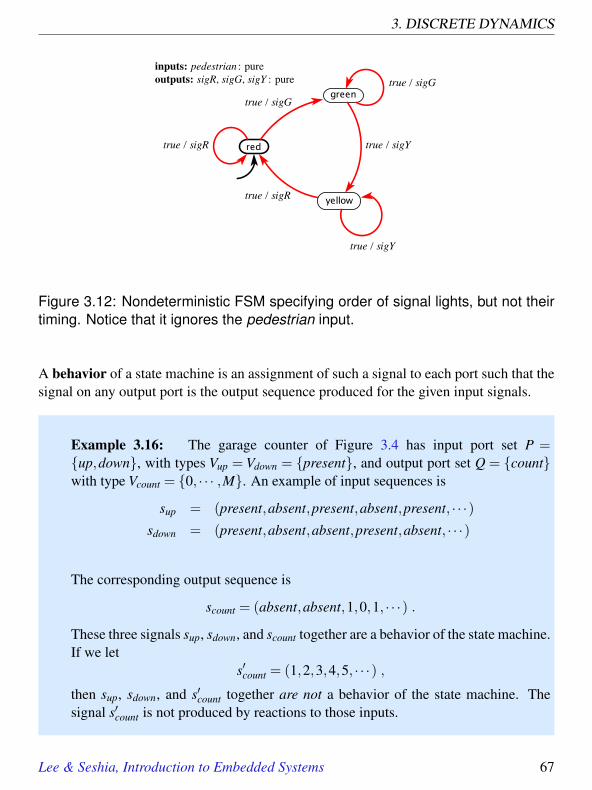
3. DISCRETE DYNAMICS
Figure 3.12: Nondeterministic FSM specifying order of signal lights, but not theirtiming. Notice that it ignores the pedestrian input.
A behavior of a state machine is an assignment of such a signal to each port such that thesignal on any output port is the output sequence produced for the given input signals.
Example 3.16: The garage counter of Figure 3.4 has input port set P =up,down, with types Vup = Vdown = present, and output port set Q = countwith type Vcount = 0, · · · ,M. An example of input sequences is
sup = (present,absent,present,absent,present, · · ·)sdown = (present,absent,absent,present,absent, · · ·)
The corresponding output sequence is
scount = (absent,absent,1,0,1, · · ·) .
These three signals sup, sdown, and scount together are a behavior of the state machine.If we let
s′count = (1,2,3,4,5, · · ·) ,then sup, sdown, and s′count together are not a behavior of the state machine. Thesignal s′count is not produced by reactions to those inputs.
Lee & Seshia, Introduction to Embedded Systems 67

3.6. BEHAVIORS AND TRACES
Deterministic state machines have the property that there is exactly one behavior for eachset of input sequences. That is, if you know the input sequences, then the output sequenceis fully determined. That is, the machine is determinate. Such a machine can be viewedas a function that maps input sequences to output sequences. Nondeterministic state ma-chines can have more than one behavior sharing the same input sequences, and hencecannot be viewed as a function mapping input sequences to output sequences.
The set of all behaviors of a state machine M is called its language, written L(M). Sinceour state machines are receptive, their languages always include all possible input se-quences.
A behavior may be more conveniently represented as a sequence of valuations called anobservable trace. Let xi represent the valuation of the input ports and yi the valuation ofthe output ports at reaction i. Then an observable trace is a sequence
((x0,y0),(x1,y1),(x2,y2), · · ·) .
An observable trace is really just another representation of a behavior.
It is often useful to be able to reason about the states that are traversed in a behavior. Anexecution trace includes the state trajectory, and may be written as a sequence
((x0,s0,y0),(x1,s1,y1),(x2,s2,y2), · · ·) ,
where s0 = initialState. This can be represented a bit more graphically as follows,
s0x0/y0−−−→ s1
x1/y1−−−→ s2x2/y2−−−→ ·· ·
This is an execution trace if for all i ∈ N, (si+1,yi) = update(si,xi) (for a deterministicmachine), or (si+1,yi) ∈ possibleUpdates(si,xi) (for a nondeterministic machine).
Example 3.17: Consider again the garage counter of Figure 3.4 with the sameinput sequences sup and sdown from Example 3.16. The corresponding executiontrace may be written
0up∧down /−−−−−−→ 0
/−−−−→ 0up / 1−−−→ 1
down / 0−−−−−→ 0up / 1−−−→ ·· ·
Here, we have used the same shorthand for valuations that is used on transitionsin Section 3.3.1. For example, the label “up / 1” means that up is present, downis absent, and count has value 1. Any notation that clearly and unambiguouslyrepresents the input and output valuations is acceptable.
68 Lee & Seshia, Introduction to Embedded Systems

3. DISCRETE DYNAMICS
Figure 3.13: A computation tree for the FSM in Figure 3.12.
For a nondeterministic machine, it may be useful to represent all the possible traces thatcorrespond to a particular input sequence, or even all the possible traces that result fromall possible input sequences. This may be done using a computation tree.
Example 3.18: Consider the non-deterministic FSM in Figure 3.12. Figure 3.13shows the computation tree for the first three reactions with any input sequence.Nodes in the tree are states and edges are labeled by the input and output valuations,where the notation true means any input valuation.
Traces and computation trees can be valuable for developing insight into the behaviors ofa state machine and for verifying that undesirable behaviors are avoided.
Lee & Seshia, Introduction to Embedded Systems 69

3.7. SUMMARY
3.7 Summary
This chapter has given an introduction to the use of state machines to model systems withdiscrete dynamics. It gives a graphical notation that is suitable for finite state machines,and an extended state machine notation that can compactly represent large numbers ofstates. It also gives a mathematical model that uses sets and functions rather than visualnotations. The mathematical notation can be useful to ensure precise interpretations ofa model and to prove properties of a model. This chapter has also discussed nondeter-minism, which can provide convenient abstractions that compactly represent families ofbehaviors.
70 Lee & Seshia, Introduction to Embedded Systems

3. DISCRETE DYNAMICS
Exercises
1. Consider an event counter that is a simplified version of the counter in Section 3.1.It has an icon like this:
This actor starts with state i and upon arrival of an event at the input, increments thestate and sends the new value to the output. Thus, e is a pure signal, and c has theform c : R→ absent∪N, assuming i ∈ N. Suppose you are to use such an eventcounter in a weather station to count the number of times that a temperature risesabove some threshold. Your task in this exercise is to generate a reasonable inputsignal e for the event counter. You will create several versions. For all versions,you will design a state machine whose input is a signal τ : R→ absent∪Z thatgives the current temperature (in degrees centigrade) once per hour. The outpute : R→absent,present will be a pure signal that goes to an event counter.
(a) For the first version, your state machine should simply produce a present out-put whenever the input is present and greater than 38 degrees. Otherwise, theoutput should be absent.
(b) For the second version, your state machine should have hysteresis. Specifi-cally, it should produce a present output the first time the input is greater than38 degrees, and subsequently, it should produce a present output anytime theinput is greater than 38 degrees but has dropped below 36 degrees since thelast time a present output was produced.
(c) For the third version, your state machine should implement the same hystere-sis as in part (b), but also produce a present output at most once per day.
2. Consider a variant of the thermostat of example 3.5. In this variant, there is only onetemperature threshold, and to avoid chattering the thermostat simply leaves the heaton or off for at least a fixed amount of time. In the initial state, if the temperature isless than or equal to 20 degrees Celsius, it turns the heater on, and leaves it on forat least 30 seconds. After that, if the temperature is greater than 20 degrees, it turnsthe heater off and leaves it off for at least 2 minutes. It turns it on again only if thetemperature is less than or equal to 20 degrees.
Lee & Seshia, Introduction to Embedded Systems 71

EXERCISES
Figure 3.14: Deterministic finite-state machine for Exercise 3
(a) Design an FSM that behaves as described, assuming it reacts exactly onceevery 30 seconds.
(b) How many possible states does your thermostat have? Is this the smallestnumber of states possible?
(c) Does this model thermostat have the time-scale invariance property?
3. Consider the deterministic finite-state machine in Figure 3.14 that models a simpletraffic light.
(a) Formally write down the description of this FSM as a 5-tuple:
(States, Inputs,Outputs,update, initialState) .
(b) Give an execution trace of this FSM of length 4 assuming the input tick ispresent on each reaction.
(c) Now consider merging the red and yellow states into a single stop state. Tran-sitions that pointed into or out of those states are now directed into or out ofthe new stop state. Other transitions and the inputs and outputs stay the same.The new stop state is the new initial state. Is the resulting state machine de-terministic? Why or why not? If it is deterministic, give a prefix of the traceof length 4. If it is non-deterministic, draw the computation tree up to depth4.
4. This problem considers variants of the FSM in Figure 3.11, which models arrivalsof pedestrians at a crosswalk. We assume that the traffic light at the crosswalk is
72 Lee & Seshia, Introduction to Embedded Systems

3. DISCRETE DYNAMICS
controlled by the FSM in Figure 3.10. In all cases, assume a time triggered model,where both the pedestrian model and the traffic light model react once per second.Assume further that in each reaction, each machine sees as inputs the output pro-duced by the other machine in the same reaction (this form of composition, whichis called synchronous composition, is studied further in Chapter 6).
(a) Suppose that instead of Figure 3.11, we use the following FSM to model thearrival of pedestrians:
Find a trace whereby a pedestrian arrives (the above machine transitions towaiting) but the pedestrian is never allowed to cross. That is, at no time afterthe pedestrian arrives is the traffic light in state red.
(b) Suppose that instead of Figure 3.11, we use the following FSM to model thearrival of pedestrians:
Here, the initial state is nondeterministically chosen to be one of none orcrossing. Find a trace whereby a pedestrian arrives (the above machine tran-sitions from none to waiting) but the pedestrian is never allowed to cross.That is, at no time after the pedestrian arrives is the traffic light in state red.
Lee & Seshia, Introduction to Embedded Systems 73

EXERCISES
5. Consider the state machine in Figure 3.15. State whether each of the following isa behavior for this machine. In each of the following, the ellipsis “· · ·” means thatthe last symbol is repeated forever. Also, for readability, absent is denoted by theshorthand a and present by the shorthand p.
(a) x = (p, p, p, p, p, · · ·), y = (0,1,1,0,0, · · ·)(b) x = (p, p, p, p, p, · · ·), y = (0,1,1,0,a, · · ·)(c) x = (a, p,a, p,a, · · ·), y = (a,1,a,0,a, · · ·)(d) x = (p, p, p, p, p, · · ·), y = (0,0,a,a,a, · · ·)(e) x = (p, p, p, p, p, · · ·), y = (0,a,0,a,a, · · ·)
6. (NOTE: This exercise is rather advanced.) This exercise studies properties of dis-crete signals as formally defined in the sidebar on page 44. Specifically, we willshow that discreteness is not a compositional property. That is, when combiningtwo discrete behaviors in a single system, the resulting combination is not neces-sarily discrete.
(a) Consider a pure signal x : R→present,absent given by
x(t) =
present if t is a non-negative integerabsent otherwise
for all t ∈ R. Show that this signal is discrete.
(b) Consider a pure signal y : R→present,absent given by
y(t) =
present if t = 1−1/n for any positive integer nabsent otherwise
Figure 3.15: State machine for Exercise 5.
74 Lee & Seshia, Introduction to Embedded Systems
3. DISCRETE DYNAMICS
for all t ∈ R. Show that this signal is discrete.
(c) Consider a signal w that is the merge of x and y in the previous two parts.That is, w(t) = present if either x(t) = present or y(t) = present, and is absentotherwise. Show that w is not discrete.
(d) Consider the example shown in Figure 3.1. Assume that each of the twosignals arrival and departure is discrete. Show that this does not imply thatthe output count is a discrete signal.
Lee & Seshia, Introduction to Embedded Systems 75

4Hybrid Systems
Contents4.1 Modal Models . . . . . . . . . . . . . . . . . . . . . . . . . . . . . 78
4.1.1 Actor Model for State Machines . . . . . . . . . . . . . . . . 78
4.1.2 Continuous Inputs . . . . . . . . . . . . . . . . . . . . . . . 79
4.1.3 State Refinements . . . . . . . . . . . . . . . . . . . . . . . 80
4.2 Classes of Hybrid Systems . . . . . . . . . . . . . . . . . . . . . . 824.2.1 Timed Automata . . . . . . . . . . . . . . . . . . . . . . . . 82
4.2.2 Higher-Order Dynamics . . . . . . . . . . . . . . . . . . . . 87
4.2.3 Supervisory control . . . . . . . . . . . . . . . . . . . . . . . 93
4.3 Summary . . . . . . . . . . . . . . . . . . . . . . . . . . . . . . . . 98Exercises . . . . . . . . . . . . . . . . . . . . . . . . . . . . . . . . . . . 100
Chapters 2 and 3 describe two very different modeling strategies, one focused on continu-ous dynamics and one on discrete dynamics. For continuous dynamics, we use differentialequations and their corresponding actor models. For discrete dynamics, we use state ma-chines.
Cyber-physical systems integrate physical dynamics and computational systems, so theycommonly combine both discrete and continuous dynamics. In this chapter, we show thatthe modeling techniques of Chapters 2 and 3 can be combined, yielding what are known as
77

4.1. MODAL MODELS
hybrid systems. Hybrid system models are often much simpler and more understandablethan brute-force models that constrain themselves to only one of the two styles in Chapters2 and 3. They are a powerful tool for understanding real-world systems.
4.1 Modal Models
In this section, we show that state machines can be generalized to admit continuous inputsand outputs and to combine discrete and continuous dynamics.
4.1.1 Actor Model for State Machines
In Section 3.3.1 we explain that state machines have inputs defined by the set Inputs thatmay be pure signals or may carry a value. In either case, the state machine has a numberof input ports, which in the case of pure signals are either present or absent, and in thecase of valued signals have a value at each reaction of the state machine.
We also explain in Section 3.3.1 that actions on transitions set the values of outputs. Theoutputs can also be represented by ports, and again the ports can carry pure signals orvalued signals. In the case of pure signals, a transition that is taken specifies whether theoutput is present or absent, and in the case of valued signals, it assigns a value or assertsthat the signal is absent. Outputs are presumed to be absent between transitions.
Given this input/output view of state machines, it is natural to think of a state machine asan actor, as illustrated in Figure 4.1. In that figure, we assume some number n of inputports named i1 · · · in. At each reaction, these ports have a value that is either present orabsent (if the port carries a pure signal) or a member of some set of values (if the portcarries a valued signal). The outputs are similar. The guards on the transitions definesubsets of possible values on input ports, and the actions assign values to output ports.Given such an actor model, it is straightforward to generalize FSMs to admit continuous-time signals as inputs.
78 Lee & Seshia, Introduction to Embedded Systems

4. HYBRID SYSTEMS
i1
in om
o1... ...
Figure 4.1: An FSM represented as an actor.
4.1.2 Continuous Inputs
We have so far assumed that state machines operate in a sequence of discrete reactions.We have assumed that inputs and outputs are absent between reactions. We will nowgeneralize this to allow inputs and outputs to be continuous-time signals.
In order to get state machine models to coexist with time-based models, we need to inter-pret state transitions to occur on the same timeline used for the time-based portion of thesystem. The notion of discrete reactions described in Section 3.1 suffices for this purpose,but we will no longer require inputs and outputs to be absent between reactions. Instead,we will define a transition to occur when a guard on an outgoing transition from the cur-rent state becomes enabled. As before, during the time between reactions, a state machineis understood to not transition between modes. But the inputs and outputs are no longerrequired to be absent during that time.
Example 4.1: Consider a thermostat modeled as a state machine with states Σ =heating,cooling, shown in Figure 4.2. This is a variant of the model of Example3.5 where instead of a discrete input that provides a temperature at each reaction, theinput is a continuous-time signal τ : R→ R where τ(t) represents the temperatureat time t. The initial state is cooling, and the transition out of this state is enabled
Lee & Seshia, Introduction to Embedded Systems 79

4.1. MODAL MODELS
at the earliest time t after the start time when τ(t)≤ 18. In this example, we assumethe outputs are pure signals heatOn and heatOff.
In the above example, the outputs are present only at the times the transitions are taken.We can also generalize FSMs to support continuous-time outputs, but to do this, we needthe notion of state refinements.
4.1.3 State Refinements
A hybrid system associates with each state of an FSM a dynamic behavior. Our first (verysimple) example uses this capability merely to produce continuous-time outputs.
Example 4.2: Suppose that instead of discrete outputs as in Example 4.1 we wishto produce a control signal whose value is 1 when the heat is on and 0 when theheat is off. Such a control signal could directly drive a heater. The thermostat inFigure 4.3 does this. In that figure, each state has a refinement that gives the valueof the output h while the state machine is in that state.
In a hybrid system, the current state of the state machine has a state refinement thatgives the dynamic behavior of the output as a function of the input. In the above simple
Figure 4.2: A thermostat modeled as an FSM with a continuous-time input signal.
80 Lee & Seshia, Introduction to Embedded Systems

4. HYBRID SYSTEMS
example, the output is constant in each state, which is rather trivial dynamics. Hybridsystems can get much more elaborate.
The general structure of a hybrid system model is shown in Figure 4.4. In that figure,there is a two-state finite-state machine. Each state is associated with a state refinementlabeled in the figure as a “time-based system.” The state refinement defines dynamicbehavior of the outputs and (possibly) additional continuous state variables. In addition,each transition can optionally specify set actions, which set the values of such additionalstate variables when a transition is taken. The example of Figure 4.3 is rather trivial, inthat it has no continuous state variables, no output actions, and no set actions.
A hybrid system is sometimes called a modal model because it has a finite number ofmodes, one for each state of the FSM, and when it is in a mode, it has dynamics specifiedby the state refinement. The states of the FSM may be referred to as modes rather thanstates, which as we will see, helps prevent confusion with states of the refinements.
The next simplest such dynamics, besides the rather trivial constant outputs of Example4.2 is found in timed automata, which we discuss next.
h
Figure 4.3: A thermostat with continuous-time output.
Lee & Seshia, Introduction to Embedded Systems 81

4.2. CLASSES OF HYBRID SYSTEMS
i1
in om
o1... ...
time-based system time-based system
Figure 4.4: Notation for hybrid systems.
4.2 Classes of Hybrid Systems
Hybrid systems can be quite elaborate. In this section, we first describe a relatively sim-ple form known as timed automata. We then illustrate more elaborate forms that modelnontrivial physical dynamics and nontrivial control systems.
4.2.1 Timed Automata
Most cyber-physical systems require measuring the passage of time and performing ac-tions at specific times. A device that measures the passage of time, a clock, has a partic-ularly simple dynamics: its state progresses linearly in time. In this section, we describetimed automata, a formalism introduced by Alur and Dill (1994), which enable the con-struction of more complicated systems from such simple clocks.
Timed automata are the simplest non-trivial hybrid systems. They are modal modelswhere the time-based refinements have very simple dynamics; all they do is measure thepassage of time. A clock is modeled by a first-order differential equation,
∀ t ∈ Tm, s(t) = a,
82 Lee & Seshia, Introduction to Embedded Systems

4. HYBRID SYSTEMS
where s : R→ R is a continuous-time signal, s(t) is the value of the clock at time t, andTm ⊂R is the subset of time during which the hybrid system is in mode m. The rate of theclock, a, is a constant while the system is in this mode.1
Example 4.3: Recall the thermostat of Example 4.1, which uses hysteresis to pre-vent chattering. An alternative implementation that would also prevent chatteringwould use a single temperature threshold, but instead would require that the heaterremain on or off for at least a minimum amount of time, regardless of the tem-perature. This design would not have the hysteresis property, but may be usefulnonetheless. This can be modeled as a timed automaton as shown in Figure 4.5. Inthat figure, each state refinement has a clock, which is a continuous-time signal swith dynamics given by
s(t) = 1 .
The value s(t) increases linearly with t. Note that in that figure, the state refinementis shown directly with the name of the state in the state bubble. This shorthand isconvenient when the refinement is relatively simple.
Notice that the initial state cooling has a set action on the dangling transition indi-cating the initial state, written as
s(t) := Tc .
As we did with extended state machines, we use the notation “:=” to emphasize thatthis is an assignment, not a predicate. This action ensures that when the thermostatstarts, it can immediately transition to the heating mode if the temperature τ(t) isless than or equal to 20 degrees. The other two transitions each have set actions thatreset the clock s to zero. The portion of the guard that specifies s(t) ≥ Th ensuresthat the heater will always be on for at least time Th. The portion of the guard thatspecifies s(t) ≥ Tc specifies that once the heater goes off, it will remain off for atleast time Tc.
A possible execution of this timed automaton is shown in Figure 4.6. In that figure,we assume that the temperature is initially above the setpoint of 20 degrees, so theFSM remains in the cooling state until the temperature drops to 20 degrees. At that
1The variant of timed automata we describe in this chapter differs from the original model of Alur andDill (1994) in that the rates of clocks in different modes can be different. This variant is sometimes describedin the literature as multi-rate timed automata.
Lee & Seshia, Introduction to Embedded Systems 83

4.2. CLASSES OF HYBRID SYSTEMS
h
Figure 4.5: A timed automaton modeling a thermostat with a single temperaturethreshold, 20, and minimum times Tc and Th in each mode.
time t1, it can take the transition immediately because s(t1) > Tc. The transitionresets s to zero and turns on the heater. The heater will remain on until time t1+Th,assuming that the temperature only rises when the heater is on. At time t1 +Th, itwill transition back to the cooling state and turn the heater off. (We assume herethat a transition is taken as soon as it is enabled. Other transition semantics arepossible.) It will cool until at least time Tc elapses and until the temperature dropsagain to 20 degrees, at which point it will turn the heater back on.
In the previous example the state of the system at any time t is not only the mode, heatingor cooling, but also the current value s(t) of the clock. We call s a continuous state vari-able, whereas heating and cooling are discrete states. Thus, note that the term “state”for such a hybrid system can become confusing. The FSM has states, but so do the refine-ment systems (unless they are memoryless). When there is any possibility of confusionwe explicitly refer to the states of the machine as modes.
Transitions between modes have actions associated with them. Sometimes, it is useful tohave transitions from one mode back to itself, just so that the action can be realized. Thisis illustrated in the next example, which also shows a timed automaton that produces apure output.
84 Lee & Seshia, Introduction to Embedded Systems

4. HYBRID SYSTEMS
h(t)
t...
(a)
(b)
(c)
s(t)
t...
τ(t)
t...20 t1 t1 + Th
0
Tc
01
Figure 4.6: (a) A temperature input to the hybrid system of Figure 4.5, (b) theoutput h, and (c) the refinement state s.
Example 4.4: The timed automaton in Figure 4.7 produces a pure output that willbe present every T time units, starting at the time when the system begins executing.Notice that the guard on the transition, s(t) ≥ T , is followed by an output action,tick, and a set action, s(t) := 0.
Figure 4.7 shows another notational shorthand that works well for simple diagrams. Theautomaton is shown directly inside the icon for its actor model.
Example 4.5: The traffic light controller of Figure 3.10 is a time triggered machinethat assumes it reacts once each second. Figure 4.8 shows a timed automaton withthe same behavior. It is more explicit about the passage of time in that its temporaldynamics do not depend on unstated assumptions about when the machine willreact.
Lee & Seshia, Introduction to Embedded Systems 85

4.2. CLASSES OF HYBRID SYSTEMS
Figure 4.7: A timed automaton that generates a pure output event every T timeunits.
Figure 4.8: A timed automaton variant of the traffic light controller of Figure 3.10.
86 Lee & Seshia, Introduction to Embedded Systems

4. HYBRID SYSTEMS
y1(t)
y2(t)
y1(t) y2(t)
0.0
0.5
1.0
1.5
2.0
2.5
3.0
0 5 10 15 20 25 30 35 40 45 50
Displacement of Masses
time
Figure 4.9: Sticky masses system considered in Example 4.6.
4.2.2 Higher-Order Dynamics
In timed automata, all that happens in the time-based refinement systems is that timepasses. Hybrid systems, however, are much more interesting when the behavior of therefinements is more complex. Specifically,
Example 4.6: Consider the physical system depicted in Figure 4.9. Two stickyround masses are attached to springs. The springs are compressed or extended and
Lee & Seshia, Introduction to Embedded Systems 87

4.2. CLASSES OF HYBRID SYSTEMS
Figure 4.10: Hybrid system model for the sticky masses system considered inExample 4.6.
then released. The masses oscillate on a frictionless table. If they collide, they sticktogether and oscillate together. After some time, the stickiness decays, and massespull apart again.
A plot of the displacement of the two masses as a function of time is shown inFigure 4.9. Both springs begin compressed, so the masses begin moving towardsone another. They almost immediately collide, and then oscillate together for abrief period until they pull apart. In this plot, they collide two more times, andalmost collide a third time.
The physics of this problem is quite simple if we assume idealized springs. Lety1(t) denote the right edge of the left mass at time t, and y2(t) denote the left edgeof the right mass at time t, as shown in Figure 4.9. Let p1 and p2 denote theneutral positions of the two masses, i.e., when the springs are neither extended norcompressed, so the force is zero. For an ideal spring, the force at time t on the mass
88 Lee & Seshia, Introduction to Embedded Systems

4. HYBRID SYSTEMS
is proportional to p1− y1(t) (for the left mass) and p2− y2(t) (for the right mass).The force is positive to the right and negative to the left.
Let the spring constants be k1 and k2, respectively. Then the force on the left springis k1(p1− y1(t)), and the force on the right spring is k2(p2− y2(t)). Let the massesbe m1 and m2 respectively. Now we can use Newton’s second law, which relatesforce, mass, and acceleration,
f = ma.
The acceleration is the second derivative of the position with respect to time, whichwe write y1(t) and y2(t). Thus, as long as the masses are separate, their dynamicsare given by
y1(t) = k1(p1− y1(t))/m1 (4.1)
y2(t) = k2(p2− y2(t))/m2. (4.2)
When the masses collide, however, the situation changes. With the masses stucktogether, they behave as a single object with mass m1 +m2. This single object ispulled in opposite directions by two springs. While the masses are stuck together,y1(t) = y2(t). Let
y(t) = y1(t) = y2(t).
The dynamics are then given by
y(t) =k1 p1 + k2 p2− (k1 + k2)y(t)
m1 +m2. (4.3)
It is easy to see now how to construct a hybrid systems model for this physicalsystem. The model is shown in Figure 4.10. It has two modes, apart and together.The refinement of the apart mode is given by (4.1) and (4.2), while the refinementof the together mode is given by (4.3).
We still have work to do, however, to label the transitions. The initial transition isshown in Figure 4.10 entering the apart mode. Thus, we are assuming the massesbegin apart. Moreover, this transition is labeled with a set action that sets the initialpositions of the two masses to i1 and i2 and the initial velocities to zero.
The transition from apart to together has the guard
y1(t) = y2(t) .
Lee & Seshia, Introduction to Embedded Systems 89
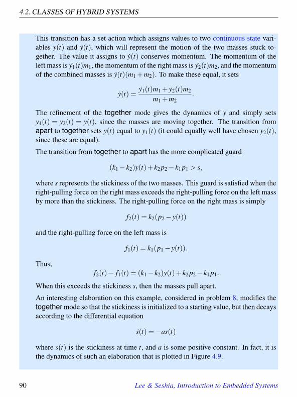
4.2. CLASSES OF HYBRID SYSTEMS
This transition has a set action which assigns values to two continuous state vari-ables y(t) and y(t), which will represent the motion of the two masses stuck to-gether. The value it assigns to y(t) conserves momentum. The momentum of theleft mass is y1(t)m1, the momentum of the right mass is y2(t)m2, and the momentumof the combined masses is y(t)(m1 +m2). To make these equal, it sets
y(t) =y1(t)m1 + y2(t)m2
m1 +m2.
The refinement of the together mode gives the dynamics of y and simply setsy1(t) = y2(t) = y(t), since the masses are moving together. The transition fromapart to together sets y(t) equal to y1(t) (it could equally well have chosen y2(t),since these are equal).
The transition from together to apart has the more complicated guard
(k1− k2)y(t)+ k2 p2− k1 p1 > s,
where s represents the stickiness of the two masses. This guard is satisfied when theright-pulling force on the right mass exceeds the right-pulling force on the left massby more than the stickiness. The right-pulling force on the right mass is simply
f2(t) = k2(p2− y(t))
and the right-pulling force on the left mass is
f1(t) = k1(p1− y(t)).
Thus,f2(t)− f1(t) = (k1− k2)y(t)+ k2 p2− k1 p1.
When this exceeds the stickiness s, then the masses pull apart.
An interesting elaboration on this example, considered in problem 8, modifies thetogether mode so that the stickiness is initialized to a starting value, but then decaysaccording to the differential equation
s(t) =−as(t)
where s(t) is the stickiness at time t, and a is some positive constant. In fact, it isthe dynamics of such an elaboration that is plotted in Figure 4.9.
90 Lee & Seshia, Introduction to Embedded Systems

4. HYBRID SYSTEMS
As in Example 4.4, it is sometimes useful to have hybrid system models with only onestate. The actions on one or more state transitions define the discrete event behavior thatcombines with the time-based behavior.
Example 4.7: Consider a bouncing ball. At time t = 0, the ball is dropped froma height y(0) = h0, where h0 is the initial height in meters. It falls freely. At somelater time t1 it hits the ground with a velocity y(t1) < 0 m/s (meters per second).A bump event is produced when the ball hits the ground. The collision is inelastic(meaning that kinetic energy is lost), and the ball bounces back up with velocity−ay(t1), where a is constant with 0 < a < 1. The ball will then rise to a certainheight and fall back to the ground repeatedly.
The behavior of the bouncing ball can be described by the hybrid system of Figure4.11. There is only one mode, called free. When it is not in contact with the ground,we know that the ball follows the second-order differential equation,
y(t) =−g, (4.4)
where g = 9.81 m/sec2 is the acceleration imposed by gravity. The continuous statevariables of the free mode are
s(t) =[
y(t)y(t)
]with the initial conditions y(0) = h0 and y(0) = 0. It is then a simple matter torewrite (4.4) as a first-order differential equation,
s(t) = f (s(t)) (4.5)
for a suitably chosen function f .
At the time t = t1 when the ball first hits the ground, the guard
y(t) = 0
is satisfied, and the self-loop transition is taken. The output bump is produced, andthe set action y(t) := −ay(t) changes y(t1) to have value −ay(t1). Then (4.4) isfollowed again until the guard becomes true again.
Lee & Seshia, Introduction to Embedded Systems 91

4.2. CLASSES OF HYBRID SYSTEMS
t1 t2
t
t1 t2
t
Figure 4.11: The motion of a bouncing ball may be described as a hybrid systemwith only one mode. The system outputs a bump each time the ball hits theground, and also outputs the position of the ball. The position and velocity areplotted versus time at the right.
By integrating (4.4) we get, for all t ∈ (0, t1),
y(t) = −gt,
y(t) = y(0)+∫ t
0y(τ)dτ = h0−
12
gt2.
So t1 > 0 is determined by y(t1) = 0. It is the solution to the equation
h0−12
gt2 = 0.
Thus,t1 =
√2h0/g.
Figure 4.11 plots the continuous state versus time.
The bouncing ball example above has an interesting difficulty that is explored in Exer-cise 7. Specifically, the time between bounces gets smaller as time increases. In fact, itgets smaller fast enough that an infinite number of bounces occur in a finite amount oftime. A system with an infinite number of discrete events in a finite amount of time is
92 Lee & Seshia, Introduction to Embedded Systems

4. HYBRID SYSTEMS
called a Zeno system, after Zeno of Elea, a pre-Socratic Greek philosopher famous forhis paradoxes. In the physical world, of course, the ball will eventually stop bouncing.The Zeno behavior is an artifact of the model. Another example of a Zeno hybrid systemis considered in Exercise 10.
4.2.3 Supervisory control
A control system involves four components: a system called the plant, the physical pro-cess that is to be controlled; the environment in which the plant operates; the sensors thatmeasure some variables of the plant and the environment; and the controller that deter-mines the mode transition structure and selects the time-based inputs to the plant. Thecontroller has two levels: the supervisory control that determines the mode transitionstructure, and the low-level control that determines the time-based inputs to the plant.Intuitively, the supervisory controller determines which of several strategies should befollowed, and the low-level controller implements the selected strategy. Hybrid systemsare ideal for modeling such two-level controllers. We show how through a detailed exam-ple.
Example 4.8: Consider an automated guided vehicle (AGV) that moves along aclosed track painted on a warehouse or factory floor. We will design a controller sothat the vehicle closely follows the track.
The vehicle has two degrees of freedom. At any time t, it can move forward alongits body axis with speed u(t) with the restriction that 0 ≤ u(t) ≤ 10 mph (milesper hour). It can also rotate about its center of gravity with an angular speed ω(t)restricted to−π≤ω(t)≤ π radians/second. We ignore the inertia of the vehicle, sowe assume that we can instantaneously change the velocity or angular speed.
Let (x(t),y(t)) ∈ R2 be the position relative to some fixed coordinate frame andθ(t) ∈ (−π,π] be the angle (in radians) of the vehicle at time t, as shown in Figure4.12. In terms of this coordinate frame, the motion of the vehicle is given by asystem of three differential equations,
x(t) = u(t)cosθ(t),y(t) = u(t)sinθ(t), (4.6)
θ(t) = ω(t).
Lee & Seshia, Introduction to Embedded Systems 93

4.2. CLASSES OF HYBRID SYSTEMS
track
AGV
globalcoordinateframe
Figure 4.12: Illustration of the automated guided vehicle of Example 4.8. Thevehicle is following a curved painted track, and has deviated from the track by adistance e(t). The coordinates of the vehicle at time t with respect to the globalcoordinate frame are (x(t),y(t),θ(t)).
Equations (4.6) describe the plant. The environment is the closed painted track. Itcould be described by an equation. We will describe it indirectly below by meansof a sensor.
The two-level controller design is based on a simple idea. The vehicle alwaysmoves at its maximum speed of 10 mph. If the vehicle strays too far to the left ofthe track, the controller steers it towards the right; if it strays too far to the rightof the track, the controller steers it towards the left. If the vehicle is close to thetrack, the controller maintains the vehicle in a straight direction. Thus the controller
94 Lee & Seshia, Introduction to Embedded Systems

4. HYBRID SYSTEMS
Figure 4.13: The automatic guided vehicle of Example 4.8 has four modes: stop,straight, left, right.
Lee & Seshia, Introduction to Embedded Systems 95

4.2. CLASSES OF HYBRID SYSTEMS
guides the vehicle in four modes, left, right, straight, and stop. In stop mode, thevehicle comes to a halt.
The following differential equations govern the AGV’s motion in the refinementsof the four modes. They describe the low-level controller, i.e., the selection of thetime-based plant inputs in each mode.
straight
x(t) = 10cosθ(t)y(t) = 10sinθ(t)θ(t) = 0
left
x(t) = 10cosθ(t)y(t) = 10sinθ(t)θ(t) = π
right
x(t) = 10cosθ(t)y(t) = 10sinθ(t)θ(t) = −π
stop
x(t) = 0
y(t) = 0
θ(t) = 0
In the stop mode, the vehicle is stopped, so x(t), y(t), and θ(t) are constant. Inthe left mode, θ(t) increases at the rate of π radians/second, so from Figure 4.12we see that the vehicle moves to the left. In the right mode, it moves to the right.In the straight mode, θ(t) is constant, and the vehicle moves straight ahead witha constant heading. The refinements of the four modes are shown in the boxes ofFigure 4.13.
96 Lee & Seshia, Introduction to Embedded Systems

4. HYBRID SYSTEMS
We design the supervisory control governing transitions between modes in sucha way that the vehicle closely follows the track, using a sensor that determineshow far the vehicle is to the left or right of the track. We can build such a sensorusing photodiodes. Let’s suppose the track is painted with a light-reflecting color,whereas the floor is relatively dark. Underneath the AGV we place an array ofphotodiodes as shown in Figure 4.14. The array is perpendicular to the AGV bodyaxis. As the AGV passes over the track, the diode directly above the track generatesmore current than the other diodes. By comparing the magnitudes of the currentsthrough the different diodes, the sensor estimates the displacement e(t) of the centerof the array (hence, the center of the AGV) from the track. We adopt the conventionthat e(t) < 0 means that the AGV is to the right of the track and e(t) > 0 means itis to the left. We model the sensor output as a function f of the AGV’s position,
∀t, e(t) = f (x(t),y(t)).
The function f of course depends on the environment—the track. We now specifythe supervisory controller precisely. We select two thresholds, 0 < ε1 < ε2, asshown in Figure 4.14. If the magnitude of the displacement is small, |e(t)| < ε1,we consider that the AGV is close enough to the track, and the AGV can movestraight ahead, in straight mode. If e(t)> ε2 (e(t) is large and positive), the AGVhas strayed too far to the left and must be steered to the right, by switching to rightmode. If e(t) < −ε2 (e(t) is large and negative), the AGV has strayed too far tothe right and must be steered to the left, by switching to left mode. This controllogic is captured in the mode transitions of Figure 4.13. The inputs are pure signalsstop and start. These model an operator that can stop or start the AGV. There is nocontinuous-time input. The outputs represent the position of the vehicle, x(t) andy(t). The initial mode is stop, and the initial values of its refinement are (x0,y0,θ0).
We analyze how the AGV will move. Figure 4.15 sketches one possible trajectory.Initially the vehicle is within distance ε1 of the track, so it moves straight. At somelater time, the vehicle goes too far to the left, so the guard
¬stop∧ e(t)> ε2
is satisfied, and there is a mode switch to right. After some time, the vehicle willagain be close enough to the track, so the guard
¬stop∧|e(t)|< ε1
Lee & Seshia, Introduction to Embedded Systems 97

4.3. SUMMARY
photodiode trackAGV
Figure 4.14: An array of photodiodes under the AGV is used to estimate thedisplacement e of the AGV relative to the track. The photodiode directly abovethe track generates more current.
is satisfied, and there is a mode switch to straight. Some time later, the vehicle istoo far to the right, so the guard
¬stop∧ e(t)<−ε2
is satisfied, and there is a mode switch to left. And so on.
The example illustrates the four components of a control system. The plant is describedby the differential equations (4.6) that govern the evolution of the continuous state attime t, (x(t),y(t),θ(t)), in terms of the plant inputs u and ω. The second componentis the environment—the closed track. The third component is the sensor, whose outputat time t, e(t) = f (x(t),y(t)), gives the position of the AGV relative to the track. Thefourth component is the two-level controller. The supervisory controller comprises thefour modes and the guards that determine when to switch between modes. The low-levelcontroller specifies how the time-based inputs to the plant, u and ω, are selected in eachmode.
4.3 Summary
Hybrid systems provide a bridge between time-based models and state-machine models.The combination of the two families of models provides a rich framework for describing
98 Lee & Seshia, Introduction to Embedded Systems

4. HYBRID SYSTEMS
initial position
straight
right
straight
left
track straight
Figure 4.15: A trajectory of the AGV, annotated with modes.
real-world systems. There are two key ideas. First, discrete events (state changes in a statemachine) get embedded in a time base. Second, a hierarchical description is particularlyuseful, where the system undergoes discrete transitions between different modes of opera-tion. Associated with each mode of operation is a time-based system called the refinementof the mode. Mode transitions are taken when guards that specify the combination of in-puts and continuous states are satisfied. The action associated with a transition, in turn,sets the continuous state in the destination mode.
The behavior of a hybrid system is understood using the tools of state machine analysisfor mode transitions and the tools of time-based analysis for the refinement systems. Thedesign of hybrid systems similarly proceeds on two levels: state machines are designed toachieve the appropriate logic of mode transitions, and continuous refinement systems aredesigned to secure the desired time-based behavior in each mode.
Lee & Seshia, Introduction to Embedded Systems 99

EXERCISES
Exercises
1. Construct (on paper is sufficient) a timed automaton similar to that of Figure 4.7which produces tick at times 1,2,3,5,6,7,8,10,11, · · · . That is, ticks are producedwith intervals between them of 1 second (three times) and 2 seconds (once).
2. The objective of this problem is to understand a timed automaton, and then to mod-ify it as specified.
(a) For the timed automaton shown below, describe the output y. Avoid impreciseor sloppy notation.
(b) Assume there is a new pure input reset, and that when this input is present,the hybrid system starts over, behaving as if it were starting at time 0 again.Modify the hybrid system from part (a) to do this.
3. You have an analog source that produces a pure tone. You can switch the source onor off by the input event on or off. Construct a timed automaton that provides the onand off signals as outputs, to be connected to the inputs of the tone generator. Yoursystem should behave as follows. Upon receiving an input event ring, it shouldproduce an 80 ms-long sound consisting of three 20 ms-long bursts of the pure toneseparated by two 10 ms intervals of silence. What does your system do if it receivestwo ring events that are 50 ms apart?
4. Automobiles today have the features listed below. Implement each feature as atimed automaton.
(a) The dome light is turned on as soon as any door is opened. It stays on for 30seconds after all doors are shut. What sensors are needed?
100 Lee & Seshia, Introduction to Embedded Systems

4. HYBRID SYSTEMS
Main
Sec
onda
ry
light
detector
R
R G
G Y
Y
Figure 4.16: Traffic lights control the intersection of a main street and a secondarystreet. A detector senses when a vehicle crosses it. The red phase of one lightmust coincide with the green and yellow phases of the other light.
(b) Once the engine is started, a beeper is sounded and a red light warning isindicated if there are passengers that have not buckled their seat belt. Thebeeper stops sounding after 30 seconds, or as soon the seat belts are buckled,whichever is sooner. The warning light is on all the time the seat belt is un-buckled. Hint: Assume the sensors provide a warn event when the ignitionis turned on and there is a seat with passenger not buckled in, or if the igni-tion is already on and a passenger sits in a seat without buckling the seatbelt.Assume further that the sensors provide a noWarn event when a passenger de-parts from a seat, or when the buckle is buckled, or when the ignition is turnedoff.
5. A programmable thermostat allows you to select 4 times, 0≤ T1≤ ·· · ≤ T4 < 24 (fora 24-hour cycle) and the corresponding setpoint temperatures a1, · · · ,a4. Constructa timed automaton that sends the event ai to the heating systems controller. Thecontroller maintains the temperature close to the value ai until it receives the nextevent. How many timers and modes do you need?
6. Figure 4.16 depicts the intersection of two one-way streets, called Main and Sec-ondary. A light on each street controls its traffic. Each light goes through a cycle
Lee & Seshia, Introduction to Embedded Systems 101

EXERCISES
consisting of a red (R), green (G), and yellow (Y) phases. It is a safety requirementthat when one light is in its green or yellow phase, the other is in its red phase. Theyellow phase is always 5 seconds long.
The traffic lights operate as follows. A sensor in the secondary road detects a ve-hicle. While no vehicle is detected, there is a 4 minute-long cycle with the mainlight having 3 minutes of green, 5 seconds of yellow, and 55 seconds of red. Thesecondary light is red for 3 minutes and 5 seconds (while the main light is greenand yellow), green for 50 seconds, then yellow for 5 seconds.
If a vehicle is detected on the secondary road, the traffic light quickly gives a rightof way to the secondary road. When this happens, the main light aborts its greenphase and immediately switches to its 5 second yellow phase. If the vehicle isdetected while the main light is yellow or red, the system continues as if there wereno vehicle.
Design a hybrid system that controls the lights. Let this hybrid system have sixpure outputs, one for each light, named mG, mY, and mR, to designate the mainlight being green, yellow, or red, respectively, and sG, sY, and sR, to designate thesecondary light being green, yellow, or red, respectively. These signals should begenerated to turn on a light. You can implicitly assume that when one light is turnedon, whichever has been on is turned off.
7. For the bouncing ball of Example 4.7, let tn be the time when the ball hits the groundfor the n-th time, and let vn = y(tn) be the velocity at that time.
(a) Find a relation between vn+1 and vn for n > 1, and then calculate vn in termsof v1.
(b) Obtain tn in terms of v1 and a. Use this to show that the bouncing ball is aZeno system. Hint: The geometric series identity might be useful, wherefor |b|< 1,
∞
∑m=0
bm =1
1−b.
(c) Calculate the maximum height reached by the ball after successive bumps.
8. Elaborate the hybrid system model of Figure 4.10 so that in the together mode, thestickiness decays according to the differential equation
s(t) =−as(t)
102 Lee & Seshia, Introduction to Embedded Systems

4. HYBRID SYSTEMS
x1
r1
v1
x2
r2
v2
w
Figure 4.17: Water tank system.
where s(t) is the stickiness at time t, and a is some positive constant. On the tran-sition into this mode, the stickiness should be initialized to some starting stickinessb.
9. Show that the trajectory of the AGV of Figure 4.13 while it is in left or right modeis a circle. What is the radius of this circle, and how long does it take to complete acircle?
10. Consider Figure 4.17 depicting a system comprising two tanks containing water.Each tank is leaking at a constant rate. Water is added at a constant rate to thesystem through a hose, which at any point in time is filling either one tank or theother. It is assumed that the hose can switch between the tanks instantaneously. Fori ∈ 1,2, let xi denote the volume of water in Tank i and vi > 0 denote the constantflow of water out of Tank i. Let w denote the constant flow of water into the system.The objective is to keep the water volumes above r1 and r2, respectively, assumingthat the water volumes are above r1 and r2 initially. This is to be achieved by acontroller that switches the inflow to Tank 1 whenever x1(t) ≤ r1(t) and to Tank 2whenever x2(t)≤ r2(t).
The hybrid automaton representing this two-tank system is given in Figure 4.18.
Answer the following questions:
Lee & Seshia, Introduction to Embedded Systems 103

EXERCISES
Figure 4.18: Hybrid automaton representing water tank system.
(a) Construct a model of this hybrid automaton in Ptolemy II, LabVIEW, orSimulink. Use the following parameter values: r1 = r2 = 0, v1 = v2 = 0.5,and w = 0.75. Set the initial state to be (q1,(0,1)). (That is, initial valuex1(0) is 0 and x2(0) is 1.)
Verify that this hybrid automaton is Zeno. What is the reason for this Zenobehavior? Simulate your model and plot how x1 and x2 vary as a function oftime t, simulating long enough to illustrate the Zeno behavior.
(b) A Zeno system may be regularized by ensuring that the time between tran-sitions is never less than some positive number ε. This can be emulated byinserting extra modes in which the hybrid automaton dwells for time ε. Useregularization to make your model from part (a) non-Zeno. Again, plot x1 andx2 for the same length of time as in the first part. State the value of ε that youused.
Include printouts of your plots with your answer.
11. Consider the following timed automaton:
104 Lee & Seshia, Introduction to Embedded Systems

4. HYBRID SYSTEMS
Assume t1 and t2 are positive real numbers.
(a) What is the minimum amount of time between events a? That is, what is thesmallest possible time between two times when the signal a is present?
(b) Suppose that the machine above is composed in a synchronous side-by-sidecomposition with the following machine:
Find a tight lower bound on the time between events a and b. That is, find alower bound on the time gap during which there are no events in signals a orb. Give an argument that your lower bound is tight.
Lee & Seshia, Introduction to Embedded Systems 105

5Composition ofState Machines
Contents5.1 Concurrent Composition . . . . . . . . . . . . . . . . . . . . . . . 109
Sidebar: About Synchrony . . . . . . . . . . . . . . . . . . . . . . . 110
5.1.1 Side-by-Side Synchronous Composition . . . . . . . . . . . . 111
5.1.2 Side-by-Side Asynchronous Composition . . . . . . . . . . . 114
Sidebar: Scheduling Semantics for Asynchronous Composition . . . . 116
5.1.3 Shared Variables . . . . . . . . . . . . . . . . . . . . . . . . 117
5.1.4 Cascade Composition . . . . . . . . . . . . . . . . . . . . . 119
5.1.5 General Composition . . . . . . . . . . . . . . . . . . . . . . 123
5.2 Hierarchical State Machines . . . . . . . . . . . . . . . . . . . . . 1245.3 Summary . . . . . . . . . . . . . . . . . . . . . . . . . . . . . . . . 128Exercises . . . . . . . . . . . . . . . . . . . . . . . . . . . . . . . . . . . 130
State machines provide a convenient way to model behaviors of systems. One disadvan-tage that they have is that for most interesting systems, the number of states is very large,often even infinite. Automated tools can handle large state spaces, but humans have moredifficulty with any direct representation of a large state space.
107

A time-honored principle in engineering is that complicated systems should be describedas compositions of simpler systems. This chapter gives a number of ways to do this withstate machines. The reader should be aware, however, that there are many subtly differentways to compose state machines. Compositions that look similar on the surface may meandifferent things to different people. The rules of notation of a model are called its syntax,and the meaning of the notation is called its semantics.
Example 5.1: In the standard syntax of arithmetic, a plus sign + has a number orexpression before it, and a number or expression after it. Hence, 1+2, a sequenceof three symbols, is a valid arithmetic expression, but 1+ is not. The semantics ofthe expression 1+ 2 is the addition of two numbers. This expression means “thenumber three, obtained by adding 1 and 2.” The expression 2+ 1 is syntacticallydifferent, but semantically identical (because addition is commutative).
The models in this book predominantly use a visual syntax, where the elements are boxes,circles, arrows, etc., rather than characters in a character set, and where the positioningof the elements is not constrained to be a sequence. Such syntaxes are less standardizedthan, for example, the syntax of arithmetic. We will see that the same syntax can havemany different semantics, which can cause no end of confusion.
Example 5.2: A now popular notation for concurrent composition of statemachines called Statecharts was introduced by Harel (1987). Although theyare all based on the same original paper, many variants of Statecharts haveevolved (von der Beeck, 1994). These variants often assign different semanticsto the same syntax.
In this chapter, we assume an actor model for extended state machines using the syntaxsummarized in Figure 5.1. The semantics of a single such state machine is described inChapter 3. This chapter will discuss the semantics that can be assigned to compositionsof multiple such machines.
The first composition technique we consider is concurrent composition. Two or morestate machines react either simultaneously or independently. If the reactions are simul-
108 Lee & Seshia, Introduction to Embedded Systems

5. COMPOSITION OF STATE MACHINES
taneous, we call it synchronous composition. If they are independent, then we call itasynchronous composition. But even within these classes of composition, many subtlevariations in the semantics are possible. These variations mostly revolve around whetherand how the state machines communicate and share variables.
The second composition technique we will consider is hierarchy. Hierarchical state ma-chines can also enable complicated systems to be described as compositions of simplersystems. Again, we will see that subtle differences in semantics are possible.
5.1 Concurrent Composition
To study concurrent composition of state machines, we will proceed through a sequenceof patterns of composition. These patterns can be combined to build arbitrarily compli-cated systems. We begin with the simplest case, side-by-side composition, where thestate machines being composed do not communicate. We then consider allowing com-munication through shared variables, showing that this creates significant subtleties thatcan complicate modeling. We then consider communication through ports, first lookingat serial composition, then expanding to arbitrary interconnections. We consider bothsynchronous and asynchronous composition for each type of composition.
i1
in om
o1... ...
Figure 5.1: Summary of notation for state machines used in this chapter.
Lee & Seshia, Introduction to Embedded Systems 109

5.1. CONCURRENT COMPOSITION
About Synchrony
The term synchronous means (1) occurring or existing at the same time or (2) moving oroperating at the same rate. In engineering and computer science, the term has a numberof meanings that are mostly consistent with these definitions, but oddly inconsistent withone another. In referring to concurrent software constructed using threads or processes,synchronous communication refers to a rendezvous style of communication, where thesender of a message must wait for the receiver to be ready to receive, and the receiver mustwait for the sender. Conceptually, the two threads see the communication occurring at thesame time, consistent with definition (1). In Java, the keyword synchronized definesblocks of code that are not permitted to execute simultaneously. Oddly, two code blocksthat are synchronized cannot “occur” (execute) at the same time, which is inconsistentwith both definitions.
In the world of software, there is yet a third meaning of the word synchronous, and itis this third meaning that we use in this chapter. This third meaning underlies the syn-chronous languages (see box on page 145). Two key ideas govern these languages. First,the outputs of components in a program are (conceptually) simultaneous with their inputs(this is called the synchrony hypothesis). Second, components in a program execute(conceptually) simultaneously and instantaneously. Real executions do not literally oc-cur simultaneously nor instantaneously, and outputs are not really simultaneous with theinputs, but a correct execution must behave as if they were. This use of the word syn-chronous is consistent with both definitions above; executions of components occur at thesame time and operate at the same rate.
In circuit design, the word synchronous refers to a style of design where a clock thatis distributed throughout a circuit drives latches that record their inputs on edges of theclock. The time between clock edges needs to be sufficient for circuits between latchesto settle. Conceptually, this model is similar to the model in synchronous languages.Assuming that the circuits between latches have zero delay is equivalent to the synchronyhypothesis, and global clock distribution gives simultaneous and instantaneous execution.
In power systems engineering, synchronous means that electrical waveforms have thesame frequency and phase. In signal processing, synchronous means that signals have thesame sample rate, or that their sample rates are fixed multiples of one another. The termsynchronous dataflow, described in Section 6.3.2, is based on this latter meaning of theword synchronous. This usage is consistent with definition (2).
110 Lee & Seshia, Introduction to Embedded Systems
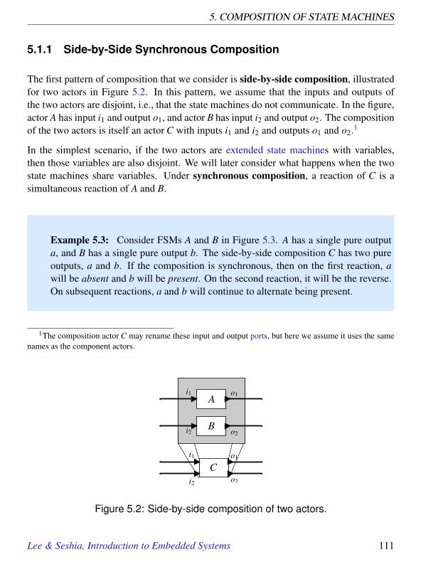
5. COMPOSITION OF STATE MACHINES
5.1.1 Side-by-Side Synchronous Composition
The first pattern of composition that we consider is side-by-side composition, illustratedfor two actors in Figure 5.2. In this pattern, we assume that the inputs and outputs ofthe two actors are disjoint, i.e., that the state machines do not communicate. In the figure,actor A has input i1 and output o1, and actor B has input i2 and output o2. The compositionof the two actors is itself an actor C with inputs i1 and i2 and outputs o1 and o2.1
In the simplest scenario, if the two actors are extended state machines with variables,then those variables are also disjoint. We will later consider what happens when the twostate machines share variables. Under synchronous composition, a reaction of C is asimultaneous reaction of A and B.
Example 5.3: Consider FSMs A and B in Figure 5.3. A has a single pure outputa, and B has a single pure output b. The side-by-side composition C has two pureoutputs, a and b. If the composition is synchronous, then on the first reaction, awill be absent and b will be present. On the second reaction, it will be the reverse.On subsequent reactions, a and b will continue to alternate being present.
1The composition actor C may rename these input and output ports, but here we assume it uses the samenames as the component actors.
Figure 5.2: Side-by-side composition of two actors.
Lee & Seshia, Introduction to Embedded Systems 111

5.1. CONCURRENT COMPOSITION
Figure 5.3: Example of side-by-side composition of two actors.
Synchronous side-by-side composition is simple for several reasons. First, recall fromSection 3.3.2 that the environment determines when a state machine reacts. In syn-chronous side-by-side composition, the environment need not be aware that C is a com-position of two state machines. Such compositions are modular in the sense that thecomposition itself becomes a component that can be further composed as if it were itselfan atomic component.
Moreover, if the two state machines A and B are deterministic, then the synchronous side-by-side composition is also deterministic. We say that a property is compositional if aproperty held by the components is also a property of the composition. For synchronousside-by-side composition, determinism is a compositional property.
In addition, a synchronous side-by-side composition of finite state machines is itself anFSM. A rigorous way to give the semantics of the composition is to define a single statemachine for the composition. Suppose that as in Section 3.3.3, state machines A and B
112 Lee & Seshia, Introduction to Embedded Systems

5. COMPOSITION OF STATE MACHINES
are given by the five tuples,
A = (StatesA, InputsA,OutputsA,updateA, initialStateA)
B = (StatesB, InputsB,OutputsB,updateB, initialStateB) .
Then the synchronous side-by-side composition C is given by
StatesC = StatesA×StatesB (5.1)
InputsC = InputsA× InputsB (5.2)
OutputsC = OutputsA×OutputsB (5.3)
initialStateC = (initialStateA, initialStateB) (5.4)
and the update function is defined by
updateC((sA,sB),(iA, iB)) = ((s′A,s′B),(oA,oB)),
where(s′A,oA) = updateA(sA, iA),
and(s′B,oB) = updateB(sB, iB),
for all sA ∈ StatesA, sB ∈ StatesB, iA ∈ InputsA, and iB ∈ InputsB.
Recall that InputsA and InputsB are sets of valuations. Each valuation in the set is anassignment of values to ports. What we mean by
InputsC = InputsA× InputsB
is that a valuation of the inputs of C must include both valuations for the inputs of A andthe inputs of B.
As usual, the single FSM C can be given pictorially rather than symbolically, as illustratedin the next example.
Example 5.4: The synchronous side-by-side composition C in Figure 5.3 is givenas a single FSM in Figure 5.4. Notice that this machine behaves exactly as describedin Example 5.3. The outputs a and b alternate being present. Notice further that(s1,s4) and (s2,s3) are not reachable states.
Lee & Seshia, Introduction to Embedded Systems 113

5.1. CONCURRENT COMPOSITION
Figure 5.4: Single state machine giving the semantics of synchronous side-by-side composition of the state machines in Figure 5.3.
5.1.2 Side-by-Side Asynchronous Composition
In an asynchronous composition of state machines, the component machines react inde-pendently. This statement is rather vague, and in fact, it has several different interpreta-tions. Each interpretation gives a semantics to the composition. The key to each semanticsis how to define a reaction of the composition C in Figure 5.2. Two possibilities are:
• Semantics 1. A reaction of C is a reaction of one of A or B, where the choice isnondeterministic.
• Semantics 2. A reaction of C is a reaction of A, B, or both A and B, where the choiceis nondeterministic. A variant of this possibility might allow neither to react.
Semantics 1 is referred to as an interleaving semantics, meaning that A or B never reactsimultaneously. Their reactions are interleaved in some order.
A significant subtlety is that under these semantics machines A and B may completelymiss input events. That is, an input to C destined for machine A may be present in areaction where the nondeterministic choice results in B reacting rather than A. If this isnot desirable, then some control over scheduling (see sidebar on page 116) or synchronouscomposition becomes a better choice.
114 Lee & Seshia, Introduction to Embedded Systems

5. COMPOSITION OF STATE MACHINES
Figure 5.5: State machine giving the semantics of asynchronous side-by-sidecomposition of the state machines in Figure 5.3.
Example 5.5: For the example in Figure 5.3, semantics 1 results in the composi-tion state machine shown in Figure 5.5. This machine is nondeterministic. Fromstate (s1,s3), when C reacts, it can move to (s2,s3) and emit no output, or it canmove to (s1,s4) and emit b. Note that if we had chosen semantics 2, then it wouldalso be able to move to (s2,s4).
For asynchronous composition under semantics 1, the symbolic definition of C has thesame definitions of StatesC, InputsC, OutputsC, and initialStateC as for synchronous com-position, given in (5.1) through (5.4). But the update function differs, becoming
updateC((sA,sB),(iA, iB)) = ((s′A,s′B),(o
′A,o′B)),
where either
(s′A,o′A) = updateA(sA, iA) and s′B = sB and o′B = absent
or(s′B,o
′B) = updateB(sB, iB) and s′A = sA and o′A = absent
Lee & Seshia, Introduction to Embedded Systems 115

5.1. CONCURRENT COMPOSITION
for all sA ∈ StatesA, sB ∈ StatesB, iA ∈ InputsA, and iB ∈ InputsB. What we mean byo′B = absent is that all outputs of B are absent. Semantics 2 can be similarly defined (seeExercise 2).
Scheduling Semantics for Asynchronous Composition
In the case of semantics 1 and 2 given in Section 5.1.2, the choice of which componentmachine reacts is nondeterministic. The model does not express any particular constraints.It is often more useful to introduce some scheduling policies, where the environment isable to influence or control the nondeterministic choice. This leads to two additionalpossible semantics for asynchronous composition:
• Semantics 3. A reaction of C is a reaction of one of A or B, where the environmentchooses which of A or B reacts.
• Semantics 4. A reaction of C is a reaction of A, B, or both A and B, where thechoice is made by the environment.
Like semantics 1, semantics 3 is an interleaving semantics.In one sense, semantics 1 and 2 are more compositional than semantics 3 and 4. To
implement semantics 3 and 4, a composition has to provide some mechanism for theenvironment to choose which component machine should react (for scheduling the com-ponent machines). This means that the hierarchy suggested in Figure 5.2 does not quitework. Actor C has to expose more of its internal structure than just the ports and theability to react.
In another sense, semantics 1 and 2 are less compositional than semantics 3 and 4because determinism is not preserved by composition. A composition of deterministicstate machines is not a deterministic state machine.
Notice further that semantics 1 is an abstraction of semantics 3 in the sense that everybehavior under semantics 3 is also a behavior under semantics 1. This notion of abstrac-tion is studied in detail in Chapter 13.
The subtle differences between these choices make asynchronous composition rathertreacherous. Considerable care is required to ensure that it is clear which semantics isused.
116 Lee & Seshia, Introduction to Embedded Systems

5. COMPOSITION OF STATE MACHINES
Figure 5.6: Model of two servers with a shared task queue, assuming asyn-chronous composition under semantics 1.
5.1.3 Shared Variables
An extended state machine has local variables that can be read and written as part oftaking a transition. Sometimes it is useful when composing state machines to allow thesevariables to be shared among a group of machines. In particular, such shared variables canbe useful for modeling interrupts, studied in Chapter 9, and threads, studied in Chapter10. However, considerable care is required to ensure that the semantics of the modelconforms with that of the program containing interrupts or threads. Many complicationsarise, including the memory consistency model and the notion of atomic operations.
Lee & Seshia, Introduction to Embedded Systems 117

5.1. CONCURRENT COMPOSITION
Example 5.6: Consider two servers that can receive requests from a network.Each request requires an unknown amount of time to service, so the servers share aqueue of requests. If one server is busy, the other server can respond to a request,even if the request arrives at the network interface of the first server.
This scenario fits a pattern similar to that in Figure 5.2, where A and B are theservers. We can model the servers as state machines as shown in Figure 5.6. In thismodel, a shared variable pending counts the number of pending job requests. Whena request arrives at the composite machine C, one of the two servers is nondeter-ministically chosen to react, assuming asynchronous composition under semantics1. If that server is idle, then it proceeds to serve the request. If the server is serv-ing another request, then one of two things can happen: it can coincidentally finishserving the request it is currently serving, issuing the output done, and proceed toserve the new one, or it can increment the count of pending requests and continue toserve the current request. The choice between these is nondeterministic, to modelthe fact that the time it takes to service a request is unknown.
If C reacts when there is no request, then again either server A or B will be selectednondeterministically to react. If the server that reacts is idle and there are oneor more pending requests, then the server transitions to serving and decrementsthe variable pending. If the server that reacts is not idle, then one of three thingscan happen. It may continue serving the current request, in which case it simplytransitions on the self transition back to serving. Or it may finish serving therequest, in which case it will transition to idle if there are no pending requests, ortransition back to serving and decrement pending if there are pending requests.
The model in the previous example exhibits many subtleties of concurrent systems. First,because of the interleaving semantics, accesses to the shared variable are atomic opera-tions, something that is quite challenging to guarantee in practice, as discussed in Chapters9 and 10. Second, the choice of semantics 1 is reasonable in this case because the inputgoes to both of the component machines, so regardless of which component machine re-acts, no input event will be missed. However, this semantics would not work if the twomachines had independent inputs, because then requests could be missed. Semantics 2can help prevent that, but what strategy should be used by the environment to determinewhich machine reacts? What if the two independent inputs both have requests present atthe same reaction of C? If we choose semantics 4 in the sidebar on page 116 to allow both
118 Lee & Seshia, Introduction to Embedded Systems
5. COMPOSITION OF STATE MACHINES
machines to react simultaneously, then what is the meaning when both machines updatethe shared variable? The updates are no longer atomic, as they are with an interleavingsemantics.
Note further that choosing asynchronous composition under semantics 1 allows behaviorsthat do not make good use of idle machines. In particular, suppose that machine A isserving, machine B is idle, and a request arrives. If the nondeterministic choice results inmachine A reacting, then it will simply increment pending. Not until the nondeterministicchoice results in B reacting will the idle machine be put to use. In fact, semantics 1 allowsbehaviors that never use one of the machines.
Shared variables may be used in synchronous compositions as well, but sophisticatedsubtleties again emerge. In particular, what should happen if in the same reaction one ma-chine reads a shared variable to evaluate a guard and another machine writes to the sharedvariable? Do we require the write before the read? What if the transition doing the writeto the shared variable also reads the same variable in its guard expression? One possibil-ity is to choose a synchronous interleaving semantics, where the component machinesreact in arbitrary order, chosen nondeterministically. This strategy has the disadvantagethat a composition of two deterministic machines may be nondeterministic. An alterna-tive version of the synchronous interleaving semantics has the component machines reactin a fixed order determined by the environment or by some additional mechanism such aspriority.
The difficulties of shared variables, particularly with asynchronous composition, reflectthe inherent complexity of concurrency models with shared variables. Clean solutionsrequire a more sophisticated semantics, to be discussed in Chapter 6. Specifically, in thatchapter, we will explain the synchronous-reactive model of computation, which gives asynchronous composition semantics that is reasonably compositional.
So far, we have considered composition of machines that do not directly communicate.We next consider what happens when the outputs of one machine are the inputs of another.
5.1.4 Cascade Composition
Consider two state machines A and B that are composed as shown in Figure 5.7. Theoutput of machine A feeds the input of B. This style of composition is called cascadecomposition or serial composition.
Lee & Seshia, Introduction to Embedded Systems 119

5.1. CONCURRENT COMPOSITION
In the figure, output port o1 from A feeds events to input port i2 of B. Assume the datatype of o1 is V1 (meaning that o1 can take values from V1 or be absent), and the data typeof i2 is V2. Then a requirement for this composition to be valid is that
V1 ⊆V2 .
This asserts that any output produced by A on port o1 is an acceptable input to B on porti2. The composition type checks.
For cascade composition, if we wish the composition to be asynchronous, then we needto introduce some machinery for buffering the data that is sent from A to B. We deferdiscussion of such asynchronous composition to Chapter 6, where dataflow and processnetwork models of computation will provide such asynchronous composition. In thischapter, we will only consider synchronous composition for cascade systems.
In synchronous composition of the cascade structure of Figure 5.7, a reaction of C consistsof a reaction of both A and B, where A reacts first, produces its output (if any), and thenB reacts. Logically, we view this as occurring in zero time, so the two reactions are in asense simultaneous and instantaneous. But they are causally related in that the outputsof A can affect the behavior of B.
Example 5.7: Consider the cascade composition of the two FSMs in Figure 5.8.Assuming synchronous semantics, the meaning of a reaction of C is given in Figure5.9. That figure makes it clear that the reactions of the two machines are simulta-neous and instantaneous. When moving from the initial state (s1, s3) to (s2, s4)(which occurs when the input a is absent), the composition machine C does not pass
Figure 5.7: Cascade composition of two actors.
120 Lee & Seshia, Introduction to Embedded Systems

5. COMPOSITION OF STATE MACHINES
Figure 5.8: Example of a cascade composition of two FSMs.
Figure 5.9: Semantics of the cascade composition of Figure 5.8, assuming syn-chronous composition.
through (s2, s3)! In fact, (s2, s3) is not a reachable state! In this way, a singlereaction of C encompasses a reaction of both A and B.
To construct the composition machine as in Figure 5.9, first form the state space as thecross product of the state spaces of the component machines, and then determine which
Lee & Seshia, Introduction to Embedded Systems 121

5.1. CONCURRENT COMPOSITION
transitions are taken under what conditions. It is important to remember that the transi-tions are simultaneous, even when one logically causes the other.
Example 5.8: Recall the traffic light model of Figure 3.10. Suppose that wewish to compose this with a model of a pedestrian crossing light, like that shownin Figure 5.10. The output sigR of the traffic light can provide the input sigR ofthe pedestrian light. Under synchronous cascade composition, the meaning of thecomposite is given in Figure 5.11. Note that unsafe states, such as (green, green),which is the state when both cars and pedestrians have a green light, are not reach-able states, and hence are not shown.
In its simplest form, cascade composition implies an ordering of the reactions of thecomponents. Since this ordering is well defined, we do not have as much difficulty withshared variables as we did with side-by-side composition. However, we will see that inmore general compositions, the ordering is not so simple.
Figure 5.10: A model of a pedestrian crossing light, to be composed in a syn-chronous cascade composition with the traffic light model of Figure 3.10.
122 Lee & Seshia, Introduction to Embedded Systems

5. COMPOSITION OF STATE MACHINES
Figure 5.11: Semantics of a synchronous cascade composition of the traffic lightmodel of Figure 3.10 with the pedestrian light model of Figure 5.10.
5.1.5 General Composition
Side-by-side and cascade composition provide the basic building blocks for building morecomplex compositions of machines. Consider for example the composition in Figure 5.12.A1 and A3 are a side-by-side composition that together define a machine B. B and A2 are acascade composition, with B feeding events to A2. However, B and A2 are also a cascadecomposition in the opposite order, with A2 feeding events to B. Cycles like this are calledfeedback, and they introduce a conundrum; which machine should react first, B or A2?This conundrum will be resolved in the next chapter when we explain the synchronous-reactive model of computation.
Lee & Seshia, Introduction to Embedded Systems 123

5.2. HIERARCHICAL STATE MACHINES
Figure 5.12: Arbitrary interconnections of state machines are combinations ofside-by-side and cascade compositions, possibly creating cycles, as in this ex-ample.
Figure 5.13: In a hierarchical FSM, a state may have a refinement that is anotherstate machine.
5.2 Hierarchical State Machines
In this section, we consider hierarchical FSMs, which date back to Statecharts (Harel,1987). There are many variants of Statecharts, often with subtle semantic differencesbetween them (von der Beeck, 1994). Here, we will focus on some of the simpler aspectsonly, and we will pick a particular semantic variant.
The key idea in hierarchical state machines is state refinement. In Figure 5.13, state B hasa refinement that is another FSM with two states, C and D. What it means for the machineto be in state B is that it is in one of states C or D.
124 Lee & Seshia, Introduction to Embedded Systems

5. COMPOSITION OF STATE MACHINES
Figure 5.14: Semantics of the hierarchical FSM in Figure 5.13.
The meaning of the hierarchy in Figure 5.13 can be understood by comparing it to theequivalent flattened FSM in Figure 5.14. The machine starts in state A. When guard g2evaluates to true, the machine transitions to state B, which means a transition to state C,the initial state of the refinement. Upon taking this transition to C, the machine performsaction a2, which may produce an output event or set a variable (if this is an extended statemachine).
There are then two ways to exit C. Either guard g1 evaluates to true, in which case themachine exits B and returns to A, or guard g4 evaluates to true and the machine transitionsto D. A subtle question is what happens if both guards g1 and g4 evaluate to true. Differentvariants of Statecharts may make different choices at this point. It seems reasonable thatthe machine should end up in state A, but which of the actions should be performed, a4,a1, or both? Such subtle questions help account for the proliferation of different variantsof Statecharts.
We choose a particular semantics that has attractive modularity properties (Lee and Tri-pakis, 2010). In this semantics, a reaction of a hierarchical FSM is defined in a depth-firstfashion. The deepest refinement of the current state reacts first, then its container statemachine, then its container, etc. In Figure 5.13, this means that if the machine is in stateB (which means that it is in either C or D), then the refinement machine reacts first. Ifit is C, and guard g4 is true, the transition is taken to D and action a4 is performed. Butthen, as part of the same reaction, the top-level FSM reacts. If guard g1 is also true, thenthe machine transitions to state A. It is important that logically these two transitions aresimultaneous and instantaneous, so the machine does not actually go to state D. Nonethe-
Lee & Seshia, Introduction to Embedded Systems 125

5.2. HIERARCHICAL STATE MACHINES
Figure 5.15: Variant of Figure 5.13 that uses a preemptive transition.
Figure 5.16: Semantics of Figure 5.15 with a preemptive transition.
less, action a4 is performed, and so is action a1. This combination corresponds to thetopmost transition of Figure 5.14.
Another subtlety is that if two actions are performed in the same reaction, they may con-flict. For example, two actions may write different values to the same output port. Or theymay set the same variable to different values. Our choice is that the actions are performedin sequence, as suggested by the semicolon in the action a4; a1. As in an imperative lan-guage like C, the semicolon denotes a sequence. If the two actions conflict, the later onedominates.
Such subtleties can be avoided by using a preemptive transition, shown in Figure 5.15,which has the semantics shown in Figure 5.16. The guards of a preemptive transition areevaluated before the refinement reacts, and if any guard evaluates to true, the refinementdoes not react. As a consequence, if the machine is in state B and g1 is true, then neither
126 Lee & Seshia, Introduction to Embedded Systems

5. COMPOSITION OF STATE MACHINES
Figure 5.17: Variant of the hierarchical state machine of Figure 5.13 that has ahistory transition.
action a3 nor a4 is performed. A preemptive transition is shown with a (red) circle at theoriginating end of the transition.
Notice in Figures 5.13 and 5.14 that whenever the machine enters B, it always enters C,never D, even if it was previously in D when leaving B. The transition from A to B iscalled a reset transition because the destination refinement is reset to its initial state,regardless of where it had previously been. A reset transition is indicated in our notationwith a hollow arrowhead at the destination end of a transition.
In Figure 5.17, the transition from A to B is a history transition, an alternative to a resettransition. In our notation, a solid arrowhead denotes a history transition. It may alsobe marked with an “H” for emphasis. When a history transition is taken, the destinationrefinement resumes in whatever state it was last in (or its initial state on the first entry).
The semantics of the history transition is shown in Figure 5.18. The initial state is labeled(A, C) to indicate that the machine is in state A, and if and when it next enters B it will goto C. The first time it goes to B, it will be in the state labeled (B, C) to indicate that it isin state B and, more specifically, C. If it then transitions to (B, D), and then back to A, itwill end up in the state labeled (A, D), which means it is in state A, but if and when it next
Lee & Seshia, Introduction to Embedded Systems 127

5.3. SUMMARY
Figure 5.18: Semantics of the hierarchical state machine of Figure 5.17 that hasa history transition.
enters B it will go to D. That is, it remembers its history, specifically where it was whenit left B.
As with concurrent composition, hierarchical state machines admit many possible mean-ings. The differences can be subtle. Considerable care is required to ensure that modelsare clear and that their semantics match what is being modeled.
5.3 Summary
Any well-engineered system is a composition of simpler components. In this chapter, wehave considered two forms of composition of state machines, concurrent composition andhierarchical composition.
For concurrent composition, we introduced both synchronous and asynchronous compo-sition, but did not complete the story. We have deferred dealing with feedback to thenext chapter, because for synchronous composition, significant subtleties arise. For asyn-chronous composition, communication via ports requires additional mechanisms that arenot (yet) part of our model of state machines. Even without communication via ports,
128 Lee & Seshia, Introduction to Embedded Systems

5. COMPOSITION OF STATE MACHINES
significant subtleties arise because there are several possible semantics for asynchronouscomposition, and each has strengths and weaknesses. One choice of semantics may besuitable for one application and not for another. These subtleties motivate the topic of thenext chapter, which provides more structure to concurrent composition and resolves mostof these questions (in a variety of ways).
For hierarchical composition, we focus on a style originally introduced by Harel (1987)known as Statecharts. We specifically focus on the ability for states in an FSM to haverefinements that are themselves state machines. The reactions of the refinement FSMs arecomposed with those of the machine that contains the refinements. As usual, there aremany possible semantics.
Lee & Seshia, Introduction to Embedded Systems 129

EXERCISES
Exercises
1. Consider the extended state machine model of Figure 3.8, the garage counter. Sup-pose that the garage has two distinct entrance and exit points. Construct a side-by-side concurrent composition of two counters that share a variable c that keeps trackof the number of cars in the garage. Specify whether you are using synchronous orasynchronous composition, and define exactly the semantics of your compositionby giving a single machine modeling the composition. If you choose synchronoussemantics, explain what happens if the two machines simultaneously modify theshared variable. If you choose asynchronous composition, explain precisely whichvariant of asynchronous semantics you have chosen and why. Is your compositionmachine deterministic?
2. For semantics 2 in Section 5.1.2, give the five tuple for a single machine represent-ing the composition C,
(StatesC, InputsC,OutputsC,updateC, initialStateC)
for the side-by-side asynchronous composition of two state machines A and B. Youranswer should be in terms of the five-tuple definitions for A and B,
(StatesA, InputsA,OutputsA,updateA, initialStateA)
and(StatesB, InputsB,OutputsB,updateB, initialStateB)
3. Consider the following synchronous composition of two state machines A and B:
130 Lee & Seshia, Introduction to Embedded Systems

5. COMPOSITION OF STATE MACHINES
Construct a single state machine C representing the composition. Which states ofthe composition are unreachable?
4. Consider the following synchronous composition of two state machines A and B:
Construct a single state machine C representing the composition. Which states ofthe composition are unreachable?
5. Consider the following hierarchical state machine:
Construct an equivalent flat FSM giving the semantics of the hierarchy. Describein words the input/output behavior of this machine. Is there a simpler machinethat exhibits the same behavior? (Note that equivalence relations between statemachines are considered in Chapter 13, but here, you can use intuition and justconsider what the state machine does when it reacts.)
Lee & Seshia, Introduction to Embedded Systems 131

6Concurrent
Models of ComputationContents
6.1 Structure of Models . . . . . . . . . . . . . . . . . . . . . . . . . . 1356.2 Synchronous-Reactive Models . . . . . . . . . . . . . . . . . . . . 136
Sidebar: Actor Networks as a System of Equations . . . . . . . . . . 137Sidebar: Fixed-Point Semantics . . . . . . . . . . . . . . . . . . . . 1386.2.1 Feedback Models . . . . . . . . . . . . . . . . . . . . . . . . 1396.2.2 Well-Formed and Ill-Formed Models . . . . . . . . . . . . . 1416.2.3 Constructing a Fixed Point . . . . . . . . . . . . . . . . . . . 142Sidebar: Synchronous-Reactive Languages . . . . . . . . . . . . . . 145
6.3 Dataflow Models of Computation . . . . . . . . . . . . . . . . . . . 1466.3.1 Dataflow Principles . . . . . . . . . . . . . . . . . . . . . . . 1466.3.2 Synchronous Dataflow . . . . . . . . . . . . . . . . . . . . . 1496.3.3 Dynamic Dataflow . . . . . . . . . . . . . . . . . . . . . . . 1536.3.4 Structured Dataflow . . . . . . . . . . . . . . . . . . . . . . 1556.3.5 Process Networks . . . . . . . . . . . . . . . . . . . . . . . . 156Sidebar: Petri Nets . . . . . . . . . . . . . . . . . . . . . . . . . . . 159
6.4 Timed Models of Computation . . . . . . . . . . . . . . . . . . . . 1606.4.1 Time-Triggered Models . . . . . . . . . . . . . . . . . . . . 160Sidebar: Models of Time . . . . . . . . . . . . . . . . . . . . . . . . 1616.4.2 Discrete Event Systems . . . . . . . . . . . . . . . . . . . . . 1626.4.3 Continuous-Time Systems . . . . . . . . . . . . . . . . . . . 163Sidebar: Probing Further: Discrete Event Semantics . . . . . . . . . 164
6.5 Summary . . . . . . . . . . . . . . . . . . . . . . . . . . . . . . . . 168Exercises . . . . . . . . . . . . . . . . . . . . . . . . . . . . . . . . . . . 169
133

In sound engineering practice, systems are built by composing components. In order forthe composition to be well understood, we need first for the individual components to bewell understood, and then for the meaning of the interaction between components to bewell understood. The previous chapter dealt with composition of finite state machines.With such composition, the components are well defined (they are FSMs), but there aremany possible interpretations for the interaction between components. The meaning of acomposition is referred to as its semantics.
This chapter focuses on the semantics of concurrent composition. The word “concurrent”literally means “running together.” A system is said to be concurrent if different parts ofthe system (components) conceptually operate at the same time. There is no particularorder to their operations. The semantics of such concurrent operation can be quite subtle,however.
The components we consider in this chapter are actors, which react to stimuli at inputports and produce stimuli on output ports. In this chapter, we will be only minimallyconcerned with how the actors themselves are defined. They may be FSMs, hardware,or programs specified in an imperative programming language. We will need to imposesome constraints on what these actors can do, but we need not constrain how they arespecified.
The semantics of a concurrent composition of actors is governed by three sets of rules thatwe collectively call a model of computation (MoC). The first set of rules specifies whatconstitutes a component. The second set specifies the concurrency mechanisms. The thirdspecifies the communication mechanisms.
In this chapter, a component will be an actor with ports and a set of execution actions.An execution action defines how the actor reacts to inputs to produce outputs and changestate. The ports will be interconnected to provide for communication between actors,and the execution actions will be invoked by the environment of the actor to cause theactor to perform its function. For example, for FSMs, one action is provided that causesa reaction. The focus of this chapter is on introducing a few of the possible concurrencyand communication mechanisms that can govern the interactions between such actors.
We begin by laying out the common structure of models that applies to all MoCs studiedin this chapter. We then proceed to describe a suite of MoCs.
134 Lee & Seshia, Introduction to Embedded Systems

6. CONCURRENT MODELS OF COMPUTATION
Figure 6.1: Any interconnection of actors can be modeled as a single (side-by-side composite) actor with feedback.
6.1 Structure of Models
In this chapter, we assume that models consist of fixed interconnections of actors likethat shown in Figure 6.1(a). The interconnections between actors specify communicationpaths. The communication itself takes the form of a signal, which consists of one or morecommunication events. For the discrete signals of Section 3.1, for example, a signal shas the form of a function
s : R→Vs∪absent,where Vs is a set of values called the type of the signal s. A communication event in thiscase is a non-absent value of s.
Example 6.1: Consider a pure signal s that is a discrete signal given by
s(t) =
present if t is a multiple of Pabsent otherwise
Lee & Seshia, Introduction to Embedded Systems 135

6.2. SYNCHRONOUS-REACTIVE MODELS
for all t ∈ R and some P ∈ R. Such a signal is called a clock signal with period P.Communication events occur every P time units.
In Chapter 2, a continuous-time signal has the form of a function
s : R→Vs,
in which case every one of the (uncountably) infinite set of values s(t), for all t ∈ R, is acommunication event. In this chapter, we will also encounter signals of the form
s : N→Vs,
where there is no time line. The signal is simply a sequence of values.
A communication event has a type, and we require that a connection between actors typecheck. That is, if an output port y with type Vy is connected to an input port x with typeVx, then
Vy ⊆Vx.
As suggested in Figure 6.1(b-d), any actor network can be reduced to a rather simple form.If we rearrange the actors as shown in Figure 6.1(b), then the actors form a side-by-sidecomposition indicated by the box with rounded corners. This box is itself an actor F asshown in Figure 6.1(c) whose input is a three-tuple (s1,s2,s3) of signals and whose outputis the same three-tuple of signals. If we let s = (s1,s2,s3), then the actor can be depictedas in Figure 6.1(d), which hides all the complexity of the model.
Notice that Figure 6.1(d) is a feedback system. By following the procedure that we usedto build it, every interconnection of actors can be structured as a similar feedback system(see Exercise 1).
6.2 Synchronous-Reactive Models
In Chapter 5 we studied synchronous composition of state machines, but we avoided thenuances of feedback compositions. For a model described as the feedback system ofFigure 6.1(d), the conundrum discussed in Section 5.1.5 takes a particularly simple form.If F in Figure 6.1(d) is realized by a state machine, then in order for it to react, we needto know its inputs at the time of the reaction. But its inputs are the same as its outputs, so
136 Lee & Seshia, Introduction to Embedded Systems

6. CONCURRENT MODELS OF COMPUTATION
in order for F to react, we need to know its outputs. But we cannot know its outputs untilafter it reacts.
Actor Networks as a System of Equations
In a model, if the actors are determinate, then each actor is a function that maps inputsignals to output signals. For example, in Figure 6.1(a), actor A may be a function relatingsignals s1 and s2 as follows,
s2 = A(s1).
Similarly, actor B relates three signals by
s1 = B(s2,s3).
Actor C is a bit more subtle, since it has no input ports. How can it be a function? Whatis the domain of the function? If the actor is determinate, then its output signal s3 is aconstant signal. The function C needs to be a constant function, one that yields the sameoutput for every input. A simple way to ensure this is to define C so that its domain is asingleton set (a set with only one element). Let /0 be the singleton set, so C can only beapplied to /0. The function C is then given by
C( /0) = s3.
Hence, Figure 6.1(a) gives a system of equations
s1 = B(s2,s3)
s2 = A(s1)
s3 = C( /0).
The semantics of such a model, therefore, is a solution to such a system of equations. Thiscan be represented compactly using the function F in Figure 6.1(d), which is
F(s1,s2,s3) = (B(s2,s3),A(s1),C( /0)).
All actors in Figure 6.1(a) have output ports; if we had an actor with no output port,then we could similarly define it as a function whose codomain is /0. The output ofsuch function is /0 for all inputs.
Lee & Seshia, Introduction to Embedded Systems 137

6.2. SYNCHRONOUS-REACTIVE MODELS
Fixed-Point Semantics
In a model, if the actors are determinate, then each actor is a function that maps inputsignals to output signals. The semantics of such a model is a system of equations (seesidebar on page 137) and the reduced form of Figure 6.1(d) becomes
s = F(s), (6.1)
where s = (s1,s2,s3). Of course, this equation only looks simple. Its complexity lies inthe definition of the function F and the structure of the domain and range of F .
Given any function F : X → X for any set X , if there is an x ∈ X such that F(x) = x,then x is called a fixed point. Equation (6.1) therefore asserts that the semantics of adeterminate actor network is a fixed point. Whether a fixed point exists, whether the fixedpoint is unique, and how to find the fixed point, all become interesting questions that arecentral to the model of computation.
In the SR model of computation, the execution of all actors is simultaneous and instan-taneous and occurs at ticks of the global clock. If the actor is determinate, then each suchexecution implements a function called a firing function. For example, in the n-th tick ofthe global clock, actor A in Figure 6.1 implements a function of the form
an : V1∪absent→V2∪absent
where Vi is the type of signal si. Hence, if si(n) is the value of si at the n-th tick, then
s2(n) = an(s1(n)).
Given such a firing function fn for each actor F we can, just as in Figure 6.1(d) define theexecution at a single tick by a fixed point,
s(n) = fn(s(n)),
where s(n) = (s1(n),s2(n),s3(n)) and fn is a function where
fn(s1(n),s2(n),s3(n)) = (bn(s2(n),s3(n)),an(s1(n)),cn( /0)).
Thus, for SR, the semantics at each tick of the global clock is a fixed point of the functionfn, just as its execution over all ticks is a fixed point of the function F .
138 Lee & Seshia, Introduction to Embedded Systems

6. CONCURRENT MODELS OF COMPUTATION
Figure 6.2: A simple well-formed feedback model.
As shown in Section 6.1 above and Exercise 1, all actor networks can be viewed as feed-back systems, so we really do have to resolve the conundrum. We do that now by givinga model of computation known as the synchronous-reactive (SR) MoC.
An SR model is a discrete system where signals are absent at all times except (possibly)at ticks of a global clock. Conceptually, execution of a model is a sequence of globalreactions that occur at discrete times, and at each such reaction, the reaction of all actorsis simultaneous and instantaneous.
6.2.1 Feedback Models
We focus first on feedback models of the form of Figure 6.1(d), where F in the figure isrealized as a state machine. At the n-th tick of the global clock, we have to find the valueof the signal s so that it is both a valid input and a valid output of the state machine, givenits current state. Let s(n) denote the value of the signal s at the n-th reaction. The goal isto determine, at each tick of the global clock, the value of s(n).
Example 6.2: Consider first a simpler example shown in Figure 6.2. (This issimpler than Figure 6.1(d) because the signal s is a single pure signal rather than anaggregation of three signals.) If A is in state s1 when that reaction occurs, then theonly possible value for s(n) is s(n) = absent because a reaction must take one ofthe transitions out of s1, and both of these transitions emit absent. Moreover, once
Lee & Seshia, Introduction to Embedded Systems 139

6.2. SYNCHRONOUS-REACTIVE MODELS
Figure 6.3: The semantics of the model in Figure 6.2.
we know that s(n) = absent, we know that the input port x has value absent, so wecan determine that A will transition to state s2.
If A is in state s2 when the reaction occurs, then the only possible value for s(n) iss(n) = present, and the machine will transition to state s1. Therefore, s alternatesbetween absent and present. The semantics of machine A in the feedback model istherefore given by Figure 6.3.
In the previous example, it is important to note that the input x and output y have thesame value in every reaction. This is what is meant by the feedback connection. Anyconnection from an output port to an input port means that the value at the input port isthe same as the value at the output port at all times.
Given a deterministic state machine in a feedback model like that of Figure 6.2, in eachstate i we can define a function ai that maps input values to output values,
ai : present,absent→ present,absent,
where the function depends on the state the machine is in. This function is defined by theupdate function.
Example 6.3: For the example in Figure 6.2, if the machine is in state s1, thenas1(x) = absent for all x ∈ present,absent.
140 Lee & Seshia, Introduction to Embedded Systems

6. CONCURRENT MODELS OF COMPUTATION
Figure 6.4: An ill-formed feedback model that has no fixed point in state s2.
The function ai is called the firing function for state i (see box on page 138). Given afiring function, to find the value s(n) at the n-th reaction, we simply need to find a values(n) such that
s(n) = ai(s(n)).
Such a value s(n) is called a fixed point of the function ai. It is easy to see how togeneralize this so that the signal s can have any type. Signal s can even be an aggregationof signals, as in Figure 6.1(d) (see box on page 138).
6.2.2 Well-Formed and Ill-Formed Models
There are two potential problems that may occur when seeking a fixed point. First, theremay be no fixed point. Second, there may be more than one fixed point. If either caseoccurs in a reachable state, we call the system ill formed. Otherwise, it is well formed.
Example 6.4: Consider machine B shown in Figure 6.4. In state s1, we get theunique fixed point s(n) = absent. In state s2, however, there is no fixed point. Ifwe attempt to choose s(n) = present, then the machine will transition to s1 and itsoutput will be absent. But the output has to be the same as the input, and the inputis present, so we get a contradiction. A similar contradiction occurs if we attemptto choose s(n) = absent.
Since state s2 is reachable, this feedback model is ill formed.
Lee & Seshia, Introduction to Embedded Systems 141

6.2. SYNCHRONOUS-REACTIVE MODELS
Figure 6.5: An ill-formed feedback model that has more than one fixed point instate s1.
Example 6.5: Consider machine C shown in Figure 6.5. In state s1, both s(n) =absent and s(n) = present are fixed points. Either choice is valid. Since state s1 isreachable, this feedback model is ill formed.
If in a reachable state there is more than one fixed point, we declare the machine to beill formed. An alternative semantics would not reject such a model, but rather would de-clare it to be nondeterministic. This would be a valid semantics, but it would have thedisadvantage that a composition of deterministic state machines is not assured of beingdeterministic. In fact, C in Figure 6.5 is deterministic, and under this alternative seman-tics, the feedback composition in the figure would not be deterministic. Determinismwould not be a compositional property. Hence, we prefer to reject such models.
6.2.3 Constructing a Fixed Point
If the type Vs of the signal s or the signals it is an aggregate of is finite, then one way to finda fixed point is by exhaustive search, which means to try all values. If exactly one fixedpoint is found, then the model is well formed. However, exhaustive search is expensive(and impossible if the types are not finite). We can develop instead a systematic procedure
142 Lee & Seshia, Introduction to Embedded Systems
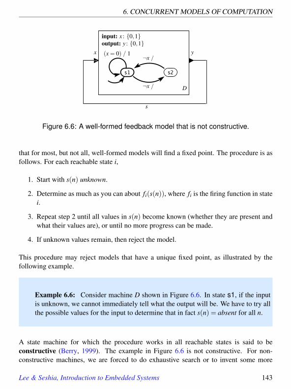
6. CONCURRENT MODELS OF COMPUTATION
Figure 6.6: A well-formed feedback model that is not constructive.
that for most, but not all, well-formed models will find a fixed point. The procedure is asfollows. For each reachable state i,
1. Start with s(n) unknown.
2. Determine as much as you can about fi(s(n)), where fi is the firing function in statei.
3. Repeat step 2 until all values in s(n) become known (whether they are present andwhat their values are), or until no more progress can be made.
4. If unknown values remain, then reject the model.
This procedure may reject models that have a unique fixed point, as illustrated by thefollowing example.
Example 6.6: Consider machine D shown in Figure 6.6. In state s1, if the inputis unknown, we cannot immediately tell what the output will be. We have to try allthe possible values for the input to determine that in fact s(n) = absent for all n.
A state machine for which the procedure works in all reachable states is said to beconstructive (Berry, 1999). The example in Figure 6.6 is not constructive. For non-constructive machines, we are forced to do exhaustive search or to invent some more
Lee & Seshia, Introduction to Embedded Systems 143

6.2. SYNCHRONOUS-REACTIVE MODELS
elaborate solution technique. Since exhaustive search is often too expensive for practicaluse, many SR languages and modeling tools (see box on page 145) reject non-constructivemodels.
Step 2 of the above procedure is key. How exactly can we determine the outputs if theinputs are not all known? This requires what is called a must-may analysis of the model.Examining the machine, we can determine what must be true of the outputs and what maybe true of the outputs.
Example 6.7: The model in Figure 6.2 is constructive. In state s1, we can imme-diately determine that the machine may not produce an output. Therefore, we canimmediately conclude that the output is absent, even though the input is unknown.Of course, once we have determined that the output is absent, we now know thatthe input is absent, and hence the procedure concludes.
In state s2, we can immediately determine that the machine must produce an output,so we can immediately conclude that the output is present.
The above procedure can be generalized to an arbitrary model structure. Consider forexample Figure 6.1(a). There is no real need to convert it to the form of Figure 6.1(d).Instead, we can just begin by labeling all signals unknown, and then in arbitrary order,examine each actor to determine whatever can be determined about the outputs, given itsinitial state. We repeat this until no further progress can be made, at which point either allsignals become known, or we reject the model as either ill-formed or non-constructive.Once we know all signals, then all actors can make state transitions, and we repeat theprocedure in the new state for the next reaction.
The constructive procedure above can be adapted to support nondeterministic machines(see Exercise 4). But now, things become even more subtle, and there are variants to thesemantics. One way to handle nondeterminism is that when executing the constructiveprocedure, when encountering a nondeterministic choice, make an arbitrary choice. Ifthe result leads to a failure of the procedure to find a fixed point, then we could eitherreject the model (not all choices lead to a well-formed or constructive model) or reject thechoice and try again.
In the SR model of computation, actors react simultaneously and instantaneously, at leastconceptually. Achieving this with realistic computation requires tight coordination of
144 Lee & Seshia, Introduction to Embedded Systems
6. CONCURRENT MODELS OF COMPUTATION
the computation. We consider next a family of models of computation that require lesscoordination.
Synchronous-Reactive Languages
The synchronous-reactive MoC has a history dating at least back to the mid 1980s whena suite of programming languages were developed. The term “reactive” comes from adistinction in computational systems between transformational systems, which acceptinput data, perform computation, and produce output data, and reactive systems, whichengage in an ongoing dialog with their environment (Harel and Pnueli, 1985). Manna andPnueli (1992) state
“The role of a reactive program ... is not to produce a final result but tomaintain some ongoing interaction with its environment.”
The distinctions between transformational and reactive systems led to the developmentof a number of innovative programming languages. The synchronous languages (Ben-veniste and Berry, 1991) take a particular approach to the design of reactive systems, inwhich pieces of the program react simultaneously and instantaneously at each tick of aglobal clock. First among these languages are Lustre (Halbwachs et al., 1991), Esterel(Berry and Gonthier, 1992), and Signal (Le Guernic et al., 1991). Statecharts (Harel,1987) and its implementation in Statemate (Harel et al., 1990) also have a strongly syn-chronous flavor.
SCADE (Berry, 2003) (Safety Critical Application Development Environment), a com-mercial product of Esterel Technologies, builds on Lustre, borrows concepts from Esterel,and provides a graphical syntax, where state machines are drawn and actor models arecomposed in a similar manner to the figures in this text. One of the main attractions ofsynchronous languages is their strong formal properties that yield quite effectively to for-mal analysis and verification techniques. For this reason, SCADE models are used in thedesign of safety-critical flight control software systems for commercial aircraft made byAirbus.
The principles of synchronous languages can also be used in the style of a coordinationlanguage rather than a programming language, as done in Ptolemy II (Edwards and Lee,2003) and ForSyDe (Sander and Jantsch, 2004). This allows for “primitives” in a systemto be complex components rather than built-in language primitives. This approach allowsheterogeneous combinations of MoCs, since the complex components may themselves begiven as compositions of further subcomponents under some other MoC.
Lee & Seshia, Introduction to Embedded Systems 145

6.3. DATAFLOW MODELS OF COMPUTATION
6.3 Dataflow Models of Computation
In this section, we consider MoCs that are much more asynchronous than SR. Reactionsmay occur simultaneously, or they may not. Whether they do or do not is not an essentialpart of the semantics. The decision as to when a reaction occurs can be much more decen-tralized, and can in fact reside with each individual actor. When reactions are dependenton one another, the dependence is due to the flow of data, rather than to the synchrony ofevents. If a reaction of actor A requires data produced by a reaction of actor B, then thereaction of A must occur after the reaction of B. A MoC where such data dependenciesare the key constraints on reactions is called a dataflow model of computation. There areseveral variants of dataflow MoCs, a few of which we consider here.
6.3.1 Dataflow Principles
In dataflow models, the signals providing communication between the actors are se-quences of message, where each message is called a token. That is, a signal s is a partialfunction of the form
s : NVs,
where Vs is the type of the signal, and where the signal is defined on an initial segment0,1, · · · ,n⊂N, or (for infinite executions) on the entire set N. Each element s(n) of thissequence is a token. A (determinate) actor will be described as a function that maps inputsequences to output sequences. We will actually use two functions, an actor function,which maps entire input sequences to entire output sequences, and a firing function,which maps a finite portion of the input sequences to output sequences, as illustrated inthe following example.
Example 6.8: Consider an actor that has one input and one output port as shownbelow
Suppose that the input type is Vx = R. Suppose that this is a Scale actor parame-terized by a parameter a ∈ R, similar to the one in Example 2.3, which multiplies
146 Lee & Seshia, Introduction to Embedded Systems

6. CONCURRENT MODELS OF COMPUTATION
inputs by a. Then
F(x1,x2,x3, · · ·) = (ax1,ax2,ax3, · · ·).
Suppose that when the actor fires, it performs one multiplication in the firing. Thenthe firing function f operates only on the first element of the input sequence, so
f (x1,x2,x3, · · ·) = f (x1) = (ax1).
The output is a sequence of length one.
As illustrated in the previous example, the actor function F combines the effects of multi-ple invocations of the firing function f . Moreover, the firing function can be invoked withonly partial information about the input sequence to the actor. In the above example, thefiring function can be invoked if one or more tokens are available on the input. The rulerequiring one token is called a firing rule for the Scale actor. A firing rule specifies thenumber of tokens required on each input port in order to fire the actor.
The Scale actor in the above example is particularly simple because the firing rule andthe firing function never vary. Not all actors are so simple.
Example 6.9: Consider now a different actor Delay with parameter d ∈ R. Theactor function is
D(x1,x2,x3, · · ·) = (d,x1,x2,x3, · · ·).
This actor prepends a sequence with a token with value d. This actor has two firingfunctions, d1 and d2, and two firing rules. The first firing rule requires no inputtokens at all and produces an output sequence of length one, so
d1(s) = (d),
where s is a sequence of any length, including length zero (the empty sequence).This firing rule is initially the one used, and it is used exactly once. The secondfiring rule requires one input token and is used for all subsequent firings. It triggersthe firing function
d2(x1, · · ·) = (x1).
Lee & Seshia, Introduction to Embedded Systems 147

6.3. DATAFLOW MODELS OF COMPUTATION
Figure 6.7: An FSM model for the Delay actor in Example 6.9.
The actor consumes one input token and produces on its output the same token. Theactor can be modeled by a state machine, as shown in Figure 6.7. In that figure, thefiring rules are implicit in the guards. The tokens required to fire are exactly thoserequired to evaluate the guards. The firing function d1 is associated with state s1,and d2 with s2.
When dataflow actors are composed, with an output of one going to an input of another,the communication mechanism is quite different from that of the previous MoCs consid-ered in this chapter. Since the firing of the actors is asynchronous, a token sent from oneactor to another must be buffered; it needs to be saved until the destination actor is readyto consume it. When the destination actor fires, it consumes one or more input tokens.After being consumed, a token may be discarded (meaning that the memory in which it isbuffered can be reused for other purposes).
Dataflow models pose a few interesting problems. One question is how to ensure thatthe memory devoted to buffering of tokens is bounded. A dataflow model may be ableto execute forever (or for a very long time); this is called an unbounded execution.For an unbounded execution, we may have to take measures to ensure that buffering ofunconsumed tokens does not overflow the available memory.
Example 6.10: Consider the following cascade composition of dataflow actors:
148 Lee & Seshia, Introduction to Embedded Systems

6. CONCURRENT MODELS OF COMPUTATION
Since A has no input ports, its firing rule is simple. It can fire at any time. Supposethat on each firing, A produces one token. What is to keep A from firing at afaster rate than B? Such faster firing could result in an unbounded build up ofunconsumed tokens on the buffer between A and B. This will eventually exhaustavailable memory.
In general, for dataflow models that are capable of unbounded execution, we will needscheduling policies that deliver bounded buffers.
A second problem that may arise is deadlock. Deadlock occurs when there are cycles, asin Figure 6.1, and a directed loop has insufficient tokens to satisfy any of the firing rules ofthe actors in the loop. The Delay actor of Example 6.9 can help prevent deadlock becauseit is able to produce an initial output token without having any input tokens available.Dataflow models with feedback will generally require Delay actors (or something similar)in every cycle.
For general dataflow models, it can be difficult to tell whether the model will deadlock,and whether there exists an unbounded execution with bounded buffers. In fact, thesetwo questions are undecidable, meaning that there is no algorithm that can answer thequestion in bounded time for all dataflow models (Buck, 1993). Fortunately, there areuseful constraints that we can impose on the design of actors that make these questionsdecidable. We examine those constraints next.
6.3.2 Synchronous Dataflow
Synchronous dataflow (SDF) is a constrained form of dataflow where for each actor,every firing consumes a fixed number of input tokens on each input port and produces afixed number of output tokens on each output port (Lee and Messerschmitt, 1987).1
1Despite the term, synchronous dataflow is not synchronous in the sense of SR. There is no global clockin SDF models, and firings of actors are asynchronous. For this reason, some authors use the term staticdataflow rather than synchronous dataflow. This does not avoid all confusion, however, because Dennis(1974) had previously coined the term “static dataflow” to refer to dataflow graphs where buffers could holdat most one token. Since there is no way to avoid a collision of terminology, we stick with the original “syn-chronous dataflow” terminology used in the literature. The term SDF arose from a signal processing concept,where two signals with sample rates that are related by a rational multiple are deemed to be synchronous.
Lee & Seshia, Introduction to Embedded Systems 149

6.3. DATAFLOW MODELS OF COMPUTATION
Figure 6.8: SDF actor A produces M tokens when it fires, and actor B consumesN tokens when it fires.
Consider a single connection between two actors, A and B, as shown in Figure 6.8. Thenotation here means that when A fires, it produces M tokens on its output port, and whenB fires, it consumes N tokens on its input port. M and N are positive integers. Supposethat A fires qA times and B fires qB times. All tokens that A produces are consumed by Bif and only if the following balance equation is satisfied,
qAM = qBN. (6.2)
Given values qA and qB satisfying (6.2), we can find a schedule that delivers unboundedexecution with bounded buffers. An example of such a schedule fires A repeatedly, qA
times, followed by B repeatedly, qB times. It can repeat this sequence forever withoutexhausting available memory.
Example 6.11: Suppose that in Figure 6.8, M = 2 and N = 3. Then qA = 3 andqB = 2 satisfy (6.2). Hence, the following schedule can be repeated forever,
A,A,A,B,B.
An alternative schedule is also available,
A,A,B,A,B.
In fact, this latter schedule has an advantage over the former one in that it requiresless memory. B fires as soon as there are enough tokens, rather than waiting for Ato complete its entire cycle.
Another solution to (6.2) is qA = 6 and qB = 4. This solution includes more firingsin the schedule than are strictly needed to keep the system in balance.
The equation is also satisfied by qA = 0 and qB = 0, but if the number of firings ofactors is zero, then no useful work is done. Clearly, this is not a solution we want.Negative solutions are also not desirable.
150 Lee & Seshia, Introduction to Embedded Systems

6. CONCURRENT MODELS OF COMPUTATION
Figure 6.9: A consistent SDF model.
Generally we will be interested in finding the least positive integer solution to thebalance equations.
In a more complicated SDF model, every connection between actors results in a balanceequation. Hence, the model defines a system of equations.
Example 6.12: Figure 6.9 shows a network with three SDF actors. The connec-tions x, y, and z, result in the following system of balance equations,
qA = qB
2qB = qC
2qA = qC.
The least positive integer solution to these equations is qA = qB = 1, and qC = 2, sothe following schedule can be repeated forever to get an unbounded execution withbounded buffers,
A,B,C,C.
The balance equations do not always have a non-trivial solution, as illustrated in the fol-lowing example.
Example 6.13: Figure 6.10 shows a network with three SDF actors where theonly solution to the balance equations is the trivial one, qA = qB = qC = 0. A
Lee & Seshia, Introduction to Embedded Systems 151

6.3. DATAFLOW MODELS OF COMPUTATION
Figure 6.10: An inconsistent SDF model.
consequence is that there is no unbounded execution with bounded buffers for thismodel. It cannot be kept in balance.
An SDF model that has a non-zero solution to the balance equations is said to be consis-tent. If the only solution is zero, then it is inconsistent. An inconsistent model has nounbounded execution with bounded buffers.
Lee and Messerschmitt (1987) showed that if the balance equations have a non-zero solu-tion, then they also have a solution where qi is a positive integer for all actors i. Moreover,for connected models (where there is a communication path between any two actors), theygave a procedure for finding the least positive integer solution. Such a procedure formsthe foundation for a scheduler for SDF models.
Consistency is sufficient to ensure bounded buffers, but it is not sufficient to ensure thatan unbounded execution exists. In particular, when there is feedback, as in Figure 6.1,then deadlock may occur. Deadlock bounds an execution.
To allow for feedback, the SDF model treats Delay actors specially. Recall from Exam-ple 6.9, that the Delay actor is able to produce output tokens before it receives any inputtokens, and then it subsequently behaves like a trivial SDF actor that copies inputs tooutputs. But such a trivial actor is not really needed, and the cost of copying inputs to out-puts is unnecessary. The Delay actor can be implemented very efficiently as a connectionwith initial tokens (those tokens that the actor is able to produce before receiving inputs).No actor is actually needed at run time. The scheduler must take the initial tokens intoaccount.
Example 6.14: Figure 6.11 shows an SDF model with initial tokens on a feedbackloop. These replace a Delay actor that is able to initially produce four tokens. The
152 Lee & Seshia, Introduction to Embedded Systems

6. CONCURRENT MODELS OF COMPUTATION
Figure 6.11: An SDF model with initial tokens on a feedback loop.
balance equations are
3qA = 2qB
2qB = 3qA.
The least positive integer solution is qA = 2, and qB = 3, so the model is consis-tent. With four initial tokens on the feedback connection, as shown, the followingschedule can be repeated forever,
A,B,A,B,B.
Were there any fewer than four initial tokens, however, the model would deadlock.If there were only three tokens, for example, then A could fire, followed by B, butin the resulting state of the buffers, neither could fire again.
In addition to the procedure for solving the balance equations, Lee and Messerschmitt(1987) gave a procedure that will either provide a schedule for an unbounded executionor will prove that no such schedule exists. Hence, both bounded buffers and deadlock aredecidable for SDF models.
6.3.3 Dynamic Dataflow
Although the ability to guarantee bounded buffers and rule out deadlock is valuable, itcomes at a price. SDF is not very expressive. It cannot directly express, for example,conditional firing, where an actor fires only if, for example, a token has a particular value.Such conditional firing is supported by a more general dataflow MoC known as dynamicdataflow (DDF). Unlike SDF actors, DDF actors can have multiple firing rules, and they
Lee & Seshia, Introduction to Embedded Systems 153

6.3. DATAFLOW MODELS OF COMPUTATION
Figure 6.12: Dynamic dataflow actors.
are not constrained to produce the same number of output tokens on each firing. TheDelay actor of Example 6.9 is directly supported by the DDF MoC, without any need forspecial treatment of initial tokens. So are two basic actors known as Switch and Select,shown in Figure 6.12.
The Select actor on the left has three firing rules. Initially, it requires one token on thebottom input port. The type of that port is Boolean, so the value of the token must be trueor false. If a token with value true is received on that input port, then the actor producesno output, but instead activates the next firing rule, which requires one token for the topleft input port, labeled T. When the actor next fires, it consumes the token on the T portand sends it to the output port. If a token with value false is received on the bottom inputport, then the actor activates a firing rule that requires a token on the bottom left input portlabeled F. When it consumes that token, it again sends it to the output port. Thus, it firestwice to produce one output.
The Switch actor performs a complementary function. It has only one firing rule, whichrequires a single token on both input ports. The token on the left input port will be sentto either the T or the F output port, depending on the Boolean value of the token receivedon the bottom input port. Hence, Switch and Select accomplish conditional routing oftokens, as illustrated in the following example.
Example 6.15: Figure 6.13 uses Switch and Select to accomplish conditionalfiring. Actor B produces a stream of Boolean-valued tokens x. This stream is repli-cated by the fork to provide the control inputs y and z to the Switch and Selectactors. Based on the value of the control tokens on these streams, the tokens pro-duced by actor A are sent to either C or D, and the resulting outputs are collectedand sent to E. This model is the DDF equivalent of the familiar if-then-elseprogramming construct in imperative languages.
154 Lee & Seshia, Introduction to Embedded Systems

6. CONCURRENT MODELS OF COMPUTATION
Figure 6.13: A DDF model that accomplishes conditional firing.
Addition of Switch and Select to the actor library means that we can no longer alwaysfind a bounded buffer schedule, nor can we provide assurances that the model will notdeadlock. Buck (1993) showed that bounded buffers and deadlock are undecidable forDDF models. Thus, in exchange for the increased expressiveness and flexibility, we havepaid a price. The models are not as readily analyzed.
Switch and Select are dataflow analogs of the goto statement in imperative languages.They provide low-level control over execution by conditionally routing tokens. Like gotostatements, using them can result in models that are very difficult to understand. Dijk-stra (1968) indicted the goto statement, discouraging its use, advocating instead the useof structured programming. Structured programming replaces goto statements withnested for loops, if-then-else, do-while, and recursion. Fortunately, structuredprogramming is also available for dataflow models, as we discuss next.
6.3.4 Structured Dataflow
Figure 6.14 shows an alternative way to accomplish conditional firing that has many ad-vantages over the DDF model in Figure 6.13. The grey box in the figure is an example ofa higher-order actor called Conditional. A higher-order actor is an actor that has one ormore models as parameters. In the example in the figure, Conditional is parameterized bytwo sub-models, one containing the actor C and the other containing the actor D. WhenConditional fires, it consumes one token from each input port and produces one tokenon its output port, so it is an SDF actor. The action it performs when it fires, however, isdependent on the value of the token that arrives at the lower input port. If that value istrue, then actor C fires. Otherwise, actor D fires.
Lee & Seshia, Introduction to Embedded Systems 155

6.3. DATAFLOW MODELS OF COMPUTATION
Figure 6.14: Structured dataflow approach to conditional firing.
This style of conditional firing is called structured dataflow, because, much like struc-tured programming, control constructs are nested hierarchically. Arbitrary data-dependenttoken routing is avoided (which is analogous to avoiding arbitrary branches using goto in-structions). Moreover, when using such Conditional actors, the overall model is stillan SDF model. In the example in Figure 6.14, every actor consumes and produces ex-actly one token on every port. Hence, the model is analyzable for deadlock and boundedbuffers.
This style of structured dataflow was introduced in LabVIEW, a design tool developed byNational Instruments (Kodosky et al., 1991). In addition to a conditional similar to that inFigure 6.14, LabVIEW provides structured dataflow constructs for iterations (analogousto for and do-while loops in an imperative language), for case statements (whichhave an arbitrary number of conditionally executed submodels), and for sequences (whichcycle through a finite set of submodels). It is also possible to support recursion usingstructured dataflow (Lee and Parks, 1995), but without careful constraints, boundednessagain becomes undecidable.
6.3.5 Process Networks
A model of computation that is closely related to dataflow models is Kahn process net-works (or simply, process networks or PN), named after Gilles Kahn, who introducedthem (Kahn, 1974). The relationship between dataflow and PN is studied in detail byLee and Parks (1995) and Lee and Matsikoudis (2009), but the short story is quite sim-
156 Lee & Seshia, Introduction to Embedded Systems

6. CONCURRENT MODELS OF COMPUTATION
ple. In PN, each actor executes concurrently in its own process. That is, instead of beingdefined by its firing rules and firing functions, a PN actor is defined by a (typically non-terminating) program that reads data tokens from input ports and writes data tokens tooutput ports. All actors execute simultaneously (conceptually, whether they actually exe-cute simultaneously or are interleaved is irrelevant).
In the original paper, Kahn (1974) gave very elegant mathematical conditions on the ac-tors that would ensure that a network of such actors was determinate in the sense thatthe sequence of tokens on every connection between actors is unique, and specificallyindependent of how the processes are scheduled. Thus, Kahn showed that concurrentexecution was possible without nondeterminacy.
Three years later, Kahn and MacQueen (1977) gave a simple, easily implemented mech-anism for programs that ensures that the mathematical conditions are met to ensure de-terminacy. A key part of the mechanism is to perform blocking reads on input portswhenever a process is to read input data. Specifically, blocking reads mean that if theprocess chooses to access data through an input port, it issues a read request and blocksuntil the data becomes available. It cannot test the input port for the availability of dataand then perform a conditional branch based on whether data are available, because sucha branch would introduce schedule-dependent behavior.
Blocking reads are closely related to firing rules. Firing rules specify the tokens requiredto continue computing (with a new firing function). Similarly, a blocking read specifies asingle token required to continue computing (by continuing execution of the process).
When a process writes to an output port, it performs a nonblocking write, meaning thatthe write succeeds immediately and returns. The process does not block to wait for thereceiving process to be ready to receive data. This is exactly how writes to output portswork in dataflow MoCs as well. Thus, the only material difference between dataflow andPN is that with PN, the actor is not broken down into firing functions. It is designed as acontinuously executing program.
Kahn and MacQueen (1977) called the processes in a PN network coroutines for aninteresting reason. A routine or subroutine is a program fragment that is “called” byanother program. The subroutine executes to completion before the calling fragmentcan continue executing. The interactions between processes in a PN model are moresymmetric, in that there is no caller and callee. When a process performs a blocking read,it is in a sense invoking a routine in the upstream process that provides the data. Similarly,when it performs a write, it is in a sense invoking a routine in the downstream process to
Lee & Seshia, Introduction to Embedded Systems 157

6.3. DATAFLOW MODELS OF COMPUTATION
Figure 6.15: A Petri net model of two concurrent programs with a mutual exclusionprotocol.
process the data. But the relationship between the producer and consumer of the data ismuch more symmetric than with subroutines.
Just like dataflow, the PN MoC poses challenging questions about boundedness of buffersand about deadlock. PN is expressive enough that these questions are undecidable. Anelegant solution to the boundedness question is given by Parks (1995) and elaborated byGeilen and Basten (2003).
An interesting variant of process networks performs blocking writes rather than non-blocking writes. That is, when a process writes to an output port, it blocks until thereceiving process is ready to receive the data. Such an interaction between processes iscalled a rendezvous. Rendezvous forms the basis for well known process formalismssuch as communicating sequential processes (CSP) (Hoare, 1978) and the calculus ofcommunicating systems (CCS) (Milner, 1980). It also forms the foundation for the Oc-cam programming language (Galletly, 1996), which enjoyed some success for a periodof time in the 1980s and 1990s for programming parallel computers.
In both the SR and dataflow models of computation considered so far, time plays a minorrole. In dataflow, time plays no role. In SR, computation occurs simultaneously andinstantaneously at each of a sequence of ticks of a global clock. Although the term “clock”implies that time plays a role, it actually does not. In the SR MoC, all that matters is thesequence. The physical time at which the ticks occur is irrelevant to the MoC. It is just asequence of ticks. Many modeling tasks, however, require a more explicit notion of time.We examine next MoCs that have such a notion.
158 Lee & Seshia, Introduction to Embedded Systems

6. CONCURRENT MODELS OF COMPUTATION
Petri Nets
Petri nets, named after Carl Adam Petri, are a popular modeling formalism related todataflow (Murata, 1989). They have two types of elements, places and transitions, de-picted as white circles and rectangles, respectively:
A place can contain any number of tokens, depicted as black circles. A transition isenabled if all places connected to it as inputs contain at least one token. Once a transitionis enabled, it can fire, consuming one token from each input place and putting one tokenon each output place. The state of a network, called its marking, is the number of tokenson each place in the network. The figure above shows a simple network with its markingbefore and after the firing of the transition. If a place provides input to more than onetransition, then the network is nondeterministic. A token on that place may trigger afiring of either destination transition.
An example of a Petri net model is shown in Figure 6.15, which models two concurrentprograms with a mutual exclusion protocol. Each of the two programs has a criticalsection, meaning that only one of the programs can be in its critical section at any time.In the model, program A is in its critical section if there is a token on place a2, andprogram B is in its critical section if there is a token on place b1. The job of the mutualexclusion protocol is to ensure that these two places cannot simultaneously have a token.
If the initial marking of the model is as shown in the figure, then both top transitions areenabled, but only one can fire (there is only one token in the place labeled mutex). Whichone fires is chosen nondeterministically. Suppose program A fires. After this firing, therewill be a token in place a2, so the corresponding bottom transition becomes enabled.Once that transition fires, the model returns to its initial marking. It is easy to see that themutual exclusion protocol is correct in this model.
Unlike dataflow buffers, places do not preserve an ordering of tokens. Petri nets with afinite number of markings are equivalent to FSMs.
Lee & Seshia, Introduction to Embedded Systems 159

6.4. TIMED MODELS OF COMPUTATION
6.4 Timed Models of Computation
For cyber-physical systems, the time at which things occur in software can matter, be-cause the software interacts with physical processes. In this section, we consider a fewconcurrent MoCs that explicitly refer to time. We describe three timed MoCs, each ofwhich have many variants. Our treatment here is necessarily brief. A complete study ofthese MoCs would require a much bigger volume.
6.4.1 Time-Triggered Models
Kopetz and Grunsteidl (1994) introduced mechanisms for periodically triggering dis-tributed computations according to a distributed clock that measures the passage of time.The result is a system architecture called a time-triggered architecture (TTA). A keycontribution was to show how a TTA could tolerate certain kinds of faults, such that fail-ures in part of the system could not disrupt the behaviors in other parts of the system (seealso Kopetz (1997) and Kopetz and Bauer (2003)). Henzinger et al. (2003a) lifted the keyidea of TTA to the programming language level, providing a well-defined semantics formodeling distributed time-triggered systems. Since then, these techniques have come intopractical use in the design of safety-critical avionics and automotive systems, becoming akey part of standards such as FlexRay, a networking standard developed by a consortiumof automotive companies.
A time-triggered MoC is similar to SR in that there is a global clock that coordinatesthe computation. But computations take time instead of being simultaneous and instan-taneous. Specifically, time-triggered MoCs associate with a computation a logical exe-cution time. The inputs to the computation are provided at ticks of the global clock, butthe outputs are not visible to other computations until the next tick of the global clock.Between ticks, there is no interaction between the computations, so concurrency diffi-culties such as race conditions do not exist. Since the computations are not (logically)instantaneous, there are no difficulties with feedback, and all models are constructive.
The Simulink modeling system, sold by The MathWorks, supports a time-triggered MoC,and in conjunction with another product called Real-Time Workshop, can translate suchmodels in embedded C code. In LabVIEW, from National Instruments, timed loops ac-complish a similar capability within a dataflow MoC.
160 Lee & Seshia, Introduction to Embedded Systems

6. CONCURRENT MODELS OF COMPUTATION
Models of TimeHow to model physical time is surprisingly subtle. How should we define simultaneityacross a distributed system? A thoughtful discussion of this question is considered byGalison (2003). What does it mean for one event to cause another? Can an event thatcauses another be simultaneous with it? Several thoughtful essays on this topic are givenin Price and Corry (2007).
In Chapter 2, we assume time is represented by a variable t ∈ R or t ∈ R+. This modelis sometimes referred to as Newtonian time. It assumes a globally shared absolute time,where any reference anywhere to the variable t will yield the same value. This notion oftime is often useful for modeling even if it does not perfectly reflect physical realities, butit has its deficiencies. Consider for example Newton’s cradle, a toy with five steel ballssuspended by strings. If you lift one ball and release it, it strikes the second ball, whichdoes not move. Instead, the fifth ball reacts by rising. Consider the momentum of themiddle ball as a function of time. The middle ball does not move, so its momentum mustbe everywhere zero. But the momentum of the first ball is somehow transfered to thefifth ball, passing through the middle ball. So the momentum cannot be always zero. Letm : R→ R represent the momentum of this ball and τ be the time of the collision. Then
m(t) =
M if t = τ0 otherwise
for all t ∈R. In a cyber-physical system, we may, however, want to represent this functionin software, in which case a sequence of samples will be needed. But how can such sampleunambiguously represent the rather unusual structure of this signal?
One option is to use superdense time (Manna and Pnueli, 1993; Maler et al., 1992; Leeand Zheng, 2005; Cataldo et al., 2006), where instead of R, time is represented by a setR×N. A time value is a tuple (t,n), where t represents Newtonian time and n representsa sequence index within an instant. In this representation, the momentum of the middleball can be unambiguously represented by a sequence where m(τ,0) = 0, m(τ,1) = M,and m(τ,2) = 0. Such a representation also handles events that are simultaneous andinstantaneous but also causally related.
Another alternative is partially ordered time, where two time values may or may notbe ordered relative to each other. When there is a chain of causal relationships betweenthem, then they must be ordered, and otherwise not.
Lee & Seshia, Introduction to Embedded Systems 161

6.4. TIMED MODELS OF COMPUTATION
In the simplest form, a time-triggered model specifies periodic computation with a fixedtime interval (the period) between ticks of the clock. Giotto (Henzinger et al., 2003a)supports modal models, where the periods differ in different modes. Some authors havefurther extended the concept of logical execution time to non-periodic systems (Liu andLee, 2003; Ghosal et al., 2004).
Time triggered models are conceptually simple, but computations are tied closely to aperiodic clock. The model becomes awkward when actions are not periodic. DE systems,considered next, encompass a richer set of timing behaviors.
6.4.2 Discrete Event Systems
Discrete-event systems (DE systems) have been used for decades as a way to build sim-ulations for an enormous variety of applications, including for example digital networks,military systems, and economic systems. A pioneering formalism for DE models is dueto Zeigler (1976), who called the formalism DEVS, abbreviating discrete event systemspecification. DEVS is an extension of Moore machines that associates a non-zero lifes-pan with each state, thus endowing the Moore machines with an explicit notion of thepassage of time (vs. a sequence of reactions).
The key idea in a DE MoC is that events are endowed with a time stamp, a value insome model of time (see box on page 161). Normally, two distinct time stamps must becomparable. That is, they are either equal, or one is earlier than the other. A DE modelis a network of actors where each actor reacts to input events in time-stamp order andproduces output events in time-stamp order.
Example 6.16: The clock signal with period P of Example 6.1 consists of eventswith time stamps nP for all n ∈ Z.
To execute a DE model, we can use an event queue, which is a list of events sorted bytime stamp. The list begins empty. Each actor in the network is interrogated for any initialevents it wishes to place on the event queue. These events may be destined for anotheractor, or they may be destined for the actor itself, in which case they will cause a reactionof the actor to occur at the appropriate time. The execution continues by selecting theearliest event in the event queue and determining which actor should receive that event.
162 Lee & Seshia, Introduction to Embedded Systems

6. CONCURRENT MODELS OF COMPUTATION
The value of that event (if any) is presented as an input to the actor, and the actor reacts(“fires”). The reaction can produce output events, and also events that simply request alater firing of the same actor at some specified time stamp.
At this point, variants of DE MoCs behave differently. Some variants, such as DEVS,require that outputs produced by the actor have a strictly larger time stamp than that of theinput just presented. From a modeling perspective, every actor imposes some non-zerodelay, in that its reactions (the outputs) become visible to other actors strictly later thanthe inputs that triggered the reaction. Other variants permit the actor to produce outputevents with the same time stamp as the input. That is, they can react instantaneously.As with SR models of computation, such instantaneous reactions can create significantsubtleties because inputs become simultaneous with outputs.
The subtleties introduced by simultaneous events can be resolved by treating DE as ageneralization of SR (Lee and Zheng, 2007). In this variant of a DE semantics, executionproceeds as follows. Again, we use an event queue and interrogate the actors for initialevents to place on the queue. We select the event from the queue with the least time stamp,and all other events with the same time stamp, present those events to actors in the modelas inputs, and then fire all actors in the manner of a constructive fixed-point iteration, asnormal with SR. In this variant of the semantics, any outputs produced by an actor mustbe simultaneous with the inputs (they have the same time stamp), so they participate inthe fixed point. If the actor wishes to produce an output event at a later time, it does soby requesting a firing at a later time (which results in the posting of an event on the eventqueue).
6.4.3 Continuous-Time Systems
In Chapter 2 we consider models of continuous-time systems based on ordinary differen-tial equations (ODEs). Specifically, we consider equations of the form
x(t) = f (x(t), t),
where x : R→Rn is a vector-valued continuous-time function. An equivalent model is anintegral equation of the form
x(t) = x(0)+∫ t
0x(τ)dτ (6.3)
= x(0)+∫ t
0f (x(τ),τ)dτ. (6.4)
Lee & Seshia, Introduction to Embedded Systems 163

6.4. TIMED MODELS OF COMPUTATION
In Chapter 2, we show that a model of a system given by such ODEs can be described asan interconnection of actors, where the communication between actors is via continuous-time signals. Equation (6.4) can be represented as the interconnection shown in Figure6.16, which conforms to the feedback pattern of Figure 6.1(d).
Example 6.17: The feedback control system of Figure 2.3, using the helicoptermodel of Example 2.3, can be redrawn as shown in Figure 6.17, which conforms tothe pattern of Figure 6.16. In this case, x = θy is a scalar-valued continuous-timefunction (or a vector of length one). The function f is defined as follows,
f (x(t), t) = (K/Iyy)(ψ(t)−x(t)),
and the initial value of the integrator is
x(0) = θy(0).
Probing Further: Discrete Event Semantics
Discrete-event models of computation have been a subject of study for many years, withseveral textbooks available (Zeigler et al., 2000; Cassandras, 1993; Fishman, 2001). Thesubtleties in the semantics are considerable (see Lee (1999); Cataldo et al. (2006); Liuet al. (2006); Liu and Lee (2008)). Instead of discussing the formal semantics here, wedescribe how a DE model is executed. Such a description is, in fact, a valid way of givingthe semantics of a model. The description is called an operational semantics (Scott andStrachey, 1971; Plotkin, 1981).
DE models are often quite large and complex, so execution performance becomes veryimportant. Because of the use of a single event queue, parallelizing or distributing execu-tion of DE models can be challenging (Misra, 1986; Fujimoto, 2000). A recently proposedstrategy called PTIDES (for programming temporally integrated distributed embeddedsystems), leverages network time synchronization to provide efficient distributed execu-tion (Zhao et al., 2007; Lee et al., 2009). The claim is that the execution is efficientenough that DE can be used not only as a simulation technology, but also as an imple-mentation technology. That is, the DE event queue and execution engine become part ofthe deployed embedded software. As of this writing, that claim has not been proven onany practical examples.
164 Lee & Seshia, Introduction to Embedded Systems

6. CONCURRENT MODELS OF COMPUTATION
Figure 6.16: Actor model of a system described by equation (6.4).
Figure 6.17: The feedback control system of Figure 2.3, using the helicoptermodel of Example 2.3, redrawn to conform to the pattern of Figure 6.16.
Such models, in fact, are actor compositions under a continuous-time model of com-putation, but unlike the previous MoCs, this one cannot strictly be executed on a digitalcomputer. A digital computer cannot directly deal with the time continuum. It can, how-ever, be approximated, often quite accurately.
The approximate execution of a continuous-time model is accomplished by a solver,which constructs a numerical approximation to the solution of an ODE. The study ofalgorithms for solvers is quite old, with the most commonly used techniques dating backto the 19th century. Here, we will consider only one of the simplest of solvers, which isknown as a forward Euler solver.
Lee & Seshia, Introduction to Embedded Systems 165

6.4. TIMED MODELS OF COMPUTATION
...
h
t
x(t).
f (x(t), t)
h 2h 3h
(a)
t
x(t).
f (x(t), t)
(b)
...
f (x(0), 0)
Figure 6.18: (a) Forward Euler approximation to the integration in (6.4), where xis assumed to be a scalar. (b) A better approximation that uses a variable stepsize and takes into account the slope of the curve.
A forward Euler solver estimates the value of x at time points 0,h,2h,3h, · · · , where h iscalled the step size. The integration is approximated as follows,
x(h) = x(0)+h f (x(0),0)x(2h) = x(h)+h f (x(h),h)x(3h) = x(2h)+h f (x(2h),2h)
· · ·x((k+1)h) = x(kh)+h f (x(kh),kh).
This process is illustrated in Figure 6.18(a), where the “true” value of x is plotted as afunction of time. The true value of x(t) is the area under that curve between 0 and t,plus the initial value x(0). At the first step of the algorithm, the increment in area isapproximated as the area of a rectangle of width h and height f (x(0),0). This increment
166 Lee & Seshia, Introduction to Embedded Systems

6. CONCURRENT MODELS OF COMPUTATION
yields an estimate for x(h), which can be used to calculate x(h) = f (x(h),h), the heightof the second rectangle. And so on.
You can see that the errors in approximation will accumulate over time. The algorithmcan be improved considerably by two key techniques. First, a variable-step solver willvary the step size based on estimates of the error to keep the error small. Second, amore sophisticated solver will take into account the slope of the curve and use trapezoidalapproximations as suggested in Figure 6.18(b). A family of such solvers known as Runge-Kutta solvers are widely used. But for our purposes here, it does not matter what solver isused. All that matters is that (a) the solver determines the step size, and (b) at each step,the solver performs some calculation to update the approximation to the integral.
When using such a solver, we can interpret the model in Figure 6.16 in a manner similarto SR and DE models. The f actor is memoryless, so it simply performs a calculation toproduce an output that depends only on the input and the current time. The integrator is astate machine whose state is updated at each reaction by the solver, which uses the inputto determine what the update should be. The state space of this state machine is infinite,since the state variable x(t) is a vector of real numbers.
Hence, a continuous-time model can be viewed as an SR model with a time step be-tween global reactions determined by a solver (Lee and Zheng, 2007). Specifically, acontinuous-time model is a network of actors, each of which is a cascade composition ofa simple memoryless computation actor and a state machine, and the actor reactions aresimultaneous and instantaneous. The times of the reactions are determined by a solver.The solver will typically consult the actors in determining the time step, so that for ex-ample events like level crossings (when a continuous signal crosses a threshold) can becaptured precisely. Hence, despite the additional complication of having to provide asolver, the mechanisms required to achieve a continuous-time model of computation arenot much different from those required to achieve SR and DE.
A popular software tool that uses a continuous-time MoC is Simulink, from The Math-Works. Simulink represents models similarly as block diagrams, which are interconnec-tions of actors. Continuous-time models can also be simulated using the textual tool MAT-LAB from the same vendor. MATRIXx, from National Instruments, also supports graph-ical continuous-time modeling. Continuous-time models can also be integrated withinLabVIEW models, either graphically using the Control Design and Simulation Module ortextually using the programming language MathScript.
Lee & Seshia, Introduction to Embedded Systems 167

6.5. SUMMARY
6.5 Summary
This chapter provides a whirlwind tour of a rather large topic, concurrent models ofcomputation. It begins with synchronous-reactive models, which are closest to the syn-chronous composition of state machines considered in the previous chapter. It then con-siders dataflow models, where execution can be more loosely coordinated. Only dataprecedences impose constraints on the order of actor computations. The chapter thenconcludes with a quick view of a few models of computation that explicitly include anotion of time. Such MoCs are particularly useful for modeling cyber-physical systems.
168 Lee & Seshia, Introduction to Embedded Systems

6. CONCURRENT MODELS OF COMPUTATION
Exercises
1. Show how each of the following actor models can be transformed into a feedbacksystem by using a reorganization similar to that in Figure 6.1(b). That is, the actorsshould be aggregated into a single side-by-side composite actor.
(a)
(b)
(c)
2. Consider the following state machine in a synchronous feedback composition:
Lee & Seshia, Introduction to Embedded Systems 169

EXERCISES
(a) Is it well-formed? Is it constructive?
(b) If it is well-formed and constructive, then find the output symbols for the first10 reactions. If not, explain where the problem is.
(c) Show the composition machine, assuming that the composition has no inputand that the only output is y.
3. For the following synchronous model, determine whether it is well formed andconstructive, and if so, determine the sequence of values of the signals s1 and s2.
4. For the following synchronous model, determine whether it is well formed andconstructive, and if so, determine the possible sequences of values of the signals s1and s2. Note that machine A is nondeterministic.
5. Recall the traffic light controller of Figure 3.10. Consider connecting the outputsof this controller to a pedestrian light controller, whose FSM is given in Figure5.10. Using your favorite modeling software that supports state machines (suchas Ptolemy II, LabVIEW Statecharts, or Simulink/Stateflow), construct the compo-sition of the above two FSMs along with a deterministic extended state machine
170 Lee & Seshia, Introduction to Embedded Systems

6. CONCURRENT MODELS OF COMPUTATION
modeling the environment and generating input symbols timeR, timeG, timeY , andisCar. For example, the environment FSM can use an internal counter to decidewhen to generate these symbols.
6. Consider the following SDF model:
The numbers adjacent to the ports indicate the number of tokens produced or con-sumed by the actor when it fires. Answer the following questions about this model.
(a) Let qA,qB, and qC denote the number of firings of actors A, B, and C, respec-tively. Write down the balance equations and find the least positive integersolution.
(b) Find a schedule for an unbounded execution that minimizes the buffer sizes onthe two communication channels. What is the resulting size of the buffers?
7. For each of the following dataflow models, determine whether there is an un-bounded execution with bounded buffers. If there is, determine the minimum buffersize.
(a)
Lee & Seshia, Introduction to Embedded Systems 171

EXERCISES
(b)
where n is some integer.(c)
where D produces an arbitrary boolean sequence.(d) For the same dataflow model as in part (c), assume you can specify a periodic
boolean output sequence produced by D. Find such a sequence that yieldsbounded buffers, give a schedule that minimizes buffer sizes, and give thebuffer sizes.
8. Consider the SDF graph shown below:
In this figure, A, B, and C are actors. Adjacent to each port is the number of tokensconsumed or produced by a firing of the actor on that port, where N and M arevariables with positive integer values. Assume the variables w, x, y, and z representthe number of initial tokens on the connection where these variables appear in thediagram. These variables have non-negative integer values.
172 Lee & Seshia, Introduction to Embedded Systems

6. CONCURRENT MODELS OF COMPUTATION
(a) Derive a simple relationship between N and M such that the model is con-sistent, or show that no positive integer values of N and M yield a consistentmodel.
(b) Assume that w = x = y = 0 and that the model is consistent and find theminimum value of z (as a function N and M) such that the model does notdeadlock.
(c) Assume that z = 0 and that the model is consistent. Find values for w, x, andy such that the model does not deadlock and w+ x+ y is minimized.
(d) Assume that w = x = y = 0 and z is whatever value you found in part (b). Letbw, bx, by, and bz be the buffer sizes for connections w, x, y, and z, respectively.What is the minimum for these buffer sizes?
Lee & Seshia, Introduction to Embedded Systems 173

Part II
Design of Embedded Systems
This part of this text studies the design of embedded systems, with emphasis on the tech-niques used to build concurrent, real-time embedded software. We proceed bottom up,discussing first in Chapter 7 the design of embedded processors, with emphasis on paral-lelism in the hardware and its implications for programmers. Chapter 8 covers memoryarchitectures, with particular emphasis on the effect they have on program timing. Chap-ter 9 covers the input and output mechanisms that enable programs to interact with theexternal physical world, with emphasis on how to reconcile the sequential nature of soft-ware with the concurrent nature of the physical world. Chapter 10 describes mechanismsfor achieving concurrency in software, threads and processes, and synchronization of con-current software tasks, including semaphores and mutual exclusion. Finally, Chapter 11covers scheduling, with particular emphasis on controlling timing in concurrent programs.


7Embedded Processors
Contents7.1 Types of Processors . . . . . . . . . . . . . . . . . . . . . . . . . . 179
7.1.1 Microcontrollers . . . . . . . . . . . . . . . . . . . . . . . . 1797.1.2 DSP Processors . . . . . . . . . . . . . . . . . . . . . . . . . 179Sidebar: Microcontrollers . . . . . . . . . . . . . . . . . . . . . . . 180Sidebar: Programmable Logic Controllers . . . . . . . . . . . . . . . 181Sidebar: The x86 Architecture . . . . . . . . . . . . . . . . . . . . . 182Sidebar: DSP Processors . . . . . . . . . . . . . . . . . . . . . . . . 1837.1.3 Graphics Processors . . . . . . . . . . . . . . . . . . . . . . 187
7.2 Parallelism . . . . . . . . . . . . . . . . . . . . . . . . . . . . . . . 1877.2.1 Parallelism vs. Concurrency . . . . . . . . . . . . . . . . . . 187Sidebar: Circular Buffers . . . . . . . . . . . . . . . . . . . . . . . . 1887.2.2 Pipelining . . . . . . . . . . . . . . . . . . . . . . . . . . . . 1927.2.3 Instruction-Level Parallelism . . . . . . . . . . . . . . . . . . 1957.2.4 Multicore Architectures . . . . . . . . . . . . . . . . . . . . 200Sidebar: Fixed-Point Numbers . . . . . . . . . . . . . . . . . . . . . 201Sidebar: Fixed-Point Numbers (continued) . . . . . . . . . . . . . . . 202Sidebar: Fixed-Point Arithmetic in C . . . . . . . . . . . . . . . . . . 203
7.3 Summary . . . . . . . . . . . . . . . . . . . . . . . . . . . . . . . . 204Exercises . . . . . . . . . . . . . . . . . . . . . . . . . . . . . . . . . . . 205
177

In general-purpose computing, the variety of instruction set architectures today is lim-ited, with the Intel x86 architecture overwhelmingly dominating all. There is no suchdominance in embedded computing. On the contrary, the variety of processors can bedaunting to a system designer. Our goal in this chapter is to give the reader the tools andvocabulary to understand the options and to critically evaluate the properties of proces-sors. We particularly focus on the mechanisms that provide concurrency and control overtiming, because these issues loom large in the design of cyber-physical systems.
When deployed in a product, embedded processors typically have a dedicated function.They control an automotive engine or measure ice thickness in the Arctic. They are notasked to perform arbitrary functions with user-defined software. Consequently, the pro-cessors can be more specialized. Making them more specialized can bring enormousbenefits. For example, they may consume far less energy, and consequently be usablewith small batteries for long periods of time. Or they may include specialized hardwareto perform operations that would be costly to perform on general-purpose hardware, suchas image analysis.
When evaluating processors, it is important to understand the difference between an in-struction set architecture (ISA) and a processor realization or a chip. The latter is apiece of silicon sold by a semiconductor vendor. The former is a definition of the in-structions that the processor can execute and certain structural constraints (such as wordsize) that realizations must share. x86 is an ISA. There are many realizations. An ISA isan abstraction shared by many realizations. A single ISA may appear in many differentchips, often made by different manufacturers, and often having widely varying perfor-mance profiles.
The advantage of sharing an ISA in a family of processors is that software tools, which arecostly to develop, may be shared, and (sometimes) the same programs may run correctlyon multiple realizations. This latter property, however, is rather treacherous, since an ISAdoes not normally include any constraints on timing. Hence, although a program mayexecute logically the same way on multiple chips, the system behavior may be radicallydifferent when the processor is embedded in a cyber-physical system.
178 Lee & Seshia, Introduction to Embedded Systems

7. EMBEDDED PROCESSORS
7.1 Types of Processors
As a consequence of the huge variety of embedded applications, there is a huge varietyof processors that are used. They range from very small, slow, inexpensive, low-powerdevices, to high-performance, special-purpose devices. This section gives an overview ofsome of the available types of processors.
7.1.1 Microcontrollers
A microcontroller (µC) is a small computer on a single integrated circuit consisting of arelatively simple central processing unit (CPU) combined with peripheral devices suchas memories, I/O devices, and timers. By some accounts, more than half of all CPUs soldworldwide are microcontrollers, although such a claim is hard to substantiate becausethe difference between microcontrollers and general-purpose processors is indistinct. Thesimplest microcontrollers operate on 8-bit words and are suitable for applications that re-quire small amounts of memory and simple logical functions (vs. performance-intensivearithmetic functions). They may consume extremely small amounts of energy, and ofteninclude a sleep mode that reduces the power consumption to nanowatts. Embedded com-ponents such as sensor network nodes and surveillance devices have been demonstratedthat can operate on a small battery for several years.
Microcontrollers can get quite elaborate. Distinguishing them from general-purpose pro-cessors can get difficult. The Intel Atom, for example, is a family of x86 CPUs usedmainly in netbooks and other small mobile computers. Because these processors aredesigned to use relatively little energy without losing too much performance relative toprocessors used in higher-end computers, they are suitable for some embedded applica-tions and in servers where cooling is problematic. AMD’s Geode is another example ofa processor near the blurry boundary between general-purpose processors and microcon-trollers.
7.1.2 DSP Processors
Many embedded applications do quite a bit of signal processing. A signal is a collectionof sampled measurements of the physical world, typically taken at a regular rate calledthe sample rate. A motion control application, for example, may read position or locationinformation from sensors at sample rates ranging from a few Hertz (Hz, or samples persecond) to a few hundred Hertz. Audio signals are sampled at rates ranging from 8,000 Hz
Lee & Seshia, Introduction to Embedded Systems 179

7.1. TYPES OF PROCESSORS
(or 8 kHz, the sample rate used in telephony for voice signals) to 44.1 kHz (the sample rateof CDs). Ultrasonic applications (such as medical imaging) and high-performance musicapplications may sample sound signals at much higher rates. Video typically uses sample
Microcontrollers
Most semiconductor vendors include one or more families of microcontrollers in theirproduct line. Some of the architectures are quite old. The Motorola 6800 and Intel 8080are 8-bit microcontrollers that appeared on the market in 1974. Descendants of thesearchitectures survive today, for example in the form of the Freescale 6811. The ZilogZ80 is a fully-compatible descendant of the 8080 that became one of the most widelymanufactured and widely used microcontrollers of all time. A derivative of the Z80 is theRabbit 2000 designed by Rabbit Semiconductor.
Another very popular and durable architecture is the Intel 8051, an 8-bit microcon-troller developed by Intel in 1980. The 8051 ISA is today supported by many vendors,including Atmel, Infineon Technologies, Dallas Semiconductor, NXP, ST Microelectron-ics, Texas Instruments, and Cypress Semiconductor. The Atmel AVR 8-bit microcon-troller, developed by Atmel in 1996, was one of the first microcontrollers to use on-chipflash memory for program storage. Although Atmel says AVR is not an acronym, it isbelieved that the architecture was conceived by two students at the Norwegian Instituteof Technology, Alf-Egil Bogen and Vegard Wollan, so it may have originated as Alf andVegard’s RISC.
Many 32-bit microcontrollers implement some variant of an ARM instruction set, de-veloped by ARM Limited. ARM originally stood for Advanced RISC Machine, andbefore that Acorn RISC Machine, but today it is simply ARM. Processors that implementthe ARM ISA are widely used in mobile phones to realize the user interface functions, aswell as in many other embedded systems. Semiconductor vendors license the instructionset from ARM Limited and produce their own chips. ARM processors are currently madeby Alcatel, Atmel, Broadcom, Cirrus Logic, Freescale, LG, Marvell Technology Group,NEC, NVIDIA, NXP, Samsung, Sharp, ST Microelectronics, Texas Instruments, VLSITechnology, Yamaha, and others.
Other notable embedded microcontroller architectures include the Motorola ColdFire(later the Freescale ColdFire), the Hitachi H8 and SuperH, the MIPS (originally devel-oped by a team led by John Hennessy at Stanford University), the PIC (originally Pro-grammable Interface Controller, from Microchip Technology), and the PowerPC (createdin 1991 by an alliance of Apple, IBM, and Motorola).
180 Lee & Seshia, Introduction to Embedded Systems

7. EMBEDDED PROCESSORS
Programmable Logic Controllers
A programmable logic controller(PLC) is a specialized form of a micro-controller for industrial automation. PLCsoriginated as replacements for controlcircuits using electrical relays to controlmachinery. They are typically designed forcontinuous operation in hostile environ-ments (high temperature, humidity, dust,etc.).
Ladder Logic Diagram
PLCs are often programmed using ladder logic, a notation originally used to specifylogic constructed with relays and switches. A relay is a switch where the contact iscontrolled by coil. When a voltage is applied to the coil, the contact closes, enablingcurrent to flow through the relay. By interconnecting contacts and coils, relays can beused to build digital controllers that follow specified patterns.
In common notation, a contact is represented by two vertical bars, and a coil by acircle, as shown in the diagram above. The above diagram has two rungs. The Motorcoil on the lower rung turns a motor on or off. The Start and Stop contacts representpushbutton switches. When an operator pushes the Start button, the contact is closed,and current can flow from the left (the power rail) to the right (ground). Start is anormally open contact. The Stop contact is normally closed, indicated by the slash,meaning that it becomes open when the operator pushes the switch. The logic in theupper rung is interesting. When the operator pushes Start, current flows to the Runcoil, causing both Run contacts to close. The motor will run, even after the Startbutton is released. When the operator pushes Stop, current is interrupted, and bothRun contacts become open, causing the motor to stop. Contacts wired in parallelperform a logical OR function, and contacts wired in series perform a logical AND.The upper rung has feedback; the meaning of the rung is a fixed point solution to thelogic equation implied by the diagram.
Today, PLCs are just microcontrollers in rugged packages with I/O interfaces suit-able for industrial control, and ladder logic is a graphical programming notation forprograms. These diagrams can get quite elaborate, with thousands of rungs. For de-tails, we recommend Kamen (1999).
Lee & Seshia, Introduction to Embedded Systems 181

7.1. TYPES OF PROCESSORS
rates of 25 or 30 Hz for consumer devices to much higher rates for specialty measurementapplications. Each sample, of course, contains an entire image (called a frame), whichitself has many samples (called pixels) distributed in space rather than time. Software-defined radio applications have sample rates that can range from hundreds of kHz (forbaseband processing) to several GHz (billions of Hertz). Other embedded applicationsthat make heavy use of signal processing include interactive games; radar, sonar, andLIDAR (light detection and ranging) imaging systems; video analytics (the extractionof information from video, for example for surveillance); driver-assist systems for cars;medical electronics; and scientific instrumentation.
Signal processing applications all share certain characteristics. First, they deal with largeamounts of data. The data may represent samples in time of a physical processor (suchas samples of a wireless radio signal), samples in space (such as images), or both (suchas video and radar). Second, they typically perform sophisticated mathematical opera-tions on the data, including filtering, system identification, frequency analysis, machinelearning, and feature extraction. These operations are mathematically intensive.
Processors designed specifically to support numerically intensive signal processing appli-cations are called DSP processors, or DSPs (digital signal processors), for short. Toget some insight into the structure of such processors and the implications for the embed-ded software designer, it is worth understanding the structure of typical signal processingalgorithms.
The x86 Architecture
The dominant ISA for desktop and portable computers is known as the x86. This termoriginates with the Intel 8086, a 16-bit microprocessor chip designed by Intel in 1978.A variant of the 8086, designated the 8088, was used in the original IBM PC, and theprocessor family has dominated the PC market ever since. Subsequent processors in thisfamily were given names ending in “86,” and generally maintained backward compatibil-ity. The Intel 80386 was the first 32-bit version of this instruction set, introduced in 1985.Today, the term “x86” usually refers to the 32-bit version, with 64-bit versions designated“x86-64.” The Intel Atom, introduced in 2008, is an x86 processor with significantlyreduced energy consumption. Although it is aimed primarily at netbooks and other smallmobile computers, it is also an attractive option for some embedded applications. Thex86 architecture has also been implemented in processors from AMD, Cyrix, and severalother manufacturers.
182 Lee & Seshia, Introduction to Embedded Systems

7. EMBEDDED PROCESSORS
A canonical signal processing algorithm, used in some form in all of the above applica-tions, is finite impulse response (FIR) filtering. The simplest form of this algorithm isstraightforward, but has profound implications for hardware. In this simplest form, an in-put signal x consists of a very long sequence of numerical values, so long that for designpurposes it should be considered infinite. Such an input can be modeled as a functionx : N→ D, where D is a set of values in some data type.1 For example, D could be theset of all 16-bit integers, in which case, x(0) is the first input value (a 16-bit integer), x(1)is the second input value, etc. For mathematical convenience, we can augment this tox : Z→D by defining x(n) = 0 for all n < 0. For each input value x(n), an FIR filter must
1For a review of this notation, see Appendix A on page 433.
DSP Processors
Specialized computer architectures for signal processing have been around for quite sometime (Allen, 1975). Single-chip DSP microprocessors first appeared in the early 1980s,beginning with the Western Electric DSP1 from Bell Labs, the S28211 from AMI, theTMS32010 from Texas Instruments, the uPD7720 from NEC, and a few others. Early ap-plications of these devices included voiceband data modems, speech synthesis, consumeraudio, graphics, and disk drive controllers. A comprehensive overview of DSP processorgenerations through the mid-1990s can be found in Lapsley et al. (1997).
Central characteristics of DSPs include a hardware multiply-accumulate unit; severalvariants of the Harvard architecture (to support multiple simultaneous data and pro-gram fetches); and addressing modes supporting auto increment, circular buffers, andbit-reversed addressing (the latter to support FFT calculation). Most support fixed-pointdata precisions of 16-24 bits, typically with much wider accumulators (40-56 bits) so thata large number of successive multiply-accumulate instructions can be executed withoutoverflow. A few DSPs have appeared with floating point hardware, but these have notdominated the marketplace.
DSPs are difficult to program compared to RISC architectures, primarily because ofcomplex specialized instructions, a pipeline that is exposed to the programmer, and asym-metric memory architectures. Until the late 1990s, these devices were almost always pro-grammed in assembly language. Even today, C programs make extensive use of librariesthat are hand-coded in assembly language to take advantage of the most esoteric featuresof the architectures.
Lee & Seshia, Introduction to Embedded Systems 183

7.1. TYPES OF PROCESSORS
z −1
1/41/4
z −1 z −1
1/41/4
tap
x(n) x(n − 1) x(n − 2) x(n − 3)
a0 a1 a2 a3
y(n)
Figure 7.1: Structure of a tapped delay line implementation of the FIR filter ofexample 7.1. This diagram can be read as a dataflow diagram. For each n ∈ N,each component in the diagram consumes one input value from each input pathand produces one output value on each output path. The boxes labeled z−1 areunit delays. Their task is to produce on the output path the previous value of theinput (or an initial value if there was no previous input). The triangles multiply theirinput by a constant, and the circles add their inputs.
compute an output value y(n) according to the formula,
y(n) =N−1
∑i=0
aix(n− i) , (7.1)
where N is the length of the FIR filter, and the coefficients ai are called its tap values.You can see from this formula why it is useful to augment the domain of the function x,since the computation of y(0), for example, involves values x(−1), x(−2), etc.
Example 7.1: Suppose N = 4 and a0 = a1 = a2 = a3 = 1/4. Then for all n ∈ N,
y(n) = (x(n)+ x(n−1)+ x(n−2)+ x(n−3))/4 .
Each output sample is the average of the most recent four input samples. Thestructure of this computation is shown in Figure 7.1. In that figure, input valuescome in from the left and propagate down the delay line, which is tapped aftereach delay element. This structure is called a tapped delay line.
184 Lee & Seshia, Introduction to Embedded Systems

7. EMBEDDED PROCESSORS
The rate at which the input values x(n) are provided and must be processed is calledthe sample rate. If you know the sample rate and N, you can determine the number ofarithmetic operations that must be computed per second.
Example 7.2: Suppose that an FIR filter is provided with samples at a rate of1 MHz (one million samples per second), and that N = 32. Then outputs mustbe computed at a rate of 1 MHz, and each output requires 32 multiplications and31 additions. A processor must be capable of sustaining a computation rate of 63million arithmetic operations per second to implement this application. Of course,to sustain the computation rate, it is necessary not only that the arithmetic hardwarebe fast enough, but also that the mechanisms for getting data in and out of memoryand on and off chip be fast enough.
An image can be similarly modeled as a function x : H×V →D, where H ⊂N representsthe horizontal index, V ⊂ N represents the vertical index, and D is the set of all possiblepixel values. A pixel (or picture element) is a sample representing the color and intensityof a point in an image. There are many ways to do this, but all use one or more numericalvalues for each pixel. The sets H and V depend on the resolution of the image.
Example 7.3: Analog television is steadily being replaced by digital formats suchas ATSC, a set of standards developed by the Advanced Television Systems Com-mittee. In the US, the vast majority of over-the-air NTSC transmissions (NationalTelevision System Committee) were replaced with ATSC on June 12, 2009. ATSCsupports a number of frame rates ranging from just below 24 Hz to 60 Hz and anumber of resolutions. High-definition video under the ATSC standard supports,for example, a resolution of 1080 by 1920 pixels at a frame rate of 30 Hz. Hence,H = 0, · · · ,1919 and V = 0, · · · ,1079. This resolution is called 1080p in theindustry. Professional video equipment today goes up to four times this resolution(4320 by 7680). Frame rates can also be much higher than 30 Hz. Very high framerates are useful for capturing extremely fast phenomena in slow motion.
Lee & Seshia, Introduction to Embedded Systems 185

7.1. TYPES OF PROCESSORS
For a grayscale image, a typical filtering operation will construct a new image y from anoriginal image x according to the following formula,
∀ i ∈ H, j ∈V, y(i, j) =i+N
∑n=i−N
j+M
∑m= j−M
an,mx(i−n, j−m) , (7.2)
where an,m are the filter coefficients. This is a two-dimensional FIR filter. Such a calcu-lation requires defining x outside the region H×V . There is quite an art to this (to avoidedge effects), but for our purposes here, it suffices to get a sense of the structure of thecomputation without being concerned for this detail.
A color image will have multiple color channels. These may represent luminance (howbright the pixel is) and chrominance (what the color of the pixel is), or they may representcolors that can be composed to get an arbitrary color. In the latter case, a common choiceis an RGBA format, which has four channels representing red, green, blue, and the alphachannel, which represents transparency. For example, a value of zero for R, G, and Brepresents the color black. A value of zero for A represents fully transparent (invisible).Each channel also has a maximum value, say 1.0. If all four channels are at the maximum,the resulting color is a fully opaque white.
The computational load of the filtering operation in (7.2) depends on the number of chan-nels, the number of filter coefficients (the values of N and M), the resolution (the sizes ofthe sets H and V ), and the frame rate.
Example 7.4: Suppose that a filtering operation like (7.2) with N = 1 and M = 1(minimal values for useful filters) is to be performed on a high-definition videosignal as in Example 7.3. Then each pixel of the output image y requires per-forming 9 multiplications and 8 additions. Suppose we have a color image withthree channels (say, RGB, without transparency), then this will need to performed3 times for each pixel. Thus, each frame of the resulting image will require1080×1920×3×9 = 55,987,200 multiplications, and a similar number of addi-tions. At 30 frames per second, this translates into 1,679,616,000 multiplicationsper second, and a similar number of additions. Since this is about the simplest oper-ation one may perform on a high-definition video signal, we can see that processorarchitectures handling such video signals must be quite fast indeed.
186 Lee & Seshia, Introduction to Embedded Systems

7. EMBEDDED PROCESSORS
In addition to the large number of arithmetic operations, the processor has to handle themovement of data down the delay line, as shown in Figure 7.1 (see box on page 188).By providing support for delay lines and multiply-accumulate instructions, as shown inExample 7.6, DSP processors can realize one tap of an FIR filter in one cycle. In thatcycle, they multiply two numbers, add the result to an accumulator, and increment ordecrement two pointers using modulo arithmetic.
7.1.3 Graphics Processors
A graphics processing unit (GPU) is a specialized processor designed especially to per-form the calculations required in graphics rendering. Such processors date back to the1970s, when they were used to render text and graphics, to combine multiple graphic pat-terns, and to draw rectangles, triangles, circles, and arcs. Modern GPUs support 3D graph-ics, shading, and digital video. Dominant providers of GPUs today are Intel, NVIDIA andAMD.
Some embedded applications, particularly games, are a good match for GPUs. Moreover,GPUs have evolved towards more general programming models, and hence have started toappear in other compute-intensive applications, such as instrumentation. GPUs are typi-cally quite power hungry, and therefore today are not a good match for energy constrainedembedded applications.
7.2 Parallelism
Most processors today provide various forms of parallelism. These mechanisms stronglyaffect the timing of the execution of a program, so embedded system designers have tounderstand them. This section provides an overview of the several forms and their conse-quences for system designers.
7.2.1 Parallelism vs. Concurrency
Concurrency is central to embedded systems. A computer program is said to be concur-rent if different parts of the program conceptually execute simultaneously. A programis said to be parallel if different parts of the program physically execute simultaneously
Lee & Seshia, Introduction to Embedded Systems 187

7.2. PARALLELISM
Circular Buffers
An FIR filter requires a delay-line like that shown in Figure 7.1. A naive implementationwould allocate an array in memory, and each time an input sample arrives, move eachelement in the array to the next higher location to make room for the new element inthe first location. This would be enormously wasteful of memory bandwidth. A betterapproach is to use a circular buffer, where an array in memory is interpreted as having aring-like structure, as shown below for a length-8 delay line:
01
234
5
67
p
Here, 8 successive memory locations, labeled 0 to 7, store the values in the delay line. Apointer p, initialized to location 0, provides access.
An FIR filter can use this circular buffer to implement the summation of (7.1). Oneimplementation first accepts a new input value x(n), and then calculates the summationbackwards, beginning with the i = N− 1 term, where in our example, N = 8. Supposethat when the nth input arrives, the value of p is some number pi ∈ 0, · · · ,7 (for thefirst input x(0), pi = 0). The program writes the new input x(n) into the location givenby p and then increments p, setting p = pi + 1. All arithmetic on p is done modulo 8,so for example, if pi = 7, then pi +1 = 0. The FIR filter calculation then reads x(n−7)from location p = pi +1 and multiplies it by a7. The result is stored in an accumulatorregister. It again increments p by one, setting it to p = pi + 2. It next reads x(n− 6)from location p = pi +2, multiplies it by a6, and adds the result to the accumulator (thisexplains the name “accumulator” for the register, since it accumulates the products in thetapped delay line). It continues until it reads x(n) from location p = pi+8, which becauseof the modulo operation is the same location that the latest input x(n) was written to, andmultiplies that value by a0. It again increments p, getting p = pi + 9 = pi + 1. Hence,at the conclusion of this operation, the value of p is pi +1, which gives the location intowhich the next input x(n+1) should be written.
188 Lee & Seshia, Introduction to Embedded Systems

7. EMBEDDED PROCESSORS
on distinct hardware (such as on multicore machines, servers in a server farm, or distinctmicroprocessors).
Non-concurrent programs specify a sequence of instructions to execute. A programminglanguage that expresses a computation as a sequence of operations is called an imperativelanguage. C is an imperative language. When using C to write concurrent programs, wemust step outside the language itself, typically using a thread library. A thread libraryuses facilities provided not by C, but rather provided by the operating system and/or thehardware. Java is a mostly imperative language extended with constructs that directlysupport threads. Thus, one can write concurrent programs in Java without stepping outsidethe language.
Every (correct) execution of a program in an imperative language must behave as if theinstructions were executed exactly in the specified sequence. It is often possible, how-ever, to execute instructions in parallel or in an order different from that specified by theprogram and still get behavior that matches what would have happened had they beenexecuted in sequence.
Example 7.5: Consider the following C statements:
double pi, piSquared, piCubed;pi = 3.14159;piSquared = pi * pi ;piCubed = pi * pi * pi;
The last two assignment statements are independent, and hence can be executed inparallel or in reverse order without changing the behavior of the program. Had wewritten them as follows, however, they would no longer be independent:
double pi, piSquared, piCubed;pi = 3.14159;piSquared = pi * pi ;piCubed = piSquared * pi;
In this case, the last statement depends on the third statement in the sense that thethird statement must complete execution before the last statement starts.
Lee & Seshia, Introduction to Embedded Systems 189

7.2. PARALLELISM
A compiler may analyze the dependencies between operations in a program and produceparallel code, if the target machine supports it. This analysis is called dataflow analy-sis. Many microprocessors today support parallel execution, using multi-issue instructionstreams or VLIW (very large instruction word) architectures. Processors with multi-issueinstruction streams can execute independent instructions simultaneously. The hardwareanalyzes instructions on-the-fly for dependencies, and when there is no dependency, exe-cutes more than one instruction at a time. In the latter, VLIW machines have assembly-level instructions that specify multiple operations to be performed together. In this case,the compiler is usually required to produce the appropriate parallel instructions. In thesecases, the dependency analysis is done at the level of assembly language or at the levelof individual operations, not at the level of lines of C. A line of C may specify multipleoperations, or even complex operations like procedure calls. In both cases (multi-issueand VLIW), an imperative program is analyzed for concurrency in order to enable paral-lel execution. The overall objective is to speed up execution of the program. The goal isimproved performance, where the presumption is that finishing a task earlier is alwaysbetter than finishing it later.
In the context of embedded systems, however, concurrency plays a part that is much morecentral than merely improving performance. Embedded programs interact with physicalprocesses, and in the physical world, many activities progress at the same time. An em-bedded program often needs to monitor and react to multiple concurrent sources of stim-ulus, and simultaneously control multiple output devices that affect the physical world.Embedded programs are almost always concurrent programs, and concurrency is an in-trinsic part of the logic of the programs. It is not just a way to get improved performance.Indeed, finishing a task earlier is not necessarily better than finishing it later. Timelinessmatters, of course; actions performed in the physical world often need to be done at theright time (neither early nor late). Picture for example an engine controller for a gasolineengine. Firing the spark plugs earlier is most certainly not better than firing them later.They must be fired at the right time.
Just as imperative programs can be executed sequentially or in parallel, concurrent pro-grams can be executed sequentially or in parallel. Sequential execution of a concurrentprogram is done typically today by a multitasking operating system, which interleavesthe execution of multiple tasks in a single sequential stream of instructions. Of course,the hardware may parallelize that execution if the processor has a multi-issue or VLIWarchitecture. Hence, a concurrent program may be converted to a sequential stream by anoperating system and back to concurrent program by the hardware, where the latter trans-lation is done to improve performance. These multiple translations greatly complicate
190 Lee & Seshia, Introduction to Embedded Systems

7. EMBEDDED PROCESSORS
the problem of ensuring that things occur at the right time. This problem is addressed inChapter 11.
Parallelism in the hardware, the main subject of this chapter, exists to improve perfor-mance for computation-intensive applications. From the programmer’s perspective, con-currency arises as a consequence of the hardware designed to improve performance, notas a consequence of the application problem being solved. In other words, the appli-cation does not (necessarily) demand that multiple activities proceed simultaneously, itjust demands that things be done very quickly. Of course, many interesting applicationswill combine both forms of concurrency, arising from parallelism and from applicationrequirements.
The sorts of algorithms found in compute-intensive embedded programs has a profoundaffect on the design of the hardware. In this section, we focus on hardware approachesthat deliver parallelism, namely pipelining, instruction-level parallelism, and multicorearchitectures. All have a strong influence on the programming models for embeddedsoftware. In Chapter 8, we give an overview of memory systems, which strongly influencehow parallelism is handled.
PC
Inst
ruct
ion
mem
ory
Mux
Add
4
fetch decode execute memory writeback
Regi
ster
bank
Mux
ALU
Dec
ode Ze
ro?
branchtaken
control hazard (conditional branch)data hazard (computed branch)da
tam
emor
y
Mux
data hazard (memory read or ALU result)
Figure 7.2: Simple pipeline (after Patterson and Hennessy (1996)).
Lee & Seshia, Introduction to Embedded Systems 191

7.2. PARALLELISM
7.2.2 Pipelining
Most modern processors are pipelined. A simple five-stage pipeline for a 32-bit machineis shown in Figure 7.2. In the figure, the shaded rectangles are latches, which are clockedat processor clock rate. On each edge of the clock, the value at the input is stored in thelatch register. The output is then held constant until the next edge of the clock, allowingthe circuits between the latches to settle. This diagram can be viewed as a synchronous-reactive model of the behavior of the processor.
In the fetch (leftmost) stage of the pipeline, a program counter (PC) provides an addressto the instruction memory. The instruction memory provides encoded instructions, whichin the figure are assumed to be 32 bits wide. In the fetch stage, the PC is incrementedby 4 (bytes), to become the address of the next instruction, unless a conditional branchinstruction is providing an entirely new address for the PC. The decode pipeline stageextracts register addresses from the 32-bit instruction and fetches the data in the specifiedregisters from the register bank. The execute pipeline stage operates on the data fetchedfrom the registers or on the PC (for a computed branch) using an arithmetic logic unit(ALU), which performs arithmetic and logical operations. The memory pipeline stagereads or writes to a memory location given by a register. The writeback pipeline stagestores results in the register file.
DSP processors normally add an extra stage or two that performs a multiplication, provideseparate ALUs for address calculation, and provide a dual data memory for simultaneousaccess to two operands (this latter design is known as a Harvard architecture). But thesimple version without the separate ALUs suffices to illustrate the issues that an embeddedsystem designer faces.
The portions of the pipeline between the latches operate in parallel. Hence, we can seeimmediately that there are simultaneously five instructions being executed, each at a dif-ferent stage of execution. This is easily visualized with a reservation table like that inFigure 7.3. The table shows hardware resources that may be simultaneously used on theleft. In this case, the register bank appears three times because the pipeline of Figure 7.2assumes that two reads and write of the register file can occur in each cycle.
The reservation table in Figure 7.3 shows a sequence A,B,C,D,E of instructions in aprogram. In cycle 5, E is being fetched while D is reading from the register bank, while Cis using the ALU, while B is reading from or writing to data memory, while A is writingresults to the register bank. The write by A occurs in cycle 5, but the read by B occurs incycle 3. Thus, the value that B reads will not be the value that A writes. This phenomenon
192 Lee & Seshia, Introduction to Embedded Systems

7. EMBEDDED PROCESSORS
is known as a data hazard, one form of pipeline hazard. Pipeline hazards are caused bythe dashed lines in Figure 7.2. Programmers normally expect that if instruction A is beforeinstruction B, then any results computed by A will be available to B, so this behavior maynot be acceptable.
Computer architects have tackled the problem of pipeline hazards in a variety of ways.The simplest technique is known as an explicit pipeline. In this technique, the pipelinehazard is simply documented, and the programmer (or compiler) must deal with it. Forthe example where B reads a register written by A, the compiler may insert three no-opinstructions (which do nothing) between A and B to ensure that the write occurs before theread. These no-op instructions form a pipeline bubble that propagates down the pipeline.
A more elaborate technique is to provide interlocks. In this technique, the instructiondecode hardware, upon encountering instruction B that reads a register written by A, willdetect the hazard and delay the execution of B until A has completed the writeback stage.For this pipeline, B should be delayed by three clock cycles to permit A to complete,as shown in Figure 7.4. This can be reduced to two cycles if slightly more complexforwarding logic is provided, which detects that A is writing the same location that B isreading, and directly provides the data rather than requiring the write to occur before theread. Interlocks therefore provide hardware that automatically inserts pipeline bubbles.
A still more elaborate technique is out-of-order execution, where hardware is providedthat detects a hazard, but instead of simply delaying execution of B, proceeds to fetch C,and if C does not read registers written by either A or B, and does not write registers read
instruction memoryregister bank read 1
ALUdata memory
A
register bank read 2
register bank write
AA
AA
A
cycle1 2 3 4 5 6 7 8
BBB
BB
B
CCC
CC
C
DDD
DD
D
hardware resources:E
EE
EE
E
9
Figure 7.3: Reservation table for the pipeline shown in Figure 7.2.
Lee & Seshia, Introduction to Embedded Systems 193

7.2. PARALLELISM
by B, then proceeds to execute C before B. This further reduces the number of pipelinebubbles.
Another form of pipeline hazard illustrated in Figure 7.2 is a control hazard. In thefigure, a conditional branch instruction changes the value of the PC if a specified registerhas value zero. The new value of the PC is provided (optionally) by the result of an ALUoperation. In this case, if A is a conditional branch instruction, then A has to have reachedthe memory stage before the PC can be updated. The instructions that follow A in memorywill have been fetched and will be at the decode and execute stages already by the time itis determined that those instructions should not in fact be executed.
Like data hazards, there are multiple techniques for dealing with control hazards. Adelayed branch simply documents the fact that the branch will be taken some number ofcycles after it is encountered, and leaves it up to the programmer (or compiler) to ensurethat the instructions that follow the conditional branch instruction are either harmless(like no-ops) or do useful work that does not depend on whether the branch is taken. Aninterlock provides hardware to insert pipeline bubbles as needed, just as with data hazards.In the most elaborate technique, speculative execution, hardware estimates whether thebranch is likely to be taken, and begins executing the instructions it expects to execute. Ifits expectation is not met, then it undoes any side effects (such as register writes) that thespeculatively executed instructions caused.
Except for explicit pipelines and delayed branches, all of these techniques introduce vari-ability in the timing of execution of an instruction sequence. Analysis of the timing of
instruction memoryregister bank read 1
ALUdata memory
A
register bank read 2
register bank write
AA
AA
A
cycle1 2 3 4 5 6 7 8
BBB
BB
B
CCC
CC
C
DDD
DD
D
hardware resources:E
EE
EE
E
9 10 11 12
inte
rlock
Figure 7.4: Reservation table for the pipeline shown in Figure 7.2 with interlocks,assuming that instruction B reads a register that is written by instruction A.
194 Lee & Seshia, Introduction to Embedded Systems

7. EMBEDDED PROCESSORS
a program can become extremely difficult when there is a deep pipeline with elaborateforwarding and speculation. Explicit pipelines are relatively common in DSP processors,which are often applied in contexts where precise timing is essential. Out-of-order andspeculative execution are common in general-purpose processors, where timing mattersonly in an aggregate sense. An embedded system designer needs to understand the re-quirements of the application and avoid processors where the requisite level of timingprecision is unachievable.
7.2.3 Instruction-Level Parallelism
Achieving high performance demands parallelism in the hardware. Such parallelismcan take two broad forms, multicore architectures, described later in Section 7.2.4, orinstruction-level parallelism (ILP), which is the subject of this section. A processorsupporting ILP is able to perform multiple independent operations in each instructioncycle. We discuss four major forms of ILP: CISC instructions, subword parallelism, su-perscalar, and VLIW.
CISC Instructions
A processor with complex (and typically, rather specialized) instructions is called a CISCmachine (complex instruction set computer). The philosophy behind such processorsis distinctly different from that of RISC machines (reduced instruction set computers)(Patterson and Ditzel, 1980). DSPs are typically CISC machines, and include instructionsspecifically supporting FIR filtering (and often other algorithms such as FFTs (fast Fouriertransforms) and Viterbi decoding). In fact, to qualify as a DSP, a processor must be ableto perform FIR filtering in one instruction cycle per tap.
Example 7.6: The Texas Instruments TMS320c54x family of DSP processorsis intended to be used in power-constrained embedded applications that demandhigh signal processing performance, such as wireless communication systems andpersonal digital assistants (PDAs). The inner loop of an FIR computation (7.1) is
1 RPT numberOfTaps - 12 MAC *AR2+, *AR3+, A
Lee & Seshia, Introduction to Embedded Systems 195

7.2. PARALLELISM
The first instruction illustrates the zero-overhead loops commonly found in DSPs.The instruction that comes after it will execute a number of times equal to oneplus the argument of the RPT instruction. The MAC instruction is a multiply-accumulate instruction, also prevalent in DSP architectures. It has three argu-ments specifying the following calculation,
a := a+ x∗ y ,
where a is the contents of an accumulator register named A, and x and y are valuesfound in memory. The addresses of these values are contained by auxiliary regis-ters AR2 and AR3. These registers are incremented automatically after the access.Moreover, these registers can be set up to implement circular buffers, as describedin the box on page 188. The c54x processor includes a section of on-chip mem-ory that supports two accesses in a single cycle, and as long as the addresses referto this section of the memory, the MAC instruction will execute in a single cycle.Thus, each cycle, the processor performs two memory fetches, one multiplication,one ordinary addition, and two (possibly modulo) address increments. All DSPshave similar capabilities.
CISC instructions can get quite esoteric.
Example 7.7: The coefficients of the FIR filter in (7.1) are often symmetric,meaning that N is even and
ai = aN−i−1 .
The reason for this is that such filters have linear phase (intuitively, this means thatsymmetric input signals result in symmetric output signals, or that all frequencycomponents are delayed by the same amount). In this case, we can reduce thenumber of multiplications by rewriting (7.1) as
y(n) =(N/2)−1
∑i=0
ai(x(n− i)+ x(n−N + i+1)) .
The Texas Instruments TMS320c54x instruction set includes a FIRS instructionthat functions similarly to the MAC in Example 7.6, but using this calculation rather
196 Lee & Seshia, Introduction to Embedded Systems

7. EMBEDDED PROCESSORS
than that of (7.1). This takes advantage of the fact that the c54x has two ALUs, andhence can do twice as many additions as multiplications. The time to execute anFIR filter now reduces to 1/2 cycle per tap.
CISC instruction sets have their disadvantages. For one, it is extremely challenging (per-haps impossible) for a compiler to make optimal use of such an instruction set. As aconsequence, DSP processors are commonly used with code libraries written and opti-mized in assembly language.
In addition, CISC instruction sets can have subtle timing issues that can interfere withachieving hard real-time scheduling. In the above examples, the layout of data in memorystrongly affects execution times. Even more subtle, the use of zero-overhead loops (theRPT instruction above) can introduce some subtle problems. On the TI c54x, interruptsare disabled during repeated execution of the instruction following the RPT. This canresult in unexpectedly long latencies in responding to interrupts.
Subword Parallelism
Many embedded applications operate on data types that are considerably smaller than theword size of the processor.
Example 7.8: In Examples 7.3 and 7.4, the data types are typically 8-bit integers,each representing a color intensity. The color of a pixel may be represented bythree bytes in the RGB format. Each of the RGB bytes has a value ranging from 0to 255 representing the intensity of the corresponding color. It would be wastefulof resources to use, say, a 64-bit ALU to process a single 8-bit number.
To support such data types, some processors support subword parallelism, where a wideALU is divided into narrower slices enabling simultaneous arithmetic or logical opera-tions on smaller words.
Lee & Seshia, Introduction to Embedded Systems 197

7.2. PARALLELISM
Example 7.9: Intel introduced subword parallelism into the widely used gen-eral purpose Pentium processor and called the technology MMX (Eden and Ka-gan, 1997). MMX instructions divide the 64-bit datapath into slices as small as 8bits, supporting simultaneous identical operations on multiple bytes of image pixeldata. The technology has been used to enhance the performance of image manip-ulation applications as well as applications supporting video streaming. Similartechniques were introduced by Sun Microsystems for SparcTMprocessors (Trem-blay et al., 1996) and by Hewlett Packard for the PA RISC processor (Lee, 1996).Many processor architectures designed for embedded applications, including manyDSP processors, also support subword parallelism.
A vector processor is one where the instruction set includes operations on multiple dataelements simultaneously. Subword parallelism is a particular form of vector processing.
Superscalar
Superscalar processors use fairly conventional sequential instruction sets, but the hard-ware can simultaneously dispatch multiple instructions to distinct hardware units whenit detects that such simultaneous dispatch will not change the behavior of the program.That is, the execution of the program is identical to what it would have been if it hadbeen executed in sequence. Such processors even support out-of-order execution, whereinstructions later in the stream are executed before earlier instructions. Superscalar pro-cessors have a significant disadvantage for embedded systems, which is that executiontimes may be extremely difficult to predict, and in the context of multitasking (interruptsand threads), may not even be repeatable. The execution times may be very sensitive tothe exact timing of interrupts, in that small variations in such timing may have big effectson the execution times of programs.
VLIW
Processors intended for embedded applications often use VLIW architectures instead ofsuperscalar in order to get more repeatable and predictable timing. VLIW (very large in-struction word) processors include multiple function units, like superscalar processors,
198 Lee & Seshia, Introduction to Embedded Systems

7. EMBEDDED PROCESSORS
but instead of dynamically determining which instructions can be executed simultane-ously, each instruction specifies what each function unit should do in a particular cycle.That is, a VLIW instruction set combines multiple independent operations into a singleinstruction. Like superscalar architectures, these multiple operations are executed simul-taneously on distinct hardware. Unlike superscalar, however, the order and simultaneityof the execution is fixed in the program rather than being decided on-the-fly. It is up to theprogrammer (working at assembly language level) or the compiler to ensure that the si-multaneous operations are indeed independent. In exchange for this additional complexityin programming, execution times become repeatable and (often) predictable.
Example 7.10: In Example 7.7, we saw the specialized instruction FIRS of thec54x architecture that specifies operations for two ALUs and one multiplier. Thiscan be thought of as a primitive form of VLIW, but subsequent generations ofprocessors are much more explicit about their VLIW nature. The Texas Instru-ments TMS320c55x, the next generation beyond the c54x, includes two multiply-accumulate units, and can support instructions that look like this:
1 MAC *AR2+, *CDP+, AC02 :: MAC *AR3+, *CDP+, AC1
Here, AC0 and AC1 are two accumulator registers and CDP is a specialized registerfor pointing to filter coefficients. The notation :: means that these two instruc-tions should be issued and executed in the same cycle. It is up to the programmeror compiler to determine whether these instructions can in fact be executed simul-taneously. Assuming the memory addresses are such that the fetches can occursimultaneously, these two MAC instructions execute in a single cycle, effectivelydividing in half the time required to execute an FIR filter.
For applications demanding higher performance still, VLIW architectures can get quiteelaborate.
Example 7.11: The Texas Instruments c6000 family of processors have a VLIWinstruction set. Included in this family are three subfamilies of processors, thec62x and c64x fixed-point processors and the c67x floating-point processors. These
Lee & Seshia, Introduction to Embedded Systems 199

7.2. PARALLELISM
processors are designed for use in wireless infrastructure (such as cellular base sta-tions and adaptive antennas), telecommunications infrastructure (such as voice overIP and video conferencing), and imaging applications (such as medical imaging,surveillance, machine vision or inspection, and radar).
Example 7.12: The TriMedia processor family, from NXP, is aimed at digi-tal television, and can perform operations like that in (7.2) very efficiently. NXPSemiconductors used to be part of Philips, a diversified consumer electronics com-pany that, among many other products, makes flat-screen TVs. The strategy in theTriMedia architecture is to make it easier for a compiler to generate efficient code,reducing the need for assembly-level programming (though it includes specializedCISC instructions that are difficult for a compiler to exploit). It makes things eas-ier for the compiler by having a larger register set than is typical (128 registers), aRISC-like instruction set, where several instructions can be issued simultaneously,and hardware supporting IEEE 754 floating point operations.
7.2.4 Multicore Architectures
A multicore machine is a combination of several processors on a single chip. Althoughmulticore machines have existed since the early 1990s, they have only recently penetratedinto general-purpose computing. This penetration accounts for much of the interest inthem today. Heterogeneous multicore machines combine a variety of processor types ona single chip, vs. multiple instances of the same processor type.
Example 7.13: Texas Instruments OMAP (open multimedia application platform)architectures are widely used in cell phones, which normally combine one or moreDSP processors with one or more processors that are closer in style to general-purpose processors. The DSP processors handle the radio, speech, and media pro-cessing (audio, images, and video). The other processors handle the user interface,database functions, networking, and downloadable applications. Specifically, the
200 Lee & Seshia, Introduction to Embedded Systems

7. EMBEDDED PROCESSORS
OMAP4440 includes a 1 GHz dual-core ARM Cortex processor, a c64x DSP, aGPU, and an image signal processor.
For embedded applications, multicore architectures have a significant potential advan-tage over single-core architectures because real-time and safety-critical tasks can have a
Fixed-Point Numbers
Many embedded processors provide hardware for integer arithmetic only. Integer arith-metic, however, can be used for non-whole numbers, with some care. Given, say, a 16-bitinteger, a programmer can imagine a binary point, which is like a decimal point, exceptthat it separates bits rather than digits of the number. For example, a 16-bit integer can beused to represent numbers in the range −1.0 to 1.0 (roughly) by placing a (conceptual)binary point just below the high-order bit of the number, as shown below:
binary point
high-order bitlow-order bit
Without the binary point, a number represented by the 16 bits is a whole number x ∈−215, · · · ,215 − 1 (assuming the twos-complement binary representation, which hasbecome nearly universal for signed integers). With the binary point, we interpret the 16bits to represent a number y = x/215. Hence, y ranges from−1 to 1−2−15. This is knownas a fixed-point number. The format of this fixed-point number can be written 1.15,indicating that there is one bit to the left of the binary point and 15 to the right. When twosuch numbers are multiplied at full precision, the result is a 32-bit number. The binarypoint is located as follows:
binary point
high-order bit low-order bit
... Continued on page 202.
Lee & Seshia, Introduction to Embedded Systems 201

7.2. PARALLELISM
Fixed-Point Numbers (continued)
The location of the binary point follows from the law of conservation of bits. Whenmultiplying two numbers with formats n.m and p.q, the result has format (n+ p).(m+q).Processors often support such full-precision multiplications, where the result goes into anaccumulator register that has at least twice as many bits as the ordinary data registers. Towrite the result back to a data register, however, we have to extract 16 bits from the 32bit result. If we extract the shaded bits on page 202, then we preserve the position of thebinary point, and the result still represents a number roughly in the range −1 to 1.
There is a loss of information, however, when we extract 16 bits from a 32-bit result.First, there is a possibility of overflow, because we are discarding the high-order bit.Suppose the two numbers being multiplied are both −1, which has binary representationin twos complement as follows:
1 0 0 0 0 0 0 0 0 0 0 0 0 0 0 0
When these two number are multiplied, the result has the following bit pattern:
1 0 0 0 0 0 0 0 0 0 0 0 0 0 0 00 0 0 0 0 0 0 0 0 0 0 0 0 0 0 0
which in twos complement, represents 1, the correct result. However, when we extractthe shaded 16 bits, the result is now −1! Indeed, 1 is not representable in the fixed-pointformat 1.15, so overflow has occurred. Programmers must guard against this, for exampleby ensuring that all numbers are strictly less than 1 in magnitude, prohibiting −1.
A second problem is that when we extract the shaded 16 bits from a 32-bit result, wediscard 15 low-order bits. There is a loss of information here. If we simply discardthe low-order 15 bits, the strategy is known as truncation. If instead we first add thefollowing bit pattern the 32-bit result, then the result is known as rounding:
00 0 0 0 0 0 0 0 0 0 0 0 0 000 1 0 0 0 0 0 0 0 0 0 0 0 0 0 0
Rounding chooses the result that closest to the full-precision result, while truncationchooses the closest result that is smaller in magnitude.
DSP processors typically perform the above extraction with either rounding ortruncation in hardware when data is moved from an accumulator to a general-purposeregister or to memory.
202 Lee & Seshia, Introduction to Embedded Systems

7. EMBEDDED PROCESSORS
Fixed-Point Arithmetic in C
Most C programmers will use float or double data types when performing arithmeticon non-whole numbers. However, many embedded processors lack hardware for floating-point arithmetic. Thus, C programs that use the float or double data types oftenresult in unacceptably slow execution, since floating point must be emulated in software.Programmers are forced to use integer arithmetic to implement operations on numbersthat are not whole numbers. How can they do that?
First, a programmer can interpret a 32-bit int differently from the standard represen-tation, using the notion of a binary point, explained in the boxes on pages 201 and 202.However, when a C program specifies that two ints be multiplied, the result is an int,not the full precision 64-bit result that we need. In fact, the strategy outlined on page201, of putting one bit to the left of the binary point and extracting the shaded bits fromthe result, will not work, because most of the shaded bits will be missing from the result.For example, suppose we want to multiply 0.5 by 0.5. This number can be represented in32-bit ints as follows:
0 1 0 0 0 0 0 0 0 0 0 0 0 0 0 0 0 0 0 0 0 0 0 0 0 0 0 0 0 0 0 0Without the binary point (which is invisible to C and to the hardware, residing only in theprogrammer’s mind), this bit pattern represents the integer 230, a large number indeed.When multiplying these two numbers, the result is 260, which is not representable in anint. Typical processors will set an overflow bit in the processor status register (whichthe programmer must check) and deliver as a result the number 0, which is the low-order32 bits of the product. To guard against this, a programmer can shift each 32 bit integerto the right by 16 bits before multiplying. In that case, the result of the multiply 0.5×0.5is the following bit pattern:
0 0 1 0 0 0 0 0 0 0 0 0 0 0 0 0 0 0 0 0 0 0 0 0 0 0 0 0 0 0 0 0With the binary point as shown, this result is interpreted as 0.25, the correct answer. Ofcourse, shifting data to the right by 16 bits discards the 16 low-order bits in the int.There is a loss of precision that amounts to truncation. The programmer may wish toround instead, adding the int 215 to the numbers before shifting to the right 16 times.Floating-point data types make things easier. The hardware (or software) keeps track ofthe amount shifting required and preserves precision when possible. However, not allembedded processors with floating-point hardware conform with the IEEE 754 standard.This can complicate the design process for the programmer, because numerical resultswill not match those produced by a desktop computer.
Lee & Seshia, Introduction to Embedded Systems 203

7.3. SUMMARY
dedicated processor. This is the reason for the heterogeneous architectures used for cellphones, since the radio and speech processing functions are hard real-time functions withconsiderable computational load. In such architectures, user applications cannot interferewith real-time functions.
This lack of interference is more problematic in general-purpose multicore architectures.It is common, for example, to use multi-level caches, where the second or higher levelcache is shared among the cores. Unfortunately, such sharing makes it very difficult toisolate the real-time behavior of the programs on separate cores, since each program cantrigger cache misses in another core. Such multi-level caches are not suitable for real-timeapplications.
A very different type of multicore architecture that is sometimes used in embedded appli-cations uses one or more soft cores together with custom hardware on a field-programmablegate array (FPGA). FPGAs are chips whose hardware function is programmable usinghardware design tools. Soft cores are processors implemented on FPGAs. The advan-tage of soft cores is that they can be tightly coupled to custom hardware more easily thanoff-the-shelf processors.
7.3 Summary
The choice of processor architecture for an embedded system has important consequencesfor the programmer. Programmers may need to use assembly language to take advantageof esoteric architectural features. For applications that require precise timing, it may bedifficult to control the timing of a program because of techniques in the hardware fordealing with pipeline hazards and parallel resources.
204 Lee & Seshia, Introduction to Embedded Systems

7. EMBEDDED PROCESSORS
Exercises
1. Consider the reservation table in Figure 7.4. Suppose that the processor includesforwarding logic that is able to tell that instruction A is writing to the same registerthat instruction B is reading from, and that therefore the result written by A can beforwarded directly to the ALU before the write is done. Assume the forwardinglogic itself takes no time. Give the revised reservation table. How many cycles arelost to the pipeline bubble?
2. Consider the following instruction, discussed in Example 7.6:
1 MAC *AR2+, *AR3+, A
Suppose the processor has three ALUs, one for each arithmetic operation on theaddresses contained in registers AR2 and AR3 and one to perform the addition inthe MAC multiply-accumulate instruction. Assume these ALUs each require oneclock cycle to execute. Assume that a multiplier also requires one clock cycle toexecute. Assume further that the register bank supports two reads and two writesper cycle, and that the accumulator register A can be written separately and takesno time to write. Give a reservation table showing the execution of a sequence ofsuch instructions.
3. Assuming fixed-point numbers with format 1.15 as described in the boxes on pages201 and 202, show that the only two numbers that cause overflow when multipliedare −1 and −1. That is, if either number is anything other than −1 in the 1.15format, then extracting the 16 shaded bits in the boxes does not result in overflow.
Lee & Seshia, Introduction to Embedded Systems 205

8Memory Architectures
Contents8.1 Memory Technologies . . . . . . . . . . . . . . . . . . . . . . . . . 208
8.1.1 RAM . . . . . . . . . . . . . . . . . . . . . . . . . . . . . . 208
8.1.2 Non-Volatile Memory . . . . . . . . . . . . . . . . . . . . . 209
8.2 Memory Hierarchy . . . . . . . . . . . . . . . . . . . . . . . . . . 2108.2.1 Memory Maps . . . . . . . . . . . . . . . . . . . . . . . . . 211
Sidebar: Harvard Architecture . . . . . . . . . . . . . . . . . . . . . 213
8.2.2 Register Files . . . . . . . . . . . . . . . . . . . . . . . . . . 214
8.2.3 Scratchpads and Caches . . . . . . . . . . . . . . . . . . . . 214
8.3 Memory Models . . . . . . . . . . . . . . . . . . . . . . . . . . . . 2198.3.1 Memory Addresses . . . . . . . . . . . . . . . . . . . . . . . 219
8.3.2 Stacks . . . . . . . . . . . . . . . . . . . . . . . . . . . . . . 220
8.3.3 Memory Protection Units . . . . . . . . . . . . . . . . . . . . 221
8.3.4 Dynamic Memory Allocation . . . . . . . . . . . . . . . . . 222
8.3.5 Memory Model of C . . . . . . . . . . . . . . . . . . . . . . 223
8.4 Summary . . . . . . . . . . . . . . . . . . . . . . . . . . . . . . . . 224Exercises . . . . . . . . . . . . . . . . . . . . . . . . . . . . . . . . . . . 225
207

8.1. MEMORY TECHNOLOGIES
Many processor architects argue that memory systems have more impact on overall sys-tem performance than data pipelines. This depends, of course, on the application, but formany applications it is true. There are three main sources of complexity in memory. First,it is commonly necessary to mix a variety of memory technologies in the same embed-ded system. Many memory technologies are volatile, meaning that the contents of thememory is lost if power is lost. Most embedded systems need at least some non-volatilememory and some volatile memory. Moreover, within these categories, there are severalchoices, and the choices have significant consequences for the system designer. Second,memory hierarchy is often needed because memories with larger capacity and/or lowerpower consumption are slower. To achieve reasonable performance at reasonable cost,faster memories must be mixed with slower memories. Third, the address space of aprocessor architecture is divided up to provide access to the various kinds of memory, toprovide support for common programming models, and to designate addresses for inter-action with devices other than memories, such as I/O devices. In this chapter, we discussthese three issues in order.
8.1 Memory Technologies
In embedded systems, memory issues loom large. The choices of memory technologieshave important consequences for the system designer. For example, a programmer mayneed to worry about whether data will persist when the power is turned off or a power-saving standby mode is entered. A memory whose contents are lost when the poweris cut off is called a volatile memory. In this section, we discuss some the availabletechnologies and their tradeoffs.
8.1.1 RAM
In addition to the register file, a microcomputer typically includes some amount of RAM(random access memory), which is a memory where individual items (bytes or words)can be written and read one at a time relatively quickly. SRAM (static RAM) is fasterthan DRAM (dynamic RAM), but it is also larger (each bit takes up more silicon area).DRAM holds data for only a short time, so each memory location must be periodicallyrefreshed. SRAM holds data for as long as power is maintained. Both types of memories
208 Lee & Seshia, Introduction to Embedded Systems

8. MEMORY ARCHITECTURES
lose their contents if power is lost, so both are volatile memory, although arguably DRAMis more volatile than SRAM because it loses its contents even if power is maintained.
Most embedded computer systems include an SRAM memory. Many also include DRAMbecause it can be impractical to provide enough memory with SRAM technology alone. Aprogrammer that is concerned about the time it takes a program to execute must be awareof whether memory addresses being accessed are mapped to SRAM or DRAM. More-over, the refresh cycle of DRAM can introduce variability to the access times because theDRAM may be busy with a refresh at the time that access is requested. In addition, theaccess history can affect access times. The time it takes to access one memory addressmay depend on what memory address was last accessed.
A manufacturer of a DRAM memory chip will specify that each memory location mustbe refreshed, say, every 64 ms, and that a number of locations (a “row”) are refreshedtogether. The mere act of reading the memory will refresh the locations that are read(and locations on the same row), but since applications may not access all rows withinthe specified time interval, DRAM has to be used with a controller that ensures that alllocations are refreshed sufficiently often to retain the data. The memory controller willstall accesses if the memory is busy with a refresh when the access is initiated. Thisintroduces variability in the timing of the program.
8.1.2 Non-Volatile Memory
Embedded systems invariably need to store data even when the power is turned off. Thereare several options for this. One, of course, is to provide battery backup so that poweris never lost. Batteries, however, wear out, and there are better options available, knowncollectively as non-volatile memories. An early form of non-volatile memory was mag-netic core memory or just core, where a ferromagnetic ring was magnetized to store data.The term “core” persists in computing to refer to computer memories, although this maychange as multicore machines become ubiquitous.
The most basic non-volatile memory today is ROM (read-only memory) or mask ROM,the contents of which is fixed at the chip factory. This can be useful for mass producedproducts that only need to have a program and constant data stored, and these data neverchange. Such programs are known as firmware, suggesting that they are not as “soft” assoftware. There are several variants of ROM that can be programmed in the field, and thetechnology has gotten good enough that these are almost always used today over maskROM. EEPROM, electrically-erasable programmable ROM, comes in several forms, but
Lee & Seshia, Introduction to Embedded Systems 209

8.2. MEMORY HIERARCHY
it is possible to write to all of these. The write time is typically much longer than the readtime, and the number of writes is limited during the lifetime of the device. A particularlyuseful form of EEPROM is flash memory. Flash is commonly used to store firmware anduser data that needs to persist when the power is turned off.
Flash memory, invented by Dr. Fujio Masuoka at Toshiba around 1980, is a particularlyconvenient form of non-volatile memory, but they present some interesting challenges forembedded systems designers. Typically, flash memories have reasonably fast read times,but not as fast as SRAM and DRAM, so frequently accessed data will typically have to bemoved from the flash to RAM before being used by a program. The write times are muchlonger than the read times, and the total number of writes are limited, so these memoriesare not a substitute for working memory.
There are two types of flash memories, known as NOR and NAND flash. NOR flashhas longer erase and write times, but it can be accessed like a RAM. NAND flash is lessexpensive and has faster erase and write times, but data must be read a block at a time,where a block is hundreds to thousands of bits. This means that from a system perspectiveit behaves more like a secondary storage device like a hard disk or optical media like CDor DVD. Both types of flash can only be erased and rewritten a bounded number of times,typically under 1,000,000 for NOR flash and under 10,000,000 for NAND flash, as of thiswriting.
The longer access times, limited number of writes, and block-wise accesses (for NANDflash), all complicate the problem for embedded system designers. These properties mustbe taken into account not only while designing hardware, but also for software.
Disk memories are also non-volatile. They can store very large amounts of data, butaccess times can become quite large. In particular, the mechanics of a spinning disk anda read-write head require that the controller wait until the head is positioned over therequested location before the data at that location can be read. The time this takes ishighly variable. Disks are also more vulnerable to vibration than the solid-state memoriesdiscussed above, and hence are more difficult to use in many embedded applications.
8.2 Memory Hierarchy
Many applications require substantial amounts of memory, more than what is availableon-chip in a microcomputer. Many processors use a memory hierarchy, which combinesdifferent memory technologies to increase the overall memory capacity while optimizing
210 Lee & Seshia, Introduction to Embedded Systems

8. MEMORY ARCHITECTURES
cost, latency, and energy consumption. Typically, a relatively small amount of on-chipSRAM will be used with a larger amount of off-chip DRAM. These can be further com-bined with a third level, such as disk drives, which have very large capacity, but lackrandom access and hence can be quite slow to read and write.
The application programmer may not be aware that memory is fragmented across thesetechnologies. A commonly used scheme called virtual memory makes the diverse tech-nologies look to the programmer like a contiguous address space. The operating sys-tem and/or the hardware provides address translation, which converts logical addressesin the address space to physical locations in one of the available memory technologies.This translation is often assisted by a specialized piece of hardware called a translationlookaside buffer (TLB), which can speed up some address translations. For an embed-ded system designer, these techniques can create serious problems because they make itvery difficult to predict or understand how long memory accesses will take. Thus, embed-ded system designers typically need to understand the memory system more deeply thangeneral-purpose programmers.
8.2.1 Memory Maps
A memory map for a processor defines how addresses get mapped to hardware. Thetotal size of the address space is constrained by the address width of the processor. A32-bit processor, for example, can address 232 locations, or 4 gigabytes (GB), assumingeach address refers to one byte. The address width typically matches the word width,except for 8-bit processors, where the address width is typically higher (often 16 bits).An ARM CortexTM - M3 architecture, for example, has the memory map shown in Figure8.1. Other architectures will have other layouts, but the pattern is similar.
Notice that this architecture separates addresses used for program memory (labeled A inthe figure) from those used for data memory (B and D). This (typical) pattern allows thesememories to be accessed via separate buses, permitting instructions and data to be fetchedsimultaneously. This effectively doubles the memory bandwidth. Such a separation ofprogram memory from data memory is known as a Harvard architecture. It contrasts
Lee & Seshia, Introduction to Embedded Systems 211

8.2. MEMORY HIERARCHY
program memory(ash)
data memory(SRAM)
peripherals(memory-mapped registers)
data memory(DRAM)
0x00000000
0x1FFFFFFF0x20000000
0x3FFFFFFF0x40000000
0x5FFFFFFF0x60000000
0x9FFFFFFF
0.5
GB
0.5
GB
0.5
GB
1.0
GB
external devices(memory mapped)
0xA0000000
0xDFFFFFFF
1.0
GB
peripherals
0xE0000000
0xFFFFFFFF 0.5
GB
private peripheral bus
A
B
C
D
E
F
G
Figure 8.1: Memory map of an ARM CortexTM - M3 architecture.
212 Lee & Seshia, Introduction to Embedded Systems

8. MEMORY ARCHITECTURES
with the classical von Neumann architecture, which stores program and data in the samememory.
Any particular realization in silicon of this architecture is constrained by this memorymap. For example, the Luminary Micro1 LM3S8962 controller, which includes an ARMCortexTM - M3 core, has 256 KB of on-chip flash memory, nowhere near the total of0.5 GB that the architecture allows. This memory is mapped to addresses 0x00000000through 0x0003FFFF. The remaining addresses that the architecture allows for pro-gram memory, which are 0x00040000 through 0x1FFFFFFF are “reserved addresses,”meaning that they should not be used by a compiler targeting this particular device.
The LM3S8962 has 64 KB of SRAM, mapped to addresses 0x20000000 through 0x2000FFFF,a small portion of area B in the figure. It also includes a number of on-chip peripherals,which are devices that are accessed by the processor using some of the memory addressesin the range from 0x40000000 to 0x5FFFFFFF (area C in the figure). These includetimers, ADCs, GPIO, UARTs, and other I/O devices. Each of these devices occupies afew of the memory addresses by providing memory-mapped registers. The processormay write to some of these registers to configure and/or control the peripheral, or to pro-vide data to be produced on an output. Some of the registers may be read to retrieve inputdata obtained by the peripheral. A few of the addresses in the private peripheral bus regionare used to access the interrupt controller.
The LM3S8962 is mounted on a printed circuit board that will provide additional de-vices such as DRAM data memory and additional external devices. As shown in Fig-ure 8.1, these will be mapped to memory addresses in the range from 0xA0000000 to0xDFFFFFFF (area E). For example, the Stellaris R© LM3S8962 evaluation board from
1Luminary Micro was acquired by Texas Instruments in 2009.
Harvard Architecture
The term “Harvard architecture” comes from the Mark I computer, which used distinctmemories for program and data. The Mark I was made with electro-mechanical relays byIBM and shipped to Harvard in 1944. The machine stored instructions on punched tapeand data in electro-mechanical counters. It was called the Automatic Sequence ControlledCalculator (ASCC) by IBM, and was devised by Howard H. Aiken to numerically solvedifferential equations. Rear Admiral Grace Murray Hopper of the United States Navy andfunding from IBM were instrumental in making the machine a reality.
Lee & Seshia, Introduction to Embedded Systems 213

8.2. MEMORY HIERARCHY
Luminary Micro includes no additional external memory, but does add a few external de-vices such as an LCD display, a MicroSD slot for additional flash memory, and a USBinterface.
This leaves many memory addresses unused. ARM has introduced a clever way to takeadvantage of these unused addresses called bit banding, where some of the unused ad-dresses can be used to access individual bits rather than entire bytes or words in the mem-ory and peripherals. This makes certain operations more efficient, since extra instructionsto mask the desired bits become unnecessary.
8.2.2 Register Files
The most tightly integrated memory in a processor is the register file. Each register inthe file stores a word. The size of a word is a key property of a processor architecture. Itis one byte on an 8-bit architecture, four bytes on a 32-bit architecture, and eight bytes ona 64-bit architecture. The register file may be implemented directly using flip flops in theprocessor circuitry, or the registers may be collected into a single memory bank, typicallyusing the same SRAM technology discussed above.
The number of registers in a processor is usually small. The reason for this is not somuch the cost of the register file hardware, but rather the cost of bits in an instructionword. An instruction set architecture (ISA) typically provides instructions that can accessone, two, or three registers. To efficiently store programs in memory, these instructionscannot require too many bits to encode them, and hence they cannot devote too many bitsto identifying the registers. If the register file has 16 registers, then each reference to aregister requires 4 bits. If an instruction can refer to 3 registers, that requires a total of 12bits. If an instruction word is 16 bits, say, then this leaves only 4 bits for other informationin the instruction, such as the identity of the instruction itself, which also must be encodedin the instruction. This identifies, for example, whether the instruction specifies that tworegisters should be added or subtracted, with the result stored in the third register.
8.2.3 Scratchpads and Caches
Many embedded applications mix memory technologies. Some memories are accessedbefore others; we say that the former are “closer” to the processor than the latter. For
214 Lee & Seshia, Introduction to Embedded Systems

8. MEMORY ARCHITECTURES
example, a close memory (SRAM) is typically used to store working data temporarilywhile the program operates on it. If the close memory has a distinct set of addresses andthe program is responsible for moving data into it or out of it to the distant memory, thenit is called a scratchpad. If the close memory duplicates data in the distant memory withthe hardware automatically handling the copying to and from, then it is called a cache.For embedded applications with tight real-time constraints, cache memories present someformidable obstacles because their timing behavior can vary substantially in ways thatare difficult to predict. On the other hand, manually managing the data in a scratchpadmemory can be quite tedious for a programmer, and automatic compiler-driven methodsfor doing so are in their infancy.
As explained in Section 8.2.1, an architecture will typically support a much larger addressspace than what can actually be stored in the physical memory of the processor, with avirtual memory system used to present the programmer with the view of a contiguousaddress space. If the processor is equipped with a memory management unit (MMU),then programs reference logical addresses and the MMU translates these to physicaladdresses. For example, using the memory map in Figure 8.1, a process might be al-lowed to use logical addresses 0x60000000 to 0x9FFFFFFF (area D in the figure),for a total of 1 GB of addressable data memory. The MMU may implement a cache thatuses however much physical memory is present in area B. When the program providesa memory address, the MMU determines whether that location is cached in area B, andif it is, translates the address and completes the fetch. If it is not, then we have a cachemiss, and the MMU handles fetching data from the secondary memory (in area D) intothe cache (area B). If the location is also not present in area D, then the MMU triggersa page fault, which can result in software handling movement of data from disk into thememory. Thus, the program is given the illusion of a vast amount of memory, with thecost that memory access times become quite difficult to predict. It is not uncommon formemory access times to vary by a factor of 1000 or more, depending on how the logicaladdresses happen to be disbursed across the physical memories.
Given this sensitivity of execution time to the memory architecture, it is important tounderstand the organization and operation of caches. That is the focus of this section.
Basic Cache Organization
Suppose that each address in a memory system comprises m bits, for a maximum ofM = 2m unique addresses. A cache memory is organized as an array of S = 2s cache sets.
Lee & Seshia, Introduction to Embedded Systems 215

8.2. MEMORY HIERARCHY
Valid Tag Block
Valid Tag Block
. . .
Valid Tag Block
Valid Tag Block
. . .
Valid Tag Block
Valid Tag Block
. . .
. .
.
Set 0
Set 1
Set S
Tag Set index Block offset
m-1 0
s bits t bits b bits
Address
1 valid bit t tag bits B = 2b bytes per block
CACHE
Figure 8.2: Cache Organization and Address Format. A cache can be viewed asan array of sets, where each set comprises of one or more cache lines. Eachcache line includes a valid bit, tag bits, and a cache block.
Each cache set in turn comprises E cache lines. A cache line stores a single block ofB = 2b bytes of data, along with valid and tag bits. The valid bit indicates whether thecache line stores meaningful information, while the tag (comprising t = m− s− b bits)uniquely identifies the block that is stored in the cache line. Figure 8.2 depicts the basiccache organization and address format.
Thus, a cache can be characterized by the tuple (m,S,E,B). These parameters are sum-marized in Table 8.1. The overall cache size C is given as C = S×E×B bytes.
Suppose a program reads the value stored at address a. Let us assume for the rest ofthis section that this value is a single data word w. The CPU first sends address a to the
216 Lee & Seshia, Introduction to Embedded Systems

8. MEMORY ARCHITECTURES
Parameter Descriptionm Number of physical address bitsS = 2s Number of (cache) setsE Number of lines per setB = 2b Block size in bytest = m− s−b Number of tag bitsC Overall cache size in bytes
Table 8.1: Summary of cache parameters.
cache to determine if it is present there. The address a can be viewed as divided into threesegments of bits: the top t bits encode the tag, the next s bits encode the set index, and thelast b bits encode the position of the word within a block. If w is present in the cache, thememory access is a cache hit; otherwise, it is a cache miss.
Caches are categorized into classes based on the value of E. We next review these cate-gories of cache memories, and describe briefly how they operate.
Direct-Mapped Caches
A cache with exactly one line per set (E = 1) is called a direct-mapped cache. For sucha cache, given a word w requested from memory, where w is stored at address a, there arethree steps in determining whether w is a cache hit or a miss:
1. Set Selection: The s bits encoding the set are extracted from address a and used asan index to select the corresponding cache set.
2. Line Matching: The next step is to check whether a copy of w is present in theunique cache line for this set. This is done by checking the valid and tag bits forthat cache line. If the valid bit is set and the tag bits of the line match those of theaddress a, then the word is present in the line and we have a cache hit. If not, wehave a cache miss.
3. Word Selection: Once the word is known to the present in the cache block, we usethe b bits of the address a encoding the word’s position within the block to read thatdata word.
Lee & Seshia, Introduction to Embedded Systems 217

8.2. MEMORY HIERARCHY
On a cache miss, the word w must be requested from the next level in the memory hier-archy. Once this block has been fetched, it will replace the block that currently occupiesthe cache line for w.
While a direct-mapped cache is simple to understand and to implement, it can suffer fromconflict misses. A conflict miss occurs when words in two or more blocks that mapto the same cache line are repeatedly accessed so that accesses to one block evict theother, resulting in a string of cache misses. Set-associative caches can help to resolve thisproblem.
Set-Associative Caches
A set-associative cache can store more than one cache line per set. If each set in a cachecan store E lines, where 1 < E < C/B, then the cache is called an E-way set-associativecache. The word “associative” comes from associative memory, which is a memorythat is addressed by its contents. That is, each word in the memory is stored along with aunique key and is retrieved using the key rather than the physical address indicating whereit is stored. An associative memory is also called a content-addressable memory.
For a set-associative cache, accessing a word w at address a consists of the followingsteps:
1. Set Selection: This step is identical to a direct-mapped cache.
2. Line Matching: This step is more complicated than for a direct-mapped cache be-cause there could be multiple lines that w might lie in; i.e., the tag bits of a couldmatch the tag bits of any of the lines in its cache set. Operationally, each set in aset-associative cache can be viewed as an associative memory, where the keys arethe concatenation of the tag and valid bits, and the data values are the contents ofthe corresponding block.
3. Word Selection: Once the cache line is matched, the word selection is performedjust as for a direct-mapped cache.
In the case of a miss, cache line replacement can be more involved than it is for a direct-mapped cache. For the latter, there is no choice in replacement since the new blockwill displace the block currently present in the cache line. However, in the case of aset-associative cache, we have an option to select the cache line from which to evict a
218 Lee & Seshia, Introduction to Embedded Systems

8. MEMORY ARCHITECTURES
block. A common policy is least-recently used (LRU), in which the cache line whosemost recent access occurred the furthest in the past is evicted. Another common policy isfirst-in, first-out (FIFO), where cache line that is evicted is the one that has been in thecache for the longest, regardless of when it was last accessed. Good cache replacementpolicies are essential for good cache performance. Note also that implementing thesecache replacement policies requires additional memory to remember the access order,with the amount of additional memory differing from policy to policy and implementationto implementation.
A fully-associative cache is one where E = C/B, i.e., there is only one set. For such acache, line matching can be quite expensive for a large cache size because an associativememory is expensive. Hence, fully-associative caches are typically only used for smallcaches, such as the translation lookaside buffers (TLBs) mentioned earlier.
8.3 Memory Models
A memory model defines how memory is used by programs. The hardware, the operatingsystem (if any), and the programming language and its compiler all contribute to thememory model. This section discusses a few of the common issues that arise with memorymodels.
8.3.1 Memory Addresses
At a minimum, a memory model defines a range of memory addresses accessible tothe program. In C, these addresses are stored in pointers. In a 32-bit architecture,memory addresses are 32-bit unsigned integers, capable of representing addresses 0 to232− 1, which is about four billion addresses. Each address refers to a byte (eight bits)in memory. The C char data type references a byte. The C int data type referencesa sequence of at least two bytes. In a 32-bit architecture, it will typically reference fourbytes, able to represent integers from −231 to 231−1. The double data type in C refersto a sequence of eight bytes encoded according to the IEEE floating point standard (IEEE754).
Since a memory address refers to a byte, when writing a program that directly manip-ulates memory addresses, there are two critical compatibility concerns. The first is thealignment of the data. An int will typically occupy four consecutive bytes starting at an
Lee & Seshia, Introduction to Embedded Systems 219

8.3. MEMORY MODELS
address that is a multiple of four. In hexadecimal notation these addresses always end in0, 4, 8, or c.
The second concern is the byte order. The first byte (at an address ending in 0, 4, 8, or c),may represent the eight low order bits of the int (a representation called little endian), orit may represent the eight high order bits of the int (a representation called big endian).Unfortunately, although many data representation questions have become universal stan-dards (such as the bit order in a byte), the byte order is not one those questions. Intel’s x86architectures and ARM processors, by default, use a little-endian representation, whereasIBM’s PowerPC uses big endian. Some processors support both. Byte order also mattersin network protocols, which generally use big endian.
The terminology comes from Gulliver’s Travels, by Jonathan Swift, where a royal edictin Lilliput requires cracking open one’s soft-boiled egg at the small end, while in the rivalkingdom of Blefuscu, inhabitants crack theirs at the big end.
8.3.2 Stacks
A stack is a region of memory that is dynamically allocated to the program in a last-in,first-out (LIFO) pattern. A stack pointer (typically a register) contains the memory ad-dress of the top of the stack. When an item is pushed onto the stack, the stack pointeris incremented and the item is stored at the new location referenced by the stack pointer.When an item is popped off the stack, the memory location referenced by the stack pointeris (typically) copied somewhere else (e.g., into a register) and the stack pointer is decre-mented.
Stacks are typically used to implement procedure calls. Given a procedure call in C,for example, the compiler produces code that pushes onto the stack the location of theinstruction to execute upon returning from the procedure, the current value of some or allof the machine registers, and the arguments to the procedure, and then sets the programcounter equal to the location of the procedure code. The data for a procedure that ispushed onto the stack is known as the stack frame of that procedure. When a procedurereturns, the compiler pops its stack frame, retrieving finally the program location at whichto resume execution.
For embedded software, it can be disastrous if the stack pointer is incremented beyond thememory allocated for the stack. Such a stack overflow can result in overwriting memorythat is being used for other purposes, leading to unpredictable results. Bounding the stack
220 Lee & Seshia, Introduction to Embedded Systems

8. MEMORY ARCHITECTURES
usage, therefore, is an important goal. This becomes particularly difficult with recursiveprograms, where a procedure calls itself. Embedded software designers often avoid usingrecursion to circumvent this difficulty.
More subtle errors can arise as a result of misuse or misunderstanding of the stack. Con-sider the following C program:
1 int* foo(int a) 2 int b;3 b = a * 10;4 return &b;5 6 int main(void) 7 int* c;8 c = foo(10);9 ...
10
The variable b is a local variable, with its memory on the stack. When the procedurereturns, the variable c will contain a pointer to memory location above the stack pointer.The contents of that memory location will be overwritten when items are next pushedonto the stack. It is therefore incorrect for the procedure foo to return a pointer to b.By the time that pointer is de-referenced (i.e., if a line in main refers to *c after line 8),the memory location may contain something entirely different from what was assigned infoo. Unfortunately, C provides no protection against such errors.
8.3.3 Memory Protection Units
A key issue in systems that support multiple simultaneous tasks is preventing one taskfrom disrupting the execution of another. This is particularly important in embeddedapplications that permit downloads of third party software, but it can also provide animportant defense against software bugs in safety-critical applications.
Many processors provide memory protection in hardware. Tasks are assigned their ownaddress space, and if a task attempts to access memory outside its own address space, asegmentation fault or other exception results. This will typically result in termination ofthe offending application.
Lee & Seshia, Introduction to Embedded Systems 221

8.3. MEMORY MODELS
8.3.4 Dynamic Memory Allocation
General-purpose software applications often have indeterminate requirements for mem-ory, depending on parameters and/or user input. To support such applications, computerscientists have developed dynamic memory allocation schemes, where a program can atany time request that the operating system allocate additional memory. The memory isallocated from a data structure known as a heap, which facilitates keeping track of whichportions of memory are in use by which application. Memory allocation occurs via anoperating system call (such as malloc in C). When the program no longer needs accessto memory that has been so allocated, it deallocates the memory (by calling free in C).
Support for memory allocation often (but not always) includes garbage collection. Forexample, garbage collection is intrinsic in the Java programming language. A garbagecollector is a task that runs either periodically or when memory gets tight that analyzesthe data structures that a program has allocated and automatically frees any portions ofmemory that are no longer referenced within the program. When using a garbage collec-tor, in principle, a programmer does not need to worry about explicitly freeing memory.
With or without garbage collection, it is possible for a program to inadvertently accu-mulate memory that is never freed. This is known as a memory leak, and for embeddedapplications, which typically must continue to execute for a long time, it can be disastrous.The program will eventually fail when physical memory is exhausted.
Another problem that arises with memory allocation schemes is memory fragmentation.This occurs when a program chaotically allocates and deallocates memory in varyingsizes. A fragmented memory has allocated and free memory chunks interspersed, andoften the free memory chunks become too small to use. In this case, defragmentation isrequired.
Defragmentation and garbage collection are both very problematic for real-time systems.Straightforward implementations of these tasks require all other executing tasks to bestopped while the defragmentation or garbage collection is performed. Implementationsusing such “stop the world” techniques can have substantial pause times, running some-times for many milliseconds. Other tasks cannot execute during this time because refer-ences to data within data structures (pointers) are inconsistent during the task. A techniquethat can reduce pause times is incremental garbage collection, which isolates sections ofmemory and garbage collects them separately. As of this writing, such techniques areexperimental and not widely deployed.
222 Lee & Seshia, Introduction to Embedded Systems

8. MEMORY ARCHITECTURES
8.3.5 Memory Model of C
C programs store data on the stack, on the heap, and in memory locations fixed by by thecompiler. Consider the following C program:
1 int a = 2;2 void foo(int b, int* c) 3 ...4 5 int main(void) 6 int d;7 int* e;8 d = ...; // Assign some value to d.9 e = malloc(sizeInBytes); // Allocate memory for e.
10 *e = ...; // Assign some value to e.11 foo(d, e);12 ...13
In this program, the variable a is a global variable because it is declared outside anyprocedure definition. The compiler will assign it a fixed memory location. The variablesb and c are parameters, which are allocated locations on the stack when the procedurefoo is called (a compiler could also put them in registers rather than on the stack). Thevariables d and e are automatic variables or local variables. They are declared withinthe body of a procedure (in this case, main). The compiler will allocate space on thestack for them.
When the procedure foo is called on line 11, the stack location for b will acquire a copyof the value of variable d assigned on line 8. This is an example of pass by value, wherea parameter’s value is copied onto the stack for use by the called procedure. The datareferred to by the pointer e, on the other hand, is stored in memory allocated on the heap,and then it is passed by reference (the pointer to it e is passed by value). The addressis stored in the stack location for c. If foo includes an assignment to *c, then then afterfoo returns, that value can be read by dereferencing e.
The global variable a is assigned an initial value on line 1. There is a subtle pitfall here,however. The memory location storing awill be initialized with value 2 when the programis loaded. This means that if the program is run a second time without reloading, thenthe initial value of a will not necessarily be 2! Its value will be whatever it was when thefirst invocation of the program ended. In most desktop operating systems, the program isreloaded on each run, so this problem does not show up. But in many embedded systems,
Lee & Seshia, Introduction to Embedded Systems 223

8.4. SUMMARY
the program is not necessarily reloaded for each run. The program may be run from thebeginning, for example, each time the system is reset. To guard against this problem, itis safer to initialize global variables in the body of main, rather than on the declarationline, as done above.
8.4 Summary
An embedded system designer needs to understand the memory architecture of the targetcomputer and the memory model of the programming language. Incorrect uses of memorycan lead to extremely subtle errors, some of which will not show up in testing. Errors thatonly show up in a fielded product can be disastrous, for both the user of the system andthe technology provider.
Specifically, a designer needs to understand which portions of the address space refer tovolatile and non-volatile memory. For time-sensitive applications (which is most embed-ded systems), the designer also needs to be aware of the memory technology and cachearchitecture (if any) in order to understand execution times of the program. In addition,the programmer needs to understand the memory model of the programming language inorder to avoid reading data that may be invalid. In addition, the programmer needs to bevery careful with dynamic memory allocation, particularly for embedded systems that areexpected to run for a very long time. Exhausting the available memory can cause systemcrashes or other undesired behavior.
224 Lee & Seshia, Introduction to Embedded Systems

8. MEMORY ARCHITECTURES
Exercises
1. Consider the function compute variance listed below, which computes thevariance of integer numbers stored int the array data.
1 int data[N];2
3 int compute_variance() 4 int sum1 = 0, sum2 = 0, result;5 int i;6
7 for(i=0; i < N; i++) 8 sum1 += data[i];9
10 sum1 /= N;11
12 for(i=0; i < N; i++) 13 sum2 += data[i] * data[i];14 15 sum2 /= N;16
17 result = (sum2 - sum1*sum1);18
19 return result;20
Suppose this program is executing on a 32-bit processor with a direct-mapped cachewith parameters (m,S,E,B) = (32,8,1,8). We make the following additional as-sumptions:
• An int is 4 bytes wide.
• sum1, sum2, result, and i are all stored in registers.
• data is stored in memory starting at address 0x0.
Answer the following questions:
(a) Consider the case where N is 16. How many cache misses will there be?
(b) Now suppose that N is 32. Recompute the number of cache misses.
(c) Now consider executing for N = 16 on a 2-way set-associative cache withparameters (m,S,E,B) = (32,8,2,4). In other words, the block size is halved,while there are two cache lines per set. How many cache misses would thecode suffer?
Lee & Seshia, Introduction to Embedded Systems 225

EXERCISES
2. Recall from Section 8.2.3 that caches use the middle range of address bits as theset index and the high order bits as the tag. Why is this done? How might cacheperformance be affected if the middle bits were used as the tag and the high orderbits were used as the set index?
3. Consider the C program and simplified memory map for a 16-bit microcontrollershown below. Assume that the stack grows from the top (area D) and that the pro-gram and static variables are stored in the bottom (area C) of the data and programmemory region. Also, assume that the entire address space has physical memoryassociated with it.
interrupt vectors
data and program memory
0x00000x000F
0x0020
0xFFFF
A
C
D
memory-mapped I/O 0x00100x001FB
stack
program and static variables
1 #include <stdio.h>2 #define FOO 0x00103 int n;4 int* m;5 void foo(int a) 6 if (a > 0) 7 n = n + 1;8 foo(n);9
10 11 int main() 12 n = 0;13 m = (int*)FOO;14 foo(*m);15 printf("n = %d\n", n);16
You may assume that in this system, an int is a 16-bit number, that there is no op-erating system and no memory protection, and that the program has been compiledand loaded into area C of the memory.
(a) For each of the variables n, m, and a, indicate where in memory (region A, B,C, or D) the variable will be stored.
(b) Determine what the program will do if the contents at address 0x0010 is 0upon entry.
(c) Determine what the program will do if the contents of memory location 0x0010is 1 upon entry.
226 Lee & Seshia, Introduction to Embedded Systems

9Input and Output
Contents9.1 I/O Hardware . . . . . . . . . . . . . . . . . . . . . . . . . . . . . 228
9.1.1 Pulse Width Modulation . . . . . . . . . . . . . . . . . . . . 2309.1.2 General-Purpose Digital I/O . . . . . . . . . . . . . . . . . . 2309.1.3 Serial Interfaces . . . . . . . . . . . . . . . . . . . . . . . . 2349.1.4 Parallel Interfaces . . . . . . . . . . . . . . . . . . . . . . . . 2389.1.5 Buses . . . . . . . . . . . . . . . . . . . . . . . . . . . . . . 238
9.2 Sequential Software in a Concurrent World . . . . . . . . . . . . . 2409.2.1 Interrupts and Exceptions . . . . . . . . . . . . . . . . . . . 240Sidebar: Basics: Timers . . . . . . . . . . . . . . . . . . . . . . . . 2429.2.2 Atomicity . . . . . . . . . . . . . . . . . . . . . . . . . . . . 2439.2.3 Interrupt Controllers . . . . . . . . . . . . . . . . . . . . . . 2449.2.4 Modeling Interrupts . . . . . . . . . . . . . . . . . . . . . . 245
9.3 The Analog/Digital Interface . . . . . . . . . . . . . . . . . . . . . 2509.3.1 Digital to Analog and Analog to Digital . . . . . . . . . . . . 2519.3.2 Signal Conditioning . . . . . . . . . . . . . . . . . . . . . . 2539.3.3 Sampling and Aliasing . . . . . . . . . . . . . . . . . . . . . 256Sidebar: Probing Further: Impulse Trains . . . . . . . . . . . . . . . 257
9.4 Summary . . . . . . . . . . . . . . . . . . . . . . . . . . . . . . . . 259Exercises . . . . . . . . . . . . . . . . . . . . . . . . . . . . . . . . . . . 260
227

9.1. I/O HARDWARE
Because cyber-physical systems integrate computing and physical dynamics, the mech-anisms in processors that support interaction with the outside world are central to anydesign. A system designer has to confront a number of issues. First, the mechanical andelectrical properties of the interfaces are important. Incorrect use of parts, such as draw-ing too much current from a pin, may cause a system to malfunction or may reduce itsuseful lifetime. Second, in the physical world, many things happen at once. Software,by contrast, is mostly sequential. Reconciling these two disparate properties is a majorchallenge, and is often the biggest risk factor in the design of embedded systems. Incor-rect interactions between sequential code and concurrent events in the physical world cancause dramatic system failures. Third, the physical world functions in a multidimensionalcontinuum of time and space. It is an analog world. The world of software, however, isdigital, and strictly quantized. Measurements of physical phenomena must be quantizedin both magnitude and time before software can operate on them. And commands to thephysical world that originate from software will also be intrinsically quantized. Under-standing the effects of this quantization is essential. In this chapter, we deal with thesethree issues in order.
9.1 I/O Hardware
Embedded processors, be they microcontrollers, DSP processors, or general-purpose pro-cessors, typically include a number of input and output (I/O) mechanisms on chip, ex-posed to designers as pins of the chip. In this section, we review some of the morecommon interfaces provided, illustrating their properties through the following runningexample.
Example 9.1: Figure 9.1 shows an evaluation board for the Luminary MicroStellaris R© microcontroller, which is an ARM CortexTM - M3 32-bit processor.The microcontroller itself is in the center below the graphics display. Many of thepins of the microcontroller are available at the connectors shown on either side ofthe microcontroller and at the top and bottom of the board. Such a board wouldtypically be used to prototype an embedded application, and in the final productit would be replaced with a custom circuit board that includes only the hardwarerequired by the application. An engineer will develop software for the board usingan integrated development environment (IDE) provided by the vendor and load the
228 Lee & Seshia, Introduction to Embedded Systems

9. INPUT AND OUTPUT
USB interface
JTAG and SWD interface
graphicsdisplay
CAN bus interface
Ethernet interface
analog(ADC)inputs
micro-controller
removable ash
memoryslot
PWM outputs
GPIO connectors
switchesconnected
to GPIO pinsspeakerconnected toGPIO or PWM
Figure 9.1: Stellaris R© LM3S8962 evaluation board (Luminary Micro R©, 2008a).(Luminary Micro was acquired by pointerTexas Instruments in 2009.)
software onto flash memory to be inserted into the slot at the bottom of the board.Alternatively, software might be loaded onto the board through the USB interfaceat the top from the development computer.
The evaluation board in the above example is more than a processor since it includes adisplay and various hardware interfaces (switches and a speaker, for example). Such aboard is often called a single-board computer or a microcomputer board. We nextdiscuss a few of the interfaces provided by a microcontroller or single-board computer.For a more comprehensive description of the many kinds of I/O interfaces in use, werecommend Valvano (2007) and Derenzo (2003).
Lee & Seshia, Introduction to Embedded Systems 229

9.1. I/O HARDWARE
9.1.1 Pulse Width Modulation
Pulse width modulation (PWM) is a technique for delivering a variable amount of powerefficiently to external hardware devices. It can be used to control for example the speed ofelectric motors, the brightness of an LED light, and the temperature of a heating element.In general, it can deliver varying amounts of power to devices that tolerate rapid andabrupt changes in voltage and current.
PWM hardware uses only digital circuits, and hence is easy to integrate on the same chipwith a microcontroller. Digital circuits, by design, produce only two voltage levels, highand low. A PWM signal rapidly switches between high and low at some fixed frequency,varying the amount of time that it holds the signal high. The duty cycle is the proportionof time that the voltage is high. If the duty cycle is 100%, then the voltage is always high.If the duty cycle is 0%, then the voltage is always low.
Many microcontrollers provide PWM peripheral devices (see Figure 9.1). To use these,a programmer typically writes a value to a memory-mapped register to set the duty cycle(the frequency may also be settable). The device then delivers power to external hardwarein proportion to the specified duty cycle.
PWM is an effective way to deliver varying amounts of power, but only to certain devices.A heating element, for example, is a resistor whose temperature increases as more cur-rent passes through it. Temperature varies slowly, compared to the frequency of a PWMsignal, so the rapidly varying voltage of the signal is averaged out by the resistor, and thetemperature will be very close to constant for a fixed duty cycle. Motors similarly aver-age out rapid variations in input voltage. So do incandescent and LED lights. Any devicewhose response to changes in current or voltage is slow compared to the frequency of thePWM signal is a candidate for being controlled via PWM.
9.1.2 General-Purpose Digital I/O
Embedded system designers frequently need to connect specialized or custom digitalhardware to embedded processors. Many embedded processors have a number of general-purpose I/O pins (GPIO), which enable the software to either read or write voltage levelsrepresenting a logical zero or one. If the processor supply voltage is VDD, in active highlogic a voltage close to VDD represents a logical one, and a voltage near zero represents alogical zero. In active low logic, these interpretations are reversed.
230 Lee & Seshia, Introduction to Embedded Systems

9. INPUT AND OUTPUT
In many designs, a GPIO pin may be configured to be an output. This enables software tothen write to a memory-mapped register to set the output voltage to be either high or low.By this mechanism, software can directly control external physical devices.
However, caution is in order. When interfacing hardware to GPIO pins, a designer needsto understand the specifications of the device. In particular, the voltage and current levelsvary by device. If a GPIO pin produces an output voltage of VDD when given a logicalone, then the designer needs to know the current limitations before connecting a deviceto it. If a device with a resistance of R ohms is connected to it, for example, then Ohm’slaw tells us that the output current will be
I =VDD/R .
It is essential to keep this current within specified tolerances. Going outside these toler-ances could cause the device to overheat and fail. A power amplifier may be needed todeliver adequate current. An amplifier may also be needed to change voltage levels.
Example 9.2: The GPIO pins of the Luminary Micro Stellaris R© microcontrollershown in Figure 9.1 may be configured to source or sink varying amounts of currentup to 18 mA. There are restrictions on what combinations of pins can handle suchrelatively high currents. For example, Luminary Micro R© (2008b) states “The high-current GPIO package pins must be selected such that there are only a maximum oftwo per side of the physical package ... with the total number of high-current GPIOoutputs not exceeding four for the entire package.” Such constraints are designedto prevent overheating of the device.
In addition, it may be important to maintain electrical isolation between processor cir-cuits and external devices. The external devices may have messy (noisy) electrical char-acteristics that will make the processor unreliable if the noise spills over into the poweror ground lines of the processor. Or the external device may operate in a very differentvoltage or power regime compared to the processor. A useful strategy is to divide a cir-cuit into electrical domains, possibly with separate power supplies, that have relativelylittle influence on one another. Isolation devices that may be used to enable communi-cation across electrical domains, including opto-isolators and transformers. The formerconvert an electrical signal in one electrical domain into light, and detect the light in the
Lee & Seshia, Introduction to Embedded Systems 231

9.1. I/O HARDWARE
other electrical domain and convert it back to an electrical signal. The latter use inductivecoupling between electrical domains.
GPIO pins can also be configured as inputs, in which case software will be able to reactto externally provided voltage levels. An input pin may be Schmitt triggered, in whichcase they have hysteresis, similar to the thermostat of Example 3.5. A Schmitt triggeredinput pin is less vulnerable to noise. It is named after Otto H. Schmitt, who invented it in1934 while he was a graduate student studying the neural impulse propagation in squidnerves.
Example 9.3: The GPIO pins of the microcontroller shown in Figure 9.1, whenconfigured as inputs, are Schmitt triggered.
In many applications, several devices may share a single electrical connection. The de-signer must take care to ensure that these devices do not simultaneously drive the voltageof this single electrical connection to different values, resulting in a short circuit that cancause overheating and device failure.
Example 9.4: Consider a factory floor where several independent microcontrollersare all able to turn off a piece of machinery by asserting a logical zero on an outputGPIO line. Such a design may provide additional safety because the microcon-trollers may be redundant, so that failure of one does not prevent a safety-relatedshutdown from occurring. If all of these GPIO lines are wired together to a singlecontrol input of the piece of machinery, then we have to take precautions to en-sure that the microcontrollers do not short each other out. This would occur if onemicrocontroller attempts to drive the shared line to a high voltage while anotherattempts to drive the same line to a low voltage.
GPIO outputs may use open collector circuits, as shown in Figure 9.2. In such a circuit,writing a logical one into the (memory mapped) register turns on the transistor, whichpulls the voltage on the output pin down to (near) zero. Writing a logical zero into theregister turns off the transistor, which leaves the output pin unconnected, or “open.”
232 Lee & Seshia, Introduction to Embedded Systems

9. INPUT AND OUTPUT
microcontroller
register
drivetransistor
GPIOpin
Figure 9.2: An open collector circuit for a GPIO pin.
A number of open collector interfaces may be connected as shown in Figure 9.3. Theshared line is connected to a pull-up resistor, which brings the voltage of the line up toVDD when all the transistors are turned off. If any one transistor is turned on, then it willbring the voltage of the entire line down to (near) zero without creating a short circuit withthe other GPIO pins. Logically, all registers must have zeros in them for the output to behigh. If any one of the registers has a one in it, then the output will be low. Assumingactive high logic, the logical function being performed is NOR, so such a circuit is calleda wired NOR. By varying the configuration, one can similarly create wired OR or wiredAND.
The term “open collector” comes from the name for the terminal of a bipolar transistor. InCMOS technologies, this type of interface will typically be called an open drain interface.It functions essentially in the same way.
Example 9.5: The GPIO pins of the microcontroller shown in Figure 9.1, whenconfigured as outputs, may be specified to be open drain circuits. They may alsooptionally provide the pull-up resistor, which conveniently reduces the number ofexternal discrete components required on a printed circuit board.
GPIO outputs may also be realized with tristate logic, which means that in addition toproducing an output high or low voltage, the pin may be simply turned off. Like an open-collector interface, this can facilitate sharing the same external circuits among multipledevices. Unlike an open-collector interface, a tristate design can assert both high and lowvoltages, rather than just one of the two.
Lee & Seshia, Introduction to Embedded Systems 233

9.1. I/O HARDWARE
microcontrollermicrocontroller
microcontroller
register
drivetransistor
pull-upresistor
VDD
GPIO pinGPIO pin
GPIO pin
Figure 9.3: A number of open collector circuits wired together.
9.1.3 Serial Interfaces
One of the key constraints faced by embedded processor designers is the need to havephysically small packages and low power consumption. A consequence is that the num-ber of pins on the processor integrated circuit is limited. Thus, each pin must be usedefficiently. In addition, when wiring together subsystems, the number of wires needs tobe limited to keep the overall bulk and cost of the product in check. Hence, wires mustalso be used efficiently. One way to use pins and wires efficiently is to send informationover them serially as sequences of bits. Such an interface is called a serial interface.A number of standards have evolved for serial interfaces so that devices from differentmanufacturers can (usually) be connected.
An old but persistent standard, RS-232, standardized by the Electronics Industries Asso-ciation (EIA), was first introduced in 1962 to connect teletypes to modems. This standarddefines electrical signals and connector types; it persists because of its simplicity and be-cause of continued prevalence of aging industrial equipment that uses it. The standarddefines how one device can transmit a byte to another device asynchronously (meaningthat the devices do not share a clock signal). On older PCs, an RS-232 connection may beprovided via a DB-9 connector, as shown in Figure 9.4. A microcontroller will typicallyuse a universal asynchronous receiver/transmitter (UART) to convert the contents ofan 8-bit register into a sequence of bits for transmission over an RS-232 serial link.
234 Lee & Seshia, Introduction to Embedded Systems

9. INPUT AND OUTPUT
DB-9 serial port DB-25 parallel port
USB IEEE 488
Figure 9.4: Connectors for serial and parallel interfaces.
For an embedded system designer, a major issue to consider is that RS-232 interfaces canbe quite slow and may slow down the application software, if the programmer is not verycareful.
Example 9.6: All variants of the Atmel AVR microcontroller include a UART thatcan be used to provide an RS-232 serial interface. To send a byte over the serialport, an application program may include the lines
1 while(!(UCSR0A & 0x20));2 UDR0 = x;
where x is a variable of type uint8 t (a C data type specifying an 8-bit unsignedinteger). The symbols UCSR0A and UDR0 are defined in header files providedin the AVR IDE. They are defined to refer to memory locations corresponding tomemory-mapped registers in the AVR architecture.
The first line above executes an empty while loop until the serial transmit buffer isempty. The AVR architecture indicates that the transmit buffer is empty by settingthe sixth bit of the memory mapped register UCSR0A to 1. When that bit becomes1, the expression !(UCSR0A & 0x20) becomes 0 and the while loop stops
Lee & Seshia, Introduction to Embedded Systems 235

9.1. I/O HARDWARE
looping. The second line loads the value to be sent, which is whatever the variablex contains, into the memory-mapped register UDR0.
Suppose you wish to send a sequence of 8 bytes stored in an array x. You could dothis with the C code
1 for(i = 0; i < 8; i++) 2 while(!(UCSR0A & 0x20));3 UDR0 = x[i];4
How long would it take to execute this code? Suppose that the serial port is set tooperate at 57600 baud, or bits per second (this is quite fast for an RS-232 inter-face). Then after loading UDR0 with an 8-bit value, it will take 8/57600 seconds orabout 139 microseconds for the 8-bit value to be sent. Suppose that the frequencyof the processor is operating at 18 MHz (relatively slow for a microcontroller).Then except for the first time through the for loop, each while loop will need toconsume approximately 2500 cycles, during which time the processor is doing nouseful work.
To receive a byte over the serial port, a programmer may use the following C code:
1 while(!(UCSR0A & 0x80));2 return UDR0;
In this case, the while loop waits until the UART has received an incoming byte.The programmer must ensure that there will be an incoming byte, or this code willexecute forever. If this code is again enclosed in a loop to receive a sequence ofbytes, then the while loop will need to consume a considerable number of cycleseach time it executes.
For both sending and receiving bytes over a serial port, a programmer may usean interrupt instead to avoid having an idle processor that is waiting for the serialcommunication to occur. Interrupts will be discussed below.
The RS-232 mechanism is very simple. The sender and receiver first must agree on atransmission rate (which is slow by modern standards). The sender initiates transmissionof a byte with a start bit, which alerts the receiver that a byte is coming. The sender thenclocks out the sequence of bits at the agreed-upon rate, following them by one or two stop
236 Lee & Seshia, Introduction to Embedded Systems

9. INPUT AND OUTPUT
bits. The receiver’s clock resets upon receiving the start bit and is expected to track thesender’s clock closely enough to be able to sample the incoming signal sequentially andrecover the sequence of bits. There are many descendants of the standard that supporthigher rate communication, such as RS-422, RS-423, and more.
Newer devices designed to connect to personal computers typically use universal serialbus (USB) interfaces, standardized by a consortium of vendors. USB 1.0 appeared in1996 and supports a data rate of 12 Mbits/sec. USB 2.0 appeared in 2000 and supportsdata rates up to 480 Mbits/sec. USB 3.0 appeared in 2008 and supports data rates up to4.8 Gbits/sec.
USB is electrically simpler than RS-232 and uses simpler, more robust connectors, asshown in Figure 9.4. But the USB standard defines much more than electrical transportof bytes, and more complicated control logic is required to support it. Since modernperipheral devices such as printers, disk drives, and audio and video devices all includemicrocontrollers, supporting the more complex USB protocol is reasonable for these de-vices.
Another serial interface that is widely implemented in embedded processors is knownas JTAG (Joint Test Action Group), or more formally as the IEEE 1149.1 standard testaccess port and boundary-scan architecture. This interface appeared in the mid 1980sto solve the problem that integrated circuit packages and printed circuit board technologyhad evolved to the point that testing circuits using electrical probes had become difficult orimpossible. Points in the circuit that needed to be accessed became inaccessible to probes.The notion of a boundary scan allows the state of a logical boundary of a circuit (whatwould traditionally have been pins accessible to probes) to be read or written seriallythrough pins that are made accessible. Today, JTAG ports are widely used to provide adebug interface to embedded processors, enabling a PC-hosted debugging environmentto examine and control the state of an embedded processor. The JTAG port is used, forexample, to read out the state of processor registers, to set breakpoints in a program, andto single step through a program. A newer variant is serial wire debug (SWD), whichprovides similar functionality with fewer pins.
There are several other serial interfaces in use today, including for example I2C (inter-integrated circuit), SPI (serial peripheral interface bus), PCI Express (peripheral compo-nent interconnect express), FireWire, MIDI (musical instrument digital interface), andserial versions of SCSI (described below). Each of these has its use. Also, network inter-faces are typically serial.
Lee & Seshia, Introduction to Embedded Systems 237

9.1. I/O HARDWARE
9.1.4 Parallel Interfaces
A serial interface sends or receives a sequence of bits sequentially over a single line. Aparallel interface uses multiple lines to simultaneously send bits. Of course, each lineof a parallel interface is also a serial interface, but the logical grouping and coordinatedaction of these lines is what makes the interface a parallel interface.
Historically, one of the most widely used parallel interfaces is the IEEE-1284 printer port,which on the IBM PC used a DB-25 connector, as shown in Figure 9.4. This interfaceoriginated in 1970 with the Centronics model 101 printer, and hence is sometimes calleda Centronics printer port. Today, printers are typically connected using USB or wirelessnetworks.
With careful programming, a group of GPIO pins can be used together to realize a parallelinterface. In fact, embedded system designers sometimes find themselves using GPIOpins to emulate an interface not supported directly by their hardware.
It seems intuitive that parallel interfaces should deliver higher performance than serialinterfaces, because more wires are used for the interconnection. However, this is notnecessarily the case. A significant challenge with parallel interfaces is maintaining syn-chrony across the multiple wires. This becomes more difficult as the physical length ofthe interconnection increases. This fact, combined with the requirement for bulkier cablesand more I/O pins has resulted in many traditionally parallel interfaces being replaced byserial interfaces.
9.1.5 Buses
A bus is an interface shared among multiple devices, in contrast to a point-to-point in-terconnection linking exactly two devices. Busses can be serial interfaces (such as USB)or parallel interfaces. A widespread parallel bus is SCSI (pronounced scuzzy, for smallcomputer system interface), commonly used to connect hard drives and tape drives tocomputers. Recent variants of SCSI interfaces, however, depart from the traditional par-allel interface to become serial interfaces. SCSI is an example of a peripheral bus archi-tecture, used to connect computers to peripherals such as sound cards and disk drives.
Other widely used peripheral bus standards include the ISA bus (industry standard archi-tecture, used in the ubiquitous IBM PC architecture), PCI (peripheral component inter-face), and Parallel ATA (advanced technology attachment). A somewhat different kind
238 Lee & Seshia, Introduction to Embedded Systems

9. INPUT AND OUTPUT
of peripheral bus standard is IEEE-488, originally developed more than 30 years ago toconnect automated test equipment to controlling computers. This interface was designedat Hewlett Packard and is also widely known as HP-IB (Hewlett Packard interface bus)and GPIB (general purpose interface bus). Many networks also use a bus architecture.
Because a bus is shared among several devices, any bus architecture must include amedia-access control (MAC) protocol to arbitrate competing accesses. A simple MACprotocol has a single bus master that interrogates bus slaves. USB uses such a mech-anism. An alternative is a time-triggered bus, where devices are assigned time slotsduring which they can transmit (or not, if they have nothing to send). A third alternativeis a token ring, where devices on the bus must acquire a token before they can use theshared medium, and the token is passed around the devices according to some pattern.A fourth alternative is to use a bus arbiter, which is a circuit that handles requests forthe bus according to some priorities. A fifth alternative is carrier sense multiple access(CSMA), where devices sense the carrier to determine whether the medium is in use be-fore beginning to use it, detect collisions that might occur when they begin to use it, andtry again later when a collision occurs.
In all cases, sharing of the physical medium has implications on the timing of applications.
Example 9.7: A peripheral bus provides a mechanism for external devices tocommunicate with a CPU. If an external device needs to transfer a large amount ofdata to the main memory, it may be inefficient and/or disruptive to require the CPUto perform each transfer. An alternative is direct memory access (DMA). In theDMA scheme used on the ISA bus, the transfer is performed by a separate devicecalled a DMA controller which takes control of the bus and transfers the data. Insome more recent designs, such as PCI, the external device directly takes control ofthe bus and performs the transfer without the help of a dedicated DMA controller.In both cases, the CPU is free to execute software while the transfer is occurring,but if the executed code needs access to the memory or the peripheral bus, then thetiming of the program is disrupted by the DMA. Such timing effects can be difficultto analyze.
Lee & Seshia, Introduction to Embedded Systems 239

9.2. SEQUENTIAL SOFTWARE IN A CONCURRENT WORLD
9.2 Sequential Software in a Concurrent World
As we saw in Example 9.6, when software interacts with the external world, the timing ofthe execution of the software may be strongly affected. Software is intrinsically sequen-tial, typically executing as fast as possible. The physical world, however, is concurrent,with many things happening at once, and with the pace at which they happen determinedby their physical properties. Bridging this mismatch in semantics is one of the majorchallenges that an embedded system designer faces. In this section, we discuss some ofthe key mechanisms for accomplishing this.
9.2.1 Interrupts and Exceptions
An interrupt is a mechanism for pausing execution of whatever a processor is currentlydoing and executing a pre-defined code sequence called an interrupt service routine(ISR) or interrupt handler. Three kinds of events may trigger an interrupt. One isa hardware interrupt, where some external hardware changes the voltage level on aninterrupt request line. In the case of a software interrupt, the program that is executingtriggers the interrupt by executing a special instruction or by writing to a memory-mappedregister. A third variant is called an exception, where the interrupt is triggered by internalhardware that detects a fault, such as a segmentation fault.
For the first two variants, once the ISR completes, the program that was interrupted re-sumes where it left off. In the case of an exception, once the ISR has completed, the pro-gram that triggered the exception is not normally resumed. Instead, the program counteris set to some fixed location where, for example, the operating system may terminate theoffending program.
Upon occurrence of an interrupt trigger, the hardware must first decide whether to re-spond. If interrupts are disabled, it will not respond. The mechanism for enabling ordisabling interrupts varies by processor. Moreover, it may be that some interrupts areenabled and others are not. Interrupts and exceptions generally have priorities, and aninterrupt will be serviced only if the processor is not already in the middle of servicingan interrupt with a higher priority. Typically, exceptions have the highest priority and arealways serviced.
When the hardware decides to service an interrupt, it will usually first disable interrupts,push the current program counter and processor status register(s) onto the stack, and
240 Lee & Seshia, Introduction to Embedded Systems

9. INPUT AND OUTPUT
branch to a designated address that will normally contain a jump to an ISR. The ISR muststore on the stack the values currently in any registers that it will use, and restore theirvalues before returning from the interrupt, so that the interrupted program can resumewhere it left off. Either the interrupt service routine or the hardware must also re-enableinterrupts before returning from the interrupt.
Example 9.8: The ARM CortexTM - M3 is a 32-bit microcontroller used in indus-trial automation and other applications. It includes a system timer called SysTick.This timer can be used to trigger an ISR to execute every 1ms. Suppose for examplethat every 1ms we would like to count down from some initial count until the countreaches zero, and then stop counting down. The following C code defines an ISRthat does this:
1 volatile uint timerCount = 0;2 void countDown(void) 3 if (timerCount != 0) 4 timerCount--;5 6
Here, the variable timerCount is a global variable, and it is decremented eachtime countDown() is invoked, until it reaches zero. We will specify below thatthis is to occur once per millisecond by registering countDown() as an ISR. Thevariable timerCount is marked with the C volatile keyword, which tells thecompiler that the value of the variable will change at unpredictable times duringexecution of the program. This prevents the compiler from performing certain op-timizations, such as caching the value of the variable in a register and reading itrepeatedly. Using a C API provided by Luminary Micro R© (2008c), we can spec-ify that countDown() should be invoked as an interrupt service routine once permillisecond as follows:
1 SysTickPeriodSet(SysCtlClockGet() / 1000);2 SysTickIntRegister(&countDown);3 SysTickEnable();4 SysTickIntEnable();
The first line sets the number of clock cycles between “ticks” of the SysTick timer.The timer will request an interrupt on each tick. SysCtlClockGet() is a library
Lee & Seshia, Introduction to Embedded Systems 241

9.2. SEQUENTIAL SOFTWARE IN A CONCURRENT WORLD
procedure that returns the number of cycles per second of the target platform’s clock(e.g., 50,000,000 for a 50 MHz part). The second line registers the ISR by providinga function pointer for the ISR (the address of the countDown() procedure).(Note: Some configurations do not support run-time registration of ISRs, as shownin this code. See the documentation for your particular system.) The third linestarts the clock, enabling ticks to occur. The fourth line enables interrupts.
The timer service we have set up can be used, for example, to perform some func-tion for two seconds and then stop. A program to do that is:
1 int main(void) 2 timerCount = 2000;3 ... initialization code from above ...4 while(timerCount != 0) 5 ... code to run for 2 seconds ...6 7
Processor vendors provide many variants of the mechanisms used in the previous exam-ple, so you will need to consult the vendor’s documentation for the particular processoryou are using. Since the code is not portable (it will not run correctly on a different pro-
Basics: Timers
Microcontrollers almost always include some number of peripheral devices called timers.A programmable interval timer (PIT), the most common type, simply counts downfrom some value to zero. The initial value is set by writing to a memory-mapped register,and when the value hits zero, the PIT raises an interrupt request. By writing to a memory-mapped control register, a timer might be set up to trigger repeatedly without having tobe reset by the software. Such repeated triggers will be more precisely periodic than whatyou would get if the ISR restarts the timer each time it gets invoked. This is because thetime between when the count reaches zero in the timer hardware and the time when thecounter gets restarted by the ISR is difficult to control and variable. For example, if thetimer reaches zero at a time when interrupts happen to be disabled, then there will be adelay before the ISR gets invoked. It cannot be invoked before interrupts are re-enabled.
242 Lee & Seshia, Introduction to Embedded Systems

9. INPUT AND OUTPUT
cessor), it is wise to isolate such code from your application logic and document carefullywhat needs to be re-implemented to target a new processor.
9.2.2 Atomicity
An interrupt service routine can be invoked between any two instructions of the mainprogram (or between any two instructions of a lower priority ISR). One of the major chal-lenges for embedded software designers is that reasoning about the possible interleavingsof instructions can become extremely difficult. In the previous example, the interruptservice routine and the main program are interacting through a shared variable, namelytimerCount. The value of that variable can change between any two atomic opera-tions of the main program. Unfortunately, it can be quite difficult to know what operationsare atomic. The term “atomic” comes from the Greek work for “indivisible,” and it is farfrom obvious to a programmer what operations are indivisible. If the programmer is writ-ing assembly code, then it may be safe to assume that each assembly language instructionis atomic, but many ISAs include assembly level instructions that are not atomic.
Example 9.9: The ARM instruction set includes a LDM instruction, which loadsmultiple registers from consecutive memory locations. It can be interrupted partway through the loads (ARM Limited, 2006).
At the level of a C program, it can be even more difficult to know what operations areatomic. Consider a single, innocent looking statement
timerCount = 2000;
On an 8-bit microcontroller, this statement may take more than one instruction cycle toexecute (an 8-bit word cannot store both the instruction and the constant 2000; in fact, theconstant alone does not fit in an 8-bit word). An interrupt could occur part way through theexecution of those cycles. Suppose that the ISR also writes to the variable timerCount.In this case, the final value of the timerCount variable may be composed of 8 bits setin the ISR and the remaining bits set by the above line of C, for example. The finalvalue could be very different from 2000, and also different from the value specified in theinterrupt service routine. Will this bug occur on a 32-bit microcontroller? The only way
Lee & Seshia, Introduction to Embedded Systems 243

9.2. SEQUENTIAL SOFTWARE IN A CONCURRENT WORLD
to know for sure is to fully understand the ISA and the compiler. In such circumstances,there is no advantage to having written the code in C instead of assembly language.
Bugs like this in a program are extremely difficult to identify and correct. Worse, theproblematic interleavings are quite unlikely to occur, and hence may not show up in test-ing. For safety-critical systems, programmers have to make every effort to avoid suchbugs. One way to do this is to build programs using higher-level concurrent models ofcomputation, as discussed in Chapter 6. Of course, the implementation of those modelsof computation needs to be correct, but presumably, that implementation is constructedby experts in concurrency, rather than by application engineers.
When working at the level of C and ISRs, a programmer must carefully reason aboutthe order of operations. Although many interleavings are possible, operations given as asequence of C statements must execute in order (more precisely, they must behave as ifthey had executed in order, even if out-of-order execution is used).
Example 9.10: In example 9.8, the programmer can rely on the statements withinmain() executing in order. Notice that in that example, the statement
timerCount = 2000;
appears before
SysTickIntEnable();
The latter statement enables the SysTick interrupt. Hence, the former statementcannot be interrupted by the SysTick interrupt.
9.2.3 Interrupt Controllers
An interrupt controller is the logic in the processor that handles interrupts. It supportssome number of interrupts and some number of priority levels. Each interrupt has aninterrupt vector, which is the address of an ISR or an index into an array called theinterrupt vector table that contains the addresses of all the ISRs.
244 Lee & Seshia, Introduction to Embedded Systems

9. INPUT AND OUTPUT
Example 9.11: The Luminary Micro LM3S8962 controller, shown in Figure 9.1,includes an ARM CortexTM - M3 core microcontroller that supports 36 interruptswith eight priority levels. If two interrupts are assigned the same priority number,then the one with the lower vector will have priority over the one with the highervector.
When an interrupt is asserted by changing the voltage on a pin, the response may be eitherlevel triggered or edge triggered. For level-triggered interrupts, the hardware assertingthe interrupt will typically hold the voltage on the line until it gets an acknowledgement,which indicates that the interrupt is being handled. For edge-triggered interrupts, thehardware asserting the interrupt changes the voltage for only a short time. In both cases,open collector lines can be used so that the same the physical line can be shared amongseveral devices (of course, the ISR will require some mechanism to determine whichdevice asserted the interrupt, for example by reading a memory-mapped register in eachdevice that could have asserted the interrupt).
Sharing interrupts among devices can be tricky, and careful consideration must be given toprevent low priority interrupts from blocking high priority interrupts. Asserting interruptsby writing to a designated address on a bus has the advantage that the same hardware cansupport many more distinct interrupts, but the disadvantage that peripheral devices getmore complex. The peripheral devices have to include an interface to the memory bus.
9.2.4 Modeling Interrupts
The behavior of interrupts can be quite difficult to fully understand, and many catastrophicsystem failures are caused by unexpected behaviors. Unfortunately, the logic of interruptcontrollers is often described in processor documentation very imprecisely, leaving manypossible behaviors unspecified. One way to make this logic more precise is to model it asan FSM.
Example 9.12: The program of Example 9.8, which performs some action for twoseconds, is shown in Figure 9.5 together with two finite state machines that modelthe ISR and the main program. The states of the FSMs correspond to positions in
Lee & Seshia, Introduction to Embedded Systems 245

9.2. SEQUENTIAL SOFTWARE IN A CONCURRENT WORLD
volatile uint timerCount = 0;void ISR(void) … disable interrupts if(timerCount != 0) timerCount--; … enable interruptsint main(void) // initialization code SysTickIntRegister(&ISR); … // other init timerCount = 2000; while(timerCount != 0) … code to run for 2 seconds … whatever comes next
ED
AB
C
Figure 9.5: State machine models and main program for a program that doessomething for two seconds and then continues to do something else.
246 Lee & Seshia, Introduction to Embedded Systems

9. INPUT AND OUTPUT
the execution labeled A through E, as shown in the program listing. These positionsare between C statements, so we are assuming here that these statements are atomicoperations (a questionable assumption in general).
We may wish to determine whether the program is assured of always reaching po-sition C. In other words, can we assert with confidence that the program will even-tually move beyond whatever computation it was to perform for two seconds? Astate machine model will help us answer that question.
The key question now becomes how to compose these state machines to correctlymodel the interaction between the two pieces of sequential code in the proceduresISR and main. It is easy to see that asynchronous composition is not the rightchoice because the interleavings are not arbitrary. In particular, main can be inter-rupted by ISR, but ISR cannot be interrupted by main. Asynchronous composi-tion would fail to capture this asymmetry.
Assuming that the interrupt is always serviced immediately upon being requested,we wish to have a model something like that shown in Figure 9.6. In that figure, atwo-state FSM models whether an interrupt is being serviced. The transition fromInactive to Active is triggered by a pure input assert, which models the timer hard-ware requesting interrupt service. When the ISR completes its execution, anotherpure input return triggers a return to the Inactive state. Notice here that the transi-tion from Inactive to Active is a preemptive transition, indicated by the small circleat the start of the transition, suggesting that it should be taken immediately whenassert occurs, and that it is a reset transition, suggesting that the state refinement ofActive should begin in its initial state upon entry.
If we combine Figures 9.5 and 9.6 we get the hierarchical FSM in Figure 9.7.Notice that the return signal is both an input and an output now. It is an outputproduced by the state refinement of Active, and it is an input to the top-level FSM,where it triggers a transition to Inactive. Having an output that is also an inputprovides a mechanism for a state refinement to trigger a transition in its containerstate machine.
To determine whether the program reaches state C, we can study the flattened statemachine shown in Figure 9.8. Studying that machine carefully, we see that in factthere is no assurance that state C will be reached! If, for example, assert is presenton every reaction, then C is never reached.
Could this happen in practice? With this program, it is improbable, but not im-possible. It could happen if the ISR itself takes longer to execute than the time
Lee & Seshia, Introduction to Embedded Systems 247

9.2. SEQUENTIAL SOFTWARE IN A CONCURRENT WORLD
ED
AB
C
Figure 9.6: Sketch of a state machine model for the interaction between an ISRand the main program.
between interrupts. Is there any assurance that this will not happen? Unfortunately,our only assurance is a vague notion that processors are faster than that. There isno guarantee.
In the above example, modeling the interaction between a main program and an interruptservice routine exposes a potential flaw in the program. Although the flaw may be unlikelyto occur in practice in this example, the fact that the flaw is present at all is disturbing.In any case, it is better to know that the flaw is present, and to decide that the risk isacceptable, than to not know it is present.
Interrupt mechanisms can be quite complex. Software that uses these mechanisms toprovide I/O to an external device is called a device driver. Writing device drivers thatare correct and robust is a challenging engineering task requiring a deep understandingof the architecture and considerable skill reasoning about concurrency. Many failures incomputer systems are caused by unexpected interactions between device drivers and otherprograms.
248 Lee & Seshia, Introduction to Embedded Systems

9. INPUT AND OUTPUT
Figure 9.7: Hierarchical state machine model for the interaction between an ISRand the main program.
Lee & Seshia, Introduction to Embedded Systems 249

9.3. THE ANALOG/DIGITAL INTERFACE
Figure 9.8: Flattened version of the hierarchical state machine in Figure 9.7.
9.3 The Analog/Digital Interface
Cyber-physical systems typically require that measurements of physical properties betaken and processed by computers that then issue commands to actuators to have someeffect on the physical world. At the boundary of the cyber and physical worlds, mea-surements must be converted to digital data, and digital data must be converted to analogeffects on the physical world. Issues that arise in these conversions include distortion dueto quantization and sampling and dealing with noise in the physical environment. Wediscuss those issues in this section.
250 Lee & Seshia, Introduction to Embedded Systems

9. INPUT AND OUTPUT
9.3.1 Digital to Analog and Analog to Digital
An analog signal varies continuously in both time and amplitude. Mathematically, such asignal might be represented as a function x : R→R, where the domain represents time andthe codomain represents amplitude. A simple conversion of such a signal to digital form isperformed by an analog comparator, which compares the value against a threshold andproduces a binary value, zero or one. For example, we could define a function q : R→0,1 by
q(t) =
0 if x < 01 otherwise
for all t ∈ R. Such a signal is discrete in amplitude, but still has a continuous time base.This signal is quantized, in this case rather harshly so that the quantized signal can onlytake on one of two values. The signal q can be viewed as an approximation of the signalx, albeit not necessarily a very good approximation.
Suppose that we set up a software system to examine this signal at regularly spaced timescalled the sample period. For example, given an analog circuit that produces the signal qas an input to a GPIO pin, we could set up a timer interrupt to regularly examine the valueat that pin and convert it to a boolean value in software. The resulting signal is a functiony : Z→0,1 given by
y(n) = q(nT )
for all n ∈ Z, where T is the sample period. This is a digital signal because it is discretein both time and amplitude.
A better approximation of the original signal x might allow more than two possible valuesfor each sample. The values could be, for example, those that can be represented by somefixed-point numbering scheme as explained in the box on page 201. An analog to digitalconverter (ADC) is a hardware device that performs such a conversion. It has two keyparameters, the sample period T and the number of bits b in the digital representation ofthe results. For the analog comparator discussed above, b = 1. The choice of b and Trepresents a tradeoff between cost and precision.
Example 9.13: For audio signals from a compact disc (CD), T = 1/44,100 andb= 16. This sample period is just adequate to accurately represent frequency rangesaudible to the human ear. And 16 bits is (barely) adequate to reduce quantizationnoise (the distortion resulting from quantization) to inaudible levels.
Lee & Seshia, Introduction to Embedded Systems 251

9.3. THE ANALOG/DIGITAL INTERFACE
For a given value b, there are 2b possible values, so having a larger value for b results in acloser approximation to the analog signal x. Moreover, as T decreases, the amount of thesignal’s temporal detail that is preserved in its digital representation increases. In practice,the larger b is, the more difficult it is to make T small. Thus, high-precision ADCs (thosewith large b) tend to support slower sampling rates (larger T ).
Example 9.14: The ATSC digital video coding standard includes a format wherethe frame rate is 30 frames per second and each frame contains 1080× 1920 =2,073,600 pixels. An ADC that is converting one color channel to a digital rep-resentation must therefore perform 2,073,600 × 30 = 62,208,000 conversions persecond, which yields a sample period T of approximately 16 nsec. With such ashort sample period, increasing b becomes very expensive. For video, a choiceof b = 8 is generally adequate to yield good visual fidelity and can be realized atreasonable cost.
A digital to analog converter (DAC) performs the converse conversion. Given a sam-pling period T and a sequence of digital values, each with b bits, it produces a continuous-time signal (a voltage vs. time) that, were it to be sampled by an ADC with paramters Tand b would yield the same digital sequence (or, at least, a similar digital sequence).
The design of ADC and DAC hardware is itself quite an art. The effects of choices ofT and b are also quite nuanced. Considerable expertise in signal processing is requiredto fully understand the implications of choices. In the remainder of this section, we giveonly a cursory view of this rather sophisticated topic. We begin with a discussion of howto mitigate the affect of noise in the environment, showing the intuitive result that it isbeneficial to filter out frequency ranges that are not of interest. We then follow with asection on how to understand the effects of sampling, reviewing the Nyquist-Shannonsampling theorem, which gives us the guideline that we should sample continuous timesignals at rates at least twice as high as the highest frequency of interest.
252 Lee & Seshia, Introduction to Embedded Systems

9. INPUT AND OUTPUT
9.3.2 Signal Conditioning1
Sensors convert physical measurements into data. Invariably, they are far from perfect, inthat the data they yield gives information about the physical phenomenon that we wish toobserve and other phenomena that we do not wish to observe. Removing or attenuatingthe effects of the phenomena we do not wish to observe is called signal conditioning.
Suppose that a sensor yields a continuous-time signal x. We model it as a sum of a desiredpart xd and an undesired part xn,
x(t) = xd(t)+ xn(t). (9.1)
The undesired part is called noise. To condition this signal, we would like to removeor reduce xn without affecting xd . In order to do this, of course, there has to be somemeaningful difference between xn and xd . Often, the two parts differ considerably in theirfrequency content.
Example 9.15: Consider using an accelerometer to measure the orientation ofa slowly moving object. The accelerometer is attached to the moving object andreacts to changes in orientation, which change the direction of the gravitational fieldwith respect to the axis of the accelerometer. But it will also report accelerationdue to vibration. Let xd be the signal due to orientation and xn be the signal due tovibration. We will assume that xn has higher frequency content than xd . Thus, byfrequency-selective filtering, we can reduce the effects of vibration.
To understand the degree to which frequency-selective filtering helps, we need to havea model of both the desired signal xd and the noise xn. Reasonable models are usuallystatistical, and analysis of the signals requires using the techniques of random processes.Although such analysis is beyond the scope of this text, we can gain insight that is usefulin many practical circumstances through a purely deterministic analysis.
Our approach will be to condition the signal x = xd +xn by filtering it with an LTI systemS called a conditioning filter. Let the output of the conditioning filter be given by
y = S(x) = S(xd + xn) = S(xd)+S(xn),
1This section may be skipped on a first reading. It requires a background in signals and systems at thelevel typically covered in a sophomore or junior engineering course.
Lee & Seshia, Introduction to Embedded Systems 253

9.3. THE ANALOG/DIGITAL INTERFACE
where we have used the linearity assumption on S. Let the error signal be defined to be
r = y− xd .
This signal tells us how far off the filtered output is from the desired signal. The energyin the signal r is defined to be
||r||2 =∞∫−∞
r2(t)dt.
We define the signal to noise ratio (SNR) to be
SNR =||xd ||2
||r||2.
Combining the above definitions, we can write this as
SNR =||xd ||2
||S(xd)− xd +S(xn)||2. (9.2)
It is customary to give SNR in decibels, written dB, defined as follows,
SNRdB = 10log10(SNR).
Note that for typical signals in the real world, the energy is effectively infinite if thesignal goes on forever. A statistical model, therefore, would use the power, defined as theexpected energy per unit time. But since we are avoiding using statistical methods here,we will stick to energy as the criterion.
A reasonable design objective for a conditioning filter is to maximize the SNR. Of course,it will not be adequate to use a filter that maximizes the SNR only for particular signalsxd and xn. We cannot know when we design the filter what these signals are, so the SNRneeds to be maximized in expectation. That is, over the ensemble of signals we mightsee when operating the system, weighted by their likelihood, the expected SNR should bemaximized.
Although determination of this filter requires statistical methods beyond the scope of thistext, we can draw some intuitively appealing conclusions by examining (9.2). The numer-ator is not affected by S, so we can ignore it and minimize the denominator. It is easy toshow that the denominator is bounded as follows,
||r||2 ≤ ||S(xd)− xd ||2 + ||S(xn)||2 (9.3)
254 Lee & Seshia, Introduction to Embedded Systems

9. INPUT AND OUTPUT
which suggests that we may be able to minimize the denominator by making S(xd) closeto xd (i.e., make ||S(xd)− xd ||2 small) while making ||S(xn)||2 small. That is, the filter Sshould do minimal damage to the desired signal xd while filtering out as much as possibleof the noise.
As illustrated in Example 9.15, xd and xn often differ in frequency content. We can getfurther insight using Parseval’s theorem, which relates the energy to the Fourier trans-form,
||r||2 =∞∫−∞
(r(t))2dt =1
2π
∞∫−∞
|R(ω)|2dω =1
2π||R||2
where R is the Fourier transform of r.
The filter S is an LTI system. It is defined equally well by the function S : (R→ R)→(R→R), by its impulse response h : R→R, a continuous-time signal, or by its transferfunction H : R→ C, the Fourier transform of the impulse response. Using the transferfunction and Parseval’s theorem, we can write
SNR =||Xd ||2
||HXd−Xd +HXn||2, (9.4)
where Xd is the Fourier transform of xd and Xn is the Fourier transform of xn. In Problem7, we explore a very simple strategy that chooses the transfer function so that H(ω) = 1in the frequency range where xd is present, and H(ω) = 0 otherwise. This strategy is notexactly realizable in practice, but an approximation of it will work well for the problemdescribed in Example 9.15.
Note that it is easy to adapt the above analysis to discrete-time signals. If r : Z→ R is adiscrete-time signal, its energy is
||r||2 =∞
∑n=−∞
(r(n))2.
If its discrete-time Fourier transform (DTFT) is R, then Parseval’s relation becomes
||r||2 =∞
∑n=−∞
(r(n))2 =1
2π
π∫−π
|R(ω)|2dω.
Note that the limits on the integral are different, covering one cycle of the periodic DTFT.All other observations above carry over unchanged.
Lee & Seshia, Introduction to Embedded Systems 255

9.3. THE ANALOG/DIGITAL INTERFACE
9.3.3 Sampling and Aliasing2
Almost every embedded system will sample and digitize sensor data. In this section, wereview the phenomenon of aliasing. We use a mathematical model for sampling by usingthe Dirac delta function δ. Define a pulse stream by
∀ t ∈ R, p(t) =∞
∑k=−∞
δ(t− kT ).
Consider a continuous-time signal x that we wish to sample with sampling period T . Thatis, we define a discrete-time signal y : Z→ R by y(n) = x(nT ). Construct first an inter-mediate continuous-time signal w(t) = x(t)p(t). We can show that the Fourier transformof w is equal to the DTFT of y. This gives us a way to relate the Fourier transform of x tothe DTFT of its samples y.
Recall that multiplication in the time domain results in convolution in the frequency do-main, so
W (ω) =1
2πX(ω)∗P(ω) =
12π
∞∫−∞
X(Ω)P(ω−Ω)dΩ.
It can be shown (see box on page 257) that the Fourier transform of p(t) is
P(ω) =2πT
∞
∑k=−∞
δ(ω− k2πT),
so
W (ω) =1
2π
∞∫−∞
X(Ω)2πT
∞
∑k=−∞
δ(ω−Ω− k2πT)dΩ
=1T
∞
∑k=−∞
∞∫−∞
X(Ω)δ(ω−Ω− k2πT)dΩ
=1T
∞
∑k=−∞
X(ω− k2πT)
where the last equality follows from the sifting property of Dirac delta functions. Thenext step is to show that
Y (ω) =W (ω/T ),
2This section may be skipped on a first reading. It requires a background in signals and systems at thelevel typically covered in a sophomore or junior engineering course.
256 Lee & Seshia, Introduction to Embedded Systems

9. INPUT AND OUTPUT
which follows easily from the definition of the DTFT Y and the Fourier transform W .From this, the Nyquist-Shannon sampling theorem follows,
Y (ω) =1T
∞
∑k=−∞
X(
ω−2πkT
).
This relates the Fourier transform X of the signal being sampled x to the DTFT Y of thediscrete-time result y.
This important relation says that the DTFT Y of y is the sum of the Fourier transform Xwith copies of it shifted by multiples of 2π/T . Also, the frequency axis is normalized
Probing Further: Impulse Trains
Consider a signal p consisting of periodically repeated Dirac delta functions with periodT ,
∀ t ∈ R, p(t) =∞
∑k=−∞
δ(t− kT ).
This signal has the Fourier series expansion
∀ t ∈ R, p(t) =∞
∑m=−∞
1T
eiω0mt ,
where the fundamental frequency is ω0 = 2π/T . The Fourier series coefficients can begiven by
∀ m ∈ Z, Pm =1T
T/2∫−T/2
[∞
∑k=−∞
δ(t− kT )
]eiω0mtdt.
The integral is over a range that includes only one of the delta functions. The quantitybeing integrated is zero everywhere in the integration range except when t = 0, so bythe sifting rule of the Dirac delta function, the integral evaluates to 1. Thus, all Fourierseries coefficients are Pm = 1/T . Using the relationship between the Fourier series andthe Fourier Transform of a periodic signal, we can write the continuous-time Fouriertransform of p as
∀ ω ∈ R, P(ω) =2πT
∞
∑k=−∞
δ(
ω− 2πT
k).
Lee & Seshia, Introduction to Embedded Systems 257

9.3. THE ANALOG/DIGITAL INTERFACE
ω
π−πω
X(ω)
Y(ω)
1
π/T−π/T
1/T......
3π−3π
Figure 9.9: Relationship between the Fourier transform of a continuous-time sig-nal and the DTFT of its discrete-time samples. The DTFT is the sum of the Fouriertransform and its copies shifted by multiples of 2π/T , the sampling frequency inradians per second. The frequency axis is also normalized.
by dividing ω by T . There are two cases to consider, depending on whether the shiftedcopies overlap.
First, if X(ω) = 0 outside the range −π/T < ω < π/T , then the copies will not overlap,and in the range −π < ω < π,
Y (ω) =1T
X(ω
T
). (9.5)
In this range of frequencies, Y has the same shape as X , scaled by 1/T . This relationshipbetween X and Y is illustrated in Figure 9.9, where X is drawn with a triangular shape.
In the second case, illustrated in Figure 9.10, X does have non-zero frequency componentshigher than π/T . Notice that in the sampled signal, the frequencies in the vicinity of πare distorted by the overlapping of frequency components above and below π/T in theoriginal signal. This distortion is called aliasing distortion.
258 Lee & Seshia, Introduction to Embedded Systems

9. INPUT AND OUTPUT
ω
ω
−π π
X(ω)
Y(ω)
1
π/T−π/T
1/T
Figure 9.10: Relationship between the Fourier transform of a continuous-timesignal and the DTFT of its discrete-time samples when the continuous-time signalhas a broad enough bandwidth to introduce aliasing distortion.
From these figures, we get the guideline that we should sample continuous time signalsat rates at least twice as high as the largest frequency component. This avoids aliasingdistortion.
9.4 Summary
This chapter has reviewed hardware and software mechanisms used to get sensor datainto processors and commands from the processor to actuators. The emphasis is on un-derstanding the principles behind the mechanisms, with a particular focus on the bridgingbetween the sequential world of software and the parallel physical world. This chapteralso covers the analog/digital interface from a signal processing perspective, emphasizingthe artifacts that may be introduced by quantization, noise, and sampling.
Lee & Seshia, Introduction to Embedded Systems 259

EXERCISES
Exercises
1. Similar to Example 9.6, consider a C program for an Atmel AVR that uses a UARTto send 8 bytes to an RS-232 serial interface, as follows:
1 for(i = 0; i < 8; i++) 2 while(!(UCSR0A & 0x20));3 UDR0 = x[i];4
Assume the processor runs at 50 MHz; also assume that initially the UART is idle,so when the code begins executing, UCSR0A & 0x20 == 0x20 is true; further,assume that the serial port is operating at 19,200 baud. How many cycles are re-quired to execute the above code? You may assume that the for statement executesin three cycles (one to increment i, one to compare it to 8, and one to perform theconditional branch); the while statement executes in 2 cycles (one to compute!(UCSR0A & 0x20) and one to perform the conditional branch); and the assig-ment to UDR0 executes in one cycle.
2. Figure 9.11 gives the sketch of a program for an Atmel AVR microcontroller thatperforms some function repeatedly for three seconds. The function is invoked bycalling the procedure foo(). The program begins by setting up a timer interruptto occur once per second (the code to do this setup is not shown). Each time theinterrupt occurs, the specified interrupt service routine is called. That routine decre-ments a counter until the counter reaches zero. The main() procedure initializes thecounter with value 3 and then invokes foo() until the counter reaches zero.
(a) We wish to assume that the segments of code in the grey boxes, labeled A, B,and C, are atomic. State conditions that make this assumption valid.
(b) Construct a state machine model for this program, assuming as in part (a)that A, B, and C, are atomic. The transitions in your state machine shouldbe labeled with “guard/action”, where the action can be any of A, B, C, ornothing. The actions A, B, or C should correspond to the sections of code inthe grey boxes with the corresponding labels. You may assume these actionsare atomic.
(c) Is your state machine deterministic? What does it tell you about how manytimes foo() may be invoked? Do all the possible behaviors of your modelcorrespond to what the programmer likely intended?
260 Lee & Seshia, Introduction to Embedded Systems

9. INPUT AND OUTPUT
#include <avr/interrupt.h>volatile uint16_t timer_count = 0;
// Interrupt service routine.SIGNAL(SIG_OUTPUT_COMPARE1A)
if(timer_count > 0) timer_count--;
// Main program.int main(void) // Set up interrupts to occur // once per second. ...
// Start a 3 second timer. timer_count = 3;
// Do something repeatedly // for 3 seconds. while(timer_count > 0) foo();
A
B
C
Figure 9.11: Sketch of a C program that performs some function by calling proce-dure foo() repeatedly for 3 seconds, using a timer interrupt to determine when tostop.
Lee & Seshia, Introduction to Embedded Systems 261

EXERCISES
Note that there are many possible answers. Simple models are preferred over elab-orate ones, and complete ones (where everything is defined) over incomplete ones.Feel free to give more than one model.
3. In a manner similar to example 9.8, create a C program for the ARM CortexTM -M3 to use the SysTick timer to invoke a system-clock ISR with a jiffy interval of10 ms that records the time since system start in a 32-bit int. How long can thisprogram run before your clock overflows?
4. Consider a dashboard display that displays “normal” when brakes in the car operatenormally and “emergency” when there is a failure. The intended behavior is thatonce “emergency” has been displayed, “normal” will not again be displayed. Thatis, “emergency” remains on the display until the system is reset.
In the following code, assume that the variable display defines what is displayed.Whatever its value, that is what appears on the dashboard.
1 volatile static uint8_t alerted;2 volatile static char* display;3 void ISRA() 4 if (alerted == 0) 5 display = "normal";6 7 8 void ISRB() 9 display = "emergency";
10 alerted = 1;11 12 void main() 13 alerted = 0;14 ...set up interrupts...15 ...enable interrupts...16 ...17
Assume that ISRA is an interrupt service routine that is invoked when the brakesare applied by the driver. Assume that ISRB is invoked if a sensor indicates that thebrakes are being applied at the same time that the accelerator pedal is depressed.Assume that neither ISR can interrupt itself, but that ISRB has higher priority than
262 Lee & Seshia, Introduction to Embedded Systems
9. INPUT AND OUTPUT
ISRA, and hence ISRB can interrupt ISRA, but ISRA cannot interrupt ISRB.Assume further (unrealistically) that each line of code is atomic.
(a) Does this program always exhibit the intended behavior? Explain. In theremaining parts of this problem, you will construct various models that willeither demonstrate that the behavior is correct or will illustrate how it can beincorrect.
(b) Construct a determinate extended state machine modeling ISRA. Assumethat:
• alerted is a variable of type 0,1 ⊂ uint8 t,
• there is a pure input A that when present indicates an interrupt request forISRA, and
• display is an output of type char*.
(c) Give the size of the state space for your solution.
(d) Explain your assumptions about when the state machine in (b) reacts. Is thistime triggered, event triggered, or neither?
(e) Construct a determinate extended state machine modeling ISRB. This one hasa pure input B that when present indicates an interrupt request for ISRB.
(f) Construct a flat (non-hierarchical) determinate extended state machine de-scribing the joint operation of the these two ISRs. Use your model to arguethe correctness of your answer to part (a).
(g) Give an equivalent hierarchical state machine. Use your model to argue thecorrectness of your answer to part (a).
5. Suppose a processor handles interrupts as specified by the following FSM:
Lee & Seshia, Introduction to Embedded Systems 263

EXERCISES
Here, we assume a more complicated interrupt controller than that considered inExample 9.12, where there are several possible interrupts and an arbiter that de-cides which interrupt to service. The above state machine shows the state of oneinterrupt. When the interrupt is asserted, the FSM transitions to the Pending state,and remains there until the arbiter provides a handle input. At that time, the FSMtransitions to the Active state and produces an acknowledge output. If another in-terrupt is asserted while in the Active state, then it transitions to Active and Pend-ing. When the ISR returns, the input return causes a transition to either Inactiveor Pending, depending on the starting point. The deassert input allows externalhardware to cancel an interrupt request before it gets serviced.
Answer the following questions.
(a) If the state is Pending and the input is return, what is the reaction?
(b) If the state is Active and the input is assert ∧ deassert, what is the reaction?
(c) Suppose the state is Inactive and the input sequence in three successive reac-tions is:
i. assert ,ii. deassert ∧ handle ,
iii. return .
264 Lee & Seshia, Introduction to Embedded Systems

9. INPUT AND OUTPUT
What are all the possible states after reacting to these inputs? Was the interrupthandled or not?
(d) Suppose that an input sequence never includes deassert. Is it true that everyassert input causes an acknowledge output? In other words, is every interruptrequest serviced? If yes, give a proof. If no, give a counterexample.
6. Suppose you are designing a processor that will support two interrupts whose logicis given by the FSM in Exercise 5. Design an FSM giving the logic of an arbiterthat assigns one of these two interrupts higher priority than the other. The inputsshould be the following pure signals:
assert1,return1,assert2,return2
to indicate requests and return from interrupt for interrupts 1 and 2, respectively.The outputs should be pure signals handle1 and handle2. Assuming the assertinputs are generated by two state machines like that in Exercise 5, can you be surethat this arbiter will handle every request that is made? Justify your answer.
7. Consider the accelerometer problem described in Example 9.15. Suppose that thechange in orientation xd is a low frequency signal with Fourier transform given by
Xd(ω) =
2 for |ω|< π0 otherwise
This is an ideally bandlimited signal with no frequency content higher than π radi-ans/second, or 0.5 Hertz. Suppose further that the vibration xn has higher frequencycomponents, having Fourier transform given by
Xn(ω) =
1 for |ω|< 10π0 otherwise
This is again an ideally bandlimited signal with frequency content up to 5 Hertz.
(a) Assume there is no frequency conditioning at all, or equivalently, the condi-tioning filter has transfer function
∀ ω ∈ R, H(ω) = 1.
Find the SNR in decibels.
Lee & Seshia, Introduction to Embedded Systems 265

EXERCISES
(b) Assume the conditioning filter is an ideal lowpass filter with transfer function
H(ω) =
1 for |ω|< π0 otherwise
Find the SNR in decibels. Is this better or worse than the result in part (a)?By how much?
(c) Find a conditioning filter that makes the error signal identically zero (or equiv-alently makes the SNR infinite). Clearly, this conditioning filter is optimal forthese signals. Explain why this isn’t necessarily the optimal filter in general.
(d) Suppose that as in part (a), there is no signal conditioning. Sample the signalx at 1 Hz and find the SNR of the resulting discrete-time signal.
(e) Describe a strategy that minimizes the amount of signal conditioning that isdone in continuous time in favor of doing signal conditioning in discrete time.The motivation for doing this is that analog circuitry can be much more ex-pensive than digital filters.
8. Consider the following program that monitors two sensors. Here sensor1 andsensor2 denote the variables storing the readouts from two sensors. The actualread is performed by the functions readSensor1() and readSensor2(), re-spectively, which are called in the interrupt service routine ISR.
1 char flag = 0;2 volatile char* display;3 volatile short sensor1, sensor2;4
5 void ISR() 6 if (flag) 7 sensor1 = readSensor1();8 else 9 sensor2 = readSensor2();
10 11 12
13 int main() 14 // ... set up interrupts ...15 // ... enable interrupts ...16 while(1) 17 if (flag) 18 if isFaulty2(sensor2) 19 display = "Sensor2 Faulty";20
266 Lee & Seshia, Introduction to Embedded Systems

9. INPUT AND OUTPUT
21 else 22 if isFaulty1(sensor1) 23 display = "Sensor1 Faulty";24 25 26 flag = !flag;27 28
Functions isFaulty1() and isFaulty2() check the sensor readings for anydiscrepancies, returning 1 if there is a fault and 0 otherwise. Assume that the vari-able display defines what is shown on the monitor to alert a human operatorabout faults. Also, you may assume that flag is modified only in the body ofmain.
Answer the following questions:
(a) Is it possible for the ISR to update the value of sensor1 while the mainfunction is checking whether sensor1 is faulty? Why or why not?
(b) Suppose a spurious error occurs that causes sensor1 or sensor2 to be afaulty value for one measurement. Is it possible for that this code would notreport “Sensor1 faulty” or “Sensor2 faulty”?
(c) Assuming the interrupt source for ISR() is timer-driven, what conditionswould cause this code to never check whether the sensors are faulty?
(d) Suppose that instead being interrupt driven, ISR and main are executed con-currently, each in its own thread. Assume a microkernel that can interruptany thread at any time and switch contexts to execute another thread. In thisscenario, is it possible for the ISR to update the value of sensor1 while themain function is checking whether sensor1 is faulty? Why or why not?
Lee & Seshia, Introduction to Embedded Systems 267

10Multitasking
Contents10.1 Imperative Programs . . . . . . . . . . . . . . . . . . . . . . . . . 272
Sidebar: Linked Lists in C . . . . . . . . . . . . . . . . . . . . . . . 275
10.2 Threads . . . . . . . . . . . . . . . . . . . . . . . . . . . . . . . . . 27610.2.1 Creating Threads . . . . . . . . . . . . . . . . . . . . . . . . 276
10.2.2 Implementing Threads . . . . . . . . . . . . . . . . . . . . . 279
10.2.3 Mutual Exclusion . . . . . . . . . . . . . . . . . . . . . . . . 280
10.2.4 Deadlock . . . . . . . . . . . . . . . . . . . . . . . . . . . . 283
Sidebar: Operating Systems . . . . . . . . . . . . . . . . . . . . . . 284
10.2.5 Memory Consistency Models . . . . . . . . . . . . . . . . . 286
10.2.6 The Problem with Threads . . . . . . . . . . . . . . . . . . . 287
10.3 Processes and Message Passing . . . . . . . . . . . . . . . . . . . . 28910.4 Summary . . . . . . . . . . . . . . . . . . . . . . . . . . . . . . . . 294Exercises . . . . . . . . . . . . . . . . . . . . . . . . . . . . . . . . . . . 295
In this chapter, we discuss mid-level mechanisms that are used in software to provideconcurrent execution of sequential code. There are a number of reasons for executingmultiple sequential programs concurrently, but they all involve timing. One reason is toimprove responsiveness by avoiding situations where long-running programs can block a
269

Concurrent model of computation
dataflow, time triggered, synchronous, etc.
Multitasking
processes, threads, message passing
Processor
interrupts, pipelining, multicore, etc.
Figure 10.1: Layers of abstraction for concurrency in programs.
program that responds to external stimuli, such as sensor data or a user request. Improvedresponsiveness reduces latency, the time between the occurrence of a stimulus and theresponse. Another reason is to improve performance by allowing a program to run simul-taneously on multiple processors or cores. This is also a timing issue, since it presumesthat it is better to complete tasks earlier than later. A third reason is to directly controlthe timing of external interactions. A program may need to perform some action, such asupdating a display, at particular times, regardless of what other tasks might be executingat that time.
We have already discussed concurrency in a variety of contexts. Figure 10.1 shows therelationship between the subject of this chapter and those of other chapters. Chapters 7and 9 cover the lowest layer in Figure 10.1, which represents how hardware provides con-current mechanisms to the software designer. Chapters 5 and 6 cover the highest layer,which consists of abstract models of concurrency, including synchronous composition,dataflow, and time-triggered models. This chapter bridges these two layers. It describesmechanisms that are implemented using the low-level mechanisms and can provide infras-tructure for realizing the high-level mechanisms. Collectively, these mid-level techniquesare called multitasking, meaning the simultaneous execution of multiple tasks.
Embedded system designers frequently use these mid-level mechanisms directly to buildapplications, but it is becoming increasingly common for designers to use instead thehigh-level mechanisms. The designer constructs a model using a software tool that sup-
270 Lee & Seshia, Introduction to Embedded Systems

10. MULTITASKING
1 #include <stdlib.h>2 #include <stdio.h>3 int x; // Value that gets updated.4 typedef void notifyProcedure(int); // Type of notify proc.5 struct element 6 notifyProcedure* listener; // Pointer to notify procedure.7 struct element* next; // Pointer to the next item.8 ;9 typedef struct element element_t; // Type of list elements.
10 element_t* head = 0; // Pointer to start of list.11 element_t* tail = 0; // Pointer to end of list.12
13 // Procedure to add a listener.14 void addListener(notifyProcedure* listener) 15 if (head == 0) 16 head = malloc(sizeof(element_t));17 head->listener = listener;18 head->next = 0;19 tail = head;20 else 21 tail->next = malloc(sizeof(element_t));22 tail = tail->next;23 tail->listener = listener;24 tail->next = 0;25 26 27 // Procedure to update x.28 void update(int newx) 29 x = newx;30 // Notify listeners.31 element_t* element = head;32 while (element != 0) 33 (*(element->listener))(newx);34 element = element->next;35 36 37 // Example of notify procedure.38 void print(int arg) 39 printf("%d ", arg);40
Figure 10.2: A C program used in a series of examples in this chapter.
Lee & Seshia, Introduction to Embedded Systems 271
10.1. IMPERATIVE PROGRAMS
ports a model of computation (or several models of computation). The model is thenautomatically or semi-automatically translated into a program that uses the mid-level orlow-level mechanisms. This translation process is variously called code generation orautocoding.
The mechanisms described in this chapter are typically provided by an operating system,a microkernel, or a library of procedures. They can be rather tricky to implement cor-rectly, and hence the implementation should be done by experts (for some of the pitfalls,see Boehm (2005)). Embedded systems application programmers often find themselveshaving to implement such mechanisms on bare iron (a processor without an operatingsystem). Doing so correctly requires deep understanding of concurrency issues.
This chapter begins with a brief description of models for sequential programs, whichenable models of concurrent compositions of such sequential programs. We then progressto discuss threads, processes, and message passing, which are three styles of compositionof sequential programs.
10.1 Imperative Programs
A programming language that expresses a computation as a sequence of operations iscalled an imperative language. C is an imperative language.
Example 10.1: In this chapter, we illustrate several key points using the exampleC program shown in Figure 10.2. This program implements a commonly useddesign pattern called the observer pattern (Gamma et al., 1994). In this pattern, anupdate procedure changes the value of a variable x. Observers (which are otherprograms or other parts of the program) will be notified whenever x is changed bycalling a callback procedure. For example, the value of x might be displayed by anobserver on a screen. Whenever the value changes, the observer needs to be notifiedso that it can update the display on the screen. The following main procedure usesthe procedures defined in Figure 10.2:
1 int main(void) 2 addListener(&print);3 addListener(&print);4 update(1);5 addListener(&print);6 update(2);
272 Lee & Seshia, Introduction to Embedded Systems

10. MULTITASKING
7 return 0;8
This test program registers the print procedure as a callback twice, then performsan update (setting x = 1), then registers the print procedure again, and finallyperforms another update (setting x = 2). The print procedure simply prints thecurrent value, so the output when executing this test program is 1 1 2 2 2.
A C program specifies a sequence of steps, where each step changes the state of thememory in the machine. In C, the state of the memory in the machine is represented bythe values of variables.
Example 10.2: In the program in Figure 10.2, the state of the memory of themachine includes the value of variable x (which is a global variable) and a list ofelements pointed to by the variable head (another global variable). The list itselfis represented as a linked list, where each element in the list contains a functionpointer referring to a procedure to be called when x changes.
During execution of the C program, the state of the memory of the machine willneed to include also the state of the stack, which includes any local variables.
Using extended state machines, we can model the execution of certain simple C programs,assuming the programs have a fixed and bounded number of variables. The variables ofthe C program will be the variables of the state machine. The states of the state machinewill represent positions in the program, and the transitions will represent execution of theprogram.
Example 10.3: Figure 10.3 shows a model of the update procedure in Figure10.2. The machine transitions from the initial Idle state when the update proce-dure is called. The call is signaled by the input arg being present; its value will bethe int argument to the update procedure. When this transition is taken, newx(on the stack) will be assigned the value of the argument. In addition, x (a globalvariable) will be updated.
Lee & Seshia, Introduction to Embedded Systems 273

10.1. IMPERATIVE PROGRAMS
Figure 10.3: Model of the update procedure in Figure 10.2.
After this first transition, the machine is in state 31, corresponding to the programcounter position just prior to the execution of line 31 in Figure 10.2. It then uncon-ditionally transitions to state 32 and sets the value of element. From state 32, thereare two possibilities; if element = 0, then the machine transitions back to Idle andproduces the pure output return. Otherwise, it transitions to 33.
On the transition from 33 to 34, the action is a procedure call to the listener withthe argument being the stack variable newx. The transition from 34 back to 32occurs upon receiving the pure input returnFromListener, which indicates that thelistener procedure returns.
The model in Figure 10.3 is not the only model we could have constructed of the updateprocedure. In constructing such a model, we need to decide on the level of detail, and weneed to decide which actions can be safely treated as atomic operations. Figure 10.3 uses
274 Lee & Seshia, Introduction to Embedded Systems

10. MULTITASKING
Linked Lists in C
A linked list is a data structure for storing a list of elements that varies in length duringexecution of a program. Each element in the list contains a payload (the value of theelement) and a pointer to the next element in the list (or a null pointer if the element is thelast one). For the program in Figure 10.2, the linked list data structure is defined by:
1 typedef void notifyProcedure(int);2 struct element 3 notifyProcedure* listener;4 struct element* next;5 ;6 typedef struct element element_t;7 element_t* head = 0;8 element_t* tail = 0;
The first line declares that notifyProcedure is a type whose value is a C procedurethat takes an int and returns nothing. Lines 2–5 declare a struct, a composite datatype in C. It has two pieces, listener (with type notifyProcedure*, which is afunction pointer, a pointer to a C procedure) and next (a pointer to an instance of thesame struct). Line 6 declares that element t is a type referring to an instance of thestructure element.
Line 7 declares head, a pointer to a list element. It is initialized to 0, a value thatindicates an empty list. The addListener procedure in Figure 10.2 creates the first listelement using the following code:
1 head = malloc(sizeof(element_t));2 head->listener = listener;3 head->next = 0;4 tail = head;
Line 1 allocates memory from the heap using malloc to store a list element and setshead to point to that element. Line 2 sets the payload of the element, and line 3 indicatesthat this is the last element in the list. Line 4 sets tail, a pointer to the last list element.When the list is not empty, the addListener procedure will use the tail pointerrather than head to append an element to the list.
Lee & Seshia, Introduction to Embedded Systems 275

10.2. THREADS
lines of code as a level of detail, but there is no assurance that a line of C code executesatomically (it usually does not).
In addition, accurate models of C programs are often not finite state systems. Consideringonly the code in Figure 10.2, a finite-state model is not appropriate because the codesupports adding an arbitrary number of listeners to the list. If we combine Figure 10.2with the main procedure in Example 10.1, then the system is finite state because onlythree listeners are put on the list. An accurate finite-state model, therefore, would need toinclude the complete program, making modular reasoning about the code very difficult.
The problems get much worse when we add concurrency to the mix. We will show inthis chapter that accurate reasoning about C programs with mid-level concurrency mech-anisms such as threads is astonishingly difficult and error prone. It is for this reason thatdesigners are tending towards the upper layer in Figure 10.1.
10.2 Threads
Threads are imperative programs that run concurrently and share a memory space. Theycan access each others’ variables. Many practitioners in the field use the term “threads”more narrowly to refer to particular ways of constructing programs that share memory, buthere we will use the term broadly to refer to any mechanism where imperative programsrun concurrently and share memory. In this broad sense, threads exist in the form ofinterrupts on almost all microprocessors, even without any operating system at all (bareiron).
10.2.1 Creating Threads
Most operating systems provide a higher-level mechanism than interrupts to realize im-perative programs that share memory. The mechanism is provided in the form of a col-lection of procedures that a programmer can use. Such procedures typically conform toa standardized API (application program interface), which makes it possible to writeprograms that are portable (they will run on multiple processors and/or multiple operatingsystems). Pthreads (or POSIX threads) is such an API; it is integrated into many modernoperating systems. Pthreads defines a set of C programming language types, functions andconstants. It was standardized by the IEEE in 1988 to unify variants of Unix. In Pthreads,
276 Lee & Seshia, Introduction to Embedded Systems

10. MULTITASKING
1 #include <pthread.h>2 #include <stdio.h>3 void* printN(void* arg) 4 int i;5 for (i = 0; i < 10; i++) 6 printf("My ID: %d\n", *(int*)arg);7 8 return NULL;9
10 int main(void) 11 pthread_t threadID1, threadID2;12 void* exitStatus;13 int x1 = 1, x2 = 2;14 pthread_create(&threadID1, NULL, printN, &x1);15 pthread_create(&threadID2, NULL, printN, &x2);16 printf("Started threads.\n");17 pthread_join(threadID1, &exitStatus);18 pthread_join(threadID2, &exitStatus);19 return 0;20
Figure 10.4: Simple multithreaded C program using Pthreads.
a thread is defined by a C procedure and created by invoking the pthread createprocedure.1
Example 10.4: A simple multithreaded C program using Pthreads is shown inFigure 10.4. The printN procedure (lines 3–9) — the procedure that the threadbegins executing — is called the start routine; in this case, the start routine printsthe argument passed to it 10 times and then exits, which will cause the thread toterminate. The main procedure creates two threads, each of which will execute thestart routine. The first one, created on line 14, will print the value 1. The secondone, created on line 15, will print the value 2. When you run this program, the
1For brevity, in the examples in this text we do not check for failures, as any well-written program usingPthreads should. For example, pthread create will return 0 if it succeeds, and a non-zero error code ifit fails. It could fail, for example, due to insufficient system resources to create another thread. Any programthat uses pthread create should check for this failure and handle it in some way. Refer to the Pthreadsdocumentation for details.
Lee & Seshia, Introduction to Embedded Systems 277

10.2. THREADS
values 1 and 2 will be printed in some interleaved order that depends on the threadscheduler. Typically, repeated runs will yield different interleaved orders of 1’s and2’s.
The pthread create procedure creates a thread and returns immediately. Thestart routine may or may not have actually started running when it returns. Lines17 and 18 use pthread join to ensure that the main program does not terminatebefore the threads have finished. Without these two lines, running the program maynot yield any output at all from the threads.
A start routine may or may not return. In embedded applications, it is quite common todefine start routines that never return. For example, the start routine might execute foreverand update a display periodically. If the start routine does not return, then any other threadthat calls its pthread join will be blocked indefinitely.
As shown in Figure 10.4, the start routine can be provided with an argument and canreturn a value. The fourth argument to pthread create is the address of the argumentto be passed to the start routine. It is important to understand the memory model of C,explained in Section 8.3.5, or some very subtle errors could occur, as illustrated in thenext example.
Example 10.5: Suppose we attempt to create a thread inside a procedure like this:
1 pthread_t createThread(int x) 2 pthread_t ID;3 pthread_create(&ID, NULL, printN, &x);4 return ID;5
This code would be incorrect because the argument to the start routine is given bya pointer to a variable on the stack. By the time the thread accesses the specifiedmemory address, the createThread procedure will likely have returned and thememory address will have been overwritten by whatever went on the stack next.
278 Lee & Seshia, Introduction to Embedded Systems

10. MULTITASKING
10.2.2 Implementing Threads
The core of an implementation of threads is a scheduler that decides which thread toexecute next when a processor is available to execute a thread. The decision may bebased on fairness, where the principle is to give every active thread an equal opportunityto run, on timing constraints, or on some measure of importance or priority. Schedulingalgorithms are discussed in detail in Chapter 11. In this section, we simply describe howa thread scheduler will work without worrying much about how it makes a decision onwhich thread to execute.
The first key question is how and when the scheduler is invoked. A simple techniquecalled cooperative multitasking does not interrupt a thread unless the thread itself callsa certain procedure or one of a certain set of procedures. For example, the scheduler mayintervene whenever any operating system service is invoked by the currently executingthread. An operating system service is invoked by making a call to a library procedure.Each thread has its own stack, and when the procedure call is made, the return addresswill be pushed onto the stack. If the scheduler determines that the currently executingthread should continue to execute, then the requested service is completed and the pro-cedure returns as normal. If instead the scheduler determines that the thread should besuspended and another thread should be selected for execution, then instead of returning,the scheduler makes a record of the stack pointer of the currently executing thread, andthen modifies the stack pointer to point to the stack of the selected thread. It then returnsas normal by popping the return address off the stack and resuming execution, but now ina new thread.
The main disadvantage of cooperative multitasking is that a program may execute for along time without making any operating system service calls, in which case other threadswill be starved. To correct for this, most operating systems include an interrupt serviceroutine that runs at fixed time intervals. This routine will maintain a system clock, whichprovides application programmers with a way to obtain the current time of day and enablesperiodic invocation of the scheduler via a timer interrupt. For an operating system with asystem clock, a jiffy is the time interval at which the system-clock ISR is invoked.
Example 10.6: The jiffy values in Linux versions have typically varied between 1ms and 10 ms.
Lee & Seshia, Introduction to Embedded Systems 279

10.2. THREADS
The value of a jiffy is determined by balancing performance concerns with required timingprecision. A smaller jiffy means that scheduling functions are performed more often,which can degrade overall performance. A larger jiffy means that the precision of thesystem clock is coarser and that task switching occurs less often, which can cause real-time constraints to be violated. Sometimes, the jiffy interval is dictated by the application.
Example 10.7: Game consoles will typically use a jiffy value synchronized to theframe rate of the targeted television system because the major time-critical task forsuch systems is to generate graphics at this frame rate. For example, NTSC is theanalog television system historically used in most of the Americas, Japan, SouthKorea, Taiwan, and a few other places. It has a frame rate of 59.94 Hz, so a suitablejiffy would be 1/59.94 or about 16.68 ms. With the PAL (phase alternating line)television standard, used in most of Europe and much of the rest of the world, theframe rate is 50 Hz, yielding a jiffy of 20 ms.
Analog television is steadily being replaced by digital formats such as ATSC. ATSCsupports a number of frame rates ranging from just below 24 Hz to 60 Hz and anumber of resolutions. Assuming a standard-compliant TV, a game console de-signer can choose the frame rate and resolution consistent with cost and qualityobjectives.
In addition to periodic interrupts and operating service calls, the scheduler might be in-voked when a thread blocks for some reason. We discuss some of the mechanisms forsuch blocking next.
10.2.3 Mutual Exclusion
A thread may be suspended between any two atomic operations to execute another threadand/or an interrupt service routine. This fact can make it extremely difficult to reasonabout interactions among threads.
Example 10.8: Recall the following procedure from Figure 10.2:
280 Lee & Seshia, Introduction to Embedded Systems

10. MULTITASKING
14 void addListener(notifyProcedure* listener) 15 if (head == 0) 16 head = malloc(sizeof(element_t));17 head->listener = listener;18 head->next = 0;19 tail = head;20 else 21 tail->next = malloc(sizeof(element_t));22 tail = tail->next;23 tail->listener = listener;24 tail->next = 0;25 26
Suppose that addListener is called from more than one thread. Then whatcould go wrong? First, two threads may be simultaneously modifying the linkedlist data structure, which can easily result in a corrupted data structure. Supposefor example that a thread is suspended just prior to executing line 23. Suppose thatwhile the thread is suspended, another thread calls addListener. When the firstthread resumes executing at line 23, the value of tail has changed. It is no longerthe value that was set in line 22! Careful analysis reveals that this could result ina list where the second to last element of the list points to a random address forthe listener (whatever was in the memory allocated by malloc), and the secondlistener that was added to the list is no longer on the list. When update is called,it will try to execute a procedure at the random address, which could result in asegmentation fault, or worse, execution of random memory contents as if they wereinstructions!
The problem illustrated in the previous example is known as a race condition. Twoconcurrent pieces of code race to access the same resource, and the exact order in whichtheir accesses occurs affects the results of the program. Not all race conditions are asbad as the previous example, where some outcomes of the race cause catastrophic failure.One way to prevent such disasters is by using a mutual exclusion lock (or mutex), asillustrated in the next example.
Lee & Seshia, Introduction to Embedded Systems 281

10.2. THREADS
Example 10.9: In Pthreads, mutexes are implemented by creating an instanceof a structure called a pthread mutex t. For example, we could modify theaddListener procedure as follows:
pthread_mutex_t lock = PTHREAD_MUTEX_INITIALIZER;
void addListener(notifyProcedure* listener) pthread_mutex_lock(&lock);if (head == 0)
... else ...
pthread_mutex_unlock(&lock);
The first line creates and initializes a global variable called lock. The first linewithin the addListener procedure acquires the lock. The principle is that onlyone thread can hold the lock at a time. The pthread mutex lock procedurewill block until the calling thread can acquire the lock.
In the above code, when addListener is called by a thread and begins executing,pthread mutex lock does not return until no other thread holds the lock. Onceit returns, this calling thread holds the lock. The pthread mutex unlock callat the end releases the lock. It is a serious error in multithreaded programming tofail to release a lock.
A mutual exclusion lock prevents any two threads from simultaneously accessing or mod-ifying a shared resource. The code between the lock and unlock is a critical section. Atany one time, only one thread can be executing code in such a critical section. A pro-grammer may need to ensure that all accesses to a shared resource are similarly protectedby locks.
Example 10.10: The update procedure in Figure 10.2 does not modify the listof listeners, but it does read the list. Suppose that thread A calls addListenerand gets suspended just after line 21, which does this:
21 tail->next = malloc(sizeof(element_t));
282 Lee & Seshia, Introduction to Embedded Systems

10. MULTITASKING
Suppose that while A is suspended, another thread B calls update, which includesthe following code:
31 element_t* element = head;32 while (element != 0) 33 (*(element->listener))(newx);34 element = element->next;35
What will happen on line 33 when element == tail->next? At that point,thread B will treat whatever random contents were in the memory returned bymalloc on line 21 as a function pointer and attempt to execute a procedure pointedto by that pointer. Again, this will result in a segmentation fault or worse.
The mutex added in Example 10.9 is not sufficient to prevent this disaster. Themutex does not prevent thread A from being suspended. Thus, we need to protectall accesses of the data structure with mutexes, which we can do by modifyingupdate as follows
void update(int newx) x = newx;// Notify listeners.pthread_mutex_lock(&lock);element_t* element = head;while (element != 0)
(*(element->listener))(newx);element = element->next;
pthread_mutex_unlock(&lock);
This will prevent the update procedure from reading the list data structure whileit is being modified by any other thread.
10.2.4 Deadlock
As mutex locks proliferate in programs, the risk of deadlock increases. A deadlock occurswhen some threads become permanently blocked trying to acquire locks. This can occur,for example, if thread A holds lock1 and then blocks trying to acquire lock2, whichis held by thread B, and then thread B blocks trying to acquire lock1. Such deadlyembraces have no clean escape. The program needs to be aborted.
Lee & Seshia, Introduction to Embedded Systems 283

10.2. THREADS
Operating Systems
The computers in embedded systems often do not interact directly with humans in thesame way that desktop or handheld computers do. As a consequence, the collection ofservices that they need from an operating system (OS) may be very different. The dom-inant general-purpose OSs for desktops today, Microsoft Windows, Mac OS X, andLinux, provide services that may or may not be required in an embedded processor. Forexample, many embedded applications do not require a graphical user interface (GUI), afile system, font management, or even a network stack.
Several operating systems have been developed specifically for embedded applications,including Windows CE (WinCE) (from Microsoft), VxWorks (from Wind River Systems,acquired by Intel in 2009), QNX (from QNX Software Systems, acquired in 2010 byResearch in Motion (RIM)), Embedded Linux (an open source community effort), andFreeRTOS (another open source community effort). These OSs share many features withgeneral-purpose OSs, but typically have specialized the kernel to become a real-timeoperating system (RTOS). An RTOS provides bounded latency on interrupt servicing aswell as a scheduler for processes that takes into account real-time constraints.
Mobile operating systems are a third class of OS designed specifically for handhelddevices such as cell phones and PDAs. Examples are Symbian OS (an open-source effortmaintained by the Symbian Foundation), Android (from Google), BlackBerry OS (fromRIM), iPhone OS (from Apple), Palm OS (from Palm, Inc., acquired by Hewlett Packardin 2010), and Windows Mobile (from Microsoft). These OSs have specialized support forwireless connectivity and media formats.
The core of any operating system is the kernel, which controls the order in whichprocesses are executed, how memory is used, and how information is communicated toperipheral devices and networks (via device drivers). A microkernel is a very small op-erating system that provides only these services (or even a subset of these services). OSsmay provide many other services, however. These could include user interface infras-tructure (integral to Mac OS X and Windows), virtual memory, memory allocation anddeallocation, memory protection (to isolate applications from the kernel and from eachother), a file system, and services for programs to interact such as semaphores, mutexes,and message passing libraries.
284 Lee & Seshia, Introduction to Embedded Systems

10. MULTITASKING
Example 10.11: Suppose that both addListener and update in Figure 10.2are protected by a mutex, as in the two previous examples. The update procedureincludes the line
33 (*(element->listener))(newx);
which calls a procedure pointed to by the list element. It would not be unreasonablefor that procedure to itself need to acquire a mutex lock. Suppose for example thatthe listener procedure needs to update a display. A display is typically a shared re-source, and therefore will likely have to be protected with its own mutex lock. Sup-pose that thread A calls update, which reaches line 33 and then blocks becausethe listener procedure tries to acquire a different lock held by thread B. Supposethen that thread B calls addListener. Deadlock!
Deadlock can be difficult to avoid. In a classic paper, Coffman et al. (1971) give necessaryconditions for deadlock to occur, any of which can be removed to avoid deadlock. Onesimple technique is to use only one lock throughout an entire multithreaded program. Thistechnique does not lead to very modular programming, however. Moreover, it can make itdifficult to meet real-time constraints because some shared resources (e.g., displays) mayneed to be held long enough to cause deadlines to be missed in other threads.
In a very simple microkernel, we can sometimes use the enabling and disabling of inter-rupts as a single global mutex. Assume that we have a single processor (not a multicore),and that interrupts are the only mechanism by which a thread may be suspended (i.e.,they do not get suspended when calling kernel services or blocking on I/O). With theseassumptions, disabling interrupts prevents a thread from being suspended. In most OSs,however, threads can be suspended for many reasons, so this technique won’t work.
A third technique is to ensure that when there are multiple mutex locks, every threadacquires the locks in the same order. This can be difficult to guarantee, however, forseveral reasons (see Exercise 2). First, most programs are written by multiple people, andthe locks acquired within a procedure are not part of the signature of the procedure. Sothis technique relies on very careful and consistent documentation and cooperation acrossa development team. And any time a lock is added, then all parts of the program thatacquire locks may have to be modified.
Second, it can make correct coding extremely difficult. If a programmer wishes to call aprocedure that acquires lock1, which by convention in the program is always the first
Lee & Seshia, Introduction to Embedded Systems 285

10.2. THREADS
lock acquired, then it must first release any locks it holds. As soon as it releases thoselocks, it may be suspended, and the resource that it held those locks to protect may bemodified. Once it has acquired lock1, it must then reacquire those locks, but it will thenneed to assume it no longer knows anything about the state of the resources, and it mayhave to redo considerable work.
There are many more ways to prevent deadlock. For example, a particularly elegant tech-nique synthesizes constraints on a scheduler to prevent deadlock (Wang et al., 2009).Nevertheless, most available techniques either impose severe constraints on the program-mer or require considerable sophistication to apply, which suggests that the problem maybe with the concurrent programming model of threads.
10.2.5 Memory Consistency Models
As if race conditions and deadlock were not problematic enough, threads also suffer frompotentially subtle problems with the memory model of the programs. Any particular im-plementation of threads offers some sort of memory consistency model, which defineshow variables that are read and written by different threads appear to those threads. Intu-itively, reading a variable should yield the last value written to the variable, but what does“last” mean? Consider a scenario, for example, where all variables are initialized withvalue zero, and thread A executes the following two statements:
1 x = 1;2 w = y;
while thread B executes the following two statements:
1 y = 1;2 z = x;
Intuitively, after both threads have executed these statements, we would expect that atleast one of the two variables w and z to have value 1. Such a guarantee is referred to assequential consistency (Lamport, 1979). Sequential consistency means that the result ofany execution is the same as if the operations of all threads are executed in some sequentialorder, and the operations of each individual thread appear in this sequence in the orderspecified by the thread.
However, sequential consistency is not guaranteed by most (or possibly all) implemen-tations of Pthreads. In fact, providing such a guarantee is rather difficult on modern
286 Lee & Seshia, Introduction to Embedded Systems

10. MULTITASKING
processors using modern compilers. A compiler, for example, is free to re-order the in-structions in each of these threads because there is no dependency between them (that isvisible to the compiler). Even if the compiler does not reorder them, the hardware might.A good defensive tactic is to very carefully guard such accesses to shared variables us-ing mutual exclusion locks (and to hope that those mutual exclusion locks themselves areimplemented correctly).
An authoritative overview of memory consistency issues is provided by Adve and Ghara-chorloo (1996), who focus on multiprocessors. Boehm (2005) provides an analysis of thememory consistency problems with threads on a single processor.
10.2.6 The Problem with Threads
Multithreaded programs can be very difficult to understand. Moreover, it can be difficultto build confidence in the programs because problems in the code may not show up intesting. A program may have the possibility of deadlock, for example, but nonethelessrun correctly for years without the deadlock ever appearing. Programmers have to bevery cautious, but reasoning about the programs is sufficiently difficult that programmingerrors are likely to persist.
In the example of Figure 10.2, we can avoid the potential deadlock of Example 10.11using a simple trick, but the trick leads to a more insidious error (an error that maynot occur in testing, and may not be noticed when it occurs, unlike a deadlock, which isalmost always noticed when it occurs).
Example 10.12: Suppose we modify the update procedure as follows:
void update(int newx) x = newx;// Copy the listpthread_mutex_lock(&lock);element_t* headc = NULL;element_t* tailc = NULL;element_t* element = head;while (element != 0) if (headc == NULL)
headc = malloc(sizeof(element_t));headc->listener = head->listener;headc->next = 0;
Lee & Seshia, Introduction to Embedded Systems 287

10.2. THREADS
tailc = headc; else
tailc->next = malloc(sizeof(element_t));tailc = tailc->next;tailc->listener = element->listener;tailc->next = 0;
element = element->next;
pthread_mutex_unlock(&lock);
// Notify listeners using the copyelement = headc;while (element != 0) (*(element->listener))(newx);element = element->next;
This implementation does not hold lock when it calls the listener procedure. In-stead, it holds the lock while it constructs a copy of the list of the listeners, and thenit releases the lock. After releasing the lock, it uses the copy of the list of listenersto notify the listeners.
This code, however, has a potentially serious problem that may not be detected intesting. Specifically, suppose that thread A calls update with argument newx =0, indicating “all systems normal.” Suppose that A is suspended just after releasingthe lock, but before performing the notifications. Suppose that while it is sus-pended, thread B calls update with argument newx = 1, meaning “emergency!the engine is on fire!” Suppose that this call to update completes before threadA gets a chance to resume. When thread A resumes, it will notify all the listeners,but it will notify them of the wrong value! If one of the listeners is updating a pilotdisplay for an aircraft, the display will indicate that all systems are normal, whenin fact the engine is on fire.
Many programmers are familiar with threads and appreciate the ease with which they ex-ploit underlying parallel hardware. It is possible, but not easy, to construct reliable andcorrect multithreaded programs. See for example Lea (1997) for an excellent “how to”guide to using threads in Java. By 2005, standard Java libraries included concurrent datastructures and mechanisms based on threads (Lea, 2005). Libraries like OpenMP (Chap-
288 Lee & Seshia, Introduction to Embedded Systems

10. MULTITASKING
man et al., 2007) also provide support for commonly used multithreaded patterns suchas parallel loop constructs. However, embedded systems programmers rarely use Java orlarge sophisticated packages like OpenMP. And even if they did, the same deadlock risksand insidious errors would occur.
Threads have a number of difficulties that make it questionable to expose them to pro-grammers as a way to build concurrent programs (Ousterhout, 1996; Sutter and Larus,2005; Lee, 2006; Hayes, 2007). In fact, before the 1990s, threads were not used at all byapplication programmers. It was the emergence of libraries like Pthreads and languageslike Java and C# that exposed these mechanisms to application programmers.
Nontrivial multithreaded programs are astonishingly difficult to understand, and can yieldinsidious errors, race conditions, and deadlock. Problems can lurk in multithreaded pro-grams through years of even intensive use of the programs. These concerns are partic-ularly important for embedded systems that affect the safety and livelihood of humans.Since virtually every embedded system involves concurrent software, engineers that de-sign embedded systems must confront the pitfalls.
10.3 Processes and Message Passing
Processes are imperative programs with their own memory spaces. These programs can-not refer to each others’ variables, and consequently they do not exhibit the same dif-ficulties as threads. Communication between the programs must occur via mechanismsprovided by the operating system, microkernel, or a library.
Implementing processes correctly generally requires hardware support in the form of amemory management unit or MMU. The MMU protects the memory of one process fromaccidental reads or writes by another process. It typically also provides address trans-lation, providing for each process the illusion of a fixed memory address space that isthe same for all processes. When a process accesses a memory location in that addressspace, the MMU shifts the address to refer to a location in the portion of physical memoryallocated to that process.
To achieve concurrency, processes need to be able to communicate. Operating systemstypically provide a variety of mechanisms, often even including the ability to create sharedmemory spaces, which of course opens the programmer to all the potential difficulties ofmultithreaded programming.
Lee & Seshia, Introduction to Embedded Systems 289

10.3. PROCESSES AND MESSAGE PASSING
1 void* producer(void* arg) 2 int i;3 for (i = 0; i < 10; i++) 4 send(i);5 6 return NULL;7 8 void* consumer(void* arg) 9 while(1)
10 printf("received %d\n", get());11 12 return NULL;13 14 int main(void) 15 pthread_t threadID1, threadID2;16 void* exitStatus;17 pthread_create(&threadID1, NULL, producer, NULL);18 pthread_create(&threadID2, NULL, consumer, NULL);19 pthread_join(threadID1, &exitStatus);20 pthread_join(threadID2, &exitStatus);21 return 0;22
Figure 10.5: Example of a simple message-passing application.
One such mechanism that has fewer difficulties is a file system. A file system is simplya way to create a body of data that is persistent in the sense that it outlives the processthat creates it. One process can create data and write it to a file, and another process canread data from the same file. It is up to the implementation of the file system to ensurethat the process reading the data does not read it before it is written. This can be done, forexample, by allowing no more than one process to operate on a file at a time.
A more flexible mechanism for communicating between processes is message passing.Here, one process creates a chunk of data, deposits it in a carefully controlled section ofmemory that is shared, and then notifies other processes that the message is ready. Thoseother processes can block waiting for the data to become ready. Message passing requiressome memory to be shared, but it is implemented in libraries that are presumably writtenby experts. An application programmer invokes a library procedure to send a message orto receive a message.
290 Lee & Seshia, Introduction to Embedded Systems

10. MULTITASKING
1 #include <pthread.h>2 struct element int payload; struct element* next;;3 typedef struct element element_t;4 element_t *head = 0, *tail = 0;5 int size = 0;6 pthread_mutex_t mutex = PTHREAD_MUTEX_INITIALIZER;7 pthread_cond_t sent = PTHREAD_COND_INITIALIZER;8
9 void send(int message) 10 pthread_mutex_lock(&mutex);11 if (head == 0) 12 head = malloc(sizeof(element_t));13 head->payload = message;14 head->next = 0;15 tail = head;16 else 17 tail->next = malloc(sizeof(element_t));18 tail = tail->next;19 tail->payload = message;20 tail->next = 0;21 22 size++;23 pthread_cond_signal(&sent);24 pthread_mutex_unlock(&mutex);25 26 int get() 27 element_t* element;28 int result;29 pthread_mutex_lock(&mutex);30 while (size == 0) 31 pthread_cond_wait(&sent, &mutex);32 33 result = head->payload;34 element = head;35 head = head->next;36 free(element);37 size--;38 pthread_mutex_unlock(&mutex);39 return result;40
Figure 10.6: Message-passing procedures to send and get messages.
Lee & Seshia, Introduction to Embedded Systems 291

10.3. PROCESSES AND MESSAGE PASSING
Example 10.13: A simple example of a message passing program is shown inFigure 10.5. This program uses a producer/consumer pattern, where one threadproduces a sequence of messages (a stream), and another thread consumes themessages. This pattern can be used to implement the observer pattern withoutdeadlock risk and without the insidious error discussed in the previous section. Theupdate procedure would always execute in a different thread from the observers,and would produce messages that are consumed by the observers.
In Figure 10.5, the code executed by the producing thread is given by theproducer procedure, and the code for the consuming thread by the consumerprocedure. The producer invokes a procedure called send (to be defined) on line4 to send an integer-valued message. The consumer uses get (also to be defined)on line 10 to receive the message. The consumer is assured that get does not re-turn until it has actually received the message. Notice that in this case, consumernever returns, so this program will not terminate on its own.
An implementation of send and get using Pthreads is shown in Figure 10.6. Thisimplementation uses a linked list similar to that in Figure 10.2, but where the pay-load is an int. Here, the linked list is implementing an unbounded first-in, first-out (FIFO) queue, where new elements are inserted at the tail and old elementsare removed from the head.
Consider first the implementation of send. It uses a mutex to ensure that send andget are not simultaneously modifying the linked list, as before. But in addition,it uses a condition variable to communicate to the consumer process that the sizeof the queue has changed. The condition variable called sent is declared and ini-tialized on line 7. On line 23, the producer thread calls pthread cond signal,which will “wake up” another thread that is blocked on the condition variable, ifthere is such a thread.
To see what it means to “wake up” another thread, look at the get procedure. Online 31, if the thread calling get has discovered that the current size of the queue iszero, then it calls pthread cond wait, which will block the thread until someother thread calls pthread cond signal. (There are other conditions that willcause pthread cond wait to return, so the code has to wait repeatedly until itfinds that the queue size is non-zero.)
It is critical that the procedures pthread cond signal andpthread cond wait be called while holding the mutex lock. Why?
292 Lee & Seshia, Introduction to Embedded Systems

10. MULTITASKING
Suppose that lines 23 and 24 were reversed, and pthread cond signal werecalled after releasing the mutex lock. Then in this case, it would be possible forpthread cond signal to be called while the consumer thread is suspended(but not yet blocked) between lines 30 and 31. In this case, when the consumerthread resumes, it will execute line 31 and block, waiting for a signal. But thesignal has already been sent! And it may not be sent again, so the consumer threadcould be permanently blocked.
Notice further on line 31 that pthread cond wait takes &mutex as an ar-gument. In fact, while the thread is blocked on the wait, it releases the mutexlock temporarily. If it were not to do this, then the producer thread would beunable to enter its critical section, and therefore would be unable to send a mes-sage. The program would deadlock. Before pthread cond wait returns, itwill re-acquire the mutex lock. Programmers have to be very careful when call-ing pthread cond wait, because the mutex lock is temporarily released dur-ing the call. As a consequence, the value of any shared variable after the call topthread cond wait may not be the same as it was before the call (see Exercise3).
The condition variables used in the previous example are a generalized form of semaphores.Semaphores are named after mechanical signals traditionally used on railroad tracks tosignal that a section of track has a train on it. Using such semaphores, it is possible to usea single section of track for trains to travel in both directions (the semaphore implementsmutual exclusion, preventing two trains from simultaneously being on the same sectionof track).
In the 1960s, Edsger W. Dijkstra, a professor in the Department of Mathematics at theEindhoven University of Technology, Netherlands, borrowed this idea to show how pro-grams could safely share resources. A counting semaphore (which Dijkstra called a PVsemaphore) is a variable whose value is a non-negative integer. A value of zero is treatedas distinctly different from a value greater than zero. In fact, the size variable in Ex-ample 10.13 functions as such a semaphore. It is incremented by sending a message,and a value of zero blocks the consumer until the value is non-zero. Condition variablesgeneralize this idea by supporting arbitrary conditions, rather than just zero or non-zero,as the gating criterion for blocking. Moreover, at least in Pthreads, condition variablesalso coordinate with mutexes to make patterns like that in Example 10.13 easier to write.Dijkstra received the 1972 Turing Award for his work on concurrent programming.
Lee & Seshia, Introduction to Embedded Systems 293

10.4. SUMMARY
Using message passing in applications can be easier than directly using threads and sharedvariables. But even message passing is not without peril. The implementation of the pro-ducer/consumer pattern in Example 10.13, in fact, has a fairly serious flaw. Specifically, itimposes no constraints on the size of the message queue. Any time a producer thread callssend, memory will be allocated to store the message, and that memory will not be deal-located until the message is consumed. If the producer thread produces messages fasterthan the consumer consumes them, then the program will eventually exhaust availablememory. This can be fixed by limiting the size of the buffer (see Exercise 4), but whatsize is appropriate? Choosing buffers that are too small can cause a program to deadlock,and choosing buffers that are too large is wasteful of resources. This problem is not trivialto solve (Lee, 2009b).
There are other pitfalls as well. Programmers may inadvertently construct message-passing programs that deadlock, where a set of threads are all waiting for messages fromone another. In addition, programmers can inadvertently construct message-passing pro-grams that are nondeterminate, in the sense that the results of the computation depend onthe (arbitrary) order in which the thread scheduler happens to schedule the threads.
The simplest solution is for application programmers to use higher-levels of abstractionfor concurrency, the top layer in Figure 10.1, as described in Chapter 6. Of course, theycan only use that strategy if they have available a reliable implementation of a higher-levelconcurrent model of computation.
10.4 Summary
This chapter has focused on mid-level abstractions for concurrent programs, above thelevel of interrupts and parallel hardware, but below the level of concurrent models ofcomputation. Specifically, it has explained threads, which are sequential programs thatexecute concurrently and share variables. We have explained mutual exclusion and theuse of semaphores. We have shown that threads are fraught with peril, and that writingcorrect multithreaded programs is extremely difficult. Message passing schemes avoidsome of the difficulties, but not all, at the expense of being somewhat more constrainingby prohibiting direct sharing of data. In the long run, designers will be better off usinghigher-levels of abstraction, as discussed in Chapter 6.
294 Lee & Seshia, Introduction to Embedded Systems

10. MULTITASKING
Exercises
1. Give an extended state-machine model of the addListener procedure in Figure10.2 similar to that in Figure 10.3,
2. Suppose that two int global variables a and b are shared among several threads.Suppose that lock a and lock b are two mutex locks that guard access to a andb. Suppose you cannot assume that reads and writes of int global variables areatomic. Consider the following code:
1 int a, b;2 pthread_mutex_t lock_a3 = PTHREAD_MUTEX_INITIALIZER;4 pthread_mutex_t lock_b5 = PTHREAD_MUTEX_INITIALIZER;6
7 void proc1(int arg) 8 pthread_mutex_lock(&lock_a);9 if (a == arg)
10 proc2(arg);11 12 pthread_mutex_unlock(&lock_a);13 14
15 void proc2(int arg) 16 pthread_mutex_lock(&lock_b);17 b = arg;18 pthread_mutex_unlock(&lock_b);19
Suppose that to ensure that deadlocks do not occur, the development team hasagreed that lock b should always be acquired before lock a by any code thatacquires both locks. Moreover, for performance reasons, the team insists that nolock be acquired unnecessarily. Consequently, it would not be acceptable to mod-ify proc1 as follows:
1 void proc1(int arg) 2 pthread_mutex_lock(&lock_b);3 pthread_mutex_lock(&lock_a);4 if (a == arg) 5 proc2(arg);6 7 pthread_mutex_unlock(&lock_a);8 pthread_mutex_unlock(&lock_b);
Lee & Seshia, Introduction to Embedded Systems 295

EXERCISES
9
A thread calling proc1 will acquire lock b unnecessarily when a is not equalto arg. 2 Give a design for proc1 that minimizes unnecessary acquisitions oflock b. Does your solution eliminate unnecessary acquisitions of lock b? Isthere any solution that does this?
3. The implementation of get in Figure 10.6 permits there to be more than one threadcalling get.
However, if we change the code on lines 30-32 to: pthread cond wait
1 if (size == 0) 2 pthread_cond_wait(&sent, &mutex);3
then this code would only work if two conditions are satisfied:
• pthread cond wait returns only if there is a matching call topthread cond signal, and
• there is only one consumer thread.
Explain why the second condition is required.
4. The producer/consumer pattern implementation in Example 10.13 has the draw-back that the size of the queue used to buffer messages is unbounded. A programcould fail by exhausting all available memory (which will cause malloc to fail).Construct a variant of the send and get procedures of Figure 10.6 that limits thebuffer size to 5 messages.
5. An alternative form of message passing called rendezvous is similar to the pro-ducer/consumer pattern of Example 10.13, but it synchronizes the producer andconsumer more tightly. In particular, in Example 10.13, the send procedure re-turns immediately, regardless of whether there is any consumer thread ready toreceive the message. In a rendezvous-style communication, the send procedurewill not return until a consumer thread has reached a corresponding call to get.Consequently, no buffering of the messages is needed. Construct implementationsof send and get that implement such a rendezvous.
2In some thread libraries, such code is actually incorrect, in that a thread will block trying to acquire alock it already holds. But we assume for this problem that if a thread attempts to acquire a lock it alreadyholds, then it is immediately granted the lock.
296 Lee & Seshia, Introduction to Embedded Systems

11Scheduling
Contents11.1 Basics of Scheduling . . . . . . . . . . . . . . . . . . . . . . . . . . 298
11.1.1 Scheduling Decisions . . . . . . . . . . . . . . . . . . . . . . 298
11.1.2 Task Models . . . . . . . . . . . . . . . . . . . . . . . . . . 300
11.1.3 Comparing Schedulers . . . . . . . . . . . . . . . . . . . . . 302
11.1.4 Implementation of a Scheduler . . . . . . . . . . . . . . . . . 303
11.2 Rate Monotonic Scheduling . . . . . . . . . . . . . . . . . . . . . . 30411.3 Earliest Deadline First . . . . . . . . . . . . . . . . . . . . . . . . . 309
11.3.1 EDF with Precedences . . . . . . . . . . . . . . . . . . . . . 312
11.4 Scheduling and Mutual Exclusion . . . . . . . . . . . . . . . . . . 31411.4.1 Priority Inversion . . . . . . . . . . . . . . . . . . . . . . . . 314
11.4.2 Priority Inheritance Protocol . . . . . . . . . . . . . . . . . . 316
11.4.3 Priority Ceiling Protocol . . . . . . . . . . . . . . . . . . . . 317
11.5 Multiprocessor Scheduling . . . . . . . . . . . . . . . . . . . . . . 31911.5.1 Scheduling Anomalies . . . . . . . . . . . . . . . . . . . . . 320
11.6 Summary . . . . . . . . . . . . . . . . . . . . . . . . . . . . . . . . 323Sidebar: Further Reading . . . . . . . . . . . . . . . . . . . . . . . . 324
Exercises . . . . . . . . . . . . . . . . . . . . . . . . . . . . . . . . . . . 325
297

11.1. BASICS OF SCHEDULING
Chapter 10 has explained multitasking, where multiple imperative tasks execute concur-rently, either interleaved on a single processor or in parallel on multiple processors. Whenthere are fewer processors than tasks (the usual case), or when tasks must be performed ata particular time, a scheduler must intervene. A scheduler makes the decision about whatto do next at certain points in time, such as the time when a processor becomes available.
Real-time systems are collections of tasks where in addition to any ordering constraintsimposed by precedences between the tasks, there are also timing constraints. These con-straints relate the execution of a task to real time, which is physical time in the envi-ronment of the computer executing the task. Typically, tasks have deadlines, which arevalues of physical time by which the task must be completed. More generally, real-timeprograms can have all manner of timing constraints, not just deadlines. For example,a task may be required to be executed no earlier than a particular time; or it may be re-quired to be executed no more than a given amount of time after another task is executed;or it may be required to execute periodically with some specified period. Tasks may bedependent on one another, and may cooperatively form an application. Or they may beunrelated except that they share processor resources. All of these situations require ascheduling strategy.
11.1 Basics of Scheduling
In this section, we discuss the range of possibilities for scheduling, the properties of tasksthat a scheduler uses to guide the process, and the implementation of schedulers in anoperating system or microkernel.
11.1.1 Scheduling Decisions
A scheduler decides what task to execute next when faced with a choice in the execu-tion of a concurrent program or set of programs. In general, a scheduler may have morethan one processor available to it (for example in a multicore system). A multiproces-sor scheduler needs to decide not only which task to execute next, but also on whichprocessor to execute it. The choice of processor is called processor assignment.
A scheduling decision is a decision to execute a task, and it has the following threeparts:
298 Lee & Seshia, Introduction to Embedded Systems

11. SCHEDULING
• assignment: which processor should execute the task;• ordering: in what order each processor should execute its tasks; and• timing: the time at which each task executes.
Each of these three decisions may be made at design time, before the program beginsexecuting, or at run time, during the execution of the program.
Depending on when the decisions are made, we can distinguish a few different types ofschedulers (Lee and Ha, 1989). A fully-static scheduler makes all three decisions atdesign time. The result of scheduling is a precise specification for each processor of whatto do when. A fully-static scheduler typically does not need semaphores or locks. Itcan use timing instead to enforce mutual exclusion and precedence constraints. However,fully-static schedulers are difficult to realize with most modern microprocessors becausethe time it takes to execute a task is difficult to predict precisely, and because tasks willtypically have data-dependent execution times (see Chapter 15).
A static order scheduler performs the task assignment and ordering at design time, butdefers until run time the decision of when in physical time to execute a task. That deci-sion may be affected, for example, by whether a mutual exclusion lock can be acquired,or whether precedence constraints have been satisfied. In static order scheduling, eachprocessor is given its marching orders before the program begins executing, and it simplyexecutes those orders as quickly as it can. It does not, for example, change the order oftasks based on the state of a semaphore or a lock. A task itself, however, may block on asemaphore or lock, in which case it blocks the entire sequence of tasks on that processor.A static order scheduler is often called an off-line scheduler.
A static assignment scheduler performs the assignment at design time and everythingelse at run time. Each processor is given a set of tasks to execute, and a run-time sched-uler decides during execution what task to execute next.
A fully-dynamic scheduler performs all decisions at run time. When a processor be-comes available (e.g., it finishes executing a task, or a task blocks acquiring a mutex), thescheduler makes a decision at that point about what task to execute next on that processor.Both static assignment and fully-dynamic schedulers are often called on-line schedulers.
There are, of course, other scheduler possibilities. For example, the assignment of a taskmay be done once for a task, at run time just prior to the first execution of the task. Forsubsequent runs of the same task, the same assignment is used. Some combinations do notmake much sense. For example, it does not make sense to determine the time of executionof a task at design time and the order at run time.
Lee & Seshia, Introduction to Embedded Systems 299

11.1. BASICS OF SCHEDULING
A preemptive scheduler may make a scheduling decision during the execution of a task,assigning a new task to the same processor. That is, a task may be in the middle of exe-cuting when the scheduler decides to stop that execution and begin execution of anothertask. The interruption of the first task is called preemption. A scheduler that always letstasks run to completion before assigning another task to execute on the same processor iscalled a non-preemptive scheduler.
In preemptive scheduling, a task may be preempted if it attempts to acquire a mutualexclusion lock and the lock is not available. When this occurs, the task is said to beblocked on the lock. When another task releases the lock, the blocked task may resume.Moreover, a task may be preempted when it releases a lock. This can occur for exampleif there is a higher priority task that is blocked on the lock. We will assume in this chapterwell-structured programs, where any task that acquires a lock eventually releases it.
11.1.2 Task Models
For a scheduler to make its decisions, it needs some information about the structure of theprogram. A typical assumption is that the scheduler is given a finite set T of tasks. Eachtask may be assumed to be finite (it terminates in finite time), or not. A typical operatingsystem scheduler does not assume that tasks terminate, but real-time schedulers often do.A scheduler may make many more assumptions about tasks, a few of which we discuss inthis section. The set of assumptions is called the task model of the scheduler.
Some schedulers assume that all tasks to be executed are known before scheduling begins,and some support arrival of tasks, meaning tasks become known to the scheduler asother tasks are being executed. Some schedulers support scenarios where each task τ ∈ Texecutes repeatedly, possibly forever, and possibly periodically. A task could also besporadic, which means that it repeats, and its timing is irregular, but that there is a lowerbound on the time between task executions. In situations where a task τ ∈ T executesrepeatedly, we need to make a distinction between the task τ and the task executionsτ1,τ2, · · · . If each task executes exactly once, then no such distinction is necessary.
Task executions may have precedence constraints, a requirement that one execution pre-cedes another. If execution i must precede j, we can write i < j. Here, i and j may bedistinct executions of the same task, or executions of different tasks.
A task execution i may have some preconditions to start or resume execution. Theseare conditions that must be satisfied before the task can execute. When the preconditions
300 Lee & Seshia, Introduction to Embedded Systems

11. SCHEDULING
oi
ei
ri si fi di
i
Figure 11.1: Summary of times associated with a task execution.
are satisfied, the task execution is said to be enabled. Precedences, for example, specifypreconditions to start a task execution. Availability of a lock may be a precondition forresumption of a task.
We next define a few terms that are summarized in Figure 11.1.
For a task execution i, we define the release time ri (also called the arrival time) to bethe earliest time at which a task is enabled. We define the start time si to be the time atwhich the execution actually starts. Obviously, we require that
si ≥ ri .
We define the finish time fi to be the time at which the task completes execution. Hence,
fi ≥ si .
The response time oi is given byoi = fi− ri .
The response time, therefore, is the time that elapses between when the task is first enabledand when it completes execution.
The execution time ei of τi is defined to be the total time that the task is actually executing.It does not include any time that the task may be blocked or preempted. Many scheduling
Lee & Seshia, Introduction to Embedded Systems 301

11.1. BASICS OF SCHEDULING
strategies assume (often unrealistically) that the execution time of a task is known andfixed. If the execution time is variable, it is common to assume (often unrealistically)that the worst-case execution time (WCET) is known. Determining execution times ofsoftware can be quite challenging, as discussed in Chapter 15.
The deadline di is the time by which a task must be completed. Sometimes, a deadlineis a real physical constraint imposed by the application, where missing the deadline isconsidered an error. Such a deadline is called a hard deadline. Scheduling with harddeadlines is called hard real-time scheduling.
Often, a deadline reflects a design decision that need not be enforced strictly. It is betterto meet the deadline, but missing the deadline is not an error. Generally it is better to notmiss the deadline by much. This case is called soft real-time scheduling.
A scheduler may use priority rather than (or in addition to) a deadline. A priority-basedscheduler assumes each task is assigned a number called a priority, and the scheduler willalways choose to execute the task with the highest priority (which is often represented bythe lowest priority number). A fixed priority is a priority that remains constant over allexecutions of a task. A dynamic priority is allowed to change for during execution.
A preemptive priority-based scheduler is a scheduler that supports arrivals of tasks andat all times is executing the enabled task with the highest priority. A non-preemptivepriority-based scheduler is a scheduler that uses priorities to determine which task toexecute next after the current task execution completes, but never interrupts a task duringexecution to schedule another task.
11.1.3 Comparing Schedulers
The choice of scheduling strategy is governed by considerations that depend on the goalsof the application. A rather simple goal is that all task executions meet their deadlines,fi ≤ di. A schedule that accomplishes this is called a feasible schedule. A scheduler thatyields a feasible schedule for any task set (that conforms to its task model) for which thereis a feasible schedule is said to be optimal with respect to feasibility.
A criterion that might be used to compare scheduling algorithms is the achievable pro-cessor utilization. The utilization is the percentage of time that the processor spendsexecuting tasks (vs. being idle). This metric is most useful for tasks that execute peri-odically. A scheduling algorithm that delivers a feasible schedule whenever processorutilization is less than or equal to 100% is obviously optimal with respect to feasibility. It
302 Lee & Seshia, Introduction to Embedded Systems

11. SCHEDULING
only fails to deliver a feasible schedule in circumstances where all scheduling algorithmswill fail to deliver a feasible schedule.
Another criterion that might be used to compare schedulers is the maximum lateness,defined for a set of task executions T as
Lmax = maxi∈T
( fi−di) .
For a feasible schedule, this number is zero or negative. But maximum lateness can alsobe used to compare infeasible schedules. For soft real-time problems, it may be tolerablefor this number to be positive, as long as it does not get too large.
A third criterion that might be used for a finite set T of task executions is the total com-pletion time or makespan, defined by
M = maxi∈T
fi−mini∈T
ri .
If the goal of scheduling is to minimize the makespan, this is really more of a performancegoal rather than a real-time requirement.
11.1.4 Implementation of a Scheduler
A scheduler may be part of a compiler or code generator (for scheduling decisions made atdesign time), part of an operating system or microkernel (for scheduling decisions madeat run time), or both (if some scheduling decisions are made at design time and some atrun time).
A run-time scheduler will typically implement tasks as threads (or as processes, but thedistinction is not important here). Sometimes, the scheduler assumes these threads com-plete in finite time, and sometimes it makes no such assumption. In either case, the sched-uler is a procedure that gets invoked at certain times. For very simple, non-preemptiveschedulers, the scheduling procedure may be invoked each time a task completes. Forpreemptive schedulers, the scheduling procedure is invoked when any of several thingsoccur:
• A timer interrupt occurs, for example at a jiffy interval.• An I/O interrupt occurs.• An operating system service is invoked.• A task attempts to acquire a mutex.
Lee & Seshia, Introduction to Embedded Systems 303

11.2. RATE MONOTONIC SCHEDULING
• A task tests a semaphore.
For interrupts, the scheduling procedure is called by the interrupt service routine (ISR).In the other cases, the scheduling procedure is called by the operating system procedurethat provides the service. In both cases, the stack contains the information required toresume execution. However, the scheduler may choose not to simply resume execution.I.e., it may choose not to immediately return from the interrupt or service procedure. Itmay choose instead to preempt whatever task is currently running and begin or resumeanother task.
To accomplish this preemption, the scheduler needs to record the fact that the task ispreempted (and, perhaps, why it is preempted), so that it can later resume this task. It canthen adjust the stack pointer to refer to the state of the task to be started or resumed. Atthat point, a return is executed, but instead of resuming execution with the task that waspreempted, execution will resume for another task.
Implementing a preemptive scheduler can be quite challenging. It requires very carefulcontrol of concurrency. For example, interrupts may need to be disabled for significantparts of the process to avoid ending up with a corrupted stack. This is why schedulingis one of the most central functions of an operating system kernel or microkernel. Thequality of the implementation strongly affects system reliability and stability.
11.2 Rate Monotonic Scheduling
Consider a scenario with T = τ1,τ2, · · · ,τn of n tasks, where the tasks must executeperiodically. Specifically, we assume that each task τi must execute to completion exactlyonce in each time interval pi. We refer to pi as the period of the task. Thus, the deadlinefor the j-th execution of τi is ri,1 + jpi, where ri,1 is the release time of the first execution.
Liu and Layland (1973) showed that a simple preemptive scheduling strategy called ratemonotonic (RM) scheduling is optimal with respect to feasibility among fixed priorityuniprocessor schedulers for the above task model. This scheduling strategy gives higherpriority to a task with a smaller period.
The simplest form of the problem has just two tasks, T = τ1,τ2 with execution timese1 and e2 and periods p1 and p2, as depicted in Figure 11.2. In the figure, the executiontime e2 of task τ2 is longer than the period p1 of task τ1. Thus, if these two tasks are toexecute on the same processor, then it is clear that a non-preemptive scheduler will not
304 Lee & Seshia, Introduction to Embedded Systems

11. SCHEDULING
e2
p2
e1
p1
τ1,1 τ1,2
τ2,2τ2,1
τ1,7τ1,6τ1,5τ1,4τ1,3τ1
τ2
Figure 11.2: Two periodic tasks T = τ1,τ2 with execution times e1 and e2 andperiods p1 and p2.
e2
p2
p1
+
τ1
τ2
Figure 11.3: Two periodic tasks T = τ1,τ2 with a preemptive schedule that giveshigher priority to τ1.
yield a feasible schedule. If task τ2 must execute to completion without interruption, thentask τ1 will miss some deadlines.
A preemptive schedule that follows the rate monotonic principle is shown in Figure 11.3.In that figure, task τ1 is given higher priority, because its period is smaller. So it executesat the beginning of each period interval, regardless of whether τ2 is executing. If τ2 isexecuting, then τ1 preempts it. The figure assumes that the time it takes to perform the
Lee & Seshia, Introduction to Embedded Systems 305

11.2. RATE MONOTONIC SCHEDULING
preemption, called the context switch time, is negligible.1 This schedule is feasible,whereas if τ2 had been given higher priority, then the schedule would not be feasible.
For the two task case, it is easy to show that among all preemptive fixed priority sched-ulers, RM is optimal with respect to feasibility, under the assumed task model with neg-ligible context switch time. This is easy to show because there are only two fixed priorityschedules for this simple case, the RM schedule, which gives higher priority to task τ1,and the non-RM schedule, which gives higher priority to task τ2. To show optimality, wesimply need to show that if the non-RM schedule is feasible, then so is the RM schedule.
1The assumption that context switch time is negligible is problematic in practice. On processors withcaches, a context switch often causes substantial cache-related delays. In addition, the operating systemoverhead for context switching can be substantial.
τ1
τ2
τ1
τ2
τ1
τ2
τ1
τ2
o2
Figure 11.4: Response time o2 of task τ2 is worst when its cycle starts at the sametime that the cycle of τ1 starts.
306 Lee & Seshia, Introduction to Embedded Systems

11. SCHEDULING
e2
p2
e1
p1
τ1
τ2
Figure 11.5: The non-RM schedule gives higher priority to τ2. It is feasible if andonly if e1 + e2 ≤ p1 for this scenario.
Before we can do this, we need to consider the possible alignments of task executions thatcan affect feasibility. As shown in Figure 11.4, the response time of the lower prioritytask is worst when its starting phase matches that of higher priority tasks. That is, theworst-case scenario occurs when all tasks start their cycles at the same time. Hence, weonly need to consider this scenario.
Under this worst-case scenario, where release times align, the non-RM schedule is feasi-ble if and only if
e1 + e2 ≤ p1 . (11.1)
This scenario is illustrated in Figure 11.5. Since task τ1 is preempted by τ2, for τ1 to notmiss its deadline, we require that e2 ≤ p1− e1, so that τ2 leaves enough time for τ1 toexecute before its deadline.
e2
p2
e1
p1
τ1
τ2
Figure 11.6: The RM schedule gives higher priority to τ1. For the RM schedule tobe feasible, it is sufficient, but not necessary, for e1 + e2 ≤ p1.
Lee & Seshia, Introduction to Embedded Systems 307
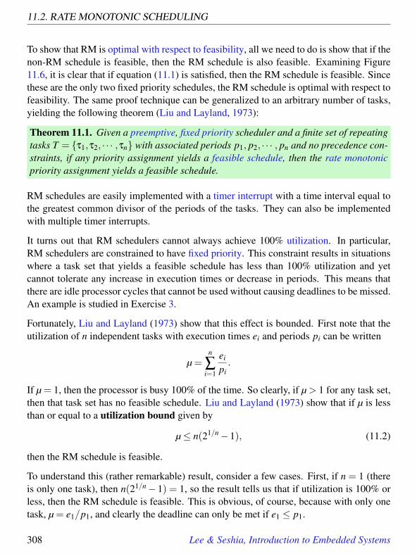
11.2. RATE MONOTONIC SCHEDULING
To show that RM is optimal with respect to feasibility, all we need to do is show that if thenon-RM schedule is feasible, then the RM schedule is also feasible. Examining Figure11.6, it is clear that if equation (11.1) is satisfied, then the RM schedule is feasible. Sincethese are the only two fixed priority schedules, the RM schedule is optimal with respect tofeasibility. The same proof technique can be generalized to an arbitrary number of tasks,yielding the following theorem (Liu and Layland, 1973):
Theorem 11.1. Given a preemptive, fixed priority scheduler and a finite set of repeatingtasks T = τ1,τ2, · · · ,τn with associated periods p1, p2, · · · , pn and no precedence con-straints, if any priority assignment yields a feasible schedule, then the rate monotonicpriority assignment yields a feasible schedule.
RM schedules are easily implemented with a timer interrupt with a time interval equal tothe greatest common divisor of the periods of the tasks. They can also be implementedwith multiple timer interrupts.
It turns out that RM schedulers cannot always achieve 100% utilization. In particular,RM schedulers are constrained to have fixed priority. This constraint results in situationswhere a task set that yields a feasible schedule has less than 100% utilization and yetcannot tolerate any increase in execution times or decrease in periods. This means thatthere are idle processor cycles that cannot be used without causing deadlines to be missed.An example is studied in Exercise 3.
Fortunately, Liu and Layland (1973) show that this effect is bounded. First note that theutilization of n independent tasks with execution times ei and periods pi can be written
µ =n
∑i=1
ei
pi.
If µ = 1, then the processor is busy 100% of the time. So clearly, if µ > 1 for any task set,then that task set has no feasible schedule. Liu and Layland (1973) show that if µ is lessthan or equal to a utilization bound given by
µ≤ n(21/n−1), (11.2)
then the RM schedule is feasible.
To understand this (rather remarkable) result, consider a few cases. First, if n = 1 (thereis only one task), then n(21/n−1) = 1, so the result tells us that if utilization is 100% orless, then the RM schedule is feasible. This is obvious, of course, because with only onetask, µ = e1/p1, and clearly the deadline can only be met if e1 ≤ p1.
308 Lee & Seshia, Introduction to Embedded Systems

11. SCHEDULING
If n = 2, then n(21/n−1) ≈ 0.828. Thus, if a task set with two tasks does not attempt touse more than 82.8% of the available processor time, then the RM schedule will meet alldeadlines.
As n gets large, the utilization bound approaches ln(2)≈ 0.693. That is
limn→∞
n(21/n−1) = ln(2)≈ 0.693.
This means that if a task set with any number of tasks does not attempt to use more than69.3% of the available processor time, then the RM schedule will meet all deadlines.
In the next section, we relax the fixed-priority constraint and show that dynamic priorityschedulers can do better than fixed priority schedulers, in the sense that they can achievehigher utilization. The cost is a somewhat more complicated implementation.
11.3 Earliest Deadline First
Given a finite set of non-repeating tasks with deadlines and no precedence constraints,a simple scheduling algorithm is earliest due date (EDD), also known as Jackson’salgorithm (Jackson, 1955). The EDD strategy simply executes the tasks in the sameorder as their deadlines, with the one with the earliest deadline going first. If two taskshave the same deadline, then their relative order does not matter.
Theorem 11.2. Given a finite set of non-repeating tasks T = τ1,τ2, · · · ,τn with associ-ated deadlines d1,d2, · · · ,dn and no precedence constraints, an EDD schedule is optimalin the sense that it minimizes the maximum lateness, compared to all other possible or-derings of the tasks.
Proof. This theorem is easy to prove with a simple interchange argument. Consideran arbitrary schedule that is not EDD. In such a schedule, because it is not EDD, theremust be two tasks τi and τ j where τi immediately precedes τ j, but d j < di. This isdepicted here:
0 fi
task i
fj dj di
task j
Lee & Seshia, Introduction to Embedded Systems 309

11.3. EARLIEST DEADLINE FIRST
Since the tasks are independent (there are no precedence constraints), reversing the orderof these two tasks yields another valid schedule, depicted here:
0 f ’i
task i
f ’j dj di
task j
We can show that the new schedule has a maximum lateness no greater than that ofthe original schedule. If we repeat the above interchange until there are no more taskseligible for such an interchange, then we have constructed the EDD schedule. Since thisschedule has a maximum lateness no greater than that of the original schedule, the EDDschedule has the minimum maximum lateness of all schedules.
To show that the second schedule has a maximum lateness no greater than that of thefirst schedule, first note that if the maximum lateness is determined by some task otherthan τi or τ j, then the two schedules have the same maximum lateness, and we are done.Otherwise, it must be that the maximum lateness of the first schedule is
Lmax = max( fi−di, f j−d j) = f j−d j,
where the latter equality is obvious from the picture and follows from the facts thatfi ≤ f j and d j < di.
The maximum lateness of the second schedule is given by
L′max = max( f ′i −di, f ′j−d j) .
Consider two cases:
Case 1: L′max = f ′i −di. In this case, since f ′i = f j, we have
L′max = f j−di ≤ f j−d j ,
where the latter inequality follows because d j < di. Hence, L′max ≤ Lmax.
Case 2: L′max = f ′j−d j. In this case, since f ′j ≤ f j, we have
L′max ≤ f j−d j ,
310 Lee & Seshia, Introduction to Embedded Systems

11. SCHEDULING
and again L′max ≤ Lmax.
In both cases, the second schedule has a maximum lateness no greater than that of thefirst schedule. QED.
EDD is also optimal with respect to feasibility, because it minimizes the maximum late-ness. However, EDD does not support arrival of tasks, and hence also does not sup-port periodic or repeated execution of tasks. Fortunately, EDD is easily extended tosupport these, yielding what is known as earliest deadline first (EDF) or Horn’s al-gorithm (Horn, 1974).
Theorem 11.3. Given a set of n independent tasks T = τ1,τ2, · · · ,τn with associateddeadlines d1,d2, · · · ,dn and arbitrary arrival times, any algorithm that at any instant ex-ecutes the task with the earliest deadline among all arrived tasks is optimal with respectto minimizing the maximum lateness.
The proof of this uses a similar interchange argument. Moreover, the result is easilyextended to support an unbounded number of arrivals. We leave it as an exercise.
Note that EDF is a dynamic priority scheduling algorithm. If a task is repeatedly executed,it may be assigned a different priority on each execution. This can make it more complexto implement. Typically, for periodic tasks, the deadline used is the end of the period ofthe task, though it is certainly possible to use other deadlines for tasks.
Although EDF is more expensive to implement than RM, in practice its performance isgenerally superior (Buttazzo, 2005b). First, RM is optimal with respect to feasibilityonly among fixed priority schedulers, whereas EDF is optimal w.r.t. feasibility amongdynamic priority schedulers. In addition, EDF also minimizes the maximum lateness.Also, in practice, EDF results in fewer preemptions (see Exercise 2), which means lessoverhead for context switching. This often compensates for the greater complexity inthe implementation. In addition, unlike RM, any EDF schedule with less than 100%utilization can tolerate increases in execution times and/or reductions in periods and stillbe feasible.
Lee & Seshia, Introduction to Embedded Systems 311

11.3. EARLIEST DEADLINE FIRST
0
1
d1= 2
d2= 5
d3= 4d6= 6
d5= 5
d4= 3
642
3 2 4 5 6EDF
1 2 4 3 5 6LDF
1 2 4 3 5 6EDF*
Figure 11.7: An example of a precedence graph for six tasks and the scheduleunder three scheduling policies. Execution times for all tasks are one time unit.
11.3.1 EDF with Precedences
Theorem 11.2 shows that EDF is optimal (it minimizes maximum lateness) for a taskset without precedences. What if there are precedences? Given a finite set of tasks,precedences between them can be represented by a precedence graph.
Example 11.1: Consider six tasks T = 1, · · · ,6, each with execution time ei = 1,with precedences as shown in Figure 11.7. The diagram means that task 1 mustexecute before either 2 or 3 can execute, that 2 must execute before either 4 or 5,and that 3 must execute before 6. The deadline for each task is shown in the figure.The schedule labeled EDF is the EDF schedule. This schedule is not feasible. Task4 misses its deadline. However, there is a feasible schedule. The schedule labeledLDF meets all deadlines.
312 Lee & Seshia, Introduction to Embedded Systems

11. SCHEDULING
The previous example shows that EDF is not optimal if there are precedences. In 1973,Lawler (1973) gave a simple algorithm that is optimal with precedences, in the sense that itminimizes the maximum lateness. The strategy is very simple. Given a fixed, finite set oftasks with deadlines, Lawler’s strategy constructs the schedule backwards, choosing firstthe last task to execute. The last task to execute is the one on which no other task dependsthat has the latest deadline. The algorithm proceeds to construct the schedule backwards,each time choosing from among the tasks whose dependents have already been scheduledthe one with the latest deadline. For the previous example, the resulting schedule, labeledLDF in Figure 11.7, is feasible. Lawler’s algorithm is called latest deadline first (LDF).
LDF is optimal in the sense that it minimizes the maximum lateness, and hence it isalso optimal with respect to feasibility. However, it does not support arrival of tasks.Fortunately, there is a simple modification of EDF, proposed by Chetto et al. (1990).EDF* (EDF with precedences), supports arrivals and minimizes the maximal lateness. Inthis modification, we adjust the deadlines of all the tasks. Suppose the set of all tasks isT . For a task execution i ∈ T , let D(i)⊂ T be the set of task executions that immediatelydepend on i in the precedence graph. For all executions i ∈ T , we define a modifieddeadline
d′i = min(di, minj∈D(i)
(d′j− e j)) .
EDF* is then just like EDF except that it uses these modified deadlines.
Example 11.2: In Figure 11.7, we see that the EDF* schedule is the same as theLDF schedule. The modified deadlines are as follows:
d′1 = 1, d′2 = 2, d′3 = 4, d′4 = 3, d′5 = 5, d′6 = 6 .
The key is that the deadline of task 2 has changed from 5 to 2, reflecting the factthat its successors have early deadlines. This causes EDF* to schedule task 2 beforetask 3, which results in a feasible schedule.
EDF* can be thought of as a technique for rationalizing deadlines. Instead of acceptingarbitrary deadlines as given, this algorithm ensures that the deadlines take into accountdeadlines of successor tasks. In the example, it makes little sense for task 2 to have a laterdeadline, 5, than its successors. So EDF* corrects this anomaly before applying EDF.
Lee & Seshia, Introduction to Embedded Systems 313

11.4. SCHEDULING AND MUTUAL EXCLUSION
11.4 Scheduling and Mutual Exclusion
Although the algorithms given so far are conceptually simple, the effects they have inpractice are far from simple and often surprise system designers. This is particularly truewhen tasks share resources and use mutual exclusion to guard access to those resources.
11.4.1 Priority Inversion
In principle, a priority-based preemptive scheduler is executing at all times the high-priority enabled task. However, when using mutual exclusion, it is possible for a task tobecome blocked during execution. If the scheduling algorithm does not account for thispossibility, serious problems can occur.
Figure 11.8: The Mars Pathfinder and a view of the surface of Mars from thecamera of the lander (image from the Wikipedia Commons).
314 Lee & Seshia, Introduction to Embedded Systems

11. SCHEDULING
Example 11.3: The Mars Pathfinder, shown in Figure 11.8, landed on Mars onJuly 4th, 1997. A few days into the mission, the Pathfinder began sporadicallymissing deadlines, causing total system resets, each with loss of data. Engineers onthe ground diagnosed the problem as priority inversion, where a low priority mete-orological task was holding a lock and blocking a high-priority task, while mediumpriority tasks executed. (Source: What Really Happened on Mars? Mike Jones,RISKS-19.49 on the comp.programming.threads newsgroup, Dec. 07, 1997, andWhat Really Happened on Mars? Glenn Reeves, Mars Pathfinder Flight SoftwareCognizant Engineer, email message, Dec. 15, 1997.)
Priority inversion is a scheduling anomaly where a high-priority task is blocked whileunrelated lower-priority tasks are executing. The phenomenon is illustrated in Figure 11.9.In the figure, task 3, a low priority task, acquires a lock at time 1. At time 2, it is preemptedby task 1, a high-priority task, which then at time 3 blocks trying to acquire the same lock.Before task 3 reaches the point where it releases the lock, however, it gets preempted byan unrelated task 2, which has medium priority. Task 2 can run for an unbounded amount
0 2 4 6 8 10
task 1
task 2
task 3
acq
uir
e lo
ck
pre
emp
t
blo
ck
pre
emp
t
rele
ase
do
ne
task 1 blocked
Figure 11.9: Illustration of priority inversion. Task 1 has highest priority, task 3lowest. Task 3 acquires a lock on a shared object, entering a critical section. Itgets preempted by task 1, which then tries to acquire the lock and blocks. Task2 preempts task 3 at time 4, keeping the higher priority task 1 blocked for anunbounded amount of time. In effect, the priorities of tasks 1 and 2 get inverted,since task 2 can keep task 1 waiting arbitrarily long.
Lee & Seshia, Introduction to Embedded Systems 315

11.4. SCHEDULING AND MUTUAL EXCLUSION
of time, and effectively prevents the higher-priority task 1 from executing. This is almostcertainly not desirable.
11.4.2 Priority Inheritance Protocol
In 1990, Sha et al. (1990) gave a solution to the priority inversion problem called priorityinheritance. In their solution, when a task blocks attempting to acquire a lock, then thetask that holds the lock inherits the priority of the blocked task. Thus, the task that holdsthe lock cannot be preempted by a task with lower priority than the one attempting toacquire the lock.
Example 11.4: Figure 11.10 illustrates priority inheritance. In the figure, whentask 1 blocks trying to acquire the lock held by task 3, task 3 resumes executing,but now with the higher priority of task 1. Thus, when task 2 becomes enabled attime 4, it does not preempt task 3. Instead, task 3 runs until it releases the lock attime 5. At that time, task 3 reverts to its original (low) priority, and task 1 resumesexecuting. Only when task 1 completes is task 2 able to execute.
0 2 4 6 8 10
task 1
task 2
task 3
acq
uir
e lo
ck
pre
emp
t
blo
ck
rele
ase
do
ne
task 1 blocked
at priority of 1
do
ne
task 2 preempted
Figure 11.10: Illustration of the priority inheritance protocol. Task 1 has highestpriority, task 3 lowest. Task 3 acquires a lock on a shared object, entering acritical section. It gets preempted by task 1, which then tries to acquire the lockand blocks. Task 3 inherits the priority of task 1, preventing preemption by task 2.
316 Lee & Seshia, Introduction to Embedded Systems

11. SCHEDULING
0 2 4 6
task 1
task 2
acq
uir
e lo
ck a
pre
emp
t
block on a
acquire lock b
a
b
block on ba
Figure 11.11: Illustration of deadlock. The lower priority task starts first and ac-quires lock a, then gets preempted by the higher priority task, which acquires lockb and then blocks trying to acquire lock a. The lower priority task then blockstrying to acquire lock b, and no further progress is possible.
11.4.3 Priority Ceiling Protocol
Priorities can interact with mutual exclusion locks in even more interesting ways. Inparticular, in 1990, Sha et al. (1990) showed that priorities can be used to prevent certainkinds of deadlocks.
Example 11.5: Figure 11.11 illustrates a scenario in which two tasks deadlock.In the figure, task 1 has higher priority. At time 1, task 2 acquires lock a. At time2, task 1 preempts task 2, and at time 3, acquires lock b. While holding lock b, itattempts to acquire lock a. Since a is held by task 2, it blocks. At time 4, task 2resumes executing. At time 5, it attempts to acquire lock b, which is held by task 1.Deadlock!
The deadlock in the previous example can be prevented by a clever technique called thepriority ceiling protocol (Sha et al., 1990). In this protocol, every lock or semaphore isassigned a priority ceiling equal to the priority of the highest-priority task that can lock it.A task τ can acquire a lock a only if the task’s priority is strictly higher than the priorityceilings of all locks currently held by other tasks. Intuitively, if we prevent task τ from
Lee & Seshia, Introduction to Embedded Systems 317

11.4. SCHEDULING AND MUTUAL EXCLUSION
0 2 4 6
task 1
task 2
lock
a
pre
emp
t
prevented from locking bby priority ceiling protocol
a
b
a b
unlock b, then a
a
Figure 11.12: Illustration of the priority ceiling protocol. In this version, locks a andb have priority ceilings equal to the priority of task 1. At time 3, task 1 attemptsto lock b, but it cannot because task 2 currently holds lock a, which has priorityceiling equal to the priority of task 1.
acquiring lock a, then we ensure that task τ will not hold lock a while later trying toacquire other locks held by other tasks. This prevents certain deadlocks from occurring.
Example 11.6: The priority ceiling protocol prevents the deadlock of Example11.5, as shown in Figure 11.12. In the figure, when task 1 attempts to acquire lockb at time 3, it is prevented from doing so. At that time, lock a is currently held byanother task (task 2). The priority ceiling assigned to lock a is equal to the priorityof task 1, since task 1 is the highest priority task that can acquire lock a. Sincethe priority of task 1 is not strictly higher than this priority ceiling, task 1 is notpermitted to acquire lock b. Instead, task 1 becomes blocked, allowing task 2 torun to completion. At time 4, task 2 acquires lock b unimpeded, and at time 5,it releases both locks. Once it has released both locks, task 1, which has higherpriority, is no longer blocked, so it resumes executing, preempting task 2.
Of course, implementing the priority ceiling protocol requires being able to determine inadvance which tasks acquire which locks. A simple conservative strategy is to examinethe source code for each task and inventory the locks that are acquired in the code. This isconservative because a particular program may or may not execute any particular line of
318 Lee & Seshia, Introduction to Embedded Systems

11. SCHEDULING
code, so just because a lock is mentioned in the code does not necessarily mean that thetask will attempt to acquire the lock.
11.5 Multiprocessor Scheduling
Scheduling tasks on a single processor is hard enough. Scheduling them on multiple pro-cessors is even harder. Consider the problem of scheduling a fixed finite set of tasks withprecedences on a finite number of processors with the goal of minimizing the makespan.This problem is known to be NP-hard. Nonetheless, effective and efficient schedulingstrategies exist. One of the simplest is known as the Hu level scheduling algorithm. Itassigns a priority to each task τ based on the level, which is the greatest sum of exe-cution times of tasks on a path in the precedence graph from τ to another task with nodependents. Tasks with larger levels have higher priority than tasks with smaller levels.
Example 11.7: For the precedence graph in Figure 11.7, task 1 has level 3, tasks2 and 3 have level 2, and tasks 4, 5, and 6 have level 1. Hence, a Hu level schedulerwill give task 1 highest priority, tasks 2 and 3 medium priority, and tasks 4, 5, and6 lowest priority.
Hu level scheduling is one of a family of critical path methods because it emphasizes thepath through the precedence graph with the greatest total execution time. Although it isnot optimal, it is known to closely approximate the optimal solution for most graphs (Kohler,1975; Adam et al., 1974).
Once priorities are assigned to tasks, a list scheduler sorts the tasks by priorities andassigns them to processors in the order of the sorted list as processors become available.
Example 11.8: A two-processor schedule constructed with the Hu level schedul-ing algorithm for the precedence graph shown in Figure 11.7 is given in Fig-ure 11.13. The makespan is 4.
Lee & Seshia, Introduction to Embedded Systems 319

11.5. MULTIPROCESSOR SCHEDULING
11.5.1 Scheduling Anomalies
Among the worst pitfalls in embedded systems design are scheduling anomalies, whereunexpected or counterintuitive behaviors emerge due to small changes in the operatingconditions of a system. We have already illustrated two such anomalies, priority inversionand deadlock. There are many others. The possible extent of the problems that canarise are well illustrated by the so-called Richard’s anomalies (Graham, 1969). Theseshow that multiprocessor schedules are non-montonic, meaning that improvements inperformance at a local level can result in degradations in performance at a global level,and brittle, meaning that small changes can have big consequences.
Richard’s anomalies are summarized in the following theorem.
Theorem 11.4. If a task set with fixed priorities, execution times, and precedence con-straints is scheduled on a fixed number of processors in accordance with the priorities,then increasing the number of processors, reducing execution times, or weakening prece-dence constraints can increase the schedule length.
Proof. The theorem can be proved with the example in Figure 11.14. The examplehas nine tasks with execution times as shown in the figure. We assume the tasks areassigned priorities so that the lower numbered tasks have higher priority than the highernumbered tasks. Note that this does not correspond to a critical path priority assignment,but it suffices to prove the theorem. The figure shows a three-processor schedule inaccordance with the priorities. Notice that the makespan is 12.
First, consider what happens if the execution times are all reduced by one time unit. Aschedule conforming to the priorities and precedences is shown below:
0
1
42
3 5 6Processor A:
2 4Processor B:
Figure 11.13: A two-processor parallel schedule for the tasks with precedencegraph shown in Figure 11.7.
320 Lee & Seshia, Introduction to Embedded Systems

11. SCHEDULING
0 4 8 12 16
proc1
proc2
proc3
2 6 10 14
3
2
1
4
9
5 7
86
time
e1 = 3
e2 = 2
e3 = 2
e4 = 2
e9 = 9
e8 = 4
e7 = 4
e6 = 4
e5 = 4
Figure 11.14: A precedence graph with nine tasks, where the lower numberedtasks have higher priority than the higher numbered tasks.
0 4 8 12 16
proc1
proc2
proc3
2 6 10 14
3
2
1
4 9
5
7
8
6
time
Notice that the makespan has increased to 13, even though the total amount of computa-tion has decreased significantly. Since computation times are rarely known exactly, thisform of brittleness is particularly troubling.
Consider next what happens if we add a fourth processor and keep everything else thesame as in the original problem. A resulting schedule is shown below:
Lee & Seshia, Introduction to Embedded Systems 321

11.5. MULTIPROCESSOR SCHEDULING
0 4 8 12 16
proc1
proc2
proc3
2 6 10 14
3
2
1
4
95
7
8
6
time
proc4
Again, the makespan has increased (to 15 this time) even though we have added 33%more processing power than originally available.
Consider finally what happens if we weaken the precedence constraints by removing theprecedences between task 4 and tasks 7 and 8. A resulting schedule is shown below:
0 4 8 12 16
proc1
proc2
proc3
2 6 10 14
3
2
1
4
9
5
7
8
6
time
The makespan has now increased to 16, even though weakening precedence constraintsincreases scheduling flexibility. A simple priority-based scheduling scheme such as thisdoes not take advantage of the weakened constraints.
This theorem is particularly troubling when we realize that execution times for softwareare rarely known exactly (see Chapter 15). Scheduling policies will be based on approxi-mations, and behavior at run time may be quite unexpected.
Another form of anomaly arises when there are mutual exclusion locks. An illustration isgiven in Figure 11.15. In this example, five tasks are assigned to two processors using astatic assignment scheduler. Tasks 2 and 4 contend for a mutex. If the execution time oftask 1 is reduced, then the order of execution of tasks 2 and 4 reverses, which results inan increased execution time. This kind of anomaly is quite common in practice.
322 Lee & Seshia, Introduction to Embedded Systems

11. SCHEDULING
0 4 8 12
proc1
proc2
2 6 10
3
1
4 5
time
2
proc1
proc2 3
1
4 5
2
0 4 8 122 6 10time
Figure 11.15: Anomaly due to mutual exclusion locks, where a reduction in theexecution time of task 1 results in an increased makespan.
11.6 Summary
Embedded software is particularly sensitive to timing effects because it inevitably inter-acts with external physical systems. A designer, therefore, needs to pay considerableattention to the scheduling of tasks. This chapter has given an overview of some of thebasic techniques for scheduling real-time tasks and parallel scheduling. It has explainedsome of the pitfalls, such as priority inversion and scheduling anomalies. A designer thatis aware of the pitfalls is better equipped to guard against them.
Lee & Seshia, Introduction to Embedded Systems 323

11.6. SUMMARY
Further Reading
Scheduling is a well-studied topic, with many basic results dating back to the 1950s. Thischapter covers only the most basic techniques and omits several important topics. For real-time scheduling textbooks, we particularly recommend Buttazzo (2005a), Stankovic andRamamritham (1988), and Liu (2000), the latter of which has particularly good coverageof scheduling of sporadic tasks. An excellent overview article is Sha et al. (2004). Ahands-on practical guide can be found in Klein et al. (1993). For an excellent overviewof the evolution of fixed-priority scheduling techniques through 2003, see Audsley et al.(2005). For soft real-time scheduling, we recommend studying time utility functions,introduced by Douglas Jensen in 1977 as a way to overcome the limited expressiveness inclassic deadline constraints in real-time systems (see, for example, Jensen et al. (1985);Ravindran et al. (2007)).
There are many more scheduling strategies than those described here. For example,deadline monotonic (DM) scheduling modifies rate monotonic to allow periodic tasksto have deadlines less than their periods (Leung and Whitehead, 1982). The Spring al-gorithm is a set of heuristics that support arrivals, precedence relations, resource con-straints, non-preemptive properties, and importance levels (Stankovic and Ramamritham,1987, 1988).
An important topic that we do not cover is feasibility analysis, which provides tech-niques for analyzing programs to determine whether feasible schedules exist. Much ofthe foundation for work in this area can be found in Harter (1987) and Joseph and Pandya(1986).
Multiprocessor scheduling is also a well-studied topic, with many core results origi-nating in the field of operations research. Classic texts on the subject are Conway et al.(1967) and Coffman (1976). Sriram and Bhattacharyya (2009) focus on embedded mul-tiprocessors and include innovative techniques for reducing synchronization overhead inmultiprocessor schedules.
It is also worth noting that a number of projects have introduced programming languageconstructs that express real-time behaviors of software. Most notable among these is Ada,a language developed under contract from the US Department of Defense (DoD) from1977 to 1983. The goal was to replace the hundreds of programming languages then usedin DoD projects with a single, unified language. An excellent discussion of languageconstructs for real time can be found in Lee and Gehlot (1985) and Wolfe et al. (1993).
324 Lee & Seshia, Introduction to Embedded Systems

11. SCHEDULING
Exercises
1. This problem studies fixed-priority scheduling. Consider two tasks to be executedperiodically on a single processor, where task 1 has period p1 = 4 and task 2 hasperiod p2 = 6.
(a) Let the execution time of task 1 be e1 = 1. Find the maximum value for theexecution time e2 of task 2 such that the RM schedule is feasible.
(b) Again let the execution time of task 1 be e1 = 1. Let non-RMS be a fixed-priority schedule that is not an RM schedule. Find the maximum value for theexecution time e2 of task 2 such that non-RMS is feasible.
(c) For both your solutions to (a) and (b) above, find the processor utilization.Which is better?
(d) For RM scheduling, are there any values for e1 and e2 that yield 100% utiliza-tion? If so, give an example.
2. This problem studies dynamic-priority scheduling. Consider two tasks to be exe-cuted periodically on a single processor, where task 1 has period p1 = 4 and task2 has period p2 = 6. Let the deadlines for each invocation of the tasks be the endof their period. That is, the first invocation of task 1 has deadline 4, the secondinvocation of task 1 has deadline 8, and so on.
(a) Let the execution time of task 1 be e1 = 1. Find the maximum value for theexecution time e2 of task 2 such that EDF is feasible.
(b) For the value of e2 that you found in part (a), compare the EDF scheduleagainst the RM schedule from Exercise 1 (a). Which schedule has less pre-emption? Which schedule has better utilization?
3. This problem compares RM and EDF schedules. Consider two tasks with periodsp1 = 2 and p2 = 3 and execution times e1 = e2 = 1. Assume that the deadline foreach execution is the end of the period.
(a) Give the RM schedule for this task set and find the processor utilization.How does this utilization compare to the Liu and Leland utilization boundof (11.2)?
(b) Show that any increase in e1 or e2 makes the RM schedule infeasible. If youhold e1 = e2 = 1 and p2 = 3 constant, is it possible to reduce p1 below 2 and
Lee & Seshia, Introduction to Embedded Systems 325

EXERCISES
still get a feasible schedule? By how much? If you hold e1 = e2 = 1 andp1 = 2 constant, is it possible to reduce p2 below 3 and still get a feasibleschedule? By how much?
(c) Increase the execution time of task 2 to be e2 = 1.5, and give an EDF schedule.Is it feasible? What is the processor utilization?
4. This problem compares fixed vs. dynamic priorities, and is based on an example byBurns and Baruah (2008). Consider two periodic tasks, where task τ1 has periodp1 = 2, and task τ2 has period p2 = 3. Assume that the execution times are e1 = 1and e2 = 1.5. Suppose that the release time of execution i of task τ1 is given by
r1,i = 0.5+2(i−1)
for i = 1,2, · · · . Suppose that the deadline of execution i of task τ1 is given by
d1,i = 2i.
Correspondingly, assume that the release times and deadlines for task τ2 are
r2,i = 3(i−1)
andd2,i = 3i.
(a) Give a feasible fixed-priority schedule.
(b) Show that if the release times of all executions of task τ1 are reduced by 0.5,then no fixed-priority schedule is feasible.
(c) Give a feasible dynamic-priority schedule with the release times of task τ1reduced to
r1,i = 2(i−1).
5. This problem studies scheduling anomalies. Consider the task precedence graphdepicted in Figure 11.16 with eight tasks. In the figure, ei denotes the executiontime of task i. Assume task i has higher priority than task j if i < j. There is nopreemption. The tasks must be scheduled respecting all precedence constraints andpriorities. We assume that all tasks arrive at time t = 0.
(a) Consider scheduling these tasks on two processors. Draw the schedule forthese tasks and report the makespan.
326 Lee & Seshia, Introduction to Embedded Systems

11. SCHEDULING
e1= 3
e2= 2
e3= 2
e8= 5
e7 = 10
e4 = 5
e5 = 5
e6 = 5
Figure 11.16: Precedence Graph for Exercise 5.
(b) Now consider scheduling these tasks on three processors. Draw the schedulefor these tasks and report the makespan. Is the makespan bigger or smallerthan that in part (a) above?
(c) Now consider the case when the execution time of each task is reduced by1 time unit. Consider scheduling these tasks on two processors. Draw theschedule for these tasks and report the makespan. Is the makespan bigger orsmaller than that in part (a) above?
6. This problem studies the interaction between real-time scheduling and mutual ex-clusion, and was formulated by Kevin Weekly.Consider the following excerpt of code:
1 pthread_mutex_t X; // Resource X: Radio communication2 pthread_mutex_t Y; // Resource Y: LCD Screen3 pthread_mutex_t Z; // Resource Z: External Memory (slow)4
5 void ISR_A() // Safety sensor Interrupt Service Routine6 pthread_mutex_lock(&Y);7 pthread_mutex_lock(&X);8 display_alert(); // Uses resource Y9 send_radio_alert(); // Uses resource X
10 pthread_mutex_unlock(&X);11 pthread_mutex_unlock(&Y);12 13
14 void taskB() // Status recorder task15 while (1) 16 static time_t starttime = time();
Lee & Seshia, Introduction to Embedded Systems 327

EXERCISES
17 pthread_mutex_lock(&X);18 pthread_mutex_lock(&Z);19 stats_t stat = get_stats();20 radio_report( stat ); // uses resource X21 record_report( stat ); // uses resource Z22 pthread_mutex_unlock(&Z);23 pthread_mutex_unlock(&X);24 sleep(100-(time()-starttime)); // schedule next excecution25 26 27
28 void taskC() // UI Updater task29 while(1) 30 pthread_mutex_lock(&Z);31 pthread_mutex_lock(&Y);32 read_log_and_display(); // uses resources Y and Z33 pthread_mutex_unlock(&Y);34 pthread_mutex_unlock(&Z);35 36
You may assume that the comments fully disclose the resource usage of the proce-dures. That is, if a comment says ”uses resource X”, then the relevant procedureuses only resource X. The scheduler running aboard the system is a priority-basedpreemptive scheduler, where taskB is higher priority than taskC. In this problem,ISR A can be thought of as an asynchronous task with the highest priority.
The intended behavior is for the system to send out a radio report every 100ms andfor the UI to update constantly. Additionally, if there is a safety interrupt, a radioreport is sent immediately and the UI alerts the user.
(a) Every so often, when there is a safety interrupt, the system completely stopsworking. In a scheduling diagram (like Figure 11.11 in the text), using thetasks A,B,C, and resources X,Y,Z, explain the cause of this behavior.Execution times do not have to be to scale in your diagram. Label your dia-gram clearly. You will be graded in part on the clarity of your answer, not juston its correctness.
(b) Using the priority ceiling protocol, show the scheduling diagram for the samesequence of events that you gave in part (a). Be sure to show all resource locksand unlocks until all tasks are finished or reached the end of an iteration. Doesexecution stop as before?
328 Lee & Seshia, Introduction to Embedded Systems

11. SCHEDULING
(c) Without changing the scheduler, how could the code in taskB be reorderedto fix the issue? Using an exhaustive search of all task/resource locking sce-narios, prove that this system will not encounter deadlock. (Hint: Your proofshould enumerate 6 cases because the 3 tasks each have 2 possible resourcesthey could block on.)
Lee & Seshia, Introduction to Embedded Systems 329

Part III
Analysis and Verification
This part of this text studies analysis of embedded systems, with emphasis on methodsfor specifying desired and undesired behaviors and checking that an implementation con-forms to its specification. Chapter 12 covers temporal logic, a formal notation that canexpress families of input/output behaviors and the evolution of the state of a system overtime. This notation can be used to specify unambiguously desired and undesired behav-iors. Chapter 13 explains what it means for one specification to be equivalent to another,and what it means for a design to implement a specification. Chapter 14 shows how tocheck algorithmically whether a design correctly implements a specification. Chapter 15illustrates how to analyze designs for quantitative properties, with emphasis on executiontime analysis for software. Such analysis is essential to achieving real-time behavior insoftware.


12Invariants and
Temporal Logic
Contents12.1 Invariants . . . . . . . . . . . . . . . . . . . . . . . . . . . . . . . . 33512.2 Linear Temporal Logic . . . . . . . . . . . . . . . . . . . . . . . . 337
12.2.1 Propositional Logic Formulas . . . . . . . . . . . . . . . . . 337
12.2.2 LTL Formulas . . . . . . . . . . . . . . . . . . . . . . . . . 339
Sidebar: Probing Further: Alternative Temporal Logics . . . . . . . . 342
12.2.3 Using LTL Formulas . . . . . . . . . . . . . . . . . . . . . . 343
12.3 Summary . . . . . . . . . . . . . . . . . . . . . . . . . . . . . . . . 345Sidebar: Safety and Liveness Properties . . . . . . . . . . . . . . . . 346
Exercises . . . . . . . . . . . . . . . . . . . . . . . . . . . . . . . . . . . 347
Every embedded system must be designed to meet certain requirements. Such systemrequirements are also called properties or specifications. The need for specifications isaptly captured by the following quotation (paraphrased from Young et al. (1985)):
“A design without specifications cannot be right or wrong, it can only besurprising!”
333

In present engineering practice, it is common to have system requirements stated in a nat-ural language such as English. As an example, consider the SpaceWire communicationprotocol that is gaining adoption with several national space agencies (European Cooper-ation for Space Standardization, 2002). Here are two properties reproduced from Section8.5.2.2 of the specification document, stating conditions on the behavior of the systemupon reset:
1. “The ErrorReset state shall be entered after a system reset, after link operation hasbeen terminated for any reason or if there is an error during link initialization.”
2. “Whenever the reset signal is asserted the state machine shall move immediately tothe ErrorReset state and remain there until the reset signal is de-asserted.”
It is important to precisely state requirements to avoid ambiguities inherent in naturallanguages. For example, consider the first property of the SpaceWire protocol statedabove. Observe that there is no mention of when the ErrorReset state is to be entered. Thesystems that implement the SpaceWire protocol are synchronous, meaning that transitionsof the state machine occur on ticks of a system clock. Given this, must the ErrorResetstate be entered on the very next tick after one of the three conditions becomes true or onsome subsequent tick of the clock? As it turns out, the document intends the system tomake the transition to ErrorReset on the very next tick, but this is not made precise by theEnglish language description.
This chapter will introduce techniques to specify system properties mathematically andprecisely. A mathematical specification of system properties is also known as a formalspecification. The specific formalism we will use is called temporal logic. As the namesuggests, temporal logic is a precise mathematical notation with associated rules for rep-resenting and reasoning about timing-related properties of systems. While temporal logichas been used by philosophers and logicians since the times of Aristotle, it is only in thelast thirty years that it has found application as a mathematical notation for specifyingsystem requirements.
One of the most common kinds of system property is an invariant. It is also one ofthe simplest forms of a temporal logic property. We will first introduce the notion of aninvariant and then generalize it to more expressive specifications in temporal logic.
334 Lee & Seshia, Introduction to Embedded Systems

12. INVARIANTS AND TEMPORAL LOGIC
12.1 Invariants
An invariant is a property that holds for a system if it remains true at all times duringoperation of the system. Put another way, an invariant holds for a system if it is true in theinitial state of the system, and it remains true as the system evolves, after every reaction,in every state.
In practice, many properties are invariants. Both properties of the SpaceWire proto-col stated above are invariants, although this might not be immediately obvious. BothSpaceWire properties specify conditions that must remain true always. Below is an ex-ample of an invariant property of a model that we have encountered in Chapter 3.
Example 12.1: Consider the model of a traffic light controller given in Figure 3.10and its environment as modeled in Figure 3.11. Consider the system formed by theasynchronous composition of these two state machines. An obvious property thatthe composed system must satisfy is that there is no pedestrian crossing when thetraffic light is green (when cars are allowed to move). This property must alwaysremain true of this system, and hence is a system invariant.
It is also desirable to specify invariant properties of software and hardware implemen-tations of embedded systems. Some of these properties specify correct programmingpractice on language constructs. For example, the C language property
“The program never dereferences a null pointer”
is an invariant specifying good programming practice. Typically dereferencing a nullpointer in a C program results in a segmentation fault, possibly leading to a system crash.Similarly, several desirable properties of concurrent programs are invariants, as illustratedin the following example.
Example 12.2: Consider the following property regarding an absence of deadlock:
If a thread A blocks while trying to acquire a mutex lock, then the threadB that holds that lock must not be blocked attempting to acquire a lockheld by A.
Lee & Seshia, Introduction to Embedded Systems 335

12.1. INVARIANTS
This property is required to be an invariant on any multithreaded program con-structed from threads A and B. The property may or may not hold for a particularprogram. If it does not hold, there is risk of deadlock.
Many system invariants also impose requirements on program data, as illustrated in theexample below.
Example 12.3: Consider the following example of a software task from the opensource Paparazzi unmanned aerial vehicle (UAV) project (Nemer et al., 2006):
1 void altitude_control_task(void) 2 if (pprz_mode == PPRZ_MODE_AUTO23 || pprz_mode == PPRZ_MODE_HOME) 4 if (vertical_mode == VERTICAL_MODE_AUTO_ALT) 5 float err = estimator_z - desired_altitude;6 desired_climb7 = pre_climb + altitude_pgain * err;8 if (desired_climb < -CLIMB_MAX) 9 desired_climb = -CLIMB_MAX;
10 11 if (desired_climb > CLIMB_MAX) 12 desired_climb = CLIMB_MAX;13 14 15 16
For this example, it is required that the value of the desired climb variable atthe end of altitude control task remains within the range [-CLIMB MAX,CLIMB MAX]. This is an example of a special kind of invariant, a postcondition,that must be maintained every time altitude control task returns. Deter-mining whether this is the case requires analyzing the control flow of the program.
336 Lee & Seshia, Introduction to Embedded Systems

12. INVARIANTS AND TEMPORAL LOGIC
12.2 Linear Temporal Logic
We now give a formal description of temporal logic and illustrate with examples of howit can be used to specify system behavior. In particular, we study a particular kind of tem-poral logic known as linear temporal logic, or LTL. There are other forms of temporallogic, some of which are briefly surveyed in sidebars.
Using LTL, one can express a property over a single, but arbitrary execution of a system.For instance, one can express the following kinds of properties in LTL:
• Occurrence of an event and its properties. For example, one can express the prop-erty that an event A must occur at least once in every trace of the system, or that itmust occur infinitely many times.
• Causal dependency between events. An example of this is the property that if anevent A occurs in a trace, then event B must also occur.
• Ordering of events. An example of this kind of property is one specifying that everyoccurrence of event A is preceded by a matching occurrence of B.
We now formalize the above intuition about the kinds of properties expressible in lineartemporal logic. In order to perform this formalization, it is helpful to fix a particularformal model of computation. We will use the theory of finite-state machines, introducedin Chapter 3.
Recall from Section 3.6 that an execution trace of a finite-state machine is a sequence ofthe form
q0, q1, q2, q3, . . . ,
where q j =(x j,s j,y j), s j is the state, x j is the input valuation, and y j is the output valuationat reaction j.
12.2.1 Propositional Logic Formulas
First, we need to be able to talk about conditions at each reaction, such as whether aninput or output is present, what the value of an input or output is, or what the state is.Let an atomic proposition be such a statement about the inputs, outputs, or states. It is apredicate (an expression that evaluates to true or false). Examples of atomic propositionsthat are relevant for the state machines in Figure 12.1 are:
Lee & Seshia, Introduction to Embedded Systems 337

12.2. LINEAR TEMPORAL LOGIC
true Always true.false Always false.
x True if input x is present.x = present True if input x is present.y = absent True if y is absent.
b True if the FSM is in state b
In each case, the expression is true or false at a reaction qi. The proposition b is true at areaction qi if qi = (x,b,y) for any valuations x and y, which means that the machine is instate b at the start of the reaction. I.e., it refers to the current state, not the next state.
A propositional logic formula or (more simply) proposition is a predicate that combinesatomic propositions using logical connectives: conjunction (logical AND, denoted ∧),disjunction (logical OR, denoted ∨), negation (logical NOT, denoted ¬), and implies(logical implication, denoted =⇒ ). Propositions for the state machines in Figure 12.1include any of the above atomic proposition and expressions using the logical connectivestogether with atomic propositions. Here are some examples:
x∧ y True if x and y are both present.x∨ y True if either x or y is present.
x = present∧ y = absent True if x is present and y is absent.¬y True if y is absent.
a =⇒ y True if whenever the FSM is in state a, theoutput y will be made present by the reaction
Figure 12.1: Two finite-state machines used to illustrate LTL formulas.
338 Lee & Seshia, Introduction to Embedded Systems

12. INVARIANTS AND TEMPORAL LOGIC
Note that if p1 and p2 are propositions, the proposition p1 =⇒ p2 is true if and only if¬p2 =⇒ ¬p1. In other words, if we wish to establish that p1 =⇒ p2 is true, it is equallyvalid to establish that ¬p2 =⇒ ¬p1 is true. In logic, the latter expression is called thecontrapositive of the former.
Note further that p1 =⇒ p2 is true if p1 is false. This is easy to see by considering thecontrapositive. The proposition ¬p2 =⇒ ¬p1 is true regardless of p2 if ¬p1 is true. Thus,another proposition that is equivalent to p1 =⇒ p2 is
¬p1∨ (p1∧ p2) .
12.2.2 LTL Formulas
An LTL formula, unlike the above propositions, applies to an entire trace
q0, q1, q2, . . . ,
rather than to just one reaction qi. The simplest LTL formulas look just like the proposi-tions above, but they apply to an entire trace rather than just a single element of the trace.If p is a proposition, then by definition, we say that LTL formula φ = p holds for thetrace q0,q1,q2, . . . if and only if p is true for q0. It may seem odd to say that the formulaholds for the entire trace even though the proposition only holds for the first element ofthe trace, but we will see that LTL provides ways to reason about the entire trace.
By convention, we will denote LTL formulas by φ, φ1, φ2, etc. and propositions by p, p1,p2, etc.
Given a state machine M and an LTL formula φ, we say that φ holds for M if φ holds forall possible traces of M. This typically requires considering all possible inputs.
Example 12.4: The LTL formula a holds for Figure 12.1(b), because all tracesbegin in state a. It does not hold for Figure 12.1(a).
The LTL formula x =⇒ y holds for both machines. In both cases, in the firstreaction, if x is present, then y will be present.
To demonstrate that an LTL formula is false for an FSM, it is sufficient to give one trace forwhich it is false. Such a trace is called a counterexample. To show that an LTL formula
Lee & Seshia, Introduction to Embedded Systems 339

12.2. LINEAR TEMPORAL LOGIC
is true for an FSM, you must demonstrate that it is true for all traces, which is often muchharder (although not so much harder when the LTL formula is a simple propositional logicformula, because in that case we only have to consider the first element of the trace).
Example 12.5: The LTL formula y is false for both FSMs in Figure 12.1. In bothcases, a counterexample is a trace where x is absent in the first reaction.
In addition to propositions, LTL formulas can also have one or more special temporaloperators. These make LTL much more interesting, because they enable reasoning aboutentire traces instead of just making assertions about the first element of a trace. There arefour main temporal operators, which we describe next.
G Operator
The property Gφ (which is read as “globally φ”) holds for a trace if φ holds for every suffixof that trace. (A suffix is a tail of a trace beginning with some reaction and including allsubsequent reactions.)
In mathematical notation, Gφ holds for the trace if and only if, for all j ≥ 0, formula φholds in the suffix q j,q j+1,q j+2, . . ..
Example 12.6: In Figure 12.1(b), G(x =⇒ y) is true for all traces of the machine,and hence holds for the machine. G(x∧ y) does not hold for the machine, becauseit is false for any trace where x is absent in any reaction. Such a trace provides acounterexample.
If φ is a propositional logic formula, then Gφ simply means that φ holds in every reaction.We will see, however, that when we combine the G operator with other temporal logicoperators, we can make much more interesting statements about traces and about statemachines.
340 Lee & Seshia, Introduction to Embedded Systems

12. INVARIANTS AND TEMPORAL LOGIC
F Operator
The property Fφ (which is read as “eventually φ” or “finally φ”) holds for a trace if φholds for some suffix of the trace.
Formally, Fφ holds for the trace if and only if, for some j ≥ 0, formula φ holds in thesuffix q j,q j+1,q j+2, . . ..
Example 12.7: In Figure 12.1(a), Fb is trivially true because the machine startsin state b, hence, for all traces, the proposition b holds for the trace itself (the veryfirst suffix).
More interestingly, G(x =⇒ Fb) holds for Figure 12.1(a). This is because if x ispresent in any reaction, then the machine will eventually be in state b. This is trueeven in suffixes that start in state a.
Notice that parentheses can be important in interpreting an LTL formula. For ex-ample, (Gx) =⇒ (Fb) is trivially true because Fb is true for all traces (since theinitial state is b).
Notice that F¬φ holds if and only if ¬Gφ. That is, stating that φ is eventually false is thesame as stating that φ is not always true.
X Operator
The property Xφ (which is read as “next state φ” ) holds for a trace q0,q1,q2, . . . if andonly if φ holds for the trace q1,q2,q3, . . ..
Example 12.8: In Figure 12.1(a), x =⇒ Xa holds for the state machine, becauseif x is present in the first reaction, then the next state will be a. G(x =⇒ Xa) doesnot hold for the state machine because it does not hold for any suffix that begins instate a. In Figure 12.1(b), G(b =⇒ Xa) holds for the state machine.
Lee & Seshia, Introduction to Embedded Systems 341

12.2. LINEAR TEMPORAL LOGIC
U Operator
The property φ1Uφ2 (which is read as “φ1 until φ2”) holds for a trace if φ2 holds for somesuffix of that trace, and φ1 holds until φ2 becomes true.
Formally, φ1Uφ2 holds for the trace if and only if there exists j ≥ 0 such that φ2 holds inthe suffix q j,q j+1,q j+2, . . . and φ1 holds in suffixes qi,qi+1,qi+2, . . ., for all i s.t. 0≤ i < j.φ1 may or may not hold for q j,q j+1,q j+2, . . ..
Probing Further: Alternative Temporal Logics
Amir Pnueli (1977) was the first to formalize temporal logic as a way of specifying pro-gram properties. For this he won the 1996 ACM Turing Award, the highest honor inComputer Science. Since his seminal paper, temporal logic has become widespread as away of specifying properties for a range of systems, including hardware, software, andcyber-physical systems.
In this chapter, we have focused on LTL, but there are several alternatives. LTL for-mulas apply to individual traces of an FSM, and in this chapter, by convention, we assertthan an LTL formula holds for an FSM if it holds for all possible traces of the FSM. Amore general logic called computation tree logic (CTL∗) explicitly provides quantifiersover possible traces of an FSM (Emerson and Clarke (1980); Ben-Ari et al. (1981)). Forexample, we can write a CTL∗ expression that holds for an FSM if there exists any tracethat satisfies some property, rather than insisting that the property must hold for all traces.CTL∗ is called a branching-time logic because whenever a reaction of the FSM has anondeterministic choice, it will simultaneously consider all options. LTL, by contrast,considers only one trace at a time, and hence it is called a linear-time logic. Our conven-tion of asserting that an LTL formula holds for an FSM if it holds for all traces cannot beexpressed directly in LTL, because LTL does not include quantifiers like “for all traces.”We have to step outside the logic to apply this convention. With CTL∗, this convention isexpressible directly in the logic.
Other temporal logic variants include real-time temporal logics (e.g., timed compu-tation tree logic or TCTL), for reasoning about real-time systems (Alur et al., 1991); andprobabilistic temporal logics, for reasoning about probabilistic models such as Markovchains or Markov decision processes (see, for example, Hansson and Jonsson (1994)).
342 Lee & Seshia, Introduction to Embedded Systems

12. INVARIANTS AND TEMPORAL LOGIC
Example 12.9: In Figure 12.1(b), aUx is true for any trace for which Fx holds.Since this does not include all traces, aUx does not hold for the state machine.
Some authors define a weaker form of the U operator that does not require φ2 to hold.Using our definition, this can be written
(Gφ1)∨ (φ1Uφ2) .
This holds if either φ1 always holds (for any suffix) or, if φ2 holds for some suffix, then φ1holds for all previous suffixes. This can equivalently be written
(F¬φ1) =⇒ (φ1Uφ2) .
Example 12.10: In Figure 12.1(b), (G¬x)∨ (aUx) holds for the state machine.
12.2.3 Using LTL Formulas
Consider the following English descriptions of properties and their corresponding LTLformalizations:
Example 12.11: “Whenever the robot is facing an obstacle, eventually it moves atleast 5 cm away from the obstacle.”
Let p denote the condition that the robot is facing an obstacle, and q denote the con-dition where the robot is at least 5 cm away from the obstacle. Then, this propertycan be formalized in LTL as
G(p =⇒ Fq) .
Lee & Seshia, Introduction to Embedded Systems 343

12.2. LINEAR TEMPORAL LOGIC
Example 12.12: Consider the SpaceWire property:“Whenever the reset signal is asserted the state machine shall move immediately tothe ErrorReset state and remain there until the reset signal is de-asserted.”
Let p be true when the reset signal is asserted, and q be true when the state of theFSM is ErrorReset. Then, the above English property is formalized in LTL as:
G(p =⇒ X(qU¬p)) .
In the above formalization, we have interpreted “immediately” to mean that thestate changes to ErrorReset in the very next time step. Moreover, the above LTLformula will fail to hold for any execution where the reset signal is asserted andnot eventually de-asserted. It was probably the intent of the standard that the resetsignal should be eventually de-asserted, but the English language statement doesnot make this clear.
Example 12.13: Consider the traffic light controller in Figure 3.10. A property ofthis controller is that the outputs always cycle through sigG, sigY and sigR. We canexpress this in LTL as follows:
G (sigG =⇒ X((¬sigR∧¬sigG)UsigY ))
∧ (sigY =⇒ X((¬sigG∧¬sigY )UsigR))
∧ (sigR =⇒ X((¬sigY ∧¬sigR)UsigG))
.
The following LTL formulas express commonly useful properties.
(a) Infinitely many occurrences: This property is of the form GFp, meaning that it isalways the case that p is true eventually. Put another way, this means that p is trueinfinitely often.
(b) Steady-state property: This property is of the form FGp, read as “from some pointin the future, p holds at all times.” This represents a steady-state property, indicating
344 Lee & Seshia, Introduction to Embedded Systems

12. INVARIANTS AND TEMPORAL LOGIC
that after some point in time, the system reaches a steady state in which p is alwaystrue.
(c) Request-response property: The formula G(p =⇒ Fq) can be interpreted to meanthat a request p will eventually produce a response q.
12.3 Summary
Dependability and correctness are central concerns in embedded systems design. Formalspecifications, in turn, are central to achieving these goals. In this chapter, we have studiedtemporal logic, one of the main approaches for writing formal specifications. This chapterhas provided techniques for precisely stating properties that must hold over time for asystem. It has specifically focused on linear temporal logic, which is able to expressmany safety and liveness properties of systems.
Lee & Seshia, Introduction to Embedded Systems 345

12.3. SUMMARY
Safety and Liveness Properties
System properties may be safety or liveness properties. Informally, a safety property isone specifying that “nothing bad happens” during execution. Similarly, a liveness prop-erty specifies that “something good will happen” during execution.
More formally, a property p is a safety property if a system execution does not satisfyp if and only if there exists a finite-length prefix of the execution that cannot be extendedto an infinite execution satisfying p. We say p is a liveness property if every finite-lengthexecution trace can be extended to an infinite execution that satisfies p. See Lamport(1977) and Alpern and Schneider (1987) for a theoretical treatment of safety and liveness.
The properties we have seen in Section 12.1 are all examples of safety properties. Live-ness properties, on the other hand, specify performance or progress requirements on asystem. For a state machine, a property of the form Fφ is a liveness property. No finiteexecution can establish that this property is not satisfied.
The following is a slightly more elaborate example of a liveness property:
“Whenever an interrupt is asserted, the corresponding interrupt service rou-tine (ISR) is eventually executed.”
In temporal logic, if p1 is the property that an interrupt is asserted, and p2 is the propertythat the interrupt service routine is executed, then this property can be written
G(p1 =⇒ Fp2) .
Note that both safety and liveness properties can constitute system invariants. For ex-ample, the above liveness property on interrupts is also an invariant; p1 =⇒ Fp2 musthold in every state.
Liveness properties can be either bounded or unbounded. A bounded liveness propertyspecifies a time bound on something desirable happening (which makes it a safety prop-erty). In the above example, if the ISR must be executed within 100 clock cycles of theinterrupt being asserted, the property is a bounded liveness property; otherwise, if there isno such time bound on the occurrence of the ISR, it is an unbounded liveness property.LTL can express a limited form of bounded liveness properties using the X operator, butit does not provide any mechanism for quantifying time directly.
346 Lee & Seshia, Introduction to Embedded Systems

12. INVARIANTS AND TEMPORAL LOGIC
Exercises
1. Consider the following state machine:
(Recall that the dashed line represents a default transition.) For each of the fol-lowing LTL formulas, determine whether it is true or false, and if it is false, give acounterexample:
(a) x =⇒ Fb
(b) G(x =⇒ F(y = 1))
(c) (Gx) =⇒ F(y = 1)
(d) (Gx) =⇒ GF(y = 1)
(e) G((b∧¬x) =⇒ FGc)
(f) G((b∧¬x) =⇒ Gc)
(g) (GF¬x) =⇒ FGc
2. This problem is concerned with specifying in linear temporal logic tasks to be per-formed by a robot. Suppose the robot must visit a set of n locations l1, l2, . . . , ln. Letpi be an atomic formula that is true if and only if the robot visits location li.
Give LTL formulas specifying the following tasks:
(a) The robot must eventually visit at least one of the n locations.
(b) The robot must eventually visit all n locations, but in any order.
(c) The robot must eventually visit all n locations, in the orderl1, l2, . . . , ln.
Lee & Seshia, Introduction to Embedded Systems 347

EXERCISES
Figure 12.2: Hierarchical state machine modeling a program and its interruptservice routine.
3. Consider a system M modeled by the hierarchical state machine of Figure 12.2,which models an interrupt-driven program. M has two modes: Inactive, in whichthe main program executes, and Active, in which the interrupt service routine (ISR)executes. The main program and ISR read and update a common variable timer-Count.
Answer the following questions:
(a) Specify the following property φ in linear temporal logic, choosing suitableatomic propositions:
φ: The main program eventually reaches program location C.(b) Does M satisfy the above LTL property? Justify your answer by constructing
the product FSM. If M does not satisfy the property, under what conditionswould it do so? Assume that the environment of M can assert the interrupt atany time.
348 Lee & Seshia, Introduction to Embedded Systems

12. INVARIANTS AND TEMPORAL LOGIC
4. Express the postcondition of Example 12.3 as an LTL formula. State your assump-tions clearly.
5. Consider the program fragment shown in Figure 10.6, which provides proceduresfor threads to communicate asynchronously by sending messages to one another.Please answer the following questions about this code. Assume the code is runningon a single processor (not a multicore machine). You may also assume that onlythe code shown accesses the static variables that are shown.
(a) Let s be an atomic proposition asserting that send releases the mutex (i.e.executes line 24). Let g be an atomic proposition asserting that get releasesthe mutex (i.e. executes line 38). Write an LTL formula asserting that g cannotoccur before s in an execution of the program. Does this formula hold for thefirst execution of any program that uses these procedures?
(b) Suppose that a program that uses the send and get procedures in Figure10.6 is aborted at an arbitrary point in its execution and then restarted at thebeginning. In the new execution, it is possible for a call to get to returnbefore any call to send has been made. Describe how this could come about.What value will get return?
(c) Suppose again that a program that uses the send and get procedures aboveis aborted at an arbitrary point in its execution and then restarted at the begin-ning. In the new execution, is it possible for deadlock to occur, where neithera call to get nor a call to send can return? If so, describe how this couldcome about and suggest a fix. If not, give an argument.
6. For each of the following questions, give a short answer and justification.
(a) TRUE or FALSE: If GFp holds for a state machine A, then so does FGp.
(b) TRUE or FALSE: G(Gp) holds for a trace if and only if Gp holds.
Lee & Seshia, Introduction to Embedded Systems 349

13Equivalence and Refinement
Contents13.1 Models as Specifications . . . . . . . . . . . . . . . . . . . . . . . . 352
Sidebar: Abstraction and Refinement . . . . . . . . . . . . . . . . . . 353
13.2 Type Equivalence and Refinement . . . . . . . . . . . . . . . . . . 35413.3 Language Equivalence and Containment . . . . . . . . . . . . . . 356
Sidebar: Finite Sequences and Accepting States . . . . . . . . . . . . 359
Sidebar: Regular Languages and Regular Expressions . . . . . . . . 360
Sidebar: Probing Further: Omega Regular Languages . . . . . . . . 361
13.4 Simulation . . . . . . . . . . . . . . . . . . . . . . . . . . . . . . . 36213.4.1 Simulation Relations . . . . . . . . . . . . . . . . . . . . . . 364
13.4.2 Formal Model . . . . . . . . . . . . . . . . . . . . . . . . . . 366
13.4.3 Transitivity . . . . . . . . . . . . . . . . . . . . . . . . . . . 367
13.4.4 Non-Uniqueness of Simulation Relations . . . . . . . . . . . 367
13.4.5 Simulation vs. Language Containment . . . . . . . . . . . . . 368
13.5 Bisimulation . . . . . . . . . . . . . . . . . . . . . . . . . . . . . . 37013.6 Summary . . . . . . . . . . . . . . . . . . . . . . . . . . . . . . . . 372Exercises . . . . . . . . . . . . . . . . . . . . . . . . . . . . . . . . . . . 373
351

13.1. MODELS AS SPECIFICATIONS
This chapter discusses some fundamental ways to compare state machines and othermodal models, such as trace equivalence, trace containment, simulation, and bisimula-tion. These mechanisms can be used to check conformance of a state machine against aspecification.
13.1 Models as Specifications
The previous chapter provided techniques for unambiguously stating properties that asystem must have to be functioning properly and safely. These properties were expressedusing linear temporal logic, which can concisely describe requirements that the trace ofa finite-state machine must satisfy. An alternative way to give requirements is to providea model, a specification, that exhibits expected behavior of the system. Typically, thespecification is quite abstract, and it may exhibit more behaviors than a useful implemen-tation of the system would. But the key to being a useful specification is that it explicitlyexcludes undesired or dangerous behaviors.
Example 13.1: A simple specification for a traffic light might state: “The lightsshould always be lighted in the order green, yellow, red. It should never, for exam-ple, go directly from green to red, or from yellow to green.” This requirement canbe given as a temporal logic formula (as is done in Example 12.13) or as an abstractmodel (as is done in Figure 3.12).
The topic of this chapter is on the use of abstract models as specifications, and on howsuch models relate to an implementation of a system and to temporal logic formulas.
Example 13.2: We will show how to demonstrate that the traffic light modelshown in Figure 3.10 is a valid implementation of the specification in Figure 3.12.Moreover, all traces of the model in Figure 3.10 satisfy the temporal logic formulain Example 12.13, but not all traces of the specification in Figure 3.12 do. Hence,these two specifications are not the same.
352 Lee & Seshia, Introduction to Embedded Systems

13. EQUIVALENCE AND REFINEMENT
This chapter is about comparing models, and about being able to say with confidence thatone model can be used in place of another. This enables an engineering design processwhere we start with abstract descriptions of desired and undesired behaviors, and suc-cessively refine our models until we have something that is detailed enough to provide
Abstraction and Refinement
This chapter focuses on relationships between models known as abstraction and refine-ment. These terms are symmetric in that the statement “model A is an abstraction ofmodel B” means the same thing as “model B is a refinement of model A.” As a generalrule, the refinement model B has more detail than the abstraction A, and the abstraction issimpler, smaller, or easier to understand.
An abstraction is sound (with respect to some formal system of properties) if propertiesthat are true of the abstraction are also true of the refinement. The formal system ofproperties could be, for example, a type system, linear temporal logic, or the languagesof state machines. If the formal system is LTL, then if every LTL formula that holds forA also holds for B, then A is a sound abstraction of B. This is useful when it is easier toprove that a formula holds for A than to prove that it holds for B, for example because thestate space of B may be much larger than the state space of A.
An abstraction is complete (with respect to some formal system of properties) if prop-erties that are true of the refinement are also true of the abstraction. For example, if theformal system of properties is LTL, then A is a complete abstraction of B if every LTLformula that holds for B also holds for A. Useful abstractions are usually sound but notcomplete, because it is hard to make a complete abstraction that is significantly simpleror smaller.
Consider for example a program B in an imperative language such as C that has multi-ple threads. We might construct an abstraction A that ignores the values of variables andreplaces all branches and control structures with nondeterministic choices. The abstrac-tion clearly has less information than the program, but it may be sufficient for provingsome properties about the program, for example a mutual exclusion property.
Lee & Seshia, Introduction to Embedded Systems 353

13.2. TYPE EQUIVALENCE AND REFINEMENT
a complete implementation. It also tells when it is safe to change an implementation,replacing it with another that might, for example, reduce the implementation cost.
13.2 Type Equivalence and Refinement
We begin with a simple relationship between two models that compares only the datatypes of their communication with their environment. Specifically, the goal is to ensurethat a model B can be used in any environment where a model A can be used withoutcausing any conflicts about data types. We will require that B can accept any inputs thatA can accept from the environment, and that any environment that can accept any outputA can produce can also accept any output that B can produce.
To make the problem concrete, assume an actor model for A and B, as shown in Figure13.1. In that figure, A has three ports, two of which are input ports represented by theset PA = x,w, and one of which is an output port represented by the set QA = y.These ports represent communication between A and its environment. The inputs havetype Vx and Vw, which means that at a reaction of the actor, the values of the inputs willbe members of the sets Vx or Vw.
If we want to replace A by B in some environment, the ports and their types impose fourconstraints:
1. The first constraint is that B does not require some input signal that the environ-ment does not provide. If the input ports of B are given by the set PB, then this isguaranteed by
PB ⊆ PA. (13.1)
The ports of B are a subset of the ports of A. It is harmless for A to have more inputports than B, because if B replaces A in some environment, it can simply ignore anyinput signals that it does not need.
2. The second constraint is that B produces all the output signals that the environmentmay require. This is ensured by the constraint
QA ⊆ QB, (13.2)
where QA is the set of output ports of A, and QB is the set of output ports of B. It isharmless for B to have additional output ports because an environment capable ofworking with A does not expect such outputs and hence can ignore them.
354 Lee & Seshia, Introduction to Embedded Systems

13. EQUIVALENCE AND REFINEMENT
The remaining two constraints deal with the types of the ports. Let the type of an inputport p ∈ PA be given by Vp. This means that an acceptable input value v on p satisfiesv ∈Vp. Let V ′p denote the type of an input port p ∈ PB.
3. The third constraint is that if the environment provides a value v ∈ Vp on an inputport p that is acceptable to A, then if p is also an input port of B, then the value isalso acceptable B; i.e., v ∈V ′p. This constraint can be written compactly as follows,
∀ p ∈ PB, Vp ⊆V ′p. (13.3)
Let the type of an output port q ∈QA be Vq, and the type of the corresponding output portq ∈ QB be V ′q.
4. The fourth constraint is that if B produces a value v ∈V ′q on an output port q, then ifq is also an output port of A, then the value must be acceptable to any environment
B
A
x: Vx
w: Vw
y: Vy
x: V'x
z: V'z
y: V'y
PA = x, w
PB = x
QA = y
QB = y, z
(1) PB ⊆ PA
(2) QA ⊆ QB
(3) ∀ p ∈ PB, Vp ⊆V ′p
(4) ∀ q ∈ QA, V ′q ⊆Vq
Figure 13.1: Summary of type refinement. If the four constraints on the right aresatisfied, then B is a type refinement of A.
Lee & Seshia, Introduction to Embedded Systems 355

13.3. LANGUAGE EQUIVALENCE AND CONTAINMENT
in which A can operate. In other words,
∀ q ∈ QA, V ′q ⊆Vq. (13.4)
The four constraints of equations (13.1) through (13.4) are summarized in Figure 13.1.When these four constraints are satisfied, we say that B is a type refinement of A. If Bis a type refinement of A, then replacing A by B in any environment will not cause typesystem problems. It could, of course, cause other problems, since the behavior of B maynot be acceptable to the environment, but that problem will be dealt with in subsequentsections.
If B is a type refinement of A, and A is a type refinement of B, then we say that A andB are type equivalent. They have the same input and output ports, and the types of theports are the same.
Example 13.3: Let A represent the nondeterministic traffic light model in Figure3.12 and B represent the more detailed deterministic model in Figure 3.10. Theports and their types are identical for both machines, so they are type equivalent.Hence, replacing A with B or vice versa in any environment will not cause typesystem problems.
Notice that since Figure 3.12 ignores the pedestrian input, it might seem reasonableto omit that port. Let A′ represent a variant of Figure 3.12 without the pedestrianinput. It is not safe to replace A′ with B in all environments, because B requires aninput pedestrian signal, but A′ can be used in an environment that provides no suchinput.
13.3 Language Equivalence and Containment
To replace a machine A with a machine B, looking at the data types of the inputs andoutputs alone is usually not enough. If A is a specification and B is an implementation,then normally A imposes more constraints than just data types. If B is an optimization ofA (e.g., a lower cost implementation or a refinement that adds functionality or leveragesnew technology), then B normally needs to conform in some way with the functionalityof A.
356 Lee & Seshia, Introduction to Embedded Systems

13. EQUIVALENCE AND REFINEMENT
In this section, we consider a stronger form of equivalence and refinement. Specifically,equivalence will mean that given a particular sequence of input valuations, the two ma-chines produce the same output valuations.
Example 13.4: The garage counter of Figure 3.4, discussed in Example 3.4, is typeequivalent to the extended state machine version in Figure 3.8. The actor model isshown below:
Counter
up : pure
down : pure
count : 0, …, M
However, these two machines are equivalent in a much stronger sense than simplytype equivalence. These two machines behave in exactly the same way, as viewedfrom the outside. Given the same input sequence, the two machines will producethe same output sequence.
Consider a port p of a state machine with type Vp. This port will have a sequence of valuesfrom the set Vp∪absent, one value at each reaction. We can represent this sequence asa function of the form
sp : N→Vp∪absent.This is the signal received on that port (if it is an input) or produced on that port (if it isan output). Recall that a behavior of a state machine is an assignment of such a signal toeach port of such a machine. Recall further that the language L(M) of a state machine Mis the set of all behaviors for that state machine. Two machines are said to be languageequivalent if they have the same language.
Example 13.5: A behavior of the garage counter is a sequence of present andabsent valuations for the two inputs, up and down, paired with the correspondingoutput sequence at the output port, count. A specific example is given in Example3.16. This is a behavior of both Figures 3.4 and 3.8. All behaviors of Figure 3.4 arealso behaviors of 3.8 and vice versa. These two machines are language equivalent.
Lee & Seshia, Introduction to Embedded Systems 357

13.3. LANGUAGE EQUIVALENCE AND CONTAINMENT
Figure 13.2: Three state machines where (a) and (b) have the same language,and that language is contained by that of (c).
In the case of a nondeterministic machine M, two distinct behaviors may share the sameinput signals. That is, given an input signal, there is more than one possible output se-quence. The language L(M) includes all possible behaviors. Just like deterministic ma-chines, two nondeterministic machines are language equivalent if they have the samelanguage.
Suppose that for two state machines A and B, L(A) ⊂ L(B). That is, B has behaviorsthat A does not have. This is called language containment. A is said to be a languagerefinement of B. Just as with type refinement, language refinement makes an assertionabout the suitability of A as a replacement for B. If every behavior of B is acceptable toan environment, then every behavior of A will also be acceptable to that environment. Acan substitute for B.
358 Lee & Seshia, Introduction to Embedded Systems

13. EQUIVALENCE AND REFINEMENT
Finite Sequences and Accepting States
A complete execution of the FSMs considered in this text is infinite. Suppose that weare interested in only the finite executions. To do this, we introduce the notion of anaccepting state, indicated with a double outline as in state b in the example below:
Let La(M) denote the subset of the language L(M) that results from executions that ter-minate in an accepting state. Equivalently, La(M) includes only those behaviors in L(M)with an infinite tail of stuttering reactions that remain in an accepting state. All suchexecutions are effectively finite, since after a finite number of reactions, the inputs andoutputs will henceforth be absent, or in LTL, FG¬p for every port p.
We call La(M) the language accepted by an FSM M. A behavior in La(M) specifiesfor each port p a finite string, or a finite sequence of values from the type Vp. For theabove example, the input strings (1), (1,0,1), (1,0,1,0,1), etc., are all in La(M). So areversions of these with an arbitrary finite number of absent values between any two presentvalues. When there is no ambiguity, we can write these strings 1, 101, 10101, etc.
In the above example, in all behaviors in La(M), the output is present a finite numberof times, in the same reactions when the input is present.
The state machines in this text are receptive, meaning that at each reaction, each inputport p can have any value in its type Vp or be absent. Hence, the language L(M) ofthe machine above includes all possible sequences of input valuations. La(M) excludesany of these that do not leave the machine in an accepting state. For example, any inputsequence with two 1’s in a row and the infinite sequence (1,0,1,0, · · ·) are in L(M) butnot in La(M).
Note that it is sometimes useful to consider language containment when referring to thelanguage accepted by the state machine, rather than the language that gives all behaviorsof the state machine.
Accepting states are also called final states, since for any behavior in La(M), it is thelast state of the machine. Accepting states are further explored in Exercise 2.
Lee & Seshia, Introduction to Embedded Systems 359

13.3. LANGUAGE EQUIVALENCE AND CONTAINMENT
Regular Languages and Regular Expressions
A language is a set of sequences of values from some set called its alphabet. A languageaccepted by an FSM is called a regular language. A classic example of a language thatis not regular has sequences of the form 0n1n, a sequence of n zeros followed by n ones.It is easy to see that no finite state machine can accept this language because the machinewould have to count the zeros to ensure that the number of ones matches. And the numberof zeros is not bounded. On the other hand, the input sequences accepted by the FSM inthe box on page 359, which have the form 10101 · · ·01, are regular.
A regular expression is a notation for describing regular languages. A central featureof regular expressions is the Kleene star (or Kleene closure), named after the Americanmathematician Stephen Kleene (who pronounced his name KLAY-nee). The notation V∗,where V is a set, means the set of all finite sequences of elements from V . For example, ifV = 0,1, then V∗ is a set that includes the empty sequence (often written λ), and everyfinite sequence of zeros and ones.
The Kleene star may be applied to sets of sequences. For example, if A = 00,11,then A∗ is the set of all finite sequences where zeros and ones always appear in pairs.In the notation of regular expressions, this is written (00|11)*, where the vertical barmeans “or.” What is inside the parentheses defines the set A.
Regular expressions are sequences of symbols from an alphabet and sets of sequences.Suppose our alphabet is A = a,b, · · · ,z, the set of lower-case characters. Then greyis a regular expression denoting a single sequence of four characters. The expressiongrey|gray denotes a set of two sequences. Parentheses can be used to group sequencesor sets of sequences. For example, (grey)|(gray) and gr(e|a)y mean the samething.
Regular expressions also provide convenience notations to make them more compactand readable. For example, the + operator means “one or more,” in contrast to the Kleenestar, which means “zero or more.” For example, a+ specifies the sequences a, aa, aaa,etc.; it is the same as a(a*). The ? operator species “zero or one.” For example,colou?r specifies a set with two sequences, color and colour; it is the same ascolo(λ|u)r, where λ denotes the empty sequence.
Regular expressions are commonly used in software systems for pattern matching. Atypical implementation provides many more convenience notations than the ones illus-trated here.
360 Lee & Seshia, Introduction to Embedded Systems

13. EQUIVALENCE AND REFINEMENT
Example 13.6: Machines M1 and M2 in Figure 13.2 are language equivalent. Bothmachines produce output 1,1,0,1,1,0, · · · , possibly interspersed with absent if theinput is absent in some reactions.
Machine M3, however, has more behaviors. It can produce any output sequencethat M1 and M2 can produce, but it can also produce other outputs given the sameinputs. Thus, M1 and M2 are both language refinements of M3.
Language containment assures that an abstraction is sound with respect to LTL formulasabout input and output sequences. That is, if A is a language refinement of B, then anyLTL formula about inputs and outputs that holds for B also holds for A.
Example 13.7: Consider again the machines in Figure 13.2. M3 might be a spec-ification. For example, if we require that any two output values 0 have at least oneintervening 1, then M3 is a suitable specification of this requirement. This require-ment can be written as an LTL formula as follows:
G((y = 0)⇒ X((y 6= 0)U(y = 1))).
Probing Further: Omega Regular Languages
The regular languages discussed in the boxes on pages 359 and 360 contain only finitesequences. But embedded systems most commonly have infinite executions. To extendthe idea of regular languages to infinite runs, we can use a Buchi automaton, namedafter Julius Richard Buchi, a Swiss logician and mathematician. A Buchi automaton isa possibly nondeterministic FSM that has one or more accepting states. The languageaccepted by the FSM is defined to be the set of behaviors that visit one or more of theaccepting states infinitely often; in other words, these behaviors satisfy the LTL formulaGF(s1 ∨ ·· · ∨ sn), where s1, · · · ,sn are the accepting states. Such a language is called anomega-regular language or ω-regular language, a generalization of regular languages.The reason for using ω in the name is because ω is used to construct infinite sequences,as explained in the box on page 439.
As we will see in Chapter 14, many model checking questions can be expressed bygiving a Buchi automaton and then checking to see whether the ω-regular language itdefines contains any sequences.
Lee & Seshia, Introduction to Embedded Systems 361

13.4. SIMULATION
If we prove that this property holds for M3, then we have implicitly proved that italso holds for M1 and M2.
We will see in the next section that language containment is not sound with respect to LTLformulas that refer to states of the state machines. In fact, language containment does notrequire the state machines to have the same states, so an LTL formula that refers to thestates of one machine may not even apply to the other machine. A sound abstraction thatreferences states will require simulation.
Language containment is sometimes called trace containment, but here the term “trace”refers only to the observable trace, not to the execution trace. As we will see next, thingsget much more subtle when considering execution traces.
13.4 Simulation
Two nondeterministic FSMs may be language equivalent but still have observable differ-ences in behavior in some environments. Language equivalence merely states that giventhe same sequences of input valuations, the two machines are capable of producing thesame sequences of output valuations. However, as they execute, they make choices al-lowed by the nondeterminism. Without being able to see into the future, these choicescould result in one of the machines getting into a state where it can no longer match theoutputs of the other.
When faced with a nondeterministic choice, each machine is free to use any policy tomake that choice. Assume that the machine cannot see into the future; that is, it cannotanticipate future inputs, and it cannot anticipate future choices that any other machinewill make. For two machines to be equivalent, we will require that each machine be ableto make choices that allow it to match the reaction of the other machine (producing thesame outputs), and further allow it to continue to do such matching in the future. It turnsout that language equivalence is not strong enough to ensure that this is possible.
Example 13.8: Consider the two state machines in Figure 13.3. Suppose that M2 isacceptable in some environment (every behavior it can exhibit in that environment
362 Lee & Seshia, Introduction to Embedded Systems

13. EQUIVALENCE AND REFINEMENT
is consistent with some specification or design intent). Is it safe for M1 to replaceM2? The two machines are language equivalent. In all behaviors, the output is oneof two finite strings, 01 or 00, for both machines. So it would seem that M1 canreplace M2. But this is not necessarily the case.
Suppose we compose each of the two machines with its own copy of the environ-ment that finds M2 acceptable. In the first reaction where x is present, M1 has nochoice but to take the transition to state b and produce the output y = 0. However,M2 must choose between f and h. Whichever choice it makes, M2 matches the out-put y = 0 of M1 but enters a state where it is no longer able to always match theoutputs of M1. If M1 can observe the state of M2 when making its choice, then inthe second reaction where x is present, it can choose a transition that M2 can nevermatch. Such a policy for M1 ensures that the behavior of M1, given the same inputs,is never the same as the behavior of M2. Hence, it is not safe to replace M2 withM1.
On the other hand, if M1 is acceptable in some environment, is it safe for M2 toreplace M1? What it means for M1 to be acceptable in the environment is thatwhatever decisions it makes are acceptable. Thus, in the second reaction where x ispresent, both outputs y= 1 and y= 0 are acceptable. In this second reaction, M2 hasno choice but to produce one or the other these outputs, and it will inevitably tran-sition to a state where it continues to match the outputs of M1 (henceforth foreverabsent). Hence it is safe for M2 to replace M1.
In the above example, we can think of the machines as maliciously trying to make M1look different from M2. Since they are free to use any policy to make choices, they arefree to use policies that are contrary to our goal to replace M2 with M1. Note that the ma-chines do not need to know the future; it is sufficient to simply have good visibility of thepresent. The question that we address in this section is: under what circumstances can weassure that there is no policy for making nondeterministic choices that can make machineM1 observably different from M2? The answer is a stronger form of equivalence calledbisimulation and a refinement relation called simulation. We begin with the simulationrelation.
Lee & Seshia, Introduction to Embedded Systems 363

13.4. SIMULATION
Figure 13.3: Two state machines that are language equivalent but where M2 doesnot simulate M1 (M1 does simulate M2).
13.4.1 Simulation Relations
First, notice that the situation given in Example 13.8 is not symmetric. It is safe for M2to replace M1, but not the other way around. Hence, M2 is a refinement of M1, in a sensethat we will now establish. M1, on the other hand, is not a refinement of M2.
The particular kind of refinement we now consider is a simulation refinement. Thefollowing statements are all equivalent:
• M2 is a simulation refinement of M1.
• M1 simulates M2.
• M1 is a simulation abstraction of M2.
Simulation is defined by a matching game. To determine whether M1 simulates M2,we play a game where M2 gets to move first in each round. The game starts with bothmachines in their initial states. M2 moves first by reacting to an input valuation. If thisinvolves a nondeterministic choice, then it is allowed to make any choice. Whatever itchoses, an output valuation results and M2’s turn is over.
364 Lee & Seshia, Introduction to Embedded Systems

13. EQUIVALENCE AND REFINEMENT
It is now M1’s turn to move. It must react to the same input valuation that M2 reactedto. If this involves a nondeterministic choice, then it must make a choice that matchesthe output valuation of M2. If there are multiple such choices, it must select one withoutknowledge of the future inputs or future moves of M2. Its strategy should be to choose onethat enables it to continue to match M2, regardless of what future inputs arrive or futuredecisions M2 makes.
Machine M1 “wins” this matching game (M1 simulates M2) if it can always match theoutput symbol of machine M2 for all possible input sequences. If in any reaction M2 canproduce an output symbol that M1 cannot match, then M1 does not simulate M2.
Example 13.9: In Figure 13.3, M1 simulates M2 but not vice versa. To see this,first play the game with M2 moving first in each round. M1 will always be ableto match M2. Then play the game with M1 moving first in each round. M2 willnot always be able to match M1. This is true even though the two machines arelanguage equivalent.
Interestingly, if M1 simulates M2, it is possible to compactly record all possible gamesover all possible inputs. Let S1 be the states of M1 and S2 be the states of M2. Then asimulation relation S⊆ S2×S1 is a set of pairs of states occupied by the two machines ineach round of the game for all possible inputs. This set summarizes all possible plays ofthe game.
Example 13.10: In Figure 13.3,
S1 = a,b,c,d
andS2 = e, f,g,h, i.
The simulation relation showing that M1 simulates M2 is
S = (e,a),(f,b),(h,b),(g,c),(i,d)
First notice that the pair (e,a) of initial states is in the relation, so the relationincludes the state of the two machines in the first round. In the second round,
Lee & Seshia, Introduction to Embedded Systems 365

13.4. SIMULATION
M2 may be in either f or h, and M1 will be in b. These two possibilities are alsoaccounted for. In the third round and beyond, M2 will be in either g or i, and M1will be in c or d.
There is no simulation relation showing that M2 simulates M1, because it does not.
A simulation relation is complete if it includes all possible plays of the game. It musttherefore account for all reachable states of M2, the machine that moves first, becauseM2’s moves are unconstrained. Since M1’s moves are constrained by the need to matchM2, it is not necessary to account for all of its reachable states.
13.4.2 Formal Model
Using the formal model of nondeterministic FSMs given in Section 3.5.1, we can formallydefine a simulation relation. Let
M1 = (States1, Inputs,Outputs,possibleUpdates1, initialState1),
andM2 = (States2, Inputs,Outputs,possibleUpdates2, initialState2).
Assume the two machines are type equivalent. If either machine is deterministic, then itspossibleUpdates function always returns a set with only one element in it. If M1 simulatesM2, the simulation relation is given as a subset of States2× States1. Note the orderinghere; the machine that moves first in the game, M2, the one being simulated, is first inStates2×States1.
To consider the reverse scenario, if M2 simulates M1, then the relation is given as a subsetof States1×States2. In this version of the game M1 must move first.
We can state the “winning” strategy mathematically. We say that M1 simulates M2 ifthere is a subset S⊆ States2×States1 such that
1. (initialState2, initialState1) ∈ S, and
2. If (s2,s1) ∈ S, then ∀ x ∈ Inputs, and∀ (s′2,y2) ∈ possibleUpdates2(s2,x),there is a (s′1,y1) ∈ possibleUpdates1(s1,x) such that:
366 Lee & Seshia, Introduction to Embedded Systems

13. EQUIVALENCE AND REFINEMENT
(a) (s′2,s′1) ∈ S, and
(b) y2 = y1.
This set S, if it exists, is called the simulation relation. It establishes a correspondencebetween states in the two machines. If it does not exist, then M1 does not simulate M2.
13.4.3 Transitivity
Simulation is transitive, meaning that if M1 simulates M2 and M2 simulates M3, then M1simulates M3. In particular, if we are given simulation relations S2,1 ⊆ States2× States1(M1 simulates M2) and S3,2 ⊆ States3×States2 (M2 simulates M3), then
S3,1 = (s3,s1) ∈ States3×States1 | there exists s2 ∈ States2 where(s3,s2) ∈ S3,2 and (s2,s1) ∈ S2,1
Example 13.11: For the machines in Figure 13.2, it is easy to show that (c)simulates (b) and that (b) simulates (a). Specifically, the simulation relations are
Sa,b = (a,ad),(b,be),(c,cf),(d,ad),(e,be),(f,cf).
andSb,c = (ad,ad),(be,bcef),(cf,bcef).
By transitivity, we can conclude that (c) simulates (a), and that the simulation rela-tion is
Sa,c = (a,ad),(b,bcef),(c,bcef),(d,ad),(e,bcef),(f,bcef),
which further supports the suggestive choices of state names.
13.4.4 Non-Uniqueness of Simulation Relations
When a machine M1 simulates another machine M2, there may be more than one simula-tion relation.
Lee & Seshia, Introduction to Embedded Systems 367
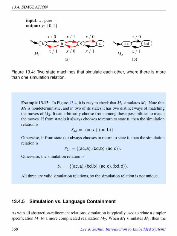
13.4. SIMULATION
Figure 13.4: Two state machines that simulate each other, where there is morethan one simulation relation.
Example 13.12: In Figure 13.4, it is easy to check that M1 simulates M2. Note thatM1 is nondeterministic, and in two of its states it has two distinct ways of matchingthe moves of M2. It can arbitrarily choose from among these possibilities to matchthe moves. If from state b it always chooses to return to state a, then the simulationrelation is
S2,1 = (ac,a),(bd,b).
Otherwise, if from state c it always chooses to return to state b, then the simulationrelation is
S2,1 = (ac,a),(bd,b),(ac,c).
Otherwise, the simulation relation is
S2,1 = (ac,a),(bd,b),(ac,c),(bd,d).
All three are valid simulation relations, so the simulation relation is not unique.
13.4.5 Simulation vs. Language Containment
As with all abstraction-refinement relations, simulation is typically used to relate a simplerspecification M1 to a more complicated realization M2. When M1 simulates M2, then the
368 Lee & Seshia, Introduction to Embedded Systems

13. EQUIVALENCE AND REFINEMENT
language of M1 contains the language of M2, but the guarantee is stronger than languagecontainment. This fact is summarized in the following theorem.
Theorem 13.1. Let M1 simulate M2. Then
L(M2)⊆ L(M1).
Proof. This theorem is easy to prove. Consider a behavior (x,y) ∈ L(M2). We need toshow that (x,y) ∈ L(M1).
Let the simulation relation be S. Find all possible execution traces for M2
((x0,s0,y0),(x1,s1,y1),(x2,s2,y2), · · ·),
that result in behavior (x,y). (If M2 is deterministic, then there will be only one executiontrace.) The simulation relation assures us that we can find an execution trace for M1
((x0,s′0,y0),(x1,s′1,y1),(x2,s′2,y2), · · ·),
where (si,s′i) ∈ S, such that given input valuation xi, M1 produces yi. Thus, (x,y) ∈L(M1).
One use of this theorem is to show that M1 does not simulate M2 by showing that M2 hasbehaviors that M1 does not have.
Example 13.13: For the examples in Figure 13.2, M2 does not simulate M3. Tosee this, just note that the language of M2 is a strict subset of the language of M3,
L(M2)⊂ L(M3),
meaning that M3 has behaviors that M2 does not have.
It is important to understand what the theorem says, and what it does not say. It does notsay, for example, that if L(M2) ⊆ L(M1) then M1 simulates M2. In fact, this statement isnot true, as we have already shown with the examples in Figure 13.3. These two machines
Lee & Seshia, Introduction to Embedded Systems 369

13.5. BISIMULATION
Figure 13.5: An example of two machines where M1 simulates M2, and M2 simu-lates M1, but they are not bisimilar.
have the same language. The two machines are observably different despite the fact thattheir input/output behaviors are the same.
Of course, if M1 and M2 are deterministic and M1 simulates M2, then their languagesare identical and M2 simulates M1. Thus, the simulation relation differs from languagecontainment only for nondeterministic FSMs.
13.5 Bisimulation
It is possible to have two machines M1 and M2 where M1 simulates M2 and M2 simu-lates M1, and yet the machines are observably different. Note that by the theorem in theprevious section, the languages of these two machines must be identical.
370 Lee & Seshia, Introduction to Embedded Systems

13. EQUIVALENCE AND REFINEMENT
Example 13.14: Consider the two machines in Figure 13.5. These two machinessimulate each other, with simulation relations as follows:
S2,1 = (e,a),(f,b),(h,b),(j,b),(g,c),(i,d),(k,c),(m,d)
(M1 simulates M2), and
S1,2 = (a,e),(b, j),(c,k),(d,m)
(M2 simulates M1). However, there is a situation in which the two machines willbe observably different. In particular, suppose that the policies for making thenondeterministic choices for the two machines work as follows. In each reaction,they flip a coin to see which machine gets to move first. Given an input valuation,that machine makes a choice of move. The machine that moves second must beable to match all of its possible choices. In this case, the machines can end up in astate where one machine can no longer match all the possible moves of the other.
Specifically, suppose that in the first move M2 gets to move first. It has three pos-sible moves, and M1 will have to match all three. Suppose it chooses to move to for h. In the next round, if M1 gets to move first, then M2 can no longer match all ofits possible moves.
Notice that this argument does not undermine the observation that these machinessimulate each other. If in each round, M2 always moves first, then M1 will alwaysbe able to match its every move. Similarly, if in each round M1 moves first, thenM2 can always match its every move (by always choosing to move to j in the firstround). The observable difference arises from the ability to alternate which ma-chines moves first.
To ensure that two machines are observably identical in all environments, we need astronger equivalence relation called bisimulation. We say that M1 is bisimilar to M2 (orM1 bisimulates M2) if we can play the matching game modified so that in each roundeither machine can move first.
As in Section 13.4.2, we can use the formal model of nondeterministic FSMs to define abisimulation relation. Let
M1 = (States1, Inputs,Outputs,possibleUpdates1, initialState1), and
M2 = (States2, Inputs,Outputs,possibleUpdates2, initialState2).
Lee & Seshia, Introduction to Embedded Systems 371

13.6. SUMMARY
Assume the two machines are type equivalent. If either machine is deterministic, thenits possibleUpdates function always returns a set with only one element in it. If M1bisimulates M2, the simulation relation is given as a subset of States2 × States1. Theordering here is not important because if M1 bisimulates M2, then M2 bisimulates M1.
We say that M1 bisimulates M2 if there is a subset S⊆ States2×States1 such that
1. (initialState2, initialState1) ∈ S, and
2. If (s2,s1) ∈ S, then ∀ x ∈ Inputs, and∀ (s′2,y2) ∈ possibleUpdates2(s2,x),there is a (s′1,y1) ∈ possibleUpdates1(s1,x) such that:
(a) (s′2,s′1) ∈ S, and
(b) y2 = y1, and
3. If (s2,s1) ∈ S, then ∀ x ∈ Inputs, and∀ (s′1,y1) ∈ possibleUpdates1(s1,x),there is a (s′2,y2) ∈ possibleUpdates2(s2,x) such that:
(a) (s′2,s′1) ∈ S, and
(b) y2 = y1.
This set S, if it exists, is called the bisimulation relation. It establishes a correspondencebetween states in the two machines. If it does not exist, then M1 does not bisimulate M2.
13.6 Summary
In this chapter, we have considered three increasingly strong abstraction-refinement re-lations for FSMs. These relations enable designers to determine when one design cansafely replace another, or when one design correctly implements a specification. The firstrelation is type refinement, which considers only the existence of input and output portsand their data types. The second relation is language refinement, which considers thesequences of valuations of inputs and outputs. The third relation is simulation, whichconsiders the state trajectories of the machines. In all three cases, we have provided botha refinement relation and an equivalence relation. The strongest equivalence relation isbisimulation, which ensures that two nondeterministic FSMs are indistinguishable fromeach each other.
372 Lee & Seshia, Introduction to Embedded Systems

13. EQUIVALENCE AND REFINEMENT
Exercises
1. In Figure 13.6 are four pairs of actors. For each pair, determine whether
• A and B are type equivalent,• A is a type refinement of B,• B is a type refinement of A, or• none of the above.
x:0,1
A Bw:0,1y: pure y: pure
(a)
x:0,1
A Bw:0,1y: pure
(b)
x:0,1
A Bw:0,1y: pure
(c)
x:0,1
A Bw:0,1y: 0, 1
(d)
Figure 13.6: Four pairs of actors whose type refinement relationships are ex-plored in Exercise 1.
Lee & Seshia, Introduction to Embedded Systems 373

EXERCISES
2. In the box on page 359, a state machine M is given that accepts finite inputs x ofthe form (1), (1,0,1), (1,0,1,0,1), etc.
(a) Write a regular expression that describes these inputs. You may ignore stut-tering reactions.
(b) Describe the output sequences in La(M) in words, and give a regular expres-sion for those output sequences. You may again ignore stuttering reactions.
(c) Create a state machine that accepts output sequences of the form (1), (1,0,1),(1,0,1,0,1), etc. (see box on page 359). Assume the input x is pure and thatwhenever the input is present, a present output is produced. Give a determin-istic solution if there is one, or explain why there is no deterministic solution.What input sequences does your machine accept.
3. The state machine in Figure 13.7 has the property that it outputs at least one 1between any two 0’s. Construct a two-state nondeterministic state machine thatsimulates this one and preserves that property. Give the simulation relation. Arethe machines bisimilar?
4. Consider the FSM in Figure 13.8, which recognizes an input code. The state ma-chine in Figure 13.9 also recognizes the same code, but has more states than theone in Figure 13.8. Show that it is equivalent by giving a bisimulation relation withthe machine in Figure 13.8.
5. Consider the state machine in Figure 13.10. Find a bisimilar state machine withonly two states, and give the bisimulation relation.
Figure 13.7: Machine that outputs at least one 1 between any two 0’s.
374 Lee & Seshia, Introduction to Embedded Systems

13. EQUIVALENCE AND REFINEMENT
Figure 13.8: A machine that implements a code recognizer. It outputs recognizeat the end of every input subsequence 1100; otherwise it outputs absent .
Figure 13.9: A machine that implements a recognizer for the same code as inFigure 13.8, but has more states.
Lee & Seshia, Introduction to Embedded Systems 375

EXERCISES
6. You are told that state machine A has one input x, and one output y, both with type1,2, and that it has states a,b,c,d. You are told nothing further. Do you haveenough information to construct a state machine B that simulates A? If so, give sucha state machine, and the simulation relation.
7. Consider a state machine with a pure input x, and output y of type 0,1. Assumethe states are
States = a,b,c,d,e, f,
and the initial state is a. The update function is given by the following table (ignor-ing stuttering):
(currentState, input) (nextState,output)(a,x) (b,1)(b,x) (c,0)(c,x) (d,0)(d,x) (e,1)(e,x) ( f ,0)( f ,x) (a,0)
(a) Draw the state transition diagram for this machine.
(b) Ignoring stuttering, give all possible behaviors for this machine.
(c) Find a state machine with three states that is bisimilar to this one. Draw thatstate machine, and give the bisimulation relation.
8. For each of the following questions, give a short answer and justification.
Figure 13.10: A machine that has more states than it needs.
376 Lee & Seshia, Introduction to Embedded Systems

13. EQUIVALENCE AND REFINEMENT
(a) TRUE or FALSE: Suppose that f is an arbitrary LTL formula that holds forstate machine A, and that A simulates another state machine B. Then we cansafely assert that f holds for B.
(b) TRUE or FALSE: Suppose that A are B are two type-equivalent state ma-chines, and that f is an LTL formula where the atomic propositions refer onlyto the inputs and outputs of A and B, not to their states. If the LTL formula fholds for state machine A, and A simulates state machine B, then f holds forB.
Lee & Seshia, Introduction to Embedded Systems 377

14Reachability Analysis and
Model Checking
Contents14.1 Open and Closed Systems . . . . . . . . . . . . . . . . . . . . . . . 380
14.2 Reachability Analysis . . . . . . . . . . . . . . . . . . . . . . . . . 382
14.2.1 Verifying Gp . . . . . . . . . . . . . . . . . . . . . . . . . . 382
14.2.2 Explicit-State Model Checking . . . . . . . . . . . . . . . . . 385
14.2.3 Symbolic Model Checking . . . . . . . . . . . . . . . . . . . 386
14.3 Abstraction in Model Checking . . . . . . . . . . . . . . . . . . . . 389
14.4 Model Checking Liveness Properties . . . . . . . . . . . . . . . . . 392
14.4.1 Properties as Automata . . . . . . . . . . . . . . . . . . . . . 393
14.4.2 Finding Acceptance Cycles . . . . . . . . . . . . . . . . . . . 396
14.5 Summary . . . . . . . . . . . . . . . . . . . . . . . . . . . . . . . . 397
Sidebar: Probing Further: Model Checking in Practice . . . . . . . . 399
Exercises . . . . . . . . . . . . . . . . . . . . . . . . . . . . . . . . . . . 400
379
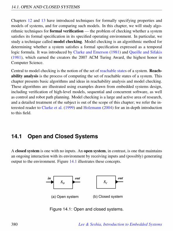
14.1. OPEN AND CLOSED SYSTEMS
Chapters 12 and 13 have introduced techniques for formally specifying properties andmodels of systems, and for comparing such models. In this chapter, we will study algo-rithmic techniques for formal verification — the problem of checking whether a systemsatisfies its formal specification in its specified operating environment. In particular, westudy a technique called model checking. Model checking is an algorithmic method fordetermining whether a system satisfies a formal specification expressed as a temporallogic formula. It was introduced by Clarke and Emerson (1981) and Queille and Sifakis(1981), which earned the creators the 2007 ACM Turing Award, the highest honor inComputer Science.
Central to model checking is the notion of the set of reachable states of a system. Reach-ability analysis is the process of computing the set of reachable states of a system. Thischapter presents basic algorithms and ideas in reachability analysis and model checking.These algorithms are illustrated using examples drawn from embedded systems design,including verification of high-level models, sequential and concurrent software, as wellas control and robot path planning. Model checking is a large and active area of research,and a detailed treatment of the subject is out of the scope of this chapter; we refer the in-terested reader to Clarke et al. (1999) and Holzmann (2004) for an in-depth introductionto this field.
14.1 Open and Closed Systems
A closed system is one with no inputs. An open system, in contrast, is one that maintainsan ongoing interaction with its environment by receiving inputs and (possibly) generatingoutput to the environment. Figure 14.1 illustrates these concepts.
outin
(a) Open system
SO
out
(b) Closed system
SC
Figure 14.1: Open and closed systems.
380 Lee & Seshia, Introduction to Embedded Systems
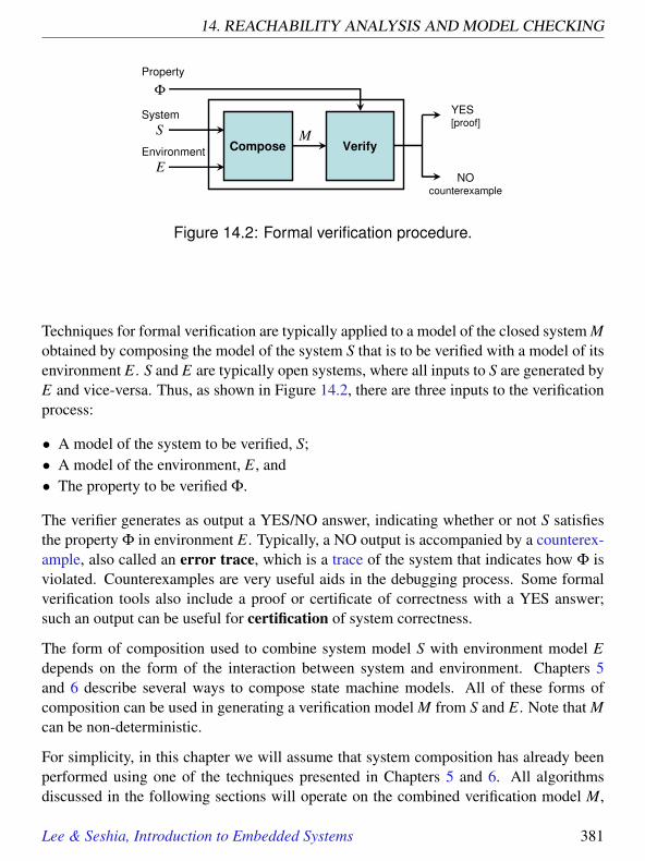
14. REACHABILITY ANALYSIS AND MODEL CHECKING
S
E
Φ
Compose Verify
Property
System
Environment
YES[proof]
NOcounterexample
M
Figure 14.2: Formal verification procedure.
Techniques for formal verification are typically applied to a model of the closed system Mobtained by composing the model of the system S that is to be verified with a model of itsenvironment E. S and E are typically open systems, where all inputs to S are generated byE and vice-versa. Thus, as shown in Figure 14.2, there are three inputs to the verificationprocess:
• A model of the system to be verified, S;• A model of the environment, E, and• The property to be verified Φ.
The verifier generates as output a YES/NO answer, indicating whether or not S satisfiesthe property Φ in environment E. Typically, a NO output is accompanied by a counterex-ample, also called an error trace, which is a trace of the system that indicates how Φ isviolated. Counterexamples are very useful aids in the debugging process. Some formalverification tools also include a proof or certificate of correctness with a YES answer;such an output can be useful for certification of system correctness.
The form of composition used to combine system model S with environment model Edepends on the form of the interaction between system and environment. Chapters 5and 6 describe several ways to compose state machine models. All of these forms ofcomposition can be used in generating a verification model M from S and E. Note that Mcan be non-deterministic.
For simplicity, in this chapter we will assume that system composition has already beenperformed using one of the techniques presented in Chapters 5 and 6. All algorithmsdiscussed in the following sections will operate on the combined verification model M,
Lee & Seshia, Introduction to Embedded Systems 381

14.2. REACHABILITY ANALYSIS
and will be concerned with answering the question of whether M satisfies property Φ.Additionally, we will assume that Φ is specified as a property in linear temporal logic.
14.2 Reachability Analysis
We consider first a special case of the model checking problem which is useful in practice.Specifically, we assume that M is a finite-state machine and Φ is an LTL formula of theform Gp, where p is a proposition. Recall from Chapter 12 that Gp is the temporal logicformula that holds in a trace when the proposition p holds in every state of that trace. Aswe have seen in Chapter 12, several system properties are expressible as Gp properties.
We will begin in Section 14.2.1 by illustrating how computing the reachable states of asystem enables one to verify a Gp property. In Section 14.2.2 we will describe a techniquefor reachability analysis of finite-state machines based on explicit enumeration of states.Finally, in Section 14.2.3, we will describe an alternative approach to analyze systemswith very large state spaces.
14.2.1 Verifying Gp
In order for a system M to satisfy Gp, where p is a proposition, every trace exhibitableby M must satisfy Gp. This property can be verified by enumerating all states of M andchecking that every state satisfies p.
When M is finite-state, in theory, such enumeration is always possible. As shown inChapter 3, the state space of M can be viewed as a directed graph where the nodes ofthe graph correspond to states of M and the edges correspond to transitions of M. Thisgraph is called the state graph of M, and the set of all states is called its state space. Withthis graph-theoretic viewpoint, one can see that checking Gp for a finite-state system Mcorresponds to traversing the state graph for M, starting from the initial state and checkingthat every state reached in this traversal satisfies p. Since M has a finite number of states,this traversal must terminate.
Example 14.1: Let the system S be the traffic light controller of Figure 3.10 andits environment E be the pedestrian model shown in Figure 3.11. Let M be the
382 Lee & Seshia, Introduction to Embedded Systems

14. REACHABILITY ANALYSIS AND MODEL CHECKING
Figure 14.3: Composition of traffic light controller (Figure 3.10) and pedestrianmodel (Figure 3.11).
synchronous composition of S and E as shown in Figure 14.3. Observe that M is aclosed system. Suppose that we wish to verify that M satisfies the property
G ¬(green∧crossing)
In other words, we want to verify that it is never the case that the traffic light isgreen while pedestrians are crossing.
The composed system M is shown in Figure 14.4 as an extended FSM. Note thatM has no inputs or outputs. M is finite-state, with a total of 188 states (using asimilar calculation to that in Example 3.12). The graph in Figure 14.4 is not the fullstate graph of M, because each node represents a set of states, one for each differentvalue of count in that node. However, through visual inspection of this graph wecan check for ourselves that no state satisfies the proposition (green∧ crossing),and hence every trace satisfies the LTL property G¬(green∧crossing).
Lee & Seshia, Introduction to Embedded Systems 383

14.2. REACHABILITY ANALYSIS
Figure 14.4: Extended state machine obtained from synchronous-reactive com-position of traffic light controller and pedestrian models. Note that this is nonde-terministic.
In practice, the seemingly simple task of verifying whether a finite-state system M satisfiesa Gp property is not as straightforward as in the previous example for the followingreasons:
• Typically, one starts only with the initial state and transition function, and the stategraph must be constructed on the fly.
• The system might have a huge number of states, possibly exponential in the size ofthe syntactic description of M. As a consequence, the state graph cannot be repre-sented using traditional data structures such as an adjacency or incidence matrix.
The next two sections describe how these challenges can be handled.
384 Lee & Seshia, Introduction to Embedded Systems

14. REACHABILITY ANALYSIS AND MODEL CHECKING
14.2.2 Explicit-State Model Checking
In this section, we discuss how to compute the reachable state set by generating andtraversing the state graph on the fly.
First, recall that the system of interest M is closed, finite-state, and can be non-deterministic.Since M has no inputs, its set of possible next states is a function of its current state alone.We denote this transition relation of M by δ, which is only a function of the current stateof M, in contrast to the possibleUpdates function introduced in Chapter 3 which is also afunction of the current input. Thus, δ(s) is the set of possible next states from state s ofM.
Algorithm 14.1 computes the set of reachable states of M, given its initial state s0 andtransition relation δ. Procedure DFS Search performs a depth-first traversal of the stategraph of M, starting with state s0. The graph is generated on-the-fly by repeatedly apply-ing δ to states visited during the traversal.
Input : Initial state s0 and transition relation δ for closed finite-statesystem M
Output: Set R of reachable states of M
1 Initialize: Stack Σ to contain a single state s0; Current set of reachedstates R := s0.
2 DFS Search() 3 while Stack Σ is not empty do4 Pop the state s at the top of Σ5 Compute δ(s), the set of all states reachable from s in one
transition6 for each s′ ∈ δ(s) do7 if s′ 6∈ R then8 R := R∪s′9 Push s′ onto Σ
10 DFS Search()11 end12 end13 end14
Algorithm 14.1: Computing the reachable state set by depth-first explicit-statesearch.
Lee & Seshia, Introduction to Embedded Systems 385

14.2. REACHABILITY ANALYSIS
The main data structures required by the algorithm are Σ, the stack storing the current pathin the state graph being explored from s0, and R, the current set of states reached duringtraversal. Since M is finite-state, at some point all states reachable from s0 will be in R,which implies that no new states will be pushed onto Σ and thus Σ will become empty.Hence, procedure DFS Search terminates and the value of R at the end of the procedureis the set of all reachable states of M.
The space and time requirements for this algorithm are linear in the size of the state graph(see Appendix B for an introduction to such complexity notions). However, the number ofnodes and edges in the state graph of M can be exponential in the size of the descriptionsof S and E. For example, if S and E together have 100 Boolean state variables (a smallnumber in practice!), the state graph of M can have a total of 2100 states, far more thanwhat contemporary computers can store in main memory. Therefore, explicit-state searchalgorithms such as DFS Search must be augmented with state compression techniques.Some of these techniques are reviewed in the sidebar on page 399.
A challenge for model checking concurrent systems is the state-explosion problem. Re-call that the state space of a composition of k finite-state systems M1,M2, . . . ,Mk (say, us-ing synchronous composition), is the cartesian product of the state spaces of M1,M2, . . . ,Mk.In other words, if M1,M2, . . . ,Mk have n1,n2, . . . ,nk states respectively, their compositioncan have Πk
i=1ni states. It is easy to see that the number of states of a concurrent composi-tion of k components grows exponentially with k. Explicitly representing the state spaceof the composite system does not scale. In the next section, we will introduce techniquesthat can mitigate this problem in some cases.
14.2.3 Symbolic Model Checking
The key idea in symbolic model checking is to represent a set of states symbolically asa propositional logic formula, rather than explicitly as a collection of individual states.Specialized data structures are often used to efficiently represent and manipulate suchformulas. Thus, in contrast to explicit-state model checking, in which individual statesare manipulated, symbolic model checking operates on sets of states.
Algorithm 14.2 (Symbolic Search) is a symbolic algorithm for computing the set ofreachable states of a closed, finite-state system M. This algorithm has the same input-output specification as the previous explicit-state algorithm DFS Search; however, alloperations in Symbolic Search are set operations.
386 Lee & Seshia, Introduction to Embedded Systems

14. REACHABILITY ANALYSIS AND MODEL CHECKING
Input : Initial state s0 and transition relation δ for closed finite-statesystem M, represented symbolically
Output: Set R of reachable states of M, represented symbolically
1 Initialize: Current set of reached states R = s02 Symbolic Search() 3 Rnew = R4 while Rnew 6= /0 do5 Rnew := s′ | ∃s ∈ R s.t. s′ ∈ δ(s)∧ s′ 6∈ R6 R := R∪Rnew
7 end8
Algorithm 14.2: Computing the reachable state set by symbolic search.
In algorithm Symbolic Search, R represents the entire set of states reached at any pointin the search, and Rnew represents the new states generated at that point. When no morenew states are generated, the algorithm terminates, with R storing all states reachablefrom s0. The key step of the algorithm is line 5, in which Rnew is computed as the setof all states s′ reachable from any state s in R in one step of the transition relation δ.This operation is called image computation, since it involves computing the image ofthe function δ. Efficient implementations of image computation that directly operate onpropositional logic formulas are central to symbolic reachability algorithms. Apart fromimage computation, the key set operations in Symbolic Search include set union andemptiness checking.
Example 14.2: We illustrate symbolic reachability analysis using the finite-statesystem in Figure 14.4.
To begin with, we need to introduce some notation. Let vl be a variable denotingthe state of the traffic light controller FSM S at the start of each reaction; i.e., vl ∈green,yellow, red,pending. Similarly, let vp denote the state of the pedestrianFSM E, where vp ∈ crossing,none,waiting.Given this notation, the initial state set s0 of the composite system M is repre-sented as the following propositional logical formula:
vl = red ∧ vp = crossing ∧ count = 0
Lee & Seshia, Introduction to Embedded Systems 387

14.2. REACHABILITY ANALYSIS
From s0, the only enabled outgoing transition is the self-loop on the initial state ofthe extended FSM in Figure 14.4. Thus, after one step of reachability computation,the set of reached states R is represented by the following formula:
vl = red ∧ vp = crossing ∧ 0≤ count ≤ 1
After two steps, R is given by
vl = red ∧ vp = crossing ∧ 0≤ count ≤ 2
and after k steps, k ≤ 60, R is represented by the formula
vl = red ∧ vp = crossing ∧ 0≤ count ≤ k
On the 61st step, we exit the state (red,crossing), and compute R as
vl = red ∧ vp = crossing ∧ 0≤ count ≤ 60
∨ vl = green ∧ vp = none ∧ count = 0
Proceeding similarly, the set of reachable states R is grown until there is no furtherchange. The final reachable set is represented as:
vl = red ∧ vp = crossing ∧ 0≤ count ≤ 60
∨ vl = green ∧ vp = none ∧ 0≤ count ≤ 60
∨ vl = pending ∧ vp = waiting ∧ 0 < count ≤ 60
∨ vl = yellow ∧ vp = waiting ∧ 0≤ count ≤ 5
In practice, the symbolic representation is much more compact than the explicit one. Theprevious example illustrates this nicely because a large number of states are compactlyrepresented by inequalities like 0 < count ≤ 60. Computer programs can be designed tooperate directly on the symbolic representation. Some examples of such programs aregiven in the box on page 399.
Symbolic model checking has been used successfully to address the state-explosion prob-lem for many classes of systems, most notably for hardware models. However, in theworst case, even symbolic set representations can be exponential in the number of systemvariables.
388 Lee & Seshia, Introduction to Embedded Systems

14. REACHABILITY ANALYSIS AND MODEL CHECKING
14.3 Abstraction in Model Checking
One of the challenges in model checking is to work with the simplest abstraction of asystem that will provide the required proofs of safety. Simpler abstractions have smallerstate spaces and can be checked more efficiently. The challenge, of course, is to knowwhat details to omit from the abstraction.
The part of the system to be abstracted away depends on the property to be verified. Thefollowing example illustrates this point.
Example 14.3: Consider the traffic light system M in Figure 14.4. Suppose that,as in Example 14.1 we wish to verify that M satisfies the property
G ¬(green∧crossing)
Suppose we abstract the variable count away from M by hiding all references tocount from the model, including all guards mentioning it and all updates to it. Thisgenerates the abstract model Mabs shown in Figure 14.5.
We observe that this abstract Mabs exhibits more behaviors than M. For instance,from the state (yellow,waiting) we can take the self-loop transition forever, stayingin that state perennially, even though in the actual system M this state must be exitedwithin five clock ticks. Moreover, every behavior of M can be exhibited by Mabs.
The interesting point is that, even with this approximation, we can prove that Mabssatisfies G ¬(green∧crossing). The value of count is irrelevant for this property.
Notice that while M has 188 states, Mabs has only 4 states. Reachability analysis onMabs is far easier than for M as we have far fewer states to explore.
There are several ways to compute an abstraction. One of the simple and extremelyuseful approaches is called localization reduction or localization abstraction (Kurshan(1994)). In localization reduction, parts of the design model that are irrelevant to theproperty being checked are abstracted away by hiding a subset of state variables. Hidinga variable corresponds to freeing that variable to evolve arbitrarily. It is the form ofabstraction used in Example 14.3 above, where count is allowed to change arbitrarily, andall transitions are made independent of the value of count.
Lee & Seshia, Introduction to Embedded Systems 389

14.3. ABSTRACTION IN MODEL CHECKING
Figure 14.5: Abstraction of the traffic light system in Figure 14.4.
Example 14.4: Consider the multithreaded program given below (adaptedfrom Ball et al. (2001)). The procedure lock unlock executes a loop withinwhich it acquires a lock, then calls the function randomCall, based on whoseresult it either releases the lock and executes another loop iteration, or it quits theloop (and then releases the lock). The execution of another loop iteration is ensuredby incrementing new, so that the condition old != new evaluates to true.
1 pthread_mutex_t lock = PTHREAD_MUTEX_INITIALIZER;2 unsigned int old, new;3
4 void lock_unlock() 5 do 6 pthread_mutex_lock(&lock);7 old = new;8 if (randomCall()) 9 pthread_mutex_unlock(&lock);
10 new++;11 12 while (old != new)13 pthread_mutex_unlock(&lock);14
390 Lee & Seshia, Introduction to Embedded Systems

14. REACHABILITY ANALYSIS AND MODEL CHECKING
Suppose the property we want to verify is that the code does not attempt to callpthread mutex lock twice in a row. Recall from Section 10.2.4 how the sys-tem can deadlock if a thread becomes permanently blocked trying to acquire a lock.This could happen in the above example if the thread, already holding lock lock,attempts to acquire it again.
If we model this program exactly, without any abstraction, then we need to reasonabout all possible values of old and new, in addition to the remaining state of theprogram. Assuming a word size of 32 in this system, the size of the state space isroughly 232× 232× n, where 232 is the number of values of old and new, and ndenotes the size of the remainder of the state space.
However, it is not necessary to reason about the precise values of old and new toprove that this program is correct. Assume, for this example, that our programminglanguage is equipped with a boolean type. Assume further that the programcan perform non-deterministic assignments. Then, we can generate the followingabstraction of the original program, written in C-like syntax, where the Booleanvariable b represents the predicate old == new.
1 pthread_mutex_t lock = PTHREAD_MUTEX_INITIALIZER;2 boolean b; // b represents the predicate (old == new)3 void lock_unlock() 4 do 5 pthread_mutex_lock(&lock);6 b = true;7 if (randomCall()) 8 pthread_mutex_unlock(&lock);9 b = false;
10 11 while (!b)12 pthread_mutex_unlock(&lock);13
It is easy to see that this abstraction retains just enough information to show that theprogram satisfies the desired property. Specifically, the lock will not be acquiredtwice because the loop is only iterated if b is set to false, which implies that thelock was released before the next attempt to acquire.
Moreover, observe that size of the state space to be explored has reduced to simply2n. This is the power of using the “right” abstraction.
Lee & Seshia, Introduction to Embedded Systems 391

14.4. MODEL CHECKING LIVENESS PROPERTIES
A major challenge for formal verification is to automatically compute simple abstrac-tions. An effective and widely-used technique is counterexample-guided abstractionrefinement (CEGAR), first introduced by Clarke et al. (2000). The basic idea (whenusing localization reduction) is to start by hiding almost all state variables except thosereferenced by the temporal logic property. The resulting abstract system will have morebehaviors than the original system. Therefore, if this abstract system satisfies an LTLformula Φ (i.e., each of its behaviors satisfies Φ), then so does the original. However, ifthe abstract system does not satisfy Φ, the model checker generates a counterexample. Ifthis counterexample is a counterexample for the original system, the process terminates,having found a genuine counterexample. Otherwise, the CEGAR approach analyzes thiscounterexample to infer which hidden variables must be made visible, and with these ad-ditional variables, recomputes an abstraction. The process continues, terminating eitherwith some abstract system being proven correct, or generating a valid counterexample forthe original system.
The CEGAR approach and several follow-up ideas have been instrumental in drivingprogress in the area of software model checking. We review some of the key ideas in thesidebar on page 399.
14.4 Model Checking Liveness Properties
So far, we have restricted ourselves to verifying properties of the form Gp, where p is anatomic proposition. An assertion that Gp holds for all traces is a very restricted kind ofsafety property. However, as we have seen in Chapter 12, several useful system propertiesare not safety properties. For instance, the property stating that “the robot must visitlocation A” is a liveness property: if visiting location A is represented by proposition q,then this property is an assertion that Fq must hold for all traces. In fact, several problems,including path planning problems for robotics and progress properties of distributed andconcurrent systems can be stated as liveness properties. It is therefore useful to extendmodel checking to handle this class of properties.
Properties of the form Fp, though liveness properties, can be partially checked using thetechniques introduced earlier in this chapter. Recall from Chapter 12 that Fp holds fora trace if and only if ¬G¬p holds for the same trace. In words, “p is true some time inthe future” iff “¬p is always false.” Therefore, we can attempt to verify that the systemsatisfies G¬p. If the verifier asserts that G¬p holds for all traces, then we know thatFp does not hold for any trace. On the other hand, if the verifier outputs “NO”, then
392 Lee & Seshia, Introduction to Embedded Systems

14. REACHABILITY ANALYSIS AND MODEL CHECKING
the accompanying counterexample provides a witness exhibiting how p may become trueeventually. This witness provides one trace for which Fp holds, but it does not prove thatFp holds for all traces (unless the machine is deterministic).
More complete checks and more complicated liveness properties require a more sophis-ticated approach. Briefly, one approach used in explicit-state model checking of LTLproperties is as follows:
1. Represent the negation of the property Φ as an automaton B, where certain statesare labeled as accepting states.
2. Construct the synchronous composition of the property automaton B and the systemautomaton M. The accepting states of the property automaton induce acceptingstates of the product automaton MB.
3. If the product automaton MB can visit an accepting state infinitely often, then itindicates that M does not satisfy Φ; otherwise, M satisfies Φ.
The above approach is known as the automata-theoretic approach to verification. Wegive a brief introduction to this subject in the rest of this section. Further details may befound in the seminal papers on this topic (Wolper et al. (1983); Vardi and Wolper (1986))and the book on the SPIN model checker (Holzmann (2004)).
14.4.1 Properties as Automata
Consider the first step of viewing properties as automata. Recall the material on omega-regular languages introduced in the box on page 361. The theory of Buchi automata andomega-regular languages, briefly introduced there, is relevant for model checking livenessproperties. Roughly speaking, an LTL property Φ has a one-to-one correspondence witha set of behaviors that satisfy Φ. This set of behaviors constitutes the language of theBuchi automaton corresponding to Φ.
For the LTL model checking approach we describe here, if Φ is the property that thesystem must satisfy, then we represent its negation ¬Φ as a Buchi automaton. We presentsome illustrative examples below.
Lee & Seshia, Introduction to Embedded Systems 393

14.4. MODEL CHECKING LIVENESS PROPERTIES
Example 14.5: Suppose that an FSM M1 models a system that executes foreverand produces a pure output h (for heartbeat), and that it is required to produce thisoutput at least once every three reactions. That is, if in two successive reactions itfails to produce the output h, then in the third it must.
We can formulate this property in LTL as the property Φ1 below:
G(h∨Xh∨X2h)
and the negation of this property is
F(¬h∧X¬h∧X2¬h)
The Buchi automaton B1 corresponding to the negation of the desired property isgiven below:
Let us examine this automaton. The language accepted by this automaton includesall behaviors that enter and stay in state d. Equivalently, the language includes allbehaviors that produce a present output on f in some reaction. When we composethe above machine with M1, if the resulting composite machine can never producef = present, then the language accepted by the composite machine is empty. Ifwe can prove that the language is empty, then we have proved that M produces theheartbeat h at least once every three reactions.
Observe that the property Φ1 in the above example is in fact a safety property. We givean example of a liveness property below.
Example 14.6: Suppose that the FSM M2 models a controller for a robot thatmust locate a room and stay there forever. Let p be the proposition that becomes
394 Lee & Seshia, Introduction to Embedded Systems

14. REACHABILITY ANALYSIS AND MODEL CHECKING
true when the robot is in the target room. Then, the desired property Φ2 can beexpressed in LTL as FGp.
The negation of this property is GF¬p. The Buchi automaton B2 corresponding tothis negated property is given below:
Notice that all accepting behaviors of B2 correspond to those where ¬p holds in-finitely often. These behaviors correspond to a cycle in the state graph for theproduct automaton where state b of B2 is visited repeatedly. This cycle is known asan acceptance cycle.
Liveness properties of the form GFp also occur naturally as specifications. This form ofproperty is useful in stating fairness properties which assert that certain desirable proper-ties hold infinitely many times, as illustrated in the following example.
Example 14.7: Consider a traffic light system such as that in Example 3.10. Wemay wish to assert that the traffic light becomes green infinitely many times in anyexecution. In other words, the state green is visited infinitely often, which can beexpressed as Φ3 = GF green.
The automaton corresponding to Φ3 is identical to that for the negation of Φ2 in Ex-ample 14.6 above with ¬p replaced by green. However, in this case the acceptingbehaviors of this automaton are the desired behaviors.
Thus, from these examples we see that the problem of detecting whether a certain ac-cepting state s in an FSM can be visited infinitely often is the workhorse of explicit-statemodel checking of LTL properties. We next present an algorithm for this problem.
Lee & Seshia, Introduction to Embedded Systems 395

14.4. MODEL CHECKING LIVENESS PROPERTIES
14.4.2 Finding Acceptance Cycles
We consider the following problem:
Given a finite-state system M, can an accepting state sa of M be visited in-finitely often?
Put another way, we seek an algorithm to check whether (i) state sa is reachable fromthe initial state s0 of M, and (ii) sa is reachable from itself. Note that asking whether astate can be visited infinitely often is not the same as asking whether it must be visitedinfinitely often.
The graph-theoretic viewpoint is useful for this problem, as it was in the case of Gpdiscussed in Section 14.2.1. Assume for the sake of argument that we have the entire stategraph constructed a priori. Then, the problem of checking whether state sa is reachablefrom s0 is simply a graph traversal problem, solvable for example by depth-first search(DFS). Further, the problem of detecting whether sa is reachable from itself amounts tochecking whether there is a cycle in the state graph containing that state.
The main challenges for solving this problem are similar to those discussed in Sec-tion 14.2.1: we must perform this search on-the-fly, and we must deal with large statespaces.
The nested depth-first search (nested DFS) algorithm, which is implemented in the SPINmodel checker (Holzmann (2004)), solves this problem and is shown as Algorithm 14.3.The algorithm begins by calling the procedure called Nested DFS Search with argument1, as shown in the Main function at the bottom. MB is obtained by composing the originalclosed system M with the automaton B representing the negation of LTL formula Φ.
As the name suggests, the idea is to perform two depth-first searches, one nested inside theother. The first DFS identifies a path from initial state s0 to the target accepting state sa.Then, from sa we start another DFS to see if we can reach sa again. The variable modeis either 1 or 2 depending on whether we are performing the first DFS or the second.Stacks Σ1 and Σ2 are used in the searches performed in modes 1 and 2 respectively. Ifsa is encountered in the second DFS, the algorithm generates as output the path leadingfrom s0 to sa with a loop on sa. The path from s0 to sa is obtained simply by reading offthe contents of stack Σ1. Likewise, the cycle from sa to itself is obtained from stack Σ2.Otherwise, the algorithm reports failure.
396 Lee & Seshia, Introduction to Embedded Systems

14. REACHABILITY ANALYSIS AND MODEL CHECKING
Search optimization and state compression techniques that are used in explicit-state reach-ability analysis can be used with nested DFS also. Further details are available in Holz-mann (2004).
14.5 Summary
This chapter gives some basic algorithms for formal verification, including model check-ing, a technique for verifying if a finite-state system satisfies a property specified in lineartemporal logic. Verification operates on closed systems, which are obtained by compos-ing a system with its operating environment. The first key concept is that of reachabilityanalysis, which verifies properties of the form Gp. The concept of abstraction, centralto the scalability of model checking, is also discussed in this chapter. This chapter alsoshows how explicit-state model checking algorithms can handle liveness properties, wherea crucial concept is the correspondence between properties and automata.
Lee & Seshia, Introduction to Embedded Systems 397

14.5. SUMMARY
Input : Initial state s0 and transition relation δ for automaton MB; Targetaccepting state sa of MB
Output: Acceptance cycle containing sa, if one exists
1 Initialize: (i) Stack Σ1 to contain a single state s0, and stack Σ2 to be empty;(ii) Two sets of reached states R1 := R2 := s0; (iii) Flag found := false.
2 Nested DFS Search(Mode mode) 3 while Stack Σmode is not empty do4 Pop the state s at the top of Σmode5 if (s = sa and mode= 1) then6 Push s onto Σ27 Nested DFS Search(2)8 return9 end
10 Compute δ(s), the set of all states reachable from s in one transition11 for each s′ ∈ δ(s) do12 if (s′ = sa and mode= 2) then13 Output path to sa with acceptance cycle using contents of stacks
Σ1 and Σ214 found := true15 return16 end17 if s′ 6∈ Rmode then18 Rmode := Rmode∪s′19 Push s′ onto Σmode20 Nested DFS Search(mode)21 end22 end23 end24 25 Main() 26 Nested DFS Search(1)27 if (found= false) then Output “no acceptance cycle with sa” end
Algorithm 14.3: Nested depth-first search algorithm.
398 Lee & Seshia, Introduction to Embedded Systems

14. REACHABILITY ANALYSIS AND MODEL CHECKING
Probing Further: Model Checking in Practice
Several tools are available for computing the set of reachable states of a finite-state sys-tem and checking that they satisfy specifications in temporal logic. One such tool is SMV(symbolic model verifier), which was first developed at Carnegie Mellon University byKenneth McMillan. SMV was the first model checking tool to use binary decision di-agrams (BDDs), a compact data structure introduced by Bryant (1986) for representinga Boolean function. The use of BDDs has proved instrumental in enabling analysis ofmore complex systems. Current symbolic model checkers also rely heavily on Booleansatisfiability (SAT) solvers (see Malik and Zhang (2009)), which are programs for de-ciding whether a propositional logic formula can evaluate to true. One of the first usesof SAT solvers in model checking was for bounded model checking (see Biere et al.(1999)), where the transition relation of the system is unrolled only a bounded num-ber of times. A few different versions of SMV are available online (see for examplehttp://nusmv.fbk.eu/).
The SPIN model checker (Holzmann, 2004) developed in the 1980’s and 1990’s atBell Labs by Gerard Holzmann and others, is another leading tool for model checking(see http://www.spinroot.com/). Rather than directly representing models ascommunicating FSMs, it uses a specification language (called Promela, for process metalanguage) that enables specifications that closely resemble multithreaded programs. SPINincorporates state-compression techniques such as hash compaction (the use of hashingto reduce the size of the stored state set) and partial-order reduction (a technique toreduce the number of reachable states to be explored by considering only a subset of thepossible process interleavings).
Automatic abstraction has played a big role in applying model checking directly to soft-ware. Two examples of abstraction-based software model checking systems are SLAMdeveloped at Microsoft Research (Ball and Rajamani, 2001) and BLAST developed at UCBerkeley (Henzinger et al., 2003b; Beyer et al., 2007). Both methods combine CEGARwith a particular form of abstraction called predicate abstraction, in which predicates in aprogram are abstracted to Boolean variables. A key step in these techniques is checkingwhether a counterexample generated on the abstract model is in fact a true counterexam-ple. This check is performed using satisfiability solvers for logics richer than propositionallogic. These solvers are called SAT-based decision procedures or satisfiability modulotheories (SMT) solvers (for more details, see Barrett et al. (2009)).
Lee & Seshia, Introduction to Embedded Systems 399

EXERCISES
Exercises
1. Consider the system M modeled by the hierarchical state machine of Figure 12.2,which models an interrupt-driven program.
Model M in the modeling language of a verification tool (such as SPIN). You willhave to construct an environment model that asserts the interrupt. Use the verifica-tion tool to check whether M satisfies φ, the property stated in Exercise 3:
φ: The main program eventually reaches program location C.
Explain the output you obtain from the verification tool.
2. Figure 14.3 shows the synchronous-reactive composition of the traffic light con-troller of Figure 3.10 and the pedestrian model of Figure 3.11.
Consider replacing the pedestrian model in Figure 14.3 with the alternative modelgiven below where the initial state is nondeterministically chosen to be one of noneor crossing:
(a) Model the composite system in the modeling language of a verification tool(such as SPIN). How many reachable states does the combined system have?How many of these are initial states?
(b) Formulate an LTL property stating that every time a pedestrian arrives, even-tually the pedestrian is allowed to cross (i.e., the traffic light enters state red).
(c) Use the verification tool to check whether the model constructed in part (a)satisfies the LTL property specified in part (b). Explain the output of theverification tool.
400 Lee & Seshia, Introduction to Embedded Systems

15Quantitative Analysis
Contents15.1 Problems of Interest . . . . . . . . . . . . . . . . . . . . . . . . . . 403
15.1.1 Extreme-Case Analysis . . . . . . . . . . . . . . . . . . . . . 40315.1.2 Threshold Analysis . . . . . . . . . . . . . . . . . . . . . . . 40415.1.3 Average-Case Analysis . . . . . . . . . . . . . . . . . . . . . 404
15.2 Programs as Graphs . . . . . . . . . . . . . . . . . . . . . . . . . . 40515.2.1 Basic Blocks . . . . . . . . . . . . . . . . . . . . . . . . . . 40615.2.2 Control-Flow Graphs . . . . . . . . . . . . . . . . . . . . . . 40615.2.3 Function Calls . . . . . . . . . . . . . . . . . . . . . . . . . 408
15.3 Factors Determining Execution Time . . . . . . . . . . . . . . . . 41015.3.1 Loop Bounds . . . . . . . . . . . . . . . . . . . . . . . . . . 41015.3.2 Exponential Path Space . . . . . . . . . . . . . . . . . . . . . 41215.3.3 Path Feasibility . . . . . . . . . . . . . . . . . . . . . . . . . 41315.3.4 Memory Hierarchy . . . . . . . . . . . . . . . . . . . . . . . 414
15.4 Basics of Execution Time Analysis . . . . . . . . . . . . . . . . . . 41615.4.1 Optimization Formulation . . . . . . . . . . . . . . . . . . . 41615.4.2 Logical Flow Constraints . . . . . . . . . . . . . . . . . . . . 41915.4.3 Bounds for Basic Blocks . . . . . . . . . . . . . . . . . . . . 423
15.5 Other Quantitative Analysis Problems . . . . . . . . . . . . . . . . 42515.5.1 Memory Bound Analysis . . . . . . . . . . . . . . . . . . . . 425Sidebar: Tools for Execution-Time Analysis . . . . . . . . . . . . . . 42615.5.2 Power and Energy Analysis . . . . . . . . . . . . . . . . . . 427
15.6 Summary . . . . . . . . . . . . . . . . . . . . . . . . . . . . . . . . 427Exercises . . . . . . . . . . . . . . . . . . . . . . . . . . . . . . . . . . . 429
401

Will my brake-by-wire system actuate the brakes within one millisecond? Answering thisquestion requires, in part, an execution-time analysis of the software that runs on theelectronic control unit (ECU) for the brake-by-wire system. Execution time of the soft-ware is an example of a quantitative property of an embedded system. The constraintthat the system actuate the brakes within one millisecond is a quantitative constraint.The analysis of quantitative properties for conformance with quantitative constraints iscentral to the correctness of embedded systems and is the topic of the present chapter.
A quantitative property of an embedded system is any property that can be measured.This includes physical parameters, such as position or velocity of a vehicle controlled bythe embedded system, weight of the system, operating temperature, power consumption,or reaction time. Our focus in this chapter is on properties of software-controlled sys-tems, with particular attention to execution time. We present program analysis techniquesthat can ensure that execution time constraints will be met. We also discuss how similartechniques can be used to analyze other quantitative properties of software, particularlyresource usage such as power, energy, and memory.
The analysis of quantitative properties requires adequate models of both the software com-ponents of the system and of the environment in which the software executes. The envi-ronment includes the processor, operating system, input-output devices, physical compo-nents with which the software interacts, and (if applicable) the communication network.The environment is sometimes also referred to as the platform on which the software ex-ecutes. Providing a comprehensive treatment of execution time analysis would requiremuch more than one chapter. The goal of this chapter is more modest. We illustratekey features of programs and their environment that must be considered in quantitativeanalysis, and we describe qualitatively some analysis techniques that are used. For con-creteness, we focus on a single quantity, execution time, and only briefly discuss otherresource-related quantitative properties.
402 Lee & Seshia, Introduction to Embedded Systems
15. QUANTITATIVE ANALYSIS
15.1 Problems of Interest
The typical quantitative analysis problem involves a software task defined by a programP, the environment E in which the program executes, and the quantity of interest q. Weassume that q can be given by a function of fP as follows,
q = fP(x,w)
where x denotes the inputs to the program P (such as data read from memory or from sen-sors, or data received over a network), and w denotes the environment parameters (such asnetwork delays or the contents of the cache when the program begins executing). Defin-ing the function fP completely is often neither feasible nor necessary; instead, practicalquantitative analysis will yield extreme values for q (highest or lowest values), averagevalues for q, or proofs that q satisfies certain threshold constraints. We elaborate on thesenext.
15.1.1 Extreme-Case Analysis
In extreme-case analysis, we may want to estimate the largest value of q for all values ofx and w,
maxx,w
fP(x,w). (15.1)
Alternatively, it can be useful to estimate the smallest value of q:
minx,w
fP(x,w). (15.2)
If q represents execution time of a program or a program fragment, then the largest value iscalled the worst-case execution time (WCET), and the smallest value is called the best-case execution time (BCET). It may be difficult to determine these numbers exactly, butfor many applications, an upper bound on the WCET or a lower bound on the BCET isall that is needed. In each case, when the computed bound equals the actual WCET orBCET, it is said to be a tight bound; otherwise, if there is a considerable gap between theactual value and the computed bound, it is said to be a loose bound. Computing loosebounds may be much easier than finding tight bounds.
Lee & Seshia, Introduction to Embedded Systems 403

15.1. PROBLEMS OF INTEREST
15.1.2 Threshold Analysis
A threshold property asks whether the quantity q is always bounded above or below bya threshold T , for any choice of x and w. Formally, the property can be expressed as
∀x,w, fP(x,w)≤ T (15.3)
or∀x,w, fP(x,w)≥ T (15.4)
Threshold analysis may provide assurances that a quantitative constraint is met, such asthe requirement that a brake-by-wire system actuate the brakes within one millisecond.
Threshold analysis may be easier to perform than extreme-case analysis. Unlike extreme-case analysis, threshold analysis does not require us to determine the maximum or mini-mum value exactly, or even to find a tight bound on these values. Instead, the analysis isprovided some guidance in the form of the target value T . Of course, it might be possibleto use extreme-case analysis to check a threshold property. Specifically, Constraint 15.3holds if the WCET does not exceed T , and Constraint 15.4 holds if the BCET is not lessthan T .
15.1.3 Average-Case Analysis
Often one is interested more in typical resource usage rather than in worst-case scenarios.This is formalized as average-case analysis. Here, the values of input x and environmentparameter w are assumed to be drawn randomly from a space of possible values X andW according to probability distributions Dx and Dw respectively. Formally, we seek toestimate the value
EDx,Dw fP(x,w) (15.5)
where EDx,Dw denotes the expected value of fP(x,w) over the distributions Dx and Dw.
One difficulty in average-case analysis is to define realistic distributions Dx and Dw thatcapture the true distribution of inputs and environment parameters with which a programwill execute.
In the rest of this chapter, we will focus on a single representative problem, namely,WCET estimation.
404 Lee & Seshia, Introduction to Embedded Systems

15. QUANTITATIVE ANALYSIS
15.2 Programs as Graphs
A fundamental abstraction used often in program analysis is to represent a program as agraph indicating the flow of control from one code segment to another. We will illustratethis abstraction and other concepts in this chapter using the following running example:
Example 15.1: Consider the function modexp that performs modular exponen-tiation, a key step in many cryptographic algorithms. In modular exponentiation,given a base b, an exponent e, and a modulus m, one must compute be mod m. Inthe program below, base, exponent and mod represent b, e and m respectively.EXP BITS denotes the number of bits in the exponent. The function uses a stan-dard shift-square-accumulate algorithm, where the base is repeatedly squared, oncefor each bit position of the exponent, and the base is accumulated into the resultonly if the corresponding bit is set.
1 #define EXP_BITS 322
3 typedef unsigned int UI;4
5 UI modexp(UI base, UI exponent, UI mod) 6 int i;7 UI result = 1;8
9 i = EXP_BITS;10 while(i > 0) 11 if ((exponent & 1) == 1) 12 result = (result * base) % mod;13 14 exponent >>= 1;15 base = (base * base) % mod;16 i--;17 18 return result;19
Lee & Seshia, Introduction to Embedded Systems 405

15.2. PROGRAMS AS GRAPHS
15.2.1 Basic Blocks
A basic block is a sequence of consecutive program statements in which the flow ofcontrol enters only at the beginning of this sequence and leaves only at the end, withouthalting or the possibility of branching except at the end.
Example 15.2: The following three statements from the modexp function inExample 15.1 form a basic block:
14 exponent >>= 1;15 base = (base * base) % mod;16 i--;
Another example of a basic block includes the initializations at the top of the func-tion, comprising lines 7 and 9:
7 result = 1;8
9 i = EXP_BITS;
15.2.2 Control-Flow Graphs
A control-flow graph (CFG) of a program P is a directed graph G = (V,E), where theset of vertices V comprises basic blocks of P, and the set of edges E indicates the flow ofcontrol between basic blocks. Figure 15.1 depicts the CFG for the modexp program ofExample 15.1. Each node of the CFG is labeled with its corresponding basic block. Inmost cases, this is simply the code as it appears in Example 15.1. The only exception isfor conditional statements, such as the conditions in while loops and if statements; inthese cases, we follow the convention of labeling the node with the condition followed bya question mark to indicate the conditional branch.
Although our illustrative example of a control-flow graph is at the level of C source code,it is possible to use the CFG representation at other levels of program representationas well, including a high-level model as well as low-level assembly code. The level ofrepresentation employed depends on the level of detail required by the context. To makethem easier to follow, our control-flow graphs will be at the level of source code.
406 Lee & Seshia, Introduction to Embedded Systems

15. QUANTITATIVE ANALYSIS
result = 1;
i = EXP_BITS;
(i > 0)?
((exponent & 1) == 1)?
result = (result * base) % mod;
exponent >>= 1;
base = (base * base) % mod;
i--;
return result;
1
0
1
0
1
2
3
4
5
6
Figure 15.1: Control-flow graph for the modexp function of Example 15.1. Allincoming edges at a node indicate transfer of control to the start of the basicblock for that node, and all outgoing edges from a node indicate an exit from theend of the basic block for that node. For clarity, we label the outgoing edges froma branch statement with 0 or 1 indicating the flow of control in case the branchevaluates to false or true, respectively. An ID number for each basic block is notedabove the node for that block; IDs range from 1 to 6 for this example.
Lee & Seshia, Introduction to Embedded Systems 407

15.2. PROGRAMS AS GRAPHS
result = 1;
i = EXP_BITS;
(i > 0)?
result = update(result);
i--;
return result;
1
0
res = r;
((exponent & 1) == 1)?
res = (res * base) % mod;
exponent >>= 1;
base = (base * base) % mod;
0
1
return res;
call
return
Figure 15.2: Control-flow graphs for the modexp call and update functions inExample 15.3. Call/return edges are indicated with dashed lines.
15.2.3 Function Calls
Programs are typically decomposed into several functions in order to systematically or-ganize the code and promote reuse and readability. The control-flow graph (CFG) repre-sentation can be extended to reason about code with function calls by introducing specialcall and return edges. These edges connect the CFG of the caller function – the onemaking the function call – to that of the callee function – the one being called. A calledge indicates a transfer of control from the caller to the callee. A return edge indicatesa transfer of control from the callee back to the caller.
408 Lee & Seshia, Introduction to Embedded Systems

15. QUANTITATIVE ANALYSIS
Example 15.3: A slight variant shown below of the modular exponentation pro-gram of Example 15.1 uses function calls and can be represented by the CFG withcall and return edges in Figure 15.2.
1 #define EXP_BITS 322 typedef unsigned int UI;3 UI exponent, base, mod;4
5 UI update(UI r) 6 UI res = r;7 if ((exponent & 1) == 1) 8 res = (res * base) % mod;9
10 exponent >>= 1;11 base = (base * base) % mod;12 return res;13 14
15 UI modexp_call() 16 UI result = 1; int i;17 i = EXP_BITS;18 while(i > 0) 19 result = update(result);20 i--;21 22 return result;23
In this modified example, the variables base, exponent, and mod are globalvariables. The update to base and exponent in the body of the while loop,along with the computation of result is now performed in a separate functionnamed update.
Non-recursive function calls can also be handled by inlining, which is the process ofcopying the code for the callee into that of the caller. If inlining is performed transitivelyfor all functions called by the code that must be analyzed, the analysis can be performedon the CFG of the code resulting from inlining, without using call and return edges.
Lee & Seshia, Introduction to Embedded Systems 409

15.3. FACTORS DETERMINING EXECUTION TIME
15.3 Factors Determining Execution Time
There are several issues one must consider in order to estimate the worst-case executiontime of a program. This section outlines some of the main issues and illustrates them withexamples. In describing these issues, we take a programmer’s viewpoint, starting with theprogram structure and then considering how the environment can impact the program’sexecution time.
15.3.1 Loop Bounds
The first point one must consider when bounding the execution time of a program iswhether the program terminates. Non-termination of a sequential program can arise fromnon-terminating loops or from an unbounded sequence of function calls. Therefore, whilewriting real-time embedded software, the programmer must ensure that all loops are guar-anteed to terminate. In order to guarantee this, one must determine for each loop a boundon the number of times that loop will execute in the worst case. Similarly, all functioncalls must have bounded recursion depth. The problems of determining bounds on loopiterations or recursion depth are undecidable in general, since the halting problem for Tur-ing machines can be reduced to either problem. (See Appendix B for an introduction toTuring machines and decidability.)
In this section, we limit ourselves to reasoning about loops. In spite of the undeciablenature of the problem, progress has been made on automatically determining loop boundsfor several patterns that arise in practice. Techniques for determining loop bounds are acurrent research topic and a full survey of these methods is out of the scope of this chapter.We will limit ourselves to presenting illustrative examples for loop bound inference.
The simplest case is that of for loops that have a specified constant bound, as in Exam-ple 15.4 below. This case occurs often in embedded software, in part due to a disciplineof programming enforced by designers who must program for real-time constraints andlimited resources.
Example 15.4: Consider the function modexp1 below. It is a slight variant of thefunction modexp introduced in Example 15.1 that performs modular exponentia-tion, in which the while loop has been expressed as an equivalent for loop.
410 Lee & Seshia, Introduction to Embedded Systems

15. QUANTITATIVE ANALYSIS
1 #define EXP_BITS 322
3 typedef unsigned int UI;4
5 UI modexp1(UI base, UI exponent, UI mod) 6 UI result = 1; int i;7
8 for(i=EXP_BITS; i > 0; i--) 9 if ((exponent & 1) == 1)
10 result = (result * base) % mod;11 12 exponent >>= 1;13 base = (base * base) % mod;14 15 return result;16
In the case of this function, it is easy to see that the for loop will take exactlyEXP BITS iterations, where EXP BITS is defined as the constant 32.
In many cases, the loop bound is not immediately obvious (as it was for the above exam-ple). To make this point, here is a variation on Example 15.4.
Example 15.5: The function listed below also performs modular exponentiation,as in Example 15.4. However, in this case, the for loop is replaced by a whileloop with a different loop condition – the loop exits when the value of exponentreaches 0. Take a moment to check whether the while loop will terminate (and ifso, why).
1 typedef unsigned int UI;2
3 UI modexp2(UI base, UI exponent, UI mod) 4 UI result = 1;5
6 while (exponent != 0) 7 if ((exponent & 1) == 1) 8 result = (result * base) % mod;9
10 exponent >>= 1;11 base = (base * base) % mod;
Lee & Seshia, Introduction to Embedded Systems 411

15.3. FACTORS DETERMINING EXECUTION TIME
12 13 return result;14
Now let us analyze the reason that this loop terminates. Notice that exponent isan unsigned int, which we will assume to be 32 bits wide. If it starts out equal to0, the loop terminates right away and the function returns result = 1. If not, ineach iteration of the loop, notice that line 10 shifts exponent one bit to the right.Since exponent is an unsigned int, after the right shift, its most significant bitwill be 0. Reasoning thus, after at most 32 right shifts, all bits of exponent mustbe set to 0, thus causing the loop to terminate. Therefore, we can conclude that theloop bound is 32.
Let us reflect on the reasoning employed in the above example. The key component ofour “proof of termination” was the observation that the number of bits of exponentdecreases by 1 each time the loop executes. This is a standard argument for provingtermination – by defining a progress measure or ranking function that maps each stateof the program to a mathematical structure called a well order. Intuitively, a well order islike a program that counts down to zero from some initial value in the natural numbers.
15.3.2 Exponential Path Space
Execution time is a path property. In other words, the amount of time taken by the pro-gram is a function of how conditional statements in the program evaluate to true or false.A major source of complexity in execution time analysis (and other program analysisproblems as well) is that the number of program paths can be very large — exponential inthe size of the program. We illustrate this point with the example below.
Example 15.6: Consider the function count listed below, which runs over a two-dimensional array, counting and accumulating non-negative and negative elementsof the array separately.
1 #define MAXSIZE 1002
3 int Array[MAXSIZE][MAXSIZE];
412 Lee & Seshia, Introduction to Embedded Systems

15. QUANTITATIVE ANALYSIS
4 int Ptotal, Pcnt, Ntotal, Ncnt;5 ...6 void count() 7 int Outer, Inner;8 for (Outer = 0; Outer < MAXSIZE; Outer++) 9 for (Inner = 0; Inner < MAXSIZE; Inner++)
10 if (Array[Outer][Inner] >= 0) 11 Ptotal += Array[Outer][Inner];12 Pcnt++;13 else 14 Ntotal += Array[Outer][Inner];15 Ncnt++;16 17 18 19
The function includes a nested loop. Each loop executes MAXSIZE (100) times.Thus, the inner body of the loop (comprising lines 10–16) will execute 10,000times – as many times as the number of elements of Array. In each iteration ofthe inner body of the loop, the conditional on line 10 can either evaluate to true orfalse, thus resulting in 210000 possible ways the loop can execute. In other words,this program has 210000 paths.
Fortunately, as we will see in Section 15.4.1, one does not need to explicitly enumerateall possible program paths in order to perform execution time analysis.
15.3.3 Path Feasibility
Another source of complexity in program analysis is that all program paths may not beexecutable. A computationally expensive function is irrelevant for execution time analysisif that function is never executed.
A path p in program P is said to be feasible if there exists an input x to P such thatP executes p on x. In general, even if P is known to terminate, determining whether apath p is feasible is a computationally intractable problem. One can encode the canonicalNP-complete problem, the Boolean satisfiability problem (see Appendix B), as a problemof checking path feasibility in a specially-constructed program. In practice, however, inmany cases, it is possible to determine path feasibility.
Lee & Seshia, Introduction to Embedded Systems 413

15.3. FACTORS DETERMINING EXECUTION TIME
Example 15.7: Recall Example 12.3 of a software task from the open sourcePaparazzi unmanned aerial vehicle (UAV) project (Nemer et al., 2006):
1 #define PPRZ_MODE_AUTO2 22 #define PPRZ_MODE_HOME 33 #define VERTICAL_MODE_AUTO_ALT 34 #define CLIMB_MAX 1.05 ...6 void altitude_control_task(void) 7 if (pprz_mode == PPRZ_MODE_AUTO28 || pprz_mode == PPRZ_MODE_HOME) 9 if (vertical_mode == VERTICAL_MODE_AUTO_ALT)
10 float err = estimator_z - desired_altitude;11 desired_climb12 = pre_climb + altitude_pgain * err;13 if (desired_climb < -CLIMB_MAX) 14 desired_climb = -CLIMB_MAX;15 16 if (desired_climb > CLIMB_MAX) 17 desired_climb = CLIMB_MAX;18 19 20 21
This program has 11 paths in all. However, the number of feasible programpaths is only 9. To see this, note that the two conditionals desired climb< -CLIMB MAX on line 13 and desired climb > CLIMB MAX on line 16cannot both be true. Thus, only three out of the four paths through the two inner-most conditional statements are feasible. This infeasible inner path can be takenfor two possible evaluations of the outermost conditional on lines 7 and 8: eitherif pprz mode == PPRZ MODE AUTO2 is true, or if that condition is false, butpprz mode == PPRZ MODE HOME is true.
15.3.4 Memory Hierarchy
The preceding sections have focused on properties of programs that affect execution time.We now discuss how properties of the execution platform, specifically of cache memories,
414 Lee & Seshia, Introduction to Embedded Systems

15. QUANTITATIVE ANALYSIS
can significantly impact execution time. We illustrate this point using Example 15.8.1 Thematerial on caches introduced in Sec. 8.2.3 is pertinent to this discussion.
Example 15.8: Consider the function dot product listed below, which com-putes the dot product of two vectors of floating point numbers. Each vector is ofdimension n, where n is an input to the function. The number of iterations of theloop depends on the value of n. However, even if we know an upper bound on n,hardware effects can still cause execution time to vary widely for similar values ofn.
1 float dot_product(float *x, float *y, int n) 2 float result = 0.0;3 int i;4 for(i=0; i < n; i++) 5 result += x[i] * y[i];6 7 return result;8
Suppose this program is executing on a 32-bit processor with a direct-mappedcache. Suppose also that the cache can hold two sets, each of which can hold 4floats. Finally, let us suppose that x and y are stored contiguously in memorystarting with address 0.
Let us first consider what happens if n = 2. In this case, the entire arrays x andy will be in the same block and thus in the same cache set. Thus, in the veryfirst iteration of the loop, the first access to read x[0] will be a cache miss, butthereafter every read to x[i] and y[i] will be a cache hit, yielding best caseperformance for loads.
Consider next what happens when n = 8. In this case, each x[i] and y[i] mapto the same cache set. Thus, not only will the first access to x[0] be a miss, thefirst access to y[0] will also be a miss. Moreover, the latter access will evict theblock containing x[0]-x[3], leading to a cache miss on x[1], x[2], and x[3]as well. The reader can see that every access to an x[i] or y[i] will lead to acache miss.
Thus, a seemingly small change in the value of n from 2 to 8 can lead to a drasticchange in execution time of this function.
1This example is based on a similar example in Bryant and O’Hallaron (2003).
Lee & Seshia, Introduction to Embedded Systems 415

15.4. BASICS OF EXECUTION TIME ANALYSIS
15.4 Basics of Execution Time Analysis
Execution time analysis is a current research topic, with many problems still to be solved.There have been over two decades of research, resulting in a vast literature. We cannotprovide a comprehensive survey of the methods in this chapter. Instead, we will presentsome of the basic concepts that find widespread use in current techniques and tools forWCET analysis. Readers interested in a more detailed treatment may find an overviewin a recent survey paper (Wilhelm et al., 2008) and further details in books (e.g., Li andMalik (1999)) and book chapters (e.g., Wilhelm (2005)).
15.4.1 Optimization Formulation
An intuitive formulation of the WCET problem can be constructed using the view ofprograms as graphs. Given a program P, let G = (V,E) denote its control-flow graph(CFG). Let n = |V | be the number of nodes (basic blocks) in G, and m = |E| denote thenumber of edges. We refer to the basic blocks by their index i, where i ranges from 1 to n.
We assume that the CFG has a unique start or source node s and a unique sink or end nodet. This assumption is not restrictive: If there are multiple start or end nodes, one can adda dummy start/end node to achieve this condition. Usually we will set s = 1 and t = n.
Let xi denote the number of times basic block i is executed. We call xi the executioncount of basic block i. Let x = (x1,x2, . . . ,xn) be a vector of variables recording executioncounts. Not all valuations of x correspond to valid program executions. We say that x isvalid if the elements of x correspond to a (valid) execution of the program. The followingexample illustrates this point.
Example 15.9: Consider the CFG for the modular exponentiation functionmodexp introduced in Example 15.1. There are six basic blocks in this function,labeled 1 to 6 in Figure 15.1. Thus, x = (x1,x2, . . . ,x6). Basic blocks 1 and 6, thestart and end, are each executed only once. Thus, x1 = x6 = 1; any other valuationcannot correspond to any program execution.
Next consider basic blocks 2 and 3, corresponding to the conditional branches i> 0 and (exponent & 1) == 1. One can observe that x2 must equal x3 +1,since the block 3 is executed every time block 2 is executed, except when the loopexits to block 6.
416 Lee & Seshia, Introduction to Embedded Systems

15. QUANTITATIVE ANALYSIS
Along similar lines, one can see that basic blocks 3 and 5 must be executed an equalnumber of times.
Flow Constraints
The intuition expressed in Example 15.9 can be formalized using the theory of networkflow, which finds use in many contexts including modeling traffic, fluid flow, and the flowof current in an electrical circuit. In particular, in our problem context, the flow mustsatisfy the following two properties:
1. Unit Flow at Source: The control flow from source node s = 1 to sink node t = nis a single execution and hence corresponds to unit flow from source to sink. Thisproperty is captured by the following two constraints:
x1 = 1 (15.6)
xn = 1 (15.7)
2. Conservation of Flow: For each node (basic block) i, the incoming flow to i fromits predecessor nodes equals the outgoing flow from i to its successor nodes.
To capture this property, we introduce additional variables to record the numberof times that each edge in the CFG is executed. Following the notation of Li andMalik (1999), let di j denote the number of times the edge from node i to node j inthe CFG is executed. Then we require that for each node i, 1≤ i≤ n,
xi = ∑j∈Pi
d ji = ∑j∈Si
di j, (15.8)
where Pi is the set of predecessors to node i and Si is the set of successors. For thesource node, P1 = /0, so the sum over predecessor nodes is omitted. Similarly, forthe sink node, Sn = /0, so the sum over successor nodes is omitted.
Taken together, the two sets of constraints presented above suffice to implicitly define allsource-to-sink execution paths of the program. Since this constraint-based representationis an implicit representation of program paths, this approach is also referred to in theliterature as implicit path enumeration or IPET.
We illustrate the generation of the above constraints with an example.
Lee & Seshia, Introduction to Embedded Systems 417

15.4. BASICS OF EXECUTION TIME ANALYSIS
Example 15.10: Consider again the function modexp of Example 15.1, with CFGdepicted in Figure 15.1.
The constraints for this CFG are as follows:
x1 = 1
x6 = 1
x1 = d12
x2 = d12 +d52 = d23 +d26
x3 = d23 = d34 +d35
x4 = d34 = d45
x5 = d35 +d45 = d52
x6 = d26
Any solution to the above system of equations will result in integer values for thexi and di j variables. Furthermore, this solution will generate valid execution countsfor basic blocks. For example, one such valid solution is
x1 = 1, d12 = 1, x2 = 2, d23 = 1, x3 = 1, d34 = 0, d35 = 1,
x4 = 0, d45 = 0, x5 = 1, d52 = 1, x6 = 1, d26 = 1.
Readers are invited to find and examine additional solutions for themselves.
Overall Optimization Problem
We are now in a position to formulate the overall optimization problem to determineworst-case execution time. The key assumption we make in this section is that we knowan upper bound wi on the execution time of the basic block i. (We will later see in Sec-tion 15.4.3 how the execution time of a single basic block can be bounded.) Then theWCET is given by the maximum ∑n
i=1 wixi over valid execution counts xi.
418 Lee & Seshia, Introduction to Embedded Systems

15. QUANTITATIVE ANALYSIS
Putting this together with the constraint formulation of the preceding section, our goal isto find values for xi that give
maxxi,1≤i≤n
n
∑i=1
wixi
subject to
x1 = xn = 1
xi = ∑j∈Pi
d ji = ∑j∈Si
di j
This optimization problem is a form of a linear programming (LP) problem (also calleda linear program), and it is solvable in polynomial time.
However, two major challenges remain:
• This formulation assumes that all source to sink paths in the CFG are feasible anddoes not bound loops in paths. As we have already seen in Section 15.3, this isnot the case in general, so solving the above maximization problem may yield apessimistic loose bound on the WCET. We will consider this challenge in Sec-tion 15.4.2.
• The upper bounds wi on execution time of basic blocks i are still to be determined.We will briefly review this topic in Section 15.4.3.
15.4.2 Logical Flow Constraints
In order to ensure that the WCET optimization is not too pessimistic by including pathsthat cannot be executed, we must add so-called logical flow constraints. These con-straints rule out infeasible paths and incorporate bounds on the number of loop iterations.We illustrate the use of such constraints with two examples.
Loop Bounds
For programs with loops, it is necessary to use bounds on loop iterations to bound execu-tion counts of basic blocks.
Lee & Seshia, Introduction to Embedded Systems 419

15.4. BASICS OF EXECUTION TIME ANALYSIS
Example 15.11: Consider the modular exponentiation program of Example 15.1for which we wrote down flow constraints in Example 15.10.
Notice that those constraints impose no upper bound on x2 or x3. As argued inExamples 15.4 and 15.5, the bound on the number of loop iterations in this exampleis 32. However, without imposing this additional constraint, since there is no upperbound on x2 or x3, the solution to our WCET optimization will be infinite, implyingthat there is no upper bound on the WCET. The following single constraint suffices:
x3 ≤ 32
From this constraint on x3, we derive the constraint that x2 ≤ 33, and also upperbounds on x4 and x5. The resulting optimization problem will then return a finitesolution, for finite values of wi.
Adding such bounds on values of xi does not change the complexity of the optimizationproblem. It is still a linear programming problem.
Infeasible Paths
Some logical flow constraints rule out combinations of basic blocks that cannot appeartogether on a single path.
Example 15.12: Consider a snippet of code from Example 15.7 describing asoftware task from the open source Paparazzi unmanned aerial vehicle (UAV)project (Nemer et al., 2006):
1 #define CLIMB_MAX 1.02 ...3 void altitude_control_task(void) 4 ...5 err = estimator_z - desired_altitude;6 desired_climb7 = pre_climb + altitude_pgain * err;8 if (desired_climb < -CLIMB_MAX)
420 Lee & Seshia, Introduction to Embedded Systems

15. QUANTITATIVE ANALYSIS
9 desired_climb = -CLIMB_MAX;10 11 if (desired_climb > CLIMB_MAX) 12 desired_climb = CLIMB_MAX;13 14 return;15
The CFG for the snippet of code shown above is given in Figure 15.3. The system offlow constraints for this CFG according to the rules in Section 15.4.1 is as follows:
x1 = 1
x5 = 1
x1 = d12 +d13
x2 = d12 = d23
x3 = d13 +d23 = d34 +d35
x4 = d34 = d45
x5 = d35 +d45
A solution for the above system of equations is
x1 = x2 = x3 = x4 = x5 = 1,
implying that each basic block gets executed exactly once, and that both condi-tionals evaluate to true. However, as we discussed in Example 15.7, it is im-possible for both conditionals to evaluate to true. Since CLIMB MAX = 1.0, ifdesired climb is less than −1.0 in basic block 1, then at the start of basicblock 3 it will be set to −1.0.
The following constraint rules out the infeasible path:
d12 +d34 ≤ 1 (15.9)
This constraint specifies that both conditional statements cannot be true together.It is of course possible for both conditionals to be false. We can check that thisconstraint excludes the infeasible path when added to the original system.
Lee & Seshia, Introduction to Embedded Systems 421

15.4. BASICS OF EXECUTION TIME ANALYSIS
err = estimator_z - desired_altitude;
desired_climb
= pre_climb + altitude_pgain * err;
(desired_climb < -CLIMB_MAX)?
desired_climb = -CLIMB_MAX;
(desired_climb > CLIMB_MAX)?
return;
1
0
0
1
2
3
4
5
desired_climb = CLIMB_MAX;
1
Figure 15.3: Control-flow graph for Example 15.12.
More formally, for a program without loops, if a set of k edges
(i1, j1),(i2, j2), . . . ,(ik, jk)
in the CFG cannot be taken together in a program execution, the following constraint isadded to the optimization problem:
di1 j1 +di2 j2 + . . .+dik jk ≤ k−1 (15.10)
For programs with loops, the constraint is more complicated since an edge can be tra-versed multiple times, so the value of a di j variable can exceed 1. We omit the details inthis case; the reader can consult Li and Malik (1999) for a more elaborate discussion ofthis topic.
In general, the constraints added above to exclude infeasible combinations of edges canchange the complexity of the optimization problem, since one must also add the following
422 Lee & Seshia, Introduction to Embedded Systems

15. QUANTITATIVE ANALYSIS
integrality constraints:
xi ∈ N, for all i = 1,2, . . . ,n (15.11)
di j ∈ N, for all i, j = 1,2, . . . ,n (15.12)
In the absence of such integrality constraints, the optimization solver can return fractionalvalues for the xi and di j variables. However, adding these constraints results in an inte-ger linear programming (ILP) problem. The ILP problem is known to be NP-hard (seeAppendix B, Section B.4). Even so, in many practical instances, one can solve these ILPproblems fairly efficiently (see for example Li and Malik (1999)).
15.4.3 Bounds for Basic Blocks
In order to complete the optimization problem for WCET analysis, we need to computeupper bounds on the execution times of basic blocks – the wi coefficients in the cost func-tion of Section 15.4.1. Execution time is typically measured in CPU cycles. Generatingsuch bounds requires detailed microarchitectural modeling. We briefly outline some ofthe issues in this section.
A simplistic approach to this problem would be to generate conservative upper boundson the execution time of each instruction in the basic block, and then add up these per-instruction bounds to obtain an upper bound on the execution time of the overall basicblock.
The problem with this approach is that there can be very wide variation in the executiontimes for some instructions, resulting in very loose upper bounds on the execution timeof a basic block. For instance, consider the latency of memory instructions (loads andstores) for a system with a data cache. The difference between the latency when thereis a cache miss versus a hit can be a factor of 100 on some platforms. In these cases,if the analysis does not differentiate between cache hits and misses, it is possible for thecomputed bound to be a hundred times larger than the execution time actually exhibited.
Several techniques have been proposed to better use program context to predict executiontime of instructions more precisely. These techniques involve detailed microarchitecturalmodeling. We mention two main approaches below:
• Integer linear programming (ILP) methods: In this approach, pioneered by Li andMalik (1999), one adds cache constraints to the ILP formulation of Section 15.4.1.
Lee & Seshia, Introduction to Embedded Systems 423

15.4. BASICS OF EXECUTION TIME ANALYSIS
Cache constraints are linear expressions used to bound the number of cache hits andmisses within basic blocks. The approach tracks the memory locations that causecache conflicts – those that map onto the same cache set, but have different tags –and adds linear constraints to record the impact of such conflicts on the number ofcache hits and misses. Measurement through simulation or execution on the actualplatform must be performed to obtain the cycle count for hits and misses. The costconstraint of the ILP is modified to compute the program path along which theoverall number of cycles, including cache hits and misses, is the largest. Furtherdetails about this approach are available in Li and Malik (1999).
• Abstract interpretation methods: Abstract interpretation is a theory of approx-imation of mathematical structures, in particular those that arise in defining thesemantic models of computer systems (Cousot and Cousot (1977)). In particular,in abstract interpretation, one performs sound approximation, where the set ofbehaviors of the system is a subset of that of the model generated by abstract inter-pretation. In the context of WCET analysis, abstract interpretation has been usedto infer invariants at program points, in order to generate loop bounds, and con-straints on the state of processor pipelines or caches at the entry and exit locationsof basic blocks. For example, such a constraint could specify the conditions underwhich variables will be available in the data cache (and hence a cache hit will re-sult). Once such constraints are generated, one can run measurements from statessatisfying those constraints in order to generate execution time estimates. Furtherdetails about this approach can be found in Wilhelm (2005).
In addition to techniques such as those described above, accurate measurement of execu-tion time is critical for finding tight WCET bounds. Some of the measurement techniquesare as follows:
1. Sampling CPU cycle counter: Certain processors include a register that records thenumber of CPU cycles elapsed since reset. For example, the time stamp counterregister on x86 architectures performs this function, and is accessible through ardtsc (“read time stamp counter”) instruction. However, with the advent of multi-core designs and power management features, care must be taken to use such CPUcycle counters to accurately measure timing. For example, it may be necessary tolock the process to a particular CPU.
2. Using a logic analyzer: A logic analyzer is an electronic instrument used to mea-sure signals and track events in a digital system. In the current context, the events of
424 Lee & Seshia, Introduction to Embedded Systems

15. QUANTITATIVE ANALYSIS
interest are the entry and exit points of the code to be timed, definable, for example,as valuations of the program counter. Logic analyzers are less intrusive than usingcycle counters, since they do not require instrumenting the code, and they can bemore accurate. However, the measurement setup is more complicated.
3. Using a cycle-accurate simulator: In many cases, timing analysis must be per-formed when the actual hardware is not yet available. In this situation, a cycle-accurate simulator of the platform provides a good alternative.
15.5 Other Quantitative Analysis Problems
Although we have focused mainly on execution time in this chapter, several other quan-titative analysis problems are relevant for embedded systems. We briefly describe two ofthese in this section.
15.5.1 Memory Bound Analysis
Embedded computing platforms have very limited memory as compared to general-purposecomputers. For example, as mentioned in Chapter 8, the Luminary Micro LM3S8962 con-troller has only 64 KB of RAM. It is therefore essential to structure the program so thatit uses memory efficiently. Tools that analyze memory consumption and compute boundson memory usage can be very useful.
There are two kinds of memory bound analysis that are relevant for embedded systems.In stack size analysis (or simply stack analysis), one needs to compute an upper boundon the amount of stack-allocated memory used by a program. Recall from Section 8.3.2that stack memory is allocated whenever a function is called or an interrupt is handled. Ifthe program exceeds the memory allocated for the stack, a stack overflow is said to occur.
If the program does not contain recursive functions and runs uninterrupted, one can boundstack usage by traversing the call graph of the program – the graph that tracks whichfunctions call which others. If the space for each stack frame is known, then one can trackthe sequence of calls and returns along paths in the call graph in order to compute theworst-case stack size.
Lee & Seshia, Introduction to Embedded Systems 425

15.5. OTHER QUANTITATIVE ANALYSIS PROBLEMS
Tools for Execution-Time Analysis
Current techniques for execution-time analysis are broadly classified into those primarilybased on static analysis and those that are measurement-based.
Static tools rely on abstract interpretation and dataflow analysis to compute facts aboutthe program at selected program locations. These facts are used to identify dependenciesbetween code fragments, generate loop bounds, and identify facts about the platform state,such as the state of the cache. These facts are used to guide timing measurements of basicblocks and combined into an optimization problem as presented in this chapter. Statictools aim to find conservative bounds on extreme-case execution time; however, they arenot easy to port to new platforms, often requiring several man-months of effort.
Measurement-based tools are primarily based on testing the program on multiple in-puts and then estimating the quantity of interest (e.g., WCET) from those measurements.Static analysis is often employed in performing a guided exploration of the space of pro-gram paths and for test generation. Measurement-based tools are easy to port to newplatforms and apply broadly to both extreme-case and average-case analysis; however,not all techniques provide guarantees for finding extreme-case execution times.
Further details about many of these tools are available in Wilhelm et al. (2008). Hereis a partial list of tools and links to papers and websites:
Name Primary Type Institution & Website/ReferencesaiT Static AbsInt Angewandte Informatik GmbH (Wilhelm, 2005)
http://www.absint.com/ait/
Bound-T Static Tidorum Ltd.http://www.bound-t.com/
Chronos Static National University of Singapore (Li et al., 2005)http://www.comp.nus.edu.sg/˜rpembed/chronos/
Heptane Static IRISA Renneshttp://www.irisa.fr/aces/work/heptane-demo/heptane.html
SWEET Static Malardalen Universityhttp://www.mrtc.mdh.se/projects/wcet/
GameTime Measurement UC BerkeleySeshia and Rakhlin (2008)
RapiTime Measurement Rapita Systems Ltd.http://www.rapitasystems.com/
SymTA/P Measurement Technical University Braunschweighttp://www.ida.ing.tu-bs.de/research/projects/symtap/
Vienna M./P. Measurement Technical University of Viennahttp://www.wcet.at/
426 Lee & Seshia, Introduction to Embedded Systems

15. QUANTITATIVE ANALYSIS
Performing stack size analysis for interrupt-driven software is significantly more compli-cated. We point the interested reader to Brylow et al. (2001).
Heap analysis is the other memory bound analysis problem that is relevant for embeddedsystems. This problem is harder than stack bound analysis since the amount of heap spaceused by a function might depend on the values of input data and may not be known priorto run-time. Moreover, the exact amount of heap space used by a program can depend onthe implementation of dynamic memory allocation and the garbage collector.
15.5.2 Power and Energy Analysis
Power and energy consumption are increasingly important factors in embedded systemdesign. Many embedded systems are autonomous and limited by battery power, so adesigner must ensure that the task can be completed within a limited energy budget. Also,the increasing ubiquity of embedded computing is increasing its energy footprint, whichmust be reduced for sustainable development.
To first order, the energy consumed by a program running on an embedded device dependson its execution time. However, estimating execution time alone is not sufficient. Forexample, energy consumption depends on circuit switching activity, which can dependmore strongly on the data values with which instructions are executed.
For this reason, most techniques for energy and power estimation of embedded soft-ware focus on estimating the average-case consumption. The average case is typicallyestimated by profiling instructions for several different data values, guided by softwarebenchmarks. For an introduction to this topic, see Tiwari et al. (1994).
15.6 Summary
Quantitative properties, involving physical parameters or specifying resource constraints,are central to embedded systems. This chapter gave an introduction to basic concepts inquantitative analysis. First, we considered various types of quantitative analysis problems,including extreme-case analysis, average-case analysis, and verifying threshold proper-ties. As a representative example, this chapter focused on execution time analysis. Sev-eral examples were presented to illustrate the main issues, including loop bounds, pathfeasibility, path explosion, and cache effects. An optimization formulation that forms the
Lee & Seshia, Introduction to Embedded Systems 427

15.6. SUMMARY
backbone of execution time analysis was presented. Finally, we briefly discussed twoother quantitative analysis problems, including computing bounds on memory usage andon power or energy consumption.
Quantitative analysis remains an active field of research – exemplifying the challenges inbridging the cyber and physical aspects of embedded systems.
428 Lee & Seshia, Introduction to Embedded Systems

15. QUANTITATIVE ANALYSIS
Exercises
1. This problem studies execution time analysis. Consider the C program listed below:
1 int arr[100];2
3 int foo(int flag) 4 int i;5 int sum = 0;6
7 if (flag) 8 for(i=0;i<100;i++)9 arr[i] = i;
10 11
12 for(i=0;i<100;i++)13 sum += arr[i];14
15 return sum;16
Assume that this program is run on a processor with data cache of size big enoughthat the entire array arr can fit in the cache.
(a) How many paths does the function foo of this program have? Describe whatthey are.
(b) Let T denote the execution time of the second for loop in the program. Howdoes executing the first for loop affect the value of T ? Justify your answer.
2. Consider the program given below:
1 void testFn(int *x, int flag) 2 while (flag != 1) 3 flag = 1;4 *x = flag;5 6 if (*x > 0)7 *x += 2;8
In answering the questions below, assume that x is not NULL.
(a) Draw the control-flow graph of this program. Identify the basic blocks withunique IDs starting with 1.
Lee & Seshia, Introduction to Embedded Systems 429

EXERCISES
(b) Is there a bound on the number of iterations of the while loop? Justify youranswer.
(c) How many total paths does this program have? How many of them are feasi-ble, and why?
(d) Write down the system of flow constraints, including any logical flow con-straints, for the control-flow graph of this program.
(e) Consider running this program uninterrupted on a platform with a data cache.Assume that the data pointed to by x is not present in the cache at the start ofthis function.For each read/write access to *x, argue whether it will be a cache hit or miss.Now, assume that *x is present in the cache at the start of this function. Iden-tify the basic blocks whose execution time will be impacted by this modifiedassumption.
430 Lee & Seshia, Introduction to Embedded Systems

Part IV
Appendices
This part of this text covers some background in mathematics and computer science thatis useful to more deeply understand the formal and algorithmic aspects of the main text.Appendix A reviews basic notations in logic, with particular emphasis on sets and func-tions. Appendix B reviews notions of complexity and computability, which can help asystem designer understand the cost of implementing a system and fundamental limitsthat make certain systems not implementable.


ASets and Functions
ContentsA.1 Sets . . . . . . . . . . . . . . . . . . . . . . . . . . . . . . . . . . . 433A.2 Relations and Functions . . . . . . . . . . . . . . . . . . . . . . . . 434
A.2.1 Restriction and Projection . . . . . . . . . . . . . . . . . . . 437
A.3 Sequences . . . . . . . . . . . . . . . . . . . . . . . . . . . . . . . . 438Sidebar: Exponential Notation for Sets of Functions . . . . . . . . . . 439
Exercises . . . . . . . . . . . . . . . . . . . . . . . . . . . . . . . . . . . 441
This appendix reviews some basic notation for sets and functions.
A.1 Sets
In this section, we review the notation for sets. A set is a collection of objects. Whenobject a is in set A, we write a ∈ A. We define the following sets:
• B= 0,1, the set of binary digits.• N= 0,1,2, · · ·, the set of natural numbers.• Z= · · · ,−1,0,1,2, · · ·, the set of integers.• R, the set of real numbers.• R+, the set of non-negative real numbers.
433

A.2. RELATIONS AND FUNCTIONS
When set A is entirely contained by set B, we say that A is a subset of B and write A⊆ B.For example, B⊆ N⊆ Z⊆ R. The sets may be equal, so the statement N⊆ N is true, forexample. The powerset of a set A is defined to be the set of all subsets. It is written 2A.The empty set, written /0, is always a member of the powerset, /0 ∈ 2A.
We define set subtraction as follows,
A\B = a ∈ A : a /∈ B
for all sets A and B. This notation is read “the set of elements a from A such that a is notin B.”
A cartesian product of sets A and B is a set written A×B and defined as follows,
A×B = (a,b) : a ∈ A,b ∈ B.
A member of this set (a,b) is called a tuple. This notation is read “the set of tuples (a,b)such that a is in A and b is in B.” A cartesian product can be formed with three or moresets, in which case the tuples have three or more elements. For example, we might write(a,b,c) ∈ A×B×C. A cartesian product of a set A with itself is written A2 = A×A. Acartesian product of a set A with itself n times, where n ∈ N is written An. A member ofthe set An is called an n-tuple. By convention, A0 is a singleton set, or a set with exactlyone element, regardless of the size of A. Specifically, we define A0 = /0. Note that A0 isnot itself the empty set. It is a singleton set containing the empty set (for insight into therationale for this definition, see the box on page 439).
A.2 Relations and Functions
A relation from set A to set B is a subset of A×B. A partial function f from set Ato set B is a relation where (a,b) ∈ f and (a,b′) ∈ f imply that b = b′. Such a partialfunction is written f : A B. A total function or simply function f from A to B is apartial function where for all a ∈ A, there is a b ∈ B such that (a,b) ∈ f . Such a functionis written f : A→ B, and the set A is called its domain and the set B its codomain. Ratherthan writing (a,b) ∈ f , we can equivalently write f (a) = b.
Example A.1: An example of a partial function is f : RR defined by f (x) =√
xfor all x ∈ R+. It is undefined for any x < 0 in its domain R.
434 Lee & Seshia, Introduction to Embedded Systems

A. SETS AND FUNCTIONS
A partial function f : A B may be defined by an assignment rule, as done in the aboveexample, where an assignment rule simply explains how to obtain the value of f (a) givena∈ A. Alternatively, the function may be defined by its graph, which is a subset of A×B.
Example A.2: The same partial function from the previous example has the graphf ⊆ R2 given by
f = (x,y) ∈ R2 : x≥ 0 and y =√
x .
Note that we use the same notation f for the function and its graph when it is clearfrom context which we are talking about.
The set of all functions f : A→ B is written (A→ B) or BA. The former notation is usedwhen the exponential notation proves awkward. For a justification of the notation BA, seethe box on page 439.
The function composition of f : A→ B and g : B→ C is written (g f ) : A→ C anddefined by
(g f )(a) = g( f (a))
for any a ∈ A. Note that in the notation (g f ), the function f is applied first. For afunction f : A → A, the composition with itself can be written ( f f ) = f 2, or moregenerally
( f f · · · f )︸ ︷︷ ︸ = f n
n times
for any n ∈ N. In case n = 1, f 1 = f . For the special case n = 0, the function f 0 isby convention the identity function, so f 0(a) = a for all a ∈ A. When the domain andcodomain of a function are the same, i.e., f ∈ AA, then f n ∈ AA for all n ∈ N.
For every function f : A→ B, there is an associated image function f : 2A→ 2B definedon the powerset of A as follows,
∀ A′ ⊆ A, f (A′) = b ∈ B : ∃ a ∈ A′, f (a) = b.
The image function f is applied to sets A′ of elements in the domain, rather than to singleelements. Rather than returning a single value, it returns the set of all values that f would
Lee & Seshia, Introduction to Embedded Systems 435

A.2. RELATIONS AND FUNCTIONS
return, given an element of A′ as an argument. We call f the lifted version of f . Whenthere is no ambiguity, we may write the lifted version of f simply as f rather than f (seeproblem 2(c) for an example of a situation where there is ambiguity).
For any A′ ⊆ A, f (A′) is called the image of A′ for the function f . The image f (A) of thedomain is called the range of the function f .
Example A.3: The image f (R) of the function f : R→ R defined by f (x) = x2 isR+.
A function f : A→ B is onto (or surjective) if f (A) = B. A function f : A→ B is one-to-one (or injective) if for all a,a′ ∈ A,
a 6= a′⇒ f (a) 6= f (a′). (A.1)
That is, no two distinct values in the domain yield the same values in the codomain. Afunction that is both one-to-one and onto is bijective.
Example A.4: The function f : R→ R defined by f (x) = 2x is bijective. Thefunction f : Z→ Z defined by f (x) = 2x is one-to-one, but not onto. The functionf : R2→ R defined by f (x,y) = xy is onto but not one-to-one.
The previous example underscores the fact that an essential part of the definition of afunction is its domain and codomain.
Proposition A.1. If f : A→ B is onto, then there is a one-to-one function h : B→ A.
Proof. Let h be defined by h(b) = a where a is any element in A such that f (a) = b.There must always be at least one such element because f is onto. We can now showthat h is one-to-one. To do this, consider any two elements b,b′ ∈ B where b 6= b′. Weneed to show that h(b) 6= h(b′). Assume to the contrary that h(b) = h(b′) = a for somea ∈ A. But then by the definition of h, f (a) = b and f (a) = b′, which implies b = b′, acontradiction.
436 Lee & Seshia, Introduction to Embedded Systems

A. SETS AND FUNCTIONS
The converse of this proposition is also easy to prove.
Proposition A.2. If h : B→ A is one-to-one, then there is an onto function f : A→ B.
Any bijection f : A→ B has an inverse f−1 : B→ A defined as follows,
f−1(b) = a ∈ A such that f (a) = b , (A.2)
for all b ∈ B. This function is defined for all b ∈ B because f is onto. And for each b ∈ Bthere is a single unique a ∈ A satisfying (A.2) because f is one-to-one. For any bijectionf , its inverse is also bijective.
A.2.1 Restriction and Projection
Given a function f : A→ B and a subset C ⊆ A, we can define a new function f |C that isthe restriction of f to C. It is defined so that for all x ∈C, f |C(x) = f (x).
Example A.5: The function f : R→ R defined by f (x) = x2 is not one-to-one.But the function f |R+ is.
Consider an n-tuple a = (a0,a1, · · · ,an−1) ∈ A0×A1× ·· ·×An−1. A projection of thisn-tuple extracts elements of the tuple to create a new tuple. Specifically, let
I = (i0, i1, · · · , im) ∈ 0,1, · · · ,n−1m
for some m ∈ N\0. That is, I is an m-tuple of indexes. Then we define the projectionof a onto I by
πI(a) = (ai0 ,ai1 , · · · ,aim) ∈ Ai0×Ai1×·· ·×Aim .
The projection may be used to permute elements of a tuple, to discard elements, or torepeat elements.
Projection of a tuple and restriction of a function are related. An n-tuple a ∈ An wherea = (a0,a1, · · · ,an−1) may be considered a function of the form a : 0,1, · · · ,n−1→ A,in which case a(0) = a0, a(1) = a1, etc. Projection is similar to restriction of this function,differing in that restriction, by itself, does not provide the ability to permute, repeat, or
Lee & Seshia, Introduction to Embedded Systems 437

A.3. SEQUENCES
renumber elements. But conceptually, the operations are similar, as illustrated by thefollowing example.
Example A.6: Consider a 3-tuple a = (a0,a1,a2) ∈ A3. This is represented bythe function a : 0,1,2 → A. Let I = 1,2. The projection b = πI(a) = (a1,a2),which itself can be represented by a function b : 0,1 → A, where b(0) = a1 andb(1) = a2.
The restriction a|I is not exactly the same function as b, however. The domain ofthe first function is 1,2, whereas the domain of the second is 0,1. In particular,a|I(1) = b(0) = a1 and a|I(2) = b(1) = a2.
A projection may be lifted just like ordinary functions. Given a set of n-tuples B ⊆ A0×A1×·· ·×An−1 and an m-tuple of indexes I ∈ 0,1, · · · ,n−1m, the lifted projection is
πI(B) = πI(b) : b ∈ B .
A.3 Sequences
A tuple (a0,a1) ∈ A2 can be interpreted as a sequence of length 2. The order of elementsin the sequence matters, and is in fact captured by the natural ordering of the naturalnumbers. The number 0 comes before the number 1. We can generalize this and recognizethat a sequence of elements from set A of length n is an n-tuple in the set An. A0 representsthe set of empty sequences, a singleton set (there is only one empty sequence).
The set of all finite sequences of elements from the set A is written A∗, where we interpret∗ as a wildcard that can take on any value in N. A member of this set with length n is ann-tuple, a finite sequence.
The set of infinite sequences of elements from A is written AN or Aω. The set of finiteand infinite sequences is written
A∗∗ = A∗∪AN .
Finite and infinite sequences play an important role in the semantics of concurrent pro-grams. They can be used, for example, to represent streams of messages sent from one
438 Lee & Seshia, Introduction to Embedded Systems

A. SETS AND FUNCTIONS
Exponential Notation for Sets of Functions
The exponential notation BA for the set of functions of form f : A→B is worth explaining.Recall that A2 is the cartesian product of set A with itself, and that 2A is the powerset of A.These two notations are naturally thought of as sets of functions. A construction attributedto John von Neumann defines the natural numbers as follows,
0 = /01 = 0= /02 = 0,1= /0, /03 = 0,1,2= /0, /0, /0, /0· · ·
With this definition, the powerset 2A is the set of functions mapping the set A into the set2. Consider one such function, f ∈ 2A. For each a ∈ A, either f (a) = 0 or f (a) = 1. Ifwe interpret “0” to mean “nonmember” and “1” to mean “member,” then indeed the setof functions 2A represents the set of all subsets of A. Each such function defines a subset.
Similarly, the cartesian product A2 can be interpreted as the set of functions ofform f : 2 → A, or using von Neumann’s numbers, f : 0,1 → A. Consider a tuplea = (a0,a1) ∈ A2. It is natural to associate with this tuple a function a : 0,1→ A wherea(0) = a0 and a(1) = a1. The argument to the function is the index into the tuple. We cannow interpret the set of functions BA of form f : A→ B as a set of tuples indexed by theset A instead of by the natural numbers.
Let ω = /0, /0, /0, /0, · · · represent the set of von Neumann numbers. This setis closely related to the set N (see problem 2). Given a set A, it is now natural to interpretAω as the set of all infinite sequences of elements from A, the same as AN.
The singleton set A0 can now be interpreted as the set of all functions whose domainis the empty set and codomain is A. There is exactly one such function (no two suchfunctions are distinguishable), and that function has an empty graph. Before, we definedA0 = /0. Using von Neumann numbers, A0 = 1, corresponding nicely with the definitionof a zero exponent on ordinary numbers. Moreover, you can think of A0 = /0 as the setof all functions with an empty graph.
It is customary in the literature to omit the bold face font for A0, 2A, and A2, writinginstead simply A0, 2A, and A2.
Lee & Seshia, Introduction to Embedded Systems 439

A.3. SEQUENCES
part of the program to another. Or they can represent successive assignments of values toa variable. For programs that terminate, finite sequences will be sufficient. For programsthat do not terminate, we need infinite sequences.
440 Lee & Seshia, Introduction to Embedded Systems

A. SETS AND FUNCTIONS
Exercises
1. This problem explores properties of onto and one-to-one functions.
(a) Show that if f : A→ B is onto and g : B→C is onto, then (g f ) : A→C isonto.
(b) Show that if f : A→ B is one-to-one and g : B→ C is one-to-one, then (g f ) : A→C is one-to-one.
2. Let ω = /0, /0, /0, /0, · · · be the von Neumann numbers as defined in the boxon page 439. This problem explores the relationship between this set and N, the setof natural numbers.
(a) Let f : ω→ N be defined by
f (x) = |x|, ∀ x ∈ ω .
That is, f (x) is the size of the set x. Show that f is bijective.
(b) The lifted version of the function f in part (a) is written f . What is the valueof f (0,0)? What is the value of f (0,0)? Note that on page 436 itis noted that when there is no ambiguity, f may be written simply f . For thisfunction, is there such ambiguity?
Lee & Seshia, Introduction to Embedded Systems 441

BComplexity and Computability
ContentsB.1 Effectiveness and Complexity of Algorithms . . . . . . . . . . . . 444
B.1.1 Big O Notation . . . . . . . . . . . . . . . . . . . . . . . . . 445
B.2 Problems, Algorithms, and Programs . . . . . . . . . . . . . . . . 447B.2.1 Fundamental Limitations of Programs . . . . . . . . . . . . . 448
B.3 Turing Machines and Undecidability . . . . . . . . . . . . . . . . . 449B.3.1 Structure of a Turing Machine . . . . . . . . . . . . . . . . . 451
B.3.2 Decidable and Undecidable Problems . . . . . . . . . . . . . 452
Sidebar: Probing Further: Recursive Functions and Sets . . . . . . . 453
B.4 Intractability: P and NP . . . . . . . . . . . . . . . . . . . . . . . . 455B.5 Summary . . . . . . . . . . . . . . . . . . . . . . . . . . . . . . . . 459Exercises . . . . . . . . . . . . . . . . . . . . . . . . . . . . . . . . . . . 460
Complexity theory and computability theory are areas of Computer Science that studythe efficiency and the limits of computation. Informally, computability theory studieswhich problems can be solved by computers, while complexity theory studies how effi-ciently a problem can be solved by computers. Both areas are problem-centric, meaningthat they are more concerned with the intrinsic ease or difficulty of problems and lessconcerned with specific techniques (algorithms) for solving them.
443

B.1. EFFECTIVENESS AND COMPLEXITY OF ALGORITHMS
In this appendix, we very briefly review selected topics from complexity and computabil-ity theory that are relevant for this book. There are excellent books that offer a detailedtreatment of these topics, including Papadimitriou (1994), Sipser (2005), and Hopcroftet al. (2007). We begin with a discussion of the complexity of algorithms. Algorithms arerealized by computer programs, and we show that there are limitations on what computerprograms can do. We then describe Turing machines, which can be used to define whatwe have come to accept as “computation,” and show how the limitations of programsmanifest themselves as undecidable problems. Finally, we close with a discussion of thecomplexity of problems, as distinct from the complexity of the algorithms that solve theproblems.
B.1 Effectiveness and Complexity of Algorithms
An algorithm is a step-by-step procedure for solving a problem. To be effective, analgorithm must complete in a finite number of steps and use a finite amount of resources(such as memory). To be useful, an algorithm must complete in a reasonable numberof steps and use a reasonable amount of resources. Of course, what is “reasonable” willdepend on the problem being solved.
Some problems are known to have no effective algorithm, as we will see below when wediscuss undecidability. For other problems, one or more effective algorithms are known,but it is not known whether the best algorithm has been found, by some measure of “best.”There are even problems where we know that there exists an effective algorithm, but noeffective algorithm is known. The following example describes such a problem.
Example B.1: Consider a function f : N→ YES, NO where f (n) = YES ifthere is a sequence of n consecutive fives in the decimal representation of π, andf (n) = NO otherwise. This function has one of two forms. Either
f (n) = YES ∀ n ∈ N,
or there is a k ∈ N such that
f (n) =
YES if n < kNO otherwise
444 Lee & Seshia, Introduction to Embedded Systems

B. COMPLEXITY AND COMPUTABILITY
It is not known which of these two forms is correct, nor, if the second form iscorrect, what k is. However, no matter what the answer is, there is an effectivealgorithm for solving this problem. In fact, the algorithm is rather simple. Eitherthe algorithm immediately returns YES, or it compares n to k and returns YES ifn < k. We know that one of these is the right algorithm, but we do not know which.Knowing that one of these is correct is sufficient to know that there is an effectivealgorithm.
For a problem with known effective algorithms, there are typically many algorithms thatwill solve the problem. Generally, we prefer algorithms with lower complexity. How dowe choose among these? This is the topic of the next subsection.
B.1.1 Big O Notation
Many problems have several known algorithms for solving them, as illustrated in thefollowing example.
Example B.2: Suppose we have a list (a1,a2, · · · ,an) of n integers, arranged inincreasing order. We would like to determine whether the list contains a particularinteger b. Here are two algorithms that accomplish this:
1. Use a linear search. Starting at the beginning of the list, compare the inputb against each entry in the list. If it is equal, return YES. Otherwise, proceedto the next entry in the list. In the worst case, this algorithm will require ncomparisons before it can give an answer.
2. Use a binary search. Start in the middle of the list and compare b to theentry a(n/2) in the middle. If it is equal, return YES. Otherwise, determinewhether b < a(n/2). If it is, then repeat the search, but over only the firsthalf of the list. Otherwise, repeat the search over the second half of the list.Although each step of this algorithm is more complicated than the steps of thefirst algorithm, usually fewer steps will be required. In the worst case, log2(n)steps are required.
Lee & Seshia, Introduction to Embedded Systems 445

B.1. EFFECTIVENESS AND COMPLEXITY OF ALGORITHMS
The difference between these two algorithms can be quite dramatic if n is large.Suppose that n = 4096. The first algorithm will require 4096 steps in the worstcase, whereas the second algorithm will require only 12 steps in the worst case.
The number of steps required by an algorithm is the time complexity of the algorithm. Itis customary when comparing algorithms to simplify the measure of time complexity byignoring some details. In the previous example, we might ignore the complexity of eachstep of the algorithm and consider only how the complexity grows with the input size n.So if algorithm (1) in Example B.2 takes K1n seconds to execute, and algorithm (2) takesK2 log2(n) seconds to execute, we would typically ignore the constant factors K1 and K2.For large n, they are not usually very helpful in determining which algorithm is better.
To facilitate such comparisons, it is customary to use big O notation. This notationfinds the term in a time complexity measure that grows fastest as a function of the sizeof the input, for large input sizes, and ignores all other terms. In addition, it discardsany constant factors in the term. Such a measure is an asymptotic complexity measurebecause it studies only the limiting growth rate as the size of the input gets large.
Example B.3: Suppose that an algorithm has time complexity 5+2n+7n3, wheren is the size of the input. This algorithm is said to have O(n3) time complexity,which is read “order n cubed.” The term 7n3 grows fastest with n, and the number7 is a relatively unimportant constant factor.
The following complexity measures are commonly used:
1. constant time: The time complexity does not depend at all on the size of the input.The complexity is O(1).
2. logarithmic time: O(logm(n)) complexity, for any fixed m.3. linear time: O(n) complexity.4. quadratic time: O(n2) complexity.5. polynomial time: O(nm) complexity, for any fixed m ∈ N.6. exponential time: O(mn) complexity for any m > 1.7. factorial time: O(n!) complexity.
446 Lee & Seshia, Introduction to Embedded Systems

B. COMPLEXITY AND COMPUTABILITY
The above list is ordered by costliness. Algorithms later in the list are usually moreexpensive to realize than algorithms earlier in the list, at least for large input size n.
Example B.4: Algorithm 1 in Example B.2 is a linear-time algorithm, whereasalgorithm 2 is a logarithmic-time algorithm. For large n, algorithm (2) is moreefficient.
The number of steps required by an algorithm, of course, is not the only measure of itscost. Some algorithms execute in rather few steps but require a great deal of memory. Thesize of the memory required can be similarly characterized using big O notation, giving ameasure of space complexity.
B.2 Problems, Algorithms, and Programs
Algorithms are developed to solve some problem. How do we know whether we havefound the best algorithm to solve a problem? The time complexity of known algorithmscan be compared, but what about algorithms we have not thought of? Are there problemsfor which there is no algorithm that can solve them? These are difficult questions.
Assume that the input to an algorithm is a member of a set W of all possible inputs, and theoutput is a member of a set Z of all possible outputs. The algorithm computes a functionf : W → Z. The function f , a mathematical object, is the problem to be solved, and thealgorithm is the mechanism by which the problem is solved.
It is important to understand the distinction between the problem and the mechanism.Many different algorithms may solve the same problem. Some algorithms will be betterthan others; for example, one algorithm may have lower time complexity than another.We next address two interesting questions:
• Is there a function of the form f : W → Z for which there is no algorithm that cancompute the function for all inputs w ∈W? This is a computability question.
• Given a particular function f : W → Z, is there a lower bound on the time complex-ity of an algorithm to compute the function? This is a complexity question.
Lee & Seshia, Introduction to Embedded Systems 447

B.2. PROBLEMS, ALGORITHMS, AND PROGRAMS
If W is a finite set, then the answer to the first question is clearly no. Given a particularfunction f : W → Z, one algorithm that will always work uses a lookup table listing f (w)for all w ∈W . Given an input w ∈W , this algorithm simply looks up the answer in thetable. This is a constant-time algorithm; it requires only one step, a table lookup. Hence,this algorithm provides the answer to the second question, which is that if W is a finiteset, then the lowest time complexity is constant time.
A lookup table algorithm may not be the best choice, even though its time complexityis constant. Suppose that W is the set of all 32-bit integers. This is a finite set with232 elements, so a table will require more than four billion entries. In addition to timecomplexity, we must consider the memory required to implement the algorithm.
The above questions become particularly interesting when the set W of possible inputsis infinite. We will focus on decision problems, where Z = YES, NO, a set withonly two elements. A decision problem seeks a yes or no answer for each w ∈W . Thesimplest infinite set of possible inputs is W =N, the natural numbers. Hence, we will nextconsider fundamental limits on decision problems of the form f : N→ YES, NO. Wewill see next that for such problems, the answer to the first question above is yes. Thereare functions of this form that are not computable.
B.2.1 Fundamental Limitations of Programs
One way to describe an algorithm is to give a computer program. A computer programis always representable as a member of the set 0,1∗, i.e., the set of finite sequences ofbits. A programming language is a subset of 0,1∗. It turns out that not all decisionproblems can be solved by computer programs.
Proposition B.1. No programming language can express a program for each and everyfunction of the form f : N→YES, NO.
Proof. To prove this proposition, it is enough to show that there are strictly morefunctions of the form f : N→ YES, NO than there are programs in a programminglanguage. It is sufficient to show that the set YES, NON is strictly larger than the set0,1∗, because a programming language is a subset of 0,1∗. This can be done witha variant of Cantor’s diagonal argument, which goes as follows.
448 Lee & Seshia, Introduction to Embedded Systems

B. COMPLEXITY AND COMPUTABILITY
First, note that the members of the set 0,1∗ can be listed in order. Specifically, we listthem in the order of binary numbers,
λ,0,1,00,01,10,11,000,001,010,011, · · · , (B.1)
where λ is the empty sequence. This list is infinite, but it includes all members of theset 0,1∗. Because the members of the set can be so listed, the set 0,1∗ is said to becountable or countably infinite.
For any programming language, every program that can be written will appear some-where in the list (B.1). Assume the first such program in the list realizes the decisionfunction f1 : N→YES, NO, the second one in the list realizes f2 : N→YES, NO,etc. We can now construct a function g : N→ YES, NO that is not computed by anyprogram in the list. Specifically, let
g(i) =
YES if fi(i) = NONO if fi(i) = YES
for all i ∈N. This function g differs from every function fi in the list, and hence it is notincluded in the list. Thus, there is no computer program in the language that computesfunction g.
This theorem tells us that programs, and hence algorithms, are not capable of solving alldecision problems. We next explore the class of problems they can solve, known as theeffectively computable functions. We do this using Turing machines.
B.3 Turing Machines and Undecidability
In 1936, Alan Turing proposed a model for computation that is now called the Turingmachine (Turing, 1936). A Turing machine, depicted in Figure B.1, is similar to a finite-state machine, but with an unlimited amount of memory. This memory has the form of aninfinite tape that the Turing machine can read from and write to. The machine comprisesa finite-state machine (FSM) controller, a read/write head, and an infinite tape organizedas a sequence of cells. Each cell contains a value drawn from a finite set Σ or the special
Lee & Seshia, Introduction to Embedded Systems 449

B.3. TURING MACHINES AND UNDECIDABILITY
FSM
Control
0 . . . 1 1 0 1 0
Infinite Tape
Read/Write Head
write
move
read
. . . empty cells
Figure B.1: Illustration of a Turing machine.
value 2, which indicates an empty cell. The FSM acts as a control for the read/write headby producing outputs that move the read/write head over the tape.
In Figure B.1, the symbols on the non-empty cells of the tape are drawn from the setΣ = 0,1, the binary digits. The FSM has two output ports. The top output port is write,which has type Σ and produces a value to write to the cell at the current position of theread/write head. The bottom output port is move, which has type L,R, where the outputsymbol L causes the read/write head to move to the left (but not off the beginning of thetape), and R causes it to move to the right. The FSM has one input port, read, which hastype Σ and receives the current value held by the cell under the read/write head.
The tape is initialized with an input string, which is an element of the set Σ∗ of finitesequences of elements of Σ, followed by an infinite sequence of empty cells. The Turingmachine starts in the initial state of the FSM with the read/write head on the left end ofthe tape. At each reaction, the FSM receives as input the value from the current cell underthe read/write head. It produces an output that specifies the new value of that cell (whichmay be the same as the current value) and a command to move the head left or right.
The control FSM of the Turing machine has two final states: an accepting state acceptand a rejecting state reject. If the Turing machine reaches accept or reject after a finitenumber of reactions, then it is said to terminate, and the execution is called a haltingcomputation. If it terminates in accept, then the execution is called an accepting com-putation. If it terminates in reject, then the execution is called a rejecting computation.It is also possible for a Turing machine to reach neither accept nor reject, meaning thatit does not halt. When a Turing machine does not halt, we say that it loops.
450 Lee & Seshia, Introduction to Embedded Systems

B. COMPLEXITY AND COMPUTABILITY
When the control FSM is deterministic, we say that the Turing machine is also determin-istic. Given an input string w∈ Σ∗, a deterministic Turing machine D will exhibit a uniquecomputation. Therefore, given an input string w ∈ Σ∗, a deterministic Turing machine Dwill either halt or not, and if it halts, it will either accept w or reject it. For simplicity,we will limit ourselves in this section to deterministic Turing machines, unless explicitlystated otherwise.
B.3.1 Structure of a Turing Machine
More formally, each deterministic Turing machine can be represented by a pair D =(Σ,M), where Σ is a finite set of symbols and M is any FSM with the following proper-ties:
• a finite set StatesM of states that includes two final states accept and reject;• an input port read of type Σ;• an output port write of type Σ; and• an output port move of type L,R.
As with any FSM, it also must have an initial state s0 and a transition function updateM,as explained in Section 3.3.3. If the read/write head is over a cell containing 2, then theinput to the read port of the FSM will be absent. If at a reaction the write output of theFSM is absent, then the cell under the read/write head will be erased, setting its contentsto 2.
A Turing machine described by D = (Σ,M) is a synchronous composition of two ma-chines, the FSM M and a tape T . The tape T is distinctly not an FSM, since it does nothave finite state. Nonetheless, the tape is a (extended) state machine, and can be describedusing the same five-tuple used in Section 3.3.3 for FSMs, except that the set StatesT is nowinfinite. The data on the tape can be modeled as a function with domain N and codomainΣ∪2, and the position of the read/write head can be modeled as a natural number, so
StatesT = N× (Σ∪2)N.
The machine T has input port write of type Σ, input port move of type L,R, and outputport read of type Σ. The updateT transition function is now easy to define formally (seeExercise 1).
Note that the machine T is the same for all Turing machines, so there is no need to includeit in the description D = (Σ,M) of a particular Turing machine. The description D can be
Lee & Seshia, Introduction to Embedded Systems 451

B.3. TURING MACHINES AND UNDECIDABILITY
understood as a program in a rather special programming language. Since all sets in theformal description of a Turing machine are finite, any Turing machine can be encoded asa finite sequence of bits in 0,1∗.
Note that although the control FSM M and the tape machine T both generate output, theTuring machine itself does not. It only computes by transitioning between states of thecontrol FSM, updating the tape, and moving left (L) or right (R). On any input stringw, we are only concerned with whether the Turing machine halts, and if so, whether itaccepts or rejects w. Thus, a Turing machine attempts to map an input string w ∈ Σ∗ toaccept, reject, but for some input strings, it may be unable to produce an answer.
We can now see that Proposition B.1 applies, and the fact that a Turing machine may notproduce an answer on some input strings is not surprising. Let Σ = 0,1. Then any inputstring w ∈ Σ∗ can be interpreted as a binary encoding of a natural number in N. Thus, aTuring machine implements a partial function of the form f : N→ accept, reject. Thefunction is partial because for some n∈N, the machine may loop. Since a Turing machineis a program, Proposition B.1 tells that Turing machines are incapable of realizing allfunctions of the form f : N→accept, reject. This limitation manifests itself as looping.
A principle that lies at heart of computer science, known as the Church-Turing thesis,asserts that every effectively computable function can be realized by a Turing machine.This principle is named for mathematicians Alonzo Church and Alan Turing. Our intuitivenotion of computation, as expressed in today’s computers, is equivalent to the Turingmachine model of computation in this sense. Computers can realize exactly the functionsthat can be realized by Turing machines: no more, no less. This connection between theinformal notion of an algorithm and the precise Turing machine model of computationis not a theorem; it cannot be proved. It is a principle that underlies what we mean bycomputation.
B.3.2 Decidable and Undecidable Problems
Turing machines, as described here, are designed to solve decision problems, which onlyhave a YES or NO answer. The input string to a Turing machine represents the encodingof a problem instance. If the Turing machine accepts, it is viewed as a YES answer, andif it rejects, it is viewed as a NO answer. There is the third possibility that the Turingmachine might loop.
452 Lee & Seshia, Introduction to Embedded Systems

B. COMPLEXITY AND COMPUTABILITY
Example B.5: Consider the problem of determining, given a directed graph Gwith two nodes s and t in G, whether there is a path from s to t. One can think ofwriting down the problem as a long string listing all nodes and edges of G, followedby s and t. Thus, an instance of this path problem can be presented to the Turingmachine as an input string on its tape. The instance of the problem is the particulargraph G, and nodes s and t. If there exists a path from s to t in G, then this is a YESproblem instance; otherwise, it is a NO problem instance.
Turing machines are typically designed to solve problems, rather than specific prob-lem instances. In this example, we would typically design a Turing machine that,for any graph G, nodes s and t, determines whether there is a path in G from s to t.
Recall that a decision problem is a function f : W → YES,NO. For a Turing machine,the domain is a set W ⊆ Σ∗ of finite sequences of symbols from the set Σ. A probleminstance is a particular w∈W , for which the “answer” to the problem is either f (w)=YES
Probing Further: Recursive Functions and Sets
Logicians make distinctions between the functions that can be realized by Turing ma-chines. The so-called total recursive functions are those where a Turing machine real-izing the function terminates for all inputs w ∈ Σ∗. The partial recursive functions arethose where a Turing machine may or may not terminate on a particular input w ∈ Σ∗. Bythese definitions, every total recursive function is also a partial recursive function, but notvice-versa.
Logicians also use Turing machines to make useful distinctions between sets. Considersets of natural numbers, and consider Turing machines where Σ = 0,1 and an inputw ∈ Σ∗ is the binary encoding of a natural number. Then a set C of natural numbers is acomputable set (or synonymously a recursive set or decidable set) if there is a Turingmachine that terminates for all inputs w ∈ N and yields accept if w ∈ C and reject ifw /∈ C. A set E ⊂ N is a computably enumerable set (or synonymously a recursivelyenumerable set or a semidecidable set) if there is a Turing machine that terminates ifand only if the input w is in E.
Lee & Seshia, Introduction to Embedded Systems 453

B.3. TURING MACHINES AND UNDECIDABILITY
or f (w) = NO. Let Y ⊆W denote the set of all YES instances of problem f . That is,
Y = w ∈W | f (w) = YES.
Given a decision problem f , a Turing machine D = (Σ,M) is called a decision procedurefor f if D accepts every string w ∈ Y , and D rejects every w ∈W \Y , where \ denotes setsubtraction. Note that a decision procedure always halts for any input string w ∈W .
A problem f is said to be decidable (or solvable) if there exists a Turing machine thatis a decision procedure for f . Otherwise, we say that the problem is undecidable (orunsolvable). For an undecidable problem f , there is no Turing machine that terminateswith the correct answer f (w) for all input strings w ∈W .
One of the important philosophical results of 20th century mathematics and computerscience is the existence of problems that are undecidable. One of the first problems to beproved undecidable is the so-called halting problem for Turing machines. This problemcan be stated as follows:
Given a Turing machine D = (Σ,M) initialized with input string w ∈ Σ∗ onits tape, decide whether or not M will halt.
Proposition B.2. (Turing, 1936) The halting problem is undecidable.
Proof. This is a decision problem h : W ′→ YES,NO, where W ′ denotes the set ofall Turing machines and their inputs. The proposition can be proved using a variant ofCantor’s diagonal argument.
It is sufficient to prove the theorem for the subset of Turing machines with binary tapesymbols, Σ = 0,1. Moreover, we can assume without loss of generality that everyTuring machine in this set can be represented by a finite sequence of binary digits (bits),so
W ′ = Σ∗×Σ∗.
Assume further that every finite sequence of bits represents a Turing machine. The formof the decision problem becomes
h : Σ∗×Σ∗→YES,NO. (B.2)
We seek a procedure to determine the value of h(D,w), where D is a finite sequenceof bits representing a Turing machine and w is a finite sequence of bits representing an
454 Lee & Seshia, Introduction to Embedded Systems

B. COMPLEXITY AND COMPUTABILITY
input to the Turing machine. The answer h(D,w) will be YES if the Turing machine Dhalts with input w and NO if it loops.
Consider the set of all effectively computable functions of the form
f : Σ∗×Σ∗→YES,NO.
These functions that can be given by a Turing machine (by the Church-Turing thesis),and hence the set of such functions can be enumerated f0, f1, f2, · · · . We will show thatthe halting problem (B.2) is not on this list. That is, there is no fi such that h = fi.
Consider a sequence of Turing machines D0,D1, · · · where Di is the sequence of bitsrepresenting the ith Turing machine, and Di halts if fi(Di,Di) =NO and loops otherwise.Since fi is a computable function, we can clearly construct such a Turing machine. Notone of the computable functions in the list f0, f1, f2, · · · can possibly equal the function h,because every function fi in the list gives the wrong answer for input (Di,Di). If Turingmachine Di halts on input w = Di, function fi evaluates to fi(Di,Di) = NO, whereash(Di,Di) = YES. Since no function in the list f0, f1, f2, · · · of computable functionsworks, the function h is not computable.
B.4 Intractability: P and NP
Section B.1 above studied asymptotic complexity, a measure of how quickly the cost (intime or space) of solving a problem with a particular algorithm grows with the size of theinput. In this section, we consider problems rather than algorithms. We are interested inwhether an algorithm with a particular asymptotic complexity exists to solve a problem.This is not the same as asking whether an algorithm with a particular complexity class isknown.
A complexity class is a collection of problems for which there exist algorithms with thesame asymptotic complexity. In this section, we very briefly introduce the complexityclasses P and NP.
First recall the concept of a deterministic Turing machine from the preceding section. Anondeterministic Turing machine N = (Σ,M) is identical to its deterministic counter-part, except that the control FSM M can be a nondeterministic FSM. On any input string
Lee & Seshia, Introduction to Embedded Systems 455

B.4. INTRACTABILITY: P AND NP
w ∈ Σ∗, a nondeterministic Turing machine N can exhibit several computations. N is saidto accept w if any computation accepts w, and N rejects w if all its computations rejectw.
A decision problem is a function f : W → YES,NO, where W ⊆ Σ∗. N is said tobe a decision procedure for f if for each input w ∈W , all of its computations halt, nomatter what nondeterministic choices are made. Note that a particular execution of anondeterministic Turing machine N may give the wrong answer. That is, it could yieldNO for input w when the right answer is f (w) = YES. It can still be a decision procedure,however, because we define the final answer to be YES if any execution yields YES. Wedo not require that all executions yield YES. This subtle point underlies the expressivepower of nondeterministic Turing machines.
An execution that accepts an input w is called a certificate. A certificate can be repre-sented by a finite list of choices made by the Turing machine such that it accepts w. Weneed only one valid certificate to know that f (w) = YES.
Given the above definitions, we are ready to introduce P and NP. P is the set of problemsdecidable by a deterministic Turing machine in polynomial time. NP, on the other hand, isthe set of problems decidable by a nondeterministic Turing machine in polynomial time.That is, a problem f is in NP if there is a nondeterministic Turing machine N that is adecision procedure for f , and for all inputs w ∈W , every execution of the Turing machinehas time complexity no greater than O(nm), for some m ∈ N.
An equivalent alternative definition of NP is the set of all problems for which one cancheck the validity of a certificate for a YES answer in polynomial time. Specifically, aproblem f is in NP if there is a nondeterministic Turing machine N that is a decisionprocedure for f , and given an input w and a certificate, we can check in polynomialtime whether the certificate is valid (i.e., whether the choices it lists do indeed result inaccepting w). Note that this says nothing about NO answers. This asymmetry is part ofthe meaning of NP.
An important notion that helps systematize the study of complexity classes is that ofcompleteness, in which we identify problems that are “representative” of a complexityclass. In the context of NP, we say that a problem A is NP-hard if any other problem Bin NP can be reduced (“translated”) to A in polynomial time. Intuitively, A is “as hard as”any problem in NP — if we had a polynomial-time algorithm for A, we could derive onefor B by first translating the instance of B to one of A, and then invoking the algorithm tosolve A. A problem A is said to be NP-complete if (i) A is in NP, and (ii) A is NP-hard.
456 Lee & Seshia, Introduction to Embedded Systems

B. COMPLEXITY AND COMPUTABILITY
In other words, an NP-complete problem is a problem in NP that is as hard as any otherproblem in NP.
Several core problems in the modeling, design, and analysis of embedded systems are NP-complete. One of these is the very first problem to be proved NP-complete, the Booleansatisfiability (SAT) problem. The SAT problem is to decide, given a propositional logicformula φ expressed over Boolean variables x1,x2, . . . ,xn, whether there exists a valuationof the xi variables such that φ(x1,x2, . . . ,xn) = true. If there exists such a valuation, wesay φ is satisfiable; otherwise, we say that φ is unsatisfiable. The SAT problem is adecision problem of the form f : W → YES,NO, where each w ∈W is an encoding ofa propositional logic formula φ.
Example B.6: Consider the following propositional logic formula φ:
(x1∨¬x2)∧ (¬x1∨ x3∨ x2)∧ (x1∨¬x3)
We can see that setting x1 = x3 = true will make φ evaluate to true. It is possible toconstruct a nondeterministic Turing machine that takes as input an encoding of theformula, where the nondeterministic choices correspond to choices of valuationsfor each variable xi, and where the machine will accept the input formula if it issatisfiable and reject it otherwise. If the input w encodes the above formula φ, thenone of the certificates demonstrating that f (w) = YES is the choices x1 = x2 = x3 =true.
Next consider the alternative formula φ′:
(x1∨¬x2)∧ (¬x1∨ x2)∧ (x1∨ x2)∧ (¬x1∨¬x2)
In this case, no matter how we assign Boolean values to the xi variables, we cannotmake φ′ = true. Thus while φ is satisfiable, φ′ is unsatisfiable. The same nonde-terministic Turing machine as above will reject an input w′ that is an encoding ofφ′. Rejecting this input means that all choices result in executions that terminate inreject.
Another problem that is very useful, but NP-complete, is checking the feasibility of aninteger linear program (ILP). Informally, the feasibility problem for integer linear pro-
Lee & Seshia, Introduction to Embedded Systems 457

B.4. INTRACTABILITY: P AND NP
grams is to find a valuation of integer variables such that each inequality in a collectionof linear inequalities over those variables is satisfied.
Given that both SAT and ILP are NP-complete, one can transform an instance of eitherproblem into an instance of the other problem, in polynomial time.
Example B.7: The following integer linear program is equivalent to the SATproblem corresponding to formula φ′ of Example B.6:
find x1,x2 ∈ 0,1such that:
x1− x2 ≥ 0
−x1 + x2 ≥ 0
x1 + x2 ≥ 1
−x1− x2 ≥ −1
One can observe that there is no valuation of x1 and x2 that will make all the aboveinequalities simultaneously true.
NP-complete problems seem to be harder than those in P; for large enough input sizes,these problems can become intractable, meaning that they cannot be practically solved.In general, it appears that to determine that f (w) = YES for some w without being givena certificate, we might have to explore all executions of the nondeterministic Turing ma-chine before finding, on the last possibility, an execution that accepts w. The numberof possible executions can be exponential in the size of the input. Indeed, there are noknown polynomial-time algorithms that solve NP-complete problems. Surprisingly, as ofthis writing, there is no proof that no such algorithm exists. It is widely believed that NPis a strictly larger set of problems than P, but without a proof, we cannot be sure. The Pversus NP question is one of the great unsolved problems in mathematics today.
Despite the lack of polynomial-time algorithms for solving NP-complete problems, manysuch problems turn out to be solvable in practice. SAT problems, for example, can oftenbe solved rather quickly, and a number of very effective SAT solvers are available. Thesesolvers use algorithms that have worst-case exponential complexity, which means thatfor some inputs they can take a very long time to complete. Yet for most inputs, they
458 Lee & Seshia, Introduction to Embedded Systems

B. COMPLEXITY AND COMPUTABILITY
complete quickly. Hence, we should not be deterred from tackling a problem just becauseit is NP-complete.
B.5 Summary
This appendix has very briefly introduced two rather large interrelated topics, the theo-ries of complexity and computability. The chapter began with a discussion of complexitymeasures for algorithms, and then established a fundamental distinction between a prob-lem to be solved and an algorithm for solving the problem. It then showed that thereare problems that cannot be solved. We then explained Turing machines, which are ca-pable of describing solution procedures for all problems that have come to be considered“computable.” The chapter then closed with a brief discussion of the complexity classes Pand NP, which are classes of problems that can be solved by algorithms with comparablecomplexity.
Lee & Seshia, Introduction to Embedded Systems 459

EXERCISES
Exercises
1. Complete the formal definition of the tape machine T by giving the initial state ofT and the mathematical description of its transition function updateT .
2. Directed, acyclic graphs (DAGs) have several uses in modeling, design, and analy-sis of embedded systems; e.g., they are used to represent precedence graphs of tasks(see Chapter 11) and control-flow graphs of loop-free programs (see Chapter 15).
A common operation on DAGs is to topologically sort the nodes of the graph. For-mally, consider a DAG G = (V,E) where V is the set of vertices v1,v2, . . . ,vnand E is the set of edges. A topological sort of G is a linear ordering of verticesv1,v2, . . . ,vn such that if (vi,v j) ∈ E (i.e., there is a directed edge from vi to v j),then vertex vi appears before vertex v j in this ordering.
The following algorithm due to Kahn (1962) topologically sorts the vertices of aDAG:
input : A DAG G = (V,E) with n vertices and m edges.output: A list L of vertices in V in topologically-sorted order.
1 L← empty list2 S← v |v is a vertex with no incoming edges3 while S is non-empty do4 Remove vertex v from S5 Insert v at end of list L6 for each vertex u such that edge (v,u) is in E do7 Mark edge (v,u)8 if all incoming edges to u are marked then9 Add u to set S
10 end11 end12 end
L contains all vertices of G in topologically sorted order.
Algorithm B.1: Topological sorting of vertices in a DAG
State the asymptotic time complexity of Algorithm B.1 using Big O notation. Provethe correctness of your answer.
460 Lee & Seshia, Introduction to Embedded Systems

Bibliography
Abelson, H. and G. J. Sussman, 1996: Structure and Interpretation of Computer Pro-grams. MIT Press, 2nd ed.
Adam, T. L., K. M. Chandy, and J. R. Dickson, 1974: A comparison of list schedules forparallel processing systems. Communications of the ACM, 17(12), 685–690.
Adve, S. V. and K. Gharachorloo, 1996: Shared memory consistency models: A tutorial.IEEE Computer, 29(12), 66–76.
Allen, J., 1975: Computer architecture for signal processing. Proceedings of the IEEE,63(4), 624– 633.
Alpern, B. and F. B. Schneider, 1987: Recognizing safety and liveness. Distributed Com-puting, 2(3), 117–126.
Alur, R., C. Courcoubetis, and D. Dill, 1991: Model-checking for probabilistic real-timesystems. In Proc. 18th Intl. Colloquium on Automata, Languages and Programming(ICALP), pp. 115–126.
Alur, R. and D. L. Dill, 1994: A theory of timed automata. Theoretical Computer Science,126(2), 183–235.
461

BIBLIOGRAPHY
Andre, C., 1996: SyncCharts: a visual representation of reactive behaviors. Tech.Rep. RR 95–52, revision: RR (96–56), University of Sophia-Antipolis. Avail-able from: http://www-sop.inria.fr/members/Charles.Andre/CA%20Publis/SYNCCHARTS/overview.html.
ARM Limited, 2006: CortexTM- M3 technical reference manual. Tech. rep. Availablefrom: http://www.arm.com.
Audsley, N. C., A. Burns, R. I. Davis, K. W. Tindell, and A. J. Wellings, 2005: Fixedpriority pre-emptive scheduling: An historical perspective. Real-Time Systems, 8(2-3), 173–198. Available from: http://www.springerlink.com/content/w602g7305r125702/.
Ball, T., R. Majumdar, T. Millstein, and S. K. Rajamani, 2001: Automatic predicate ab-straction of c programs. In ACM SIGPLAN Conference on Programming LanguageDesign and Implementation, vol. 36 of ACM SIGPLAN Notices, pp. 203–213.
Ball, T. and S. K. Rajamani, 2001: The SLAM toolkit. In 13th International Confer-ence on Computer Aided Verification (CAV), Springer, vol. 2102 of Lecture Notes inComputer Science, pp. 260–264.
Barr, M. and A. Massa, 2006: Programming Embedded Systems. O’Reilly, 2nd ed.
Barrett, C., R. Sebastiani, S. A. Seshia, and C. Tinelli, 2009: Satisfiability modulo theo-ries. In Biere, A., H. van Maaren, and T. Walsh, eds., Handbook of Satisfiability, IOSPress, vol. 4, chap. 8.
Ben-Ari, M., Z. Manna, and A. Pnueli, 1981: The temporal logic of branching time. In8th Annual ACM Symposium on Principles of Programming Languages.
Benveniste, A. and G. Berry, 1991: The synchronous approach to reactive and real-timesystems. Proceedings of the IEEE, 79(9), 1270–1282.
Berger, A. S., 2002: Embedded Systems Design: An Introduction to Processes, Tools, &Techniques. CMP Books.
Berry, G., 1999: The Constructive Semantics of Pure Esterel - Draft Version 3. BookDraft. Available from: http://www-sop.inria.fr/meije/esterel/doc/main-papers.html.
—, 2003: The effectiveness of synchronous languages for the development of safety-critical systems. White paper, Esterel Technologies.
462 Lee & Seshia, Introduction to Embedded Systems

BIBLIOGRAPHY
Berry, G. and G. Gonthier, 1992: The Esterel synchronous programming language: De-sign, semantics, implementation. Science of Computer Programming, 19(2), 87–152.
Beyer, D., T. A. Henzinger, R. Jhala, and R. Majumdar, 2007: The software model checkerBlast. International Journal on Software Tools for Technology Transfer (STTT), 9(5-6),505–525.
Biere, A., A. Cimatti, E. M. Clarke, and Y. Zhu, 1999: Symbolic model checking with-out BDDs. In 5th International Conference on Tools and Algorithms for Constructionand Analysis of Systems (TACAS), Springer, vol. 1579 of Lecture Notes in ComputerScience, pp. 193–207.
Boehm, H.-J., 2005: Threads cannot be implemented as a library. In Programming Lan-guage Design and Implementation (PLDI), ACM SIGPLAN Notices, vol. 40(6), pp.261 – 268.
Booch, G., I. Jacobson, and J. Rumbaugh, 1998: The Unified Modeling Language UserGuide. Addison-Wesley.
Bryant, R. E., 1986: Graph-based algorithms for Boolean function manipulation. IEEETransactions on Computers, C-35(8), 677–691.
Bryant, R. E. and D. R. O’Hallaron, 2003: Computer Systems: A Programmer’s Perspec-tive. Prentice Hall.
Brylow, D., N. Damgaard, and J. Palsberg, 2001: Static checking of interrupt-driven soft-ware. In Proc. Intl. Conference on Software Engineering (ICSE), pp. 47–56.
Buck, J. T., 1993: Scheduling Dynamic Dataflow Graphs with Bounded Memory Us-ing the Token Flow Model. Ph.d. thesis, University of California, Berkeley. Availablefrom: http://ptolemy.eecs.berkeley.edu/publications/papers/93/jbuckThesis/.
Burns, A. and S. Baruah, 2008: Sustainability in real-time scheduling. Journal of Com-puting Science and Engineering, 2(1), 74–97.
Burns, A. and A. Wellings, 2001: Real-Time Systems and Programming Languages: Ada95, Real-Time Java and Real-Time POSIX. Addison-Wesley, 3rd ed.
Buttazzo, G. C., 2005a: Hard Real-Time Computing Systems: Predictable SchedulingAlgorithms and Applications. Springer, 2nd ed.
Lee & Seshia, Introduction to Embedded Systems 463

BIBLIOGRAPHY
—, 2005b: Rate monotonic vs. EDF: judgment day. Real-Time Systems, 29(1), 5–26.doi:10.1023/B:TIME.0000048932.30002.d9.
Cassandras, C. G., 1993: Discrete Event Systems, Modeling and Performance Analysis.Irwin.
Cataldo, A., E. A. Lee, X. Liu, E. Matsikoudis, and H. Zheng, 2006: A construc-tive fixed-point theorem and the feedback semantics of timed systems. In Work-shop on Discrete Event Systems (WODES), Ann Arbor, Michigan. Availablefrom: http://ptolemy.eecs.berkeley.edu/publications/papers/06/constructive/.
Chapman, B., G. Jost, and R. van der Pas, 2007: Using OpenMP: Portable Shared Mem-ory Parallel Programming. MIT Press.
Chetto, H., M. Silly, and T. Bouchentouf, 1990: Dynamic scheduling of real-time tasksunder precedence constraints. Real-Time Systems, 2(3), 181–194.
Clarke, E. M. and E. A. Emerson, 1981: Design and synthesis of synchronization skele-tons using branching-time temporal logic. In Logic of Programs, pp. 52–71.
Clarke, E. M., O. Grumberg, S. Jha, Y. Lu, and H. Veith, 2000: Counterexample-guidedabstraction refinement. In 12th International Conference on Computer Aided Verifica-tion (CAV), Springer, vol. 1855 of Lecture Notes in Computer Science, pp. 154–169.
Clarke, E. M., O. Grumberg, and D. Peled, 1999: Model Checking. MIT Press.
Coffman, E. G., Jr., M. J. Elphick, and A. Shoshani, 1971: System deadlocks. ComputingSurveys, 3(2), 67–78.
Coffman, E. G., Jr. (Ed), 1976: Computer and Job Scheduling Theory. Wiley.
Conway, R. W., W. L. Maxwell, and L. W. Miller, 1967: Theory of Scheduling. Addison-Wesley.
Cousot, P. and R. Cousot, 1977: Abstract interpretation: A unified lattice model for staticanalysis of programs by construction or approximation of fixpoints. In Symposium onPrinciples of Programming Languages (POPL), ACM Press, pp. 238–252.
Dennis, J. B., 1974: First version data flow procedure language. Tech. Rep. MAC TM61,MIT Laboratory for Computer Science.
464 Lee & Seshia, Introduction to Embedded Systems

BIBLIOGRAPHY
Derenzo, S. E., 2003: Practical Interfacing in the Laboratory: Using a PC for Instrumen-tation, Data Analysis and Control. Cambridge University Press.
Dijkstra, E. W., 1968: Go to statement considered harmful (letter to the editor). Commu-nications of the ACM, 11(3), 147–148.
Eden, M. and M. Kagan, 1997: The Pentium R© processor with MMXTM technology. InIEEE International Conference (COMPCON), IEEE, San Jose, CA, USA, pp. 260–262.
Edwards, S. A., 2000: Languages for Digital Embedded Systems. Kluwer Academic Pub-lishers.
Edwards, S. A. and E. A. Lee, 2003: The semantics and execution of a synchronousblock-diagram language. Science of Computer Programming, 48(1), 21–42. doi:10.1016/S0167-6423(02)00096-5.
Eidson, J. C., E. A. Lee, S. Matic, S. A. Seshia, and J. Zou, 2009: Time-centric models for designing embedded cyber-physical systems. Technical Re-port UCB/EECS-2009-135, EECS Department, University of California, Berke-ley. Available from: http://www.eecs.berkeley.edu/Pubs/TechRpts/2009/EECS-2009-135.html.
Emerson, E. A. and E. M. Clarke, 1980: Characterizing correctness properties of parallelprograms using fixpoints. In Proc. 7th Intl. Colloquium on Automata, Languages andProgramming (ICALP), Lecture Notes in Computer Science 85, pp. 169–181.
European Cooperation for Space Standardization, 2002: Space engineering – SpaceWire– links, nodes, routers, and networks (draft ECSS-E-50-12A). Available from: http://spacewire.esa.int/.
Fishman, G. S., 2001: Discrete-Event Simulation: Modeling, Programming, and Analysis.Springer-Verlag.
Fujimoto, R., 2000: Parallel and Distributed Simulation Systems. John Wiley and Sons.
Gajski, D. D., S. Abdi, A. Gerstlauer, and G. Schirner, 2009: Embedded System Design -Modeling, Synthesis, and Verification. Springer.
Galison, P., 2003: Einstein’s Clocks, Poincare’s Maps. W. W. Norton & Company, NewYork.
Galletly, J., 1996: Occam-2. University College London Press, 2nd ed.
Lee & Seshia, Introduction to Embedded Systems 465

BIBLIOGRAPHY
Gamma, E., R. Helm, R. Johnson, and J. Vlissides, 1994: Design Patterns: Elements ofReusable Object-Oriented Software. Addison Wesley.
Geilen, M. and T. Basten, 2003: Requirements on the execution of Kahn process net-works. In European Symposium on Programming Languages and Systems, Springer,LNCS, pp. 319–334.
Ghosal, A., T. A. Henzinger, C. M. Kirsch, and M. A. Sanvido, 2004: Event-driven pro-gramming with logical execution times. In Seventh International Workshop on HybridSystems: Computation and Control (HSCC), Springer-Verlag, vol. LNCS 2993, pp.357–371.
Goldstein, H., 1980: Classical Mechanics. Addison-Wesley, 2nd ed.
Graham, R. L., 1969: Bounds on multiprocessing timing anomalies. SIAM Journal onApplied Mathematics, 17(2), 416–429.
Halbwachs, N., P. Caspi, P. Raymond, and D. Pilaud, 1991: The synchronous data flowprogramming language LUSTRE. Proceedings of the IEEE, 79(9), 1305–1319.
Hansson, H. and B. Jonsson, 1994: A logic for reasoning about time and reliability. For-mal Aspects of Computing, 6, 512–535.
Harel, D., 1987: Statecharts: A visual formalism for complex systems. Science of Com-puter Programming, 8, 231–274.
Harel, D., H. Lachover, A. Naamad, A. Pnueli, M. Politi, R. Sherman, A. Shtull-Trauring,and M. Trakhtenbrot, 1990: STATEMATE: A working environment for the develop-ment of complex reactive systems. IEEE Transactions on Software Engineering, 16(4),403 – 414. doi:10.1109/32.54292.
Harel, D. and A. Pnueli, 1985: On the development of reactive systems. In Apt, K. R., ed.,Logic and Models for Verification and Specification of Concurrent Systems, Springer-Verlag, vol. F13 of NATO ASI Series, pp. 477–498.
Harter, E. K., 1987: Response times in level structured systems. ACM Transactions onComputer Systems, 5(3), 232–248.
Hayes, B., 2007: Computing in a parallel universe. American Scientist, 95, 476–480.
Henzinger, T. A., B. Horowitz, and C. M. Kirsch, 2003a: Giotto: A time-triggeredlanguage for embedded programming. Proceedings of IEEE, 91(1), 84–99. doi:10.1109/JPROC.2002.805825.
466 Lee & Seshia, Introduction to Embedded Systems

BIBLIOGRAPHY
Henzinger, T. A., R. Jhala, R. Majumdar, and G. Sutre, 2003b: Software verification withBlast. In 10th SPIN Workshop on Model Checking Software (SPIN), Springer-Verlag,vol. LNCS 2648, pp. 235–239.
Hoare, C. A. R., 1978: Communicating sequential processes. Communications of theACM, 21(8), 666–677.
Hoffmann, G., D. G. Rajnarqan, S. L. Waslander, D. Dostal, J. S. Jang, and C. J. Tomlin,2004: The Stanford testbed of autonomous rotorcraft for multi agent control (starmac).In Digital Avionics Systems Conference (DASC). doi:10.1109/DASC.2004.1390847.
Holzmann, G. J., 2004: The SPIN Model Checker – Primer and Reference Manual.Addison-Wesley, Boston.
Hopcroft, J. and J. Ullman, 1979: Introduction to Automata Theory, Languages, andComputation. Addison-Wesley, Reading, MA.
Hopcroft, J. E., R. Motwani, and J. D. Ullman, 2007: Introduction to Automata Theory,Languages, and Computation. Addison-Wesley, 3rd ed.
Horn, W., 1974: Some simple scheduling algorithms. Naval Research Logistics Quar-terly, 21(1), 177 – 185.
Jackson, J. R., 1955: Scheduling a production line to minimize maximum tardiness. Man-agement Science Research Project 43, University of California Los Angeles.
Jantsch, A., 2003: Modeling Embedded Systems and SoCs - Concurrency and Time inModels of Computation. Morgan Kaufmann.
Jensen, E. D., C. D. Locke, and H. Tokuda, 1985: A time-driven scheduling model forreal-time operating systems. In Real-Time Systems Symposium (RTSS), IEEE, pp. 112–122.
Joseph, M. and P. Pandya, 1986: Finding response times in a real-time system. The Com-puter Journal (British Computer Society), 29(5), 390–395.
Kahn, A. B., 1962: Topological sorting of large networks. Communications of the ACM,5(11), 558–562.
Kahn, G., 1974: The semantics of a simple language for parallel programming. In Proc.of the IFIP Congress 74, North-Holland Publishing Co., pp. 471–475.
Lee & Seshia, Introduction to Embedded Systems 467

BIBLIOGRAPHY
Kahn, G. and D. B. MacQueen, 1977: Coroutines and networks of parallel processes. InGilchrist, B., ed., Information Processing, North-Holland Publishing Co., pp. 993–998.
Kamal, R., 2008: Embedded Systems: Architecture, Programming, and Design. McGrawHill.
Kamen, E. W., 1999: Industrial Controls and Manufacturing. Academic Press.
Klein, M. H., T. Ralya, B. Pollak, R. Obenza, and M. G. Harbour, 1993: A Practitioner’sGuide for Real-Time Analysis. Kluwer Academic Publishers.
Kodosky, J., J. MacCrisken, and G. Rymar, 1991: Visual programming using structureddata flow. In IEEE Workshop on Visual Languages, IEEE Computer Society Press,Kobe, Japan, pp. 34–39.
Kohler, W. H., 1975: A preliminary evaluation of the critical path method for schedul-ing tasks on multiprocessor systems. IEEE Transactions on Computers, 24(12), 1235–1238.
Koopman, P., 2010: Better Embedded System Software. Drumnadrochit Education. Avail-able from: http://www.koopman.us/book.html.
Kopetz, H., 1997: Real-Time Systems : Design Principles for Distributed EmbeddedApplications. Springer.
Kopetz, H. and G. Bauer, 2003: The time-triggered architecture. Proceedings of the IEEE,91(1), 112–126.
Kopetz, H. and G. Grunsteidl, 1994: TTP - a protocol for fault-tolerant real-time systems.Computer, 27(1), 14–23.
Kremen, R., 2008: Operating inside a beating heart. Technology Review, Octo-ber 21, 2008. Available from: http://www.technologyreview.com/biomedicine/21582/.
Kurshan, R., 1994: Automata-theoretic verification of coordinating processes. In Cohen,G. and J.-P. Quadrat, eds., 11th International Conference on Analysis and Optimizationof Systems – Discrete Event Systems, Springer Berlin / Heidelberg, vol. 199 of LectureNotes in Control and Information Sciences, pp. 16–28.
Lamport, L., 1977: Proving the correctness of multiprocess programs. IEEE Trans. Soft-ware Eng., 3(2), 125–143.
468 Lee & Seshia, Introduction to Embedded Systems

BIBLIOGRAPHY
—, 1979: How to make a multiprocessor computer that correctly executes multiprocessprograms. IEEE Transactions on Computers, 28(9), 690–691.
Landau, L. D. and E. M. Lifshitz, 1976: Mechanics. Pergamon Press, 3rd ed.
Lapsley, P., J. Bier, A. Shoham, and E. A. Lee, 1997: DSP Processor Fudamentals –Architectures and Features. IEEE Press, New York.
Lawler, E. L., 1973: Optimal scheduling of a single machine subject to precedence con-straints. Management Science, 19(5), 544–546.
Le Guernic, P., T. Gauthier, M. Le Borgne, and C. Le Maire, 1991: Programming real-time applications with SIGNAL. Proceedings of the IEEE, 79(9), 1321 – 1336. doi:10.1109/5.97301.
Lea, D., 1997: Concurrent Programming in Java: Design Principles and Patterns.Addison-Wesley, Reading MA.
—, 2005: The java.util.concurrent synchronizer framework. Science of Computer Pro-gramming, 58(3), 293–309.
Lee, E. A., 1999: Modeling concurrent real-time processes using discrete events. Annalsof Software Engineering, 7, 25–45. doi:10.1023/A:1018998524196.
—, 2001: Soft walls - modifying flight control systems to limit the flight space of com-mercial aircraft. Technical Memorandum UCB/ERL M001/31, UC Berkeley. Availablefrom: http://ptolemy.eecs.berkeley.edu/publications/papers/01/softwalls2/.
—, 2003: Soft walls: Frequently asked questions. Technical Memorandum UCB/ERLM03/31, UC Berkeley. Available from: http://ptolemy.eecs.berkeley.edu/papers/03/softwalls/.
—, 2006: The problem with threads. Computer, 39(5), 33–42. doi:10.1109/MC.2006.180.
—, 2009a: Computing needs time. Tech. Rep. UCB/EECS-2009-30, EECS Depart-ment, University of California, Berkeley. Available from: http://www.eecs.berkeley.edu/Pubs/TechRpts/2009/EECS-2009-30.html.
—, 2009b: Disciplined message passing. Technical Report UCB/EECS-2009-7, EECSDepartment, University of California, Berkeley. Available from: http://www.eecs.berkeley.edu/Pubs/TechRpts/2009/EECS-2009-7.html.
Lee & Seshia, Introduction to Embedded Systems 469

BIBLIOGRAPHY
Lee, E. A. and S. Ha, 1989: Scheduling strategies for multiprocessor real-time DSP.In Global Telecommunications Conference (GLOBECOM), vol. 2, pp. 1279 –1283.doi:10.1109/GLOCOM.1989.64160.
Lee, E. A., S. Matic, S. A. Seshia, and J. Zou, 2009: The case for timing-centric dis-tributed software. In IEEE International Conference on Distributed Computing Sys-tems Workshops: Workshop on Cyber-Physical Systems, IEEE, Montreal, Canada, pp.57–64. Available from: http://chess.eecs.berkeley.edu/pubs/607.html.
Lee, E. A. and E. Matsikoudis, 2009: The semantics of dataflow with firing. In Huet,G., G. Plotkin, J.-J. Levy, and Y. Bertot, eds., From Semantics to Computer Sci-ence: Essays in memory of Gilles Kahn, Cambridge University Press. Availablefrom: http://ptolemy.eecs.berkeley.edu/publications/papers/08/DataflowWithFiring/.
Lee, E. A. and D. G. Messerschmitt, 1987: Synchronous data flow. Proceedings of theIEEE, 75(9), 1235–1245. doi:10.1109/PROC.1987.13876.
Lee, E. A. and T. M. Parks, 1995: Dataflow process networks. Proceedings of the IEEE,83(5), 773–801. doi:10.1109/5.381846.
Lee, E. A. and S. Tripakis, 2010: Modal models in Ptolemy. In 3rd International Work-shop on Equation-Based Object-Oriented Modeling Languages and Tools (EOOLT),Linkoping University Electronic Press, Linkoping University, Oslo, Norway, vol. 47,pp. 11–21. Available from: http://chess.eecs.berkeley.edu/pubs/700.html.
Lee, E. A. and P. Varaiya, 2011: Structure and Interpretation of Signals and Systems.LeeVaraiya.org, 2nd ed. Available from: http://LeeVaraiya.org.
Lee, E. A. and H. Zheng, 2005: Operational semantics of hybrid systems. In Morari, M.and L. Thiele, eds., Hybrid Systems: Computation and Control (HSCC), Springer-Verlag, Zurich, Switzerland, vol. LNCS 3414, pp. 25–53. doi:10.1007/978-3-540-31954-2_2.
—, 2007: Leveraging synchronous language principles for heterogeneous modeling anddesign of embedded systems. In EMSOFT , ACM, Salzburg, Austria, pp. 114 – 123.doi:10.1145/1289927.1289949.
470 Lee & Seshia, Introduction to Embedded Systems

BIBLIOGRAPHY
Lee, I. and V. Gehlot, 1985: Language constructs for distributed real-time programming.In Proc. Real-Time Systems Symposium (RTSS), San Diego, CA, pp. 57–66.
Lee, R. B., 1996: Subword parallelism with MAX2. IEEE Micro, 16(4), 51–59.
Leung, J. Y.-T. and J. Whitehead, 1982: On the complexity of fixed priority scheduling ofperiodic real-time tasks. Performance Evaluation, 2(4), 237–250.
Li, X., Y. Liang, T. Mitra, and A. Roychoudhury, 2005: Chronos: A timing analyzer forembedded software. Technical report, National University of Singapore.
Li, Y.-T. S. and S. Malik, 1999: Performance Analysis of Real-Time Embedded Software.Kluwer Academic Publishers.
Liu, C. L. and J. W. Layland, 1973: Scheduling algorithms for multiprogramming in ahard real time environment. Journal of the ACM, 20(1), 46–61.
Liu, J. and E. A. Lee, 2003: Timed multitasking for real-time embedded software. IEEEControl Systems Magazine, 23(1), 65–75. doi:10.1109/MCS.2003.1172830.
Liu, J. W. S., 2000: Real-Time Systems. Prentice-Hall.
Liu, X. and E. A. Lee, 2008: CPO semantics of timed interactive actor networks. Theoret-ical Computer Science, 409(1), 110–125. doi:10.1016/j.tcs.2008.08.044.
Liu, X., E. Matsikoudis, and E. A. Lee, 2006: Modeling timed concurrent systems. InCONCUR 2006 - Concurrency Theory, Springer, Bonn, Germany, vol. LNCS 4137,pp. 1–15. doi:10.1007/11817949_1.
Luminary Micro R©, 2008a: Stellaris R© LM3S8962 evaluation board user’s manual. Tech.rep., Luminary Micro, Inc. Available from: http://www.luminarymicro.com.
—, 2008b: Stellaris R© LM3S8962 microcontroller data sheet. Tech. rep., Luminary Mi-cro, Inc. Available from: http://www.luminarymicro.com.
—, 2008c: Stellaris R© peripheral driver library - user’s guide. Tech. rep., Luminary Mi-cro, Inc. Available from: http://www.luminarymicro.com.
Maler, O., Z. Manna, and A. Pnueli, 1992: From timed to hybrid systems. In Real-Time:Theory and Practice, REX Workshop, Springer-Verlag, pp. 447–484.
Malik, S. and L. Zhang, 2009: Boolean satisfiability: From theoretical hardness to practi-cal success. Communications of the ACM, 52(8), 76–82.
Lee & Seshia, Introduction to Embedded Systems 471

BIBLIOGRAPHY
Manna, Z. and A. Pnueli, 1992: The Temporal Logic of Reactive and Concurrent Systems.Springer, Berlin.
—, 1993: Verifying hybrid systems. In Hybrid Systems, vol. LNCS 736, pp. 4–35.
Marion, J. B. and S. Thornton, 1995: Classical Dynamics of Systems and Particles. Thom-son, 4th ed.
Marwedel, P., 2011: Embedded System Design - Embedded Systems Foundations ofCyber-Physical Systems. Springer, 2nd ed. Available from: http://springer.com/978-94-007-0256-1.
Mealy, G. H., 1955: A method for synthesizing sequential circuits. Bell System TechnicalJournal, 34, 1045–1079.
Milner, R., 1980: A Calculus of Communicating Systems, vol. 92 of Lecture Notes inComputer Science. Springer.
Mishra, P. and N. D. Dutt, 2005: Functional Verification of Programmable EmbeddedProcessors - A Top-down Approach. Springer.
Misra, J., 1986: Distributed discrete event simulation. ACM Computing Surveys, 18(1),39–65.
Moore, E. F., 1956: Gedanken-experiments on sequential machines. Annals of Mathe-matical Studies, 34(Automata Studies, C. E. Shannon and J. McCarthy (Eds.)),129–153.
Murata, T., 1989: Petri nets: Properties, analysis and applications. Proceedings of IEEE,77(4), 541–580.
Nemer, F., H. Cass, P. Sainrat, J.-P. Bahsoun, and M. D. Michiel, 2006: Papabench:A free real-time benchmark. In 6th Intl. Workshop on Worst-Case Execution Time(WCET) Analysis. Available from: http://www.irit.fr/recherches/ARCHI/MARCH/rubrique.php3?id_rubrique=97.
Noergaard, T., 2005: Embedded Systems Architecture: A Comprehensive Guide for Engi-neers and Programmers. Elsevier.
Oshana, R., 2006: DSP Software Development Techniques for Embedded and Real-TimeSystems. Embedded Technology Series, Elsevier.
472 Lee & Seshia, Introduction to Embedded Systems

BIBLIOGRAPHY
Ousterhout, J. K., 1996: Why threads are a bad idea (for most purposes) (invited presen-tation). In Usenix Annual Technical Conference.
Papadimitriou, C., 1994: Computational Complexity. Addison-Wesley.
Parab, J. S., V. G. Shelake, R. K. Kamat, and G. M. Naik, 2007: Exploring C for Micro-controllers. Springer.
Parks, T. M., 1995: Bounded scheduling of process networks. Ph.D. Thesis Tech. Re-port UCB/ERL M95/105, UC Berkeley. Available from: http://ptolemy.eecs.berkeley.edu/papers/95/parksThesis.
Patterson, D. A. and D. R. Ditzel, 1980: The case for the reduced instruction set computer.ACM SIGARCH Computer Architecture News, 8(6), 25–33.
Patterson, D. A. and J. L. Hennessy, 1996: Computer Architecture: A Quantitative Ap-proach. Morgan Kaufmann, 2nd ed.
Plotkin, G., 1981: A Structural Approach to Operational Semantics.
Pnueli, A., 1977: The temporal logic of programs. In 18th Annual Symposium on Foun-dations of Computer Science (FOCS), pp. 46–57.
Pottie, G. and W. Kaiser, 2005: Principles of Embedded Networked Systems Design. Cam-bridge University Press.
Price, H. and R. Corry, eds., 2007: Causation, Physics, and the Constitution of Reality.Clarendon Press, Oxford.
Queille, J.-P. and J. Sifakis, 1981: Iterative methods for the analysis of Petri nets. InSelected Papers from the First and the Second European Workshop on Application andTheory of Petri Nets, pp. 161–167.
Ravindran, B., J. Anderson, and E. D. Jensen, 2007: On distributed real-time schedulingin networked embedded systems in the presence of crash failures. In IFIFP Workshopon Software Technologies for Future Embedded and Ubiquitous Systems (SEUS), IEEEISORC.
Rice, J., 2008: Heart surgeons as video gamers. Technology Review, June 10, 2008.Available from: http://www.technologyreview.com/biomedicine/20873/.
Lee & Seshia, Introduction to Embedded Systems 473

BIBLIOGRAPHY
Sander, I. and A. Jantsch, 2004: System modeling and transformational design refinementin forsyde. IEEE Transactions on Computer-Aided Design of Circuits and Systems,23(1), 17–32.
Schaumont, P. R., 2010: A Practical Introduction to Hardware/Software Code-sign. Springer. Available from: http://www.springerlink.com/content/978-1-4419-5999-7.
Scott, D. and C. Strachey, 1971: Toward a mathematical semantics for computer lan-guages. In Symposium on Computers and Automata, Polytechnic Institute of Brooklyn,pp. 19–46.
Seshia, S. A. and A. Rakhlin, 2008: Game-theoretic timing analysis. In Proc. IEEE/ACMInternational Conference on Computer-Aided Design (ICCAD), pp. 575–582. doi:10.1109/ICCAD.2008.4681634.
Sha, L., T. Abdelzaher, K.-E. Arzen, A. Cervin, T. Baker, A. Burns, G. Buttazzo,M. Caccamo, J. Lehoczky, and A. K. Mok, 2004: Real time scheduling theory:A historical perspective. Real-Time Systems, 28(2), 101–155. doi:10.1023/B:TIME.0000045315.61234.1e.
Sha, L., R. Rajkumar, and J. P. Hehoczky, 1990: Priority inheritance protocols: An ap-proach to real-time synchronization. IEEE Transactions on Computers, 39(9), 1175–1185.
Simon, D. E., 2006: An Embedded Software Primer. Addison-Wesley.
Sipser, M., 2005: Introduction to the Theory of Computation. Course Technology (Thom-son), 2nd ed.
Sriram, S. and S. S. Bhattacharyya, 2009: Embedded Multiprocessors: Scheduling andSynchronization. CRC press, 2nd ed.
Stankovic, J. A., I. Lee, A. Mok, and R. Rajkumar, 2005: Opportunities and obligationsfor physical computing systems. Computer, 23–31.
Stankovic, J. A. and K. Ramamritham, 1987: The design of the Spring kernel. In Real-Time Systems Symposium (RTSS), IEEE, pp. 146–157.
—, 1988: Tutorial on Hard Real-Time Systems. IEEE Computer Society Press.
474 Lee & Seshia, Introduction to Embedded Systems

BIBLIOGRAPHY
Sutter, H. and J. Larus, 2005: Software and the concurrency revolution. ACM Queue, 3(7),54–62.
Tiwari, V., S. Malik, and A. Wolfe, 1994: Power analysis of embedded software: a firststep towards software power minimization. IEEE Transactions on VLSI, 2(4), 437–445.
Tremblay, M., J. M. O’Connor, V. Narayannan, and H. Liang, 1996: VIS speeds newmedia processing. IEEE Micro, 16(4), 10–20.
Turing, A. M., 1936: On computable numbers with an application to the entschei-dungsproblem. Proceedings of the London Mathematical Society, 42, 230–265.
Vahid, F. and T. Givargis, 2010: Programming Embedded Systems - An Introduction toTime-Oriented Programming. UniWorld Publishing, 2nd ed. Available from: http://www.programmingembeddedsystems.com/.
Valvano, J. W., 2007: Embedded Microcomputer Systems - Real Time Interfacing. Thom-son, 2nd ed.
Vardi, M. Y. and P. Wolper, 1986: Automata-theoretic techniques for modal logics ofprograms. Journal of Computer and System Sciences, 32(2), 183–221.
von der Beeck, M., 1994: A comparison of Statecharts variants. In Langmaack, H., W. P.de Roever, and J. Vytopil, eds., Third International Symposium on Formal Techniquesin Real-Time and Fault-Tolerant Systems, Springer-Verlag, Lubeck, Germany, vol. 863of Lecture Notes in Computer Science, pp. 128–148.
Wang, Y., S. Lafortune, T. Kelly, M. Kudlur, and S. Mahlke, 2009: The theory ofdeadlock avoidance via discrete control. In Principles of Programming Languages(POPL), ACM SIGPLAN Notices, Savannah, Georgia, USA, vol. 44, pp. 252–263.doi:10.1145/1594834.1480913.
Wiener, N., 1948: Cybernetics: Or Control and Communication in the Animal and theMachine. Librairie Hermann & Cie, Paris, and MIT Press.Cambridge, MA.
Wilhelm, R., 2005: Determining Bounds on Execution Times. In Zurawski, R., ed., Hand-book on Embedded Systems, CRC Press.
Wilhelm, R., J. Engblom, A. Ermedahl, N. Holsti, S. Thesing, D. Whalley, G. Bernat,C. Ferdinand, R. Heckmann, T. Mitra, F. Mueller, I. Puaut, P. Puschner, J. Staschulat,and P. Stenstr, 2008: The worst-case execution-time problem - overview of methods
Lee & Seshia, Introduction to Embedded Systems 475

BIBLIOGRAPHY
and survey of tools. ACM Transactions on Embedded Computing Systems (TECS), 7(3),1–53.
Wolf, W., 2000: Computers as Components: Principles of Embedded Computer SystemsDesign. Morgan Kaufman.
Wolfe, V., S. Davidson, and I. Lee, 1993: RTC: Language support for real-time concur-rency. Real-Time Systems, 5(1), 63–87.
Wolper, P., M. Y. Vardi, and A. P. Sistla, 1983: Reasoning about infinite computationpaths. In 24th Annual Symposium on Foundations of Computer Science (FOCS), pp.185–194.
Young, W., W. Boebert, and R. Kain, 1985: Proving a computer system secure. ScientificHoneyweller, 6(2), 18–27.
Zeigler, B., 1976: Theory of Modeling and Simulation. Wiley Interscience, New York.
Zeigler, B. P., H. Praehofer, and T. G. Kim, 2000: Theory of Modeling and Simulation.Academic Press, 2nd ed.
Zhao, Y., E. A. Lee, and J. Liu, 2007: A programming model for time-synchronized dis-tributed real-time systems. In Real-Time and Embedded Technology and ApplicationsSymposium (RTAS), IEEE, Bellevue, WA, USA, pp. 259 – 268. doi:10.1109/RTAS.2007.5.
476 Lee & Seshia, Introduction to Embedded Systems

Notation Index
x|t≤τ restriction in time 29¬ negation 50∧ conjunction 50∨ disjunction 50L(M) language 68:= assignment 51VCC supply voltage 230=⇒ implies 338Gφ globally 340Fφ eventually 341Uφ until 342Xφ next state 341La(M) language accepted by an FSM 359λ empty sequence 360B= 0,1 binary digits 433N= 0,1,2, · · · natural numbers 433Z= · · · ,−1,0,1,2, · · · integers 433R real numbers 433R+ non-negative real numbers 433A⊆ B subset 434
477

NOTATION INDEX
2A powerset 434/0 empty set 434A\B set subtraction 434A×B cartesian product 434(a,b) ∈ A×B tuple 434A0 singleton set 434f : A→ B function 434f : A B partial function 434g f function composition 435f n : A→ A function to a power 435f 0(a) identity function 435f : 2A→ 2B image function 435(A→ B) set of all functions from A to B 435BA set of all functions from A to B 435πI projection 437πI lifted projection 438f |C restriction 437A∗ finite sequences 438AN infinite sequences 438ω = /0, /0, /0, /0, · · · von Neumann numbers 439Aω infinite sequences 439A∗∗ finite and infinite sequences 4382 empty cell 450
478 Lee & Seshia, Introduction to Embedded Systems

Index
ω-regular language, 361n-tuple, 4341080p, 18532-bit architecture, 214, 2193D graphics, 18764-bit architecture, 2148-bit architecture, 214
6800, 1806811, 1808051, 1808080, 1808086, 18280386, 182
A-440, 38abstract interpretation, 424, 426abstraction, xiv, 12, 14, 116, 353, 389acceleration, 21acceleration of gravity, 91acceptance cycle, 395accepting computation, 450, 456accepting state, 359, 361, 393, 450
accumulator, 188, 196acquire a lock, 282action, 51, 274action-reaction law, 24active high logic, 230, 233active low logic, 230actor, 26, 77, 108, 134, 164, 354actor function, 146actor model for state machines, 78actor models, 25Ada, 324adaptive antennas, 200ADC, 213, 251adder, 28address space, 211, 221address translation, 211, 289ADL, xixAGV, 93Aiken, Howard H., 213Airbus, 3, 145Alcatel, 180algorithm, 444
479

INDEX
aliasing distortion, 258alignment, 219allocation, 222alphabet, 360ALU, 192AMD, 179, 182, 187AMI, 183amplifier, 231analog, 228, 251analog comparator, 251analog to digital converter, 251analysis, 8, 331Android, 284anti-aircraft gun, 4API, 241, 276Apple, 180, 284application program interface, 276arithmetic logic unit, 192ARM, 180, 220ARM CortexTM, 211, 213, 228, 241, 245,
262ARM instruction set, 243ARM Limited, 180arrival of tasks, 300, 311, 313arrival time, 301assignment, 51, 83, 477assignment rule, 435assignment to a processor, 299associative memory, 218, 219asymptotic complexity, 446, 455asynchronous, 146, 234asynchronous composition, 109, 114, 247Atmel, 180, 260Atmel AVR, 9, 180, 235, 260Atom, Intel, 179, 182atomic operation, 14, 117, 118, 243, 247,
274, 280
atomic proposition, 337ATSC, 185, 252, 280audio, 183, 251auto increment, 183autocoding, 272automata, 82automated guided vehicle, 93automatic variable, 223automotive, 182automotive safety, 3AVR, 180, 260
Buchi automaton, 361, 393Buchi, Julius Richard, 361balance equation, 150bare iron, 272, 276baseband processing, 182basic block, 406baud, 236BCET, 403BDD, 399behavior, 67, 74, 357, 369, 376Bell Labs, 58, 183, 399best-case execution time, 403BIBO stable, 31big endian, 220big O notation, 446bijective, 436, 441binary decision diagram, 399binary digits, 433, 477binary point, 201, 203binary search, 445bipolar transistor, 233bisimilar, 371bisimulates, 372bisimulation, 363, 371bisimulation relation, 371, 372bit banding, 214
480 Lee & Seshia, Introduction to Embedded Systems

INDEX
bit-reversed addressing, 183BlackBerry OS, 284BLAST, 399Blefuscu, 220block, 216block diagrams, 167blocked, 300, 314blocking reads, 157blocking writes, 158Bogen, Alf-Egil, 180Boolean satisfiability, 399, 413, 457boundary scan, 237bounded buffers, 149bounded liveness, 346bounded model checking, 399bounded-input bounded-output stable, 31branching-time logic, 342breakpoint, 237brittle, xiv, 320Broadcom, 180bus, 238bus arbiter, 239bus master, 239byte, 219
C data type, 235C programming language, 189, 272c54x, 195, 196c55x, 199c6000, 199c62x, 199c64x, 199, 201c67x, 199C#, 289cache, 13, 204, 215, 414cache constraints, 423cache hit, 217cache line, 216
cache miss, 215, 217cache organization, 216cache set, 215calculus of communicating systems, 158call edge, 408call graph, 425callback, 272callee function, 408caller function, 408Cantor’s diagonal argument, 448, 454carrier sense multiple access, 239cartesian product, 434, 439, 478cascade composition, 26, 119, 148causal, 29CCS, 158CD, 180, 210, 251CEGAR, 392, 399cellular base stations, 200central processing unit, 179Centronics, 238certificate, 456certification, 381CFG, 406char, 219chattering, 50, 52chip, 178chrominance, 186Church, Alonzo, 452Church-Turing thesis, 452, 455circuit design, 110circular buffer, 183, 188, 196Cirrus Logic, 180CISC, 195, 200classical mechanics, 19clock, 82, 110, 139clock signal, 136, 162closed system, 380, 383, 397
Lee & Seshia, Introduction to Embedded Systems 481
INDEX
CMOS, 233code generation, 272codomain, 137, 251, 434coil, 181ColdFire, 180color, 185, 197color channels, 186communicating sequential processes, 158communication event, 135compact disc, 251compiler, 190complete, 353completeness, 456complex instruction set computer, 195complexity, 446complexity class, 455Complexity theory, 443component, 134compositional, 112, 116, 142computability theory, 443computable function, 452computable set, 453computably enumerable set, 453computation tree, 69computation tree logic, 342computed branch, 192concurrent, 134, 175, 187, 269condition variable, 292conditional branch, 192conditional branch instruction, 194conditioning filter, 253conflict miss, 218conjunction, 50, 338, 477consistent, 152constant time, 446constructive, 143, 160, 163consumer electronics, 200
contact, 181content-addressable memory, 218context switch time, 306continuous, 42continuous state, 84, 90, 91continuous-time model of computation, 165continuous-time signal, 21, 24, 25, 29, 43,
78, 79, 164continuous-time system, 25contrapositive, 339control hazard, 194control law, 5control system, 4control-flow graph, 406, 407controller, 93convolution, 256cooperative multitasking, 279coordination language, 145core, 209coroutines, 157CortexTM, ARM, 211, 213, 228, 241, 245,
262countable, 449countably infinite, 449counterexample, 339, 381, 392counterexample-guided abstraction refinement,
392counting semaphore, 293CPS, xii, 1, 12CPU, 179critical path, 319, 320critical section, 159, 282crosswalk, 60, 63, 72cryptographic algorithm, 405CSMA, 239CSP, 158CTL∗, 342
482 Lee & Seshia, Introduction to Embedded Systems

INDEX
cyber-physical system, xii, 1, 4, 12, 160,228
cybernetics, 4cyberspace, 4cycle-accurate simulator, 425Cypress Semiconductor, 180Cyrix, 182
DAC, 252Dallas Semiconductor, 180data hazard, 193dataflow, xiii, xix, 54, 120, 146, 159, 160dataflow analysis, 190dB, 254DB-25, 238DB-9, 234DDF, 153DE, 162deadline, 298, 302, 326deadline monotonic, 324deadlock, 149, 152, 283, 289, 317, 320deallocate, 222debugging, 237decibels, 254decidable, 153, 454decidable set, 453decision problem, 448, 452, 453, 456decision procedure, 454, 456decode pipeline stage, 192default transition, 53, 53, 57, 347defragmentation, 222delay, 30, 163delay line, 184delayed branch, 194delta function, 256, 257design, 8, 175design time, 299, 303desired part, 253
determinate, xiv, 57, 68, 137, 138, 294deterministic, 56, 112, 140, 374, 451deterministic Turing machine, 451, 455device driver, 248, 284DEVS, 162DFS, 396differential equation, 9, 19, 77, 213digital, 228digital signal, 251digital signal processor, 182, 183digital television, 200digital to analog converter, 252Dijkstra, Edsger W., 293Dirac delta function, 256, 257direct memory access, 239direct-mapped cache, 217directed cycles, 32discrete, 42, 44, 74discrete dynamics, 42, 47, 66discrete event, 43discrete signal, 44, 135discrete state, 84discrete system, 42, 139discrete-event systems, 162discrete-time Fourier transform, 255disjunction, 50, 338, 477disk drive, 210, 211disk drive controllers, 183DM, 324DMA, 239DMA controller, 239DoD, 324domain, 137, 434double, 219DRAM, 208, 211, 213driver-assist system, 182DSP, xix, 182, 183, 192, 195, 198, 200, 228
Lee & Seshia, Introduction to Embedded Systems 483
INDEX
DSP processors, 182DSP1, 183DTFT, 255duty cycle, 230DVD, 210dynamic dataflow, 153dynamic memory allocation, 222dynamic priority, 302, 311, 325, 326dynamic RAM, 208dynamics, xiii, 12, 17, 19, 82
earliest deadline first, 311earliest due date, 309ECU, 402EDD, 309EDF, 311, 312, 325, 326EDF*, 313edge triggered, 245EEPROM, 209effective, 444effectively computable, 449, 452, 455EIA, 234Eindhoven University of Technology, 293electrical domain, 231electrical isolation, 231Electronics Industries Association, 234Embedded Linux, 284embedded software, xiembedded systems, xiempty cell, 450, 478empty sequence, 360, 477empty set, 434, 478enabled, 48, 301energy, 254energy conservation, 50energy:of a discrete-time signal, 255engine controller, 190
environment, 45, 51, 63, 66, 93, 112, 116,381
error signal, 32error trace, 381Esterel, 145Esterel Technologies, 145event queue, 162event triggered, 45, 51, 263eventually, 341, 477exception, 240execute pipeline stage, 192execution action, 134execution count, 416execution time, 301execution trace, 68, 72, 337, 362, 369execution-time analysis, 402exhaustive search, 142explicit pipeline, 193exponential time, 446extended state machine, 57, 60, 83, 108,
111, 117, 125, 170, 273, 357
f=ma, 89factorial time, 446fairness, 279, 395fast Fourier transforms, 195fault handler, 43feasibility analysis, 324feasible path, 413feasible schedule, 302, 305, 308feature extraction, 182feedback, 4, 29, 32, 123, 136, 149, 169feedback control, 5fetch pipeline stage, 192FFT, 183, 195fidelity, 12, 37field-programmable gate array, 204FIFO, 219, 292
484 Lee & Seshia, Introduction to Embedded Systems

INDEX
file system, 284, 290filtering, 182final state, 359, 450finally, 341finish time, 301finite and infinite sequences, 438, 478finite impulse response, 183finite sequences, 438, 448, 450, 452, 453,
478finite-state machine, 47, 81, 337, 382, 449FIR, 183, 184, 188, 195
two dimensional, 186FireWire, 237firing, 163firing function, 138, 141, 146firing rule, 147firmware, 209first-in, first-out, 219, 292fixed point, 138, 141, 181fixed priority, 302, 304, 306, 308, 325, 326fixed-point number, 13, 201fixed-point semantics, 138flash memory, 180, 210, 229FlexRay, 160flight control, 145flight envelope protection, 3flip flop, 214floating-point, 199floating-point standard, 203fly-by-wire, 3font, 284force, 21formal specification, 334formal verification, 15, 380, 397forward Euler, 165forwarding, 193Fourier transform, 255
FPGA, 204fragmentation, 222frame, 182frame rate, 280free, 222FreeRTOS, 284Freescale, 180Freescale 6811, 180Freescale ColdFire, 180frequency analysis, 182FSM, 47, 134, 159, 245fully-associative cache, 219fully-dynamic scheduler, 299fully-static scheduler, 299function, 434, 478function composition, 435, 478function pointer, 242, 273, 275function to a power, 478
game consoles, 280games, 182, 187garage counter, 57garbage collection, 222garbage collector, 222, 427gasoline engine, 190GB, 211general-purpose computing, 178general-purpose I/O, 230general-purpose OS, 284Geode, 179geometric series identity, 102get, 349GHz, 182gigabytes, 211Gill, Helen, xii, 4global variable, 223, 241, 273, 282, 295,
409globally, 340, 477
Lee & Seshia, Introduction to Embedded Systems 485

INDEX
Google, 284goto, 155GPIB, 239GPIO, 213, 230, 238, 251GPU, 187, 201graph, 435, 439graphical user interface, 284graphics, 183, 187graphics processing unit, 187gravity, 91grayscale, 186guard, 48GUI, 284Gulliver’s Travels, 220
H8, 180halting computation, 450halting problem, 410, 454handheld device, 284hard deadline, 302hard real-time scheduling, 197, 302hardware interrupt, 240Harvard architecture, 183, 192, 211, 213hash compaction, 399heap, 222, 223, 275heap analysis, 427heartbeat, 394heating element, 230helicopter, 24Hennessy, John, 180Hertz, 179heterogeneous multicore, 200Hewlett Packard, 198, 239, 284hexadecimal notation, 220hierarchical FSM, 124, 247higher-order actor, 155history transition, 127Hitachi H8, 180
hold a lock, 282Holzmann, Gerard, 399Hopper, Grace M., 213Horn’s algorithm, 311HP-IB, 239Hu level scheduling, 319HVAC, 50hybrid system, 9, 42, 78hybrid systems modeling, 20hysteresis, 50, 52, 71, 83, 232Hz, 179
I2C, 237I/O, 228IBM, 180, 213IBM PC, 182, 238icons, 27IDE, 228, 235identity function, 435, 478IEEE 1149.1, 237IEEE 754, 200, 203, 219IEEE floating point standard, 219IEEE-1284, 238IEEE-488, 239ill formed, 141ILP, 195, 423, 457image, 387, 436image computation, 387image function, 435, 478imperative, 126, 134, 154, 155, 189, 272,
298, 353implicit path enumeration, 417implies, 338, 477importance, 324impulse response, 255inconsistent, 152incremental garbage collection, 222inductive coupling, 232
486 Lee & Seshia, Introduction to Embedded Systems

INDEX
industrial automation, 181, 241inelastic, 91Infineon Technologies, 180infinite sequences, 438, 478infinitely often, 344, 361, 395initial segment, 146initial state, 48, 55initially at rest, 34injective, 436inlining, 409insidious error, 287, 289, 292instruction memory, 192instruction set architecture, 178, 214instruction-level parallelism, 195instrumentation, 182, 187int, 219integer linear program, 423, 457integers, 433, 477integral equation, 19integrality, 423integrated development environment, 228Intel, 187, 198, 284Intel 80386, 182Intel 8051, 180Intel 8080, 180Intel 8086, 182Intel Atom, 179, 182Intel x86, 178intensity, 185inter-integrated circuit, 237interchange argument, 309, 311interleaving semantics, 114, 116, 118interlock, 193interrupt, 117, 198, 236, 240, 251, 276, 285,
303, 308interrupt controller, 213, 244interrupt handler, 240
interrupt service routine, 240, 304interrupt vector, 244interrupt vector table, 244intractable, 458invariant, 11, 334, 335, 424inverse, 437IPET, 417iPhone OS, 284ISA, 178, 180, 182, 214, 243ISA bus, 238, 239ISR, 240, 304IT, 2
Jackson’s algorithm, 309Java, 189, 222, 289Jensen, E. Douglas, 324jiffy, 262, 279, 303Joint Test Action Group, 237Jonathan Swift, 220JTAG, 237
Kahn process network, 156Kahn, Gilles, 156kernel, 284kHz, 180kinetic energy, 91Kleene closure, 360Kleene star, 360Kleene, Stephen, 360
LabVIEW, 20, 54, 156, 160, 167, 170ladder logic, 181language, 68, 353, 357, 360, 393, 477language accepted by an FSM, 359, 360,
361, 477language containment, 14, 358, 359language equivalence, 357language refinement, 358
Lee & Seshia, Introduction to Embedded Systems 487

INDEX
last-in, first-out, 220latch, 192latency, 270lateness, 303, 309, 311–313latest deadline first, 313law of conservation of bits, 202LCD display, 214LDF, 313LDM instruction, 243least-recently used, 219level triggered, 245LG, 180LIDAR, 182LIFO, 220lifted, 436, 438, 441lifted projection, 438, 478Lilliput, 220linear phase, 196linear program, 419linear programming, 419linear search, 445linear systems, 30linear temporal logic, 337, 352, 353, 382,
397linear time, 446linear time-invariant system, 31linear-time logic, 342linked list, 273, 275, 292Linux, 279, 284list scheduler, 319little endian, 220liveness property, 346, 392, 394LM3S8962, 229LM3S8962 controller, 213, 245local variable, 221, 223, 273localization, 7, 9localization abstraction, 389
localization reduction, 389, 392lock, 281, 299logarithmic time, 446logic analyzer, 424logical address, 215logical connectives, 338logical execution time, 160logical flow constraints, 419logical system, 12loose bound, 403, 419low-level control, 93LP, 419LRU, 219LTI, 31, 253, 255LTL, 337, 342, 359, 361, 377LTL formula, 339, 382luminance, 186Luminary Micro, 213, 228, 229, 231, 245Lustre, 145
MAC, 239Mac OS X, 284machine learning, 182machine vision, 200magnetic core memory, 209makespan, 303, 319, 326malloc, 222, 275, 281, 283, 296Mark I, 213marking, 159Markov chain, 342Markov decision process, 342Mars Pathfinder, 314, 315Marvell Technology Group, 180mask ROM, 209Masuoka, Fujio, 210matching game, 364, 371MathScript, 167MathWorks, 20, 160, 167
488 Lee & Seshia, Introduction to Embedded Systems

INDEX
MATLAB, 167MATRIXx, 167McMillan, Kenneth, 399Mealy machine, 58Mealy, George H., 58mechanics, 20media-access control, 239medical electronics, 182medical imaging, 180, 200memory addresses, 219memory allocation, 284memory consistency, 117, 286memory fragmentation, 222memory hierarchy, 208, 210memory leak, 222memory management unit, 215memory map, 211, 212memory model, 219, 286memory pipeline stage, 192memory protection, 221, 221, 284, 289memory-mapped register, 213, 230, 231, 235,
240, 242, 245memoryless, 30, 167message passing, 284, 290, 296Microchip Technology, 180microcomputer board, 229microcontroller, 179, 228, 235microkernel, 272, 284, 285, 303MicroSD, 214Microsoft Windows, 284MIDI, 237MIPS, 180MMU, 215, 289mobile operating system, 284MoC, 134modal model, 81, 162mode, 81, 84
model, 12model checking, 361, 380, 397model of computation, 134, 272model-order reduction, 23modeling, 8, 17modem, 183, 234modular, 112modular exponentiation, 405moment of inertia tensor, 22momentum, 90Moore machine, 58, 162Moore, Edward F., 58motion control, 179motor, 230Motorola, 180Motorola 6800, 180Motorola ColdFire, 180mph, 93multi-issue instruction streams, 190multicore, 200, 209, 298multiply-accumulate instruction, 196multiprocessor scheduler, 298multitasking, 270, 298multitasking operating system, 190multithreaded programming, 282music, 180musical instrument digital interface, 237must-may analysis, 144mutex, 281, 284, 292, 293, 295, 299, 303,
335mutual exclusion, 159, 281, 293, 294, 299,
300, 314, 322, 353
NAND flash, 210National Instruments, 20, 156, 160, 167National Science Foundation, xii, 4National Television System Committee, 185natural numbers, 433, 448, 477
Lee & Seshia, Introduction to Embedded Systems 489

INDEX
NEC, 180, 183negation, 50, 338, 477nested depth-first search, 396netbook, 179, 182network fabric, 5network flow, 417network stack, 284neural impulse propagation, 232Newton’s cradle, 161Newton’s second law, 21, 89Newton’s third law, 24Newtonian mechanics, 20Newtonian time, 161next state, 341, 477no-op, 193noise, 253non-montonic, 320non-negative real numbers, 433, 477non-preemptive, 300non-preemptive priority-based scheduler, 302non-volatile memory, 209, 210nonblocking write, 157nondeterministic, 64, 114, 159, 353, 358nondeterministic FSM, 64, 362, 366, 371,
455nondeterministic Turing machine, 455NOR flash, 210normally closed, 181normally open, 181Norwegian Institute of Technology, 180NP, 456NP-complete, 413, 456NP-hard, 319, 423, 456NTSC, 185, 280NVIDIA, 180, 187NXP, 180, 200Nyquist-Shannon sampling theorem, 252, 257
observable trace, 68, 362observer pattern, 272Occam, 158ODE, 20, 42, 163off-line scheduler, 299Ohm’s law, 231OMAP, 200OMAP4440, 201omega-regular language, 361, 393on-line scheduler, 299one-to-one, 44, 393, 436onto, 436open collector, 232, 233, 234, 245open drain, 233, 233open system, 380OpenMP, 288operating system, 272, 284, 303operational semantics, 164operations research, 324optical media, 210optimal with respect to feasibility, 302, 304,
306, 308, 311, 313opto-isolator, 231order preserving, 44ordering, 299ordinary differential equation, 20OS, 284OS X, 284out-of-order execution, 193, 198, 244overflow, 202
P, 456P versus NP, 458PA RISC processor, 198page fault, 215PAL, 280Palm OS, 284Palm, Inc., 284
490 Lee & Seshia, Introduction to Embedded Systems

INDEX
parallel, 187Parallel ATA, 238parallel interface, 238parameter, 59, 223Parseval’s theorem, 255partial function, 57, 146, 434, 452, 478partial recursive functions, 453partial-order reduction, 399partially ordered time, 161pass by reference, 223pass by value, 223Pathfinder, 314, 315pause time, 222payload, 275, 292PC, 192PCI, 238, 239PCI Express, 237PDA, 195, 284pedestrian, 72Pentium, 198performance, 190, 270, 303period, 162, 304peripheral bus, 238, 239peripherals, 213permuting elements of a tuple, 437personal digital assistants, 195Petri nets, 159Petri, Carl Adam, 159phase alternating line, 280Philips, 200physical address, 215physical plant, 5physical system, 12, 19PIC, 180pipeline, 13, 191, 192pipeline bubble, 193pipeline hazard, 193
PIT, 242pitch, 21pixel, 185pixels, 182place, 159plant, 93platform, 5, 402PLC, 181PN, 156Pnueli, Amir, 342pointer, 219, 222polynomial time, 419, 446, 456popping off a stack, 220port, 25, 45, 78, 111, 354portable, 242, 276POSIX threads, 276postcondition, 336, 349power, 254power amplifier, 231power rail, 181power systems engineering, 110PowerPC, 180, 220powerset, 434, 435, 439, 478precedence constraints, 299, 300precedence graph, 312, 460preconditions, 300predicate, 48, 51, 337, 399predicate abstraction, 399preemption, 300, 308preemptive priority-based scheduler, 302preemptive transition, 126, 247print-on-demand service, 6printed circuit board, 213printer port, 238printing press, 6priority, 54, 119, 302priority ceiling, 317
Lee & Seshia, Introduction to Embedded Systems 491

INDEX
priority inheritance, 316priority inversion, 315, 320priority-based preemptive scheduler, 314probabilistic temporal logic, 342probabilities, 64problem, 447, 455problem instance, 452process, 110, 157, 215, 289process network, 120, 156processor assignment, 298processor realization, 178producer/consumer pattern, 292, 296program counter, 192programmable interval timer, 242programmable logic controller, 181programming language, 448, 452progress measure, 412projection, 437, 478Promela, 399property, 333proportional control, 34proportional-integrator (PI) controller, 40proposition, 338, 382propositional logic formula, 338, 386, 399,
457prototype, 9pthread cond signal, 291–293pthread cond t, 291, 292pthread cond wait, 291–293, 296pthread create, 277, 278pthread join, 277, 278pthread mutex lock, 282pthread mutex t, 282pthread mutex unlock, 282pthread t, 277Pthreads, 276, 292PTIDES, 164
Ptolemy II, xviii, 170pull-up resistor, 233, 233pulse width modulation, 230pure signal, 43, 74, 78, 135pushing onto a stack, 220PV semaphore, 293PWM, 230
QNX, 284QNX Software Systems, 284quadratic time, 446quadrotor, 6, 9quantitative constraint, 402quantitative property, 402quantization noise, 251quantized, 251queue, 292
Rabbit 2000, 180Rabbit Semiconductor, 180race condition, 160, 281, 289radar, 182RAM, 208random access memory, 208range, 436ranking function, 412rate monotonic, 304, 308, 324reachability analysis, 380, 397reachable state, 62, 113, 121, 122, 141, 366,
380reaction, 45, 47, 51, 55, 66, 78, 79, 114,
134, 354, 387, 450reactive system, 145read-only memory, 209real numbers, 433, 477real time, 175, 201, 298, 342, 410real-time operating system, 284real-time system, 298
492 Lee & Seshia, Introduction to Embedded Systems

INDEX
real-time temporal logic, 342Real-Time Workshop, 160receptive, 57, 68, 359recursion, 410recursive programs, 221recursive set, 453recursively enumerable set, 453reduced instruction set computers, 195redundant, 232refinement, 80, 353, 364refresh of DRAM, 208register bank, 192register file, 214regular expression, 360, 374regular language, 360, 361regularizing Zeno systems, 104rejecting computation, 450, 456rejecting state, 450relation, 434relay, 181release a lock, 282release time, 301, 307, 326rendezvous, 110, 158, 296Research in Motion, 284reservation table, 192reserved address, 213reset transition, 127, 247resolution, 185response time, 301, 307responsiveness, 269restriction, 437, 478restriction in time, 29, 477return edge, 408RGB, 197RGBA, 186Richard’s anomalies, 320RIM, 284
RISC, 180, 183, 195, 200RM, 304, 311, 325Robostix, 9roll, 20ROM, 209rounding, 202routine, 157RS-232, 234RS-422, 237RS-423, 237RTES, xivRTOS, 284run time, 299run-time scheduler, 299rung, 181Runge-Kutta solver, 167
S28211, 183safety property, 346, 392, 394safety-critical system, 244sample period, 251sample rate, 149, 179, 185sampling theorem, 257Samsung, 180SAT, 399, 457SAT solver, 458SAT-based decision procedures, 399satisfiability modulo theories, 399satisfiable, 457scheduler, 279, 284, 298scheduling, 116scheduling anomalies, 320scheduling decision, 298Schmitt trigger, 232Schmitt, Otto H., 232scientific instrumentation, 182scratchpad, 215SCSI, 237, 238
Lee & Seshia, Introduction to Embedded Systems 493

INDEX
SDF, 149, 171segmentation fault, 221, 240, 281, 283, 335self transition, 48, 118semantics, 54, 108, 114, 134, 438semaphore, 284, 293, 294, 299, 304, 317semidecidable set, 453send, 349sensor, 93sensor network, 179sequence, 438sequential consistency, 286serial composition, 119serial interface, 234serial peripheral interface bus, 237serial wire debug, 237server, 118set, 433set action, 60, 81, 83, 89, 91set of all functions, 435set subtraction, 434, 454, 478set-associative cache, 218setpoint, 50, 83, 101shading, 187shared variable, 243Sharp, 180short circuit, 232side-by-side composition, 111, 136Signal, 145signal, 21, 43, 44, 135, 179, 357signal conditioning, 253signal processing, 110, 179signal to noise ratio, 254simulates, 366simulation, 362, 363, 364simulation abstraction, 364simulation refinement, 364simulation relation, 14, 365, 366, 367
Simulink, 20, 54, 160, 167, 170simultaneous and instantaneous, 110, 120,
125, 138, 139, 160, 161, 167single-board computer, 229singleton set, 46, 137, 434, 438, 439, 478six degrees of freedom, 20SLAM, 399slave, 239sleep mode, 179slow motion video, 185SMT, 399SMV, 399SNR, 254soft core, 204soft real-time scheduling, 302, 324soft walls, 3software interrupt, 240software-defined radio, 182solid-state, 210solvable, 454solver, 165, 167sonar, 182sound, 353, 361sound approximation, 424space complexity, 447SparcTMprocessors, 198specification, 14, 66, 333, 352, 361speculative execution, 194speech synthesis, 183SPI, 237SPIN, 399sporadic, 300, 324Spring algorithm, 324squid nerves, 232SR, 138, 139, 160, 167SRAM, 208, 211, 214ST Microelectronics, 180
494 Lee & Seshia, Introduction to Embedded Systems

INDEX
stable system, 31stack, 220, 223, 240, 273, 279, 304, 386,
425stack analysis, 425stack frame, 220, 425stack overflow, 220, 425stack pointer, 220, 279, 304stack size analysis, 425Stanford University, 180STARMAC, 6start bit, 236start routine, 277, 278start time, 301starvation, 279state, 46, 55state compression, 386state graph, 382state machine, 9, 47, 77, 167, 451state refinement, 80, 124, 247state space, 47, 61, 62, 382state-explosion problem, 386Statecharts, xiii, 54, 108, 124, 145, 170Stateflow, 54, 170STATEMATE, 54static assignment scheduler, 299, 322static dataflow, 149static order scheduler, 299static properties, 12static RAM, 208steady state, 345Stellaris R©, 213, 228, 229, 231step size, 166stochastic model, 64stop bit, 237stop the world, 222stream, 292strictly causal, 29, 32, 58
string, 359struct, 275structured dataflow, 156structured programming, 155stutter, 53stuttering, 53, 359, 374subroutine, 157subset, 434, 477subword parallelism, 197suffix, 340Sun Microsystems, 198superdense time, 161SuperH, 180superposition, 30superscalar, 198supervisory control, 93, 93supply voltage, 230, 477surjective, 436surveillance, 179, 182, 200suspended, 279SWD, 237Symbian Foundation, 284Symbian OS, 284symbolic model checking, 386symmetric FIR filter, 196SyncCharts, 54synchronized keyword in Java, 110synchronous, 110synchronous composition, 73, 109, 111, 114,
119, 386, 393, 451synchronous dataflow, 110, 149synchronous interleaving semantics, 119synchronous language, 110, 145synchronous-reactive, 119, 123, 139, 145,
192synchrony hypothesis, 110syntax, 108
Lee & Seshia, Introduction to Embedded Systems 495

INDEX
system, 12system clock, 279system identification, 182SysTick, 241, 262
tag bit, 216tap values, 184tapped delay line, 184, 184task execution, 300task model, 300, 302TCTL, 342telephony, 180telesurgery, 3teletype, 234television, 200, 280temporal logic, 334, 337temporal operator, 340termination, 410, 450Texas Instruments, 180, 183, 195, 196, 199,
200, 213thermostat, 50, 50, 79thread, 110, 117, 198, 276, 303, 353thread library, 189threshold property, 404tick, 139tight bound, 403time, 25, 161time complexity, 446, 456time of day, 279time stamp, 162time stamp counter register, 424time synchronization, 164time triggered, 51, 51, 60, 73, 85, 263time utility functions, 324time-invariant systems, 30time-scale invariance, 52, 72time-triggered architecture, 160time-triggered bus, 239
timed automata, 82timed computation tree logic, 342timed loops, 160timer, 213, 241, 242, 279, 303, 308timing, 299timing constraint, 298tine, 38TLB, 211, 219TMS320, 195, 196, 199TMS32010, 183token, 146, 159token ring, 239Tomlin, Claire, 6topological sort, 460, 460torque, 22Toshiba, 210total completion time, 303total function, 434total recursive function, 453trace, 68, 352, 381trace containment, 362tracking error, 35traffic light, 60, 63, 72transfer function, 255transformational system, 145transformer, 231transistor, 232transition, 48, 78, 79transition function, 55, 384, 451transition in Petri nets, 159transition relation, 65, 385transitivity of simulation, 367translation lookaside buffer, 211TriMedia, 200tristate, 233truncation, 202, 203TTA, 160
496 Lee & Seshia, Introduction to Embedded Systems

INDEX
tuning fork, 38tuple, 434, 478Turing Award, 293, 342, 380Turing machine, 410, 449Turing, Alan, 449, 452twos-complement, 201type, 46, 66, 120, 135, 146, 353, 354, 450,
451type check, 120, 136type equivalent, 356, 366, 372type refinement, 356, 358
UART, 213, 234uint8 t, 235ultrasound, 180UML, 54unbounded execution, 148unbounded liveness, 346undecidable, 149, 155, 158, 410, 454undesired part, 253unified modeling language, 54unit delay, 184unit step, 31, 39universal serial bus, 237unsatisfiable, 457unsigned integer, 235unsolvable, 454until, 342, 477uPD7720, 183update, 292update function, 55, 140update relation, 65USB, 214, 229, 237, 238, 239utilization, 302, 308, 311, 325utilization bound, 308, 325
valid bit, 216
valuation, 46, 46–48, 51, 55, 68, 113, 337,357, 362
variable, 57variable-step solver, 167vector processor, 198vehicle health management, 7very large instruction word, 190, 198video, 180video analytics, 182virtual memory, 211, 215, 284Viterbi decoding, 195VLIW, 190, 198VLSI Technology, 180voice over IP, 200voiceband data modems, 183volatile, 208volatile keyword, 241volatile memory, 208von Neumann architecture, 213von Neumann numbers, 439, 441, 478von Neumann, John, 439VxWorks, 284
WCET, 302, 403, 404, 416well formed, 141well order, 412Western Electric, 183Wiener, Norbert, 4WinCE, 284Wind River Systems, 284Windows, 284Windows CE, 284Windows Mobile, 284wired AND, 233wired NOR, 233wired OR, 233Wollan, Vegard, 180word, 214
Lee & Seshia, Introduction to Embedded Systems 497

INDEX
worst-case execution time, 302, 403writeback pipeline stage, 192
x86, 178, 179, 182, 220, 424x86-64, 182
Yamaha, 180yaw, 20
Z80, 180Zeno, 93, 102, 104Zeno of Elea, 93zero-overhead loop, 196Zilog Z80, 180
498 Lee & Seshia, Introduction to Embedded Systems