BEAM047 FUNDAMENTALS OF FINANCIAL MANAGEMENT

Prof. Pengguo Wang

Lecture 9: Risk Management: An Introduction to Derivatives

2

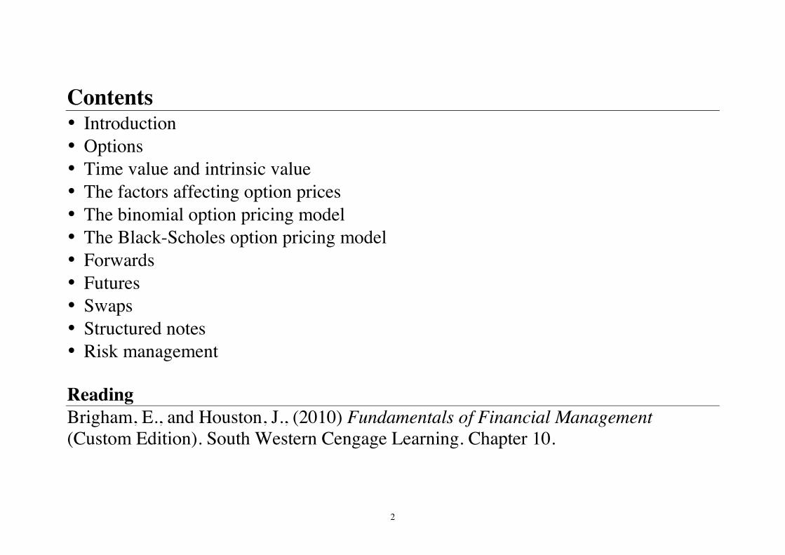
Contents • Introduction • Options • Time value and intrinsic value • The factors affecting option prices • The binomial option pricing model • The Black-Scholes option pricing model • Forwards • Futures • Swaps • Structured notes • Risk management Reading Brigham, E., and Houston, J., (2010) Fundamentals of Financial Management (Custom Edition). South Western Cengage Learning. Chapter 10.

3

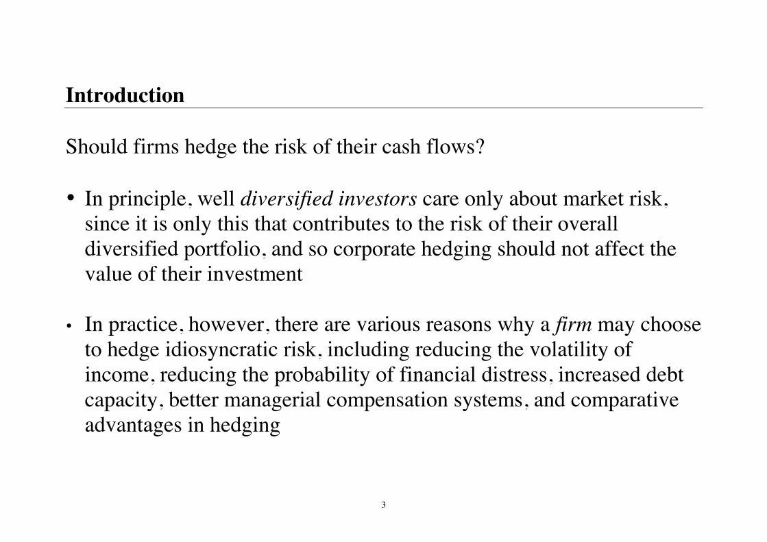
Introduction Should firms hedge the risk of their cash flows? • In principle, well diversified investors care only about market risk,

since it is only this that contributes to the risk of their overall diversified portfolio, and so corporate hedging should not affect the value of their investment

• In practice, however, there are various reasons why a firm may choose

to hedge idiosyncratic risk, including reducing the volatility of income, reducing the probability of financial distress, increased debt capacity, better managerial compensation systems, and comparative advantages in hedging

4

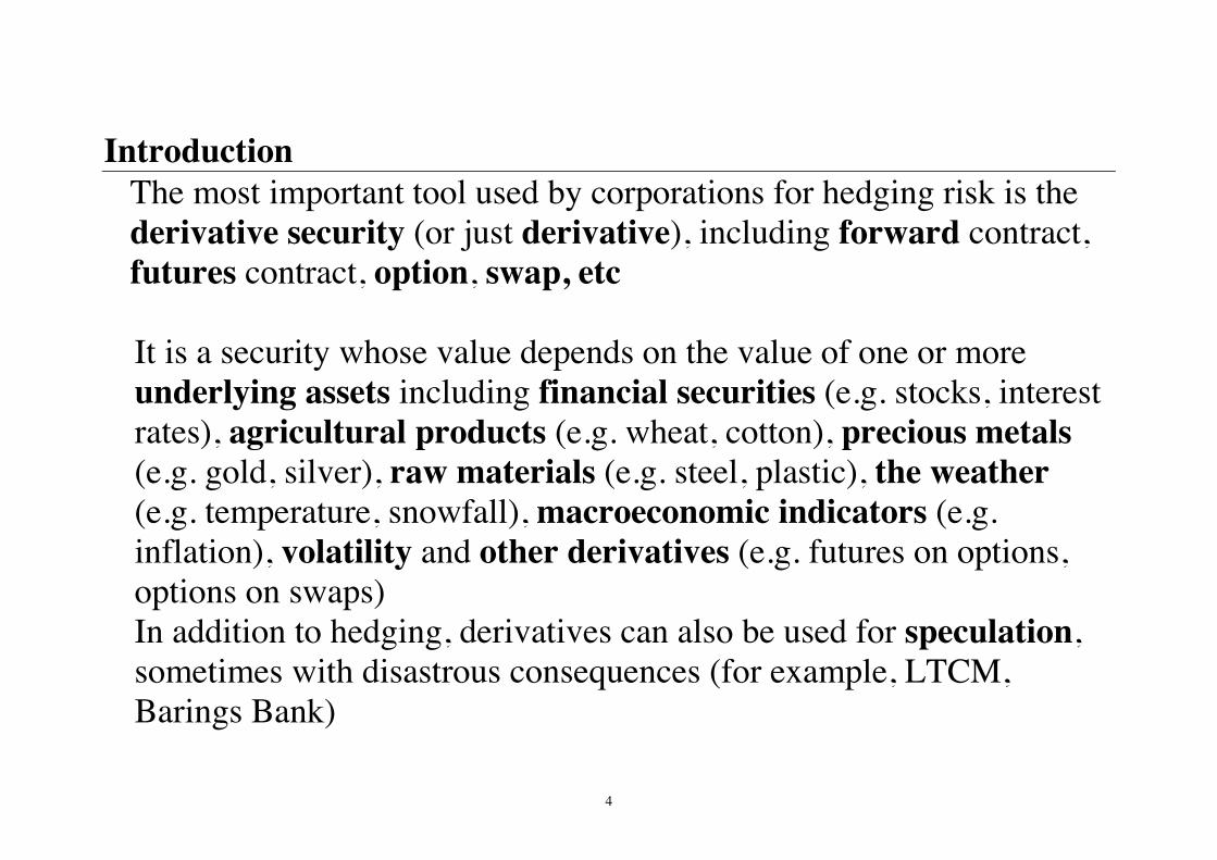
Introduction The most important tool used by corporations for hedging risk is the derivative security (or just derivative), including forward contract, futures contract, option, swap, etc

It is a security whose value depends on the value of one or more underlying assets including financial securities (e.g. stocks, interest rates), agricultural products (e.g. wheat, cotton), precious metals (e.g. gold, silver), raw materials (e.g. steel, plastic), the weather (e.g. temperature, snowfall), macroeconomic indicators (e.g. inflation), volatility and other derivatives (e.g. futures on options, options on swaps) In addition to hedging, derivatives can also be used for speculation, sometimes with disastrous consequences (for example, LTCM, Barings Bank)

5

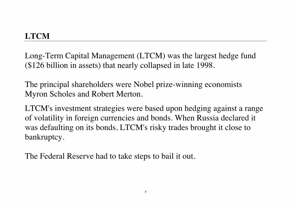
LTCM Long-Term Capital Management (LTCM) was the largest hedge fund ($126 billion in assets) that nearly collapsed in late 1998. The principal shareholders were Nobel prize-winning economists Myron Scholes and Robert Merton.

LTCM's investment strategies were based upon hedging against a range of volatility in foreign currencies and bonds. When Russia declared it was defaulting on its bonds, LTCM's risky trades brought it close to bankruptcy. The Federal Reserve had to take steps to bail it out.

6

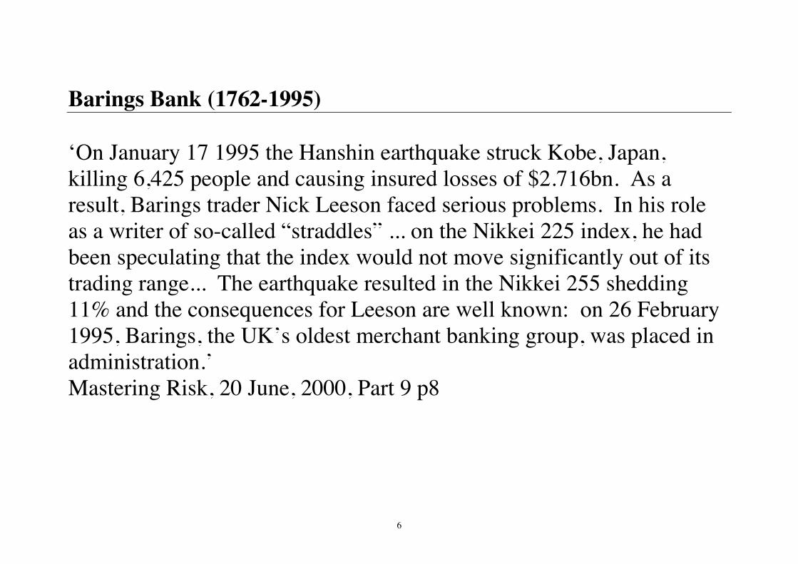
Barings Bank (1762-1995) ‘On January 17 1995 the Hanshin earthquake struck Kobe, Japan, killing 6,425 people and causing insured losses of $2.716bn. As a result, Barings trader Nick Leeson faced serious problems. In his role as a writer of so-called “straddles” ... on the Nikkei 225 index, he had been speculating that the index would not move significantly out of its trading range... The earthquake resulted in the Nikkei 255 shedding 11% and the consequences for Leeson are well known: on 26 February 1995, Barings, the UK’s oldest merchant banking group, was placed in administration.’ Mastering Risk, 20 June, 2000, Part 9 p8

7

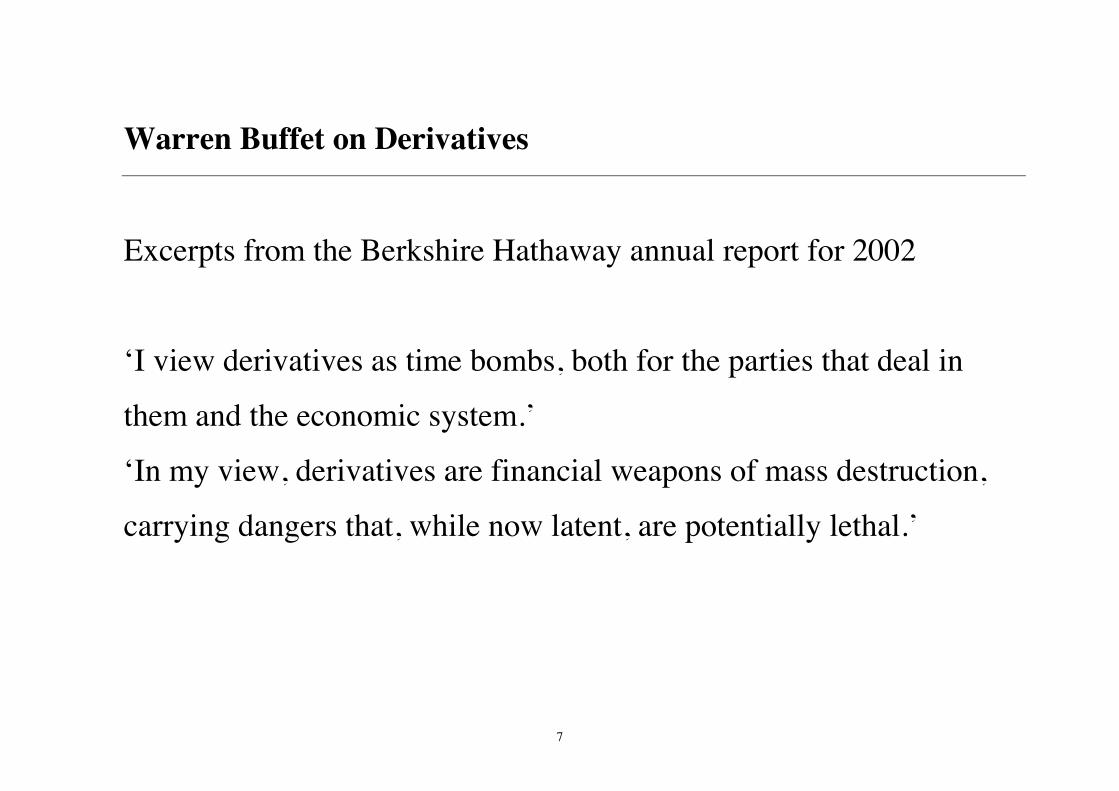
Warren Buffet on Derivatives

Excerpts from the Berkshire Hathaway annual report for 2002

‘I view derivatives as time bombs, both for the parties that deal in

them and the economic system.’

‘In my view, derivatives are financial weapons of mass destruction,

carrying dangers that, while now latent, are potentially lethal.’

8

Introduction

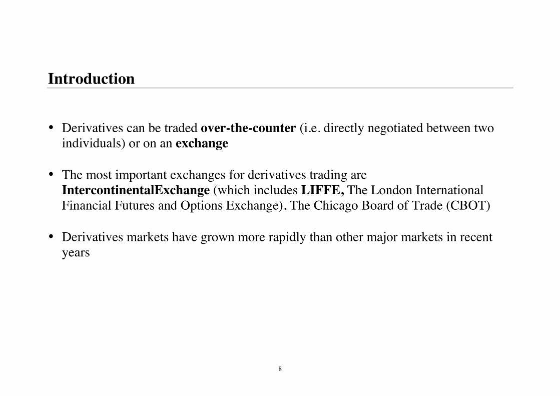
• Derivatives can be traded over-the-counter (i.e. directly negotiated between two

individuals) or on an exchange • The most important exchanges for derivatives trading are

IntercontinentalExchange (which includes LIFFE, The London International Financial Futures and Options Exchange), The Chicago Board of Trade (CBOT)

• Derivatives markets have grown more rapidly than other major markets in recent years

9

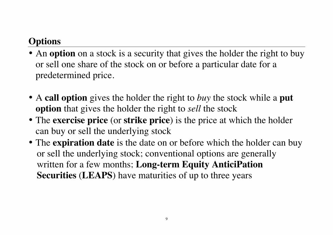
Options • An option on a stock is a security that gives the holder the right to buy

or sell one share of the stock on or before a particular date for a predetermined price.

• A call option gives the holder the right to buy the stock while a put option that gives the holder the right to sell the stock

• The exercise price (or strike price) is the price at which the holder can buy or sell the underlying stock

• The expiration date is the date on or before which the holder can buy or sell the underlying stock; conventional options are generally written for a few months; Long-term Equity AnticiPation Securities (LEAPS) have maturities of up to three years

10

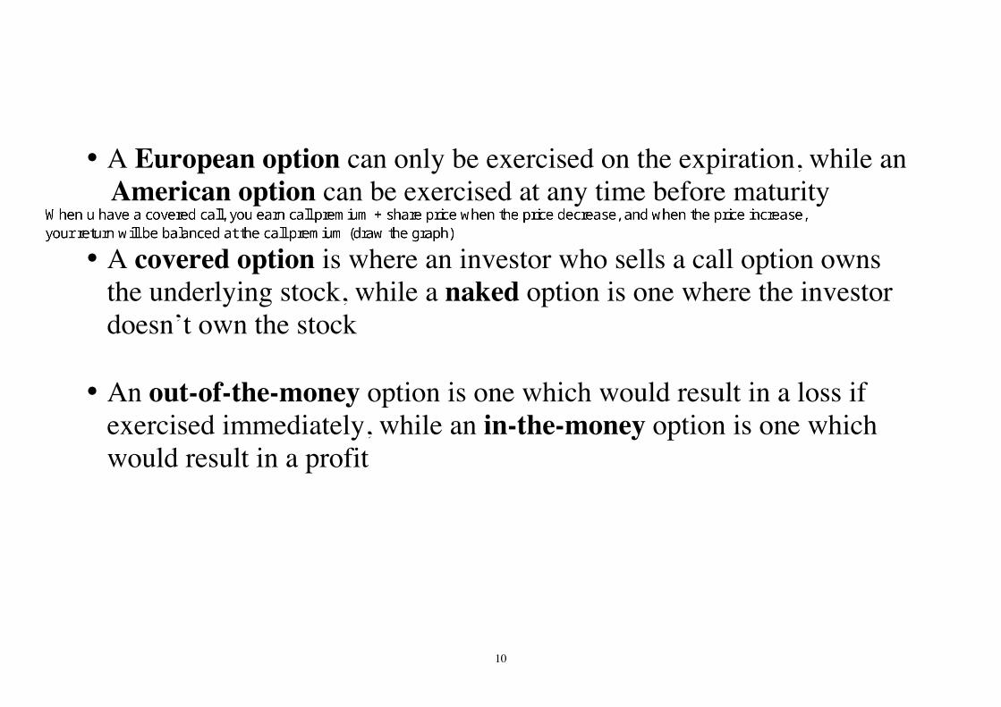
• A European option can only be exercised on the expiration, while an

American option can be exercised at any time before maturity

• A covered option is where an investor who sells a call option owns the underlying stock, while a naked option is one where the investor doesn’t own the stock

• An out-of-the-money option is one which would result in a loss if exercised immediately, while an in-the-money option is one which would result in a profit

11

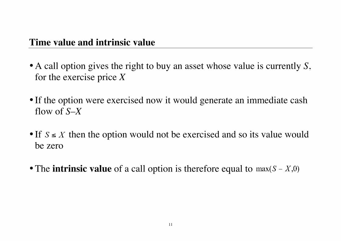
Time value and intrinsic value • A call option gives the right to buy an asset whose value is currently S,

for the exercise price X • If the option were exercised now it would generate an immediate cash

flow of S–X • If then the option would not be exercised and so its value would

be zero • The intrinsic value of a call option is therefore equal to

12

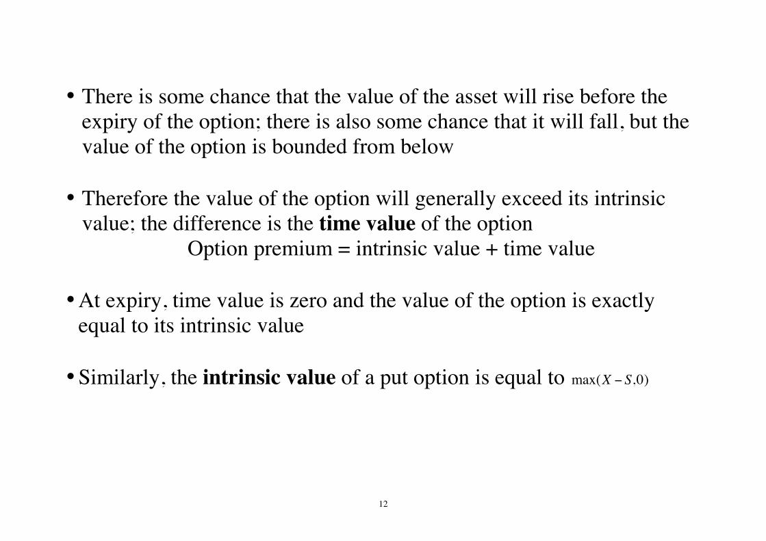
• There is some chance that the value of the asset will rise before the expiry of the option; there is also some chance that it will fall, but the value of the option is bounded from below

• Therefore the value of the option will generally exceed its intrinsic

value; the difference is the time value of the option Option premium = intrinsic value + time value

• At expiry, time value is zero and the value of the option is exactly

equal to its intrinsic value

• Similarly, the intrinsic value of a put option is equal to max(X − S,0)

13

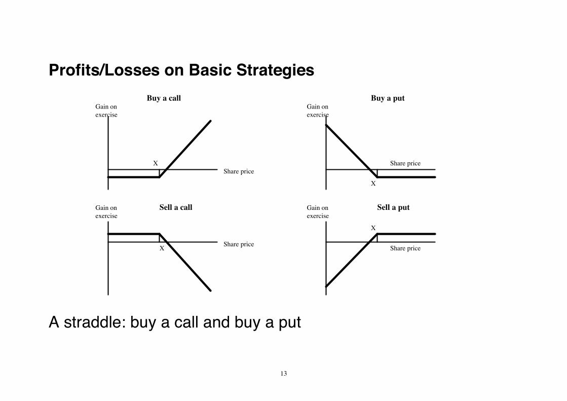
Profits/Losses on Basic Strategies

A straddle: buy a call and buy a put

Share priceShare priceX

X

Gain onexercise

Gain onexercise

Share priceX

Gain onexercise

Share price

X

Gain onexercise

Buy a put

Sell a put

Buy a call

Sell a call

14

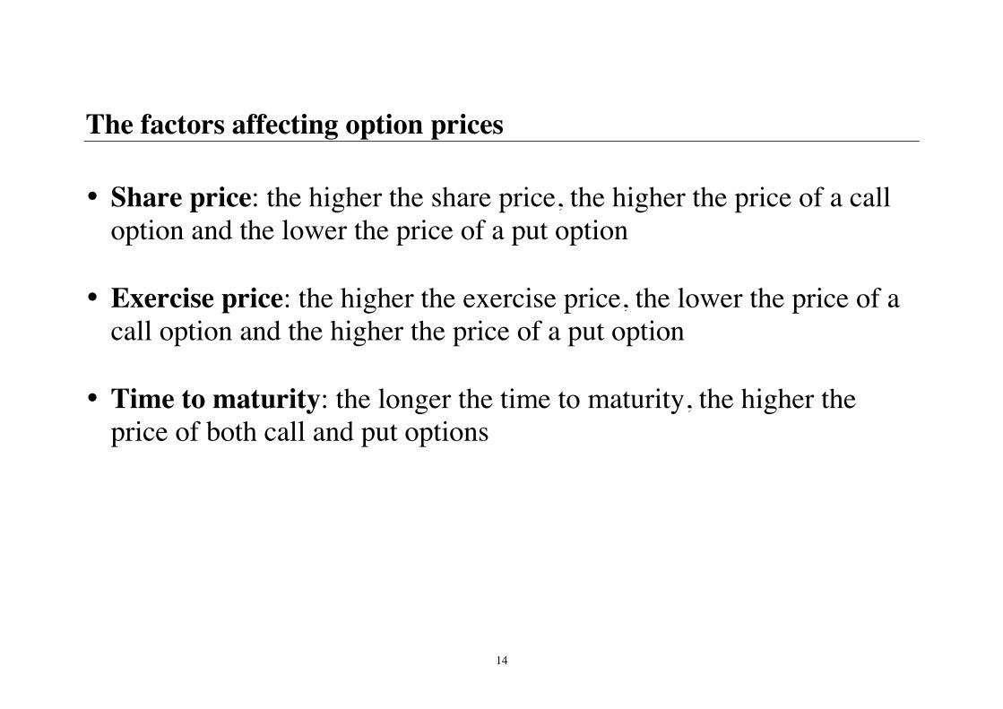
The factors affecting option prices • Share price: the higher the share price, the higher the price of a call

option and the lower the price of a put option • Exercise price: the higher the exercise price, the lower the price of a

call option and the higher the price of a put option • Time to maturity: the longer the time to maturity, the higher the

price of both call and put options

15

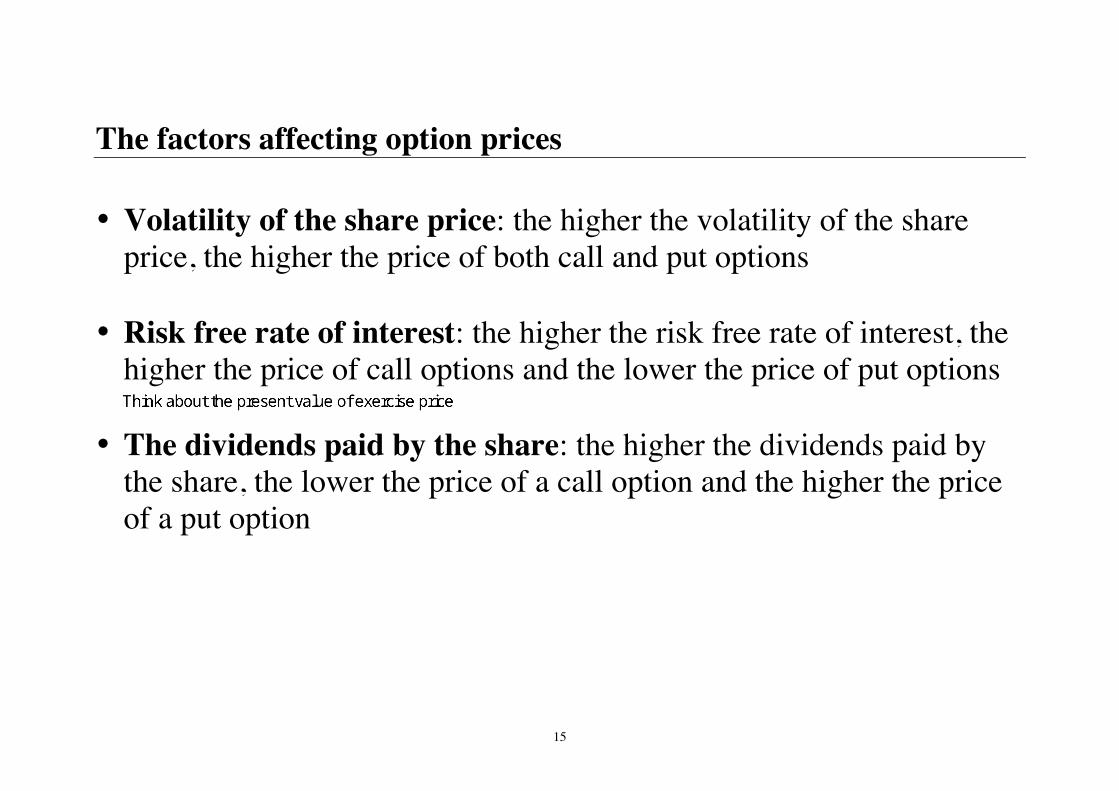
The factors affecting option prices • Volatility of the share price: the higher the volatility of the share

price, the higher the price of both call and put options

• Risk free rate of interest: the higher the risk free rate of interest, the higher the price of call options and the lower the price of put options

• The dividends paid by the share: the higher the dividends paid by

the share, the lower the price of a call option and the higher the price of a put option

16

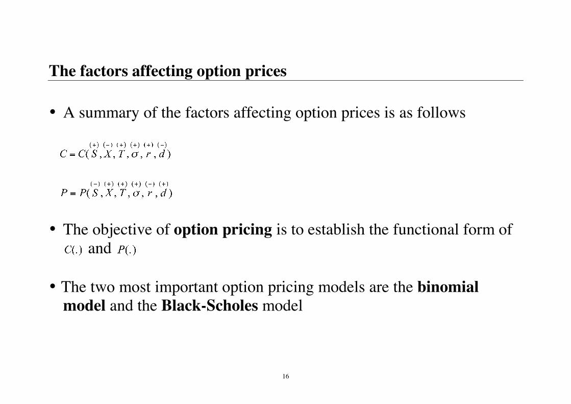
The factors affecting option prices • A summary of the factors affecting option prices is as follows

• The objective of option pricing is to establish the functional form of

and

• The two most important option pricing models are the binomial model and the Black-Scholes model

17

The binomial option pricing model • The binomial option-pricing model is probably the most widely used

option-pricing model • The binomial model assumes that over short periods of time, the share

price moves either up or down by fixed proportions • The resulting ‘tree’ for the share price implies a unique ‘tree’ for the

option price • The nature of the option contract determines the value of the option at

the terminal nodes of the tree

18

The binomial option pricing model • No-arbitrage arguments can then be used to find the equilibrium

price of the option at earlier nodes of the tree • By working backwards, we can therefore deduce the equilibrium price

of the option at the current date

• The binomial model can be easily programmed in Excel or Visual Basic and can be adapted to numerous, and often quite complicated, option-pricing problems

19

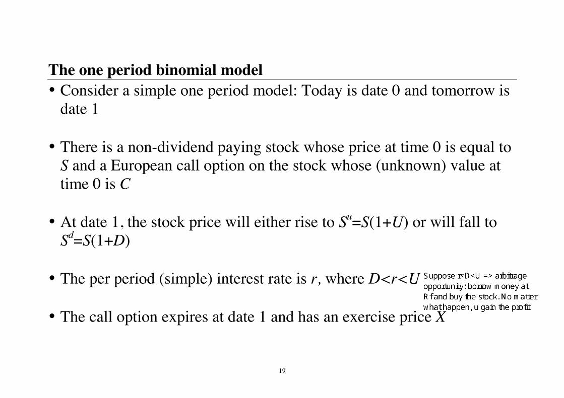
The one period binomial model • Consider a simple one period model: Today is date 0 and tomorrow is

date 1 • There is a non-dividend paying stock whose price at time 0 is equal to

S and a European call option on the stock whose (unknown) value at time 0 is C

• At date 1, the stock price will either rise to Su=S(1+U) or will fall to

Sd=S(1+D) • The per period (simple) interest rate is r, where D<r<U • The call option expires at date 1 and has an exercise price X

20

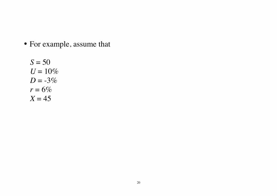
• For example, assume that

S = 50 U = 10% D = -3% r = 6% X = 45

21

The one period binomial model • We can construct a

binomial tree for the stock price as follows

ġ

• The option price next period is given by their expiration values

)0,max( XSC uu −= and )0,max( XSC dd −=

• Our objective is to find the

equilibrium price of the option, C

22

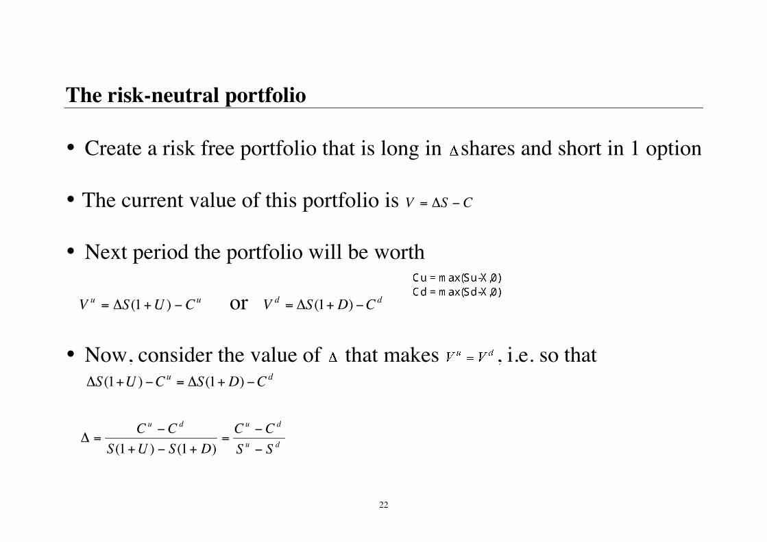
The risk-neutral portfolio • Create a risk free portfolio that is long in shares and short in 1 option • The current value of this portfolio is CSV −∆= • Next period the portfolio will be worth

uu CUSV −+∆= )1( or dd CDSV −+∆= )1( • Now, consider the value of that makes , i.e. so that

du CDSCUS −+∆=−+∆ )1()1(

du

dudu

SSCC

DSUSCC

−

−=

+−+

−=∆

)1()1(

23

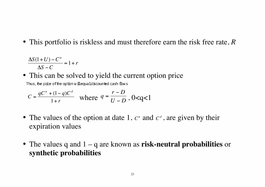
• This portfolio is riskless and must therefore earn the risk free rate, R

rCS

CUS u

+=−∆

−+∆ 1)1(

• This can be solved to yield the current option price

rCqqCC

du

+

−+=

1)1(

where DUDrq

−

−= , 0<q<1

• The values of the option at date 1, uC and dC , are given by their

expiration values • The values q and 1 – q are known as risk-neutral probabilities or

synthetic probabilities

24

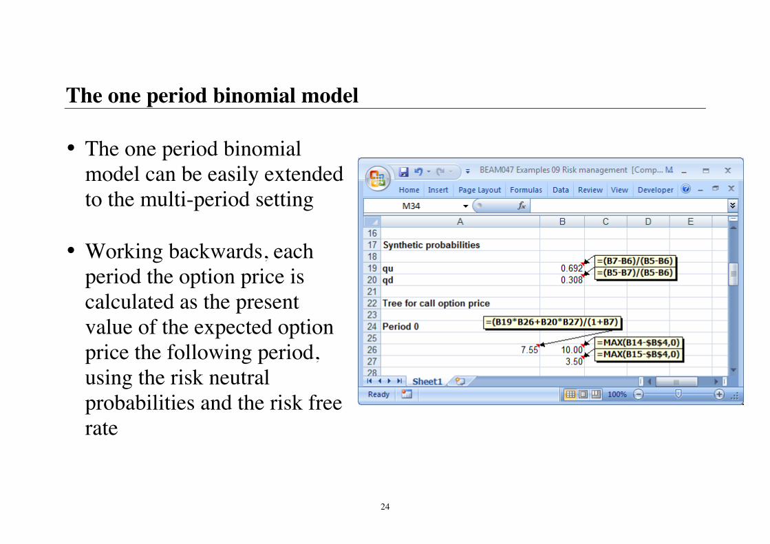
The one period binomial model • The one period binomial

model can be easily extended to the multi-period setting

• Working backwards, each

period the option price is calculated as the present value of the expected option price the following period, using the risk neutral probabilities and the risk free rate

25

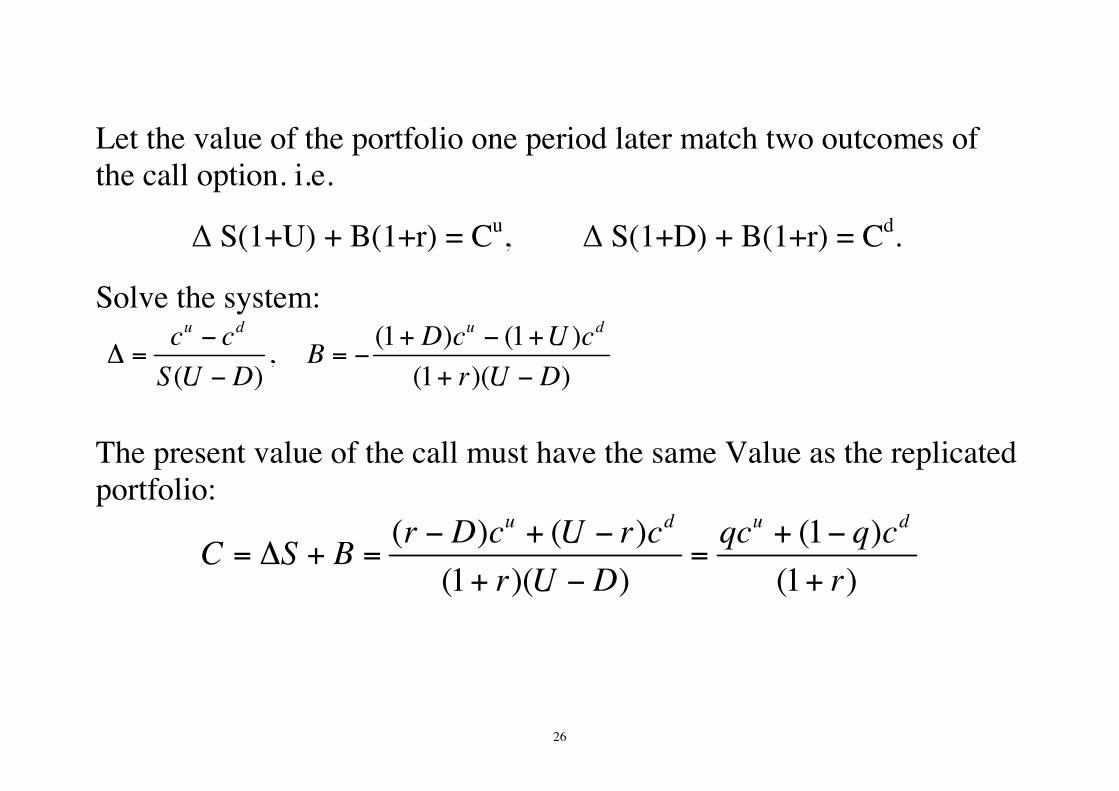
Replicating portfolio approach* Combine the stock and a risk-free bond to replicate the call option’s cash flows. Hold ∆ shares of stock and have B pounds invested in the bond earning riskless rate r or borrow B pounds with riskless rate r. Su B(1+r) Cu = max(0, Su - X) S B C Sd

B(1+r) Cd = max(0, Sd – X) The current value of the portfolio = ∆S+B.

26

Let the value of the portfolio one period later match two outcomes of the call option. i.e.

∆ S(1+U) + B(1+r) = Cu, ∆ S(1+D) + B(1+r) = Cd. Solve the system:

(1 ) (1 ),

( ) (1 )( )

u d u dc c D c U cBS U D r U D

− + − +∆ = = −

− + −

The present value of the call must have the same Value as the replicated portfolio:

( ) ( ) (1 )(1 )( ) (1 )

u d u dr D c U r c qc q cC S Br U D r

− + − + −= ∆ + = =

+ − +

27

The Black-Scholes model • The binomial model assumes that in each (discrete) period, the share

price moves either up or down by discrete amounts • Black and Scholes (1973) derived an option pricing model that

assumes instead that the share price moves continuously • The advantage of this formulation is that it permits the derivation of a

closed form solution to the price of an option that is very easy to implement

28

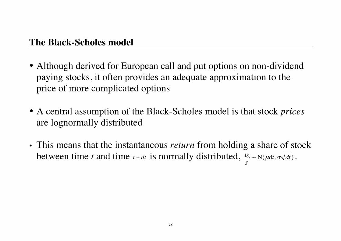
The Black-Scholes model • Although derived for European call and put options on non-dividend

paying stocks, it often provides an adequate approximation to the price of more complicated options

• A central assumption of the Black-Scholes model is that stock prices

are lognormally distributed • This means that the instantaneous return from holding a share of stock

between time t and time t dt+ is normally distributed, d t

t

SS

N( d , )t dtµ σ∼ .

29

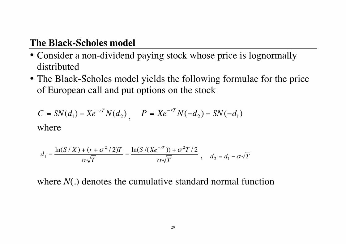
The Black-Scholes model • Consider a non-dividend paying stock whose price is lognormally

distributed • The Black-Scholes model yields the following formulae for the price

of European call and put options on the stock

)()( 21 dNXedSNC rT−−= , )()( 12 dSNdNXeP rT −−−= − where T

TXeST

TrXSdrT

σ

σ

σ

σ 2/))/(ln()2/()/ln( 22

1+

=++

=−

, Tdd σ−= 12 where N(.) denotes the cumulative standard normal function

30

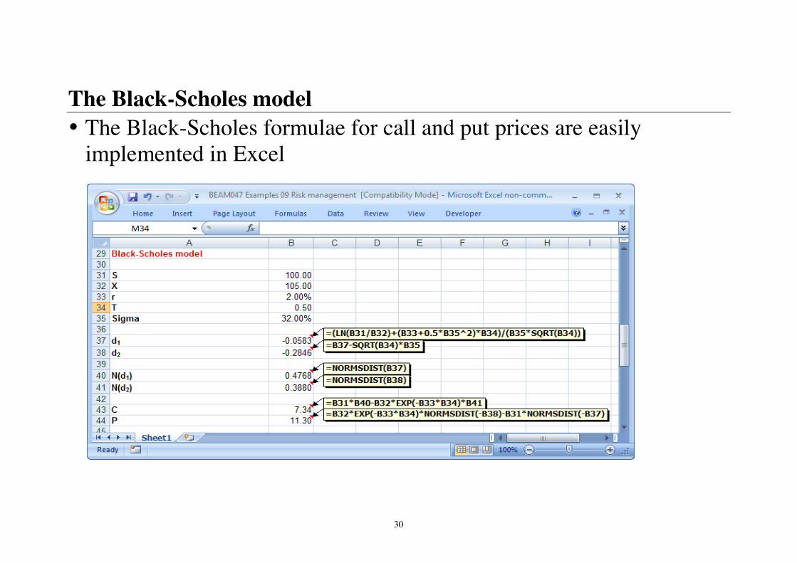
The Black-Scholes model • The Black-Scholes formulae for call and put prices are easily

implemented in Excel

31

Forward contracts • A forward contract is a contract made at time 0, to buy or sell an

asset or good at some time in the future, T, on terms agreed at time 0 • The terms include the quantity, quality, price and delivery

arrangements • A forward contract is therefore a contract for forward delivery rather

than spot delivery; the market for spot delivery is called the spot market, while the market for forward delivery is called the forward market

32

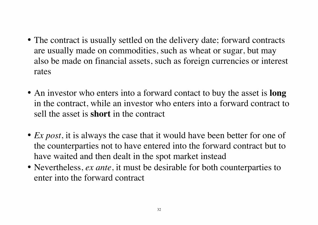
• The contract is usually settled on the delivery date; forward contracts are usually made on commodities, such as wheat or sugar, but may also be made on financial assets, such as foreign currencies or interest rates

• An investor who enters into a forward contact to buy the asset is long

in the contract, while an investor who enters into a forward contract to sell the asset is short in the contract

• Ex post, it is always the case that it would have been better for one of

the counterparties not to have entered into the forward contract but to have waited and then dealt in the spot market instead

• Nevertheless, ex ante, it must be desirable for both counterparties to enter into the forward contract

33

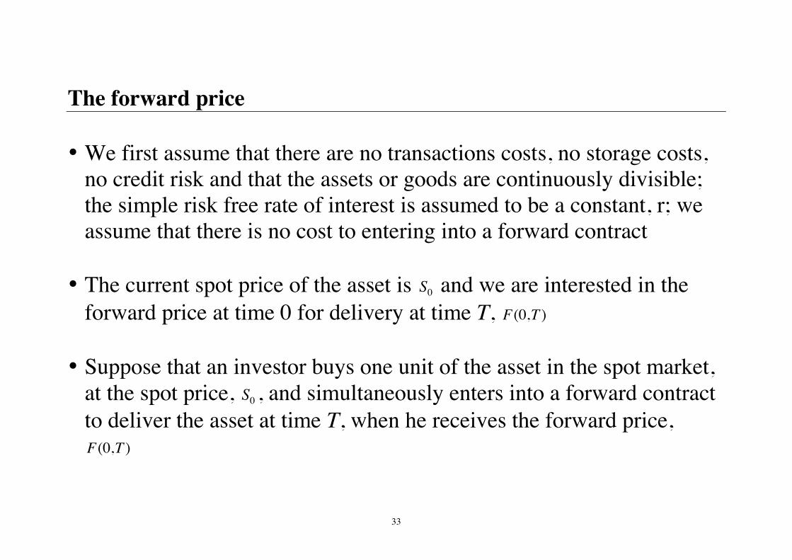
The forward price • We first assume that there are no transactions costs, no storage costs,

no credit risk and that the assets or goods are continuously divisible; the simple risk free rate of interest is assumed to be a constant, r; we assume that there is no cost to entering into a forward contract

• The current spot price of the asset is 0S and we are interested in the

forward price at time 0 for delivery at time T, ),0( TF • Suppose that an investor buys one unit of the asset in the spot market,

at the spot price, 0S , and simultaneously enters into a forward contract to deliver the asset at time T, when he receives the forward price,

),0( TF

34

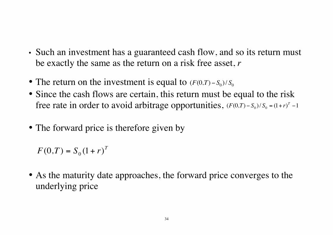
• Such an investment has a guaranteed cash flow, and so its return must

be exactly the same as the return on a risk free asset, r

• The return on the investment is equal to 00 /)),0(( SSTF − • Since the cash flows are certain, this return must be equal to the risk

free rate in order to avoid arbitrage opportunities, 1)1(/)),0(( 00 −+=− TrSSTF • The forward price is therefore given by

TrSTF )1(),0( 0 += • As the maturity date approaches, the forward price converges to the

underlying price

35

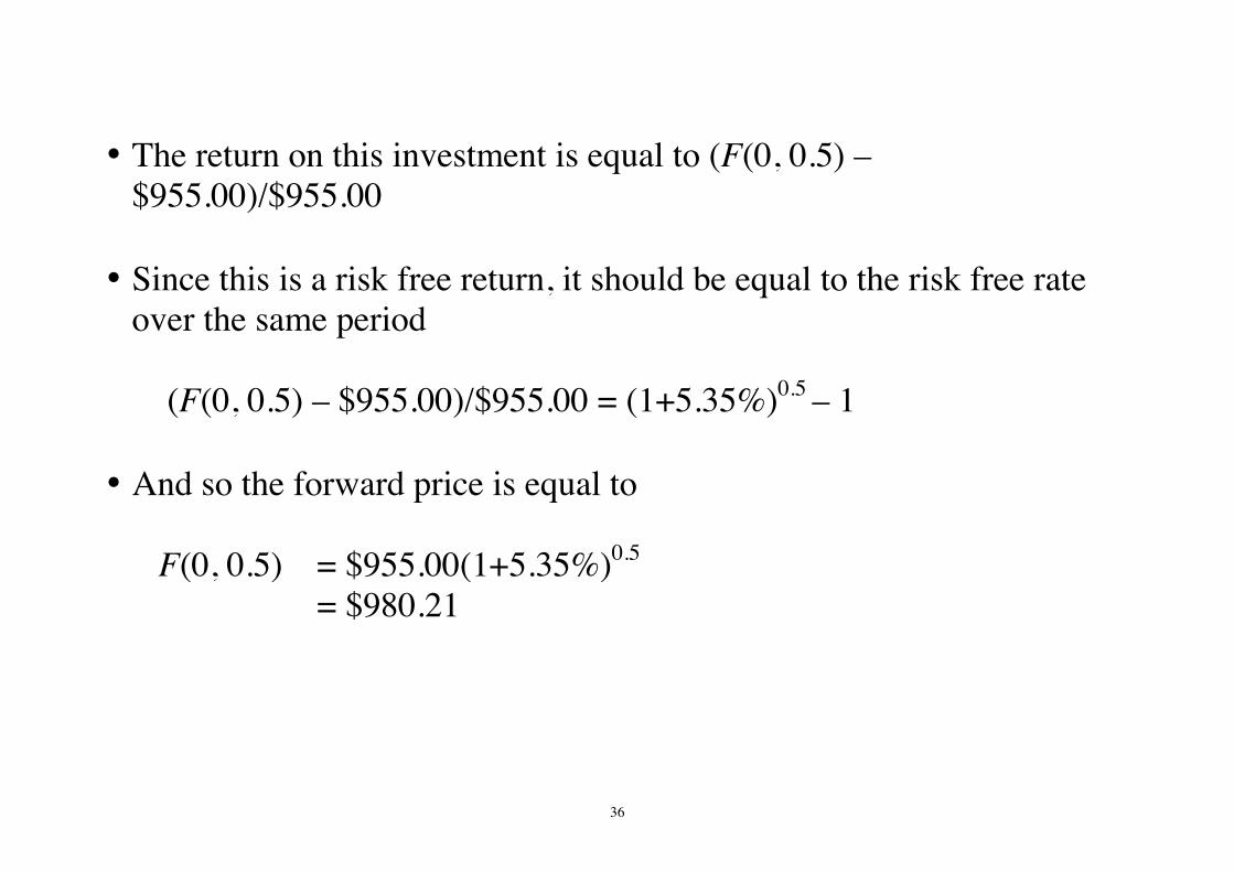
The forward price

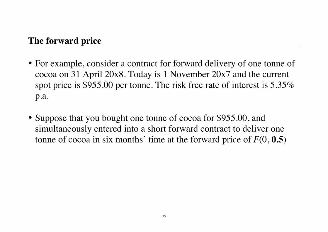
• For example, consider a contract for forward delivery of one tonne of cocoa on 31 April 20x8. Today is 1 November 20x7 and the current spot price is $955.00 per tonne. The risk free rate of interest is 5.35% p.a.

• Suppose that you bought one tonne of cocoa for $955.00, and

simultaneously entered into a short forward contract to deliver one tonne of cocoa in six months’ time at the forward price of F(0, 0.5)

36

• The return on this investment is equal to (F(0, 0.5) – $955.00)/$955.00

• Since this is a risk free return, it should be equal to the risk free rate

over the same period

(F(0, 0.5) – $955.00)/$955.00 = (1+5.35%)0.5 – 1 • And so the forward price is equal to

F(0, 0.5) = $955.00(1+5.35%)0.5 = $980.21

37

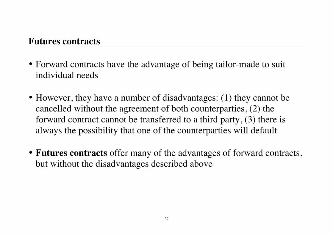
Futures contracts • Forward contracts have the advantage of being tailor-made to suit

individual needs • However, they have a number of disadvantages: (1) they cannot be

cancelled without the agreement of both counterparties, (2) the forward contract cannot be transferred to a third party, (3) there is always the possibility that one of the counterparties will default

• Futures contracts offer many of the advantages of forward contracts,

but without the disadvantages described above

38

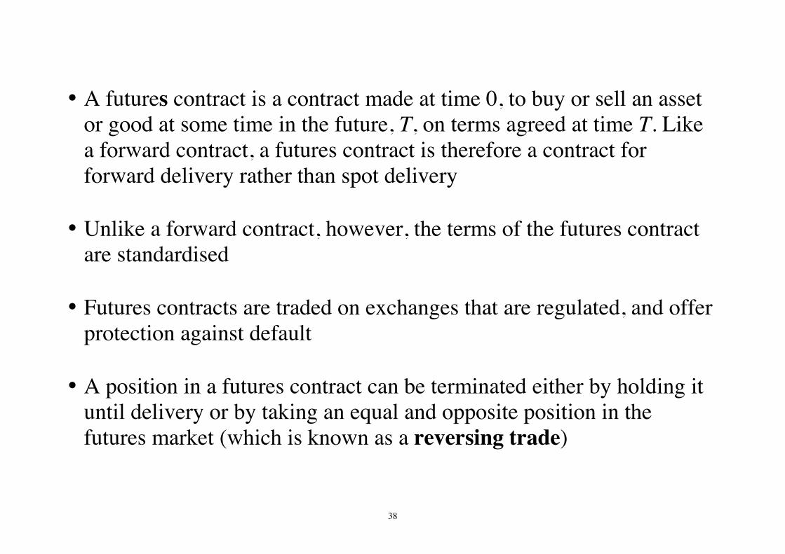
• A futures contract is a contract made at time 0, to buy or sell an asset or good at some time in the future, T, on terms agreed at time T. Like a forward contract, a futures contract is therefore a contract for forward delivery rather than spot delivery

• Unlike a forward contract, however, the terms of the futures contract

are standardised • Futures contracts are traded on exchanges that are regulated, and offer

protection against default • A position in a futures contract can be terminated either by holding it

until delivery or by taking an equal and opposite position in the futures market (which is known as a reversing trade)

39

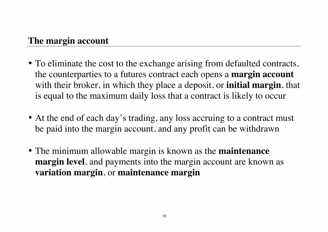
The margin account • To eliminate the cost to the exchange arising from defaulted contracts,

the counterparties to a futures contract each opens a margin account with their broker, in which they place a deposit, or initial margin, that is equal to the maximum daily loss that a contract is likely to occur

• At the end of each day’s trading, any loss accruing to a contract must

be paid into the margin account, and any profit can be withdrawn • The minimum allowable margin is known as the maintenance

margin level, and payments into the margin account are known as variation margin, or maintenance margin

40

The margin account • This is known as marking-to-market • If a counterparty fails to mark-to-market then the contract is closed;

that day’s losses will be covered by the balance of the margin account; since futures contracts are marked-to-market, the largest loss that can occur through default is the change in the futures price in a single day; to ensure that this is covered by the surplus in the margin account, futures exchanges usually operate a system of price limits

• The margin is known as the performance bond in some exchanges

41

Forward prices and futures prices • Since futures contracts are marked-to-market, their value on any

particular day is equal to zero • The delivery price of a futures contract and the spot price will

generally differ, but they are obviously related • Similar to a forward contract, as the delivery date approaches, the spot

and futures prices will converge • It is reasonable to assume that since forwards and futures are both

contracts for future delivery, their prices will be similar

42

Forward prices and futures prices • However, forward and futures contracts are fundamentally different

since the former involves a single cash flow at the delivery date, while the latter involves daily cash flows in the form of initial and variation margin

• Nevertheless, if interest rates are constant, futures and forward prices

must be identical in order to preclude arbitrage opportunities.

43

Swaps • Swaps are contractual agreements between individuals or companies

to exchange cash flows, e.g. Interest rate swaps Currency swaps Credit default swap

• Consider interest rate swaps for two companies, and two sources of finance, namely fixed and floating rate loans.

• The fixed rate loan is available at a known rate of interest that is fixed

for the maturity of the loan. The floating rate loan is available at variable rate, usually quoted as LIBOR plus a fixed amount

44

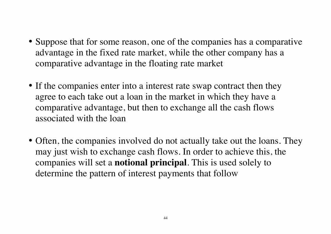
• Suppose that for some reason, one of the companies has a comparative advantage in the fixed rate market, while the other company has a comparative advantage in the floating rate market

• If the companies enter into a interest rate swap contract then they

agree to each take out a loan in the market in which they have a comparative advantage, but then to exchange all the cash flows associated with the loan

• Often, the companies involved do not actually take out the loans. They may just wish to exchange cash flows. In order to achieve this, the companies will set a notional principal. This is used solely to determine the pattern of interest payments that follow

45

• Currency swaps are agreements to exchange cash flows denominated in one currency with cash flows denominated in another

• As with interest rate swaps, currency swaps may arise because a firm may have a comparative advantage in one currency, while another firm may have a comparative advantage in another currency

• A credit default swap (CDS) is a swap agreement that the seller of the

CDS will compensate the buyer in the event of a loan default. The buyer of the CDS makes a series of payments to the seller and, in exchange, receives a payoff if the loan defaults.

• Swaps are usually arranged through an intermediary bank who will

earn a fixed percentage commission.

46

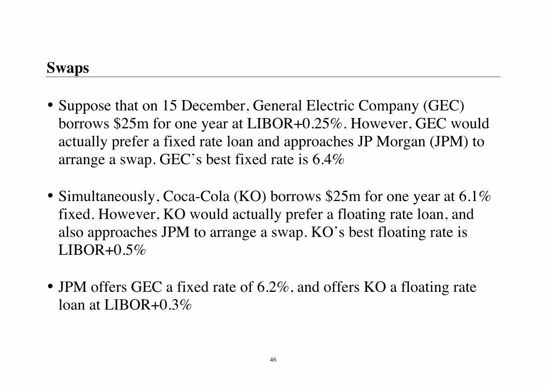
Swaps • Suppose that on 15 December, General Electric Company (GEC)

borrows $25m for one year at LIBOR+0.25%. However, GEC would actually prefer a fixed rate loan and approaches JP Morgan (JPM) to arrange a swap. GEC’s best fixed rate is 6.4%

• Simultaneously, Coca-Cola (KO) borrows $25m for one year at 6.1%

fixed. However, KO would actually prefer a floating rate loan, and also approaches JPM to arrange a swap. KO’s best floating rate is LIBOR+0.5%

• JPM offers GEC a fixed rate of 6.2%, and offers KO a floating rate

loan at LIBOR+0.3%

47

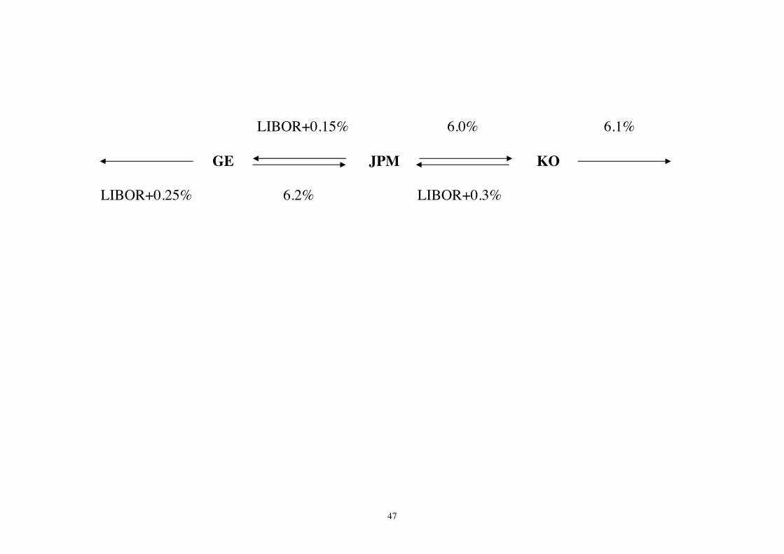
LIBOR+0.15% 6.0% 6.1%

GE JPM KO LIBOR+0.25% 6.2% LIBOR+0.3%

48

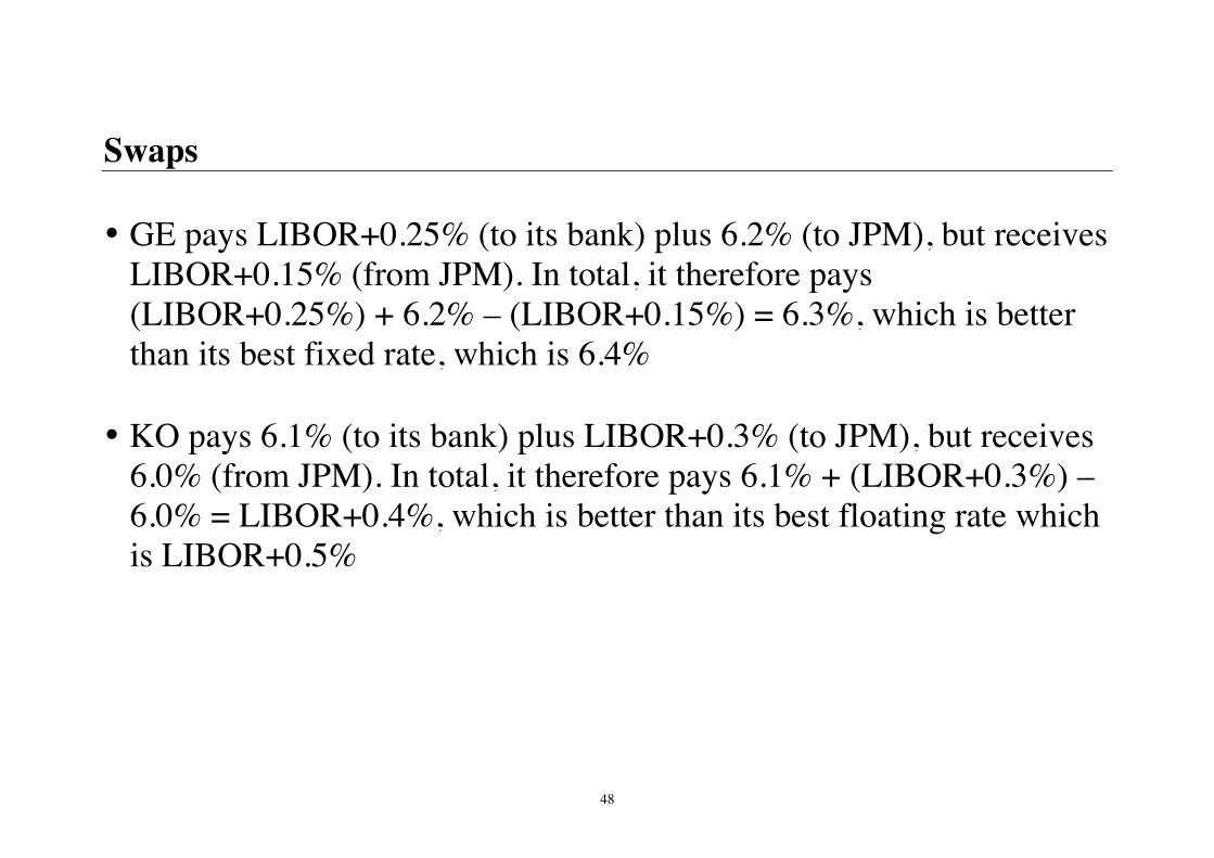
Swaps • GE pays LIBOR+0.25% (to its bank) plus 6.2% (to JPM), but receives

LIBOR+0.15% (from JPM). In total, it therefore pays (LIBOR+0.25%) + 6.2% – (LIBOR+0.15%) = 6.3%, which is better than its best fixed rate, which is 6.4%

• KO pays 6.1% (to its bank) plus LIBOR+0.3% (to JPM), but receives

6.0% (from JPM). In total, it therefore pays 6.1% + (LIBOR+0.3%) – 6.0% = LIBOR+0.4%, which is better than its best floating rate which is LIBOR+0.5%

49

• JPM receives 6.2% (from GE) plus LIBOR+0.3% (from KO) but pays LIBOR+0.15% (to GE) and 6.0% (to KO). In total, it makes 6.2% + (LIBOR+0.3%) – (LIBOR+0.15%) – 6.0% = 0.35%, which is better than nothing!

• In practice, only the netted amounts would be paid, which reduces the

credit risk for all parties • Also, JPM may only enter into a swap contract with one of the firms,

but hedge the resulting interest rate risk that it would face by buying or selling interest rate futures

50

Structured notes • We know a financial security is associated with a stream of future

cash flows.

• A structured note is a debt obligation that is derived from some other debt obligation

• Examples of structured notes include collateralized mortgage

obligations (bonds whose cash flows are guaranteed by pools of mortgages that are placed with a trustee) and collateralized debt obligations (CDO) (bonds whose cash flows are guaranteed by pools of debt instruments in general)

51

Risk management • Risk Management is the management of unpredictable events that

have adverse consequences for a firm • Firms can use derivatives to hedge risk • A long hedge is where a firm buys a derivative in anticipation of (or

to guard against) a rise in the price of an asset; a short hedge is where a firm buys a derivative in anticipation of (or to guard against) a fall in the price of an asset

• A perfect hedge arises when the gain or loss on the hedged

transaction exactly offsets the loss or gain on the unhedged position e.g. 3 month sterling interest rate, unit of trading: £500,000.

52

Risk management

A structured way to manage risks within a firm is as follows: • Identify the risks that the firm faces, e.g.

Demand risks Input risks Financial risks Personnel risks Environmental risks Insurable risks

• Measure the potential effect of each risk

53

• Decide how each relevant risk should be handled, e.g.

(a) Transfer the risk to an insurance company (b) Purchase derivative contracts to reduce risk (c) Reduce the probability of the occurrence of an adverse event (d) Reduce the magnitude of the loss associated with an adverse event

• Risk management decisions, like all corporate decisions, should be

based on a cost/benefit analysis for each feasible alternative

54

Exercise To measure the risk of an option, its beta can be computed. It can be calculated as the beta of the replicating portfolio - the weighted average beta of the securities that make up the portfolio:

option S B SS B S

S B S B S Bβ β β β

∆ ∆= + =

∆ + ∆ + ∆ +

Since the replicating portfolio consists of S∆ dollars invested in the stock and B dollars invested in the bond and the risk-free bond’s beta is zero. For a call option, ∆ is greater than zero and B is less than zero. Thus, for stocks with positive betas, calls will have larger betas than the underlying stock. Suppose that Yahoo stock is trading for $40. The stock’s historical volatility (standard deviation) is 70% per year. Assume that the risk-free rate is 5% and that the firm pays no dividends. (i) What is the value of a six-month European call option with a $45 strike price? (ii) Calculate the beta of the six-month Yahoo call option with a $45 strike price? Assume that Yahoo has a stock beta of 2.21.

55

Case study Chapter 10 Integrated Case.