
CEBoK Module 09 Cost and Schedule Risk Analysis
96
© 2002-2013 ICEAA. All rights reserved. v1.2 Unit III - Module 9 1 Cost and Schedule Risk Analysis: Basic How to adjust your estimate for uncertainty and historical cost and schedule growth “As we know, / There are known knowns. / There are things we know we know. We also know / There are known unknowns. / That is to say We know there are some things / We do not know. But there are also unknown unknowns, / The ones we don't know / We don't know.” - “The Unknown” from Pieces of Intelligence: The Existential Poetry of Donald Rumsfeld, Hart Seely, 2003 [DoD news briefing, 02/12/2002] Presented at the 2017 ICEAA Professional Development & Training Workshop www.iceaaonline.com/portland2017
-
Upload
khangminh22 -
Category
Documents
-
view
0 -
download
0
Transcript of CEBoK Module 09 Cost and Schedule Risk Analysis
copy 2002-2013 ICEAA All rights reserved
v12
Unit III - Module 9 1
Cost and Schedule Risk Analysis Basic
How to adjust your estimate for uncertainty and historical cost and schedule growth
ldquoAs we know There are known knowns There are things we know we know We also know There are known unknowns That is to say
We know there are some things We do not know But there are also unknown unknowns The ones we dont know We dont knowrdquo
- ldquoThe Unknownrdquo from Pieces of Intelligence The Existential Poetry of DonaldRumsfeld Hart Seely 2003 [DoD news briefing 02122002]
Presented at the 2017 ICEAA Professional Development amp Training Workshop wwwiceaaonlinecomportland2017
copy 2002-2013 ICEAA All rights reserved
v12
Acknowledgmentsbull ICEAA is indebted to TASC Inc for the
development and maintenance of theCost Estimating Body of Knowledge (CEBoKreg)ndash ICEAA is also indebted to Technomics Inc for the
independent review and maintenance of CEBoKreg
bull ICEAA is also indebted to the following individuals who have made significant contributions to the development review and maintenance of CostPROF and CEBoK reg
bull Module 9 Cost and Schedule Risk Analysisndash Lead authors Richard L Coleman Jessica R Summerville
Eric R Druker Richard C Leendash Senior reviewers Richard L Coleman Michael F Jeffers Kevin
Cincotta Fred K Blackburnndash Reviewer Bethia L Cullisndash Managing editor Peter J Braxton
2Unit III - Module 9
Presented at the 2017 ICEAA Professional Development amp Training Workshop wwwiceaaonlinecomportland2017
copy 2002-2013 ICEAA All rights reserved
v12
Unit III - Module 9 3
Unit IndexUnit I ndash Cost EstimatingUnit II ndash Cost Analysis TechniquesUnit III ndash Analytical Methods
6 Basic Data Analysis Principles7 Learning Curve Analysis8 Regression Analysis9 Cost and Schedule Risk Analysis10Probability and Statistics
Unit IV ndash Specialized CostingUnit V ndash Management Applications
Presented at the 2017 ICEAA Professional Development amp Training Workshop wwwiceaaonlinecomportland2017
copy 2002-2013 ICEAA All rights reserved
v12
Unit III - Module 9 4
Risk Overviewbull Key Ideas
ndash Risk bias (accuracy)ndash Uncertainty (precision)ndash Cost realismndash Risk vs Sensitivityndash Inputs vs Outputs Risk
bull Practical Applicationsndash Probabilistic Cost Estimates
bull S-Curvesbull Budgeting to Percentiles
ndash Risk Scoring and Mapping
bull Analytical Constructsndash Probability Distributions for Riskndash Percentilesndash Prediction Intervals (PI)ndash Correlation
bull Related Topicsndash Data Collection for
Risk Analysisndash Monte Carlo Simulationndash Risk Managementndash Schedule Analysis
10
Presented at the 2017 ICEAA Professional Development amp Training Workshop wwwiceaaonlinecomportland2017
copy 2002-2013 ICEAA All rights reserved
v12
Agendabull Cost Risk Analysis
ndash Introductionndash Distributions
bull Fitting distributions to historical databull Measuring technical uncertaintybull Measuring estimating uncertainty
ndash Aggregating riskbull Simulationbull Method of momentsbull Correlation
ndash Risk measuresndash Risk allocationndash Joint confidence level analysisndash Practical exercises
bull Comparing simulation with method of moments
Unit III - Module 9 5
Presented at the 2017 ICEAA Professional Development amp Training Workshop wwwiceaaonlinecomportland2017
copy 2002-2013 ICEAA All rights reserved
v12
Unit III - Module 9 6
Introductionbull Cost estimates in many cases project many years in the future
ndash Cost estimates are inherently uncertain regardless of whether risk is included (modeled)
bull Sources of uncertainty include (but are not limited to)ndash Scope and requirements (what is being estimated)ndash Technology readinessndash Manufacturing readinessndash Inflationndash Model uncertainty
bull The cost analysis profession recognizes the importance of risk and has incorporated risk analysis as an integral part of the estimating process
Presented at the 2017 ICEAA Professional Development amp Training Workshop wwwiceaaonlinecomportland2017
copy 2002-2013 ICEAA All rights reserved
v12
Risk Analysis Termsbull Risk is the chance of uncertainty or loss
bull Uncertainty is the indefiniteness about the outcome of a situationndash Includes both favorable and unfavorable events
bull Cost Risk is a measure of the chance that due to unfavorable events the planned or budgeted cost of a project will be exceeded
bull Cost Uncertainty Analysis is a process of quantifying the cost estimating uncertainty due to variance in the cost estimating models as well as variance in the technical performance and programmatic input variables
bull Cost Risk Analysis is a process of quantifying the cost impacts of the unfavorable events
Unit III - Module 9 7
Presented at the 2017 ICEAA Professional Development amp Training Workshop wwwiceaaonlinecomportland2017
copy 2002-2013 ICEAA All rights reserved
v12
Unit III - Module 9 8
Are Our Costs Realisticbull We claim our costs are realisticbull We claim we estimate costs at the 50th percentile
ndash This should mean we have 50 low and 50 high outcomes
bull But we have an unchanging cost growth pattern showing only 12 of our estimates are high (underrun) and 88 are low (overrun)ndash As shown in the graphic on the next slide
bull The conclusion is inescapable our costs are not realistic
bull This also means our costs are at the 12th percentile not the 50th percentile
What Percentile Are We At Now (And Where Are We Going) R Coleman E Druker P Braxton B Cullis C Kanick SCEA 2009 DoDCAS 2010
Presented at the 2017 ICEAA Professional Development amp Training Workshop wwwiceaaonlinecomportland2017
copy 2002-2013 ICEAA All rights reserved
v12
88 Dollars ( in millions)
Co
st G
row
th F
acto
r
0
1
2
3
4
5
6
7
8
0 5000 10000 15000 20000 25000 30000 35000
lsquoUnit III - Module 9 9
Historical Cost Growth
Average program cost growthRampD 21 Prod 19
Fraction of programs ending on-or-under cost target
7-16
Note This pattern appears to be fractal
Uncohorted dollar weighted
This is the line of no growth
The Cost Growth Factor is 10 meaning (Final Cost)(Initial Cost) = 1
Grew to 75 times planned cost
Risk in Cost Estimating General Introduction amp The BMDO Approach 33rd DoDCAS 2000 R L Coleman J R Summerville M DuBois B Myers
Note apparent bounds
Presented at the 2017 ICEAA Professional Development amp Training Workshop wwwiceaaonlinecomportland2017
88 Dollars ( in millions)
Cost Growth Factor
0
1
2
3
4
5
6
7
8
0
5000
10000
15000
20000
25000
30000
35000
copy 2002-2013 ICEAA All rights reserved
v12
Sources of Cost Risk
Unit III - Module 9 10
l Security Risksl Critical failure modesl Energy Environmental Risksl Schedule problems and delaysl Inadequate cost estimates
n Process (need to assess contractorrsquos assumptions)
n Models l ldquoNew Ways of Doing Businessrdquol Inflationl Systems Engineeringl Cost Improvement Curve
Assumptions
l State-of-the-Art-Advance (Technology Readiness)
l Technical Risk Sourcesn Physical propertiesn Material Propertiesn Radiation Properties
(emission and reception)l Material Availability Risksl Testing Modeling Risksl Integration Interface Risksl Program Personnell Safety Risksl Software Design Risks
Historical cost data available
Amount of cost risk depends on the Basis of the Estimate
Presented at the 2017 ICEAA Professional Development amp Training Workshop wwwiceaaonlinecomportland2017
copy 2002-2013 ICEAA All rights reserved
v12
Point Estimates of Costbull Funding organizations need best estimate of cost for
bullCostperformance tradeoff studiesbullCostbenefit analysesbullBudget planning
bull But program cost is nebulous heavily impacted bybullTechnological (im)maturitybullProgrammatic considerationsbullSchedule slipsbullUnforeseen events
bull Point cost estimates cannot be ldquocorrectrdquo becausebullEvery cost element contains uncertaintybullTotal system cost is sum of these WBS elements
bull Actual program cost falls within a range surrounding the best estimate (with some degree of confidence)bullThe best we can hope to do is to understand the uncertaintybullUnderstanding the uncertainty will help us make provision for it
Unit III - Module 9 11
Presented at the 2017 ICEAA Professional Development amp Training Workshop wwwiceaaonlinecomportland2017
copy 2002-2013 ICEAA All rights reserved
v12
Unit III - Module 9 12
Types of Riskbull Cost Growth = Cost Estimating Growth + SkedTech Growth
+ Requirements Growth + Threat Growthbull Cost Risk = Cost Estimating Risk + SkedTech Risk +
Requirements Risk + Threat Riskndash Cost Estimating Risk Risk due to cost estimating errors and the statistical
uncertainty in the estimate ndash ScheduleTechnical Risk Risk due to inability to conquer problems posed
by the intended design in the current CARD or System Specificationsndash Requirements Risk Risk resulting from an as-yet-unseen design shift from
the current CARD or System Specifications arising due to shortfalls in the documents
bull Due to the inability of the intended design to perform the (unchanged) intended mission
bull We didnrsquot understand the solutionndash Threat Risk Risk due to an unrevealed threat eg shift from the current
STAR or threat assessmentbull The problem changedO
ften
impl
icit
or o
mitt
ed
1 2
Presented at the 2017 ICEAA Professional Development amp Training Workshop wwwiceaaonlinecomportland2017
copy 2002-2013 ICEAA All rights reserved
v12
Point Estimates Vs Risk Estimates
Unit III - Module 9 13
DDTampE Flight Unit Production TotalPoint Estimate 63807 5179 6697 70505CER Risk Only - Mean 71176 4805 6426 78018Full Risk - Mean 78937 6490 8091 87430Point Esimtate + 30 82949 6733 8706 91657Full Risk - 70th Percentile 87939 7980 9608 97011
Estimated Total Cost in Millions
Note that the mean is 24 higher than the point estimate and the 70th
percentile is 38 higher than the point estimate
Presented at the 2017 ICEAA Professional Development amp Training Workshop wwwiceaaonlinecomportland2017
copy 2002-2013 ICEAA All rights reserved
v12
Cost Risk and Probabilitybull Cost risk or cost uncertainty analysis represents cost as a
probability distributionbull A probability distribution is a mathematical rule associating a
probability a to each possible outcome or event of interestbull There are two ways to present a probability distribution ndash as a
probability density function (ldquoPDF) and as a cumulative distribution function (ldquoS-curverdquo or ldquoCDFrdquo)
Unit III - Module 9 14
Lognormal Distribution PDF and CDF
0102030405060708090100
200 300 400 500 600 700 800 900 1000Cost $
Con
fiden
ce L
evel
0
00002
00004
00006
00008
0001
00012
00014
00016
Prob
abili
ty D
ensi
ty
CDFPDF
Presented at the 2017 ICEAA Professional Development amp Training Workshop wwwiceaaonlinecomportland2017
copy 2002-2013 ICEAA All rights reserved
v12
Unit III - Module 9 15
Probability Model ndash Distributionbull Normal
ndash Best behavior most iconic
ndash Theoretically (although not practically) allows negative costs which spook some users
ndash Symmetric needs mean shift to reflect propensity for positive growth
bull Lognormalndash A natural result in
non-linear CERsndash Indistinguishable
from Normal at CVs below 25
ndash Skewed
10
4
10
Presented at the 2017 ICEAA Professional Development amp Training Workshop wwwiceaaonlinecomportland2017
copy 2002-2013 ICEAA All rights reserved
v12
Unit III - Module 9 16
bull Triangularndash Most commonndash Easy to use easy to understandndash Modes medians do not addndash Skewed
bull Betandash Rare now but formerly popularndash Solves negative cost and duration issuesndash Many parameters ndash simplifications like PERT
Beta are possiblendash Skewed
bull Bernoullindash Probability is only assigned to two possible
outcomes success and failure (p and 1-p)ndash Simplest of all discrete distributionsndash Mean = pndash Variance = p(1-p)
10
Probability Model ndash Distribution
10
10
Presented at the 2017 ICEAA Professional Development amp Training Workshop wwwiceaaonlinecomportland2017
copy 2002-2013 ICEAA All rights reserved
v12
Unit III - Module 9 17
bull Normalndash If there is a sufficiently large number of independently identically distributed
elements (or not too correlated and not too skewed) then the distribution of total cost is normal due to the Central Limit Theorem
bull Lognormalndash For smaller data sets with large amounts of (positive) correlation and
skewness the lognormal distribution may be a better approximation of total cost
ndash Many total cost distributions in smaller data sets test as both normal and lognormal
bull Triangularndash The sum of triangles is not a triangle so this distribution should generally not
be used to characterize total costbull Convolved
ndash If total cost distribution is derived using simulation then it may not particularly resemble anything In this case we simply have a convolved or simulated total cost distribution
Probability ndash Top-Level Distribution
NEW
Presented at the 2017 ICEAA Professional Development amp Training Workshop wwwiceaaonlinecomportland2017
copy 2002-2013 ICEAA All rights reserved
v12
S-Curves and Confidence Levels
Unit III - Module 9 1818
100
70
25
Probability(Confidence
Level)
Cost Estimate(Dollars)
50
The S curve is the cumulative probability distribution coming out of the statistical summing process
70 confidence that project will cost indicated amount or less
Provides information on potential cost as a result of identified project risks
Provides insight into establishing reserve levels
X Y
MR
X = Point estimateZ = Project requirementY = Cost estimate where there is a 70 change that
final actual cost will be less than cost estimateY-Z= Manage reserve (MR) which is REQUIRED to meet 70 CL
Z
X not always = Z but is based on same content
Presented at the 2017 ICEAA Professional Development amp Training Workshop wwwiceaaonlinecomportland2017
copy 2002-2013 ICEAA All rights reserved
v12
19
Example ndash Normal Distribution
bull Normal distribution with mean equal to 100 and standard deviation equal to 20
bull Median and mode also equal 100bull The 80th Percentile is 117
40 60 80 100 120 140 160
80 of distribution(area under curve)is less than 117
117
Presented at the 2017 ICEAA Professional Development amp Training Workshop wwwiceaaonlinecomportland2017
copy 2002-2013 ICEAA All rights reserved
v12
20
Confidence Levelsbull The output of a cost risk analysis is a probability
distributionndash Typically displayed as a cumulative distribution function or
ldquoS-curverdquondash Confidence levels are simply percentiles of the distribution
0
10
20
30
40
50
60
70
80
90
100
30 60 90 120 150 180
Conf
iden
ce L
evel
Presented at the 2017 ICEAA Professional Development amp Training Workshop wwwiceaaonlinecomportland2017
copy 2002-2013 ICEAA All rights reserved
v12
Measuring Parametric Model Uncertainty
bull When developing estimates using cost-estimating relationships (CERs) there are two major sources of uncertaintyndash Technical (model input) uncertaintyndash Estimating uncertainty
bull Technical uncertainty reflects the uncertainty inherent in the model inputsndash Typical parametric model inputs include weight lines of code
heritage and other performance and management inputs
bull Estimating uncertainty measures the uncertainty inherent in the model due to the modelrsquos inability to capture all aspects of variability in the data
21
Presented at the 2017 ICEAA Professional Development amp Training Workshop wwwiceaaonlinecomportland2017
copy 2002-2013 ICEAA All rights reserved
v12
Parametric Model Examplebull The NASAAir Force Cost Model (NAFCOM) is a
parametric model for estimating acquisition costs for spacecraft and launch vehicles
bull The CERs in NAFCOM have the formCost = C WeightVNewDesignWTechnicalXManagementY ClassZ
bull There is technical uncertainty about each of the parametersndash Parametric models are applied early in a program so there
is significant amount of uncertainty in the weightndash Heritage is also tricky it is inherently subjective and project
personnel are typically optimisticndash Technical characteristics can also change as a program
matures and requirements change
22
Presented at the 2017 ICEAA Professional Development amp Training Workshop wwwiceaaonlinecomportland2017
copy 2002-2013 ICEAA All rights reserved
v12
Weight Uncertaintybull Aerospace weight growth study average satellite
weight growth from program inception to launch is 28
23
Aerospace Weight Growth Data
-10
0
10
20
30
40
50
60
0 4 8 12 16 20 24 28 32 36 40 44 48 52 56 60 64 68 72 76 80 84 88 92 96 100
Percent Program Completion
Perc
ent W
eigh
t Gro
wth
Presented at the 2017 ICEAA Professional Development amp Training Workshop wwwiceaaonlinecomportland2017
copy 2002-2013 ICEAA All rights reserved
v12
Estimating Uncertaintybull CERs do not perfectly fit the historical data
ndash There are non-repeatable random effects that cannot be predicted
bull For examplendash Parts breaking during testingndash Strikes which are difficult to predict
bull This results in an underlying uncertainty distribution about an estimatendash The outcome of a CER represents only one point on an
uncertainty distributionbull Typically mean or median depending upon the CER
methodology
24
Presented at the 2017 ICEAA Professional Development amp Training Workshop wwwiceaaonlinecomportland2017
copy 2002-2013 ICEAA All rights reserved
v12
Estimating Uncertainty (2)
25
Presented at the 2017 ICEAA Professional Development amp Training Workshop wwwiceaaonlinecomportland2017
copy 2002-2013 ICEAA All rights reserved
v12
Estimating Uncertainty (3)bull In the case of a linear regression the estimating
uncertainty follows a normal distributionndash The estimate is the mean and the standard error of the
estimate from the regression is the standard deviation of the normal distribution
bull In the case of a log-transformed linear regression the estimating uncertainty follows a lognormal distributionndash The estimate is the median of the lognormal and the
standard error of the estimate from the regression is the standard deviation of the normal distribution (in log-space)
bull There is additional uncertainty about an estimate based upon the distance of what is being estimated from the mean of the input datandash This results in a prediction interval
26
Presented at the 2017 ICEAA Professional Development amp Training Workshop wwwiceaaonlinecomportland2017
copy 2002-2013 ICEAA All rights reserved
v12
Aggregating Riskbull Risk is typically applied at the same level at
which we estimate cost that is at the Work Breakdown Structure (WBS) level
bull The estimates for each WBS are developedndash These estimates sum to yield the total system cost
bull For an n-element WBS the total cost is the sum of the cost for each of the n elements
27
nXXXCostSystem +++= 21
Presented at the 2017 ICEAA Professional Development amp Training Workshop wwwiceaaonlinecomportland2017
copy 2002-2013 ICEAA All rights reserved
v12
WBS Examplebull Launch Vehicle
ndash Structurebull Vehicle Structurebull Tank Structure
ndash Thermal Controlbull Active Thermal Controlbull Induced Thermal Controlbull Tank Thermal Control
ndash Main Propulsion Systemndash Liquid Rocket Enginendash Electric Power and Distributionndash Command Control and Data Handlingndash System Integration
28
Presented at the 2017 ICEAA Professional Development amp Training Workshop wwwiceaaonlinecomportland2017
copy 2002-2013 ICEAA All rights reserved
v12
WBS and Risk
29
Presented at the 2017 ICEAA Professional Development amp Training Workshop wwwiceaaonlinecomportland2017
copy 2002-2013 ICEAA All rights reserved
v12
Aggregating Riskbull This leads us to the issue of aggregating the risks across the
WBSbull For example if we want to determine the 70th percentile of the
overall cost risk distribution how do we proceed bull Note that we cannot simply add the 70th percentiles of each of
the cost risk distributionsbull We can add means and variances (taking correlation into
account more on that later) but that is all
Variance of Total Cost =
30
Mean of Total Cost = ( )E X E Xk
k
n
kk
n
kk
n
= = =aringaelig
egraveccediloumloslashdivide
= =aring aring1 1 1
m
Var X kk
n
=aringaelig
egraveccediloumloslashdivide1
= s r s skk
n
iji
j
i jj
n2
1 1
1
22+aring aringaring
= =
-
=
Presented at the 2017 ICEAA Professional Development amp Training Workshop wwwiceaaonlinecomportland2017
copy 2002-2013 ICEAA All rights reserved
v12
Percentiles Do Not Addbull As a notional example consider two independent normal
distributionsndash One distribution has mean equal to 100 and standard deviation
equal to 20ndash The second distribution has mean 300 and standard deviation of 80
bull The sum of two independent normally distributed random variables is also normally distributed
bull To combine the two distributions we add the means and add the variancesndash Total mean is
ndash Total standard deviation is
31
400300100 =+
8258020 22 raquo+
Presented at the 2017 ICEAA Professional Development amp Training Workshop wwwiceaaonlinecomportland2017
copy 2002-2013 ICEAA All rights reserved
v12
Percentiles Do Not Add (2)bull The 80th percentiles for the individual distributions are
117 and 367 respbull The 80th percentile of the combined distribution is
469 but the sum of the two 80th percentiles is 484bull To see why this is the case note that the percentiles
of a normal distribution are determined by the mean and the standard deviationndash The standard deviations are not added when normal distributions
are combined rather the variances are combinedndash Sum of variances is ndash The standard deviation of this sum is
32
22 ba +22 ba +
Presented at the 2017 ICEAA Professional Development amp Training Workshop wwwiceaaonlinecomportland2017
copy 2002-2013 ICEAA All rights reserved
v12
Percentiles Do Not Add (3)bull Since bull We can write
bull The left side of this inequality represents the risk of the combined distributions while the right side represents the sums of the individual risks
bull Combining two missions that are independent results in a diversification of riskndash The total portfolio is not as risky on a relative basis as each
individual project
33
2222 2 bababa ++lt+
baba +lt+ 22
Presented at the 2017 ICEAA Professional Development amp Training Workshop wwwiceaaonlinecomportland2017
copy 2002-2013 ICEAA All rights reserved
v12
Methods for Aggregating Riskbull Since percentiles do not add we have to find other
ways to aggregate riskbull One method is to use Monte Carlo simulationbull Unless cost risk is represented by normal
distributions for all WBS elements summing the means and variances does not result in a completely accurate depiction of overall system cost risk
bull The normal distribution is not a realistic distribution for representing risk in many or even most situations since regarding project risk more can go wrong than can go right which means the risk is NOT symmetric unlike the Gaussian bell curve
34
Presented at the 2017 ICEAA Professional Development amp Training Workshop wwwiceaaonlinecomportland2017
copy 2002-2013 ICEAA All rights reserved
v12
Unit III - Module 9 35
Monte Carlo Simulationfor Risk Analysis
bull When risk analysis is performed multiple risks are gatheredndash These risks may have various probability
distributions
bull Monte Carlo is the most commonly accepted way to produce an accurate characterization of the distribution of the combined effect of these many risksndash Using this distribution we can produce percentiles
for cost impacts due to risk occurrences
10
Presented at the 2017 ICEAA Professional Development amp Training Workshop wwwiceaaonlinecomportland2017
copy 2002-2013 ICEAA All rights reserved
v12
Monte Carlo Simulationbull Simulation is a means for solving problems that are
analytically intractablendash Involves repeated random sampling
bull It was developed during the Manhattan Project as a way to model the interactions inside an atom during nuclear fissionndash Allowed for more sophisticated mathematical modeling of atomic
phenomena
bull Most computer packages use pseudo-random number generators that produce seemingly random results from an initial seedndash Example is the linear congruential generator
36
( ) mbaXX nn mod1 +=+
Presented at the 2017 ICEAA Professional Development amp Training Workshop wwwiceaaonlinecomportland2017
copy 2002-2013 ICEAA All rights reserved
v12Using Random Numbers to Simulate Distributions
bull WBS cost risk is typically measured by a probability distributionbull The most common method for simulating a probability
distribution is the inverse methodbull This involve obtaining a simulated random value from a uniform
distribution and then inverting this through the cumulative distribution function (CDF) to obtain the simulated value
bull As an example for a uniform distribution on the interval [0100]
bull In this case the CDF random value of 05 translates to 10005 = 50
37
( )100
1=xf ( )
100xxF = ( ) xxF 1001 =-
Presented at the 2017 ICEAA Professional Development amp Training Workshop wwwiceaaonlinecomportland2017
copy 2002-2013 ICEAA All rights reserved
v12
Simulating a Triangular Distribution
bull For a triangular distribution with low = 0 most likely = 50 and high = 150 the CDF is given by
bull The inverse function is given by
38
( )iumliumlicirc
iumliumliacute
igrave
poundlt--
poundpound=
1505021
1500050
50015000
2
2
2
xxx
xxxF
( )iumliumlicirc
iumliumliacute
igrave
poundltdivideoslashouml
ccedilegraveaelig +--
poundpound=-
131
21
37501
250017500150
3107500
1
xx
xxxF
Presented at the 2017 ICEAA Professional Development amp Training Workshop wwwiceaaonlinecomportland2017
copy 2002-2013 ICEAA All rights reserved
v12
Simulating a Triangular Distribution (2)
bull If the simulated uniform value is equal to 02 the corresponding inverse value from the CDF inverse is approximately 387
39
0
01
02
03
04
05
06
07
08
09
1
0 30 60 90 120 150
Presented at the 2017 ICEAA Professional Development amp Training Workshop wwwiceaaonlinecomportland2017
copy 2002-2013 ICEAA All rights reserved
v12
Monte Carlo and the WBSbull Simulation involves repeated trials
40
WBS Draw1 2 3 4 5
System 2912 3566 4390 2954 4655 Sum
Structure 80 105 55 80 57 SumVehicle Structure 50 70 30 40 20Tank Structure 30 35 25 40 37
Thermal Control 32 36 35 29 33 SumActive Thermal Control 10 15 12 7 10Induced Thermal Control 12 14 13 14 14Tank Thermal Control 10 7 10 8 9
Main Propulsion System 100 150 125 140 100
Liquid Rocket Engine 1000 1100 1800 900 2200
Electric Power and Distribution 100 125 150 75 90
Command Control and Data Handling 200 250 225 230 275
System Integration 1400 1800 2000 1500 1900
Presented at the 2017 ICEAA Professional Development amp Training Workshop wwwiceaaonlinecomportland2017
copy 2002-2013 ICEAA All rights reserved
v12
Number of Trialsbull Monte Carlo involves a repeated number of trialsbull The greater the number of trials the more accurate the
simulation will approximate the overall cost risk behavior of the system
bull After 100 trials the histogram looks very jagged
41
Presented at the 2017 ICEAA Professional Development amp Training Workshop wwwiceaaonlinecomportland2017
copy 2002-2013 ICEAA All rights reserved
v12
Number of Trials (2)
42
1000 Trials
10000 Trials
50000 Trials Additional trials give a more accurate depiction of the final result
Presented at the 2017 ICEAA Professional Development amp Training Workshop wwwiceaaonlinecomportland2017
copy 2002-2013 ICEAA All rights reserved
v12
Number of Trials (3)bull If we want to simulate the underlying
mean within 1 with 95 confidence for example then we require
43
divideoslash
oumlccedilegrave
aelig poundpound-
=
dividedividedivide
oslash
ouml
ccedilccedilccedil
egrave
aeligpound
-pound
-=
divideoslashouml
ccedilegraveaelig poundpound=
nZ
n
nnX
n
X
n
n
011
010Pr
011
010Pr
011990Pr950
___
___
sm
sm
sm
sm
sm
mm
Presented at the 2017 ICEAA Professional Development amp Training Workshop wwwiceaaonlinecomportland2017
copy 2002-2013 ICEAA All rights reserved
v12
Number of Trials (4)bull This means that the number of trials required is determined by
bull Solving for n we find that at least
trials are neededbull Note that this term involves the coefficient of variation of the
distribution which means that distributions with less dispersion require fewer trials to accurate simulate
44
96101
=ns
m
ms41638
Presented at the 2017 ICEAA Professional Development amp Training Workshop wwwiceaaonlinecomportland2017
copy 2002-2013 ICEAA All rights reserved
v12
Number of Trials (5)bull Simulating percentiles requires more trials than for simulating
meansbull Let Pn represent the number of trials in the sample at or below
the 70th percentile of the underlying distribution (suppose this is known)
bull By the Central Limit Theorem Pnn follows a normal distribution with mean equal to the 70th percentile and variance equal to
bull By a similar process for the mean we find that the number of trials needed to simulate the 70th percentile within 1 with 95 confidence is
45
( )n
FF 700700 1-
n
n
PPn -41638
Presented at the 2017 ICEAA Professional Development amp Training Workshop wwwiceaaonlinecomportland2017
copy 2002-2013 ICEAA All rights reserved
v12
Number of Trials (6)bull If Pn 070 for all n then n is approximately
bull For the sake of comparison suppose CV = 03 (reasonable approximation for hardware development) then the number of trials needed to simulate the mean with the same accuracy is then ldquoonlyrdquo 11525
bull More trials are needed to accurately simulate percentiles than means
46
( ) 46416703041638
70704168341638 =divide
oslashouml
ccedilegraveaelig=divide
oslashouml
ccedilegraveaelig -
=-
nnn
PPn
n
n
Presented at the 2017 ICEAA Professional Development amp Training Workshop wwwiceaaonlinecomportland2017
copy 2002-2013 ICEAA All rights reserved
v12
Methods of Simulationbull Monte Carlo simulation is a standard term for
simulationbull However there is an improvement on Monte Carlo
that improves the accuracy of the results of a simulation for a given number of trials
bull This method is call the Latin Hypercube approach to simulationndash Similar to Monte Carlo but an equal number of draws are taken
from a set of subintervals for example dividing the interval (01) into [00001) [0102)hellip [0910]
ndash Instead of 10 trials from [01] we have one trial from each subinterval
ndash Rough rule of thumb is Latin Hypercube takes 30 fewer trials to achieve similar accuracy to Monte Carlo
47
Presented at the 2017 ICEAA Professional Development amp Training Workshop wwwiceaaonlinecomportland2017
copy 2002-2013 ICEAA All rights reserved
v12
Probability Model ndash Correlationbull Correlation exists between work breakdown structure
(WBS) cost element costs and between cost and schedule
bull Correlation is a necessary consideration in cost risk analysis
bull Correlation is a number that can vary between -1 and +1 and represents the strength of the relationship between the two variablesndash If both variable have a tendency to move in the same direction
correlation is positivendash If when one variable increases the other tends to decrease and
vice-versa the correlation between the two variables is negative
Presented at the 2017 ICEAA Professional Development amp Training Workshop wwwiceaaonlinecomportland2017
copy 2002-2013 ICEAA All rights reserved
v12
Correlation And Causationbull Note that correlation is not causation however
causation implies correlationndash For example shark attacks and ice cream sales at the beach
bull For example for a launch vehicle structure increasing the diameter will not only result in an increase in the structures cost but will also result in higher costs for thermal coating (paint etc)
bull Also simply because two subsystems do not appear to be related does not mean they are not correlatedndash For example structures and computer equipment seemingly
have little relation to one another however an external factor such as a funding cut or a strike will impact all subsystems leading to delays and increasing cost across the board
ndash Thus everything in a WBS has some correlationUnit III - Module 9 49
Presented at the 2017 ICEAA Professional Development amp Training Workshop wwwiceaaonlinecomportland2017
copy 2002-2013 ICEAA All rights reserved
v12
The Importance of Correlationbull Percent that total cost standard deviation is underestimated
when correlation assumed to be 0 instead of r given nWBS elements
Unit III - Module 9 5050
0
20
40
60
80
100
0 01 02 03 04 05 06 07 08 09 1Actual Correlation
Perce
nt Un
deres
timate
d
n = 10
n = 30
n = 100n = 1000
0
20
40
60
80
100
0 01 02 03 04 05 06 07 08 09 1Actual Correlation
Perce
nt Un
deres
timate
d
n = 10
n = 30
n = 100n = 1000
Reference 32nd Annual DOD Cost Analysis Symposium Advanced Training Session ldquoWhy Correlation Matters in Cost Estimatingrdquo Stephen A Book
Presented at the 2017 ICEAA Professional Development amp Training Workshop wwwiceaaonlinecomportland2017
copy 2002-2013 ICEAA All rights reserved
v12
The Importance of Correlation (2)bull For example if correlation is assumed to be 0 for all
elements in a 30 element WBS and the actual correlation is 20 then the total cost standard deviation is underestimated by 60
bull For example assume the total cost is modeled as a normal distribution with mean = 100
bull If correlation is assumed to be zero with total cost standard deviation = 12 when correlation is actually 20 then the true underlying standard deviation is actually 30
bull 70th percentile with zero correlation assumption is 106
bull 70th percentile with 20 correlation is 116 Unit III - Module 9 51
Presented at the 2017 ICEAA Professional Development amp Training Workshop wwwiceaaonlinecomportland2017
copy 2002-2013 ICEAA All rights reserved
v12
Measures of Correlationbull Two measures of correlation are commonly used in
cost risk analysesndash Pearsonrsquos product-moment correlation coefficient ndash Spearmanrsquos rank correlation coefficient
bull Garvey and others recommend using Pearsonrsquos product-moment correlation coefficient correlation for cost risk analysesndash Method of moments uses this but there are two options in
simulationndash Popular simulation packages like Risk and Crystal Ball use
rank correlation but in practice this has been found to make little difference
ndash Pearson product-moment correlation has been incorporated into Risk+
52
Presented at the 2017 ICEAA Professional Development amp Training Workshop wwwiceaaonlinecomportland2017
copy 2002-2013 ICEAA All rights reserved
v12
Pearson Correlationbull Pearsonrsquos product-moment correlation measures
degree of linearity between two random variables bull If two random variables are perfectly linear (eg Y =
aX + b) with positive slope then the Pearson product-moment correlation between X and Y denoted by rXY is +1
53
X X
Y Y Y
XNegative Correlation Positive Correlation No Correlation
middotmiddot
middotmiddot
middotmiddot middotmiddot
middotmiddot
middot
middot
middotmiddotmiddot
middotmiddot
middotmiddot
middotmiddot middot
middot
middot
middotmiddotmiddotmiddotmiddotmiddotmiddotmiddot
middotmiddotmiddotmiddot
middotmiddot
middotmiddot middotmiddotmiddotmiddot
middotmiddotmiddot
middotmiddotmiddotmiddot
middotmiddotmiddot
middotmiddotmiddot
middotmiddot
middot
middot middotmiddot
middot middotmiddotmiddotmiddot middotmiddot middot middotmiddot middot middot
middotmiddot middot
middotmiddotmiddotmiddotmiddot middot middotmiddot
middotmiddot
middot
middotmiddot
middotmiddot middot
middot middot middot
middotmiddot middot
middotmiddotmiddot
middotmiddot
middot middot
Presented at the 2017 ICEAA Professional Development amp Training Workshop wwwiceaaonlinecomportland2017
copy 2002-2013 ICEAA All rights reserved
v12
Spearman Correlationbull Spearmanrsquos rank correlation measures the
monotonicity between two random variablesbull If two random variables are perfectly monotonically
increasing (eg Y = X2) then the Spearman rank correlation denoted by rXY is +1
bull The two measures can be significantly different
54
10 20 30 40 50 60
100
200
300
096 097 098 099 1
1
060
020
040
080
Eff
ort (
Staf
f-M
onth
s)
Software Size I KDSI
y = 28z12y
z x
yy = x100
0 pound x pound 1
Figure 5-9A Figure 5-9B
Pearson Correlation = 09976 Rank Correlation = 1
Pearson Correlation = 024 Rank Correlation = 1
X(x ) ~ Unif(01)
Reference Probability Methods for Cost Uncertainty Analysis A Systems Engineering Perspective Paul R Garvey
Presented at the 2017 ICEAA Professional Development amp Training Workshop wwwiceaaonlinecomportland2017
copy 2002-2013 ICEAA All rights reserved
v12
Unit III - Module 9 55
200
250
300
350
400
1000 1200 1400 1600 1800 2000
Recurring Production
SEPM
200
250
300
350
400
1000 1200 1400 1600 1800 2000
Recurring Production
SEPM
Functional Correlationbull Old No Functional
Correlation Simulation run with WBS items entered as values
bull New Simulation run with functional dependencies entered as they are in cost model
CorrelatedNot Correlated
Note shift of mean and increased variability
Presented at the 2017 ICEAA Professional Development amp Training Workshop wwwiceaaonlinecomportland2017
copy 2002-2013 ICEAA All rights reserved
v12
Risk Measuresbull ldquoWestern Europe conquered the word because of a
technological revolution that started because of attempts to measure the worldrdquo ndash Phillipe Jorion ndash In the same way attempts to measure risk will lead to better project
managementbull Risk management for DoD and NASA agencies focuses
primarily on funding projects to a single percentile ndash NASA policy explicitly mentions 70 and 50ndash This is known as ldquoValue at Riskrdquo and is prevalent in the banking and
financial industry
56
Presented at the 2017 ICEAA Professional Development amp Training Workshop wwwiceaaonlinecomportland2017
copy 2002-2013 ICEAA All rights reserved
v12
Value at Risk (VaR)bull VaR is a percentile of the cost risk
distributionndash VaR funding at the 70th percentile means that
there is a 30 chance of final project cost exceeding the funded amount (budget)
bull VaR has some meritsndash Common measure can be used to compare
different projects and programsndash Easily understood by senior managers and
decision makers
57
Presented at the 2017 ICEAA Professional Development amp Training Workshop wwwiceaaonlinecomportland2017
copy 2002-2013 ICEAA All rights reserved
v12
Why 70th or 80th Percentilebull Typical policy guidance involves funding at the 70th or 80th
percentile Why fund as such a low percentilebull There is some incentive to not over-fundbull For a normal distribution an inflection point occurs near the 80th
percentile meaning that for values above 80 confidence achieving higher levels of confidence can only be achieved by spending greater dollar amounts at an increasing rate
58
-05-04-03-02-01
00102030405
0 05 1 15 2 25 3
Standard Deviations from Mean
Normal Distribution
First DerivativeSlopeVelocity
Second DerivativeConvexityAcceleration
Inflection point at one standard deviation above the mean (~84th
percentile)
Presented at the 2017 ICEAA Professional Development amp Training Workshop wwwiceaaonlinecomportland2017
copy 2002-2013 ICEAA All rights reserved
v12
Funding Above Inflection Pointsbull As the percentile goes above the 80th percentile the amount
needed to achieve that higher level of confidence begins to increase at an increasing rate as is evident from the graph
59
0
10
20
30
40
50
60
70
50 55 60 65 70 75 80 85 90 95 100
$ Ab
ove
MEa
n to
Ach
ieve
Per
cent
ile
Percentile (Confidence Level)
Presented at the 2017 ICEAA Professional Development amp Training Workshop wwwiceaaonlinecomportland2017
copy 2002-2013 ICEAA All rights reserved
v12
Why Budget to the 70th or 80thbull Government projects are funded at the 70th or 80th percentilesbull Why not the 90th or 99th percentile Wonrsquot that help prevent
overrunsndash As we have seen percentiles do not add across programs
bull The sum of the 80th percentiles does NOT equal the total 80th percentile
ndash This is because the individual programs are riskier than the entire suite of missions
bull Known as the ldquoPortfolio effectrdquo (more or this later)
ndash Funding at the 80th gives confidence that the entire portfolio will be adequately funded
bull And since there is an inflection point near the 80th percentile funding above that level quickly becomes cost prohibitive
60
Presented at the 2017 ICEAA Professional Development amp Training Workshop wwwiceaaonlinecomportland2017
copy 2002-2013 ICEAA All rights reserved
v12
Inflection Points for Lognormalbull For a lognormal the inflection point
variesndash Coefficient of variation equal to 10 equates to an
inflection point at the 70th percentile
61
0
10
20
30
40
50
60
70
050 060 070 080 090 100
Coef
ficen
t of V
aria
tion
Percentile of the Inflection Point
Presented at the 2017 ICEAA Professional Development amp Training Workshop wwwiceaaonlinecomportland2017
copy 2002-2013 ICEAA All rights reserved
v12
Issues with Percentile Fundingbull However risk management does not stop at a
specific percentilendash What happens when the 70th percentile is exceeded
bull Any effective risk management policy should prescribe what happens after a bad event occursndash With VaR we only know when a bad event has occurred ndash Also funding at a relatively low level means we have no true
sense of the real risks that should be guarded against
62
Presented at the 2017 ICEAA Professional Development amp Training Workshop wwwiceaaonlinecomportland2017
copy 2002-2013 ICEAA All rights reserved
v12
ldquoHere There Be Dragonsrdquobull On old maps uncharted territory was often
marked with monsters or dragons
63
A section of the Carta Marina by Olaus Magnus 16th Century
Presented at the 2017 ICEAA Professional Development amp Training Workshop wwwiceaaonlinecomportland2017
copy 2002-2013 ICEAA All rights reserved
v12
Distribution Comparisonbull Four different distributions with the same 70th
percentile
bull Should we expect the tails to be similar
64
0
10
20
30
40
50
60
70
80
0 100 200 300 400 500 600
Perc
entil
eCo
nfid
ence
Lev
el
Triangular
Normal
Lognormal
Pareto
Presented at the 2017 ICEAA Professional Development amp Training Workshop wwwiceaaonlinecomportland2017
copy 2002-2013 ICEAA All rights reserved
v12Distribution Comparison Tail Behavior
bull The normal and triangular distributions have similar tails but the lognormal and Pareto have much fatter right tails
65
70
75
80
85
90
95
100
500 1500 2500 3500 4500 5500
Perc
entil
eCo
nfid
ence
Lev
el
Triangular
Normal
Lognormal
Pareto
Here There Be Dragons
Presented at the 2017 ICEAA Professional Development amp Training Workshop wwwiceaaonlinecomportland2017
copy 2002-2013 ICEAA All rights reserved
v12Distribution Comparison ndash Tail Behavior (Table)
bull There is significant tail risk for the lognormal and the Paretobull The 99th percentile for the Pareto is 1000 times greater than
the 70th percentilendash Risk seen in financial markets and in catastrophic risks like natural
disasters bull Four different projects follow the four different risk profiles seen
in this example should clearly have different risk management approaches but 70th percentile funding indicates the same risk management approach for all four
66
Percentile Triangular Normal Lognormal Pareto 70th $600 $600 $600 $600 80th $680 $660 $770 $1430 90th $770 $750 $1070 $5880 95th $840 $820 $1410 $23750 99th $930 $950 $2350 $600000
Presented at the 2017 ICEAA Professional Development amp Training Workshop wwwiceaaonlinecomportland2017
copy 2002-2013 ICEAA All rights reserved
v12Percentile Budgeting is Not Risk Management
bull Percentile budgeting ne effective risk management policybull Suppose that you are shopping for a new car You
mention that safety is your top concern The salesman says he has a great safe car available You ask about the air bags Do they work The salesman answers ldquoOf course Seventy percent of the time they work fine Only 30 of the time the air bags will fail to deployrdquo Would you buy such a car Hedge fund manager David Einhorn has stated ldquoRisk management is the air bag that must always work but only in the multi-sigma event where you have an accidentrdquo
67
Risk management is the air bag that must always work but only in the multi-sigma event where you
have an accident
Presented at the 2017 ICEAA Professional Development amp Training Workshop wwwiceaaonlinecomportland2017
copy 2002-2013 ICEAA All rights reserved
v12
Joint Confidence Level Analysisbull Schedules are risky toobull For 98 recent NASA missions average
schedule growth was 38ndash Not as high as cost growth but still significant
68
0
5
10
15
20
25
30
35
40
Schedule
Cost
Presented at the 2017 ICEAA Professional Development amp Training Workshop wwwiceaaonlinecomportland2017
copy 2002-2013 ICEAA All rights reserved
v12
Schedules Impact Costbull Changes in schedule can have enormous
impacts on cost ndash Schedule slips can lead to cost increases
bull Fixed programmatic costs must be paid on a regular basisndash Achieving schedule milestones early can result in cost
savings
bull Schedule is an important consideration in cost analysis including cost risk analysis
bull However we must be careful in correctly integrating cost and schedule riskndash Schedule is not simply an input but is dependent on many of
the same factors that drive cost
69
Presented at the 2017 ICEAA Professional Development amp Training Workshop wwwiceaaonlinecomportland2017
copy 2002-2013 ICEAA All rights reserved
v12
The Relationship of Cost to Schedulebull Cost and schedule are positively correlated
ndash A larger program with bigger scope with take longer to complete than a smaller simpler program
bull However longer schedules do not always equate to higher cost nor shorter schedules with lower costndash Highly compressed schedules relative to the
optimal schedule can lead to large overrunsbull Compressed schedules are commonplace for
many planetary missions
70
Presented at the 2017 ICEAA Professional Development amp Training Workshop wwwiceaaonlinecomportland2017
copy 2002-2013 ICEAA All rights reserved
v12The Impact of Schedule GrowthCompression on Cost
bull Compressed schedules lead to cost growth and based on existing research is actually more expensive than schedule slippages
71
0
20
40
60
80
100
120
140
160
-50 -25 0 25 50 75 100
Percentage Change in Schedule
Perc
enta
ge C
hang
e in
Cos
t due
to
Sche
dule
Cha
nge
Source Smart CB ldquoCost and Schedule Interrelationshipsrdquo 2007 NASA Cost Symposium
Presented at the 2017 ICEAA Professional Development amp Training Workshop wwwiceaaonlinecomportland2017
copy 2002-2013 ICEAA All rights reserved
v12Schedule as an Independent Variable
bull Why not simply add schedule as an input to cost-estimating relationships (CERs)
bull Schedule is often treated as an independent variable ndash schedules are often determined independently of cost considerationsndash Cost may not be considered explicitly although budgets and
schedules are determined based on scope and other common factors
bull In 2006 SAIC undertook a research task to determine the impact of schedule on cost and added schedule as an independent variable to the CERs in the NASAAir Force Cost Model (NAFCOM) to see if schedule provided any improvement in goodness of fit
72
Presented at the 2017 ICEAA Professional Development amp Training Workshop wwwiceaaonlinecomportland2017
copy 2002-2013 ICEAA All rights reserved
v12
Schedule is a Dependent Variablebull Since NAFCOM includes an exhaustive list of cost drivers the inclusion
of schedule should give an indication of whether there is any additional independent value added from schedule independent of the cost drivers
bull In the study schedule was added to 10 subsystem-level CERs
ndash In each case the addition of schedule did NOTimprove the goodness of fit and schedule was NOT found to be a statistically significant cost driver (given the presence of the other variables) for any of the 10 CERs
bull Standard errors for the CERs increased due to decrease in degrees of freedom
bull Thus schedule as an independent variable did not provide any additional explanation of variation in historical cost
bull This is because schedule is truly NOT an independent variable but a dependent variable and is a function of the same factors that drive cost
73
Presented at the 2017 ICEAA Professional Development amp Training Workshop wwwiceaaonlinecomportland2017
copy 2002-2013 ICEAA All rights reserved
v12
Incorporation of Schedule in Cost Risk
bull When using subjective methods care must be taken in applying schedule to cost risk analysis
bull Since schedule is a dependent variable treating it independently from other factors when assessing its impact on cost can lead to a double count of independent variables in the cost risk analysis
bull Direct inclusion of schedule in a cost risk analysis effectively doubles the influence of each cost driver
ndash Incorrectly leads to broader risk ranges
74
CostWeight
HeritageNewness
Technology Readiness Schedule
Presented at the 2017 ICEAA Professional Development amp Training Workshop wwwiceaaonlinecomportland2017
copy 2002-2013 ICEAA All rights reserved
v12Subjective Cost Risk Methods and Overinclusion of Risk Factors
bull Subjective methods are suitable when data are scarce or not availablebull However care must be taken not to treat correlated sources of risk
such as schedule as independent of each otherbull Example ndash a subjective risk analysis incorporated technology readiness
design risk requirements stability integration risk and schedule and treated each source of risk as independent
bull Risk triangle high value without schedule risk was 31 times the point estimate
bull Risk triangle high value with schedule risk added on top of other sources of risk treated independently was 34 times the point estimate
bull Risk triangle taking correlation between sources of risk into account in a rigorous statistical manner has a high value 15 times the point estimate less than half the effect when treating sources of risk as independent
75
Presented at the 2017 ICEAA Professional Development amp Training Workshop wwwiceaaonlinecomportland2017
copy 2002-2013 ICEAA All rights reserved
v12Fundamental Equation of Cost and Schedule Interrelationships
bull The Fundamental Equation of the Relationship Between Cost and Schedule is
Time = Moneybull This is a well known adage that time is money Your boss at
work may even mention this to you from time to time or if you are the boss you are all too aware of this iron law
bull Because time is money cost and schedule risk should be modeled jointly not with schedule as an independent cost driver
bull Note that cost and schedule are not perfectly correlatedndash Cost can sometimes ldquobuy downrdquo schedule extra money can be
spent to meet a deadline since in some cases additional effort to hasten the completion of a task
76
Presented at the 2017 ICEAA Professional Development amp Training Workshop wwwiceaaonlinecomportland2017
copy 2002-2013 ICEAA All rights reserved
v12How to (Correctly) Incorporate Schedule into Cost Risk Analysis
bull The best way to model cost and schedule risk is to develop a joint cost and schedule model based on the same data
bull Since such models are not currently available the next best approach is to model cost and schedule independently and then integrate cost and schedule risk analyses using joint probability distributions taking into account correlation between cost and schedulendash This approach pioneered by Paul Garvey and Steve Book is
considered industry best practicendash This is a practical method mathematically tractable and follows
naturally from the Fundamental Equation of Cost and Schedule Interrelationships
77
Book S A ldquoQuantifying the Relationship Between Cost and Schedulerdquo The Measurable News Winter 2007-2008 pp 11-15Garvey PR Probability Methods for Cost Uncertainty Analysis A Systems Engineering Perspective New York Marcel Dekker 2000 pp 308-335
Presented at the 2017 ICEAA Professional Development amp Training Workshop wwwiceaaonlinecomportland2017
copy 2002-2013 ICEAA All rights reserved
v12
Joint Lognormal and Normal Distributions
bull Cost and schedule are typically modeled as some combination of Normal and Lognormal probability distributionsndash Studies by The Aerospace Corporation the MITRE
Corporation Wyle Labs and SAIC have found that the Lognormal probability distribution almost always serves as a good model for both the schedule distribution and the cost distribution
ndash The Normal distribution may also be appropriate in some instances and depending upon the level of confidence at which budgets are set may even be more conservative and logically consistent than the Normal distribution
ndash Joint Lognormal and Normal distributions are defined by a pair of mean and standard deviations and a level of correlation between the two
78
Presented at the 2017 ICEAA Professional Development amp Training Workshop wwwiceaaonlinecomportland2017
copy 2002-2013 ICEAA All rights reserved
v12Modeling Cost and Schedule as a Bivariate Distribution
bull In the approach set forth by Book and Garvey cost risk is assessed and the top-level distribution is modeled as a Lognormal (or Normal) distribution schedule risk is assessed and the overall schedule risk is modeled as a Lognormal (or Normal) distribution
bull The two distributions are combined into a Bivariate distribution by assigning a correlation between the two and by treating the two distributions as the marginal distributions of a Bivariate Lognormal distributionndash Other combinations include a Bivariate Normal or a Bivariate
Normal-Lognormal
79
Presented at the 2017 ICEAA Professional Development amp Training Workshop wwwiceaaonlinecomportland2017
copy 2002-2013 ICEAA All rights reserved
v12Bivariate Lognormal Distribution for Cost and Schedule
bull Cost is often observed to be Lognormal when strong positive correlations are present among the systemrsquos WBS cost element costs
bull A systemrsquos schedule is often observed (from Monte Carlo simulations) to be Lognormal if it is the sum of many positively correlated schedule activities in an overall schedule network
bull If Lognormal distributions characterize a systemrsquos cost and schedule then the Bivariate Lognormal could serve as an assumed model of their joint distributionndash In this case the marginal distribution of each of cost and schedule is
Lognormalbull Other possibilities for modeling cost and schedule as a Bivariate
distribution include a Bivariate Normal or a Bivariate Normal-Lognormal distributionndash All these combinations are analytically tractable
80
Presented at the 2017 ICEAA Professional Development amp Training Workshop wwwiceaaonlinecomportland2017
copy 2002-2013 ICEAA All rights reserved
v12Bivariate Lognormal for Cost and Schedule
bull Contour Plots of a Bivariate Lognormal
81
Presented at the 2017 ICEAA Professional Development amp Training Workshop wwwiceaaonlinecomportland2017
copy 2002-2013 ICEAA All rights reserved
v12Correlation Between Cost and Schedule
bull Cost and schedule are positively correlated but not perfectly sondash For example it is possible to have a schedule underrun and a cost
overrunbull Based on cost and schedule growth data for 50 completed NASA
programs the correlation between development cost and development schedule is 70
82
00
200
400
600
800
1000
1200
-500 00 500 1000 1500 2000 2500Historical Cost Growth
Hist
oric
al S
ched
ule
Gro
wth
r = 715
Presented at the 2017 ICEAA Professional Development amp Training Workshop wwwiceaaonlinecomportland2017
copy 2002-2013 ICEAA All rights reserved
v12Correlation Between Cost and Schedule Caveats
bull Based on historical data recommended correlation between cost and schedule is 70 but this could be higher or lower depending upon program circumstancesndash If program is budget constrained cost and schedule will be
more highly correlated (go as you pay)ndash If program is schedule constrained cost and schedule will
have lower correlation perhaps even negative correlation ndash Smaller programs have smaller correlation between cost and
schedule riskbull Relatively easy to ldquohurry uprdquo and finish on time or even early if
needed
83
Presented at the 2017 ICEAA Professional Development amp Training Workshop wwwiceaaonlinecomportland2017
copy 2002-2013 ICEAA All rights reserved
v12
Conditional Confidence Levelsbull Given a programrsquos project schedule we can determine the cost
risk distribution conditional upon the given schedulebull Conditional cost S-curves are steeper than unconditional
(marginal) cost S-curves between some uncertainty has been removed because schedule is fixed
84
Presented at the 2017 ICEAA Professional Development amp Training Workshop wwwiceaaonlinecomportland2017
copy 2002-2013 ICEAA All rights reserved
v12
Joint Confidence Levelsbull Joint 65 confidence represents the probability of
achieving both 65 confidence in cost AND 65 confidence in schedulendash This is different than achieving 65 cost confidence alone
or achieving 65 schedule confidence alonebull Due to the imperfect correlation between cost and schedule it
is possible to achieve a 65 cost confidence with a lower level of schedule confidence
bull Restricting the schedule confidence thus requires additional $ to achieve a given level of confidence
85
X
Y
Possible Values for Which X gt a Possible Values for
Which X gt a and Y gt b
a
b
Presented at the 2017 ICEAA Professional Development amp Training Workshop wwwiceaaonlinecomportland2017
copy 2002-2013 ICEAA All rights reserved
v12Joint Confidence Levels Versus Cost Confidence Levels Only
bull Example of the differences between cost confidence schedule confidence conditional cost confidence and joint cost and schedule confidence
86
Joint Cost-Schedule Confidence Iso-Curves
Cost (RY$M)
Sche
dule
(Mon
ths)
65 Confidence
50 Confidence
70 Confidence
65 Cost Confidence AggressiveSchedule65 Cost ConfidenceScheduleGiven 65 Schedule ConfidenceUnconditional 65 CostConfidenceUnconditional 65 ScheduleConfidence
65 Cost Confidence 65 Joint Cost and Schedule
Confidence for 65 Schedule Confidence
Presented at the 2017 ICEAA Professional Development amp Training Workshop wwwiceaaonlinecomportland2017
copy 2002-2013 ICEAA All rights reserved
v12
Joint Cost and Schedule Confidence
bull Can examine pairs of cost and schedule that achieve a given level of confidence
bull Provides insights into the trade-offs between cost and schedule for a given level of confidencendash Possible to increase cost confidence by giving a
project more time in some instances or possible to ldquobuy downrdquo schedule
bull But these have limits and are shown in the iso-cost and schedule confidence curves
87
Presented at the 2017 ICEAA Professional Development amp Training Workshop wwwiceaaonlinecomportland2017
copy 2002-2013 ICEAA All rights reserved
v12Cost and Schedule Trade-offs for a Given Level of Joint Confidence
bull Hypothetical Example
88
Cost (RY$M)
Schedule (Months)
$100 48$99 48$89 49$87 50$85 51$85 52$84 53$83 55$83 55$83 56
Cost and Schedule 65 Confidence Iso-Curve
4748495051525354555657
$80 $82 $84 $86 $88 $90 $92 $94 $96 $98 $100
Cost (RY$ M)
Sche
dule
(Mon
ths)
Presented at the 2017 ICEAA Professional Development amp Training Workshop wwwiceaaonlinecomportland2017
copy 2002-2013 ICEAA All rights reserved
v12Policy Considerations for Confidence Levels
bull For large programs the difference between the amount of money needed to achieve 65 cost confidence independent of schedule and joint 65 cost and schedule confidence can represent hundreds of millions and even billions of dollars
89
Joint Cost-Schedule Confidence Iso-Curves
Cost (RY$M)
Sche
dule
(Mon
ths)
65 Confidence
65 Cost Confidence AggressiveSchedule
65 Cost ConfidenceScheduleGiven 65 Schedule Confidence
Unconditional 65 CostConfidence
Joint Cost and Schedule Confidence for 65 Cost Confidence and Program Baseline Schedule is Less Than 35
65 Cost Confidence Independent of Schedule Cost Needed to Achieve
Both 65 Joint Cost and Schedule Confidence for the Schedule with 65 Confidence
Presented at the 2017 ICEAA Professional Development amp Training Workshop wwwiceaaonlinecomportland2017
copy 2002-2013 ICEAA All rights reserved
v12
Copulasbull More generally any combination of distributions can
be used (more than just normal and lognormal)ndash Termed ldquocopulardquo from the Italian word for ldquocouplerdquondash Copulas are a way to combine marginal distributions of any
number and type into a joint distributionbull More formally a copula is a multivariate joint distribution defined
on the n-dimensional unit cube [0 1]n such that every marginal distribution is uniform on the interval [0 1]
bull (The bivariate form of) Sklarrsquos theorem states that for any bivariate distribution function H(x y) let F(x) = H(x infin) and G(y) = H(infin y) be the univariate marginal probability distribution functions Then there exists a copula C such that H(xy)=C(F(x)G(y))
ndash Copulas are widely used in risk management for investments and insurance
bull Considered industry best practice (Li 2000)bull Marketed as part of JP Morganrsquos CreditMetrics suite of tools
(Gupton et Al 1997)90
Presented at the 2017 ICEAA Professional Development amp Training Workshop wwwiceaaonlinecomportland2017
copy 2002-2013 ICEAA All rights reserved
v12Parametric Joint Cost and Schedule Analysis
bull A parametric model based on a consistent data set with a set of overlapping cost and schedule drivers is a cleaner way to model cost and schedule
91
CostWeight
HeritageNewness
Technology Readiness
Schedule
0
20
40
60
80
100
Confidence
Joint Cost and Schedule Confidence
Schedule
Cost
Lognormal Distribution PDF and CDF
0102030405060708090100
200 300 400 500 600 700 800 900 1000Cost $
Con
fiden
ce L
evel
0
00002
00004
00006
00008
0001
00012
00014
00016
Prob
abili
ty D
ensi
ty
CDFPDF
Lognormal Distribution PDF and CDF
0102030405060708090100
200 300 400 500 600 700 800 900 1000Cost $
Con
fiden
ce L
evel
0
00002
00004
00006
00008
0001
00012
00014
00016
Prob
abili
ty D
ensi
ty
CDFPDF
Presented at the 2017 ICEAA Professional Development amp Training Workshop wwwiceaaonlinecomportland2017
copy 2002-2013 ICEAA All rights reserved
v12Parametric Joint Cost and Schedule Analysis (2)
bull Joint cost and schedule risk analysis produced naturally by the integrated modelndash Addresses several issues with the copula
approachbull Tail dependencybull Correlation ndash no need to assign correlation
between cost and schedulebull Consistency of cost and schedule models
92
Presented at the 2017 ICEAA Professional Development amp Training Workshop wwwiceaaonlinecomportland2017
copy 2002-2013 ICEAA All rights reserved
v12
Resource-Loaded Schedulesbull Involves assigning cost and schedule risks to a resource-loaded schedule
networkbull Bottom-up approach
ndash More labor intensive than parametrics but can also provide more insight
ndash Can answer questions than parametric typically cannot such as how much do reserve requirements decrease if a specific risk is retired
bull Currently being implemented in Constellation programbull Has same issue as all bottom-up models hard to count all the risks and model
them discretely
ndash As a result there is a tendency to reflect less risk than indicated by history
ndash ldquoThere are more things in heaven and earth Horatio than are dreamt of in your philosophyrdquo William Shakespeare Hamlet Act I Scene V
93
Presented at the 2017 ICEAA Professional Development amp Training Workshop wwwiceaaonlinecomportland2017
copy 2002-2013 ICEAA All rights reserved
v12Resource-Loaded Schedules Vs Parametrics
bull Parametric most appropriate for early estimatesndash But also good for high-level checks as project progresses
bull As plans take shape lower level modeling may be more appropriate
94 1
CONCEPTUALDEVELOPMENT
PROJECTDEFINITION DESIGN DEVELOPMENT OPERATIONS
PARAMETRIC PARAMETRIC
ANALOGY
ENGINEERING (Bottoms Up)
$PARAMETRIC
DETAILED
$
Pre Phase A Phase B Phase CDPhase A Phase EPre Phase A Phase B Phase CDPhase A Phase E
Risk = f(Cost Estimating Relationship Inputs eg mass power data rate TRL new design etc)
Risk = f(cost and schedule variation of the analogous elements)
Risk = f(variation of detailed inputs eg labor hours rates materials etc)
Presented at the 2017 ICEAA Professional Development amp Training Workshop wwwiceaaonlinecomportland2017
copy 2002-2013 ICEAA All rights reserved
v12
Resource-Loaded Schedulesbull Methodology has been demonstrated in other
industriesndash Construction oil and gasndash Analysis has not been traditionally done on highly uncertain
complex development projects bull Methodology focuses on project baseline schedule
ndash In baseline schedule all tasks are resource loaded to represent a baseline schedule and cost standpoint
ndash Resource loaded schedule is ldquorolledrdquo up to a manageable level
ndash Based on the risk and uncertainties identified schedule distributions are applied to each rolled up task
ndash Cost uncertainties are also applied to rolled up tasksbull Uncertainties include labor rate man power etc
ndash A Monte Carlo simulation is run to develop joint cost-schedule distributions
95
Presented at the 2017 ICEAA Professional Development amp Training Workshop wwwiceaaonlinecomportland2017
copy 2002-2013 ICEAA All rights reserved
v12
Unit III - Module 9 96
Execution ndash Cross Checksbull Means The mean cost growth factor for WBS items
can be compared to history as a way to cross check results
bull CVs The CV of the cost growth factors for WBS items can be compared to history as a way to cross check results
bull Inputs Checks are performed on inputs or other parameters to see if historical values are in line with program assumptionsndash Example Historical risk scores can be compared to program
risk scores to see if risk assessors are being realistic and to see if the underlying database is representative of the program
11
Presented at the 2017 ICEAA Professional Development amp Training Workshop wwwiceaaonlinecomportland2017
- Cost and Schedule Risk Analysis Basic
- Acknowledgments
- Unit Index
- Risk Overview
- Agenda
- Introduction
- Risk Analysis Terms
- Are Our Costs Realistic
- Historical Cost Growth
- Sources of Cost Risk
- Point Estimates of Cost
- Types of Risk
- Point Estimates Vs Risk Estimates
- Cost Risk and Probability
- Probability Model ndash Distribution
- Probability Model ndash Distribution
- Probability ndash Top-Level Distribution
- S-Curves and Confidence Levels
- Example ndash Normal Distribution
- Confidence Levels
- Measuring Parametric Model Uncertainty
- Parametric Model Example
- Weight Uncertainty
- Estimating Uncertainty
- Estimating Uncertainty (2)
- Estimating Uncertainty (3)
- Aggregating Risk
- WBS Example
- WBS and Risk
- Aggregating Risk
- Percentiles Do Not Add
- Percentiles Do Not Add (2)
- Percentiles Do Not Add (3)
- Methods for Aggregating Risk
- Monte Carlo Simulationfor Risk Analysis
- Monte Carlo Simulation
- Using Random Numbers to Simulate Distributions
- Simulating a Triangular Distribution
- Simulating a Triangular Distribution (2)
- Monte Carlo and the WBS
- Number of Trials
- Number of Trials (2)
- Number of Trials (3)
- Number of Trials (4)
- Number of Trials (5)
- Number of Trials (6)
- Methods of Simulation
- Probability Model ndash Correlation
- Correlation And Causation
- The Importance of Correlation
- The Importance of Correlation (2)
- Measures of Correlation
- Pearson Correlation
- Spearman Correlation
- Functional Correlation
- Risk Measures
- Value at Risk (VaR)
- Why 70th or 80th Percentile
- Funding Above Inflection Points
- Why Budget to the 70th or 80th
- Inflection Points for Lognormal
- Issues with Percentile Funding
- ldquoHere There Be Dragonsrdquo
- Distribution Comparison
- Distribution Comparison Tail Behavior
- Distribution Comparison ndash Tail Behavior (Table)
- Percentile Budgeting is Not Risk Management
- Joint Confidence Level Analysis
- Schedules Impact Cost
- The Relationship of Cost to Schedule
- The Impact of Schedule GrowthCompression on Cost
- Schedule as an Independent Variable
- Schedule is a Dependent Variable
- Incorporation of Schedule in Cost Risk
- Subjective Cost Risk Methods and Overinclusion of Risk Factors
- Fundamental Equation of Cost and Schedule Interrelationships
- How to (Correctly) Incorporate Schedule into Cost Risk Analysis
- Joint Lognormal and Normal Distributions
- Modeling Cost and Schedule as a Bivariate Distribution
- Bivariate Lognormal Distribution for Cost and Schedule
- Bivariate Lognormal for Cost and Schedule
- Correlation Between Cost and Schedule
- Correlation Between Cost and Schedule Caveats
- Conditional Confidence Levels
- Joint Confidence Levels
- Joint Confidence Levels Versus Cost Confidence Levels Only
- Joint Cost and Schedule Confidence
- Cost and Schedule Trade-offs for a Given Level of Joint Confidence
- Policy Considerations for Confidence Levels
- Copulas
- Parametric Joint Cost and Schedule Analysis
- Parametric Joint Cost and Schedule Analysis (2)
- Resource-Loaded Schedules
- Resource-Loaded Schedules Vs Parametrics
- Resource-Loaded Schedules
- Execution ndash Cross Checks
-
copy 2002-2013 ICEAA All rights reserved
v12
Unit III - Module 9 3
Unit IndexUnit I ndash Cost EstimatingUnit II ndash Cost Analysis TechniquesUnit III ndash Analytical Methods
6 Basic Data Analysis Principles7 Learning Curve Analysis8 Regression Analysis9 Cost and Schedule Risk Analysis10Probability and Statistics
Unit IV ndash Specialized CostingUnit V ndash Management Applications
Presented at the 2017 ICEAA Professional Development amp Training Workshop wwwiceaaonlinecomportland2017
copy 2002-2013 ICEAA All rights reserved
v12
Unit III - Module 9 4
Risk Overviewbull Key Ideas
ndash Risk bias (accuracy)ndash Uncertainty (precision)ndash Cost realismndash Risk vs Sensitivityndash Inputs vs Outputs Risk
bull Practical Applicationsndash Probabilistic Cost Estimates
bull S-Curvesbull Budgeting to Percentiles
ndash Risk Scoring and Mapping
bull Analytical Constructsndash Probability Distributions for Riskndash Percentilesndash Prediction Intervals (PI)ndash Correlation
bull Related Topicsndash Data Collection for
Risk Analysisndash Monte Carlo Simulationndash Risk Managementndash Schedule Analysis
10
Presented at the 2017 ICEAA Professional Development amp Training Workshop wwwiceaaonlinecomportland2017
copy 2002-2013 ICEAA All rights reserved
v12
Agendabull Cost Risk Analysis
ndash Introductionndash Distributions
bull Fitting distributions to historical databull Measuring technical uncertaintybull Measuring estimating uncertainty
ndash Aggregating riskbull Simulationbull Method of momentsbull Correlation
ndash Risk measuresndash Risk allocationndash Joint confidence level analysisndash Practical exercises
bull Comparing simulation with method of moments
Unit III - Module 9 5
Presented at the 2017 ICEAA Professional Development amp Training Workshop wwwiceaaonlinecomportland2017
copy 2002-2013 ICEAA All rights reserved
v12
Unit III - Module 9 6
Introductionbull Cost estimates in many cases project many years in the future
ndash Cost estimates are inherently uncertain regardless of whether risk is included (modeled)
bull Sources of uncertainty include (but are not limited to)ndash Scope and requirements (what is being estimated)ndash Technology readinessndash Manufacturing readinessndash Inflationndash Model uncertainty
bull The cost analysis profession recognizes the importance of risk and has incorporated risk analysis as an integral part of the estimating process
Presented at the 2017 ICEAA Professional Development amp Training Workshop wwwiceaaonlinecomportland2017
copy 2002-2013 ICEAA All rights reserved
v12
Risk Analysis Termsbull Risk is the chance of uncertainty or loss
bull Uncertainty is the indefiniteness about the outcome of a situationndash Includes both favorable and unfavorable events
bull Cost Risk is a measure of the chance that due to unfavorable events the planned or budgeted cost of a project will be exceeded
bull Cost Uncertainty Analysis is a process of quantifying the cost estimating uncertainty due to variance in the cost estimating models as well as variance in the technical performance and programmatic input variables
bull Cost Risk Analysis is a process of quantifying the cost impacts of the unfavorable events
Unit III - Module 9 7
Presented at the 2017 ICEAA Professional Development amp Training Workshop wwwiceaaonlinecomportland2017
copy 2002-2013 ICEAA All rights reserved
v12
Unit III - Module 9 8
Are Our Costs Realisticbull We claim our costs are realisticbull We claim we estimate costs at the 50th percentile
ndash This should mean we have 50 low and 50 high outcomes
bull But we have an unchanging cost growth pattern showing only 12 of our estimates are high (underrun) and 88 are low (overrun)ndash As shown in the graphic on the next slide
bull The conclusion is inescapable our costs are not realistic
bull This also means our costs are at the 12th percentile not the 50th percentile
What Percentile Are We At Now (And Where Are We Going) R Coleman E Druker P Braxton B Cullis C Kanick SCEA 2009 DoDCAS 2010
Presented at the 2017 ICEAA Professional Development amp Training Workshop wwwiceaaonlinecomportland2017
copy 2002-2013 ICEAA All rights reserved
v12
88 Dollars ( in millions)
Co
st G
row
th F
acto
r
0
1
2
3
4
5
6
7
8
0 5000 10000 15000 20000 25000 30000 35000
lsquoUnit III - Module 9 9
Historical Cost Growth
Average program cost growthRampD 21 Prod 19
Fraction of programs ending on-or-under cost target
7-16
Note This pattern appears to be fractal
Uncohorted dollar weighted
This is the line of no growth
The Cost Growth Factor is 10 meaning (Final Cost)(Initial Cost) = 1
Grew to 75 times planned cost
Risk in Cost Estimating General Introduction amp The BMDO Approach 33rd DoDCAS 2000 R L Coleman J R Summerville M DuBois B Myers
Note apparent bounds
Presented at the 2017 ICEAA Professional Development amp Training Workshop wwwiceaaonlinecomportland2017
88 Dollars ( in millions)
Cost Growth Factor
0
1
2
3
4
5
6
7
8
0
5000
10000
15000
20000
25000
30000
35000
copy 2002-2013 ICEAA All rights reserved
v12
Sources of Cost Risk
Unit III - Module 9 10
l Security Risksl Critical failure modesl Energy Environmental Risksl Schedule problems and delaysl Inadequate cost estimates
n Process (need to assess contractorrsquos assumptions)
n Models l ldquoNew Ways of Doing Businessrdquol Inflationl Systems Engineeringl Cost Improvement Curve
Assumptions
l State-of-the-Art-Advance (Technology Readiness)
l Technical Risk Sourcesn Physical propertiesn Material Propertiesn Radiation Properties
(emission and reception)l Material Availability Risksl Testing Modeling Risksl Integration Interface Risksl Program Personnell Safety Risksl Software Design Risks
Historical cost data available
Amount of cost risk depends on the Basis of the Estimate
Presented at the 2017 ICEAA Professional Development amp Training Workshop wwwiceaaonlinecomportland2017
copy 2002-2013 ICEAA All rights reserved
v12
Point Estimates of Costbull Funding organizations need best estimate of cost for
bullCostperformance tradeoff studiesbullCostbenefit analysesbullBudget planning
bull But program cost is nebulous heavily impacted bybullTechnological (im)maturitybullProgrammatic considerationsbullSchedule slipsbullUnforeseen events
bull Point cost estimates cannot be ldquocorrectrdquo becausebullEvery cost element contains uncertaintybullTotal system cost is sum of these WBS elements
bull Actual program cost falls within a range surrounding the best estimate (with some degree of confidence)bullThe best we can hope to do is to understand the uncertaintybullUnderstanding the uncertainty will help us make provision for it
Unit III - Module 9 11
Presented at the 2017 ICEAA Professional Development amp Training Workshop wwwiceaaonlinecomportland2017
copy 2002-2013 ICEAA All rights reserved
v12
Unit III - Module 9 12
Types of Riskbull Cost Growth = Cost Estimating Growth + SkedTech Growth
+ Requirements Growth + Threat Growthbull Cost Risk = Cost Estimating Risk + SkedTech Risk +
Requirements Risk + Threat Riskndash Cost Estimating Risk Risk due to cost estimating errors and the statistical
uncertainty in the estimate ndash ScheduleTechnical Risk Risk due to inability to conquer problems posed
by the intended design in the current CARD or System Specificationsndash Requirements Risk Risk resulting from an as-yet-unseen design shift from
the current CARD or System Specifications arising due to shortfalls in the documents
bull Due to the inability of the intended design to perform the (unchanged) intended mission
bull We didnrsquot understand the solutionndash Threat Risk Risk due to an unrevealed threat eg shift from the current
STAR or threat assessmentbull The problem changedO
ften
impl
icit
or o
mitt
ed
1 2
Presented at the 2017 ICEAA Professional Development amp Training Workshop wwwiceaaonlinecomportland2017
copy 2002-2013 ICEAA All rights reserved
v12
Point Estimates Vs Risk Estimates
Unit III - Module 9 13
DDTampE Flight Unit Production TotalPoint Estimate 63807 5179 6697 70505CER Risk Only - Mean 71176 4805 6426 78018Full Risk - Mean 78937 6490 8091 87430Point Esimtate + 30 82949 6733 8706 91657Full Risk - 70th Percentile 87939 7980 9608 97011
Estimated Total Cost in Millions
Note that the mean is 24 higher than the point estimate and the 70th
percentile is 38 higher than the point estimate
Presented at the 2017 ICEAA Professional Development amp Training Workshop wwwiceaaonlinecomportland2017
copy 2002-2013 ICEAA All rights reserved
v12
Cost Risk and Probabilitybull Cost risk or cost uncertainty analysis represents cost as a
probability distributionbull A probability distribution is a mathematical rule associating a
probability a to each possible outcome or event of interestbull There are two ways to present a probability distribution ndash as a
probability density function (ldquoPDF) and as a cumulative distribution function (ldquoS-curverdquo or ldquoCDFrdquo)
Unit III - Module 9 14
Lognormal Distribution PDF and CDF
0102030405060708090100
200 300 400 500 600 700 800 900 1000Cost $
Con
fiden
ce L
evel
0
00002
00004
00006
00008
0001
00012
00014
00016
Prob
abili
ty D
ensi
ty
CDFPDF
Presented at the 2017 ICEAA Professional Development amp Training Workshop wwwiceaaonlinecomportland2017
copy 2002-2013 ICEAA All rights reserved
v12
Unit III - Module 9 15
Probability Model ndash Distributionbull Normal
ndash Best behavior most iconic
ndash Theoretically (although not practically) allows negative costs which spook some users
ndash Symmetric needs mean shift to reflect propensity for positive growth
bull Lognormalndash A natural result in
non-linear CERsndash Indistinguishable
from Normal at CVs below 25
ndash Skewed
10
4
10
Presented at the 2017 ICEAA Professional Development amp Training Workshop wwwiceaaonlinecomportland2017
copy 2002-2013 ICEAA All rights reserved
v12
Unit III - Module 9 16
bull Triangularndash Most commonndash Easy to use easy to understandndash Modes medians do not addndash Skewed
bull Betandash Rare now but formerly popularndash Solves negative cost and duration issuesndash Many parameters ndash simplifications like PERT
Beta are possiblendash Skewed
bull Bernoullindash Probability is only assigned to two possible
outcomes success and failure (p and 1-p)ndash Simplest of all discrete distributionsndash Mean = pndash Variance = p(1-p)
10
Probability Model ndash Distribution
10
10
Presented at the 2017 ICEAA Professional Development amp Training Workshop wwwiceaaonlinecomportland2017
copy 2002-2013 ICEAA All rights reserved
v12
Unit III - Module 9 17
bull Normalndash If there is a sufficiently large number of independently identically distributed
elements (or not too correlated and not too skewed) then the distribution of total cost is normal due to the Central Limit Theorem
bull Lognormalndash For smaller data sets with large amounts of (positive) correlation and
skewness the lognormal distribution may be a better approximation of total cost
ndash Many total cost distributions in smaller data sets test as both normal and lognormal
bull Triangularndash The sum of triangles is not a triangle so this distribution should generally not
be used to characterize total costbull Convolved
ndash If total cost distribution is derived using simulation then it may not particularly resemble anything In this case we simply have a convolved or simulated total cost distribution
Probability ndash Top-Level Distribution
NEW
Presented at the 2017 ICEAA Professional Development amp Training Workshop wwwiceaaonlinecomportland2017
copy 2002-2013 ICEAA All rights reserved
v12
S-Curves and Confidence Levels
Unit III - Module 9 1818
100
70
25
Probability(Confidence
Level)
Cost Estimate(Dollars)
50
The S curve is the cumulative probability distribution coming out of the statistical summing process
70 confidence that project will cost indicated amount or less
Provides information on potential cost as a result of identified project risks
Provides insight into establishing reserve levels
X Y
MR
X = Point estimateZ = Project requirementY = Cost estimate where there is a 70 change that
final actual cost will be less than cost estimateY-Z= Manage reserve (MR) which is REQUIRED to meet 70 CL
Z
X not always = Z but is based on same content
Presented at the 2017 ICEAA Professional Development amp Training Workshop wwwiceaaonlinecomportland2017
copy 2002-2013 ICEAA All rights reserved
v12
19
Example ndash Normal Distribution
bull Normal distribution with mean equal to 100 and standard deviation equal to 20
bull Median and mode also equal 100bull The 80th Percentile is 117
40 60 80 100 120 140 160
80 of distribution(area under curve)is less than 117
117
Presented at the 2017 ICEAA Professional Development amp Training Workshop wwwiceaaonlinecomportland2017
copy 2002-2013 ICEAA All rights reserved
v12
20
Confidence Levelsbull The output of a cost risk analysis is a probability
distributionndash Typically displayed as a cumulative distribution function or
ldquoS-curverdquondash Confidence levels are simply percentiles of the distribution
0
10
20
30
40
50
60
70
80
90
100
30 60 90 120 150 180
Conf
iden
ce L
evel
Presented at the 2017 ICEAA Professional Development amp Training Workshop wwwiceaaonlinecomportland2017
copy 2002-2013 ICEAA All rights reserved
v12
Measuring Parametric Model Uncertainty
bull When developing estimates using cost-estimating relationships (CERs) there are two major sources of uncertaintyndash Technical (model input) uncertaintyndash Estimating uncertainty
bull Technical uncertainty reflects the uncertainty inherent in the model inputsndash Typical parametric model inputs include weight lines of code
heritage and other performance and management inputs
bull Estimating uncertainty measures the uncertainty inherent in the model due to the modelrsquos inability to capture all aspects of variability in the data
21
Presented at the 2017 ICEAA Professional Development amp Training Workshop wwwiceaaonlinecomportland2017
copy 2002-2013 ICEAA All rights reserved
v12
Parametric Model Examplebull The NASAAir Force Cost Model (NAFCOM) is a
parametric model for estimating acquisition costs for spacecraft and launch vehicles
bull The CERs in NAFCOM have the formCost = C WeightVNewDesignWTechnicalXManagementY ClassZ
bull There is technical uncertainty about each of the parametersndash Parametric models are applied early in a program so there
is significant amount of uncertainty in the weightndash Heritage is also tricky it is inherently subjective and project
personnel are typically optimisticndash Technical characteristics can also change as a program
matures and requirements change
22
Presented at the 2017 ICEAA Professional Development amp Training Workshop wwwiceaaonlinecomportland2017
copy 2002-2013 ICEAA All rights reserved
v12
Weight Uncertaintybull Aerospace weight growth study average satellite
weight growth from program inception to launch is 28
23
Aerospace Weight Growth Data
-10
0
10
20
30
40
50
60
0 4 8 12 16 20 24 28 32 36 40 44 48 52 56 60 64 68 72 76 80 84 88 92 96 100
Percent Program Completion
Perc
ent W
eigh
t Gro
wth
Presented at the 2017 ICEAA Professional Development amp Training Workshop wwwiceaaonlinecomportland2017
copy 2002-2013 ICEAA All rights reserved
v12
Estimating Uncertaintybull CERs do not perfectly fit the historical data
ndash There are non-repeatable random effects that cannot be predicted
bull For examplendash Parts breaking during testingndash Strikes which are difficult to predict
bull This results in an underlying uncertainty distribution about an estimatendash The outcome of a CER represents only one point on an
uncertainty distributionbull Typically mean or median depending upon the CER
methodology
24
Presented at the 2017 ICEAA Professional Development amp Training Workshop wwwiceaaonlinecomportland2017
copy 2002-2013 ICEAA All rights reserved
v12
Estimating Uncertainty (2)
25
Presented at the 2017 ICEAA Professional Development amp Training Workshop wwwiceaaonlinecomportland2017
copy 2002-2013 ICEAA All rights reserved
v12
Estimating Uncertainty (3)bull In the case of a linear regression the estimating
uncertainty follows a normal distributionndash The estimate is the mean and the standard error of the
estimate from the regression is the standard deviation of the normal distribution
bull In the case of a log-transformed linear regression the estimating uncertainty follows a lognormal distributionndash The estimate is the median of the lognormal and the
standard error of the estimate from the regression is the standard deviation of the normal distribution (in log-space)
bull There is additional uncertainty about an estimate based upon the distance of what is being estimated from the mean of the input datandash This results in a prediction interval
26
Presented at the 2017 ICEAA Professional Development amp Training Workshop wwwiceaaonlinecomportland2017
copy 2002-2013 ICEAA All rights reserved
v12
Aggregating Riskbull Risk is typically applied at the same level at
which we estimate cost that is at the Work Breakdown Structure (WBS) level
bull The estimates for each WBS are developedndash These estimates sum to yield the total system cost
bull For an n-element WBS the total cost is the sum of the cost for each of the n elements
27
nXXXCostSystem +++= 21
Presented at the 2017 ICEAA Professional Development amp Training Workshop wwwiceaaonlinecomportland2017
copy 2002-2013 ICEAA All rights reserved
v12
WBS Examplebull Launch Vehicle
ndash Structurebull Vehicle Structurebull Tank Structure
ndash Thermal Controlbull Active Thermal Controlbull Induced Thermal Controlbull Tank Thermal Control
ndash Main Propulsion Systemndash Liquid Rocket Enginendash Electric Power and Distributionndash Command Control and Data Handlingndash System Integration
28
Presented at the 2017 ICEAA Professional Development amp Training Workshop wwwiceaaonlinecomportland2017
copy 2002-2013 ICEAA All rights reserved
v12
WBS and Risk
29
Presented at the 2017 ICEAA Professional Development amp Training Workshop wwwiceaaonlinecomportland2017
copy 2002-2013 ICEAA All rights reserved
v12
Aggregating Riskbull This leads us to the issue of aggregating the risks across the
WBSbull For example if we want to determine the 70th percentile of the
overall cost risk distribution how do we proceed bull Note that we cannot simply add the 70th percentiles of each of
the cost risk distributionsbull We can add means and variances (taking correlation into
account more on that later) but that is all
Variance of Total Cost =
30
Mean of Total Cost = ( )E X E Xk
k
n
kk
n
kk
n
= = =aringaelig
egraveccediloumloslashdivide
= =aring aring1 1 1
m
Var X kk
n
=aringaelig
egraveccediloumloslashdivide1
= s r s skk
n
iji
j
i jj
n2
1 1
1
22+aring aringaring
= =
-
=
Presented at the 2017 ICEAA Professional Development amp Training Workshop wwwiceaaonlinecomportland2017
copy 2002-2013 ICEAA All rights reserved
v12
Percentiles Do Not Addbull As a notional example consider two independent normal
distributionsndash One distribution has mean equal to 100 and standard deviation
equal to 20ndash The second distribution has mean 300 and standard deviation of 80
bull The sum of two independent normally distributed random variables is also normally distributed
bull To combine the two distributions we add the means and add the variancesndash Total mean is
ndash Total standard deviation is
31
400300100 =+
8258020 22 raquo+
Presented at the 2017 ICEAA Professional Development amp Training Workshop wwwiceaaonlinecomportland2017
copy 2002-2013 ICEAA All rights reserved
v12
Percentiles Do Not Add (2)bull The 80th percentiles for the individual distributions are
117 and 367 respbull The 80th percentile of the combined distribution is
469 but the sum of the two 80th percentiles is 484bull To see why this is the case note that the percentiles
of a normal distribution are determined by the mean and the standard deviationndash The standard deviations are not added when normal distributions
are combined rather the variances are combinedndash Sum of variances is ndash The standard deviation of this sum is
32
22 ba +22 ba +
Presented at the 2017 ICEAA Professional Development amp Training Workshop wwwiceaaonlinecomportland2017
copy 2002-2013 ICEAA All rights reserved
v12
Percentiles Do Not Add (3)bull Since bull We can write
bull The left side of this inequality represents the risk of the combined distributions while the right side represents the sums of the individual risks
bull Combining two missions that are independent results in a diversification of riskndash The total portfolio is not as risky on a relative basis as each
individual project
33
2222 2 bababa ++lt+
baba +lt+ 22
Presented at the 2017 ICEAA Professional Development amp Training Workshop wwwiceaaonlinecomportland2017
copy 2002-2013 ICEAA All rights reserved
v12
Methods for Aggregating Riskbull Since percentiles do not add we have to find other
ways to aggregate riskbull One method is to use Monte Carlo simulationbull Unless cost risk is represented by normal
distributions for all WBS elements summing the means and variances does not result in a completely accurate depiction of overall system cost risk
bull The normal distribution is not a realistic distribution for representing risk in many or even most situations since regarding project risk more can go wrong than can go right which means the risk is NOT symmetric unlike the Gaussian bell curve
34
Presented at the 2017 ICEAA Professional Development amp Training Workshop wwwiceaaonlinecomportland2017
copy 2002-2013 ICEAA All rights reserved
v12
Unit III - Module 9 35
Monte Carlo Simulationfor Risk Analysis
bull When risk analysis is performed multiple risks are gatheredndash These risks may have various probability
distributions
bull Monte Carlo is the most commonly accepted way to produce an accurate characterization of the distribution of the combined effect of these many risksndash Using this distribution we can produce percentiles
for cost impacts due to risk occurrences
10
Presented at the 2017 ICEAA Professional Development amp Training Workshop wwwiceaaonlinecomportland2017
copy 2002-2013 ICEAA All rights reserved
v12
Monte Carlo Simulationbull Simulation is a means for solving problems that are
analytically intractablendash Involves repeated random sampling
bull It was developed during the Manhattan Project as a way to model the interactions inside an atom during nuclear fissionndash Allowed for more sophisticated mathematical modeling of atomic
phenomena
bull Most computer packages use pseudo-random number generators that produce seemingly random results from an initial seedndash Example is the linear congruential generator
36
( ) mbaXX nn mod1 +=+
Presented at the 2017 ICEAA Professional Development amp Training Workshop wwwiceaaonlinecomportland2017
copy 2002-2013 ICEAA All rights reserved
v12Using Random Numbers to Simulate Distributions
bull WBS cost risk is typically measured by a probability distributionbull The most common method for simulating a probability
distribution is the inverse methodbull This involve obtaining a simulated random value from a uniform
distribution and then inverting this through the cumulative distribution function (CDF) to obtain the simulated value
bull As an example for a uniform distribution on the interval [0100]
bull In this case the CDF random value of 05 translates to 10005 = 50
37
( )100
1=xf ( )
100xxF = ( ) xxF 1001 =-
Presented at the 2017 ICEAA Professional Development amp Training Workshop wwwiceaaonlinecomportland2017
copy 2002-2013 ICEAA All rights reserved
v12
Simulating a Triangular Distribution
bull For a triangular distribution with low = 0 most likely = 50 and high = 150 the CDF is given by
bull The inverse function is given by
38
( )iumliumlicirc
iumliumliacute
igrave
poundlt--
poundpound=
1505021
1500050
50015000
2
2
2
xxx
xxxF
( )iumliumlicirc
iumliumliacute
igrave
poundltdivideoslashouml
ccedilegraveaelig +--
poundpound=-
131
21
37501
250017500150
3107500
1
xx
xxxF
Presented at the 2017 ICEAA Professional Development amp Training Workshop wwwiceaaonlinecomportland2017
copy 2002-2013 ICEAA All rights reserved
v12
Simulating a Triangular Distribution (2)
bull If the simulated uniform value is equal to 02 the corresponding inverse value from the CDF inverse is approximately 387
39
0
01
02
03
04
05
06
07
08
09
1
0 30 60 90 120 150
Presented at the 2017 ICEAA Professional Development amp Training Workshop wwwiceaaonlinecomportland2017
copy 2002-2013 ICEAA All rights reserved
v12
Monte Carlo and the WBSbull Simulation involves repeated trials
40
WBS Draw1 2 3 4 5
System 2912 3566 4390 2954 4655 Sum
Structure 80 105 55 80 57 SumVehicle Structure 50 70 30 40 20Tank Structure 30 35 25 40 37
Thermal Control 32 36 35 29 33 SumActive Thermal Control 10 15 12 7 10Induced Thermal Control 12 14 13 14 14Tank Thermal Control 10 7 10 8 9
Main Propulsion System 100 150 125 140 100
Liquid Rocket Engine 1000 1100 1800 900 2200
Electric Power and Distribution 100 125 150 75 90
Command Control and Data Handling 200 250 225 230 275
System Integration 1400 1800 2000 1500 1900
Presented at the 2017 ICEAA Professional Development amp Training Workshop wwwiceaaonlinecomportland2017
copy 2002-2013 ICEAA All rights reserved
v12
Number of Trialsbull Monte Carlo involves a repeated number of trialsbull The greater the number of trials the more accurate the
simulation will approximate the overall cost risk behavior of the system
bull After 100 trials the histogram looks very jagged
41
Presented at the 2017 ICEAA Professional Development amp Training Workshop wwwiceaaonlinecomportland2017
copy 2002-2013 ICEAA All rights reserved
v12
Number of Trials (2)
42
1000 Trials
10000 Trials
50000 Trials Additional trials give a more accurate depiction of the final result
Presented at the 2017 ICEAA Professional Development amp Training Workshop wwwiceaaonlinecomportland2017
copy 2002-2013 ICEAA All rights reserved
v12
Number of Trials (3)bull If we want to simulate the underlying
mean within 1 with 95 confidence for example then we require
43
divideoslash
oumlccedilegrave
aelig poundpound-
=
dividedividedivide
oslash
ouml
ccedilccedilccedil
egrave
aeligpound
-pound
-=
divideoslashouml
ccedilegraveaelig poundpound=
nZ
n
nnX
n
X
n
n
011
010Pr
011
010Pr
011990Pr950
___
___
sm
sm
sm
sm
sm
mm
Presented at the 2017 ICEAA Professional Development amp Training Workshop wwwiceaaonlinecomportland2017
copy 2002-2013 ICEAA All rights reserved
v12
Number of Trials (4)bull This means that the number of trials required is determined by
bull Solving for n we find that at least
trials are neededbull Note that this term involves the coefficient of variation of the
distribution which means that distributions with less dispersion require fewer trials to accurate simulate
44
96101
=ns
m
ms41638
Presented at the 2017 ICEAA Professional Development amp Training Workshop wwwiceaaonlinecomportland2017
copy 2002-2013 ICEAA All rights reserved
v12
Number of Trials (5)bull Simulating percentiles requires more trials than for simulating
meansbull Let Pn represent the number of trials in the sample at or below
the 70th percentile of the underlying distribution (suppose this is known)
bull By the Central Limit Theorem Pnn follows a normal distribution with mean equal to the 70th percentile and variance equal to
bull By a similar process for the mean we find that the number of trials needed to simulate the 70th percentile within 1 with 95 confidence is
45
( )n
FF 700700 1-
n
n
PPn -41638
Presented at the 2017 ICEAA Professional Development amp Training Workshop wwwiceaaonlinecomportland2017
copy 2002-2013 ICEAA All rights reserved
v12
Number of Trials (6)bull If Pn 070 for all n then n is approximately
bull For the sake of comparison suppose CV = 03 (reasonable approximation for hardware development) then the number of trials needed to simulate the mean with the same accuracy is then ldquoonlyrdquo 11525
bull More trials are needed to accurately simulate percentiles than means
46
( ) 46416703041638
70704168341638 =divide
oslashouml
ccedilegraveaelig=divide
oslashouml
ccedilegraveaelig -
=-
nnn
PPn
n
n
Presented at the 2017 ICEAA Professional Development amp Training Workshop wwwiceaaonlinecomportland2017
copy 2002-2013 ICEAA All rights reserved
v12
Methods of Simulationbull Monte Carlo simulation is a standard term for
simulationbull However there is an improvement on Monte Carlo
that improves the accuracy of the results of a simulation for a given number of trials
bull This method is call the Latin Hypercube approach to simulationndash Similar to Monte Carlo but an equal number of draws are taken
from a set of subintervals for example dividing the interval (01) into [00001) [0102)hellip [0910]
ndash Instead of 10 trials from [01] we have one trial from each subinterval
ndash Rough rule of thumb is Latin Hypercube takes 30 fewer trials to achieve similar accuracy to Monte Carlo
47
Presented at the 2017 ICEAA Professional Development amp Training Workshop wwwiceaaonlinecomportland2017
copy 2002-2013 ICEAA All rights reserved
v12
Probability Model ndash Correlationbull Correlation exists between work breakdown structure
(WBS) cost element costs and between cost and schedule
bull Correlation is a necessary consideration in cost risk analysis
bull Correlation is a number that can vary between -1 and +1 and represents the strength of the relationship between the two variablesndash If both variable have a tendency to move in the same direction
correlation is positivendash If when one variable increases the other tends to decrease and
vice-versa the correlation between the two variables is negative
Presented at the 2017 ICEAA Professional Development amp Training Workshop wwwiceaaonlinecomportland2017
copy 2002-2013 ICEAA All rights reserved
v12
Correlation And Causationbull Note that correlation is not causation however
causation implies correlationndash For example shark attacks and ice cream sales at the beach
bull For example for a launch vehicle structure increasing the diameter will not only result in an increase in the structures cost but will also result in higher costs for thermal coating (paint etc)
bull Also simply because two subsystems do not appear to be related does not mean they are not correlatedndash For example structures and computer equipment seemingly
have little relation to one another however an external factor such as a funding cut or a strike will impact all subsystems leading to delays and increasing cost across the board
ndash Thus everything in a WBS has some correlationUnit III - Module 9 49
Presented at the 2017 ICEAA Professional Development amp Training Workshop wwwiceaaonlinecomportland2017
copy 2002-2013 ICEAA All rights reserved
v12
The Importance of Correlationbull Percent that total cost standard deviation is underestimated
when correlation assumed to be 0 instead of r given nWBS elements
Unit III - Module 9 5050
0
20
40
60
80
100
0 01 02 03 04 05 06 07 08 09 1Actual Correlation
Perce
nt Un
deres
timate
d
n = 10
n = 30
n = 100n = 1000
0
20
40
60
80
100
0 01 02 03 04 05 06 07 08 09 1Actual Correlation
Perce
nt Un
deres
timate
d
n = 10
n = 30
n = 100n = 1000
Reference 32nd Annual DOD Cost Analysis Symposium Advanced Training Session ldquoWhy Correlation Matters in Cost Estimatingrdquo Stephen A Book
Presented at the 2017 ICEAA Professional Development amp Training Workshop wwwiceaaonlinecomportland2017
copy 2002-2013 ICEAA All rights reserved
v12
The Importance of Correlation (2)bull For example if correlation is assumed to be 0 for all
elements in a 30 element WBS and the actual correlation is 20 then the total cost standard deviation is underestimated by 60
bull For example assume the total cost is modeled as a normal distribution with mean = 100
bull If correlation is assumed to be zero with total cost standard deviation = 12 when correlation is actually 20 then the true underlying standard deviation is actually 30
bull 70th percentile with zero correlation assumption is 106
bull 70th percentile with 20 correlation is 116 Unit III - Module 9 51
Presented at the 2017 ICEAA Professional Development amp Training Workshop wwwiceaaonlinecomportland2017
copy 2002-2013 ICEAA All rights reserved
v12
Measures of Correlationbull Two measures of correlation are commonly used in
cost risk analysesndash Pearsonrsquos product-moment correlation coefficient ndash Spearmanrsquos rank correlation coefficient
bull Garvey and others recommend using Pearsonrsquos product-moment correlation coefficient correlation for cost risk analysesndash Method of moments uses this but there are two options in
simulationndash Popular simulation packages like Risk and Crystal Ball use
rank correlation but in practice this has been found to make little difference
ndash Pearson product-moment correlation has been incorporated into Risk+
52
Presented at the 2017 ICEAA Professional Development amp Training Workshop wwwiceaaonlinecomportland2017
copy 2002-2013 ICEAA All rights reserved
v12
Pearson Correlationbull Pearsonrsquos product-moment correlation measures
degree of linearity between two random variables bull If two random variables are perfectly linear (eg Y =
aX + b) with positive slope then the Pearson product-moment correlation between X and Y denoted by rXY is +1
53
X X
Y Y Y
XNegative Correlation Positive Correlation No Correlation
middotmiddot
middotmiddot
middotmiddot middotmiddot
middotmiddot
middot
middot
middotmiddotmiddot
middotmiddot
middotmiddot
middotmiddot middot
middot
middot
middotmiddotmiddotmiddotmiddotmiddotmiddotmiddot
middotmiddotmiddotmiddot
middotmiddot
middotmiddot middotmiddotmiddotmiddot
middotmiddotmiddot
middotmiddotmiddotmiddot
middotmiddotmiddot
middotmiddotmiddot
middotmiddot
middot
middot middotmiddot
middot middotmiddotmiddotmiddot middotmiddot middot middotmiddot middot middot
middotmiddot middot
middotmiddotmiddotmiddotmiddot middot middotmiddot
middotmiddot
middot
middotmiddot
middotmiddot middot
middot middot middot
middotmiddot middot
middotmiddotmiddot
middotmiddot
middot middot
Presented at the 2017 ICEAA Professional Development amp Training Workshop wwwiceaaonlinecomportland2017
copy 2002-2013 ICEAA All rights reserved
v12
Spearman Correlationbull Spearmanrsquos rank correlation measures the
monotonicity between two random variablesbull If two random variables are perfectly monotonically
increasing (eg Y = X2) then the Spearman rank correlation denoted by rXY is +1
bull The two measures can be significantly different
54
10 20 30 40 50 60
100
200
300
096 097 098 099 1
1
060
020
040
080
Eff
ort (
Staf
f-M
onth
s)
Software Size I KDSI
y = 28z12y
z x
yy = x100
0 pound x pound 1
Figure 5-9A Figure 5-9B
Pearson Correlation = 09976 Rank Correlation = 1
Pearson Correlation = 024 Rank Correlation = 1
X(x ) ~ Unif(01)
Reference Probability Methods for Cost Uncertainty Analysis A Systems Engineering Perspective Paul R Garvey
Presented at the 2017 ICEAA Professional Development amp Training Workshop wwwiceaaonlinecomportland2017
copy 2002-2013 ICEAA All rights reserved
v12
Unit III - Module 9 55
200
250
300
350
400
1000 1200 1400 1600 1800 2000
Recurring Production
SEPM
200
250
300
350
400
1000 1200 1400 1600 1800 2000
Recurring Production
SEPM
Functional Correlationbull Old No Functional
Correlation Simulation run with WBS items entered as values
bull New Simulation run with functional dependencies entered as they are in cost model
CorrelatedNot Correlated
Note shift of mean and increased variability
Presented at the 2017 ICEAA Professional Development amp Training Workshop wwwiceaaonlinecomportland2017
copy 2002-2013 ICEAA All rights reserved
v12
Risk Measuresbull ldquoWestern Europe conquered the word because of a
technological revolution that started because of attempts to measure the worldrdquo ndash Phillipe Jorion ndash In the same way attempts to measure risk will lead to better project
managementbull Risk management for DoD and NASA agencies focuses
primarily on funding projects to a single percentile ndash NASA policy explicitly mentions 70 and 50ndash This is known as ldquoValue at Riskrdquo and is prevalent in the banking and
financial industry
56
Presented at the 2017 ICEAA Professional Development amp Training Workshop wwwiceaaonlinecomportland2017
copy 2002-2013 ICEAA All rights reserved
v12
Value at Risk (VaR)bull VaR is a percentile of the cost risk
distributionndash VaR funding at the 70th percentile means that
there is a 30 chance of final project cost exceeding the funded amount (budget)
bull VaR has some meritsndash Common measure can be used to compare
different projects and programsndash Easily understood by senior managers and
decision makers
57
Presented at the 2017 ICEAA Professional Development amp Training Workshop wwwiceaaonlinecomportland2017
copy 2002-2013 ICEAA All rights reserved
v12
Why 70th or 80th Percentilebull Typical policy guidance involves funding at the 70th or 80th
percentile Why fund as such a low percentilebull There is some incentive to not over-fundbull For a normal distribution an inflection point occurs near the 80th
percentile meaning that for values above 80 confidence achieving higher levels of confidence can only be achieved by spending greater dollar amounts at an increasing rate
58
-05-04-03-02-01
00102030405
0 05 1 15 2 25 3
Standard Deviations from Mean
Normal Distribution
First DerivativeSlopeVelocity
Second DerivativeConvexityAcceleration
Inflection point at one standard deviation above the mean (~84th
percentile)
Presented at the 2017 ICEAA Professional Development amp Training Workshop wwwiceaaonlinecomportland2017
copy 2002-2013 ICEAA All rights reserved
v12
Funding Above Inflection Pointsbull As the percentile goes above the 80th percentile the amount
needed to achieve that higher level of confidence begins to increase at an increasing rate as is evident from the graph
59
0
10
20
30
40
50
60
70
50 55 60 65 70 75 80 85 90 95 100
$ Ab
ove
MEa
n to
Ach
ieve
Per
cent
ile
Percentile (Confidence Level)
Presented at the 2017 ICEAA Professional Development amp Training Workshop wwwiceaaonlinecomportland2017
copy 2002-2013 ICEAA All rights reserved
v12
Why Budget to the 70th or 80thbull Government projects are funded at the 70th or 80th percentilesbull Why not the 90th or 99th percentile Wonrsquot that help prevent
overrunsndash As we have seen percentiles do not add across programs
bull The sum of the 80th percentiles does NOT equal the total 80th percentile
ndash This is because the individual programs are riskier than the entire suite of missions
bull Known as the ldquoPortfolio effectrdquo (more or this later)
ndash Funding at the 80th gives confidence that the entire portfolio will be adequately funded
bull And since there is an inflection point near the 80th percentile funding above that level quickly becomes cost prohibitive
60
Presented at the 2017 ICEAA Professional Development amp Training Workshop wwwiceaaonlinecomportland2017
copy 2002-2013 ICEAA All rights reserved
v12
Inflection Points for Lognormalbull For a lognormal the inflection point
variesndash Coefficient of variation equal to 10 equates to an
inflection point at the 70th percentile
61
0
10
20
30
40
50
60
70
050 060 070 080 090 100
Coef
ficen
t of V
aria
tion
Percentile of the Inflection Point
Presented at the 2017 ICEAA Professional Development amp Training Workshop wwwiceaaonlinecomportland2017
copy 2002-2013 ICEAA All rights reserved
v12
Issues with Percentile Fundingbull However risk management does not stop at a
specific percentilendash What happens when the 70th percentile is exceeded
bull Any effective risk management policy should prescribe what happens after a bad event occursndash With VaR we only know when a bad event has occurred ndash Also funding at a relatively low level means we have no true
sense of the real risks that should be guarded against
62
Presented at the 2017 ICEAA Professional Development amp Training Workshop wwwiceaaonlinecomportland2017
copy 2002-2013 ICEAA All rights reserved
v12
ldquoHere There Be Dragonsrdquobull On old maps uncharted territory was often
marked with monsters or dragons
63
A section of the Carta Marina by Olaus Magnus 16th Century
Presented at the 2017 ICEAA Professional Development amp Training Workshop wwwiceaaonlinecomportland2017
copy 2002-2013 ICEAA All rights reserved
v12
Distribution Comparisonbull Four different distributions with the same 70th
percentile
bull Should we expect the tails to be similar
64
0
10
20
30
40
50
60
70
80
0 100 200 300 400 500 600
Perc
entil
eCo
nfid
ence
Lev
el
Triangular
Normal
Lognormal
Pareto
Presented at the 2017 ICEAA Professional Development amp Training Workshop wwwiceaaonlinecomportland2017
copy 2002-2013 ICEAA All rights reserved
v12Distribution Comparison Tail Behavior
bull The normal and triangular distributions have similar tails but the lognormal and Pareto have much fatter right tails
65
70
75
80
85
90
95
100
500 1500 2500 3500 4500 5500
Perc
entil
eCo
nfid
ence
Lev
el
Triangular
Normal
Lognormal
Pareto
Here There Be Dragons
Presented at the 2017 ICEAA Professional Development amp Training Workshop wwwiceaaonlinecomportland2017
copy 2002-2013 ICEAA All rights reserved
v12Distribution Comparison ndash Tail Behavior (Table)
bull There is significant tail risk for the lognormal and the Paretobull The 99th percentile for the Pareto is 1000 times greater than
the 70th percentilendash Risk seen in financial markets and in catastrophic risks like natural
disasters bull Four different projects follow the four different risk profiles seen
in this example should clearly have different risk management approaches but 70th percentile funding indicates the same risk management approach for all four
66
Percentile Triangular Normal Lognormal Pareto 70th $600 $600 $600 $600 80th $680 $660 $770 $1430 90th $770 $750 $1070 $5880 95th $840 $820 $1410 $23750 99th $930 $950 $2350 $600000
Presented at the 2017 ICEAA Professional Development amp Training Workshop wwwiceaaonlinecomportland2017
copy 2002-2013 ICEAA All rights reserved
v12Percentile Budgeting is Not Risk Management
bull Percentile budgeting ne effective risk management policybull Suppose that you are shopping for a new car You
mention that safety is your top concern The salesman says he has a great safe car available You ask about the air bags Do they work The salesman answers ldquoOf course Seventy percent of the time they work fine Only 30 of the time the air bags will fail to deployrdquo Would you buy such a car Hedge fund manager David Einhorn has stated ldquoRisk management is the air bag that must always work but only in the multi-sigma event where you have an accidentrdquo
67
Risk management is the air bag that must always work but only in the multi-sigma event where you
have an accident
Presented at the 2017 ICEAA Professional Development amp Training Workshop wwwiceaaonlinecomportland2017
copy 2002-2013 ICEAA All rights reserved
v12
Joint Confidence Level Analysisbull Schedules are risky toobull For 98 recent NASA missions average
schedule growth was 38ndash Not as high as cost growth but still significant
68
0
5
10
15
20
25
30
35
40
Schedule
Cost
Presented at the 2017 ICEAA Professional Development amp Training Workshop wwwiceaaonlinecomportland2017
copy 2002-2013 ICEAA All rights reserved
v12
Schedules Impact Costbull Changes in schedule can have enormous
impacts on cost ndash Schedule slips can lead to cost increases
bull Fixed programmatic costs must be paid on a regular basisndash Achieving schedule milestones early can result in cost
savings
bull Schedule is an important consideration in cost analysis including cost risk analysis
bull However we must be careful in correctly integrating cost and schedule riskndash Schedule is not simply an input but is dependent on many of
the same factors that drive cost
69
Presented at the 2017 ICEAA Professional Development amp Training Workshop wwwiceaaonlinecomportland2017
copy 2002-2013 ICEAA All rights reserved
v12
The Relationship of Cost to Schedulebull Cost and schedule are positively correlated
ndash A larger program with bigger scope with take longer to complete than a smaller simpler program
bull However longer schedules do not always equate to higher cost nor shorter schedules with lower costndash Highly compressed schedules relative to the
optimal schedule can lead to large overrunsbull Compressed schedules are commonplace for
many planetary missions
70
Presented at the 2017 ICEAA Professional Development amp Training Workshop wwwiceaaonlinecomportland2017
copy 2002-2013 ICEAA All rights reserved
v12The Impact of Schedule GrowthCompression on Cost
bull Compressed schedules lead to cost growth and based on existing research is actually more expensive than schedule slippages
71
0
20
40
60
80
100
120
140
160
-50 -25 0 25 50 75 100
Percentage Change in Schedule
Perc
enta
ge C
hang
e in
Cos
t due
to
Sche
dule
Cha
nge
Source Smart CB ldquoCost and Schedule Interrelationshipsrdquo 2007 NASA Cost Symposium
Presented at the 2017 ICEAA Professional Development amp Training Workshop wwwiceaaonlinecomportland2017
copy 2002-2013 ICEAA All rights reserved
v12Schedule as an Independent Variable
bull Why not simply add schedule as an input to cost-estimating relationships (CERs)
bull Schedule is often treated as an independent variable ndash schedules are often determined independently of cost considerationsndash Cost may not be considered explicitly although budgets and
schedules are determined based on scope and other common factors
bull In 2006 SAIC undertook a research task to determine the impact of schedule on cost and added schedule as an independent variable to the CERs in the NASAAir Force Cost Model (NAFCOM) to see if schedule provided any improvement in goodness of fit
72
Presented at the 2017 ICEAA Professional Development amp Training Workshop wwwiceaaonlinecomportland2017
copy 2002-2013 ICEAA All rights reserved
v12
Schedule is a Dependent Variablebull Since NAFCOM includes an exhaustive list of cost drivers the inclusion
of schedule should give an indication of whether there is any additional independent value added from schedule independent of the cost drivers
bull In the study schedule was added to 10 subsystem-level CERs
ndash In each case the addition of schedule did NOTimprove the goodness of fit and schedule was NOT found to be a statistically significant cost driver (given the presence of the other variables) for any of the 10 CERs
bull Standard errors for the CERs increased due to decrease in degrees of freedom
bull Thus schedule as an independent variable did not provide any additional explanation of variation in historical cost
bull This is because schedule is truly NOT an independent variable but a dependent variable and is a function of the same factors that drive cost
73
Presented at the 2017 ICEAA Professional Development amp Training Workshop wwwiceaaonlinecomportland2017
copy 2002-2013 ICEAA All rights reserved
v12
Incorporation of Schedule in Cost Risk
bull When using subjective methods care must be taken in applying schedule to cost risk analysis
bull Since schedule is a dependent variable treating it independently from other factors when assessing its impact on cost can lead to a double count of independent variables in the cost risk analysis
bull Direct inclusion of schedule in a cost risk analysis effectively doubles the influence of each cost driver
ndash Incorrectly leads to broader risk ranges
74
CostWeight
HeritageNewness
Technology Readiness Schedule
Presented at the 2017 ICEAA Professional Development amp Training Workshop wwwiceaaonlinecomportland2017
copy 2002-2013 ICEAA All rights reserved
v12Subjective Cost Risk Methods and Overinclusion of Risk Factors
bull Subjective methods are suitable when data are scarce or not availablebull However care must be taken not to treat correlated sources of risk
such as schedule as independent of each otherbull Example ndash a subjective risk analysis incorporated technology readiness
design risk requirements stability integration risk and schedule and treated each source of risk as independent
bull Risk triangle high value without schedule risk was 31 times the point estimate
bull Risk triangle high value with schedule risk added on top of other sources of risk treated independently was 34 times the point estimate
bull Risk triangle taking correlation between sources of risk into account in a rigorous statistical manner has a high value 15 times the point estimate less than half the effect when treating sources of risk as independent
75
Presented at the 2017 ICEAA Professional Development amp Training Workshop wwwiceaaonlinecomportland2017
copy 2002-2013 ICEAA All rights reserved
v12Fundamental Equation of Cost and Schedule Interrelationships
bull The Fundamental Equation of the Relationship Between Cost and Schedule is
Time = Moneybull This is a well known adage that time is money Your boss at
work may even mention this to you from time to time or if you are the boss you are all too aware of this iron law
bull Because time is money cost and schedule risk should be modeled jointly not with schedule as an independent cost driver
bull Note that cost and schedule are not perfectly correlatedndash Cost can sometimes ldquobuy downrdquo schedule extra money can be
spent to meet a deadline since in some cases additional effort to hasten the completion of a task
76
Presented at the 2017 ICEAA Professional Development amp Training Workshop wwwiceaaonlinecomportland2017
copy 2002-2013 ICEAA All rights reserved
v12How to (Correctly) Incorporate Schedule into Cost Risk Analysis
bull The best way to model cost and schedule risk is to develop a joint cost and schedule model based on the same data
bull Since such models are not currently available the next best approach is to model cost and schedule independently and then integrate cost and schedule risk analyses using joint probability distributions taking into account correlation between cost and schedulendash This approach pioneered by Paul Garvey and Steve Book is
considered industry best practicendash This is a practical method mathematically tractable and follows
naturally from the Fundamental Equation of Cost and Schedule Interrelationships
77
Book S A ldquoQuantifying the Relationship Between Cost and Schedulerdquo The Measurable News Winter 2007-2008 pp 11-15Garvey PR Probability Methods for Cost Uncertainty Analysis A Systems Engineering Perspective New York Marcel Dekker 2000 pp 308-335
Presented at the 2017 ICEAA Professional Development amp Training Workshop wwwiceaaonlinecomportland2017
copy 2002-2013 ICEAA All rights reserved
v12
Joint Lognormal and Normal Distributions
bull Cost and schedule are typically modeled as some combination of Normal and Lognormal probability distributionsndash Studies by The Aerospace Corporation the MITRE
Corporation Wyle Labs and SAIC have found that the Lognormal probability distribution almost always serves as a good model for both the schedule distribution and the cost distribution
ndash The Normal distribution may also be appropriate in some instances and depending upon the level of confidence at which budgets are set may even be more conservative and logically consistent than the Normal distribution
ndash Joint Lognormal and Normal distributions are defined by a pair of mean and standard deviations and a level of correlation between the two
78
Presented at the 2017 ICEAA Professional Development amp Training Workshop wwwiceaaonlinecomportland2017
copy 2002-2013 ICEAA All rights reserved
v12Modeling Cost and Schedule as a Bivariate Distribution
bull In the approach set forth by Book and Garvey cost risk is assessed and the top-level distribution is modeled as a Lognormal (or Normal) distribution schedule risk is assessed and the overall schedule risk is modeled as a Lognormal (or Normal) distribution
bull The two distributions are combined into a Bivariate distribution by assigning a correlation between the two and by treating the two distributions as the marginal distributions of a Bivariate Lognormal distributionndash Other combinations include a Bivariate Normal or a Bivariate
Normal-Lognormal
79
Presented at the 2017 ICEAA Professional Development amp Training Workshop wwwiceaaonlinecomportland2017
copy 2002-2013 ICEAA All rights reserved
v12Bivariate Lognormal Distribution for Cost and Schedule
bull Cost is often observed to be Lognormal when strong positive correlations are present among the systemrsquos WBS cost element costs
bull A systemrsquos schedule is often observed (from Monte Carlo simulations) to be Lognormal if it is the sum of many positively correlated schedule activities in an overall schedule network
bull If Lognormal distributions characterize a systemrsquos cost and schedule then the Bivariate Lognormal could serve as an assumed model of their joint distributionndash In this case the marginal distribution of each of cost and schedule is
Lognormalbull Other possibilities for modeling cost and schedule as a Bivariate
distribution include a Bivariate Normal or a Bivariate Normal-Lognormal distributionndash All these combinations are analytically tractable
80
Presented at the 2017 ICEAA Professional Development amp Training Workshop wwwiceaaonlinecomportland2017
copy 2002-2013 ICEAA All rights reserved
v12Bivariate Lognormal for Cost and Schedule
bull Contour Plots of a Bivariate Lognormal
81
Presented at the 2017 ICEAA Professional Development amp Training Workshop wwwiceaaonlinecomportland2017
copy 2002-2013 ICEAA All rights reserved
v12Correlation Between Cost and Schedule
bull Cost and schedule are positively correlated but not perfectly sondash For example it is possible to have a schedule underrun and a cost
overrunbull Based on cost and schedule growth data for 50 completed NASA
programs the correlation between development cost and development schedule is 70
82
00
200
400
600
800
1000
1200
-500 00 500 1000 1500 2000 2500Historical Cost Growth
Hist
oric
al S
ched
ule
Gro
wth
r = 715
Presented at the 2017 ICEAA Professional Development amp Training Workshop wwwiceaaonlinecomportland2017
copy 2002-2013 ICEAA All rights reserved
v12Correlation Between Cost and Schedule Caveats
bull Based on historical data recommended correlation between cost and schedule is 70 but this could be higher or lower depending upon program circumstancesndash If program is budget constrained cost and schedule will be
more highly correlated (go as you pay)ndash If program is schedule constrained cost and schedule will
have lower correlation perhaps even negative correlation ndash Smaller programs have smaller correlation between cost and
schedule riskbull Relatively easy to ldquohurry uprdquo and finish on time or even early if
needed
83
Presented at the 2017 ICEAA Professional Development amp Training Workshop wwwiceaaonlinecomportland2017
copy 2002-2013 ICEAA All rights reserved
v12
Conditional Confidence Levelsbull Given a programrsquos project schedule we can determine the cost
risk distribution conditional upon the given schedulebull Conditional cost S-curves are steeper than unconditional
(marginal) cost S-curves between some uncertainty has been removed because schedule is fixed
84
Presented at the 2017 ICEAA Professional Development amp Training Workshop wwwiceaaonlinecomportland2017
copy 2002-2013 ICEAA All rights reserved
v12
Joint Confidence Levelsbull Joint 65 confidence represents the probability of
achieving both 65 confidence in cost AND 65 confidence in schedulendash This is different than achieving 65 cost confidence alone
or achieving 65 schedule confidence alonebull Due to the imperfect correlation between cost and schedule it
is possible to achieve a 65 cost confidence with a lower level of schedule confidence
bull Restricting the schedule confidence thus requires additional $ to achieve a given level of confidence
85
X
Y
Possible Values for Which X gt a Possible Values for
Which X gt a and Y gt b
a
b
Presented at the 2017 ICEAA Professional Development amp Training Workshop wwwiceaaonlinecomportland2017
copy 2002-2013 ICEAA All rights reserved
v12Joint Confidence Levels Versus Cost Confidence Levels Only
bull Example of the differences between cost confidence schedule confidence conditional cost confidence and joint cost and schedule confidence
86
Joint Cost-Schedule Confidence Iso-Curves
Cost (RY$M)
Sche
dule
(Mon
ths)
65 Confidence
50 Confidence
70 Confidence
65 Cost Confidence AggressiveSchedule65 Cost ConfidenceScheduleGiven 65 Schedule ConfidenceUnconditional 65 CostConfidenceUnconditional 65 ScheduleConfidence
65 Cost Confidence 65 Joint Cost and Schedule
Confidence for 65 Schedule Confidence
Presented at the 2017 ICEAA Professional Development amp Training Workshop wwwiceaaonlinecomportland2017
copy 2002-2013 ICEAA All rights reserved
v12
Joint Cost and Schedule Confidence
bull Can examine pairs of cost and schedule that achieve a given level of confidence
bull Provides insights into the trade-offs between cost and schedule for a given level of confidencendash Possible to increase cost confidence by giving a
project more time in some instances or possible to ldquobuy downrdquo schedule
bull But these have limits and are shown in the iso-cost and schedule confidence curves
87
Presented at the 2017 ICEAA Professional Development amp Training Workshop wwwiceaaonlinecomportland2017
copy 2002-2013 ICEAA All rights reserved
v12Cost and Schedule Trade-offs for a Given Level of Joint Confidence
bull Hypothetical Example
88
Cost (RY$M)
Schedule (Months)
$100 48$99 48$89 49$87 50$85 51$85 52$84 53$83 55$83 55$83 56
Cost and Schedule 65 Confidence Iso-Curve
4748495051525354555657
$80 $82 $84 $86 $88 $90 $92 $94 $96 $98 $100
Cost (RY$ M)
Sche
dule
(Mon
ths)
Presented at the 2017 ICEAA Professional Development amp Training Workshop wwwiceaaonlinecomportland2017
copy 2002-2013 ICEAA All rights reserved
v12Policy Considerations for Confidence Levels
bull For large programs the difference between the amount of money needed to achieve 65 cost confidence independent of schedule and joint 65 cost and schedule confidence can represent hundreds of millions and even billions of dollars
89
Joint Cost-Schedule Confidence Iso-Curves
Cost (RY$M)
Sche
dule
(Mon
ths)
65 Confidence
65 Cost Confidence AggressiveSchedule
65 Cost ConfidenceScheduleGiven 65 Schedule Confidence
Unconditional 65 CostConfidence
Joint Cost and Schedule Confidence for 65 Cost Confidence and Program Baseline Schedule is Less Than 35
65 Cost Confidence Independent of Schedule Cost Needed to Achieve
Both 65 Joint Cost and Schedule Confidence for the Schedule with 65 Confidence
Presented at the 2017 ICEAA Professional Development amp Training Workshop wwwiceaaonlinecomportland2017
copy 2002-2013 ICEAA All rights reserved
v12
Copulasbull More generally any combination of distributions can
be used (more than just normal and lognormal)ndash Termed ldquocopulardquo from the Italian word for ldquocouplerdquondash Copulas are a way to combine marginal distributions of any
number and type into a joint distributionbull More formally a copula is a multivariate joint distribution defined
on the n-dimensional unit cube [0 1]n such that every marginal distribution is uniform on the interval [0 1]
bull (The bivariate form of) Sklarrsquos theorem states that for any bivariate distribution function H(x y) let F(x) = H(x infin) and G(y) = H(infin y) be the univariate marginal probability distribution functions Then there exists a copula C such that H(xy)=C(F(x)G(y))
ndash Copulas are widely used in risk management for investments and insurance
bull Considered industry best practice (Li 2000)bull Marketed as part of JP Morganrsquos CreditMetrics suite of tools
(Gupton et Al 1997)90
Presented at the 2017 ICEAA Professional Development amp Training Workshop wwwiceaaonlinecomportland2017
copy 2002-2013 ICEAA All rights reserved
v12Parametric Joint Cost and Schedule Analysis
bull A parametric model based on a consistent data set with a set of overlapping cost and schedule drivers is a cleaner way to model cost and schedule
91
CostWeight
HeritageNewness
Technology Readiness
Schedule
0
20
40
60
80
100
Confidence
Joint Cost and Schedule Confidence
Schedule
Cost
Lognormal Distribution PDF and CDF
0102030405060708090100
200 300 400 500 600 700 800 900 1000Cost $
Con
fiden
ce L
evel
0
00002
00004
00006
00008
0001
00012
00014
00016
Prob
abili
ty D
ensi
ty
CDFPDF
Lognormal Distribution PDF and CDF
0102030405060708090100
200 300 400 500 600 700 800 900 1000Cost $
Con
fiden
ce L
evel
0
00002
00004
00006
00008
0001
00012
00014
00016
Prob
abili
ty D
ensi
ty
CDFPDF
Presented at the 2017 ICEAA Professional Development amp Training Workshop wwwiceaaonlinecomportland2017
copy 2002-2013 ICEAA All rights reserved
v12Parametric Joint Cost and Schedule Analysis (2)
bull Joint cost and schedule risk analysis produced naturally by the integrated modelndash Addresses several issues with the copula
approachbull Tail dependencybull Correlation ndash no need to assign correlation
between cost and schedulebull Consistency of cost and schedule models
92
Presented at the 2017 ICEAA Professional Development amp Training Workshop wwwiceaaonlinecomportland2017
copy 2002-2013 ICEAA All rights reserved
v12
Resource-Loaded Schedulesbull Involves assigning cost and schedule risks to a resource-loaded schedule
networkbull Bottom-up approach
ndash More labor intensive than parametrics but can also provide more insight
ndash Can answer questions than parametric typically cannot such as how much do reserve requirements decrease if a specific risk is retired
bull Currently being implemented in Constellation programbull Has same issue as all bottom-up models hard to count all the risks and model
them discretely
ndash As a result there is a tendency to reflect less risk than indicated by history
ndash ldquoThere are more things in heaven and earth Horatio than are dreamt of in your philosophyrdquo William Shakespeare Hamlet Act I Scene V
93
Presented at the 2017 ICEAA Professional Development amp Training Workshop wwwiceaaonlinecomportland2017
copy 2002-2013 ICEAA All rights reserved
v12Resource-Loaded Schedules Vs Parametrics
bull Parametric most appropriate for early estimatesndash But also good for high-level checks as project progresses
bull As plans take shape lower level modeling may be more appropriate
94 1
CONCEPTUALDEVELOPMENT
PROJECTDEFINITION DESIGN DEVELOPMENT OPERATIONS
PARAMETRIC PARAMETRIC
ANALOGY
ENGINEERING (Bottoms Up)
$PARAMETRIC
DETAILED
$
Pre Phase A Phase B Phase CDPhase A Phase EPre Phase A Phase B Phase CDPhase A Phase E
Risk = f(Cost Estimating Relationship Inputs eg mass power data rate TRL new design etc)
Risk = f(cost and schedule variation of the analogous elements)
Risk = f(variation of detailed inputs eg labor hours rates materials etc)
Presented at the 2017 ICEAA Professional Development amp Training Workshop wwwiceaaonlinecomportland2017
copy 2002-2013 ICEAA All rights reserved
v12
Resource-Loaded Schedulesbull Methodology has been demonstrated in other
industriesndash Construction oil and gasndash Analysis has not been traditionally done on highly uncertain
complex development projects bull Methodology focuses on project baseline schedule
ndash In baseline schedule all tasks are resource loaded to represent a baseline schedule and cost standpoint
ndash Resource loaded schedule is ldquorolledrdquo up to a manageable level
ndash Based on the risk and uncertainties identified schedule distributions are applied to each rolled up task
ndash Cost uncertainties are also applied to rolled up tasksbull Uncertainties include labor rate man power etc
ndash A Monte Carlo simulation is run to develop joint cost-schedule distributions
95
Presented at the 2017 ICEAA Professional Development amp Training Workshop wwwiceaaonlinecomportland2017
copy 2002-2013 ICEAA All rights reserved
v12
Unit III - Module 9 96
Execution ndash Cross Checksbull Means The mean cost growth factor for WBS items
can be compared to history as a way to cross check results
bull CVs The CV of the cost growth factors for WBS items can be compared to history as a way to cross check results
bull Inputs Checks are performed on inputs or other parameters to see if historical values are in line with program assumptionsndash Example Historical risk scores can be compared to program
risk scores to see if risk assessors are being realistic and to see if the underlying database is representative of the program
11
Presented at the 2017 ICEAA Professional Development amp Training Workshop wwwiceaaonlinecomportland2017
- Cost and Schedule Risk Analysis Basic
- Acknowledgments
- Unit Index
- Risk Overview
- Agenda
- Introduction
- Risk Analysis Terms
- Are Our Costs Realistic
- Historical Cost Growth
- Sources of Cost Risk
- Point Estimates of Cost
- Types of Risk
- Point Estimates Vs Risk Estimates
- Cost Risk and Probability
- Probability Model ndash Distribution
- Probability Model ndash Distribution
- Probability ndash Top-Level Distribution
- S-Curves and Confidence Levels
- Example ndash Normal Distribution
- Confidence Levels
- Measuring Parametric Model Uncertainty
- Parametric Model Example
- Weight Uncertainty
- Estimating Uncertainty
- Estimating Uncertainty (2)
- Estimating Uncertainty (3)
- Aggregating Risk
- WBS Example
- WBS and Risk
- Aggregating Risk
- Percentiles Do Not Add
- Percentiles Do Not Add (2)
- Percentiles Do Not Add (3)
- Methods for Aggregating Risk
- Monte Carlo Simulationfor Risk Analysis
- Monte Carlo Simulation
- Using Random Numbers to Simulate Distributions
- Simulating a Triangular Distribution
- Simulating a Triangular Distribution (2)
- Monte Carlo and the WBS
- Number of Trials
- Number of Trials (2)
- Number of Trials (3)
- Number of Trials (4)
- Number of Trials (5)
- Number of Trials (6)
- Methods of Simulation
- Probability Model ndash Correlation
- Correlation And Causation
- The Importance of Correlation
- The Importance of Correlation (2)
- Measures of Correlation
- Pearson Correlation
- Spearman Correlation
- Functional Correlation
- Risk Measures
- Value at Risk (VaR)
- Why 70th or 80th Percentile
- Funding Above Inflection Points
- Why Budget to the 70th or 80th
- Inflection Points for Lognormal
- Issues with Percentile Funding
- ldquoHere There Be Dragonsrdquo
- Distribution Comparison
- Distribution Comparison Tail Behavior
- Distribution Comparison ndash Tail Behavior (Table)
- Percentile Budgeting is Not Risk Management
- Joint Confidence Level Analysis
- Schedules Impact Cost
- The Relationship of Cost to Schedule
- The Impact of Schedule GrowthCompression on Cost
- Schedule as an Independent Variable
- Schedule is a Dependent Variable
- Incorporation of Schedule in Cost Risk
- Subjective Cost Risk Methods and Overinclusion of Risk Factors
- Fundamental Equation of Cost and Schedule Interrelationships
- How to (Correctly) Incorporate Schedule into Cost Risk Analysis
- Joint Lognormal and Normal Distributions
- Modeling Cost and Schedule as a Bivariate Distribution
- Bivariate Lognormal Distribution for Cost and Schedule
- Bivariate Lognormal for Cost and Schedule
- Correlation Between Cost and Schedule
- Correlation Between Cost and Schedule Caveats
- Conditional Confidence Levels
- Joint Confidence Levels
- Joint Confidence Levels Versus Cost Confidence Levels Only
- Joint Cost and Schedule Confidence
- Cost and Schedule Trade-offs for a Given Level of Joint Confidence
- Policy Considerations for Confidence Levels
- Copulas
- Parametric Joint Cost and Schedule Analysis
- Parametric Joint Cost and Schedule Analysis (2)
- Resource-Loaded Schedules
- Resource-Loaded Schedules Vs Parametrics
- Resource-Loaded Schedules
- Execution ndash Cross Checks
-
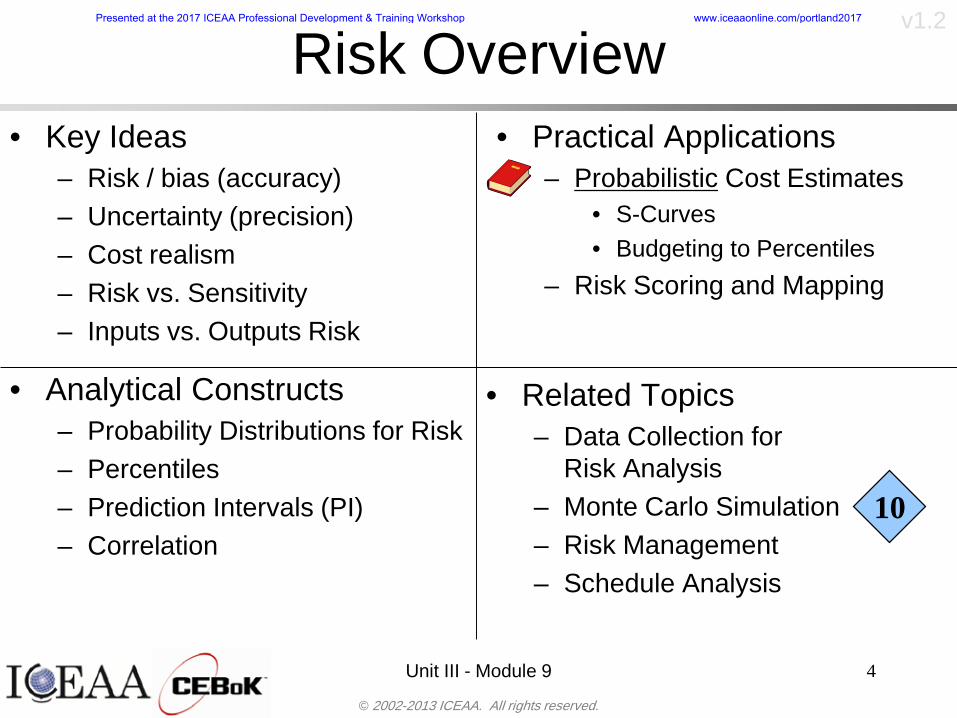
copy 2002-2013 ICEAA All rights reserved
v12
Unit III - Module 9 4
Risk Overviewbull Key Ideas
ndash Risk bias (accuracy)ndash Uncertainty (precision)ndash Cost realismndash Risk vs Sensitivityndash Inputs vs Outputs Risk
bull Practical Applicationsndash Probabilistic Cost Estimates
bull S-Curvesbull Budgeting to Percentiles
ndash Risk Scoring and Mapping
bull Analytical Constructsndash Probability Distributions for Riskndash Percentilesndash Prediction Intervals (PI)ndash Correlation
bull Related Topicsndash Data Collection for
Risk Analysisndash Monte Carlo Simulationndash Risk Managementndash Schedule Analysis
10
Presented at the 2017 ICEAA Professional Development amp Training Workshop wwwiceaaonlinecomportland2017
copy 2002-2013 ICEAA All rights reserved
v12
Agendabull Cost Risk Analysis
ndash Introductionndash Distributions
bull Fitting distributions to historical databull Measuring technical uncertaintybull Measuring estimating uncertainty
ndash Aggregating riskbull Simulationbull Method of momentsbull Correlation
ndash Risk measuresndash Risk allocationndash Joint confidence level analysisndash Practical exercises
bull Comparing simulation with method of moments
Unit III - Module 9 5
Presented at the 2017 ICEAA Professional Development amp Training Workshop wwwiceaaonlinecomportland2017
copy 2002-2013 ICEAA All rights reserved
v12
Unit III - Module 9 6
Introductionbull Cost estimates in many cases project many years in the future
ndash Cost estimates are inherently uncertain regardless of whether risk is included (modeled)
bull Sources of uncertainty include (but are not limited to)ndash Scope and requirements (what is being estimated)ndash Technology readinessndash Manufacturing readinessndash Inflationndash Model uncertainty
bull The cost analysis profession recognizes the importance of risk and has incorporated risk analysis as an integral part of the estimating process
Presented at the 2017 ICEAA Professional Development amp Training Workshop wwwiceaaonlinecomportland2017
copy 2002-2013 ICEAA All rights reserved
v12
Risk Analysis Termsbull Risk is the chance of uncertainty or loss
bull Uncertainty is the indefiniteness about the outcome of a situationndash Includes both favorable and unfavorable events
bull Cost Risk is a measure of the chance that due to unfavorable events the planned or budgeted cost of a project will be exceeded
bull Cost Uncertainty Analysis is a process of quantifying the cost estimating uncertainty due to variance in the cost estimating models as well as variance in the technical performance and programmatic input variables
bull Cost Risk Analysis is a process of quantifying the cost impacts of the unfavorable events
Unit III - Module 9 7
Presented at the 2017 ICEAA Professional Development amp Training Workshop wwwiceaaonlinecomportland2017
copy 2002-2013 ICEAA All rights reserved
v12
Unit III - Module 9 8
Are Our Costs Realisticbull We claim our costs are realisticbull We claim we estimate costs at the 50th percentile
ndash This should mean we have 50 low and 50 high outcomes
bull But we have an unchanging cost growth pattern showing only 12 of our estimates are high (underrun) and 88 are low (overrun)ndash As shown in the graphic on the next slide
bull The conclusion is inescapable our costs are not realistic
bull This also means our costs are at the 12th percentile not the 50th percentile
What Percentile Are We At Now (And Where Are We Going) R Coleman E Druker P Braxton B Cullis C Kanick SCEA 2009 DoDCAS 2010
Presented at the 2017 ICEAA Professional Development amp Training Workshop wwwiceaaonlinecomportland2017
copy 2002-2013 ICEAA All rights reserved
v12
88 Dollars ( in millions)
Co
st G
row
th F
acto
r
0
1
2
3
4
5
6
7
8
0 5000 10000 15000 20000 25000 30000 35000
lsquoUnit III - Module 9 9
Historical Cost Growth
Average program cost growthRampD 21 Prod 19
Fraction of programs ending on-or-under cost target
7-16
Note This pattern appears to be fractal
Uncohorted dollar weighted
This is the line of no growth
The Cost Growth Factor is 10 meaning (Final Cost)(Initial Cost) = 1
Grew to 75 times planned cost
Risk in Cost Estimating General Introduction amp The BMDO Approach 33rd DoDCAS 2000 R L Coleman J R Summerville M DuBois B Myers
Note apparent bounds
Presented at the 2017 ICEAA Professional Development amp Training Workshop wwwiceaaonlinecomportland2017
88 Dollars ( in millions)
Cost Growth Factor
0
1
2
3
4
5
6
7
8
0
5000
10000
15000
20000
25000
30000
35000
copy 2002-2013 ICEAA All rights reserved
v12
Sources of Cost Risk
Unit III - Module 9 10
l Security Risksl Critical failure modesl Energy Environmental Risksl Schedule problems and delaysl Inadequate cost estimates
n Process (need to assess contractorrsquos assumptions)
n Models l ldquoNew Ways of Doing Businessrdquol Inflationl Systems Engineeringl Cost Improvement Curve
Assumptions
l State-of-the-Art-Advance (Technology Readiness)
l Technical Risk Sourcesn Physical propertiesn Material Propertiesn Radiation Properties
(emission and reception)l Material Availability Risksl Testing Modeling Risksl Integration Interface Risksl Program Personnell Safety Risksl Software Design Risks
Historical cost data available
Amount of cost risk depends on the Basis of the Estimate
Presented at the 2017 ICEAA Professional Development amp Training Workshop wwwiceaaonlinecomportland2017
copy 2002-2013 ICEAA All rights reserved
v12
Point Estimates of Costbull Funding organizations need best estimate of cost for
bullCostperformance tradeoff studiesbullCostbenefit analysesbullBudget planning
bull But program cost is nebulous heavily impacted bybullTechnological (im)maturitybullProgrammatic considerationsbullSchedule slipsbullUnforeseen events
bull Point cost estimates cannot be ldquocorrectrdquo becausebullEvery cost element contains uncertaintybullTotal system cost is sum of these WBS elements
bull Actual program cost falls within a range surrounding the best estimate (with some degree of confidence)bullThe best we can hope to do is to understand the uncertaintybullUnderstanding the uncertainty will help us make provision for it
Unit III - Module 9 11
Presented at the 2017 ICEAA Professional Development amp Training Workshop wwwiceaaonlinecomportland2017
copy 2002-2013 ICEAA All rights reserved
v12
Unit III - Module 9 12
Types of Riskbull Cost Growth = Cost Estimating Growth + SkedTech Growth
+ Requirements Growth + Threat Growthbull Cost Risk = Cost Estimating Risk + SkedTech Risk +
Requirements Risk + Threat Riskndash Cost Estimating Risk Risk due to cost estimating errors and the statistical
uncertainty in the estimate ndash ScheduleTechnical Risk Risk due to inability to conquer problems posed
by the intended design in the current CARD or System Specificationsndash Requirements Risk Risk resulting from an as-yet-unseen design shift from
the current CARD or System Specifications arising due to shortfalls in the documents
bull Due to the inability of the intended design to perform the (unchanged) intended mission
bull We didnrsquot understand the solutionndash Threat Risk Risk due to an unrevealed threat eg shift from the current
STAR or threat assessmentbull The problem changedO
ften
impl
icit
or o
mitt
ed
1 2
Presented at the 2017 ICEAA Professional Development amp Training Workshop wwwiceaaonlinecomportland2017
copy 2002-2013 ICEAA All rights reserved
v12
Point Estimates Vs Risk Estimates
Unit III - Module 9 13
DDTampE Flight Unit Production TotalPoint Estimate 63807 5179 6697 70505CER Risk Only - Mean 71176 4805 6426 78018Full Risk - Mean 78937 6490 8091 87430Point Esimtate + 30 82949 6733 8706 91657Full Risk - 70th Percentile 87939 7980 9608 97011
Estimated Total Cost in Millions
Note that the mean is 24 higher than the point estimate and the 70th
percentile is 38 higher than the point estimate
Presented at the 2017 ICEAA Professional Development amp Training Workshop wwwiceaaonlinecomportland2017
copy 2002-2013 ICEAA All rights reserved
v12
Cost Risk and Probabilitybull Cost risk or cost uncertainty analysis represents cost as a
probability distributionbull A probability distribution is a mathematical rule associating a
probability a to each possible outcome or event of interestbull There are two ways to present a probability distribution ndash as a
probability density function (ldquoPDF) and as a cumulative distribution function (ldquoS-curverdquo or ldquoCDFrdquo)
Unit III - Module 9 14
Lognormal Distribution PDF and CDF
0102030405060708090100
200 300 400 500 600 700 800 900 1000Cost $
Con
fiden
ce L
evel
0
00002
00004
00006
00008
0001
00012
00014
00016
Prob
abili
ty D
ensi
ty
CDFPDF
Presented at the 2017 ICEAA Professional Development amp Training Workshop wwwiceaaonlinecomportland2017
copy 2002-2013 ICEAA All rights reserved
v12
Unit III - Module 9 15
Probability Model ndash Distributionbull Normal
ndash Best behavior most iconic
ndash Theoretically (although not practically) allows negative costs which spook some users
ndash Symmetric needs mean shift to reflect propensity for positive growth
bull Lognormalndash A natural result in
non-linear CERsndash Indistinguishable
from Normal at CVs below 25
ndash Skewed
10
4
10
Presented at the 2017 ICEAA Professional Development amp Training Workshop wwwiceaaonlinecomportland2017
copy 2002-2013 ICEAA All rights reserved
v12
Unit III - Module 9 16
bull Triangularndash Most commonndash Easy to use easy to understandndash Modes medians do not addndash Skewed
bull Betandash Rare now but formerly popularndash Solves negative cost and duration issuesndash Many parameters ndash simplifications like PERT
Beta are possiblendash Skewed
bull Bernoullindash Probability is only assigned to two possible
outcomes success and failure (p and 1-p)ndash Simplest of all discrete distributionsndash Mean = pndash Variance = p(1-p)
10
Probability Model ndash Distribution
10
10
Presented at the 2017 ICEAA Professional Development amp Training Workshop wwwiceaaonlinecomportland2017
copy 2002-2013 ICEAA All rights reserved
v12
Unit III - Module 9 17
bull Normalndash If there is a sufficiently large number of independently identically distributed
elements (or not too correlated and not too skewed) then the distribution of total cost is normal due to the Central Limit Theorem
bull Lognormalndash For smaller data sets with large amounts of (positive) correlation and
skewness the lognormal distribution may be a better approximation of total cost
ndash Many total cost distributions in smaller data sets test as both normal and lognormal
bull Triangularndash The sum of triangles is not a triangle so this distribution should generally not
be used to characterize total costbull Convolved
ndash If total cost distribution is derived using simulation then it may not particularly resemble anything In this case we simply have a convolved or simulated total cost distribution
Probability ndash Top-Level Distribution
NEW
Presented at the 2017 ICEAA Professional Development amp Training Workshop wwwiceaaonlinecomportland2017
copy 2002-2013 ICEAA All rights reserved
v12
S-Curves and Confidence Levels
Unit III - Module 9 1818
100
70
25
Probability(Confidence
Level)
Cost Estimate(Dollars)
50
The S curve is the cumulative probability distribution coming out of the statistical summing process
70 confidence that project will cost indicated amount or less
Provides information on potential cost as a result of identified project risks
Provides insight into establishing reserve levels
X Y
MR
X = Point estimateZ = Project requirementY = Cost estimate where there is a 70 change that
final actual cost will be less than cost estimateY-Z= Manage reserve (MR) which is REQUIRED to meet 70 CL
Z
X not always = Z but is based on same content
Presented at the 2017 ICEAA Professional Development amp Training Workshop wwwiceaaonlinecomportland2017
copy 2002-2013 ICEAA All rights reserved
v12
19
Example ndash Normal Distribution
bull Normal distribution with mean equal to 100 and standard deviation equal to 20
bull Median and mode also equal 100bull The 80th Percentile is 117
40 60 80 100 120 140 160
80 of distribution(area under curve)is less than 117
117
Presented at the 2017 ICEAA Professional Development amp Training Workshop wwwiceaaonlinecomportland2017
copy 2002-2013 ICEAA All rights reserved
v12
20
Confidence Levelsbull The output of a cost risk analysis is a probability
distributionndash Typically displayed as a cumulative distribution function or
ldquoS-curverdquondash Confidence levels are simply percentiles of the distribution
0
10
20
30
40
50
60
70
80
90
100
30 60 90 120 150 180
Conf
iden
ce L
evel
Presented at the 2017 ICEAA Professional Development amp Training Workshop wwwiceaaonlinecomportland2017
copy 2002-2013 ICEAA All rights reserved
v12
Measuring Parametric Model Uncertainty
bull When developing estimates using cost-estimating relationships (CERs) there are two major sources of uncertaintyndash Technical (model input) uncertaintyndash Estimating uncertainty
bull Technical uncertainty reflects the uncertainty inherent in the model inputsndash Typical parametric model inputs include weight lines of code
heritage and other performance and management inputs
bull Estimating uncertainty measures the uncertainty inherent in the model due to the modelrsquos inability to capture all aspects of variability in the data
21
Presented at the 2017 ICEAA Professional Development amp Training Workshop wwwiceaaonlinecomportland2017
copy 2002-2013 ICEAA All rights reserved
v12
Parametric Model Examplebull The NASAAir Force Cost Model (NAFCOM) is a
parametric model for estimating acquisition costs for spacecraft and launch vehicles
bull The CERs in NAFCOM have the formCost = C WeightVNewDesignWTechnicalXManagementY ClassZ
bull There is technical uncertainty about each of the parametersndash Parametric models are applied early in a program so there
is significant amount of uncertainty in the weightndash Heritage is also tricky it is inherently subjective and project
personnel are typically optimisticndash Technical characteristics can also change as a program
matures and requirements change
22
Presented at the 2017 ICEAA Professional Development amp Training Workshop wwwiceaaonlinecomportland2017
copy 2002-2013 ICEAA All rights reserved
v12
Weight Uncertaintybull Aerospace weight growth study average satellite
weight growth from program inception to launch is 28
23
Aerospace Weight Growth Data
-10
0
10
20
30
40
50
60
0 4 8 12 16 20 24 28 32 36 40 44 48 52 56 60 64 68 72 76 80 84 88 92 96 100
Percent Program Completion
Perc
ent W
eigh
t Gro
wth
Presented at the 2017 ICEAA Professional Development amp Training Workshop wwwiceaaonlinecomportland2017
copy 2002-2013 ICEAA All rights reserved
v12
Estimating Uncertaintybull CERs do not perfectly fit the historical data
ndash There are non-repeatable random effects that cannot be predicted
bull For examplendash Parts breaking during testingndash Strikes which are difficult to predict
bull This results in an underlying uncertainty distribution about an estimatendash The outcome of a CER represents only one point on an
uncertainty distributionbull Typically mean or median depending upon the CER
methodology
24
Presented at the 2017 ICEAA Professional Development amp Training Workshop wwwiceaaonlinecomportland2017
copy 2002-2013 ICEAA All rights reserved
v12
Estimating Uncertainty (2)
25
Presented at the 2017 ICEAA Professional Development amp Training Workshop wwwiceaaonlinecomportland2017
copy 2002-2013 ICEAA All rights reserved
v12
Estimating Uncertainty (3)bull In the case of a linear regression the estimating
uncertainty follows a normal distributionndash The estimate is the mean and the standard error of the
estimate from the regression is the standard deviation of the normal distribution
bull In the case of a log-transformed linear regression the estimating uncertainty follows a lognormal distributionndash The estimate is the median of the lognormal and the
standard error of the estimate from the regression is the standard deviation of the normal distribution (in log-space)
bull There is additional uncertainty about an estimate based upon the distance of what is being estimated from the mean of the input datandash This results in a prediction interval
26
Presented at the 2017 ICEAA Professional Development amp Training Workshop wwwiceaaonlinecomportland2017
copy 2002-2013 ICEAA All rights reserved
v12
Aggregating Riskbull Risk is typically applied at the same level at
which we estimate cost that is at the Work Breakdown Structure (WBS) level
bull The estimates for each WBS are developedndash These estimates sum to yield the total system cost
bull For an n-element WBS the total cost is the sum of the cost for each of the n elements
27
nXXXCostSystem +++= 21
Presented at the 2017 ICEAA Professional Development amp Training Workshop wwwiceaaonlinecomportland2017
copy 2002-2013 ICEAA All rights reserved
v12
WBS Examplebull Launch Vehicle
ndash Structurebull Vehicle Structurebull Tank Structure
ndash Thermal Controlbull Active Thermal Controlbull Induced Thermal Controlbull Tank Thermal Control
ndash Main Propulsion Systemndash Liquid Rocket Enginendash Electric Power and Distributionndash Command Control and Data Handlingndash System Integration
28
Presented at the 2017 ICEAA Professional Development amp Training Workshop wwwiceaaonlinecomportland2017
copy 2002-2013 ICEAA All rights reserved
v12
WBS and Risk
29
Presented at the 2017 ICEAA Professional Development amp Training Workshop wwwiceaaonlinecomportland2017
copy 2002-2013 ICEAA All rights reserved
v12
Aggregating Riskbull This leads us to the issue of aggregating the risks across the
WBSbull For example if we want to determine the 70th percentile of the
overall cost risk distribution how do we proceed bull Note that we cannot simply add the 70th percentiles of each of
the cost risk distributionsbull We can add means and variances (taking correlation into
account more on that later) but that is all
Variance of Total Cost =
30
Mean of Total Cost = ( )E X E Xk
k
n
kk
n
kk
n
= = =aringaelig
egraveccediloumloslashdivide
= =aring aring1 1 1
m
Var X kk
n
=aringaelig
egraveccediloumloslashdivide1
= s r s skk
n
iji
j
i jj
n2
1 1
1
22+aring aringaring
= =
-
=
Presented at the 2017 ICEAA Professional Development amp Training Workshop wwwiceaaonlinecomportland2017
copy 2002-2013 ICEAA All rights reserved
v12
Percentiles Do Not Addbull As a notional example consider two independent normal
distributionsndash One distribution has mean equal to 100 and standard deviation
equal to 20ndash The second distribution has mean 300 and standard deviation of 80
bull The sum of two independent normally distributed random variables is also normally distributed
bull To combine the two distributions we add the means and add the variancesndash Total mean is
ndash Total standard deviation is
31
400300100 =+
8258020 22 raquo+
Presented at the 2017 ICEAA Professional Development amp Training Workshop wwwiceaaonlinecomportland2017
copy 2002-2013 ICEAA All rights reserved
v12
Percentiles Do Not Add (2)bull The 80th percentiles for the individual distributions are
117 and 367 respbull The 80th percentile of the combined distribution is
469 but the sum of the two 80th percentiles is 484bull To see why this is the case note that the percentiles
of a normal distribution are determined by the mean and the standard deviationndash The standard deviations are not added when normal distributions
are combined rather the variances are combinedndash Sum of variances is ndash The standard deviation of this sum is
32
22 ba +22 ba +
Presented at the 2017 ICEAA Professional Development amp Training Workshop wwwiceaaonlinecomportland2017
copy 2002-2013 ICEAA All rights reserved
v12
Percentiles Do Not Add (3)bull Since bull We can write
bull The left side of this inequality represents the risk of the combined distributions while the right side represents the sums of the individual risks
bull Combining two missions that are independent results in a diversification of riskndash The total portfolio is not as risky on a relative basis as each
individual project
33
2222 2 bababa ++lt+
baba +lt+ 22
Presented at the 2017 ICEAA Professional Development amp Training Workshop wwwiceaaonlinecomportland2017
copy 2002-2013 ICEAA All rights reserved
v12
Methods for Aggregating Riskbull Since percentiles do not add we have to find other
ways to aggregate riskbull One method is to use Monte Carlo simulationbull Unless cost risk is represented by normal
distributions for all WBS elements summing the means and variances does not result in a completely accurate depiction of overall system cost risk
bull The normal distribution is not a realistic distribution for representing risk in many or even most situations since regarding project risk more can go wrong than can go right which means the risk is NOT symmetric unlike the Gaussian bell curve
34
Presented at the 2017 ICEAA Professional Development amp Training Workshop wwwiceaaonlinecomportland2017
copy 2002-2013 ICEAA All rights reserved
v12
Unit III - Module 9 35
Monte Carlo Simulationfor Risk Analysis
bull When risk analysis is performed multiple risks are gatheredndash These risks may have various probability
distributions
bull Monte Carlo is the most commonly accepted way to produce an accurate characterization of the distribution of the combined effect of these many risksndash Using this distribution we can produce percentiles
for cost impacts due to risk occurrences
10
Presented at the 2017 ICEAA Professional Development amp Training Workshop wwwiceaaonlinecomportland2017
copy 2002-2013 ICEAA All rights reserved
v12
Monte Carlo Simulationbull Simulation is a means for solving problems that are
analytically intractablendash Involves repeated random sampling
bull It was developed during the Manhattan Project as a way to model the interactions inside an atom during nuclear fissionndash Allowed for more sophisticated mathematical modeling of atomic
phenomena
bull Most computer packages use pseudo-random number generators that produce seemingly random results from an initial seedndash Example is the linear congruential generator
36
( ) mbaXX nn mod1 +=+
Presented at the 2017 ICEAA Professional Development amp Training Workshop wwwiceaaonlinecomportland2017
copy 2002-2013 ICEAA All rights reserved
v12Using Random Numbers to Simulate Distributions
bull WBS cost risk is typically measured by a probability distributionbull The most common method for simulating a probability
distribution is the inverse methodbull This involve obtaining a simulated random value from a uniform
distribution and then inverting this through the cumulative distribution function (CDF) to obtain the simulated value
bull As an example for a uniform distribution on the interval [0100]
bull In this case the CDF random value of 05 translates to 10005 = 50
37
( )100
1=xf ( )
100xxF = ( ) xxF 1001 =-
Presented at the 2017 ICEAA Professional Development amp Training Workshop wwwiceaaonlinecomportland2017
copy 2002-2013 ICEAA All rights reserved
v12
Simulating a Triangular Distribution
bull For a triangular distribution with low = 0 most likely = 50 and high = 150 the CDF is given by
bull The inverse function is given by
38
( )iumliumlicirc
iumliumliacute
igrave
poundlt--
poundpound=
1505021
1500050
50015000
2
2
2
xxx
xxxF
( )iumliumlicirc
iumliumliacute
igrave
poundltdivideoslashouml
ccedilegraveaelig +--
poundpound=-
131
21
37501
250017500150
3107500
1
xx
xxxF
Presented at the 2017 ICEAA Professional Development amp Training Workshop wwwiceaaonlinecomportland2017
copy 2002-2013 ICEAA All rights reserved
v12
Simulating a Triangular Distribution (2)
bull If the simulated uniform value is equal to 02 the corresponding inverse value from the CDF inverse is approximately 387
39
0
01
02
03
04
05
06
07
08
09
1
0 30 60 90 120 150
Presented at the 2017 ICEAA Professional Development amp Training Workshop wwwiceaaonlinecomportland2017
copy 2002-2013 ICEAA All rights reserved
v12
Monte Carlo and the WBSbull Simulation involves repeated trials
40
WBS Draw1 2 3 4 5
System 2912 3566 4390 2954 4655 Sum
Structure 80 105 55 80 57 SumVehicle Structure 50 70 30 40 20Tank Structure 30 35 25 40 37
Thermal Control 32 36 35 29 33 SumActive Thermal Control 10 15 12 7 10Induced Thermal Control 12 14 13 14 14Tank Thermal Control 10 7 10 8 9
Main Propulsion System 100 150 125 140 100
Liquid Rocket Engine 1000 1100 1800 900 2200
Electric Power and Distribution 100 125 150 75 90
Command Control and Data Handling 200 250 225 230 275
System Integration 1400 1800 2000 1500 1900
Presented at the 2017 ICEAA Professional Development amp Training Workshop wwwiceaaonlinecomportland2017
copy 2002-2013 ICEAA All rights reserved
v12
Number of Trialsbull Monte Carlo involves a repeated number of trialsbull The greater the number of trials the more accurate the
simulation will approximate the overall cost risk behavior of the system
bull After 100 trials the histogram looks very jagged
41
Presented at the 2017 ICEAA Professional Development amp Training Workshop wwwiceaaonlinecomportland2017
copy 2002-2013 ICEAA All rights reserved
v12
Number of Trials (2)
42
1000 Trials
10000 Trials
50000 Trials Additional trials give a more accurate depiction of the final result
Presented at the 2017 ICEAA Professional Development amp Training Workshop wwwiceaaonlinecomportland2017
copy 2002-2013 ICEAA All rights reserved
v12
Number of Trials (3)bull If we want to simulate the underlying
mean within 1 with 95 confidence for example then we require
43
divideoslash
oumlccedilegrave
aelig poundpound-
=
dividedividedivide
oslash
ouml
ccedilccedilccedil
egrave
aeligpound
-pound
-=
divideoslashouml
ccedilegraveaelig poundpound=
nZ
n
nnX
n
X
n
n
011
010Pr
011
010Pr
011990Pr950
___
___
sm
sm
sm
sm
sm
mm
Presented at the 2017 ICEAA Professional Development amp Training Workshop wwwiceaaonlinecomportland2017
copy 2002-2013 ICEAA All rights reserved
v12
Number of Trials (4)bull This means that the number of trials required is determined by
bull Solving for n we find that at least
trials are neededbull Note that this term involves the coefficient of variation of the
distribution which means that distributions with less dispersion require fewer trials to accurate simulate
44
96101
=ns
m
ms41638
Presented at the 2017 ICEAA Professional Development amp Training Workshop wwwiceaaonlinecomportland2017
copy 2002-2013 ICEAA All rights reserved
v12
Number of Trials (5)bull Simulating percentiles requires more trials than for simulating
meansbull Let Pn represent the number of trials in the sample at or below
the 70th percentile of the underlying distribution (suppose this is known)
bull By the Central Limit Theorem Pnn follows a normal distribution with mean equal to the 70th percentile and variance equal to
bull By a similar process for the mean we find that the number of trials needed to simulate the 70th percentile within 1 with 95 confidence is
45
( )n
FF 700700 1-
n
n
PPn -41638
Presented at the 2017 ICEAA Professional Development amp Training Workshop wwwiceaaonlinecomportland2017
copy 2002-2013 ICEAA All rights reserved
v12
Number of Trials (6)bull If Pn 070 for all n then n is approximately
bull For the sake of comparison suppose CV = 03 (reasonable approximation for hardware development) then the number of trials needed to simulate the mean with the same accuracy is then ldquoonlyrdquo 11525
bull More trials are needed to accurately simulate percentiles than means
46
( ) 46416703041638
70704168341638 =divide
oslashouml
ccedilegraveaelig=divide
oslashouml
ccedilegraveaelig -
=-
nnn
PPn
n
n
Presented at the 2017 ICEAA Professional Development amp Training Workshop wwwiceaaonlinecomportland2017
copy 2002-2013 ICEAA All rights reserved
v12
Methods of Simulationbull Monte Carlo simulation is a standard term for
simulationbull However there is an improvement on Monte Carlo
that improves the accuracy of the results of a simulation for a given number of trials
bull This method is call the Latin Hypercube approach to simulationndash Similar to Monte Carlo but an equal number of draws are taken
from a set of subintervals for example dividing the interval (01) into [00001) [0102)hellip [0910]
ndash Instead of 10 trials from [01] we have one trial from each subinterval
ndash Rough rule of thumb is Latin Hypercube takes 30 fewer trials to achieve similar accuracy to Monte Carlo
47
Presented at the 2017 ICEAA Professional Development amp Training Workshop wwwiceaaonlinecomportland2017
copy 2002-2013 ICEAA All rights reserved
v12
Probability Model ndash Correlationbull Correlation exists between work breakdown structure
(WBS) cost element costs and between cost and schedule
bull Correlation is a necessary consideration in cost risk analysis
bull Correlation is a number that can vary between -1 and +1 and represents the strength of the relationship between the two variablesndash If both variable have a tendency to move in the same direction
correlation is positivendash If when one variable increases the other tends to decrease and
vice-versa the correlation between the two variables is negative
Presented at the 2017 ICEAA Professional Development amp Training Workshop wwwiceaaonlinecomportland2017
copy 2002-2013 ICEAA All rights reserved
v12
Correlation And Causationbull Note that correlation is not causation however
causation implies correlationndash For example shark attacks and ice cream sales at the beach
bull For example for a launch vehicle structure increasing the diameter will not only result in an increase in the structures cost but will also result in higher costs for thermal coating (paint etc)
bull Also simply because two subsystems do not appear to be related does not mean they are not correlatedndash For example structures and computer equipment seemingly
have little relation to one another however an external factor such as a funding cut or a strike will impact all subsystems leading to delays and increasing cost across the board
ndash Thus everything in a WBS has some correlationUnit III - Module 9 49
Presented at the 2017 ICEAA Professional Development amp Training Workshop wwwiceaaonlinecomportland2017
copy 2002-2013 ICEAA All rights reserved
v12
The Importance of Correlationbull Percent that total cost standard deviation is underestimated
when correlation assumed to be 0 instead of r given nWBS elements
Unit III - Module 9 5050
0
20
40
60
80
100
0 01 02 03 04 05 06 07 08 09 1Actual Correlation
Perce
nt Un
deres
timate
d
n = 10
n = 30
n = 100n = 1000
0
20
40
60
80
100
0 01 02 03 04 05 06 07 08 09 1Actual Correlation
Perce
nt Un
deres
timate
d
n = 10
n = 30
n = 100n = 1000
Reference 32nd Annual DOD Cost Analysis Symposium Advanced Training Session ldquoWhy Correlation Matters in Cost Estimatingrdquo Stephen A Book
Presented at the 2017 ICEAA Professional Development amp Training Workshop wwwiceaaonlinecomportland2017
copy 2002-2013 ICEAA All rights reserved
v12
The Importance of Correlation (2)bull For example if correlation is assumed to be 0 for all
elements in a 30 element WBS and the actual correlation is 20 then the total cost standard deviation is underestimated by 60
bull For example assume the total cost is modeled as a normal distribution with mean = 100
bull If correlation is assumed to be zero with total cost standard deviation = 12 when correlation is actually 20 then the true underlying standard deviation is actually 30
bull 70th percentile with zero correlation assumption is 106
bull 70th percentile with 20 correlation is 116 Unit III - Module 9 51
Presented at the 2017 ICEAA Professional Development amp Training Workshop wwwiceaaonlinecomportland2017
copy 2002-2013 ICEAA All rights reserved
v12
Measures of Correlationbull Two measures of correlation are commonly used in
cost risk analysesndash Pearsonrsquos product-moment correlation coefficient ndash Spearmanrsquos rank correlation coefficient
bull Garvey and others recommend using Pearsonrsquos product-moment correlation coefficient correlation for cost risk analysesndash Method of moments uses this but there are two options in
simulationndash Popular simulation packages like Risk and Crystal Ball use
rank correlation but in practice this has been found to make little difference
ndash Pearson product-moment correlation has been incorporated into Risk+
52
Presented at the 2017 ICEAA Professional Development amp Training Workshop wwwiceaaonlinecomportland2017
copy 2002-2013 ICEAA All rights reserved
v12
Pearson Correlationbull Pearsonrsquos product-moment correlation measures
degree of linearity between two random variables bull If two random variables are perfectly linear (eg Y =
aX + b) with positive slope then the Pearson product-moment correlation between X and Y denoted by rXY is +1
53
X X
Y Y Y
XNegative Correlation Positive Correlation No Correlation
middotmiddot
middotmiddot
middotmiddot middotmiddot
middotmiddot
middot
middot
middotmiddotmiddot
middotmiddot
middotmiddot
middotmiddot middot
middot
middot
middotmiddotmiddotmiddotmiddotmiddotmiddotmiddot
middotmiddotmiddotmiddot
middotmiddot
middotmiddot middotmiddotmiddotmiddot
middotmiddotmiddot
middotmiddotmiddotmiddot
middotmiddotmiddot
middotmiddotmiddot
middotmiddot
middot
middot middotmiddot
middot middotmiddotmiddotmiddot middotmiddot middot middotmiddot middot middot
middotmiddot middot
middotmiddotmiddotmiddotmiddot middot middotmiddot
middotmiddot
middot
middotmiddot
middotmiddot middot
middot middot middot
middotmiddot middot
middotmiddotmiddot
middotmiddot
middot middot
Presented at the 2017 ICEAA Professional Development amp Training Workshop wwwiceaaonlinecomportland2017
copy 2002-2013 ICEAA All rights reserved
v12
Spearman Correlationbull Spearmanrsquos rank correlation measures the
monotonicity between two random variablesbull If two random variables are perfectly monotonically
increasing (eg Y = X2) then the Spearman rank correlation denoted by rXY is +1
bull The two measures can be significantly different
54
10 20 30 40 50 60
100
200
300
096 097 098 099 1
1
060
020
040
080
Eff
ort (
Staf
f-M
onth
s)
Software Size I KDSI
y = 28z12y
z x
yy = x100
0 pound x pound 1
Figure 5-9A Figure 5-9B
Pearson Correlation = 09976 Rank Correlation = 1
Pearson Correlation = 024 Rank Correlation = 1
X(x ) ~ Unif(01)
Reference Probability Methods for Cost Uncertainty Analysis A Systems Engineering Perspective Paul R Garvey
Presented at the 2017 ICEAA Professional Development amp Training Workshop wwwiceaaonlinecomportland2017
copy 2002-2013 ICEAA All rights reserved
v12
Unit III - Module 9 55
200
250
300
350
400
1000 1200 1400 1600 1800 2000
Recurring Production
SEPM
200
250
300
350
400
1000 1200 1400 1600 1800 2000
Recurring Production
SEPM
Functional Correlationbull Old No Functional
Correlation Simulation run with WBS items entered as values
bull New Simulation run with functional dependencies entered as they are in cost model
CorrelatedNot Correlated
Note shift of mean and increased variability
Presented at the 2017 ICEAA Professional Development amp Training Workshop wwwiceaaonlinecomportland2017
copy 2002-2013 ICEAA All rights reserved
v12
Risk Measuresbull ldquoWestern Europe conquered the word because of a
technological revolution that started because of attempts to measure the worldrdquo ndash Phillipe Jorion ndash In the same way attempts to measure risk will lead to better project
managementbull Risk management for DoD and NASA agencies focuses
primarily on funding projects to a single percentile ndash NASA policy explicitly mentions 70 and 50ndash This is known as ldquoValue at Riskrdquo and is prevalent in the banking and
financial industry
56
Presented at the 2017 ICEAA Professional Development amp Training Workshop wwwiceaaonlinecomportland2017
copy 2002-2013 ICEAA All rights reserved
v12
Value at Risk (VaR)bull VaR is a percentile of the cost risk
distributionndash VaR funding at the 70th percentile means that
there is a 30 chance of final project cost exceeding the funded amount (budget)
bull VaR has some meritsndash Common measure can be used to compare
different projects and programsndash Easily understood by senior managers and
decision makers
57
Presented at the 2017 ICEAA Professional Development amp Training Workshop wwwiceaaonlinecomportland2017
copy 2002-2013 ICEAA All rights reserved
v12
Why 70th or 80th Percentilebull Typical policy guidance involves funding at the 70th or 80th
percentile Why fund as such a low percentilebull There is some incentive to not over-fundbull For a normal distribution an inflection point occurs near the 80th
percentile meaning that for values above 80 confidence achieving higher levels of confidence can only be achieved by spending greater dollar amounts at an increasing rate
58
-05-04-03-02-01
00102030405
0 05 1 15 2 25 3
Standard Deviations from Mean
Normal Distribution
First DerivativeSlopeVelocity
Second DerivativeConvexityAcceleration
Inflection point at one standard deviation above the mean (~84th
percentile)
Presented at the 2017 ICEAA Professional Development amp Training Workshop wwwiceaaonlinecomportland2017
copy 2002-2013 ICEAA All rights reserved
v12
Funding Above Inflection Pointsbull As the percentile goes above the 80th percentile the amount
needed to achieve that higher level of confidence begins to increase at an increasing rate as is evident from the graph
59
0
10
20
30
40
50
60
70
50 55 60 65 70 75 80 85 90 95 100
$ Ab
ove
MEa
n to
Ach
ieve
Per
cent
ile
Percentile (Confidence Level)
Presented at the 2017 ICEAA Professional Development amp Training Workshop wwwiceaaonlinecomportland2017
copy 2002-2013 ICEAA All rights reserved
v12
Why Budget to the 70th or 80thbull Government projects are funded at the 70th or 80th percentilesbull Why not the 90th or 99th percentile Wonrsquot that help prevent
overrunsndash As we have seen percentiles do not add across programs
bull The sum of the 80th percentiles does NOT equal the total 80th percentile
ndash This is because the individual programs are riskier than the entire suite of missions
bull Known as the ldquoPortfolio effectrdquo (more or this later)
ndash Funding at the 80th gives confidence that the entire portfolio will be adequately funded
bull And since there is an inflection point near the 80th percentile funding above that level quickly becomes cost prohibitive
60
Presented at the 2017 ICEAA Professional Development amp Training Workshop wwwiceaaonlinecomportland2017
copy 2002-2013 ICEAA All rights reserved
v12
Inflection Points for Lognormalbull For a lognormal the inflection point
variesndash Coefficient of variation equal to 10 equates to an
inflection point at the 70th percentile
61
0
10
20
30
40
50
60
70
050 060 070 080 090 100
Coef
ficen
t of V
aria
tion
Percentile of the Inflection Point
Presented at the 2017 ICEAA Professional Development amp Training Workshop wwwiceaaonlinecomportland2017
copy 2002-2013 ICEAA All rights reserved
v12
Issues with Percentile Fundingbull However risk management does not stop at a
specific percentilendash What happens when the 70th percentile is exceeded
bull Any effective risk management policy should prescribe what happens after a bad event occursndash With VaR we only know when a bad event has occurred ndash Also funding at a relatively low level means we have no true
sense of the real risks that should be guarded against
62
Presented at the 2017 ICEAA Professional Development amp Training Workshop wwwiceaaonlinecomportland2017
copy 2002-2013 ICEAA All rights reserved
v12
ldquoHere There Be Dragonsrdquobull On old maps uncharted territory was often
marked with monsters or dragons
63
A section of the Carta Marina by Olaus Magnus 16th Century
Presented at the 2017 ICEAA Professional Development amp Training Workshop wwwiceaaonlinecomportland2017
copy 2002-2013 ICEAA All rights reserved
v12
Distribution Comparisonbull Four different distributions with the same 70th
percentile
bull Should we expect the tails to be similar
64
0
10
20
30
40
50
60
70
80
0 100 200 300 400 500 600
Perc
entil
eCo
nfid
ence
Lev
el
Triangular
Normal
Lognormal
Pareto
Presented at the 2017 ICEAA Professional Development amp Training Workshop wwwiceaaonlinecomportland2017
copy 2002-2013 ICEAA All rights reserved
v12Distribution Comparison Tail Behavior
bull The normal and triangular distributions have similar tails but the lognormal and Pareto have much fatter right tails
65
70
75
80
85
90
95
100
500 1500 2500 3500 4500 5500
Perc
entil
eCo
nfid
ence
Lev
el
Triangular
Normal
Lognormal
Pareto
Here There Be Dragons
Presented at the 2017 ICEAA Professional Development amp Training Workshop wwwiceaaonlinecomportland2017
copy 2002-2013 ICEAA All rights reserved
v12Distribution Comparison ndash Tail Behavior (Table)
bull There is significant tail risk for the lognormal and the Paretobull The 99th percentile for the Pareto is 1000 times greater than
the 70th percentilendash Risk seen in financial markets and in catastrophic risks like natural
disasters bull Four different projects follow the four different risk profiles seen
in this example should clearly have different risk management approaches but 70th percentile funding indicates the same risk management approach for all four
66
Percentile Triangular Normal Lognormal Pareto 70th $600 $600 $600 $600 80th $680 $660 $770 $1430 90th $770 $750 $1070 $5880 95th $840 $820 $1410 $23750 99th $930 $950 $2350 $600000
Presented at the 2017 ICEAA Professional Development amp Training Workshop wwwiceaaonlinecomportland2017
copy 2002-2013 ICEAA All rights reserved
v12Percentile Budgeting is Not Risk Management
bull Percentile budgeting ne effective risk management policybull Suppose that you are shopping for a new car You
mention that safety is your top concern The salesman says he has a great safe car available You ask about the air bags Do they work The salesman answers ldquoOf course Seventy percent of the time they work fine Only 30 of the time the air bags will fail to deployrdquo Would you buy such a car Hedge fund manager David Einhorn has stated ldquoRisk management is the air bag that must always work but only in the multi-sigma event where you have an accidentrdquo
67
Risk management is the air bag that must always work but only in the multi-sigma event where you
have an accident
Presented at the 2017 ICEAA Professional Development amp Training Workshop wwwiceaaonlinecomportland2017
copy 2002-2013 ICEAA All rights reserved
v12
Joint Confidence Level Analysisbull Schedules are risky toobull For 98 recent NASA missions average
schedule growth was 38ndash Not as high as cost growth but still significant
68
0
5
10
15
20
25
30
35
40
Schedule
Cost
Presented at the 2017 ICEAA Professional Development amp Training Workshop wwwiceaaonlinecomportland2017
copy 2002-2013 ICEAA All rights reserved
v12
Schedules Impact Costbull Changes in schedule can have enormous
impacts on cost ndash Schedule slips can lead to cost increases
bull Fixed programmatic costs must be paid on a regular basisndash Achieving schedule milestones early can result in cost
savings
bull Schedule is an important consideration in cost analysis including cost risk analysis
bull However we must be careful in correctly integrating cost and schedule riskndash Schedule is not simply an input but is dependent on many of
the same factors that drive cost
69
Presented at the 2017 ICEAA Professional Development amp Training Workshop wwwiceaaonlinecomportland2017
copy 2002-2013 ICEAA All rights reserved
v12
The Relationship of Cost to Schedulebull Cost and schedule are positively correlated
ndash A larger program with bigger scope with take longer to complete than a smaller simpler program
bull However longer schedules do not always equate to higher cost nor shorter schedules with lower costndash Highly compressed schedules relative to the
optimal schedule can lead to large overrunsbull Compressed schedules are commonplace for
many planetary missions
70
Presented at the 2017 ICEAA Professional Development amp Training Workshop wwwiceaaonlinecomportland2017
copy 2002-2013 ICEAA All rights reserved
v12The Impact of Schedule GrowthCompression on Cost
bull Compressed schedules lead to cost growth and based on existing research is actually more expensive than schedule slippages
71
0
20
40
60
80
100
120
140
160
-50 -25 0 25 50 75 100
Percentage Change in Schedule
Perc
enta
ge C
hang
e in
Cos
t due
to
Sche
dule
Cha
nge
Source Smart CB ldquoCost and Schedule Interrelationshipsrdquo 2007 NASA Cost Symposium
Presented at the 2017 ICEAA Professional Development amp Training Workshop wwwiceaaonlinecomportland2017
copy 2002-2013 ICEAA All rights reserved
v12Schedule as an Independent Variable
bull Why not simply add schedule as an input to cost-estimating relationships (CERs)
bull Schedule is often treated as an independent variable ndash schedules are often determined independently of cost considerationsndash Cost may not be considered explicitly although budgets and
schedules are determined based on scope and other common factors
bull In 2006 SAIC undertook a research task to determine the impact of schedule on cost and added schedule as an independent variable to the CERs in the NASAAir Force Cost Model (NAFCOM) to see if schedule provided any improvement in goodness of fit
72
Presented at the 2017 ICEAA Professional Development amp Training Workshop wwwiceaaonlinecomportland2017
copy 2002-2013 ICEAA All rights reserved
v12
Schedule is a Dependent Variablebull Since NAFCOM includes an exhaustive list of cost drivers the inclusion
of schedule should give an indication of whether there is any additional independent value added from schedule independent of the cost drivers
bull In the study schedule was added to 10 subsystem-level CERs
ndash In each case the addition of schedule did NOTimprove the goodness of fit and schedule was NOT found to be a statistically significant cost driver (given the presence of the other variables) for any of the 10 CERs
bull Standard errors for the CERs increased due to decrease in degrees of freedom
bull Thus schedule as an independent variable did not provide any additional explanation of variation in historical cost
bull This is because schedule is truly NOT an independent variable but a dependent variable and is a function of the same factors that drive cost
73
Presented at the 2017 ICEAA Professional Development amp Training Workshop wwwiceaaonlinecomportland2017
copy 2002-2013 ICEAA All rights reserved
v12
Incorporation of Schedule in Cost Risk
bull When using subjective methods care must be taken in applying schedule to cost risk analysis
bull Since schedule is a dependent variable treating it independently from other factors when assessing its impact on cost can lead to a double count of independent variables in the cost risk analysis
bull Direct inclusion of schedule in a cost risk analysis effectively doubles the influence of each cost driver
ndash Incorrectly leads to broader risk ranges
74
CostWeight
HeritageNewness
Technology Readiness Schedule
Presented at the 2017 ICEAA Professional Development amp Training Workshop wwwiceaaonlinecomportland2017
copy 2002-2013 ICEAA All rights reserved
v12Subjective Cost Risk Methods and Overinclusion of Risk Factors
bull Subjective methods are suitable when data are scarce or not availablebull However care must be taken not to treat correlated sources of risk
such as schedule as independent of each otherbull Example ndash a subjective risk analysis incorporated technology readiness
design risk requirements stability integration risk and schedule and treated each source of risk as independent
bull Risk triangle high value without schedule risk was 31 times the point estimate
bull Risk triangle high value with schedule risk added on top of other sources of risk treated independently was 34 times the point estimate
bull Risk triangle taking correlation between sources of risk into account in a rigorous statistical manner has a high value 15 times the point estimate less than half the effect when treating sources of risk as independent
75
Presented at the 2017 ICEAA Professional Development amp Training Workshop wwwiceaaonlinecomportland2017
copy 2002-2013 ICEAA All rights reserved
v12Fundamental Equation of Cost and Schedule Interrelationships
bull The Fundamental Equation of the Relationship Between Cost and Schedule is
Time = Moneybull This is a well known adage that time is money Your boss at
work may even mention this to you from time to time or if you are the boss you are all too aware of this iron law
bull Because time is money cost and schedule risk should be modeled jointly not with schedule as an independent cost driver
bull Note that cost and schedule are not perfectly correlatedndash Cost can sometimes ldquobuy downrdquo schedule extra money can be
spent to meet a deadline since in some cases additional effort to hasten the completion of a task
76
Presented at the 2017 ICEAA Professional Development amp Training Workshop wwwiceaaonlinecomportland2017
copy 2002-2013 ICEAA All rights reserved
v12How to (Correctly) Incorporate Schedule into Cost Risk Analysis
bull The best way to model cost and schedule risk is to develop a joint cost and schedule model based on the same data
bull Since such models are not currently available the next best approach is to model cost and schedule independently and then integrate cost and schedule risk analyses using joint probability distributions taking into account correlation between cost and schedulendash This approach pioneered by Paul Garvey and Steve Book is
considered industry best practicendash This is a practical method mathematically tractable and follows
naturally from the Fundamental Equation of Cost and Schedule Interrelationships
77
Book S A ldquoQuantifying the Relationship Between Cost and Schedulerdquo The Measurable News Winter 2007-2008 pp 11-15Garvey PR Probability Methods for Cost Uncertainty Analysis A Systems Engineering Perspective New York Marcel Dekker 2000 pp 308-335
Presented at the 2017 ICEAA Professional Development amp Training Workshop wwwiceaaonlinecomportland2017
copy 2002-2013 ICEAA All rights reserved
v12
Joint Lognormal and Normal Distributions
bull Cost and schedule are typically modeled as some combination of Normal and Lognormal probability distributionsndash Studies by The Aerospace Corporation the MITRE
Corporation Wyle Labs and SAIC have found that the Lognormal probability distribution almost always serves as a good model for both the schedule distribution and the cost distribution
ndash The Normal distribution may also be appropriate in some instances and depending upon the level of confidence at which budgets are set may even be more conservative and logically consistent than the Normal distribution
ndash Joint Lognormal and Normal distributions are defined by a pair of mean and standard deviations and a level of correlation between the two
78
Presented at the 2017 ICEAA Professional Development amp Training Workshop wwwiceaaonlinecomportland2017
copy 2002-2013 ICEAA All rights reserved
v12Modeling Cost and Schedule as a Bivariate Distribution
bull In the approach set forth by Book and Garvey cost risk is assessed and the top-level distribution is modeled as a Lognormal (or Normal) distribution schedule risk is assessed and the overall schedule risk is modeled as a Lognormal (or Normal) distribution
bull The two distributions are combined into a Bivariate distribution by assigning a correlation between the two and by treating the two distributions as the marginal distributions of a Bivariate Lognormal distributionndash Other combinations include a Bivariate Normal or a Bivariate
Normal-Lognormal
79
Presented at the 2017 ICEAA Professional Development amp Training Workshop wwwiceaaonlinecomportland2017
copy 2002-2013 ICEAA All rights reserved
v12Bivariate Lognormal Distribution for Cost and Schedule
bull Cost is often observed to be Lognormal when strong positive correlations are present among the systemrsquos WBS cost element costs
bull A systemrsquos schedule is often observed (from Monte Carlo simulations) to be Lognormal if it is the sum of many positively correlated schedule activities in an overall schedule network
bull If Lognormal distributions characterize a systemrsquos cost and schedule then the Bivariate Lognormal could serve as an assumed model of their joint distributionndash In this case the marginal distribution of each of cost and schedule is
Lognormalbull Other possibilities for modeling cost and schedule as a Bivariate
distribution include a Bivariate Normal or a Bivariate Normal-Lognormal distributionndash All these combinations are analytically tractable
80
Presented at the 2017 ICEAA Professional Development amp Training Workshop wwwiceaaonlinecomportland2017
copy 2002-2013 ICEAA All rights reserved
v12Bivariate Lognormal for Cost and Schedule
bull Contour Plots of a Bivariate Lognormal
81
Presented at the 2017 ICEAA Professional Development amp Training Workshop wwwiceaaonlinecomportland2017
copy 2002-2013 ICEAA All rights reserved
v12Correlation Between Cost and Schedule
bull Cost and schedule are positively correlated but not perfectly sondash For example it is possible to have a schedule underrun and a cost
overrunbull Based on cost and schedule growth data for 50 completed NASA
programs the correlation between development cost and development schedule is 70
82
00
200
400
600
800
1000
1200
-500 00 500 1000 1500 2000 2500Historical Cost Growth
Hist
oric
al S
ched
ule
Gro
wth
r = 715
Presented at the 2017 ICEAA Professional Development amp Training Workshop wwwiceaaonlinecomportland2017
copy 2002-2013 ICEAA All rights reserved
v12Correlation Between Cost and Schedule Caveats
bull Based on historical data recommended correlation between cost and schedule is 70 but this could be higher or lower depending upon program circumstancesndash If program is budget constrained cost and schedule will be
more highly correlated (go as you pay)ndash If program is schedule constrained cost and schedule will
have lower correlation perhaps even negative correlation ndash Smaller programs have smaller correlation between cost and
schedule riskbull Relatively easy to ldquohurry uprdquo and finish on time or even early if
needed
83
Presented at the 2017 ICEAA Professional Development amp Training Workshop wwwiceaaonlinecomportland2017
copy 2002-2013 ICEAA All rights reserved
v12
Conditional Confidence Levelsbull Given a programrsquos project schedule we can determine the cost
risk distribution conditional upon the given schedulebull Conditional cost S-curves are steeper than unconditional
(marginal) cost S-curves between some uncertainty has been removed because schedule is fixed
84
Presented at the 2017 ICEAA Professional Development amp Training Workshop wwwiceaaonlinecomportland2017
copy 2002-2013 ICEAA All rights reserved
v12
Joint Confidence Levelsbull Joint 65 confidence represents the probability of
achieving both 65 confidence in cost AND 65 confidence in schedulendash This is different than achieving 65 cost confidence alone
or achieving 65 schedule confidence alonebull Due to the imperfect correlation between cost and schedule it
is possible to achieve a 65 cost confidence with a lower level of schedule confidence
bull Restricting the schedule confidence thus requires additional $ to achieve a given level of confidence
85
X
Y
Possible Values for Which X gt a Possible Values for
Which X gt a and Y gt b
a
b
Presented at the 2017 ICEAA Professional Development amp Training Workshop wwwiceaaonlinecomportland2017
copy 2002-2013 ICEAA All rights reserved
v12Joint Confidence Levels Versus Cost Confidence Levels Only
bull Example of the differences between cost confidence schedule confidence conditional cost confidence and joint cost and schedule confidence
86
Joint Cost-Schedule Confidence Iso-Curves
Cost (RY$M)
Sche
dule
(Mon
ths)
65 Confidence
50 Confidence
70 Confidence
65 Cost Confidence AggressiveSchedule65 Cost ConfidenceScheduleGiven 65 Schedule ConfidenceUnconditional 65 CostConfidenceUnconditional 65 ScheduleConfidence
65 Cost Confidence 65 Joint Cost and Schedule
Confidence for 65 Schedule Confidence
Presented at the 2017 ICEAA Professional Development amp Training Workshop wwwiceaaonlinecomportland2017
copy 2002-2013 ICEAA All rights reserved
v12
Joint Cost and Schedule Confidence
bull Can examine pairs of cost and schedule that achieve a given level of confidence
bull Provides insights into the trade-offs between cost and schedule for a given level of confidencendash Possible to increase cost confidence by giving a
project more time in some instances or possible to ldquobuy downrdquo schedule
bull But these have limits and are shown in the iso-cost and schedule confidence curves
87
Presented at the 2017 ICEAA Professional Development amp Training Workshop wwwiceaaonlinecomportland2017
copy 2002-2013 ICEAA All rights reserved
v12Cost and Schedule Trade-offs for a Given Level of Joint Confidence
bull Hypothetical Example
88
Cost (RY$M)
Schedule (Months)
$100 48$99 48$89 49$87 50$85 51$85 52$84 53$83 55$83 55$83 56
Cost and Schedule 65 Confidence Iso-Curve
4748495051525354555657
$80 $82 $84 $86 $88 $90 $92 $94 $96 $98 $100
Cost (RY$ M)
Sche
dule
(Mon
ths)
Presented at the 2017 ICEAA Professional Development amp Training Workshop wwwiceaaonlinecomportland2017
copy 2002-2013 ICEAA All rights reserved
v12Policy Considerations for Confidence Levels
bull For large programs the difference between the amount of money needed to achieve 65 cost confidence independent of schedule and joint 65 cost and schedule confidence can represent hundreds of millions and even billions of dollars
89
Joint Cost-Schedule Confidence Iso-Curves
Cost (RY$M)
Sche
dule
(Mon
ths)
65 Confidence
65 Cost Confidence AggressiveSchedule
65 Cost ConfidenceScheduleGiven 65 Schedule Confidence
Unconditional 65 CostConfidence
Joint Cost and Schedule Confidence for 65 Cost Confidence and Program Baseline Schedule is Less Than 35
65 Cost Confidence Independent of Schedule Cost Needed to Achieve
Both 65 Joint Cost and Schedule Confidence for the Schedule with 65 Confidence
Presented at the 2017 ICEAA Professional Development amp Training Workshop wwwiceaaonlinecomportland2017
copy 2002-2013 ICEAA All rights reserved
v12
Copulasbull More generally any combination of distributions can
be used (more than just normal and lognormal)ndash Termed ldquocopulardquo from the Italian word for ldquocouplerdquondash Copulas are a way to combine marginal distributions of any
number and type into a joint distributionbull More formally a copula is a multivariate joint distribution defined
on the n-dimensional unit cube [0 1]n such that every marginal distribution is uniform on the interval [0 1]
bull (The bivariate form of) Sklarrsquos theorem states that for any bivariate distribution function H(x y) let F(x) = H(x infin) and G(y) = H(infin y) be the univariate marginal probability distribution functions Then there exists a copula C such that H(xy)=C(F(x)G(y))
ndash Copulas are widely used in risk management for investments and insurance
bull Considered industry best practice (Li 2000)bull Marketed as part of JP Morganrsquos CreditMetrics suite of tools
(Gupton et Al 1997)90
Presented at the 2017 ICEAA Professional Development amp Training Workshop wwwiceaaonlinecomportland2017
copy 2002-2013 ICEAA All rights reserved
v12Parametric Joint Cost and Schedule Analysis
bull A parametric model based on a consistent data set with a set of overlapping cost and schedule drivers is a cleaner way to model cost and schedule
91
CostWeight
HeritageNewness
Technology Readiness
Schedule
0
20
40
60
80
100
Confidence
Joint Cost and Schedule Confidence
Schedule
Cost
Lognormal Distribution PDF and CDF
0102030405060708090100
200 300 400 500 600 700 800 900 1000Cost $
Con
fiden
ce L
evel
0
00002
00004
00006
00008
0001
00012
00014
00016
Prob
abili
ty D
ensi
ty
CDFPDF
Lognormal Distribution PDF and CDF
0102030405060708090100
200 300 400 500 600 700 800 900 1000Cost $
Con
fiden
ce L
evel
0
00002
00004
00006
00008
0001
00012
00014
00016
Prob
abili
ty D
ensi
ty
CDFPDF
Presented at the 2017 ICEAA Professional Development amp Training Workshop wwwiceaaonlinecomportland2017
copy 2002-2013 ICEAA All rights reserved
v12Parametric Joint Cost and Schedule Analysis (2)
bull Joint cost and schedule risk analysis produced naturally by the integrated modelndash Addresses several issues with the copula
approachbull Tail dependencybull Correlation ndash no need to assign correlation
between cost and schedulebull Consistency of cost and schedule models
92
Presented at the 2017 ICEAA Professional Development amp Training Workshop wwwiceaaonlinecomportland2017
copy 2002-2013 ICEAA All rights reserved
v12
Resource-Loaded Schedulesbull Involves assigning cost and schedule risks to a resource-loaded schedule
networkbull Bottom-up approach
ndash More labor intensive than parametrics but can also provide more insight
ndash Can answer questions than parametric typically cannot such as how much do reserve requirements decrease if a specific risk is retired
bull Currently being implemented in Constellation programbull Has same issue as all bottom-up models hard to count all the risks and model
them discretely
ndash As a result there is a tendency to reflect less risk than indicated by history
ndash ldquoThere are more things in heaven and earth Horatio than are dreamt of in your philosophyrdquo William Shakespeare Hamlet Act I Scene V
93
Presented at the 2017 ICEAA Professional Development amp Training Workshop wwwiceaaonlinecomportland2017
copy 2002-2013 ICEAA All rights reserved
v12Resource-Loaded Schedules Vs Parametrics
bull Parametric most appropriate for early estimatesndash But also good for high-level checks as project progresses
bull As plans take shape lower level modeling may be more appropriate
94 1
CONCEPTUALDEVELOPMENT
PROJECTDEFINITION DESIGN DEVELOPMENT OPERATIONS
PARAMETRIC PARAMETRIC
ANALOGY
ENGINEERING (Bottoms Up)
$PARAMETRIC
DETAILED
$
Pre Phase A Phase B Phase CDPhase A Phase EPre Phase A Phase B Phase CDPhase A Phase E
Risk = f(Cost Estimating Relationship Inputs eg mass power data rate TRL new design etc)
Risk = f(cost and schedule variation of the analogous elements)
Risk = f(variation of detailed inputs eg labor hours rates materials etc)
Presented at the 2017 ICEAA Professional Development amp Training Workshop wwwiceaaonlinecomportland2017
copy 2002-2013 ICEAA All rights reserved
v12
Resource-Loaded Schedulesbull Methodology has been demonstrated in other
industriesndash Construction oil and gasndash Analysis has not been traditionally done on highly uncertain
complex development projects bull Methodology focuses on project baseline schedule
ndash In baseline schedule all tasks are resource loaded to represent a baseline schedule and cost standpoint
ndash Resource loaded schedule is ldquorolledrdquo up to a manageable level
ndash Based on the risk and uncertainties identified schedule distributions are applied to each rolled up task
ndash Cost uncertainties are also applied to rolled up tasksbull Uncertainties include labor rate man power etc
ndash A Monte Carlo simulation is run to develop joint cost-schedule distributions
95
Presented at the 2017 ICEAA Professional Development amp Training Workshop wwwiceaaonlinecomportland2017
copy 2002-2013 ICEAA All rights reserved
v12
Unit III - Module 9 96
Execution ndash Cross Checksbull Means The mean cost growth factor for WBS items
can be compared to history as a way to cross check results
bull CVs The CV of the cost growth factors for WBS items can be compared to history as a way to cross check results
bull Inputs Checks are performed on inputs or other parameters to see if historical values are in line with program assumptionsndash Example Historical risk scores can be compared to program
risk scores to see if risk assessors are being realistic and to see if the underlying database is representative of the program
11
Presented at the 2017 ICEAA Professional Development amp Training Workshop wwwiceaaonlinecomportland2017
- Cost and Schedule Risk Analysis Basic
- Acknowledgments
- Unit Index
- Risk Overview
- Agenda
- Introduction
- Risk Analysis Terms
- Are Our Costs Realistic
- Historical Cost Growth
- Sources of Cost Risk
- Point Estimates of Cost
- Types of Risk
- Point Estimates Vs Risk Estimates
- Cost Risk and Probability
- Probability Model ndash Distribution
- Probability Model ndash Distribution
- Probability ndash Top-Level Distribution
- S-Curves and Confidence Levels
- Example ndash Normal Distribution
- Confidence Levels
- Measuring Parametric Model Uncertainty
- Parametric Model Example
- Weight Uncertainty
- Estimating Uncertainty
- Estimating Uncertainty (2)
- Estimating Uncertainty (3)
- Aggregating Risk
- WBS Example
- WBS and Risk
- Aggregating Risk
- Percentiles Do Not Add
- Percentiles Do Not Add (2)
- Percentiles Do Not Add (3)
- Methods for Aggregating Risk
- Monte Carlo Simulationfor Risk Analysis
- Monte Carlo Simulation
- Using Random Numbers to Simulate Distributions
- Simulating a Triangular Distribution
- Simulating a Triangular Distribution (2)
- Monte Carlo and the WBS
- Number of Trials
- Number of Trials (2)
- Number of Trials (3)
- Number of Trials (4)
- Number of Trials (5)
- Number of Trials (6)
- Methods of Simulation
- Probability Model ndash Correlation
- Correlation And Causation
- The Importance of Correlation
- The Importance of Correlation (2)
- Measures of Correlation
- Pearson Correlation
- Spearman Correlation
- Functional Correlation
- Risk Measures
- Value at Risk (VaR)
- Why 70th or 80th Percentile
- Funding Above Inflection Points
- Why Budget to the 70th or 80th
- Inflection Points for Lognormal
- Issues with Percentile Funding
- ldquoHere There Be Dragonsrdquo
- Distribution Comparison
- Distribution Comparison Tail Behavior
- Distribution Comparison ndash Tail Behavior (Table)
- Percentile Budgeting is Not Risk Management
- Joint Confidence Level Analysis
- Schedules Impact Cost
- The Relationship of Cost to Schedule
- The Impact of Schedule GrowthCompression on Cost
- Schedule as an Independent Variable
- Schedule is a Dependent Variable
- Incorporation of Schedule in Cost Risk
- Subjective Cost Risk Methods and Overinclusion of Risk Factors
- Fundamental Equation of Cost and Schedule Interrelationships
- How to (Correctly) Incorporate Schedule into Cost Risk Analysis
- Joint Lognormal and Normal Distributions
- Modeling Cost and Schedule as a Bivariate Distribution
- Bivariate Lognormal Distribution for Cost and Schedule
- Bivariate Lognormal for Cost and Schedule
- Correlation Between Cost and Schedule
- Correlation Between Cost and Schedule Caveats
- Conditional Confidence Levels
- Joint Confidence Levels
- Joint Confidence Levels Versus Cost Confidence Levels Only
- Joint Cost and Schedule Confidence
- Cost and Schedule Trade-offs for a Given Level of Joint Confidence
- Policy Considerations for Confidence Levels
- Copulas
- Parametric Joint Cost and Schedule Analysis
- Parametric Joint Cost and Schedule Analysis (2)
- Resource-Loaded Schedules
- Resource-Loaded Schedules Vs Parametrics
- Resource-Loaded Schedules
- Execution ndash Cross Checks
-
copy 2002-2013 ICEAA All rights reserved
v12
Risk Analysis Termsbull Risk is the chance of uncertainty or loss
bull Uncertainty is the indefiniteness about the outcome of a situationndash Includes both favorable and unfavorable events
bull Cost Risk is a measure of the chance that due to unfavorable events the planned or budgeted cost of a project will be exceeded
bull Cost Uncertainty Analysis is a process of quantifying the cost estimating uncertainty due to variance in the cost estimating models as well as variance in the technical performance and programmatic input variables
bull Cost Risk Analysis is a process of quantifying the cost impacts of the unfavorable events
Unit III - Module 9 7
Presented at the 2017 ICEAA Professional Development amp Training Workshop wwwiceaaonlinecomportland2017
copy 2002-2013 ICEAA All rights reserved
v12
Unit III - Module 9 8
Are Our Costs Realisticbull We claim our costs are realisticbull We claim we estimate costs at the 50th percentile
ndash This should mean we have 50 low and 50 high outcomes
bull But we have an unchanging cost growth pattern showing only 12 of our estimates are high (underrun) and 88 are low (overrun)ndash As shown in the graphic on the next slide
bull The conclusion is inescapable our costs are not realistic
bull This also means our costs are at the 12th percentile not the 50th percentile
What Percentile Are We At Now (And Where Are We Going) R Coleman E Druker P Braxton B Cullis C Kanick SCEA 2009 DoDCAS 2010
Presented at the 2017 ICEAA Professional Development amp Training Workshop wwwiceaaonlinecomportland2017
copy 2002-2013 ICEAA All rights reserved
v12
88 Dollars ( in millions)
Co
st G
row
th F
acto
r
0
1
2
3
4
5
6
7
8
0 5000 10000 15000 20000 25000 30000 35000
lsquoUnit III - Module 9 9
Historical Cost Growth
Average program cost growthRampD 21 Prod 19
Fraction of programs ending on-or-under cost target
7-16
Note This pattern appears to be fractal
Uncohorted dollar weighted
This is the line of no growth
The Cost Growth Factor is 10 meaning (Final Cost)(Initial Cost) = 1
Grew to 75 times planned cost
Risk in Cost Estimating General Introduction amp The BMDO Approach 33rd DoDCAS 2000 R L Coleman J R Summerville M DuBois B Myers
Note apparent bounds
Presented at the 2017 ICEAA Professional Development amp Training Workshop wwwiceaaonlinecomportland2017
88 Dollars ( in millions)
Cost Growth Factor
0
1
2
3
4
5
6
7
8
0
5000
10000
15000
20000
25000
30000
35000
copy 2002-2013 ICEAA All rights reserved
v12
Sources of Cost Risk
Unit III - Module 9 10
l Security Risksl Critical failure modesl Energy Environmental Risksl Schedule problems and delaysl Inadequate cost estimates
n Process (need to assess contractorrsquos assumptions)
n Models l ldquoNew Ways of Doing Businessrdquol Inflationl Systems Engineeringl Cost Improvement Curve
Assumptions
l State-of-the-Art-Advance (Technology Readiness)
l Technical Risk Sourcesn Physical propertiesn Material Propertiesn Radiation Properties
(emission and reception)l Material Availability Risksl Testing Modeling Risksl Integration Interface Risksl Program Personnell Safety Risksl Software Design Risks
Historical cost data available
Amount of cost risk depends on the Basis of the Estimate
Presented at the 2017 ICEAA Professional Development amp Training Workshop wwwiceaaonlinecomportland2017
copy 2002-2013 ICEAA All rights reserved
v12
Point Estimates of Costbull Funding organizations need best estimate of cost for
bullCostperformance tradeoff studiesbullCostbenefit analysesbullBudget planning
bull But program cost is nebulous heavily impacted bybullTechnological (im)maturitybullProgrammatic considerationsbullSchedule slipsbullUnforeseen events
bull Point cost estimates cannot be ldquocorrectrdquo becausebullEvery cost element contains uncertaintybullTotal system cost is sum of these WBS elements
bull Actual program cost falls within a range surrounding the best estimate (with some degree of confidence)bullThe best we can hope to do is to understand the uncertaintybullUnderstanding the uncertainty will help us make provision for it
Unit III - Module 9 11
Presented at the 2017 ICEAA Professional Development amp Training Workshop wwwiceaaonlinecomportland2017
copy 2002-2013 ICEAA All rights reserved
v12
Unit III - Module 9 12
Types of Riskbull Cost Growth = Cost Estimating Growth + SkedTech Growth
+ Requirements Growth + Threat Growthbull Cost Risk = Cost Estimating Risk + SkedTech Risk +
Requirements Risk + Threat Riskndash Cost Estimating Risk Risk due to cost estimating errors and the statistical
uncertainty in the estimate ndash ScheduleTechnical Risk Risk due to inability to conquer problems posed
by the intended design in the current CARD or System Specificationsndash Requirements Risk Risk resulting from an as-yet-unseen design shift from
the current CARD or System Specifications arising due to shortfalls in the documents
bull Due to the inability of the intended design to perform the (unchanged) intended mission
bull We didnrsquot understand the solutionndash Threat Risk Risk due to an unrevealed threat eg shift from the current
STAR or threat assessmentbull The problem changedO
ften
impl
icit
or o
mitt
ed
1 2
Presented at the 2017 ICEAA Professional Development amp Training Workshop wwwiceaaonlinecomportland2017
copy 2002-2013 ICEAA All rights reserved
v12
Point Estimates Vs Risk Estimates
Unit III - Module 9 13
DDTampE Flight Unit Production TotalPoint Estimate 63807 5179 6697 70505CER Risk Only - Mean 71176 4805 6426 78018Full Risk - Mean 78937 6490 8091 87430Point Esimtate + 30 82949 6733 8706 91657Full Risk - 70th Percentile 87939 7980 9608 97011
Estimated Total Cost in Millions
Note that the mean is 24 higher than the point estimate and the 70th
percentile is 38 higher than the point estimate
Presented at the 2017 ICEAA Professional Development amp Training Workshop wwwiceaaonlinecomportland2017
copy 2002-2013 ICEAA All rights reserved
v12
Cost Risk and Probabilitybull Cost risk or cost uncertainty analysis represents cost as a
probability distributionbull A probability distribution is a mathematical rule associating a
probability a to each possible outcome or event of interestbull There are two ways to present a probability distribution ndash as a
probability density function (ldquoPDF) and as a cumulative distribution function (ldquoS-curverdquo or ldquoCDFrdquo)
Unit III - Module 9 14
Lognormal Distribution PDF and CDF
0102030405060708090100
200 300 400 500 600 700 800 900 1000Cost $
Con
fiden
ce L
evel
0
00002
00004
00006
00008
0001
00012
00014
00016
Prob
abili
ty D
ensi
ty
CDFPDF
Presented at the 2017 ICEAA Professional Development amp Training Workshop wwwiceaaonlinecomportland2017
copy 2002-2013 ICEAA All rights reserved
v12
Unit III - Module 9 15
Probability Model ndash Distributionbull Normal
ndash Best behavior most iconic
ndash Theoretically (although not practically) allows negative costs which spook some users
ndash Symmetric needs mean shift to reflect propensity for positive growth
bull Lognormalndash A natural result in
non-linear CERsndash Indistinguishable
from Normal at CVs below 25
ndash Skewed
10
4
10
Presented at the 2017 ICEAA Professional Development amp Training Workshop wwwiceaaonlinecomportland2017
copy 2002-2013 ICEAA All rights reserved
v12
Unit III - Module 9 16
bull Triangularndash Most commonndash Easy to use easy to understandndash Modes medians do not addndash Skewed
bull Betandash Rare now but formerly popularndash Solves negative cost and duration issuesndash Many parameters ndash simplifications like PERT
Beta are possiblendash Skewed
bull Bernoullindash Probability is only assigned to two possible
outcomes success and failure (p and 1-p)ndash Simplest of all discrete distributionsndash Mean = pndash Variance = p(1-p)
10
Probability Model ndash Distribution
10
10
Presented at the 2017 ICEAA Professional Development amp Training Workshop wwwiceaaonlinecomportland2017
copy 2002-2013 ICEAA All rights reserved
v12
Unit III - Module 9 17
bull Normalndash If there is a sufficiently large number of independently identically distributed
elements (or not too correlated and not too skewed) then the distribution of total cost is normal due to the Central Limit Theorem
bull Lognormalndash For smaller data sets with large amounts of (positive) correlation and
skewness the lognormal distribution may be a better approximation of total cost
ndash Many total cost distributions in smaller data sets test as both normal and lognormal
bull Triangularndash The sum of triangles is not a triangle so this distribution should generally not
be used to characterize total costbull Convolved
ndash If total cost distribution is derived using simulation then it may not particularly resemble anything In this case we simply have a convolved or simulated total cost distribution
Probability ndash Top-Level Distribution
NEW
Presented at the 2017 ICEAA Professional Development amp Training Workshop wwwiceaaonlinecomportland2017
copy 2002-2013 ICEAA All rights reserved
v12
S-Curves and Confidence Levels
Unit III - Module 9 1818
100
70
25
Probability(Confidence
Level)
Cost Estimate(Dollars)
50
The S curve is the cumulative probability distribution coming out of the statistical summing process
70 confidence that project will cost indicated amount or less
Provides information on potential cost as a result of identified project risks
Provides insight into establishing reserve levels
X Y
MR
X = Point estimateZ = Project requirementY = Cost estimate where there is a 70 change that
final actual cost will be less than cost estimateY-Z= Manage reserve (MR) which is REQUIRED to meet 70 CL
Z
X not always = Z but is based on same content
Presented at the 2017 ICEAA Professional Development amp Training Workshop wwwiceaaonlinecomportland2017
copy 2002-2013 ICEAA All rights reserved
v12
19
Example ndash Normal Distribution
bull Normal distribution with mean equal to 100 and standard deviation equal to 20
bull Median and mode also equal 100bull The 80th Percentile is 117
40 60 80 100 120 140 160
80 of distribution(area under curve)is less than 117
117
Presented at the 2017 ICEAA Professional Development amp Training Workshop wwwiceaaonlinecomportland2017
copy 2002-2013 ICEAA All rights reserved
v12
20
Confidence Levelsbull The output of a cost risk analysis is a probability
distributionndash Typically displayed as a cumulative distribution function or
ldquoS-curverdquondash Confidence levels are simply percentiles of the distribution
0
10
20
30
40
50
60
70
80
90
100
30 60 90 120 150 180
Conf
iden
ce L
evel
Presented at the 2017 ICEAA Professional Development amp Training Workshop wwwiceaaonlinecomportland2017
copy 2002-2013 ICEAA All rights reserved
v12
Measuring Parametric Model Uncertainty
bull When developing estimates using cost-estimating relationships (CERs) there are two major sources of uncertaintyndash Technical (model input) uncertaintyndash Estimating uncertainty
bull Technical uncertainty reflects the uncertainty inherent in the model inputsndash Typical parametric model inputs include weight lines of code
heritage and other performance and management inputs
bull Estimating uncertainty measures the uncertainty inherent in the model due to the modelrsquos inability to capture all aspects of variability in the data
21
Presented at the 2017 ICEAA Professional Development amp Training Workshop wwwiceaaonlinecomportland2017
copy 2002-2013 ICEAA All rights reserved
v12
Parametric Model Examplebull The NASAAir Force Cost Model (NAFCOM) is a
parametric model for estimating acquisition costs for spacecraft and launch vehicles
bull The CERs in NAFCOM have the formCost = C WeightVNewDesignWTechnicalXManagementY ClassZ
bull There is technical uncertainty about each of the parametersndash Parametric models are applied early in a program so there
is significant amount of uncertainty in the weightndash Heritage is also tricky it is inherently subjective and project
personnel are typically optimisticndash Technical characteristics can also change as a program
matures and requirements change
22
Presented at the 2017 ICEAA Professional Development amp Training Workshop wwwiceaaonlinecomportland2017
copy 2002-2013 ICEAA All rights reserved
v12
Weight Uncertaintybull Aerospace weight growth study average satellite
weight growth from program inception to launch is 28
23
Aerospace Weight Growth Data
-10
0
10
20
30
40
50
60
0 4 8 12 16 20 24 28 32 36 40 44 48 52 56 60 64 68 72 76 80 84 88 92 96 100
Percent Program Completion
Perc
ent W
eigh
t Gro
wth
Presented at the 2017 ICEAA Professional Development amp Training Workshop wwwiceaaonlinecomportland2017
copy 2002-2013 ICEAA All rights reserved
v12
Estimating Uncertaintybull CERs do not perfectly fit the historical data
ndash There are non-repeatable random effects that cannot be predicted
bull For examplendash Parts breaking during testingndash Strikes which are difficult to predict
bull This results in an underlying uncertainty distribution about an estimatendash The outcome of a CER represents only one point on an
uncertainty distributionbull Typically mean or median depending upon the CER
methodology
24
Presented at the 2017 ICEAA Professional Development amp Training Workshop wwwiceaaonlinecomportland2017
copy 2002-2013 ICEAA All rights reserved
v12
Estimating Uncertainty (2)
25
Presented at the 2017 ICEAA Professional Development amp Training Workshop wwwiceaaonlinecomportland2017
copy 2002-2013 ICEAA All rights reserved
v12
Estimating Uncertainty (3)bull In the case of a linear regression the estimating
uncertainty follows a normal distributionndash The estimate is the mean and the standard error of the
estimate from the regression is the standard deviation of the normal distribution
bull In the case of a log-transformed linear regression the estimating uncertainty follows a lognormal distributionndash The estimate is the median of the lognormal and the
standard error of the estimate from the regression is the standard deviation of the normal distribution (in log-space)
bull There is additional uncertainty about an estimate based upon the distance of what is being estimated from the mean of the input datandash This results in a prediction interval
26
Presented at the 2017 ICEAA Professional Development amp Training Workshop wwwiceaaonlinecomportland2017
copy 2002-2013 ICEAA All rights reserved
v12
Aggregating Riskbull Risk is typically applied at the same level at
which we estimate cost that is at the Work Breakdown Structure (WBS) level
bull The estimates for each WBS are developedndash These estimates sum to yield the total system cost
bull For an n-element WBS the total cost is the sum of the cost for each of the n elements
27
nXXXCostSystem +++= 21
Presented at the 2017 ICEAA Professional Development amp Training Workshop wwwiceaaonlinecomportland2017
copy 2002-2013 ICEAA All rights reserved
v12
WBS Examplebull Launch Vehicle
ndash Structurebull Vehicle Structurebull Tank Structure
ndash Thermal Controlbull Active Thermal Controlbull Induced Thermal Controlbull Tank Thermal Control
ndash Main Propulsion Systemndash Liquid Rocket Enginendash Electric Power and Distributionndash Command Control and Data Handlingndash System Integration
28
Presented at the 2017 ICEAA Professional Development amp Training Workshop wwwiceaaonlinecomportland2017
copy 2002-2013 ICEAA All rights reserved
v12
WBS and Risk
29
Presented at the 2017 ICEAA Professional Development amp Training Workshop wwwiceaaonlinecomportland2017
copy 2002-2013 ICEAA All rights reserved
v12
Aggregating Riskbull This leads us to the issue of aggregating the risks across the
WBSbull For example if we want to determine the 70th percentile of the
overall cost risk distribution how do we proceed bull Note that we cannot simply add the 70th percentiles of each of
the cost risk distributionsbull We can add means and variances (taking correlation into
account more on that later) but that is all
Variance of Total Cost =
30
Mean of Total Cost = ( )E X E Xk
k
n
kk
n
kk
n
= = =aringaelig
egraveccediloumloslashdivide
= =aring aring1 1 1
m
Var X kk
n
=aringaelig
egraveccediloumloslashdivide1
= s r s skk
n
iji
j
i jj
n2
1 1
1
22+aring aringaring
= =
-
=
Presented at the 2017 ICEAA Professional Development amp Training Workshop wwwiceaaonlinecomportland2017
copy 2002-2013 ICEAA All rights reserved
v12
Percentiles Do Not Addbull As a notional example consider two independent normal
distributionsndash One distribution has mean equal to 100 and standard deviation
equal to 20ndash The second distribution has mean 300 and standard deviation of 80
bull The sum of two independent normally distributed random variables is also normally distributed
bull To combine the two distributions we add the means and add the variancesndash Total mean is
ndash Total standard deviation is
31
400300100 =+
8258020 22 raquo+
Presented at the 2017 ICEAA Professional Development amp Training Workshop wwwiceaaonlinecomportland2017
copy 2002-2013 ICEAA All rights reserved
v12
Percentiles Do Not Add (2)bull The 80th percentiles for the individual distributions are
117 and 367 respbull The 80th percentile of the combined distribution is
469 but the sum of the two 80th percentiles is 484bull To see why this is the case note that the percentiles
of a normal distribution are determined by the mean and the standard deviationndash The standard deviations are not added when normal distributions
are combined rather the variances are combinedndash Sum of variances is ndash The standard deviation of this sum is
32
22 ba +22 ba +
Presented at the 2017 ICEAA Professional Development amp Training Workshop wwwiceaaonlinecomportland2017
copy 2002-2013 ICEAA All rights reserved
v12
Percentiles Do Not Add (3)bull Since bull We can write
bull The left side of this inequality represents the risk of the combined distributions while the right side represents the sums of the individual risks
bull Combining two missions that are independent results in a diversification of riskndash The total portfolio is not as risky on a relative basis as each
individual project
33
2222 2 bababa ++lt+
baba +lt+ 22
Presented at the 2017 ICEAA Professional Development amp Training Workshop wwwiceaaonlinecomportland2017
copy 2002-2013 ICEAA All rights reserved
v12
Methods for Aggregating Riskbull Since percentiles do not add we have to find other
ways to aggregate riskbull One method is to use Monte Carlo simulationbull Unless cost risk is represented by normal
distributions for all WBS elements summing the means and variances does not result in a completely accurate depiction of overall system cost risk
bull The normal distribution is not a realistic distribution for representing risk in many or even most situations since regarding project risk more can go wrong than can go right which means the risk is NOT symmetric unlike the Gaussian bell curve
34
Presented at the 2017 ICEAA Professional Development amp Training Workshop wwwiceaaonlinecomportland2017
copy 2002-2013 ICEAA All rights reserved
v12
Unit III - Module 9 35
Monte Carlo Simulationfor Risk Analysis
bull When risk analysis is performed multiple risks are gatheredndash These risks may have various probability
distributions
bull Monte Carlo is the most commonly accepted way to produce an accurate characterization of the distribution of the combined effect of these many risksndash Using this distribution we can produce percentiles
for cost impacts due to risk occurrences
10
Presented at the 2017 ICEAA Professional Development amp Training Workshop wwwiceaaonlinecomportland2017
copy 2002-2013 ICEAA All rights reserved
v12
Monte Carlo Simulationbull Simulation is a means for solving problems that are
analytically intractablendash Involves repeated random sampling
bull It was developed during the Manhattan Project as a way to model the interactions inside an atom during nuclear fissionndash Allowed for more sophisticated mathematical modeling of atomic
phenomena
bull Most computer packages use pseudo-random number generators that produce seemingly random results from an initial seedndash Example is the linear congruential generator
36
( ) mbaXX nn mod1 +=+
Presented at the 2017 ICEAA Professional Development amp Training Workshop wwwiceaaonlinecomportland2017
copy 2002-2013 ICEAA All rights reserved
v12Using Random Numbers to Simulate Distributions
bull WBS cost risk is typically measured by a probability distributionbull The most common method for simulating a probability
distribution is the inverse methodbull This involve obtaining a simulated random value from a uniform
distribution and then inverting this through the cumulative distribution function (CDF) to obtain the simulated value
bull As an example for a uniform distribution on the interval [0100]
bull In this case the CDF random value of 05 translates to 10005 = 50
37
( )100
1=xf ( )
100xxF = ( ) xxF 1001 =-
Presented at the 2017 ICEAA Professional Development amp Training Workshop wwwiceaaonlinecomportland2017
copy 2002-2013 ICEAA All rights reserved
v12
Simulating a Triangular Distribution
bull For a triangular distribution with low = 0 most likely = 50 and high = 150 the CDF is given by
bull The inverse function is given by
38
( )iumliumlicirc
iumliumliacute
igrave
poundlt--
poundpound=
1505021
1500050
50015000
2
2
2
xxx
xxxF
( )iumliumlicirc
iumliumliacute
igrave
poundltdivideoslashouml
ccedilegraveaelig +--
poundpound=-
131
21
37501
250017500150
3107500
1
xx
xxxF
Presented at the 2017 ICEAA Professional Development amp Training Workshop wwwiceaaonlinecomportland2017
copy 2002-2013 ICEAA All rights reserved
v12
Simulating a Triangular Distribution (2)
bull If the simulated uniform value is equal to 02 the corresponding inverse value from the CDF inverse is approximately 387
39
0
01
02
03
04
05
06
07
08
09
1
0 30 60 90 120 150
Presented at the 2017 ICEAA Professional Development amp Training Workshop wwwiceaaonlinecomportland2017
copy 2002-2013 ICEAA All rights reserved
v12
Monte Carlo and the WBSbull Simulation involves repeated trials
40
WBS Draw1 2 3 4 5
System 2912 3566 4390 2954 4655 Sum
Structure 80 105 55 80 57 SumVehicle Structure 50 70 30 40 20Tank Structure 30 35 25 40 37
Thermal Control 32 36 35 29 33 SumActive Thermal Control 10 15 12 7 10Induced Thermal Control 12 14 13 14 14Tank Thermal Control 10 7 10 8 9
Main Propulsion System 100 150 125 140 100
Liquid Rocket Engine 1000 1100 1800 900 2200
Electric Power and Distribution 100 125 150 75 90
Command Control and Data Handling 200 250 225 230 275
System Integration 1400 1800 2000 1500 1900
Presented at the 2017 ICEAA Professional Development amp Training Workshop wwwiceaaonlinecomportland2017
copy 2002-2013 ICEAA All rights reserved
v12
Number of Trialsbull Monte Carlo involves a repeated number of trialsbull The greater the number of trials the more accurate the
simulation will approximate the overall cost risk behavior of the system
bull After 100 trials the histogram looks very jagged
41
Presented at the 2017 ICEAA Professional Development amp Training Workshop wwwiceaaonlinecomportland2017
copy 2002-2013 ICEAA All rights reserved
v12
Number of Trials (2)
42
1000 Trials
10000 Trials
50000 Trials Additional trials give a more accurate depiction of the final result
Presented at the 2017 ICEAA Professional Development amp Training Workshop wwwiceaaonlinecomportland2017
copy 2002-2013 ICEAA All rights reserved
v12
Number of Trials (3)bull If we want to simulate the underlying
mean within 1 with 95 confidence for example then we require
43
divideoslash
oumlccedilegrave
aelig poundpound-
=
dividedividedivide
oslash
ouml
ccedilccedilccedil
egrave
aeligpound
-pound
-=
divideoslashouml
ccedilegraveaelig poundpound=
nZ
n
nnX
n
X
n
n
011
010Pr
011
010Pr
011990Pr950
___
___
sm
sm
sm
sm
sm
mm
Presented at the 2017 ICEAA Professional Development amp Training Workshop wwwiceaaonlinecomportland2017
copy 2002-2013 ICEAA All rights reserved
v12
Number of Trials (4)bull This means that the number of trials required is determined by
bull Solving for n we find that at least
trials are neededbull Note that this term involves the coefficient of variation of the
distribution which means that distributions with less dispersion require fewer trials to accurate simulate
44
96101
=ns
m
ms41638
Presented at the 2017 ICEAA Professional Development amp Training Workshop wwwiceaaonlinecomportland2017
copy 2002-2013 ICEAA All rights reserved
v12
Number of Trials (5)bull Simulating percentiles requires more trials than for simulating
meansbull Let Pn represent the number of trials in the sample at or below
the 70th percentile of the underlying distribution (suppose this is known)
bull By the Central Limit Theorem Pnn follows a normal distribution with mean equal to the 70th percentile and variance equal to
bull By a similar process for the mean we find that the number of trials needed to simulate the 70th percentile within 1 with 95 confidence is
45
( )n
FF 700700 1-
n
n
PPn -41638
Presented at the 2017 ICEAA Professional Development amp Training Workshop wwwiceaaonlinecomportland2017
copy 2002-2013 ICEAA All rights reserved
v12
Number of Trials (6)bull If Pn 070 for all n then n is approximately
bull For the sake of comparison suppose CV = 03 (reasonable approximation for hardware development) then the number of trials needed to simulate the mean with the same accuracy is then ldquoonlyrdquo 11525
bull More trials are needed to accurately simulate percentiles than means
46
( ) 46416703041638
70704168341638 =divide
oslashouml
ccedilegraveaelig=divide
oslashouml
ccedilegraveaelig -
=-
nnn
PPn
n
n
Presented at the 2017 ICEAA Professional Development amp Training Workshop wwwiceaaonlinecomportland2017
copy 2002-2013 ICEAA All rights reserved
v12
Methods of Simulationbull Monte Carlo simulation is a standard term for
simulationbull However there is an improvement on Monte Carlo
that improves the accuracy of the results of a simulation for a given number of trials
bull This method is call the Latin Hypercube approach to simulationndash Similar to Monte Carlo but an equal number of draws are taken
from a set of subintervals for example dividing the interval (01) into [00001) [0102)hellip [0910]
ndash Instead of 10 trials from [01] we have one trial from each subinterval
ndash Rough rule of thumb is Latin Hypercube takes 30 fewer trials to achieve similar accuracy to Monte Carlo
47
Presented at the 2017 ICEAA Professional Development amp Training Workshop wwwiceaaonlinecomportland2017
copy 2002-2013 ICEAA All rights reserved
v12
Probability Model ndash Correlationbull Correlation exists between work breakdown structure
(WBS) cost element costs and between cost and schedule
bull Correlation is a necessary consideration in cost risk analysis
bull Correlation is a number that can vary between -1 and +1 and represents the strength of the relationship between the two variablesndash If both variable have a tendency to move in the same direction
correlation is positivendash If when one variable increases the other tends to decrease and
vice-versa the correlation between the two variables is negative
Presented at the 2017 ICEAA Professional Development amp Training Workshop wwwiceaaonlinecomportland2017
copy 2002-2013 ICEAA All rights reserved
v12
Correlation And Causationbull Note that correlation is not causation however
causation implies correlationndash For example shark attacks and ice cream sales at the beach
bull For example for a launch vehicle structure increasing the diameter will not only result in an increase in the structures cost but will also result in higher costs for thermal coating (paint etc)
bull Also simply because two subsystems do not appear to be related does not mean they are not correlatedndash For example structures and computer equipment seemingly
have little relation to one another however an external factor such as a funding cut or a strike will impact all subsystems leading to delays and increasing cost across the board
ndash Thus everything in a WBS has some correlationUnit III - Module 9 49
Presented at the 2017 ICEAA Professional Development amp Training Workshop wwwiceaaonlinecomportland2017
copy 2002-2013 ICEAA All rights reserved
v12
The Importance of Correlationbull Percent that total cost standard deviation is underestimated
when correlation assumed to be 0 instead of r given nWBS elements
Unit III - Module 9 5050
0
20
40
60
80
100
0 01 02 03 04 05 06 07 08 09 1Actual Correlation
Perce
nt Un
deres
timate
d
n = 10
n = 30
n = 100n = 1000
0
20
40
60
80
100
0 01 02 03 04 05 06 07 08 09 1Actual Correlation
Perce
nt Un
deres
timate
d
n = 10
n = 30
n = 100n = 1000
Reference 32nd Annual DOD Cost Analysis Symposium Advanced Training Session ldquoWhy Correlation Matters in Cost Estimatingrdquo Stephen A Book
Presented at the 2017 ICEAA Professional Development amp Training Workshop wwwiceaaonlinecomportland2017
copy 2002-2013 ICEAA All rights reserved
v12
The Importance of Correlation (2)bull For example if correlation is assumed to be 0 for all
elements in a 30 element WBS and the actual correlation is 20 then the total cost standard deviation is underestimated by 60
bull For example assume the total cost is modeled as a normal distribution with mean = 100
bull If correlation is assumed to be zero with total cost standard deviation = 12 when correlation is actually 20 then the true underlying standard deviation is actually 30
bull 70th percentile with zero correlation assumption is 106
bull 70th percentile with 20 correlation is 116 Unit III - Module 9 51
Presented at the 2017 ICEAA Professional Development amp Training Workshop wwwiceaaonlinecomportland2017
copy 2002-2013 ICEAA All rights reserved
v12
Measures of Correlationbull Two measures of correlation are commonly used in
cost risk analysesndash Pearsonrsquos product-moment correlation coefficient ndash Spearmanrsquos rank correlation coefficient
bull Garvey and others recommend using Pearsonrsquos product-moment correlation coefficient correlation for cost risk analysesndash Method of moments uses this but there are two options in
simulationndash Popular simulation packages like Risk and Crystal Ball use
rank correlation but in practice this has been found to make little difference
ndash Pearson product-moment correlation has been incorporated into Risk+
52
Presented at the 2017 ICEAA Professional Development amp Training Workshop wwwiceaaonlinecomportland2017
copy 2002-2013 ICEAA All rights reserved
v12
Pearson Correlationbull Pearsonrsquos product-moment correlation measures
degree of linearity between two random variables bull If two random variables are perfectly linear (eg Y =
aX + b) with positive slope then the Pearson product-moment correlation between X and Y denoted by rXY is +1
53
X X
Y Y Y
XNegative Correlation Positive Correlation No Correlation
middotmiddot
middotmiddot
middotmiddot middotmiddot
middotmiddot
middot
middot
middotmiddotmiddot
middotmiddot
middotmiddot
middotmiddot middot
middot
middot
middotmiddotmiddotmiddotmiddotmiddotmiddotmiddot
middotmiddotmiddotmiddot
middotmiddot
middotmiddot middotmiddotmiddotmiddot
middotmiddotmiddot
middotmiddotmiddotmiddot
middotmiddotmiddot
middotmiddotmiddot
middotmiddot
middot
middot middotmiddot
middot middotmiddotmiddotmiddot middotmiddot middot middotmiddot middot middot
middotmiddot middot
middotmiddotmiddotmiddotmiddot middot middotmiddot
middotmiddot
middot
middotmiddot
middotmiddot middot
middot middot middot
middotmiddot middot
middotmiddotmiddot
middotmiddot
middot middot
Presented at the 2017 ICEAA Professional Development amp Training Workshop wwwiceaaonlinecomportland2017
copy 2002-2013 ICEAA All rights reserved
v12
Spearman Correlationbull Spearmanrsquos rank correlation measures the
monotonicity between two random variablesbull If two random variables are perfectly monotonically
increasing (eg Y = X2) then the Spearman rank correlation denoted by rXY is +1
bull The two measures can be significantly different
54
10 20 30 40 50 60
100
200
300
096 097 098 099 1
1
060
020
040
080
Eff
ort (
Staf
f-M
onth
s)
Software Size I KDSI
y = 28z12y
z x
yy = x100
0 pound x pound 1
Figure 5-9A Figure 5-9B
Pearson Correlation = 09976 Rank Correlation = 1
Pearson Correlation = 024 Rank Correlation = 1
X(x ) ~ Unif(01)
Reference Probability Methods for Cost Uncertainty Analysis A Systems Engineering Perspective Paul R Garvey
Presented at the 2017 ICEAA Professional Development amp Training Workshop wwwiceaaonlinecomportland2017
copy 2002-2013 ICEAA All rights reserved
v12
Unit III - Module 9 55
200
250
300
350
400
1000 1200 1400 1600 1800 2000
Recurring Production
SEPM
200
250
300
350
400
1000 1200 1400 1600 1800 2000
Recurring Production
SEPM
Functional Correlationbull Old No Functional
Correlation Simulation run with WBS items entered as values
bull New Simulation run with functional dependencies entered as they are in cost model
CorrelatedNot Correlated
Note shift of mean and increased variability
Presented at the 2017 ICEAA Professional Development amp Training Workshop wwwiceaaonlinecomportland2017
copy 2002-2013 ICEAA All rights reserved
v12
Risk Measuresbull ldquoWestern Europe conquered the word because of a
technological revolution that started because of attempts to measure the worldrdquo ndash Phillipe Jorion ndash In the same way attempts to measure risk will lead to better project
managementbull Risk management for DoD and NASA agencies focuses
primarily on funding projects to a single percentile ndash NASA policy explicitly mentions 70 and 50ndash This is known as ldquoValue at Riskrdquo and is prevalent in the banking and
financial industry
56
Presented at the 2017 ICEAA Professional Development amp Training Workshop wwwiceaaonlinecomportland2017
copy 2002-2013 ICEAA All rights reserved
v12
Value at Risk (VaR)bull VaR is a percentile of the cost risk
distributionndash VaR funding at the 70th percentile means that
there is a 30 chance of final project cost exceeding the funded amount (budget)
bull VaR has some meritsndash Common measure can be used to compare
different projects and programsndash Easily understood by senior managers and
decision makers
57
Presented at the 2017 ICEAA Professional Development amp Training Workshop wwwiceaaonlinecomportland2017
copy 2002-2013 ICEAA All rights reserved
v12
Why 70th or 80th Percentilebull Typical policy guidance involves funding at the 70th or 80th
percentile Why fund as such a low percentilebull There is some incentive to not over-fundbull For a normal distribution an inflection point occurs near the 80th
percentile meaning that for values above 80 confidence achieving higher levels of confidence can only be achieved by spending greater dollar amounts at an increasing rate
58
-05-04-03-02-01
00102030405
0 05 1 15 2 25 3
Standard Deviations from Mean
Normal Distribution
First DerivativeSlopeVelocity
Second DerivativeConvexityAcceleration
Inflection point at one standard deviation above the mean (~84th
percentile)
Presented at the 2017 ICEAA Professional Development amp Training Workshop wwwiceaaonlinecomportland2017
copy 2002-2013 ICEAA All rights reserved
v12
Funding Above Inflection Pointsbull As the percentile goes above the 80th percentile the amount
needed to achieve that higher level of confidence begins to increase at an increasing rate as is evident from the graph
59
0
10
20
30
40
50
60
70
50 55 60 65 70 75 80 85 90 95 100
$ Ab
ove
MEa
n to
Ach
ieve
Per
cent
ile
Percentile (Confidence Level)
Presented at the 2017 ICEAA Professional Development amp Training Workshop wwwiceaaonlinecomportland2017
copy 2002-2013 ICEAA All rights reserved
v12
Why Budget to the 70th or 80thbull Government projects are funded at the 70th or 80th percentilesbull Why not the 90th or 99th percentile Wonrsquot that help prevent
overrunsndash As we have seen percentiles do not add across programs
bull The sum of the 80th percentiles does NOT equal the total 80th percentile
ndash This is because the individual programs are riskier than the entire suite of missions
bull Known as the ldquoPortfolio effectrdquo (more or this later)
ndash Funding at the 80th gives confidence that the entire portfolio will be adequately funded
bull And since there is an inflection point near the 80th percentile funding above that level quickly becomes cost prohibitive
60
Presented at the 2017 ICEAA Professional Development amp Training Workshop wwwiceaaonlinecomportland2017
copy 2002-2013 ICEAA All rights reserved
v12
Inflection Points for Lognormalbull For a lognormal the inflection point
variesndash Coefficient of variation equal to 10 equates to an
inflection point at the 70th percentile
61
0
10
20
30
40
50
60
70
050 060 070 080 090 100
Coef
ficen
t of V
aria
tion
Percentile of the Inflection Point
Presented at the 2017 ICEAA Professional Development amp Training Workshop wwwiceaaonlinecomportland2017
copy 2002-2013 ICEAA All rights reserved
v12
Issues with Percentile Fundingbull However risk management does not stop at a
specific percentilendash What happens when the 70th percentile is exceeded
bull Any effective risk management policy should prescribe what happens after a bad event occursndash With VaR we only know when a bad event has occurred ndash Also funding at a relatively low level means we have no true
sense of the real risks that should be guarded against
62
Presented at the 2017 ICEAA Professional Development amp Training Workshop wwwiceaaonlinecomportland2017
copy 2002-2013 ICEAA All rights reserved
v12
ldquoHere There Be Dragonsrdquobull On old maps uncharted territory was often
marked with monsters or dragons
63
A section of the Carta Marina by Olaus Magnus 16th Century
Presented at the 2017 ICEAA Professional Development amp Training Workshop wwwiceaaonlinecomportland2017
copy 2002-2013 ICEAA All rights reserved
v12
Distribution Comparisonbull Four different distributions with the same 70th
percentile
bull Should we expect the tails to be similar
64
0
10
20
30
40
50
60
70
80
0 100 200 300 400 500 600
Perc
entil
eCo
nfid
ence
Lev
el
Triangular
Normal
Lognormal
Pareto
Presented at the 2017 ICEAA Professional Development amp Training Workshop wwwiceaaonlinecomportland2017
copy 2002-2013 ICEAA All rights reserved
v12Distribution Comparison Tail Behavior
bull The normal and triangular distributions have similar tails but the lognormal and Pareto have much fatter right tails
65
70
75
80
85
90
95
100
500 1500 2500 3500 4500 5500
Perc
entil
eCo
nfid
ence
Lev
el
Triangular
Normal
Lognormal
Pareto
Here There Be Dragons
Presented at the 2017 ICEAA Professional Development amp Training Workshop wwwiceaaonlinecomportland2017
copy 2002-2013 ICEAA All rights reserved
v12Distribution Comparison ndash Tail Behavior (Table)
bull There is significant tail risk for the lognormal and the Paretobull The 99th percentile for the Pareto is 1000 times greater than
the 70th percentilendash Risk seen in financial markets and in catastrophic risks like natural
disasters bull Four different projects follow the four different risk profiles seen
in this example should clearly have different risk management approaches but 70th percentile funding indicates the same risk management approach for all four
66
Percentile Triangular Normal Lognormal Pareto 70th $600 $600 $600 $600 80th $680 $660 $770 $1430 90th $770 $750 $1070 $5880 95th $840 $820 $1410 $23750 99th $930 $950 $2350 $600000
Presented at the 2017 ICEAA Professional Development amp Training Workshop wwwiceaaonlinecomportland2017
copy 2002-2013 ICEAA All rights reserved
v12Percentile Budgeting is Not Risk Management
bull Percentile budgeting ne effective risk management policybull Suppose that you are shopping for a new car You
mention that safety is your top concern The salesman says he has a great safe car available You ask about the air bags Do they work The salesman answers ldquoOf course Seventy percent of the time they work fine Only 30 of the time the air bags will fail to deployrdquo Would you buy such a car Hedge fund manager David Einhorn has stated ldquoRisk management is the air bag that must always work but only in the multi-sigma event where you have an accidentrdquo
67
Risk management is the air bag that must always work but only in the multi-sigma event where you
have an accident
Presented at the 2017 ICEAA Professional Development amp Training Workshop wwwiceaaonlinecomportland2017
copy 2002-2013 ICEAA All rights reserved
v12
Joint Confidence Level Analysisbull Schedules are risky toobull For 98 recent NASA missions average
schedule growth was 38ndash Not as high as cost growth but still significant
68
0
5
10
15
20
25
30
35
40
Schedule
Cost
Presented at the 2017 ICEAA Professional Development amp Training Workshop wwwiceaaonlinecomportland2017
copy 2002-2013 ICEAA All rights reserved
v12
Schedules Impact Costbull Changes in schedule can have enormous
impacts on cost ndash Schedule slips can lead to cost increases
bull Fixed programmatic costs must be paid on a regular basisndash Achieving schedule milestones early can result in cost
savings
bull Schedule is an important consideration in cost analysis including cost risk analysis
bull However we must be careful in correctly integrating cost and schedule riskndash Schedule is not simply an input but is dependent on many of
the same factors that drive cost
69
Presented at the 2017 ICEAA Professional Development amp Training Workshop wwwiceaaonlinecomportland2017
copy 2002-2013 ICEAA All rights reserved
v12
The Relationship of Cost to Schedulebull Cost and schedule are positively correlated
ndash A larger program with bigger scope with take longer to complete than a smaller simpler program
bull However longer schedules do not always equate to higher cost nor shorter schedules with lower costndash Highly compressed schedules relative to the
optimal schedule can lead to large overrunsbull Compressed schedules are commonplace for
many planetary missions
70
Presented at the 2017 ICEAA Professional Development amp Training Workshop wwwiceaaonlinecomportland2017
copy 2002-2013 ICEAA All rights reserved
v12The Impact of Schedule GrowthCompression on Cost
bull Compressed schedules lead to cost growth and based on existing research is actually more expensive than schedule slippages
71
0
20
40
60
80
100
120
140
160
-50 -25 0 25 50 75 100
Percentage Change in Schedule
Perc
enta
ge C
hang
e in
Cos
t due
to
Sche
dule
Cha
nge
Source Smart CB ldquoCost and Schedule Interrelationshipsrdquo 2007 NASA Cost Symposium
Presented at the 2017 ICEAA Professional Development amp Training Workshop wwwiceaaonlinecomportland2017
copy 2002-2013 ICEAA All rights reserved
v12Schedule as an Independent Variable
bull Why not simply add schedule as an input to cost-estimating relationships (CERs)
bull Schedule is often treated as an independent variable ndash schedules are often determined independently of cost considerationsndash Cost may not be considered explicitly although budgets and
schedules are determined based on scope and other common factors
bull In 2006 SAIC undertook a research task to determine the impact of schedule on cost and added schedule as an independent variable to the CERs in the NASAAir Force Cost Model (NAFCOM) to see if schedule provided any improvement in goodness of fit
72
Presented at the 2017 ICEAA Professional Development amp Training Workshop wwwiceaaonlinecomportland2017
copy 2002-2013 ICEAA All rights reserved
v12
Schedule is a Dependent Variablebull Since NAFCOM includes an exhaustive list of cost drivers the inclusion
of schedule should give an indication of whether there is any additional independent value added from schedule independent of the cost drivers
bull In the study schedule was added to 10 subsystem-level CERs
ndash In each case the addition of schedule did NOTimprove the goodness of fit and schedule was NOT found to be a statistically significant cost driver (given the presence of the other variables) for any of the 10 CERs
bull Standard errors for the CERs increased due to decrease in degrees of freedom
bull Thus schedule as an independent variable did not provide any additional explanation of variation in historical cost
bull This is because schedule is truly NOT an independent variable but a dependent variable and is a function of the same factors that drive cost
73
Presented at the 2017 ICEAA Professional Development amp Training Workshop wwwiceaaonlinecomportland2017
copy 2002-2013 ICEAA All rights reserved
v12
Incorporation of Schedule in Cost Risk
bull When using subjective methods care must be taken in applying schedule to cost risk analysis
bull Since schedule is a dependent variable treating it independently from other factors when assessing its impact on cost can lead to a double count of independent variables in the cost risk analysis
bull Direct inclusion of schedule in a cost risk analysis effectively doubles the influence of each cost driver
ndash Incorrectly leads to broader risk ranges
74
CostWeight
HeritageNewness
Technology Readiness Schedule
Presented at the 2017 ICEAA Professional Development amp Training Workshop wwwiceaaonlinecomportland2017
copy 2002-2013 ICEAA All rights reserved
v12Subjective Cost Risk Methods and Overinclusion of Risk Factors
bull Subjective methods are suitable when data are scarce or not availablebull However care must be taken not to treat correlated sources of risk
such as schedule as independent of each otherbull Example ndash a subjective risk analysis incorporated technology readiness
design risk requirements stability integration risk and schedule and treated each source of risk as independent
bull Risk triangle high value without schedule risk was 31 times the point estimate
bull Risk triangle high value with schedule risk added on top of other sources of risk treated independently was 34 times the point estimate
bull Risk triangle taking correlation between sources of risk into account in a rigorous statistical manner has a high value 15 times the point estimate less than half the effect when treating sources of risk as independent
75
Presented at the 2017 ICEAA Professional Development amp Training Workshop wwwiceaaonlinecomportland2017
copy 2002-2013 ICEAA All rights reserved
v12Fundamental Equation of Cost and Schedule Interrelationships
bull The Fundamental Equation of the Relationship Between Cost and Schedule is
Time = Moneybull This is a well known adage that time is money Your boss at
work may even mention this to you from time to time or if you are the boss you are all too aware of this iron law
bull Because time is money cost and schedule risk should be modeled jointly not with schedule as an independent cost driver
bull Note that cost and schedule are not perfectly correlatedndash Cost can sometimes ldquobuy downrdquo schedule extra money can be
spent to meet a deadline since in some cases additional effort to hasten the completion of a task
76
Presented at the 2017 ICEAA Professional Development amp Training Workshop wwwiceaaonlinecomportland2017
copy 2002-2013 ICEAA All rights reserved
v12How to (Correctly) Incorporate Schedule into Cost Risk Analysis
bull The best way to model cost and schedule risk is to develop a joint cost and schedule model based on the same data
bull Since such models are not currently available the next best approach is to model cost and schedule independently and then integrate cost and schedule risk analyses using joint probability distributions taking into account correlation between cost and schedulendash This approach pioneered by Paul Garvey and Steve Book is
considered industry best practicendash This is a practical method mathematically tractable and follows
naturally from the Fundamental Equation of Cost and Schedule Interrelationships
77
Book S A ldquoQuantifying the Relationship Between Cost and Schedulerdquo The Measurable News Winter 2007-2008 pp 11-15Garvey PR Probability Methods for Cost Uncertainty Analysis A Systems Engineering Perspective New York Marcel Dekker 2000 pp 308-335
Presented at the 2017 ICEAA Professional Development amp Training Workshop wwwiceaaonlinecomportland2017
copy 2002-2013 ICEAA All rights reserved
v12
Joint Lognormal and Normal Distributions
bull Cost and schedule are typically modeled as some combination of Normal and Lognormal probability distributionsndash Studies by The Aerospace Corporation the MITRE
Corporation Wyle Labs and SAIC have found that the Lognormal probability distribution almost always serves as a good model for both the schedule distribution and the cost distribution
ndash The Normal distribution may also be appropriate in some instances and depending upon the level of confidence at which budgets are set may even be more conservative and logically consistent than the Normal distribution
ndash Joint Lognormal and Normal distributions are defined by a pair of mean and standard deviations and a level of correlation between the two
78
Presented at the 2017 ICEAA Professional Development amp Training Workshop wwwiceaaonlinecomportland2017
copy 2002-2013 ICEAA All rights reserved
v12Modeling Cost and Schedule as a Bivariate Distribution
bull In the approach set forth by Book and Garvey cost risk is assessed and the top-level distribution is modeled as a Lognormal (or Normal) distribution schedule risk is assessed and the overall schedule risk is modeled as a Lognormal (or Normal) distribution
bull The two distributions are combined into a Bivariate distribution by assigning a correlation between the two and by treating the two distributions as the marginal distributions of a Bivariate Lognormal distributionndash Other combinations include a Bivariate Normal or a Bivariate
Normal-Lognormal
79
Presented at the 2017 ICEAA Professional Development amp Training Workshop wwwiceaaonlinecomportland2017
copy 2002-2013 ICEAA All rights reserved
v12Bivariate Lognormal Distribution for Cost and Schedule
bull Cost is often observed to be Lognormal when strong positive correlations are present among the systemrsquos WBS cost element costs
bull A systemrsquos schedule is often observed (from Monte Carlo simulations) to be Lognormal if it is the sum of many positively correlated schedule activities in an overall schedule network
bull If Lognormal distributions characterize a systemrsquos cost and schedule then the Bivariate Lognormal could serve as an assumed model of their joint distributionndash In this case the marginal distribution of each of cost and schedule is
Lognormalbull Other possibilities for modeling cost and schedule as a Bivariate
distribution include a Bivariate Normal or a Bivariate Normal-Lognormal distributionndash All these combinations are analytically tractable
80
Presented at the 2017 ICEAA Professional Development amp Training Workshop wwwiceaaonlinecomportland2017
copy 2002-2013 ICEAA All rights reserved
v12Bivariate Lognormal for Cost and Schedule
bull Contour Plots of a Bivariate Lognormal
81
Presented at the 2017 ICEAA Professional Development amp Training Workshop wwwiceaaonlinecomportland2017
copy 2002-2013 ICEAA All rights reserved
v12Correlation Between Cost and Schedule
bull Cost and schedule are positively correlated but not perfectly sondash For example it is possible to have a schedule underrun and a cost
overrunbull Based on cost and schedule growth data for 50 completed NASA
programs the correlation between development cost and development schedule is 70
82
00
200
400
600
800
1000
1200
-500 00 500 1000 1500 2000 2500Historical Cost Growth
Hist
oric
al S
ched
ule
Gro
wth
r = 715
Presented at the 2017 ICEAA Professional Development amp Training Workshop wwwiceaaonlinecomportland2017
copy 2002-2013 ICEAA All rights reserved
v12Correlation Between Cost and Schedule Caveats
bull Based on historical data recommended correlation between cost and schedule is 70 but this could be higher or lower depending upon program circumstancesndash If program is budget constrained cost and schedule will be
more highly correlated (go as you pay)ndash If program is schedule constrained cost and schedule will
have lower correlation perhaps even negative correlation ndash Smaller programs have smaller correlation between cost and
schedule riskbull Relatively easy to ldquohurry uprdquo and finish on time or even early if
needed
83
Presented at the 2017 ICEAA Professional Development amp Training Workshop wwwiceaaonlinecomportland2017
copy 2002-2013 ICEAA All rights reserved
v12
Conditional Confidence Levelsbull Given a programrsquos project schedule we can determine the cost
risk distribution conditional upon the given schedulebull Conditional cost S-curves are steeper than unconditional
(marginal) cost S-curves between some uncertainty has been removed because schedule is fixed
84
Presented at the 2017 ICEAA Professional Development amp Training Workshop wwwiceaaonlinecomportland2017
copy 2002-2013 ICEAA All rights reserved
v12
Joint Confidence Levelsbull Joint 65 confidence represents the probability of
achieving both 65 confidence in cost AND 65 confidence in schedulendash This is different than achieving 65 cost confidence alone
or achieving 65 schedule confidence alonebull Due to the imperfect correlation between cost and schedule it
is possible to achieve a 65 cost confidence with a lower level of schedule confidence
bull Restricting the schedule confidence thus requires additional $ to achieve a given level of confidence
85
X
Y
Possible Values for Which X gt a Possible Values for
Which X gt a and Y gt b
a
b
Presented at the 2017 ICEAA Professional Development amp Training Workshop wwwiceaaonlinecomportland2017
copy 2002-2013 ICEAA All rights reserved
v12Joint Confidence Levels Versus Cost Confidence Levels Only
bull Example of the differences between cost confidence schedule confidence conditional cost confidence and joint cost and schedule confidence
86
Joint Cost-Schedule Confidence Iso-Curves
Cost (RY$M)
Sche
dule
(Mon
ths)
65 Confidence
50 Confidence
70 Confidence
65 Cost Confidence AggressiveSchedule65 Cost ConfidenceScheduleGiven 65 Schedule ConfidenceUnconditional 65 CostConfidenceUnconditional 65 ScheduleConfidence
65 Cost Confidence 65 Joint Cost and Schedule
Confidence for 65 Schedule Confidence
Presented at the 2017 ICEAA Professional Development amp Training Workshop wwwiceaaonlinecomportland2017
copy 2002-2013 ICEAA All rights reserved
v12
Joint Cost and Schedule Confidence
bull Can examine pairs of cost and schedule that achieve a given level of confidence
bull Provides insights into the trade-offs between cost and schedule for a given level of confidencendash Possible to increase cost confidence by giving a
project more time in some instances or possible to ldquobuy downrdquo schedule
bull But these have limits and are shown in the iso-cost and schedule confidence curves
87
Presented at the 2017 ICEAA Professional Development amp Training Workshop wwwiceaaonlinecomportland2017
copy 2002-2013 ICEAA All rights reserved
v12Cost and Schedule Trade-offs for a Given Level of Joint Confidence
bull Hypothetical Example
88
Cost (RY$M)
Schedule (Months)
$100 48$99 48$89 49$87 50$85 51$85 52$84 53$83 55$83 55$83 56
Cost and Schedule 65 Confidence Iso-Curve
4748495051525354555657
$80 $82 $84 $86 $88 $90 $92 $94 $96 $98 $100
Cost (RY$ M)
Sche
dule
(Mon
ths)
Presented at the 2017 ICEAA Professional Development amp Training Workshop wwwiceaaonlinecomportland2017
copy 2002-2013 ICEAA All rights reserved
v12Policy Considerations for Confidence Levels
bull For large programs the difference between the amount of money needed to achieve 65 cost confidence independent of schedule and joint 65 cost and schedule confidence can represent hundreds of millions and even billions of dollars
89
Joint Cost-Schedule Confidence Iso-Curves
Cost (RY$M)
Sche
dule
(Mon
ths)
65 Confidence
65 Cost Confidence AggressiveSchedule
65 Cost ConfidenceScheduleGiven 65 Schedule Confidence
Unconditional 65 CostConfidence
Joint Cost and Schedule Confidence for 65 Cost Confidence and Program Baseline Schedule is Less Than 35
65 Cost Confidence Independent of Schedule Cost Needed to Achieve
Both 65 Joint Cost and Schedule Confidence for the Schedule with 65 Confidence
Presented at the 2017 ICEAA Professional Development amp Training Workshop wwwiceaaonlinecomportland2017
copy 2002-2013 ICEAA All rights reserved
v12
Copulasbull More generally any combination of distributions can
be used (more than just normal and lognormal)ndash Termed ldquocopulardquo from the Italian word for ldquocouplerdquondash Copulas are a way to combine marginal distributions of any
number and type into a joint distributionbull More formally a copula is a multivariate joint distribution defined
on the n-dimensional unit cube [0 1]n such that every marginal distribution is uniform on the interval [0 1]
bull (The bivariate form of) Sklarrsquos theorem states that for any bivariate distribution function H(x y) let F(x) = H(x infin) and G(y) = H(infin y) be the univariate marginal probability distribution functions Then there exists a copula C such that H(xy)=C(F(x)G(y))
ndash Copulas are widely used in risk management for investments and insurance
bull Considered industry best practice (Li 2000)bull Marketed as part of JP Morganrsquos CreditMetrics suite of tools
(Gupton et Al 1997)90
Presented at the 2017 ICEAA Professional Development amp Training Workshop wwwiceaaonlinecomportland2017
copy 2002-2013 ICEAA All rights reserved
v12Parametric Joint Cost and Schedule Analysis
bull A parametric model based on a consistent data set with a set of overlapping cost and schedule drivers is a cleaner way to model cost and schedule
91
CostWeight
HeritageNewness
Technology Readiness
Schedule
0
20
40
60
80
100
Confidence
Joint Cost and Schedule Confidence
Schedule
Cost
Lognormal Distribution PDF and CDF
0102030405060708090100
200 300 400 500 600 700 800 900 1000Cost $
Con
fiden
ce L
evel
0
00002
00004
00006
00008
0001
00012
00014
00016
Prob
abili
ty D
ensi
ty
CDFPDF
Lognormal Distribution PDF and CDF
0102030405060708090100
200 300 400 500 600 700 800 900 1000Cost $
Con
fiden
ce L
evel
0
00002
00004
00006
00008
0001
00012
00014
00016
Prob
abili
ty D
ensi
ty
CDFPDF
Presented at the 2017 ICEAA Professional Development amp Training Workshop wwwiceaaonlinecomportland2017
copy 2002-2013 ICEAA All rights reserved
v12Parametric Joint Cost and Schedule Analysis (2)
bull Joint cost and schedule risk analysis produced naturally by the integrated modelndash Addresses several issues with the copula
approachbull Tail dependencybull Correlation ndash no need to assign correlation
between cost and schedulebull Consistency of cost and schedule models
92
Presented at the 2017 ICEAA Professional Development amp Training Workshop wwwiceaaonlinecomportland2017
copy 2002-2013 ICEAA All rights reserved
v12
Resource-Loaded Schedulesbull Involves assigning cost and schedule risks to a resource-loaded schedule
networkbull Bottom-up approach
ndash More labor intensive than parametrics but can also provide more insight
ndash Can answer questions than parametric typically cannot such as how much do reserve requirements decrease if a specific risk is retired
bull Currently being implemented in Constellation programbull Has same issue as all bottom-up models hard to count all the risks and model
them discretely
ndash As a result there is a tendency to reflect less risk than indicated by history
ndash ldquoThere are more things in heaven and earth Horatio than are dreamt of in your philosophyrdquo William Shakespeare Hamlet Act I Scene V
93
Presented at the 2017 ICEAA Professional Development amp Training Workshop wwwiceaaonlinecomportland2017
copy 2002-2013 ICEAA All rights reserved
v12Resource-Loaded Schedules Vs Parametrics
bull Parametric most appropriate for early estimatesndash But also good for high-level checks as project progresses
bull As plans take shape lower level modeling may be more appropriate
94 1
CONCEPTUALDEVELOPMENT
PROJECTDEFINITION DESIGN DEVELOPMENT OPERATIONS
PARAMETRIC PARAMETRIC
ANALOGY
ENGINEERING (Bottoms Up)
$PARAMETRIC
DETAILED
$
Pre Phase A Phase B Phase CDPhase A Phase EPre Phase A Phase B Phase CDPhase A Phase E
Risk = f(Cost Estimating Relationship Inputs eg mass power data rate TRL new design etc)
Risk = f(cost and schedule variation of the analogous elements)
Risk = f(variation of detailed inputs eg labor hours rates materials etc)
Presented at the 2017 ICEAA Professional Development amp Training Workshop wwwiceaaonlinecomportland2017
copy 2002-2013 ICEAA All rights reserved
v12
Resource-Loaded Schedulesbull Methodology has been demonstrated in other
industriesndash Construction oil and gasndash Analysis has not been traditionally done on highly uncertain
complex development projects bull Methodology focuses on project baseline schedule
ndash In baseline schedule all tasks are resource loaded to represent a baseline schedule and cost standpoint
ndash Resource loaded schedule is ldquorolledrdquo up to a manageable level
ndash Based on the risk and uncertainties identified schedule distributions are applied to each rolled up task
ndash Cost uncertainties are also applied to rolled up tasksbull Uncertainties include labor rate man power etc
ndash A Monte Carlo simulation is run to develop joint cost-schedule distributions
95
Presented at the 2017 ICEAA Professional Development amp Training Workshop wwwiceaaonlinecomportland2017
copy 2002-2013 ICEAA All rights reserved
v12
Unit III - Module 9 96
Execution ndash Cross Checksbull Means The mean cost growth factor for WBS items
can be compared to history as a way to cross check results
bull CVs The CV of the cost growth factors for WBS items can be compared to history as a way to cross check results
bull Inputs Checks are performed on inputs or other parameters to see if historical values are in line with program assumptionsndash Example Historical risk scores can be compared to program
risk scores to see if risk assessors are being realistic and to see if the underlying database is representative of the program
11
Presented at the 2017 ICEAA Professional Development amp Training Workshop wwwiceaaonlinecomportland2017
- Cost and Schedule Risk Analysis Basic
- Acknowledgments
- Unit Index
- Risk Overview
- Agenda
- Introduction
- Risk Analysis Terms
- Are Our Costs Realistic
- Historical Cost Growth
- Sources of Cost Risk
- Point Estimates of Cost
- Types of Risk
- Point Estimates Vs Risk Estimates
- Cost Risk and Probability
- Probability Model ndash Distribution
- Probability Model ndash Distribution
- Probability ndash Top-Level Distribution
- S-Curves and Confidence Levels
- Example ndash Normal Distribution
- Confidence Levels
- Measuring Parametric Model Uncertainty
- Parametric Model Example
- Weight Uncertainty
- Estimating Uncertainty
- Estimating Uncertainty (2)
- Estimating Uncertainty (3)
- Aggregating Risk
- WBS Example
- WBS and Risk
- Aggregating Risk
- Percentiles Do Not Add
- Percentiles Do Not Add (2)
- Percentiles Do Not Add (3)
- Methods for Aggregating Risk
- Monte Carlo Simulationfor Risk Analysis
- Monte Carlo Simulation
- Using Random Numbers to Simulate Distributions
- Simulating a Triangular Distribution
- Simulating a Triangular Distribution (2)
- Monte Carlo and the WBS
- Number of Trials
- Number of Trials (2)
- Number of Trials (3)
- Number of Trials (4)
- Number of Trials (5)
- Number of Trials (6)
- Methods of Simulation
- Probability Model ndash Correlation
- Correlation And Causation
- The Importance of Correlation
- The Importance of Correlation (2)
- Measures of Correlation
- Pearson Correlation
- Spearman Correlation
- Functional Correlation
- Risk Measures
- Value at Risk (VaR)
- Why 70th or 80th Percentile
- Funding Above Inflection Points
- Why Budget to the 70th or 80th
- Inflection Points for Lognormal
- Issues with Percentile Funding
- ldquoHere There Be Dragonsrdquo
- Distribution Comparison
- Distribution Comparison Tail Behavior
- Distribution Comparison ndash Tail Behavior (Table)
- Percentile Budgeting is Not Risk Management
- Joint Confidence Level Analysis
- Schedules Impact Cost
- The Relationship of Cost to Schedule
- The Impact of Schedule GrowthCompression on Cost
- Schedule as an Independent Variable
- Schedule is a Dependent Variable
- Incorporation of Schedule in Cost Risk
- Subjective Cost Risk Methods and Overinclusion of Risk Factors
- Fundamental Equation of Cost and Schedule Interrelationships
- How to (Correctly) Incorporate Schedule into Cost Risk Analysis
- Joint Lognormal and Normal Distributions
- Modeling Cost and Schedule as a Bivariate Distribution
- Bivariate Lognormal Distribution for Cost and Schedule
- Bivariate Lognormal for Cost and Schedule
- Correlation Between Cost and Schedule
- Correlation Between Cost and Schedule Caveats
- Conditional Confidence Levels
- Joint Confidence Levels
- Joint Confidence Levels Versus Cost Confidence Levels Only
- Joint Cost and Schedule Confidence
- Cost and Schedule Trade-offs for a Given Level of Joint Confidence
- Policy Considerations for Confidence Levels
- Copulas
- Parametric Joint Cost and Schedule Analysis
- Parametric Joint Cost and Schedule Analysis (2)
- Resource-Loaded Schedules
- Resource-Loaded Schedules Vs Parametrics
- Resource-Loaded Schedules
- Execution ndash Cross Checks
-
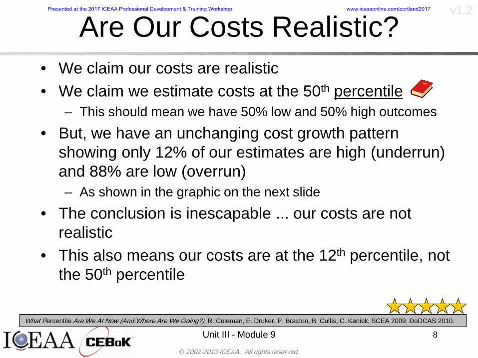
copy 2002-2013 ICEAA All rights reserved
v12
Unit III - Module 9 8
Are Our Costs Realisticbull We claim our costs are realisticbull We claim we estimate costs at the 50th percentile
ndash This should mean we have 50 low and 50 high outcomes
bull But we have an unchanging cost growth pattern showing only 12 of our estimates are high (underrun) and 88 are low (overrun)ndash As shown in the graphic on the next slide
bull The conclusion is inescapable our costs are not realistic
bull This also means our costs are at the 12th percentile not the 50th percentile
What Percentile Are We At Now (And Where Are We Going) R Coleman E Druker P Braxton B Cullis C Kanick SCEA 2009 DoDCAS 2010
Presented at the 2017 ICEAA Professional Development amp Training Workshop wwwiceaaonlinecomportland2017
copy 2002-2013 ICEAA All rights reserved
v12
88 Dollars ( in millions)
Co
st G
row
th F
acto
r
0
1
2
3
4
5
6
7
8
0 5000 10000 15000 20000 25000 30000 35000
lsquoUnit III - Module 9 9
Historical Cost Growth
Average program cost growthRampD 21 Prod 19
Fraction of programs ending on-or-under cost target
7-16
Note This pattern appears to be fractal
Uncohorted dollar weighted
This is the line of no growth
The Cost Growth Factor is 10 meaning (Final Cost)(Initial Cost) = 1
Grew to 75 times planned cost
Risk in Cost Estimating General Introduction amp The BMDO Approach 33rd DoDCAS 2000 R L Coleman J R Summerville M DuBois B Myers
Note apparent bounds
Presented at the 2017 ICEAA Professional Development amp Training Workshop wwwiceaaonlinecomportland2017
88 Dollars ( in millions)
Cost Growth Factor
0
1
2
3
4
5
6
7
8
0
5000
10000
15000
20000
25000
30000
35000
copy 2002-2013 ICEAA All rights reserved
v12
Sources of Cost Risk
Unit III - Module 9 10
l Security Risksl Critical failure modesl Energy Environmental Risksl Schedule problems and delaysl Inadequate cost estimates
n Process (need to assess contractorrsquos assumptions)
n Models l ldquoNew Ways of Doing Businessrdquol Inflationl Systems Engineeringl Cost Improvement Curve
Assumptions
l State-of-the-Art-Advance (Technology Readiness)
l Technical Risk Sourcesn Physical propertiesn Material Propertiesn Radiation Properties
(emission and reception)l Material Availability Risksl Testing Modeling Risksl Integration Interface Risksl Program Personnell Safety Risksl Software Design Risks
Historical cost data available
Amount of cost risk depends on the Basis of the Estimate
Presented at the 2017 ICEAA Professional Development amp Training Workshop wwwiceaaonlinecomportland2017
copy 2002-2013 ICEAA All rights reserved
v12
Point Estimates of Costbull Funding organizations need best estimate of cost for
bullCostperformance tradeoff studiesbullCostbenefit analysesbullBudget planning
bull But program cost is nebulous heavily impacted bybullTechnological (im)maturitybullProgrammatic considerationsbullSchedule slipsbullUnforeseen events
bull Point cost estimates cannot be ldquocorrectrdquo becausebullEvery cost element contains uncertaintybullTotal system cost is sum of these WBS elements
bull Actual program cost falls within a range surrounding the best estimate (with some degree of confidence)bullThe best we can hope to do is to understand the uncertaintybullUnderstanding the uncertainty will help us make provision for it
Unit III - Module 9 11
Presented at the 2017 ICEAA Professional Development amp Training Workshop wwwiceaaonlinecomportland2017
copy 2002-2013 ICEAA All rights reserved
v12
Unit III - Module 9 12
Types of Riskbull Cost Growth = Cost Estimating Growth + SkedTech Growth
+ Requirements Growth + Threat Growthbull Cost Risk = Cost Estimating Risk + SkedTech Risk +
Requirements Risk + Threat Riskndash Cost Estimating Risk Risk due to cost estimating errors and the statistical
uncertainty in the estimate ndash ScheduleTechnical Risk Risk due to inability to conquer problems posed
by the intended design in the current CARD or System Specificationsndash Requirements Risk Risk resulting from an as-yet-unseen design shift from
the current CARD or System Specifications arising due to shortfalls in the documents
bull Due to the inability of the intended design to perform the (unchanged) intended mission
bull We didnrsquot understand the solutionndash Threat Risk Risk due to an unrevealed threat eg shift from the current
STAR or threat assessmentbull The problem changedO
ften
impl
icit
or o
mitt
ed
1 2
Presented at the 2017 ICEAA Professional Development amp Training Workshop wwwiceaaonlinecomportland2017
copy 2002-2013 ICEAA All rights reserved
v12
Point Estimates Vs Risk Estimates
Unit III - Module 9 13
DDTampE Flight Unit Production TotalPoint Estimate 63807 5179 6697 70505CER Risk Only - Mean 71176 4805 6426 78018Full Risk - Mean 78937 6490 8091 87430Point Esimtate + 30 82949 6733 8706 91657Full Risk - 70th Percentile 87939 7980 9608 97011
Estimated Total Cost in Millions
Note that the mean is 24 higher than the point estimate and the 70th
percentile is 38 higher than the point estimate
Presented at the 2017 ICEAA Professional Development amp Training Workshop wwwiceaaonlinecomportland2017
copy 2002-2013 ICEAA All rights reserved
v12
Cost Risk and Probabilitybull Cost risk or cost uncertainty analysis represents cost as a
probability distributionbull A probability distribution is a mathematical rule associating a
probability a to each possible outcome or event of interestbull There are two ways to present a probability distribution ndash as a
probability density function (ldquoPDF) and as a cumulative distribution function (ldquoS-curverdquo or ldquoCDFrdquo)
Unit III - Module 9 14
Lognormal Distribution PDF and CDF
0102030405060708090100
200 300 400 500 600 700 800 900 1000Cost $
Con
fiden
ce L
evel
0
00002
00004
00006
00008
0001
00012
00014
00016
Prob
abili
ty D
ensi
ty
CDFPDF
Presented at the 2017 ICEAA Professional Development amp Training Workshop wwwiceaaonlinecomportland2017
copy 2002-2013 ICEAA All rights reserved
v12
Unit III - Module 9 15
Probability Model ndash Distributionbull Normal
ndash Best behavior most iconic
ndash Theoretically (although not practically) allows negative costs which spook some users
ndash Symmetric needs mean shift to reflect propensity for positive growth
bull Lognormalndash A natural result in
non-linear CERsndash Indistinguishable
from Normal at CVs below 25
ndash Skewed
10
4
10
Presented at the 2017 ICEAA Professional Development amp Training Workshop wwwiceaaonlinecomportland2017
copy 2002-2013 ICEAA All rights reserved
v12
Unit III - Module 9 16
bull Triangularndash Most commonndash Easy to use easy to understandndash Modes medians do not addndash Skewed
bull Betandash Rare now but formerly popularndash Solves negative cost and duration issuesndash Many parameters ndash simplifications like PERT
Beta are possiblendash Skewed
bull Bernoullindash Probability is only assigned to two possible
outcomes success and failure (p and 1-p)ndash Simplest of all discrete distributionsndash Mean = pndash Variance = p(1-p)
10
Probability Model ndash Distribution
10
10
Presented at the 2017 ICEAA Professional Development amp Training Workshop wwwiceaaonlinecomportland2017
copy 2002-2013 ICEAA All rights reserved
v12
Unit III - Module 9 17
bull Normalndash If there is a sufficiently large number of independently identically distributed
elements (or not too correlated and not too skewed) then the distribution of total cost is normal due to the Central Limit Theorem
bull Lognormalndash For smaller data sets with large amounts of (positive) correlation and
skewness the lognormal distribution may be a better approximation of total cost
ndash Many total cost distributions in smaller data sets test as both normal and lognormal
bull Triangularndash The sum of triangles is not a triangle so this distribution should generally not
be used to characterize total costbull Convolved
ndash If total cost distribution is derived using simulation then it may not particularly resemble anything In this case we simply have a convolved or simulated total cost distribution
Probability ndash Top-Level Distribution
NEW
Presented at the 2017 ICEAA Professional Development amp Training Workshop wwwiceaaonlinecomportland2017
copy 2002-2013 ICEAA All rights reserved
v12
S-Curves and Confidence Levels
Unit III - Module 9 1818
100
70
25
Probability(Confidence
Level)
Cost Estimate(Dollars)
50
The S curve is the cumulative probability distribution coming out of the statistical summing process
70 confidence that project will cost indicated amount or less
Provides information on potential cost as a result of identified project risks
Provides insight into establishing reserve levels
X Y
MR
X = Point estimateZ = Project requirementY = Cost estimate where there is a 70 change that
final actual cost will be less than cost estimateY-Z= Manage reserve (MR) which is REQUIRED to meet 70 CL
Z
X not always = Z but is based on same content
Presented at the 2017 ICEAA Professional Development amp Training Workshop wwwiceaaonlinecomportland2017
copy 2002-2013 ICEAA All rights reserved
v12
19
Example ndash Normal Distribution
bull Normal distribution with mean equal to 100 and standard deviation equal to 20
bull Median and mode also equal 100bull The 80th Percentile is 117
40 60 80 100 120 140 160
80 of distribution(area under curve)is less than 117
117
Presented at the 2017 ICEAA Professional Development amp Training Workshop wwwiceaaonlinecomportland2017
copy 2002-2013 ICEAA All rights reserved
v12
20
Confidence Levelsbull The output of a cost risk analysis is a probability
distributionndash Typically displayed as a cumulative distribution function or
ldquoS-curverdquondash Confidence levels are simply percentiles of the distribution
0
10
20
30
40
50
60
70
80
90
100
30 60 90 120 150 180
Conf
iden
ce L
evel
Presented at the 2017 ICEAA Professional Development amp Training Workshop wwwiceaaonlinecomportland2017
copy 2002-2013 ICEAA All rights reserved
v12
Measuring Parametric Model Uncertainty
bull When developing estimates using cost-estimating relationships (CERs) there are two major sources of uncertaintyndash Technical (model input) uncertaintyndash Estimating uncertainty
bull Technical uncertainty reflects the uncertainty inherent in the model inputsndash Typical parametric model inputs include weight lines of code
heritage and other performance and management inputs
bull Estimating uncertainty measures the uncertainty inherent in the model due to the modelrsquos inability to capture all aspects of variability in the data
21
Presented at the 2017 ICEAA Professional Development amp Training Workshop wwwiceaaonlinecomportland2017
copy 2002-2013 ICEAA All rights reserved
v12
Parametric Model Examplebull The NASAAir Force Cost Model (NAFCOM) is a
parametric model for estimating acquisition costs for spacecraft and launch vehicles
bull The CERs in NAFCOM have the formCost = C WeightVNewDesignWTechnicalXManagementY ClassZ
bull There is technical uncertainty about each of the parametersndash Parametric models are applied early in a program so there
is significant amount of uncertainty in the weightndash Heritage is also tricky it is inherently subjective and project
personnel are typically optimisticndash Technical characteristics can also change as a program
matures and requirements change
22
Presented at the 2017 ICEAA Professional Development amp Training Workshop wwwiceaaonlinecomportland2017
copy 2002-2013 ICEAA All rights reserved
v12
Weight Uncertaintybull Aerospace weight growth study average satellite
weight growth from program inception to launch is 28
23
Aerospace Weight Growth Data
-10
0
10
20
30
40
50
60
0 4 8 12 16 20 24 28 32 36 40 44 48 52 56 60 64 68 72 76 80 84 88 92 96 100
Percent Program Completion
Perc
ent W
eigh
t Gro
wth
Presented at the 2017 ICEAA Professional Development amp Training Workshop wwwiceaaonlinecomportland2017
copy 2002-2013 ICEAA All rights reserved
v12
Estimating Uncertaintybull CERs do not perfectly fit the historical data
ndash There are non-repeatable random effects that cannot be predicted
bull For examplendash Parts breaking during testingndash Strikes which are difficult to predict
bull This results in an underlying uncertainty distribution about an estimatendash The outcome of a CER represents only one point on an
uncertainty distributionbull Typically mean or median depending upon the CER
methodology
24
Presented at the 2017 ICEAA Professional Development amp Training Workshop wwwiceaaonlinecomportland2017
copy 2002-2013 ICEAA All rights reserved
v12
Estimating Uncertainty (2)
25
Presented at the 2017 ICEAA Professional Development amp Training Workshop wwwiceaaonlinecomportland2017
copy 2002-2013 ICEAA All rights reserved
v12
Estimating Uncertainty (3)bull In the case of a linear regression the estimating
uncertainty follows a normal distributionndash The estimate is the mean and the standard error of the
estimate from the regression is the standard deviation of the normal distribution
bull In the case of a log-transformed linear regression the estimating uncertainty follows a lognormal distributionndash The estimate is the median of the lognormal and the
standard error of the estimate from the regression is the standard deviation of the normal distribution (in log-space)
bull There is additional uncertainty about an estimate based upon the distance of what is being estimated from the mean of the input datandash This results in a prediction interval
26
Presented at the 2017 ICEAA Professional Development amp Training Workshop wwwiceaaonlinecomportland2017
copy 2002-2013 ICEAA All rights reserved
v12
Aggregating Riskbull Risk is typically applied at the same level at
which we estimate cost that is at the Work Breakdown Structure (WBS) level
bull The estimates for each WBS are developedndash These estimates sum to yield the total system cost
bull For an n-element WBS the total cost is the sum of the cost for each of the n elements
27
nXXXCostSystem +++= 21
Presented at the 2017 ICEAA Professional Development amp Training Workshop wwwiceaaonlinecomportland2017
copy 2002-2013 ICEAA All rights reserved
v12
WBS Examplebull Launch Vehicle
ndash Structurebull Vehicle Structurebull Tank Structure
ndash Thermal Controlbull Active Thermal Controlbull Induced Thermal Controlbull Tank Thermal Control
ndash Main Propulsion Systemndash Liquid Rocket Enginendash Electric Power and Distributionndash Command Control and Data Handlingndash System Integration
28
Presented at the 2017 ICEAA Professional Development amp Training Workshop wwwiceaaonlinecomportland2017
copy 2002-2013 ICEAA All rights reserved
v12
WBS and Risk
29
Presented at the 2017 ICEAA Professional Development amp Training Workshop wwwiceaaonlinecomportland2017
copy 2002-2013 ICEAA All rights reserved
v12
Aggregating Riskbull This leads us to the issue of aggregating the risks across the
WBSbull For example if we want to determine the 70th percentile of the
overall cost risk distribution how do we proceed bull Note that we cannot simply add the 70th percentiles of each of
the cost risk distributionsbull We can add means and variances (taking correlation into
account more on that later) but that is all
Variance of Total Cost =
30
Mean of Total Cost = ( )E X E Xk
k
n
kk
n
kk
n
= = =aringaelig
egraveccediloumloslashdivide
= =aring aring1 1 1
m
Var X kk
n
=aringaelig
egraveccediloumloslashdivide1
= s r s skk
n
iji
j
i jj
n2
1 1
1
22+aring aringaring
= =
-
=
Presented at the 2017 ICEAA Professional Development amp Training Workshop wwwiceaaonlinecomportland2017
copy 2002-2013 ICEAA All rights reserved
v12
Percentiles Do Not Addbull As a notional example consider two independent normal
distributionsndash One distribution has mean equal to 100 and standard deviation
equal to 20ndash The second distribution has mean 300 and standard deviation of 80
bull The sum of two independent normally distributed random variables is also normally distributed
bull To combine the two distributions we add the means and add the variancesndash Total mean is
ndash Total standard deviation is
31
400300100 =+
8258020 22 raquo+
Presented at the 2017 ICEAA Professional Development amp Training Workshop wwwiceaaonlinecomportland2017
copy 2002-2013 ICEAA All rights reserved
v12
Percentiles Do Not Add (2)bull The 80th percentiles for the individual distributions are
117 and 367 respbull The 80th percentile of the combined distribution is
469 but the sum of the two 80th percentiles is 484bull To see why this is the case note that the percentiles
of a normal distribution are determined by the mean and the standard deviationndash The standard deviations are not added when normal distributions
are combined rather the variances are combinedndash Sum of variances is ndash The standard deviation of this sum is
32
22 ba +22 ba +
Presented at the 2017 ICEAA Professional Development amp Training Workshop wwwiceaaonlinecomportland2017
copy 2002-2013 ICEAA All rights reserved
v12
Percentiles Do Not Add (3)bull Since bull We can write
bull The left side of this inequality represents the risk of the combined distributions while the right side represents the sums of the individual risks
bull Combining two missions that are independent results in a diversification of riskndash The total portfolio is not as risky on a relative basis as each
individual project
33
2222 2 bababa ++lt+
baba +lt+ 22
Presented at the 2017 ICEAA Professional Development amp Training Workshop wwwiceaaonlinecomportland2017
copy 2002-2013 ICEAA All rights reserved
v12
Methods for Aggregating Riskbull Since percentiles do not add we have to find other
ways to aggregate riskbull One method is to use Monte Carlo simulationbull Unless cost risk is represented by normal
distributions for all WBS elements summing the means and variances does not result in a completely accurate depiction of overall system cost risk
bull The normal distribution is not a realistic distribution for representing risk in many or even most situations since regarding project risk more can go wrong than can go right which means the risk is NOT symmetric unlike the Gaussian bell curve
34
Presented at the 2017 ICEAA Professional Development amp Training Workshop wwwiceaaonlinecomportland2017
copy 2002-2013 ICEAA All rights reserved
v12
Unit III - Module 9 35
Monte Carlo Simulationfor Risk Analysis
bull When risk analysis is performed multiple risks are gatheredndash These risks may have various probability
distributions
bull Monte Carlo is the most commonly accepted way to produce an accurate characterization of the distribution of the combined effect of these many risksndash Using this distribution we can produce percentiles
for cost impacts due to risk occurrences
10
Presented at the 2017 ICEAA Professional Development amp Training Workshop wwwiceaaonlinecomportland2017
copy 2002-2013 ICEAA All rights reserved
v12
Monte Carlo Simulationbull Simulation is a means for solving problems that are
analytically intractablendash Involves repeated random sampling
bull It was developed during the Manhattan Project as a way to model the interactions inside an atom during nuclear fissionndash Allowed for more sophisticated mathematical modeling of atomic
phenomena
bull Most computer packages use pseudo-random number generators that produce seemingly random results from an initial seedndash Example is the linear congruential generator
36
( ) mbaXX nn mod1 +=+
Presented at the 2017 ICEAA Professional Development amp Training Workshop wwwiceaaonlinecomportland2017
copy 2002-2013 ICEAA All rights reserved
v12Using Random Numbers to Simulate Distributions
bull WBS cost risk is typically measured by a probability distributionbull The most common method for simulating a probability
distribution is the inverse methodbull This involve obtaining a simulated random value from a uniform
distribution and then inverting this through the cumulative distribution function (CDF) to obtain the simulated value
bull As an example for a uniform distribution on the interval [0100]
bull In this case the CDF random value of 05 translates to 10005 = 50
37
( )100
1=xf ( )
100xxF = ( ) xxF 1001 =-
Presented at the 2017 ICEAA Professional Development amp Training Workshop wwwiceaaonlinecomportland2017
copy 2002-2013 ICEAA All rights reserved
v12
Simulating a Triangular Distribution
bull For a triangular distribution with low = 0 most likely = 50 and high = 150 the CDF is given by
bull The inverse function is given by
38
( )iumliumlicirc
iumliumliacute
igrave
poundlt--
poundpound=
1505021
1500050
50015000
2
2
2
xxx
xxxF
( )iumliumlicirc
iumliumliacute
igrave
poundltdivideoslashouml
ccedilegraveaelig +--
poundpound=-
131
21
37501
250017500150
3107500
1
xx
xxxF
Presented at the 2017 ICEAA Professional Development amp Training Workshop wwwiceaaonlinecomportland2017
copy 2002-2013 ICEAA All rights reserved
v12
Simulating a Triangular Distribution (2)
bull If the simulated uniform value is equal to 02 the corresponding inverse value from the CDF inverse is approximately 387
39
0
01
02
03
04
05
06
07
08
09
1
0 30 60 90 120 150
Presented at the 2017 ICEAA Professional Development amp Training Workshop wwwiceaaonlinecomportland2017
copy 2002-2013 ICEAA All rights reserved
v12
Monte Carlo and the WBSbull Simulation involves repeated trials
40
WBS Draw1 2 3 4 5
System 2912 3566 4390 2954 4655 Sum
Structure 80 105 55 80 57 SumVehicle Structure 50 70 30 40 20Tank Structure 30 35 25 40 37
Thermal Control 32 36 35 29 33 SumActive Thermal Control 10 15 12 7 10Induced Thermal Control 12 14 13 14 14Tank Thermal Control 10 7 10 8 9
Main Propulsion System 100 150 125 140 100
Liquid Rocket Engine 1000 1100 1800 900 2200
Electric Power and Distribution 100 125 150 75 90
Command Control and Data Handling 200 250 225 230 275
System Integration 1400 1800 2000 1500 1900
Presented at the 2017 ICEAA Professional Development amp Training Workshop wwwiceaaonlinecomportland2017
copy 2002-2013 ICEAA All rights reserved
v12
Number of Trialsbull Monte Carlo involves a repeated number of trialsbull The greater the number of trials the more accurate the
simulation will approximate the overall cost risk behavior of the system
bull After 100 trials the histogram looks very jagged
41
Presented at the 2017 ICEAA Professional Development amp Training Workshop wwwiceaaonlinecomportland2017
copy 2002-2013 ICEAA All rights reserved
v12
Number of Trials (2)
42
1000 Trials
10000 Trials
50000 Trials Additional trials give a more accurate depiction of the final result
Presented at the 2017 ICEAA Professional Development amp Training Workshop wwwiceaaonlinecomportland2017
copy 2002-2013 ICEAA All rights reserved
v12
Number of Trials (3)bull If we want to simulate the underlying
mean within 1 with 95 confidence for example then we require
43
divideoslash
oumlccedilegrave
aelig poundpound-
=
dividedividedivide
oslash
ouml
ccedilccedilccedil
egrave
aeligpound
-pound
-=
divideoslashouml
ccedilegraveaelig poundpound=
nZ
n
nnX
n
X
n
n
011
010Pr
011
010Pr
011990Pr950
___
___
sm
sm
sm
sm
sm
mm
Presented at the 2017 ICEAA Professional Development amp Training Workshop wwwiceaaonlinecomportland2017
copy 2002-2013 ICEAA All rights reserved
v12
Number of Trials (4)bull This means that the number of trials required is determined by
bull Solving for n we find that at least
trials are neededbull Note that this term involves the coefficient of variation of the
distribution which means that distributions with less dispersion require fewer trials to accurate simulate
44
96101
=ns
m
ms41638
Presented at the 2017 ICEAA Professional Development amp Training Workshop wwwiceaaonlinecomportland2017
copy 2002-2013 ICEAA All rights reserved
v12
Number of Trials (5)bull Simulating percentiles requires more trials than for simulating
meansbull Let Pn represent the number of trials in the sample at or below
the 70th percentile of the underlying distribution (suppose this is known)
bull By the Central Limit Theorem Pnn follows a normal distribution with mean equal to the 70th percentile and variance equal to
bull By a similar process for the mean we find that the number of trials needed to simulate the 70th percentile within 1 with 95 confidence is
45
( )n
FF 700700 1-
n
n
PPn -41638
Presented at the 2017 ICEAA Professional Development amp Training Workshop wwwiceaaonlinecomportland2017
copy 2002-2013 ICEAA All rights reserved
v12
Number of Trials (6)bull If Pn 070 for all n then n is approximately
bull For the sake of comparison suppose CV = 03 (reasonable approximation for hardware development) then the number of trials needed to simulate the mean with the same accuracy is then ldquoonlyrdquo 11525
bull More trials are needed to accurately simulate percentiles than means
46
( ) 46416703041638
70704168341638 =divide
oslashouml
ccedilegraveaelig=divide
oslashouml
ccedilegraveaelig -
=-
nnn
PPn
n
n
Presented at the 2017 ICEAA Professional Development amp Training Workshop wwwiceaaonlinecomportland2017
copy 2002-2013 ICEAA All rights reserved
v12
Methods of Simulationbull Monte Carlo simulation is a standard term for
simulationbull However there is an improvement on Monte Carlo
that improves the accuracy of the results of a simulation for a given number of trials
bull This method is call the Latin Hypercube approach to simulationndash Similar to Monte Carlo but an equal number of draws are taken
from a set of subintervals for example dividing the interval (01) into [00001) [0102)hellip [0910]
ndash Instead of 10 trials from [01] we have one trial from each subinterval
ndash Rough rule of thumb is Latin Hypercube takes 30 fewer trials to achieve similar accuracy to Monte Carlo
47
Presented at the 2017 ICEAA Professional Development amp Training Workshop wwwiceaaonlinecomportland2017
copy 2002-2013 ICEAA All rights reserved
v12
Probability Model ndash Correlationbull Correlation exists between work breakdown structure
(WBS) cost element costs and between cost and schedule
bull Correlation is a necessary consideration in cost risk analysis
bull Correlation is a number that can vary between -1 and +1 and represents the strength of the relationship between the two variablesndash If both variable have a tendency to move in the same direction
correlation is positivendash If when one variable increases the other tends to decrease and
vice-versa the correlation between the two variables is negative
Presented at the 2017 ICEAA Professional Development amp Training Workshop wwwiceaaonlinecomportland2017
copy 2002-2013 ICEAA All rights reserved
v12
Correlation And Causationbull Note that correlation is not causation however
causation implies correlationndash For example shark attacks and ice cream sales at the beach
bull For example for a launch vehicle structure increasing the diameter will not only result in an increase in the structures cost but will also result in higher costs for thermal coating (paint etc)
bull Also simply because two subsystems do not appear to be related does not mean they are not correlatedndash For example structures and computer equipment seemingly
have little relation to one another however an external factor such as a funding cut or a strike will impact all subsystems leading to delays and increasing cost across the board
ndash Thus everything in a WBS has some correlationUnit III - Module 9 49
Presented at the 2017 ICEAA Professional Development amp Training Workshop wwwiceaaonlinecomportland2017
copy 2002-2013 ICEAA All rights reserved
v12
The Importance of Correlationbull Percent that total cost standard deviation is underestimated
when correlation assumed to be 0 instead of r given nWBS elements
Unit III - Module 9 5050
0
20
40
60
80
100
0 01 02 03 04 05 06 07 08 09 1Actual Correlation
Perce
nt Un
deres
timate
d
n = 10
n = 30
n = 100n = 1000
0
20
40
60
80
100
0 01 02 03 04 05 06 07 08 09 1Actual Correlation
Perce
nt Un
deres
timate
d
n = 10
n = 30
n = 100n = 1000
Reference 32nd Annual DOD Cost Analysis Symposium Advanced Training Session ldquoWhy Correlation Matters in Cost Estimatingrdquo Stephen A Book
Presented at the 2017 ICEAA Professional Development amp Training Workshop wwwiceaaonlinecomportland2017
copy 2002-2013 ICEAA All rights reserved
v12
The Importance of Correlation (2)bull For example if correlation is assumed to be 0 for all
elements in a 30 element WBS and the actual correlation is 20 then the total cost standard deviation is underestimated by 60
bull For example assume the total cost is modeled as a normal distribution with mean = 100
bull If correlation is assumed to be zero with total cost standard deviation = 12 when correlation is actually 20 then the true underlying standard deviation is actually 30
bull 70th percentile with zero correlation assumption is 106
bull 70th percentile with 20 correlation is 116 Unit III - Module 9 51
Presented at the 2017 ICEAA Professional Development amp Training Workshop wwwiceaaonlinecomportland2017
copy 2002-2013 ICEAA All rights reserved
v12
Measures of Correlationbull Two measures of correlation are commonly used in
cost risk analysesndash Pearsonrsquos product-moment correlation coefficient ndash Spearmanrsquos rank correlation coefficient
bull Garvey and others recommend using Pearsonrsquos product-moment correlation coefficient correlation for cost risk analysesndash Method of moments uses this but there are two options in
simulationndash Popular simulation packages like Risk and Crystal Ball use
rank correlation but in practice this has been found to make little difference
ndash Pearson product-moment correlation has been incorporated into Risk+
52
Presented at the 2017 ICEAA Professional Development amp Training Workshop wwwiceaaonlinecomportland2017
copy 2002-2013 ICEAA All rights reserved
v12
Pearson Correlationbull Pearsonrsquos product-moment correlation measures
degree of linearity between two random variables bull If two random variables are perfectly linear (eg Y =
aX + b) with positive slope then the Pearson product-moment correlation between X and Y denoted by rXY is +1
53
X X
Y Y Y
XNegative Correlation Positive Correlation No Correlation
middotmiddot
middotmiddot
middotmiddot middotmiddot
middotmiddot
middot
middot
middotmiddotmiddot
middotmiddot
middotmiddot
middotmiddot middot
middot
middot
middotmiddotmiddotmiddotmiddotmiddotmiddotmiddot
middotmiddotmiddotmiddot
middotmiddot
middotmiddot middotmiddotmiddotmiddot
middotmiddotmiddot
middotmiddotmiddotmiddot
middotmiddotmiddot
middotmiddotmiddot
middotmiddot
middot
middot middotmiddot
middot middotmiddotmiddotmiddot middotmiddot middot middotmiddot middot middot
middotmiddot middot
middotmiddotmiddotmiddotmiddot middot middotmiddot
middotmiddot
middot
middotmiddot
middotmiddot middot
middot middot middot
middotmiddot middot
middotmiddotmiddot
middotmiddot
middot middot
Presented at the 2017 ICEAA Professional Development amp Training Workshop wwwiceaaonlinecomportland2017
copy 2002-2013 ICEAA All rights reserved
v12
Spearman Correlationbull Spearmanrsquos rank correlation measures the
monotonicity between two random variablesbull If two random variables are perfectly monotonically
increasing (eg Y = X2) then the Spearman rank correlation denoted by rXY is +1
bull The two measures can be significantly different
54
10 20 30 40 50 60
100
200
300
096 097 098 099 1
1
060
020
040
080
Eff
ort (
Staf
f-M
onth
s)
Software Size I KDSI
y = 28z12y
z x
yy = x100
0 pound x pound 1
Figure 5-9A Figure 5-9B
Pearson Correlation = 09976 Rank Correlation = 1
Pearson Correlation = 024 Rank Correlation = 1
X(x ) ~ Unif(01)
Reference Probability Methods for Cost Uncertainty Analysis A Systems Engineering Perspective Paul R Garvey
Presented at the 2017 ICEAA Professional Development amp Training Workshop wwwiceaaonlinecomportland2017
copy 2002-2013 ICEAA All rights reserved
v12
Unit III - Module 9 55
200
250
300
350
400
1000 1200 1400 1600 1800 2000
Recurring Production
SEPM
200
250
300
350
400
1000 1200 1400 1600 1800 2000
Recurring Production
SEPM
Functional Correlationbull Old No Functional
Correlation Simulation run with WBS items entered as values
bull New Simulation run with functional dependencies entered as they are in cost model
CorrelatedNot Correlated
Note shift of mean and increased variability
Presented at the 2017 ICEAA Professional Development amp Training Workshop wwwiceaaonlinecomportland2017
copy 2002-2013 ICEAA All rights reserved
v12
Risk Measuresbull ldquoWestern Europe conquered the word because of a
technological revolution that started because of attempts to measure the worldrdquo ndash Phillipe Jorion ndash In the same way attempts to measure risk will lead to better project
managementbull Risk management for DoD and NASA agencies focuses
primarily on funding projects to a single percentile ndash NASA policy explicitly mentions 70 and 50ndash This is known as ldquoValue at Riskrdquo and is prevalent in the banking and
financial industry
56
Presented at the 2017 ICEAA Professional Development amp Training Workshop wwwiceaaonlinecomportland2017
copy 2002-2013 ICEAA All rights reserved
v12
Value at Risk (VaR)bull VaR is a percentile of the cost risk
distributionndash VaR funding at the 70th percentile means that
there is a 30 chance of final project cost exceeding the funded amount (budget)
bull VaR has some meritsndash Common measure can be used to compare
different projects and programsndash Easily understood by senior managers and
decision makers
57
Presented at the 2017 ICEAA Professional Development amp Training Workshop wwwiceaaonlinecomportland2017
copy 2002-2013 ICEAA All rights reserved
v12
Why 70th or 80th Percentilebull Typical policy guidance involves funding at the 70th or 80th
percentile Why fund as such a low percentilebull There is some incentive to not over-fundbull For a normal distribution an inflection point occurs near the 80th
percentile meaning that for values above 80 confidence achieving higher levels of confidence can only be achieved by spending greater dollar amounts at an increasing rate
58
-05-04-03-02-01
00102030405
0 05 1 15 2 25 3
Standard Deviations from Mean
Normal Distribution
First DerivativeSlopeVelocity
Second DerivativeConvexityAcceleration
Inflection point at one standard deviation above the mean (~84th
percentile)
Presented at the 2017 ICEAA Professional Development amp Training Workshop wwwiceaaonlinecomportland2017
copy 2002-2013 ICEAA All rights reserved
v12
Funding Above Inflection Pointsbull As the percentile goes above the 80th percentile the amount
needed to achieve that higher level of confidence begins to increase at an increasing rate as is evident from the graph
59
0
10
20
30
40
50
60
70
50 55 60 65 70 75 80 85 90 95 100
$ Ab
ove
MEa
n to
Ach
ieve
Per
cent
ile
Percentile (Confidence Level)
Presented at the 2017 ICEAA Professional Development amp Training Workshop wwwiceaaonlinecomportland2017
copy 2002-2013 ICEAA All rights reserved
v12
Why Budget to the 70th or 80thbull Government projects are funded at the 70th or 80th percentilesbull Why not the 90th or 99th percentile Wonrsquot that help prevent
overrunsndash As we have seen percentiles do not add across programs
bull The sum of the 80th percentiles does NOT equal the total 80th percentile
ndash This is because the individual programs are riskier than the entire suite of missions
bull Known as the ldquoPortfolio effectrdquo (more or this later)
ndash Funding at the 80th gives confidence that the entire portfolio will be adequately funded
bull And since there is an inflection point near the 80th percentile funding above that level quickly becomes cost prohibitive
60
Presented at the 2017 ICEAA Professional Development amp Training Workshop wwwiceaaonlinecomportland2017
copy 2002-2013 ICEAA All rights reserved
v12
Inflection Points for Lognormalbull For a lognormal the inflection point
variesndash Coefficient of variation equal to 10 equates to an
inflection point at the 70th percentile
61
0
10
20
30
40
50
60
70
050 060 070 080 090 100
Coef
ficen
t of V
aria
tion
Percentile of the Inflection Point
Presented at the 2017 ICEAA Professional Development amp Training Workshop wwwiceaaonlinecomportland2017
copy 2002-2013 ICEAA All rights reserved
v12
Issues with Percentile Fundingbull However risk management does not stop at a
specific percentilendash What happens when the 70th percentile is exceeded
bull Any effective risk management policy should prescribe what happens after a bad event occursndash With VaR we only know when a bad event has occurred ndash Also funding at a relatively low level means we have no true
sense of the real risks that should be guarded against
62
Presented at the 2017 ICEAA Professional Development amp Training Workshop wwwiceaaonlinecomportland2017
copy 2002-2013 ICEAA All rights reserved
v12
ldquoHere There Be Dragonsrdquobull On old maps uncharted territory was often
marked with monsters or dragons
63
A section of the Carta Marina by Olaus Magnus 16th Century
Presented at the 2017 ICEAA Professional Development amp Training Workshop wwwiceaaonlinecomportland2017
copy 2002-2013 ICEAA All rights reserved
v12
Distribution Comparisonbull Four different distributions with the same 70th
percentile
bull Should we expect the tails to be similar
64
0
10
20
30
40
50
60
70
80
0 100 200 300 400 500 600
Perc
entil
eCo
nfid
ence
Lev
el
Triangular
Normal
Lognormal
Pareto
Presented at the 2017 ICEAA Professional Development amp Training Workshop wwwiceaaonlinecomportland2017
copy 2002-2013 ICEAA All rights reserved
v12Distribution Comparison Tail Behavior
bull The normal and triangular distributions have similar tails but the lognormal and Pareto have much fatter right tails
65
70
75
80
85
90
95
100
500 1500 2500 3500 4500 5500
Perc
entil
eCo
nfid
ence
Lev
el
Triangular
Normal
Lognormal
Pareto
Here There Be Dragons
Presented at the 2017 ICEAA Professional Development amp Training Workshop wwwiceaaonlinecomportland2017
copy 2002-2013 ICEAA All rights reserved
v12Distribution Comparison ndash Tail Behavior (Table)
bull There is significant tail risk for the lognormal and the Paretobull The 99th percentile for the Pareto is 1000 times greater than
the 70th percentilendash Risk seen in financial markets and in catastrophic risks like natural
disasters bull Four different projects follow the four different risk profiles seen
in this example should clearly have different risk management approaches but 70th percentile funding indicates the same risk management approach for all four
66
Percentile Triangular Normal Lognormal Pareto 70th $600 $600 $600 $600 80th $680 $660 $770 $1430 90th $770 $750 $1070 $5880 95th $840 $820 $1410 $23750 99th $930 $950 $2350 $600000
Presented at the 2017 ICEAA Professional Development amp Training Workshop wwwiceaaonlinecomportland2017
copy 2002-2013 ICEAA All rights reserved
v12Percentile Budgeting is Not Risk Management
bull Percentile budgeting ne effective risk management policybull Suppose that you are shopping for a new car You
mention that safety is your top concern The salesman says he has a great safe car available You ask about the air bags Do they work The salesman answers ldquoOf course Seventy percent of the time they work fine Only 30 of the time the air bags will fail to deployrdquo Would you buy such a car Hedge fund manager David Einhorn has stated ldquoRisk management is the air bag that must always work but only in the multi-sigma event where you have an accidentrdquo
67
Risk management is the air bag that must always work but only in the multi-sigma event where you
have an accident
Presented at the 2017 ICEAA Professional Development amp Training Workshop wwwiceaaonlinecomportland2017
copy 2002-2013 ICEAA All rights reserved
v12
Joint Confidence Level Analysisbull Schedules are risky toobull For 98 recent NASA missions average
schedule growth was 38ndash Not as high as cost growth but still significant
68
0
5
10
15
20
25
30
35
40
Schedule
Cost
Presented at the 2017 ICEAA Professional Development amp Training Workshop wwwiceaaonlinecomportland2017
copy 2002-2013 ICEAA All rights reserved
v12
Schedules Impact Costbull Changes in schedule can have enormous
impacts on cost ndash Schedule slips can lead to cost increases
bull Fixed programmatic costs must be paid on a regular basisndash Achieving schedule milestones early can result in cost
savings
bull Schedule is an important consideration in cost analysis including cost risk analysis
bull However we must be careful in correctly integrating cost and schedule riskndash Schedule is not simply an input but is dependent on many of
the same factors that drive cost
69
Presented at the 2017 ICEAA Professional Development amp Training Workshop wwwiceaaonlinecomportland2017
copy 2002-2013 ICEAA All rights reserved
v12
The Relationship of Cost to Schedulebull Cost and schedule are positively correlated
ndash A larger program with bigger scope with take longer to complete than a smaller simpler program
bull However longer schedules do not always equate to higher cost nor shorter schedules with lower costndash Highly compressed schedules relative to the
optimal schedule can lead to large overrunsbull Compressed schedules are commonplace for
many planetary missions
70
Presented at the 2017 ICEAA Professional Development amp Training Workshop wwwiceaaonlinecomportland2017
copy 2002-2013 ICEAA All rights reserved
v12The Impact of Schedule GrowthCompression on Cost
bull Compressed schedules lead to cost growth and based on existing research is actually more expensive than schedule slippages
71
0
20
40
60
80
100
120
140
160
-50 -25 0 25 50 75 100
Percentage Change in Schedule
Perc
enta
ge C
hang
e in
Cos
t due
to
Sche
dule
Cha
nge
Source Smart CB ldquoCost and Schedule Interrelationshipsrdquo 2007 NASA Cost Symposium
Presented at the 2017 ICEAA Professional Development amp Training Workshop wwwiceaaonlinecomportland2017
copy 2002-2013 ICEAA All rights reserved
v12Schedule as an Independent Variable
bull Why not simply add schedule as an input to cost-estimating relationships (CERs)
bull Schedule is often treated as an independent variable ndash schedules are often determined independently of cost considerationsndash Cost may not be considered explicitly although budgets and
schedules are determined based on scope and other common factors
bull In 2006 SAIC undertook a research task to determine the impact of schedule on cost and added schedule as an independent variable to the CERs in the NASAAir Force Cost Model (NAFCOM) to see if schedule provided any improvement in goodness of fit
72
Presented at the 2017 ICEAA Professional Development amp Training Workshop wwwiceaaonlinecomportland2017
copy 2002-2013 ICEAA All rights reserved
v12
Schedule is a Dependent Variablebull Since NAFCOM includes an exhaustive list of cost drivers the inclusion
of schedule should give an indication of whether there is any additional independent value added from schedule independent of the cost drivers
bull In the study schedule was added to 10 subsystem-level CERs
ndash In each case the addition of schedule did NOTimprove the goodness of fit and schedule was NOT found to be a statistically significant cost driver (given the presence of the other variables) for any of the 10 CERs
bull Standard errors for the CERs increased due to decrease in degrees of freedom
bull Thus schedule as an independent variable did not provide any additional explanation of variation in historical cost
bull This is because schedule is truly NOT an independent variable but a dependent variable and is a function of the same factors that drive cost
73
Presented at the 2017 ICEAA Professional Development amp Training Workshop wwwiceaaonlinecomportland2017
copy 2002-2013 ICEAA All rights reserved
v12
Incorporation of Schedule in Cost Risk
bull When using subjective methods care must be taken in applying schedule to cost risk analysis
bull Since schedule is a dependent variable treating it independently from other factors when assessing its impact on cost can lead to a double count of independent variables in the cost risk analysis
bull Direct inclusion of schedule in a cost risk analysis effectively doubles the influence of each cost driver
ndash Incorrectly leads to broader risk ranges
74
CostWeight
HeritageNewness
Technology Readiness Schedule
Presented at the 2017 ICEAA Professional Development amp Training Workshop wwwiceaaonlinecomportland2017
copy 2002-2013 ICEAA All rights reserved
v12Subjective Cost Risk Methods and Overinclusion of Risk Factors
bull Subjective methods are suitable when data are scarce or not availablebull However care must be taken not to treat correlated sources of risk
such as schedule as independent of each otherbull Example ndash a subjective risk analysis incorporated technology readiness
design risk requirements stability integration risk and schedule and treated each source of risk as independent
bull Risk triangle high value without schedule risk was 31 times the point estimate
bull Risk triangle high value with schedule risk added on top of other sources of risk treated independently was 34 times the point estimate
bull Risk triangle taking correlation between sources of risk into account in a rigorous statistical manner has a high value 15 times the point estimate less than half the effect when treating sources of risk as independent
75
Presented at the 2017 ICEAA Professional Development amp Training Workshop wwwiceaaonlinecomportland2017
copy 2002-2013 ICEAA All rights reserved
v12Fundamental Equation of Cost and Schedule Interrelationships
bull The Fundamental Equation of the Relationship Between Cost and Schedule is
Time = Moneybull This is a well known adage that time is money Your boss at
work may even mention this to you from time to time or if you are the boss you are all too aware of this iron law
bull Because time is money cost and schedule risk should be modeled jointly not with schedule as an independent cost driver
bull Note that cost and schedule are not perfectly correlatedndash Cost can sometimes ldquobuy downrdquo schedule extra money can be
spent to meet a deadline since in some cases additional effort to hasten the completion of a task
76
Presented at the 2017 ICEAA Professional Development amp Training Workshop wwwiceaaonlinecomportland2017
copy 2002-2013 ICEAA All rights reserved
v12How to (Correctly) Incorporate Schedule into Cost Risk Analysis
bull The best way to model cost and schedule risk is to develop a joint cost and schedule model based on the same data
bull Since such models are not currently available the next best approach is to model cost and schedule independently and then integrate cost and schedule risk analyses using joint probability distributions taking into account correlation between cost and schedulendash This approach pioneered by Paul Garvey and Steve Book is
considered industry best practicendash This is a practical method mathematically tractable and follows
naturally from the Fundamental Equation of Cost and Schedule Interrelationships
77
Book S A ldquoQuantifying the Relationship Between Cost and Schedulerdquo The Measurable News Winter 2007-2008 pp 11-15Garvey PR Probability Methods for Cost Uncertainty Analysis A Systems Engineering Perspective New York Marcel Dekker 2000 pp 308-335
Presented at the 2017 ICEAA Professional Development amp Training Workshop wwwiceaaonlinecomportland2017
copy 2002-2013 ICEAA All rights reserved
v12
Joint Lognormal and Normal Distributions
bull Cost and schedule are typically modeled as some combination of Normal and Lognormal probability distributionsndash Studies by The Aerospace Corporation the MITRE
Corporation Wyle Labs and SAIC have found that the Lognormal probability distribution almost always serves as a good model for both the schedule distribution and the cost distribution
ndash The Normal distribution may also be appropriate in some instances and depending upon the level of confidence at which budgets are set may even be more conservative and logically consistent than the Normal distribution
ndash Joint Lognormal and Normal distributions are defined by a pair of mean and standard deviations and a level of correlation between the two
78
Presented at the 2017 ICEAA Professional Development amp Training Workshop wwwiceaaonlinecomportland2017
copy 2002-2013 ICEAA All rights reserved
v12Modeling Cost and Schedule as a Bivariate Distribution
bull In the approach set forth by Book and Garvey cost risk is assessed and the top-level distribution is modeled as a Lognormal (or Normal) distribution schedule risk is assessed and the overall schedule risk is modeled as a Lognormal (or Normal) distribution
bull The two distributions are combined into a Bivariate distribution by assigning a correlation between the two and by treating the two distributions as the marginal distributions of a Bivariate Lognormal distributionndash Other combinations include a Bivariate Normal or a Bivariate
Normal-Lognormal
79
Presented at the 2017 ICEAA Professional Development amp Training Workshop wwwiceaaonlinecomportland2017
copy 2002-2013 ICEAA All rights reserved
v12Bivariate Lognormal Distribution for Cost and Schedule
bull Cost is often observed to be Lognormal when strong positive correlations are present among the systemrsquos WBS cost element costs
bull A systemrsquos schedule is often observed (from Monte Carlo simulations) to be Lognormal if it is the sum of many positively correlated schedule activities in an overall schedule network
bull If Lognormal distributions characterize a systemrsquos cost and schedule then the Bivariate Lognormal could serve as an assumed model of their joint distributionndash In this case the marginal distribution of each of cost and schedule is
Lognormalbull Other possibilities for modeling cost and schedule as a Bivariate
distribution include a Bivariate Normal or a Bivariate Normal-Lognormal distributionndash All these combinations are analytically tractable
80
Presented at the 2017 ICEAA Professional Development amp Training Workshop wwwiceaaonlinecomportland2017
copy 2002-2013 ICEAA All rights reserved
v12Bivariate Lognormal for Cost and Schedule
bull Contour Plots of a Bivariate Lognormal
81
Presented at the 2017 ICEAA Professional Development amp Training Workshop wwwiceaaonlinecomportland2017
copy 2002-2013 ICEAA All rights reserved
v12Correlation Between Cost and Schedule
bull Cost and schedule are positively correlated but not perfectly sondash For example it is possible to have a schedule underrun and a cost
overrunbull Based on cost and schedule growth data for 50 completed NASA
programs the correlation between development cost and development schedule is 70
82
00
200
400
600
800
1000
1200
-500 00 500 1000 1500 2000 2500Historical Cost Growth
Hist
oric
al S
ched
ule
Gro
wth
r = 715
Presented at the 2017 ICEAA Professional Development amp Training Workshop wwwiceaaonlinecomportland2017
copy 2002-2013 ICEAA All rights reserved
v12Correlation Between Cost and Schedule Caveats
bull Based on historical data recommended correlation between cost and schedule is 70 but this could be higher or lower depending upon program circumstancesndash If program is budget constrained cost and schedule will be
more highly correlated (go as you pay)ndash If program is schedule constrained cost and schedule will
have lower correlation perhaps even negative correlation ndash Smaller programs have smaller correlation between cost and
schedule riskbull Relatively easy to ldquohurry uprdquo and finish on time or even early if
needed
83
Presented at the 2017 ICEAA Professional Development amp Training Workshop wwwiceaaonlinecomportland2017
copy 2002-2013 ICEAA All rights reserved
v12
Conditional Confidence Levelsbull Given a programrsquos project schedule we can determine the cost
risk distribution conditional upon the given schedulebull Conditional cost S-curves are steeper than unconditional
(marginal) cost S-curves between some uncertainty has been removed because schedule is fixed
84
Presented at the 2017 ICEAA Professional Development amp Training Workshop wwwiceaaonlinecomportland2017
copy 2002-2013 ICEAA All rights reserved
v12
Joint Confidence Levelsbull Joint 65 confidence represents the probability of
achieving both 65 confidence in cost AND 65 confidence in schedulendash This is different than achieving 65 cost confidence alone
or achieving 65 schedule confidence alonebull Due to the imperfect correlation between cost and schedule it
is possible to achieve a 65 cost confidence with a lower level of schedule confidence
bull Restricting the schedule confidence thus requires additional $ to achieve a given level of confidence
85
X
Y
Possible Values for Which X gt a Possible Values for
Which X gt a and Y gt b
a
b
Presented at the 2017 ICEAA Professional Development amp Training Workshop wwwiceaaonlinecomportland2017
copy 2002-2013 ICEAA All rights reserved
v12Joint Confidence Levels Versus Cost Confidence Levels Only
bull Example of the differences between cost confidence schedule confidence conditional cost confidence and joint cost and schedule confidence
86
Joint Cost-Schedule Confidence Iso-Curves
Cost (RY$M)
Sche
dule
(Mon
ths)
65 Confidence
50 Confidence
70 Confidence
65 Cost Confidence AggressiveSchedule65 Cost ConfidenceScheduleGiven 65 Schedule ConfidenceUnconditional 65 CostConfidenceUnconditional 65 ScheduleConfidence
65 Cost Confidence 65 Joint Cost and Schedule
Confidence for 65 Schedule Confidence
Presented at the 2017 ICEAA Professional Development amp Training Workshop wwwiceaaonlinecomportland2017
copy 2002-2013 ICEAA All rights reserved
v12
Joint Cost and Schedule Confidence
bull Can examine pairs of cost and schedule that achieve a given level of confidence
bull Provides insights into the trade-offs between cost and schedule for a given level of confidencendash Possible to increase cost confidence by giving a
project more time in some instances or possible to ldquobuy downrdquo schedule
bull But these have limits and are shown in the iso-cost and schedule confidence curves
87
Presented at the 2017 ICEAA Professional Development amp Training Workshop wwwiceaaonlinecomportland2017
copy 2002-2013 ICEAA All rights reserved
v12Cost and Schedule Trade-offs for a Given Level of Joint Confidence
bull Hypothetical Example
88
Cost (RY$M)
Schedule (Months)
$100 48$99 48$89 49$87 50$85 51$85 52$84 53$83 55$83 55$83 56
Cost and Schedule 65 Confidence Iso-Curve
4748495051525354555657
$80 $82 $84 $86 $88 $90 $92 $94 $96 $98 $100
Cost (RY$ M)
Sche
dule
(Mon
ths)
Presented at the 2017 ICEAA Professional Development amp Training Workshop wwwiceaaonlinecomportland2017
copy 2002-2013 ICEAA All rights reserved
v12Policy Considerations for Confidence Levels
bull For large programs the difference between the amount of money needed to achieve 65 cost confidence independent of schedule and joint 65 cost and schedule confidence can represent hundreds of millions and even billions of dollars
89
Joint Cost-Schedule Confidence Iso-Curves
Cost (RY$M)
Sche
dule
(Mon
ths)
65 Confidence
65 Cost Confidence AggressiveSchedule
65 Cost ConfidenceScheduleGiven 65 Schedule Confidence
Unconditional 65 CostConfidence
Joint Cost and Schedule Confidence for 65 Cost Confidence and Program Baseline Schedule is Less Than 35
65 Cost Confidence Independent of Schedule Cost Needed to Achieve
Both 65 Joint Cost and Schedule Confidence for the Schedule with 65 Confidence
Presented at the 2017 ICEAA Professional Development amp Training Workshop wwwiceaaonlinecomportland2017
copy 2002-2013 ICEAA All rights reserved
v12
Copulasbull More generally any combination of distributions can
be used (more than just normal and lognormal)ndash Termed ldquocopulardquo from the Italian word for ldquocouplerdquondash Copulas are a way to combine marginal distributions of any
number and type into a joint distributionbull More formally a copula is a multivariate joint distribution defined
on the n-dimensional unit cube [0 1]n such that every marginal distribution is uniform on the interval [0 1]
bull (The bivariate form of) Sklarrsquos theorem states that for any bivariate distribution function H(x y) let F(x) = H(x infin) and G(y) = H(infin y) be the univariate marginal probability distribution functions Then there exists a copula C such that H(xy)=C(F(x)G(y))
ndash Copulas are widely used in risk management for investments and insurance
bull Considered industry best practice (Li 2000)bull Marketed as part of JP Morganrsquos CreditMetrics suite of tools
(Gupton et Al 1997)90
Presented at the 2017 ICEAA Professional Development amp Training Workshop wwwiceaaonlinecomportland2017
copy 2002-2013 ICEAA All rights reserved
v12Parametric Joint Cost and Schedule Analysis
bull A parametric model based on a consistent data set with a set of overlapping cost and schedule drivers is a cleaner way to model cost and schedule
91
CostWeight
HeritageNewness
Technology Readiness
Schedule
0
20
40
60
80
100
Confidence
Joint Cost and Schedule Confidence
Schedule
Cost
Lognormal Distribution PDF and CDF
0102030405060708090100
200 300 400 500 600 700 800 900 1000Cost $
Con
fiden
ce L
evel
0
00002
00004
00006
00008
0001
00012
00014
00016
Prob
abili
ty D
ensi
ty
CDFPDF
Lognormal Distribution PDF and CDF
0102030405060708090100
200 300 400 500 600 700 800 900 1000Cost $
Con
fiden
ce L
evel
0
00002
00004
00006
00008
0001
00012
00014
00016
Prob
abili
ty D
ensi
ty
CDFPDF
Presented at the 2017 ICEAA Professional Development amp Training Workshop wwwiceaaonlinecomportland2017
copy 2002-2013 ICEAA All rights reserved
v12Parametric Joint Cost and Schedule Analysis (2)
bull Joint cost and schedule risk analysis produced naturally by the integrated modelndash Addresses several issues with the copula
approachbull Tail dependencybull Correlation ndash no need to assign correlation
between cost and schedulebull Consistency of cost and schedule models
92
Presented at the 2017 ICEAA Professional Development amp Training Workshop wwwiceaaonlinecomportland2017
copy 2002-2013 ICEAA All rights reserved
v12
Resource-Loaded Schedulesbull Involves assigning cost and schedule risks to a resource-loaded schedule
networkbull Bottom-up approach
ndash More labor intensive than parametrics but can also provide more insight
ndash Can answer questions than parametric typically cannot such as how much do reserve requirements decrease if a specific risk is retired
bull Currently being implemented in Constellation programbull Has same issue as all bottom-up models hard to count all the risks and model
them discretely
ndash As a result there is a tendency to reflect less risk than indicated by history
ndash ldquoThere are more things in heaven and earth Horatio than are dreamt of in your philosophyrdquo William Shakespeare Hamlet Act I Scene V
93
Presented at the 2017 ICEAA Professional Development amp Training Workshop wwwiceaaonlinecomportland2017
copy 2002-2013 ICEAA All rights reserved
v12Resource-Loaded Schedules Vs Parametrics
bull Parametric most appropriate for early estimatesndash But also good for high-level checks as project progresses
bull As plans take shape lower level modeling may be more appropriate
94 1
CONCEPTUALDEVELOPMENT
PROJECTDEFINITION DESIGN DEVELOPMENT OPERATIONS
PARAMETRIC PARAMETRIC
ANALOGY
ENGINEERING (Bottoms Up)
$PARAMETRIC
DETAILED
$
Pre Phase A Phase B Phase CDPhase A Phase EPre Phase A Phase B Phase CDPhase A Phase E
Risk = f(Cost Estimating Relationship Inputs eg mass power data rate TRL new design etc)
Risk = f(cost and schedule variation of the analogous elements)
Risk = f(variation of detailed inputs eg labor hours rates materials etc)
Presented at the 2017 ICEAA Professional Development amp Training Workshop wwwiceaaonlinecomportland2017
copy 2002-2013 ICEAA All rights reserved
v12
Resource-Loaded Schedulesbull Methodology has been demonstrated in other
industriesndash Construction oil and gasndash Analysis has not been traditionally done on highly uncertain
complex development projects bull Methodology focuses on project baseline schedule
ndash In baseline schedule all tasks are resource loaded to represent a baseline schedule and cost standpoint
ndash Resource loaded schedule is ldquorolledrdquo up to a manageable level
ndash Based on the risk and uncertainties identified schedule distributions are applied to each rolled up task
ndash Cost uncertainties are also applied to rolled up tasksbull Uncertainties include labor rate man power etc
ndash A Monte Carlo simulation is run to develop joint cost-schedule distributions
95
Presented at the 2017 ICEAA Professional Development amp Training Workshop wwwiceaaonlinecomportland2017
copy 2002-2013 ICEAA All rights reserved
v12
Unit III - Module 9 96
Execution ndash Cross Checksbull Means The mean cost growth factor for WBS items
can be compared to history as a way to cross check results
bull CVs The CV of the cost growth factors for WBS items can be compared to history as a way to cross check results
bull Inputs Checks are performed on inputs or other parameters to see if historical values are in line with program assumptionsndash Example Historical risk scores can be compared to program
risk scores to see if risk assessors are being realistic and to see if the underlying database is representative of the program
11
Presented at the 2017 ICEAA Professional Development amp Training Workshop wwwiceaaonlinecomportland2017
- Cost and Schedule Risk Analysis Basic
- Acknowledgments
- Unit Index
- Risk Overview
- Agenda
- Introduction
- Risk Analysis Terms
- Are Our Costs Realistic
- Historical Cost Growth
- Sources of Cost Risk
- Point Estimates of Cost
- Types of Risk
- Point Estimates Vs Risk Estimates
- Cost Risk and Probability
- Probability Model ndash Distribution
- Probability Model ndash Distribution
- Probability ndash Top-Level Distribution
- S-Curves and Confidence Levels
- Example ndash Normal Distribution
- Confidence Levels
- Measuring Parametric Model Uncertainty
- Parametric Model Example
- Weight Uncertainty
- Estimating Uncertainty
- Estimating Uncertainty (2)
- Estimating Uncertainty (3)
- Aggregating Risk
- WBS Example
- WBS and Risk
- Aggregating Risk
- Percentiles Do Not Add
- Percentiles Do Not Add (2)
- Percentiles Do Not Add (3)
- Methods for Aggregating Risk
- Monte Carlo Simulationfor Risk Analysis
- Monte Carlo Simulation
- Using Random Numbers to Simulate Distributions
- Simulating a Triangular Distribution
- Simulating a Triangular Distribution (2)
- Monte Carlo and the WBS
- Number of Trials
- Number of Trials (2)
- Number of Trials (3)
- Number of Trials (4)
- Number of Trials (5)
- Number of Trials (6)
- Methods of Simulation
- Probability Model ndash Correlation
- Correlation And Causation
- The Importance of Correlation
- The Importance of Correlation (2)
- Measures of Correlation
- Pearson Correlation
- Spearman Correlation
- Functional Correlation
- Risk Measures
- Value at Risk (VaR)
- Why 70th or 80th Percentile
- Funding Above Inflection Points
- Why Budget to the 70th or 80th
- Inflection Points for Lognormal
- Issues with Percentile Funding
- ldquoHere There Be Dragonsrdquo
- Distribution Comparison
- Distribution Comparison Tail Behavior
- Distribution Comparison ndash Tail Behavior (Table)
- Percentile Budgeting is Not Risk Management
- Joint Confidence Level Analysis
- Schedules Impact Cost
- The Relationship of Cost to Schedule
- The Impact of Schedule GrowthCompression on Cost
- Schedule as an Independent Variable
- Schedule is a Dependent Variable
- Incorporation of Schedule in Cost Risk
- Subjective Cost Risk Methods and Overinclusion of Risk Factors
- Fundamental Equation of Cost and Schedule Interrelationships
- How to (Correctly) Incorporate Schedule into Cost Risk Analysis
- Joint Lognormal and Normal Distributions
- Modeling Cost and Schedule as a Bivariate Distribution
- Bivariate Lognormal Distribution for Cost and Schedule
- Bivariate Lognormal for Cost and Schedule
- Correlation Between Cost and Schedule
- Correlation Between Cost and Schedule Caveats
- Conditional Confidence Levels
- Joint Confidence Levels
- Joint Confidence Levels Versus Cost Confidence Levels Only
- Joint Cost and Schedule Confidence
- Cost and Schedule Trade-offs for a Given Level of Joint Confidence
- Policy Considerations for Confidence Levels
- Copulas
- Parametric Joint Cost and Schedule Analysis
- Parametric Joint Cost and Schedule Analysis (2)
- Resource-Loaded Schedules
- Resource-Loaded Schedules Vs Parametrics
- Resource-Loaded Schedules
- Execution ndash Cross Checks
-
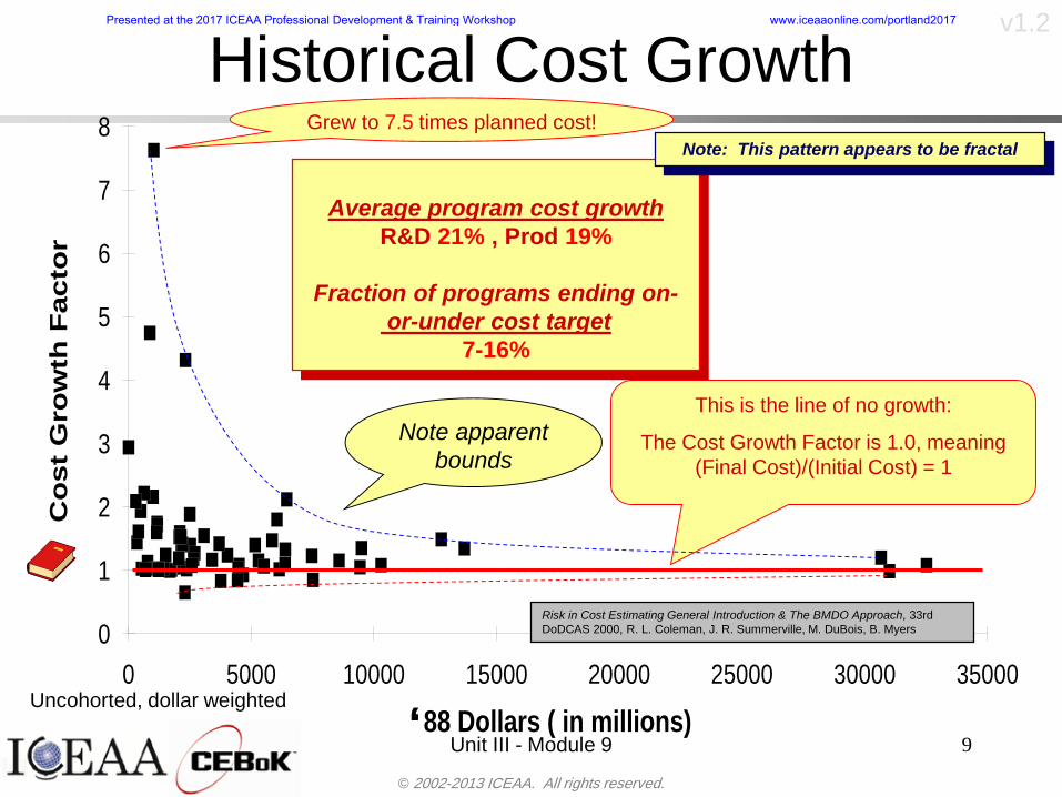
copy 2002-2013 ICEAA All rights reserved
v12
88 Dollars ( in millions)
Co
st G
row
th F
acto
r
0
1
2
3
4
5
6
7
8
0 5000 10000 15000 20000 25000 30000 35000
lsquoUnit III - Module 9 9
Historical Cost Growth
Average program cost growthRampD 21 Prod 19
Fraction of programs ending on-or-under cost target
7-16
Note This pattern appears to be fractal
Uncohorted dollar weighted
This is the line of no growth
The Cost Growth Factor is 10 meaning (Final Cost)(Initial Cost) = 1
Grew to 75 times planned cost
Risk in Cost Estimating General Introduction amp The BMDO Approach 33rd DoDCAS 2000 R L Coleman J R Summerville M DuBois B Myers
Note apparent bounds
Presented at the 2017 ICEAA Professional Development amp Training Workshop wwwiceaaonlinecomportland2017
88 Dollars ( in millions)
Cost Growth Factor
0
1
2
3
4
5
6
7
8
0
5000
10000
15000
20000
25000
30000
35000
copy 2002-2013 ICEAA All rights reserved
v12
Sources of Cost Risk
Unit III - Module 9 10
l Security Risksl Critical failure modesl Energy Environmental Risksl Schedule problems and delaysl Inadequate cost estimates
n Process (need to assess contractorrsquos assumptions)
n Models l ldquoNew Ways of Doing Businessrdquol Inflationl Systems Engineeringl Cost Improvement Curve
Assumptions
l State-of-the-Art-Advance (Technology Readiness)
l Technical Risk Sourcesn Physical propertiesn Material Propertiesn Radiation Properties
(emission and reception)l Material Availability Risksl Testing Modeling Risksl Integration Interface Risksl Program Personnell Safety Risksl Software Design Risks
Historical cost data available
Amount of cost risk depends on the Basis of the Estimate
Presented at the 2017 ICEAA Professional Development amp Training Workshop wwwiceaaonlinecomportland2017
copy 2002-2013 ICEAA All rights reserved
v12
Point Estimates of Costbull Funding organizations need best estimate of cost for
bullCostperformance tradeoff studiesbullCostbenefit analysesbullBudget planning
bull But program cost is nebulous heavily impacted bybullTechnological (im)maturitybullProgrammatic considerationsbullSchedule slipsbullUnforeseen events
bull Point cost estimates cannot be ldquocorrectrdquo becausebullEvery cost element contains uncertaintybullTotal system cost is sum of these WBS elements
bull Actual program cost falls within a range surrounding the best estimate (with some degree of confidence)bullThe best we can hope to do is to understand the uncertaintybullUnderstanding the uncertainty will help us make provision for it
Unit III - Module 9 11
Presented at the 2017 ICEAA Professional Development amp Training Workshop wwwiceaaonlinecomportland2017
copy 2002-2013 ICEAA All rights reserved
v12
Unit III - Module 9 12
Types of Riskbull Cost Growth = Cost Estimating Growth + SkedTech Growth
+ Requirements Growth + Threat Growthbull Cost Risk = Cost Estimating Risk + SkedTech Risk +
Requirements Risk + Threat Riskndash Cost Estimating Risk Risk due to cost estimating errors and the statistical
uncertainty in the estimate ndash ScheduleTechnical Risk Risk due to inability to conquer problems posed
by the intended design in the current CARD or System Specificationsndash Requirements Risk Risk resulting from an as-yet-unseen design shift from
the current CARD or System Specifications arising due to shortfalls in the documents
bull Due to the inability of the intended design to perform the (unchanged) intended mission
bull We didnrsquot understand the solutionndash Threat Risk Risk due to an unrevealed threat eg shift from the current
STAR or threat assessmentbull The problem changedO
ften
impl
icit
or o
mitt
ed
1 2
Presented at the 2017 ICEAA Professional Development amp Training Workshop wwwiceaaonlinecomportland2017
copy 2002-2013 ICEAA All rights reserved
v12
Point Estimates Vs Risk Estimates
Unit III - Module 9 13
DDTampE Flight Unit Production TotalPoint Estimate 63807 5179 6697 70505CER Risk Only - Mean 71176 4805 6426 78018Full Risk - Mean 78937 6490 8091 87430Point Esimtate + 30 82949 6733 8706 91657Full Risk - 70th Percentile 87939 7980 9608 97011
Estimated Total Cost in Millions
Note that the mean is 24 higher than the point estimate and the 70th
percentile is 38 higher than the point estimate
Presented at the 2017 ICEAA Professional Development amp Training Workshop wwwiceaaonlinecomportland2017
copy 2002-2013 ICEAA All rights reserved
v12
Cost Risk and Probabilitybull Cost risk or cost uncertainty analysis represents cost as a
probability distributionbull A probability distribution is a mathematical rule associating a
probability a to each possible outcome or event of interestbull There are two ways to present a probability distribution ndash as a
probability density function (ldquoPDF) and as a cumulative distribution function (ldquoS-curverdquo or ldquoCDFrdquo)
Unit III - Module 9 14
Lognormal Distribution PDF and CDF
0102030405060708090100
200 300 400 500 600 700 800 900 1000Cost $
Con
fiden
ce L
evel
0
00002
00004
00006
00008
0001
00012
00014
00016
Prob
abili
ty D
ensi
ty
CDFPDF
Presented at the 2017 ICEAA Professional Development amp Training Workshop wwwiceaaonlinecomportland2017
copy 2002-2013 ICEAA All rights reserved
v12
Unit III - Module 9 15
Probability Model ndash Distributionbull Normal
ndash Best behavior most iconic
ndash Theoretically (although not practically) allows negative costs which spook some users
ndash Symmetric needs mean shift to reflect propensity for positive growth
bull Lognormalndash A natural result in
non-linear CERsndash Indistinguishable
from Normal at CVs below 25
ndash Skewed
10
4
10
Presented at the 2017 ICEAA Professional Development amp Training Workshop wwwiceaaonlinecomportland2017
copy 2002-2013 ICEAA All rights reserved
v12
Unit III - Module 9 16
bull Triangularndash Most commonndash Easy to use easy to understandndash Modes medians do not addndash Skewed
bull Betandash Rare now but formerly popularndash Solves negative cost and duration issuesndash Many parameters ndash simplifications like PERT
Beta are possiblendash Skewed
bull Bernoullindash Probability is only assigned to two possible
outcomes success and failure (p and 1-p)ndash Simplest of all discrete distributionsndash Mean = pndash Variance = p(1-p)
10
Probability Model ndash Distribution
10
10
Presented at the 2017 ICEAA Professional Development amp Training Workshop wwwiceaaonlinecomportland2017
copy 2002-2013 ICEAA All rights reserved
v12
Unit III - Module 9 17
bull Normalndash If there is a sufficiently large number of independently identically distributed
elements (or not too correlated and not too skewed) then the distribution of total cost is normal due to the Central Limit Theorem
bull Lognormalndash For smaller data sets with large amounts of (positive) correlation and
skewness the lognormal distribution may be a better approximation of total cost
ndash Many total cost distributions in smaller data sets test as both normal and lognormal
bull Triangularndash The sum of triangles is not a triangle so this distribution should generally not
be used to characterize total costbull Convolved
ndash If total cost distribution is derived using simulation then it may not particularly resemble anything In this case we simply have a convolved or simulated total cost distribution
Probability ndash Top-Level Distribution
NEW
Presented at the 2017 ICEAA Professional Development amp Training Workshop wwwiceaaonlinecomportland2017
copy 2002-2013 ICEAA All rights reserved
v12
S-Curves and Confidence Levels
Unit III - Module 9 1818
100
70
25
Probability(Confidence
Level)
Cost Estimate(Dollars)
50
The S curve is the cumulative probability distribution coming out of the statistical summing process
70 confidence that project will cost indicated amount or less
Provides information on potential cost as a result of identified project risks
Provides insight into establishing reserve levels
X Y
MR
X = Point estimateZ = Project requirementY = Cost estimate where there is a 70 change that
final actual cost will be less than cost estimateY-Z= Manage reserve (MR) which is REQUIRED to meet 70 CL
Z
X not always = Z but is based on same content
Presented at the 2017 ICEAA Professional Development amp Training Workshop wwwiceaaonlinecomportland2017
copy 2002-2013 ICEAA All rights reserved
v12
19
Example ndash Normal Distribution
bull Normal distribution with mean equal to 100 and standard deviation equal to 20
bull Median and mode also equal 100bull The 80th Percentile is 117
40 60 80 100 120 140 160
80 of distribution(area under curve)is less than 117
117
Presented at the 2017 ICEAA Professional Development amp Training Workshop wwwiceaaonlinecomportland2017
copy 2002-2013 ICEAA All rights reserved
v12
20
Confidence Levelsbull The output of a cost risk analysis is a probability
distributionndash Typically displayed as a cumulative distribution function or
ldquoS-curverdquondash Confidence levels are simply percentiles of the distribution
0
10
20
30
40
50
60
70
80
90
100
30 60 90 120 150 180
Conf
iden
ce L
evel
Presented at the 2017 ICEAA Professional Development amp Training Workshop wwwiceaaonlinecomportland2017
copy 2002-2013 ICEAA All rights reserved
v12
Measuring Parametric Model Uncertainty
bull When developing estimates using cost-estimating relationships (CERs) there are two major sources of uncertaintyndash Technical (model input) uncertaintyndash Estimating uncertainty
bull Technical uncertainty reflects the uncertainty inherent in the model inputsndash Typical parametric model inputs include weight lines of code
heritage and other performance and management inputs
bull Estimating uncertainty measures the uncertainty inherent in the model due to the modelrsquos inability to capture all aspects of variability in the data
21
Presented at the 2017 ICEAA Professional Development amp Training Workshop wwwiceaaonlinecomportland2017
copy 2002-2013 ICEAA All rights reserved
v12
Parametric Model Examplebull The NASAAir Force Cost Model (NAFCOM) is a
parametric model for estimating acquisition costs for spacecraft and launch vehicles
bull The CERs in NAFCOM have the formCost = C WeightVNewDesignWTechnicalXManagementY ClassZ
bull There is technical uncertainty about each of the parametersndash Parametric models are applied early in a program so there
is significant amount of uncertainty in the weightndash Heritage is also tricky it is inherently subjective and project
personnel are typically optimisticndash Technical characteristics can also change as a program
matures and requirements change
22
Presented at the 2017 ICEAA Professional Development amp Training Workshop wwwiceaaonlinecomportland2017
copy 2002-2013 ICEAA All rights reserved
v12
Weight Uncertaintybull Aerospace weight growth study average satellite
weight growth from program inception to launch is 28
23
Aerospace Weight Growth Data
-10
0
10
20
30
40
50
60
0 4 8 12 16 20 24 28 32 36 40 44 48 52 56 60 64 68 72 76 80 84 88 92 96 100
Percent Program Completion
Perc
ent W
eigh
t Gro
wth
Presented at the 2017 ICEAA Professional Development amp Training Workshop wwwiceaaonlinecomportland2017
copy 2002-2013 ICEAA All rights reserved
v12
Estimating Uncertaintybull CERs do not perfectly fit the historical data
ndash There are non-repeatable random effects that cannot be predicted
bull For examplendash Parts breaking during testingndash Strikes which are difficult to predict
bull This results in an underlying uncertainty distribution about an estimatendash The outcome of a CER represents only one point on an
uncertainty distributionbull Typically mean or median depending upon the CER
methodology
24
Presented at the 2017 ICEAA Professional Development amp Training Workshop wwwiceaaonlinecomportland2017
copy 2002-2013 ICEAA All rights reserved
v12
Estimating Uncertainty (2)
25
Presented at the 2017 ICEAA Professional Development amp Training Workshop wwwiceaaonlinecomportland2017
copy 2002-2013 ICEAA All rights reserved
v12
Estimating Uncertainty (3)bull In the case of a linear regression the estimating
uncertainty follows a normal distributionndash The estimate is the mean and the standard error of the
estimate from the regression is the standard deviation of the normal distribution
bull In the case of a log-transformed linear regression the estimating uncertainty follows a lognormal distributionndash The estimate is the median of the lognormal and the
standard error of the estimate from the regression is the standard deviation of the normal distribution (in log-space)
bull There is additional uncertainty about an estimate based upon the distance of what is being estimated from the mean of the input datandash This results in a prediction interval
26
Presented at the 2017 ICEAA Professional Development amp Training Workshop wwwiceaaonlinecomportland2017
copy 2002-2013 ICEAA All rights reserved
v12
Aggregating Riskbull Risk is typically applied at the same level at
which we estimate cost that is at the Work Breakdown Structure (WBS) level
bull The estimates for each WBS are developedndash These estimates sum to yield the total system cost
bull For an n-element WBS the total cost is the sum of the cost for each of the n elements
27
nXXXCostSystem +++= 21
Presented at the 2017 ICEAA Professional Development amp Training Workshop wwwiceaaonlinecomportland2017
copy 2002-2013 ICEAA All rights reserved
v12
WBS Examplebull Launch Vehicle
ndash Structurebull Vehicle Structurebull Tank Structure
ndash Thermal Controlbull Active Thermal Controlbull Induced Thermal Controlbull Tank Thermal Control
ndash Main Propulsion Systemndash Liquid Rocket Enginendash Electric Power and Distributionndash Command Control and Data Handlingndash System Integration
28
Presented at the 2017 ICEAA Professional Development amp Training Workshop wwwiceaaonlinecomportland2017
copy 2002-2013 ICEAA All rights reserved
v12
WBS and Risk
29
Presented at the 2017 ICEAA Professional Development amp Training Workshop wwwiceaaonlinecomportland2017
copy 2002-2013 ICEAA All rights reserved
v12
Aggregating Riskbull This leads us to the issue of aggregating the risks across the
WBSbull For example if we want to determine the 70th percentile of the
overall cost risk distribution how do we proceed bull Note that we cannot simply add the 70th percentiles of each of
the cost risk distributionsbull We can add means and variances (taking correlation into
account more on that later) but that is all
Variance of Total Cost =
30
Mean of Total Cost = ( )E X E Xk
k
n
kk
n
kk
n
= = =aringaelig
egraveccediloumloslashdivide
= =aring aring1 1 1
m
Var X kk
n
=aringaelig
egraveccediloumloslashdivide1
= s r s skk
n
iji
j
i jj
n2
1 1
1
22+aring aringaring
= =
-
=
Presented at the 2017 ICEAA Professional Development amp Training Workshop wwwiceaaonlinecomportland2017
copy 2002-2013 ICEAA All rights reserved
v12
Percentiles Do Not Addbull As a notional example consider two independent normal
distributionsndash One distribution has mean equal to 100 and standard deviation
equal to 20ndash The second distribution has mean 300 and standard deviation of 80
bull The sum of two independent normally distributed random variables is also normally distributed
bull To combine the two distributions we add the means and add the variancesndash Total mean is
ndash Total standard deviation is
31
400300100 =+
8258020 22 raquo+
Presented at the 2017 ICEAA Professional Development amp Training Workshop wwwiceaaonlinecomportland2017
copy 2002-2013 ICEAA All rights reserved
v12
Percentiles Do Not Add (2)bull The 80th percentiles for the individual distributions are
117 and 367 respbull The 80th percentile of the combined distribution is
469 but the sum of the two 80th percentiles is 484bull To see why this is the case note that the percentiles
of a normal distribution are determined by the mean and the standard deviationndash The standard deviations are not added when normal distributions
are combined rather the variances are combinedndash Sum of variances is ndash The standard deviation of this sum is
32
22 ba +22 ba +
Presented at the 2017 ICEAA Professional Development amp Training Workshop wwwiceaaonlinecomportland2017
copy 2002-2013 ICEAA All rights reserved
v12
Percentiles Do Not Add (3)bull Since bull We can write
bull The left side of this inequality represents the risk of the combined distributions while the right side represents the sums of the individual risks
bull Combining two missions that are independent results in a diversification of riskndash The total portfolio is not as risky on a relative basis as each
individual project
33
2222 2 bababa ++lt+
baba +lt+ 22
Presented at the 2017 ICEAA Professional Development amp Training Workshop wwwiceaaonlinecomportland2017
copy 2002-2013 ICEAA All rights reserved
v12
Methods for Aggregating Riskbull Since percentiles do not add we have to find other
ways to aggregate riskbull One method is to use Monte Carlo simulationbull Unless cost risk is represented by normal
distributions for all WBS elements summing the means and variances does not result in a completely accurate depiction of overall system cost risk
bull The normal distribution is not a realistic distribution for representing risk in many or even most situations since regarding project risk more can go wrong than can go right which means the risk is NOT symmetric unlike the Gaussian bell curve
34
Presented at the 2017 ICEAA Professional Development amp Training Workshop wwwiceaaonlinecomportland2017
copy 2002-2013 ICEAA All rights reserved
v12
Unit III - Module 9 35
Monte Carlo Simulationfor Risk Analysis
bull When risk analysis is performed multiple risks are gatheredndash These risks may have various probability
distributions
bull Monte Carlo is the most commonly accepted way to produce an accurate characterization of the distribution of the combined effect of these many risksndash Using this distribution we can produce percentiles
for cost impacts due to risk occurrences
10
Presented at the 2017 ICEAA Professional Development amp Training Workshop wwwiceaaonlinecomportland2017
copy 2002-2013 ICEAA All rights reserved
v12
Monte Carlo Simulationbull Simulation is a means for solving problems that are
analytically intractablendash Involves repeated random sampling
bull It was developed during the Manhattan Project as a way to model the interactions inside an atom during nuclear fissionndash Allowed for more sophisticated mathematical modeling of atomic
phenomena
bull Most computer packages use pseudo-random number generators that produce seemingly random results from an initial seedndash Example is the linear congruential generator
36
( ) mbaXX nn mod1 +=+
Presented at the 2017 ICEAA Professional Development amp Training Workshop wwwiceaaonlinecomportland2017
copy 2002-2013 ICEAA All rights reserved
v12Using Random Numbers to Simulate Distributions
bull WBS cost risk is typically measured by a probability distributionbull The most common method for simulating a probability
distribution is the inverse methodbull This involve obtaining a simulated random value from a uniform
distribution and then inverting this through the cumulative distribution function (CDF) to obtain the simulated value
bull As an example for a uniform distribution on the interval [0100]
bull In this case the CDF random value of 05 translates to 10005 = 50
37
( )100
1=xf ( )
100xxF = ( ) xxF 1001 =-
Presented at the 2017 ICEAA Professional Development amp Training Workshop wwwiceaaonlinecomportland2017
copy 2002-2013 ICEAA All rights reserved
v12
Simulating a Triangular Distribution
bull For a triangular distribution with low = 0 most likely = 50 and high = 150 the CDF is given by
bull The inverse function is given by
38
( )iumliumlicirc
iumliumliacute
igrave
poundlt--
poundpound=
1505021
1500050
50015000
2
2
2
xxx
xxxF
( )iumliumlicirc
iumliumliacute
igrave
poundltdivideoslashouml
ccedilegraveaelig +--
poundpound=-
131
21
37501
250017500150
3107500
1
xx
xxxF
Presented at the 2017 ICEAA Professional Development amp Training Workshop wwwiceaaonlinecomportland2017
copy 2002-2013 ICEAA All rights reserved
v12
Simulating a Triangular Distribution (2)
bull If the simulated uniform value is equal to 02 the corresponding inverse value from the CDF inverse is approximately 387
39
0
01
02
03
04
05
06
07
08
09
1
0 30 60 90 120 150
Presented at the 2017 ICEAA Professional Development amp Training Workshop wwwiceaaonlinecomportland2017
copy 2002-2013 ICEAA All rights reserved
v12
Monte Carlo and the WBSbull Simulation involves repeated trials
40
WBS Draw1 2 3 4 5
System 2912 3566 4390 2954 4655 Sum
Structure 80 105 55 80 57 SumVehicle Structure 50 70 30 40 20Tank Structure 30 35 25 40 37
Thermal Control 32 36 35 29 33 SumActive Thermal Control 10 15 12 7 10Induced Thermal Control 12 14 13 14 14Tank Thermal Control 10 7 10 8 9
Main Propulsion System 100 150 125 140 100
Liquid Rocket Engine 1000 1100 1800 900 2200
Electric Power and Distribution 100 125 150 75 90
Command Control and Data Handling 200 250 225 230 275
System Integration 1400 1800 2000 1500 1900
Presented at the 2017 ICEAA Professional Development amp Training Workshop wwwiceaaonlinecomportland2017
copy 2002-2013 ICEAA All rights reserved
v12
Number of Trialsbull Monte Carlo involves a repeated number of trialsbull The greater the number of trials the more accurate the
simulation will approximate the overall cost risk behavior of the system
bull After 100 trials the histogram looks very jagged
41
Presented at the 2017 ICEAA Professional Development amp Training Workshop wwwiceaaonlinecomportland2017
copy 2002-2013 ICEAA All rights reserved
v12
Number of Trials (2)
42
1000 Trials
10000 Trials
50000 Trials Additional trials give a more accurate depiction of the final result
Presented at the 2017 ICEAA Professional Development amp Training Workshop wwwiceaaonlinecomportland2017
copy 2002-2013 ICEAA All rights reserved
v12
Number of Trials (3)bull If we want to simulate the underlying
mean within 1 with 95 confidence for example then we require
43
divideoslash
oumlccedilegrave
aelig poundpound-
=
dividedividedivide
oslash
ouml
ccedilccedilccedil
egrave
aeligpound
-pound
-=
divideoslashouml
ccedilegraveaelig poundpound=
nZ
n
nnX
n
X
n
n
011
010Pr
011
010Pr
011990Pr950
___
___
sm
sm
sm
sm
sm
mm
Presented at the 2017 ICEAA Professional Development amp Training Workshop wwwiceaaonlinecomportland2017
copy 2002-2013 ICEAA All rights reserved
v12
Number of Trials (4)bull This means that the number of trials required is determined by
bull Solving for n we find that at least
trials are neededbull Note that this term involves the coefficient of variation of the
distribution which means that distributions with less dispersion require fewer trials to accurate simulate
44
96101
=ns
m
ms41638
Presented at the 2017 ICEAA Professional Development amp Training Workshop wwwiceaaonlinecomportland2017
copy 2002-2013 ICEAA All rights reserved
v12
Number of Trials (5)bull Simulating percentiles requires more trials than for simulating
meansbull Let Pn represent the number of trials in the sample at or below
the 70th percentile of the underlying distribution (suppose this is known)
bull By the Central Limit Theorem Pnn follows a normal distribution with mean equal to the 70th percentile and variance equal to
bull By a similar process for the mean we find that the number of trials needed to simulate the 70th percentile within 1 with 95 confidence is
45
( )n
FF 700700 1-
n
n
PPn -41638
Presented at the 2017 ICEAA Professional Development amp Training Workshop wwwiceaaonlinecomportland2017
copy 2002-2013 ICEAA All rights reserved
v12
Number of Trials (6)bull If Pn 070 for all n then n is approximately
bull For the sake of comparison suppose CV = 03 (reasonable approximation for hardware development) then the number of trials needed to simulate the mean with the same accuracy is then ldquoonlyrdquo 11525
bull More trials are needed to accurately simulate percentiles than means
46
( ) 46416703041638
70704168341638 =divide
oslashouml
ccedilegraveaelig=divide
oslashouml
ccedilegraveaelig -
=-
nnn
PPn
n
n
Presented at the 2017 ICEAA Professional Development amp Training Workshop wwwiceaaonlinecomportland2017
copy 2002-2013 ICEAA All rights reserved
v12
Methods of Simulationbull Monte Carlo simulation is a standard term for
simulationbull However there is an improvement on Monte Carlo
that improves the accuracy of the results of a simulation for a given number of trials
bull This method is call the Latin Hypercube approach to simulationndash Similar to Monte Carlo but an equal number of draws are taken
from a set of subintervals for example dividing the interval (01) into [00001) [0102)hellip [0910]
ndash Instead of 10 trials from [01] we have one trial from each subinterval
ndash Rough rule of thumb is Latin Hypercube takes 30 fewer trials to achieve similar accuracy to Monte Carlo
47
Presented at the 2017 ICEAA Professional Development amp Training Workshop wwwiceaaonlinecomportland2017
copy 2002-2013 ICEAA All rights reserved
v12
Probability Model ndash Correlationbull Correlation exists between work breakdown structure
(WBS) cost element costs and between cost and schedule
bull Correlation is a necessary consideration in cost risk analysis
bull Correlation is a number that can vary between -1 and +1 and represents the strength of the relationship between the two variablesndash If both variable have a tendency to move in the same direction
correlation is positivendash If when one variable increases the other tends to decrease and
vice-versa the correlation between the two variables is negative
Presented at the 2017 ICEAA Professional Development amp Training Workshop wwwiceaaonlinecomportland2017
copy 2002-2013 ICEAA All rights reserved
v12
Correlation And Causationbull Note that correlation is not causation however
causation implies correlationndash For example shark attacks and ice cream sales at the beach
bull For example for a launch vehicle structure increasing the diameter will not only result in an increase in the structures cost but will also result in higher costs for thermal coating (paint etc)
bull Also simply because two subsystems do not appear to be related does not mean they are not correlatedndash For example structures and computer equipment seemingly
have little relation to one another however an external factor such as a funding cut or a strike will impact all subsystems leading to delays and increasing cost across the board
ndash Thus everything in a WBS has some correlationUnit III - Module 9 49
Presented at the 2017 ICEAA Professional Development amp Training Workshop wwwiceaaonlinecomportland2017
copy 2002-2013 ICEAA All rights reserved
v12
The Importance of Correlationbull Percent that total cost standard deviation is underestimated
when correlation assumed to be 0 instead of r given nWBS elements
Unit III - Module 9 5050
0
20
40
60
80
100
0 01 02 03 04 05 06 07 08 09 1Actual Correlation
Perce
nt Un
deres
timate
d
n = 10
n = 30
n = 100n = 1000
0
20
40
60
80
100
0 01 02 03 04 05 06 07 08 09 1Actual Correlation
Perce
nt Un
deres
timate
d
n = 10
n = 30
n = 100n = 1000
Reference 32nd Annual DOD Cost Analysis Symposium Advanced Training Session ldquoWhy Correlation Matters in Cost Estimatingrdquo Stephen A Book
Presented at the 2017 ICEAA Professional Development amp Training Workshop wwwiceaaonlinecomportland2017
copy 2002-2013 ICEAA All rights reserved
v12
The Importance of Correlation (2)bull For example if correlation is assumed to be 0 for all
elements in a 30 element WBS and the actual correlation is 20 then the total cost standard deviation is underestimated by 60
bull For example assume the total cost is modeled as a normal distribution with mean = 100
bull If correlation is assumed to be zero with total cost standard deviation = 12 when correlation is actually 20 then the true underlying standard deviation is actually 30
bull 70th percentile with zero correlation assumption is 106
bull 70th percentile with 20 correlation is 116 Unit III - Module 9 51
Presented at the 2017 ICEAA Professional Development amp Training Workshop wwwiceaaonlinecomportland2017
copy 2002-2013 ICEAA All rights reserved
v12
Measures of Correlationbull Two measures of correlation are commonly used in
cost risk analysesndash Pearsonrsquos product-moment correlation coefficient ndash Spearmanrsquos rank correlation coefficient
bull Garvey and others recommend using Pearsonrsquos product-moment correlation coefficient correlation for cost risk analysesndash Method of moments uses this but there are two options in
simulationndash Popular simulation packages like Risk and Crystal Ball use
rank correlation but in practice this has been found to make little difference
ndash Pearson product-moment correlation has been incorporated into Risk+
52
Presented at the 2017 ICEAA Professional Development amp Training Workshop wwwiceaaonlinecomportland2017
copy 2002-2013 ICEAA All rights reserved
v12
Pearson Correlationbull Pearsonrsquos product-moment correlation measures
degree of linearity between two random variables bull If two random variables are perfectly linear (eg Y =
aX + b) with positive slope then the Pearson product-moment correlation between X and Y denoted by rXY is +1
53
X X
Y Y Y
XNegative Correlation Positive Correlation No Correlation
middotmiddot
middotmiddot
middotmiddot middotmiddot
middotmiddot
middot
middot
middotmiddotmiddot
middotmiddot
middotmiddot
middotmiddot middot
middot
middot
middotmiddotmiddotmiddotmiddotmiddotmiddotmiddot
middotmiddotmiddotmiddot
middotmiddot
middotmiddot middotmiddotmiddotmiddot
middotmiddotmiddot
middotmiddotmiddotmiddot
middotmiddotmiddot
middotmiddotmiddot
middotmiddot
middot
middot middotmiddot
middot middotmiddotmiddotmiddot middotmiddot middot middotmiddot middot middot
middotmiddot middot
middotmiddotmiddotmiddotmiddot middot middotmiddot
middotmiddot
middot
middotmiddot
middotmiddot middot
middot middot middot
middotmiddot middot
middotmiddotmiddot
middotmiddot
middot middot
Presented at the 2017 ICEAA Professional Development amp Training Workshop wwwiceaaonlinecomportland2017
copy 2002-2013 ICEAA All rights reserved
v12
Spearman Correlationbull Spearmanrsquos rank correlation measures the
monotonicity between two random variablesbull If two random variables are perfectly monotonically
increasing (eg Y = X2) then the Spearman rank correlation denoted by rXY is +1
bull The two measures can be significantly different
54
10 20 30 40 50 60
100
200
300
096 097 098 099 1
1
060
020
040
080
Eff
ort (
Staf
f-M
onth
s)
Software Size I KDSI
y = 28z12y
z x
yy = x100
0 pound x pound 1
Figure 5-9A Figure 5-9B
Pearson Correlation = 09976 Rank Correlation = 1
Pearson Correlation = 024 Rank Correlation = 1
X(x ) ~ Unif(01)
Reference Probability Methods for Cost Uncertainty Analysis A Systems Engineering Perspective Paul R Garvey
Presented at the 2017 ICEAA Professional Development amp Training Workshop wwwiceaaonlinecomportland2017
copy 2002-2013 ICEAA All rights reserved
v12
Unit III - Module 9 55
200
250
300
350
400
1000 1200 1400 1600 1800 2000
Recurring Production
SEPM
200
250
300
350
400
1000 1200 1400 1600 1800 2000
Recurring Production
SEPM
Functional Correlationbull Old No Functional
Correlation Simulation run with WBS items entered as values
bull New Simulation run with functional dependencies entered as they are in cost model
CorrelatedNot Correlated
Note shift of mean and increased variability
Presented at the 2017 ICEAA Professional Development amp Training Workshop wwwiceaaonlinecomportland2017
copy 2002-2013 ICEAA All rights reserved
v12
Risk Measuresbull ldquoWestern Europe conquered the word because of a
technological revolution that started because of attempts to measure the worldrdquo ndash Phillipe Jorion ndash In the same way attempts to measure risk will lead to better project
managementbull Risk management for DoD and NASA agencies focuses
primarily on funding projects to a single percentile ndash NASA policy explicitly mentions 70 and 50ndash This is known as ldquoValue at Riskrdquo and is prevalent in the banking and
financial industry
56
Presented at the 2017 ICEAA Professional Development amp Training Workshop wwwiceaaonlinecomportland2017
copy 2002-2013 ICEAA All rights reserved
v12
Value at Risk (VaR)bull VaR is a percentile of the cost risk
distributionndash VaR funding at the 70th percentile means that
there is a 30 chance of final project cost exceeding the funded amount (budget)
bull VaR has some meritsndash Common measure can be used to compare
different projects and programsndash Easily understood by senior managers and
decision makers
57
Presented at the 2017 ICEAA Professional Development amp Training Workshop wwwiceaaonlinecomportland2017
copy 2002-2013 ICEAA All rights reserved
v12
Why 70th or 80th Percentilebull Typical policy guidance involves funding at the 70th or 80th
percentile Why fund as such a low percentilebull There is some incentive to not over-fundbull For a normal distribution an inflection point occurs near the 80th
percentile meaning that for values above 80 confidence achieving higher levels of confidence can only be achieved by spending greater dollar amounts at an increasing rate
58
-05-04-03-02-01
00102030405
0 05 1 15 2 25 3
Standard Deviations from Mean
Normal Distribution
First DerivativeSlopeVelocity
Second DerivativeConvexityAcceleration
Inflection point at one standard deviation above the mean (~84th
percentile)
Presented at the 2017 ICEAA Professional Development amp Training Workshop wwwiceaaonlinecomportland2017
copy 2002-2013 ICEAA All rights reserved
v12
Funding Above Inflection Pointsbull As the percentile goes above the 80th percentile the amount
needed to achieve that higher level of confidence begins to increase at an increasing rate as is evident from the graph
59
0
10
20
30
40
50
60
70
50 55 60 65 70 75 80 85 90 95 100
$ Ab
ove
MEa
n to
Ach
ieve
Per
cent
ile
Percentile (Confidence Level)
Presented at the 2017 ICEAA Professional Development amp Training Workshop wwwiceaaonlinecomportland2017
copy 2002-2013 ICEAA All rights reserved
v12
Why Budget to the 70th or 80thbull Government projects are funded at the 70th or 80th percentilesbull Why not the 90th or 99th percentile Wonrsquot that help prevent
overrunsndash As we have seen percentiles do not add across programs
bull The sum of the 80th percentiles does NOT equal the total 80th percentile
ndash This is because the individual programs are riskier than the entire suite of missions
bull Known as the ldquoPortfolio effectrdquo (more or this later)
ndash Funding at the 80th gives confidence that the entire portfolio will be adequately funded
bull And since there is an inflection point near the 80th percentile funding above that level quickly becomes cost prohibitive
60
Presented at the 2017 ICEAA Professional Development amp Training Workshop wwwiceaaonlinecomportland2017
copy 2002-2013 ICEAA All rights reserved
v12
Inflection Points for Lognormalbull For a lognormal the inflection point
variesndash Coefficient of variation equal to 10 equates to an
inflection point at the 70th percentile
61
0
10
20
30
40
50
60
70
050 060 070 080 090 100
Coef
ficen
t of V
aria
tion
Percentile of the Inflection Point
Presented at the 2017 ICEAA Professional Development amp Training Workshop wwwiceaaonlinecomportland2017
copy 2002-2013 ICEAA All rights reserved
v12
Issues with Percentile Fundingbull However risk management does not stop at a
specific percentilendash What happens when the 70th percentile is exceeded
bull Any effective risk management policy should prescribe what happens after a bad event occursndash With VaR we only know when a bad event has occurred ndash Also funding at a relatively low level means we have no true
sense of the real risks that should be guarded against
62
Presented at the 2017 ICEAA Professional Development amp Training Workshop wwwiceaaonlinecomportland2017
copy 2002-2013 ICEAA All rights reserved
v12
ldquoHere There Be Dragonsrdquobull On old maps uncharted territory was often
marked with monsters or dragons
63
A section of the Carta Marina by Olaus Magnus 16th Century
Presented at the 2017 ICEAA Professional Development amp Training Workshop wwwiceaaonlinecomportland2017
copy 2002-2013 ICEAA All rights reserved
v12
Distribution Comparisonbull Four different distributions with the same 70th
percentile
bull Should we expect the tails to be similar
64
0
10
20
30
40
50
60
70
80
0 100 200 300 400 500 600
Perc
entil
eCo
nfid
ence
Lev
el
Triangular
Normal
Lognormal
Pareto
Presented at the 2017 ICEAA Professional Development amp Training Workshop wwwiceaaonlinecomportland2017
copy 2002-2013 ICEAA All rights reserved
v12Distribution Comparison Tail Behavior
bull The normal and triangular distributions have similar tails but the lognormal and Pareto have much fatter right tails
65
70
75
80
85
90
95
100
500 1500 2500 3500 4500 5500
Perc
entil
eCo
nfid
ence
Lev
el
Triangular
Normal
Lognormal
Pareto
Here There Be Dragons
Presented at the 2017 ICEAA Professional Development amp Training Workshop wwwiceaaonlinecomportland2017
copy 2002-2013 ICEAA All rights reserved
v12Distribution Comparison ndash Tail Behavior (Table)
bull There is significant tail risk for the lognormal and the Paretobull The 99th percentile for the Pareto is 1000 times greater than
the 70th percentilendash Risk seen in financial markets and in catastrophic risks like natural
disasters bull Four different projects follow the four different risk profiles seen
in this example should clearly have different risk management approaches but 70th percentile funding indicates the same risk management approach for all four
66
Percentile Triangular Normal Lognormal Pareto 70th $600 $600 $600 $600 80th $680 $660 $770 $1430 90th $770 $750 $1070 $5880 95th $840 $820 $1410 $23750 99th $930 $950 $2350 $600000
Presented at the 2017 ICEAA Professional Development amp Training Workshop wwwiceaaonlinecomportland2017
copy 2002-2013 ICEAA All rights reserved
v12Percentile Budgeting is Not Risk Management
bull Percentile budgeting ne effective risk management policybull Suppose that you are shopping for a new car You
mention that safety is your top concern The salesman says he has a great safe car available You ask about the air bags Do they work The salesman answers ldquoOf course Seventy percent of the time they work fine Only 30 of the time the air bags will fail to deployrdquo Would you buy such a car Hedge fund manager David Einhorn has stated ldquoRisk management is the air bag that must always work but only in the multi-sigma event where you have an accidentrdquo
67
Risk management is the air bag that must always work but only in the multi-sigma event where you
have an accident
Presented at the 2017 ICEAA Professional Development amp Training Workshop wwwiceaaonlinecomportland2017
copy 2002-2013 ICEAA All rights reserved
v12
Joint Confidence Level Analysisbull Schedules are risky toobull For 98 recent NASA missions average
schedule growth was 38ndash Not as high as cost growth but still significant
68
0
5
10
15
20
25
30
35
40
Schedule
Cost
Presented at the 2017 ICEAA Professional Development amp Training Workshop wwwiceaaonlinecomportland2017
copy 2002-2013 ICEAA All rights reserved
v12
Schedules Impact Costbull Changes in schedule can have enormous
impacts on cost ndash Schedule slips can lead to cost increases
bull Fixed programmatic costs must be paid on a regular basisndash Achieving schedule milestones early can result in cost
savings
bull Schedule is an important consideration in cost analysis including cost risk analysis
bull However we must be careful in correctly integrating cost and schedule riskndash Schedule is not simply an input but is dependent on many of
the same factors that drive cost
69
Presented at the 2017 ICEAA Professional Development amp Training Workshop wwwiceaaonlinecomportland2017
copy 2002-2013 ICEAA All rights reserved
v12
The Relationship of Cost to Schedulebull Cost and schedule are positively correlated
ndash A larger program with bigger scope with take longer to complete than a smaller simpler program
bull However longer schedules do not always equate to higher cost nor shorter schedules with lower costndash Highly compressed schedules relative to the
optimal schedule can lead to large overrunsbull Compressed schedules are commonplace for
many planetary missions
70
Presented at the 2017 ICEAA Professional Development amp Training Workshop wwwiceaaonlinecomportland2017
copy 2002-2013 ICEAA All rights reserved
v12The Impact of Schedule GrowthCompression on Cost
bull Compressed schedules lead to cost growth and based on existing research is actually more expensive than schedule slippages
71
0
20
40
60
80
100
120
140
160
-50 -25 0 25 50 75 100
Percentage Change in Schedule
Perc
enta
ge C
hang
e in
Cos
t due
to
Sche
dule
Cha
nge
Source Smart CB ldquoCost and Schedule Interrelationshipsrdquo 2007 NASA Cost Symposium
Presented at the 2017 ICEAA Professional Development amp Training Workshop wwwiceaaonlinecomportland2017
copy 2002-2013 ICEAA All rights reserved
v12Schedule as an Independent Variable
bull Why not simply add schedule as an input to cost-estimating relationships (CERs)
bull Schedule is often treated as an independent variable ndash schedules are often determined independently of cost considerationsndash Cost may not be considered explicitly although budgets and
schedules are determined based on scope and other common factors
bull In 2006 SAIC undertook a research task to determine the impact of schedule on cost and added schedule as an independent variable to the CERs in the NASAAir Force Cost Model (NAFCOM) to see if schedule provided any improvement in goodness of fit
72
Presented at the 2017 ICEAA Professional Development amp Training Workshop wwwiceaaonlinecomportland2017
copy 2002-2013 ICEAA All rights reserved
v12
Schedule is a Dependent Variablebull Since NAFCOM includes an exhaustive list of cost drivers the inclusion
of schedule should give an indication of whether there is any additional independent value added from schedule independent of the cost drivers
bull In the study schedule was added to 10 subsystem-level CERs
ndash In each case the addition of schedule did NOTimprove the goodness of fit and schedule was NOT found to be a statistically significant cost driver (given the presence of the other variables) for any of the 10 CERs
bull Standard errors for the CERs increased due to decrease in degrees of freedom
bull Thus schedule as an independent variable did not provide any additional explanation of variation in historical cost
bull This is because schedule is truly NOT an independent variable but a dependent variable and is a function of the same factors that drive cost
73
Presented at the 2017 ICEAA Professional Development amp Training Workshop wwwiceaaonlinecomportland2017
copy 2002-2013 ICEAA All rights reserved
v12
Incorporation of Schedule in Cost Risk
bull When using subjective methods care must be taken in applying schedule to cost risk analysis
bull Since schedule is a dependent variable treating it independently from other factors when assessing its impact on cost can lead to a double count of independent variables in the cost risk analysis
bull Direct inclusion of schedule in a cost risk analysis effectively doubles the influence of each cost driver
ndash Incorrectly leads to broader risk ranges
74
CostWeight
HeritageNewness
Technology Readiness Schedule
Presented at the 2017 ICEAA Professional Development amp Training Workshop wwwiceaaonlinecomportland2017
copy 2002-2013 ICEAA All rights reserved
v12Subjective Cost Risk Methods and Overinclusion of Risk Factors
bull Subjective methods are suitable when data are scarce or not availablebull However care must be taken not to treat correlated sources of risk
such as schedule as independent of each otherbull Example ndash a subjective risk analysis incorporated technology readiness
design risk requirements stability integration risk and schedule and treated each source of risk as independent
bull Risk triangle high value without schedule risk was 31 times the point estimate
bull Risk triangle high value with schedule risk added on top of other sources of risk treated independently was 34 times the point estimate
bull Risk triangle taking correlation between sources of risk into account in a rigorous statistical manner has a high value 15 times the point estimate less than half the effect when treating sources of risk as independent
75
Presented at the 2017 ICEAA Professional Development amp Training Workshop wwwiceaaonlinecomportland2017
copy 2002-2013 ICEAA All rights reserved
v12Fundamental Equation of Cost and Schedule Interrelationships
bull The Fundamental Equation of the Relationship Between Cost and Schedule is
Time = Moneybull This is a well known adage that time is money Your boss at
work may even mention this to you from time to time or if you are the boss you are all too aware of this iron law
bull Because time is money cost and schedule risk should be modeled jointly not with schedule as an independent cost driver
bull Note that cost and schedule are not perfectly correlatedndash Cost can sometimes ldquobuy downrdquo schedule extra money can be
spent to meet a deadline since in some cases additional effort to hasten the completion of a task
76
Presented at the 2017 ICEAA Professional Development amp Training Workshop wwwiceaaonlinecomportland2017
copy 2002-2013 ICEAA All rights reserved
v12How to (Correctly) Incorporate Schedule into Cost Risk Analysis
bull The best way to model cost and schedule risk is to develop a joint cost and schedule model based on the same data
bull Since such models are not currently available the next best approach is to model cost and schedule independently and then integrate cost and schedule risk analyses using joint probability distributions taking into account correlation between cost and schedulendash This approach pioneered by Paul Garvey and Steve Book is
considered industry best practicendash This is a practical method mathematically tractable and follows
naturally from the Fundamental Equation of Cost and Schedule Interrelationships
77
Book S A ldquoQuantifying the Relationship Between Cost and Schedulerdquo The Measurable News Winter 2007-2008 pp 11-15Garvey PR Probability Methods for Cost Uncertainty Analysis A Systems Engineering Perspective New York Marcel Dekker 2000 pp 308-335
Presented at the 2017 ICEAA Professional Development amp Training Workshop wwwiceaaonlinecomportland2017
copy 2002-2013 ICEAA All rights reserved
v12
Joint Lognormal and Normal Distributions
bull Cost and schedule are typically modeled as some combination of Normal and Lognormal probability distributionsndash Studies by The Aerospace Corporation the MITRE
Corporation Wyle Labs and SAIC have found that the Lognormal probability distribution almost always serves as a good model for both the schedule distribution and the cost distribution
ndash The Normal distribution may also be appropriate in some instances and depending upon the level of confidence at which budgets are set may even be more conservative and logically consistent than the Normal distribution
ndash Joint Lognormal and Normal distributions are defined by a pair of mean and standard deviations and a level of correlation between the two
78
Presented at the 2017 ICEAA Professional Development amp Training Workshop wwwiceaaonlinecomportland2017
copy 2002-2013 ICEAA All rights reserved
v12Modeling Cost and Schedule as a Bivariate Distribution
bull In the approach set forth by Book and Garvey cost risk is assessed and the top-level distribution is modeled as a Lognormal (or Normal) distribution schedule risk is assessed and the overall schedule risk is modeled as a Lognormal (or Normal) distribution
bull The two distributions are combined into a Bivariate distribution by assigning a correlation between the two and by treating the two distributions as the marginal distributions of a Bivariate Lognormal distributionndash Other combinations include a Bivariate Normal or a Bivariate
Normal-Lognormal
79
Presented at the 2017 ICEAA Professional Development amp Training Workshop wwwiceaaonlinecomportland2017
copy 2002-2013 ICEAA All rights reserved
v12Bivariate Lognormal Distribution for Cost and Schedule
bull Cost is often observed to be Lognormal when strong positive correlations are present among the systemrsquos WBS cost element costs
bull A systemrsquos schedule is often observed (from Monte Carlo simulations) to be Lognormal if it is the sum of many positively correlated schedule activities in an overall schedule network
bull If Lognormal distributions characterize a systemrsquos cost and schedule then the Bivariate Lognormal could serve as an assumed model of their joint distributionndash In this case the marginal distribution of each of cost and schedule is
Lognormalbull Other possibilities for modeling cost and schedule as a Bivariate
distribution include a Bivariate Normal or a Bivariate Normal-Lognormal distributionndash All these combinations are analytically tractable
80
Presented at the 2017 ICEAA Professional Development amp Training Workshop wwwiceaaonlinecomportland2017
copy 2002-2013 ICEAA All rights reserved
v12Bivariate Lognormal for Cost and Schedule
bull Contour Plots of a Bivariate Lognormal
81
Presented at the 2017 ICEAA Professional Development amp Training Workshop wwwiceaaonlinecomportland2017
copy 2002-2013 ICEAA All rights reserved
v12Correlation Between Cost and Schedule
bull Cost and schedule are positively correlated but not perfectly sondash For example it is possible to have a schedule underrun and a cost
overrunbull Based on cost and schedule growth data for 50 completed NASA
programs the correlation between development cost and development schedule is 70
82
00
200
400
600
800
1000
1200
-500 00 500 1000 1500 2000 2500Historical Cost Growth
Hist
oric
al S
ched
ule
Gro
wth
r = 715
Presented at the 2017 ICEAA Professional Development amp Training Workshop wwwiceaaonlinecomportland2017
copy 2002-2013 ICEAA All rights reserved
v12Correlation Between Cost and Schedule Caveats
bull Based on historical data recommended correlation between cost and schedule is 70 but this could be higher or lower depending upon program circumstancesndash If program is budget constrained cost and schedule will be
more highly correlated (go as you pay)ndash If program is schedule constrained cost and schedule will
have lower correlation perhaps even negative correlation ndash Smaller programs have smaller correlation between cost and
schedule riskbull Relatively easy to ldquohurry uprdquo and finish on time or even early if
needed
83
Presented at the 2017 ICEAA Professional Development amp Training Workshop wwwiceaaonlinecomportland2017
copy 2002-2013 ICEAA All rights reserved
v12
Conditional Confidence Levelsbull Given a programrsquos project schedule we can determine the cost
risk distribution conditional upon the given schedulebull Conditional cost S-curves are steeper than unconditional
(marginal) cost S-curves between some uncertainty has been removed because schedule is fixed
84
Presented at the 2017 ICEAA Professional Development amp Training Workshop wwwiceaaonlinecomportland2017
copy 2002-2013 ICEAA All rights reserved
v12
Joint Confidence Levelsbull Joint 65 confidence represents the probability of
achieving both 65 confidence in cost AND 65 confidence in schedulendash This is different than achieving 65 cost confidence alone
or achieving 65 schedule confidence alonebull Due to the imperfect correlation between cost and schedule it
is possible to achieve a 65 cost confidence with a lower level of schedule confidence
bull Restricting the schedule confidence thus requires additional $ to achieve a given level of confidence
85
X
Y
Possible Values for Which X gt a Possible Values for
Which X gt a and Y gt b
a
b
Presented at the 2017 ICEAA Professional Development amp Training Workshop wwwiceaaonlinecomportland2017
copy 2002-2013 ICEAA All rights reserved
v12Joint Confidence Levels Versus Cost Confidence Levels Only
bull Example of the differences between cost confidence schedule confidence conditional cost confidence and joint cost and schedule confidence
86
Joint Cost-Schedule Confidence Iso-Curves
Cost (RY$M)
Sche
dule
(Mon
ths)
65 Confidence
50 Confidence
70 Confidence
65 Cost Confidence AggressiveSchedule65 Cost ConfidenceScheduleGiven 65 Schedule ConfidenceUnconditional 65 CostConfidenceUnconditional 65 ScheduleConfidence
65 Cost Confidence 65 Joint Cost and Schedule
Confidence for 65 Schedule Confidence
Presented at the 2017 ICEAA Professional Development amp Training Workshop wwwiceaaonlinecomportland2017
copy 2002-2013 ICEAA All rights reserved
v12
Joint Cost and Schedule Confidence
bull Can examine pairs of cost and schedule that achieve a given level of confidence
bull Provides insights into the trade-offs between cost and schedule for a given level of confidencendash Possible to increase cost confidence by giving a
project more time in some instances or possible to ldquobuy downrdquo schedule
bull But these have limits and are shown in the iso-cost and schedule confidence curves
87
Presented at the 2017 ICEAA Professional Development amp Training Workshop wwwiceaaonlinecomportland2017
copy 2002-2013 ICEAA All rights reserved
v12Cost and Schedule Trade-offs for a Given Level of Joint Confidence
bull Hypothetical Example
88
Cost (RY$M)
Schedule (Months)
$100 48$99 48$89 49$87 50$85 51$85 52$84 53$83 55$83 55$83 56
Cost and Schedule 65 Confidence Iso-Curve
4748495051525354555657
$80 $82 $84 $86 $88 $90 $92 $94 $96 $98 $100
Cost (RY$ M)
Sche
dule
(Mon
ths)
Presented at the 2017 ICEAA Professional Development amp Training Workshop wwwiceaaonlinecomportland2017
copy 2002-2013 ICEAA All rights reserved
v12Policy Considerations for Confidence Levels
bull For large programs the difference between the amount of money needed to achieve 65 cost confidence independent of schedule and joint 65 cost and schedule confidence can represent hundreds of millions and even billions of dollars
89
Joint Cost-Schedule Confidence Iso-Curves
Cost (RY$M)
Sche
dule
(Mon
ths)
65 Confidence
65 Cost Confidence AggressiveSchedule
65 Cost ConfidenceScheduleGiven 65 Schedule Confidence
Unconditional 65 CostConfidence
Joint Cost and Schedule Confidence for 65 Cost Confidence and Program Baseline Schedule is Less Than 35
65 Cost Confidence Independent of Schedule Cost Needed to Achieve
Both 65 Joint Cost and Schedule Confidence for the Schedule with 65 Confidence
Presented at the 2017 ICEAA Professional Development amp Training Workshop wwwiceaaonlinecomportland2017
copy 2002-2013 ICEAA All rights reserved
v12
Copulasbull More generally any combination of distributions can
be used (more than just normal and lognormal)ndash Termed ldquocopulardquo from the Italian word for ldquocouplerdquondash Copulas are a way to combine marginal distributions of any
number and type into a joint distributionbull More formally a copula is a multivariate joint distribution defined
on the n-dimensional unit cube [0 1]n such that every marginal distribution is uniform on the interval [0 1]
bull (The bivariate form of) Sklarrsquos theorem states that for any bivariate distribution function H(x y) let F(x) = H(x infin) and G(y) = H(infin y) be the univariate marginal probability distribution functions Then there exists a copula C such that H(xy)=C(F(x)G(y))
ndash Copulas are widely used in risk management for investments and insurance
bull Considered industry best practice (Li 2000)bull Marketed as part of JP Morganrsquos CreditMetrics suite of tools
(Gupton et Al 1997)90
Presented at the 2017 ICEAA Professional Development amp Training Workshop wwwiceaaonlinecomportland2017
copy 2002-2013 ICEAA All rights reserved
v12Parametric Joint Cost and Schedule Analysis
bull A parametric model based on a consistent data set with a set of overlapping cost and schedule drivers is a cleaner way to model cost and schedule
91
CostWeight
HeritageNewness
Technology Readiness
Schedule
0
20
40
60
80
100
Confidence
Joint Cost and Schedule Confidence
Schedule
Cost
Lognormal Distribution PDF and CDF
0102030405060708090100
200 300 400 500 600 700 800 900 1000Cost $
Con
fiden
ce L
evel
0
00002
00004
00006
00008
0001
00012
00014
00016
Prob
abili
ty D
ensi
ty
CDFPDF
Lognormal Distribution PDF and CDF
0102030405060708090100
200 300 400 500 600 700 800 900 1000Cost $
Con
fiden
ce L
evel
0
00002
00004
00006
00008
0001
00012
00014
00016
Prob
abili
ty D
ensi
ty
CDFPDF
Presented at the 2017 ICEAA Professional Development amp Training Workshop wwwiceaaonlinecomportland2017
copy 2002-2013 ICEAA All rights reserved
v12Parametric Joint Cost and Schedule Analysis (2)
bull Joint cost and schedule risk analysis produced naturally by the integrated modelndash Addresses several issues with the copula
approachbull Tail dependencybull Correlation ndash no need to assign correlation
between cost and schedulebull Consistency of cost and schedule models
92
Presented at the 2017 ICEAA Professional Development amp Training Workshop wwwiceaaonlinecomportland2017
copy 2002-2013 ICEAA All rights reserved
v12
Resource-Loaded Schedulesbull Involves assigning cost and schedule risks to a resource-loaded schedule
networkbull Bottom-up approach
ndash More labor intensive than parametrics but can also provide more insight
ndash Can answer questions than parametric typically cannot such as how much do reserve requirements decrease if a specific risk is retired
bull Currently being implemented in Constellation programbull Has same issue as all bottom-up models hard to count all the risks and model
them discretely
ndash As a result there is a tendency to reflect less risk than indicated by history
ndash ldquoThere are more things in heaven and earth Horatio than are dreamt of in your philosophyrdquo William Shakespeare Hamlet Act I Scene V
93
Presented at the 2017 ICEAA Professional Development amp Training Workshop wwwiceaaonlinecomportland2017
copy 2002-2013 ICEAA All rights reserved
v12Resource-Loaded Schedules Vs Parametrics
bull Parametric most appropriate for early estimatesndash But also good for high-level checks as project progresses
bull As plans take shape lower level modeling may be more appropriate
94 1
CONCEPTUALDEVELOPMENT
PROJECTDEFINITION DESIGN DEVELOPMENT OPERATIONS
PARAMETRIC PARAMETRIC
ANALOGY
ENGINEERING (Bottoms Up)
$PARAMETRIC
DETAILED
$
Pre Phase A Phase B Phase CDPhase A Phase EPre Phase A Phase B Phase CDPhase A Phase E
Risk = f(Cost Estimating Relationship Inputs eg mass power data rate TRL new design etc)
Risk = f(cost and schedule variation of the analogous elements)
Risk = f(variation of detailed inputs eg labor hours rates materials etc)
Presented at the 2017 ICEAA Professional Development amp Training Workshop wwwiceaaonlinecomportland2017
copy 2002-2013 ICEAA All rights reserved
v12
Resource-Loaded Schedulesbull Methodology has been demonstrated in other
industriesndash Construction oil and gasndash Analysis has not been traditionally done on highly uncertain
complex development projects bull Methodology focuses on project baseline schedule
ndash In baseline schedule all tasks are resource loaded to represent a baseline schedule and cost standpoint
ndash Resource loaded schedule is ldquorolledrdquo up to a manageable level
ndash Based on the risk and uncertainties identified schedule distributions are applied to each rolled up task
ndash Cost uncertainties are also applied to rolled up tasksbull Uncertainties include labor rate man power etc
ndash A Monte Carlo simulation is run to develop joint cost-schedule distributions
95
Presented at the 2017 ICEAA Professional Development amp Training Workshop wwwiceaaonlinecomportland2017
copy 2002-2013 ICEAA All rights reserved
v12
Unit III - Module 9 96
Execution ndash Cross Checksbull Means The mean cost growth factor for WBS items
can be compared to history as a way to cross check results
bull CVs The CV of the cost growth factors for WBS items can be compared to history as a way to cross check results
bull Inputs Checks are performed on inputs or other parameters to see if historical values are in line with program assumptionsndash Example Historical risk scores can be compared to program
risk scores to see if risk assessors are being realistic and to see if the underlying database is representative of the program
11
Presented at the 2017 ICEAA Professional Development amp Training Workshop wwwiceaaonlinecomportland2017
- Cost and Schedule Risk Analysis Basic
- Acknowledgments
- Unit Index
- Risk Overview
- Agenda
- Introduction
- Risk Analysis Terms
- Are Our Costs Realistic
- Historical Cost Growth
- Sources of Cost Risk
- Point Estimates of Cost
- Types of Risk
- Point Estimates Vs Risk Estimates
- Cost Risk and Probability
- Probability Model ndash Distribution
- Probability Model ndash Distribution
- Probability ndash Top-Level Distribution
- S-Curves and Confidence Levels
- Example ndash Normal Distribution
- Confidence Levels
- Measuring Parametric Model Uncertainty
- Parametric Model Example
- Weight Uncertainty
- Estimating Uncertainty
- Estimating Uncertainty (2)
- Estimating Uncertainty (3)
- Aggregating Risk
- WBS Example
- WBS and Risk
- Aggregating Risk
- Percentiles Do Not Add
- Percentiles Do Not Add (2)
- Percentiles Do Not Add (3)
- Methods for Aggregating Risk
- Monte Carlo Simulationfor Risk Analysis
- Monte Carlo Simulation
- Using Random Numbers to Simulate Distributions
- Simulating a Triangular Distribution
- Simulating a Triangular Distribution (2)
- Monte Carlo and the WBS
- Number of Trials
- Number of Trials (2)
- Number of Trials (3)
- Number of Trials (4)
- Number of Trials (5)
- Number of Trials (6)
- Methods of Simulation
- Probability Model ndash Correlation
- Correlation And Causation
- The Importance of Correlation
- The Importance of Correlation (2)
- Measures of Correlation
- Pearson Correlation
- Spearman Correlation
- Functional Correlation
- Risk Measures
- Value at Risk (VaR)
- Why 70th or 80th Percentile
- Funding Above Inflection Points
- Why Budget to the 70th or 80th
- Inflection Points for Lognormal
- Issues with Percentile Funding
- ldquoHere There Be Dragonsrdquo
- Distribution Comparison
- Distribution Comparison Tail Behavior
- Distribution Comparison ndash Tail Behavior (Table)
- Percentile Budgeting is Not Risk Management
- Joint Confidence Level Analysis
- Schedules Impact Cost
- The Relationship of Cost to Schedule
- The Impact of Schedule GrowthCompression on Cost
- Schedule as an Independent Variable
- Schedule is a Dependent Variable
- Incorporation of Schedule in Cost Risk
- Subjective Cost Risk Methods and Overinclusion of Risk Factors
- Fundamental Equation of Cost and Schedule Interrelationships
- How to (Correctly) Incorporate Schedule into Cost Risk Analysis
- Joint Lognormal and Normal Distributions
- Modeling Cost and Schedule as a Bivariate Distribution
- Bivariate Lognormal Distribution for Cost and Schedule
- Bivariate Lognormal for Cost and Schedule
- Correlation Between Cost and Schedule
- Correlation Between Cost and Schedule Caveats
- Conditional Confidence Levels
- Joint Confidence Levels
- Joint Confidence Levels Versus Cost Confidence Levels Only
- Joint Cost and Schedule Confidence
- Cost and Schedule Trade-offs for a Given Level of Joint Confidence
- Policy Considerations for Confidence Levels
- Copulas
- Parametric Joint Cost and Schedule Analysis
- Parametric Joint Cost and Schedule Analysis (2)
- Resource-Loaded Schedules
- Resource-Loaded Schedules Vs Parametrics
- Resource-Loaded Schedules
- Execution ndash Cross Checks
-
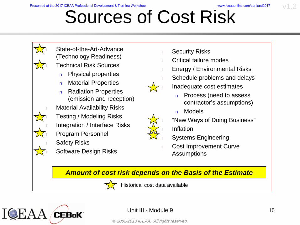
copy 2002-2013 ICEAA All rights reserved
v12
Sources of Cost Risk
Unit III - Module 9 10
l Security Risksl Critical failure modesl Energy Environmental Risksl Schedule problems and delaysl Inadequate cost estimates
n Process (need to assess contractorrsquos assumptions)
n Models l ldquoNew Ways of Doing Businessrdquol Inflationl Systems Engineeringl Cost Improvement Curve
Assumptions
l State-of-the-Art-Advance (Technology Readiness)
l Technical Risk Sourcesn Physical propertiesn Material Propertiesn Radiation Properties
(emission and reception)l Material Availability Risksl Testing Modeling Risksl Integration Interface Risksl Program Personnell Safety Risksl Software Design Risks
Historical cost data available
Amount of cost risk depends on the Basis of the Estimate
Presented at the 2017 ICEAA Professional Development amp Training Workshop wwwiceaaonlinecomportland2017
copy 2002-2013 ICEAA All rights reserved
v12
Point Estimates of Costbull Funding organizations need best estimate of cost for
bullCostperformance tradeoff studiesbullCostbenefit analysesbullBudget planning
bull But program cost is nebulous heavily impacted bybullTechnological (im)maturitybullProgrammatic considerationsbullSchedule slipsbullUnforeseen events
bull Point cost estimates cannot be ldquocorrectrdquo becausebullEvery cost element contains uncertaintybullTotal system cost is sum of these WBS elements
bull Actual program cost falls within a range surrounding the best estimate (with some degree of confidence)bullThe best we can hope to do is to understand the uncertaintybullUnderstanding the uncertainty will help us make provision for it
Unit III - Module 9 11
Presented at the 2017 ICEAA Professional Development amp Training Workshop wwwiceaaonlinecomportland2017
copy 2002-2013 ICEAA All rights reserved
v12
Unit III - Module 9 12
Types of Riskbull Cost Growth = Cost Estimating Growth + SkedTech Growth
+ Requirements Growth + Threat Growthbull Cost Risk = Cost Estimating Risk + SkedTech Risk +
Requirements Risk + Threat Riskndash Cost Estimating Risk Risk due to cost estimating errors and the statistical
uncertainty in the estimate ndash ScheduleTechnical Risk Risk due to inability to conquer problems posed
by the intended design in the current CARD or System Specificationsndash Requirements Risk Risk resulting from an as-yet-unseen design shift from
the current CARD or System Specifications arising due to shortfalls in the documents
bull Due to the inability of the intended design to perform the (unchanged) intended mission
bull We didnrsquot understand the solutionndash Threat Risk Risk due to an unrevealed threat eg shift from the current
STAR or threat assessmentbull The problem changedO
ften
impl
icit
or o
mitt
ed
1 2
Presented at the 2017 ICEAA Professional Development amp Training Workshop wwwiceaaonlinecomportland2017
copy 2002-2013 ICEAA All rights reserved
v12
Point Estimates Vs Risk Estimates
Unit III - Module 9 13
DDTampE Flight Unit Production TotalPoint Estimate 63807 5179 6697 70505CER Risk Only - Mean 71176 4805 6426 78018Full Risk - Mean 78937 6490 8091 87430Point Esimtate + 30 82949 6733 8706 91657Full Risk - 70th Percentile 87939 7980 9608 97011
Estimated Total Cost in Millions
Note that the mean is 24 higher than the point estimate and the 70th
percentile is 38 higher than the point estimate
Presented at the 2017 ICEAA Professional Development amp Training Workshop wwwiceaaonlinecomportland2017
copy 2002-2013 ICEAA All rights reserved
v12
Cost Risk and Probabilitybull Cost risk or cost uncertainty analysis represents cost as a
probability distributionbull A probability distribution is a mathematical rule associating a
probability a to each possible outcome or event of interestbull There are two ways to present a probability distribution ndash as a
probability density function (ldquoPDF) and as a cumulative distribution function (ldquoS-curverdquo or ldquoCDFrdquo)
Unit III - Module 9 14
Lognormal Distribution PDF and CDF
0102030405060708090100
200 300 400 500 600 700 800 900 1000Cost $
Con
fiden
ce L
evel
0
00002
00004
00006
00008
0001
00012
00014
00016
Prob
abili
ty D
ensi
ty
CDFPDF
Presented at the 2017 ICEAA Professional Development amp Training Workshop wwwiceaaonlinecomportland2017
copy 2002-2013 ICEAA All rights reserved
v12
Unit III - Module 9 15
Probability Model ndash Distributionbull Normal
ndash Best behavior most iconic
ndash Theoretically (although not practically) allows negative costs which spook some users
ndash Symmetric needs mean shift to reflect propensity for positive growth
bull Lognormalndash A natural result in
non-linear CERsndash Indistinguishable
from Normal at CVs below 25
ndash Skewed
10
4
10
Presented at the 2017 ICEAA Professional Development amp Training Workshop wwwiceaaonlinecomportland2017
copy 2002-2013 ICEAA All rights reserved
v12
Unit III - Module 9 16
bull Triangularndash Most commonndash Easy to use easy to understandndash Modes medians do not addndash Skewed
bull Betandash Rare now but formerly popularndash Solves negative cost and duration issuesndash Many parameters ndash simplifications like PERT
Beta are possiblendash Skewed
bull Bernoullindash Probability is only assigned to two possible
outcomes success and failure (p and 1-p)ndash Simplest of all discrete distributionsndash Mean = pndash Variance = p(1-p)
10
Probability Model ndash Distribution
10
10
Presented at the 2017 ICEAA Professional Development amp Training Workshop wwwiceaaonlinecomportland2017
copy 2002-2013 ICEAA All rights reserved
v12
Unit III - Module 9 17
bull Normalndash If there is a sufficiently large number of independently identically distributed
elements (or not too correlated and not too skewed) then the distribution of total cost is normal due to the Central Limit Theorem
bull Lognormalndash For smaller data sets with large amounts of (positive) correlation and
skewness the lognormal distribution may be a better approximation of total cost
ndash Many total cost distributions in smaller data sets test as both normal and lognormal
bull Triangularndash The sum of triangles is not a triangle so this distribution should generally not
be used to characterize total costbull Convolved
ndash If total cost distribution is derived using simulation then it may not particularly resemble anything In this case we simply have a convolved or simulated total cost distribution
Probability ndash Top-Level Distribution
NEW
Presented at the 2017 ICEAA Professional Development amp Training Workshop wwwiceaaonlinecomportland2017
copy 2002-2013 ICEAA All rights reserved
v12
S-Curves and Confidence Levels
Unit III - Module 9 1818
100
70
25
Probability(Confidence
Level)
Cost Estimate(Dollars)
50
The S curve is the cumulative probability distribution coming out of the statistical summing process
70 confidence that project will cost indicated amount or less
Provides information on potential cost as a result of identified project risks
Provides insight into establishing reserve levels
X Y
MR
X = Point estimateZ = Project requirementY = Cost estimate where there is a 70 change that
final actual cost will be less than cost estimateY-Z= Manage reserve (MR) which is REQUIRED to meet 70 CL
Z
X not always = Z but is based on same content
Presented at the 2017 ICEAA Professional Development amp Training Workshop wwwiceaaonlinecomportland2017
copy 2002-2013 ICEAA All rights reserved
v12
19
Example ndash Normal Distribution
bull Normal distribution with mean equal to 100 and standard deviation equal to 20
bull Median and mode also equal 100bull The 80th Percentile is 117
40 60 80 100 120 140 160
80 of distribution(area under curve)is less than 117
117
Presented at the 2017 ICEAA Professional Development amp Training Workshop wwwiceaaonlinecomportland2017
copy 2002-2013 ICEAA All rights reserved
v12
20
Confidence Levelsbull The output of a cost risk analysis is a probability
distributionndash Typically displayed as a cumulative distribution function or
ldquoS-curverdquondash Confidence levels are simply percentiles of the distribution
0
10
20
30
40
50
60
70
80
90
100
30 60 90 120 150 180
Conf
iden
ce L
evel
Presented at the 2017 ICEAA Professional Development amp Training Workshop wwwiceaaonlinecomportland2017
copy 2002-2013 ICEAA All rights reserved
v12
Measuring Parametric Model Uncertainty
bull When developing estimates using cost-estimating relationships (CERs) there are two major sources of uncertaintyndash Technical (model input) uncertaintyndash Estimating uncertainty
bull Technical uncertainty reflects the uncertainty inherent in the model inputsndash Typical parametric model inputs include weight lines of code
heritage and other performance and management inputs
bull Estimating uncertainty measures the uncertainty inherent in the model due to the modelrsquos inability to capture all aspects of variability in the data
21
Presented at the 2017 ICEAA Professional Development amp Training Workshop wwwiceaaonlinecomportland2017
copy 2002-2013 ICEAA All rights reserved
v12
Parametric Model Examplebull The NASAAir Force Cost Model (NAFCOM) is a
parametric model for estimating acquisition costs for spacecraft and launch vehicles
bull The CERs in NAFCOM have the formCost = C WeightVNewDesignWTechnicalXManagementY ClassZ
bull There is technical uncertainty about each of the parametersndash Parametric models are applied early in a program so there
is significant amount of uncertainty in the weightndash Heritage is also tricky it is inherently subjective and project
personnel are typically optimisticndash Technical characteristics can also change as a program
matures and requirements change
22
Presented at the 2017 ICEAA Professional Development amp Training Workshop wwwiceaaonlinecomportland2017
copy 2002-2013 ICEAA All rights reserved
v12
Weight Uncertaintybull Aerospace weight growth study average satellite
weight growth from program inception to launch is 28
23
Aerospace Weight Growth Data
-10
0
10
20
30
40
50
60
0 4 8 12 16 20 24 28 32 36 40 44 48 52 56 60 64 68 72 76 80 84 88 92 96 100
Percent Program Completion
Perc
ent W
eigh
t Gro
wth
Presented at the 2017 ICEAA Professional Development amp Training Workshop wwwiceaaonlinecomportland2017
copy 2002-2013 ICEAA All rights reserved
v12
Estimating Uncertaintybull CERs do not perfectly fit the historical data
ndash There are non-repeatable random effects that cannot be predicted
bull For examplendash Parts breaking during testingndash Strikes which are difficult to predict
bull This results in an underlying uncertainty distribution about an estimatendash The outcome of a CER represents only one point on an
uncertainty distributionbull Typically mean or median depending upon the CER
methodology
24
Presented at the 2017 ICEAA Professional Development amp Training Workshop wwwiceaaonlinecomportland2017
copy 2002-2013 ICEAA All rights reserved
v12
Estimating Uncertainty (2)
25
Presented at the 2017 ICEAA Professional Development amp Training Workshop wwwiceaaonlinecomportland2017
copy 2002-2013 ICEAA All rights reserved
v12
Estimating Uncertainty (3)bull In the case of a linear regression the estimating
uncertainty follows a normal distributionndash The estimate is the mean and the standard error of the
estimate from the regression is the standard deviation of the normal distribution
bull In the case of a log-transformed linear regression the estimating uncertainty follows a lognormal distributionndash The estimate is the median of the lognormal and the
standard error of the estimate from the regression is the standard deviation of the normal distribution (in log-space)
bull There is additional uncertainty about an estimate based upon the distance of what is being estimated from the mean of the input datandash This results in a prediction interval
26
Presented at the 2017 ICEAA Professional Development amp Training Workshop wwwiceaaonlinecomportland2017
copy 2002-2013 ICEAA All rights reserved
v12
Aggregating Riskbull Risk is typically applied at the same level at
which we estimate cost that is at the Work Breakdown Structure (WBS) level
bull The estimates for each WBS are developedndash These estimates sum to yield the total system cost
bull For an n-element WBS the total cost is the sum of the cost for each of the n elements
27
nXXXCostSystem +++= 21
Presented at the 2017 ICEAA Professional Development amp Training Workshop wwwiceaaonlinecomportland2017
copy 2002-2013 ICEAA All rights reserved
v12
WBS Examplebull Launch Vehicle
ndash Structurebull Vehicle Structurebull Tank Structure
ndash Thermal Controlbull Active Thermal Controlbull Induced Thermal Controlbull Tank Thermal Control
ndash Main Propulsion Systemndash Liquid Rocket Enginendash Electric Power and Distributionndash Command Control and Data Handlingndash System Integration
28
Presented at the 2017 ICEAA Professional Development amp Training Workshop wwwiceaaonlinecomportland2017
copy 2002-2013 ICEAA All rights reserved
v12
WBS and Risk
29
Presented at the 2017 ICEAA Professional Development amp Training Workshop wwwiceaaonlinecomportland2017
copy 2002-2013 ICEAA All rights reserved
v12
Aggregating Riskbull This leads us to the issue of aggregating the risks across the
WBSbull For example if we want to determine the 70th percentile of the
overall cost risk distribution how do we proceed bull Note that we cannot simply add the 70th percentiles of each of
the cost risk distributionsbull We can add means and variances (taking correlation into
account more on that later) but that is all
Variance of Total Cost =
30
Mean of Total Cost = ( )E X E Xk
k
n
kk
n
kk
n
= = =aringaelig
egraveccediloumloslashdivide
= =aring aring1 1 1
m
Var X kk
n
=aringaelig
egraveccediloumloslashdivide1
= s r s skk
n
iji
j
i jj
n2
1 1
1
22+aring aringaring
= =
-
=
Presented at the 2017 ICEAA Professional Development amp Training Workshop wwwiceaaonlinecomportland2017
copy 2002-2013 ICEAA All rights reserved
v12
Percentiles Do Not Addbull As a notional example consider two independent normal
distributionsndash One distribution has mean equal to 100 and standard deviation
equal to 20ndash The second distribution has mean 300 and standard deviation of 80
bull The sum of two independent normally distributed random variables is also normally distributed
bull To combine the two distributions we add the means and add the variancesndash Total mean is
ndash Total standard deviation is
31
400300100 =+
8258020 22 raquo+
Presented at the 2017 ICEAA Professional Development amp Training Workshop wwwiceaaonlinecomportland2017
copy 2002-2013 ICEAA All rights reserved
v12
Percentiles Do Not Add (2)bull The 80th percentiles for the individual distributions are
117 and 367 respbull The 80th percentile of the combined distribution is
469 but the sum of the two 80th percentiles is 484bull To see why this is the case note that the percentiles
of a normal distribution are determined by the mean and the standard deviationndash The standard deviations are not added when normal distributions
are combined rather the variances are combinedndash Sum of variances is ndash The standard deviation of this sum is
32
22 ba +22 ba +
Presented at the 2017 ICEAA Professional Development amp Training Workshop wwwiceaaonlinecomportland2017
copy 2002-2013 ICEAA All rights reserved
v12
Percentiles Do Not Add (3)bull Since bull We can write
bull The left side of this inequality represents the risk of the combined distributions while the right side represents the sums of the individual risks
bull Combining two missions that are independent results in a diversification of riskndash The total portfolio is not as risky on a relative basis as each
individual project
33
2222 2 bababa ++lt+
baba +lt+ 22
Presented at the 2017 ICEAA Professional Development amp Training Workshop wwwiceaaonlinecomportland2017
copy 2002-2013 ICEAA All rights reserved
v12
Methods for Aggregating Riskbull Since percentiles do not add we have to find other
ways to aggregate riskbull One method is to use Monte Carlo simulationbull Unless cost risk is represented by normal
distributions for all WBS elements summing the means and variances does not result in a completely accurate depiction of overall system cost risk
bull The normal distribution is not a realistic distribution for representing risk in many or even most situations since regarding project risk more can go wrong than can go right which means the risk is NOT symmetric unlike the Gaussian bell curve
34
Presented at the 2017 ICEAA Professional Development amp Training Workshop wwwiceaaonlinecomportland2017
copy 2002-2013 ICEAA All rights reserved
v12
Unit III - Module 9 35
Monte Carlo Simulationfor Risk Analysis
bull When risk analysis is performed multiple risks are gatheredndash These risks may have various probability
distributions
bull Monte Carlo is the most commonly accepted way to produce an accurate characterization of the distribution of the combined effect of these many risksndash Using this distribution we can produce percentiles
for cost impacts due to risk occurrences
10
Presented at the 2017 ICEAA Professional Development amp Training Workshop wwwiceaaonlinecomportland2017
copy 2002-2013 ICEAA All rights reserved
v12
Monte Carlo Simulationbull Simulation is a means for solving problems that are
analytically intractablendash Involves repeated random sampling
bull It was developed during the Manhattan Project as a way to model the interactions inside an atom during nuclear fissionndash Allowed for more sophisticated mathematical modeling of atomic
phenomena
bull Most computer packages use pseudo-random number generators that produce seemingly random results from an initial seedndash Example is the linear congruential generator
36
( ) mbaXX nn mod1 +=+
Presented at the 2017 ICEAA Professional Development amp Training Workshop wwwiceaaonlinecomportland2017
copy 2002-2013 ICEAA All rights reserved
v12Using Random Numbers to Simulate Distributions
bull WBS cost risk is typically measured by a probability distributionbull The most common method for simulating a probability
distribution is the inverse methodbull This involve obtaining a simulated random value from a uniform
distribution and then inverting this through the cumulative distribution function (CDF) to obtain the simulated value
bull As an example for a uniform distribution on the interval [0100]
bull In this case the CDF random value of 05 translates to 10005 = 50
37
( )100
1=xf ( )
100xxF = ( ) xxF 1001 =-
Presented at the 2017 ICEAA Professional Development amp Training Workshop wwwiceaaonlinecomportland2017
copy 2002-2013 ICEAA All rights reserved
v12
Simulating a Triangular Distribution
bull For a triangular distribution with low = 0 most likely = 50 and high = 150 the CDF is given by
bull The inverse function is given by
38
( )iumliumlicirc
iumliumliacute
igrave
poundlt--
poundpound=
1505021
1500050
50015000
2
2
2
xxx
xxxF
( )iumliumlicirc
iumliumliacute
igrave
poundltdivideoslashouml
ccedilegraveaelig +--
poundpound=-
131
21
37501
250017500150
3107500
1
xx
xxxF
Presented at the 2017 ICEAA Professional Development amp Training Workshop wwwiceaaonlinecomportland2017
copy 2002-2013 ICEAA All rights reserved
v12
Simulating a Triangular Distribution (2)
bull If the simulated uniform value is equal to 02 the corresponding inverse value from the CDF inverse is approximately 387
39
0
01
02
03
04
05
06
07
08
09
1
0 30 60 90 120 150
Presented at the 2017 ICEAA Professional Development amp Training Workshop wwwiceaaonlinecomportland2017
copy 2002-2013 ICEAA All rights reserved
v12
Monte Carlo and the WBSbull Simulation involves repeated trials
40
WBS Draw1 2 3 4 5
System 2912 3566 4390 2954 4655 Sum
Structure 80 105 55 80 57 SumVehicle Structure 50 70 30 40 20Tank Structure 30 35 25 40 37
Thermal Control 32 36 35 29 33 SumActive Thermal Control 10 15 12 7 10Induced Thermal Control 12 14 13 14 14Tank Thermal Control 10 7 10 8 9
Main Propulsion System 100 150 125 140 100
Liquid Rocket Engine 1000 1100 1800 900 2200
Electric Power and Distribution 100 125 150 75 90
Command Control and Data Handling 200 250 225 230 275
System Integration 1400 1800 2000 1500 1900
Presented at the 2017 ICEAA Professional Development amp Training Workshop wwwiceaaonlinecomportland2017
copy 2002-2013 ICEAA All rights reserved
v12
Number of Trialsbull Monte Carlo involves a repeated number of trialsbull The greater the number of trials the more accurate the
simulation will approximate the overall cost risk behavior of the system
bull After 100 trials the histogram looks very jagged
41
Presented at the 2017 ICEAA Professional Development amp Training Workshop wwwiceaaonlinecomportland2017
copy 2002-2013 ICEAA All rights reserved
v12
Number of Trials (2)
42
1000 Trials
10000 Trials
50000 Trials Additional trials give a more accurate depiction of the final result
Presented at the 2017 ICEAA Professional Development amp Training Workshop wwwiceaaonlinecomportland2017
copy 2002-2013 ICEAA All rights reserved
v12
Number of Trials (3)bull If we want to simulate the underlying
mean within 1 with 95 confidence for example then we require
43
divideoslash
oumlccedilegrave
aelig poundpound-
=
dividedividedivide
oslash
ouml
ccedilccedilccedil
egrave
aeligpound
-pound
-=
divideoslashouml
ccedilegraveaelig poundpound=
nZ
n
nnX
n
X
n
n
011
010Pr
011
010Pr
011990Pr950
___
___
sm
sm
sm
sm
sm
mm
Presented at the 2017 ICEAA Professional Development amp Training Workshop wwwiceaaonlinecomportland2017
copy 2002-2013 ICEAA All rights reserved
v12
Number of Trials (4)bull This means that the number of trials required is determined by
bull Solving for n we find that at least
trials are neededbull Note that this term involves the coefficient of variation of the
distribution which means that distributions with less dispersion require fewer trials to accurate simulate
44
96101
=ns
m
ms41638
Presented at the 2017 ICEAA Professional Development amp Training Workshop wwwiceaaonlinecomportland2017
copy 2002-2013 ICEAA All rights reserved
v12
Number of Trials (5)bull Simulating percentiles requires more trials than for simulating
meansbull Let Pn represent the number of trials in the sample at or below
the 70th percentile of the underlying distribution (suppose this is known)
bull By the Central Limit Theorem Pnn follows a normal distribution with mean equal to the 70th percentile and variance equal to
bull By a similar process for the mean we find that the number of trials needed to simulate the 70th percentile within 1 with 95 confidence is
45
( )n
FF 700700 1-
n
n
PPn -41638
Presented at the 2017 ICEAA Professional Development amp Training Workshop wwwiceaaonlinecomportland2017
copy 2002-2013 ICEAA All rights reserved
v12
Number of Trials (6)bull If Pn 070 for all n then n is approximately
bull For the sake of comparison suppose CV = 03 (reasonable approximation for hardware development) then the number of trials needed to simulate the mean with the same accuracy is then ldquoonlyrdquo 11525
bull More trials are needed to accurately simulate percentiles than means
46
( ) 46416703041638
70704168341638 =divide
oslashouml
ccedilegraveaelig=divide
oslashouml
ccedilegraveaelig -
=-
nnn
PPn
n
n
Presented at the 2017 ICEAA Professional Development amp Training Workshop wwwiceaaonlinecomportland2017
copy 2002-2013 ICEAA All rights reserved
v12
Methods of Simulationbull Monte Carlo simulation is a standard term for
simulationbull However there is an improvement on Monte Carlo
that improves the accuracy of the results of a simulation for a given number of trials
bull This method is call the Latin Hypercube approach to simulationndash Similar to Monte Carlo but an equal number of draws are taken
from a set of subintervals for example dividing the interval (01) into [00001) [0102)hellip [0910]
ndash Instead of 10 trials from [01] we have one trial from each subinterval
ndash Rough rule of thumb is Latin Hypercube takes 30 fewer trials to achieve similar accuracy to Monte Carlo
47
Presented at the 2017 ICEAA Professional Development amp Training Workshop wwwiceaaonlinecomportland2017
copy 2002-2013 ICEAA All rights reserved
v12
Probability Model ndash Correlationbull Correlation exists between work breakdown structure
(WBS) cost element costs and between cost and schedule
bull Correlation is a necessary consideration in cost risk analysis
bull Correlation is a number that can vary between -1 and +1 and represents the strength of the relationship between the two variablesndash If both variable have a tendency to move in the same direction
correlation is positivendash If when one variable increases the other tends to decrease and
vice-versa the correlation between the two variables is negative
Presented at the 2017 ICEAA Professional Development amp Training Workshop wwwiceaaonlinecomportland2017
copy 2002-2013 ICEAA All rights reserved
v12
Correlation And Causationbull Note that correlation is not causation however
causation implies correlationndash For example shark attacks and ice cream sales at the beach
bull For example for a launch vehicle structure increasing the diameter will not only result in an increase in the structures cost but will also result in higher costs for thermal coating (paint etc)
bull Also simply because two subsystems do not appear to be related does not mean they are not correlatedndash For example structures and computer equipment seemingly
have little relation to one another however an external factor such as a funding cut or a strike will impact all subsystems leading to delays and increasing cost across the board
ndash Thus everything in a WBS has some correlationUnit III - Module 9 49
Presented at the 2017 ICEAA Professional Development amp Training Workshop wwwiceaaonlinecomportland2017
copy 2002-2013 ICEAA All rights reserved
v12
The Importance of Correlationbull Percent that total cost standard deviation is underestimated
when correlation assumed to be 0 instead of r given nWBS elements
Unit III - Module 9 5050
0
20
40
60
80
100
0 01 02 03 04 05 06 07 08 09 1Actual Correlation
Perce
nt Un
deres
timate
d
n = 10
n = 30
n = 100n = 1000
0
20
40
60
80
100
0 01 02 03 04 05 06 07 08 09 1Actual Correlation
Perce
nt Un
deres
timate
d
n = 10
n = 30
n = 100n = 1000
Reference 32nd Annual DOD Cost Analysis Symposium Advanced Training Session ldquoWhy Correlation Matters in Cost Estimatingrdquo Stephen A Book
Presented at the 2017 ICEAA Professional Development amp Training Workshop wwwiceaaonlinecomportland2017
copy 2002-2013 ICEAA All rights reserved
v12
The Importance of Correlation (2)bull For example if correlation is assumed to be 0 for all
elements in a 30 element WBS and the actual correlation is 20 then the total cost standard deviation is underestimated by 60
bull For example assume the total cost is modeled as a normal distribution with mean = 100
bull If correlation is assumed to be zero with total cost standard deviation = 12 when correlation is actually 20 then the true underlying standard deviation is actually 30
bull 70th percentile with zero correlation assumption is 106
bull 70th percentile with 20 correlation is 116 Unit III - Module 9 51
Presented at the 2017 ICEAA Professional Development amp Training Workshop wwwiceaaonlinecomportland2017
copy 2002-2013 ICEAA All rights reserved
v12
Measures of Correlationbull Two measures of correlation are commonly used in
cost risk analysesndash Pearsonrsquos product-moment correlation coefficient ndash Spearmanrsquos rank correlation coefficient
bull Garvey and others recommend using Pearsonrsquos product-moment correlation coefficient correlation for cost risk analysesndash Method of moments uses this but there are two options in
simulationndash Popular simulation packages like Risk and Crystal Ball use
rank correlation but in practice this has been found to make little difference
ndash Pearson product-moment correlation has been incorporated into Risk+
52
Presented at the 2017 ICEAA Professional Development amp Training Workshop wwwiceaaonlinecomportland2017
copy 2002-2013 ICEAA All rights reserved
v12
Pearson Correlationbull Pearsonrsquos product-moment correlation measures
degree of linearity between two random variables bull If two random variables are perfectly linear (eg Y =
aX + b) with positive slope then the Pearson product-moment correlation between X and Y denoted by rXY is +1
53
X X
Y Y Y
XNegative Correlation Positive Correlation No Correlation
middotmiddot
middotmiddot
middotmiddot middotmiddot
middotmiddot
middot
middot
middotmiddotmiddot
middotmiddot
middotmiddot
middotmiddot middot
middot
middot
middotmiddotmiddotmiddotmiddotmiddotmiddotmiddot
middotmiddotmiddotmiddot
middotmiddot
middotmiddot middotmiddotmiddotmiddot
middotmiddotmiddot
middotmiddotmiddotmiddot
middotmiddotmiddot
middotmiddotmiddot
middotmiddot
middot
middot middotmiddot
middot middotmiddotmiddotmiddot middotmiddot middot middotmiddot middot middot
middotmiddot middot
middotmiddotmiddotmiddotmiddot middot middotmiddot
middotmiddot
middot
middotmiddot
middotmiddot middot
middot middot middot
middotmiddot middot
middotmiddotmiddot
middotmiddot
middot middot
Presented at the 2017 ICEAA Professional Development amp Training Workshop wwwiceaaonlinecomportland2017
copy 2002-2013 ICEAA All rights reserved
v12
Spearman Correlationbull Spearmanrsquos rank correlation measures the
monotonicity between two random variablesbull If two random variables are perfectly monotonically
increasing (eg Y = X2) then the Spearman rank correlation denoted by rXY is +1
bull The two measures can be significantly different
54
10 20 30 40 50 60
100
200
300
096 097 098 099 1
1
060
020
040
080
Eff
ort (
Staf
f-M
onth
s)
Software Size I KDSI
y = 28z12y
z x
yy = x100
0 pound x pound 1
Figure 5-9A Figure 5-9B
Pearson Correlation = 09976 Rank Correlation = 1
Pearson Correlation = 024 Rank Correlation = 1
X(x ) ~ Unif(01)
Reference Probability Methods for Cost Uncertainty Analysis A Systems Engineering Perspective Paul R Garvey
Presented at the 2017 ICEAA Professional Development amp Training Workshop wwwiceaaonlinecomportland2017
copy 2002-2013 ICEAA All rights reserved
v12
Unit III - Module 9 55
200
250
300
350
400
1000 1200 1400 1600 1800 2000
Recurring Production
SEPM
200
250
300
350
400
1000 1200 1400 1600 1800 2000
Recurring Production
SEPM
Functional Correlationbull Old No Functional
Correlation Simulation run with WBS items entered as values
bull New Simulation run with functional dependencies entered as they are in cost model
CorrelatedNot Correlated
Note shift of mean and increased variability
Presented at the 2017 ICEAA Professional Development amp Training Workshop wwwiceaaonlinecomportland2017
copy 2002-2013 ICEAA All rights reserved
v12
Risk Measuresbull ldquoWestern Europe conquered the word because of a
technological revolution that started because of attempts to measure the worldrdquo ndash Phillipe Jorion ndash In the same way attempts to measure risk will lead to better project
managementbull Risk management for DoD and NASA agencies focuses
primarily on funding projects to a single percentile ndash NASA policy explicitly mentions 70 and 50ndash This is known as ldquoValue at Riskrdquo and is prevalent in the banking and
financial industry
56
Presented at the 2017 ICEAA Professional Development amp Training Workshop wwwiceaaonlinecomportland2017
copy 2002-2013 ICEAA All rights reserved
v12
Value at Risk (VaR)bull VaR is a percentile of the cost risk
distributionndash VaR funding at the 70th percentile means that
there is a 30 chance of final project cost exceeding the funded amount (budget)
bull VaR has some meritsndash Common measure can be used to compare
different projects and programsndash Easily understood by senior managers and
decision makers
57
Presented at the 2017 ICEAA Professional Development amp Training Workshop wwwiceaaonlinecomportland2017
copy 2002-2013 ICEAA All rights reserved
v12
Why 70th or 80th Percentilebull Typical policy guidance involves funding at the 70th or 80th
percentile Why fund as such a low percentilebull There is some incentive to not over-fundbull For a normal distribution an inflection point occurs near the 80th
percentile meaning that for values above 80 confidence achieving higher levels of confidence can only be achieved by spending greater dollar amounts at an increasing rate
58
-05-04-03-02-01
00102030405
0 05 1 15 2 25 3
Standard Deviations from Mean
Normal Distribution
First DerivativeSlopeVelocity
Second DerivativeConvexityAcceleration
Inflection point at one standard deviation above the mean (~84th
percentile)
Presented at the 2017 ICEAA Professional Development amp Training Workshop wwwiceaaonlinecomportland2017
copy 2002-2013 ICEAA All rights reserved
v12
Funding Above Inflection Pointsbull As the percentile goes above the 80th percentile the amount
needed to achieve that higher level of confidence begins to increase at an increasing rate as is evident from the graph
59
0
10
20
30
40
50
60
70
50 55 60 65 70 75 80 85 90 95 100
$ Ab
ove
MEa
n to
Ach
ieve
Per
cent
ile
Percentile (Confidence Level)
Presented at the 2017 ICEAA Professional Development amp Training Workshop wwwiceaaonlinecomportland2017
copy 2002-2013 ICEAA All rights reserved
v12
Why Budget to the 70th or 80thbull Government projects are funded at the 70th or 80th percentilesbull Why not the 90th or 99th percentile Wonrsquot that help prevent
overrunsndash As we have seen percentiles do not add across programs
bull The sum of the 80th percentiles does NOT equal the total 80th percentile
ndash This is because the individual programs are riskier than the entire suite of missions
bull Known as the ldquoPortfolio effectrdquo (more or this later)
ndash Funding at the 80th gives confidence that the entire portfolio will be adequately funded
bull And since there is an inflection point near the 80th percentile funding above that level quickly becomes cost prohibitive
60
Presented at the 2017 ICEAA Professional Development amp Training Workshop wwwiceaaonlinecomportland2017
copy 2002-2013 ICEAA All rights reserved
v12
Inflection Points for Lognormalbull For a lognormal the inflection point
variesndash Coefficient of variation equal to 10 equates to an
inflection point at the 70th percentile
61
0
10
20
30
40
50
60
70
050 060 070 080 090 100
Coef
ficen
t of V
aria
tion
Percentile of the Inflection Point
Presented at the 2017 ICEAA Professional Development amp Training Workshop wwwiceaaonlinecomportland2017
copy 2002-2013 ICEAA All rights reserved
v12
Issues with Percentile Fundingbull However risk management does not stop at a
specific percentilendash What happens when the 70th percentile is exceeded
bull Any effective risk management policy should prescribe what happens after a bad event occursndash With VaR we only know when a bad event has occurred ndash Also funding at a relatively low level means we have no true
sense of the real risks that should be guarded against
62
Presented at the 2017 ICEAA Professional Development amp Training Workshop wwwiceaaonlinecomportland2017
copy 2002-2013 ICEAA All rights reserved
v12
ldquoHere There Be Dragonsrdquobull On old maps uncharted territory was often
marked with monsters or dragons
63
A section of the Carta Marina by Olaus Magnus 16th Century
Presented at the 2017 ICEAA Professional Development amp Training Workshop wwwiceaaonlinecomportland2017
copy 2002-2013 ICEAA All rights reserved
v12
Distribution Comparisonbull Four different distributions with the same 70th
percentile
bull Should we expect the tails to be similar
64
0
10
20
30
40
50
60
70
80
0 100 200 300 400 500 600
Perc
entil
eCo
nfid
ence
Lev
el
Triangular
Normal
Lognormal
Pareto
Presented at the 2017 ICEAA Professional Development amp Training Workshop wwwiceaaonlinecomportland2017
copy 2002-2013 ICEAA All rights reserved
v12Distribution Comparison Tail Behavior
bull The normal and triangular distributions have similar tails but the lognormal and Pareto have much fatter right tails
65
70
75
80
85
90
95
100
500 1500 2500 3500 4500 5500
Perc
entil
eCo
nfid
ence
Lev
el
Triangular
Normal
Lognormal
Pareto
Here There Be Dragons
Presented at the 2017 ICEAA Professional Development amp Training Workshop wwwiceaaonlinecomportland2017
copy 2002-2013 ICEAA All rights reserved
v12Distribution Comparison ndash Tail Behavior (Table)
bull There is significant tail risk for the lognormal and the Paretobull The 99th percentile for the Pareto is 1000 times greater than
the 70th percentilendash Risk seen in financial markets and in catastrophic risks like natural
disasters bull Four different projects follow the four different risk profiles seen
in this example should clearly have different risk management approaches but 70th percentile funding indicates the same risk management approach for all four
66
Percentile Triangular Normal Lognormal Pareto 70th $600 $600 $600 $600 80th $680 $660 $770 $1430 90th $770 $750 $1070 $5880 95th $840 $820 $1410 $23750 99th $930 $950 $2350 $600000
Presented at the 2017 ICEAA Professional Development amp Training Workshop wwwiceaaonlinecomportland2017
copy 2002-2013 ICEAA All rights reserved
v12Percentile Budgeting is Not Risk Management
bull Percentile budgeting ne effective risk management policybull Suppose that you are shopping for a new car You
mention that safety is your top concern The salesman says he has a great safe car available You ask about the air bags Do they work The salesman answers ldquoOf course Seventy percent of the time they work fine Only 30 of the time the air bags will fail to deployrdquo Would you buy such a car Hedge fund manager David Einhorn has stated ldquoRisk management is the air bag that must always work but only in the multi-sigma event where you have an accidentrdquo
67
Risk management is the air bag that must always work but only in the multi-sigma event where you
have an accident
Presented at the 2017 ICEAA Professional Development amp Training Workshop wwwiceaaonlinecomportland2017
copy 2002-2013 ICEAA All rights reserved
v12
Joint Confidence Level Analysisbull Schedules are risky toobull For 98 recent NASA missions average
schedule growth was 38ndash Not as high as cost growth but still significant
68
0
5
10
15
20
25
30
35
40
Schedule
Cost
Presented at the 2017 ICEAA Professional Development amp Training Workshop wwwiceaaonlinecomportland2017
copy 2002-2013 ICEAA All rights reserved
v12
Schedules Impact Costbull Changes in schedule can have enormous
impacts on cost ndash Schedule slips can lead to cost increases
bull Fixed programmatic costs must be paid on a regular basisndash Achieving schedule milestones early can result in cost
savings
bull Schedule is an important consideration in cost analysis including cost risk analysis
bull However we must be careful in correctly integrating cost and schedule riskndash Schedule is not simply an input but is dependent on many of
the same factors that drive cost
69
Presented at the 2017 ICEAA Professional Development amp Training Workshop wwwiceaaonlinecomportland2017
copy 2002-2013 ICEAA All rights reserved
v12
The Relationship of Cost to Schedulebull Cost and schedule are positively correlated
ndash A larger program with bigger scope with take longer to complete than a smaller simpler program
bull However longer schedules do not always equate to higher cost nor shorter schedules with lower costndash Highly compressed schedules relative to the
optimal schedule can lead to large overrunsbull Compressed schedules are commonplace for
many planetary missions
70
Presented at the 2017 ICEAA Professional Development amp Training Workshop wwwiceaaonlinecomportland2017
copy 2002-2013 ICEAA All rights reserved
v12The Impact of Schedule GrowthCompression on Cost
bull Compressed schedules lead to cost growth and based on existing research is actually more expensive than schedule slippages
71
0
20
40
60
80
100
120
140
160
-50 -25 0 25 50 75 100
Percentage Change in Schedule
Perc
enta
ge C
hang
e in
Cos
t due
to
Sche
dule
Cha
nge
Source Smart CB ldquoCost and Schedule Interrelationshipsrdquo 2007 NASA Cost Symposium
Presented at the 2017 ICEAA Professional Development amp Training Workshop wwwiceaaonlinecomportland2017
copy 2002-2013 ICEAA All rights reserved
v12Schedule as an Independent Variable
bull Why not simply add schedule as an input to cost-estimating relationships (CERs)
bull Schedule is often treated as an independent variable ndash schedules are often determined independently of cost considerationsndash Cost may not be considered explicitly although budgets and
schedules are determined based on scope and other common factors
bull In 2006 SAIC undertook a research task to determine the impact of schedule on cost and added schedule as an independent variable to the CERs in the NASAAir Force Cost Model (NAFCOM) to see if schedule provided any improvement in goodness of fit
72
Presented at the 2017 ICEAA Professional Development amp Training Workshop wwwiceaaonlinecomportland2017
copy 2002-2013 ICEAA All rights reserved
v12
Schedule is a Dependent Variablebull Since NAFCOM includes an exhaustive list of cost drivers the inclusion
of schedule should give an indication of whether there is any additional independent value added from schedule independent of the cost drivers
bull In the study schedule was added to 10 subsystem-level CERs
ndash In each case the addition of schedule did NOTimprove the goodness of fit and schedule was NOT found to be a statistically significant cost driver (given the presence of the other variables) for any of the 10 CERs
bull Standard errors for the CERs increased due to decrease in degrees of freedom
bull Thus schedule as an independent variable did not provide any additional explanation of variation in historical cost
bull This is because schedule is truly NOT an independent variable but a dependent variable and is a function of the same factors that drive cost
73
Presented at the 2017 ICEAA Professional Development amp Training Workshop wwwiceaaonlinecomportland2017
copy 2002-2013 ICEAA All rights reserved
v12
Incorporation of Schedule in Cost Risk
bull When using subjective methods care must be taken in applying schedule to cost risk analysis
bull Since schedule is a dependent variable treating it independently from other factors when assessing its impact on cost can lead to a double count of independent variables in the cost risk analysis
bull Direct inclusion of schedule in a cost risk analysis effectively doubles the influence of each cost driver
ndash Incorrectly leads to broader risk ranges
74
CostWeight
HeritageNewness
Technology Readiness Schedule
Presented at the 2017 ICEAA Professional Development amp Training Workshop wwwiceaaonlinecomportland2017
copy 2002-2013 ICEAA All rights reserved
v12Subjective Cost Risk Methods and Overinclusion of Risk Factors
bull Subjective methods are suitable when data are scarce or not availablebull However care must be taken not to treat correlated sources of risk
such as schedule as independent of each otherbull Example ndash a subjective risk analysis incorporated technology readiness
design risk requirements stability integration risk and schedule and treated each source of risk as independent
bull Risk triangle high value without schedule risk was 31 times the point estimate
bull Risk triangle high value with schedule risk added on top of other sources of risk treated independently was 34 times the point estimate
bull Risk triangle taking correlation between sources of risk into account in a rigorous statistical manner has a high value 15 times the point estimate less than half the effect when treating sources of risk as independent
75
Presented at the 2017 ICEAA Professional Development amp Training Workshop wwwiceaaonlinecomportland2017
copy 2002-2013 ICEAA All rights reserved
v12Fundamental Equation of Cost and Schedule Interrelationships
bull The Fundamental Equation of the Relationship Between Cost and Schedule is
Time = Moneybull This is a well known adage that time is money Your boss at
work may even mention this to you from time to time or if you are the boss you are all too aware of this iron law
bull Because time is money cost and schedule risk should be modeled jointly not with schedule as an independent cost driver
bull Note that cost and schedule are not perfectly correlatedndash Cost can sometimes ldquobuy downrdquo schedule extra money can be
spent to meet a deadline since in some cases additional effort to hasten the completion of a task
76
Presented at the 2017 ICEAA Professional Development amp Training Workshop wwwiceaaonlinecomportland2017
copy 2002-2013 ICEAA All rights reserved
v12How to (Correctly) Incorporate Schedule into Cost Risk Analysis
bull The best way to model cost and schedule risk is to develop a joint cost and schedule model based on the same data
bull Since such models are not currently available the next best approach is to model cost and schedule independently and then integrate cost and schedule risk analyses using joint probability distributions taking into account correlation between cost and schedulendash This approach pioneered by Paul Garvey and Steve Book is
considered industry best practicendash This is a practical method mathematically tractable and follows
naturally from the Fundamental Equation of Cost and Schedule Interrelationships
77
Book S A ldquoQuantifying the Relationship Between Cost and Schedulerdquo The Measurable News Winter 2007-2008 pp 11-15Garvey PR Probability Methods for Cost Uncertainty Analysis A Systems Engineering Perspective New York Marcel Dekker 2000 pp 308-335
Presented at the 2017 ICEAA Professional Development amp Training Workshop wwwiceaaonlinecomportland2017
copy 2002-2013 ICEAA All rights reserved
v12
Joint Lognormal and Normal Distributions
bull Cost and schedule are typically modeled as some combination of Normal and Lognormal probability distributionsndash Studies by The Aerospace Corporation the MITRE
Corporation Wyle Labs and SAIC have found that the Lognormal probability distribution almost always serves as a good model for both the schedule distribution and the cost distribution
ndash The Normal distribution may also be appropriate in some instances and depending upon the level of confidence at which budgets are set may even be more conservative and logically consistent than the Normal distribution
ndash Joint Lognormal and Normal distributions are defined by a pair of mean and standard deviations and a level of correlation between the two
78
Presented at the 2017 ICEAA Professional Development amp Training Workshop wwwiceaaonlinecomportland2017
copy 2002-2013 ICEAA All rights reserved
v12Modeling Cost and Schedule as a Bivariate Distribution
bull In the approach set forth by Book and Garvey cost risk is assessed and the top-level distribution is modeled as a Lognormal (or Normal) distribution schedule risk is assessed and the overall schedule risk is modeled as a Lognormal (or Normal) distribution
bull The two distributions are combined into a Bivariate distribution by assigning a correlation between the two and by treating the two distributions as the marginal distributions of a Bivariate Lognormal distributionndash Other combinations include a Bivariate Normal or a Bivariate
Normal-Lognormal
79
Presented at the 2017 ICEAA Professional Development amp Training Workshop wwwiceaaonlinecomportland2017
copy 2002-2013 ICEAA All rights reserved
v12Bivariate Lognormal Distribution for Cost and Schedule
bull Cost is often observed to be Lognormal when strong positive correlations are present among the systemrsquos WBS cost element costs
bull A systemrsquos schedule is often observed (from Monte Carlo simulations) to be Lognormal if it is the sum of many positively correlated schedule activities in an overall schedule network
bull If Lognormal distributions characterize a systemrsquos cost and schedule then the Bivariate Lognormal could serve as an assumed model of their joint distributionndash In this case the marginal distribution of each of cost and schedule is
Lognormalbull Other possibilities for modeling cost and schedule as a Bivariate
distribution include a Bivariate Normal or a Bivariate Normal-Lognormal distributionndash All these combinations are analytically tractable
80
Presented at the 2017 ICEAA Professional Development amp Training Workshop wwwiceaaonlinecomportland2017
copy 2002-2013 ICEAA All rights reserved
v12Bivariate Lognormal for Cost and Schedule
bull Contour Plots of a Bivariate Lognormal
81
Presented at the 2017 ICEAA Professional Development amp Training Workshop wwwiceaaonlinecomportland2017
copy 2002-2013 ICEAA All rights reserved
v12Correlation Between Cost and Schedule
bull Cost and schedule are positively correlated but not perfectly sondash For example it is possible to have a schedule underrun and a cost
overrunbull Based on cost and schedule growth data for 50 completed NASA
programs the correlation between development cost and development schedule is 70
82
00
200
400
600
800
1000
1200
-500 00 500 1000 1500 2000 2500Historical Cost Growth
Hist
oric
al S
ched
ule
Gro
wth
r = 715
Presented at the 2017 ICEAA Professional Development amp Training Workshop wwwiceaaonlinecomportland2017
copy 2002-2013 ICEAA All rights reserved
v12Correlation Between Cost and Schedule Caveats
bull Based on historical data recommended correlation between cost and schedule is 70 but this could be higher or lower depending upon program circumstancesndash If program is budget constrained cost and schedule will be
more highly correlated (go as you pay)ndash If program is schedule constrained cost and schedule will
have lower correlation perhaps even negative correlation ndash Smaller programs have smaller correlation between cost and
schedule riskbull Relatively easy to ldquohurry uprdquo and finish on time or even early if
needed
83
Presented at the 2017 ICEAA Professional Development amp Training Workshop wwwiceaaonlinecomportland2017
copy 2002-2013 ICEAA All rights reserved
v12
Conditional Confidence Levelsbull Given a programrsquos project schedule we can determine the cost
risk distribution conditional upon the given schedulebull Conditional cost S-curves are steeper than unconditional
(marginal) cost S-curves between some uncertainty has been removed because schedule is fixed
84
Presented at the 2017 ICEAA Professional Development amp Training Workshop wwwiceaaonlinecomportland2017
copy 2002-2013 ICEAA All rights reserved
v12
Joint Confidence Levelsbull Joint 65 confidence represents the probability of
achieving both 65 confidence in cost AND 65 confidence in schedulendash This is different than achieving 65 cost confidence alone
or achieving 65 schedule confidence alonebull Due to the imperfect correlation between cost and schedule it
is possible to achieve a 65 cost confidence with a lower level of schedule confidence
bull Restricting the schedule confidence thus requires additional $ to achieve a given level of confidence
85
X
Y
Possible Values for Which X gt a Possible Values for
Which X gt a and Y gt b
a
b
Presented at the 2017 ICEAA Professional Development amp Training Workshop wwwiceaaonlinecomportland2017
copy 2002-2013 ICEAA All rights reserved
v12Joint Confidence Levels Versus Cost Confidence Levels Only
bull Example of the differences between cost confidence schedule confidence conditional cost confidence and joint cost and schedule confidence
86
Joint Cost-Schedule Confidence Iso-Curves
Cost (RY$M)
Sche
dule
(Mon
ths)
65 Confidence
50 Confidence
70 Confidence
65 Cost Confidence AggressiveSchedule65 Cost ConfidenceScheduleGiven 65 Schedule ConfidenceUnconditional 65 CostConfidenceUnconditional 65 ScheduleConfidence
65 Cost Confidence 65 Joint Cost and Schedule
Confidence for 65 Schedule Confidence
Presented at the 2017 ICEAA Professional Development amp Training Workshop wwwiceaaonlinecomportland2017
copy 2002-2013 ICEAA All rights reserved
v12
Joint Cost and Schedule Confidence
bull Can examine pairs of cost and schedule that achieve a given level of confidence
bull Provides insights into the trade-offs between cost and schedule for a given level of confidencendash Possible to increase cost confidence by giving a
project more time in some instances or possible to ldquobuy downrdquo schedule
bull But these have limits and are shown in the iso-cost and schedule confidence curves
87
Presented at the 2017 ICEAA Professional Development amp Training Workshop wwwiceaaonlinecomportland2017
copy 2002-2013 ICEAA All rights reserved
v12Cost and Schedule Trade-offs for a Given Level of Joint Confidence
bull Hypothetical Example
88
Cost (RY$M)
Schedule (Months)
$100 48$99 48$89 49$87 50$85 51$85 52$84 53$83 55$83 55$83 56
Cost and Schedule 65 Confidence Iso-Curve
4748495051525354555657
$80 $82 $84 $86 $88 $90 $92 $94 $96 $98 $100
Cost (RY$ M)
Sche
dule
(Mon
ths)
Presented at the 2017 ICEAA Professional Development amp Training Workshop wwwiceaaonlinecomportland2017
copy 2002-2013 ICEAA All rights reserved
v12Policy Considerations for Confidence Levels
bull For large programs the difference between the amount of money needed to achieve 65 cost confidence independent of schedule and joint 65 cost and schedule confidence can represent hundreds of millions and even billions of dollars
89
Joint Cost-Schedule Confidence Iso-Curves
Cost (RY$M)
Sche
dule
(Mon
ths)
65 Confidence
65 Cost Confidence AggressiveSchedule
65 Cost ConfidenceScheduleGiven 65 Schedule Confidence
Unconditional 65 CostConfidence
Joint Cost and Schedule Confidence for 65 Cost Confidence and Program Baseline Schedule is Less Than 35
65 Cost Confidence Independent of Schedule Cost Needed to Achieve
Both 65 Joint Cost and Schedule Confidence for the Schedule with 65 Confidence
Presented at the 2017 ICEAA Professional Development amp Training Workshop wwwiceaaonlinecomportland2017
copy 2002-2013 ICEAA All rights reserved
v12
Copulasbull More generally any combination of distributions can
be used (more than just normal and lognormal)ndash Termed ldquocopulardquo from the Italian word for ldquocouplerdquondash Copulas are a way to combine marginal distributions of any
number and type into a joint distributionbull More formally a copula is a multivariate joint distribution defined
on the n-dimensional unit cube [0 1]n such that every marginal distribution is uniform on the interval [0 1]
bull (The bivariate form of) Sklarrsquos theorem states that for any bivariate distribution function H(x y) let F(x) = H(x infin) and G(y) = H(infin y) be the univariate marginal probability distribution functions Then there exists a copula C such that H(xy)=C(F(x)G(y))
ndash Copulas are widely used in risk management for investments and insurance
bull Considered industry best practice (Li 2000)bull Marketed as part of JP Morganrsquos CreditMetrics suite of tools
(Gupton et Al 1997)90
Presented at the 2017 ICEAA Professional Development amp Training Workshop wwwiceaaonlinecomportland2017
copy 2002-2013 ICEAA All rights reserved
v12Parametric Joint Cost and Schedule Analysis
bull A parametric model based on a consistent data set with a set of overlapping cost and schedule drivers is a cleaner way to model cost and schedule
91
CostWeight
HeritageNewness
Technology Readiness
Schedule
0
20
40
60
80
100
Confidence
Joint Cost and Schedule Confidence
Schedule
Cost
Lognormal Distribution PDF and CDF
0102030405060708090100
200 300 400 500 600 700 800 900 1000Cost $
Con
fiden
ce L
evel
0
00002
00004
00006
00008
0001
00012
00014
00016
Prob
abili
ty D
ensi
ty
CDFPDF
Lognormal Distribution PDF and CDF
0102030405060708090100
200 300 400 500 600 700 800 900 1000Cost $
Con
fiden
ce L
evel
0
00002
00004
00006
00008
0001
00012
00014
00016
Prob
abili
ty D
ensi
ty
CDFPDF
Presented at the 2017 ICEAA Professional Development amp Training Workshop wwwiceaaonlinecomportland2017
copy 2002-2013 ICEAA All rights reserved
v12Parametric Joint Cost and Schedule Analysis (2)
bull Joint cost and schedule risk analysis produced naturally by the integrated modelndash Addresses several issues with the copula
approachbull Tail dependencybull Correlation ndash no need to assign correlation
between cost and schedulebull Consistency of cost and schedule models
92
Presented at the 2017 ICEAA Professional Development amp Training Workshop wwwiceaaonlinecomportland2017
copy 2002-2013 ICEAA All rights reserved
v12
Resource-Loaded Schedulesbull Involves assigning cost and schedule risks to a resource-loaded schedule
networkbull Bottom-up approach
ndash More labor intensive than parametrics but can also provide more insight
ndash Can answer questions than parametric typically cannot such as how much do reserve requirements decrease if a specific risk is retired
bull Currently being implemented in Constellation programbull Has same issue as all bottom-up models hard to count all the risks and model
them discretely
ndash As a result there is a tendency to reflect less risk than indicated by history
ndash ldquoThere are more things in heaven and earth Horatio than are dreamt of in your philosophyrdquo William Shakespeare Hamlet Act I Scene V
93
Presented at the 2017 ICEAA Professional Development amp Training Workshop wwwiceaaonlinecomportland2017
copy 2002-2013 ICEAA All rights reserved
v12Resource-Loaded Schedules Vs Parametrics
bull Parametric most appropriate for early estimatesndash But also good for high-level checks as project progresses
bull As plans take shape lower level modeling may be more appropriate
94 1
CONCEPTUALDEVELOPMENT
PROJECTDEFINITION DESIGN DEVELOPMENT OPERATIONS
PARAMETRIC PARAMETRIC
ANALOGY
ENGINEERING (Bottoms Up)
$PARAMETRIC
DETAILED
$
Pre Phase A Phase B Phase CDPhase A Phase EPre Phase A Phase B Phase CDPhase A Phase E
Risk = f(Cost Estimating Relationship Inputs eg mass power data rate TRL new design etc)
Risk = f(cost and schedule variation of the analogous elements)
Risk = f(variation of detailed inputs eg labor hours rates materials etc)
Presented at the 2017 ICEAA Professional Development amp Training Workshop wwwiceaaonlinecomportland2017
copy 2002-2013 ICEAA All rights reserved
v12
Resource-Loaded Schedulesbull Methodology has been demonstrated in other
industriesndash Construction oil and gasndash Analysis has not been traditionally done on highly uncertain
complex development projects bull Methodology focuses on project baseline schedule
ndash In baseline schedule all tasks are resource loaded to represent a baseline schedule and cost standpoint
ndash Resource loaded schedule is ldquorolledrdquo up to a manageable level
ndash Based on the risk and uncertainties identified schedule distributions are applied to each rolled up task
ndash Cost uncertainties are also applied to rolled up tasksbull Uncertainties include labor rate man power etc
ndash A Monte Carlo simulation is run to develop joint cost-schedule distributions
95
Presented at the 2017 ICEAA Professional Development amp Training Workshop wwwiceaaonlinecomportland2017
copy 2002-2013 ICEAA All rights reserved
v12
Unit III - Module 9 96
Execution ndash Cross Checksbull Means The mean cost growth factor for WBS items
can be compared to history as a way to cross check results
bull CVs The CV of the cost growth factors for WBS items can be compared to history as a way to cross check results
bull Inputs Checks are performed on inputs or other parameters to see if historical values are in line with program assumptionsndash Example Historical risk scores can be compared to program
risk scores to see if risk assessors are being realistic and to see if the underlying database is representative of the program
11
Presented at the 2017 ICEAA Professional Development amp Training Workshop wwwiceaaonlinecomportland2017
- Cost and Schedule Risk Analysis Basic
- Acknowledgments
- Unit Index
- Risk Overview
- Agenda
- Introduction
- Risk Analysis Terms
- Are Our Costs Realistic
- Historical Cost Growth
- Sources of Cost Risk
- Point Estimates of Cost
- Types of Risk
- Point Estimates Vs Risk Estimates
- Cost Risk and Probability
- Probability Model ndash Distribution
- Probability Model ndash Distribution
- Probability ndash Top-Level Distribution
- S-Curves and Confidence Levels
- Example ndash Normal Distribution
- Confidence Levels
- Measuring Parametric Model Uncertainty
- Parametric Model Example
- Weight Uncertainty
- Estimating Uncertainty
- Estimating Uncertainty (2)
- Estimating Uncertainty (3)
- Aggregating Risk
- WBS Example
- WBS and Risk
- Aggregating Risk
- Percentiles Do Not Add
- Percentiles Do Not Add (2)
- Percentiles Do Not Add (3)
- Methods for Aggregating Risk
- Monte Carlo Simulationfor Risk Analysis
- Monte Carlo Simulation
- Using Random Numbers to Simulate Distributions
- Simulating a Triangular Distribution
- Simulating a Triangular Distribution (2)
- Monte Carlo and the WBS
- Number of Trials
- Number of Trials (2)
- Number of Trials (3)
- Number of Trials (4)
- Number of Trials (5)
- Number of Trials (6)
- Methods of Simulation
- Probability Model ndash Correlation
- Correlation And Causation
- The Importance of Correlation
- The Importance of Correlation (2)
- Measures of Correlation
- Pearson Correlation
- Spearman Correlation
- Functional Correlation
- Risk Measures
- Value at Risk (VaR)
- Why 70th or 80th Percentile
- Funding Above Inflection Points
- Why Budget to the 70th or 80th
- Inflection Points for Lognormal
- Issues with Percentile Funding
- ldquoHere There Be Dragonsrdquo
- Distribution Comparison
- Distribution Comparison Tail Behavior
- Distribution Comparison ndash Tail Behavior (Table)
- Percentile Budgeting is Not Risk Management
- Joint Confidence Level Analysis
- Schedules Impact Cost
- The Relationship of Cost to Schedule
- The Impact of Schedule GrowthCompression on Cost
- Schedule as an Independent Variable
- Schedule is a Dependent Variable
- Incorporation of Schedule in Cost Risk
- Subjective Cost Risk Methods and Overinclusion of Risk Factors
- Fundamental Equation of Cost and Schedule Interrelationships
- How to (Correctly) Incorporate Schedule into Cost Risk Analysis
- Joint Lognormal and Normal Distributions
- Modeling Cost and Schedule as a Bivariate Distribution
- Bivariate Lognormal Distribution for Cost and Schedule
- Bivariate Lognormal for Cost and Schedule
- Correlation Between Cost and Schedule
- Correlation Between Cost and Schedule Caveats
- Conditional Confidence Levels
- Joint Confidence Levels
- Joint Confidence Levels Versus Cost Confidence Levels Only
- Joint Cost and Schedule Confidence
- Cost and Schedule Trade-offs for a Given Level of Joint Confidence
- Policy Considerations for Confidence Levels
- Copulas
- Parametric Joint Cost and Schedule Analysis
- Parametric Joint Cost and Schedule Analysis (2)
- Resource-Loaded Schedules
- Resource-Loaded Schedules Vs Parametrics
- Resource-Loaded Schedules
- Execution ndash Cross Checks
-
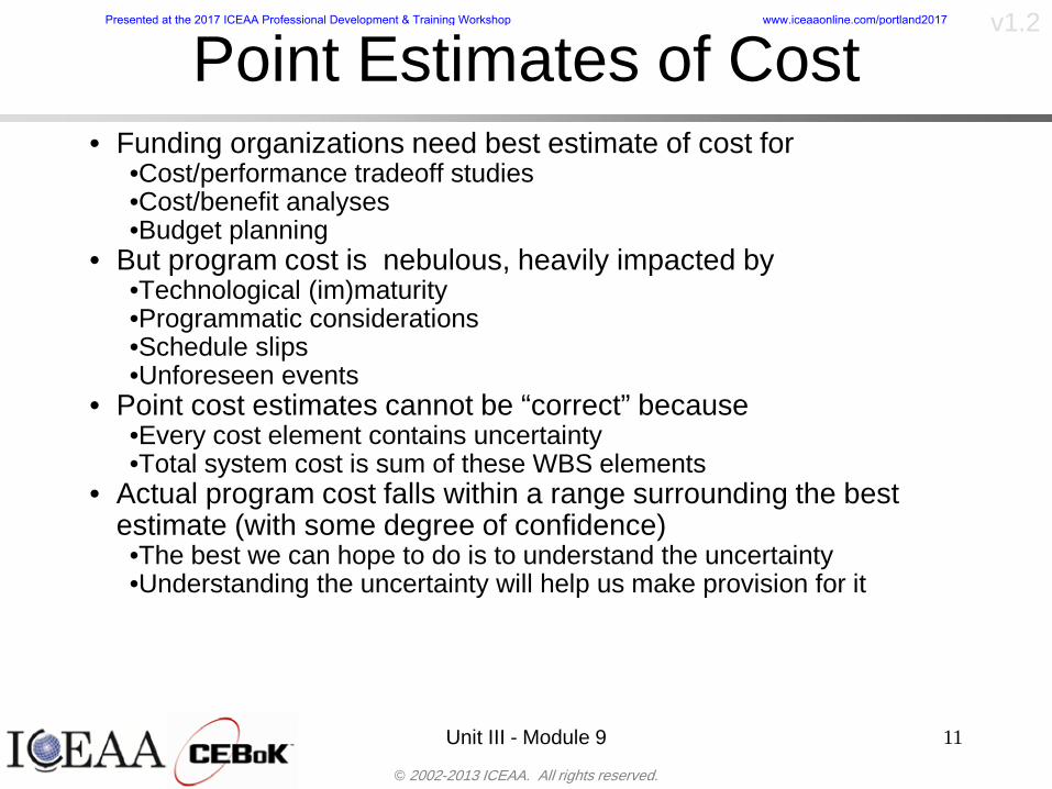
copy 2002-2013 ICEAA All rights reserved
v12
Point Estimates of Costbull Funding organizations need best estimate of cost for
bullCostperformance tradeoff studiesbullCostbenefit analysesbullBudget planning
bull But program cost is nebulous heavily impacted bybullTechnological (im)maturitybullProgrammatic considerationsbullSchedule slipsbullUnforeseen events
bull Point cost estimates cannot be ldquocorrectrdquo becausebullEvery cost element contains uncertaintybullTotal system cost is sum of these WBS elements
bull Actual program cost falls within a range surrounding the best estimate (with some degree of confidence)bullThe best we can hope to do is to understand the uncertaintybullUnderstanding the uncertainty will help us make provision for it
Unit III - Module 9 11
Presented at the 2017 ICEAA Professional Development amp Training Workshop wwwiceaaonlinecomportland2017
copy 2002-2013 ICEAA All rights reserved
v12
Unit III - Module 9 12
Types of Riskbull Cost Growth = Cost Estimating Growth + SkedTech Growth
+ Requirements Growth + Threat Growthbull Cost Risk = Cost Estimating Risk + SkedTech Risk +
Requirements Risk + Threat Riskndash Cost Estimating Risk Risk due to cost estimating errors and the statistical
uncertainty in the estimate ndash ScheduleTechnical Risk Risk due to inability to conquer problems posed
by the intended design in the current CARD or System Specificationsndash Requirements Risk Risk resulting from an as-yet-unseen design shift from
the current CARD or System Specifications arising due to shortfalls in the documents
bull Due to the inability of the intended design to perform the (unchanged) intended mission
bull We didnrsquot understand the solutionndash Threat Risk Risk due to an unrevealed threat eg shift from the current
STAR or threat assessmentbull The problem changedO
ften
impl
icit
or o
mitt
ed
1 2
Presented at the 2017 ICEAA Professional Development amp Training Workshop wwwiceaaonlinecomportland2017
copy 2002-2013 ICEAA All rights reserved
v12
Point Estimates Vs Risk Estimates
Unit III - Module 9 13
DDTampE Flight Unit Production TotalPoint Estimate 63807 5179 6697 70505CER Risk Only - Mean 71176 4805 6426 78018Full Risk - Mean 78937 6490 8091 87430Point Esimtate + 30 82949 6733 8706 91657Full Risk - 70th Percentile 87939 7980 9608 97011
Estimated Total Cost in Millions
Note that the mean is 24 higher than the point estimate and the 70th
percentile is 38 higher than the point estimate
Presented at the 2017 ICEAA Professional Development amp Training Workshop wwwiceaaonlinecomportland2017
copy 2002-2013 ICEAA All rights reserved
v12
Cost Risk and Probabilitybull Cost risk or cost uncertainty analysis represents cost as a
probability distributionbull A probability distribution is a mathematical rule associating a
probability a to each possible outcome or event of interestbull There are two ways to present a probability distribution ndash as a
probability density function (ldquoPDF) and as a cumulative distribution function (ldquoS-curverdquo or ldquoCDFrdquo)
Unit III - Module 9 14
Lognormal Distribution PDF and CDF
0102030405060708090100
200 300 400 500 600 700 800 900 1000Cost $
Con
fiden
ce L
evel
0
00002
00004
00006
00008
0001
00012
00014
00016
Prob
abili
ty D
ensi
ty
CDFPDF
Presented at the 2017 ICEAA Professional Development amp Training Workshop wwwiceaaonlinecomportland2017
copy 2002-2013 ICEAA All rights reserved
v12
Unit III - Module 9 15
Probability Model ndash Distributionbull Normal
ndash Best behavior most iconic
ndash Theoretically (although not practically) allows negative costs which spook some users
ndash Symmetric needs mean shift to reflect propensity for positive growth
bull Lognormalndash A natural result in
non-linear CERsndash Indistinguishable
from Normal at CVs below 25
ndash Skewed
10
4
10
Presented at the 2017 ICEAA Professional Development amp Training Workshop wwwiceaaonlinecomportland2017
copy 2002-2013 ICEAA All rights reserved
v12
Unit III - Module 9 16
bull Triangularndash Most commonndash Easy to use easy to understandndash Modes medians do not addndash Skewed
bull Betandash Rare now but formerly popularndash Solves negative cost and duration issuesndash Many parameters ndash simplifications like PERT
Beta are possiblendash Skewed
bull Bernoullindash Probability is only assigned to two possible
outcomes success and failure (p and 1-p)ndash Simplest of all discrete distributionsndash Mean = pndash Variance = p(1-p)
10
Probability Model ndash Distribution
10
10
Presented at the 2017 ICEAA Professional Development amp Training Workshop wwwiceaaonlinecomportland2017
copy 2002-2013 ICEAA All rights reserved
v12
Unit III - Module 9 17
bull Normalndash If there is a sufficiently large number of independently identically distributed
elements (or not too correlated and not too skewed) then the distribution of total cost is normal due to the Central Limit Theorem
bull Lognormalndash For smaller data sets with large amounts of (positive) correlation and
skewness the lognormal distribution may be a better approximation of total cost
ndash Many total cost distributions in smaller data sets test as both normal and lognormal
bull Triangularndash The sum of triangles is not a triangle so this distribution should generally not
be used to characterize total costbull Convolved
ndash If total cost distribution is derived using simulation then it may not particularly resemble anything In this case we simply have a convolved or simulated total cost distribution
Probability ndash Top-Level Distribution
NEW
Presented at the 2017 ICEAA Professional Development amp Training Workshop wwwiceaaonlinecomportland2017
copy 2002-2013 ICEAA All rights reserved
v12
S-Curves and Confidence Levels
Unit III - Module 9 1818
100
70
25
Probability(Confidence
Level)
Cost Estimate(Dollars)
50
The S curve is the cumulative probability distribution coming out of the statistical summing process
70 confidence that project will cost indicated amount or less
Provides information on potential cost as a result of identified project risks
Provides insight into establishing reserve levels
X Y
MR
X = Point estimateZ = Project requirementY = Cost estimate where there is a 70 change that
final actual cost will be less than cost estimateY-Z= Manage reserve (MR) which is REQUIRED to meet 70 CL
Z
X not always = Z but is based on same content
Presented at the 2017 ICEAA Professional Development amp Training Workshop wwwiceaaonlinecomportland2017
copy 2002-2013 ICEAA All rights reserved
v12
19
Example ndash Normal Distribution
bull Normal distribution with mean equal to 100 and standard deviation equal to 20
bull Median and mode also equal 100bull The 80th Percentile is 117
40 60 80 100 120 140 160
80 of distribution(area under curve)is less than 117
117
Presented at the 2017 ICEAA Professional Development amp Training Workshop wwwiceaaonlinecomportland2017
copy 2002-2013 ICEAA All rights reserved
v12
20
Confidence Levelsbull The output of a cost risk analysis is a probability
distributionndash Typically displayed as a cumulative distribution function or
ldquoS-curverdquondash Confidence levels are simply percentiles of the distribution
0
10
20
30
40
50
60
70
80
90
100
30 60 90 120 150 180
Conf
iden
ce L
evel
Presented at the 2017 ICEAA Professional Development amp Training Workshop wwwiceaaonlinecomportland2017
copy 2002-2013 ICEAA All rights reserved
v12
Measuring Parametric Model Uncertainty
bull When developing estimates using cost-estimating relationships (CERs) there are two major sources of uncertaintyndash Technical (model input) uncertaintyndash Estimating uncertainty
bull Technical uncertainty reflects the uncertainty inherent in the model inputsndash Typical parametric model inputs include weight lines of code
heritage and other performance and management inputs
bull Estimating uncertainty measures the uncertainty inherent in the model due to the modelrsquos inability to capture all aspects of variability in the data
21
Presented at the 2017 ICEAA Professional Development amp Training Workshop wwwiceaaonlinecomportland2017
copy 2002-2013 ICEAA All rights reserved
v12
Parametric Model Examplebull The NASAAir Force Cost Model (NAFCOM) is a
parametric model for estimating acquisition costs for spacecraft and launch vehicles
bull The CERs in NAFCOM have the formCost = C WeightVNewDesignWTechnicalXManagementY ClassZ
bull There is technical uncertainty about each of the parametersndash Parametric models are applied early in a program so there
is significant amount of uncertainty in the weightndash Heritage is also tricky it is inherently subjective and project
personnel are typically optimisticndash Technical characteristics can also change as a program
matures and requirements change
22
Presented at the 2017 ICEAA Professional Development amp Training Workshop wwwiceaaonlinecomportland2017
copy 2002-2013 ICEAA All rights reserved
v12
Weight Uncertaintybull Aerospace weight growth study average satellite
weight growth from program inception to launch is 28
23
Aerospace Weight Growth Data
-10
0
10
20
30
40
50
60
0 4 8 12 16 20 24 28 32 36 40 44 48 52 56 60 64 68 72 76 80 84 88 92 96 100
Percent Program Completion
Perc
ent W
eigh
t Gro
wth
Presented at the 2017 ICEAA Professional Development amp Training Workshop wwwiceaaonlinecomportland2017
copy 2002-2013 ICEAA All rights reserved
v12
Estimating Uncertaintybull CERs do not perfectly fit the historical data
ndash There are non-repeatable random effects that cannot be predicted
bull For examplendash Parts breaking during testingndash Strikes which are difficult to predict
bull This results in an underlying uncertainty distribution about an estimatendash The outcome of a CER represents only one point on an
uncertainty distributionbull Typically mean or median depending upon the CER
methodology
24
Presented at the 2017 ICEAA Professional Development amp Training Workshop wwwiceaaonlinecomportland2017
copy 2002-2013 ICEAA All rights reserved
v12
Estimating Uncertainty (2)
25
Presented at the 2017 ICEAA Professional Development amp Training Workshop wwwiceaaonlinecomportland2017
copy 2002-2013 ICEAA All rights reserved
v12
Estimating Uncertainty (3)bull In the case of a linear regression the estimating
uncertainty follows a normal distributionndash The estimate is the mean and the standard error of the
estimate from the regression is the standard deviation of the normal distribution
bull In the case of a log-transformed linear regression the estimating uncertainty follows a lognormal distributionndash The estimate is the median of the lognormal and the
standard error of the estimate from the regression is the standard deviation of the normal distribution (in log-space)
bull There is additional uncertainty about an estimate based upon the distance of what is being estimated from the mean of the input datandash This results in a prediction interval
26
Presented at the 2017 ICEAA Professional Development amp Training Workshop wwwiceaaonlinecomportland2017
copy 2002-2013 ICEAA All rights reserved
v12
Aggregating Riskbull Risk is typically applied at the same level at
which we estimate cost that is at the Work Breakdown Structure (WBS) level
bull The estimates for each WBS are developedndash These estimates sum to yield the total system cost
bull For an n-element WBS the total cost is the sum of the cost for each of the n elements
27
nXXXCostSystem +++= 21
Presented at the 2017 ICEAA Professional Development amp Training Workshop wwwiceaaonlinecomportland2017
copy 2002-2013 ICEAA All rights reserved
v12
WBS Examplebull Launch Vehicle
ndash Structurebull Vehicle Structurebull Tank Structure
ndash Thermal Controlbull Active Thermal Controlbull Induced Thermal Controlbull Tank Thermal Control
ndash Main Propulsion Systemndash Liquid Rocket Enginendash Electric Power and Distributionndash Command Control and Data Handlingndash System Integration
28
Presented at the 2017 ICEAA Professional Development amp Training Workshop wwwiceaaonlinecomportland2017
copy 2002-2013 ICEAA All rights reserved
v12
WBS and Risk
29
Presented at the 2017 ICEAA Professional Development amp Training Workshop wwwiceaaonlinecomportland2017
copy 2002-2013 ICEAA All rights reserved
v12
Aggregating Riskbull This leads us to the issue of aggregating the risks across the
WBSbull For example if we want to determine the 70th percentile of the
overall cost risk distribution how do we proceed bull Note that we cannot simply add the 70th percentiles of each of
the cost risk distributionsbull We can add means and variances (taking correlation into
account more on that later) but that is all
Variance of Total Cost =
30
Mean of Total Cost = ( )E X E Xk
k
n
kk
n
kk
n
= = =aringaelig
egraveccediloumloslashdivide
= =aring aring1 1 1
m
Var X kk
n
=aringaelig
egraveccediloumloslashdivide1
= s r s skk
n
iji
j
i jj
n2
1 1
1
22+aring aringaring
= =
-
=
Presented at the 2017 ICEAA Professional Development amp Training Workshop wwwiceaaonlinecomportland2017
copy 2002-2013 ICEAA All rights reserved
v12
Percentiles Do Not Addbull As a notional example consider two independent normal
distributionsndash One distribution has mean equal to 100 and standard deviation
equal to 20ndash The second distribution has mean 300 and standard deviation of 80
bull The sum of two independent normally distributed random variables is also normally distributed
bull To combine the two distributions we add the means and add the variancesndash Total mean is
ndash Total standard deviation is
31
400300100 =+
8258020 22 raquo+
Presented at the 2017 ICEAA Professional Development amp Training Workshop wwwiceaaonlinecomportland2017
copy 2002-2013 ICEAA All rights reserved
v12
Percentiles Do Not Add (2)bull The 80th percentiles for the individual distributions are
117 and 367 respbull The 80th percentile of the combined distribution is
469 but the sum of the two 80th percentiles is 484bull To see why this is the case note that the percentiles
of a normal distribution are determined by the mean and the standard deviationndash The standard deviations are not added when normal distributions
are combined rather the variances are combinedndash Sum of variances is ndash The standard deviation of this sum is
32
22 ba +22 ba +
Presented at the 2017 ICEAA Professional Development amp Training Workshop wwwiceaaonlinecomportland2017
copy 2002-2013 ICEAA All rights reserved
v12
Percentiles Do Not Add (3)bull Since bull We can write
bull The left side of this inequality represents the risk of the combined distributions while the right side represents the sums of the individual risks
bull Combining two missions that are independent results in a diversification of riskndash The total portfolio is not as risky on a relative basis as each
individual project
33
2222 2 bababa ++lt+
baba +lt+ 22
Presented at the 2017 ICEAA Professional Development amp Training Workshop wwwiceaaonlinecomportland2017
copy 2002-2013 ICEAA All rights reserved
v12
Methods for Aggregating Riskbull Since percentiles do not add we have to find other
ways to aggregate riskbull One method is to use Monte Carlo simulationbull Unless cost risk is represented by normal
distributions for all WBS elements summing the means and variances does not result in a completely accurate depiction of overall system cost risk
bull The normal distribution is not a realistic distribution for representing risk in many or even most situations since regarding project risk more can go wrong than can go right which means the risk is NOT symmetric unlike the Gaussian bell curve
34
Presented at the 2017 ICEAA Professional Development amp Training Workshop wwwiceaaonlinecomportland2017
copy 2002-2013 ICEAA All rights reserved
v12
Unit III - Module 9 35
Monte Carlo Simulationfor Risk Analysis
bull When risk analysis is performed multiple risks are gatheredndash These risks may have various probability
distributions
bull Monte Carlo is the most commonly accepted way to produce an accurate characterization of the distribution of the combined effect of these many risksndash Using this distribution we can produce percentiles
for cost impacts due to risk occurrences
10
Presented at the 2017 ICEAA Professional Development amp Training Workshop wwwiceaaonlinecomportland2017
copy 2002-2013 ICEAA All rights reserved
v12
Monte Carlo Simulationbull Simulation is a means for solving problems that are
analytically intractablendash Involves repeated random sampling
bull It was developed during the Manhattan Project as a way to model the interactions inside an atom during nuclear fissionndash Allowed for more sophisticated mathematical modeling of atomic
phenomena
bull Most computer packages use pseudo-random number generators that produce seemingly random results from an initial seedndash Example is the linear congruential generator
36
( ) mbaXX nn mod1 +=+
Presented at the 2017 ICEAA Professional Development amp Training Workshop wwwiceaaonlinecomportland2017
copy 2002-2013 ICEAA All rights reserved
v12Using Random Numbers to Simulate Distributions
bull WBS cost risk is typically measured by a probability distributionbull The most common method for simulating a probability
distribution is the inverse methodbull This involve obtaining a simulated random value from a uniform
distribution and then inverting this through the cumulative distribution function (CDF) to obtain the simulated value
bull As an example for a uniform distribution on the interval [0100]
bull In this case the CDF random value of 05 translates to 10005 = 50
37
( )100
1=xf ( )
100xxF = ( ) xxF 1001 =-
Presented at the 2017 ICEAA Professional Development amp Training Workshop wwwiceaaonlinecomportland2017
copy 2002-2013 ICEAA All rights reserved
v12
Simulating a Triangular Distribution
bull For a triangular distribution with low = 0 most likely = 50 and high = 150 the CDF is given by
bull The inverse function is given by
38
( )iumliumlicirc
iumliumliacute
igrave
poundlt--
poundpound=
1505021
1500050
50015000
2
2
2
xxx
xxxF
( )iumliumlicirc
iumliumliacute
igrave
poundltdivideoslashouml
ccedilegraveaelig +--
poundpound=-
131
21
37501
250017500150
3107500
1
xx
xxxF
Presented at the 2017 ICEAA Professional Development amp Training Workshop wwwiceaaonlinecomportland2017
copy 2002-2013 ICEAA All rights reserved
v12
Simulating a Triangular Distribution (2)
bull If the simulated uniform value is equal to 02 the corresponding inverse value from the CDF inverse is approximately 387
39
0
01
02
03
04
05
06
07
08
09
1
0 30 60 90 120 150
Presented at the 2017 ICEAA Professional Development amp Training Workshop wwwiceaaonlinecomportland2017
copy 2002-2013 ICEAA All rights reserved
v12
Monte Carlo and the WBSbull Simulation involves repeated trials
40
WBS Draw1 2 3 4 5
System 2912 3566 4390 2954 4655 Sum
Structure 80 105 55 80 57 SumVehicle Structure 50 70 30 40 20Tank Structure 30 35 25 40 37
Thermal Control 32 36 35 29 33 SumActive Thermal Control 10 15 12 7 10Induced Thermal Control 12 14 13 14 14Tank Thermal Control 10 7 10 8 9
Main Propulsion System 100 150 125 140 100
Liquid Rocket Engine 1000 1100 1800 900 2200
Electric Power and Distribution 100 125 150 75 90
Command Control and Data Handling 200 250 225 230 275
System Integration 1400 1800 2000 1500 1900
Presented at the 2017 ICEAA Professional Development amp Training Workshop wwwiceaaonlinecomportland2017
copy 2002-2013 ICEAA All rights reserved
v12
Number of Trialsbull Monte Carlo involves a repeated number of trialsbull The greater the number of trials the more accurate the
simulation will approximate the overall cost risk behavior of the system
bull After 100 trials the histogram looks very jagged
41
Presented at the 2017 ICEAA Professional Development amp Training Workshop wwwiceaaonlinecomportland2017
copy 2002-2013 ICEAA All rights reserved
v12
Number of Trials (2)
42
1000 Trials
10000 Trials
50000 Trials Additional trials give a more accurate depiction of the final result
Presented at the 2017 ICEAA Professional Development amp Training Workshop wwwiceaaonlinecomportland2017
copy 2002-2013 ICEAA All rights reserved
v12
Number of Trials (3)bull If we want to simulate the underlying
mean within 1 with 95 confidence for example then we require
43
divideoslash
oumlccedilegrave
aelig poundpound-
=
dividedividedivide
oslash
ouml
ccedilccedilccedil
egrave
aeligpound
-pound
-=
divideoslashouml
ccedilegraveaelig poundpound=
nZ
n
nnX
n
X
n
n
011
010Pr
011
010Pr
011990Pr950
___
___
sm
sm
sm
sm
sm
mm
Presented at the 2017 ICEAA Professional Development amp Training Workshop wwwiceaaonlinecomportland2017
copy 2002-2013 ICEAA All rights reserved
v12
Number of Trials (4)bull This means that the number of trials required is determined by
bull Solving for n we find that at least
trials are neededbull Note that this term involves the coefficient of variation of the
distribution which means that distributions with less dispersion require fewer trials to accurate simulate
44
96101
=ns
m
ms41638
Presented at the 2017 ICEAA Professional Development amp Training Workshop wwwiceaaonlinecomportland2017
copy 2002-2013 ICEAA All rights reserved
v12
Number of Trials (5)bull Simulating percentiles requires more trials than for simulating
meansbull Let Pn represent the number of trials in the sample at or below
the 70th percentile of the underlying distribution (suppose this is known)
bull By the Central Limit Theorem Pnn follows a normal distribution with mean equal to the 70th percentile and variance equal to
bull By a similar process for the mean we find that the number of trials needed to simulate the 70th percentile within 1 with 95 confidence is
45
( )n
FF 700700 1-
n
n
PPn -41638
Presented at the 2017 ICEAA Professional Development amp Training Workshop wwwiceaaonlinecomportland2017
copy 2002-2013 ICEAA All rights reserved
v12
Number of Trials (6)bull If Pn 070 for all n then n is approximately
bull For the sake of comparison suppose CV = 03 (reasonable approximation for hardware development) then the number of trials needed to simulate the mean with the same accuracy is then ldquoonlyrdquo 11525
bull More trials are needed to accurately simulate percentiles than means
46
( ) 46416703041638
70704168341638 =divide
oslashouml
ccedilegraveaelig=divide
oslashouml
ccedilegraveaelig -
=-
nnn
PPn
n
n
Presented at the 2017 ICEAA Professional Development amp Training Workshop wwwiceaaonlinecomportland2017
copy 2002-2013 ICEAA All rights reserved
v12
Methods of Simulationbull Monte Carlo simulation is a standard term for
simulationbull However there is an improvement on Monte Carlo
that improves the accuracy of the results of a simulation for a given number of trials
bull This method is call the Latin Hypercube approach to simulationndash Similar to Monte Carlo but an equal number of draws are taken
from a set of subintervals for example dividing the interval (01) into [00001) [0102)hellip [0910]
ndash Instead of 10 trials from [01] we have one trial from each subinterval
ndash Rough rule of thumb is Latin Hypercube takes 30 fewer trials to achieve similar accuracy to Monte Carlo
47
Presented at the 2017 ICEAA Professional Development amp Training Workshop wwwiceaaonlinecomportland2017
copy 2002-2013 ICEAA All rights reserved
v12
Probability Model ndash Correlationbull Correlation exists between work breakdown structure
(WBS) cost element costs and between cost and schedule
bull Correlation is a necessary consideration in cost risk analysis
bull Correlation is a number that can vary between -1 and +1 and represents the strength of the relationship between the two variablesndash If both variable have a tendency to move in the same direction
correlation is positivendash If when one variable increases the other tends to decrease and
vice-versa the correlation between the two variables is negative
Presented at the 2017 ICEAA Professional Development amp Training Workshop wwwiceaaonlinecomportland2017
copy 2002-2013 ICEAA All rights reserved
v12
Correlation And Causationbull Note that correlation is not causation however
causation implies correlationndash For example shark attacks and ice cream sales at the beach
bull For example for a launch vehicle structure increasing the diameter will not only result in an increase in the structures cost but will also result in higher costs for thermal coating (paint etc)
bull Also simply because two subsystems do not appear to be related does not mean they are not correlatedndash For example structures and computer equipment seemingly
have little relation to one another however an external factor such as a funding cut or a strike will impact all subsystems leading to delays and increasing cost across the board
ndash Thus everything in a WBS has some correlationUnit III - Module 9 49
Presented at the 2017 ICEAA Professional Development amp Training Workshop wwwiceaaonlinecomportland2017
copy 2002-2013 ICEAA All rights reserved
v12
The Importance of Correlationbull Percent that total cost standard deviation is underestimated
when correlation assumed to be 0 instead of r given nWBS elements
Unit III - Module 9 5050
0
20
40
60
80
100
0 01 02 03 04 05 06 07 08 09 1Actual Correlation
Perce
nt Un
deres
timate
d
n = 10
n = 30
n = 100n = 1000
0
20
40
60
80
100
0 01 02 03 04 05 06 07 08 09 1Actual Correlation
Perce
nt Un
deres
timate
d
n = 10
n = 30
n = 100n = 1000
Reference 32nd Annual DOD Cost Analysis Symposium Advanced Training Session ldquoWhy Correlation Matters in Cost Estimatingrdquo Stephen A Book
Presented at the 2017 ICEAA Professional Development amp Training Workshop wwwiceaaonlinecomportland2017
copy 2002-2013 ICEAA All rights reserved
v12
The Importance of Correlation (2)bull For example if correlation is assumed to be 0 for all
elements in a 30 element WBS and the actual correlation is 20 then the total cost standard deviation is underestimated by 60
bull For example assume the total cost is modeled as a normal distribution with mean = 100
bull If correlation is assumed to be zero with total cost standard deviation = 12 when correlation is actually 20 then the true underlying standard deviation is actually 30
bull 70th percentile with zero correlation assumption is 106
bull 70th percentile with 20 correlation is 116 Unit III - Module 9 51
Presented at the 2017 ICEAA Professional Development amp Training Workshop wwwiceaaonlinecomportland2017
copy 2002-2013 ICEAA All rights reserved
v12
Measures of Correlationbull Two measures of correlation are commonly used in
cost risk analysesndash Pearsonrsquos product-moment correlation coefficient ndash Spearmanrsquos rank correlation coefficient
bull Garvey and others recommend using Pearsonrsquos product-moment correlation coefficient correlation for cost risk analysesndash Method of moments uses this but there are two options in
simulationndash Popular simulation packages like Risk and Crystal Ball use
rank correlation but in practice this has been found to make little difference
ndash Pearson product-moment correlation has been incorporated into Risk+
52
Presented at the 2017 ICEAA Professional Development amp Training Workshop wwwiceaaonlinecomportland2017
copy 2002-2013 ICEAA All rights reserved
v12
Pearson Correlationbull Pearsonrsquos product-moment correlation measures
degree of linearity between two random variables bull If two random variables are perfectly linear (eg Y =
aX + b) with positive slope then the Pearson product-moment correlation between X and Y denoted by rXY is +1
53
X X
Y Y Y
XNegative Correlation Positive Correlation No Correlation
middotmiddot
middotmiddot
middotmiddot middotmiddot
middotmiddot
middot
middot
middotmiddotmiddot
middotmiddot
middotmiddot
middotmiddot middot
middot
middot
middotmiddotmiddotmiddotmiddotmiddotmiddotmiddot
middotmiddotmiddotmiddot
middotmiddot
middotmiddot middotmiddotmiddotmiddot
middotmiddotmiddot
middotmiddotmiddotmiddot
middotmiddotmiddot
middotmiddotmiddot
middotmiddot
middot
middot middotmiddot
middot middotmiddotmiddotmiddot middotmiddot middot middotmiddot middot middot
middotmiddot middot
middotmiddotmiddotmiddotmiddot middot middotmiddot
middotmiddot
middot
middotmiddot
middotmiddot middot
middot middot middot
middotmiddot middot
middotmiddotmiddot
middotmiddot
middot middot
Presented at the 2017 ICEAA Professional Development amp Training Workshop wwwiceaaonlinecomportland2017
copy 2002-2013 ICEAA All rights reserved
v12
Spearman Correlationbull Spearmanrsquos rank correlation measures the
monotonicity between two random variablesbull If two random variables are perfectly monotonically
increasing (eg Y = X2) then the Spearman rank correlation denoted by rXY is +1
bull The two measures can be significantly different
54
10 20 30 40 50 60
100
200
300
096 097 098 099 1
1
060
020
040
080
Eff
ort (
Staf
f-M
onth
s)
Software Size I KDSI
y = 28z12y
z x
yy = x100
0 pound x pound 1
Figure 5-9A Figure 5-9B
Pearson Correlation = 09976 Rank Correlation = 1
Pearson Correlation = 024 Rank Correlation = 1
X(x ) ~ Unif(01)
Reference Probability Methods for Cost Uncertainty Analysis A Systems Engineering Perspective Paul R Garvey
Presented at the 2017 ICEAA Professional Development amp Training Workshop wwwiceaaonlinecomportland2017
copy 2002-2013 ICEAA All rights reserved
v12
Unit III - Module 9 55
200
250
300
350
400
1000 1200 1400 1600 1800 2000
Recurring Production
SEPM
200
250
300
350
400
1000 1200 1400 1600 1800 2000
Recurring Production
SEPM
Functional Correlationbull Old No Functional
Correlation Simulation run with WBS items entered as values
bull New Simulation run with functional dependencies entered as they are in cost model
CorrelatedNot Correlated
Note shift of mean and increased variability
Presented at the 2017 ICEAA Professional Development amp Training Workshop wwwiceaaonlinecomportland2017
copy 2002-2013 ICEAA All rights reserved
v12
Risk Measuresbull ldquoWestern Europe conquered the word because of a
technological revolution that started because of attempts to measure the worldrdquo ndash Phillipe Jorion ndash In the same way attempts to measure risk will lead to better project
managementbull Risk management for DoD and NASA agencies focuses
primarily on funding projects to a single percentile ndash NASA policy explicitly mentions 70 and 50ndash This is known as ldquoValue at Riskrdquo and is prevalent in the banking and
financial industry
56
Presented at the 2017 ICEAA Professional Development amp Training Workshop wwwiceaaonlinecomportland2017
copy 2002-2013 ICEAA All rights reserved
v12
Value at Risk (VaR)bull VaR is a percentile of the cost risk
distributionndash VaR funding at the 70th percentile means that
there is a 30 chance of final project cost exceeding the funded amount (budget)
bull VaR has some meritsndash Common measure can be used to compare
different projects and programsndash Easily understood by senior managers and
decision makers
57
Presented at the 2017 ICEAA Professional Development amp Training Workshop wwwiceaaonlinecomportland2017
copy 2002-2013 ICEAA All rights reserved
v12
Why 70th or 80th Percentilebull Typical policy guidance involves funding at the 70th or 80th
percentile Why fund as such a low percentilebull There is some incentive to not over-fundbull For a normal distribution an inflection point occurs near the 80th
percentile meaning that for values above 80 confidence achieving higher levels of confidence can only be achieved by spending greater dollar amounts at an increasing rate
58
-05-04-03-02-01
00102030405
0 05 1 15 2 25 3
Standard Deviations from Mean
Normal Distribution
First DerivativeSlopeVelocity
Second DerivativeConvexityAcceleration
Inflection point at one standard deviation above the mean (~84th
percentile)
Presented at the 2017 ICEAA Professional Development amp Training Workshop wwwiceaaonlinecomportland2017
copy 2002-2013 ICEAA All rights reserved
v12
Funding Above Inflection Pointsbull As the percentile goes above the 80th percentile the amount
needed to achieve that higher level of confidence begins to increase at an increasing rate as is evident from the graph
59
0
10
20
30
40
50
60
70
50 55 60 65 70 75 80 85 90 95 100
$ Ab
ove
MEa
n to
Ach
ieve
Per
cent
ile
Percentile (Confidence Level)
Presented at the 2017 ICEAA Professional Development amp Training Workshop wwwiceaaonlinecomportland2017
copy 2002-2013 ICEAA All rights reserved
v12
Why Budget to the 70th or 80thbull Government projects are funded at the 70th or 80th percentilesbull Why not the 90th or 99th percentile Wonrsquot that help prevent
overrunsndash As we have seen percentiles do not add across programs
bull The sum of the 80th percentiles does NOT equal the total 80th percentile
ndash This is because the individual programs are riskier than the entire suite of missions
bull Known as the ldquoPortfolio effectrdquo (more or this later)
ndash Funding at the 80th gives confidence that the entire portfolio will be adequately funded
bull And since there is an inflection point near the 80th percentile funding above that level quickly becomes cost prohibitive
60
Presented at the 2017 ICEAA Professional Development amp Training Workshop wwwiceaaonlinecomportland2017
copy 2002-2013 ICEAA All rights reserved
v12
Inflection Points for Lognormalbull For a lognormal the inflection point
variesndash Coefficient of variation equal to 10 equates to an
inflection point at the 70th percentile
61
0
10
20
30
40
50
60
70
050 060 070 080 090 100
Coef
ficen
t of V
aria
tion
Percentile of the Inflection Point
Presented at the 2017 ICEAA Professional Development amp Training Workshop wwwiceaaonlinecomportland2017
copy 2002-2013 ICEAA All rights reserved
v12
Issues with Percentile Fundingbull However risk management does not stop at a
specific percentilendash What happens when the 70th percentile is exceeded
bull Any effective risk management policy should prescribe what happens after a bad event occursndash With VaR we only know when a bad event has occurred ndash Also funding at a relatively low level means we have no true
sense of the real risks that should be guarded against
62
Presented at the 2017 ICEAA Professional Development amp Training Workshop wwwiceaaonlinecomportland2017
copy 2002-2013 ICEAA All rights reserved
v12
ldquoHere There Be Dragonsrdquobull On old maps uncharted territory was often
marked with monsters or dragons
63
A section of the Carta Marina by Olaus Magnus 16th Century
Presented at the 2017 ICEAA Professional Development amp Training Workshop wwwiceaaonlinecomportland2017
copy 2002-2013 ICEAA All rights reserved
v12
Distribution Comparisonbull Four different distributions with the same 70th
percentile
bull Should we expect the tails to be similar
64
0
10
20
30
40
50
60
70
80
0 100 200 300 400 500 600
Perc
entil
eCo
nfid
ence
Lev
el
Triangular
Normal
Lognormal
Pareto
Presented at the 2017 ICEAA Professional Development amp Training Workshop wwwiceaaonlinecomportland2017
copy 2002-2013 ICEAA All rights reserved
v12Distribution Comparison Tail Behavior
bull The normal and triangular distributions have similar tails but the lognormal and Pareto have much fatter right tails
65
70
75
80
85
90
95
100
500 1500 2500 3500 4500 5500
Perc
entil
eCo
nfid
ence
Lev
el
Triangular
Normal
Lognormal
Pareto
Here There Be Dragons
Presented at the 2017 ICEAA Professional Development amp Training Workshop wwwiceaaonlinecomportland2017
copy 2002-2013 ICEAA All rights reserved
v12Distribution Comparison ndash Tail Behavior (Table)
bull There is significant tail risk for the lognormal and the Paretobull The 99th percentile for the Pareto is 1000 times greater than
the 70th percentilendash Risk seen in financial markets and in catastrophic risks like natural
disasters bull Four different projects follow the four different risk profiles seen
in this example should clearly have different risk management approaches but 70th percentile funding indicates the same risk management approach for all four
66
Percentile Triangular Normal Lognormal Pareto 70th $600 $600 $600 $600 80th $680 $660 $770 $1430 90th $770 $750 $1070 $5880 95th $840 $820 $1410 $23750 99th $930 $950 $2350 $600000
Presented at the 2017 ICEAA Professional Development amp Training Workshop wwwiceaaonlinecomportland2017
copy 2002-2013 ICEAA All rights reserved
v12Percentile Budgeting is Not Risk Management
bull Percentile budgeting ne effective risk management policybull Suppose that you are shopping for a new car You
mention that safety is your top concern The salesman says he has a great safe car available You ask about the air bags Do they work The salesman answers ldquoOf course Seventy percent of the time they work fine Only 30 of the time the air bags will fail to deployrdquo Would you buy such a car Hedge fund manager David Einhorn has stated ldquoRisk management is the air bag that must always work but only in the multi-sigma event where you have an accidentrdquo
67
Risk management is the air bag that must always work but only in the multi-sigma event where you
have an accident
Presented at the 2017 ICEAA Professional Development amp Training Workshop wwwiceaaonlinecomportland2017
copy 2002-2013 ICEAA All rights reserved
v12
Joint Confidence Level Analysisbull Schedules are risky toobull For 98 recent NASA missions average
schedule growth was 38ndash Not as high as cost growth but still significant
68
0
5
10
15
20
25
30
35
40
Schedule
Cost
Presented at the 2017 ICEAA Professional Development amp Training Workshop wwwiceaaonlinecomportland2017
copy 2002-2013 ICEAA All rights reserved
v12
Schedules Impact Costbull Changes in schedule can have enormous
impacts on cost ndash Schedule slips can lead to cost increases
bull Fixed programmatic costs must be paid on a regular basisndash Achieving schedule milestones early can result in cost
savings
bull Schedule is an important consideration in cost analysis including cost risk analysis
bull However we must be careful in correctly integrating cost and schedule riskndash Schedule is not simply an input but is dependent on many of
the same factors that drive cost
69
Presented at the 2017 ICEAA Professional Development amp Training Workshop wwwiceaaonlinecomportland2017
copy 2002-2013 ICEAA All rights reserved
v12
The Relationship of Cost to Schedulebull Cost and schedule are positively correlated
ndash A larger program with bigger scope with take longer to complete than a smaller simpler program
bull However longer schedules do not always equate to higher cost nor shorter schedules with lower costndash Highly compressed schedules relative to the
optimal schedule can lead to large overrunsbull Compressed schedules are commonplace for
many planetary missions
70
Presented at the 2017 ICEAA Professional Development amp Training Workshop wwwiceaaonlinecomportland2017
copy 2002-2013 ICEAA All rights reserved
v12The Impact of Schedule GrowthCompression on Cost
bull Compressed schedules lead to cost growth and based on existing research is actually more expensive than schedule slippages
71
0
20
40
60
80
100
120
140
160
-50 -25 0 25 50 75 100
Percentage Change in Schedule
Perc
enta
ge C
hang
e in
Cos
t due
to
Sche
dule
Cha
nge
Source Smart CB ldquoCost and Schedule Interrelationshipsrdquo 2007 NASA Cost Symposium
Presented at the 2017 ICEAA Professional Development amp Training Workshop wwwiceaaonlinecomportland2017
copy 2002-2013 ICEAA All rights reserved
v12Schedule as an Independent Variable
bull Why not simply add schedule as an input to cost-estimating relationships (CERs)
bull Schedule is often treated as an independent variable ndash schedules are often determined independently of cost considerationsndash Cost may not be considered explicitly although budgets and
schedules are determined based on scope and other common factors
bull In 2006 SAIC undertook a research task to determine the impact of schedule on cost and added schedule as an independent variable to the CERs in the NASAAir Force Cost Model (NAFCOM) to see if schedule provided any improvement in goodness of fit
72
Presented at the 2017 ICEAA Professional Development amp Training Workshop wwwiceaaonlinecomportland2017
copy 2002-2013 ICEAA All rights reserved
v12
Schedule is a Dependent Variablebull Since NAFCOM includes an exhaustive list of cost drivers the inclusion
of schedule should give an indication of whether there is any additional independent value added from schedule independent of the cost drivers
bull In the study schedule was added to 10 subsystem-level CERs
ndash In each case the addition of schedule did NOTimprove the goodness of fit and schedule was NOT found to be a statistically significant cost driver (given the presence of the other variables) for any of the 10 CERs
bull Standard errors for the CERs increased due to decrease in degrees of freedom
bull Thus schedule as an independent variable did not provide any additional explanation of variation in historical cost
bull This is because schedule is truly NOT an independent variable but a dependent variable and is a function of the same factors that drive cost
73
Presented at the 2017 ICEAA Professional Development amp Training Workshop wwwiceaaonlinecomportland2017
copy 2002-2013 ICEAA All rights reserved
v12
Incorporation of Schedule in Cost Risk
bull When using subjective methods care must be taken in applying schedule to cost risk analysis
bull Since schedule is a dependent variable treating it independently from other factors when assessing its impact on cost can lead to a double count of independent variables in the cost risk analysis
bull Direct inclusion of schedule in a cost risk analysis effectively doubles the influence of each cost driver
ndash Incorrectly leads to broader risk ranges
74
CostWeight
HeritageNewness
Technology Readiness Schedule
Presented at the 2017 ICEAA Professional Development amp Training Workshop wwwiceaaonlinecomportland2017
copy 2002-2013 ICEAA All rights reserved
v12Subjective Cost Risk Methods and Overinclusion of Risk Factors
bull Subjective methods are suitable when data are scarce or not availablebull However care must be taken not to treat correlated sources of risk
such as schedule as independent of each otherbull Example ndash a subjective risk analysis incorporated technology readiness
design risk requirements stability integration risk and schedule and treated each source of risk as independent
bull Risk triangle high value without schedule risk was 31 times the point estimate
bull Risk triangle high value with schedule risk added on top of other sources of risk treated independently was 34 times the point estimate
bull Risk triangle taking correlation between sources of risk into account in a rigorous statistical manner has a high value 15 times the point estimate less than half the effect when treating sources of risk as independent
75
Presented at the 2017 ICEAA Professional Development amp Training Workshop wwwiceaaonlinecomportland2017
copy 2002-2013 ICEAA All rights reserved
v12Fundamental Equation of Cost and Schedule Interrelationships
bull The Fundamental Equation of the Relationship Between Cost and Schedule is
Time = Moneybull This is a well known adage that time is money Your boss at
work may even mention this to you from time to time or if you are the boss you are all too aware of this iron law
bull Because time is money cost and schedule risk should be modeled jointly not with schedule as an independent cost driver
bull Note that cost and schedule are not perfectly correlatedndash Cost can sometimes ldquobuy downrdquo schedule extra money can be
spent to meet a deadline since in some cases additional effort to hasten the completion of a task
76
Presented at the 2017 ICEAA Professional Development amp Training Workshop wwwiceaaonlinecomportland2017
copy 2002-2013 ICEAA All rights reserved
v12How to (Correctly) Incorporate Schedule into Cost Risk Analysis
bull The best way to model cost and schedule risk is to develop a joint cost and schedule model based on the same data
bull Since such models are not currently available the next best approach is to model cost and schedule independently and then integrate cost and schedule risk analyses using joint probability distributions taking into account correlation between cost and schedulendash This approach pioneered by Paul Garvey and Steve Book is
considered industry best practicendash This is a practical method mathematically tractable and follows
naturally from the Fundamental Equation of Cost and Schedule Interrelationships
77
Book S A ldquoQuantifying the Relationship Between Cost and Schedulerdquo The Measurable News Winter 2007-2008 pp 11-15Garvey PR Probability Methods for Cost Uncertainty Analysis A Systems Engineering Perspective New York Marcel Dekker 2000 pp 308-335
Presented at the 2017 ICEAA Professional Development amp Training Workshop wwwiceaaonlinecomportland2017
copy 2002-2013 ICEAA All rights reserved
v12
Joint Lognormal and Normal Distributions
bull Cost and schedule are typically modeled as some combination of Normal and Lognormal probability distributionsndash Studies by The Aerospace Corporation the MITRE
Corporation Wyle Labs and SAIC have found that the Lognormal probability distribution almost always serves as a good model for both the schedule distribution and the cost distribution
ndash The Normal distribution may also be appropriate in some instances and depending upon the level of confidence at which budgets are set may even be more conservative and logically consistent than the Normal distribution
ndash Joint Lognormal and Normal distributions are defined by a pair of mean and standard deviations and a level of correlation between the two
78
Presented at the 2017 ICEAA Professional Development amp Training Workshop wwwiceaaonlinecomportland2017
copy 2002-2013 ICEAA All rights reserved
v12Modeling Cost and Schedule as a Bivariate Distribution
bull In the approach set forth by Book and Garvey cost risk is assessed and the top-level distribution is modeled as a Lognormal (or Normal) distribution schedule risk is assessed and the overall schedule risk is modeled as a Lognormal (or Normal) distribution
bull The two distributions are combined into a Bivariate distribution by assigning a correlation between the two and by treating the two distributions as the marginal distributions of a Bivariate Lognormal distributionndash Other combinations include a Bivariate Normal or a Bivariate
Normal-Lognormal
79
Presented at the 2017 ICEAA Professional Development amp Training Workshop wwwiceaaonlinecomportland2017
copy 2002-2013 ICEAA All rights reserved
v12Bivariate Lognormal Distribution for Cost and Schedule
bull Cost is often observed to be Lognormal when strong positive correlations are present among the systemrsquos WBS cost element costs
bull A systemrsquos schedule is often observed (from Monte Carlo simulations) to be Lognormal if it is the sum of many positively correlated schedule activities in an overall schedule network
bull If Lognormal distributions characterize a systemrsquos cost and schedule then the Bivariate Lognormal could serve as an assumed model of their joint distributionndash In this case the marginal distribution of each of cost and schedule is
Lognormalbull Other possibilities for modeling cost and schedule as a Bivariate
distribution include a Bivariate Normal or a Bivariate Normal-Lognormal distributionndash All these combinations are analytically tractable
80
Presented at the 2017 ICEAA Professional Development amp Training Workshop wwwiceaaonlinecomportland2017
copy 2002-2013 ICEAA All rights reserved
v12Bivariate Lognormal for Cost and Schedule
bull Contour Plots of a Bivariate Lognormal
81
Presented at the 2017 ICEAA Professional Development amp Training Workshop wwwiceaaonlinecomportland2017
copy 2002-2013 ICEAA All rights reserved
v12Correlation Between Cost and Schedule
bull Cost and schedule are positively correlated but not perfectly sondash For example it is possible to have a schedule underrun and a cost
overrunbull Based on cost and schedule growth data for 50 completed NASA
programs the correlation between development cost and development schedule is 70
82
00
200
400
600
800
1000
1200
-500 00 500 1000 1500 2000 2500Historical Cost Growth
Hist
oric
al S
ched
ule
Gro
wth
r = 715
Presented at the 2017 ICEAA Professional Development amp Training Workshop wwwiceaaonlinecomportland2017
copy 2002-2013 ICEAA All rights reserved
v12Correlation Between Cost and Schedule Caveats
bull Based on historical data recommended correlation between cost and schedule is 70 but this could be higher or lower depending upon program circumstancesndash If program is budget constrained cost and schedule will be
more highly correlated (go as you pay)ndash If program is schedule constrained cost and schedule will
have lower correlation perhaps even negative correlation ndash Smaller programs have smaller correlation between cost and
schedule riskbull Relatively easy to ldquohurry uprdquo and finish on time or even early if
needed
83
Presented at the 2017 ICEAA Professional Development amp Training Workshop wwwiceaaonlinecomportland2017
copy 2002-2013 ICEAA All rights reserved
v12
Conditional Confidence Levelsbull Given a programrsquos project schedule we can determine the cost
risk distribution conditional upon the given schedulebull Conditional cost S-curves are steeper than unconditional
(marginal) cost S-curves between some uncertainty has been removed because schedule is fixed
84
Presented at the 2017 ICEAA Professional Development amp Training Workshop wwwiceaaonlinecomportland2017
copy 2002-2013 ICEAA All rights reserved
v12
Joint Confidence Levelsbull Joint 65 confidence represents the probability of
achieving both 65 confidence in cost AND 65 confidence in schedulendash This is different than achieving 65 cost confidence alone
or achieving 65 schedule confidence alonebull Due to the imperfect correlation between cost and schedule it
is possible to achieve a 65 cost confidence with a lower level of schedule confidence
bull Restricting the schedule confidence thus requires additional $ to achieve a given level of confidence
85
X
Y
Possible Values for Which X gt a Possible Values for
Which X gt a and Y gt b
a
b
Presented at the 2017 ICEAA Professional Development amp Training Workshop wwwiceaaonlinecomportland2017
copy 2002-2013 ICEAA All rights reserved
v12Joint Confidence Levels Versus Cost Confidence Levels Only
bull Example of the differences between cost confidence schedule confidence conditional cost confidence and joint cost and schedule confidence
86
Joint Cost-Schedule Confidence Iso-Curves
Cost (RY$M)
Sche
dule
(Mon
ths)
65 Confidence
50 Confidence
70 Confidence
65 Cost Confidence AggressiveSchedule65 Cost ConfidenceScheduleGiven 65 Schedule ConfidenceUnconditional 65 CostConfidenceUnconditional 65 ScheduleConfidence
65 Cost Confidence 65 Joint Cost and Schedule
Confidence for 65 Schedule Confidence
Presented at the 2017 ICEAA Professional Development amp Training Workshop wwwiceaaonlinecomportland2017
copy 2002-2013 ICEAA All rights reserved
v12
Joint Cost and Schedule Confidence
bull Can examine pairs of cost and schedule that achieve a given level of confidence
bull Provides insights into the trade-offs between cost and schedule for a given level of confidencendash Possible to increase cost confidence by giving a
project more time in some instances or possible to ldquobuy downrdquo schedule
bull But these have limits and are shown in the iso-cost and schedule confidence curves
87
Presented at the 2017 ICEAA Professional Development amp Training Workshop wwwiceaaonlinecomportland2017
copy 2002-2013 ICEAA All rights reserved
v12Cost and Schedule Trade-offs for a Given Level of Joint Confidence
bull Hypothetical Example
88
Cost (RY$M)
Schedule (Months)
$100 48$99 48$89 49$87 50$85 51$85 52$84 53$83 55$83 55$83 56
Cost and Schedule 65 Confidence Iso-Curve
4748495051525354555657
$80 $82 $84 $86 $88 $90 $92 $94 $96 $98 $100
Cost (RY$ M)
Sche
dule
(Mon
ths)
Presented at the 2017 ICEAA Professional Development amp Training Workshop wwwiceaaonlinecomportland2017
copy 2002-2013 ICEAA All rights reserved
v12Policy Considerations for Confidence Levels
bull For large programs the difference between the amount of money needed to achieve 65 cost confidence independent of schedule and joint 65 cost and schedule confidence can represent hundreds of millions and even billions of dollars
89
Joint Cost-Schedule Confidence Iso-Curves
Cost (RY$M)
Sche
dule
(Mon
ths)
65 Confidence
65 Cost Confidence AggressiveSchedule
65 Cost ConfidenceScheduleGiven 65 Schedule Confidence
Unconditional 65 CostConfidence
Joint Cost and Schedule Confidence for 65 Cost Confidence and Program Baseline Schedule is Less Than 35
65 Cost Confidence Independent of Schedule Cost Needed to Achieve
Both 65 Joint Cost and Schedule Confidence for the Schedule with 65 Confidence
Presented at the 2017 ICEAA Professional Development amp Training Workshop wwwiceaaonlinecomportland2017
copy 2002-2013 ICEAA All rights reserved
v12
Copulasbull More generally any combination of distributions can
be used (more than just normal and lognormal)ndash Termed ldquocopulardquo from the Italian word for ldquocouplerdquondash Copulas are a way to combine marginal distributions of any
number and type into a joint distributionbull More formally a copula is a multivariate joint distribution defined
on the n-dimensional unit cube [0 1]n such that every marginal distribution is uniform on the interval [0 1]
bull (The bivariate form of) Sklarrsquos theorem states that for any bivariate distribution function H(x y) let F(x) = H(x infin) and G(y) = H(infin y) be the univariate marginal probability distribution functions Then there exists a copula C such that H(xy)=C(F(x)G(y))
ndash Copulas are widely used in risk management for investments and insurance
bull Considered industry best practice (Li 2000)bull Marketed as part of JP Morganrsquos CreditMetrics suite of tools
(Gupton et Al 1997)90
Presented at the 2017 ICEAA Professional Development amp Training Workshop wwwiceaaonlinecomportland2017
copy 2002-2013 ICEAA All rights reserved
v12Parametric Joint Cost and Schedule Analysis
bull A parametric model based on a consistent data set with a set of overlapping cost and schedule drivers is a cleaner way to model cost and schedule
91
CostWeight
HeritageNewness
Technology Readiness
Schedule
0
20
40
60
80
100
Confidence
Joint Cost and Schedule Confidence
Schedule
Cost
Lognormal Distribution PDF and CDF
0102030405060708090100
200 300 400 500 600 700 800 900 1000Cost $
Con
fiden
ce L
evel
0
00002
00004
00006
00008
0001
00012
00014
00016
Prob
abili
ty D
ensi
ty
CDFPDF
Lognormal Distribution PDF and CDF
0102030405060708090100
200 300 400 500 600 700 800 900 1000Cost $
Con
fiden
ce L
evel
0
00002
00004
00006
00008
0001
00012
00014
00016
Prob
abili
ty D
ensi
ty
CDFPDF
Presented at the 2017 ICEAA Professional Development amp Training Workshop wwwiceaaonlinecomportland2017
copy 2002-2013 ICEAA All rights reserved
v12Parametric Joint Cost and Schedule Analysis (2)
bull Joint cost and schedule risk analysis produced naturally by the integrated modelndash Addresses several issues with the copula
approachbull Tail dependencybull Correlation ndash no need to assign correlation
between cost and schedulebull Consistency of cost and schedule models
92
Presented at the 2017 ICEAA Professional Development amp Training Workshop wwwiceaaonlinecomportland2017
copy 2002-2013 ICEAA All rights reserved
v12
Resource-Loaded Schedulesbull Involves assigning cost and schedule risks to a resource-loaded schedule
networkbull Bottom-up approach
ndash More labor intensive than parametrics but can also provide more insight
ndash Can answer questions than parametric typically cannot such as how much do reserve requirements decrease if a specific risk is retired
bull Currently being implemented in Constellation programbull Has same issue as all bottom-up models hard to count all the risks and model
them discretely
ndash As a result there is a tendency to reflect less risk than indicated by history
ndash ldquoThere are more things in heaven and earth Horatio than are dreamt of in your philosophyrdquo William Shakespeare Hamlet Act I Scene V
93
Presented at the 2017 ICEAA Professional Development amp Training Workshop wwwiceaaonlinecomportland2017
copy 2002-2013 ICEAA All rights reserved
v12Resource-Loaded Schedules Vs Parametrics
bull Parametric most appropriate for early estimatesndash But also good for high-level checks as project progresses
bull As plans take shape lower level modeling may be more appropriate
94 1
CONCEPTUALDEVELOPMENT
PROJECTDEFINITION DESIGN DEVELOPMENT OPERATIONS
PARAMETRIC PARAMETRIC
ANALOGY
ENGINEERING (Bottoms Up)
$PARAMETRIC
DETAILED
$
Pre Phase A Phase B Phase CDPhase A Phase EPre Phase A Phase B Phase CDPhase A Phase E
Risk = f(Cost Estimating Relationship Inputs eg mass power data rate TRL new design etc)
Risk = f(cost and schedule variation of the analogous elements)
Risk = f(variation of detailed inputs eg labor hours rates materials etc)
Presented at the 2017 ICEAA Professional Development amp Training Workshop wwwiceaaonlinecomportland2017
copy 2002-2013 ICEAA All rights reserved
v12
Resource-Loaded Schedulesbull Methodology has been demonstrated in other
industriesndash Construction oil and gasndash Analysis has not been traditionally done on highly uncertain
complex development projects bull Methodology focuses on project baseline schedule
ndash In baseline schedule all tasks are resource loaded to represent a baseline schedule and cost standpoint
ndash Resource loaded schedule is ldquorolledrdquo up to a manageable level
ndash Based on the risk and uncertainties identified schedule distributions are applied to each rolled up task
ndash Cost uncertainties are also applied to rolled up tasksbull Uncertainties include labor rate man power etc
ndash A Monte Carlo simulation is run to develop joint cost-schedule distributions
95
Presented at the 2017 ICEAA Professional Development amp Training Workshop wwwiceaaonlinecomportland2017
copy 2002-2013 ICEAA All rights reserved
v12
Unit III - Module 9 96
Execution ndash Cross Checksbull Means The mean cost growth factor for WBS items
can be compared to history as a way to cross check results
bull CVs The CV of the cost growth factors for WBS items can be compared to history as a way to cross check results
bull Inputs Checks are performed on inputs or other parameters to see if historical values are in line with program assumptionsndash Example Historical risk scores can be compared to program
risk scores to see if risk assessors are being realistic and to see if the underlying database is representative of the program
11
Presented at the 2017 ICEAA Professional Development amp Training Workshop wwwiceaaonlinecomportland2017
- Cost and Schedule Risk Analysis Basic
- Acknowledgments
- Unit Index
- Risk Overview
- Agenda
- Introduction
- Risk Analysis Terms
- Are Our Costs Realistic
- Historical Cost Growth
- Sources of Cost Risk
- Point Estimates of Cost
- Types of Risk
- Point Estimates Vs Risk Estimates
- Cost Risk and Probability
- Probability Model ndash Distribution
- Probability Model ndash Distribution
- Probability ndash Top-Level Distribution
- S-Curves and Confidence Levels
- Example ndash Normal Distribution
- Confidence Levels
- Measuring Parametric Model Uncertainty
- Parametric Model Example
- Weight Uncertainty
- Estimating Uncertainty
- Estimating Uncertainty (2)
- Estimating Uncertainty (3)
- Aggregating Risk
- WBS Example
- WBS and Risk
- Aggregating Risk
- Percentiles Do Not Add
- Percentiles Do Not Add (2)
- Percentiles Do Not Add (3)
- Methods for Aggregating Risk
- Monte Carlo Simulationfor Risk Analysis
- Monte Carlo Simulation
- Using Random Numbers to Simulate Distributions
- Simulating a Triangular Distribution
- Simulating a Triangular Distribution (2)
- Monte Carlo and the WBS
- Number of Trials
- Number of Trials (2)
- Number of Trials (3)
- Number of Trials (4)
- Number of Trials (5)
- Number of Trials (6)
- Methods of Simulation
- Probability Model ndash Correlation
- Correlation And Causation
- The Importance of Correlation
- The Importance of Correlation (2)
- Measures of Correlation
- Pearson Correlation
- Spearman Correlation
- Functional Correlation
- Risk Measures
- Value at Risk (VaR)
- Why 70th or 80th Percentile
- Funding Above Inflection Points
- Why Budget to the 70th or 80th
- Inflection Points for Lognormal
- Issues with Percentile Funding
- ldquoHere There Be Dragonsrdquo
- Distribution Comparison
- Distribution Comparison Tail Behavior
- Distribution Comparison ndash Tail Behavior (Table)
- Percentile Budgeting is Not Risk Management
- Joint Confidence Level Analysis
- Schedules Impact Cost
- The Relationship of Cost to Schedule
- The Impact of Schedule GrowthCompression on Cost
- Schedule as an Independent Variable
- Schedule is a Dependent Variable
- Incorporation of Schedule in Cost Risk
- Subjective Cost Risk Methods and Overinclusion of Risk Factors
- Fundamental Equation of Cost and Schedule Interrelationships
- How to (Correctly) Incorporate Schedule into Cost Risk Analysis
- Joint Lognormal and Normal Distributions
- Modeling Cost and Schedule as a Bivariate Distribution
- Bivariate Lognormal Distribution for Cost and Schedule
- Bivariate Lognormal for Cost and Schedule
- Correlation Between Cost and Schedule
- Correlation Between Cost and Schedule Caveats
- Conditional Confidence Levels
- Joint Confidence Levels
- Joint Confidence Levels Versus Cost Confidence Levels Only
- Joint Cost and Schedule Confidence
- Cost and Schedule Trade-offs for a Given Level of Joint Confidence
- Policy Considerations for Confidence Levels
- Copulas
- Parametric Joint Cost and Schedule Analysis
- Parametric Joint Cost and Schedule Analysis (2)
- Resource-Loaded Schedules
- Resource-Loaded Schedules Vs Parametrics
- Resource-Loaded Schedules
- Execution ndash Cross Checks
-
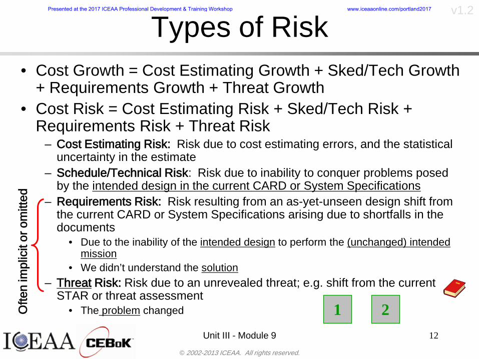
copy 2002-2013 ICEAA All rights reserved
v12
Unit III - Module 9 12
Types of Riskbull Cost Growth = Cost Estimating Growth + SkedTech Growth
+ Requirements Growth + Threat Growthbull Cost Risk = Cost Estimating Risk + SkedTech Risk +
Requirements Risk + Threat Riskndash Cost Estimating Risk Risk due to cost estimating errors and the statistical
uncertainty in the estimate ndash ScheduleTechnical Risk Risk due to inability to conquer problems posed
by the intended design in the current CARD or System Specificationsndash Requirements Risk Risk resulting from an as-yet-unseen design shift from
the current CARD or System Specifications arising due to shortfalls in the documents
bull Due to the inability of the intended design to perform the (unchanged) intended mission
bull We didnrsquot understand the solutionndash Threat Risk Risk due to an unrevealed threat eg shift from the current
STAR or threat assessmentbull The problem changedO
ften
impl
icit
or o
mitt
ed
1 2
Presented at the 2017 ICEAA Professional Development amp Training Workshop wwwiceaaonlinecomportland2017
copy 2002-2013 ICEAA All rights reserved
v12
Point Estimates Vs Risk Estimates
Unit III - Module 9 13
DDTampE Flight Unit Production TotalPoint Estimate 63807 5179 6697 70505CER Risk Only - Mean 71176 4805 6426 78018Full Risk - Mean 78937 6490 8091 87430Point Esimtate + 30 82949 6733 8706 91657Full Risk - 70th Percentile 87939 7980 9608 97011
Estimated Total Cost in Millions
Note that the mean is 24 higher than the point estimate and the 70th
percentile is 38 higher than the point estimate
Presented at the 2017 ICEAA Professional Development amp Training Workshop wwwiceaaonlinecomportland2017
copy 2002-2013 ICEAA All rights reserved
v12
Cost Risk and Probabilitybull Cost risk or cost uncertainty analysis represents cost as a
probability distributionbull A probability distribution is a mathematical rule associating a
probability a to each possible outcome or event of interestbull There are two ways to present a probability distribution ndash as a
probability density function (ldquoPDF) and as a cumulative distribution function (ldquoS-curverdquo or ldquoCDFrdquo)
Unit III - Module 9 14
Lognormal Distribution PDF and CDF
0102030405060708090100
200 300 400 500 600 700 800 900 1000Cost $
Con
fiden
ce L
evel
0
00002
00004
00006
00008
0001
00012
00014
00016
Prob
abili
ty D
ensi
ty
CDFPDF
Presented at the 2017 ICEAA Professional Development amp Training Workshop wwwiceaaonlinecomportland2017
copy 2002-2013 ICEAA All rights reserved
v12
Unit III - Module 9 15
Probability Model ndash Distributionbull Normal
ndash Best behavior most iconic
ndash Theoretically (although not practically) allows negative costs which spook some users
ndash Symmetric needs mean shift to reflect propensity for positive growth
bull Lognormalndash A natural result in
non-linear CERsndash Indistinguishable
from Normal at CVs below 25
ndash Skewed
10
4
10
Presented at the 2017 ICEAA Professional Development amp Training Workshop wwwiceaaonlinecomportland2017
copy 2002-2013 ICEAA All rights reserved
v12
Unit III - Module 9 16
bull Triangularndash Most commonndash Easy to use easy to understandndash Modes medians do not addndash Skewed
bull Betandash Rare now but formerly popularndash Solves negative cost and duration issuesndash Many parameters ndash simplifications like PERT
Beta are possiblendash Skewed
bull Bernoullindash Probability is only assigned to two possible
outcomes success and failure (p and 1-p)ndash Simplest of all discrete distributionsndash Mean = pndash Variance = p(1-p)
10
Probability Model ndash Distribution
10
10
Presented at the 2017 ICEAA Professional Development amp Training Workshop wwwiceaaonlinecomportland2017
copy 2002-2013 ICEAA All rights reserved
v12
Unit III - Module 9 17
bull Normalndash If there is a sufficiently large number of independently identically distributed
elements (or not too correlated and not too skewed) then the distribution of total cost is normal due to the Central Limit Theorem
bull Lognormalndash For smaller data sets with large amounts of (positive) correlation and
skewness the lognormal distribution may be a better approximation of total cost
ndash Many total cost distributions in smaller data sets test as both normal and lognormal
bull Triangularndash The sum of triangles is not a triangle so this distribution should generally not
be used to characterize total costbull Convolved
ndash If total cost distribution is derived using simulation then it may not particularly resemble anything In this case we simply have a convolved or simulated total cost distribution
Probability ndash Top-Level Distribution
NEW
Presented at the 2017 ICEAA Professional Development amp Training Workshop wwwiceaaonlinecomportland2017
copy 2002-2013 ICEAA All rights reserved
v12
S-Curves and Confidence Levels
Unit III - Module 9 1818
100
70
25
Probability(Confidence
Level)
Cost Estimate(Dollars)
50
The S curve is the cumulative probability distribution coming out of the statistical summing process
70 confidence that project will cost indicated amount or less
Provides information on potential cost as a result of identified project risks
Provides insight into establishing reserve levels
X Y
MR
X = Point estimateZ = Project requirementY = Cost estimate where there is a 70 change that
final actual cost will be less than cost estimateY-Z= Manage reserve (MR) which is REQUIRED to meet 70 CL
Z
X not always = Z but is based on same content
Presented at the 2017 ICEAA Professional Development amp Training Workshop wwwiceaaonlinecomportland2017
copy 2002-2013 ICEAA All rights reserved
v12
19
Example ndash Normal Distribution
bull Normal distribution with mean equal to 100 and standard deviation equal to 20
bull Median and mode also equal 100bull The 80th Percentile is 117
40 60 80 100 120 140 160
80 of distribution(area under curve)is less than 117
117
Presented at the 2017 ICEAA Professional Development amp Training Workshop wwwiceaaonlinecomportland2017
copy 2002-2013 ICEAA All rights reserved
v12
20
Confidence Levelsbull The output of a cost risk analysis is a probability
distributionndash Typically displayed as a cumulative distribution function or
ldquoS-curverdquondash Confidence levels are simply percentiles of the distribution
0
10
20
30
40
50
60
70
80
90
100
30 60 90 120 150 180
Conf
iden
ce L
evel
Presented at the 2017 ICEAA Professional Development amp Training Workshop wwwiceaaonlinecomportland2017
copy 2002-2013 ICEAA All rights reserved
v12
Measuring Parametric Model Uncertainty
bull When developing estimates using cost-estimating relationships (CERs) there are two major sources of uncertaintyndash Technical (model input) uncertaintyndash Estimating uncertainty
bull Technical uncertainty reflects the uncertainty inherent in the model inputsndash Typical parametric model inputs include weight lines of code
heritage and other performance and management inputs
bull Estimating uncertainty measures the uncertainty inherent in the model due to the modelrsquos inability to capture all aspects of variability in the data
21
Presented at the 2017 ICEAA Professional Development amp Training Workshop wwwiceaaonlinecomportland2017
copy 2002-2013 ICEAA All rights reserved
v12
Parametric Model Examplebull The NASAAir Force Cost Model (NAFCOM) is a
parametric model for estimating acquisition costs for spacecraft and launch vehicles
bull The CERs in NAFCOM have the formCost = C WeightVNewDesignWTechnicalXManagementY ClassZ
bull There is technical uncertainty about each of the parametersndash Parametric models are applied early in a program so there
is significant amount of uncertainty in the weightndash Heritage is also tricky it is inherently subjective and project
personnel are typically optimisticndash Technical characteristics can also change as a program
matures and requirements change
22
Presented at the 2017 ICEAA Professional Development amp Training Workshop wwwiceaaonlinecomportland2017
copy 2002-2013 ICEAA All rights reserved
v12
Weight Uncertaintybull Aerospace weight growth study average satellite
weight growth from program inception to launch is 28
23
Aerospace Weight Growth Data
-10
0
10
20
30
40
50
60
0 4 8 12 16 20 24 28 32 36 40 44 48 52 56 60 64 68 72 76 80 84 88 92 96 100
Percent Program Completion
Perc
ent W
eigh
t Gro
wth
Presented at the 2017 ICEAA Professional Development amp Training Workshop wwwiceaaonlinecomportland2017
copy 2002-2013 ICEAA All rights reserved
v12
Estimating Uncertaintybull CERs do not perfectly fit the historical data
ndash There are non-repeatable random effects that cannot be predicted
bull For examplendash Parts breaking during testingndash Strikes which are difficult to predict
bull This results in an underlying uncertainty distribution about an estimatendash The outcome of a CER represents only one point on an
uncertainty distributionbull Typically mean or median depending upon the CER
methodology
24
Presented at the 2017 ICEAA Professional Development amp Training Workshop wwwiceaaonlinecomportland2017
copy 2002-2013 ICEAA All rights reserved
v12
Estimating Uncertainty (2)
25
Presented at the 2017 ICEAA Professional Development amp Training Workshop wwwiceaaonlinecomportland2017
copy 2002-2013 ICEAA All rights reserved
v12
Estimating Uncertainty (3)bull In the case of a linear regression the estimating
uncertainty follows a normal distributionndash The estimate is the mean and the standard error of the
estimate from the regression is the standard deviation of the normal distribution
bull In the case of a log-transformed linear regression the estimating uncertainty follows a lognormal distributionndash The estimate is the median of the lognormal and the
standard error of the estimate from the regression is the standard deviation of the normal distribution (in log-space)
bull There is additional uncertainty about an estimate based upon the distance of what is being estimated from the mean of the input datandash This results in a prediction interval
26
Presented at the 2017 ICEAA Professional Development amp Training Workshop wwwiceaaonlinecomportland2017
copy 2002-2013 ICEAA All rights reserved
v12
Aggregating Riskbull Risk is typically applied at the same level at
which we estimate cost that is at the Work Breakdown Structure (WBS) level
bull The estimates for each WBS are developedndash These estimates sum to yield the total system cost
bull For an n-element WBS the total cost is the sum of the cost for each of the n elements
27
nXXXCostSystem +++= 21
Presented at the 2017 ICEAA Professional Development amp Training Workshop wwwiceaaonlinecomportland2017
copy 2002-2013 ICEAA All rights reserved
v12
WBS Examplebull Launch Vehicle
ndash Structurebull Vehicle Structurebull Tank Structure
ndash Thermal Controlbull Active Thermal Controlbull Induced Thermal Controlbull Tank Thermal Control
ndash Main Propulsion Systemndash Liquid Rocket Enginendash Electric Power and Distributionndash Command Control and Data Handlingndash System Integration
28
Presented at the 2017 ICEAA Professional Development amp Training Workshop wwwiceaaonlinecomportland2017
copy 2002-2013 ICEAA All rights reserved
v12
WBS and Risk
29
Presented at the 2017 ICEAA Professional Development amp Training Workshop wwwiceaaonlinecomportland2017
copy 2002-2013 ICEAA All rights reserved
v12
Aggregating Riskbull This leads us to the issue of aggregating the risks across the
WBSbull For example if we want to determine the 70th percentile of the
overall cost risk distribution how do we proceed bull Note that we cannot simply add the 70th percentiles of each of
the cost risk distributionsbull We can add means and variances (taking correlation into
account more on that later) but that is all
Variance of Total Cost =
30
Mean of Total Cost = ( )E X E Xk
k
n
kk
n
kk
n
= = =aringaelig
egraveccediloumloslashdivide
= =aring aring1 1 1
m
Var X kk
n
=aringaelig
egraveccediloumloslashdivide1
= s r s skk
n
iji
j
i jj
n2
1 1
1
22+aring aringaring
= =
-
=
Presented at the 2017 ICEAA Professional Development amp Training Workshop wwwiceaaonlinecomportland2017
copy 2002-2013 ICEAA All rights reserved
v12
Percentiles Do Not Addbull As a notional example consider two independent normal
distributionsndash One distribution has mean equal to 100 and standard deviation
equal to 20ndash The second distribution has mean 300 and standard deviation of 80
bull The sum of two independent normally distributed random variables is also normally distributed
bull To combine the two distributions we add the means and add the variancesndash Total mean is
ndash Total standard deviation is
31
400300100 =+
8258020 22 raquo+
Presented at the 2017 ICEAA Professional Development amp Training Workshop wwwiceaaonlinecomportland2017
copy 2002-2013 ICEAA All rights reserved
v12
Percentiles Do Not Add (2)bull The 80th percentiles for the individual distributions are
117 and 367 respbull The 80th percentile of the combined distribution is
469 but the sum of the two 80th percentiles is 484bull To see why this is the case note that the percentiles
of a normal distribution are determined by the mean and the standard deviationndash The standard deviations are not added when normal distributions
are combined rather the variances are combinedndash Sum of variances is ndash The standard deviation of this sum is
32
22 ba +22 ba +
Presented at the 2017 ICEAA Professional Development amp Training Workshop wwwiceaaonlinecomportland2017
copy 2002-2013 ICEAA All rights reserved
v12
Percentiles Do Not Add (3)bull Since bull We can write
bull The left side of this inequality represents the risk of the combined distributions while the right side represents the sums of the individual risks
bull Combining two missions that are independent results in a diversification of riskndash The total portfolio is not as risky on a relative basis as each
individual project
33
2222 2 bababa ++lt+
baba +lt+ 22
Presented at the 2017 ICEAA Professional Development amp Training Workshop wwwiceaaonlinecomportland2017
copy 2002-2013 ICEAA All rights reserved
v12
Methods for Aggregating Riskbull Since percentiles do not add we have to find other
ways to aggregate riskbull One method is to use Monte Carlo simulationbull Unless cost risk is represented by normal
distributions for all WBS elements summing the means and variances does not result in a completely accurate depiction of overall system cost risk
bull The normal distribution is not a realistic distribution for representing risk in many or even most situations since regarding project risk more can go wrong than can go right which means the risk is NOT symmetric unlike the Gaussian bell curve
34
Presented at the 2017 ICEAA Professional Development amp Training Workshop wwwiceaaonlinecomportland2017
copy 2002-2013 ICEAA All rights reserved
v12
Unit III - Module 9 35
Monte Carlo Simulationfor Risk Analysis
bull When risk analysis is performed multiple risks are gatheredndash These risks may have various probability
distributions
bull Monte Carlo is the most commonly accepted way to produce an accurate characterization of the distribution of the combined effect of these many risksndash Using this distribution we can produce percentiles
for cost impacts due to risk occurrences
10
Presented at the 2017 ICEAA Professional Development amp Training Workshop wwwiceaaonlinecomportland2017
copy 2002-2013 ICEAA All rights reserved
v12
Monte Carlo Simulationbull Simulation is a means for solving problems that are
analytically intractablendash Involves repeated random sampling
bull It was developed during the Manhattan Project as a way to model the interactions inside an atom during nuclear fissionndash Allowed for more sophisticated mathematical modeling of atomic
phenomena
bull Most computer packages use pseudo-random number generators that produce seemingly random results from an initial seedndash Example is the linear congruential generator
36
( ) mbaXX nn mod1 +=+
Presented at the 2017 ICEAA Professional Development amp Training Workshop wwwiceaaonlinecomportland2017
copy 2002-2013 ICEAA All rights reserved
v12Using Random Numbers to Simulate Distributions
bull WBS cost risk is typically measured by a probability distributionbull The most common method for simulating a probability
distribution is the inverse methodbull This involve obtaining a simulated random value from a uniform
distribution and then inverting this through the cumulative distribution function (CDF) to obtain the simulated value
bull As an example for a uniform distribution on the interval [0100]
bull In this case the CDF random value of 05 translates to 10005 = 50
37
( )100
1=xf ( )
100xxF = ( ) xxF 1001 =-
Presented at the 2017 ICEAA Professional Development amp Training Workshop wwwiceaaonlinecomportland2017
copy 2002-2013 ICEAA All rights reserved
v12
Simulating a Triangular Distribution
bull For a triangular distribution with low = 0 most likely = 50 and high = 150 the CDF is given by
bull The inverse function is given by
38
( )iumliumlicirc
iumliumliacute
igrave
poundlt--
poundpound=
1505021
1500050
50015000
2
2
2
xxx
xxxF
( )iumliumlicirc
iumliumliacute
igrave
poundltdivideoslashouml
ccedilegraveaelig +--
poundpound=-
131
21
37501
250017500150
3107500
1
xx
xxxF
Presented at the 2017 ICEAA Professional Development amp Training Workshop wwwiceaaonlinecomportland2017
copy 2002-2013 ICEAA All rights reserved
v12
Simulating a Triangular Distribution (2)
bull If the simulated uniform value is equal to 02 the corresponding inverse value from the CDF inverse is approximately 387
39
0
01
02
03
04
05
06
07
08
09
1
0 30 60 90 120 150
Presented at the 2017 ICEAA Professional Development amp Training Workshop wwwiceaaonlinecomportland2017
copy 2002-2013 ICEAA All rights reserved
v12
Monte Carlo and the WBSbull Simulation involves repeated trials
40
WBS Draw1 2 3 4 5
System 2912 3566 4390 2954 4655 Sum
Structure 80 105 55 80 57 SumVehicle Structure 50 70 30 40 20Tank Structure 30 35 25 40 37
Thermal Control 32 36 35 29 33 SumActive Thermal Control 10 15 12 7 10Induced Thermal Control 12 14 13 14 14Tank Thermal Control 10 7 10 8 9
Main Propulsion System 100 150 125 140 100
Liquid Rocket Engine 1000 1100 1800 900 2200
Electric Power and Distribution 100 125 150 75 90
Command Control and Data Handling 200 250 225 230 275
System Integration 1400 1800 2000 1500 1900
Presented at the 2017 ICEAA Professional Development amp Training Workshop wwwiceaaonlinecomportland2017
copy 2002-2013 ICEAA All rights reserved
v12
Number of Trialsbull Monte Carlo involves a repeated number of trialsbull The greater the number of trials the more accurate the
simulation will approximate the overall cost risk behavior of the system
bull After 100 trials the histogram looks very jagged
41
Presented at the 2017 ICEAA Professional Development amp Training Workshop wwwiceaaonlinecomportland2017
copy 2002-2013 ICEAA All rights reserved
v12
Number of Trials (2)
42
1000 Trials
10000 Trials
50000 Trials Additional trials give a more accurate depiction of the final result
Presented at the 2017 ICEAA Professional Development amp Training Workshop wwwiceaaonlinecomportland2017
copy 2002-2013 ICEAA All rights reserved
v12
Number of Trials (3)bull If we want to simulate the underlying
mean within 1 with 95 confidence for example then we require
43
divideoslash
oumlccedilegrave
aelig poundpound-
=
dividedividedivide
oslash
ouml
ccedilccedilccedil
egrave
aeligpound
-pound
-=
divideoslashouml
ccedilegraveaelig poundpound=
nZ
n
nnX
n
X
n
n
011
010Pr
011
010Pr
011990Pr950
___
___
sm
sm
sm
sm
sm
mm
Presented at the 2017 ICEAA Professional Development amp Training Workshop wwwiceaaonlinecomportland2017
copy 2002-2013 ICEAA All rights reserved
v12
Number of Trials (4)bull This means that the number of trials required is determined by
bull Solving for n we find that at least
trials are neededbull Note that this term involves the coefficient of variation of the
distribution which means that distributions with less dispersion require fewer trials to accurate simulate
44
96101
=ns
m
ms41638
Presented at the 2017 ICEAA Professional Development amp Training Workshop wwwiceaaonlinecomportland2017
copy 2002-2013 ICEAA All rights reserved
v12
Number of Trials (5)bull Simulating percentiles requires more trials than for simulating
meansbull Let Pn represent the number of trials in the sample at or below
the 70th percentile of the underlying distribution (suppose this is known)
bull By the Central Limit Theorem Pnn follows a normal distribution with mean equal to the 70th percentile and variance equal to
bull By a similar process for the mean we find that the number of trials needed to simulate the 70th percentile within 1 with 95 confidence is
45
( )n
FF 700700 1-
n
n
PPn -41638
Presented at the 2017 ICEAA Professional Development amp Training Workshop wwwiceaaonlinecomportland2017
copy 2002-2013 ICEAA All rights reserved
v12
Number of Trials (6)bull If Pn 070 for all n then n is approximately
bull For the sake of comparison suppose CV = 03 (reasonable approximation for hardware development) then the number of trials needed to simulate the mean with the same accuracy is then ldquoonlyrdquo 11525
bull More trials are needed to accurately simulate percentiles than means
46
( ) 46416703041638
70704168341638 =divide
oslashouml
ccedilegraveaelig=divide
oslashouml
ccedilegraveaelig -
=-
nnn
PPn
n
n
Presented at the 2017 ICEAA Professional Development amp Training Workshop wwwiceaaonlinecomportland2017
copy 2002-2013 ICEAA All rights reserved
v12
Methods of Simulationbull Monte Carlo simulation is a standard term for
simulationbull However there is an improvement on Monte Carlo
that improves the accuracy of the results of a simulation for a given number of trials
bull This method is call the Latin Hypercube approach to simulationndash Similar to Monte Carlo but an equal number of draws are taken
from a set of subintervals for example dividing the interval (01) into [00001) [0102)hellip [0910]
ndash Instead of 10 trials from [01] we have one trial from each subinterval
ndash Rough rule of thumb is Latin Hypercube takes 30 fewer trials to achieve similar accuracy to Monte Carlo
47
Presented at the 2017 ICEAA Professional Development amp Training Workshop wwwiceaaonlinecomportland2017
copy 2002-2013 ICEAA All rights reserved
v12
Probability Model ndash Correlationbull Correlation exists between work breakdown structure
(WBS) cost element costs and between cost and schedule
bull Correlation is a necessary consideration in cost risk analysis
bull Correlation is a number that can vary between -1 and +1 and represents the strength of the relationship between the two variablesndash If both variable have a tendency to move in the same direction
correlation is positivendash If when one variable increases the other tends to decrease and
vice-versa the correlation between the two variables is negative
Presented at the 2017 ICEAA Professional Development amp Training Workshop wwwiceaaonlinecomportland2017
copy 2002-2013 ICEAA All rights reserved
v12
Correlation And Causationbull Note that correlation is not causation however
causation implies correlationndash For example shark attacks and ice cream sales at the beach
bull For example for a launch vehicle structure increasing the diameter will not only result in an increase in the structures cost but will also result in higher costs for thermal coating (paint etc)
bull Also simply because two subsystems do not appear to be related does not mean they are not correlatedndash For example structures and computer equipment seemingly
have little relation to one another however an external factor such as a funding cut or a strike will impact all subsystems leading to delays and increasing cost across the board
ndash Thus everything in a WBS has some correlationUnit III - Module 9 49
Presented at the 2017 ICEAA Professional Development amp Training Workshop wwwiceaaonlinecomportland2017
copy 2002-2013 ICEAA All rights reserved
v12
The Importance of Correlationbull Percent that total cost standard deviation is underestimated
when correlation assumed to be 0 instead of r given nWBS elements
Unit III - Module 9 5050
0
20
40
60
80
100
0 01 02 03 04 05 06 07 08 09 1Actual Correlation
Perce
nt Un
deres
timate
d
n = 10
n = 30
n = 100n = 1000
0
20
40
60
80
100
0 01 02 03 04 05 06 07 08 09 1Actual Correlation
Perce
nt Un
deres
timate
d
n = 10
n = 30
n = 100n = 1000
Reference 32nd Annual DOD Cost Analysis Symposium Advanced Training Session ldquoWhy Correlation Matters in Cost Estimatingrdquo Stephen A Book
Presented at the 2017 ICEAA Professional Development amp Training Workshop wwwiceaaonlinecomportland2017
copy 2002-2013 ICEAA All rights reserved
v12
The Importance of Correlation (2)bull For example if correlation is assumed to be 0 for all
elements in a 30 element WBS and the actual correlation is 20 then the total cost standard deviation is underestimated by 60
bull For example assume the total cost is modeled as a normal distribution with mean = 100
bull If correlation is assumed to be zero with total cost standard deviation = 12 when correlation is actually 20 then the true underlying standard deviation is actually 30
bull 70th percentile with zero correlation assumption is 106
bull 70th percentile with 20 correlation is 116 Unit III - Module 9 51
Presented at the 2017 ICEAA Professional Development amp Training Workshop wwwiceaaonlinecomportland2017
copy 2002-2013 ICEAA All rights reserved
v12
Measures of Correlationbull Two measures of correlation are commonly used in
cost risk analysesndash Pearsonrsquos product-moment correlation coefficient ndash Spearmanrsquos rank correlation coefficient
bull Garvey and others recommend using Pearsonrsquos product-moment correlation coefficient correlation for cost risk analysesndash Method of moments uses this but there are two options in
simulationndash Popular simulation packages like Risk and Crystal Ball use
rank correlation but in practice this has been found to make little difference
ndash Pearson product-moment correlation has been incorporated into Risk+
52
Presented at the 2017 ICEAA Professional Development amp Training Workshop wwwiceaaonlinecomportland2017
copy 2002-2013 ICEAA All rights reserved
v12
Pearson Correlationbull Pearsonrsquos product-moment correlation measures
degree of linearity between two random variables bull If two random variables are perfectly linear (eg Y =
aX + b) with positive slope then the Pearson product-moment correlation between X and Y denoted by rXY is +1
53
X X
Y Y Y
XNegative Correlation Positive Correlation No Correlation
middotmiddot
middotmiddot
middotmiddot middotmiddot
middotmiddot
middot
middot
middotmiddotmiddot
middotmiddot
middotmiddot
middotmiddot middot
middot
middot
middotmiddotmiddotmiddotmiddotmiddotmiddotmiddot
middotmiddotmiddotmiddot
middotmiddot
middotmiddot middotmiddotmiddotmiddot
middotmiddotmiddot
middotmiddotmiddotmiddot
middotmiddotmiddot
middotmiddotmiddot
middotmiddot
middot
middot middotmiddot
middot middotmiddotmiddotmiddot middotmiddot middot middotmiddot middot middot
middotmiddot middot
middotmiddotmiddotmiddotmiddot middot middotmiddot
middotmiddot
middot
middotmiddot
middotmiddot middot
middot middot middot
middotmiddot middot
middotmiddotmiddot
middotmiddot
middot middot
Presented at the 2017 ICEAA Professional Development amp Training Workshop wwwiceaaonlinecomportland2017
copy 2002-2013 ICEAA All rights reserved
v12
Spearman Correlationbull Spearmanrsquos rank correlation measures the
monotonicity between two random variablesbull If two random variables are perfectly monotonically
increasing (eg Y = X2) then the Spearman rank correlation denoted by rXY is +1
bull The two measures can be significantly different
54
10 20 30 40 50 60
100
200
300
096 097 098 099 1
1
060
020
040
080
Eff
ort (
Staf
f-M
onth
s)
Software Size I KDSI
y = 28z12y
z x
yy = x100
0 pound x pound 1
Figure 5-9A Figure 5-9B
Pearson Correlation = 09976 Rank Correlation = 1
Pearson Correlation = 024 Rank Correlation = 1
X(x ) ~ Unif(01)
Reference Probability Methods for Cost Uncertainty Analysis A Systems Engineering Perspective Paul R Garvey
Presented at the 2017 ICEAA Professional Development amp Training Workshop wwwiceaaonlinecomportland2017
copy 2002-2013 ICEAA All rights reserved
v12
Unit III - Module 9 55
200
250
300
350
400
1000 1200 1400 1600 1800 2000
Recurring Production
SEPM
200
250
300
350
400
1000 1200 1400 1600 1800 2000
Recurring Production
SEPM
Functional Correlationbull Old No Functional
Correlation Simulation run with WBS items entered as values
bull New Simulation run with functional dependencies entered as they are in cost model
CorrelatedNot Correlated
Note shift of mean and increased variability
Presented at the 2017 ICEAA Professional Development amp Training Workshop wwwiceaaonlinecomportland2017
copy 2002-2013 ICEAA All rights reserved
v12
Risk Measuresbull ldquoWestern Europe conquered the word because of a
technological revolution that started because of attempts to measure the worldrdquo ndash Phillipe Jorion ndash In the same way attempts to measure risk will lead to better project
managementbull Risk management for DoD and NASA agencies focuses
primarily on funding projects to a single percentile ndash NASA policy explicitly mentions 70 and 50ndash This is known as ldquoValue at Riskrdquo and is prevalent in the banking and
financial industry
56
Presented at the 2017 ICEAA Professional Development amp Training Workshop wwwiceaaonlinecomportland2017
copy 2002-2013 ICEAA All rights reserved
v12
Value at Risk (VaR)bull VaR is a percentile of the cost risk
distributionndash VaR funding at the 70th percentile means that
there is a 30 chance of final project cost exceeding the funded amount (budget)
bull VaR has some meritsndash Common measure can be used to compare
different projects and programsndash Easily understood by senior managers and
decision makers
57
Presented at the 2017 ICEAA Professional Development amp Training Workshop wwwiceaaonlinecomportland2017
copy 2002-2013 ICEAA All rights reserved
v12
Why 70th or 80th Percentilebull Typical policy guidance involves funding at the 70th or 80th
percentile Why fund as such a low percentilebull There is some incentive to not over-fundbull For a normal distribution an inflection point occurs near the 80th
percentile meaning that for values above 80 confidence achieving higher levels of confidence can only be achieved by spending greater dollar amounts at an increasing rate
58
-05-04-03-02-01
00102030405
0 05 1 15 2 25 3
Standard Deviations from Mean
Normal Distribution
First DerivativeSlopeVelocity
Second DerivativeConvexityAcceleration
Inflection point at one standard deviation above the mean (~84th
percentile)
Presented at the 2017 ICEAA Professional Development amp Training Workshop wwwiceaaonlinecomportland2017
copy 2002-2013 ICEAA All rights reserved
v12
Funding Above Inflection Pointsbull As the percentile goes above the 80th percentile the amount
needed to achieve that higher level of confidence begins to increase at an increasing rate as is evident from the graph
59
0
10
20
30
40
50
60
70
50 55 60 65 70 75 80 85 90 95 100
$ Ab
ove
MEa
n to
Ach
ieve
Per
cent
ile
Percentile (Confidence Level)
Presented at the 2017 ICEAA Professional Development amp Training Workshop wwwiceaaonlinecomportland2017
copy 2002-2013 ICEAA All rights reserved
v12
Why Budget to the 70th or 80thbull Government projects are funded at the 70th or 80th percentilesbull Why not the 90th or 99th percentile Wonrsquot that help prevent
overrunsndash As we have seen percentiles do not add across programs
bull The sum of the 80th percentiles does NOT equal the total 80th percentile
ndash This is because the individual programs are riskier than the entire suite of missions
bull Known as the ldquoPortfolio effectrdquo (more or this later)
ndash Funding at the 80th gives confidence that the entire portfolio will be adequately funded
bull And since there is an inflection point near the 80th percentile funding above that level quickly becomes cost prohibitive
60
Presented at the 2017 ICEAA Professional Development amp Training Workshop wwwiceaaonlinecomportland2017
copy 2002-2013 ICEAA All rights reserved
v12
Inflection Points for Lognormalbull For a lognormal the inflection point
variesndash Coefficient of variation equal to 10 equates to an
inflection point at the 70th percentile
61
0
10
20
30
40
50
60
70
050 060 070 080 090 100
Coef
ficen
t of V
aria
tion
Percentile of the Inflection Point
Presented at the 2017 ICEAA Professional Development amp Training Workshop wwwiceaaonlinecomportland2017
copy 2002-2013 ICEAA All rights reserved
v12
Issues with Percentile Fundingbull However risk management does not stop at a
specific percentilendash What happens when the 70th percentile is exceeded
bull Any effective risk management policy should prescribe what happens after a bad event occursndash With VaR we only know when a bad event has occurred ndash Also funding at a relatively low level means we have no true
sense of the real risks that should be guarded against
62
Presented at the 2017 ICEAA Professional Development amp Training Workshop wwwiceaaonlinecomportland2017
copy 2002-2013 ICEAA All rights reserved
v12
ldquoHere There Be Dragonsrdquobull On old maps uncharted territory was often
marked with monsters or dragons
63
A section of the Carta Marina by Olaus Magnus 16th Century
Presented at the 2017 ICEAA Professional Development amp Training Workshop wwwiceaaonlinecomportland2017
copy 2002-2013 ICEAA All rights reserved
v12
Distribution Comparisonbull Four different distributions with the same 70th
percentile
bull Should we expect the tails to be similar
64
0
10
20
30
40
50
60
70
80
0 100 200 300 400 500 600
Perc
entil
eCo
nfid
ence
Lev
el
Triangular
Normal
Lognormal
Pareto
Presented at the 2017 ICEAA Professional Development amp Training Workshop wwwiceaaonlinecomportland2017
copy 2002-2013 ICEAA All rights reserved
v12Distribution Comparison Tail Behavior
bull The normal and triangular distributions have similar tails but the lognormal and Pareto have much fatter right tails
65
70
75
80
85
90
95
100
500 1500 2500 3500 4500 5500
Perc
entil
eCo
nfid
ence
Lev
el
Triangular
Normal
Lognormal
Pareto
Here There Be Dragons
Presented at the 2017 ICEAA Professional Development amp Training Workshop wwwiceaaonlinecomportland2017
copy 2002-2013 ICEAA All rights reserved
v12Distribution Comparison ndash Tail Behavior (Table)
bull There is significant tail risk for the lognormal and the Paretobull The 99th percentile for the Pareto is 1000 times greater than
the 70th percentilendash Risk seen in financial markets and in catastrophic risks like natural
disasters bull Four different projects follow the four different risk profiles seen
in this example should clearly have different risk management approaches but 70th percentile funding indicates the same risk management approach for all four
66
Percentile Triangular Normal Lognormal Pareto 70th $600 $600 $600 $600 80th $680 $660 $770 $1430 90th $770 $750 $1070 $5880 95th $840 $820 $1410 $23750 99th $930 $950 $2350 $600000
Presented at the 2017 ICEAA Professional Development amp Training Workshop wwwiceaaonlinecomportland2017
copy 2002-2013 ICEAA All rights reserved
v12Percentile Budgeting is Not Risk Management
bull Percentile budgeting ne effective risk management policybull Suppose that you are shopping for a new car You
mention that safety is your top concern The salesman says he has a great safe car available You ask about the air bags Do they work The salesman answers ldquoOf course Seventy percent of the time they work fine Only 30 of the time the air bags will fail to deployrdquo Would you buy such a car Hedge fund manager David Einhorn has stated ldquoRisk management is the air bag that must always work but only in the multi-sigma event where you have an accidentrdquo
67
Risk management is the air bag that must always work but only in the multi-sigma event where you
have an accident
Presented at the 2017 ICEAA Professional Development amp Training Workshop wwwiceaaonlinecomportland2017
copy 2002-2013 ICEAA All rights reserved
v12
Joint Confidence Level Analysisbull Schedules are risky toobull For 98 recent NASA missions average
schedule growth was 38ndash Not as high as cost growth but still significant
68
0
5
10
15
20
25
30
35
40
Schedule
Cost
Presented at the 2017 ICEAA Professional Development amp Training Workshop wwwiceaaonlinecomportland2017
copy 2002-2013 ICEAA All rights reserved
v12
Schedules Impact Costbull Changes in schedule can have enormous
impacts on cost ndash Schedule slips can lead to cost increases
bull Fixed programmatic costs must be paid on a regular basisndash Achieving schedule milestones early can result in cost
savings
bull Schedule is an important consideration in cost analysis including cost risk analysis
bull However we must be careful in correctly integrating cost and schedule riskndash Schedule is not simply an input but is dependent on many of
the same factors that drive cost
69
Presented at the 2017 ICEAA Professional Development amp Training Workshop wwwiceaaonlinecomportland2017
copy 2002-2013 ICEAA All rights reserved
v12
The Relationship of Cost to Schedulebull Cost and schedule are positively correlated
ndash A larger program with bigger scope with take longer to complete than a smaller simpler program
bull However longer schedules do not always equate to higher cost nor shorter schedules with lower costndash Highly compressed schedules relative to the
optimal schedule can lead to large overrunsbull Compressed schedules are commonplace for
many planetary missions
70
Presented at the 2017 ICEAA Professional Development amp Training Workshop wwwiceaaonlinecomportland2017
copy 2002-2013 ICEAA All rights reserved
v12The Impact of Schedule GrowthCompression on Cost
bull Compressed schedules lead to cost growth and based on existing research is actually more expensive than schedule slippages
71
0
20
40
60
80
100
120
140
160
-50 -25 0 25 50 75 100
Percentage Change in Schedule
Perc
enta
ge C
hang
e in
Cos
t due
to
Sche
dule
Cha
nge
Source Smart CB ldquoCost and Schedule Interrelationshipsrdquo 2007 NASA Cost Symposium
Presented at the 2017 ICEAA Professional Development amp Training Workshop wwwiceaaonlinecomportland2017
copy 2002-2013 ICEAA All rights reserved
v12Schedule as an Independent Variable
bull Why not simply add schedule as an input to cost-estimating relationships (CERs)
bull Schedule is often treated as an independent variable ndash schedules are often determined independently of cost considerationsndash Cost may not be considered explicitly although budgets and
schedules are determined based on scope and other common factors
bull In 2006 SAIC undertook a research task to determine the impact of schedule on cost and added schedule as an independent variable to the CERs in the NASAAir Force Cost Model (NAFCOM) to see if schedule provided any improvement in goodness of fit
72
Presented at the 2017 ICEAA Professional Development amp Training Workshop wwwiceaaonlinecomportland2017
copy 2002-2013 ICEAA All rights reserved
v12
Schedule is a Dependent Variablebull Since NAFCOM includes an exhaustive list of cost drivers the inclusion
of schedule should give an indication of whether there is any additional independent value added from schedule independent of the cost drivers
bull In the study schedule was added to 10 subsystem-level CERs
ndash In each case the addition of schedule did NOTimprove the goodness of fit and schedule was NOT found to be a statistically significant cost driver (given the presence of the other variables) for any of the 10 CERs
bull Standard errors for the CERs increased due to decrease in degrees of freedom
bull Thus schedule as an independent variable did not provide any additional explanation of variation in historical cost
bull This is because schedule is truly NOT an independent variable but a dependent variable and is a function of the same factors that drive cost
73
Presented at the 2017 ICEAA Professional Development amp Training Workshop wwwiceaaonlinecomportland2017
copy 2002-2013 ICEAA All rights reserved
v12
Incorporation of Schedule in Cost Risk
bull When using subjective methods care must be taken in applying schedule to cost risk analysis
bull Since schedule is a dependent variable treating it independently from other factors when assessing its impact on cost can lead to a double count of independent variables in the cost risk analysis
bull Direct inclusion of schedule in a cost risk analysis effectively doubles the influence of each cost driver
ndash Incorrectly leads to broader risk ranges
74
CostWeight
HeritageNewness
Technology Readiness Schedule
Presented at the 2017 ICEAA Professional Development amp Training Workshop wwwiceaaonlinecomportland2017
copy 2002-2013 ICEAA All rights reserved
v12Subjective Cost Risk Methods and Overinclusion of Risk Factors
bull Subjective methods are suitable when data are scarce or not availablebull However care must be taken not to treat correlated sources of risk
such as schedule as independent of each otherbull Example ndash a subjective risk analysis incorporated technology readiness
design risk requirements stability integration risk and schedule and treated each source of risk as independent
bull Risk triangle high value without schedule risk was 31 times the point estimate
bull Risk triangle high value with schedule risk added on top of other sources of risk treated independently was 34 times the point estimate
bull Risk triangle taking correlation between sources of risk into account in a rigorous statistical manner has a high value 15 times the point estimate less than half the effect when treating sources of risk as independent
75
Presented at the 2017 ICEAA Professional Development amp Training Workshop wwwiceaaonlinecomportland2017
copy 2002-2013 ICEAA All rights reserved
v12Fundamental Equation of Cost and Schedule Interrelationships
bull The Fundamental Equation of the Relationship Between Cost and Schedule is
Time = Moneybull This is a well known adage that time is money Your boss at
work may even mention this to you from time to time or if you are the boss you are all too aware of this iron law
bull Because time is money cost and schedule risk should be modeled jointly not with schedule as an independent cost driver
bull Note that cost and schedule are not perfectly correlatedndash Cost can sometimes ldquobuy downrdquo schedule extra money can be
spent to meet a deadline since in some cases additional effort to hasten the completion of a task
76
Presented at the 2017 ICEAA Professional Development amp Training Workshop wwwiceaaonlinecomportland2017
copy 2002-2013 ICEAA All rights reserved
v12How to (Correctly) Incorporate Schedule into Cost Risk Analysis
bull The best way to model cost and schedule risk is to develop a joint cost and schedule model based on the same data
bull Since such models are not currently available the next best approach is to model cost and schedule independently and then integrate cost and schedule risk analyses using joint probability distributions taking into account correlation between cost and schedulendash This approach pioneered by Paul Garvey and Steve Book is
considered industry best practicendash This is a practical method mathematically tractable and follows
naturally from the Fundamental Equation of Cost and Schedule Interrelationships
77
Book S A ldquoQuantifying the Relationship Between Cost and Schedulerdquo The Measurable News Winter 2007-2008 pp 11-15Garvey PR Probability Methods for Cost Uncertainty Analysis A Systems Engineering Perspective New York Marcel Dekker 2000 pp 308-335
Presented at the 2017 ICEAA Professional Development amp Training Workshop wwwiceaaonlinecomportland2017
copy 2002-2013 ICEAA All rights reserved
v12
Joint Lognormal and Normal Distributions
bull Cost and schedule are typically modeled as some combination of Normal and Lognormal probability distributionsndash Studies by The Aerospace Corporation the MITRE
Corporation Wyle Labs and SAIC have found that the Lognormal probability distribution almost always serves as a good model for both the schedule distribution and the cost distribution
ndash The Normal distribution may also be appropriate in some instances and depending upon the level of confidence at which budgets are set may even be more conservative and logically consistent than the Normal distribution
ndash Joint Lognormal and Normal distributions are defined by a pair of mean and standard deviations and a level of correlation between the two
78
Presented at the 2017 ICEAA Professional Development amp Training Workshop wwwiceaaonlinecomportland2017
copy 2002-2013 ICEAA All rights reserved
v12Modeling Cost and Schedule as a Bivariate Distribution
bull In the approach set forth by Book and Garvey cost risk is assessed and the top-level distribution is modeled as a Lognormal (or Normal) distribution schedule risk is assessed and the overall schedule risk is modeled as a Lognormal (or Normal) distribution
bull The two distributions are combined into a Bivariate distribution by assigning a correlation between the two and by treating the two distributions as the marginal distributions of a Bivariate Lognormal distributionndash Other combinations include a Bivariate Normal or a Bivariate
Normal-Lognormal
79
Presented at the 2017 ICEAA Professional Development amp Training Workshop wwwiceaaonlinecomportland2017
copy 2002-2013 ICEAA All rights reserved
v12Bivariate Lognormal Distribution for Cost and Schedule
bull Cost is often observed to be Lognormal when strong positive correlations are present among the systemrsquos WBS cost element costs
bull A systemrsquos schedule is often observed (from Monte Carlo simulations) to be Lognormal if it is the sum of many positively correlated schedule activities in an overall schedule network
bull If Lognormal distributions characterize a systemrsquos cost and schedule then the Bivariate Lognormal could serve as an assumed model of their joint distributionndash In this case the marginal distribution of each of cost and schedule is
Lognormalbull Other possibilities for modeling cost and schedule as a Bivariate
distribution include a Bivariate Normal or a Bivariate Normal-Lognormal distributionndash All these combinations are analytically tractable
80
Presented at the 2017 ICEAA Professional Development amp Training Workshop wwwiceaaonlinecomportland2017
copy 2002-2013 ICEAA All rights reserved
v12Bivariate Lognormal for Cost and Schedule
bull Contour Plots of a Bivariate Lognormal
81
Presented at the 2017 ICEAA Professional Development amp Training Workshop wwwiceaaonlinecomportland2017
copy 2002-2013 ICEAA All rights reserved
v12Correlation Between Cost and Schedule
bull Cost and schedule are positively correlated but not perfectly sondash For example it is possible to have a schedule underrun and a cost
overrunbull Based on cost and schedule growth data for 50 completed NASA
programs the correlation between development cost and development schedule is 70
82
00
200
400
600
800
1000
1200
-500 00 500 1000 1500 2000 2500Historical Cost Growth
Hist
oric
al S
ched
ule
Gro
wth
r = 715
Presented at the 2017 ICEAA Professional Development amp Training Workshop wwwiceaaonlinecomportland2017
copy 2002-2013 ICEAA All rights reserved
v12Correlation Between Cost and Schedule Caveats
bull Based on historical data recommended correlation between cost and schedule is 70 but this could be higher or lower depending upon program circumstancesndash If program is budget constrained cost and schedule will be
more highly correlated (go as you pay)ndash If program is schedule constrained cost and schedule will
have lower correlation perhaps even negative correlation ndash Smaller programs have smaller correlation between cost and
schedule riskbull Relatively easy to ldquohurry uprdquo and finish on time or even early if
needed
83
Presented at the 2017 ICEAA Professional Development amp Training Workshop wwwiceaaonlinecomportland2017
copy 2002-2013 ICEAA All rights reserved
v12
Conditional Confidence Levelsbull Given a programrsquos project schedule we can determine the cost
risk distribution conditional upon the given schedulebull Conditional cost S-curves are steeper than unconditional
(marginal) cost S-curves between some uncertainty has been removed because schedule is fixed
84
Presented at the 2017 ICEAA Professional Development amp Training Workshop wwwiceaaonlinecomportland2017
copy 2002-2013 ICEAA All rights reserved
v12
Joint Confidence Levelsbull Joint 65 confidence represents the probability of
achieving both 65 confidence in cost AND 65 confidence in schedulendash This is different than achieving 65 cost confidence alone
or achieving 65 schedule confidence alonebull Due to the imperfect correlation between cost and schedule it
is possible to achieve a 65 cost confidence with a lower level of schedule confidence
bull Restricting the schedule confidence thus requires additional $ to achieve a given level of confidence
85
X
Y
Possible Values for Which X gt a Possible Values for
Which X gt a and Y gt b
a
b
Presented at the 2017 ICEAA Professional Development amp Training Workshop wwwiceaaonlinecomportland2017
copy 2002-2013 ICEAA All rights reserved
v12Joint Confidence Levels Versus Cost Confidence Levels Only
bull Example of the differences between cost confidence schedule confidence conditional cost confidence and joint cost and schedule confidence
86
Joint Cost-Schedule Confidence Iso-Curves
Cost (RY$M)
Sche
dule
(Mon
ths)
65 Confidence
50 Confidence
70 Confidence
65 Cost Confidence AggressiveSchedule65 Cost ConfidenceScheduleGiven 65 Schedule ConfidenceUnconditional 65 CostConfidenceUnconditional 65 ScheduleConfidence
65 Cost Confidence 65 Joint Cost and Schedule
Confidence for 65 Schedule Confidence
Presented at the 2017 ICEAA Professional Development amp Training Workshop wwwiceaaonlinecomportland2017
copy 2002-2013 ICEAA All rights reserved
v12
Joint Cost and Schedule Confidence
bull Can examine pairs of cost and schedule that achieve a given level of confidence
bull Provides insights into the trade-offs between cost and schedule for a given level of confidencendash Possible to increase cost confidence by giving a
project more time in some instances or possible to ldquobuy downrdquo schedule
bull But these have limits and are shown in the iso-cost and schedule confidence curves
87
Presented at the 2017 ICEAA Professional Development amp Training Workshop wwwiceaaonlinecomportland2017
copy 2002-2013 ICEAA All rights reserved
v12Cost and Schedule Trade-offs for a Given Level of Joint Confidence
bull Hypothetical Example
88
Cost (RY$M)
Schedule (Months)
$100 48$99 48$89 49$87 50$85 51$85 52$84 53$83 55$83 55$83 56
Cost and Schedule 65 Confidence Iso-Curve
4748495051525354555657
$80 $82 $84 $86 $88 $90 $92 $94 $96 $98 $100
Cost (RY$ M)
Sche
dule
(Mon
ths)
Presented at the 2017 ICEAA Professional Development amp Training Workshop wwwiceaaonlinecomportland2017
copy 2002-2013 ICEAA All rights reserved
v12Policy Considerations for Confidence Levels
bull For large programs the difference between the amount of money needed to achieve 65 cost confidence independent of schedule and joint 65 cost and schedule confidence can represent hundreds of millions and even billions of dollars
89
Joint Cost-Schedule Confidence Iso-Curves
Cost (RY$M)
Sche
dule
(Mon
ths)
65 Confidence
65 Cost Confidence AggressiveSchedule
65 Cost ConfidenceScheduleGiven 65 Schedule Confidence
Unconditional 65 CostConfidence
Joint Cost and Schedule Confidence for 65 Cost Confidence and Program Baseline Schedule is Less Than 35
65 Cost Confidence Independent of Schedule Cost Needed to Achieve
Both 65 Joint Cost and Schedule Confidence for the Schedule with 65 Confidence
Presented at the 2017 ICEAA Professional Development amp Training Workshop wwwiceaaonlinecomportland2017
copy 2002-2013 ICEAA All rights reserved
v12
Copulasbull More generally any combination of distributions can
be used (more than just normal and lognormal)ndash Termed ldquocopulardquo from the Italian word for ldquocouplerdquondash Copulas are a way to combine marginal distributions of any
number and type into a joint distributionbull More formally a copula is a multivariate joint distribution defined
on the n-dimensional unit cube [0 1]n such that every marginal distribution is uniform on the interval [0 1]
bull (The bivariate form of) Sklarrsquos theorem states that for any bivariate distribution function H(x y) let F(x) = H(x infin) and G(y) = H(infin y) be the univariate marginal probability distribution functions Then there exists a copula C such that H(xy)=C(F(x)G(y))
ndash Copulas are widely used in risk management for investments and insurance
bull Considered industry best practice (Li 2000)bull Marketed as part of JP Morganrsquos CreditMetrics suite of tools
(Gupton et Al 1997)90
Presented at the 2017 ICEAA Professional Development amp Training Workshop wwwiceaaonlinecomportland2017
copy 2002-2013 ICEAA All rights reserved
v12Parametric Joint Cost and Schedule Analysis
bull A parametric model based on a consistent data set with a set of overlapping cost and schedule drivers is a cleaner way to model cost and schedule
91
CostWeight
HeritageNewness
Technology Readiness
Schedule
0
20
40
60
80
100
Confidence
Joint Cost and Schedule Confidence
Schedule
Cost
Lognormal Distribution PDF and CDF
0102030405060708090100
200 300 400 500 600 700 800 900 1000Cost $
Con
fiden
ce L
evel
0
00002
00004
00006
00008
0001
00012
00014
00016
Prob
abili
ty D
ensi
ty
CDFPDF
Lognormal Distribution PDF and CDF
0102030405060708090100
200 300 400 500 600 700 800 900 1000Cost $
Con
fiden
ce L
evel
0
00002
00004
00006
00008
0001
00012
00014
00016
Prob
abili
ty D
ensi
ty
CDFPDF
Presented at the 2017 ICEAA Professional Development amp Training Workshop wwwiceaaonlinecomportland2017
copy 2002-2013 ICEAA All rights reserved
v12Parametric Joint Cost and Schedule Analysis (2)
bull Joint cost and schedule risk analysis produced naturally by the integrated modelndash Addresses several issues with the copula
approachbull Tail dependencybull Correlation ndash no need to assign correlation
between cost and schedulebull Consistency of cost and schedule models
92
Presented at the 2017 ICEAA Professional Development amp Training Workshop wwwiceaaonlinecomportland2017
copy 2002-2013 ICEAA All rights reserved
v12
Resource-Loaded Schedulesbull Involves assigning cost and schedule risks to a resource-loaded schedule
networkbull Bottom-up approach
ndash More labor intensive than parametrics but can also provide more insight
ndash Can answer questions than parametric typically cannot such as how much do reserve requirements decrease if a specific risk is retired
bull Currently being implemented in Constellation programbull Has same issue as all bottom-up models hard to count all the risks and model
them discretely
ndash As a result there is a tendency to reflect less risk than indicated by history
ndash ldquoThere are more things in heaven and earth Horatio than are dreamt of in your philosophyrdquo William Shakespeare Hamlet Act I Scene V
93
Presented at the 2017 ICEAA Professional Development amp Training Workshop wwwiceaaonlinecomportland2017
copy 2002-2013 ICEAA All rights reserved
v12Resource-Loaded Schedules Vs Parametrics
bull Parametric most appropriate for early estimatesndash But also good for high-level checks as project progresses
bull As plans take shape lower level modeling may be more appropriate
94 1
CONCEPTUALDEVELOPMENT
PROJECTDEFINITION DESIGN DEVELOPMENT OPERATIONS
PARAMETRIC PARAMETRIC
ANALOGY
ENGINEERING (Bottoms Up)
$PARAMETRIC
DETAILED
$
Pre Phase A Phase B Phase CDPhase A Phase EPre Phase A Phase B Phase CDPhase A Phase E
Risk = f(Cost Estimating Relationship Inputs eg mass power data rate TRL new design etc)
Risk = f(cost and schedule variation of the analogous elements)
Risk = f(variation of detailed inputs eg labor hours rates materials etc)
Presented at the 2017 ICEAA Professional Development amp Training Workshop wwwiceaaonlinecomportland2017
copy 2002-2013 ICEAA All rights reserved
v12
Resource-Loaded Schedulesbull Methodology has been demonstrated in other
industriesndash Construction oil and gasndash Analysis has not been traditionally done on highly uncertain
complex development projects bull Methodology focuses on project baseline schedule
ndash In baseline schedule all tasks are resource loaded to represent a baseline schedule and cost standpoint
ndash Resource loaded schedule is ldquorolledrdquo up to a manageable level
ndash Based on the risk and uncertainties identified schedule distributions are applied to each rolled up task
ndash Cost uncertainties are also applied to rolled up tasksbull Uncertainties include labor rate man power etc
ndash A Monte Carlo simulation is run to develop joint cost-schedule distributions
95
Presented at the 2017 ICEAA Professional Development amp Training Workshop wwwiceaaonlinecomportland2017
copy 2002-2013 ICEAA All rights reserved
v12
Unit III - Module 9 96
Execution ndash Cross Checksbull Means The mean cost growth factor for WBS items
can be compared to history as a way to cross check results
bull CVs The CV of the cost growth factors for WBS items can be compared to history as a way to cross check results
bull Inputs Checks are performed on inputs or other parameters to see if historical values are in line with program assumptionsndash Example Historical risk scores can be compared to program
risk scores to see if risk assessors are being realistic and to see if the underlying database is representative of the program
11
Presented at the 2017 ICEAA Professional Development amp Training Workshop wwwiceaaonlinecomportland2017
- Cost and Schedule Risk Analysis Basic
- Acknowledgments
- Unit Index
- Risk Overview
- Agenda
- Introduction
- Risk Analysis Terms
- Are Our Costs Realistic
- Historical Cost Growth
- Sources of Cost Risk
- Point Estimates of Cost
- Types of Risk
- Point Estimates Vs Risk Estimates
- Cost Risk and Probability
- Probability Model ndash Distribution
- Probability Model ndash Distribution
- Probability ndash Top-Level Distribution
- S-Curves and Confidence Levels
- Example ndash Normal Distribution
- Confidence Levels
- Measuring Parametric Model Uncertainty
- Parametric Model Example
- Weight Uncertainty
- Estimating Uncertainty
- Estimating Uncertainty (2)
- Estimating Uncertainty (3)
- Aggregating Risk
- WBS Example
- WBS and Risk
- Aggregating Risk
- Percentiles Do Not Add
- Percentiles Do Not Add (2)
- Percentiles Do Not Add (3)
- Methods for Aggregating Risk
- Monte Carlo Simulationfor Risk Analysis
- Monte Carlo Simulation
- Using Random Numbers to Simulate Distributions
- Simulating a Triangular Distribution
- Simulating a Triangular Distribution (2)
- Monte Carlo and the WBS
- Number of Trials
- Number of Trials (2)
- Number of Trials (3)
- Number of Trials (4)
- Number of Trials (5)
- Number of Trials (6)
- Methods of Simulation
- Probability Model ndash Correlation
- Correlation And Causation
- The Importance of Correlation
- The Importance of Correlation (2)
- Measures of Correlation
- Pearson Correlation
- Spearman Correlation
- Functional Correlation
- Risk Measures
- Value at Risk (VaR)
- Why 70th or 80th Percentile
- Funding Above Inflection Points
- Why Budget to the 70th or 80th
- Inflection Points for Lognormal
- Issues with Percentile Funding
- ldquoHere There Be Dragonsrdquo
- Distribution Comparison
- Distribution Comparison Tail Behavior
- Distribution Comparison ndash Tail Behavior (Table)
- Percentile Budgeting is Not Risk Management
- Joint Confidence Level Analysis
- Schedules Impact Cost
- The Relationship of Cost to Schedule
- The Impact of Schedule GrowthCompression on Cost
- Schedule as an Independent Variable
- Schedule is a Dependent Variable
- Incorporation of Schedule in Cost Risk
- Subjective Cost Risk Methods and Overinclusion of Risk Factors
- Fundamental Equation of Cost and Schedule Interrelationships
- How to (Correctly) Incorporate Schedule into Cost Risk Analysis
- Joint Lognormal and Normal Distributions
- Modeling Cost and Schedule as a Bivariate Distribution
- Bivariate Lognormal Distribution for Cost and Schedule
- Bivariate Lognormal for Cost and Schedule
- Correlation Between Cost and Schedule
- Correlation Between Cost and Schedule Caveats
- Conditional Confidence Levels
- Joint Confidence Levels
- Joint Confidence Levels Versus Cost Confidence Levels Only
- Joint Cost and Schedule Confidence
- Cost and Schedule Trade-offs for a Given Level of Joint Confidence
- Policy Considerations for Confidence Levels
- Copulas
- Parametric Joint Cost and Schedule Analysis
- Parametric Joint Cost and Schedule Analysis (2)
- Resource-Loaded Schedules
- Resource-Loaded Schedules Vs Parametrics
- Resource-Loaded Schedules
- Execution ndash Cross Checks
-
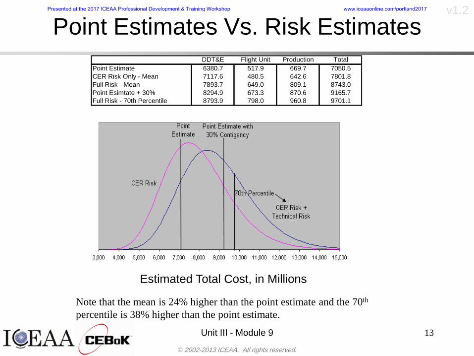
copy 2002-2013 ICEAA All rights reserved
v12
Point Estimates Vs Risk Estimates
Unit III - Module 9 13
DDTampE Flight Unit Production TotalPoint Estimate 63807 5179 6697 70505CER Risk Only - Mean 71176 4805 6426 78018Full Risk - Mean 78937 6490 8091 87430Point Esimtate + 30 82949 6733 8706 91657Full Risk - 70th Percentile 87939 7980 9608 97011
Estimated Total Cost in Millions
Note that the mean is 24 higher than the point estimate and the 70th
percentile is 38 higher than the point estimate
Presented at the 2017 ICEAA Professional Development amp Training Workshop wwwiceaaonlinecomportland2017
copy 2002-2013 ICEAA All rights reserved
v12
Cost Risk and Probabilitybull Cost risk or cost uncertainty analysis represents cost as a
probability distributionbull A probability distribution is a mathematical rule associating a
probability a to each possible outcome or event of interestbull There are two ways to present a probability distribution ndash as a
probability density function (ldquoPDF) and as a cumulative distribution function (ldquoS-curverdquo or ldquoCDFrdquo)
Unit III - Module 9 14
Lognormal Distribution PDF and CDF
0102030405060708090100
200 300 400 500 600 700 800 900 1000Cost $
Con
fiden
ce L
evel
0
00002
00004
00006
00008
0001
00012
00014
00016
Prob
abili
ty D
ensi
ty
CDFPDF
Presented at the 2017 ICEAA Professional Development amp Training Workshop wwwiceaaonlinecomportland2017
copy 2002-2013 ICEAA All rights reserved
v12
Unit III - Module 9 15
Probability Model ndash Distributionbull Normal
ndash Best behavior most iconic
ndash Theoretically (although not practically) allows negative costs which spook some users
ndash Symmetric needs mean shift to reflect propensity for positive growth
bull Lognormalndash A natural result in
non-linear CERsndash Indistinguishable
from Normal at CVs below 25
ndash Skewed
10
4
10
Presented at the 2017 ICEAA Professional Development amp Training Workshop wwwiceaaonlinecomportland2017
copy 2002-2013 ICEAA All rights reserved
v12
Unit III - Module 9 16
bull Triangularndash Most commonndash Easy to use easy to understandndash Modes medians do not addndash Skewed
bull Betandash Rare now but formerly popularndash Solves negative cost and duration issuesndash Many parameters ndash simplifications like PERT
Beta are possiblendash Skewed
bull Bernoullindash Probability is only assigned to two possible
outcomes success and failure (p and 1-p)ndash Simplest of all discrete distributionsndash Mean = pndash Variance = p(1-p)
10
Probability Model ndash Distribution
10
10
Presented at the 2017 ICEAA Professional Development amp Training Workshop wwwiceaaonlinecomportland2017
copy 2002-2013 ICEAA All rights reserved
v12
Unit III - Module 9 17
bull Normalndash If there is a sufficiently large number of independently identically distributed
elements (or not too correlated and not too skewed) then the distribution of total cost is normal due to the Central Limit Theorem
bull Lognormalndash For smaller data sets with large amounts of (positive) correlation and
skewness the lognormal distribution may be a better approximation of total cost
ndash Many total cost distributions in smaller data sets test as both normal and lognormal
bull Triangularndash The sum of triangles is not a triangle so this distribution should generally not
be used to characterize total costbull Convolved
ndash If total cost distribution is derived using simulation then it may not particularly resemble anything In this case we simply have a convolved or simulated total cost distribution
Probability ndash Top-Level Distribution
NEW
Presented at the 2017 ICEAA Professional Development amp Training Workshop wwwiceaaonlinecomportland2017
copy 2002-2013 ICEAA All rights reserved
v12
S-Curves and Confidence Levels
Unit III - Module 9 1818
100
70
25
Probability(Confidence
Level)
Cost Estimate(Dollars)
50
The S curve is the cumulative probability distribution coming out of the statistical summing process
70 confidence that project will cost indicated amount or less
Provides information on potential cost as a result of identified project risks
Provides insight into establishing reserve levels
X Y
MR
X = Point estimateZ = Project requirementY = Cost estimate where there is a 70 change that
final actual cost will be less than cost estimateY-Z= Manage reserve (MR) which is REQUIRED to meet 70 CL
Z
X not always = Z but is based on same content
Presented at the 2017 ICEAA Professional Development amp Training Workshop wwwiceaaonlinecomportland2017
copy 2002-2013 ICEAA All rights reserved
v12
19
Example ndash Normal Distribution
bull Normal distribution with mean equal to 100 and standard deviation equal to 20
bull Median and mode also equal 100bull The 80th Percentile is 117
40 60 80 100 120 140 160
80 of distribution(area under curve)is less than 117
117
Presented at the 2017 ICEAA Professional Development amp Training Workshop wwwiceaaonlinecomportland2017
copy 2002-2013 ICEAA All rights reserved
v12
20
Confidence Levelsbull The output of a cost risk analysis is a probability
distributionndash Typically displayed as a cumulative distribution function or
ldquoS-curverdquondash Confidence levels are simply percentiles of the distribution
0
10
20
30
40
50
60
70
80
90
100
30 60 90 120 150 180
Conf
iden
ce L
evel
Presented at the 2017 ICEAA Professional Development amp Training Workshop wwwiceaaonlinecomportland2017
copy 2002-2013 ICEAA All rights reserved
v12
Measuring Parametric Model Uncertainty
bull When developing estimates using cost-estimating relationships (CERs) there are two major sources of uncertaintyndash Technical (model input) uncertaintyndash Estimating uncertainty
bull Technical uncertainty reflects the uncertainty inherent in the model inputsndash Typical parametric model inputs include weight lines of code
heritage and other performance and management inputs
bull Estimating uncertainty measures the uncertainty inherent in the model due to the modelrsquos inability to capture all aspects of variability in the data
21
Presented at the 2017 ICEAA Professional Development amp Training Workshop wwwiceaaonlinecomportland2017
copy 2002-2013 ICEAA All rights reserved
v12
Parametric Model Examplebull The NASAAir Force Cost Model (NAFCOM) is a
parametric model for estimating acquisition costs for spacecraft and launch vehicles
bull The CERs in NAFCOM have the formCost = C WeightVNewDesignWTechnicalXManagementY ClassZ
bull There is technical uncertainty about each of the parametersndash Parametric models are applied early in a program so there
is significant amount of uncertainty in the weightndash Heritage is also tricky it is inherently subjective and project
personnel are typically optimisticndash Technical characteristics can also change as a program
matures and requirements change
22
Presented at the 2017 ICEAA Professional Development amp Training Workshop wwwiceaaonlinecomportland2017
copy 2002-2013 ICEAA All rights reserved
v12
Weight Uncertaintybull Aerospace weight growth study average satellite
weight growth from program inception to launch is 28
23
Aerospace Weight Growth Data
-10
0
10
20
30
40
50
60
0 4 8 12 16 20 24 28 32 36 40 44 48 52 56 60 64 68 72 76 80 84 88 92 96 100
Percent Program Completion
Perc
ent W
eigh
t Gro
wth
Presented at the 2017 ICEAA Professional Development amp Training Workshop wwwiceaaonlinecomportland2017
copy 2002-2013 ICEAA All rights reserved
v12
Estimating Uncertaintybull CERs do not perfectly fit the historical data
ndash There are non-repeatable random effects that cannot be predicted
bull For examplendash Parts breaking during testingndash Strikes which are difficult to predict
bull This results in an underlying uncertainty distribution about an estimatendash The outcome of a CER represents only one point on an
uncertainty distributionbull Typically mean or median depending upon the CER
methodology
24
Presented at the 2017 ICEAA Professional Development amp Training Workshop wwwiceaaonlinecomportland2017
copy 2002-2013 ICEAA All rights reserved
v12
Estimating Uncertainty (2)
25
Presented at the 2017 ICEAA Professional Development amp Training Workshop wwwiceaaonlinecomportland2017
copy 2002-2013 ICEAA All rights reserved
v12
Estimating Uncertainty (3)bull In the case of a linear regression the estimating
uncertainty follows a normal distributionndash The estimate is the mean and the standard error of the
estimate from the regression is the standard deviation of the normal distribution
bull In the case of a log-transformed linear regression the estimating uncertainty follows a lognormal distributionndash The estimate is the median of the lognormal and the
standard error of the estimate from the regression is the standard deviation of the normal distribution (in log-space)
bull There is additional uncertainty about an estimate based upon the distance of what is being estimated from the mean of the input datandash This results in a prediction interval
26
Presented at the 2017 ICEAA Professional Development amp Training Workshop wwwiceaaonlinecomportland2017
copy 2002-2013 ICEAA All rights reserved
v12
Aggregating Riskbull Risk is typically applied at the same level at
which we estimate cost that is at the Work Breakdown Structure (WBS) level
bull The estimates for each WBS are developedndash These estimates sum to yield the total system cost
bull For an n-element WBS the total cost is the sum of the cost for each of the n elements
27
nXXXCostSystem +++= 21
Presented at the 2017 ICEAA Professional Development amp Training Workshop wwwiceaaonlinecomportland2017
copy 2002-2013 ICEAA All rights reserved
v12
WBS Examplebull Launch Vehicle
ndash Structurebull Vehicle Structurebull Tank Structure
ndash Thermal Controlbull Active Thermal Controlbull Induced Thermal Controlbull Tank Thermal Control
ndash Main Propulsion Systemndash Liquid Rocket Enginendash Electric Power and Distributionndash Command Control and Data Handlingndash System Integration
28
Presented at the 2017 ICEAA Professional Development amp Training Workshop wwwiceaaonlinecomportland2017
copy 2002-2013 ICEAA All rights reserved
v12
WBS and Risk
29
Presented at the 2017 ICEAA Professional Development amp Training Workshop wwwiceaaonlinecomportland2017
copy 2002-2013 ICEAA All rights reserved
v12
Aggregating Riskbull This leads us to the issue of aggregating the risks across the
WBSbull For example if we want to determine the 70th percentile of the
overall cost risk distribution how do we proceed bull Note that we cannot simply add the 70th percentiles of each of
the cost risk distributionsbull We can add means and variances (taking correlation into
account more on that later) but that is all
Variance of Total Cost =
30
Mean of Total Cost = ( )E X E Xk
k
n
kk
n
kk
n
= = =aringaelig
egraveccediloumloslashdivide
= =aring aring1 1 1
m
Var X kk
n
=aringaelig
egraveccediloumloslashdivide1
= s r s skk
n
iji
j
i jj
n2
1 1
1
22+aring aringaring
= =
-
=
Presented at the 2017 ICEAA Professional Development amp Training Workshop wwwiceaaonlinecomportland2017
copy 2002-2013 ICEAA All rights reserved
v12
Percentiles Do Not Addbull As a notional example consider two independent normal
distributionsndash One distribution has mean equal to 100 and standard deviation
equal to 20ndash The second distribution has mean 300 and standard deviation of 80
bull The sum of two independent normally distributed random variables is also normally distributed
bull To combine the two distributions we add the means and add the variancesndash Total mean is
ndash Total standard deviation is
31
400300100 =+
8258020 22 raquo+
Presented at the 2017 ICEAA Professional Development amp Training Workshop wwwiceaaonlinecomportland2017
copy 2002-2013 ICEAA All rights reserved
v12
Percentiles Do Not Add (2)bull The 80th percentiles for the individual distributions are
117 and 367 respbull The 80th percentile of the combined distribution is
469 but the sum of the two 80th percentiles is 484bull To see why this is the case note that the percentiles
of a normal distribution are determined by the mean and the standard deviationndash The standard deviations are not added when normal distributions
are combined rather the variances are combinedndash Sum of variances is ndash The standard deviation of this sum is
32
22 ba +22 ba +
Presented at the 2017 ICEAA Professional Development amp Training Workshop wwwiceaaonlinecomportland2017
copy 2002-2013 ICEAA All rights reserved
v12
Percentiles Do Not Add (3)bull Since bull We can write
bull The left side of this inequality represents the risk of the combined distributions while the right side represents the sums of the individual risks
bull Combining two missions that are independent results in a diversification of riskndash The total portfolio is not as risky on a relative basis as each
individual project
33
2222 2 bababa ++lt+
baba +lt+ 22
Presented at the 2017 ICEAA Professional Development amp Training Workshop wwwiceaaonlinecomportland2017
copy 2002-2013 ICEAA All rights reserved
v12
Methods for Aggregating Riskbull Since percentiles do not add we have to find other
ways to aggregate riskbull One method is to use Monte Carlo simulationbull Unless cost risk is represented by normal
distributions for all WBS elements summing the means and variances does not result in a completely accurate depiction of overall system cost risk
bull The normal distribution is not a realistic distribution for representing risk in many or even most situations since regarding project risk more can go wrong than can go right which means the risk is NOT symmetric unlike the Gaussian bell curve
34
Presented at the 2017 ICEAA Professional Development amp Training Workshop wwwiceaaonlinecomportland2017
copy 2002-2013 ICEAA All rights reserved
v12
Unit III - Module 9 35
Monte Carlo Simulationfor Risk Analysis
bull When risk analysis is performed multiple risks are gatheredndash These risks may have various probability
distributions
bull Monte Carlo is the most commonly accepted way to produce an accurate characterization of the distribution of the combined effect of these many risksndash Using this distribution we can produce percentiles
for cost impacts due to risk occurrences
10
Presented at the 2017 ICEAA Professional Development amp Training Workshop wwwiceaaonlinecomportland2017
copy 2002-2013 ICEAA All rights reserved
v12
Monte Carlo Simulationbull Simulation is a means for solving problems that are
analytically intractablendash Involves repeated random sampling
bull It was developed during the Manhattan Project as a way to model the interactions inside an atom during nuclear fissionndash Allowed for more sophisticated mathematical modeling of atomic
phenomena
bull Most computer packages use pseudo-random number generators that produce seemingly random results from an initial seedndash Example is the linear congruential generator
36
( ) mbaXX nn mod1 +=+
Presented at the 2017 ICEAA Professional Development amp Training Workshop wwwiceaaonlinecomportland2017
copy 2002-2013 ICEAA All rights reserved
v12Using Random Numbers to Simulate Distributions
bull WBS cost risk is typically measured by a probability distributionbull The most common method for simulating a probability
distribution is the inverse methodbull This involve obtaining a simulated random value from a uniform
distribution and then inverting this through the cumulative distribution function (CDF) to obtain the simulated value
bull As an example for a uniform distribution on the interval [0100]
bull In this case the CDF random value of 05 translates to 10005 = 50
37
( )100
1=xf ( )
100xxF = ( ) xxF 1001 =-
Presented at the 2017 ICEAA Professional Development amp Training Workshop wwwiceaaonlinecomportland2017
copy 2002-2013 ICEAA All rights reserved
v12
Simulating a Triangular Distribution
bull For a triangular distribution with low = 0 most likely = 50 and high = 150 the CDF is given by
bull The inverse function is given by
38
( )iumliumlicirc
iumliumliacute
igrave
poundlt--
poundpound=
1505021
1500050
50015000
2
2
2
xxx
xxxF
( )iumliumlicirc
iumliumliacute
igrave
poundltdivideoslashouml
ccedilegraveaelig +--
poundpound=-
131
21
37501
250017500150
3107500
1
xx
xxxF
Presented at the 2017 ICEAA Professional Development amp Training Workshop wwwiceaaonlinecomportland2017
copy 2002-2013 ICEAA All rights reserved
v12
Simulating a Triangular Distribution (2)
bull If the simulated uniform value is equal to 02 the corresponding inverse value from the CDF inverse is approximately 387
39
0
01
02
03
04
05
06
07
08
09
1
0 30 60 90 120 150
Presented at the 2017 ICEAA Professional Development amp Training Workshop wwwiceaaonlinecomportland2017
copy 2002-2013 ICEAA All rights reserved
v12
Monte Carlo and the WBSbull Simulation involves repeated trials
40
WBS Draw1 2 3 4 5
System 2912 3566 4390 2954 4655 Sum
Structure 80 105 55 80 57 SumVehicle Structure 50 70 30 40 20Tank Structure 30 35 25 40 37
Thermal Control 32 36 35 29 33 SumActive Thermal Control 10 15 12 7 10Induced Thermal Control 12 14 13 14 14Tank Thermal Control 10 7 10 8 9
Main Propulsion System 100 150 125 140 100
Liquid Rocket Engine 1000 1100 1800 900 2200
Electric Power and Distribution 100 125 150 75 90
Command Control and Data Handling 200 250 225 230 275
System Integration 1400 1800 2000 1500 1900
Presented at the 2017 ICEAA Professional Development amp Training Workshop wwwiceaaonlinecomportland2017
copy 2002-2013 ICEAA All rights reserved
v12
Number of Trialsbull Monte Carlo involves a repeated number of trialsbull The greater the number of trials the more accurate the
simulation will approximate the overall cost risk behavior of the system
bull After 100 trials the histogram looks very jagged
41
Presented at the 2017 ICEAA Professional Development amp Training Workshop wwwiceaaonlinecomportland2017
copy 2002-2013 ICEAA All rights reserved
v12
Number of Trials (2)
42
1000 Trials
10000 Trials
50000 Trials Additional trials give a more accurate depiction of the final result
Presented at the 2017 ICEAA Professional Development amp Training Workshop wwwiceaaonlinecomportland2017
copy 2002-2013 ICEAA All rights reserved
v12
Number of Trials (3)bull If we want to simulate the underlying
mean within 1 with 95 confidence for example then we require
43
divideoslash
oumlccedilegrave
aelig poundpound-
=
dividedividedivide
oslash
ouml
ccedilccedilccedil
egrave
aeligpound
-pound
-=
divideoslashouml
ccedilegraveaelig poundpound=
nZ
n
nnX
n
X
n
n
011
010Pr
011
010Pr
011990Pr950
___
___
sm
sm
sm
sm
sm
mm
Presented at the 2017 ICEAA Professional Development amp Training Workshop wwwiceaaonlinecomportland2017
copy 2002-2013 ICEAA All rights reserved
v12
Number of Trials (4)bull This means that the number of trials required is determined by
bull Solving for n we find that at least
trials are neededbull Note that this term involves the coefficient of variation of the
distribution which means that distributions with less dispersion require fewer trials to accurate simulate
44
96101
=ns
m
ms41638
Presented at the 2017 ICEAA Professional Development amp Training Workshop wwwiceaaonlinecomportland2017
copy 2002-2013 ICEAA All rights reserved
v12
Number of Trials (5)bull Simulating percentiles requires more trials than for simulating
meansbull Let Pn represent the number of trials in the sample at or below
the 70th percentile of the underlying distribution (suppose this is known)
bull By the Central Limit Theorem Pnn follows a normal distribution with mean equal to the 70th percentile and variance equal to
bull By a similar process for the mean we find that the number of trials needed to simulate the 70th percentile within 1 with 95 confidence is
45
( )n
FF 700700 1-
n
n
PPn -41638
Presented at the 2017 ICEAA Professional Development amp Training Workshop wwwiceaaonlinecomportland2017
copy 2002-2013 ICEAA All rights reserved
v12
Number of Trials (6)bull If Pn 070 for all n then n is approximately
bull For the sake of comparison suppose CV = 03 (reasonable approximation for hardware development) then the number of trials needed to simulate the mean with the same accuracy is then ldquoonlyrdquo 11525
bull More trials are needed to accurately simulate percentiles than means
46
( ) 46416703041638
70704168341638 =divide
oslashouml
ccedilegraveaelig=divide
oslashouml
ccedilegraveaelig -
=-
nnn
PPn
n
n
Presented at the 2017 ICEAA Professional Development amp Training Workshop wwwiceaaonlinecomportland2017
copy 2002-2013 ICEAA All rights reserved
v12
Methods of Simulationbull Monte Carlo simulation is a standard term for
simulationbull However there is an improvement on Monte Carlo
that improves the accuracy of the results of a simulation for a given number of trials
bull This method is call the Latin Hypercube approach to simulationndash Similar to Monte Carlo but an equal number of draws are taken
from a set of subintervals for example dividing the interval (01) into [00001) [0102)hellip [0910]
ndash Instead of 10 trials from [01] we have one trial from each subinterval
ndash Rough rule of thumb is Latin Hypercube takes 30 fewer trials to achieve similar accuracy to Monte Carlo
47
Presented at the 2017 ICEAA Professional Development amp Training Workshop wwwiceaaonlinecomportland2017
copy 2002-2013 ICEAA All rights reserved
v12
Probability Model ndash Correlationbull Correlation exists between work breakdown structure
(WBS) cost element costs and between cost and schedule
bull Correlation is a necessary consideration in cost risk analysis
bull Correlation is a number that can vary between -1 and +1 and represents the strength of the relationship between the two variablesndash If both variable have a tendency to move in the same direction
correlation is positivendash If when one variable increases the other tends to decrease and
vice-versa the correlation between the two variables is negative
Presented at the 2017 ICEAA Professional Development amp Training Workshop wwwiceaaonlinecomportland2017
copy 2002-2013 ICEAA All rights reserved
v12
Correlation And Causationbull Note that correlation is not causation however
causation implies correlationndash For example shark attacks and ice cream sales at the beach
bull For example for a launch vehicle structure increasing the diameter will not only result in an increase in the structures cost but will also result in higher costs for thermal coating (paint etc)
bull Also simply because two subsystems do not appear to be related does not mean they are not correlatedndash For example structures and computer equipment seemingly
have little relation to one another however an external factor such as a funding cut or a strike will impact all subsystems leading to delays and increasing cost across the board
ndash Thus everything in a WBS has some correlationUnit III - Module 9 49
Presented at the 2017 ICEAA Professional Development amp Training Workshop wwwiceaaonlinecomportland2017
copy 2002-2013 ICEAA All rights reserved
v12
The Importance of Correlationbull Percent that total cost standard deviation is underestimated
when correlation assumed to be 0 instead of r given nWBS elements
Unit III - Module 9 5050
0
20
40
60
80
100
0 01 02 03 04 05 06 07 08 09 1Actual Correlation
Perce
nt Un
deres
timate
d
n = 10
n = 30
n = 100n = 1000
0
20
40
60
80
100
0 01 02 03 04 05 06 07 08 09 1Actual Correlation
Perce
nt Un
deres
timate
d
n = 10
n = 30
n = 100n = 1000
Reference 32nd Annual DOD Cost Analysis Symposium Advanced Training Session ldquoWhy Correlation Matters in Cost Estimatingrdquo Stephen A Book
Presented at the 2017 ICEAA Professional Development amp Training Workshop wwwiceaaonlinecomportland2017
copy 2002-2013 ICEAA All rights reserved
v12
The Importance of Correlation (2)bull For example if correlation is assumed to be 0 for all
elements in a 30 element WBS and the actual correlation is 20 then the total cost standard deviation is underestimated by 60
bull For example assume the total cost is modeled as a normal distribution with mean = 100
bull If correlation is assumed to be zero with total cost standard deviation = 12 when correlation is actually 20 then the true underlying standard deviation is actually 30
bull 70th percentile with zero correlation assumption is 106
bull 70th percentile with 20 correlation is 116 Unit III - Module 9 51
Presented at the 2017 ICEAA Professional Development amp Training Workshop wwwiceaaonlinecomportland2017
copy 2002-2013 ICEAA All rights reserved
v12
Measures of Correlationbull Two measures of correlation are commonly used in
cost risk analysesndash Pearsonrsquos product-moment correlation coefficient ndash Spearmanrsquos rank correlation coefficient
bull Garvey and others recommend using Pearsonrsquos product-moment correlation coefficient correlation for cost risk analysesndash Method of moments uses this but there are two options in
simulationndash Popular simulation packages like Risk and Crystal Ball use
rank correlation but in practice this has been found to make little difference
ndash Pearson product-moment correlation has been incorporated into Risk+
52
Presented at the 2017 ICEAA Professional Development amp Training Workshop wwwiceaaonlinecomportland2017
copy 2002-2013 ICEAA All rights reserved
v12
Pearson Correlationbull Pearsonrsquos product-moment correlation measures
degree of linearity between two random variables bull If two random variables are perfectly linear (eg Y =
aX + b) with positive slope then the Pearson product-moment correlation between X and Y denoted by rXY is +1
53
X X
Y Y Y
XNegative Correlation Positive Correlation No Correlation
middotmiddot
middotmiddot
middotmiddot middotmiddot
middotmiddot
middot
middot
middotmiddotmiddot
middotmiddot
middotmiddot
middotmiddot middot
middot
middot
middotmiddotmiddotmiddotmiddotmiddotmiddotmiddot
middotmiddotmiddotmiddot
middotmiddot
middotmiddot middotmiddotmiddotmiddot
middotmiddotmiddot
middotmiddotmiddotmiddot
middotmiddotmiddot
middotmiddotmiddot
middotmiddot
middot
middot middotmiddot
middot middotmiddotmiddotmiddot middotmiddot middot middotmiddot middot middot
middotmiddot middot
middotmiddotmiddotmiddotmiddot middot middotmiddot
middotmiddot
middot
middotmiddot
middotmiddot middot
middot middot middot
middotmiddot middot
middotmiddotmiddot
middotmiddot
middot middot
Presented at the 2017 ICEAA Professional Development amp Training Workshop wwwiceaaonlinecomportland2017
copy 2002-2013 ICEAA All rights reserved
v12
Spearman Correlationbull Spearmanrsquos rank correlation measures the
monotonicity between two random variablesbull If two random variables are perfectly monotonically
increasing (eg Y = X2) then the Spearman rank correlation denoted by rXY is +1
bull The two measures can be significantly different
54
10 20 30 40 50 60
100
200
300
096 097 098 099 1
1
060
020
040
080
Eff
ort (
Staf
f-M
onth
s)
Software Size I KDSI
y = 28z12y
z x
yy = x100
0 pound x pound 1
Figure 5-9A Figure 5-9B
Pearson Correlation = 09976 Rank Correlation = 1
Pearson Correlation = 024 Rank Correlation = 1
X(x ) ~ Unif(01)
Reference Probability Methods for Cost Uncertainty Analysis A Systems Engineering Perspective Paul R Garvey
Presented at the 2017 ICEAA Professional Development amp Training Workshop wwwiceaaonlinecomportland2017
copy 2002-2013 ICEAA All rights reserved
v12
Unit III - Module 9 55
200
250
300
350
400
1000 1200 1400 1600 1800 2000
Recurring Production
SEPM
200
250
300
350
400
1000 1200 1400 1600 1800 2000
Recurring Production
SEPM
Functional Correlationbull Old No Functional
Correlation Simulation run with WBS items entered as values
bull New Simulation run with functional dependencies entered as they are in cost model
CorrelatedNot Correlated
Note shift of mean and increased variability
Presented at the 2017 ICEAA Professional Development amp Training Workshop wwwiceaaonlinecomportland2017
copy 2002-2013 ICEAA All rights reserved
v12
Risk Measuresbull ldquoWestern Europe conquered the word because of a
technological revolution that started because of attempts to measure the worldrdquo ndash Phillipe Jorion ndash In the same way attempts to measure risk will lead to better project
managementbull Risk management for DoD and NASA agencies focuses
primarily on funding projects to a single percentile ndash NASA policy explicitly mentions 70 and 50ndash This is known as ldquoValue at Riskrdquo and is prevalent in the banking and
financial industry
56
Presented at the 2017 ICEAA Professional Development amp Training Workshop wwwiceaaonlinecomportland2017
copy 2002-2013 ICEAA All rights reserved
v12
Value at Risk (VaR)bull VaR is a percentile of the cost risk
distributionndash VaR funding at the 70th percentile means that
there is a 30 chance of final project cost exceeding the funded amount (budget)
bull VaR has some meritsndash Common measure can be used to compare
different projects and programsndash Easily understood by senior managers and
decision makers
57
Presented at the 2017 ICEAA Professional Development amp Training Workshop wwwiceaaonlinecomportland2017
copy 2002-2013 ICEAA All rights reserved
v12
Why 70th or 80th Percentilebull Typical policy guidance involves funding at the 70th or 80th
percentile Why fund as such a low percentilebull There is some incentive to not over-fundbull For a normal distribution an inflection point occurs near the 80th
percentile meaning that for values above 80 confidence achieving higher levels of confidence can only be achieved by spending greater dollar amounts at an increasing rate
58
-05-04-03-02-01
00102030405
0 05 1 15 2 25 3
Standard Deviations from Mean
Normal Distribution
First DerivativeSlopeVelocity
Second DerivativeConvexityAcceleration
Inflection point at one standard deviation above the mean (~84th
percentile)
Presented at the 2017 ICEAA Professional Development amp Training Workshop wwwiceaaonlinecomportland2017
copy 2002-2013 ICEAA All rights reserved
v12
Funding Above Inflection Pointsbull As the percentile goes above the 80th percentile the amount
needed to achieve that higher level of confidence begins to increase at an increasing rate as is evident from the graph
59
0
10
20
30
40
50
60
70
50 55 60 65 70 75 80 85 90 95 100
$ Ab
ove
MEa
n to
Ach
ieve
Per
cent
ile
Percentile (Confidence Level)
Presented at the 2017 ICEAA Professional Development amp Training Workshop wwwiceaaonlinecomportland2017
copy 2002-2013 ICEAA All rights reserved
v12
Why Budget to the 70th or 80thbull Government projects are funded at the 70th or 80th percentilesbull Why not the 90th or 99th percentile Wonrsquot that help prevent
overrunsndash As we have seen percentiles do not add across programs
bull The sum of the 80th percentiles does NOT equal the total 80th percentile
ndash This is because the individual programs are riskier than the entire suite of missions
bull Known as the ldquoPortfolio effectrdquo (more or this later)
ndash Funding at the 80th gives confidence that the entire portfolio will be adequately funded
bull And since there is an inflection point near the 80th percentile funding above that level quickly becomes cost prohibitive
60
Presented at the 2017 ICEAA Professional Development amp Training Workshop wwwiceaaonlinecomportland2017
copy 2002-2013 ICEAA All rights reserved
v12
Inflection Points for Lognormalbull For a lognormal the inflection point
variesndash Coefficient of variation equal to 10 equates to an
inflection point at the 70th percentile
61
0
10
20
30
40
50
60
70
050 060 070 080 090 100
Coef
ficen
t of V
aria
tion
Percentile of the Inflection Point
Presented at the 2017 ICEAA Professional Development amp Training Workshop wwwiceaaonlinecomportland2017
copy 2002-2013 ICEAA All rights reserved
v12
Issues with Percentile Fundingbull However risk management does not stop at a
specific percentilendash What happens when the 70th percentile is exceeded
bull Any effective risk management policy should prescribe what happens after a bad event occursndash With VaR we only know when a bad event has occurred ndash Also funding at a relatively low level means we have no true
sense of the real risks that should be guarded against
62
Presented at the 2017 ICEAA Professional Development amp Training Workshop wwwiceaaonlinecomportland2017
copy 2002-2013 ICEAA All rights reserved
v12
ldquoHere There Be Dragonsrdquobull On old maps uncharted territory was often
marked with monsters or dragons
63
A section of the Carta Marina by Olaus Magnus 16th Century
Presented at the 2017 ICEAA Professional Development amp Training Workshop wwwiceaaonlinecomportland2017
copy 2002-2013 ICEAA All rights reserved
v12
Distribution Comparisonbull Four different distributions with the same 70th
percentile
bull Should we expect the tails to be similar
64
0
10
20
30
40
50
60
70
80
0 100 200 300 400 500 600
Perc
entil
eCo
nfid
ence
Lev
el
Triangular
Normal
Lognormal
Pareto
Presented at the 2017 ICEAA Professional Development amp Training Workshop wwwiceaaonlinecomportland2017
copy 2002-2013 ICEAA All rights reserved
v12Distribution Comparison Tail Behavior
bull The normal and triangular distributions have similar tails but the lognormal and Pareto have much fatter right tails
65
70
75
80
85
90
95
100
500 1500 2500 3500 4500 5500
Perc
entil
eCo
nfid
ence
Lev
el
Triangular
Normal
Lognormal
Pareto
Here There Be Dragons
Presented at the 2017 ICEAA Professional Development amp Training Workshop wwwiceaaonlinecomportland2017
copy 2002-2013 ICEAA All rights reserved
v12Distribution Comparison ndash Tail Behavior (Table)
bull There is significant tail risk for the lognormal and the Paretobull The 99th percentile for the Pareto is 1000 times greater than
the 70th percentilendash Risk seen in financial markets and in catastrophic risks like natural
disasters bull Four different projects follow the four different risk profiles seen
in this example should clearly have different risk management approaches but 70th percentile funding indicates the same risk management approach for all four
66
Percentile Triangular Normal Lognormal Pareto 70th $600 $600 $600 $600 80th $680 $660 $770 $1430 90th $770 $750 $1070 $5880 95th $840 $820 $1410 $23750 99th $930 $950 $2350 $600000
Presented at the 2017 ICEAA Professional Development amp Training Workshop wwwiceaaonlinecomportland2017
copy 2002-2013 ICEAA All rights reserved
v12Percentile Budgeting is Not Risk Management
bull Percentile budgeting ne effective risk management policybull Suppose that you are shopping for a new car You
mention that safety is your top concern The salesman says he has a great safe car available You ask about the air bags Do they work The salesman answers ldquoOf course Seventy percent of the time they work fine Only 30 of the time the air bags will fail to deployrdquo Would you buy such a car Hedge fund manager David Einhorn has stated ldquoRisk management is the air bag that must always work but only in the multi-sigma event where you have an accidentrdquo
67
Risk management is the air bag that must always work but only in the multi-sigma event where you
have an accident
Presented at the 2017 ICEAA Professional Development amp Training Workshop wwwiceaaonlinecomportland2017
copy 2002-2013 ICEAA All rights reserved
v12
Joint Confidence Level Analysisbull Schedules are risky toobull For 98 recent NASA missions average
schedule growth was 38ndash Not as high as cost growth but still significant
68
0
5
10
15
20
25
30
35
40
Schedule
Cost
Presented at the 2017 ICEAA Professional Development amp Training Workshop wwwiceaaonlinecomportland2017
copy 2002-2013 ICEAA All rights reserved
v12
Schedules Impact Costbull Changes in schedule can have enormous
impacts on cost ndash Schedule slips can lead to cost increases
bull Fixed programmatic costs must be paid on a regular basisndash Achieving schedule milestones early can result in cost
savings
bull Schedule is an important consideration in cost analysis including cost risk analysis
bull However we must be careful in correctly integrating cost and schedule riskndash Schedule is not simply an input but is dependent on many of
the same factors that drive cost
69
Presented at the 2017 ICEAA Professional Development amp Training Workshop wwwiceaaonlinecomportland2017
copy 2002-2013 ICEAA All rights reserved
v12
The Relationship of Cost to Schedulebull Cost and schedule are positively correlated
ndash A larger program with bigger scope with take longer to complete than a smaller simpler program
bull However longer schedules do not always equate to higher cost nor shorter schedules with lower costndash Highly compressed schedules relative to the
optimal schedule can lead to large overrunsbull Compressed schedules are commonplace for
many planetary missions
70
Presented at the 2017 ICEAA Professional Development amp Training Workshop wwwiceaaonlinecomportland2017
copy 2002-2013 ICEAA All rights reserved
v12The Impact of Schedule GrowthCompression on Cost
bull Compressed schedules lead to cost growth and based on existing research is actually more expensive than schedule slippages
71
0
20
40
60
80
100
120
140
160
-50 -25 0 25 50 75 100
Percentage Change in Schedule
Perc
enta
ge C
hang
e in
Cos
t due
to
Sche
dule
Cha
nge
Source Smart CB ldquoCost and Schedule Interrelationshipsrdquo 2007 NASA Cost Symposium
Presented at the 2017 ICEAA Professional Development amp Training Workshop wwwiceaaonlinecomportland2017
copy 2002-2013 ICEAA All rights reserved
v12Schedule as an Independent Variable
bull Why not simply add schedule as an input to cost-estimating relationships (CERs)
bull Schedule is often treated as an independent variable ndash schedules are often determined independently of cost considerationsndash Cost may not be considered explicitly although budgets and
schedules are determined based on scope and other common factors
bull In 2006 SAIC undertook a research task to determine the impact of schedule on cost and added schedule as an independent variable to the CERs in the NASAAir Force Cost Model (NAFCOM) to see if schedule provided any improvement in goodness of fit
72
Presented at the 2017 ICEAA Professional Development amp Training Workshop wwwiceaaonlinecomportland2017
copy 2002-2013 ICEAA All rights reserved
v12
Schedule is a Dependent Variablebull Since NAFCOM includes an exhaustive list of cost drivers the inclusion
of schedule should give an indication of whether there is any additional independent value added from schedule independent of the cost drivers
bull In the study schedule was added to 10 subsystem-level CERs
ndash In each case the addition of schedule did NOTimprove the goodness of fit and schedule was NOT found to be a statistically significant cost driver (given the presence of the other variables) for any of the 10 CERs
bull Standard errors for the CERs increased due to decrease in degrees of freedom
bull Thus schedule as an independent variable did not provide any additional explanation of variation in historical cost
bull This is because schedule is truly NOT an independent variable but a dependent variable and is a function of the same factors that drive cost
73
Presented at the 2017 ICEAA Professional Development amp Training Workshop wwwiceaaonlinecomportland2017
copy 2002-2013 ICEAA All rights reserved
v12
Incorporation of Schedule in Cost Risk
bull When using subjective methods care must be taken in applying schedule to cost risk analysis
bull Since schedule is a dependent variable treating it independently from other factors when assessing its impact on cost can lead to a double count of independent variables in the cost risk analysis
bull Direct inclusion of schedule in a cost risk analysis effectively doubles the influence of each cost driver
ndash Incorrectly leads to broader risk ranges
74
CostWeight
HeritageNewness
Technology Readiness Schedule
Presented at the 2017 ICEAA Professional Development amp Training Workshop wwwiceaaonlinecomportland2017
copy 2002-2013 ICEAA All rights reserved
v12Subjective Cost Risk Methods and Overinclusion of Risk Factors
bull Subjective methods are suitable when data are scarce or not availablebull However care must be taken not to treat correlated sources of risk
such as schedule as independent of each otherbull Example ndash a subjective risk analysis incorporated technology readiness
design risk requirements stability integration risk and schedule and treated each source of risk as independent
bull Risk triangle high value without schedule risk was 31 times the point estimate
bull Risk triangle high value with schedule risk added on top of other sources of risk treated independently was 34 times the point estimate
bull Risk triangle taking correlation between sources of risk into account in a rigorous statistical manner has a high value 15 times the point estimate less than half the effect when treating sources of risk as independent
75
Presented at the 2017 ICEAA Professional Development amp Training Workshop wwwiceaaonlinecomportland2017
copy 2002-2013 ICEAA All rights reserved
v12Fundamental Equation of Cost and Schedule Interrelationships
bull The Fundamental Equation of the Relationship Between Cost and Schedule is
Time = Moneybull This is a well known adage that time is money Your boss at
work may even mention this to you from time to time or if you are the boss you are all too aware of this iron law
bull Because time is money cost and schedule risk should be modeled jointly not with schedule as an independent cost driver
bull Note that cost and schedule are not perfectly correlatedndash Cost can sometimes ldquobuy downrdquo schedule extra money can be
spent to meet a deadline since in some cases additional effort to hasten the completion of a task
76
Presented at the 2017 ICEAA Professional Development amp Training Workshop wwwiceaaonlinecomportland2017
copy 2002-2013 ICEAA All rights reserved
v12How to (Correctly) Incorporate Schedule into Cost Risk Analysis
bull The best way to model cost and schedule risk is to develop a joint cost and schedule model based on the same data
bull Since such models are not currently available the next best approach is to model cost and schedule independently and then integrate cost and schedule risk analyses using joint probability distributions taking into account correlation between cost and schedulendash This approach pioneered by Paul Garvey and Steve Book is
considered industry best practicendash This is a practical method mathematically tractable and follows
naturally from the Fundamental Equation of Cost and Schedule Interrelationships
77
Book S A ldquoQuantifying the Relationship Between Cost and Schedulerdquo The Measurable News Winter 2007-2008 pp 11-15Garvey PR Probability Methods for Cost Uncertainty Analysis A Systems Engineering Perspective New York Marcel Dekker 2000 pp 308-335
Presented at the 2017 ICEAA Professional Development amp Training Workshop wwwiceaaonlinecomportland2017
copy 2002-2013 ICEAA All rights reserved
v12
Joint Lognormal and Normal Distributions
bull Cost and schedule are typically modeled as some combination of Normal and Lognormal probability distributionsndash Studies by The Aerospace Corporation the MITRE
Corporation Wyle Labs and SAIC have found that the Lognormal probability distribution almost always serves as a good model for both the schedule distribution and the cost distribution
ndash The Normal distribution may also be appropriate in some instances and depending upon the level of confidence at which budgets are set may even be more conservative and logically consistent than the Normal distribution
ndash Joint Lognormal and Normal distributions are defined by a pair of mean and standard deviations and a level of correlation between the two
78
Presented at the 2017 ICEAA Professional Development amp Training Workshop wwwiceaaonlinecomportland2017
copy 2002-2013 ICEAA All rights reserved
v12Modeling Cost and Schedule as a Bivariate Distribution
bull In the approach set forth by Book and Garvey cost risk is assessed and the top-level distribution is modeled as a Lognormal (or Normal) distribution schedule risk is assessed and the overall schedule risk is modeled as a Lognormal (or Normal) distribution
bull The two distributions are combined into a Bivariate distribution by assigning a correlation between the two and by treating the two distributions as the marginal distributions of a Bivariate Lognormal distributionndash Other combinations include a Bivariate Normal or a Bivariate
Normal-Lognormal
79
Presented at the 2017 ICEAA Professional Development amp Training Workshop wwwiceaaonlinecomportland2017
copy 2002-2013 ICEAA All rights reserved
v12Bivariate Lognormal Distribution for Cost and Schedule
bull Cost is often observed to be Lognormal when strong positive correlations are present among the systemrsquos WBS cost element costs
bull A systemrsquos schedule is often observed (from Monte Carlo simulations) to be Lognormal if it is the sum of many positively correlated schedule activities in an overall schedule network
bull If Lognormal distributions characterize a systemrsquos cost and schedule then the Bivariate Lognormal could serve as an assumed model of their joint distributionndash In this case the marginal distribution of each of cost and schedule is
Lognormalbull Other possibilities for modeling cost and schedule as a Bivariate
distribution include a Bivariate Normal or a Bivariate Normal-Lognormal distributionndash All these combinations are analytically tractable
80
Presented at the 2017 ICEAA Professional Development amp Training Workshop wwwiceaaonlinecomportland2017
copy 2002-2013 ICEAA All rights reserved
v12Bivariate Lognormal for Cost and Schedule
bull Contour Plots of a Bivariate Lognormal
81
Presented at the 2017 ICEAA Professional Development amp Training Workshop wwwiceaaonlinecomportland2017
copy 2002-2013 ICEAA All rights reserved
v12Correlation Between Cost and Schedule
bull Cost and schedule are positively correlated but not perfectly sondash For example it is possible to have a schedule underrun and a cost
overrunbull Based on cost and schedule growth data for 50 completed NASA
programs the correlation between development cost and development schedule is 70
82
00
200
400
600
800
1000
1200
-500 00 500 1000 1500 2000 2500Historical Cost Growth
Hist
oric
al S
ched
ule
Gro
wth
r = 715
Presented at the 2017 ICEAA Professional Development amp Training Workshop wwwiceaaonlinecomportland2017
copy 2002-2013 ICEAA All rights reserved
v12Correlation Between Cost and Schedule Caveats
bull Based on historical data recommended correlation between cost and schedule is 70 but this could be higher or lower depending upon program circumstancesndash If program is budget constrained cost and schedule will be
more highly correlated (go as you pay)ndash If program is schedule constrained cost and schedule will
have lower correlation perhaps even negative correlation ndash Smaller programs have smaller correlation between cost and
schedule riskbull Relatively easy to ldquohurry uprdquo and finish on time or even early if
needed
83
Presented at the 2017 ICEAA Professional Development amp Training Workshop wwwiceaaonlinecomportland2017
copy 2002-2013 ICEAA All rights reserved
v12
Conditional Confidence Levelsbull Given a programrsquos project schedule we can determine the cost
risk distribution conditional upon the given schedulebull Conditional cost S-curves are steeper than unconditional
(marginal) cost S-curves between some uncertainty has been removed because schedule is fixed
84
Presented at the 2017 ICEAA Professional Development amp Training Workshop wwwiceaaonlinecomportland2017
copy 2002-2013 ICEAA All rights reserved
v12
Joint Confidence Levelsbull Joint 65 confidence represents the probability of
achieving both 65 confidence in cost AND 65 confidence in schedulendash This is different than achieving 65 cost confidence alone
or achieving 65 schedule confidence alonebull Due to the imperfect correlation between cost and schedule it
is possible to achieve a 65 cost confidence with a lower level of schedule confidence
bull Restricting the schedule confidence thus requires additional $ to achieve a given level of confidence
85
X
Y
Possible Values for Which X gt a Possible Values for
Which X gt a and Y gt b
a
b
Presented at the 2017 ICEAA Professional Development amp Training Workshop wwwiceaaonlinecomportland2017
copy 2002-2013 ICEAA All rights reserved
v12Joint Confidence Levels Versus Cost Confidence Levels Only
bull Example of the differences between cost confidence schedule confidence conditional cost confidence and joint cost and schedule confidence
86
Joint Cost-Schedule Confidence Iso-Curves
Cost (RY$M)
Sche
dule
(Mon
ths)
65 Confidence
50 Confidence
70 Confidence
65 Cost Confidence AggressiveSchedule65 Cost ConfidenceScheduleGiven 65 Schedule ConfidenceUnconditional 65 CostConfidenceUnconditional 65 ScheduleConfidence
65 Cost Confidence 65 Joint Cost and Schedule
Confidence for 65 Schedule Confidence
Presented at the 2017 ICEAA Professional Development amp Training Workshop wwwiceaaonlinecomportland2017
copy 2002-2013 ICEAA All rights reserved
v12
Joint Cost and Schedule Confidence
bull Can examine pairs of cost and schedule that achieve a given level of confidence
bull Provides insights into the trade-offs between cost and schedule for a given level of confidencendash Possible to increase cost confidence by giving a
project more time in some instances or possible to ldquobuy downrdquo schedule
bull But these have limits and are shown in the iso-cost and schedule confidence curves
87
Presented at the 2017 ICEAA Professional Development amp Training Workshop wwwiceaaonlinecomportland2017
copy 2002-2013 ICEAA All rights reserved
v12Cost and Schedule Trade-offs for a Given Level of Joint Confidence
bull Hypothetical Example
88
Cost (RY$M)
Schedule (Months)
$100 48$99 48$89 49$87 50$85 51$85 52$84 53$83 55$83 55$83 56
Cost and Schedule 65 Confidence Iso-Curve
4748495051525354555657
$80 $82 $84 $86 $88 $90 $92 $94 $96 $98 $100
Cost (RY$ M)
Sche
dule
(Mon
ths)
Presented at the 2017 ICEAA Professional Development amp Training Workshop wwwiceaaonlinecomportland2017
copy 2002-2013 ICEAA All rights reserved
v12Policy Considerations for Confidence Levels
bull For large programs the difference between the amount of money needed to achieve 65 cost confidence independent of schedule and joint 65 cost and schedule confidence can represent hundreds of millions and even billions of dollars
89
Joint Cost-Schedule Confidence Iso-Curves
Cost (RY$M)
Sche
dule
(Mon
ths)
65 Confidence
65 Cost Confidence AggressiveSchedule
65 Cost ConfidenceScheduleGiven 65 Schedule Confidence
Unconditional 65 CostConfidence
Joint Cost and Schedule Confidence for 65 Cost Confidence and Program Baseline Schedule is Less Than 35
65 Cost Confidence Independent of Schedule Cost Needed to Achieve
Both 65 Joint Cost and Schedule Confidence for the Schedule with 65 Confidence
Presented at the 2017 ICEAA Professional Development amp Training Workshop wwwiceaaonlinecomportland2017
copy 2002-2013 ICEAA All rights reserved
v12
Copulasbull More generally any combination of distributions can
be used (more than just normal and lognormal)ndash Termed ldquocopulardquo from the Italian word for ldquocouplerdquondash Copulas are a way to combine marginal distributions of any
number and type into a joint distributionbull More formally a copula is a multivariate joint distribution defined
on the n-dimensional unit cube [0 1]n such that every marginal distribution is uniform on the interval [0 1]
bull (The bivariate form of) Sklarrsquos theorem states that for any bivariate distribution function H(x y) let F(x) = H(x infin) and G(y) = H(infin y) be the univariate marginal probability distribution functions Then there exists a copula C such that H(xy)=C(F(x)G(y))
ndash Copulas are widely used in risk management for investments and insurance
bull Considered industry best practice (Li 2000)bull Marketed as part of JP Morganrsquos CreditMetrics suite of tools
(Gupton et Al 1997)90
Presented at the 2017 ICEAA Professional Development amp Training Workshop wwwiceaaonlinecomportland2017
copy 2002-2013 ICEAA All rights reserved
v12Parametric Joint Cost and Schedule Analysis
bull A parametric model based on a consistent data set with a set of overlapping cost and schedule drivers is a cleaner way to model cost and schedule
91
CostWeight
HeritageNewness
Technology Readiness
Schedule
0
20
40
60
80
100
Confidence
Joint Cost and Schedule Confidence
Schedule
Cost
Lognormal Distribution PDF and CDF
0102030405060708090100
200 300 400 500 600 700 800 900 1000Cost $
Con
fiden
ce L
evel
0
00002
00004
00006
00008
0001
00012
00014
00016
Prob
abili
ty D
ensi
ty
CDFPDF
Lognormal Distribution PDF and CDF
0102030405060708090100
200 300 400 500 600 700 800 900 1000Cost $
Con
fiden
ce L
evel
0
00002
00004
00006
00008
0001
00012
00014
00016
Prob
abili
ty D
ensi
ty
CDFPDF
Presented at the 2017 ICEAA Professional Development amp Training Workshop wwwiceaaonlinecomportland2017
copy 2002-2013 ICEAA All rights reserved
v12Parametric Joint Cost and Schedule Analysis (2)
bull Joint cost and schedule risk analysis produced naturally by the integrated modelndash Addresses several issues with the copula
approachbull Tail dependencybull Correlation ndash no need to assign correlation
between cost and schedulebull Consistency of cost and schedule models
92
Presented at the 2017 ICEAA Professional Development amp Training Workshop wwwiceaaonlinecomportland2017
copy 2002-2013 ICEAA All rights reserved
v12
Resource-Loaded Schedulesbull Involves assigning cost and schedule risks to a resource-loaded schedule
networkbull Bottom-up approach
ndash More labor intensive than parametrics but can also provide more insight
ndash Can answer questions than parametric typically cannot such as how much do reserve requirements decrease if a specific risk is retired
bull Currently being implemented in Constellation programbull Has same issue as all bottom-up models hard to count all the risks and model
them discretely
ndash As a result there is a tendency to reflect less risk than indicated by history
ndash ldquoThere are more things in heaven and earth Horatio than are dreamt of in your philosophyrdquo William Shakespeare Hamlet Act I Scene V
93
Presented at the 2017 ICEAA Professional Development amp Training Workshop wwwiceaaonlinecomportland2017
copy 2002-2013 ICEAA All rights reserved
v12Resource-Loaded Schedules Vs Parametrics
bull Parametric most appropriate for early estimatesndash But also good for high-level checks as project progresses
bull As plans take shape lower level modeling may be more appropriate
94 1
CONCEPTUALDEVELOPMENT
PROJECTDEFINITION DESIGN DEVELOPMENT OPERATIONS
PARAMETRIC PARAMETRIC
ANALOGY
ENGINEERING (Bottoms Up)
$PARAMETRIC
DETAILED
$
Pre Phase A Phase B Phase CDPhase A Phase EPre Phase A Phase B Phase CDPhase A Phase E
Risk = f(Cost Estimating Relationship Inputs eg mass power data rate TRL new design etc)
Risk = f(cost and schedule variation of the analogous elements)
Risk = f(variation of detailed inputs eg labor hours rates materials etc)
Presented at the 2017 ICEAA Professional Development amp Training Workshop wwwiceaaonlinecomportland2017
copy 2002-2013 ICEAA All rights reserved
v12
Resource-Loaded Schedulesbull Methodology has been demonstrated in other
industriesndash Construction oil and gasndash Analysis has not been traditionally done on highly uncertain
complex development projects bull Methodology focuses on project baseline schedule
ndash In baseline schedule all tasks are resource loaded to represent a baseline schedule and cost standpoint
ndash Resource loaded schedule is ldquorolledrdquo up to a manageable level
ndash Based on the risk and uncertainties identified schedule distributions are applied to each rolled up task
ndash Cost uncertainties are also applied to rolled up tasksbull Uncertainties include labor rate man power etc
ndash A Monte Carlo simulation is run to develop joint cost-schedule distributions
95
Presented at the 2017 ICEAA Professional Development amp Training Workshop wwwiceaaonlinecomportland2017
copy 2002-2013 ICEAA All rights reserved
v12
Unit III - Module 9 96
Execution ndash Cross Checksbull Means The mean cost growth factor for WBS items
can be compared to history as a way to cross check results
bull CVs The CV of the cost growth factors for WBS items can be compared to history as a way to cross check results
bull Inputs Checks are performed on inputs or other parameters to see if historical values are in line with program assumptionsndash Example Historical risk scores can be compared to program
risk scores to see if risk assessors are being realistic and to see if the underlying database is representative of the program
11
Presented at the 2017 ICEAA Professional Development amp Training Workshop wwwiceaaonlinecomportland2017
- Cost and Schedule Risk Analysis Basic
- Acknowledgments
- Unit Index
- Risk Overview
- Agenda
- Introduction
- Risk Analysis Terms
- Are Our Costs Realistic
- Historical Cost Growth
- Sources of Cost Risk
- Point Estimates of Cost
- Types of Risk
- Point Estimates Vs Risk Estimates
- Cost Risk and Probability
- Probability Model ndash Distribution
- Probability Model ndash Distribution
- Probability ndash Top-Level Distribution
- S-Curves and Confidence Levels
- Example ndash Normal Distribution
- Confidence Levels
- Measuring Parametric Model Uncertainty
- Parametric Model Example
- Weight Uncertainty
- Estimating Uncertainty
- Estimating Uncertainty (2)
- Estimating Uncertainty (3)
- Aggregating Risk
- WBS Example
- WBS and Risk
- Aggregating Risk
- Percentiles Do Not Add
- Percentiles Do Not Add (2)
- Percentiles Do Not Add (3)
- Methods for Aggregating Risk
- Monte Carlo Simulationfor Risk Analysis
- Monte Carlo Simulation
- Using Random Numbers to Simulate Distributions
- Simulating a Triangular Distribution
- Simulating a Triangular Distribution (2)
- Monte Carlo and the WBS
- Number of Trials
- Number of Trials (2)
- Number of Trials (3)
- Number of Trials (4)
- Number of Trials (5)
- Number of Trials (6)
- Methods of Simulation
- Probability Model ndash Correlation
- Correlation And Causation
- The Importance of Correlation
- The Importance of Correlation (2)
- Measures of Correlation
- Pearson Correlation
- Spearman Correlation
- Functional Correlation
- Risk Measures
- Value at Risk (VaR)
- Why 70th or 80th Percentile
- Funding Above Inflection Points
- Why Budget to the 70th or 80th
- Inflection Points for Lognormal
- Issues with Percentile Funding
- ldquoHere There Be Dragonsrdquo
- Distribution Comparison
- Distribution Comparison Tail Behavior
- Distribution Comparison ndash Tail Behavior (Table)
- Percentile Budgeting is Not Risk Management
- Joint Confidence Level Analysis
- Schedules Impact Cost
- The Relationship of Cost to Schedule
- The Impact of Schedule GrowthCompression on Cost
- Schedule as an Independent Variable
- Schedule is a Dependent Variable
- Incorporation of Schedule in Cost Risk
- Subjective Cost Risk Methods and Overinclusion of Risk Factors
- Fundamental Equation of Cost and Schedule Interrelationships
- How to (Correctly) Incorporate Schedule into Cost Risk Analysis
- Joint Lognormal and Normal Distributions
- Modeling Cost and Schedule as a Bivariate Distribution
- Bivariate Lognormal Distribution for Cost and Schedule
- Bivariate Lognormal for Cost and Schedule
- Correlation Between Cost and Schedule
- Correlation Between Cost and Schedule Caveats
- Conditional Confidence Levels
- Joint Confidence Levels
- Joint Confidence Levels Versus Cost Confidence Levels Only
- Joint Cost and Schedule Confidence
- Cost and Schedule Trade-offs for a Given Level of Joint Confidence
- Policy Considerations for Confidence Levels
- Copulas
- Parametric Joint Cost and Schedule Analysis
- Parametric Joint Cost and Schedule Analysis (2)
- Resource-Loaded Schedules
- Resource-Loaded Schedules Vs Parametrics
- Resource-Loaded Schedules
- Execution ndash Cross Checks
-
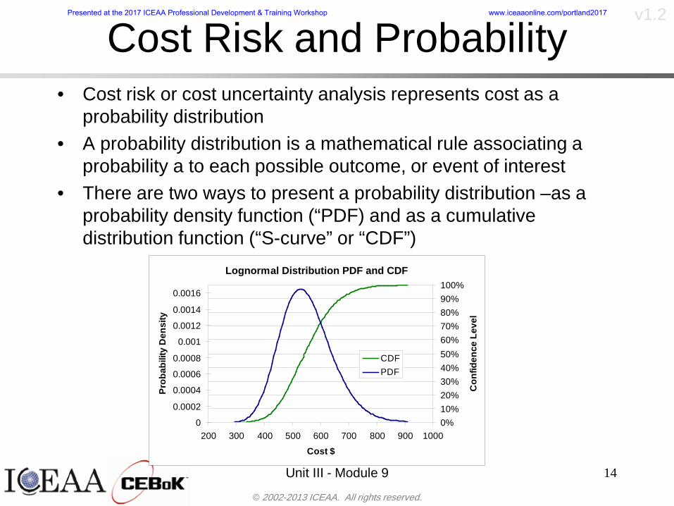
copy 2002-2013 ICEAA All rights reserved
v12
Cost Risk and Probabilitybull Cost risk or cost uncertainty analysis represents cost as a
probability distributionbull A probability distribution is a mathematical rule associating a
probability a to each possible outcome or event of interestbull There are two ways to present a probability distribution ndash as a
probability density function (ldquoPDF) and as a cumulative distribution function (ldquoS-curverdquo or ldquoCDFrdquo)
Unit III - Module 9 14
Lognormal Distribution PDF and CDF
0102030405060708090100
200 300 400 500 600 700 800 900 1000Cost $
Con
fiden
ce L
evel
0
00002
00004
00006
00008
0001
00012
00014
00016
Prob
abili
ty D
ensi
ty
CDFPDF
Presented at the 2017 ICEAA Professional Development amp Training Workshop wwwiceaaonlinecomportland2017
copy 2002-2013 ICEAA All rights reserved
v12
Unit III - Module 9 15
Probability Model ndash Distributionbull Normal
ndash Best behavior most iconic
ndash Theoretically (although not practically) allows negative costs which spook some users
ndash Symmetric needs mean shift to reflect propensity for positive growth
bull Lognormalndash A natural result in
non-linear CERsndash Indistinguishable
from Normal at CVs below 25
ndash Skewed
10
4
10
Presented at the 2017 ICEAA Professional Development amp Training Workshop wwwiceaaonlinecomportland2017
copy 2002-2013 ICEAA All rights reserved
v12
Unit III - Module 9 16
bull Triangularndash Most commonndash Easy to use easy to understandndash Modes medians do not addndash Skewed
bull Betandash Rare now but formerly popularndash Solves negative cost and duration issuesndash Many parameters ndash simplifications like PERT
Beta are possiblendash Skewed
bull Bernoullindash Probability is only assigned to two possible
outcomes success and failure (p and 1-p)ndash Simplest of all discrete distributionsndash Mean = pndash Variance = p(1-p)
10
Probability Model ndash Distribution
10
10
Presented at the 2017 ICEAA Professional Development amp Training Workshop wwwiceaaonlinecomportland2017
copy 2002-2013 ICEAA All rights reserved
v12
Unit III - Module 9 17
bull Normalndash If there is a sufficiently large number of independently identically distributed
elements (or not too correlated and not too skewed) then the distribution of total cost is normal due to the Central Limit Theorem
bull Lognormalndash For smaller data sets with large amounts of (positive) correlation and
skewness the lognormal distribution may be a better approximation of total cost
ndash Many total cost distributions in smaller data sets test as both normal and lognormal
bull Triangularndash The sum of triangles is not a triangle so this distribution should generally not
be used to characterize total costbull Convolved
ndash If total cost distribution is derived using simulation then it may not particularly resemble anything In this case we simply have a convolved or simulated total cost distribution
Probability ndash Top-Level Distribution
NEW
Presented at the 2017 ICEAA Professional Development amp Training Workshop wwwiceaaonlinecomportland2017
copy 2002-2013 ICEAA All rights reserved
v12
S-Curves and Confidence Levels
Unit III - Module 9 1818
100
70
25
Probability(Confidence
Level)
Cost Estimate(Dollars)
50
The S curve is the cumulative probability distribution coming out of the statistical summing process
70 confidence that project will cost indicated amount or less
Provides information on potential cost as a result of identified project risks
Provides insight into establishing reserve levels
X Y
MR
X = Point estimateZ = Project requirementY = Cost estimate where there is a 70 change that
final actual cost will be less than cost estimateY-Z= Manage reserve (MR) which is REQUIRED to meet 70 CL
Z
X not always = Z but is based on same content
Presented at the 2017 ICEAA Professional Development amp Training Workshop wwwiceaaonlinecomportland2017
copy 2002-2013 ICEAA All rights reserved
v12
19
Example ndash Normal Distribution
bull Normal distribution with mean equal to 100 and standard deviation equal to 20
bull Median and mode also equal 100bull The 80th Percentile is 117
40 60 80 100 120 140 160
80 of distribution(area under curve)is less than 117
117
Presented at the 2017 ICEAA Professional Development amp Training Workshop wwwiceaaonlinecomportland2017
copy 2002-2013 ICEAA All rights reserved
v12
20
Confidence Levelsbull The output of a cost risk analysis is a probability
distributionndash Typically displayed as a cumulative distribution function or
ldquoS-curverdquondash Confidence levels are simply percentiles of the distribution
0
10
20
30
40
50
60
70
80
90
100
30 60 90 120 150 180
Conf
iden
ce L
evel
Presented at the 2017 ICEAA Professional Development amp Training Workshop wwwiceaaonlinecomportland2017
copy 2002-2013 ICEAA All rights reserved
v12
Measuring Parametric Model Uncertainty
bull When developing estimates using cost-estimating relationships (CERs) there are two major sources of uncertaintyndash Technical (model input) uncertaintyndash Estimating uncertainty
bull Technical uncertainty reflects the uncertainty inherent in the model inputsndash Typical parametric model inputs include weight lines of code
heritage and other performance and management inputs
bull Estimating uncertainty measures the uncertainty inherent in the model due to the modelrsquos inability to capture all aspects of variability in the data
21
Presented at the 2017 ICEAA Professional Development amp Training Workshop wwwiceaaonlinecomportland2017
copy 2002-2013 ICEAA All rights reserved
v12
Parametric Model Examplebull The NASAAir Force Cost Model (NAFCOM) is a
parametric model for estimating acquisition costs for spacecraft and launch vehicles
bull The CERs in NAFCOM have the formCost = C WeightVNewDesignWTechnicalXManagementY ClassZ
bull There is technical uncertainty about each of the parametersndash Parametric models are applied early in a program so there
is significant amount of uncertainty in the weightndash Heritage is also tricky it is inherently subjective and project
personnel are typically optimisticndash Technical characteristics can also change as a program
matures and requirements change
22
Presented at the 2017 ICEAA Professional Development amp Training Workshop wwwiceaaonlinecomportland2017
copy 2002-2013 ICEAA All rights reserved
v12
Weight Uncertaintybull Aerospace weight growth study average satellite
weight growth from program inception to launch is 28
23
Aerospace Weight Growth Data
-10
0
10
20
30
40
50
60
0 4 8 12 16 20 24 28 32 36 40 44 48 52 56 60 64 68 72 76 80 84 88 92 96 100
Percent Program Completion
Perc
ent W
eigh
t Gro
wth
Presented at the 2017 ICEAA Professional Development amp Training Workshop wwwiceaaonlinecomportland2017
copy 2002-2013 ICEAA All rights reserved
v12
Estimating Uncertaintybull CERs do not perfectly fit the historical data
ndash There are non-repeatable random effects that cannot be predicted
bull For examplendash Parts breaking during testingndash Strikes which are difficult to predict
bull This results in an underlying uncertainty distribution about an estimatendash The outcome of a CER represents only one point on an
uncertainty distributionbull Typically mean or median depending upon the CER
methodology
24
Presented at the 2017 ICEAA Professional Development amp Training Workshop wwwiceaaonlinecomportland2017
copy 2002-2013 ICEAA All rights reserved
v12
Estimating Uncertainty (2)
25
Presented at the 2017 ICEAA Professional Development amp Training Workshop wwwiceaaonlinecomportland2017
copy 2002-2013 ICEAA All rights reserved
v12
Estimating Uncertainty (3)bull In the case of a linear regression the estimating
uncertainty follows a normal distributionndash The estimate is the mean and the standard error of the
estimate from the regression is the standard deviation of the normal distribution
bull In the case of a log-transformed linear regression the estimating uncertainty follows a lognormal distributionndash The estimate is the median of the lognormal and the
standard error of the estimate from the regression is the standard deviation of the normal distribution (in log-space)
bull There is additional uncertainty about an estimate based upon the distance of what is being estimated from the mean of the input datandash This results in a prediction interval
26
Presented at the 2017 ICEAA Professional Development amp Training Workshop wwwiceaaonlinecomportland2017
copy 2002-2013 ICEAA All rights reserved
v12
Aggregating Riskbull Risk is typically applied at the same level at
which we estimate cost that is at the Work Breakdown Structure (WBS) level
bull The estimates for each WBS are developedndash These estimates sum to yield the total system cost
bull For an n-element WBS the total cost is the sum of the cost for each of the n elements
27
nXXXCostSystem +++= 21
Presented at the 2017 ICEAA Professional Development amp Training Workshop wwwiceaaonlinecomportland2017
copy 2002-2013 ICEAA All rights reserved
v12
WBS Examplebull Launch Vehicle
ndash Structurebull Vehicle Structurebull Tank Structure
ndash Thermal Controlbull Active Thermal Controlbull Induced Thermal Controlbull Tank Thermal Control
ndash Main Propulsion Systemndash Liquid Rocket Enginendash Electric Power and Distributionndash Command Control and Data Handlingndash System Integration
28
Presented at the 2017 ICEAA Professional Development amp Training Workshop wwwiceaaonlinecomportland2017
copy 2002-2013 ICEAA All rights reserved
v12
WBS and Risk
29
Presented at the 2017 ICEAA Professional Development amp Training Workshop wwwiceaaonlinecomportland2017
copy 2002-2013 ICEAA All rights reserved
v12
Aggregating Riskbull This leads us to the issue of aggregating the risks across the
WBSbull For example if we want to determine the 70th percentile of the
overall cost risk distribution how do we proceed bull Note that we cannot simply add the 70th percentiles of each of
the cost risk distributionsbull We can add means and variances (taking correlation into
account more on that later) but that is all
Variance of Total Cost =
30
Mean of Total Cost = ( )E X E Xk
k
n
kk
n
kk
n
= = =aringaelig
egraveccediloumloslashdivide
= =aring aring1 1 1
m
Var X kk
n
=aringaelig
egraveccediloumloslashdivide1
= s r s skk
n
iji
j
i jj
n2
1 1
1
22+aring aringaring
= =
-
=
Presented at the 2017 ICEAA Professional Development amp Training Workshop wwwiceaaonlinecomportland2017
copy 2002-2013 ICEAA All rights reserved
v12
Percentiles Do Not Addbull As a notional example consider two independent normal
distributionsndash One distribution has mean equal to 100 and standard deviation
equal to 20ndash The second distribution has mean 300 and standard deviation of 80
bull The sum of two independent normally distributed random variables is also normally distributed
bull To combine the two distributions we add the means and add the variancesndash Total mean is
ndash Total standard deviation is
31
400300100 =+
8258020 22 raquo+
Presented at the 2017 ICEAA Professional Development amp Training Workshop wwwiceaaonlinecomportland2017
copy 2002-2013 ICEAA All rights reserved
v12
Percentiles Do Not Add (2)bull The 80th percentiles for the individual distributions are
117 and 367 respbull The 80th percentile of the combined distribution is
469 but the sum of the two 80th percentiles is 484bull To see why this is the case note that the percentiles
of a normal distribution are determined by the mean and the standard deviationndash The standard deviations are not added when normal distributions
are combined rather the variances are combinedndash Sum of variances is ndash The standard deviation of this sum is
32
22 ba +22 ba +
Presented at the 2017 ICEAA Professional Development amp Training Workshop wwwiceaaonlinecomportland2017
copy 2002-2013 ICEAA All rights reserved
v12
Percentiles Do Not Add (3)bull Since bull We can write
bull The left side of this inequality represents the risk of the combined distributions while the right side represents the sums of the individual risks
bull Combining two missions that are independent results in a diversification of riskndash The total portfolio is not as risky on a relative basis as each
individual project
33
2222 2 bababa ++lt+
baba +lt+ 22
Presented at the 2017 ICEAA Professional Development amp Training Workshop wwwiceaaonlinecomportland2017
copy 2002-2013 ICEAA All rights reserved
v12
Methods for Aggregating Riskbull Since percentiles do not add we have to find other
ways to aggregate riskbull One method is to use Monte Carlo simulationbull Unless cost risk is represented by normal
distributions for all WBS elements summing the means and variances does not result in a completely accurate depiction of overall system cost risk
bull The normal distribution is not a realistic distribution for representing risk in many or even most situations since regarding project risk more can go wrong than can go right which means the risk is NOT symmetric unlike the Gaussian bell curve
34
Presented at the 2017 ICEAA Professional Development amp Training Workshop wwwiceaaonlinecomportland2017
copy 2002-2013 ICEAA All rights reserved
v12
Unit III - Module 9 35
Monte Carlo Simulationfor Risk Analysis
bull When risk analysis is performed multiple risks are gatheredndash These risks may have various probability
distributions
bull Monte Carlo is the most commonly accepted way to produce an accurate characterization of the distribution of the combined effect of these many risksndash Using this distribution we can produce percentiles
for cost impacts due to risk occurrences
10
Presented at the 2017 ICEAA Professional Development amp Training Workshop wwwiceaaonlinecomportland2017
copy 2002-2013 ICEAA All rights reserved
v12
Monte Carlo Simulationbull Simulation is a means for solving problems that are
analytically intractablendash Involves repeated random sampling
bull It was developed during the Manhattan Project as a way to model the interactions inside an atom during nuclear fissionndash Allowed for more sophisticated mathematical modeling of atomic
phenomena
bull Most computer packages use pseudo-random number generators that produce seemingly random results from an initial seedndash Example is the linear congruential generator
36
( ) mbaXX nn mod1 +=+
Presented at the 2017 ICEAA Professional Development amp Training Workshop wwwiceaaonlinecomportland2017
copy 2002-2013 ICEAA All rights reserved
v12Using Random Numbers to Simulate Distributions
bull WBS cost risk is typically measured by a probability distributionbull The most common method for simulating a probability
distribution is the inverse methodbull This involve obtaining a simulated random value from a uniform
distribution and then inverting this through the cumulative distribution function (CDF) to obtain the simulated value
bull As an example for a uniform distribution on the interval [0100]
bull In this case the CDF random value of 05 translates to 10005 = 50
37
( )100
1=xf ( )
100xxF = ( ) xxF 1001 =-
Presented at the 2017 ICEAA Professional Development amp Training Workshop wwwiceaaonlinecomportland2017
copy 2002-2013 ICEAA All rights reserved
v12
Simulating a Triangular Distribution
bull For a triangular distribution with low = 0 most likely = 50 and high = 150 the CDF is given by
bull The inverse function is given by
38
( )iumliumlicirc
iumliumliacute
igrave
poundlt--
poundpound=
1505021
1500050
50015000
2
2
2
xxx
xxxF
( )iumliumlicirc
iumliumliacute
igrave
poundltdivideoslashouml
ccedilegraveaelig +--
poundpound=-
131
21
37501
250017500150
3107500
1
xx
xxxF
Presented at the 2017 ICEAA Professional Development amp Training Workshop wwwiceaaonlinecomportland2017
copy 2002-2013 ICEAA All rights reserved
v12
Simulating a Triangular Distribution (2)
bull If the simulated uniform value is equal to 02 the corresponding inverse value from the CDF inverse is approximately 387
39
0
01
02
03
04
05
06
07
08
09
1
0 30 60 90 120 150
Presented at the 2017 ICEAA Professional Development amp Training Workshop wwwiceaaonlinecomportland2017
copy 2002-2013 ICEAA All rights reserved
v12
Monte Carlo and the WBSbull Simulation involves repeated trials
40
WBS Draw1 2 3 4 5
System 2912 3566 4390 2954 4655 Sum
Structure 80 105 55 80 57 SumVehicle Structure 50 70 30 40 20Tank Structure 30 35 25 40 37
Thermal Control 32 36 35 29 33 SumActive Thermal Control 10 15 12 7 10Induced Thermal Control 12 14 13 14 14Tank Thermal Control 10 7 10 8 9
Main Propulsion System 100 150 125 140 100
Liquid Rocket Engine 1000 1100 1800 900 2200
Electric Power and Distribution 100 125 150 75 90
Command Control and Data Handling 200 250 225 230 275
System Integration 1400 1800 2000 1500 1900
Presented at the 2017 ICEAA Professional Development amp Training Workshop wwwiceaaonlinecomportland2017
copy 2002-2013 ICEAA All rights reserved
v12
Number of Trialsbull Monte Carlo involves a repeated number of trialsbull The greater the number of trials the more accurate the
simulation will approximate the overall cost risk behavior of the system
bull After 100 trials the histogram looks very jagged
41
Presented at the 2017 ICEAA Professional Development amp Training Workshop wwwiceaaonlinecomportland2017
copy 2002-2013 ICEAA All rights reserved
v12
Number of Trials (2)
42
1000 Trials
10000 Trials
50000 Trials Additional trials give a more accurate depiction of the final result
Presented at the 2017 ICEAA Professional Development amp Training Workshop wwwiceaaonlinecomportland2017
copy 2002-2013 ICEAA All rights reserved
v12
Number of Trials (3)bull If we want to simulate the underlying
mean within 1 with 95 confidence for example then we require
43
divideoslash
oumlccedilegrave
aelig poundpound-
=
dividedividedivide
oslash
ouml
ccedilccedilccedil
egrave
aeligpound
-pound
-=
divideoslashouml
ccedilegraveaelig poundpound=
nZ
n
nnX
n
X
n
n
011
010Pr
011
010Pr
011990Pr950
___
___
sm
sm
sm
sm
sm
mm
Presented at the 2017 ICEAA Professional Development amp Training Workshop wwwiceaaonlinecomportland2017
copy 2002-2013 ICEAA All rights reserved
v12
Number of Trials (4)bull This means that the number of trials required is determined by
bull Solving for n we find that at least
trials are neededbull Note that this term involves the coefficient of variation of the
distribution which means that distributions with less dispersion require fewer trials to accurate simulate
44
96101
=ns
m
ms41638
Presented at the 2017 ICEAA Professional Development amp Training Workshop wwwiceaaonlinecomportland2017
copy 2002-2013 ICEAA All rights reserved
v12
Number of Trials (5)bull Simulating percentiles requires more trials than for simulating
meansbull Let Pn represent the number of trials in the sample at or below
the 70th percentile of the underlying distribution (suppose this is known)
bull By the Central Limit Theorem Pnn follows a normal distribution with mean equal to the 70th percentile and variance equal to
bull By a similar process for the mean we find that the number of trials needed to simulate the 70th percentile within 1 with 95 confidence is
45
( )n
FF 700700 1-
n
n
PPn -41638
Presented at the 2017 ICEAA Professional Development amp Training Workshop wwwiceaaonlinecomportland2017
copy 2002-2013 ICEAA All rights reserved
v12
Number of Trials (6)bull If Pn 070 for all n then n is approximately
bull For the sake of comparison suppose CV = 03 (reasonable approximation for hardware development) then the number of trials needed to simulate the mean with the same accuracy is then ldquoonlyrdquo 11525
bull More trials are needed to accurately simulate percentiles than means
46
( ) 46416703041638
70704168341638 =divide
oslashouml
ccedilegraveaelig=divide
oslashouml
ccedilegraveaelig -
=-
nnn
PPn
n
n
Presented at the 2017 ICEAA Professional Development amp Training Workshop wwwiceaaonlinecomportland2017
copy 2002-2013 ICEAA All rights reserved
v12
Methods of Simulationbull Monte Carlo simulation is a standard term for
simulationbull However there is an improvement on Monte Carlo
that improves the accuracy of the results of a simulation for a given number of trials
bull This method is call the Latin Hypercube approach to simulationndash Similar to Monte Carlo but an equal number of draws are taken
from a set of subintervals for example dividing the interval (01) into [00001) [0102)hellip [0910]
ndash Instead of 10 trials from [01] we have one trial from each subinterval
ndash Rough rule of thumb is Latin Hypercube takes 30 fewer trials to achieve similar accuracy to Monte Carlo
47
Presented at the 2017 ICEAA Professional Development amp Training Workshop wwwiceaaonlinecomportland2017
copy 2002-2013 ICEAA All rights reserved
v12
Probability Model ndash Correlationbull Correlation exists between work breakdown structure
(WBS) cost element costs and between cost and schedule
bull Correlation is a necessary consideration in cost risk analysis
bull Correlation is a number that can vary between -1 and +1 and represents the strength of the relationship between the two variablesndash If both variable have a tendency to move in the same direction
correlation is positivendash If when one variable increases the other tends to decrease and
vice-versa the correlation between the two variables is negative
Presented at the 2017 ICEAA Professional Development amp Training Workshop wwwiceaaonlinecomportland2017
copy 2002-2013 ICEAA All rights reserved
v12
Correlation And Causationbull Note that correlation is not causation however
causation implies correlationndash For example shark attacks and ice cream sales at the beach
bull For example for a launch vehicle structure increasing the diameter will not only result in an increase in the structures cost but will also result in higher costs for thermal coating (paint etc)
bull Also simply because two subsystems do not appear to be related does not mean they are not correlatedndash For example structures and computer equipment seemingly
have little relation to one another however an external factor such as a funding cut or a strike will impact all subsystems leading to delays and increasing cost across the board
ndash Thus everything in a WBS has some correlationUnit III - Module 9 49
Presented at the 2017 ICEAA Professional Development amp Training Workshop wwwiceaaonlinecomportland2017
copy 2002-2013 ICEAA All rights reserved
v12
The Importance of Correlationbull Percent that total cost standard deviation is underestimated
when correlation assumed to be 0 instead of r given nWBS elements
Unit III - Module 9 5050
0
20
40
60
80
100
0 01 02 03 04 05 06 07 08 09 1Actual Correlation
Perce
nt Un
deres
timate
d
n = 10
n = 30
n = 100n = 1000
0
20
40
60
80
100
0 01 02 03 04 05 06 07 08 09 1Actual Correlation
Perce
nt Un
deres
timate
d
n = 10
n = 30
n = 100n = 1000
Reference 32nd Annual DOD Cost Analysis Symposium Advanced Training Session ldquoWhy Correlation Matters in Cost Estimatingrdquo Stephen A Book
Presented at the 2017 ICEAA Professional Development amp Training Workshop wwwiceaaonlinecomportland2017
copy 2002-2013 ICEAA All rights reserved
v12
The Importance of Correlation (2)bull For example if correlation is assumed to be 0 for all
elements in a 30 element WBS and the actual correlation is 20 then the total cost standard deviation is underestimated by 60
bull For example assume the total cost is modeled as a normal distribution with mean = 100
bull If correlation is assumed to be zero with total cost standard deviation = 12 when correlation is actually 20 then the true underlying standard deviation is actually 30
bull 70th percentile with zero correlation assumption is 106
bull 70th percentile with 20 correlation is 116 Unit III - Module 9 51
Presented at the 2017 ICEAA Professional Development amp Training Workshop wwwiceaaonlinecomportland2017
copy 2002-2013 ICEAA All rights reserved
v12
Measures of Correlationbull Two measures of correlation are commonly used in
cost risk analysesndash Pearsonrsquos product-moment correlation coefficient ndash Spearmanrsquos rank correlation coefficient
bull Garvey and others recommend using Pearsonrsquos product-moment correlation coefficient correlation for cost risk analysesndash Method of moments uses this but there are two options in
simulationndash Popular simulation packages like Risk and Crystal Ball use
rank correlation but in practice this has been found to make little difference
ndash Pearson product-moment correlation has been incorporated into Risk+
52
Presented at the 2017 ICEAA Professional Development amp Training Workshop wwwiceaaonlinecomportland2017
copy 2002-2013 ICEAA All rights reserved
v12
Pearson Correlationbull Pearsonrsquos product-moment correlation measures
degree of linearity between two random variables bull If two random variables are perfectly linear (eg Y =
aX + b) with positive slope then the Pearson product-moment correlation between X and Y denoted by rXY is +1
53
X X
Y Y Y
XNegative Correlation Positive Correlation No Correlation
middotmiddot
middotmiddot
middotmiddot middotmiddot
middotmiddot
middot
middot
middotmiddotmiddot
middotmiddot
middotmiddot
middotmiddot middot
middot
middot
middotmiddotmiddotmiddotmiddotmiddotmiddotmiddot
middotmiddotmiddotmiddot
middotmiddot
middotmiddot middotmiddotmiddotmiddot
middotmiddotmiddot
middotmiddotmiddotmiddot
middotmiddotmiddot
middotmiddotmiddot
middotmiddot
middot
middot middotmiddot
middot middotmiddotmiddotmiddot middotmiddot middot middotmiddot middot middot
middotmiddot middot
middotmiddotmiddotmiddotmiddot middot middotmiddot
middotmiddot
middot
middotmiddot
middotmiddot middot
middot middot middot
middotmiddot middot
middotmiddotmiddot
middotmiddot
middot middot
Presented at the 2017 ICEAA Professional Development amp Training Workshop wwwiceaaonlinecomportland2017
copy 2002-2013 ICEAA All rights reserved
v12
Spearman Correlationbull Spearmanrsquos rank correlation measures the
monotonicity between two random variablesbull If two random variables are perfectly monotonically
increasing (eg Y = X2) then the Spearman rank correlation denoted by rXY is +1
bull The two measures can be significantly different
54
10 20 30 40 50 60
100
200
300
096 097 098 099 1
1
060
020
040
080
Eff
ort (
Staf
f-M
onth
s)
Software Size I KDSI
y = 28z12y
z x
yy = x100
0 pound x pound 1
Figure 5-9A Figure 5-9B
Pearson Correlation = 09976 Rank Correlation = 1
Pearson Correlation = 024 Rank Correlation = 1
X(x ) ~ Unif(01)
Reference Probability Methods for Cost Uncertainty Analysis A Systems Engineering Perspective Paul R Garvey
Presented at the 2017 ICEAA Professional Development amp Training Workshop wwwiceaaonlinecomportland2017
copy 2002-2013 ICEAA All rights reserved
v12
Unit III - Module 9 55
200
250
300
350
400
1000 1200 1400 1600 1800 2000
Recurring Production
SEPM
200
250
300
350
400
1000 1200 1400 1600 1800 2000
Recurring Production
SEPM
Functional Correlationbull Old No Functional
Correlation Simulation run with WBS items entered as values
bull New Simulation run with functional dependencies entered as they are in cost model
CorrelatedNot Correlated
Note shift of mean and increased variability
Presented at the 2017 ICEAA Professional Development amp Training Workshop wwwiceaaonlinecomportland2017
copy 2002-2013 ICEAA All rights reserved
v12
Risk Measuresbull ldquoWestern Europe conquered the word because of a
technological revolution that started because of attempts to measure the worldrdquo ndash Phillipe Jorion ndash In the same way attempts to measure risk will lead to better project
managementbull Risk management for DoD and NASA agencies focuses
primarily on funding projects to a single percentile ndash NASA policy explicitly mentions 70 and 50ndash This is known as ldquoValue at Riskrdquo and is prevalent in the banking and
financial industry
56
Presented at the 2017 ICEAA Professional Development amp Training Workshop wwwiceaaonlinecomportland2017
copy 2002-2013 ICEAA All rights reserved
v12
Value at Risk (VaR)bull VaR is a percentile of the cost risk
distributionndash VaR funding at the 70th percentile means that
there is a 30 chance of final project cost exceeding the funded amount (budget)
bull VaR has some meritsndash Common measure can be used to compare
different projects and programsndash Easily understood by senior managers and
decision makers
57
Presented at the 2017 ICEAA Professional Development amp Training Workshop wwwiceaaonlinecomportland2017
copy 2002-2013 ICEAA All rights reserved
v12
Why 70th or 80th Percentilebull Typical policy guidance involves funding at the 70th or 80th
percentile Why fund as such a low percentilebull There is some incentive to not over-fundbull For a normal distribution an inflection point occurs near the 80th
percentile meaning that for values above 80 confidence achieving higher levels of confidence can only be achieved by spending greater dollar amounts at an increasing rate
58
-05-04-03-02-01
00102030405
0 05 1 15 2 25 3
Standard Deviations from Mean
Normal Distribution
First DerivativeSlopeVelocity
Second DerivativeConvexityAcceleration
Inflection point at one standard deviation above the mean (~84th
percentile)
Presented at the 2017 ICEAA Professional Development amp Training Workshop wwwiceaaonlinecomportland2017
copy 2002-2013 ICEAA All rights reserved
v12
Funding Above Inflection Pointsbull As the percentile goes above the 80th percentile the amount
needed to achieve that higher level of confidence begins to increase at an increasing rate as is evident from the graph
59
0
10
20
30
40
50
60
70
50 55 60 65 70 75 80 85 90 95 100
$ Ab
ove
MEa
n to
Ach
ieve
Per
cent
ile
Percentile (Confidence Level)
Presented at the 2017 ICEAA Professional Development amp Training Workshop wwwiceaaonlinecomportland2017
copy 2002-2013 ICEAA All rights reserved
v12
Why Budget to the 70th or 80thbull Government projects are funded at the 70th or 80th percentilesbull Why not the 90th or 99th percentile Wonrsquot that help prevent
overrunsndash As we have seen percentiles do not add across programs
bull The sum of the 80th percentiles does NOT equal the total 80th percentile
ndash This is because the individual programs are riskier than the entire suite of missions
bull Known as the ldquoPortfolio effectrdquo (more or this later)
ndash Funding at the 80th gives confidence that the entire portfolio will be adequately funded
bull And since there is an inflection point near the 80th percentile funding above that level quickly becomes cost prohibitive
60
Presented at the 2017 ICEAA Professional Development amp Training Workshop wwwiceaaonlinecomportland2017
copy 2002-2013 ICEAA All rights reserved
v12
Inflection Points for Lognormalbull For a lognormal the inflection point
variesndash Coefficient of variation equal to 10 equates to an
inflection point at the 70th percentile
61
0
10
20
30
40
50
60
70
050 060 070 080 090 100
Coef
ficen
t of V
aria
tion
Percentile of the Inflection Point
Presented at the 2017 ICEAA Professional Development amp Training Workshop wwwiceaaonlinecomportland2017
copy 2002-2013 ICEAA All rights reserved
v12
Issues with Percentile Fundingbull However risk management does not stop at a
specific percentilendash What happens when the 70th percentile is exceeded
bull Any effective risk management policy should prescribe what happens after a bad event occursndash With VaR we only know when a bad event has occurred ndash Also funding at a relatively low level means we have no true
sense of the real risks that should be guarded against
62
Presented at the 2017 ICEAA Professional Development amp Training Workshop wwwiceaaonlinecomportland2017
copy 2002-2013 ICEAA All rights reserved
v12
ldquoHere There Be Dragonsrdquobull On old maps uncharted territory was often
marked with monsters or dragons
63
A section of the Carta Marina by Olaus Magnus 16th Century
Presented at the 2017 ICEAA Professional Development amp Training Workshop wwwiceaaonlinecomportland2017
copy 2002-2013 ICEAA All rights reserved
v12
Distribution Comparisonbull Four different distributions with the same 70th
percentile
bull Should we expect the tails to be similar
64
0
10
20
30
40
50
60
70
80
0 100 200 300 400 500 600
Perc
entil
eCo
nfid
ence
Lev
el
Triangular
Normal
Lognormal
Pareto
Presented at the 2017 ICEAA Professional Development amp Training Workshop wwwiceaaonlinecomportland2017
copy 2002-2013 ICEAA All rights reserved
v12Distribution Comparison Tail Behavior
bull The normal and triangular distributions have similar tails but the lognormal and Pareto have much fatter right tails
65
70
75
80
85
90
95
100
500 1500 2500 3500 4500 5500
Perc
entil
eCo
nfid
ence
Lev
el
Triangular
Normal
Lognormal
Pareto
Here There Be Dragons
Presented at the 2017 ICEAA Professional Development amp Training Workshop wwwiceaaonlinecomportland2017
copy 2002-2013 ICEAA All rights reserved
v12Distribution Comparison ndash Tail Behavior (Table)
bull There is significant tail risk for the lognormal and the Paretobull The 99th percentile for the Pareto is 1000 times greater than
the 70th percentilendash Risk seen in financial markets and in catastrophic risks like natural
disasters bull Four different projects follow the four different risk profiles seen
in this example should clearly have different risk management approaches but 70th percentile funding indicates the same risk management approach for all four
66
Percentile Triangular Normal Lognormal Pareto 70th $600 $600 $600 $600 80th $680 $660 $770 $1430 90th $770 $750 $1070 $5880 95th $840 $820 $1410 $23750 99th $930 $950 $2350 $600000
Presented at the 2017 ICEAA Professional Development amp Training Workshop wwwiceaaonlinecomportland2017
copy 2002-2013 ICEAA All rights reserved
v12Percentile Budgeting is Not Risk Management
bull Percentile budgeting ne effective risk management policybull Suppose that you are shopping for a new car You
mention that safety is your top concern The salesman says he has a great safe car available You ask about the air bags Do they work The salesman answers ldquoOf course Seventy percent of the time they work fine Only 30 of the time the air bags will fail to deployrdquo Would you buy such a car Hedge fund manager David Einhorn has stated ldquoRisk management is the air bag that must always work but only in the multi-sigma event where you have an accidentrdquo
67
Risk management is the air bag that must always work but only in the multi-sigma event where you
have an accident
Presented at the 2017 ICEAA Professional Development amp Training Workshop wwwiceaaonlinecomportland2017
copy 2002-2013 ICEAA All rights reserved
v12
Joint Confidence Level Analysisbull Schedules are risky toobull For 98 recent NASA missions average
schedule growth was 38ndash Not as high as cost growth but still significant
68
0
5
10
15
20
25
30
35
40
Schedule
Cost
Presented at the 2017 ICEAA Professional Development amp Training Workshop wwwiceaaonlinecomportland2017
copy 2002-2013 ICEAA All rights reserved
v12
Schedules Impact Costbull Changes in schedule can have enormous
impacts on cost ndash Schedule slips can lead to cost increases
bull Fixed programmatic costs must be paid on a regular basisndash Achieving schedule milestones early can result in cost
savings
bull Schedule is an important consideration in cost analysis including cost risk analysis
bull However we must be careful in correctly integrating cost and schedule riskndash Schedule is not simply an input but is dependent on many of
the same factors that drive cost
69
Presented at the 2017 ICEAA Professional Development amp Training Workshop wwwiceaaonlinecomportland2017
copy 2002-2013 ICEAA All rights reserved
v12
The Relationship of Cost to Schedulebull Cost and schedule are positively correlated
ndash A larger program with bigger scope with take longer to complete than a smaller simpler program
bull However longer schedules do not always equate to higher cost nor shorter schedules with lower costndash Highly compressed schedules relative to the
optimal schedule can lead to large overrunsbull Compressed schedules are commonplace for
many planetary missions
70
Presented at the 2017 ICEAA Professional Development amp Training Workshop wwwiceaaonlinecomportland2017
copy 2002-2013 ICEAA All rights reserved
v12The Impact of Schedule GrowthCompression on Cost
bull Compressed schedules lead to cost growth and based on existing research is actually more expensive than schedule slippages
71
0
20
40
60
80
100
120
140
160
-50 -25 0 25 50 75 100
Percentage Change in Schedule
Perc
enta
ge C
hang
e in
Cos
t due
to
Sche
dule
Cha
nge
Source Smart CB ldquoCost and Schedule Interrelationshipsrdquo 2007 NASA Cost Symposium
Presented at the 2017 ICEAA Professional Development amp Training Workshop wwwiceaaonlinecomportland2017
copy 2002-2013 ICEAA All rights reserved
v12Schedule as an Independent Variable
bull Why not simply add schedule as an input to cost-estimating relationships (CERs)
bull Schedule is often treated as an independent variable ndash schedules are often determined independently of cost considerationsndash Cost may not be considered explicitly although budgets and
schedules are determined based on scope and other common factors
bull In 2006 SAIC undertook a research task to determine the impact of schedule on cost and added schedule as an independent variable to the CERs in the NASAAir Force Cost Model (NAFCOM) to see if schedule provided any improvement in goodness of fit
72
Presented at the 2017 ICEAA Professional Development amp Training Workshop wwwiceaaonlinecomportland2017
copy 2002-2013 ICEAA All rights reserved
v12
Schedule is a Dependent Variablebull Since NAFCOM includes an exhaustive list of cost drivers the inclusion
of schedule should give an indication of whether there is any additional independent value added from schedule independent of the cost drivers
bull In the study schedule was added to 10 subsystem-level CERs
ndash In each case the addition of schedule did NOTimprove the goodness of fit and schedule was NOT found to be a statistically significant cost driver (given the presence of the other variables) for any of the 10 CERs
bull Standard errors for the CERs increased due to decrease in degrees of freedom
bull Thus schedule as an independent variable did not provide any additional explanation of variation in historical cost
bull This is because schedule is truly NOT an independent variable but a dependent variable and is a function of the same factors that drive cost
73
Presented at the 2017 ICEAA Professional Development amp Training Workshop wwwiceaaonlinecomportland2017
copy 2002-2013 ICEAA All rights reserved
v12
Incorporation of Schedule in Cost Risk
bull When using subjective methods care must be taken in applying schedule to cost risk analysis
bull Since schedule is a dependent variable treating it independently from other factors when assessing its impact on cost can lead to a double count of independent variables in the cost risk analysis
bull Direct inclusion of schedule in a cost risk analysis effectively doubles the influence of each cost driver
ndash Incorrectly leads to broader risk ranges
74
CostWeight
HeritageNewness
Technology Readiness Schedule
Presented at the 2017 ICEAA Professional Development amp Training Workshop wwwiceaaonlinecomportland2017
copy 2002-2013 ICEAA All rights reserved
v12Subjective Cost Risk Methods and Overinclusion of Risk Factors
bull Subjective methods are suitable when data are scarce or not availablebull However care must be taken not to treat correlated sources of risk
such as schedule as independent of each otherbull Example ndash a subjective risk analysis incorporated technology readiness
design risk requirements stability integration risk and schedule and treated each source of risk as independent
bull Risk triangle high value without schedule risk was 31 times the point estimate
bull Risk triangle high value with schedule risk added on top of other sources of risk treated independently was 34 times the point estimate
bull Risk triangle taking correlation between sources of risk into account in a rigorous statistical manner has a high value 15 times the point estimate less than half the effect when treating sources of risk as independent
75
Presented at the 2017 ICEAA Professional Development amp Training Workshop wwwiceaaonlinecomportland2017
copy 2002-2013 ICEAA All rights reserved
v12Fundamental Equation of Cost and Schedule Interrelationships
bull The Fundamental Equation of the Relationship Between Cost and Schedule is
Time = Moneybull This is a well known adage that time is money Your boss at
work may even mention this to you from time to time or if you are the boss you are all too aware of this iron law
bull Because time is money cost and schedule risk should be modeled jointly not with schedule as an independent cost driver
bull Note that cost and schedule are not perfectly correlatedndash Cost can sometimes ldquobuy downrdquo schedule extra money can be
spent to meet a deadline since in some cases additional effort to hasten the completion of a task
76
Presented at the 2017 ICEAA Professional Development amp Training Workshop wwwiceaaonlinecomportland2017
copy 2002-2013 ICEAA All rights reserved
v12How to (Correctly) Incorporate Schedule into Cost Risk Analysis
bull The best way to model cost and schedule risk is to develop a joint cost and schedule model based on the same data
bull Since such models are not currently available the next best approach is to model cost and schedule independently and then integrate cost and schedule risk analyses using joint probability distributions taking into account correlation between cost and schedulendash This approach pioneered by Paul Garvey and Steve Book is
considered industry best practicendash This is a practical method mathematically tractable and follows
naturally from the Fundamental Equation of Cost and Schedule Interrelationships
77
Book S A ldquoQuantifying the Relationship Between Cost and Schedulerdquo The Measurable News Winter 2007-2008 pp 11-15Garvey PR Probability Methods for Cost Uncertainty Analysis A Systems Engineering Perspective New York Marcel Dekker 2000 pp 308-335
Presented at the 2017 ICEAA Professional Development amp Training Workshop wwwiceaaonlinecomportland2017
copy 2002-2013 ICEAA All rights reserved
v12
Joint Lognormal and Normal Distributions
bull Cost and schedule are typically modeled as some combination of Normal and Lognormal probability distributionsndash Studies by The Aerospace Corporation the MITRE
Corporation Wyle Labs and SAIC have found that the Lognormal probability distribution almost always serves as a good model for both the schedule distribution and the cost distribution
ndash The Normal distribution may also be appropriate in some instances and depending upon the level of confidence at which budgets are set may even be more conservative and logically consistent than the Normal distribution
ndash Joint Lognormal and Normal distributions are defined by a pair of mean and standard deviations and a level of correlation between the two
78
Presented at the 2017 ICEAA Professional Development amp Training Workshop wwwiceaaonlinecomportland2017
copy 2002-2013 ICEAA All rights reserved
v12Modeling Cost and Schedule as a Bivariate Distribution
bull In the approach set forth by Book and Garvey cost risk is assessed and the top-level distribution is modeled as a Lognormal (or Normal) distribution schedule risk is assessed and the overall schedule risk is modeled as a Lognormal (or Normal) distribution
bull The two distributions are combined into a Bivariate distribution by assigning a correlation between the two and by treating the two distributions as the marginal distributions of a Bivariate Lognormal distributionndash Other combinations include a Bivariate Normal or a Bivariate
Normal-Lognormal
79
Presented at the 2017 ICEAA Professional Development amp Training Workshop wwwiceaaonlinecomportland2017
copy 2002-2013 ICEAA All rights reserved
v12Bivariate Lognormal Distribution for Cost and Schedule
bull Cost is often observed to be Lognormal when strong positive correlations are present among the systemrsquos WBS cost element costs
bull A systemrsquos schedule is often observed (from Monte Carlo simulations) to be Lognormal if it is the sum of many positively correlated schedule activities in an overall schedule network
bull If Lognormal distributions characterize a systemrsquos cost and schedule then the Bivariate Lognormal could serve as an assumed model of their joint distributionndash In this case the marginal distribution of each of cost and schedule is
Lognormalbull Other possibilities for modeling cost and schedule as a Bivariate
distribution include a Bivariate Normal or a Bivariate Normal-Lognormal distributionndash All these combinations are analytically tractable
80
Presented at the 2017 ICEAA Professional Development amp Training Workshop wwwiceaaonlinecomportland2017
copy 2002-2013 ICEAA All rights reserved
v12Bivariate Lognormal for Cost and Schedule
bull Contour Plots of a Bivariate Lognormal
81
Presented at the 2017 ICEAA Professional Development amp Training Workshop wwwiceaaonlinecomportland2017
copy 2002-2013 ICEAA All rights reserved
v12Correlation Between Cost and Schedule
bull Cost and schedule are positively correlated but not perfectly sondash For example it is possible to have a schedule underrun and a cost
overrunbull Based on cost and schedule growth data for 50 completed NASA
programs the correlation between development cost and development schedule is 70
82
00
200
400
600
800
1000
1200
-500 00 500 1000 1500 2000 2500Historical Cost Growth
Hist
oric
al S
ched
ule
Gro
wth
r = 715
Presented at the 2017 ICEAA Professional Development amp Training Workshop wwwiceaaonlinecomportland2017
copy 2002-2013 ICEAA All rights reserved
v12Correlation Between Cost and Schedule Caveats
bull Based on historical data recommended correlation between cost and schedule is 70 but this could be higher or lower depending upon program circumstancesndash If program is budget constrained cost and schedule will be
more highly correlated (go as you pay)ndash If program is schedule constrained cost and schedule will
have lower correlation perhaps even negative correlation ndash Smaller programs have smaller correlation between cost and
schedule riskbull Relatively easy to ldquohurry uprdquo and finish on time or even early if
needed
83
Presented at the 2017 ICEAA Professional Development amp Training Workshop wwwiceaaonlinecomportland2017
copy 2002-2013 ICEAA All rights reserved
v12
Conditional Confidence Levelsbull Given a programrsquos project schedule we can determine the cost
risk distribution conditional upon the given schedulebull Conditional cost S-curves are steeper than unconditional
(marginal) cost S-curves between some uncertainty has been removed because schedule is fixed
84
Presented at the 2017 ICEAA Professional Development amp Training Workshop wwwiceaaonlinecomportland2017
copy 2002-2013 ICEAA All rights reserved
v12
Joint Confidence Levelsbull Joint 65 confidence represents the probability of
achieving both 65 confidence in cost AND 65 confidence in schedulendash This is different than achieving 65 cost confidence alone
or achieving 65 schedule confidence alonebull Due to the imperfect correlation between cost and schedule it
is possible to achieve a 65 cost confidence with a lower level of schedule confidence
bull Restricting the schedule confidence thus requires additional $ to achieve a given level of confidence
85
X
Y
Possible Values for Which X gt a Possible Values for
Which X gt a and Y gt b
a
b
Presented at the 2017 ICEAA Professional Development amp Training Workshop wwwiceaaonlinecomportland2017
copy 2002-2013 ICEAA All rights reserved
v12Joint Confidence Levels Versus Cost Confidence Levels Only
bull Example of the differences between cost confidence schedule confidence conditional cost confidence and joint cost and schedule confidence
86
Joint Cost-Schedule Confidence Iso-Curves
Cost (RY$M)
Sche
dule
(Mon
ths)
65 Confidence
50 Confidence
70 Confidence
65 Cost Confidence AggressiveSchedule65 Cost ConfidenceScheduleGiven 65 Schedule ConfidenceUnconditional 65 CostConfidenceUnconditional 65 ScheduleConfidence
65 Cost Confidence 65 Joint Cost and Schedule
Confidence for 65 Schedule Confidence
Presented at the 2017 ICEAA Professional Development amp Training Workshop wwwiceaaonlinecomportland2017
copy 2002-2013 ICEAA All rights reserved
v12
Joint Cost and Schedule Confidence
bull Can examine pairs of cost and schedule that achieve a given level of confidence
bull Provides insights into the trade-offs between cost and schedule for a given level of confidencendash Possible to increase cost confidence by giving a
project more time in some instances or possible to ldquobuy downrdquo schedule
bull But these have limits and are shown in the iso-cost and schedule confidence curves
87
Presented at the 2017 ICEAA Professional Development amp Training Workshop wwwiceaaonlinecomportland2017
copy 2002-2013 ICEAA All rights reserved
v12Cost and Schedule Trade-offs for a Given Level of Joint Confidence
bull Hypothetical Example
88
Cost (RY$M)
Schedule (Months)
$100 48$99 48$89 49$87 50$85 51$85 52$84 53$83 55$83 55$83 56
Cost and Schedule 65 Confidence Iso-Curve
4748495051525354555657
$80 $82 $84 $86 $88 $90 $92 $94 $96 $98 $100
Cost (RY$ M)
Sche
dule
(Mon
ths)
Presented at the 2017 ICEAA Professional Development amp Training Workshop wwwiceaaonlinecomportland2017
copy 2002-2013 ICEAA All rights reserved
v12Policy Considerations for Confidence Levels
bull For large programs the difference between the amount of money needed to achieve 65 cost confidence independent of schedule and joint 65 cost and schedule confidence can represent hundreds of millions and even billions of dollars
89
Joint Cost-Schedule Confidence Iso-Curves
Cost (RY$M)
Sche
dule
(Mon
ths)
65 Confidence
65 Cost Confidence AggressiveSchedule
65 Cost ConfidenceScheduleGiven 65 Schedule Confidence
Unconditional 65 CostConfidence
Joint Cost and Schedule Confidence for 65 Cost Confidence and Program Baseline Schedule is Less Than 35
65 Cost Confidence Independent of Schedule Cost Needed to Achieve
Both 65 Joint Cost and Schedule Confidence for the Schedule with 65 Confidence
Presented at the 2017 ICEAA Professional Development amp Training Workshop wwwiceaaonlinecomportland2017
copy 2002-2013 ICEAA All rights reserved
v12
Copulasbull More generally any combination of distributions can
be used (more than just normal and lognormal)ndash Termed ldquocopulardquo from the Italian word for ldquocouplerdquondash Copulas are a way to combine marginal distributions of any
number and type into a joint distributionbull More formally a copula is a multivariate joint distribution defined
on the n-dimensional unit cube [0 1]n such that every marginal distribution is uniform on the interval [0 1]
bull (The bivariate form of) Sklarrsquos theorem states that for any bivariate distribution function H(x y) let F(x) = H(x infin) and G(y) = H(infin y) be the univariate marginal probability distribution functions Then there exists a copula C such that H(xy)=C(F(x)G(y))
ndash Copulas are widely used in risk management for investments and insurance
bull Considered industry best practice (Li 2000)bull Marketed as part of JP Morganrsquos CreditMetrics suite of tools
(Gupton et Al 1997)90
Presented at the 2017 ICEAA Professional Development amp Training Workshop wwwiceaaonlinecomportland2017
copy 2002-2013 ICEAA All rights reserved
v12Parametric Joint Cost and Schedule Analysis
bull A parametric model based on a consistent data set with a set of overlapping cost and schedule drivers is a cleaner way to model cost and schedule
91
CostWeight
HeritageNewness
Technology Readiness
Schedule
0
20
40
60
80
100
Confidence
Joint Cost and Schedule Confidence
Schedule
Cost
Lognormal Distribution PDF and CDF
0102030405060708090100
200 300 400 500 600 700 800 900 1000Cost $
Con
fiden
ce L
evel
0
00002
00004
00006
00008
0001
00012
00014
00016
Prob
abili
ty D
ensi
ty
CDFPDF
Lognormal Distribution PDF and CDF
0102030405060708090100
200 300 400 500 600 700 800 900 1000Cost $
Con
fiden
ce L
evel
0
00002
00004
00006
00008
0001
00012
00014
00016
Prob
abili
ty D
ensi
ty
CDFPDF
Presented at the 2017 ICEAA Professional Development amp Training Workshop wwwiceaaonlinecomportland2017
copy 2002-2013 ICEAA All rights reserved
v12Parametric Joint Cost and Schedule Analysis (2)
bull Joint cost and schedule risk analysis produced naturally by the integrated modelndash Addresses several issues with the copula
approachbull Tail dependencybull Correlation ndash no need to assign correlation
between cost and schedulebull Consistency of cost and schedule models
92
Presented at the 2017 ICEAA Professional Development amp Training Workshop wwwiceaaonlinecomportland2017
copy 2002-2013 ICEAA All rights reserved
v12
Resource-Loaded Schedulesbull Involves assigning cost and schedule risks to a resource-loaded schedule
networkbull Bottom-up approach
ndash More labor intensive than parametrics but can also provide more insight
ndash Can answer questions than parametric typically cannot such as how much do reserve requirements decrease if a specific risk is retired
bull Currently being implemented in Constellation programbull Has same issue as all bottom-up models hard to count all the risks and model
them discretely
ndash As a result there is a tendency to reflect less risk than indicated by history
ndash ldquoThere are more things in heaven and earth Horatio than are dreamt of in your philosophyrdquo William Shakespeare Hamlet Act I Scene V
93
Presented at the 2017 ICEAA Professional Development amp Training Workshop wwwiceaaonlinecomportland2017
copy 2002-2013 ICEAA All rights reserved
v12Resource-Loaded Schedules Vs Parametrics
bull Parametric most appropriate for early estimatesndash But also good for high-level checks as project progresses
bull As plans take shape lower level modeling may be more appropriate
94 1
CONCEPTUALDEVELOPMENT
PROJECTDEFINITION DESIGN DEVELOPMENT OPERATIONS
PARAMETRIC PARAMETRIC
ANALOGY
ENGINEERING (Bottoms Up)
$PARAMETRIC
DETAILED
$
Pre Phase A Phase B Phase CDPhase A Phase EPre Phase A Phase B Phase CDPhase A Phase E
Risk = f(Cost Estimating Relationship Inputs eg mass power data rate TRL new design etc)
Risk = f(cost and schedule variation of the analogous elements)
Risk = f(variation of detailed inputs eg labor hours rates materials etc)
Presented at the 2017 ICEAA Professional Development amp Training Workshop wwwiceaaonlinecomportland2017
copy 2002-2013 ICEAA All rights reserved
v12
Resource-Loaded Schedulesbull Methodology has been demonstrated in other
industriesndash Construction oil and gasndash Analysis has not been traditionally done on highly uncertain
complex development projects bull Methodology focuses on project baseline schedule
ndash In baseline schedule all tasks are resource loaded to represent a baseline schedule and cost standpoint
ndash Resource loaded schedule is ldquorolledrdquo up to a manageable level
ndash Based on the risk and uncertainties identified schedule distributions are applied to each rolled up task
ndash Cost uncertainties are also applied to rolled up tasksbull Uncertainties include labor rate man power etc
ndash A Monte Carlo simulation is run to develop joint cost-schedule distributions
95
Presented at the 2017 ICEAA Professional Development amp Training Workshop wwwiceaaonlinecomportland2017
copy 2002-2013 ICEAA All rights reserved
v12
Unit III - Module 9 96
Execution ndash Cross Checksbull Means The mean cost growth factor for WBS items
can be compared to history as a way to cross check results
bull CVs The CV of the cost growth factors for WBS items can be compared to history as a way to cross check results
bull Inputs Checks are performed on inputs or other parameters to see if historical values are in line with program assumptionsndash Example Historical risk scores can be compared to program
risk scores to see if risk assessors are being realistic and to see if the underlying database is representative of the program
11
Presented at the 2017 ICEAA Professional Development amp Training Workshop wwwiceaaonlinecomportland2017
- Cost and Schedule Risk Analysis Basic
- Acknowledgments
- Unit Index
- Risk Overview
- Agenda
- Introduction
- Risk Analysis Terms
- Are Our Costs Realistic
- Historical Cost Growth
- Sources of Cost Risk
- Point Estimates of Cost
- Types of Risk
- Point Estimates Vs Risk Estimates
- Cost Risk and Probability
- Probability Model ndash Distribution
- Probability Model ndash Distribution
- Probability ndash Top-Level Distribution
- S-Curves and Confidence Levels
- Example ndash Normal Distribution
- Confidence Levels
- Measuring Parametric Model Uncertainty
- Parametric Model Example
- Weight Uncertainty
- Estimating Uncertainty
- Estimating Uncertainty (2)
- Estimating Uncertainty (3)
- Aggregating Risk
- WBS Example
- WBS and Risk
- Aggregating Risk
- Percentiles Do Not Add
- Percentiles Do Not Add (2)
- Percentiles Do Not Add (3)
- Methods for Aggregating Risk
- Monte Carlo Simulationfor Risk Analysis
- Monte Carlo Simulation
- Using Random Numbers to Simulate Distributions
- Simulating a Triangular Distribution
- Simulating a Triangular Distribution (2)
- Monte Carlo and the WBS
- Number of Trials
- Number of Trials (2)
- Number of Trials (3)
- Number of Trials (4)
- Number of Trials (5)
- Number of Trials (6)
- Methods of Simulation
- Probability Model ndash Correlation
- Correlation And Causation
- The Importance of Correlation
- The Importance of Correlation (2)
- Measures of Correlation
- Pearson Correlation
- Spearman Correlation
- Functional Correlation
- Risk Measures
- Value at Risk (VaR)
- Why 70th or 80th Percentile
- Funding Above Inflection Points
- Why Budget to the 70th or 80th
- Inflection Points for Lognormal
- Issues with Percentile Funding
- ldquoHere There Be Dragonsrdquo
- Distribution Comparison
- Distribution Comparison Tail Behavior
- Distribution Comparison ndash Tail Behavior (Table)
- Percentile Budgeting is Not Risk Management
- Joint Confidence Level Analysis
- Schedules Impact Cost
- The Relationship of Cost to Schedule
- The Impact of Schedule GrowthCompression on Cost
- Schedule as an Independent Variable
- Schedule is a Dependent Variable
- Incorporation of Schedule in Cost Risk
- Subjective Cost Risk Methods and Overinclusion of Risk Factors
- Fundamental Equation of Cost and Schedule Interrelationships
- How to (Correctly) Incorporate Schedule into Cost Risk Analysis
- Joint Lognormal and Normal Distributions
- Modeling Cost and Schedule as a Bivariate Distribution
- Bivariate Lognormal Distribution for Cost and Schedule
- Bivariate Lognormal for Cost and Schedule
- Correlation Between Cost and Schedule
- Correlation Between Cost and Schedule Caveats
- Conditional Confidence Levels
- Joint Confidence Levels
- Joint Confidence Levels Versus Cost Confidence Levels Only
- Joint Cost and Schedule Confidence
- Cost and Schedule Trade-offs for a Given Level of Joint Confidence
- Policy Considerations for Confidence Levels
- Copulas
- Parametric Joint Cost and Schedule Analysis
- Parametric Joint Cost and Schedule Analysis (2)
- Resource-Loaded Schedules
- Resource-Loaded Schedules Vs Parametrics
- Resource-Loaded Schedules
- Execution ndash Cross Checks
-
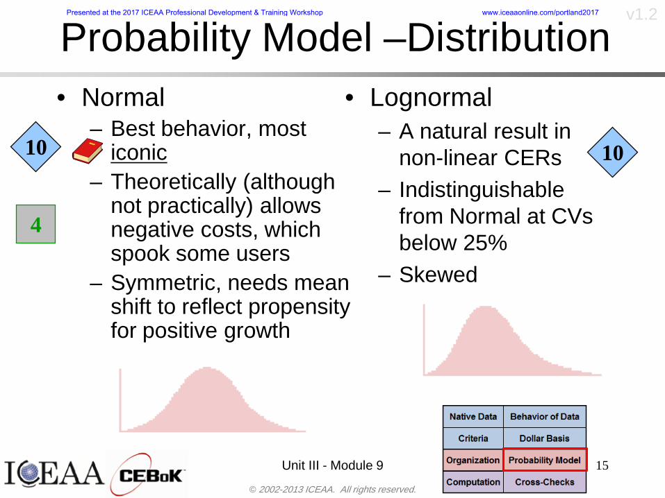
copy 2002-2013 ICEAA All rights reserved
v12
Unit III - Module 9 15
Probability Model ndash Distributionbull Normal
ndash Best behavior most iconic
ndash Theoretically (although not practically) allows negative costs which spook some users
ndash Symmetric needs mean shift to reflect propensity for positive growth
bull Lognormalndash A natural result in
non-linear CERsndash Indistinguishable
from Normal at CVs below 25
ndash Skewed
10
4
10
Presented at the 2017 ICEAA Professional Development amp Training Workshop wwwiceaaonlinecomportland2017
copy 2002-2013 ICEAA All rights reserved
v12
Unit III - Module 9 16
bull Triangularndash Most commonndash Easy to use easy to understandndash Modes medians do not addndash Skewed
bull Betandash Rare now but formerly popularndash Solves negative cost and duration issuesndash Many parameters ndash simplifications like PERT
Beta are possiblendash Skewed
bull Bernoullindash Probability is only assigned to two possible
outcomes success and failure (p and 1-p)ndash Simplest of all discrete distributionsndash Mean = pndash Variance = p(1-p)
10
Probability Model ndash Distribution
10
10
Presented at the 2017 ICEAA Professional Development amp Training Workshop wwwiceaaonlinecomportland2017
copy 2002-2013 ICEAA All rights reserved
v12
Unit III - Module 9 17
bull Normalndash If there is a sufficiently large number of independently identically distributed
elements (or not too correlated and not too skewed) then the distribution of total cost is normal due to the Central Limit Theorem
bull Lognormalndash For smaller data sets with large amounts of (positive) correlation and
skewness the lognormal distribution may be a better approximation of total cost
ndash Many total cost distributions in smaller data sets test as both normal and lognormal
bull Triangularndash The sum of triangles is not a triangle so this distribution should generally not
be used to characterize total costbull Convolved
ndash If total cost distribution is derived using simulation then it may not particularly resemble anything In this case we simply have a convolved or simulated total cost distribution
Probability ndash Top-Level Distribution
NEW
Presented at the 2017 ICEAA Professional Development amp Training Workshop wwwiceaaonlinecomportland2017
copy 2002-2013 ICEAA All rights reserved
v12
S-Curves and Confidence Levels
Unit III - Module 9 1818
100
70
25
Probability(Confidence
Level)
Cost Estimate(Dollars)
50
The S curve is the cumulative probability distribution coming out of the statistical summing process
70 confidence that project will cost indicated amount or less
Provides information on potential cost as a result of identified project risks
Provides insight into establishing reserve levels
X Y
MR
X = Point estimateZ = Project requirementY = Cost estimate where there is a 70 change that
final actual cost will be less than cost estimateY-Z= Manage reserve (MR) which is REQUIRED to meet 70 CL
Z
X not always = Z but is based on same content
Presented at the 2017 ICEAA Professional Development amp Training Workshop wwwiceaaonlinecomportland2017
copy 2002-2013 ICEAA All rights reserved
v12
19
Example ndash Normal Distribution
bull Normal distribution with mean equal to 100 and standard deviation equal to 20
bull Median and mode also equal 100bull The 80th Percentile is 117
40 60 80 100 120 140 160
80 of distribution(area under curve)is less than 117
117
Presented at the 2017 ICEAA Professional Development amp Training Workshop wwwiceaaonlinecomportland2017
copy 2002-2013 ICEAA All rights reserved
v12
20
Confidence Levelsbull The output of a cost risk analysis is a probability
distributionndash Typically displayed as a cumulative distribution function or
ldquoS-curverdquondash Confidence levels are simply percentiles of the distribution
0
10
20
30
40
50
60
70
80
90
100
30 60 90 120 150 180
Conf
iden
ce L
evel
Presented at the 2017 ICEAA Professional Development amp Training Workshop wwwiceaaonlinecomportland2017
copy 2002-2013 ICEAA All rights reserved
v12
Measuring Parametric Model Uncertainty
bull When developing estimates using cost-estimating relationships (CERs) there are two major sources of uncertaintyndash Technical (model input) uncertaintyndash Estimating uncertainty
bull Technical uncertainty reflects the uncertainty inherent in the model inputsndash Typical parametric model inputs include weight lines of code
heritage and other performance and management inputs
bull Estimating uncertainty measures the uncertainty inherent in the model due to the modelrsquos inability to capture all aspects of variability in the data
21
Presented at the 2017 ICEAA Professional Development amp Training Workshop wwwiceaaonlinecomportland2017
copy 2002-2013 ICEAA All rights reserved
v12
Parametric Model Examplebull The NASAAir Force Cost Model (NAFCOM) is a
parametric model for estimating acquisition costs for spacecraft and launch vehicles
bull The CERs in NAFCOM have the formCost = C WeightVNewDesignWTechnicalXManagementY ClassZ
bull There is technical uncertainty about each of the parametersndash Parametric models are applied early in a program so there
is significant amount of uncertainty in the weightndash Heritage is also tricky it is inherently subjective and project
personnel are typically optimisticndash Technical characteristics can also change as a program
matures and requirements change
22
Presented at the 2017 ICEAA Professional Development amp Training Workshop wwwiceaaonlinecomportland2017
copy 2002-2013 ICEAA All rights reserved
v12
Weight Uncertaintybull Aerospace weight growth study average satellite
weight growth from program inception to launch is 28
23
Aerospace Weight Growth Data
-10
0
10
20
30
40
50
60
0 4 8 12 16 20 24 28 32 36 40 44 48 52 56 60 64 68 72 76 80 84 88 92 96 100
Percent Program Completion
Perc
ent W
eigh
t Gro
wth
Presented at the 2017 ICEAA Professional Development amp Training Workshop wwwiceaaonlinecomportland2017
copy 2002-2013 ICEAA All rights reserved
v12
Estimating Uncertaintybull CERs do not perfectly fit the historical data
ndash There are non-repeatable random effects that cannot be predicted
bull For examplendash Parts breaking during testingndash Strikes which are difficult to predict
bull This results in an underlying uncertainty distribution about an estimatendash The outcome of a CER represents only one point on an
uncertainty distributionbull Typically mean or median depending upon the CER
methodology
24
Presented at the 2017 ICEAA Professional Development amp Training Workshop wwwiceaaonlinecomportland2017
copy 2002-2013 ICEAA All rights reserved
v12
Estimating Uncertainty (2)
25
Presented at the 2017 ICEAA Professional Development amp Training Workshop wwwiceaaonlinecomportland2017
copy 2002-2013 ICEAA All rights reserved
v12
Estimating Uncertainty (3)bull In the case of a linear regression the estimating
uncertainty follows a normal distributionndash The estimate is the mean and the standard error of the
estimate from the regression is the standard deviation of the normal distribution
bull In the case of a log-transformed linear regression the estimating uncertainty follows a lognormal distributionndash The estimate is the median of the lognormal and the
standard error of the estimate from the regression is the standard deviation of the normal distribution (in log-space)
bull There is additional uncertainty about an estimate based upon the distance of what is being estimated from the mean of the input datandash This results in a prediction interval
26
Presented at the 2017 ICEAA Professional Development amp Training Workshop wwwiceaaonlinecomportland2017
copy 2002-2013 ICEAA All rights reserved
v12
Aggregating Riskbull Risk is typically applied at the same level at
which we estimate cost that is at the Work Breakdown Structure (WBS) level
bull The estimates for each WBS are developedndash These estimates sum to yield the total system cost
bull For an n-element WBS the total cost is the sum of the cost for each of the n elements
27
nXXXCostSystem +++= 21
Presented at the 2017 ICEAA Professional Development amp Training Workshop wwwiceaaonlinecomportland2017
copy 2002-2013 ICEAA All rights reserved
v12
WBS Examplebull Launch Vehicle
ndash Structurebull Vehicle Structurebull Tank Structure
ndash Thermal Controlbull Active Thermal Controlbull Induced Thermal Controlbull Tank Thermal Control
ndash Main Propulsion Systemndash Liquid Rocket Enginendash Electric Power and Distributionndash Command Control and Data Handlingndash System Integration
28
Presented at the 2017 ICEAA Professional Development amp Training Workshop wwwiceaaonlinecomportland2017
copy 2002-2013 ICEAA All rights reserved
v12
WBS and Risk
29
Presented at the 2017 ICEAA Professional Development amp Training Workshop wwwiceaaonlinecomportland2017
copy 2002-2013 ICEAA All rights reserved
v12
Aggregating Riskbull This leads us to the issue of aggregating the risks across the
WBSbull For example if we want to determine the 70th percentile of the
overall cost risk distribution how do we proceed bull Note that we cannot simply add the 70th percentiles of each of
the cost risk distributionsbull We can add means and variances (taking correlation into
account more on that later) but that is all
Variance of Total Cost =
30
Mean of Total Cost = ( )E X E Xk
k
n
kk
n
kk
n
= = =aringaelig
egraveccediloumloslashdivide
= =aring aring1 1 1
m
Var X kk
n
=aringaelig
egraveccediloumloslashdivide1
= s r s skk
n
iji
j
i jj
n2
1 1
1
22+aring aringaring
= =
-
=
Presented at the 2017 ICEAA Professional Development amp Training Workshop wwwiceaaonlinecomportland2017
copy 2002-2013 ICEAA All rights reserved
v12
Percentiles Do Not Addbull As a notional example consider two independent normal
distributionsndash One distribution has mean equal to 100 and standard deviation
equal to 20ndash The second distribution has mean 300 and standard deviation of 80
bull The sum of two independent normally distributed random variables is also normally distributed
bull To combine the two distributions we add the means and add the variancesndash Total mean is
ndash Total standard deviation is
31
400300100 =+
8258020 22 raquo+
Presented at the 2017 ICEAA Professional Development amp Training Workshop wwwiceaaonlinecomportland2017
copy 2002-2013 ICEAA All rights reserved
v12
Percentiles Do Not Add (2)bull The 80th percentiles for the individual distributions are
117 and 367 respbull The 80th percentile of the combined distribution is
469 but the sum of the two 80th percentiles is 484bull To see why this is the case note that the percentiles
of a normal distribution are determined by the mean and the standard deviationndash The standard deviations are not added when normal distributions
are combined rather the variances are combinedndash Sum of variances is ndash The standard deviation of this sum is
32
22 ba +22 ba +
Presented at the 2017 ICEAA Professional Development amp Training Workshop wwwiceaaonlinecomportland2017
copy 2002-2013 ICEAA All rights reserved
v12
Percentiles Do Not Add (3)bull Since bull We can write
bull The left side of this inequality represents the risk of the combined distributions while the right side represents the sums of the individual risks
bull Combining two missions that are independent results in a diversification of riskndash The total portfolio is not as risky on a relative basis as each
individual project
33
2222 2 bababa ++lt+
baba +lt+ 22
Presented at the 2017 ICEAA Professional Development amp Training Workshop wwwiceaaonlinecomportland2017
copy 2002-2013 ICEAA All rights reserved
v12
Methods for Aggregating Riskbull Since percentiles do not add we have to find other
ways to aggregate riskbull One method is to use Monte Carlo simulationbull Unless cost risk is represented by normal
distributions for all WBS elements summing the means and variances does not result in a completely accurate depiction of overall system cost risk
bull The normal distribution is not a realistic distribution for representing risk in many or even most situations since regarding project risk more can go wrong than can go right which means the risk is NOT symmetric unlike the Gaussian bell curve
34
Presented at the 2017 ICEAA Professional Development amp Training Workshop wwwiceaaonlinecomportland2017
copy 2002-2013 ICEAA All rights reserved
v12
Unit III - Module 9 35
Monte Carlo Simulationfor Risk Analysis
bull When risk analysis is performed multiple risks are gatheredndash These risks may have various probability
distributions
bull Monte Carlo is the most commonly accepted way to produce an accurate characterization of the distribution of the combined effect of these many risksndash Using this distribution we can produce percentiles
for cost impacts due to risk occurrences
10
Presented at the 2017 ICEAA Professional Development amp Training Workshop wwwiceaaonlinecomportland2017
copy 2002-2013 ICEAA All rights reserved
v12
Monte Carlo Simulationbull Simulation is a means for solving problems that are
analytically intractablendash Involves repeated random sampling
bull It was developed during the Manhattan Project as a way to model the interactions inside an atom during nuclear fissionndash Allowed for more sophisticated mathematical modeling of atomic
phenomena
bull Most computer packages use pseudo-random number generators that produce seemingly random results from an initial seedndash Example is the linear congruential generator
36
( ) mbaXX nn mod1 +=+
Presented at the 2017 ICEAA Professional Development amp Training Workshop wwwiceaaonlinecomportland2017
copy 2002-2013 ICEAA All rights reserved
v12Using Random Numbers to Simulate Distributions
bull WBS cost risk is typically measured by a probability distributionbull The most common method for simulating a probability
distribution is the inverse methodbull This involve obtaining a simulated random value from a uniform
distribution and then inverting this through the cumulative distribution function (CDF) to obtain the simulated value
bull As an example for a uniform distribution on the interval [0100]
bull In this case the CDF random value of 05 translates to 10005 = 50
37
( )100
1=xf ( )
100xxF = ( ) xxF 1001 =-
Presented at the 2017 ICEAA Professional Development amp Training Workshop wwwiceaaonlinecomportland2017
copy 2002-2013 ICEAA All rights reserved
v12
Simulating a Triangular Distribution
bull For a triangular distribution with low = 0 most likely = 50 and high = 150 the CDF is given by
bull The inverse function is given by
38
( )iumliumlicirc
iumliumliacute
igrave
poundlt--
poundpound=
1505021
1500050
50015000
2
2
2
xxx
xxxF
( )iumliumlicirc
iumliumliacute
igrave
poundltdivideoslashouml
ccedilegraveaelig +--
poundpound=-
131
21
37501
250017500150
3107500
1
xx
xxxF
Presented at the 2017 ICEAA Professional Development amp Training Workshop wwwiceaaonlinecomportland2017
copy 2002-2013 ICEAA All rights reserved
v12
Simulating a Triangular Distribution (2)
bull If the simulated uniform value is equal to 02 the corresponding inverse value from the CDF inverse is approximately 387
39
0
01
02
03
04
05
06
07
08
09
1
0 30 60 90 120 150
Presented at the 2017 ICEAA Professional Development amp Training Workshop wwwiceaaonlinecomportland2017
copy 2002-2013 ICEAA All rights reserved
v12
Monte Carlo and the WBSbull Simulation involves repeated trials
40
WBS Draw1 2 3 4 5
System 2912 3566 4390 2954 4655 Sum
Structure 80 105 55 80 57 SumVehicle Structure 50 70 30 40 20Tank Structure 30 35 25 40 37
Thermal Control 32 36 35 29 33 SumActive Thermal Control 10 15 12 7 10Induced Thermal Control 12 14 13 14 14Tank Thermal Control 10 7 10 8 9
Main Propulsion System 100 150 125 140 100
Liquid Rocket Engine 1000 1100 1800 900 2200
Electric Power and Distribution 100 125 150 75 90
Command Control and Data Handling 200 250 225 230 275
System Integration 1400 1800 2000 1500 1900
Presented at the 2017 ICEAA Professional Development amp Training Workshop wwwiceaaonlinecomportland2017
copy 2002-2013 ICEAA All rights reserved
v12
Number of Trialsbull Monte Carlo involves a repeated number of trialsbull The greater the number of trials the more accurate the
simulation will approximate the overall cost risk behavior of the system
bull After 100 trials the histogram looks very jagged
41
Presented at the 2017 ICEAA Professional Development amp Training Workshop wwwiceaaonlinecomportland2017
copy 2002-2013 ICEAA All rights reserved
v12
Number of Trials (2)
42
1000 Trials
10000 Trials
50000 Trials Additional trials give a more accurate depiction of the final result
Presented at the 2017 ICEAA Professional Development amp Training Workshop wwwiceaaonlinecomportland2017
copy 2002-2013 ICEAA All rights reserved
v12
Number of Trials (3)bull If we want to simulate the underlying
mean within 1 with 95 confidence for example then we require
43
divideoslash
oumlccedilegrave
aelig poundpound-
=
dividedividedivide
oslash
ouml
ccedilccedilccedil
egrave
aeligpound
-pound
-=
divideoslashouml
ccedilegraveaelig poundpound=
nZ
n
nnX
n
X
n
n
011
010Pr
011
010Pr
011990Pr950
___
___
sm
sm
sm
sm
sm
mm
Presented at the 2017 ICEAA Professional Development amp Training Workshop wwwiceaaonlinecomportland2017
copy 2002-2013 ICEAA All rights reserved
v12
Number of Trials (4)bull This means that the number of trials required is determined by
bull Solving for n we find that at least
trials are neededbull Note that this term involves the coefficient of variation of the
distribution which means that distributions with less dispersion require fewer trials to accurate simulate
44
96101
=ns
m
ms41638
Presented at the 2017 ICEAA Professional Development amp Training Workshop wwwiceaaonlinecomportland2017
copy 2002-2013 ICEAA All rights reserved
v12
Number of Trials (5)bull Simulating percentiles requires more trials than for simulating
meansbull Let Pn represent the number of trials in the sample at or below
the 70th percentile of the underlying distribution (suppose this is known)
bull By the Central Limit Theorem Pnn follows a normal distribution with mean equal to the 70th percentile and variance equal to
bull By a similar process for the mean we find that the number of trials needed to simulate the 70th percentile within 1 with 95 confidence is
45
( )n
FF 700700 1-
n
n
PPn -41638
Presented at the 2017 ICEAA Professional Development amp Training Workshop wwwiceaaonlinecomportland2017
copy 2002-2013 ICEAA All rights reserved
v12
Number of Trials (6)bull If Pn 070 for all n then n is approximately
bull For the sake of comparison suppose CV = 03 (reasonable approximation for hardware development) then the number of trials needed to simulate the mean with the same accuracy is then ldquoonlyrdquo 11525
bull More trials are needed to accurately simulate percentiles than means
46
( ) 46416703041638
70704168341638 =divide
oslashouml
ccedilegraveaelig=divide
oslashouml
ccedilegraveaelig -
=-
nnn
PPn
n
n
Presented at the 2017 ICEAA Professional Development amp Training Workshop wwwiceaaonlinecomportland2017
copy 2002-2013 ICEAA All rights reserved
v12
Methods of Simulationbull Monte Carlo simulation is a standard term for
simulationbull However there is an improvement on Monte Carlo
that improves the accuracy of the results of a simulation for a given number of trials
bull This method is call the Latin Hypercube approach to simulationndash Similar to Monte Carlo but an equal number of draws are taken
from a set of subintervals for example dividing the interval (01) into [00001) [0102)hellip [0910]
ndash Instead of 10 trials from [01] we have one trial from each subinterval
ndash Rough rule of thumb is Latin Hypercube takes 30 fewer trials to achieve similar accuracy to Monte Carlo
47
Presented at the 2017 ICEAA Professional Development amp Training Workshop wwwiceaaonlinecomportland2017
copy 2002-2013 ICEAA All rights reserved
v12
Probability Model ndash Correlationbull Correlation exists between work breakdown structure
(WBS) cost element costs and between cost and schedule
bull Correlation is a necessary consideration in cost risk analysis
bull Correlation is a number that can vary between -1 and +1 and represents the strength of the relationship between the two variablesndash If both variable have a tendency to move in the same direction
correlation is positivendash If when one variable increases the other tends to decrease and
vice-versa the correlation between the two variables is negative
Presented at the 2017 ICEAA Professional Development amp Training Workshop wwwiceaaonlinecomportland2017
copy 2002-2013 ICEAA All rights reserved
v12
Correlation And Causationbull Note that correlation is not causation however
causation implies correlationndash For example shark attacks and ice cream sales at the beach
bull For example for a launch vehicle structure increasing the diameter will not only result in an increase in the structures cost but will also result in higher costs for thermal coating (paint etc)
bull Also simply because two subsystems do not appear to be related does not mean they are not correlatedndash For example structures and computer equipment seemingly
have little relation to one another however an external factor such as a funding cut or a strike will impact all subsystems leading to delays and increasing cost across the board
ndash Thus everything in a WBS has some correlationUnit III - Module 9 49
Presented at the 2017 ICEAA Professional Development amp Training Workshop wwwiceaaonlinecomportland2017
copy 2002-2013 ICEAA All rights reserved
v12
The Importance of Correlationbull Percent that total cost standard deviation is underestimated
when correlation assumed to be 0 instead of r given nWBS elements
Unit III - Module 9 5050
0
20
40
60
80
100
0 01 02 03 04 05 06 07 08 09 1Actual Correlation
Perce
nt Un
deres
timate
d
n = 10
n = 30
n = 100n = 1000
0
20
40
60
80
100
0 01 02 03 04 05 06 07 08 09 1Actual Correlation
Perce
nt Un
deres
timate
d
n = 10
n = 30
n = 100n = 1000
Reference 32nd Annual DOD Cost Analysis Symposium Advanced Training Session ldquoWhy Correlation Matters in Cost Estimatingrdquo Stephen A Book
Presented at the 2017 ICEAA Professional Development amp Training Workshop wwwiceaaonlinecomportland2017
copy 2002-2013 ICEAA All rights reserved
v12
The Importance of Correlation (2)bull For example if correlation is assumed to be 0 for all
elements in a 30 element WBS and the actual correlation is 20 then the total cost standard deviation is underestimated by 60
bull For example assume the total cost is modeled as a normal distribution with mean = 100
bull If correlation is assumed to be zero with total cost standard deviation = 12 when correlation is actually 20 then the true underlying standard deviation is actually 30
bull 70th percentile with zero correlation assumption is 106
bull 70th percentile with 20 correlation is 116 Unit III - Module 9 51
Presented at the 2017 ICEAA Professional Development amp Training Workshop wwwiceaaonlinecomportland2017
copy 2002-2013 ICEAA All rights reserved
v12
Measures of Correlationbull Two measures of correlation are commonly used in
cost risk analysesndash Pearsonrsquos product-moment correlation coefficient ndash Spearmanrsquos rank correlation coefficient
bull Garvey and others recommend using Pearsonrsquos product-moment correlation coefficient correlation for cost risk analysesndash Method of moments uses this but there are two options in
simulationndash Popular simulation packages like Risk and Crystal Ball use
rank correlation but in practice this has been found to make little difference
ndash Pearson product-moment correlation has been incorporated into Risk+
52
Presented at the 2017 ICEAA Professional Development amp Training Workshop wwwiceaaonlinecomportland2017
copy 2002-2013 ICEAA All rights reserved
v12
Pearson Correlationbull Pearsonrsquos product-moment correlation measures
degree of linearity between two random variables bull If two random variables are perfectly linear (eg Y =
aX + b) with positive slope then the Pearson product-moment correlation between X and Y denoted by rXY is +1
53
X X
Y Y Y
XNegative Correlation Positive Correlation No Correlation
middotmiddot
middotmiddot
middotmiddot middotmiddot
middotmiddot
middot
middot
middotmiddotmiddot
middotmiddot
middotmiddot
middotmiddot middot
middot
middot
middotmiddotmiddotmiddotmiddotmiddotmiddotmiddot
middotmiddotmiddotmiddot
middotmiddot
middotmiddot middotmiddotmiddotmiddot
middotmiddotmiddot
middotmiddotmiddotmiddot
middotmiddotmiddot
middotmiddotmiddot
middotmiddot
middot
middot middotmiddot
middot middotmiddotmiddotmiddot middotmiddot middot middotmiddot middot middot
middotmiddot middot
middotmiddotmiddotmiddotmiddot middot middotmiddot
middotmiddot
middot
middotmiddot
middotmiddot middot
middot middot middot
middotmiddot middot
middotmiddotmiddot
middotmiddot
middot middot
Presented at the 2017 ICEAA Professional Development amp Training Workshop wwwiceaaonlinecomportland2017
copy 2002-2013 ICEAA All rights reserved
v12
Spearman Correlationbull Spearmanrsquos rank correlation measures the
monotonicity between two random variablesbull If two random variables are perfectly monotonically
increasing (eg Y = X2) then the Spearman rank correlation denoted by rXY is +1
bull The two measures can be significantly different
54
10 20 30 40 50 60
100
200
300
096 097 098 099 1
1
060
020
040
080
Eff
ort (
Staf
f-M
onth
s)
Software Size I KDSI
y = 28z12y
z x
yy = x100
0 pound x pound 1
Figure 5-9A Figure 5-9B
Pearson Correlation = 09976 Rank Correlation = 1
Pearson Correlation = 024 Rank Correlation = 1
X(x ) ~ Unif(01)
Reference Probability Methods for Cost Uncertainty Analysis A Systems Engineering Perspective Paul R Garvey
Presented at the 2017 ICEAA Professional Development amp Training Workshop wwwiceaaonlinecomportland2017
copy 2002-2013 ICEAA All rights reserved
v12
Unit III - Module 9 55
200
250
300
350
400
1000 1200 1400 1600 1800 2000
Recurring Production
SEPM
200
250
300
350
400
1000 1200 1400 1600 1800 2000
Recurring Production
SEPM
Functional Correlationbull Old No Functional
Correlation Simulation run with WBS items entered as values
bull New Simulation run with functional dependencies entered as they are in cost model
CorrelatedNot Correlated
Note shift of mean and increased variability
Presented at the 2017 ICEAA Professional Development amp Training Workshop wwwiceaaonlinecomportland2017
copy 2002-2013 ICEAA All rights reserved
v12
Risk Measuresbull ldquoWestern Europe conquered the word because of a
technological revolution that started because of attempts to measure the worldrdquo ndash Phillipe Jorion ndash In the same way attempts to measure risk will lead to better project
managementbull Risk management for DoD and NASA agencies focuses
primarily on funding projects to a single percentile ndash NASA policy explicitly mentions 70 and 50ndash This is known as ldquoValue at Riskrdquo and is prevalent in the banking and
financial industry
56
Presented at the 2017 ICEAA Professional Development amp Training Workshop wwwiceaaonlinecomportland2017
copy 2002-2013 ICEAA All rights reserved
v12
Value at Risk (VaR)bull VaR is a percentile of the cost risk
distributionndash VaR funding at the 70th percentile means that
there is a 30 chance of final project cost exceeding the funded amount (budget)
bull VaR has some meritsndash Common measure can be used to compare
different projects and programsndash Easily understood by senior managers and
decision makers
57
Presented at the 2017 ICEAA Professional Development amp Training Workshop wwwiceaaonlinecomportland2017
copy 2002-2013 ICEAA All rights reserved
v12
Why 70th or 80th Percentilebull Typical policy guidance involves funding at the 70th or 80th
percentile Why fund as such a low percentilebull There is some incentive to not over-fundbull For a normal distribution an inflection point occurs near the 80th
percentile meaning that for values above 80 confidence achieving higher levels of confidence can only be achieved by spending greater dollar amounts at an increasing rate
58
-05-04-03-02-01
00102030405
0 05 1 15 2 25 3
Standard Deviations from Mean
Normal Distribution
First DerivativeSlopeVelocity
Second DerivativeConvexityAcceleration
Inflection point at one standard deviation above the mean (~84th
percentile)
Presented at the 2017 ICEAA Professional Development amp Training Workshop wwwiceaaonlinecomportland2017
copy 2002-2013 ICEAA All rights reserved
v12
Funding Above Inflection Pointsbull As the percentile goes above the 80th percentile the amount
needed to achieve that higher level of confidence begins to increase at an increasing rate as is evident from the graph
59
0
10
20
30
40
50
60
70
50 55 60 65 70 75 80 85 90 95 100
$ Ab
ove
MEa
n to
Ach
ieve
Per
cent
ile
Percentile (Confidence Level)
Presented at the 2017 ICEAA Professional Development amp Training Workshop wwwiceaaonlinecomportland2017
copy 2002-2013 ICEAA All rights reserved
v12
Why Budget to the 70th or 80thbull Government projects are funded at the 70th or 80th percentilesbull Why not the 90th or 99th percentile Wonrsquot that help prevent
overrunsndash As we have seen percentiles do not add across programs
bull The sum of the 80th percentiles does NOT equal the total 80th percentile
ndash This is because the individual programs are riskier than the entire suite of missions
bull Known as the ldquoPortfolio effectrdquo (more or this later)
ndash Funding at the 80th gives confidence that the entire portfolio will be adequately funded
bull And since there is an inflection point near the 80th percentile funding above that level quickly becomes cost prohibitive
60
Presented at the 2017 ICEAA Professional Development amp Training Workshop wwwiceaaonlinecomportland2017
copy 2002-2013 ICEAA All rights reserved
v12
Inflection Points for Lognormalbull For a lognormal the inflection point
variesndash Coefficient of variation equal to 10 equates to an
inflection point at the 70th percentile
61
0
10
20
30
40
50
60
70
050 060 070 080 090 100
Coef
ficen
t of V
aria
tion
Percentile of the Inflection Point
Presented at the 2017 ICEAA Professional Development amp Training Workshop wwwiceaaonlinecomportland2017
copy 2002-2013 ICEAA All rights reserved
v12
Issues with Percentile Fundingbull However risk management does not stop at a
specific percentilendash What happens when the 70th percentile is exceeded
bull Any effective risk management policy should prescribe what happens after a bad event occursndash With VaR we only know when a bad event has occurred ndash Also funding at a relatively low level means we have no true
sense of the real risks that should be guarded against
62
Presented at the 2017 ICEAA Professional Development amp Training Workshop wwwiceaaonlinecomportland2017
copy 2002-2013 ICEAA All rights reserved
v12
ldquoHere There Be Dragonsrdquobull On old maps uncharted territory was often
marked with monsters or dragons
63
A section of the Carta Marina by Olaus Magnus 16th Century
Presented at the 2017 ICEAA Professional Development amp Training Workshop wwwiceaaonlinecomportland2017
copy 2002-2013 ICEAA All rights reserved
v12
Distribution Comparisonbull Four different distributions with the same 70th
percentile
bull Should we expect the tails to be similar
64
0
10
20
30
40
50
60
70
80
0 100 200 300 400 500 600
Perc
entil
eCo
nfid
ence
Lev
el
Triangular
Normal
Lognormal
Pareto
Presented at the 2017 ICEAA Professional Development amp Training Workshop wwwiceaaonlinecomportland2017
copy 2002-2013 ICEAA All rights reserved
v12Distribution Comparison Tail Behavior
bull The normal and triangular distributions have similar tails but the lognormal and Pareto have much fatter right tails
65
70
75
80
85
90
95
100
500 1500 2500 3500 4500 5500
Perc
entil
eCo
nfid
ence
Lev
el
Triangular
Normal
Lognormal
Pareto
Here There Be Dragons
Presented at the 2017 ICEAA Professional Development amp Training Workshop wwwiceaaonlinecomportland2017
copy 2002-2013 ICEAA All rights reserved
v12Distribution Comparison ndash Tail Behavior (Table)
bull There is significant tail risk for the lognormal and the Paretobull The 99th percentile for the Pareto is 1000 times greater than
the 70th percentilendash Risk seen in financial markets and in catastrophic risks like natural
disasters bull Four different projects follow the four different risk profiles seen
in this example should clearly have different risk management approaches but 70th percentile funding indicates the same risk management approach for all four
66
Percentile Triangular Normal Lognormal Pareto 70th $600 $600 $600 $600 80th $680 $660 $770 $1430 90th $770 $750 $1070 $5880 95th $840 $820 $1410 $23750 99th $930 $950 $2350 $600000
Presented at the 2017 ICEAA Professional Development amp Training Workshop wwwiceaaonlinecomportland2017
copy 2002-2013 ICEAA All rights reserved
v12Percentile Budgeting is Not Risk Management
bull Percentile budgeting ne effective risk management policybull Suppose that you are shopping for a new car You
mention that safety is your top concern The salesman says he has a great safe car available You ask about the air bags Do they work The salesman answers ldquoOf course Seventy percent of the time they work fine Only 30 of the time the air bags will fail to deployrdquo Would you buy such a car Hedge fund manager David Einhorn has stated ldquoRisk management is the air bag that must always work but only in the multi-sigma event where you have an accidentrdquo
67
Risk management is the air bag that must always work but only in the multi-sigma event where you
have an accident
Presented at the 2017 ICEAA Professional Development amp Training Workshop wwwiceaaonlinecomportland2017
copy 2002-2013 ICEAA All rights reserved
v12
Joint Confidence Level Analysisbull Schedules are risky toobull For 98 recent NASA missions average
schedule growth was 38ndash Not as high as cost growth but still significant
68
0
5
10
15
20
25
30
35
40
Schedule
Cost
Presented at the 2017 ICEAA Professional Development amp Training Workshop wwwiceaaonlinecomportland2017
copy 2002-2013 ICEAA All rights reserved
v12
Schedules Impact Costbull Changes in schedule can have enormous
impacts on cost ndash Schedule slips can lead to cost increases
bull Fixed programmatic costs must be paid on a regular basisndash Achieving schedule milestones early can result in cost
savings
bull Schedule is an important consideration in cost analysis including cost risk analysis
bull However we must be careful in correctly integrating cost and schedule riskndash Schedule is not simply an input but is dependent on many of
the same factors that drive cost
69
Presented at the 2017 ICEAA Professional Development amp Training Workshop wwwiceaaonlinecomportland2017
copy 2002-2013 ICEAA All rights reserved
v12
The Relationship of Cost to Schedulebull Cost and schedule are positively correlated
ndash A larger program with bigger scope with take longer to complete than a smaller simpler program
bull However longer schedules do not always equate to higher cost nor shorter schedules with lower costndash Highly compressed schedules relative to the
optimal schedule can lead to large overrunsbull Compressed schedules are commonplace for
many planetary missions
70
Presented at the 2017 ICEAA Professional Development amp Training Workshop wwwiceaaonlinecomportland2017
copy 2002-2013 ICEAA All rights reserved
v12The Impact of Schedule GrowthCompression on Cost
bull Compressed schedules lead to cost growth and based on existing research is actually more expensive than schedule slippages
71
0
20
40
60
80
100
120
140
160
-50 -25 0 25 50 75 100
Percentage Change in Schedule
Perc
enta
ge C
hang
e in
Cos
t due
to
Sche
dule
Cha
nge
Source Smart CB ldquoCost and Schedule Interrelationshipsrdquo 2007 NASA Cost Symposium
Presented at the 2017 ICEAA Professional Development amp Training Workshop wwwiceaaonlinecomportland2017
copy 2002-2013 ICEAA All rights reserved
v12Schedule as an Independent Variable
bull Why not simply add schedule as an input to cost-estimating relationships (CERs)
bull Schedule is often treated as an independent variable ndash schedules are often determined independently of cost considerationsndash Cost may not be considered explicitly although budgets and
schedules are determined based on scope and other common factors
bull In 2006 SAIC undertook a research task to determine the impact of schedule on cost and added schedule as an independent variable to the CERs in the NASAAir Force Cost Model (NAFCOM) to see if schedule provided any improvement in goodness of fit
72
Presented at the 2017 ICEAA Professional Development amp Training Workshop wwwiceaaonlinecomportland2017
copy 2002-2013 ICEAA All rights reserved
v12
Schedule is a Dependent Variablebull Since NAFCOM includes an exhaustive list of cost drivers the inclusion
of schedule should give an indication of whether there is any additional independent value added from schedule independent of the cost drivers
bull In the study schedule was added to 10 subsystem-level CERs
ndash In each case the addition of schedule did NOTimprove the goodness of fit and schedule was NOT found to be a statistically significant cost driver (given the presence of the other variables) for any of the 10 CERs
bull Standard errors for the CERs increased due to decrease in degrees of freedom
bull Thus schedule as an independent variable did not provide any additional explanation of variation in historical cost
bull This is because schedule is truly NOT an independent variable but a dependent variable and is a function of the same factors that drive cost
73
Presented at the 2017 ICEAA Professional Development amp Training Workshop wwwiceaaonlinecomportland2017
copy 2002-2013 ICEAA All rights reserved
v12
Incorporation of Schedule in Cost Risk
bull When using subjective methods care must be taken in applying schedule to cost risk analysis
bull Since schedule is a dependent variable treating it independently from other factors when assessing its impact on cost can lead to a double count of independent variables in the cost risk analysis
bull Direct inclusion of schedule in a cost risk analysis effectively doubles the influence of each cost driver
ndash Incorrectly leads to broader risk ranges
74
CostWeight
HeritageNewness
Technology Readiness Schedule
Presented at the 2017 ICEAA Professional Development amp Training Workshop wwwiceaaonlinecomportland2017
copy 2002-2013 ICEAA All rights reserved
v12Subjective Cost Risk Methods and Overinclusion of Risk Factors
bull Subjective methods are suitable when data are scarce or not availablebull However care must be taken not to treat correlated sources of risk
such as schedule as independent of each otherbull Example ndash a subjective risk analysis incorporated technology readiness
design risk requirements stability integration risk and schedule and treated each source of risk as independent
bull Risk triangle high value without schedule risk was 31 times the point estimate
bull Risk triangle high value with schedule risk added on top of other sources of risk treated independently was 34 times the point estimate
bull Risk triangle taking correlation between sources of risk into account in a rigorous statistical manner has a high value 15 times the point estimate less than half the effect when treating sources of risk as independent
75
Presented at the 2017 ICEAA Professional Development amp Training Workshop wwwiceaaonlinecomportland2017
copy 2002-2013 ICEAA All rights reserved
v12Fundamental Equation of Cost and Schedule Interrelationships
bull The Fundamental Equation of the Relationship Between Cost and Schedule is
Time = Moneybull This is a well known adage that time is money Your boss at
work may even mention this to you from time to time or if you are the boss you are all too aware of this iron law
bull Because time is money cost and schedule risk should be modeled jointly not with schedule as an independent cost driver
bull Note that cost and schedule are not perfectly correlatedndash Cost can sometimes ldquobuy downrdquo schedule extra money can be
spent to meet a deadline since in some cases additional effort to hasten the completion of a task
76
Presented at the 2017 ICEAA Professional Development amp Training Workshop wwwiceaaonlinecomportland2017
copy 2002-2013 ICEAA All rights reserved
v12How to (Correctly) Incorporate Schedule into Cost Risk Analysis
bull The best way to model cost and schedule risk is to develop a joint cost and schedule model based on the same data
bull Since such models are not currently available the next best approach is to model cost and schedule independently and then integrate cost and schedule risk analyses using joint probability distributions taking into account correlation between cost and schedulendash This approach pioneered by Paul Garvey and Steve Book is
considered industry best practicendash This is a practical method mathematically tractable and follows
naturally from the Fundamental Equation of Cost and Schedule Interrelationships
77
Book S A ldquoQuantifying the Relationship Between Cost and Schedulerdquo The Measurable News Winter 2007-2008 pp 11-15Garvey PR Probability Methods for Cost Uncertainty Analysis A Systems Engineering Perspective New York Marcel Dekker 2000 pp 308-335
Presented at the 2017 ICEAA Professional Development amp Training Workshop wwwiceaaonlinecomportland2017
copy 2002-2013 ICEAA All rights reserved
v12
Joint Lognormal and Normal Distributions
bull Cost and schedule are typically modeled as some combination of Normal and Lognormal probability distributionsndash Studies by The Aerospace Corporation the MITRE
Corporation Wyle Labs and SAIC have found that the Lognormal probability distribution almost always serves as a good model for both the schedule distribution and the cost distribution
ndash The Normal distribution may also be appropriate in some instances and depending upon the level of confidence at which budgets are set may even be more conservative and logically consistent than the Normal distribution
ndash Joint Lognormal and Normal distributions are defined by a pair of mean and standard deviations and a level of correlation between the two
78
Presented at the 2017 ICEAA Professional Development amp Training Workshop wwwiceaaonlinecomportland2017
copy 2002-2013 ICEAA All rights reserved
v12Modeling Cost and Schedule as a Bivariate Distribution
bull In the approach set forth by Book and Garvey cost risk is assessed and the top-level distribution is modeled as a Lognormal (or Normal) distribution schedule risk is assessed and the overall schedule risk is modeled as a Lognormal (or Normal) distribution
bull The two distributions are combined into a Bivariate distribution by assigning a correlation between the two and by treating the two distributions as the marginal distributions of a Bivariate Lognormal distributionndash Other combinations include a Bivariate Normal or a Bivariate
Normal-Lognormal
79
Presented at the 2017 ICEAA Professional Development amp Training Workshop wwwiceaaonlinecomportland2017
copy 2002-2013 ICEAA All rights reserved
v12Bivariate Lognormal Distribution for Cost and Schedule
bull Cost is often observed to be Lognormal when strong positive correlations are present among the systemrsquos WBS cost element costs
bull A systemrsquos schedule is often observed (from Monte Carlo simulations) to be Lognormal if it is the sum of many positively correlated schedule activities in an overall schedule network
bull If Lognormal distributions characterize a systemrsquos cost and schedule then the Bivariate Lognormal could serve as an assumed model of their joint distributionndash In this case the marginal distribution of each of cost and schedule is
Lognormalbull Other possibilities for modeling cost and schedule as a Bivariate
distribution include a Bivariate Normal or a Bivariate Normal-Lognormal distributionndash All these combinations are analytically tractable
80
Presented at the 2017 ICEAA Professional Development amp Training Workshop wwwiceaaonlinecomportland2017
copy 2002-2013 ICEAA All rights reserved
v12Bivariate Lognormal for Cost and Schedule
bull Contour Plots of a Bivariate Lognormal
81
Presented at the 2017 ICEAA Professional Development amp Training Workshop wwwiceaaonlinecomportland2017
copy 2002-2013 ICEAA All rights reserved
v12Correlation Between Cost and Schedule
bull Cost and schedule are positively correlated but not perfectly sondash For example it is possible to have a schedule underrun and a cost
overrunbull Based on cost and schedule growth data for 50 completed NASA
programs the correlation between development cost and development schedule is 70
82
00
200
400
600
800
1000
1200
-500 00 500 1000 1500 2000 2500Historical Cost Growth
Hist
oric
al S
ched
ule
Gro
wth
r = 715
Presented at the 2017 ICEAA Professional Development amp Training Workshop wwwiceaaonlinecomportland2017
copy 2002-2013 ICEAA All rights reserved
v12Correlation Between Cost and Schedule Caveats
bull Based on historical data recommended correlation between cost and schedule is 70 but this could be higher or lower depending upon program circumstancesndash If program is budget constrained cost and schedule will be
more highly correlated (go as you pay)ndash If program is schedule constrained cost and schedule will
have lower correlation perhaps even negative correlation ndash Smaller programs have smaller correlation between cost and
schedule riskbull Relatively easy to ldquohurry uprdquo and finish on time or even early if
needed
83
Presented at the 2017 ICEAA Professional Development amp Training Workshop wwwiceaaonlinecomportland2017
copy 2002-2013 ICEAA All rights reserved
v12
Conditional Confidence Levelsbull Given a programrsquos project schedule we can determine the cost
risk distribution conditional upon the given schedulebull Conditional cost S-curves are steeper than unconditional
(marginal) cost S-curves between some uncertainty has been removed because schedule is fixed
84
Presented at the 2017 ICEAA Professional Development amp Training Workshop wwwiceaaonlinecomportland2017
copy 2002-2013 ICEAA All rights reserved
v12
Joint Confidence Levelsbull Joint 65 confidence represents the probability of
achieving both 65 confidence in cost AND 65 confidence in schedulendash This is different than achieving 65 cost confidence alone
or achieving 65 schedule confidence alonebull Due to the imperfect correlation between cost and schedule it
is possible to achieve a 65 cost confidence with a lower level of schedule confidence
bull Restricting the schedule confidence thus requires additional $ to achieve a given level of confidence
85
X
Y
Possible Values for Which X gt a Possible Values for
Which X gt a and Y gt b
a
b
Presented at the 2017 ICEAA Professional Development amp Training Workshop wwwiceaaonlinecomportland2017
copy 2002-2013 ICEAA All rights reserved
v12Joint Confidence Levels Versus Cost Confidence Levels Only
bull Example of the differences between cost confidence schedule confidence conditional cost confidence and joint cost and schedule confidence
86
Joint Cost-Schedule Confidence Iso-Curves
Cost (RY$M)
Sche
dule
(Mon
ths)
65 Confidence
50 Confidence
70 Confidence
65 Cost Confidence AggressiveSchedule65 Cost ConfidenceScheduleGiven 65 Schedule ConfidenceUnconditional 65 CostConfidenceUnconditional 65 ScheduleConfidence
65 Cost Confidence 65 Joint Cost and Schedule
Confidence for 65 Schedule Confidence
Presented at the 2017 ICEAA Professional Development amp Training Workshop wwwiceaaonlinecomportland2017
copy 2002-2013 ICEAA All rights reserved
v12
Joint Cost and Schedule Confidence
bull Can examine pairs of cost and schedule that achieve a given level of confidence
bull Provides insights into the trade-offs between cost and schedule for a given level of confidencendash Possible to increase cost confidence by giving a
project more time in some instances or possible to ldquobuy downrdquo schedule
bull But these have limits and are shown in the iso-cost and schedule confidence curves
87
Presented at the 2017 ICEAA Professional Development amp Training Workshop wwwiceaaonlinecomportland2017
copy 2002-2013 ICEAA All rights reserved
v12Cost and Schedule Trade-offs for a Given Level of Joint Confidence
bull Hypothetical Example
88
Cost (RY$M)
Schedule (Months)
$100 48$99 48$89 49$87 50$85 51$85 52$84 53$83 55$83 55$83 56
Cost and Schedule 65 Confidence Iso-Curve
4748495051525354555657
$80 $82 $84 $86 $88 $90 $92 $94 $96 $98 $100
Cost (RY$ M)
Sche
dule
(Mon
ths)
Presented at the 2017 ICEAA Professional Development amp Training Workshop wwwiceaaonlinecomportland2017
copy 2002-2013 ICEAA All rights reserved
v12Policy Considerations for Confidence Levels
bull For large programs the difference between the amount of money needed to achieve 65 cost confidence independent of schedule and joint 65 cost and schedule confidence can represent hundreds of millions and even billions of dollars
89
Joint Cost-Schedule Confidence Iso-Curves
Cost (RY$M)
Sche
dule
(Mon
ths)
65 Confidence
65 Cost Confidence AggressiveSchedule
65 Cost ConfidenceScheduleGiven 65 Schedule Confidence
Unconditional 65 CostConfidence
Joint Cost and Schedule Confidence for 65 Cost Confidence and Program Baseline Schedule is Less Than 35
65 Cost Confidence Independent of Schedule Cost Needed to Achieve
Both 65 Joint Cost and Schedule Confidence for the Schedule with 65 Confidence
Presented at the 2017 ICEAA Professional Development amp Training Workshop wwwiceaaonlinecomportland2017
copy 2002-2013 ICEAA All rights reserved
v12
Copulasbull More generally any combination of distributions can
be used (more than just normal and lognormal)ndash Termed ldquocopulardquo from the Italian word for ldquocouplerdquondash Copulas are a way to combine marginal distributions of any
number and type into a joint distributionbull More formally a copula is a multivariate joint distribution defined
on the n-dimensional unit cube [0 1]n such that every marginal distribution is uniform on the interval [0 1]
bull (The bivariate form of) Sklarrsquos theorem states that for any bivariate distribution function H(x y) let F(x) = H(x infin) and G(y) = H(infin y) be the univariate marginal probability distribution functions Then there exists a copula C such that H(xy)=C(F(x)G(y))
ndash Copulas are widely used in risk management for investments and insurance
bull Considered industry best practice (Li 2000)bull Marketed as part of JP Morganrsquos CreditMetrics suite of tools
(Gupton et Al 1997)90
Presented at the 2017 ICEAA Professional Development amp Training Workshop wwwiceaaonlinecomportland2017
copy 2002-2013 ICEAA All rights reserved
v12Parametric Joint Cost and Schedule Analysis
bull A parametric model based on a consistent data set with a set of overlapping cost and schedule drivers is a cleaner way to model cost and schedule
91
CostWeight
HeritageNewness
Technology Readiness
Schedule
0
20
40
60
80
100
Confidence
Joint Cost and Schedule Confidence
Schedule
Cost
Lognormal Distribution PDF and CDF
0102030405060708090100
200 300 400 500 600 700 800 900 1000Cost $
Con
fiden
ce L
evel
0
00002
00004
00006
00008
0001
00012
00014
00016
Prob
abili
ty D
ensi
ty
CDFPDF
Lognormal Distribution PDF and CDF
0102030405060708090100
200 300 400 500 600 700 800 900 1000Cost $
Con
fiden
ce L
evel
0
00002
00004
00006
00008
0001
00012
00014
00016
Prob
abili
ty D
ensi
ty
CDFPDF
Presented at the 2017 ICEAA Professional Development amp Training Workshop wwwiceaaonlinecomportland2017
copy 2002-2013 ICEAA All rights reserved
v12Parametric Joint Cost and Schedule Analysis (2)
bull Joint cost and schedule risk analysis produced naturally by the integrated modelndash Addresses several issues with the copula
approachbull Tail dependencybull Correlation ndash no need to assign correlation
between cost and schedulebull Consistency of cost and schedule models
92
Presented at the 2017 ICEAA Professional Development amp Training Workshop wwwiceaaonlinecomportland2017
copy 2002-2013 ICEAA All rights reserved
v12
Resource-Loaded Schedulesbull Involves assigning cost and schedule risks to a resource-loaded schedule
networkbull Bottom-up approach
ndash More labor intensive than parametrics but can also provide more insight
ndash Can answer questions than parametric typically cannot such as how much do reserve requirements decrease if a specific risk is retired
bull Currently being implemented in Constellation programbull Has same issue as all bottom-up models hard to count all the risks and model
them discretely
ndash As a result there is a tendency to reflect less risk than indicated by history
ndash ldquoThere are more things in heaven and earth Horatio than are dreamt of in your philosophyrdquo William Shakespeare Hamlet Act I Scene V
93
Presented at the 2017 ICEAA Professional Development amp Training Workshop wwwiceaaonlinecomportland2017
copy 2002-2013 ICEAA All rights reserved
v12Resource-Loaded Schedules Vs Parametrics
bull Parametric most appropriate for early estimatesndash But also good for high-level checks as project progresses
bull As plans take shape lower level modeling may be more appropriate
94 1
CONCEPTUALDEVELOPMENT
PROJECTDEFINITION DESIGN DEVELOPMENT OPERATIONS
PARAMETRIC PARAMETRIC
ANALOGY
ENGINEERING (Bottoms Up)
$PARAMETRIC
DETAILED
$
Pre Phase A Phase B Phase CDPhase A Phase EPre Phase A Phase B Phase CDPhase A Phase E
Risk = f(Cost Estimating Relationship Inputs eg mass power data rate TRL new design etc)
Risk = f(cost and schedule variation of the analogous elements)
Risk = f(variation of detailed inputs eg labor hours rates materials etc)
Presented at the 2017 ICEAA Professional Development amp Training Workshop wwwiceaaonlinecomportland2017
copy 2002-2013 ICEAA All rights reserved
v12
Resource-Loaded Schedulesbull Methodology has been demonstrated in other
industriesndash Construction oil and gasndash Analysis has not been traditionally done on highly uncertain
complex development projects bull Methodology focuses on project baseline schedule
ndash In baseline schedule all tasks are resource loaded to represent a baseline schedule and cost standpoint
ndash Resource loaded schedule is ldquorolledrdquo up to a manageable level
ndash Based on the risk and uncertainties identified schedule distributions are applied to each rolled up task
ndash Cost uncertainties are also applied to rolled up tasksbull Uncertainties include labor rate man power etc
ndash A Monte Carlo simulation is run to develop joint cost-schedule distributions
95
Presented at the 2017 ICEAA Professional Development amp Training Workshop wwwiceaaonlinecomportland2017
copy 2002-2013 ICEAA All rights reserved
v12
Unit III - Module 9 96
Execution ndash Cross Checksbull Means The mean cost growth factor for WBS items
can be compared to history as a way to cross check results
bull CVs The CV of the cost growth factors for WBS items can be compared to history as a way to cross check results
bull Inputs Checks are performed on inputs or other parameters to see if historical values are in line with program assumptionsndash Example Historical risk scores can be compared to program
risk scores to see if risk assessors are being realistic and to see if the underlying database is representative of the program
11
Presented at the 2017 ICEAA Professional Development amp Training Workshop wwwiceaaonlinecomportland2017
- Cost and Schedule Risk Analysis Basic
- Acknowledgments
- Unit Index
- Risk Overview
- Agenda
- Introduction
- Risk Analysis Terms
- Are Our Costs Realistic
- Historical Cost Growth
- Sources of Cost Risk
- Point Estimates of Cost
- Types of Risk
- Point Estimates Vs Risk Estimates
- Cost Risk and Probability
- Probability Model ndash Distribution
- Probability Model ndash Distribution
- Probability ndash Top-Level Distribution
- S-Curves and Confidence Levels
- Example ndash Normal Distribution
- Confidence Levels
- Measuring Parametric Model Uncertainty
- Parametric Model Example
- Weight Uncertainty
- Estimating Uncertainty
- Estimating Uncertainty (2)
- Estimating Uncertainty (3)
- Aggregating Risk
- WBS Example
- WBS and Risk
- Aggregating Risk
- Percentiles Do Not Add
- Percentiles Do Not Add (2)
- Percentiles Do Not Add (3)
- Methods for Aggregating Risk
- Monte Carlo Simulationfor Risk Analysis
- Monte Carlo Simulation
- Using Random Numbers to Simulate Distributions
- Simulating a Triangular Distribution
- Simulating a Triangular Distribution (2)
- Monte Carlo and the WBS
- Number of Trials
- Number of Trials (2)
- Number of Trials (3)
- Number of Trials (4)
- Number of Trials (5)
- Number of Trials (6)
- Methods of Simulation
- Probability Model ndash Correlation
- Correlation And Causation
- The Importance of Correlation
- The Importance of Correlation (2)
- Measures of Correlation
- Pearson Correlation
- Spearman Correlation
- Functional Correlation
- Risk Measures
- Value at Risk (VaR)
- Why 70th or 80th Percentile
- Funding Above Inflection Points
- Why Budget to the 70th or 80th
- Inflection Points for Lognormal
- Issues with Percentile Funding
- ldquoHere There Be Dragonsrdquo
- Distribution Comparison
- Distribution Comparison Tail Behavior
- Distribution Comparison ndash Tail Behavior (Table)
- Percentile Budgeting is Not Risk Management
- Joint Confidence Level Analysis
- Schedules Impact Cost
- The Relationship of Cost to Schedule
- The Impact of Schedule GrowthCompression on Cost
- Schedule as an Independent Variable
- Schedule is a Dependent Variable
- Incorporation of Schedule in Cost Risk
- Subjective Cost Risk Methods and Overinclusion of Risk Factors
- Fundamental Equation of Cost and Schedule Interrelationships
- How to (Correctly) Incorporate Schedule into Cost Risk Analysis
- Joint Lognormal and Normal Distributions
- Modeling Cost and Schedule as a Bivariate Distribution
- Bivariate Lognormal Distribution for Cost and Schedule
- Bivariate Lognormal for Cost and Schedule
- Correlation Between Cost and Schedule
- Correlation Between Cost and Schedule Caveats
- Conditional Confidence Levels
- Joint Confidence Levels
- Joint Confidence Levels Versus Cost Confidence Levels Only
- Joint Cost and Schedule Confidence
- Cost and Schedule Trade-offs for a Given Level of Joint Confidence
- Policy Considerations for Confidence Levels
- Copulas
- Parametric Joint Cost and Schedule Analysis
- Parametric Joint Cost and Schedule Analysis (2)
- Resource-Loaded Schedules
- Resource-Loaded Schedules Vs Parametrics
- Resource-Loaded Schedules
- Execution ndash Cross Checks
-
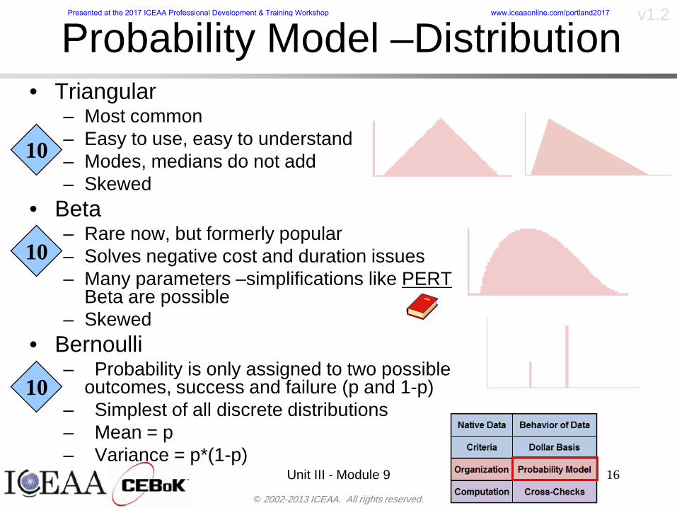
copy 2002-2013 ICEAA All rights reserved
v12
Unit III - Module 9 16
bull Triangularndash Most commonndash Easy to use easy to understandndash Modes medians do not addndash Skewed
bull Betandash Rare now but formerly popularndash Solves negative cost and duration issuesndash Many parameters ndash simplifications like PERT
Beta are possiblendash Skewed
bull Bernoullindash Probability is only assigned to two possible
outcomes success and failure (p and 1-p)ndash Simplest of all discrete distributionsndash Mean = pndash Variance = p(1-p)
10
Probability Model ndash Distribution
10
10
Presented at the 2017 ICEAA Professional Development amp Training Workshop wwwiceaaonlinecomportland2017
copy 2002-2013 ICEAA All rights reserved
v12
Unit III - Module 9 17
bull Normalndash If there is a sufficiently large number of independently identically distributed
elements (or not too correlated and not too skewed) then the distribution of total cost is normal due to the Central Limit Theorem
bull Lognormalndash For smaller data sets with large amounts of (positive) correlation and
skewness the lognormal distribution may be a better approximation of total cost
ndash Many total cost distributions in smaller data sets test as both normal and lognormal
bull Triangularndash The sum of triangles is not a triangle so this distribution should generally not
be used to characterize total costbull Convolved
ndash If total cost distribution is derived using simulation then it may not particularly resemble anything In this case we simply have a convolved or simulated total cost distribution
Probability ndash Top-Level Distribution
NEW
Presented at the 2017 ICEAA Professional Development amp Training Workshop wwwiceaaonlinecomportland2017
copy 2002-2013 ICEAA All rights reserved
v12
S-Curves and Confidence Levels
Unit III - Module 9 1818
100
70
25
Probability(Confidence
Level)
Cost Estimate(Dollars)
50
The S curve is the cumulative probability distribution coming out of the statistical summing process
70 confidence that project will cost indicated amount or less
Provides information on potential cost as a result of identified project risks
Provides insight into establishing reserve levels
X Y
MR
X = Point estimateZ = Project requirementY = Cost estimate where there is a 70 change that
final actual cost will be less than cost estimateY-Z= Manage reserve (MR) which is REQUIRED to meet 70 CL
Z
X not always = Z but is based on same content
Presented at the 2017 ICEAA Professional Development amp Training Workshop wwwiceaaonlinecomportland2017
copy 2002-2013 ICEAA All rights reserved
v12
19
Example ndash Normal Distribution
bull Normal distribution with mean equal to 100 and standard deviation equal to 20
bull Median and mode also equal 100bull The 80th Percentile is 117
40 60 80 100 120 140 160
80 of distribution(area under curve)is less than 117
117
Presented at the 2017 ICEAA Professional Development amp Training Workshop wwwiceaaonlinecomportland2017
copy 2002-2013 ICEAA All rights reserved
v12
20
Confidence Levelsbull The output of a cost risk analysis is a probability
distributionndash Typically displayed as a cumulative distribution function or
ldquoS-curverdquondash Confidence levels are simply percentiles of the distribution
0
10
20
30
40
50
60
70
80
90
100
30 60 90 120 150 180
Conf
iden
ce L
evel
Presented at the 2017 ICEAA Professional Development amp Training Workshop wwwiceaaonlinecomportland2017
copy 2002-2013 ICEAA All rights reserved
v12
Measuring Parametric Model Uncertainty
bull When developing estimates using cost-estimating relationships (CERs) there are two major sources of uncertaintyndash Technical (model input) uncertaintyndash Estimating uncertainty
bull Technical uncertainty reflects the uncertainty inherent in the model inputsndash Typical parametric model inputs include weight lines of code
heritage and other performance and management inputs
bull Estimating uncertainty measures the uncertainty inherent in the model due to the modelrsquos inability to capture all aspects of variability in the data
21
Presented at the 2017 ICEAA Professional Development amp Training Workshop wwwiceaaonlinecomportland2017
copy 2002-2013 ICEAA All rights reserved
v12
Parametric Model Examplebull The NASAAir Force Cost Model (NAFCOM) is a
parametric model for estimating acquisition costs for spacecraft and launch vehicles
bull The CERs in NAFCOM have the formCost = C WeightVNewDesignWTechnicalXManagementY ClassZ
bull There is technical uncertainty about each of the parametersndash Parametric models are applied early in a program so there
is significant amount of uncertainty in the weightndash Heritage is also tricky it is inherently subjective and project
personnel are typically optimisticndash Technical characteristics can also change as a program
matures and requirements change
22
Presented at the 2017 ICEAA Professional Development amp Training Workshop wwwiceaaonlinecomportland2017
copy 2002-2013 ICEAA All rights reserved
v12
Weight Uncertaintybull Aerospace weight growth study average satellite
weight growth from program inception to launch is 28
23
Aerospace Weight Growth Data
-10
0
10
20
30
40
50
60
0 4 8 12 16 20 24 28 32 36 40 44 48 52 56 60 64 68 72 76 80 84 88 92 96 100
Percent Program Completion
Perc
ent W
eigh
t Gro
wth
Presented at the 2017 ICEAA Professional Development amp Training Workshop wwwiceaaonlinecomportland2017
copy 2002-2013 ICEAA All rights reserved
v12
Estimating Uncertaintybull CERs do not perfectly fit the historical data
ndash There are non-repeatable random effects that cannot be predicted
bull For examplendash Parts breaking during testingndash Strikes which are difficult to predict
bull This results in an underlying uncertainty distribution about an estimatendash The outcome of a CER represents only one point on an
uncertainty distributionbull Typically mean or median depending upon the CER
methodology
24
Presented at the 2017 ICEAA Professional Development amp Training Workshop wwwiceaaonlinecomportland2017
copy 2002-2013 ICEAA All rights reserved
v12
Estimating Uncertainty (2)
25
Presented at the 2017 ICEAA Professional Development amp Training Workshop wwwiceaaonlinecomportland2017
copy 2002-2013 ICEAA All rights reserved
v12
Estimating Uncertainty (3)bull In the case of a linear regression the estimating
uncertainty follows a normal distributionndash The estimate is the mean and the standard error of the
estimate from the regression is the standard deviation of the normal distribution
bull In the case of a log-transformed linear regression the estimating uncertainty follows a lognormal distributionndash The estimate is the median of the lognormal and the
standard error of the estimate from the regression is the standard deviation of the normal distribution (in log-space)
bull There is additional uncertainty about an estimate based upon the distance of what is being estimated from the mean of the input datandash This results in a prediction interval
26
Presented at the 2017 ICEAA Professional Development amp Training Workshop wwwiceaaonlinecomportland2017
copy 2002-2013 ICEAA All rights reserved
v12
Aggregating Riskbull Risk is typically applied at the same level at
which we estimate cost that is at the Work Breakdown Structure (WBS) level
bull The estimates for each WBS are developedndash These estimates sum to yield the total system cost
bull For an n-element WBS the total cost is the sum of the cost for each of the n elements
27
nXXXCostSystem +++= 21
Presented at the 2017 ICEAA Professional Development amp Training Workshop wwwiceaaonlinecomportland2017
copy 2002-2013 ICEAA All rights reserved
v12
WBS Examplebull Launch Vehicle
ndash Structurebull Vehicle Structurebull Tank Structure
ndash Thermal Controlbull Active Thermal Controlbull Induced Thermal Controlbull Tank Thermal Control
ndash Main Propulsion Systemndash Liquid Rocket Enginendash Electric Power and Distributionndash Command Control and Data Handlingndash System Integration
28
Presented at the 2017 ICEAA Professional Development amp Training Workshop wwwiceaaonlinecomportland2017
copy 2002-2013 ICEAA All rights reserved
v12
WBS and Risk
29
Presented at the 2017 ICEAA Professional Development amp Training Workshop wwwiceaaonlinecomportland2017
copy 2002-2013 ICEAA All rights reserved
v12
Aggregating Riskbull This leads us to the issue of aggregating the risks across the
WBSbull For example if we want to determine the 70th percentile of the
overall cost risk distribution how do we proceed bull Note that we cannot simply add the 70th percentiles of each of
the cost risk distributionsbull We can add means and variances (taking correlation into
account more on that later) but that is all
Variance of Total Cost =
30
Mean of Total Cost = ( )E X E Xk
k
n
kk
n
kk
n
= = =aringaelig
egraveccediloumloslashdivide
= =aring aring1 1 1
m
Var X kk
n
=aringaelig
egraveccediloumloslashdivide1
= s r s skk
n
iji
j
i jj
n2
1 1
1
22+aring aringaring
= =
-
=
Presented at the 2017 ICEAA Professional Development amp Training Workshop wwwiceaaonlinecomportland2017
copy 2002-2013 ICEAA All rights reserved
v12
Percentiles Do Not Addbull As a notional example consider two independent normal
distributionsndash One distribution has mean equal to 100 and standard deviation
equal to 20ndash The second distribution has mean 300 and standard deviation of 80
bull The sum of two independent normally distributed random variables is also normally distributed
bull To combine the two distributions we add the means and add the variancesndash Total mean is
ndash Total standard deviation is
31
400300100 =+
8258020 22 raquo+
Presented at the 2017 ICEAA Professional Development amp Training Workshop wwwiceaaonlinecomportland2017
copy 2002-2013 ICEAA All rights reserved
v12
Percentiles Do Not Add (2)bull The 80th percentiles for the individual distributions are
117 and 367 respbull The 80th percentile of the combined distribution is
469 but the sum of the two 80th percentiles is 484bull To see why this is the case note that the percentiles
of a normal distribution are determined by the mean and the standard deviationndash The standard deviations are not added when normal distributions
are combined rather the variances are combinedndash Sum of variances is ndash The standard deviation of this sum is
32
22 ba +22 ba +
Presented at the 2017 ICEAA Professional Development amp Training Workshop wwwiceaaonlinecomportland2017
copy 2002-2013 ICEAA All rights reserved
v12
Percentiles Do Not Add (3)bull Since bull We can write
bull The left side of this inequality represents the risk of the combined distributions while the right side represents the sums of the individual risks
bull Combining two missions that are independent results in a diversification of riskndash The total portfolio is not as risky on a relative basis as each
individual project
33
2222 2 bababa ++lt+
baba +lt+ 22
Presented at the 2017 ICEAA Professional Development amp Training Workshop wwwiceaaonlinecomportland2017
copy 2002-2013 ICEAA All rights reserved
v12
Methods for Aggregating Riskbull Since percentiles do not add we have to find other
ways to aggregate riskbull One method is to use Monte Carlo simulationbull Unless cost risk is represented by normal
distributions for all WBS elements summing the means and variances does not result in a completely accurate depiction of overall system cost risk
bull The normal distribution is not a realistic distribution for representing risk in many or even most situations since regarding project risk more can go wrong than can go right which means the risk is NOT symmetric unlike the Gaussian bell curve
34
Presented at the 2017 ICEAA Professional Development amp Training Workshop wwwiceaaonlinecomportland2017
copy 2002-2013 ICEAA All rights reserved
v12
Unit III - Module 9 35
Monte Carlo Simulationfor Risk Analysis
bull When risk analysis is performed multiple risks are gatheredndash These risks may have various probability
distributions
bull Monte Carlo is the most commonly accepted way to produce an accurate characterization of the distribution of the combined effect of these many risksndash Using this distribution we can produce percentiles
for cost impacts due to risk occurrences
10
Presented at the 2017 ICEAA Professional Development amp Training Workshop wwwiceaaonlinecomportland2017
copy 2002-2013 ICEAA All rights reserved
v12
Monte Carlo Simulationbull Simulation is a means for solving problems that are
analytically intractablendash Involves repeated random sampling
bull It was developed during the Manhattan Project as a way to model the interactions inside an atom during nuclear fissionndash Allowed for more sophisticated mathematical modeling of atomic
phenomena
bull Most computer packages use pseudo-random number generators that produce seemingly random results from an initial seedndash Example is the linear congruential generator
36
( ) mbaXX nn mod1 +=+
Presented at the 2017 ICEAA Professional Development amp Training Workshop wwwiceaaonlinecomportland2017
copy 2002-2013 ICEAA All rights reserved
v12Using Random Numbers to Simulate Distributions
bull WBS cost risk is typically measured by a probability distributionbull The most common method for simulating a probability
distribution is the inverse methodbull This involve obtaining a simulated random value from a uniform
distribution and then inverting this through the cumulative distribution function (CDF) to obtain the simulated value
bull As an example for a uniform distribution on the interval [0100]
bull In this case the CDF random value of 05 translates to 10005 = 50
37
( )100
1=xf ( )
100xxF = ( ) xxF 1001 =-
Presented at the 2017 ICEAA Professional Development amp Training Workshop wwwiceaaonlinecomportland2017
copy 2002-2013 ICEAA All rights reserved
v12
Simulating a Triangular Distribution
bull For a triangular distribution with low = 0 most likely = 50 and high = 150 the CDF is given by
bull The inverse function is given by
38
( )iumliumlicirc
iumliumliacute
igrave
poundlt--
poundpound=
1505021
1500050
50015000
2
2
2
xxx
xxxF
( )iumliumlicirc
iumliumliacute
igrave
poundltdivideoslashouml
ccedilegraveaelig +--
poundpound=-
131
21
37501
250017500150
3107500
1
xx
xxxF
Presented at the 2017 ICEAA Professional Development amp Training Workshop wwwiceaaonlinecomportland2017
copy 2002-2013 ICEAA All rights reserved
v12
Simulating a Triangular Distribution (2)
bull If the simulated uniform value is equal to 02 the corresponding inverse value from the CDF inverse is approximately 387
39
0
01
02
03
04
05
06
07
08
09
1
0 30 60 90 120 150
Presented at the 2017 ICEAA Professional Development amp Training Workshop wwwiceaaonlinecomportland2017
copy 2002-2013 ICEAA All rights reserved
v12
Monte Carlo and the WBSbull Simulation involves repeated trials
40
WBS Draw1 2 3 4 5
System 2912 3566 4390 2954 4655 Sum
Structure 80 105 55 80 57 SumVehicle Structure 50 70 30 40 20Tank Structure 30 35 25 40 37
Thermal Control 32 36 35 29 33 SumActive Thermal Control 10 15 12 7 10Induced Thermal Control 12 14 13 14 14Tank Thermal Control 10 7 10 8 9
Main Propulsion System 100 150 125 140 100
Liquid Rocket Engine 1000 1100 1800 900 2200
Electric Power and Distribution 100 125 150 75 90
Command Control and Data Handling 200 250 225 230 275
System Integration 1400 1800 2000 1500 1900
Presented at the 2017 ICEAA Professional Development amp Training Workshop wwwiceaaonlinecomportland2017
copy 2002-2013 ICEAA All rights reserved
v12
Number of Trialsbull Monte Carlo involves a repeated number of trialsbull The greater the number of trials the more accurate the
simulation will approximate the overall cost risk behavior of the system
bull After 100 trials the histogram looks very jagged
41
Presented at the 2017 ICEAA Professional Development amp Training Workshop wwwiceaaonlinecomportland2017
copy 2002-2013 ICEAA All rights reserved
v12
Number of Trials (2)
42
1000 Trials
10000 Trials
50000 Trials Additional trials give a more accurate depiction of the final result
Presented at the 2017 ICEAA Professional Development amp Training Workshop wwwiceaaonlinecomportland2017
copy 2002-2013 ICEAA All rights reserved
v12
Number of Trials (3)bull If we want to simulate the underlying
mean within 1 with 95 confidence for example then we require
43
divideoslash
oumlccedilegrave
aelig poundpound-
=
dividedividedivide
oslash
ouml
ccedilccedilccedil
egrave
aeligpound
-pound
-=
divideoslashouml
ccedilegraveaelig poundpound=
nZ
n
nnX
n
X
n
n
011
010Pr
011
010Pr
011990Pr950
___
___
sm
sm
sm
sm
sm
mm
Presented at the 2017 ICEAA Professional Development amp Training Workshop wwwiceaaonlinecomportland2017
copy 2002-2013 ICEAA All rights reserved
v12
Number of Trials (4)bull This means that the number of trials required is determined by
bull Solving for n we find that at least
trials are neededbull Note that this term involves the coefficient of variation of the
distribution which means that distributions with less dispersion require fewer trials to accurate simulate
44
96101
=ns
m
ms41638
Presented at the 2017 ICEAA Professional Development amp Training Workshop wwwiceaaonlinecomportland2017
copy 2002-2013 ICEAA All rights reserved
v12
Number of Trials (5)bull Simulating percentiles requires more trials than for simulating
meansbull Let Pn represent the number of trials in the sample at or below
the 70th percentile of the underlying distribution (suppose this is known)
bull By the Central Limit Theorem Pnn follows a normal distribution with mean equal to the 70th percentile and variance equal to
bull By a similar process for the mean we find that the number of trials needed to simulate the 70th percentile within 1 with 95 confidence is
45
( )n
FF 700700 1-
n
n
PPn -41638
Presented at the 2017 ICEAA Professional Development amp Training Workshop wwwiceaaonlinecomportland2017
copy 2002-2013 ICEAA All rights reserved
v12
Number of Trials (6)bull If Pn 070 for all n then n is approximately
bull For the sake of comparison suppose CV = 03 (reasonable approximation for hardware development) then the number of trials needed to simulate the mean with the same accuracy is then ldquoonlyrdquo 11525
bull More trials are needed to accurately simulate percentiles than means
46
( ) 46416703041638
70704168341638 =divide
oslashouml
ccedilegraveaelig=divide
oslashouml
ccedilegraveaelig -
=-
nnn
PPn
n
n
Presented at the 2017 ICEAA Professional Development amp Training Workshop wwwiceaaonlinecomportland2017
copy 2002-2013 ICEAA All rights reserved
v12
Methods of Simulationbull Monte Carlo simulation is a standard term for
simulationbull However there is an improvement on Monte Carlo
that improves the accuracy of the results of a simulation for a given number of trials
bull This method is call the Latin Hypercube approach to simulationndash Similar to Monte Carlo but an equal number of draws are taken
from a set of subintervals for example dividing the interval (01) into [00001) [0102)hellip [0910]
ndash Instead of 10 trials from [01] we have one trial from each subinterval
ndash Rough rule of thumb is Latin Hypercube takes 30 fewer trials to achieve similar accuracy to Monte Carlo
47
Presented at the 2017 ICEAA Professional Development amp Training Workshop wwwiceaaonlinecomportland2017
copy 2002-2013 ICEAA All rights reserved
v12
Probability Model ndash Correlationbull Correlation exists between work breakdown structure
(WBS) cost element costs and between cost and schedule
bull Correlation is a necessary consideration in cost risk analysis
bull Correlation is a number that can vary between -1 and +1 and represents the strength of the relationship between the two variablesndash If both variable have a tendency to move in the same direction
correlation is positivendash If when one variable increases the other tends to decrease and
vice-versa the correlation between the two variables is negative
Presented at the 2017 ICEAA Professional Development amp Training Workshop wwwiceaaonlinecomportland2017
copy 2002-2013 ICEAA All rights reserved
v12
Correlation And Causationbull Note that correlation is not causation however
causation implies correlationndash For example shark attacks and ice cream sales at the beach
bull For example for a launch vehicle structure increasing the diameter will not only result in an increase in the structures cost but will also result in higher costs for thermal coating (paint etc)
bull Also simply because two subsystems do not appear to be related does not mean they are not correlatedndash For example structures and computer equipment seemingly
have little relation to one another however an external factor such as a funding cut or a strike will impact all subsystems leading to delays and increasing cost across the board
ndash Thus everything in a WBS has some correlationUnit III - Module 9 49
Presented at the 2017 ICEAA Professional Development amp Training Workshop wwwiceaaonlinecomportland2017
copy 2002-2013 ICEAA All rights reserved
v12
The Importance of Correlationbull Percent that total cost standard deviation is underestimated
when correlation assumed to be 0 instead of r given nWBS elements
Unit III - Module 9 5050
0
20
40
60
80
100
0 01 02 03 04 05 06 07 08 09 1Actual Correlation
Perce
nt Un
deres
timate
d
n = 10
n = 30
n = 100n = 1000
0
20
40
60
80
100
0 01 02 03 04 05 06 07 08 09 1Actual Correlation
Perce
nt Un
deres
timate
d
n = 10
n = 30
n = 100n = 1000
Reference 32nd Annual DOD Cost Analysis Symposium Advanced Training Session ldquoWhy Correlation Matters in Cost Estimatingrdquo Stephen A Book
Presented at the 2017 ICEAA Professional Development amp Training Workshop wwwiceaaonlinecomportland2017
copy 2002-2013 ICEAA All rights reserved
v12
The Importance of Correlation (2)bull For example if correlation is assumed to be 0 for all
elements in a 30 element WBS and the actual correlation is 20 then the total cost standard deviation is underestimated by 60
bull For example assume the total cost is modeled as a normal distribution with mean = 100
bull If correlation is assumed to be zero with total cost standard deviation = 12 when correlation is actually 20 then the true underlying standard deviation is actually 30
bull 70th percentile with zero correlation assumption is 106
bull 70th percentile with 20 correlation is 116 Unit III - Module 9 51
Presented at the 2017 ICEAA Professional Development amp Training Workshop wwwiceaaonlinecomportland2017
copy 2002-2013 ICEAA All rights reserved
v12
Measures of Correlationbull Two measures of correlation are commonly used in
cost risk analysesndash Pearsonrsquos product-moment correlation coefficient ndash Spearmanrsquos rank correlation coefficient
bull Garvey and others recommend using Pearsonrsquos product-moment correlation coefficient correlation for cost risk analysesndash Method of moments uses this but there are two options in
simulationndash Popular simulation packages like Risk and Crystal Ball use
rank correlation but in practice this has been found to make little difference
ndash Pearson product-moment correlation has been incorporated into Risk+
52
Presented at the 2017 ICEAA Professional Development amp Training Workshop wwwiceaaonlinecomportland2017
copy 2002-2013 ICEAA All rights reserved
v12
Pearson Correlationbull Pearsonrsquos product-moment correlation measures
degree of linearity between two random variables bull If two random variables are perfectly linear (eg Y =
aX + b) with positive slope then the Pearson product-moment correlation between X and Y denoted by rXY is +1
53
X X
Y Y Y
XNegative Correlation Positive Correlation No Correlation
middotmiddot
middotmiddot
middotmiddot middotmiddot
middotmiddot
middot
middot
middotmiddotmiddot
middotmiddot
middotmiddot
middotmiddot middot
middot
middot
middotmiddotmiddotmiddotmiddotmiddotmiddotmiddot
middotmiddotmiddotmiddot
middotmiddot
middotmiddot middotmiddotmiddotmiddot
middotmiddotmiddot
middotmiddotmiddotmiddot
middotmiddotmiddot
middotmiddotmiddot
middotmiddot
middot
middot middotmiddot
middot middotmiddotmiddotmiddot middotmiddot middot middotmiddot middot middot
middotmiddot middot
middotmiddotmiddotmiddotmiddot middot middotmiddot
middotmiddot
middot
middotmiddot
middotmiddot middot
middot middot middot
middotmiddot middot
middotmiddotmiddot
middotmiddot
middot middot
Presented at the 2017 ICEAA Professional Development amp Training Workshop wwwiceaaonlinecomportland2017
copy 2002-2013 ICEAA All rights reserved
v12
Spearman Correlationbull Spearmanrsquos rank correlation measures the
monotonicity between two random variablesbull If two random variables are perfectly monotonically
increasing (eg Y = X2) then the Spearman rank correlation denoted by rXY is +1
bull The two measures can be significantly different
54
10 20 30 40 50 60
100
200
300
096 097 098 099 1
1
060
020
040
080
Eff
ort (
Staf
f-M
onth
s)
Software Size I KDSI
y = 28z12y
z x
yy = x100
0 pound x pound 1
Figure 5-9A Figure 5-9B
Pearson Correlation = 09976 Rank Correlation = 1
Pearson Correlation = 024 Rank Correlation = 1
X(x ) ~ Unif(01)
Reference Probability Methods for Cost Uncertainty Analysis A Systems Engineering Perspective Paul R Garvey
Presented at the 2017 ICEAA Professional Development amp Training Workshop wwwiceaaonlinecomportland2017
copy 2002-2013 ICEAA All rights reserved
v12
Unit III - Module 9 55
200
250
300
350
400
1000 1200 1400 1600 1800 2000
Recurring Production
SEPM
200
250
300
350
400
1000 1200 1400 1600 1800 2000
Recurring Production
SEPM
Functional Correlationbull Old No Functional
Correlation Simulation run with WBS items entered as values
bull New Simulation run with functional dependencies entered as they are in cost model
CorrelatedNot Correlated
Note shift of mean and increased variability
Presented at the 2017 ICEAA Professional Development amp Training Workshop wwwiceaaonlinecomportland2017
copy 2002-2013 ICEAA All rights reserved
v12
Risk Measuresbull ldquoWestern Europe conquered the word because of a
technological revolution that started because of attempts to measure the worldrdquo ndash Phillipe Jorion ndash In the same way attempts to measure risk will lead to better project
managementbull Risk management for DoD and NASA agencies focuses
primarily on funding projects to a single percentile ndash NASA policy explicitly mentions 70 and 50ndash This is known as ldquoValue at Riskrdquo and is prevalent in the banking and
financial industry
56
Presented at the 2017 ICEAA Professional Development amp Training Workshop wwwiceaaonlinecomportland2017
copy 2002-2013 ICEAA All rights reserved
v12
Value at Risk (VaR)bull VaR is a percentile of the cost risk
distributionndash VaR funding at the 70th percentile means that
there is a 30 chance of final project cost exceeding the funded amount (budget)
bull VaR has some meritsndash Common measure can be used to compare
different projects and programsndash Easily understood by senior managers and
decision makers
57
Presented at the 2017 ICEAA Professional Development amp Training Workshop wwwiceaaonlinecomportland2017
copy 2002-2013 ICEAA All rights reserved
v12
Why 70th or 80th Percentilebull Typical policy guidance involves funding at the 70th or 80th
percentile Why fund as such a low percentilebull There is some incentive to not over-fundbull For a normal distribution an inflection point occurs near the 80th
percentile meaning that for values above 80 confidence achieving higher levels of confidence can only be achieved by spending greater dollar amounts at an increasing rate
58
-05-04-03-02-01
00102030405
0 05 1 15 2 25 3
Standard Deviations from Mean
Normal Distribution
First DerivativeSlopeVelocity
Second DerivativeConvexityAcceleration
Inflection point at one standard deviation above the mean (~84th
percentile)
Presented at the 2017 ICEAA Professional Development amp Training Workshop wwwiceaaonlinecomportland2017
copy 2002-2013 ICEAA All rights reserved
v12
Funding Above Inflection Pointsbull As the percentile goes above the 80th percentile the amount
needed to achieve that higher level of confidence begins to increase at an increasing rate as is evident from the graph
59
0
10
20
30
40
50
60
70
50 55 60 65 70 75 80 85 90 95 100
$ Ab
ove
MEa
n to
Ach
ieve
Per
cent
ile
Percentile (Confidence Level)
Presented at the 2017 ICEAA Professional Development amp Training Workshop wwwiceaaonlinecomportland2017
copy 2002-2013 ICEAA All rights reserved
v12
Why Budget to the 70th or 80thbull Government projects are funded at the 70th or 80th percentilesbull Why not the 90th or 99th percentile Wonrsquot that help prevent
overrunsndash As we have seen percentiles do not add across programs
bull The sum of the 80th percentiles does NOT equal the total 80th percentile
ndash This is because the individual programs are riskier than the entire suite of missions
bull Known as the ldquoPortfolio effectrdquo (more or this later)
ndash Funding at the 80th gives confidence that the entire portfolio will be adequately funded
bull And since there is an inflection point near the 80th percentile funding above that level quickly becomes cost prohibitive
60
Presented at the 2017 ICEAA Professional Development amp Training Workshop wwwiceaaonlinecomportland2017
copy 2002-2013 ICEAA All rights reserved
v12
Inflection Points for Lognormalbull For a lognormal the inflection point
variesndash Coefficient of variation equal to 10 equates to an
inflection point at the 70th percentile
61
0
10
20
30
40
50
60
70
050 060 070 080 090 100
Coef
ficen
t of V
aria
tion
Percentile of the Inflection Point
Presented at the 2017 ICEAA Professional Development amp Training Workshop wwwiceaaonlinecomportland2017
copy 2002-2013 ICEAA All rights reserved
v12
Issues with Percentile Fundingbull However risk management does not stop at a
specific percentilendash What happens when the 70th percentile is exceeded
bull Any effective risk management policy should prescribe what happens after a bad event occursndash With VaR we only know when a bad event has occurred ndash Also funding at a relatively low level means we have no true
sense of the real risks that should be guarded against
62
Presented at the 2017 ICEAA Professional Development amp Training Workshop wwwiceaaonlinecomportland2017
copy 2002-2013 ICEAA All rights reserved
v12
ldquoHere There Be Dragonsrdquobull On old maps uncharted territory was often
marked with monsters or dragons
63
A section of the Carta Marina by Olaus Magnus 16th Century
Presented at the 2017 ICEAA Professional Development amp Training Workshop wwwiceaaonlinecomportland2017
copy 2002-2013 ICEAA All rights reserved
v12
Distribution Comparisonbull Four different distributions with the same 70th
percentile
bull Should we expect the tails to be similar
64
0
10
20
30
40
50
60
70
80
0 100 200 300 400 500 600
Perc
entil
eCo
nfid
ence
Lev
el
Triangular
Normal
Lognormal
Pareto
Presented at the 2017 ICEAA Professional Development amp Training Workshop wwwiceaaonlinecomportland2017
copy 2002-2013 ICEAA All rights reserved
v12Distribution Comparison Tail Behavior
bull The normal and triangular distributions have similar tails but the lognormal and Pareto have much fatter right tails
65
70
75
80
85
90
95
100
500 1500 2500 3500 4500 5500
Perc
entil
eCo
nfid
ence
Lev
el
Triangular
Normal
Lognormal
Pareto
Here There Be Dragons
Presented at the 2017 ICEAA Professional Development amp Training Workshop wwwiceaaonlinecomportland2017
copy 2002-2013 ICEAA All rights reserved
v12Distribution Comparison ndash Tail Behavior (Table)
bull There is significant tail risk for the lognormal and the Paretobull The 99th percentile for the Pareto is 1000 times greater than
the 70th percentilendash Risk seen in financial markets and in catastrophic risks like natural
disasters bull Four different projects follow the four different risk profiles seen
in this example should clearly have different risk management approaches but 70th percentile funding indicates the same risk management approach for all four
66
Percentile Triangular Normal Lognormal Pareto 70th $600 $600 $600 $600 80th $680 $660 $770 $1430 90th $770 $750 $1070 $5880 95th $840 $820 $1410 $23750 99th $930 $950 $2350 $600000
Presented at the 2017 ICEAA Professional Development amp Training Workshop wwwiceaaonlinecomportland2017
copy 2002-2013 ICEAA All rights reserved
v12Percentile Budgeting is Not Risk Management
bull Percentile budgeting ne effective risk management policybull Suppose that you are shopping for a new car You
mention that safety is your top concern The salesman says he has a great safe car available You ask about the air bags Do they work The salesman answers ldquoOf course Seventy percent of the time they work fine Only 30 of the time the air bags will fail to deployrdquo Would you buy such a car Hedge fund manager David Einhorn has stated ldquoRisk management is the air bag that must always work but only in the multi-sigma event where you have an accidentrdquo
67
Risk management is the air bag that must always work but only in the multi-sigma event where you
have an accident
Presented at the 2017 ICEAA Professional Development amp Training Workshop wwwiceaaonlinecomportland2017
copy 2002-2013 ICEAA All rights reserved
v12
Joint Confidence Level Analysisbull Schedules are risky toobull For 98 recent NASA missions average
schedule growth was 38ndash Not as high as cost growth but still significant
68
0
5
10
15
20
25
30
35
40
Schedule
Cost
Presented at the 2017 ICEAA Professional Development amp Training Workshop wwwiceaaonlinecomportland2017
copy 2002-2013 ICEAA All rights reserved
v12
Schedules Impact Costbull Changes in schedule can have enormous
impacts on cost ndash Schedule slips can lead to cost increases
bull Fixed programmatic costs must be paid on a regular basisndash Achieving schedule milestones early can result in cost
savings
bull Schedule is an important consideration in cost analysis including cost risk analysis
bull However we must be careful in correctly integrating cost and schedule riskndash Schedule is not simply an input but is dependent on many of
the same factors that drive cost
69
Presented at the 2017 ICEAA Professional Development amp Training Workshop wwwiceaaonlinecomportland2017
copy 2002-2013 ICEAA All rights reserved
v12
The Relationship of Cost to Schedulebull Cost and schedule are positively correlated
ndash A larger program with bigger scope with take longer to complete than a smaller simpler program
bull However longer schedules do not always equate to higher cost nor shorter schedules with lower costndash Highly compressed schedules relative to the
optimal schedule can lead to large overrunsbull Compressed schedules are commonplace for
many planetary missions
70
Presented at the 2017 ICEAA Professional Development amp Training Workshop wwwiceaaonlinecomportland2017
copy 2002-2013 ICEAA All rights reserved
v12The Impact of Schedule GrowthCompression on Cost
bull Compressed schedules lead to cost growth and based on existing research is actually more expensive than schedule slippages
71
0
20
40
60
80
100
120
140
160
-50 -25 0 25 50 75 100
Percentage Change in Schedule
Perc
enta
ge C
hang
e in
Cos
t due
to
Sche
dule
Cha
nge
Source Smart CB ldquoCost and Schedule Interrelationshipsrdquo 2007 NASA Cost Symposium
Presented at the 2017 ICEAA Professional Development amp Training Workshop wwwiceaaonlinecomportland2017
copy 2002-2013 ICEAA All rights reserved
v12Schedule as an Independent Variable
bull Why not simply add schedule as an input to cost-estimating relationships (CERs)
bull Schedule is often treated as an independent variable ndash schedules are often determined independently of cost considerationsndash Cost may not be considered explicitly although budgets and
schedules are determined based on scope and other common factors
bull In 2006 SAIC undertook a research task to determine the impact of schedule on cost and added schedule as an independent variable to the CERs in the NASAAir Force Cost Model (NAFCOM) to see if schedule provided any improvement in goodness of fit
72
Presented at the 2017 ICEAA Professional Development amp Training Workshop wwwiceaaonlinecomportland2017
copy 2002-2013 ICEAA All rights reserved
v12
Schedule is a Dependent Variablebull Since NAFCOM includes an exhaustive list of cost drivers the inclusion
of schedule should give an indication of whether there is any additional independent value added from schedule independent of the cost drivers
bull In the study schedule was added to 10 subsystem-level CERs
ndash In each case the addition of schedule did NOTimprove the goodness of fit and schedule was NOT found to be a statistically significant cost driver (given the presence of the other variables) for any of the 10 CERs
bull Standard errors for the CERs increased due to decrease in degrees of freedom
bull Thus schedule as an independent variable did not provide any additional explanation of variation in historical cost
bull This is because schedule is truly NOT an independent variable but a dependent variable and is a function of the same factors that drive cost
73
Presented at the 2017 ICEAA Professional Development amp Training Workshop wwwiceaaonlinecomportland2017
copy 2002-2013 ICEAA All rights reserved
v12
Incorporation of Schedule in Cost Risk
bull When using subjective methods care must be taken in applying schedule to cost risk analysis
bull Since schedule is a dependent variable treating it independently from other factors when assessing its impact on cost can lead to a double count of independent variables in the cost risk analysis
bull Direct inclusion of schedule in a cost risk analysis effectively doubles the influence of each cost driver
ndash Incorrectly leads to broader risk ranges
74
CostWeight
HeritageNewness
Technology Readiness Schedule
Presented at the 2017 ICEAA Professional Development amp Training Workshop wwwiceaaonlinecomportland2017
copy 2002-2013 ICEAA All rights reserved
v12Subjective Cost Risk Methods and Overinclusion of Risk Factors
bull Subjective methods are suitable when data are scarce or not availablebull However care must be taken not to treat correlated sources of risk
such as schedule as independent of each otherbull Example ndash a subjective risk analysis incorporated technology readiness
design risk requirements stability integration risk and schedule and treated each source of risk as independent
bull Risk triangle high value without schedule risk was 31 times the point estimate
bull Risk triangle high value with schedule risk added on top of other sources of risk treated independently was 34 times the point estimate
bull Risk triangle taking correlation between sources of risk into account in a rigorous statistical manner has a high value 15 times the point estimate less than half the effect when treating sources of risk as independent
75
Presented at the 2017 ICEAA Professional Development amp Training Workshop wwwiceaaonlinecomportland2017
copy 2002-2013 ICEAA All rights reserved
v12Fundamental Equation of Cost and Schedule Interrelationships
bull The Fundamental Equation of the Relationship Between Cost and Schedule is
Time = Moneybull This is a well known adage that time is money Your boss at
work may even mention this to you from time to time or if you are the boss you are all too aware of this iron law
bull Because time is money cost and schedule risk should be modeled jointly not with schedule as an independent cost driver
bull Note that cost and schedule are not perfectly correlatedndash Cost can sometimes ldquobuy downrdquo schedule extra money can be
spent to meet a deadline since in some cases additional effort to hasten the completion of a task
76
Presented at the 2017 ICEAA Professional Development amp Training Workshop wwwiceaaonlinecomportland2017
copy 2002-2013 ICEAA All rights reserved
v12How to (Correctly) Incorporate Schedule into Cost Risk Analysis
bull The best way to model cost and schedule risk is to develop a joint cost and schedule model based on the same data
bull Since such models are not currently available the next best approach is to model cost and schedule independently and then integrate cost and schedule risk analyses using joint probability distributions taking into account correlation between cost and schedulendash This approach pioneered by Paul Garvey and Steve Book is
considered industry best practicendash This is a practical method mathematically tractable and follows
naturally from the Fundamental Equation of Cost and Schedule Interrelationships
77
Book S A ldquoQuantifying the Relationship Between Cost and Schedulerdquo The Measurable News Winter 2007-2008 pp 11-15Garvey PR Probability Methods for Cost Uncertainty Analysis A Systems Engineering Perspective New York Marcel Dekker 2000 pp 308-335
Presented at the 2017 ICEAA Professional Development amp Training Workshop wwwiceaaonlinecomportland2017
copy 2002-2013 ICEAA All rights reserved
v12
Joint Lognormal and Normal Distributions
bull Cost and schedule are typically modeled as some combination of Normal and Lognormal probability distributionsndash Studies by The Aerospace Corporation the MITRE
Corporation Wyle Labs and SAIC have found that the Lognormal probability distribution almost always serves as a good model for both the schedule distribution and the cost distribution
ndash The Normal distribution may also be appropriate in some instances and depending upon the level of confidence at which budgets are set may even be more conservative and logically consistent than the Normal distribution
ndash Joint Lognormal and Normal distributions are defined by a pair of mean and standard deviations and a level of correlation between the two
78
Presented at the 2017 ICEAA Professional Development amp Training Workshop wwwiceaaonlinecomportland2017
copy 2002-2013 ICEAA All rights reserved
v12Modeling Cost and Schedule as a Bivariate Distribution
bull In the approach set forth by Book and Garvey cost risk is assessed and the top-level distribution is modeled as a Lognormal (or Normal) distribution schedule risk is assessed and the overall schedule risk is modeled as a Lognormal (or Normal) distribution
bull The two distributions are combined into a Bivariate distribution by assigning a correlation between the two and by treating the two distributions as the marginal distributions of a Bivariate Lognormal distributionndash Other combinations include a Bivariate Normal or a Bivariate
Normal-Lognormal
79
Presented at the 2017 ICEAA Professional Development amp Training Workshop wwwiceaaonlinecomportland2017
copy 2002-2013 ICEAA All rights reserved
v12Bivariate Lognormal Distribution for Cost and Schedule
bull Cost is often observed to be Lognormal when strong positive correlations are present among the systemrsquos WBS cost element costs
bull A systemrsquos schedule is often observed (from Monte Carlo simulations) to be Lognormal if it is the sum of many positively correlated schedule activities in an overall schedule network
bull If Lognormal distributions characterize a systemrsquos cost and schedule then the Bivariate Lognormal could serve as an assumed model of their joint distributionndash In this case the marginal distribution of each of cost and schedule is
Lognormalbull Other possibilities for modeling cost and schedule as a Bivariate
distribution include a Bivariate Normal or a Bivariate Normal-Lognormal distributionndash All these combinations are analytically tractable
80
Presented at the 2017 ICEAA Professional Development amp Training Workshop wwwiceaaonlinecomportland2017
copy 2002-2013 ICEAA All rights reserved
v12Bivariate Lognormal for Cost and Schedule
bull Contour Plots of a Bivariate Lognormal
81
Presented at the 2017 ICEAA Professional Development amp Training Workshop wwwiceaaonlinecomportland2017
copy 2002-2013 ICEAA All rights reserved
v12Correlation Between Cost and Schedule
bull Cost and schedule are positively correlated but not perfectly sondash For example it is possible to have a schedule underrun and a cost
overrunbull Based on cost and schedule growth data for 50 completed NASA
programs the correlation between development cost and development schedule is 70
82
00
200
400
600
800
1000
1200
-500 00 500 1000 1500 2000 2500Historical Cost Growth
Hist
oric
al S
ched
ule
Gro
wth
r = 715
Presented at the 2017 ICEAA Professional Development amp Training Workshop wwwiceaaonlinecomportland2017
copy 2002-2013 ICEAA All rights reserved
v12Correlation Between Cost and Schedule Caveats
bull Based on historical data recommended correlation between cost and schedule is 70 but this could be higher or lower depending upon program circumstancesndash If program is budget constrained cost and schedule will be
more highly correlated (go as you pay)ndash If program is schedule constrained cost and schedule will
have lower correlation perhaps even negative correlation ndash Smaller programs have smaller correlation between cost and
schedule riskbull Relatively easy to ldquohurry uprdquo and finish on time or even early if
needed
83
Presented at the 2017 ICEAA Professional Development amp Training Workshop wwwiceaaonlinecomportland2017
copy 2002-2013 ICEAA All rights reserved
v12
Conditional Confidence Levelsbull Given a programrsquos project schedule we can determine the cost
risk distribution conditional upon the given schedulebull Conditional cost S-curves are steeper than unconditional
(marginal) cost S-curves between some uncertainty has been removed because schedule is fixed
84
Presented at the 2017 ICEAA Professional Development amp Training Workshop wwwiceaaonlinecomportland2017
copy 2002-2013 ICEAA All rights reserved
v12
Joint Confidence Levelsbull Joint 65 confidence represents the probability of
achieving both 65 confidence in cost AND 65 confidence in schedulendash This is different than achieving 65 cost confidence alone
or achieving 65 schedule confidence alonebull Due to the imperfect correlation between cost and schedule it
is possible to achieve a 65 cost confidence with a lower level of schedule confidence
bull Restricting the schedule confidence thus requires additional $ to achieve a given level of confidence
85
X
Y
Possible Values for Which X gt a Possible Values for
Which X gt a and Y gt b
a
b
Presented at the 2017 ICEAA Professional Development amp Training Workshop wwwiceaaonlinecomportland2017
copy 2002-2013 ICEAA All rights reserved
v12Joint Confidence Levels Versus Cost Confidence Levels Only
bull Example of the differences between cost confidence schedule confidence conditional cost confidence and joint cost and schedule confidence
86
Joint Cost-Schedule Confidence Iso-Curves
Cost (RY$M)
Sche
dule
(Mon
ths)
65 Confidence
50 Confidence
70 Confidence
65 Cost Confidence AggressiveSchedule65 Cost ConfidenceScheduleGiven 65 Schedule ConfidenceUnconditional 65 CostConfidenceUnconditional 65 ScheduleConfidence
65 Cost Confidence 65 Joint Cost and Schedule
Confidence for 65 Schedule Confidence
Presented at the 2017 ICEAA Professional Development amp Training Workshop wwwiceaaonlinecomportland2017
copy 2002-2013 ICEAA All rights reserved
v12
Joint Cost and Schedule Confidence
bull Can examine pairs of cost and schedule that achieve a given level of confidence
bull Provides insights into the trade-offs between cost and schedule for a given level of confidencendash Possible to increase cost confidence by giving a
project more time in some instances or possible to ldquobuy downrdquo schedule
bull But these have limits and are shown in the iso-cost and schedule confidence curves
87
Presented at the 2017 ICEAA Professional Development amp Training Workshop wwwiceaaonlinecomportland2017
copy 2002-2013 ICEAA All rights reserved
v12Cost and Schedule Trade-offs for a Given Level of Joint Confidence
bull Hypothetical Example
88
Cost (RY$M)
Schedule (Months)
$100 48$99 48$89 49$87 50$85 51$85 52$84 53$83 55$83 55$83 56
Cost and Schedule 65 Confidence Iso-Curve
4748495051525354555657
$80 $82 $84 $86 $88 $90 $92 $94 $96 $98 $100
Cost (RY$ M)
Sche
dule
(Mon
ths)
Presented at the 2017 ICEAA Professional Development amp Training Workshop wwwiceaaonlinecomportland2017
copy 2002-2013 ICEAA All rights reserved
v12Policy Considerations for Confidence Levels
bull For large programs the difference between the amount of money needed to achieve 65 cost confidence independent of schedule and joint 65 cost and schedule confidence can represent hundreds of millions and even billions of dollars
89
Joint Cost-Schedule Confidence Iso-Curves
Cost (RY$M)
Sche
dule
(Mon
ths)
65 Confidence
65 Cost Confidence AggressiveSchedule
65 Cost ConfidenceScheduleGiven 65 Schedule Confidence
Unconditional 65 CostConfidence
Joint Cost and Schedule Confidence for 65 Cost Confidence and Program Baseline Schedule is Less Than 35
65 Cost Confidence Independent of Schedule Cost Needed to Achieve
Both 65 Joint Cost and Schedule Confidence for the Schedule with 65 Confidence
Presented at the 2017 ICEAA Professional Development amp Training Workshop wwwiceaaonlinecomportland2017
copy 2002-2013 ICEAA All rights reserved
v12
Copulasbull More generally any combination of distributions can
be used (more than just normal and lognormal)ndash Termed ldquocopulardquo from the Italian word for ldquocouplerdquondash Copulas are a way to combine marginal distributions of any
number and type into a joint distributionbull More formally a copula is a multivariate joint distribution defined
on the n-dimensional unit cube [0 1]n such that every marginal distribution is uniform on the interval [0 1]
bull (The bivariate form of) Sklarrsquos theorem states that for any bivariate distribution function H(x y) let F(x) = H(x infin) and G(y) = H(infin y) be the univariate marginal probability distribution functions Then there exists a copula C such that H(xy)=C(F(x)G(y))
ndash Copulas are widely used in risk management for investments and insurance
bull Considered industry best practice (Li 2000)bull Marketed as part of JP Morganrsquos CreditMetrics suite of tools
(Gupton et Al 1997)90
Presented at the 2017 ICEAA Professional Development amp Training Workshop wwwiceaaonlinecomportland2017
copy 2002-2013 ICEAA All rights reserved
v12Parametric Joint Cost and Schedule Analysis
bull A parametric model based on a consistent data set with a set of overlapping cost and schedule drivers is a cleaner way to model cost and schedule
91
CostWeight
HeritageNewness
Technology Readiness
Schedule
0
20
40
60
80
100
Confidence
Joint Cost and Schedule Confidence
Schedule
Cost
Lognormal Distribution PDF and CDF
0102030405060708090100
200 300 400 500 600 700 800 900 1000Cost $
Con
fiden
ce L
evel
0
00002
00004
00006
00008
0001
00012
00014
00016
Prob
abili
ty D
ensi
ty
CDFPDF
Lognormal Distribution PDF and CDF
0102030405060708090100
200 300 400 500 600 700 800 900 1000Cost $
Con
fiden
ce L
evel
0
00002
00004
00006
00008
0001
00012
00014
00016
Prob
abili
ty D
ensi
ty
CDFPDF
Presented at the 2017 ICEAA Professional Development amp Training Workshop wwwiceaaonlinecomportland2017
copy 2002-2013 ICEAA All rights reserved
v12Parametric Joint Cost and Schedule Analysis (2)
bull Joint cost and schedule risk analysis produced naturally by the integrated modelndash Addresses several issues with the copula
approachbull Tail dependencybull Correlation ndash no need to assign correlation
between cost and schedulebull Consistency of cost and schedule models
92
Presented at the 2017 ICEAA Professional Development amp Training Workshop wwwiceaaonlinecomportland2017
copy 2002-2013 ICEAA All rights reserved
v12
Resource-Loaded Schedulesbull Involves assigning cost and schedule risks to a resource-loaded schedule
networkbull Bottom-up approach
ndash More labor intensive than parametrics but can also provide more insight
ndash Can answer questions than parametric typically cannot such as how much do reserve requirements decrease if a specific risk is retired
bull Currently being implemented in Constellation programbull Has same issue as all bottom-up models hard to count all the risks and model
them discretely
ndash As a result there is a tendency to reflect less risk than indicated by history
ndash ldquoThere are more things in heaven and earth Horatio than are dreamt of in your philosophyrdquo William Shakespeare Hamlet Act I Scene V
93
Presented at the 2017 ICEAA Professional Development amp Training Workshop wwwiceaaonlinecomportland2017
copy 2002-2013 ICEAA All rights reserved
v12Resource-Loaded Schedules Vs Parametrics
bull Parametric most appropriate for early estimatesndash But also good for high-level checks as project progresses
bull As plans take shape lower level modeling may be more appropriate
94 1
CONCEPTUALDEVELOPMENT
PROJECTDEFINITION DESIGN DEVELOPMENT OPERATIONS
PARAMETRIC PARAMETRIC
ANALOGY
ENGINEERING (Bottoms Up)
$PARAMETRIC
DETAILED
$
Pre Phase A Phase B Phase CDPhase A Phase EPre Phase A Phase B Phase CDPhase A Phase E
Risk = f(Cost Estimating Relationship Inputs eg mass power data rate TRL new design etc)
Risk = f(cost and schedule variation of the analogous elements)
Risk = f(variation of detailed inputs eg labor hours rates materials etc)
Presented at the 2017 ICEAA Professional Development amp Training Workshop wwwiceaaonlinecomportland2017
copy 2002-2013 ICEAA All rights reserved
v12
Resource-Loaded Schedulesbull Methodology has been demonstrated in other
industriesndash Construction oil and gasndash Analysis has not been traditionally done on highly uncertain
complex development projects bull Methodology focuses on project baseline schedule
ndash In baseline schedule all tasks are resource loaded to represent a baseline schedule and cost standpoint
ndash Resource loaded schedule is ldquorolledrdquo up to a manageable level
ndash Based on the risk and uncertainties identified schedule distributions are applied to each rolled up task
ndash Cost uncertainties are also applied to rolled up tasksbull Uncertainties include labor rate man power etc
ndash A Monte Carlo simulation is run to develop joint cost-schedule distributions
95
Presented at the 2017 ICEAA Professional Development amp Training Workshop wwwiceaaonlinecomportland2017
copy 2002-2013 ICEAA All rights reserved
v12
Unit III - Module 9 96
Execution ndash Cross Checksbull Means The mean cost growth factor for WBS items
can be compared to history as a way to cross check results
bull CVs The CV of the cost growth factors for WBS items can be compared to history as a way to cross check results
bull Inputs Checks are performed on inputs or other parameters to see if historical values are in line with program assumptionsndash Example Historical risk scores can be compared to program
risk scores to see if risk assessors are being realistic and to see if the underlying database is representative of the program
11
Presented at the 2017 ICEAA Professional Development amp Training Workshop wwwiceaaonlinecomportland2017
- Cost and Schedule Risk Analysis Basic
- Acknowledgments
- Unit Index
- Risk Overview
- Agenda
- Introduction
- Risk Analysis Terms
- Are Our Costs Realistic
- Historical Cost Growth
- Sources of Cost Risk
- Point Estimates of Cost
- Types of Risk
- Point Estimates Vs Risk Estimates
- Cost Risk and Probability
- Probability Model ndash Distribution
- Probability Model ndash Distribution
- Probability ndash Top-Level Distribution
- S-Curves and Confidence Levels
- Example ndash Normal Distribution
- Confidence Levels
- Measuring Parametric Model Uncertainty
- Parametric Model Example
- Weight Uncertainty
- Estimating Uncertainty
- Estimating Uncertainty (2)
- Estimating Uncertainty (3)
- Aggregating Risk
- WBS Example
- WBS and Risk
- Aggregating Risk
- Percentiles Do Not Add
- Percentiles Do Not Add (2)
- Percentiles Do Not Add (3)
- Methods for Aggregating Risk
- Monte Carlo Simulationfor Risk Analysis
- Monte Carlo Simulation
- Using Random Numbers to Simulate Distributions
- Simulating a Triangular Distribution
- Simulating a Triangular Distribution (2)
- Monte Carlo and the WBS
- Number of Trials
- Number of Trials (2)
- Number of Trials (3)
- Number of Trials (4)
- Number of Trials (5)
- Number of Trials (6)
- Methods of Simulation
- Probability Model ndash Correlation
- Correlation And Causation
- The Importance of Correlation
- The Importance of Correlation (2)
- Measures of Correlation
- Pearson Correlation
- Spearman Correlation
- Functional Correlation
- Risk Measures
- Value at Risk (VaR)
- Why 70th or 80th Percentile
- Funding Above Inflection Points
- Why Budget to the 70th or 80th
- Inflection Points for Lognormal
- Issues with Percentile Funding
- ldquoHere There Be Dragonsrdquo
- Distribution Comparison
- Distribution Comparison Tail Behavior
- Distribution Comparison ndash Tail Behavior (Table)
- Percentile Budgeting is Not Risk Management
- Joint Confidence Level Analysis
- Schedules Impact Cost
- The Relationship of Cost to Schedule
- The Impact of Schedule GrowthCompression on Cost
- Schedule as an Independent Variable
- Schedule is a Dependent Variable
- Incorporation of Schedule in Cost Risk
- Subjective Cost Risk Methods and Overinclusion of Risk Factors
- Fundamental Equation of Cost and Schedule Interrelationships
- How to (Correctly) Incorporate Schedule into Cost Risk Analysis
- Joint Lognormal and Normal Distributions
- Modeling Cost and Schedule as a Bivariate Distribution
- Bivariate Lognormal Distribution for Cost and Schedule
- Bivariate Lognormal for Cost and Schedule
- Correlation Between Cost and Schedule
- Correlation Between Cost and Schedule Caveats
- Conditional Confidence Levels
- Joint Confidence Levels
- Joint Confidence Levels Versus Cost Confidence Levels Only
- Joint Cost and Schedule Confidence
- Cost and Schedule Trade-offs for a Given Level of Joint Confidence
- Policy Considerations for Confidence Levels
- Copulas
- Parametric Joint Cost and Schedule Analysis
- Parametric Joint Cost and Schedule Analysis (2)
- Resource-Loaded Schedules
- Resource-Loaded Schedules Vs Parametrics
- Resource-Loaded Schedules
- Execution ndash Cross Checks
-
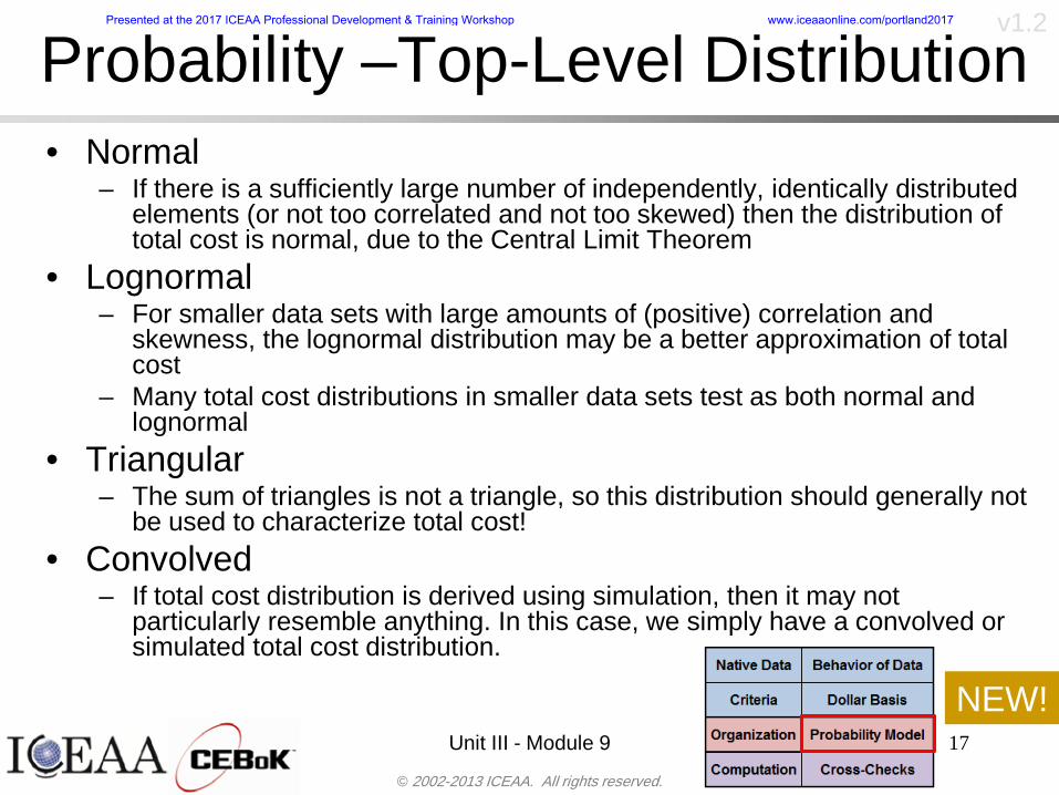
copy 2002-2013 ICEAA All rights reserved
v12
Unit III - Module 9 17
bull Normalndash If there is a sufficiently large number of independently identically distributed
elements (or not too correlated and not too skewed) then the distribution of total cost is normal due to the Central Limit Theorem
bull Lognormalndash For smaller data sets with large amounts of (positive) correlation and
skewness the lognormal distribution may be a better approximation of total cost
ndash Many total cost distributions in smaller data sets test as both normal and lognormal
bull Triangularndash The sum of triangles is not a triangle so this distribution should generally not
be used to characterize total costbull Convolved
ndash If total cost distribution is derived using simulation then it may not particularly resemble anything In this case we simply have a convolved or simulated total cost distribution
Probability ndash Top-Level Distribution
NEW
Presented at the 2017 ICEAA Professional Development amp Training Workshop wwwiceaaonlinecomportland2017
copy 2002-2013 ICEAA All rights reserved
v12
S-Curves and Confidence Levels
Unit III - Module 9 1818
100
70
25
Probability(Confidence
Level)
Cost Estimate(Dollars)
50
The S curve is the cumulative probability distribution coming out of the statistical summing process
70 confidence that project will cost indicated amount or less
Provides information on potential cost as a result of identified project risks
Provides insight into establishing reserve levels
X Y
MR
X = Point estimateZ = Project requirementY = Cost estimate where there is a 70 change that
final actual cost will be less than cost estimateY-Z= Manage reserve (MR) which is REQUIRED to meet 70 CL
Z
X not always = Z but is based on same content
Presented at the 2017 ICEAA Professional Development amp Training Workshop wwwiceaaonlinecomportland2017
copy 2002-2013 ICEAA All rights reserved
v12
19
Example ndash Normal Distribution
bull Normal distribution with mean equal to 100 and standard deviation equal to 20
bull Median and mode also equal 100bull The 80th Percentile is 117
40 60 80 100 120 140 160
80 of distribution(area under curve)is less than 117
117
Presented at the 2017 ICEAA Professional Development amp Training Workshop wwwiceaaonlinecomportland2017
copy 2002-2013 ICEAA All rights reserved
v12
20
Confidence Levelsbull The output of a cost risk analysis is a probability
distributionndash Typically displayed as a cumulative distribution function or
ldquoS-curverdquondash Confidence levels are simply percentiles of the distribution
0
10
20
30
40
50
60
70
80
90
100
30 60 90 120 150 180
Conf
iden
ce L
evel
Presented at the 2017 ICEAA Professional Development amp Training Workshop wwwiceaaonlinecomportland2017
copy 2002-2013 ICEAA All rights reserved
v12
Measuring Parametric Model Uncertainty
bull When developing estimates using cost-estimating relationships (CERs) there are two major sources of uncertaintyndash Technical (model input) uncertaintyndash Estimating uncertainty
bull Technical uncertainty reflects the uncertainty inherent in the model inputsndash Typical parametric model inputs include weight lines of code
heritage and other performance and management inputs
bull Estimating uncertainty measures the uncertainty inherent in the model due to the modelrsquos inability to capture all aspects of variability in the data
21
Presented at the 2017 ICEAA Professional Development amp Training Workshop wwwiceaaonlinecomportland2017
copy 2002-2013 ICEAA All rights reserved
v12
Parametric Model Examplebull The NASAAir Force Cost Model (NAFCOM) is a
parametric model for estimating acquisition costs for spacecraft and launch vehicles
bull The CERs in NAFCOM have the formCost = C WeightVNewDesignWTechnicalXManagementY ClassZ
bull There is technical uncertainty about each of the parametersndash Parametric models are applied early in a program so there
is significant amount of uncertainty in the weightndash Heritage is also tricky it is inherently subjective and project
personnel are typically optimisticndash Technical characteristics can also change as a program
matures and requirements change
22
Presented at the 2017 ICEAA Professional Development amp Training Workshop wwwiceaaonlinecomportland2017
copy 2002-2013 ICEAA All rights reserved
v12
Weight Uncertaintybull Aerospace weight growth study average satellite
weight growth from program inception to launch is 28
23
Aerospace Weight Growth Data
-10
0
10
20
30
40
50
60
0 4 8 12 16 20 24 28 32 36 40 44 48 52 56 60 64 68 72 76 80 84 88 92 96 100
Percent Program Completion
Perc
ent W
eigh
t Gro
wth
Presented at the 2017 ICEAA Professional Development amp Training Workshop wwwiceaaonlinecomportland2017
copy 2002-2013 ICEAA All rights reserved
v12
Estimating Uncertaintybull CERs do not perfectly fit the historical data
ndash There are non-repeatable random effects that cannot be predicted
bull For examplendash Parts breaking during testingndash Strikes which are difficult to predict
bull This results in an underlying uncertainty distribution about an estimatendash The outcome of a CER represents only one point on an
uncertainty distributionbull Typically mean or median depending upon the CER
methodology
24
Presented at the 2017 ICEAA Professional Development amp Training Workshop wwwiceaaonlinecomportland2017
copy 2002-2013 ICEAA All rights reserved
v12
Estimating Uncertainty (2)
25
Presented at the 2017 ICEAA Professional Development amp Training Workshop wwwiceaaonlinecomportland2017
copy 2002-2013 ICEAA All rights reserved
v12
Estimating Uncertainty (3)bull In the case of a linear regression the estimating
uncertainty follows a normal distributionndash The estimate is the mean and the standard error of the
estimate from the regression is the standard deviation of the normal distribution
bull In the case of a log-transformed linear regression the estimating uncertainty follows a lognormal distributionndash The estimate is the median of the lognormal and the
standard error of the estimate from the regression is the standard deviation of the normal distribution (in log-space)
bull There is additional uncertainty about an estimate based upon the distance of what is being estimated from the mean of the input datandash This results in a prediction interval
26
Presented at the 2017 ICEAA Professional Development amp Training Workshop wwwiceaaonlinecomportland2017
copy 2002-2013 ICEAA All rights reserved
v12
Aggregating Riskbull Risk is typically applied at the same level at
which we estimate cost that is at the Work Breakdown Structure (WBS) level
bull The estimates for each WBS are developedndash These estimates sum to yield the total system cost
bull For an n-element WBS the total cost is the sum of the cost for each of the n elements
27
nXXXCostSystem +++= 21
Presented at the 2017 ICEAA Professional Development amp Training Workshop wwwiceaaonlinecomportland2017
copy 2002-2013 ICEAA All rights reserved
v12
WBS Examplebull Launch Vehicle
ndash Structurebull Vehicle Structurebull Tank Structure
ndash Thermal Controlbull Active Thermal Controlbull Induced Thermal Controlbull Tank Thermal Control
ndash Main Propulsion Systemndash Liquid Rocket Enginendash Electric Power and Distributionndash Command Control and Data Handlingndash System Integration
28
Presented at the 2017 ICEAA Professional Development amp Training Workshop wwwiceaaonlinecomportland2017
copy 2002-2013 ICEAA All rights reserved
v12
WBS and Risk
29
Presented at the 2017 ICEAA Professional Development amp Training Workshop wwwiceaaonlinecomportland2017
copy 2002-2013 ICEAA All rights reserved
v12
Aggregating Riskbull This leads us to the issue of aggregating the risks across the
WBSbull For example if we want to determine the 70th percentile of the
overall cost risk distribution how do we proceed bull Note that we cannot simply add the 70th percentiles of each of
the cost risk distributionsbull We can add means and variances (taking correlation into
account more on that later) but that is all
Variance of Total Cost =
30
Mean of Total Cost = ( )E X E Xk
k
n
kk
n
kk
n
= = =aringaelig
egraveccediloumloslashdivide
= =aring aring1 1 1
m
Var X kk
n
=aringaelig
egraveccediloumloslashdivide1
= s r s skk
n
iji
j
i jj
n2
1 1
1
22+aring aringaring
= =
-
=
Presented at the 2017 ICEAA Professional Development amp Training Workshop wwwiceaaonlinecomportland2017
copy 2002-2013 ICEAA All rights reserved
v12
Percentiles Do Not Addbull As a notional example consider two independent normal
distributionsndash One distribution has mean equal to 100 and standard deviation
equal to 20ndash The second distribution has mean 300 and standard deviation of 80
bull The sum of two independent normally distributed random variables is also normally distributed
bull To combine the two distributions we add the means and add the variancesndash Total mean is
ndash Total standard deviation is
31
400300100 =+
8258020 22 raquo+
Presented at the 2017 ICEAA Professional Development amp Training Workshop wwwiceaaonlinecomportland2017
copy 2002-2013 ICEAA All rights reserved
v12
Percentiles Do Not Add (2)bull The 80th percentiles for the individual distributions are
117 and 367 respbull The 80th percentile of the combined distribution is
469 but the sum of the two 80th percentiles is 484bull To see why this is the case note that the percentiles
of a normal distribution are determined by the mean and the standard deviationndash The standard deviations are not added when normal distributions
are combined rather the variances are combinedndash Sum of variances is ndash The standard deviation of this sum is
32
22 ba +22 ba +
Presented at the 2017 ICEAA Professional Development amp Training Workshop wwwiceaaonlinecomportland2017
copy 2002-2013 ICEAA All rights reserved
v12
Percentiles Do Not Add (3)bull Since bull We can write
bull The left side of this inequality represents the risk of the combined distributions while the right side represents the sums of the individual risks
bull Combining two missions that are independent results in a diversification of riskndash The total portfolio is not as risky on a relative basis as each
individual project
33
2222 2 bababa ++lt+
baba +lt+ 22
Presented at the 2017 ICEAA Professional Development amp Training Workshop wwwiceaaonlinecomportland2017
copy 2002-2013 ICEAA All rights reserved
v12
Methods for Aggregating Riskbull Since percentiles do not add we have to find other
ways to aggregate riskbull One method is to use Monte Carlo simulationbull Unless cost risk is represented by normal
distributions for all WBS elements summing the means and variances does not result in a completely accurate depiction of overall system cost risk
bull The normal distribution is not a realistic distribution for representing risk in many or even most situations since regarding project risk more can go wrong than can go right which means the risk is NOT symmetric unlike the Gaussian bell curve
34
Presented at the 2017 ICEAA Professional Development amp Training Workshop wwwiceaaonlinecomportland2017
copy 2002-2013 ICEAA All rights reserved
v12
Unit III - Module 9 35
Monte Carlo Simulationfor Risk Analysis
bull When risk analysis is performed multiple risks are gatheredndash These risks may have various probability
distributions
bull Monte Carlo is the most commonly accepted way to produce an accurate characterization of the distribution of the combined effect of these many risksndash Using this distribution we can produce percentiles
for cost impacts due to risk occurrences
10
Presented at the 2017 ICEAA Professional Development amp Training Workshop wwwiceaaonlinecomportland2017
copy 2002-2013 ICEAA All rights reserved
v12
Monte Carlo Simulationbull Simulation is a means for solving problems that are
analytically intractablendash Involves repeated random sampling
bull It was developed during the Manhattan Project as a way to model the interactions inside an atom during nuclear fissionndash Allowed for more sophisticated mathematical modeling of atomic
phenomena
bull Most computer packages use pseudo-random number generators that produce seemingly random results from an initial seedndash Example is the linear congruential generator
36
( ) mbaXX nn mod1 +=+
Presented at the 2017 ICEAA Professional Development amp Training Workshop wwwiceaaonlinecomportland2017
copy 2002-2013 ICEAA All rights reserved
v12Using Random Numbers to Simulate Distributions
bull WBS cost risk is typically measured by a probability distributionbull The most common method for simulating a probability
distribution is the inverse methodbull This involve obtaining a simulated random value from a uniform
distribution and then inverting this through the cumulative distribution function (CDF) to obtain the simulated value
bull As an example for a uniform distribution on the interval [0100]
bull In this case the CDF random value of 05 translates to 10005 = 50
37
( )100
1=xf ( )
100xxF = ( ) xxF 1001 =-
Presented at the 2017 ICEAA Professional Development amp Training Workshop wwwiceaaonlinecomportland2017
copy 2002-2013 ICEAA All rights reserved
v12
Simulating a Triangular Distribution
bull For a triangular distribution with low = 0 most likely = 50 and high = 150 the CDF is given by
bull The inverse function is given by
38
( )iumliumlicirc
iumliumliacute
igrave
poundlt--
poundpound=
1505021
1500050
50015000
2
2
2
xxx
xxxF
( )iumliumlicirc
iumliumliacute
igrave
poundltdivideoslashouml
ccedilegraveaelig +--
poundpound=-
131
21
37501
250017500150
3107500
1
xx
xxxF
Presented at the 2017 ICEAA Professional Development amp Training Workshop wwwiceaaonlinecomportland2017
copy 2002-2013 ICEAA All rights reserved
v12
Simulating a Triangular Distribution (2)
bull If the simulated uniform value is equal to 02 the corresponding inverse value from the CDF inverse is approximately 387
39
0
01
02
03
04
05
06
07
08
09
1
0 30 60 90 120 150
Presented at the 2017 ICEAA Professional Development amp Training Workshop wwwiceaaonlinecomportland2017
copy 2002-2013 ICEAA All rights reserved
v12
Monte Carlo and the WBSbull Simulation involves repeated trials
40
WBS Draw1 2 3 4 5
System 2912 3566 4390 2954 4655 Sum
Structure 80 105 55 80 57 SumVehicle Structure 50 70 30 40 20Tank Structure 30 35 25 40 37
Thermal Control 32 36 35 29 33 SumActive Thermal Control 10 15 12 7 10Induced Thermal Control 12 14 13 14 14Tank Thermal Control 10 7 10 8 9
Main Propulsion System 100 150 125 140 100
Liquid Rocket Engine 1000 1100 1800 900 2200
Electric Power and Distribution 100 125 150 75 90
Command Control and Data Handling 200 250 225 230 275
System Integration 1400 1800 2000 1500 1900
Presented at the 2017 ICEAA Professional Development amp Training Workshop wwwiceaaonlinecomportland2017
copy 2002-2013 ICEAA All rights reserved
v12
Number of Trialsbull Monte Carlo involves a repeated number of trialsbull The greater the number of trials the more accurate the
simulation will approximate the overall cost risk behavior of the system
bull After 100 trials the histogram looks very jagged
41
Presented at the 2017 ICEAA Professional Development amp Training Workshop wwwiceaaonlinecomportland2017
copy 2002-2013 ICEAA All rights reserved
v12
Number of Trials (2)
42
1000 Trials
10000 Trials
50000 Trials Additional trials give a more accurate depiction of the final result
Presented at the 2017 ICEAA Professional Development amp Training Workshop wwwiceaaonlinecomportland2017
copy 2002-2013 ICEAA All rights reserved
v12
Number of Trials (3)bull If we want to simulate the underlying
mean within 1 with 95 confidence for example then we require
43
divideoslash
oumlccedilegrave
aelig poundpound-
=
dividedividedivide
oslash
ouml
ccedilccedilccedil
egrave
aeligpound
-pound
-=
divideoslashouml
ccedilegraveaelig poundpound=
nZ
n
nnX
n
X
n
n
011
010Pr
011
010Pr
011990Pr950
___
___
sm
sm
sm
sm
sm
mm
Presented at the 2017 ICEAA Professional Development amp Training Workshop wwwiceaaonlinecomportland2017
copy 2002-2013 ICEAA All rights reserved
v12
Number of Trials (4)bull This means that the number of trials required is determined by
bull Solving for n we find that at least
trials are neededbull Note that this term involves the coefficient of variation of the
distribution which means that distributions with less dispersion require fewer trials to accurate simulate
44
96101
=ns
m
ms41638
Presented at the 2017 ICEAA Professional Development amp Training Workshop wwwiceaaonlinecomportland2017
copy 2002-2013 ICEAA All rights reserved
v12
Number of Trials (5)bull Simulating percentiles requires more trials than for simulating
meansbull Let Pn represent the number of trials in the sample at or below
the 70th percentile of the underlying distribution (suppose this is known)
bull By the Central Limit Theorem Pnn follows a normal distribution with mean equal to the 70th percentile and variance equal to
bull By a similar process for the mean we find that the number of trials needed to simulate the 70th percentile within 1 with 95 confidence is
45
( )n
FF 700700 1-
n
n
PPn -41638
Presented at the 2017 ICEAA Professional Development amp Training Workshop wwwiceaaonlinecomportland2017
copy 2002-2013 ICEAA All rights reserved
v12
Number of Trials (6)bull If Pn 070 for all n then n is approximately
bull For the sake of comparison suppose CV = 03 (reasonable approximation for hardware development) then the number of trials needed to simulate the mean with the same accuracy is then ldquoonlyrdquo 11525
bull More trials are needed to accurately simulate percentiles than means
46
( ) 46416703041638
70704168341638 =divide
oslashouml
ccedilegraveaelig=divide
oslashouml
ccedilegraveaelig -
=-
nnn
PPn
n
n
Presented at the 2017 ICEAA Professional Development amp Training Workshop wwwiceaaonlinecomportland2017
copy 2002-2013 ICEAA All rights reserved
v12
Methods of Simulationbull Monte Carlo simulation is a standard term for
simulationbull However there is an improvement on Monte Carlo
that improves the accuracy of the results of a simulation for a given number of trials
bull This method is call the Latin Hypercube approach to simulationndash Similar to Monte Carlo but an equal number of draws are taken
from a set of subintervals for example dividing the interval (01) into [00001) [0102)hellip [0910]
ndash Instead of 10 trials from [01] we have one trial from each subinterval
ndash Rough rule of thumb is Latin Hypercube takes 30 fewer trials to achieve similar accuracy to Monte Carlo
47
Presented at the 2017 ICEAA Professional Development amp Training Workshop wwwiceaaonlinecomportland2017
copy 2002-2013 ICEAA All rights reserved
v12
Probability Model ndash Correlationbull Correlation exists between work breakdown structure
(WBS) cost element costs and between cost and schedule
bull Correlation is a necessary consideration in cost risk analysis
bull Correlation is a number that can vary between -1 and +1 and represents the strength of the relationship between the two variablesndash If both variable have a tendency to move in the same direction
correlation is positivendash If when one variable increases the other tends to decrease and
vice-versa the correlation between the two variables is negative
Presented at the 2017 ICEAA Professional Development amp Training Workshop wwwiceaaonlinecomportland2017
copy 2002-2013 ICEAA All rights reserved
v12
Correlation And Causationbull Note that correlation is not causation however
causation implies correlationndash For example shark attacks and ice cream sales at the beach
bull For example for a launch vehicle structure increasing the diameter will not only result in an increase in the structures cost but will also result in higher costs for thermal coating (paint etc)
bull Also simply because two subsystems do not appear to be related does not mean they are not correlatedndash For example structures and computer equipment seemingly
have little relation to one another however an external factor such as a funding cut or a strike will impact all subsystems leading to delays and increasing cost across the board
ndash Thus everything in a WBS has some correlationUnit III - Module 9 49
Presented at the 2017 ICEAA Professional Development amp Training Workshop wwwiceaaonlinecomportland2017
copy 2002-2013 ICEAA All rights reserved
v12
The Importance of Correlationbull Percent that total cost standard deviation is underestimated
when correlation assumed to be 0 instead of r given nWBS elements
Unit III - Module 9 5050
0
20
40
60
80
100
0 01 02 03 04 05 06 07 08 09 1Actual Correlation
Perce
nt Un
deres
timate
d
n = 10
n = 30
n = 100n = 1000
0
20
40
60
80
100
0 01 02 03 04 05 06 07 08 09 1Actual Correlation
Perce
nt Un
deres
timate
d
n = 10
n = 30
n = 100n = 1000
Reference 32nd Annual DOD Cost Analysis Symposium Advanced Training Session ldquoWhy Correlation Matters in Cost Estimatingrdquo Stephen A Book
Presented at the 2017 ICEAA Professional Development amp Training Workshop wwwiceaaonlinecomportland2017
copy 2002-2013 ICEAA All rights reserved
v12
The Importance of Correlation (2)bull For example if correlation is assumed to be 0 for all
elements in a 30 element WBS and the actual correlation is 20 then the total cost standard deviation is underestimated by 60
bull For example assume the total cost is modeled as a normal distribution with mean = 100
bull If correlation is assumed to be zero with total cost standard deviation = 12 when correlation is actually 20 then the true underlying standard deviation is actually 30
bull 70th percentile with zero correlation assumption is 106
bull 70th percentile with 20 correlation is 116 Unit III - Module 9 51
Presented at the 2017 ICEAA Professional Development amp Training Workshop wwwiceaaonlinecomportland2017
copy 2002-2013 ICEAA All rights reserved
v12
Measures of Correlationbull Two measures of correlation are commonly used in
cost risk analysesndash Pearsonrsquos product-moment correlation coefficient ndash Spearmanrsquos rank correlation coefficient
bull Garvey and others recommend using Pearsonrsquos product-moment correlation coefficient correlation for cost risk analysesndash Method of moments uses this but there are two options in
simulationndash Popular simulation packages like Risk and Crystal Ball use
rank correlation but in practice this has been found to make little difference
ndash Pearson product-moment correlation has been incorporated into Risk+
52
Presented at the 2017 ICEAA Professional Development amp Training Workshop wwwiceaaonlinecomportland2017
copy 2002-2013 ICEAA All rights reserved
v12
Pearson Correlationbull Pearsonrsquos product-moment correlation measures
degree of linearity between two random variables bull If two random variables are perfectly linear (eg Y =
aX + b) with positive slope then the Pearson product-moment correlation between X and Y denoted by rXY is +1
53
X X
Y Y Y
XNegative Correlation Positive Correlation No Correlation
middotmiddot
middotmiddot
middotmiddot middotmiddot
middotmiddot
middot
middot
middotmiddotmiddot
middotmiddot
middotmiddot
middotmiddot middot
middot
middot
middotmiddotmiddotmiddotmiddotmiddotmiddotmiddot
middotmiddotmiddotmiddot
middotmiddot
middotmiddot middotmiddotmiddotmiddot
middotmiddotmiddot
middotmiddotmiddotmiddot
middotmiddotmiddot
middotmiddotmiddot
middotmiddot
middot
middot middotmiddot
middot middotmiddotmiddotmiddot middotmiddot middot middotmiddot middot middot
middotmiddot middot
middotmiddotmiddotmiddotmiddot middot middotmiddot
middotmiddot
middot
middotmiddot
middotmiddot middot
middot middot middot
middotmiddot middot
middotmiddotmiddot
middotmiddot
middot middot
Presented at the 2017 ICEAA Professional Development amp Training Workshop wwwiceaaonlinecomportland2017
copy 2002-2013 ICEAA All rights reserved
v12
Spearman Correlationbull Spearmanrsquos rank correlation measures the
monotonicity between two random variablesbull If two random variables are perfectly monotonically
increasing (eg Y = X2) then the Spearman rank correlation denoted by rXY is +1
bull The two measures can be significantly different
54
10 20 30 40 50 60
100
200
300
096 097 098 099 1
1
060
020
040
080
Eff
ort (
Staf
f-M
onth
s)
Software Size I KDSI
y = 28z12y
z x
yy = x100
0 pound x pound 1
Figure 5-9A Figure 5-9B
Pearson Correlation = 09976 Rank Correlation = 1
Pearson Correlation = 024 Rank Correlation = 1
X(x ) ~ Unif(01)
Reference Probability Methods for Cost Uncertainty Analysis A Systems Engineering Perspective Paul R Garvey
Presented at the 2017 ICEAA Professional Development amp Training Workshop wwwiceaaonlinecomportland2017
copy 2002-2013 ICEAA All rights reserved
v12
Unit III - Module 9 55
200
250
300
350
400
1000 1200 1400 1600 1800 2000
Recurring Production
SEPM
200
250
300
350
400
1000 1200 1400 1600 1800 2000
Recurring Production
SEPM
Functional Correlationbull Old No Functional
Correlation Simulation run with WBS items entered as values
bull New Simulation run with functional dependencies entered as they are in cost model
CorrelatedNot Correlated
Note shift of mean and increased variability
Presented at the 2017 ICEAA Professional Development amp Training Workshop wwwiceaaonlinecomportland2017
copy 2002-2013 ICEAA All rights reserved
v12
Risk Measuresbull ldquoWestern Europe conquered the word because of a
technological revolution that started because of attempts to measure the worldrdquo ndash Phillipe Jorion ndash In the same way attempts to measure risk will lead to better project
managementbull Risk management for DoD and NASA agencies focuses
primarily on funding projects to a single percentile ndash NASA policy explicitly mentions 70 and 50ndash This is known as ldquoValue at Riskrdquo and is prevalent in the banking and
financial industry
56
Presented at the 2017 ICEAA Professional Development amp Training Workshop wwwiceaaonlinecomportland2017
copy 2002-2013 ICEAA All rights reserved
v12
Value at Risk (VaR)bull VaR is a percentile of the cost risk
distributionndash VaR funding at the 70th percentile means that
there is a 30 chance of final project cost exceeding the funded amount (budget)
bull VaR has some meritsndash Common measure can be used to compare
different projects and programsndash Easily understood by senior managers and
decision makers
57
Presented at the 2017 ICEAA Professional Development amp Training Workshop wwwiceaaonlinecomportland2017
copy 2002-2013 ICEAA All rights reserved
v12
Why 70th or 80th Percentilebull Typical policy guidance involves funding at the 70th or 80th
percentile Why fund as such a low percentilebull There is some incentive to not over-fundbull For a normal distribution an inflection point occurs near the 80th
percentile meaning that for values above 80 confidence achieving higher levels of confidence can only be achieved by spending greater dollar amounts at an increasing rate
58
-05-04-03-02-01
00102030405
0 05 1 15 2 25 3
Standard Deviations from Mean
Normal Distribution
First DerivativeSlopeVelocity
Second DerivativeConvexityAcceleration
Inflection point at one standard deviation above the mean (~84th
percentile)
Presented at the 2017 ICEAA Professional Development amp Training Workshop wwwiceaaonlinecomportland2017
copy 2002-2013 ICEAA All rights reserved
v12
Funding Above Inflection Pointsbull As the percentile goes above the 80th percentile the amount
needed to achieve that higher level of confidence begins to increase at an increasing rate as is evident from the graph
59
0
10
20
30
40
50
60
70
50 55 60 65 70 75 80 85 90 95 100
$ Ab
ove
MEa
n to
Ach
ieve
Per
cent
ile
Percentile (Confidence Level)
Presented at the 2017 ICEAA Professional Development amp Training Workshop wwwiceaaonlinecomportland2017
copy 2002-2013 ICEAA All rights reserved
v12
Why Budget to the 70th or 80thbull Government projects are funded at the 70th or 80th percentilesbull Why not the 90th or 99th percentile Wonrsquot that help prevent
overrunsndash As we have seen percentiles do not add across programs
bull The sum of the 80th percentiles does NOT equal the total 80th percentile
ndash This is because the individual programs are riskier than the entire suite of missions
bull Known as the ldquoPortfolio effectrdquo (more or this later)
ndash Funding at the 80th gives confidence that the entire portfolio will be adequately funded
bull And since there is an inflection point near the 80th percentile funding above that level quickly becomes cost prohibitive
60
Presented at the 2017 ICEAA Professional Development amp Training Workshop wwwiceaaonlinecomportland2017
copy 2002-2013 ICEAA All rights reserved
v12
Inflection Points for Lognormalbull For a lognormal the inflection point
variesndash Coefficient of variation equal to 10 equates to an
inflection point at the 70th percentile
61
0
10
20
30
40
50
60
70
050 060 070 080 090 100
Coef
ficen
t of V
aria
tion
Percentile of the Inflection Point
Presented at the 2017 ICEAA Professional Development amp Training Workshop wwwiceaaonlinecomportland2017
copy 2002-2013 ICEAA All rights reserved
v12
Issues with Percentile Fundingbull However risk management does not stop at a
specific percentilendash What happens when the 70th percentile is exceeded
bull Any effective risk management policy should prescribe what happens after a bad event occursndash With VaR we only know when a bad event has occurred ndash Also funding at a relatively low level means we have no true
sense of the real risks that should be guarded against
62
Presented at the 2017 ICEAA Professional Development amp Training Workshop wwwiceaaonlinecomportland2017
copy 2002-2013 ICEAA All rights reserved
v12
ldquoHere There Be Dragonsrdquobull On old maps uncharted territory was often
marked with monsters or dragons
63
A section of the Carta Marina by Olaus Magnus 16th Century
Presented at the 2017 ICEAA Professional Development amp Training Workshop wwwiceaaonlinecomportland2017
copy 2002-2013 ICEAA All rights reserved
v12
Distribution Comparisonbull Four different distributions with the same 70th
percentile
bull Should we expect the tails to be similar
64
0
10
20
30
40
50
60
70
80
0 100 200 300 400 500 600
Perc
entil
eCo
nfid
ence
Lev
el
Triangular
Normal
Lognormal
Pareto
Presented at the 2017 ICEAA Professional Development amp Training Workshop wwwiceaaonlinecomportland2017
copy 2002-2013 ICEAA All rights reserved
v12Distribution Comparison Tail Behavior
bull The normal and triangular distributions have similar tails but the lognormal and Pareto have much fatter right tails
65
70
75
80
85
90
95
100
500 1500 2500 3500 4500 5500
Perc
entil
eCo
nfid
ence
Lev
el
Triangular
Normal
Lognormal
Pareto
Here There Be Dragons
Presented at the 2017 ICEAA Professional Development amp Training Workshop wwwiceaaonlinecomportland2017
copy 2002-2013 ICEAA All rights reserved
v12Distribution Comparison ndash Tail Behavior (Table)
bull There is significant tail risk for the lognormal and the Paretobull The 99th percentile for the Pareto is 1000 times greater than
the 70th percentilendash Risk seen in financial markets and in catastrophic risks like natural
disasters bull Four different projects follow the four different risk profiles seen
in this example should clearly have different risk management approaches but 70th percentile funding indicates the same risk management approach for all four
66
Percentile Triangular Normal Lognormal Pareto 70th $600 $600 $600 $600 80th $680 $660 $770 $1430 90th $770 $750 $1070 $5880 95th $840 $820 $1410 $23750 99th $930 $950 $2350 $600000
Presented at the 2017 ICEAA Professional Development amp Training Workshop wwwiceaaonlinecomportland2017
copy 2002-2013 ICEAA All rights reserved
v12Percentile Budgeting is Not Risk Management
bull Percentile budgeting ne effective risk management policybull Suppose that you are shopping for a new car You
mention that safety is your top concern The salesman says he has a great safe car available You ask about the air bags Do they work The salesman answers ldquoOf course Seventy percent of the time they work fine Only 30 of the time the air bags will fail to deployrdquo Would you buy such a car Hedge fund manager David Einhorn has stated ldquoRisk management is the air bag that must always work but only in the multi-sigma event where you have an accidentrdquo
67
Risk management is the air bag that must always work but only in the multi-sigma event where you
have an accident
Presented at the 2017 ICEAA Professional Development amp Training Workshop wwwiceaaonlinecomportland2017
copy 2002-2013 ICEAA All rights reserved
v12
Joint Confidence Level Analysisbull Schedules are risky toobull For 98 recent NASA missions average
schedule growth was 38ndash Not as high as cost growth but still significant
68
0
5
10
15
20
25
30
35
40
Schedule
Cost
Presented at the 2017 ICEAA Professional Development amp Training Workshop wwwiceaaonlinecomportland2017
copy 2002-2013 ICEAA All rights reserved
v12
Schedules Impact Costbull Changes in schedule can have enormous
impacts on cost ndash Schedule slips can lead to cost increases
bull Fixed programmatic costs must be paid on a regular basisndash Achieving schedule milestones early can result in cost
savings
bull Schedule is an important consideration in cost analysis including cost risk analysis
bull However we must be careful in correctly integrating cost and schedule riskndash Schedule is not simply an input but is dependent on many of
the same factors that drive cost
69
Presented at the 2017 ICEAA Professional Development amp Training Workshop wwwiceaaonlinecomportland2017
copy 2002-2013 ICEAA All rights reserved
v12
The Relationship of Cost to Schedulebull Cost and schedule are positively correlated
ndash A larger program with bigger scope with take longer to complete than a smaller simpler program
bull However longer schedules do not always equate to higher cost nor shorter schedules with lower costndash Highly compressed schedules relative to the
optimal schedule can lead to large overrunsbull Compressed schedules are commonplace for
many planetary missions
70
Presented at the 2017 ICEAA Professional Development amp Training Workshop wwwiceaaonlinecomportland2017
copy 2002-2013 ICEAA All rights reserved
v12The Impact of Schedule GrowthCompression on Cost
bull Compressed schedules lead to cost growth and based on existing research is actually more expensive than schedule slippages
71
0
20
40
60
80
100
120
140
160
-50 -25 0 25 50 75 100
Percentage Change in Schedule
Perc
enta
ge C
hang
e in
Cos
t due
to
Sche
dule
Cha
nge
Source Smart CB ldquoCost and Schedule Interrelationshipsrdquo 2007 NASA Cost Symposium
Presented at the 2017 ICEAA Professional Development amp Training Workshop wwwiceaaonlinecomportland2017
copy 2002-2013 ICEAA All rights reserved
v12Schedule as an Independent Variable
bull Why not simply add schedule as an input to cost-estimating relationships (CERs)
bull Schedule is often treated as an independent variable ndash schedules are often determined independently of cost considerationsndash Cost may not be considered explicitly although budgets and
schedules are determined based on scope and other common factors
bull In 2006 SAIC undertook a research task to determine the impact of schedule on cost and added schedule as an independent variable to the CERs in the NASAAir Force Cost Model (NAFCOM) to see if schedule provided any improvement in goodness of fit
72
Presented at the 2017 ICEAA Professional Development amp Training Workshop wwwiceaaonlinecomportland2017
copy 2002-2013 ICEAA All rights reserved
v12
Schedule is a Dependent Variablebull Since NAFCOM includes an exhaustive list of cost drivers the inclusion
of schedule should give an indication of whether there is any additional independent value added from schedule independent of the cost drivers
bull In the study schedule was added to 10 subsystem-level CERs
ndash In each case the addition of schedule did NOTimprove the goodness of fit and schedule was NOT found to be a statistically significant cost driver (given the presence of the other variables) for any of the 10 CERs
bull Standard errors for the CERs increased due to decrease in degrees of freedom
bull Thus schedule as an independent variable did not provide any additional explanation of variation in historical cost
bull This is because schedule is truly NOT an independent variable but a dependent variable and is a function of the same factors that drive cost
73
Presented at the 2017 ICEAA Professional Development amp Training Workshop wwwiceaaonlinecomportland2017
copy 2002-2013 ICEAA All rights reserved
v12
Incorporation of Schedule in Cost Risk
bull When using subjective methods care must be taken in applying schedule to cost risk analysis
bull Since schedule is a dependent variable treating it independently from other factors when assessing its impact on cost can lead to a double count of independent variables in the cost risk analysis
bull Direct inclusion of schedule in a cost risk analysis effectively doubles the influence of each cost driver
ndash Incorrectly leads to broader risk ranges
74
CostWeight
HeritageNewness
Technology Readiness Schedule
Presented at the 2017 ICEAA Professional Development amp Training Workshop wwwiceaaonlinecomportland2017
copy 2002-2013 ICEAA All rights reserved
v12Subjective Cost Risk Methods and Overinclusion of Risk Factors
bull Subjective methods are suitable when data are scarce or not availablebull However care must be taken not to treat correlated sources of risk
such as schedule as independent of each otherbull Example ndash a subjective risk analysis incorporated technology readiness
design risk requirements stability integration risk and schedule and treated each source of risk as independent
bull Risk triangle high value without schedule risk was 31 times the point estimate
bull Risk triangle high value with schedule risk added on top of other sources of risk treated independently was 34 times the point estimate
bull Risk triangle taking correlation between sources of risk into account in a rigorous statistical manner has a high value 15 times the point estimate less than half the effect when treating sources of risk as independent
75
Presented at the 2017 ICEAA Professional Development amp Training Workshop wwwiceaaonlinecomportland2017
copy 2002-2013 ICEAA All rights reserved
v12Fundamental Equation of Cost and Schedule Interrelationships
bull The Fundamental Equation of the Relationship Between Cost and Schedule is
Time = Moneybull This is a well known adage that time is money Your boss at
work may even mention this to you from time to time or if you are the boss you are all too aware of this iron law
bull Because time is money cost and schedule risk should be modeled jointly not with schedule as an independent cost driver
bull Note that cost and schedule are not perfectly correlatedndash Cost can sometimes ldquobuy downrdquo schedule extra money can be
spent to meet a deadline since in some cases additional effort to hasten the completion of a task
76
Presented at the 2017 ICEAA Professional Development amp Training Workshop wwwiceaaonlinecomportland2017
copy 2002-2013 ICEAA All rights reserved
v12How to (Correctly) Incorporate Schedule into Cost Risk Analysis
bull The best way to model cost and schedule risk is to develop a joint cost and schedule model based on the same data
bull Since such models are not currently available the next best approach is to model cost and schedule independently and then integrate cost and schedule risk analyses using joint probability distributions taking into account correlation between cost and schedulendash This approach pioneered by Paul Garvey and Steve Book is
considered industry best practicendash This is a practical method mathematically tractable and follows
naturally from the Fundamental Equation of Cost and Schedule Interrelationships
77
Book S A ldquoQuantifying the Relationship Between Cost and Schedulerdquo The Measurable News Winter 2007-2008 pp 11-15Garvey PR Probability Methods for Cost Uncertainty Analysis A Systems Engineering Perspective New York Marcel Dekker 2000 pp 308-335
Presented at the 2017 ICEAA Professional Development amp Training Workshop wwwiceaaonlinecomportland2017
copy 2002-2013 ICEAA All rights reserved
v12
Joint Lognormal and Normal Distributions
bull Cost and schedule are typically modeled as some combination of Normal and Lognormal probability distributionsndash Studies by The Aerospace Corporation the MITRE
Corporation Wyle Labs and SAIC have found that the Lognormal probability distribution almost always serves as a good model for both the schedule distribution and the cost distribution
ndash The Normal distribution may also be appropriate in some instances and depending upon the level of confidence at which budgets are set may even be more conservative and logically consistent than the Normal distribution
ndash Joint Lognormal and Normal distributions are defined by a pair of mean and standard deviations and a level of correlation between the two
78
Presented at the 2017 ICEAA Professional Development amp Training Workshop wwwiceaaonlinecomportland2017
copy 2002-2013 ICEAA All rights reserved
v12Modeling Cost and Schedule as a Bivariate Distribution
bull In the approach set forth by Book and Garvey cost risk is assessed and the top-level distribution is modeled as a Lognormal (or Normal) distribution schedule risk is assessed and the overall schedule risk is modeled as a Lognormal (or Normal) distribution
bull The two distributions are combined into a Bivariate distribution by assigning a correlation between the two and by treating the two distributions as the marginal distributions of a Bivariate Lognormal distributionndash Other combinations include a Bivariate Normal or a Bivariate
Normal-Lognormal
79
Presented at the 2017 ICEAA Professional Development amp Training Workshop wwwiceaaonlinecomportland2017
copy 2002-2013 ICEAA All rights reserved
v12Bivariate Lognormal Distribution for Cost and Schedule
bull Cost is often observed to be Lognormal when strong positive correlations are present among the systemrsquos WBS cost element costs
bull A systemrsquos schedule is often observed (from Monte Carlo simulations) to be Lognormal if it is the sum of many positively correlated schedule activities in an overall schedule network
bull If Lognormal distributions characterize a systemrsquos cost and schedule then the Bivariate Lognormal could serve as an assumed model of their joint distributionndash In this case the marginal distribution of each of cost and schedule is
Lognormalbull Other possibilities for modeling cost and schedule as a Bivariate
distribution include a Bivariate Normal or a Bivariate Normal-Lognormal distributionndash All these combinations are analytically tractable
80
Presented at the 2017 ICEAA Professional Development amp Training Workshop wwwiceaaonlinecomportland2017
copy 2002-2013 ICEAA All rights reserved
v12Bivariate Lognormal for Cost and Schedule
bull Contour Plots of a Bivariate Lognormal
81
Presented at the 2017 ICEAA Professional Development amp Training Workshop wwwiceaaonlinecomportland2017
copy 2002-2013 ICEAA All rights reserved
v12Correlation Between Cost and Schedule
bull Cost and schedule are positively correlated but not perfectly sondash For example it is possible to have a schedule underrun and a cost
overrunbull Based on cost and schedule growth data for 50 completed NASA
programs the correlation between development cost and development schedule is 70
82
00
200
400
600
800
1000
1200
-500 00 500 1000 1500 2000 2500Historical Cost Growth
Hist
oric
al S
ched
ule
Gro
wth
r = 715
Presented at the 2017 ICEAA Professional Development amp Training Workshop wwwiceaaonlinecomportland2017
copy 2002-2013 ICEAA All rights reserved
v12Correlation Between Cost and Schedule Caveats
bull Based on historical data recommended correlation between cost and schedule is 70 but this could be higher or lower depending upon program circumstancesndash If program is budget constrained cost and schedule will be
more highly correlated (go as you pay)ndash If program is schedule constrained cost and schedule will
have lower correlation perhaps even negative correlation ndash Smaller programs have smaller correlation between cost and
schedule riskbull Relatively easy to ldquohurry uprdquo and finish on time or even early if
needed
83
Presented at the 2017 ICEAA Professional Development amp Training Workshop wwwiceaaonlinecomportland2017
copy 2002-2013 ICEAA All rights reserved
v12
Conditional Confidence Levelsbull Given a programrsquos project schedule we can determine the cost
risk distribution conditional upon the given schedulebull Conditional cost S-curves are steeper than unconditional
(marginal) cost S-curves between some uncertainty has been removed because schedule is fixed
84
Presented at the 2017 ICEAA Professional Development amp Training Workshop wwwiceaaonlinecomportland2017
copy 2002-2013 ICEAA All rights reserved
v12
Joint Confidence Levelsbull Joint 65 confidence represents the probability of
achieving both 65 confidence in cost AND 65 confidence in schedulendash This is different than achieving 65 cost confidence alone
or achieving 65 schedule confidence alonebull Due to the imperfect correlation between cost and schedule it
is possible to achieve a 65 cost confidence with a lower level of schedule confidence
bull Restricting the schedule confidence thus requires additional $ to achieve a given level of confidence
85
X
Y
Possible Values for Which X gt a Possible Values for
Which X gt a and Y gt b
a
b
Presented at the 2017 ICEAA Professional Development amp Training Workshop wwwiceaaonlinecomportland2017
copy 2002-2013 ICEAA All rights reserved
v12Joint Confidence Levels Versus Cost Confidence Levels Only
bull Example of the differences between cost confidence schedule confidence conditional cost confidence and joint cost and schedule confidence
86
Joint Cost-Schedule Confidence Iso-Curves
Cost (RY$M)
Sche
dule
(Mon
ths)
65 Confidence
50 Confidence
70 Confidence
65 Cost Confidence AggressiveSchedule65 Cost ConfidenceScheduleGiven 65 Schedule ConfidenceUnconditional 65 CostConfidenceUnconditional 65 ScheduleConfidence
65 Cost Confidence 65 Joint Cost and Schedule
Confidence for 65 Schedule Confidence
Presented at the 2017 ICEAA Professional Development amp Training Workshop wwwiceaaonlinecomportland2017
copy 2002-2013 ICEAA All rights reserved
v12
Joint Cost and Schedule Confidence
bull Can examine pairs of cost and schedule that achieve a given level of confidence
bull Provides insights into the trade-offs between cost and schedule for a given level of confidencendash Possible to increase cost confidence by giving a
project more time in some instances or possible to ldquobuy downrdquo schedule
bull But these have limits and are shown in the iso-cost and schedule confidence curves
87
Presented at the 2017 ICEAA Professional Development amp Training Workshop wwwiceaaonlinecomportland2017
copy 2002-2013 ICEAA All rights reserved
v12Cost and Schedule Trade-offs for a Given Level of Joint Confidence
bull Hypothetical Example
88
Cost (RY$M)
Schedule (Months)
$100 48$99 48$89 49$87 50$85 51$85 52$84 53$83 55$83 55$83 56
Cost and Schedule 65 Confidence Iso-Curve
4748495051525354555657
$80 $82 $84 $86 $88 $90 $92 $94 $96 $98 $100
Cost (RY$ M)
Sche
dule
(Mon
ths)
Presented at the 2017 ICEAA Professional Development amp Training Workshop wwwiceaaonlinecomportland2017
copy 2002-2013 ICEAA All rights reserved
v12Policy Considerations for Confidence Levels
bull For large programs the difference between the amount of money needed to achieve 65 cost confidence independent of schedule and joint 65 cost and schedule confidence can represent hundreds of millions and even billions of dollars
89
Joint Cost-Schedule Confidence Iso-Curves
Cost (RY$M)
Sche
dule
(Mon
ths)
65 Confidence
65 Cost Confidence AggressiveSchedule
65 Cost ConfidenceScheduleGiven 65 Schedule Confidence
Unconditional 65 CostConfidence
Joint Cost and Schedule Confidence for 65 Cost Confidence and Program Baseline Schedule is Less Than 35
65 Cost Confidence Independent of Schedule Cost Needed to Achieve
Both 65 Joint Cost and Schedule Confidence for the Schedule with 65 Confidence
Presented at the 2017 ICEAA Professional Development amp Training Workshop wwwiceaaonlinecomportland2017
copy 2002-2013 ICEAA All rights reserved
v12
Copulasbull More generally any combination of distributions can
be used (more than just normal and lognormal)ndash Termed ldquocopulardquo from the Italian word for ldquocouplerdquondash Copulas are a way to combine marginal distributions of any
number and type into a joint distributionbull More formally a copula is a multivariate joint distribution defined
on the n-dimensional unit cube [0 1]n such that every marginal distribution is uniform on the interval [0 1]
bull (The bivariate form of) Sklarrsquos theorem states that for any bivariate distribution function H(x y) let F(x) = H(x infin) and G(y) = H(infin y) be the univariate marginal probability distribution functions Then there exists a copula C such that H(xy)=C(F(x)G(y))
ndash Copulas are widely used in risk management for investments and insurance
bull Considered industry best practice (Li 2000)bull Marketed as part of JP Morganrsquos CreditMetrics suite of tools
(Gupton et Al 1997)90
Presented at the 2017 ICEAA Professional Development amp Training Workshop wwwiceaaonlinecomportland2017
copy 2002-2013 ICEAA All rights reserved
v12Parametric Joint Cost and Schedule Analysis
bull A parametric model based on a consistent data set with a set of overlapping cost and schedule drivers is a cleaner way to model cost and schedule
91
CostWeight
HeritageNewness
Technology Readiness
Schedule
0
20
40
60
80
100
Confidence
Joint Cost and Schedule Confidence
Schedule
Cost
Lognormal Distribution PDF and CDF
0102030405060708090100
200 300 400 500 600 700 800 900 1000Cost $
Con
fiden
ce L
evel
0
00002
00004
00006
00008
0001
00012
00014
00016
Prob
abili
ty D
ensi
ty
CDFPDF
Lognormal Distribution PDF and CDF
0102030405060708090100
200 300 400 500 600 700 800 900 1000Cost $
Con
fiden
ce L
evel
0
00002
00004
00006
00008
0001
00012
00014
00016
Prob
abili
ty D
ensi
ty
CDFPDF
Presented at the 2017 ICEAA Professional Development amp Training Workshop wwwiceaaonlinecomportland2017
copy 2002-2013 ICEAA All rights reserved
v12Parametric Joint Cost and Schedule Analysis (2)
bull Joint cost and schedule risk analysis produced naturally by the integrated modelndash Addresses several issues with the copula
approachbull Tail dependencybull Correlation ndash no need to assign correlation
between cost and schedulebull Consistency of cost and schedule models
92
Presented at the 2017 ICEAA Professional Development amp Training Workshop wwwiceaaonlinecomportland2017
copy 2002-2013 ICEAA All rights reserved
v12
Resource-Loaded Schedulesbull Involves assigning cost and schedule risks to a resource-loaded schedule
networkbull Bottom-up approach
ndash More labor intensive than parametrics but can also provide more insight
ndash Can answer questions than parametric typically cannot such as how much do reserve requirements decrease if a specific risk is retired
bull Currently being implemented in Constellation programbull Has same issue as all bottom-up models hard to count all the risks and model
them discretely
ndash As a result there is a tendency to reflect less risk than indicated by history
ndash ldquoThere are more things in heaven and earth Horatio than are dreamt of in your philosophyrdquo William Shakespeare Hamlet Act I Scene V
93
Presented at the 2017 ICEAA Professional Development amp Training Workshop wwwiceaaonlinecomportland2017
copy 2002-2013 ICEAA All rights reserved
v12Resource-Loaded Schedules Vs Parametrics
bull Parametric most appropriate for early estimatesndash But also good for high-level checks as project progresses
bull As plans take shape lower level modeling may be more appropriate
94 1
CONCEPTUALDEVELOPMENT
PROJECTDEFINITION DESIGN DEVELOPMENT OPERATIONS
PARAMETRIC PARAMETRIC
ANALOGY
ENGINEERING (Bottoms Up)
$PARAMETRIC
DETAILED
$
Pre Phase A Phase B Phase CDPhase A Phase EPre Phase A Phase B Phase CDPhase A Phase E
Risk = f(Cost Estimating Relationship Inputs eg mass power data rate TRL new design etc)
Risk = f(cost and schedule variation of the analogous elements)
Risk = f(variation of detailed inputs eg labor hours rates materials etc)
Presented at the 2017 ICEAA Professional Development amp Training Workshop wwwiceaaonlinecomportland2017
copy 2002-2013 ICEAA All rights reserved
v12
Resource-Loaded Schedulesbull Methodology has been demonstrated in other
industriesndash Construction oil and gasndash Analysis has not been traditionally done on highly uncertain
complex development projects bull Methodology focuses on project baseline schedule
ndash In baseline schedule all tasks are resource loaded to represent a baseline schedule and cost standpoint
ndash Resource loaded schedule is ldquorolledrdquo up to a manageable level
ndash Based on the risk and uncertainties identified schedule distributions are applied to each rolled up task
ndash Cost uncertainties are also applied to rolled up tasksbull Uncertainties include labor rate man power etc
ndash A Monte Carlo simulation is run to develop joint cost-schedule distributions
95
Presented at the 2017 ICEAA Professional Development amp Training Workshop wwwiceaaonlinecomportland2017
copy 2002-2013 ICEAA All rights reserved
v12
Unit III - Module 9 96
Execution ndash Cross Checksbull Means The mean cost growth factor for WBS items
can be compared to history as a way to cross check results
bull CVs The CV of the cost growth factors for WBS items can be compared to history as a way to cross check results
bull Inputs Checks are performed on inputs or other parameters to see if historical values are in line with program assumptionsndash Example Historical risk scores can be compared to program
risk scores to see if risk assessors are being realistic and to see if the underlying database is representative of the program
11
Presented at the 2017 ICEAA Professional Development amp Training Workshop wwwiceaaonlinecomportland2017
- Cost and Schedule Risk Analysis Basic
- Acknowledgments
- Unit Index
- Risk Overview
- Agenda
- Introduction
- Risk Analysis Terms
- Are Our Costs Realistic
- Historical Cost Growth
- Sources of Cost Risk
- Point Estimates of Cost
- Types of Risk
- Point Estimates Vs Risk Estimates
- Cost Risk and Probability
- Probability Model ndash Distribution
- Probability Model ndash Distribution
- Probability ndash Top-Level Distribution
- S-Curves and Confidence Levels
- Example ndash Normal Distribution
- Confidence Levels
- Measuring Parametric Model Uncertainty
- Parametric Model Example
- Weight Uncertainty
- Estimating Uncertainty
- Estimating Uncertainty (2)
- Estimating Uncertainty (3)
- Aggregating Risk
- WBS Example
- WBS and Risk
- Aggregating Risk
- Percentiles Do Not Add
- Percentiles Do Not Add (2)
- Percentiles Do Not Add (3)
- Methods for Aggregating Risk
- Monte Carlo Simulationfor Risk Analysis
- Monte Carlo Simulation
- Using Random Numbers to Simulate Distributions
- Simulating a Triangular Distribution
- Simulating a Triangular Distribution (2)
- Monte Carlo and the WBS
- Number of Trials
- Number of Trials (2)
- Number of Trials (3)
- Number of Trials (4)
- Number of Trials (5)
- Number of Trials (6)
- Methods of Simulation
- Probability Model ndash Correlation
- Correlation And Causation
- The Importance of Correlation
- The Importance of Correlation (2)
- Measures of Correlation
- Pearson Correlation
- Spearman Correlation
- Functional Correlation
- Risk Measures
- Value at Risk (VaR)
- Why 70th or 80th Percentile
- Funding Above Inflection Points
- Why Budget to the 70th or 80th
- Inflection Points for Lognormal
- Issues with Percentile Funding
- ldquoHere There Be Dragonsrdquo
- Distribution Comparison
- Distribution Comparison Tail Behavior
- Distribution Comparison ndash Tail Behavior (Table)
- Percentile Budgeting is Not Risk Management
- Joint Confidence Level Analysis
- Schedules Impact Cost
- The Relationship of Cost to Schedule
- The Impact of Schedule GrowthCompression on Cost
- Schedule as an Independent Variable
- Schedule is a Dependent Variable
- Incorporation of Schedule in Cost Risk
- Subjective Cost Risk Methods and Overinclusion of Risk Factors
- Fundamental Equation of Cost and Schedule Interrelationships
- How to (Correctly) Incorporate Schedule into Cost Risk Analysis
- Joint Lognormal and Normal Distributions
- Modeling Cost and Schedule as a Bivariate Distribution
- Bivariate Lognormal Distribution for Cost and Schedule
- Bivariate Lognormal for Cost and Schedule
- Correlation Between Cost and Schedule
- Correlation Between Cost and Schedule Caveats
- Conditional Confidence Levels
- Joint Confidence Levels
- Joint Confidence Levels Versus Cost Confidence Levels Only
- Joint Cost and Schedule Confidence
- Cost and Schedule Trade-offs for a Given Level of Joint Confidence
- Policy Considerations for Confidence Levels
- Copulas
- Parametric Joint Cost and Schedule Analysis
- Parametric Joint Cost and Schedule Analysis (2)
- Resource-Loaded Schedules
- Resource-Loaded Schedules Vs Parametrics
- Resource-Loaded Schedules
- Execution ndash Cross Checks
-
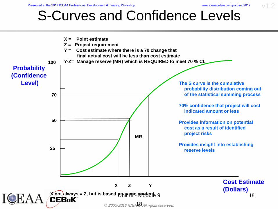
copy 2002-2013 ICEAA All rights reserved
v12
S-Curves and Confidence Levels
Unit III - Module 9 1818
100
70
25
Probability(Confidence
Level)
Cost Estimate(Dollars)
50
The S curve is the cumulative probability distribution coming out of the statistical summing process
70 confidence that project will cost indicated amount or less
Provides information on potential cost as a result of identified project risks
Provides insight into establishing reserve levels
X Y
MR
X = Point estimateZ = Project requirementY = Cost estimate where there is a 70 change that
final actual cost will be less than cost estimateY-Z= Manage reserve (MR) which is REQUIRED to meet 70 CL
Z
X not always = Z but is based on same content
Presented at the 2017 ICEAA Professional Development amp Training Workshop wwwiceaaonlinecomportland2017
copy 2002-2013 ICEAA All rights reserved
v12
19
Example ndash Normal Distribution
bull Normal distribution with mean equal to 100 and standard deviation equal to 20
bull Median and mode also equal 100bull The 80th Percentile is 117
40 60 80 100 120 140 160
80 of distribution(area under curve)is less than 117
117
Presented at the 2017 ICEAA Professional Development amp Training Workshop wwwiceaaonlinecomportland2017
copy 2002-2013 ICEAA All rights reserved
v12
20
Confidence Levelsbull The output of a cost risk analysis is a probability
distributionndash Typically displayed as a cumulative distribution function or
ldquoS-curverdquondash Confidence levels are simply percentiles of the distribution
0
10
20
30
40
50
60
70
80
90
100
30 60 90 120 150 180
Conf
iden
ce L
evel
Presented at the 2017 ICEAA Professional Development amp Training Workshop wwwiceaaonlinecomportland2017
copy 2002-2013 ICEAA All rights reserved
v12
Measuring Parametric Model Uncertainty
bull When developing estimates using cost-estimating relationships (CERs) there are two major sources of uncertaintyndash Technical (model input) uncertaintyndash Estimating uncertainty
bull Technical uncertainty reflects the uncertainty inherent in the model inputsndash Typical parametric model inputs include weight lines of code
heritage and other performance and management inputs
bull Estimating uncertainty measures the uncertainty inherent in the model due to the modelrsquos inability to capture all aspects of variability in the data
21
Presented at the 2017 ICEAA Professional Development amp Training Workshop wwwiceaaonlinecomportland2017
copy 2002-2013 ICEAA All rights reserved
v12
Parametric Model Examplebull The NASAAir Force Cost Model (NAFCOM) is a
parametric model for estimating acquisition costs for spacecraft and launch vehicles
bull The CERs in NAFCOM have the formCost = C WeightVNewDesignWTechnicalXManagementY ClassZ
bull There is technical uncertainty about each of the parametersndash Parametric models are applied early in a program so there
is significant amount of uncertainty in the weightndash Heritage is also tricky it is inherently subjective and project
personnel are typically optimisticndash Technical characteristics can also change as a program
matures and requirements change
22
Presented at the 2017 ICEAA Professional Development amp Training Workshop wwwiceaaonlinecomportland2017
copy 2002-2013 ICEAA All rights reserved
v12
Weight Uncertaintybull Aerospace weight growth study average satellite
weight growth from program inception to launch is 28
23
Aerospace Weight Growth Data
-10
0
10
20
30
40
50
60
0 4 8 12 16 20 24 28 32 36 40 44 48 52 56 60 64 68 72 76 80 84 88 92 96 100
Percent Program Completion
Perc
ent W
eigh
t Gro
wth
Presented at the 2017 ICEAA Professional Development amp Training Workshop wwwiceaaonlinecomportland2017
copy 2002-2013 ICEAA All rights reserved
v12
Estimating Uncertaintybull CERs do not perfectly fit the historical data
ndash There are non-repeatable random effects that cannot be predicted
bull For examplendash Parts breaking during testingndash Strikes which are difficult to predict
bull This results in an underlying uncertainty distribution about an estimatendash The outcome of a CER represents only one point on an
uncertainty distributionbull Typically mean or median depending upon the CER
methodology
24
Presented at the 2017 ICEAA Professional Development amp Training Workshop wwwiceaaonlinecomportland2017
copy 2002-2013 ICEAA All rights reserved
v12
Estimating Uncertainty (2)
25
Presented at the 2017 ICEAA Professional Development amp Training Workshop wwwiceaaonlinecomportland2017
copy 2002-2013 ICEAA All rights reserved
v12
Estimating Uncertainty (3)bull In the case of a linear regression the estimating
uncertainty follows a normal distributionndash The estimate is the mean and the standard error of the
estimate from the regression is the standard deviation of the normal distribution
bull In the case of a log-transformed linear regression the estimating uncertainty follows a lognormal distributionndash The estimate is the median of the lognormal and the
standard error of the estimate from the regression is the standard deviation of the normal distribution (in log-space)
bull There is additional uncertainty about an estimate based upon the distance of what is being estimated from the mean of the input datandash This results in a prediction interval
26
Presented at the 2017 ICEAA Professional Development amp Training Workshop wwwiceaaonlinecomportland2017
copy 2002-2013 ICEAA All rights reserved
v12
Aggregating Riskbull Risk is typically applied at the same level at
which we estimate cost that is at the Work Breakdown Structure (WBS) level
bull The estimates for each WBS are developedndash These estimates sum to yield the total system cost
bull For an n-element WBS the total cost is the sum of the cost for each of the n elements
27
nXXXCostSystem +++= 21
Presented at the 2017 ICEAA Professional Development amp Training Workshop wwwiceaaonlinecomportland2017
copy 2002-2013 ICEAA All rights reserved
v12
WBS Examplebull Launch Vehicle
ndash Structurebull Vehicle Structurebull Tank Structure
ndash Thermal Controlbull Active Thermal Controlbull Induced Thermal Controlbull Tank Thermal Control
ndash Main Propulsion Systemndash Liquid Rocket Enginendash Electric Power and Distributionndash Command Control and Data Handlingndash System Integration
28
Presented at the 2017 ICEAA Professional Development amp Training Workshop wwwiceaaonlinecomportland2017
copy 2002-2013 ICEAA All rights reserved
v12
WBS and Risk
29
Presented at the 2017 ICEAA Professional Development amp Training Workshop wwwiceaaonlinecomportland2017
copy 2002-2013 ICEAA All rights reserved
v12
Aggregating Riskbull This leads us to the issue of aggregating the risks across the
WBSbull For example if we want to determine the 70th percentile of the
overall cost risk distribution how do we proceed bull Note that we cannot simply add the 70th percentiles of each of
the cost risk distributionsbull We can add means and variances (taking correlation into
account more on that later) but that is all
Variance of Total Cost =
30
Mean of Total Cost = ( )E X E Xk
k
n
kk
n
kk
n
= = =aringaelig
egraveccediloumloslashdivide
= =aring aring1 1 1
m
Var X kk
n
=aringaelig
egraveccediloumloslashdivide1
= s r s skk
n
iji
j
i jj
n2
1 1
1
22+aring aringaring
= =
-
=
Presented at the 2017 ICEAA Professional Development amp Training Workshop wwwiceaaonlinecomportland2017
copy 2002-2013 ICEAA All rights reserved
v12
Percentiles Do Not Addbull As a notional example consider two independent normal
distributionsndash One distribution has mean equal to 100 and standard deviation
equal to 20ndash The second distribution has mean 300 and standard deviation of 80
bull The sum of two independent normally distributed random variables is also normally distributed
bull To combine the two distributions we add the means and add the variancesndash Total mean is
ndash Total standard deviation is
31
400300100 =+
8258020 22 raquo+
Presented at the 2017 ICEAA Professional Development amp Training Workshop wwwiceaaonlinecomportland2017
copy 2002-2013 ICEAA All rights reserved
v12
Percentiles Do Not Add (2)bull The 80th percentiles for the individual distributions are
117 and 367 respbull The 80th percentile of the combined distribution is
469 but the sum of the two 80th percentiles is 484bull To see why this is the case note that the percentiles
of a normal distribution are determined by the mean and the standard deviationndash The standard deviations are not added when normal distributions
are combined rather the variances are combinedndash Sum of variances is ndash The standard deviation of this sum is
32
22 ba +22 ba +
Presented at the 2017 ICEAA Professional Development amp Training Workshop wwwiceaaonlinecomportland2017
copy 2002-2013 ICEAA All rights reserved
v12
Percentiles Do Not Add (3)bull Since bull We can write
bull The left side of this inequality represents the risk of the combined distributions while the right side represents the sums of the individual risks
bull Combining two missions that are independent results in a diversification of riskndash The total portfolio is not as risky on a relative basis as each
individual project
33
2222 2 bababa ++lt+
baba +lt+ 22
Presented at the 2017 ICEAA Professional Development amp Training Workshop wwwiceaaonlinecomportland2017
copy 2002-2013 ICEAA All rights reserved
v12
Methods for Aggregating Riskbull Since percentiles do not add we have to find other
ways to aggregate riskbull One method is to use Monte Carlo simulationbull Unless cost risk is represented by normal
distributions for all WBS elements summing the means and variances does not result in a completely accurate depiction of overall system cost risk
bull The normal distribution is not a realistic distribution for representing risk in many or even most situations since regarding project risk more can go wrong than can go right which means the risk is NOT symmetric unlike the Gaussian bell curve
34
Presented at the 2017 ICEAA Professional Development amp Training Workshop wwwiceaaonlinecomportland2017
copy 2002-2013 ICEAA All rights reserved
v12
Unit III - Module 9 35
Monte Carlo Simulationfor Risk Analysis
bull When risk analysis is performed multiple risks are gatheredndash These risks may have various probability
distributions
bull Monte Carlo is the most commonly accepted way to produce an accurate characterization of the distribution of the combined effect of these many risksndash Using this distribution we can produce percentiles
for cost impacts due to risk occurrences
10
Presented at the 2017 ICEAA Professional Development amp Training Workshop wwwiceaaonlinecomportland2017
copy 2002-2013 ICEAA All rights reserved
v12
Monte Carlo Simulationbull Simulation is a means for solving problems that are
analytically intractablendash Involves repeated random sampling
bull It was developed during the Manhattan Project as a way to model the interactions inside an atom during nuclear fissionndash Allowed for more sophisticated mathematical modeling of atomic
phenomena
bull Most computer packages use pseudo-random number generators that produce seemingly random results from an initial seedndash Example is the linear congruential generator
36
( ) mbaXX nn mod1 +=+
Presented at the 2017 ICEAA Professional Development amp Training Workshop wwwiceaaonlinecomportland2017
copy 2002-2013 ICEAA All rights reserved
v12Using Random Numbers to Simulate Distributions
bull WBS cost risk is typically measured by a probability distributionbull The most common method for simulating a probability
distribution is the inverse methodbull This involve obtaining a simulated random value from a uniform
distribution and then inverting this through the cumulative distribution function (CDF) to obtain the simulated value
bull As an example for a uniform distribution on the interval [0100]
bull In this case the CDF random value of 05 translates to 10005 = 50
37
( )100
1=xf ( )
100xxF = ( ) xxF 1001 =-
Presented at the 2017 ICEAA Professional Development amp Training Workshop wwwiceaaonlinecomportland2017
copy 2002-2013 ICEAA All rights reserved
v12
Simulating a Triangular Distribution
bull For a triangular distribution with low = 0 most likely = 50 and high = 150 the CDF is given by
bull The inverse function is given by
38
( )iumliumlicirc
iumliumliacute
igrave
poundlt--
poundpound=
1505021
1500050
50015000
2
2
2
xxx
xxxF
( )iumliumlicirc
iumliumliacute
igrave
poundltdivideoslashouml
ccedilegraveaelig +--
poundpound=-
131
21
37501
250017500150
3107500
1
xx
xxxF
Presented at the 2017 ICEAA Professional Development amp Training Workshop wwwiceaaonlinecomportland2017
copy 2002-2013 ICEAA All rights reserved
v12
Simulating a Triangular Distribution (2)
bull If the simulated uniform value is equal to 02 the corresponding inverse value from the CDF inverse is approximately 387
39
0
01
02
03
04
05
06
07
08
09
1
0 30 60 90 120 150
Presented at the 2017 ICEAA Professional Development amp Training Workshop wwwiceaaonlinecomportland2017
copy 2002-2013 ICEAA All rights reserved
v12
Monte Carlo and the WBSbull Simulation involves repeated trials
40
WBS Draw1 2 3 4 5
System 2912 3566 4390 2954 4655 Sum
Structure 80 105 55 80 57 SumVehicle Structure 50 70 30 40 20Tank Structure 30 35 25 40 37
Thermal Control 32 36 35 29 33 SumActive Thermal Control 10 15 12 7 10Induced Thermal Control 12 14 13 14 14Tank Thermal Control 10 7 10 8 9
Main Propulsion System 100 150 125 140 100
Liquid Rocket Engine 1000 1100 1800 900 2200
Electric Power and Distribution 100 125 150 75 90
Command Control and Data Handling 200 250 225 230 275
System Integration 1400 1800 2000 1500 1900
Presented at the 2017 ICEAA Professional Development amp Training Workshop wwwiceaaonlinecomportland2017
copy 2002-2013 ICEAA All rights reserved
v12
Number of Trialsbull Monte Carlo involves a repeated number of trialsbull The greater the number of trials the more accurate the
simulation will approximate the overall cost risk behavior of the system
bull After 100 trials the histogram looks very jagged
41
Presented at the 2017 ICEAA Professional Development amp Training Workshop wwwiceaaonlinecomportland2017
copy 2002-2013 ICEAA All rights reserved
v12
Number of Trials (2)
42
1000 Trials
10000 Trials
50000 Trials Additional trials give a more accurate depiction of the final result
Presented at the 2017 ICEAA Professional Development amp Training Workshop wwwiceaaonlinecomportland2017
copy 2002-2013 ICEAA All rights reserved
v12
Number of Trials (3)bull If we want to simulate the underlying
mean within 1 with 95 confidence for example then we require
43
divideoslash
oumlccedilegrave
aelig poundpound-
=
dividedividedivide
oslash
ouml
ccedilccedilccedil
egrave
aeligpound
-pound
-=
divideoslashouml
ccedilegraveaelig poundpound=
nZ
n
nnX
n
X
n
n
011
010Pr
011
010Pr
011990Pr950
___
___
sm
sm
sm
sm
sm
mm
Presented at the 2017 ICEAA Professional Development amp Training Workshop wwwiceaaonlinecomportland2017
copy 2002-2013 ICEAA All rights reserved
v12
Number of Trials (4)bull This means that the number of trials required is determined by
bull Solving for n we find that at least
trials are neededbull Note that this term involves the coefficient of variation of the
distribution which means that distributions with less dispersion require fewer trials to accurate simulate
44
96101
=ns
m
ms41638
Presented at the 2017 ICEAA Professional Development amp Training Workshop wwwiceaaonlinecomportland2017
copy 2002-2013 ICEAA All rights reserved
v12
Number of Trials (5)bull Simulating percentiles requires more trials than for simulating
meansbull Let Pn represent the number of trials in the sample at or below
the 70th percentile of the underlying distribution (suppose this is known)
bull By the Central Limit Theorem Pnn follows a normal distribution with mean equal to the 70th percentile and variance equal to
bull By a similar process for the mean we find that the number of trials needed to simulate the 70th percentile within 1 with 95 confidence is
45
( )n
FF 700700 1-
n
n
PPn -41638
Presented at the 2017 ICEAA Professional Development amp Training Workshop wwwiceaaonlinecomportland2017
copy 2002-2013 ICEAA All rights reserved
v12
Number of Trials (6)bull If Pn 070 for all n then n is approximately
bull For the sake of comparison suppose CV = 03 (reasonable approximation for hardware development) then the number of trials needed to simulate the mean with the same accuracy is then ldquoonlyrdquo 11525
bull More trials are needed to accurately simulate percentiles than means
46
( ) 46416703041638
70704168341638 =divide
oslashouml
ccedilegraveaelig=divide
oslashouml
ccedilegraveaelig -
=-
nnn
PPn
n
n
Presented at the 2017 ICEAA Professional Development amp Training Workshop wwwiceaaonlinecomportland2017
copy 2002-2013 ICEAA All rights reserved
v12
Methods of Simulationbull Monte Carlo simulation is a standard term for
simulationbull However there is an improvement on Monte Carlo
that improves the accuracy of the results of a simulation for a given number of trials
bull This method is call the Latin Hypercube approach to simulationndash Similar to Monte Carlo but an equal number of draws are taken
from a set of subintervals for example dividing the interval (01) into [00001) [0102)hellip [0910]
ndash Instead of 10 trials from [01] we have one trial from each subinterval
ndash Rough rule of thumb is Latin Hypercube takes 30 fewer trials to achieve similar accuracy to Monte Carlo
47
Presented at the 2017 ICEAA Professional Development amp Training Workshop wwwiceaaonlinecomportland2017
copy 2002-2013 ICEAA All rights reserved
v12
Probability Model ndash Correlationbull Correlation exists between work breakdown structure
(WBS) cost element costs and between cost and schedule
bull Correlation is a necessary consideration in cost risk analysis
bull Correlation is a number that can vary between -1 and +1 and represents the strength of the relationship between the two variablesndash If both variable have a tendency to move in the same direction
correlation is positivendash If when one variable increases the other tends to decrease and
vice-versa the correlation between the two variables is negative
Presented at the 2017 ICEAA Professional Development amp Training Workshop wwwiceaaonlinecomportland2017
copy 2002-2013 ICEAA All rights reserved
v12
Correlation And Causationbull Note that correlation is not causation however
causation implies correlationndash For example shark attacks and ice cream sales at the beach
bull For example for a launch vehicle structure increasing the diameter will not only result in an increase in the structures cost but will also result in higher costs for thermal coating (paint etc)
bull Also simply because two subsystems do not appear to be related does not mean they are not correlatedndash For example structures and computer equipment seemingly
have little relation to one another however an external factor such as a funding cut or a strike will impact all subsystems leading to delays and increasing cost across the board
ndash Thus everything in a WBS has some correlationUnit III - Module 9 49
Presented at the 2017 ICEAA Professional Development amp Training Workshop wwwiceaaonlinecomportland2017
copy 2002-2013 ICEAA All rights reserved
v12
The Importance of Correlationbull Percent that total cost standard deviation is underestimated
when correlation assumed to be 0 instead of r given nWBS elements
Unit III - Module 9 5050
0
20
40
60
80
100
0 01 02 03 04 05 06 07 08 09 1Actual Correlation
Perce
nt Un
deres
timate
d
n = 10
n = 30
n = 100n = 1000
0
20
40
60
80
100
0 01 02 03 04 05 06 07 08 09 1Actual Correlation
Perce
nt Un
deres
timate
d
n = 10
n = 30
n = 100n = 1000
Reference 32nd Annual DOD Cost Analysis Symposium Advanced Training Session ldquoWhy Correlation Matters in Cost Estimatingrdquo Stephen A Book
Presented at the 2017 ICEAA Professional Development amp Training Workshop wwwiceaaonlinecomportland2017
copy 2002-2013 ICEAA All rights reserved
v12
The Importance of Correlation (2)bull For example if correlation is assumed to be 0 for all
elements in a 30 element WBS and the actual correlation is 20 then the total cost standard deviation is underestimated by 60
bull For example assume the total cost is modeled as a normal distribution with mean = 100
bull If correlation is assumed to be zero with total cost standard deviation = 12 when correlation is actually 20 then the true underlying standard deviation is actually 30
bull 70th percentile with zero correlation assumption is 106
bull 70th percentile with 20 correlation is 116 Unit III - Module 9 51
Presented at the 2017 ICEAA Professional Development amp Training Workshop wwwiceaaonlinecomportland2017
copy 2002-2013 ICEAA All rights reserved
v12
Measures of Correlationbull Two measures of correlation are commonly used in
cost risk analysesndash Pearsonrsquos product-moment correlation coefficient ndash Spearmanrsquos rank correlation coefficient
bull Garvey and others recommend using Pearsonrsquos product-moment correlation coefficient correlation for cost risk analysesndash Method of moments uses this but there are two options in
simulationndash Popular simulation packages like Risk and Crystal Ball use
rank correlation but in practice this has been found to make little difference
ndash Pearson product-moment correlation has been incorporated into Risk+
52
Presented at the 2017 ICEAA Professional Development amp Training Workshop wwwiceaaonlinecomportland2017
copy 2002-2013 ICEAA All rights reserved
v12
Pearson Correlationbull Pearsonrsquos product-moment correlation measures
degree of linearity between two random variables bull If two random variables are perfectly linear (eg Y =
aX + b) with positive slope then the Pearson product-moment correlation between X and Y denoted by rXY is +1
53
X X
Y Y Y
XNegative Correlation Positive Correlation No Correlation
middotmiddot
middotmiddot
middotmiddot middotmiddot
middotmiddot
middot
middot
middotmiddotmiddot
middotmiddot
middotmiddot
middotmiddot middot
middot
middot
middotmiddotmiddotmiddotmiddotmiddotmiddotmiddot
middotmiddotmiddotmiddot
middotmiddot
middotmiddot middotmiddotmiddotmiddot
middotmiddotmiddot
middotmiddotmiddotmiddot
middotmiddotmiddot
middotmiddotmiddot
middotmiddot
middot
middot middotmiddot
middot middotmiddotmiddotmiddot middotmiddot middot middotmiddot middot middot
middotmiddot middot
middotmiddotmiddotmiddotmiddot middot middotmiddot
middotmiddot
middot
middotmiddot
middotmiddot middot
middot middot middot
middotmiddot middot
middotmiddotmiddot
middotmiddot
middot middot
Presented at the 2017 ICEAA Professional Development amp Training Workshop wwwiceaaonlinecomportland2017
copy 2002-2013 ICEAA All rights reserved
v12
Spearman Correlationbull Spearmanrsquos rank correlation measures the
monotonicity between two random variablesbull If two random variables are perfectly monotonically
increasing (eg Y = X2) then the Spearman rank correlation denoted by rXY is +1
bull The two measures can be significantly different
54
10 20 30 40 50 60
100
200
300
096 097 098 099 1
1
060
020
040
080
Eff
ort (
Staf
f-M
onth
s)
Software Size I KDSI
y = 28z12y
z x
yy = x100
0 pound x pound 1
Figure 5-9A Figure 5-9B
Pearson Correlation = 09976 Rank Correlation = 1
Pearson Correlation = 024 Rank Correlation = 1
X(x ) ~ Unif(01)
Reference Probability Methods for Cost Uncertainty Analysis A Systems Engineering Perspective Paul R Garvey
Presented at the 2017 ICEAA Professional Development amp Training Workshop wwwiceaaonlinecomportland2017
copy 2002-2013 ICEAA All rights reserved
v12
Unit III - Module 9 55
200
250
300
350
400
1000 1200 1400 1600 1800 2000
Recurring Production
SEPM
200
250
300
350
400
1000 1200 1400 1600 1800 2000
Recurring Production
SEPM
Functional Correlationbull Old No Functional
Correlation Simulation run with WBS items entered as values
bull New Simulation run with functional dependencies entered as they are in cost model
CorrelatedNot Correlated
Note shift of mean and increased variability
Presented at the 2017 ICEAA Professional Development amp Training Workshop wwwiceaaonlinecomportland2017
copy 2002-2013 ICEAA All rights reserved
v12
Risk Measuresbull ldquoWestern Europe conquered the word because of a
technological revolution that started because of attempts to measure the worldrdquo ndash Phillipe Jorion ndash In the same way attempts to measure risk will lead to better project
managementbull Risk management for DoD and NASA agencies focuses
primarily on funding projects to a single percentile ndash NASA policy explicitly mentions 70 and 50ndash This is known as ldquoValue at Riskrdquo and is prevalent in the banking and
financial industry
56
Presented at the 2017 ICEAA Professional Development amp Training Workshop wwwiceaaonlinecomportland2017
copy 2002-2013 ICEAA All rights reserved
v12
Value at Risk (VaR)bull VaR is a percentile of the cost risk
distributionndash VaR funding at the 70th percentile means that
there is a 30 chance of final project cost exceeding the funded amount (budget)
bull VaR has some meritsndash Common measure can be used to compare
different projects and programsndash Easily understood by senior managers and
decision makers
57
Presented at the 2017 ICEAA Professional Development amp Training Workshop wwwiceaaonlinecomportland2017
copy 2002-2013 ICEAA All rights reserved
v12
Why 70th or 80th Percentilebull Typical policy guidance involves funding at the 70th or 80th
percentile Why fund as such a low percentilebull There is some incentive to not over-fundbull For a normal distribution an inflection point occurs near the 80th
percentile meaning that for values above 80 confidence achieving higher levels of confidence can only be achieved by spending greater dollar amounts at an increasing rate
58
-05-04-03-02-01
00102030405
0 05 1 15 2 25 3
Standard Deviations from Mean
Normal Distribution
First DerivativeSlopeVelocity
Second DerivativeConvexityAcceleration
Inflection point at one standard deviation above the mean (~84th
percentile)
Presented at the 2017 ICEAA Professional Development amp Training Workshop wwwiceaaonlinecomportland2017
copy 2002-2013 ICEAA All rights reserved
v12
Funding Above Inflection Pointsbull As the percentile goes above the 80th percentile the amount
needed to achieve that higher level of confidence begins to increase at an increasing rate as is evident from the graph
59
0
10
20
30
40
50
60
70
50 55 60 65 70 75 80 85 90 95 100
$ Ab
ove
MEa
n to
Ach
ieve
Per
cent
ile
Percentile (Confidence Level)
Presented at the 2017 ICEAA Professional Development amp Training Workshop wwwiceaaonlinecomportland2017
copy 2002-2013 ICEAA All rights reserved
v12
Why Budget to the 70th or 80thbull Government projects are funded at the 70th or 80th percentilesbull Why not the 90th or 99th percentile Wonrsquot that help prevent
overrunsndash As we have seen percentiles do not add across programs
bull The sum of the 80th percentiles does NOT equal the total 80th percentile
ndash This is because the individual programs are riskier than the entire suite of missions
bull Known as the ldquoPortfolio effectrdquo (more or this later)
ndash Funding at the 80th gives confidence that the entire portfolio will be adequately funded
bull And since there is an inflection point near the 80th percentile funding above that level quickly becomes cost prohibitive
60
Presented at the 2017 ICEAA Professional Development amp Training Workshop wwwiceaaonlinecomportland2017
copy 2002-2013 ICEAA All rights reserved
v12
Inflection Points for Lognormalbull For a lognormal the inflection point
variesndash Coefficient of variation equal to 10 equates to an
inflection point at the 70th percentile
61
0
10
20
30
40
50
60
70
050 060 070 080 090 100
Coef
ficen
t of V
aria
tion
Percentile of the Inflection Point
Presented at the 2017 ICEAA Professional Development amp Training Workshop wwwiceaaonlinecomportland2017
copy 2002-2013 ICEAA All rights reserved
v12
Issues with Percentile Fundingbull However risk management does not stop at a
specific percentilendash What happens when the 70th percentile is exceeded
bull Any effective risk management policy should prescribe what happens after a bad event occursndash With VaR we only know when a bad event has occurred ndash Also funding at a relatively low level means we have no true
sense of the real risks that should be guarded against
62
Presented at the 2017 ICEAA Professional Development amp Training Workshop wwwiceaaonlinecomportland2017
copy 2002-2013 ICEAA All rights reserved
v12
ldquoHere There Be Dragonsrdquobull On old maps uncharted territory was often
marked with monsters or dragons
63
A section of the Carta Marina by Olaus Magnus 16th Century
Presented at the 2017 ICEAA Professional Development amp Training Workshop wwwiceaaonlinecomportland2017
copy 2002-2013 ICEAA All rights reserved
v12
Distribution Comparisonbull Four different distributions with the same 70th
percentile
bull Should we expect the tails to be similar
64
0
10
20
30
40
50
60
70
80
0 100 200 300 400 500 600
Perc
entil
eCo
nfid
ence
Lev
el
Triangular
Normal
Lognormal
Pareto
Presented at the 2017 ICEAA Professional Development amp Training Workshop wwwiceaaonlinecomportland2017
copy 2002-2013 ICEAA All rights reserved
v12Distribution Comparison Tail Behavior
bull The normal and triangular distributions have similar tails but the lognormal and Pareto have much fatter right tails
65
70
75
80
85
90
95
100
500 1500 2500 3500 4500 5500
Perc
entil
eCo
nfid
ence
Lev
el
Triangular
Normal
Lognormal
Pareto
Here There Be Dragons
Presented at the 2017 ICEAA Professional Development amp Training Workshop wwwiceaaonlinecomportland2017
copy 2002-2013 ICEAA All rights reserved
v12Distribution Comparison ndash Tail Behavior (Table)
bull There is significant tail risk for the lognormal and the Paretobull The 99th percentile for the Pareto is 1000 times greater than
the 70th percentilendash Risk seen in financial markets and in catastrophic risks like natural
disasters bull Four different projects follow the four different risk profiles seen
in this example should clearly have different risk management approaches but 70th percentile funding indicates the same risk management approach for all four
66
Percentile Triangular Normal Lognormal Pareto 70th $600 $600 $600 $600 80th $680 $660 $770 $1430 90th $770 $750 $1070 $5880 95th $840 $820 $1410 $23750 99th $930 $950 $2350 $600000
Presented at the 2017 ICEAA Professional Development amp Training Workshop wwwiceaaonlinecomportland2017
copy 2002-2013 ICEAA All rights reserved
v12Percentile Budgeting is Not Risk Management
bull Percentile budgeting ne effective risk management policybull Suppose that you are shopping for a new car You
mention that safety is your top concern The salesman says he has a great safe car available You ask about the air bags Do they work The salesman answers ldquoOf course Seventy percent of the time they work fine Only 30 of the time the air bags will fail to deployrdquo Would you buy such a car Hedge fund manager David Einhorn has stated ldquoRisk management is the air bag that must always work but only in the multi-sigma event where you have an accidentrdquo
67
Risk management is the air bag that must always work but only in the multi-sigma event where you
have an accident
Presented at the 2017 ICEAA Professional Development amp Training Workshop wwwiceaaonlinecomportland2017
copy 2002-2013 ICEAA All rights reserved
v12
Joint Confidence Level Analysisbull Schedules are risky toobull For 98 recent NASA missions average
schedule growth was 38ndash Not as high as cost growth but still significant
68
0
5
10
15
20
25
30
35
40
Schedule
Cost
Presented at the 2017 ICEAA Professional Development amp Training Workshop wwwiceaaonlinecomportland2017
copy 2002-2013 ICEAA All rights reserved
v12
Schedules Impact Costbull Changes in schedule can have enormous
impacts on cost ndash Schedule slips can lead to cost increases
bull Fixed programmatic costs must be paid on a regular basisndash Achieving schedule milestones early can result in cost
savings
bull Schedule is an important consideration in cost analysis including cost risk analysis
bull However we must be careful in correctly integrating cost and schedule riskndash Schedule is not simply an input but is dependent on many of
the same factors that drive cost
69
Presented at the 2017 ICEAA Professional Development amp Training Workshop wwwiceaaonlinecomportland2017
copy 2002-2013 ICEAA All rights reserved
v12
The Relationship of Cost to Schedulebull Cost and schedule are positively correlated
ndash A larger program with bigger scope with take longer to complete than a smaller simpler program
bull However longer schedules do not always equate to higher cost nor shorter schedules with lower costndash Highly compressed schedules relative to the
optimal schedule can lead to large overrunsbull Compressed schedules are commonplace for
many planetary missions
70
Presented at the 2017 ICEAA Professional Development amp Training Workshop wwwiceaaonlinecomportland2017
copy 2002-2013 ICEAA All rights reserved
v12The Impact of Schedule GrowthCompression on Cost
bull Compressed schedules lead to cost growth and based on existing research is actually more expensive than schedule slippages
71
0
20
40
60
80
100
120
140
160
-50 -25 0 25 50 75 100
Percentage Change in Schedule
Perc
enta
ge C
hang
e in
Cos
t due
to
Sche
dule
Cha
nge
Source Smart CB ldquoCost and Schedule Interrelationshipsrdquo 2007 NASA Cost Symposium
Presented at the 2017 ICEAA Professional Development amp Training Workshop wwwiceaaonlinecomportland2017
copy 2002-2013 ICEAA All rights reserved
v12Schedule as an Independent Variable
bull Why not simply add schedule as an input to cost-estimating relationships (CERs)
bull Schedule is often treated as an independent variable ndash schedules are often determined independently of cost considerationsndash Cost may not be considered explicitly although budgets and
schedules are determined based on scope and other common factors
bull In 2006 SAIC undertook a research task to determine the impact of schedule on cost and added schedule as an independent variable to the CERs in the NASAAir Force Cost Model (NAFCOM) to see if schedule provided any improvement in goodness of fit
72
Presented at the 2017 ICEAA Professional Development amp Training Workshop wwwiceaaonlinecomportland2017
copy 2002-2013 ICEAA All rights reserved
v12
Schedule is a Dependent Variablebull Since NAFCOM includes an exhaustive list of cost drivers the inclusion
of schedule should give an indication of whether there is any additional independent value added from schedule independent of the cost drivers
bull In the study schedule was added to 10 subsystem-level CERs
ndash In each case the addition of schedule did NOTimprove the goodness of fit and schedule was NOT found to be a statistically significant cost driver (given the presence of the other variables) for any of the 10 CERs
bull Standard errors for the CERs increased due to decrease in degrees of freedom
bull Thus schedule as an independent variable did not provide any additional explanation of variation in historical cost
bull This is because schedule is truly NOT an independent variable but a dependent variable and is a function of the same factors that drive cost
73
Presented at the 2017 ICEAA Professional Development amp Training Workshop wwwiceaaonlinecomportland2017
copy 2002-2013 ICEAA All rights reserved
v12
Incorporation of Schedule in Cost Risk
bull When using subjective methods care must be taken in applying schedule to cost risk analysis
bull Since schedule is a dependent variable treating it independently from other factors when assessing its impact on cost can lead to a double count of independent variables in the cost risk analysis
bull Direct inclusion of schedule in a cost risk analysis effectively doubles the influence of each cost driver
ndash Incorrectly leads to broader risk ranges
74
CostWeight
HeritageNewness
Technology Readiness Schedule
Presented at the 2017 ICEAA Professional Development amp Training Workshop wwwiceaaonlinecomportland2017
copy 2002-2013 ICEAA All rights reserved
v12Subjective Cost Risk Methods and Overinclusion of Risk Factors
bull Subjective methods are suitable when data are scarce or not availablebull However care must be taken not to treat correlated sources of risk
such as schedule as independent of each otherbull Example ndash a subjective risk analysis incorporated technology readiness
design risk requirements stability integration risk and schedule and treated each source of risk as independent
bull Risk triangle high value without schedule risk was 31 times the point estimate
bull Risk triangle high value with schedule risk added on top of other sources of risk treated independently was 34 times the point estimate
bull Risk triangle taking correlation between sources of risk into account in a rigorous statistical manner has a high value 15 times the point estimate less than half the effect when treating sources of risk as independent
75
Presented at the 2017 ICEAA Professional Development amp Training Workshop wwwiceaaonlinecomportland2017
copy 2002-2013 ICEAA All rights reserved
v12Fundamental Equation of Cost and Schedule Interrelationships
bull The Fundamental Equation of the Relationship Between Cost and Schedule is
Time = Moneybull This is a well known adage that time is money Your boss at
work may even mention this to you from time to time or if you are the boss you are all too aware of this iron law
bull Because time is money cost and schedule risk should be modeled jointly not with schedule as an independent cost driver
bull Note that cost and schedule are not perfectly correlatedndash Cost can sometimes ldquobuy downrdquo schedule extra money can be
spent to meet a deadline since in some cases additional effort to hasten the completion of a task
76
Presented at the 2017 ICEAA Professional Development amp Training Workshop wwwiceaaonlinecomportland2017
copy 2002-2013 ICEAA All rights reserved
v12How to (Correctly) Incorporate Schedule into Cost Risk Analysis
bull The best way to model cost and schedule risk is to develop a joint cost and schedule model based on the same data
bull Since such models are not currently available the next best approach is to model cost and schedule independently and then integrate cost and schedule risk analyses using joint probability distributions taking into account correlation between cost and schedulendash This approach pioneered by Paul Garvey and Steve Book is
considered industry best practicendash This is a practical method mathematically tractable and follows
naturally from the Fundamental Equation of Cost and Schedule Interrelationships
77
Book S A ldquoQuantifying the Relationship Between Cost and Schedulerdquo The Measurable News Winter 2007-2008 pp 11-15Garvey PR Probability Methods for Cost Uncertainty Analysis A Systems Engineering Perspective New York Marcel Dekker 2000 pp 308-335
Presented at the 2017 ICEAA Professional Development amp Training Workshop wwwiceaaonlinecomportland2017
copy 2002-2013 ICEAA All rights reserved
v12
Joint Lognormal and Normal Distributions
bull Cost and schedule are typically modeled as some combination of Normal and Lognormal probability distributionsndash Studies by The Aerospace Corporation the MITRE
Corporation Wyle Labs and SAIC have found that the Lognormal probability distribution almost always serves as a good model for both the schedule distribution and the cost distribution
ndash The Normal distribution may also be appropriate in some instances and depending upon the level of confidence at which budgets are set may even be more conservative and logically consistent than the Normal distribution
ndash Joint Lognormal and Normal distributions are defined by a pair of mean and standard deviations and a level of correlation between the two
78
Presented at the 2017 ICEAA Professional Development amp Training Workshop wwwiceaaonlinecomportland2017
copy 2002-2013 ICEAA All rights reserved
v12Modeling Cost and Schedule as a Bivariate Distribution
bull In the approach set forth by Book and Garvey cost risk is assessed and the top-level distribution is modeled as a Lognormal (or Normal) distribution schedule risk is assessed and the overall schedule risk is modeled as a Lognormal (or Normal) distribution
bull The two distributions are combined into a Bivariate distribution by assigning a correlation between the two and by treating the two distributions as the marginal distributions of a Bivariate Lognormal distributionndash Other combinations include a Bivariate Normal or a Bivariate
Normal-Lognormal
79
Presented at the 2017 ICEAA Professional Development amp Training Workshop wwwiceaaonlinecomportland2017
copy 2002-2013 ICEAA All rights reserved
v12Bivariate Lognormal Distribution for Cost and Schedule
bull Cost is often observed to be Lognormal when strong positive correlations are present among the systemrsquos WBS cost element costs
bull A systemrsquos schedule is often observed (from Monte Carlo simulations) to be Lognormal if it is the sum of many positively correlated schedule activities in an overall schedule network
bull If Lognormal distributions characterize a systemrsquos cost and schedule then the Bivariate Lognormal could serve as an assumed model of their joint distributionndash In this case the marginal distribution of each of cost and schedule is
Lognormalbull Other possibilities for modeling cost and schedule as a Bivariate
distribution include a Bivariate Normal or a Bivariate Normal-Lognormal distributionndash All these combinations are analytically tractable
80
Presented at the 2017 ICEAA Professional Development amp Training Workshop wwwiceaaonlinecomportland2017
copy 2002-2013 ICEAA All rights reserved
v12Bivariate Lognormal for Cost and Schedule
bull Contour Plots of a Bivariate Lognormal
81
Presented at the 2017 ICEAA Professional Development amp Training Workshop wwwiceaaonlinecomportland2017
copy 2002-2013 ICEAA All rights reserved
v12Correlation Between Cost and Schedule
bull Cost and schedule are positively correlated but not perfectly sondash For example it is possible to have a schedule underrun and a cost
overrunbull Based on cost and schedule growth data for 50 completed NASA
programs the correlation between development cost and development schedule is 70
82
00
200
400
600
800
1000
1200
-500 00 500 1000 1500 2000 2500Historical Cost Growth
Hist
oric
al S
ched
ule
Gro
wth
r = 715
Presented at the 2017 ICEAA Professional Development amp Training Workshop wwwiceaaonlinecomportland2017
copy 2002-2013 ICEAA All rights reserved
v12Correlation Between Cost and Schedule Caveats
bull Based on historical data recommended correlation between cost and schedule is 70 but this could be higher or lower depending upon program circumstancesndash If program is budget constrained cost and schedule will be
more highly correlated (go as you pay)ndash If program is schedule constrained cost and schedule will
have lower correlation perhaps even negative correlation ndash Smaller programs have smaller correlation between cost and
schedule riskbull Relatively easy to ldquohurry uprdquo and finish on time or even early if
needed
83
Presented at the 2017 ICEAA Professional Development amp Training Workshop wwwiceaaonlinecomportland2017
copy 2002-2013 ICEAA All rights reserved
v12
Conditional Confidence Levelsbull Given a programrsquos project schedule we can determine the cost
risk distribution conditional upon the given schedulebull Conditional cost S-curves are steeper than unconditional
(marginal) cost S-curves between some uncertainty has been removed because schedule is fixed
84
Presented at the 2017 ICEAA Professional Development amp Training Workshop wwwiceaaonlinecomportland2017
copy 2002-2013 ICEAA All rights reserved
v12
Joint Confidence Levelsbull Joint 65 confidence represents the probability of
achieving both 65 confidence in cost AND 65 confidence in schedulendash This is different than achieving 65 cost confidence alone
or achieving 65 schedule confidence alonebull Due to the imperfect correlation between cost and schedule it
is possible to achieve a 65 cost confidence with a lower level of schedule confidence
bull Restricting the schedule confidence thus requires additional $ to achieve a given level of confidence
85
X
Y
Possible Values for Which X gt a Possible Values for
Which X gt a and Y gt b
a
b
Presented at the 2017 ICEAA Professional Development amp Training Workshop wwwiceaaonlinecomportland2017
copy 2002-2013 ICEAA All rights reserved
v12Joint Confidence Levels Versus Cost Confidence Levels Only
bull Example of the differences between cost confidence schedule confidence conditional cost confidence and joint cost and schedule confidence
86
Joint Cost-Schedule Confidence Iso-Curves
Cost (RY$M)
Sche
dule
(Mon
ths)
65 Confidence
50 Confidence
70 Confidence
65 Cost Confidence AggressiveSchedule65 Cost ConfidenceScheduleGiven 65 Schedule ConfidenceUnconditional 65 CostConfidenceUnconditional 65 ScheduleConfidence
65 Cost Confidence 65 Joint Cost and Schedule
Confidence for 65 Schedule Confidence
Presented at the 2017 ICEAA Professional Development amp Training Workshop wwwiceaaonlinecomportland2017
copy 2002-2013 ICEAA All rights reserved
v12
Joint Cost and Schedule Confidence
bull Can examine pairs of cost and schedule that achieve a given level of confidence
bull Provides insights into the trade-offs between cost and schedule for a given level of confidencendash Possible to increase cost confidence by giving a
project more time in some instances or possible to ldquobuy downrdquo schedule
bull But these have limits and are shown in the iso-cost and schedule confidence curves
87
Presented at the 2017 ICEAA Professional Development amp Training Workshop wwwiceaaonlinecomportland2017
copy 2002-2013 ICEAA All rights reserved
v12Cost and Schedule Trade-offs for a Given Level of Joint Confidence
bull Hypothetical Example
88
Cost (RY$M)
Schedule (Months)
$100 48$99 48$89 49$87 50$85 51$85 52$84 53$83 55$83 55$83 56
Cost and Schedule 65 Confidence Iso-Curve
4748495051525354555657
$80 $82 $84 $86 $88 $90 $92 $94 $96 $98 $100
Cost (RY$ M)
Sche
dule
(Mon
ths)
Presented at the 2017 ICEAA Professional Development amp Training Workshop wwwiceaaonlinecomportland2017
copy 2002-2013 ICEAA All rights reserved
v12Policy Considerations for Confidence Levels
bull For large programs the difference between the amount of money needed to achieve 65 cost confidence independent of schedule and joint 65 cost and schedule confidence can represent hundreds of millions and even billions of dollars
89
Joint Cost-Schedule Confidence Iso-Curves
Cost (RY$M)
Sche
dule
(Mon
ths)
65 Confidence
65 Cost Confidence AggressiveSchedule
65 Cost ConfidenceScheduleGiven 65 Schedule Confidence
Unconditional 65 CostConfidence
Joint Cost and Schedule Confidence for 65 Cost Confidence and Program Baseline Schedule is Less Than 35
65 Cost Confidence Independent of Schedule Cost Needed to Achieve
Both 65 Joint Cost and Schedule Confidence for the Schedule with 65 Confidence
Presented at the 2017 ICEAA Professional Development amp Training Workshop wwwiceaaonlinecomportland2017
copy 2002-2013 ICEAA All rights reserved
v12
Copulasbull More generally any combination of distributions can
be used (more than just normal and lognormal)ndash Termed ldquocopulardquo from the Italian word for ldquocouplerdquondash Copulas are a way to combine marginal distributions of any
number and type into a joint distributionbull More formally a copula is a multivariate joint distribution defined
on the n-dimensional unit cube [0 1]n such that every marginal distribution is uniform on the interval [0 1]
bull (The bivariate form of) Sklarrsquos theorem states that for any bivariate distribution function H(x y) let F(x) = H(x infin) and G(y) = H(infin y) be the univariate marginal probability distribution functions Then there exists a copula C such that H(xy)=C(F(x)G(y))
ndash Copulas are widely used in risk management for investments and insurance
bull Considered industry best practice (Li 2000)bull Marketed as part of JP Morganrsquos CreditMetrics suite of tools
(Gupton et Al 1997)90
Presented at the 2017 ICEAA Professional Development amp Training Workshop wwwiceaaonlinecomportland2017
copy 2002-2013 ICEAA All rights reserved
v12Parametric Joint Cost and Schedule Analysis
bull A parametric model based on a consistent data set with a set of overlapping cost and schedule drivers is a cleaner way to model cost and schedule
91
CostWeight
HeritageNewness
Technology Readiness
Schedule
0
20
40
60
80
100
Confidence
Joint Cost and Schedule Confidence
Schedule
Cost
Lognormal Distribution PDF and CDF
0102030405060708090100
200 300 400 500 600 700 800 900 1000Cost $
Con
fiden
ce L
evel
0
00002
00004
00006
00008
0001
00012
00014
00016
Prob
abili
ty D
ensi
ty
CDFPDF
Lognormal Distribution PDF and CDF
0102030405060708090100
200 300 400 500 600 700 800 900 1000Cost $
Con
fiden
ce L
evel
0
00002
00004
00006
00008
0001
00012
00014
00016
Prob
abili
ty D
ensi
ty
CDFPDF
Presented at the 2017 ICEAA Professional Development amp Training Workshop wwwiceaaonlinecomportland2017
copy 2002-2013 ICEAA All rights reserved
v12Parametric Joint Cost and Schedule Analysis (2)
bull Joint cost and schedule risk analysis produced naturally by the integrated modelndash Addresses several issues with the copula
approachbull Tail dependencybull Correlation ndash no need to assign correlation
between cost and schedulebull Consistency of cost and schedule models
92
Presented at the 2017 ICEAA Professional Development amp Training Workshop wwwiceaaonlinecomportland2017
copy 2002-2013 ICEAA All rights reserved
v12
Resource-Loaded Schedulesbull Involves assigning cost and schedule risks to a resource-loaded schedule
networkbull Bottom-up approach
ndash More labor intensive than parametrics but can also provide more insight
ndash Can answer questions than parametric typically cannot such as how much do reserve requirements decrease if a specific risk is retired
bull Currently being implemented in Constellation programbull Has same issue as all bottom-up models hard to count all the risks and model
them discretely
ndash As a result there is a tendency to reflect less risk than indicated by history
ndash ldquoThere are more things in heaven and earth Horatio than are dreamt of in your philosophyrdquo William Shakespeare Hamlet Act I Scene V
93
Presented at the 2017 ICEAA Professional Development amp Training Workshop wwwiceaaonlinecomportland2017
copy 2002-2013 ICEAA All rights reserved
v12Resource-Loaded Schedules Vs Parametrics
bull Parametric most appropriate for early estimatesndash But also good for high-level checks as project progresses
bull As plans take shape lower level modeling may be more appropriate
94 1
CONCEPTUALDEVELOPMENT
PROJECTDEFINITION DESIGN DEVELOPMENT OPERATIONS
PARAMETRIC PARAMETRIC
ANALOGY
ENGINEERING (Bottoms Up)
$PARAMETRIC
DETAILED
$
Pre Phase A Phase B Phase CDPhase A Phase EPre Phase A Phase B Phase CDPhase A Phase E
Risk = f(Cost Estimating Relationship Inputs eg mass power data rate TRL new design etc)
Risk = f(cost and schedule variation of the analogous elements)
Risk = f(variation of detailed inputs eg labor hours rates materials etc)
Presented at the 2017 ICEAA Professional Development amp Training Workshop wwwiceaaonlinecomportland2017
copy 2002-2013 ICEAA All rights reserved
v12
Resource-Loaded Schedulesbull Methodology has been demonstrated in other
industriesndash Construction oil and gasndash Analysis has not been traditionally done on highly uncertain
complex development projects bull Methodology focuses on project baseline schedule
ndash In baseline schedule all tasks are resource loaded to represent a baseline schedule and cost standpoint
ndash Resource loaded schedule is ldquorolledrdquo up to a manageable level
ndash Based on the risk and uncertainties identified schedule distributions are applied to each rolled up task
ndash Cost uncertainties are also applied to rolled up tasksbull Uncertainties include labor rate man power etc
ndash A Monte Carlo simulation is run to develop joint cost-schedule distributions
95
Presented at the 2017 ICEAA Professional Development amp Training Workshop wwwiceaaonlinecomportland2017
copy 2002-2013 ICEAA All rights reserved
v12
Unit III - Module 9 96
Execution ndash Cross Checksbull Means The mean cost growth factor for WBS items
can be compared to history as a way to cross check results
bull CVs The CV of the cost growth factors for WBS items can be compared to history as a way to cross check results
bull Inputs Checks are performed on inputs or other parameters to see if historical values are in line with program assumptionsndash Example Historical risk scores can be compared to program
risk scores to see if risk assessors are being realistic and to see if the underlying database is representative of the program
11
Presented at the 2017 ICEAA Professional Development amp Training Workshop wwwiceaaonlinecomportland2017
- Cost and Schedule Risk Analysis Basic
- Acknowledgments
- Unit Index
- Risk Overview
- Agenda
- Introduction
- Risk Analysis Terms
- Are Our Costs Realistic
- Historical Cost Growth
- Sources of Cost Risk
- Point Estimates of Cost
- Types of Risk
- Point Estimates Vs Risk Estimates
- Cost Risk and Probability
- Probability Model ndash Distribution
- Probability Model ndash Distribution
- Probability ndash Top-Level Distribution
- S-Curves and Confidence Levels
- Example ndash Normal Distribution
- Confidence Levels
- Measuring Parametric Model Uncertainty
- Parametric Model Example
- Weight Uncertainty
- Estimating Uncertainty
- Estimating Uncertainty (2)
- Estimating Uncertainty (3)
- Aggregating Risk
- WBS Example
- WBS and Risk
- Aggregating Risk
- Percentiles Do Not Add
- Percentiles Do Not Add (2)
- Percentiles Do Not Add (3)
- Methods for Aggregating Risk
- Monte Carlo Simulationfor Risk Analysis
- Monte Carlo Simulation
- Using Random Numbers to Simulate Distributions
- Simulating a Triangular Distribution
- Simulating a Triangular Distribution (2)
- Monte Carlo and the WBS
- Number of Trials
- Number of Trials (2)
- Number of Trials (3)
- Number of Trials (4)
- Number of Trials (5)
- Number of Trials (6)
- Methods of Simulation
- Probability Model ndash Correlation
- Correlation And Causation
- The Importance of Correlation
- The Importance of Correlation (2)
- Measures of Correlation
- Pearson Correlation
- Spearman Correlation
- Functional Correlation
- Risk Measures
- Value at Risk (VaR)
- Why 70th or 80th Percentile
- Funding Above Inflection Points
- Why Budget to the 70th or 80th
- Inflection Points for Lognormal
- Issues with Percentile Funding
- ldquoHere There Be Dragonsrdquo
- Distribution Comparison
- Distribution Comparison Tail Behavior
- Distribution Comparison ndash Tail Behavior (Table)
- Percentile Budgeting is Not Risk Management
- Joint Confidence Level Analysis
- Schedules Impact Cost
- The Relationship of Cost to Schedule
- The Impact of Schedule GrowthCompression on Cost
- Schedule as an Independent Variable
- Schedule is a Dependent Variable
- Incorporation of Schedule in Cost Risk
- Subjective Cost Risk Methods and Overinclusion of Risk Factors
- Fundamental Equation of Cost and Schedule Interrelationships
- How to (Correctly) Incorporate Schedule into Cost Risk Analysis
- Joint Lognormal and Normal Distributions
- Modeling Cost and Schedule as a Bivariate Distribution
- Bivariate Lognormal Distribution for Cost and Schedule
- Bivariate Lognormal for Cost and Schedule
- Correlation Between Cost and Schedule
- Correlation Between Cost and Schedule Caveats
- Conditional Confidence Levels
- Joint Confidence Levels
- Joint Confidence Levels Versus Cost Confidence Levels Only
- Joint Cost and Schedule Confidence
- Cost and Schedule Trade-offs for a Given Level of Joint Confidence
- Policy Considerations for Confidence Levels
- Copulas
- Parametric Joint Cost and Schedule Analysis
- Parametric Joint Cost and Schedule Analysis (2)
- Resource-Loaded Schedules
- Resource-Loaded Schedules Vs Parametrics
- Resource-Loaded Schedules
- Execution ndash Cross Checks
-
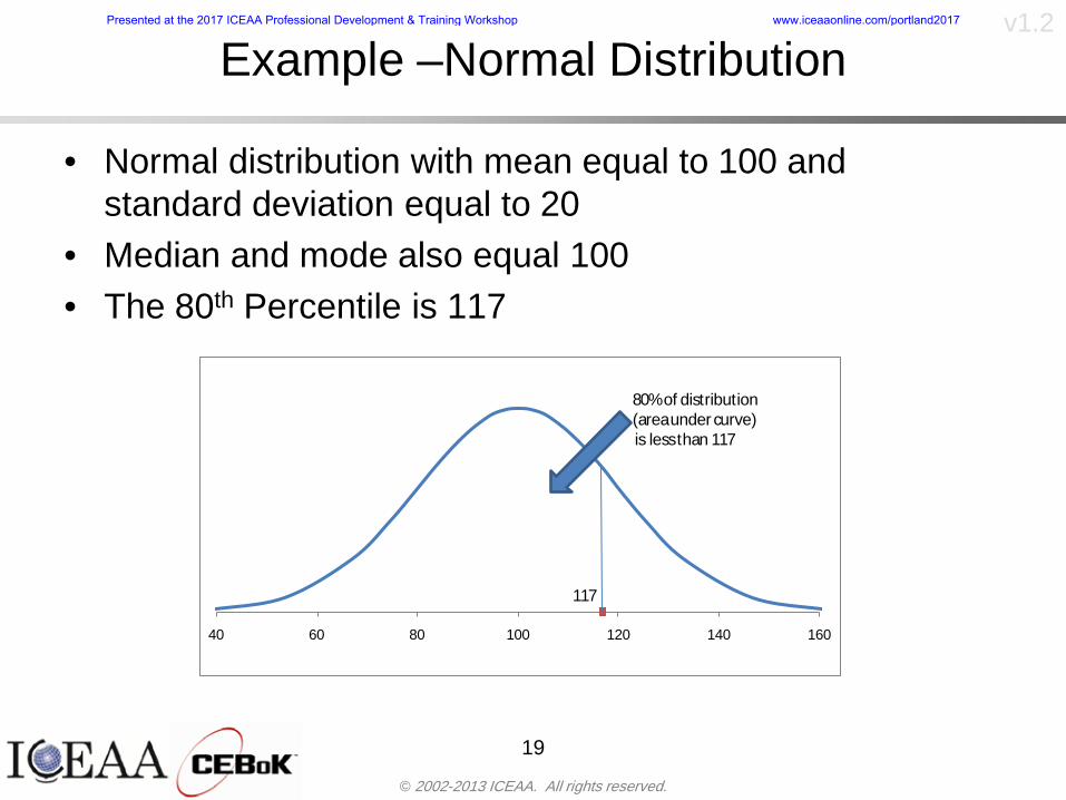
copy 2002-2013 ICEAA All rights reserved
v12
19
Example ndash Normal Distribution
bull Normal distribution with mean equal to 100 and standard deviation equal to 20
bull Median and mode also equal 100bull The 80th Percentile is 117
40 60 80 100 120 140 160
80 of distribution(area under curve)is less than 117
117
Presented at the 2017 ICEAA Professional Development amp Training Workshop wwwiceaaonlinecomportland2017
copy 2002-2013 ICEAA All rights reserved
v12
20
Confidence Levelsbull The output of a cost risk analysis is a probability
distributionndash Typically displayed as a cumulative distribution function or
ldquoS-curverdquondash Confidence levels are simply percentiles of the distribution
0
10
20
30
40
50
60
70
80
90
100
30 60 90 120 150 180
Conf
iden
ce L
evel
Presented at the 2017 ICEAA Professional Development amp Training Workshop wwwiceaaonlinecomportland2017
copy 2002-2013 ICEAA All rights reserved
v12
Measuring Parametric Model Uncertainty
bull When developing estimates using cost-estimating relationships (CERs) there are two major sources of uncertaintyndash Technical (model input) uncertaintyndash Estimating uncertainty
bull Technical uncertainty reflects the uncertainty inherent in the model inputsndash Typical parametric model inputs include weight lines of code
heritage and other performance and management inputs
bull Estimating uncertainty measures the uncertainty inherent in the model due to the modelrsquos inability to capture all aspects of variability in the data
21
Presented at the 2017 ICEAA Professional Development amp Training Workshop wwwiceaaonlinecomportland2017
copy 2002-2013 ICEAA All rights reserved
v12
Parametric Model Examplebull The NASAAir Force Cost Model (NAFCOM) is a
parametric model for estimating acquisition costs for spacecraft and launch vehicles
bull The CERs in NAFCOM have the formCost = C WeightVNewDesignWTechnicalXManagementY ClassZ
bull There is technical uncertainty about each of the parametersndash Parametric models are applied early in a program so there
is significant amount of uncertainty in the weightndash Heritage is also tricky it is inherently subjective and project
personnel are typically optimisticndash Technical characteristics can also change as a program
matures and requirements change
22
Presented at the 2017 ICEAA Professional Development amp Training Workshop wwwiceaaonlinecomportland2017
copy 2002-2013 ICEAA All rights reserved
v12
Weight Uncertaintybull Aerospace weight growth study average satellite
weight growth from program inception to launch is 28
23
Aerospace Weight Growth Data
-10
0
10
20
30
40
50
60
0 4 8 12 16 20 24 28 32 36 40 44 48 52 56 60 64 68 72 76 80 84 88 92 96 100
Percent Program Completion
Perc
ent W
eigh
t Gro
wth
Presented at the 2017 ICEAA Professional Development amp Training Workshop wwwiceaaonlinecomportland2017
copy 2002-2013 ICEAA All rights reserved
v12
Estimating Uncertaintybull CERs do not perfectly fit the historical data
ndash There are non-repeatable random effects that cannot be predicted
bull For examplendash Parts breaking during testingndash Strikes which are difficult to predict
bull This results in an underlying uncertainty distribution about an estimatendash The outcome of a CER represents only one point on an
uncertainty distributionbull Typically mean or median depending upon the CER
methodology
24
Presented at the 2017 ICEAA Professional Development amp Training Workshop wwwiceaaonlinecomportland2017
copy 2002-2013 ICEAA All rights reserved
v12
Estimating Uncertainty (2)
25
Presented at the 2017 ICEAA Professional Development amp Training Workshop wwwiceaaonlinecomportland2017
copy 2002-2013 ICEAA All rights reserved
v12
Estimating Uncertainty (3)bull In the case of a linear regression the estimating
uncertainty follows a normal distributionndash The estimate is the mean and the standard error of the
estimate from the regression is the standard deviation of the normal distribution
bull In the case of a log-transformed linear regression the estimating uncertainty follows a lognormal distributionndash The estimate is the median of the lognormal and the
standard error of the estimate from the regression is the standard deviation of the normal distribution (in log-space)
bull There is additional uncertainty about an estimate based upon the distance of what is being estimated from the mean of the input datandash This results in a prediction interval
26
Presented at the 2017 ICEAA Professional Development amp Training Workshop wwwiceaaonlinecomportland2017
copy 2002-2013 ICEAA All rights reserved
v12
Aggregating Riskbull Risk is typically applied at the same level at
which we estimate cost that is at the Work Breakdown Structure (WBS) level
bull The estimates for each WBS are developedndash These estimates sum to yield the total system cost
bull For an n-element WBS the total cost is the sum of the cost for each of the n elements
27
nXXXCostSystem +++= 21
Presented at the 2017 ICEAA Professional Development amp Training Workshop wwwiceaaonlinecomportland2017
copy 2002-2013 ICEAA All rights reserved
v12
WBS Examplebull Launch Vehicle
ndash Structurebull Vehicle Structurebull Tank Structure
ndash Thermal Controlbull Active Thermal Controlbull Induced Thermal Controlbull Tank Thermal Control
ndash Main Propulsion Systemndash Liquid Rocket Enginendash Electric Power and Distributionndash Command Control and Data Handlingndash System Integration
28
Presented at the 2017 ICEAA Professional Development amp Training Workshop wwwiceaaonlinecomportland2017
copy 2002-2013 ICEAA All rights reserved
v12
WBS and Risk
29
Presented at the 2017 ICEAA Professional Development amp Training Workshop wwwiceaaonlinecomportland2017
copy 2002-2013 ICEAA All rights reserved
v12
Aggregating Riskbull This leads us to the issue of aggregating the risks across the
WBSbull For example if we want to determine the 70th percentile of the
overall cost risk distribution how do we proceed bull Note that we cannot simply add the 70th percentiles of each of
the cost risk distributionsbull We can add means and variances (taking correlation into
account more on that later) but that is all
Variance of Total Cost =
30
Mean of Total Cost = ( )E X E Xk
k
n
kk
n
kk
n
= = =aringaelig
egraveccediloumloslashdivide
= =aring aring1 1 1
m
Var X kk
n
=aringaelig
egraveccediloumloslashdivide1
= s r s skk
n
iji
j
i jj
n2
1 1
1
22+aring aringaring
= =
-
=
Presented at the 2017 ICEAA Professional Development amp Training Workshop wwwiceaaonlinecomportland2017
copy 2002-2013 ICEAA All rights reserved
v12
Percentiles Do Not Addbull As a notional example consider two independent normal
distributionsndash One distribution has mean equal to 100 and standard deviation
equal to 20ndash The second distribution has mean 300 and standard deviation of 80
bull The sum of two independent normally distributed random variables is also normally distributed
bull To combine the two distributions we add the means and add the variancesndash Total mean is
ndash Total standard deviation is
31
400300100 =+
8258020 22 raquo+
Presented at the 2017 ICEAA Professional Development amp Training Workshop wwwiceaaonlinecomportland2017
copy 2002-2013 ICEAA All rights reserved
v12
Percentiles Do Not Add (2)bull The 80th percentiles for the individual distributions are
117 and 367 respbull The 80th percentile of the combined distribution is
469 but the sum of the two 80th percentiles is 484bull To see why this is the case note that the percentiles
of a normal distribution are determined by the mean and the standard deviationndash The standard deviations are not added when normal distributions
are combined rather the variances are combinedndash Sum of variances is ndash The standard deviation of this sum is
32
22 ba +22 ba +
Presented at the 2017 ICEAA Professional Development amp Training Workshop wwwiceaaonlinecomportland2017
copy 2002-2013 ICEAA All rights reserved
v12
Percentiles Do Not Add (3)bull Since bull We can write
bull The left side of this inequality represents the risk of the combined distributions while the right side represents the sums of the individual risks
bull Combining two missions that are independent results in a diversification of riskndash The total portfolio is not as risky on a relative basis as each
individual project
33
2222 2 bababa ++lt+
baba +lt+ 22
Presented at the 2017 ICEAA Professional Development amp Training Workshop wwwiceaaonlinecomportland2017
copy 2002-2013 ICEAA All rights reserved
v12
Methods for Aggregating Riskbull Since percentiles do not add we have to find other
ways to aggregate riskbull One method is to use Monte Carlo simulationbull Unless cost risk is represented by normal
distributions for all WBS elements summing the means and variances does not result in a completely accurate depiction of overall system cost risk
bull The normal distribution is not a realistic distribution for representing risk in many or even most situations since regarding project risk more can go wrong than can go right which means the risk is NOT symmetric unlike the Gaussian bell curve
34
Presented at the 2017 ICEAA Professional Development amp Training Workshop wwwiceaaonlinecomportland2017
copy 2002-2013 ICEAA All rights reserved
v12
Unit III - Module 9 35
Monte Carlo Simulationfor Risk Analysis
bull When risk analysis is performed multiple risks are gatheredndash These risks may have various probability
distributions
bull Monte Carlo is the most commonly accepted way to produce an accurate characterization of the distribution of the combined effect of these many risksndash Using this distribution we can produce percentiles
for cost impacts due to risk occurrences
10
Presented at the 2017 ICEAA Professional Development amp Training Workshop wwwiceaaonlinecomportland2017
copy 2002-2013 ICEAA All rights reserved
v12
Monte Carlo Simulationbull Simulation is a means for solving problems that are
analytically intractablendash Involves repeated random sampling
bull It was developed during the Manhattan Project as a way to model the interactions inside an atom during nuclear fissionndash Allowed for more sophisticated mathematical modeling of atomic
phenomena
bull Most computer packages use pseudo-random number generators that produce seemingly random results from an initial seedndash Example is the linear congruential generator
36
( ) mbaXX nn mod1 +=+
Presented at the 2017 ICEAA Professional Development amp Training Workshop wwwiceaaonlinecomportland2017
copy 2002-2013 ICEAA All rights reserved
v12Using Random Numbers to Simulate Distributions
bull WBS cost risk is typically measured by a probability distributionbull The most common method for simulating a probability
distribution is the inverse methodbull This involve obtaining a simulated random value from a uniform
distribution and then inverting this through the cumulative distribution function (CDF) to obtain the simulated value
bull As an example for a uniform distribution on the interval [0100]
bull In this case the CDF random value of 05 translates to 10005 = 50
37
( )100
1=xf ( )
100xxF = ( ) xxF 1001 =-
Presented at the 2017 ICEAA Professional Development amp Training Workshop wwwiceaaonlinecomportland2017
copy 2002-2013 ICEAA All rights reserved
v12
Simulating a Triangular Distribution
bull For a triangular distribution with low = 0 most likely = 50 and high = 150 the CDF is given by
bull The inverse function is given by
38
( )iumliumlicirc
iumliumliacute
igrave
poundlt--
poundpound=
1505021
1500050
50015000
2
2
2
xxx
xxxF
( )iumliumlicirc
iumliumliacute
igrave
poundltdivideoslashouml
ccedilegraveaelig +--
poundpound=-
131
21
37501
250017500150
3107500
1
xx
xxxF
Presented at the 2017 ICEAA Professional Development amp Training Workshop wwwiceaaonlinecomportland2017
copy 2002-2013 ICEAA All rights reserved
v12
Simulating a Triangular Distribution (2)
bull If the simulated uniform value is equal to 02 the corresponding inverse value from the CDF inverse is approximately 387
39
0
01
02
03
04
05
06
07
08
09
1
0 30 60 90 120 150
Presented at the 2017 ICEAA Professional Development amp Training Workshop wwwiceaaonlinecomportland2017
copy 2002-2013 ICEAA All rights reserved
v12
Monte Carlo and the WBSbull Simulation involves repeated trials
40
WBS Draw1 2 3 4 5
System 2912 3566 4390 2954 4655 Sum
Structure 80 105 55 80 57 SumVehicle Structure 50 70 30 40 20Tank Structure 30 35 25 40 37
Thermal Control 32 36 35 29 33 SumActive Thermal Control 10 15 12 7 10Induced Thermal Control 12 14 13 14 14Tank Thermal Control 10 7 10 8 9
Main Propulsion System 100 150 125 140 100
Liquid Rocket Engine 1000 1100 1800 900 2200
Electric Power and Distribution 100 125 150 75 90
Command Control and Data Handling 200 250 225 230 275
System Integration 1400 1800 2000 1500 1900
Presented at the 2017 ICEAA Professional Development amp Training Workshop wwwiceaaonlinecomportland2017
copy 2002-2013 ICEAA All rights reserved
v12
Number of Trialsbull Monte Carlo involves a repeated number of trialsbull The greater the number of trials the more accurate the
simulation will approximate the overall cost risk behavior of the system
bull After 100 trials the histogram looks very jagged
41
Presented at the 2017 ICEAA Professional Development amp Training Workshop wwwiceaaonlinecomportland2017
copy 2002-2013 ICEAA All rights reserved
v12
Number of Trials (2)
42
1000 Trials
10000 Trials
50000 Trials Additional trials give a more accurate depiction of the final result
Presented at the 2017 ICEAA Professional Development amp Training Workshop wwwiceaaonlinecomportland2017
copy 2002-2013 ICEAA All rights reserved
v12
Number of Trials (3)bull If we want to simulate the underlying
mean within 1 with 95 confidence for example then we require
43
divideoslash
oumlccedilegrave
aelig poundpound-
=
dividedividedivide
oslash
ouml
ccedilccedilccedil
egrave
aeligpound
-pound
-=
divideoslashouml
ccedilegraveaelig poundpound=
nZ
n
nnX
n
X
n
n
011
010Pr
011
010Pr
011990Pr950
___
___
sm
sm
sm
sm
sm
mm
Presented at the 2017 ICEAA Professional Development amp Training Workshop wwwiceaaonlinecomportland2017
copy 2002-2013 ICEAA All rights reserved
v12
Number of Trials (4)bull This means that the number of trials required is determined by
bull Solving for n we find that at least
trials are neededbull Note that this term involves the coefficient of variation of the
distribution which means that distributions with less dispersion require fewer trials to accurate simulate
44
96101
=ns
m
ms41638
Presented at the 2017 ICEAA Professional Development amp Training Workshop wwwiceaaonlinecomportland2017
copy 2002-2013 ICEAA All rights reserved
v12
Number of Trials (5)bull Simulating percentiles requires more trials than for simulating
meansbull Let Pn represent the number of trials in the sample at or below
the 70th percentile of the underlying distribution (suppose this is known)
bull By the Central Limit Theorem Pnn follows a normal distribution with mean equal to the 70th percentile and variance equal to
bull By a similar process for the mean we find that the number of trials needed to simulate the 70th percentile within 1 with 95 confidence is
45
( )n
FF 700700 1-
n
n
PPn -41638
Presented at the 2017 ICEAA Professional Development amp Training Workshop wwwiceaaonlinecomportland2017
copy 2002-2013 ICEAA All rights reserved
v12
Number of Trials (6)bull If Pn 070 for all n then n is approximately
bull For the sake of comparison suppose CV = 03 (reasonable approximation for hardware development) then the number of trials needed to simulate the mean with the same accuracy is then ldquoonlyrdquo 11525
bull More trials are needed to accurately simulate percentiles than means
46
( ) 46416703041638
70704168341638 =divide
oslashouml
ccedilegraveaelig=divide
oslashouml
ccedilegraveaelig -
=-
nnn
PPn
n
n
Presented at the 2017 ICEAA Professional Development amp Training Workshop wwwiceaaonlinecomportland2017
copy 2002-2013 ICEAA All rights reserved
v12
Methods of Simulationbull Monte Carlo simulation is a standard term for
simulationbull However there is an improvement on Monte Carlo
that improves the accuracy of the results of a simulation for a given number of trials
bull This method is call the Latin Hypercube approach to simulationndash Similar to Monte Carlo but an equal number of draws are taken
from a set of subintervals for example dividing the interval (01) into [00001) [0102)hellip [0910]
ndash Instead of 10 trials from [01] we have one trial from each subinterval
ndash Rough rule of thumb is Latin Hypercube takes 30 fewer trials to achieve similar accuracy to Monte Carlo
47
Presented at the 2017 ICEAA Professional Development amp Training Workshop wwwiceaaonlinecomportland2017
copy 2002-2013 ICEAA All rights reserved
v12
Probability Model ndash Correlationbull Correlation exists between work breakdown structure
(WBS) cost element costs and between cost and schedule
bull Correlation is a necessary consideration in cost risk analysis
bull Correlation is a number that can vary between -1 and +1 and represents the strength of the relationship between the two variablesndash If both variable have a tendency to move in the same direction
correlation is positivendash If when one variable increases the other tends to decrease and
vice-versa the correlation between the two variables is negative
Presented at the 2017 ICEAA Professional Development amp Training Workshop wwwiceaaonlinecomportland2017
copy 2002-2013 ICEAA All rights reserved
v12
Correlation And Causationbull Note that correlation is not causation however
causation implies correlationndash For example shark attacks and ice cream sales at the beach
bull For example for a launch vehicle structure increasing the diameter will not only result in an increase in the structures cost but will also result in higher costs for thermal coating (paint etc)
bull Also simply because two subsystems do not appear to be related does not mean they are not correlatedndash For example structures and computer equipment seemingly
have little relation to one another however an external factor such as a funding cut or a strike will impact all subsystems leading to delays and increasing cost across the board
ndash Thus everything in a WBS has some correlationUnit III - Module 9 49
Presented at the 2017 ICEAA Professional Development amp Training Workshop wwwiceaaonlinecomportland2017
copy 2002-2013 ICEAA All rights reserved
v12
The Importance of Correlationbull Percent that total cost standard deviation is underestimated
when correlation assumed to be 0 instead of r given nWBS elements
Unit III - Module 9 5050
0
20
40
60
80
100
0 01 02 03 04 05 06 07 08 09 1Actual Correlation
Perce
nt Un
deres
timate
d
n = 10
n = 30
n = 100n = 1000
0
20
40
60
80
100
0 01 02 03 04 05 06 07 08 09 1Actual Correlation
Perce
nt Un
deres
timate
d
n = 10
n = 30
n = 100n = 1000
Reference 32nd Annual DOD Cost Analysis Symposium Advanced Training Session ldquoWhy Correlation Matters in Cost Estimatingrdquo Stephen A Book
Presented at the 2017 ICEAA Professional Development amp Training Workshop wwwiceaaonlinecomportland2017
copy 2002-2013 ICEAA All rights reserved
v12
The Importance of Correlation (2)bull For example if correlation is assumed to be 0 for all
elements in a 30 element WBS and the actual correlation is 20 then the total cost standard deviation is underestimated by 60
bull For example assume the total cost is modeled as a normal distribution with mean = 100
bull If correlation is assumed to be zero with total cost standard deviation = 12 when correlation is actually 20 then the true underlying standard deviation is actually 30
bull 70th percentile with zero correlation assumption is 106
bull 70th percentile with 20 correlation is 116 Unit III - Module 9 51
Presented at the 2017 ICEAA Professional Development amp Training Workshop wwwiceaaonlinecomportland2017
copy 2002-2013 ICEAA All rights reserved
v12
Measures of Correlationbull Two measures of correlation are commonly used in
cost risk analysesndash Pearsonrsquos product-moment correlation coefficient ndash Spearmanrsquos rank correlation coefficient
bull Garvey and others recommend using Pearsonrsquos product-moment correlation coefficient correlation for cost risk analysesndash Method of moments uses this but there are two options in
simulationndash Popular simulation packages like Risk and Crystal Ball use
rank correlation but in practice this has been found to make little difference
ndash Pearson product-moment correlation has been incorporated into Risk+
52
Presented at the 2017 ICEAA Professional Development amp Training Workshop wwwiceaaonlinecomportland2017
copy 2002-2013 ICEAA All rights reserved
v12
Pearson Correlationbull Pearsonrsquos product-moment correlation measures
degree of linearity between two random variables bull If two random variables are perfectly linear (eg Y =
aX + b) with positive slope then the Pearson product-moment correlation between X and Y denoted by rXY is +1
53
X X
Y Y Y
XNegative Correlation Positive Correlation No Correlation
middotmiddot
middotmiddot
middotmiddot middotmiddot
middotmiddot
middot
middot
middotmiddotmiddot
middotmiddot
middotmiddot
middotmiddot middot
middot
middot
middotmiddotmiddotmiddotmiddotmiddotmiddotmiddot
middotmiddotmiddotmiddot
middotmiddot
middotmiddot middotmiddotmiddotmiddot
middotmiddotmiddot
middotmiddotmiddotmiddot
middotmiddotmiddot
middotmiddotmiddot
middotmiddot
middot
middot middotmiddot
middot middotmiddotmiddotmiddot middotmiddot middot middotmiddot middot middot
middotmiddot middot
middotmiddotmiddotmiddotmiddot middot middotmiddot
middotmiddot
middot
middotmiddot
middotmiddot middot
middot middot middot
middotmiddot middot
middotmiddotmiddot
middotmiddot
middot middot
Presented at the 2017 ICEAA Professional Development amp Training Workshop wwwiceaaonlinecomportland2017
copy 2002-2013 ICEAA All rights reserved
v12
Spearman Correlationbull Spearmanrsquos rank correlation measures the
monotonicity between two random variablesbull If two random variables are perfectly monotonically
increasing (eg Y = X2) then the Spearman rank correlation denoted by rXY is +1
bull The two measures can be significantly different
54
10 20 30 40 50 60
100
200
300
096 097 098 099 1
1
060
020
040
080
Eff
ort (
Staf
f-M
onth
s)
Software Size I KDSI
y = 28z12y
z x
yy = x100
0 pound x pound 1
Figure 5-9A Figure 5-9B
Pearson Correlation = 09976 Rank Correlation = 1
Pearson Correlation = 024 Rank Correlation = 1
X(x ) ~ Unif(01)
Reference Probability Methods for Cost Uncertainty Analysis A Systems Engineering Perspective Paul R Garvey
Presented at the 2017 ICEAA Professional Development amp Training Workshop wwwiceaaonlinecomportland2017
copy 2002-2013 ICEAA All rights reserved
v12
Unit III - Module 9 55
200
250
300
350
400
1000 1200 1400 1600 1800 2000
Recurring Production
SEPM
200
250
300
350
400
1000 1200 1400 1600 1800 2000
Recurring Production
SEPM
Functional Correlationbull Old No Functional
Correlation Simulation run with WBS items entered as values
bull New Simulation run with functional dependencies entered as they are in cost model
CorrelatedNot Correlated
Note shift of mean and increased variability
Presented at the 2017 ICEAA Professional Development amp Training Workshop wwwiceaaonlinecomportland2017
copy 2002-2013 ICEAA All rights reserved
v12
Risk Measuresbull ldquoWestern Europe conquered the word because of a
technological revolution that started because of attempts to measure the worldrdquo ndash Phillipe Jorion ndash In the same way attempts to measure risk will lead to better project
managementbull Risk management for DoD and NASA agencies focuses
primarily on funding projects to a single percentile ndash NASA policy explicitly mentions 70 and 50ndash This is known as ldquoValue at Riskrdquo and is prevalent in the banking and
financial industry
56
Presented at the 2017 ICEAA Professional Development amp Training Workshop wwwiceaaonlinecomportland2017
copy 2002-2013 ICEAA All rights reserved
v12
Value at Risk (VaR)bull VaR is a percentile of the cost risk
distributionndash VaR funding at the 70th percentile means that
there is a 30 chance of final project cost exceeding the funded amount (budget)
bull VaR has some meritsndash Common measure can be used to compare
different projects and programsndash Easily understood by senior managers and
decision makers
57
Presented at the 2017 ICEAA Professional Development amp Training Workshop wwwiceaaonlinecomportland2017
copy 2002-2013 ICEAA All rights reserved
v12
Why 70th or 80th Percentilebull Typical policy guidance involves funding at the 70th or 80th
percentile Why fund as such a low percentilebull There is some incentive to not over-fundbull For a normal distribution an inflection point occurs near the 80th
percentile meaning that for values above 80 confidence achieving higher levels of confidence can only be achieved by spending greater dollar amounts at an increasing rate
58
-05-04-03-02-01
00102030405
0 05 1 15 2 25 3
Standard Deviations from Mean
Normal Distribution
First DerivativeSlopeVelocity
Second DerivativeConvexityAcceleration
Inflection point at one standard deviation above the mean (~84th
percentile)
Presented at the 2017 ICEAA Professional Development amp Training Workshop wwwiceaaonlinecomportland2017
copy 2002-2013 ICEAA All rights reserved
v12
Funding Above Inflection Pointsbull As the percentile goes above the 80th percentile the amount
needed to achieve that higher level of confidence begins to increase at an increasing rate as is evident from the graph
59
0
10
20
30
40
50
60
70
50 55 60 65 70 75 80 85 90 95 100
$ Ab
ove
MEa
n to
Ach
ieve
Per
cent
ile
Percentile (Confidence Level)
Presented at the 2017 ICEAA Professional Development amp Training Workshop wwwiceaaonlinecomportland2017
copy 2002-2013 ICEAA All rights reserved
v12
Why Budget to the 70th or 80thbull Government projects are funded at the 70th or 80th percentilesbull Why not the 90th or 99th percentile Wonrsquot that help prevent
overrunsndash As we have seen percentiles do not add across programs
bull The sum of the 80th percentiles does NOT equal the total 80th percentile
ndash This is because the individual programs are riskier than the entire suite of missions
bull Known as the ldquoPortfolio effectrdquo (more or this later)
ndash Funding at the 80th gives confidence that the entire portfolio will be adequately funded
bull And since there is an inflection point near the 80th percentile funding above that level quickly becomes cost prohibitive
60
Presented at the 2017 ICEAA Professional Development amp Training Workshop wwwiceaaonlinecomportland2017
copy 2002-2013 ICEAA All rights reserved
v12
Inflection Points for Lognormalbull For a lognormal the inflection point
variesndash Coefficient of variation equal to 10 equates to an
inflection point at the 70th percentile
61
0
10
20
30
40
50
60
70
050 060 070 080 090 100
Coef
ficen
t of V
aria
tion
Percentile of the Inflection Point
Presented at the 2017 ICEAA Professional Development amp Training Workshop wwwiceaaonlinecomportland2017
copy 2002-2013 ICEAA All rights reserved
v12
Issues with Percentile Fundingbull However risk management does not stop at a
specific percentilendash What happens when the 70th percentile is exceeded
bull Any effective risk management policy should prescribe what happens after a bad event occursndash With VaR we only know when a bad event has occurred ndash Also funding at a relatively low level means we have no true
sense of the real risks that should be guarded against
62
Presented at the 2017 ICEAA Professional Development amp Training Workshop wwwiceaaonlinecomportland2017
copy 2002-2013 ICEAA All rights reserved
v12
ldquoHere There Be Dragonsrdquobull On old maps uncharted territory was often
marked with monsters or dragons
63
A section of the Carta Marina by Olaus Magnus 16th Century
Presented at the 2017 ICEAA Professional Development amp Training Workshop wwwiceaaonlinecomportland2017
copy 2002-2013 ICEAA All rights reserved
v12
Distribution Comparisonbull Four different distributions with the same 70th
percentile
bull Should we expect the tails to be similar
64
0
10
20
30
40
50
60
70
80
0 100 200 300 400 500 600
Perc
entil
eCo
nfid
ence
Lev
el
Triangular
Normal
Lognormal
Pareto
Presented at the 2017 ICEAA Professional Development amp Training Workshop wwwiceaaonlinecomportland2017
copy 2002-2013 ICEAA All rights reserved
v12Distribution Comparison Tail Behavior
bull The normal and triangular distributions have similar tails but the lognormal and Pareto have much fatter right tails
65
70
75
80
85
90
95
100
500 1500 2500 3500 4500 5500
Perc
entil
eCo
nfid
ence
Lev
el
Triangular
Normal
Lognormal
Pareto
Here There Be Dragons
Presented at the 2017 ICEAA Professional Development amp Training Workshop wwwiceaaonlinecomportland2017
copy 2002-2013 ICEAA All rights reserved
v12Distribution Comparison ndash Tail Behavior (Table)
bull There is significant tail risk for the lognormal and the Paretobull The 99th percentile for the Pareto is 1000 times greater than
the 70th percentilendash Risk seen in financial markets and in catastrophic risks like natural
disasters bull Four different projects follow the four different risk profiles seen
in this example should clearly have different risk management approaches but 70th percentile funding indicates the same risk management approach for all four
66
Percentile Triangular Normal Lognormal Pareto 70th $600 $600 $600 $600 80th $680 $660 $770 $1430 90th $770 $750 $1070 $5880 95th $840 $820 $1410 $23750 99th $930 $950 $2350 $600000
Presented at the 2017 ICEAA Professional Development amp Training Workshop wwwiceaaonlinecomportland2017
copy 2002-2013 ICEAA All rights reserved
v12Percentile Budgeting is Not Risk Management
bull Percentile budgeting ne effective risk management policybull Suppose that you are shopping for a new car You
mention that safety is your top concern The salesman says he has a great safe car available You ask about the air bags Do they work The salesman answers ldquoOf course Seventy percent of the time they work fine Only 30 of the time the air bags will fail to deployrdquo Would you buy such a car Hedge fund manager David Einhorn has stated ldquoRisk management is the air bag that must always work but only in the multi-sigma event where you have an accidentrdquo
67
Risk management is the air bag that must always work but only in the multi-sigma event where you
have an accident
Presented at the 2017 ICEAA Professional Development amp Training Workshop wwwiceaaonlinecomportland2017
copy 2002-2013 ICEAA All rights reserved
v12
Joint Confidence Level Analysisbull Schedules are risky toobull For 98 recent NASA missions average
schedule growth was 38ndash Not as high as cost growth but still significant
68
0
5
10
15
20
25
30
35
40
Schedule
Cost
Presented at the 2017 ICEAA Professional Development amp Training Workshop wwwiceaaonlinecomportland2017
copy 2002-2013 ICEAA All rights reserved
v12
Schedules Impact Costbull Changes in schedule can have enormous
impacts on cost ndash Schedule slips can lead to cost increases
bull Fixed programmatic costs must be paid on a regular basisndash Achieving schedule milestones early can result in cost
savings
bull Schedule is an important consideration in cost analysis including cost risk analysis
bull However we must be careful in correctly integrating cost and schedule riskndash Schedule is not simply an input but is dependent on many of
the same factors that drive cost
69
Presented at the 2017 ICEAA Professional Development amp Training Workshop wwwiceaaonlinecomportland2017
copy 2002-2013 ICEAA All rights reserved
v12
The Relationship of Cost to Schedulebull Cost and schedule are positively correlated
ndash A larger program with bigger scope with take longer to complete than a smaller simpler program
bull However longer schedules do not always equate to higher cost nor shorter schedules with lower costndash Highly compressed schedules relative to the
optimal schedule can lead to large overrunsbull Compressed schedules are commonplace for
many planetary missions
70
Presented at the 2017 ICEAA Professional Development amp Training Workshop wwwiceaaonlinecomportland2017
copy 2002-2013 ICEAA All rights reserved
v12The Impact of Schedule GrowthCompression on Cost
bull Compressed schedules lead to cost growth and based on existing research is actually more expensive than schedule slippages
71
0
20
40
60
80
100
120
140
160
-50 -25 0 25 50 75 100
Percentage Change in Schedule
Perc
enta
ge C
hang
e in
Cos
t due
to
Sche
dule
Cha
nge
Source Smart CB ldquoCost and Schedule Interrelationshipsrdquo 2007 NASA Cost Symposium
Presented at the 2017 ICEAA Professional Development amp Training Workshop wwwiceaaonlinecomportland2017
copy 2002-2013 ICEAA All rights reserved
v12Schedule as an Independent Variable
bull Why not simply add schedule as an input to cost-estimating relationships (CERs)
bull Schedule is often treated as an independent variable ndash schedules are often determined independently of cost considerationsndash Cost may not be considered explicitly although budgets and
schedules are determined based on scope and other common factors
bull In 2006 SAIC undertook a research task to determine the impact of schedule on cost and added schedule as an independent variable to the CERs in the NASAAir Force Cost Model (NAFCOM) to see if schedule provided any improvement in goodness of fit
72
Presented at the 2017 ICEAA Professional Development amp Training Workshop wwwiceaaonlinecomportland2017
copy 2002-2013 ICEAA All rights reserved
v12
Schedule is a Dependent Variablebull Since NAFCOM includes an exhaustive list of cost drivers the inclusion
of schedule should give an indication of whether there is any additional independent value added from schedule independent of the cost drivers
bull In the study schedule was added to 10 subsystem-level CERs
ndash In each case the addition of schedule did NOTimprove the goodness of fit and schedule was NOT found to be a statistically significant cost driver (given the presence of the other variables) for any of the 10 CERs
bull Standard errors for the CERs increased due to decrease in degrees of freedom
bull Thus schedule as an independent variable did not provide any additional explanation of variation in historical cost
bull This is because schedule is truly NOT an independent variable but a dependent variable and is a function of the same factors that drive cost
73
Presented at the 2017 ICEAA Professional Development amp Training Workshop wwwiceaaonlinecomportland2017
copy 2002-2013 ICEAA All rights reserved
v12
Incorporation of Schedule in Cost Risk
bull When using subjective methods care must be taken in applying schedule to cost risk analysis
bull Since schedule is a dependent variable treating it independently from other factors when assessing its impact on cost can lead to a double count of independent variables in the cost risk analysis
bull Direct inclusion of schedule in a cost risk analysis effectively doubles the influence of each cost driver
ndash Incorrectly leads to broader risk ranges
74
CostWeight
HeritageNewness
Technology Readiness Schedule
Presented at the 2017 ICEAA Professional Development amp Training Workshop wwwiceaaonlinecomportland2017
copy 2002-2013 ICEAA All rights reserved
v12Subjective Cost Risk Methods and Overinclusion of Risk Factors
bull Subjective methods are suitable when data are scarce or not availablebull However care must be taken not to treat correlated sources of risk
such as schedule as independent of each otherbull Example ndash a subjective risk analysis incorporated technology readiness
design risk requirements stability integration risk and schedule and treated each source of risk as independent
bull Risk triangle high value without schedule risk was 31 times the point estimate
bull Risk triangle high value with schedule risk added on top of other sources of risk treated independently was 34 times the point estimate
bull Risk triangle taking correlation between sources of risk into account in a rigorous statistical manner has a high value 15 times the point estimate less than half the effect when treating sources of risk as independent
75
Presented at the 2017 ICEAA Professional Development amp Training Workshop wwwiceaaonlinecomportland2017
copy 2002-2013 ICEAA All rights reserved
v12Fundamental Equation of Cost and Schedule Interrelationships
bull The Fundamental Equation of the Relationship Between Cost and Schedule is
Time = Moneybull This is a well known adage that time is money Your boss at
work may even mention this to you from time to time or if you are the boss you are all too aware of this iron law
bull Because time is money cost and schedule risk should be modeled jointly not with schedule as an independent cost driver
bull Note that cost and schedule are not perfectly correlatedndash Cost can sometimes ldquobuy downrdquo schedule extra money can be
spent to meet a deadline since in some cases additional effort to hasten the completion of a task
76
Presented at the 2017 ICEAA Professional Development amp Training Workshop wwwiceaaonlinecomportland2017
copy 2002-2013 ICEAA All rights reserved
v12How to (Correctly) Incorporate Schedule into Cost Risk Analysis
bull The best way to model cost and schedule risk is to develop a joint cost and schedule model based on the same data
bull Since such models are not currently available the next best approach is to model cost and schedule independently and then integrate cost and schedule risk analyses using joint probability distributions taking into account correlation between cost and schedulendash This approach pioneered by Paul Garvey and Steve Book is
considered industry best practicendash This is a practical method mathematically tractable and follows
naturally from the Fundamental Equation of Cost and Schedule Interrelationships
77
Book S A ldquoQuantifying the Relationship Between Cost and Schedulerdquo The Measurable News Winter 2007-2008 pp 11-15Garvey PR Probability Methods for Cost Uncertainty Analysis A Systems Engineering Perspective New York Marcel Dekker 2000 pp 308-335
Presented at the 2017 ICEAA Professional Development amp Training Workshop wwwiceaaonlinecomportland2017
copy 2002-2013 ICEAA All rights reserved
v12
Joint Lognormal and Normal Distributions
bull Cost and schedule are typically modeled as some combination of Normal and Lognormal probability distributionsndash Studies by The Aerospace Corporation the MITRE
Corporation Wyle Labs and SAIC have found that the Lognormal probability distribution almost always serves as a good model for both the schedule distribution and the cost distribution
ndash The Normal distribution may also be appropriate in some instances and depending upon the level of confidence at which budgets are set may even be more conservative and logically consistent than the Normal distribution
ndash Joint Lognormal and Normal distributions are defined by a pair of mean and standard deviations and a level of correlation between the two
78
Presented at the 2017 ICEAA Professional Development amp Training Workshop wwwiceaaonlinecomportland2017
copy 2002-2013 ICEAA All rights reserved
v12Modeling Cost and Schedule as a Bivariate Distribution
bull In the approach set forth by Book and Garvey cost risk is assessed and the top-level distribution is modeled as a Lognormal (or Normal) distribution schedule risk is assessed and the overall schedule risk is modeled as a Lognormal (or Normal) distribution
bull The two distributions are combined into a Bivariate distribution by assigning a correlation between the two and by treating the two distributions as the marginal distributions of a Bivariate Lognormal distributionndash Other combinations include a Bivariate Normal or a Bivariate
Normal-Lognormal
79
Presented at the 2017 ICEAA Professional Development amp Training Workshop wwwiceaaonlinecomportland2017
copy 2002-2013 ICEAA All rights reserved
v12Bivariate Lognormal Distribution for Cost and Schedule
bull Cost is often observed to be Lognormal when strong positive correlations are present among the systemrsquos WBS cost element costs
bull A systemrsquos schedule is often observed (from Monte Carlo simulations) to be Lognormal if it is the sum of many positively correlated schedule activities in an overall schedule network
bull If Lognormal distributions characterize a systemrsquos cost and schedule then the Bivariate Lognormal could serve as an assumed model of their joint distributionndash In this case the marginal distribution of each of cost and schedule is
Lognormalbull Other possibilities for modeling cost and schedule as a Bivariate
distribution include a Bivariate Normal or a Bivariate Normal-Lognormal distributionndash All these combinations are analytically tractable
80
Presented at the 2017 ICEAA Professional Development amp Training Workshop wwwiceaaonlinecomportland2017
copy 2002-2013 ICEAA All rights reserved
v12Bivariate Lognormal for Cost and Schedule
bull Contour Plots of a Bivariate Lognormal
81
Presented at the 2017 ICEAA Professional Development amp Training Workshop wwwiceaaonlinecomportland2017
copy 2002-2013 ICEAA All rights reserved
v12Correlation Between Cost and Schedule
bull Cost and schedule are positively correlated but not perfectly sondash For example it is possible to have a schedule underrun and a cost
overrunbull Based on cost and schedule growth data for 50 completed NASA
programs the correlation between development cost and development schedule is 70
82
00
200
400
600
800
1000
1200
-500 00 500 1000 1500 2000 2500Historical Cost Growth
Hist
oric
al S
ched
ule
Gro
wth
r = 715
Presented at the 2017 ICEAA Professional Development amp Training Workshop wwwiceaaonlinecomportland2017
copy 2002-2013 ICEAA All rights reserved
v12Correlation Between Cost and Schedule Caveats
bull Based on historical data recommended correlation between cost and schedule is 70 but this could be higher or lower depending upon program circumstancesndash If program is budget constrained cost and schedule will be
more highly correlated (go as you pay)ndash If program is schedule constrained cost and schedule will
have lower correlation perhaps even negative correlation ndash Smaller programs have smaller correlation between cost and
schedule riskbull Relatively easy to ldquohurry uprdquo and finish on time or even early if
needed
83
Presented at the 2017 ICEAA Professional Development amp Training Workshop wwwiceaaonlinecomportland2017
copy 2002-2013 ICEAA All rights reserved
v12
Conditional Confidence Levelsbull Given a programrsquos project schedule we can determine the cost
risk distribution conditional upon the given schedulebull Conditional cost S-curves are steeper than unconditional
(marginal) cost S-curves between some uncertainty has been removed because schedule is fixed
84
Presented at the 2017 ICEAA Professional Development amp Training Workshop wwwiceaaonlinecomportland2017
copy 2002-2013 ICEAA All rights reserved
v12
Joint Confidence Levelsbull Joint 65 confidence represents the probability of
achieving both 65 confidence in cost AND 65 confidence in schedulendash This is different than achieving 65 cost confidence alone
or achieving 65 schedule confidence alonebull Due to the imperfect correlation between cost and schedule it
is possible to achieve a 65 cost confidence with a lower level of schedule confidence
bull Restricting the schedule confidence thus requires additional $ to achieve a given level of confidence
85
X
Y
Possible Values for Which X gt a Possible Values for
Which X gt a and Y gt b
a
b
Presented at the 2017 ICEAA Professional Development amp Training Workshop wwwiceaaonlinecomportland2017
copy 2002-2013 ICEAA All rights reserved
v12Joint Confidence Levels Versus Cost Confidence Levels Only
bull Example of the differences between cost confidence schedule confidence conditional cost confidence and joint cost and schedule confidence
86
Joint Cost-Schedule Confidence Iso-Curves
Cost (RY$M)
Sche
dule
(Mon
ths)
65 Confidence
50 Confidence
70 Confidence
65 Cost Confidence AggressiveSchedule65 Cost ConfidenceScheduleGiven 65 Schedule ConfidenceUnconditional 65 CostConfidenceUnconditional 65 ScheduleConfidence
65 Cost Confidence 65 Joint Cost and Schedule
Confidence for 65 Schedule Confidence
Presented at the 2017 ICEAA Professional Development amp Training Workshop wwwiceaaonlinecomportland2017
copy 2002-2013 ICEAA All rights reserved
v12
Joint Cost and Schedule Confidence
bull Can examine pairs of cost and schedule that achieve a given level of confidence
bull Provides insights into the trade-offs between cost and schedule for a given level of confidencendash Possible to increase cost confidence by giving a
project more time in some instances or possible to ldquobuy downrdquo schedule
bull But these have limits and are shown in the iso-cost and schedule confidence curves
87
Presented at the 2017 ICEAA Professional Development amp Training Workshop wwwiceaaonlinecomportland2017
copy 2002-2013 ICEAA All rights reserved
v12Cost and Schedule Trade-offs for a Given Level of Joint Confidence
bull Hypothetical Example
88
Cost (RY$M)
Schedule (Months)
$100 48$99 48$89 49$87 50$85 51$85 52$84 53$83 55$83 55$83 56
Cost and Schedule 65 Confidence Iso-Curve
4748495051525354555657
$80 $82 $84 $86 $88 $90 $92 $94 $96 $98 $100
Cost (RY$ M)
Sche
dule
(Mon
ths)
Presented at the 2017 ICEAA Professional Development amp Training Workshop wwwiceaaonlinecomportland2017
copy 2002-2013 ICEAA All rights reserved
v12Policy Considerations for Confidence Levels
bull For large programs the difference between the amount of money needed to achieve 65 cost confidence independent of schedule and joint 65 cost and schedule confidence can represent hundreds of millions and even billions of dollars
89
Joint Cost-Schedule Confidence Iso-Curves
Cost (RY$M)
Sche
dule
(Mon
ths)
65 Confidence
65 Cost Confidence AggressiveSchedule
65 Cost ConfidenceScheduleGiven 65 Schedule Confidence
Unconditional 65 CostConfidence
Joint Cost and Schedule Confidence for 65 Cost Confidence and Program Baseline Schedule is Less Than 35
65 Cost Confidence Independent of Schedule Cost Needed to Achieve
Both 65 Joint Cost and Schedule Confidence for the Schedule with 65 Confidence
Presented at the 2017 ICEAA Professional Development amp Training Workshop wwwiceaaonlinecomportland2017
copy 2002-2013 ICEAA All rights reserved
v12
Copulasbull More generally any combination of distributions can
be used (more than just normal and lognormal)ndash Termed ldquocopulardquo from the Italian word for ldquocouplerdquondash Copulas are a way to combine marginal distributions of any
number and type into a joint distributionbull More formally a copula is a multivariate joint distribution defined
on the n-dimensional unit cube [0 1]n such that every marginal distribution is uniform on the interval [0 1]
bull (The bivariate form of) Sklarrsquos theorem states that for any bivariate distribution function H(x y) let F(x) = H(x infin) and G(y) = H(infin y) be the univariate marginal probability distribution functions Then there exists a copula C such that H(xy)=C(F(x)G(y))
ndash Copulas are widely used in risk management for investments and insurance
bull Considered industry best practice (Li 2000)bull Marketed as part of JP Morganrsquos CreditMetrics suite of tools
(Gupton et Al 1997)90
Presented at the 2017 ICEAA Professional Development amp Training Workshop wwwiceaaonlinecomportland2017
copy 2002-2013 ICEAA All rights reserved
v12Parametric Joint Cost and Schedule Analysis
bull A parametric model based on a consistent data set with a set of overlapping cost and schedule drivers is a cleaner way to model cost and schedule
91
CostWeight
HeritageNewness
Technology Readiness
Schedule
0
20
40
60
80
100
Confidence
Joint Cost and Schedule Confidence
Schedule
Cost
Lognormal Distribution PDF and CDF
0102030405060708090100
200 300 400 500 600 700 800 900 1000Cost $
Con
fiden
ce L
evel
0
00002
00004
00006
00008
0001
00012
00014
00016
Prob
abili
ty D
ensi
ty
CDFPDF
Lognormal Distribution PDF and CDF
0102030405060708090100
200 300 400 500 600 700 800 900 1000Cost $
Con
fiden
ce L
evel
0
00002
00004
00006
00008
0001
00012
00014
00016
Prob
abili
ty D
ensi
ty
CDFPDF
Presented at the 2017 ICEAA Professional Development amp Training Workshop wwwiceaaonlinecomportland2017
copy 2002-2013 ICEAA All rights reserved
v12Parametric Joint Cost and Schedule Analysis (2)
bull Joint cost and schedule risk analysis produced naturally by the integrated modelndash Addresses several issues with the copula
approachbull Tail dependencybull Correlation ndash no need to assign correlation
between cost and schedulebull Consistency of cost and schedule models
92
Presented at the 2017 ICEAA Professional Development amp Training Workshop wwwiceaaonlinecomportland2017
copy 2002-2013 ICEAA All rights reserved
v12
Resource-Loaded Schedulesbull Involves assigning cost and schedule risks to a resource-loaded schedule
networkbull Bottom-up approach
ndash More labor intensive than parametrics but can also provide more insight
ndash Can answer questions than parametric typically cannot such as how much do reserve requirements decrease if a specific risk is retired
bull Currently being implemented in Constellation programbull Has same issue as all bottom-up models hard to count all the risks and model
them discretely
ndash As a result there is a tendency to reflect less risk than indicated by history
ndash ldquoThere are more things in heaven and earth Horatio than are dreamt of in your philosophyrdquo William Shakespeare Hamlet Act I Scene V
93
Presented at the 2017 ICEAA Professional Development amp Training Workshop wwwiceaaonlinecomportland2017
copy 2002-2013 ICEAA All rights reserved
v12Resource-Loaded Schedules Vs Parametrics
bull Parametric most appropriate for early estimatesndash But also good for high-level checks as project progresses
bull As plans take shape lower level modeling may be more appropriate
94 1
CONCEPTUALDEVELOPMENT
PROJECTDEFINITION DESIGN DEVELOPMENT OPERATIONS
PARAMETRIC PARAMETRIC
ANALOGY
ENGINEERING (Bottoms Up)
$PARAMETRIC
DETAILED
$
Pre Phase A Phase B Phase CDPhase A Phase EPre Phase A Phase B Phase CDPhase A Phase E
Risk = f(Cost Estimating Relationship Inputs eg mass power data rate TRL new design etc)
Risk = f(cost and schedule variation of the analogous elements)
Risk = f(variation of detailed inputs eg labor hours rates materials etc)
Presented at the 2017 ICEAA Professional Development amp Training Workshop wwwiceaaonlinecomportland2017
copy 2002-2013 ICEAA All rights reserved
v12
Resource-Loaded Schedulesbull Methodology has been demonstrated in other
industriesndash Construction oil and gasndash Analysis has not been traditionally done on highly uncertain
complex development projects bull Methodology focuses on project baseline schedule
ndash In baseline schedule all tasks are resource loaded to represent a baseline schedule and cost standpoint
ndash Resource loaded schedule is ldquorolledrdquo up to a manageable level
ndash Based on the risk and uncertainties identified schedule distributions are applied to each rolled up task
ndash Cost uncertainties are also applied to rolled up tasksbull Uncertainties include labor rate man power etc
ndash A Monte Carlo simulation is run to develop joint cost-schedule distributions
95
Presented at the 2017 ICEAA Professional Development amp Training Workshop wwwiceaaonlinecomportland2017
copy 2002-2013 ICEAA All rights reserved
v12
Unit III - Module 9 96
Execution ndash Cross Checksbull Means The mean cost growth factor for WBS items
can be compared to history as a way to cross check results
bull CVs The CV of the cost growth factors for WBS items can be compared to history as a way to cross check results
bull Inputs Checks are performed on inputs or other parameters to see if historical values are in line with program assumptionsndash Example Historical risk scores can be compared to program
risk scores to see if risk assessors are being realistic and to see if the underlying database is representative of the program
11
Presented at the 2017 ICEAA Professional Development amp Training Workshop wwwiceaaonlinecomportland2017
- Cost and Schedule Risk Analysis Basic
- Acknowledgments
- Unit Index
- Risk Overview
- Agenda
- Introduction
- Risk Analysis Terms
- Are Our Costs Realistic
- Historical Cost Growth
- Sources of Cost Risk
- Point Estimates of Cost
- Types of Risk
- Point Estimates Vs Risk Estimates
- Cost Risk and Probability
- Probability Model ndash Distribution
- Probability Model ndash Distribution
- Probability ndash Top-Level Distribution
- S-Curves and Confidence Levels
- Example ndash Normal Distribution
- Confidence Levels
- Measuring Parametric Model Uncertainty
- Parametric Model Example
- Weight Uncertainty
- Estimating Uncertainty
- Estimating Uncertainty (2)
- Estimating Uncertainty (3)
- Aggregating Risk
- WBS Example
- WBS and Risk
- Aggregating Risk
- Percentiles Do Not Add
- Percentiles Do Not Add (2)
- Percentiles Do Not Add (3)
- Methods for Aggregating Risk
- Monte Carlo Simulationfor Risk Analysis
- Monte Carlo Simulation
- Using Random Numbers to Simulate Distributions
- Simulating a Triangular Distribution
- Simulating a Triangular Distribution (2)
- Monte Carlo and the WBS
- Number of Trials
- Number of Trials (2)
- Number of Trials (3)
- Number of Trials (4)
- Number of Trials (5)
- Number of Trials (6)
- Methods of Simulation
- Probability Model ndash Correlation
- Correlation And Causation
- The Importance of Correlation
- The Importance of Correlation (2)
- Measures of Correlation
- Pearson Correlation
- Spearman Correlation
- Functional Correlation
- Risk Measures
- Value at Risk (VaR)
- Why 70th or 80th Percentile
- Funding Above Inflection Points
- Why Budget to the 70th or 80th
- Inflection Points for Lognormal
- Issues with Percentile Funding
- ldquoHere There Be Dragonsrdquo
- Distribution Comparison
- Distribution Comparison Tail Behavior
- Distribution Comparison ndash Tail Behavior (Table)
- Percentile Budgeting is Not Risk Management
- Joint Confidence Level Analysis
- Schedules Impact Cost
- The Relationship of Cost to Schedule
- The Impact of Schedule GrowthCompression on Cost
- Schedule as an Independent Variable
- Schedule is a Dependent Variable
- Incorporation of Schedule in Cost Risk
- Subjective Cost Risk Methods and Overinclusion of Risk Factors
- Fundamental Equation of Cost and Schedule Interrelationships
- How to (Correctly) Incorporate Schedule into Cost Risk Analysis
- Joint Lognormal and Normal Distributions
- Modeling Cost and Schedule as a Bivariate Distribution
- Bivariate Lognormal Distribution for Cost and Schedule
- Bivariate Lognormal for Cost and Schedule
- Correlation Between Cost and Schedule
- Correlation Between Cost and Schedule Caveats
- Conditional Confidence Levels
- Joint Confidence Levels
- Joint Confidence Levels Versus Cost Confidence Levels Only
- Joint Cost and Schedule Confidence
- Cost and Schedule Trade-offs for a Given Level of Joint Confidence
- Policy Considerations for Confidence Levels
- Copulas
- Parametric Joint Cost and Schedule Analysis
- Parametric Joint Cost and Schedule Analysis (2)
- Resource-Loaded Schedules
- Resource-Loaded Schedules Vs Parametrics
- Resource-Loaded Schedules
- Execution ndash Cross Checks
-
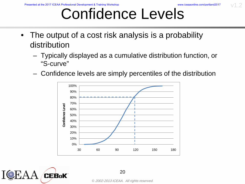
copy 2002-2013 ICEAA All rights reserved
v12
20
Confidence Levelsbull The output of a cost risk analysis is a probability
distributionndash Typically displayed as a cumulative distribution function or
ldquoS-curverdquondash Confidence levels are simply percentiles of the distribution
0
10
20
30
40
50
60
70
80
90
100
30 60 90 120 150 180
Conf
iden
ce L
evel
Presented at the 2017 ICEAA Professional Development amp Training Workshop wwwiceaaonlinecomportland2017
copy 2002-2013 ICEAA All rights reserved
v12
Measuring Parametric Model Uncertainty
bull When developing estimates using cost-estimating relationships (CERs) there are two major sources of uncertaintyndash Technical (model input) uncertaintyndash Estimating uncertainty
bull Technical uncertainty reflects the uncertainty inherent in the model inputsndash Typical parametric model inputs include weight lines of code
heritage and other performance and management inputs
bull Estimating uncertainty measures the uncertainty inherent in the model due to the modelrsquos inability to capture all aspects of variability in the data
21
Presented at the 2017 ICEAA Professional Development amp Training Workshop wwwiceaaonlinecomportland2017
copy 2002-2013 ICEAA All rights reserved
v12
Parametric Model Examplebull The NASAAir Force Cost Model (NAFCOM) is a
parametric model for estimating acquisition costs for spacecraft and launch vehicles
bull The CERs in NAFCOM have the formCost = C WeightVNewDesignWTechnicalXManagementY ClassZ
bull There is technical uncertainty about each of the parametersndash Parametric models are applied early in a program so there
is significant amount of uncertainty in the weightndash Heritage is also tricky it is inherently subjective and project
personnel are typically optimisticndash Technical characteristics can also change as a program
matures and requirements change
22
Presented at the 2017 ICEAA Professional Development amp Training Workshop wwwiceaaonlinecomportland2017
copy 2002-2013 ICEAA All rights reserved
v12
Weight Uncertaintybull Aerospace weight growth study average satellite
weight growth from program inception to launch is 28
23
Aerospace Weight Growth Data
-10
0
10
20
30
40
50
60
0 4 8 12 16 20 24 28 32 36 40 44 48 52 56 60 64 68 72 76 80 84 88 92 96 100
Percent Program Completion
Perc
ent W
eigh
t Gro
wth
Presented at the 2017 ICEAA Professional Development amp Training Workshop wwwiceaaonlinecomportland2017
copy 2002-2013 ICEAA All rights reserved
v12
Estimating Uncertaintybull CERs do not perfectly fit the historical data
ndash There are non-repeatable random effects that cannot be predicted
bull For examplendash Parts breaking during testingndash Strikes which are difficult to predict
bull This results in an underlying uncertainty distribution about an estimatendash The outcome of a CER represents only one point on an
uncertainty distributionbull Typically mean or median depending upon the CER
methodology
24
Presented at the 2017 ICEAA Professional Development amp Training Workshop wwwiceaaonlinecomportland2017
copy 2002-2013 ICEAA All rights reserved
v12
Estimating Uncertainty (2)
25
Presented at the 2017 ICEAA Professional Development amp Training Workshop wwwiceaaonlinecomportland2017
copy 2002-2013 ICEAA All rights reserved
v12
Estimating Uncertainty (3)bull In the case of a linear regression the estimating
uncertainty follows a normal distributionndash The estimate is the mean and the standard error of the
estimate from the regression is the standard deviation of the normal distribution
bull In the case of a log-transformed linear regression the estimating uncertainty follows a lognormal distributionndash The estimate is the median of the lognormal and the
standard error of the estimate from the regression is the standard deviation of the normal distribution (in log-space)
bull There is additional uncertainty about an estimate based upon the distance of what is being estimated from the mean of the input datandash This results in a prediction interval
26
Presented at the 2017 ICEAA Professional Development amp Training Workshop wwwiceaaonlinecomportland2017
copy 2002-2013 ICEAA All rights reserved
v12
Aggregating Riskbull Risk is typically applied at the same level at
which we estimate cost that is at the Work Breakdown Structure (WBS) level
bull The estimates for each WBS are developedndash These estimates sum to yield the total system cost
bull For an n-element WBS the total cost is the sum of the cost for each of the n elements
27
nXXXCostSystem +++= 21
Presented at the 2017 ICEAA Professional Development amp Training Workshop wwwiceaaonlinecomportland2017
copy 2002-2013 ICEAA All rights reserved
v12
WBS Examplebull Launch Vehicle
ndash Structurebull Vehicle Structurebull Tank Structure
ndash Thermal Controlbull Active Thermal Controlbull Induced Thermal Controlbull Tank Thermal Control
ndash Main Propulsion Systemndash Liquid Rocket Enginendash Electric Power and Distributionndash Command Control and Data Handlingndash System Integration
28
Presented at the 2017 ICEAA Professional Development amp Training Workshop wwwiceaaonlinecomportland2017
copy 2002-2013 ICEAA All rights reserved
v12
WBS and Risk
29
Presented at the 2017 ICEAA Professional Development amp Training Workshop wwwiceaaonlinecomportland2017
copy 2002-2013 ICEAA All rights reserved
v12
Aggregating Riskbull This leads us to the issue of aggregating the risks across the
WBSbull For example if we want to determine the 70th percentile of the
overall cost risk distribution how do we proceed bull Note that we cannot simply add the 70th percentiles of each of
the cost risk distributionsbull We can add means and variances (taking correlation into
account more on that later) but that is all
Variance of Total Cost =
30
Mean of Total Cost = ( )E X E Xk
k
n
kk
n
kk
n
= = =aringaelig
egraveccediloumloslashdivide
= =aring aring1 1 1
m
Var X kk
n
=aringaelig
egraveccediloumloslashdivide1
= s r s skk
n
iji
j
i jj
n2
1 1
1
22+aring aringaring
= =
-
=
Presented at the 2017 ICEAA Professional Development amp Training Workshop wwwiceaaonlinecomportland2017
copy 2002-2013 ICEAA All rights reserved
v12
Percentiles Do Not Addbull As a notional example consider two independent normal
distributionsndash One distribution has mean equal to 100 and standard deviation
equal to 20ndash The second distribution has mean 300 and standard deviation of 80
bull The sum of two independent normally distributed random variables is also normally distributed
bull To combine the two distributions we add the means and add the variancesndash Total mean is
ndash Total standard deviation is
31
400300100 =+
8258020 22 raquo+
Presented at the 2017 ICEAA Professional Development amp Training Workshop wwwiceaaonlinecomportland2017
copy 2002-2013 ICEAA All rights reserved
v12
Percentiles Do Not Add (2)bull The 80th percentiles for the individual distributions are
117 and 367 respbull The 80th percentile of the combined distribution is
469 but the sum of the two 80th percentiles is 484bull To see why this is the case note that the percentiles
of a normal distribution are determined by the mean and the standard deviationndash The standard deviations are not added when normal distributions
are combined rather the variances are combinedndash Sum of variances is ndash The standard deviation of this sum is
32
22 ba +22 ba +
Presented at the 2017 ICEAA Professional Development amp Training Workshop wwwiceaaonlinecomportland2017
copy 2002-2013 ICEAA All rights reserved
v12
Percentiles Do Not Add (3)bull Since bull We can write
bull The left side of this inequality represents the risk of the combined distributions while the right side represents the sums of the individual risks
bull Combining two missions that are independent results in a diversification of riskndash The total portfolio is not as risky on a relative basis as each
individual project
33
2222 2 bababa ++lt+
baba +lt+ 22
Presented at the 2017 ICEAA Professional Development amp Training Workshop wwwiceaaonlinecomportland2017
copy 2002-2013 ICEAA All rights reserved
v12
Methods for Aggregating Riskbull Since percentiles do not add we have to find other
ways to aggregate riskbull One method is to use Monte Carlo simulationbull Unless cost risk is represented by normal
distributions for all WBS elements summing the means and variances does not result in a completely accurate depiction of overall system cost risk
bull The normal distribution is not a realistic distribution for representing risk in many or even most situations since regarding project risk more can go wrong than can go right which means the risk is NOT symmetric unlike the Gaussian bell curve
34
Presented at the 2017 ICEAA Professional Development amp Training Workshop wwwiceaaonlinecomportland2017
copy 2002-2013 ICEAA All rights reserved
v12
Unit III - Module 9 35
Monte Carlo Simulationfor Risk Analysis
bull When risk analysis is performed multiple risks are gatheredndash These risks may have various probability
distributions
bull Monte Carlo is the most commonly accepted way to produce an accurate characterization of the distribution of the combined effect of these many risksndash Using this distribution we can produce percentiles
for cost impacts due to risk occurrences
10
Presented at the 2017 ICEAA Professional Development amp Training Workshop wwwiceaaonlinecomportland2017
copy 2002-2013 ICEAA All rights reserved
v12
Monte Carlo Simulationbull Simulation is a means for solving problems that are
analytically intractablendash Involves repeated random sampling
bull It was developed during the Manhattan Project as a way to model the interactions inside an atom during nuclear fissionndash Allowed for more sophisticated mathematical modeling of atomic
phenomena
bull Most computer packages use pseudo-random number generators that produce seemingly random results from an initial seedndash Example is the linear congruential generator
36
( ) mbaXX nn mod1 +=+
Presented at the 2017 ICEAA Professional Development amp Training Workshop wwwiceaaonlinecomportland2017
copy 2002-2013 ICEAA All rights reserved
v12Using Random Numbers to Simulate Distributions
bull WBS cost risk is typically measured by a probability distributionbull The most common method for simulating a probability
distribution is the inverse methodbull This involve obtaining a simulated random value from a uniform
distribution and then inverting this through the cumulative distribution function (CDF) to obtain the simulated value
bull As an example for a uniform distribution on the interval [0100]
bull In this case the CDF random value of 05 translates to 10005 = 50
37
( )100
1=xf ( )
100xxF = ( ) xxF 1001 =-
Presented at the 2017 ICEAA Professional Development amp Training Workshop wwwiceaaonlinecomportland2017
copy 2002-2013 ICEAA All rights reserved
v12
Simulating a Triangular Distribution
bull For a triangular distribution with low = 0 most likely = 50 and high = 150 the CDF is given by
bull The inverse function is given by
38
( )iumliumlicirc
iumliumliacute
igrave
poundlt--
poundpound=
1505021
1500050
50015000
2
2
2
xxx
xxxF
( )iumliumlicirc
iumliumliacute
igrave
poundltdivideoslashouml
ccedilegraveaelig +--
poundpound=-
131
21
37501
250017500150
3107500
1
xx
xxxF
Presented at the 2017 ICEAA Professional Development amp Training Workshop wwwiceaaonlinecomportland2017
copy 2002-2013 ICEAA All rights reserved
v12
Simulating a Triangular Distribution (2)
bull If the simulated uniform value is equal to 02 the corresponding inverse value from the CDF inverse is approximately 387
39
0
01
02
03
04
05
06
07
08
09
1
0 30 60 90 120 150
Presented at the 2017 ICEAA Professional Development amp Training Workshop wwwiceaaonlinecomportland2017
copy 2002-2013 ICEAA All rights reserved
v12
Monte Carlo and the WBSbull Simulation involves repeated trials
40
WBS Draw1 2 3 4 5
System 2912 3566 4390 2954 4655 Sum
Structure 80 105 55 80 57 SumVehicle Structure 50 70 30 40 20Tank Structure 30 35 25 40 37
Thermal Control 32 36 35 29 33 SumActive Thermal Control 10 15 12 7 10Induced Thermal Control 12 14 13 14 14Tank Thermal Control 10 7 10 8 9
Main Propulsion System 100 150 125 140 100
Liquid Rocket Engine 1000 1100 1800 900 2200
Electric Power and Distribution 100 125 150 75 90
Command Control and Data Handling 200 250 225 230 275
System Integration 1400 1800 2000 1500 1900
Presented at the 2017 ICEAA Professional Development amp Training Workshop wwwiceaaonlinecomportland2017
copy 2002-2013 ICEAA All rights reserved
v12
Number of Trialsbull Monte Carlo involves a repeated number of trialsbull The greater the number of trials the more accurate the
simulation will approximate the overall cost risk behavior of the system
bull After 100 trials the histogram looks very jagged
41
Presented at the 2017 ICEAA Professional Development amp Training Workshop wwwiceaaonlinecomportland2017
copy 2002-2013 ICEAA All rights reserved
v12
Number of Trials (2)
42
1000 Trials
10000 Trials
50000 Trials Additional trials give a more accurate depiction of the final result
Presented at the 2017 ICEAA Professional Development amp Training Workshop wwwiceaaonlinecomportland2017
copy 2002-2013 ICEAA All rights reserved
v12
Number of Trials (3)bull If we want to simulate the underlying
mean within 1 with 95 confidence for example then we require
43
divideoslash
oumlccedilegrave
aelig poundpound-
=
dividedividedivide
oslash
ouml
ccedilccedilccedil
egrave
aeligpound
-pound
-=
divideoslashouml
ccedilegraveaelig poundpound=
nZ
n
nnX
n
X
n
n
011
010Pr
011
010Pr
011990Pr950
___
___
sm
sm
sm
sm
sm
mm
Presented at the 2017 ICEAA Professional Development amp Training Workshop wwwiceaaonlinecomportland2017
copy 2002-2013 ICEAA All rights reserved
v12
Number of Trials (4)bull This means that the number of trials required is determined by
bull Solving for n we find that at least
trials are neededbull Note that this term involves the coefficient of variation of the
distribution which means that distributions with less dispersion require fewer trials to accurate simulate
44
96101
=ns
m
ms41638
Presented at the 2017 ICEAA Professional Development amp Training Workshop wwwiceaaonlinecomportland2017
copy 2002-2013 ICEAA All rights reserved
v12
Number of Trials (5)bull Simulating percentiles requires more trials than for simulating
meansbull Let Pn represent the number of trials in the sample at or below
the 70th percentile of the underlying distribution (suppose this is known)
bull By the Central Limit Theorem Pnn follows a normal distribution with mean equal to the 70th percentile and variance equal to
bull By a similar process for the mean we find that the number of trials needed to simulate the 70th percentile within 1 with 95 confidence is
45
( )n
FF 700700 1-
n
n
PPn -41638
Presented at the 2017 ICEAA Professional Development amp Training Workshop wwwiceaaonlinecomportland2017
copy 2002-2013 ICEAA All rights reserved
v12
Number of Trials (6)bull If Pn 070 for all n then n is approximately
bull For the sake of comparison suppose CV = 03 (reasonable approximation for hardware development) then the number of trials needed to simulate the mean with the same accuracy is then ldquoonlyrdquo 11525
bull More trials are needed to accurately simulate percentiles than means
46
( ) 46416703041638
70704168341638 =divide
oslashouml
ccedilegraveaelig=divide
oslashouml
ccedilegraveaelig -
=-
nnn
PPn
n
n
Presented at the 2017 ICEAA Professional Development amp Training Workshop wwwiceaaonlinecomportland2017
copy 2002-2013 ICEAA All rights reserved
v12
Methods of Simulationbull Monte Carlo simulation is a standard term for
simulationbull However there is an improvement on Monte Carlo
that improves the accuracy of the results of a simulation for a given number of trials
bull This method is call the Latin Hypercube approach to simulationndash Similar to Monte Carlo but an equal number of draws are taken
from a set of subintervals for example dividing the interval (01) into [00001) [0102)hellip [0910]
ndash Instead of 10 trials from [01] we have one trial from each subinterval
ndash Rough rule of thumb is Latin Hypercube takes 30 fewer trials to achieve similar accuracy to Monte Carlo
47
Presented at the 2017 ICEAA Professional Development amp Training Workshop wwwiceaaonlinecomportland2017
copy 2002-2013 ICEAA All rights reserved
v12
Probability Model ndash Correlationbull Correlation exists between work breakdown structure
(WBS) cost element costs and between cost and schedule
bull Correlation is a necessary consideration in cost risk analysis
bull Correlation is a number that can vary between -1 and +1 and represents the strength of the relationship between the two variablesndash If both variable have a tendency to move in the same direction
correlation is positivendash If when one variable increases the other tends to decrease and
vice-versa the correlation between the two variables is negative
Presented at the 2017 ICEAA Professional Development amp Training Workshop wwwiceaaonlinecomportland2017
copy 2002-2013 ICEAA All rights reserved
v12
Correlation And Causationbull Note that correlation is not causation however
causation implies correlationndash For example shark attacks and ice cream sales at the beach
bull For example for a launch vehicle structure increasing the diameter will not only result in an increase in the structures cost but will also result in higher costs for thermal coating (paint etc)
bull Also simply because two subsystems do not appear to be related does not mean they are not correlatedndash For example structures and computer equipment seemingly
have little relation to one another however an external factor such as a funding cut or a strike will impact all subsystems leading to delays and increasing cost across the board
ndash Thus everything in a WBS has some correlationUnit III - Module 9 49
Presented at the 2017 ICEAA Professional Development amp Training Workshop wwwiceaaonlinecomportland2017
copy 2002-2013 ICEAA All rights reserved
v12
The Importance of Correlationbull Percent that total cost standard deviation is underestimated
when correlation assumed to be 0 instead of r given nWBS elements
Unit III - Module 9 5050
0
20
40
60
80
100
0 01 02 03 04 05 06 07 08 09 1Actual Correlation
Perce
nt Un
deres
timate
d
n = 10
n = 30
n = 100n = 1000
0
20
40
60
80
100
0 01 02 03 04 05 06 07 08 09 1Actual Correlation
Perce
nt Un
deres
timate
d
n = 10
n = 30
n = 100n = 1000
Reference 32nd Annual DOD Cost Analysis Symposium Advanced Training Session ldquoWhy Correlation Matters in Cost Estimatingrdquo Stephen A Book
Presented at the 2017 ICEAA Professional Development amp Training Workshop wwwiceaaonlinecomportland2017
copy 2002-2013 ICEAA All rights reserved
v12
The Importance of Correlation (2)bull For example if correlation is assumed to be 0 for all
elements in a 30 element WBS and the actual correlation is 20 then the total cost standard deviation is underestimated by 60
bull For example assume the total cost is modeled as a normal distribution with mean = 100
bull If correlation is assumed to be zero with total cost standard deviation = 12 when correlation is actually 20 then the true underlying standard deviation is actually 30
bull 70th percentile with zero correlation assumption is 106
bull 70th percentile with 20 correlation is 116 Unit III - Module 9 51
Presented at the 2017 ICEAA Professional Development amp Training Workshop wwwiceaaonlinecomportland2017
copy 2002-2013 ICEAA All rights reserved
v12
Measures of Correlationbull Two measures of correlation are commonly used in
cost risk analysesndash Pearsonrsquos product-moment correlation coefficient ndash Spearmanrsquos rank correlation coefficient
bull Garvey and others recommend using Pearsonrsquos product-moment correlation coefficient correlation for cost risk analysesndash Method of moments uses this but there are two options in
simulationndash Popular simulation packages like Risk and Crystal Ball use
rank correlation but in practice this has been found to make little difference
ndash Pearson product-moment correlation has been incorporated into Risk+
52
Presented at the 2017 ICEAA Professional Development amp Training Workshop wwwiceaaonlinecomportland2017
copy 2002-2013 ICEAA All rights reserved
v12
Pearson Correlationbull Pearsonrsquos product-moment correlation measures
degree of linearity between two random variables bull If two random variables are perfectly linear (eg Y =
aX + b) with positive slope then the Pearson product-moment correlation between X and Y denoted by rXY is +1
53
X X
Y Y Y
XNegative Correlation Positive Correlation No Correlation
middotmiddot
middotmiddot
middotmiddot middotmiddot
middotmiddot
middot
middot
middotmiddotmiddot
middotmiddot
middotmiddot
middotmiddot middot
middot
middot
middotmiddotmiddotmiddotmiddotmiddotmiddotmiddot
middotmiddotmiddotmiddot
middotmiddot
middotmiddot middotmiddotmiddotmiddot
middotmiddotmiddot
middotmiddotmiddotmiddot
middotmiddotmiddot
middotmiddotmiddot
middotmiddot
middot
middot middotmiddot
middot middotmiddotmiddotmiddot middotmiddot middot middotmiddot middot middot
middotmiddot middot
middotmiddotmiddotmiddotmiddot middot middotmiddot
middotmiddot
middot
middotmiddot
middotmiddot middot
middot middot middot
middotmiddot middot
middotmiddotmiddot
middotmiddot
middot middot
Presented at the 2017 ICEAA Professional Development amp Training Workshop wwwiceaaonlinecomportland2017
copy 2002-2013 ICEAA All rights reserved
v12
Spearman Correlationbull Spearmanrsquos rank correlation measures the
monotonicity between two random variablesbull If two random variables are perfectly monotonically
increasing (eg Y = X2) then the Spearman rank correlation denoted by rXY is +1
bull The two measures can be significantly different
54
10 20 30 40 50 60
100
200
300
096 097 098 099 1
1
060
020
040
080
Eff
ort (
Staf
f-M
onth
s)
Software Size I KDSI
y = 28z12y
z x
yy = x100
0 pound x pound 1
Figure 5-9A Figure 5-9B
Pearson Correlation = 09976 Rank Correlation = 1
Pearson Correlation = 024 Rank Correlation = 1
X(x ) ~ Unif(01)
Reference Probability Methods for Cost Uncertainty Analysis A Systems Engineering Perspective Paul R Garvey
Presented at the 2017 ICEAA Professional Development amp Training Workshop wwwiceaaonlinecomportland2017
copy 2002-2013 ICEAA All rights reserved
v12
Unit III - Module 9 55
200
250
300
350
400
1000 1200 1400 1600 1800 2000
Recurring Production
SEPM
200
250
300
350
400
1000 1200 1400 1600 1800 2000
Recurring Production
SEPM
Functional Correlationbull Old No Functional
Correlation Simulation run with WBS items entered as values
bull New Simulation run with functional dependencies entered as they are in cost model
CorrelatedNot Correlated
Note shift of mean and increased variability
Presented at the 2017 ICEAA Professional Development amp Training Workshop wwwiceaaonlinecomportland2017
copy 2002-2013 ICEAA All rights reserved
v12
Risk Measuresbull ldquoWestern Europe conquered the word because of a
technological revolution that started because of attempts to measure the worldrdquo ndash Phillipe Jorion ndash In the same way attempts to measure risk will lead to better project
managementbull Risk management for DoD and NASA agencies focuses
primarily on funding projects to a single percentile ndash NASA policy explicitly mentions 70 and 50ndash This is known as ldquoValue at Riskrdquo and is prevalent in the banking and
financial industry
56
Presented at the 2017 ICEAA Professional Development amp Training Workshop wwwiceaaonlinecomportland2017
copy 2002-2013 ICEAA All rights reserved
v12
Value at Risk (VaR)bull VaR is a percentile of the cost risk
distributionndash VaR funding at the 70th percentile means that
there is a 30 chance of final project cost exceeding the funded amount (budget)
bull VaR has some meritsndash Common measure can be used to compare
different projects and programsndash Easily understood by senior managers and
decision makers
57
Presented at the 2017 ICEAA Professional Development amp Training Workshop wwwiceaaonlinecomportland2017
copy 2002-2013 ICEAA All rights reserved
v12
Why 70th or 80th Percentilebull Typical policy guidance involves funding at the 70th or 80th
percentile Why fund as such a low percentilebull There is some incentive to not over-fundbull For a normal distribution an inflection point occurs near the 80th
percentile meaning that for values above 80 confidence achieving higher levels of confidence can only be achieved by spending greater dollar amounts at an increasing rate
58
-05-04-03-02-01
00102030405
0 05 1 15 2 25 3
Standard Deviations from Mean
Normal Distribution
First DerivativeSlopeVelocity
Second DerivativeConvexityAcceleration
Inflection point at one standard deviation above the mean (~84th
percentile)
Presented at the 2017 ICEAA Professional Development amp Training Workshop wwwiceaaonlinecomportland2017
copy 2002-2013 ICEAA All rights reserved
v12
Funding Above Inflection Pointsbull As the percentile goes above the 80th percentile the amount
needed to achieve that higher level of confidence begins to increase at an increasing rate as is evident from the graph
59
0
10
20
30
40
50
60
70
50 55 60 65 70 75 80 85 90 95 100
$ Ab
ove
MEa
n to
Ach
ieve
Per
cent
ile
Percentile (Confidence Level)
Presented at the 2017 ICEAA Professional Development amp Training Workshop wwwiceaaonlinecomportland2017
copy 2002-2013 ICEAA All rights reserved
v12
Why Budget to the 70th or 80thbull Government projects are funded at the 70th or 80th percentilesbull Why not the 90th or 99th percentile Wonrsquot that help prevent
overrunsndash As we have seen percentiles do not add across programs
bull The sum of the 80th percentiles does NOT equal the total 80th percentile
ndash This is because the individual programs are riskier than the entire suite of missions
bull Known as the ldquoPortfolio effectrdquo (more or this later)
ndash Funding at the 80th gives confidence that the entire portfolio will be adequately funded
bull And since there is an inflection point near the 80th percentile funding above that level quickly becomes cost prohibitive
60
Presented at the 2017 ICEAA Professional Development amp Training Workshop wwwiceaaonlinecomportland2017
copy 2002-2013 ICEAA All rights reserved
v12
Inflection Points for Lognormalbull For a lognormal the inflection point
variesndash Coefficient of variation equal to 10 equates to an
inflection point at the 70th percentile
61
0
10
20
30
40
50
60
70
050 060 070 080 090 100
Coef
ficen
t of V
aria
tion
Percentile of the Inflection Point
Presented at the 2017 ICEAA Professional Development amp Training Workshop wwwiceaaonlinecomportland2017
copy 2002-2013 ICEAA All rights reserved
v12
Issues with Percentile Fundingbull However risk management does not stop at a
specific percentilendash What happens when the 70th percentile is exceeded
bull Any effective risk management policy should prescribe what happens after a bad event occursndash With VaR we only know when a bad event has occurred ndash Also funding at a relatively low level means we have no true
sense of the real risks that should be guarded against
62
Presented at the 2017 ICEAA Professional Development amp Training Workshop wwwiceaaonlinecomportland2017
copy 2002-2013 ICEAA All rights reserved
v12
ldquoHere There Be Dragonsrdquobull On old maps uncharted territory was often
marked with monsters or dragons
63
A section of the Carta Marina by Olaus Magnus 16th Century
Presented at the 2017 ICEAA Professional Development amp Training Workshop wwwiceaaonlinecomportland2017
copy 2002-2013 ICEAA All rights reserved
v12
Distribution Comparisonbull Four different distributions with the same 70th
percentile
bull Should we expect the tails to be similar
64
0
10
20
30
40
50
60
70
80
0 100 200 300 400 500 600
Perc
entil
eCo
nfid
ence
Lev
el
Triangular
Normal
Lognormal
Pareto
Presented at the 2017 ICEAA Professional Development amp Training Workshop wwwiceaaonlinecomportland2017
copy 2002-2013 ICEAA All rights reserved
v12Distribution Comparison Tail Behavior
bull The normal and triangular distributions have similar tails but the lognormal and Pareto have much fatter right tails
65
70
75
80
85
90
95
100
500 1500 2500 3500 4500 5500
Perc
entil
eCo
nfid
ence
Lev
el
Triangular
Normal
Lognormal
Pareto
Here There Be Dragons
Presented at the 2017 ICEAA Professional Development amp Training Workshop wwwiceaaonlinecomportland2017
copy 2002-2013 ICEAA All rights reserved
v12Distribution Comparison ndash Tail Behavior (Table)
bull There is significant tail risk for the lognormal and the Paretobull The 99th percentile for the Pareto is 1000 times greater than
the 70th percentilendash Risk seen in financial markets and in catastrophic risks like natural
disasters bull Four different projects follow the four different risk profiles seen
in this example should clearly have different risk management approaches but 70th percentile funding indicates the same risk management approach for all four
66
Percentile Triangular Normal Lognormal Pareto 70th $600 $600 $600 $600 80th $680 $660 $770 $1430 90th $770 $750 $1070 $5880 95th $840 $820 $1410 $23750 99th $930 $950 $2350 $600000
Presented at the 2017 ICEAA Professional Development amp Training Workshop wwwiceaaonlinecomportland2017
copy 2002-2013 ICEAA All rights reserved
v12Percentile Budgeting is Not Risk Management
bull Percentile budgeting ne effective risk management policybull Suppose that you are shopping for a new car You
mention that safety is your top concern The salesman says he has a great safe car available You ask about the air bags Do they work The salesman answers ldquoOf course Seventy percent of the time they work fine Only 30 of the time the air bags will fail to deployrdquo Would you buy such a car Hedge fund manager David Einhorn has stated ldquoRisk management is the air bag that must always work but only in the multi-sigma event where you have an accidentrdquo
67
Risk management is the air bag that must always work but only in the multi-sigma event where you
have an accident
Presented at the 2017 ICEAA Professional Development amp Training Workshop wwwiceaaonlinecomportland2017
copy 2002-2013 ICEAA All rights reserved
v12
Joint Confidence Level Analysisbull Schedules are risky toobull For 98 recent NASA missions average
schedule growth was 38ndash Not as high as cost growth but still significant
68
0
5
10
15
20
25
30
35
40
Schedule
Cost
Presented at the 2017 ICEAA Professional Development amp Training Workshop wwwiceaaonlinecomportland2017
copy 2002-2013 ICEAA All rights reserved
v12
Schedules Impact Costbull Changes in schedule can have enormous
impacts on cost ndash Schedule slips can lead to cost increases
bull Fixed programmatic costs must be paid on a regular basisndash Achieving schedule milestones early can result in cost
savings
bull Schedule is an important consideration in cost analysis including cost risk analysis
bull However we must be careful in correctly integrating cost and schedule riskndash Schedule is not simply an input but is dependent on many of
the same factors that drive cost
69
Presented at the 2017 ICEAA Professional Development amp Training Workshop wwwiceaaonlinecomportland2017
copy 2002-2013 ICEAA All rights reserved
v12
The Relationship of Cost to Schedulebull Cost and schedule are positively correlated
ndash A larger program with bigger scope with take longer to complete than a smaller simpler program
bull However longer schedules do not always equate to higher cost nor shorter schedules with lower costndash Highly compressed schedules relative to the
optimal schedule can lead to large overrunsbull Compressed schedules are commonplace for
many planetary missions
70
Presented at the 2017 ICEAA Professional Development amp Training Workshop wwwiceaaonlinecomportland2017
copy 2002-2013 ICEAA All rights reserved
v12The Impact of Schedule GrowthCompression on Cost
bull Compressed schedules lead to cost growth and based on existing research is actually more expensive than schedule slippages
71
0
20
40
60
80
100
120
140
160
-50 -25 0 25 50 75 100
Percentage Change in Schedule
Perc
enta
ge C
hang
e in
Cos
t due
to
Sche
dule
Cha
nge
Source Smart CB ldquoCost and Schedule Interrelationshipsrdquo 2007 NASA Cost Symposium
Presented at the 2017 ICEAA Professional Development amp Training Workshop wwwiceaaonlinecomportland2017
copy 2002-2013 ICEAA All rights reserved
v12Schedule as an Independent Variable
bull Why not simply add schedule as an input to cost-estimating relationships (CERs)
bull Schedule is often treated as an independent variable ndash schedules are often determined independently of cost considerationsndash Cost may not be considered explicitly although budgets and
schedules are determined based on scope and other common factors
bull In 2006 SAIC undertook a research task to determine the impact of schedule on cost and added schedule as an independent variable to the CERs in the NASAAir Force Cost Model (NAFCOM) to see if schedule provided any improvement in goodness of fit
72
Presented at the 2017 ICEAA Professional Development amp Training Workshop wwwiceaaonlinecomportland2017
copy 2002-2013 ICEAA All rights reserved
v12
Schedule is a Dependent Variablebull Since NAFCOM includes an exhaustive list of cost drivers the inclusion
of schedule should give an indication of whether there is any additional independent value added from schedule independent of the cost drivers
bull In the study schedule was added to 10 subsystem-level CERs
ndash In each case the addition of schedule did NOTimprove the goodness of fit and schedule was NOT found to be a statistically significant cost driver (given the presence of the other variables) for any of the 10 CERs
bull Standard errors for the CERs increased due to decrease in degrees of freedom
bull Thus schedule as an independent variable did not provide any additional explanation of variation in historical cost
bull This is because schedule is truly NOT an independent variable but a dependent variable and is a function of the same factors that drive cost
73
Presented at the 2017 ICEAA Professional Development amp Training Workshop wwwiceaaonlinecomportland2017
copy 2002-2013 ICEAA All rights reserved
v12
Incorporation of Schedule in Cost Risk
bull When using subjective methods care must be taken in applying schedule to cost risk analysis
bull Since schedule is a dependent variable treating it independently from other factors when assessing its impact on cost can lead to a double count of independent variables in the cost risk analysis
bull Direct inclusion of schedule in a cost risk analysis effectively doubles the influence of each cost driver
ndash Incorrectly leads to broader risk ranges
74
CostWeight
HeritageNewness
Technology Readiness Schedule
Presented at the 2017 ICEAA Professional Development amp Training Workshop wwwiceaaonlinecomportland2017
copy 2002-2013 ICEAA All rights reserved
v12Subjective Cost Risk Methods and Overinclusion of Risk Factors
bull Subjective methods are suitable when data are scarce or not availablebull However care must be taken not to treat correlated sources of risk
such as schedule as independent of each otherbull Example ndash a subjective risk analysis incorporated technology readiness
design risk requirements stability integration risk and schedule and treated each source of risk as independent
bull Risk triangle high value without schedule risk was 31 times the point estimate
bull Risk triangle high value with schedule risk added on top of other sources of risk treated independently was 34 times the point estimate
bull Risk triangle taking correlation between sources of risk into account in a rigorous statistical manner has a high value 15 times the point estimate less than half the effect when treating sources of risk as independent
75
Presented at the 2017 ICEAA Professional Development amp Training Workshop wwwiceaaonlinecomportland2017
copy 2002-2013 ICEAA All rights reserved
v12Fundamental Equation of Cost and Schedule Interrelationships
bull The Fundamental Equation of the Relationship Between Cost and Schedule is
Time = Moneybull This is a well known adage that time is money Your boss at
work may even mention this to you from time to time or if you are the boss you are all too aware of this iron law
bull Because time is money cost and schedule risk should be modeled jointly not with schedule as an independent cost driver
bull Note that cost and schedule are not perfectly correlatedndash Cost can sometimes ldquobuy downrdquo schedule extra money can be
spent to meet a deadline since in some cases additional effort to hasten the completion of a task
76
Presented at the 2017 ICEAA Professional Development amp Training Workshop wwwiceaaonlinecomportland2017
copy 2002-2013 ICEAA All rights reserved
v12How to (Correctly) Incorporate Schedule into Cost Risk Analysis
bull The best way to model cost and schedule risk is to develop a joint cost and schedule model based on the same data
bull Since such models are not currently available the next best approach is to model cost and schedule independently and then integrate cost and schedule risk analyses using joint probability distributions taking into account correlation between cost and schedulendash This approach pioneered by Paul Garvey and Steve Book is
considered industry best practicendash This is a practical method mathematically tractable and follows
naturally from the Fundamental Equation of Cost and Schedule Interrelationships
77
Book S A ldquoQuantifying the Relationship Between Cost and Schedulerdquo The Measurable News Winter 2007-2008 pp 11-15Garvey PR Probability Methods for Cost Uncertainty Analysis A Systems Engineering Perspective New York Marcel Dekker 2000 pp 308-335
Presented at the 2017 ICEAA Professional Development amp Training Workshop wwwiceaaonlinecomportland2017
copy 2002-2013 ICEAA All rights reserved
v12
Joint Lognormal and Normal Distributions
bull Cost and schedule are typically modeled as some combination of Normal and Lognormal probability distributionsndash Studies by The Aerospace Corporation the MITRE
Corporation Wyle Labs and SAIC have found that the Lognormal probability distribution almost always serves as a good model for both the schedule distribution and the cost distribution
ndash The Normal distribution may also be appropriate in some instances and depending upon the level of confidence at which budgets are set may even be more conservative and logically consistent than the Normal distribution
ndash Joint Lognormal and Normal distributions are defined by a pair of mean and standard deviations and a level of correlation between the two
78
Presented at the 2017 ICEAA Professional Development amp Training Workshop wwwiceaaonlinecomportland2017
copy 2002-2013 ICEAA All rights reserved
v12Modeling Cost and Schedule as a Bivariate Distribution
bull In the approach set forth by Book and Garvey cost risk is assessed and the top-level distribution is modeled as a Lognormal (or Normal) distribution schedule risk is assessed and the overall schedule risk is modeled as a Lognormal (or Normal) distribution
bull The two distributions are combined into a Bivariate distribution by assigning a correlation between the two and by treating the two distributions as the marginal distributions of a Bivariate Lognormal distributionndash Other combinations include a Bivariate Normal or a Bivariate
Normal-Lognormal
79
Presented at the 2017 ICEAA Professional Development amp Training Workshop wwwiceaaonlinecomportland2017
copy 2002-2013 ICEAA All rights reserved
v12Bivariate Lognormal Distribution for Cost and Schedule
bull Cost is often observed to be Lognormal when strong positive correlations are present among the systemrsquos WBS cost element costs
bull A systemrsquos schedule is often observed (from Monte Carlo simulations) to be Lognormal if it is the sum of many positively correlated schedule activities in an overall schedule network
bull If Lognormal distributions characterize a systemrsquos cost and schedule then the Bivariate Lognormal could serve as an assumed model of their joint distributionndash In this case the marginal distribution of each of cost and schedule is
Lognormalbull Other possibilities for modeling cost and schedule as a Bivariate
distribution include a Bivariate Normal or a Bivariate Normal-Lognormal distributionndash All these combinations are analytically tractable
80
Presented at the 2017 ICEAA Professional Development amp Training Workshop wwwiceaaonlinecomportland2017
copy 2002-2013 ICEAA All rights reserved
v12Bivariate Lognormal for Cost and Schedule
bull Contour Plots of a Bivariate Lognormal
81
Presented at the 2017 ICEAA Professional Development amp Training Workshop wwwiceaaonlinecomportland2017
copy 2002-2013 ICEAA All rights reserved
v12Correlation Between Cost and Schedule
bull Cost and schedule are positively correlated but not perfectly sondash For example it is possible to have a schedule underrun and a cost
overrunbull Based on cost and schedule growth data for 50 completed NASA
programs the correlation between development cost and development schedule is 70
82
00
200
400
600
800
1000
1200
-500 00 500 1000 1500 2000 2500Historical Cost Growth
Hist
oric
al S
ched
ule
Gro
wth
r = 715
Presented at the 2017 ICEAA Professional Development amp Training Workshop wwwiceaaonlinecomportland2017
copy 2002-2013 ICEAA All rights reserved
v12Correlation Between Cost and Schedule Caveats
bull Based on historical data recommended correlation between cost and schedule is 70 but this could be higher or lower depending upon program circumstancesndash If program is budget constrained cost and schedule will be
more highly correlated (go as you pay)ndash If program is schedule constrained cost and schedule will
have lower correlation perhaps even negative correlation ndash Smaller programs have smaller correlation between cost and
schedule riskbull Relatively easy to ldquohurry uprdquo and finish on time or even early if
needed
83
Presented at the 2017 ICEAA Professional Development amp Training Workshop wwwiceaaonlinecomportland2017
copy 2002-2013 ICEAA All rights reserved
v12
Conditional Confidence Levelsbull Given a programrsquos project schedule we can determine the cost
risk distribution conditional upon the given schedulebull Conditional cost S-curves are steeper than unconditional
(marginal) cost S-curves between some uncertainty has been removed because schedule is fixed
84
Presented at the 2017 ICEAA Professional Development amp Training Workshop wwwiceaaonlinecomportland2017
copy 2002-2013 ICEAA All rights reserved
v12
Joint Confidence Levelsbull Joint 65 confidence represents the probability of
achieving both 65 confidence in cost AND 65 confidence in schedulendash This is different than achieving 65 cost confidence alone
or achieving 65 schedule confidence alonebull Due to the imperfect correlation between cost and schedule it
is possible to achieve a 65 cost confidence with a lower level of schedule confidence
bull Restricting the schedule confidence thus requires additional $ to achieve a given level of confidence
85
X
Y
Possible Values for Which X gt a Possible Values for
Which X gt a and Y gt b
a
b
Presented at the 2017 ICEAA Professional Development amp Training Workshop wwwiceaaonlinecomportland2017
copy 2002-2013 ICEAA All rights reserved
v12Joint Confidence Levels Versus Cost Confidence Levels Only
bull Example of the differences between cost confidence schedule confidence conditional cost confidence and joint cost and schedule confidence
86
Joint Cost-Schedule Confidence Iso-Curves
Cost (RY$M)
Sche
dule
(Mon
ths)
65 Confidence
50 Confidence
70 Confidence
65 Cost Confidence AggressiveSchedule65 Cost ConfidenceScheduleGiven 65 Schedule ConfidenceUnconditional 65 CostConfidenceUnconditional 65 ScheduleConfidence
65 Cost Confidence 65 Joint Cost and Schedule
Confidence for 65 Schedule Confidence
Presented at the 2017 ICEAA Professional Development amp Training Workshop wwwiceaaonlinecomportland2017
copy 2002-2013 ICEAA All rights reserved
v12
Joint Cost and Schedule Confidence
bull Can examine pairs of cost and schedule that achieve a given level of confidence
bull Provides insights into the trade-offs between cost and schedule for a given level of confidencendash Possible to increase cost confidence by giving a
project more time in some instances or possible to ldquobuy downrdquo schedule
bull But these have limits and are shown in the iso-cost and schedule confidence curves
87
Presented at the 2017 ICEAA Professional Development amp Training Workshop wwwiceaaonlinecomportland2017
copy 2002-2013 ICEAA All rights reserved
v12Cost and Schedule Trade-offs for a Given Level of Joint Confidence
bull Hypothetical Example
88
Cost (RY$M)
Schedule (Months)
$100 48$99 48$89 49$87 50$85 51$85 52$84 53$83 55$83 55$83 56
Cost and Schedule 65 Confidence Iso-Curve
4748495051525354555657
$80 $82 $84 $86 $88 $90 $92 $94 $96 $98 $100
Cost (RY$ M)
Sche
dule
(Mon
ths)
Presented at the 2017 ICEAA Professional Development amp Training Workshop wwwiceaaonlinecomportland2017
copy 2002-2013 ICEAA All rights reserved
v12Policy Considerations for Confidence Levels
bull For large programs the difference between the amount of money needed to achieve 65 cost confidence independent of schedule and joint 65 cost and schedule confidence can represent hundreds of millions and even billions of dollars
89
Joint Cost-Schedule Confidence Iso-Curves
Cost (RY$M)
Sche
dule
(Mon
ths)
65 Confidence
65 Cost Confidence AggressiveSchedule
65 Cost ConfidenceScheduleGiven 65 Schedule Confidence
Unconditional 65 CostConfidence
Joint Cost and Schedule Confidence for 65 Cost Confidence and Program Baseline Schedule is Less Than 35
65 Cost Confidence Independent of Schedule Cost Needed to Achieve
Both 65 Joint Cost and Schedule Confidence for the Schedule with 65 Confidence
Presented at the 2017 ICEAA Professional Development amp Training Workshop wwwiceaaonlinecomportland2017
copy 2002-2013 ICEAA All rights reserved
v12
Copulasbull More generally any combination of distributions can
be used (more than just normal and lognormal)ndash Termed ldquocopulardquo from the Italian word for ldquocouplerdquondash Copulas are a way to combine marginal distributions of any
number and type into a joint distributionbull More formally a copula is a multivariate joint distribution defined
on the n-dimensional unit cube [0 1]n such that every marginal distribution is uniform on the interval [0 1]
bull (The bivariate form of) Sklarrsquos theorem states that for any bivariate distribution function H(x y) let F(x) = H(x infin) and G(y) = H(infin y) be the univariate marginal probability distribution functions Then there exists a copula C such that H(xy)=C(F(x)G(y))
ndash Copulas are widely used in risk management for investments and insurance
bull Considered industry best practice (Li 2000)bull Marketed as part of JP Morganrsquos CreditMetrics suite of tools
(Gupton et Al 1997)90
Presented at the 2017 ICEAA Professional Development amp Training Workshop wwwiceaaonlinecomportland2017
copy 2002-2013 ICEAA All rights reserved
v12Parametric Joint Cost and Schedule Analysis
bull A parametric model based on a consistent data set with a set of overlapping cost and schedule drivers is a cleaner way to model cost and schedule
91
CostWeight
HeritageNewness
Technology Readiness
Schedule
0
20
40
60
80
100
Confidence
Joint Cost and Schedule Confidence
Schedule
Cost
Lognormal Distribution PDF and CDF
0102030405060708090100
200 300 400 500 600 700 800 900 1000Cost $
Con
fiden
ce L
evel
0
00002
00004
00006
00008
0001
00012
00014
00016
Prob
abili
ty D
ensi
ty
CDFPDF
Lognormal Distribution PDF and CDF
0102030405060708090100
200 300 400 500 600 700 800 900 1000Cost $
Con
fiden
ce L
evel
0
00002
00004
00006
00008
0001
00012
00014
00016
Prob
abili
ty D
ensi
ty
CDFPDF
Presented at the 2017 ICEAA Professional Development amp Training Workshop wwwiceaaonlinecomportland2017
copy 2002-2013 ICEAA All rights reserved
v12Parametric Joint Cost and Schedule Analysis (2)
bull Joint cost and schedule risk analysis produced naturally by the integrated modelndash Addresses several issues with the copula
approachbull Tail dependencybull Correlation ndash no need to assign correlation
between cost and schedulebull Consistency of cost and schedule models
92
Presented at the 2017 ICEAA Professional Development amp Training Workshop wwwiceaaonlinecomportland2017
copy 2002-2013 ICEAA All rights reserved
v12
Resource-Loaded Schedulesbull Involves assigning cost and schedule risks to a resource-loaded schedule
networkbull Bottom-up approach
ndash More labor intensive than parametrics but can also provide more insight
ndash Can answer questions than parametric typically cannot such as how much do reserve requirements decrease if a specific risk is retired
bull Currently being implemented in Constellation programbull Has same issue as all bottom-up models hard to count all the risks and model
them discretely
ndash As a result there is a tendency to reflect less risk than indicated by history
ndash ldquoThere are more things in heaven and earth Horatio than are dreamt of in your philosophyrdquo William Shakespeare Hamlet Act I Scene V
93
Presented at the 2017 ICEAA Professional Development amp Training Workshop wwwiceaaonlinecomportland2017
copy 2002-2013 ICEAA All rights reserved
v12Resource-Loaded Schedules Vs Parametrics
bull Parametric most appropriate for early estimatesndash But also good for high-level checks as project progresses
bull As plans take shape lower level modeling may be more appropriate
94 1
CONCEPTUALDEVELOPMENT
PROJECTDEFINITION DESIGN DEVELOPMENT OPERATIONS
PARAMETRIC PARAMETRIC
ANALOGY
ENGINEERING (Bottoms Up)
$PARAMETRIC
DETAILED
$
Pre Phase A Phase B Phase CDPhase A Phase EPre Phase A Phase B Phase CDPhase A Phase E
Risk = f(Cost Estimating Relationship Inputs eg mass power data rate TRL new design etc)
Risk = f(cost and schedule variation of the analogous elements)
Risk = f(variation of detailed inputs eg labor hours rates materials etc)
Presented at the 2017 ICEAA Professional Development amp Training Workshop wwwiceaaonlinecomportland2017
copy 2002-2013 ICEAA All rights reserved
v12
Resource-Loaded Schedulesbull Methodology has been demonstrated in other
industriesndash Construction oil and gasndash Analysis has not been traditionally done on highly uncertain
complex development projects bull Methodology focuses on project baseline schedule
ndash In baseline schedule all tasks are resource loaded to represent a baseline schedule and cost standpoint
ndash Resource loaded schedule is ldquorolledrdquo up to a manageable level
ndash Based on the risk and uncertainties identified schedule distributions are applied to each rolled up task
ndash Cost uncertainties are also applied to rolled up tasksbull Uncertainties include labor rate man power etc
ndash A Monte Carlo simulation is run to develop joint cost-schedule distributions
95
Presented at the 2017 ICEAA Professional Development amp Training Workshop wwwiceaaonlinecomportland2017
copy 2002-2013 ICEAA All rights reserved
v12
Unit III - Module 9 96
Execution ndash Cross Checksbull Means The mean cost growth factor for WBS items
can be compared to history as a way to cross check results
bull CVs The CV of the cost growth factors for WBS items can be compared to history as a way to cross check results
bull Inputs Checks are performed on inputs or other parameters to see if historical values are in line with program assumptionsndash Example Historical risk scores can be compared to program
risk scores to see if risk assessors are being realistic and to see if the underlying database is representative of the program
11
Presented at the 2017 ICEAA Professional Development amp Training Workshop wwwiceaaonlinecomportland2017
- Cost and Schedule Risk Analysis Basic
- Acknowledgments
- Unit Index
- Risk Overview
- Agenda
- Introduction
- Risk Analysis Terms
- Are Our Costs Realistic
- Historical Cost Growth
- Sources of Cost Risk
- Point Estimates of Cost
- Types of Risk
- Point Estimates Vs Risk Estimates
- Cost Risk and Probability
- Probability Model ndash Distribution
- Probability Model ndash Distribution
- Probability ndash Top-Level Distribution
- S-Curves and Confidence Levels
- Example ndash Normal Distribution
- Confidence Levels
- Measuring Parametric Model Uncertainty
- Parametric Model Example
- Weight Uncertainty
- Estimating Uncertainty
- Estimating Uncertainty (2)
- Estimating Uncertainty (3)
- Aggregating Risk
- WBS Example
- WBS and Risk
- Aggregating Risk
- Percentiles Do Not Add
- Percentiles Do Not Add (2)
- Percentiles Do Not Add (3)
- Methods for Aggregating Risk
- Monte Carlo Simulationfor Risk Analysis
- Monte Carlo Simulation
- Using Random Numbers to Simulate Distributions
- Simulating a Triangular Distribution
- Simulating a Triangular Distribution (2)
- Monte Carlo and the WBS
- Number of Trials
- Number of Trials (2)
- Number of Trials (3)
- Number of Trials (4)
- Number of Trials (5)
- Number of Trials (6)
- Methods of Simulation
- Probability Model ndash Correlation
- Correlation And Causation
- The Importance of Correlation
- The Importance of Correlation (2)
- Measures of Correlation
- Pearson Correlation
- Spearman Correlation
- Functional Correlation
- Risk Measures
- Value at Risk (VaR)
- Why 70th or 80th Percentile
- Funding Above Inflection Points
- Why Budget to the 70th or 80th
- Inflection Points for Lognormal
- Issues with Percentile Funding
- ldquoHere There Be Dragonsrdquo
- Distribution Comparison
- Distribution Comparison Tail Behavior
- Distribution Comparison ndash Tail Behavior (Table)
- Percentile Budgeting is Not Risk Management
- Joint Confidence Level Analysis
- Schedules Impact Cost
- The Relationship of Cost to Schedule
- The Impact of Schedule GrowthCompression on Cost
- Schedule as an Independent Variable
- Schedule is a Dependent Variable
- Incorporation of Schedule in Cost Risk
- Subjective Cost Risk Methods and Overinclusion of Risk Factors
- Fundamental Equation of Cost and Schedule Interrelationships
- How to (Correctly) Incorporate Schedule into Cost Risk Analysis
- Joint Lognormal and Normal Distributions
- Modeling Cost and Schedule as a Bivariate Distribution
- Bivariate Lognormal Distribution for Cost and Schedule
- Bivariate Lognormal for Cost and Schedule
- Correlation Between Cost and Schedule
- Correlation Between Cost and Schedule Caveats
- Conditional Confidence Levels
- Joint Confidence Levels
- Joint Confidence Levels Versus Cost Confidence Levels Only
- Joint Cost and Schedule Confidence
- Cost and Schedule Trade-offs for a Given Level of Joint Confidence
- Policy Considerations for Confidence Levels
- Copulas
- Parametric Joint Cost and Schedule Analysis
- Parametric Joint Cost and Schedule Analysis (2)
- Resource-Loaded Schedules
- Resource-Loaded Schedules Vs Parametrics
- Resource-Loaded Schedules
- Execution ndash Cross Checks
-
copy 2002-2013 ICEAA All rights reserved
v12
Parametric Model Examplebull The NASAAir Force Cost Model (NAFCOM) is a
parametric model for estimating acquisition costs for spacecraft and launch vehicles
bull The CERs in NAFCOM have the formCost = C WeightVNewDesignWTechnicalXManagementY ClassZ
bull There is technical uncertainty about each of the parametersndash Parametric models are applied early in a program so there
is significant amount of uncertainty in the weightndash Heritage is also tricky it is inherently subjective and project
personnel are typically optimisticndash Technical characteristics can also change as a program
matures and requirements change
22
Presented at the 2017 ICEAA Professional Development amp Training Workshop wwwiceaaonlinecomportland2017
copy 2002-2013 ICEAA All rights reserved
v12
Weight Uncertaintybull Aerospace weight growth study average satellite
weight growth from program inception to launch is 28
23
Aerospace Weight Growth Data
-10
0
10
20
30
40
50
60
0 4 8 12 16 20 24 28 32 36 40 44 48 52 56 60 64 68 72 76 80 84 88 92 96 100
Percent Program Completion
Perc
ent W
eigh
t Gro
wth
Presented at the 2017 ICEAA Professional Development amp Training Workshop wwwiceaaonlinecomportland2017
copy 2002-2013 ICEAA All rights reserved
v12
Estimating Uncertaintybull CERs do not perfectly fit the historical data
ndash There are non-repeatable random effects that cannot be predicted
bull For examplendash Parts breaking during testingndash Strikes which are difficult to predict
bull This results in an underlying uncertainty distribution about an estimatendash The outcome of a CER represents only one point on an
uncertainty distributionbull Typically mean or median depending upon the CER
methodology
24
Presented at the 2017 ICEAA Professional Development amp Training Workshop wwwiceaaonlinecomportland2017
copy 2002-2013 ICEAA All rights reserved
v12
Estimating Uncertainty (2)
25
Presented at the 2017 ICEAA Professional Development amp Training Workshop wwwiceaaonlinecomportland2017
copy 2002-2013 ICEAA All rights reserved
v12
Estimating Uncertainty (3)bull In the case of a linear regression the estimating
uncertainty follows a normal distributionndash The estimate is the mean and the standard error of the
estimate from the regression is the standard deviation of the normal distribution
bull In the case of a log-transformed linear regression the estimating uncertainty follows a lognormal distributionndash The estimate is the median of the lognormal and the
standard error of the estimate from the regression is the standard deviation of the normal distribution (in log-space)
bull There is additional uncertainty about an estimate based upon the distance of what is being estimated from the mean of the input datandash This results in a prediction interval
26
Presented at the 2017 ICEAA Professional Development amp Training Workshop wwwiceaaonlinecomportland2017
copy 2002-2013 ICEAA All rights reserved
v12
Aggregating Riskbull Risk is typically applied at the same level at
which we estimate cost that is at the Work Breakdown Structure (WBS) level
bull The estimates for each WBS are developedndash These estimates sum to yield the total system cost
bull For an n-element WBS the total cost is the sum of the cost for each of the n elements
27
nXXXCostSystem +++= 21
Presented at the 2017 ICEAA Professional Development amp Training Workshop wwwiceaaonlinecomportland2017
copy 2002-2013 ICEAA All rights reserved
v12
WBS Examplebull Launch Vehicle
ndash Structurebull Vehicle Structurebull Tank Structure
ndash Thermal Controlbull Active Thermal Controlbull Induced Thermal Controlbull Tank Thermal Control
ndash Main Propulsion Systemndash Liquid Rocket Enginendash Electric Power and Distributionndash Command Control and Data Handlingndash System Integration
28
Presented at the 2017 ICEAA Professional Development amp Training Workshop wwwiceaaonlinecomportland2017
copy 2002-2013 ICEAA All rights reserved
v12
WBS and Risk
29
Presented at the 2017 ICEAA Professional Development amp Training Workshop wwwiceaaonlinecomportland2017
copy 2002-2013 ICEAA All rights reserved
v12
Aggregating Riskbull This leads us to the issue of aggregating the risks across the
WBSbull For example if we want to determine the 70th percentile of the
overall cost risk distribution how do we proceed bull Note that we cannot simply add the 70th percentiles of each of
the cost risk distributionsbull We can add means and variances (taking correlation into
account more on that later) but that is all
Variance of Total Cost =
30
Mean of Total Cost = ( )E X E Xk
k
n
kk
n
kk
n
= = =aringaelig
egraveccediloumloslashdivide
= =aring aring1 1 1
m
Var X kk
n
=aringaelig
egraveccediloumloslashdivide1
= s r s skk
n
iji
j
i jj
n2
1 1
1
22+aring aringaring
= =
-
=
Presented at the 2017 ICEAA Professional Development amp Training Workshop wwwiceaaonlinecomportland2017
copy 2002-2013 ICEAA All rights reserved
v12
Percentiles Do Not Addbull As a notional example consider two independent normal
distributionsndash One distribution has mean equal to 100 and standard deviation
equal to 20ndash The second distribution has mean 300 and standard deviation of 80
bull The sum of two independent normally distributed random variables is also normally distributed
bull To combine the two distributions we add the means and add the variancesndash Total mean is
ndash Total standard deviation is
31
400300100 =+
8258020 22 raquo+
Presented at the 2017 ICEAA Professional Development amp Training Workshop wwwiceaaonlinecomportland2017
copy 2002-2013 ICEAA All rights reserved
v12
Percentiles Do Not Add (2)bull The 80th percentiles for the individual distributions are
117 and 367 respbull The 80th percentile of the combined distribution is
469 but the sum of the two 80th percentiles is 484bull To see why this is the case note that the percentiles
of a normal distribution are determined by the mean and the standard deviationndash The standard deviations are not added when normal distributions
are combined rather the variances are combinedndash Sum of variances is ndash The standard deviation of this sum is
32
22 ba +22 ba +
Presented at the 2017 ICEAA Professional Development amp Training Workshop wwwiceaaonlinecomportland2017
copy 2002-2013 ICEAA All rights reserved
v12
Percentiles Do Not Add (3)bull Since bull We can write
bull The left side of this inequality represents the risk of the combined distributions while the right side represents the sums of the individual risks
bull Combining two missions that are independent results in a diversification of riskndash The total portfolio is not as risky on a relative basis as each
individual project
33
2222 2 bababa ++lt+
baba +lt+ 22
Presented at the 2017 ICEAA Professional Development amp Training Workshop wwwiceaaonlinecomportland2017
copy 2002-2013 ICEAA All rights reserved
v12
Methods for Aggregating Riskbull Since percentiles do not add we have to find other
ways to aggregate riskbull One method is to use Monte Carlo simulationbull Unless cost risk is represented by normal
distributions for all WBS elements summing the means and variances does not result in a completely accurate depiction of overall system cost risk
bull The normal distribution is not a realistic distribution for representing risk in many or even most situations since regarding project risk more can go wrong than can go right which means the risk is NOT symmetric unlike the Gaussian bell curve
34
Presented at the 2017 ICEAA Professional Development amp Training Workshop wwwiceaaonlinecomportland2017
copy 2002-2013 ICEAA All rights reserved
v12
Unit III - Module 9 35
Monte Carlo Simulationfor Risk Analysis
bull When risk analysis is performed multiple risks are gatheredndash These risks may have various probability
distributions
bull Monte Carlo is the most commonly accepted way to produce an accurate characterization of the distribution of the combined effect of these many risksndash Using this distribution we can produce percentiles
for cost impacts due to risk occurrences
10
Presented at the 2017 ICEAA Professional Development amp Training Workshop wwwiceaaonlinecomportland2017
copy 2002-2013 ICEAA All rights reserved
v12
Monte Carlo Simulationbull Simulation is a means for solving problems that are
analytically intractablendash Involves repeated random sampling
bull It was developed during the Manhattan Project as a way to model the interactions inside an atom during nuclear fissionndash Allowed for more sophisticated mathematical modeling of atomic
phenomena
bull Most computer packages use pseudo-random number generators that produce seemingly random results from an initial seedndash Example is the linear congruential generator
36
( ) mbaXX nn mod1 +=+
Presented at the 2017 ICEAA Professional Development amp Training Workshop wwwiceaaonlinecomportland2017
copy 2002-2013 ICEAA All rights reserved
v12Using Random Numbers to Simulate Distributions
bull WBS cost risk is typically measured by a probability distributionbull The most common method for simulating a probability
distribution is the inverse methodbull This involve obtaining a simulated random value from a uniform
distribution and then inverting this through the cumulative distribution function (CDF) to obtain the simulated value
bull As an example for a uniform distribution on the interval [0100]
bull In this case the CDF random value of 05 translates to 10005 = 50
37
( )100
1=xf ( )
100xxF = ( ) xxF 1001 =-
Presented at the 2017 ICEAA Professional Development amp Training Workshop wwwiceaaonlinecomportland2017
copy 2002-2013 ICEAA All rights reserved
v12
Simulating a Triangular Distribution
bull For a triangular distribution with low = 0 most likely = 50 and high = 150 the CDF is given by
bull The inverse function is given by
38
( )iumliumlicirc
iumliumliacute
igrave
poundlt--
poundpound=
1505021
1500050
50015000
2
2
2
xxx
xxxF
( )iumliumlicirc
iumliumliacute
igrave
poundltdivideoslashouml
ccedilegraveaelig +--
poundpound=-
131
21
37501
250017500150
3107500
1
xx
xxxF
Presented at the 2017 ICEAA Professional Development amp Training Workshop wwwiceaaonlinecomportland2017
copy 2002-2013 ICEAA All rights reserved
v12
Simulating a Triangular Distribution (2)
bull If the simulated uniform value is equal to 02 the corresponding inverse value from the CDF inverse is approximately 387
39
0
01
02
03
04
05
06
07
08
09
1
0 30 60 90 120 150
Presented at the 2017 ICEAA Professional Development amp Training Workshop wwwiceaaonlinecomportland2017
copy 2002-2013 ICEAA All rights reserved
v12
Monte Carlo and the WBSbull Simulation involves repeated trials
40
WBS Draw1 2 3 4 5
System 2912 3566 4390 2954 4655 Sum
Structure 80 105 55 80 57 SumVehicle Structure 50 70 30 40 20Tank Structure 30 35 25 40 37
Thermal Control 32 36 35 29 33 SumActive Thermal Control 10 15 12 7 10Induced Thermal Control 12 14 13 14 14Tank Thermal Control 10 7 10 8 9
Main Propulsion System 100 150 125 140 100
Liquid Rocket Engine 1000 1100 1800 900 2200
Electric Power and Distribution 100 125 150 75 90
Command Control and Data Handling 200 250 225 230 275
System Integration 1400 1800 2000 1500 1900
Presented at the 2017 ICEAA Professional Development amp Training Workshop wwwiceaaonlinecomportland2017
copy 2002-2013 ICEAA All rights reserved
v12
Number of Trialsbull Monte Carlo involves a repeated number of trialsbull The greater the number of trials the more accurate the
simulation will approximate the overall cost risk behavior of the system
bull After 100 trials the histogram looks very jagged
41
Presented at the 2017 ICEAA Professional Development amp Training Workshop wwwiceaaonlinecomportland2017
copy 2002-2013 ICEAA All rights reserved
v12
Number of Trials (2)
42
1000 Trials
10000 Trials
50000 Trials Additional trials give a more accurate depiction of the final result
Presented at the 2017 ICEAA Professional Development amp Training Workshop wwwiceaaonlinecomportland2017
copy 2002-2013 ICEAA All rights reserved
v12
Number of Trials (3)bull If we want to simulate the underlying
mean within 1 with 95 confidence for example then we require
43
divideoslash
oumlccedilegrave
aelig poundpound-
=
dividedividedivide
oslash
ouml
ccedilccedilccedil
egrave
aeligpound
-pound
-=
divideoslashouml
ccedilegraveaelig poundpound=
nZ
n
nnX
n
X
n
n
011
010Pr
011
010Pr
011990Pr950
___
___
sm
sm
sm
sm
sm
mm
Presented at the 2017 ICEAA Professional Development amp Training Workshop wwwiceaaonlinecomportland2017
copy 2002-2013 ICEAA All rights reserved
v12
Number of Trials (4)bull This means that the number of trials required is determined by
bull Solving for n we find that at least
trials are neededbull Note that this term involves the coefficient of variation of the
distribution which means that distributions with less dispersion require fewer trials to accurate simulate
44
96101
=ns
m
ms41638
Presented at the 2017 ICEAA Professional Development amp Training Workshop wwwiceaaonlinecomportland2017
copy 2002-2013 ICEAA All rights reserved
v12
Number of Trials (5)bull Simulating percentiles requires more trials than for simulating
meansbull Let Pn represent the number of trials in the sample at or below
the 70th percentile of the underlying distribution (suppose this is known)
bull By the Central Limit Theorem Pnn follows a normal distribution with mean equal to the 70th percentile and variance equal to
bull By a similar process for the mean we find that the number of trials needed to simulate the 70th percentile within 1 with 95 confidence is
45
( )n
FF 700700 1-
n
n
PPn -41638
Presented at the 2017 ICEAA Professional Development amp Training Workshop wwwiceaaonlinecomportland2017
copy 2002-2013 ICEAA All rights reserved
v12
Number of Trials (6)bull If Pn 070 for all n then n is approximately
bull For the sake of comparison suppose CV = 03 (reasonable approximation for hardware development) then the number of trials needed to simulate the mean with the same accuracy is then ldquoonlyrdquo 11525
bull More trials are needed to accurately simulate percentiles than means
46
( ) 46416703041638
70704168341638 =divide
oslashouml
ccedilegraveaelig=divide
oslashouml
ccedilegraveaelig -
=-
nnn
PPn
n
n
Presented at the 2017 ICEAA Professional Development amp Training Workshop wwwiceaaonlinecomportland2017
copy 2002-2013 ICEAA All rights reserved
v12
Methods of Simulationbull Monte Carlo simulation is a standard term for
simulationbull However there is an improvement on Monte Carlo
that improves the accuracy of the results of a simulation for a given number of trials
bull This method is call the Latin Hypercube approach to simulationndash Similar to Monte Carlo but an equal number of draws are taken
from a set of subintervals for example dividing the interval (01) into [00001) [0102)hellip [0910]
ndash Instead of 10 trials from [01] we have one trial from each subinterval
ndash Rough rule of thumb is Latin Hypercube takes 30 fewer trials to achieve similar accuracy to Monte Carlo
47
Presented at the 2017 ICEAA Professional Development amp Training Workshop wwwiceaaonlinecomportland2017
copy 2002-2013 ICEAA All rights reserved
v12
Probability Model ndash Correlationbull Correlation exists between work breakdown structure
(WBS) cost element costs and between cost and schedule
bull Correlation is a necessary consideration in cost risk analysis
bull Correlation is a number that can vary between -1 and +1 and represents the strength of the relationship between the two variablesndash If both variable have a tendency to move in the same direction
correlation is positivendash If when one variable increases the other tends to decrease and
vice-versa the correlation between the two variables is negative
Presented at the 2017 ICEAA Professional Development amp Training Workshop wwwiceaaonlinecomportland2017
copy 2002-2013 ICEAA All rights reserved
v12
Correlation And Causationbull Note that correlation is not causation however
causation implies correlationndash For example shark attacks and ice cream sales at the beach
bull For example for a launch vehicle structure increasing the diameter will not only result in an increase in the structures cost but will also result in higher costs for thermal coating (paint etc)
bull Also simply because two subsystems do not appear to be related does not mean they are not correlatedndash For example structures and computer equipment seemingly
have little relation to one another however an external factor such as a funding cut or a strike will impact all subsystems leading to delays and increasing cost across the board
ndash Thus everything in a WBS has some correlationUnit III - Module 9 49
Presented at the 2017 ICEAA Professional Development amp Training Workshop wwwiceaaonlinecomportland2017
copy 2002-2013 ICEAA All rights reserved
v12
The Importance of Correlationbull Percent that total cost standard deviation is underestimated
when correlation assumed to be 0 instead of r given nWBS elements
Unit III - Module 9 5050
0
20
40
60
80
100
0 01 02 03 04 05 06 07 08 09 1Actual Correlation
Perce
nt Un
deres
timate
d
n = 10
n = 30
n = 100n = 1000
0
20
40
60
80
100
0 01 02 03 04 05 06 07 08 09 1Actual Correlation
Perce
nt Un
deres
timate
d
n = 10
n = 30
n = 100n = 1000
Reference 32nd Annual DOD Cost Analysis Symposium Advanced Training Session ldquoWhy Correlation Matters in Cost Estimatingrdquo Stephen A Book
Presented at the 2017 ICEAA Professional Development amp Training Workshop wwwiceaaonlinecomportland2017
copy 2002-2013 ICEAA All rights reserved
v12
The Importance of Correlation (2)bull For example if correlation is assumed to be 0 for all
elements in a 30 element WBS and the actual correlation is 20 then the total cost standard deviation is underestimated by 60
bull For example assume the total cost is modeled as a normal distribution with mean = 100
bull If correlation is assumed to be zero with total cost standard deviation = 12 when correlation is actually 20 then the true underlying standard deviation is actually 30
bull 70th percentile with zero correlation assumption is 106
bull 70th percentile with 20 correlation is 116 Unit III - Module 9 51
Presented at the 2017 ICEAA Professional Development amp Training Workshop wwwiceaaonlinecomportland2017
copy 2002-2013 ICEAA All rights reserved
v12
Measures of Correlationbull Two measures of correlation are commonly used in
cost risk analysesndash Pearsonrsquos product-moment correlation coefficient ndash Spearmanrsquos rank correlation coefficient
bull Garvey and others recommend using Pearsonrsquos product-moment correlation coefficient correlation for cost risk analysesndash Method of moments uses this but there are two options in
simulationndash Popular simulation packages like Risk and Crystal Ball use
rank correlation but in practice this has been found to make little difference
ndash Pearson product-moment correlation has been incorporated into Risk+
52
Presented at the 2017 ICEAA Professional Development amp Training Workshop wwwiceaaonlinecomportland2017
copy 2002-2013 ICEAA All rights reserved
v12
Pearson Correlationbull Pearsonrsquos product-moment correlation measures
degree of linearity between two random variables bull If two random variables are perfectly linear (eg Y =
aX + b) with positive slope then the Pearson product-moment correlation between X and Y denoted by rXY is +1
53
X X
Y Y Y
XNegative Correlation Positive Correlation No Correlation
middotmiddot
middotmiddot
middotmiddot middotmiddot
middotmiddot
middot
middot
middotmiddotmiddot
middotmiddot
middotmiddot
middotmiddot middot
middot
middot
middotmiddotmiddotmiddotmiddotmiddotmiddotmiddot
middotmiddotmiddotmiddot
middotmiddot
middotmiddot middotmiddotmiddotmiddot
middotmiddotmiddot
middotmiddotmiddotmiddot
middotmiddotmiddot
middotmiddotmiddot
middotmiddot
middot
middot middotmiddot
middot middotmiddotmiddotmiddot middotmiddot middot middotmiddot middot middot
middotmiddot middot
middotmiddotmiddotmiddotmiddot middot middotmiddot
middotmiddot
middot
middotmiddot
middotmiddot middot
middot middot middot
middotmiddot middot
middotmiddotmiddot
middotmiddot
middot middot
Presented at the 2017 ICEAA Professional Development amp Training Workshop wwwiceaaonlinecomportland2017
copy 2002-2013 ICEAA All rights reserved
v12
Spearman Correlationbull Spearmanrsquos rank correlation measures the
monotonicity between two random variablesbull If two random variables are perfectly monotonically
increasing (eg Y = X2) then the Spearman rank correlation denoted by rXY is +1
bull The two measures can be significantly different
54
10 20 30 40 50 60
100
200
300
096 097 098 099 1
1
060
020
040
080
Eff
ort (
Staf
f-M
onth
s)
Software Size I KDSI
y = 28z12y
z x
yy = x100
0 pound x pound 1
Figure 5-9A Figure 5-9B
Pearson Correlation = 09976 Rank Correlation = 1
Pearson Correlation = 024 Rank Correlation = 1
X(x ) ~ Unif(01)
Reference Probability Methods for Cost Uncertainty Analysis A Systems Engineering Perspective Paul R Garvey
Presented at the 2017 ICEAA Professional Development amp Training Workshop wwwiceaaonlinecomportland2017
copy 2002-2013 ICEAA All rights reserved
v12
Unit III - Module 9 55
200
250
300
350
400
1000 1200 1400 1600 1800 2000
Recurring Production
SEPM
200
250
300
350
400
1000 1200 1400 1600 1800 2000
Recurring Production
SEPM
Functional Correlationbull Old No Functional
Correlation Simulation run with WBS items entered as values
bull New Simulation run with functional dependencies entered as they are in cost model
CorrelatedNot Correlated
Note shift of mean and increased variability
Presented at the 2017 ICEAA Professional Development amp Training Workshop wwwiceaaonlinecomportland2017
copy 2002-2013 ICEAA All rights reserved
v12
Risk Measuresbull ldquoWestern Europe conquered the word because of a
technological revolution that started because of attempts to measure the worldrdquo ndash Phillipe Jorion ndash In the same way attempts to measure risk will lead to better project
managementbull Risk management for DoD and NASA agencies focuses
primarily on funding projects to a single percentile ndash NASA policy explicitly mentions 70 and 50ndash This is known as ldquoValue at Riskrdquo and is prevalent in the banking and
financial industry
56
Presented at the 2017 ICEAA Professional Development amp Training Workshop wwwiceaaonlinecomportland2017
copy 2002-2013 ICEAA All rights reserved
v12
Value at Risk (VaR)bull VaR is a percentile of the cost risk
distributionndash VaR funding at the 70th percentile means that
there is a 30 chance of final project cost exceeding the funded amount (budget)
bull VaR has some meritsndash Common measure can be used to compare
different projects and programsndash Easily understood by senior managers and
decision makers
57
Presented at the 2017 ICEAA Professional Development amp Training Workshop wwwiceaaonlinecomportland2017
copy 2002-2013 ICEAA All rights reserved
v12
Why 70th or 80th Percentilebull Typical policy guidance involves funding at the 70th or 80th
percentile Why fund as such a low percentilebull There is some incentive to not over-fundbull For a normal distribution an inflection point occurs near the 80th
percentile meaning that for values above 80 confidence achieving higher levels of confidence can only be achieved by spending greater dollar amounts at an increasing rate
58
-05-04-03-02-01
00102030405
0 05 1 15 2 25 3
Standard Deviations from Mean
Normal Distribution
First DerivativeSlopeVelocity
Second DerivativeConvexityAcceleration
Inflection point at one standard deviation above the mean (~84th
percentile)
Presented at the 2017 ICEAA Professional Development amp Training Workshop wwwiceaaonlinecomportland2017
copy 2002-2013 ICEAA All rights reserved
v12
Funding Above Inflection Pointsbull As the percentile goes above the 80th percentile the amount
needed to achieve that higher level of confidence begins to increase at an increasing rate as is evident from the graph
59
0
10
20
30
40
50
60
70
50 55 60 65 70 75 80 85 90 95 100
$ Ab
ove
MEa
n to
Ach
ieve
Per
cent
ile
Percentile (Confidence Level)
Presented at the 2017 ICEAA Professional Development amp Training Workshop wwwiceaaonlinecomportland2017
copy 2002-2013 ICEAA All rights reserved
v12
Why Budget to the 70th or 80thbull Government projects are funded at the 70th or 80th percentilesbull Why not the 90th or 99th percentile Wonrsquot that help prevent
overrunsndash As we have seen percentiles do not add across programs
bull The sum of the 80th percentiles does NOT equal the total 80th percentile
ndash This is because the individual programs are riskier than the entire suite of missions
bull Known as the ldquoPortfolio effectrdquo (more or this later)
ndash Funding at the 80th gives confidence that the entire portfolio will be adequately funded
bull And since there is an inflection point near the 80th percentile funding above that level quickly becomes cost prohibitive
60
Presented at the 2017 ICEAA Professional Development amp Training Workshop wwwiceaaonlinecomportland2017
copy 2002-2013 ICEAA All rights reserved
v12
Inflection Points for Lognormalbull For a lognormal the inflection point
variesndash Coefficient of variation equal to 10 equates to an
inflection point at the 70th percentile
61
0
10
20
30
40
50
60
70
050 060 070 080 090 100
Coef
ficen
t of V
aria
tion
Percentile of the Inflection Point
Presented at the 2017 ICEAA Professional Development amp Training Workshop wwwiceaaonlinecomportland2017
copy 2002-2013 ICEAA All rights reserved
v12
Issues with Percentile Fundingbull However risk management does not stop at a
specific percentilendash What happens when the 70th percentile is exceeded
bull Any effective risk management policy should prescribe what happens after a bad event occursndash With VaR we only know when a bad event has occurred ndash Also funding at a relatively low level means we have no true
sense of the real risks that should be guarded against
62
Presented at the 2017 ICEAA Professional Development amp Training Workshop wwwiceaaonlinecomportland2017
copy 2002-2013 ICEAA All rights reserved
v12
ldquoHere There Be Dragonsrdquobull On old maps uncharted territory was often
marked with monsters or dragons
63
A section of the Carta Marina by Olaus Magnus 16th Century
Presented at the 2017 ICEAA Professional Development amp Training Workshop wwwiceaaonlinecomportland2017
copy 2002-2013 ICEAA All rights reserved
v12
Distribution Comparisonbull Four different distributions with the same 70th
percentile
bull Should we expect the tails to be similar
64
0
10
20
30
40
50
60
70
80
0 100 200 300 400 500 600
Perc
entil
eCo
nfid
ence
Lev
el
Triangular
Normal
Lognormal
Pareto
Presented at the 2017 ICEAA Professional Development amp Training Workshop wwwiceaaonlinecomportland2017
copy 2002-2013 ICEAA All rights reserved
v12Distribution Comparison Tail Behavior
bull The normal and triangular distributions have similar tails but the lognormal and Pareto have much fatter right tails
65
70
75
80
85
90
95
100
500 1500 2500 3500 4500 5500
Perc
entil
eCo
nfid
ence
Lev
el
Triangular
Normal
Lognormal
Pareto
Here There Be Dragons
Presented at the 2017 ICEAA Professional Development amp Training Workshop wwwiceaaonlinecomportland2017
copy 2002-2013 ICEAA All rights reserved
v12Distribution Comparison ndash Tail Behavior (Table)
bull There is significant tail risk for the lognormal and the Paretobull The 99th percentile for the Pareto is 1000 times greater than
the 70th percentilendash Risk seen in financial markets and in catastrophic risks like natural
disasters bull Four different projects follow the four different risk profiles seen
in this example should clearly have different risk management approaches but 70th percentile funding indicates the same risk management approach for all four
66
Percentile Triangular Normal Lognormal Pareto 70th $600 $600 $600 $600 80th $680 $660 $770 $1430 90th $770 $750 $1070 $5880 95th $840 $820 $1410 $23750 99th $930 $950 $2350 $600000
Presented at the 2017 ICEAA Professional Development amp Training Workshop wwwiceaaonlinecomportland2017
copy 2002-2013 ICEAA All rights reserved
v12Percentile Budgeting is Not Risk Management
bull Percentile budgeting ne effective risk management policybull Suppose that you are shopping for a new car You
mention that safety is your top concern The salesman says he has a great safe car available You ask about the air bags Do they work The salesman answers ldquoOf course Seventy percent of the time they work fine Only 30 of the time the air bags will fail to deployrdquo Would you buy such a car Hedge fund manager David Einhorn has stated ldquoRisk management is the air bag that must always work but only in the multi-sigma event where you have an accidentrdquo
67
Risk management is the air bag that must always work but only in the multi-sigma event where you
have an accident
Presented at the 2017 ICEAA Professional Development amp Training Workshop wwwiceaaonlinecomportland2017
copy 2002-2013 ICEAA All rights reserved
v12
Joint Confidence Level Analysisbull Schedules are risky toobull For 98 recent NASA missions average
schedule growth was 38ndash Not as high as cost growth but still significant
68
0
5
10
15
20
25
30
35
40
Schedule
Cost
Presented at the 2017 ICEAA Professional Development amp Training Workshop wwwiceaaonlinecomportland2017
copy 2002-2013 ICEAA All rights reserved
v12
Schedules Impact Costbull Changes in schedule can have enormous
impacts on cost ndash Schedule slips can lead to cost increases
bull Fixed programmatic costs must be paid on a regular basisndash Achieving schedule milestones early can result in cost
savings
bull Schedule is an important consideration in cost analysis including cost risk analysis
bull However we must be careful in correctly integrating cost and schedule riskndash Schedule is not simply an input but is dependent on many of
the same factors that drive cost
69
Presented at the 2017 ICEAA Professional Development amp Training Workshop wwwiceaaonlinecomportland2017
copy 2002-2013 ICEAA All rights reserved
v12
The Relationship of Cost to Schedulebull Cost and schedule are positively correlated
ndash A larger program with bigger scope with take longer to complete than a smaller simpler program
bull However longer schedules do not always equate to higher cost nor shorter schedules with lower costndash Highly compressed schedules relative to the
optimal schedule can lead to large overrunsbull Compressed schedules are commonplace for
many planetary missions
70
Presented at the 2017 ICEAA Professional Development amp Training Workshop wwwiceaaonlinecomportland2017
copy 2002-2013 ICEAA All rights reserved
v12The Impact of Schedule GrowthCompression on Cost
bull Compressed schedules lead to cost growth and based on existing research is actually more expensive than schedule slippages
71
0
20
40
60
80
100
120
140
160
-50 -25 0 25 50 75 100
Percentage Change in Schedule
Perc
enta
ge C
hang
e in
Cos
t due
to
Sche
dule
Cha
nge
Source Smart CB ldquoCost and Schedule Interrelationshipsrdquo 2007 NASA Cost Symposium
Presented at the 2017 ICEAA Professional Development amp Training Workshop wwwiceaaonlinecomportland2017
copy 2002-2013 ICEAA All rights reserved
v12Schedule as an Independent Variable
bull Why not simply add schedule as an input to cost-estimating relationships (CERs)
bull Schedule is often treated as an independent variable ndash schedules are often determined independently of cost considerationsndash Cost may not be considered explicitly although budgets and
schedules are determined based on scope and other common factors
bull In 2006 SAIC undertook a research task to determine the impact of schedule on cost and added schedule as an independent variable to the CERs in the NASAAir Force Cost Model (NAFCOM) to see if schedule provided any improvement in goodness of fit
72
Presented at the 2017 ICEAA Professional Development amp Training Workshop wwwiceaaonlinecomportland2017
copy 2002-2013 ICEAA All rights reserved
v12
Schedule is a Dependent Variablebull Since NAFCOM includes an exhaustive list of cost drivers the inclusion
of schedule should give an indication of whether there is any additional independent value added from schedule independent of the cost drivers
bull In the study schedule was added to 10 subsystem-level CERs
ndash In each case the addition of schedule did NOTimprove the goodness of fit and schedule was NOT found to be a statistically significant cost driver (given the presence of the other variables) for any of the 10 CERs
bull Standard errors for the CERs increased due to decrease in degrees of freedom
bull Thus schedule as an independent variable did not provide any additional explanation of variation in historical cost
bull This is because schedule is truly NOT an independent variable but a dependent variable and is a function of the same factors that drive cost
73
Presented at the 2017 ICEAA Professional Development amp Training Workshop wwwiceaaonlinecomportland2017
copy 2002-2013 ICEAA All rights reserved
v12
Incorporation of Schedule in Cost Risk
bull When using subjective methods care must be taken in applying schedule to cost risk analysis
bull Since schedule is a dependent variable treating it independently from other factors when assessing its impact on cost can lead to a double count of independent variables in the cost risk analysis
bull Direct inclusion of schedule in a cost risk analysis effectively doubles the influence of each cost driver
ndash Incorrectly leads to broader risk ranges
74
CostWeight
HeritageNewness
Technology Readiness Schedule
Presented at the 2017 ICEAA Professional Development amp Training Workshop wwwiceaaonlinecomportland2017
copy 2002-2013 ICEAA All rights reserved
v12Subjective Cost Risk Methods and Overinclusion of Risk Factors
bull Subjective methods are suitable when data are scarce or not availablebull However care must be taken not to treat correlated sources of risk
such as schedule as independent of each otherbull Example ndash a subjective risk analysis incorporated technology readiness
design risk requirements stability integration risk and schedule and treated each source of risk as independent
bull Risk triangle high value without schedule risk was 31 times the point estimate
bull Risk triangle high value with schedule risk added on top of other sources of risk treated independently was 34 times the point estimate
bull Risk triangle taking correlation between sources of risk into account in a rigorous statistical manner has a high value 15 times the point estimate less than half the effect when treating sources of risk as independent
75
Presented at the 2017 ICEAA Professional Development amp Training Workshop wwwiceaaonlinecomportland2017
copy 2002-2013 ICEAA All rights reserved
v12Fundamental Equation of Cost and Schedule Interrelationships
bull The Fundamental Equation of the Relationship Between Cost and Schedule is
Time = Moneybull This is a well known adage that time is money Your boss at
work may even mention this to you from time to time or if you are the boss you are all too aware of this iron law
bull Because time is money cost and schedule risk should be modeled jointly not with schedule as an independent cost driver
bull Note that cost and schedule are not perfectly correlatedndash Cost can sometimes ldquobuy downrdquo schedule extra money can be
spent to meet a deadline since in some cases additional effort to hasten the completion of a task
76
Presented at the 2017 ICEAA Professional Development amp Training Workshop wwwiceaaonlinecomportland2017
copy 2002-2013 ICEAA All rights reserved
v12How to (Correctly) Incorporate Schedule into Cost Risk Analysis
bull The best way to model cost and schedule risk is to develop a joint cost and schedule model based on the same data
bull Since such models are not currently available the next best approach is to model cost and schedule independently and then integrate cost and schedule risk analyses using joint probability distributions taking into account correlation between cost and schedulendash This approach pioneered by Paul Garvey and Steve Book is
considered industry best practicendash This is a practical method mathematically tractable and follows
naturally from the Fundamental Equation of Cost and Schedule Interrelationships
77
Book S A ldquoQuantifying the Relationship Between Cost and Schedulerdquo The Measurable News Winter 2007-2008 pp 11-15Garvey PR Probability Methods for Cost Uncertainty Analysis A Systems Engineering Perspective New York Marcel Dekker 2000 pp 308-335
Presented at the 2017 ICEAA Professional Development amp Training Workshop wwwiceaaonlinecomportland2017
copy 2002-2013 ICEAA All rights reserved
v12
Joint Lognormal and Normal Distributions
bull Cost and schedule are typically modeled as some combination of Normal and Lognormal probability distributionsndash Studies by The Aerospace Corporation the MITRE
Corporation Wyle Labs and SAIC have found that the Lognormal probability distribution almost always serves as a good model for both the schedule distribution and the cost distribution
ndash The Normal distribution may also be appropriate in some instances and depending upon the level of confidence at which budgets are set may even be more conservative and logically consistent than the Normal distribution
ndash Joint Lognormal and Normal distributions are defined by a pair of mean and standard deviations and a level of correlation between the two
78
Presented at the 2017 ICEAA Professional Development amp Training Workshop wwwiceaaonlinecomportland2017
copy 2002-2013 ICEAA All rights reserved
v12Modeling Cost and Schedule as a Bivariate Distribution
bull In the approach set forth by Book and Garvey cost risk is assessed and the top-level distribution is modeled as a Lognormal (or Normal) distribution schedule risk is assessed and the overall schedule risk is modeled as a Lognormal (or Normal) distribution
bull The two distributions are combined into a Bivariate distribution by assigning a correlation between the two and by treating the two distributions as the marginal distributions of a Bivariate Lognormal distributionndash Other combinations include a Bivariate Normal or a Bivariate
Normal-Lognormal
79
Presented at the 2017 ICEAA Professional Development amp Training Workshop wwwiceaaonlinecomportland2017
copy 2002-2013 ICEAA All rights reserved
v12Bivariate Lognormal Distribution for Cost and Schedule
bull Cost is often observed to be Lognormal when strong positive correlations are present among the systemrsquos WBS cost element costs
bull A systemrsquos schedule is often observed (from Monte Carlo simulations) to be Lognormal if it is the sum of many positively correlated schedule activities in an overall schedule network
bull If Lognormal distributions characterize a systemrsquos cost and schedule then the Bivariate Lognormal could serve as an assumed model of their joint distributionndash In this case the marginal distribution of each of cost and schedule is
Lognormalbull Other possibilities for modeling cost and schedule as a Bivariate
distribution include a Bivariate Normal or a Bivariate Normal-Lognormal distributionndash All these combinations are analytically tractable
80
Presented at the 2017 ICEAA Professional Development amp Training Workshop wwwiceaaonlinecomportland2017
copy 2002-2013 ICEAA All rights reserved
v12Bivariate Lognormal for Cost and Schedule
bull Contour Plots of a Bivariate Lognormal
81
Presented at the 2017 ICEAA Professional Development amp Training Workshop wwwiceaaonlinecomportland2017
copy 2002-2013 ICEAA All rights reserved
v12Correlation Between Cost and Schedule
bull Cost and schedule are positively correlated but not perfectly sondash For example it is possible to have a schedule underrun and a cost
overrunbull Based on cost and schedule growth data for 50 completed NASA
programs the correlation between development cost and development schedule is 70
82
00
200
400
600
800
1000
1200
-500 00 500 1000 1500 2000 2500Historical Cost Growth
Hist
oric
al S
ched
ule
Gro
wth
r = 715
Presented at the 2017 ICEAA Professional Development amp Training Workshop wwwiceaaonlinecomportland2017
copy 2002-2013 ICEAA All rights reserved
v12Correlation Between Cost and Schedule Caveats
bull Based on historical data recommended correlation between cost and schedule is 70 but this could be higher or lower depending upon program circumstancesndash If program is budget constrained cost and schedule will be
more highly correlated (go as you pay)ndash If program is schedule constrained cost and schedule will
have lower correlation perhaps even negative correlation ndash Smaller programs have smaller correlation between cost and
schedule riskbull Relatively easy to ldquohurry uprdquo and finish on time or even early if
needed
83
Presented at the 2017 ICEAA Professional Development amp Training Workshop wwwiceaaonlinecomportland2017
copy 2002-2013 ICEAA All rights reserved
v12
Conditional Confidence Levelsbull Given a programrsquos project schedule we can determine the cost
risk distribution conditional upon the given schedulebull Conditional cost S-curves are steeper than unconditional
(marginal) cost S-curves between some uncertainty has been removed because schedule is fixed
84
Presented at the 2017 ICEAA Professional Development amp Training Workshop wwwiceaaonlinecomportland2017
copy 2002-2013 ICEAA All rights reserved
v12
Joint Confidence Levelsbull Joint 65 confidence represents the probability of
achieving both 65 confidence in cost AND 65 confidence in schedulendash This is different than achieving 65 cost confidence alone
or achieving 65 schedule confidence alonebull Due to the imperfect correlation between cost and schedule it
is possible to achieve a 65 cost confidence with a lower level of schedule confidence
bull Restricting the schedule confidence thus requires additional $ to achieve a given level of confidence
85
X
Y
Possible Values for Which X gt a Possible Values for
Which X gt a and Y gt b
a
b
Presented at the 2017 ICEAA Professional Development amp Training Workshop wwwiceaaonlinecomportland2017
copy 2002-2013 ICEAA All rights reserved
v12Joint Confidence Levels Versus Cost Confidence Levels Only
bull Example of the differences between cost confidence schedule confidence conditional cost confidence and joint cost and schedule confidence
86
Joint Cost-Schedule Confidence Iso-Curves
Cost (RY$M)
Sche
dule
(Mon
ths)
65 Confidence
50 Confidence
70 Confidence
65 Cost Confidence AggressiveSchedule65 Cost ConfidenceScheduleGiven 65 Schedule ConfidenceUnconditional 65 CostConfidenceUnconditional 65 ScheduleConfidence
65 Cost Confidence 65 Joint Cost and Schedule
Confidence for 65 Schedule Confidence
Presented at the 2017 ICEAA Professional Development amp Training Workshop wwwiceaaonlinecomportland2017
copy 2002-2013 ICEAA All rights reserved
v12
Joint Cost and Schedule Confidence
bull Can examine pairs of cost and schedule that achieve a given level of confidence
bull Provides insights into the trade-offs between cost and schedule for a given level of confidencendash Possible to increase cost confidence by giving a
project more time in some instances or possible to ldquobuy downrdquo schedule
bull But these have limits and are shown in the iso-cost and schedule confidence curves
87
Presented at the 2017 ICEAA Professional Development amp Training Workshop wwwiceaaonlinecomportland2017
copy 2002-2013 ICEAA All rights reserved
v12Cost and Schedule Trade-offs for a Given Level of Joint Confidence
bull Hypothetical Example
88
Cost (RY$M)
Schedule (Months)
$100 48$99 48$89 49$87 50$85 51$85 52$84 53$83 55$83 55$83 56
Cost and Schedule 65 Confidence Iso-Curve
4748495051525354555657
$80 $82 $84 $86 $88 $90 $92 $94 $96 $98 $100
Cost (RY$ M)
Sche
dule
(Mon
ths)
Presented at the 2017 ICEAA Professional Development amp Training Workshop wwwiceaaonlinecomportland2017
copy 2002-2013 ICEAA All rights reserved
v12Policy Considerations for Confidence Levels
bull For large programs the difference between the amount of money needed to achieve 65 cost confidence independent of schedule and joint 65 cost and schedule confidence can represent hundreds of millions and even billions of dollars
89
Joint Cost-Schedule Confidence Iso-Curves
Cost (RY$M)
Sche
dule
(Mon
ths)
65 Confidence
65 Cost Confidence AggressiveSchedule
65 Cost ConfidenceScheduleGiven 65 Schedule Confidence
Unconditional 65 CostConfidence
Joint Cost and Schedule Confidence for 65 Cost Confidence and Program Baseline Schedule is Less Than 35
65 Cost Confidence Independent of Schedule Cost Needed to Achieve
Both 65 Joint Cost and Schedule Confidence for the Schedule with 65 Confidence
Presented at the 2017 ICEAA Professional Development amp Training Workshop wwwiceaaonlinecomportland2017
copy 2002-2013 ICEAA All rights reserved
v12
Copulasbull More generally any combination of distributions can
be used (more than just normal and lognormal)ndash Termed ldquocopulardquo from the Italian word for ldquocouplerdquondash Copulas are a way to combine marginal distributions of any
number and type into a joint distributionbull More formally a copula is a multivariate joint distribution defined
on the n-dimensional unit cube [0 1]n such that every marginal distribution is uniform on the interval [0 1]
bull (The bivariate form of) Sklarrsquos theorem states that for any bivariate distribution function H(x y) let F(x) = H(x infin) and G(y) = H(infin y) be the univariate marginal probability distribution functions Then there exists a copula C such that H(xy)=C(F(x)G(y))
ndash Copulas are widely used in risk management for investments and insurance
bull Considered industry best practice (Li 2000)bull Marketed as part of JP Morganrsquos CreditMetrics suite of tools
(Gupton et Al 1997)90
Presented at the 2017 ICEAA Professional Development amp Training Workshop wwwiceaaonlinecomportland2017
copy 2002-2013 ICEAA All rights reserved
v12Parametric Joint Cost and Schedule Analysis
bull A parametric model based on a consistent data set with a set of overlapping cost and schedule drivers is a cleaner way to model cost and schedule
91
CostWeight
HeritageNewness
Technology Readiness
Schedule
0
20
40
60
80
100
Confidence
Joint Cost and Schedule Confidence
Schedule
Cost
Lognormal Distribution PDF and CDF
0102030405060708090100
200 300 400 500 600 700 800 900 1000Cost $
Con
fiden
ce L
evel
0
00002
00004
00006
00008
0001
00012
00014
00016
Prob
abili
ty D
ensi
ty
CDFPDF
Lognormal Distribution PDF and CDF
0102030405060708090100
200 300 400 500 600 700 800 900 1000Cost $
Con
fiden
ce L
evel
0
00002
00004
00006
00008
0001
00012
00014
00016
Prob
abili
ty D
ensi
ty
CDFPDF
Presented at the 2017 ICEAA Professional Development amp Training Workshop wwwiceaaonlinecomportland2017
copy 2002-2013 ICEAA All rights reserved
v12Parametric Joint Cost and Schedule Analysis (2)
bull Joint cost and schedule risk analysis produced naturally by the integrated modelndash Addresses several issues with the copula
approachbull Tail dependencybull Correlation ndash no need to assign correlation
between cost and schedulebull Consistency of cost and schedule models
92
Presented at the 2017 ICEAA Professional Development amp Training Workshop wwwiceaaonlinecomportland2017
copy 2002-2013 ICEAA All rights reserved
v12
Resource-Loaded Schedulesbull Involves assigning cost and schedule risks to a resource-loaded schedule
networkbull Bottom-up approach
ndash More labor intensive than parametrics but can also provide more insight
ndash Can answer questions than parametric typically cannot such as how much do reserve requirements decrease if a specific risk is retired
bull Currently being implemented in Constellation programbull Has same issue as all bottom-up models hard to count all the risks and model
them discretely
ndash As a result there is a tendency to reflect less risk than indicated by history
ndash ldquoThere are more things in heaven and earth Horatio than are dreamt of in your philosophyrdquo William Shakespeare Hamlet Act I Scene V
93
Presented at the 2017 ICEAA Professional Development amp Training Workshop wwwiceaaonlinecomportland2017
copy 2002-2013 ICEAA All rights reserved
v12Resource-Loaded Schedules Vs Parametrics
bull Parametric most appropriate for early estimatesndash But also good for high-level checks as project progresses
bull As plans take shape lower level modeling may be more appropriate
94 1
CONCEPTUALDEVELOPMENT
PROJECTDEFINITION DESIGN DEVELOPMENT OPERATIONS
PARAMETRIC PARAMETRIC
ANALOGY
ENGINEERING (Bottoms Up)
$PARAMETRIC
DETAILED
$
Pre Phase A Phase B Phase CDPhase A Phase EPre Phase A Phase B Phase CDPhase A Phase E
Risk = f(Cost Estimating Relationship Inputs eg mass power data rate TRL new design etc)
Risk = f(cost and schedule variation of the analogous elements)
Risk = f(variation of detailed inputs eg labor hours rates materials etc)
Presented at the 2017 ICEAA Professional Development amp Training Workshop wwwiceaaonlinecomportland2017
copy 2002-2013 ICEAA All rights reserved
v12
Resource-Loaded Schedulesbull Methodology has been demonstrated in other
industriesndash Construction oil and gasndash Analysis has not been traditionally done on highly uncertain
complex development projects bull Methodology focuses on project baseline schedule
ndash In baseline schedule all tasks are resource loaded to represent a baseline schedule and cost standpoint
ndash Resource loaded schedule is ldquorolledrdquo up to a manageable level
ndash Based on the risk and uncertainties identified schedule distributions are applied to each rolled up task
ndash Cost uncertainties are also applied to rolled up tasksbull Uncertainties include labor rate man power etc
ndash A Monte Carlo simulation is run to develop joint cost-schedule distributions
95
Presented at the 2017 ICEAA Professional Development amp Training Workshop wwwiceaaonlinecomportland2017
copy 2002-2013 ICEAA All rights reserved
v12
Unit III - Module 9 96
Execution ndash Cross Checksbull Means The mean cost growth factor for WBS items
can be compared to history as a way to cross check results
bull CVs The CV of the cost growth factors for WBS items can be compared to history as a way to cross check results
bull Inputs Checks are performed on inputs or other parameters to see if historical values are in line with program assumptionsndash Example Historical risk scores can be compared to program
risk scores to see if risk assessors are being realistic and to see if the underlying database is representative of the program
11
Presented at the 2017 ICEAA Professional Development amp Training Workshop wwwiceaaonlinecomportland2017
- Cost and Schedule Risk Analysis Basic
- Acknowledgments
- Unit Index
- Risk Overview
- Agenda
- Introduction
- Risk Analysis Terms
- Are Our Costs Realistic
- Historical Cost Growth
- Sources of Cost Risk
- Point Estimates of Cost
- Types of Risk
- Point Estimates Vs Risk Estimates
- Cost Risk and Probability
- Probability Model ndash Distribution
- Probability Model ndash Distribution
- Probability ndash Top-Level Distribution
- S-Curves and Confidence Levels
- Example ndash Normal Distribution
- Confidence Levels
- Measuring Parametric Model Uncertainty
- Parametric Model Example
- Weight Uncertainty
- Estimating Uncertainty
- Estimating Uncertainty (2)
- Estimating Uncertainty (3)
- Aggregating Risk
- WBS Example
- WBS and Risk
- Aggregating Risk
- Percentiles Do Not Add
- Percentiles Do Not Add (2)
- Percentiles Do Not Add (3)
- Methods for Aggregating Risk
- Monte Carlo Simulationfor Risk Analysis
- Monte Carlo Simulation
- Using Random Numbers to Simulate Distributions
- Simulating a Triangular Distribution
- Simulating a Triangular Distribution (2)
- Monte Carlo and the WBS
- Number of Trials
- Number of Trials (2)
- Number of Trials (3)
- Number of Trials (4)
- Number of Trials (5)
- Number of Trials (6)
- Methods of Simulation
- Probability Model ndash Correlation
- Correlation And Causation
- The Importance of Correlation
- The Importance of Correlation (2)
- Measures of Correlation
- Pearson Correlation
- Spearman Correlation
- Functional Correlation
- Risk Measures
- Value at Risk (VaR)
- Why 70th or 80th Percentile
- Funding Above Inflection Points
- Why Budget to the 70th or 80th
- Inflection Points for Lognormal
- Issues with Percentile Funding
- ldquoHere There Be Dragonsrdquo
- Distribution Comparison
- Distribution Comparison Tail Behavior
- Distribution Comparison ndash Tail Behavior (Table)
- Percentile Budgeting is Not Risk Management
- Joint Confidence Level Analysis
- Schedules Impact Cost
- The Relationship of Cost to Schedule
- The Impact of Schedule GrowthCompression on Cost
- Schedule as an Independent Variable
- Schedule is a Dependent Variable
- Incorporation of Schedule in Cost Risk
- Subjective Cost Risk Methods and Overinclusion of Risk Factors
- Fundamental Equation of Cost and Schedule Interrelationships
- How to (Correctly) Incorporate Schedule into Cost Risk Analysis
- Joint Lognormal and Normal Distributions
- Modeling Cost and Schedule as a Bivariate Distribution
- Bivariate Lognormal Distribution for Cost and Schedule
- Bivariate Lognormal for Cost and Schedule
- Correlation Between Cost and Schedule
- Correlation Between Cost and Schedule Caveats
- Conditional Confidence Levels
- Joint Confidence Levels
- Joint Confidence Levels Versus Cost Confidence Levels Only
- Joint Cost and Schedule Confidence
- Cost and Schedule Trade-offs for a Given Level of Joint Confidence
- Policy Considerations for Confidence Levels
- Copulas
- Parametric Joint Cost and Schedule Analysis
- Parametric Joint Cost and Schedule Analysis (2)
- Resource-Loaded Schedules
- Resource-Loaded Schedules Vs Parametrics
- Resource-Loaded Schedules
- Execution ndash Cross Checks
-
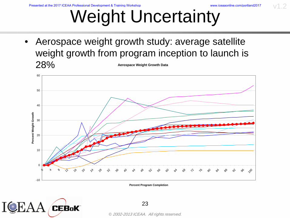
copy 2002-2013 ICEAA All rights reserved
v12
Weight Uncertaintybull Aerospace weight growth study average satellite
weight growth from program inception to launch is 28
23
Aerospace Weight Growth Data
-10
0
10
20
30
40
50
60
0 4 8 12 16 20 24 28 32 36 40 44 48 52 56 60 64 68 72 76 80 84 88 92 96 100
Percent Program Completion
Perc
ent W
eigh
t Gro
wth
Presented at the 2017 ICEAA Professional Development amp Training Workshop wwwiceaaonlinecomportland2017
copy 2002-2013 ICEAA All rights reserved
v12
Estimating Uncertaintybull CERs do not perfectly fit the historical data
ndash There are non-repeatable random effects that cannot be predicted
bull For examplendash Parts breaking during testingndash Strikes which are difficult to predict
bull This results in an underlying uncertainty distribution about an estimatendash The outcome of a CER represents only one point on an
uncertainty distributionbull Typically mean or median depending upon the CER
methodology
24
Presented at the 2017 ICEAA Professional Development amp Training Workshop wwwiceaaonlinecomportland2017
copy 2002-2013 ICEAA All rights reserved
v12
Estimating Uncertainty (2)
25
Presented at the 2017 ICEAA Professional Development amp Training Workshop wwwiceaaonlinecomportland2017
copy 2002-2013 ICEAA All rights reserved
v12
Estimating Uncertainty (3)bull In the case of a linear regression the estimating
uncertainty follows a normal distributionndash The estimate is the mean and the standard error of the
estimate from the regression is the standard deviation of the normal distribution
bull In the case of a log-transformed linear regression the estimating uncertainty follows a lognormal distributionndash The estimate is the median of the lognormal and the
standard error of the estimate from the regression is the standard deviation of the normal distribution (in log-space)
bull There is additional uncertainty about an estimate based upon the distance of what is being estimated from the mean of the input datandash This results in a prediction interval
26
Presented at the 2017 ICEAA Professional Development amp Training Workshop wwwiceaaonlinecomportland2017
copy 2002-2013 ICEAA All rights reserved
v12
Aggregating Riskbull Risk is typically applied at the same level at
which we estimate cost that is at the Work Breakdown Structure (WBS) level
bull The estimates for each WBS are developedndash These estimates sum to yield the total system cost
bull For an n-element WBS the total cost is the sum of the cost for each of the n elements
27
nXXXCostSystem +++= 21
Presented at the 2017 ICEAA Professional Development amp Training Workshop wwwiceaaonlinecomportland2017
copy 2002-2013 ICEAA All rights reserved
v12
WBS Examplebull Launch Vehicle
ndash Structurebull Vehicle Structurebull Tank Structure
ndash Thermal Controlbull Active Thermal Controlbull Induced Thermal Controlbull Tank Thermal Control
ndash Main Propulsion Systemndash Liquid Rocket Enginendash Electric Power and Distributionndash Command Control and Data Handlingndash System Integration
28
Presented at the 2017 ICEAA Professional Development amp Training Workshop wwwiceaaonlinecomportland2017
copy 2002-2013 ICEAA All rights reserved
v12
WBS and Risk
29
Presented at the 2017 ICEAA Professional Development amp Training Workshop wwwiceaaonlinecomportland2017
copy 2002-2013 ICEAA All rights reserved
v12
Aggregating Riskbull This leads us to the issue of aggregating the risks across the
WBSbull For example if we want to determine the 70th percentile of the
overall cost risk distribution how do we proceed bull Note that we cannot simply add the 70th percentiles of each of
the cost risk distributionsbull We can add means and variances (taking correlation into
account more on that later) but that is all
Variance of Total Cost =
30
Mean of Total Cost = ( )E X E Xk
k
n
kk
n
kk
n
= = =aringaelig
egraveccediloumloslashdivide
= =aring aring1 1 1
m
Var X kk
n
=aringaelig
egraveccediloumloslashdivide1
= s r s skk
n
iji
j
i jj
n2
1 1
1
22+aring aringaring
= =
-
=
Presented at the 2017 ICEAA Professional Development amp Training Workshop wwwiceaaonlinecomportland2017
copy 2002-2013 ICEAA All rights reserved
v12
Percentiles Do Not Addbull As a notional example consider two independent normal
distributionsndash One distribution has mean equal to 100 and standard deviation
equal to 20ndash The second distribution has mean 300 and standard deviation of 80
bull The sum of two independent normally distributed random variables is also normally distributed
bull To combine the two distributions we add the means and add the variancesndash Total mean is
ndash Total standard deviation is
31
400300100 =+
8258020 22 raquo+
Presented at the 2017 ICEAA Professional Development amp Training Workshop wwwiceaaonlinecomportland2017
copy 2002-2013 ICEAA All rights reserved
v12
Percentiles Do Not Add (2)bull The 80th percentiles for the individual distributions are
117 and 367 respbull The 80th percentile of the combined distribution is
469 but the sum of the two 80th percentiles is 484bull To see why this is the case note that the percentiles
of a normal distribution are determined by the mean and the standard deviationndash The standard deviations are not added when normal distributions
are combined rather the variances are combinedndash Sum of variances is ndash The standard deviation of this sum is
32
22 ba +22 ba +
Presented at the 2017 ICEAA Professional Development amp Training Workshop wwwiceaaonlinecomportland2017
copy 2002-2013 ICEAA All rights reserved
v12
Percentiles Do Not Add (3)bull Since bull We can write
bull The left side of this inequality represents the risk of the combined distributions while the right side represents the sums of the individual risks
bull Combining two missions that are independent results in a diversification of riskndash The total portfolio is not as risky on a relative basis as each
individual project
33
2222 2 bababa ++lt+
baba +lt+ 22
Presented at the 2017 ICEAA Professional Development amp Training Workshop wwwiceaaonlinecomportland2017
copy 2002-2013 ICEAA All rights reserved
v12
Methods for Aggregating Riskbull Since percentiles do not add we have to find other
ways to aggregate riskbull One method is to use Monte Carlo simulationbull Unless cost risk is represented by normal
distributions for all WBS elements summing the means and variances does not result in a completely accurate depiction of overall system cost risk
bull The normal distribution is not a realistic distribution for representing risk in many or even most situations since regarding project risk more can go wrong than can go right which means the risk is NOT symmetric unlike the Gaussian bell curve
34
Presented at the 2017 ICEAA Professional Development amp Training Workshop wwwiceaaonlinecomportland2017
copy 2002-2013 ICEAA All rights reserved
v12
Unit III - Module 9 35
Monte Carlo Simulationfor Risk Analysis
bull When risk analysis is performed multiple risks are gatheredndash These risks may have various probability
distributions
bull Monte Carlo is the most commonly accepted way to produce an accurate characterization of the distribution of the combined effect of these many risksndash Using this distribution we can produce percentiles
for cost impacts due to risk occurrences
10
Presented at the 2017 ICEAA Professional Development amp Training Workshop wwwiceaaonlinecomportland2017
copy 2002-2013 ICEAA All rights reserved
v12
Monte Carlo Simulationbull Simulation is a means for solving problems that are
analytically intractablendash Involves repeated random sampling
bull It was developed during the Manhattan Project as a way to model the interactions inside an atom during nuclear fissionndash Allowed for more sophisticated mathematical modeling of atomic
phenomena
bull Most computer packages use pseudo-random number generators that produce seemingly random results from an initial seedndash Example is the linear congruential generator
36
( ) mbaXX nn mod1 +=+
Presented at the 2017 ICEAA Professional Development amp Training Workshop wwwiceaaonlinecomportland2017
copy 2002-2013 ICEAA All rights reserved
v12Using Random Numbers to Simulate Distributions
bull WBS cost risk is typically measured by a probability distributionbull The most common method for simulating a probability
distribution is the inverse methodbull This involve obtaining a simulated random value from a uniform
distribution and then inverting this through the cumulative distribution function (CDF) to obtain the simulated value
bull As an example for a uniform distribution on the interval [0100]
bull In this case the CDF random value of 05 translates to 10005 = 50
37
( )100
1=xf ( )
100xxF = ( ) xxF 1001 =-
Presented at the 2017 ICEAA Professional Development amp Training Workshop wwwiceaaonlinecomportland2017
copy 2002-2013 ICEAA All rights reserved
v12
Simulating a Triangular Distribution
bull For a triangular distribution with low = 0 most likely = 50 and high = 150 the CDF is given by
bull The inverse function is given by
38
( )iumliumlicirc
iumliumliacute
igrave
poundlt--
poundpound=
1505021
1500050
50015000
2
2
2
xxx
xxxF
( )iumliumlicirc
iumliumliacute
igrave
poundltdivideoslashouml
ccedilegraveaelig +--
poundpound=-
131
21
37501
250017500150
3107500
1
xx
xxxF
Presented at the 2017 ICEAA Professional Development amp Training Workshop wwwiceaaonlinecomportland2017
copy 2002-2013 ICEAA All rights reserved
v12
Simulating a Triangular Distribution (2)
bull If the simulated uniform value is equal to 02 the corresponding inverse value from the CDF inverse is approximately 387
39
0
01
02
03
04
05
06
07
08
09
1
0 30 60 90 120 150
Presented at the 2017 ICEAA Professional Development amp Training Workshop wwwiceaaonlinecomportland2017
copy 2002-2013 ICEAA All rights reserved
v12
Monte Carlo and the WBSbull Simulation involves repeated trials
40
WBS Draw1 2 3 4 5
System 2912 3566 4390 2954 4655 Sum
Structure 80 105 55 80 57 SumVehicle Structure 50 70 30 40 20Tank Structure 30 35 25 40 37
Thermal Control 32 36 35 29 33 SumActive Thermal Control 10 15 12 7 10Induced Thermal Control 12 14 13 14 14Tank Thermal Control 10 7 10 8 9
Main Propulsion System 100 150 125 140 100
Liquid Rocket Engine 1000 1100 1800 900 2200
Electric Power and Distribution 100 125 150 75 90
Command Control and Data Handling 200 250 225 230 275
System Integration 1400 1800 2000 1500 1900
Presented at the 2017 ICEAA Professional Development amp Training Workshop wwwiceaaonlinecomportland2017
copy 2002-2013 ICEAA All rights reserved
v12
Number of Trialsbull Monte Carlo involves a repeated number of trialsbull The greater the number of trials the more accurate the
simulation will approximate the overall cost risk behavior of the system
bull After 100 trials the histogram looks very jagged
41
Presented at the 2017 ICEAA Professional Development amp Training Workshop wwwiceaaonlinecomportland2017
copy 2002-2013 ICEAA All rights reserved
v12
Number of Trials (2)
42
1000 Trials
10000 Trials
50000 Trials Additional trials give a more accurate depiction of the final result
Presented at the 2017 ICEAA Professional Development amp Training Workshop wwwiceaaonlinecomportland2017
copy 2002-2013 ICEAA All rights reserved
v12
Number of Trials (3)bull If we want to simulate the underlying
mean within 1 with 95 confidence for example then we require
43
divideoslash
oumlccedilegrave
aelig poundpound-
=
dividedividedivide
oslash
ouml
ccedilccedilccedil
egrave
aeligpound
-pound
-=
divideoslashouml
ccedilegraveaelig poundpound=
nZ
n
nnX
n
X
n
n
011
010Pr
011
010Pr
011990Pr950
___
___
sm
sm
sm
sm
sm
mm
Presented at the 2017 ICEAA Professional Development amp Training Workshop wwwiceaaonlinecomportland2017
copy 2002-2013 ICEAA All rights reserved
v12
Number of Trials (4)bull This means that the number of trials required is determined by
bull Solving for n we find that at least
trials are neededbull Note that this term involves the coefficient of variation of the
distribution which means that distributions with less dispersion require fewer trials to accurate simulate
44
96101
=ns
m
ms41638
Presented at the 2017 ICEAA Professional Development amp Training Workshop wwwiceaaonlinecomportland2017
copy 2002-2013 ICEAA All rights reserved
v12
Number of Trials (5)bull Simulating percentiles requires more trials than for simulating
meansbull Let Pn represent the number of trials in the sample at or below
the 70th percentile of the underlying distribution (suppose this is known)
bull By the Central Limit Theorem Pnn follows a normal distribution with mean equal to the 70th percentile and variance equal to
bull By a similar process for the mean we find that the number of trials needed to simulate the 70th percentile within 1 with 95 confidence is
45
( )n
FF 700700 1-
n
n
PPn -41638
Presented at the 2017 ICEAA Professional Development amp Training Workshop wwwiceaaonlinecomportland2017
copy 2002-2013 ICEAA All rights reserved
v12
Number of Trials (6)bull If Pn 070 for all n then n is approximately
bull For the sake of comparison suppose CV = 03 (reasonable approximation for hardware development) then the number of trials needed to simulate the mean with the same accuracy is then ldquoonlyrdquo 11525
bull More trials are needed to accurately simulate percentiles than means
46
( ) 46416703041638
70704168341638 =divide
oslashouml
ccedilegraveaelig=divide
oslashouml
ccedilegraveaelig -
=-
nnn
PPn
n
n
Presented at the 2017 ICEAA Professional Development amp Training Workshop wwwiceaaonlinecomportland2017
copy 2002-2013 ICEAA All rights reserved
v12
Methods of Simulationbull Monte Carlo simulation is a standard term for
simulationbull However there is an improvement on Monte Carlo
that improves the accuracy of the results of a simulation for a given number of trials
bull This method is call the Latin Hypercube approach to simulationndash Similar to Monte Carlo but an equal number of draws are taken
from a set of subintervals for example dividing the interval (01) into [00001) [0102)hellip [0910]
ndash Instead of 10 trials from [01] we have one trial from each subinterval
ndash Rough rule of thumb is Latin Hypercube takes 30 fewer trials to achieve similar accuracy to Monte Carlo
47
Presented at the 2017 ICEAA Professional Development amp Training Workshop wwwiceaaonlinecomportland2017
copy 2002-2013 ICEAA All rights reserved
v12
Probability Model ndash Correlationbull Correlation exists between work breakdown structure
(WBS) cost element costs and between cost and schedule
bull Correlation is a necessary consideration in cost risk analysis
bull Correlation is a number that can vary between -1 and +1 and represents the strength of the relationship between the two variablesndash If both variable have a tendency to move in the same direction
correlation is positivendash If when one variable increases the other tends to decrease and
vice-versa the correlation between the two variables is negative
Presented at the 2017 ICEAA Professional Development amp Training Workshop wwwiceaaonlinecomportland2017
copy 2002-2013 ICEAA All rights reserved
v12
Correlation And Causationbull Note that correlation is not causation however
causation implies correlationndash For example shark attacks and ice cream sales at the beach
bull For example for a launch vehicle structure increasing the diameter will not only result in an increase in the structures cost but will also result in higher costs for thermal coating (paint etc)
bull Also simply because two subsystems do not appear to be related does not mean they are not correlatedndash For example structures and computer equipment seemingly
have little relation to one another however an external factor such as a funding cut or a strike will impact all subsystems leading to delays and increasing cost across the board
ndash Thus everything in a WBS has some correlationUnit III - Module 9 49
Presented at the 2017 ICEAA Professional Development amp Training Workshop wwwiceaaonlinecomportland2017
copy 2002-2013 ICEAA All rights reserved
v12
The Importance of Correlationbull Percent that total cost standard deviation is underestimated
when correlation assumed to be 0 instead of r given nWBS elements
Unit III - Module 9 5050
0
20
40
60
80
100
0 01 02 03 04 05 06 07 08 09 1Actual Correlation
Perce
nt Un
deres
timate
d
n = 10
n = 30
n = 100n = 1000
0
20
40
60
80
100
0 01 02 03 04 05 06 07 08 09 1Actual Correlation
Perce
nt Un
deres
timate
d
n = 10
n = 30
n = 100n = 1000
Reference 32nd Annual DOD Cost Analysis Symposium Advanced Training Session ldquoWhy Correlation Matters in Cost Estimatingrdquo Stephen A Book
Presented at the 2017 ICEAA Professional Development amp Training Workshop wwwiceaaonlinecomportland2017
copy 2002-2013 ICEAA All rights reserved
v12
The Importance of Correlation (2)bull For example if correlation is assumed to be 0 for all
elements in a 30 element WBS and the actual correlation is 20 then the total cost standard deviation is underestimated by 60
bull For example assume the total cost is modeled as a normal distribution with mean = 100
bull If correlation is assumed to be zero with total cost standard deviation = 12 when correlation is actually 20 then the true underlying standard deviation is actually 30
bull 70th percentile with zero correlation assumption is 106
bull 70th percentile with 20 correlation is 116 Unit III - Module 9 51
Presented at the 2017 ICEAA Professional Development amp Training Workshop wwwiceaaonlinecomportland2017
copy 2002-2013 ICEAA All rights reserved
v12
Measures of Correlationbull Two measures of correlation are commonly used in
cost risk analysesndash Pearsonrsquos product-moment correlation coefficient ndash Spearmanrsquos rank correlation coefficient
bull Garvey and others recommend using Pearsonrsquos product-moment correlation coefficient correlation for cost risk analysesndash Method of moments uses this but there are two options in
simulationndash Popular simulation packages like Risk and Crystal Ball use
rank correlation but in practice this has been found to make little difference
ndash Pearson product-moment correlation has been incorporated into Risk+
52
Presented at the 2017 ICEAA Professional Development amp Training Workshop wwwiceaaonlinecomportland2017
copy 2002-2013 ICEAA All rights reserved
v12
Pearson Correlationbull Pearsonrsquos product-moment correlation measures
degree of linearity between two random variables bull If two random variables are perfectly linear (eg Y =
aX + b) with positive slope then the Pearson product-moment correlation between X and Y denoted by rXY is +1
53
X X
Y Y Y
XNegative Correlation Positive Correlation No Correlation
middotmiddot
middotmiddot
middotmiddot middotmiddot
middotmiddot
middot
middot
middotmiddotmiddot
middotmiddot
middotmiddot
middotmiddot middot
middot
middot
middotmiddotmiddotmiddotmiddotmiddotmiddotmiddot
middotmiddotmiddotmiddot
middotmiddot
middotmiddot middotmiddotmiddotmiddot
middotmiddotmiddot
middotmiddotmiddotmiddot
middotmiddotmiddot
middotmiddotmiddot
middotmiddot
middot
middot middotmiddot
middot middotmiddotmiddotmiddot middotmiddot middot middotmiddot middot middot
middotmiddot middot
middotmiddotmiddotmiddotmiddot middot middotmiddot
middotmiddot
middot
middotmiddot
middotmiddot middot
middot middot middot
middotmiddot middot
middotmiddotmiddot
middotmiddot
middot middot
Presented at the 2017 ICEAA Professional Development amp Training Workshop wwwiceaaonlinecomportland2017
copy 2002-2013 ICEAA All rights reserved
v12
Spearman Correlationbull Spearmanrsquos rank correlation measures the
monotonicity between two random variablesbull If two random variables are perfectly monotonically
increasing (eg Y = X2) then the Spearman rank correlation denoted by rXY is +1
bull The two measures can be significantly different
54
10 20 30 40 50 60
100
200
300
096 097 098 099 1
1
060
020
040
080
Eff
ort (
Staf
f-M
onth
s)
Software Size I KDSI
y = 28z12y
z x
yy = x100
0 pound x pound 1
Figure 5-9A Figure 5-9B
Pearson Correlation = 09976 Rank Correlation = 1
Pearson Correlation = 024 Rank Correlation = 1
X(x ) ~ Unif(01)
Reference Probability Methods for Cost Uncertainty Analysis A Systems Engineering Perspective Paul R Garvey
Presented at the 2017 ICEAA Professional Development amp Training Workshop wwwiceaaonlinecomportland2017
copy 2002-2013 ICEAA All rights reserved
v12
Unit III - Module 9 55
200
250
300
350
400
1000 1200 1400 1600 1800 2000
Recurring Production
SEPM
200
250
300
350
400
1000 1200 1400 1600 1800 2000
Recurring Production
SEPM
Functional Correlationbull Old No Functional
Correlation Simulation run with WBS items entered as values
bull New Simulation run with functional dependencies entered as they are in cost model
CorrelatedNot Correlated
Note shift of mean and increased variability
Presented at the 2017 ICEAA Professional Development amp Training Workshop wwwiceaaonlinecomportland2017
copy 2002-2013 ICEAA All rights reserved
v12
Risk Measuresbull ldquoWestern Europe conquered the word because of a
technological revolution that started because of attempts to measure the worldrdquo ndash Phillipe Jorion ndash In the same way attempts to measure risk will lead to better project
managementbull Risk management for DoD and NASA agencies focuses
primarily on funding projects to a single percentile ndash NASA policy explicitly mentions 70 and 50ndash This is known as ldquoValue at Riskrdquo and is prevalent in the banking and
financial industry
56
Presented at the 2017 ICEAA Professional Development amp Training Workshop wwwiceaaonlinecomportland2017
copy 2002-2013 ICEAA All rights reserved
v12
Value at Risk (VaR)bull VaR is a percentile of the cost risk
distributionndash VaR funding at the 70th percentile means that
there is a 30 chance of final project cost exceeding the funded amount (budget)
bull VaR has some meritsndash Common measure can be used to compare
different projects and programsndash Easily understood by senior managers and
decision makers
57
Presented at the 2017 ICEAA Professional Development amp Training Workshop wwwiceaaonlinecomportland2017
copy 2002-2013 ICEAA All rights reserved
v12
Why 70th or 80th Percentilebull Typical policy guidance involves funding at the 70th or 80th
percentile Why fund as such a low percentilebull There is some incentive to not over-fundbull For a normal distribution an inflection point occurs near the 80th
percentile meaning that for values above 80 confidence achieving higher levels of confidence can only be achieved by spending greater dollar amounts at an increasing rate
58
-05-04-03-02-01
00102030405
0 05 1 15 2 25 3
Standard Deviations from Mean
Normal Distribution
First DerivativeSlopeVelocity
Second DerivativeConvexityAcceleration
Inflection point at one standard deviation above the mean (~84th
percentile)
Presented at the 2017 ICEAA Professional Development amp Training Workshop wwwiceaaonlinecomportland2017
copy 2002-2013 ICEAA All rights reserved
v12
Funding Above Inflection Pointsbull As the percentile goes above the 80th percentile the amount
needed to achieve that higher level of confidence begins to increase at an increasing rate as is evident from the graph
59
0
10
20
30
40
50
60
70
50 55 60 65 70 75 80 85 90 95 100
$ Ab
ove
MEa
n to
Ach
ieve
Per
cent
ile
Percentile (Confidence Level)
Presented at the 2017 ICEAA Professional Development amp Training Workshop wwwiceaaonlinecomportland2017
copy 2002-2013 ICEAA All rights reserved
v12
Why Budget to the 70th or 80thbull Government projects are funded at the 70th or 80th percentilesbull Why not the 90th or 99th percentile Wonrsquot that help prevent
overrunsndash As we have seen percentiles do not add across programs
bull The sum of the 80th percentiles does NOT equal the total 80th percentile
ndash This is because the individual programs are riskier than the entire suite of missions
bull Known as the ldquoPortfolio effectrdquo (more or this later)
ndash Funding at the 80th gives confidence that the entire portfolio will be adequately funded
bull And since there is an inflection point near the 80th percentile funding above that level quickly becomes cost prohibitive
60
Presented at the 2017 ICEAA Professional Development amp Training Workshop wwwiceaaonlinecomportland2017
copy 2002-2013 ICEAA All rights reserved
v12
Inflection Points for Lognormalbull For a lognormal the inflection point
variesndash Coefficient of variation equal to 10 equates to an
inflection point at the 70th percentile
61
0
10
20
30
40
50
60
70
050 060 070 080 090 100
Coef
ficen
t of V
aria
tion
Percentile of the Inflection Point
Presented at the 2017 ICEAA Professional Development amp Training Workshop wwwiceaaonlinecomportland2017
copy 2002-2013 ICEAA All rights reserved
v12
Issues with Percentile Fundingbull However risk management does not stop at a
specific percentilendash What happens when the 70th percentile is exceeded
bull Any effective risk management policy should prescribe what happens after a bad event occursndash With VaR we only know when a bad event has occurred ndash Also funding at a relatively low level means we have no true
sense of the real risks that should be guarded against
62
Presented at the 2017 ICEAA Professional Development amp Training Workshop wwwiceaaonlinecomportland2017
copy 2002-2013 ICEAA All rights reserved
v12
ldquoHere There Be Dragonsrdquobull On old maps uncharted territory was often
marked with monsters or dragons
63
A section of the Carta Marina by Olaus Magnus 16th Century
Presented at the 2017 ICEAA Professional Development amp Training Workshop wwwiceaaonlinecomportland2017
copy 2002-2013 ICEAA All rights reserved
v12
Distribution Comparisonbull Four different distributions with the same 70th
percentile
bull Should we expect the tails to be similar
64
0
10
20
30
40
50
60
70
80
0 100 200 300 400 500 600
Perc
entil
eCo
nfid
ence
Lev
el
Triangular
Normal
Lognormal
Pareto
Presented at the 2017 ICEAA Professional Development amp Training Workshop wwwiceaaonlinecomportland2017
copy 2002-2013 ICEAA All rights reserved
v12Distribution Comparison Tail Behavior
bull The normal and triangular distributions have similar tails but the lognormal and Pareto have much fatter right tails
65
70
75
80
85
90
95
100
500 1500 2500 3500 4500 5500
Perc
entil
eCo
nfid
ence
Lev
el
Triangular
Normal
Lognormal
Pareto
Here There Be Dragons
Presented at the 2017 ICEAA Professional Development amp Training Workshop wwwiceaaonlinecomportland2017
copy 2002-2013 ICEAA All rights reserved
v12Distribution Comparison ndash Tail Behavior (Table)
bull There is significant tail risk for the lognormal and the Paretobull The 99th percentile for the Pareto is 1000 times greater than
the 70th percentilendash Risk seen in financial markets and in catastrophic risks like natural
disasters bull Four different projects follow the four different risk profiles seen
in this example should clearly have different risk management approaches but 70th percentile funding indicates the same risk management approach for all four
66
Percentile Triangular Normal Lognormal Pareto 70th $600 $600 $600 $600 80th $680 $660 $770 $1430 90th $770 $750 $1070 $5880 95th $840 $820 $1410 $23750 99th $930 $950 $2350 $600000
Presented at the 2017 ICEAA Professional Development amp Training Workshop wwwiceaaonlinecomportland2017
copy 2002-2013 ICEAA All rights reserved
v12Percentile Budgeting is Not Risk Management
bull Percentile budgeting ne effective risk management policybull Suppose that you are shopping for a new car You
mention that safety is your top concern The salesman says he has a great safe car available You ask about the air bags Do they work The salesman answers ldquoOf course Seventy percent of the time they work fine Only 30 of the time the air bags will fail to deployrdquo Would you buy such a car Hedge fund manager David Einhorn has stated ldquoRisk management is the air bag that must always work but only in the multi-sigma event where you have an accidentrdquo
67
Risk management is the air bag that must always work but only in the multi-sigma event where you
have an accident
Presented at the 2017 ICEAA Professional Development amp Training Workshop wwwiceaaonlinecomportland2017
copy 2002-2013 ICEAA All rights reserved
v12
Joint Confidence Level Analysisbull Schedules are risky toobull For 98 recent NASA missions average
schedule growth was 38ndash Not as high as cost growth but still significant
68
0
5
10
15
20
25
30
35
40
Schedule
Cost
Presented at the 2017 ICEAA Professional Development amp Training Workshop wwwiceaaonlinecomportland2017
copy 2002-2013 ICEAA All rights reserved
v12
Schedules Impact Costbull Changes in schedule can have enormous
impacts on cost ndash Schedule slips can lead to cost increases
bull Fixed programmatic costs must be paid on a regular basisndash Achieving schedule milestones early can result in cost
savings
bull Schedule is an important consideration in cost analysis including cost risk analysis
bull However we must be careful in correctly integrating cost and schedule riskndash Schedule is not simply an input but is dependent on many of
the same factors that drive cost
69
Presented at the 2017 ICEAA Professional Development amp Training Workshop wwwiceaaonlinecomportland2017
copy 2002-2013 ICEAA All rights reserved
v12
The Relationship of Cost to Schedulebull Cost and schedule are positively correlated
ndash A larger program with bigger scope with take longer to complete than a smaller simpler program
bull However longer schedules do not always equate to higher cost nor shorter schedules with lower costndash Highly compressed schedules relative to the
optimal schedule can lead to large overrunsbull Compressed schedules are commonplace for
many planetary missions
70
Presented at the 2017 ICEAA Professional Development amp Training Workshop wwwiceaaonlinecomportland2017
copy 2002-2013 ICEAA All rights reserved
v12The Impact of Schedule GrowthCompression on Cost
bull Compressed schedules lead to cost growth and based on existing research is actually more expensive than schedule slippages
71
0
20
40
60
80
100
120
140
160
-50 -25 0 25 50 75 100
Percentage Change in Schedule
Perc
enta
ge C
hang
e in
Cos
t due
to
Sche
dule
Cha
nge
Source Smart CB ldquoCost and Schedule Interrelationshipsrdquo 2007 NASA Cost Symposium
Presented at the 2017 ICEAA Professional Development amp Training Workshop wwwiceaaonlinecomportland2017
copy 2002-2013 ICEAA All rights reserved
v12Schedule as an Independent Variable
bull Why not simply add schedule as an input to cost-estimating relationships (CERs)
bull Schedule is often treated as an independent variable ndash schedules are often determined independently of cost considerationsndash Cost may not be considered explicitly although budgets and
schedules are determined based on scope and other common factors
bull In 2006 SAIC undertook a research task to determine the impact of schedule on cost and added schedule as an independent variable to the CERs in the NASAAir Force Cost Model (NAFCOM) to see if schedule provided any improvement in goodness of fit
72
Presented at the 2017 ICEAA Professional Development amp Training Workshop wwwiceaaonlinecomportland2017
copy 2002-2013 ICEAA All rights reserved
v12
Schedule is a Dependent Variablebull Since NAFCOM includes an exhaustive list of cost drivers the inclusion
of schedule should give an indication of whether there is any additional independent value added from schedule independent of the cost drivers
bull In the study schedule was added to 10 subsystem-level CERs
ndash In each case the addition of schedule did NOTimprove the goodness of fit and schedule was NOT found to be a statistically significant cost driver (given the presence of the other variables) for any of the 10 CERs
bull Standard errors for the CERs increased due to decrease in degrees of freedom
bull Thus schedule as an independent variable did not provide any additional explanation of variation in historical cost
bull This is because schedule is truly NOT an independent variable but a dependent variable and is a function of the same factors that drive cost
73
Presented at the 2017 ICEAA Professional Development amp Training Workshop wwwiceaaonlinecomportland2017
copy 2002-2013 ICEAA All rights reserved
v12
Incorporation of Schedule in Cost Risk
bull When using subjective methods care must be taken in applying schedule to cost risk analysis
bull Since schedule is a dependent variable treating it independently from other factors when assessing its impact on cost can lead to a double count of independent variables in the cost risk analysis
bull Direct inclusion of schedule in a cost risk analysis effectively doubles the influence of each cost driver
ndash Incorrectly leads to broader risk ranges
74
CostWeight
HeritageNewness
Technology Readiness Schedule
Presented at the 2017 ICEAA Professional Development amp Training Workshop wwwiceaaonlinecomportland2017
copy 2002-2013 ICEAA All rights reserved
v12Subjective Cost Risk Methods and Overinclusion of Risk Factors
bull Subjective methods are suitable when data are scarce or not availablebull However care must be taken not to treat correlated sources of risk
such as schedule as independent of each otherbull Example ndash a subjective risk analysis incorporated technology readiness
design risk requirements stability integration risk and schedule and treated each source of risk as independent
bull Risk triangle high value without schedule risk was 31 times the point estimate
bull Risk triangle high value with schedule risk added on top of other sources of risk treated independently was 34 times the point estimate
bull Risk triangle taking correlation between sources of risk into account in a rigorous statistical manner has a high value 15 times the point estimate less than half the effect when treating sources of risk as independent
75
Presented at the 2017 ICEAA Professional Development amp Training Workshop wwwiceaaonlinecomportland2017
copy 2002-2013 ICEAA All rights reserved
v12Fundamental Equation of Cost and Schedule Interrelationships
bull The Fundamental Equation of the Relationship Between Cost and Schedule is
Time = Moneybull This is a well known adage that time is money Your boss at
work may even mention this to you from time to time or if you are the boss you are all too aware of this iron law
bull Because time is money cost and schedule risk should be modeled jointly not with schedule as an independent cost driver
bull Note that cost and schedule are not perfectly correlatedndash Cost can sometimes ldquobuy downrdquo schedule extra money can be
spent to meet a deadline since in some cases additional effort to hasten the completion of a task
76
Presented at the 2017 ICEAA Professional Development amp Training Workshop wwwiceaaonlinecomportland2017
copy 2002-2013 ICEAA All rights reserved
v12How to (Correctly) Incorporate Schedule into Cost Risk Analysis
bull The best way to model cost and schedule risk is to develop a joint cost and schedule model based on the same data
bull Since such models are not currently available the next best approach is to model cost and schedule independently and then integrate cost and schedule risk analyses using joint probability distributions taking into account correlation between cost and schedulendash This approach pioneered by Paul Garvey and Steve Book is
considered industry best practicendash This is a practical method mathematically tractable and follows
naturally from the Fundamental Equation of Cost and Schedule Interrelationships
77
Book S A ldquoQuantifying the Relationship Between Cost and Schedulerdquo The Measurable News Winter 2007-2008 pp 11-15Garvey PR Probability Methods for Cost Uncertainty Analysis A Systems Engineering Perspective New York Marcel Dekker 2000 pp 308-335
Presented at the 2017 ICEAA Professional Development amp Training Workshop wwwiceaaonlinecomportland2017
copy 2002-2013 ICEAA All rights reserved
v12
Joint Lognormal and Normal Distributions
bull Cost and schedule are typically modeled as some combination of Normal and Lognormal probability distributionsndash Studies by The Aerospace Corporation the MITRE
Corporation Wyle Labs and SAIC have found that the Lognormal probability distribution almost always serves as a good model for both the schedule distribution and the cost distribution
ndash The Normal distribution may also be appropriate in some instances and depending upon the level of confidence at which budgets are set may even be more conservative and logically consistent than the Normal distribution
ndash Joint Lognormal and Normal distributions are defined by a pair of mean and standard deviations and a level of correlation between the two
78
Presented at the 2017 ICEAA Professional Development amp Training Workshop wwwiceaaonlinecomportland2017
copy 2002-2013 ICEAA All rights reserved
v12Modeling Cost and Schedule as a Bivariate Distribution
bull In the approach set forth by Book and Garvey cost risk is assessed and the top-level distribution is modeled as a Lognormal (or Normal) distribution schedule risk is assessed and the overall schedule risk is modeled as a Lognormal (or Normal) distribution
bull The two distributions are combined into a Bivariate distribution by assigning a correlation between the two and by treating the two distributions as the marginal distributions of a Bivariate Lognormal distributionndash Other combinations include a Bivariate Normal or a Bivariate
Normal-Lognormal
79
Presented at the 2017 ICEAA Professional Development amp Training Workshop wwwiceaaonlinecomportland2017
copy 2002-2013 ICEAA All rights reserved
v12Bivariate Lognormal Distribution for Cost and Schedule
bull Cost is often observed to be Lognormal when strong positive correlations are present among the systemrsquos WBS cost element costs
bull A systemrsquos schedule is often observed (from Monte Carlo simulations) to be Lognormal if it is the sum of many positively correlated schedule activities in an overall schedule network
bull If Lognormal distributions characterize a systemrsquos cost and schedule then the Bivariate Lognormal could serve as an assumed model of their joint distributionndash In this case the marginal distribution of each of cost and schedule is
Lognormalbull Other possibilities for modeling cost and schedule as a Bivariate
distribution include a Bivariate Normal or a Bivariate Normal-Lognormal distributionndash All these combinations are analytically tractable
80
Presented at the 2017 ICEAA Professional Development amp Training Workshop wwwiceaaonlinecomportland2017
copy 2002-2013 ICEAA All rights reserved
v12Bivariate Lognormal for Cost and Schedule
bull Contour Plots of a Bivariate Lognormal
81
Presented at the 2017 ICEAA Professional Development amp Training Workshop wwwiceaaonlinecomportland2017
copy 2002-2013 ICEAA All rights reserved
v12Correlation Between Cost and Schedule
bull Cost and schedule are positively correlated but not perfectly sondash For example it is possible to have a schedule underrun and a cost
overrunbull Based on cost and schedule growth data for 50 completed NASA
programs the correlation between development cost and development schedule is 70
82
00
200
400
600
800
1000
1200
-500 00 500 1000 1500 2000 2500Historical Cost Growth
Hist
oric
al S
ched
ule
Gro
wth
r = 715
Presented at the 2017 ICEAA Professional Development amp Training Workshop wwwiceaaonlinecomportland2017
copy 2002-2013 ICEAA All rights reserved
v12Correlation Between Cost and Schedule Caveats
bull Based on historical data recommended correlation between cost and schedule is 70 but this could be higher or lower depending upon program circumstancesndash If program is budget constrained cost and schedule will be
more highly correlated (go as you pay)ndash If program is schedule constrained cost and schedule will
have lower correlation perhaps even negative correlation ndash Smaller programs have smaller correlation between cost and
schedule riskbull Relatively easy to ldquohurry uprdquo and finish on time or even early if
needed
83
Presented at the 2017 ICEAA Professional Development amp Training Workshop wwwiceaaonlinecomportland2017
copy 2002-2013 ICEAA All rights reserved
v12
Conditional Confidence Levelsbull Given a programrsquos project schedule we can determine the cost
risk distribution conditional upon the given schedulebull Conditional cost S-curves are steeper than unconditional
(marginal) cost S-curves between some uncertainty has been removed because schedule is fixed
84
Presented at the 2017 ICEAA Professional Development amp Training Workshop wwwiceaaonlinecomportland2017
copy 2002-2013 ICEAA All rights reserved
v12
Joint Confidence Levelsbull Joint 65 confidence represents the probability of
achieving both 65 confidence in cost AND 65 confidence in schedulendash This is different than achieving 65 cost confidence alone
or achieving 65 schedule confidence alonebull Due to the imperfect correlation between cost and schedule it
is possible to achieve a 65 cost confidence with a lower level of schedule confidence
bull Restricting the schedule confidence thus requires additional $ to achieve a given level of confidence
85
X
Y
Possible Values for Which X gt a Possible Values for
Which X gt a and Y gt b
a
b
Presented at the 2017 ICEAA Professional Development amp Training Workshop wwwiceaaonlinecomportland2017
copy 2002-2013 ICEAA All rights reserved
v12Joint Confidence Levels Versus Cost Confidence Levels Only
bull Example of the differences between cost confidence schedule confidence conditional cost confidence and joint cost and schedule confidence
86
Joint Cost-Schedule Confidence Iso-Curves
Cost (RY$M)
Sche
dule
(Mon
ths)
65 Confidence
50 Confidence
70 Confidence
65 Cost Confidence AggressiveSchedule65 Cost ConfidenceScheduleGiven 65 Schedule ConfidenceUnconditional 65 CostConfidenceUnconditional 65 ScheduleConfidence
65 Cost Confidence 65 Joint Cost and Schedule
Confidence for 65 Schedule Confidence
Presented at the 2017 ICEAA Professional Development amp Training Workshop wwwiceaaonlinecomportland2017
copy 2002-2013 ICEAA All rights reserved
v12
Joint Cost and Schedule Confidence
bull Can examine pairs of cost and schedule that achieve a given level of confidence
bull Provides insights into the trade-offs between cost and schedule for a given level of confidencendash Possible to increase cost confidence by giving a
project more time in some instances or possible to ldquobuy downrdquo schedule
bull But these have limits and are shown in the iso-cost and schedule confidence curves
87
Presented at the 2017 ICEAA Professional Development amp Training Workshop wwwiceaaonlinecomportland2017
copy 2002-2013 ICEAA All rights reserved
v12Cost and Schedule Trade-offs for a Given Level of Joint Confidence
bull Hypothetical Example
88
Cost (RY$M)
Schedule (Months)
$100 48$99 48$89 49$87 50$85 51$85 52$84 53$83 55$83 55$83 56
Cost and Schedule 65 Confidence Iso-Curve
4748495051525354555657
$80 $82 $84 $86 $88 $90 $92 $94 $96 $98 $100
Cost (RY$ M)
Sche
dule
(Mon
ths)
Presented at the 2017 ICEAA Professional Development amp Training Workshop wwwiceaaonlinecomportland2017
copy 2002-2013 ICEAA All rights reserved
v12Policy Considerations for Confidence Levels
bull For large programs the difference between the amount of money needed to achieve 65 cost confidence independent of schedule and joint 65 cost and schedule confidence can represent hundreds of millions and even billions of dollars
89
Joint Cost-Schedule Confidence Iso-Curves
Cost (RY$M)
Sche
dule
(Mon
ths)
65 Confidence
65 Cost Confidence AggressiveSchedule
65 Cost ConfidenceScheduleGiven 65 Schedule Confidence
Unconditional 65 CostConfidence
Joint Cost and Schedule Confidence for 65 Cost Confidence and Program Baseline Schedule is Less Than 35
65 Cost Confidence Independent of Schedule Cost Needed to Achieve
Both 65 Joint Cost and Schedule Confidence for the Schedule with 65 Confidence
Presented at the 2017 ICEAA Professional Development amp Training Workshop wwwiceaaonlinecomportland2017
copy 2002-2013 ICEAA All rights reserved
v12
Copulasbull More generally any combination of distributions can
be used (more than just normal and lognormal)ndash Termed ldquocopulardquo from the Italian word for ldquocouplerdquondash Copulas are a way to combine marginal distributions of any
number and type into a joint distributionbull More formally a copula is a multivariate joint distribution defined
on the n-dimensional unit cube [0 1]n such that every marginal distribution is uniform on the interval [0 1]
bull (The bivariate form of) Sklarrsquos theorem states that for any bivariate distribution function H(x y) let F(x) = H(x infin) and G(y) = H(infin y) be the univariate marginal probability distribution functions Then there exists a copula C such that H(xy)=C(F(x)G(y))
ndash Copulas are widely used in risk management for investments and insurance
bull Considered industry best practice (Li 2000)bull Marketed as part of JP Morganrsquos CreditMetrics suite of tools
(Gupton et Al 1997)90
Presented at the 2017 ICEAA Professional Development amp Training Workshop wwwiceaaonlinecomportland2017
copy 2002-2013 ICEAA All rights reserved
v12Parametric Joint Cost and Schedule Analysis
bull A parametric model based on a consistent data set with a set of overlapping cost and schedule drivers is a cleaner way to model cost and schedule
91
CostWeight
HeritageNewness
Technology Readiness
Schedule
0
20
40
60
80
100
Confidence
Joint Cost and Schedule Confidence
Schedule
Cost
Lognormal Distribution PDF and CDF
0102030405060708090100
200 300 400 500 600 700 800 900 1000Cost $
Con
fiden
ce L
evel
0
00002
00004
00006
00008
0001
00012
00014
00016
Prob
abili
ty D
ensi
ty
CDFPDF
Lognormal Distribution PDF and CDF
0102030405060708090100
200 300 400 500 600 700 800 900 1000Cost $
Con
fiden
ce L
evel
0
00002
00004
00006
00008
0001
00012
00014
00016
Prob
abili
ty D
ensi
ty
CDFPDF
Presented at the 2017 ICEAA Professional Development amp Training Workshop wwwiceaaonlinecomportland2017
copy 2002-2013 ICEAA All rights reserved
v12Parametric Joint Cost and Schedule Analysis (2)
bull Joint cost and schedule risk analysis produced naturally by the integrated modelndash Addresses several issues with the copula
approachbull Tail dependencybull Correlation ndash no need to assign correlation
between cost and schedulebull Consistency of cost and schedule models
92
Presented at the 2017 ICEAA Professional Development amp Training Workshop wwwiceaaonlinecomportland2017
copy 2002-2013 ICEAA All rights reserved
v12
Resource-Loaded Schedulesbull Involves assigning cost and schedule risks to a resource-loaded schedule
networkbull Bottom-up approach
ndash More labor intensive than parametrics but can also provide more insight
ndash Can answer questions than parametric typically cannot such as how much do reserve requirements decrease if a specific risk is retired
bull Currently being implemented in Constellation programbull Has same issue as all bottom-up models hard to count all the risks and model
them discretely
ndash As a result there is a tendency to reflect less risk than indicated by history
ndash ldquoThere are more things in heaven and earth Horatio than are dreamt of in your philosophyrdquo William Shakespeare Hamlet Act I Scene V
93
Presented at the 2017 ICEAA Professional Development amp Training Workshop wwwiceaaonlinecomportland2017
copy 2002-2013 ICEAA All rights reserved
v12Resource-Loaded Schedules Vs Parametrics
bull Parametric most appropriate for early estimatesndash But also good for high-level checks as project progresses
bull As plans take shape lower level modeling may be more appropriate
94 1
CONCEPTUALDEVELOPMENT
PROJECTDEFINITION DESIGN DEVELOPMENT OPERATIONS
PARAMETRIC PARAMETRIC
ANALOGY
ENGINEERING (Bottoms Up)
$PARAMETRIC
DETAILED
$
Pre Phase A Phase B Phase CDPhase A Phase EPre Phase A Phase B Phase CDPhase A Phase E
Risk = f(Cost Estimating Relationship Inputs eg mass power data rate TRL new design etc)
Risk = f(cost and schedule variation of the analogous elements)
Risk = f(variation of detailed inputs eg labor hours rates materials etc)
Presented at the 2017 ICEAA Professional Development amp Training Workshop wwwiceaaonlinecomportland2017
copy 2002-2013 ICEAA All rights reserved
v12
Resource-Loaded Schedulesbull Methodology has been demonstrated in other
industriesndash Construction oil and gasndash Analysis has not been traditionally done on highly uncertain
complex development projects bull Methodology focuses on project baseline schedule
ndash In baseline schedule all tasks are resource loaded to represent a baseline schedule and cost standpoint
ndash Resource loaded schedule is ldquorolledrdquo up to a manageable level
ndash Based on the risk and uncertainties identified schedule distributions are applied to each rolled up task
ndash Cost uncertainties are also applied to rolled up tasksbull Uncertainties include labor rate man power etc
ndash A Monte Carlo simulation is run to develop joint cost-schedule distributions
95
Presented at the 2017 ICEAA Professional Development amp Training Workshop wwwiceaaonlinecomportland2017
copy 2002-2013 ICEAA All rights reserved
v12
Unit III - Module 9 96
Execution ndash Cross Checksbull Means The mean cost growth factor for WBS items
can be compared to history as a way to cross check results
bull CVs The CV of the cost growth factors for WBS items can be compared to history as a way to cross check results
bull Inputs Checks are performed on inputs or other parameters to see if historical values are in line with program assumptionsndash Example Historical risk scores can be compared to program
risk scores to see if risk assessors are being realistic and to see if the underlying database is representative of the program
11
Presented at the 2017 ICEAA Professional Development amp Training Workshop wwwiceaaonlinecomportland2017
- Cost and Schedule Risk Analysis Basic
- Acknowledgments
- Unit Index
- Risk Overview
- Agenda
- Introduction
- Risk Analysis Terms
- Are Our Costs Realistic
- Historical Cost Growth
- Sources of Cost Risk
- Point Estimates of Cost
- Types of Risk
- Point Estimates Vs Risk Estimates
- Cost Risk and Probability
- Probability Model ndash Distribution
- Probability Model ndash Distribution
- Probability ndash Top-Level Distribution
- S-Curves and Confidence Levels
- Example ndash Normal Distribution
- Confidence Levels
- Measuring Parametric Model Uncertainty
- Parametric Model Example
- Weight Uncertainty
- Estimating Uncertainty
- Estimating Uncertainty (2)
- Estimating Uncertainty (3)
- Aggregating Risk
- WBS Example
- WBS and Risk
- Aggregating Risk
- Percentiles Do Not Add
- Percentiles Do Not Add (2)
- Percentiles Do Not Add (3)
- Methods for Aggregating Risk
- Monte Carlo Simulationfor Risk Analysis
- Monte Carlo Simulation
- Using Random Numbers to Simulate Distributions
- Simulating a Triangular Distribution
- Simulating a Triangular Distribution (2)
- Monte Carlo and the WBS
- Number of Trials
- Number of Trials (2)
- Number of Trials (3)
- Number of Trials (4)
- Number of Trials (5)
- Number of Trials (6)
- Methods of Simulation
- Probability Model ndash Correlation
- Correlation And Causation
- The Importance of Correlation
- The Importance of Correlation (2)
- Measures of Correlation
- Pearson Correlation
- Spearman Correlation
- Functional Correlation
- Risk Measures
- Value at Risk (VaR)
- Why 70th or 80th Percentile
- Funding Above Inflection Points
- Why Budget to the 70th or 80th
- Inflection Points for Lognormal
- Issues with Percentile Funding
- ldquoHere There Be Dragonsrdquo
- Distribution Comparison
- Distribution Comparison Tail Behavior
- Distribution Comparison ndash Tail Behavior (Table)
- Percentile Budgeting is Not Risk Management
- Joint Confidence Level Analysis
- Schedules Impact Cost
- The Relationship of Cost to Schedule
- The Impact of Schedule GrowthCompression on Cost
- Schedule as an Independent Variable
- Schedule is a Dependent Variable
- Incorporation of Schedule in Cost Risk
- Subjective Cost Risk Methods and Overinclusion of Risk Factors
- Fundamental Equation of Cost and Schedule Interrelationships
- How to (Correctly) Incorporate Schedule into Cost Risk Analysis
- Joint Lognormal and Normal Distributions
- Modeling Cost and Schedule as a Bivariate Distribution
- Bivariate Lognormal Distribution for Cost and Schedule
- Bivariate Lognormal for Cost and Schedule
- Correlation Between Cost and Schedule
- Correlation Between Cost and Schedule Caveats
- Conditional Confidence Levels
- Joint Confidence Levels
- Joint Confidence Levels Versus Cost Confidence Levels Only
- Joint Cost and Schedule Confidence
- Cost and Schedule Trade-offs for a Given Level of Joint Confidence
- Policy Considerations for Confidence Levels
- Copulas
- Parametric Joint Cost and Schedule Analysis
- Parametric Joint Cost and Schedule Analysis (2)
- Resource-Loaded Schedules
- Resource-Loaded Schedules Vs Parametrics
- Resource-Loaded Schedules
- Execution ndash Cross Checks
-
copy 2002-2013 ICEAA All rights reserved
v12
Estimating Uncertaintybull CERs do not perfectly fit the historical data
ndash There are non-repeatable random effects that cannot be predicted
bull For examplendash Parts breaking during testingndash Strikes which are difficult to predict
bull This results in an underlying uncertainty distribution about an estimatendash The outcome of a CER represents only one point on an
uncertainty distributionbull Typically mean or median depending upon the CER
methodology
24
Presented at the 2017 ICEAA Professional Development amp Training Workshop wwwiceaaonlinecomportland2017
copy 2002-2013 ICEAA All rights reserved
v12
Estimating Uncertainty (2)
25
Presented at the 2017 ICEAA Professional Development amp Training Workshop wwwiceaaonlinecomportland2017
copy 2002-2013 ICEAA All rights reserved
v12
Estimating Uncertainty (3)bull In the case of a linear regression the estimating
uncertainty follows a normal distributionndash The estimate is the mean and the standard error of the
estimate from the regression is the standard deviation of the normal distribution
bull In the case of a log-transformed linear regression the estimating uncertainty follows a lognormal distributionndash The estimate is the median of the lognormal and the
standard error of the estimate from the regression is the standard deviation of the normal distribution (in log-space)
bull There is additional uncertainty about an estimate based upon the distance of what is being estimated from the mean of the input datandash This results in a prediction interval
26
Presented at the 2017 ICEAA Professional Development amp Training Workshop wwwiceaaonlinecomportland2017
copy 2002-2013 ICEAA All rights reserved
v12
Aggregating Riskbull Risk is typically applied at the same level at
which we estimate cost that is at the Work Breakdown Structure (WBS) level
bull The estimates for each WBS are developedndash These estimates sum to yield the total system cost
bull For an n-element WBS the total cost is the sum of the cost for each of the n elements
27
nXXXCostSystem +++= 21
Presented at the 2017 ICEAA Professional Development amp Training Workshop wwwiceaaonlinecomportland2017
copy 2002-2013 ICEAA All rights reserved
v12
WBS Examplebull Launch Vehicle
ndash Structurebull Vehicle Structurebull Tank Structure
ndash Thermal Controlbull Active Thermal Controlbull Induced Thermal Controlbull Tank Thermal Control
ndash Main Propulsion Systemndash Liquid Rocket Enginendash Electric Power and Distributionndash Command Control and Data Handlingndash System Integration
28
Presented at the 2017 ICEAA Professional Development amp Training Workshop wwwiceaaonlinecomportland2017
copy 2002-2013 ICEAA All rights reserved
v12
WBS and Risk
29
Presented at the 2017 ICEAA Professional Development amp Training Workshop wwwiceaaonlinecomportland2017
copy 2002-2013 ICEAA All rights reserved
v12
Aggregating Riskbull This leads us to the issue of aggregating the risks across the
WBSbull For example if we want to determine the 70th percentile of the
overall cost risk distribution how do we proceed bull Note that we cannot simply add the 70th percentiles of each of
the cost risk distributionsbull We can add means and variances (taking correlation into
account more on that later) but that is all
Variance of Total Cost =
30
Mean of Total Cost = ( )E X E Xk
k
n
kk
n
kk
n
= = =aringaelig
egraveccediloumloslashdivide
= =aring aring1 1 1
m
Var X kk
n
=aringaelig
egraveccediloumloslashdivide1
= s r s skk
n
iji
j
i jj
n2
1 1
1
22+aring aringaring
= =
-
=
Presented at the 2017 ICEAA Professional Development amp Training Workshop wwwiceaaonlinecomportland2017
copy 2002-2013 ICEAA All rights reserved
v12
Percentiles Do Not Addbull As a notional example consider two independent normal
distributionsndash One distribution has mean equal to 100 and standard deviation
equal to 20ndash The second distribution has mean 300 and standard deviation of 80
bull The sum of two independent normally distributed random variables is also normally distributed
bull To combine the two distributions we add the means and add the variancesndash Total mean is
ndash Total standard deviation is
31
400300100 =+
8258020 22 raquo+
Presented at the 2017 ICEAA Professional Development amp Training Workshop wwwiceaaonlinecomportland2017
copy 2002-2013 ICEAA All rights reserved
v12
Percentiles Do Not Add (2)bull The 80th percentiles for the individual distributions are
117 and 367 respbull The 80th percentile of the combined distribution is
469 but the sum of the two 80th percentiles is 484bull To see why this is the case note that the percentiles
of a normal distribution are determined by the mean and the standard deviationndash The standard deviations are not added when normal distributions
are combined rather the variances are combinedndash Sum of variances is ndash The standard deviation of this sum is
32
22 ba +22 ba +
Presented at the 2017 ICEAA Professional Development amp Training Workshop wwwiceaaonlinecomportland2017
copy 2002-2013 ICEAA All rights reserved
v12
Percentiles Do Not Add (3)bull Since bull We can write
bull The left side of this inequality represents the risk of the combined distributions while the right side represents the sums of the individual risks
bull Combining two missions that are independent results in a diversification of riskndash The total portfolio is not as risky on a relative basis as each
individual project
33
2222 2 bababa ++lt+
baba +lt+ 22
Presented at the 2017 ICEAA Professional Development amp Training Workshop wwwiceaaonlinecomportland2017
copy 2002-2013 ICEAA All rights reserved
v12
Methods for Aggregating Riskbull Since percentiles do not add we have to find other
ways to aggregate riskbull One method is to use Monte Carlo simulationbull Unless cost risk is represented by normal
distributions for all WBS elements summing the means and variances does not result in a completely accurate depiction of overall system cost risk
bull The normal distribution is not a realistic distribution for representing risk in many or even most situations since regarding project risk more can go wrong than can go right which means the risk is NOT symmetric unlike the Gaussian bell curve
34
Presented at the 2017 ICEAA Professional Development amp Training Workshop wwwiceaaonlinecomportland2017
copy 2002-2013 ICEAA All rights reserved
v12
Unit III - Module 9 35
Monte Carlo Simulationfor Risk Analysis
bull When risk analysis is performed multiple risks are gatheredndash These risks may have various probability
distributions
bull Monte Carlo is the most commonly accepted way to produce an accurate characterization of the distribution of the combined effect of these many risksndash Using this distribution we can produce percentiles
for cost impacts due to risk occurrences
10
Presented at the 2017 ICEAA Professional Development amp Training Workshop wwwiceaaonlinecomportland2017
copy 2002-2013 ICEAA All rights reserved
v12
Monte Carlo Simulationbull Simulation is a means for solving problems that are
analytically intractablendash Involves repeated random sampling
bull It was developed during the Manhattan Project as a way to model the interactions inside an atom during nuclear fissionndash Allowed for more sophisticated mathematical modeling of atomic
phenomena
bull Most computer packages use pseudo-random number generators that produce seemingly random results from an initial seedndash Example is the linear congruential generator
36
( ) mbaXX nn mod1 +=+
Presented at the 2017 ICEAA Professional Development amp Training Workshop wwwiceaaonlinecomportland2017
copy 2002-2013 ICEAA All rights reserved
v12Using Random Numbers to Simulate Distributions
bull WBS cost risk is typically measured by a probability distributionbull The most common method for simulating a probability
distribution is the inverse methodbull This involve obtaining a simulated random value from a uniform
distribution and then inverting this through the cumulative distribution function (CDF) to obtain the simulated value
bull As an example for a uniform distribution on the interval [0100]
bull In this case the CDF random value of 05 translates to 10005 = 50
37
( )100
1=xf ( )
100xxF = ( ) xxF 1001 =-
Presented at the 2017 ICEAA Professional Development amp Training Workshop wwwiceaaonlinecomportland2017
copy 2002-2013 ICEAA All rights reserved
v12
Simulating a Triangular Distribution
bull For a triangular distribution with low = 0 most likely = 50 and high = 150 the CDF is given by
bull The inverse function is given by
38
( )iumliumlicirc
iumliumliacute
igrave
poundlt--
poundpound=
1505021
1500050
50015000
2
2
2
xxx
xxxF
( )iumliumlicirc
iumliumliacute
igrave
poundltdivideoslashouml
ccedilegraveaelig +--
poundpound=-
131
21
37501
250017500150
3107500
1
xx
xxxF
Presented at the 2017 ICEAA Professional Development amp Training Workshop wwwiceaaonlinecomportland2017
copy 2002-2013 ICEAA All rights reserved
v12
Simulating a Triangular Distribution (2)
bull If the simulated uniform value is equal to 02 the corresponding inverse value from the CDF inverse is approximately 387
39
0
01
02
03
04
05
06
07
08
09
1
0 30 60 90 120 150
Presented at the 2017 ICEAA Professional Development amp Training Workshop wwwiceaaonlinecomportland2017
copy 2002-2013 ICEAA All rights reserved
v12
Monte Carlo and the WBSbull Simulation involves repeated trials
40
WBS Draw1 2 3 4 5
System 2912 3566 4390 2954 4655 Sum
Structure 80 105 55 80 57 SumVehicle Structure 50 70 30 40 20Tank Structure 30 35 25 40 37
Thermal Control 32 36 35 29 33 SumActive Thermal Control 10 15 12 7 10Induced Thermal Control 12 14 13 14 14Tank Thermal Control 10 7 10 8 9
Main Propulsion System 100 150 125 140 100
Liquid Rocket Engine 1000 1100 1800 900 2200
Electric Power and Distribution 100 125 150 75 90
Command Control and Data Handling 200 250 225 230 275
System Integration 1400 1800 2000 1500 1900
Presented at the 2017 ICEAA Professional Development amp Training Workshop wwwiceaaonlinecomportland2017
copy 2002-2013 ICEAA All rights reserved
v12
Number of Trialsbull Monte Carlo involves a repeated number of trialsbull The greater the number of trials the more accurate the
simulation will approximate the overall cost risk behavior of the system
bull After 100 trials the histogram looks very jagged
41
Presented at the 2017 ICEAA Professional Development amp Training Workshop wwwiceaaonlinecomportland2017
copy 2002-2013 ICEAA All rights reserved
v12
Number of Trials (2)
42
1000 Trials
10000 Trials
50000 Trials Additional trials give a more accurate depiction of the final result
Presented at the 2017 ICEAA Professional Development amp Training Workshop wwwiceaaonlinecomportland2017
copy 2002-2013 ICEAA All rights reserved
v12
Number of Trials (3)bull If we want to simulate the underlying
mean within 1 with 95 confidence for example then we require
43
divideoslash
oumlccedilegrave
aelig poundpound-
=
dividedividedivide
oslash
ouml
ccedilccedilccedil
egrave
aeligpound
-pound
-=
divideoslashouml
ccedilegraveaelig poundpound=
nZ
n
nnX
n
X
n
n
011
010Pr
011
010Pr
011990Pr950
___
___
sm
sm
sm
sm
sm
mm
Presented at the 2017 ICEAA Professional Development amp Training Workshop wwwiceaaonlinecomportland2017
copy 2002-2013 ICEAA All rights reserved
v12
Number of Trials (4)bull This means that the number of trials required is determined by
bull Solving for n we find that at least
trials are neededbull Note that this term involves the coefficient of variation of the
distribution which means that distributions with less dispersion require fewer trials to accurate simulate
44
96101
=ns
m
ms41638
Presented at the 2017 ICEAA Professional Development amp Training Workshop wwwiceaaonlinecomportland2017
copy 2002-2013 ICEAA All rights reserved
v12
Number of Trials (5)bull Simulating percentiles requires more trials than for simulating
meansbull Let Pn represent the number of trials in the sample at or below
the 70th percentile of the underlying distribution (suppose this is known)
bull By the Central Limit Theorem Pnn follows a normal distribution with mean equal to the 70th percentile and variance equal to
bull By a similar process for the mean we find that the number of trials needed to simulate the 70th percentile within 1 with 95 confidence is
45
( )n
FF 700700 1-
n
n
PPn -41638
Presented at the 2017 ICEAA Professional Development amp Training Workshop wwwiceaaonlinecomportland2017
copy 2002-2013 ICEAA All rights reserved
v12
Number of Trials (6)bull If Pn 070 for all n then n is approximately
bull For the sake of comparison suppose CV = 03 (reasonable approximation for hardware development) then the number of trials needed to simulate the mean with the same accuracy is then ldquoonlyrdquo 11525
bull More trials are needed to accurately simulate percentiles than means
46
( ) 46416703041638
70704168341638 =divide
oslashouml
ccedilegraveaelig=divide
oslashouml
ccedilegraveaelig -
=-
nnn
PPn
n
n
Presented at the 2017 ICEAA Professional Development amp Training Workshop wwwiceaaonlinecomportland2017
copy 2002-2013 ICEAA All rights reserved
v12
Methods of Simulationbull Monte Carlo simulation is a standard term for
simulationbull However there is an improvement on Monte Carlo
that improves the accuracy of the results of a simulation for a given number of trials
bull This method is call the Latin Hypercube approach to simulationndash Similar to Monte Carlo but an equal number of draws are taken
from a set of subintervals for example dividing the interval (01) into [00001) [0102)hellip [0910]
ndash Instead of 10 trials from [01] we have one trial from each subinterval
ndash Rough rule of thumb is Latin Hypercube takes 30 fewer trials to achieve similar accuracy to Monte Carlo
47
Presented at the 2017 ICEAA Professional Development amp Training Workshop wwwiceaaonlinecomportland2017
copy 2002-2013 ICEAA All rights reserved
v12
Probability Model ndash Correlationbull Correlation exists between work breakdown structure
(WBS) cost element costs and between cost and schedule
bull Correlation is a necessary consideration in cost risk analysis
bull Correlation is a number that can vary between -1 and +1 and represents the strength of the relationship between the two variablesndash If both variable have a tendency to move in the same direction
correlation is positivendash If when one variable increases the other tends to decrease and
vice-versa the correlation between the two variables is negative
Presented at the 2017 ICEAA Professional Development amp Training Workshop wwwiceaaonlinecomportland2017
copy 2002-2013 ICEAA All rights reserved
v12
Correlation And Causationbull Note that correlation is not causation however
causation implies correlationndash For example shark attacks and ice cream sales at the beach
bull For example for a launch vehicle structure increasing the diameter will not only result in an increase in the structures cost but will also result in higher costs for thermal coating (paint etc)
bull Also simply because two subsystems do not appear to be related does not mean they are not correlatedndash For example structures and computer equipment seemingly
have little relation to one another however an external factor such as a funding cut or a strike will impact all subsystems leading to delays and increasing cost across the board
ndash Thus everything in a WBS has some correlationUnit III - Module 9 49
Presented at the 2017 ICEAA Professional Development amp Training Workshop wwwiceaaonlinecomportland2017
copy 2002-2013 ICEAA All rights reserved
v12
The Importance of Correlationbull Percent that total cost standard deviation is underestimated
when correlation assumed to be 0 instead of r given nWBS elements
Unit III - Module 9 5050
0
20
40
60
80
100
0 01 02 03 04 05 06 07 08 09 1Actual Correlation
Perce
nt Un
deres
timate
d
n = 10
n = 30
n = 100n = 1000
0
20
40
60
80
100
0 01 02 03 04 05 06 07 08 09 1Actual Correlation
Perce
nt Un
deres
timate
d
n = 10
n = 30
n = 100n = 1000
Reference 32nd Annual DOD Cost Analysis Symposium Advanced Training Session ldquoWhy Correlation Matters in Cost Estimatingrdquo Stephen A Book
Presented at the 2017 ICEAA Professional Development amp Training Workshop wwwiceaaonlinecomportland2017
copy 2002-2013 ICEAA All rights reserved
v12
The Importance of Correlation (2)bull For example if correlation is assumed to be 0 for all
elements in a 30 element WBS and the actual correlation is 20 then the total cost standard deviation is underestimated by 60
bull For example assume the total cost is modeled as a normal distribution with mean = 100
bull If correlation is assumed to be zero with total cost standard deviation = 12 when correlation is actually 20 then the true underlying standard deviation is actually 30
bull 70th percentile with zero correlation assumption is 106
bull 70th percentile with 20 correlation is 116 Unit III - Module 9 51
Presented at the 2017 ICEAA Professional Development amp Training Workshop wwwiceaaonlinecomportland2017
copy 2002-2013 ICEAA All rights reserved
v12
Measures of Correlationbull Two measures of correlation are commonly used in
cost risk analysesndash Pearsonrsquos product-moment correlation coefficient ndash Spearmanrsquos rank correlation coefficient
bull Garvey and others recommend using Pearsonrsquos product-moment correlation coefficient correlation for cost risk analysesndash Method of moments uses this but there are two options in
simulationndash Popular simulation packages like Risk and Crystal Ball use
rank correlation but in practice this has been found to make little difference
ndash Pearson product-moment correlation has been incorporated into Risk+
52
Presented at the 2017 ICEAA Professional Development amp Training Workshop wwwiceaaonlinecomportland2017
copy 2002-2013 ICEAA All rights reserved
v12
Pearson Correlationbull Pearsonrsquos product-moment correlation measures
degree of linearity between two random variables bull If two random variables are perfectly linear (eg Y =
aX + b) with positive slope then the Pearson product-moment correlation between X and Y denoted by rXY is +1
53
X X
Y Y Y
XNegative Correlation Positive Correlation No Correlation
middotmiddot
middotmiddot
middotmiddot middotmiddot
middotmiddot
middot
middot
middotmiddotmiddot
middotmiddot
middotmiddot
middotmiddot middot
middot
middot
middotmiddotmiddotmiddotmiddotmiddotmiddotmiddot
middotmiddotmiddotmiddot
middotmiddot
middotmiddot middotmiddotmiddotmiddot
middotmiddotmiddot
middotmiddotmiddotmiddot
middotmiddotmiddot
middotmiddotmiddot
middotmiddot
middot
middot middotmiddot
middot middotmiddotmiddotmiddot middotmiddot middot middotmiddot middot middot
middotmiddot middot
middotmiddotmiddotmiddotmiddot middot middotmiddot
middotmiddot
middot
middotmiddot
middotmiddot middot
middot middot middot
middotmiddot middot
middotmiddotmiddot
middotmiddot
middot middot
Presented at the 2017 ICEAA Professional Development amp Training Workshop wwwiceaaonlinecomportland2017
copy 2002-2013 ICEAA All rights reserved
v12
Spearman Correlationbull Spearmanrsquos rank correlation measures the
monotonicity between two random variablesbull If two random variables are perfectly monotonically
increasing (eg Y = X2) then the Spearman rank correlation denoted by rXY is +1
bull The two measures can be significantly different
54
10 20 30 40 50 60
100
200
300
096 097 098 099 1
1
060
020
040
080
Eff
ort (
Staf
f-M
onth
s)
Software Size I KDSI
y = 28z12y
z x
yy = x100
0 pound x pound 1
Figure 5-9A Figure 5-9B
Pearson Correlation = 09976 Rank Correlation = 1
Pearson Correlation = 024 Rank Correlation = 1
X(x ) ~ Unif(01)
Reference Probability Methods for Cost Uncertainty Analysis A Systems Engineering Perspective Paul R Garvey
Presented at the 2017 ICEAA Professional Development amp Training Workshop wwwiceaaonlinecomportland2017
copy 2002-2013 ICEAA All rights reserved
v12
Unit III - Module 9 55
200
250
300
350
400
1000 1200 1400 1600 1800 2000
Recurring Production
SEPM
200
250
300
350
400
1000 1200 1400 1600 1800 2000
Recurring Production
SEPM
Functional Correlationbull Old No Functional
Correlation Simulation run with WBS items entered as values
bull New Simulation run with functional dependencies entered as they are in cost model
CorrelatedNot Correlated
Note shift of mean and increased variability
Presented at the 2017 ICEAA Professional Development amp Training Workshop wwwiceaaonlinecomportland2017
copy 2002-2013 ICEAA All rights reserved
v12
Risk Measuresbull ldquoWestern Europe conquered the word because of a
technological revolution that started because of attempts to measure the worldrdquo ndash Phillipe Jorion ndash In the same way attempts to measure risk will lead to better project
managementbull Risk management for DoD and NASA agencies focuses
primarily on funding projects to a single percentile ndash NASA policy explicitly mentions 70 and 50ndash This is known as ldquoValue at Riskrdquo and is prevalent in the banking and
financial industry
56
Presented at the 2017 ICEAA Professional Development amp Training Workshop wwwiceaaonlinecomportland2017
copy 2002-2013 ICEAA All rights reserved
v12
Value at Risk (VaR)bull VaR is a percentile of the cost risk
distributionndash VaR funding at the 70th percentile means that
there is a 30 chance of final project cost exceeding the funded amount (budget)
bull VaR has some meritsndash Common measure can be used to compare
different projects and programsndash Easily understood by senior managers and
decision makers
57
Presented at the 2017 ICEAA Professional Development amp Training Workshop wwwiceaaonlinecomportland2017
copy 2002-2013 ICEAA All rights reserved
v12
Why 70th or 80th Percentilebull Typical policy guidance involves funding at the 70th or 80th
percentile Why fund as such a low percentilebull There is some incentive to not over-fundbull For a normal distribution an inflection point occurs near the 80th
percentile meaning that for values above 80 confidence achieving higher levels of confidence can only be achieved by spending greater dollar amounts at an increasing rate
58
-05-04-03-02-01
00102030405
0 05 1 15 2 25 3
Standard Deviations from Mean
Normal Distribution
First DerivativeSlopeVelocity
Second DerivativeConvexityAcceleration
Inflection point at one standard deviation above the mean (~84th
percentile)
Presented at the 2017 ICEAA Professional Development amp Training Workshop wwwiceaaonlinecomportland2017
copy 2002-2013 ICEAA All rights reserved
v12
Funding Above Inflection Pointsbull As the percentile goes above the 80th percentile the amount
needed to achieve that higher level of confidence begins to increase at an increasing rate as is evident from the graph
59
0
10
20
30
40
50
60
70
50 55 60 65 70 75 80 85 90 95 100
$ Ab
ove
MEa
n to
Ach
ieve
Per
cent
ile
Percentile (Confidence Level)
Presented at the 2017 ICEAA Professional Development amp Training Workshop wwwiceaaonlinecomportland2017
copy 2002-2013 ICEAA All rights reserved
v12
Why Budget to the 70th or 80thbull Government projects are funded at the 70th or 80th percentilesbull Why not the 90th or 99th percentile Wonrsquot that help prevent
overrunsndash As we have seen percentiles do not add across programs
bull The sum of the 80th percentiles does NOT equal the total 80th percentile
ndash This is because the individual programs are riskier than the entire suite of missions
bull Known as the ldquoPortfolio effectrdquo (more or this later)
ndash Funding at the 80th gives confidence that the entire portfolio will be adequately funded
bull And since there is an inflection point near the 80th percentile funding above that level quickly becomes cost prohibitive
60
Presented at the 2017 ICEAA Professional Development amp Training Workshop wwwiceaaonlinecomportland2017
copy 2002-2013 ICEAA All rights reserved
v12
Inflection Points for Lognormalbull For a lognormal the inflection point
variesndash Coefficient of variation equal to 10 equates to an
inflection point at the 70th percentile
61
0
10
20
30
40
50
60
70
050 060 070 080 090 100
Coef
ficen
t of V
aria
tion
Percentile of the Inflection Point
Presented at the 2017 ICEAA Professional Development amp Training Workshop wwwiceaaonlinecomportland2017
copy 2002-2013 ICEAA All rights reserved
v12
Issues with Percentile Fundingbull However risk management does not stop at a
specific percentilendash What happens when the 70th percentile is exceeded
bull Any effective risk management policy should prescribe what happens after a bad event occursndash With VaR we only know when a bad event has occurred ndash Also funding at a relatively low level means we have no true
sense of the real risks that should be guarded against
62
Presented at the 2017 ICEAA Professional Development amp Training Workshop wwwiceaaonlinecomportland2017
copy 2002-2013 ICEAA All rights reserved
v12
ldquoHere There Be Dragonsrdquobull On old maps uncharted territory was often
marked with monsters or dragons
63
A section of the Carta Marina by Olaus Magnus 16th Century
Presented at the 2017 ICEAA Professional Development amp Training Workshop wwwiceaaonlinecomportland2017
copy 2002-2013 ICEAA All rights reserved
v12
Distribution Comparisonbull Four different distributions with the same 70th
percentile
bull Should we expect the tails to be similar
64
0
10
20
30
40
50
60
70
80
0 100 200 300 400 500 600
Perc
entil
eCo
nfid
ence
Lev
el
Triangular
Normal
Lognormal
Pareto
Presented at the 2017 ICEAA Professional Development amp Training Workshop wwwiceaaonlinecomportland2017
copy 2002-2013 ICEAA All rights reserved
v12Distribution Comparison Tail Behavior
bull The normal and triangular distributions have similar tails but the lognormal and Pareto have much fatter right tails
65
70
75
80
85
90
95
100
500 1500 2500 3500 4500 5500
Perc
entil
eCo
nfid
ence
Lev
el
Triangular
Normal
Lognormal
Pareto
Here There Be Dragons
Presented at the 2017 ICEAA Professional Development amp Training Workshop wwwiceaaonlinecomportland2017
copy 2002-2013 ICEAA All rights reserved
v12Distribution Comparison ndash Tail Behavior (Table)
bull There is significant tail risk for the lognormal and the Paretobull The 99th percentile for the Pareto is 1000 times greater than
the 70th percentilendash Risk seen in financial markets and in catastrophic risks like natural
disasters bull Four different projects follow the four different risk profiles seen
in this example should clearly have different risk management approaches but 70th percentile funding indicates the same risk management approach for all four
66
Percentile Triangular Normal Lognormal Pareto 70th $600 $600 $600 $600 80th $680 $660 $770 $1430 90th $770 $750 $1070 $5880 95th $840 $820 $1410 $23750 99th $930 $950 $2350 $600000
Presented at the 2017 ICEAA Professional Development amp Training Workshop wwwiceaaonlinecomportland2017
copy 2002-2013 ICEAA All rights reserved
v12Percentile Budgeting is Not Risk Management
bull Percentile budgeting ne effective risk management policybull Suppose that you are shopping for a new car You
mention that safety is your top concern The salesman says he has a great safe car available You ask about the air bags Do they work The salesman answers ldquoOf course Seventy percent of the time they work fine Only 30 of the time the air bags will fail to deployrdquo Would you buy such a car Hedge fund manager David Einhorn has stated ldquoRisk management is the air bag that must always work but only in the multi-sigma event where you have an accidentrdquo
67
Risk management is the air bag that must always work but only in the multi-sigma event where you
have an accident
Presented at the 2017 ICEAA Professional Development amp Training Workshop wwwiceaaonlinecomportland2017
copy 2002-2013 ICEAA All rights reserved
v12
Joint Confidence Level Analysisbull Schedules are risky toobull For 98 recent NASA missions average
schedule growth was 38ndash Not as high as cost growth but still significant
68
0
5
10
15
20
25
30
35
40
Schedule
Cost
Presented at the 2017 ICEAA Professional Development amp Training Workshop wwwiceaaonlinecomportland2017
copy 2002-2013 ICEAA All rights reserved
v12
Schedules Impact Costbull Changes in schedule can have enormous
impacts on cost ndash Schedule slips can lead to cost increases
bull Fixed programmatic costs must be paid on a regular basisndash Achieving schedule milestones early can result in cost
savings
bull Schedule is an important consideration in cost analysis including cost risk analysis
bull However we must be careful in correctly integrating cost and schedule riskndash Schedule is not simply an input but is dependent on many of
the same factors that drive cost
69
Presented at the 2017 ICEAA Professional Development amp Training Workshop wwwiceaaonlinecomportland2017
copy 2002-2013 ICEAA All rights reserved
v12
The Relationship of Cost to Schedulebull Cost and schedule are positively correlated
ndash A larger program with bigger scope with take longer to complete than a smaller simpler program
bull However longer schedules do not always equate to higher cost nor shorter schedules with lower costndash Highly compressed schedules relative to the
optimal schedule can lead to large overrunsbull Compressed schedules are commonplace for
many planetary missions
70
Presented at the 2017 ICEAA Professional Development amp Training Workshop wwwiceaaonlinecomportland2017
copy 2002-2013 ICEAA All rights reserved
v12The Impact of Schedule GrowthCompression on Cost
bull Compressed schedules lead to cost growth and based on existing research is actually more expensive than schedule slippages
71
0
20
40
60
80
100
120
140
160
-50 -25 0 25 50 75 100
Percentage Change in Schedule
Perc
enta
ge C
hang
e in
Cos
t due
to
Sche
dule
Cha
nge
Source Smart CB ldquoCost and Schedule Interrelationshipsrdquo 2007 NASA Cost Symposium
Presented at the 2017 ICEAA Professional Development amp Training Workshop wwwiceaaonlinecomportland2017
copy 2002-2013 ICEAA All rights reserved
v12Schedule as an Independent Variable
bull Why not simply add schedule as an input to cost-estimating relationships (CERs)
bull Schedule is often treated as an independent variable ndash schedules are often determined independently of cost considerationsndash Cost may not be considered explicitly although budgets and
schedules are determined based on scope and other common factors
bull In 2006 SAIC undertook a research task to determine the impact of schedule on cost and added schedule as an independent variable to the CERs in the NASAAir Force Cost Model (NAFCOM) to see if schedule provided any improvement in goodness of fit
72
Presented at the 2017 ICEAA Professional Development amp Training Workshop wwwiceaaonlinecomportland2017
copy 2002-2013 ICEAA All rights reserved
v12
Schedule is a Dependent Variablebull Since NAFCOM includes an exhaustive list of cost drivers the inclusion
of schedule should give an indication of whether there is any additional independent value added from schedule independent of the cost drivers
bull In the study schedule was added to 10 subsystem-level CERs
ndash In each case the addition of schedule did NOTimprove the goodness of fit and schedule was NOT found to be a statistically significant cost driver (given the presence of the other variables) for any of the 10 CERs
bull Standard errors for the CERs increased due to decrease in degrees of freedom
bull Thus schedule as an independent variable did not provide any additional explanation of variation in historical cost
bull This is because schedule is truly NOT an independent variable but a dependent variable and is a function of the same factors that drive cost
73
Presented at the 2017 ICEAA Professional Development amp Training Workshop wwwiceaaonlinecomportland2017
copy 2002-2013 ICEAA All rights reserved
v12
Incorporation of Schedule in Cost Risk
bull When using subjective methods care must be taken in applying schedule to cost risk analysis
bull Since schedule is a dependent variable treating it independently from other factors when assessing its impact on cost can lead to a double count of independent variables in the cost risk analysis
bull Direct inclusion of schedule in a cost risk analysis effectively doubles the influence of each cost driver
ndash Incorrectly leads to broader risk ranges
74
CostWeight
HeritageNewness
Technology Readiness Schedule
Presented at the 2017 ICEAA Professional Development amp Training Workshop wwwiceaaonlinecomportland2017
copy 2002-2013 ICEAA All rights reserved
v12Subjective Cost Risk Methods and Overinclusion of Risk Factors
bull Subjective methods are suitable when data are scarce or not availablebull However care must be taken not to treat correlated sources of risk
such as schedule as independent of each otherbull Example ndash a subjective risk analysis incorporated technology readiness
design risk requirements stability integration risk and schedule and treated each source of risk as independent
bull Risk triangle high value without schedule risk was 31 times the point estimate
bull Risk triangle high value with schedule risk added on top of other sources of risk treated independently was 34 times the point estimate
bull Risk triangle taking correlation between sources of risk into account in a rigorous statistical manner has a high value 15 times the point estimate less than half the effect when treating sources of risk as independent
75
Presented at the 2017 ICEAA Professional Development amp Training Workshop wwwiceaaonlinecomportland2017
copy 2002-2013 ICEAA All rights reserved
v12Fundamental Equation of Cost and Schedule Interrelationships
bull The Fundamental Equation of the Relationship Between Cost and Schedule is
Time = Moneybull This is a well known adage that time is money Your boss at
work may even mention this to you from time to time or if you are the boss you are all too aware of this iron law
bull Because time is money cost and schedule risk should be modeled jointly not with schedule as an independent cost driver
bull Note that cost and schedule are not perfectly correlatedndash Cost can sometimes ldquobuy downrdquo schedule extra money can be
spent to meet a deadline since in some cases additional effort to hasten the completion of a task
76
Presented at the 2017 ICEAA Professional Development amp Training Workshop wwwiceaaonlinecomportland2017
copy 2002-2013 ICEAA All rights reserved
v12How to (Correctly) Incorporate Schedule into Cost Risk Analysis
bull The best way to model cost and schedule risk is to develop a joint cost and schedule model based on the same data
bull Since such models are not currently available the next best approach is to model cost and schedule independently and then integrate cost and schedule risk analyses using joint probability distributions taking into account correlation between cost and schedulendash This approach pioneered by Paul Garvey and Steve Book is
considered industry best practicendash This is a practical method mathematically tractable and follows
naturally from the Fundamental Equation of Cost and Schedule Interrelationships
77
Book S A ldquoQuantifying the Relationship Between Cost and Schedulerdquo The Measurable News Winter 2007-2008 pp 11-15Garvey PR Probability Methods for Cost Uncertainty Analysis A Systems Engineering Perspective New York Marcel Dekker 2000 pp 308-335
Presented at the 2017 ICEAA Professional Development amp Training Workshop wwwiceaaonlinecomportland2017
copy 2002-2013 ICEAA All rights reserved
v12
Joint Lognormal and Normal Distributions
bull Cost and schedule are typically modeled as some combination of Normal and Lognormal probability distributionsndash Studies by The Aerospace Corporation the MITRE
Corporation Wyle Labs and SAIC have found that the Lognormal probability distribution almost always serves as a good model for both the schedule distribution and the cost distribution
ndash The Normal distribution may also be appropriate in some instances and depending upon the level of confidence at which budgets are set may even be more conservative and logically consistent than the Normal distribution
ndash Joint Lognormal and Normal distributions are defined by a pair of mean and standard deviations and a level of correlation between the two
78
Presented at the 2017 ICEAA Professional Development amp Training Workshop wwwiceaaonlinecomportland2017
copy 2002-2013 ICEAA All rights reserved
v12Modeling Cost and Schedule as a Bivariate Distribution
bull In the approach set forth by Book and Garvey cost risk is assessed and the top-level distribution is modeled as a Lognormal (or Normal) distribution schedule risk is assessed and the overall schedule risk is modeled as a Lognormal (or Normal) distribution
bull The two distributions are combined into a Bivariate distribution by assigning a correlation between the two and by treating the two distributions as the marginal distributions of a Bivariate Lognormal distributionndash Other combinations include a Bivariate Normal or a Bivariate
Normal-Lognormal
79
Presented at the 2017 ICEAA Professional Development amp Training Workshop wwwiceaaonlinecomportland2017
copy 2002-2013 ICEAA All rights reserved
v12Bivariate Lognormal Distribution for Cost and Schedule
bull Cost is often observed to be Lognormal when strong positive correlations are present among the systemrsquos WBS cost element costs
bull A systemrsquos schedule is often observed (from Monte Carlo simulations) to be Lognormal if it is the sum of many positively correlated schedule activities in an overall schedule network
bull If Lognormal distributions characterize a systemrsquos cost and schedule then the Bivariate Lognormal could serve as an assumed model of their joint distributionndash In this case the marginal distribution of each of cost and schedule is
Lognormalbull Other possibilities for modeling cost and schedule as a Bivariate
distribution include a Bivariate Normal or a Bivariate Normal-Lognormal distributionndash All these combinations are analytically tractable
80
Presented at the 2017 ICEAA Professional Development amp Training Workshop wwwiceaaonlinecomportland2017
copy 2002-2013 ICEAA All rights reserved
v12Bivariate Lognormal for Cost and Schedule
bull Contour Plots of a Bivariate Lognormal
81
Presented at the 2017 ICEAA Professional Development amp Training Workshop wwwiceaaonlinecomportland2017
copy 2002-2013 ICEAA All rights reserved
v12Correlation Between Cost and Schedule
bull Cost and schedule are positively correlated but not perfectly sondash For example it is possible to have a schedule underrun and a cost
overrunbull Based on cost and schedule growth data for 50 completed NASA
programs the correlation between development cost and development schedule is 70
82
00
200
400
600
800
1000
1200
-500 00 500 1000 1500 2000 2500Historical Cost Growth
Hist
oric
al S
ched
ule
Gro
wth
r = 715
Presented at the 2017 ICEAA Professional Development amp Training Workshop wwwiceaaonlinecomportland2017
copy 2002-2013 ICEAA All rights reserved
v12Correlation Between Cost and Schedule Caveats
bull Based on historical data recommended correlation between cost and schedule is 70 but this could be higher or lower depending upon program circumstancesndash If program is budget constrained cost and schedule will be
more highly correlated (go as you pay)ndash If program is schedule constrained cost and schedule will
have lower correlation perhaps even negative correlation ndash Smaller programs have smaller correlation between cost and
schedule riskbull Relatively easy to ldquohurry uprdquo and finish on time or even early if
needed
83
Presented at the 2017 ICEAA Professional Development amp Training Workshop wwwiceaaonlinecomportland2017
copy 2002-2013 ICEAA All rights reserved
v12
Conditional Confidence Levelsbull Given a programrsquos project schedule we can determine the cost
risk distribution conditional upon the given schedulebull Conditional cost S-curves are steeper than unconditional
(marginal) cost S-curves between some uncertainty has been removed because schedule is fixed
84
Presented at the 2017 ICEAA Professional Development amp Training Workshop wwwiceaaonlinecomportland2017
copy 2002-2013 ICEAA All rights reserved
v12
Joint Confidence Levelsbull Joint 65 confidence represents the probability of
achieving both 65 confidence in cost AND 65 confidence in schedulendash This is different than achieving 65 cost confidence alone
or achieving 65 schedule confidence alonebull Due to the imperfect correlation between cost and schedule it
is possible to achieve a 65 cost confidence with a lower level of schedule confidence
bull Restricting the schedule confidence thus requires additional $ to achieve a given level of confidence
85
X
Y
Possible Values for Which X gt a Possible Values for
Which X gt a and Y gt b
a
b
Presented at the 2017 ICEAA Professional Development amp Training Workshop wwwiceaaonlinecomportland2017
copy 2002-2013 ICEAA All rights reserved
v12Joint Confidence Levels Versus Cost Confidence Levels Only
bull Example of the differences between cost confidence schedule confidence conditional cost confidence and joint cost and schedule confidence
86
Joint Cost-Schedule Confidence Iso-Curves
Cost (RY$M)
Sche
dule
(Mon
ths)
65 Confidence
50 Confidence
70 Confidence
65 Cost Confidence AggressiveSchedule65 Cost ConfidenceScheduleGiven 65 Schedule ConfidenceUnconditional 65 CostConfidenceUnconditional 65 ScheduleConfidence
65 Cost Confidence 65 Joint Cost and Schedule
Confidence for 65 Schedule Confidence
Presented at the 2017 ICEAA Professional Development amp Training Workshop wwwiceaaonlinecomportland2017
copy 2002-2013 ICEAA All rights reserved
v12
Joint Cost and Schedule Confidence
bull Can examine pairs of cost and schedule that achieve a given level of confidence
bull Provides insights into the trade-offs between cost and schedule for a given level of confidencendash Possible to increase cost confidence by giving a
project more time in some instances or possible to ldquobuy downrdquo schedule
bull But these have limits and are shown in the iso-cost and schedule confidence curves
87
Presented at the 2017 ICEAA Professional Development amp Training Workshop wwwiceaaonlinecomportland2017
copy 2002-2013 ICEAA All rights reserved
v12Cost and Schedule Trade-offs for a Given Level of Joint Confidence
bull Hypothetical Example
88
Cost (RY$M)
Schedule (Months)
$100 48$99 48$89 49$87 50$85 51$85 52$84 53$83 55$83 55$83 56
Cost and Schedule 65 Confidence Iso-Curve
4748495051525354555657
$80 $82 $84 $86 $88 $90 $92 $94 $96 $98 $100
Cost (RY$ M)
Sche
dule
(Mon
ths)
Presented at the 2017 ICEAA Professional Development amp Training Workshop wwwiceaaonlinecomportland2017
copy 2002-2013 ICEAA All rights reserved
v12Policy Considerations for Confidence Levels
bull For large programs the difference between the amount of money needed to achieve 65 cost confidence independent of schedule and joint 65 cost and schedule confidence can represent hundreds of millions and even billions of dollars
89
Joint Cost-Schedule Confidence Iso-Curves
Cost (RY$M)
Sche
dule
(Mon
ths)
65 Confidence
65 Cost Confidence AggressiveSchedule
65 Cost ConfidenceScheduleGiven 65 Schedule Confidence
Unconditional 65 CostConfidence
Joint Cost and Schedule Confidence for 65 Cost Confidence and Program Baseline Schedule is Less Than 35
65 Cost Confidence Independent of Schedule Cost Needed to Achieve
Both 65 Joint Cost and Schedule Confidence for the Schedule with 65 Confidence
Presented at the 2017 ICEAA Professional Development amp Training Workshop wwwiceaaonlinecomportland2017
copy 2002-2013 ICEAA All rights reserved
v12
Copulasbull More generally any combination of distributions can
be used (more than just normal and lognormal)ndash Termed ldquocopulardquo from the Italian word for ldquocouplerdquondash Copulas are a way to combine marginal distributions of any
number and type into a joint distributionbull More formally a copula is a multivariate joint distribution defined
on the n-dimensional unit cube [0 1]n such that every marginal distribution is uniform on the interval [0 1]
bull (The bivariate form of) Sklarrsquos theorem states that for any bivariate distribution function H(x y) let F(x) = H(x infin) and G(y) = H(infin y) be the univariate marginal probability distribution functions Then there exists a copula C such that H(xy)=C(F(x)G(y))
ndash Copulas are widely used in risk management for investments and insurance
bull Considered industry best practice (Li 2000)bull Marketed as part of JP Morganrsquos CreditMetrics suite of tools
(Gupton et Al 1997)90
Presented at the 2017 ICEAA Professional Development amp Training Workshop wwwiceaaonlinecomportland2017
copy 2002-2013 ICEAA All rights reserved
v12Parametric Joint Cost and Schedule Analysis
bull A parametric model based on a consistent data set with a set of overlapping cost and schedule drivers is a cleaner way to model cost and schedule
91
CostWeight
HeritageNewness
Technology Readiness
Schedule
0
20
40
60
80
100
Confidence
Joint Cost and Schedule Confidence
Schedule
Cost
Lognormal Distribution PDF and CDF
0102030405060708090100
200 300 400 500 600 700 800 900 1000Cost $
Con
fiden
ce L
evel
0
00002
00004
00006
00008
0001
00012
00014
00016
Prob
abili
ty D
ensi
ty
CDFPDF
Lognormal Distribution PDF and CDF
0102030405060708090100
200 300 400 500 600 700 800 900 1000Cost $
Con
fiden
ce L
evel
0
00002
00004
00006
00008
0001
00012
00014
00016
Prob
abili
ty D
ensi
ty
CDFPDF
Presented at the 2017 ICEAA Professional Development amp Training Workshop wwwiceaaonlinecomportland2017
copy 2002-2013 ICEAA All rights reserved
v12Parametric Joint Cost and Schedule Analysis (2)
bull Joint cost and schedule risk analysis produced naturally by the integrated modelndash Addresses several issues with the copula
approachbull Tail dependencybull Correlation ndash no need to assign correlation
between cost and schedulebull Consistency of cost and schedule models
92
Presented at the 2017 ICEAA Professional Development amp Training Workshop wwwiceaaonlinecomportland2017
copy 2002-2013 ICEAA All rights reserved
v12
Resource-Loaded Schedulesbull Involves assigning cost and schedule risks to a resource-loaded schedule
networkbull Bottom-up approach
ndash More labor intensive than parametrics but can also provide more insight
ndash Can answer questions than parametric typically cannot such as how much do reserve requirements decrease if a specific risk is retired
bull Currently being implemented in Constellation programbull Has same issue as all bottom-up models hard to count all the risks and model
them discretely
ndash As a result there is a tendency to reflect less risk than indicated by history
ndash ldquoThere are more things in heaven and earth Horatio than are dreamt of in your philosophyrdquo William Shakespeare Hamlet Act I Scene V
93
Presented at the 2017 ICEAA Professional Development amp Training Workshop wwwiceaaonlinecomportland2017
copy 2002-2013 ICEAA All rights reserved
v12Resource-Loaded Schedules Vs Parametrics
bull Parametric most appropriate for early estimatesndash But also good for high-level checks as project progresses
bull As plans take shape lower level modeling may be more appropriate
94 1
CONCEPTUALDEVELOPMENT
PROJECTDEFINITION DESIGN DEVELOPMENT OPERATIONS
PARAMETRIC PARAMETRIC
ANALOGY
ENGINEERING (Bottoms Up)
$PARAMETRIC
DETAILED
$
Pre Phase A Phase B Phase CDPhase A Phase EPre Phase A Phase B Phase CDPhase A Phase E
Risk = f(Cost Estimating Relationship Inputs eg mass power data rate TRL new design etc)
Risk = f(cost and schedule variation of the analogous elements)
Risk = f(variation of detailed inputs eg labor hours rates materials etc)
Presented at the 2017 ICEAA Professional Development amp Training Workshop wwwiceaaonlinecomportland2017
copy 2002-2013 ICEAA All rights reserved
v12
Resource-Loaded Schedulesbull Methodology has been demonstrated in other
industriesndash Construction oil and gasndash Analysis has not been traditionally done on highly uncertain
complex development projects bull Methodology focuses on project baseline schedule
ndash In baseline schedule all tasks are resource loaded to represent a baseline schedule and cost standpoint
ndash Resource loaded schedule is ldquorolledrdquo up to a manageable level
ndash Based on the risk and uncertainties identified schedule distributions are applied to each rolled up task
ndash Cost uncertainties are also applied to rolled up tasksbull Uncertainties include labor rate man power etc
ndash A Monte Carlo simulation is run to develop joint cost-schedule distributions
95
Presented at the 2017 ICEAA Professional Development amp Training Workshop wwwiceaaonlinecomportland2017
copy 2002-2013 ICEAA All rights reserved
v12
Unit III - Module 9 96
Execution ndash Cross Checksbull Means The mean cost growth factor for WBS items
can be compared to history as a way to cross check results
bull CVs The CV of the cost growth factors for WBS items can be compared to history as a way to cross check results
bull Inputs Checks are performed on inputs or other parameters to see if historical values are in line with program assumptionsndash Example Historical risk scores can be compared to program
risk scores to see if risk assessors are being realistic and to see if the underlying database is representative of the program
11
Presented at the 2017 ICEAA Professional Development amp Training Workshop wwwiceaaonlinecomportland2017
- Cost and Schedule Risk Analysis Basic
- Acknowledgments
- Unit Index
- Risk Overview
- Agenda
- Introduction
- Risk Analysis Terms
- Are Our Costs Realistic
- Historical Cost Growth
- Sources of Cost Risk
- Point Estimates of Cost
- Types of Risk
- Point Estimates Vs Risk Estimates
- Cost Risk and Probability
- Probability Model ndash Distribution
- Probability Model ndash Distribution
- Probability ndash Top-Level Distribution
- S-Curves and Confidence Levels
- Example ndash Normal Distribution
- Confidence Levels
- Measuring Parametric Model Uncertainty
- Parametric Model Example
- Weight Uncertainty
- Estimating Uncertainty
- Estimating Uncertainty (2)
- Estimating Uncertainty (3)
- Aggregating Risk
- WBS Example
- WBS and Risk
- Aggregating Risk
- Percentiles Do Not Add
- Percentiles Do Not Add (2)
- Percentiles Do Not Add (3)
- Methods for Aggregating Risk
- Monte Carlo Simulationfor Risk Analysis
- Monte Carlo Simulation
- Using Random Numbers to Simulate Distributions
- Simulating a Triangular Distribution
- Simulating a Triangular Distribution (2)
- Monte Carlo and the WBS
- Number of Trials
- Number of Trials (2)
- Number of Trials (3)
- Number of Trials (4)
- Number of Trials (5)
- Number of Trials (6)
- Methods of Simulation
- Probability Model ndash Correlation
- Correlation And Causation
- The Importance of Correlation
- The Importance of Correlation (2)
- Measures of Correlation
- Pearson Correlation
- Spearman Correlation
- Functional Correlation
- Risk Measures
- Value at Risk (VaR)
- Why 70th or 80th Percentile
- Funding Above Inflection Points
- Why Budget to the 70th or 80th
- Inflection Points for Lognormal
- Issues with Percentile Funding
- ldquoHere There Be Dragonsrdquo
- Distribution Comparison
- Distribution Comparison Tail Behavior
- Distribution Comparison ndash Tail Behavior (Table)
- Percentile Budgeting is Not Risk Management
- Joint Confidence Level Analysis
- Schedules Impact Cost
- The Relationship of Cost to Schedule
- The Impact of Schedule GrowthCompression on Cost
- Schedule as an Independent Variable
- Schedule is a Dependent Variable
- Incorporation of Schedule in Cost Risk
- Subjective Cost Risk Methods and Overinclusion of Risk Factors
- Fundamental Equation of Cost and Schedule Interrelationships
- How to (Correctly) Incorporate Schedule into Cost Risk Analysis
- Joint Lognormal and Normal Distributions
- Modeling Cost and Schedule as a Bivariate Distribution
- Bivariate Lognormal Distribution for Cost and Schedule
- Bivariate Lognormal for Cost and Schedule
- Correlation Between Cost and Schedule
- Correlation Between Cost and Schedule Caveats
- Conditional Confidence Levels
- Joint Confidence Levels
- Joint Confidence Levels Versus Cost Confidence Levels Only
- Joint Cost and Schedule Confidence
- Cost and Schedule Trade-offs for a Given Level of Joint Confidence
- Policy Considerations for Confidence Levels
- Copulas
- Parametric Joint Cost and Schedule Analysis
- Parametric Joint Cost and Schedule Analysis (2)
- Resource-Loaded Schedules
- Resource-Loaded Schedules Vs Parametrics
- Resource-Loaded Schedules
- Execution ndash Cross Checks
-
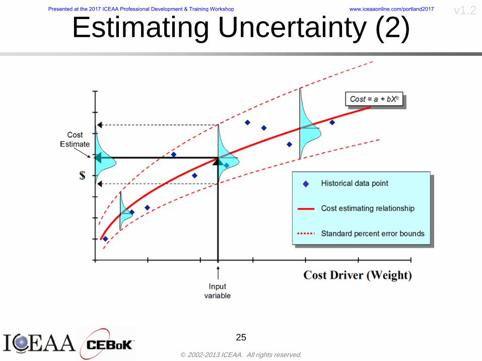
copy 2002-2013 ICEAA All rights reserved
v12
Estimating Uncertainty (2)
25
Presented at the 2017 ICEAA Professional Development amp Training Workshop wwwiceaaonlinecomportland2017
copy 2002-2013 ICEAA All rights reserved
v12
Estimating Uncertainty (3)bull In the case of a linear regression the estimating
uncertainty follows a normal distributionndash The estimate is the mean and the standard error of the
estimate from the regression is the standard deviation of the normal distribution
bull In the case of a log-transformed linear regression the estimating uncertainty follows a lognormal distributionndash The estimate is the median of the lognormal and the
standard error of the estimate from the regression is the standard deviation of the normal distribution (in log-space)
bull There is additional uncertainty about an estimate based upon the distance of what is being estimated from the mean of the input datandash This results in a prediction interval
26
Presented at the 2017 ICEAA Professional Development amp Training Workshop wwwiceaaonlinecomportland2017
copy 2002-2013 ICEAA All rights reserved
v12
Aggregating Riskbull Risk is typically applied at the same level at
which we estimate cost that is at the Work Breakdown Structure (WBS) level
bull The estimates for each WBS are developedndash These estimates sum to yield the total system cost
bull For an n-element WBS the total cost is the sum of the cost for each of the n elements
27
nXXXCostSystem +++= 21
Presented at the 2017 ICEAA Professional Development amp Training Workshop wwwiceaaonlinecomportland2017
copy 2002-2013 ICEAA All rights reserved
v12
WBS Examplebull Launch Vehicle
ndash Structurebull Vehicle Structurebull Tank Structure
ndash Thermal Controlbull Active Thermal Controlbull Induced Thermal Controlbull Tank Thermal Control
ndash Main Propulsion Systemndash Liquid Rocket Enginendash Electric Power and Distributionndash Command Control and Data Handlingndash System Integration
28
Presented at the 2017 ICEAA Professional Development amp Training Workshop wwwiceaaonlinecomportland2017
copy 2002-2013 ICEAA All rights reserved
v12
WBS and Risk
29
Presented at the 2017 ICEAA Professional Development amp Training Workshop wwwiceaaonlinecomportland2017
copy 2002-2013 ICEAA All rights reserved
v12
Aggregating Riskbull This leads us to the issue of aggregating the risks across the
WBSbull For example if we want to determine the 70th percentile of the
overall cost risk distribution how do we proceed bull Note that we cannot simply add the 70th percentiles of each of
the cost risk distributionsbull We can add means and variances (taking correlation into
account more on that later) but that is all
Variance of Total Cost =
30
Mean of Total Cost = ( )E X E Xk
k
n
kk
n
kk
n
= = =aringaelig
egraveccediloumloslashdivide
= =aring aring1 1 1
m
Var X kk
n
=aringaelig
egraveccediloumloslashdivide1
= s r s skk
n
iji
j
i jj
n2
1 1
1
22+aring aringaring
= =
-
=
Presented at the 2017 ICEAA Professional Development amp Training Workshop wwwiceaaonlinecomportland2017
copy 2002-2013 ICEAA All rights reserved
v12
Percentiles Do Not Addbull As a notional example consider two independent normal
distributionsndash One distribution has mean equal to 100 and standard deviation
equal to 20ndash The second distribution has mean 300 and standard deviation of 80
bull The sum of two independent normally distributed random variables is also normally distributed
bull To combine the two distributions we add the means and add the variancesndash Total mean is
ndash Total standard deviation is
31
400300100 =+
8258020 22 raquo+
Presented at the 2017 ICEAA Professional Development amp Training Workshop wwwiceaaonlinecomportland2017
copy 2002-2013 ICEAA All rights reserved
v12
Percentiles Do Not Add (2)bull The 80th percentiles for the individual distributions are
117 and 367 respbull The 80th percentile of the combined distribution is
469 but the sum of the two 80th percentiles is 484bull To see why this is the case note that the percentiles
of a normal distribution are determined by the mean and the standard deviationndash The standard deviations are not added when normal distributions
are combined rather the variances are combinedndash Sum of variances is ndash The standard deviation of this sum is
32
22 ba +22 ba +
Presented at the 2017 ICEAA Professional Development amp Training Workshop wwwiceaaonlinecomportland2017
copy 2002-2013 ICEAA All rights reserved
v12
Percentiles Do Not Add (3)bull Since bull We can write
bull The left side of this inequality represents the risk of the combined distributions while the right side represents the sums of the individual risks
bull Combining two missions that are independent results in a diversification of riskndash The total portfolio is not as risky on a relative basis as each
individual project
33
2222 2 bababa ++lt+
baba +lt+ 22
Presented at the 2017 ICEAA Professional Development amp Training Workshop wwwiceaaonlinecomportland2017
copy 2002-2013 ICEAA All rights reserved
v12
Methods for Aggregating Riskbull Since percentiles do not add we have to find other
ways to aggregate riskbull One method is to use Monte Carlo simulationbull Unless cost risk is represented by normal
distributions for all WBS elements summing the means and variances does not result in a completely accurate depiction of overall system cost risk
bull The normal distribution is not a realistic distribution for representing risk in many or even most situations since regarding project risk more can go wrong than can go right which means the risk is NOT symmetric unlike the Gaussian bell curve
34
Presented at the 2017 ICEAA Professional Development amp Training Workshop wwwiceaaonlinecomportland2017
copy 2002-2013 ICEAA All rights reserved
v12
Unit III - Module 9 35
Monte Carlo Simulationfor Risk Analysis
bull When risk analysis is performed multiple risks are gatheredndash These risks may have various probability
distributions
bull Monte Carlo is the most commonly accepted way to produce an accurate characterization of the distribution of the combined effect of these many risksndash Using this distribution we can produce percentiles
for cost impacts due to risk occurrences
10
Presented at the 2017 ICEAA Professional Development amp Training Workshop wwwiceaaonlinecomportland2017
copy 2002-2013 ICEAA All rights reserved
v12
Monte Carlo Simulationbull Simulation is a means for solving problems that are
analytically intractablendash Involves repeated random sampling
bull It was developed during the Manhattan Project as a way to model the interactions inside an atom during nuclear fissionndash Allowed for more sophisticated mathematical modeling of atomic
phenomena
bull Most computer packages use pseudo-random number generators that produce seemingly random results from an initial seedndash Example is the linear congruential generator
36
( ) mbaXX nn mod1 +=+
Presented at the 2017 ICEAA Professional Development amp Training Workshop wwwiceaaonlinecomportland2017
copy 2002-2013 ICEAA All rights reserved
v12Using Random Numbers to Simulate Distributions
bull WBS cost risk is typically measured by a probability distributionbull The most common method for simulating a probability
distribution is the inverse methodbull This involve obtaining a simulated random value from a uniform
distribution and then inverting this through the cumulative distribution function (CDF) to obtain the simulated value
bull As an example for a uniform distribution on the interval [0100]
bull In this case the CDF random value of 05 translates to 10005 = 50
37
( )100
1=xf ( )
100xxF = ( ) xxF 1001 =-
Presented at the 2017 ICEAA Professional Development amp Training Workshop wwwiceaaonlinecomportland2017
copy 2002-2013 ICEAA All rights reserved
v12
Simulating a Triangular Distribution
bull For a triangular distribution with low = 0 most likely = 50 and high = 150 the CDF is given by
bull The inverse function is given by
38
( )iumliumlicirc
iumliumliacute
igrave
poundlt--
poundpound=
1505021
1500050
50015000
2
2
2
xxx
xxxF
( )iumliumlicirc
iumliumliacute
igrave
poundltdivideoslashouml
ccedilegraveaelig +--
poundpound=-
131
21
37501
250017500150
3107500
1
xx
xxxF
Presented at the 2017 ICEAA Professional Development amp Training Workshop wwwiceaaonlinecomportland2017
copy 2002-2013 ICEAA All rights reserved
v12
Simulating a Triangular Distribution (2)
bull If the simulated uniform value is equal to 02 the corresponding inverse value from the CDF inverse is approximately 387
39
0
01
02
03
04
05
06
07
08
09
1
0 30 60 90 120 150
Presented at the 2017 ICEAA Professional Development amp Training Workshop wwwiceaaonlinecomportland2017
copy 2002-2013 ICEAA All rights reserved
v12
Monte Carlo and the WBSbull Simulation involves repeated trials
40
WBS Draw1 2 3 4 5
System 2912 3566 4390 2954 4655 Sum
Structure 80 105 55 80 57 SumVehicle Structure 50 70 30 40 20Tank Structure 30 35 25 40 37
Thermal Control 32 36 35 29 33 SumActive Thermal Control 10 15 12 7 10Induced Thermal Control 12 14 13 14 14Tank Thermal Control 10 7 10 8 9
Main Propulsion System 100 150 125 140 100
Liquid Rocket Engine 1000 1100 1800 900 2200
Electric Power and Distribution 100 125 150 75 90
Command Control and Data Handling 200 250 225 230 275
System Integration 1400 1800 2000 1500 1900
Presented at the 2017 ICEAA Professional Development amp Training Workshop wwwiceaaonlinecomportland2017
copy 2002-2013 ICEAA All rights reserved
v12
Number of Trialsbull Monte Carlo involves a repeated number of trialsbull The greater the number of trials the more accurate the
simulation will approximate the overall cost risk behavior of the system
bull After 100 trials the histogram looks very jagged
41
Presented at the 2017 ICEAA Professional Development amp Training Workshop wwwiceaaonlinecomportland2017
copy 2002-2013 ICEAA All rights reserved
v12
Number of Trials (2)
42
1000 Trials
10000 Trials
50000 Trials Additional trials give a more accurate depiction of the final result
Presented at the 2017 ICEAA Professional Development amp Training Workshop wwwiceaaonlinecomportland2017
copy 2002-2013 ICEAA All rights reserved
v12
Number of Trials (3)bull If we want to simulate the underlying
mean within 1 with 95 confidence for example then we require
43
divideoslash
oumlccedilegrave
aelig poundpound-
=
dividedividedivide
oslash
ouml
ccedilccedilccedil
egrave
aeligpound
-pound
-=
divideoslashouml
ccedilegraveaelig poundpound=
nZ
n
nnX
n
X
n
n
011
010Pr
011
010Pr
011990Pr950
___
___
sm
sm
sm
sm
sm
mm
Presented at the 2017 ICEAA Professional Development amp Training Workshop wwwiceaaonlinecomportland2017
copy 2002-2013 ICEAA All rights reserved
v12
Number of Trials (4)bull This means that the number of trials required is determined by
bull Solving for n we find that at least
trials are neededbull Note that this term involves the coefficient of variation of the
distribution which means that distributions with less dispersion require fewer trials to accurate simulate
44
96101
=ns
m
ms41638
Presented at the 2017 ICEAA Professional Development amp Training Workshop wwwiceaaonlinecomportland2017
copy 2002-2013 ICEAA All rights reserved
v12
Number of Trials (5)bull Simulating percentiles requires more trials than for simulating
meansbull Let Pn represent the number of trials in the sample at or below
the 70th percentile of the underlying distribution (suppose this is known)
bull By the Central Limit Theorem Pnn follows a normal distribution with mean equal to the 70th percentile and variance equal to
bull By a similar process for the mean we find that the number of trials needed to simulate the 70th percentile within 1 with 95 confidence is
45
( )n
FF 700700 1-
n
n
PPn -41638
Presented at the 2017 ICEAA Professional Development amp Training Workshop wwwiceaaonlinecomportland2017
copy 2002-2013 ICEAA All rights reserved
v12
Number of Trials (6)bull If Pn 070 for all n then n is approximately
bull For the sake of comparison suppose CV = 03 (reasonable approximation for hardware development) then the number of trials needed to simulate the mean with the same accuracy is then ldquoonlyrdquo 11525
bull More trials are needed to accurately simulate percentiles than means
46
( ) 46416703041638
70704168341638 =divide
oslashouml
ccedilegraveaelig=divide
oslashouml
ccedilegraveaelig -
=-
nnn
PPn
n
n
Presented at the 2017 ICEAA Professional Development amp Training Workshop wwwiceaaonlinecomportland2017
copy 2002-2013 ICEAA All rights reserved
v12
Methods of Simulationbull Monte Carlo simulation is a standard term for
simulationbull However there is an improvement on Monte Carlo
that improves the accuracy of the results of a simulation for a given number of trials
bull This method is call the Latin Hypercube approach to simulationndash Similar to Monte Carlo but an equal number of draws are taken
from a set of subintervals for example dividing the interval (01) into [00001) [0102)hellip [0910]
ndash Instead of 10 trials from [01] we have one trial from each subinterval
ndash Rough rule of thumb is Latin Hypercube takes 30 fewer trials to achieve similar accuracy to Monte Carlo
47
Presented at the 2017 ICEAA Professional Development amp Training Workshop wwwiceaaonlinecomportland2017
copy 2002-2013 ICEAA All rights reserved
v12
Probability Model ndash Correlationbull Correlation exists between work breakdown structure
(WBS) cost element costs and between cost and schedule
bull Correlation is a necessary consideration in cost risk analysis
bull Correlation is a number that can vary between -1 and +1 and represents the strength of the relationship between the two variablesndash If both variable have a tendency to move in the same direction
correlation is positivendash If when one variable increases the other tends to decrease and
vice-versa the correlation between the two variables is negative
Presented at the 2017 ICEAA Professional Development amp Training Workshop wwwiceaaonlinecomportland2017
copy 2002-2013 ICEAA All rights reserved
v12
Correlation And Causationbull Note that correlation is not causation however
causation implies correlationndash For example shark attacks and ice cream sales at the beach
bull For example for a launch vehicle structure increasing the diameter will not only result in an increase in the structures cost but will also result in higher costs for thermal coating (paint etc)
bull Also simply because two subsystems do not appear to be related does not mean they are not correlatedndash For example structures and computer equipment seemingly
have little relation to one another however an external factor such as a funding cut or a strike will impact all subsystems leading to delays and increasing cost across the board
ndash Thus everything in a WBS has some correlationUnit III - Module 9 49
Presented at the 2017 ICEAA Professional Development amp Training Workshop wwwiceaaonlinecomportland2017
copy 2002-2013 ICEAA All rights reserved
v12
The Importance of Correlationbull Percent that total cost standard deviation is underestimated
when correlation assumed to be 0 instead of r given nWBS elements
Unit III - Module 9 5050
0
20
40
60
80
100
0 01 02 03 04 05 06 07 08 09 1Actual Correlation
Perce
nt Un
deres
timate
d
n = 10
n = 30
n = 100n = 1000
0
20
40
60
80
100
0 01 02 03 04 05 06 07 08 09 1Actual Correlation
Perce
nt Un
deres
timate
d
n = 10
n = 30
n = 100n = 1000
Reference 32nd Annual DOD Cost Analysis Symposium Advanced Training Session ldquoWhy Correlation Matters in Cost Estimatingrdquo Stephen A Book
Presented at the 2017 ICEAA Professional Development amp Training Workshop wwwiceaaonlinecomportland2017
copy 2002-2013 ICEAA All rights reserved
v12
The Importance of Correlation (2)bull For example if correlation is assumed to be 0 for all
elements in a 30 element WBS and the actual correlation is 20 then the total cost standard deviation is underestimated by 60
bull For example assume the total cost is modeled as a normal distribution with mean = 100
bull If correlation is assumed to be zero with total cost standard deviation = 12 when correlation is actually 20 then the true underlying standard deviation is actually 30
bull 70th percentile with zero correlation assumption is 106
bull 70th percentile with 20 correlation is 116 Unit III - Module 9 51
Presented at the 2017 ICEAA Professional Development amp Training Workshop wwwiceaaonlinecomportland2017
copy 2002-2013 ICEAA All rights reserved
v12
Measures of Correlationbull Two measures of correlation are commonly used in
cost risk analysesndash Pearsonrsquos product-moment correlation coefficient ndash Spearmanrsquos rank correlation coefficient
bull Garvey and others recommend using Pearsonrsquos product-moment correlation coefficient correlation for cost risk analysesndash Method of moments uses this but there are two options in
simulationndash Popular simulation packages like Risk and Crystal Ball use
rank correlation but in practice this has been found to make little difference
ndash Pearson product-moment correlation has been incorporated into Risk+
52
Presented at the 2017 ICEAA Professional Development amp Training Workshop wwwiceaaonlinecomportland2017
copy 2002-2013 ICEAA All rights reserved
v12
Pearson Correlationbull Pearsonrsquos product-moment correlation measures
degree of linearity between two random variables bull If two random variables are perfectly linear (eg Y =
aX + b) with positive slope then the Pearson product-moment correlation between X and Y denoted by rXY is +1
53
X X
Y Y Y
XNegative Correlation Positive Correlation No Correlation
middotmiddot
middotmiddot
middotmiddot middotmiddot
middotmiddot
middot
middot
middotmiddotmiddot
middotmiddot
middotmiddot
middotmiddot middot
middot
middot
middotmiddotmiddotmiddotmiddotmiddotmiddotmiddot
middotmiddotmiddotmiddot
middotmiddot
middotmiddot middotmiddotmiddotmiddot
middotmiddotmiddot
middotmiddotmiddotmiddot
middotmiddotmiddot
middotmiddotmiddot
middotmiddot
middot
middot middotmiddot
middot middotmiddotmiddotmiddot middotmiddot middot middotmiddot middot middot
middotmiddot middot
middotmiddotmiddotmiddotmiddot middot middotmiddot
middotmiddot
middot
middotmiddot
middotmiddot middot
middot middot middot
middotmiddot middot
middotmiddotmiddot
middotmiddot
middot middot
Presented at the 2017 ICEAA Professional Development amp Training Workshop wwwiceaaonlinecomportland2017
copy 2002-2013 ICEAA All rights reserved
v12
Spearman Correlationbull Spearmanrsquos rank correlation measures the
monotonicity between two random variablesbull If two random variables are perfectly monotonically
increasing (eg Y = X2) then the Spearman rank correlation denoted by rXY is +1
bull The two measures can be significantly different
54
10 20 30 40 50 60
100
200
300
096 097 098 099 1
1
060
020
040
080
Eff
ort (
Staf
f-M
onth
s)
Software Size I KDSI
y = 28z12y
z x
yy = x100
0 pound x pound 1
Figure 5-9A Figure 5-9B
Pearson Correlation = 09976 Rank Correlation = 1
Pearson Correlation = 024 Rank Correlation = 1
X(x ) ~ Unif(01)
Reference Probability Methods for Cost Uncertainty Analysis A Systems Engineering Perspective Paul R Garvey
Presented at the 2017 ICEAA Professional Development amp Training Workshop wwwiceaaonlinecomportland2017
copy 2002-2013 ICEAA All rights reserved
v12
Unit III - Module 9 55
200
250
300
350
400
1000 1200 1400 1600 1800 2000
Recurring Production
SEPM
200
250
300
350
400
1000 1200 1400 1600 1800 2000
Recurring Production
SEPM
Functional Correlationbull Old No Functional
Correlation Simulation run with WBS items entered as values
bull New Simulation run with functional dependencies entered as they are in cost model
CorrelatedNot Correlated
Note shift of mean and increased variability
Presented at the 2017 ICEAA Professional Development amp Training Workshop wwwiceaaonlinecomportland2017
copy 2002-2013 ICEAA All rights reserved
v12
Risk Measuresbull ldquoWestern Europe conquered the word because of a
technological revolution that started because of attempts to measure the worldrdquo ndash Phillipe Jorion ndash In the same way attempts to measure risk will lead to better project
managementbull Risk management for DoD and NASA agencies focuses
primarily on funding projects to a single percentile ndash NASA policy explicitly mentions 70 and 50ndash This is known as ldquoValue at Riskrdquo and is prevalent in the banking and
financial industry
56
Presented at the 2017 ICEAA Professional Development amp Training Workshop wwwiceaaonlinecomportland2017
copy 2002-2013 ICEAA All rights reserved
v12
Value at Risk (VaR)bull VaR is a percentile of the cost risk
distributionndash VaR funding at the 70th percentile means that
there is a 30 chance of final project cost exceeding the funded amount (budget)
bull VaR has some meritsndash Common measure can be used to compare
different projects and programsndash Easily understood by senior managers and
decision makers
57
Presented at the 2017 ICEAA Professional Development amp Training Workshop wwwiceaaonlinecomportland2017
copy 2002-2013 ICEAA All rights reserved
v12
Why 70th or 80th Percentilebull Typical policy guidance involves funding at the 70th or 80th
percentile Why fund as such a low percentilebull There is some incentive to not over-fundbull For a normal distribution an inflection point occurs near the 80th
percentile meaning that for values above 80 confidence achieving higher levels of confidence can only be achieved by spending greater dollar amounts at an increasing rate
58
-05-04-03-02-01
00102030405
0 05 1 15 2 25 3
Standard Deviations from Mean
Normal Distribution
First DerivativeSlopeVelocity
Second DerivativeConvexityAcceleration
Inflection point at one standard deviation above the mean (~84th
percentile)
Presented at the 2017 ICEAA Professional Development amp Training Workshop wwwiceaaonlinecomportland2017
copy 2002-2013 ICEAA All rights reserved
v12
Funding Above Inflection Pointsbull As the percentile goes above the 80th percentile the amount
needed to achieve that higher level of confidence begins to increase at an increasing rate as is evident from the graph
59
0
10
20
30
40
50
60
70
50 55 60 65 70 75 80 85 90 95 100
$ Ab
ove
MEa
n to
Ach
ieve
Per
cent
ile
Percentile (Confidence Level)
Presented at the 2017 ICEAA Professional Development amp Training Workshop wwwiceaaonlinecomportland2017
copy 2002-2013 ICEAA All rights reserved
v12
Why Budget to the 70th or 80thbull Government projects are funded at the 70th or 80th percentilesbull Why not the 90th or 99th percentile Wonrsquot that help prevent
overrunsndash As we have seen percentiles do not add across programs
bull The sum of the 80th percentiles does NOT equal the total 80th percentile
ndash This is because the individual programs are riskier than the entire suite of missions
bull Known as the ldquoPortfolio effectrdquo (more or this later)
ndash Funding at the 80th gives confidence that the entire portfolio will be adequately funded
bull And since there is an inflection point near the 80th percentile funding above that level quickly becomes cost prohibitive
60
Presented at the 2017 ICEAA Professional Development amp Training Workshop wwwiceaaonlinecomportland2017
copy 2002-2013 ICEAA All rights reserved
v12
Inflection Points for Lognormalbull For a lognormal the inflection point
variesndash Coefficient of variation equal to 10 equates to an
inflection point at the 70th percentile
61
0
10
20
30
40
50
60
70
050 060 070 080 090 100
Coef
ficen
t of V
aria
tion
Percentile of the Inflection Point
Presented at the 2017 ICEAA Professional Development amp Training Workshop wwwiceaaonlinecomportland2017
copy 2002-2013 ICEAA All rights reserved
v12
Issues with Percentile Fundingbull However risk management does not stop at a
specific percentilendash What happens when the 70th percentile is exceeded
bull Any effective risk management policy should prescribe what happens after a bad event occursndash With VaR we only know when a bad event has occurred ndash Also funding at a relatively low level means we have no true
sense of the real risks that should be guarded against
62
Presented at the 2017 ICEAA Professional Development amp Training Workshop wwwiceaaonlinecomportland2017
copy 2002-2013 ICEAA All rights reserved
v12
ldquoHere There Be Dragonsrdquobull On old maps uncharted territory was often
marked with monsters or dragons
63
A section of the Carta Marina by Olaus Magnus 16th Century
Presented at the 2017 ICEAA Professional Development amp Training Workshop wwwiceaaonlinecomportland2017
copy 2002-2013 ICEAA All rights reserved
v12
Distribution Comparisonbull Four different distributions with the same 70th
percentile
bull Should we expect the tails to be similar
64
0
10
20
30
40
50
60
70
80
0 100 200 300 400 500 600
Perc
entil
eCo
nfid
ence
Lev
el
Triangular
Normal
Lognormal
Pareto
Presented at the 2017 ICEAA Professional Development amp Training Workshop wwwiceaaonlinecomportland2017
copy 2002-2013 ICEAA All rights reserved
v12Distribution Comparison Tail Behavior
bull The normal and triangular distributions have similar tails but the lognormal and Pareto have much fatter right tails
65
70
75
80
85
90
95
100
500 1500 2500 3500 4500 5500
Perc
entil
eCo
nfid
ence
Lev
el
Triangular
Normal
Lognormal
Pareto
Here There Be Dragons
Presented at the 2017 ICEAA Professional Development amp Training Workshop wwwiceaaonlinecomportland2017
copy 2002-2013 ICEAA All rights reserved
v12Distribution Comparison ndash Tail Behavior (Table)
bull There is significant tail risk for the lognormal and the Paretobull The 99th percentile for the Pareto is 1000 times greater than
the 70th percentilendash Risk seen in financial markets and in catastrophic risks like natural
disasters bull Four different projects follow the four different risk profiles seen
in this example should clearly have different risk management approaches but 70th percentile funding indicates the same risk management approach for all four
66
Percentile Triangular Normal Lognormal Pareto 70th $600 $600 $600 $600 80th $680 $660 $770 $1430 90th $770 $750 $1070 $5880 95th $840 $820 $1410 $23750 99th $930 $950 $2350 $600000
Presented at the 2017 ICEAA Professional Development amp Training Workshop wwwiceaaonlinecomportland2017
copy 2002-2013 ICEAA All rights reserved
v12Percentile Budgeting is Not Risk Management
bull Percentile budgeting ne effective risk management policybull Suppose that you are shopping for a new car You
mention that safety is your top concern The salesman says he has a great safe car available You ask about the air bags Do they work The salesman answers ldquoOf course Seventy percent of the time they work fine Only 30 of the time the air bags will fail to deployrdquo Would you buy such a car Hedge fund manager David Einhorn has stated ldquoRisk management is the air bag that must always work but only in the multi-sigma event where you have an accidentrdquo
67
Risk management is the air bag that must always work but only in the multi-sigma event where you
have an accident
Presented at the 2017 ICEAA Professional Development amp Training Workshop wwwiceaaonlinecomportland2017
copy 2002-2013 ICEAA All rights reserved
v12
Joint Confidence Level Analysisbull Schedules are risky toobull For 98 recent NASA missions average
schedule growth was 38ndash Not as high as cost growth but still significant
68
0
5
10
15
20
25
30
35
40
Schedule
Cost
Presented at the 2017 ICEAA Professional Development amp Training Workshop wwwiceaaonlinecomportland2017
copy 2002-2013 ICEAA All rights reserved
v12
Schedules Impact Costbull Changes in schedule can have enormous
impacts on cost ndash Schedule slips can lead to cost increases
bull Fixed programmatic costs must be paid on a regular basisndash Achieving schedule milestones early can result in cost
savings
bull Schedule is an important consideration in cost analysis including cost risk analysis
bull However we must be careful in correctly integrating cost and schedule riskndash Schedule is not simply an input but is dependent on many of
the same factors that drive cost
69
Presented at the 2017 ICEAA Professional Development amp Training Workshop wwwiceaaonlinecomportland2017
copy 2002-2013 ICEAA All rights reserved
v12
The Relationship of Cost to Schedulebull Cost and schedule are positively correlated
ndash A larger program with bigger scope with take longer to complete than a smaller simpler program
bull However longer schedules do not always equate to higher cost nor shorter schedules with lower costndash Highly compressed schedules relative to the
optimal schedule can lead to large overrunsbull Compressed schedules are commonplace for
many planetary missions
70
Presented at the 2017 ICEAA Professional Development amp Training Workshop wwwiceaaonlinecomportland2017
copy 2002-2013 ICEAA All rights reserved
v12The Impact of Schedule GrowthCompression on Cost
bull Compressed schedules lead to cost growth and based on existing research is actually more expensive than schedule slippages
71
0
20
40
60
80
100
120
140
160
-50 -25 0 25 50 75 100
Percentage Change in Schedule
Perc
enta
ge C
hang
e in
Cos
t due
to
Sche
dule
Cha
nge
Source Smart CB ldquoCost and Schedule Interrelationshipsrdquo 2007 NASA Cost Symposium
Presented at the 2017 ICEAA Professional Development amp Training Workshop wwwiceaaonlinecomportland2017
copy 2002-2013 ICEAA All rights reserved
v12Schedule as an Independent Variable
bull Why not simply add schedule as an input to cost-estimating relationships (CERs)
bull Schedule is often treated as an independent variable ndash schedules are often determined independently of cost considerationsndash Cost may not be considered explicitly although budgets and
schedules are determined based on scope and other common factors
bull In 2006 SAIC undertook a research task to determine the impact of schedule on cost and added schedule as an independent variable to the CERs in the NASAAir Force Cost Model (NAFCOM) to see if schedule provided any improvement in goodness of fit
72
Presented at the 2017 ICEAA Professional Development amp Training Workshop wwwiceaaonlinecomportland2017
copy 2002-2013 ICEAA All rights reserved
v12
Schedule is a Dependent Variablebull Since NAFCOM includes an exhaustive list of cost drivers the inclusion
of schedule should give an indication of whether there is any additional independent value added from schedule independent of the cost drivers
bull In the study schedule was added to 10 subsystem-level CERs
ndash In each case the addition of schedule did NOTimprove the goodness of fit and schedule was NOT found to be a statistically significant cost driver (given the presence of the other variables) for any of the 10 CERs
bull Standard errors for the CERs increased due to decrease in degrees of freedom
bull Thus schedule as an independent variable did not provide any additional explanation of variation in historical cost
bull This is because schedule is truly NOT an independent variable but a dependent variable and is a function of the same factors that drive cost
73
Presented at the 2017 ICEAA Professional Development amp Training Workshop wwwiceaaonlinecomportland2017
copy 2002-2013 ICEAA All rights reserved
v12
Incorporation of Schedule in Cost Risk
bull When using subjective methods care must be taken in applying schedule to cost risk analysis
bull Since schedule is a dependent variable treating it independently from other factors when assessing its impact on cost can lead to a double count of independent variables in the cost risk analysis
bull Direct inclusion of schedule in a cost risk analysis effectively doubles the influence of each cost driver
ndash Incorrectly leads to broader risk ranges
74
CostWeight
HeritageNewness
Technology Readiness Schedule
Presented at the 2017 ICEAA Professional Development amp Training Workshop wwwiceaaonlinecomportland2017
copy 2002-2013 ICEAA All rights reserved
v12Subjective Cost Risk Methods and Overinclusion of Risk Factors
bull Subjective methods are suitable when data are scarce or not availablebull However care must be taken not to treat correlated sources of risk
such as schedule as independent of each otherbull Example ndash a subjective risk analysis incorporated technology readiness
design risk requirements stability integration risk and schedule and treated each source of risk as independent
bull Risk triangle high value without schedule risk was 31 times the point estimate
bull Risk triangle high value with schedule risk added on top of other sources of risk treated independently was 34 times the point estimate
bull Risk triangle taking correlation between sources of risk into account in a rigorous statistical manner has a high value 15 times the point estimate less than half the effect when treating sources of risk as independent
75
Presented at the 2017 ICEAA Professional Development amp Training Workshop wwwiceaaonlinecomportland2017
copy 2002-2013 ICEAA All rights reserved
v12Fundamental Equation of Cost and Schedule Interrelationships
bull The Fundamental Equation of the Relationship Between Cost and Schedule is
Time = Moneybull This is a well known adage that time is money Your boss at
work may even mention this to you from time to time or if you are the boss you are all too aware of this iron law
bull Because time is money cost and schedule risk should be modeled jointly not with schedule as an independent cost driver
bull Note that cost and schedule are not perfectly correlatedndash Cost can sometimes ldquobuy downrdquo schedule extra money can be
spent to meet a deadline since in some cases additional effort to hasten the completion of a task
76
Presented at the 2017 ICEAA Professional Development amp Training Workshop wwwiceaaonlinecomportland2017
copy 2002-2013 ICEAA All rights reserved
v12How to (Correctly) Incorporate Schedule into Cost Risk Analysis
bull The best way to model cost and schedule risk is to develop a joint cost and schedule model based on the same data
bull Since such models are not currently available the next best approach is to model cost and schedule independently and then integrate cost and schedule risk analyses using joint probability distributions taking into account correlation between cost and schedulendash This approach pioneered by Paul Garvey and Steve Book is
considered industry best practicendash This is a practical method mathematically tractable and follows
naturally from the Fundamental Equation of Cost and Schedule Interrelationships
77
Book S A ldquoQuantifying the Relationship Between Cost and Schedulerdquo The Measurable News Winter 2007-2008 pp 11-15Garvey PR Probability Methods for Cost Uncertainty Analysis A Systems Engineering Perspective New York Marcel Dekker 2000 pp 308-335
Presented at the 2017 ICEAA Professional Development amp Training Workshop wwwiceaaonlinecomportland2017
copy 2002-2013 ICEAA All rights reserved
v12
Joint Lognormal and Normal Distributions
bull Cost and schedule are typically modeled as some combination of Normal and Lognormal probability distributionsndash Studies by The Aerospace Corporation the MITRE
Corporation Wyle Labs and SAIC have found that the Lognormal probability distribution almost always serves as a good model for both the schedule distribution and the cost distribution
ndash The Normal distribution may also be appropriate in some instances and depending upon the level of confidence at which budgets are set may even be more conservative and logically consistent than the Normal distribution
ndash Joint Lognormal and Normal distributions are defined by a pair of mean and standard deviations and a level of correlation between the two
78
Presented at the 2017 ICEAA Professional Development amp Training Workshop wwwiceaaonlinecomportland2017
copy 2002-2013 ICEAA All rights reserved
v12Modeling Cost and Schedule as a Bivariate Distribution
bull In the approach set forth by Book and Garvey cost risk is assessed and the top-level distribution is modeled as a Lognormal (or Normal) distribution schedule risk is assessed and the overall schedule risk is modeled as a Lognormal (or Normal) distribution
bull The two distributions are combined into a Bivariate distribution by assigning a correlation between the two and by treating the two distributions as the marginal distributions of a Bivariate Lognormal distributionndash Other combinations include a Bivariate Normal or a Bivariate
Normal-Lognormal
79
Presented at the 2017 ICEAA Professional Development amp Training Workshop wwwiceaaonlinecomportland2017
copy 2002-2013 ICEAA All rights reserved
v12Bivariate Lognormal Distribution for Cost and Schedule
bull Cost is often observed to be Lognormal when strong positive correlations are present among the systemrsquos WBS cost element costs
bull A systemrsquos schedule is often observed (from Monte Carlo simulations) to be Lognormal if it is the sum of many positively correlated schedule activities in an overall schedule network
bull If Lognormal distributions characterize a systemrsquos cost and schedule then the Bivariate Lognormal could serve as an assumed model of their joint distributionndash In this case the marginal distribution of each of cost and schedule is
Lognormalbull Other possibilities for modeling cost and schedule as a Bivariate
distribution include a Bivariate Normal or a Bivariate Normal-Lognormal distributionndash All these combinations are analytically tractable
80
Presented at the 2017 ICEAA Professional Development amp Training Workshop wwwiceaaonlinecomportland2017
copy 2002-2013 ICEAA All rights reserved
v12Bivariate Lognormal for Cost and Schedule
bull Contour Plots of a Bivariate Lognormal
81
Presented at the 2017 ICEAA Professional Development amp Training Workshop wwwiceaaonlinecomportland2017
copy 2002-2013 ICEAA All rights reserved
v12Correlation Between Cost and Schedule
bull Cost and schedule are positively correlated but not perfectly sondash For example it is possible to have a schedule underrun and a cost
overrunbull Based on cost and schedule growth data for 50 completed NASA
programs the correlation between development cost and development schedule is 70
82
00
200
400
600
800
1000
1200
-500 00 500 1000 1500 2000 2500Historical Cost Growth
Hist
oric
al S
ched
ule
Gro
wth
r = 715
Presented at the 2017 ICEAA Professional Development amp Training Workshop wwwiceaaonlinecomportland2017
copy 2002-2013 ICEAA All rights reserved
v12Correlation Between Cost and Schedule Caveats
bull Based on historical data recommended correlation between cost and schedule is 70 but this could be higher or lower depending upon program circumstancesndash If program is budget constrained cost and schedule will be
more highly correlated (go as you pay)ndash If program is schedule constrained cost and schedule will
have lower correlation perhaps even negative correlation ndash Smaller programs have smaller correlation between cost and
schedule riskbull Relatively easy to ldquohurry uprdquo and finish on time or even early if
needed
83
Presented at the 2017 ICEAA Professional Development amp Training Workshop wwwiceaaonlinecomportland2017
copy 2002-2013 ICEAA All rights reserved
v12
Conditional Confidence Levelsbull Given a programrsquos project schedule we can determine the cost
risk distribution conditional upon the given schedulebull Conditional cost S-curves are steeper than unconditional
(marginal) cost S-curves between some uncertainty has been removed because schedule is fixed
84
Presented at the 2017 ICEAA Professional Development amp Training Workshop wwwiceaaonlinecomportland2017
copy 2002-2013 ICEAA All rights reserved
v12
Joint Confidence Levelsbull Joint 65 confidence represents the probability of
achieving both 65 confidence in cost AND 65 confidence in schedulendash This is different than achieving 65 cost confidence alone
or achieving 65 schedule confidence alonebull Due to the imperfect correlation between cost and schedule it
is possible to achieve a 65 cost confidence with a lower level of schedule confidence
bull Restricting the schedule confidence thus requires additional $ to achieve a given level of confidence
85
X
Y
Possible Values for Which X gt a Possible Values for
Which X gt a and Y gt b
a
b
Presented at the 2017 ICEAA Professional Development amp Training Workshop wwwiceaaonlinecomportland2017
copy 2002-2013 ICEAA All rights reserved
v12Joint Confidence Levels Versus Cost Confidence Levels Only
bull Example of the differences between cost confidence schedule confidence conditional cost confidence and joint cost and schedule confidence
86
Joint Cost-Schedule Confidence Iso-Curves
Cost (RY$M)
Sche
dule
(Mon
ths)
65 Confidence
50 Confidence
70 Confidence
65 Cost Confidence AggressiveSchedule65 Cost ConfidenceScheduleGiven 65 Schedule ConfidenceUnconditional 65 CostConfidenceUnconditional 65 ScheduleConfidence
65 Cost Confidence 65 Joint Cost and Schedule
Confidence for 65 Schedule Confidence
Presented at the 2017 ICEAA Professional Development amp Training Workshop wwwiceaaonlinecomportland2017
copy 2002-2013 ICEAA All rights reserved
v12
Joint Cost and Schedule Confidence
bull Can examine pairs of cost and schedule that achieve a given level of confidence
bull Provides insights into the trade-offs between cost and schedule for a given level of confidencendash Possible to increase cost confidence by giving a
project more time in some instances or possible to ldquobuy downrdquo schedule
bull But these have limits and are shown in the iso-cost and schedule confidence curves
87
Presented at the 2017 ICEAA Professional Development amp Training Workshop wwwiceaaonlinecomportland2017
copy 2002-2013 ICEAA All rights reserved
v12Cost and Schedule Trade-offs for a Given Level of Joint Confidence
bull Hypothetical Example
88
Cost (RY$M)
Schedule (Months)
$100 48$99 48$89 49$87 50$85 51$85 52$84 53$83 55$83 55$83 56
Cost and Schedule 65 Confidence Iso-Curve
4748495051525354555657
$80 $82 $84 $86 $88 $90 $92 $94 $96 $98 $100
Cost (RY$ M)
Sche
dule
(Mon
ths)
Presented at the 2017 ICEAA Professional Development amp Training Workshop wwwiceaaonlinecomportland2017
copy 2002-2013 ICEAA All rights reserved
v12Policy Considerations for Confidence Levels
bull For large programs the difference between the amount of money needed to achieve 65 cost confidence independent of schedule and joint 65 cost and schedule confidence can represent hundreds of millions and even billions of dollars
89
Joint Cost-Schedule Confidence Iso-Curves
Cost (RY$M)
Sche
dule
(Mon
ths)
65 Confidence
65 Cost Confidence AggressiveSchedule
65 Cost ConfidenceScheduleGiven 65 Schedule Confidence
Unconditional 65 CostConfidence
Joint Cost and Schedule Confidence for 65 Cost Confidence and Program Baseline Schedule is Less Than 35
65 Cost Confidence Independent of Schedule Cost Needed to Achieve
Both 65 Joint Cost and Schedule Confidence for the Schedule with 65 Confidence
Presented at the 2017 ICEAA Professional Development amp Training Workshop wwwiceaaonlinecomportland2017
copy 2002-2013 ICEAA All rights reserved
v12
Copulasbull More generally any combination of distributions can
be used (more than just normal and lognormal)ndash Termed ldquocopulardquo from the Italian word for ldquocouplerdquondash Copulas are a way to combine marginal distributions of any
number and type into a joint distributionbull More formally a copula is a multivariate joint distribution defined
on the n-dimensional unit cube [0 1]n such that every marginal distribution is uniform on the interval [0 1]
bull (The bivariate form of) Sklarrsquos theorem states that for any bivariate distribution function H(x y) let F(x) = H(x infin) and G(y) = H(infin y) be the univariate marginal probability distribution functions Then there exists a copula C such that H(xy)=C(F(x)G(y))
ndash Copulas are widely used in risk management for investments and insurance
bull Considered industry best practice (Li 2000)bull Marketed as part of JP Morganrsquos CreditMetrics suite of tools
(Gupton et Al 1997)90
Presented at the 2017 ICEAA Professional Development amp Training Workshop wwwiceaaonlinecomportland2017
copy 2002-2013 ICEAA All rights reserved
v12Parametric Joint Cost and Schedule Analysis
bull A parametric model based on a consistent data set with a set of overlapping cost and schedule drivers is a cleaner way to model cost and schedule
91
CostWeight
HeritageNewness
Technology Readiness
Schedule
0
20
40
60
80
100
Confidence
Joint Cost and Schedule Confidence
Schedule
Cost
Lognormal Distribution PDF and CDF
0102030405060708090100
200 300 400 500 600 700 800 900 1000Cost $
Con
fiden
ce L
evel
0
00002
00004
00006
00008
0001
00012
00014
00016
Prob
abili
ty D
ensi
ty
CDFPDF
Lognormal Distribution PDF and CDF
0102030405060708090100
200 300 400 500 600 700 800 900 1000Cost $
Con
fiden
ce L
evel
0
00002
00004
00006
00008
0001
00012
00014
00016
Prob
abili
ty D
ensi
ty
CDFPDF
Presented at the 2017 ICEAA Professional Development amp Training Workshop wwwiceaaonlinecomportland2017
copy 2002-2013 ICEAA All rights reserved
v12Parametric Joint Cost and Schedule Analysis (2)
bull Joint cost and schedule risk analysis produced naturally by the integrated modelndash Addresses several issues with the copula
approachbull Tail dependencybull Correlation ndash no need to assign correlation
between cost and schedulebull Consistency of cost and schedule models
92
Presented at the 2017 ICEAA Professional Development amp Training Workshop wwwiceaaonlinecomportland2017
copy 2002-2013 ICEAA All rights reserved
v12
Resource-Loaded Schedulesbull Involves assigning cost and schedule risks to a resource-loaded schedule
networkbull Bottom-up approach
ndash More labor intensive than parametrics but can also provide more insight
ndash Can answer questions than parametric typically cannot such as how much do reserve requirements decrease if a specific risk is retired
bull Currently being implemented in Constellation programbull Has same issue as all bottom-up models hard to count all the risks and model
them discretely
ndash As a result there is a tendency to reflect less risk than indicated by history
ndash ldquoThere are more things in heaven and earth Horatio than are dreamt of in your philosophyrdquo William Shakespeare Hamlet Act I Scene V
93
Presented at the 2017 ICEAA Professional Development amp Training Workshop wwwiceaaonlinecomportland2017
copy 2002-2013 ICEAA All rights reserved
v12Resource-Loaded Schedules Vs Parametrics
bull Parametric most appropriate for early estimatesndash But also good for high-level checks as project progresses
bull As plans take shape lower level modeling may be more appropriate
94 1
CONCEPTUALDEVELOPMENT
PROJECTDEFINITION DESIGN DEVELOPMENT OPERATIONS
PARAMETRIC PARAMETRIC
ANALOGY
ENGINEERING (Bottoms Up)
$PARAMETRIC
DETAILED
$
Pre Phase A Phase B Phase CDPhase A Phase EPre Phase A Phase B Phase CDPhase A Phase E
Risk = f(Cost Estimating Relationship Inputs eg mass power data rate TRL new design etc)
Risk = f(cost and schedule variation of the analogous elements)
Risk = f(variation of detailed inputs eg labor hours rates materials etc)
Presented at the 2017 ICEAA Professional Development amp Training Workshop wwwiceaaonlinecomportland2017
copy 2002-2013 ICEAA All rights reserved
v12
Resource-Loaded Schedulesbull Methodology has been demonstrated in other
industriesndash Construction oil and gasndash Analysis has not been traditionally done on highly uncertain
complex development projects bull Methodology focuses on project baseline schedule
ndash In baseline schedule all tasks are resource loaded to represent a baseline schedule and cost standpoint
ndash Resource loaded schedule is ldquorolledrdquo up to a manageable level
ndash Based on the risk and uncertainties identified schedule distributions are applied to each rolled up task
ndash Cost uncertainties are also applied to rolled up tasksbull Uncertainties include labor rate man power etc
ndash A Monte Carlo simulation is run to develop joint cost-schedule distributions
95
Presented at the 2017 ICEAA Professional Development amp Training Workshop wwwiceaaonlinecomportland2017
copy 2002-2013 ICEAA All rights reserved
v12
Unit III - Module 9 96
Execution ndash Cross Checksbull Means The mean cost growth factor for WBS items
can be compared to history as a way to cross check results
bull CVs The CV of the cost growth factors for WBS items can be compared to history as a way to cross check results
bull Inputs Checks are performed on inputs or other parameters to see if historical values are in line with program assumptionsndash Example Historical risk scores can be compared to program
risk scores to see if risk assessors are being realistic and to see if the underlying database is representative of the program
11
Presented at the 2017 ICEAA Professional Development amp Training Workshop wwwiceaaonlinecomportland2017
- Cost and Schedule Risk Analysis Basic
- Acknowledgments
- Unit Index
- Risk Overview
- Agenda
- Introduction
- Risk Analysis Terms
- Are Our Costs Realistic
- Historical Cost Growth
- Sources of Cost Risk
- Point Estimates of Cost
- Types of Risk
- Point Estimates Vs Risk Estimates
- Cost Risk and Probability
- Probability Model ndash Distribution
- Probability Model ndash Distribution
- Probability ndash Top-Level Distribution
- S-Curves and Confidence Levels
- Example ndash Normal Distribution
- Confidence Levels
- Measuring Parametric Model Uncertainty
- Parametric Model Example
- Weight Uncertainty
- Estimating Uncertainty
- Estimating Uncertainty (2)
- Estimating Uncertainty (3)
- Aggregating Risk
- WBS Example
- WBS and Risk
- Aggregating Risk
- Percentiles Do Not Add
- Percentiles Do Not Add (2)
- Percentiles Do Not Add (3)
- Methods for Aggregating Risk
- Monte Carlo Simulationfor Risk Analysis
- Monte Carlo Simulation
- Using Random Numbers to Simulate Distributions
- Simulating a Triangular Distribution
- Simulating a Triangular Distribution (2)
- Monte Carlo and the WBS
- Number of Trials
- Number of Trials (2)
- Number of Trials (3)
- Number of Trials (4)
- Number of Trials (5)
- Number of Trials (6)
- Methods of Simulation
- Probability Model ndash Correlation
- Correlation And Causation
- The Importance of Correlation
- The Importance of Correlation (2)
- Measures of Correlation
- Pearson Correlation
- Spearman Correlation
- Functional Correlation
- Risk Measures
- Value at Risk (VaR)
- Why 70th or 80th Percentile
- Funding Above Inflection Points
- Why Budget to the 70th or 80th
- Inflection Points for Lognormal
- Issues with Percentile Funding
- ldquoHere There Be Dragonsrdquo
- Distribution Comparison
- Distribution Comparison Tail Behavior
- Distribution Comparison ndash Tail Behavior (Table)
- Percentile Budgeting is Not Risk Management
- Joint Confidence Level Analysis
- Schedules Impact Cost
- The Relationship of Cost to Schedule
- The Impact of Schedule GrowthCompression on Cost
- Schedule as an Independent Variable
- Schedule is a Dependent Variable
- Incorporation of Schedule in Cost Risk
- Subjective Cost Risk Methods and Overinclusion of Risk Factors
- Fundamental Equation of Cost and Schedule Interrelationships
- How to (Correctly) Incorporate Schedule into Cost Risk Analysis
- Joint Lognormal and Normal Distributions
- Modeling Cost and Schedule as a Bivariate Distribution
- Bivariate Lognormal Distribution for Cost and Schedule
- Bivariate Lognormal for Cost and Schedule
- Correlation Between Cost and Schedule
- Correlation Between Cost and Schedule Caveats
- Conditional Confidence Levels
- Joint Confidence Levels
- Joint Confidence Levels Versus Cost Confidence Levels Only
- Joint Cost and Schedule Confidence
- Cost and Schedule Trade-offs for a Given Level of Joint Confidence
- Policy Considerations for Confidence Levels
- Copulas
- Parametric Joint Cost and Schedule Analysis
- Parametric Joint Cost and Schedule Analysis (2)
- Resource-Loaded Schedules
- Resource-Loaded Schedules Vs Parametrics
- Resource-Loaded Schedules
- Execution ndash Cross Checks
-
copy 2002-2013 ICEAA All rights reserved
v12
Aggregating Riskbull Risk is typically applied at the same level at
which we estimate cost that is at the Work Breakdown Structure (WBS) level
bull The estimates for each WBS are developedndash These estimates sum to yield the total system cost
bull For an n-element WBS the total cost is the sum of the cost for each of the n elements
27
nXXXCostSystem +++= 21
Presented at the 2017 ICEAA Professional Development amp Training Workshop wwwiceaaonlinecomportland2017
copy 2002-2013 ICEAA All rights reserved
v12
WBS Examplebull Launch Vehicle
ndash Structurebull Vehicle Structurebull Tank Structure
ndash Thermal Controlbull Active Thermal Controlbull Induced Thermal Controlbull Tank Thermal Control
ndash Main Propulsion Systemndash Liquid Rocket Enginendash Electric Power and Distributionndash Command Control and Data Handlingndash System Integration
28
Presented at the 2017 ICEAA Professional Development amp Training Workshop wwwiceaaonlinecomportland2017
copy 2002-2013 ICEAA All rights reserved
v12
WBS and Risk
29
Presented at the 2017 ICEAA Professional Development amp Training Workshop wwwiceaaonlinecomportland2017
copy 2002-2013 ICEAA All rights reserved
v12
Aggregating Riskbull This leads us to the issue of aggregating the risks across the
WBSbull For example if we want to determine the 70th percentile of the
overall cost risk distribution how do we proceed bull Note that we cannot simply add the 70th percentiles of each of
the cost risk distributionsbull We can add means and variances (taking correlation into
account more on that later) but that is all
Variance of Total Cost =
30
Mean of Total Cost = ( )E X E Xk
k
n
kk
n
kk
n
= = =aringaelig
egraveccediloumloslashdivide
= =aring aring1 1 1
m
Var X kk
n
=aringaelig
egraveccediloumloslashdivide1
= s r s skk
n
iji
j
i jj
n2
1 1
1
22+aring aringaring
= =
-
=
Presented at the 2017 ICEAA Professional Development amp Training Workshop wwwiceaaonlinecomportland2017
copy 2002-2013 ICEAA All rights reserved
v12
Percentiles Do Not Addbull As a notional example consider two independent normal
distributionsndash One distribution has mean equal to 100 and standard deviation
equal to 20ndash The second distribution has mean 300 and standard deviation of 80
bull The sum of two independent normally distributed random variables is also normally distributed
bull To combine the two distributions we add the means and add the variancesndash Total mean is
ndash Total standard deviation is
31
400300100 =+
8258020 22 raquo+
Presented at the 2017 ICEAA Professional Development amp Training Workshop wwwiceaaonlinecomportland2017
copy 2002-2013 ICEAA All rights reserved
v12
Percentiles Do Not Add (2)bull The 80th percentiles for the individual distributions are
117 and 367 respbull The 80th percentile of the combined distribution is
469 but the sum of the two 80th percentiles is 484bull To see why this is the case note that the percentiles
of a normal distribution are determined by the mean and the standard deviationndash The standard deviations are not added when normal distributions
are combined rather the variances are combinedndash Sum of variances is ndash The standard deviation of this sum is
32
22 ba +22 ba +
Presented at the 2017 ICEAA Professional Development amp Training Workshop wwwiceaaonlinecomportland2017
copy 2002-2013 ICEAA All rights reserved
v12
Percentiles Do Not Add (3)bull Since bull We can write
bull The left side of this inequality represents the risk of the combined distributions while the right side represents the sums of the individual risks
bull Combining two missions that are independent results in a diversification of riskndash The total portfolio is not as risky on a relative basis as each
individual project
33
2222 2 bababa ++lt+
baba +lt+ 22
Presented at the 2017 ICEAA Professional Development amp Training Workshop wwwiceaaonlinecomportland2017
copy 2002-2013 ICEAA All rights reserved
v12
Methods for Aggregating Riskbull Since percentiles do not add we have to find other
ways to aggregate riskbull One method is to use Monte Carlo simulationbull Unless cost risk is represented by normal
distributions for all WBS elements summing the means and variances does not result in a completely accurate depiction of overall system cost risk
bull The normal distribution is not a realistic distribution for representing risk in many or even most situations since regarding project risk more can go wrong than can go right which means the risk is NOT symmetric unlike the Gaussian bell curve
34
Presented at the 2017 ICEAA Professional Development amp Training Workshop wwwiceaaonlinecomportland2017
copy 2002-2013 ICEAA All rights reserved
v12
Unit III - Module 9 35
Monte Carlo Simulationfor Risk Analysis
bull When risk analysis is performed multiple risks are gatheredndash These risks may have various probability
distributions
bull Monte Carlo is the most commonly accepted way to produce an accurate characterization of the distribution of the combined effect of these many risksndash Using this distribution we can produce percentiles
for cost impacts due to risk occurrences
10
Presented at the 2017 ICEAA Professional Development amp Training Workshop wwwiceaaonlinecomportland2017
copy 2002-2013 ICEAA All rights reserved
v12
Monte Carlo Simulationbull Simulation is a means for solving problems that are
analytically intractablendash Involves repeated random sampling
bull It was developed during the Manhattan Project as a way to model the interactions inside an atom during nuclear fissionndash Allowed for more sophisticated mathematical modeling of atomic
phenomena
bull Most computer packages use pseudo-random number generators that produce seemingly random results from an initial seedndash Example is the linear congruential generator
36
( ) mbaXX nn mod1 +=+
Presented at the 2017 ICEAA Professional Development amp Training Workshop wwwiceaaonlinecomportland2017
copy 2002-2013 ICEAA All rights reserved
v12Using Random Numbers to Simulate Distributions
bull WBS cost risk is typically measured by a probability distributionbull The most common method for simulating a probability
distribution is the inverse methodbull This involve obtaining a simulated random value from a uniform
distribution and then inverting this through the cumulative distribution function (CDF) to obtain the simulated value
bull As an example for a uniform distribution on the interval [0100]
bull In this case the CDF random value of 05 translates to 10005 = 50
37
( )100
1=xf ( )
100xxF = ( ) xxF 1001 =-
Presented at the 2017 ICEAA Professional Development amp Training Workshop wwwiceaaonlinecomportland2017
copy 2002-2013 ICEAA All rights reserved
v12
Simulating a Triangular Distribution
bull For a triangular distribution with low = 0 most likely = 50 and high = 150 the CDF is given by
bull The inverse function is given by
38
( )iumliumlicirc
iumliumliacute
igrave
poundlt--
poundpound=
1505021
1500050
50015000
2
2
2
xxx
xxxF
( )iumliumlicirc
iumliumliacute
igrave
poundltdivideoslashouml
ccedilegraveaelig +--
poundpound=-
131
21
37501
250017500150
3107500
1
xx
xxxF
Presented at the 2017 ICEAA Professional Development amp Training Workshop wwwiceaaonlinecomportland2017
copy 2002-2013 ICEAA All rights reserved
v12
Simulating a Triangular Distribution (2)
bull If the simulated uniform value is equal to 02 the corresponding inverse value from the CDF inverse is approximately 387
39
0
01
02
03
04
05
06
07
08
09
1
0 30 60 90 120 150
Presented at the 2017 ICEAA Professional Development amp Training Workshop wwwiceaaonlinecomportland2017
copy 2002-2013 ICEAA All rights reserved
v12
Monte Carlo and the WBSbull Simulation involves repeated trials
40
WBS Draw1 2 3 4 5
System 2912 3566 4390 2954 4655 Sum
Structure 80 105 55 80 57 SumVehicle Structure 50 70 30 40 20Tank Structure 30 35 25 40 37
Thermal Control 32 36 35 29 33 SumActive Thermal Control 10 15 12 7 10Induced Thermal Control 12 14 13 14 14Tank Thermal Control 10 7 10 8 9
Main Propulsion System 100 150 125 140 100
Liquid Rocket Engine 1000 1100 1800 900 2200
Electric Power and Distribution 100 125 150 75 90
Command Control and Data Handling 200 250 225 230 275
System Integration 1400 1800 2000 1500 1900
Presented at the 2017 ICEAA Professional Development amp Training Workshop wwwiceaaonlinecomportland2017
copy 2002-2013 ICEAA All rights reserved
v12
Number of Trialsbull Monte Carlo involves a repeated number of trialsbull The greater the number of trials the more accurate the
simulation will approximate the overall cost risk behavior of the system
bull After 100 trials the histogram looks very jagged
41
Presented at the 2017 ICEAA Professional Development amp Training Workshop wwwiceaaonlinecomportland2017
copy 2002-2013 ICEAA All rights reserved
v12
Number of Trials (2)
42
1000 Trials
10000 Trials
50000 Trials Additional trials give a more accurate depiction of the final result
Presented at the 2017 ICEAA Professional Development amp Training Workshop wwwiceaaonlinecomportland2017
copy 2002-2013 ICEAA All rights reserved
v12
Number of Trials (3)bull If we want to simulate the underlying
mean within 1 with 95 confidence for example then we require
43
divideoslash
oumlccedilegrave
aelig poundpound-
=
dividedividedivide
oslash
ouml
ccedilccedilccedil
egrave
aeligpound
-pound
-=
divideoslashouml
ccedilegraveaelig poundpound=
nZ
n
nnX
n
X
n
n
011
010Pr
011
010Pr
011990Pr950
___
___
sm
sm
sm
sm
sm
mm
Presented at the 2017 ICEAA Professional Development amp Training Workshop wwwiceaaonlinecomportland2017
copy 2002-2013 ICEAA All rights reserved
v12
Number of Trials (4)bull This means that the number of trials required is determined by
bull Solving for n we find that at least
trials are neededbull Note that this term involves the coefficient of variation of the
distribution which means that distributions with less dispersion require fewer trials to accurate simulate
44
96101
=ns
m
ms41638
Presented at the 2017 ICEAA Professional Development amp Training Workshop wwwiceaaonlinecomportland2017
copy 2002-2013 ICEAA All rights reserved
v12
Number of Trials (5)bull Simulating percentiles requires more trials than for simulating
meansbull Let Pn represent the number of trials in the sample at or below
the 70th percentile of the underlying distribution (suppose this is known)
bull By the Central Limit Theorem Pnn follows a normal distribution with mean equal to the 70th percentile and variance equal to
bull By a similar process for the mean we find that the number of trials needed to simulate the 70th percentile within 1 with 95 confidence is
45
( )n
FF 700700 1-
n
n
PPn -41638
Presented at the 2017 ICEAA Professional Development amp Training Workshop wwwiceaaonlinecomportland2017
copy 2002-2013 ICEAA All rights reserved
v12
Number of Trials (6)bull If Pn 070 for all n then n is approximately
bull For the sake of comparison suppose CV = 03 (reasonable approximation for hardware development) then the number of trials needed to simulate the mean with the same accuracy is then ldquoonlyrdquo 11525
bull More trials are needed to accurately simulate percentiles than means
46
( ) 46416703041638
70704168341638 =divide
oslashouml
ccedilegraveaelig=divide
oslashouml
ccedilegraveaelig -
=-
nnn
PPn
n
n
Presented at the 2017 ICEAA Professional Development amp Training Workshop wwwiceaaonlinecomportland2017
copy 2002-2013 ICEAA All rights reserved
v12
Methods of Simulationbull Monte Carlo simulation is a standard term for
simulationbull However there is an improvement on Monte Carlo
that improves the accuracy of the results of a simulation for a given number of trials
bull This method is call the Latin Hypercube approach to simulationndash Similar to Monte Carlo but an equal number of draws are taken
from a set of subintervals for example dividing the interval (01) into [00001) [0102)hellip [0910]
ndash Instead of 10 trials from [01] we have one trial from each subinterval
ndash Rough rule of thumb is Latin Hypercube takes 30 fewer trials to achieve similar accuracy to Monte Carlo
47
Presented at the 2017 ICEAA Professional Development amp Training Workshop wwwiceaaonlinecomportland2017
copy 2002-2013 ICEAA All rights reserved
v12
Probability Model ndash Correlationbull Correlation exists between work breakdown structure
(WBS) cost element costs and between cost and schedule
bull Correlation is a necessary consideration in cost risk analysis
bull Correlation is a number that can vary between -1 and +1 and represents the strength of the relationship between the two variablesndash If both variable have a tendency to move in the same direction
correlation is positivendash If when one variable increases the other tends to decrease and
vice-versa the correlation between the two variables is negative
Presented at the 2017 ICEAA Professional Development amp Training Workshop wwwiceaaonlinecomportland2017
copy 2002-2013 ICEAA All rights reserved
v12
Correlation And Causationbull Note that correlation is not causation however
causation implies correlationndash For example shark attacks and ice cream sales at the beach
bull For example for a launch vehicle structure increasing the diameter will not only result in an increase in the structures cost but will also result in higher costs for thermal coating (paint etc)
bull Also simply because two subsystems do not appear to be related does not mean they are not correlatedndash For example structures and computer equipment seemingly
have little relation to one another however an external factor such as a funding cut or a strike will impact all subsystems leading to delays and increasing cost across the board
ndash Thus everything in a WBS has some correlationUnit III - Module 9 49
Presented at the 2017 ICEAA Professional Development amp Training Workshop wwwiceaaonlinecomportland2017
copy 2002-2013 ICEAA All rights reserved
v12
The Importance of Correlationbull Percent that total cost standard deviation is underestimated
when correlation assumed to be 0 instead of r given nWBS elements
Unit III - Module 9 5050
0
20
40
60
80
100
0 01 02 03 04 05 06 07 08 09 1Actual Correlation
Perce
nt Un
deres
timate
d
n = 10
n = 30
n = 100n = 1000
0
20
40
60
80
100
0 01 02 03 04 05 06 07 08 09 1Actual Correlation
Perce
nt Un
deres
timate
d
n = 10
n = 30
n = 100n = 1000
Reference 32nd Annual DOD Cost Analysis Symposium Advanced Training Session ldquoWhy Correlation Matters in Cost Estimatingrdquo Stephen A Book
Presented at the 2017 ICEAA Professional Development amp Training Workshop wwwiceaaonlinecomportland2017
copy 2002-2013 ICEAA All rights reserved
v12
The Importance of Correlation (2)bull For example if correlation is assumed to be 0 for all
elements in a 30 element WBS and the actual correlation is 20 then the total cost standard deviation is underestimated by 60
bull For example assume the total cost is modeled as a normal distribution with mean = 100
bull If correlation is assumed to be zero with total cost standard deviation = 12 when correlation is actually 20 then the true underlying standard deviation is actually 30
bull 70th percentile with zero correlation assumption is 106
bull 70th percentile with 20 correlation is 116 Unit III - Module 9 51
Presented at the 2017 ICEAA Professional Development amp Training Workshop wwwiceaaonlinecomportland2017
copy 2002-2013 ICEAA All rights reserved
v12
Measures of Correlationbull Two measures of correlation are commonly used in
cost risk analysesndash Pearsonrsquos product-moment correlation coefficient ndash Spearmanrsquos rank correlation coefficient
bull Garvey and others recommend using Pearsonrsquos product-moment correlation coefficient correlation for cost risk analysesndash Method of moments uses this but there are two options in
simulationndash Popular simulation packages like Risk and Crystal Ball use
rank correlation but in practice this has been found to make little difference
ndash Pearson product-moment correlation has been incorporated into Risk+
52
Presented at the 2017 ICEAA Professional Development amp Training Workshop wwwiceaaonlinecomportland2017
copy 2002-2013 ICEAA All rights reserved
v12
Pearson Correlationbull Pearsonrsquos product-moment correlation measures
degree of linearity between two random variables bull If two random variables are perfectly linear (eg Y =
aX + b) with positive slope then the Pearson product-moment correlation between X and Y denoted by rXY is +1
53
X X
Y Y Y
XNegative Correlation Positive Correlation No Correlation
middotmiddot
middotmiddot
middotmiddot middotmiddot
middotmiddot
middot
middot
middotmiddotmiddot
middotmiddot
middotmiddot
middotmiddot middot
middot
middot
middotmiddotmiddotmiddotmiddotmiddotmiddotmiddot
middotmiddotmiddotmiddot
middotmiddot
middotmiddot middotmiddotmiddotmiddot
middotmiddotmiddot
middotmiddotmiddotmiddot
middotmiddotmiddot
middotmiddotmiddot
middotmiddot
middot
middot middotmiddot
middot middotmiddotmiddotmiddot middotmiddot middot middotmiddot middot middot
middotmiddot middot
middotmiddotmiddotmiddotmiddot middot middotmiddot
middotmiddot
middot
middotmiddot
middotmiddot middot
middot middot middot
middotmiddot middot
middotmiddotmiddot
middotmiddot
middot middot
Presented at the 2017 ICEAA Professional Development amp Training Workshop wwwiceaaonlinecomportland2017
copy 2002-2013 ICEAA All rights reserved
v12
Spearman Correlationbull Spearmanrsquos rank correlation measures the
monotonicity between two random variablesbull If two random variables are perfectly monotonically
increasing (eg Y = X2) then the Spearman rank correlation denoted by rXY is +1
bull The two measures can be significantly different
54
10 20 30 40 50 60
100
200
300
096 097 098 099 1
1
060
020
040
080
Eff
ort (
Staf
f-M
onth
s)
Software Size I KDSI
y = 28z12y
z x
yy = x100
0 pound x pound 1
Figure 5-9A Figure 5-9B
Pearson Correlation = 09976 Rank Correlation = 1
Pearson Correlation = 024 Rank Correlation = 1
X(x ) ~ Unif(01)
Reference Probability Methods for Cost Uncertainty Analysis A Systems Engineering Perspective Paul R Garvey
Presented at the 2017 ICEAA Professional Development amp Training Workshop wwwiceaaonlinecomportland2017
copy 2002-2013 ICEAA All rights reserved
v12
Unit III - Module 9 55
200
250
300
350
400
1000 1200 1400 1600 1800 2000
Recurring Production
SEPM
200
250
300
350
400
1000 1200 1400 1600 1800 2000
Recurring Production
SEPM
Functional Correlationbull Old No Functional
Correlation Simulation run with WBS items entered as values
bull New Simulation run with functional dependencies entered as they are in cost model
CorrelatedNot Correlated
Note shift of mean and increased variability
Presented at the 2017 ICEAA Professional Development amp Training Workshop wwwiceaaonlinecomportland2017
copy 2002-2013 ICEAA All rights reserved
v12
Risk Measuresbull ldquoWestern Europe conquered the word because of a
technological revolution that started because of attempts to measure the worldrdquo ndash Phillipe Jorion ndash In the same way attempts to measure risk will lead to better project
managementbull Risk management for DoD and NASA agencies focuses
primarily on funding projects to a single percentile ndash NASA policy explicitly mentions 70 and 50ndash This is known as ldquoValue at Riskrdquo and is prevalent in the banking and
financial industry
56
Presented at the 2017 ICEAA Professional Development amp Training Workshop wwwiceaaonlinecomportland2017
copy 2002-2013 ICEAA All rights reserved
v12
Value at Risk (VaR)bull VaR is a percentile of the cost risk
distributionndash VaR funding at the 70th percentile means that
there is a 30 chance of final project cost exceeding the funded amount (budget)
bull VaR has some meritsndash Common measure can be used to compare
different projects and programsndash Easily understood by senior managers and
decision makers
57
Presented at the 2017 ICEAA Professional Development amp Training Workshop wwwiceaaonlinecomportland2017
copy 2002-2013 ICEAA All rights reserved
v12
Why 70th or 80th Percentilebull Typical policy guidance involves funding at the 70th or 80th
percentile Why fund as such a low percentilebull There is some incentive to not over-fundbull For a normal distribution an inflection point occurs near the 80th
percentile meaning that for values above 80 confidence achieving higher levels of confidence can only be achieved by spending greater dollar amounts at an increasing rate
58
-05-04-03-02-01
00102030405
0 05 1 15 2 25 3
Standard Deviations from Mean
Normal Distribution
First DerivativeSlopeVelocity
Second DerivativeConvexityAcceleration
Inflection point at one standard deviation above the mean (~84th
percentile)
Presented at the 2017 ICEAA Professional Development amp Training Workshop wwwiceaaonlinecomportland2017
copy 2002-2013 ICEAA All rights reserved
v12
Funding Above Inflection Pointsbull As the percentile goes above the 80th percentile the amount
needed to achieve that higher level of confidence begins to increase at an increasing rate as is evident from the graph
59
0
10
20
30
40
50
60
70
50 55 60 65 70 75 80 85 90 95 100
$ Ab
ove
MEa
n to
Ach
ieve
Per
cent
ile
Percentile (Confidence Level)
Presented at the 2017 ICEAA Professional Development amp Training Workshop wwwiceaaonlinecomportland2017
copy 2002-2013 ICEAA All rights reserved
v12
Why Budget to the 70th or 80thbull Government projects are funded at the 70th or 80th percentilesbull Why not the 90th or 99th percentile Wonrsquot that help prevent
overrunsndash As we have seen percentiles do not add across programs
bull The sum of the 80th percentiles does NOT equal the total 80th percentile
ndash This is because the individual programs are riskier than the entire suite of missions
bull Known as the ldquoPortfolio effectrdquo (more or this later)
ndash Funding at the 80th gives confidence that the entire portfolio will be adequately funded
bull And since there is an inflection point near the 80th percentile funding above that level quickly becomes cost prohibitive
60
Presented at the 2017 ICEAA Professional Development amp Training Workshop wwwiceaaonlinecomportland2017
copy 2002-2013 ICEAA All rights reserved
v12
Inflection Points for Lognormalbull For a lognormal the inflection point
variesndash Coefficient of variation equal to 10 equates to an
inflection point at the 70th percentile
61
0
10
20
30
40
50
60
70
050 060 070 080 090 100
Coef
ficen
t of V
aria
tion
Percentile of the Inflection Point
Presented at the 2017 ICEAA Professional Development amp Training Workshop wwwiceaaonlinecomportland2017
copy 2002-2013 ICEAA All rights reserved
v12
Issues with Percentile Fundingbull However risk management does not stop at a
specific percentilendash What happens when the 70th percentile is exceeded
bull Any effective risk management policy should prescribe what happens after a bad event occursndash With VaR we only know when a bad event has occurred ndash Also funding at a relatively low level means we have no true
sense of the real risks that should be guarded against
62
Presented at the 2017 ICEAA Professional Development amp Training Workshop wwwiceaaonlinecomportland2017
copy 2002-2013 ICEAA All rights reserved
v12
ldquoHere There Be Dragonsrdquobull On old maps uncharted territory was often
marked with monsters or dragons
63
A section of the Carta Marina by Olaus Magnus 16th Century
Presented at the 2017 ICEAA Professional Development amp Training Workshop wwwiceaaonlinecomportland2017
copy 2002-2013 ICEAA All rights reserved
v12
Distribution Comparisonbull Four different distributions with the same 70th
percentile
bull Should we expect the tails to be similar
64
0
10
20
30
40
50
60
70
80
0 100 200 300 400 500 600
Perc
entil
eCo
nfid
ence
Lev
el
Triangular
Normal
Lognormal
Pareto
Presented at the 2017 ICEAA Professional Development amp Training Workshop wwwiceaaonlinecomportland2017
copy 2002-2013 ICEAA All rights reserved
v12Distribution Comparison Tail Behavior
bull The normal and triangular distributions have similar tails but the lognormal and Pareto have much fatter right tails
65
70
75
80
85
90
95
100
500 1500 2500 3500 4500 5500
Perc
entil
eCo
nfid
ence
Lev
el
Triangular
Normal
Lognormal
Pareto
Here There Be Dragons
Presented at the 2017 ICEAA Professional Development amp Training Workshop wwwiceaaonlinecomportland2017
copy 2002-2013 ICEAA All rights reserved
v12Distribution Comparison ndash Tail Behavior (Table)
bull There is significant tail risk for the lognormal and the Paretobull The 99th percentile for the Pareto is 1000 times greater than
the 70th percentilendash Risk seen in financial markets and in catastrophic risks like natural
disasters bull Four different projects follow the four different risk profiles seen
in this example should clearly have different risk management approaches but 70th percentile funding indicates the same risk management approach for all four
66
Percentile Triangular Normal Lognormal Pareto 70th $600 $600 $600 $600 80th $680 $660 $770 $1430 90th $770 $750 $1070 $5880 95th $840 $820 $1410 $23750 99th $930 $950 $2350 $600000
Presented at the 2017 ICEAA Professional Development amp Training Workshop wwwiceaaonlinecomportland2017
copy 2002-2013 ICEAA All rights reserved
v12Percentile Budgeting is Not Risk Management
bull Percentile budgeting ne effective risk management policybull Suppose that you are shopping for a new car You
mention that safety is your top concern The salesman says he has a great safe car available You ask about the air bags Do they work The salesman answers ldquoOf course Seventy percent of the time they work fine Only 30 of the time the air bags will fail to deployrdquo Would you buy such a car Hedge fund manager David Einhorn has stated ldquoRisk management is the air bag that must always work but only in the multi-sigma event where you have an accidentrdquo
67
Risk management is the air bag that must always work but only in the multi-sigma event where you
have an accident
Presented at the 2017 ICEAA Professional Development amp Training Workshop wwwiceaaonlinecomportland2017
copy 2002-2013 ICEAA All rights reserved
v12
Joint Confidence Level Analysisbull Schedules are risky toobull For 98 recent NASA missions average
schedule growth was 38ndash Not as high as cost growth but still significant
68
0
5
10
15
20
25
30
35
40
Schedule
Cost
Presented at the 2017 ICEAA Professional Development amp Training Workshop wwwiceaaonlinecomportland2017
copy 2002-2013 ICEAA All rights reserved
v12
Schedules Impact Costbull Changes in schedule can have enormous
impacts on cost ndash Schedule slips can lead to cost increases
bull Fixed programmatic costs must be paid on a regular basisndash Achieving schedule milestones early can result in cost
savings
bull Schedule is an important consideration in cost analysis including cost risk analysis
bull However we must be careful in correctly integrating cost and schedule riskndash Schedule is not simply an input but is dependent on many of
the same factors that drive cost
69
Presented at the 2017 ICEAA Professional Development amp Training Workshop wwwiceaaonlinecomportland2017
copy 2002-2013 ICEAA All rights reserved
v12
The Relationship of Cost to Schedulebull Cost and schedule are positively correlated
ndash A larger program with bigger scope with take longer to complete than a smaller simpler program
bull However longer schedules do not always equate to higher cost nor shorter schedules with lower costndash Highly compressed schedules relative to the
optimal schedule can lead to large overrunsbull Compressed schedules are commonplace for
many planetary missions
70
Presented at the 2017 ICEAA Professional Development amp Training Workshop wwwiceaaonlinecomportland2017
copy 2002-2013 ICEAA All rights reserved
v12The Impact of Schedule GrowthCompression on Cost
bull Compressed schedules lead to cost growth and based on existing research is actually more expensive than schedule slippages
71
0
20
40
60
80
100
120
140
160
-50 -25 0 25 50 75 100
Percentage Change in Schedule
Perc
enta
ge C
hang
e in
Cos
t due
to
Sche
dule
Cha
nge
Source Smart CB ldquoCost and Schedule Interrelationshipsrdquo 2007 NASA Cost Symposium
Presented at the 2017 ICEAA Professional Development amp Training Workshop wwwiceaaonlinecomportland2017
copy 2002-2013 ICEAA All rights reserved
v12Schedule as an Independent Variable
bull Why not simply add schedule as an input to cost-estimating relationships (CERs)
bull Schedule is often treated as an independent variable ndash schedules are often determined independently of cost considerationsndash Cost may not be considered explicitly although budgets and
schedules are determined based on scope and other common factors
bull In 2006 SAIC undertook a research task to determine the impact of schedule on cost and added schedule as an independent variable to the CERs in the NASAAir Force Cost Model (NAFCOM) to see if schedule provided any improvement in goodness of fit
72
Presented at the 2017 ICEAA Professional Development amp Training Workshop wwwiceaaonlinecomportland2017
copy 2002-2013 ICEAA All rights reserved
v12
Schedule is a Dependent Variablebull Since NAFCOM includes an exhaustive list of cost drivers the inclusion
of schedule should give an indication of whether there is any additional independent value added from schedule independent of the cost drivers
bull In the study schedule was added to 10 subsystem-level CERs
ndash In each case the addition of schedule did NOTimprove the goodness of fit and schedule was NOT found to be a statistically significant cost driver (given the presence of the other variables) for any of the 10 CERs
bull Standard errors for the CERs increased due to decrease in degrees of freedom
bull Thus schedule as an independent variable did not provide any additional explanation of variation in historical cost
bull This is because schedule is truly NOT an independent variable but a dependent variable and is a function of the same factors that drive cost
73
Presented at the 2017 ICEAA Professional Development amp Training Workshop wwwiceaaonlinecomportland2017
copy 2002-2013 ICEAA All rights reserved
v12
Incorporation of Schedule in Cost Risk
bull When using subjective methods care must be taken in applying schedule to cost risk analysis
bull Since schedule is a dependent variable treating it independently from other factors when assessing its impact on cost can lead to a double count of independent variables in the cost risk analysis
bull Direct inclusion of schedule in a cost risk analysis effectively doubles the influence of each cost driver
ndash Incorrectly leads to broader risk ranges
74
CostWeight
HeritageNewness
Technology Readiness Schedule
Presented at the 2017 ICEAA Professional Development amp Training Workshop wwwiceaaonlinecomportland2017
copy 2002-2013 ICEAA All rights reserved
v12Subjective Cost Risk Methods and Overinclusion of Risk Factors
bull Subjective methods are suitable when data are scarce or not availablebull However care must be taken not to treat correlated sources of risk
such as schedule as independent of each otherbull Example ndash a subjective risk analysis incorporated technology readiness
design risk requirements stability integration risk and schedule and treated each source of risk as independent
bull Risk triangle high value without schedule risk was 31 times the point estimate
bull Risk triangle high value with schedule risk added on top of other sources of risk treated independently was 34 times the point estimate
bull Risk triangle taking correlation between sources of risk into account in a rigorous statistical manner has a high value 15 times the point estimate less than half the effect when treating sources of risk as independent
75
Presented at the 2017 ICEAA Professional Development amp Training Workshop wwwiceaaonlinecomportland2017
copy 2002-2013 ICEAA All rights reserved
v12Fundamental Equation of Cost and Schedule Interrelationships
bull The Fundamental Equation of the Relationship Between Cost and Schedule is
Time = Moneybull This is a well known adage that time is money Your boss at
work may even mention this to you from time to time or if you are the boss you are all too aware of this iron law
bull Because time is money cost and schedule risk should be modeled jointly not with schedule as an independent cost driver
bull Note that cost and schedule are not perfectly correlatedndash Cost can sometimes ldquobuy downrdquo schedule extra money can be
spent to meet a deadline since in some cases additional effort to hasten the completion of a task
76
Presented at the 2017 ICEAA Professional Development amp Training Workshop wwwiceaaonlinecomportland2017
copy 2002-2013 ICEAA All rights reserved
v12How to (Correctly) Incorporate Schedule into Cost Risk Analysis
bull The best way to model cost and schedule risk is to develop a joint cost and schedule model based on the same data
bull Since such models are not currently available the next best approach is to model cost and schedule independently and then integrate cost and schedule risk analyses using joint probability distributions taking into account correlation between cost and schedulendash This approach pioneered by Paul Garvey and Steve Book is
considered industry best practicendash This is a practical method mathematically tractable and follows
naturally from the Fundamental Equation of Cost and Schedule Interrelationships
77
Book S A ldquoQuantifying the Relationship Between Cost and Schedulerdquo The Measurable News Winter 2007-2008 pp 11-15Garvey PR Probability Methods for Cost Uncertainty Analysis A Systems Engineering Perspective New York Marcel Dekker 2000 pp 308-335
Presented at the 2017 ICEAA Professional Development amp Training Workshop wwwiceaaonlinecomportland2017
copy 2002-2013 ICEAA All rights reserved
v12
Joint Lognormal and Normal Distributions
bull Cost and schedule are typically modeled as some combination of Normal and Lognormal probability distributionsndash Studies by The Aerospace Corporation the MITRE
Corporation Wyle Labs and SAIC have found that the Lognormal probability distribution almost always serves as a good model for both the schedule distribution and the cost distribution
ndash The Normal distribution may also be appropriate in some instances and depending upon the level of confidence at which budgets are set may even be more conservative and logically consistent than the Normal distribution
ndash Joint Lognormal and Normal distributions are defined by a pair of mean and standard deviations and a level of correlation between the two
78
Presented at the 2017 ICEAA Professional Development amp Training Workshop wwwiceaaonlinecomportland2017
copy 2002-2013 ICEAA All rights reserved
v12Modeling Cost and Schedule as a Bivariate Distribution
bull In the approach set forth by Book and Garvey cost risk is assessed and the top-level distribution is modeled as a Lognormal (or Normal) distribution schedule risk is assessed and the overall schedule risk is modeled as a Lognormal (or Normal) distribution
bull The two distributions are combined into a Bivariate distribution by assigning a correlation between the two and by treating the two distributions as the marginal distributions of a Bivariate Lognormal distributionndash Other combinations include a Bivariate Normal or a Bivariate
Normal-Lognormal
79
Presented at the 2017 ICEAA Professional Development amp Training Workshop wwwiceaaonlinecomportland2017
copy 2002-2013 ICEAA All rights reserved
v12Bivariate Lognormal Distribution for Cost and Schedule
bull Cost is often observed to be Lognormal when strong positive correlations are present among the systemrsquos WBS cost element costs
bull A systemrsquos schedule is often observed (from Monte Carlo simulations) to be Lognormal if it is the sum of many positively correlated schedule activities in an overall schedule network
bull If Lognormal distributions characterize a systemrsquos cost and schedule then the Bivariate Lognormal could serve as an assumed model of their joint distributionndash In this case the marginal distribution of each of cost and schedule is
Lognormalbull Other possibilities for modeling cost and schedule as a Bivariate
distribution include a Bivariate Normal or a Bivariate Normal-Lognormal distributionndash All these combinations are analytically tractable
80
Presented at the 2017 ICEAA Professional Development amp Training Workshop wwwiceaaonlinecomportland2017
copy 2002-2013 ICEAA All rights reserved
v12Bivariate Lognormal for Cost and Schedule
bull Contour Plots of a Bivariate Lognormal
81
Presented at the 2017 ICEAA Professional Development amp Training Workshop wwwiceaaonlinecomportland2017
copy 2002-2013 ICEAA All rights reserved
v12Correlation Between Cost and Schedule
bull Cost and schedule are positively correlated but not perfectly sondash For example it is possible to have a schedule underrun and a cost
overrunbull Based on cost and schedule growth data for 50 completed NASA
programs the correlation between development cost and development schedule is 70
82
00
200
400
600
800
1000
1200
-500 00 500 1000 1500 2000 2500Historical Cost Growth
Hist
oric
al S
ched
ule
Gro
wth
r = 715
Presented at the 2017 ICEAA Professional Development amp Training Workshop wwwiceaaonlinecomportland2017
copy 2002-2013 ICEAA All rights reserved
v12Correlation Between Cost and Schedule Caveats
bull Based on historical data recommended correlation between cost and schedule is 70 but this could be higher or lower depending upon program circumstancesndash If program is budget constrained cost and schedule will be
more highly correlated (go as you pay)ndash If program is schedule constrained cost and schedule will
have lower correlation perhaps even negative correlation ndash Smaller programs have smaller correlation between cost and
schedule riskbull Relatively easy to ldquohurry uprdquo and finish on time or even early if
needed
83
Presented at the 2017 ICEAA Professional Development amp Training Workshop wwwiceaaonlinecomportland2017
copy 2002-2013 ICEAA All rights reserved
v12
Conditional Confidence Levelsbull Given a programrsquos project schedule we can determine the cost
risk distribution conditional upon the given schedulebull Conditional cost S-curves are steeper than unconditional
(marginal) cost S-curves between some uncertainty has been removed because schedule is fixed
84
Presented at the 2017 ICEAA Professional Development amp Training Workshop wwwiceaaonlinecomportland2017
copy 2002-2013 ICEAA All rights reserved
v12
Joint Confidence Levelsbull Joint 65 confidence represents the probability of
achieving both 65 confidence in cost AND 65 confidence in schedulendash This is different than achieving 65 cost confidence alone
or achieving 65 schedule confidence alonebull Due to the imperfect correlation between cost and schedule it
is possible to achieve a 65 cost confidence with a lower level of schedule confidence
bull Restricting the schedule confidence thus requires additional $ to achieve a given level of confidence
85
X
Y
Possible Values for Which X gt a Possible Values for
Which X gt a and Y gt b
a
b
Presented at the 2017 ICEAA Professional Development amp Training Workshop wwwiceaaonlinecomportland2017
copy 2002-2013 ICEAA All rights reserved
v12Joint Confidence Levels Versus Cost Confidence Levels Only
bull Example of the differences between cost confidence schedule confidence conditional cost confidence and joint cost and schedule confidence
86
Joint Cost-Schedule Confidence Iso-Curves
Cost (RY$M)
Sche
dule
(Mon
ths)
65 Confidence
50 Confidence
70 Confidence
65 Cost Confidence AggressiveSchedule65 Cost ConfidenceScheduleGiven 65 Schedule ConfidenceUnconditional 65 CostConfidenceUnconditional 65 ScheduleConfidence
65 Cost Confidence 65 Joint Cost and Schedule
Confidence for 65 Schedule Confidence
Presented at the 2017 ICEAA Professional Development amp Training Workshop wwwiceaaonlinecomportland2017
copy 2002-2013 ICEAA All rights reserved
v12
Joint Cost and Schedule Confidence
bull Can examine pairs of cost and schedule that achieve a given level of confidence
bull Provides insights into the trade-offs between cost and schedule for a given level of confidencendash Possible to increase cost confidence by giving a
project more time in some instances or possible to ldquobuy downrdquo schedule
bull But these have limits and are shown in the iso-cost and schedule confidence curves
87
Presented at the 2017 ICEAA Professional Development amp Training Workshop wwwiceaaonlinecomportland2017
copy 2002-2013 ICEAA All rights reserved
v12Cost and Schedule Trade-offs for a Given Level of Joint Confidence
bull Hypothetical Example
88
Cost (RY$M)
Schedule (Months)
$100 48$99 48$89 49$87 50$85 51$85 52$84 53$83 55$83 55$83 56
Cost and Schedule 65 Confidence Iso-Curve
4748495051525354555657
$80 $82 $84 $86 $88 $90 $92 $94 $96 $98 $100
Cost (RY$ M)
Sche
dule
(Mon
ths)
Presented at the 2017 ICEAA Professional Development amp Training Workshop wwwiceaaonlinecomportland2017
copy 2002-2013 ICEAA All rights reserved
v12Policy Considerations for Confidence Levels
bull For large programs the difference between the amount of money needed to achieve 65 cost confidence independent of schedule and joint 65 cost and schedule confidence can represent hundreds of millions and even billions of dollars
89
Joint Cost-Schedule Confidence Iso-Curves
Cost (RY$M)
Sche
dule
(Mon
ths)
65 Confidence
65 Cost Confidence AggressiveSchedule
65 Cost ConfidenceScheduleGiven 65 Schedule Confidence
Unconditional 65 CostConfidence
Joint Cost and Schedule Confidence for 65 Cost Confidence and Program Baseline Schedule is Less Than 35
65 Cost Confidence Independent of Schedule Cost Needed to Achieve
Both 65 Joint Cost and Schedule Confidence for the Schedule with 65 Confidence
Presented at the 2017 ICEAA Professional Development amp Training Workshop wwwiceaaonlinecomportland2017
copy 2002-2013 ICEAA All rights reserved
v12
Copulasbull More generally any combination of distributions can
be used (more than just normal and lognormal)ndash Termed ldquocopulardquo from the Italian word for ldquocouplerdquondash Copulas are a way to combine marginal distributions of any
number and type into a joint distributionbull More formally a copula is a multivariate joint distribution defined
on the n-dimensional unit cube [0 1]n such that every marginal distribution is uniform on the interval [0 1]
bull (The bivariate form of) Sklarrsquos theorem states that for any bivariate distribution function H(x y) let F(x) = H(x infin) and G(y) = H(infin y) be the univariate marginal probability distribution functions Then there exists a copula C such that H(xy)=C(F(x)G(y))
ndash Copulas are widely used in risk management for investments and insurance
bull Considered industry best practice (Li 2000)bull Marketed as part of JP Morganrsquos CreditMetrics suite of tools
(Gupton et Al 1997)90
Presented at the 2017 ICEAA Professional Development amp Training Workshop wwwiceaaonlinecomportland2017
copy 2002-2013 ICEAA All rights reserved
v12Parametric Joint Cost and Schedule Analysis
bull A parametric model based on a consistent data set with a set of overlapping cost and schedule drivers is a cleaner way to model cost and schedule
91
CostWeight
HeritageNewness
Technology Readiness
Schedule
0
20
40
60
80
100
Confidence
Joint Cost and Schedule Confidence
Schedule
Cost
Lognormal Distribution PDF and CDF
0102030405060708090100
200 300 400 500 600 700 800 900 1000Cost $
Con
fiden
ce L
evel
0
00002
00004
00006
00008
0001
00012
00014
00016
Prob
abili
ty D
ensi
ty
CDFPDF
Lognormal Distribution PDF and CDF
0102030405060708090100
200 300 400 500 600 700 800 900 1000Cost $
Con
fiden
ce L
evel
0
00002
00004
00006
00008
0001
00012
00014
00016
Prob
abili
ty D
ensi
ty
CDFPDF
Presented at the 2017 ICEAA Professional Development amp Training Workshop wwwiceaaonlinecomportland2017
copy 2002-2013 ICEAA All rights reserved
v12Parametric Joint Cost and Schedule Analysis (2)
bull Joint cost and schedule risk analysis produced naturally by the integrated modelndash Addresses several issues with the copula
approachbull Tail dependencybull Correlation ndash no need to assign correlation
between cost and schedulebull Consistency of cost and schedule models
92
Presented at the 2017 ICEAA Professional Development amp Training Workshop wwwiceaaonlinecomportland2017
copy 2002-2013 ICEAA All rights reserved
v12
Resource-Loaded Schedulesbull Involves assigning cost and schedule risks to a resource-loaded schedule
networkbull Bottom-up approach
ndash More labor intensive than parametrics but can also provide more insight
ndash Can answer questions than parametric typically cannot such as how much do reserve requirements decrease if a specific risk is retired
bull Currently being implemented in Constellation programbull Has same issue as all bottom-up models hard to count all the risks and model
them discretely
ndash As a result there is a tendency to reflect less risk than indicated by history
ndash ldquoThere are more things in heaven and earth Horatio than are dreamt of in your philosophyrdquo William Shakespeare Hamlet Act I Scene V
93
Presented at the 2017 ICEAA Professional Development amp Training Workshop wwwiceaaonlinecomportland2017
copy 2002-2013 ICEAA All rights reserved
v12Resource-Loaded Schedules Vs Parametrics
bull Parametric most appropriate for early estimatesndash But also good for high-level checks as project progresses
bull As plans take shape lower level modeling may be more appropriate
94 1
CONCEPTUALDEVELOPMENT
PROJECTDEFINITION DESIGN DEVELOPMENT OPERATIONS
PARAMETRIC PARAMETRIC
ANALOGY
ENGINEERING (Bottoms Up)
$PARAMETRIC
DETAILED
$
Pre Phase A Phase B Phase CDPhase A Phase EPre Phase A Phase B Phase CDPhase A Phase E
Risk = f(Cost Estimating Relationship Inputs eg mass power data rate TRL new design etc)
Risk = f(cost and schedule variation of the analogous elements)
Risk = f(variation of detailed inputs eg labor hours rates materials etc)
Presented at the 2017 ICEAA Professional Development amp Training Workshop wwwiceaaonlinecomportland2017
copy 2002-2013 ICEAA All rights reserved
v12
Resource-Loaded Schedulesbull Methodology has been demonstrated in other
industriesndash Construction oil and gasndash Analysis has not been traditionally done on highly uncertain
complex development projects bull Methodology focuses on project baseline schedule
ndash In baseline schedule all tasks are resource loaded to represent a baseline schedule and cost standpoint
ndash Resource loaded schedule is ldquorolledrdquo up to a manageable level
ndash Based on the risk and uncertainties identified schedule distributions are applied to each rolled up task
ndash Cost uncertainties are also applied to rolled up tasksbull Uncertainties include labor rate man power etc
ndash A Monte Carlo simulation is run to develop joint cost-schedule distributions
95
Presented at the 2017 ICEAA Professional Development amp Training Workshop wwwiceaaonlinecomportland2017
copy 2002-2013 ICEAA All rights reserved
v12
Unit III - Module 9 96
Execution ndash Cross Checksbull Means The mean cost growth factor for WBS items
can be compared to history as a way to cross check results
bull CVs The CV of the cost growth factors for WBS items can be compared to history as a way to cross check results
bull Inputs Checks are performed on inputs or other parameters to see if historical values are in line with program assumptionsndash Example Historical risk scores can be compared to program
risk scores to see if risk assessors are being realistic and to see if the underlying database is representative of the program
11
Presented at the 2017 ICEAA Professional Development amp Training Workshop wwwiceaaonlinecomportland2017
- Cost and Schedule Risk Analysis Basic
- Acknowledgments
- Unit Index
- Risk Overview
- Agenda
- Introduction
- Risk Analysis Terms
- Are Our Costs Realistic
- Historical Cost Growth
- Sources of Cost Risk
- Point Estimates of Cost
- Types of Risk
- Point Estimates Vs Risk Estimates
- Cost Risk and Probability
- Probability Model ndash Distribution
- Probability Model ndash Distribution
- Probability ndash Top-Level Distribution
- S-Curves and Confidence Levels
- Example ndash Normal Distribution
- Confidence Levels
- Measuring Parametric Model Uncertainty
- Parametric Model Example
- Weight Uncertainty
- Estimating Uncertainty
- Estimating Uncertainty (2)
- Estimating Uncertainty (3)
- Aggregating Risk
- WBS Example
- WBS and Risk
- Aggregating Risk
- Percentiles Do Not Add
- Percentiles Do Not Add (2)
- Percentiles Do Not Add (3)
- Methods for Aggregating Risk
- Monte Carlo Simulationfor Risk Analysis
- Monte Carlo Simulation
- Using Random Numbers to Simulate Distributions
- Simulating a Triangular Distribution
- Simulating a Triangular Distribution (2)
- Monte Carlo and the WBS
- Number of Trials
- Number of Trials (2)
- Number of Trials (3)
- Number of Trials (4)
- Number of Trials (5)
- Number of Trials (6)
- Methods of Simulation
- Probability Model ndash Correlation
- Correlation And Causation
- The Importance of Correlation
- The Importance of Correlation (2)
- Measures of Correlation
- Pearson Correlation
- Spearman Correlation
- Functional Correlation
- Risk Measures
- Value at Risk (VaR)
- Why 70th or 80th Percentile
- Funding Above Inflection Points
- Why Budget to the 70th or 80th
- Inflection Points for Lognormal
- Issues with Percentile Funding
- ldquoHere There Be Dragonsrdquo
- Distribution Comparison
- Distribution Comparison Tail Behavior
- Distribution Comparison ndash Tail Behavior (Table)
- Percentile Budgeting is Not Risk Management
- Joint Confidence Level Analysis
- Schedules Impact Cost
- The Relationship of Cost to Schedule
- The Impact of Schedule GrowthCompression on Cost
- Schedule as an Independent Variable
- Schedule is a Dependent Variable
- Incorporation of Schedule in Cost Risk
- Subjective Cost Risk Methods and Overinclusion of Risk Factors
- Fundamental Equation of Cost and Schedule Interrelationships
- How to (Correctly) Incorporate Schedule into Cost Risk Analysis
- Joint Lognormal and Normal Distributions
- Modeling Cost and Schedule as a Bivariate Distribution
- Bivariate Lognormal Distribution for Cost and Schedule
- Bivariate Lognormal for Cost and Schedule
- Correlation Between Cost and Schedule
- Correlation Between Cost and Schedule Caveats
- Conditional Confidence Levels
- Joint Confidence Levels
- Joint Confidence Levels Versus Cost Confidence Levels Only
- Joint Cost and Schedule Confidence
- Cost and Schedule Trade-offs for a Given Level of Joint Confidence
- Policy Considerations for Confidence Levels
- Copulas
- Parametric Joint Cost and Schedule Analysis
- Parametric Joint Cost and Schedule Analysis (2)
- Resource-Loaded Schedules
- Resource-Loaded Schedules Vs Parametrics
- Resource-Loaded Schedules
- Execution ndash Cross Checks
-
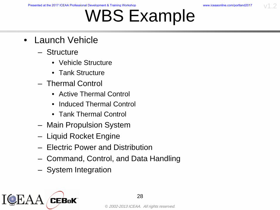
copy 2002-2013 ICEAA All rights reserved
v12
WBS Examplebull Launch Vehicle
ndash Structurebull Vehicle Structurebull Tank Structure
ndash Thermal Controlbull Active Thermal Controlbull Induced Thermal Controlbull Tank Thermal Control
ndash Main Propulsion Systemndash Liquid Rocket Enginendash Electric Power and Distributionndash Command Control and Data Handlingndash System Integration
28
Presented at the 2017 ICEAA Professional Development amp Training Workshop wwwiceaaonlinecomportland2017
copy 2002-2013 ICEAA All rights reserved
v12
WBS and Risk
29
Presented at the 2017 ICEAA Professional Development amp Training Workshop wwwiceaaonlinecomportland2017
copy 2002-2013 ICEAA All rights reserved
v12
Aggregating Riskbull This leads us to the issue of aggregating the risks across the
WBSbull For example if we want to determine the 70th percentile of the
overall cost risk distribution how do we proceed bull Note that we cannot simply add the 70th percentiles of each of
the cost risk distributionsbull We can add means and variances (taking correlation into
account more on that later) but that is all
Variance of Total Cost =
30
Mean of Total Cost = ( )E X E Xk
k
n
kk
n
kk
n
= = =aringaelig
egraveccediloumloslashdivide
= =aring aring1 1 1
m
Var X kk
n
=aringaelig
egraveccediloumloslashdivide1
= s r s skk
n
iji
j
i jj
n2
1 1
1
22+aring aringaring
= =
-
=
Presented at the 2017 ICEAA Professional Development amp Training Workshop wwwiceaaonlinecomportland2017
copy 2002-2013 ICEAA All rights reserved
v12
Percentiles Do Not Addbull As a notional example consider two independent normal
distributionsndash One distribution has mean equal to 100 and standard deviation
equal to 20ndash The second distribution has mean 300 and standard deviation of 80
bull The sum of two independent normally distributed random variables is also normally distributed
bull To combine the two distributions we add the means and add the variancesndash Total mean is
ndash Total standard deviation is
31
400300100 =+
8258020 22 raquo+
Presented at the 2017 ICEAA Professional Development amp Training Workshop wwwiceaaonlinecomportland2017
copy 2002-2013 ICEAA All rights reserved
v12
Percentiles Do Not Add (2)bull The 80th percentiles for the individual distributions are
117 and 367 respbull The 80th percentile of the combined distribution is
469 but the sum of the two 80th percentiles is 484bull To see why this is the case note that the percentiles
of a normal distribution are determined by the mean and the standard deviationndash The standard deviations are not added when normal distributions
are combined rather the variances are combinedndash Sum of variances is ndash The standard deviation of this sum is
32
22 ba +22 ba +
Presented at the 2017 ICEAA Professional Development amp Training Workshop wwwiceaaonlinecomportland2017
copy 2002-2013 ICEAA All rights reserved
v12
Percentiles Do Not Add (3)bull Since bull We can write
bull The left side of this inequality represents the risk of the combined distributions while the right side represents the sums of the individual risks
bull Combining two missions that are independent results in a diversification of riskndash The total portfolio is not as risky on a relative basis as each
individual project
33
2222 2 bababa ++lt+
baba +lt+ 22
Presented at the 2017 ICEAA Professional Development amp Training Workshop wwwiceaaonlinecomportland2017
copy 2002-2013 ICEAA All rights reserved
v12
Methods for Aggregating Riskbull Since percentiles do not add we have to find other
ways to aggregate riskbull One method is to use Monte Carlo simulationbull Unless cost risk is represented by normal
distributions for all WBS elements summing the means and variances does not result in a completely accurate depiction of overall system cost risk
bull The normal distribution is not a realistic distribution for representing risk in many or even most situations since regarding project risk more can go wrong than can go right which means the risk is NOT symmetric unlike the Gaussian bell curve
34
Presented at the 2017 ICEAA Professional Development amp Training Workshop wwwiceaaonlinecomportland2017
copy 2002-2013 ICEAA All rights reserved
v12
Unit III - Module 9 35
Monte Carlo Simulationfor Risk Analysis
bull When risk analysis is performed multiple risks are gatheredndash These risks may have various probability
distributions
bull Monte Carlo is the most commonly accepted way to produce an accurate characterization of the distribution of the combined effect of these many risksndash Using this distribution we can produce percentiles
for cost impacts due to risk occurrences
10
Presented at the 2017 ICEAA Professional Development amp Training Workshop wwwiceaaonlinecomportland2017
copy 2002-2013 ICEAA All rights reserved
v12
Monte Carlo Simulationbull Simulation is a means for solving problems that are
analytically intractablendash Involves repeated random sampling
bull It was developed during the Manhattan Project as a way to model the interactions inside an atom during nuclear fissionndash Allowed for more sophisticated mathematical modeling of atomic
phenomena
bull Most computer packages use pseudo-random number generators that produce seemingly random results from an initial seedndash Example is the linear congruential generator
36
( ) mbaXX nn mod1 +=+
Presented at the 2017 ICEAA Professional Development amp Training Workshop wwwiceaaonlinecomportland2017
copy 2002-2013 ICEAA All rights reserved
v12Using Random Numbers to Simulate Distributions
bull WBS cost risk is typically measured by a probability distributionbull The most common method for simulating a probability
distribution is the inverse methodbull This involve obtaining a simulated random value from a uniform
distribution and then inverting this through the cumulative distribution function (CDF) to obtain the simulated value
bull As an example for a uniform distribution on the interval [0100]
bull In this case the CDF random value of 05 translates to 10005 = 50
37
( )100
1=xf ( )
100xxF = ( ) xxF 1001 =-
Presented at the 2017 ICEAA Professional Development amp Training Workshop wwwiceaaonlinecomportland2017
copy 2002-2013 ICEAA All rights reserved
v12
Simulating a Triangular Distribution
bull For a triangular distribution with low = 0 most likely = 50 and high = 150 the CDF is given by
bull The inverse function is given by
38
( )iumliumlicirc
iumliumliacute
igrave
poundlt--
poundpound=
1505021
1500050
50015000
2
2
2
xxx
xxxF
( )iumliumlicirc
iumliumliacute
igrave
poundltdivideoslashouml
ccedilegraveaelig +--
poundpound=-
131
21
37501
250017500150
3107500
1
xx
xxxF
Presented at the 2017 ICEAA Professional Development amp Training Workshop wwwiceaaonlinecomportland2017
copy 2002-2013 ICEAA All rights reserved
v12
Simulating a Triangular Distribution (2)
bull If the simulated uniform value is equal to 02 the corresponding inverse value from the CDF inverse is approximately 387
39
0
01
02
03
04
05
06
07
08
09
1
0 30 60 90 120 150
Presented at the 2017 ICEAA Professional Development amp Training Workshop wwwiceaaonlinecomportland2017
copy 2002-2013 ICEAA All rights reserved
v12
Monte Carlo and the WBSbull Simulation involves repeated trials
40
WBS Draw1 2 3 4 5
System 2912 3566 4390 2954 4655 Sum
Structure 80 105 55 80 57 SumVehicle Structure 50 70 30 40 20Tank Structure 30 35 25 40 37
Thermal Control 32 36 35 29 33 SumActive Thermal Control 10 15 12 7 10Induced Thermal Control 12 14 13 14 14Tank Thermal Control 10 7 10 8 9
Main Propulsion System 100 150 125 140 100
Liquid Rocket Engine 1000 1100 1800 900 2200
Electric Power and Distribution 100 125 150 75 90
Command Control and Data Handling 200 250 225 230 275
System Integration 1400 1800 2000 1500 1900
Presented at the 2017 ICEAA Professional Development amp Training Workshop wwwiceaaonlinecomportland2017
copy 2002-2013 ICEAA All rights reserved
v12
Number of Trialsbull Monte Carlo involves a repeated number of trialsbull The greater the number of trials the more accurate the
simulation will approximate the overall cost risk behavior of the system
bull After 100 trials the histogram looks very jagged
41
Presented at the 2017 ICEAA Professional Development amp Training Workshop wwwiceaaonlinecomportland2017
copy 2002-2013 ICEAA All rights reserved
v12
Number of Trials (2)
42
1000 Trials
10000 Trials
50000 Trials Additional trials give a more accurate depiction of the final result
Presented at the 2017 ICEAA Professional Development amp Training Workshop wwwiceaaonlinecomportland2017
copy 2002-2013 ICEAA All rights reserved
v12
Number of Trials (3)bull If we want to simulate the underlying
mean within 1 with 95 confidence for example then we require
43
divideoslash
oumlccedilegrave
aelig poundpound-
=
dividedividedivide
oslash
ouml
ccedilccedilccedil
egrave
aeligpound
-pound
-=
divideoslashouml
ccedilegraveaelig poundpound=
nZ
n
nnX
n
X
n
n
011
010Pr
011
010Pr
011990Pr950
___
___
sm
sm
sm
sm
sm
mm
Presented at the 2017 ICEAA Professional Development amp Training Workshop wwwiceaaonlinecomportland2017
copy 2002-2013 ICEAA All rights reserved
v12
Number of Trials (4)bull This means that the number of trials required is determined by
bull Solving for n we find that at least
trials are neededbull Note that this term involves the coefficient of variation of the
distribution which means that distributions with less dispersion require fewer trials to accurate simulate
44
96101
=ns
m
ms41638
Presented at the 2017 ICEAA Professional Development amp Training Workshop wwwiceaaonlinecomportland2017
copy 2002-2013 ICEAA All rights reserved
v12
Number of Trials (5)bull Simulating percentiles requires more trials than for simulating
meansbull Let Pn represent the number of trials in the sample at or below
the 70th percentile of the underlying distribution (suppose this is known)
bull By the Central Limit Theorem Pnn follows a normal distribution with mean equal to the 70th percentile and variance equal to
bull By a similar process for the mean we find that the number of trials needed to simulate the 70th percentile within 1 with 95 confidence is
45
( )n
FF 700700 1-
n
n
PPn -41638
Presented at the 2017 ICEAA Professional Development amp Training Workshop wwwiceaaonlinecomportland2017
copy 2002-2013 ICEAA All rights reserved
v12
Number of Trials (6)bull If Pn 070 for all n then n is approximately
bull For the sake of comparison suppose CV = 03 (reasonable approximation for hardware development) then the number of trials needed to simulate the mean with the same accuracy is then ldquoonlyrdquo 11525
bull More trials are needed to accurately simulate percentiles than means
46
( ) 46416703041638
70704168341638 =divide
oslashouml
ccedilegraveaelig=divide
oslashouml
ccedilegraveaelig -
=-
nnn
PPn
n
n
Presented at the 2017 ICEAA Professional Development amp Training Workshop wwwiceaaonlinecomportland2017
copy 2002-2013 ICEAA All rights reserved
v12
Methods of Simulationbull Monte Carlo simulation is a standard term for
simulationbull However there is an improvement on Monte Carlo
that improves the accuracy of the results of a simulation for a given number of trials
bull This method is call the Latin Hypercube approach to simulationndash Similar to Monte Carlo but an equal number of draws are taken
from a set of subintervals for example dividing the interval (01) into [00001) [0102)hellip [0910]
ndash Instead of 10 trials from [01] we have one trial from each subinterval
ndash Rough rule of thumb is Latin Hypercube takes 30 fewer trials to achieve similar accuracy to Monte Carlo
47
Presented at the 2017 ICEAA Professional Development amp Training Workshop wwwiceaaonlinecomportland2017
copy 2002-2013 ICEAA All rights reserved
v12
Probability Model ndash Correlationbull Correlation exists between work breakdown structure
(WBS) cost element costs and between cost and schedule
bull Correlation is a necessary consideration in cost risk analysis
bull Correlation is a number that can vary between -1 and +1 and represents the strength of the relationship between the two variablesndash If both variable have a tendency to move in the same direction
correlation is positivendash If when one variable increases the other tends to decrease and
vice-versa the correlation between the two variables is negative
Presented at the 2017 ICEAA Professional Development amp Training Workshop wwwiceaaonlinecomportland2017
copy 2002-2013 ICEAA All rights reserved
v12
Correlation And Causationbull Note that correlation is not causation however
causation implies correlationndash For example shark attacks and ice cream sales at the beach
bull For example for a launch vehicle structure increasing the diameter will not only result in an increase in the structures cost but will also result in higher costs for thermal coating (paint etc)
bull Also simply because two subsystems do not appear to be related does not mean they are not correlatedndash For example structures and computer equipment seemingly
have little relation to one another however an external factor such as a funding cut or a strike will impact all subsystems leading to delays and increasing cost across the board
ndash Thus everything in a WBS has some correlationUnit III - Module 9 49
Presented at the 2017 ICEAA Professional Development amp Training Workshop wwwiceaaonlinecomportland2017
copy 2002-2013 ICEAA All rights reserved
v12
The Importance of Correlationbull Percent that total cost standard deviation is underestimated
when correlation assumed to be 0 instead of r given nWBS elements
Unit III - Module 9 5050
0
20
40
60
80
100
0 01 02 03 04 05 06 07 08 09 1Actual Correlation
Perce
nt Un
deres
timate
d
n = 10
n = 30
n = 100n = 1000
0
20
40
60
80
100
0 01 02 03 04 05 06 07 08 09 1Actual Correlation
Perce
nt Un
deres
timate
d
n = 10
n = 30
n = 100n = 1000
Reference 32nd Annual DOD Cost Analysis Symposium Advanced Training Session ldquoWhy Correlation Matters in Cost Estimatingrdquo Stephen A Book
Presented at the 2017 ICEAA Professional Development amp Training Workshop wwwiceaaonlinecomportland2017
copy 2002-2013 ICEAA All rights reserved
v12
The Importance of Correlation (2)bull For example if correlation is assumed to be 0 for all
elements in a 30 element WBS and the actual correlation is 20 then the total cost standard deviation is underestimated by 60
bull For example assume the total cost is modeled as a normal distribution with mean = 100
bull If correlation is assumed to be zero with total cost standard deviation = 12 when correlation is actually 20 then the true underlying standard deviation is actually 30
bull 70th percentile with zero correlation assumption is 106
bull 70th percentile with 20 correlation is 116 Unit III - Module 9 51
Presented at the 2017 ICEAA Professional Development amp Training Workshop wwwiceaaonlinecomportland2017
copy 2002-2013 ICEAA All rights reserved
v12
Measures of Correlationbull Two measures of correlation are commonly used in
cost risk analysesndash Pearsonrsquos product-moment correlation coefficient ndash Spearmanrsquos rank correlation coefficient
bull Garvey and others recommend using Pearsonrsquos product-moment correlation coefficient correlation for cost risk analysesndash Method of moments uses this but there are two options in
simulationndash Popular simulation packages like Risk and Crystal Ball use
rank correlation but in practice this has been found to make little difference
ndash Pearson product-moment correlation has been incorporated into Risk+
52
Presented at the 2017 ICEAA Professional Development amp Training Workshop wwwiceaaonlinecomportland2017
copy 2002-2013 ICEAA All rights reserved
v12
Pearson Correlationbull Pearsonrsquos product-moment correlation measures
degree of linearity between two random variables bull If two random variables are perfectly linear (eg Y =
aX + b) with positive slope then the Pearson product-moment correlation between X and Y denoted by rXY is +1
53
X X
Y Y Y
XNegative Correlation Positive Correlation No Correlation
middotmiddot
middotmiddot
middotmiddot middotmiddot
middotmiddot
middot
middot
middotmiddotmiddot
middotmiddot
middotmiddot
middotmiddot middot
middot
middot
middotmiddotmiddotmiddotmiddotmiddotmiddotmiddot
middotmiddotmiddotmiddot
middotmiddot
middotmiddot middotmiddotmiddotmiddot
middotmiddotmiddot
middotmiddotmiddotmiddot
middotmiddotmiddot
middotmiddotmiddot
middotmiddot
middot
middot middotmiddot
middot middotmiddotmiddotmiddot middotmiddot middot middotmiddot middot middot
middotmiddot middot
middotmiddotmiddotmiddotmiddot middot middotmiddot
middotmiddot
middot
middotmiddot
middotmiddot middot
middot middot middot
middotmiddot middot
middotmiddotmiddot
middotmiddot
middot middot
Presented at the 2017 ICEAA Professional Development amp Training Workshop wwwiceaaonlinecomportland2017
copy 2002-2013 ICEAA All rights reserved
v12
Spearman Correlationbull Spearmanrsquos rank correlation measures the
monotonicity between two random variablesbull If two random variables are perfectly monotonically
increasing (eg Y = X2) then the Spearman rank correlation denoted by rXY is +1
bull The two measures can be significantly different
54
10 20 30 40 50 60
100
200
300
096 097 098 099 1
1
060
020
040
080
Eff
ort (
Staf
f-M
onth
s)
Software Size I KDSI
y = 28z12y
z x
yy = x100
0 pound x pound 1
Figure 5-9A Figure 5-9B
Pearson Correlation = 09976 Rank Correlation = 1
Pearson Correlation = 024 Rank Correlation = 1
X(x ) ~ Unif(01)
Reference Probability Methods for Cost Uncertainty Analysis A Systems Engineering Perspective Paul R Garvey
Presented at the 2017 ICEAA Professional Development amp Training Workshop wwwiceaaonlinecomportland2017
copy 2002-2013 ICEAA All rights reserved
v12
Unit III - Module 9 55
200
250
300
350
400
1000 1200 1400 1600 1800 2000
Recurring Production
SEPM
200
250
300
350
400
1000 1200 1400 1600 1800 2000
Recurring Production
SEPM
Functional Correlationbull Old No Functional
Correlation Simulation run with WBS items entered as values
bull New Simulation run with functional dependencies entered as they are in cost model
CorrelatedNot Correlated
Note shift of mean and increased variability
Presented at the 2017 ICEAA Professional Development amp Training Workshop wwwiceaaonlinecomportland2017
copy 2002-2013 ICEAA All rights reserved
v12
Risk Measuresbull ldquoWestern Europe conquered the word because of a
technological revolution that started because of attempts to measure the worldrdquo ndash Phillipe Jorion ndash In the same way attempts to measure risk will lead to better project
managementbull Risk management for DoD and NASA agencies focuses
primarily on funding projects to a single percentile ndash NASA policy explicitly mentions 70 and 50ndash This is known as ldquoValue at Riskrdquo and is prevalent in the banking and
financial industry
56
Presented at the 2017 ICEAA Professional Development amp Training Workshop wwwiceaaonlinecomportland2017
copy 2002-2013 ICEAA All rights reserved
v12
Value at Risk (VaR)bull VaR is a percentile of the cost risk
distributionndash VaR funding at the 70th percentile means that
there is a 30 chance of final project cost exceeding the funded amount (budget)
bull VaR has some meritsndash Common measure can be used to compare
different projects and programsndash Easily understood by senior managers and
decision makers
57
Presented at the 2017 ICEAA Professional Development amp Training Workshop wwwiceaaonlinecomportland2017
copy 2002-2013 ICEAA All rights reserved
v12
Why 70th or 80th Percentilebull Typical policy guidance involves funding at the 70th or 80th
percentile Why fund as such a low percentilebull There is some incentive to not over-fundbull For a normal distribution an inflection point occurs near the 80th
percentile meaning that for values above 80 confidence achieving higher levels of confidence can only be achieved by spending greater dollar amounts at an increasing rate
58
-05-04-03-02-01
00102030405
0 05 1 15 2 25 3
Standard Deviations from Mean
Normal Distribution
First DerivativeSlopeVelocity
Second DerivativeConvexityAcceleration
Inflection point at one standard deviation above the mean (~84th
percentile)
Presented at the 2017 ICEAA Professional Development amp Training Workshop wwwiceaaonlinecomportland2017
copy 2002-2013 ICEAA All rights reserved
v12
Funding Above Inflection Pointsbull As the percentile goes above the 80th percentile the amount
needed to achieve that higher level of confidence begins to increase at an increasing rate as is evident from the graph
59
0
10
20
30
40
50
60
70
50 55 60 65 70 75 80 85 90 95 100
$ Ab
ove
MEa
n to
Ach
ieve
Per
cent
ile
Percentile (Confidence Level)
Presented at the 2017 ICEAA Professional Development amp Training Workshop wwwiceaaonlinecomportland2017
copy 2002-2013 ICEAA All rights reserved
v12
Why Budget to the 70th or 80thbull Government projects are funded at the 70th or 80th percentilesbull Why not the 90th or 99th percentile Wonrsquot that help prevent
overrunsndash As we have seen percentiles do not add across programs
bull The sum of the 80th percentiles does NOT equal the total 80th percentile
ndash This is because the individual programs are riskier than the entire suite of missions
bull Known as the ldquoPortfolio effectrdquo (more or this later)
ndash Funding at the 80th gives confidence that the entire portfolio will be adequately funded
bull And since there is an inflection point near the 80th percentile funding above that level quickly becomes cost prohibitive
60
Presented at the 2017 ICEAA Professional Development amp Training Workshop wwwiceaaonlinecomportland2017
copy 2002-2013 ICEAA All rights reserved
v12
Inflection Points for Lognormalbull For a lognormal the inflection point
variesndash Coefficient of variation equal to 10 equates to an
inflection point at the 70th percentile
61
0
10
20
30
40
50
60
70
050 060 070 080 090 100
Coef
ficen
t of V
aria
tion
Percentile of the Inflection Point
Presented at the 2017 ICEAA Professional Development amp Training Workshop wwwiceaaonlinecomportland2017
copy 2002-2013 ICEAA All rights reserved
v12
Issues with Percentile Fundingbull However risk management does not stop at a
specific percentilendash What happens when the 70th percentile is exceeded
bull Any effective risk management policy should prescribe what happens after a bad event occursndash With VaR we only know when a bad event has occurred ndash Also funding at a relatively low level means we have no true
sense of the real risks that should be guarded against
62
Presented at the 2017 ICEAA Professional Development amp Training Workshop wwwiceaaonlinecomportland2017
copy 2002-2013 ICEAA All rights reserved
v12
ldquoHere There Be Dragonsrdquobull On old maps uncharted territory was often
marked with monsters or dragons
63
A section of the Carta Marina by Olaus Magnus 16th Century
Presented at the 2017 ICEAA Professional Development amp Training Workshop wwwiceaaonlinecomportland2017
copy 2002-2013 ICEAA All rights reserved
v12
Distribution Comparisonbull Four different distributions with the same 70th
percentile
bull Should we expect the tails to be similar
64
0
10
20
30
40
50
60
70
80
0 100 200 300 400 500 600
Perc
entil
eCo
nfid
ence
Lev
el
Triangular
Normal
Lognormal
Pareto
Presented at the 2017 ICEAA Professional Development amp Training Workshop wwwiceaaonlinecomportland2017
copy 2002-2013 ICEAA All rights reserved
v12Distribution Comparison Tail Behavior
bull The normal and triangular distributions have similar tails but the lognormal and Pareto have much fatter right tails
65
70
75
80
85
90
95
100
500 1500 2500 3500 4500 5500
Perc
entil
eCo
nfid
ence
Lev
el
Triangular
Normal
Lognormal
Pareto
Here There Be Dragons
Presented at the 2017 ICEAA Professional Development amp Training Workshop wwwiceaaonlinecomportland2017
copy 2002-2013 ICEAA All rights reserved
v12Distribution Comparison ndash Tail Behavior (Table)
bull There is significant tail risk for the lognormal and the Paretobull The 99th percentile for the Pareto is 1000 times greater than
the 70th percentilendash Risk seen in financial markets and in catastrophic risks like natural
disasters bull Four different projects follow the four different risk profiles seen
in this example should clearly have different risk management approaches but 70th percentile funding indicates the same risk management approach for all four
66
Percentile Triangular Normal Lognormal Pareto 70th $600 $600 $600 $600 80th $680 $660 $770 $1430 90th $770 $750 $1070 $5880 95th $840 $820 $1410 $23750 99th $930 $950 $2350 $600000
Presented at the 2017 ICEAA Professional Development amp Training Workshop wwwiceaaonlinecomportland2017
copy 2002-2013 ICEAA All rights reserved
v12Percentile Budgeting is Not Risk Management
bull Percentile budgeting ne effective risk management policybull Suppose that you are shopping for a new car You
mention that safety is your top concern The salesman says he has a great safe car available You ask about the air bags Do they work The salesman answers ldquoOf course Seventy percent of the time they work fine Only 30 of the time the air bags will fail to deployrdquo Would you buy such a car Hedge fund manager David Einhorn has stated ldquoRisk management is the air bag that must always work but only in the multi-sigma event where you have an accidentrdquo
67
Risk management is the air bag that must always work but only in the multi-sigma event where you
have an accident
Presented at the 2017 ICEAA Professional Development amp Training Workshop wwwiceaaonlinecomportland2017
copy 2002-2013 ICEAA All rights reserved
v12
Joint Confidence Level Analysisbull Schedules are risky toobull For 98 recent NASA missions average
schedule growth was 38ndash Not as high as cost growth but still significant
68
0
5
10
15
20
25
30
35
40
Schedule
Cost
Presented at the 2017 ICEAA Professional Development amp Training Workshop wwwiceaaonlinecomportland2017
copy 2002-2013 ICEAA All rights reserved
v12
Schedules Impact Costbull Changes in schedule can have enormous
impacts on cost ndash Schedule slips can lead to cost increases
bull Fixed programmatic costs must be paid on a regular basisndash Achieving schedule milestones early can result in cost
savings
bull Schedule is an important consideration in cost analysis including cost risk analysis
bull However we must be careful in correctly integrating cost and schedule riskndash Schedule is not simply an input but is dependent on many of
the same factors that drive cost
69
Presented at the 2017 ICEAA Professional Development amp Training Workshop wwwiceaaonlinecomportland2017
copy 2002-2013 ICEAA All rights reserved
v12
The Relationship of Cost to Schedulebull Cost and schedule are positively correlated
ndash A larger program with bigger scope with take longer to complete than a smaller simpler program
bull However longer schedules do not always equate to higher cost nor shorter schedules with lower costndash Highly compressed schedules relative to the
optimal schedule can lead to large overrunsbull Compressed schedules are commonplace for
many planetary missions
70
Presented at the 2017 ICEAA Professional Development amp Training Workshop wwwiceaaonlinecomportland2017
copy 2002-2013 ICEAA All rights reserved
v12The Impact of Schedule GrowthCompression on Cost
bull Compressed schedules lead to cost growth and based on existing research is actually more expensive than schedule slippages
71
0
20
40
60
80
100
120
140
160
-50 -25 0 25 50 75 100
Percentage Change in Schedule
Perc
enta
ge C
hang
e in
Cos
t due
to
Sche
dule
Cha
nge
Source Smart CB ldquoCost and Schedule Interrelationshipsrdquo 2007 NASA Cost Symposium
Presented at the 2017 ICEAA Professional Development amp Training Workshop wwwiceaaonlinecomportland2017
copy 2002-2013 ICEAA All rights reserved
v12Schedule as an Independent Variable
bull Why not simply add schedule as an input to cost-estimating relationships (CERs)
bull Schedule is often treated as an independent variable ndash schedules are often determined independently of cost considerationsndash Cost may not be considered explicitly although budgets and
schedules are determined based on scope and other common factors
bull In 2006 SAIC undertook a research task to determine the impact of schedule on cost and added schedule as an independent variable to the CERs in the NASAAir Force Cost Model (NAFCOM) to see if schedule provided any improvement in goodness of fit
72
Presented at the 2017 ICEAA Professional Development amp Training Workshop wwwiceaaonlinecomportland2017
copy 2002-2013 ICEAA All rights reserved
v12
Schedule is a Dependent Variablebull Since NAFCOM includes an exhaustive list of cost drivers the inclusion
of schedule should give an indication of whether there is any additional independent value added from schedule independent of the cost drivers
bull In the study schedule was added to 10 subsystem-level CERs
ndash In each case the addition of schedule did NOTimprove the goodness of fit and schedule was NOT found to be a statistically significant cost driver (given the presence of the other variables) for any of the 10 CERs
bull Standard errors for the CERs increased due to decrease in degrees of freedom
bull Thus schedule as an independent variable did not provide any additional explanation of variation in historical cost
bull This is because schedule is truly NOT an independent variable but a dependent variable and is a function of the same factors that drive cost
73
Presented at the 2017 ICEAA Professional Development amp Training Workshop wwwiceaaonlinecomportland2017
copy 2002-2013 ICEAA All rights reserved
v12
Incorporation of Schedule in Cost Risk
bull When using subjective methods care must be taken in applying schedule to cost risk analysis
bull Since schedule is a dependent variable treating it independently from other factors when assessing its impact on cost can lead to a double count of independent variables in the cost risk analysis
bull Direct inclusion of schedule in a cost risk analysis effectively doubles the influence of each cost driver
ndash Incorrectly leads to broader risk ranges
74
CostWeight
HeritageNewness
Technology Readiness Schedule
Presented at the 2017 ICEAA Professional Development amp Training Workshop wwwiceaaonlinecomportland2017
copy 2002-2013 ICEAA All rights reserved
v12Subjective Cost Risk Methods and Overinclusion of Risk Factors
bull Subjective methods are suitable when data are scarce or not availablebull However care must be taken not to treat correlated sources of risk
such as schedule as independent of each otherbull Example ndash a subjective risk analysis incorporated technology readiness
design risk requirements stability integration risk and schedule and treated each source of risk as independent
bull Risk triangle high value without schedule risk was 31 times the point estimate
bull Risk triangle high value with schedule risk added on top of other sources of risk treated independently was 34 times the point estimate
bull Risk triangle taking correlation between sources of risk into account in a rigorous statistical manner has a high value 15 times the point estimate less than half the effect when treating sources of risk as independent
75
Presented at the 2017 ICEAA Professional Development amp Training Workshop wwwiceaaonlinecomportland2017
copy 2002-2013 ICEAA All rights reserved
v12Fundamental Equation of Cost and Schedule Interrelationships
bull The Fundamental Equation of the Relationship Between Cost and Schedule is
Time = Moneybull This is a well known adage that time is money Your boss at
work may even mention this to you from time to time or if you are the boss you are all too aware of this iron law
bull Because time is money cost and schedule risk should be modeled jointly not with schedule as an independent cost driver
bull Note that cost and schedule are not perfectly correlatedndash Cost can sometimes ldquobuy downrdquo schedule extra money can be
spent to meet a deadline since in some cases additional effort to hasten the completion of a task
76
Presented at the 2017 ICEAA Professional Development amp Training Workshop wwwiceaaonlinecomportland2017
copy 2002-2013 ICEAA All rights reserved
v12How to (Correctly) Incorporate Schedule into Cost Risk Analysis
bull The best way to model cost and schedule risk is to develop a joint cost and schedule model based on the same data
bull Since such models are not currently available the next best approach is to model cost and schedule independently and then integrate cost and schedule risk analyses using joint probability distributions taking into account correlation between cost and schedulendash This approach pioneered by Paul Garvey and Steve Book is
considered industry best practicendash This is a practical method mathematically tractable and follows
naturally from the Fundamental Equation of Cost and Schedule Interrelationships
77
Book S A ldquoQuantifying the Relationship Between Cost and Schedulerdquo The Measurable News Winter 2007-2008 pp 11-15Garvey PR Probability Methods for Cost Uncertainty Analysis A Systems Engineering Perspective New York Marcel Dekker 2000 pp 308-335
Presented at the 2017 ICEAA Professional Development amp Training Workshop wwwiceaaonlinecomportland2017
copy 2002-2013 ICEAA All rights reserved
v12
Joint Lognormal and Normal Distributions
bull Cost and schedule are typically modeled as some combination of Normal and Lognormal probability distributionsndash Studies by The Aerospace Corporation the MITRE
Corporation Wyle Labs and SAIC have found that the Lognormal probability distribution almost always serves as a good model for both the schedule distribution and the cost distribution
ndash The Normal distribution may also be appropriate in some instances and depending upon the level of confidence at which budgets are set may even be more conservative and logically consistent than the Normal distribution
ndash Joint Lognormal and Normal distributions are defined by a pair of mean and standard deviations and a level of correlation between the two
78
Presented at the 2017 ICEAA Professional Development amp Training Workshop wwwiceaaonlinecomportland2017
copy 2002-2013 ICEAA All rights reserved
v12Modeling Cost and Schedule as a Bivariate Distribution
bull In the approach set forth by Book and Garvey cost risk is assessed and the top-level distribution is modeled as a Lognormal (or Normal) distribution schedule risk is assessed and the overall schedule risk is modeled as a Lognormal (or Normal) distribution
bull The two distributions are combined into a Bivariate distribution by assigning a correlation between the two and by treating the two distributions as the marginal distributions of a Bivariate Lognormal distributionndash Other combinations include a Bivariate Normal or a Bivariate
Normal-Lognormal
79
Presented at the 2017 ICEAA Professional Development amp Training Workshop wwwiceaaonlinecomportland2017
copy 2002-2013 ICEAA All rights reserved
v12Bivariate Lognormal Distribution for Cost and Schedule
bull Cost is often observed to be Lognormal when strong positive correlations are present among the systemrsquos WBS cost element costs
bull A systemrsquos schedule is often observed (from Monte Carlo simulations) to be Lognormal if it is the sum of many positively correlated schedule activities in an overall schedule network
bull If Lognormal distributions characterize a systemrsquos cost and schedule then the Bivariate Lognormal could serve as an assumed model of their joint distributionndash In this case the marginal distribution of each of cost and schedule is
Lognormalbull Other possibilities for modeling cost and schedule as a Bivariate
distribution include a Bivariate Normal or a Bivariate Normal-Lognormal distributionndash All these combinations are analytically tractable
80
Presented at the 2017 ICEAA Professional Development amp Training Workshop wwwiceaaonlinecomportland2017
copy 2002-2013 ICEAA All rights reserved
v12Bivariate Lognormal for Cost and Schedule
bull Contour Plots of a Bivariate Lognormal
81
Presented at the 2017 ICEAA Professional Development amp Training Workshop wwwiceaaonlinecomportland2017
copy 2002-2013 ICEAA All rights reserved
v12Correlation Between Cost and Schedule
bull Cost and schedule are positively correlated but not perfectly sondash For example it is possible to have a schedule underrun and a cost
overrunbull Based on cost and schedule growth data for 50 completed NASA
programs the correlation between development cost and development schedule is 70
82
00
200
400
600
800
1000
1200
-500 00 500 1000 1500 2000 2500Historical Cost Growth
Hist
oric
al S
ched
ule
Gro
wth
r = 715
Presented at the 2017 ICEAA Professional Development amp Training Workshop wwwiceaaonlinecomportland2017
copy 2002-2013 ICEAA All rights reserved
v12Correlation Between Cost and Schedule Caveats
bull Based on historical data recommended correlation between cost and schedule is 70 but this could be higher or lower depending upon program circumstancesndash If program is budget constrained cost and schedule will be
more highly correlated (go as you pay)ndash If program is schedule constrained cost and schedule will
have lower correlation perhaps even negative correlation ndash Smaller programs have smaller correlation between cost and
schedule riskbull Relatively easy to ldquohurry uprdquo and finish on time or even early if
needed
83
Presented at the 2017 ICEAA Professional Development amp Training Workshop wwwiceaaonlinecomportland2017
copy 2002-2013 ICEAA All rights reserved
v12
Conditional Confidence Levelsbull Given a programrsquos project schedule we can determine the cost
risk distribution conditional upon the given schedulebull Conditional cost S-curves are steeper than unconditional
(marginal) cost S-curves between some uncertainty has been removed because schedule is fixed
84
Presented at the 2017 ICEAA Professional Development amp Training Workshop wwwiceaaonlinecomportland2017
copy 2002-2013 ICEAA All rights reserved
v12
Joint Confidence Levelsbull Joint 65 confidence represents the probability of
achieving both 65 confidence in cost AND 65 confidence in schedulendash This is different than achieving 65 cost confidence alone
or achieving 65 schedule confidence alonebull Due to the imperfect correlation between cost and schedule it
is possible to achieve a 65 cost confidence with a lower level of schedule confidence
bull Restricting the schedule confidence thus requires additional $ to achieve a given level of confidence
85
X
Y
Possible Values for Which X gt a Possible Values for
Which X gt a and Y gt b
a
b
Presented at the 2017 ICEAA Professional Development amp Training Workshop wwwiceaaonlinecomportland2017
copy 2002-2013 ICEAA All rights reserved
v12Joint Confidence Levels Versus Cost Confidence Levels Only
bull Example of the differences between cost confidence schedule confidence conditional cost confidence and joint cost and schedule confidence
86
Joint Cost-Schedule Confidence Iso-Curves
Cost (RY$M)
Sche
dule
(Mon
ths)
65 Confidence
50 Confidence
70 Confidence
65 Cost Confidence AggressiveSchedule65 Cost ConfidenceScheduleGiven 65 Schedule ConfidenceUnconditional 65 CostConfidenceUnconditional 65 ScheduleConfidence
65 Cost Confidence 65 Joint Cost and Schedule
Confidence for 65 Schedule Confidence
Presented at the 2017 ICEAA Professional Development amp Training Workshop wwwiceaaonlinecomportland2017
copy 2002-2013 ICEAA All rights reserved
v12
Joint Cost and Schedule Confidence
bull Can examine pairs of cost and schedule that achieve a given level of confidence
bull Provides insights into the trade-offs between cost and schedule for a given level of confidencendash Possible to increase cost confidence by giving a
project more time in some instances or possible to ldquobuy downrdquo schedule
bull But these have limits and are shown in the iso-cost and schedule confidence curves
87
Presented at the 2017 ICEAA Professional Development amp Training Workshop wwwiceaaonlinecomportland2017
copy 2002-2013 ICEAA All rights reserved
v12Cost and Schedule Trade-offs for a Given Level of Joint Confidence
bull Hypothetical Example
88
Cost (RY$M)
Schedule (Months)
$100 48$99 48$89 49$87 50$85 51$85 52$84 53$83 55$83 55$83 56
Cost and Schedule 65 Confidence Iso-Curve
4748495051525354555657
$80 $82 $84 $86 $88 $90 $92 $94 $96 $98 $100
Cost (RY$ M)
Sche
dule
(Mon
ths)
Presented at the 2017 ICEAA Professional Development amp Training Workshop wwwiceaaonlinecomportland2017
copy 2002-2013 ICEAA All rights reserved
v12Policy Considerations for Confidence Levels
bull For large programs the difference between the amount of money needed to achieve 65 cost confidence independent of schedule and joint 65 cost and schedule confidence can represent hundreds of millions and even billions of dollars
89
Joint Cost-Schedule Confidence Iso-Curves
Cost (RY$M)
Sche
dule
(Mon
ths)
65 Confidence
65 Cost Confidence AggressiveSchedule
65 Cost ConfidenceScheduleGiven 65 Schedule Confidence
Unconditional 65 CostConfidence
Joint Cost and Schedule Confidence for 65 Cost Confidence and Program Baseline Schedule is Less Than 35
65 Cost Confidence Independent of Schedule Cost Needed to Achieve
Both 65 Joint Cost and Schedule Confidence for the Schedule with 65 Confidence
Presented at the 2017 ICEAA Professional Development amp Training Workshop wwwiceaaonlinecomportland2017
copy 2002-2013 ICEAA All rights reserved
v12
Copulasbull More generally any combination of distributions can
be used (more than just normal and lognormal)ndash Termed ldquocopulardquo from the Italian word for ldquocouplerdquondash Copulas are a way to combine marginal distributions of any
number and type into a joint distributionbull More formally a copula is a multivariate joint distribution defined
on the n-dimensional unit cube [0 1]n such that every marginal distribution is uniform on the interval [0 1]
bull (The bivariate form of) Sklarrsquos theorem states that for any bivariate distribution function H(x y) let F(x) = H(x infin) and G(y) = H(infin y) be the univariate marginal probability distribution functions Then there exists a copula C such that H(xy)=C(F(x)G(y))
ndash Copulas are widely used in risk management for investments and insurance
bull Considered industry best practice (Li 2000)bull Marketed as part of JP Morganrsquos CreditMetrics suite of tools
(Gupton et Al 1997)90
Presented at the 2017 ICEAA Professional Development amp Training Workshop wwwiceaaonlinecomportland2017
copy 2002-2013 ICEAA All rights reserved
v12Parametric Joint Cost and Schedule Analysis
bull A parametric model based on a consistent data set with a set of overlapping cost and schedule drivers is a cleaner way to model cost and schedule
91
CostWeight
HeritageNewness
Technology Readiness
Schedule
0
20
40
60
80
100
Confidence
Joint Cost and Schedule Confidence
Schedule
Cost
Lognormal Distribution PDF and CDF
0102030405060708090100
200 300 400 500 600 700 800 900 1000Cost $
Con
fiden
ce L
evel
0
00002
00004
00006
00008
0001
00012
00014
00016
Prob
abili
ty D
ensi
ty
CDFPDF
Lognormal Distribution PDF and CDF
0102030405060708090100
200 300 400 500 600 700 800 900 1000Cost $
Con
fiden
ce L
evel
0
00002
00004
00006
00008
0001
00012
00014
00016
Prob
abili
ty D
ensi
ty
CDFPDF
Presented at the 2017 ICEAA Professional Development amp Training Workshop wwwiceaaonlinecomportland2017
copy 2002-2013 ICEAA All rights reserved
v12Parametric Joint Cost and Schedule Analysis (2)
bull Joint cost and schedule risk analysis produced naturally by the integrated modelndash Addresses several issues with the copula
approachbull Tail dependencybull Correlation ndash no need to assign correlation
between cost and schedulebull Consistency of cost and schedule models
92
Presented at the 2017 ICEAA Professional Development amp Training Workshop wwwiceaaonlinecomportland2017
copy 2002-2013 ICEAA All rights reserved
v12
Resource-Loaded Schedulesbull Involves assigning cost and schedule risks to a resource-loaded schedule
networkbull Bottom-up approach
ndash More labor intensive than parametrics but can also provide more insight
ndash Can answer questions than parametric typically cannot such as how much do reserve requirements decrease if a specific risk is retired
bull Currently being implemented in Constellation programbull Has same issue as all bottom-up models hard to count all the risks and model
them discretely
ndash As a result there is a tendency to reflect less risk than indicated by history
ndash ldquoThere are more things in heaven and earth Horatio than are dreamt of in your philosophyrdquo William Shakespeare Hamlet Act I Scene V
93
Presented at the 2017 ICEAA Professional Development amp Training Workshop wwwiceaaonlinecomportland2017
copy 2002-2013 ICEAA All rights reserved
v12Resource-Loaded Schedules Vs Parametrics
bull Parametric most appropriate for early estimatesndash But also good for high-level checks as project progresses
bull As plans take shape lower level modeling may be more appropriate
94 1
CONCEPTUALDEVELOPMENT
PROJECTDEFINITION DESIGN DEVELOPMENT OPERATIONS
PARAMETRIC PARAMETRIC
ANALOGY
ENGINEERING (Bottoms Up)
$PARAMETRIC
DETAILED
$
Pre Phase A Phase B Phase CDPhase A Phase EPre Phase A Phase B Phase CDPhase A Phase E
Risk = f(Cost Estimating Relationship Inputs eg mass power data rate TRL new design etc)
Risk = f(cost and schedule variation of the analogous elements)
Risk = f(variation of detailed inputs eg labor hours rates materials etc)
Presented at the 2017 ICEAA Professional Development amp Training Workshop wwwiceaaonlinecomportland2017
copy 2002-2013 ICEAA All rights reserved
v12
Resource-Loaded Schedulesbull Methodology has been demonstrated in other
industriesndash Construction oil and gasndash Analysis has not been traditionally done on highly uncertain
complex development projects bull Methodology focuses on project baseline schedule
ndash In baseline schedule all tasks are resource loaded to represent a baseline schedule and cost standpoint
ndash Resource loaded schedule is ldquorolledrdquo up to a manageable level
ndash Based on the risk and uncertainties identified schedule distributions are applied to each rolled up task
ndash Cost uncertainties are also applied to rolled up tasksbull Uncertainties include labor rate man power etc
ndash A Monte Carlo simulation is run to develop joint cost-schedule distributions
95
Presented at the 2017 ICEAA Professional Development amp Training Workshop wwwiceaaonlinecomportland2017
copy 2002-2013 ICEAA All rights reserved
v12
Unit III - Module 9 96
Execution ndash Cross Checksbull Means The mean cost growth factor for WBS items
can be compared to history as a way to cross check results
bull CVs The CV of the cost growth factors for WBS items can be compared to history as a way to cross check results
bull Inputs Checks are performed on inputs or other parameters to see if historical values are in line with program assumptionsndash Example Historical risk scores can be compared to program
risk scores to see if risk assessors are being realistic and to see if the underlying database is representative of the program
11
Presented at the 2017 ICEAA Professional Development amp Training Workshop wwwiceaaonlinecomportland2017
- Cost and Schedule Risk Analysis Basic
- Acknowledgments
- Unit Index
- Risk Overview
- Agenda
- Introduction
- Risk Analysis Terms
- Are Our Costs Realistic
- Historical Cost Growth
- Sources of Cost Risk
- Point Estimates of Cost
- Types of Risk
- Point Estimates Vs Risk Estimates
- Cost Risk and Probability
- Probability Model ndash Distribution
- Probability Model ndash Distribution
- Probability ndash Top-Level Distribution
- S-Curves and Confidence Levels
- Example ndash Normal Distribution
- Confidence Levels
- Measuring Parametric Model Uncertainty
- Parametric Model Example
- Weight Uncertainty
- Estimating Uncertainty
- Estimating Uncertainty (2)
- Estimating Uncertainty (3)
- Aggregating Risk
- WBS Example
- WBS and Risk
- Aggregating Risk
- Percentiles Do Not Add
- Percentiles Do Not Add (2)
- Percentiles Do Not Add (3)
- Methods for Aggregating Risk
- Monte Carlo Simulationfor Risk Analysis
- Monte Carlo Simulation
- Using Random Numbers to Simulate Distributions
- Simulating a Triangular Distribution
- Simulating a Triangular Distribution (2)
- Monte Carlo and the WBS
- Number of Trials
- Number of Trials (2)
- Number of Trials (3)
- Number of Trials (4)
- Number of Trials (5)
- Number of Trials (6)
- Methods of Simulation
- Probability Model ndash Correlation
- Correlation And Causation
- The Importance of Correlation
- The Importance of Correlation (2)
- Measures of Correlation
- Pearson Correlation
- Spearman Correlation
- Functional Correlation
- Risk Measures
- Value at Risk (VaR)
- Why 70th or 80th Percentile
- Funding Above Inflection Points
- Why Budget to the 70th or 80th
- Inflection Points for Lognormal
- Issues with Percentile Funding
- ldquoHere There Be Dragonsrdquo
- Distribution Comparison
- Distribution Comparison Tail Behavior
- Distribution Comparison ndash Tail Behavior (Table)
- Percentile Budgeting is Not Risk Management
- Joint Confidence Level Analysis
- Schedules Impact Cost
- The Relationship of Cost to Schedule
- The Impact of Schedule GrowthCompression on Cost
- Schedule as an Independent Variable
- Schedule is a Dependent Variable
- Incorporation of Schedule in Cost Risk
- Subjective Cost Risk Methods and Overinclusion of Risk Factors
- Fundamental Equation of Cost and Schedule Interrelationships
- How to (Correctly) Incorporate Schedule into Cost Risk Analysis
- Joint Lognormal and Normal Distributions
- Modeling Cost and Schedule as a Bivariate Distribution
- Bivariate Lognormal Distribution for Cost and Schedule
- Bivariate Lognormal for Cost and Schedule
- Correlation Between Cost and Schedule
- Correlation Between Cost and Schedule Caveats
- Conditional Confidence Levels
- Joint Confidence Levels
- Joint Confidence Levels Versus Cost Confidence Levels Only
- Joint Cost and Schedule Confidence
- Cost and Schedule Trade-offs for a Given Level of Joint Confidence
- Policy Considerations for Confidence Levels
- Copulas
- Parametric Joint Cost and Schedule Analysis
- Parametric Joint Cost and Schedule Analysis (2)
- Resource-Loaded Schedules
- Resource-Loaded Schedules Vs Parametrics
- Resource-Loaded Schedules
- Execution ndash Cross Checks
-
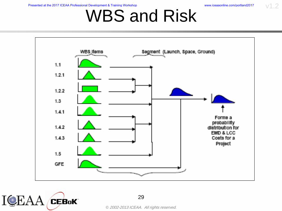
copy 2002-2013 ICEAA All rights reserved
v12
WBS and Risk
29
Presented at the 2017 ICEAA Professional Development amp Training Workshop wwwiceaaonlinecomportland2017
copy 2002-2013 ICEAA All rights reserved
v12
Aggregating Riskbull This leads us to the issue of aggregating the risks across the
WBSbull For example if we want to determine the 70th percentile of the
overall cost risk distribution how do we proceed bull Note that we cannot simply add the 70th percentiles of each of
the cost risk distributionsbull We can add means and variances (taking correlation into
account more on that later) but that is all
Variance of Total Cost =
30
Mean of Total Cost = ( )E X E Xk
k
n
kk
n
kk
n
= = =aringaelig
egraveccediloumloslashdivide
= =aring aring1 1 1
m
Var X kk
n
=aringaelig
egraveccediloumloslashdivide1
= s r s skk
n
iji
j
i jj
n2
1 1
1
22+aring aringaring
= =
-
=
Presented at the 2017 ICEAA Professional Development amp Training Workshop wwwiceaaonlinecomportland2017
copy 2002-2013 ICEAA All rights reserved
v12
Percentiles Do Not Addbull As a notional example consider two independent normal
distributionsndash One distribution has mean equal to 100 and standard deviation
equal to 20ndash The second distribution has mean 300 and standard deviation of 80
bull The sum of two independent normally distributed random variables is also normally distributed
bull To combine the two distributions we add the means and add the variancesndash Total mean is
ndash Total standard deviation is
31
400300100 =+
8258020 22 raquo+
Presented at the 2017 ICEAA Professional Development amp Training Workshop wwwiceaaonlinecomportland2017
copy 2002-2013 ICEAA All rights reserved
v12
Percentiles Do Not Add (2)bull The 80th percentiles for the individual distributions are
117 and 367 respbull The 80th percentile of the combined distribution is
469 but the sum of the two 80th percentiles is 484bull To see why this is the case note that the percentiles
of a normal distribution are determined by the mean and the standard deviationndash The standard deviations are not added when normal distributions
are combined rather the variances are combinedndash Sum of variances is ndash The standard deviation of this sum is
32
22 ba +22 ba +
Presented at the 2017 ICEAA Professional Development amp Training Workshop wwwiceaaonlinecomportland2017
copy 2002-2013 ICEAA All rights reserved
v12
Percentiles Do Not Add (3)bull Since bull We can write
bull The left side of this inequality represents the risk of the combined distributions while the right side represents the sums of the individual risks
bull Combining two missions that are independent results in a diversification of riskndash The total portfolio is not as risky on a relative basis as each
individual project
33
2222 2 bababa ++lt+
baba +lt+ 22
Presented at the 2017 ICEAA Professional Development amp Training Workshop wwwiceaaonlinecomportland2017
copy 2002-2013 ICEAA All rights reserved
v12
Methods for Aggregating Riskbull Since percentiles do not add we have to find other
ways to aggregate riskbull One method is to use Monte Carlo simulationbull Unless cost risk is represented by normal
distributions for all WBS elements summing the means and variances does not result in a completely accurate depiction of overall system cost risk
bull The normal distribution is not a realistic distribution for representing risk in many or even most situations since regarding project risk more can go wrong than can go right which means the risk is NOT symmetric unlike the Gaussian bell curve
34
Presented at the 2017 ICEAA Professional Development amp Training Workshop wwwiceaaonlinecomportland2017
copy 2002-2013 ICEAA All rights reserved
v12
Unit III - Module 9 35
Monte Carlo Simulationfor Risk Analysis
bull When risk analysis is performed multiple risks are gatheredndash These risks may have various probability
distributions
bull Monte Carlo is the most commonly accepted way to produce an accurate characterization of the distribution of the combined effect of these many risksndash Using this distribution we can produce percentiles
for cost impacts due to risk occurrences
10
Presented at the 2017 ICEAA Professional Development amp Training Workshop wwwiceaaonlinecomportland2017
copy 2002-2013 ICEAA All rights reserved
v12
Monte Carlo Simulationbull Simulation is a means for solving problems that are
analytically intractablendash Involves repeated random sampling
bull It was developed during the Manhattan Project as a way to model the interactions inside an atom during nuclear fissionndash Allowed for more sophisticated mathematical modeling of atomic
phenomena
bull Most computer packages use pseudo-random number generators that produce seemingly random results from an initial seedndash Example is the linear congruential generator
36
( ) mbaXX nn mod1 +=+
Presented at the 2017 ICEAA Professional Development amp Training Workshop wwwiceaaonlinecomportland2017
copy 2002-2013 ICEAA All rights reserved
v12Using Random Numbers to Simulate Distributions
bull WBS cost risk is typically measured by a probability distributionbull The most common method for simulating a probability
distribution is the inverse methodbull This involve obtaining a simulated random value from a uniform
distribution and then inverting this through the cumulative distribution function (CDF) to obtain the simulated value
bull As an example for a uniform distribution on the interval [0100]
bull In this case the CDF random value of 05 translates to 10005 = 50
37
( )100
1=xf ( )
100xxF = ( ) xxF 1001 =-
Presented at the 2017 ICEAA Professional Development amp Training Workshop wwwiceaaonlinecomportland2017
copy 2002-2013 ICEAA All rights reserved
v12
Simulating a Triangular Distribution
bull For a triangular distribution with low = 0 most likely = 50 and high = 150 the CDF is given by
bull The inverse function is given by
38
( )iumliumlicirc
iumliumliacute
igrave
poundlt--
poundpound=
1505021
1500050
50015000
2
2
2
xxx
xxxF
( )iumliumlicirc
iumliumliacute
igrave
poundltdivideoslashouml
ccedilegraveaelig +--
poundpound=-
131
21
37501
250017500150
3107500
1
xx
xxxF
Presented at the 2017 ICEAA Professional Development amp Training Workshop wwwiceaaonlinecomportland2017
copy 2002-2013 ICEAA All rights reserved
v12
Simulating a Triangular Distribution (2)
bull If the simulated uniform value is equal to 02 the corresponding inverse value from the CDF inverse is approximately 387
39
0
01
02
03
04
05
06
07
08
09
1
0 30 60 90 120 150
Presented at the 2017 ICEAA Professional Development amp Training Workshop wwwiceaaonlinecomportland2017
copy 2002-2013 ICEAA All rights reserved
v12
Monte Carlo and the WBSbull Simulation involves repeated trials
40
WBS Draw1 2 3 4 5
System 2912 3566 4390 2954 4655 Sum
Structure 80 105 55 80 57 SumVehicle Structure 50 70 30 40 20Tank Structure 30 35 25 40 37
Thermal Control 32 36 35 29 33 SumActive Thermal Control 10 15 12 7 10Induced Thermal Control 12 14 13 14 14Tank Thermal Control 10 7 10 8 9
Main Propulsion System 100 150 125 140 100
Liquid Rocket Engine 1000 1100 1800 900 2200
Electric Power and Distribution 100 125 150 75 90
Command Control and Data Handling 200 250 225 230 275
System Integration 1400 1800 2000 1500 1900
Presented at the 2017 ICEAA Professional Development amp Training Workshop wwwiceaaonlinecomportland2017
copy 2002-2013 ICEAA All rights reserved
v12
Number of Trialsbull Monte Carlo involves a repeated number of trialsbull The greater the number of trials the more accurate the
simulation will approximate the overall cost risk behavior of the system
bull After 100 trials the histogram looks very jagged
41
Presented at the 2017 ICEAA Professional Development amp Training Workshop wwwiceaaonlinecomportland2017
copy 2002-2013 ICEAA All rights reserved
v12
Number of Trials (2)
42
1000 Trials
10000 Trials
50000 Trials Additional trials give a more accurate depiction of the final result
Presented at the 2017 ICEAA Professional Development amp Training Workshop wwwiceaaonlinecomportland2017
copy 2002-2013 ICEAA All rights reserved
v12
Number of Trials (3)bull If we want to simulate the underlying
mean within 1 with 95 confidence for example then we require
43
divideoslash
oumlccedilegrave
aelig poundpound-
=
dividedividedivide
oslash
ouml
ccedilccedilccedil
egrave
aeligpound
-pound
-=
divideoslashouml
ccedilegraveaelig poundpound=
nZ
n
nnX
n
X
n
n
011
010Pr
011
010Pr
011990Pr950
___
___
sm
sm
sm
sm
sm
mm
Presented at the 2017 ICEAA Professional Development amp Training Workshop wwwiceaaonlinecomportland2017
copy 2002-2013 ICEAA All rights reserved
v12
Number of Trials (4)bull This means that the number of trials required is determined by
bull Solving for n we find that at least
trials are neededbull Note that this term involves the coefficient of variation of the
distribution which means that distributions with less dispersion require fewer trials to accurate simulate
44
96101
=ns
m
ms41638
Presented at the 2017 ICEAA Professional Development amp Training Workshop wwwiceaaonlinecomportland2017
copy 2002-2013 ICEAA All rights reserved
v12
Number of Trials (5)bull Simulating percentiles requires more trials than for simulating
meansbull Let Pn represent the number of trials in the sample at or below
the 70th percentile of the underlying distribution (suppose this is known)
bull By the Central Limit Theorem Pnn follows a normal distribution with mean equal to the 70th percentile and variance equal to
bull By a similar process for the mean we find that the number of trials needed to simulate the 70th percentile within 1 with 95 confidence is
45
( )n
FF 700700 1-
n
n
PPn -41638
Presented at the 2017 ICEAA Professional Development amp Training Workshop wwwiceaaonlinecomportland2017
copy 2002-2013 ICEAA All rights reserved
v12
Number of Trials (6)bull If Pn 070 for all n then n is approximately
bull For the sake of comparison suppose CV = 03 (reasonable approximation for hardware development) then the number of trials needed to simulate the mean with the same accuracy is then ldquoonlyrdquo 11525
bull More trials are needed to accurately simulate percentiles than means
46
( ) 46416703041638
70704168341638 =divide
oslashouml
ccedilegraveaelig=divide
oslashouml
ccedilegraveaelig -
=-
nnn
PPn
n
n
Presented at the 2017 ICEAA Professional Development amp Training Workshop wwwiceaaonlinecomportland2017
copy 2002-2013 ICEAA All rights reserved
v12
Methods of Simulationbull Monte Carlo simulation is a standard term for
simulationbull However there is an improvement on Monte Carlo
that improves the accuracy of the results of a simulation for a given number of trials
bull This method is call the Latin Hypercube approach to simulationndash Similar to Monte Carlo but an equal number of draws are taken
from a set of subintervals for example dividing the interval (01) into [00001) [0102)hellip [0910]
ndash Instead of 10 trials from [01] we have one trial from each subinterval
ndash Rough rule of thumb is Latin Hypercube takes 30 fewer trials to achieve similar accuracy to Monte Carlo
47
Presented at the 2017 ICEAA Professional Development amp Training Workshop wwwiceaaonlinecomportland2017
copy 2002-2013 ICEAA All rights reserved
v12
Probability Model ndash Correlationbull Correlation exists between work breakdown structure
(WBS) cost element costs and between cost and schedule
bull Correlation is a necessary consideration in cost risk analysis
bull Correlation is a number that can vary between -1 and +1 and represents the strength of the relationship between the two variablesndash If both variable have a tendency to move in the same direction
correlation is positivendash If when one variable increases the other tends to decrease and
vice-versa the correlation between the two variables is negative
Presented at the 2017 ICEAA Professional Development amp Training Workshop wwwiceaaonlinecomportland2017
copy 2002-2013 ICEAA All rights reserved
v12
Correlation And Causationbull Note that correlation is not causation however
causation implies correlationndash For example shark attacks and ice cream sales at the beach
bull For example for a launch vehicle structure increasing the diameter will not only result in an increase in the structures cost but will also result in higher costs for thermal coating (paint etc)
bull Also simply because two subsystems do not appear to be related does not mean they are not correlatedndash For example structures and computer equipment seemingly
have little relation to one another however an external factor such as a funding cut or a strike will impact all subsystems leading to delays and increasing cost across the board
ndash Thus everything in a WBS has some correlationUnit III - Module 9 49
Presented at the 2017 ICEAA Professional Development amp Training Workshop wwwiceaaonlinecomportland2017
copy 2002-2013 ICEAA All rights reserved
v12
The Importance of Correlationbull Percent that total cost standard deviation is underestimated
when correlation assumed to be 0 instead of r given nWBS elements
Unit III - Module 9 5050
0
20
40
60
80
100
0 01 02 03 04 05 06 07 08 09 1Actual Correlation
Perce
nt Un
deres
timate
d
n = 10
n = 30
n = 100n = 1000
0
20
40
60
80
100
0 01 02 03 04 05 06 07 08 09 1Actual Correlation
Perce
nt Un
deres
timate
d
n = 10
n = 30
n = 100n = 1000
Reference 32nd Annual DOD Cost Analysis Symposium Advanced Training Session ldquoWhy Correlation Matters in Cost Estimatingrdquo Stephen A Book
Presented at the 2017 ICEAA Professional Development amp Training Workshop wwwiceaaonlinecomportland2017
copy 2002-2013 ICEAA All rights reserved
v12
The Importance of Correlation (2)bull For example if correlation is assumed to be 0 for all
elements in a 30 element WBS and the actual correlation is 20 then the total cost standard deviation is underestimated by 60
bull For example assume the total cost is modeled as a normal distribution with mean = 100
bull If correlation is assumed to be zero with total cost standard deviation = 12 when correlation is actually 20 then the true underlying standard deviation is actually 30
bull 70th percentile with zero correlation assumption is 106
bull 70th percentile with 20 correlation is 116 Unit III - Module 9 51
Presented at the 2017 ICEAA Professional Development amp Training Workshop wwwiceaaonlinecomportland2017
copy 2002-2013 ICEAA All rights reserved
v12
Measures of Correlationbull Two measures of correlation are commonly used in
cost risk analysesndash Pearsonrsquos product-moment correlation coefficient ndash Spearmanrsquos rank correlation coefficient
bull Garvey and others recommend using Pearsonrsquos product-moment correlation coefficient correlation for cost risk analysesndash Method of moments uses this but there are two options in
simulationndash Popular simulation packages like Risk and Crystal Ball use
rank correlation but in practice this has been found to make little difference
ndash Pearson product-moment correlation has been incorporated into Risk+
52
Presented at the 2017 ICEAA Professional Development amp Training Workshop wwwiceaaonlinecomportland2017
copy 2002-2013 ICEAA All rights reserved
v12
Pearson Correlationbull Pearsonrsquos product-moment correlation measures
degree of linearity between two random variables bull If two random variables are perfectly linear (eg Y =
aX + b) with positive slope then the Pearson product-moment correlation between X and Y denoted by rXY is +1
53
X X
Y Y Y
XNegative Correlation Positive Correlation No Correlation
middotmiddot
middotmiddot
middotmiddot middotmiddot
middotmiddot
middot
middot
middotmiddotmiddot
middotmiddot
middotmiddot
middotmiddot middot
middot
middot
middotmiddotmiddotmiddotmiddotmiddotmiddotmiddot
middotmiddotmiddotmiddot
middotmiddot
middotmiddot middotmiddotmiddotmiddot
middotmiddotmiddot
middotmiddotmiddotmiddot
middotmiddotmiddot
middotmiddotmiddot
middotmiddot
middot
middot middotmiddot
middot middotmiddotmiddotmiddot middotmiddot middot middotmiddot middot middot
middotmiddot middot
middotmiddotmiddotmiddotmiddot middot middotmiddot
middotmiddot
middot
middotmiddot
middotmiddot middot
middot middot middot
middotmiddot middot
middotmiddotmiddot
middotmiddot
middot middot
Presented at the 2017 ICEAA Professional Development amp Training Workshop wwwiceaaonlinecomportland2017
copy 2002-2013 ICEAA All rights reserved
v12
Spearman Correlationbull Spearmanrsquos rank correlation measures the
monotonicity between two random variablesbull If two random variables are perfectly monotonically
increasing (eg Y = X2) then the Spearman rank correlation denoted by rXY is +1
bull The two measures can be significantly different
54
10 20 30 40 50 60
100
200
300
096 097 098 099 1
1
060
020
040
080
Eff
ort (
Staf
f-M
onth
s)
Software Size I KDSI
y = 28z12y
z x
yy = x100
0 pound x pound 1
Figure 5-9A Figure 5-9B
Pearson Correlation = 09976 Rank Correlation = 1
Pearson Correlation = 024 Rank Correlation = 1
X(x ) ~ Unif(01)
Reference Probability Methods for Cost Uncertainty Analysis A Systems Engineering Perspective Paul R Garvey
Presented at the 2017 ICEAA Professional Development amp Training Workshop wwwiceaaonlinecomportland2017
copy 2002-2013 ICEAA All rights reserved
v12
Unit III - Module 9 55
200
250
300
350
400
1000 1200 1400 1600 1800 2000
Recurring Production
SEPM
200
250
300
350
400
1000 1200 1400 1600 1800 2000
Recurring Production
SEPM
Functional Correlationbull Old No Functional
Correlation Simulation run with WBS items entered as values
bull New Simulation run with functional dependencies entered as they are in cost model
CorrelatedNot Correlated
Note shift of mean and increased variability
Presented at the 2017 ICEAA Professional Development amp Training Workshop wwwiceaaonlinecomportland2017
copy 2002-2013 ICEAA All rights reserved
v12
Risk Measuresbull ldquoWestern Europe conquered the word because of a
technological revolution that started because of attempts to measure the worldrdquo ndash Phillipe Jorion ndash In the same way attempts to measure risk will lead to better project
managementbull Risk management for DoD and NASA agencies focuses
primarily on funding projects to a single percentile ndash NASA policy explicitly mentions 70 and 50ndash This is known as ldquoValue at Riskrdquo and is prevalent in the banking and
financial industry
56
Presented at the 2017 ICEAA Professional Development amp Training Workshop wwwiceaaonlinecomportland2017
copy 2002-2013 ICEAA All rights reserved
v12
Value at Risk (VaR)bull VaR is a percentile of the cost risk
distributionndash VaR funding at the 70th percentile means that
there is a 30 chance of final project cost exceeding the funded amount (budget)
bull VaR has some meritsndash Common measure can be used to compare
different projects and programsndash Easily understood by senior managers and
decision makers
57
Presented at the 2017 ICEAA Professional Development amp Training Workshop wwwiceaaonlinecomportland2017
copy 2002-2013 ICEAA All rights reserved
v12
Why 70th or 80th Percentilebull Typical policy guidance involves funding at the 70th or 80th
percentile Why fund as such a low percentilebull There is some incentive to not over-fundbull For a normal distribution an inflection point occurs near the 80th
percentile meaning that for values above 80 confidence achieving higher levels of confidence can only be achieved by spending greater dollar amounts at an increasing rate
58
-05-04-03-02-01
00102030405
0 05 1 15 2 25 3
Standard Deviations from Mean
Normal Distribution
First DerivativeSlopeVelocity
Second DerivativeConvexityAcceleration
Inflection point at one standard deviation above the mean (~84th
percentile)
Presented at the 2017 ICEAA Professional Development amp Training Workshop wwwiceaaonlinecomportland2017
copy 2002-2013 ICEAA All rights reserved
v12
Funding Above Inflection Pointsbull As the percentile goes above the 80th percentile the amount
needed to achieve that higher level of confidence begins to increase at an increasing rate as is evident from the graph
59
0
10
20
30
40
50
60
70
50 55 60 65 70 75 80 85 90 95 100
$ Ab
ove
MEa
n to
Ach
ieve
Per
cent
ile
Percentile (Confidence Level)
Presented at the 2017 ICEAA Professional Development amp Training Workshop wwwiceaaonlinecomportland2017
copy 2002-2013 ICEAA All rights reserved
v12
Why Budget to the 70th or 80thbull Government projects are funded at the 70th or 80th percentilesbull Why not the 90th or 99th percentile Wonrsquot that help prevent
overrunsndash As we have seen percentiles do not add across programs
bull The sum of the 80th percentiles does NOT equal the total 80th percentile
ndash This is because the individual programs are riskier than the entire suite of missions
bull Known as the ldquoPortfolio effectrdquo (more or this later)
ndash Funding at the 80th gives confidence that the entire portfolio will be adequately funded
bull And since there is an inflection point near the 80th percentile funding above that level quickly becomes cost prohibitive
60
Presented at the 2017 ICEAA Professional Development amp Training Workshop wwwiceaaonlinecomportland2017
copy 2002-2013 ICEAA All rights reserved
v12
Inflection Points for Lognormalbull For a lognormal the inflection point
variesndash Coefficient of variation equal to 10 equates to an
inflection point at the 70th percentile
61
0
10
20
30
40
50
60
70
050 060 070 080 090 100
Coef
ficen
t of V
aria
tion
Percentile of the Inflection Point
Presented at the 2017 ICEAA Professional Development amp Training Workshop wwwiceaaonlinecomportland2017
copy 2002-2013 ICEAA All rights reserved
v12
Issues with Percentile Fundingbull However risk management does not stop at a
specific percentilendash What happens when the 70th percentile is exceeded
bull Any effective risk management policy should prescribe what happens after a bad event occursndash With VaR we only know when a bad event has occurred ndash Also funding at a relatively low level means we have no true
sense of the real risks that should be guarded against
62
Presented at the 2017 ICEAA Professional Development amp Training Workshop wwwiceaaonlinecomportland2017
copy 2002-2013 ICEAA All rights reserved
v12
ldquoHere There Be Dragonsrdquobull On old maps uncharted territory was often
marked with monsters or dragons
63
A section of the Carta Marina by Olaus Magnus 16th Century
Presented at the 2017 ICEAA Professional Development amp Training Workshop wwwiceaaonlinecomportland2017
copy 2002-2013 ICEAA All rights reserved
v12
Distribution Comparisonbull Four different distributions with the same 70th
percentile
bull Should we expect the tails to be similar
64
0
10
20
30
40
50
60
70
80
0 100 200 300 400 500 600
Perc
entil
eCo
nfid
ence
Lev
el
Triangular
Normal
Lognormal
Pareto
Presented at the 2017 ICEAA Professional Development amp Training Workshop wwwiceaaonlinecomportland2017
copy 2002-2013 ICEAA All rights reserved
v12Distribution Comparison Tail Behavior
bull The normal and triangular distributions have similar tails but the lognormal and Pareto have much fatter right tails
65
70
75
80
85
90
95
100
500 1500 2500 3500 4500 5500
Perc
entil
eCo
nfid
ence
Lev
el
Triangular
Normal
Lognormal
Pareto
Here There Be Dragons
Presented at the 2017 ICEAA Professional Development amp Training Workshop wwwiceaaonlinecomportland2017
copy 2002-2013 ICEAA All rights reserved
v12Distribution Comparison ndash Tail Behavior (Table)
bull There is significant tail risk for the lognormal and the Paretobull The 99th percentile for the Pareto is 1000 times greater than
the 70th percentilendash Risk seen in financial markets and in catastrophic risks like natural
disasters bull Four different projects follow the four different risk profiles seen
in this example should clearly have different risk management approaches but 70th percentile funding indicates the same risk management approach for all four
66
Percentile Triangular Normal Lognormal Pareto 70th $600 $600 $600 $600 80th $680 $660 $770 $1430 90th $770 $750 $1070 $5880 95th $840 $820 $1410 $23750 99th $930 $950 $2350 $600000
Presented at the 2017 ICEAA Professional Development amp Training Workshop wwwiceaaonlinecomportland2017
copy 2002-2013 ICEAA All rights reserved
v12Percentile Budgeting is Not Risk Management
bull Percentile budgeting ne effective risk management policybull Suppose that you are shopping for a new car You
mention that safety is your top concern The salesman says he has a great safe car available You ask about the air bags Do they work The salesman answers ldquoOf course Seventy percent of the time they work fine Only 30 of the time the air bags will fail to deployrdquo Would you buy such a car Hedge fund manager David Einhorn has stated ldquoRisk management is the air bag that must always work but only in the multi-sigma event where you have an accidentrdquo
67
Risk management is the air bag that must always work but only in the multi-sigma event where you
have an accident
Presented at the 2017 ICEAA Professional Development amp Training Workshop wwwiceaaonlinecomportland2017
copy 2002-2013 ICEAA All rights reserved
v12
Joint Confidence Level Analysisbull Schedules are risky toobull For 98 recent NASA missions average
schedule growth was 38ndash Not as high as cost growth but still significant
68
0
5
10
15
20
25
30
35
40
Schedule
Cost
Presented at the 2017 ICEAA Professional Development amp Training Workshop wwwiceaaonlinecomportland2017
copy 2002-2013 ICEAA All rights reserved
v12
Schedules Impact Costbull Changes in schedule can have enormous
impacts on cost ndash Schedule slips can lead to cost increases
bull Fixed programmatic costs must be paid on a regular basisndash Achieving schedule milestones early can result in cost
savings
bull Schedule is an important consideration in cost analysis including cost risk analysis
bull However we must be careful in correctly integrating cost and schedule riskndash Schedule is not simply an input but is dependent on many of
the same factors that drive cost
69
Presented at the 2017 ICEAA Professional Development amp Training Workshop wwwiceaaonlinecomportland2017
copy 2002-2013 ICEAA All rights reserved
v12
The Relationship of Cost to Schedulebull Cost and schedule are positively correlated
ndash A larger program with bigger scope with take longer to complete than a smaller simpler program
bull However longer schedules do not always equate to higher cost nor shorter schedules with lower costndash Highly compressed schedules relative to the
optimal schedule can lead to large overrunsbull Compressed schedules are commonplace for
many planetary missions
70
Presented at the 2017 ICEAA Professional Development amp Training Workshop wwwiceaaonlinecomportland2017
copy 2002-2013 ICEAA All rights reserved
v12The Impact of Schedule GrowthCompression on Cost
bull Compressed schedules lead to cost growth and based on existing research is actually more expensive than schedule slippages
71
0
20
40
60
80
100
120
140
160
-50 -25 0 25 50 75 100
Percentage Change in Schedule
Perc
enta
ge C
hang
e in
Cos
t due
to
Sche
dule
Cha
nge
Source Smart CB ldquoCost and Schedule Interrelationshipsrdquo 2007 NASA Cost Symposium
Presented at the 2017 ICEAA Professional Development amp Training Workshop wwwiceaaonlinecomportland2017
copy 2002-2013 ICEAA All rights reserved
v12Schedule as an Independent Variable
bull Why not simply add schedule as an input to cost-estimating relationships (CERs)
bull Schedule is often treated as an independent variable ndash schedules are often determined independently of cost considerationsndash Cost may not be considered explicitly although budgets and
schedules are determined based on scope and other common factors
bull In 2006 SAIC undertook a research task to determine the impact of schedule on cost and added schedule as an independent variable to the CERs in the NASAAir Force Cost Model (NAFCOM) to see if schedule provided any improvement in goodness of fit
72
Presented at the 2017 ICEAA Professional Development amp Training Workshop wwwiceaaonlinecomportland2017
copy 2002-2013 ICEAA All rights reserved
v12
Schedule is a Dependent Variablebull Since NAFCOM includes an exhaustive list of cost drivers the inclusion
of schedule should give an indication of whether there is any additional independent value added from schedule independent of the cost drivers
bull In the study schedule was added to 10 subsystem-level CERs
ndash In each case the addition of schedule did NOTimprove the goodness of fit and schedule was NOT found to be a statistically significant cost driver (given the presence of the other variables) for any of the 10 CERs
bull Standard errors for the CERs increased due to decrease in degrees of freedom
bull Thus schedule as an independent variable did not provide any additional explanation of variation in historical cost
bull This is because schedule is truly NOT an independent variable but a dependent variable and is a function of the same factors that drive cost
73
Presented at the 2017 ICEAA Professional Development amp Training Workshop wwwiceaaonlinecomportland2017
copy 2002-2013 ICEAA All rights reserved
v12
Incorporation of Schedule in Cost Risk
bull When using subjective methods care must be taken in applying schedule to cost risk analysis
bull Since schedule is a dependent variable treating it independently from other factors when assessing its impact on cost can lead to a double count of independent variables in the cost risk analysis
bull Direct inclusion of schedule in a cost risk analysis effectively doubles the influence of each cost driver
ndash Incorrectly leads to broader risk ranges
74
CostWeight
HeritageNewness
Technology Readiness Schedule
Presented at the 2017 ICEAA Professional Development amp Training Workshop wwwiceaaonlinecomportland2017
copy 2002-2013 ICEAA All rights reserved
v12Subjective Cost Risk Methods and Overinclusion of Risk Factors
bull Subjective methods are suitable when data are scarce or not availablebull However care must be taken not to treat correlated sources of risk
such as schedule as independent of each otherbull Example ndash a subjective risk analysis incorporated technology readiness
design risk requirements stability integration risk and schedule and treated each source of risk as independent
bull Risk triangle high value without schedule risk was 31 times the point estimate
bull Risk triangle high value with schedule risk added on top of other sources of risk treated independently was 34 times the point estimate
bull Risk triangle taking correlation between sources of risk into account in a rigorous statistical manner has a high value 15 times the point estimate less than half the effect when treating sources of risk as independent
75
Presented at the 2017 ICEAA Professional Development amp Training Workshop wwwiceaaonlinecomportland2017
copy 2002-2013 ICEAA All rights reserved
v12Fundamental Equation of Cost and Schedule Interrelationships
bull The Fundamental Equation of the Relationship Between Cost and Schedule is
Time = Moneybull This is a well known adage that time is money Your boss at
work may even mention this to you from time to time or if you are the boss you are all too aware of this iron law
bull Because time is money cost and schedule risk should be modeled jointly not with schedule as an independent cost driver
bull Note that cost and schedule are not perfectly correlatedndash Cost can sometimes ldquobuy downrdquo schedule extra money can be
spent to meet a deadline since in some cases additional effort to hasten the completion of a task
76
Presented at the 2017 ICEAA Professional Development amp Training Workshop wwwiceaaonlinecomportland2017
copy 2002-2013 ICEAA All rights reserved
v12How to (Correctly) Incorporate Schedule into Cost Risk Analysis
bull The best way to model cost and schedule risk is to develop a joint cost and schedule model based on the same data
bull Since such models are not currently available the next best approach is to model cost and schedule independently and then integrate cost and schedule risk analyses using joint probability distributions taking into account correlation between cost and schedulendash This approach pioneered by Paul Garvey and Steve Book is
considered industry best practicendash This is a practical method mathematically tractable and follows
naturally from the Fundamental Equation of Cost and Schedule Interrelationships
77
Book S A ldquoQuantifying the Relationship Between Cost and Schedulerdquo The Measurable News Winter 2007-2008 pp 11-15Garvey PR Probability Methods for Cost Uncertainty Analysis A Systems Engineering Perspective New York Marcel Dekker 2000 pp 308-335
Presented at the 2017 ICEAA Professional Development amp Training Workshop wwwiceaaonlinecomportland2017
copy 2002-2013 ICEAA All rights reserved
v12
Joint Lognormal and Normal Distributions
bull Cost and schedule are typically modeled as some combination of Normal and Lognormal probability distributionsndash Studies by The Aerospace Corporation the MITRE
Corporation Wyle Labs and SAIC have found that the Lognormal probability distribution almost always serves as a good model for both the schedule distribution and the cost distribution
ndash The Normal distribution may also be appropriate in some instances and depending upon the level of confidence at which budgets are set may even be more conservative and logically consistent than the Normal distribution
ndash Joint Lognormal and Normal distributions are defined by a pair of mean and standard deviations and a level of correlation between the two
78
Presented at the 2017 ICEAA Professional Development amp Training Workshop wwwiceaaonlinecomportland2017
copy 2002-2013 ICEAA All rights reserved
v12Modeling Cost and Schedule as a Bivariate Distribution
bull In the approach set forth by Book and Garvey cost risk is assessed and the top-level distribution is modeled as a Lognormal (or Normal) distribution schedule risk is assessed and the overall schedule risk is modeled as a Lognormal (or Normal) distribution
bull The two distributions are combined into a Bivariate distribution by assigning a correlation between the two and by treating the two distributions as the marginal distributions of a Bivariate Lognormal distributionndash Other combinations include a Bivariate Normal or a Bivariate
Normal-Lognormal
79
Presented at the 2017 ICEAA Professional Development amp Training Workshop wwwiceaaonlinecomportland2017
copy 2002-2013 ICEAA All rights reserved
v12Bivariate Lognormal Distribution for Cost and Schedule
bull Cost is often observed to be Lognormal when strong positive correlations are present among the systemrsquos WBS cost element costs
bull A systemrsquos schedule is often observed (from Monte Carlo simulations) to be Lognormal if it is the sum of many positively correlated schedule activities in an overall schedule network
bull If Lognormal distributions characterize a systemrsquos cost and schedule then the Bivariate Lognormal could serve as an assumed model of their joint distributionndash In this case the marginal distribution of each of cost and schedule is
Lognormalbull Other possibilities for modeling cost and schedule as a Bivariate
distribution include a Bivariate Normal or a Bivariate Normal-Lognormal distributionndash All these combinations are analytically tractable
80
Presented at the 2017 ICEAA Professional Development amp Training Workshop wwwiceaaonlinecomportland2017
copy 2002-2013 ICEAA All rights reserved
v12Bivariate Lognormal for Cost and Schedule
bull Contour Plots of a Bivariate Lognormal
81
Presented at the 2017 ICEAA Professional Development amp Training Workshop wwwiceaaonlinecomportland2017
copy 2002-2013 ICEAA All rights reserved
v12Correlation Between Cost and Schedule
bull Cost and schedule are positively correlated but not perfectly sondash For example it is possible to have a schedule underrun and a cost
overrunbull Based on cost and schedule growth data for 50 completed NASA
programs the correlation between development cost and development schedule is 70
82
00
200
400
600
800
1000
1200
-500 00 500 1000 1500 2000 2500Historical Cost Growth
Hist
oric
al S
ched
ule
Gro
wth
r = 715
Presented at the 2017 ICEAA Professional Development amp Training Workshop wwwiceaaonlinecomportland2017
copy 2002-2013 ICEAA All rights reserved
v12Correlation Between Cost and Schedule Caveats
bull Based on historical data recommended correlation between cost and schedule is 70 but this could be higher or lower depending upon program circumstancesndash If program is budget constrained cost and schedule will be
more highly correlated (go as you pay)ndash If program is schedule constrained cost and schedule will
have lower correlation perhaps even negative correlation ndash Smaller programs have smaller correlation between cost and
schedule riskbull Relatively easy to ldquohurry uprdquo and finish on time or even early if
needed
83
Presented at the 2017 ICEAA Professional Development amp Training Workshop wwwiceaaonlinecomportland2017
copy 2002-2013 ICEAA All rights reserved
v12
Conditional Confidence Levelsbull Given a programrsquos project schedule we can determine the cost
risk distribution conditional upon the given schedulebull Conditional cost S-curves are steeper than unconditional
(marginal) cost S-curves between some uncertainty has been removed because schedule is fixed
84
Presented at the 2017 ICEAA Professional Development amp Training Workshop wwwiceaaonlinecomportland2017
copy 2002-2013 ICEAA All rights reserved
v12
Joint Confidence Levelsbull Joint 65 confidence represents the probability of
achieving both 65 confidence in cost AND 65 confidence in schedulendash This is different than achieving 65 cost confidence alone
or achieving 65 schedule confidence alonebull Due to the imperfect correlation between cost and schedule it
is possible to achieve a 65 cost confidence with a lower level of schedule confidence
bull Restricting the schedule confidence thus requires additional $ to achieve a given level of confidence
85
X
Y
Possible Values for Which X gt a Possible Values for
Which X gt a and Y gt b
a
b
Presented at the 2017 ICEAA Professional Development amp Training Workshop wwwiceaaonlinecomportland2017
copy 2002-2013 ICEAA All rights reserved
v12Joint Confidence Levels Versus Cost Confidence Levels Only
bull Example of the differences between cost confidence schedule confidence conditional cost confidence and joint cost and schedule confidence
86
Joint Cost-Schedule Confidence Iso-Curves
Cost (RY$M)
Sche
dule
(Mon
ths)
65 Confidence
50 Confidence
70 Confidence
65 Cost Confidence AggressiveSchedule65 Cost ConfidenceScheduleGiven 65 Schedule ConfidenceUnconditional 65 CostConfidenceUnconditional 65 ScheduleConfidence
65 Cost Confidence 65 Joint Cost and Schedule
Confidence for 65 Schedule Confidence
Presented at the 2017 ICEAA Professional Development amp Training Workshop wwwiceaaonlinecomportland2017
copy 2002-2013 ICEAA All rights reserved
v12
Joint Cost and Schedule Confidence
bull Can examine pairs of cost and schedule that achieve a given level of confidence
bull Provides insights into the trade-offs between cost and schedule for a given level of confidencendash Possible to increase cost confidence by giving a
project more time in some instances or possible to ldquobuy downrdquo schedule
bull But these have limits and are shown in the iso-cost and schedule confidence curves
87
Presented at the 2017 ICEAA Professional Development amp Training Workshop wwwiceaaonlinecomportland2017
copy 2002-2013 ICEAA All rights reserved
v12Cost and Schedule Trade-offs for a Given Level of Joint Confidence
bull Hypothetical Example
88
Cost (RY$M)
Schedule (Months)
$100 48$99 48$89 49$87 50$85 51$85 52$84 53$83 55$83 55$83 56
Cost and Schedule 65 Confidence Iso-Curve
4748495051525354555657
$80 $82 $84 $86 $88 $90 $92 $94 $96 $98 $100
Cost (RY$ M)
Sche
dule
(Mon
ths)
Presented at the 2017 ICEAA Professional Development amp Training Workshop wwwiceaaonlinecomportland2017
copy 2002-2013 ICEAA All rights reserved
v12Policy Considerations for Confidence Levels
bull For large programs the difference between the amount of money needed to achieve 65 cost confidence independent of schedule and joint 65 cost and schedule confidence can represent hundreds of millions and even billions of dollars
89
Joint Cost-Schedule Confidence Iso-Curves
Cost (RY$M)
Sche
dule
(Mon
ths)
65 Confidence
65 Cost Confidence AggressiveSchedule
65 Cost ConfidenceScheduleGiven 65 Schedule Confidence
Unconditional 65 CostConfidence
Joint Cost and Schedule Confidence for 65 Cost Confidence and Program Baseline Schedule is Less Than 35
65 Cost Confidence Independent of Schedule Cost Needed to Achieve
Both 65 Joint Cost and Schedule Confidence for the Schedule with 65 Confidence
Presented at the 2017 ICEAA Professional Development amp Training Workshop wwwiceaaonlinecomportland2017
copy 2002-2013 ICEAA All rights reserved
v12
Copulasbull More generally any combination of distributions can
be used (more than just normal and lognormal)ndash Termed ldquocopulardquo from the Italian word for ldquocouplerdquondash Copulas are a way to combine marginal distributions of any
number and type into a joint distributionbull More formally a copula is a multivariate joint distribution defined
on the n-dimensional unit cube [0 1]n such that every marginal distribution is uniform on the interval [0 1]
bull (The bivariate form of) Sklarrsquos theorem states that for any bivariate distribution function H(x y) let F(x) = H(x infin) and G(y) = H(infin y) be the univariate marginal probability distribution functions Then there exists a copula C such that H(xy)=C(F(x)G(y))
ndash Copulas are widely used in risk management for investments and insurance
bull Considered industry best practice (Li 2000)bull Marketed as part of JP Morganrsquos CreditMetrics suite of tools
(Gupton et Al 1997)90
Presented at the 2017 ICEAA Professional Development amp Training Workshop wwwiceaaonlinecomportland2017
copy 2002-2013 ICEAA All rights reserved
v12Parametric Joint Cost and Schedule Analysis
bull A parametric model based on a consistent data set with a set of overlapping cost and schedule drivers is a cleaner way to model cost and schedule
91
CostWeight
HeritageNewness
Technology Readiness
Schedule
0
20
40
60
80
100
Confidence
Joint Cost and Schedule Confidence
Schedule
Cost
Lognormal Distribution PDF and CDF
0102030405060708090100
200 300 400 500 600 700 800 900 1000Cost $
Con
fiden
ce L
evel
0
00002
00004
00006
00008
0001
00012
00014
00016
Prob
abili
ty D
ensi
ty
CDFPDF
Lognormal Distribution PDF and CDF
0102030405060708090100
200 300 400 500 600 700 800 900 1000Cost $
Con
fiden
ce L
evel
0
00002
00004
00006
00008
0001
00012
00014
00016
Prob
abili
ty D
ensi
ty
CDFPDF
Presented at the 2017 ICEAA Professional Development amp Training Workshop wwwiceaaonlinecomportland2017
copy 2002-2013 ICEAA All rights reserved
v12Parametric Joint Cost and Schedule Analysis (2)
bull Joint cost and schedule risk analysis produced naturally by the integrated modelndash Addresses several issues with the copula
approachbull Tail dependencybull Correlation ndash no need to assign correlation
between cost and schedulebull Consistency of cost and schedule models
92
Presented at the 2017 ICEAA Professional Development amp Training Workshop wwwiceaaonlinecomportland2017
copy 2002-2013 ICEAA All rights reserved
v12
Resource-Loaded Schedulesbull Involves assigning cost and schedule risks to a resource-loaded schedule
networkbull Bottom-up approach
ndash More labor intensive than parametrics but can also provide more insight
ndash Can answer questions than parametric typically cannot such as how much do reserve requirements decrease if a specific risk is retired
bull Currently being implemented in Constellation programbull Has same issue as all bottom-up models hard to count all the risks and model
them discretely
ndash As a result there is a tendency to reflect less risk than indicated by history
ndash ldquoThere are more things in heaven and earth Horatio than are dreamt of in your philosophyrdquo William Shakespeare Hamlet Act I Scene V
93
Presented at the 2017 ICEAA Professional Development amp Training Workshop wwwiceaaonlinecomportland2017
copy 2002-2013 ICEAA All rights reserved
v12Resource-Loaded Schedules Vs Parametrics
bull Parametric most appropriate for early estimatesndash But also good for high-level checks as project progresses
bull As plans take shape lower level modeling may be more appropriate
94 1
CONCEPTUALDEVELOPMENT
PROJECTDEFINITION DESIGN DEVELOPMENT OPERATIONS
PARAMETRIC PARAMETRIC
ANALOGY
ENGINEERING (Bottoms Up)
$PARAMETRIC
DETAILED
$
Pre Phase A Phase B Phase CDPhase A Phase EPre Phase A Phase B Phase CDPhase A Phase E
Risk = f(Cost Estimating Relationship Inputs eg mass power data rate TRL new design etc)
Risk = f(cost and schedule variation of the analogous elements)
Risk = f(variation of detailed inputs eg labor hours rates materials etc)
Presented at the 2017 ICEAA Professional Development amp Training Workshop wwwiceaaonlinecomportland2017
copy 2002-2013 ICEAA All rights reserved
v12
Resource-Loaded Schedulesbull Methodology has been demonstrated in other
industriesndash Construction oil and gasndash Analysis has not been traditionally done on highly uncertain
complex development projects bull Methodology focuses on project baseline schedule
ndash In baseline schedule all tasks are resource loaded to represent a baseline schedule and cost standpoint
ndash Resource loaded schedule is ldquorolledrdquo up to a manageable level
ndash Based on the risk and uncertainties identified schedule distributions are applied to each rolled up task
ndash Cost uncertainties are also applied to rolled up tasksbull Uncertainties include labor rate man power etc
ndash A Monte Carlo simulation is run to develop joint cost-schedule distributions
95
Presented at the 2017 ICEAA Professional Development amp Training Workshop wwwiceaaonlinecomportland2017
copy 2002-2013 ICEAA All rights reserved
v12
Unit III - Module 9 96
Execution ndash Cross Checksbull Means The mean cost growth factor for WBS items
can be compared to history as a way to cross check results
bull CVs The CV of the cost growth factors for WBS items can be compared to history as a way to cross check results
bull Inputs Checks are performed on inputs or other parameters to see if historical values are in line with program assumptionsndash Example Historical risk scores can be compared to program
risk scores to see if risk assessors are being realistic and to see if the underlying database is representative of the program
11
Presented at the 2017 ICEAA Professional Development amp Training Workshop wwwiceaaonlinecomportland2017
- Cost and Schedule Risk Analysis Basic
- Acknowledgments
- Unit Index
- Risk Overview
- Agenda
- Introduction
- Risk Analysis Terms
- Are Our Costs Realistic
- Historical Cost Growth
- Sources of Cost Risk
- Point Estimates of Cost
- Types of Risk
- Point Estimates Vs Risk Estimates
- Cost Risk and Probability
- Probability Model ndash Distribution
- Probability Model ndash Distribution
- Probability ndash Top-Level Distribution
- S-Curves and Confidence Levels
- Example ndash Normal Distribution
- Confidence Levels
- Measuring Parametric Model Uncertainty
- Parametric Model Example
- Weight Uncertainty
- Estimating Uncertainty
- Estimating Uncertainty (2)
- Estimating Uncertainty (3)
- Aggregating Risk
- WBS Example
- WBS and Risk
- Aggregating Risk
- Percentiles Do Not Add
- Percentiles Do Not Add (2)
- Percentiles Do Not Add (3)
- Methods for Aggregating Risk
- Monte Carlo Simulationfor Risk Analysis
- Monte Carlo Simulation
- Using Random Numbers to Simulate Distributions
- Simulating a Triangular Distribution
- Simulating a Triangular Distribution (2)
- Monte Carlo and the WBS
- Number of Trials
- Number of Trials (2)
- Number of Trials (3)
- Number of Trials (4)
- Number of Trials (5)
- Number of Trials (6)
- Methods of Simulation
- Probability Model ndash Correlation
- Correlation And Causation
- The Importance of Correlation
- The Importance of Correlation (2)
- Measures of Correlation
- Pearson Correlation
- Spearman Correlation
- Functional Correlation
- Risk Measures
- Value at Risk (VaR)
- Why 70th or 80th Percentile
- Funding Above Inflection Points
- Why Budget to the 70th or 80th
- Inflection Points for Lognormal
- Issues with Percentile Funding
- ldquoHere There Be Dragonsrdquo
- Distribution Comparison
- Distribution Comparison Tail Behavior
- Distribution Comparison ndash Tail Behavior (Table)
- Percentile Budgeting is Not Risk Management
- Joint Confidence Level Analysis
- Schedules Impact Cost
- The Relationship of Cost to Schedule
- The Impact of Schedule GrowthCompression on Cost
- Schedule as an Independent Variable
- Schedule is a Dependent Variable
- Incorporation of Schedule in Cost Risk
- Subjective Cost Risk Methods and Overinclusion of Risk Factors
- Fundamental Equation of Cost and Schedule Interrelationships
- How to (Correctly) Incorporate Schedule into Cost Risk Analysis
- Joint Lognormal and Normal Distributions
- Modeling Cost and Schedule as a Bivariate Distribution
- Bivariate Lognormal Distribution for Cost and Schedule
- Bivariate Lognormal for Cost and Schedule
- Correlation Between Cost and Schedule
- Correlation Between Cost and Schedule Caveats
- Conditional Confidence Levels
- Joint Confidence Levels
- Joint Confidence Levels Versus Cost Confidence Levels Only
- Joint Cost and Schedule Confidence
- Cost and Schedule Trade-offs for a Given Level of Joint Confidence
- Policy Considerations for Confidence Levels
- Copulas
- Parametric Joint Cost and Schedule Analysis
- Parametric Joint Cost and Schedule Analysis (2)
- Resource-Loaded Schedules
- Resource-Loaded Schedules Vs Parametrics
- Resource-Loaded Schedules
- Execution ndash Cross Checks
-
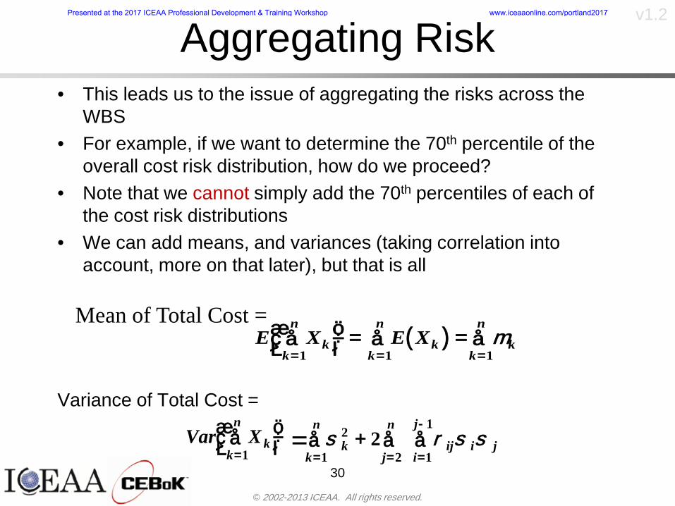
copy 2002-2013 ICEAA All rights reserved
v12
Aggregating Riskbull This leads us to the issue of aggregating the risks across the
WBSbull For example if we want to determine the 70th percentile of the
overall cost risk distribution how do we proceed bull Note that we cannot simply add the 70th percentiles of each of
the cost risk distributionsbull We can add means and variances (taking correlation into
account more on that later) but that is all
Variance of Total Cost =
30
Mean of Total Cost = ( )E X E Xk
k
n
kk
n
kk
n
= = =aringaelig
egraveccediloumloslashdivide
= =aring aring1 1 1
m
Var X kk
n
=aringaelig
egraveccediloumloslashdivide1
= s r s skk
n
iji
j
i jj
n2
1 1
1
22+aring aringaring
= =
-
=
Presented at the 2017 ICEAA Professional Development amp Training Workshop wwwiceaaonlinecomportland2017
copy 2002-2013 ICEAA All rights reserved
v12
Percentiles Do Not Addbull As a notional example consider two independent normal
distributionsndash One distribution has mean equal to 100 and standard deviation
equal to 20ndash The second distribution has mean 300 and standard deviation of 80
bull The sum of two independent normally distributed random variables is also normally distributed
bull To combine the two distributions we add the means and add the variancesndash Total mean is
ndash Total standard deviation is
31
400300100 =+
8258020 22 raquo+
Presented at the 2017 ICEAA Professional Development amp Training Workshop wwwiceaaonlinecomportland2017
copy 2002-2013 ICEAA All rights reserved
v12
Percentiles Do Not Add (2)bull The 80th percentiles for the individual distributions are
117 and 367 respbull The 80th percentile of the combined distribution is
469 but the sum of the two 80th percentiles is 484bull To see why this is the case note that the percentiles
of a normal distribution are determined by the mean and the standard deviationndash The standard deviations are not added when normal distributions
are combined rather the variances are combinedndash Sum of variances is ndash The standard deviation of this sum is
32
22 ba +22 ba +
Presented at the 2017 ICEAA Professional Development amp Training Workshop wwwiceaaonlinecomportland2017
copy 2002-2013 ICEAA All rights reserved
v12
Percentiles Do Not Add (3)bull Since bull We can write
bull The left side of this inequality represents the risk of the combined distributions while the right side represents the sums of the individual risks
bull Combining two missions that are independent results in a diversification of riskndash The total portfolio is not as risky on a relative basis as each
individual project
33
2222 2 bababa ++lt+
baba +lt+ 22
Presented at the 2017 ICEAA Professional Development amp Training Workshop wwwiceaaonlinecomportland2017
copy 2002-2013 ICEAA All rights reserved
v12
Methods for Aggregating Riskbull Since percentiles do not add we have to find other
ways to aggregate riskbull One method is to use Monte Carlo simulationbull Unless cost risk is represented by normal
distributions for all WBS elements summing the means and variances does not result in a completely accurate depiction of overall system cost risk
bull The normal distribution is not a realistic distribution for representing risk in many or even most situations since regarding project risk more can go wrong than can go right which means the risk is NOT symmetric unlike the Gaussian bell curve
34
Presented at the 2017 ICEAA Professional Development amp Training Workshop wwwiceaaonlinecomportland2017
copy 2002-2013 ICEAA All rights reserved
v12
Unit III - Module 9 35
Monte Carlo Simulationfor Risk Analysis
bull When risk analysis is performed multiple risks are gatheredndash These risks may have various probability
distributions
bull Monte Carlo is the most commonly accepted way to produce an accurate characterization of the distribution of the combined effect of these many risksndash Using this distribution we can produce percentiles
for cost impacts due to risk occurrences
10
Presented at the 2017 ICEAA Professional Development amp Training Workshop wwwiceaaonlinecomportland2017
copy 2002-2013 ICEAA All rights reserved
v12
Monte Carlo Simulationbull Simulation is a means for solving problems that are
analytically intractablendash Involves repeated random sampling
bull It was developed during the Manhattan Project as a way to model the interactions inside an atom during nuclear fissionndash Allowed for more sophisticated mathematical modeling of atomic
phenomena
bull Most computer packages use pseudo-random number generators that produce seemingly random results from an initial seedndash Example is the linear congruential generator
36
( ) mbaXX nn mod1 +=+
Presented at the 2017 ICEAA Professional Development amp Training Workshop wwwiceaaonlinecomportland2017
copy 2002-2013 ICEAA All rights reserved
v12Using Random Numbers to Simulate Distributions
bull WBS cost risk is typically measured by a probability distributionbull The most common method for simulating a probability
distribution is the inverse methodbull This involve obtaining a simulated random value from a uniform
distribution and then inverting this through the cumulative distribution function (CDF) to obtain the simulated value
bull As an example for a uniform distribution on the interval [0100]
bull In this case the CDF random value of 05 translates to 10005 = 50
37
( )100
1=xf ( )
100xxF = ( ) xxF 1001 =-
Presented at the 2017 ICEAA Professional Development amp Training Workshop wwwiceaaonlinecomportland2017
copy 2002-2013 ICEAA All rights reserved
v12
Simulating a Triangular Distribution
bull For a triangular distribution with low = 0 most likely = 50 and high = 150 the CDF is given by
bull The inverse function is given by
38
( )iumliumlicirc
iumliumliacute
igrave
poundlt--
poundpound=
1505021
1500050
50015000
2
2
2
xxx
xxxF
( )iumliumlicirc
iumliumliacute
igrave
poundltdivideoslashouml
ccedilegraveaelig +--
poundpound=-
131
21
37501
250017500150
3107500
1
xx
xxxF
Presented at the 2017 ICEAA Professional Development amp Training Workshop wwwiceaaonlinecomportland2017
copy 2002-2013 ICEAA All rights reserved
v12
Simulating a Triangular Distribution (2)
bull If the simulated uniform value is equal to 02 the corresponding inverse value from the CDF inverse is approximately 387
39
0
01
02
03
04
05
06
07
08
09
1
0 30 60 90 120 150
Presented at the 2017 ICEAA Professional Development amp Training Workshop wwwiceaaonlinecomportland2017
copy 2002-2013 ICEAA All rights reserved
v12
Monte Carlo and the WBSbull Simulation involves repeated trials
40
WBS Draw1 2 3 4 5
System 2912 3566 4390 2954 4655 Sum
Structure 80 105 55 80 57 SumVehicle Structure 50 70 30 40 20Tank Structure 30 35 25 40 37
Thermal Control 32 36 35 29 33 SumActive Thermal Control 10 15 12 7 10Induced Thermal Control 12 14 13 14 14Tank Thermal Control 10 7 10 8 9
Main Propulsion System 100 150 125 140 100
Liquid Rocket Engine 1000 1100 1800 900 2200
Electric Power and Distribution 100 125 150 75 90
Command Control and Data Handling 200 250 225 230 275
System Integration 1400 1800 2000 1500 1900
Presented at the 2017 ICEAA Professional Development amp Training Workshop wwwiceaaonlinecomportland2017
copy 2002-2013 ICEAA All rights reserved
v12
Number of Trialsbull Monte Carlo involves a repeated number of trialsbull The greater the number of trials the more accurate the
simulation will approximate the overall cost risk behavior of the system
bull After 100 trials the histogram looks very jagged
41
Presented at the 2017 ICEAA Professional Development amp Training Workshop wwwiceaaonlinecomportland2017
copy 2002-2013 ICEAA All rights reserved
v12
Number of Trials (2)
42
1000 Trials
10000 Trials
50000 Trials Additional trials give a more accurate depiction of the final result
Presented at the 2017 ICEAA Professional Development amp Training Workshop wwwiceaaonlinecomportland2017
copy 2002-2013 ICEAA All rights reserved
v12
Number of Trials (3)bull If we want to simulate the underlying
mean within 1 with 95 confidence for example then we require
43
divideoslash
oumlccedilegrave
aelig poundpound-
=
dividedividedivide
oslash
ouml
ccedilccedilccedil
egrave
aeligpound
-pound
-=
divideoslashouml
ccedilegraveaelig poundpound=
nZ
n
nnX
n
X
n
n
011
010Pr
011
010Pr
011990Pr950
___
___
sm
sm
sm
sm
sm
mm
Presented at the 2017 ICEAA Professional Development amp Training Workshop wwwiceaaonlinecomportland2017
copy 2002-2013 ICEAA All rights reserved
v12
Number of Trials (4)bull This means that the number of trials required is determined by
bull Solving for n we find that at least
trials are neededbull Note that this term involves the coefficient of variation of the
distribution which means that distributions with less dispersion require fewer trials to accurate simulate
44
96101
=ns
m
ms41638
Presented at the 2017 ICEAA Professional Development amp Training Workshop wwwiceaaonlinecomportland2017
copy 2002-2013 ICEAA All rights reserved
v12
Number of Trials (5)bull Simulating percentiles requires more trials than for simulating
meansbull Let Pn represent the number of trials in the sample at or below
the 70th percentile of the underlying distribution (suppose this is known)
bull By the Central Limit Theorem Pnn follows a normal distribution with mean equal to the 70th percentile and variance equal to
bull By a similar process for the mean we find that the number of trials needed to simulate the 70th percentile within 1 with 95 confidence is
45
( )n
FF 700700 1-
n
n
PPn -41638
Presented at the 2017 ICEAA Professional Development amp Training Workshop wwwiceaaonlinecomportland2017
copy 2002-2013 ICEAA All rights reserved
v12
Number of Trials (6)bull If Pn 070 for all n then n is approximately
bull For the sake of comparison suppose CV = 03 (reasonable approximation for hardware development) then the number of trials needed to simulate the mean with the same accuracy is then ldquoonlyrdquo 11525
bull More trials are needed to accurately simulate percentiles than means
46
( ) 46416703041638
70704168341638 =divide
oslashouml
ccedilegraveaelig=divide
oslashouml
ccedilegraveaelig -
=-
nnn
PPn
n
n
Presented at the 2017 ICEAA Professional Development amp Training Workshop wwwiceaaonlinecomportland2017
copy 2002-2013 ICEAA All rights reserved
v12
Methods of Simulationbull Monte Carlo simulation is a standard term for
simulationbull However there is an improvement on Monte Carlo
that improves the accuracy of the results of a simulation for a given number of trials
bull This method is call the Latin Hypercube approach to simulationndash Similar to Monte Carlo but an equal number of draws are taken
from a set of subintervals for example dividing the interval (01) into [00001) [0102)hellip [0910]
ndash Instead of 10 trials from [01] we have one trial from each subinterval
ndash Rough rule of thumb is Latin Hypercube takes 30 fewer trials to achieve similar accuracy to Monte Carlo
47
Presented at the 2017 ICEAA Professional Development amp Training Workshop wwwiceaaonlinecomportland2017
copy 2002-2013 ICEAA All rights reserved
v12
Probability Model ndash Correlationbull Correlation exists between work breakdown structure
(WBS) cost element costs and between cost and schedule
bull Correlation is a necessary consideration in cost risk analysis
bull Correlation is a number that can vary between -1 and +1 and represents the strength of the relationship between the two variablesndash If both variable have a tendency to move in the same direction
correlation is positivendash If when one variable increases the other tends to decrease and
vice-versa the correlation between the two variables is negative
Presented at the 2017 ICEAA Professional Development amp Training Workshop wwwiceaaonlinecomportland2017
copy 2002-2013 ICEAA All rights reserved
v12
Correlation And Causationbull Note that correlation is not causation however
causation implies correlationndash For example shark attacks and ice cream sales at the beach
bull For example for a launch vehicle structure increasing the diameter will not only result in an increase in the structures cost but will also result in higher costs for thermal coating (paint etc)
bull Also simply because two subsystems do not appear to be related does not mean they are not correlatedndash For example structures and computer equipment seemingly
have little relation to one another however an external factor such as a funding cut or a strike will impact all subsystems leading to delays and increasing cost across the board
ndash Thus everything in a WBS has some correlationUnit III - Module 9 49
Presented at the 2017 ICEAA Professional Development amp Training Workshop wwwiceaaonlinecomportland2017
copy 2002-2013 ICEAA All rights reserved
v12
The Importance of Correlationbull Percent that total cost standard deviation is underestimated
when correlation assumed to be 0 instead of r given nWBS elements
Unit III - Module 9 5050
0
20
40
60
80
100
0 01 02 03 04 05 06 07 08 09 1Actual Correlation
Perce
nt Un
deres
timate
d
n = 10
n = 30
n = 100n = 1000
0
20
40
60
80
100
0 01 02 03 04 05 06 07 08 09 1Actual Correlation
Perce
nt Un
deres
timate
d
n = 10
n = 30
n = 100n = 1000
Reference 32nd Annual DOD Cost Analysis Symposium Advanced Training Session ldquoWhy Correlation Matters in Cost Estimatingrdquo Stephen A Book
Presented at the 2017 ICEAA Professional Development amp Training Workshop wwwiceaaonlinecomportland2017
copy 2002-2013 ICEAA All rights reserved
v12
The Importance of Correlation (2)bull For example if correlation is assumed to be 0 for all
elements in a 30 element WBS and the actual correlation is 20 then the total cost standard deviation is underestimated by 60
bull For example assume the total cost is modeled as a normal distribution with mean = 100
bull If correlation is assumed to be zero with total cost standard deviation = 12 when correlation is actually 20 then the true underlying standard deviation is actually 30
bull 70th percentile with zero correlation assumption is 106
bull 70th percentile with 20 correlation is 116 Unit III - Module 9 51
Presented at the 2017 ICEAA Professional Development amp Training Workshop wwwiceaaonlinecomportland2017
copy 2002-2013 ICEAA All rights reserved
v12
Measures of Correlationbull Two measures of correlation are commonly used in
cost risk analysesndash Pearsonrsquos product-moment correlation coefficient ndash Spearmanrsquos rank correlation coefficient
bull Garvey and others recommend using Pearsonrsquos product-moment correlation coefficient correlation for cost risk analysesndash Method of moments uses this but there are two options in
simulationndash Popular simulation packages like Risk and Crystal Ball use
rank correlation but in practice this has been found to make little difference
ndash Pearson product-moment correlation has been incorporated into Risk+
52
Presented at the 2017 ICEAA Professional Development amp Training Workshop wwwiceaaonlinecomportland2017
copy 2002-2013 ICEAA All rights reserved
v12
Pearson Correlationbull Pearsonrsquos product-moment correlation measures
degree of linearity between two random variables bull If two random variables are perfectly linear (eg Y =
aX + b) with positive slope then the Pearson product-moment correlation between X and Y denoted by rXY is +1
53
X X
Y Y Y
XNegative Correlation Positive Correlation No Correlation
middotmiddot
middotmiddot
middotmiddot middotmiddot
middotmiddot
middot
middot
middotmiddotmiddot
middotmiddot
middotmiddot
middotmiddot middot
middot
middot
middotmiddotmiddotmiddotmiddotmiddotmiddotmiddot
middotmiddotmiddotmiddot
middotmiddot
middotmiddot middotmiddotmiddotmiddot
middotmiddotmiddot
middotmiddotmiddotmiddot
middotmiddotmiddot
middotmiddotmiddot
middotmiddot
middot
middot middotmiddot
middot middotmiddotmiddotmiddot middotmiddot middot middotmiddot middot middot
middotmiddot middot
middotmiddotmiddotmiddotmiddot middot middotmiddot
middotmiddot
middot
middotmiddot
middotmiddot middot
middot middot middot
middotmiddot middot
middotmiddotmiddot
middotmiddot
middot middot
Presented at the 2017 ICEAA Professional Development amp Training Workshop wwwiceaaonlinecomportland2017
copy 2002-2013 ICEAA All rights reserved
v12
Spearman Correlationbull Spearmanrsquos rank correlation measures the
monotonicity between two random variablesbull If two random variables are perfectly monotonically
increasing (eg Y = X2) then the Spearman rank correlation denoted by rXY is +1
bull The two measures can be significantly different
54
10 20 30 40 50 60
100
200
300
096 097 098 099 1
1
060
020
040
080
Eff
ort (
Staf
f-M
onth
s)
Software Size I KDSI
y = 28z12y
z x
yy = x100
0 pound x pound 1
Figure 5-9A Figure 5-9B
Pearson Correlation = 09976 Rank Correlation = 1
Pearson Correlation = 024 Rank Correlation = 1
X(x ) ~ Unif(01)
Reference Probability Methods for Cost Uncertainty Analysis A Systems Engineering Perspective Paul R Garvey
Presented at the 2017 ICEAA Professional Development amp Training Workshop wwwiceaaonlinecomportland2017
copy 2002-2013 ICEAA All rights reserved
v12
Unit III - Module 9 55
200
250
300
350
400
1000 1200 1400 1600 1800 2000
Recurring Production
SEPM
200
250
300
350
400
1000 1200 1400 1600 1800 2000
Recurring Production
SEPM
Functional Correlationbull Old No Functional
Correlation Simulation run with WBS items entered as values
bull New Simulation run with functional dependencies entered as they are in cost model
CorrelatedNot Correlated
Note shift of mean and increased variability
Presented at the 2017 ICEAA Professional Development amp Training Workshop wwwiceaaonlinecomportland2017
copy 2002-2013 ICEAA All rights reserved
v12
Risk Measuresbull ldquoWestern Europe conquered the word because of a
technological revolution that started because of attempts to measure the worldrdquo ndash Phillipe Jorion ndash In the same way attempts to measure risk will lead to better project
managementbull Risk management for DoD and NASA agencies focuses
primarily on funding projects to a single percentile ndash NASA policy explicitly mentions 70 and 50ndash This is known as ldquoValue at Riskrdquo and is prevalent in the banking and
financial industry
56
Presented at the 2017 ICEAA Professional Development amp Training Workshop wwwiceaaonlinecomportland2017
copy 2002-2013 ICEAA All rights reserved
v12
Value at Risk (VaR)bull VaR is a percentile of the cost risk
distributionndash VaR funding at the 70th percentile means that
there is a 30 chance of final project cost exceeding the funded amount (budget)
bull VaR has some meritsndash Common measure can be used to compare
different projects and programsndash Easily understood by senior managers and
decision makers
57
Presented at the 2017 ICEAA Professional Development amp Training Workshop wwwiceaaonlinecomportland2017
copy 2002-2013 ICEAA All rights reserved
v12
Why 70th or 80th Percentilebull Typical policy guidance involves funding at the 70th or 80th
percentile Why fund as such a low percentilebull There is some incentive to not over-fundbull For a normal distribution an inflection point occurs near the 80th
percentile meaning that for values above 80 confidence achieving higher levels of confidence can only be achieved by spending greater dollar amounts at an increasing rate
58
-05-04-03-02-01
00102030405
0 05 1 15 2 25 3
Standard Deviations from Mean
Normal Distribution
First DerivativeSlopeVelocity
Second DerivativeConvexityAcceleration
Inflection point at one standard deviation above the mean (~84th
percentile)
Presented at the 2017 ICEAA Professional Development amp Training Workshop wwwiceaaonlinecomportland2017
copy 2002-2013 ICEAA All rights reserved
v12
Funding Above Inflection Pointsbull As the percentile goes above the 80th percentile the amount
needed to achieve that higher level of confidence begins to increase at an increasing rate as is evident from the graph
59
0
10
20
30
40
50
60
70
50 55 60 65 70 75 80 85 90 95 100
$ Ab
ove
MEa
n to
Ach
ieve
Per
cent
ile
Percentile (Confidence Level)
Presented at the 2017 ICEAA Professional Development amp Training Workshop wwwiceaaonlinecomportland2017
copy 2002-2013 ICEAA All rights reserved
v12
Why Budget to the 70th or 80thbull Government projects are funded at the 70th or 80th percentilesbull Why not the 90th or 99th percentile Wonrsquot that help prevent
overrunsndash As we have seen percentiles do not add across programs
bull The sum of the 80th percentiles does NOT equal the total 80th percentile
ndash This is because the individual programs are riskier than the entire suite of missions
bull Known as the ldquoPortfolio effectrdquo (more or this later)
ndash Funding at the 80th gives confidence that the entire portfolio will be adequately funded
bull And since there is an inflection point near the 80th percentile funding above that level quickly becomes cost prohibitive
60
Presented at the 2017 ICEAA Professional Development amp Training Workshop wwwiceaaonlinecomportland2017
copy 2002-2013 ICEAA All rights reserved
v12
Inflection Points for Lognormalbull For a lognormal the inflection point
variesndash Coefficient of variation equal to 10 equates to an
inflection point at the 70th percentile
61
0
10
20
30
40
50
60
70
050 060 070 080 090 100
Coef
ficen
t of V
aria
tion
Percentile of the Inflection Point
Presented at the 2017 ICEAA Professional Development amp Training Workshop wwwiceaaonlinecomportland2017
copy 2002-2013 ICEAA All rights reserved
v12
Issues with Percentile Fundingbull However risk management does not stop at a
specific percentilendash What happens when the 70th percentile is exceeded
bull Any effective risk management policy should prescribe what happens after a bad event occursndash With VaR we only know when a bad event has occurred ndash Also funding at a relatively low level means we have no true
sense of the real risks that should be guarded against
62
Presented at the 2017 ICEAA Professional Development amp Training Workshop wwwiceaaonlinecomportland2017
copy 2002-2013 ICEAA All rights reserved
v12
ldquoHere There Be Dragonsrdquobull On old maps uncharted territory was often
marked with monsters or dragons
63
A section of the Carta Marina by Olaus Magnus 16th Century
Presented at the 2017 ICEAA Professional Development amp Training Workshop wwwiceaaonlinecomportland2017
copy 2002-2013 ICEAA All rights reserved
v12
Distribution Comparisonbull Four different distributions with the same 70th
percentile
bull Should we expect the tails to be similar
64
0
10
20
30
40
50
60
70
80
0 100 200 300 400 500 600
Perc
entil
eCo
nfid
ence
Lev
el
Triangular
Normal
Lognormal
Pareto
Presented at the 2017 ICEAA Professional Development amp Training Workshop wwwiceaaonlinecomportland2017
copy 2002-2013 ICEAA All rights reserved
v12Distribution Comparison Tail Behavior
bull The normal and triangular distributions have similar tails but the lognormal and Pareto have much fatter right tails
65
70
75
80
85
90
95
100
500 1500 2500 3500 4500 5500
Perc
entil
eCo
nfid
ence
Lev
el
Triangular
Normal
Lognormal
Pareto
Here There Be Dragons
Presented at the 2017 ICEAA Professional Development amp Training Workshop wwwiceaaonlinecomportland2017
copy 2002-2013 ICEAA All rights reserved
v12Distribution Comparison ndash Tail Behavior (Table)
bull There is significant tail risk for the lognormal and the Paretobull The 99th percentile for the Pareto is 1000 times greater than
the 70th percentilendash Risk seen in financial markets and in catastrophic risks like natural
disasters bull Four different projects follow the four different risk profiles seen
in this example should clearly have different risk management approaches but 70th percentile funding indicates the same risk management approach for all four
66
Percentile Triangular Normal Lognormal Pareto 70th $600 $600 $600 $600 80th $680 $660 $770 $1430 90th $770 $750 $1070 $5880 95th $840 $820 $1410 $23750 99th $930 $950 $2350 $600000
Presented at the 2017 ICEAA Professional Development amp Training Workshop wwwiceaaonlinecomportland2017
copy 2002-2013 ICEAA All rights reserved
v12Percentile Budgeting is Not Risk Management
bull Percentile budgeting ne effective risk management policybull Suppose that you are shopping for a new car You
mention that safety is your top concern The salesman says he has a great safe car available You ask about the air bags Do they work The salesman answers ldquoOf course Seventy percent of the time they work fine Only 30 of the time the air bags will fail to deployrdquo Would you buy such a car Hedge fund manager David Einhorn has stated ldquoRisk management is the air bag that must always work but only in the multi-sigma event where you have an accidentrdquo
67
Risk management is the air bag that must always work but only in the multi-sigma event where you
have an accident
Presented at the 2017 ICEAA Professional Development amp Training Workshop wwwiceaaonlinecomportland2017
copy 2002-2013 ICEAA All rights reserved
v12
Joint Confidence Level Analysisbull Schedules are risky toobull For 98 recent NASA missions average
schedule growth was 38ndash Not as high as cost growth but still significant
68
0
5
10
15
20
25
30
35
40
Schedule
Cost
Presented at the 2017 ICEAA Professional Development amp Training Workshop wwwiceaaonlinecomportland2017
copy 2002-2013 ICEAA All rights reserved
v12
Schedules Impact Costbull Changes in schedule can have enormous
impacts on cost ndash Schedule slips can lead to cost increases
bull Fixed programmatic costs must be paid on a regular basisndash Achieving schedule milestones early can result in cost
savings
bull Schedule is an important consideration in cost analysis including cost risk analysis
bull However we must be careful in correctly integrating cost and schedule riskndash Schedule is not simply an input but is dependent on many of
the same factors that drive cost
69
Presented at the 2017 ICEAA Professional Development amp Training Workshop wwwiceaaonlinecomportland2017
copy 2002-2013 ICEAA All rights reserved
v12
The Relationship of Cost to Schedulebull Cost and schedule are positively correlated
ndash A larger program with bigger scope with take longer to complete than a smaller simpler program
bull However longer schedules do not always equate to higher cost nor shorter schedules with lower costndash Highly compressed schedules relative to the
optimal schedule can lead to large overrunsbull Compressed schedules are commonplace for
many planetary missions
70
Presented at the 2017 ICEAA Professional Development amp Training Workshop wwwiceaaonlinecomportland2017
copy 2002-2013 ICEAA All rights reserved
v12The Impact of Schedule GrowthCompression on Cost
bull Compressed schedules lead to cost growth and based on existing research is actually more expensive than schedule slippages
71
0
20
40
60
80
100
120
140
160
-50 -25 0 25 50 75 100
Percentage Change in Schedule
Perc
enta
ge C
hang
e in
Cos
t due
to
Sche
dule
Cha
nge
Source Smart CB ldquoCost and Schedule Interrelationshipsrdquo 2007 NASA Cost Symposium
Presented at the 2017 ICEAA Professional Development amp Training Workshop wwwiceaaonlinecomportland2017
copy 2002-2013 ICEAA All rights reserved
v12Schedule as an Independent Variable
bull Why not simply add schedule as an input to cost-estimating relationships (CERs)
bull Schedule is often treated as an independent variable ndash schedules are often determined independently of cost considerationsndash Cost may not be considered explicitly although budgets and
schedules are determined based on scope and other common factors
bull In 2006 SAIC undertook a research task to determine the impact of schedule on cost and added schedule as an independent variable to the CERs in the NASAAir Force Cost Model (NAFCOM) to see if schedule provided any improvement in goodness of fit
72
Presented at the 2017 ICEAA Professional Development amp Training Workshop wwwiceaaonlinecomportland2017
copy 2002-2013 ICEAA All rights reserved
v12
Schedule is a Dependent Variablebull Since NAFCOM includes an exhaustive list of cost drivers the inclusion
of schedule should give an indication of whether there is any additional independent value added from schedule independent of the cost drivers
bull In the study schedule was added to 10 subsystem-level CERs
ndash In each case the addition of schedule did NOTimprove the goodness of fit and schedule was NOT found to be a statistically significant cost driver (given the presence of the other variables) for any of the 10 CERs
bull Standard errors for the CERs increased due to decrease in degrees of freedom
bull Thus schedule as an independent variable did not provide any additional explanation of variation in historical cost
bull This is because schedule is truly NOT an independent variable but a dependent variable and is a function of the same factors that drive cost
73
Presented at the 2017 ICEAA Professional Development amp Training Workshop wwwiceaaonlinecomportland2017
copy 2002-2013 ICEAA All rights reserved
v12
Incorporation of Schedule in Cost Risk
bull When using subjective methods care must be taken in applying schedule to cost risk analysis
bull Since schedule is a dependent variable treating it independently from other factors when assessing its impact on cost can lead to a double count of independent variables in the cost risk analysis
bull Direct inclusion of schedule in a cost risk analysis effectively doubles the influence of each cost driver
ndash Incorrectly leads to broader risk ranges
74
CostWeight
HeritageNewness
Technology Readiness Schedule
Presented at the 2017 ICEAA Professional Development amp Training Workshop wwwiceaaonlinecomportland2017
copy 2002-2013 ICEAA All rights reserved
v12Subjective Cost Risk Methods and Overinclusion of Risk Factors
bull Subjective methods are suitable when data are scarce or not availablebull However care must be taken not to treat correlated sources of risk
such as schedule as independent of each otherbull Example ndash a subjective risk analysis incorporated technology readiness
design risk requirements stability integration risk and schedule and treated each source of risk as independent
bull Risk triangle high value without schedule risk was 31 times the point estimate
bull Risk triangle high value with schedule risk added on top of other sources of risk treated independently was 34 times the point estimate
bull Risk triangle taking correlation between sources of risk into account in a rigorous statistical manner has a high value 15 times the point estimate less than half the effect when treating sources of risk as independent
75
Presented at the 2017 ICEAA Professional Development amp Training Workshop wwwiceaaonlinecomportland2017
copy 2002-2013 ICEAA All rights reserved
v12Fundamental Equation of Cost and Schedule Interrelationships
bull The Fundamental Equation of the Relationship Between Cost and Schedule is
Time = Moneybull This is a well known adage that time is money Your boss at
work may even mention this to you from time to time or if you are the boss you are all too aware of this iron law
bull Because time is money cost and schedule risk should be modeled jointly not with schedule as an independent cost driver
bull Note that cost and schedule are not perfectly correlatedndash Cost can sometimes ldquobuy downrdquo schedule extra money can be
spent to meet a deadline since in some cases additional effort to hasten the completion of a task
76
Presented at the 2017 ICEAA Professional Development amp Training Workshop wwwiceaaonlinecomportland2017
copy 2002-2013 ICEAA All rights reserved
v12How to (Correctly) Incorporate Schedule into Cost Risk Analysis
bull The best way to model cost and schedule risk is to develop a joint cost and schedule model based on the same data
bull Since such models are not currently available the next best approach is to model cost and schedule independently and then integrate cost and schedule risk analyses using joint probability distributions taking into account correlation between cost and schedulendash This approach pioneered by Paul Garvey and Steve Book is
considered industry best practicendash This is a practical method mathematically tractable and follows
naturally from the Fundamental Equation of Cost and Schedule Interrelationships
77
Book S A ldquoQuantifying the Relationship Between Cost and Schedulerdquo The Measurable News Winter 2007-2008 pp 11-15Garvey PR Probability Methods for Cost Uncertainty Analysis A Systems Engineering Perspective New York Marcel Dekker 2000 pp 308-335
Presented at the 2017 ICEAA Professional Development amp Training Workshop wwwiceaaonlinecomportland2017
copy 2002-2013 ICEAA All rights reserved
v12
Joint Lognormal and Normal Distributions
bull Cost and schedule are typically modeled as some combination of Normal and Lognormal probability distributionsndash Studies by The Aerospace Corporation the MITRE
Corporation Wyle Labs and SAIC have found that the Lognormal probability distribution almost always serves as a good model for both the schedule distribution and the cost distribution
ndash The Normal distribution may also be appropriate in some instances and depending upon the level of confidence at which budgets are set may even be more conservative and logically consistent than the Normal distribution
ndash Joint Lognormal and Normal distributions are defined by a pair of mean and standard deviations and a level of correlation between the two
78
Presented at the 2017 ICEAA Professional Development amp Training Workshop wwwiceaaonlinecomportland2017
copy 2002-2013 ICEAA All rights reserved
v12Modeling Cost and Schedule as a Bivariate Distribution
bull In the approach set forth by Book and Garvey cost risk is assessed and the top-level distribution is modeled as a Lognormal (or Normal) distribution schedule risk is assessed and the overall schedule risk is modeled as a Lognormal (or Normal) distribution
bull The two distributions are combined into a Bivariate distribution by assigning a correlation between the two and by treating the two distributions as the marginal distributions of a Bivariate Lognormal distributionndash Other combinations include a Bivariate Normal or a Bivariate
Normal-Lognormal
79
Presented at the 2017 ICEAA Professional Development amp Training Workshop wwwiceaaonlinecomportland2017
copy 2002-2013 ICEAA All rights reserved
v12Bivariate Lognormal Distribution for Cost and Schedule
bull Cost is often observed to be Lognormal when strong positive correlations are present among the systemrsquos WBS cost element costs
bull A systemrsquos schedule is often observed (from Monte Carlo simulations) to be Lognormal if it is the sum of many positively correlated schedule activities in an overall schedule network
bull If Lognormal distributions characterize a systemrsquos cost and schedule then the Bivariate Lognormal could serve as an assumed model of their joint distributionndash In this case the marginal distribution of each of cost and schedule is
Lognormalbull Other possibilities for modeling cost and schedule as a Bivariate
distribution include a Bivariate Normal or a Bivariate Normal-Lognormal distributionndash All these combinations are analytically tractable
80
Presented at the 2017 ICEAA Professional Development amp Training Workshop wwwiceaaonlinecomportland2017
copy 2002-2013 ICEAA All rights reserved
v12Bivariate Lognormal for Cost and Schedule
bull Contour Plots of a Bivariate Lognormal
81
Presented at the 2017 ICEAA Professional Development amp Training Workshop wwwiceaaonlinecomportland2017
copy 2002-2013 ICEAA All rights reserved
v12Correlation Between Cost and Schedule
bull Cost and schedule are positively correlated but not perfectly sondash For example it is possible to have a schedule underrun and a cost
overrunbull Based on cost and schedule growth data for 50 completed NASA
programs the correlation between development cost and development schedule is 70
82
00
200
400
600
800
1000
1200
-500 00 500 1000 1500 2000 2500Historical Cost Growth
Hist
oric
al S
ched
ule
Gro
wth
r = 715
Presented at the 2017 ICEAA Professional Development amp Training Workshop wwwiceaaonlinecomportland2017
copy 2002-2013 ICEAA All rights reserved
v12Correlation Between Cost and Schedule Caveats
bull Based on historical data recommended correlation between cost and schedule is 70 but this could be higher or lower depending upon program circumstancesndash If program is budget constrained cost and schedule will be
more highly correlated (go as you pay)ndash If program is schedule constrained cost and schedule will
have lower correlation perhaps even negative correlation ndash Smaller programs have smaller correlation between cost and
schedule riskbull Relatively easy to ldquohurry uprdquo and finish on time or even early if
needed
83
Presented at the 2017 ICEAA Professional Development amp Training Workshop wwwiceaaonlinecomportland2017
copy 2002-2013 ICEAA All rights reserved
v12
Conditional Confidence Levelsbull Given a programrsquos project schedule we can determine the cost
risk distribution conditional upon the given schedulebull Conditional cost S-curves are steeper than unconditional
(marginal) cost S-curves between some uncertainty has been removed because schedule is fixed
84
Presented at the 2017 ICEAA Professional Development amp Training Workshop wwwiceaaonlinecomportland2017
copy 2002-2013 ICEAA All rights reserved
v12
Joint Confidence Levelsbull Joint 65 confidence represents the probability of
achieving both 65 confidence in cost AND 65 confidence in schedulendash This is different than achieving 65 cost confidence alone
or achieving 65 schedule confidence alonebull Due to the imperfect correlation between cost and schedule it
is possible to achieve a 65 cost confidence with a lower level of schedule confidence
bull Restricting the schedule confidence thus requires additional $ to achieve a given level of confidence
85
X
Y
Possible Values for Which X gt a Possible Values for
Which X gt a and Y gt b
a
b
Presented at the 2017 ICEAA Professional Development amp Training Workshop wwwiceaaonlinecomportland2017
copy 2002-2013 ICEAA All rights reserved
v12Joint Confidence Levels Versus Cost Confidence Levels Only
bull Example of the differences between cost confidence schedule confidence conditional cost confidence and joint cost and schedule confidence
86
Joint Cost-Schedule Confidence Iso-Curves
Cost (RY$M)
Sche
dule
(Mon
ths)
65 Confidence
50 Confidence
70 Confidence
65 Cost Confidence AggressiveSchedule65 Cost ConfidenceScheduleGiven 65 Schedule ConfidenceUnconditional 65 CostConfidenceUnconditional 65 ScheduleConfidence
65 Cost Confidence 65 Joint Cost and Schedule
Confidence for 65 Schedule Confidence
Presented at the 2017 ICEAA Professional Development amp Training Workshop wwwiceaaonlinecomportland2017
copy 2002-2013 ICEAA All rights reserved
v12
Joint Cost and Schedule Confidence
bull Can examine pairs of cost and schedule that achieve a given level of confidence
bull Provides insights into the trade-offs between cost and schedule for a given level of confidencendash Possible to increase cost confidence by giving a
project more time in some instances or possible to ldquobuy downrdquo schedule
bull But these have limits and are shown in the iso-cost and schedule confidence curves
87
Presented at the 2017 ICEAA Professional Development amp Training Workshop wwwiceaaonlinecomportland2017
copy 2002-2013 ICEAA All rights reserved
v12Cost and Schedule Trade-offs for a Given Level of Joint Confidence
bull Hypothetical Example
88
Cost (RY$M)
Schedule (Months)
$100 48$99 48$89 49$87 50$85 51$85 52$84 53$83 55$83 55$83 56
Cost and Schedule 65 Confidence Iso-Curve
4748495051525354555657
$80 $82 $84 $86 $88 $90 $92 $94 $96 $98 $100
Cost (RY$ M)
Sche
dule
(Mon
ths)
Presented at the 2017 ICEAA Professional Development amp Training Workshop wwwiceaaonlinecomportland2017
copy 2002-2013 ICEAA All rights reserved
v12Policy Considerations for Confidence Levels
bull For large programs the difference between the amount of money needed to achieve 65 cost confidence independent of schedule and joint 65 cost and schedule confidence can represent hundreds of millions and even billions of dollars
89
Joint Cost-Schedule Confidence Iso-Curves
Cost (RY$M)
Sche
dule
(Mon
ths)
65 Confidence
65 Cost Confidence AggressiveSchedule
65 Cost ConfidenceScheduleGiven 65 Schedule Confidence
Unconditional 65 CostConfidence
Joint Cost and Schedule Confidence for 65 Cost Confidence and Program Baseline Schedule is Less Than 35
65 Cost Confidence Independent of Schedule Cost Needed to Achieve
Both 65 Joint Cost and Schedule Confidence for the Schedule with 65 Confidence
Presented at the 2017 ICEAA Professional Development amp Training Workshop wwwiceaaonlinecomportland2017
copy 2002-2013 ICEAA All rights reserved
v12
Copulasbull More generally any combination of distributions can
be used (more than just normal and lognormal)ndash Termed ldquocopulardquo from the Italian word for ldquocouplerdquondash Copulas are a way to combine marginal distributions of any
number and type into a joint distributionbull More formally a copula is a multivariate joint distribution defined
on the n-dimensional unit cube [0 1]n such that every marginal distribution is uniform on the interval [0 1]
bull (The bivariate form of) Sklarrsquos theorem states that for any bivariate distribution function H(x y) let F(x) = H(x infin) and G(y) = H(infin y) be the univariate marginal probability distribution functions Then there exists a copula C such that H(xy)=C(F(x)G(y))
ndash Copulas are widely used in risk management for investments and insurance
bull Considered industry best practice (Li 2000)bull Marketed as part of JP Morganrsquos CreditMetrics suite of tools
(Gupton et Al 1997)90
Presented at the 2017 ICEAA Professional Development amp Training Workshop wwwiceaaonlinecomportland2017
copy 2002-2013 ICEAA All rights reserved
v12Parametric Joint Cost and Schedule Analysis
bull A parametric model based on a consistent data set with a set of overlapping cost and schedule drivers is a cleaner way to model cost and schedule
91
CostWeight
HeritageNewness
Technology Readiness
Schedule
0
20
40
60
80
100
Confidence
Joint Cost and Schedule Confidence
Schedule
Cost
Lognormal Distribution PDF and CDF
0102030405060708090100
200 300 400 500 600 700 800 900 1000Cost $
Con
fiden
ce L
evel
0
00002
00004
00006
00008
0001
00012
00014
00016
Prob
abili
ty D
ensi
ty
CDFPDF
Lognormal Distribution PDF and CDF
0102030405060708090100
200 300 400 500 600 700 800 900 1000Cost $
Con
fiden
ce L
evel
0
00002
00004
00006
00008
0001
00012
00014
00016
Prob
abili
ty D
ensi
ty
CDFPDF
Presented at the 2017 ICEAA Professional Development amp Training Workshop wwwiceaaonlinecomportland2017
copy 2002-2013 ICEAA All rights reserved
v12Parametric Joint Cost and Schedule Analysis (2)
bull Joint cost and schedule risk analysis produced naturally by the integrated modelndash Addresses several issues with the copula
approachbull Tail dependencybull Correlation ndash no need to assign correlation
between cost and schedulebull Consistency of cost and schedule models
92
Presented at the 2017 ICEAA Professional Development amp Training Workshop wwwiceaaonlinecomportland2017
copy 2002-2013 ICEAA All rights reserved
v12
Resource-Loaded Schedulesbull Involves assigning cost and schedule risks to a resource-loaded schedule
networkbull Bottom-up approach
ndash More labor intensive than parametrics but can also provide more insight
ndash Can answer questions than parametric typically cannot such as how much do reserve requirements decrease if a specific risk is retired
bull Currently being implemented in Constellation programbull Has same issue as all bottom-up models hard to count all the risks and model
them discretely
ndash As a result there is a tendency to reflect less risk than indicated by history
ndash ldquoThere are more things in heaven and earth Horatio than are dreamt of in your philosophyrdquo William Shakespeare Hamlet Act I Scene V
93
Presented at the 2017 ICEAA Professional Development amp Training Workshop wwwiceaaonlinecomportland2017
copy 2002-2013 ICEAA All rights reserved
v12Resource-Loaded Schedules Vs Parametrics
bull Parametric most appropriate for early estimatesndash But also good for high-level checks as project progresses
bull As plans take shape lower level modeling may be more appropriate
94 1
CONCEPTUALDEVELOPMENT
PROJECTDEFINITION DESIGN DEVELOPMENT OPERATIONS
PARAMETRIC PARAMETRIC
ANALOGY
ENGINEERING (Bottoms Up)
$PARAMETRIC
DETAILED
$
Pre Phase A Phase B Phase CDPhase A Phase EPre Phase A Phase B Phase CDPhase A Phase E
Risk = f(Cost Estimating Relationship Inputs eg mass power data rate TRL new design etc)
Risk = f(cost and schedule variation of the analogous elements)
Risk = f(variation of detailed inputs eg labor hours rates materials etc)
Presented at the 2017 ICEAA Professional Development amp Training Workshop wwwiceaaonlinecomportland2017
copy 2002-2013 ICEAA All rights reserved
v12
Resource-Loaded Schedulesbull Methodology has been demonstrated in other
industriesndash Construction oil and gasndash Analysis has not been traditionally done on highly uncertain
complex development projects bull Methodology focuses on project baseline schedule
ndash In baseline schedule all tasks are resource loaded to represent a baseline schedule and cost standpoint
ndash Resource loaded schedule is ldquorolledrdquo up to a manageable level
ndash Based on the risk and uncertainties identified schedule distributions are applied to each rolled up task
ndash Cost uncertainties are also applied to rolled up tasksbull Uncertainties include labor rate man power etc
ndash A Monte Carlo simulation is run to develop joint cost-schedule distributions
95
Presented at the 2017 ICEAA Professional Development amp Training Workshop wwwiceaaonlinecomportland2017
copy 2002-2013 ICEAA All rights reserved
v12
Unit III - Module 9 96
Execution ndash Cross Checksbull Means The mean cost growth factor for WBS items
can be compared to history as a way to cross check results
bull CVs The CV of the cost growth factors for WBS items can be compared to history as a way to cross check results
bull Inputs Checks are performed on inputs or other parameters to see if historical values are in line with program assumptionsndash Example Historical risk scores can be compared to program
risk scores to see if risk assessors are being realistic and to see if the underlying database is representative of the program
11
Presented at the 2017 ICEAA Professional Development amp Training Workshop wwwiceaaonlinecomportland2017
- Cost and Schedule Risk Analysis Basic
- Acknowledgments
- Unit Index
- Risk Overview
- Agenda
- Introduction
- Risk Analysis Terms
- Are Our Costs Realistic
- Historical Cost Growth
- Sources of Cost Risk
- Point Estimates of Cost
- Types of Risk
- Point Estimates Vs Risk Estimates
- Cost Risk and Probability
- Probability Model ndash Distribution
- Probability Model ndash Distribution
- Probability ndash Top-Level Distribution
- S-Curves and Confidence Levels
- Example ndash Normal Distribution
- Confidence Levels
- Measuring Parametric Model Uncertainty
- Parametric Model Example
- Weight Uncertainty
- Estimating Uncertainty
- Estimating Uncertainty (2)
- Estimating Uncertainty (3)
- Aggregating Risk
- WBS Example
- WBS and Risk
- Aggregating Risk
- Percentiles Do Not Add
- Percentiles Do Not Add (2)
- Percentiles Do Not Add (3)
- Methods for Aggregating Risk
- Monte Carlo Simulationfor Risk Analysis
- Monte Carlo Simulation
- Using Random Numbers to Simulate Distributions
- Simulating a Triangular Distribution
- Simulating a Triangular Distribution (2)
- Monte Carlo and the WBS
- Number of Trials
- Number of Trials (2)
- Number of Trials (3)
- Number of Trials (4)
- Number of Trials (5)
- Number of Trials (6)
- Methods of Simulation
- Probability Model ndash Correlation
- Correlation And Causation
- The Importance of Correlation
- The Importance of Correlation (2)
- Measures of Correlation
- Pearson Correlation
- Spearman Correlation
- Functional Correlation
- Risk Measures
- Value at Risk (VaR)
- Why 70th or 80th Percentile
- Funding Above Inflection Points
- Why Budget to the 70th or 80th
- Inflection Points for Lognormal
- Issues with Percentile Funding
- ldquoHere There Be Dragonsrdquo
- Distribution Comparison
- Distribution Comparison Tail Behavior
- Distribution Comparison ndash Tail Behavior (Table)
- Percentile Budgeting is Not Risk Management
- Joint Confidence Level Analysis
- Schedules Impact Cost
- The Relationship of Cost to Schedule
- The Impact of Schedule GrowthCompression on Cost
- Schedule as an Independent Variable
- Schedule is a Dependent Variable
- Incorporation of Schedule in Cost Risk
- Subjective Cost Risk Methods and Overinclusion of Risk Factors
- Fundamental Equation of Cost and Schedule Interrelationships
- How to (Correctly) Incorporate Schedule into Cost Risk Analysis
- Joint Lognormal and Normal Distributions
- Modeling Cost and Schedule as a Bivariate Distribution
- Bivariate Lognormal Distribution for Cost and Schedule
- Bivariate Lognormal for Cost and Schedule
- Correlation Between Cost and Schedule
- Correlation Between Cost and Schedule Caveats
- Conditional Confidence Levels
- Joint Confidence Levels
- Joint Confidence Levels Versus Cost Confidence Levels Only
- Joint Cost and Schedule Confidence
- Cost and Schedule Trade-offs for a Given Level of Joint Confidence
- Policy Considerations for Confidence Levels
- Copulas
- Parametric Joint Cost and Schedule Analysis
- Parametric Joint Cost and Schedule Analysis (2)
- Resource-Loaded Schedules
- Resource-Loaded Schedules Vs Parametrics
- Resource-Loaded Schedules
- Execution ndash Cross Checks
-
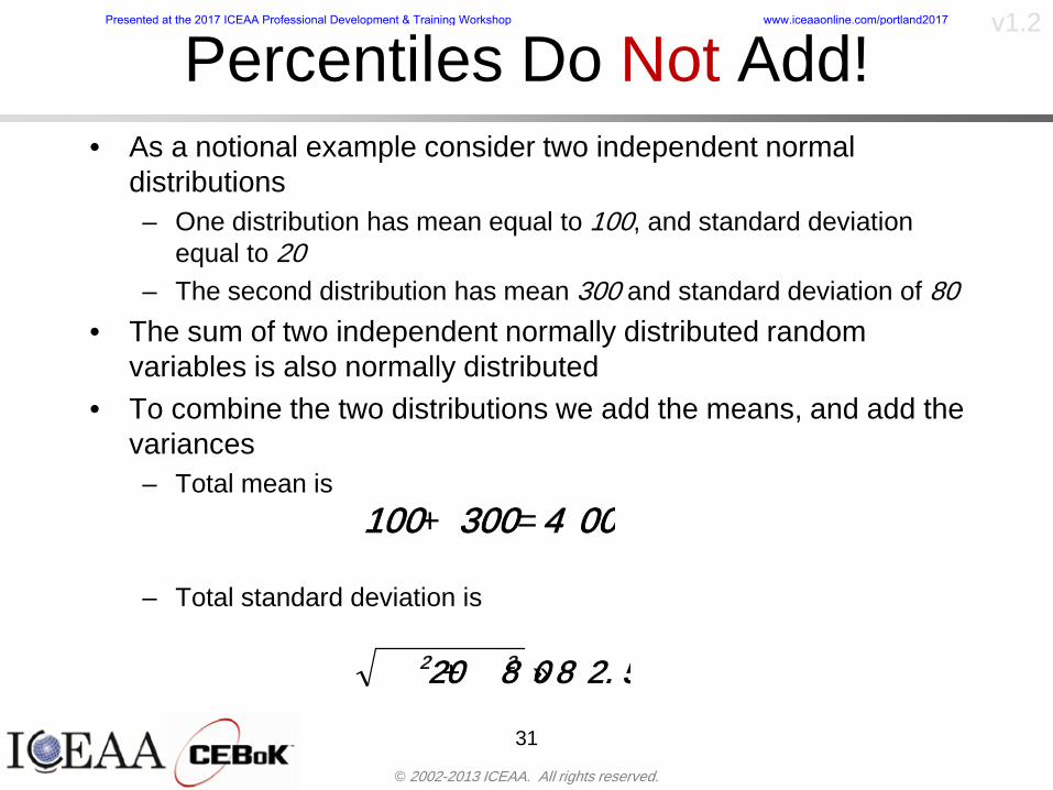
copy 2002-2013 ICEAA All rights reserved
v12
Percentiles Do Not Addbull As a notional example consider two independent normal
distributionsndash One distribution has mean equal to 100 and standard deviation
equal to 20ndash The second distribution has mean 300 and standard deviation of 80
bull The sum of two independent normally distributed random variables is also normally distributed
bull To combine the two distributions we add the means and add the variancesndash Total mean is
ndash Total standard deviation is
31
400300100 =+
8258020 22 raquo+
Presented at the 2017 ICEAA Professional Development amp Training Workshop wwwiceaaonlinecomportland2017
copy 2002-2013 ICEAA All rights reserved
v12
Percentiles Do Not Add (2)bull The 80th percentiles for the individual distributions are
117 and 367 respbull The 80th percentile of the combined distribution is
469 but the sum of the two 80th percentiles is 484bull To see why this is the case note that the percentiles
of a normal distribution are determined by the mean and the standard deviationndash The standard deviations are not added when normal distributions
are combined rather the variances are combinedndash Sum of variances is ndash The standard deviation of this sum is
32
22 ba +22 ba +
Presented at the 2017 ICEAA Professional Development amp Training Workshop wwwiceaaonlinecomportland2017
copy 2002-2013 ICEAA All rights reserved
v12
Percentiles Do Not Add (3)bull Since bull We can write
bull The left side of this inequality represents the risk of the combined distributions while the right side represents the sums of the individual risks
bull Combining two missions that are independent results in a diversification of riskndash The total portfolio is not as risky on a relative basis as each
individual project
33
2222 2 bababa ++lt+
baba +lt+ 22
Presented at the 2017 ICEAA Professional Development amp Training Workshop wwwiceaaonlinecomportland2017
copy 2002-2013 ICEAA All rights reserved
v12
Methods for Aggregating Riskbull Since percentiles do not add we have to find other
ways to aggregate riskbull One method is to use Monte Carlo simulationbull Unless cost risk is represented by normal
distributions for all WBS elements summing the means and variances does not result in a completely accurate depiction of overall system cost risk
bull The normal distribution is not a realistic distribution for representing risk in many or even most situations since regarding project risk more can go wrong than can go right which means the risk is NOT symmetric unlike the Gaussian bell curve
34
Presented at the 2017 ICEAA Professional Development amp Training Workshop wwwiceaaonlinecomportland2017
copy 2002-2013 ICEAA All rights reserved
v12
Unit III - Module 9 35
Monte Carlo Simulationfor Risk Analysis
bull When risk analysis is performed multiple risks are gatheredndash These risks may have various probability
distributions
bull Monte Carlo is the most commonly accepted way to produce an accurate characterization of the distribution of the combined effect of these many risksndash Using this distribution we can produce percentiles
for cost impacts due to risk occurrences
10
Presented at the 2017 ICEAA Professional Development amp Training Workshop wwwiceaaonlinecomportland2017
copy 2002-2013 ICEAA All rights reserved
v12
Monte Carlo Simulationbull Simulation is a means for solving problems that are
analytically intractablendash Involves repeated random sampling
bull It was developed during the Manhattan Project as a way to model the interactions inside an atom during nuclear fissionndash Allowed for more sophisticated mathematical modeling of atomic
phenomena
bull Most computer packages use pseudo-random number generators that produce seemingly random results from an initial seedndash Example is the linear congruential generator
36
( ) mbaXX nn mod1 +=+
Presented at the 2017 ICEAA Professional Development amp Training Workshop wwwiceaaonlinecomportland2017
copy 2002-2013 ICEAA All rights reserved
v12Using Random Numbers to Simulate Distributions
bull WBS cost risk is typically measured by a probability distributionbull The most common method for simulating a probability
distribution is the inverse methodbull This involve obtaining a simulated random value from a uniform
distribution and then inverting this through the cumulative distribution function (CDF) to obtain the simulated value
bull As an example for a uniform distribution on the interval [0100]
bull In this case the CDF random value of 05 translates to 10005 = 50
37
( )100
1=xf ( )
100xxF = ( ) xxF 1001 =-
Presented at the 2017 ICEAA Professional Development amp Training Workshop wwwiceaaonlinecomportland2017
copy 2002-2013 ICEAA All rights reserved
v12
Simulating a Triangular Distribution
bull For a triangular distribution with low = 0 most likely = 50 and high = 150 the CDF is given by
bull The inverse function is given by
38
( )iumliumlicirc
iumliumliacute
igrave
poundlt--
poundpound=
1505021
1500050
50015000
2
2
2
xxx
xxxF
( )iumliumlicirc
iumliumliacute
igrave
poundltdivideoslashouml
ccedilegraveaelig +--
poundpound=-
131
21
37501
250017500150
3107500
1
xx
xxxF
Presented at the 2017 ICEAA Professional Development amp Training Workshop wwwiceaaonlinecomportland2017
copy 2002-2013 ICEAA All rights reserved
v12
Simulating a Triangular Distribution (2)
bull If the simulated uniform value is equal to 02 the corresponding inverse value from the CDF inverse is approximately 387
39
0
01
02
03
04
05
06
07
08
09
1
0 30 60 90 120 150
Presented at the 2017 ICEAA Professional Development amp Training Workshop wwwiceaaonlinecomportland2017
copy 2002-2013 ICEAA All rights reserved
v12
Monte Carlo and the WBSbull Simulation involves repeated trials
40
WBS Draw1 2 3 4 5
System 2912 3566 4390 2954 4655 Sum
Structure 80 105 55 80 57 SumVehicle Structure 50 70 30 40 20Tank Structure 30 35 25 40 37
Thermal Control 32 36 35 29 33 SumActive Thermal Control 10 15 12 7 10Induced Thermal Control 12 14 13 14 14Tank Thermal Control 10 7 10 8 9
Main Propulsion System 100 150 125 140 100
Liquid Rocket Engine 1000 1100 1800 900 2200
Electric Power and Distribution 100 125 150 75 90
Command Control and Data Handling 200 250 225 230 275
System Integration 1400 1800 2000 1500 1900
Presented at the 2017 ICEAA Professional Development amp Training Workshop wwwiceaaonlinecomportland2017
copy 2002-2013 ICEAA All rights reserved
v12
Number of Trialsbull Monte Carlo involves a repeated number of trialsbull The greater the number of trials the more accurate the
simulation will approximate the overall cost risk behavior of the system
bull After 100 trials the histogram looks very jagged
41
Presented at the 2017 ICEAA Professional Development amp Training Workshop wwwiceaaonlinecomportland2017
copy 2002-2013 ICEAA All rights reserved
v12
Number of Trials (2)
42
1000 Trials
10000 Trials
50000 Trials Additional trials give a more accurate depiction of the final result
Presented at the 2017 ICEAA Professional Development amp Training Workshop wwwiceaaonlinecomportland2017
copy 2002-2013 ICEAA All rights reserved
v12
Number of Trials (3)bull If we want to simulate the underlying
mean within 1 with 95 confidence for example then we require
43
divideoslash
oumlccedilegrave
aelig poundpound-
=
dividedividedivide
oslash
ouml
ccedilccedilccedil
egrave
aeligpound
-pound
-=
divideoslashouml
ccedilegraveaelig poundpound=
nZ
n
nnX
n
X
n
n
011
010Pr
011
010Pr
011990Pr950
___
___
sm
sm
sm
sm
sm
mm
Presented at the 2017 ICEAA Professional Development amp Training Workshop wwwiceaaonlinecomportland2017
copy 2002-2013 ICEAA All rights reserved
v12
Number of Trials (4)bull This means that the number of trials required is determined by
bull Solving for n we find that at least
trials are neededbull Note that this term involves the coefficient of variation of the
distribution which means that distributions with less dispersion require fewer trials to accurate simulate
44
96101
=ns
m
ms41638
Presented at the 2017 ICEAA Professional Development amp Training Workshop wwwiceaaonlinecomportland2017
copy 2002-2013 ICEAA All rights reserved
v12
Number of Trials (5)bull Simulating percentiles requires more trials than for simulating
meansbull Let Pn represent the number of trials in the sample at or below
the 70th percentile of the underlying distribution (suppose this is known)
bull By the Central Limit Theorem Pnn follows a normal distribution with mean equal to the 70th percentile and variance equal to
bull By a similar process for the mean we find that the number of trials needed to simulate the 70th percentile within 1 with 95 confidence is
45
( )n
FF 700700 1-
n
n
PPn -41638
Presented at the 2017 ICEAA Professional Development amp Training Workshop wwwiceaaonlinecomportland2017
copy 2002-2013 ICEAA All rights reserved
v12
Number of Trials (6)bull If Pn 070 for all n then n is approximately
bull For the sake of comparison suppose CV = 03 (reasonable approximation for hardware development) then the number of trials needed to simulate the mean with the same accuracy is then ldquoonlyrdquo 11525
bull More trials are needed to accurately simulate percentiles than means
46
( ) 46416703041638
70704168341638 =divide
oslashouml
ccedilegraveaelig=divide
oslashouml
ccedilegraveaelig -
=-
nnn
PPn
n
n
Presented at the 2017 ICEAA Professional Development amp Training Workshop wwwiceaaonlinecomportland2017
copy 2002-2013 ICEAA All rights reserved
v12
Methods of Simulationbull Monte Carlo simulation is a standard term for
simulationbull However there is an improvement on Monte Carlo
that improves the accuracy of the results of a simulation for a given number of trials
bull This method is call the Latin Hypercube approach to simulationndash Similar to Monte Carlo but an equal number of draws are taken
from a set of subintervals for example dividing the interval (01) into [00001) [0102)hellip [0910]
ndash Instead of 10 trials from [01] we have one trial from each subinterval
ndash Rough rule of thumb is Latin Hypercube takes 30 fewer trials to achieve similar accuracy to Monte Carlo
47
Presented at the 2017 ICEAA Professional Development amp Training Workshop wwwiceaaonlinecomportland2017
copy 2002-2013 ICEAA All rights reserved
v12
Probability Model ndash Correlationbull Correlation exists between work breakdown structure
(WBS) cost element costs and between cost and schedule
bull Correlation is a necessary consideration in cost risk analysis
bull Correlation is a number that can vary between -1 and +1 and represents the strength of the relationship between the two variablesndash If both variable have a tendency to move in the same direction
correlation is positivendash If when one variable increases the other tends to decrease and
vice-versa the correlation between the two variables is negative
Presented at the 2017 ICEAA Professional Development amp Training Workshop wwwiceaaonlinecomportland2017
copy 2002-2013 ICEAA All rights reserved
v12
Correlation And Causationbull Note that correlation is not causation however
causation implies correlationndash For example shark attacks and ice cream sales at the beach
bull For example for a launch vehicle structure increasing the diameter will not only result in an increase in the structures cost but will also result in higher costs for thermal coating (paint etc)
bull Also simply because two subsystems do not appear to be related does not mean they are not correlatedndash For example structures and computer equipment seemingly
have little relation to one another however an external factor such as a funding cut or a strike will impact all subsystems leading to delays and increasing cost across the board
ndash Thus everything in a WBS has some correlationUnit III - Module 9 49
Presented at the 2017 ICEAA Professional Development amp Training Workshop wwwiceaaonlinecomportland2017
copy 2002-2013 ICEAA All rights reserved
v12
The Importance of Correlationbull Percent that total cost standard deviation is underestimated
when correlation assumed to be 0 instead of r given nWBS elements
Unit III - Module 9 5050
0
20
40
60
80
100
0 01 02 03 04 05 06 07 08 09 1Actual Correlation
Perce
nt Un
deres
timate
d
n = 10
n = 30
n = 100n = 1000
0
20
40
60
80
100
0 01 02 03 04 05 06 07 08 09 1Actual Correlation
Perce
nt Un
deres
timate
d
n = 10
n = 30
n = 100n = 1000
Reference 32nd Annual DOD Cost Analysis Symposium Advanced Training Session ldquoWhy Correlation Matters in Cost Estimatingrdquo Stephen A Book
Presented at the 2017 ICEAA Professional Development amp Training Workshop wwwiceaaonlinecomportland2017
copy 2002-2013 ICEAA All rights reserved
v12
The Importance of Correlation (2)bull For example if correlation is assumed to be 0 for all
elements in a 30 element WBS and the actual correlation is 20 then the total cost standard deviation is underestimated by 60
bull For example assume the total cost is modeled as a normal distribution with mean = 100
bull If correlation is assumed to be zero with total cost standard deviation = 12 when correlation is actually 20 then the true underlying standard deviation is actually 30
bull 70th percentile with zero correlation assumption is 106
bull 70th percentile with 20 correlation is 116 Unit III - Module 9 51
Presented at the 2017 ICEAA Professional Development amp Training Workshop wwwiceaaonlinecomportland2017
copy 2002-2013 ICEAA All rights reserved
v12
Measures of Correlationbull Two measures of correlation are commonly used in
cost risk analysesndash Pearsonrsquos product-moment correlation coefficient ndash Spearmanrsquos rank correlation coefficient
bull Garvey and others recommend using Pearsonrsquos product-moment correlation coefficient correlation for cost risk analysesndash Method of moments uses this but there are two options in
simulationndash Popular simulation packages like Risk and Crystal Ball use
rank correlation but in practice this has been found to make little difference
ndash Pearson product-moment correlation has been incorporated into Risk+
52
Presented at the 2017 ICEAA Professional Development amp Training Workshop wwwiceaaonlinecomportland2017
copy 2002-2013 ICEAA All rights reserved
v12
Pearson Correlationbull Pearsonrsquos product-moment correlation measures
degree of linearity between two random variables bull If two random variables are perfectly linear (eg Y =
aX + b) with positive slope then the Pearson product-moment correlation between X and Y denoted by rXY is +1
53
X X
Y Y Y
XNegative Correlation Positive Correlation No Correlation
middotmiddot
middotmiddot
middotmiddot middotmiddot
middotmiddot
middot
middot
middotmiddotmiddot
middotmiddot
middotmiddot
middotmiddot middot
middot
middot
middotmiddotmiddotmiddotmiddotmiddotmiddotmiddot
middotmiddotmiddotmiddot
middotmiddot
middotmiddot middotmiddotmiddotmiddot
middotmiddotmiddot
middotmiddotmiddotmiddot
middotmiddotmiddot
middotmiddotmiddot
middotmiddot
middot
middot middotmiddot
middot middotmiddotmiddotmiddot middotmiddot middot middotmiddot middot middot
middotmiddot middot
middotmiddotmiddotmiddotmiddot middot middotmiddot
middotmiddot
middot
middotmiddot
middotmiddot middot
middot middot middot
middotmiddot middot
middotmiddotmiddot
middotmiddot
middot middot
Presented at the 2017 ICEAA Professional Development amp Training Workshop wwwiceaaonlinecomportland2017
copy 2002-2013 ICEAA All rights reserved
v12
Spearman Correlationbull Spearmanrsquos rank correlation measures the
monotonicity between two random variablesbull If two random variables are perfectly monotonically
increasing (eg Y = X2) then the Spearman rank correlation denoted by rXY is +1
bull The two measures can be significantly different
54
10 20 30 40 50 60
100
200
300
096 097 098 099 1
1
060
020
040
080
Eff
ort (
Staf
f-M
onth
s)
Software Size I KDSI
y = 28z12y
z x
yy = x100
0 pound x pound 1
Figure 5-9A Figure 5-9B
Pearson Correlation = 09976 Rank Correlation = 1
Pearson Correlation = 024 Rank Correlation = 1
X(x ) ~ Unif(01)
Reference Probability Methods for Cost Uncertainty Analysis A Systems Engineering Perspective Paul R Garvey
Presented at the 2017 ICEAA Professional Development amp Training Workshop wwwiceaaonlinecomportland2017
copy 2002-2013 ICEAA All rights reserved
v12
Unit III - Module 9 55
200
250
300
350
400
1000 1200 1400 1600 1800 2000
Recurring Production
SEPM
200
250
300
350
400
1000 1200 1400 1600 1800 2000
Recurring Production
SEPM
Functional Correlationbull Old No Functional
Correlation Simulation run with WBS items entered as values
bull New Simulation run with functional dependencies entered as they are in cost model
CorrelatedNot Correlated
Note shift of mean and increased variability
Presented at the 2017 ICEAA Professional Development amp Training Workshop wwwiceaaonlinecomportland2017
copy 2002-2013 ICEAA All rights reserved
v12
Risk Measuresbull ldquoWestern Europe conquered the word because of a
technological revolution that started because of attempts to measure the worldrdquo ndash Phillipe Jorion ndash In the same way attempts to measure risk will lead to better project
managementbull Risk management for DoD and NASA agencies focuses
primarily on funding projects to a single percentile ndash NASA policy explicitly mentions 70 and 50ndash This is known as ldquoValue at Riskrdquo and is prevalent in the banking and
financial industry
56
Presented at the 2017 ICEAA Professional Development amp Training Workshop wwwiceaaonlinecomportland2017
copy 2002-2013 ICEAA All rights reserved
v12
Value at Risk (VaR)bull VaR is a percentile of the cost risk
distributionndash VaR funding at the 70th percentile means that
there is a 30 chance of final project cost exceeding the funded amount (budget)
bull VaR has some meritsndash Common measure can be used to compare
different projects and programsndash Easily understood by senior managers and
decision makers
57
Presented at the 2017 ICEAA Professional Development amp Training Workshop wwwiceaaonlinecomportland2017
copy 2002-2013 ICEAA All rights reserved
v12
Why 70th or 80th Percentilebull Typical policy guidance involves funding at the 70th or 80th
percentile Why fund as such a low percentilebull There is some incentive to not over-fundbull For a normal distribution an inflection point occurs near the 80th
percentile meaning that for values above 80 confidence achieving higher levels of confidence can only be achieved by spending greater dollar amounts at an increasing rate
58
-05-04-03-02-01
00102030405
0 05 1 15 2 25 3
Standard Deviations from Mean
Normal Distribution
First DerivativeSlopeVelocity
Second DerivativeConvexityAcceleration
Inflection point at one standard deviation above the mean (~84th
percentile)
Presented at the 2017 ICEAA Professional Development amp Training Workshop wwwiceaaonlinecomportland2017
copy 2002-2013 ICEAA All rights reserved
v12
Funding Above Inflection Pointsbull As the percentile goes above the 80th percentile the amount
needed to achieve that higher level of confidence begins to increase at an increasing rate as is evident from the graph
59
0
10
20
30
40
50
60
70
50 55 60 65 70 75 80 85 90 95 100
$ Ab
ove
MEa
n to
Ach
ieve
Per
cent
ile
Percentile (Confidence Level)
Presented at the 2017 ICEAA Professional Development amp Training Workshop wwwiceaaonlinecomportland2017
copy 2002-2013 ICEAA All rights reserved
v12
Why Budget to the 70th or 80thbull Government projects are funded at the 70th or 80th percentilesbull Why not the 90th or 99th percentile Wonrsquot that help prevent
overrunsndash As we have seen percentiles do not add across programs
bull The sum of the 80th percentiles does NOT equal the total 80th percentile
ndash This is because the individual programs are riskier than the entire suite of missions
bull Known as the ldquoPortfolio effectrdquo (more or this later)
ndash Funding at the 80th gives confidence that the entire portfolio will be adequately funded
bull And since there is an inflection point near the 80th percentile funding above that level quickly becomes cost prohibitive
60
Presented at the 2017 ICEAA Professional Development amp Training Workshop wwwiceaaonlinecomportland2017
copy 2002-2013 ICEAA All rights reserved
v12
Inflection Points for Lognormalbull For a lognormal the inflection point
variesndash Coefficient of variation equal to 10 equates to an
inflection point at the 70th percentile
61
0
10
20
30
40
50
60
70
050 060 070 080 090 100
Coef
ficen
t of V
aria
tion
Percentile of the Inflection Point
Presented at the 2017 ICEAA Professional Development amp Training Workshop wwwiceaaonlinecomportland2017
copy 2002-2013 ICEAA All rights reserved
v12
Issues with Percentile Fundingbull However risk management does not stop at a
specific percentilendash What happens when the 70th percentile is exceeded
bull Any effective risk management policy should prescribe what happens after a bad event occursndash With VaR we only know when a bad event has occurred ndash Also funding at a relatively low level means we have no true
sense of the real risks that should be guarded against
62
Presented at the 2017 ICEAA Professional Development amp Training Workshop wwwiceaaonlinecomportland2017
copy 2002-2013 ICEAA All rights reserved
v12
ldquoHere There Be Dragonsrdquobull On old maps uncharted territory was often
marked with monsters or dragons
63
A section of the Carta Marina by Olaus Magnus 16th Century
Presented at the 2017 ICEAA Professional Development amp Training Workshop wwwiceaaonlinecomportland2017
copy 2002-2013 ICEAA All rights reserved
v12
Distribution Comparisonbull Four different distributions with the same 70th
percentile
bull Should we expect the tails to be similar
64
0
10
20
30
40
50
60
70
80
0 100 200 300 400 500 600
Perc
entil
eCo
nfid
ence
Lev
el
Triangular
Normal
Lognormal
Pareto
Presented at the 2017 ICEAA Professional Development amp Training Workshop wwwiceaaonlinecomportland2017
copy 2002-2013 ICEAA All rights reserved
v12Distribution Comparison Tail Behavior
bull The normal and triangular distributions have similar tails but the lognormal and Pareto have much fatter right tails
65
70
75
80
85
90
95
100
500 1500 2500 3500 4500 5500
Perc
entil
eCo
nfid
ence
Lev
el
Triangular
Normal
Lognormal
Pareto
Here There Be Dragons
Presented at the 2017 ICEAA Professional Development amp Training Workshop wwwiceaaonlinecomportland2017
copy 2002-2013 ICEAA All rights reserved
v12Distribution Comparison ndash Tail Behavior (Table)
bull There is significant tail risk for the lognormal and the Paretobull The 99th percentile for the Pareto is 1000 times greater than
the 70th percentilendash Risk seen in financial markets and in catastrophic risks like natural
disasters bull Four different projects follow the four different risk profiles seen
in this example should clearly have different risk management approaches but 70th percentile funding indicates the same risk management approach for all four
66
Percentile Triangular Normal Lognormal Pareto 70th $600 $600 $600 $600 80th $680 $660 $770 $1430 90th $770 $750 $1070 $5880 95th $840 $820 $1410 $23750 99th $930 $950 $2350 $600000
Presented at the 2017 ICEAA Professional Development amp Training Workshop wwwiceaaonlinecomportland2017
copy 2002-2013 ICEAA All rights reserved
v12Percentile Budgeting is Not Risk Management
bull Percentile budgeting ne effective risk management policybull Suppose that you are shopping for a new car You
mention that safety is your top concern The salesman says he has a great safe car available You ask about the air bags Do they work The salesman answers ldquoOf course Seventy percent of the time they work fine Only 30 of the time the air bags will fail to deployrdquo Would you buy such a car Hedge fund manager David Einhorn has stated ldquoRisk management is the air bag that must always work but only in the multi-sigma event where you have an accidentrdquo
67
Risk management is the air bag that must always work but only in the multi-sigma event where you
have an accident
Presented at the 2017 ICEAA Professional Development amp Training Workshop wwwiceaaonlinecomportland2017
copy 2002-2013 ICEAA All rights reserved
v12
Joint Confidence Level Analysisbull Schedules are risky toobull For 98 recent NASA missions average
schedule growth was 38ndash Not as high as cost growth but still significant
68
0
5
10
15
20
25
30
35
40
Schedule
Cost
Presented at the 2017 ICEAA Professional Development amp Training Workshop wwwiceaaonlinecomportland2017
copy 2002-2013 ICEAA All rights reserved
v12
Schedules Impact Costbull Changes in schedule can have enormous
impacts on cost ndash Schedule slips can lead to cost increases
bull Fixed programmatic costs must be paid on a regular basisndash Achieving schedule milestones early can result in cost
savings
bull Schedule is an important consideration in cost analysis including cost risk analysis
bull However we must be careful in correctly integrating cost and schedule riskndash Schedule is not simply an input but is dependent on many of
the same factors that drive cost
69
Presented at the 2017 ICEAA Professional Development amp Training Workshop wwwiceaaonlinecomportland2017
copy 2002-2013 ICEAA All rights reserved
v12
The Relationship of Cost to Schedulebull Cost and schedule are positively correlated
ndash A larger program with bigger scope with take longer to complete than a smaller simpler program
bull However longer schedules do not always equate to higher cost nor shorter schedules with lower costndash Highly compressed schedules relative to the
optimal schedule can lead to large overrunsbull Compressed schedules are commonplace for
many planetary missions
70
Presented at the 2017 ICEAA Professional Development amp Training Workshop wwwiceaaonlinecomportland2017
copy 2002-2013 ICEAA All rights reserved
v12The Impact of Schedule GrowthCompression on Cost
bull Compressed schedules lead to cost growth and based on existing research is actually more expensive than schedule slippages
71
0
20
40
60
80
100
120
140
160
-50 -25 0 25 50 75 100
Percentage Change in Schedule
Perc
enta
ge C
hang
e in
Cos
t due
to
Sche
dule
Cha
nge
Source Smart CB ldquoCost and Schedule Interrelationshipsrdquo 2007 NASA Cost Symposium
Presented at the 2017 ICEAA Professional Development amp Training Workshop wwwiceaaonlinecomportland2017
copy 2002-2013 ICEAA All rights reserved
v12Schedule as an Independent Variable
bull Why not simply add schedule as an input to cost-estimating relationships (CERs)
bull Schedule is often treated as an independent variable ndash schedules are often determined independently of cost considerationsndash Cost may not be considered explicitly although budgets and
schedules are determined based on scope and other common factors
bull In 2006 SAIC undertook a research task to determine the impact of schedule on cost and added schedule as an independent variable to the CERs in the NASAAir Force Cost Model (NAFCOM) to see if schedule provided any improvement in goodness of fit
72
Presented at the 2017 ICEAA Professional Development amp Training Workshop wwwiceaaonlinecomportland2017
copy 2002-2013 ICEAA All rights reserved
v12
Schedule is a Dependent Variablebull Since NAFCOM includes an exhaustive list of cost drivers the inclusion
of schedule should give an indication of whether there is any additional independent value added from schedule independent of the cost drivers
bull In the study schedule was added to 10 subsystem-level CERs
ndash In each case the addition of schedule did NOTimprove the goodness of fit and schedule was NOT found to be a statistically significant cost driver (given the presence of the other variables) for any of the 10 CERs
bull Standard errors for the CERs increased due to decrease in degrees of freedom
bull Thus schedule as an independent variable did not provide any additional explanation of variation in historical cost
bull This is because schedule is truly NOT an independent variable but a dependent variable and is a function of the same factors that drive cost
73
Presented at the 2017 ICEAA Professional Development amp Training Workshop wwwiceaaonlinecomportland2017
copy 2002-2013 ICEAA All rights reserved
v12
Incorporation of Schedule in Cost Risk
bull When using subjective methods care must be taken in applying schedule to cost risk analysis
bull Since schedule is a dependent variable treating it independently from other factors when assessing its impact on cost can lead to a double count of independent variables in the cost risk analysis
bull Direct inclusion of schedule in a cost risk analysis effectively doubles the influence of each cost driver
ndash Incorrectly leads to broader risk ranges
74
CostWeight
HeritageNewness
Technology Readiness Schedule
Presented at the 2017 ICEAA Professional Development amp Training Workshop wwwiceaaonlinecomportland2017
copy 2002-2013 ICEAA All rights reserved
v12Subjective Cost Risk Methods and Overinclusion of Risk Factors
bull Subjective methods are suitable when data are scarce or not availablebull However care must be taken not to treat correlated sources of risk
such as schedule as independent of each otherbull Example ndash a subjective risk analysis incorporated technology readiness
design risk requirements stability integration risk and schedule and treated each source of risk as independent
bull Risk triangle high value without schedule risk was 31 times the point estimate
bull Risk triangle high value with schedule risk added on top of other sources of risk treated independently was 34 times the point estimate
bull Risk triangle taking correlation between sources of risk into account in a rigorous statistical manner has a high value 15 times the point estimate less than half the effect when treating sources of risk as independent
75
Presented at the 2017 ICEAA Professional Development amp Training Workshop wwwiceaaonlinecomportland2017
copy 2002-2013 ICEAA All rights reserved
v12Fundamental Equation of Cost and Schedule Interrelationships
bull The Fundamental Equation of the Relationship Between Cost and Schedule is
Time = Moneybull This is a well known adage that time is money Your boss at
work may even mention this to you from time to time or if you are the boss you are all too aware of this iron law
bull Because time is money cost and schedule risk should be modeled jointly not with schedule as an independent cost driver
bull Note that cost and schedule are not perfectly correlatedndash Cost can sometimes ldquobuy downrdquo schedule extra money can be
spent to meet a deadline since in some cases additional effort to hasten the completion of a task
76
Presented at the 2017 ICEAA Professional Development amp Training Workshop wwwiceaaonlinecomportland2017
copy 2002-2013 ICEAA All rights reserved
v12How to (Correctly) Incorporate Schedule into Cost Risk Analysis
bull The best way to model cost and schedule risk is to develop a joint cost and schedule model based on the same data
bull Since such models are not currently available the next best approach is to model cost and schedule independently and then integrate cost and schedule risk analyses using joint probability distributions taking into account correlation between cost and schedulendash This approach pioneered by Paul Garvey and Steve Book is
considered industry best practicendash This is a practical method mathematically tractable and follows
naturally from the Fundamental Equation of Cost and Schedule Interrelationships
77
Book S A ldquoQuantifying the Relationship Between Cost and Schedulerdquo The Measurable News Winter 2007-2008 pp 11-15Garvey PR Probability Methods for Cost Uncertainty Analysis A Systems Engineering Perspective New York Marcel Dekker 2000 pp 308-335
Presented at the 2017 ICEAA Professional Development amp Training Workshop wwwiceaaonlinecomportland2017
copy 2002-2013 ICEAA All rights reserved
v12
Joint Lognormal and Normal Distributions
bull Cost and schedule are typically modeled as some combination of Normal and Lognormal probability distributionsndash Studies by The Aerospace Corporation the MITRE
Corporation Wyle Labs and SAIC have found that the Lognormal probability distribution almost always serves as a good model for both the schedule distribution and the cost distribution
ndash The Normal distribution may also be appropriate in some instances and depending upon the level of confidence at which budgets are set may even be more conservative and logically consistent than the Normal distribution
ndash Joint Lognormal and Normal distributions are defined by a pair of mean and standard deviations and a level of correlation between the two
78
Presented at the 2017 ICEAA Professional Development amp Training Workshop wwwiceaaonlinecomportland2017
copy 2002-2013 ICEAA All rights reserved
v12Modeling Cost and Schedule as a Bivariate Distribution
bull In the approach set forth by Book and Garvey cost risk is assessed and the top-level distribution is modeled as a Lognormal (or Normal) distribution schedule risk is assessed and the overall schedule risk is modeled as a Lognormal (or Normal) distribution
bull The two distributions are combined into a Bivariate distribution by assigning a correlation between the two and by treating the two distributions as the marginal distributions of a Bivariate Lognormal distributionndash Other combinations include a Bivariate Normal or a Bivariate
Normal-Lognormal
79
Presented at the 2017 ICEAA Professional Development amp Training Workshop wwwiceaaonlinecomportland2017
copy 2002-2013 ICEAA All rights reserved
v12Bivariate Lognormal Distribution for Cost and Schedule
bull Cost is often observed to be Lognormal when strong positive correlations are present among the systemrsquos WBS cost element costs
bull A systemrsquos schedule is often observed (from Monte Carlo simulations) to be Lognormal if it is the sum of many positively correlated schedule activities in an overall schedule network
bull If Lognormal distributions characterize a systemrsquos cost and schedule then the Bivariate Lognormal could serve as an assumed model of their joint distributionndash In this case the marginal distribution of each of cost and schedule is
Lognormalbull Other possibilities for modeling cost and schedule as a Bivariate
distribution include a Bivariate Normal or a Bivariate Normal-Lognormal distributionndash All these combinations are analytically tractable
80
Presented at the 2017 ICEAA Professional Development amp Training Workshop wwwiceaaonlinecomportland2017
copy 2002-2013 ICEAA All rights reserved
v12Bivariate Lognormal for Cost and Schedule
bull Contour Plots of a Bivariate Lognormal
81
Presented at the 2017 ICEAA Professional Development amp Training Workshop wwwiceaaonlinecomportland2017
copy 2002-2013 ICEAA All rights reserved
v12Correlation Between Cost and Schedule
bull Cost and schedule are positively correlated but not perfectly sondash For example it is possible to have a schedule underrun and a cost
overrunbull Based on cost and schedule growth data for 50 completed NASA
programs the correlation between development cost and development schedule is 70
82
00
200
400
600
800
1000
1200
-500 00 500 1000 1500 2000 2500Historical Cost Growth
Hist
oric
al S
ched
ule
Gro
wth
r = 715
Presented at the 2017 ICEAA Professional Development amp Training Workshop wwwiceaaonlinecomportland2017
copy 2002-2013 ICEAA All rights reserved
v12Correlation Between Cost and Schedule Caveats
bull Based on historical data recommended correlation between cost and schedule is 70 but this could be higher or lower depending upon program circumstancesndash If program is budget constrained cost and schedule will be
more highly correlated (go as you pay)ndash If program is schedule constrained cost and schedule will
have lower correlation perhaps even negative correlation ndash Smaller programs have smaller correlation between cost and
schedule riskbull Relatively easy to ldquohurry uprdquo and finish on time or even early if
needed
83
Presented at the 2017 ICEAA Professional Development amp Training Workshop wwwiceaaonlinecomportland2017
copy 2002-2013 ICEAA All rights reserved
v12
Conditional Confidence Levelsbull Given a programrsquos project schedule we can determine the cost
risk distribution conditional upon the given schedulebull Conditional cost S-curves are steeper than unconditional
(marginal) cost S-curves between some uncertainty has been removed because schedule is fixed
84
Presented at the 2017 ICEAA Professional Development amp Training Workshop wwwiceaaonlinecomportland2017
copy 2002-2013 ICEAA All rights reserved
v12
Joint Confidence Levelsbull Joint 65 confidence represents the probability of
achieving both 65 confidence in cost AND 65 confidence in schedulendash This is different than achieving 65 cost confidence alone
or achieving 65 schedule confidence alonebull Due to the imperfect correlation between cost and schedule it
is possible to achieve a 65 cost confidence with a lower level of schedule confidence
bull Restricting the schedule confidence thus requires additional $ to achieve a given level of confidence
85
X
Y
Possible Values for Which X gt a Possible Values for
Which X gt a and Y gt b
a
b
Presented at the 2017 ICEAA Professional Development amp Training Workshop wwwiceaaonlinecomportland2017
copy 2002-2013 ICEAA All rights reserved
v12Joint Confidence Levels Versus Cost Confidence Levels Only
bull Example of the differences between cost confidence schedule confidence conditional cost confidence and joint cost and schedule confidence
86
Joint Cost-Schedule Confidence Iso-Curves
Cost (RY$M)
Sche
dule
(Mon
ths)
65 Confidence
50 Confidence
70 Confidence
65 Cost Confidence AggressiveSchedule65 Cost ConfidenceScheduleGiven 65 Schedule ConfidenceUnconditional 65 CostConfidenceUnconditional 65 ScheduleConfidence
65 Cost Confidence 65 Joint Cost and Schedule
Confidence for 65 Schedule Confidence
Presented at the 2017 ICEAA Professional Development amp Training Workshop wwwiceaaonlinecomportland2017
copy 2002-2013 ICEAA All rights reserved
v12
Joint Cost and Schedule Confidence
bull Can examine pairs of cost and schedule that achieve a given level of confidence
bull Provides insights into the trade-offs between cost and schedule for a given level of confidencendash Possible to increase cost confidence by giving a
project more time in some instances or possible to ldquobuy downrdquo schedule
bull But these have limits and are shown in the iso-cost and schedule confidence curves
87
Presented at the 2017 ICEAA Professional Development amp Training Workshop wwwiceaaonlinecomportland2017
copy 2002-2013 ICEAA All rights reserved
v12Cost and Schedule Trade-offs for a Given Level of Joint Confidence
bull Hypothetical Example
88
Cost (RY$M)
Schedule (Months)
$100 48$99 48$89 49$87 50$85 51$85 52$84 53$83 55$83 55$83 56
Cost and Schedule 65 Confidence Iso-Curve
4748495051525354555657
$80 $82 $84 $86 $88 $90 $92 $94 $96 $98 $100
Cost (RY$ M)
Sche
dule
(Mon
ths)
Presented at the 2017 ICEAA Professional Development amp Training Workshop wwwiceaaonlinecomportland2017
copy 2002-2013 ICEAA All rights reserved
v12Policy Considerations for Confidence Levels
bull For large programs the difference between the amount of money needed to achieve 65 cost confidence independent of schedule and joint 65 cost and schedule confidence can represent hundreds of millions and even billions of dollars
89
Joint Cost-Schedule Confidence Iso-Curves
Cost (RY$M)
Sche
dule
(Mon
ths)
65 Confidence
65 Cost Confidence AggressiveSchedule
65 Cost ConfidenceScheduleGiven 65 Schedule Confidence
Unconditional 65 CostConfidence
Joint Cost and Schedule Confidence for 65 Cost Confidence and Program Baseline Schedule is Less Than 35
65 Cost Confidence Independent of Schedule Cost Needed to Achieve
Both 65 Joint Cost and Schedule Confidence for the Schedule with 65 Confidence
Presented at the 2017 ICEAA Professional Development amp Training Workshop wwwiceaaonlinecomportland2017
copy 2002-2013 ICEAA All rights reserved
v12
Copulasbull More generally any combination of distributions can
be used (more than just normal and lognormal)ndash Termed ldquocopulardquo from the Italian word for ldquocouplerdquondash Copulas are a way to combine marginal distributions of any
number and type into a joint distributionbull More formally a copula is a multivariate joint distribution defined
on the n-dimensional unit cube [0 1]n such that every marginal distribution is uniform on the interval [0 1]
bull (The bivariate form of) Sklarrsquos theorem states that for any bivariate distribution function H(x y) let F(x) = H(x infin) and G(y) = H(infin y) be the univariate marginal probability distribution functions Then there exists a copula C such that H(xy)=C(F(x)G(y))
ndash Copulas are widely used in risk management for investments and insurance
bull Considered industry best practice (Li 2000)bull Marketed as part of JP Morganrsquos CreditMetrics suite of tools
(Gupton et Al 1997)90
Presented at the 2017 ICEAA Professional Development amp Training Workshop wwwiceaaonlinecomportland2017
copy 2002-2013 ICEAA All rights reserved
v12Parametric Joint Cost and Schedule Analysis
bull A parametric model based on a consistent data set with a set of overlapping cost and schedule drivers is a cleaner way to model cost and schedule
91
CostWeight
HeritageNewness
Technology Readiness
Schedule
0
20
40
60
80
100
Confidence
Joint Cost and Schedule Confidence
Schedule
Cost
Lognormal Distribution PDF and CDF
0102030405060708090100
200 300 400 500 600 700 800 900 1000Cost $
Con
fiden
ce L
evel
0
00002
00004
00006
00008
0001
00012
00014
00016
Prob
abili
ty D
ensi
ty
CDFPDF
Lognormal Distribution PDF and CDF
0102030405060708090100
200 300 400 500 600 700 800 900 1000Cost $
Con
fiden
ce L
evel
0
00002
00004
00006
00008
0001
00012
00014
00016
Prob
abili
ty D
ensi
ty
CDFPDF
Presented at the 2017 ICEAA Professional Development amp Training Workshop wwwiceaaonlinecomportland2017
copy 2002-2013 ICEAA All rights reserved
v12Parametric Joint Cost and Schedule Analysis (2)
bull Joint cost and schedule risk analysis produced naturally by the integrated modelndash Addresses several issues with the copula
approachbull Tail dependencybull Correlation ndash no need to assign correlation
between cost and schedulebull Consistency of cost and schedule models
92
Presented at the 2017 ICEAA Professional Development amp Training Workshop wwwiceaaonlinecomportland2017
copy 2002-2013 ICEAA All rights reserved
v12
Resource-Loaded Schedulesbull Involves assigning cost and schedule risks to a resource-loaded schedule
networkbull Bottom-up approach
ndash More labor intensive than parametrics but can also provide more insight
ndash Can answer questions than parametric typically cannot such as how much do reserve requirements decrease if a specific risk is retired
bull Currently being implemented in Constellation programbull Has same issue as all bottom-up models hard to count all the risks and model
them discretely
ndash As a result there is a tendency to reflect less risk than indicated by history
ndash ldquoThere are more things in heaven and earth Horatio than are dreamt of in your philosophyrdquo William Shakespeare Hamlet Act I Scene V
93
Presented at the 2017 ICEAA Professional Development amp Training Workshop wwwiceaaonlinecomportland2017
copy 2002-2013 ICEAA All rights reserved
v12Resource-Loaded Schedules Vs Parametrics
bull Parametric most appropriate for early estimatesndash But also good for high-level checks as project progresses
bull As plans take shape lower level modeling may be more appropriate
94 1
CONCEPTUALDEVELOPMENT
PROJECTDEFINITION DESIGN DEVELOPMENT OPERATIONS
PARAMETRIC PARAMETRIC
ANALOGY
ENGINEERING (Bottoms Up)
$PARAMETRIC
DETAILED
$
Pre Phase A Phase B Phase CDPhase A Phase EPre Phase A Phase B Phase CDPhase A Phase E
Risk = f(Cost Estimating Relationship Inputs eg mass power data rate TRL new design etc)
Risk = f(cost and schedule variation of the analogous elements)
Risk = f(variation of detailed inputs eg labor hours rates materials etc)
Presented at the 2017 ICEAA Professional Development amp Training Workshop wwwiceaaonlinecomportland2017
copy 2002-2013 ICEAA All rights reserved
v12
Resource-Loaded Schedulesbull Methodology has been demonstrated in other
industriesndash Construction oil and gasndash Analysis has not been traditionally done on highly uncertain
complex development projects bull Methodology focuses on project baseline schedule
ndash In baseline schedule all tasks are resource loaded to represent a baseline schedule and cost standpoint
ndash Resource loaded schedule is ldquorolledrdquo up to a manageable level
ndash Based on the risk and uncertainties identified schedule distributions are applied to each rolled up task
ndash Cost uncertainties are also applied to rolled up tasksbull Uncertainties include labor rate man power etc
ndash A Monte Carlo simulation is run to develop joint cost-schedule distributions
95
Presented at the 2017 ICEAA Professional Development amp Training Workshop wwwiceaaonlinecomportland2017
copy 2002-2013 ICEAA All rights reserved
v12
Unit III - Module 9 96
Execution ndash Cross Checksbull Means The mean cost growth factor for WBS items
can be compared to history as a way to cross check results
bull CVs The CV of the cost growth factors for WBS items can be compared to history as a way to cross check results
bull Inputs Checks are performed on inputs or other parameters to see if historical values are in line with program assumptionsndash Example Historical risk scores can be compared to program
risk scores to see if risk assessors are being realistic and to see if the underlying database is representative of the program
11
Presented at the 2017 ICEAA Professional Development amp Training Workshop wwwiceaaonlinecomportland2017
- Cost and Schedule Risk Analysis Basic
- Acknowledgments
- Unit Index
- Risk Overview
- Agenda
- Introduction
- Risk Analysis Terms
- Are Our Costs Realistic
- Historical Cost Growth
- Sources of Cost Risk
- Point Estimates of Cost
- Types of Risk
- Point Estimates Vs Risk Estimates
- Cost Risk and Probability
- Probability Model ndash Distribution
- Probability Model ndash Distribution
- Probability ndash Top-Level Distribution
- S-Curves and Confidence Levels
- Example ndash Normal Distribution
- Confidence Levels
- Measuring Parametric Model Uncertainty
- Parametric Model Example
- Weight Uncertainty
- Estimating Uncertainty
- Estimating Uncertainty (2)
- Estimating Uncertainty (3)
- Aggregating Risk
- WBS Example
- WBS and Risk
- Aggregating Risk
- Percentiles Do Not Add
- Percentiles Do Not Add (2)
- Percentiles Do Not Add (3)
- Methods for Aggregating Risk
- Monte Carlo Simulationfor Risk Analysis
- Monte Carlo Simulation
- Using Random Numbers to Simulate Distributions
- Simulating a Triangular Distribution
- Simulating a Triangular Distribution (2)
- Monte Carlo and the WBS
- Number of Trials
- Number of Trials (2)
- Number of Trials (3)
- Number of Trials (4)
- Number of Trials (5)
- Number of Trials (6)
- Methods of Simulation
- Probability Model ndash Correlation
- Correlation And Causation
- The Importance of Correlation
- The Importance of Correlation (2)
- Measures of Correlation
- Pearson Correlation
- Spearman Correlation
- Functional Correlation
- Risk Measures
- Value at Risk (VaR)
- Why 70th or 80th Percentile
- Funding Above Inflection Points
- Why Budget to the 70th or 80th
- Inflection Points for Lognormal
- Issues with Percentile Funding
- ldquoHere There Be Dragonsrdquo
- Distribution Comparison
- Distribution Comparison Tail Behavior
- Distribution Comparison ndash Tail Behavior (Table)
- Percentile Budgeting is Not Risk Management
- Joint Confidence Level Analysis
- Schedules Impact Cost
- The Relationship of Cost to Schedule
- The Impact of Schedule GrowthCompression on Cost
- Schedule as an Independent Variable
- Schedule is a Dependent Variable
- Incorporation of Schedule in Cost Risk
- Subjective Cost Risk Methods and Overinclusion of Risk Factors
- Fundamental Equation of Cost and Schedule Interrelationships
- How to (Correctly) Incorporate Schedule into Cost Risk Analysis
- Joint Lognormal and Normal Distributions
- Modeling Cost and Schedule as a Bivariate Distribution
- Bivariate Lognormal Distribution for Cost and Schedule
- Bivariate Lognormal for Cost and Schedule
- Correlation Between Cost and Schedule
- Correlation Between Cost and Schedule Caveats
- Conditional Confidence Levels
- Joint Confidence Levels
- Joint Confidence Levels Versus Cost Confidence Levels Only
- Joint Cost and Schedule Confidence
- Cost and Schedule Trade-offs for a Given Level of Joint Confidence
- Policy Considerations for Confidence Levels
- Copulas
- Parametric Joint Cost and Schedule Analysis
- Parametric Joint Cost and Schedule Analysis (2)
- Resource-Loaded Schedules
- Resource-Loaded Schedules Vs Parametrics
- Resource-Loaded Schedules
- Execution ndash Cross Checks
-
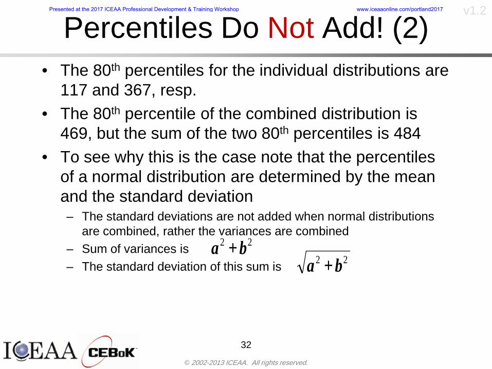
copy 2002-2013 ICEAA All rights reserved
v12
Percentiles Do Not Add (2)bull The 80th percentiles for the individual distributions are
117 and 367 respbull The 80th percentile of the combined distribution is
469 but the sum of the two 80th percentiles is 484bull To see why this is the case note that the percentiles
of a normal distribution are determined by the mean and the standard deviationndash The standard deviations are not added when normal distributions
are combined rather the variances are combinedndash Sum of variances is ndash The standard deviation of this sum is
32
22 ba +22 ba +
Presented at the 2017 ICEAA Professional Development amp Training Workshop wwwiceaaonlinecomportland2017
copy 2002-2013 ICEAA All rights reserved
v12
Percentiles Do Not Add (3)bull Since bull We can write
bull The left side of this inequality represents the risk of the combined distributions while the right side represents the sums of the individual risks
bull Combining two missions that are independent results in a diversification of riskndash The total portfolio is not as risky on a relative basis as each
individual project
33
2222 2 bababa ++lt+
baba +lt+ 22
Presented at the 2017 ICEAA Professional Development amp Training Workshop wwwiceaaonlinecomportland2017
copy 2002-2013 ICEAA All rights reserved
v12
Methods for Aggregating Riskbull Since percentiles do not add we have to find other
ways to aggregate riskbull One method is to use Monte Carlo simulationbull Unless cost risk is represented by normal
distributions for all WBS elements summing the means and variances does not result in a completely accurate depiction of overall system cost risk
bull The normal distribution is not a realistic distribution for representing risk in many or even most situations since regarding project risk more can go wrong than can go right which means the risk is NOT symmetric unlike the Gaussian bell curve
34
Presented at the 2017 ICEAA Professional Development amp Training Workshop wwwiceaaonlinecomportland2017
copy 2002-2013 ICEAA All rights reserved
v12
Unit III - Module 9 35
Monte Carlo Simulationfor Risk Analysis
bull When risk analysis is performed multiple risks are gatheredndash These risks may have various probability
distributions
bull Monte Carlo is the most commonly accepted way to produce an accurate characterization of the distribution of the combined effect of these many risksndash Using this distribution we can produce percentiles
for cost impacts due to risk occurrences
10
Presented at the 2017 ICEAA Professional Development amp Training Workshop wwwiceaaonlinecomportland2017
copy 2002-2013 ICEAA All rights reserved
v12
Monte Carlo Simulationbull Simulation is a means for solving problems that are
analytically intractablendash Involves repeated random sampling
bull It was developed during the Manhattan Project as a way to model the interactions inside an atom during nuclear fissionndash Allowed for more sophisticated mathematical modeling of atomic
phenomena
bull Most computer packages use pseudo-random number generators that produce seemingly random results from an initial seedndash Example is the linear congruential generator
36
( ) mbaXX nn mod1 +=+
Presented at the 2017 ICEAA Professional Development amp Training Workshop wwwiceaaonlinecomportland2017
copy 2002-2013 ICEAA All rights reserved
v12Using Random Numbers to Simulate Distributions
bull WBS cost risk is typically measured by a probability distributionbull The most common method for simulating a probability
distribution is the inverse methodbull This involve obtaining a simulated random value from a uniform
distribution and then inverting this through the cumulative distribution function (CDF) to obtain the simulated value
bull As an example for a uniform distribution on the interval [0100]
bull In this case the CDF random value of 05 translates to 10005 = 50
37
( )100
1=xf ( )
100xxF = ( ) xxF 1001 =-
Presented at the 2017 ICEAA Professional Development amp Training Workshop wwwiceaaonlinecomportland2017
copy 2002-2013 ICEAA All rights reserved
v12
Simulating a Triangular Distribution
bull For a triangular distribution with low = 0 most likely = 50 and high = 150 the CDF is given by
bull The inverse function is given by
38
( )iumliumlicirc
iumliumliacute
igrave
poundlt--
poundpound=
1505021
1500050
50015000
2
2
2
xxx
xxxF
( )iumliumlicirc
iumliumliacute
igrave
poundltdivideoslashouml
ccedilegraveaelig +--
poundpound=-
131
21
37501
250017500150
3107500
1
xx
xxxF
Presented at the 2017 ICEAA Professional Development amp Training Workshop wwwiceaaonlinecomportland2017
copy 2002-2013 ICEAA All rights reserved
v12
Simulating a Triangular Distribution (2)
bull If the simulated uniform value is equal to 02 the corresponding inverse value from the CDF inverse is approximately 387
39
0
01
02
03
04
05
06
07
08
09
1
0 30 60 90 120 150
Presented at the 2017 ICEAA Professional Development amp Training Workshop wwwiceaaonlinecomportland2017
copy 2002-2013 ICEAA All rights reserved
v12
Monte Carlo and the WBSbull Simulation involves repeated trials
40
WBS Draw1 2 3 4 5
System 2912 3566 4390 2954 4655 Sum
Structure 80 105 55 80 57 SumVehicle Structure 50 70 30 40 20Tank Structure 30 35 25 40 37
Thermal Control 32 36 35 29 33 SumActive Thermal Control 10 15 12 7 10Induced Thermal Control 12 14 13 14 14Tank Thermal Control 10 7 10 8 9
Main Propulsion System 100 150 125 140 100
Liquid Rocket Engine 1000 1100 1800 900 2200
Electric Power and Distribution 100 125 150 75 90
Command Control and Data Handling 200 250 225 230 275
System Integration 1400 1800 2000 1500 1900
Presented at the 2017 ICEAA Professional Development amp Training Workshop wwwiceaaonlinecomportland2017
copy 2002-2013 ICEAA All rights reserved
v12
Number of Trialsbull Monte Carlo involves a repeated number of trialsbull The greater the number of trials the more accurate the
simulation will approximate the overall cost risk behavior of the system
bull After 100 trials the histogram looks very jagged
41
Presented at the 2017 ICEAA Professional Development amp Training Workshop wwwiceaaonlinecomportland2017
copy 2002-2013 ICEAA All rights reserved
v12
Number of Trials (2)
42
1000 Trials
10000 Trials
50000 Trials Additional trials give a more accurate depiction of the final result
Presented at the 2017 ICEAA Professional Development amp Training Workshop wwwiceaaonlinecomportland2017
copy 2002-2013 ICEAA All rights reserved
v12
Number of Trials (3)bull If we want to simulate the underlying
mean within 1 with 95 confidence for example then we require
43
divideoslash
oumlccedilegrave
aelig poundpound-
=
dividedividedivide
oslash
ouml
ccedilccedilccedil
egrave
aeligpound
-pound
-=
divideoslashouml
ccedilegraveaelig poundpound=
nZ
n
nnX
n
X
n
n
011
010Pr
011
010Pr
011990Pr950
___
___
sm
sm
sm
sm
sm
mm
Presented at the 2017 ICEAA Professional Development amp Training Workshop wwwiceaaonlinecomportland2017
copy 2002-2013 ICEAA All rights reserved
v12
Number of Trials (4)bull This means that the number of trials required is determined by
bull Solving for n we find that at least
trials are neededbull Note that this term involves the coefficient of variation of the
distribution which means that distributions with less dispersion require fewer trials to accurate simulate
44
96101
=ns
m
ms41638
Presented at the 2017 ICEAA Professional Development amp Training Workshop wwwiceaaonlinecomportland2017
copy 2002-2013 ICEAA All rights reserved
v12
Number of Trials (5)bull Simulating percentiles requires more trials than for simulating
meansbull Let Pn represent the number of trials in the sample at or below
the 70th percentile of the underlying distribution (suppose this is known)
bull By the Central Limit Theorem Pnn follows a normal distribution with mean equal to the 70th percentile and variance equal to
bull By a similar process for the mean we find that the number of trials needed to simulate the 70th percentile within 1 with 95 confidence is
45
( )n
FF 700700 1-
n
n
PPn -41638
Presented at the 2017 ICEAA Professional Development amp Training Workshop wwwiceaaonlinecomportland2017
copy 2002-2013 ICEAA All rights reserved
v12
Number of Trials (6)bull If Pn 070 for all n then n is approximately
bull For the sake of comparison suppose CV = 03 (reasonable approximation for hardware development) then the number of trials needed to simulate the mean with the same accuracy is then ldquoonlyrdquo 11525
bull More trials are needed to accurately simulate percentiles than means
46
( ) 46416703041638
70704168341638 =divide
oslashouml
ccedilegraveaelig=divide
oslashouml
ccedilegraveaelig -
=-
nnn
PPn
n
n
Presented at the 2017 ICEAA Professional Development amp Training Workshop wwwiceaaonlinecomportland2017
copy 2002-2013 ICEAA All rights reserved
v12
Methods of Simulationbull Monte Carlo simulation is a standard term for
simulationbull However there is an improvement on Monte Carlo
that improves the accuracy of the results of a simulation for a given number of trials
bull This method is call the Latin Hypercube approach to simulationndash Similar to Monte Carlo but an equal number of draws are taken
from a set of subintervals for example dividing the interval (01) into [00001) [0102)hellip [0910]
ndash Instead of 10 trials from [01] we have one trial from each subinterval
ndash Rough rule of thumb is Latin Hypercube takes 30 fewer trials to achieve similar accuracy to Monte Carlo
47
Presented at the 2017 ICEAA Professional Development amp Training Workshop wwwiceaaonlinecomportland2017
copy 2002-2013 ICEAA All rights reserved
v12
Probability Model ndash Correlationbull Correlation exists between work breakdown structure
(WBS) cost element costs and between cost and schedule
bull Correlation is a necessary consideration in cost risk analysis
bull Correlation is a number that can vary between -1 and +1 and represents the strength of the relationship between the two variablesndash If both variable have a tendency to move in the same direction
correlation is positivendash If when one variable increases the other tends to decrease and
vice-versa the correlation between the two variables is negative
Presented at the 2017 ICEAA Professional Development amp Training Workshop wwwiceaaonlinecomportland2017
copy 2002-2013 ICEAA All rights reserved
v12
Correlation And Causationbull Note that correlation is not causation however
causation implies correlationndash For example shark attacks and ice cream sales at the beach
bull For example for a launch vehicle structure increasing the diameter will not only result in an increase in the structures cost but will also result in higher costs for thermal coating (paint etc)
bull Also simply because two subsystems do not appear to be related does not mean they are not correlatedndash For example structures and computer equipment seemingly
have little relation to one another however an external factor such as a funding cut or a strike will impact all subsystems leading to delays and increasing cost across the board
ndash Thus everything in a WBS has some correlationUnit III - Module 9 49
Presented at the 2017 ICEAA Professional Development amp Training Workshop wwwiceaaonlinecomportland2017
copy 2002-2013 ICEAA All rights reserved
v12
The Importance of Correlationbull Percent that total cost standard deviation is underestimated
when correlation assumed to be 0 instead of r given nWBS elements
Unit III - Module 9 5050
0
20
40
60
80
100
0 01 02 03 04 05 06 07 08 09 1Actual Correlation
Perce
nt Un
deres
timate
d
n = 10
n = 30
n = 100n = 1000
0
20
40
60
80
100
0 01 02 03 04 05 06 07 08 09 1Actual Correlation
Perce
nt Un
deres
timate
d
n = 10
n = 30
n = 100n = 1000
Reference 32nd Annual DOD Cost Analysis Symposium Advanced Training Session ldquoWhy Correlation Matters in Cost Estimatingrdquo Stephen A Book
Presented at the 2017 ICEAA Professional Development amp Training Workshop wwwiceaaonlinecomportland2017
copy 2002-2013 ICEAA All rights reserved
v12
The Importance of Correlation (2)bull For example if correlation is assumed to be 0 for all
elements in a 30 element WBS and the actual correlation is 20 then the total cost standard deviation is underestimated by 60
bull For example assume the total cost is modeled as a normal distribution with mean = 100
bull If correlation is assumed to be zero with total cost standard deviation = 12 when correlation is actually 20 then the true underlying standard deviation is actually 30
bull 70th percentile with zero correlation assumption is 106
bull 70th percentile with 20 correlation is 116 Unit III - Module 9 51
Presented at the 2017 ICEAA Professional Development amp Training Workshop wwwiceaaonlinecomportland2017
copy 2002-2013 ICEAA All rights reserved
v12
Measures of Correlationbull Two measures of correlation are commonly used in
cost risk analysesndash Pearsonrsquos product-moment correlation coefficient ndash Spearmanrsquos rank correlation coefficient
bull Garvey and others recommend using Pearsonrsquos product-moment correlation coefficient correlation for cost risk analysesndash Method of moments uses this but there are two options in
simulationndash Popular simulation packages like Risk and Crystal Ball use
rank correlation but in practice this has been found to make little difference
ndash Pearson product-moment correlation has been incorporated into Risk+
52
Presented at the 2017 ICEAA Professional Development amp Training Workshop wwwiceaaonlinecomportland2017
copy 2002-2013 ICEAA All rights reserved
v12
Pearson Correlationbull Pearsonrsquos product-moment correlation measures
degree of linearity between two random variables bull If two random variables are perfectly linear (eg Y =
aX + b) with positive slope then the Pearson product-moment correlation between X and Y denoted by rXY is +1
53
X X
Y Y Y
XNegative Correlation Positive Correlation No Correlation
middotmiddot
middotmiddot
middotmiddot middotmiddot
middotmiddot
middot
middot
middotmiddotmiddot
middotmiddot
middotmiddot
middotmiddot middot
middot
middot
middotmiddotmiddotmiddotmiddotmiddotmiddotmiddot
middotmiddotmiddotmiddot
middotmiddot
middotmiddot middotmiddotmiddotmiddot
middotmiddotmiddot
middotmiddotmiddotmiddot
middotmiddotmiddot
middotmiddotmiddot
middotmiddot
middot
middot middotmiddot
middot middotmiddotmiddotmiddot middotmiddot middot middotmiddot middot middot
middotmiddot middot
middotmiddotmiddotmiddotmiddot middot middotmiddot
middotmiddot
middot
middotmiddot
middotmiddot middot
middot middot middot
middotmiddot middot
middotmiddotmiddot
middotmiddot
middot middot
Presented at the 2017 ICEAA Professional Development amp Training Workshop wwwiceaaonlinecomportland2017
copy 2002-2013 ICEAA All rights reserved
v12
Spearman Correlationbull Spearmanrsquos rank correlation measures the
monotonicity between two random variablesbull If two random variables are perfectly monotonically
increasing (eg Y = X2) then the Spearman rank correlation denoted by rXY is +1
bull The two measures can be significantly different
54
10 20 30 40 50 60
100
200
300
096 097 098 099 1
1
060
020
040
080
Eff
ort (
Staf
f-M
onth
s)
Software Size I KDSI
y = 28z12y
z x
yy = x100
0 pound x pound 1
Figure 5-9A Figure 5-9B
Pearson Correlation = 09976 Rank Correlation = 1
Pearson Correlation = 024 Rank Correlation = 1
X(x ) ~ Unif(01)
Reference Probability Methods for Cost Uncertainty Analysis A Systems Engineering Perspective Paul R Garvey
Presented at the 2017 ICEAA Professional Development amp Training Workshop wwwiceaaonlinecomportland2017
copy 2002-2013 ICEAA All rights reserved
v12
Unit III - Module 9 55
200
250
300
350
400
1000 1200 1400 1600 1800 2000
Recurring Production
SEPM
200
250
300
350
400
1000 1200 1400 1600 1800 2000
Recurring Production
SEPM
Functional Correlationbull Old No Functional
Correlation Simulation run with WBS items entered as values
bull New Simulation run with functional dependencies entered as they are in cost model
CorrelatedNot Correlated
Note shift of mean and increased variability
Presented at the 2017 ICEAA Professional Development amp Training Workshop wwwiceaaonlinecomportland2017
copy 2002-2013 ICEAA All rights reserved
v12
Risk Measuresbull ldquoWestern Europe conquered the word because of a
technological revolution that started because of attempts to measure the worldrdquo ndash Phillipe Jorion ndash In the same way attempts to measure risk will lead to better project
managementbull Risk management for DoD and NASA agencies focuses
primarily on funding projects to a single percentile ndash NASA policy explicitly mentions 70 and 50ndash This is known as ldquoValue at Riskrdquo and is prevalent in the banking and
financial industry
56
Presented at the 2017 ICEAA Professional Development amp Training Workshop wwwiceaaonlinecomportland2017
copy 2002-2013 ICEAA All rights reserved
v12
Value at Risk (VaR)bull VaR is a percentile of the cost risk
distributionndash VaR funding at the 70th percentile means that
there is a 30 chance of final project cost exceeding the funded amount (budget)
bull VaR has some meritsndash Common measure can be used to compare
different projects and programsndash Easily understood by senior managers and
decision makers
57
Presented at the 2017 ICEAA Professional Development amp Training Workshop wwwiceaaonlinecomportland2017
copy 2002-2013 ICEAA All rights reserved
v12
Why 70th or 80th Percentilebull Typical policy guidance involves funding at the 70th or 80th
percentile Why fund as such a low percentilebull There is some incentive to not over-fundbull For a normal distribution an inflection point occurs near the 80th
percentile meaning that for values above 80 confidence achieving higher levels of confidence can only be achieved by spending greater dollar amounts at an increasing rate
58
-05-04-03-02-01
00102030405
0 05 1 15 2 25 3
Standard Deviations from Mean
Normal Distribution
First DerivativeSlopeVelocity
Second DerivativeConvexityAcceleration
Inflection point at one standard deviation above the mean (~84th
percentile)
Presented at the 2017 ICEAA Professional Development amp Training Workshop wwwiceaaonlinecomportland2017
copy 2002-2013 ICEAA All rights reserved
v12
Funding Above Inflection Pointsbull As the percentile goes above the 80th percentile the amount
needed to achieve that higher level of confidence begins to increase at an increasing rate as is evident from the graph
59
0
10
20
30
40
50
60
70
50 55 60 65 70 75 80 85 90 95 100
$ Ab
ove
MEa
n to
Ach
ieve
Per
cent
ile
Percentile (Confidence Level)
Presented at the 2017 ICEAA Professional Development amp Training Workshop wwwiceaaonlinecomportland2017
copy 2002-2013 ICEAA All rights reserved
v12
Why Budget to the 70th or 80thbull Government projects are funded at the 70th or 80th percentilesbull Why not the 90th or 99th percentile Wonrsquot that help prevent
overrunsndash As we have seen percentiles do not add across programs
bull The sum of the 80th percentiles does NOT equal the total 80th percentile
ndash This is because the individual programs are riskier than the entire suite of missions
bull Known as the ldquoPortfolio effectrdquo (more or this later)
ndash Funding at the 80th gives confidence that the entire portfolio will be adequately funded
bull And since there is an inflection point near the 80th percentile funding above that level quickly becomes cost prohibitive
60
Presented at the 2017 ICEAA Professional Development amp Training Workshop wwwiceaaonlinecomportland2017
copy 2002-2013 ICEAA All rights reserved
v12
Inflection Points for Lognormalbull For a lognormal the inflection point
variesndash Coefficient of variation equal to 10 equates to an
inflection point at the 70th percentile
61
0
10
20
30
40
50
60
70
050 060 070 080 090 100
Coef
ficen
t of V
aria
tion
Percentile of the Inflection Point
Presented at the 2017 ICEAA Professional Development amp Training Workshop wwwiceaaonlinecomportland2017
copy 2002-2013 ICEAA All rights reserved
v12
Issues with Percentile Fundingbull However risk management does not stop at a
specific percentilendash What happens when the 70th percentile is exceeded
bull Any effective risk management policy should prescribe what happens after a bad event occursndash With VaR we only know when a bad event has occurred ndash Also funding at a relatively low level means we have no true
sense of the real risks that should be guarded against
62
Presented at the 2017 ICEAA Professional Development amp Training Workshop wwwiceaaonlinecomportland2017
copy 2002-2013 ICEAA All rights reserved
v12
ldquoHere There Be Dragonsrdquobull On old maps uncharted territory was often
marked with monsters or dragons
63
A section of the Carta Marina by Olaus Magnus 16th Century
Presented at the 2017 ICEAA Professional Development amp Training Workshop wwwiceaaonlinecomportland2017
copy 2002-2013 ICEAA All rights reserved
v12
Distribution Comparisonbull Four different distributions with the same 70th
percentile
bull Should we expect the tails to be similar
64
0
10
20
30
40
50
60
70
80
0 100 200 300 400 500 600
Perc
entil
eCo
nfid
ence
Lev
el
Triangular
Normal
Lognormal
Pareto
Presented at the 2017 ICEAA Professional Development amp Training Workshop wwwiceaaonlinecomportland2017
copy 2002-2013 ICEAA All rights reserved
v12Distribution Comparison Tail Behavior
bull The normal and triangular distributions have similar tails but the lognormal and Pareto have much fatter right tails
65
70
75
80
85
90
95
100
500 1500 2500 3500 4500 5500
Perc
entil
eCo
nfid
ence
Lev
el
Triangular
Normal
Lognormal
Pareto
Here There Be Dragons
Presented at the 2017 ICEAA Professional Development amp Training Workshop wwwiceaaonlinecomportland2017
copy 2002-2013 ICEAA All rights reserved
v12Distribution Comparison ndash Tail Behavior (Table)
bull There is significant tail risk for the lognormal and the Paretobull The 99th percentile for the Pareto is 1000 times greater than
the 70th percentilendash Risk seen in financial markets and in catastrophic risks like natural
disasters bull Four different projects follow the four different risk profiles seen
in this example should clearly have different risk management approaches but 70th percentile funding indicates the same risk management approach for all four
66
Percentile Triangular Normal Lognormal Pareto 70th $600 $600 $600 $600 80th $680 $660 $770 $1430 90th $770 $750 $1070 $5880 95th $840 $820 $1410 $23750 99th $930 $950 $2350 $600000
Presented at the 2017 ICEAA Professional Development amp Training Workshop wwwiceaaonlinecomportland2017
copy 2002-2013 ICEAA All rights reserved
v12Percentile Budgeting is Not Risk Management
bull Percentile budgeting ne effective risk management policybull Suppose that you are shopping for a new car You
mention that safety is your top concern The salesman says he has a great safe car available You ask about the air bags Do they work The salesman answers ldquoOf course Seventy percent of the time they work fine Only 30 of the time the air bags will fail to deployrdquo Would you buy such a car Hedge fund manager David Einhorn has stated ldquoRisk management is the air bag that must always work but only in the multi-sigma event where you have an accidentrdquo
67
Risk management is the air bag that must always work but only in the multi-sigma event where you
have an accident
Presented at the 2017 ICEAA Professional Development amp Training Workshop wwwiceaaonlinecomportland2017
copy 2002-2013 ICEAA All rights reserved
v12
Joint Confidence Level Analysisbull Schedules are risky toobull For 98 recent NASA missions average
schedule growth was 38ndash Not as high as cost growth but still significant
68
0
5
10
15
20
25
30
35
40
Schedule
Cost
Presented at the 2017 ICEAA Professional Development amp Training Workshop wwwiceaaonlinecomportland2017
copy 2002-2013 ICEAA All rights reserved
v12
Schedules Impact Costbull Changes in schedule can have enormous
impacts on cost ndash Schedule slips can lead to cost increases
bull Fixed programmatic costs must be paid on a regular basisndash Achieving schedule milestones early can result in cost
savings
bull Schedule is an important consideration in cost analysis including cost risk analysis
bull However we must be careful in correctly integrating cost and schedule riskndash Schedule is not simply an input but is dependent on many of
the same factors that drive cost
69
Presented at the 2017 ICEAA Professional Development amp Training Workshop wwwiceaaonlinecomportland2017
copy 2002-2013 ICEAA All rights reserved
v12
The Relationship of Cost to Schedulebull Cost and schedule are positively correlated
ndash A larger program with bigger scope with take longer to complete than a smaller simpler program
bull However longer schedules do not always equate to higher cost nor shorter schedules with lower costndash Highly compressed schedules relative to the
optimal schedule can lead to large overrunsbull Compressed schedules are commonplace for
many planetary missions
70
Presented at the 2017 ICEAA Professional Development amp Training Workshop wwwiceaaonlinecomportland2017
copy 2002-2013 ICEAA All rights reserved
v12The Impact of Schedule GrowthCompression on Cost
bull Compressed schedules lead to cost growth and based on existing research is actually more expensive than schedule slippages
71
0
20
40
60
80
100
120
140
160
-50 -25 0 25 50 75 100
Percentage Change in Schedule
Perc
enta
ge C
hang
e in
Cos
t due
to
Sche
dule
Cha
nge
Source Smart CB ldquoCost and Schedule Interrelationshipsrdquo 2007 NASA Cost Symposium
Presented at the 2017 ICEAA Professional Development amp Training Workshop wwwiceaaonlinecomportland2017
copy 2002-2013 ICEAA All rights reserved
v12Schedule as an Independent Variable
bull Why not simply add schedule as an input to cost-estimating relationships (CERs)
bull Schedule is often treated as an independent variable ndash schedules are often determined independently of cost considerationsndash Cost may not be considered explicitly although budgets and
schedules are determined based on scope and other common factors
bull In 2006 SAIC undertook a research task to determine the impact of schedule on cost and added schedule as an independent variable to the CERs in the NASAAir Force Cost Model (NAFCOM) to see if schedule provided any improvement in goodness of fit
72
Presented at the 2017 ICEAA Professional Development amp Training Workshop wwwiceaaonlinecomportland2017
copy 2002-2013 ICEAA All rights reserved
v12
Schedule is a Dependent Variablebull Since NAFCOM includes an exhaustive list of cost drivers the inclusion
of schedule should give an indication of whether there is any additional independent value added from schedule independent of the cost drivers
bull In the study schedule was added to 10 subsystem-level CERs
ndash In each case the addition of schedule did NOTimprove the goodness of fit and schedule was NOT found to be a statistically significant cost driver (given the presence of the other variables) for any of the 10 CERs
bull Standard errors for the CERs increased due to decrease in degrees of freedom
bull Thus schedule as an independent variable did not provide any additional explanation of variation in historical cost
bull This is because schedule is truly NOT an independent variable but a dependent variable and is a function of the same factors that drive cost
73
Presented at the 2017 ICEAA Professional Development amp Training Workshop wwwiceaaonlinecomportland2017
copy 2002-2013 ICEAA All rights reserved
v12
Incorporation of Schedule in Cost Risk
bull When using subjective methods care must be taken in applying schedule to cost risk analysis
bull Since schedule is a dependent variable treating it independently from other factors when assessing its impact on cost can lead to a double count of independent variables in the cost risk analysis
bull Direct inclusion of schedule in a cost risk analysis effectively doubles the influence of each cost driver
ndash Incorrectly leads to broader risk ranges
74
CostWeight
HeritageNewness
Technology Readiness Schedule
Presented at the 2017 ICEAA Professional Development amp Training Workshop wwwiceaaonlinecomportland2017
copy 2002-2013 ICEAA All rights reserved
v12Subjective Cost Risk Methods and Overinclusion of Risk Factors
bull Subjective methods are suitable when data are scarce or not availablebull However care must be taken not to treat correlated sources of risk
such as schedule as independent of each otherbull Example ndash a subjective risk analysis incorporated technology readiness
design risk requirements stability integration risk and schedule and treated each source of risk as independent
bull Risk triangle high value without schedule risk was 31 times the point estimate
bull Risk triangle high value with schedule risk added on top of other sources of risk treated independently was 34 times the point estimate
bull Risk triangle taking correlation between sources of risk into account in a rigorous statistical manner has a high value 15 times the point estimate less than half the effect when treating sources of risk as independent
75
Presented at the 2017 ICEAA Professional Development amp Training Workshop wwwiceaaonlinecomportland2017
copy 2002-2013 ICEAA All rights reserved
v12Fundamental Equation of Cost and Schedule Interrelationships
bull The Fundamental Equation of the Relationship Between Cost and Schedule is
Time = Moneybull This is a well known adage that time is money Your boss at
work may even mention this to you from time to time or if you are the boss you are all too aware of this iron law
bull Because time is money cost and schedule risk should be modeled jointly not with schedule as an independent cost driver
bull Note that cost and schedule are not perfectly correlatedndash Cost can sometimes ldquobuy downrdquo schedule extra money can be
spent to meet a deadline since in some cases additional effort to hasten the completion of a task
76
Presented at the 2017 ICEAA Professional Development amp Training Workshop wwwiceaaonlinecomportland2017
copy 2002-2013 ICEAA All rights reserved
v12How to (Correctly) Incorporate Schedule into Cost Risk Analysis
bull The best way to model cost and schedule risk is to develop a joint cost and schedule model based on the same data
bull Since such models are not currently available the next best approach is to model cost and schedule independently and then integrate cost and schedule risk analyses using joint probability distributions taking into account correlation between cost and schedulendash This approach pioneered by Paul Garvey and Steve Book is
considered industry best practicendash This is a practical method mathematically tractable and follows
naturally from the Fundamental Equation of Cost and Schedule Interrelationships
77
Book S A ldquoQuantifying the Relationship Between Cost and Schedulerdquo The Measurable News Winter 2007-2008 pp 11-15Garvey PR Probability Methods for Cost Uncertainty Analysis A Systems Engineering Perspective New York Marcel Dekker 2000 pp 308-335
Presented at the 2017 ICEAA Professional Development amp Training Workshop wwwiceaaonlinecomportland2017
copy 2002-2013 ICEAA All rights reserved
v12
Joint Lognormal and Normal Distributions
bull Cost and schedule are typically modeled as some combination of Normal and Lognormal probability distributionsndash Studies by The Aerospace Corporation the MITRE
Corporation Wyle Labs and SAIC have found that the Lognormal probability distribution almost always serves as a good model for both the schedule distribution and the cost distribution
ndash The Normal distribution may also be appropriate in some instances and depending upon the level of confidence at which budgets are set may even be more conservative and logically consistent than the Normal distribution
ndash Joint Lognormal and Normal distributions are defined by a pair of mean and standard deviations and a level of correlation between the two
78
Presented at the 2017 ICEAA Professional Development amp Training Workshop wwwiceaaonlinecomportland2017
copy 2002-2013 ICEAA All rights reserved
v12Modeling Cost and Schedule as a Bivariate Distribution
bull In the approach set forth by Book and Garvey cost risk is assessed and the top-level distribution is modeled as a Lognormal (or Normal) distribution schedule risk is assessed and the overall schedule risk is modeled as a Lognormal (or Normal) distribution
bull The two distributions are combined into a Bivariate distribution by assigning a correlation between the two and by treating the two distributions as the marginal distributions of a Bivariate Lognormal distributionndash Other combinations include a Bivariate Normal or a Bivariate
Normal-Lognormal
79
Presented at the 2017 ICEAA Professional Development amp Training Workshop wwwiceaaonlinecomportland2017
copy 2002-2013 ICEAA All rights reserved
v12Bivariate Lognormal Distribution for Cost and Schedule
bull Cost is often observed to be Lognormal when strong positive correlations are present among the systemrsquos WBS cost element costs
bull A systemrsquos schedule is often observed (from Monte Carlo simulations) to be Lognormal if it is the sum of many positively correlated schedule activities in an overall schedule network
bull If Lognormal distributions characterize a systemrsquos cost and schedule then the Bivariate Lognormal could serve as an assumed model of their joint distributionndash In this case the marginal distribution of each of cost and schedule is
Lognormalbull Other possibilities for modeling cost and schedule as a Bivariate
distribution include a Bivariate Normal or a Bivariate Normal-Lognormal distributionndash All these combinations are analytically tractable
80
Presented at the 2017 ICEAA Professional Development amp Training Workshop wwwiceaaonlinecomportland2017
copy 2002-2013 ICEAA All rights reserved
v12Bivariate Lognormal for Cost and Schedule
bull Contour Plots of a Bivariate Lognormal
81
Presented at the 2017 ICEAA Professional Development amp Training Workshop wwwiceaaonlinecomportland2017
copy 2002-2013 ICEAA All rights reserved
v12Correlation Between Cost and Schedule
bull Cost and schedule are positively correlated but not perfectly sondash For example it is possible to have a schedule underrun and a cost
overrunbull Based on cost and schedule growth data for 50 completed NASA
programs the correlation between development cost and development schedule is 70
82
00
200
400
600
800
1000
1200
-500 00 500 1000 1500 2000 2500Historical Cost Growth
Hist
oric
al S
ched
ule
Gro
wth
r = 715
Presented at the 2017 ICEAA Professional Development amp Training Workshop wwwiceaaonlinecomportland2017
copy 2002-2013 ICEAA All rights reserved
v12Correlation Between Cost and Schedule Caveats
bull Based on historical data recommended correlation between cost and schedule is 70 but this could be higher or lower depending upon program circumstancesndash If program is budget constrained cost and schedule will be
more highly correlated (go as you pay)ndash If program is schedule constrained cost and schedule will
have lower correlation perhaps even negative correlation ndash Smaller programs have smaller correlation between cost and
schedule riskbull Relatively easy to ldquohurry uprdquo and finish on time or even early if
needed
83
Presented at the 2017 ICEAA Professional Development amp Training Workshop wwwiceaaonlinecomportland2017
copy 2002-2013 ICEAA All rights reserved
v12
Conditional Confidence Levelsbull Given a programrsquos project schedule we can determine the cost
risk distribution conditional upon the given schedulebull Conditional cost S-curves are steeper than unconditional
(marginal) cost S-curves between some uncertainty has been removed because schedule is fixed
84
Presented at the 2017 ICEAA Professional Development amp Training Workshop wwwiceaaonlinecomportland2017
copy 2002-2013 ICEAA All rights reserved
v12
Joint Confidence Levelsbull Joint 65 confidence represents the probability of
achieving both 65 confidence in cost AND 65 confidence in schedulendash This is different than achieving 65 cost confidence alone
or achieving 65 schedule confidence alonebull Due to the imperfect correlation between cost and schedule it
is possible to achieve a 65 cost confidence with a lower level of schedule confidence
bull Restricting the schedule confidence thus requires additional $ to achieve a given level of confidence
85
X
Y
Possible Values for Which X gt a Possible Values for
Which X gt a and Y gt b
a
b
Presented at the 2017 ICEAA Professional Development amp Training Workshop wwwiceaaonlinecomportland2017
copy 2002-2013 ICEAA All rights reserved
v12Joint Confidence Levels Versus Cost Confidence Levels Only
bull Example of the differences between cost confidence schedule confidence conditional cost confidence and joint cost and schedule confidence
86
Joint Cost-Schedule Confidence Iso-Curves
Cost (RY$M)
Sche
dule
(Mon
ths)
65 Confidence
50 Confidence
70 Confidence
65 Cost Confidence AggressiveSchedule65 Cost ConfidenceScheduleGiven 65 Schedule ConfidenceUnconditional 65 CostConfidenceUnconditional 65 ScheduleConfidence
65 Cost Confidence 65 Joint Cost and Schedule
Confidence for 65 Schedule Confidence
Presented at the 2017 ICEAA Professional Development amp Training Workshop wwwiceaaonlinecomportland2017
copy 2002-2013 ICEAA All rights reserved
v12
Joint Cost and Schedule Confidence
bull Can examine pairs of cost and schedule that achieve a given level of confidence
bull Provides insights into the trade-offs between cost and schedule for a given level of confidencendash Possible to increase cost confidence by giving a
project more time in some instances or possible to ldquobuy downrdquo schedule
bull But these have limits and are shown in the iso-cost and schedule confidence curves
87
Presented at the 2017 ICEAA Professional Development amp Training Workshop wwwiceaaonlinecomportland2017
copy 2002-2013 ICEAA All rights reserved
v12Cost and Schedule Trade-offs for a Given Level of Joint Confidence
bull Hypothetical Example
88
Cost (RY$M)
Schedule (Months)
$100 48$99 48$89 49$87 50$85 51$85 52$84 53$83 55$83 55$83 56
Cost and Schedule 65 Confidence Iso-Curve
4748495051525354555657
$80 $82 $84 $86 $88 $90 $92 $94 $96 $98 $100
Cost (RY$ M)
Sche
dule
(Mon
ths)
Presented at the 2017 ICEAA Professional Development amp Training Workshop wwwiceaaonlinecomportland2017
copy 2002-2013 ICEAA All rights reserved
v12Policy Considerations for Confidence Levels
bull For large programs the difference between the amount of money needed to achieve 65 cost confidence independent of schedule and joint 65 cost and schedule confidence can represent hundreds of millions and even billions of dollars
89
Joint Cost-Schedule Confidence Iso-Curves
Cost (RY$M)
Sche
dule
(Mon
ths)
65 Confidence
65 Cost Confidence AggressiveSchedule
65 Cost ConfidenceScheduleGiven 65 Schedule Confidence
Unconditional 65 CostConfidence
Joint Cost and Schedule Confidence for 65 Cost Confidence and Program Baseline Schedule is Less Than 35
65 Cost Confidence Independent of Schedule Cost Needed to Achieve
Both 65 Joint Cost and Schedule Confidence for the Schedule with 65 Confidence
Presented at the 2017 ICEAA Professional Development amp Training Workshop wwwiceaaonlinecomportland2017
copy 2002-2013 ICEAA All rights reserved
v12
Copulasbull More generally any combination of distributions can
be used (more than just normal and lognormal)ndash Termed ldquocopulardquo from the Italian word for ldquocouplerdquondash Copulas are a way to combine marginal distributions of any
number and type into a joint distributionbull More formally a copula is a multivariate joint distribution defined
on the n-dimensional unit cube [0 1]n such that every marginal distribution is uniform on the interval [0 1]
bull (The bivariate form of) Sklarrsquos theorem states that for any bivariate distribution function H(x y) let F(x) = H(x infin) and G(y) = H(infin y) be the univariate marginal probability distribution functions Then there exists a copula C such that H(xy)=C(F(x)G(y))
ndash Copulas are widely used in risk management for investments and insurance
bull Considered industry best practice (Li 2000)bull Marketed as part of JP Morganrsquos CreditMetrics suite of tools
(Gupton et Al 1997)90
Presented at the 2017 ICEAA Professional Development amp Training Workshop wwwiceaaonlinecomportland2017
copy 2002-2013 ICEAA All rights reserved
v12Parametric Joint Cost and Schedule Analysis
bull A parametric model based on a consistent data set with a set of overlapping cost and schedule drivers is a cleaner way to model cost and schedule
91
CostWeight
HeritageNewness
Technology Readiness
Schedule
0
20
40
60
80
100
Confidence
Joint Cost and Schedule Confidence
Schedule
Cost
Lognormal Distribution PDF and CDF
0102030405060708090100
200 300 400 500 600 700 800 900 1000Cost $
Con
fiden
ce L
evel
0
00002
00004
00006
00008
0001
00012
00014
00016
Prob
abili
ty D
ensi
ty
CDFPDF
Lognormal Distribution PDF and CDF
0102030405060708090100
200 300 400 500 600 700 800 900 1000Cost $
Con
fiden
ce L
evel
0
00002
00004
00006
00008
0001
00012
00014
00016
Prob
abili
ty D
ensi
ty
CDFPDF
Presented at the 2017 ICEAA Professional Development amp Training Workshop wwwiceaaonlinecomportland2017
copy 2002-2013 ICEAA All rights reserved
v12Parametric Joint Cost and Schedule Analysis (2)
bull Joint cost and schedule risk analysis produced naturally by the integrated modelndash Addresses several issues with the copula
approachbull Tail dependencybull Correlation ndash no need to assign correlation
between cost and schedulebull Consistency of cost and schedule models
92
Presented at the 2017 ICEAA Professional Development amp Training Workshop wwwiceaaonlinecomportland2017
copy 2002-2013 ICEAA All rights reserved
v12
Resource-Loaded Schedulesbull Involves assigning cost and schedule risks to a resource-loaded schedule
networkbull Bottom-up approach
ndash More labor intensive than parametrics but can also provide more insight
ndash Can answer questions than parametric typically cannot such as how much do reserve requirements decrease if a specific risk is retired
bull Currently being implemented in Constellation programbull Has same issue as all bottom-up models hard to count all the risks and model
them discretely
ndash As a result there is a tendency to reflect less risk than indicated by history
ndash ldquoThere are more things in heaven and earth Horatio than are dreamt of in your philosophyrdquo William Shakespeare Hamlet Act I Scene V
93
Presented at the 2017 ICEAA Professional Development amp Training Workshop wwwiceaaonlinecomportland2017
copy 2002-2013 ICEAA All rights reserved
v12Resource-Loaded Schedules Vs Parametrics
bull Parametric most appropriate for early estimatesndash But also good for high-level checks as project progresses
bull As plans take shape lower level modeling may be more appropriate
94 1
CONCEPTUALDEVELOPMENT
PROJECTDEFINITION DESIGN DEVELOPMENT OPERATIONS
PARAMETRIC PARAMETRIC
ANALOGY
ENGINEERING (Bottoms Up)
$PARAMETRIC
DETAILED
$
Pre Phase A Phase B Phase CDPhase A Phase EPre Phase A Phase B Phase CDPhase A Phase E
Risk = f(Cost Estimating Relationship Inputs eg mass power data rate TRL new design etc)
Risk = f(cost and schedule variation of the analogous elements)
Risk = f(variation of detailed inputs eg labor hours rates materials etc)
Presented at the 2017 ICEAA Professional Development amp Training Workshop wwwiceaaonlinecomportland2017
copy 2002-2013 ICEAA All rights reserved
v12
Resource-Loaded Schedulesbull Methodology has been demonstrated in other
industriesndash Construction oil and gasndash Analysis has not been traditionally done on highly uncertain
complex development projects bull Methodology focuses on project baseline schedule
ndash In baseline schedule all tasks are resource loaded to represent a baseline schedule and cost standpoint
ndash Resource loaded schedule is ldquorolledrdquo up to a manageable level
ndash Based on the risk and uncertainties identified schedule distributions are applied to each rolled up task
ndash Cost uncertainties are also applied to rolled up tasksbull Uncertainties include labor rate man power etc
ndash A Monte Carlo simulation is run to develop joint cost-schedule distributions
95
Presented at the 2017 ICEAA Professional Development amp Training Workshop wwwiceaaonlinecomportland2017
copy 2002-2013 ICEAA All rights reserved
v12
Unit III - Module 9 96
Execution ndash Cross Checksbull Means The mean cost growth factor for WBS items
can be compared to history as a way to cross check results
bull CVs The CV of the cost growth factors for WBS items can be compared to history as a way to cross check results
bull Inputs Checks are performed on inputs or other parameters to see if historical values are in line with program assumptionsndash Example Historical risk scores can be compared to program
risk scores to see if risk assessors are being realistic and to see if the underlying database is representative of the program
11
Presented at the 2017 ICEAA Professional Development amp Training Workshop wwwiceaaonlinecomportland2017
- Cost and Schedule Risk Analysis Basic
- Acknowledgments
- Unit Index
- Risk Overview
- Agenda
- Introduction
- Risk Analysis Terms
- Are Our Costs Realistic
- Historical Cost Growth
- Sources of Cost Risk
- Point Estimates of Cost
- Types of Risk
- Point Estimates Vs Risk Estimates
- Cost Risk and Probability
- Probability Model ndash Distribution
- Probability Model ndash Distribution
- Probability ndash Top-Level Distribution
- S-Curves and Confidence Levels
- Example ndash Normal Distribution
- Confidence Levels
- Measuring Parametric Model Uncertainty
- Parametric Model Example
- Weight Uncertainty
- Estimating Uncertainty
- Estimating Uncertainty (2)
- Estimating Uncertainty (3)
- Aggregating Risk
- WBS Example
- WBS and Risk
- Aggregating Risk
- Percentiles Do Not Add
- Percentiles Do Not Add (2)
- Percentiles Do Not Add (3)
- Methods for Aggregating Risk
- Monte Carlo Simulationfor Risk Analysis
- Monte Carlo Simulation
- Using Random Numbers to Simulate Distributions
- Simulating a Triangular Distribution
- Simulating a Triangular Distribution (2)
- Monte Carlo and the WBS
- Number of Trials
- Number of Trials (2)
- Number of Trials (3)
- Number of Trials (4)
- Number of Trials (5)
- Number of Trials (6)
- Methods of Simulation
- Probability Model ndash Correlation
- Correlation And Causation
- The Importance of Correlation
- The Importance of Correlation (2)
- Measures of Correlation
- Pearson Correlation
- Spearman Correlation
- Functional Correlation
- Risk Measures
- Value at Risk (VaR)
- Why 70th or 80th Percentile
- Funding Above Inflection Points
- Why Budget to the 70th or 80th
- Inflection Points for Lognormal
- Issues with Percentile Funding
- ldquoHere There Be Dragonsrdquo
- Distribution Comparison
- Distribution Comparison Tail Behavior
- Distribution Comparison ndash Tail Behavior (Table)
- Percentile Budgeting is Not Risk Management
- Joint Confidence Level Analysis
- Schedules Impact Cost
- The Relationship of Cost to Schedule
- The Impact of Schedule GrowthCompression on Cost
- Schedule as an Independent Variable
- Schedule is a Dependent Variable
- Incorporation of Schedule in Cost Risk
- Subjective Cost Risk Methods and Overinclusion of Risk Factors
- Fundamental Equation of Cost and Schedule Interrelationships
- How to (Correctly) Incorporate Schedule into Cost Risk Analysis
- Joint Lognormal and Normal Distributions
- Modeling Cost and Schedule as a Bivariate Distribution
- Bivariate Lognormal Distribution for Cost and Schedule
- Bivariate Lognormal for Cost and Schedule
- Correlation Between Cost and Schedule
- Correlation Between Cost and Schedule Caveats
- Conditional Confidence Levels
- Joint Confidence Levels
- Joint Confidence Levels Versus Cost Confidence Levels Only
- Joint Cost and Schedule Confidence
- Cost and Schedule Trade-offs for a Given Level of Joint Confidence
- Policy Considerations for Confidence Levels
- Copulas
- Parametric Joint Cost and Schedule Analysis
- Parametric Joint Cost and Schedule Analysis (2)
- Resource-Loaded Schedules
- Resource-Loaded Schedules Vs Parametrics
- Resource-Loaded Schedules
- Execution ndash Cross Checks
-
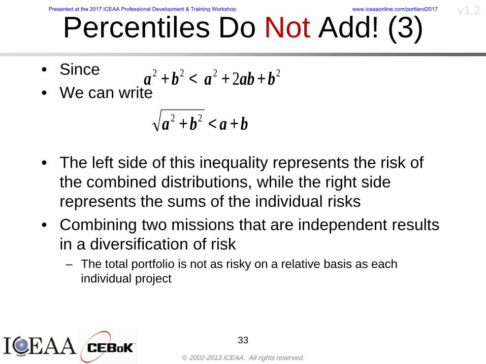
copy 2002-2013 ICEAA All rights reserved
v12
Percentiles Do Not Add (3)bull Since bull We can write
bull The left side of this inequality represents the risk of the combined distributions while the right side represents the sums of the individual risks
bull Combining two missions that are independent results in a diversification of riskndash The total portfolio is not as risky on a relative basis as each
individual project
33
2222 2 bababa ++lt+
baba +lt+ 22
Presented at the 2017 ICEAA Professional Development amp Training Workshop wwwiceaaonlinecomportland2017
copy 2002-2013 ICEAA All rights reserved
v12
Methods for Aggregating Riskbull Since percentiles do not add we have to find other
ways to aggregate riskbull One method is to use Monte Carlo simulationbull Unless cost risk is represented by normal
distributions for all WBS elements summing the means and variances does not result in a completely accurate depiction of overall system cost risk
bull The normal distribution is not a realistic distribution for representing risk in many or even most situations since regarding project risk more can go wrong than can go right which means the risk is NOT symmetric unlike the Gaussian bell curve
34
Presented at the 2017 ICEAA Professional Development amp Training Workshop wwwiceaaonlinecomportland2017
copy 2002-2013 ICEAA All rights reserved
v12
Unit III - Module 9 35
Monte Carlo Simulationfor Risk Analysis
bull When risk analysis is performed multiple risks are gatheredndash These risks may have various probability
distributions
bull Monte Carlo is the most commonly accepted way to produce an accurate characterization of the distribution of the combined effect of these many risksndash Using this distribution we can produce percentiles
for cost impacts due to risk occurrences
10
Presented at the 2017 ICEAA Professional Development amp Training Workshop wwwiceaaonlinecomportland2017
copy 2002-2013 ICEAA All rights reserved
v12
Monte Carlo Simulationbull Simulation is a means for solving problems that are
analytically intractablendash Involves repeated random sampling
bull It was developed during the Manhattan Project as a way to model the interactions inside an atom during nuclear fissionndash Allowed for more sophisticated mathematical modeling of atomic
phenomena
bull Most computer packages use pseudo-random number generators that produce seemingly random results from an initial seedndash Example is the linear congruential generator
36
( ) mbaXX nn mod1 +=+
Presented at the 2017 ICEAA Professional Development amp Training Workshop wwwiceaaonlinecomportland2017
copy 2002-2013 ICEAA All rights reserved
v12Using Random Numbers to Simulate Distributions
bull WBS cost risk is typically measured by a probability distributionbull The most common method for simulating a probability
distribution is the inverse methodbull This involve obtaining a simulated random value from a uniform
distribution and then inverting this through the cumulative distribution function (CDF) to obtain the simulated value
bull As an example for a uniform distribution on the interval [0100]
bull In this case the CDF random value of 05 translates to 10005 = 50
37
( )100
1=xf ( )
100xxF = ( ) xxF 1001 =-
Presented at the 2017 ICEAA Professional Development amp Training Workshop wwwiceaaonlinecomportland2017
copy 2002-2013 ICEAA All rights reserved
v12
Simulating a Triangular Distribution
bull For a triangular distribution with low = 0 most likely = 50 and high = 150 the CDF is given by
bull The inverse function is given by
38
( )iumliumlicirc
iumliumliacute
igrave
poundlt--
poundpound=
1505021
1500050
50015000
2
2
2
xxx
xxxF
( )iumliumlicirc
iumliumliacute
igrave
poundltdivideoslashouml
ccedilegraveaelig +--
poundpound=-
131
21
37501
250017500150
3107500
1
xx
xxxF
Presented at the 2017 ICEAA Professional Development amp Training Workshop wwwiceaaonlinecomportland2017
copy 2002-2013 ICEAA All rights reserved
v12
Simulating a Triangular Distribution (2)
bull If the simulated uniform value is equal to 02 the corresponding inverse value from the CDF inverse is approximately 387
39
0
01
02
03
04
05
06
07
08
09
1
0 30 60 90 120 150
Presented at the 2017 ICEAA Professional Development amp Training Workshop wwwiceaaonlinecomportland2017
copy 2002-2013 ICEAA All rights reserved
v12
Monte Carlo and the WBSbull Simulation involves repeated trials
40
WBS Draw1 2 3 4 5
System 2912 3566 4390 2954 4655 Sum
Structure 80 105 55 80 57 SumVehicle Structure 50 70 30 40 20Tank Structure 30 35 25 40 37
Thermal Control 32 36 35 29 33 SumActive Thermal Control 10 15 12 7 10Induced Thermal Control 12 14 13 14 14Tank Thermal Control 10 7 10 8 9
Main Propulsion System 100 150 125 140 100
Liquid Rocket Engine 1000 1100 1800 900 2200
Electric Power and Distribution 100 125 150 75 90
Command Control and Data Handling 200 250 225 230 275
System Integration 1400 1800 2000 1500 1900
Presented at the 2017 ICEAA Professional Development amp Training Workshop wwwiceaaonlinecomportland2017
copy 2002-2013 ICEAA All rights reserved
v12
Number of Trialsbull Monte Carlo involves a repeated number of trialsbull The greater the number of trials the more accurate the
simulation will approximate the overall cost risk behavior of the system
bull After 100 trials the histogram looks very jagged
41
Presented at the 2017 ICEAA Professional Development amp Training Workshop wwwiceaaonlinecomportland2017
copy 2002-2013 ICEAA All rights reserved
v12
Number of Trials (2)
42
1000 Trials
10000 Trials
50000 Trials Additional trials give a more accurate depiction of the final result
Presented at the 2017 ICEAA Professional Development amp Training Workshop wwwiceaaonlinecomportland2017
copy 2002-2013 ICEAA All rights reserved
v12
Number of Trials (3)bull If we want to simulate the underlying
mean within 1 with 95 confidence for example then we require
43
divideoslash
oumlccedilegrave
aelig poundpound-
=
dividedividedivide
oslash
ouml
ccedilccedilccedil
egrave
aeligpound
-pound
-=
divideoslashouml
ccedilegraveaelig poundpound=
nZ
n
nnX
n
X
n
n
011
010Pr
011
010Pr
011990Pr950
___
___
sm
sm
sm
sm
sm
mm
Presented at the 2017 ICEAA Professional Development amp Training Workshop wwwiceaaonlinecomportland2017
copy 2002-2013 ICEAA All rights reserved
v12
Number of Trials (4)bull This means that the number of trials required is determined by
bull Solving for n we find that at least
trials are neededbull Note that this term involves the coefficient of variation of the
distribution which means that distributions with less dispersion require fewer trials to accurate simulate
44
96101
=ns
m
ms41638
Presented at the 2017 ICEAA Professional Development amp Training Workshop wwwiceaaonlinecomportland2017
copy 2002-2013 ICEAA All rights reserved
v12
Number of Trials (5)bull Simulating percentiles requires more trials than for simulating
meansbull Let Pn represent the number of trials in the sample at or below
the 70th percentile of the underlying distribution (suppose this is known)
bull By the Central Limit Theorem Pnn follows a normal distribution with mean equal to the 70th percentile and variance equal to
bull By a similar process for the mean we find that the number of trials needed to simulate the 70th percentile within 1 with 95 confidence is
45
( )n
FF 700700 1-
n
n
PPn -41638
Presented at the 2017 ICEAA Professional Development amp Training Workshop wwwiceaaonlinecomportland2017
copy 2002-2013 ICEAA All rights reserved
v12
Number of Trials (6)bull If Pn 070 for all n then n is approximately
bull For the sake of comparison suppose CV = 03 (reasonable approximation for hardware development) then the number of trials needed to simulate the mean with the same accuracy is then ldquoonlyrdquo 11525
bull More trials are needed to accurately simulate percentiles than means
46
( ) 46416703041638
70704168341638 =divide
oslashouml
ccedilegraveaelig=divide
oslashouml
ccedilegraveaelig -
=-
nnn
PPn
n
n
Presented at the 2017 ICEAA Professional Development amp Training Workshop wwwiceaaonlinecomportland2017
copy 2002-2013 ICEAA All rights reserved
v12
Methods of Simulationbull Monte Carlo simulation is a standard term for
simulationbull However there is an improvement on Monte Carlo
that improves the accuracy of the results of a simulation for a given number of trials
bull This method is call the Latin Hypercube approach to simulationndash Similar to Monte Carlo but an equal number of draws are taken
from a set of subintervals for example dividing the interval (01) into [00001) [0102)hellip [0910]
ndash Instead of 10 trials from [01] we have one trial from each subinterval
ndash Rough rule of thumb is Latin Hypercube takes 30 fewer trials to achieve similar accuracy to Monte Carlo
47
Presented at the 2017 ICEAA Professional Development amp Training Workshop wwwiceaaonlinecomportland2017
copy 2002-2013 ICEAA All rights reserved
v12
Probability Model ndash Correlationbull Correlation exists between work breakdown structure
(WBS) cost element costs and between cost and schedule
bull Correlation is a necessary consideration in cost risk analysis
bull Correlation is a number that can vary between -1 and +1 and represents the strength of the relationship between the two variablesndash If both variable have a tendency to move in the same direction
correlation is positivendash If when one variable increases the other tends to decrease and
vice-versa the correlation between the two variables is negative
Presented at the 2017 ICEAA Professional Development amp Training Workshop wwwiceaaonlinecomportland2017
copy 2002-2013 ICEAA All rights reserved
v12
Correlation And Causationbull Note that correlation is not causation however
causation implies correlationndash For example shark attacks and ice cream sales at the beach
bull For example for a launch vehicle structure increasing the diameter will not only result in an increase in the structures cost but will also result in higher costs for thermal coating (paint etc)
bull Also simply because two subsystems do not appear to be related does not mean they are not correlatedndash For example structures and computer equipment seemingly
have little relation to one another however an external factor such as a funding cut or a strike will impact all subsystems leading to delays and increasing cost across the board
ndash Thus everything in a WBS has some correlationUnit III - Module 9 49
Presented at the 2017 ICEAA Professional Development amp Training Workshop wwwiceaaonlinecomportland2017
copy 2002-2013 ICEAA All rights reserved
v12
The Importance of Correlationbull Percent that total cost standard deviation is underestimated
when correlation assumed to be 0 instead of r given nWBS elements
Unit III - Module 9 5050
0
20
40
60
80
100
0 01 02 03 04 05 06 07 08 09 1Actual Correlation
Perce
nt Un
deres
timate
d
n = 10
n = 30
n = 100n = 1000
0
20
40
60
80
100
0 01 02 03 04 05 06 07 08 09 1Actual Correlation
Perce
nt Un
deres
timate
d
n = 10
n = 30
n = 100n = 1000
Reference 32nd Annual DOD Cost Analysis Symposium Advanced Training Session ldquoWhy Correlation Matters in Cost Estimatingrdquo Stephen A Book
Presented at the 2017 ICEAA Professional Development amp Training Workshop wwwiceaaonlinecomportland2017
copy 2002-2013 ICEAA All rights reserved
v12
The Importance of Correlation (2)bull For example if correlation is assumed to be 0 for all
elements in a 30 element WBS and the actual correlation is 20 then the total cost standard deviation is underestimated by 60
bull For example assume the total cost is modeled as a normal distribution with mean = 100
bull If correlation is assumed to be zero with total cost standard deviation = 12 when correlation is actually 20 then the true underlying standard deviation is actually 30
bull 70th percentile with zero correlation assumption is 106
bull 70th percentile with 20 correlation is 116 Unit III - Module 9 51
Presented at the 2017 ICEAA Professional Development amp Training Workshop wwwiceaaonlinecomportland2017
copy 2002-2013 ICEAA All rights reserved
v12
Measures of Correlationbull Two measures of correlation are commonly used in
cost risk analysesndash Pearsonrsquos product-moment correlation coefficient ndash Spearmanrsquos rank correlation coefficient
bull Garvey and others recommend using Pearsonrsquos product-moment correlation coefficient correlation for cost risk analysesndash Method of moments uses this but there are two options in
simulationndash Popular simulation packages like Risk and Crystal Ball use
rank correlation but in practice this has been found to make little difference
ndash Pearson product-moment correlation has been incorporated into Risk+
52
Presented at the 2017 ICEAA Professional Development amp Training Workshop wwwiceaaonlinecomportland2017
copy 2002-2013 ICEAA All rights reserved
v12
Pearson Correlationbull Pearsonrsquos product-moment correlation measures
degree of linearity between two random variables bull If two random variables are perfectly linear (eg Y =
aX + b) with positive slope then the Pearson product-moment correlation between X and Y denoted by rXY is +1
53
X X
Y Y Y
XNegative Correlation Positive Correlation No Correlation
middotmiddot
middotmiddot
middotmiddot middotmiddot
middotmiddot
middot
middot
middotmiddotmiddot
middotmiddot
middotmiddot
middotmiddot middot
middot
middot
middotmiddotmiddotmiddotmiddotmiddotmiddotmiddot
middotmiddotmiddotmiddot
middotmiddot
middotmiddot middotmiddotmiddotmiddot
middotmiddotmiddot
middotmiddotmiddotmiddot
middotmiddotmiddot
middotmiddotmiddot
middotmiddot
middot
middot middotmiddot
middot middotmiddotmiddotmiddot middotmiddot middot middotmiddot middot middot
middotmiddot middot
middotmiddotmiddotmiddotmiddot middot middotmiddot
middotmiddot
middot
middotmiddot
middotmiddot middot
middot middot middot
middotmiddot middot
middotmiddotmiddot
middotmiddot
middot middot
Presented at the 2017 ICEAA Professional Development amp Training Workshop wwwiceaaonlinecomportland2017
copy 2002-2013 ICEAA All rights reserved
v12
Spearman Correlationbull Spearmanrsquos rank correlation measures the
monotonicity between two random variablesbull If two random variables are perfectly monotonically
increasing (eg Y = X2) then the Spearman rank correlation denoted by rXY is +1
bull The two measures can be significantly different
54
10 20 30 40 50 60
100
200
300
096 097 098 099 1
1
060
020
040
080
Eff
ort (
Staf
f-M
onth
s)
Software Size I KDSI
y = 28z12y
z x
yy = x100
0 pound x pound 1
Figure 5-9A Figure 5-9B
Pearson Correlation = 09976 Rank Correlation = 1
Pearson Correlation = 024 Rank Correlation = 1
X(x ) ~ Unif(01)
Reference Probability Methods for Cost Uncertainty Analysis A Systems Engineering Perspective Paul R Garvey
Presented at the 2017 ICEAA Professional Development amp Training Workshop wwwiceaaonlinecomportland2017
copy 2002-2013 ICEAA All rights reserved
v12
Unit III - Module 9 55
200
250
300
350
400
1000 1200 1400 1600 1800 2000
Recurring Production
SEPM
200
250
300
350
400
1000 1200 1400 1600 1800 2000
Recurring Production
SEPM
Functional Correlationbull Old No Functional
Correlation Simulation run with WBS items entered as values
bull New Simulation run with functional dependencies entered as they are in cost model
CorrelatedNot Correlated
Note shift of mean and increased variability
Presented at the 2017 ICEAA Professional Development amp Training Workshop wwwiceaaonlinecomportland2017
copy 2002-2013 ICEAA All rights reserved
v12
Risk Measuresbull ldquoWestern Europe conquered the word because of a
technological revolution that started because of attempts to measure the worldrdquo ndash Phillipe Jorion ndash In the same way attempts to measure risk will lead to better project
managementbull Risk management for DoD and NASA agencies focuses
primarily on funding projects to a single percentile ndash NASA policy explicitly mentions 70 and 50ndash This is known as ldquoValue at Riskrdquo and is prevalent in the banking and
financial industry
56
Presented at the 2017 ICEAA Professional Development amp Training Workshop wwwiceaaonlinecomportland2017
copy 2002-2013 ICEAA All rights reserved
v12
Value at Risk (VaR)bull VaR is a percentile of the cost risk
distributionndash VaR funding at the 70th percentile means that
there is a 30 chance of final project cost exceeding the funded amount (budget)
bull VaR has some meritsndash Common measure can be used to compare
different projects and programsndash Easily understood by senior managers and
decision makers
57
Presented at the 2017 ICEAA Professional Development amp Training Workshop wwwiceaaonlinecomportland2017
copy 2002-2013 ICEAA All rights reserved
v12
Why 70th or 80th Percentilebull Typical policy guidance involves funding at the 70th or 80th
percentile Why fund as such a low percentilebull There is some incentive to not over-fundbull For a normal distribution an inflection point occurs near the 80th
percentile meaning that for values above 80 confidence achieving higher levels of confidence can only be achieved by spending greater dollar amounts at an increasing rate
58
-05-04-03-02-01
00102030405
0 05 1 15 2 25 3
Standard Deviations from Mean
Normal Distribution
First DerivativeSlopeVelocity
Second DerivativeConvexityAcceleration
Inflection point at one standard deviation above the mean (~84th
percentile)
Presented at the 2017 ICEAA Professional Development amp Training Workshop wwwiceaaonlinecomportland2017
copy 2002-2013 ICEAA All rights reserved
v12
Funding Above Inflection Pointsbull As the percentile goes above the 80th percentile the amount
needed to achieve that higher level of confidence begins to increase at an increasing rate as is evident from the graph
59
0
10
20
30
40
50
60
70
50 55 60 65 70 75 80 85 90 95 100
$ Ab
ove
MEa
n to
Ach
ieve
Per
cent
ile
Percentile (Confidence Level)
Presented at the 2017 ICEAA Professional Development amp Training Workshop wwwiceaaonlinecomportland2017
copy 2002-2013 ICEAA All rights reserved
v12
Why Budget to the 70th or 80thbull Government projects are funded at the 70th or 80th percentilesbull Why not the 90th or 99th percentile Wonrsquot that help prevent
overrunsndash As we have seen percentiles do not add across programs
bull The sum of the 80th percentiles does NOT equal the total 80th percentile
ndash This is because the individual programs are riskier than the entire suite of missions
bull Known as the ldquoPortfolio effectrdquo (more or this later)
ndash Funding at the 80th gives confidence that the entire portfolio will be adequately funded
bull And since there is an inflection point near the 80th percentile funding above that level quickly becomes cost prohibitive
60
Presented at the 2017 ICEAA Professional Development amp Training Workshop wwwiceaaonlinecomportland2017
copy 2002-2013 ICEAA All rights reserved
v12
Inflection Points for Lognormalbull For a lognormal the inflection point
variesndash Coefficient of variation equal to 10 equates to an
inflection point at the 70th percentile
61
0
10
20
30
40
50
60
70
050 060 070 080 090 100
Coef
ficen
t of V
aria
tion
Percentile of the Inflection Point
Presented at the 2017 ICEAA Professional Development amp Training Workshop wwwiceaaonlinecomportland2017
copy 2002-2013 ICEAA All rights reserved
v12
Issues with Percentile Fundingbull However risk management does not stop at a
specific percentilendash What happens when the 70th percentile is exceeded
bull Any effective risk management policy should prescribe what happens after a bad event occursndash With VaR we only know when a bad event has occurred ndash Also funding at a relatively low level means we have no true
sense of the real risks that should be guarded against
62
Presented at the 2017 ICEAA Professional Development amp Training Workshop wwwiceaaonlinecomportland2017
copy 2002-2013 ICEAA All rights reserved
v12
ldquoHere There Be Dragonsrdquobull On old maps uncharted territory was often
marked with monsters or dragons
63
A section of the Carta Marina by Olaus Magnus 16th Century
Presented at the 2017 ICEAA Professional Development amp Training Workshop wwwiceaaonlinecomportland2017
copy 2002-2013 ICEAA All rights reserved
v12
Distribution Comparisonbull Four different distributions with the same 70th
percentile
bull Should we expect the tails to be similar
64
0
10
20
30
40
50
60
70
80
0 100 200 300 400 500 600
Perc
entil
eCo
nfid
ence
Lev
el
Triangular
Normal
Lognormal
Pareto
Presented at the 2017 ICEAA Professional Development amp Training Workshop wwwiceaaonlinecomportland2017
copy 2002-2013 ICEAA All rights reserved
v12Distribution Comparison Tail Behavior
bull The normal and triangular distributions have similar tails but the lognormal and Pareto have much fatter right tails
65
70
75
80
85
90
95
100
500 1500 2500 3500 4500 5500
Perc
entil
eCo
nfid
ence
Lev
el
Triangular
Normal
Lognormal
Pareto
Here There Be Dragons
Presented at the 2017 ICEAA Professional Development amp Training Workshop wwwiceaaonlinecomportland2017
copy 2002-2013 ICEAA All rights reserved
v12Distribution Comparison ndash Tail Behavior (Table)
bull There is significant tail risk for the lognormal and the Paretobull The 99th percentile for the Pareto is 1000 times greater than
the 70th percentilendash Risk seen in financial markets and in catastrophic risks like natural
disasters bull Four different projects follow the four different risk profiles seen
in this example should clearly have different risk management approaches but 70th percentile funding indicates the same risk management approach for all four
66
Percentile Triangular Normal Lognormal Pareto 70th $600 $600 $600 $600 80th $680 $660 $770 $1430 90th $770 $750 $1070 $5880 95th $840 $820 $1410 $23750 99th $930 $950 $2350 $600000
Presented at the 2017 ICEAA Professional Development amp Training Workshop wwwiceaaonlinecomportland2017
copy 2002-2013 ICEAA All rights reserved
v12Percentile Budgeting is Not Risk Management
bull Percentile budgeting ne effective risk management policybull Suppose that you are shopping for a new car You
mention that safety is your top concern The salesman says he has a great safe car available You ask about the air bags Do they work The salesman answers ldquoOf course Seventy percent of the time they work fine Only 30 of the time the air bags will fail to deployrdquo Would you buy such a car Hedge fund manager David Einhorn has stated ldquoRisk management is the air bag that must always work but only in the multi-sigma event where you have an accidentrdquo
67
Risk management is the air bag that must always work but only in the multi-sigma event where you
have an accident
Presented at the 2017 ICEAA Professional Development amp Training Workshop wwwiceaaonlinecomportland2017
copy 2002-2013 ICEAA All rights reserved
v12
Joint Confidence Level Analysisbull Schedules are risky toobull For 98 recent NASA missions average
schedule growth was 38ndash Not as high as cost growth but still significant
68
0
5
10
15
20
25
30
35
40
Schedule
Cost
Presented at the 2017 ICEAA Professional Development amp Training Workshop wwwiceaaonlinecomportland2017
copy 2002-2013 ICEAA All rights reserved
v12
Schedules Impact Costbull Changes in schedule can have enormous
impacts on cost ndash Schedule slips can lead to cost increases
bull Fixed programmatic costs must be paid on a regular basisndash Achieving schedule milestones early can result in cost
savings
bull Schedule is an important consideration in cost analysis including cost risk analysis
bull However we must be careful in correctly integrating cost and schedule riskndash Schedule is not simply an input but is dependent on many of
the same factors that drive cost
69
Presented at the 2017 ICEAA Professional Development amp Training Workshop wwwiceaaonlinecomportland2017
copy 2002-2013 ICEAA All rights reserved
v12
The Relationship of Cost to Schedulebull Cost and schedule are positively correlated
ndash A larger program with bigger scope with take longer to complete than a smaller simpler program
bull However longer schedules do not always equate to higher cost nor shorter schedules with lower costndash Highly compressed schedules relative to the
optimal schedule can lead to large overrunsbull Compressed schedules are commonplace for
many planetary missions
70
Presented at the 2017 ICEAA Professional Development amp Training Workshop wwwiceaaonlinecomportland2017
copy 2002-2013 ICEAA All rights reserved
v12The Impact of Schedule GrowthCompression on Cost
bull Compressed schedules lead to cost growth and based on existing research is actually more expensive than schedule slippages
71
0
20
40
60
80
100
120
140
160
-50 -25 0 25 50 75 100
Percentage Change in Schedule
Perc
enta
ge C
hang
e in
Cos
t due
to
Sche
dule
Cha
nge
Source Smart CB ldquoCost and Schedule Interrelationshipsrdquo 2007 NASA Cost Symposium
Presented at the 2017 ICEAA Professional Development amp Training Workshop wwwiceaaonlinecomportland2017
copy 2002-2013 ICEAA All rights reserved
v12Schedule as an Independent Variable
bull Why not simply add schedule as an input to cost-estimating relationships (CERs)
bull Schedule is often treated as an independent variable ndash schedules are often determined independently of cost considerationsndash Cost may not be considered explicitly although budgets and
schedules are determined based on scope and other common factors
bull In 2006 SAIC undertook a research task to determine the impact of schedule on cost and added schedule as an independent variable to the CERs in the NASAAir Force Cost Model (NAFCOM) to see if schedule provided any improvement in goodness of fit
72
Presented at the 2017 ICEAA Professional Development amp Training Workshop wwwiceaaonlinecomportland2017
copy 2002-2013 ICEAA All rights reserved
v12
Schedule is a Dependent Variablebull Since NAFCOM includes an exhaustive list of cost drivers the inclusion
of schedule should give an indication of whether there is any additional independent value added from schedule independent of the cost drivers
bull In the study schedule was added to 10 subsystem-level CERs
ndash In each case the addition of schedule did NOTimprove the goodness of fit and schedule was NOT found to be a statistically significant cost driver (given the presence of the other variables) for any of the 10 CERs
bull Standard errors for the CERs increased due to decrease in degrees of freedom
bull Thus schedule as an independent variable did not provide any additional explanation of variation in historical cost
bull This is because schedule is truly NOT an independent variable but a dependent variable and is a function of the same factors that drive cost
73
Presented at the 2017 ICEAA Professional Development amp Training Workshop wwwiceaaonlinecomportland2017
copy 2002-2013 ICEAA All rights reserved
v12
Incorporation of Schedule in Cost Risk
bull When using subjective methods care must be taken in applying schedule to cost risk analysis
bull Since schedule is a dependent variable treating it independently from other factors when assessing its impact on cost can lead to a double count of independent variables in the cost risk analysis
bull Direct inclusion of schedule in a cost risk analysis effectively doubles the influence of each cost driver
ndash Incorrectly leads to broader risk ranges
74
CostWeight
HeritageNewness
Technology Readiness Schedule
Presented at the 2017 ICEAA Professional Development amp Training Workshop wwwiceaaonlinecomportland2017
copy 2002-2013 ICEAA All rights reserved
v12Subjective Cost Risk Methods and Overinclusion of Risk Factors
bull Subjective methods are suitable when data are scarce or not availablebull However care must be taken not to treat correlated sources of risk
such as schedule as independent of each otherbull Example ndash a subjective risk analysis incorporated technology readiness
design risk requirements stability integration risk and schedule and treated each source of risk as independent
bull Risk triangle high value without schedule risk was 31 times the point estimate
bull Risk triangle high value with schedule risk added on top of other sources of risk treated independently was 34 times the point estimate
bull Risk triangle taking correlation between sources of risk into account in a rigorous statistical manner has a high value 15 times the point estimate less than half the effect when treating sources of risk as independent
75
Presented at the 2017 ICEAA Professional Development amp Training Workshop wwwiceaaonlinecomportland2017
copy 2002-2013 ICEAA All rights reserved
v12Fundamental Equation of Cost and Schedule Interrelationships
bull The Fundamental Equation of the Relationship Between Cost and Schedule is
Time = Moneybull This is a well known adage that time is money Your boss at
work may even mention this to you from time to time or if you are the boss you are all too aware of this iron law
bull Because time is money cost and schedule risk should be modeled jointly not with schedule as an independent cost driver
bull Note that cost and schedule are not perfectly correlatedndash Cost can sometimes ldquobuy downrdquo schedule extra money can be
spent to meet a deadline since in some cases additional effort to hasten the completion of a task
76
Presented at the 2017 ICEAA Professional Development amp Training Workshop wwwiceaaonlinecomportland2017
copy 2002-2013 ICEAA All rights reserved
v12How to (Correctly) Incorporate Schedule into Cost Risk Analysis
bull The best way to model cost and schedule risk is to develop a joint cost and schedule model based on the same data
bull Since such models are not currently available the next best approach is to model cost and schedule independently and then integrate cost and schedule risk analyses using joint probability distributions taking into account correlation between cost and schedulendash This approach pioneered by Paul Garvey and Steve Book is
considered industry best practicendash This is a practical method mathematically tractable and follows
naturally from the Fundamental Equation of Cost and Schedule Interrelationships
77
Book S A ldquoQuantifying the Relationship Between Cost and Schedulerdquo The Measurable News Winter 2007-2008 pp 11-15Garvey PR Probability Methods for Cost Uncertainty Analysis A Systems Engineering Perspective New York Marcel Dekker 2000 pp 308-335
Presented at the 2017 ICEAA Professional Development amp Training Workshop wwwiceaaonlinecomportland2017
copy 2002-2013 ICEAA All rights reserved
v12
Joint Lognormal and Normal Distributions
bull Cost and schedule are typically modeled as some combination of Normal and Lognormal probability distributionsndash Studies by The Aerospace Corporation the MITRE
Corporation Wyle Labs and SAIC have found that the Lognormal probability distribution almost always serves as a good model for both the schedule distribution and the cost distribution
ndash The Normal distribution may also be appropriate in some instances and depending upon the level of confidence at which budgets are set may even be more conservative and logically consistent than the Normal distribution
ndash Joint Lognormal and Normal distributions are defined by a pair of mean and standard deviations and a level of correlation between the two
78
Presented at the 2017 ICEAA Professional Development amp Training Workshop wwwiceaaonlinecomportland2017
copy 2002-2013 ICEAA All rights reserved
v12Modeling Cost and Schedule as a Bivariate Distribution
bull In the approach set forth by Book and Garvey cost risk is assessed and the top-level distribution is modeled as a Lognormal (or Normal) distribution schedule risk is assessed and the overall schedule risk is modeled as a Lognormal (or Normal) distribution
bull The two distributions are combined into a Bivariate distribution by assigning a correlation between the two and by treating the two distributions as the marginal distributions of a Bivariate Lognormal distributionndash Other combinations include a Bivariate Normal or a Bivariate
Normal-Lognormal
79
Presented at the 2017 ICEAA Professional Development amp Training Workshop wwwiceaaonlinecomportland2017
copy 2002-2013 ICEAA All rights reserved
v12Bivariate Lognormal Distribution for Cost and Schedule
bull Cost is often observed to be Lognormal when strong positive correlations are present among the systemrsquos WBS cost element costs
bull A systemrsquos schedule is often observed (from Monte Carlo simulations) to be Lognormal if it is the sum of many positively correlated schedule activities in an overall schedule network
bull If Lognormal distributions characterize a systemrsquos cost and schedule then the Bivariate Lognormal could serve as an assumed model of their joint distributionndash In this case the marginal distribution of each of cost and schedule is
Lognormalbull Other possibilities for modeling cost and schedule as a Bivariate
distribution include a Bivariate Normal or a Bivariate Normal-Lognormal distributionndash All these combinations are analytically tractable
80
Presented at the 2017 ICEAA Professional Development amp Training Workshop wwwiceaaonlinecomportland2017
copy 2002-2013 ICEAA All rights reserved
v12Bivariate Lognormal for Cost and Schedule
bull Contour Plots of a Bivariate Lognormal
81
Presented at the 2017 ICEAA Professional Development amp Training Workshop wwwiceaaonlinecomportland2017
copy 2002-2013 ICEAA All rights reserved
v12Correlation Between Cost and Schedule
bull Cost and schedule are positively correlated but not perfectly sondash For example it is possible to have a schedule underrun and a cost
overrunbull Based on cost and schedule growth data for 50 completed NASA
programs the correlation between development cost and development schedule is 70
82
00
200
400
600
800
1000
1200
-500 00 500 1000 1500 2000 2500Historical Cost Growth
Hist
oric
al S
ched
ule
Gro
wth
r = 715
Presented at the 2017 ICEAA Professional Development amp Training Workshop wwwiceaaonlinecomportland2017
copy 2002-2013 ICEAA All rights reserved
v12Correlation Between Cost and Schedule Caveats
bull Based on historical data recommended correlation between cost and schedule is 70 but this could be higher or lower depending upon program circumstancesndash If program is budget constrained cost and schedule will be
more highly correlated (go as you pay)ndash If program is schedule constrained cost and schedule will
have lower correlation perhaps even negative correlation ndash Smaller programs have smaller correlation between cost and
schedule riskbull Relatively easy to ldquohurry uprdquo and finish on time or even early if
needed
83
Presented at the 2017 ICEAA Professional Development amp Training Workshop wwwiceaaonlinecomportland2017
copy 2002-2013 ICEAA All rights reserved
v12
Conditional Confidence Levelsbull Given a programrsquos project schedule we can determine the cost
risk distribution conditional upon the given schedulebull Conditional cost S-curves are steeper than unconditional
(marginal) cost S-curves between some uncertainty has been removed because schedule is fixed
84
Presented at the 2017 ICEAA Professional Development amp Training Workshop wwwiceaaonlinecomportland2017
copy 2002-2013 ICEAA All rights reserved
v12
Joint Confidence Levelsbull Joint 65 confidence represents the probability of
achieving both 65 confidence in cost AND 65 confidence in schedulendash This is different than achieving 65 cost confidence alone
or achieving 65 schedule confidence alonebull Due to the imperfect correlation between cost and schedule it
is possible to achieve a 65 cost confidence with a lower level of schedule confidence
bull Restricting the schedule confidence thus requires additional $ to achieve a given level of confidence
85
X
Y
Possible Values for Which X gt a Possible Values for
Which X gt a and Y gt b
a
b
Presented at the 2017 ICEAA Professional Development amp Training Workshop wwwiceaaonlinecomportland2017
copy 2002-2013 ICEAA All rights reserved
v12Joint Confidence Levels Versus Cost Confidence Levels Only
bull Example of the differences between cost confidence schedule confidence conditional cost confidence and joint cost and schedule confidence
86
Joint Cost-Schedule Confidence Iso-Curves
Cost (RY$M)
Sche
dule
(Mon
ths)
65 Confidence
50 Confidence
70 Confidence
65 Cost Confidence AggressiveSchedule65 Cost ConfidenceScheduleGiven 65 Schedule ConfidenceUnconditional 65 CostConfidenceUnconditional 65 ScheduleConfidence
65 Cost Confidence 65 Joint Cost and Schedule
Confidence for 65 Schedule Confidence
Presented at the 2017 ICEAA Professional Development amp Training Workshop wwwiceaaonlinecomportland2017
copy 2002-2013 ICEAA All rights reserved
v12
Joint Cost and Schedule Confidence
bull Can examine pairs of cost and schedule that achieve a given level of confidence
bull Provides insights into the trade-offs between cost and schedule for a given level of confidencendash Possible to increase cost confidence by giving a
project more time in some instances or possible to ldquobuy downrdquo schedule
bull But these have limits and are shown in the iso-cost and schedule confidence curves
87
Presented at the 2017 ICEAA Professional Development amp Training Workshop wwwiceaaonlinecomportland2017
copy 2002-2013 ICEAA All rights reserved
v12Cost and Schedule Trade-offs for a Given Level of Joint Confidence
bull Hypothetical Example
88
Cost (RY$M)
Schedule (Months)
$100 48$99 48$89 49$87 50$85 51$85 52$84 53$83 55$83 55$83 56
Cost and Schedule 65 Confidence Iso-Curve
4748495051525354555657
$80 $82 $84 $86 $88 $90 $92 $94 $96 $98 $100
Cost (RY$ M)
Sche
dule
(Mon
ths)
Presented at the 2017 ICEAA Professional Development amp Training Workshop wwwiceaaonlinecomportland2017
copy 2002-2013 ICEAA All rights reserved
v12Policy Considerations for Confidence Levels
bull For large programs the difference between the amount of money needed to achieve 65 cost confidence independent of schedule and joint 65 cost and schedule confidence can represent hundreds of millions and even billions of dollars
89
Joint Cost-Schedule Confidence Iso-Curves
Cost (RY$M)
Sche
dule
(Mon
ths)
65 Confidence
65 Cost Confidence AggressiveSchedule
65 Cost ConfidenceScheduleGiven 65 Schedule Confidence
Unconditional 65 CostConfidence
Joint Cost and Schedule Confidence for 65 Cost Confidence and Program Baseline Schedule is Less Than 35
65 Cost Confidence Independent of Schedule Cost Needed to Achieve
Both 65 Joint Cost and Schedule Confidence for the Schedule with 65 Confidence
Presented at the 2017 ICEAA Professional Development amp Training Workshop wwwiceaaonlinecomportland2017
copy 2002-2013 ICEAA All rights reserved
v12
Copulasbull More generally any combination of distributions can
be used (more than just normal and lognormal)ndash Termed ldquocopulardquo from the Italian word for ldquocouplerdquondash Copulas are a way to combine marginal distributions of any
number and type into a joint distributionbull More formally a copula is a multivariate joint distribution defined
on the n-dimensional unit cube [0 1]n such that every marginal distribution is uniform on the interval [0 1]
bull (The bivariate form of) Sklarrsquos theorem states that for any bivariate distribution function H(x y) let F(x) = H(x infin) and G(y) = H(infin y) be the univariate marginal probability distribution functions Then there exists a copula C such that H(xy)=C(F(x)G(y))
ndash Copulas are widely used in risk management for investments and insurance
bull Considered industry best practice (Li 2000)bull Marketed as part of JP Morganrsquos CreditMetrics suite of tools
(Gupton et Al 1997)90
Presented at the 2017 ICEAA Professional Development amp Training Workshop wwwiceaaonlinecomportland2017
copy 2002-2013 ICEAA All rights reserved
v12Parametric Joint Cost and Schedule Analysis
bull A parametric model based on a consistent data set with a set of overlapping cost and schedule drivers is a cleaner way to model cost and schedule
91
CostWeight
HeritageNewness
Technology Readiness
Schedule
0
20
40
60
80
100
Confidence
Joint Cost and Schedule Confidence
Schedule
Cost
Lognormal Distribution PDF and CDF
0102030405060708090100
200 300 400 500 600 700 800 900 1000Cost $
Con
fiden
ce L
evel
0
00002
00004
00006
00008
0001
00012
00014
00016
Prob
abili
ty D
ensi
ty
CDFPDF
Lognormal Distribution PDF and CDF
0102030405060708090100
200 300 400 500 600 700 800 900 1000Cost $
Con
fiden
ce L
evel
0
00002
00004
00006
00008
0001
00012
00014
00016
Prob
abili
ty D
ensi
ty
CDFPDF
Presented at the 2017 ICEAA Professional Development amp Training Workshop wwwiceaaonlinecomportland2017
copy 2002-2013 ICEAA All rights reserved
v12Parametric Joint Cost and Schedule Analysis (2)
bull Joint cost and schedule risk analysis produced naturally by the integrated modelndash Addresses several issues with the copula
approachbull Tail dependencybull Correlation ndash no need to assign correlation
between cost and schedulebull Consistency of cost and schedule models
92
Presented at the 2017 ICEAA Professional Development amp Training Workshop wwwiceaaonlinecomportland2017
copy 2002-2013 ICEAA All rights reserved
v12
Resource-Loaded Schedulesbull Involves assigning cost and schedule risks to a resource-loaded schedule
networkbull Bottom-up approach
ndash More labor intensive than parametrics but can also provide more insight
ndash Can answer questions than parametric typically cannot such as how much do reserve requirements decrease if a specific risk is retired
bull Currently being implemented in Constellation programbull Has same issue as all bottom-up models hard to count all the risks and model
them discretely
ndash As a result there is a tendency to reflect less risk than indicated by history
ndash ldquoThere are more things in heaven and earth Horatio than are dreamt of in your philosophyrdquo William Shakespeare Hamlet Act I Scene V
93
Presented at the 2017 ICEAA Professional Development amp Training Workshop wwwiceaaonlinecomportland2017
copy 2002-2013 ICEAA All rights reserved
v12Resource-Loaded Schedules Vs Parametrics
bull Parametric most appropriate for early estimatesndash But also good for high-level checks as project progresses
bull As plans take shape lower level modeling may be more appropriate
94 1
CONCEPTUALDEVELOPMENT
PROJECTDEFINITION DESIGN DEVELOPMENT OPERATIONS
PARAMETRIC PARAMETRIC
ANALOGY
ENGINEERING (Bottoms Up)
$PARAMETRIC
DETAILED
$
Pre Phase A Phase B Phase CDPhase A Phase EPre Phase A Phase B Phase CDPhase A Phase E
Risk = f(Cost Estimating Relationship Inputs eg mass power data rate TRL new design etc)
Risk = f(cost and schedule variation of the analogous elements)
Risk = f(variation of detailed inputs eg labor hours rates materials etc)
Presented at the 2017 ICEAA Professional Development amp Training Workshop wwwiceaaonlinecomportland2017
copy 2002-2013 ICEAA All rights reserved
v12
Resource-Loaded Schedulesbull Methodology has been demonstrated in other
industriesndash Construction oil and gasndash Analysis has not been traditionally done on highly uncertain
complex development projects bull Methodology focuses on project baseline schedule
ndash In baseline schedule all tasks are resource loaded to represent a baseline schedule and cost standpoint
ndash Resource loaded schedule is ldquorolledrdquo up to a manageable level
ndash Based on the risk and uncertainties identified schedule distributions are applied to each rolled up task
ndash Cost uncertainties are also applied to rolled up tasksbull Uncertainties include labor rate man power etc
ndash A Monte Carlo simulation is run to develop joint cost-schedule distributions
95
Presented at the 2017 ICEAA Professional Development amp Training Workshop wwwiceaaonlinecomportland2017
copy 2002-2013 ICEAA All rights reserved
v12
Unit III - Module 9 96
Execution ndash Cross Checksbull Means The mean cost growth factor for WBS items
can be compared to history as a way to cross check results
bull CVs The CV of the cost growth factors for WBS items can be compared to history as a way to cross check results
bull Inputs Checks are performed on inputs or other parameters to see if historical values are in line with program assumptionsndash Example Historical risk scores can be compared to program
risk scores to see if risk assessors are being realistic and to see if the underlying database is representative of the program
11
Presented at the 2017 ICEAA Professional Development amp Training Workshop wwwiceaaonlinecomportland2017
- Cost and Schedule Risk Analysis Basic
- Acknowledgments
- Unit Index
- Risk Overview
- Agenda
- Introduction
- Risk Analysis Terms
- Are Our Costs Realistic
- Historical Cost Growth
- Sources of Cost Risk
- Point Estimates of Cost
- Types of Risk
- Point Estimates Vs Risk Estimates
- Cost Risk and Probability
- Probability Model ndash Distribution
- Probability Model ndash Distribution
- Probability ndash Top-Level Distribution
- S-Curves and Confidence Levels
- Example ndash Normal Distribution
- Confidence Levels
- Measuring Parametric Model Uncertainty
- Parametric Model Example
- Weight Uncertainty
- Estimating Uncertainty
- Estimating Uncertainty (2)
- Estimating Uncertainty (3)
- Aggregating Risk
- WBS Example
- WBS and Risk
- Aggregating Risk
- Percentiles Do Not Add
- Percentiles Do Not Add (2)
- Percentiles Do Not Add (3)
- Methods for Aggregating Risk
- Monte Carlo Simulationfor Risk Analysis
- Monte Carlo Simulation
- Using Random Numbers to Simulate Distributions
- Simulating a Triangular Distribution
- Simulating a Triangular Distribution (2)
- Monte Carlo and the WBS
- Number of Trials
- Number of Trials (2)
- Number of Trials (3)
- Number of Trials (4)
- Number of Trials (5)
- Number of Trials (6)
- Methods of Simulation
- Probability Model ndash Correlation
- Correlation And Causation
- The Importance of Correlation
- The Importance of Correlation (2)
- Measures of Correlation
- Pearson Correlation
- Spearman Correlation
- Functional Correlation
- Risk Measures
- Value at Risk (VaR)
- Why 70th or 80th Percentile
- Funding Above Inflection Points
- Why Budget to the 70th or 80th
- Inflection Points for Lognormal
- Issues with Percentile Funding
- ldquoHere There Be Dragonsrdquo
- Distribution Comparison
- Distribution Comparison Tail Behavior
- Distribution Comparison ndash Tail Behavior (Table)
- Percentile Budgeting is Not Risk Management
- Joint Confidence Level Analysis
- Schedules Impact Cost
- The Relationship of Cost to Schedule
- The Impact of Schedule GrowthCompression on Cost
- Schedule as an Independent Variable
- Schedule is a Dependent Variable
- Incorporation of Schedule in Cost Risk
- Subjective Cost Risk Methods and Overinclusion of Risk Factors
- Fundamental Equation of Cost and Schedule Interrelationships
- How to (Correctly) Incorporate Schedule into Cost Risk Analysis
- Joint Lognormal and Normal Distributions
- Modeling Cost and Schedule as a Bivariate Distribution
- Bivariate Lognormal Distribution for Cost and Schedule
- Bivariate Lognormal for Cost and Schedule
- Correlation Between Cost and Schedule
- Correlation Between Cost and Schedule Caveats
- Conditional Confidence Levels
- Joint Confidence Levels
- Joint Confidence Levels Versus Cost Confidence Levels Only
- Joint Cost and Schedule Confidence
- Cost and Schedule Trade-offs for a Given Level of Joint Confidence
- Policy Considerations for Confidence Levels
- Copulas
- Parametric Joint Cost and Schedule Analysis
- Parametric Joint Cost and Schedule Analysis (2)
- Resource-Loaded Schedules
- Resource-Loaded Schedules Vs Parametrics
- Resource-Loaded Schedules
- Execution ndash Cross Checks
-
copy 2002-2013 ICEAA All rights reserved
v12
Unit III - Module 9 35
Monte Carlo Simulationfor Risk Analysis
bull When risk analysis is performed multiple risks are gatheredndash These risks may have various probability
distributions
bull Monte Carlo is the most commonly accepted way to produce an accurate characterization of the distribution of the combined effect of these many risksndash Using this distribution we can produce percentiles
for cost impacts due to risk occurrences
10
Presented at the 2017 ICEAA Professional Development amp Training Workshop wwwiceaaonlinecomportland2017
copy 2002-2013 ICEAA All rights reserved
v12
Monte Carlo Simulationbull Simulation is a means for solving problems that are
analytically intractablendash Involves repeated random sampling
bull It was developed during the Manhattan Project as a way to model the interactions inside an atom during nuclear fissionndash Allowed for more sophisticated mathematical modeling of atomic
phenomena
bull Most computer packages use pseudo-random number generators that produce seemingly random results from an initial seedndash Example is the linear congruential generator
36
( ) mbaXX nn mod1 +=+
Presented at the 2017 ICEAA Professional Development amp Training Workshop wwwiceaaonlinecomportland2017
copy 2002-2013 ICEAA All rights reserved
v12Using Random Numbers to Simulate Distributions
bull WBS cost risk is typically measured by a probability distributionbull The most common method for simulating a probability
distribution is the inverse methodbull This involve obtaining a simulated random value from a uniform
distribution and then inverting this through the cumulative distribution function (CDF) to obtain the simulated value
bull As an example for a uniform distribution on the interval [0100]
bull In this case the CDF random value of 05 translates to 10005 = 50
37
( )100
1=xf ( )
100xxF = ( ) xxF 1001 =-
Presented at the 2017 ICEAA Professional Development amp Training Workshop wwwiceaaonlinecomportland2017
copy 2002-2013 ICEAA All rights reserved
v12
Simulating a Triangular Distribution
bull For a triangular distribution with low = 0 most likely = 50 and high = 150 the CDF is given by
bull The inverse function is given by
38
( )iumliumlicirc
iumliumliacute
igrave
poundlt--
poundpound=
1505021
1500050
50015000
2
2
2
xxx
xxxF
( )iumliumlicirc
iumliumliacute
igrave
poundltdivideoslashouml
ccedilegraveaelig +--
poundpound=-
131
21
37501
250017500150
3107500
1
xx
xxxF
Presented at the 2017 ICEAA Professional Development amp Training Workshop wwwiceaaonlinecomportland2017
copy 2002-2013 ICEAA All rights reserved
v12
Simulating a Triangular Distribution (2)
bull If the simulated uniform value is equal to 02 the corresponding inverse value from the CDF inverse is approximately 387
39
0
01
02
03
04
05
06
07
08
09
1
0 30 60 90 120 150
Presented at the 2017 ICEAA Professional Development amp Training Workshop wwwiceaaonlinecomportland2017
copy 2002-2013 ICEAA All rights reserved
v12
Monte Carlo and the WBSbull Simulation involves repeated trials
40
WBS Draw1 2 3 4 5
System 2912 3566 4390 2954 4655 Sum
Structure 80 105 55 80 57 SumVehicle Structure 50 70 30 40 20Tank Structure 30 35 25 40 37
Thermal Control 32 36 35 29 33 SumActive Thermal Control 10 15 12 7 10Induced Thermal Control 12 14 13 14 14Tank Thermal Control 10 7 10 8 9
Main Propulsion System 100 150 125 140 100
Liquid Rocket Engine 1000 1100 1800 900 2200
Electric Power and Distribution 100 125 150 75 90
Command Control and Data Handling 200 250 225 230 275
System Integration 1400 1800 2000 1500 1900
Presented at the 2017 ICEAA Professional Development amp Training Workshop wwwiceaaonlinecomportland2017
copy 2002-2013 ICEAA All rights reserved
v12
Number of Trialsbull Monte Carlo involves a repeated number of trialsbull The greater the number of trials the more accurate the
simulation will approximate the overall cost risk behavior of the system
bull After 100 trials the histogram looks very jagged
41
Presented at the 2017 ICEAA Professional Development amp Training Workshop wwwiceaaonlinecomportland2017
copy 2002-2013 ICEAA All rights reserved
v12
Number of Trials (2)
42
1000 Trials
10000 Trials
50000 Trials Additional trials give a more accurate depiction of the final result
Presented at the 2017 ICEAA Professional Development amp Training Workshop wwwiceaaonlinecomportland2017
copy 2002-2013 ICEAA All rights reserved
v12
Number of Trials (3)bull If we want to simulate the underlying
mean within 1 with 95 confidence for example then we require
43
divideoslash
oumlccedilegrave
aelig poundpound-
=
dividedividedivide
oslash
ouml
ccedilccedilccedil
egrave
aeligpound
-pound
-=
divideoslashouml
ccedilegraveaelig poundpound=
nZ
n
nnX
n
X
n
n
011
010Pr
011
010Pr
011990Pr950
___
___
sm
sm
sm
sm
sm
mm
Presented at the 2017 ICEAA Professional Development amp Training Workshop wwwiceaaonlinecomportland2017
copy 2002-2013 ICEAA All rights reserved
v12
Number of Trials (4)bull This means that the number of trials required is determined by
bull Solving for n we find that at least
trials are neededbull Note that this term involves the coefficient of variation of the
distribution which means that distributions with less dispersion require fewer trials to accurate simulate
44
96101
=ns
m
ms41638
Presented at the 2017 ICEAA Professional Development amp Training Workshop wwwiceaaonlinecomportland2017
copy 2002-2013 ICEAA All rights reserved
v12
Number of Trials (5)bull Simulating percentiles requires more trials than for simulating
meansbull Let Pn represent the number of trials in the sample at or below
the 70th percentile of the underlying distribution (suppose this is known)
bull By the Central Limit Theorem Pnn follows a normal distribution with mean equal to the 70th percentile and variance equal to
bull By a similar process for the mean we find that the number of trials needed to simulate the 70th percentile within 1 with 95 confidence is
45
( )n
FF 700700 1-
n
n
PPn -41638
Presented at the 2017 ICEAA Professional Development amp Training Workshop wwwiceaaonlinecomportland2017
copy 2002-2013 ICEAA All rights reserved
v12
Number of Trials (6)bull If Pn 070 for all n then n is approximately
bull For the sake of comparison suppose CV = 03 (reasonable approximation for hardware development) then the number of trials needed to simulate the mean with the same accuracy is then ldquoonlyrdquo 11525
bull More trials are needed to accurately simulate percentiles than means
46
( ) 46416703041638
70704168341638 =divide
oslashouml
ccedilegraveaelig=divide
oslashouml
ccedilegraveaelig -
=-
nnn
PPn
n
n
Presented at the 2017 ICEAA Professional Development amp Training Workshop wwwiceaaonlinecomportland2017
copy 2002-2013 ICEAA All rights reserved
v12
Methods of Simulationbull Monte Carlo simulation is a standard term for
simulationbull However there is an improvement on Monte Carlo
that improves the accuracy of the results of a simulation for a given number of trials
bull This method is call the Latin Hypercube approach to simulationndash Similar to Monte Carlo but an equal number of draws are taken
from a set of subintervals for example dividing the interval (01) into [00001) [0102)hellip [0910]
ndash Instead of 10 trials from [01] we have one trial from each subinterval
ndash Rough rule of thumb is Latin Hypercube takes 30 fewer trials to achieve similar accuracy to Monte Carlo
47
Presented at the 2017 ICEAA Professional Development amp Training Workshop wwwiceaaonlinecomportland2017
copy 2002-2013 ICEAA All rights reserved
v12
Probability Model ndash Correlationbull Correlation exists between work breakdown structure
(WBS) cost element costs and between cost and schedule
bull Correlation is a necessary consideration in cost risk analysis
bull Correlation is a number that can vary between -1 and +1 and represents the strength of the relationship between the two variablesndash If both variable have a tendency to move in the same direction
correlation is positivendash If when one variable increases the other tends to decrease and
vice-versa the correlation between the two variables is negative
Presented at the 2017 ICEAA Professional Development amp Training Workshop wwwiceaaonlinecomportland2017
copy 2002-2013 ICEAA All rights reserved
v12
Correlation And Causationbull Note that correlation is not causation however
causation implies correlationndash For example shark attacks and ice cream sales at the beach
bull For example for a launch vehicle structure increasing the diameter will not only result in an increase in the structures cost but will also result in higher costs for thermal coating (paint etc)
bull Also simply because two subsystems do not appear to be related does not mean they are not correlatedndash For example structures and computer equipment seemingly
have little relation to one another however an external factor such as a funding cut or a strike will impact all subsystems leading to delays and increasing cost across the board
ndash Thus everything in a WBS has some correlationUnit III - Module 9 49
Presented at the 2017 ICEAA Professional Development amp Training Workshop wwwiceaaonlinecomportland2017
copy 2002-2013 ICEAA All rights reserved
v12
The Importance of Correlationbull Percent that total cost standard deviation is underestimated
when correlation assumed to be 0 instead of r given nWBS elements
Unit III - Module 9 5050
0
20
40
60
80
100
0 01 02 03 04 05 06 07 08 09 1Actual Correlation
Perce
nt Un
deres
timate
d
n = 10
n = 30
n = 100n = 1000
0
20
40
60
80
100
0 01 02 03 04 05 06 07 08 09 1Actual Correlation
Perce
nt Un
deres
timate
d
n = 10
n = 30
n = 100n = 1000
Reference 32nd Annual DOD Cost Analysis Symposium Advanced Training Session ldquoWhy Correlation Matters in Cost Estimatingrdquo Stephen A Book
Presented at the 2017 ICEAA Professional Development amp Training Workshop wwwiceaaonlinecomportland2017
copy 2002-2013 ICEAA All rights reserved
v12
The Importance of Correlation (2)bull For example if correlation is assumed to be 0 for all
elements in a 30 element WBS and the actual correlation is 20 then the total cost standard deviation is underestimated by 60
bull For example assume the total cost is modeled as a normal distribution with mean = 100
bull If correlation is assumed to be zero with total cost standard deviation = 12 when correlation is actually 20 then the true underlying standard deviation is actually 30
bull 70th percentile with zero correlation assumption is 106
bull 70th percentile with 20 correlation is 116 Unit III - Module 9 51
Presented at the 2017 ICEAA Professional Development amp Training Workshop wwwiceaaonlinecomportland2017
copy 2002-2013 ICEAA All rights reserved
v12
Measures of Correlationbull Two measures of correlation are commonly used in
cost risk analysesndash Pearsonrsquos product-moment correlation coefficient ndash Spearmanrsquos rank correlation coefficient
bull Garvey and others recommend using Pearsonrsquos product-moment correlation coefficient correlation for cost risk analysesndash Method of moments uses this but there are two options in
simulationndash Popular simulation packages like Risk and Crystal Ball use
rank correlation but in practice this has been found to make little difference
ndash Pearson product-moment correlation has been incorporated into Risk+
52
Presented at the 2017 ICEAA Professional Development amp Training Workshop wwwiceaaonlinecomportland2017
copy 2002-2013 ICEAA All rights reserved
v12
Pearson Correlationbull Pearsonrsquos product-moment correlation measures
degree of linearity between two random variables bull If two random variables are perfectly linear (eg Y =
aX + b) with positive slope then the Pearson product-moment correlation between X and Y denoted by rXY is +1
53
X X
Y Y Y
XNegative Correlation Positive Correlation No Correlation
middotmiddot
middotmiddot
middotmiddot middotmiddot
middotmiddot
middot
middot
middotmiddotmiddot
middotmiddot
middotmiddot
middotmiddot middot
middot
middot
middotmiddotmiddotmiddotmiddotmiddotmiddotmiddot
middotmiddotmiddotmiddot
middotmiddot
middotmiddot middotmiddotmiddotmiddot
middotmiddotmiddot
middotmiddotmiddotmiddot
middotmiddotmiddot
middotmiddotmiddot
middotmiddot
middot
middot middotmiddot
middot middotmiddotmiddotmiddot middotmiddot middot middotmiddot middot middot
middotmiddot middot
middotmiddotmiddotmiddotmiddot middot middotmiddot
middotmiddot
middot
middotmiddot
middotmiddot middot
middot middot middot
middotmiddot middot
middotmiddotmiddot
middotmiddot
middot middot
Presented at the 2017 ICEAA Professional Development amp Training Workshop wwwiceaaonlinecomportland2017
copy 2002-2013 ICEAA All rights reserved
v12
Spearman Correlationbull Spearmanrsquos rank correlation measures the
monotonicity between two random variablesbull If two random variables are perfectly monotonically
increasing (eg Y = X2) then the Spearman rank correlation denoted by rXY is +1
bull The two measures can be significantly different
54
10 20 30 40 50 60
100
200
300
096 097 098 099 1
1
060
020
040
080
Eff
ort (
Staf
f-M
onth
s)
Software Size I KDSI
y = 28z12y
z x
yy = x100
0 pound x pound 1
Figure 5-9A Figure 5-9B
Pearson Correlation = 09976 Rank Correlation = 1
Pearson Correlation = 024 Rank Correlation = 1
X(x ) ~ Unif(01)
Reference Probability Methods for Cost Uncertainty Analysis A Systems Engineering Perspective Paul R Garvey
Presented at the 2017 ICEAA Professional Development amp Training Workshop wwwiceaaonlinecomportland2017
copy 2002-2013 ICEAA All rights reserved
v12
Unit III - Module 9 55
200
250
300
350
400
1000 1200 1400 1600 1800 2000
Recurring Production
SEPM
200
250
300
350
400
1000 1200 1400 1600 1800 2000
Recurring Production
SEPM
Functional Correlationbull Old No Functional
Correlation Simulation run with WBS items entered as values
bull New Simulation run with functional dependencies entered as they are in cost model
CorrelatedNot Correlated
Note shift of mean and increased variability
Presented at the 2017 ICEAA Professional Development amp Training Workshop wwwiceaaonlinecomportland2017
copy 2002-2013 ICEAA All rights reserved
v12
Risk Measuresbull ldquoWestern Europe conquered the word because of a
technological revolution that started because of attempts to measure the worldrdquo ndash Phillipe Jorion ndash In the same way attempts to measure risk will lead to better project
managementbull Risk management for DoD and NASA agencies focuses
primarily on funding projects to a single percentile ndash NASA policy explicitly mentions 70 and 50ndash This is known as ldquoValue at Riskrdquo and is prevalent in the banking and
financial industry
56
Presented at the 2017 ICEAA Professional Development amp Training Workshop wwwiceaaonlinecomportland2017
copy 2002-2013 ICEAA All rights reserved
v12
Value at Risk (VaR)bull VaR is a percentile of the cost risk
distributionndash VaR funding at the 70th percentile means that
there is a 30 chance of final project cost exceeding the funded amount (budget)
bull VaR has some meritsndash Common measure can be used to compare
different projects and programsndash Easily understood by senior managers and
decision makers
57
Presented at the 2017 ICEAA Professional Development amp Training Workshop wwwiceaaonlinecomportland2017
copy 2002-2013 ICEAA All rights reserved
v12
Why 70th or 80th Percentilebull Typical policy guidance involves funding at the 70th or 80th
percentile Why fund as such a low percentilebull There is some incentive to not over-fundbull For a normal distribution an inflection point occurs near the 80th
percentile meaning that for values above 80 confidence achieving higher levels of confidence can only be achieved by spending greater dollar amounts at an increasing rate
58
-05-04-03-02-01
00102030405
0 05 1 15 2 25 3
Standard Deviations from Mean
Normal Distribution
First DerivativeSlopeVelocity
Second DerivativeConvexityAcceleration
Inflection point at one standard deviation above the mean (~84th
percentile)
Presented at the 2017 ICEAA Professional Development amp Training Workshop wwwiceaaonlinecomportland2017
copy 2002-2013 ICEAA All rights reserved
v12
Funding Above Inflection Pointsbull As the percentile goes above the 80th percentile the amount
needed to achieve that higher level of confidence begins to increase at an increasing rate as is evident from the graph
59
0
10
20
30
40
50
60
70
50 55 60 65 70 75 80 85 90 95 100
$ Ab
ove
MEa
n to
Ach
ieve
Per
cent
ile
Percentile (Confidence Level)
Presented at the 2017 ICEAA Professional Development amp Training Workshop wwwiceaaonlinecomportland2017
copy 2002-2013 ICEAA All rights reserved
v12
Why Budget to the 70th or 80thbull Government projects are funded at the 70th or 80th percentilesbull Why not the 90th or 99th percentile Wonrsquot that help prevent
overrunsndash As we have seen percentiles do not add across programs
bull The sum of the 80th percentiles does NOT equal the total 80th percentile
ndash This is because the individual programs are riskier than the entire suite of missions
bull Known as the ldquoPortfolio effectrdquo (more or this later)
ndash Funding at the 80th gives confidence that the entire portfolio will be adequately funded
bull And since there is an inflection point near the 80th percentile funding above that level quickly becomes cost prohibitive
60
Presented at the 2017 ICEAA Professional Development amp Training Workshop wwwiceaaonlinecomportland2017
copy 2002-2013 ICEAA All rights reserved
v12
Inflection Points for Lognormalbull For a lognormal the inflection point
variesndash Coefficient of variation equal to 10 equates to an
inflection point at the 70th percentile
61
0
10
20
30
40
50
60
70
050 060 070 080 090 100
Coef
ficen
t of V
aria
tion
Percentile of the Inflection Point
Presented at the 2017 ICEAA Professional Development amp Training Workshop wwwiceaaonlinecomportland2017
copy 2002-2013 ICEAA All rights reserved
v12
Issues with Percentile Fundingbull However risk management does not stop at a
specific percentilendash What happens when the 70th percentile is exceeded
bull Any effective risk management policy should prescribe what happens after a bad event occursndash With VaR we only know when a bad event has occurred ndash Also funding at a relatively low level means we have no true
sense of the real risks that should be guarded against
62
Presented at the 2017 ICEAA Professional Development amp Training Workshop wwwiceaaonlinecomportland2017
copy 2002-2013 ICEAA All rights reserved
v12
ldquoHere There Be Dragonsrdquobull On old maps uncharted territory was often
marked with monsters or dragons
63
A section of the Carta Marina by Olaus Magnus 16th Century
Presented at the 2017 ICEAA Professional Development amp Training Workshop wwwiceaaonlinecomportland2017
copy 2002-2013 ICEAA All rights reserved
v12
Distribution Comparisonbull Four different distributions with the same 70th
percentile
bull Should we expect the tails to be similar
64
0
10
20
30
40
50
60
70
80
0 100 200 300 400 500 600
Perc
entil
eCo
nfid
ence
Lev
el
Triangular
Normal
Lognormal
Pareto
Presented at the 2017 ICEAA Professional Development amp Training Workshop wwwiceaaonlinecomportland2017
copy 2002-2013 ICEAA All rights reserved
v12Distribution Comparison Tail Behavior
bull The normal and triangular distributions have similar tails but the lognormal and Pareto have much fatter right tails
65
70
75
80
85
90
95
100
500 1500 2500 3500 4500 5500
Perc
entil
eCo
nfid
ence
Lev
el
Triangular
Normal
Lognormal
Pareto
Here There Be Dragons
Presented at the 2017 ICEAA Professional Development amp Training Workshop wwwiceaaonlinecomportland2017
copy 2002-2013 ICEAA All rights reserved
v12Distribution Comparison ndash Tail Behavior (Table)
bull There is significant tail risk for the lognormal and the Paretobull The 99th percentile for the Pareto is 1000 times greater than
the 70th percentilendash Risk seen in financial markets and in catastrophic risks like natural
disasters bull Four different projects follow the four different risk profiles seen
in this example should clearly have different risk management approaches but 70th percentile funding indicates the same risk management approach for all four
66
Percentile Triangular Normal Lognormal Pareto 70th $600 $600 $600 $600 80th $680 $660 $770 $1430 90th $770 $750 $1070 $5880 95th $840 $820 $1410 $23750 99th $930 $950 $2350 $600000
Presented at the 2017 ICEAA Professional Development amp Training Workshop wwwiceaaonlinecomportland2017
copy 2002-2013 ICEAA All rights reserved
v12Percentile Budgeting is Not Risk Management
bull Percentile budgeting ne effective risk management policybull Suppose that you are shopping for a new car You
mention that safety is your top concern The salesman says he has a great safe car available You ask about the air bags Do they work The salesman answers ldquoOf course Seventy percent of the time they work fine Only 30 of the time the air bags will fail to deployrdquo Would you buy such a car Hedge fund manager David Einhorn has stated ldquoRisk management is the air bag that must always work but only in the multi-sigma event where you have an accidentrdquo
67
Risk management is the air bag that must always work but only in the multi-sigma event where you
have an accident
Presented at the 2017 ICEAA Professional Development amp Training Workshop wwwiceaaonlinecomportland2017
copy 2002-2013 ICEAA All rights reserved
v12
Joint Confidence Level Analysisbull Schedules are risky toobull For 98 recent NASA missions average
schedule growth was 38ndash Not as high as cost growth but still significant
68
0
5
10
15
20
25
30
35
40
Schedule
Cost
Presented at the 2017 ICEAA Professional Development amp Training Workshop wwwiceaaonlinecomportland2017
copy 2002-2013 ICEAA All rights reserved
v12
Schedules Impact Costbull Changes in schedule can have enormous
impacts on cost ndash Schedule slips can lead to cost increases
bull Fixed programmatic costs must be paid on a regular basisndash Achieving schedule milestones early can result in cost
savings
bull Schedule is an important consideration in cost analysis including cost risk analysis
bull However we must be careful in correctly integrating cost and schedule riskndash Schedule is not simply an input but is dependent on many of
the same factors that drive cost
69
Presented at the 2017 ICEAA Professional Development amp Training Workshop wwwiceaaonlinecomportland2017
copy 2002-2013 ICEAA All rights reserved
v12
The Relationship of Cost to Schedulebull Cost and schedule are positively correlated
ndash A larger program with bigger scope with take longer to complete than a smaller simpler program
bull However longer schedules do not always equate to higher cost nor shorter schedules with lower costndash Highly compressed schedules relative to the
optimal schedule can lead to large overrunsbull Compressed schedules are commonplace for
many planetary missions
70
Presented at the 2017 ICEAA Professional Development amp Training Workshop wwwiceaaonlinecomportland2017
copy 2002-2013 ICEAA All rights reserved
v12The Impact of Schedule GrowthCompression on Cost
bull Compressed schedules lead to cost growth and based on existing research is actually more expensive than schedule slippages
71
0
20
40
60
80
100
120
140
160
-50 -25 0 25 50 75 100
Percentage Change in Schedule
Perc
enta
ge C
hang
e in
Cos
t due
to
Sche
dule
Cha
nge
Source Smart CB ldquoCost and Schedule Interrelationshipsrdquo 2007 NASA Cost Symposium
Presented at the 2017 ICEAA Professional Development amp Training Workshop wwwiceaaonlinecomportland2017
copy 2002-2013 ICEAA All rights reserved
v12Schedule as an Independent Variable
bull Why not simply add schedule as an input to cost-estimating relationships (CERs)
bull Schedule is often treated as an independent variable ndash schedules are often determined independently of cost considerationsndash Cost may not be considered explicitly although budgets and
schedules are determined based on scope and other common factors
bull In 2006 SAIC undertook a research task to determine the impact of schedule on cost and added schedule as an independent variable to the CERs in the NASAAir Force Cost Model (NAFCOM) to see if schedule provided any improvement in goodness of fit
72
Presented at the 2017 ICEAA Professional Development amp Training Workshop wwwiceaaonlinecomportland2017
copy 2002-2013 ICEAA All rights reserved
v12
Schedule is a Dependent Variablebull Since NAFCOM includes an exhaustive list of cost drivers the inclusion
of schedule should give an indication of whether there is any additional independent value added from schedule independent of the cost drivers
bull In the study schedule was added to 10 subsystem-level CERs
ndash In each case the addition of schedule did NOTimprove the goodness of fit and schedule was NOT found to be a statistically significant cost driver (given the presence of the other variables) for any of the 10 CERs
bull Standard errors for the CERs increased due to decrease in degrees of freedom
bull Thus schedule as an independent variable did not provide any additional explanation of variation in historical cost
bull This is because schedule is truly NOT an independent variable but a dependent variable and is a function of the same factors that drive cost
73
Presented at the 2017 ICEAA Professional Development amp Training Workshop wwwiceaaonlinecomportland2017
copy 2002-2013 ICEAA All rights reserved
v12
Incorporation of Schedule in Cost Risk
bull When using subjective methods care must be taken in applying schedule to cost risk analysis
bull Since schedule is a dependent variable treating it independently from other factors when assessing its impact on cost can lead to a double count of independent variables in the cost risk analysis
bull Direct inclusion of schedule in a cost risk analysis effectively doubles the influence of each cost driver
ndash Incorrectly leads to broader risk ranges
74
CostWeight
HeritageNewness
Technology Readiness Schedule
Presented at the 2017 ICEAA Professional Development amp Training Workshop wwwiceaaonlinecomportland2017
copy 2002-2013 ICEAA All rights reserved
v12Subjective Cost Risk Methods and Overinclusion of Risk Factors
bull Subjective methods are suitable when data are scarce or not availablebull However care must be taken not to treat correlated sources of risk
such as schedule as independent of each otherbull Example ndash a subjective risk analysis incorporated technology readiness
design risk requirements stability integration risk and schedule and treated each source of risk as independent
bull Risk triangle high value without schedule risk was 31 times the point estimate
bull Risk triangle high value with schedule risk added on top of other sources of risk treated independently was 34 times the point estimate
bull Risk triangle taking correlation between sources of risk into account in a rigorous statistical manner has a high value 15 times the point estimate less than half the effect when treating sources of risk as independent
75
Presented at the 2017 ICEAA Professional Development amp Training Workshop wwwiceaaonlinecomportland2017
copy 2002-2013 ICEAA All rights reserved
v12Fundamental Equation of Cost and Schedule Interrelationships
bull The Fundamental Equation of the Relationship Between Cost and Schedule is
Time = Moneybull This is a well known adage that time is money Your boss at
work may even mention this to you from time to time or if you are the boss you are all too aware of this iron law
bull Because time is money cost and schedule risk should be modeled jointly not with schedule as an independent cost driver
bull Note that cost and schedule are not perfectly correlatedndash Cost can sometimes ldquobuy downrdquo schedule extra money can be
spent to meet a deadline since in some cases additional effort to hasten the completion of a task
76
Presented at the 2017 ICEAA Professional Development amp Training Workshop wwwiceaaonlinecomportland2017
copy 2002-2013 ICEAA All rights reserved
v12How to (Correctly) Incorporate Schedule into Cost Risk Analysis
bull The best way to model cost and schedule risk is to develop a joint cost and schedule model based on the same data
bull Since such models are not currently available the next best approach is to model cost and schedule independently and then integrate cost and schedule risk analyses using joint probability distributions taking into account correlation between cost and schedulendash This approach pioneered by Paul Garvey and Steve Book is
considered industry best practicendash This is a practical method mathematically tractable and follows
naturally from the Fundamental Equation of Cost and Schedule Interrelationships
77
Book S A ldquoQuantifying the Relationship Between Cost and Schedulerdquo The Measurable News Winter 2007-2008 pp 11-15Garvey PR Probability Methods for Cost Uncertainty Analysis A Systems Engineering Perspective New York Marcel Dekker 2000 pp 308-335
Presented at the 2017 ICEAA Professional Development amp Training Workshop wwwiceaaonlinecomportland2017
copy 2002-2013 ICEAA All rights reserved
v12
Joint Lognormal and Normal Distributions
bull Cost and schedule are typically modeled as some combination of Normal and Lognormal probability distributionsndash Studies by The Aerospace Corporation the MITRE
Corporation Wyle Labs and SAIC have found that the Lognormal probability distribution almost always serves as a good model for both the schedule distribution and the cost distribution
ndash The Normal distribution may also be appropriate in some instances and depending upon the level of confidence at which budgets are set may even be more conservative and logically consistent than the Normal distribution
ndash Joint Lognormal and Normal distributions are defined by a pair of mean and standard deviations and a level of correlation between the two
78
Presented at the 2017 ICEAA Professional Development amp Training Workshop wwwiceaaonlinecomportland2017
copy 2002-2013 ICEAA All rights reserved
v12Modeling Cost and Schedule as a Bivariate Distribution
bull In the approach set forth by Book and Garvey cost risk is assessed and the top-level distribution is modeled as a Lognormal (or Normal) distribution schedule risk is assessed and the overall schedule risk is modeled as a Lognormal (or Normal) distribution
bull The two distributions are combined into a Bivariate distribution by assigning a correlation between the two and by treating the two distributions as the marginal distributions of a Bivariate Lognormal distributionndash Other combinations include a Bivariate Normal or a Bivariate
Normal-Lognormal
79
Presented at the 2017 ICEAA Professional Development amp Training Workshop wwwiceaaonlinecomportland2017
copy 2002-2013 ICEAA All rights reserved
v12Bivariate Lognormal Distribution for Cost and Schedule
bull Cost is often observed to be Lognormal when strong positive correlations are present among the systemrsquos WBS cost element costs
bull A systemrsquos schedule is often observed (from Monte Carlo simulations) to be Lognormal if it is the sum of many positively correlated schedule activities in an overall schedule network
bull If Lognormal distributions characterize a systemrsquos cost and schedule then the Bivariate Lognormal could serve as an assumed model of their joint distributionndash In this case the marginal distribution of each of cost and schedule is
Lognormalbull Other possibilities for modeling cost and schedule as a Bivariate
distribution include a Bivariate Normal or a Bivariate Normal-Lognormal distributionndash All these combinations are analytically tractable
80
Presented at the 2017 ICEAA Professional Development amp Training Workshop wwwiceaaonlinecomportland2017
copy 2002-2013 ICEAA All rights reserved
v12Bivariate Lognormal for Cost and Schedule
bull Contour Plots of a Bivariate Lognormal
81
Presented at the 2017 ICEAA Professional Development amp Training Workshop wwwiceaaonlinecomportland2017
copy 2002-2013 ICEAA All rights reserved
v12Correlation Between Cost and Schedule
bull Cost and schedule are positively correlated but not perfectly sondash For example it is possible to have a schedule underrun and a cost
overrunbull Based on cost and schedule growth data for 50 completed NASA
programs the correlation between development cost and development schedule is 70
82
00
200
400
600
800
1000
1200
-500 00 500 1000 1500 2000 2500Historical Cost Growth
Hist
oric
al S
ched
ule
Gro
wth
r = 715
Presented at the 2017 ICEAA Professional Development amp Training Workshop wwwiceaaonlinecomportland2017
copy 2002-2013 ICEAA All rights reserved
v12Correlation Between Cost and Schedule Caveats
bull Based on historical data recommended correlation between cost and schedule is 70 but this could be higher or lower depending upon program circumstancesndash If program is budget constrained cost and schedule will be
more highly correlated (go as you pay)ndash If program is schedule constrained cost and schedule will
have lower correlation perhaps even negative correlation ndash Smaller programs have smaller correlation between cost and
schedule riskbull Relatively easy to ldquohurry uprdquo and finish on time or even early if
needed
83
Presented at the 2017 ICEAA Professional Development amp Training Workshop wwwiceaaonlinecomportland2017
copy 2002-2013 ICEAA All rights reserved
v12
Conditional Confidence Levelsbull Given a programrsquos project schedule we can determine the cost
risk distribution conditional upon the given schedulebull Conditional cost S-curves are steeper than unconditional
(marginal) cost S-curves between some uncertainty has been removed because schedule is fixed
84
Presented at the 2017 ICEAA Professional Development amp Training Workshop wwwiceaaonlinecomportland2017
copy 2002-2013 ICEAA All rights reserved
v12
Joint Confidence Levelsbull Joint 65 confidence represents the probability of
achieving both 65 confidence in cost AND 65 confidence in schedulendash This is different than achieving 65 cost confidence alone
or achieving 65 schedule confidence alonebull Due to the imperfect correlation between cost and schedule it
is possible to achieve a 65 cost confidence with a lower level of schedule confidence
bull Restricting the schedule confidence thus requires additional $ to achieve a given level of confidence
85
X
Y
Possible Values for Which X gt a Possible Values for
Which X gt a and Y gt b
a
b
Presented at the 2017 ICEAA Professional Development amp Training Workshop wwwiceaaonlinecomportland2017
copy 2002-2013 ICEAA All rights reserved
v12Joint Confidence Levels Versus Cost Confidence Levels Only
bull Example of the differences between cost confidence schedule confidence conditional cost confidence and joint cost and schedule confidence
86
Joint Cost-Schedule Confidence Iso-Curves
Cost (RY$M)
Sche
dule
(Mon
ths)
65 Confidence
50 Confidence
70 Confidence
65 Cost Confidence AggressiveSchedule65 Cost ConfidenceScheduleGiven 65 Schedule ConfidenceUnconditional 65 CostConfidenceUnconditional 65 ScheduleConfidence
65 Cost Confidence 65 Joint Cost and Schedule
Confidence for 65 Schedule Confidence
Presented at the 2017 ICEAA Professional Development amp Training Workshop wwwiceaaonlinecomportland2017
copy 2002-2013 ICEAA All rights reserved
v12
Joint Cost and Schedule Confidence
bull Can examine pairs of cost and schedule that achieve a given level of confidence
bull Provides insights into the trade-offs between cost and schedule for a given level of confidencendash Possible to increase cost confidence by giving a
project more time in some instances or possible to ldquobuy downrdquo schedule
bull But these have limits and are shown in the iso-cost and schedule confidence curves
87
Presented at the 2017 ICEAA Professional Development amp Training Workshop wwwiceaaonlinecomportland2017
copy 2002-2013 ICEAA All rights reserved
v12Cost and Schedule Trade-offs for a Given Level of Joint Confidence
bull Hypothetical Example
88
Cost (RY$M)
Schedule (Months)
$100 48$99 48$89 49$87 50$85 51$85 52$84 53$83 55$83 55$83 56
Cost and Schedule 65 Confidence Iso-Curve
4748495051525354555657
$80 $82 $84 $86 $88 $90 $92 $94 $96 $98 $100
Cost (RY$ M)
Sche
dule
(Mon
ths)
Presented at the 2017 ICEAA Professional Development amp Training Workshop wwwiceaaonlinecomportland2017
copy 2002-2013 ICEAA All rights reserved
v12Policy Considerations for Confidence Levels
bull For large programs the difference between the amount of money needed to achieve 65 cost confidence independent of schedule and joint 65 cost and schedule confidence can represent hundreds of millions and even billions of dollars
89
Joint Cost-Schedule Confidence Iso-Curves
Cost (RY$M)
Sche
dule
(Mon
ths)
65 Confidence
65 Cost Confidence AggressiveSchedule
65 Cost ConfidenceScheduleGiven 65 Schedule Confidence
Unconditional 65 CostConfidence
Joint Cost and Schedule Confidence for 65 Cost Confidence and Program Baseline Schedule is Less Than 35
65 Cost Confidence Independent of Schedule Cost Needed to Achieve
Both 65 Joint Cost and Schedule Confidence for the Schedule with 65 Confidence
Presented at the 2017 ICEAA Professional Development amp Training Workshop wwwiceaaonlinecomportland2017
copy 2002-2013 ICEAA All rights reserved
v12
Copulasbull More generally any combination of distributions can
be used (more than just normal and lognormal)ndash Termed ldquocopulardquo from the Italian word for ldquocouplerdquondash Copulas are a way to combine marginal distributions of any
number and type into a joint distributionbull More formally a copula is a multivariate joint distribution defined
on the n-dimensional unit cube [0 1]n such that every marginal distribution is uniform on the interval [0 1]
bull (The bivariate form of) Sklarrsquos theorem states that for any bivariate distribution function H(x y) let F(x) = H(x infin) and G(y) = H(infin y) be the univariate marginal probability distribution functions Then there exists a copula C such that H(xy)=C(F(x)G(y))
ndash Copulas are widely used in risk management for investments and insurance
bull Considered industry best practice (Li 2000)bull Marketed as part of JP Morganrsquos CreditMetrics suite of tools
(Gupton et Al 1997)90
Presented at the 2017 ICEAA Professional Development amp Training Workshop wwwiceaaonlinecomportland2017
copy 2002-2013 ICEAA All rights reserved
v12Parametric Joint Cost and Schedule Analysis
bull A parametric model based on a consistent data set with a set of overlapping cost and schedule drivers is a cleaner way to model cost and schedule
91
CostWeight
HeritageNewness
Technology Readiness
Schedule
0
20
40
60
80
100
Confidence
Joint Cost and Schedule Confidence
Schedule
Cost
Lognormal Distribution PDF and CDF
0102030405060708090100
200 300 400 500 600 700 800 900 1000Cost $
Con
fiden
ce L
evel
0
00002
00004
00006
00008
0001
00012
00014
00016
Prob
abili
ty D
ensi
ty
CDFPDF
Lognormal Distribution PDF and CDF
0102030405060708090100
200 300 400 500 600 700 800 900 1000Cost $
Con
fiden
ce L
evel
0
00002
00004
00006
00008
0001
00012
00014
00016
Prob
abili
ty D
ensi
ty
CDFPDF
Presented at the 2017 ICEAA Professional Development amp Training Workshop wwwiceaaonlinecomportland2017
copy 2002-2013 ICEAA All rights reserved
v12Parametric Joint Cost and Schedule Analysis (2)
bull Joint cost and schedule risk analysis produced naturally by the integrated modelndash Addresses several issues with the copula
approachbull Tail dependencybull Correlation ndash no need to assign correlation
between cost and schedulebull Consistency of cost and schedule models
92
Presented at the 2017 ICEAA Professional Development amp Training Workshop wwwiceaaonlinecomportland2017
copy 2002-2013 ICEAA All rights reserved
v12
Resource-Loaded Schedulesbull Involves assigning cost and schedule risks to a resource-loaded schedule
networkbull Bottom-up approach
ndash More labor intensive than parametrics but can also provide more insight
ndash Can answer questions than parametric typically cannot such as how much do reserve requirements decrease if a specific risk is retired
bull Currently being implemented in Constellation programbull Has same issue as all bottom-up models hard to count all the risks and model
them discretely
ndash As a result there is a tendency to reflect less risk than indicated by history
ndash ldquoThere are more things in heaven and earth Horatio than are dreamt of in your philosophyrdquo William Shakespeare Hamlet Act I Scene V
93
Presented at the 2017 ICEAA Professional Development amp Training Workshop wwwiceaaonlinecomportland2017
copy 2002-2013 ICEAA All rights reserved
v12Resource-Loaded Schedules Vs Parametrics
bull Parametric most appropriate for early estimatesndash But also good for high-level checks as project progresses
bull As plans take shape lower level modeling may be more appropriate
94 1
CONCEPTUALDEVELOPMENT
PROJECTDEFINITION DESIGN DEVELOPMENT OPERATIONS
PARAMETRIC PARAMETRIC
ANALOGY
ENGINEERING (Bottoms Up)
$PARAMETRIC
DETAILED
$
Pre Phase A Phase B Phase CDPhase A Phase EPre Phase A Phase B Phase CDPhase A Phase E
Risk = f(Cost Estimating Relationship Inputs eg mass power data rate TRL new design etc)
Risk = f(cost and schedule variation of the analogous elements)
Risk = f(variation of detailed inputs eg labor hours rates materials etc)
Presented at the 2017 ICEAA Professional Development amp Training Workshop wwwiceaaonlinecomportland2017
copy 2002-2013 ICEAA All rights reserved
v12
Resource-Loaded Schedulesbull Methodology has been demonstrated in other
industriesndash Construction oil and gasndash Analysis has not been traditionally done on highly uncertain
complex development projects bull Methodology focuses on project baseline schedule
ndash In baseline schedule all tasks are resource loaded to represent a baseline schedule and cost standpoint
ndash Resource loaded schedule is ldquorolledrdquo up to a manageable level
ndash Based on the risk and uncertainties identified schedule distributions are applied to each rolled up task
ndash Cost uncertainties are also applied to rolled up tasksbull Uncertainties include labor rate man power etc
ndash A Monte Carlo simulation is run to develop joint cost-schedule distributions
95
Presented at the 2017 ICEAA Professional Development amp Training Workshop wwwiceaaonlinecomportland2017
copy 2002-2013 ICEAA All rights reserved
v12
Unit III - Module 9 96
Execution ndash Cross Checksbull Means The mean cost growth factor for WBS items
can be compared to history as a way to cross check results
bull CVs The CV of the cost growth factors for WBS items can be compared to history as a way to cross check results
bull Inputs Checks are performed on inputs or other parameters to see if historical values are in line with program assumptionsndash Example Historical risk scores can be compared to program
risk scores to see if risk assessors are being realistic and to see if the underlying database is representative of the program
11
Presented at the 2017 ICEAA Professional Development amp Training Workshop wwwiceaaonlinecomportland2017
- Cost and Schedule Risk Analysis Basic
- Acknowledgments
- Unit Index
- Risk Overview
- Agenda
- Introduction
- Risk Analysis Terms
- Are Our Costs Realistic
- Historical Cost Growth
- Sources of Cost Risk
- Point Estimates of Cost
- Types of Risk
- Point Estimates Vs Risk Estimates
- Cost Risk and Probability
- Probability Model ndash Distribution
- Probability Model ndash Distribution
- Probability ndash Top-Level Distribution
- S-Curves and Confidence Levels
- Example ndash Normal Distribution
- Confidence Levels
- Measuring Parametric Model Uncertainty
- Parametric Model Example
- Weight Uncertainty
- Estimating Uncertainty
- Estimating Uncertainty (2)
- Estimating Uncertainty (3)
- Aggregating Risk
- WBS Example
- WBS and Risk
- Aggregating Risk
- Percentiles Do Not Add
- Percentiles Do Not Add (2)
- Percentiles Do Not Add (3)
- Methods for Aggregating Risk
- Monte Carlo Simulationfor Risk Analysis
- Monte Carlo Simulation
- Using Random Numbers to Simulate Distributions
- Simulating a Triangular Distribution
- Simulating a Triangular Distribution (2)
- Monte Carlo and the WBS
- Number of Trials
- Number of Trials (2)
- Number of Trials (3)
- Number of Trials (4)
- Number of Trials (5)
- Number of Trials (6)
- Methods of Simulation
- Probability Model ndash Correlation
- Correlation And Causation
- The Importance of Correlation
- The Importance of Correlation (2)
- Measures of Correlation
- Pearson Correlation
- Spearman Correlation
- Functional Correlation
- Risk Measures
- Value at Risk (VaR)
- Why 70th or 80th Percentile
- Funding Above Inflection Points
- Why Budget to the 70th or 80th
- Inflection Points for Lognormal
- Issues with Percentile Funding
- ldquoHere There Be Dragonsrdquo
- Distribution Comparison
- Distribution Comparison Tail Behavior
- Distribution Comparison ndash Tail Behavior (Table)
- Percentile Budgeting is Not Risk Management
- Joint Confidence Level Analysis
- Schedules Impact Cost
- The Relationship of Cost to Schedule
- The Impact of Schedule GrowthCompression on Cost
- Schedule as an Independent Variable
- Schedule is a Dependent Variable
- Incorporation of Schedule in Cost Risk
- Subjective Cost Risk Methods and Overinclusion of Risk Factors
- Fundamental Equation of Cost and Schedule Interrelationships
- How to (Correctly) Incorporate Schedule into Cost Risk Analysis
- Joint Lognormal and Normal Distributions
- Modeling Cost and Schedule as a Bivariate Distribution
- Bivariate Lognormal Distribution for Cost and Schedule
- Bivariate Lognormal for Cost and Schedule
- Correlation Between Cost and Schedule
- Correlation Between Cost and Schedule Caveats
- Conditional Confidence Levels
- Joint Confidence Levels
- Joint Confidence Levels Versus Cost Confidence Levels Only
- Joint Cost and Schedule Confidence
- Cost and Schedule Trade-offs for a Given Level of Joint Confidence
- Policy Considerations for Confidence Levels
- Copulas
- Parametric Joint Cost and Schedule Analysis
- Parametric Joint Cost and Schedule Analysis (2)
- Resource-Loaded Schedules
- Resource-Loaded Schedules Vs Parametrics
- Resource-Loaded Schedules
- Execution ndash Cross Checks
-

copy 2002-2013 ICEAA All rights reserved
v12
Monte Carlo Simulationbull Simulation is a means for solving problems that are
analytically intractablendash Involves repeated random sampling
bull It was developed during the Manhattan Project as a way to model the interactions inside an atom during nuclear fissionndash Allowed for more sophisticated mathematical modeling of atomic
phenomena
bull Most computer packages use pseudo-random number generators that produce seemingly random results from an initial seedndash Example is the linear congruential generator
36
( ) mbaXX nn mod1 +=+
Presented at the 2017 ICEAA Professional Development amp Training Workshop wwwiceaaonlinecomportland2017
copy 2002-2013 ICEAA All rights reserved
v12Using Random Numbers to Simulate Distributions
bull WBS cost risk is typically measured by a probability distributionbull The most common method for simulating a probability
distribution is the inverse methodbull This involve obtaining a simulated random value from a uniform
distribution and then inverting this through the cumulative distribution function (CDF) to obtain the simulated value
bull As an example for a uniform distribution on the interval [0100]
bull In this case the CDF random value of 05 translates to 10005 = 50
37
( )100
1=xf ( )
100xxF = ( ) xxF 1001 =-
Presented at the 2017 ICEAA Professional Development amp Training Workshop wwwiceaaonlinecomportland2017
copy 2002-2013 ICEAA All rights reserved
v12
Simulating a Triangular Distribution
bull For a triangular distribution with low = 0 most likely = 50 and high = 150 the CDF is given by
bull The inverse function is given by
38
( )iumliumlicirc
iumliumliacute
igrave
poundlt--
poundpound=
1505021
1500050
50015000
2
2
2
xxx
xxxF
( )iumliumlicirc
iumliumliacute
igrave
poundltdivideoslashouml
ccedilegraveaelig +--
poundpound=-
131
21
37501
250017500150
3107500
1
xx
xxxF
Presented at the 2017 ICEAA Professional Development amp Training Workshop wwwiceaaonlinecomportland2017
copy 2002-2013 ICEAA All rights reserved
v12
Simulating a Triangular Distribution (2)
bull If the simulated uniform value is equal to 02 the corresponding inverse value from the CDF inverse is approximately 387
39
0
01
02
03
04
05
06
07
08
09
1
0 30 60 90 120 150
Presented at the 2017 ICEAA Professional Development amp Training Workshop wwwiceaaonlinecomportland2017
copy 2002-2013 ICEAA All rights reserved
v12
Monte Carlo and the WBSbull Simulation involves repeated trials
40
WBS Draw1 2 3 4 5
System 2912 3566 4390 2954 4655 Sum
Structure 80 105 55 80 57 SumVehicle Structure 50 70 30 40 20Tank Structure 30 35 25 40 37
Thermal Control 32 36 35 29 33 SumActive Thermal Control 10 15 12 7 10Induced Thermal Control 12 14 13 14 14Tank Thermal Control 10 7 10 8 9
Main Propulsion System 100 150 125 140 100
Liquid Rocket Engine 1000 1100 1800 900 2200
Electric Power and Distribution 100 125 150 75 90
Command Control and Data Handling 200 250 225 230 275
System Integration 1400 1800 2000 1500 1900
Presented at the 2017 ICEAA Professional Development amp Training Workshop wwwiceaaonlinecomportland2017
copy 2002-2013 ICEAA All rights reserved
v12
Number of Trialsbull Monte Carlo involves a repeated number of trialsbull The greater the number of trials the more accurate the
simulation will approximate the overall cost risk behavior of the system
bull After 100 trials the histogram looks very jagged
41
Presented at the 2017 ICEAA Professional Development amp Training Workshop wwwiceaaonlinecomportland2017
copy 2002-2013 ICEAA All rights reserved
v12
Number of Trials (2)
42
1000 Trials
10000 Trials
50000 Trials Additional trials give a more accurate depiction of the final result
Presented at the 2017 ICEAA Professional Development amp Training Workshop wwwiceaaonlinecomportland2017
copy 2002-2013 ICEAA All rights reserved
v12
Number of Trials (3)bull If we want to simulate the underlying
mean within 1 with 95 confidence for example then we require
43
divideoslash
oumlccedilegrave
aelig poundpound-
=
dividedividedivide
oslash
ouml
ccedilccedilccedil
egrave
aeligpound
-pound
-=
divideoslashouml
ccedilegraveaelig poundpound=
nZ
n
nnX
n
X
n
n
011
010Pr
011
010Pr
011990Pr950
___
___
sm
sm
sm
sm
sm
mm
Presented at the 2017 ICEAA Professional Development amp Training Workshop wwwiceaaonlinecomportland2017
copy 2002-2013 ICEAA All rights reserved
v12
Number of Trials (4)bull This means that the number of trials required is determined by
bull Solving for n we find that at least
trials are neededbull Note that this term involves the coefficient of variation of the
distribution which means that distributions with less dispersion require fewer trials to accurate simulate
44
96101
=ns
m
ms41638
Presented at the 2017 ICEAA Professional Development amp Training Workshop wwwiceaaonlinecomportland2017
copy 2002-2013 ICEAA All rights reserved
v12
Number of Trials (5)bull Simulating percentiles requires more trials than for simulating
meansbull Let Pn represent the number of trials in the sample at or below
the 70th percentile of the underlying distribution (suppose this is known)
bull By the Central Limit Theorem Pnn follows a normal distribution with mean equal to the 70th percentile and variance equal to
bull By a similar process for the mean we find that the number of trials needed to simulate the 70th percentile within 1 with 95 confidence is
45
( )n
FF 700700 1-
n
n
PPn -41638
Presented at the 2017 ICEAA Professional Development amp Training Workshop wwwiceaaonlinecomportland2017
copy 2002-2013 ICEAA All rights reserved
v12
Number of Trials (6)bull If Pn 070 for all n then n is approximately
bull For the sake of comparison suppose CV = 03 (reasonable approximation for hardware development) then the number of trials needed to simulate the mean with the same accuracy is then ldquoonlyrdquo 11525
bull More trials are needed to accurately simulate percentiles than means
46
( ) 46416703041638
70704168341638 =divide
oslashouml
ccedilegraveaelig=divide
oslashouml
ccedilegraveaelig -
=-
nnn
PPn
n
n
Presented at the 2017 ICEAA Professional Development amp Training Workshop wwwiceaaonlinecomportland2017
copy 2002-2013 ICEAA All rights reserved
v12
Methods of Simulationbull Monte Carlo simulation is a standard term for
simulationbull However there is an improvement on Monte Carlo
that improves the accuracy of the results of a simulation for a given number of trials
bull This method is call the Latin Hypercube approach to simulationndash Similar to Monte Carlo but an equal number of draws are taken
from a set of subintervals for example dividing the interval (01) into [00001) [0102)hellip [0910]
ndash Instead of 10 trials from [01] we have one trial from each subinterval
ndash Rough rule of thumb is Latin Hypercube takes 30 fewer trials to achieve similar accuracy to Monte Carlo
47
Presented at the 2017 ICEAA Professional Development amp Training Workshop wwwiceaaonlinecomportland2017
copy 2002-2013 ICEAA All rights reserved
v12
Probability Model ndash Correlationbull Correlation exists between work breakdown structure
(WBS) cost element costs and between cost and schedule
bull Correlation is a necessary consideration in cost risk analysis
bull Correlation is a number that can vary between -1 and +1 and represents the strength of the relationship between the two variablesndash If both variable have a tendency to move in the same direction
correlation is positivendash If when one variable increases the other tends to decrease and
vice-versa the correlation between the two variables is negative
Presented at the 2017 ICEAA Professional Development amp Training Workshop wwwiceaaonlinecomportland2017
copy 2002-2013 ICEAA All rights reserved
v12
Correlation And Causationbull Note that correlation is not causation however
causation implies correlationndash For example shark attacks and ice cream sales at the beach
bull For example for a launch vehicle structure increasing the diameter will not only result in an increase in the structures cost but will also result in higher costs for thermal coating (paint etc)
bull Also simply because two subsystems do not appear to be related does not mean they are not correlatedndash For example structures and computer equipment seemingly
have little relation to one another however an external factor such as a funding cut or a strike will impact all subsystems leading to delays and increasing cost across the board
ndash Thus everything in a WBS has some correlationUnit III - Module 9 49
Presented at the 2017 ICEAA Professional Development amp Training Workshop wwwiceaaonlinecomportland2017
copy 2002-2013 ICEAA All rights reserved
v12
The Importance of Correlationbull Percent that total cost standard deviation is underestimated
when correlation assumed to be 0 instead of r given nWBS elements
Unit III - Module 9 5050
0
20
40
60
80
100
0 01 02 03 04 05 06 07 08 09 1Actual Correlation
Perce
nt Un
deres
timate
d
n = 10
n = 30
n = 100n = 1000
0
20
40
60
80
100
0 01 02 03 04 05 06 07 08 09 1Actual Correlation
Perce
nt Un
deres
timate
d
n = 10
n = 30
n = 100n = 1000
Reference 32nd Annual DOD Cost Analysis Symposium Advanced Training Session ldquoWhy Correlation Matters in Cost Estimatingrdquo Stephen A Book
Presented at the 2017 ICEAA Professional Development amp Training Workshop wwwiceaaonlinecomportland2017
copy 2002-2013 ICEAA All rights reserved
v12
The Importance of Correlation (2)bull For example if correlation is assumed to be 0 for all
elements in a 30 element WBS and the actual correlation is 20 then the total cost standard deviation is underestimated by 60
bull For example assume the total cost is modeled as a normal distribution with mean = 100
bull If correlation is assumed to be zero with total cost standard deviation = 12 when correlation is actually 20 then the true underlying standard deviation is actually 30
bull 70th percentile with zero correlation assumption is 106
bull 70th percentile with 20 correlation is 116 Unit III - Module 9 51
Presented at the 2017 ICEAA Professional Development amp Training Workshop wwwiceaaonlinecomportland2017
copy 2002-2013 ICEAA All rights reserved
v12
Measures of Correlationbull Two measures of correlation are commonly used in
cost risk analysesndash Pearsonrsquos product-moment correlation coefficient ndash Spearmanrsquos rank correlation coefficient
bull Garvey and others recommend using Pearsonrsquos product-moment correlation coefficient correlation for cost risk analysesndash Method of moments uses this but there are two options in
simulationndash Popular simulation packages like Risk and Crystal Ball use
rank correlation but in practice this has been found to make little difference
ndash Pearson product-moment correlation has been incorporated into Risk+
52
Presented at the 2017 ICEAA Professional Development amp Training Workshop wwwiceaaonlinecomportland2017
copy 2002-2013 ICEAA All rights reserved
v12
Pearson Correlationbull Pearsonrsquos product-moment correlation measures
degree of linearity between two random variables bull If two random variables are perfectly linear (eg Y =
aX + b) with positive slope then the Pearson product-moment correlation between X and Y denoted by rXY is +1
53
X X
Y Y Y
XNegative Correlation Positive Correlation No Correlation
middotmiddot
middotmiddot
middotmiddot middotmiddot
middotmiddot
middot
middot
middotmiddotmiddot
middotmiddot
middotmiddot
middotmiddot middot
middot
middot
middotmiddotmiddotmiddotmiddotmiddotmiddotmiddot
middotmiddotmiddotmiddot
middotmiddot
middotmiddot middotmiddotmiddotmiddot
middotmiddotmiddot
middotmiddotmiddotmiddot
middotmiddotmiddot
middotmiddotmiddot
middotmiddot
middot
middot middotmiddot
middot middotmiddotmiddotmiddot middotmiddot middot middotmiddot middot middot
middotmiddot middot
middotmiddotmiddotmiddotmiddot middot middotmiddot
middotmiddot
middot
middotmiddot
middotmiddot middot
middot middot middot
middotmiddot middot
middotmiddotmiddot
middotmiddot
middot middot
Presented at the 2017 ICEAA Professional Development amp Training Workshop wwwiceaaonlinecomportland2017
copy 2002-2013 ICEAA All rights reserved
v12
Spearman Correlationbull Spearmanrsquos rank correlation measures the
monotonicity between two random variablesbull If two random variables are perfectly monotonically
increasing (eg Y = X2) then the Spearman rank correlation denoted by rXY is +1
bull The two measures can be significantly different
54
10 20 30 40 50 60
100
200
300
096 097 098 099 1
1
060
020
040
080
Eff
ort (
Staf
f-M
onth
s)
Software Size I KDSI
y = 28z12y
z x
yy = x100
0 pound x pound 1
Figure 5-9A Figure 5-9B
Pearson Correlation = 09976 Rank Correlation = 1
Pearson Correlation = 024 Rank Correlation = 1
X(x ) ~ Unif(01)
Reference Probability Methods for Cost Uncertainty Analysis A Systems Engineering Perspective Paul R Garvey
Presented at the 2017 ICEAA Professional Development amp Training Workshop wwwiceaaonlinecomportland2017
copy 2002-2013 ICEAA All rights reserved
v12
Unit III - Module 9 55
200
250
300
350
400
1000 1200 1400 1600 1800 2000
Recurring Production
SEPM
200
250
300
350
400
1000 1200 1400 1600 1800 2000
Recurring Production
SEPM
Functional Correlationbull Old No Functional
Correlation Simulation run with WBS items entered as values
bull New Simulation run with functional dependencies entered as they are in cost model
CorrelatedNot Correlated
Note shift of mean and increased variability
Presented at the 2017 ICEAA Professional Development amp Training Workshop wwwiceaaonlinecomportland2017
copy 2002-2013 ICEAA All rights reserved
v12
Risk Measuresbull ldquoWestern Europe conquered the word because of a
technological revolution that started because of attempts to measure the worldrdquo ndash Phillipe Jorion ndash In the same way attempts to measure risk will lead to better project
managementbull Risk management for DoD and NASA agencies focuses
primarily on funding projects to a single percentile ndash NASA policy explicitly mentions 70 and 50ndash This is known as ldquoValue at Riskrdquo and is prevalent in the banking and
financial industry
56
Presented at the 2017 ICEAA Professional Development amp Training Workshop wwwiceaaonlinecomportland2017
copy 2002-2013 ICEAA All rights reserved
v12
Value at Risk (VaR)bull VaR is a percentile of the cost risk
distributionndash VaR funding at the 70th percentile means that
there is a 30 chance of final project cost exceeding the funded amount (budget)
bull VaR has some meritsndash Common measure can be used to compare
different projects and programsndash Easily understood by senior managers and
decision makers
57
Presented at the 2017 ICEAA Professional Development amp Training Workshop wwwiceaaonlinecomportland2017
copy 2002-2013 ICEAA All rights reserved
v12
Why 70th or 80th Percentilebull Typical policy guidance involves funding at the 70th or 80th
percentile Why fund as such a low percentilebull There is some incentive to not over-fundbull For a normal distribution an inflection point occurs near the 80th
percentile meaning that for values above 80 confidence achieving higher levels of confidence can only be achieved by spending greater dollar amounts at an increasing rate
58
-05-04-03-02-01
00102030405
0 05 1 15 2 25 3
Standard Deviations from Mean
Normal Distribution
First DerivativeSlopeVelocity
Second DerivativeConvexityAcceleration
Inflection point at one standard deviation above the mean (~84th
percentile)
Presented at the 2017 ICEAA Professional Development amp Training Workshop wwwiceaaonlinecomportland2017
copy 2002-2013 ICEAA All rights reserved
v12
Funding Above Inflection Pointsbull As the percentile goes above the 80th percentile the amount
needed to achieve that higher level of confidence begins to increase at an increasing rate as is evident from the graph
59
0
10
20
30
40
50
60
70
50 55 60 65 70 75 80 85 90 95 100
$ Ab
ove
MEa
n to
Ach
ieve
Per
cent
ile
Percentile (Confidence Level)
Presented at the 2017 ICEAA Professional Development amp Training Workshop wwwiceaaonlinecomportland2017
copy 2002-2013 ICEAA All rights reserved
v12
Why Budget to the 70th or 80thbull Government projects are funded at the 70th or 80th percentilesbull Why not the 90th or 99th percentile Wonrsquot that help prevent
overrunsndash As we have seen percentiles do not add across programs
bull The sum of the 80th percentiles does NOT equal the total 80th percentile
ndash This is because the individual programs are riskier than the entire suite of missions
bull Known as the ldquoPortfolio effectrdquo (more or this later)
ndash Funding at the 80th gives confidence that the entire portfolio will be adequately funded
bull And since there is an inflection point near the 80th percentile funding above that level quickly becomes cost prohibitive
60
Presented at the 2017 ICEAA Professional Development amp Training Workshop wwwiceaaonlinecomportland2017
copy 2002-2013 ICEAA All rights reserved
v12
Inflection Points for Lognormalbull For a lognormal the inflection point
variesndash Coefficient of variation equal to 10 equates to an
inflection point at the 70th percentile
61
0
10
20
30
40
50
60
70
050 060 070 080 090 100
Coef
ficen
t of V
aria
tion
Percentile of the Inflection Point
Presented at the 2017 ICEAA Professional Development amp Training Workshop wwwiceaaonlinecomportland2017
copy 2002-2013 ICEAA All rights reserved
v12
Issues with Percentile Fundingbull However risk management does not stop at a
specific percentilendash What happens when the 70th percentile is exceeded
bull Any effective risk management policy should prescribe what happens after a bad event occursndash With VaR we only know when a bad event has occurred ndash Also funding at a relatively low level means we have no true
sense of the real risks that should be guarded against
62
Presented at the 2017 ICEAA Professional Development amp Training Workshop wwwiceaaonlinecomportland2017
copy 2002-2013 ICEAA All rights reserved
v12
ldquoHere There Be Dragonsrdquobull On old maps uncharted territory was often
marked with monsters or dragons
63
A section of the Carta Marina by Olaus Magnus 16th Century
Presented at the 2017 ICEAA Professional Development amp Training Workshop wwwiceaaonlinecomportland2017
copy 2002-2013 ICEAA All rights reserved
v12
Distribution Comparisonbull Four different distributions with the same 70th
percentile
bull Should we expect the tails to be similar
64
0
10
20
30
40
50
60
70
80
0 100 200 300 400 500 600
Perc
entil
eCo
nfid
ence
Lev
el
Triangular
Normal
Lognormal
Pareto
Presented at the 2017 ICEAA Professional Development amp Training Workshop wwwiceaaonlinecomportland2017
copy 2002-2013 ICEAA All rights reserved
v12Distribution Comparison Tail Behavior
bull The normal and triangular distributions have similar tails but the lognormal and Pareto have much fatter right tails
65
70
75
80
85
90
95
100
500 1500 2500 3500 4500 5500
Perc
entil
eCo
nfid
ence
Lev
el
Triangular
Normal
Lognormal
Pareto
Here There Be Dragons
Presented at the 2017 ICEAA Professional Development amp Training Workshop wwwiceaaonlinecomportland2017
copy 2002-2013 ICEAA All rights reserved
v12Distribution Comparison ndash Tail Behavior (Table)
bull There is significant tail risk for the lognormal and the Paretobull The 99th percentile for the Pareto is 1000 times greater than
the 70th percentilendash Risk seen in financial markets and in catastrophic risks like natural
disasters bull Four different projects follow the four different risk profiles seen
in this example should clearly have different risk management approaches but 70th percentile funding indicates the same risk management approach for all four
66
Percentile Triangular Normal Lognormal Pareto 70th $600 $600 $600 $600 80th $680 $660 $770 $1430 90th $770 $750 $1070 $5880 95th $840 $820 $1410 $23750 99th $930 $950 $2350 $600000
Presented at the 2017 ICEAA Professional Development amp Training Workshop wwwiceaaonlinecomportland2017
copy 2002-2013 ICEAA All rights reserved
v12Percentile Budgeting is Not Risk Management
bull Percentile budgeting ne effective risk management policybull Suppose that you are shopping for a new car You
mention that safety is your top concern The salesman says he has a great safe car available You ask about the air bags Do they work The salesman answers ldquoOf course Seventy percent of the time they work fine Only 30 of the time the air bags will fail to deployrdquo Would you buy such a car Hedge fund manager David Einhorn has stated ldquoRisk management is the air bag that must always work but only in the multi-sigma event where you have an accidentrdquo
67
Risk management is the air bag that must always work but only in the multi-sigma event where you
have an accident
Presented at the 2017 ICEAA Professional Development amp Training Workshop wwwiceaaonlinecomportland2017
copy 2002-2013 ICEAA All rights reserved
v12
Joint Confidence Level Analysisbull Schedules are risky toobull For 98 recent NASA missions average
schedule growth was 38ndash Not as high as cost growth but still significant
68
0
5
10
15
20
25
30
35
40
Schedule
Cost
Presented at the 2017 ICEAA Professional Development amp Training Workshop wwwiceaaonlinecomportland2017
copy 2002-2013 ICEAA All rights reserved
v12
Schedules Impact Costbull Changes in schedule can have enormous
impacts on cost ndash Schedule slips can lead to cost increases
bull Fixed programmatic costs must be paid on a regular basisndash Achieving schedule milestones early can result in cost
savings
bull Schedule is an important consideration in cost analysis including cost risk analysis
bull However we must be careful in correctly integrating cost and schedule riskndash Schedule is not simply an input but is dependent on many of
the same factors that drive cost
69
Presented at the 2017 ICEAA Professional Development amp Training Workshop wwwiceaaonlinecomportland2017
copy 2002-2013 ICEAA All rights reserved
v12
The Relationship of Cost to Schedulebull Cost and schedule are positively correlated
ndash A larger program with bigger scope with take longer to complete than a smaller simpler program
bull However longer schedules do not always equate to higher cost nor shorter schedules with lower costndash Highly compressed schedules relative to the
optimal schedule can lead to large overrunsbull Compressed schedules are commonplace for
many planetary missions
70
Presented at the 2017 ICEAA Professional Development amp Training Workshop wwwiceaaonlinecomportland2017
copy 2002-2013 ICEAA All rights reserved
v12The Impact of Schedule GrowthCompression on Cost
bull Compressed schedules lead to cost growth and based on existing research is actually more expensive than schedule slippages
71
0
20
40
60
80
100
120
140
160
-50 -25 0 25 50 75 100
Percentage Change in Schedule
Perc
enta
ge C
hang
e in
Cos
t due
to
Sche
dule
Cha
nge
Source Smart CB ldquoCost and Schedule Interrelationshipsrdquo 2007 NASA Cost Symposium
Presented at the 2017 ICEAA Professional Development amp Training Workshop wwwiceaaonlinecomportland2017
copy 2002-2013 ICEAA All rights reserved
v12Schedule as an Independent Variable
bull Why not simply add schedule as an input to cost-estimating relationships (CERs)
bull Schedule is often treated as an independent variable ndash schedules are often determined independently of cost considerationsndash Cost may not be considered explicitly although budgets and
schedules are determined based on scope and other common factors
bull In 2006 SAIC undertook a research task to determine the impact of schedule on cost and added schedule as an independent variable to the CERs in the NASAAir Force Cost Model (NAFCOM) to see if schedule provided any improvement in goodness of fit
72
Presented at the 2017 ICEAA Professional Development amp Training Workshop wwwiceaaonlinecomportland2017
copy 2002-2013 ICEAA All rights reserved
v12
Schedule is a Dependent Variablebull Since NAFCOM includes an exhaustive list of cost drivers the inclusion
of schedule should give an indication of whether there is any additional independent value added from schedule independent of the cost drivers
bull In the study schedule was added to 10 subsystem-level CERs
ndash In each case the addition of schedule did NOTimprove the goodness of fit and schedule was NOT found to be a statistically significant cost driver (given the presence of the other variables) for any of the 10 CERs
bull Standard errors for the CERs increased due to decrease in degrees of freedom
bull Thus schedule as an independent variable did not provide any additional explanation of variation in historical cost
bull This is because schedule is truly NOT an independent variable but a dependent variable and is a function of the same factors that drive cost
73
Presented at the 2017 ICEAA Professional Development amp Training Workshop wwwiceaaonlinecomportland2017
copy 2002-2013 ICEAA All rights reserved
v12
Incorporation of Schedule in Cost Risk
bull When using subjective methods care must be taken in applying schedule to cost risk analysis
bull Since schedule is a dependent variable treating it independently from other factors when assessing its impact on cost can lead to a double count of independent variables in the cost risk analysis
bull Direct inclusion of schedule in a cost risk analysis effectively doubles the influence of each cost driver
ndash Incorrectly leads to broader risk ranges
74
CostWeight
HeritageNewness
Technology Readiness Schedule
Presented at the 2017 ICEAA Professional Development amp Training Workshop wwwiceaaonlinecomportland2017
copy 2002-2013 ICEAA All rights reserved
v12Subjective Cost Risk Methods and Overinclusion of Risk Factors
bull Subjective methods are suitable when data are scarce or not availablebull However care must be taken not to treat correlated sources of risk
such as schedule as independent of each otherbull Example ndash a subjective risk analysis incorporated technology readiness
design risk requirements stability integration risk and schedule and treated each source of risk as independent
bull Risk triangle high value without schedule risk was 31 times the point estimate
bull Risk triangle high value with schedule risk added on top of other sources of risk treated independently was 34 times the point estimate
bull Risk triangle taking correlation between sources of risk into account in a rigorous statistical manner has a high value 15 times the point estimate less than half the effect when treating sources of risk as independent
75
Presented at the 2017 ICEAA Professional Development amp Training Workshop wwwiceaaonlinecomportland2017
copy 2002-2013 ICEAA All rights reserved
v12Fundamental Equation of Cost and Schedule Interrelationships
bull The Fundamental Equation of the Relationship Between Cost and Schedule is
Time = Moneybull This is a well known adage that time is money Your boss at
work may even mention this to you from time to time or if you are the boss you are all too aware of this iron law
bull Because time is money cost and schedule risk should be modeled jointly not with schedule as an independent cost driver
bull Note that cost and schedule are not perfectly correlatedndash Cost can sometimes ldquobuy downrdquo schedule extra money can be
spent to meet a deadline since in some cases additional effort to hasten the completion of a task
76
Presented at the 2017 ICEAA Professional Development amp Training Workshop wwwiceaaonlinecomportland2017
copy 2002-2013 ICEAA All rights reserved
v12How to (Correctly) Incorporate Schedule into Cost Risk Analysis
bull The best way to model cost and schedule risk is to develop a joint cost and schedule model based on the same data
bull Since such models are not currently available the next best approach is to model cost and schedule independently and then integrate cost and schedule risk analyses using joint probability distributions taking into account correlation between cost and schedulendash This approach pioneered by Paul Garvey and Steve Book is
considered industry best practicendash This is a practical method mathematically tractable and follows
naturally from the Fundamental Equation of Cost and Schedule Interrelationships
77
Book S A ldquoQuantifying the Relationship Between Cost and Schedulerdquo The Measurable News Winter 2007-2008 pp 11-15Garvey PR Probability Methods for Cost Uncertainty Analysis A Systems Engineering Perspective New York Marcel Dekker 2000 pp 308-335
Presented at the 2017 ICEAA Professional Development amp Training Workshop wwwiceaaonlinecomportland2017
copy 2002-2013 ICEAA All rights reserved
v12
Joint Lognormal and Normal Distributions
bull Cost and schedule are typically modeled as some combination of Normal and Lognormal probability distributionsndash Studies by The Aerospace Corporation the MITRE
Corporation Wyle Labs and SAIC have found that the Lognormal probability distribution almost always serves as a good model for both the schedule distribution and the cost distribution
ndash The Normal distribution may also be appropriate in some instances and depending upon the level of confidence at which budgets are set may even be more conservative and logically consistent than the Normal distribution
ndash Joint Lognormal and Normal distributions are defined by a pair of mean and standard deviations and a level of correlation between the two
78
Presented at the 2017 ICEAA Professional Development amp Training Workshop wwwiceaaonlinecomportland2017
copy 2002-2013 ICEAA All rights reserved
v12Modeling Cost and Schedule as a Bivariate Distribution
bull In the approach set forth by Book and Garvey cost risk is assessed and the top-level distribution is modeled as a Lognormal (or Normal) distribution schedule risk is assessed and the overall schedule risk is modeled as a Lognormal (or Normal) distribution
bull The two distributions are combined into a Bivariate distribution by assigning a correlation between the two and by treating the two distributions as the marginal distributions of a Bivariate Lognormal distributionndash Other combinations include a Bivariate Normal or a Bivariate
Normal-Lognormal
79
Presented at the 2017 ICEAA Professional Development amp Training Workshop wwwiceaaonlinecomportland2017
copy 2002-2013 ICEAA All rights reserved
v12Bivariate Lognormal Distribution for Cost and Schedule
bull Cost is often observed to be Lognormal when strong positive correlations are present among the systemrsquos WBS cost element costs
bull A systemrsquos schedule is often observed (from Monte Carlo simulations) to be Lognormal if it is the sum of many positively correlated schedule activities in an overall schedule network
bull If Lognormal distributions characterize a systemrsquos cost and schedule then the Bivariate Lognormal could serve as an assumed model of their joint distributionndash In this case the marginal distribution of each of cost and schedule is
Lognormalbull Other possibilities for modeling cost and schedule as a Bivariate
distribution include a Bivariate Normal or a Bivariate Normal-Lognormal distributionndash All these combinations are analytically tractable
80
Presented at the 2017 ICEAA Professional Development amp Training Workshop wwwiceaaonlinecomportland2017
copy 2002-2013 ICEAA All rights reserved
v12Bivariate Lognormal for Cost and Schedule
bull Contour Plots of a Bivariate Lognormal
81
Presented at the 2017 ICEAA Professional Development amp Training Workshop wwwiceaaonlinecomportland2017
copy 2002-2013 ICEAA All rights reserved
v12Correlation Between Cost and Schedule
bull Cost and schedule are positively correlated but not perfectly sondash For example it is possible to have a schedule underrun and a cost
overrunbull Based on cost and schedule growth data for 50 completed NASA
programs the correlation between development cost and development schedule is 70
82
00
200
400
600
800
1000
1200
-500 00 500 1000 1500 2000 2500Historical Cost Growth
Hist
oric
al S
ched
ule
Gro
wth
r = 715
Presented at the 2017 ICEAA Professional Development amp Training Workshop wwwiceaaonlinecomportland2017
copy 2002-2013 ICEAA All rights reserved
v12Correlation Between Cost and Schedule Caveats
bull Based on historical data recommended correlation between cost and schedule is 70 but this could be higher or lower depending upon program circumstancesndash If program is budget constrained cost and schedule will be
more highly correlated (go as you pay)ndash If program is schedule constrained cost and schedule will
have lower correlation perhaps even negative correlation ndash Smaller programs have smaller correlation between cost and
schedule riskbull Relatively easy to ldquohurry uprdquo and finish on time or even early if
needed
83
Presented at the 2017 ICEAA Professional Development amp Training Workshop wwwiceaaonlinecomportland2017
copy 2002-2013 ICEAA All rights reserved
v12
Conditional Confidence Levelsbull Given a programrsquos project schedule we can determine the cost
risk distribution conditional upon the given schedulebull Conditional cost S-curves are steeper than unconditional
(marginal) cost S-curves between some uncertainty has been removed because schedule is fixed
84
Presented at the 2017 ICEAA Professional Development amp Training Workshop wwwiceaaonlinecomportland2017
copy 2002-2013 ICEAA All rights reserved
v12
Joint Confidence Levelsbull Joint 65 confidence represents the probability of
achieving both 65 confidence in cost AND 65 confidence in schedulendash This is different than achieving 65 cost confidence alone
or achieving 65 schedule confidence alonebull Due to the imperfect correlation between cost and schedule it
is possible to achieve a 65 cost confidence with a lower level of schedule confidence
bull Restricting the schedule confidence thus requires additional $ to achieve a given level of confidence
85
X
Y
Possible Values for Which X gt a Possible Values for
Which X gt a and Y gt b
a
b
Presented at the 2017 ICEAA Professional Development amp Training Workshop wwwiceaaonlinecomportland2017
copy 2002-2013 ICEAA All rights reserved
v12Joint Confidence Levels Versus Cost Confidence Levels Only
bull Example of the differences between cost confidence schedule confidence conditional cost confidence and joint cost and schedule confidence
86
Joint Cost-Schedule Confidence Iso-Curves
Cost (RY$M)
Sche
dule
(Mon
ths)
65 Confidence
50 Confidence
70 Confidence
65 Cost Confidence AggressiveSchedule65 Cost ConfidenceScheduleGiven 65 Schedule ConfidenceUnconditional 65 CostConfidenceUnconditional 65 ScheduleConfidence
65 Cost Confidence 65 Joint Cost and Schedule
Confidence for 65 Schedule Confidence
Presented at the 2017 ICEAA Professional Development amp Training Workshop wwwiceaaonlinecomportland2017
copy 2002-2013 ICEAA All rights reserved
v12
Joint Cost and Schedule Confidence
bull Can examine pairs of cost and schedule that achieve a given level of confidence
bull Provides insights into the trade-offs between cost and schedule for a given level of confidencendash Possible to increase cost confidence by giving a
project more time in some instances or possible to ldquobuy downrdquo schedule
bull But these have limits and are shown in the iso-cost and schedule confidence curves
87
Presented at the 2017 ICEAA Professional Development amp Training Workshop wwwiceaaonlinecomportland2017
copy 2002-2013 ICEAA All rights reserved
v12Cost and Schedule Trade-offs for a Given Level of Joint Confidence
bull Hypothetical Example
88
Cost (RY$M)
Schedule (Months)
$100 48$99 48$89 49$87 50$85 51$85 52$84 53$83 55$83 55$83 56
Cost and Schedule 65 Confidence Iso-Curve
4748495051525354555657
$80 $82 $84 $86 $88 $90 $92 $94 $96 $98 $100
Cost (RY$ M)
Sche
dule
(Mon
ths)
Presented at the 2017 ICEAA Professional Development amp Training Workshop wwwiceaaonlinecomportland2017
copy 2002-2013 ICEAA All rights reserved
v12Policy Considerations for Confidence Levels
bull For large programs the difference between the amount of money needed to achieve 65 cost confidence independent of schedule and joint 65 cost and schedule confidence can represent hundreds of millions and even billions of dollars
89
Joint Cost-Schedule Confidence Iso-Curves
Cost (RY$M)
Sche
dule
(Mon
ths)
65 Confidence
65 Cost Confidence AggressiveSchedule
65 Cost ConfidenceScheduleGiven 65 Schedule Confidence
Unconditional 65 CostConfidence
Joint Cost and Schedule Confidence for 65 Cost Confidence and Program Baseline Schedule is Less Than 35
65 Cost Confidence Independent of Schedule Cost Needed to Achieve
Both 65 Joint Cost and Schedule Confidence for the Schedule with 65 Confidence
Presented at the 2017 ICEAA Professional Development amp Training Workshop wwwiceaaonlinecomportland2017
copy 2002-2013 ICEAA All rights reserved
v12
Copulasbull More generally any combination of distributions can
be used (more than just normal and lognormal)ndash Termed ldquocopulardquo from the Italian word for ldquocouplerdquondash Copulas are a way to combine marginal distributions of any
number and type into a joint distributionbull More formally a copula is a multivariate joint distribution defined
on the n-dimensional unit cube [0 1]n such that every marginal distribution is uniform on the interval [0 1]
bull (The bivariate form of) Sklarrsquos theorem states that for any bivariate distribution function H(x y) let F(x) = H(x infin) and G(y) = H(infin y) be the univariate marginal probability distribution functions Then there exists a copula C such that H(xy)=C(F(x)G(y))
ndash Copulas are widely used in risk management for investments and insurance
bull Considered industry best practice (Li 2000)bull Marketed as part of JP Morganrsquos CreditMetrics suite of tools
(Gupton et Al 1997)90
Presented at the 2017 ICEAA Professional Development amp Training Workshop wwwiceaaonlinecomportland2017
copy 2002-2013 ICEAA All rights reserved
v12Parametric Joint Cost and Schedule Analysis
bull A parametric model based on a consistent data set with a set of overlapping cost and schedule drivers is a cleaner way to model cost and schedule
91
CostWeight
HeritageNewness
Technology Readiness
Schedule
0
20
40
60
80
100
Confidence
Joint Cost and Schedule Confidence
Schedule
Cost
Lognormal Distribution PDF and CDF
0102030405060708090100
200 300 400 500 600 700 800 900 1000Cost $
Con
fiden
ce L
evel
0
00002
00004
00006
00008
0001
00012
00014
00016
Prob
abili
ty D
ensi
ty
CDFPDF
Lognormal Distribution PDF and CDF
0102030405060708090100
200 300 400 500 600 700 800 900 1000Cost $
Con
fiden
ce L
evel
0
00002
00004
00006
00008
0001
00012
00014
00016
Prob
abili
ty D
ensi
ty
CDFPDF
Presented at the 2017 ICEAA Professional Development amp Training Workshop wwwiceaaonlinecomportland2017
copy 2002-2013 ICEAA All rights reserved
v12Parametric Joint Cost and Schedule Analysis (2)
bull Joint cost and schedule risk analysis produced naturally by the integrated modelndash Addresses several issues with the copula
approachbull Tail dependencybull Correlation ndash no need to assign correlation
between cost and schedulebull Consistency of cost and schedule models
92
Presented at the 2017 ICEAA Professional Development amp Training Workshop wwwiceaaonlinecomportland2017
copy 2002-2013 ICEAA All rights reserved
v12
Resource-Loaded Schedulesbull Involves assigning cost and schedule risks to a resource-loaded schedule
networkbull Bottom-up approach
ndash More labor intensive than parametrics but can also provide more insight
ndash Can answer questions than parametric typically cannot such as how much do reserve requirements decrease if a specific risk is retired
bull Currently being implemented in Constellation programbull Has same issue as all bottom-up models hard to count all the risks and model
them discretely
ndash As a result there is a tendency to reflect less risk than indicated by history
ndash ldquoThere are more things in heaven and earth Horatio than are dreamt of in your philosophyrdquo William Shakespeare Hamlet Act I Scene V
93
Presented at the 2017 ICEAA Professional Development amp Training Workshop wwwiceaaonlinecomportland2017
copy 2002-2013 ICEAA All rights reserved
v12Resource-Loaded Schedules Vs Parametrics
bull Parametric most appropriate for early estimatesndash But also good for high-level checks as project progresses
bull As plans take shape lower level modeling may be more appropriate
94 1
CONCEPTUALDEVELOPMENT
PROJECTDEFINITION DESIGN DEVELOPMENT OPERATIONS
PARAMETRIC PARAMETRIC
ANALOGY
ENGINEERING (Bottoms Up)
$PARAMETRIC
DETAILED
$
Pre Phase A Phase B Phase CDPhase A Phase EPre Phase A Phase B Phase CDPhase A Phase E
Risk = f(Cost Estimating Relationship Inputs eg mass power data rate TRL new design etc)
Risk = f(cost and schedule variation of the analogous elements)
Risk = f(variation of detailed inputs eg labor hours rates materials etc)
Presented at the 2017 ICEAA Professional Development amp Training Workshop wwwiceaaonlinecomportland2017
copy 2002-2013 ICEAA All rights reserved
v12
Resource-Loaded Schedulesbull Methodology has been demonstrated in other
industriesndash Construction oil and gasndash Analysis has not been traditionally done on highly uncertain
complex development projects bull Methodology focuses on project baseline schedule
ndash In baseline schedule all tasks are resource loaded to represent a baseline schedule and cost standpoint
ndash Resource loaded schedule is ldquorolledrdquo up to a manageable level
ndash Based on the risk and uncertainties identified schedule distributions are applied to each rolled up task
ndash Cost uncertainties are also applied to rolled up tasksbull Uncertainties include labor rate man power etc
ndash A Monte Carlo simulation is run to develop joint cost-schedule distributions
95
Presented at the 2017 ICEAA Professional Development amp Training Workshop wwwiceaaonlinecomportland2017
copy 2002-2013 ICEAA All rights reserved
v12
Unit III - Module 9 96
Execution ndash Cross Checksbull Means The mean cost growth factor for WBS items
can be compared to history as a way to cross check results
bull CVs The CV of the cost growth factors for WBS items can be compared to history as a way to cross check results
bull Inputs Checks are performed on inputs or other parameters to see if historical values are in line with program assumptionsndash Example Historical risk scores can be compared to program
risk scores to see if risk assessors are being realistic and to see if the underlying database is representative of the program
11
Presented at the 2017 ICEAA Professional Development amp Training Workshop wwwiceaaonlinecomportland2017
- Cost and Schedule Risk Analysis Basic
- Acknowledgments
- Unit Index
- Risk Overview
- Agenda
- Introduction
- Risk Analysis Terms
- Are Our Costs Realistic
- Historical Cost Growth
- Sources of Cost Risk
- Point Estimates of Cost
- Types of Risk
- Point Estimates Vs Risk Estimates
- Cost Risk and Probability
- Probability Model ndash Distribution
- Probability Model ndash Distribution
- Probability ndash Top-Level Distribution
- S-Curves and Confidence Levels
- Example ndash Normal Distribution
- Confidence Levels
- Measuring Parametric Model Uncertainty
- Parametric Model Example
- Weight Uncertainty
- Estimating Uncertainty
- Estimating Uncertainty (2)
- Estimating Uncertainty (3)
- Aggregating Risk
- WBS Example
- WBS and Risk
- Aggregating Risk
- Percentiles Do Not Add
- Percentiles Do Not Add (2)
- Percentiles Do Not Add (3)
- Methods for Aggregating Risk
- Monte Carlo Simulationfor Risk Analysis
- Monte Carlo Simulation
- Using Random Numbers to Simulate Distributions
- Simulating a Triangular Distribution
- Simulating a Triangular Distribution (2)
- Monte Carlo and the WBS
- Number of Trials
- Number of Trials (2)
- Number of Trials (3)
- Number of Trials (4)
- Number of Trials (5)
- Number of Trials (6)
- Methods of Simulation
- Probability Model ndash Correlation
- Correlation And Causation
- The Importance of Correlation
- The Importance of Correlation (2)
- Measures of Correlation
- Pearson Correlation
- Spearman Correlation
- Functional Correlation
- Risk Measures
- Value at Risk (VaR)
- Why 70th or 80th Percentile
- Funding Above Inflection Points
- Why Budget to the 70th or 80th
- Inflection Points for Lognormal
- Issues with Percentile Funding
- ldquoHere There Be Dragonsrdquo
- Distribution Comparison
- Distribution Comparison Tail Behavior
- Distribution Comparison ndash Tail Behavior (Table)
- Percentile Budgeting is Not Risk Management
- Joint Confidence Level Analysis
- Schedules Impact Cost
- The Relationship of Cost to Schedule
- The Impact of Schedule GrowthCompression on Cost
- Schedule as an Independent Variable
- Schedule is a Dependent Variable
- Incorporation of Schedule in Cost Risk
- Subjective Cost Risk Methods and Overinclusion of Risk Factors
- Fundamental Equation of Cost and Schedule Interrelationships
- How to (Correctly) Incorporate Schedule into Cost Risk Analysis
- Joint Lognormal and Normal Distributions
- Modeling Cost and Schedule as a Bivariate Distribution
- Bivariate Lognormal Distribution for Cost and Schedule
- Bivariate Lognormal for Cost and Schedule
- Correlation Between Cost and Schedule
- Correlation Between Cost and Schedule Caveats
- Conditional Confidence Levels
- Joint Confidence Levels
- Joint Confidence Levels Versus Cost Confidence Levels Only
- Joint Cost and Schedule Confidence
- Cost and Schedule Trade-offs for a Given Level of Joint Confidence
- Policy Considerations for Confidence Levels
- Copulas
- Parametric Joint Cost and Schedule Analysis
- Parametric Joint Cost and Schedule Analysis (2)
- Resource-Loaded Schedules
- Resource-Loaded Schedules Vs Parametrics
- Resource-Loaded Schedules
- Execution ndash Cross Checks
-
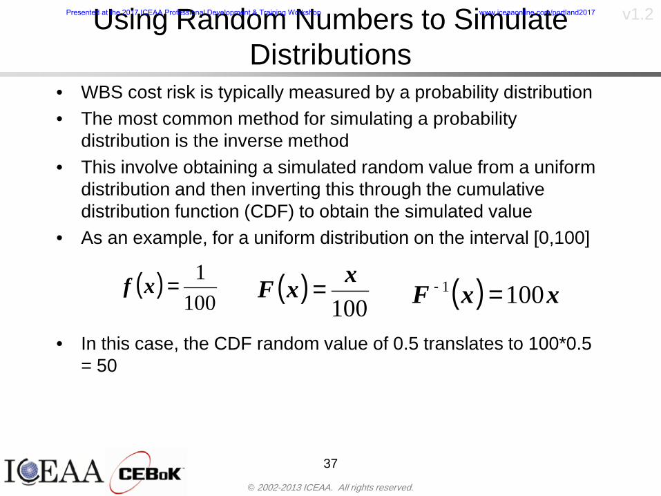
copy 2002-2013 ICEAA All rights reserved
v12Using Random Numbers to Simulate Distributions
bull WBS cost risk is typically measured by a probability distributionbull The most common method for simulating a probability
distribution is the inverse methodbull This involve obtaining a simulated random value from a uniform
distribution and then inverting this through the cumulative distribution function (CDF) to obtain the simulated value
bull As an example for a uniform distribution on the interval [0100]
bull In this case the CDF random value of 05 translates to 10005 = 50
37
( )100
1=xf ( )
100xxF = ( ) xxF 1001 =-
Presented at the 2017 ICEAA Professional Development amp Training Workshop wwwiceaaonlinecomportland2017
copy 2002-2013 ICEAA All rights reserved
v12
Simulating a Triangular Distribution
bull For a triangular distribution with low = 0 most likely = 50 and high = 150 the CDF is given by
bull The inverse function is given by
38
( )iumliumlicirc
iumliumliacute
igrave
poundlt--
poundpound=
1505021
1500050
50015000
2
2
2
xxx
xxxF
( )iumliumlicirc
iumliumliacute
igrave
poundltdivideoslashouml
ccedilegraveaelig +--
poundpound=-
131
21
37501
250017500150
3107500
1
xx
xxxF
Presented at the 2017 ICEAA Professional Development amp Training Workshop wwwiceaaonlinecomportland2017
copy 2002-2013 ICEAA All rights reserved
v12
Simulating a Triangular Distribution (2)
bull If the simulated uniform value is equal to 02 the corresponding inverse value from the CDF inverse is approximately 387
39
0
01
02
03
04
05
06
07
08
09
1
0 30 60 90 120 150
Presented at the 2017 ICEAA Professional Development amp Training Workshop wwwiceaaonlinecomportland2017
copy 2002-2013 ICEAA All rights reserved
v12
Monte Carlo and the WBSbull Simulation involves repeated trials
40
WBS Draw1 2 3 4 5
System 2912 3566 4390 2954 4655 Sum
Structure 80 105 55 80 57 SumVehicle Structure 50 70 30 40 20Tank Structure 30 35 25 40 37
Thermal Control 32 36 35 29 33 SumActive Thermal Control 10 15 12 7 10Induced Thermal Control 12 14 13 14 14Tank Thermal Control 10 7 10 8 9
Main Propulsion System 100 150 125 140 100
Liquid Rocket Engine 1000 1100 1800 900 2200
Electric Power and Distribution 100 125 150 75 90
Command Control and Data Handling 200 250 225 230 275
System Integration 1400 1800 2000 1500 1900
Presented at the 2017 ICEAA Professional Development amp Training Workshop wwwiceaaonlinecomportland2017
copy 2002-2013 ICEAA All rights reserved
v12
Number of Trialsbull Monte Carlo involves a repeated number of trialsbull The greater the number of trials the more accurate the
simulation will approximate the overall cost risk behavior of the system
bull After 100 trials the histogram looks very jagged
41
Presented at the 2017 ICEAA Professional Development amp Training Workshop wwwiceaaonlinecomportland2017
copy 2002-2013 ICEAA All rights reserved
v12
Number of Trials (2)
42
1000 Trials
10000 Trials
50000 Trials Additional trials give a more accurate depiction of the final result
Presented at the 2017 ICEAA Professional Development amp Training Workshop wwwiceaaonlinecomportland2017
copy 2002-2013 ICEAA All rights reserved
v12
Number of Trials (3)bull If we want to simulate the underlying
mean within 1 with 95 confidence for example then we require
43
divideoslash
oumlccedilegrave
aelig poundpound-
=
dividedividedivide
oslash
ouml
ccedilccedilccedil
egrave
aeligpound
-pound
-=
divideoslashouml
ccedilegraveaelig poundpound=
nZ
n
nnX
n
X
n
n
011
010Pr
011
010Pr
011990Pr950
___
___
sm
sm
sm
sm
sm
mm
Presented at the 2017 ICEAA Professional Development amp Training Workshop wwwiceaaonlinecomportland2017
copy 2002-2013 ICEAA All rights reserved
v12
Number of Trials (4)bull This means that the number of trials required is determined by
bull Solving for n we find that at least
trials are neededbull Note that this term involves the coefficient of variation of the
distribution which means that distributions with less dispersion require fewer trials to accurate simulate
44
96101
=ns
m
ms41638
Presented at the 2017 ICEAA Professional Development amp Training Workshop wwwiceaaonlinecomportland2017
copy 2002-2013 ICEAA All rights reserved
v12
Number of Trials (5)bull Simulating percentiles requires more trials than for simulating
meansbull Let Pn represent the number of trials in the sample at or below
the 70th percentile of the underlying distribution (suppose this is known)
bull By the Central Limit Theorem Pnn follows a normal distribution with mean equal to the 70th percentile and variance equal to
bull By a similar process for the mean we find that the number of trials needed to simulate the 70th percentile within 1 with 95 confidence is
45
( )n
FF 700700 1-
n
n
PPn -41638
Presented at the 2017 ICEAA Professional Development amp Training Workshop wwwiceaaonlinecomportland2017
copy 2002-2013 ICEAA All rights reserved
v12
Number of Trials (6)bull If Pn 070 for all n then n is approximately
bull For the sake of comparison suppose CV = 03 (reasonable approximation for hardware development) then the number of trials needed to simulate the mean with the same accuracy is then ldquoonlyrdquo 11525
bull More trials are needed to accurately simulate percentiles than means
46
( ) 46416703041638
70704168341638 =divide
oslashouml
ccedilegraveaelig=divide
oslashouml
ccedilegraveaelig -
=-
nnn
PPn
n
n
Presented at the 2017 ICEAA Professional Development amp Training Workshop wwwiceaaonlinecomportland2017
copy 2002-2013 ICEAA All rights reserved
v12
Methods of Simulationbull Monte Carlo simulation is a standard term for
simulationbull However there is an improvement on Monte Carlo
that improves the accuracy of the results of a simulation for a given number of trials
bull This method is call the Latin Hypercube approach to simulationndash Similar to Monte Carlo but an equal number of draws are taken
from a set of subintervals for example dividing the interval (01) into [00001) [0102)hellip [0910]
ndash Instead of 10 trials from [01] we have one trial from each subinterval
ndash Rough rule of thumb is Latin Hypercube takes 30 fewer trials to achieve similar accuracy to Monte Carlo
47
Presented at the 2017 ICEAA Professional Development amp Training Workshop wwwiceaaonlinecomportland2017
copy 2002-2013 ICEAA All rights reserved
v12
Probability Model ndash Correlationbull Correlation exists between work breakdown structure
(WBS) cost element costs and between cost and schedule
bull Correlation is a necessary consideration in cost risk analysis
bull Correlation is a number that can vary between -1 and +1 and represents the strength of the relationship between the two variablesndash If both variable have a tendency to move in the same direction
correlation is positivendash If when one variable increases the other tends to decrease and
vice-versa the correlation between the two variables is negative
Presented at the 2017 ICEAA Professional Development amp Training Workshop wwwiceaaonlinecomportland2017
copy 2002-2013 ICEAA All rights reserved
v12
Correlation And Causationbull Note that correlation is not causation however
causation implies correlationndash For example shark attacks and ice cream sales at the beach
bull For example for a launch vehicle structure increasing the diameter will not only result in an increase in the structures cost but will also result in higher costs for thermal coating (paint etc)
bull Also simply because two subsystems do not appear to be related does not mean they are not correlatedndash For example structures and computer equipment seemingly
have little relation to one another however an external factor such as a funding cut or a strike will impact all subsystems leading to delays and increasing cost across the board
ndash Thus everything in a WBS has some correlationUnit III - Module 9 49
Presented at the 2017 ICEAA Professional Development amp Training Workshop wwwiceaaonlinecomportland2017
copy 2002-2013 ICEAA All rights reserved
v12
The Importance of Correlationbull Percent that total cost standard deviation is underestimated
when correlation assumed to be 0 instead of r given nWBS elements
Unit III - Module 9 5050
0
20
40
60
80
100
0 01 02 03 04 05 06 07 08 09 1Actual Correlation
Perce
nt Un
deres
timate
d
n = 10
n = 30
n = 100n = 1000
0
20
40
60
80
100
0 01 02 03 04 05 06 07 08 09 1Actual Correlation
Perce
nt Un
deres
timate
d
n = 10
n = 30
n = 100n = 1000
Reference 32nd Annual DOD Cost Analysis Symposium Advanced Training Session ldquoWhy Correlation Matters in Cost Estimatingrdquo Stephen A Book
Presented at the 2017 ICEAA Professional Development amp Training Workshop wwwiceaaonlinecomportland2017
copy 2002-2013 ICEAA All rights reserved
v12
The Importance of Correlation (2)bull For example if correlation is assumed to be 0 for all
elements in a 30 element WBS and the actual correlation is 20 then the total cost standard deviation is underestimated by 60
bull For example assume the total cost is modeled as a normal distribution with mean = 100
bull If correlation is assumed to be zero with total cost standard deviation = 12 when correlation is actually 20 then the true underlying standard deviation is actually 30
bull 70th percentile with zero correlation assumption is 106
bull 70th percentile with 20 correlation is 116 Unit III - Module 9 51
Presented at the 2017 ICEAA Professional Development amp Training Workshop wwwiceaaonlinecomportland2017
copy 2002-2013 ICEAA All rights reserved
v12
Measures of Correlationbull Two measures of correlation are commonly used in
cost risk analysesndash Pearsonrsquos product-moment correlation coefficient ndash Spearmanrsquos rank correlation coefficient
bull Garvey and others recommend using Pearsonrsquos product-moment correlation coefficient correlation for cost risk analysesndash Method of moments uses this but there are two options in
simulationndash Popular simulation packages like Risk and Crystal Ball use
rank correlation but in practice this has been found to make little difference
ndash Pearson product-moment correlation has been incorporated into Risk+
52
Presented at the 2017 ICEAA Professional Development amp Training Workshop wwwiceaaonlinecomportland2017
copy 2002-2013 ICEAA All rights reserved
v12
Pearson Correlationbull Pearsonrsquos product-moment correlation measures
degree of linearity between two random variables bull If two random variables are perfectly linear (eg Y =
aX + b) with positive slope then the Pearson product-moment correlation between X and Y denoted by rXY is +1
53
X X
Y Y Y
XNegative Correlation Positive Correlation No Correlation
middotmiddot
middotmiddot
middotmiddot middotmiddot
middotmiddot
middot
middot
middotmiddotmiddot
middotmiddot
middotmiddot
middotmiddot middot
middot
middot
middotmiddotmiddotmiddotmiddotmiddotmiddotmiddot
middotmiddotmiddotmiddot
middotmiddot
middotmiddot middotmiddotmiddotmiddot
middotmiddotmiddot
middotmiddotmiddotmiddot
middotmiddotmiddot
middotmiddotmiddot
middotmiddot
middot
middot middotmiddot
middot middotmiddotmiddotmiddot middotmiddot middot middotmiddot middot middot
middotmiddot middot
middotmiddotmiddotmiddotmiddot middot middotmiddot
middotmiddot
middot
middotmiddot
middotmiddot middot
middot middot middot
middotmiddot middot
middotmiddotmiddot
middotmiddot
middot middot
Presented at the 2017 ICEAA Professional Development amp Training Workshop wwwiceaaonlinecomportland2017
copy 2002-2013 ICEAA All rights reserved
v12
Spearman Correlationbull Spearmanrsquos rank correlation measures the
monotonicity between two random variablesbull If two random variables are perfectly monotonically
increasing (eg Y = X2) then the Spearman rank correlation denoted by rXY is +1
bull The two measures can be significantly different
54
10 20 30 40 50 60
100
200
300
096 097 098 099 1
1
060
020
040
080
Eff
ort (
Staf
f-M
onth
s)
Software Size I KDSI
y = 28z12y
z x
yy = x100
0 pound x pound 1
Figure 5-9A Figure 5-9B
Pearson Correlation = 09976 Rank Correlation = 1
Pearson Correlation = 024 Rank Correlation = 1
X(x ) ~ Unif(01)
Reference Probability Methods for Cost Uncertainty Analysis A Systems Engineering Perspective Paul R Garvey
Presented at the 2017 ICEAA Professional Development amp Training Workshop wwwiceaaonlinecomportland2017
copy 2002-2013 ICEAA All rights reserved
v12
Unit III - Module 9 55
200
250
300
350
400
1000 1200 1400 1600 1800 2000
Recurring Production
SEPM
200
250
300
350
400
1000 1200 1400 1600 1800 2000
Recurring Production
SEPM
Functional Correlationbull Old No Functional
Correlation Simulation run with WBS items entered as values
bull New Simulation run with functional dependencies entered as they are in cost model
CorrelatedNot Correlated
Note shift of mean and increased variability
Presented at the 2017 ICEAA Professional Development amp Training Workshop wwwiceaaonlinecomportland2017
copy 2002-2013 ICEAA All rights reserved
v12
Risk Measuresbull ldquoWestern Europe conquered the word because of a
technological revolution that started because of attempts to measure the worldrdquo ndash Phillipe Jorion ndash In the same way attempts to measure risk will lead to better project
managementbull Risk management for DoD and NASA agencies focuses
primarily on funding projects to a single percentile ndash NASA policy explicitly mentions 70 and 50ndash This is known as ldquoValue at Riskrdquo and is prevalent in the banking and
financial industry
56
Presented at the 2017 ICEAA Professional Development amp Training Workshop wwwiceaaonlinecomportland2017
copy 2002-2013 ICEAA All rights reserved
v12
Value at Risk (VaR)bull VaR is a percentile of the cost risk
distributionndash VaR funding at the 70th percentile means that
there is a 30 chance of final project cost exceeding the funded amount (budget)
bull VaR has some meritsndash Common measure can be used to compare
different projects and programsndash Easily understood by senior managers and
decision makers
57
Presented at the 2017 ICEAA Professional Development amp Training Workshop wwwiceaaonlinecomportland2017
copy 2002-2013 ICEAA All rights reserved
v12
Why 70th or 80th Percentilebull Typical policy guidance involves funding at the 70th or 80th
percentile Why fund as such a low percentilebull There is some incentive to not over-fundbull For a normal distribution an inflection point occurs near the 80th
percentile meaning that for values above 80 confidence achieving higher levels of confidence can only be achieved by spending greater dollar amounts at an increasing rate
58
-05-04-03-02-01
00102030405
0 05 1 15 2 25 3
Standard Deviations from Mean
Normal Distribution
First DerivativeSlopeVelocity
Second DerivativeConvexityAcceleration
Inflection point at one standard deviation above the mean (~84th
percentile)
Presented at the 2017 ICEAA Professional Development amp Training Workshop wwwiceaaonlinecomportland2017
copy 2002-2013 ICEAA All rights reserved
v12
Funding Above Inflection Pointsbull As the percentile goes above the 80th percentile the amount
needed to achieve that higher level of confidence begins to increase at an increasing rate as is evident from the graph
59
0
10
20
30
40
50
60
70
50 55 60 65 70 75 80 85 90 95 100
$ Ab
ove
MEa
n to
Ach
ieve
Per
cent
ile
Percentile (Confidence Level)
Presented at the 2017 ICEAA Professional Development amp Training Workshop wwwiceaaonlinecomportland2017
copy 2002-2013 ICEAA All rights reserved
v12
Why Budget to the 70th or 80thbull Government projects are funded at the 70th or 80th percentilesbull Why not the 90th or 99th percentile Wonrsquot that help prevent
overrunsndash As we have seen percentiles do not add across programs
bull The sum of the 80th percentiles does NOT equal the total 80th percentile
ndash This is because the individual programs are riskier than the entire suite of missions
bull Known as the ldquoPortfolio effectrdquo (more or this later)
ndash Funding at the 80th gives confidence that the entire portfolio will be adequately funded
bull And since there is an inflection point near the 80th percentile funding above that level quickly becomes cost prohibitive
60
Presented at the 2017 ICEAA Professional Development amp Training Workshop wwwiceaaonlinecomportland2017
copy 2002-2013 ICEAA All rights reserved
v12
Inflection Points for Lognormalbull For a lognormal the inflection point
variesndash Coefficient of variation equal to 10 equates to an
inflection point at the 70th percentile
61
0
10
20
30
40
50
60
70
050 060 070 080 090 100
Coef
ficen
t of V
aria
tion
Percentile of the Inflection Point
Presented at the 2017 ICEAA Professional Development amp Training Workshop wwwiceaaonlinecomportland2017
copy 2002-2013 ICEAA All rights reserved
v12
Issues with Percentile Fundingbull However risk management does not stop at a
specific percentilendash What happens when the 70th percentile is exceeded
bull Any effective risk management policy should prescribe what happens after a bad event occursndash With VaR we only know when a bad event has occurred ndash Also funding at a relatively low level means we have no true
sense of the real risks that should be guarded against
62
Presented at the 2017 ICEAA Professional Development amp Training Workshop wwwiceaaonlinecomportland2017
copy 2002-2013 ICEAA All rights reserved
v12
ldquoHere There Be Dragonsrdquobull On old maps uncharted territory was often
marked with monsters or dragons
63
A section of the Carta Marina by Olaus Magnus 16th Century
Presented at the 2017 ICEAA Professional Development amp Training Workshop wwwiceaaonlinecomportland2017
copy 2002-2013 ICEAA All rights reserved
v12
Distribution Comparisonbull Four different distributions with the same 70th
percentile
bull Should we expect the tails to be similar
64
0
10
20
30
40
50
60
70
80
0 100 200 300 400 500 600
Perc
entil
eCo
nfid
ence
Lev
el
Triangular
Normal
Lognormal
Pareto
Presented at the 2017 ICEAA Professional Development amp Training Workshop wwwiceaaonlinecomportland2017
copy 2002-2013 ICEAA All rights reserved
v12Distribution Comparison Tail Behavior
bull The normal and triangular distributions have similar tails but the lognormal and Pareto have much fatter right tails
65
70
75
80
85
90
95
100
500 1500 2500 3500 4500 5500
Perc
entil
eCo
nfid
ence
Lev
el
Triangular
Normal
Lognormal
Pareto
Here There Be Dragons
Presented at the 2017 ICEAA Professional Development amp Training Workshop wwwiceaaonlinecomportland2017
copy 2002-2013 ICEAA All rights reserved
v12Distribution Comparison ndash Tail Behavior (Table)
bull There is significant tail risk for the lognormal and the Paretobull The 99th percentile for the Pareto is 1000 times greater than
the 70th percentilendash Risk seen in financial markets and in catastrophic risks like natural
disasters bull Four different projects follow the four different risk profiles seen
in this example should clearly have different risk management approaches but 70th percentile funding indicates the same risk management approach for all four
66
Percentile Triangular Normal Lognormal Pareto 70th $600 $600 $600 $600 80th $680 $660 $770 $1430 90th $770 $750 $1070 $5880 95th $840 $820 $1410 $23750 99th $930 $950 $2350 $600000
Presented at the 2017 ICEAA Professional Development amp Training Workshop wwwiceaaonlinecomportland2017
copy 2002-2013 ICEAA All rights reserved
v12Percentile Budgeting is Not Risk Management
bull Percentile budgeting ne effective risk management policybull Suppose that you are shopping for a new car You
mention that safety is your top concern The salesman says he has a great safe car available You ask about the air bags Do they work The salesman answers ldquoOf course Seventy percent of the time they work fine Only 30 of the time the air bags will fail to deployrdquo Would you buy such a car Hedge fund manager David Einhorn has stated ldquoRisk management is the air bag that must always work but only in the multi-sigma event where you have an accidentrdquo
67
Risk management is the air bag that must always work but only in the multi-sigma event where you
have an accident
Presented at the 2017 ICEAA Professional Development amp Training Workshop wwwiceaaonlinecomportland2017
copy 2002-2013 ICEAA All rights reserved
v12
Joint Confidence Level Analysisbull Schedules are risky toobull For 98 recent NASA missions average
schedule growth was 38ndash Not as high as cost growth but still significant
68
0
5
10
15
20
25
30
35
40
Schedule
Cost
Presented at the 2017 ICEAA Professional Development amp Training Workshop wwwiceaaonlinecomportland2017
copy 2002-2013 ICEAA All rights reserved
v12
Schedules Impact Costbull Changes in schedule can have enormous
impacts on cost ndash Schedule slips can lead to cost increases
bull Fixed programmatic costs must be paid on a regular basisndash Achieving schedule milestones early can result in cost
savings
bull Schedule is an important consideration in cost analysis including cost risk analysis
bull However we must be careful in correctly integrating cost and schedule riskndash Schedule is not simply an input but is dependent on many of
the same factors that drive cost
69
Presented at the 2017 ICEAA Professional Development amp Training Workshop wwwiceaaonlinecomportland2017
copy 2002-2013 ICEAA All rights reserved
v12
The Relationship of Cost to Schedulebull Cost and schedule are positively correlated
ndash A larger program with bigger scope with take longer to complete than a smaller simpler program
bull However longer schedules do not always equate to higher cost nor shorter schedules with lower costndash Highly compressed schedules relative to the
optimal schedule can lead to large overrunsbull Compressed schedules are commonplace for
many planetary missions
70
Presented at the 2017 ICEAA Professional Development amp Training Workshop wwwiceaaonlinecomportland2017
copy 2002-2013 ICEAA All rights reserved
v12The Impact of Schedule GrowthCompression on Cost
bull Compressed schedules lead to cost growth and based on existing research is actually more expensive than schedule slippages
71
0
20
40
60
80
100
120
140
160
-50 -25 0 25 50 75 100
Percentage Change in Schedule
Perc
enta
ge C
hang
e in
Cos
t due
to
Sche
dule
Cha
nge
Source Smart CB ldquoCost and Schedule Interrelationshipsrdquo 2007 NASA Cost Symposium
Presented at the 2017 ICEAA Professional Development amp Training Workshop wwwiceaaonlinecomportland2017
copy 2002-2013 ICEAA All rights reserved
v12Schedule as an Independent Variable
bull Why not simply add schedule as an input to cost-estimating relationships (CERs)
bull Schedule is often treated as an independent variable ndash schedules are often determined independently of cost considerationsndash Cost may not be considered explicitly although budgets and
schedules are determined based on scope and other common factors
bull In 2006 SAIC undertook a research task to determine the impact of schedule on cost and added schedule as an independent variable to the CERs in the NASAAir Force Cost Model (NAFCOM) to see if schedule provided any improvement in goodness of fit
72
Presented at the 2017 ICEAA Professional Development amp Training Workshop wwwiceaaonlinecomportland2017
copy 2002-2013 ICEAA All rights reserved
v12
Schedule is a Dependent Variablebull Since NAFCOM includes an exhaustive list of cost drivers the inclusion
of schedule should give an indication of whether there is any additional independent value added from schedule independent of the cost drivers
bull In the study schedule was added to 10 subsystem-level CERs
ndash In each case the addition of schedule did NOTimprove the goodness of fit and schedule was NOT found to be a statistically significant cost driver (given the presence of the other variables) for any of the 10 CERs
bull Standard errors for the CERs increased due to decrease in degrees of freedom
bull Thus schedule as an independent variable did not provide any additional explanation of variation in historical cost
bull This is because schedule is truly NOT an independent variable but a dependent variable and is a function of the same factors that drive cost
73
Presented at the 2017 ICEAA Professional Development amp Training Workshop wwwiceaaonlinecomportland2017
copy 2002-2013 ICEAA All rights reserved
v12
Incorporation of Schedule in Cost Risk
bull When using subjective methods care must be taken in applying schedule to cost risk analysis
bull Since schedule is a dependent variable treating it independently from other factors when assessing its impact on cost can lead to a double count of independent variables in the cost risk analysis
bull Direct inclusion of schedule in a cost risk analysis effectively doubles the influence of each cost driver
ndash Incorrectly leads to broader risk ranges
74
CostWeight
HeritageNewness
Technology Readiness Schedule
Presented at the 2017 ICEAA Professional Development amp Training Workshop wwwiceaaonlinecomportland2017
copy 2002-2013 ICEAA All rights reserved
v12Subjective Cost Risk Methods and Overinclusion of Risk Factors
bull Subjective methods are suitable when data are scarce or not availablebull However care must be taken not to treat correlated sources of risk
such as schedule as independent of each otherbull Example ndash a subjective risk analysis incorporated technology readiness
design risk requirements stability integration risk and schedule and treated each source of risk as independent
bull Risk triangle high value without schedule risk was 31 times the point estimate
bull Risk triangle high value with schedule risk added on top of other sources of risk treated independently was 34 times the point estimate
bull Risk triangle taking correlation between sources of risk into account in a rigorous statistical manner has a high value 15 times the point estimate less than half the effect when treating sources of risk as independent
75
Presented at the 2017 ICEAA Professional Development amp Training Workshop wwwiceaaonlinecomportland2017
copy 2002-2013 ICEAA All rights reserved
v12Fundamental Equation of Cost and Schedule Interrelationships
bull The Fundamental Equation of the Relationship Between Cost and Schedule is
Time = Moneybull This is a well known adage that time is money Your boss at
work may even mention this to you from time to time or if you are the boss you are all too aware of this iron law
bull Because time is money cost and schedule risk should be modeled jointly not with schedule as an independent cost driver
bull Note that cost and schedule are not perfectly correlatedndash Cost can sometimes ldquobuy downrdquo schedule extra money can be
spent to meet a deadline since in some cases additional effort to hasten the completion of a task
76
Presented at the 2017 ICEAA Professional Development amp Training Workshop wwwiceaaonlinecomportland2017
copy 2002-2013 ICEAA All rights reserved
v12How to (Correctly) Incorporate Schedule into Cost Risk Analysis
bull The best way to model cost and schedule risk is to develop a joint cost and schedule model based on the same data
bull Since such models are not currently available the next best approach is to model cost and schedule independently and then integrate cost and schedule risk analyses using joint probability distributions taking into account correlation between cost and schedulendash This approach pioneered by Paul Garvey and Steve Book is
considered industry best practicendash This is a practical method mathematically tractable and follows
naturally from the Fundamental Equation of Cost and Schedule Interrelationships
77
Book S A ldquoQuantifying the Relationship Between Cost and Schedulerdquo The Measurable News Winter 2007-2008 pp 11-15Garvey PR Probability Methods for Cost Uncertainty Analysis A Systems Engineering Perspective New York Marcel Dekker 2000 pp 308-335
Presented at the 2017 ICEAA Professional Development amp Training Workshop wwwiceaaonlinecomportland2017
copy 2002-2013 ICEAA All rights reserved
v12
Joint Lognormal and Normal Distributions
bull Cost and schedule are typically modeled as some combination of Normal and Lognormal probability distributionsndash Studies by The Aerospace Corporation the MITRE
Corporation Wyle Labs and SAIC have found that the Lognormal probability distribution almost always serves as a good model for both the schedule distribution and the cost distribution
ndash The Normal distribution may also be appropriate in some instances and depending upon the level of confidence at which budgets are set may even be more conservative and logically consistent than the Normal distribution
ndash Joint Lognormal and Normal distributions are defined by a pair of mean and standard deviations and a level of correlation between the two
78
Presented at the 2017 ICEAA Professional Development amp Training Workshop wwwiceaaonlinecomportland2017
copy 2002-2013 ICEAA All rights reserved
v12Modeling Cost and Schedule as a Bivariate Distribution
bull In the approach set forth by Book and Garvey cost risk is assessed and the top-level distribution is modeled as a Lognormal (or Normal) distribution schedule risk is assessed and the overall schedule risk is modeled as a Lognormal (or Normal) distribution
bull The two distributions are combined into a Bivariate distribution by assigning a correlation between the two and by treating the two distributions as the marginal distributions of a Bivariate Lognormal distributionndash Other combinations include a Bivariate Normal or a Bivariate
Normal-Lognormal
79
Presented at the 2017 ICEAA Professional Development amp Training Workshop wwwiceaaonlinecomportland2017
copy 2002-2013 ICEAA All rights reserved
v12Bivariate Lognormal Distribution for Cost and Schedule
bull Cost is often observed to be Lognormal when strong positive correlations are present among the systemrsquos WBS cost element costs
bull A systemrsquos schedule is often observed (from Monte Carlo simulations) to be Lognormal if it is the sum of many positively correlated schedule activities in an overall schedule network
bull If Lognormal distributions characterize a systemrsquos cost and schedule then the Bivariate Lognormal could serve as an assumed model of their joint distributionndash In this case the marginal distribution of each of cost and schedule is
Lognormalbull Other possibilities for modeling cost and schedule as a Bivariate
distribution include a Bivariate Normal or a Bivariate Normal-Lognormal distributionndash All these combinations are analytically tractable
80
Presented at the 2017 ICEAA Professional Development amp Training Workshop wwwiceaaonlinecomportland2017
copy 2002-2013 ICEAA All rights reserved
v12Bivariate Lognormal for Cost and Schedule
bull Contour Plots of a Bivariate Lognormal
81
Presented at the 2017 ICEAA Professional Development amp Training Workshop wwwiceaaonlinecomportland2017
copy 2002-2013 ICEAA All rights reserved
v12Correlation Between Cost and Schedule
bull Cost and schedule are positively correlated but not perfectly sondash For example it is possible to have a schedule underrun and a cost
overrunbull Based on cost and schedule growth data for 50 completed NASA
programs the correlation between development cost and development schedule is 70
82
00
200
400
600
800
1000
1200
-500 00 500 1000 1500 2000 2500Historical Cost Growth
Hist
oric
al S
ched
ule
Gro
wth
r = 715
Presented at the 2017 ICEAA Professional Development amp Training Workshop wwwiceaaonlinecomportland2017
copy 2002-2013 ICEAA All rights reserved
v12Correlation Between Cost and Schedule Caveats
bull Based on historical data recommended correlation between cost and schedule is 70 but this could be higher or lower depending upon program circumstancesndash If program is budget constrained cost and schedule will be
more highly correlated (go as you pay)ndash If program is schedule constrained cost and schedule will
have lower correlation perhaps even negative correlation ndash Smaller programs have smaller correlation between cost and
schedule riskbull Relatively easy to ldquohurry uprdquo and finish on time or even early if
needed
83
Presented at the 2017 ICEAA Professional Development amp Training Workshop wwwiceaaonlinecomportland2017
copy 2002-2013 ICEAA All rights reserved
v12
Conditional Confidence Levelsbull Given a programrsquos project schedule we can determine the cost
risk distribution conditional upon the given schedulebull Conditional cost S-curves are steeper than unconditional
(marginal) cost S-curves between some uncertainty has been removed because schedule is fixed
84
Presented at the 2017 ICEAA Professional Development amp Training Workshop wwwiceaaonlinecomportland2017
copy 2002-2013 ICEAA All rights reserved
v12
Joint Confidence Levelsbull Joint 65 confidence represents the probability of
achieving both 65 confidence in cost AND 65 confidence in schedulendash This is different than achieving 65 cost confidence alone
or achieving 65 schedule confidence alonebull Due to the imperfect correlation between cost and schedule it
is possible to achieve a 65 cost confidence with a lower level of schedule confidence
bull Restricting the schedule confidence thus requires additional $ to achieve a given level of confidence
85
X
Y
Possible Values for Which X gt a Possible Values for
Which X gt a and Y gt b
a
b
Presented at the 2017 ICEAA Professional Development amp Training Workshop wwwiceaaonlinecomportland2017
copy 2002-2013 ICEAA All rights reserved
v12Joint Confidence Levels Versus Cost Confidence Levels Only
bull Example of the differences between cost confidence schedule confidence conditional cost confidence and joint cost and schedule confidence
86
Joint Cost-Schedule Confidence Iso-Curves
Cost (RY$M)
Sche
dule
(Mon
ths)
65 Confidence
50 Confidence
70 Confidence
65 Cost Confidence AggressiveSchedule65 Cost ConfidenceScheduleGiven 65 Schedule ConfidenceUnconditional 65 CostConfidenceUnconditional 65 ScheduleConfidence
65 Cost Confidence 65 Joint Cost and Schedule
Confidence for 65 Schedule Confidence
Presented at the 2017 ICEAA Professional Development amp Training Workshop wwwiceaaonlinecomportland2017
copy 2002-2013 ICEAA All rights reserved
v12
Joint Cost and Schedule Confidence
bull Can examine pairs of cost and schedule that achieve a given level of confidence
bull Provides insights into the trade-offs between cost and schedule for a given level of confidencendash Possible to increase cost confidence by giving a
project more time in some instances or possible to ldquobuy downrdquo schedule
bull But these have limits and are shown in the iso-cost and schedule confidence curves
87
Presented at the 2017 ICEAA Professional Development amp Training Workshop wwwiceaaonlinecomportland2017
copy 2002-2013 ICEAA All rights reserved
v12Cost and Schedule Trade-offs for a Given Level of Joint Confidence
bull Hypothetical Example
88
Cost (RY$M)
Schedule (Months)
$100 48$99 48$89 49$87 50$85 51$85 52$84 53$83 55$83 55$83 56
Cost and Schedule 65 Confidence Iso-Curve
4748495051525354555657
$80 $82 $84 $86 $88 $90 $92 $94 $96 $98 $100
Cost (RY$ M)
Sche
dule
(Mon
ths)
Presented at the 2017 ICEAA Professional Development amp Training Workshop wwwiceaaonlinecomportland2017
copy 2002-2013 ICEAA All rights reserved
v12Policy Considerations for Confidence Levels
bull For large programs the difference between the amount of money needed to achieve 65 cost confidence independent of schedule and joint 65 cost and schedule confidence can represent hundreds of millions and even billions of dollars
89
Joint Cost-Schedule Confidence Iso-Curves
Cost (RY$M)
Sche
dule
(Mon
ths)
65 Confidence
65 Cost Confidence AggressiveSchedule
65 Cost ConfidenceScheduleGiven 65 Schedule Confidence
Unconditional 65 CostConfidence
Joint Cost and Schedule Confidence for 65 Cost Confidence and Program Baseline Schedule is Less Than 35
65 Cost Confidence Independent of Schedule Cost Needed to Achieve
Both 65 Joint Cost and Schedule Confidence for the Schedule with 65 Confidence
Presented at the 2017 ICEAA Professional Development amp Training Workshop wwwiceaaonlinecomportland2017
copy 2002-2013 ICEAA All rights reserved
v12
Copulasbull More generally any combination of distributions can
be used (more than just normal and lognormal)ndash Termed ldquocopulardquo from the Italian word for ldquocouplerdquondash Copulas are a way to combine marginal distributions of any
number and type into a joint distributionbull More formally a copula is a multivariate joint distribution defined
on the n-dimensional unit cube [0 1]n such that every marginal distribution is uniform on the interval [0 1]
bull (The bivariate form of) Sklarrsquos theorem states that for any bivariate distribution function H(x y) let F(x) = H(x infin) and G(y) = H(infin y) be the univariate marginal probability distribution functions Then there exists a copula C such that H(xy)=C(F(x)G(y))
ndash Copulas are widely used in risk management for investments and insurance
bull Considered industry best practice (Li 2000)bull Marketed as part of JP Morganrsquos CreditMetrics suite of tools
(Gupton et Al 1997)90
Presented at the 2017 ICEAA Professional Development amp Training Workshop wwwiceaaonlinecomportland2017
copy 2002-2013 ICEAA All rights reserved
v12Parametric Joint Cost and Schedule Analysis
bull A parametric model based on a consistent data set with a set of overlapping cost and schedule drivers is a cleaner way to model cost and schedule
91
CostWeight
HeritageNewness
Technology Readiness
Schedule
0
20
40
60
80
100
Confidence
Joint Cost and Schedule Confidence
Schedule
Cost
Lognormal Distribution PDF and CDF
0102030405060708090100
200 300 400 500 600 700 800 900 1000Cost $
Con
fiden
ce L
evel
0
00002
00004
00006
00008
0001
00012
00014
00016
Prob
abili
ty D
ensi
ty
CDFPDF
Lognormal Distribution PDF and CDF
0102030405060708090100
200 300 400 500 600 700 800 900 1000Cost $
Con
fiden
ce L
evel
0
00002
00004
00006
00008
0001
00012
00014
00016
Prob
abili
ty D
ensi
ty
CDFPDF
Presented at the 2017 ICEAA Professional Development amp Training Workshop wwwiceaaonlinecomportland2017
copy 2002-2013 ICEAA All rights reserved
v12Parametric Joint Cost and Schedule Analysis (2)
bull Joint cost and schedule risk analysis produced naturally by the integrated modelndash Addresses several issues with the copula
approachbull Tail dependencybull Correlation ndash no need to assign correlation
between cost and schedulebull Consistency of cost and schedule models
92
Presented at the 2017 ICEAA Professional Development amp Training Workshop wwwiceaaonlinecomportland2017
copy 2002-2013 ICEAA All rights reserved
v12
Resource-Loaded Schedulesbull Involves assigning cost and schedule risks to a resource-loaded schedule
networkbull Bottom-up approach
ndash More labor intensive than parametrics but can also provide more insight
ndash Can answer questions than parametric typically cannot such as how much do reserve requirements decrease if a specific risk is retired
bull Currently being implemented in Constellation programbull Has same issue as all bottom-up models hard to count all the risks and model
them discretely
ndash As a result there is a tendency to reflect less risk than indicated by history
ndash ldquoThere are more things in heaven and earth Horatio than are dreamt of in your philosophyrdquo William Shakespeare Hamlet Act I Scene V
93
Presented at the 2017 ICEAA Professional Development amp Training Workshop wwwiceaaonlinecomportland2017
copy 2002-2013 ICEAA All rights reserved
v12Resource-Loaded Schedules Vs Parametrics
bull Parametric most appropriate for early estimatesndash But also good for high-level checks as project progresses
bull As plans take shape lower level modeling may be more appropriate
94 1
CONCEPTUALDEVELOPMENT
PROJECTDEFINITION DESIGN DEVELOPMENT OPERATIONS
PARAMETRIC PARAMETRIC
ANALOGY
ENGINEERING (Bottoms Up)
$PARAMETRIC
DETAILED
$
Pre Phase A Phase B Phase CDPhase A Phase EPre Phase A Phase B Phase CDPhase A Phase E
Risk = f(Cost Estimating Relationship Inputs eg mass power data rate TRL new design etc)
Risk = f(cost and schedule variation of the analogous elements)
Risk = f(variation of detailed inputs eg labor hours rates materials etc)
Presented at the 2017 ICEAA Professional Development amp Training Workshop wwwiceaaonlinecomportland2017
copy 2002-2013 ICEAA All rights reserved
v12
Resource-Loaded Schedulesbull Methodology has been demonstrated in other
industriesndash Construction oil and gasndash Analysis has not been traditionally done on highly uncertain
complex development projects bull Methodology focuses on project baseline schedule
ndash In baseline schedule all tasks are resource loaded to represent a baseline schedule and cost standpoint
ndash Resource loaded schedule is ldquorolledrdquo up to a manageable level
ndash Based on the risk and uncertainties identified schedule distributions are applied to each rolled up task
ndash Cost uncertainties are also applied to rolled up tasksbull Uncertainties include labor rate man power etc
ndash A Monte Carlo simulation is run to develop joint cost-schedule distributions
95
Presented at the 2017 ICEAA Professional Development amp Training Workshop wwwiceaaonlinecomportland2017
copy 2002-2013 ICEAA All rights reserved
v12
Unit III - Module 9 96
Execution ndash Cross Checksbull Means The mean cost growth factor for WBS items
can be compared to history as a way to cross check results
bull CVs The CV of the cost growth factors for WBS items can be compared to history as a way to cross check results
bull Inputs Checks are performed on inputs or other parameters to see if historical values are in line with program assumptionsndash Example Historical risk scores can be compared to program
risk scores to see if risk assessors are being realistic and to see if the underlying database is representative of the program
11
Presented at the 2017 ICEAA Professional Development amp Training Workshop wwwiceaaonlinecomportland2017
- Cost and Schedule Risk Analysis Basic
- Acknowledgments
- Unit Index
- Risk Overview
- Agenda
- Introduction
- Risk Analysis Terms
- Are Our Costs Realistic
- Historical Cost Growth
- Sources of Cost Risk
- Point Estimates of Cost
- Types of Risk
- Point Estimates Vs Risk Estimates
- Cost Risk and Probability
- Probability Model ndash Distribution
- Probability Model ndash Distribution
- Probability ndash Top-Level Distribution
- S-Curves and Confidence Levels
- Example ndash Normal Distribution
- Confidence Levels
- Measuring Parametric Model Uncertainty
- Parametric Model Example
- Weight Uncertainty
- Estimating Uncertainty
- Estimating Uncertainty (2)
- Estimating Uncertainty (3)
- Aggregating Risk
- WBS Example
- WBS and Risk
- Aggregating Risk
- Percentiles Do Not Add
- Percentiles Do Not Add (2)
- Percentiles Do Not Add (3)
- Methods for Aggregating Risk
- Monte Carlo Simulationfor Risk Analysis
- Monte Carlo Simulation
- Using Random Numbers to Simulate Distributions
- Simulating a Triangular Distribution
- Simulating a Triangular Distribution (2)
- Monte Carlo and the WBS
- Number of Trials
- Number of Trials (2)
- Number of Trials (3)
- Number of Trials (4)
- Number of Trials (5)
- Number of Trials (6)
- Methods of Simulation
- Probability Model ndash Correlation
- Correlation And Causation
- The Importance of Correlation
- The Importance of Correlation (2)
- Measures of Correlation
- Pearson Correlation
- Spearman Correlation
- Functional Correlation
- Risk Measures
- Value at Risk (VaR)
- Why 70th or 80th Percentile
- Funding Above Inflection Points
- Why Budget to the 70th or 80th
- Inflection Points for Lognormal
- Issues with Percentile Funding
- ldquoHere There Be Dragonsrdquo
- Distribution Comparison
- Distribution Comparison Tail Behavior
- Distribution Comparison ndash Tail Behavior (Table)
- Percentile Budgeting is Not Risk Management
- Joint Confidence Level Analysis
- Schedules Impact Cost
- The Relationship of Cost to Schedule
- The Impact of Schedule GrowthCompression on Cost
- Schedule as an Independent Variable
- Schedule is a Dependent Variable
- Incorporation of Schedule in Cost Risk
- Subjective Cost Risk Methods and Overinclusion of Risk Factors
- Fundamental Equation of Cost and Schedule Interrelationships
- How to (Correctly) Incorporate Schedule into Cost Risk Analysis
- Joint Lognormal and Normal Distributions
- Modeling Cost and Schedule as a Bivariate Distribution
- Bivariate Lognormal Distribution for Cost and Schedule
- Bivariate Lognormal for Cost and Schedule
- Correlation Between Cost and Schedule
- Correlation Between Cost and Schedule Caveats
- Conditional Confidence Levels
- Joint Confidence Levels
- Joint Confidence Levels Versus Cost Confidence Levels Only
- Joint Cost and Schedule Confidence
- Cost and Schedule Trade-offs for a Given Level of Joint Confidence
- Policy Considerations for Confidence Levels
- Copulas
- Parametric Joint Cost and Schedule Analysis
- Parametric Joint Cost and Schedule Analysis (2)
- Resource-Loaded Schedules
- Resource-Loaded Schedules Vs Parametrics
- Resource-Loaded Schedules
- Execution ndash Cross Checks
-
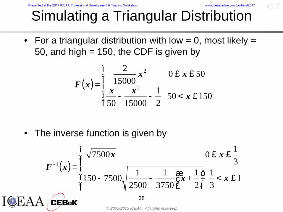
copy 2002-2013 ICEAA All rights reserved
v12
Simulating a Triangular Distribution
bull For a triangular distribution with low = 0 most likely = 50 and high = 150 the CDF is given by
bull The inverse function is given by
38
( )iumliumlicirc
iumliumliacute
igrave
poundlt--
poundpound=
1505021
1500050
50015000
2
2
2
xxx
xxxF
( )iumliumlicirc
iumliumliacute
igrave
poundltdivideoslashouml
ccedilegraveaelig +--
poundpound=-
131
21
37501
250017500150
3107500
1
xx
xxxF
Presented at the 2017 ICEAA Professional Development amp Training Workshop wwwiceaaonlinecomportland2017
copy 2002-2013 ICEAA All rights reserved
v12
Simulating a Triangular Distribution (2)
bull If the simulated uniform value is equal to 02 the corresponding inverse value from the CDF inverse is approximately 387
39
0
01
02
03
04
05
06
07
08
09
1
0 30 60 90 120 150
Presented at the 2017 ICEAA Professional Development amp Training Workshop wwwiceaaonlinecomportland2017
copy 2002-2013 ICEAA All rights reserved
v12
Monte Carlo and the WBSbull Simulation involves repeated trials
40
WBS Draw1 2 3 4 5
System 2912 3566 4390 2954 4655 Sum
Structure 80 105 55 80 57 SumVehicle Structure 50 70 30 40 20Tank Structure 30 35 25 40 37
Thermal Control 32 36 35 29 33 SumActive Thermal Control 10 15 12 7 10Induced Thermal Control 12 14 13 14 14Tank Thermal Control 10 7 10 8 9
Main Propulsion System 100 150 125 140 100
Liquid Rocket Engine 1000 1100 1800 900 2200
Electric Power and Distribution 100 125 150 75 90
Command Control and Data Handling 200 250 225 230 275
System Integration 1400 1800 2000 1500 1900
Presented at the 2017 ICEAA Professional Development amp Training Workshop wwwiceaaonlinecomportland2017
copy 2002-2013 ICEAA All rights reserved
v12
Number of Trialsbull Monte Carlo involves a repeated number of trialsbull The greater the number of trials the more accurate the
simulation will approximate the overall cost risk behavior of the system
bull After 100 trials the histogram looks very jagged
41
Presented at the 2017 ICEAA Professional Development amp Training Workshop wwwiceaaonlinecomportland2017
copy 2002-2013 ICEAA All rights reserved
v12
Number of Trials (2)
42
1000 Trials
10000 Trials
50000 Trials Additional trials give a more accurate depiction of the final result
Presented at the 2017 ICEAA Professional Development amp Training Workshop wwwiceaaonlinecomportland2017
copy 2002-2013 ICEAA All rights reserved
v12
Number of Trials (3)bull If we want to simulate the underlying
mean within 1 with 95 confidence for example then we require
43
divideoslash
oumlccedilegrave
aelig poundpound-
=
dividedividedivide
oslash
ouml
ccedilccedilccedil
egrave
aeligpound
-pound
-=
divideoslashouml
ccedilegraveaelig poundpound=
nZ
n
nnX
n
X
n
n
011
010Pr
011
010Pr
011990Pr950
___
___
sm
sm
sm
sm
sm
mm
Presented at the 2017 ICEAA Professional Development amp Training Workshop wwwiceaaonlinecomportland2017
copy 2002-2013 ICEAA All rights reserved
v12
Number of Trials (4)bull This means that the number of trials required is determined by
bull Solving for n we find that at least
trials are neededbull Note that this term involves the coefficient of variation of the
distribution which means that distributions with less dispersion require fewer trials to accurate simulate
44
96101
=ns
m
ms41638
Presented at the 2017 ICEAA Professional Development amp Training Workshop wwwiceaaonlinecomportland2017
copy 2002-2013 ICEAA All rights reserved
v12
Number of Trials (5)bull Simulating percentiles requires more trials than for simulating
meansbull Let Pn represent the number of trials in the sample at or below
the 70th percentile of the underlying distribution (suppose this is known)
bull By the Central Limit Theorem Pnn follows a normal distribution with mean equal to the 70th percentile and variance equal to
bull By a similar process for the mean we find that the number of trials needed to simulate the 70th percentile within 1 with 95 confidence is
45
( )n
FF 700700 1-
n
n
PPn -41638
Presented at the 2017 ICEAA Professional Development amp Training Workshop wwwiceaaonlinecomportland2017
copy 2002-2013 ICEAA All rights reserved
v12
Number of Trials (6)bull If Pn 070 for all n then n is approximately
bull For the sake of comparison suppose CV = 03 (reasonable approximation for hardware development) then the number of trials needed to simulate the mean with the same accuracy is then ldquoonlyrdquo 11525
bull More trials are needed to accurately simulate percentiles than means
46
( ) 46416703041638
70704168341638 =divide
oslashouml
ccedilegraveaelig=divide
oslashouml
ccedilegraveaelig -
=-
nnn
PPn
n
n
Presented at the 2017 ICEAA Professional Development amp Training Workshop wwwiceaaonlinecomportland2017
copy 2002-2013 ICEAA All rights reserved
v12
Methods of Simulationbull Monte Carlo simulation is a standard term for
simulationbull However there is an improvement on Monte Carlo
that improves the accuracy of the results of a simulation for a given number of trials
bull This method is call the Latin Hypercube approach to simulationndash Similar to Monte Carlo but an equal number of draws are taken
from a set of subintervals for example dividing the interval (01) into [00001) [0102)hellip [0910]
ndash Instead of 10 trials from [01] we have one trial from each subinterval
ndash Rough rule of thumb is Latin Hypercube takes 30 fewer trials to achieve similar accuracy to Monte Carlo
47
Presented at the 2017 ICEAA Professional Development amp Training Workshop wwwiceaaonlinecomportland2017
copy 2002-2013 ICEAA All rights reserved
v12
Probability Model ndash Correlationbull Correlation exists between work breakdown structure
(WBS) cost element costs and between cost and schedule
bull Correlation is a necessary consideration in cost risk analysis
bull Correlation is a number that can vary between -1 and +1 and represents the strength of the relationship between the two variablesndash If both variable have a tendency to move in the same direction
correlation is positivendash If when one variable increases the other tends to decrease and
vice-versa the correlation between the two variables is negative
Presented at the 2017 ICEAA Professional Development amp Training Workshop wwwiceaaonlinecomportland2017
copy 2002-2013 ICEAA All rights reserved
v12
Correlation And Causationbull Note that correlation is not causation however
causation implies correlationndash For example shark attacks and ice cream sales at the beach
bull For example for a launch vehicle structure increasing the diameter will not only result in an increase in the structures cost but will also result in higher costs for thermal coating (paint etc)
bull Also simply because two subsystems do not appear to be related does not mean they are not correlatedndash For example structures and computer equipment seemingly
have little relation to one another however an external factor such as a funding cut or a strike will impact all subsystems leading to delays and increasing cost across the board
ndash Thus everything in a WBS has some correlationUnit III - Module 9 49
Presented at the 2017 ICEAA Professional Development amp Training Workshop wwwiceaaonlinecomportland2017
copy 2002-2013 ICEAA All rights reserved
v12
The Importance of Correlationbull Percent that total cost standard deviation is underestimated
when correlation assumed to be 0 instead of r given nWBS elements
Unit III - Module 9 5050
0
20
40
60
80
100
0 01 02 03 04 05 06 07 08 09 1Actual Correlation
Perce
nt Un
deres
timate
d
n = 10
n = 30
n = 100n = 1000
0
20
40
60
80
100
0 01 02 03 04 05 06 07 08 09 1Actual Correlation
Perce
nt Un
deres
timate
d
n = 10
n = 30
n = 100n = 1000
Reference 32nd Annual DOD Cost Analysis Symposium Advanced Training Session ldquoWhy Correlation Matters in Cost Estimatingrdquo Stephen A Book
Presented at the 2017 ICEAA Professional Development amp Training Workshop wwwiceaaonlinecomportland2017
copy 2002-2013 ICEAA All rights reserved
v12
The Importance of Correlation (2)bull For example if correlation is assumed to be 0 for all
elements in a 30 element WBS and the actual correlation is 20 then the total cost standard deviation is underestimated by 60
bull For example assume the total cost is modeled as a normal distribution with mean = 100
bull If correlation is assumed to be zero with total cost standard deviation = 12 when correlation is actually 20 then the true underlying standard deviation is actually 30
bull 70th percentile with zero correlation assumption is 106
bull 70th percentile with 20 correlation is 116 Unit III - Module 9 51
Presented at the 2017 ICEAA Professional Development amp Training Workshop wwwiceaaonlinecomportland2017
copy 2002-2013 ICEAA All rights reserved
v12
Measures of Correlationbull Two measures of correlation are commonly used in
cost risk analysesndash Pearsonrsquos product-moment correlation coefficient ndash Spearmanrsquos rank correlation coefficient
bull Garvey and others recommend using Pearsonrsquos product-moment correlation coefficient correlation for cost risk analysesndash Method of moments uses this but there are two options in
simulationndash Popular simulation packages like Risk and Crystal Ball use
rank correlation but in practice this has been found to make little difference
ndash Pearson product-moment correlation has been incorporated into Risk+
52
Presented at the 2017 ICEAA Professional Development amp Training Workshop wwwiceaaonlinecomportland2017
copy 2002-2013 ICEAA All rights reserved
v12
Pearson Correlationbull Pearsonrsquos product-moment correlation measures
degree of linearity between two random variables bull If two random variables are perfectly linear (eg Y =
aX + b) with positive slope then the Pearson product-moment correlation between X and Y denoted by rXY is +1
53
X X
Y Y Y
XNegative Correlation Positive Correlation No Correlation
middotmiddot
middotmiddot
middotmiddot middotmiddot
middotmiddot
middot
middot
middotmiddotmiddot
middotmiddot
middotmiddot
middotmiddot middot
middot
middot
middotmiddotmiddotmiddotmiddotmiddotmiddotmiddot
middotmiddotmiddotmiddot
middotmiddot
middotmiddot middotmiddotmiddotmiddot
middotmiddotmiddot
middotmiddotmiddotmiddot
middotmiddotmiddot
middotmiddotmiddot
middotmiddot
middot
middot middotmiddot
middot middotmiddotmiddotmiddot middotmiddot middot middotmiddot middot middot
middotmiddot middot
middotmiddotmiddotmiddotmiddot middot middotmiddot
middotmiddot
middot
middotmiddot
middotmiddot middot
middot middot middot
middotmiddot middot
middotmiddotmiddot
middotmiddot
middot middot
Presented at the 2017 ICEAA Professional Development amp Training Workshop wwwiceaaonlinecomportland2017
copy 2002-2013 ICEAA All rights reserved
v12
Spearman Correlationbull Spearmanrsquos rank correlation measures the
monotonicity between two random variablesbull If two random variables are perfectly monotonically
increasing (eg Y = X2) then the Spearman rank correlation denoted by rXY is +1
bull The two measures can be significantly different
54
10 20 30 40 50 60
100
200
300
096 097 098 099 1
1
060
020
040
080
Eff
ort (
Staf
f-M
onth
s)
Software Size I KDSI
y = 28z12y
z x
yy = x100
0 pound x pound 1
Figure 5-9A Figure 5-9B
Pearson Correlation = 09976 Rank Correlation = 1
Pearson Correlation = 024 Rank Correlation = 1
X(x ) ~ Unif(01)
Reference Probability Methods for Cost Uncertainty Analysis A Systems Engineering Perspective Paul R Garvey
Presented at the 2017 ICEAA Professional Development amp Training Workshop wwwiceaaonlinecomportland2017
copy 2002-2013 ICEAA All rights reserved
v12
Unit III - Module 9 55
200
250
300
350
400
1000 1200 1400 1600 1800 2000
Recurring Production
SEPM
200
250
300
350
400
1000 1200 1400 1600 1800 2000
Recurring Production
SEPM
Functional Correlationbull Old No Functional
Correlation Simulation run with WBS items entered as values
bull New Simulation run with functional dependencies entered as they are in cost model
CorrelatedNot Correlated
Note shift of mean and increased variability
Presented at the 2017 ICEAA Professional Development amp Training Workshop wwwiceaaonlinecomportland2017
copy 2002-2013 ICEAA All rights reserved
v12
Risk Measuresbull ldquoWestern Europe conquered the word because of a
technological revolution that started because of attempts to measure the worldrdquo ndash Phillipe Jorion ndash In the same way attempts to measure risk will lead to better project
managementbull Risk management for DoD and NASA agencies focuses
primarily on funding projects to a single percentile ndash NASA policy explicitly mentions 70 and 50ndash This is known as ldquoValue at Riskrdquo and is prevalent in the banking and
financial industry
56
Presented at the 2017 ICEAA Professional Development amp Training Workshop wwwiceaaonlinecomportland2017
copy 2002-2013 ICEAA All rights reserved
v12
Value at Risk (VaR)bull VaR is a percentile of the cost risk
distributionndash VaR funding at the 70th percentile means that
there is a 30 chance of final project cost exceeding the funded amount (budget)
bull VaR has some meritsndash Common measure can be used to compare
different projects and programsndash Easily understood by senior managers and
decision makers
57
Presented at the 2017 ICEAA Professional Development amp Training Workshop wwwiceaaonlinecomportland2017
copy 2002-2013 ICEAA All rights reserved
v12
Why 70th or 80th Percentilebull Typical policy guidance involves funding at the 70th or 80th
percentile Why fund as such a low percentilebull There is some incentive to not over-fundbull For a normal distribution an inflection point occurs near the 80th
percentile meaning that for values above 80 confidence achieving higher levels of confidence can only be achieved by spending greater dollar amounts at an increasing rate
58
-05-04-03-02-01
00102030405
0 05 1 15 2 25 3
Standard Deviations from Mean
Normal Distribution
First DerivativeSlopeVelocity
Second DerivativeConvexityAcceleration
Inflection point at one standard deviation above the mean (~84th
percentile)
Presented at the 2017 ICEAA Professional Development amp Training Workshop wwwiceaaonlinecomportland2017
copy 2002-2013 ICEAA All rights reserved
v12
Funding Above Inflection Pointsbull As the percentile goes above the 80th percentile the amount
needed to achieve that higher level of confidence begins to increase at an increasing rate as is evident from the graph
59
0
10
20
30
40
50
60
70
50 55 60 65 70 75 80 85 90 95 100
$ Ab
ove
MEa
n to
Ach
ieve
Per
cent
ile
Percentile (Confidence Level)
Presented at the 2017 ICEAA Professional Development amp Training Workshop wwwiceaaonlinecomportland2017
copy 2002-2013 ICEAA All rights reserved
v12
Why Budget to the 70th or 80thbull Government projects are funded at the 70th or 80th percentilesbull Why not the 90th or 99th percentile Wonrsquot that help prevent
overrunsndash As we have seen percentiles do not add across programs
bull The sum of the 80th percentiles does NOT equal the total 80th percentile
ndash This is because the individual programs are riskier than the entire suite of missions
bull Known as the ldquoPortfolio effectrdquo (more or this later)
ndash Funding at the 80th gives confidence that the entire portfolio will be adequately funded
bull And since there is an inflection point near the 80th percentile funding above that level quickly becomes cost prohibitive
60
Presented at the 2017 ICEAA Professional Development amp Training Workshop wwwiceaaonlinecomportland2017
copy 2002-2013 ICEAA All rights reserved
v12
Inflection Points for Lognormalbull For a lognormal the inflection point
variesndash Coefficient of variation equal to 10 equates to an
inflection point at the 70th percentile
61
0
10
20
30
40
50
60
70
050 060 070 080 090 100
Coef
ficen
t of V
aria
tion
Percentile of the Inflection Point
Presented at the 2017 ICEAA Professional Development amp Training Workshop wwwiceaaonlinecomportland2017
copy 2002-2013 ICEAA All rights reserved
v12
Issues with Percentile Fundingbull However risk management does not stop at a
specific percentilendash What happens when the 70th percentile is exceeded
bull Any effective risk management policy should prescribe what happens after a bad event occursndash With VaR we only know when a bad event has occurred ndash Also funding at a relatively low level means we have no true
sense of the real risks that should be guarded against
62
Presented at the 2017 ICEAA Professional Development amp Training Workshop wwwiceaaonlinecomportland2017
copy 2002-2013 ICEAA All rights reserved
v12
ldquoHere There Be Dragonsrdquobull On old maps uncharted territory was often
marked with monsters or dragons
63
A section of the Carta Marina by Olaus Magnus 16th Century
Presented at the 2017 ICEAA Professional Development amp Training Workshop wwwiceaaonlinecomportland2017
copy 2002-2013 ICEAA All rights reserved
v12
Distribution Comparisonbull Four different distributions with the same 70th
percentile
bull Should we expect the tails to be similar
64
0
10
20
30
40
50
60
70
80
0 100 200 300 400 500 600
Perc
entil
eCo
nfid
ence
Lev
el
Triangular
Normal
Lognormal
Pareto
Presented at the 2017 ICEAA Professional Development amp Training Workshop wwwiceaaonlinecomportland2017
copy 2002-2013 ICEAA All rights reserved
v12Distribution Comparison Tail Behavior
bull The normal and triangular distributions have similar tails but the lognormal and Pareto have much fatter right tails
65
70
75
80
85
90
95
100
500 1500 2500 3500 4500 5500
Perc
entil
eCo
nfid
ence
Lev
el
Triangular
Normal
Lognormal
Pareto
Here There Be Dragons
Presented at the 2017 ICEAA Professional Development amp Training Workshop wwwiceaaonlinecomportland2017
copy 2002-2013 ICEAA All rights reserved
v12Distribution Comparison ndash Tail Behavior (Table)
bull There is significant tail risk for the lognormal and the Paretobull The 99th percentile for the Pareto is 1000 times greater than
the 70th percentilendash Risk seen in financial markets and in catastrophic risks like natural
disasters bull Four different projects follow the four different risk profiles seen
in this example should clearly have different risk management approaches but 70th percentile funding indicates the same risk management approach for all four
66
Percentile Triangular Normal Lognormal Pareto 70th $600 $600 $600 $600 80th $680 $660 $770 $1430 90th $770 $750 $1070 $5880 95th $840 $820 $1410 $23750 99th $930 $950 $2350 $600000
Presented at the 2017 ICEAA Professional Development amp Training Workshop wwwiceaaonlinecomportland2017
copy 2002-2013 ICEAA All rights reserved
v12Percentile Budgeting is Not Risk Management
bull Percentile budgeting ne effective risk management policybull Suppose that you are shopping for a new car You
mention that safety is your top concern The salesman says he has a great safe car available You ask about the air bags Do they work The salesman answers ldquoOf course Seventy percent of the time they work fine Only 30 of the time the air bags will fail to deployrdquo Would you buy such a car Hedge fund manager David Einhorn has stated ldquoRisk management is the air bag that must always work but only in the multi-sigma event where you have an accidentrdquo
67
Risk management is the air bag that must always work but only in the multi-sigma event where you
have an accident
Presented at the 2017 ICEAA Professional Development amp Training Workshop wwwiceaaonlinecomportland2017
copy 2002-2013 ICEAA All rights reserved
v12
Joint Confidence Level Analysisbull Schedules are risky toobull For 98 recent NASA missions average
schedule growth was 38ndash Not as high as cost growth but still significant
68
0
5
10
15
20
25
30
35
40
Schedule
Cost
Presented at the 2017 ICEAA Professional Development amp Training Workshop wwwiceaaonlinecomportland2017
copy 2002-2013 ICEAA All rights reserved
v12
Schedules Impact Costbull Changes in schedule can have enormous
impacts on cost ndash Schedule slips can lead to cost increases
bull Fixed programmatic costs must be paid on a regular basisndash Achieving schedule milestones early can result in cost
savings
bull Schedule is an important consideration in cost analysis including cost risk analysis
bull However we must be careful in correctly integrating cost and schedule riskndash Schedule is not simply an input but is dependent on many of
the same factors that drive cost
69
Presented at the 2017 ICEAA Professional Development amp Training Workshop wwwiceaaonlinecomportland2017
copy 2002-2013 ICEAA All rights reserved
v12
The Relationship of Cost to Schedulebull Cost and schedule are positively correlated
ndash A larger program with bigger scope with take longer to complete than a smaller simpler program
bull However longer schedules do not always equate to higher cost nor shorter schedules with lower costndash Highly compressed schedules relative to the
optimal schedule can lead to large overrunsbull Compressed schedules are commonplace for
many planetary missions
70
Presented at the 2017 ICEAA Professional Development amp Training Workshop wwwiceaaonlinecomportland2017
copy 2002-2013 ICEAA All rights reserved
v12The Impact of Schedule GrowthCompression on Cost
bull Compressed schedules lead to cost growth and based on existing research is actually more expensive than schedule slippages
71
0
20
40
60
80
100
120
140
160
-50 -25 0 25 50 75 100
Percentage Change in Schedule
Perc
enta
ge C
hang
e in
Cos
t due
to
Sche
dule
Cha
nge
Source Smart CB ldquoCost and Schedule Interrelationshipsrdquo 2007 NASA Cost Symposium
Presented at the 2017 ICEAA Professional Development amp Training Workshop wwwiceaaonlinecomportland2017
copy 2002-2013 ICEAA All rights reserved
v12Schedule as an Independent Variable
bull Why not simply add schedule as an input to cost-estimating relationships (CERs)
bull Schedule is often treated as an independent variable ndash schedules are often determined independently of cost considerationsndash Cost may not be considered explicitly although budgets and
schedules are determined based on scope and other common factors
bull In 2006 SAIC undertook a research task to determine the impact of schedule on cost and added schedule as an independent variable to the CERs in the NASAAir Force Cost Model (NAFCOM) to see if schedule provided any improvement in goodness of fit
72
Presented at the 2017 ICEAA Professional Development amp Training Workshop wwwiceaaonlinecomportland2017
copy 2002-2013 ICEAA All rights reserved
v12
Schedule is a Dependent Variablebull Since NAFCOM includes an exhaustive list of cost drivers the inclusion
of schedule should give an indication of whether there is any additional independent value added from schedule independent of the cost drivers
bull In the study schedule was added to 10 subsystem-level CERs
ndash In each case the addition of schedule did NOTimprove the goodness of fit and schedule was NOT found to be a statistically significant cost driver (given the presence of the other variables) for any of the 10 CERs
bull Standard errors for the CERs increased due to decrease in degrees of freedom
bull Thus schedule as an independent variable did not provide any additional explanation of variation in historical cost
bull This is because schedule is truly NOT an independent variable but a dependent variable and is a function of the same factors that drive cost
73
Presented at the 2017 ICEAA Professional Development amp Training Workshop wwwiceaaonlinecomportland2017
copy 2002-2013 ICEAA All rights reserved
v12
Incorporation of Schedule in Cost Risk
bull When using subjective methods care must be taken in applying schedule to cost risk analysis
bull Since schedule is a dependent variable treating it independently from other factors when assessing its impact on cost can lead to a double count of independent variables in the cost risk analysis
bull Direct inclusion of schedule in a cost risk analysis effectively doubles the influence of each cost driver
ndash Incorrectly leads to broader risk ranges
74
CostWeight
HeritageNewness
Technology Readiness Schedule
Presented at the 2017 ICEAA Professional Development amp Training Workshop wwwiceaaonlinecomportland2017
copy 2002-2013 ICEAA All rights reserved
v12Subjective Cost Risk Methods and Overinclusion of Risk Factors
bull Subjective methods are suitable when data are scarce or not availablebull However care must be taken not to treat correlated sources of risk
such as schedule as independent of each otherbull Example ndash a subjective risk analysis incorporated technology readiness
design risk requirements stability integration risk and schedule and treated each source of risk as independent
bull Risk triangle high value without schedule risk was 31 times the point estimate
bull Risk triangle high value with schedule risk added on top of other sources of risk treated independently was 34 times the point estimate
bull Risk triangle taking correlation between sources of risk into account in a rigorous statistical manner has a high value 15 times the point estimate less than half the effect when treating sources of risk as independent
75
Presented at the 2017 ICEAA Professional Development amp Training Workshop wwwiceaaonlinecomportland2017
copy 2002-2013 ICEAA All rights reserved
v12Fundamental Equation of Cost and Schedule Interrelationships
bull The Fundamental Equation of the Relationship Between Cost and Schedule is
Time = Moneybull This is a well known adage that time is money Your boss at
work may even mention this to you from time to time or if you are the boss you are all too aware of this iron law
bull Because time is money cost and schedule risk should be modeled jointly not with schedule as an independent cost driver
bull Note that cost and schedule are not perfectly correlatedndash Cost can sometimes ldquobuy downrdquo schedule extra money can be
spent to meet a deadline since in some cases additional effort to hasten the completion of a task
76
Presented at the 2017 ICEAA Professional Development amp Training Workshop wwwiceaaonlinecomportland2017
copy 2002-2013 ICEAA All rights reserved
v12How to (Correctly) Incorporate Schedule into Cost Risk Analysis
bull The best way to model cost and schedule risk is to develop a joint cost and schedule model based on the same data
bull Since such models are not currently available the next best approach is to model cost and schedule independently and then integrate cost and schedule risk analyses using joint probability distributions taking into account correlation between cost and schedulendash This approach pioneered by Paul Garvey and Steve Book is
considered industry best practicendash This is a practical method mathematically tractable and follows
naturally from the Fundamental Equation of Cost and Schedule Interrelationships
77
Book S A ldquoQuantifying the Relationship Between Cost and Schedulerdquo The Measurable News Winter 2007-2008 pp 11-15Garvey PR Probability Methods for Cost Uncertainty Analysis A Systems Engineering Perspective New York Marcel Dekker 2000 pp 308-335
Presented at the 2017 ICEAA Professional Development amp Training Workshop wwwiceaaonlinecomportland2017
copy 2002-2013 ICEAA All rights reserved
v12
Joint Lognormal and Normal Distributions
bull Cost and schedule are typically modeled as some combination of Normal and Lognormal probability distributionsndash Studies by The Aerospace Corporation the MITRE
Corporation Wyle Labs and SAIC have found that the Lognormal probability distribution almost always serves as a good model for both the schedule distribution and the cost distribution
ndash The Normal distribution may also be appropriate in some instances and depending upon the level of confidence at which budgets are set may even be more conservative and logically consistent than the Normal distribution
ndash Joint Lognormal and Normal distributions are defined by a pair of mean and standard deviations and a level of correlation between the two
78
Presented at the 2017 ICEAA Professional Development amp Training Workshop wwwiceaaonlinecomportland2017
copy 2002-2013 ICEAA All rights reserved
v12Modeling Cost and Schedule as a Bivariate Distribution
bull In the approach set forth by Book and Garvey cost risk is assessed and the top-level distribution is modeled as a Lognormal (or Normal) distribution schedule risk is assessed and the overall schedule risk is modeled as a Lognormal (or Normal) distribution
bull The two distributions are combined into a Bivariate distribution by assigning a correlation between the two and by treating the two distributions as the marginal distributions of a Bivariate Lognormal distributionndash Other combinations include a Bivariate Normal or a Bivariate
Normal-Lognormal
79
Presented at the 2017 ICEAA Professional Development amp Training Workshop wwwiceaaonlinecomportland2017
copy 2002-2013 ICEAA All rights reserved
v12Bivariate Lognormal Distribution for Cost and Schedule
bull Cost is often observed to be Lognormal when strong positive correlations are present among the systemrsquos WBS cost element costs
bull A systemrsquos schedule is often observed (from Monte Carlo simulations) to be Lognormal if it is the sum of many positively correlated schedule activities in an overall schedule network
bull If Lognormal distributions characterize a systemrsquos cost and schedule then the Bivariate Lognormal could serve as an assumed model of their joint distributionndash In this case the marginal distribution of each of cost and schedule is
Lognormalbull Other possibilities for modeling cost and schedule as a Bivariate
distribution include a Bivariate Normal or a Bivariate Normal-Lognormal distributionndash All these combinations are analytically tractable
80
Presented at the 2017 ICEAA Professional Development amp Training Workshop wwwiceaaonlinecomportland2017
copy 2002-2013 ICEAA All rights reserved
v12Bivariate Lognormal for Cost and Schedule
bull Contour Plots of a Bivariate Lognormal
81
Presented at the 2017 ICEAA Professional Development amp Training Workshop wwwiceaaonlinecomportland2017
copy 2002-2013 ICEAA All rights reserved
v12Correlation Between Cost and Schedule
bull Cost and schedule are positively correlated but not perfectly sondash For example it is possible to have a schedule underrun and a cost
overrunbull Based on cost and schedule growth data for 50 completed NASA
programs the correlation between development cost and development schedule is 70
82
00
200
400
600
800
1000
1200
-500 00 500 1000 1500 2000 2500Historical Cost Growth
Hist
oric
al S
ched
ule
Gro
wth
r = 715
Presented at the 2017 ICEAA Professional Development amp Training Workshop wwwiceaaonlinecomportland2017
copy 2002-2013 ICEAA All rights reserved
v12Correlation Between Cost and Schedule Caveats
bull Based on historical data recommended correlation between cost and schedule is 70 but this could be higher or lower depending upon program circumstancesndash If program is budget constrained cost and schedule will be
more highly correlated (go as you pay)ndash If program is schedule constrained cost and schedule will
have lower correlation perhaps even negative correlation ndash Smaller programs have smaller correlation between cost and
schedule riskbull Relatively easy to ldquohurry uprdquo and finish on time or even early if
needed
83
Presented at the 2017 ICEAA Professional Development amp Training Workshop wwwiceaaonlinecomportland2017
copy 2002-2013 ICEAA All rights reserved
v12
Conditional Confidence Levelsbull Given a programrsquos project schedule we can determine the cost
risk distribution conditional upon the given schedulebull Conditional cost S-curves are steeper than unconditional
(marginal) cost S-curves between some uncertainty has been removed because schedule is fixed
84
Presented at the 2017 ICEAA Professional Development amp Training Workshop wwwiceaaonlinecomportland2017
copy 2002-2013 ICEAA All rights reserved
v12
Joint Confidence Levelsbull Joint 65 confidence represents the probability of
achieving both 65 confidence in cost AND 65 confidence in schedulendash This is different than achieving 65 cost confidence alone
or achieving 65 schedule confidence alonebull Due to the imperfect correlation between cost and schedule it
is possible to achieve a 65 cost confidence with a lower level of schedule confidence
bull Restricting the schedule confidence thus requires additional $ to achieve a given level of confidence
85
X
Y
Possible Values for Which X gt a Possible Values for
Which X gt a and Y gt b
a
b
Presented at the 2017 ICEAA Professional Development amp Training Workshop wwwiceaaonlinecomportland2017
copy 2002-2013 ICEAA All rights reserved
v12Joint Confidence Levels Versus Cost Confidence Levels Only
bull Example of the differences between cost confidence schedule confidence conditional cost confidence and joint cost and schedule confidence
86
Joint Cost-Schedule Confidence Iso-Curves
Cost (RY$M)
Sche
dule
(Mon
ths)
65 Confidence
50 Confidence
70 Confidence
65 Cost Confidence AggressiveSchedule65 Cost ConfidenceScheduleGiven 65 Schedule ConfidenceUnconditional 65 CostConfidenceUnconditional 65 ScheduleConfidence
65 Cost Confidence 65 Joint Cost and Schedule
Confidence for 65 Schedule Confidence
Presented at the 2017 ICEAA Professional Development amp Training Workshop wwwiceaaonlinecomportland2017
copy 2002-2013 ICEAA All rights reserved
v12
Joint Cost and Schedule Confidence
bull Can examine pairs of cost and schedule that achieve a given level of confidence
bull Provides insights into the trade-offs between cost and schedule for a given level of confidencendash Possible to increase cost confidence by giving a
project more time in some instances or possible to ldquobuy downrdquo schedule
bull But these have limits and are shown in the iso-cost and schedule confidence curves
87
Presented at the 2017 ICEAA Professional Development amp Training Workshop wwwiceaaonlinecomportland2017
copy 2002-2013 ICEAA All rights reserved
v12Cost and Schedule Trade-offs for a Given Level of Joint Confidence
bull Hypothetical Example
88
Cost (RY$M)
Schedule (Months)
$100 48$99 48$89 49$87 50$85 51$85 52$84 53$83 55$83 55$83 56
Cost and Schedule 65 Confidence Iso-Curve
4748495051525354555657
$80 $82 $84 $86 $88 $90 $92 $94 $96 $98 $100
Cost (RY$ M)
Sche
dule
(Mon
ths)
Presented at the 2017 ICEAA Professional Development amp Training Workshop wwwiceaaonlinecomportland2017
copy 2002-2013 ICEAA All rights reserved
v12Policy Considerations for Confidence Levels
bull For large programs the difference between the amount of money needed to achieve 65 cost confidence independent of schedule and joint 65 cost and schedule confidence can represent hundreds of millions and even billions of dollars
89
Joint Cost-Schedule Confidence Iso-Curves
Cost (RY$M)
Sche
dule
(Mon
ths)
65 Confidence
65 Cost Confidence AggressiveSchedule
65 Cost ConfidenceScheduleGiven 65 Schedule Confidence
Unconditional 65 CostConfidence
Joint Cost and Schedule Confidence for 65 Cost Confidence and Program Baseline Schedule is Less Than 35
65 Cost Confidence Independent of Schedule Cost Needed to Achieve
Both 65 Joint Cost and Schedule Confidence for the Schedule with 65 Confidence
Presented at the 2017 ICEAA Professional Development amp Training Workshop wwwiceaaonlinecomportland2017
copy 2002-2013 ICEAA All rights reserved
v12
Copulasbull More generally any combination of distributions can
be used (more than just normal and lognormal)ndash Termed ldquocopulardquo from the Italian word for ldquocouplerdquondash Copulas are a way to combine marginal distributions of any
number and type into a joint distributionbull More formally a copula is a multivariate joint distribution defined
on the n-dimensional unit cube [0 1]n such that every marginal distribution is uniform on the interval [0 1]
bull (The bivariate form of) Sklarrsquos theorem states that for any bivariate distribution function H(x y) let F(x) = H(x infin) and G(y) = H(infin y) be the univariate marginal probability distribution functions Then there exists a copula C such that H(xy)=C(F(x)G(y))
ndash Copulas are widely used in risk management for investments and insurance
bull Considered industry best practice (Li 2000)bull Marketed as part of JP Morganrsquos CreditMetrics suite of tools
(Gupton et Al 1997)90
Presented at the 2017 ICEAA Professional Development amp Training Workshop wwwiceaaonlinecomportland2017
copy 2002-2013 ICEAA All rights reserved
v12Parametric Joint Cost and Schedule Analysis
bull A parametric model based on a consistent data set with a set of overlapping cost and schedule drivers is a cleaner way to model cost and schedule
91
CostWeight
HeritageNewness
Technology Readiness
Schedule
0
20
40
60
80
100
Confidence
Joint Cost and Schedule Confidence
Schedule
Cost
Lognormal Distribution PDF and CDF
0102030405060708090100
200 300 400 500 600 700 800 900 1000Cost $
Con
fiden
ce L
evel
0
00002
00004
00006
00008
0001
00012
00014
00016
Prob
abili
ty D
ensi
ty
CDFPDF
Lognormal Distribution PDF and CDF
0102030405060708090100
200 300 400 500 600 700 800 900 1000Cost $
Con
fiden
ce L
evel
0
00002
00004
00006
00008
0001
00012
00014
00016
Prob
abili
ty D
ensi
ty
CDFPDF
Presented at the 2017 ICEAA Professional Development amp Training Workshop wwwiceaaonlinecomportland2017
copy 2002-2013 ICEAA All rights reserved
v12Parametric Joint Cost and Schedule Analysis (2)
bull Joint cost and schedule risk analysis produced naturally by the integrated modelndash Addresses several issues with the copula
approachbull Tail dependencybull Correlation ndash no need to assign correlation
between cost and schedulebull Consistency of cost and schedule models
92
Presented at the 2017 ICEAA Professional Development amp Training Workshop wwwiceaaonlinecomportland2017
copy 2002-2013 ICEAA All rights reserved
v12
Resource-Loaded Schedulesbull Involves assigning cost and schedule risks to a resource-loaded schedule
networkbull Bottom-up approach
ndash More labor intensive than parametrics but can also provide more insight
ndash Can answer questions than parametric typically cannot such as how much do reserve requirements decrease if a specific risk is retired
bull Currently being implemented in Constellation programbull Has same issue as all bottom-up models hard to count all the risks and model
them discretely
ndash As a result there is a tendency to reflect less risk than indicated by history
ndash ldquoThere are more things in heaven and earth Horatio than are dreamt of in your philosophyrdquo William Shakespeare Hamlet Act I Scene V
93
Presented at the 2017 ICEAA Professional Development amp Training Workshop wwwiceaaonlinecomportland2017
copy 2002-2013 ICEAA All rights reserved
v12Resource-Loaded Schedules Vs Parametrics
bull Parametric most appropriate for early estimatesndash But also good for high-level checks as project progresses
bull As plans take shape lower level modeling may be more appropriate
94 1
CONCEPTUALDEVELOPMENT
PROJECTDEFINITION DESIGN DEVELOPMENT OPERATIONS
PARAMETRIC PARAMETRIC
ANALOGY
ENGINEERING (Bottoms Up)
$PARAMETRIC
DETAILED
$
Pre Phase A Phase B Phase CDPhase A Phase EPre Phase A Phase B Phase CDPhase A Phase E
Risk = f(Cost Estimating Relationship Inputs eg mass power data rate TRL new design etc)
Risk = f(cost and schedule variation of the analogous elements)
Risk = f(variation of detailed inputs eg labor hours rates materials etc)
Presented at the 2017 ICEAA Professional Development amp Training Workshop wwwiceaaonlinecomportland2017
copy 2002-2013 ICEAA All rights reserved
v12
Resource-Loaded Schedulesbull Methodology has been demonstrated in other
industriesndash Construction oil and gasndash Analysis has not been traditionally done on highly uncertain
complex development projects bull Methodology focuses on project baseline schedule
ndash In baseline schedule all tasks are resource loaded to represent a baseline schedule and cost standpoint
ndash Resource loaded schedule is ldquorolledrdquo up to a manageable level
ndash Based on the risk and uncertainties identified schedule distributions are applied to each rolled up task
ndash Cost uncertainties are also applied to rolled up tasksbull Uncertainties include labor rate man power etc
ndash A Monte Carlo simulation is run to develop joint cost-schedule distributions
95
Presented at the 2017 ICEAA Professional Development amp Training Workshop wwwiceaaonlinecomportland2017
copy 2002-2013 ICEAA All rights reserved
v12
Unit III - Module 9 96
Execution ndash Cross Checksbull Means The mean cost growth factor for WBS items
can be compared to history as a way to cross check results
bull CVs The CV of the cost growth factors for WBS items can be compared to history as a way to cross check results
bull Inputs Checks are performed on inputs or other parameters to see if historical values are in line with program assumptionsndash Example Historical risk scores can be compared to program
risk scores to see if risk assessors are being realistic and to see if the underlying database is representative of the program
11
Presented at the 2017 ICEAA Professional Development amp Training Workshop wwwiceaaonlinecomportland2017
- Cost and Schedule Risk Analysis Basic
- Acknowledgments
- Unit Index
- Risk Overview
- Agenda
- Introduction
- Risk Analysis Terms
- Are Our Costs Realistic
- Historical Cost Growth
- Sources of Cost Risk
- Point Estimates of Cost
- Types of Risk
- Point Estimates Vs Risk Estimates
- Cost Risk and Probability
- Probability Model ndash Distribution
- Probability Model ndash Distribution
- Probability ndash Top-Level Distribution
- S-Curves and Confidence Levels
- Example ndash Normal Distribution
- Confidence Levels
- Measuring Parametric Model Uncertainty
- Parametric Model Example
- Weight Uncertainty
- Estimating Uncertainty
- Estimating Uncertainty (2)
- Estimating Uncertainty (3)
- Aggregating Risk
- WBS Example
- WBS and Risk
- Aggregating Risk
- Percentiles Do Not Add
- Percentiles Do Not Add (2)
- Percentiles Do Not Add (3)
- Methods for Aggregating Risk
- Monte Carlo Simulationfor Risk Analysis
- Monte Carlo Simulation
- Using Random Numbers to Simulate Distributions
- Simulating a Triangular Distribution
- Simulating a Triangular Distribution (2)
- Monte Carlo and the WBS
- Number of Trials
- Number of Trials (2)
- Number of Trials (3)
- Number of Trials (4)
- Number of Trials (5)
- Number of Trials (6)
- Methods of Simulation
- Probability Model ndash Correlation
- Correlation And Causation
- The Importance of Correlation
- The Importance of Correlation (2)
- Measures of Correlation
- Pearson Correlation
- Spearman Correlation
- Functional Correlation
- Risk Measures
- Value at Risk (VaR)
- Why 70th or 80th Percentile
- Funding Above Inflection Points
- Why Budget to the 70th or 80th
- Inflection Points for Lognormal
- Issues with Percentile Funding
- ldquoHere There Be Dragonsrdquo
- Distribution Comparison
- Distribution Comparison Tail Behavior
- Distribution Comparison ndash Tail Behavior (Table)
- Percentile Budgeting is Not Risk Management
- Joint Confidence Level Analysis
- Schedules Impact Cost
- The Relationship of Cost to Schedule
- The Impact of Schedule GrowthCompression on Cost
- Schedule as an Independent Variable
- Schedule is a Dependent Variable
- Incorporation of Schedule in Cost Risk
- Subjective Cost Risk Methods and Overinclusion of Risk Factors
- Fundamental Equation of Cost and Schedule Interrelationships
- How to (Correctly) Incorporate Schedule into Cost Risk Analysis
- Joint Lognormal and Normal Distributions
- Modeling Cost and Schedule as a Bivariate Distribution
- Bivariate Lognormal Distribution for Cost and Schedule
- Bivariate Lognormal for Cost and Schedule
- Correlation Between Cost and Schedule
- Correlation Between Cost and Schedule Caveats
- Conditional Confidence Levels
- Joint Confidence Levels
- Joint Confidence Levels Versus Cost Confidence Levels Only
- Joint Cost and Schedule Confidence
- Cost and Schedule Trade-offs for a Given Level of Joint Confidence
- Policy Considerations for Confidence Levels
- Copulas
- Parametric Joint Cost and Schedule Analysis
- Parametric Joint Cost and Schedule Analysis (2)
- Resource-Loaded Schedules
- Resource-Loaded Schedules Vs Parametrics
- Resource-Loaded Schedules
- Execution ndash Cross Checks
-
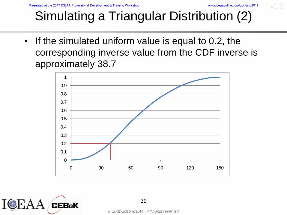
copy 2002-2013 ICEAA All rights reserved
v12
Simulating a Triangular Distribution (2)
bull If the simulated uniform value is equal to 02 the corresponding inverse value from the CDF inverse is approximately 387
39
0
01
02
03
04
05
06
07
08
09
1
0 30 60 90 120 150
Presented at the 2017 ICEAA Professional Development amp Training Workshop wwwiceaaonlinecomportland2017
copy 2002-2013 ICEAA All rights reserved
v12
Monte Carlo and the WBSbull Simulation involves repeated trials
40
WBS Draw1 2 3 4 5
System 2912 3566 4390 2954 4655 Sum
Structure 80 105 55 80 57 SumVehicle Structure 50 70 30 40 20Tank Structure 30 35 25 40 37
Thermal Control 32 36 35 29 33 SumActive Thermal Control 10 15 12 7 10Induced Thermal Control 12 14 13 14 14Tank Thermal Control 10 7 10 8 9
Main Propulsion System 100 150 125 140 100
Liquid Rocket Engine 1000 1100 1800 900 2200
Electric Power and Distribution 100 125 150 75 90
Command Control and Data Handling 200 250 225 230 275
System Integration 1400 1800 2000 1500 1900
Presented at the 2017 ICEAA Professional Development amp Training Workshop wwwiceaaonlinecomportland2017
copy 2002-2013 ICEAA All rights reserved
v12
Number of Trialsbull Monte Carlo involves a repeated number of trialsbull The greater the number of trials the more accurate the
simulation will approximate the overall cost risk behavior of the system
bull After 100 trials the histogram looks very jagged
41
Presented at the 2017 ICEAA Professional Development amp Training Workshop wwwiceaaonlinecomportland2017
copy 2002-2013 ICEAA All rights reserved
v12
Number of Trials (2)
42
1000 Trials
10000 Trials
50000 Trials Additional trials give a more accurate depiction of the final result
Presented at the 2017 ICEAA Professional Development amp Training Workshop wwwiceaaonlinecomportland2017
copy 2002-2013 ICEAA All rights reserved
v12
Number of Trials (3)bull If we want to simulate the underlying
mean within 1 with 95 confidence for example then we require
43
divideoslash
oumlccedilegrave
aelig poundpound-
=
dividedividedivide
oslash
ouml
ccedilccedilccedil
egrave
aeligpound
-pound
-=
divideoslashouml
ccedilegraveaelig poundpound=
nZ
n
nnX
n
X
n
n
011
010Pr
011
010Pr
011990Pr950
___
___
sm
sm
sm
sm
sm
mm
Presented at the 2017 ICEAA Professional Development amp Training Workshop wwwiceaaonlinecomportland2017
copy 2002-2013 ICEAA All rights reserved
v12
Number of Trials (4)bull This means that the number of trials required is determined by
bull Solving for n we find that at least
trials are neededbull Note that this term involves the coefficient of variation of the
distribution which means that distributions with less dispersion require fewer trials to accurate simulate
44
96101
=ns
m
ms41638
Presented at the 2017 ICEAA Professional Development amp Training Workshop wwwiceaaonlinecomportland2017
copy 2002-2013 ICEAA All rights reserved
v12
Number of Trials (5)bull Simulating percentiles requires more trials than for simulating
meansbull Let Pn represent the number of trials in the sample at or below
the 70th percentile of the underlying distribution (suppose this is known)
bull By the Central Limit Theorem Pnn follows a normal distribution with mean equal to the 70th percentile and variance equal to
bull By a similar process for the mean we find that the number of trials needed to simulate the 70th percentile within 1 with 95 confidence is
45
( )n
FF 700700 1-
n
n
PPn -41638
Presented at the 2017 ICEAA Professional Development amp Training Workshop wwwiceaaonlinecomportland2017
copy 2002-2013 ICEAA All rights reserved
v12
Number of Trials (6)bull If Pn 070 for all n then n is approximately
bull For the sake of comparison suppose CV = 03 (reasonable approximation for hardware development) then the number of trials needed to simulate the mean with the same accuracy is then ldquoonlyrdquo 11525
bull More trials are needed to accurately simulate percentiles than means
46
( ) 46416703041638
70704168341638 =divide
oslashouml
ccedilegraveaelig=divide
oslashouml
ccedilegraveaelig -
=-
nnn
PPn
n
n
Presented at the 2017 ICEAA Professional Development amp Training Workshop wwwiceaaonlinecomportland2017
copy 2002-2013 ICEAA All rights reserved
v12
Methods of Simulationbull Monte Carlo simulation is a standard term for
simulationbull However there is an improvement on Monte Carlo
that improves the accuracy of the results of a simulation for a given number of trials
bull This method is call the Latin Hypercube approach to simulationndash Similar to Monte Carlo but an equal number of draws are taken
from a set of subintervals for example dividing the interval (01) into [00001) [0102)hellip [0910]
ndash Instead of 10 trials from [01] we have one trial from each subinterval
ndash Rough rule of thumb is Latin Hypercube takes 30 fewer trials to achieve similar accuracy to Monte Carlo
47
Presented at the 2017 ICEAA Professional Development amp Training Workshop wwwiceaaonlinecomportland2017
copy 2002-2013 ICEAA All rights reserved
v12
Probability Model ndash Correlationbull Correlation exists between work breakdown structure
(WBS) cost element costs and between cost and schedule
bull Correlation is a necessary consideration in cost risk analysis
bull Correlation is a number that can vary between -1 and +1 and represents the strength of the relationship between the two variablesndash If both variable have a tendency to move in the same direction
correlation is positivendash If when one variable increases the other tends to decrease and
vice-versa the correlation between the two variables is negative
Presented at the 2017 ICEAA Professional Development amp Training Workshop wwwiceaaonlinecomportland2017
copy 2002-2013 ICEAA All rights reserved
v12
Correlation And Causationbull Note that correlation is not causation however
causation implies correlationndash For example shark attacks and ice cream sales at the beach
bull For example for a launch vehicle structure increasing the diameter will not only result in an increase in the structures cost but will also result in higher costs for thermal coating (paint etc)
bull Also simply because two subsystems do not appear to be related does not mean they are not correlatedndash For example structures and computer equipment seemingly
have little relation to one another however an external factor such as a funding cut or a strike will impact all subsystems leading to delays and increasing cost across the board
ndash Thus everything in a WBS has some correlationUnit III - Module 9 49
Presented at the 2017 ICEAA Professional Development amp Training Workshop wwwiceaaonlinecomportland2017
copy 2002-2013 ICEAA All rights reserved
v12
The Importance of Correlationbull Percent that total cost standard deviation is underestimated
when correlation assumed to be 0 instead of r given nWBS elements
Unit III - Module 9 5050
0
20
40
60
80
100
0 01 02 03 04 05 06 07 08 09 1Actual Correlation
Perce
nt Un
deres
timate
d
n = 10
n = 30
n = 100n = 1000
0
20
40
60
80
100
0 01 02 03 04 05 06 07 08 09 1Actual Correlation
Perce
nt Un
deres
timate
d
n = 10
n = 30
n = 100n = 1000
Reference 32nd Annual DOD Cost Analysis Symposium Advanced Training Session ldquoWhy Correlation Matters in Cost Estimatingrdquo Stephen A Book
Presented at the 2017 ICEAA Professional Development amp Training Workshop wwwiceaaonlinecomportland2017
copy 2002-2013 ICEAA All rights reserved
v12
The Importance of Correlation (2)bull For example if correlation is assumed to be 0 for all
elements in a 30 element WBS and the actual correlation is 20 then the total cost standard deviation is underestimated by 60
bull For example assume the total cost is modeled as a normal distribution with mean = 100
bull If correlation is assumed to be zero with total cost standard deviation = 12 when correlation is actually 20 then the true underlying standard deviation is actually 30
bull 70th percentile with zero correlation assumption is 106
bull 70th percentile with 20 correlation is 116 Unit III - Module 9 51
Presented at the 2017 ICEAA Professional Development amp Training Workshop wwwiceaaonlinecomportland2017
copy 2002-2013 ICEAA All rights reserved
v12
Measures of Correlationbull Two measures of correlation are commonly used in
cost risk analysesndash Pearsonrsquos product-moment correlation coefficient ndash Spearmanrsquos rank correlation coefficient
bull Garvey and others recommend using Pearsonrsquos product-moment correlation coefficient correlation for cost risk analysesndash Method of moments uses this but there are two options in
simulationndash Popular simulation packages like Risk and Crystal Ball use
rank correlation but in practice this has been found to make little difference
ndash Pearson product-moment correlation has been incorporated into Risk+
52
Presented at the 2017 ICEAA Professional Development amp Training Workshop wwwiceaaonlinecomportland2017
copy 2002-2013 ICEAA All rights reserved
v12
Pearson Correlationbull Pearsonrsquos product-moment correlation measures
degree of linearity between two random variables bull If two random variables are perfectly linear (eg Y =
aX + b) with positive slope then the Pearson product-moment correlation between X and Y denoted by rXY is +1
53
X X
Y Y Y
XNegative Correlation Positive Correlation No Correlation
middotmiddot
middotmiddot
middotmiddot middotmiddot
middotmiddot
middot
middot
middotmiddotmiddot
middotmiddot
middotmiddot
middotmiddot middot
middot
middot
middotmiddotmiddotmiddotmiddotmiddotmiddotmiddot
middotmiddotmiddotmiddot
middotmiddot
middotmiddot middotmiddotmiddotmiddot
middotmiddotmiddot
middotmiddotmiddotmiddot
middotmiddotmiddot
middotmiddotmiddot
middotmiddot
middot
middot middotmiddot
middot middotmiddotmiddotmiddot middotmiddot middot middotmiddot middot middot
middotmiddot middot
middotmiddotmiddotmiddotmiddot middot middotmiddot
middotmiddot
middot
middotmiddot
middotmiddot middot
middot middot middot
middotmiddot middot
middotmiddotmiddot
middotmiddot
middot middot
Presented at the 2017 ICEAA Professional Development amp Training Workshop wwwiceaaonlinecomportland2017
copy 2002-2013 ICEAA All rights reserved
v12
Spearman Correlationbull Spearmanrsquos rank correlation measures the
monotonicity between two random variablesbull If two random variables are perfectly monotonically
increasing (eg Y = X2) then the Spearman rank correlation denoted by rXY is +1
bull The two measures can be significantly different
54
10 20 30 40 50 60
100
200
300
096 097 098 099 1
1
060
020
040
080
Eff
ort (
Staf
f-M
onth
s)
Software Size I KDSI
y = 28z12y
z x
yy = x100
0 pound x pound 1
Figure 5-9A Figure 5-9B
Pearson Correlation = 09976 Rank Correlation = 1
Pearson Correlation = 024 Rank Correlation = 1
X(x ) ~ Unif(01)
Reference Probability Methods for Cost Uncertainty Analysis A Systems Engineering Perspective Paul R Garvey
Presented at the 2017 ICEAA Professional Development amp Training Workshop wwwiceaaonlinecomportland2017
copy 2002-2013 ICEAA All rights reserved
v12
Unit III - Module 9 55
200
250
300
350
400
1000 1200 1400 1600 1800 2000
Recurring Production
SEPM
200
250
300
350
400
1000 1200 1400 1600 1800 2000
Recurring Production
SEPM
Functional Correlationbull Old No Functional
Correlation Simulation run with WBS items entered as values
bull New Simulation run with functional dependencies entered as they are in cost model
CorrelatedNot Correlated
Note shift of mean and increased variability
Presented at the 2017 ICEAA Professional Development amp Training Workshop wwwiceaaonlinecomportland2017
copy 2002-2013 ICEAA All rights reserved
v12
Risk Measuresbull ldquoWestern Europe conquered the word because of a
technological revolution that started because of attempts to measure the worldrdquo ndash Phillipe Jorion ndash In the same way attempts to measure risk will lead to better project
managementbull Risk management for DoD and NASA agencies focuses
primarily on funding projects to a single percentile ndash NASA policy explicitly mentions 70 and 50ndash This is known as ldquoValue at Riskrdquo and is prevalent in the banking and
financial industry
56
Presented at the 2017 ICEAA Professional Development amp Training Workshop wwwiceaaonlinecomportland2017
copy 2002-2013 ICEAA All rights reserved
v12
Value at Risk (VaR)bull VaR is a percentile of the cost risk
distributionndash VaR funding at the 70th percentile means that
there is a 30 chance of final project cost exceeding the funded amount (budget)
bull VaR has some meritsndash Common measure can be used to compare
different projects and programsndash Easily understood by senior managers and
decision makers
57
Presented at the 2017 ICEAA Professional Development amp Training Workshop wwwiceaaonlinecomportland2017
copy 2002-2013 ICEAA All rights reserved
v12
Why 70th or 80th Percentilebull Typical policy guidance involves funding at the 70th or 80th
percentile Why fund as such a low percentilebull There is some incentive to not over-fundbull For a normal distribution an inflection point occurs near the 80th
percentile meaning that for values above 80 confidence achieving higher levels of confidence can only be achieved by spending greater dollar amounts at an increasing rate
58
-05-04-03-02-01
00102030405
0 05 1 15 2 25 3
Standard Deviations from Mean
Normal Distribution
First DerivativeSlopeVelocity
Second DerivativeConvexityAcceleration
Inflection point at one standard deviation above the mean (~84th
percentile)
Presented at the 2017 ICEAA Professional Development amp Training Workshop wwwiceaaonlinecomportland2017
copy 2002-2013 ICEAA All rights reserved
v12
Funding Above Inflection Pointsbull As the percentile goes above the 80th percentile the amount
needed to achieve that higher level of confidence begins to increase at an increasing rate as is evident from the graph
59
0
10
20
30
40
50
60
70
50 55 60 65 70 75 80 85 90 95 100
$ Ab
ove
MEa
n to
Ach
ieve
Per
cent
ile
Percentile (Confidence Level)
Presented at the 2017 ICEAA Professional Development amp Training Workshop wwwiceaaonlinecomportland2017
copy 2002-2013 ICEAA All rights reserved
v12
Why Budget to the 70th or 80thbull Government projects are funded at the 70th or 80th percentilesbull Why not the 90th or 99th percentile Wonrsquot that help prevent
overrunsndash As we have seen percentiles do not add across programs
bull The sum of the 80th percentiles does NOT equal the total 80th percentile
ndash This is because the individual programs are riskier than the entire suite of missions
bull Known as the ldquoPortfolio effectrdquo (more or this later)
ndash Funding at the 80th gives confidence that the entire portfolio will be adequately funded
bull And since there is an inflection point near the 80th percentile funding above that level quickly becomes cost prohibitive
60
Presented at the 2017 ICEAA Professional Development amp Training Workshop wwwiceaaonlinecomportland2017
copy 2002-2013 ICEAA All rights reserved
v12
Inflection Points for Lognormalbull For a lognormal the inflection point
variesndash Coefficient of variation equal to 10 equates to an
inflection point at the 70th percentile
61
0
10
20
30
40
50
60
70
050 060 070 080 090 100
Coef
ficen
t of V
aria
tion
Percentile of the Inflection Point
Presented at the 2017 ICEAA Professional Development amp Training Workshop wwwiceaaonlinecomportland2017
copy 2002-2013 ICEAA All rights reserved
v12
Issues with Percentile Fundingbull However risk management does not stop at a
specific percentilendash What happens when the 70th percentile is exceeded
bull Any effective risk management policy should prescribe what happens after a bad event occursndash With VaR we only know when a bad event has occurred ndash Also funding at a relatively low level means we have no true
sense of the real risks that should be guarded against
62
Presented at the 2017 ICEAA Professional Development amp Training Workshop wwwiceaaonlinecomportland2017
copy 2002-2013 ICEAA All rights reserved
v12
ldquoHere There Be Dragonsrdquobull On old maps uncharted territory was often
marked with monsters or dragons
63
A section of the Carta Marina by Olaus Magnus 16th Century
Presented at the 2017 ICEAA Professional Development amp Training Workshop wwwiceaaonlinecomportland2017
copy 2002-2013 ICEAA All rights reserved
v12
Distribution Comparisonbull Four different distributions with the same 70th
percentile
bull Should we expect the tails to be similar
64
0
10
20
30
40
50
60
70
80
0 100 200 300 400 500 600
Perc
entil
eCo
nfid
ence
Lev
el
Triangular
Normal
Lognormal
Pareto
Presented at the 2017 ICEAA Professional Development amp Training Workshop wwwiceaaonlinecomportland2017
copy 2002-2013 ICEAA All rights reserved
v12Distribution Comparison Tail Behavior
bull The normal and triangular distributions have similar tails but the lognormal and Pareto have much fatter right tails
65
70
75
80
85
90
95
100
500 1500 2500 3500 4500 5500
Perc
entil
eCo
nfid
ence
Lev
el
Triangular
Normal
Lognormal
Pareto
Here There Be Dragons
Presented at the 2017 ICEAA Professional Development amp Training Workshop wwwiceaaonlinecomportland2017
copy 2002-2013 ICEAA All rights reserved
v12Distribution Comparison ndash Tail Behavior (Table)
bull There is significant tail risk for the lognormal and the Paretobull The 99th percentile for the Pareto is 1000 times greater than
the 70th percentilendash Risk seen in financial markets and in catastrophic risks like natural
disasters bull Four different projects follow the four different risk profiles seen
in this example should clearly have different risk management approaches but 70th percentile funding indicates the same risk management approach for all four
66
Percentile Triangular Normal Lognormal Pareto 70th $600 $600 $600 $600 80th $680 $660 $770 $1430 90th $770 $750 $1070 $5880 95th $840 $820 $1410 $23750 99th $930 $950 $2350 $600000
Presented at the 2017 ICEAA Professional Development amp Training Workshop wwwiceaaonlinecomportland2017
copy 2002-2013 ICEAA All rights reserved
v12Percentile Budgeting is Not Risk Management
bull Percentile budgeting ne effective risk management policybull Suppose that you are shopping for a new car You
mention that safety is your top concern The salesman says he has a great safe car available You ask about the air bags Do they work The salesman answers ldquoOf course Seventy percent of the time they work fine Only 30 of the time the air bags will fail to deployrdquo Would you buy such a car Hedge fund manager David Einhorn has stated ldquoRisk management is the air bag that must always work but only in the multi-sigma event where you have an accidentrdquo
67
Risk management is the air bag that must always work but only in the multi-sigma event where you
have an accident
Presented at the 2017 ICEAA Professional Development amp Training Workshop wwwiceaaonlinecomportland2017
copy 2002-2013 ICEAA All rights reserved
v12
Joint Confidence Level Analysisbull Schedules are risky toobull For 98 recent NASA missions average
schedule growth was 38ndash Not as high as cost growth but still significant
68
0
5
10
15
20
25
30
35
40
Schedule
Cost
Presented at the 2017 ICEAA Professional Development amp Training Workshop wwwiceaaonlinecomportland2017
copy 2002-2013 ICEAA All rights reserved
v12
Schedules Impact Costbull Changes in schedule can have enormous
impacts on cost ndash Schedule slips can lead to cost increases
bull Fixed programmatic costs must be paid on a regular basisndash Achieving schedule milestones early can result in cost
savings
bull Schedule is an important consideration in cost analysis including cost risk analysis
bull However we must be careful in correctly integrating cost and schedule riskndash Schedule is not simply an input but is dependent on many of
the same factors that drive cost
69
Presented at the 2017 ICEAA Professional Development amp Training Workshop wwwiceaaonlinecomportland2017
copy 2002-2013 ICEAA All rights reserved
v12
The Relationship of Cost to Schedulebull Cost and schedule are positively correlated
ndash A larger program with bigger scope with take longer to complete than a smaller simpler program
bull However longer schedules do not always equate to higher cost nor shorter schedules with lower costndash Highly compressed schedules relative to the
optimal schedule can lead to large overrunsbull Compressed schedules are commonplace for
many planetary missions
70
Presented at the 2017 ICEAA Professional Development amp Training Workshop wwwiceaaonlinecomportland2017
copy 2002-2013 ICEAA All rights reserved
v12The Impact of Schedule GrowthCompression on Cost
bull Compressed schedules lead to cost growth and based on existing research is actually more expensive than schedule slippages
71
0
20
40
60
80
100
120
140
160
-50 -25 0 25 50 75 100
Percentage Change in Schedule
Perc
enta
ge C
hang
e in
Cos
t due
to
Sche
dule
Cha
nge
Source Smart CB ldquoCost and Schedule Interrelationshipsrdquo 2007 NASA Cost Symposium
Presented at the 2017 ICEAA Professional Development amp Training Workshop wwwiceaaonlinecomportland2017
copy 2002-2013 ICEAA All rights reserved
v12Schedule as an Independent Variable
bull Why not simply add schedule as an input to cost-estimating relationships (CERs)
bull Schedule is often treated as an independent variable ndash schedules are often determined independently of cost considerationsndash Cost may not be considered explicitly although budgets and
schedules are determined based on scope and other common factors
bull In 2006 SAIC undertook a research task to determine the impact of schedule on cost and added schedule as an independent variable to the CERs in the NASAAir Force Cost Model (NAFCOM) to see if schedule provided any improvement in goodness of fit
72
Presented at the 2017 ICEAA Professional Development amp Training Workshop wwwiceaaonlinecomportland2017
copy 2002-2013 ICEAA All rights reserved
v12
Schedule is a Dependent Variablebull Since NAFCOM includes an exhaustive list of cost drivers the inclusion
of schedule should give an indication of whether there is any additional independent value added from schedule independent of the cost drivers
bull In the study schedule was added to 10 subsystem-level CERs
ndash In each case the addition of schedule did NOTimprove the goodness of fit and schedule was NOT found to be a statistically significant cost driver (given the presence of the other variables) for any of the 10 CERs
bull Standard errors for the CERs increased due to decrease in degrees of freedom
bull Thus schedule as an independent variable did not provide any additional explanation of variation in historical cost
bull This is because schedule is truly NOT an independent variable but a dependent variable and is a function of the same factors that drive cost
73
Presented at the 2017 ICEAA Professional Development amp Training Workshop wwwiceaaonlinecomportland2017
copy 2002-2013 ICEAA All rights reserved
v12
Incorporation of Schedule in Cost Risk
bull When using subjective methods care must be taken in applying schedule to cost risk analysis
bull Since schedule is a dependent variable treating it independently from other factors when assessing its impact on cost can lead to a double count of independent variables in the cost risk analysis
bull Direct inclusion of schedule in a cost risk analysis effectively doubles the influence of each cost driver
ndash Incorrectly leads to broader risk ranges
74
CostWeight
HeritageNewness
Technology Readiness Schedule
Presented at the 2017 ICEAA Professional Development amp Training Workshop wwwiceaaonlinecomportland2017
copy 2002-2013 ICEAA All rights reserved
v12Subjective Cost Risk Methods and Overinclusion of Risk Factors
bull Subjective methods are suitable when data are scarce or not availablebull However care must be taken not to treat correlated sources of risk
such as schedule as independent of each otherbull Example ndash a subjective risk analysis incorporated technology readiness
design risk requirements stability integration risk and schedule and treated each source of risk as independent
bull Risk triangle high value without schedule risk was 31 times the point estimate
bull Risk triangle high value with schedule risk added on top of other sources of risk treated independently was 34 times the point estimate
bull Risk triangle taking correlation between sources of risk into account in a rigorous statistical manner has a high value 15 times the point estimate less than half the effect when treating sources of risk as independent
75
Presented at the 2017 ICEAA Professional Development amp Training Workshop wwwiceaaonlinecomportland2017
copy 2002-2013 ICEAA All rights reserved
v12Fundamental Equation of Cost and Schedule Interrelationships
bull The Fundamental Equation of the Relationship Between Cost and Schedule is
Time = Moneybull This is a well known adage that time is money Your boss at
work may even mention this to you from time to time or if you are the boss you are all too aware of this iron law
bull Because time is money cost and schedule risk should be modeled jointly not with schedule as an independent cost driver
bull Note that cost and schedule are not perfectly correlatedndash Cost can sometimes ldquobuy downrdquo schedule extra money can be
spent to meet a deadline since in some cases additional effort to hasten the completion of a task
76
Presented at the 2017 ICEAA Professional Development amp Training Workshop wwwiceaaonlinecomportland2017
copy 2002-2013 ICEAA All rights reserved
v12How to (Correctly) Incorporate Schedule into Cost Risk Analysis
bull The best way to model cost and schedule risk is to develop a joint cost and schedule model based on the same data
bull Since such models are not currently available the next best approach is to model cost and schedule independently and then integrate cost and schedule risk analyses using joint probability distributions taking into account correlation between cost and schedulendash This approach pioneered by Paul Garvey and Steve Book is
considered industry best practicendash This is a practical method mathematically tractable and follows
naturally from the Fundamental Equation of Cost and Schedule Interrelationships
77
Book S A ldquoQuantifying the Relationship Between Cost and Schedulerdquo The Measurable News Winter 2007-2008 pp 11-15Garvey PR Probability Methods for Cost Uncertainty Analysis A Systems Engineering Perspective New York Marcel Dekker 2000 pp 308-335
Presented at the 2017 ICEAA Professional Development amp Training Workshop wwwiceaaonlinecomportland2017
copy 2002-2013 ICEAA All rights reserved
v12
Joint Lognormal and Normal Distributions
bull Cost and schedule are typically modeled as some combination of Normal and Lognormal probability distributionsndash Studies by The Aerospace Corporation the MITRE
Corporation Wyle Labs and SAIC have found that the Lognormal probability distribution almost always serves as a good model for both the schedule distribution and the cost distribution
ndash The Normal distribution may also be appropriate in some instances and depending upon the level of confidence at which budgets are set may even be more conservative and logically consistent than the Normal distribution
ndash Joint Lognormal and Normal distributions are defined by a pair of mean and standard deviations and a level of correlation between the two
78
Presented at the 2017 ICEAA Professional Development amp Training Workshop wwwiceaaonlinecomportland2017
copy 2002-2013 ICEAA All rights reserved
v12Modeling Cost and Schedule as a Bivariate Distribution
bull In the approach set forth by Book and Garvey cost risk is assessed and the top-level distribution is modeled as a Lognormal (or Normal) distribution schedule risk is assessed and the overall schedule risk is modeled as a Lognormal (or Normal) distribution
bull The two distributions are combined into a Bivariate distribution by assigning a correlation between the two and by treating the two distributions as the marginal distributions of a Bivariate Lognormal distributionndash Other combinations include a Bivariate Normal or a Bivariate
Normal-Lognormal
79
Presented at the 2017 ICEAA Professional Development amp Training Workshop wwwiceaaonlinecomportland2017
copy 2002-2013 ICEAA All rights reserved
v12Bivariate Lognormal Distribution for Cost and Schedule
bull Cost is often observed to be Lognormal when strong positive correlations are present among the systemrsquos WBS cost element costs
bull A systemrsquos schedule is often observed (from Monte Carlo simulations) to be Lognormal if it is the sum of many positively correlated schedule activities in an overall schedule network
bull If Lognormal distributions characterize a systemrsquos cost and schedule then the Bivariate Lognormal could serve as an assumed model of their joint distributionndash In this case the marginal distribution of each of cost and schedule is
Lognormalbull Other possibilities for modeling cost and schedule as a Bivariate
distribution include a Bivariate Normal or a Bivariate Normal-Lognormal distributionndash All these combinations are analytically tractable
80
Presented at the 2017 ICEAA Professional Development amp Training Workshop wwwiceaaonlinecomportland2017
copy 2002-2013 ICEAA All rights reserved
v12Bivariate Lognormal for Cost and Schedule
bull Contour Plots of a Bivariate Lognormal
81
Presented at the 2017 ICEAA Professional Development amp Training Workshop wwwiceaaonlinecomportland2017
copy 2002-2013 ICEAA All rights reserved
v12Correlation Between Cost and Schedule
bull Cost and schedule are positively correlated but not perfectly sondash For example it is possible to have a schedule underrun and a cost
overrunbull Based on cost and schedule growth data for 50 completed NASA
programs the correlation between development cost and development schedule is 70
82
00
200
400
600
800
1000
1200
-500 00 500 1000 1500 2000 2500Historical Cost Growth
Hist
oric
al S
ched
ule
Gro
wth
r = 715
Presented at the 2017 ICEAA Professional Development amp Training Workshop wwwiceaaonlinecomportland2017
copy 2002-2013 ICEAA All rights reserved
v12Correlation Between Cost and Schedule Caveats
bull Based on historical data recommended correlation between cost and schedule is 70 but this could be higher or lower depending upon program circumstancesndash If program is budget constrained cost and schedule will be
more highly correlated (go as you pay)ndash If program is schedule constrained cost and schedule will
have lower correlation perhaps even negative correlation ndash Smaller programs have smaller correlation between cost and
schedule riskbull Relatively easy to ldquohurry uprdquo and finish on time or even early if
needed
83
Presented at the 2017 ICEAA Professional Development amp Training Workshop wwwiceaaonlinecomportland2017
copy 2002-2013 ICEAA All rights reserved
v12
Conditional Confidence Levelsbull Given a programrsquos project schedule we can determine the cost
risk distribution conditional upon the given schedulebull Conditional cost S-curves are steeper than unconditional
(marginal) cost S-curves between some uncertainty has been removed because schedule is fixed
84
Presented at the 2017 ICEAA Professional Development amp Training Workshop wwwiceaaonlinecomportland2017
copy 2002-2013 ICEAA All rights reserved
v12
Joint Confidence Levelsbull Joint 65 confidence represents the probability of
achieving both 65 confidence in cost AND 65 confidence in schedulendash This is different than achieving 65 cost confidence alone
or achieving 65 schedule confidence alonebull Due to the imperfect correlation between cost and schedule it
is possible to achieve a 65 cost confidence with a lower level of schedule confidence
bull Restricting the schedule confidence thus requires additional $ to achieve a given level of confidence
85
X
Y
Possible Values for Which X gt a Possible Values for
Which X gt a and Y gt b
a
b
Presented at the 2017 ICEAA Professional Development amp Training Workshop wwwiceaaonlinecomportland2017
copy 2002-2013 ICEAA All rights reserved
v12Joint Confidence Levels Versus Cost Confidence Levels Only
bull Example of the differences between cost confidence schedule confidence conditional cost confidence and joint cost and schedule confidence
86
Joint Cost-Schedule Confidence Iso-Curves
Cost (RY$M)
Sche
dule
(Mon
ths)
65 Confidence
50 Confidence
70 Confidence
65 Cost Confidence AggressiveSchedule65 Cost ConfidenceScheduleGiven 65 Schedule ConfidenceUnconditional 65 CostConfidenceUnconditional 65 ScheduleConfidence
65 Cost Confidence 65 Joint Cost and Schedule
Confidence for 65 Schedule Confidence
Presented at the 2017 ICEAA Professional Development amp Training Workshop wwwiceaaonlinecomportland2017
copy 2002-2013 ICEAA All rights reserved
v12
Joint Cost and Schedule Confidence
bull Can examine pairs of cost and schedule that achieve a given level of confidence
bull Provides insights into the trade-offs between cost and schedule for a given level of confidencendash Possible to increase cost confidence by giving a
project more time in some instances or possible to ldquobuy downrdquo schedule
bull But these have limits and are shown in the iso-cost and schedule confidence curves
87
Presented at the 2017 ICEAA Professional Development amp Training Workshop wwwiceaaonlinecomportland2017
copy 2002-2013 ICEAA All rights reserved
v12Cost and Schedule Trade-offs for a Given Level of Joint Confidence
bull Hypothetical Example
88
Cost (RY$M)
Schedule (Months)
$100 48$99 48$89 49$87 50$85 51$85 52$84 53$83 55$83 55$83 56
Cost and Schedule 65 Confidence Iso-Curve
4748495051525354555657
$80 $82 $84 $86 $88 $90 $92 $94 $96 $98 $100
Cost (RY$ M)
Sche
dule
(Mon
ths)
Presented at the 2017 ICEAA Professional Development amp Training Workshop wwwiceaaonlinecomportland2017
copy 2002-2013 ICEAA All rights reserved
v12Policy Considerations for Confidence Levels
bull For large programs the difference between the amount of money needed to achieve 65 cost confidence independent of schedule and joint 65 cost and schedule confidence can represent hundreds of millions and even billions of dollars
89
Joint Cost-Schedule Confidence Iso-Curves
Cost (RY$M)
Sche
dule
(Mon
ths)
65 Confidence
65 Cost Confidence AggressiveSchedule
65 Cost ConfidenceScheduleGiven 65 Schedule Confidence
Unconditional 65 CostConfidence
Joint Cost and Schedule Confidence for 65 Cost Confidence and Program Baseline Schedule is Less Than 35
65 Cost Confidence Independent of Schedule Cost Needed to Achieve
Both 65 Joint Cost and Schedule Confidence for the Schedule with 65 Confidence
Presented at the 2017 ICEAA Professional Development amp Training Workshop wwwiceaaonlinecomportland2017
copy 2002-2013 ICEAA All rights reserved
v12
Copulasbull More generally any combination of distributions can
be used (more than just normal and lognormal)ndash Termed ldquocopulardquo from the Italian word for ldquocouplerdquondash Copulas are a way to combine marginal distributions of any
number and type into a joint distributionbull More formally a copula is a multivariate joint distribution defined
on the n-dimensional unit cube [0 1]n such that every marginal distribution is uniform on the interval [0 1]
bull (The bivariate form of) Sklarrsquos theorem states that for any bivariate distribution function H(x y) let F(x) = H(x infin) and G(y) = H(infin y) be the univariate marginal probability distribution functions Then there exists a copula C such that H(xy)=C(F(x)G(y))
ndash Copulas are widely used in risk management for investments and insurance
bull Considered industry best practice (Li 2000)bull Marketed as part of JP Morganrsquos CreditMetrics suite of tools
(Gupton et Al 1997)90
Presented at the 2017 ICEAA Professional Development amp Training Workshop wwwiceaaonlinecomportland2017
copy 2002-2013 ICEAA All rights reserved
v12Parametric Joint Cost and Schedule Analysis
bull A parametric model based on a consistent data set with a set of overlapping cost and schedule drivers is a cleaner way to model cost and schedule
91
CostWeight
HeritageNewness
Technology Readiness
Schedule
0
20
40
60
80
100
Confidence
Joint Cost and Schedule Confidence
Schedule
Cost
Lognormal Distribution PDF and CDF
0102030405060708090100
200 300 400 500 600 700 800 900 1000Cost $
Con
fiden
ce L
evel
0
00002
00004
00006
00008
0001
00012
00014
00016
Prob
abili
ty D
ensi
ty
CDFPDF
Lognormal Distribution PDF and CDF
0102030405060708090100
200 300 400 500 600 700 800 900 1000Cost $
Con
fiden
ce L
evel
0
00002
00004
00006
00008
0001
00012
00014
00016
Prob
abili
ty D
ensi
ty
CDFPDF
Presented at the 2017 ICEAA Professional Development amp Training Workshop wwwiceaaonlinecomportland2017
copy 2002-2013 ICEAA All rights reserved
v12Parametric Joint Cost and Schedule Analysis (2)
bull Joint cost and schedule risk analysis produced naturally by the integrated modelndash Addresses several issues with the copula
approachbull Tail dependencybull Correlation ndash no need to assign correlation
between cost and schedulebull Consistency of cost and schedule models
92
Presented at the 2017 ICEAA Professional Development amp Training Workshop wwwiceaaonlinecomportland2017
copy 2002-2013 ICEAA All rights reserved
v12
Resource-Loaded Schedulesbull Involves assigning cost and schedule risks to a resource-loaded schedule
networkbull Bottom-up approach
ndash More labor intensive than parametrics but can also provide more insight
ndash Can answer questions than parametric typically cannot such as how much do reserve requirements decrease if a specific risk is retired
bull Currently being implemented in Constellation programbull Has same issue as all bottom-up models hard to count all the risks and model
them discretely
ndash As a result there is a tendency to reflect less risk than indicated by history
ndash ldquoThere are more things in heaven and earth Horatio than are dreamt of in your philosophyrdquo William Shakespeare Hamlet Act I Scene V
93
Presented at the 2017 ICEAA Professional Development amp Training Workshop wwwiceaaonlinecomportland2017
copy 2002-2013 ICEAA All rights reserved
v12Resource-Loaded Schedules Vs Parametrics
bull Parametric most appropriate for early estimatesndash But also good for high-level checks as project progresses
bull As plans take shape lower level modeling may be more appropriate
94 1
CONCEPTUALDEVELOPMENT
PROJECTDEFINITION DESIGN DEVELOPMENT OPERATIONS
PARAMETRIC PARAMETRIC
ANALOGY
ENGINEERING (Bottoms Up)
$PARAMETRIC
DETAILED
$
Pre Phase A Phase B Phase CDPhase A Phase EPre Phase A Phase B Phase CDPhase A Phase E
Risk = f(Cost Estimating Relationship Inputs eg mass power data rate TRL new design etc)
Risk = f(cost and schedule variation of the analogous elements)
Risk = f(variation of detailed inputs eg labor hours rates materials etc)
Presented at the 2017 ICEAA Professional Development amp Training Workshop wwwiceaaonlinecomportland2017
copy 2002-2013 ICEAA All rights reserved
v12
Resource-Loaded Schedulesbull Methodology has been demonstrated in other
industriesndash Construction oil and gasndash Analysis has not been traditionally done on highly uncertain
complex development projects bull Methodology focuses on project baseline schedule
ndash In baseline schedule all tasks are resource loaded to represent a baseline schedule and cost standpoint
ndash Resource loaded schedule is ldquorolledrdquo up to a manageable level
ndash Based on the risk and uncertainties identified schedule distributions are applied to each rolled up task
ndash Cost uncertainties are also applied to rolled up tasksbull Uncertainties include labor rate man power etc
ndash A Monte Carlo simulation is run to develop joint cost-schedule distributions
95
Presented at the 2017 ICEAA Professional Development amp Training Workshop wwwiceaaonlinecomportland2017
copy 2002-2013 ICEAA All rights reserved
v12
Unit III - Module 9 96
Execution ndash Cross Checksbull Means The mean cost growth factor for WBS items
can be compared to history as a way to cross check results
bull CVs The CV of the cost growth factors for WBS items can be compared to history as a way to cross check results
bull Inputs Checks are performed on inputs or other parameters to see if historical values are in line with program assumptionsndash Example Historical risk scores can be compared to program
risk scores to see if risk assessors are being realistic and to see if the underlying database is representative of the program
11
Presented at the 2017 ICEAA Professional Development amp Training Workshop wwwiceaaonlinecomportland2017
- Cost and Schedule Risk Analysis Basic
- Acknowledgments
- Unit Index
- Risk Overview
- Agenda
- Introduction
- Risk Analysis Terms
- Are Our Costs Realistic
- Historical Cost Growth
- Sources of Cost Risk
- Point Estimates of Cost
- Types of Risk
- Point Estimates Vs Risk Estimates
- Cost Risk and Probability
- Probability Model ndash Distribution
- Probability Model ndash Distribution
- Probability ndash Top-Level Distribution
- S-Curves and Confidence Levels
- Example ndash Normal Distribution
- Confidence Levels
- Measuring Parametric Model Uncertainty
- Parametric Model Example
- Weight Uncertainty
- Estimating Uncertainty
- Estimating Uncertainty (2)
- Estimating Uncertainty (3)
- Aggregating Risk
- WBS Example
- WBS and Risk
- Aggregating Risk
- Percentiles Do Not Add
- Percentiles Do Not Add (2)
- Percentiles Do Not Add (3)
- Methods for Aggregating Risk
- Monte Carlo Simulationfor Risk Analysis
- Monte Carlo Simulation
- Using Random Numbers to Simulate Distributions
- Simulating a Triangular Distribution
- Simulating a Triangular Distribution (2)
- Monte Carlo and the WBS
- Number of Trials
- Number of Trials (2)
- Number of Trials (3)
- Number of Trials (4)
- Number of Trials (5)
- Number of Trials (6)
- Methods of Simulation
- Probability Model ndash Correlation
- Correlation And Causation
- The Importance of Correlation
- The Importance of Correlation (2)
- Measures of Correlation
- Pearson Correlation
- Spearman Correlation
- Functional Correlation
- Risk Measures
- Value at Risk (VaR)
- Why 70th or 80th Percentile
- Funding Above Inflection Points
- Why Budget to the 70th or 80th
- Inflection Points for Lognormal
- Issues with Percentile Funding
- ldquoHere There Be Dragonsrdquo
- Distribution Comparison
- Distribution Comparison Tail Behavior
- Distribution Comparison ndash Tail Behavior (Table)
- Percentile Budgeting is Not Risk Management
- Joint Confidence Level Analysis
- Schedules Impact Cost
- The Relationship of Cost to Schedule
- The Impact of Schedule GrowthCompression on Cost
- Schedule as an Independent Variable
- Schedule is a Dependent Variable
- Incorporation of Schedule in Cost Risk
- Subjective Cost Risk Methods and Overinclusion of Risk Factors
- Fundamental Equation of Cost and Schedule Interrelationships
- How to (Correctly) Incorporate Schedule into Cost Risk Analysis
- Joint Lognormal and Normal Distributions
- Modeling Cost and Schedule as a Bivariate Distribution
- Bivariate Lognormal Distribution for Cost and Schedule
- Bivariate Lognormal for Cost and Schedule
- Correlation Between Cost and Schedule
- Correlation Between Cost and Schedule Caveats
- Conditional Confidence Levels
- Joint Confidence Levels
- Joint Confidence Levels Versus Cost Confidence Levels Only
- Joint Cost and Schedule Confidence
- Cost and Schedule Trade-offs for a Given Level of Joint Confidence
- Policy Considerations for Confidence Levels
- Copulas
- Parametric Joint Cost and Schedule Analysis
- Parametric Joint Cost and Schedule Analysis (2)
- Resource-Loaded Schedules
- Resource-Loaded Schedules Vs Parametrics
- Resource-Loaded Schedules
- Execution ndash Cross Checks
-
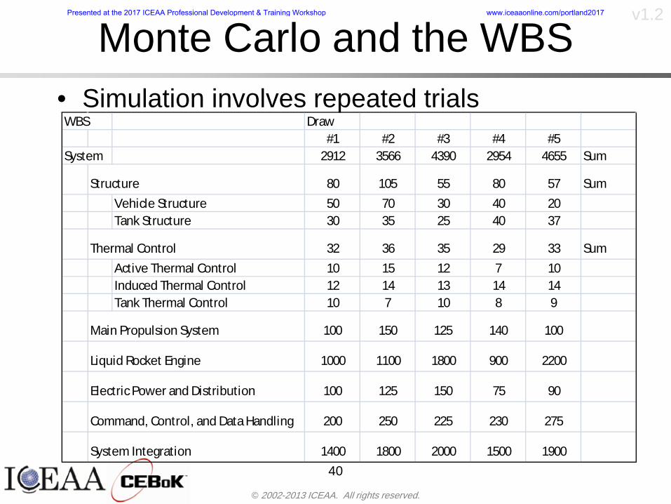
copy 2002-2013 ICEAA All rights reserved
v12
Monte Carlo and the WBSbull Simulation involves repeated trials
40
WBS Draw1 2 3 4 5
System 2912 3566 4390 2954 4655 Sum
Structure 80 105 55 80 57 SumVehicle Structure 50 70 30 40 20Tank Structure 30 35 25 40 37
Thermal Control 32 36 35 29 33 SumActive Thermal Control 10 15 12 7 10Induced Thermal Control 12 14 13 14 14Tank Thermal Control 10 7 10 8 9
Main Propulsion System 100 150 125 140 100
Liquid Rocket Engine 1000 1100 1800 900 2200
Electric Power and Distribution 100 125 150 75 90
Command Control and Data Handling 200 250 225 230 275
System Integration 1400 1800 2000 1500 1900
Presented at the 2017 ICEAA Professional Development amp Training Workshop wwwiceaaonlinecomportland2017
copy 2002-2013 ICEAA All rights reserved
v12
Number of Trialsbull Monte Carlo involves a repeated number of trialsbull The greater the number of trials the more accurate the
simulation will approximate the overall cost risk behavior of the system
bull After 100 trials the histogram looks very jagged
41
Presented at the 2017 ICEAA Professional Development amp Training Workshop wwwiceaaonlinecomportland2017
copy 2002-2013 ICEAA All rights reserved
v12
Number of Trials (2)
42
1000 Trials
10000 Trials
50000 Trials Additional trials give a more accurate depiction of the final result
Presented at the 2017 ICEAA Professional Development amp Training Workshop wwwiceaaonlinecomportland2017
copy 2002-2013 ICEAA All rights reserved
v12
Number of Trials (3)bull If we want to simulate the underlying
mean within 1 with 95 confidence for example then we require
43
divideoslash
oumlccedilegrave
aelig poundpound-
=
dividedividedivide
oslash
ouml
ccedilccedilccedil
egrave
aeligpound
-pound
-=
divideoslashouml
ccedilegraveaelig poundpound=
nZ
n
nnX
n
X
n
n
011
010Pr
011
010Pr
011990Pr950
___
___
sm
sm
sm
sm
sm
mm
Presented at the 2017 ICEAA Professional Development amp Training Workshop wwwiceaaonlinecomportland2017
copy 2002-2013 ICEAA All rights reserved
v12
Number of Trials (4)bull This means that the number of trials required is determined by
bull Solving for n we find that at least
trials are neededbull Note that this term involves the coefficient of variation of the
distribution which means that distributions with less dispersion require fewer trials to accurate simulate
44
96101
=ns
m
ms41638
Presented at the 2017 ICEAA Professional Development amp Training Workshop wwwiceaaonlinecomportland2017
copy 2002-2013 ICEAA All rights reserved
v12
Number of Trials (5)bull Simulating percentiles requires more trials than for simulating
meansbull Let Pn represent the number of trials in the sample at or below
the 70th percentile of the underlying distribution (suppose this is known)
bull By the Central Limit Theorem Pnn follows a normal distribution with mean equal to the 70th percentile and variance equal to
bull By a similar process for the mean we find that the number of trials needed to simulate the 70th percentile within 1 with 95 confidence is
45
( )n
FF 700700 1-
n
n
PPn -41638
Presented at the 2017 ICEAA Professional Development amp Training Workshop wwwiceaaonlinecomportland2017
copy 2002-2013 ICEAA All rights reserved
v12
Number of Trials (6)bull If Pn 070 for all n then n is approximately
bull For the sake of comparison suppose CV = 03 (reasonable approximation for hardware development) then the number of trials needed to simulate the mean with the same accuracy is then ldquoonlyrdquo 11525
bull More trials are needed to accurately simulate percentiles than means
46
( ) 46416703041638
70704168341638 =divide
oslashouml
ccedilegraveaelig=divide
oslashouml
ccedilegraveaelig -
=-
nnn
PPn
n
n
Presented at the 2017 ICEAA Professional Development amp Training Workshop wwwiceaaonlinecomportland2017
copy 2002-2013 ICEAA All rights reserved
v12
Methods of Simulationbull Monte Carlo simulation is a standard term for
simulationbull However there is an improvement on Monte Carlo
that improves the accuracy of the results of a simulation for a given number of trials
bull This method is call the Latin Hypercube approach to simulationndash Similar to Monte Carlo but an equal number of draws are taken
from a set of subintervals for example dividing the interval (01) into [00001) [0102)hellip [0910]
ndash Instead of 10 trials from [01] we have one trial from each subinterval
ndash Rough rule of thumb is Latin Hypercube takes 30 fewer trials to achieve similar accuracy to Monte Carlo
47
Presented at the 2017 ICEAA Professional Development amp Training Workshop wwwiceaaonlinecomportland2017
copy 2002-2013 ICEAA All rights reserved
v12
Probability Model ndash Correlationbull Correlation exists between work breakdown structure
(WBS) cost element costs and between cost and schedule
bull Correlation is a necessary consideration in cost risk analysis
bull Correlation is a number that can vary between -1 and +1 and represents the strength of the relationship between the two variablesndash If both variable have a tendency to move in the same direction
correlation is positivendash If when one variable increases the other tends to decrease and
vice-versa the correlation between the two variables is negative
Presented at the 2017 ICEAA Professional Development amp Training Workshop wwwiceaaonlinecomportland2017
copy 2002-2013 ICEAA All rights reserved
v12
Correlation And Causationbull Note that correlation is not causation however
causation implies correlationndash For example shark attacks and ice cream sales at the beach
bull For example for a launch vehicle structure increasing the diameter will not only result in an increase in the structures cost but will also result in higher costs for thermal coating (paint etc)
bull Also simply because two subsystems do not appear to be related does not mean they are not correlatedndash For example structures and computer equipment seemingly
have little relation to one another however an external factor such as a funding cut or a strike will impact all subsystems leading to delays and increasing cost across the board
ndash Thus everything in a WBS has some correlationUnit III - Module 9 49
Presented at the 2017 ICEAA Professional Development amp Training Workshop wwwiceaaonlinecomportland2017
copy 2002-2013 ICEAA All rights reserved
v12
The Importance of Correlationbull Percent that total cost standard deviation is underestimated
when correlation assumed to be 0 instead of r given nWBS elements
Unit III - Module 9 5050
0
20
40
60
80
100
0 01 02 03 04 05 06 07 08 09 1Actual Correlation
Perce
nt Un
deres
timate
d
n = 10
n = 30
n = 100n = 1000
0
20
40
60
80
100
0 01 02 03 04 05 06 07 08 09 1Actual Correlation
Perce
nt Un
deres
timate
d
n = 10
n = 30
n = 100n = 1000
Reference 32nd Annual DOD Cost Analysis Symposium Advanced Training Session ldquoWhy Correlation Matters in Cost Estimatingrdquo Stephen A Book
Presented at the 2017 ICEAA Professional Development amp Training Workshop wwwiceaaonlinecomportland2017
copy 2002-2013 ICEAA All rights reserved
v12
The Importance of Correlation (2)bull For example if correlation is assumed to be 0 for all
elements in a 30 element WBS and the actual correlation is 20 then the total cost standard deviation is underestimated by 60
bull For example assume the total cost is modeled as a normal distribution with mean = 100
bull If correlation is assumed to be zero with total cost standard deviation = 12 when correlation is actually 20 then the true underlying standard deviation is actually 30
bull 70th percentile with zero correlation assumption is 106
bull 70th percentile with 20 correlation is 116 Unit III - Module 9 51
Presented at the 2017 ICEAA Professional Development amp Training Workshop wwwiceaaonlinecomportland2017
copy 2002-2013 ICEAA All rights reserved
v12
Measures of Correlationbull Two measures of correlation are commonly used in
cost risk analysesndash Pearsonrsquos product-moment correlation coefficient ndash Spearmanrsquos rank correlation coefficient
bull Garvey and others recommend using Pearsonrsquos product-moment correlation coefficient correlation for cost risk analysesndash Method of moments uses this but there are two options in
simulationndash Popular simulation packages like Risk and Crystal Ball use
rank correlation but in practice this has been found to make little difference
ndash Pearson product-moment correlation has been incorporated into Risk+
52
Presented at the 2017 ICEAA Professional Development amp Training Workshop wwwiceaaonlinecomportland2017
copy 2002-2013 ICEAA All rights reserved
v12
Pearson Correlationbull Pearsonrsquos product-moment correlation measures
degree of linearity between two random variables bull If two random variables are perfectly linear (eg Y =
aX + b) with positive slope then the Pearson product-moment correlation between X and Y denoted by rXY is +1
53
X X
Y Y Y
XNegative Correlation Positive Correlation No Correlation
middotmiddot
middotmiddot
middotmiddot middotmiddot
middotmiddot
middot
middot
middotmiddotmiddot
middotmiddot
middotmiddot
middotmiddot middot
middot
middot
middotmiddotmiddotmiddotmiddotmiddotmiddotmiddot
middotmiddotmiddotmiddot
middotmiddot
middotmiddot middotmiddotmiddotmiddot
middotmiddotmiddot
middotmiddotmiddotmiddot
middotmiddotmiddot
middotmiddotmiddot
middotmiddot
middot
middot middotmiddot
middot middotmiddotmiddotmiddot middotmiddot middot middotmiddot middot middot
middotmiddot middot
middotmiddotmiddotmiddotmiddot middot middotmiddot
middotmiddot
middot
middotmiddot
middotmiddot middot
middot middot middot
middotmiddot middot
middotmiddotmiddot
middotmiddot
middot middot
Presented at the 2017 ICEAA Professional Development amp Training Workshop wwwiceaaonlinecomportland2017
copy 2002-2013 ICEAA All rights reserved
v12
Spearman Correlationbull Spearmanrsquos rank correlation measures the
monotonicity between two random variablesbull If two random variables are perfectly monotonically
increasing (eg Y = X2) then the Spearman rank correlation denoted by rXY is +1
bull The two measures can be significantly different
54
10 20 30 40 50 60
100
200
300
096 097 098 099 1
1
060
020
040
080
Eff
ort (
Staf
f-M
onth
s)
Software Size I KDSI
y = 28z12y
z x
yy = x100
0 pound x pound 1
Figure 5-9A Figure 5-9B
Pearson Correlation = 09976 Rank Correlation = 1
Pearson Correlation = 024 Rank Correlation = 1
X(x ) ~ Unif(01)
Reference Probability Methods for Cost Uncertainty Analysis A Systems Engineering Perspective Paul R Garvey
Presented at the 2017 ICEAA Professional Development amp Training Workshop wwwiceaaonlinecomportland2017
copy 2002-2013 ICEAA All rights reserved
v12
Unit III - Module 9 55
200
250
300
350
400
1000 1200 1400 1600 1800 2000
Recurring Production
SEPM
200
250
300
350
400
1000 1200 1400 1600 1800 2000
Recurring Production
SEPM
Functional Correlationbull Old No Functional
Correlation Simulation run with WBS items entered as values
bull New Simulation run with functional dependencies entered as they are in cost model
CorrelatedNot Correlated
Note shift of mean and increased variability
Presented at the 2017 ICEAA Professional Development amp Training Workshop wwwiceaaonlinecomportland2017
copy 2002-2013 ICEAA All rights reserved
v12
Risk Measuresbull ldquoWestern Europe conquered the word because of a
technological revolution that started because of attempts to measure the worldrdquo ndash Phillipe Jorion ndash In the same way attempts to measure risk will lead to better project
managementbull Risk management for DoD and NASA agencies focuses
primarily on funding projects to a single percentile ndash NASA policy explicitly mentions 70 and 50ndash This is known as ldquoValue at Riskrdquo and is prevalent in the banking and
financial industry
56
Presented at the 2017 ICEAA Professional Development amp Training Workshop wwwiceaaonlinecomportland2017
copy 2002-2013 ICEAA All rights reserved
v12
Value at Risk (VaR)bull VaR is a percentile of the cost risk
distributionndash VaR funding at the 70th percentile means that
there is a 30 chance of final project cost exceeding the funded amount (budget)
bull VaR has some meritsndash Common measure can be used to compare
different projects and programsndash Easily understood by senior managers and
decision makers
57
Presented at the 2017 ICEAA Professional Development amp Training Workshop wwwiceaaonlinecomportland2017
copy 2002-2013 ICEAA All rights reserved
v12
Why 70th or 80th Percentilebull Typical policy guidance involves funding at the 70th or 80th
percentile Why fund as such a low percentilebull There is some incentive to not over-fundbull For a normal distribution an inflection point occurs near the 80th
percentile meaning that for values above 80 confidence achieving higher levels of confidence can only be achieved by spending greater dollar amounts at an increasing rate
58
-05-04-03-02-01
00102030405
0 05 1 15 2 25 3
Standard Deviations from Mean
Normal Distribution
First DerivativeSlopeVelocity
Second DerivativeConvexityAcceleration
Inflection point at one standard deviation above the mean (~84th
percentile)
Presented at the 2017 ICEAA Professional Development amp Training Workshop wwwiceaaonlinecomportland2017
copy 2002-2013 ICEAA All rights reserved
v12
Funding Above Inflection Pointsbull As the percentile goes above the 80th percentile the amount
needed to achieve that higher level of confidence begins to increase at an increasing rate as is evident from the graph
59
0
10
20
30
40
50
60
70
50 55 60 65 70 75 80 85 90 95 100
$ Ab
ove
MEa
n to
Ach
ieve
Per
cent
ile
Percentile (Confidence Level)
Presented at the 2017 ICEAA Professional Development amp Training Workshop wwwiceaaonlinecomportland2017
copy 2002-2013 ICEAA All rights reserved
v12
Why Budget to the 70th or 80thbull Government projects are funded at the 70th or 80th percentilesbull Why not the 90th or 99th percentile Wonrsquot that help prevent
overrunsndash As we have seen percentiles do not add across programs
bull The sum of the 80th percentiles does NOT equal the total 80th percentile
ndash This is because the individual programs are riskier than the entire suite of missions
bull Known as the ldquoPortfolio effectrdquo (more or this later)
ndash Funding at the 80th gives confidence that the entire portfolio will be adequately funded
bull And since there is an inflection point near the 80th percentile funding above that level quickly becomes cost prohibitive
60
Presented at the 2017 ICEAA Professional Development amp Training Workshop wwwiceaaonlinecomportland2017
copy 2002-2013 ICEAA All rights reserved
v12
Inflection Points for Lognormalbull For a lognormal the inflection point
variesndash Coefficient of variation equal to 10 equates to an
inflection point at the 70th percentile
61
0
10
20
30
40
50
60
70
050 060 070 080 090 100
Coef
ficen
t of V
aria
tion
Percentile of the Inflection Point
Presented at the 2017 ICEAA Professional Development amp Training Workshop wwwiceaaonlinecomportland2017
copy 2002-2013 ICEAA All rights reserved
v12
Issues with Percentile Fundingbull However risk management does not stop at a
specific percentilendash What happens when the 70th percentile is exceeded
bull Any effective risk management policy should prescribe what happens after a bad event occursndash With VaR we only know when a bad event has occurred ndash Also funding at a relatively low level means we have no true
sense of the real risks that should be guarded against
62
Presented at the 2017 ICEAA Professional Development amp Training Workshop wwwiceaaonlinecomportland2017
copy 2002-2013 ICEAA All rights reserved
v12
ldquoHere There Be Dragonsrdquobull On old maps uncharted territory was often
marked with monsters or dragons
63
A section of the Carta Marina by Olaus Magnus 16th Century
Presented at the 2017 ICEAA Professional Development amp Training Workshop wwwiceaaonlinecomportland2017
copy 2002-2013 ICEAA All rights reserved
v12
Distribution Comparisonbull Four different distributions with the same 70th
percentile
bull Should we expect the tails to be similar
64
0
10
20
30
40
50
60
70
80
0 100 200 300 400 500 600
Perc
entil
eCo
nfid
ence
Lev
el
Triangular
Normal
Lognormal
Pareto
Presented at the 2017 ICEAA Professional Development amp Training Workshop wwwiceaaonlinecomportland2017
copy 2002-2013 ICEAA All rights reserved
v12Distribution Comparison Tail Behavior
bull The normal and triangular distributions have similar tails but the lognormal and Pareto have much fatter right tails
65
70
75
80
85
90
95
100
500 1500 2500 3500 4500 5500
Perc
entil
eCo
nfid
ence
Lev
el
Triangular
Normal
Lognormal
Pareto
Here There Be Dragons
Presented at the 2017 ICEAA Professional Development amp Training Workshop wwwiceaaonlinecomportland2017
copy 2002-2013 ICEAA All rights reserved
v12Distribution Comparison ndash Tail Behavior (Table)
bull There is significant tail risk for the lognormal and the Paretobull The 99th percentile for the Pareto is 1000 times greater than
the 70th percentilendash Risk seen in financial markets and in catastrophic risks like natural
disasters bull Four different projects follow the four different risk profiles seen
in this example should clearly have different risk management approaches but 70th percentile funding indicates the same risk management approach for all four
66
Percentile Triangular Normal Lognormal Pareto 70th $600 $600 $600 $600 80th $680 $660 $770 $1430 90th $770 $750 $1070 $5880 95th $840 $820 $1410 $23750 99th $930 $950 $2350 $600000
Presented at the 2017 ICEAA Professional Development amp Training Workshop wwwiceaaonlinecomportland2017
copy 2002-2013 ICEAA All rights reserved
v12Percentile Budgeting is Not Risk Management
bull Percentile budgeting ne effective risk management policybull Suppose that you are shopping for a new car You
mention that safety is your top concern The salesman says he has a great safe car available You ask about the air bags Do they work The salesman answers ldquoOf course Seventy percent of the time they work fine Only 30 of the time the air bags will fail to deployrdquo Would you buy such a car Hedge fund manager David Einhorn has stated ldquoRisk management is the air bag that must always work but only in the multi-sigma event where you have an accidentrdquo
67
Risk management is the air bag that must always work but only in the multi-sigma event where you
have an accident
Presented at the 2017 ICEAA Professional Development amp Training Workshop wwwiceaaonlinecomportland2017
copy 2002-2013 ICEAA All rights reserved
v12
Joint Confidence Level Analysisbull Schedules are risky toobull For 98 recent NASA missions average
schedule growth was 38ndash Not as high as cost growth but still significant
68
0
5
10
15
20
25
30
35
40
Schedule
Cost
Presented at the 2017 ICEAA Professional Development amp Training Workshop wwwiceaaonlinecomportland2017
copy 2002-2013 ICEAA All rights reserved
v12
Schedules Impact Costbull Changes in schedule can have enormous
impacts on cost ndash Schedule slips can lead to cost increases
bull Fixed programmatic costs must be paid on a regular basisndash Achieving schedule milestones early can result in cost
savings
bull Schedule is an important consideration in cost analysis including cost risk analysis
bull However we must be careful in correctly integrating cost and schedule riskndash Schedule is not simply an input but is dependent on many of
the same factors that drive cost
69
Presented at the 2017 ICEAA Professional Development amp Training Workshop wwwiceaaonlinecomportland2017
copy 2002-2013 ICEAA All rights reserved
v12
The Relationship of Cost to Schedulebull Cost and schedule are positively correlated
ndash A larger program with bigger scope with take longer to complete than a smaller simpler program
bull However longer schedules do not always equate to higher cost nor shorter schedules with lower costndash Highly compressed schedules relative to the
optimal schedule can lead to large overrunsbull Compressed schedules are commonplace for
many planetary missions
70
Presented at the 2017 ICEAA Professional Development amp Training Workshop wwwiceaaonlinecomportland2017
copy 2002-2013 ICEAA All rights reserved
v12The Impact of Schedule GrowthCompression on Cost
bull Compressed schedules lead to cost growth and based on existing research is actually more expensive than schedule slippages
71
0
20
40
60
80
100
120
140
160
-50 -25 0 25 50 75 100
Percentage Change in Schedule
Perc
enta
ge C
hang
e in
Cos
t due
to
Sche
dule
Cha
nge
Source Smart CB ldquoCost and Schedule Interrelationshipsrdquo 2007 NASA Cost Symposium
Presented at the 2017 ICEAA Professional Development amp Training Workshop wwwiceaaonlinecomportland2017
copy 2002-2013 ICEAA All rights reserved
v12Schedule as an Independent Variable
bull Why not simply add schedule as an input to cost-estimating relationships (CERs)
bull Schedule is often treated as an independent variable ndash schedules are often determined independently of cost considerationsndash Cost may not be considered explicitly although budgets and
schedules are determined based on scope and other common factors
bull In 2006 SAIC undertook a research task to determine the impact of schedule on cost and added schedule as an independent variable to the CERs in the NASAAir Force Cost Model (NAFCOM) to see if schedule provided any improvement in goodness of fit
72
Presented at the 2017 ICEAA Professional Development amp Training Workshop wwwiceaaonlinecomportland2017
copy 2002-2013 ICEAA All rights reserved
v12
Schedule is a Dependent Variablebull Since NAFCOM includes an exhaustive list of cost drivers the inclusion
of schedule should give an indication of whether there is any additional independent value added from schedule independent of the cost drivers
bull In the study schedule was added to 10 subsystem-level CERs
ndash In each case the addition of schedule did NOTimprove the goodness of fit and schedule was NOT found to be a statistically significant cost driver (given the presence of the other variables) for any of the 10 CERs
bull Standard errors for the CERs increased due to decrease in degrees of freedom
bull Thus schedule as an independent variable did not provide any additional explanation of variation in historical cost
bull This is because schedule is truly NOT an independent variable but a dependent variable and is a function of the same factors that drive cost
73
Presented at the 2017 ICEAA Professional Development amp Training Workshop wwwiceaaonlinecomportland2017
copy 2002-2013 ICEAA All rights reserved
v12
Incorporation of Schedule in Cost Risk
bull When using subjective methods care must be taken in applying schedule to cost risk analysis
bull Since schedule is a dependent variable treating it independently from other factors when assessing its impact on cost can lead to a double count of independent variables in the cost risk analysis
bull Direct inclusion of schedule in a cost risk analysis effectively doubles the influence of each cost driver
ndash Incorrectly leads to broader risk ranges
74
CostWeight
HeritageNewness
Technology Readiness Schedule
Presented at the 2017 ICEAA Professional Development amp Training Workshop wwwiceaaonlinecomportland2017
copy 2002-2013 ICEAA All rights reserved
v12Subjective Cost Risk Methods and Overinclusion of Risk Factors
bull Subjective methods are suitable when data are scarce or not availablebull However care must be taken not to treat correlated sources of risk
such as schedule as independent of each otherbull Example ndash a subjective risk analysis incorporated technology readiness
design risk requirements stability integration risk and schedule and treated each source of risk as independent
bull Risk triangle high value without schedule risk was 31 times the point estimate
bull Risk triangle high value with schedule risk added on top of other sources of risk treated independently was 34 times the point estimate
bull Risk triangle taking correlation between sources of risk into account in a rigorous statistical manner has a high value 15 times the point estimate less than half the effect when treating sources of risk as independent
75
Presented at the 2017 ICEAA Professional Development amp Training Workshop wwwiceaaonlinecomportland2017
copy 2002-2013 ICEAA All rights reserved
v12Fundamental Equation of Cost and Schedule Interrelationships
bull The Fundamental Equation of the Relationship Between Cost and Schedule is
Time = Moneybull This is a well known adage that time is money Your boss at
work may even mention this to you from time to time or if you are the boss you are all too aware of this iron law
bull Because time is money cost and schedule risk should be modeled jointly not with schedule as an independent cost driver
bull Note that cost and schedule are not perfectly correlatedndash Cost can sometimes ldquobuy downrdquo schedule extra money can be
spent to meet a deadline since in some cases additional effort to hasten the completion of a task
76
Presented at the 2017 ICEAA Professional Development amp Training Workshop wwwiceaaonlinecomportland2017
copy 2002-2013 ICEAA All rights reserved
v12How to (Correctly) Incorporate Schedule into Cost Risk Analysis
bull The best way to model cost and schedule risk is to develop a joint cost and schedule model based on the same data
bull Since such models are not currently available the next best approach is to model cost and schedule independently and then integrate cost and schedule risk analyses using joint probability distributions taking into account correlation between cost and schedulendash This approach pioneered by Paul Garvey and Steve Book is
considered industry best practicendash This is a practical method mathematically tractable and follows
naturally from the Fundamental Equation of Cost and Schedule Interrelationships
77
Book S A ldquoQuantifying the Relationship Between Cost and Schedulerdquo The Measurable News Winter 2007-2008 pp 11-15Garvey PR Probability Methods for Cost Uncertainty Analysis A Systems Engineering Perspective New York Marcel Dekker 2000 pp 308-335
Presented at the 2017 ICEAA Professional Development amp Training Workshop wwwiceaaonlinecomportland2017
copy 2002-2013 ICEAA All rights reserved
v12
Joint Lognormal and Normal Distributions
bull Cost and schedule are typically modeled as some combination of Normal and Lognormal probability distributionsndash Studies by The Aerospace Corporation the MITRE
Corporation Wyle Labs and SAIC have found that the Lognormal probability distribution almost always serves as a good model for both the schedule distribution and the cost distribution
ndash The Normal distribution may also be appropriate in some instances and depending upon the level of confidence at which budgets are set may even be more conservative and logically consistent than the Normal distribution
ndash Joint Lognormal and Normal distributions are defined by a pair of mean and standard deviations and a level of correlation between the two
78
Presented at the 2017 ICEAA Professional Development amp Training Workshop wwwiceaaonlinecomportland2017
copy 2002-2013 ICEAA All rights reserved
v12Modeling Cost and Schedule as a Bivariate Distribution
bull In the approach set forth by Book and Garvey cost risk is assessed and the top-level distribution is modeled as a Lognormal (or Normal) distribution schedule risk is assessed and the overall schedule risk is modeled as a Lognormal (or Normal) distribution
bull The two distributions are combined into a Bivariate distribution by assigning a correlation between the two and by treating the two distributions as the marginal distributions of a Bivariate Lognormal distributionndash Other combinations include a Bivariate Normal or a Bivariate
Normal-Lognormal
79
Presented at the 2017 ICEAA Professional Development amp Training Workshop wwwiceaaonlinecomportland2017
copy 2002-2013 ICEAA All rights reserved
v12Bivariate Lognormal Distribution for Cost and Schedule
bull Cost is often observed to be Lognormal when strong positive correlations are present among the systemrsquos WBS cost element costs
bull A systemrsquos schedule is often observed (from Monte Carlo simulations) to be Lognormal if it is the sum of many positively correlated schedule activities in an overall schedule network
bull If Lognormal distributions characterize a systemrsquos cost and schedule then the Bivariate Lognormal could serve as an assumed model of their joint distributionndash In this case the marginal distribution of each of cost and schedule is
Lognormalbull Other possibilities for modeling cost and schedule as a Bivariate
distribution include a Bivariate Normal or a Bivariate Normal-Lognormal distributionndash All these combinations are analytically tractable
80
Presented at the 2017 ICEAA Professional Development amp Training Workshop wwwiceaaonlinecomportland2017
copy 2002-2013 ICEAA All rights reserved
v12Bivariate Lognormal for Cost and Schedule
bull Contour Plots of a Bivariate Lognormal
81
Presented at the 2017 ICEAA Professional Development amp Training Workshop wwwiceaaonlinecomportland2017
copy 2002-2013 ICEAA All rights reserved
v12Correlation Between Cost and Schedule
bull Cost and schedule are positively correlated but not perfectly sondash For example it is possible to have a schedule underrun and a cost
overrunbull Based on cost and schedule growth data for 50 completed NASA
programs the correlation between development cost and development schedule is 70
82
00
200
400
600
800
1000
1200
-500 00 500 1000 1500 2000 2500Historical Cost Growth
Hist
oric
al S
ched
ule
Gro
wth
r = 715
Presented at the 2017 ICEAA Professional Development amp Training Workshop wwwiceaaonlinecomportland2017
copy 2002-2013 ICEAA All rights reserved
v12Correlation Between Cost and Schedule Caveats
bull Based on historical data recommended correlation between cost and schedule is 70 but this could be higher or lower depending upon program circumstancesndash If program is budget constrained cost and schedule will be
more highly correlated (go as you pay)ndash If program is schedule constrained cost and schedule will
have lower correlation perhaps even negative correlation ndash Smaller programs have smaller correlation between cost and
schedule riskbull Relatively easy to ldquohurry uprdquo and finish on time or even early if
needed
83
Presented at the 2017 ICEAA Professional Development amp Training Workshop wwwiceaaonlinecomportland2017
copy 2002-2013 ICEAA All rights reserved
v12
Conditional Confidence Levelsbull Given a programrsquos project schedule we can determine the cost
risk distribution conditional upon the given schedulebull Conditional cost S-curves are steeper than unconditional
(marginal) cost S-curves between some uncertainty has been removed because schedule is fixed
84
Presented at the 2017 ICEAA Professional Development amp Training Workshop wwwiceaaonlinecomportland2017
copy 2002-2013 ICEAA All rights reserved
v12
Joint Confidence Levelsbull Joint 65 confidence represents the probability of
achieving both 65 confidence in cost AND 65 confidence in schedulendash This is different than achieving 65 cost confidence alone
or achieving 65 schedule confidence alonebull Due to the imperfect correlation between cost and schedule it
is possible to achieve a 65 cost confidence with a lower level of schedule confidence
bull Restricting the schedule confidence thus requires additional $ to achieve a given level of confidence
85
X
Y
Possible Values for Which X gt a Possible Values for
Which X gt a and Y gt b
a
b
Presented at the 2017 ICEAA Professional Development amp Training Workshop wwwiceaaonlinecomportland2017
copy 2002-2013 ICEAA All rights reserved
v12Joint Confidence Levels Versus Cost Confidence Levels Only
bull Example of the differences between cost confidence schedule confidence conditional cost confidence and joint cost and schedule confidence
86
Joint Cost-Schedule Confidence Iso-Curves
Cost (RY$M)
Sche
dule
(Mon
ths)
65 Confidence
50 Confidence
70 Confidence
65 Cost Confidence AggressiveSchedule65 Cost ConfidenceScheduleGiven 65 Schedule ConfidenceUnconditional 65 CostConfidenceUnconditional 65 ScheduleConfidence
65 Cost Confidence 65 Joint Cost and Schedule
Confidence for 65 Schedule Confidence
Presented at the 2017 ICEAA Professional Development amp Training Workshop wwwiceaaonlinecomportland2017
copy 2002-2013 ICEAA All rights reserved
v12
Joint Cost and Schedule Confidence
bull Can examine pairs of cost and schedule that achieve a given level of confidence
bull Provides insights into the trade-offs between cost and schedule for a given level of confidencendash Possible to increase cost confidence by giving a
project more time in some instances or possible to ldquobuy downrdquo schedule
bull But these have limits and are shown in the iso-cost and schedule confidence curves
87
Presented at the 2017 ICEAA Professional Development amp Training Workshop wwwiceaaonlinecomportland2017
copy 2002-2013 ICEAA All rights reserved
v12Cost and Schedule Trade-offs for a Given Level of Joint Confidence
bull Hypothetical Example
88
Cost (RY$M)
Schedule (Months)
$100 48$99 48$89 49$87 50$85 51$85 52$84 53$83 55$83 55$83 56
Cost and Schedule 65 Confidence Iso-Curve
4748495051525354555657
$80 $82 $84 $86 $88 $90 $92 $94 $96 $98 $100
Cost (RY$ M)
Sche
dule
(Mon
ths)
Presented at the 2017 ICEAA Professional Development amp Training Workshop wwwiceaaonlinecomportland2017
copy 2002-2013 ICEAA All rights reserved
v12Policy Considerations for Confidence Levels
bull For large programs the difference between the amount of money needed to achieve 65 cost confidence independent of schedule and joint 65 cost and schedule confidence can represent hundreds of millions and even billions of dollars
89
Joint Cost-Schedule Confidence Iso-Curves
Cost (RY$M)
Sche
dule
(Mon
ths)
65 Confidence
65 Cost Confidence AggressiveSchedule
65 Cost ConfidenceScheduleGiven 65 Schedule Confidence
Unconditional 65 CostConfidence
Joint Cost and Schedule Confidence for 65 Cost Confidence and Program Baseline Schedule is Less Than 35
65 Cost Confidence Independent of Schedule Cost Needed to Achieve
Both 65 Joint Cost and Schedule Confidence for the Schedule with 65 Confidence
Presented at the 2017 ICEAA Professional Development amp Training Workshop wwwiceaaonlinecomportland2017
copy 2002-2013 ICEAA All rights reserved
v12
Copulasbull More generally any combination of distributions can
be used (more than just normal and lognormal)ndash Termed ldquocopulardquo from the Italian word for ldquocouplerdquondash Copulas are a way to combine marginal distributions of any
number and type into a joint distributionbull More formally a copula is a multivariate joint distribution defined
on the n-dimensional unit cube [0 1]n such that every marginal distribution is uniform on the interval [0 1]
bull (The bivariate form of) Sklarrsquos theorem states that for any bivariate distribution function H(x y) let F(x) = H(x infin) and G(y) = H(infin y) be the univariate marginal probability distribution functions Then there exists a copula C such that H(xy)=C(F(x)G(y))
ndash Copulas are widely used in risk management for investments and insurance
bull Considered industry best practice (Li 2000)bull Marketed as part of JP Morganrsquos CreditMetrics suite of tools
(Gupton et Al 1997)90
Presented at the 2017 ICEAA Professional Development amp Training Workshop wwwiceaaonlinecomportland2017
copy 2002-2013 ICEAA All rights reserved
v12Parametric Joint Cost and Schedule Analysis
bull A parametric model based on a consistent data set with a set of overlapping cost and schedule drivers is a cleaner way to model cost and schedule
91
CostWeight
HeritageNewness
Technology Readiness
Schedule
0
20
40
60
80
100
Confidence
Joint Cost and Schedule Confidence
Schedule
Cost
Lognormal Distribution PDF and CDF
0102030405060708090100
200 300 400 500 600 700 800 900 1000Cost $
Con
fiden
ce L
evel
0
00002
00004
00006
00008
0001
00012
00014
00016
Prob
abili
ty D
ensi
ty
CDFPDF
Lognormal Distribution PDF and CDF
0102030405060708090100
200 300 400 500 600 700 800 900 1000Cost $
Con
fiden
ce L
evel
0
00002
00004
00006
00008
0001
00012
00014
00016
Prob
abili
ty D
ensi
ty
CDFPDF
Presented at the 2017 ICEAA Professional Development amp Training Workshop wwwiceaaonlinecomportland2017
copy 2002-2013 ICEAA All rights reserved
v12Parametric Joint Cost and Schedule Analysis (2)
bull Joint cost and schedule risk analysis produced naturally by the integrated modelndash Addresses several issues with the copula
approachbull Tail dependencybull Correlation ndash no need to assign correlation
between cost and schedulebull Consistency of cost and schedule models
92
Presented at the 2017 ICEAA Professional Development amp Training Workshop wwwiceaaonlinecomportland2017
copy 2002-2013 ICEAA All rights reserved
v12
Resource-Loaded Schedulesbull Involves assigning cost and schedule risks to a resource-loaded schedule
networkbull Bottom-up approach
ndash More labor intensive than parametrics but can also provide more insight
ndash Can answer questions than parametric typically cannot such as how much do reserve requirements decrease if a specific risk is retired
bull Currently being implemented in Constellation programbull Has same issue as all bottom-up models hard to count all the risks and model
them discretely
ndash As a result there is a tendency to reflect less risk than indicated by history
ndash ldquoThere are more things in heaven and earth Horatio than are dreamt of in your philosophyrdquo William Shakespeare Hamlet Act I Scene V
93
Presented at the 2017 ICEAA Professional Development amp Training Workshop wwwiceaaonlinecomportland2017
copy 2002-2013 ICEAA All rights reserved
v12Resource-Loaded Schedules Vs Parametrics
bull Parametric most appropriate for early estimatesndash But also good for high-level checks as project progresses
bull As plans take shape lower level modeling may be more appropriate
94 1
CONCEPTUALDEVELOPMENT
PROJECTDEFINITION DESIGN DEVELOPMENT OPERATIONS
PARAMETRIC PARAMETRIC
ANALOGY
ENGINEERING (Bottoms Up)
$PARAMETRIC
DETAILED
$
Pre Phase A Phase B Phase CDPhase A Phase EPre Phase A Phase B Phase CDPhase A Phase E
Risk = f(Cost Estimating Relationship Inputs eg mass power data rate TRL new design etc)
Risk = f(cost and schedule variation of the analogous elements)
Risk = f(variation of detailed inputs eg labor hours rates materials etc)
Presented at the 2017 ICEAA Professional Development amp Training Workshop wwwiceaaonlinecomportland2017
copy 2002-2013 ICEAA All rights reserved
v12
Resource-Loaded Schedulesbull Methodology has been demonstrated in other
industriesndash Construction oil and gasndash Analysis has not been traditionally done on highly uncertain
complex development projects bull Methodology focuses on project baseline schedule
ndash In baseline schedule all tasks are resource loaded to represent a baseline schedule and cost standpoint
ndash Resource loaded schedule is ldquorolledrdquo up to a manageable level
ndash Based on the risk and uncertainties identified schedule distributions are applied to each rolled up task
ndash Cost uncertainties are also applied to rolled up tasksbull Uncertainties include labor rate man power etc
ndash A Monte Carlo simulation is run to develop joint cost-schedule distributions
95
Presented at the 2017 ICEAA Professional Development amp Training Workshop wwwiceaaonlinecomportland2017
copy 2002-2013 ICEAA All rights reserved
v12
Unit III - Module 9 96
Execution ndash Cross Checksbull Means The mean cost growth factor for WBS items
can be compared to history as a way to cross check results
bull CVs The CV of the cost growth factors for WBS items can be compared to history as a way to cross check results
bull Inputs Checks are performed on inputs or other parameters to see if historical values are in line with program assumptionsndash Example Historical risk scores can be compared to program
risk scores to see if risk assessors are being realistic and to see if the underlying database is representative of the program
11
Presented at the 2017 ICEAA Professional Development amp Training Workshop wwwiceaaonlinecomportland2017
- Cost and Schedule Risk Analysis Basic
- Acknowledgments
- Unit Index
- Risk Overview
- Agenda
- Introduction
- Risk Analysis Terms
- Are Our Costs Realistic
- Historical Cost Growth
- Sources of Cost Risk
- Point Estimates of Cost
- Types of Risk
- Point Estimates Vs Risk Estimates
- Cost Risk and Probability
- Probability Model ndash Distribution
- Probability Model ndash Distribution
- Probability ndash Top-Level Distribution
- S-Curves and Confidence Levels
- Example ndash Normal Distribution
- Confidence Levels
- Measuring Parametric Model Uncertainty
- Parametric Model Example
- Weight Uncertainty
- Estimating Uncertainty
- Estimating Uncertainty (2)
- Estimating Uncertainty (3)
- Aggregating Risk
- WBS Example
- WBS and Risk
- Aggregating Risk
- Percentiles Do Not Add
- Percentiles Do Not Add (2)
- Percentiles Do Not Add (3)
- Methods for Aggregating Risk
- Monte Carlo Simulationfor Risk Analysis
- Monte Carlo Simulation
- Using Random Numbers to Simulate Distributions
- Simulating a Triangular Distribution
- Simulating a Triangular Distribution (2)
- Monte Carlo and the WBS
- Number of Trials
- Number of Trials (2)
- Number of Trials (3)
- Number of Trials (4)
- Number of Trials (5)
- Number of Trials (6)
- Methods of Simulation
- Probability Model ndash Correlation
- Correlation And Causation
- The Importance of Correlation
- The Importance of Correlation (2)
- Measures of Correlation
- Pearson Correlation
- Spearman Correlation
- Functional Correlation
- Risk Measures
- Value at Risk (VaR)
- Why 70th or 80th Percentile
- Funding Above Inflection Points
- Why Budget to the 70th or 80th
- Inflection Points for Lognormal
- Issues with Percentile Funding
- ldquoHere There Be Dragonsrdquo
- Distribution Comparison
- Distribution Comparison Tail Behavior
- Distribution Comparison ndash Tail Behavior (Table)
- Percentile Budgeting is Not Risk Management
- Joint Confidence Level Analysis
- Schedules Impact Cost
- The Relationship of Cost to Schedule
- The Impact of Schedule GrowthCompression on Cost
- Schedule as an Independent Variable
- Schedule is a Dependent Variable
- Incorporation of Schedule in Cost Risk
- Subjective Cost Risk Methods and Overinclusion of Risk Factors
- Fundamental Equation of Cost and Schedule Interrelationships
- How to (Correctly) Incorporate Schedule into Cost Risk Analysis
- Joint Lognormal and Normal Distributions
- Modeling Cost and Schedule as a Bivariate Distribution
- Bivariate Lognormal Distribution for Cost and Schedule
- Bivariate Lognormal for Cost and Schedule
- Correlation Between Cost and Schedule
- Correlation Between Cost and Schedule Caveats
- Conditional Confidence Levels
- Joint Confidence Levels
- Joint Confidence Levels Versus Cost Confidence Levels Only
- Joint Cost and Schedule Confidence
- Cost and Schedule Trade-offs for a Given Level of Joint Confidence
- Policy Considerations for Confidence Levels
- Copulas
- Parametric Joint Cost and Schedule Analysis
- Parametric Joint Cost and Schedule Analysis (2)
- Resource-Loaded Schedules
- Resource-Loaded Schedules Vs Parametrics
- Resource-Loaded Schedules
- Execution ndash Cross Checks
-
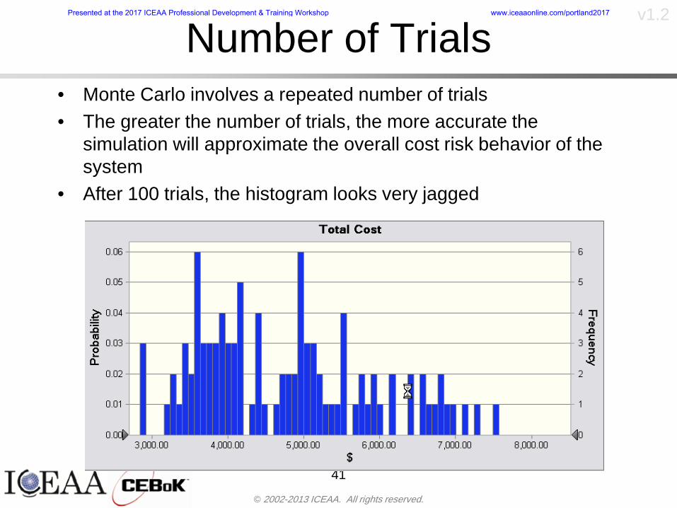
copy 2002-2013 ICEAA All rights reserved
v12
Number of Trialsbull Monte Carlo involves a repeated number of trialsbull The greater the number of trials the more accurate the
simulation will approximate the overall cost risk behavior of the system
bull After 100 trials the histogram looks very jagged
41
Presented at the 2017 ICEAA Professional Development amp Training Workshop wwwiceaaonlinecomportland2017
copy 2002-2013 ICEAA All rights reserved
v12
Number of Trials (2)
42
1000 Trials
10000 Trials
50000 Trials Additional trials give a more accurate depiction of the final result
Presented at the 2017 ICEAA Professional Development amp Training Workshop wwwiceaaonlinecomportland2017
copy 2002-2013 ICEAA All rights reserved
v12
Number of Trials (3)bull If we want to simulate the underlying
mean within 1 with 95 confidence for example then we require
43
divideoslash
oumlccedilegrave
aelig poundpound-
=
dividedividedivide
oslash
ouml
ccedilccedilccedil
egrave
aeligpound
-pound
-=
divideoslashouml
ccedilegraveaelig poundpound=
nZ
n
nnX
n
X
n
n
011
010Pr
011
010Pr
011990Pr950
___
___
sm
sm
sm
sm
sm
mm
Presented at the 2017 ICEAA Professional Development amp Training Workshop wwwiceaaonlinecomportland2017
copy 2002-2013 ICEAA All rights reserved
v12
Number of Trials (4)bull This means that the number of trials required is determined by
bull Solving for n we find that at least
trials are neededbull Note that this term involves the coefficient of variation of the
distribution which means that distributions with less dispersion require fewer trials to accurate simulate
44
96101
=ns
m
ms41638
Presented at the 2017 ICEAA Professional Development amp Training Workshop wwwiceaaonlinecomportland2017
copy 2002-2013 ICEAA All rights reserved
v12
Number of Trials (5)bull Simulating percentiles requires more trials than for simulating
meansbull Let Pn represent the number of trials in the sample at or below
the 70th percentile of the underlying distribution (suppose this is known)
bull By the Central Limit Theorem Pnn follows a normal distribution with mean equal to the 70th percentile and variance equal to
bull By a similar process for the mean we find that the number of trials needed to simulate the 70th percentile within 1 with 95 confidence is
45
( )n
FF 700700 1-
n
n
PPn -41638
Presented at the 2017 ICEAA Professional Development amp Training Workshop wwwiceaaonlinecomportland2017
copy 2002-2013 ICEAA All rights reserved
v12
Number of Trials (6)bull If Pn 070 for all n then n is approximately
bull For the sake of comparison suppose CV = 03 (reasonable approximation for hardware development) then the number of trials needed to simulate the mean with the same accuracy is then ldquoonlyrdquo 11525
bull More trials are needed to accurately simulate percentiles than means
46
( ) 46416703041638
70704168341638 =divide
oslashouml
ccedilegraveaelig=divide
oslashouml
ccedilegraveaelig -
=-
nnn
PPn
n
n
Presented at the 2017 ICEAA Professional Development amp Training Workshop wwwiceaaonlinecomportland2017
copy 2002-2013 ICEAA All rights reserved
v12
Methods of Simulationbull Monte Carlo simulation is a standard term for
simulationbull However there is an improvement on Monte Carlo
that improves the accuracy of the results of a simulation for a given number of trials
bull This method is call the Latin Hypercube approach to simulationndash Similar to Monte Carlo but an equal number of draws are taken
from a set of subintervals for example dividing the interval (01) into [00001) [0102)hellip [0910]
ndash Instead of 10 trials from [01] we have one trial from each subinterval
ndash Rough rule of thumb is Latin Hypercube takes 30 fewer trials to achieve similar accuracy to Monte Carlo
47
Presented at the 2017 ICEAA Professional Development amp Training Workshop wwwiceaaonlinecomportland2017
copy 2002-2013 ICEAA All rights reserved
v12
Probability Model ndash Correlationbull Correlation exists between work breakdown structure
(WBS) cost element costs and between cost and schedule
bull Correlation is a necessary consideration in cost risk analysis
bull Correlation is a number that can vary between -1 and +1 and represents the strength of the relationship between the two variablesndash If both variable have a tendency to move in the same direction
correlation is positivendash If when one variable increases the other tends to decrease and
vice-versa the correlation between the two variables is negative
Presented at the 2017 ICEAA Professional Development amp Training Workshop wwwiceaaonlinecomportland2017
copy 2002-2013 ICEAA All rights reserved
v12
Correlation And Causationbull Note that correlation is not causation however
causation implies correlationndash For example shark attacks and ice cream sales at the beach
bull For example for a launch vehicle structure increasing the diameter will not only result in an increase in the structures cost but will also result in higher costs for thermal coating (paint etc)
bull Also simply because two subsystems do not appear to be related does not mean they are not correlatedndash For example structures and computer equipment seemingly
have little relation to one another however an external factor such as a funding cut or a strike will impact all subsystems leading to delays and increasing cost across the board
ndash Thus everything in a WBS has some correlationUnit III - Module 9 49
Presented at the 2017 ICEAA Professional Development amp Training Workshop wwwiceaaonlinecomportland2017
copy 2002-2013 ICEAA All rights reserved
v12
The Importance of Correlationbull Percent that total cost standard deviation is underestimated
when correlation assumed to be 0 instead of r given nWBS elements
Unit III - Module 9 5050
0
20
40
60
80
100
0 01 02 03 04 05 06 07 08 09 1Actual Correlation
Perce
nt Un
deres
timate
d
n = 10
n = 30
n = 100n = 1000
0
20
40
60
80
100
0 01 02 03 04 05 06 07 08 09 1Actual Correlation
Perce
nt Un
deres
timate
d
n = 10
n = 30
n = 100n = 1000
Reference 32nd Annual DOD Cost Analysis Symposium Advanced Training Session ldquoWhy Correlation Matters in Cost Estimatingrdquo Stephen A Book
Presented at the 2017 ICEAA Professional Development amp Training Workshop wwwiceaaonlinecomportland2017
copy 2002-2013 ICEAA All rights reserved
v12
The Importance of Correlation (2)bull For example if correlation is assumed to be 0 for all
elements in a 30 element WBS and the actual correlation is 20 then the total cost standard deviation is underestimated by 60
bull For example assume the total cost is modeled as a normal distribution with mean = 100
bull If correlation is assumed to be zero with total cost standard deviation = 12 when correlation is actually 20 then the true underlying standard deviation is actually 30
bull 70th percentile with zero correlation assumption is 106
bull 70th percentile with 20 correlation is 116 Unit III - Module 9 51
Presented at the 2017 ICEAA Professional Development amp Training Workshop wwwiceaaonlinecomportland2017
copy 2002-2013 ICEAA All rights reserved
v12
Measures of Correlationbull Two measures of correlation are commonly used in
cost risk analysesndash Pearsonrsquos product-moment correlation coefficient ndash Spearmanrsquos rank correlation coefficient
bull Garvey and others recommend using Pearsonrsquos product-moment correlation coefficient correlation for cost risk analysesndash Method of moments uses this but there are two options in
simulationndash Popular simulation packages like Risk and Crystal Ball use
rank correlation but in practice this has been found to make little difference
ndash Pearson product-moment correlation has been incorporated into Risk+
52
Presented at the 2017 ICEAA Professional Development amp Training Workshop wwwiceaaonlinecomportland2017
copy 2002-2013 ICEAA All rights reserved
v12
Pearson Correlationbull Pearsonrsquos product-moment correlation measures
degree of linearity between two random variables bull If two random variables are perfectly linear (eg Y =
aX + b) with positive slope then the Pearson product-moment correlation between X and Y denoted by rXY is +1
53
X X
Y Y Y
XNegative Correlation Positive Correlation No Correlation
middotmiddot
middotmiddot
middotmiddot middotmiddot
middotmiddot
middot
middot
middotmiddotmiddot
middotmiddot
middotmiddot
middotmiddot middot
middot
middot
middotmiddotmiddotmiddotmiddotmiddotmiddotmiddot
middotmiddotmiddotmiddot
middotmiddot
middotmiddot middotmiddotmiddotmiddot
middotmiddotmiddot
middotmiddotmiddotmiddot
middotmiddotmiddot
middotmiddotmiddot
middotmiddot
middot
middot middotmiddot
middot middotmiddotmiddotmiddot middotmiddot middot middotmiddot middot middot
middotmiddot middot
middotmiddotmiddotmiddotmiddot middot middotmiddot
middotmiddot
middot
middotmiddot
middotmiddot middot
middot middot middot
middotmiddot middot
middotmiddotmiddot
middotmiddot
middot middot
Presented at the 2017 ICEAA Professional Development amp Training Workshop wwwiceaaonlinecomportland2017
copy 2002-2013 ICEAA All rights reserved
v12
Spearman Correlationbull Spearmanrsquos rank correlation measures the
monotonicity between two random variablesbull If two random variables are perfectly monotonically
increasing (eg Y = X2) then the Spearman rank correlation denoted by rXY is +1
bull The two measures can be significantly different
54
10 20 30 40 50 60
100
200
300
096 097 098 099 1
1
060
020
040
080
Eff
ort (
Staf
f-M
onth
s)
Software Size I KDSI
y = 28z12y
z x
yy = x100
0 pound x pound 1
Figure 5-9A Figure 5-9B
Pearson Correlation = 09976 Rank Correlation = 1
Pearson Correlation = 024 Rank Correlation = 1
X(x ) ~ Unif(01)
Reference Probability Methods for Cost Uncertainty Analysis A Systems Engineering Perspective Paul R Garvey
Presented at the 2017 ICEAA Professional Development amp Training Workshop wwwiceaaonlinecomportland2017
copy 2002-2013 ICEAA All rights reserved
v12
Unit III - Module 9 55
200
250
300
350
400
1000 1200 1400 1600 1800 2000
Recurring Production
SEPM
200
250
300
350
400
1000 1200 1400 1600 1800 2000
Recurring Production
SEPM
Functional Correlationbull Old No Functional
Correlation Simulation run with WBS items entered as values
bull New Simulation run with functional dependencies entered as they are in cost model
CorrelatedNot Correlated
Note shift of mean and increased variability
Presented at the 2017 ICEAA Professional Development amp Training Workshop wwwiceaaonlinecomportland2017
copy 2002-2013 ICEAA All rights reserved
v12
Risk Measuresbull ldquoWestern Europe conquered the word because of a
technological revolution that started because of attempts to measure the worldrdquo ndash Phillipe Jorion ndash In the same way attempts to measure risk will lead to better project
managementbull Risk management for DoD and NASA agencies focuses
primarily on funding projects to a single percentile ndash NASA policy explicitly mentions 70 and 50ndash This is known as ldquoValue at Riskrdquo and is prevalent in the banking and
financial industry
56
Presented at the 2017 ICEAA Professional Development amp Training Workshop wwwiceaaonlinecomportland2017
copy 2002-2013 ICEAA All rights reserved
v12
Value at Risk (VaR)bull VaR is a percentile of the cost risk
distributionndash VaR funding at the 70th percentile means that
there is a 30 chance of final project cost exceeding the funded amount (budget)
bull VaR has some meritsndash Common measure can be used to compare
different projects and programsndash Easily understood by senior managers and
decision makers
57
Presented at the 2017 ICEAA Professional Development amp Training Workshop wwwiceaaonlinecomportland2017
copy 2002-2013 ICEAA All rights reserved
v12
Why 70th or 80th Percentilebull Typical policy guidance involves funding at the 70th or 80th
percentile Why fund as such a low percentilebull There is some incentive to not over-fundbull For a normal distribution an inflection point occurs near the 80th
percentile meaning that for values above 80 confidence achieving higher levels of confidence can only be achieved by spending greater dollar amounts at an increasing rate
58
-05-04-03-02-01
00102030405
0 05 1 15 2 25 3
Standard Deviations from Mean
Normal Distribution
First DerivativeSlopeVelocity
Second DerivativeConvexityAcceleration
Inflection point at one standard deviation above the mean (~84th
percentile)
Presented at the 2017 ICEAA Professional Development amp Training Workshop wwwiceaaonlinecomportland2017
copy 2002-2013 ICEAA All rights reserved
v12
Funding Above Inflection Pointsbull As the percentile goes above the 80th percentile the amount
needed to achieve that higher level of confidence begins to increase at an increasing rate as is evident from the graph
59
0
10
20
30
40
50
60
70
50 55 60 65 70 75 80 85 90 95 100
$ Ab
ove
MEa
n to
Ach
ieve
Per
cent
ile
Percentile (Confidence Level)
Presented at the 2017 ICEAA Professional Development amp Training Workshop wwwiceaaonlinecomportland2017
copy 2002-2013 ICEAA All rights reserved
v12
Why Budget to the 70th or 80thbull Government projects are funded at the 70th or 80th percentilesbull Why not the 90th or 99th percentile Wonrsquot that help prevent
overrunsndash As we have seen percentiles do not add across programs
bull The sum of the 80th percentiles does NOT equal the total 80th percentile
ndash This is because the individual programs are riskier than the entire suite of missions
bull Known as the ldquoPortfolio effectrdquo (more or this later)
ndash Funding at the 80th gives confidence that the entire portfolio will be adequately funded
bull And since there is an inflection point near the 80th percentile funding above that level quickly becomes cost prohibitive
60
Presented at the 2017 ICEAA Professional Development amp Training Workshop wwwiceaaonlinecomportland2017
copy 2002-2013 ICEAA All rights reserved
v12
Inflection Points for Lognormalbull For a lognormal the inflection point
variesndash Coefficient of variation equal to 10 equates to an
inflection point at the 70th percentile
61
0
10
20
30
40
50
60
70
050 060 070 080 090 100
Coef
ficen
t of V
aria
tion
Percentile of the Inflection Point
Presented at the 2017 ICEAA Professional Development amp Training Workshop wwwiceaaonlinecomportland2017
copy 2002-2013 ICEAA All rights reserved
v12
Issues with Percentile Fundingbull However risk management does not stop at a
specific percentilendash What happens when the 70th percentile is exceeded
bull Any effective risk management policy should prescribe what happens after a bad event occursndash With VaR we only know when a bad event has occurred ndash Also funding at a relatively low level means we have no true
sense of the real risks that should be guarded against
62
Presented at the 2017 ICEAA Professional Development amp Training Workshop wwwiceaaonlinecomportland2017
copy 2002-2013 ICEAA All rights reserved
v12
ldquoHere There Be Dragonsrdquobull On old maps uncharted territory was often
marked with monsters or dragons
63
A section of the Carta Marina by Olaus Magnus 16th Century
Presented at the 2017 ICEAA Professional Development amp Training Workshop wwwiceaaonlinecomportland2017
copy 2002-2013 ICEAA All rights reserved
v12
Distribution Comparisonbull Four different distributions with the same 70th
percentile
bull Should we expect the tails to be similar
64
0
10
20
30
40
50
60
70
80
0 100 200 300 400 500 600
Perc
entil
eCo
nfid
ence
Lev
el
Triangular
Normal
Lognormal
Pareto
Presented at the 2017 ICEAA Professional Development amp Training Workshop wwwiceaaonlinecomportland2017
copy 2002-2013 ICEAA All rights reserved
v12Distribution Comparison Tail Behavior
bull The normal and triangular distributions have similar tails but the lognormal and Pareto have much fatter right tails
65
70
75
80
85
90
95
100
500 1500 2500 3500 4500 5500
Perc
entil
eCo
nfid
ence
Lev
el
Triangular
Normal
Lognormal
Pareto
Here There Be Dragons
Presented at the 2017 ICEAA Professional Development amp Training Workshop wwwiceaaonlinecomportland2017
copy 2002-2013 ICEAA All rights reserved
v12Distribution Comparison ndash Tail Behavior (Table)
bull There is significant tail risk for the lognormal and the Paretobull The 99th percentile for the Pareto is 1000 times greater than
the 70th percentilendash Risk seen in financial markets and in catastrophic risks like natural
disasters bull Four different projects follow the four different risk profiles seen
in this example should clearly have different risk management approaches but 70th percentile funding indicates the same risk management approach for all four
66
Percentile Triangular Normal Lognormal Pareto 70th $600 $600 $600 $600 80th $680 $660 $770 $1430 90th $770 $750 $1070 $5880 95th $840 $820 $1410 $23750 99th $930 $950 $2350 $600000
Presented at the 2017 ICEAA Professional Development amp Training Workshop wwwiceaaonlinecomportland2017
copy 2002-2013 ICEAA All rights reserved
v12Percentile Budgeting is Not Risk Management
bull Percentile budgeting ne effective risk management policybull Suppose that you are shopping for a new car You
mention that safety is your top concern The salesman says he has a great safe car available You ask about the air bags Do they work The salesman answers ldquoOf course Seventy percent of the time they work fine Only 30 of the time the air bags will fail to deployrdquo Would you buy such a car Hedge fund manager David Einhorn has stated ldquoRisk management is the air bag that must always work but only in the multi-sigma event where you have an accidentrdquo
67
Risk management is the air bag that must always work but only in the multi-sigma event where you
have an accident
Presented at the 2017 ICEAA Professional Development amp Training Workshop wwwiceaaonlinecomportland2017
copy 2002-2013 ICEAA All rights reserved
v12
Joint Confidence Level Analysisbull Schedules are risky toobull For 98 recent NASA missions average
schedule growth was 38ndash Not as high as cost growth but still significant
68
0
5
10
15
20
25
30
35
40
Schedule
Cost
Presented at the 2017 ICEAA Professional Development amp Training Workshop wwwiceaaonlinecomportland2017
copy 2002-2013 ICEAA All rights reserved
v12
Schedules Impact Costbull Changes in schedule can have enormous
impacts on cost ndash Schedule slips can lead to cost increases
bull Fixed programmatic costs must be paid on a regular basisndash Achieving schedule milestones early can result in cost
savings
bull Schedule is an important consideration in cost analysis including cost risk analysis
bull However we must be careful in correctly integrating cost and schedule riskndash Schedule is not simply an input but is dependent on many of
the same factors that drive cost
69
Presented at the 2017 ICEAA Professional Development amp Training Workshop wwwiceaaonlinecomportland2017
copy 2002-2013 ICEAA All rights reserved
v12
The Relationship of Cost to Schedulebull Cost and schedule are positively correlated
ndash A larger program with bigger scope with take longer to complete than a smaller simpler program
bull However longer schedules do not always equate to higher cost nor shorter schedules with lower costndash Highly compressed schedules relative to the
optimal schedule can lead to large overrunsbull Compressed schedules are commonplace for
many planetary missions
70
Presented at the 2017 ICEAA Professional Development amp Training Workshop wwwiceaaonlinecomportland2017
copy 2002-2013 ICEAA All rights reserved
v12The Impact of Schedule GrowthCompression on Cost
bull Compressed schedules lead to cost growth and based on existing research is actually more expensive than schedule slippages
71
0
20
40
60
80
100
120
140
160
-50 -25 0 25 50 75 100
Percentage Change in Schedule
Perc
enta
ge C
hang
e in
Cos
t due
to
Sche
dule
Cha
nge
Source Smart CB ldquoCost and Schedule Interrelationshipsrdquo 2007 NASA Cost Symposium
Presented at the 2017 ICEAA Professional Development amp Training Workshop wwwiceaaonlinecomportland2017
copy 2002-2013 ICEAA All rights reserved
v12Schedule as an Independent Variable
bull Why not simply add schedule as an input to cost-estimating relationships (CERs)
bull Schedule is often treated as an independent variable ndash schedules are often determined independently of cost considerationsndash Cost may not be considered explicitly although budgets and
schedules are determined based on scope and other common factors
bull In 2006 SAIC undertook a research task to determine the impact of schedule on cost and added schedule as an independent variable to the CERs in the NASAAir Force Cost Model (NAFCOM) to see if schedule provided any improvement in goodness of fit
72
Presented at the 2017 ICEAA Professional Development amp Training Workshop wwwiceaaonlinecomportland2017
copy 2002-2013 ICEAA All rights reserved
v12
Schedule is a Dependent Variablebull Since NAFCOM includes an exhaustive list of cost drivers the inclusion
of schedule should give an indication of whether there is any additional independent value added from schedule independent of the cost drivers
bull In the study schedule was added to 10 subsystem-level CERs
ndash In each case the addition of schedule did NOTimprove the goodness of fit and schedule was NOT found to be a statistically significant cost driver (given the presence of the other variables) for any of the 10 CERs
bull Standard errors for the CERs increased due to decrease in degrees of freedom
bull Thus schedule as an independent variable did not provide any additional explanation of variation in historical cost
bull This is because schedule is truly NOT an independent variable but a dependent variable and is a function of the same factors that drive cost
73
Presented at the 2017 ICEAA Professional Development amp Training Workshop wwwiceaaonlinecomportland2017
copy 2002-2013 ICEAA All rights reserved
v12
Incorporation of Schedule in Cost Risk
bull When using subjective methods care must be taken in applying schedule to cost risk analysis
bull Since schedule is a dependent variable treating it independently from other factors when assessing its impact on cost can lead to a double count of independent variables in the cost risk analysis
bull Direct inclusion of schedule in a cost risk analysis effectively doubles the influence of each cost driver
ndash Incorrectly leads to broader risk ranges
74
CostWeight
HeritageNewness
Technology Readiness Schedule
Presented at the 2017 ICEAA Professional Development amp Training Workshop wwwiceaaonlinecomportland2017
copy 2002-2013 ICEAA All rights reserved
v12Subjective Cost Risk Methods and Overinclusion of Risk Factors
bull Subjective methods are suitable when data are scarce or not availablebull However care must be taken not to treat correlated sources of risk
such as schedule as independent of each otherbull Example ndash a subjective risk analysis incorporated technology readiness
design risk requirements stability integration risk and schedule and treated each source of risk as independent
bull Risk triangle high value without schedule risk was 31 times the point estimate
bull Risk triangle high value with schedule risk added on top of other sources of risk treated independently was 34 times the point estimate
bull Risk triangle taking correlation between sources of risk into account in a rigorous statistical manner has a high value 15 times the point estimate less than half the effect when treating sources of risk as independent
75
Presented at the 2017 ICEAA Professional Development amp Training Workshop wwwiceaaonlinecomportland2017
copy 2002-2013 ICEAA All rights reserved
v12Fundamental Equation of Cost and Schedule Interrelationships
bull The Fundamental Equation of the Relationship Between Cost and Schedule is
Time = Moneybull This is a well known adage that time is money Your boss at
work may even mention this to you from time to time or if you are the boss you are all too aware of this iron law
bull Because time is money cost and schedule risk should be modeled jointly not with schedule as an independent cost driver
bull Note that cost and schedule are not perfectly correlatedndash Cost can sometimes ldquobuy downrdquo schedule extra money can be
spent to meet a deadline since in some cases additional effort to hasten the completion of a task
76
Presented at the 2017 ICEAA Professional Development amp Training Workshop wwwiceaaonlinecomportland2017
copy 2002-2013 ICEAA All rights reserved
v12How to (Correctly) Incorporate Schedule into Cost Risk Analysis
bull The best way to model cost and schedule risk is to develop a joint cost and schedule model based on the same data
bull Since such models are not currently available the next best approach is to model cost and schedule independently and then integrate cost and schedule risk analyses using joint probability distributions taking into account correlation between cost and schedulendash This approach pioneered by Paul Garvey and Steve Book is
considered industry best practicendash This is a practical method mathematically tractable and follows
naturally from the Fundamental Equation of Cost and Schedule Interrelationships
77
Book S A ldquoQuantifying the Relationship Between Cost and Schedulerdquo The Measurable News Winter 2007-2008 pp 11-15Garvey PR Probability Methods for Cost Uncertainty Analysis A Systems Engineering Perspective New York Marcel Dekker 2000 pp 308-335
Presented at the 2017 ICEAA Professional Development amp Training Workshop wwwiceaaonlinecomportland2017
copy 2002-2013 ICEAA All rights reserved
v12
Joint Lognormal and Normal Distributions
bull Cost and schedule are typically modeled as some combination of Normal and Lognormal probability distributionsndash Studies by The Aerospace Corporation the MITRE
Corporation Wyle Labs and SAIC have found that the Lognormal probability distribution almost always serves as a good model for both the schedule distribution and the cost distribution
ndash The Normal distribution may also be appropriate in some instances and depending upon the level of confidence at which budgets are set may even be more conservative and logically consistent than the Normal distribution
ndash Joint Lognormal and Normal distributions are defined by a pair of mean and standard deviations and a level of correlation between the two
78
Presented at the 2017 ICEAA Professional Development amp Training Workshop wwwiceaaonlinecomportland2017
copy 2002-2013 ICEAA All rights reserved
v12Modeling Cost and Schedule as a Bivariate Distribution
bull In the approach set forth by Book and Garvey cost risk is assessed and the top-level distribution is modeled as a Lognormal (or Normal) distribution schedule risk is assessed and the overall schedule risk is modeled as a Lognormal (or Normal) distribution
bull The two distributions are combined into a Bivariate distribution by assigning a correlation between the two and by treating the two distributions as the marginal distributions of a Bivariate Lognormal distributionndash Other combinations include a Bivariate Normal or a Bivariate
Normal-Lognormal
79
Presented at the 2017 ICEAA Professional Development amp Training Workshop wwwiceaaonlinecomportland2017
copy 2002-2013 ICEAA All rights reserved
v12Bivariate Lognormal Distribution for Cost and Schedule
bull Cost is often observed to be Lognormal when strong positive correlations are present among the systemrsquos WBS cost element costs
bull A systemrsquos schedule is often observed (from Monte Carlo simulations) to be Lognormal if it is the sum of many positively correlated schedule activities in an overall schedule network
bull If Lognormal distributions characterize a systemrsquos cost and schedule then the Bivariate Lognormal could serve as an assumed model of their joint distributionndash In this case the marginal distribution of each of cost and schedule is
Lognormalbull Other possibilities for modeling cost and schedule as a Bivariate
distribution include a Bivariate Normal or a Bivariate Normal-Lognormal distributionndash All these combinations are analytically tractable
80
Presented at the 2017 ICEAA Professional Development amp Training Workshop wwwiceaaonlinecomportland2017
copy 2002-2013 ICEAA All rights reserved
v12Bivariate Lognormal for Cost and Schedule
bull Contour Plots of a Bivariate Lognormal
81
Presented at the 2017 ICEAA Professional Development amp Training Workshop wwwiceaaonlinecomportland2017
copy 2002-2013 ICEAA All rights reserved
v12Correlation Between Cost and Schedule
bull Cost and schedule are positively correlated but not perfectly sondash For example it is possible to have a schedule underrun and a cost
overrunbull Based on cost and schedule growth data for 50 completed NASA
programs the correlation between development cost and development schedule is 70
82
00
200
400
600
800
1000
1200
-500 00 500 1000 1500 2000 2500Historical Cost Growth
Hist
oric
al S
ched
ule
Gro
wth
r = 715
Presented at the 2017 ICEAA Professional Development amp Training Workshop wwwiceaaonlinecomportland2017
copy 2002-2013 ICEAA All rights reserved
v12Correlation Between Cost and Schedule Caveats
bull Based on historical data recommended correlation between cost and schedule is 70 but this could be higher or lower depending upon program circumstancesndash If program is budget constrained cost and schedule will be
more highly correlated (go as you pay)ndash If program is schedule constrained cost and schedule will
have lower correlation perhaps even negative correlation ndash Smaller programs have smaller correlation between cost and
schedule riskbull Relatively easy to ldquohurry uprdquo and finish on time or even early if
needed
83
Presented at the 2017 ICEAA Professional Development amp Training Workshop wwwiceaaonlinecomportland2017
copy 2002-2013 ICEAA All rights reserved
v12
Conditional Confidence Levelsbull Given a programrsquos project schedule we can determine the cost
risk distribution conditional upon the given schedulebull Conditional cost S-curves are steeper than unconditional
(marginal) cost S-curves between some uncertainty has been removed because schedule is fixed
84
Presented at the 2017 ICEAA Professional Development amp Training Workshop wwwiceaaonlinecomportland2017
copy 2002-2013 ICEAA All rights reserved
v12
Joint Confidence Levelsbull Joint 65 confidence represents the probability of
achieving both 65 confidence in cost AND 65 confidence in schedulendash This is different than achieving 65 cost confidence alone
or achieving 65 schedule confidence alonebull Due to the imperfect correlation between cost and schedule it
is possible to achieve a 65 cost confidence with a lower level of schedule confidence
bull Restricting the schedule confidence thus requires additional $ to achieve a given level of confidence
85
X
Y
Possible Values for Which X gt a Possible Values for
Which X gt a and Y gt b
a
b
Presented at the 2017 ICEAA Professional Development amp Training Workshop wwwiceaaonlinecomportland2017
copy 2002-2013 ICEAA All rights reserved
v12Joint Confidence Levels Versus Cost Confidence Levels Only
bull Example of the differences between cost confidence schedule confidence conditional cost confidence and joint cost and schedule confidence
86
Joint Cost-Schedule Confidence Iso-Curves
Cost (RY$M)
Sche
dule
(Mon
ths)
65 Confidence
50 Confidence
70 Confidence
65 Cost Confidence AggressiveSchedule65 Cost ConfidenceScheduleGiven 65 Schedule ConfidenceUnconditional 65 CostConfidenceUnconditional 65 ScheduleConfidence
65 Cost Confidence 65 Joint Cost and Schedule
Confidence for 65 Schedule Confidence
Presented at the 2017 ICEAA Professional Development amp Training Workshop wwwiceaaonlinecomportland2017
copy 2002-2013 ICEAA All rights reserved
v12
Joint Cost and Schedule Confidence
bull Can examine pairs of cost and schedule that achieve a given level of confidence
bull Provides insights into the trade-offs between cost and schedule for a given level of confidencendash Possible to increase cost confidence by giving a
project more time in some instances or possible to ldquobuy downrdquo schedule
bull But these have limits and are shown in the iso-cost and schedule confidence curves
87
Presented at the 2017 ICEAA Professional Development amp Training Workshop wwwiceaaonlinecomportland2017
copy 2002-2013 ICEAA All rights reserved
v12Cost and Schedule Trade-offs for a Given Level of Joint Confidence
bull Hypothetical Example
88
Cost (RY$M)
Schedule (Months)
$100 48$99 48$89 49$87 50$85 51$85 52$84 53$83 55$83 55$83 56
Cost and Schedule 65 Confidence Iso-Curve
4748495051525354555657
$80 $82 $84 $86 $88 $90 $92 $94 $96 $98 $100
Cost (RY$ M)
Sche
dule
(Mon
ths)
Presented at the 2017 ICEAA Professional Development amp Training Workshop wwwiceaaonlinecomportland2017
copy 2002-2013 ICEAA All rights reserved
v12Policy Considerations for Confidence Levels
bull For large programs the difference between the amount of money needed to achieve 65 cost confidence independent of schedule and joint 65 cost and schedule confidence can represent hundreds of millions and even billions of dollars
89
Joint Cost-Schedule Confidence Iso-Curves
Cost (RY$M)
Sche
dule
(Mon
ths)
65 Confidence
65 Cost Confidence AggressiveSchedule
65 Cost ConfidenceScheduleGiven 65 Schedule Confidence
Unconditional 65 CostConfidence
Joint Cost and Schedule Confidence for 65 Cost Confidence and Program Baseline Schedule is Less Than 35
65 Cost Confidence Independent of Schedule Cost Needed to Achieve
Both 65 Joint Cost and Schedule Confidence for the Schedule with 65 Confidence
Presented at the 2017 ICEAA Professional Development amp Training Workshop wwwiceaaonlinecomportland2017
copy 2002-2013 ICEAA All rights reserved
v12
Copulasbull More generally any combination of distributions can
be used (more than just normal and lognormal)ndash Termed ldquocopulardquo from the Italian word for ldquocouplerdquondash Copulas are a way to combine marginal distributions of any
number and type into a joint distributionbull More formally a copula is a multivariate joint distribution defined
on the n-dimensional unit cube [0 1]n such that every marginal distribution is uniform on the interval [0 1]
bull (The bivariate form of) Sklarrsquos theorem states that for any bivariate distribution function H(x y) let F(x) = H(x infin) and G(y) = H(infin y) be the univariate marginal probability distribution functions Then there exists a copula C such that H(xy)=C(F(x)G(y))
ndash Copulas are widely used in risk management for investments and insurance
bull Considered industry best practice (Li 2000)bull Marketed as part of JP Morganrsquos CreditMetrics suite of tools
(Gupton et Al 1997)90
Presented at the 2017 ICEAA Professional Development amp Training Workshop wwwiceaaonlinecomportland2017
copy 2002-2013 ICEAA All rights reserved
v12Parametric Joint Cost and Schedule Analysis
bull A parametric model based on a consistent data set with a set of overlapping cost and schedule drivers is a cleaner way to model cost and schedule
91
CostWeight
HeritageNewness
Technology Readiness
Schedule
0
20
40
60
80
100
Confidence
Joint Cost and Schedule Confidence
Schedule
Cost
Lognormal Distribution PDF and CDF
0102030405060708090100
200 300 400 500 600 700 800 900 1000Cost $
Con
fiden
ce L
evel
0
00002
00004
00006
00008
0001
00012
00014
00016
Prob
abili
ty D
ensi
ty
CDFPDF
Lognormal Distribution PDF and CDF
0102030405060708090100
200 300 400 500 600 700 800 900 1000Cost $
Con
fiden
ce L
evel
0
00002
00004
00006
00008
0001
00012
00014
00016
Prob
abili
ty D
ensi
ty
CDFPDF
Presented at the 2017 ICEAA Professional Development amp Training Workshop wwwiceaaonlinecomportland2017
copy 2002-2013 ICEAA All rights reserved
v12Parametric Joint Cost and Schedule Analysis (2)
bull Joint cost and schedule risk analysis produced naturally by the integrated modelndash Addresses several issues with the copula
approachbull Tail dependencybull Correlation ndash no need to assign correlation
between cost and schedulebull Consistency of cost and schedule models
92
Presented at the 2017 ICEAA Professional Development amp Training Workshop wwwiceaaonlinecomportland2017
copy 2002-2013 ICEAA All rights reserved
v12
Resource-Loaded Schedulesbull Involves assigning cost and schedule risks to a resource-loaded schedule
networkbull Bottom-up approach
ndash More labor intensive than parametrics but can also provide more insight
ndash Can answer questions than parametric typically cannot such as how much do reserve requirements decrease if a specific risk is retired
bull Currently being implemented in Constellation programbull Has same issue as all bottom-up models hard to count all the risks and model
them discretely
ndash As a result there is a tendency to reflect less risk than indicated by history
ndash ldquoThere are more things in heaven and earth Horatio than are dreamt of in your philosophyrdquo William Shakespeare Hamlet Act I Scene V
93
Presented at the 2017 ICEAA Professional Development amp Training Workshop wwwiceaaonlinecomportland2017
copy 2002-2013 ICEAA All rights reserved
v12Resource-Loaded Schedules Vs Parametrics
bull Parametric most appropriate for early estimatesndash But also good for high-level checks as project progresses
bull As plans take shape lower level modeling may be more appropriate
94 1
CONCEPTUALDEVELOPMENT
PROJECTDEFINITION DESIGN DEVELOPMENT OPERATIONS
PARAMETRIC PARAMETRIC
ANALOGY
ENGINEERING (Bottoms Up)
$PARAMETRIC
DETAILED
$
Pre Phase A Phase B Phase CDPhase A Phase EPre Phase A Phase B Phase CDPhase A Phase E
Risk = f(Cost Estimating Relationship Inputs eg mass power data rate TRL new design etc)
Risk = f(cost and schedule variation of the analogous elements)
Risk = f(variation of detailed inputs eg labor hours rates materials etc)
Presented at the 2017 ICEAA Professional Development amp Training Workshop wwwiceaaonlinecomportland2017
copy 2002-2013 ICEAA All rights reserved
v12
Resource-Loaded Schedulesbull Methodology has been demonstrated in other
industriesndash Construction oil and gasndash Analysis has not been traditionally done on highly uncertain
complex development projects bull Methodology focuses on project baseline schedule
ndash In baseline schedule all tasks are resource loaded to represent a baseline schedule and cost standpoint
ndash Resource loaded schedule is ldquorolledrdquo up to a manageable level
ndash Based on the risk and uncertainties identified schedule distributions are applied to each rolled up task
ndash Cost uncertainties are also applied to rolled up tasksbull Uncertainties include labor rate man power etc
ndash A Monte Carlo simulation is run to develop joint cost-schedule distributions
95
Presented at the 2017 ICEAA Professional Development amp Training Workshop wwwiceaaonlinecomportland2017
copy 2002-2013 ICEAA All rights reserved
v12
Unit III - Module 9 96
Execution ndash Cross Checksbull Means The mean cost growth factor for WBS items
can be compared to history as a way to cross check results
bull CVs The CV of the cost growth factors for WBS items can be compared to history as a way to cross check results
bull Inputs Checks are performed on inputs or other parameters to see if historical values are in line with program assumptionsndash Example Historical risk scores can be compared to program
risk scores to see if risk assessors are being realistic and to see if the underlying database is representative of the program
11
Presented at the 2017 ICEAA Professional Development amp Training Workshop wwwiceaaonlinecomportland2017
- Cost and Schedule Risk Analysis Basic
- Acknowledgments
- Unit Index
- Risk Overview
- Agenda
- Introduction
- Risk Analysis Terms
- Are Our Costs Realistic
- Historical Cost Growth
- Sources of Cost Risk
- Point Estimates of Cost
- Types of Risk
- Point Estimates Vs Risk Estimates
- Cost Risk and Probability
- Probability Model ndash Distribution
- Probability Model ndash Distribution
- Probability ndash Top-Level Distribution
- S-Curves and Confidence Levels
- Example ndash Normal Distribution
- Confidence Levels
- Measuring Parametric Model Uncertainty
- Parametric Model Example
- Weight Uncertainty
- Estimating Uncertainty
- Estimating Uncertainty (2)
- Estimating Uncertainty (3)
- Aggregating Risk
- WBS Example
- WBS and Risk
- Aggregating Risk
- Percentiles Do Not Add
- Percentiles Do Not Add (2)
- Percentiles Do Not Add (3)
- Methods for Aggregating Risk
- Monte Carlo Simulationfor Risk Analysis
- Monte Carlo Simulation
- Using Random Numbers to Simulate Distributions
- Simulating a Triangular Distribution
- Simulating a Triangular Distribution (2)
- Monte Carlo and the WBS
- Number of Trials
- Number of Trials (2)
- Number of Trials (3)
- Number of Trials (4)
- Number of Trials (5)
- Number of Trials (6)
- Methods of Simulation
- Probability Model ndash Correlation
- Correlation And Causation
- The Importance of Correlation
- The Importance of Correlation (2)
- Measures of Correlation
- Pearson Correlation
- Spearman Correlation
- Functional Correlation
- Risk Measures
- Value at Risk (VaR)
- Why 70th or 80th Percentile
- Funding Above Inflection Points
- Why Budget to the 70th or 80th
- Inflection Points for Lognormal
- Issues with Percentile Funding
- ldquoHere There Be Dragonsrdquo
- Distribution Comparison
- Distribution Comparison Tail Behavior
- Distribution Comparison ndash Tail Behavior (Table)
- Percentile Budgeting is Not Risk Management
- Joint Confidence Level Analysis
- Schedules Impact Cost
- The Relationship of Cost to Schedule
- The Impact of Schedule GrowthCompression on Cost
- Schedule as an Independent Variable
- Schedule is a Dependent Variable
- Incorporation of Schedule in Cost Risk
- Subjective Cost Risk Methods and Overinclusion of Risk Factors
- Fundamental Equation of Cost and Schedule Interrelationships
- How to (Correctly) Incorporate Schedule into Cost Risk Analysis
- Joint Lognormal and Normal Distributions
- Modeling Cost and Schedule as a Bivariate Distribution
- Bivariate Lognormal Distribution for Cost and Schedule
- Bivariate Lognormal for Cost and Schedule
- Correlation Between Cost and Schedule
- Correlation Between Cost and Schedule Caveats
- Conditional Confidence Levels
- Joint Confidence Levels
- Joint Confidence Levels Versus Cost Confidence Levels Only
- Joint Cost and Schedule Confidence
- Cost and Schedule Trade-offs for a Given Level of Joint Confidence
- Policy Considerations for Confidence Levels
- Copulas
- Parametric Joint Cost and Schedule Analysis
- Parametric Joint Cost and Schedule Analysis (2)
- Resource-Loaded Schedules
- Resource-Loaded Schedules Vs Parametrics
- Resource-Loaded Schedules
- Execution ndash Cross Checks
-
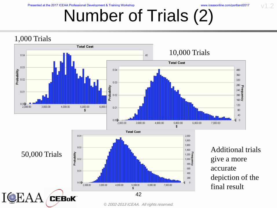
copy 2002-2013 ICEAA All rights reserved
v12
Number of Trials (2)
42
1000 Trials
10000 Trials
50000 Trials Additional trials give a more accurate depiction of the final result
Presented at the 2017 ICEAA Professional Development amp Training Workshop wwwiceaaonlinecomportland2017
copy 2002-2013 ICEAA All rights reserved
v12
Number of Trials (3)bull If we want to simulate the underlying
mean within 1 with 95 confidence for example then we require
43
divideoslash
oumlccedilegrave
aelig poundpound-
=
dividedividedivide
oslash
ouml
ccedilccedilccedil
egrave
aeligpound
-pound
-=
divideoslashouml
ccedilegraveaelig poundpound=
nZ
n
nnX
n
X
n
n
011
010Pr
011
010Pr
011990Pr950
___
___
sm
sm
sm
sm
sm
mm
Presented at the 2017 ICEAA Professional Development amp Training Workshop wwwiceaaonlinecomportland2017
copy 2002-2013 ICEAA All rights reserved
v12
Number of Trials (4)bull This means that the number of trials required is determined by
bull Solving for n we find that at least
trials are neededbull Note that this term involves the coefficient of variation of the
distribution which means that distributions with less dispersion require fewer trials to accurate simulate
44
96101
=ns
m
ms41638
Presented at the 2017 ICEAA Professional Development amp Training Workshop wwwiceaaonlinecomportland2017
copy 2002-2013 ICEAA All rights reserved
v12
Number of Trials (5)bull Simulating percentiles requires more trials than for simulating
meansbull Let Pn represent the number of trials in the sample at or below
the 70th percentile of the underlying distribution (suppose this is known)
bull By the Central Limit Theorem Pnn follows a normal distribution with mean equal to the 70th percentile and variance equal to
bull By a similar process for the mean we find that the number of trials needed to simulate the 70th percentile within 1 with 95 confidence is
45
( )n
FF 700700 1-
n
n
PPn -41638
Presented at the 2017 ICEAA Professional Development amp Training Workshop wwwiceaaonlinecomportland2017
copy 2002-2013 ICEAA All rights reserved
v12
Number of Trials (6)bull If Pn 070 for all n then n is approximately
bull For the sake of comparison suppose CV = 03 (reasonable approximation for hardware development) then the number of trials needed to simulate the mean with the same accuracy is then ldquoonlyrdquo 11525
bull More trials are needed to accurately simulate percentiles than means
46
( ) 46416703041638
70704168341638 =divide
oslashouml
ccedilegraveaelig=divide
oslashouml
ccedilegraveaelig -
=-
nnn
PPn
n
n
Presented at the 2017 ICEAA Professional Development amp Training Workshop wwwiceaaonlinecomportland2017
copy 2002-2013 ICEAA All rights reserved
v12
Methods of Simulationbull Monte Carlo simulation is a standard term for
simulationbull However there is an improvement on Monte Carlo
that improves the accuracy of the results of a simulation for a given number of trials
bull This method is call the Latin Hypercube approach to simulationndash Similar to Monte Carlo but an equal number of draws are taken
from a set of subintervals for example dividing the interval (01) into [00001) [0102)hellip [0910]
ndash Instead of 10 trials from [01] we have one trial from each subinterval
ndash Rough rule of thumb is Latin Hypercube takes 30 fewer trials to achieve similar accuracy to Monte Carlo
47
Presented at the 2017 ICEAA Professional Development amp Training Workshop wwwiceaaonlinecomportland2017
copy 2002-2013 ICEAA All rights reserved
v12
Probability Model ndash Correlationbull Correlation exists between work breakdown structure
(WBS) cost element costs and between cost and schedule
bull Correlation is a necessary consideration in cost risk analysis
bull Correlation is a number that can vary between -1 and +1 and represents the strength of the relationship between the two variablesndash If both variable have a tendency to move in the same direction
correlation is positivendash If when one variable increases the other tends to decrease and
vice-versa the correlation between the two variables is negative
Presented at the 2017 ICEAA Professional Development amp Training Workshop wwwiceaaonlinecomportland2017
copy 2002-2013 ICEAA All rights reserved
v12
Correlation And Causationbull Note that correlation is not causation however
causation implies correlationndash For example shark attacks and ice cream sales at the beach
bull For example for a launch vehicle structure increasing the diameter will not only result in an increase in the structures cost but will also result in higher costs for thermal coating (paint etc)
bull Also simply because two subsystems do not appear to be related does not mean they are not correlatedndash For example structures and computer equipment seemingly
have little relation to one another however an external factor such as a funding cut or a strike will impact all subsystems leading to delays and increasing cost across the board
ndash Thus everything in a WBS has some correlationUnit III - Module 9 49
Presented at the 2017 ICEAA Professional Development amp Training Workshop wwwiceaaonlinecomportland2017
copy 2002-2013 ICEAA All rights reserved
v12
The Importance of Correlationbull Percent that total cost standard deviation is underestimated
when correlation assumed to be 0 instead of r given nWBS elements
Unit III - Module 9 5050
0
20
40
60
80
100
0 01 02 03 04 05 06 07 08 09 1Actual Correlation
Perce
nt Un
deres
timate
d
n = 10
n = 30
n = 100n = 1000
0
20
40
60
80
100
0 01 02 03 04 05 06 07 08 09 1Actual Correlation
Perce
nt Un
deres
timate
d
n = 10
n = 30
n = 100n = 1000
Reference 32nd Annual DOD Cost Analysis Symposium Advanced Training Session ldquoWhy Correlation Matters in Cost Estimatingrdquo Stephen A Book
Presented at the 2017 ICEAA Professional Development amp Training Workshop wwwiceaaonlinecomportland2017
copy 2002-2013 ICEAA All rights reserved
v12
The Importance of Correlation (2)bull For example if correlation is assumed to be 0 for all
elements in a 30 element WBS and the actual correlation is 20 then the total cost standard deviation is underestimated by 60
bull For example assume the total cost is modeled as a normal distribution with mean = 100
bull If correlation is assumed to be zero with total cost standard deviation = 12 when correlation is actually 20 then the true underlying standard deviation is actually 30
bull 70th percentile with zero correlation assumption is 106
bull 70th percentile with 20 correlation is 116 Unit III - Module 9 51
Presented at the 2017 ICEAA Professional Development amp Training Workshop wwwiceaaonlinecomportland2017
copy 2002-2013 ICEAA All rights reserved
v12
Measures of Correlationbull Two measures of correlation are commonly used in
cost risk analysesndash Pearsonrsquos product-moment correlation coefficient ndash Spearmanrsquos rank correlation coefficient
bull Garvey and others recommend using Pearsonrsquos product-moment correlation coefficient correlation for cost risk analysesndash Method of moments uses this but there are two options in
simulationndash Popular simulation packages like Risk and Crystal Ball use
rank correlation but in practice this has been found to make little difference
ndash Pearson product-moment correlation has been incorporated into Risk+
52
Presented at the 2017 ICEAA Professional Development amp Training Workshop wwwiceaaonlinecomportland2017
copy 2002-2013 ICEAA All rights reserved
v12
Pearson Correlationbull Pearsonrsquos product-moment correlation measures
degree of linearity between two random variables bull If two random variables are perfectly linear (eg Y =
aX + b) with positive slope then the Pearson product-moment correlation between X and Y denoted by rXY is +1
53
X X
Y Y Y
XNegative Correlation Positive Correlation No Correlation
middotmiddot
middotmiddot
middotmiddot middotmiddot
middotmiddot
middot
middot
middotmiddotmiddot
middotmiddot
middotmiddot
middotmiddot middot
middot
middot
middotmiddotmiddotmiddotmiddotmiddotmiddotmiddot
middotmiddotmiddotmiddot
middotmiddot
middotmiddot middotmiddotmiddotmiddot
middotmiddotmiddot
middotmiddotmiddotmiddot
middotmiddotmiddot
middotmiddotmiddot
middotmiddot
middot
middot middotmiddot
middot middotmiddotmiddotmiddot middotmiddot middot middotmiddot middot middot
middotmiddot middot
middotmiddotmiddotmiddotmiddot middot middotmiddot
middotmiddot
middot
middotmiddot
middotmiddot middot
middot middot middot
middotmiddot middot
middotmiddotmiddot
middotmiddot
middot middot
Presented at the 2017 ICEAA Professional Development amp Training Workshop wwwiceaaonlinecomportland2017
copy 2002-2013 ICEAA All rights reserved
v12
Spearman Correlationbull Spearmanrsquos rank correlation measures the
monotonicity between two random variablesbull If two random variables are perfectly monotonically
increasing (eg Y = X2) then the Spearman rank correlation denoted by rXY is +1
bull The two measures can be significantly different
54
10 20 30 40 50 60
100
200
300
096 097 098 099 1
1
060
020
040
080
Eff
ort (
Staf
f-M
onth
s)
Software Size I KDSI
y = 28z12y
z x
yy = x100
0 pound x pound 1
Figure 5-9A Figure 5-9B
Pearson Correlation = 09976 Rank Correlation = 1
Pearson Correlation = 024 Rank Correlation = 1
X(x ) ~ Unif(01)
Reference Probability Methods for Cost Uncertainty Analysis A Systems Engineering Perspective Paul R Garvey
Presented at the 2017 ICEAA Professional Development amp Training Workshop wwwiceaaonlinecomportland2017
copy 2002-2013 ICEAA All rights reserved
v12
Unit III - Module 9 55
200
250
300
350
400
1000 1200 1400 1600 1800 2000
Recurring Production
SEPM
200
250
300
350
400
1000 1200 1400 1600 1800 2000
Recurring Production
SEPM
Functional Correlationbull Old No Functional
Correlation Simulation run with WBS items entered as values
bull New Simulation run with functional dependencies entered as they are in cost model
CorrelatedNot Correlated
Note shift of mean and increased variability
Presented at the 2017 ICEAA Professional Development amp Training Workshop wwwiceaaonlinecomportland2017
copy 2002-2013 ICEAA All rights reserved
v12
Risk Measuresbull ldquoWestern Europe conquered the word because of a
technological revolution that started because of attempts to measure the worldrdquo ndash Phillipe Jorion ndash In the same way attempts to measure risk will lead to better project
managementbull Risk management for DoD and NASA agencies focuses
primarily on funding projects to a single percentile ndash NASA policy explicitly mentions 70 and 50ndash This is known as ldquoValue at Riskrdquo and is prevalent in the banking and
financial industry
56
Presented at the 2017 ICEAA Professional Development amp Training Workshop wwwiceaaonlinecomportland2017
copy 2002-2013 ICEAA All rights reserved
v12
Value at Risk (VaR)bull VaR is a percentile of the cost risk
distributionndash VaR funding at the 70th percentile means that
there is a 30 chance of final project cost exceeding the funded amount (budget)
bull VaR has some meritsndash Common measure can be used to compare
different projects and programsndash Easily understood by senior managers and
decision makers
57
Presented at the 2017 ICEAA Professional Development amp Training Workshop wwwiceaaonlinecomportland2017
copy 2002-2013 ICEAA All rights reserved
v12
Why 70th or 80th Percentilebull Typical policy guidance involves funding at the 70th or 80th
percentile Why fund as such a low percentilebull There is some incentive to not over-fundbull For a normal distribution an inflection point occurs near the 80th
percentile meaning that for values above 80 confidence achieving higher levels of confidence can only be achieved by spending greater dollar amounts at an increasing rate
58
-05-04-03-02-01
00102030405
0 05 1 15 2 25 3
Standard Deviations from Mean
Normal Distribution
First DerivativeSlopeVelocity
Second DerivativeConvexityAcceleration
Inflection point at one standard deviation above the mean (~84th
percentile)
Presented at the 2017 ICEAA Professional Development amp Training Workshop wwwiceaaonlinecomportland2017
copy 2002-2013 ICEAA All rights reserved
v12
Funding Above Inflection Pointsbull As the percentile goes above the 80th percentile the amount
needed to achieve that higher level of confidence begins to increase at an increasing rate as is evident from the graph
59
0
10
20
30
40
50
60
70
50 55 60 65 70 75 80 85 90 95 100
$ Ab
ove
MEa
n to
Ach
ieve
Per
cent
ile
Percentile (Confidence Level)
Presented at the 2017 ICEAA Professional Development amp Training Workshop wwwiceaaonlinecomportland2017
copy 2002-2013 ICEAA All rights reserved
v12
Why Budget to the 70th or 80thbull Government projects are funded at the 70th or 80th percentilesbull Why not the 90th or 99th percentile Wonrsquot that help prevent
overrunsndash As we have seen percentiles do not add across programs
bull The sum of the 80th percentiles does NOT equal the total 80th percentile
ndash This is because the individual programs are riskier than the entire suite of missions
bull Known as the ldquoPortfolio effectrdquo (more or this later)
ndash Funding at the 80th gives confidence that the entire portfolio will be adequately funded
bull And since there is an inflection point near the 80th percentile funding above that level quickly becomes cost prohibitive
60
Presented at the 2017 ICEAA Professional Development amp Training Workshop wwwiceaaonlinecomportland2017
copy 2002-2013 ICEAA All rights reserved
v12
Inflection Points for Lognormalbull For a lognormal the inflection point
variesndash Coefficient of variation equal to 10 equates to an
inflection point at the 70th percentile
61
0
10
20
30
40
50
60
70
050 060 070 080 090 100
Coef
ficen
t of V
aria
tion
Percentile of the Inflection Point
Presented at the 2017 ICEAA Professional Development amp Training Workshop wwwiceaaonlinecomportland2017
copy 2002-2013 ICEAA All rights reserved
v12
Issues with Percentile Fundingbull However risk management does not stop at a
specific percentilendash What happens when the 70th percentile is exceeded
bull Any effective risk management policy should prescribe what happens after a bad event occursndash With VaR we only know when a bad event has occurred ndash Also funding at a relatively low level means we have no true
sense of the real risks that should be guarded against
62
Presented at the 2017 ICEAA Professional Development amp Training Workshop wwwiceaaonlinecomportland2017
copy 2002-2013 ICEAA All rights reserved
v12
ldquoHere There Be Dragonsrdquobull On old maps uncharted territory was often
marked with monsters or dragons
63
A section of the Carta Marina by Olaus Magnus 16th Century
Presented at the 2017 ICEAA Professional Development amp Training Workshop wwwiceaaonlinecomportland2017
copy 2002-2013 ICEAA All rights reserved
v12
Distribution Comparisonbull Four different distributions with the same 70th
percentile
bull Should we expect the tails to be similar
64
0
10
20
30
40
50
60
70
80
0 100 200 300 400 500 600
Perc
entil
eCo
nfid
ence
Lev
el
Triangular
Normal
Lognormal
Pareto
Presented at the 2017 ICEAA Professional Development amp Training Workshop wwwiceaaonlinecomportland2017
copy 2002-2013 ICEAA All rights reserved
v12Distribution Comparison Tail Behavior
bull The normal and triangular distributions have similar tails but the lognormal and Pareto have much fatter right tails
65
70
75
80
85
90
95
100
500 1500 2500 3500 4500 5500
Perc
entil
eCo
nfid
ence
Lev
el
Triangular
Normal
Lognormal
Pareto
Here There Be Dragons
Presented at the 2017 ICEAA Professional Development amp Training Workshop wwwiceaaonlinecomportland2017
copy 2002-2013 ICEAA All rights reserved
v12Distribution Comparison ndash Tail Behavior (Table)
bull There is significant tail risk for the lognormal and the Paretobull The 99th percentile for the Pareto is 1000 times greater than
the 70th percentilendash Risk seen in financial markets and in catastrophic risks like natural
disasters bull Four different projects follow the four different risk profiles seen
in this example should clearly have different risk management approaches but 70th percentile funding indicates the same risk management approach for all four
66
Percentile Triangular Normal Lognormal Pareto 70th $600 $600 $600 $600 80th $680 $660 $770 $1430 90th $770 $750 $1070 $5880 95th $840 $820 $1410 $23750 99th $930 $950 $2350 $600000
Presented at the 2017 ICEAA Professional Development amp Training Workshop wwwiceaaonlinecomportland2017
copy 2002-2013 ICEAA All rights reserved
v12Percentile Budgeting is Not Risk Management
bull Percentile budgeting ne effective risk management policybull Suppose that you are shopping for a new car You
mention that safety is your top concern The salesman says he has a great safe car available You ask about the air bags Do they work The salesman answers ldquoOf course Seventy percent of the time they work fine Only 30 of the time the air bags will fail to deployrdquo Would you buy such a car Hedge fund manager David Einhorn has stated ldquoRisk management is the air bag that must always work but only in the multi-sigma event where you have an accidentrdquo
67
Risk management is the air bag that must always work but only in the multi-sigma event where you
have an accident
Presented at the 2017 ICEAA Professional Development amp Training Workshop wwwiceaaonlinecomportland2017
copy 2002-2013 ICEAA All rights reserved
v12
Joint Confidence Level Analysisbull Schedules are risky toobull For 98 recent NASA missions average
schedule growth was 38ndash Not as high as cost growth but still significant
68
0
5
10
15
20
25
30
35
40
Schedule
Cost
Presented at the 2017 ICEAA Professional Development amp Training Workshop wwwiceaaonlinecomportland2017
copy 2002-2013 ICEAA All rights reserved
v12
Schedules Impact Costbull Changes in schedule can have enormous
impacts on cost ndash Schedule slips can lead to cost increases
bull Fixed programmatic costs must be paid on a regular basisndash Achieving schedule milestones early can result in cost
savings
bull Schedule is an important consideration in cost analysis including cost risk analysis
bull However we must be careful in correctly integrating cost and schedule riskndash Schedule is not simply an input but is dependent on many of
the same factors that drive cost
69
Presented at the 2017 ICEAA Professional Development amp Training Workshop wwwiceaaonlinecomportland2017
copy 2002-2013 ICEAA All rights reserved
v12
The Relationship of Cost to Schedulebull Cost and schedule are positively correlated
ndash A larger program with bigger scope with take longer to complete than a smaller simpler program
bull However longer schedules do not always equate to higher cost nor shorter schedules with lower costndash Highly compressed schedules relative to the
optimal schedule can lead to large overrunsbull Compressed schedules are commonplace for
many planetary missions
70
Presented at the 2017 ICEAA Professional Development amp Training Workshop wwwiceaaonlinecomportland2017
copy 2002-2013 ICEAA All rights reserved
v12The Impact of Schedule GrowthCompression on Cost
bull Compressed schedules lead to cost growth and based on existing research is actually more expensive than schedule slippages
71
0
20
40
60
80
100
120
140
160
-50 -25 0 25 50 75 100
Percentage Change in Schedule
Perc
enta
ge C
hang
e in
Cos
t due
to
Sche
dule
Cha
nge
Source Smart CB ldquoCost and Schedule Interrelationshipsrdquo 2007 NASA Cost Symposium
Presented at the 2017 ICEAA Professional Development amp Training Workshop wwwiceaaonlinecomportland2017
copy 2002-2013 ICEAA All rights reserved
v12Schedule as an Independent Variable
bull Why not simply add schedule as an input to cost-estimating relationships (CERs)
bull Schedule is often treated as an independent variable ndash schedules are often determined independently of cost considerationsndash Cost may not be considered explicitly although budgets and
schedules are determined based on scope and other common factors
bull In 2006 SAIC undertook a research task to determine the impact of schedule on cost and added schedule as an independent variable to the CERs in the NASAAir Force Cost Model (NAFCOM) to see if schedule provided any improvement in goodness of fit
72
Presented at the 2017 ICEAA Professional Development amp Training Workshop wwwiceaaonlinecomportland2017
copy 2002-2013 ICEAA All rights reserved
v12
Schedule is a Dependent Variablebull Since NAFCOM includes an exhaustive list of cost drivers the inclusion
of schedule should give an indication of whether there is any additional independent value added from schedule independent of the cost drivers
bull In the study schedule was added to 10 subsystem-level CERs
ndash In each case the addition of schedule did NOTimprove the goodness of fit and schedule was NOT found to be a statistically significant cost driver (given the presence of the other variables) for any of the 10 CERs
bull Standard errors for the CERs increased due to decrease in degrees of freedom
bull Thus schedule as an independent variable did not provide any additional explanation of variation in historical cost
bull This is because schedule is truly NOT an independent variable but a dependent variable and is a function of the same factors that drive cost
73
Presented at the 2017 ICEAA Professional Development amp Training Workshop wwwiceaaonlinecomportland2017
copy 2002-2013 ICEAA All rights reserved
v12
Incorporation of Schedule in Cost Risk
bull When using subjective methods care must be taken in applying schedule to cost risk analysis
bull Since schedule is a dependent variable treating it independently from other factors when assessing its impact on cost can lead to a double count of independent variables in the cost risk analysis
bull Direct inclusion of schedule in a cost risk analysis effectively doubles the influence of each cost driver
ndash Incorrectly leads to broader risk ranges
74
CostWeight
HeritageNewness
Technology Readiness Schedule
Presented at the 2017 ICEAA Professional Development amp Training Workshop wwwiceaaonlinecomportland2017
copy 2002-2013 ICEAA All rights reserved
v12Subjective Cost Risk Methods and Overinclusion of Risk Factors
bull Subjective methods are suitable when data are scarce or not availablebull However care must be taken not to treat correlated sources of risk
such as schedule as independent of each otherbull Example ndash a subjective risk analysis incorporated technology readiness
design risk requirements stability integration risk and schedule and treated each source of risk as independent
bull Risk triangle high value without schedule risk was 31 times the point estimate
bull Risk triangle high value with schedule risk added on top of other sources of risk treated independently was 34 times the point estimate
bull Risk triangle taking correlation between sources of risk into account in a rigorous statistical manner has a high value 15 times the point estimate less than half the effect when treating sources of risk as independent
75
Presented at the 2017 ICEAA Professional Development amp Training Workshop wwwiceaaonlinecomportland2017
copy 2002-2013 ICEAA All rights reserved
v12Fundamental Equation of Cost and Schedule Interrelationships
bull The Fundamental Equation of the Relationship Between Cost and Schedule is
Time = Moneybull This is a well known adage that time is money Your boss at
work may even mention this to you from time to time or if you are the boss you are all too aware of this iron law
bull Because time is money cost and schedule risk should be modeled jointly not with schedule as an independent cost driver
bull Note that cost and schedule are not perfectly correlatedndash Cost can sometimes ldquobuy downrdquo schedule extra money can be
spent to meet a deadline since in some cases additional effort to hasten the completion of a task
76
Presented at the 2017 ICEAA Professional Development amp Training Workshop wwwiceaaonlinecomportland2017
copy 2002-2013 ICEAA All rights reserved
v12How to (Correctly) Incorporate Schedule into Cost Risk Analysis
bull The best way to model cost and schedule risk is to develop a joint cost and schedule model based on the same data
bull Since such models are not currently available the next best approach is to model cost and schedule independently and then integrate cost and schedule risk analyses using joint probability distributions taking into account correlation between cost and schedulendash This approach pioneered by Paul Garvey and Steve Book is
considered industry best practicendash This is a practical method mathematically tractable and follows
naturally from the Fundamental Equation of Cost and Schedule Interrelationships
77
Book S A ldquoQuantifying the Relationship Between Cost and Schedulerdquo The Measurable News Winter 2007-2008 pp 11-15Garvey PR Probability Methods for Cost Uncertainty Analysis A Systems Engineering Perspective New York Marcel Dekker 2000 pp 308-335
Presented at the 2017 ICEAA Professional Development amp Training Workshop wwwiceaaonlinecomportland2017
copy 2002-2013 ICEAA All rights reserved
v12
Joint Lognormal and Normal Distributions
bull Cost and schedule are typically modeled as some combination of Normal and Lognormal probability distributionsndash Studies by The Aerospace Corporation the MITRE
Corporation Wyle Labs and SAIC have found that the Lognormal probability distribution almost always serves as a good model for both the schedule distribution and the cost distribution
ndash The Normal distribution may also be appropriate in some instances and depending upon the level of confidence at which budgets are set may even be more conservative and logically consistent than the Normal distribution
ndash Joint Lognormal and Normal distributions are defined by a pair of mean and standard deviations and a level of correlation between the two
78
Presented at the 2017 ICEAA Professional Development amp Training Workshop wwwiceaaonlinecomportland2017
copy 2002-2013 ICEAA All rights reserved
v12Modeling Cost and Schedule as a Bivariate Distribution
bull In the approach set forth by Book and Garvey cost risk is assessed and the top-level distribution is modeled as a Lognormal (or Normal) distribution schedule risk is assessed and the overall schedule risk is modeled as a Lognormal (or Normal) distribution
bull The two distributions are combined into a Bivariate distribution by assigning a correlation between the two and by treating the two distributions as the marginal distributions of a Bivariate Lognormal distributionndash Other combinations include a Bivariate Normal or a Bivariate
Normal-Lognormal
79
Presented at the 2017 ICEAA Professional Development amp Training Workshop wwwiceaaonlinecomportland2017
copy 2002-2013 ICEAA All rights reserved
v12Bivariate Lognormal Distribution for Cost and Schedule
bull Cost is often observed to be Lognormal when strong positive correlations are present among the systemrsquos WBS cost element costs
bull A systemrsquos schedule is often observed (from Monte Carlo simulations) to be Lognormal if it is the sum of many positively correlated schedule activities in an overall schedule network
bull If Lognormal distributions characterize a systemrsquos cost and schedule then the Bivariate Lognormal could serve as an assumed model of their joint distributionndash In this case the marginal distribution of each of cost and schedule is
Lognormalbull Other possibilities for modeling cost and schedule as a Bivariate
distribution include a Bivariate Normal or a Bivariate Normal-Lognormal distributionndash All these combinations are analytically tractable
80
Presented at the 2017 ICEAA Professional Development amp Training Workshop wwwiceaaonlinecomportland2017
copy 2002-2013 ICEAA All rights reserved
v12Bivariate Lognormal for Cost and Schedule
bull Contour Plots of a Bivariate Lognormal
81
Presented at the 2017 ICEAA Professional Development amp Training Workshop wwwiceaaonlinecomportland2017
copy 2002-2013 ICEAA All rights reserved
v12Correlation Between Cost and Schedule
bull Cost and schedule are positively correlated but not perfectly sondash For example it is possible to have a schedule underrun and a cost
overrunbull Based on cost and schedule growth data for 50 completed NASA
programs the correlation between development cost and development schedule is 70
82
00
200
400
600
800
1000
1200
-500 00 500 1000 1500 2000 2500Historical Cost Growth
Hist
oric
al S
ched
ule
Gro
wth
r = 715
Presented at the 2017 ICEAA Professional Development amp Training Workshop wwwiceaaonlinecomportland2017
copy 2002-2013 ICEAA All rights reserved
v12Correlation Between Cost and Schedule Caveats
bull Based on historical data recommended correlation between cost and schedule is 70 but this could be higher or lower depending upon program circumstancesndash If program is budget constrained cost and schedule will be
more highly correlated (go as you pay)ndash If program is schedule constrained cost and schedule will
have lower correlation perhaps even negative correlation ndash Smaller programs have smaller correlation between cost and
schedule riskbull Relatively easy to ldquohurry uprdquo and finish on time or even early if
needed
83
Presented at the 2017 ICEAA Professional Development amp Training Workshop wwwiceaaonlinecomportland2017
copy 2002-2013 ICEAA All rights reserved
v12
Conditional Confidence Levelsbull Given a programrsquos project schedule we can determine the cost
risk distribution conditional upon the given schedulebull Conditional cost S-curves are steeper than unconditional
(marginal) cost S-curves between some uncertainty has been removed because schedule is fixed
84
Presented at the 2017 ICEAA Professional Development amp Training Workshop wwwiceaaonlinecomportland2017
copy 2002-2013 ICEAA All rights reserved
v12
Joint Confidence Levelsbull Joint 65 confidence represents the probability of
achieving both 65 confidence in cost AND 65 confidence in schedulendash This is different than achieving 65 cost confidence alone
or achieving 65 schedule confidence alonebull Due to the imperfect correlation between cost and schedule it
is possible to achieve a 65 cost confidence with a lower level of schedule confidence
bull Restricting the schedule confidence thus requires additional $ to achieve a given level of confidence
85
X
Y
Possible Values for Which X gt a Possible Values for
Which X gt a and Y gt b
a
b
Presented at the 2017 ICEAA Professional Development amp Training Workshop wwwiceaaonlinecomportland2017
copy 2002-2013 ICEAA All rights reserved
v12Joint Confidence Levels Versus Cost Confidence Levels Only
bull Example of the differences between cost confidence schedule confidence conditional cost confidence and joint cost and schedule confidence
86
Joint Cost-Schedule Confidence Iso-Curves
Cost (RY$M)
Sche
dule
(Mon
ths)
65 Confidence
50 Confidence
70 Confidence
65 Cost Confidence AggressiveSchedule65 Cost ConfidenceScheduleGiven 65 Schedule ConfidenceUnconditional 65 CostConfidenceUnconditional 65 ScheduleConfidence
65 Cost Confidence 65 Joint Cost and Schedule
Confidence for 65 Schedule Confidence
Presented at the 2017 ICEAA Professional Development amp Training Workshop wwwiceaaonlinecomportland2017
copy 2002-2013 ICEAA All rights reserved
v12
Joint Cost and Schedule Confidence
bull Can examine pairs of cost and schedule that achieve a given level of confidence
bull Provides insights into the trade-offs between cost and schedule for a given level of confidencendash Possible to increase cost confidence by giving a
project more time in some instances or possible to ldquobuy downrdquo schedule
bull But these have limits and are shown in the iso-cost and schedule confidence curves
87
Presented at the 2017 ICEAA Professional Development amp Training Workshop wwwiceaaonlinecomportland2017
copy 2002-2013 ICEAA All rights reserved
v12Cost and Schedule Trade-offs for a Given Level of Joint Confidence
bull Hypothetical Example
88
Cost (RY$M)
Schedule (Months)
$100 48$99 48$89 49$87 50$85 51$85 52$84 53$83 55$83 55$83 56
Cost and Schedule 65 Confidence Iso-Curve
4748495051525354555657
$80 $82 $84 $86 $88 $90 $92 $94 $96 $98 $100
Cost (RY$ M)
Sche
dule
(Mon
ths)
Presented at the 2017 ICEAA Professional Development amp Training Workshop wwwiceaaonlinecomportland2017
copy 2002-2013 ICEAA All rights reserved
v12Policy Considerations for Confidence Levels
bull For large programs the difference between the amount of money needed to achieve 65 cost confidence independent of schedule and joint 65 cost and schedule confidence can represent hundreds of millions and even billions of dollars
89
Joint Cost-Schedule Confidence Iso-Curves
Cost (RY$M)
Sche
dule
(Mon
ths)
65 Confidence
65 Cost Confidence AggressiveSchedule
65 Cost ConfidenceScheduleGiven 65 Schedule Confidence
Unconditional 65 CostConfidence
Joint Cost and Schedule Confidence for 65 Cost Confidence and Program Baseline Schedule is Less Than 35
65 Cost Confidence Independent of Schedule Cost Needed to Achieve
Both 65 Joint Cost and Schedule Confidence for the Schedule with 65 Confidence
Presented at the 2017 ICEAA Professional Development amp Training Workshop wwwiceaaonlinecomportland2017
copy 2002-2013 ICEAA All rights reserved
v12
Copulasbull More generally any combination of distributions can
be used (more than just normal and lognormal)ndash Termed ldquocopulardquo from the Italian word for ldquocouplerdquondash Copulas are a way to combine marginal distributions of any
number and type into a joint distributionbull More formally a copula is a multivariate joint distribution defined
on the n-dimensional unit cube [0 1]n such that every marginal distribution is uniform on the interval [0 1]
bull (The bivariate form of) Sklarrsquos theorem states that for any bivariate distribution function H(x y) let F(x) = H(x infin) and G(y) = H(infin y) be the univariate marginal probability distribution functions Then there exists a copula C such that H(xy)=C(F(x)G(y))
ndash Copulas are widely used in risk management for investments and insurance
bull Considered industry best practice (Li 2000)bull Marketed as part of JP Morganrsquos CreditMetrics suite of tools
(Gupton et Al 1997)90
Presented at the 2017 ICEAA Professional Development amp Training Workshop wwwiceaaonlinecomportland2017
copy 2002-2013 ICEAA All rights reserved
v12Parametric Joint Cost and Schedule Analysis
bull A parametric model based on a consistent data set with a set of overlapping cost and schedule drivers is a cleaner way to model cost and schedule
91
CostWeight
HeritageNewness
Technology Readiness
Schedule
0
20
40
60
80
100
Confidence
Joint Cost and Schedule Confidence
Schedule
Cost
Lognormal Distribution PDF and CDF
0102030405060708090100
200 300 400 500 600 700 800 900 1000Cost $
Con
fiden
ce L
evel
0
00002
00004
00006
00008
0001
00012
00014
00016
Prob
abili
ty D
ensi
ty
CDFPDF
Lognormal Distribution PDF and CDF
0102030405060708090100
200 300 400 500 600 700 800 900 1000Cost $
Con
fiden
ce L
evel
0
00002
00004
00006
00008
0001
00012
00014
00016
Prob
abili
ty D
ensi
ty
CDFPDF
Presented at the 2017 ICEAA Professional Development amp Training Workshop wwwiceaaonlinecomportland2017
copy 2002-2013 ICEAA All rights reserved
v12Parametric Joint Cost and Schedule Analysis (2)
bull Joint cost and schedule risk analysis produced naturally by the integrated modelndash Addresses several issues with the copula
approachbull Tail dependencybull Correlation ndash no need to assign correlation
between cost and schedulebull Consistency of cost and schedule models
92
Presented at the 2017 ICEAA Professional Development amp Training Workshop wwwiceaaonlinecomportland2017
copy 2002-2013 ICEAA All rights reserved
v12
Resource-Loaded Schedulesbull Involves assigning cost and schedule risks to a resource-loaded schedule
networkbull Bottom-up approach
ndash More labor intensive than parametrics but can also provide more insight
ndash Can answer questions than parametric typically cannot such as how much do reserve requirements decrease if a specific risk is retired
bull Currently being implemented in Constellation programbull Has same issue as all bottom-up models hard to count all the risks and model
them discretely
ndash As a result there is a tendency to reflect less risk than indicated by history
ndash ldquoThere are more things in heaven and earth Horatio than are dreamt of in your philosophyrdquo William Shakespeare Hamlet Act I Scene V
93
Presented at the 2017 ICEAA Professional Development amp Training Workshop wwwiceaaonlinecomportland2017
copy 2002-2013 ICEAA All rights reserved
v12Resource-Loaded Schedules Vs Parametrics
bull Parametric most appropriate for early estimatesndash But also good for high-level checks as project progresses
bull As plans take shape lower level modeling may be more appropriate
94 1
CONCEPTUALDEVELOPMENT
PROJECTDEFINITION DESIGN DEVELOPMENT OPERATIONS
PARAMETRIC PARAMETRIC
ANALOGY
ENGINEERING (Bottoms Up)
$PARAMETRIC
DETAILED
$
Pre Phase A Phase B Phase CDPhase A Phase EPre Phase A Phase B Phase CDPhase A Phase E
Risk = f(Cost Estimating Relationship Inputs eg mass power data rate TRL new design etc)
Risk = f(cost and schedule variation of the analogous elements)
Risk = f(variation of detailed inputs eg labor hours rates materials etc)
Presented at the 2017 ICEAA Professional Development amp Training Workshop wwwiceaaonlinecomportland2017
copy 2002-2013 ICEAA All rights reserved
v12
Resource-Loaded Schedulesbull Methodology has been demonstrated in other
industriesndash Construction oil and gasndash Analysis has not been traditionally done on highly uncertain
complex development projects bull Methodology focuses on project baseline schedule
ndash In baseline schedule all tasks are resource loaded to represent a baseline schedule and cost standpoint
ndash Resource loaded schedule is ldquorolledrdquo up to a manageable level
ndash Based on the risk and uncertainties identified schedule distributions are applied to each rolled up task
ndash Cost uncertainties are also applied to rolled up tasksbull Uncertainties include labor rate man power etc
ndash A Monte Carlo simulation is run to develop joint cost-schedule distributions
95
Presented at the 2017 ICEAA Professional Development amp Training Workshop wwwiceaaonlinecomportland2017
copy 2002-2013 ICEAA All rights reserved
v12
Unit III - Module 9 96
Execution ndash Cross Checksbull Means The mean cost growth factor for WBS items
can be compared to history as a way to cross check results
bull CVs The CV of the cost growth factors for WBS items can be compared to history as a way to cross check results
bull Inputs Checks are performed on inputs or other parameters to see if historical values are in line with program assumptionsndash Example Historical risk scores can be compared to program
risk scores to see if risk assessors are being realistic and to see if the underlying database is representative of the program
11
Presented at the 2017 ICEAA Professional Development amp Training Workshop wwwiceaaonlinecomportland2017
- Cost and Schedule Risk Analysis Basic
- Acknowledgments
- Unit Index
- Risk Overview
- Agenda
- Introduction
- Risk Analysis Terms
- Are Our Costs Realistic
- Historical Cost Growth
- Sources of Cost Risk
- Point Estimates of Cost
- Types of Risk
- Point Estimates Vs Risk Estimates
- Cost Risk and Probability
- Probability Model ndash Distribution
- Probability Model ndash Distribution
- Probability ndash Top-Level Distribution
- S-Curves and Confidence Levels
- Example ndash Normal Distribution
- Confidence Levels
- Measuring Parametric Model Uncertainty
- Parametric Model Example
- Weight Uncertainty
- Estimating Uncertainty
- Estimating Uncertainty (2)
- Estimating Uncertainty (3)
- Aggregating Risk
- WBS Example
- WBS and Risk
- Aggregating Risk
- Percentiles Do Not Add
- Percentiles Do Not Add (2)
- Percentiles Do Not Add (3)
- Methods for Aggregating Risk
- Monte Carlo Simulationfor Risk Analysis
- Monte Carlo Simulation
- Using Random Numbers to Simulate Distributions
- Simulating a Triangular Distribution
- Simulating a Triangular Distribution (2)
- Monte Carlo and the WBS
- Number of Trials
- Number of Trials (2)
- Number of Trials (3)
- Number of Trials (4)
- Number of Trials (5)
- Number of Trials (6)
- Methods of Simulation
- Probability Model ndash Correlation
- Correlation And Causation
- The Importance of Correlation
- The Importance of Correlation (2)
- Measures of Correlation
- Pearson Correlation
- Spearman Correlation
- Functional Correlation
- Risk Measures
- Value at Risk (VaR)
- Why 70th or 80th Percentile
- Funding Above Inflection Points
- Why Budget to the 70th or 80th
- Inflection Points for Lognormal
- Issues with Percentile Funding
- ldquoHere There Be Dragonsrdquo
- Distribution Comparison
- Distribution Comparison Tail Behavior
- Distribution Comparison ndash Tail Behavior (Table)
- Percentile Budgeting is Not Risk Management
- Joint Confidence Level Analysis
- Schedules Impact Cost
- The Relationship of Cost to Schedule
- The Impact of Schedule GrowthCompression on Cost
- Schedule as an Independent Variable
- Schedule is a Dependent Variable
- Incorporation of Schedule in Cost Risk
- Subjective Cost Risk Methods and Overinclusion of Risk Factors
- Fundamental Equation of Cost and Schedule Interrelationships
- How to (Correctly) Incorporate Schedule into Cost Risk Analysis
- Joint Lognormal and Normal Distributions
- Modeling Cost and Schedule as a Bivariate Distribution
- Bivariate Lognormal Distribution for Cost and Schedule
- Bivariate Lognormal for Cost and Schedule
- Correlation Between Cost and Schedule
- Correlation Between Cost and Schedule Caveats
- Conditional Confidence Levels
- Joint Confidence Levels
- Joint Confidence Levels Versus Cost Confidence Levels Only
- Joint Cost and Schedule Confidence
- Cost and Schedule Trade-offs for a Given Level of Joint Confidence
- Policy Considerations for Confidence Levels
- Copulas
- Parametric Joint Cost and Schedule Analysis
- Parametric Joint Cost and Schedule Analysis (2)
- Resource-Loaded Schedules
- Resource-Loaded Schedules Vs Parametrics
- Resource-Loaded Schedules
- Execution ndash Cross Checks
-
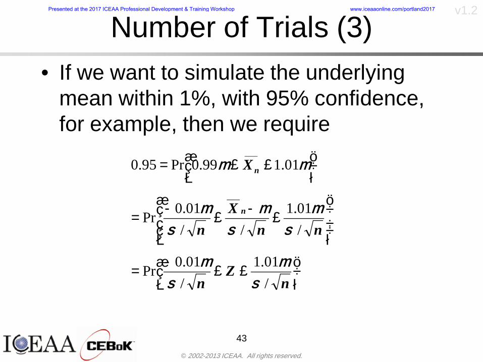
copy 2002-2013 ICEAA All rights reserved
v12
Number of Trials (3)bull If we want to simulate the underlying
mean within 1 with 95 confidence for example then we require
43
divideoslash
oumlccedilegrave
aelig poundpound-
=
dividedividedivide
oslash
ouml
ccedilccedilccedil
egrave
aeligpound
-pound
-=
divideoslashouml
ccedilegraveaelig poundpound=
nZ
n
nnX
n
X
n
n
011
010Pr
011
010Pr
011990Pr950
___
___
sm
sm
sm
sm
sm
mm
Presented at the 2017 ICEAA Professional Development amp Training Workshop wwwiceaaonlinecomportland2017
copy 2002-2013 ICEAA All rights reserved
v12
Number of Trials (4)bull This means that the number of trials required is determined by
bull Solving for n we find that at least
trials are neededbull Note that this term involves the coefficient of variation of the
distribution which means that distributions with less dispersion require fewer trials to accurate simulate
44
96101
=ns
m
ms41638
Presented at the 2017 ICEAA Professional Development amp Training Workshop wwwiceaaonlinecomportland2017
copy 2002-2013 ICEAA All rights reserved
v12
Number of Trials (5)bull Simulating percentiles requires more trials than for simulating
meansbull Let Pn represent the number of trials in the sample at or below
the 70th percentile of the underlying distribution (suppose this is known)
bull By the Central Limit Theorem Pnn follows a normal distribution with mean equal to the 70th percentile and variance equal to
bull By a similar process for the mean we find that the number of trials needed to simulate the 70th percentile within 1 with 95 confidence is
45
( )n
FF 700700 1-
n
n
PPn -41638
Presented at the 2017 ICEAA Professional Development amp Training Workshop wwwiceaaonlinecomportland2017
copy 2002-2013 ICEAA All rights reserved
v12
Number of Trials (6)bull If Pn 070 for all n then n is approximately
bull For the sake of comparison suppose CV = 03 (reasonable approximation for hardware development) then the number of trials needed to simulate the mean with the same accuracy is then ldquoonlyrdquo 11525
bull More trials are needed to accurately simulate percentiles than means
46
( ) 46416703041638
70704168341638 =divide
oslashouml
ccedilegraveaelig=divide
oslashouml
ccedilegraveaelig -
=-
nnn
PPn
n
n
Presented at the 2017 ICEAA Professional Development amp Training Workshop wwwiceaaonlinecomportland2017
copy 2002-2013 ICEAA All rights reserved
v12
Methods of Simulationbull Monte Carlo simulation is a standard term for
simulationbull However there is an improvement on Monte Carlo
that improves the accuracy of the results of a simulation for a given number of trials
bull This method is call the Latin Hypercube approach to simulationndash Similar to Monte Carlo but an equal number of draws are taken
from a set of subintervals for example dividing the interval (01) into [00001) [0102)hellip [0910]
ndash Instead of 10 trials from [01] we have one trial from each subinterval
ndash Rough rule of thumb is Latin Hypercube takes 30 fewer trials to achieve similar accuracy to Monte Carlo
47
Presented at the 2017 ICEAA Professional Development amp Training Workshop wwwiceaaonlinecomportland2017
copy 2002-2013 ICEAA All rights reserved
v12
Probability Model ndash Correlationbull Correlation exists between work breakdown structure
(WBS) cost element costs and between cost and schedule
bull Correlation is a necessary consideration in cost risk analysis
bull Correlation is a number that can vary between -1 and +1 and represents the strength of the relationship between the two variablesndash If both variable have a tendency to move in the same direction
correlation is positivendash If when one variable increases the other tends to decrease and
vice-versa the correlation between the two variables is negative
Presented at the 2017 ICEAA Professional Development amp Training Workshop wwwiceaaonlinecomportland2017
copy 2002-2013 ICEAA All rights reserved
v12
Correlation And Causationbull Note that correlation is not causation however
causation implies correlationndash For example shark attacks and ice cream sales at the beach
bull For example for a launch vehicle structure increasing the diameter will not only result in an increase in the structures cost but will also result in higher costs for thermal coating (paint etc)
bull Also simply because two subsystems do not appear to be related does not mean they are not correlatedndash For example structures and computer equipment seemingly
have little relation to one another however an external factor such as a funding cut or a strike will impact all subsystems leading to delays and increasing cost across the board
ndash Thus everything in a WBS has some correlationUnit III - Module 9 49
Presented at the 2017 ICEAA Professional Development amp Training Workshop wwwiceaaonlinecomportland2017
copy 2002-2013 ICEAA All rights reserved
v12
The Importance of Correlationbull Percent that total cost standard deviation is underestimated
when correlation assumed to be 0 instead of r given nWBS elements
Unit III - Module 9 5050
0
20
40
60
80
100
0 01 02 03 04 05 06 07 08 09 1Actual Correlation
Perce
nt Un
deres
timate
d
n = 10
n = 30
n = 100n = 1000
0
20
40
60
80
100
0 01 02 03 04 05 06 07 08 09 1Actual Correlation
Perce
nt Un
deres
timate
d
n = 10
n = 30
n = 100n = 1000
Reference 32nd Annual DOD Cost Analysis Symposium Advanced Training Session ldquoWhy Correlation Matters in Cost Estimatingrdquo Stephen A Book
Presented at the 2017 ICEAA Professional Development amp Training Workshop wwwiceaaonlinecomportland2017
copy 2002-2013 ICEAA All rights reserved
v12
The Importance of Correlation (2)bull For example if correlation is assumed to be 0 for all
elements in a 30 element WBS and the actual correlation is 20 then the total cost standard deviation is underestimated by 60
bull For example assume the total cost is modeled as a normal distribution with mean = 100
bull If correlation is assumed to be zero with total cost standard deviation = 12 when correlation is actually 20 then the true underlying standard deviation is actually 30
bull 70th percentile with zero correlation assumption is 106
bull 70th percentile with 20 correlation is 116 Unit III - Module 9 51
Presented at the 2017 ICEAA Professional Development amp Training Workshop wwwiceaaonlinecomportland2017
copy 2002-2013 ICEAA All rights reserved
v12
Measures of Correlationbull Two measures of correlation are commonly used in
cost risk analysesndash Pearsonrsquos product-moment correlation coefficient ndash Spearmanrsquos rank correlation coefficient
bull Garvey and others recommend using Pearsonrsquos product-moment correlation coefficient correlation for cost risk analysesndash Method of moments uses this but there are two options in
simulationndash Popular simulation packages like Risk and Crystal Ball use
rank correlation but in practice this has been found to make little difference
ndash Pearson product-moment correlation has been incorporated into Risk+
52
Presented at the 2017 ICEAA Professional Development amp Training Workshop wwwiceaaonlinecomportland2017
copy 2002-2013 ICEAA All rights reserved
v12
Pearson Correlationbull Pearsonrsquos product-moment correlation measures
degree of linearity between two random variables bull If two random variables are perfectly linear (eg Y =
aX + b) with positive slope then the Pearson product-moment correlation between X and Y denoted by rXY is +1
53
X X
Y Y Y
XNegative Correlation Positive Correlation No Correlation
middotmiddot
middotmiddot
middotmiddot middotmiddot
middotmiddot
middot
middot
middotmiddotmiddot
middotmiddot
middotmiddot
middotmiddot middot
middot
middot
middotmiddotmiddotmiddotmiddotmiddotmiddotmiddot
middotmiddotmiddotmiddot
middotmiddot
middotmiddot middotmiddotmiddotmiddot
middotmiddotmiddot
middotmiddotmiddotmiddot
middotmiddotmiddot
middotmiddotmiddot
middotmiddot
middot
middot middotmiddot
middot middotmiddotmiddotmiddot middotmiddot middot middotmiddot middot middot
middotmiddot middot
middotmiddotmiddotmiddotmiddot middot middotmiddot
middotmiddot
middot
middotmiddot
middotmiddot middot
middot middot middot
middotmiddot middot
middotmiddotmiddot
middotmiddot
middot middot
Presented at the 2017 ICEAA Professional Development amp Training Workshop wwwiceaaonlinecomportland2017
copy 2002-2013 ICEAA All rights reserved
v12
Spearman Correlationbull Spearmanrsquos rank correlation measures the
monotonicity between two random variablesbull If two random variables are perfectly monotonically
increasing (eg Y = X2) then the Spearman rank correlation denoted by rXY is +1
bull The two measures can be significantly different
54
10 20 30 40 50 60
100
200
300
096 097 098 099 1
1
060
020
040
080
Eff
ort (
Staf
f-M
onth
s)
Software Size I KDSI
y = 28z12y
z x
yy = x100
0 pound x pound 1
Figure 5-9A Figure 5-9B
Pearson Correlation = 09976 Rank Correlation = 1
Pearson Correlation = 024 Rank Correlation = 1
X(x ) ~ Unif(01)
Reference Probability Methods for Cost Uncertainty Analysis A Systems Engineering Perspective Paul R Garvey
Presented at the 2017 ICEAA Professional Development amp Training Workshop wwwiceaaonlinecomportland2017
copy 2002-2013 ICEAA All rights reserved
v12
Unit III - Module 9 55
200
250
300
350
400
1000 1200 1400 1600 1800 2000
Recurring Production
SEPM
200
250
300
350
400
1000 1200 1400 1600 1800 2000
Recurring Production
SEPM
Functional Correlationbull Old No Functional
Correlation Simulation run with WBS items entered as values
bull New Simulation run with functional dependencies entered as they are in cost model
CorrelatedNot Correlated
Note shift of mean and increased variability
Presented at the 2017 ICEAA Professional Development amp Training Workshop wwwiceaaonlinecomportland2017
copy 2002-2013 ICEAA All rights reserved
v12
Risk Measuresbull ldquoWestern Europe conquered the word because of a
technological revolution that started because of attempts to measure the worldrdquo ndash Phillipe Jorion ndash In the same way attempts to measure risk will lead to better project
managementbull Risk management for DoD and NASA agencies focuses
primarily on funding projects to a single percentile ndash NASA policy explicitly mentions 70 and 50ndash This is known as ldquoValue at Riskrdquo and is prevalent in the banking and
financial industry
56
Presented at the 2017 ICEAA Professional Development amp Training Workshop wwwiceaaonlinecomportland2017
copy 2002-2013 ICEAA All rights reserved
v12
Value at Risk (VaR)bull VaR is a percentile of the cost risk
distributionndash VaR funding at the 70th percentile means that
there is a 30 chance of final project cost exceeding the funded amount (budget)
bull VaR has some meritsndash Common measure can be used to compare
different projects and programsndash Easily understood by senior managers and
decision makers
57
Presented at the 2017 ICEAA Professional Development amp Training Workshop wwwiceaaonlinecomportland2017
copy 2002-2013 ICEAA All rights reserved
v12
Why 70th or 80th Percentilebull Typical policy guidance involves funding at the 70th or 80th
percentile Why fund as such a low percentilebull There is some incentive to not over-fundbull For a normal distribution an inflection point occurs near the 80th
percentile meaning that for values above 80 confidence achieving higher levels of confidence can only be achieved by spending greater dollar amounts at an increasing rate
58
-05-04-03-02-01
00102030405
0 05 1 15 2 25 3
Standard Deviations from Mean
Normal Distribution
First DerivativeSlopeVelocity
Second DerivativeConvexityAcceleration
Inflection point at one standard deviation above the mean (~84th
percentile)
Presented at the 2017 ICEAA Professional Development amp Training Workshop wwwiceaaonlinecomportland2017
copy 2002-2013 ICEAA All rights reserved
v12
Funding Above Inflection Pointsbull As the percentile goes above the 80th percentile the amount
needed to achieve that higher level of confidence begins to increase at an increasing rate as is evident from the graph
59
0
10
20
30
40
50
60
70
50 55 60 65 70 75 80 85 90 95 100
$ Ab
ove
MEa
n to
Ach
ieve
Per
cent
ile
Percentile (Confidence Level)
Presented at the 2017 ICEAA Professional Development amp Training Workshop wwwiceaaonlinecomportland2017
copy 2002-2013 ICEAA All rights reserved
v12
Why Budget to the 70th or 80thbull Government projects are funded at the 70th or 80th percentilesbull Why not the 90th or 99th percentile Wonrsquot that help prevent
overrunsndash As we have seen percentiles do not add across programs
bull The sum of the 80th percentiles does NOT equal the total 80th percentile
ndash This is because the individual programs are riskier than the entire suite of missions
bull Known as the ldquoPortfolio effectrdquo (more or this later)
ndash Funding at the 80th gives confidence that the entire portfolio will be adequately funded
bull And since there is an inflection point near the 80th percentile funding above that level quickly becomes cost prohibitive
60
Presented at the 2017 ICEAA Professional Development amp Training Workshop wwwiceaaonlinecomportland2017
copy 2002-2013 ICEAA All rights reserved
v12
Inflection Points for Lognormalbull For a lognormal the inflection point
variesndash Coefficient of variation equal to 10 equates to an
inflection point at the 70th percentile
61
0
10
20
30
40
50
60
70
050 060 070 080 090 100
Coef
ficen
t of V
aria
tion
Percentile of the Inflection Point
Presented at the 2017 ICEAA Professional Development amp Training Workshop wwwiceaaonlinecomportland2017
copy 2002-2013 ICEAA All rights reserved
v12
Issues with Percentile Fundingbull However risk management does not stop at a
specific percentilendash What happens when the 70th percentile is exceeded
bull Any effective risk management policy should prescribe what happens after a bad event occursndash With VaR we only know when a bad event has occurred ndash Also funding at a relatively low level means we have no true
sense of the real risks that should be guarded against
62
Presented at the 2017 ICEAA Professional Development amp Training Workshop wwwiceaaonlinecomportland2017
copy 2002-2013 ICEAA All rights reserved
v12
ldquoHere There Be Dragonsrdquobull On old maps uncharted territory was often
marked with monsters or dragons
63
A section of the Carta Marina by Olaus Magnus 16th Century
Presented at the 2017 ICEAA Professional Development amp Training Workshop wwwiceaaonlinecomportland2017
copy 2002-2013 ICEAA All rights reserved
v12
Distribution Comparisonbull Four different distributions with the same 70th
percentile
bull Should we expect the tails to be similar
64
0
10
20
30
40
50
60
70
80
0 100 200 300 400 500 600
Perc
entil
eCo
nfid
ence
Lev
el
Triangular
Normal
Lognormal
Pareto
Presented at the 2017 ICEAA Professional Development amp Training Workshop wwwiceaaonlinecomportland2017
copy 2002-2013 ICEAA All rights reserved
v12Distribution Comparison Tail Behavior
bull The normal and triangular distributions have similar tails but the lognormal and Pareto have much fatter right tails
65
70
75
80
85
90
95
100
500 1500 2500 3500 4500 5500
Perc
entil
eCo
nfid
ence
Lev
el
Triangular
Normal
Lognormal
Pareto
Here There Be Dragons
Presented at the 2017 ICEAA Professional Development amp Training Workshop wwwiceaaonlinecomportland2017
copy 2002-2013 ICEAA All rights reserved
v12Distribution Comparison ndash Tail Behavior (Table)
bull There is significant tail risk for the lognormal and the Paretobull The 99th percentile for the Pareto is 1000 times greater than
the 70th percentilendash Risk seen in financial markets and in catastrophic risks like natural
disasters bull Four different projects follow the four different risk profiles seen
in this example should clearly have different risk management approaches but 70th percentile funding indicates the same risk management approach for all four
66
Percentile Triangular Normal Lognormal Pareto 70th $600 $600 $600 $600 80th $680 $660 $770 $1430 90th $770 $750 $1070 $5880 95th $840 $820 $1410 $23750 99th $930 $950 $2350 $600000
Presented at the 2017 ICEAA Professional Development amp Training Workshop wwwiceaaonlinecomportland2017
copy 2002-2013 ICEAA All rights reserved
v12Percentile Budgeting is Not Risk Management
bull Percentile budgeting ne effective risk management policybull Suppose that you are shopping for a new car You
mention that safety is your top concern The salesman says he has a great safe car available You ask about the air bags Do they work The salesman answers ldquoOf course Seventy percent of the time they work fine Only 30 of the time the air bags will fail to deployrdquo Would you buy such a car Hedge fund manager David Einhorn has stated ldquoRisk management is the air bag that must always work but only in the multi-sigma event where you have an accidentrdquo
67
Risk management is the air bag that must always work but only in the multi-sigma event where you
have an accident
Presented at the 2017 ICEAA Professional Development amp Training Workshop wwwiceaaonlinecomportland2017
copy 2002-2013 ICEAA All rights reserved
v12
Joint Confidence Level Analysisbull Schedules are risky toobull For 98 recent NASA missions average
schedule growth was 38ndash Not as high as cost growth but still significant
68
0
5
10
15
20
25
30
35
40
Schedule
Cost
Presented at the 2017 ICEAA Professional Development amp Training Workshop wwwiceaaonlinecomportland2017
copy 2002-2013 ICEAA All rights reserved
v12
Schedules Impact Costbull Changes in schedule can have enormous
impacts on cost ndash Schedule slips can lead to cost increases
bull Fixed programmatic costs must be paid on a regular basisndash Achieving schedule milestones early can result in cost
savings
bull Schedule is an important consideration in cost analysis including cost risk analysis
bull However we must be careful in correctly integrating cost and schedule riskndash Schedule is not simply an input but is dependent on many of
the same factors that drive cost
69
Presented at the 2017 ICEAA Professional Development amp Training Workshop wwwiceaaonlinecomportland2017
copy 2002-2013 ICEAA All rights reserved
v12
The Relationship of Cost to Schedulebull Cost and schedule are positively correlated
ndash A larger program with bigger scope with take longer to complete than a smaller simpler program
bull However longer schedules do not always equate to higher cost nor shorter schedules with lower costndash Highly compressed schedules relative to the
optimal schedule can lead to large overrunsbull Compressed schedules are commonplace for
many planetary missions
70
Presented at the 2017 ICEAA Professional Development amp Training Workshop wwwiceaaonlinecomportland2017
copy 2002-2013 ICEAA All rights reserved
v12The Impact of Schedule GrowthCompression on Cost
bull Compressed schedules lead to cost growth and based on existing research is actually more expensive than schedule slippages
71
0
20
40
60
80
100
120
140
160
-50 -25 0 25 50 75 100
Percentage Change in Schedule
Perc
enta
ge C
hang
e in
Cos
t due
to
Sche
dule
Cha
nge
Source Smart CB ldquoCost and Schedule Interrelationshipsrdquo 2007 NASA Cost Symposium
Presented at the 2017 ICEAA Professional Development amp Training Workshop wwwiceaaonlinecomportland2017
copy 2002-2013 ICEAA All rights reserved
v12Schedule as an Independent Variable
bull Why not simply add schedule as an input to cost-estimating relationships (CERs)
bull Schedule is often treated as an independent variable ndash schedules are often determined independently of cost considerationsndash Cost may not be considered explicitly although budgets and
schedules are determined based on scope and other common factors
bull In 2006 SAIC undertook a research task to determine the impact of schedule on cost and added schedule as an independent variable to the CERs in the NASAAir Force Cost Model (NAFCOM) to see if schedule provided any improvement in goodness of fit
72
Presented at the 2017 ICEAA Professional Development amp Training Workshop wwwiceaaonlinecomportland2017
copy 2002-2013 ICEAA All rights reserved
v12
Schedule is a Dependent Variablebull Since NAFCOM includes an exhaustive list of cost drivers the inclusion
of schedule should give an indication of whether there is any additional independent value added from schedule independent of the cost drivers
bull In the study schedule was added to 10 subsystem-level CERs
ndash In each case the addition of schedule did NOTimprove the goodness of fit and schedule was NOT found to be a statistically significant cost driver (given the presence of the other variables) for any of the 10 CERs
bull Standard errors for the CERs increased due to decrease in degrees of freedom
bull Thus schedule as an independent variable did not provide any additional explanation of variation in historical cost
bull This is because schedule is truly NOT an independent variable but a dependent variable and is a function of the same factors that drive cost
73
Presented at the 2017 ICEAA Professional Development amp Training Workshop wwwiceaaonlinecomportland2017
copy 2002-2013 ICEAA All rights reserved
v12
Incorporation of Schedule in Cost Risk
bull When using subjective methods care must be taken in applying schedule to cost risk analysis
bull Since schedule is a dependent variable treating it independently from other factors when assessing its impact on cost can lead to a double count of independent variables in the cost risk analysis
bull Direct inclusion of schedule in a cost risk analysis effectively doubles the influence of each cost driver
ndash Incorrectly leads to broader risk ranges
74
CostWeight
HeritageNewness
Technology Readiness Schedule
Presented at the 2017 ICEAA Professional Development amp Training Workshop wwwiceaaonlinecomportland2017
copy 2002-2013 ICEAA All rights reserved
v12Subjective Cost Risk Methods and Overinclusion of Risk Factors
bull Subjective methods are suitable when data are scarce or not availablebull However care must be taken not to treat correlated sources of risk
such as schedule as independent of each otherbull Example ndash a subjective risk analysis incorporated technology readiness
design risk requirements stability integration risk and schedule and treated each source of risk as independent
bull Risk triangle high value without schedule risk was 31 times the point estimate
bull Risk triangle high value with schedule risk added on top of other sources of risk treated independently was 34 times the point estimate
bull Risk triangle taking correlation between sources of risk into account in a rigorous statistical manner has a high value 15 times the point estimate less than half the effect when treating sources of risk as independent
75
Presented at the 2017 ICEAA Professional Development amp Training Workshop wwwiceaaonlinecomportland2017
copy 2002-2013 ICEAA All rights reserved
v12Fundamental Equation of Cost and Schedule Interrelationships
bull The Fundamental Equation of the Relationship Between Cost and Schedule is
Time = Moneybull This is a well known adage that time is money Your boss at
work may even mention this to you from time to time or if you are the boss you are all too aware of this iron law
bull Because time is money cost and schedule risk should be modeled jointly not with schedule as an independent cost driver
bull Note that cost and schedule are not perfectly correlatedndash Cost can sometimes ldquobuy downrdquo schedule extra money can be
spent to meet a deadline since in some cases additional effort to hasten the completion of a task
76
Presented at the 2017 ICEAA Professional Development amp Training Workshop wwwiceaaonlinecomportland2017
copy 2002-2013 ICEAA All rights reserved
v12How to (Correctly) Incorporate Schedule into Cost Risk Analysis
bull The best way to model cost and schedule risk is to develop a joint cost and schedule model based on the same data
bull Since such models are not currently available the next best approach is to model cost and schedule independently and then integrate cost and schedule risk analyses using joint probability distributions taking into account correlation between cost and schedulendash This approach pioneered by Paul Garvey and Steve Book is
considered industry best practicendash This is a practical method mathematically tractable and follows
naturally from the Fundamental Equation of Cost and Schedule Interrelationships
77
Book S A ldquoQuantifying the Relationship Between Cost and Schedulerdquo The Measurable News Winter 2007-2008 pp 11-15Garvey PR Probability Methods for Cost Uncertainty Analysis A Systems Engineering Perspective New York Marcel Dekker 2000 pp 308-335
Presented at the 2017 ICEAA Professional Development amp Training Workshop wwwiceaaonlinecomportland2017
copy 2002-2013 ICEAA All rights reserved
v12
Joint Lognormal and Normal Distributions
bull Cost and schedule are typically modeled as some combination of Normal and Lognormal probability distributionsndash Studies by The Aerospace Corporation the MITRE
Corporation Wyle Labs and SAIC have found that the Lognormal probability distribution almost always serves as a good model for both the schedule distribution and the cost distribution
ndash The Normal distribution may also be appropriate in some instances and depending upon the level of confidence at which budgets are set may even be more conservative and logically consistent than the Normal distribution
ndash Joint Lognormal and Normal distributions are defined by a pair of mean and standard deviations and a level of correlation between the two
78
Presented at the 2017 ICEAA Professional Development amp Training Workshop wwwiceaaonlinecomportland2017
copy 2002-2013 ICEAA All rights reserved
v12Modeling Cost and Schedule as a Bivariate Distribution
bull In the approach set forth by Book and Garvey cost risk is assessed and the top-level distribution is modeled as a Lognormal (or Normal) distribution schedule risk is assessed and the overall schedule risk is modeled as a Lognormal (or Normal) distribution
bull The two distributions are combined into a Bivariate distribution by assigning a correlation between the two and by treating the two distributions as the marginal distributions of a Bivariate Lognormal distributionndash Other combinations include a Bivariate Normal or a Bivariate
Normal-Lognormal
79
Presented at the 2017 ICEAA Professional Development amp Training Workshop wwwiceaaonlinecomportland2017
copy 2002-2013 ICEAA All rights reserved
v12Bivariate Lognormal Distribution for Cost and Schedule
bull Cost is often observed to be Lognormal when strong positive correlations are present among the systemrsquos WBS cost element costs
bull A systemrsquos schedule is often observed (from Monte Carlo simulations) to be Lognormal if it is the sum of many positively correlated schedule activities in an overall schedule network
bull If Lognormal distributions characterize a systemrsquos cost and schedule then the Bivariate Lognormal could serve as an assumed model of their joint distributionndash In this case the marginal distribution of each of cost and schedule is
Lognormalbull Other possibilities for modeling cost and schedule as a Bivariate
distribution include a Bivariate Normal or a Bivariate Normal-Lognormal distributionndash All these combinations are analytically tractable
80
Presented at the 2017 ICEAA Professional Development amp Training Workshop wwwiceaaonlinecomportland2017
copy 2002-2013 ICEAA All rights reserved
v12Bivariate Lognormal for Cost and Schedule
bull Contour Plots of a Bivariate Lognormal
81
Presented at the 2017 ICEAA Professional Development amp Training Workshop wwwiceaaonlinecomportland2017
copy 2002-2013 ICEAA All rights reserved
v12Correlation Between Cost and Schedule
bull Cost and schedule are positively correlated but not perfectly sondash For example it is possible to have a schedule underrun and a cost
overrunbull Based on cost and schedule growth data for 50 completed NASA
programs the correlation between development cost and development schedule is 70
82
00
200
400
600
800
1000
1200
-500 00 500 1000 1500 2000 2500Historical Cost Growth
Hist
oric
al S
ched
ule
Gro
wth
r = 715
Presented at the 2017 ICEAA Professional Development amp Training Workshop wwwiceaaonlinecomportland2017
copy 2002-2013 ICEAA All rights reserved
v12Correlation Between Cost and Schedule Caveats
bull Based on historical data recommended correlation between cost and schedule is 70 but this could be higher or lower depending upon program circumstancesndash If program is budget constrained cost and schedule will be
more highly correlated (go as you pay)ndash If program is schedule constrained cost and schedule will
have lower correlation perhaps even negative correlation ndash Smaller programs have smaller correlation between cost and
schedule riskbull Relatively easy to ldquohurry uprdquo and finish on time or even early if
needed
83
Presented at the 2017 ICEAA Professional Development amp Training Workshop wwwiceaaonlinecomportland2017
copy 2002-2013 ICEAA All rights reserved
v12
Conditional Confidence Levelsbull Given a programrsquos project schedule we can determine the cost
risk distribution conditional upon the given schedulebull Conditional cost S-curves are steeper than unconditional
(marginal) cost S-curves between some uncertainty has been removed because schedule is fixed
84
Presented at the 2017 ICEAA Professional Development amp Training Workshop wwwiceaaonlinecomportland2017
copy 2002-2013 ICEAA All rights reserved
v12
Joint Confidence Levelsbull Joint 65 confidence represents the probability of
achieving both 65 confidence in cost AND 65 confidence in schedulendash This is different than achieving 65 cost confidence alone
or achieving 65 schedule confidence alonebull Due to the imperfect correlation between cost and schedule it
is possible to achieve a 65 cost confidence with a lower level of schedule confidence
bull Restricting the schedule confidence thus requires additional $ to achieve a given level of confidence
85
X
Y
Possible Values for Which X gt a Possible Values for
Which X gt a and Y gt b
a
b
Presented at the 2017 ICEAA Professional Development amp Training Workshop wwwiceaaonlinecomportland2017
copy 2002-2013 ICEAA All rights reserved
v12Joint Confidence Levels Versus Cost Confidence Levels Only
bull Example of the differences between cost confidence schedule confidence conditional cost confidence and joint cost and schedule confidence
86
Joint Cost-Schedule Confidence Iso-Curves
Cost (RY$M)
Sche
dule
(Mon
ths)
65 Confidence
50 Confidence
70 Confidence
65 Cost Confidence AggressiveSchedule65 Cost ConfidenceScheduleGiven 65 Schedule ConfidenceUnconditional 65 CostConfidenceUnconditional 65 ScheduleConfidence
65 Cost Confidence 65 Joint Cost and Schedule
Confidence for 65 Schedule Confidence
Presented at the 2017 ICEAA Professional Development amp Training Workshop wwwiceaaonlinecomportland2017
copy 2002-2013 ICEAA All rights reserved
v12
Joint Cost and Schedule Confidence
bull Can examine pairs of cost and schedule that achieve a given level of confidence
bull Provides insights into the trade-offs between cost and schedule for a given level of confidencendash Possible to increase cost confidence by giving a
project more time in some instances or possible to ldquobuy downrdquo schedule
bull But these have limits and are shown in the iso-cost and schedule confidence curves
87
Presented at the 2017 ICEAA Professional Development amp Training Workshop wwwiceaaonlinecomportland2017
copy 2002-2013 ICEAA All rights reserved
v12Cost and Schedule Trade-offs for a Given Level of Joint Confidence
bull Hypothetical Example
88
Cost (RY$M)
Schedule (Months)
$100 48$99 48$89 49$87 50$85 51$85 52$84 53$83 55$83 55$83 56
Cost and Schedule 65 Confidence Iso-Curve
4748495051525354555657
$80 $82 $84 $86 $88 $90 $92 $94 $96 $98 $100
Cost (RY$ M)
Sche
dule
(Mon
ths)
Presented at the 2017 ICEAA Professional Development amp Training Workshop wwwiceaaonlinecomportland2017
copy 2002-2013 ICEAA All rights reserved
v12Policy Considerations for Confidence Levels
bull For large programs the difference between the amount of money needed to achieve 65 cost confidence independent of schedule and joint 65 cost and schedule confidence can represent hundreds of millions and even billions of dollars
89
Joint Cost-Schedule Confidence Iso-Curves
Cost (RY$M)
Sche
dule
(Mon
ths)
65 Confidence
65 Cost Confidence AggressiveSchedule
65 Cost ConfidenceScheduleGiven 65 Schedule Confidence
Unconditional 65 CostConfidence
Joint Cost and Schedule Confidence for 65 Cost Confidence and Program Baseline Schedule is Less Than 35
65 Cost Confidence Independent of Schedule Cost Needed to Achieve
Both 65 Joint Cost and Schedule Confidence for the Schedule with 65 Confidence
Presented at the 2017 ICEAA Professional Development amp Training Workshop wwwiceaaonlinecomportland2017
copy 2002-2013 ICEAA All rights reserved
v12
Copulasbull More generally any combination of distributions can
be used (more than just normal and lognormal)ndash Termed ldquocopulardquo from the Italian word for ldquocouplerdquondash Copulas are a way to combine marginal distributions of any
number and type into a joint distributionbull More formally a copula is a multivariate joint distribution defined
on the n-dimensional unit cube [0 1]n such that every marginal distribution is uniform on the interval [0 1]
bull (The bivariate form of) Sklarrsquos theorem states that for any bivariate distribution function H(x y) let F(x) = H(x infin) and G(y) = H(infin y) be the univariate marginal probability distribution functions Then there exists a copula C such that H(xy)=C(F(x)G(y))
ndash Copulas are widely used in risk management for investments and insurance
bull Considered industry best practice (Li 2000)bull Marketed as part of JP Morganrsquos CreditMetrics suite of tools
(Gupton et Al 1997)90
Presented at the 2017 ICEAA Professional Development amp Training Workshop wwwiceaaonlinecomportland2017
copy 2002-2013 ICEAA All rights reserved
v12Parametric Joint Cost and Schedule Analysis
bull A parametric model based on a consistent data set with a set of overlapping cost and schedule drivers is a cleaner way to model cost and schedule
91
CostWeight
HeritageNewness
Technology Readiness
Schedule
0
20
40
60
80
100
Confidence
Joint Cost and Schedule Confidence
Schedule
Cost
Lognormal Distribution PDF and CDF
0102030405060708090100
200 300 400 500 600 700 800 900 1000Cost $
Con
fiden
ce L
evel
0
00002
00004
00006
00008
0001
00012
00014
00016
Prob
abili
ty D
ensi
ty
CDFPDF
Lognormal Distribution PDF and CDF
0102030405060708090100
200 300 400 500 600 700 800 900 1000Cost $
Con
fiden
ce L
evel
0
00002
00004
00006
00008
0001
00012
00014
00016
Prob
abili
ty D
ensi
ty
CDFPDF
Presented at the 2017 ICEAA Professional Development amp Training Workshop wwwiceaaonlinecomportland2017
copy 2002-2013 ICEAA All rights reserved
v12Parametric Joint Cost and Schedule Analysis (2)
bull Joint cost and schedule risk analysis produced naturally by the integrated modelndash Addresses several issues with the copula
approachbull Tail dependencybull Correlation ndash no need to assign correlation
between cost and schedulebull Consistency of cost and schedule models
92
Presented at the 2017 ICEAA Professional Development amp Training Workshop wwwiceaaonlinecomportland2017
copy 2002-2013 ICEAA All rights reserved
v12
Resource-Loaded Schedulesbull Involves assigning cost and schedule risks to a resource-loaded schedule
networkbull Bottom-up approach
ndash More labor intensive than parametrics but can also provide more insight
ndash Can answer questions than parametric typically cannot such as how much do reserve requirements decrease if a specific risk is retired
bull Currently being implemented in Constellation programbull Has same issue as all bottom-up models hard to count all the risks and model
them discretely
ndash As a result there is a tendency to reflect less risk than indicated by history
ndash ldquoThere are more things in heaven and earth Horatio than are dreamt of in your philosophyrdquo William Shakespeare Hamlet Act I Scene V
93
Presented at the 2017 ICEAA Professional Development amp Training Workshop wwwiceaaonlinecomportland2017
copy 2002-2013 ICEAA All rights reserved
v12Resource-Loaded Schedules Vs Parametrics
bull Parametric most appropriate for early estimatesndash But also good for high-level checks as project progresses
bull As plans take shape lower level modeling may be more appropriate
94 1
CONCEPTUALDEVELOPMENT
PROJECTDEFINITION DESIGN DEVELOPMENT OPERATIONS
PARAMETRIC PARAMETRIC
ANALOGY
ENGINEERING (Bottoms Up)
$PARAMETRIC
DETAILED
$
Pre Phase A Phase B Phase CDPhase A Phase EPre Phase A Phase B Phase CDPhase A Phase E
Risk = f(Cost Estimating Relationship Inputs eg mass power data rate TRL new design etc)
Risk = f(cost and schedule variation of the analogous elements)
Risk = f(variation of detailed inputs eg labor hours rates materials etc)
Presented at the 2017 ICEAA Professional Development amp Training Workshop wwwiceaaonlinecomportland2017
copy 2002-2013 ICEAA All rights reserved
v12
Resource-Loaded Schedulesbull Methodology has been demonstrated in other
industriesndash Construction oil and gasndash Analysis has not been traditionally done on highly uncertain
complex development projects bull Methodology focuses on project baseline schedule
ndash In baseline schedule all tasks are resource loaded to represent a baseline schedule and cost standpoint
ndash Resource loaded schedule is ldquorolledrdquo up to a manageable level
ndash Based on the risk and uncertainties identified schedule distributions are applied to each rolled up task
ndash Cost uncertainties are also applied to rolled up tasksbull Uncertainties include labor rate man power etc
ndash A Monte Carlo simulation is run to develop joint cost-schedule distributions
95
Presented at the 2017 ICEAA Professional Development amp Training Workshop wwwiceaaonlinecomportland2017
copy 2002-2013 ICEAA All rights reserved
v12
Unit III - Module 9 96
Execution ndash Cross Checksbull Means The mean cost growth factor for WBS items
can be compared to history as a way to cross check results
bull CVs The CV of the cost growth factors for WBS items can be compared to history as a way to cross check results
bull Inputs Checks are performed on inputs or other parameters to see if historical values are in line with program assumptionsndash Example Historical risk scores can be compared to program
risk scores to see if risk assessors are being realistic and to see if the underlying database is representative of the program
11
Presented at the 2017 ICEAA Professional Development amp Training Workshop wwwiceaaonlinecomportland2017
- Cost and Schedule Risk Analysis Basic
- Acknowledgments
- Unit Index
- Risk Overview
- Agenda
- Introduction
- Risk Analysis Terms
- Are Our Costs Realistic
- Historical Cost Growth
- Sources of Cost Risk
- Point Estimates of Cost
- Types of Risk
- Point Estimates Vs Risk Estimates
- Cost Risk and Probability
- Probability Model ndash Distribution
- Probability Model ndash Distribution
- Probability ndash Top-Level Distribution
- S-Curves and Confidence Levels
- Example ndash Normal Distribution
- Confidence Levels
- Measuring Parametric Model Uncertainty
- Parametric Model Example
- Weight Uncertainty
- Estimating Uncertainty
- Estimating Uncertainty (2)
- Estimating Uncertainty (3)
- Aggregating Risk
- WBS Example
- WBS and Risk
- Aggregating Risk
- Percentiles Do Not Add
- Percentiles Do Not Add (2)
- Percentiles Do Not Add (3)
- Methods for Aggregating Risk
- Monte Carlo Simulationfor Risk Analysis
- Monte Carlo Simulation
- Using Random Numbers to Simulate Distributions
- Simulating a Triangular Distribution
- Simulating a Triangular Distribution (2)
- Monte Carlo and the WBS
- Number of Trials
- Number of Trials (2)
- Number of Trials (3)
- Number of Trials (4)
- Number of Trials (5)
- Number of Trials (6)
- Methods of Simulation
- Probability Model ndash Correlation
- Correlation And Causation
- The Importance of Correlation
- The Importance of Correlation (2)
- Measures of Correlation
- Pearson Correlation
- Spearman Correlation
- Functional Correlation
- Risk Measures
- Value at Risk (VaR)
- Why 70th or 80th Percentile
- Funding Above Inflection Points
- Why Budget to the 70th or 80th
- Inflection Points for Lognormal
- Issues with Percentile Funding
- ldquoHere There Be Dragonsrdquo
- Distribution Comparison
- Distribution Comparison Tail Behavior
- Distribution Comparison ndash Tail Behavior (Table)
- Percentile Budgeting is Not Risk Management
- Joint Confidence Level Analysis
- Schedules Impact Cost
- The Relationship of Cost to Schedule
- The Impact of Schedule GrowthCompression on Cost
- Schedule as an Independent Variable
- Schedule is a Dependent Variable
- Incorporation of Schedule in Cost Risk
- Subjective Cost Risk Methods and Overinclusion of Risk Factors
- Fundamental Equation of Cost and Schedule Interrelationships
- How to (Correctly) Incorporate Schedule into Cost Risk Analysis
- Joint Lognormal and Normal Distributions
- Modeling Cost and Schedule as a Bivariate Distribution
- Bivariate Lognormal Distribution for Cost and Schedule
- Bivariate Lognormal for Cost and Schedule
- Correlation Between Cost and Schedule
- Correlation Between Cost and Schedule Caveats
- Conditional Confidence Levels
- Joint Confidence Levels
- Joint Confidence Levels Versus Cost Confidence Levels Only
- Joint Cost and Schedule Confidence
- Cost and Schedule Trade-offs for a Given Level of Joint Confidence
- Policy Considerations for Confidence Levels
- Copulas
- Parametric Joint Cost and Schedule Analysis
- Parametric Joint Cost and Schedule Analysis (2)
- Resource-Loaded Schedules
- Resource-Loaded Schedules Vs Parametrics
- Resource-Loaded Schedules
- Execution ndash Cross Checks
-
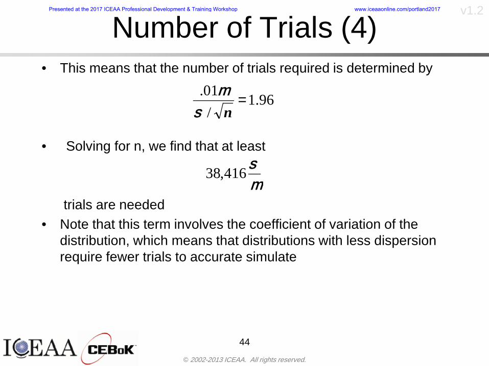
copy 2002-2013 ICEAA All rights reserved
v12
Number of Trials (4)bull This means that the number of trials required is determined by
bull Solving for n we find that at least
trials are neededbull Note that this term involves the coefficient of variation of the
distribution which means that distributions with less dispersion require fewer trials to accurate simulate
44
96101
=ns
m
ms41638
Presented at the 2017 ICEAA Professional Development amp Training Workshop wwwiceaaonlinecomportland2017
copy 2002-2013 ICEAA All rights reserved
v12
Number of Trials (5)bull Simulating percentiles requires more trials than for simulating
meansbull Let Pn represent the number of trials in the sample at or below
the 70th percentile of the underlying distribution (suppose this is known)
bull By the Central Limit Theorem Pnn follows a normal distribution with mean equal to the 70th percentile and variance equal to
bull By a similar process for the mean we find that the number of trials needed to simulate the 70th percentile within 1 with 95 confidence is
45
( )n
FF 700700 1-
n
n
PPn -41638
Presented at the 2017 ICEAA Professional Development amp Training Workshop wwwiceaaonlinecomportland2017
copy 2002-2013 ICEAA All rights reserved
v12
Number of Trials (6)bull If Pn 070 for all n then n is approximately
bull For the sake of comparison suppose CV = 03 (reasonable approximation for hardware development) then the number of trials needed to simulate the mean with the same accuracy is then ldquoonlyrdquo 11525
bull More trials are needed to accurately simulate percentiles than means
46
( ) 46416703041638
70704168341638 =divide
oslashouml
ccedilegraveaelig=divide
oslashouml
ccedilegraveaelig -
=-
nnn
PPn
n
n
Presented at the 2017 ICEAA Professional Development amp Training Workshop wwwiceaaonlinecomportland2017
copy 2002-2013 ICEAA All rights reserved
v12
Methods of Simulationbull Monte Carlo simulation is a standard term for
simulationbull However there is an improvement on Monte Carlo
that improves the accuracy of the results of a simulation for a given number of trials
bull This method is call the Latin Hypercube approach to simulationndash Similar to Monte Carlo but an equal number of draws are taken
from a set of subintervals for example dividing the interval (01) into [00001) [0102)hellip [0910]
ndash Instead of 10 trials from [01] we have one trial from each subinterval
ndash Rough rule of thumb is Latin Hypercube takes 30 fewer trials to achieve similar accuracy to Monte Carlo
47
Presented at the 2017 ICEAA Professional Development amp Training Workshop wwwiceaaonlinecomportland2017
copy 2002-2013 ICEAA All rights reserved
v12
Probability Model ndash Correlationbull Correlation exists between work breakdown structure
(WBS) cost element costs and between cost and schedule
bull Correlation is a necessary consideration in cost risk analysis
bull Correlation is a number that can vary between -1 and +1 and represents the strength of the relationship between the two variablesndash If both variable have a tendency to move in the same direction
correlation is positivendash If when one variable increases the other tends to decrease and
vice-versa the correlation between the two variables is negative
Presented at the 2017 ICEAA Professional Development amp Training Workshop wwwiceaaonlinecomportland2017
copy 2002-2013 ICEAA All rights reserved
v12
Correlation And Causationbull Note that correlation is not causation however
causation implies correlationndash For example shark attacks and ice cream sales at the beach
bull For example for a launch vehicle structure increasing the diameter will not only result in an increase in the structures cost but will also result in higher costs for thermal coating (paint etc)
bull Also simply because two subsystems do not appear to be related does not mean they are not correlatedndash For example structures and computer equipment seemingly
have little relation to one another however an external factor such as a funding cut or a strike will impact all subsystems leading to delays and increasing cost across the board
ndash Thus everything in a WBS has some correlationUnit III - Module 9 49
Presented at the 2017 ICEAA Professional Development amp Training Workshop wwwiceaaonlinecomportland2017
copy 2002-2013 ICEAA All rights reserved
v12
The Importance of Correlationbull Percent that total cost standard deviation is underestimated
when correlation assumed to be 0 instead of r given nWBS elements
Unit III - Module 9 5050
0
20
40
60
80
100
0 01 02 03 04 05 06 07 08 09 1Actual Correlation
Perce
nt Un
deres
timate
d
n = 10
n = 30
n = 100n = 1000
0
20
40
60
80
100
0 01 02 03 04 05 06 07 08 09 1Actual Correlation
Perce
nt Un
deres
timate
d
n = 10
n = 30
n = 100n = 1000
Reference 32nd Annual DOD Cost Analysis Symposium Advanced Training Session ldquoWhy Correlation Matters in Cost Estimatingrdquo Stephen A Book
Presented at the 2017 ICEAA Professional Development amp Training Workshop wwwiceaaonlinecomportland2017
copy 2002-2013 ICEAA All rights reserved
v12
The Importance of Correlation (2)bull For example if correlation is assumed to be 0 for all
elements in a 30 element WBS and the actual correlation is 20 then the total cost standard deviation is underestimated by 60
bull For example assume the total cost is modeled as a normal distribution with mean = 100
bull If correlation is assumed to be zero with total cost standard deviation = 12 when correlation is actually 20 then the true underlying standard deviation is actually 30
bull 70th percentile with zero correlation assumption is 106
bull 70th percentile with 20 correlation is 116 Unit III - Module 9 51
Presented at the 2017 ICEAA Professional Development amp Training Workshop wwwiceaaonlinecomportland2017
copy 2002-2013 ICEAA All rights reserved
v12
Measures of Correlationbull Two measures of correlation are commonly used in
cost risk analysesndash Pearsonrsquos product-moment correlation coefficient ndash Spearmanrsquos rank correlation coefficient
bull Garvey and others recommend using Pearsonrsquos product-moment correlation coefficient correlation for cost risk analysesndash Method of moments uses this but there are two options in
simulationndash Popular simulation packages like Risk and Crystal Ball use
rank correlation but in practice this has been found to make little difference
ndash Pearson product-moment correlation has been incorporated into Risk+
52
Presented at the 2017 ICEAA Professional Development amp Training Workshop wwwiceaaonlinecomportland2017
copy 2002-2013 ICEAA All rights reserved
v12
Pearson Correlationbull Pearsonrsquos product-moment correlation measures
degree of linearity between two random variables bull If two random variables are perfectly linear (eg Y =
aX + b) with positive slope then the Pearson product-moment correlation between X and Y denoted by rXY is +1
53
X X
Y Y Y
XNegative Correlation Positive Correlation No Correlation
middotmiddot
middotmiddot
middotmiddot middotmiddot
middotmiddot
middot
middot
middotmiddotmiddot
middotmiddot
middotmiddot
middotmiddot middot
middot
middot
middotmiddotmiddotmiddotmiddotmiddotmiddotmiddot
middotmiddotmiddotmiddot
middotmiddot
middotmiddot middotmiddotmiddotmiddot
middotmiddotmiddot
middotmiddotmiddotmiddot
middotmiddotmiddot
middotmiddotmiddot
middotmiddot
middot
middot middotmiddot
middot middotmiddotmiddotmiddot middotmiddot middot middotmiddot middot middot
middotmiddot middot
middotmiddotmiddotmiddotmiddot middot middotmiddot
middotmiddot
middot
middotmiddot
middotmiddot middot
middot middot middot
middotmiddot middot
middotmiddotmiddot
middotmiddot
middot middot
Presented at the 2017 ICEAA Professional Development amp Training Workshop wwwiceaaonlinecomportland2017
copy 2002-2013 ICEAA All rights reserved
v12
Spearman Correlationbull Spearmanrsquos rank correlation measures the
monotonicity between two random variablesbull If two random variables are perfectly monotonically
increasing (eg Y = X2) then the Spearman rank correlation denoted by rXY is +1
bull The two measures can be significantly different
54
10 20 30 40 50 60
100
200
300
096 097 098 099 1
1
060
020
040
080
Eff
ort (
Staf
f-M
onth
s)
Software Size I KDSI
y = 28z12y
z x
yy = x100
0 pound x pound 1
Figure 5-9A Figure 5-9B
Pearson Correlation = 09976 Rank Correlation = 1
Pearson Correlation = 024 Rank Correlation = 1
X(x ) ~ Unif(01)
Reference Probability Methods for Cost Uncertainty Analysis A Systems Engineering Perspective Paul R Garvey
Presented at the 2017 ICEAA Professional Development amp Training Workshop wwwiceaaonlinecomportland2017
copy 2002-2013 ICEAA All rights reserved
v12
Unit III - Module 9 55
200
250
300
350
400
1000 1200 1400 1600 1800 2000
Recurring Production
SEPM
200
250
300
350
400
1000 1200 1400 1600 1800 2000
Recurring Production
SEPM
Functional Correlationbull Old No Functional
Correlation Simulation run with WBS items entered as values
bull New Simulation run with functional dependencies entered as they are in cost model
CorrelatedNot Correlated
Note shift of mean and increased variability
Presented at the 2017 ICEAA Professional Development amp Training Workshop wwwiceaaonlinecomportland2017
copy 2002-2013 ICEAA All rights reserved
v12
Risk Measuresbull ldquoWestern Europe conquered the word because of a
technological revolution that started because of attempts to measure the worldrdquo ndash Phillipe Jorion ndash In the same way attempts to measure risk will lead to better project
managementbull Risk management for DoD and NASA agencies focuses
primarily on funding projects to a single percentile ndash NASA policy explicitly mentions 70 and 50ndash This is known as ldquoValue at Riskrdquo and is prevalent in the banking and
financial industry
56
Presented at the 2017 ICEAA Professional Development amp Training Workshop wwwiceaaonlinecomportland2017
copy 2002-2013 ICEAA All rights reserved
v12
Value at Risk (VaR)bull VaR is a percentile of the cost risk
distributionndash VaR funding at the 70th percentile means that
there is a 30 chance of final project cost exceeding the funded amount (budget)
bull VaR has some meritsndash Common measure can be used to compare
different projects and programsndash Easily understood by senior managers and
decision makers
57
Presented at the 2017 ICEAA Professional Development amp Training Workshop wwwiceaaonlinecomportland2017
copy 2002-2013 ICEAA All rights reserved
v12
Why 70th or 80th Percentilebull Typical policy guidance involves funding at the 70th or 80th
percentile Why fund as such a low percentilebull There is some incentive to not over-fundbull For a normal distribution an inflection point occurs near the 80th
percentile meaning that for values above 80 confidence achieving higher levels of confidence can only be achieved by spending greater dollar amounts at an increasing rate
58
-05-04-03-02-01
00102030405
0 05 1 15 2 25 3
Standard Deviations from Mean
Normal Distribution
First DerivativeSlopeVelocity
Second DerivativeConvexityAcceleration
Inflection point at one standard deviation above the mean (~84th
percentile)
Presented at the 2017 ICEAA Professional Development amp Training Workshop wwwiceaaonlinecomportland2017
copy 2002-2013 ICEAA All rights reserved
v12
Funding Above Inflection Pointsbull As the percentile goes above the 80th percentile the amount
needed to achieve that higher level of confidence begins to increase at an increasing rate as is evident from the graph
59
0
10
20
30
40
50
60
70
50 55 60 65 70 75 80 85 90 95 100
$ Ab
ove
MEa
n to
Ach
ieve
Per
cent
ile
Percentile (Confidence Level)
Presented at the 2017 ICEAA Professional Development amp Training Workshop wwwiceaaonlinecomportland2017
copy 2002-2013 ICEAA All rights reserved
v12
Why Budget to the 70th or 80thbull Government projects are funded at the 70th or 80th percentilesbull Why not the 90th or 99th percentile Wonrsquot that help prevent
overrunsndash As we have seen percentiles do not add across programs
bull The sum of the 80th percentiles does NOT equal the total 80th percentile
ndash This is because the individual programs are riskier than the entire suite of missions
bull Known as the ldquoPortfolio effectrdquo (more or this later)
ndash Funding at the 80th gives confidence that the entire portfolio will be adequately funded
bull And since there is an inflection point near the 80th percentile funding above that level quickly becomes cost prohibitive
60
Presented at the 2017 ICEAA Professional Development amp Training Workshop wwwiceaaonlinecomportland2017
copy 2002-2013 ICEAA All rights reserved
v12
Inflection Points for Lognormalbull For a lognormal the inflection point
variesndash Coefficient of variation equal to 10 equates to an
inflection point at the 70th percentile
61
0
10
20
30
40
50
60
70
050 060 070 080 090 100
Coef
ficen
t of V
aria
tion
Percentile of the Inflection Point
Presented at the 2017 ICEAA Professional Development amp Training Workshop wwwiceaaonlinecomportland2017
copy 2002-2013 ICEAA All rights reserved
v12
Issues with Percentile Fundingbull However risk management does not stop at a
specific percentilendash What happens when the 70th percentile is exceeded
bull Any effective risk management policy should prescribe what happens after a bad event occursndash With VaR we only know when a bad event has occurred ndash Also funding at a relatively low level means we have no true
sense of the real risks that should be guarded against
62
Presented at the 2017 ICEAA Professional Development amp Training Workshop wwwiceaaonlinecomportland2017
copy 2002-2013 ICEAA All rights reserved
v12
ldquoHere There Be Dragonsrdquobull On old maps uncharted territory was often
marked with monsters or dragons
63
A section of the Carta Marina by Olaus Magnus 16th Century
Presented at the 2017 ICEAA Professional Development amp Training Workshop wwwiceaaonlinecomportland2017
copy 2002-2013 ICEAA All rights reserved
v12
Distribution Comparisonbull Four different distributions with the same 70th
percentile
bull Should we expect the tails to be similar
64
0
10
20
30
40
50
60
70
80
0 100 200 300 400 500 600
Perc
entil
eCo
nfid
ence
Lev
el
Triangular
Normal
Lognormal
Pareto
Presented at the 2017 ICEAA Professional Development amp Training Workshop wwwiceaaonlinecomportland2017
copy 2002-2013 ICEAA All rights reserved
v12Distribution Comparison Tail Behavior
bull The normal and triangular distributions have similar tails but the lognormal and Pareto have much fatter right tails
65
70
75
80
85
90
95
100
500 1500 2500 3500 4500 5500
Perc
entil
eCo
nfid
ence
Lev
el
Triangular
Normal
Lognormal
Pareto
Here There Be Dragons
Presented at the 2017 ICEAA Professional Development amp Training Workshop wwwiceaaonlinecomportland2017
copy 2002-2013 ICEAA All rights reserved
v12Distribution Comparison ndash Tail Behavior (Table)
bull There is significant tail risk for the lognormal and the Paretobull The 99th percentile for the Pareto is 1000 times greater than
the 70th percentilendash Risk seen in financial markets and in catastrophic risks like natural
disasters bull Four different projects follow the four different risk profiles seen
in this example should clearly have different risk management approaches but 70th percentile funding indicates the same risk management approach for all four
66
Percentile Triangular Normal Lognormal Pareto 70th $600 $600 $600 $600 80th $680 $660 $770 $1430 90th $770 $750 $1070 $5880 95th $840 $820 $1410 $23750 99th $930 $950 $2350 $600000
Presented at the 2017 ICEAA Professional Development amp Training Workshop wwwiceaaonlinecomportland2017
copy 2002-2013 ICEAA All rights reserved
v12Percentile Budgeting is Not Risk Management
bull Percentile budgeting ne effective risk management policybull Suppose that you are shopping for a new car You
mention that safety is your top concern The salesman says he has a great safe car available You ask about the air bags Do they work The salesman answers ldquoOf course Seventy percent of the time they work fine Only 30 of the time the air bags will fail to deployrdquo Would you buy such a car Hedge fund manager David Einhorn has stated ldquoRisk management is the air bag that must always work but only in the multi-sigma event where you have an accidentrdquo
67
Risk management is the air bag that must always work but only in the multi-sigma event where you
have an accident
Presented at the 2017 ICEAA Professional Development amp Training Workshop wwwiceaaonlinecomportland2017
copy 2002-2013 ICEAA All rights reserved
v12
Joint Confidence Level Analysisbull Schedules are risky toobull For 98 recent NASA missions average
schedule growth was 38ndash Not as high as cost growth but still significant
68
0
5
10
15
20
25
30
35
40
Schedule
Cost
Presented at the 2017 ICEAA Professional Development amp Training Workshop wwwiceaaonlinecomportland2017
copy 2002-2013 ICEAA All rights reserved
v12
Schedules Impact Costbull Changes in schedule can have enormous
impacts on cost ndash Schedule slips can lead to cost increases
bull Fixed programmatic costs must be paid on a regular basisndash Achieving schedule milestones early can result in cost
savings
bull Schedule is an important consideration in cost analysis including cost risk analysis
bull However we must be careful in correctly integrating cost and schedule riskndash Schedule is not simply an input but is dependent on many of
the same factors that drive cost
69
Presented at the 2017 ICEAA Professional Development amp Training Workshop wwwiceaaonlinecomportland2017
copy 2002-2013 ICEAA All rights reserved
v12
The Relationship of Cost to Schedulebull Cost and schedule are positively correlated
ndash A larger program with bigger scope with take longer to complete than a smaller simpler program
bull However longer schedules do not always equate to higher cost nor shorter schedules with lower costndash Highly compressed schedules relative to the
optimal schedule can lead to large overrunsbull Compressed schedules are commonplace for
many planetary missions
70
Presented at the 2017 ICEAA Professional Development amp Training Workshop wwwiceaaonlinecomportland2017
copy 2002-2013 ICEAA All rights reserved
v12The Impact of Schedule GrowthCompression on Cost
bull Compressed schedules lead to cost growth and based on existing research is actually more expensive than schedule slippages
71
0
20
40
60
80
100
120
140
160
-50 -25 0 25 50 75 100
Percentage Change in Schedule
Perc
enta
ge C
hang
e in
Cos
t due
to
Sche
dule
Cha
nge
Source Smart CB ldquoCost and Schedule Interrelationshipsrdquo 2007 NASA Cost Symposium
Presented at the 2017 ICEAA Professional Development amp Training Workshop wwwiceaaonlinecomportland2017
copy 2002-2013 ICEAA All rights reserved
v12Schedule as an Independent Variable
bull Why not simply add schedule as an input to cost-estimating relationships (CERs)
bull Schedule is often treated as an independent variable ndash schedules are often determined independently of cost considerationsndash Cost may not be considered explicitly although budgets and
schedules are determined based on scope and other common factors
bull In 2006 SAIC undertook a research task to determine the impact of schedule on cost and added schedule as an independent variable to the CERs in the NASAAir Force Cost Model (NAFCOM) to see if schedule provided any improvement in goodness of fit
72
Presented at the 2017 ICEAA Professional Development amp Training Workshop wwwiceaaonlinecomportland2017
copy 2002-2013 ICEAA All rights reserved
v12
Schedule is a Dependent Variablebull Since NAFCOM includes an exhaustive list of cost drivers the inclusion
of schedule should give an indication of whether there is any additional independent value added from schedule independent of the cost drivers
bull In the study schedule was added to 10 subsystem-level CERs
ndash In each case the addition of schedule did NOTimprove the goodness of fit and schedule was NOT found to be a statistically significant cost driver (given the presence of the other variables) for any of the 10 CERs
bull Standard errors for the CERs increased due to decrease in degrees of freedom
bull Thus schedule as an independent variable did not provide any additional explanation of variation in historical cost
bull This is because schedule is truly NOT an independent variable but a dependent variable and is a function of the same factors that drive cost
73
Presented at the 2017 ICEAA Professional Development amp Training Workshop wwwiceaaonlinecomportland2017
copy 2002-2013 ICEAA All rights reserved
v12
Incorporation of Schedule in Cost Risk
bull When using subjective methods care must be taken in applying schedule to cost risk analysis
bull Since schedule is a dependent variable treating it independently from other factors when assessing its impact on cost can lead to a double count of independent variables in the cost risk analysis
bull Direct inclusion of schedule in a cost risk analysis effectively doubles the influence of each cost driver
ndash Incorrectly leads to broader risk ranges
74
CostWeight
HeritageNewness
Technology Readiness Schedule
Presented at the 2017 ICEAA Professional Development amp Training Workshop wwwiceaaonlinecomportland2017
copy 2002-2013 ICEAA All rights reserved
v12Subjective Cost Risk Methods and Overinclusion of Risk Factors
bull Subjective methods are suitable when data are scarce or not availablebull However care must be taken not to treat correlated sources of risk
such as schedule as independent of each otherbull Example ndash a subjective risk analysis incorporated technology readiness
design risk requirements stability integration risk and schedule and treated each source of risk as independent
bull Risk triangle high value without schedule risk was 31 times the point estimate
bull Risk triangle high value with schedule risk added on top of other sources of risk treated independently was 34 times the point estimate
bull Risk triangle taking correlation between sources of risk into account in a rigorous statistical manner has a high value 15 times the point estimate less than half the effect when treating sources of risk as independent
75
Presented at the 2017 ICEAA Professional Development amp Training Workshop wwwiceaaonlinecomportland2017
copy 2002-2013 ICEAA All rights reserved
v12Fundamental Equation of Cost and Schedule Interrelationships
bull The Fundamental Equation of the Relationship Between Cost and Schedule is
Time = Moneybull This is a well known adage that time is money Your boss at
work may even mention this to you from time to time or if you are the boss you are all too aware of this iron law
bull Because time is money cost and schedule risk should be modeled jointly not with schedule as an independent cost driver
bull Note that cost and schedule are not perfectly correlatedndash Cost can sometimes ldquobuy downrdquo schedule extra money can be
spent to meet a deadline since in some cases additional effort to hasten the completion of a task
76
Presented at the 2017 ICEAA Professional Development amp Training Workshop wwwiceaaonlinecomportland2017
copy 2002-2013 ICEAA All rights reserved
v12How to (Correctly) Incorporate Schedule into Cost Risk Analysis
bull The best way to model cost and schedule risk is to develop a joint cost and schedule model based on the same data
bull Since such models are not currently available the next best approach is to model cost and schedule independently and then integrate cost and schedule risk analyses using joint probability distributions taking into account correlation between cost and schedulendash This approach pioneered by Paul Garvey and Steve Book is
considered industry best practicendash This is a practical method mathematically tractable and follows
naturally from the Fundamental Equation of Cost and Schedule Interrelationships
77
Book S A ldquoQuantifying the Relationship Between Cost and Schedulerdquo The Measurable News Winter 2007-2008 pp 11-15Garvey PR Probability Methods for Cost Uncertainty Analysis A Systems Engineering Perspective New York Marcel Dekker 2000 pp 308-335
Presented at the 2017 ICEAA Professional Development amp Training Workshop wwwiceaaonlinecomportland2017
copy 2002-2013 ICEAA All rights reserved
v12
Joint Lognormal and Normal Distributions
bull Cost and schedule are typically modeled as some combination of Normal and Lognormal probability distributionsndash Studies by The Aerospace Corporation the MITRE
Corporation Wyle Labs and SAIC have found that the Lognormal probability distribution almost always serves as a good model for both the schedule distribution and the cost distribution
ndash The Normal distribution may also be appropriate in some instances and depending upon the level of confidence at which budgets are set may even be more conservative and logically consistent than the Normal distribution
ndash Joint Lognormal and Normal distributions are defined by a pair of mean and standard deviations and a level of correlation between the two
78
Presented at the 2017 ICEAA Professional Development amp Training Workshop wwwiceaaonlinecomportland2017
copy 2002-2013 ICEAA All rights reserved
v12Modeling Cost and Schedule as a Bivariate Distribution
bull In the approach set forth by Book and Garvey cost risk is assessed and the top-level distribution is modeled as a Lognormal (or Normal) distribution schedule risk is assessed and the overall schedule risk is modeled as a Lognormal (or Normal) distribution
bull The two distributions are combined into a Bivariate distribution by assigning a correlation between the two and by treating the two distributions as the marginal distributions of a Bivariate Lognormal distributionndash Other combinations include a Bivariate Normal or a Bivariate
Normal-Lognormal
79
Presented at the 2017 ICEAA Professional Development amp Training Workshop wwwiceaaonlinecomportland2017
copy 2002-2013 ICEAA All rights reserved
v12Bivariate Lognormal Distribution for Cost and Schedule
bull Cost is often observed to be Lognormal when strong positive correlations are present among the systemrsquos WBS cost element costs
bull A systemrsquos schedule is often observed (from Monte Carlo simulations) to be Lognormal if it is the sum of many positively correlated schedule activities in an overall schedule network
bull If Lognormal distributions characterize a systemrsquos cost and schedule then the Bivariate Lognormal could serve as an assumed model of their joint distributionndash In this case the marginal distribution of each of cost and schedule is
Lognormalbull Other possibilities for modeling cost and schedule as a Bivariate
distribution include a Bivariate Normal or a Bivariate Normal-Lognormal distributionndash All these combinations are analytically tractable
80
Presented at the 2017 ICEAA Professional Development amp Training Workshop wwwiceaaonlinecomportland2017
copy 2002-2013 ICEAA All rights reserved
v12Bivariate Lognormal for Cost and Schedule
bull Contour Plots of a Bivariate Lognormal
81
Presented at the 2017 ICEAA Professional Development amp Training Workshop wwwiceaaonlinecomportland2017
copy 2002-2013 ICEAA All rights reserved
v12Correlation Between Cost and Schedule
bull Cost and schedule are positively correlated but not perfectly sondash For example it is possible to have a schedule underrun and a cost
overrunbull Based on cost and schedule growth data for 50 completed NASA
programs the correlation between development cost and development schedule is 70
82
00
200
400
600
800
1000
1200
-500 00 500 1000 1500 2000 2500Historical Cost Growth
Hist
oric
al S
ched
ule
Gro
wth
r = 715
Presented at the 2017 ICEAA Professional Development amp Training Workshop wwwiceaaonlinecomportland2017
copy 2002-2013 ICEAA All rights reserved
v12Correlation Between Cost and Schedule Caveats
bull Based on historical data recommended correlation between cost and schedule is 70 but this could be higher or lower depending upon program circumstancesndash If program is budget constrained cost and schedule will be
more highly correlated (go as you pay)ndash If program is schedule constrained cost and schedule will
have lower correlation perhaps even negative correlation ndash Smaller programs have smaller correlation between cost and
schedule riskbull Relatively easy to ldquohurry uprdquo and finish on time or even early if
needed
83
Presented at the 2017 ICEAA Professional Development amp Training Workshop wwwiceaaonlinecomportland2017
copy 2002-2013 ICEAA All rights reserved
v12
Conditional Confidence Levelsbull Given a programrsquos project schedule we can determine the cost
risk distribution conditional upon the given schedulebull Conditional cost S-curves are steeper than unconditional
(marginal) cost S-curves between some uncertainty has been removed because schedule is fixed
84
Presented at the 2017 ICEAA Professional Development amp Training Workshop wwwiceaaonlinecomportland2017
copy 2002-2013 ICEAA All rights reserved
v12
Joint Confidence Levelsbull Joint 65 confidence represents the probability of
achieving both 65 confidence in cost AND 65 confidence in schedulendash This is different than achieving 65 cost confidence alone
or achieving 65 schedule confidence alonebull Due to the imperfect correlation between cost and schedule it
is possible to achieve a 65 cost confidence with a lower level of schedule confidence
bull Restricting the schedule confidence thus requires additional $ to achieve a given level of confidence
85
X
Y
Possible Values for Which X gt a Possible Values for
Which X gt a and Y gt b
a
b
Presented at the 2017 ICEAA Professional Development amp Training Workshop wwwiceaaonlinecomportland2017
copy 2002-2013 ICEAA All rights reserved
v12Joint Confidence Levels Versus Cost Confidence Levels Only
bull Example of the differences between cost confidence schedule confidence conditional cost confidence and joint cost and schedule confidence
86
Joint Cost-Schedule Confidence Iso-Curves
Cost (RY$M)
Sche
dule
(Mon
ths)
65 Confidence
50 Confidence
70 Confidence
65 Cost Confidence AggressiveSchedule65 Cost ConfidenceScheduleGiven 65 Schedule ConfidenceUnconditional 65 CostConfidenceUnconditional 65 ScheduleConfidence
65 Cost Confidence 65 Joint Cost and Schedule
Confidence for 65 Schedule Confidence
Presented at the 2017 ICEAA Professional Development amp Training Workshop wwwiceaaonlinecomportland2017
copy 2002-2013 ICEAA All rights reserved
v12
Joint Cost and Schedule Confidence
bull Can examine pairs of cost and schedule that achieve a given level of confidence
bull Provides insights into the trade-offs between cost and schedule for a given level of confidencendash Possible to increase cost confidence by giving a
project more time in some instances or possible to ldquobuy downrdquo schedule
bull But these have limits and are shown in the iso-cost and schedule confidence curves
87
Presented at the 2017 ICEAA Professional Development amp Training Workshop wwwiceaaonlinecomportland2017
copy 2002-2013 ICEAA All rights reserved
v12Cost and Schedule Trade-offs for a Given Level of Joint Confidence
bull Hypothetical Example
88
Cost (RY$M)
Schedule (Months)
$100 48$99 48$89 49$87 50$85 51$85 52$84 53$83 55$83 55$83 56
Cost and Schedule 65 Confidence Iso-Curve
4748495051525354555657
$80 $82 $84 $86 $88 $90 $92 $94 $96 $98 $100
Cost (RY$ M)
Sche
dule
(Mon
ths)
Presented at the 2017 ICEAA Professional Development amp Training Workshop wwwiceaaonlinecomportland2017
copy 2002-2013 ICEAA All rights reserved
v12Policy Considerations for Confidence Levels
bull For large programs the difference between the amount of money needed to achieve 65 cost confidence independent of schedule and joint 65 cost and schedule confidence can represent hundreds of millions and even billions of dollars
89
Joint Cost-Schedule Confidence Iso-Curves
Cost (RY$M)
Sche
dule
(Mon
ths)
65 Confidence
65 Cost Confidence AggressiveSchedule
65 Cost ConfidenceScheduleGiven 65 Schedule Confidence
Unconditional 65 CostConfidence
Joint Cost and Schedule Confidence for 65 Cost Confidence and Program Baseline Schedule is Less Than 35
65 Cost Confidence Independent of Schedule Cost Needed to Achieve
Both 65 Joint Cost and Schedule Confidence for the Schedule with 65 Confidence
Presented at the 2017 ICEAA Professional Development amp Training Workshop wwwiceaaonlinecomportland2017
copy 2002-2013 ICEAA All rights reserved
v12
Copulasbull More generally any combination of distributions can
be used (more than just normal and lognormal)ndash Termed ldquocopulardquo from the Italian word for ldquocouplerdquondash Copulas are a way to combine marginal distributions of any
number and type into a joint distributionbull More formally a copula is a multivariate joint distribution defined
on the n-dimensional unit cube [0 1]n such that every marginal distribution is uniform on the interval [0 1]
bull (The bivariate form of) Sklarrsquos theorem states that for any bivariate distribution function H(x y) let F(x) = H(x infin) and G(y) = H(infin y) be the univariate marginal probability distribution functions Then there exists a copula C such that H(xy)=C(F(x)G(y))
ndash Copulas are widely used in risk management for investments and insurance
bull Considered industry best practice (Li 2000)bull Marketed as part of JP Morganrsquos CreditMetrics suite of tools
(Gupton et Al 1997)90
Presented at the 2017 ICEAA Professional Development amp Training Workshop wwwiceaaonlinecomportland2017
copy 2002-2013 ICEAA All rights reserved
v12Parametric Joint Cost and Schedule Analysis
bull A parametric model based on a consistent data set with a set of overlapping cost and schedule drivers is a cleaner way to model cost and schedule
91
CostWeight
HeritageNewness
Technology Readiness
Schedule
0
20
40
60
80
100
Confidence
Joint Cost and Schedule Confidence
Schedule
Cost
Lognormal Distribution PDF and CDF
0102030405060708090100
200 300 400 500 600 700 800 900 1000Cost $
Con
fiden
ce L
evel
0
00002
00004
00006
00008
0001
00012
00014
00016
Prob
abili
ty D
ensi
ty
CDFPDF
Lognormal Distribution PDF and CDF
0102030405060708090100
200 300 400 500 600 700 800 900 1000Cost $
Con
fiden
ce L
evel
0
00002
00004
00006
00008
0001
00012
00014
00016
Prob
abili
ty D
ensi
ty
CDFPDF
Presented at the 2017 ICEAA Professional Development amp Training Workshop wwwiceaaonlinecomportland2017
copy 2002-2013 ICEAA All rights reserved
v12Parametric Joint Cost and Schedule Analysis (2)
bull Joint cost and schedule risk analysis produced naturally by the integrated modelndash Addresses several issues with the copula
approachbull Tail dependencybull Correlation ndash no need to assign correlation
between cost and schedulebull Consistency of cost and schedule models
92
Presented at the 2017 ICEAA Professional Development amp Training Workshop wwwiceaaonlinecomportland2017
copy 2002-2013 ICEAA All rights reserved
v12
Resource-Loaded Schedulesbull Involves assigning cost and schedule risks to a resource-loaded schedule
networkbull Bottom-up approach
ndash More labor intensive than parametrics but can also provide more insight
ndash Can answer questions than parametric typically cannot such as how much do reserve requirements decrease if a specific risk is retired
bull Currently being implemented in Constellation programbull Has same issue as all bottom-up models hard to count all the risks and model
them discretely
ndash As a result there is a tendency to reflect less risk than indicated by history
ndash ldquoThere are more things in heaven and earth Horatio than are dreamt of in your philosophyrdquo William Shakespeare Hamlet Act I Scene V
93
Presented at the 2017 ICEAA Professional Development amp Training Workshop wwwiceaaonlinecomportland2017
copy 2002-2013 ICEAA All rights reserved
v12Resource-Loaded Schedules Vs Parametrics
bull Parametric most appropriate for early estimatesndash But also good for high-level checks as project progresses
bull As plans take shape lower level modeling may be more appropriate
94 1
CONCEPTUALDEVELOPMENT
PROJECTDEFINITION DESIGN DEVELOPMENT OPERATIONS
PARAMETRIC PARAMETRIC
ANALOGY
ENGINEERING (Bottoms Up)
$PARAMETRIC
DETAILED
$
Pre Phase A Phase B Phase CDPhase A Phase EPre Phase A Phase B Phase CDPhase A Phase E
Risk = f(Cost Estimating Relationship Inputs eg mass power data rate TRL new design etc)
Risk = f(cost and schedule variation of the analogous elements)
Risk = f(variation of detailed inputs eg labor hours rates materials etc)
Presented at the 2017 ICEAA Professional Development amp Training Workshop wwwiceaaonlinecomportland2017
copy 2002-2013 ICEAA All rights reserved
v12
Resource-Loaded Schedulesbull Methodology has been demonstrated in other
industriesndash Construction oil and gasndash Analysis has not been traditionally done on highly uncertain
complex development projects bull Methodology focuses on project baseline schedule
ndash In baseline schedule all tasks are resource loaded to represent a baseline schedule and cost standpoint
ndash Resource loaded schedule is ldquorolledrdquo up to a manageable level
ndash Based on the risk and uncertainties identified schedule distributions are applied to each rolled up task
ndash Cost uncertainties are also applied to rolled up tasksbull Uncertainties include labor rate man power etc
ndash A Monte Carlo simulation is run to develop joint cost-schedule distributions
95
Presented at the 2017 ICEAA Professional Development amp Training Workshop wwwiceaaonlinecomportland2017
copy 2002-2013 ICEAA All rights reserved
v12
Unit III - Module 9 96
Execution ndash Cross Checksbull Means The mean cost growth factor for WBS items
can be compared to history as a way to cross check results
bull CVs The CV of the cost growth factors for WBS items can be compared to history as a way to cross check results
bull Inputs Checks are performed on inputs or other parameters to see if historical values are in line with program assumptionsndash Example Historical risk scores can be compared to program
risk scores to see if risk assessors are being realistic and to see if the underlying database is representative of the program
11
Presented at the 2017 ICEAA Professional Development amp Training Workshop wwwiceaaonlinecomportland2017
- Cost and Schedule Risk Analysis Basic
- Acknowledgments
- Unit Index
- Risk Overview
- Agenda
- Introduction
- Risk Analysis Terms
- Are Our Costs Realistic
- Historical Cost Growth
- Sources of Cost Risk
- Point Estimates of Cost
- Types of Risk
- Point Estimates Vs Risk Estimates
- Cost Risk and Probability
- Probability Model ndash Distribution
- Probability Model ndash Distribution
- Probability ndash Top-Level Distribution
- S-Curves and Confidence Levels
- Example ndash Normal Distribution
- Confidence Levels
- Measuring Parametric Model Uncertainty
- Parametric Model Example
- Weight Uncertainty
- Estimating Uncertainty
- Estimating Uncertainty (2)
- Estimating Uncertainty (3)
- Aggregating Risk
- WBS Example
- WBS and Risk
- Aggregating Risk
- Percentiles Do Not Add
- Percentiles Do Not Add (2)
- Percentiles Do Not Add (3)
- Methods for Aggregating Risk
- Monte Carlo Simulationfor Risk Analysis
- Monte Carlo Simulation
- Using Random Numbers to Simulate Distributions
- Simulating a Triangular Distribution
- Simulating a Triangular Distribution (2)
- Monte Carlo and the WBS
- Number of Trials
- Number of Trials (2)
- Number of Trials (3)
- Number of Trials (4)
- Number of Trials (5)
- Number of Trials (6)
- Methods of Simulation
- Probability Model ndash Correlation
- Correlation And Causation
- The Importance of Correlation
- The Importance of Correlation (2)
- Measures of Correlation
- Pearson Correlation
- Spearman Correlation
- Functional Correlation
- Risk Measures
- Value at Risk (VaR)
- Why 70th or 80th Percentile
- Funding Above Inflection Points
- Why Budget to the 70th or 80th
- Inflection Points for Lognormal
- Issues with Percentile Funding
- ldquoHere There Be Dragonsrdquo
- Distribution Comparison
- Distribution Comparison Tail Behavior
- Distribution Comparison ndash Tail Behavior (Table)
- Percentile Budgeting is Not Risk Management
- Joint Confidence Level Analysis
- Schedules Impact Cost
- The Relationship of Cost to Schedule
- The Impact of Schedule GrowthCompression on Cost
- Schedule as an Independent Variable
- Schedule is a Dependent Variable
- Incorporation of Schedule in Cost Risk
- Subjective Cost Risk Methods and Overinclusion of Risk Factors
- Fundamental Equation of Cost and Schedule Interrelationships
- How to (Correctly) Incorporate Schedule into Cost Risk Analysis
- Joint Lognormal and Normal Distributions
- Modeling Cost and Schedule as a Bivariate Distribution
- Bivariate Lognormal Distribution for Cost and Schedule
- Bivariate Lognormal for Cost and Schedule
- Correlation Between Cost and Schedule
- Correlation Between Cost and Schedule Caveats
- Conditional Confidence Levels
- Joint Confidence Levels
- Joint Confidence Levels Versus Cost Confidence Levels Only
- Joint Cost and Schedule Confidence
- Cost and Schedule Trade-offs for a Given Level of Joint Confidence
- Policy Considerations for Confidence Levels
- Copulas
- Parametric Joint Cost and Schedule Analysis
- Parametric Joint Cost and Schedule Analysis (2)
- Resource-Loaded Schedules
- Resource-Loaded Schedules Vs Parametrics
- Resource-Loaded Schedules
- Execution ndash Cross Checks
-
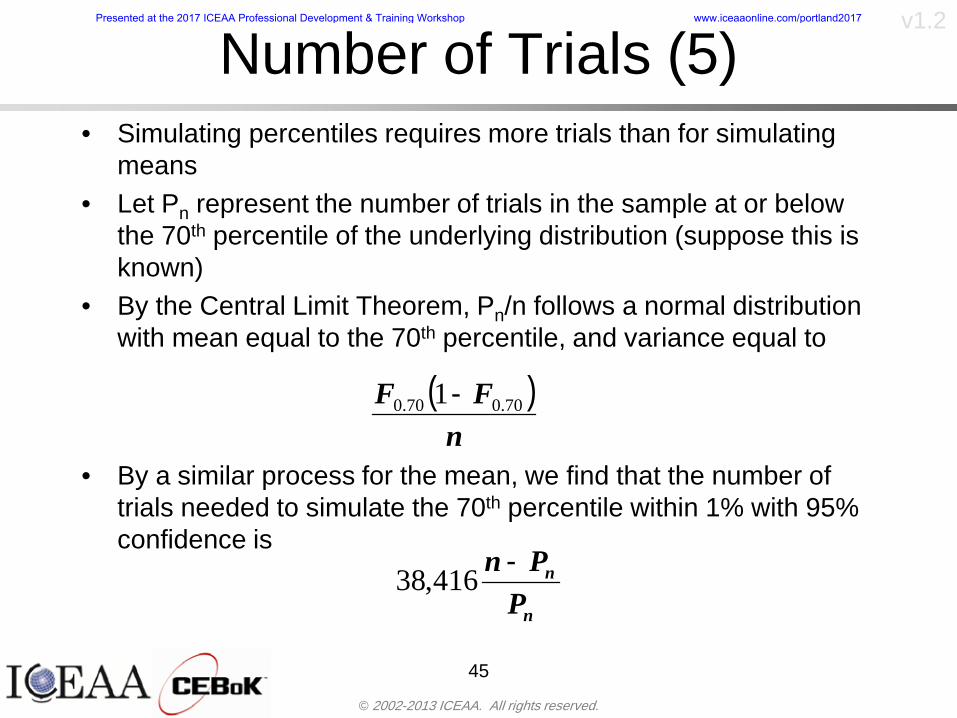
copy 2002-2013 ICEAA All rights reserved
v12
Number of Trials (5)bull Simulating percentiles requires more trials than for simulating
meansbull Let Pn represent the number of trials in the sample at or below
the 70th percentile of the underlying distribution (suppose this is known)
bull By the Central Limit Theorem Pnn follows a normal distribution with mean equal to the 70th percentile and variance equal to
bull By a similar process for the mean we find that the number of trials needed to simulate the 70th percentile within 1 with 95 confidence is
45
( )n
FF 700700 1-
n
n
PPn -41638
Presented at the 2017 ICEAA Professional Development amp Training Workshop wwwiceaaonlinecomportland2017
copy 2002-2013 ICEAA All rights reserved
v12
Number of Trials (6)bull If Pn 070 for all n then n is approximately
bull For the sake of comparison suppose CV = 03 (reasonable approximation for hardware development) then the number of trials needed to simulate the mean with the same accuracy is then ldquoonlyrdquo 11525
bull More trials are needed to accurately simulate percentiles than means
46
( ) 46416703041638
70704168341638 =divide
oslashouml
ccedilegraveaelig=divide
oslashouml
ccedilegraveaelig -
=-
nnn
PPn
n
n
Presented at the 2017 ICEAA Professional Development amp Training Workshop wwwiceaaonlinecomportland2017
copy 2002-2013 ICEAA All rights reserved
v12
Methods of Simulationbull Monte Carlo simulation is a standard term for
simulationbull However there is an improvement on Monte Carlo
that improves the accuracy of the results of a simulation for a given number of trials
bull This method is call the Latin Hypercube approach to simulationndash Similar to Monte Carlo but an equal number of draws are taken
from a set of subintervals for example dividing the interval (01) into [00001) [0102)hellip [0910]
ndash Instead of 10 trials from [01] we have one trial from each subinterval
ndash Rough rule of thumb is Latin Hypercube takes 30 fewer trials to achieve similar accuracy to Monte Carlo
47
Presented at the 2017 ICEAA Professional Development amp Training Workshop wwwiceaaonlinecomportland2017
copy 2002-2013 ICEAA All rights reserved
v12
Probability Model ndash Correlationbull Correlation exists between work breakdown structure
(WBS) cost element costs and between cost and schedule
bull Correlation is a necessary consideration in cost risk analysis
bull Correlation is a number that can vary between -1 and +1 and represents the strength of the relationship between the two variablesndash If both variable have a tendency to move in the same direction
correlation is positivendash If when one variable increases the other tends to decrease and
vice-versa the correlation between the two variables is negative
Presented at the 2017 ICEAA Professional Development amp Training Workshop wwwiceaaonlinecomportland2017
copy 2002-2013 ICEAA All rights reserved
v12
Correlation And Causationbull Note that correlation is not causation however
causation implies correlationndash For example shark attacks and ice cream sales at the beach
bull For example for a launch vehicle structure increasing the diameter will not only result in an increase in the structures cost but will also result in higher costs for thermal coating (paint etc)
bull Also simply because two subsystems do not appear to be related does not mean they are not correlatedndash For example structures and computer equipment seemingly
have little relation to one another however an external factor such as a funding cut or a strike will impact all subsystems leading to delays and increasing cost across the board
ndash Thus everything in a WBS has some correlationUnit III - Module 9 49
Presented at the 2017 ICEAA Professional Development amp Training Workshop wwwiceaaonlinecomportland2017
copy 2002-2013 ICEAA All rights reserved
v12
The Importance of Correlationbull Percent that total cost standard deviation is underestimated
when correlation assumed to be 0 instead of r given nWBS elements
Unit III - Module 9 5050
0
20
40
60
80
100
0 01 02 03 04 05 06 07 08 09 1Actual Correlation
Perce
nt Un
deres
timate
d
n = 10
n = 30
n = 100n = 1000
0
20
40
60
80
100
0 01 02 03 04 05 06 07 08 09 1Actual Correlation
Perce
nt Un
deres
timate
d
n = 10
n = 30
n = 100n = 1000
Reference 32nd Annual DOD Cost Analysis Symposium Advanced Training Session ldquoWhy Correlation Matters in Cost Estimatingrdquo Stephen A Book
Presented at the 2017 ICEAA Professional Development amp Training Workshop wwwiceaaonlinecomportland2017
copy 2002-2013 ICEAA All rights reserved
v12
The Importance of Correlation (2)bull For example if correlation is assumed to be 0 for all
elements in a 30 element WBS and the actual correlation is 20 then the total cost standard deviation is underestimated by 60
bull For example assume the total cost is modeled as a normal distribution with mean = 100
bull If correlation is assumed to be zero with total cost standard deviation = 12 when correlation is actually 20 then the true underlying standard deviation is actually 30
bull 70th percentile with zero correlation assumption is 106
bull 70th percentile with 20 correlation is 116 Unit III - Module 9 51
Presented at the 2017 ICEAA Professional Development amp Training Workshop wwwiceaaonlinecomportland2017
copy 2002-2013 ICEAA All rights reserved
v12
Measures of Correlationbull Two measures of correlation are commonly used in
cost risk analysesndash Pearsonrsquos product-moment correlation coefficient ndash Spearmanrsquos rank correlation coefficient
bull Garvey and others recommend using Pearsonrsquos product-moment correlation coefficient correlation for cost risk analysesndash Method of moments uses this but there are two options in
simulationndash Popular simulation packages like Risk and Crystal Ball use
rank correlation but in practice this has been found to make little difference
ndash Pearson product-moment correlation has been incorporated into Risk+
52
Presented at the 2017 ICEAA Professional Development amp Training Workshop wwwiceaaonlinecomportland2017
copy 2002-2013 ICEAA All rights reserved
v12
Pearson Correlationbull Pearsonrsquos product-moment correlation measures
degree of linearity between two random variables bull If two random variables are perfectly linear (eg Y =
aX + b) with positive slope then the Pearson product-moment correlation between X and Y denoted by rXY is +1
53
X X
Y Y Y
XNegative Correlation Positive Correlation No Correlation
middotmiddot
middotmiddot
middotmiddot middotmiddot
middotmiddot
middot
middot
middotmiddotmiddot
middotmiddot
middotmiddot
middotmiddot middot
middot
middot
middotmiddotmiddotmiddotmiddotmiddotmiddotmiddot
middotmiddotmiddotmiddot
middotmiddot
middotmiddot middotmiddotmiddotmiddot
middotmiddotmiddot
middotmiddotmiddotmiddot
middotmiddotmiddot
middotmiddotmiddot
middotmiddot
middot
middot middotmiddot
middot middotmiddotmiddotmiddot middotmiddot middot middotmiddot middot middot
middotmiddot middot
middotmiddotmiddotmiddotmiddot middot middotmiddot
middotmiddot
middot
middotmiddot
middotmiddot middot
middot middot middot
middotmiddot middot
middotmiddotmiddot
middotmiddot
middot middot
Presented at the 2017 ICEAA Professional Development amp Training Workshop wwwiceaaonlinecomportland2017
copy 2002-2013 ICEAA All rights reserved
v12
Spearman Correlationbull Spearmanrsquos rank correlation measures the
monotonicity between two random variablesbull If two random variables are perfectly monotonically
increasing (eg Y = X2) then the Spearman rank correlation denoted by rXY is +1
bull The two measures can be significantly different
54
10 20 30 40 50 60
100
200
300
096 097 098 099 1
1
060
020
040
080
Eff
ort (
Staf
f-M
onth
s)
Software Size I KDSI
y = 28z12y
z x
yy = x100
0 pound x pound 1
Figure 5-9A Figure 5-9B
Pearson Correlation = 09976 Rank Correlation = 1
Pearson Correlation = 024 Rank Correlation = 1
X(x ) ~ Unif(01)
Reference Probability Methods for Cost Uncertainty Analysis A Systems Engineering Perspective Paul R Garvey
Presented at the 2017 ICEAA Professional Development amp Training Workshop wwwiceaaonlinecomportland2017
copy 2002-2013 ICEAA All rights reserved
v12
Unit III - Module 9 55
200
250
300
350
400
1000 1200 1400 1600 1800 2000
Recurring Production
SEPM
200
250
300
350
400
1000 1200 1400 1600 1800 2000
Recurring Production
SEPM
Functional Correlationbull Old No Functional
Correlation Simulation run with WBS items entered as values
bull New Simulation run with functional dependencies entered as they are in cost model
CorrelatedNot Correlated
Note shift of mean and increased variability
Presented at the 2017 ICEAA Professional Development amp Training Workshop wwwiceaaonlinecomportland2017
copy 2002-2013 ICEAA All rights reserved
v12
Risk Measuresbull ldquoWestern Europe conquered the word because of a
technological revolution that started because of attempts to measure the worldrdquo ndash Phillipe Jorion ndash In the same way attempts to measure risk will lead to better project
managementbull Risk management for DoD and NASA agencies focuses
primarily on funding projects to a single percentile ndash NASA policy explicitly mentions 70 and 50ndash This is known as ldquoValue at Riskrdquo and is prevalent in the banking and
financial industry
56
Presented at the 2017 ICEAA Professional Development amp Training Workshop wwwiceaaonlinecomportland2017
copy 2002-2013 ICEAA All rights reserved
v12
Value at Risk (VaR)bull VaR is a percentile of the cost risk
distributionndash VaR funding at the 70th percentile means that
there is a 30 chance of final project cost exceeding the funded amount (budget)
bull VaR has some meritsndash Common measure can be used to compare
different projects and programsndash Easily understood by senior managers and
decision makers
57
Presented at the 2017 ICEAA Professional Development amp Training Workshop wwwiceaaonlinecomportland2017
copy 2002-2013 ICEAA All rights reserved
v12
Why 70th or 80th Percentilebull Typical policy guidance involves funding at the 70th or 80th
percentile Why fund as such a low percentilebull There is some incentive to not over-fundbull For a normal distribution an inflection point occurs near the 80th
percentile meaning that for values above 80 confidence achieving higher levels of confidence can only be achieved by spending greater dollar amounts at an increasing rate
58
-05-04-03-02-01
00102030405
0 05 1 15 2 25 3
Standard Deviations from Mean
Normal Distribution
First DerivativeSlopeVelocity
Second DerivativeConvexityAcceleration
Inflection point at one standard deviation above the mean (~84th
percentile)
Presented at the 2017 ICEAA Professional Development amp Training Workshop wwwiceaaonlinecomportland2017
copy 2002-2013 ICEAA All rights reserved
v12
Funding Above Inflection Pointsbull As the percentile goes above the 80th percentile the amount
needed to achieve that higher level of confidence begins to increase at an increasing rate as is evident from the graph
59
0
10
20
30
40
50
60
70
50 55 60 65 70 75 80 85 90 95 100
$ Ab
ove
MEa
n to
Ach
ieve
Per
cent
ile
Percentile (Confidence Level)
Presented at the 2017 ICEAA Professional Development amp Training Workshop wwwiceaaonlinecomportland2017
copy 2002-2013 ICEAA All rights reserved
v12
Why Budget to the 70th or 80thbull Government projects are funded at the 70th or 80th percentilesbull Why not the 90th or 99th percentile Wonrsquot that help prevent
overrunsndash As we have seen percentiles do not add across programs
bull The sum of the 80th percentiles does NOT equal the total 80th percentile
ndash This is because the individual programs are riskier than the entire suite of missions
bull Known as the ldquoPortfolio effectrdquo (more or this later)
ndash Funding at the 80th gives confidence that the entire portfolio will be adequately funded
bull And since there is an inflection point near the 80th percentile funding above that level quickly becomes cost prohibitive
60
Presented at the 2017 ICEAA Professional Development amp Training Workshop wwwiceaaonlinecomportland2017
copy 2002-2013 ICEAA All rights reserved
v12
Inflection Points for Lognormalbull For a lognormal the inflection point
variesndash Coefficient of variation equal to 10 equates to an
inflection point at the 70th percentile
61
0
10
20
30
40
50
60
70
050 060 070 080 090 100
Coef
ficen
t of V
aria
tion
Percentile of the Inflection Point
Presented at the 2017 ICEAA Professional Development amp Training Workshop wwwiceaaonlinecomportland2017
copy 2002-2013 ICEAA All rights reserved
v12
Issues with Percentile Fundingbull However risk management does not stop at a
specific percentilendash What happens when the 70th percentile is exceeded
bull Any effective risk management policy should prescribe what happens after a bad event occursndash With VaR we only know when a bad event has occurred ndash Also funding at a relatively low level means we have no true
sense of the real risks that should be guarded against
62
Presented at the 2017 ICEAA Professional Development amp Training Workshop wwwiceaaonlinecomportland2017
copy 2002-2013 ICEAA All rights reserved
v12
ldquoHere There Be Dragonsrdquobull On old maps uncharted territory was often
marked with monsters or dragons
63
A section of the Carta Marina by Olaus Magnus 16th Century
Presented at the 2017 ICEAA Professional Development amp Training Workshop wwwiceaaonlinecomportland2017
copy 2002-2013 ICEAA All rights reserved
v12
Distribution Comparisonbull Four different distributions with the same 70th
percentile
bull Should we expect the tails to be similar
64
0
10
20
30
40
50
60
70
80
0 100 200 300 400 500 600
Perc
entil
eCo
nfid
ence
Lev
el
Triangular
Normal
Lognormal
Pareto
Presented at the 2017 ICEAA Professional Development amp Training Workshop wwwiceaaonlinecomportland2017
copy 2002-2013 ICEAA All rights reserved
v12Distribution Comparison Tail Behavior
bull The normal and triangular distributions have similar tails but the lognormal and Pareto have much fatter right tails
65
70
75
80
85
90
95
100
500 1500 2500 3500 4500 5500
Perc
entil
eCo
nfid
ence
Lev
el
Triangular
Normal
Lognormal
Pareto
Here There Be Dragons
Presented at the 2017 ICEAA Professional Development amp Training Workshop wwwiceaaonlinecomportland2017
copy 2002-2013 ICEAA All rights reserved
v12Distribution Comparison ndash Tail Behavior (Table)
bull There is significant tail risk for the lognormal and the Paretobull The 99th percentile for the Pareto is 1000 times greater than
the 70th percentilendash Risk seen in financial markets and in catastrophic risks like natural
disasters bull Four different projects follow the four different risk profiles seen
in this example should clearly have different risk management approaches but 70th percentile funding indicates the same risk management approach for all four
66
Percentile Triangular Normal Lognormal Pareto 70th $600 $600 $600 $600 80th $680 $660 $770 $1430 90th $770 $750 $1070 $5880 95th $840 $820 $1410 $23750 99th $930 $950 $2350 $600000
Presented at the 2017 ICEAA Professional Development amp Training Workshop wwwiceaaonlinecomportland2017
copy 2002-2013 ICEAA All rights reserved
v12Percentile Budgeting is Not Risk Management
bull Percentile budgeting ne effective risk management policybull Suppose that you are shopping for a new car You
mention that safety is your top concern The salesman says he has a great safe car available You ask about the air bags Do they work The salesman answers ldquoOf course Seventy percent of the time they work fine Only 30 of the time the air bags will fail to deployrdquo Would you buy such a car Hedge fund manager David Einhorn has stated ldquoRisk management is the air bag that must always work but only in the multi-sigma event where you have an accidentrdquo
67
Risk management is the air bag that must always work but only in the multi-sigma event where you
have an accident
Presented at the 2017 ICEAA Professional Development amp Training Workshop wwwiceaaonlinecomportland2017
copy 2002-2013 ICEAA All rights reserved
v12
Joint Confidence Level Analysisbull Schedules are risky toobull For 98 recent NASA missions average
schedule growth was 38ndash Not as high as cost growth but still significant
68
0
5
10
15
20
25
30
35
40
Schedule
Cost
Presented at the 2017 ICEAA Professional Development amp Training Workshop wwwiceaaonlinecomportland2017
copy 2002-2013 ICEAA All rights reserved
v12
Schedules Impact Costbull Changes in schedule can have enormous
impacts on cost ndash Schedule slips can lead to cost increases
bull Fixed programmatic costs must be paid on a regular basisndash Achieving schedule milestones early can result in cost
savings
bull Schedule is an important consideration in cost analysis including cost risk analysis
bull However we must be careful in correctly integrating cost and schedule riskndash Schedule is not simply an input but is dependent on many of
the same factors that drive cost
69
Presented at the 2017 ICEAA Professional Development amp Training Workshop wwwiceaaonlinecomportland2017
copy 2002-2013 ICEAA All rights reserved
v12
The Relationship of Cost to Schedulebull Cost and schedule are positively correlated
ndash A larger program with bigger scope with take longer to complete than a smaller simpler program
bull However longer schedules do not always equate to higher cost nor shorter schedules with lower costndash Highly compressed schedules relative to the
optimal schedule can lead to large overrunsbull Compressed schedules are commonplace for
many planetary missions
70
Presented at the 2017 ICEAA Professional Development amp Training Workshop wwwiceaaonlinecomportland2017
copy 2002-2013 ICEAA All rights reserved
v12The Impact of Schedule GrowthCompression on Cost
bull Compressed schedules lead to cost growth and based on existing research is actually more expensive than schedule slippages
71
0
20
40
60
80
100
120
140
160
-50 -25 0 25 50 75 100
Percentage Change in Schedule
Perc
enta
ge C
hang
e in
Cos
t due
to
Sche
dule
Cha
nge
Source Smart CB ldquoCost and Schedule Interrelationshipsrdquo 2007 NASA Cost Symposium
Presented at the 2017 ICEAA Professional Development amp Training Workshop wwwiceaaonlinecomportland2017
copy 2002-2013 ICEAA All rights reserved
v12Schedule as an Independent Variable
bull Why not simply add schedule as an input to cost-estimating relationships (CERs)
bull Schedule is often treated as an independent variable ndash schedules are often determined independently of cost considerationsndash Cost may not be considered explicitly although budgets and
schedules are determined based on scope and other common factors
bull In 2006 SAIC undertook a research task to determine the impact of schedule on cost and added schedule as an independent variable to the CERs in the NASAAir Force Cost Model (NAFCOM) to see if schedule provided any improvement in goodness of fit
72
Presented at the 2017 ICEAA Professional Development amp Training Workshop wwwiceaaonlinecomportland2017
copy 2002-2013 ICEAA All rights reserved
v12
Schedule is a Dependent Variablebull Since NAFCOM includes an exhaustive list of cost drivers the inclusion
of schedule should give an indication of whether there is any additional independent value added from schedule independent of the cost drivers
bull In the study schedule was added to 10 subsystem-level CERs
ndash In each case the addition of schedule did NOTimprove the goodness of fit and schedule was NOT found to be a statistically significant cost driver (given the presence of the other variables) for any of the 10 CERs
bull Standard errors for the CERs increased due to decrease in degrees of freedom
bull Thus schedule as an independent variable did not provide any additional explanation of variation in historical cost
bull This is because schedule is truly NOT an independent variable but a dependent variable and is a function of the same factors that drive cost
73
Presented at the 2017 ICEAA Professional Development amp Training Workshop wwwiceaaonlinecomportland2017
copy 2002-2013 ICEAA All rights reserved
v12
Incorporation of Schedule in Cost Risk
bull When using subjective methods care must be taken in applying schedule to cost risk analysis
bull Since schedule is a dependent variable treating it independently from other factors when assessing its impact on cost can lead to a double count of independent variables in the cost risk analysis
bull Direct inclusion of schedule in a cost risk analysis effectively doubles the influence of each cost driver
ndash Incorrectly leads to broader risk ranges
74
CostWeight
HeritageNewness
Technology Readiness Schedule
Presented at the 2017 ICEAA Professional Development amp Training Workshop wwwiceaaonlinecomportland2017
copy 2002-2013 ICEAA All rights reserved
v12Subjective Cost Risk Methods and Overinclusion of Risk Factors
bull Subjective methods are suitable when data are scarce or not availablebull However care must be taken not to treat correlated sources of risk
such as schedule as independent of each otherbull Example ndash a subjective risk analysis incorporated technology readiness
design risk requirements stability integration risk and schedule and treated each source of risk as independent
bull Risk triangle high value without schedule risk was 31 times the point estimate
bull Risk triangle high value with schedule risk added on top of other sources of risk treated independently was 34 times the point estimate
bull Risk triangle taking correlation between sources of risk into account in a rigorous statistical manner has a high value 15 times the point estimate less than half the effect when treating sources of risk as independent
75
Presented at the 2017 ICEAA Professional Development amp Training Workshop wwwiceaaonlinecomportland2017
copy 2002-2013 ICEAA All rights reserved
v12Fundamental Equation of Cost and Schedule Interrelationships
bull The Fundamental Equation of the Relationship Between Cost and Schedule is
Time = Moneybull This is a well known adage that time is money Your boss at
work may even mention this to you from time to time or if you are the boss you are all too aware of this iron law
bull Because time is money cost and schedule risk should be modeled jointly not with schedule as an independent cost driver
bull Note that cost and schedule are not perfectly correlatedndash Cost can sometimes ldquobuy downrdquo schedule extra money can be
spent to meet a deadline since in some cases additional effort to hasten the completion of a task
76
Presented at the 2017 ICEAA Professional Development amp Training Workshop wwwiceaaonlinecomportland2017
copy 2002-2013 ICEAA All rights reserved
v12How to (Correctly) Incorporate Schedule into Cost Risk Analysis
bull The best way to model cost and schedule risk is to develop a joint cost and schedule model based on the same data
bull Since such models are not currently available the next best approach is to model cost and schedule independently and then integrate cost and schedule risk analyses using joint probability distributions taking into account correlation between cost and schedulendash This approach pioneered by Paul Garvey and Steve Book is
considered industry best practicendash This is a practical method mathematically tractable and follows
naturally from the Fundamental Equation of Cost and Schedule Interrelationships
77
Book S A ldquoQuantifying the Relationship Between Cost and Schedulerdquo The Measurable News Winter 2007-2008 pp 11-15Garvey PR Probability Methods for Cost Uncertainty Analysis A Systems Engineering Perspective New York Marcel Dekker 2000 pp 308-335
Presented at the 2017 ICEAA Professional Development amp Training Workshop wwwiceaaonlinecomportland2017
copy 2002-2013 ICEAA All rights reserved
v12
Joint Lognormal and Normal Distributions
bull Cost and schedule are typically modeled as some combination of Normal and Lognormal probability distributionsndash Studies by The Aerospace Corporation the MITRE
Corporation Wyle Labs and SAIC have found that the Lognormal probability distribution almost always serves as a good model for both the schedule distribution and the cost distribution
ndash The Normal distribution may also be appropriate in some instances and depending upon the level of confidence at which budgets are set may even be more conservative and logically consistent than the Normal distribution
ndash Joint Lognormal and Normal distributions are defined by a pair of mean and standard deviations and a level of correlation between the two
78
Presented at the 2017 ICEAA Professional Development amp Training Workshop wwwiceaaonlinecomportland2017
copy 2002-2013 ICEAA All rights reserved
v12Modeling Cost and Schedule as a Bivariate Distribution
bull In the approach set forth by Book and Garvey cost risk is assessed and the top-level distribution is modeled as a Lognormal (or Normal) distribution schedule risk is assessed and the overall schedule risk is modeled as a Lognormal (or Normal) distribution
bull The two distributions are combined into a Bivariate distribution by assigning a correlation between the two and by treating the two distributions as the marginal distributions of a Bivariate Lognormal distributionndash Other combinations include a Bivariate Normal or a Bivariate
Normal-Lognormal
79
Presented at the 2017 ICEAA Professional Development amp Training Workshop wwwiceaaonlinecomportland2017
copy 2002-2013 ICEAA All rights reserved
v12Bivariate Lognormal Distribution for Cost and Schedule
bull Cost is often observed to be Lognormal when strong positive correlations are present among the systemrsquos WBS cost element costs
bull A systemrsquos schedule is often observed (from Monte Carlo simulations) to be Lognormal if it is the sum of many positively correlated schedule activities in an overall schedule network
bull If Lognormal distributions characterize a systemrsquos cost and schedule then the Bivariate Lognormal could serve as an assumed model of their joint distributionndash In this case the marginal distribution of each of cost and schedule is
Lognormalbull Other possibilities for modeling cost and schedule as a Bivariate
distribution include a Bivariate Normal or a Bivariate Normal-Lognormal distributionndash All these combinations are analytically tractable
80
Presented at the 2017 ICEAA Professional Development amp Training Workshop wwwiceaaonlinecomportland2017
copy 2002-2013 ICEAA All rights reserved
v12Bivariate Lognormal for Cost and Schedule
bull Contour Plots of a Bivariate Lognormal
81
Presented at the 2017 ICEAA Professional Development amp Training Workshop wwwiceaaonlinecomportland2017
copy 2002-2013 ICEAA All rights reserved
v12Correlation Between Cost and Schedule
bull Cost and schedule are positively correlated but not perfectly sondash For example it is possible to have a schedule underrun and a cost
overrunbull Based on cost and schedule growth data for 50 completed NASA
programs the correlation between development cost and development schedule is 70
82
00
200
400
600
800
1000
1200
-500 00 500 1000 1500 2000 2500Historical Cost Growth
Hist
oric
al S
ched
ule
Gro
wth
r = 715
Presented at the 2017 ICEAA Professional Development amp Training Workshop wwwiceaaonlinecomportland2017
copy 2002-2013 ICEAA All rights reserved
v12Correlation Between Cost and Schedule Caveats
bull Based on historical data recommended correlation between cost and schedule is 70 but this could be higher or lower depending upon program circumstancesndash If program is budget constrained cost and schedule will be
more highly correlated (go as you pay)ndash If program is schedule constrained cost and schedule will
have lower correlation perhaps even negative correlation ndash Smaller programs have smaller correlation between cost and
schedule riskbull Relatively easy to ldquohurry uprdquo and finish on time or even early if
needed
83
Presented at the 2017 ICEAA Professional Development amp Training Workshop wwwiceaaonlinecomportland2017
copy 2002-2013 ICEAA All rights reserved
v12
Conditional Confidence Levelsbull Given a programrsquos project schedule we can determine the cost
risk distribution conditional upon the given schedulebull Conditional cost S-curves are steeper than unconditional
(marginal) cost S-curves between some uncertainty has been removed because schedule is fixed
84
Presented at the 2017 ICEAA Professional Development amp Training Workshop wwwiceaaonlinecomportland2017
copy 2002-2013 ICEAA All rights reserved
v12
Joint Confidence Levelsbull Joint 65 confidence represents the probability of
achieving both 65 confidence in cost AND 65 confidence in schedulendash This is different than achieving 65 cost confidence alone
or achieving 65 schedule confidence alonebull Due to the imperfect correlation between cost and schedule it
is possible to achieve a 65 cost confidence with a lower level of schedule confidence
bull Restricting the schedule confidence thus requires additional $ to achieve a given level of confidence
85
X
Y
Possible Values for Which X gt a Possible Values for
Which X gt a and Y gt b
a
b
Presented at the 2017 ICEAA Professional Development amp Training Workshop wwwiceaaonlinecomportland2017
copy 2002-2013 ICEAA All rights reserved
v12Joint Confidence Levels Versus Cost Confidence Levels Only
bull Example of the differences between cost confidence schedule confidence conditional cost confidence and joint cost and schedule confidence
86
Joint Cost-Schedule Confidence Iso-Curves
Cost (RY$M)
Sche
dule
(Mon
ths)
65 Confidence
50 Confidence
70 Confidence
65 Cost Confidence AggressiveSchedule65 Cost ConfidenceScheduleGiven 65 Schedule ConfidenceUnconditional 65 CostConfidenceUnconditional 65 ScheduleConfidence
65 Cost Confidence 65 Joint Cost and Schedule
Confidence for 65 Schedule Confidence
Presented at the 2017 ICEAA Professional Development amp Training Workshop wwwiceaaonlinecomportland2017
copy 2002-2013 ICEAA All rights reserved
v12
Joint Cost and Schedule Confidence
bull Can examine pairs of cost and schedule that achieve a given level of confidence
bull Provides insights into the trade-offs between cost and schedule for a given level of confidencendash Possible to increase cost confidence by giving a
project more time in some instances or possible to ldquobuy downrdquo schedule
bull But these have limits and are shown in the iso-cost and schedule confidence curves
87
Presented at the 2017 ICEAA Professional Development amp Training Workshop wwwiceaaonlinecomportland2017
copy 2002-2013 ICEAA All rights reserved
v12Cost and Schedule Trade-offs for a Given Level of Joint Confidence
bull Hypothetical Example
88
Cost (RY$M)
Schedule (Months)
$100 48$99 48$89 49$87 50$85 51$85 52$84 53$83 55$83 55$83 56
Cost and Schedule 65 Confidence Iso-Curve
4748495051525354555657
$80 $82 $84 $86 $88 $90 $92 $94 $96 $98 $100
Cost (RY$ M)
Sche
dule
(Mon
ths)
Presented at the 2017 ICEAA Professional Development amp Training Workshop wwwiceaaonlinecomportland2017
copy 2002-2013 ICEAA All rights reserved
v12Policy Considerations for Confidence Levels
bull For large programs the difference between the amount of money needed to achieve 65 cost confidence independent of schedule and joint 65 cost and schedule confidence can represent hundreds of millions and even billions of dollars
89
Joint Cost-Schedule Confidence Iso-Curves
Cost (RY$M)
Sche
dule
(Mon
ths)
65 Confidence
65 Cost Confidence AggressiveSchedule
65 Cost ConfidenceScheduleGiven 65 Schedule Confidence
Unconditional 65 CostConfidence
Joint Cost and Schedule Confidence for 65 Cost Confidence and Program Baseline Schedule is Less Than 35
65 Cost Confidence Independent of Schedule Cost Needed to Achieve
Both 65 Joint Cost and Schedule Confidence for the Schedule with 65 Confidence
Presented at the 2017 ICEAA Professional Development amp Training Workshop wwwiceaaonlinecomportland2017
copy 2002-2013 ICEAA All rights reserved
v12
Copulasbull More generally any combination of distributions can
be used (more than just normal and lognormal)ndash Termed ldquocopulardquo from the Italian word for ldquocouplerdquondash Copulas are a way to combine marginal distributions of any
number and type into a joint distributionbull More formally a copula is a multivariate joint distribution defined
on the n-dimensional unit cube [0 1]n such that every marginal distribution is uniform on the interval [0 1]
bull (The bivariate form of) Sklarrsquos theorem states that for any bivariate distribution function H(x y) let F(x) = H(x infin) and G(y) = H(infin y) be the univariate marginal probability distribution functions Then there exists a copula C such that H(xy)=C(F(x)G(y))
ndash Copulas are widely used in risk management for investments and insurance
bull Considered industry best practice (Li 2000)bull Marketed as part of JP Morganrsquos CreditMetrics suite of tools
(Gupton et Al 1997)90
Presented at the 2017 ICEAA Professional Development amp Training Workshop wwwiceaaonlinecomportland2017
copy 2002-2013 ICEAA All rights reserved
v12Parametric Joint Cost and Schedule Analysis
bull A parametric model based on a consistent data set with a set of overlapping cost and schedule drivers is a cleaner way to model cost and schedule
91
CostWeight
HeritageNewness
Technology Readiness
Schedule
0
20
40
60
80
100
Confidence
Joint Cost and Schedule Confidence
Schedule
Cost
Lognormal Distribution PDF and CDF
0102030405060708090100
200 300 400 500 600 700 800 900 1000Cost $
Con
fiden
ce L
evel
0
00002
00004
00006
00008
0001
00012
00014
00016
Prob
abili
ty D
ensi
ty
CDFPDF
Lognormal Distribution PDF and CDF
0102030405060708090100
200 300 400 500 600 700 800 900 1000Cost $
Con
fiden
ce L
evel
0
00002
00004
00006
00008
0001
00012
00014
00016
Prob
abili
ty D
ensi
ty
CDFPDF
Presented at the 2017 ICEAA Professional Development amp Training Workshop wwwiceaaonlinecomportland2017
copy 2002-2013 ICEAA All rights reserved
v12Parametric Joint Cost and Schedule Analysis (2)
bull Joint cost and schedule risk analysis produced naturally by the integrated modelndash Addresses several issues with the copula
approachbull Tail dependencybull Correlation ndash no need to assign correlation
between cost and schedulebull Consistency of cost and schedule models
92
Presented at the 2017 ICEAA Professional Development amp Training Workshop wwwiceaaonlinecomportland2017
copy 2002-2013 ICEAA All rights reserved
v12
Resource-Loaded Schedulesbull Involves assigning cost and schedule risks to a resource-loaded schedule
networkbull Bottom-up approach
ndash More labor intensive than parametrics but can also provide more insight
ndash Can answer questions than parametric typically cannot such as how much do reserve requirements decrease if a specific risk is retired
bull Currently being implemented in Constellation programbull Has same issue as all bottom-up models hard to count all the risks and model
them discretely
ndash As a result there is a tendency to reflect less risk than indicated by history
ndash ldquoThere are more things in heaven and earth Horatio than are dreamt of in your philosophyrdquo William Shakespeare Hamlet Act I Scene V
93
Presented at the 2017 ICEAA Professional Development amp Training Workshop wwwiceaaonlinecomportland2017
copy 2002-2013 ICEAA All rights reserved
v12Resource-Loaded Schedules Vs Parametrics
bull Parametric most appropriate for early estimatesndash But also good for high-level checks as project progresses
bull As plans take shape lower level modeling may be more appropriate
94 1
CONCEPTUALDEVELOPMENT
PROJECTDEFINITION DESIGN DEVELOPMENT OPERATIONS
PARAMETRIC PARAMETRIC
ANALOGY
ENGINEERING (Bottoms Up)
$PARAMETRIC
DETAILED
$
Pre Phase A Phase B Phase CDPhase A Phase EPre Phase A Phase B Phase CDPhase A Phase E
Risk = f(Cost Estimating Relationship Inputs eg mass power data rate TRL new design etc)
Risk = f(cost and schedule variation of the analogous elements)
Risk = f(variation of detailed inputs eg labor hours rates materials etc)
Presented at the 2017 ICEAA Professional Development amp Training Workshop wwwiceaaonlinecomportland2017
copy 2002-2013 ICEAA All rights reserved
v12
Resource-Loaded Schedulesbull Methodology has been demonstrated in other
industriesndash Construction oil and gasndash Analysis has not been traditionally done on highly uncertain
complex development projects bull Methodology focuses on project baseline schedule
ndash In baseline schedule all tasks are resource loaded to represent a baseline schedule and cost standpoint
ndash Resource loaded schedule is ldquorolledrdquo up to a manageable level
ndash Based on the risk and uncertainties identified schedule distributions are applied to each rolled up task
ndash Cost uncertainties are also applied to rolled up tasksbull Uncertainties include labor rate man power etc
ndash A Monte Carlo simulation is run to develop joint cost-schedule distributions
95
Presented at the 2017 ICEAA Professional Development amp Training Workshop wwwiceaaonlinecomportland2017
copy 2002-2013 ICEAA All rights reserved
v12
Unit III - Module 9 96
Execution ndash Cross Checksbull Means The mean cost growth factor for WBS items
can be compared to history as a way to cross check results
bull CVs The CV of the cost growth factors for WBS items can be compared to history as a way to cross check results
bull Inputs Checks are performed on inputs or other parameters to see if historical values are in line with program assumptionsndash Example Historical risk scores can be compared to program
risk scores to see if risk assessors are being realistic and to see if the underlying database is representative of the program
11
Presented at the 2017 ICEAA Professional Development amp Training Workshop wwwiceaaonlinecomportland2017
- Cost and Schedule Risk Analysis Basic
- Acknowledgments
- Unit Index
- Risk Overview
- Agenda
- Introduction
- Risk Analysis Terms
- Are Our Costs Realistic
- Historical Cost Growth
- Sources of Cost Risk
- Point Estimates of Cost
- Types of Risk
- Point Estimates Vs Risk Estimates
- Cost Risk and Probability
- Probability Model ndash Distribution
- Probability Model ndash Distribution
- Probability ndash Top-Level Distribution
- S-Curves and Confidence Levels
- Example ndash Normal Distribution
- Confidence Levels
- Measuring Parametric Model Uncertainty
- Parametric Model Example
- Weight Uncertainty
- Estimating Uncertainty
- Estimating Uncertainty (2)
- Estimating Uncertainty (3)
- Aggregating Risk
- WBS Example
- WBS and Risk
- Aggregating Risk
- Percentiles Do Not Add
- Percentiles Do Not Add (2)
- Percentiles Do Not Add (3)
- Methods for Aggregating Risk
- Monte Carlo Simulationfor Risk Analysis
- Monte Carlo Simulation
- Using Random Numbers to Simulate Distributions
- Simulating a Triangular Distribution
- Simulating a Triangular Distribution (2)
- Monte Carlo and the WBS
- Number of Trials
- Number of Trials (2)
- Number of Trials (3)
- Number of Trials (4)
- Number of Trials (5)
- Number of Trials (6)
- Methods of Simulation
- Probability Model ndash Correlation
- Correlation And Causation
- The Importance of Correlation
- The Importance of Correlation (2)
- Measures of Correlation
- Pearson Correlation
- Spearman Correlation
- Functional Correlation
- Risk Measures
- Value at Risk (VaR)
- Why 70th or 80th Percentile
- Funding Above Inflection Points
- Why Budget to the 70th or 80th
- Inflection Points for Lognormal
- Issues with Percentile Funding
- ldquoHere There Be Dragonsrdquo
- Distribution Comparison
- Distribution Comparison Tail Behavior
- Distribution Comparison ndash Tail Behavior (Table)
- Percentile Budgeting is Not Risk Management
- Joint Confidence Level Analysis
- Schedules Impact Cost
- The Relationship of Cost to Schedule
- The Impact of Schedule GrowthCompression on Cost
- Schedule as an Independent Variable
- Schedule is a Dependent Variable
- Incorporation of Schedule in Cost Risk
- Subjective Cost Risk Methods and Overinclusion of Risk Factors
- Fundamental Equation of Cost and Schedule Interrelationships
- How to (Correctly) Incorporate Schedule into Cost Risk Analysis
- Joint Lognormal and Normal Distributions
- Modeling Cost and Schedule as a Bivariate Distribution
- Bivariate Lognormal Distribution for Cost and Schedule
- Bivariate Lognormal for Cost and Schedule
- Correlation Between Cost and Schedule
- Correlation Between Cost and Schedule Caveats
- Conditional Confidence Levels
- Joint Confidence Levels
- Joint Confidence Levels Versus Cost Confidence Levels Only
- Joint Cost and Schedule Confidence
- Cost and Schedule Trade-offs for a Given Level of Joint Confidence
- Policy Considerations for Confidence Levels
- Copulas
- Parametric Joint Cost and Schedule Analysis
- Parametric Joint Cost and Schedule Analysis (2)
- Resource-Loaded Schedules
- Resource-Loaded Schedules Vs Parametrics
- Resource-Loaded Schedules
- Execution ndash Cross Checks
-
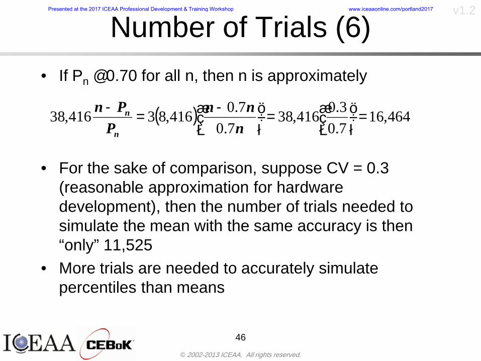
copy 2002-2013 ICEAA All rights reserved
v12
Methods of Simulationbull Monte Carlo simulation is a standard term for
simulationbull However there is an improvement on Monte Carlo
that improves the accuracy of the results of a simulation for a given number of trials
bull This method is call the Latin Hypercube approach to simulationndash Similar to Monte Carlo but an equal number of draws are taken
from a set of subintervals for example dividing the interval (01) into [00001) [0102)hellip [0910]
ndash Instead of 10 trials from [01] we have one trial from each subinterval
ndash Rough rule of thumb is Latin Hypercube takes 30 fewer trials to achieve similar accuracy to Monte Carlo
47
Presented at the 2017 ICEAA Professional Development amp Training Workshop wwwiceaaonlinecomportland2017
copy 2002-2013 ICEAA All rights reserved
v12
Probability Model ndash Correlationbull Correlation exists between work breakdown structure
(WBS) cost element costs and between cost and schedule
bull Correlation is a necessary consideration in cost risk analysis
bull Correlation is a number that can vary between -1 and +1 and represents the strength of the relationship between the two variablesndash If both variable have a tendency to move in the same direction
correlation is positivendash If when one variable increases the other tends to decrease and
vice-versa the correlation between the two variables is negative
Presented at the 2017 ICEAA Professional Development amp Training Workshop wwwiceaaonlinecomportland2017
copy 2002-2013 ICEAA All rights reserved
v12
Correlation And Causationbull Note that correlation is not causation however
causation implies correlationndash For example shark attacks and ice cream sales at the beach
bull For example for a launch vehicle structure increasing the diameter will not only result in an increase in the structures cost but will also result in higher costs for thermal coating (paint etc)
bull Also simply because two subsystems do not appear to be related does not mean they are not correlatedndash For example structures and computer equipment seemingly
have little relation to one another however an external factor such as a funding cut or a strike will impact all subsystems leading to delays and increasing cost across the board
ndash Thus everything in a WBS has some correlationUnit III - Module 9 49
Presented at the 2017 ICEAA Professional Development amp Training Workshop wwwiceaaonlinecomportland2017
copy 2002-2013 ICEAA All rights reserved
v12
The Importance of Correlationbull Percent that total cost standard deviation is underestimated
when correlation assumed to be 0 instead of r given nWBS elements
Unit III - Module 9 5050
0
20
40
60
80
100
0 01 02 03 04 05 06 07 08 09 1Actual Correlation
Perce
nt Un
deres
timate
d
n = 10
n = 30
n = 100n = 1000
0
20
40
60
80
100
0 01 02 03 04 05 06 07 08 09 1Actual Correlation
Perce
nt Un
deres
timate
d
n = 10
n = 30
n = 100n = 1000
Reference 32nd Annual DOD Cost Analysis Symposium Advanced Training Session ldquoWhy Correlation Matters in Cost Estimatingrdquo Stephen A Book
Presented at the 2017 ICEAA Professional Development amp Training Workshop wwwiceaaonlinecomportland2017
copy 2002-2013 ICEAA All rights reserved
v12
The Importance of Correlation (2)bull For example if correlation is assumed to be 0 for all
elements in a 30 element WBS and the actual correlation is 20 then the total cost standard deviation is underestimated by 60
bull For example assume the total cost is modeled as a normal distribution with mean = 100
bull If correlation is assumed to be zero with total cost standard deviation = 12 when correlation is actually 20 then the true underlying standard deviation is actually 30
bull 70th percentile with zero correlation assumption is 106
bull 70th percentile with 20 correlation is 116 Unit III - Module 9 51
Presented at the 2017 ICEAA Professional Development amp Training Workshop wwwiceaaonlinecomportland2017
copy 2002-2013 ICEAA All rights reserved
v12
Measures of Correlationbull Two measures of correlation are commonly used in
cost risk analysesndash Pearsonrsquos product-moment correlation coefficient ndash Spearmanrsquos rank correlation coefficient
bull Garvey and others recommend using Pearsonrsquos product-moment correlation coefficient correlation for cost risk analysesndash Method of moments uses this but there are two options in
simulationndash Popular simulation packages like Risk and Crystal Ball use
rank correlation but in practice this has been found to make little difference
ndash Pearson product-moment correlation has been incorporated into Risk+
52
Presented at the 2017 ICEAA Professional Development amp Training Workshop wwwiceaaonlinecomportland2017
copy 2002-2013 ICEAA All rights reserved
v12
Pearson Correlationbull Pearsonrsquos product-moment correlation measures
degree of linearity between two random variables bull If two random variables are perfectly linear (eg Y =
aX + b) with positive slope then the Pearson product-moment correlation between X and Y denoted by rXY is +1
53
X X
Y Y Y
XNegative Correlation Positive Correlation No Correlation
middotmiddot
middotmiddot
middotmiddot middotmiddot
middotmiddot
middot
middot
middotmiddotmiddot
middotmiddot
middotmiddot
middotmiddot middot
middot
middot
middotmiddotmiddotmiddotmiddotmiddotmiddotmiddot
middotmiddotmiddotmiddot
middotmiddot
middotmiddot middotmiddotmiddotmiddot
middotmiddotmiddot
middotmiddotmiddotmiddot
middotmiddotmiddot
middotmiddotmiddot
middotmiddot
middot
middot middotmiddot
middot middotmiddotmiddotmiddot middotmiddot middot middotmiddot middot middot
middotmiddot middot
middotmiddotmiddotmiddotmiddot middot middotmiddot
middotmiddot
middot
middotmiddot
middotmiddot middot
middot middot middot
middotmiddot middot
middotmiddotmiddot
middotmiddot
middot middot
Presented at the 2017 ICEAA Professional Development amp Training Workshop wwwiceaaonlinecomportland2017
copy 2002-2013 ICEAA All rights reserved
v12
Spearman Correlationbull Spearmanrsquos rank correlation measures the
monotonicity between two random variablesbull If two random variables are perfectly monotonically
increasing (eg Y = X2) then the Spearman rank correlation denoted by rXY is +1
bull The two measures can be significantly different
54
10 20 30 40 50 60
100
200
300
096 097 098 099 1
1
060
020
040
080
Eff
ort (
Staf
f-M
onth
s)
Software Size I KDSI
y = 28z12y
z x
yy = x100
0 pound x pound 1
Figure 5-9A Figure 5-9B
Pearson Correlation = 09976 Rank Correlation = 1
Pearson Correlation = 024 Rank Correlation = 1
X(x ) ~ Unif(01)
Reference Probability Methods for Cost Uncertainty Analysis A Systems Engineering Perspective Paul R Garvey
Presented at the 2017 ICEAA Professional Development amp Training Workshop wwwiceaaonlinecomportland2017
copy 2002-2013 ICEAA All rights reserved
v12
Unit III - Module 9 55
200
250
300
350
400
1000 1200 1400 1600 1800 2000
Recurring Production
SEPM
200
250
300
350
400
1000 1200 1400 1600 1800 2000
Recurring Production
SEPM
Functional Correlationbull Old No Functional
Correlation Simulation run with WBS items entered as values
bull New Simulation run with functional dependencies entered as they are in cost model
CorrelatedNot Correlated
Note shift of mean and increased variability
Presented at the 2017 ICEAA Professional Development amp Training Workshop wwwiceaaonlinecomportland2017
copy 2002-2013 ICEAA All rights reserved
v12
Risk Measuresbull ldquoWestern Europe conquered the word because of a
technological revolution that started because of attempts to measure the worldrdquo ndash Phillipe Jorion ndash In the same way attempts to measure risk will lead to better project
managementbull Risk management for DoD and NASA agencies focuses
primarily on funding projects to a single percentile ndash NASA policy explicitly mentions 70 and 50ndash This is known as ldquoValue at Riskrdquo and is prevalent in the banking and
financial industry
56
Presented at the 2017 ICEAA Professional Development amp Training Workshop wwwiceaaonlinecomportland2017
copy 2002-2013 ICEAA All rights reserved
v12
Value at Risk (VaR)bull VaR is a percentile of the cost risk
distributionndash VaR funding at the 70th percentile means that
there is a 30 chance of final project cost exceeding the funded amount (budget)
bull VaR has some meritsndash Common measure can be used to compare
different projects and programsndash Easily understood by senior managers and
decision makers
57
Presented at the 2017 ICEAA Professional Development amp Training Workshop wwwiceaaonlinecomportland2017
copy 2002-2013 ICEAA All rights reserved
v12
Why 70th or 80th Percentilebull Typical policy guidance involves funding at the 70th or 80th
percentile Why fund as such a low percentilebull There is some incentive to not over-fundbull For a normal distribution an inflection point occurs near the 80th
percentile meaning that for values above 80 confidence achieving higher levels of confidence can only be achieved by spending greater dollar amounts at an increasing rate
58
-05-04-03-02-01
00102030405
0 05 1 15 2 25 3
Standard Deviations from Mean
Normal Distribution
First DerivativeSlopeVelocity
Second DerivativeConvexityAcceleration
Inflection point at one standard deviation above the mean (~84th
percentile)
Presented at the 2017 ICEAA Professional Development amp Training Workshop wwwiceaaonlinecomportland2017
copy 2002-2013 ICEAA All rights reserved
v12
Funding Above Inflection Pointsbull As the percentile goes above the 80th percentile the amount
needed to achieve that higher level of confidence begins to increase at an increasing rate as is evident from the graph
59
0
10
20
30
40
50
60
70
50 55 60 65 70 75 80 85 90 95 100
$ Ab
ove
MEa
n to
Ach
ieve
Per
cent
ile
Percentile (Confidence Level)
Presented at the 2017 ICEAA Professional Development amp Training Workshop wwwiceaaonlinecomportland2017
copy 2002-2013 ICEAA All rights reserved
v12
Why Budget to the 70th or 80thbull Government projects are funded at the 70th or 80th percentilesbull Why not the 90th or 99th percentile Wonrsquot that help prevent
overrunsndash As we have seen percentiles do not add across programs
bull The sum of the 80th percentiles does NOT equal the total 80th percentile
ndash This is because the individual programs are riskier than the entire suite of missions
bull Known as the ldquoPortfolio effectrdquo (more or this later)
ndash Funding at the 80th gives confidence that the entire portfolio will be adequately funded
bull And since there is an inflection point near the 80th percentile funding above that level quickly becomes cost prohibitive
60
Presented at the 2017 ICEAA Professional Development amp Training Workshop wwwiceaaonlinecomportland2017
copy 2002-2013 ICEAA All rights reserved
v12
Inflection Points for Lognormalbull For a lognormal the inflection point
variesndash Coefficient of variation equal to 10 equates to an
inflection point at the 70th percentile
61
0
10
20
30
40
50
60
70
050 060 070 080 090 100
Coef
ficen
t of V
aria
tion
Percentile of the Inflection Point
Presented at the 2017 ICEAA Professional Development amp Training Workshop wwwiceaaonlinecomportland2017
copy 2002-2013 ICEAA All rights reserved
v12
Issues with Percentile Fundingbull However risk management does not stop at a
specific percentilendash What happens when the 70th percentile is exceeded
bull Any effective risk management policy should prescribe what happens after a bad event occursndash With VaR we only know when a bad event has occurred ndash Also funding at a relatively low level means we have no true
sense of the real risks that should be guarded against
62
Presented at the 2017 ICEAA Professional Development amp Training Workshop wwwiceaaonlinecomportland2017
copy 2002-2013 ICEAA All rights reserved
v12
ldquoHere There Be Dragonsrdquobull On old maps uncharted territory was often
marked with monsters or dragons
63
A section of the Carta Marina by Olaus Magnus 16th Century
Presented at the 2017 ICEAA Professional Development amp Training Workshop wwwiceaaonlinecomportland2017
copy 2002-2013 ICEAA All rights reserved
v12
Distribution Comparisonbull Four different distributions with the same 70th
percentile
bull Should we expect the tails to be similar
64
0
10
20
30
40
50
60
70
80
0 100 200 300 400 500 600
Perc
entil
eCo
nfid
ence
Lev
el
Triangular
Normal
Lognormal
Pareto
Presented at the 2017 ICEAA Professional Development amp Training Workshop wwwiceaaonlinecomportland2017
copy 2002-2013 ICEAA All rights reserved
v12Distribution Comparison Tail Behavior
bull The normal and triangular distributions have similar tails but the lognormal and Pareto have much fatter right tails
65
70
75
80
85
90
95
100
500 1500 2500 3500 4500 5500
Perc
entil
eCo
nfid
ence
Lev
el
Triangular
Normal
Lognormal
Pareto
Here There Be Dragons
Presented at the 2017 ICEAA Professional Development amp Training Workshop wwwiceaaonlinecomportland2017
copy 2002-2013 ICEAA All rights reserved
v12Distribution Comparison ndash Tail Behavior (Table)
bull There is significant tail risk for the lognormal and the Paretobull The 99th percentile for the Pareto is 1000 times greater than
the 70th percentilendash Risk seen in financial markets and in catastrophic risks like natural
disasters bull Four different projects follow the four different risk profiles seen
in this example should clearly have different risk management approaches but 70th percentile funding indicates the same risk management approach for all four
66
Percentile Triangular Normal Lognormal Pareto 70th $600 $600 $600 $600 80th $680 $660 $770 $1430 90th $770 $750 $1070 $5880 95th $840 $820 $1410 $23750 99th $930 $950 $2350 $600000
Presented at the 2017 ICEAA Professional Development amp Training Workshop wwwiceaaonlinecomportland2017
copy 2002-2013 ICEAA All rights reserved
v12Percentile Budgeting is Not Risk Management
bull Percentile budgeting ne effective risk management policybull Suppose that you are shopping for a new car You
mention that safety is your top concern The salesman says he has a great safe car available You ask about the air bags Do they work The salesman answers ldquoOf course Seventy percent of the time they work fine Only 30 of the time the air bags will fail to deployrdquo Would you buy such a car Hedge fund manager David Einhorn has stated ldquoRisk management is the air bag that must always work but only in the multi-sigma event where you have an accidentrdquo
67
Risk management is the air bag that must always work but only in the multi-sigma event where you
have an accident
Presented at the 2017 ICEAA Professional Development amp Training Workshop wwwiceaaonlinecomportland2017
copy 2002-2013 ICEAA All rights reserved
v12
Joint Confidence Level Analysisbull Schedules are risky toobull For 98 recent NASA missions average
schedule growth was 38ndash Not as high as cost growth but still significant
68
0
5
10
15
20
25
30
35
40
Schedule
Cost
Presented at the 2017 ICEAA Professional Development amp Training Workshop wwwiceaaonlinecomportland2017
copy 2002-2013 ICEAA All rights reserved
v12
Schedules Impact Costbull Changes in schedule can have enormous
impacts on cost ndash Schedule slips can lead to cost increases
bull Fixed programmatic costs must be paid on a regular basisndash Achieving schedule milestones early can result in cost
savings
bull Schedule is an important consideration in cost analysis including cost risk analysis
bull However we must be careful in correctly integrating cost and schedule riskndash Schedule is not simply an input but is dependent on many of
the same factors that drive cost
69
Presented at the 2017 ICEAA Professional Development amp Training Workshop wwwiceaaonlinecomportland2017
copy 2002-2013 ICEAA All rights reserved
v12
The Relationship of Cost to Schedulebull Cost and schedule are positively correlated
ndash A larger program with bigger scope with take longer to complete than a smaller simpler program
bull However longer schedules do not always equate to higher cost nor shorter schedules with lower costndash Highly compressed schedules relative to the
optimal schedule can lead to large overrunsbull Compressed schedules are commonplace for
many planetary missions
70
Presented at the 2017 ICEAA Professional Development amp Training Workshop wwwiceaaonlinecomportland2017
copy 2002-2013 ICEAA All rights reserved
v12The Impact of Schedule GrowthCompression on Cost
bull Compressed schedules lead to cost growth and based on existing research is actually more expensive than schedule slippages
71
0
20
40
60
80
100
120
140
160
-50 -25 0 25 50 75 100
Percentage Change in Schedule
Perc
enta
ge C
hang
e in
Cos
t due
to
Sche
dule
Cha
nge
Source Smart CB ldquoCost and Schedule Interrelationshipsrdquo 2007 NASA Cost Symposium
Presented at the 2017 ICEAA Professional Development amp Training Workshop wwwiceaaonlinecomportland2017
copy 2002-2013 ICEAA All rights reserved
v12Schedule as an Independent Variable
bull Why not simply add schedule as an input to cost-estimating relationships (CERs)
bull Schedule is often treated as an independent variable ndash schedules are often determined independently of cost considerationsndash Cost may not be considered explicitly although budgets and
schedules are determined based on scope and other common factors
bull In 2006 SAIC undertook a research task to determine the impact of schedule on cost and added schedule as an independent variable to the CERs in the NASAAir Force Cost Model (NAFCOM) to see if schedule provided any improvement in goodness of fit
72
Presented at the 2017 ICEAA Professional Development amp Training Workshop wwwiceaaonlinecomportland2017
copy 2002-2013 ICEAA All rights reserved
v12
Schedule is a Dependent Variablebull Since NAFCOM includes an exhaustive list of cost drivers the inclusion
of schedule should give an indication of whether there is any additional independent value added from schedule independent of the cost drivers
bull In the study schedule was added to 10 subsystem-level CERs
ndash In each case the addition of schedule did NOTimprove the goodness of fit and schedule was NOT found to be a statistically significant cost driver (given the presence of the other variables) for any of the 10 CERs
bull Standard errors for the CERs increased due to decrease in degrees of freedom
bull Thus schedule as an independent variable did not provide any additional explanation of variation in historical cost
bull This is because schedule is truly NOT an independent variable but a dependent variable and is a function of the same factors that drive cost
73
Presented at the 2017 ICEAA Professional Development amp Training Workshop wwwiceaaonlinecomportland2017
copy 2002-2013 ICEAA All rights reserved
v12
Incorporation of Schedule in Cost Risk
bull When using subjective methods care must be taken in applying schedule to cost risk analysis
bull Since schedule is a dependent variable treating it independently from other factors when assessing its impact on cost can lead to a double count of independent variables in the cost risk analysis
bull Direct inclusion of schedule in a cost risk analysis effectively doubles the influence of each cost driver
ndash Incorrectly leads to broader risk ranges
74
CostWeight
HeritageNewness
Technology Readiness Schedule
Presented at the 2017 ICEAA Professional Development amp Training Workshop wwwiceaaonlinecomportland2017
copy 2002-2013 ICEAA All rights reserved
v12Subjective Cost Risk Methods and Overinclusion of Risk Factors
bull Subjective methods are suitable when data are scarce or not availablebull However care must be taken not to treat correlated sources of risk
such as schedule as independent of each otherbull Example ndash a subjective risk analysis incorporated technology readiness
design risk requirements stability integration risk and schedule and treated each source of risk as independent
bull Risk triangle high value without schedule risk was 31 times the point estimate
bull Risk triangle high value with schedule risk added on top of other sources of risk treated independently was 34 times the point estimate
bull Risk triangle taking correlation between sources of risk into account in a rigorous statistical manner has a high value 15 times the point estimate less than half the effect when treating sources of risk as independent
75
Presented at the 2017 ICEAA Professional Development amp Training Workshop wwwiceaaonlinecomportland2017
copy 2002-2013 ICEAA All rights reserved
v12Fundamental Equation of Cost and Schedule Interrelationships
bull The Fundamental Equation of the Relationship Between Cost and Schedule is
Time = Moneybull This is a well known adage that time is money Your boss at
work may even mention this to you from time to time or if you are the boss you are all too aware of this iron law
bull Because time is money cost and schedule risk should be modeled jointly not with schedule as an independent cost driver
bull Note that cost and schedule are not perfectly correlatedndash Cost can sometimes ldquobuy downrdquo schedule extra money can be
spent to meet a deadline since in some cases additional effort to hasten the completion of a task
76
Presented at the 2017 ICEAA Professional Development amp Training Workshop wwwiceaaonlinecomportland2017
copy 2002-2013 ICEAA All rights reserved
v12How to (Correctly) Incorporate Schedule into Cost Risk Analysis
bull The best way to model cost and schedule risk is to develop a joint cost and schedule model based on the same data
bull Since such models are not currently available the next best approach is to model cost and schedule independently and then integrate cost and schedule risk analyses using joint probability distributions taking into account correlation between cost and schedulendash This approach pioneered by Paul Garvey and Steve Book is
considered industry best practicendash This is a practical method mathematically tractable and follows
naturally from the Fundamental Equation of Cost and Schedule Interrelationships
77
Book S A ldquoQuantifying the Relationship Between Cost and Schedulerdquo The Measurable News Winter 2007-2008 pp 11-15Garvey PR Probability Methods for Cost Uncertainty Analysis A Systems Engineering Perspective New York Marcel Dekker 2000 pp 308-335
Presented at the 2017 ICEAA Professional Development amp Training Workshop wwwiceaaonlinecomportland2017
copy 2002-2013 ICEAA All rights reserved
v12
Joint Lognormal and Normal Distributions
bull Cost and schedule are typically modeled as some combination of Normal and Lognormal probability distributionsndash Studies by The Aerospace Corporation the MITRE
Corporation Wyle Labs and SAIC have found that the Lognormal probability distribution almost always serves as a good model for both the schedule distribution and the cost distribution
ndash The Normal distribution may also be appropriate in some instances and depending upon the level of confidence at which budgets are set may even be more conservative and logically consistent than the Normal distribution
ndash Joint Lognormal and Normal distributions are defined by a pair of mean and standard deviations and a level of correlation between the two
78
Presented at the 2017 ICEAA Professional Development amp Training Workshop wwwiceaaonlinecomportland2017
copy 2002-2013 ICEAA All rights reserved
v12Modeling Cost and Schedule as a Bivariate Distribution
bull In the approach set forth by Book and Garvey cost risk is assessed and the top-level distribution is modeled as a Lognormal (or Normal) distribution schedule risk is assessed and the overall schedule risk is modeled as a Lognormal (or Normal) distribution
bull The two distributions are combined into a Bivariate distribution by assigning a correlation between the two and by treating the two distributions as the marginal distributions of a Bivariate Lognormal distributionndash Other combinations include a Bivariate Normal or a Bivariate
Normal-Lognormal
79
Presented at the 2017 ICEAA Professional Development amp Training Workshop wwwiceaaonlinecomportland2017
copy 2002-2013 ICEAA All rights reserved
v12Bivariate Lognormal Distribution for Cost and Schedule
bull Cost is often observed to be Lognormal when strong positive correlations are present among the systemrsquos WBS cost element costs
bull A systemrsquos schedule is often observed (from Monte Carlo simulations) to be Lognormal if it is the sum of many positively correlated schedule activities in an overall schedule network
bull If Lognormal distributions characterize a systemrsquos cost and schedule then the Bivariate Lognormal could serve as an assumed model of their joint distributionndash In this case the marginal distribution of each of cost and schedule is
Lognormalbull Other possibilities for modeling cost and schedule as a Bivariate
distribution include a Bivariate Normal or a Bivariate Normal-Lognormal distributionndash All these combinations are analytically tractable
80
Presented at the 2017 ICEAA Professional Development amp Training Workshop wwwiceaaonlinecomportland2017
copy 2002-2013 ICEAA All rights reserved
v12Bivariate Lognormal for Cost and Schedule
bull Contour Plots of a Bivariate Lognormal
81
Presented at the 2017 ICEAA Professional Development amp Training Workshop wwwiceaaonlinecomportland2017
copy 2002-2013 ICEAA All rights reserved
v12Correlation Between Cost and Schedule
bull Cost and schedule are positively correlated but not perfectly sondash For example it is possible to have a schedule underrun and a cost
overrunbull Based on cost and schedule growth data for 50 completed NASA
programs the correlation between development cost and development schedule is 70
82
00
200
400
600
800
1000
1200
-500 00 500 1000 1500 2000 2500Historical Cost Growth
Hist
oric
al S
ched
ule
Gro
wth
r = 715
Presented at the 2017 ICEAA Professional Development amp Training Workshop wwwiceaaonlinecomportland2017
copy 2002-2013 ICEAA All rights reserved
v12Correlation Between Cost and Schedule Caveats
bull Based on historical data recommended correlation between cost and schedule is 70 but this could be higher or lower depending upon program circumstancesndash If program is budget constrained cost and schedule will be
more highly correlated (go as you pay)ndash If program is schedule constrained cost and schedule will
have lower correlation perhaps even negative correlation ndash Smaller programs have smaller correlation between cost and
schedule riskbull Relatively easy to ldquohurry uprdquo and finish on time or even early if
needed
83
Presented at the 2017 ICEAA Professional Development amp Training Workshop wwwiceaaonlinecomportland2017
copy 2002-2013 ICEAA All rights reserved
v12
Conditional Confidence Levelsbull Given a programrsquos project schedule we can determine the cost
risk distribution conditional upon the given schedulebull Conditional cost S-curves are steeper than unconditional
(marginal) cost S-curves between some uncertainty has been removed because schedule is fixed
84
Presented at the 2017 ICEAA Professional Development amp Training Workshop wwwiceaaonlinecomportland2017
copy 2002-2013 ICEAA All rights reserved
v12
Joint Confidence Levelsbull Joint 65 confidence represents the probability of
achieving both 65 confidence in cost AND 65 confidence in schedulendash This is different than achieving 65 cost confidence alone
or achieving 65 schedule confidence alonebull Due to the imperfect correlation between cost and schedule it
is possible to achieve a 65 cost confidence with a lower level of schedule confidence
bull Restricting the schedule confidence thus requires additional $ to achieve a given level of confidence
85
X
Y
Possible Values for Which X gt a Possible Values for
Which X gt a and Y gt b
a
b
Presented at the 2017 ICEAA Professional Development amp Training Workshop wwwiceaaonlinecomportland2017
copy 2002-2013 ICEAA All rights reserved
v12Joint Confidence Levels Versus Cost Confidence Levels Only
bull Example of the differences between cost confidence schedule confidence conditional cost confidence and joint cost and schedule confidence
86
Joint Cost-Schedule Confidence Iso-Curves
Cost (RY$M)
Sche
dule
(Mon
ths)
65 Confidence
50 Confidence
70 Confidence
65 Cost Confidence AggressiveSchedule65 Cost ConfidenceScheduleGiven 65 Schedule ConfidenceUnconditional 65 CostConfidenceUnconditional 65 ScheduleConfidence
65 Cost Confidence 65 Joint Cost and Schedule
Confidence for 65 Schedule Confidence
Presented at the 2017 ICEAA Professional Development amp Training Workshop wwwiceaaonlinecomportland2017
copy 2002-2013 ICEAA All rights reserved
v12
Joint Cost and Schedule Confidence
bull Can examine pairs of cost and schedule that achieve a given level of confidence
bull Provides insights into the trade-offs between cost and schedule for a given level of confidencendash Possible to increase cost confidence by giving a
project more time in some instances or possible to ldquobuy downrdquo schedule
bull But these have limits and are shown in the iso-cost and schedule confidence curves
87
Presented at the 2017 ICEAA Professional Development amp Training Workshop wwwiceaaonlinecomportland2017
copy 2002-2013 ICEAA All rights reserved
v12Cost and Schedule Trade-offs for a Given Level of Joint Confidence
bull Hypothetical Example
88
Cost (RY$M)
Schedule (Months)
$100 48$99 48$89 49$87 50$85 51$85 52$84 53$83 55$83 55$83 56
Cost and Schedule 65 Confidence Iso-Curve
4748495051525354555657
$80 $82 $84 $86 $88 $90 $92 $94 $96 $98 $100
Cost (RY$ M)
Sche
dule
(Mon
ths)
Presented at the 2017 ICEAA Professional Development amp Training Workshop wwwiceaaonlinecomportland2017
copy 2002-2013 ICEAA All rights reserved
v12Policy Considerations for Confidence Levels
bull For large programs the difference between the amount of money needed to achieve 65 cost confidence independent of schedule and joint 65 cost and schedule confidence can represent hundreds of millions and even billions of dollars
89
Joint Cost-Schedule Confidence Iso-Curves
Cost (RY$M)
Sche
dule
(Mon
ths)
65 Confidence
65 Cost Confidence AggressiveSchedule
65 Cost ConfidenceScheduleGiven 65 Schedule Confidence
Unconditional 65 CostConfidence
Joint Cost and Schedule Confidence for 65 Cost Confidence and Program Baseline Schedule is Less Than 35
65 Cost Confidence Independent of Schedule Cost Needed to Achieve
Both 65 Joint Cost and Schedule Confidence for the Schedule with 65 Confidence
Presented at the 2017 ICEAA Professional Development amp Training Workshop wwwiceaaonlinecomportland2017
copy 2002-2013 ICEAA All rights reserved
v12
Copulasbull More generally any combination of distributions can
be used (more than just normal and lognormal)ndash Termed ldquocopulardquo from the Italian word for ldquocouplerdquondash Copulas are a way to combine marginal distributions of any
number and type into a joint distributionbull More formally a copula is a multivariate joint distribution defined
on the n-dimensional unit cube [0 1]n such that every marginal distribution is uniform on the interval [0 1]
bull (The bivariate form of) Sklarrsquos theorem states that for any bivariate distribution function H(x y) let F(x) = H(x infin) and G(y) = H(infin y) be the univariate marginal probability distribution functions Then there exists a copula C such that H(xy)=C(F(x)G(y))
ndash Copulas are widely used in risk management for investments and insurance
bull Considered industry best practice (Li 2000)bull Marketed as part of JP Morganrsquos CreditMetrics suite of tools
(Gupton et Al 1997)90
Presented at the 2017 ICEAA Professional Development amp Training Workshop wwwiceaaonlinecomportland2017
copy 2002-2013 ICEAA All rights reserved
v12Parametric Joint Cost and Schedule Analysis
bull A parametric model based on a consistent data set with a set of overlapping cost and schedule drivers is a cleaner way to model cost and schedule
91
CostWeight
HeritageNewness
Technology Readiness
Schedule
0
20
40
60
80
100
Confidence
Joint Cost and Schedule Confidence
Schedule
Cost
Lognormal Distribution PDF and CDF
0102030405060708090100
200 300 400 500 600 700 800 900 1000Cost $
Con
fiden
ce L
evel
0
00002
00004
00006
00008
0001
00012
00014
00016
Prob
abili
ty D
ensi
ty
CDFPDF
Lognormal Distribution PDF and CDF
0102030405060708090100
200 300 400 500 600 700 800 900 1000Cost $
Con
fiden
ce L
evel
0
00002
00004
00006
00008
0001
00012
00014
00016
Prob
abili
ty D
ensi
ty
CDFPDF
Presented at the 2017 ICEAA Professional Development amp Training Workshop wwwiceaaonlinecomportland2017
copy 2002-2013 ICEAA All rights reserved
v12Parametric Joint Cost and Schedule Analysis (2)
bull Joint cost and schedule risk analysis produced naturally by the integrated modelndash Addresses several issues with the copula
approachbull Tail dependencybull Correlation ndash no need to assign correlation
between cost and schedulebull Consistency of cost and schedule models
92
Presented at the 2017 ICEAA Professional Development amp Training Workshop wwwiceaaonlinecomportland2017
copy 2002-2013 ICEAA All rights reserved
v12
Resource-Loaded Schedulesbull Involves assigning cost and schedule risks to a resource-loaded schedule
networkbull Bottom-up approach
ndash More labor intensive than parametrics but can also provide more insight
ndash Can answer questions than parametric typically cannot such as how much do reserve requirements decrease if a specific risk is retired
bull Currently being implemented in Constellation programbull Has same issue as all bottom-up models hard to count all the risks and model
them discretely
ndash As a result there is a tendency to reflect less risk than indicated by history
ndash ldquoThere are more things in heaven and earth Horatio than are dreamt of in your philosophyrdquo William Shakespeare Hamlet Act I Scene V
93
Presented at the 2017 ICEAA Professional Development amp Training Workshop wwwiceaaonlinecomportland2017
copy 2002-2013 ICEAA All rights reserved
v12Resource-Loaded Schedules Vs Parametrics
bull Parametric most appropriate for early estimatesndash But also good for high-level checks as project progresses
bull As plans take shape lower level modeling may be more appropriate
94 1
CONCEPTUALDEVELOPMENT
PROJECTDEFINITION DESIGN DEVELOPMENT OPERATIONS
PARAMETRIC PARAMETRIC
ANALOGY
ENGINEERING (Bottoms Up)
$PARAMETRIC
DETAILED
$
Pre Phase A Phase B Phase CDPhase A Phase EPre Phase A Phase B Phase CDPhase A Phase E
Risk = f(Cost Estimating Relationship Inputs eg mass power data rate TRL new design etc)
Risk = f(cost and schedule variation of the analogous elements)
Risk = f(variation of detailed inputs eg labor hours rates materials etc)
Presented at the 2017 ICEAA Professional Development amp Training Workshop wwwiceaaonlinecomportland2017
copy 2002-2013 ICEAA All rights reserved
v12
Resource-Loaded Schedulesbull Methodology has been demonstrated in other
industriesndash Construction oil and gasndash Analysis has not been traditionally done on highly uncertain
complex development projects bull Methodology focuses on project baseline schedule
ndash In baseline schedule all tasks are resource loaded to represent a baseline schedule and cost standpoint
ndash Resource loaded schedule is ldquorolledrdquo up to a manageable level
ndash Based on the risk and uncertainties identified schedule distributions are applied to each rolled up task
ndash Cost uncertainties are also applied to rolled up tasksbull Uncertainties include labor rate man power etc
ndash A Monte Carlo simulation is run to develop joint cost-schedule distributions
95
Presented at the 2017 ICEAA Professional Development amp Training Workshop wwwiceaaonlinecomportland2017
copy 2002-2013 ICEAA All rights reserved
v12
Unit III - Module 9 96
Execution ndash Cross Checksbull Means The mean cost growth factor for WBS items
can be compared to history as a way to cross check results
bull CVs The CV of the cost growth factors for WBS items can be compared to history as a way to cross check results
bull Inputs Checks are performed on inputs or other parameters to see if historical values are in line with program assumptionsndash Example Historical risk scores can be compared to program
risk scores to see if risk assessors are being realistic and to see if the underlying database is representative of the program
11
Presented at the 2017 ICEAA Professional Development amp Training Workshop wwwiceaaonlinecomportland2017
- Cost and Schedule Risk Analysis Basic
- Acknowledgments
- Unit Index
- Risk Overview
- Agenda
- Introduction
- Risk Analysis Terms
- Are Our Costs Realistic
- Historical Cost Growth
- Sources of Cost Risk
- Point Estimates of Cost
- Types of Risk
- Point Estimates Vs Risk Estimates
- Cost Risk and Probability
- Probability Model ndash Distribution
- Probability Model ndash Distribution
- Probability ndash Top-Level Distribution
- S-Curves and Confidence Levels
- Example ndash Normal Distribution
- Confidence Levels
- Measuring Parametric Model Uncertainty
- Parametric Model Example
- Weight Uncertainty
- Estimating Uncertainty
- Estimating Uncertainty (2)
- Estimating Uncertainty (3)
- Aggregating Risk
- WBS Example
- WBS and Risk
- Aggregating Risk
- Percentiles Do Not Add
- Percentiles Do Not Add (2)
- Percentiles Do Not Add (3)
- Methods for Aggregating Risk
- Monte Carlo Simulationfor Risk Analysis
- Monte Carlo Simulation
- Using Random Numbers to Simulate Distributions
- Simulating a Triangular Distribution
- Simulating a Triangular Distribution (2)
- Monte Carlo and the WBS
- Number of Trials
- Number of Trials (2)
- Number of Trials (3)
- Number of Trials (4)
- Number of Trials (5)
- Number of Trials (6)
- Methods of Simulation
- Probability Model ndash Correlation
- Correlation And Causation
- The Importance of Correlation
- The Importance of Correlation (2)
- Measures of Correlation
- Pearson Correlation
- Spearman Correlation
- Functional Correlation
- Risk Measures
- Value at Risk (VaR)
- Why 70th or 80th Percentile
- Funding Above Inflection Points
- Why Budget to the 70th or 80th
- Inflection Points for Lognormal
- Issues with Percentile Funding
- ldquoHere There Be Dragonsrdquo
- Distribution Comparison
- Distribution Comparison Tail Behavior
- Distribution Comparison ndash Tail Behavior (Table)
- Percentile Budgeting is Not Risk Management
- Joint Confidence Level Analysis
- Schedules Impact Cost
- The Relationship of Cost to Schedule
- The Impact of Schedule GrowthCompression on Cost
- Schedule as an Independent Variable
- Schedule is a Dependent Variable
- Incorporation of Schedule in Cost Risk
- Subjective Cost Risk Methods and Overinclusion of Risk Factors
- Fundamental Equation of Cost and Schedule Interrelationships
- How to (Correctly) Incorporate Schedule into Cost Risk Analysis
- Joint Lognormal and Normal Distributions
- Modeling Cost and Schedule as a Bivariate Distribution
- Bivariate Lognormal Distribution for Cost and Schedule
- Bivariate Lognormal for Cost and Schedule
- Correlation Between Cost and Schedule
- Correlation Between Cost and Schedule Caveats
- Conditional Confidence Levels
- Joint Confidence Levels
- Joint Confidence Levels Versus Cost Confidence Levels Only
- Joint Cost and Schedule Confidence
- Cost and Schedule Trade-offs for a Given Level of Joint Confidence
- Policy Considerations for Confidence Levels
- Copulas
- Parametric Joint Cost and Schedule Analysis
- Parametric Joint Cost and Schedule Analysis (2)
- Resource-Loaded Schedules
- Resource-Loaded Schedules Vs Parametrics
- Resource-Loaded Schedules
- Execution ndash Cross Checks
-
copy 2002-2013 ICEAA All rights reserved
v12
Correlation And Causationbull Note that correlation is not causation however
causation implies correlationndash For example shark attacks and ice cream sales at the beach
bull For example for a launch vehicle structure increasing the diameter will not only result in an increase in the structures cost but will also result in higher costs for thermal coating (paint etc)
bull Also simply because two subsystems do not appear to be related does not mean they are not correlatedndash For example structures and computer equipment seemingly
have little relation to one another however an external factor such as a funding cut or a strike will impact all subsystems leading to delays and increasing cost across the board
ndash Thus everything in a WBS has some correlationUnit III - Module 9 49
Presented at the 2017 ICEAA Professional Development amp Training Workshop wwwiceaaonlinecomportland2017
copy 2002-2013 ICEAA All rights reserved
v12
The Importance of Correlationbull Percent that total cost standard deviation is underestimated
when correlation assumed to be 0 instead of r given nWBS elements
Unit III - Module 9 5050
0
20
40
60
80
100
0 01 02 03 04 05 06 07 08 09 1Actual Correlation
Perce
nt Un
deres
timate
d
n = 10
n = 30
n = 100n = 1000
0
20
40
60
80
100
0 01 02 03 04 05 06 07 08 09 1Actual Correlation
Perce
nt Un
deres
timate
d
n = 10
n = 30
n = 100n = 1000
Reference 32nd Annual DOD Cost Analysis Symposium Advanced Training Session ldquoWhy Correlation Matters in Cost Estimatingrdquo Stephen A Book
Presented at the 2017 ICEAA Professional Development amp Training Workshop wwwiceaaonlinecomportland2017
copy 2002-2013 ICEAA All rights reserved
v12
The Importance of Correlation (2)bull For example if correlation is assumed to be 0 for all
elements in a 30 element WBS and the actual correlation is 20 then the total cost standard deviation is underestimated by 60
bull For example assume the total cost is modeled as a normal distribution with mean = 100
bull If correlation is assumed to be zero with total cost standard deviation = 12 when correlation is actually 20 then the true underlying standard deviation is actually 30
bull 70th percentile with zero correlation assumption is 106
bull 70th percentile with 20 correlation is 116 Unit III - Module 9 51
Presented at the 2017 ICEAA Professional Development amp Training Workshop wwwiceaaonlinecomportland2017
copy 2002-2013 ICEAA All rights reserved
v12
Measures of Correlationbull Two measures of correlation are commonly used in
cost risk analysesndash Pearsonrsquos product-moment correlation coefficient ndash Spearmanrsquos rank correlation coefficient
bull Garvey and others recommend using Pearsonrsquos product-moment correlation coefficient correlation for cost risk analysesndash Method of moments uses this but there are two options in
simulationndash Popular simulation packages like Risk and Crystal Ball use
rank correlation but in practice this has been found to make little difference
ndash Pearson product-moment correlation has been incorporated into Risk+
52
Presented at the 2017 ICEAA Professional Development amp Training Workshop wwwiceaaonlinecomportland2017
copy 2002-2013 ICEAA All rights reserved
v12
Pearson Correlationbull Pearsonrsquos product-moment correlation measures
degree of linearity between two random variables bull If two random variables are perfectly linear (eg Y =
aX + b) with positive slope then the Pearson product-moment correlation between X and Y denoted by rXY is +1
53
X X
Y Y Y
XNegative Correlation Positive Correlation No Correlation
middotmiddot
middotmiddot
middotmiddot middotmiddot
middotmiddot
middot
middot
middotmiddotmiddot
middotmiddot
middotmiddot
middotmiddot middot
middot
middot
middotmiddotmiddotmiddotmiddotmiddotmiddotmiddot
middotmiddotmiddotmiddot
middotmiddot
middotmiddot middotmiddotmiddotmiddot
middotmiddotmiddot
middotmiddotmiddotmiddot
middotmiddotmiddot
middotmiddotmiddot
middotmiddot
middot
middot middotmiddot
middot middotmiddotmiddotmiddot middotmiddot middot middotmiddot middot middot
middotmiddot middot
middotmiddotmiddotmiddotmiddot middot middotmiddot
middotmiddot
middot
middotmiddot
middotmiddot middot
middot middot middot
middotmiddot middot
middotmiddotmiddot
middotmiddot
middot middot
Presented at the 2017 ICEAA Professional Development amp Training Workshop wwwiceaaonlinecomportland2017
copy 2002-2013 ICEAA All rights reserved
v12
Spearman Correlationbull Spearmanrsquos rank correlation measures the
monotonicity between two random variablesbull If two random variables are perfectly monotonically
increasing (eg Y = X2) then the Spearman rank correlation denoted by rXY is +1
bull The two measures can be significantly different
54
10 20 30 40 50 60
100
200
300
096 097 098 099 1
1
060
020
040
080
Eff
ort (
Staf
f-M
onth
s)
Software Size I KDSI
y = 28z12y
z x
yy = x100
0 pound x pound 1
Figure 5-9A Figure 5-9B
Pearson Correlation = 09976 Rank Correlation = 1
Pearson Correlation = 024 Rank Correlation = 1
X(x ) ~ Unif(01)
Reference Probability Methods for Cost Uncertainty Analysis A Systems Engineering Perspective Paul R Garvey
Presented at the 2017 ICEAA Professional Development amp Training Workshop wwwiceaaonlinecomportland2017
copy 2002-2013 ICEAA All rights reserved
v12
Unit III - Module 9 55
200
250
300
350
400
1000 1200 1400 1600 1800 2000
Recurring Production
SEPM
200
250
300
350
400
1000 1200 1400 1600 1800 2000
Recurring Production
SEPM
Functional Correlationbull Old No Functional
Correlation Simulation run with WBS items entered as values
bull New Simulation run with functional dependencies entered as they are in cost model
CorrelatedNot Correlated
Note shift of mean and increased variability
Presented at the 2017 ICEAA Professional Development amp Training Workshop wwwiceaaonlinecomportland2017
copy 2002-2013 ICEAA All rights reserved
v12
Risk Measuresbull ldquoWestern Europe conquered the word because of a
technological revolution that started because of attempts to measure the worldrdquo ndash Phillipe Jorion ndash In the same way attempts to measure risk will lead to better project
managementbull Risk management for DoD and NASA agencies focuses
primarily on funding projects to a single percentile ndash NASA policy explicitly mentions 70 and 50ndash This is known as ldquoValue at Riskrdquo and is prevalent in the banking and
financial industry
56
Presented at the 2017 ICEAA Professional Development amp Training Workshop wwwiceaaonlinecomportland2017
copy 2002-2013 ICEAA All rights reserved
v12
Value at Risk (VaR)bull VaR is a percentile of the cost risk
distributionndash VaR funding at the 70th percentile means that
there is a 30 chance of final project cost exceeding the funded amount (budget)
bull VaR has some meritsndash Common measure can be used to compare
different projects and programsndash Easily understood by senior managers and
decision makers
57
Presented at the 2017 ICEAA Professional Development amp Training Workshop wwwiceaaonlinecomportland2017
copy 2002-2013 ICEAA All rights reserved
v12
Why 70th or 80th Percentilebull Typical policy guidance involves funding at the 70th or 80th
percentile Why fund as such a low percentilebull There is some incentive to not over-fundbull For a normal distribution an inflection point occurs near the 80th
percentile meaning that for values above 80 confidence achieving higher levels of confidence can only be achieved by spending greater dollar amounts at an increasing rate
58
-05-04-03-02-01
00102030405
0 05 1 15 2 25 3
Standard Deviations from Mean
Normal Distribution
First DerivativeSlopeVelocity
Second DerivativeConvexityAcceleration
Inflection point at one standard deviation above the mean (~84th
percentile)
Presented at the 2017 ICEAA Professional Development amp Training Workshop wwwiceaaonlinecomportland2017
copy 2002-2013 ICEAA All rights reserved
v12
Funding Above Inflection Pointsbull As the percentile goes above the 80th percentile the amount
needed to achieve that higher level of confidence begins to increase at an increasing rate as is evident from the graph
59
0
10
20
30
40
50
60
70
50 55 60 65 70 75 80 85 90 95 100
$ Ab
ove
MEa
n to
Ach
ieve
Per
cent
ile
Percentile (Confidence Level)
Presented at the 2017 ICEAA Professional Development amp Training Workshop wwwiceaaonlinecomportland2017
copy 2002-2013 ICEAA All rights reserved
v12
Why Budget to the 70th or 80thbull Government projects are funded at the 70th or 80th percentilesbull Why not the 90th or 99th percentile Wonrsquot that help prevent
overrunsndash As we have seen percentiles do not add across programs
bull The sum of the 80th percentiles does NOT equal the total 80th percentile
ndash This is because the individual programs are riskier than the entire suite of missions
bull Known as the ldquoPortfolio effectrdquo (more or this later)
ndash Funding at the 80th gives confidence that the entire portfolio will be adequately funded
bull And since there is an inflection point near the 80th percentile funding above that level quickly becomes cost prohibitive
60
Presented at the 2017 ICEAA Professional Development amp Training Workshop wwwiceaaonlinecomportland2017
copy 2002-2013 ICEAA All rights reserved
v12
Inflection Points for Lognormalbull For a lognormal the inflection point
variesndash Coefficient of variation equal to 10 equates to an
inflection point at the 70th percentile
61
0
10
20
30
40
50
60
70
050 060 070 080 090 100
Coef
ficen
t of V
aria
tion
Percentile of the Inflection Point
Presented at the 2017 ICEAA Professional Development amp Training Workshop wwwiceaaonlinecomportland2017
copy 2002-2013 ICEAA All rights reserved
v12
Issues with Percentile Fundingbull However risk management does not stop at a
specific percentilendash What happens when the 70th percentile is exceeded
bull Any effective risk management policy should prescribe what happens after a bad event occursndash With VaR we only know when a bad event has occurred ndash Also funding at a relatively low level means we have no true
sense of the real risks that should be guarded against
62
Presented at the 2017 ICEAA Professional Development amp Training Workshop wwwiceaaonlinecomportland2017
copy 2002-2013 ICEAA All rights reserved
v12
ldquoHere There Be Dragonsrdquobull On old maps uncharted territory was often
marked with monsters or dragons
63
A section of the Carta Marina by Olaus Magnus 16th Century
Presented at the 2017 ICEAA Professional Development amp Training Workshop wwwiceaaonlinecomportland2017
copy 2002-2013 ICEAA All rights reserved
v12
Distribution Comparisonbull Four different distributions with the same 70th
percentile
bull Should we expect the tails to be similar
64
0
10
20
30
40
50
60
70
80
0 100 200 300 400 500 600
Perc
entil
eCo
nfid
ence
Lev
el
Triangular
Normal
Lognormal
Pareto
Presented at the 2017 ICEAA Professional Development amp Training Workshop wwwiceaaonlinecomportland2017
copy 2002-2013 ICEAA All rights reserved
v12Distribution Comparison Tail Behavior
bull The normal and triangular distributions have similar tails but the lognormal and Pareto have much fatter right tails
65
70
75
80
85
90
95
100
500 1500 2500 3500 4500 5500
Perc
entil
eCo
nfid
ence
Lev
el
Triangular
Normal
Lognormal
Pareto
Here There Be Dragons
Presented at the 2017 ICEAA Professional Development amp Training Workshop wwwiceaaonlinecomportland2017
copy 2002-2013 ICEAA All rights reserved
v12Distribution Comparison ndash Tail Behavior (Table)
bull There is significant tail risk for the lognormal and the Paretobull The 99th percentile for the Pareto is 1000 times greater than
the 70th percentilendash Risk seen in financial markets and in catastrophic risks like natural
disasters bull Four different projects follow the four different risk profiles seen
in this example should clearly have different risk management approaches but 70th percentile funding indicates the same risk management approach for all four
66
Percentile Triangular Normal Lognormal Pareto 70th $600 $600 $600 $600 80th $680 $660 $770 $1430 90th $770 $750 $1070 $5880 95th $840 $820 $1410 $23750 99th $930 $950 $2350 $600000
Presented at the 2017 ICEAA Professional Development amp Training Workshop wwwiceaaonlinecomportland2017
copy 2002-2013 ICEAA All rights reserved
v12Percentile Budgeting is Not Risk Management
bull Percentile budgeting ne effective risk management policybull Suppose that you are shopping for a new car You
mention that safety is your top concern The salesman says he has a great safe car available You ask about the air bags Do they work The salesman answers ldquoOf course Seventy percent of the time they work fine Only 30 of the time the air bags will fail to deployrdquo Would you buy such a car Hedge fund manager David Einhorn has stated ldquoRisk management is the air bag that must always work but only in the multi-sigma event where you have an accidentrdquo
67
Risk management is the air bag that must always work but only in the multi-sigma event where you
have an accident
Presented at the 2017 ICEAA Professional Development amp Training Workshop wwwiceaaonlinecomportland2017
copy 2002-2013 ICEAA All rights reserved
v12
Joint Confidence Level Analysisbull Schedules are risky toobull For 98 recent NASA missions average
schedule growth was 38ndash Not as high as cost growth but still significant
68
0
5
10
15
20
25
30
35
40
Schedule
Cost
Presented at the 2017 ICEAA Professional Development amp Training Workshop wwwiceaaonlinecomportland2017
copy 2002-2013 ICEAA All rights reserved
v12
Schedules Impact Costbull Changes in schedule can have enormous
impacts on cost ndash Schedule slips can lead to cost increases
bull Fixed programmatic costs must be paid on a regular basisndash Achieving schedule milestones early can result in cost
savings
bull Schedule is an important consideration in cost analysis including cost risk analysis
bull However we must be careful in correctly integrating cost and schedule riskndash Schedule is not simply an input but is dependent on many of
the same factors that drive cost
69
Presented at the 2017 ICEAA Professional Development amp Training Workshop wwwiceaaonlinecomportland2017
copy 2002-2013 ICEAA All rights reserved
v12
The Relationship of Cost to Schedulebull Cost and schedule are positively correlated
ndash A larger program with bigger scope with take longer to complete than a smaller simpler program
bull However longer schedules do not always equate to higher cost nor shorter schedules with lower costndash Highly compressed schedules relative to the
optimal schedule can lead to large overrunsbull Compressed schedules are commonplace for
many planetary missions
70
Presented at the 2017 ICEAA Professional Development amp Training Workshop wwwiceaaonlinecomportland2017
copy 2002-2013 ICEAA All rights reserved
v12The Impact of Schedule GrowthCompression on Cost
bull Compressed schedules lead to cost growth and based on existing research is actually more expensive than schedule slippages
71
0
20
40
60
80
100
120
140
160
-50 -25 0 25 50 75 100
Percentage Change in Schedule
Perc
enta
ge C
hang
e in
Cos
t due
to
Sche
dule
Cha
nge
Source Smart CB ldquoCost and Schedule Interrelationshipsrdquo 2007 NASA Cost Symposium
Presented at the 2017 ICEAA Professional Development amp Training Workshop wwwiceaaonlinecomportland2017
copy 2002-2013 ICEAA All rights reserved
v12Schedule as an Independent Variable
bull Why not simply add schedule as an input to cost-estimating relationships (CERs)
bull Schedule is often treated as an independent variable ndash schedules are often determined independently of cost considerationsndash Cost may not be considered explicitly although budgets and
schedules are determined based on scope and other common factors
bull In 2006 SAIC undertook a research task to determine the impact of schedule on cost and added schedule as an independent variable to the CERs in the NASAAir Force Cost Model (NAFCOM) to see if schedule provided any improvement in goodness of fit
72
Presented at the 2017 ICEAA Professional Development amp Training Workshop wwwiceaaonlinecomportland2017
copy 2002-2013 ICEAA All rights reserved
v12
Schedule is a Dependent Variablebull Since NAFCOM includes an exhaustive list of cost drivers the inclusion
of schedule should give an indication of whether there is any additional independent value added from schedule independent of the cost drivers
bull In the study schedule was added to 10 subsystem-level CERs
ndash In each case the addition of schedule did NOTimprove the goodness of fit and schedule was NOT found to be a statistically significant cost driver (given the presence of the other variables) for any of the 10 CERs
bull Standard errors for the CERs increased due to decrease in degrees of freedom
bull Thus schedule as an independent variable did not provide any additional explanation of variation in historical cost
bull This is because schedule is truly NOT an independent variable but a dependent variable and is a function of the same factors that drive cost
73
Presented at the 2017 ICEAA Professional Development amp Training Workshop wwwiceaaonlinecomportland2017
copy 2002-2013 ICEAA All rights reserved
v12
Incorporation of Schedule in Cost Risk
bull When using subjective methods care must be taken in applying schedule to cost risk analysis
bull Since schedule is a dependent variable treating it independently from other factors when assessing its impact on cost can lead to a double count of independent variables in the cost risk analysis
bull Direct inclusion of schedule in a cost risk analysis effectively doubles the influence of each cost driver
ndash Incorrectly leads to broader risk ranges
74
CostWeight
HeritageNewness
Technology Readiness Schedule
Presented at the 2017 ICEAA Professional Development amp Training Workshop wwwiceaaonlinecomportland2017
copy 2002-2013 ICEAA All rights reserved
v12Subjective Cost Risk Methods and Overinclusion of Risk Factors
bull Subjective methods are suitable when data are scarce or not availablebull However care must be taken not to treat correlated sources of risk
such as schedule as independent of each otherbull Example ndash a subjective risk analysis incorporated technology readiness
design risk requirements stability integration risk and schedule and treated each source of risk as independent
bull Risk triangle high value without schedule risk was 31 times the point estimate
bull Risk triangle high value with schedule risk added on top of other sources of risk treated independently was 34 times the point estimate
bull Risk triangle taking correlation between sources of risk into account in a rigorous statistical manner has a high value 15 times the point estimate less than half the effect when treating sources of risk as independent
75
Presented at the 2017 ICEAA Professional Development amp Training Workshop wwwiceaaonlinecomportland2017
copy 2002-2013 ICEAA All rights reserved
v12Fundamental Equation of Cost and Schedule Interrelationships
bull The Fundamental Equation of the Relationship Between Cost and Schedule is
Time = Moneybull This is a well known adage that time is money Your boss at
work may even mention this to you from time to time or if you are the boss you are all too aware of this iron law
bull Because time is money cost and schedule risk should be modeled jointly not with schedule as an independent cost driver
bull Note that cost and schedule are not perfectly correlatedndash Cost can sometimes ldquobuy downrdquo schedule extra money can be
spent to meet a deadline since in some cases additional effort to hasten the completion of a task
76
Presented at the 2017 ICEAA Professional Development amp Training Workshop wwwiceaaonlinecomportland2017
copy 2002-2013 ICEAA All rights reserved
v12How to (Correctly) Incorporate Schedule into Cost Risk Analysis
bull The best way to model cost and schedule risk is to develop a joint cost and schedule model based on the same data
bull Since such models are not currently available the next best approach is to model cost and schedule independently and then integrate cost and schedule risk analyses using joint probability distributions taking into account correlation between cost and schedulendash This approach pioneered by Paul Garvey and Steve Book is
considered industry best practicendash This is a practical method mathematically tractable and follows
naturally from the Fundamental Equation of Cost and Schedule Interrelationships
77
Book S A ldquoQuantifying the Relationship Between Cost and Schedulerdquo The Measurable News Winter 2007-2008 pp 11-15Garvey PR Probability Methods for Cost Uncertainty Analysis A Systems Engineering Perspective New York Marcel Dekker 2000 pp 308-335
Presented at the 2017 ICEAA Professional Development amp Training Workshop wwwiceaaonlinecomportland2017
copy 2002-2013 ICEAA All rights reserved
v12
Joint Lognormal and Normal Distributions
bull Cost and schedule are typically modeled as some combination of Normal and Lognormal probability distributionsndash Studies by The Aerospace Corporation the MITRE
Corporation Wyle Labs and SAIC have found that the Lognormal probability distribution almost always serves as a good model for both the schedule distribution and the cost distribution
ndash The Normal distribution may also be appropriate in some instances and depending upon the level of confidence at which budgets are set may even be more conservative and logically consistent than the Normal distribution
ndash Joint Lognormal and Normal distributions are defined by a pair of mean and standard deviations and a level of correlation between the two
78
Presented at the 2017 ICEAA Professional Development amp Training Workshop wwwiceaaonlinecomportland2017
copy 2002-2013 ICEAA All rights reserved
v12Modeling Cost and Schedule as a Bivariate Distribution
bull In the approach set forth by Book and Garvey cost risk is assessed and the top-level distribution is modeled as a Lognormal (or Normal) distribution schedule risk is assessed and the overall schedule risk is modeled as a Lognormal (or Normal) distribution
bull The two distributions are combined into a Bivariate distribution by assigning a correlation between the two and by treating the two distributions as the marginal distributions of a Bivariate Lognormal distributionndash Other combinations include a Bivariate Normal or a Bivariate
Normal-Lognormal
79
Presented at the 2017 ICEAA Professional Development amp Training Workshop wwwiceaaonlinecomportland2017
copy 2002-2013 ICEAA All rights reserved
v12Bivariate Lognormal Distribution for Cost and Schedule
bull Cost is often observed to be Lognormal when strong positive correlations are present among the systemrsquos WBS cost element costs
bull A systemrsquos schedule is often observed (from Monte Carlo simulations) to be Lognormal if it is the sum of many positively correlated schedule activities in an overall schedule network
bull If Lognormal distributions characterize a systemrsquos cost and schedule then the Bivariate Lognormal could serve as an assumed model of their joint distributionndash In this case the marginal distribution of each of cost and schedule is
Lognormalbull Other possibilities for modeling cost and schedule as a Bivariate
distribution include a Bivariate Normal or a Bivariate Normal-Lognormal distributionndash All these combinations are analytically tractable
80
Presented at the 2017 ICEAA Professional Development amp Training Workshop wwwiceaaonlinecomportland2017
copy 2002-2013 ICEAA All rights reserved
v12Bivariate Lognormal for Cost and Schedule
bull Contour Plots of a Bivariate Lognormal
81
Presented at the 2017 ICEAA Professional Development amp Training Workshop wwwiceaaonlinecomportland2017
copy 2002-2013 ICEAA All rights reserved
v12Correlation Between Cost and Schedule
bull Cost and schedule are positively correlated but not perfectly sondash For example it is possible to have a schedule underrun and a cost
overrunbull Based on cost and schedule growth data for 50 completed NASA
programs the correlation between development cost and development schedule is 70
82
00
200
400
600
800
1000
1200
-500 00 500 1000 1500 2000 2500Historical Cost Growth
Hist
oric
al S
ched
ule
Gro
wth
r = 715
Presented at the 2017 ICEAA Professional Development amp Training Workshop wwwiceaaonlinecomportland2017
copy 2002-2013 ICEAA All rights reserved
v12Correlation Between Cost and Schedule Caveats
bull Based on historical data recommended correlation between cost and schedule is 70 but this could be higher or lower depending upon program circumstancesndash If program is budget constrained cost and schedule will be
more highly correlated (go as you pay)ndash If program is schedule constrained cost and schedule will
have lower correlation perhaps even negative correlation ndash Smaller programs have smaller correlation between cost and
schedule riskbull Relatively easy to ldquohurry uprdquo and finish on time or even early if
needed
83
Presented at the 2017 ICEAA Professional Development amp Training Workshop wwwiceaaonlinecomportland2017
copy 2002-2013 ICEAA All rights reserved
v12
Conditional Confidence Levelsbull Given a programrsquos project schedule we can determine the cost
risk distribution conditional upon the given schedulebull Conditional cost S-curves are steeper than unconditional
(marginal) cost S-curves between some uncertainty has been removed because schedule is fixed
84
Presented at the 2017 ICEAA Professional Development amp Training Workshop wwwiceaaonlinecomportland2017
copy 2002-2013 ICEAA All rights reserved
v12
Joint Confidence Levelsbull Joint 65 confidence represents the probability of
achieving both 65 confidence in cost AND 65 confidence in schedulendash This is different than achieving 65 cost confidence alone
or achieving 65 schedule confidence alonebull Due to the imperfect correlation between cost and schedule it
is possible to achieve a 65 cost confidence with a lower level of schedule confidence
bull Restricting the schedule confidence thus requires additional $ to achieve a given level of confidence
85
X
Y
Possible Values for Which X gt a Possible Values for
Which X gt a and Y gt b
a
b
Presented at the 2017 ICEAA Professional Development amp Training Workshop wwwiceaaonlinecomportland2017
copy 2002-2013 ICEAA All rights reserved
v12Joint Confidence Levels Versus Cost Confidence Levels Only
bull Example of the differences between cost confidence schedule confidence conditional cost confidence and joint cost and schedule confidence
86
Joint Cost-Schedule Confidence Iso-Curves
Cost (RY$M)
Sche
dule
(Mon
ths)
65 Confidence
50 Confidence
70 Confidence
65 Cost Confidence AggressiveSchedule65 Cost ConfidenceScheduleGiven 65 Schedule ConfidenceUnconditional 65 CostConfidenceUnconditional 65 ScheduleConfidence
65 Cost Confidence 65 Joint Cost and Schedule
Confidence for 65 Schedule Confidence
Presented at the 2017 ICEAA Professional Development amp Training Workshop wwwiceaaonlinecomportland2017
copy 2002-2013 ICEAA All rights reserved
v12
Joint Cost and Schedule Confidence
bull Can examine pairs of cost and schedule that achieve a given level of confidence
bull Provides insights into the trade-offs between cost and schedule for a given level of confidencendash Possible to increase cost confidence by giving a
project more time in some instances or possible to ldquobuy downrdquo schedule
bull But these have limits and are shown in the iso-cost and schedule confidence curves
87
Presented at the 2017 ICEAA Professional Development amp Training Workshop wwwiceaaonlinecomportland2017
copy 2002-2013 ICEAA All rights reserved
v12Cost and Schedule Trade-offs for a Given Level of Joint Confidence
bull Hypothetical Example
88
Cost (RY$M)
Schedule (Months)
$100 48$99 48$89 49$87 50$85 51$85 52$84 53$83 55$83 55$83 56
Cost and Schedule 65 Confidence Iso-Curve
4748495051525354555657
$80 $82 $84 $86 $88 $90 $92 $94 $96 $98 $100
Cost (RY$ M)
Sche
dule
(Mon
ths)
Presented at the 2017 ICEAA Professional Development amp Training Workshop wwwiceaaonlinecomportland2017
copy 2002-2013 ICEAA All rights reserved
v12Policy Considerations for Confidence Levels
bull For large programs the difference between the amount of money needed to achieve 65 cost confidence independent of schedule and joint 65 cost and schedule confidence can represent hundreds of millions and even billions of dollars
89
Joint Cost-Schedule Confidence Iso-Curves
Cost (RY$M)
Sche
dule
(Mon
ths)
65 Confidence
65 Cost Confidence AggressiveSchedule
65 Cost ConfidenceScheduleGiven 65 Schedule Confidence
Unconditional 65 CostConfidence
Joint Cost and Schedule Confidence for 65 Cost Confidence and Program Baseline Schedule is Less Than 35
65 Cost Confidence Independent of Schedule Cost Needed to Achieve
Both 65 Joint Cost and Schedule Confidence for the Schedule with 65 Confidence
Presented at the 2017 ICEAA Professional Development amp Training Workshop wwwiceaaonlinecomportland2017
copy 2002-2013 ICEAA All rights reserved
v12
Copulasbull More generally any combination of distributions can
be used (more than just normal and lognormal)ndash Termed ldquocopulardquo from the Italian word for ldquocouplerdquondash Copulas are a way to combine marginal distributions of any
number and type into a joint distributionbull More formally a copula is a multivariate joint distribution defined
on the n-dimensional unit cube [0 1]n such that every marginal distribution is uniform on the interval [0 1]
bull (The bivariate form of) Sklarrsquos theorem states that for any bivariate distribution function H(x y) let F(x) = H(x infin) and G(y) = H(infin y) be the univariate marginal probability distribution functions Then there exists a copula C such that H(xy)=C(F(x)G(y))
ndash Copulas are widely used in risk management for investments and insurance
bull Considered industry best practice (Li 2000)bull Marketed as part of JP Morganrsquos CreditMetrics suite of tools
(Gupton et Al 1997)90
Presented at the 2017 ICEAA Professional Development amp Training Workshop wwwiceaaonlinecomportland2017
copy 2002-2013 ICEAA All rights reserved
v12Parametric Joint Cost and Schedule Analysis
bull A parametric model based on a consistent data set with a set of overlapping cost and schedule drivers is a cleaner way to model cost and schedule
91
CostWeight
HeritageNewness
Technology Readiness
Schedule
0
20
40
60
80
100
Confidence
Joint Cost and Schedule Confidence
Schedule
Cost
Lognormal Distribution PDF and CDF
0102030405060708090100
200 300 400 500 600 700 800 900 1000Cost $
Con
fiden
ce L
evel
0
00002
00004
00006
00008
0001
00012
00014
00016
Prob
abili
ty D
ensi
ty
CDFPDF
Lognormal Distribution PDF and CDF
0102030405060708090100
200 300 400 500 600 700 800 900 1000Cost $
Con
fiden
ce L
evel
0
00002
00004
00006
00008
0001
00012
00014
00016
Prob
abili
ty D
ensi
ty
CDFPDF
Presented at the 2017 ICEAA Professional Development amp Training Workshop wwwiceaaonlinecomportland2017
copy 2002-2013 ICEAA All rights reserved
v12Parametric Joint Cost and Schedule Analysis (2)
bull Joint cost and schedule risk analysis produced naturally by the integrated modelndash Addresses several issues with the copula
approachbull Tail dependencybull Correlation ndash no need to assign correlation
between cost and schedulebull Consistency of cost and schedule models
92
Presented at the 2017 ICEAA Professional Development amp Training Workshop wwwiceaaonlinecomportland2017
copy 2002-2013 ICEAA All rights reserved
v12
Resource-Loaded Schedulesbull Involves assigning cost and schedule risks to a resource-loaded schedule
networkbull Bottom-up approach
ndash More labor intensive than parametrics but can also provide more insight
ndash Can answer questions than parametric typically cannot such as how much do reserve requirements decrease if a specific risk is retired
bull Currently being implemented in Constellation programbull Has same issue as all bottom-up models hard to count all the risks and model
them discretely
ndash As a result there is a tendency to reflect less risk than indicated by history
ndash ldquoThere are more things in heaven and earth Horatio than are dreamt of in your philosophyrdquo William Shakespeare Hamlet Act I Scene V
93
Presented at the 2017 ICEAA Professional Development amp Training Workshop wwwiceaaonlinecomportland2017
copy 2002-2013 ICEAA All rights reserved
v12Resource-Loaded Schedules Vs Parametrics
bull Parametric most appropriate for early estimatesndash But also good for high-level checks as project progresses
bull As plans take shape lower level modeling may be more appropriate
94 1
CONCEPTUALDEVELOPMENT
PROJECTDEFINITION DESIGN DEVELOPMENT OPERATIONS
PARAMETRIC PARAMETRIC
ANALOGY
ENGINEERING (Bottoms Up)
$PARAMETRIC
DETAILED
$
Pre Phase A Phase B Phase CDPhase A Phase EPre Phase A Phase B Phase CDPhase A Phase E
Risk = f(Cost Estimating Relationship Inputs eg mass power data rate TRL new design etc)
Risk = f(cost and schedule variation of the analogous elements)
Risk = f(variation of detailed inputs eg labor hours rates materials etc)
Presented at the 2017 ICEAA Professional Development amp Training Workshop wwwiceaaonlinecomportland2017
copy 2002-2013 ICEAA All rights reserved
v12
Resource-Loaded Schedulesbull Methodology has been demonstrated in other
industriesndash Construction oil and gasndash Analysis has not been traditionally done on highly uncertain
complex development projects bull Methodology focuses on project baseline schedule
ndash In baseline schedule all tasks are resource loaded to represent a baseline schedule and cost standpoint
ndash Resource loaded schedule is ldquorolledrdquo up to a manageable level
ndash Based on the risk and uncertainties identified schedule distributions are applied to each rolled up task
ndash Cost uncertainties are also applied to rolled up tasksbull Uncertainties include labor rate man power etc
ndash A Monte Carlo simulation is run to develop joint cost-schedule distributions
95
Presented at the 2017 ICEAA Professional Development amp Training Workshop wwwiceaaonlinecomportland2017
copy 2002-2013 ICEAA All rights reserved
v12
Unit III - Module 9 96
Execution ndash Cross Checksbull Means The mean cost growth factor for WBS items
can be compared to history as a way to cross check results
bull CVs The CV of the cost growth factors for WBS items can be compared to history as a way to cross check results
bull Inputs Checks are performed on inputs or other parameters to see if historical values are in line with program assumptionsndash Example Historical risk scores can be compared to program
risk scores to see if risk assessors are being realistic and to see if the underlying database is representative of the program
11
Presented at the 2017 ICEAA Professional Development amp Training Workshop wwwiceaaonlinecomportland2017
- Cost and Schedule Risk Analysis Basic
- Acknowledgments
- Unit Index
- Risk Overview
- Agenda
- Introduction
- Risk Analysis Terms
- Are Our Costs Realistic
- Historical Cost Growth
- Sources of Cost Risk
- Point Estimates of Cost
- Types of Risk
- Point Estimates Vs Risk Estimates
- Cost Risk and Probability
- Probability Model ndash Distribution
- Probability Model ndash Distribution
- Probability ndash Top-Level Distribution
- S-Curves and Confidence Levels
- Example ndash Normal Distribution
- Confidence Levels
- Measuring Parametric Model Uncertainty
- Parametric Model Example
- Weight Uncertainty
- Estimating Uncertainty
- Estimating Uncertainty (2)
- Estimating Uncertainty (3)
- Aggregating Risk
- WBS Example
- WBS and Risk
- Aggregating Risk
- Percentiles Do Not Add
- Percentiles Do Not Add (2)
- Percentiles Do Not Add (3)
- Methods for Aggregating Risk
- Monte Carlo Simulationfor Risk Analysis
- Monte Carlo Simulation
- Using Random Numbers to Simulate Distributions
- Simulating a Triangular Distribution
- Simulating a Triangular Distribution (2)
- Monte Carlo and the WBS
- Number of Trials
- Number of Trials (2)
- Number of Trials (3)
- Number of Trials (4)
- Number of Trials (5)
- Number of Trials (6)
- Methods of Simulation
- Probability Model ndash Correlation
- Correlation And Causation
- The Importance of Correlation
- The Importance of Correlation (2)
- Measures of Correlation
- Pearson Correlation
- Spearman Correlation
- Functional Correlation
- Risk Measures
- Value at Risk (VaR)
- Why 70th or 80th Percentile
- Funding Above Inflection Points
- Why Budget to the 70th or 80th
- Inflection Points for Lognormal
- Issues with Percentile Funding
- ldquoHere There Be Dragonsrdquo
- Distribution Comparison
- Distribution Comparison Tail Behavior
- Distribution Comparison ndash Tail Behavior (Table)
- Percentile Budgeting is Not Risk Management
- Joint Confidence Level Analysis
- Schedules Impact Cost
- The Relationship of Cost to Schedule
- The Impact of Schedule GrowthCompression on Cost
- Schedule as an Independent Variable
- Schedule is a Dependent Variable
- Incorporation of Schedule in Cost Risk
- Subjective Cost Risk Methods and Overinclusion of Risk Factors
- Fundamental Equation of Cost and Schedule Interrelationships
- How to (Correctly) Incorporate Schedule into Cost Risk Analysis
- Joint Lognormal and Normal Distributions
- Modeling Cost and Schedule as a Bivariate Distribution
- Bivariate Lognormal Distribution for Cost and Schedule
- Bivariate Lognormal for Cost and Schedule
- Correlation Between Cost and Schedule
- Correlation Between Cost and Schedule Caveats
- Conditional Confidence Levels
- Joint Confidence Levels
- Joint Confidence Levels Versus Cost Confidence Levels Only
- Joint Cost and Schedule Confidence
- Cost and Schedule Trade-offs for a Given Level of Joint Confidence
- Policy Considerations for Confidence Levels
- Copulas
- Parametric Joint Cost and Schedule Analysis
- Parametric Joint Cost and Schedule Analysis (2)
- Resource-Loaded Schedules
- Resource-Loaded Schedules Vs Parametrics
- Resource-Loaded Schedules
- Execution ndash Cross Checks
-
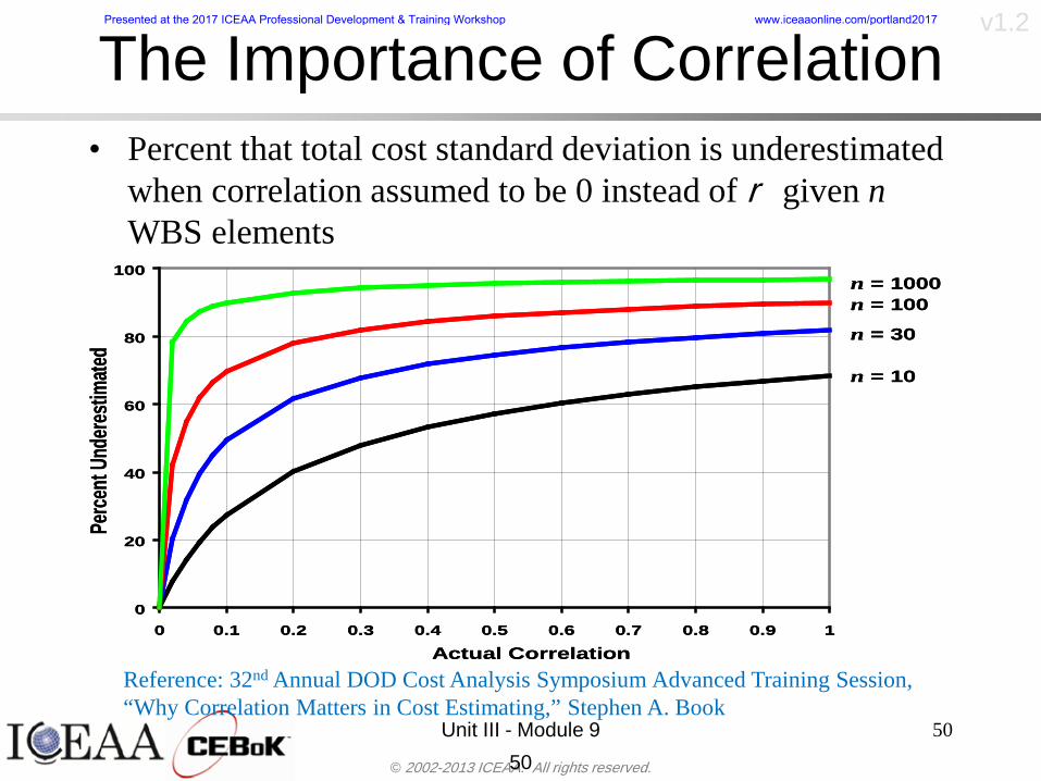
copy 2002-2013 ICEAA All rights reserved
v12
The Importance of Correlationbull Percent that total cost standard deviation is underestimated
when correlation assumed to be 0 instead of r given nWBS elements
Unit III - Module 9 5050
0
20
40
60
80
100
0 01 02 03 04 05 06 07 08 09 1Actual Correlation
Perce
nt Un
deres
timate
d
n = 10
n = 30
n = 100n = 1000
0
20
40
60
80
100
0 01 02 03 04 05 06 07 08 09 1Actual Correlation
Perce
nt Un
deres
timate
d
n = 10
n = 30
n = 100n = 1000
Reference 32nd Annual DOD Cost Analysis Symposium Advanced Training Session ldquoWhy Correlation Matters in Cost Estimatingrdquo Stephen A Book
Presented at the 2017 ICEAA Professional Development amp Training Workshop wwwiceaaonlinecomportland2017
copy 2002-2013 ICEAA All rights reserved
v12
The Importance of Correlation (2)bull For example if correlation is assumed to be 0 for all
elements in a 30 element WBS and the actual correlation is 20 then the total cost standard deviation is underestimated by 60
bull For example assume the total cost is modeled as a normal distribution with mean = 100
bull If correlation is assumed to be zero with total cost standard deviation = 12 when correlation is actually 20 then the true underlying standard deviation is actually 30
bull 70th percentile with zero correlation assumption is 106
bull 70th percentile with 20 correlation is 116 Unit III - Module 9 51
Presented at the 2017 ICEAA Professional Development amp Training Workshop wwwiceaaonlinecomportland2017
copy 2002-2013 ICEAA All rights reserved
v12
Measures of Correlationbull Two measures of correlation are commonly used in
cost risk analysesndash Pearsonrsquos product-moment correlation coefficient ndash Spearmanrsquos rank correlation coefficient
bull Garvey and others recommend using Pearsonrsquos product-moment correlation coefficient correlation for cost risk analysesndash Method of moments uses this but there are two options in
simulationndash Popular simulation packages like Risk and Crystal Ball use
rank correlation but in practice this has been found to make little difference
ndash Pearson product-moment correlation has been incorporated into Risk+
52
Presented at the 2017 ICEAA Professional Development amp Training Workshop wwwiceaaonlinecomportland2017
copy 2002-2013 ICEAA All rights reserved
v12
Pearson Correlationbull Pearsonrsquos product-moment correlation measures
degree of linearity between two random variables bull If two random variables are perfectly linear (eg Y =
aX + b) with positive slope then the Pearson product-moment correlation between X and Y denoted by rXY is +1
53
X X
Y Y Y
XNegative Correlation Positive Correlation No Correlation
middotmiddot
middotmiddot
middotmiddot middotmiddot
middotmiddot
middot
middot
middotmiddotmiddot
middotmiddot
middotmiddot
middotmiddot middot
middot
middot
middotmiddotmiddotmiddotmiddotmiddotmiddotmiddot
middotmiddotmiddotmiddot
middotmiddot
middotmiddot middotmiddotmiddotmiddot
middotmiddotmiddot
middotmiddotmiddotmiddot
middotmiddotmiddot
middotmiddotmiddot
middotmiddot
middot
middot middotmiddot
middot middotmiddotmiddotmiddot middotmiddot middot middotmiddot middot middot
middotmiddot middot
middotmiddotmiddotmiddotmiddot middot middotmiddot
middotmiddot
middot
middotmiddot
middotmiddot middot
middot middot middot
middotmiddot middot
middotmiddotmiddot
middotmiddot
middot middot
Presented at the 2017 ICEAA Professional Development amp Training Workshop wwwiceaaonlinecomportland2017
copy 2002-2013 ICEAA All rights reserved
v12
Spearman Correlationbull Spearmanrsquos rank correlation measures the
monotonicity between two random variablesbull If two random variables are perfectly monotonically
increasing (eg Y = X2) then the Spearman rank correlation denoted by rXY is +1
bull The two measures can be significantly different
54
10 20 30 40 50 60
100
200
300
096 097 098 099 1
1
060
020
040
080
Eff
ort (
Staf
f-M
onth
s)
Software Size I KDSI
y = 28z12y
z x
yy = x100
0 pound x pound 1
Figure 5-9A Figure 5-9B
Pearson Correlation = 09976 Rank Correlation = 1
Pearson Correlation = 024 Rank Correlation = 1
X(x ) ~ Unif(01)
Reference Probability Methods for Cost Uncertainty Analysis A Systems Engineering Perspective Paul R Garvey
Presented at the 2017 ICEAA Professional Development amp Training Workshop wwwiceaaonlinecomportland2017
copy 2002-2013 ICEAA All rights reserved
v12
Unit III - Module 9 55
200
250
300
350
400
1000 1200 1400 1600 1800 2000
Recurring Production
SEPM
200
250
300
350
400
1000 1200 1400 1600 1800 2000
Recurring Production
SEPM
Functional Correlationbull Old No Functional
Correlation Simulation run with WBS items entered as values
bull New Simulation run with functional dependencies entered as they are in cost model
CorrelatedNot Correlated
Note shift of mean and increased variability
Presented at the 2017 ICEAA Professional Development amp Training Workshop wwwiceaaonlinecomportland2017
copy 2002-2013 ICEAA All rights reserved
v12
Risk Measuresbull ldquoWestern Europe conquered the word because of a
technological revolution that started because of attempts to measure the worldrdquo ndash Phillipe Jorion ndash In the same way attempts to measure risk will lead to better project
managementbull Risk management for DoD and NASA agencies focuses
primarily on funding projects to a single percentile ndash NASA policy explicitly mentions 70 and 50ndash This is known as ldquoValue at Riskrdquo and is prevalent in the banking and
financial industry
56
Presented at the 2017 ICEAA Professional Development amp Training Workshop wwwiceaaonlinecomportland2017
copy 2002-2013 ICEAA All rights reserved
v12
Value at Risk (VaR)bull VaR is a percentile of the cost risk
distributionndash VaR funding at the 70th percentile means that
there is a 30 chance of final project cost exceeding the funded amount (budget)
bull VaR has some meritsndash Common measure can be used to compare
different projects and programsndash Easily understood by senior managers and
decision makers
57
Presented at the 2017 ICEAA Professional Development amp Training Workshop wwwiceaaonlinecomportland2017
copy 2002-2013 ICEAA All rights reserved
v12
Why 70th or 80th Percentilebull Typical policy guidance involves funding at the 70th or 80th
percentile Why fund as such a low percentilebull There is some incentive to not over-fundbull For a normal distribution an inflection point occurs near the 80th
percentile meaning that for values above 80 confidence achieving higher levels of confidence can only be achieved by spending greater dollar amounts at an increasing rate
58
-05-04-03-02-01
00102030405
0 05 1 15 2 25 3
Standard Deviations from Mean
Normal Distribution
First DerivativeSlopeVelocity
Second DerivativeConvexityAcceleration
Inflection point at one standard deviation above the mean (~84th
percentile)
Presented at the 2017 ICEAA Professional Development amp Training Workshop wwwiceaaonlinecomportland2017
copy 2002-2013 ICEAA All rights reserved
v12
Funding Above Inflection Pointsbull As the percentile goes above the 80th percentile the amount
needed to achieve that higher level of confidence begins to increase at an increasing rate as is evident from the graph
59
0
10
20
30
40
50
60
70
50 55 60 65 70 75 80 85 90 95 100
$ Ab
ove
MEa
n to
Ach
ieve
Per
cent
ile
Percentile (Confidence Level)
Presented at the 2017 ICEAA Professional Development amp Training Workshop wwwiceaaonlinecomportland2017
copy 2002-2013 ICEAA All rights reserved
v12
Why Budget to the 70th or 80thbull Government projects are funded at the 70th or 80th percentilesbull Why not the 90th or 99th percentile Wonrsquot that help prevent
overrunsndash As we have seen percentiles do not add across programs
bull The sum of the 80th percentiles does NOT equal the total 80th percentile
ndash This is because the individual programs are riskier than the entire suite of missions
bull Known as the ldquoPortfolio effectrdquo (more or this later)
ndash Funding at the 80th gives confidence that the entire portfolio will be adequately funded
bull And since there is an inflection point near the 80th percentile funding above that level quickly becomes cost prohibitive
60
Presented at the 2017 ICEAA Professional Development amp Training Workshop wwwiceaaonlinecomportland2017
copy 2002-2013 ICEAA All rights reserved
v12
Inflection Points for Lognormalbull For a lognormal the inflection point
variesndash Coefficient of variation equal to 10 equates to an
inflection point at the 70th percentile
61
0
10
20
30
40
50
60
70
050 060 070 080 090 100
Coef
ficen
t of V
aria
tion
Percentile of the Inflection Point
Presented at the 2017 ICEAA Professional Development amp Training Workshop wwwiceaaonlinecomportland2017
copy 2002-2013 ICEAA All rights reserved
v12
Issues with Percentile Fundingbull However risk management does not stop at a
specific percentilendash What happens when the 70th percentile is exceeded
bull Any effective risk management policy should prescribe what happens after a bad event occursndash With VaR we only know when a bad event has occurred ndash Also funding at a relatively low level means we have no true
sense of the real risks that should be guarded against
62
Presented at the 2017 ICEAA Professional Development amp Training Workshop wwwiceaaonlinecomportland2017
copy 2002-2013 ICEAA All rights reserved
v12
ldquoHere There Be Dragonsrdquobull On old maps uncharted territory was often
marked with monsters or dragons
63
A section of the Carta Marina by Olaus Magnus 16th Century
Presented at the 2017 ICEAA Professional Development amp Training Workshop wwwiceaaonlinecomportland2017
copy 2002-2013 ICEAA All rights reserved
v12
Distribution Comparisonbull Four different distributions with the same 70th
percentile
bull Should we expect the tails to be similar
64
0
10
20
30
40
50
60
70
80
0 100 200 300 400 500 600
Perc
entil
eCo
nfid
ence
Lev
el
Triangular
Normal
Lognormal
Pareto
Presented at the 2017 ICEAA Professional Development amp Training Workshop wwwiceaaonlinecomportland2017
copy 2002-2013 ICEAA All rights reserved
v12Distribution Comparison Tail Behavior
bull The normal and triangular distributions have similar tails but the lognormal and Pareto have much fatter right tails
65
70
75
80
85
90
95
100
500 1500 2500 3500 4500 5500
Perc
entil
eCo
nfid
ence
Lev
el
Triangular
Normal
Lognormal
Pareto
Here There Be Dragons
Presented at the 2017 ICEAA Professional Development amp Training Workshop wwwiceaaonlinecomportland2017
copy 2002-2013 ICEAA All rights reserved
v12Distribution Comparison ndash Tail Behavior (Table)
bull There is significant tail risk for the lognormal and the Paretobull The 99th percentile for the Pareto is 1000 times greater than
the 70th percentilendash Risk seen in financial markets and in catastrophic risks like natural
disasters bull Four different projects follow the four different risk profiles seen
in this example should clearly have different risk management approaches but 70th percentile funding indicates the same risk management approach for all four
66
Percentile Triangular Normal Lognormal Pareto 70th $600 $600 $600 $600 80th $680 $660 $770 $1430 90th $770 $750 $1070 $5880 95th $840 $820 $1410 $23750 99th $930 $950 $2350 $600000
Presented at the 2017 ICEAA Professional Development amp Training Workshop wwwiceaaonlinecomportland2017
copy 2002-2013 ICEAA All rights reserved
v12Percentile Budgeting is Not Risk Management
bull Percentile budgeting ne effective risk management policybull Suppose that you are shopping for a new car You
mention that safety is your top concern The salesman says he has a great safe car available You ask about the air bags Do they work The salesman answers ldquoOf course Seventy percent of the time they work fine Only 30 of the time the air bags will fail to deployrdquo Would you buy such a car Hedge fund manager David Einhorn has stated ldquoRisk management is the air bag that must always work but only in the multi-sigma event where you have an accidentrdquo
67
Risk management is the air bag that must always work but only in the multi-sigma event where you
have an accident
Presented at the 2017 ICEAA Professional Development amp Training Workshop wwwiceaaonlinecomportland2017
copy 2002-2013 ICEAA All rights reserved
v12
Joint Confidence Level Analysisbull Schedules are risky toobull For 98 recent NASA missions average
schedule growth was 38ndash Not as high as cost growth but still significant
68
0
5
10
15
20
25
30
35
40
Schedule
Cost
Presented at the 2017 ICEAA Professional Development amp Training Workshop wwwiceaaonlinecomportland2017
copy 2002-2013 ICEAA All rights reserved
v12
Schedules Impact Costbull Changes in schedule can have enormous
impacts on cost ndash Schedule slips can lead to cost increases
bull Fixed programmatic costs must be paid on a regular basisndash Achieving schedule milestones early can result in cost
savings
bull Schedule is an important consideration in cost analysis including cost risk analysis
bull However we must be careful in correctly integrating cost and schedule riskndash Schedule is not simply an input but is dependent on many of
the same factors that drive cost
69
Presented at the 2017 ICEAA Professional Development amp Training Workshop wwwiceaaonlinecomportland2017
copy 2002-2013 ICEAA All rights reserved
v12
The Relationship of Cost to Schedulebull Cost and schedule are positively correlated
ndash A larger program with bigger scope with take longer to complete than a smaller simpler program
bull However longer schedules do not always equate to higher cost nor shorter schedules with lower costndash Highly compressed schedules relative to the
optimal schedule can lead to large overrunsbull Compressed schedules are commonplace for
many planetary missions
70
Presented at the 2017 ICEAA Professional Development amp Training Workshop wwwiceaaonlinecomportland2017
copy 2002-2013 ICEAA All rights reserved
v12The Impact of Schedule GrowthCompression on Cost
bull Compressed schedules lead to cost growth and based on existing research is actually more expensive than schedule slippages
71
0
20
40
60
80
100
120
140
160
-50 -25 0 25 50 75 100
Percentage Change in Schedule
Perc
enta
ge C
hang
e in
Cos
t due
to
Sche
dule
Cha
nge
Source Smart CB ldquoCost and Schedule Interrelationshipsrdquo 2007 NASA Cost Symposium
Presented at the 2017 ICEAA Professional Development amp Training Workshop wwwiceaaonlinecomportland2017
copy 2002-2013 ICEAA All rights reserved
v12Schedule as an Independent Variable
bull Why not simply add schedule as an input to cost-estimating relationships (CERs)
bull Schedule is often treated as an independent variable ndash schedules are often determined independently of cost considerationsndash Cost may not be considered explicitly although budgets and
schedules are determined based on scope and other common factors
bull In 2006 SAIC undertook a research task to determine the impact of schedule on cost and added schedule as an independent variable to the CERs in the NASAAir Force Cost Model (NAFCOM) to see if schedule provided any improvement in goodness of fit
72
Presented at the 2017 ICEAA Professional Development amp Training Workshop wwwiceaaonlinecomportland2017
copy 2002-2013 ICEAA All rights reserved
v12
Schedule is a Dependent Variablebull Since NAFCOM includes an exhaustive list of cost drivers the inclusion
of schedule should give an indication of whether there is any additional independent value added from schedule independent of the cost drivers
bull In the study schedule was added to 10 subsystem-level CERs
ndash In each case the addition of schedule did NOTimprove the goodness of fit and schedule was NOT found to be a statistically significant cost driver (given the presence of the other variables) for any of the 10 CERs
bull Standard errors for the CERs increased due to decrease in degrees of freedom
bull Thus schedule as an independent variable did not provide any additional explanation of variation in historical cost
bull This is because schedule is truly NOT an independent variable but a dependent variable and is a function of the same factors that drive cost
73
Presented at the 2017 ICEAA Professional Development amp Training Workshop wwwiceaaonlinecomportland2017
copy 2002-2013 ICEAA All rights reserved
v12
Incorporation of Schedule in Cost Risk
bull When using subjective methods care must be taken in applying schedule to cost risk analysis
bull Since schedule is a dependent variable treating it independently from other factors when assessing its impact on cost can lead to a double count of independent variables in the cost risk analysis
bull Direct inclusion of schedule in a cost risk analysis effectively doubles the influence of each cost driver
ndash Incorrectly leads to broader risk ranges
74
CostWeight
HeritageNewness
Technology Readiness Schedule
Presented at the 2017 ICEAA Professional Development amp Training Workshop wwwiceaaonlinecomportland2017
copy 2002-2013 ICEAA All rights reserved
v12Subjective Cost Risk Methods and Overinclusion of Risk Factors
bull Subjective methods are suitable when data are scarce or not availablebull However care must be taken not to treat correlated sources of risk
such as schedule as independent of each otherbull Example ndash a subjective risk analysis incorporated technology readiness
design risk requirements stability integration risk and schedule and treated each source of risk as independent
bull Risk triangle high value without schedule risk was 31 times the point estimate
bull Risk triangle high value with schedule risk added on top of other sources of risk treated independently was 34 times the point estimate
bull Risk triangle taking correlation between sources of risk into account in a rigorous statistical manner has a high value 15 times the point estimate less than half the effect when treating sources of risk as independent
75
Presented at the 2017 ICEAA Professional Development amp Training Workshop wwwiceaaonlinecomportland2017
copy 2002-2013 ICEAA All rights reserved
v12Fundamental Equation of Cost and Schedule Interrelationships
bull The Fundamental Equation of the Relationship Between Cost and Schedule is
Time = Moneybull This is a well known adage that time is money Your boss at
work may even mention this to you from time to time or if you are the boss you are all too aware of this iron law
bull Because time is money cost and schedule risk should be modeled jointly not with schedule as an independent cost driver
bull Note that cost and schedule are not perfectly correlatedndash Cost can sometimes ldquobuy downrdquo schedule extra money can be
spent to meet a deadline since in some cases additional effort to hasten the completion of a task
76
Presented at the 2017 ICEAA Professional Development amp Training Workshop wwwiceaaonlinecomportland2017
copy 2002-2013 ICEAA All rights reserved
v12How to (Correctly) Incorporate Schedule into Cost Risk Analysis
bull The best way to model cost and schedule risk is to develop a joint cost and schedule model based on the same data
bull Since such models are not currently available the next best approach is to model cost and schedule independently and then integrate cost and schedule risk analyses using joint probability distributions taking into account correlation between cost and schedulendash This approach pioneered by Paul Garvey and Steve Book is
considered industry best practicendash This is a practical method mathematically tractable and follows
naturally from the Fundamental Equation of Cost and Schedule Interrelationships
77
Book S A ldquoQuantifying the Relationship Between Cost and Schedulerdquo The Measurable News Winter 2007-2008 pp 11-15Garvey PR Probability Methods for Cost Uncertainty Analysis A Systems Engineering Perspective New York Marcel Dekker 2000 pp 308-335
Presented at the 2017 ICEAA Professional Development amp Training Workshop wwwiceaaonlinecomportland2017
copy 2002-2013 ICEAA All rights reserved
v12
Joint Lognormal and Normal Distributions
bull Cost and schedule are typically modeled as some combination of Normal and Lognormal probability distributionsndash Studies by The Aerospace Corporation the MITRE
Corporation Wyle Labs and SAIC have found that the Lognormal probability distribution almost always serves as a good model for both the schedule distribution and the cost distribution
ndash The Normal distribution may also be appropriate in some instances and depending upon the level of confidence at which budgets are set may even be more conservative and logically consistent than the Normal distribution
ndash Joint Lognormal and Normal distributions are defined by a pair of mean and standard deviations and a level of correlation between the two
78
Presented at the 2017 ICEAA Professional Development amp Training Workshop wwwiceaaonlinecomportland2017
copy 2002-2013 ICEAA All rights reserved
v12Modeling Cost and Schedule as a Bivariate Distribution
bull In the approach set forth by Book and Garvey cost risk is assessed and the top-level distribution is modeled as a Lognormal (or Normal) distribution schedule risk is assessed and the overall schedule risk is modeled as a Lognormal (or Normal) distribution
bull The two distributions are combined into a Bivariate distribution by assigning a correlation between the two and by treating the two distributions as the marginal distributions of a Bivariate Lognormal distributionndash Other combinations include a Bivariate Normal or a Bivariate
Normal-Lognormal
79
Presented at the 2017 ICEAA Professional Development amp Training Workshop wwwiceaaonlinecomportland2017
copy 2002-2013 ICEAA All rights reserved
v12Bivariate Lognormal Distribution for Cost and Schedule
bull Cost is often observed to be Lognormal when strong positive correlations are present among the systemrsquos WBS cost element costs
bull A systemrsquos schedule is often observed (from Monte Carlo simulations) to be Lognormal if it is the sum of many positively correlated schedule activities in an overall schedule network
bull If Lognormal distributions characterize a systemrsquos cost and schedule then the Bivariate Lognormal could serve as an assumed model of their joint distributionndash In this case the marginal distribution of each of cost and schedule is
Lognormalbull Other possibilities for modeling cost and schedule as a Bivariate
distribution include a Bivariate Normal or a Bivariate Normal-Lognormal distributionndash All these combinations are analytically tractable
80
Presented at the 2017 ICEAA Professional Development amp Training Workshop wwwiceaaonlinecomportland2017
copy 2002-2013 ICEAA All rights reserved
v12Bivariate Lognormal for Cost and Schedule
bull Contour Plots of a Bivariate Lognormal
81
Presented at the 2017 ICEAA Professional Development amp Training Workshop wwwiceaaonlinecomportland2017
copy 2002-2013 ICEAA All rights reserved
v12Correlation Between Cost and Schedule
bull Cost and schedule are positively correlated but not perfectly sondash For example it is possible to have a schedule underrun and a cost
overrunbull Based on cost and schedule growth data for 50 completed NASA
programs the correlation between development cost and development schedule is 70
82
00
200
400
600
800
1000
1200
-500 00 500 1000 1500 2000 2500Historical Cost Growth
Hist
oric
al S
ched
ule
Gro
wth
r = 715
Presented at the 2017 ICEAA Professional Development amp Training Workshop wwwiceaaonlinecomportland2017
copy 2002-2013 ICEAA All rights reserved
v12Correlation Between Cost and Schedule Caveats
bull Based on historical data recommended correlation between cost and schedule is 70 but this could be higher or lower depending upon program circumstancesndash If program is budget constrained cost and schedule will be
more highly correlated (go as you pay)ndash If program is schedule constrained cost and schedule will
have lower correlation perhaps even negative correlation ndash Smaller programs have smaller correlation between cost and
schedule riskbull Relatively easy to ldquohurry uprdquo and finish on time or even early if
needed
83
Presented at the 2017 ICEAA Professional Development amp Training Workshop wwwiceaaonlinecomportland2017
copy 2002-2013 ICEAA All rights reserved
v12
Conditional Confidence Levelsbull Given a programrsquos project schedule we can determine the cost
risk distribution conditional upon the given schedulebull Conditional cost S-curves are steeper than unconditional
(marginal) cost S-curves between some uncertainty has been removed because schedule is fixed
84
Presented at the 2017 ICEAA Professional Development amp Training Workshop wwwiceaaonlinecomportland2017
copy 2002-2013 ICEAA All rights reserved
v12
Joint Confidence Levelsbull Joint 65 confidence represents the probability of
achieving both 65 confidence in cost AND 65 confidence in schedulendash This is different than achieving 65 cost confidence alone
or achieving 65 schedule confidence alonebull Due to the imperfect correlation between cost and schedule it
is possible to achieve a 65 cost confidence with a lower level of schedule confidence
bull Restricting the schedule confidence thus requires additional $ to achieve a given level of confidence
85
X
Y
Possible Values for Which X gt a Possible Values for
Which X gt a and Y gt b
a
b
Presented at the 2017 ICEAA Professional Development amp Training Workshop wwwiceaaonlinecomportland2017
copy 2002-2013 ICEAA All rights reserved
v12Joint Confidence Levels Versus Cost Confidence Levels Only
bull Example of the differences between cost confidence schedule confidence conditional cost confidence and joint cost and schedule confidence
86
Joint Cost-Schedule Confidence Iso-Curves
Cost (RY$M)
Sche
dule
(Mon
ths)
65 Confidence
50 Confidence
70 Confidence
65 Cost Confidence AggressiveSchedule65 Cost ConfidenceScheduleGiven 65 Schedule ConfidenceUnconditional 65 CostConfidenceUnconditional 65 ScheduleConfidence
65 Cost Confidence 65 Joint Cost and Schedule
Confidence for 65 Schedule Confidence
Presented at the 2017 ICEAA Professional Development amp Training Workshop wwwiceaaonlinecomportland2017
copy 2002-2013 ICEAA All rights reserved
v12
Joint Cost and Schedule Confidence
bull Can examine pairs of cost and schedule that achieve a given level of confidence
bull Provides insights into the trade-offs between cost and schedule for a given level of confidencendash Possible to increase cost confidence by giving a
project more time in some instances or possible to ldquobuy downrdquo schedule
bull But these have limits and are shown in the iso-cost and schedule confidence curves
87
Presented at the 2017 ICEAA Professional Development amp Training Workshop wwwiceaaonlinecomportland2017
copy 2002-2013 ICEAA All rights reserved
v12Cost and Schedule Trade-offs for a Given Level of Joint Confidence
bull Hypothetical Example
88
Cost (RY$M)
Schedule (Months)
$100 48$99 48$89 49$87 50$85 51$85 52$84 53$83 55$83 55$83 56
Cost and Schedule 65 Confidence Iso-Curve
4748495051525354555657
$80 $82 $84 $86 $88 $90 $92 $94 $96 $98 $100
Cost (RY$ M)
Sche
dule
(Mon
ths)
Presented at the 2017 ICEAA Professional Development amp Training Workshop wwwiceaaonlinecomportland2017
copy 2002-2013 ICEAA All rights reserved
v12Policy Considerations for Confidence Levels
bull For large programs the difference between the amount of money needed to achieve 65 cost confidence independent of schedule and joint 65 cost and schedule confidence can represent hundreds of millions and even billions of dollars
89
Joint Cost-Schedule Confidence Iso-Curves
Cost (RY$M)
Sche
dule
(Mon
ths)
65 Confidence
65 Cost Confidence AggressiveSchedule
65 Cost ConfidenceScheduleGiven 65 Schedule Confidence
Unconditional 65 CostConfidence
Joint Cost and Schedule Confidence for 65 Cost Confidence and Program Baseline Schedule is Less Than 35
65 Cost Confidence Independent of Schedule Cost Needed to Achieve
Both 65 Joint Cost and Schedule Confidence for the Schedule with 65 Confidence
Presented at the 2017 ICEAA Professional Development amp Training Workshop wwwiceaaonlinecomportland2017
copy 2002-2013 ICEAA All rights reserved
v12
Copulasbull More generally any combination of distributions can
be used (more than just normal and lognormal)ndash Termed ldquocopulardquo from the Italian word for ldquocouplerdquondash Copulas are a way to combine marginal distributions of any
number and type into a joint distributionbull More formally a copula is a multivariate joint distribution defined
on the n-dimensional unit cube [0 1]n such that every marginal distribution is uniform on the interval [0 1]
bull (The bivariate form of) Sklarrsquos theorem states that for any bivariate distribution function H(x y) let F(x) = H(x infin) and G(y) = H(infin y) be the univariate marginal probability distribution functions Then there exists a copula C such that H(xy)=C(F(x)G(y))
ndash Copulas are widely used in risk management for investments and insurance
bull Considered industry best practice (Li 2000)bull Marketed as part of JP Morganrsquos CreditMetrics suite of tools
(Gupton et Al 1997)90
Presented at the 2017 ICEAA Professional Development amp Training Workshop wwwiceaaonlinecomportland2017
copy 2002-2013 ICEAA All rights reserved
v12Parametric Joint Cost and Schedule Analysis
bull A parametric model based on a consistent data set with a set of overlapping cost and schedule drivers is a cleaner way to model cost and schedule
91
CostWeight
HeritageNewness
Technology Readiness
Schedule
0
20
40
60
80
100
Confidence
Joint Cost and Schedule Confidence
Schedule
Cost
Lognormal Distribution PDF and CDF
0102030405060708090100
200 300 400 500 600 700 800 900 1000Cost $
Con
fiden
ce L
evel
0
00002
00004
00006
00008
0001
00012
00014
00016
Prob
abili
ty D
ensi
ty
CDFPDF
Lognormal Distribution PDF and CDF
0102030405060708090100
200 300 400 500 600 700 800 900 1000Cost $
Con
fiden
ce L
evel
0
00002
00004
00006
00008
0001
00012
00014
00016
Prob
abili
ty D
ensi
ty
CDFPDF
Presented at the 2017 ICEAA Professional Development amp Training Workshop wwwiceaaonlinecomportland2017
copy 2002-2013 ICEAA All rights reserved
v12Parametric Joint Cost and Schedule Analysis (2)
bull Joint cost and schedule risk analysis produced naturally by the integrated modelndash Addresses several issues with the copula
approachbull Tail dependencybull Correlation ndash no need to assign correlation
between cost and schedulebull Consistency of cost and schedule models
92
Presented at the 2017 ICEAA Professional Development amp Training Workshop wwwiceaaonlinecomportland2017
copy 2002-2013 ICEAA All rights reserved
v12
Resource-Loaded Schedulesbull Involves assigning cost and schedule risks to a resource-loaded schedule
networkbull Bottom-up approach
ndash More labor intensive than parametrics but can also provide more insight
ndash Can answer questions than parametric typically cannot such as how much do reserve requirements decrease if a specific risk is retired
bull Currently being implemented in Constellation programbull Has same issue as all bottom-up models hard to count all the risks and model
them discretely
ndash As a result there is a tendency to reflect less risk than indicated by history
ndash ldquoThere are more things in heaven and earth Horatio than are dreamt of in your philosophyrdquo William Shakespeare Hamlet Act I Scene V
93
Presented at the 2017 ICEAA Professional Development amp Training Workshop wwwiceaaonlinecomportland2017
copy 2002-2013 ICEAA All rights reserved
v12Resource-Loaded Schedules Vs Parametrics
bull Parametric most appropriate for early estimatesndash But also good for high-level checks as project progresses
bull As plans take shape lower level modeling may be more appropriate
94 1
CONCEPTUALDEVELOPMENT
PROJECTDEFINITION DESIGN DEVELOPMENT OPERATIONS
PARAMETRIC PARAMETRIC
ANALOGY
ENGINEERING (Bottoms Up)
$PARAMETRIC
DETAILED
$
Pre Phase A Phase B Phase CDPhase A Phase EPre Phase A Phase B Phase CDPhase A Phase E
Risk = f(Cost Estimating Relationship Inputs eg mass power data rate TRL new design etc)
Risk = f(cost and schedule variation of the analogous elements)
Risk = f(variation of detailed inputs eg labor hours rates materials etc)
Presented at the 2017 ICEAA Professional Development amp Training Workshop wwwiceaaonlinecomportland2017
copy 2002-2013 ICEAA All rights reserved
v12
Resource-Loaded Schedulesbull Methodology has been demonstrated in other
industriesndash Construction oil and gasndash Analysis has not been traditionally done on highly uncertain
complex development projects bull Methodology focuses on project baseline schedule
ndash In baseline schedule all tasks are resource loaded to represent a baseline schedule and cost standpoint
ndash Resource loaded schedule is ldquorolledrdquo up to a manageable level
ndash Based on the risk and uncertainties identified schedule distributions are applied to each rolled up task
ndash Cost uncertainties are also applied to rolled up tasksbull Uncertainties include labor rate man power etc
ndash A Monte Carlo simulation is run to develop joint cost-schedule distributions
95
Presented at the 2017 ICEAA Professional Development amp Training Workshop wwwiceaaonlinecomportland2017
copy 2002-2013 ICEAA All rights reserved
v12
Unit III - Module 9 96
Execution ndash Cross Checksbull Means The mean cost growth factor for WBS items
can be compared to history as a way to cross check results
bull CVs The CV of the cost growth factors for WBS items can be compared to history as a way to cross check results
bull Inputs Checks are performed on inputs or other parameters to see if historical values are in line with program assumptionsndash Example Historical risk scores can be compared to program
risk scores to see if risk assessors are being realistic and to see if the underlying database is representative of the program
11
Presented at the 2017 ICEAA Professional Development amp Training Workshop wwwiceaaonlinecomportland2017
- Cost and Schedule Risk Analysis Basic
- Acknowledgments
- Unit Index
- Risk Overview
- Agenda
- Introduction
- Risk Analysis Terms
- Are Our Costs Realistic
- Historical Cost Growth
- Sources of Cost Risk
- Point Estimates of Cost
- Types of Risk
- Point Estimates Vs Risk Estimates
- Cost Risk and Probability
- Probability Model ndash Distribution
- Probability Model ndash Distribution
- Probability ndash Top-Level Distribution
- S-Curves and Confidence Levels
- Example ndash Normal Distribution
- Confidence Levels
- Measuring Parametric Model Uncertainty
- Parametric Model Example
- Weight Uncertainty
- Estimating Uncertainty
- Estimating Uncertainty (2)
- Estimating Uncertainty (3)
- Aggregating Risk
- WBS Example
- WBS and Risk
- Aggregating Risk
- Percentiles Do Not Add
- Percentiles Do Not Add (2)
- Percentiles Do Not Add (3)
- Methods for Aggregating Risk
- Monte Carlo Simulationfor Risk Analysis
- Monte Carlo Simulation
- Using Random Numbers to Simulate Distributions
- Simulating a Triangular Distribution
- Simulating a Triangular Distribution (2)
- Monte Carlo and the WBS
- Number of Trials
- Number of Trials (2)
- Number of Trials (3)
- Number of Trials (4)
- Number of Trials (5)
- Number of Trials (6)
- Methods of Simulation
- Probability Model ndash Correlation
- Correlation And Causation
- The Importance of Correlation
- The Importance of Correlation (2)
- Measures of Correlation
- Pearson Correlation
- Spearman Correlation
- Functional Correlation
- Risk Measures
- Value at Risk (VaR)
- Why 70th or 80th Percentile
- Funding Above Inflection Points
- Why Budget to the 70th or 80th
- Inflection Points for Lognormal
- Issues with Percentile Funding
- ldquoHere There Be Dragonsrdquo
- Distribution Comparison
- Distribution Comparison Tail Behavior
- Distribution Comparison ndash Tail Behavior (Table)
- Percentile Budgeting is Not Risk Management
- Joint Confidence Level Analysis
- Schedules Impact Cost
- The Relationship of Cost to Schedule
- The Impact of Schedule GrowthCompression on Cost
- Schedule as an Independent Variable
- Schedule is a Dependent Variable
- Incorporation of Schedule in Cost Risk
- Subjective Cost Risk Methods and Overinclusion of Risk Factors
- Fundamental Equation of Cost and Schedule Interrelationships
- How to (Correctly) Incorporate Schedule into Cost Risk Analysis
- Joint Lognormal and Normal Distributions
- Modeling Cost and Schedule as a Bivariate Distribution
- Bivariate Lognormal Distribution for Cost and Schedule
- Bivariate Lognormal for Cost and Schedule
- Correlation Between Cost and Schedule
- Correlation Between Cost and Schedule Caveats
- Conditional Confidence Levels
- Joint Confidence Levels
- Joint Confidence Levels Versus Cost Confidence Levels Only
- Joint Cost and Schedule Confidence
- Cost and Schedule Trade-offs for a Given Level of Joint Confidence
- Policy Considerations for Confidence Levels
- Copulas
- Parametric Joint Cost and Schedule Analysis
- Parametric Joint Cost and Schedule Analysis (2)
- Resource-Loaded Schedules
- Resource-Loaded Schedules Vs Parametrics
- Resource-Loaded Schedules
- Execution ndash Cross Checks
-
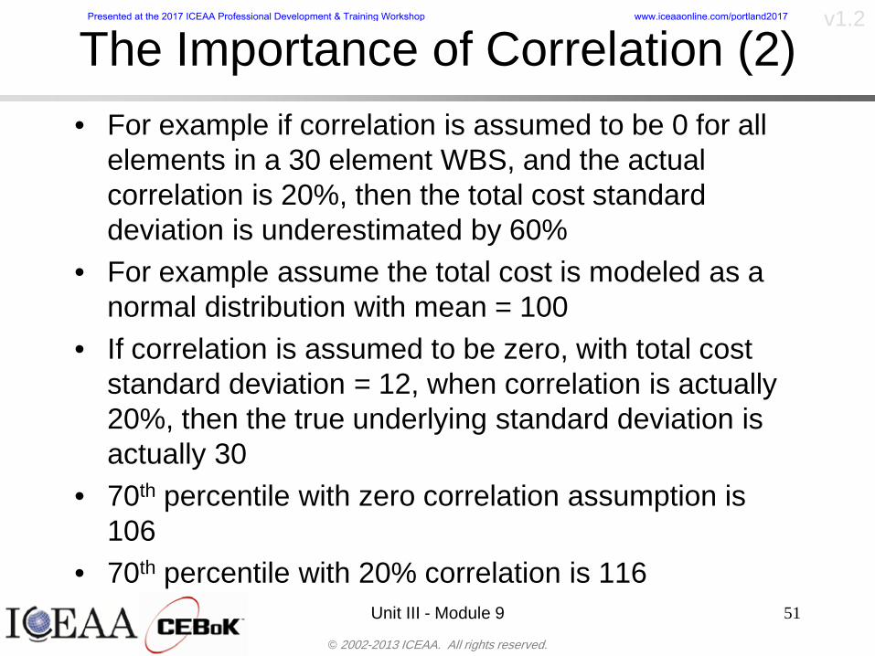
copy 2002-2013 ICEAA All rights reserved
v12
The Importance of Correlation (2)bull For example if correlation is assumed to be 0 for all
elements in a 30 element WBS and the actual correlation is 20 then the total cost standard deviation is underestimated by 60
bull For example assume the total cost is modeled as a normal distribution with mean = 100
bull If correlation is assumed to be zero with total cost standard deviation = 12 when correlation is actually 20 then the true underlying standard deviation is actually 30
bull 70th percentile with zero correlation assumption is 106
bull 70th percentile with 20 correlation is 116 Unit III - Module 9 51
Presented at the 2017 ICEAA Professional Development amp Training Workshop wwwiceaaonlinecomportland2017
copy 2002-2013 ICEAA All rights reserved
v12
Measures of Correlationbull Two measures of correlation are commonly used in
cost risk analysesndash Pearsonrsquos product-moment correlation coefficient ndash Spearmanrsquos rank correlation coefficient
bull Garvey and others recommend using Pearsonrsquos product-moment correlation coefficient correlation for cost risk analysesndash Method of moments uses this but there are two options in
simulationndash Popular simulation packages like Risk and Crystal Ball use
rank correlation but in practice this has been found to make little difference
ndash Pearson product-moment correlation has been incorporated into Risk+
52
Presented at the 2017 ICEAA Professional Development amp Training Workshop wwwiceaaonlinecomportland2017
copy 2002-2013 ICEAA All rights reserved
v12
Pearson Correlationbull Pearsonrsquos product-moment correlation measures
degree of linearity between two random variables bull If two random variables are perfectly linear (eg Y =
aX + b) with positive slope then the Pearson product-moment correlation between X and Y denoted by rXY is +1
53
X X
Y Y Y
XNegative Correlation Positive Correlation No Correlation
middotmiddot
middotmiddot
middotmiddot middotmiddot
middotmiddot
middot
middot
middotmiddotmiddot
middotmiddot
middotmiddot
middotmiddot middot
middot
middot
middotmiddotmiddotmiddotmiddotmiddotmiddotmiddot
middotmiddotmiddotmiddot
middotmiddot
middotmiddot middotmiddotmiddotmiddot
middotmiddotmiddot
middotmiddotmiddotmiddot
middotmiddotmiddot
middotmiddotmiddot
middotmiddot
middot
middot middotmiddot
middot middotmiddotmiddotmiddot middotmiddot middot middotmiddot middot middot
middotmiddot middot
middotmiddotmiddotmiddotmiddot middot middotmiddot
middotmiddot
middot
middotmiddot
middotmiddot middot
middot middot middot
middotmiddot middot
middotmiddotmiddot
middotmiddot
middot middot
Presented at the 2017 ICEAA Professional Development amp Training Workshop wwwiceaaonlinecomportland2017
copy 2002-2013 ICEAA All rights reserved
v12
Spearman Correlationbull Spearmanrsquos rank correlation measures the
monotonicity between two random variablesbull If two random variables are perfectly monotonically
increasing (eg Y = X2) then the Spearman rank correlation denoted by rXY is +1
bull The two measures can be significantly different
54
10 20 30 40 50 60
100
200
300
096 097 098 099 1
1
060
020
040
080
Eff
ort (
Staf
f-M
onth
s)
Software Size I KDSI
y = 28z12y
z x
yy = x100
0 pound x pound 1
Figure 5-9A Figure 5-9B
Pearson Correlation = 09976 Rank Correlation = 1
Pearson Correlation = 024 Rank Correlation = 1
X(x ) ~ Unif(01)
Reference Probability Methods for Cost Uncertainty Analysis A Systems Engineering Perspective Paul R Garvey
Presented at the 2017 ICEAA Professional Development amp Training Workshop wwwiceaaonlinecomportland2017
copy 2002-2013 ICEAA All rights reserved
v12
Unit III - Module 9 55
200
250
300
350
400
1000 1200 1400 1600 1800 2000
Recurring Production
SEPM
200
250
300
350
400
1000 1200 1400 1600 1800 2000
Recurring Production
SEPM
Functional Correlationbull Old No Functional
Correlation Simulation run with WBS items entered as values
bull New Simulation run with functional dependencies entered as they are in cost model
CorrelatedNot Correlated
Note shift of mean and increased variability
Presented at the 2017 ICEAA Professional Development amp Training Workshop wwwiceaaonlinecomportland2017
copy 2002-2013 ICEAA All rights reserved
v12
Risk Measuresbull ldquoWestern Europe conquered the word because of a
technological revolution that started because of attempts to measure the worldrdquo ndash Phillipe Jorion ndash In the same way attempts to measure risk will lead to better project
managementbull Risk management for DoD and NASA agencies focuses
primarily on funding projects to a single percentile ndash NASA policy explicitly mentions 70 and 50ndash This is known as ldquoValue at Riskrdquo and is prevalent in the banking and
financial industry
56
Presented at the 2017 ICEAA Professional Development amp Training Workshop wwwiceaaonlinecomportland2017
copy 2002-2013 ICEAA All rights reserved
v12
Value at Risk (VaR)bull VaR is a percentile of the cost risk
distributionndash VaR funding at the 70th percentile means that
there is a 30 chance of final project cost exceeding the funded amount (budget)
bull VaR has some meritsndash Common measure can be used to compare
different projects and programsndash Easily understood by senior managers and
decision makers
57
Presented at the 2017 ICEAA Professional Development amp Training Workshop wwwiceaaonlinecomportland2017
copy 2002-2013 ICEAA All rights reserved
v12
Why 70th or 80th Percentilebull Typical policy guidance involves funding at the 70th or 80th
percentile Why fund as such a low percentilebull There is some incentive to not over-fundbull For a normal distribution an inflection point occurs near the 80th
percentile meaning that for values above 80 confidence achieving higher levels of confidence can only be achieved by spending greater dollar amounts at an increasing rate
58
-05-04-03-02-01
00102030405
0 05 1 15 2 25 3
Standard Deviations from Mean
Normal Distribution
First DerivativeSlopeVelocity
Second DerivativeConvexityAcceleration
Inflection point at one standard deviation above the mean (~84th
percentile)
Presented at the 2017 ICEAA Professional Development amp Training Workshop wwwiceaaonlinecomportland2017
copy 2002-2013 ICEAA All rights reserved
v12
Funding Above Inflection Pointsbull As the percentile goes above the 80th percentile the amount
needed to achieve that higher level of confidence begins to increase at an increasing rate as is evident from the graph
59
0
10
20
30
40
50
60
70
50 55 60 65 70 75 80 85 90 95 100
$ Ab
ove
MEa
n to
Ach
ieve
Per
cent
ile
Percentile (Confidence Level)
Presented at the 2017 ICEAA Professional Development amp Training Workshop wwwiceaaonlinecomportland2017
copy 2002-2013 ICEAA All rights reserved
v12
Why Budget to the 70th or 80thbull Government projects are funded at the 70th or 80th percentilesbull Why not the 90th or 99th percentile Wonrsquot that help prevent
overrunsndash As we have seen percentiles do not add across programs
bull The sum of the 80th percentiles does NOT equal the total 80th percentile
ndash This is because the individual programs are riskier than the entire suite of missions
bull Known as the ldquoPortfolio effectrdquo (more or this later)
ndash Funding at the 80th gives confidence that the entire portfolio will be adequately funded
bull And since there is an inflection point near the 80th percentile funding above that level quickly becomes cost prohibitive
60
Presented at the 2017 ICEAA Professional Development amp Training Workshop wwwiceaaonlinecomportland2017
copy 2002-2013 ICEAA All rights reserved
v12
Inflection Points for Lognormalbull For a lognormal the inflection point
variesndash Coefficient of variation equal to 10 equates to an
inflection point at the 70th percentile
61
0
10
20
30
40
50
60
70
050 060 070 080 090 100
Coef
ficen
t of V
aria
tion
Percentile of the Inflection Point
Presented at the 2017 ICEAA Professional Development amp Training Workshop wwwiceaaonlinecomportland2017
copy 2002-2013 ICEAA All rights reserved
v12
Issues with Percentile Fundingbull However risk management does not stop at a
specific percentilendash What happens when the 70th percentile is exceeded
bull Any effective risk management policy should prescribe what happens after a bad event occursndash With VaR we only know when a bad event has occurred ndash Also funding at a relatively low level means we have no true
sense of the real risks that should be guarded against
62
Presented at the 2017 ICEAA Professional Development amp Training Workshop wwwiceaaonlinecomportland2017
copy 2002-2013 ICEAA All rights reserved
v12
ldquoHere There Be Dragonsrdquobull On old maps uncharted territory was often
marked with monsters or dragons
63
A section of the Carta Marina by Olaus Magnus 16th Century
Presented at the 2017 ICEAA Professional Development amp Training Workshop wwwiceaaonlinecomportland2017
copy 2002-2013 ICEAA All rights reserved
v12
Distribution Comparisonbull Four different distributions with the same 70th
percentile
bull Should we expect the tails to be similar
64
0
10
20
30
40
50
60
70
80
0 100 200 300 400 500 600
Perc
entil
eCo
nfid
ence
Lev
el
Triangular
Normal
Lognormal
Pareto
Presented at the 2017 ICEAA Professional Development amp Training Workshop wwwiceaaonlinecomportland2017
copy 2002-2013 ICEAA All rights reserved
v12Distribution Comparison Tail Behavior
bull The normal and triangular distributions have similar tails but the lognormal and Pareto have much fatter right tails
65
70
75
80
85
90
95
100
500 1500 2500 3500 4500 5500
Perc
entil
eCo
nfid
ence
Lev
el
Triangular
Normal
Lognormal
Pareto
Here There Be Dragons
Presented at the 2017 ICEAA Professional Development amp Training Workshop wwwiceaaonlinecomportland2017
copy 2002-2013 ICEAA All rights reserved
v12Distribution Comparison ndash Tail Behavior (Table)
bull There is significant tail risk for the lognormal and the Paretobull The 99th percentile for the Pareto is 1000 times greater than
the 70th percentilendash Risk seen in financial markets and in catastrophic risks like natural
disasters bull Four different projects follow the four different risk profiles seen
in this example should clearly have different risk management approaches but 70th percentile funding indicates the same risk management approach for all four
66
Percentile Triangular Normal Lognormal Pareto 70th $600 $600 $600 $600 80th $680 $660 $770 $1430 90th $770 $750 $1070 $5880 95th $840 $820 $1410 $23750 99th $930 $950 $2350 $600000
Presented at the 2017 ICEAA Professional Development amp Training Workshop wwwiceaaonlinecomportland2017
copy 2002-2013 ICEAA All rights reserved
v12Percentile Budgeting is Not Risk Management
bull Percentile budgeting ne effective risk management policybull Suppose that you are shopping for a new car You
mention that safety is your top concern The salesman says he has a great safe car available You ask about the air bags Do they work The salesman answers ldquoOf course Seventy percent of the time they work fine Only 30 of the time the air bags will fail to deployrdquo Would you buy such a car Hedge fund manager David Einhorn has stated ldquoRisk management is the air bag that must always work but only in the multi-sigma event where you have an accidentrdquo
67
Risk management is the air bag that must always work but only in the multi-sigma event where you
have an accident
Presented at the 2017 ICEAA Professional Development amp Training Workshop wwwiceaaonlinecomportland2017
copy 2002-2013 ICEAA All rights reserved
v12
Joint Confidence Level Analysisbull Schedules are risky toobull For 98 recent NASA missions average
schedule growth was 38ndash Not as high as cost growth but still significant
68
0
5
10
15
20
25
30
35
40
Schedule
Cost
Presented at the 2017 ICEAA Professional Development amp Training Workshop wwwiceaaonlinecomportland2017
copy 2002-2013 ICEAA All rights reserved
v12
Schedules Impact Costbull Changes in schedule can have enormous
impacts on cost ndash Schedule slips can lead to cost increases
bull Fixed programmatic costs must be paid on a regular basisndash Achieving schedule milestones early can result in cost
savings
bull Schedule is an important consideration in cost analysis including cost risk analysis
bull However we must be careful in correctly integrating cost and schedule riskndash Schedule is not simply an input but is dependent on many of
the same factors that drive cost
69
Presented at the 2017 ICEAA Professional Development amp Training Workshop wwwiceaaonlinecomportland2017
copy 2002-2013 ICEAA All rights reserved
v12
The Relationship of Cost to Schedulebull Cost and schedule are positively correlated
ndash A larger program with bigger scope with take longer to complete than a smaller simpler program
bull However longer schedules do not always equate to higher cost nor shorter schedules with lower costndash Highly compressed schedules relative to the
optimal schedule can lead to large overrunsbull Compressed schedules are commonplace for
many planetary missions
70
Presented at the 2017 ICEAA Professional Development amp Training Workshop wwwiceaaonlinecomportland2017
copy 2002-2013 ICEAA All rights reserved
v12The Impact of Schedule GrowthCompression on Cost
bull Compressed schedules lead to cost growth and based on existing research is actually more expensive than schedule slippages
71
0
20
40
60
80
100
120
140
160
-50 -25 0 25 50 75 100
Percentage Change in Schedule
Perc
enta
ge C
hang
e in
Cos
t due
to
Sche
dule
Cha
nge
Source Smart CB ldquoCost and Schedule Interrelationshipsrdquo 2007 NASA Cost Symposium
Presented at the 2017 ICEAA Professional Development amp Training Workshop wwwiceaaonlinecomportland2017
copy 2002-2013 ICEAA All rights reserved
v12Schedule as an Independent Variable
bull Why not simply add schedule as an input to cost-estimating relationships (CERs)
bull Schedule is often treated as an independent variable ndash schedules are often determined independently of cost considerationsndash Cost may not be considered explicitly although budgets and
schedules are determined based on scope and other common factors
bull In 2006 SAIC undertook a research task to determine the impact of schedule on cost and added schedule as an independent variable to the CERs in the NASAAir Force Cost Model (NAFCOM) to see if schedule provided any improvement in goodness of fit
72
Presented at the 2017 ICEAA Professional Development amp Training Workshop wwwiceaaonlinecomportland2017
copy 2002-2013 ICEAA All rights reserved
v12
Schedule is a Dependent Variablebull Since NAFCOM includes an exhaustive list of cost drivers the inclusion
of schedule should give an indication of whether there is any additional independent value added from schedule independent of the cost drivers
bull In the study schedule was added to 10 subsystem-level CERs
ndash In each case the addition of schedule did NOTimprove the goodness of fit and schedule was NOT found to be a statistically significant cost driver (given the presence of the other variables) for any of the 10 CERs
bull Standard errors for the CERs increased due to decrease in degrees of freedom
bull Thus schedule as an independent variable did not provide any additional explanation of variation in historical cost
bull This is because schedule is truly NOT an independent variable but a dependent variable and is a function of the same factors that drive cost
73
Presented at the 2017 ICEAA Professional Development amp Training Workshop wwwiceaaonlinecomportland2017
copy 2002-2013 ICEAA All rights reserved
v12
Incorporation of Schedule in Cost Risk
bull When using subjective methods care must be taken in applying schedule to cost risk analysis
bull Since schedule is a dependent variable treating it independently from other factors when assessing its impact on cost can lead to a double count of independent variables in the cost risk analysis
bull Direct inclusion of schedule in a cost risk analysis effectively doubles the influence of each cost driver
ndash Incorrectly leads to broader risk ranges
74
CostWeight
HeritageNewness
Technology Readiness Schedule
Presented at the 2017 ICEAA Professional Development amp Training Workshop wwwiceaaonlinecomportland2017
copy 2002-2013 ICEAA All rights reserved
v12Subjective Cost Risk Methods and Overinclusion of Risk Factors
bull Subjective methods are suitable when data are scarce or not availablebull However care must be taken not to treat correlated sources of risk
such as schedule as independent of each otherbull Example ndash a subjective risk analysis incorporated technology readiness
design risk requirements stability integration risk and schedule and treated each source of risk as independent
bull Risk triangle high value without schedule risk was 31 times the point estimate
bull Risk triangle high value with schedule risk added on top of other sources of risk treated independently was 34 times the point estimate
bull Risk triangle taking correlation between sources of risk into account in a rigorous statistical manner has a high value 15 times the point estimate less than half the effect when treating sources of risk as independent
75
Presented at the 2017 ICEAA Professional Development amp Training Workshop wwwiceaaonlinecomportland2017
copy 2002-2013 ICEAA All rights reserved
v12Fundamental Equation of Cost and Schedule Interrelationships
bull The Fundamental Equation of the Relationship Between Cost and Schedule is
Time = Moneybull This is a well known adage that time is money Your boss at
work may even mention this to you from time to time or if you are the boss you are all too aware of this iron law
bull Because time is money cost and schedule risk should be modeled jointly not with schedule as an independent cost driver
bull Note that cost and schedule are not perfectly correlatedndash Cost can sometimes ldquobuy downrdquo schedule extra money can be
spent to meet a deadline since in some cases additional effort to hasten the completion of a task
76
Presented at the 2017 ICEAA Professional Development amp Training Workshop wwwiceaaonlinecomportland2017
copy 2002-2013 ICEAA All rights reserved
v12How to (Correctly) Incorporate Schedule into Cost Risk Analysis
bull The best way to model cost and schedule risk is to develop a joint cost and schedule model based on the same data
bull Since such models are not currently available the next best approach is to model cost and schedule independently and then integrate cost and schedule risk analyses using joint probability distributions taking into account correlation between cost and schedulendash This approach pioneered by Paul Garvey and Steve Book is
considered industry best practicendash This is a practical method mathematically tractable and follows
naturally from the Fundamental Equation of Cost and Schedule Interrelationships
77
Book S A ldquoQuantifying the Relationship Between Cost and Schedulerdquo The Measurable News Winter 2007-2008 pp 11-15Garvey PR Probability Methods for Cost Uncertainty Analysis A Systems Engineering Perspective New York Marcel Dekker 2000 pp 308-335
Presented at the 2017 ICEAA Professional Development amp Training Workshop wwwiceaaonlinecomportland2017
copy 2002-2013 ICEAA All rights reserved
v12
Joint Lognormal and Normal Distributions
bull Cost and schedule are typically modeled as some combination of Normal and Lognormal probability distributionsndash Studies by The Aerospace Corporation the MITRE
Corporation Wyle Labs and SAIC have found that the Lognormal probability distribution almost always serves as a good model for both the schedule distribution and the cost distribution
ndash The Normal distribution may also be appropriate in some instances and depending upon the level of confidence at which budgets are set may even be more conservative and logically consistent than the Normal distribution
ndash Joint Lognormal and Normal distributions are defined by a pair of mean and standard deviations and a level of correlation between the two
78
Presented at the 2017 ICEAA Professional Development amp Training Workshop wwwiceaaonlinecomportland2017
copy 2002-2013 ICEAA All rights reserved
v12Modeling Cost and Schedule as a Bivariate Distribution
bull In the approach set forth by Book and Garvey cost risk is assessed and the top-level distribution is modeled as a Lognormal (or Normal) distribution schedule risk is assessed and the overall schedule risk is modeled as a Lognormal (or Normal) distribution
bull The two distributions are combined into a Bivariate distribution by assigning a correlation between the two and by treating the two distributions as the marginal distributions of a Bivariate Lognormal distributionndash Other combinations include a Bivariate Normal or a Bivariate
Normal-Lognormal
79
Presented at the 2017 ICEAA Professional Development amp Training Workshop wwwiceaaonlinecomportland2017
copy 2002-2013 ICEAA All rights reserved
v12Bivariate Lognormal Distribution for Cost and Schedule
bull Cost is often observed to be Lognormal when strong positive correlations are present among the systemrsquos WBS cost element costs
bull A systemrsquos schedule is often observed (from Monte Carlo simulations) to be Lognormal if it is the sum of many positively correlated schedule activities in an overall schedule network
bull If Lognormal distributions characterize a systemrsquos cost and schedule then the Bivariate Lognormal could serve as an assumed model of their joint distributionndash In this case the marginal distribution of each of cost and schedule is
Lognormalbull Other possibilities for modeling cost and schedule as a Bivariate
distribution include a Bivariate Normal or a Bivariate Normal-Lognormal distributionndash All these combinations are analytically tractable
80
Presented at the 2017 ICEAA Professional Development amp Training Workshop wwwiceaaonlinecomportland2017
copy 2002-2013 ICEAA All rights reserved
v12Bivariate Lognormal for Cost and Schedule
bull Contour Plots of a Bivariate Lognormal
81
Presented at the 2017 ICEAA Professional Development amp Training Workshop wwwiceaaonlinecomportland2017
copy 2002-2013 ICEAA All rights reserved
v12Correlation Between Cost and Schedule
bull Cost and schedule are positively correlated but not perfectly sondash For example it is possible to have a schedule underrun and a cost
overrunbull Based on cost and schedule growth data for 50 completed NASA
programs the correlation between development cost and development schedule is 70
82
00
200
400
600
800
1000
1200
-500 00 500 1000 1500 2000 2500Historical Cost Growth
Hist
oric
al S
ched
ule
Gro
wth
r = 715
Presented at the 2017 ICEAA Professional Development amp Training Workshop wwwiceaaonlinecomportland2017
copy 2002-2013 ICEAA All rights reserved
v12Correlation Between Cost and Schedule Caveats
bull Based on historical data recommended correlation between cost and schedule is 70 but this could be higher or lower depending upon program circumstancesndash If program is budget constrained cost and schedule will be
more highly correlated (go as you pay)ndash If program is schedule constrained cost and schedule will
have lower correlation perhaps even negative correlation ndash Smaller programs have smaller correlation between cost and
schedule riskbull Relatively easy to ldquohurry uprdquo and finish on time or even early if
needed
83
Presented at the 2017 ICEAA Professional Development amp Training Workshop wwwiceaaonlinecomportland2017
copy 2002-2013 ICEAA All rights reserved
v12
Conditional Confidence Levelsbull Given a programrsquos project schedule we can determine the cost
risk distribution conditional upon the given schedulebull Conditional cost S-curves are steeper than unconditional
(marginal) cost S-curves between some uncertainty has been removed because schedule is fixed
84
Presented at the 2017 ICEAA Professional Development amp Training Workshop wwwiceaaonlinecomportland2017
copy 2002-2013 ICEAA All rights reserved
v12
Joint Confidence Levelsbull Joint 65 confidence represents the probability of
achieving both 65 confidence in cost AND 65 confidence in schedulendash This is different than achieving 65 cost confidence alone
or achieving 65 schedule confidence alonebull Due to the imperfect correlation between cost and schedule it
is possible to achieve a 65 cost confidence with a lower level of schedule confidence
bull Restricting the schedule confidence thus requires additional $ to achieve a given level of confidence
85
X
Y
Possible Values for Which X gt a Possible Values for
Which X gt a and Y gt b
a
b
Presented at the 2017 ICEAA Professional Development amp Training Workshop wwwiceaaonlinecomportland2017
copy 2002-2013 ICEAA All rights reserved
v12Joint Confidence Levels Versus Cost Confidence Levels Only
bull Example of the differences between cost confidence schedule confidence conditional cost confidence and joint cost and schedule confidence
86
Joint Cost-Schedule Confidence Iso-Curves
Cost (RY$M)
Sche
dule
(Mon
ths)
65 Confidence
50 Confidence
70 Confidence
65 Cost Confidence AggressiveSchedule65 Cost ConfidenceScheduleGiven 65 Schedule ConfidenceUnconditional 65 CostConfidenceUnconditional 65 ScheduleConfidence
65 Cost Confidence 65 Joint Cost and Schedule
Confidence for 65 Schedule Confidence
Presented at the 2017 ICEAA Professional Development amp Training Workshop wwwiceaaonlinecomportland2017
copy 2002-2013 ICEAA All rights reserved
v12
Joint Cost and Schedule Confidence
bull Can examine pairs of cost and schedule that achieve a given level of confidence
bull Provides insights into the trade-offs between cost and schedule for a given level of confidencendash Possible to increase cost confidence by giving a
project more time in some instances or possible to ldquobuy downrdquo schedule
bull But these have limits and are shown in the iso-cost and schedule confidence curves
87
Presented at the 2017 ICEAA Professional Development amp Training Workshop wwwiceaaonlinecomportland2017
copy 2002-2013 ICEAA All rights reserved
v12Cost and Schedule Trade-offs for a Given Level of Joint Confidence
bull Hypothetical Example
88
Cost (RY$M)
Schedule (Months)
$100 48$99 48$89 49$87 50$85 51$85 52$84 53$83 55$83 55$83 56
Cost and Schedule 65 Confidence Iso-Curve
4748495051525354555657
$80 $82 $84 $86 $88 $90 $92 $94 $96 $98 $100
Cost (RY$ M)
Sche
dule
(Mon
ths)
Presented at the 2017 ICEAA Professional Development amp Training Workshop wwwiceaaonlinecomportland2017
copy 2002-2013 ICEAA All rights reserved
v12Policy Considerations for Confidence Levels
bull For large programs the difference between the amount of money needed to achieve 65 cost confidence independent of schedule and joint 65 cost and schedule confidence can represent hundreds of millions and even billions of dollars
89
Joint Cost-Schedule Confidence Iso-Curves
Cost (RY$M)
Sche
dule
(Mon
ths)
65 Confidence
65 Cost Confidence AggressiveSchedule
65 Cost ConfidenceScheduleGiven 65 Schedule Confidence
Unconditional 65 CostConfidence
Joint Cost and Schedule Confidence for 65 Cost Confidence and Program Baseline Schedule is Less Than 35
65 Cost Confidence Independent of Schedule Cost Needed to Achieve
Both 65 Joint Cost and Schedule Confidence for the Schedule with 65 Confidence
Presented at the 2017 ICEAA Professional Development amp Training Workshop wwwiceaaonlinecomportland2017
copy 2002-2013 ICEAA All rights reserved
v12
Copulasbull More generally any combination of distributions can
be used (more than just normal and lognormal)ndash Termed ldquocopulardquo from the Italian word for ldquocouplerdquondash Copulas are a way to combine marginal distributions of any
number and type into a joint distributionbull More formally a copula is a multivariate joint distribution defined
on the n-dimensional unit cube [0 1]n such that every marginal distribution is uniform on the interval [0 1]
bull (The bivariate form of) Sklarrsquos theorem states that for any bivariate distribution function H(x y) let F(x) = H(x infin) and G(y) = H(infin y) be the univariate marginal probability distribution functions Then there exists a copula C such that H(xy)=C(F(x)G(y))
ndash Copulas are widely used in risk management for investments and insurance
bull Considered industry best practice (Li 2000)bull Marketed as part of JP Morganrsquos CreditMetrics suite of tools
(Gupton et Al 1997)90
Presented at the 2017 ICEAA Professional Development amp Training Workshop wwwiceaaonlinecomportland2017
copy 2002-2013 ICEAA All rights reserved
v12Parametric Joint Cost and Schedule Analysis
bull A parametric model based on a consistent data set with a set of overlapping cost and schedule drivers is a cleaner way to model cost and schedule
91
CostWeight
HeritageNewness
Technology Readiness
Schedule
0
20
40
60
80
100
Confidence
Joint Cost and Schedule Confidence
Schedule
Cost
Lognormal Distribution PDF and CDF
0102030405060708090100
200 300 400 500 600 700 800 900 1000Cost $
Con
fiden
ce L
evel
0
00002
00004
00006
00008
0001
00012
00014
00016
Prob
abili
ty D
ensi
ty
CDFPDF
Lognormal Distribution PDF and CDF
0102030405060708090100
200 300 400 500 600 700 800 900 1000Cost $
Con
fiden
ce L
evel
0
00002
00004
00006
00008
0001
00012
00014
00016
Prob
abili
ty D
ensi
ty
CDFPDF
Presented at the 2017 ICEAA Professional Development amp Training Workshop wwwiceaaonlinecomportland2017
copy 2002-2013 ICEAA All rights reserved
v12Parametric Joint Cost and Schedule Analysis (2)
bull Joint cost and schedule risk analysis produced naturally by the integrated modelndash Addresses several issues with the copula
approachbull Tail dependencybull Correlation ndash no need to assign correlation
between cost and schedulebull Consistency of cost and schedule models
92
Presented at the 2017 ICEAA Professional Development amp Training Workshop wwwiceaaonlinecomportland2017
copy 2002-2013 ICEAA All rights reserved
v12
Resource-Loaded Schedulesbull Involves assigning cost and schedule risks to a resource-loaded schedule
networkbull Bottom-up approach
ndash More labor intensive than parametrics but can also provide more insight
ndash Can answer questions than parametric typically cannot such as how much do reserve requirements decrease if a specific risk is retired
bull Currently being implemented in Constellation programbull Has same issue as all bottom-up models hard to count all the risks and model
them discretely
ndash As a result there is a tendency to reflect less risk than indicated by history
ndash ldquoThere are more things in heaven and earth Horatio than are dreamt of in your philosophyrdquo William Shakespeare Hamlet Act I Scene V
93
Presented at the 2017 ICEAA Professional Development amp Training Workshop wwwiceaaonlinecomportland2017
copy 2002-2013 ICEAA All rights reserved
v12Resource-Loaded Schedules Vs Parametrics
bull Parametric most appropriate for early estimatesndash But also good for high-level checks as project progresses
bull As plans take shape lower level modeling may be more appropriate
94 1
CONCEPTUALDEVELOPMENT
PROJECTDEFINITION DESIGN DEVELOPMENT OPERATIONS
PARAMETRIC PARAMETRIC
ANALOGY
ENGINEERING (Bottoms Up)
$PARAMETRIC
DETAILED
$
Pre Phase A Phase B Phase CDPhase A Phase EPre Phase A Phase B Phase CDPhase A Phase E
Risk = f(Cost Estimating Relationship Inputs eg mass power data rate TRL new design etc)
Risk = f(cost and schedule variation of the analogous elements)
Risk = f(variation of detailed inputs eg labor hours rates materials etc)
Presented at the 2017 ICEAA Professional Development amp Training Workshop wwwiceaaonlinecomportland2017
copy 2002-2013 ICEAA All rights reserved
v12
Resource-Loaded Schedulesbull Methodology has been demonstrated in other
industriesndash Construction oil and gasndash Analysis has not been traditionally done on highly uncertain
complex development projects bull Methodology focuses on project baseline schedule
ndash In baseline schedule all tasks are resource loaded to represent a baseline schedule and cost standpoint
ndash Resource loaded schedule is ldquorolledrdquo up to a manageable level
ndash Based on the risk and uncertainties identified schedule distributions are applied to each rolled up task
ndash Cost uncertainties are also applied to rolled up tasksbull Uncertainties include labor rate man power etc
ndash A Monte Carlo simulation is run to develop joint cost-schedule distributions
95
Presented at the 2017 ICEAA Professional Development amp Training Workshop wwwiceaaonlinecomportland2017
copy 2002-2013 ICEAA All rights reserved
v12
Unit III - Module 9 96
Execution ndash Cross Checksbull Means The mean cost growth factor for WBS items
can be compared to history as a way to cross check results
bull CVs The CV of the cost growth factors for WBS items can be compared to history as a way to cross check results
bull Inputs Checks are performed on inputs or other parameters to see if historical values are in line with program assumptionsndash Example Historical risk scores can be compared to program
risk scores to see if risk assessors are being realistic and to see if the underlying database is representative of the program
11
Presented at the 2017 ICEAA Professional Development amp Training Workshop wwwiceaaonlinecomportland2017
- Cost and Schedule Risk Analysis Basic
- Acknowledgments
- Unit Index
- Risk Overview
- Agenda
- Introduction
- Risk Analysis Terms
- Are Our Costs Realistic
- Historical Cost Growth
- Sources of Cost Risk
- Point Estimates of Cost
- Types of Risk
- Point Estimates Vs Risk Estimates
- Cost Risk and Probability
- Probability Model ndash Distribution
- Probability Model ndash Distribution
- Probability ndash Top-Level Distribution
- S-Curves and Confidence Levels
- Example ndash Normal Distribution
- Confidence Levels
- Measuring Parametric Model Uncertainty
- Parametric Model Example
- Weight Uncertainty
- Estimating Uncertainty
- Estimating Uncertainty (2)
- Estimating Uncertainty (3)
- Aggregating Risk
- WBS Example
- WBS and Risk
- Aggregating Risk
- Percentiles Do Not Add
- Percentiles Do Not Add (2)
- Percentiles Do Not Add (3)
- Methods for Aggregating Risk
- Monte Carlo Simulationfor Risk Analysis
- Monte Carlo Simulation
- Using Random Numbers to Simulate Distributions
- Simulating a Triangular Distribution
- Simulating a Triangular Distribution (2)
- Monte Carlo and the WBS
- Number of Trials
- Number of Trials (2)
- Number of Trials (3)
- Number of Trials (4)
- Number of Trials (5)
- Number of Trials (6)
- Methods of Simulation
- Probability Model ndash Correlation
- Correlation And Causation
- The Importance of Correlation
- The Importance of Correlation (2)
- Measures of Correlation
- Pearson Correlation
- Spearman Correlation
- Functional Correlation
- Risk Measures
- Value at Risk (VaR)
- Why 70th or 80th Percentile
- Funding Above Inflection Points
- Why Budget to the 70th or 80th
- Inflection Points for Lognormal
- Issues with Percentile Funding
- ldquoHere There Be Dragonsrdquo
- Distribution Comparison
- Distribution Comparison Tail Behavior
- Distribution Comparison ndash Tail Behavior (Table)
- Percentile Budgeting is Not Risk Management
- Joint Confidence Level Analysis
- Schedules Impact Cost
- The Relationship of Cost to Schedule
- The Impact of Schedule GrowthCompression on Cost
- Schedule as an Independent Variable
- Schedule is a Dependent Variable
- Incorporation of Schedule in Cost Risk
- Subjective Cost Risk Methods and Overinclusion of Risk Factors
- Fundamental Equation of Cost and Schedule Interrelationships
- How to (Correctly) Incorporate Schedule into Cost Risk Analysis
- Joint Lognormal and Normal Distributions
- Modeling Cost and Schedule as a Bivariate Distribution
- Bivariate Lognormal Distribution for Cost and Schedule
- Bivariate Lognormal for Cost and Schedule
- Correlation Between Cost and Schedule
- Correlation Between Cost and Schedule Caveats
- Conditional Confidence Levels
- Joint Confidence Levels
- Joint Confidence Levels Versus Cost Confidence Levels Only
- Joint Cost and Schedule Confidence
- Cost and Schedule Trade-offs for a Given Level of Joint Confidence
- Policy Considerations for Confidence Levels
- Copulas
- Parametric Joint Cost and Schedule Analysis
- Parametric Joint Cost and Schedule Analysis (2)
- Resource-Loaded Schedules
- Resource-Loaded Schedules Vs Parametrics
- Resource-Loaded Schedules
- Execution ndash Cross Checks
-
copy 2002-2013 ICEAA All rights reserved
v12
Measures of Correlationbull Two measures of correlation are commonly used in
cost risk analysesndash Pearsonrsquos product-moment correlation coefficient ndash Spearmanrsquos rank correlation coefficient
bull Garvey and others recommend using Pearsonrsquos product-moment correlation coefficient correlation for cost risk analysesndash Method of moments uses this but there are two options in
simulationndash Popular simulation packages like Risk and Crystal Ball use
rank correlation but in practice this has been found to make little difference
ndash Pearson product-moment correlation has been incorporated into Risk+
52
Presented at the 2017 ICEAA Professional Development amp Training Workshop wwwiceaaonlinecomportland2017
copy 2002-2013 ICEAA All rights reserved
v12
Pearson Correlationbull Pearsonrsquos product-moment correlation measures
degree of linearity between two random variables bull If two random variables are perfectly linear (eg Y =
aX + b) with positive slope then the Pearson product-moment correlation between X and Y denoted by rXY is +1
53
X X
Y Y Y
XNegative Correlation Positive Correlation No Correlation
middotmiddot
middotmiddot
middotmiddot middotmiddot
middotmiddot
middot
middot
middotmiddotmiddot
middotmiddot
middotmiddot
middotmiddot middot
middot
middot
middotmiddotmiddotmiddotmiddotmiddotmiddotmiddot
middotmiddotmiddotmiddot
middotmiddot
middotmiddot middotmiddotmiddotmiddot
middotmiddotmiddot
middotmiddotmiddotmiddot
middotmiddotmiddot
middotmiddotmiddot
middotmiddot
middot
middot middotmiddot
middot middotmiddotmiddotmiddot middotmiddot middot middotmiddot middot middot
middotmiddot middot
middotmiddotmiddotmiddotmiddot middot middotmiddot
middotmiddot
middot
middotmiddot
middotmiddot middot
middot middot middot
middotmiddot middot
middotmiddotmiddot
middotmiddot
middot middot
Presented at the 2017 ICEAA Professional Development amp Training Workshop wwwiceaaonlinecomportland2017
copy 2002-2013 ICEAA All rights reserved
v12
Spearman Correlationbull Spearmanrsquos rank correlation measures the
monotonicity between two random variablesbull If two random variables are perfectly monotonically
increasing (eg Y = X2) then the Spearman rank correlation denoted by rXY is +1
bull The two measures can be significantly different
54
10 20 30 40 50 60
100
200
300
096 097 098 099 1
1
060
020
040
080
Eff
ort (
Staf
f-M
onth
s)
Software Size I KDSI
y = 28z12y
z x
yy = x100
0 pound x pound 1
Figure 5-9A Figure 5-9B
Pearson Correlation = 09976 Rank Correlation = 1
Pearson Correlation = 024 Rank Correlation = 1
X(x ) ~ Unif(01)
Reference Probability Methods for Cost Uncertainty Analysis A Systems Engineering Perspective Paul R Garvey
Presented at the 2017 ICEAA Professional Development amp Training Workshop wwwiceaaonlinecomportland2017
copy 2002-2013 ICEAA All rights reserved
v12
Unit III - Module 9 55
200
250
300
350
400
1000 1200 1400 1600 1800 2000
Recurring Production
SEPM
200
250
300
350
400
1000 1200 1400 1600 1800 2000
Recurring Production
SEPM
Functional Correlationbull Old No Functional
Correlation Simulation run with WBS items entered as values
bull New Simulation run with functional dependencies entered as they are in cost model
CorrelatedNot Correlated
Note shift of mean and increased variability
Presented at the 2017 ICEAA Professional Development amp Training Workshop wwwiceaaonlinecomportland2017
copy 2002-2013 ICEAA All rights reserved
v12
Risk Measuresbull ldquoWestern Europe conquered the word because of a
technological revolution that started because of attempts to measure the worldrdquo ndash Phillipe Jorion ndash In the same way attempts to measure risk will lead to better project
managementbull Risk management for DoD and NASA agencies focuses
primarily on funding projects to a single percentile ndash NASA policy explicitly mentions 70 and 50ndash This is known as ldquoValue at Riskrdquo and is prevalent in the banking and
financial industry
56
Presented at the 2017 ICEAA Professional Development amp Training Workshop wwwiceaaonlinecomportland2017
copy 2002-2013 ICEAA All rights reserved
v12
Value at Risk (VaR)bull VaR is a percentile of the cost risk
distributionndash VaR funding at the 70th percentile means that
there is a 30 chance of final project cost exceeding the funded amount (budget)
bull VaR has some meritsndash Common measure can be used to compare
different projects and programsndash Easily understood by senior managers and
decision makers
57
Presented at the 2017 ICEAA Professional Development amp Training Workshop wwwiceaaonlinecomportland2017
copy 2002-2013 ICEAA All rights reserved
v12
Why 70th or 80th Percentilebull Typical policy guidance involves funding at the 70th or 80th
percentile Why fund as such a low percentilebull There is some incentive to not over-fundbull For a normal distribution an inflection point occurs near the 80th
percentile meaning that for values above 80 confidence achieving higher levels of confidence can only be achieved by spending greater dollar amounts at an increasing rate
58
-05-04-03-02-01
00102030405
0 05 1 15 2 25 3
Standard Deviations from Mean
Normal Distribution
First DerivativeSlopeVelocity
Second DerivativeConvexityAcceleration
Inflection point at one standard deviation above the mean (~84th
percentile)
Presented at the 2017 ICEAA Professional Development amp Training Workshop wwwiceaaonlinecomportland2017
copy 2002-2013 ICEAA All rights reserved
v12
Funding Above Inflection Pointsbull As the percentile goes above the 80th percentile the amount
needed to achieve that higher level of confidence begins to increase at an increasing rate as is evident from the graph
59
0
10
20
30
40
50
60
70
50 55 60 65 70 75 80 85 90 95 100
$ Ab
ove
MEa
n to
Ach
ieve
Per
cent
ile
Percentile (Confidence Level)
Presented at the 2017 ICEAA Professional Development amp Training Workshop wwwiceaaonlinecomportland2017
copy 2002-2013 ICEAA All rights reserved
v12
Why Budget to the 70th or 80thbull Government projects are funded at the 70th or 80th percentilesbull Why not the 90th or 99th percentile Wonrsquot that help prevent
overrunsndash As we have seen percentiles do not add across programs
bull The sum of the 80th percentiles does NOT equal the total 80th percentile
ndash This is because the individual programs are riskier than the entire suite of missions
bull Known as the ldquoPortfolio effectrdquo (more or this later)
ndash Funding at the 80th gives confidence that the entire portfolio will be adequately funded
bull And since there is an inflection point near the 80th percentile funding above that level quickly becomes cost prohibitive
60
Presented at the 2017 ICEAA Professional Development amp Training Workshop wwwiceaaonlinecomportland2017
copy 2002-2013 ICEAA All rights reserved
v12
Inflection Points for Lognormalbull For a lognormal the inflection point
variesndash Coefficient of variation equal to 10 equates to an
inflection point at the 70th percentile
61
0
10
20
30
40
50
60
70
050 060 070 080 090 100
Coef
ficen
t of V
aria
tion
Percentile of the Inflection Point
Presented at the 2017 ICEAA Professional Development amp Training Workshop wwwiceaaonlinecomportland2017
copy 2002-2013 ICEAA All rights reserved
v12
Issues with Percentile Fundingbull However risk management does not stop at a
specific percentilendash What happens when the 70th percentile is exceeded
bull Any effective risk management policy should prescribe what happens after a bad event occursndash With VaR we only know when a bad event has occurred ndash Also funding at a relatively low level means we have no true
sense of the real risks that should be guarded against
62
Presented at the 2017 ICEAA Professional Development amp Training Workshop wwwiceaaonlinecomportland2017
copy 2002-2013 ICEAA All rights reserved
v12
ldquoHere There Be Dragonsrdquobull On old maps uncharted territory was often
marked with monsters or dragons
63
A section of the Carta Marina by Olaus Magnus 16th Century
Presented at the 2017 ICEAA Professional Development amp Training Workshop wwwiceaaonlinecomportland2017
copy 2002-2013 ICEAA All rights reserved
v12
Distribution Comparisonbull Four different distributions with the same 70th
percentile
bull Should we expect the tails to be similar
64
0
10
20
30
40
50
60
70
80
0 100 200 300 400 500 600
Perc
entil
eCo
nfid
ence
Lev
el
Triangular
Normal
Lognormal
Pareto
Presented at the 2017 ICEAA Professional Development amp Training Workshop wwwiceaaonlinecomportland2017
copy 2002-2013 ICEAA All rights reserved
v12Distribution Comparison Tail Behavior
bull The normal and triangular distributions have similar tails but the lognormal and Pareto have much fatter right tails
65
70
75
80
85
90
95
100
500 1500 2500 3500 4500 5500
Perc
entil
eCo
nfid
ence
Lev
el
Triangular
Normal
Lognormal
Pareto
Here There Be Dragons
Presented at the 2017 ICEAA Professional Development amp Training Workshop wwwiceaaonlinecomportland2017
copy 2002-2013 ICEAA All rights reserved
v12Distribution Comparison ndash Tail Behavior (Table)
bull There is significant tail risk for the lognormal and the Paretobull The 99th percentile for the Pareto is 1000 times greater than
the 70th percentilendash Risk seen in financial markets and in catastrophic risks like natural
disasters bull Four different projects follow the four different risk profiles seen
in this example should clearly have different risk management approaches but 70th percentile funding indicates the same risk management approach for all four
66
Percentile Triangular Normal Lognormal Pareto 70th $600 $600 $600 $600 80th $680 $660 $770 $1430 90th $770 $750 $1070 $5880 95th $840 $820 $1410 $23750 99th $930 $950 $2350 $600000
Presented at the 2017 ICEAA Professional Development amp Training Workshop wwwiceaaonlinecomportland2017
copy 2002-2013 ICEAA All rights reserved
v12Percentile Budgeting is Not Risk Management
bull Percentile budgeting ne effective risk management policybull Suppose that you are shopping for a new car You
mention that safety is your top concern The salesman says he has a great safe car available You ask about the air bags Do they work The salesman answers ldquoOf course Seventy percent of the time they work fine Only 30 of the time the air bags will fail to deployrdquo Would you buy such a car Hedge fund manager David Einhorn has stated ldquoRisk management is the air bag that must always work but only in the multi-sigma event where you have an accidentrdquo
67
Risk management is the air bag that must always work but only in the multi-sigma event where you
have an accident
Presented at the 2017 ICEAA Professional Development amp Training Workshop wwwiceaaonlinecomportland2017
copy 2002-2013 ICEAA All rights reserved
v12
Joint Confidence Level Analysisbull Schedules are risky toobull For 98 recent NASA missions average
schedule growth was 38ndash Not as high as cost growth but still significant
68
0
5
10
15
20
25
30
35
40
Schedule
Cost
Presented at the 2017 ICEAA Professional Development amp Training Workshop wwwiceaaonlinecomportland2017
copy 2002-2013 ICEAA All rights reserved
v12
Schedules Impact Costbull Changes in schedule can have enormous
impacts on cost ndash Schedule slips can lead to cost increases
bull Fixed programmatic costs must be paid on a regular basisndash Achieving schedule milestones early can result in cost
savings
bull Schedule is an important consideration in cost analysis including cost risk analysis
bull However we must be careful in correctly integrating cost and schedule riskndash Schedule is not simply an input but is dependent on many of
the same factors that drive cost
69
Presented at the 2017 ICEAA Professional Development amp Training Workshop wwwiceaaonlinecomportland2017
copy 2002-2013 ICEAA All rights reserved
v12
The Relationship of Cost to Schedulebull Cost and schedule are positively correlated
ndash A larger program with bigger scope with take longer to complete than a smaller simpler program
bull However longer schedules do not always equate to higher cost nor shorter schedules with lower costndash Highly compressed schedules relative to the
optimal schedule can lead to large overrunsbull Compressed schedules are commonplace for
many planetary missions
70
Presented at the 2017 ICEAA Professional Development amp Training Workshop wwwiceaaonlinecomportland2017
copy 2002-2013 ICEAA All rights reserved
v12The Impact of Schedule GrowthCompression on Cost
bull Compressed schedules lead to cost growth and based on existing research is actually more expensive than schedule slippages
71
0
20
40
60
80
100
120
140
160
-50 -25 0 25 50 75 100
Percentage Change in Schedule
Perc
enta
ge C
hang
e in
Cos
t due
to
Sche
dule
Cha
nge
Source Smart CB ldquoCost and Schedule Interrelationshipsrdquo 2007 NASA Cost Symposium
Presented at the 2017 ICEAA Professional Development amp Training Workshop wwwiceaaonlinecomportland2017
copy 2002-2013 ICEAA All rights reserved
v12Schedule as an Independent Variable
bull Why not simply add schedule as an input to cost-estimating relationships (CERs)
bull Schedule is often treated as an independent variable ndash schedules are often determined independently of cost considerationsndash Cost may not be considered explicitly although budgets and
schedules are determined based on scope and other common factors
bull In 2006 SAIC undertook a research task to determine the impact of schedule on cost and added schedule as an independent variable to the CERs in the NASAAir Force Cost Model (NAFCOM) to see if schedule provided any improvement in goodness of fit
72
Presented at the 2017 ICEAA Professional Development amp Training Workshop wwwiceaaonlinecomportland2017
copy 2002-2013 ICEAA All rights reserved
v12
Schedule is a Dependent Variablebull Since NAFCOM includes an exhaustive list of cost drivers the inclusion
of schedule should give an indication of whether there is any additional independent value added from schedule independent of the cost drivers
bull In the study schedule was added to 10 subsystem-level CERs
ndash In each case the addition of schedule did NOTimprove the goodness of fit and schedule was NOT found to be a statistically significant cost driver (given the presence of the other variables) for any of the 10 CERs
bull Standard errors for the CERs increased due to decrease in degrees of freedom
bull Thus schedule as an independent variable did not provide any additional explanation of variation in historical cost
bull This is because schedule is truly NOT an independent variable but a dependent variable and is a function of the same factors that drive cost
73
Presented at the 2017 ICEAA Professional Development amp Training Workshop wwwiceaaonlinecomportland2017
copy 2002-2013 ICEAA All rights reserved
v12
Incorporation of Schedule in Cost Risk
bull When using subjective methods care must be taken in applying schedule to cost risk analysis
bull Since schedule is a dependent variable treating it independently from other factors when assessing its impact on cost can lead to a double count of independent variables in the cost risk analysis
bull Direct inclusion of schedule in a cost risk analysis effectively doubles the influence of each cost driver
ndash Incorrectly leads to broader risk ranges
74
CostWeight
HeritageNewness
Technology Readiness Schedule
Presented at the 2017 ICEAA Professional Development amp Training Workshop wwwiceaaonlinecomportland2017
copy 2002-2013 ICEAA All rights reserved
v12Subjective Cost Risk Methods and Overinclusion of Risk Factors
bull Subjective methods are suitable when data are scarce or not availablebull However care must be taken not to treat correlated sources of risk
such as schedule as independent of each otherbull Example ndash a subjective risk analysis incorporated technology readiness
design risk requirements stability integration risk and schedule and treated each source of risk as independent
bull Risk triangle high value without schedule risk was 31 times the point estimate
bull Risk triangle high value with schedule risk added on top of other sources of risk treated independently was 34 times the point estimate
bull Risk triangle taking correlation between sources of risk into account in a rigorous statistical manner has a high value 15 times the point estimate less than half the effect when treating sources of risk as independent
75
Presented at the 2017 ICEAA Professional Development amp Training Workshop wwwiceaaonlinecomportland2017
copy 2002-2013 ICEAA All rights reserved
v12Fundamental Equation of Cost and Schedule Interrelationships
bull The Fundamental Equation of the Relationship Between Cost and Schedule is
Time = Moneybull This is a well known adage that time is money Your boss at
work may even mention this to you from time to time or if you are the boss you are all too aware of this iron law
bull Because time is money cost and schedule risk should be modeled jointly not with schedule as an independent cost driver
bull Note that cost and schedule are not perfectly correlatedndash Cost can sometimes ldquobuy downrdquo schedule extra money can be
spent to meet a deadline since in some cases additional effort to hasten the completion of a task
76
Presented at the 2017 ICEAA Professional Development amp Training Workshop wwwiceaaonlinecomportland2017
copy 2002-2013 ICEAA All rights reserved
v12How to (Correctly) Incorporate Schedule into Cost Risk Analysis
bull The best way to model cost and schedule risk is to develop a joint cost and schedule model based on the same data
bull Since such models are not currently available the next best approach is to model cost and schedule independently and then integrate cost and schedule risk analyses using joint probability distributions taking into account correlation between cost and schedulendash This approach pioneered by Paul Garvey and Steve Book is
considered industry best practicendash This is a practical method mathematically tractable and follows
naturally from the Fundamental Equation of Cost and Schedule Interrelationships
77
Book S A ldquoQuantifying the Relationship Between Cost and Schedulerdquo The Measurable News Winter 2007-2008 pp 11-15Garvey PR Probability Methods for Cost Uncertainty Analysis A Systems Engineering Perspective New York Marcel Dekker 2000 pp 308-335
Presented at the 2017 ICEAA Professional Development amp Training Workshop wwwiceaaonlinecomportland2017
copy 2002-2013 ICEAA All rights reserved
v12
Joint Lognormal and Normal Distributions
bull Cost and schedule are typically modeled as some combination of Normal and Lognormal probability distributionsndash Studies by The Aerospace Corporation the MITRE
Corporation Wyle Labs and SAIC have found that the Lognormal probability distribution almost always serves as a good model for both the schedule distribution and the cost distribution
ndash The Normal distribution may also be appropriate in some instances and depending upon the level of confidence at which budgets are set may even be more conservative and logically consistent than the Normal distribution
ndash Joint Lognormal and Normal distributions are defined by a pair of mean and standard deviations and a level of correlation between the two
78
Presented at the 2017 ICEAA Professional Development amp Training Workshop wwwiceaaonlinecomportland2017
copy 2002-2013 ICEAA All rights reserved
v12Modeling Cost and Schedule as a Bivariate Distribution
bull In the approach set forth by Book and Garvey cost risk is assessed and the top-level distribution is modeled as a Lognormal (or Normal) distribution schedule risk is assessed and the overall schedule risk is modeled as a Lognormal (or Normal) distribution
bull The two distributions are combined into a Bivariate distribution by assigning a correlation between the two and by treating the two distributions as the marginal distributions of a Bivariate Lognormal distributionndash Other combinations include a Bivariate Normal or a Bivariate
Normal-Lognormal
79
Presented at the 2017 ICEAA Professional Development amp Training Workshop wwwiceaaonlinecomportland2017
copy 2002-2013 ICEAA All rights reserved
v12Bivariate Lognormal Distribution for Cost and Schedule
bull Cost is often observed to be Lognormal when strong positive correlations are present among the systemrsquos WBS cost element costs
bull A systemrsquos schedule is often observed (from Monte Carlo simulations) to be Lognormal if it is the sum of many positively correlated schedule activities in an overall schedule network
bull If Lognormal distributions characterize a systemrsquos cost and schedule then the Bivariate Lognormal could serve as an assumed model of their joint distributionndash In this case the marginal distribution of each of cost and schedule is
Lognormalbull Other possibilities for modeling cost and schedule as a Bivariate
distribution include a Bivariate Normal or a Bivariate Normal-Lognormal distributionndash All these combinations are analytically tractable
80
Presented at the 2017 ICEAA Professional Development amp Training Workshop wwwiceaaonlinecomportland2017
copy 2002-2013 ICEAA All rights reserved
v12Bivariate Lognormal for Cost and Schedule
bull Contour Plots of a Bivariate Lognormal
81
Presented at the 2017 ICEAA Professional Development amp Training Workshop wwwiceaaonlinecomportland2017
copy 2002-2013 ICEAA All rights reserved
v12Correlation Between Cost and Schedule
bull Cost and schedule are positively correlated but not perfectly sondash For example it is possible to have a schedule underrun and a cost
overrunbull Based on cost and schedule growth data for 50 completed NASA
programs the correlation between development cost and development schedule is 70
82
00
200
400
600
800
1000
1200
-500 00 500 1000 1500 2000 2500Historical Cost Growth
Hist
oric
al S
ched
ule
Gro
wth
r = 715
Presented at the 2017 ICEAA Professional Development amp Training Workshop wwwiceaaonlinecomportland2017
copy 2002-2013 ICEAA All rights reserved
v12Correlation Between Cost and Schedule Caveats
bull Based on historical data recommended correlation between cost and schedule is 70 but this could be higher or lower depending upon program circumstancesndash If program is budget constrained cost and schedule will be
more highly correlated (go as you pay)ndash If program is schedule constrained cost and schedule will
have lower correlation perhaps even negative correlation ndash Smaller programs have smaller correlation between cost and
schedule riskbull Relatively easy to ldquohurry uprdquo and finish on time or even early if
needed
83
Presented at the 2017 ICEAA Professional Development amp Training Workshop wwwiceaaonlinecomportland2017
copy 2002-2013 ICEAA All rights reserved
v12
Conditional Confidence Levelsbull Given a programrsquos project schedule we can determine the cost
risk distribution conditional upon the given schedulebull Conditional cost S-curves are steeper than unconditional
(marginal) cost S-curves between some uncertainty has been removed because schedule is fixed
84
Presented at the 2017 ICEAA Professional Development amp Training Workshop wwwiceaaonlinecomportland2017
copy 2002-2013 ICEAA All rights reserved
v12
Joint Confidence Levelsbull Joint 65 confidence represents the probability of
achieving both 65 confidence in cost AND 65 confidence in schedulendash This is different than achieving 65 cost confidence alone
or achieving 65 schedule confidence alonebull Due to the imperfect correlation between cost and schedule it
is possible to achieve a 65 cost confidence with a lower level of schedule confidence
bull Restricting the schedule confidence thus requires additional $ to achieve a given level of confidence
85
X
Y
Possible Values for Which X gt a Possible Values for
Which X gt a and Y gt b
a
b
Presented at the 2017 ICEAA Professional Development amp Training Workshop wwwiceaaonlinecomportland2017
copy 2002-2013 ICEAA All rights reserved
v12Joint Confidence Levels Versus Cost Confidence Levels Only
bull Example of the differences between cost confidence schedule confidence conditional cost confidence and joint cost and schedule confidence
86
Joint Cost-Schedule Confidence Iso-Curves
Cost (RY$M)
Sche
dule
(Mon
ths)
65 Confidence
50 Confidence
70 Confidence
65 Cost Confidence AggressiveSchedule65 Cost ConfidenceScheduleGiven 65 Schedule ConfidenceUnconditional 65 CostConfidenceUnconditional 65 ScheduleConfidence
65 Cost Confidence 65 Joint Cost and Schedule
Confidence for 65 Schedule Confidence
Presented at the 2017 ICEAA Professional Development amp Training Workshop wwwiceaaonlinecomportland2017
copy 2002-2013 ICEAA All rights reserved
v12
Joint Cost and Schedule Confidence
bull Can examine pairs of cost and schedule that achieve a given level of confidence
bull Provides insights into the trade-offs between cost and schedule for a given level of confidencendash Possible to increase cost confidence by giving a
project more time in some instances or possible to ldquobuy downrdquo schedule
bull But these have limits and are shown in the iso-cost and schedule confidence curves
87
Presented at the 2017 ICEAA Professional Development amp Training Workshop wwwiceaaonlinecomportland2017
copy 2002-2013 ICEAA All rights reserved
v12Cost and Schedule Trade-offs for a Given Level of Joint Confidence
bull Hypothetical Example
88
Cost (RY$M)
Schedule (Months)
$100 48$99 48$89 49$87 50$85 51$85 52$84 53$83 55$83 55$83 56
Cost and Schedule 65 Confidence Iso-Curve
4748495051525354555657
$80 $82 $84 $86 $88 $90 $92 $94 $96 $98 $100
Cost (RY$ M)
Sche
dule
(Mon
ths)
Presented at the 2017 ICEAA Professional Development amp Training Workshop wwwiceaaonlinecomportland2017
copy 2002-2013 ICEAA All rights reserved
v12Policy Considerations for Confidence Levels
bull For large programs the difference between the amount of money needed to achieve 65 cost confidence independent of schedule and joint 65 cost and schedule confidence can represent hundreds of millions and even billions of dollars
89
Joint Cost-Schedule Confidence Iso-Curves
Cost (RY$M)
Sche
dule
(Mon
ths)
65 Confidence
65 Cost Confidence AggressiveSchedule
65 Cost ConfidenceScheduleGiven 65 Schedule Confidence
Unconditional 65 CostConfidence
Joint Cost and Schedule Confidence for 65 Cost Confidence and Program Baseline Schedule is Less Than 35
65 Cost Confidence Independent of Schedule Cost Needed to Achieve
Both 65 Joint Cost and Schedule Confidence for the Schedule with 65 Confidence
Presented at the 2017 ICEAA Professional Development amp Training Workshop wwwiceaaonlinecomportland2017
copy 2002-2013 ICEAA All rights reserved
v12
Copulasbull More generally any combination of distributions can
be used (more than just normal and lognormal)ndash Termed ldquocopulardquo from the Italian word for ldquocouplerdquondash Copulas are a way to combine marginal distributions of any
number and type into a joint distributionbull More formally a copula is a multivariate joint distribution defined
on the n-dimensional unit cube [0 1]n such that every marginal distribution is uniform on the interval [0 1]
bull (The bivariate form of) Sklarrsquos theorem states that for any bivariate distribution function H(x y) let F(x) = H(x infin) and G(y) = H(infin y) be the univariate marginal probability distribution functions Then there exists a copula C such that H(xy)=C(F(x)G(y))
ndash Copulas are widely used in risk management for investments and insurance
bull Considered industry best practice (Li 2000)bull Marketed as part of JP Morganrsquos CreditMetrics suite of tools
(Gupton et Al 1997)90
Presented at the 2017 ICEAA Professional Development amp Training Workshop wwwiceaaonlinecomportland2017
copy 2002-2013 ICEAA All rights reserved
v12Parametric Joint Cost and Schedule Analysis
bull A parametric model based on a consistent data set with a set of overlapping cost and schedule drivers is a cleaner way to model cost and schedule
91
CostWeight
HeritageNewness
Technology Readiness
Schedule
0
20
40
60
80
100
Confidence
Joint Cost and Schedule Confidence
Schedule
Cost
Lognormal Distribution PDF and CDF
0102030405060708090100
200 300 400 500 600 700 800 900 1000Cost $
Con
fiden
ce L
evel
0
00002
00004
00006
00008
0001
00012
00014
00016
Prob
abili
ty D
ensi
ty
CDFPDF
Lognormal Distribution PDF and CDF
0102030405060708090100
200 300 400 500 600 700 800 900 1000Cost $
Con
fiden
ce L
evel
0
00002
00004
00006
00008
0001
00012
00014
00016
Prob
abili
ty D
ensi
ty
CDFPDF
Presented at the 2017 ICEAA Professional Development amp Training Workshop wwwiceaaonlinecomportland2017
copy 2002-2013 ICEAA All rights reserved
v12Parametric Joint Cost and Schedule Analysis (2)
bull Joint cost and schedule risk analysis produced naturally by the integrated modelndash Addresses several issues with the copula
approachbull Tail dependencybull Correlation ndash no need to assign correlation
between cost and schedulebull Consistency of cost and schedule models
92
Presented at the 2017 ICEAA Professional Development amp Training Workshop wwwiceaaonlinecomportland2017
copy 2002-2013 ICEAA All rights reserved
v12
Resource-Loaded Schedulesbull Involves assigning cost and schedule risks to a resource-loaded schedule
networkbull Bottom-up approach
ndash More labor intensive than parametrics but can also provide more insight
ndash Can answer questions than parametric typically cannot such as how much do reserve requirements decrease if a specific risk is retired
bull Currently being implemented in Constellation programbull Has same issue as all bottom-up models hard to count all the risks and model
them discretely
ndash As a result there is a tendency to reflect less risk than indicated by history
ndash ldquoThere are more things in heaven and earth Horatio than are dreamt of in your philosophyrdquo William Shakespeare Hamlet Act I Scene V
93
Presented at the 2017 ICEAA Professional Development amp Training Workshop wwwiceaaonlinecomportland2017
copy 2002-2013 ICEAA All rights reserved
v12Resource-Loaded Schedules Vs Parametrics
bull Parametric most appropriate for early estimatesndash But also good for high-level checks as project progresses
bull As plans take shape lower level modeling may be more appropriate
94 1
CONCEPTUALDEVELOPMENT
PROJECTDEFINITION DESIGN DEVELOPMENT OPERATIONS
PARAMETRIC PARAMETRIC
ANALOGY
ENGINEERING (Bottoms Up)
$PARAMETRIC
DETAILED
$
Pre Phase A Phase B Phase CDPhase A Phase EPre Phase A Phase B Phase CDPhase A Phase E
Risk = f(Cost Estimating Relationship Inputs eg mass power data rate TRL new design etc)
Risk = f(cost and schedule variation of the analogous elements)
Risk = f(variation of detailed inputs eg labor hours rates materials etc)
Presented at the 2017 ICEAA Professional Development amp Training Workshop wwwiceaaonlinecomportland2017
copy 2002-2013 ICEAA All rights reserved
v12
Resource-Loaded Schedulesbull Methodology has been demonstrated in other
industriesndash Construction oil and gasndash Analysis has not been traditionally done on highly uncertain
complex development projects bull Methodology focuses on project baseline schedule
ndash In baseline schedule all tasks are resource loaded to represent a baseline schedule and cost standpoint
ndash Resource loaded schedule is ldquorolledrdquo up to a manageable level
ndash Based on the risk and uncertainties identified schedule distributions are applied to each rolled up task
ndash Cost uncertainties are also applied to rolled up tasksbull Uncertainties include labor rate man power etc
ndash A Monte Carlo simulation is run to develop joint cost-schedule distributions
95
Presented at the 2017 ICEAA Professional Development amp Training Workshop wwwiceaaonlinecomportland2017
copy 2002-2013 ICEAA All rights reserved
v12
Unit III - Module 9 96
Execution ndash Cross Checksbull Means The mean cost growth factor for WBS items
can be compared to history as a way to cross check results
bull CVs The CV of the cost growth factors for WBS items can be compared to history as a way to cross check results
bull Inputs Checks are performed on inputs or other parameters to see if historical values are in line with program assumptionsndash Example Historical risk scores can be compared to program
risk scores to see if risk assessors are being realistic and to see if the underlying database is representative of the program
11
Presented at the 2017 ICEAA Professional Development amp Training Workshop wwwiceaaonlinecomportland2017
- Cost and Schedule Risk Analysis Basic
- Acknowledgments
- Unit Index
- Risk Overview
- Agenda
- Introduction
- Risk Analysis Terms
- Are Our Costs Realistic
- Historical Cost Growth
- Sources of Cost Risk
- Point Estimates of Cost
- Types of Risk
- Point Estimates Vs Risk Estimates
- Cost Risk and Probability
- Probability Model ndash Distribution
- Probability Model ndash Distribution
- Probability ndash Top-Level Distribution
- S-Curves and Confidence Levels
- Example ndash Normal Distribution
- Confidence Levels
- Measuring Parametric Model Uncertainty
- Parametric Model Example
- Weight Uncertainty
- Estimating Uncertainty
- Estimating Uncertainty (2)
- Estimating Uncertainty (3)
- Aggregating Risk
- WBS Example
- WBS and Risk
- Aggregating Risk
- Percentiles Do Not Add
- Percentiles Do Not Add (2)
- Percentiles Do Not Add (3)
- Methods for Aggregating Risk
- Monte Carlo Simulationfor Risk Analysis
- Monte Carlo Simulation
- Using Random Numbers to Simulate Distributions
- Simulating a Triangular Distribution
- Simulating a Triangular Distribution (2)
- Monte Carlo and the WBS
- Number of Trials
- Number of Trials (2)
- Number of Trials (3)
- Number of Trials (4)
- Number of Trials (5)
- Number of Trials (6)
- Methods of Simulation
- Probability Model ndash Correlation
- Correlation And Causation
- The Importance of Correlation
- The Importance of Correlation (2)
- Measures of Correlation
- Pearson Correlation
- Spearman Correlation
- Functional Correlation
- Risk Measures
- Value at Risk (VaR)
- Why 70th or 80th Percentile
- Funding Above Inflection Points
- Why Budget to the 70th or 80th
- Inflection Points for Lognormal
- Issues with Percentile Funding
- ldquoHere There Be Dragonsrdquo
- Distribution Comparison
- Distribution Comparison Tail Behavior
- Distribution Comparison ndash Tail Behavior (Table)
- Percentile Budgeting is Not Risk Management
- Joint Confidence Level Analysis
- Schedules Impact Cost
- The Relationship of Cost to Schedule
- The Impact of Schedule GrowthCompression on Cost
- Schedule as an Independent Variable
- Schedule is a Dependent Variable
- Incorporation of Schedule in Cost Risk
- Subjective Cost Risk Methods and Overinclusion of Risk Factors
- Fundamental Equation of Cost and Schedule Interrelationships
- How to (Correctly) Incorporate Schedule into Cost Risk Analysis
- Joint Lognormal and Normal Distributions
- Modeling Cost and Schedule as a Bivariate Distribution
- Bivariate Lognormal Distribution for Cost and Schedule
- Bivariate Lognormal for Cost and Schedule
- Correlation Between Cost and Schedule
- Correlation Between Cost and Schedule Caveats
- Conditional Confidence Levels
- Joint Confidence Levels
- Joint Confidence Levels Versus Cost Confidence Levels Only
- Joint Cost and Schedule Confidence
- Cost and Schedule Trade-offs for a Given Level of Joint Confidence
- Policy Considerations for Confidence Levels
- Copulas
- Parametric Joint Cost and Schedule Analysis
- Parametric Joint Cost and Schedule Analysis (2)
- Resource-Loaded Schedules
- Resource-Loaded Schedules Vs Parametrics
- Resource-Loaded Schedules
- Execution ndash Cross Checks
-
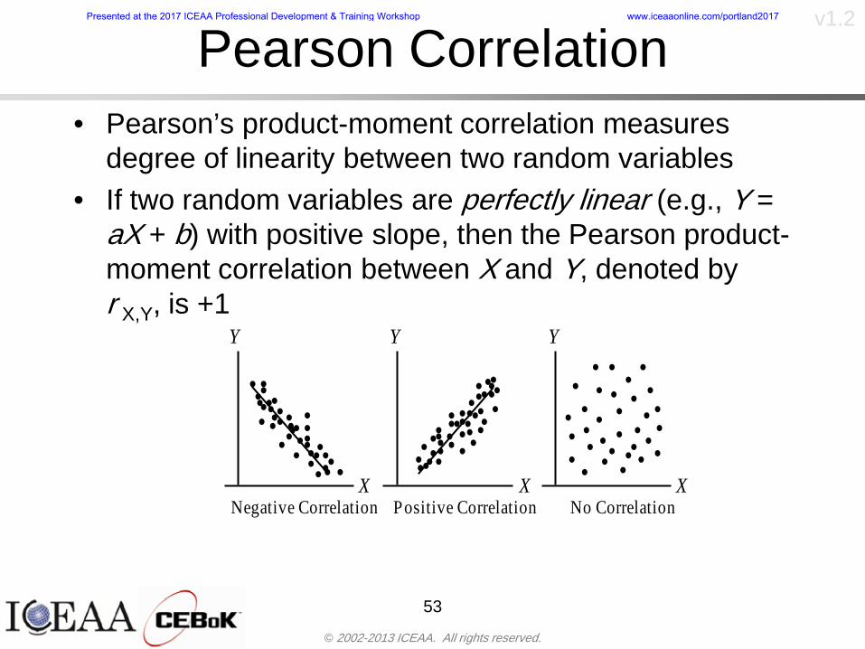
copy 2002-2013 ICEAA All rights reserved
v12
Pearson Correlationbull Pearsonrsquos product-moment correlation measures
degree of linearity between two random variables bull If two random variables are perfectly linear (eg Y =
aX + b) with positive slope then the Pearson product-moment correlation between X and Y denoted by rXY is +1
53
X X
Y Y Y
XNegative Correlation Positive Correlation No Correlation
middotmiddot
middotmiddot
middotmiddot middotmiddot
middotmiddot
middot
middot
middotmiddotmiddot
middotmiddot
middotmiddot
middotmiddot middot
middot
middot
middotmiddotmiddotmiddotmiddotmiddotmiddotmiddot
middotmiddotmiddotmiddot
middotmiddot
middotmiddot middotmiddotmiddotmiddot
middotmiddotmiddot
middotmiddotmiddotmiddot
middotmiddotmiddot
middotmiddotmiddot
middotmiddot
middot
middot middotmiddot
middot middotmiddotmiddotmiddot middotmiddot middot middotmiddot middot middot
middotmiddot middot
middotmiddotmiddotmiddotmiddot middot middotmiddot
middotmiddot
middot
middotmiddot
middotmiddot middot
middot middot middot
middotmiddot middot
middotmiddotmiddot
middotmiddot
middot middot
Presented at the 2017 ICEAA Professional Development amp Training Workshop wwwiceaaonlinecomportland2017
copy 2002-2013 ICEAA All rights reserved
v12
Spearman Correlationbull Spearmanrsquos rank correlation measures the
monotonicity between two random variablesbull If two random variables are perfectly monotonically
increasing (eg Y = X2) then the Spearman rank correlation denoted by rXY is +1
bull The two measures can be significantly different
54
10 20 30 40 50 60
100
200
300
096 097 098 099 1
1
060
020
040
080
Eff
ort (
Staf
f-M
onth
s)
Software Size I KDSI
y = 28z12y
z x
yy = x100
0 pound x pound 1
Figure 5-9A Figure 5-9B
Pearson Correlation = 09976 Rank Correlation = 1
Pearson Correlation = 024 Rank Correlation = 1
X(x ) ~ Unif(01)
Reference Probability Methods for Cost Uncertainty Analysis A Systems Engineering Perspective Paul R Garvey
Presented at the 2017 ICEAA Professional Development amp Training Workshop wwwiceaaonlinecomportland2017
copy 2002-2013 ICEAA All rights reserved
v12
Unit III - Module 9 55
200
250
300
350
400
1000 1200 1400 1600 1800 2000
Recurring Production
SEPM
200
250
300
350
400
1000 1200 1400 1600 1800 2000
Recurring Production
SEPM
Functional Correlationbull Old No Functional
Correlation Simulation run with WBS items entered as values
bull New Simulation run with functional dependencies entered as they are in cost model
CorrelatedNot Correlated
Note shift of mean and increased variability
Presented at the 2017 ICEAA Professional Development amp Training Workshop wwwiceaaonlinecomportland2017
copy 2002-2013 ICEAA All rights reserved
v12
Risk Measuresbull ldquoWestern Europe conquered the word because of a
technological revolution that started because of attempts to measure the worldrdquo ndash Phillipe Jorion ndash In the same way attempts to measure risk will lead to better project
managementbull Risk management for DoD and NASA agencies focuses
primarily on funding projects to a single percentile ndash NASA policy explicitly mentions 70 and 50ndash This is known as ldquoValue at Riskrdquo and is prevalent in the banking and
financial industry
56
Presented at the 2017 ICEAA Professional Development amp Training Workshop wwwiceaaonlinecomportland2017
copy 2002-2013 ICEAA All rights reserved
v12
Value at Risk (VaR)bull VaR is a percentile of the cost risk
distributionndash VaR funding at the 70th percentile means that
there is a 30 chance of final project cost exceeding the funded amount (budget)
bull VaR has some meritsndash Common measure can be used to compare
different projects and programsndash Easily understood by senior managers and
decision makers
57
Presented at the 2017 ICEAA Professional Development amp Training Workshop wwwiceaaonlinecomportland2017
copy 2002-2013 ICEAA All rights reserved
v12
Why 70th or 80th Percentilebull Typical policy guidance involves funding at the 70th or 80th
percentile Why fund as such a low percentilebull There is some incentive to not over-fundbull For a normal distribution an inflection point occurs near the 80th
percentile meaning that for values above 80 confidence achieving higher levels of confidence can only be achieved by spending greater dollar amounts at an increasing rate
58
-05-04-03-02-01
00102030405
0 05 1 15 2 25 3
Standard Deviations from Mean
Normal Distribution
First DerivativeSlopeVelocity
Second DerivativeConvexityAcceleration
Inflection point at one standard deviation above the mean (~84th
percentile)
Presented at the 2017 ICEAA Professional Development amp Training Workshop wwwiceaaonlinecomportland2017
copy 2002-2013 ICEAA All rights reserved
v12
Funding Above Inflection Pointsbull As the percentile goes above the 80th percentile the amount
needed to achieve that higher level of confidence begins to increase at an increasing rate as is evident from the graph
59
0
10
20
30
40
50
60
70
50 55 60 65 70 75 80 85 90 95 100
$ Ab
ove
MEa
n to
Ach
ieve
Per
cent
ile
Percentile (Confidence Level)
Presented at the 2017 ICEAA Professional Development amp Training Workshop wwwiceaaonlinecomportland2017
copy 2002-2013 ICEAA All rights reserved
v12
Why Budget to the 70th or 80thbull Government projects are funded at the 70th or 80th percentilesbull Why not the 90th or 99th percentile Wonrsquot that help prevent
overrunsndash As we have seen percentiles do not add across programs
bull The sum of the 80th percentiles does NOT equal the total 80th percentile
ndash This is because the individual programs are riskier than the entire suite of missions
bull Known as the ldquoPortfolio effectrdquo (more or this later)
ndash Funding at the 80th gives confidence that the entire portfolio will be adequately funded
bull And since there is an inflection point near the 80th percentile funding above that level quickly becomes cost prohibitive
60
Presented at the 2017 ICEAA Professional Development amp Training Workshop wwwiceaaonlinecomportland2017
copy 2002-2013 ICEAA All rights reserved
v12
Inflection Points for Lognormalbull For a lognormal the inflection point
variesndash Coefficient of variation equal to 10 equates to an
inflection point at the 70th percentile
61
0
10
20
30
40
50
60
70
050 060 070 080 090 100
Coef
ficen
t of V
aria
tion
Percentile of the Inflection Point
Presented at the 2017 ICEAA Professional Development amp Training Workshop wwwiceaaonlinecomportland2017
copy 2002-2013 ICEAA All rights reserved
v12
Issues with Percentile Fundingbull However risk management does not stop at a
specific percentilendash What happens when the 70th percentile is exceeded
bull Any effective risk management policy should prescribe what happens after a bad event occursndash With VaR we only know when a bad event has occurred ndash Also funding at a relatively low level means we have no true
sense of the real risks that should be guarded against
62
Presented at the 2017 ICEAA Professional Development amp Training Workshop wwwiceaaonlinecomportland2017
copy 2002-2013 ICEAA All rights reserved
v12
ldquoHere There Be Dragonsrdquobull On old maps uncharted territory was often
marked with monsters or dragons
63
A section of the Carta Marina by Olaus Magnus 16th Century
Presented at the 2017 ICEAA Professional Development amp Training Workshop wwwiceaaonlinecomportland2017
copy 2002-2013 ICEAA All rights reserved
v12
Distribution Comparisonbull Four different distributions with the same 70th
percentile
bull Should we expect the tails to be similar
64
0
10
20
30
40
50
60
70
80
0 100 200 300 400 500 600
Perc
entil
eCo
nfid
ence
Lev
el
Triangular
Normal
Lognormal
Pareto
Presented at the 2017 ICEAA Professional Development amp Training Workshop wwwiceaaonlinecomportland2017
copy 2002-2013 ICEAA All rights reserved
v12Distribution Comparison Tail Behavior
bull The normal and triangular distributions have similar tails but the lognormal and Pareto have much fatter right tails
65
70
75
80
85
90
95
100
500 1500 2500 3500 4500 5500
Perc
entil
eCo
nfid
ence
Lev
el
Triangular
Normal
Lognormal
Pareto
Here There Be Dragons
Presented at the 2017 ICEAA Professional Development amp Training Workshop wwwiceaaonlinecomportland2017
copy 2002-2013 ICEAA All rights reserved
v12Distribution Comparison ndash Tail Behavior (Table)
bull There is significant tail risk for the lognormal and the Paretobull The 99th percentile for the Pareto is 1000 times greater than
the 70th percentilendash Risk seen in financial markets and in catastrophic risks like natural
disasters bull Four different projects follow the four different risk profiles seen
in this example should clearly have different risk management approaches but 70th percentile funding indicates the same risk management approach for all four
66
Percentile Triangular Normal Lognormal Pareto 70th $600 $600 $600 $600 80th $680 $660 $770 $1430 90th $770 $750 $1070 $5880 95th $840 $820 $1410 $23750 99th $930 $950 $2350 $600000
Presented at the 2017 ICEAA Professional Development amp Training Workshop wwwiceaaonlinecomportland2017
copy 2002-2013 ICEAA All rights reserved
v12Percentile Budgeting is Not Risk Management
bull Percentile budgeting ne effective risk management policybull Suppose that you are shopping for a new car You
mention that safety is your top concern The salesman says he has a great safe car available You ask about the air bags Do they work The salesman answers ldquoOf course Seventy percent of the time they work fine Only 30 of the time the air bags will fail to deployrdquo Would you buy such a car Hedge fund manager David Einhorn has stated ldquoRisk management is the air bag that must always work but only in the multi-sigma event where you have an accidentrdquo
67
Risk management is the air bag that must always work but only in the multi-sigma event where you
have an accident
Presented at the 2017 ICEAA Professional Development amp Training Workshop wwwiceaaonlinecomportland2017
copy 2002-2013 ICEAA All rights reserved
v12
Joint Confidence Level Analysisbull Schedules are risky toobull For 98 recent NASA missions average
schedule growth was 38ndash Not as high as cost growth but still significant
68
0
5
10
15
20
25
30
35
40
Schedule
Cost
Presented at the 2017 ICEAA Professional Development amp Training Workshop wwwiceaaonlinecomportland2017
copy 2002-2013 ICEAA All rights reserved
v12
Schedules Impact Costbull Changes in schedule can have enormous
impacts on cost ndash Schedule slips can lead to cost increases
bull Fixed programmatic costs must be paid on a regular basisndash Achieving schedule milestones early can result in cost
savings
bull Schedule is an important consideration in cost analysis including cost risk analysis
bull However we must be careful in correctly integrating cost and schedule riskndash Schedule is not simply an input but is dependent on many of
the same factors that drive cost
69
Presented at the 2017 ICEAA Professional Development amp Training Workshop wwwiceaaonlinecomportland2017
copy 2002-2013 ICEAA All rights reserved
v12
The Relationship of Cost to Schedulebull Cost and schedule are positively correlated
ndash A larger program with bigger scope with take longer to complete than a smaller simpler program
bull However longer schedules do not always equate to higher cost nor shorter schedules with lower costndash Highly compressed schedules relative to the
optimal schedule can lead to large overrunsbull Compressed schedules are commonplace for
many planetary missions
70
Presented at the 2017 ICEAA Professional Development amp Training Workshop wwwiceaaonlinecomportland2017
copy 2002-2013 ICEAA All rights reserved
v12The Impact of Schedule GrowthCompression on Cost
bull Compressed schedules lead to cost growth and based on existing research is actually more expensive than schedule slippages
71
0
20
40
60
80
100
120
140
160
-50 -25 0 25 50 75 100
Percentage Change in Schedule
Perc
enta
ge C
hang
e in
Cos
t due
to
Sche
dule
Cha
nge
Source Smart CB ldquoCost and Schedule Interrelationshipsrdquo 2007 NASA Cost Symposium
Presented at the 2017 ICEAA Professional Development amp Training Workshop wwwiceaaonlinecomportland2017
copy 2002-2013 ICEAA All rights reserved
v12Schedule as an Independent Variable
bull Why not simply add schedule as an input to cost-estimating relationships (CERs)
bull Schedule is often treated as an independent variable ndash schedules are often determined independently of cost considerationsndash Cost may not be considered explicitly although budgets and
schedules are determined based on scope and other common factors
bull In 2006 SAIC undertook a research task to determine the impact of schedule on cost and added schedule as an independent variable to the CERs in the NASAAir Force Cost Model (NAFCOM) to see if schedule provided any improvement in goodness of fit
72
Presented at the 2017 ICEAA Professional Development amp Training Workshop wwwiceaaonlinecomportland2017
copy 2002-2013 ICEAA All rights reserved
v12
Schedule is a Dependent Variablebull Since NAFCOM includes an exhaustive list of cost drivers the inclusion
of schedule should give an indication of whether there is any additional independent value added from schedule independent of the cost drivers
bull In the study schedule was added to 10 subsystem-level CERs
ndash In each case the addition of schedule did NOTimprove the goodness of fit and schedule was NOT found to be a statistically significant cost driver (given the presence of the other variables) for any of the 10 CERs
bull Standard errors for the CERs increased due to decrease in degrees of freedom
bull Thus schedule as an independent variable did not provide any additional explanation of variation in historical cost
bull This is because schedule is truly NOT an independent variable but a dependent variable and is a function of the same factors that drive cost
73
Presented at the 2017 ICEAA Professional Development amp Training Workshop wwwiceaaonlinecomportland2017
copy 2002-2013 ICEAA All rights reserved
v12
Incorporation of Schedule in Cost Risk
bull When using subjective methods care must be taken in applying schedule to cost risk analysis
bull Since schedule is a dependent variable treating it independently from other factors when assessing its impact on cost can lead to a double count of independent variables in the cost risk analysis
bull Direct inclusion of schedule in a cost risk analysis effectively doubles the influence of each cost driver
ndash Incorrectly leads to broader risk ranges
74
CostWeight
HeritageNewness
Technology Readiness Schedule
Presented at the 2017 ICEAA Professional Development amp Training Workshop wwwiceaaonlinecomportland2017
copy 2002-2013 ICEAA All rights reserved
v12Subjective Cost Risk Methods and Overinclusion of Risk Factors
bull Subjective methods are suitable when data are scarce or not availablebull However care must be taken not to treat correlated sources of risk
such as schedule as independent of each otherbull Example ndash a subjective risk analysis incorporated technology readiness
design risk requirements stability integration risk and schedule and treated each source of risk as independent
bull Risk triangle high value without schedule risk was 31 times the point estimate
bull Risk triangle high value with schedule risk added on top of other sources of risk treated independently was 34 times the point estimate
bull Risk triangle taking correlation between sources of risk into account in a rigorous statistical manner has a high value 15 times the point estimate less than half the effect when treating sources of risk as independent
75
Presented at the 2017 ICEAA Professional Development amp Training Workshop wwwiceaaonlinecomportland2017
copy 2002-2013 ICEAA All rights reserved
v12Fundamental Equation of Cost and Schedule Interrelationships
bull The Fundamental Equation of the Relationship Between Cost and Schedule is
Time = Moneybull This is a well known adage that time is money Your boss at
work may even mention this to you from time to time or if you are the boss you are all too aware of this iron law
bull Because time is money cost and schedule risk should be modeled jointly not with schedule as an independent cost driver
bull Note that cost and schedule are not perfectly correlatedndash Cost can sometimes ldquobuy downrdquo schedule extra money can be
spent to meet a deadline since in some cases additional effort to hasten the completion of a task
76
Presented at the 2017 ICEAA Professional Development amp Training Workshop wwwiceaaonlinecomportland2017
copy 2002-2013 ICEAA All rights reserved
v12How to (Correctly) Incorporate Schedule into Cost Risk Analysis
bull The best way to model cost and schedule risk is to develop a joint cost and schedule model based on the same data
bull Since such models are not currently available the next best approach is to model cost and schedule independently and then integrate cost and schedule risk analyses using joint probability distributions taking into account correlation between cost and schedulendash This approach pioneered by Paul Garvey and Steve Book is
considered industry best practicendash This is a practical method mathematically tractable and follows
naturally from the Fundamental Equation of Cost and Schedule Interrelationships
77
Book S A ldquoQuantifying the Relationship Between Cost and Schedulerdquo The Measurable News Winter 2007-2008 pp 11-15Garvey PR Probability Methods for Cost Uncertainty Analysis A Systems Engineering Perspective New York Marcel Dekker 2000 pp 308-335
Presented at the 2017 ICEAA Professional Development amp Training Workshop wwwiceaaonlinecomportland2017
copy 2002-2013 ICEAA All rights reserved
v12
Joint Lognormal and Normal Distributions
bull Cost and schedule are typically modeled as some combination of Normal and Lognormal probability distributionsndash Studies by The Aerospace Corporation the MITRE
Corporation Wyle Labs and SAIC have found that the Lognormal probability distribution almost always serves as a good model for both the schedule distribution and the cost distribution
ndash The Normal distribution may also be appropriate in some instances and depending upon the level of confidence at which budgets are set may even be more conservative and logically consistent than the Normal distribution
ndash Joint Lognormal and Normal distributions are defined by a pair of mean and standard deviations and a level of correlation between the two
78
Presented at the 2017 ICEAA Professional Development amp Training Workshop wwwiceaaonlinecomportland2017
copy 2002-2013 ICEAA All rights reserved
v12Modeling Cost and Schedule as a Bivariate Distribution
bull In the approach set forth by Book and Garvey cost risk is assessed and the top-level distribution is modeled as a Lognormal (or Normal) distribution schedule risk is assessed and the overall schedule risk is modeled as a Lognormal (or Normal) distribution
bull The two distributions are combined into a Bivariate distribution by assigning a correlation between the two and by treating the two distributions as the marginal distributions of a Bivariate Lognormal distributionndash Other combinations include a Bivariate Normal or a Bivariate
Normal-Lognormal
79
Presented at the 2017 ICEAA Professional Development amp Training Workshop wwwiceaaonlinecomportland2017
copy 2002-2013 ICEAA All rights reserved
v12Bivariate Lognormal Distribution for Cost and Schedule
bull Cost is often observed to be Lognormal when strong positive correlations are present among the systemrsquos WBS cost element costs
bull A systemrsquos schedule is often observed (from Monte Carlo simulations) to be Lognormal if it is the sum of many positively correlated schedule activities in an overall schedule network
bull If Lognormal distributions characterize a systemrsquos cost and schedule then the Bivariate Lognormal could serve as an assumed model of their joint distributionndash In this case the marginal distribution of each of cost and schedule is
Lognormalbull Other possibilities for modeling cost and schedule as a Bivariate
distribution include a Bivariate Normal or a Bivariate Normal-Lognormal distributionndash All these combinations are analytically tractable
80
Presented at the 2017 ICEAA Professional Development amp Training Workshop wwwiceaaonlinecomportland2017
copy 2002-2013 ICEAA All rights reserved
v12Bivariate Lognormal for Cost and Schedule
bull Contour Plots of a Bivariate Lognormal
81
Presented at the 2017 ICEAA Professional Development amp Training Workshop wwwiceaaonlinecomportland2017
copy 2002-2013 ICEAA All rights reserved
v12Correlation Between Cost and Schedule
bull Cost and schedule are positively correlated but not perfectly sondash For example it is possible to have a schedule underrun and a cost
overrunbull Based on cost and schedule growth data for 50 completed NASA
programs the correlation between development cost and development schedule is 70
82
00
200
400
600
800
1000
1200
-500 00 500 1000 1500 2000 2500Historical Cost Growth
Hist
oric
al S
ched
ule
Gro
wth
r = 715
Presented at the 2017 ICEAA Professional Development amp Training Workshop wwwiceaaonlinecomportland2017
copy 2002-2013 ICEAA All rights reserved
v12Correlation Between Cost and Schedule Caveats
bull Based on historical data recommended correlation between cost and schedule is 70 but this could be higher or lower depending upon program circumstancesndash If program is budget constrained cost and schedule will be
more highly correlated (go as you pay)ndash If program is schedule constrained cost and schedule will
have lower correlation perhaps even negative correlation ndash Smaller programs have smaller correlation between cost and
schedule riskbull Relatively easy to ldquohurry uprdquo and finish on time or even early if
needed
83
Presented at the 2017 ICEAA Professional Development amp Training Workshop wwwiceaaonlinecomportland2017
copy 2002-2013 ICEAA All rights reserved
v12
Conditional Confidence Levelsbull Given a programrsquos project schedule we can determine the cost
risk distribution conditional upon the given schedulebull Conditional cost S-curves are steeper than unconditional
(marginal) cost S-curves between some uncertainty has been removed because schedule is fixed
84
Presented at the 2017 ICEAA Professional Development amp Training Workshop wwwiceaaonlinecomportland2017
copy 2002-2013 ICEAA All rights reserved
v12
Joint Confidence Levelsbull Joint 65 confidence represents the probability of
achieving both 65 confidence in cost AND 65 confidence in schedulendash This is different than achieving 65 cost confidence alone
or achieving 65 schedule confidence alonebull Due to the imperfect correlation between cost and schedule it
is possible to achieve a 65 cost confidence with a lower level of schedule confidence
bull Restricting the schedule confidence thus requires additional $ to achieve a given level of confidence
85
X
Y
Possible Values for Which X gt a Possible Values for
Which X gt a and Y gt b
a
b
Presented at the 2017 ICEAA Professional Development amp Training Workshop wwwiceaaonlinecomportland2017
copy 2002-2013 ICEAA All rights reserved
v12Joint Confidence Levels Versus Cost Confidence Levels Only
bull Example of the differences between cost confidence schedule confidence conditional cost confidence and joint cost and schedule confidence
86
Joint Cost-Schedule Confidence Iso-Curves
Cost (RY$M)
Sche
dule
(Mon
ths)
65 Confidence
50 Confidence
70 Confidence
65 Cost Confidence AggressiveSchedule65 Cost ConfidenceScheduleGiven 65 Schedule ConfidenceUnconditional 65 CostConfidenceUnconditional 65 ScheduleConfidence
65 Cost Confidence 65 Joint Cost and Schedule
Confidence for 65 Schedule Confidence
Presented at the 2017 ICEAA Professional Development amp Training Workshop wwwiceaaonlinecomportland2017
copy 2002-2013 ICEAA All rights reserved
v12
Joint Cost and Schedule Confidence
bull Can examine pairs of cost and schedule that achieve a given level of confidence
bull Provides insights into the trade-offs between cost and schedule for a given level of confidencendash Possible to increase cost confidence by giving a
project more time in some instances or possible to ldquobuy downrdquo schedule
bull But these have limits and are shown in the iso-cost and schedule confidence curves
87
Presented at the 2017 ICEAA Professional Development amp Training Workshop wwwiceaaonlinecomportland2017
copy 2002-2013 ICEAA All rights reserved
v12Cost and Schedule Trade-offs for a Given Level of Joint Confidence
bull Hypothetical Example
88
Cost (RY$M)
Schedule (Months)
$100 48$99 48$89 49$87 50$85 51$85 52$84 53$83 55$83 55$83 56
Cost and Schedule 65 Confidence Iso-Curve
4748495051525354555657
$80 $82 $84 $86 $88 $90 $92 $94 $96 $98 $100
Cost (RY$ M)
Sche
dule
(Mon
ths)
Presented at the 2017 ICEAA Professional Development amp Training Workshop wwwiceaaonlinecomportland2017
copy 2002-2013 ICEAA All rights reserved
v12Policy Considerations for Confidence Levels
bull For large programs the difference between the amount of money needed to achieve 65 cost confidence independent of schedule and joint 65 cost and schedule confidence can represent hundreds of millions and even billions of dollars
89
Joint Cost-Schedule Confidence Iso-Curves
Cost (RY$M)
Sche
dule
(Mon
ths)
65 Confidence
65 Cost Confidence AggressiveSchedule
65 Cost ConfidenceScheduleGiven 65 Schedule Confidence
Unconditional 65 CostConfidence
Joint Cost and Schedule Confidence for 65 Cost Confidence and Program Baseline Schedule is Less Than 35
65 Cost Confidence Independent of Schedule Cost Needed to Achieve
Both 65 Joint Cost and Schedule Confidence for the Schedule with 65 Confidence
Presented at the 2017 ICEAA Professional Development amp Training Workshop wwwiceaaonlinecomportland2017
copy 2002-2013 ICEAA All rights reserved
v12
Copulasbull More generally any combination of distributions can
be used (more than just normal and lognormal)ndash Termed ldquocopulardquo from the Italian word for ldquocouplerdquondash Copulas are a way to combine marginal distributions of any
number and type into a joint distributionbull More formally a copula is a multivariate joint distribution defined
on the n-dimensional unit cube [0 1]n such that every marginal distribution is uniform on the interval [0 1]
bull (The bivariate form of) Sklarrsquos theorem states that for any bivariate distribution function H(x y) let F(x) = H(x infin) and G(y) = H(infin y) be the univariate marginal probability distribution functions Then there exists a copula C such that H(xy)=C(F(x)G(y))
ndash Copulas are widely used in risk management for investments and insurance
bull Considered industry best practice (Li 2000)bull Marketed as part of JP Morganrsquos CreditMetrics suite of tools
(Gupton et Al 1997)90
Presented at the 2017 ICEAA Professional Development amp Training Workshop wwwiceaaonlinecomportland2017
copy 2002-2013 ICEAA All rights reserved
v12Parametric Joint Cost and Schedule Analysis
bull A parametric model based on a consistent data set with a set of overlapping cost and schedule drivers is a cleaner way to model cost and schedule
91
CostWeight
HeritageNewness
Technology Readiness
Schedule
0
20
40
60
80
100
Confidence
Joint Cost and Schedule Confidence
Schedule
Cost
Lognormal Distribution PDF and CDF
0102030405060708090100
200 300 400 500 600 700 800 900 1000Cost $
Con
fiden
ce L
evel
0
00002
00004
00006
00008
0001
00012
00014
00016
Prob
abili
ty D
ensi
ty
CDFPDF
Lognormal Distribution PDF and CDF
0102030405060708090100
200 300 400 500 600 700 800 900 1000Cost $
Con
fiden
ce L
evel
0
00002
00004
00006
00008
0001
00012
00014
00016
Prob
abili
ty D
ensi
ty
CDFPDF
Presented at the 2017 ICEAA Professional Development amp Training Workshop wwwiceaaonlinecomportland2017
copy 2002-2013 ICEAA All rights reserved
v12Parametric Joint Cost and Schedule Analysis (2)
bull Joint cost and schedule risk analysis produced naturally by the integrated modelndash Addresses several issues with the copula
approachbull Tail dependencybull Correlation ndash no need to assign correlation
between cost and schedulebull Consistency of cost and schedule models
92
Presented at the 2017 ICEAA Professional Development amp Training Workshop wwwiceaaonlinecomportland2017
copy 2002-2013 ICEAA All rights reserved
v12
Resource-Loaded Schedulesbull Involves assigning cost and schedule risks to a resource-loaded schedule
networkbull Bottom-up approach
ndash More labor intensive than parametrics but can also provide more insight
ndash Can answer questions than parametric typically cannot such as how much do reserve requirements decrease if a specific risk is retired
bull Currently being implemented in Constellation programbull Has same issue as all bottom-up models hard to count all the risks and model
them discretely
ndash As a result there is a tendency to reflect less risk than indicated by history
ndash ldquoThere are more things in heaven and earth Horatio than are dreamt of in your philosophyrdquo William Shakespeare Hamlet Act I Scene V
93
Presented at the 2017 ICEAA Professional Development amp Training Workshop wwwiceaaonlinecomportland2017
copy 2002-2013 ICEAA All rights reserved
v12Resource-Loaded Schedules Vs Parametrics
bull Parametric most appropriate for early estimatesndash But also good for high-level checks as project progresses
bull As plans take shape lower level modeling may be more appropriate
94 1
CONCEPTUALDEVELOPMENT
PROJECTDEFINITION DESIGN DEVELOPMENT OPERATIONS
PARAMETRIC PARAMETRIC
ANALOGY
ENGINEERING (Bottoms Up)
$PARAMETRIC
DETAILED
$
Pre Phase A Phase B Phase CDPhase A Phase EPre Phase A Phase B Phase CDPhase A Phase E
Risk = f(Cost Estimating Relationship Inputs eg mass power data rate TRL new design etc)
Risk = f(cost and schedule variation of the analogous elements)
Risk = f(variation of detailed inputs eg labor hours rates materials etc)
Presented at the 2017 ICEAA Professional Development amp Training Workshop wwwiceaaonlinecomportland2017
copy 2002-2013 ICEAA All rights reserved
v12
Resource-Loaded Schedulesbull Methodology has been demonstrated in other
industriesndash Construction oil and gasndash Analysis has not been traditionally done on highly uncertain
complex development projects bull Methodology focuses on project baseline schedule
ndash In baseline schedule all tasks are resource loaded to represent a baseline schedule and cost standpoint
ndash Resource loaded schedule is ldquorolledrdquo up to a manageable level
ndash Based on the risk and uncertainties identified schedule distributions are applied to each rolled up task
ndash Cost uncertainties are also applied to rolled up tasksbull Uncertainties include labor rate man power etc
ndash A Monte Carlo simulation is run to develop joint cost-schedule distributions
95
Presented at the 2017 ICEAA Professional Development amp Training Workshop wwwiceaaonlinecomportland2017
copy 2002-2013 ICEAA All rights reserved
v12
Unit III - Module 9 96
Execution ndash Cross Checksbull Means The mean cost growth factor for WBS items
can be compared to history as a way to cross check results
bull CVs The CV of the cost growth factors for WBS items can be compared to history as a way to cross check results
bull Inputs Checks are performed on inputs or other parameters to see if historical values are in line with program assumptionsndash Example Historical risk scores can be compared to program
risk scores to see if risk assessors are being realistic and to see if the underlying database is representative of the program
11
Presented at the 2017 ICEAA Professional Development amp Training Workshop wwwiceaaonlinecomportland2017
- Cost and Schedule Risk Analysis Basic
- Acknowledgments
- Unit Index
- Risk Overview
- Agenda
- Introduction
- Risk Analysis Terms
- Are Our Costs Realistic
- Historical Cost Growth
- Sources of Cost Risk
- Point Estimates of Cost
- Types of Risk
- Point Estimates Vs Risk Estimates
- Cost Risk and Probability
- Probability Model ndash Distribution
- Probability Model ndash Distribution
- Probability ndash Top-Level Distribution
- S-Curves and Confidence Levels
- Example ndash Normal Distribution
- Confidence Levels
- Measuring Parametric Model Uncertainty
- Parametric Model Example
- Weight Uncertainty
- Estimating Uncertainty
- Estimating Uncertainty (2)
- Estimating Uncertainty (3)
- Aggregating Risk
- WBS Example
- WBS and Risk
- Aggregating Risk
- Percentiles Do Not Add
- Percentiles Do Not Add (2)
- Percentiles Do Not Add (3)
- Methods for Aggregating Risk
- Monte Carlo Simulationfor Risk Analysis
- Monte Carlo Simulation
- Using Random Numbers to Simulate Distributions
- Simulating a Triangular Distribution
- Simulating a Triangular Distribution (2)
- Monte Carlo and the WBS
- Number of Trials
- Number of Trials (2)
- Number of Trials (3)
- Number of Trials (4)
- Number of Trials (5)
- Number of Trials (6)
- Methods of Simulation
- Probability Model ndash Correlation
- Correlation And Causation
- The Importance of Correlation
- The Importance of Correlation (2)
- Measures of Correlation
- Pearson Correlation
- Spearman Correlation
- Functional Correlation
- Risk Measures
- Value at Risk (VaR)
- Why 70th or 80th Percentile
- Funding Above Inflection Points
- Why Budget to the 70th or 80th
- Inflection Points for Lognormal
- Issues with Percentile Funding
- ldquoHere There Be Dragonsrdquo
- Distribution Comparison
- Distribution Comparison Tail Behavior
- Distribution Comparison ndash Tail Behavior (Table)
- Percentile Budgeting is Not Risk Management
- Joint Confidence Level Analysis
- Schedules Impact Cost
- The Relationship of Cost to Schedule
- The Impact of Schedule GrowthCompression on Cost
- Schedule as an Independent Variable
- Schedule is a Dependent Variable
- Incorporation of Schedule in Cost Risk
- Subjective Cost Risk Methods and Overinclusion of Risk Factors
- Fundamental Equation of Cost and Schedule Interrelationships
- How to (Correctly) Incorporate Schedule into Cost Risk Analysis
- Joint Lognormal and Normal Distributions
- Modeling Cost and Schedule as a Bivariate Distribution
- Bivariate Lognormal Distribution for Cost and Schedule
- Bivariate Lognormal for Cost and Schedule
- Correlation Between Cost and Schedule
- Correlation Between Cost and Schedule Caveats
- Conditional Confidence Levels
- Joint Confidence Levels
- Joint Confidence Levels Versus Cost Confidence Levels Only
- Joint Cost and Schedule Confidence
- Cost and Schedule Trade-offs for a Given Level of Joint Confidence
- Policy Considerations for Confidence Levels
- Copulas
- Parametric Joint Cost and Schedule Analysis
- Parametric Joint Cost and Schedule Analysis (2)
- Resource-Loaded Schedules
- Resource-Loaded Schedules Vs Parametrics
- Resource-Loaded Schedules
- Execution ndash Cross Checks
-
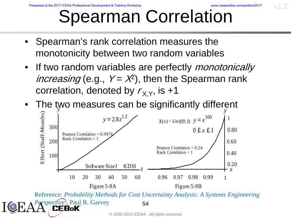
copy 2002-2013 ICEAA All rights reserved
v12
Spearman Correlationbull Spearmanrsquos rank correlation measures the
monotonicity between two random variablesbull If two random variables are perfectly monotonically
increasing (eg Y = X2) then the Spearman rank correlation denoted by rXY is +1
bull The two measures can be significantly different
54
10 20 30 40 50 60
100
200
300
096 097 098 099 1
1
060
020
040
080
Eff
ort (
Staf
f-M
onth
s)
Software Size I KDSI
y = 28z12y
z x
yy = x100
0 pound x pound 1
Figure 5-9A Figure 5-9B
Pearson Correlation = 09976 Rank Correlation = 1
Pearson Correlation = 024 Rank Correlation = 1
X(x ) ~ Unif(01)
Reference Probability Methods for Cost Uncertainty Analysis A Systems Engineering Perspective Paul R Garvey
Presented at the 2017 ICEAA Professional Development amp Training Workshop wwwiceaaonlinecomportland2017
copy 2002-2013 ICEAA All rights reserved
v12
Unit III - Module 9 55
200
250
300
350
400
1000 1200 1400 1600 1800 2000
Recurring Production
SEPM
200
250
300
350
400
1000 1200 1400 1600 1800 2000
Recurring Production
SEPM
Functional Correlationbull Old No Functional
Correlation Simulation run with WBS items entered as values
bull New Simulation run with functional dependencies entered as they are in cost model
CorrelatedNot Correlated
Note shift of mean and increased variability
Presented at the 2017 ICEAA Professional Development amp Training Workshop wwwiceaaonlinecomportland2017
copy 2002-2013 ICEAA All rights reserved
v12
Risk Measuresbull ldquoWestern Europe conquered the word because of a
technological revolution that started because of attempts to measure the worldrdquo ndash Phillipe Jorion ndash In the same way attempts to measure risk will lead to better project
managementbull Risk management for DoD and NASA agencies focuses
primarily on funding projects to a single percentile ndash NASA policy explicitly mentions 70 and 50ndash This is known as ldquoValue at Riskrdquo and is prevalent in the banking and
financial industry
56
Presented at the 2017 ICEAA Professional Development amp Training Workshop wwwiceaaonlinecomportland2017
copy 2002-2013 ICEAA All rights reserved
v12
Value at Risk (VaR)bull VaR is a percentile of the cost risk
distributionndash VaR funding at the 70th percentile means that
there is a 30 chance of final project cost exceeding the funded amount (budget)
bull VaR has some meritsndash Common measure can be used to compare
different projects and programsndash Easily understood by senior managers and
decision makers
57
Presented at the 2017 ICEAA Professional Development amp Training Workshop wwwiceaaonlinecomportland2017
copy 2002-2013 ICEAA All rights reserved
v12
Why 70th or 80th Percentilebull Typical policy guidance involves funding at the 70th or 80th
percentile Why fund as such a low percentilebull There is some incentive to not over-fundbull For a normal distribution an inflection point occurs near the 80th
percentile meaning that for values above 80 confidence achieving higher levels of confidence can only be achieved by spending greater dollar amounts at an increasing rate
58
-05-04-03-02-01
00102030405
0 05 1 15 2 25 3
Standard Deviations from Mean
Normal Distribution
First DerivativeSlopeVelocity
Second DerivativeConvexityAcceleration
Inflection point at one standard deviation above the mean (~84th
percentile)
Presented at the 2017 ICEAA Professional Development amp Training Workshop wwwiceaaonlinecomportland2017
copy 2002-2013 ICEAA All rights reserved
v12
Funding Above Inflection Pointsbull As the percentile goes above the 80th percentile the amount
needed to achieve that higher level of confidence begins to increase at an increasing rate as is evident from the graph
59
0
10
20
30
40
50
60
70
50 55 60 65 70 75 80 85 90 95 100
$ Ab
ove
MEa
n to
Ach
ieve
Per
cent
ile
Percentile (Confidence Level)
Presented at the 2017 ICEAA Professional Development amp Training Workshop wwwiceaaonlinecomportland2017
copy 2002-2013 ICEAA All rights reserved
v12
Why Budget to the 70th or 80thbull Government projects are funded at the 70th or 80th percentilesbull Why not the 90th or 99th percentile Wonrsquot that help prevent
overrunsndash As we have seen percentiles do not add across programs
bull The sum of the 80th percentiles does NOT equal the total 80th percentile
ndash This is because the individual programs are riskier than the entire suite of missions
bull Known as the ldquoPortfolio effectrdquo (more or this later)
ndash Funding at the 80th gives confidence that the entire portfolio will be adequately funded
bull And since there is an inflection point near the 80th percentile funding above that level quickly becomes cost prohibitive
60
Presented at the 2017 ICEAA Professional Development amp Training Workshop wwwiceaaonlinecomportland2017
copy 2002-2013 ICEAA All rights reserved
v12
Inflection Points for Lognormalbull For a lognormal the inflection point
variesndash Coefficient of variation equal to 10 equates to an
inflection point at the 70th percentile
61
0
10
20
30
40
50
60
70
050 060 070 080 090 100
Coef
ficen
t of V
aria
tion
Percentile of the Inflection Point
Presented at the 2017 ICEAA Professional Development amp Training Workshop wwwiceaaonlinecomportland2017
copy 2002-2013 ICEAA All rights reserved
v12
Issues with Percentile Fundingbull However risk management does not stop at a
specific percentilendash What happens when the 70th percentile is exceeded
bull Any effective risk management policy should prescribe what happens after a bad event occursndash With VaR we only know when a bad event has occurred ndash Also funding at a relatively low level means we have no true
sense of the real risks that should be guarded against
62
Presented at the 2017 ICEAA Professional Development amp Training Workshop wwwiceaaonlinecomportland2017
copy 2002-2013 ICEAA All rights reserved
v12
ldquoHere There Be Dragonsrdquobull On old maps uncharted territory was often
marked with monsters or dragons
63
A section of the Carta Marina by Olaus Magnus 16th Century
Presented at the 2017 ICEAA Professional Development amp Training Workshop wwwiceaaonlinecomportland2017
copy 2002-2013 ICEAA All rights reserved
v12
Distribution Comparisonbull Four different distributions with the same 70th
percentile
bull Should we expect the tails to be similar
64
0
10
20
30
40
50
60
70
80
0 100 200 300 400 500 600
Perc
entil
eCo
nfid
ence
Lev
el
Triangular
Normal
Lognormal
Pareto
Presented at the 2017 ICEAA Professional Development amp Training Workshop wwwiceaaonlinecomportland2017
copy 2002-2013 ICEAA All rights reserved
v12Distribution Comparison Tail Behavior
bull The normal and triangular distributions have similar tails but the lognormal and Pareto have much fatter right tails
65
70
75
80
85
90
95
100
500 1500 2500 3500 4500 5500
Perc
entil
eCo
nfid
ence
Lev
el
Triangular
Normal
Lognormal
Pareto
Here There Be Dragons
Presented at the 2017 ICEAA Professional Development amp Training Workshop wwwiceaaonlinecomportland2017
copy 2002-2013 ICEAA All rights reserved
v12Distribution Comparison ndash Tail Behavior (Table)
bull There is significant tail risk for the lognormal and the Paretobull The 99th percentile for the Pareto is 1000 times greater than
the 70th percentilendash Risk seen in financial markets and in catastrophic risks like natural
disasters bull Four different projects follow the four different risk profiles seen
in this example should clearly have different risk management approaches but 70th percentile funding indicates the same risk management approach for all four
66
Percentile Triangular Normal Lognormal Pareto 70th $600 $600 $600 $600 80th $680 $660 $770 $1430 90th $770 $750 $1070 $5880 95th $840 $820 $1410 $23750 99th $930 $950 $2350 $600000
Presented at the 2017 ICEAA Professional Development amp Training Workshop wwwiceaaonlinecomportland2017
copy 2002-2013 ICEAA All rights reserved
v12Percentile Budgeting is Not Risk Management
bull Percentile budgeting ne effective risk management policybull Suppose that you are shopping for a new car You
mention that safety is your top concern The salesman says he has a great safe car available You ask about the air bags Do they work The salesman answers ldquoOf course Seventy percent of the time they work fine Only 30 of the time the air bags will fail to deployrdquo Would you buy such a car Hedge fund manager David Einhorn has stated ldquoRisk management is the air bag that must always work but only in the multi-sigma event where you have an accidentrdquo
67
Risk management is the air bag that must always work but only in the multi-sigma event where you
have an accident
Presented at the 2017 ICEAA Professional Development amp Training Workshop wwwiceaaonlinecomportland2017
copy 2002-2013 ICEAA All rights reserved
v12
Joint Confidence Level Analysisbull Schedules are risky toobull For 98 recent NASA missions average
schedule growth was 38ndash Not as high as cost growth but still significant
68
0
5
10
15
20
25
30
35
40
Schedule
Cost
Presented at the 2017 ICEAA Professional Development amp Training Workshop wwwiceaaonlinecomportland2017
copy 2002-2013 ICEAA All rights reserved
v12
Schedules Impact Costbull Changes in schedule can have enormous
impacts on cost ndash Schedule slips can lead to cost increases
bull Fixed programmatic costs must be paid on a regular basisndash Achieving schedule milestones early can result in cost
savings
bull Schedule is an important consideration in cost analysis including cost risk analysis
bull However we must be careful in correctly integrating cost and schedule riskndash Schedule is not simply an input but is dependent on many of
the same factors that drive cost
69
Presented at the 2017 ICEAA Professional Development amp Training Workshop wwwiceaaonlinecomportland2017
copy 2002-2013 ICEAA All rights reserved
v12
The Relationship of Cost to Schedulebull Cost and schedule are positively correlated
ndash A larger program with bigger scope with take longer to complete than a smaller simpler program
bull However longer schedules do not always equate to higher cost nor shorter schedules with lower costndash Highly compressed schedules relative to the
optimal schedule can lead to large overrunsbull Compressed schedules are commonplace for
many planetary missions
70
Presented at the 2017 ICEAA Professional Development amp Training Workshop wwwiceaaonlinecomportland2017
copy 2002-2013 ICEAA All rights reserved
v12The Impact of Schedule GrowthCompression on Cost
bull Compressed schedules lead to cost growth and based on existing research is actually more expensive than schedule slippages
71
0
20
40
60
80
100
120
140
160
-50 -25 0 25 50 75 100
Percentage Change in Schedule
Perc
enta
ge C
hang
e in
Cos
t due
to
Sche
dule
Cha
nge
Source Smart CB ldquoCost and Schedule Interrelationshipsrdquo 2007 NASA Cost Symposium
Presented at the 2017 ICEAA Professional Development amp Training Workshop wwwiceaaonlinecomportland2017
copy 2002-2013 ICEAA All rights reserved
v12Schedule as an Independent Variable
bull Why not simply add schedule as an input to cost-estimating relationships (CERs)
bull Schedule is often treated as an independent variable ndash schedules are often determined independently of cost considerationsndash Cost may not be considered explicitly although budgets and
schedules are determined based on scope and other common factors
bull In 2006 SAIC undertook a research task to determine the impact of schedule on cost and added schedule as an independent variable to the CERs in the NASAAir Force Cost Model (NAFCOM) to see if schedule provided any improvement in goodness of fit
72
Presented at the 2017 ICEAA Professional Development amp Training Workshop wwwiceaaonlinecomportland2017
copy 2002-2013 ICEAA All rights reserved
v12
Schedule is a Dependent Variablebull Since NAFCOM includes an exhaustive list of cost drivers the inclusion
of schedule should give an indication of whether there is any additional independent value added from schedule independent of the cost drivers
bull In the study schedule was added to 10 subsystem-level CERs
ndash In each case the addition of schedule did NOTimprove the goodness of fit and schedule was NOT found to be a statistically significant cost driver (given the presence of the other variables) for any of the 10 CERs
bull Standard errors for the CERs increased due to decrease in degrees of freedom
bull Thus schedule as an independent variable did not provide any additional explanation of variation in historical cost
bull This is because schedule is truly NOT an independent variable but a dependent variable and is a function of the same factors that drive cost
73
Presented at the 2017 ICEAA Professional Development amp Training Workshop wwwiceaaonlinecomportland2017
copy 2002-2013 ICEAA All rights reserved
v12
Incorporation of Schedule in Cost Risk
bull When using subjective methods care must be taken in applying schedule to cost risk analysis
bull Since schedule is a dependent variable treating it independently from other factors when assessing its impact on cost can lead to a double count of independent variables in the cost risk analysis
bull Direct inclusion of schedule in a cost risk analysis effectively doubles the influence of each cost driver
ndash Incorrectly leads to broader risk ranges
74
CostWeight
HeritageNewness
Technology Readiness Schedule
Presented at the 2017 ICEAA Professional Development amp Training Workshop wwwiceaaonlinecomportland2017
copy 2002-2013 ICEAA All rights reserved
v12Subjective Cost Risk Methods and Overinclusion of Risk Factors
bull Subjective methods are suitable when data are scarce or not availablebull However care must be taken not to treat correlated sources of risk
such as schedule as independent of each otherbull Example ndash a subjective risk analysis incorporated technology readiness
design risk requirements stability integration risk and schedule and treated each source of risk as independent
bull Risk triangle high value without schedule risk was 31 times the point estimate
bull Risk triangle high value with schedule risk added on top of other sources of risk treated independently was 34 times the point estimate
bull Risk triangle taking correlation between sources of risk into account in a rigorous statistical manner has a high value 15 times the point estimate less than half the effect when treating sources of risk as independent
75
Presented at the 2017 ICEAA Professional Development amp Training Workshop wwwiceaaonlinecomportland2017
copy 2002-2013 ICEAA All rights reserved
v12Fundamental Equation of Cost and Schedule Interrelationships
bull The Fundamental Equation of the Relationship Between Cost and Schedule is
Time = Moneybull This is a well known adage that time is money Your boss at
work may even mention this to you from time to time or if you are the boss you are all too aware of this iron law
bull Because time is money cost and schedule risk should be modeled jointly not with schedule as an independent cost driver
bull Note that cost and schedule are not perfectly correlatedndash Cost can sometimes ldquobuy downrdquo schedule extra money can be
spent to meet a deadline since in some cases additional effort to hasten the completion of a task
76
Presented at the 2017 ICEAA Professional Development amp Training Workshop wwwiceaaonlinecomportland2017
copy 2002-2013 ICEAA All rights reserved
v12How to (Correctly) Incorporate Schedule into Cost Risk Analysis
bull The best way to model cost and schedule risk is to develop a joint cost and schedule model based on the same data
bull Since such models are not currently available the next best approach is to model cost and schedule independently and then integrate cost and schedule risk analyses using joint probability distributions taking into account correlation between cost and schedulendash This approach pioneered by Paul Garvey and Steve Book is
considered industry best practicendash This is a practical method mathematically tractable and follows
naturally from the Fundamental Equation of Cost and Schedule Interrelationships
77
Book S A ldquoQuantifying the Relationship Between Cost and Schedulerdquo The Measurable News Winter 2007-2008 pp 11-15Garvey PR Probability Methods for Cost Uncertainty Analysis A Systems Engineering Perspective New York Marcel Dekker 2000 pp 308-335
Presented at the 2017 ICEAA Professional Development amp Training Workshop wwwiceaaonlinecomportland2017
copy 2002-2013 ICEAA All rights reserved
v12
Joint Lognormal and Normal Distributions
bull Cost and schedule are typically modeled as some combination of Normal and Lognormal probability distributionsndash Studies by The Aerospace Corporation the MITRE
Corporation Wyle Labs and SAIC have found that the Lognormal probability distribution almost always serves as a good model for both the schedule distribution and the cost distribution
ndash The Normal distribution may also be appropriate in some instances and depending upon the level of confidence at which budgets are set may even be more conservative and logically consistent than the Normal distribution
ndash Joint Lognormal and Normal distributions are defined by a pair of mean and standard deviations and a level of correlation between the two
78
Presented at the 2017 ICEAA Professional Development amp Training Workshop wwwiceaaonlinecomportland2017
copy 2002-2013 ICEAA All rights reserved
v12Modeling Cost and Schedule as a Bivariate Distribution
bull In the approach set forth by Book and Garvey cost risk is assessed and the top-level distribution is modeled as a Lognormal (or Normal) distribution schedule risk is assessed and the overall schedule risk is modeled as a Lognormal (or Normal) distribution
bull The two distributions are combined into a Bivariate distribution by assigning a correlation between the two and by treating the two distributions as the marginal distributions of a Bivariate Lognormal distributionndash Other combinations include a Bivariate Normal or a Bivariate
Normal-Lognormal
79
Presented at the 2017 ICEAA Professional Development amp Training Workshop wwwiceaaonlinecomportland2017
copy 2002-2013 ICEAA All rights reserved
v12Bivariate Lognormal Distribution for Cost and Schedule
bull Cost is often observed to be Lognormal when strong positive correlations are present among the systemrsquos WBS cost element costs
bull A systemrsquos schedule is often observed (from Monte Carlo simulations) to be Lognormal if it is the sum of many positively correlated schedule activities in an overall schedule network
bull If Lognormal distributions characterize a systemrsquos cost and schedule then the Bivariate Lognormal could serve as an assumed model of their joint distributionndash In this case the marginal distribution of each of cost and schedule is
Lognormalbull Other possibilities for modeling cost and schedule as a Bivariate
distribution include a Bivariate Normal or a Bivariate Normal-Lognormal distributionndash All these combinations are analytically tractable
80
Presented at the 2017 ICEAA Professional Development amp Training Workshop wwwiceaaonlinecomportland2017
copy 2002-2013 ICEAA All rights reserved
v12Bivariate Lognormal for Cost and Schedule
bull Contour Plots of a Bivariate Lognormal
81
Presented at the 2017 ICEAA Professional Development amp Training Workshop wwwiceaaonlinecomportland2017
copy 2002-2013 ICEAA All rights reserved
v12Correlation Between Cost and Schedule
bull Cost and schedule are positively correlated but not perfectly sondash For example it is possible to have a schedule underrun and a cost
overrunbull Based on cost and schedule growth data for 50 completed NASA
programs the correlation between development cost and development schedule is 70
82
00
200
400
600
800
1000
1200
-500 00 500 1000 1500 2000 2500Historical Cost Growth
Hist
oric
al S
ched
ule
Gro
wth
r = 715
Presented at the 2017 ICEAA Professional Development amp Training Workshop wwwiceaaonlinecomportland2017
copy 2002-2013 ICEAA All rights reserved
v12Correlation Between Cost and Schedule Caveats
bull Based on historical data recommended correlation between cost and schedule is 70 but this could be higher or lower depending upon program circumstancesndash If program is budget constrained cost and schedule will be
more highly correlated (go as you pay)ndash If program is schedule constrained cost and schedule will
have lower correlation perhaps even negative correlation ndash Smaller programs have smaller correlation between cost and
schedule riskbull Relatively easy to ldquohurry uprdquo and finish on time or even early if
needed
83
Presented at the 2017 ICEAA Professional Development amp Training Workshop wwwiceaaonlinecomportland2017
copy 2002-2013 ICEAA All rights reserved
v12
Conditional Confidence Levelsbull Given a programrsquos project schedule we can determine the cost
risk distribution conditional upon the given schedulebull Conditional cost S-curves are steeper than unconditional
(marginal) cost S-curves between some uncertainty has been removed because schedule is fixed
84
Presented at the 2017 ICEAA Professional Development amp Training Workshop wwwiceaaonlinecomportland2017
copy 2002-2013 ICEAA All rights reserved
v12
Joint Confidence Levelsbull Joint 65 confidence represents the probability of
achieving both 65 confidence in cost AND 65 confidence in schedulendash This is different than achieving 65 cost confidence alone
or achieving 65 schedule confidence alonebull Due to the imperfect correlation between cost and schedule it
is possible to achieve a 65 cost confidence with a lower level of schedule confidence
bull Restricting the schedule confidence thus requires additional $ to achieve a given level of confidence
85
X
Y
Possible Values for Which X gt a Possible Values for
Which X gt a and Y gt b
a
b
Presented at the 2017 ICEAA Professional Development amp Training Workshop wwwiceaaonlinecomportland2017
copy 2002-2013 ICEAA All rights reserved
v12Joint Confidence Levels Versus Cost Confidence Levels Only
bull Example of the differences between cost confidence schedule confidence conditional cost confidence and joint cost and schedule confidence
86
Joint Cost-Schedule Confidence Iso-Curves
Cost (RY$M)
Sche
dule
(Mon
ths)
65 Confidence
50 Confidence
70 Confidence
65 Cost Confidence AggressiveSchedule65 Cost ConfidenceScheduleGiven 65 Schedule ConfidenceUnconditional 65 CostConfidenceUnconditional 65 ScheduleConfidence
65 Cost Confidence 65 Joint Cost and Schedule
Confidence for 65 Schedule Confidence
Presented at the 2017 ICEAA Professional Development amp Training Workshop wwwiceaaonlinecomportland2017
copy 2002-2013 ICEAA All rights reserved
v12
Joint Cost and Schedule Confidence
bull Can examine pairs of cost and schedule that achieve a given level of confidence
bull Provides insights into the trade-offs between cost and schedule for a given level of confidencendash Possible to increase cost confidence by giving a
project more time in some instances or possible to ldquobuy downrdquo schedule
bull But these have limits and are shown in the iso-cost and schedule confidence curves
87
Presented at the 2017 ICEAA Professional Development amp Training Workshop wwwiceaaonlinecomportland2017
copy 2002-2013 ICEAA All rights reserved
v12Cost and Schedule Trade-offs for a Given Level of Joint Confidence
bull Hypothetical Example
88
Cost (RY$M)
Schedule (Months)
$100 48$99 48$89 49$87 50$85 51$85 52$84 53$83 55$83 55$83 56
Cost and Schedule 65 Confidence Iso-Curve
4748495051525354555657
$80 $82 $84 $86 $88 $90 $92 $94 $96 $98 $100
Cost (RY$ M)
Sche
dule
(Mon
ths)
Presented at the 2017 ICEAA Professional Development amp Training Workshop wwwiceaaonlinecomportland2017
copy 2002-2013 ICEAA All rights reserved
v12Policy Considerations for Confidence Levels
bull For large programs the difference between the amount of money needed to achieve 65 cost confidence independent of schedule and joint 65 cost and schedule confidence can represent hundreds of millions and even billions of dollars
89
Joint Cost-Schedule Confidence Iso-Curves
Cost (RY$M)
Sche
dule
(Mon
ths)
65 Confidence
65 Cost Confidence AggressiveSchedule
65 Cost ConfidenceScheduleGiven 65 Schedule Confidence
Unconditional 65 CostConfidence
Joint Cost and Schedule Confidence for 65 Cost Confidence and Program Baseline Schedule is Less Than 35
65 Cost Confidence Independent of Schedule Cost Needed to Achieve
Both 65 Joint Cost and Schedule Confidence for the Schedule with 65 Confidence
Presented at the 2017 ICEAA Professional Development amp Training Workshop wwwiceaaonlinecomportland2017
copy 2002-2013 ICEAA All rights reserved
v12
Copulasbull More generally any combination of distributions can
be used (more than just normal and lognormal)ndash Termed ldquocopulardquo from the Italian word for ldquocouplerdquondash Copulas are a way to combine marginal distributions of any
number and type into a joint distributionbull More formally a copula is a multivariate joint distribution defined
on the n-dimensional unit cube [0 1]n such that every marginal distribution is uniform on the interval [0 1]
bull (The bivariate form of) Sklarrsquos theorem states that for any bivariate distribution function H(x y) let F(x) = H(x infin) and G(y) = H(infin y) be the univariate marginal probability distribution functions Then there exists a copula C such that H(xy)=C(F(x)G(y))
ndash Copulas are widely used in risk management for investments and insurance
bull Considered industry best practice (Li 2000)bull Marketed as part of JP Morganrsquos CreditMetrics suite of tools
(Gupton et Al 1997)90
Presented at the 2017 ICEAA Professional Development amp Training Workshop wwwiceaaonlinecomportland2017
copy 2002-2013 ICEAA All rights reserved
v12Parametric Joint Cost and Schedule Analysis
bull A parametric model based on a consistent data set with a set of overlapping cost and schedule drivers is a cleaner way to model cost and schedule
91
CostWeight
HeritageNewness
Technology Readiness
Schedule
0
20
40
60
80
100
Confidence
Joint Cost and Schedule Confidence
Schedule
Cost
Lognormal Distribution PDF and CDF
0102030405060708090100
200 300 400 500 600 700 800 900 1000Cost $
Con
fiden
ce L
evel
0
00002
00004
00006
00008
0001
00012
00014
00016
Prob
abili
ty D
ensi
ty
CDFPDF
Lognormal Distribution PDF and CDF
0102030405060708090100
200 300 400 500 600 700 800 900 1000Cost $
Con
fiden
ce L
evel
0
00002
00004
00006
00008
0001
00012
00014
00016
Prob
abili
ty D
ensi
ty
CDFPDF
Presented at the 2017 ICEAA Professional Development amp Training Workshop wwwiceaaonlinecomportland2017
copy 2002-2013 ICEAA All rights reserved
v12Parametric Joint Cost and Schedule Analysis (2)
bull Joint cost and schedule risk analysis produced naturally by the integrated modelndash Addresses several issues with the copula
approachbull Tail dependencybull Correlation ndash no need to assign correlation
between cost and schedulebull Consistency of cost and schedule models
92
Presented at the 2017 ICEAA Professional Development amp Training Workshop wwwiceaaonlinecomportland2017
copy 2002-2013 ICEAA All rights reserved
v12
Resource-Loaded Schedulesbull Involves assigning cost and schedule risks to a resource-loaded schedule
networkbull Bottom-up approach
ndash More labor intensive than parametrics but can also provide more insight
ndash Can answer questions than parametric typically cannot such as how much do reserve requirements decrease if a specific risk is retired
bull Currently being implemented in Constellation programbull Has same issue as all bottom-up models hard to count all the risks and model
them discretely
ndash As a result there is a tendency to reflect less risk than indicated by history
ndash ldquoThere are more things in heaven and earth Horatio than are dreamt of in your philosophyrdquo William Shakespeare Hamlet Act I Scene V
93
Presented at the 2017 ICEAA Professional Development amp Training Workshop wwwiceaaonlinecomportland2017
copy 2002-2013 ICEAA All rights reserved
v12Resource-Loaded Schedules Vs Parametrics
bull Parametric most appropriate for early estimatesndash But also good for high-level checks as project progresses
bull As plans take shape lower level modeling may be more appropriate
94 1
CONCEPTUALDEVELOPMENT
PROJECTDEFINITION DESIGN DEVELOPMENT OPERATIONS
PARAMETRIC PARAMETRIC
ANALOGY
ENGINEERING (Bottoms Up)
$PARAMETRIC
DETAILED
$
Pre Phase A Phase B Phase CDPhase A Phase EPre Phase A Phase B Phase CDPhase A Phase E
Risk = f(Cost Estimating Relationship Inputs eg mass power data rate TRL new design etc)
Risk = f(cost and schedule variation of the analogous elements)
Risk = f(variation of detailed inputs eg labor hours rates materials etc)
Presented at the 2017 ICEAA Professional Development amp Training Workshop wwwiceaaonlinecomportland2017
copy 2002-2013 ICEAA All rights reserved
v12
Resource-Loaded Schedulesbull Methodology has been demonstrated in other
industriesndash Construction oil and gasndash Analysis has not been traditionally done on highly uncertain
complex development projects bull Methodology focuses on project baseline schedule
ndash In baseline schedule all tasks are resource loaded to represent a baseline schedule and cost standpoint
ndash Resource loaded schedule is ldquorolledrdquo up to a manageable level
ndash Based on the risk and uncertainties identified schedule distributions are applied to each rolled up task
ndash Cost uncertainties are also applied to rolled up tasksbull Uncertainties include labor rate man power etc
ndash A Monte Carlo simulation is run to develop joint cost-schedule distributions
95
Presented at the 2017 ICEAA Professional Development amp Training Workshop wwwiceaaonlinecomportland2017
copy 2002-2013 ICEAA All rights reserved
v12
Unit III - Module 9 96
Execution ndash Cross Checksbull Means The mean cost growth factor for WBS items
can be compared to history as a way to cross check results
bull CVs The CV of the cost growth factors for WBS items can be compared to history as a way to cross check results
bull Inputs Checks are performed on inputs or other parameters to see if historical values are in line with program assumptionsndash Example Historical risk scores can be compared to program
risk scores to see if risk assessors are being realistic and to see if the underlying database is representative of the program
11
Presented at the 2017 ICEAA Professional Development amp Training Workshop wwwiceaaonlinecomportland2017
- Cost and Schedule Risk Analysis Basic
- Acknowledgments
- Unit Index
- Risk Overview
- Agenda
- Introduction
- Risk Analysis Terms
- Are Our Costs Realistic
- Historical Cost Growth
- Sources of Cost Risk
- Point Estimates of Cost
- Types of Risk
- Point Estimates Vs Risk Estimates
- Cost Risk and Probability
- Probability Model ndash Distribution
- Probability Model ndash Distribution
- Probability ndash Top-Level Distribution
- S-Curves and Confidence Levels
- Example ndash Normal Distribution
- Confidence Levels
- Measuring Parametric Model Uncertainty
- Parametric Model Example
- Weight Uncertainty
- Estimating Uncertainty
- Estimating Uncertainty (2)
- Estimating Uncertainty (3)
- Aggregating Risk
- WBS Example
- WBS and Risk
- Aggregating Risk
- Percentiles Do Not Add
- Percentiles Do Not Add (2)
- Percentiles Do Not Add (3)
- Methods for Aggregating Risk
- Monte Carlo Simulationfor Risk Analysis
- Monte Carlo Simulation
- Using Random Numbers to Simulate Distributions
- Simulating a Triangular Distribution
- Simulating a Triangular Distribution (2)
- Monte Carlo and the WBS
- Number of Trials
- Number of Trials (2)
- Number of Trials (3)
- Number of Trials (4)
- Number of Trials (5)
- Number of Trials (6)
- Methods of Simulation
- Probability Model ndash Correlation
- Correlation And Causation
- The Importance of Correlation
- The Importance of Correlation (2)
- Measures of Correlation
- Pearson Correlation
- Spearman Correlation
- Functional Correlation
- Risk Measures
- Value at Risk (VaR)
- Why 70th or 80th Percentile
- Funding Above Inflection Points
- Why Budget to the 70th or 80th
- Inflection Points for Lognormal
- Issues with Percentile Funding
- ldquoHere There Be Dragonsrdquo
- Distribution Comparison
- Distribution Comparison Tail Behavior
- Distribution Comparison ndash Tail Behavior (Table)
- Percentile Budgeting is Not Risk Management
- Joint Confidence Level Analysis
- Schedules Impact Cost
- The Relationship of Cost to Schedule
- The Impact of Schedule GrowthCompression on Cost
- Schedule as an Independent Variable
- Schedule is a Dependent Variable
- Incorporation of Schedule in Cost Risk
- Subjective Cost Risk Methods and Overinclusion of Risk Factors
- Fundamental Equation of Cost and Schedule Interrelationships
- How to (Correctly) Incorporate Schedule into Cost Risk Analysis
- Joint Lognormal and Normal Distributions
- Modeling Cost and Schedule as a Bivariate Distribution
- Bivariate Lognormal Distribution for Cost and Schedule
- Bivariate Lognormal for Cost and Schedule
- Correlation Between Cost and Schedule
- Correlation Between Cost and Schedule Caveats
- Conditional Confidence Levels
- Joint Confidence Levels
- Joint Confidence Levels Versus Cost Confidence Levels Only
- Joint Cost and Schedule Confidence
- Cost and Schedule Trade-offs for a Given Level of Joint Confidence
- Policy Considerations for Confidence Levels
- Copulas
- Parametric Joint Cost and Schedule Analysis
- Parametric Joint Cost and Schedule Analysis (2)
- Resource-Loaded Schedules
- Resource-Loaded Schedules Vs Parametrics
- Resource-Loaded Schedules
- Execution ndash Cross Checks
-
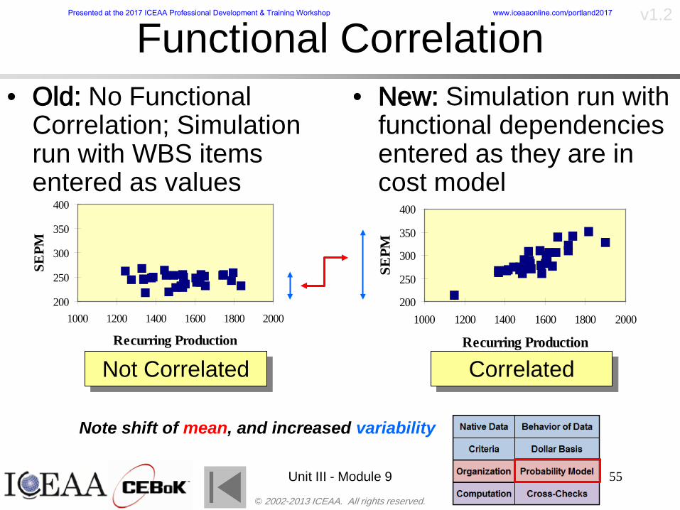
copy 2002-2013 ICEAA All rights reserved
v12
Unit III - Module 9 55
200
250
300
350
400
1000 1200 1400 1600 1800 2000
Recurring Production
SEPM
200
250
300
350
400
1000 1200 1400 1600 1800 2000
Recurring Production
SEPM
Functional Correlationbull Old No Functional
Correlation Simulation run with WBS items entered as values
bull New Simulation run with functional dependencies entered as they are in cost model
CorrelatedNot Correlated
Note shift of mean and increased variability
Presented at the 2017 ICEAA Professional Development amp Training Workshop wwwiceaaonlinecomportland2017
copy 2002-2013 ICEAA All rights reserved
v12
Risk Measuresbull ldquoWestern Europe conquered the word because of a
technological revolution that started because of attempts to measure the worldrdquo ndash Phillipe Jorion ndash In the same way attempts to measure risk will lead to better project
managementbull Risk management for DoD and NASA agencies focuses
primarily on funding projects to a single percentile ndash NASA policy explicitly mentions 70 and 50ndash This is known as ldquoValue at Riskrdquo and is prevalent in the banking and
financial industry
56
Presented at the 2017 ICEAA Professional Development amp Training Workshop wwwiceaaonlinecomportland2017
copy 2002-2013 ICEAA All rights reserved
v12
Value at Risk (VaR)bull VaR is a percentile of the cost risk
distributionndash VaR funding at the 70th percentile means that
there is a 30 chance of final project cost exceeding the funded amount (budget)
bull VaR has some meritsndash Common measure can be used to compare
different projects and programsndash Easily understood by senior managers and
decision makers
57
Presented at the 2017 ICEAA Professional Development amp Training Workshop wwwiceaaonlinecomportland2017
copy 2002-2013 ICEAA All rights reserved
v12
Why 70th or 80th Percentilebull Typical policy guidance involves funding at the 70th or 80th
percentile Why fund as such a low percentilebull There is some incentive to not over-fundbull For a normal distribution an inflection point occurs near the 80th
percentile meaning that for values above 80 confidence achieving higher levels of confidence can only be achieved by spending greater dollar amounts at an increasing rate
58
-05-04-03-02-01
00102030405
0 05 1 15 2 25 3
Standard Deviations from Mean
Normal Distribution
First DerivativeSlopeVelocity
Second DerivativeConvexityAcceleration
Inflection point at one standard deviation above the mean (~84th
percentile)
Presented at the 2017 ICEAA Professional Development amp Training Workshop wwwiceaaonlinecomportland2017
copy 2002-2013 ICEAA All rights reserved
v12
Funding Above Inflection Pointsbull As the percentile goes above the 80th percentile the amount
needed to achieve that higher level of confidence begins to increase at an increasing rate as is evident from the graph
59
0
10
20
30
40
50
60
70
50 55 60 65 70 75 80 85 90 95 100
$ Ab
ove
MEa
n to
Ach
ieve
Per
cent
ile
Percentile (Confidence Level)
Presented at the 2017 ICEAA Professional Development amp Training Workshop wwwiceaaonlinecomportland2017
copy 2002-2013 ICEAA All rights reserved
v12
Why Budget to the 70th or 80thbull Government projects are funded at the 70th or 80th percentilesbull Why not the 90th or 99th percentile Wonrsquot that help prevent
overrunsndash As we have seen percentiles do not add across programs
bull The sum of the 80th percentiles does NOT equal the total 80th percentile
ndash This is because the individual programs are riskier than the entire suite of missions
bull Known as the ldquoPortfolio effectrdquo (more or this later)
ndash Funding at the 80th gives confidence that the entire portfolio will be adequately funded
bull And since there is an inflection point near the 80th percentile funding above that level quickly becomes cost prohibitive
60
Presented at the 2017 ICEAA Professional Development amp Training Workshop wwwiceaaonlinecomportland2017
copy 2002-2013 ICEAA All rights reserved
v12
Inflection Points for Lognormalbull For a lognormal the inflection point
variesndash Coefficient of variation equal to 10 equates to an
inflection point at the 70th percentile
61
0
10
20
30
40
50
60
70
050 060 070 080 090 100
Coef
ficen
t of V
aria
tion
Percentile of the Inflection Point
Presented at the 2017 ICEAA Professional Development amp Training Workshop wwwiceaaonlinecomportland2017
copy 2002-2013 ICEAA All rights reserved
v12
Issues with Percentile Fundingbull However risk management does not stop at a
specific percentilendash What happens when the 70th percentile is exceeded
bull Any effective risk management policy should prescribe what happens after a bad event occursndash With VaR we only know when a bad event has occurred ndash Also funding at a relatively low level means we have no true
sense of the real risks that should be guarded against
62
Presented at the 2017 ICEAA Professional Development amp Training Workshop wwwiceaaonlinecomportland2017
copy 2002-2013 ICEAA All rights reserved
v12
ldquoHere There Be Dragonsrdquobull On old maps uncharted territory was often
marked with monsters or dragons
63
A section of the Carta Marina by Olaus Magnus 16th Century
Presented at the 2017 ICEAA Professional Development amp Training Workshop wwwiceaaonlinecomportland2017
copy 2002-2013 ICEAA All rights reserved
v12
Distribution Comparisonbull Four different distributions with the same 70th
percentile
bull Should we expect the tails to be similar
64
0
10
20
30
40
50
60
70
80
0 100 200 300 400 500 600
Perc
entil
eCo
nfid
ence
Lev
el
Triangular
Normal
Lognormal
Pareto
Presented at the 2017 ICEAA Professional Development amp Training Workshop wwwiceaaonlinecomportland2017
copy 2002-2013 ICEAA All rights reserved
v12Distribution Comparison Tail Behavior
bull The normal and triangular distributions have similar tails but the lognormal and Pareto have much fatter right tails
65
70
75
80
85
90
95
100
500 1500 2500 3500 4500 5500
Perc
entil
eCo
nfid
ence
Lev
el
Triangular
Normal
Lognormal
Pareto
Here There Be Dragons
Presented at the 2017 ICEAA Professional Development amp Training Workshop wwwiceaaonlinecomportland2017
copy 2002-2013 ICEAA All rights reserved
v12Distribution Comparison ndash Tail Behavior (Table)
bull There is significant tail risk for the lognormal and the Paretobull The 99th percentile for the Pareto is 1000 times greater than
the 70th percentilendash Risk seen in financial markets and in catastrophic risks like natural
disasters bull Four different projects follow the four different risk profiles seen
in this example should clearly have different risk management approaches but 70th percentile funding indicates the same risk management approach for all four
66
Percentile Triangular Normal Lognormal Pareto 70th $600 $600 $600 $600 80th $680 $660 $770 $1430 90th $770 $750 $1070 $5880 95th $840 $820 $1410 $23750 99th $930 $950 $2350 $600000
Presented at the 2017 ICEAA Professional Development amp Training Workshop wwwiceaaonlinecomportland2017
copy 2002-2013 ICEAA All rights reserved
v12Percentile Budgeting is Not Risk Management
bull Percentile budgeting ne effective risk management policybull Suppose that you are shopping for a new car You
mention that safety is your top concern The salesman says he has a great safe car available You ask about the air bags Do they work The salesman answers ldquoOf course Seventy percent of the time they work fine Only 30 of the time the air bags will fail to deployrdquo Would you buy such a car Hedge fund manager David Einhorn has stated ldquoRisk management is the air bag that must always work but only in the multi-sigma event where you have an accidentrdquo
67
Risk management is the air bag that must always work but only in the multi-sigma event where you
have an accident
Presented at the 2017 ICEAA Professional Development amp Training Workshop wwwiceaaonlinecomportland2017
copy 2002-2013 ICEAA All rights reserved
v12
Joint Confidence Level Analysisbull Schedules are risky toobull For 98 recent NASA missions average
schedule growth was 38ndash Not as high as cost growth but still significant
68
0
5
10
15
20
25
30
35
40
Schedule
Cost
Presented at the 2017 ICEAA Professional Development amp Training Workshop wwwiceaaonlinecomportland2017
copy 2002-2013 ICEAA All rights reserved
v12
Schedules Impact Costbull Changes in schedule can have enormous
impacts on cost ndash Schedule slips can lead to cost increases
bull Fixed programmatic costs must be paid on a regular basisndash Achieving schedule milestones early can result in cost
savings
bull Schedule is an important consideration in cost analysis including cost risk analysis
bull However we must be careful in correctly integrating cost and schedule riskndash Schedule is not simply an input but is dependent on many of
the same factors that drive cost
69
Presented at the 2017 ICEAA Professional Development amp Training Workshop wwwiceaaonlinecomportland2017
copy 2002-2013 ICEAA All rights reserved
v12
The Relationship of Cost to Schedulebull Cost and schedule are positively correlated
ndash A larger program with bigger scope with take longer to complete than a smaller simpler program
bull However longer schedules do not always equate to higher cost nor shorter schedules with lower costndash Highly compressed schedules relative to the
optimal schedule can lead to large overrunsbull Compressed schedules are commonplace for
many planetary missions
70
Presented at the 2017 ICEAA Professional Development amp Training Workshop wwwiceaaonlinecomportland2017
copy 2002-2013 ICEAA All rights reserved
v12The Impact of Schedule GrowthCompression on Cost
bull Compressed schedules lead to cost growth and based on existing research is actually more expensive than schedule slippages
71
0
20
40
60
80
100
120
140
160
-50 -25 0 25 50 75 100
Percentage Change in Schedule
Perc
enta
ge C
hang
e in
Cos
t due
to
Sche
dule
Cha
nge
Source Smart CB ldquoCost and Schedule Interrelationshipsrdquo 2007 NASA Cost Symposium
Presented at the 2017 ICEAA Professional Development amp Training Workshop wwwiceaaonlinecomportland2017
copy 2002-2013 ICEAA All rights reserved
v12Schedule as an Independent Variable
bull Why not simply add schedule as an input to cost-estimating relationships (CERs)
bull Schedule is often treated as an independent variable ndash schedules are often determined independently of cost considerationsndash Cost may not be considered explicitly although budgets and
schedules are determined based on scope and other common factors
bull In 2006 SAIC undertook a research task to determine the impact of schedule on cost and added schedule as an independent variable to the CERs in the NASAAir Force Cost Model (NAFCOM) to see if schedule provided any improvement in goodness of fit
72
Presented at the 2017 ICEAA Professional Development amp Training Workshop wwwiceaaonlinecomportland2017
copy 2002-2013 ICEAA All rights reserved
v12
Schedule is a Dependent Variablebull Since NAFCOM includes an exhaustive list of cost drivers the inclusion
of schedule should give an indication of whether there is any additional independent value added from schedule independent of the cost drivers
bull In the study schedule was added to 10 subsystem-level CERs
ndash In each case the addition of schedule did NOTimprove the goodness of fit and schedule was NOT found to be a statistically significant cost driver (given the presence of the other variables) for any of the 10 CERs
bull Standard errors for the CERs increased due to decrease in degrees of freedom
bull Thus schedule as an independent variable did not provide any additional explanation of variation in historical cost
bull This is because schedule is truly NOT an independent variable but a dependent variable and is a function of the same factors that drive cost
73
Presented at the 2017 ICEAA Professional Development amp Training Workshop wwwiceaaonlinecomportland2017
copy 2002-2013 ICEAA All rights reserved
v12
Incorporation of Schedule in Cost Risk
bull When using subjective methods care must be taken in applying schedule to cost risk analysis
bull Since schedule is a dependent variable treating it independently from other factors when assessing its impact on cost can lead to a double count of independent variables in the cost risk analysis
bull Direct inclusion of schedule in a cost risk analysis effectively doubles the influence of each cost driver
ndash Incorrectly leads to broader risk ranges
74
CostWeight
HeritageNewness
Technology Readiness Schedule
Presented at the 2017 ICEAA Professional Development amp Training Workshop wwwiceaaonlinecomportland2017
copy 2002-2013 ICEAA All rights reserved
v12Subjective Cost Risk Methods and Overinclusion of Risk Factors
bull Subjective methods are suitable when data are scarce or not availablebull However care must be taken not to treat correlated sources of risk
such as schedule as independent of each otherbull Example ndash a subjective risk analysis incorporated technology readiness
design risk requirements stability integration risk and schedule and treated each source of risk as independent
bull Risk triangle high value without schedule risk was 31 times the point estimate
bull Risk triangle high value with schedule risk added on top of other sources of risk treated independently was 34 times the point estimate
bull Risk triangle taking correlation between sources of risk into account in a rigorous statistical manner has a high value 15 times the point estimate less than half the effect when treating sources of risk as independent
75
Presented at the 2017 ICEAA Professional Development amp Training Workshop wwwiceaaonlinecomportland2017
copy 2002-2013 ICEAA All rights reserved
v12Fundamental Equation of Cost and Schedule Interrelationships
bull The Fundamental Equation of the Relationship Between Cost and Schedule is
Time = Moneybull This is a well known adage that time is money Your boss at
work may even mention this to you from time to time or if you are the boss you are all too aware of this iron law
bull Because time is money cost and schedule risk should be modeled jointly not with schedule as an independent cost driver
bull Note that cost and schedule are not perfectly correlatedndash Cost can sometimes ldquobuy downrdquo schedule extra money can be
spent to meet a deadline since in some cases additional effort to hasten the completion of a task
76
Presented at the 2017 ICEAA Professional Development amp Training Workshop wwwiceaaonlinecomportland2017
copy 2002-2013 ICEAA All rights reserved
v12How to (Correctly) Incorporate Schedule into Cost Risk Analysis
bull The best way to model cost and schedule risk is to develop a joint cost and schedule model based on the same data
bull Since such models are not currently available the next best approach is to model cost and schedule independently and then integrate cost and schedule risk analyses using joint probability distributions taking into account correlation between cost and schedulendash This approach pioneered by Paul Garvey and Steve Book is
considered industry best practicendash This is a practical method mathematically tractable and follows
naturally from the Fundamental Equation of Cost and Schedule Interrelationships
77
Book S A ldquoQuantifying the Relationship Between Cost and Schedulerdquo The Measurable News Winter 2007-2008 pp 11-15Garvey PR Probability Methods for Cost Uncertainty Analysis A Systems Engineering Perspective New York Marcel Dekker 2000 pp 308-335
Presented at the 2017 ICEAA Professional Development amp Training Workshop wwwiceaaonlinecomportland2017
copy 2002-2013 ICEAA All rights reserved
v12
Joint Lognormal and Normal Distributions
bull Cost and schedule are typically modeled as some combination of Normal and Lognormal probability distributionsndash Studies by The Aerospace Corporation the MITRE
Corporation Wyle Labs and SAIC have found that the Lognormal probability distribution almost always serves as a good model for both the schedule distribution and the cost distribution
ndash The Normal distribution may also be appropriate in some instances and depending upon the level of confidence at which budgets are set may even be more conservative and logically consistent than the Normal distribution
ndash Joint Lognormal and Normal distributions are defined by a pair of mean and standard deviations and a level of correlation between the two
78
Presented at the 2017 ICEAA Professional Development amp Training Workshop wwwiceaaonlinecomportland2017
copy 2002-2013 ICEAA All rights reserved
v12Modeling Cost and Schedule as a Bivariate Distribution
bull In the approach set forth by Book and Garvey cost risk is assessed and the top-level distribution is modeled as a Lognormal (or Normal) distribution schedule risk is assessed and the overall schedule risk is modeled as a Lognormal (or Normal) distribution
bull The two distributions are combined into a Bivariate distribution by assigning a correlation between the two and by treating the two distributions as the marginal distributions of a Bivariate Lognormal distributionndash Other combinations include a Bivariate Normal or a Bivariate
Normal-Lognormal
79
Presented at the 2017 ICEAA Professional Development amp Training Workshop wwwiceaaonlinecomportland2017
copy 2002-2013 ICEAA All rights reserved
v12Bivariate Lognormal Distribution for Cost and Schedule
bull Cost is often observed to be Lognormal when strong positive correlations are present among the systemrsquos WBS cost element costs
bull A systemrsquos schedule is often observed (from Monte Carlo simulations) to be Lognormal if it is the sum of many positively correlated schedule activities in an overall schedule network
bull If Lognormal distributions characterize a systemrsquos cost and schedule then the Bivariate Lognormal could serve as an assumed model of their joint distributionndash In this case the marginal distribution of each of cost and schedule is
Lognormalbull Other possibilities for modeling cost and schedule as a Bivariate
distribution include a Bivariate Normal or a Bivariate Normal-Lognormal distributionndash All these combinations are analytically tractable
80
Presented at the 2017 ICEAA Professional Development amp Training Workshop wwwiceaaonlinecomportland2017
copy 2002-2013 ICEAA All rights reserved
v12Bivariate Lognormal for Cost and Schedule
bull Contour Plots of a Bivariate Lognormal
81
Presented at the 2017 ICEAA Professional Development amp Training Workshop wwwiceaaonlinecomportland2017
copy 2002-2013 ICEAA All rights reserved
v12Correlation Between Cost and Schedule
bull Cost and schedule are positively correlated but not perfectly sondash For example it is possible to have a schedule underrun and a cost
overrunbull Based on cost and schedule growth data for 50 completed NASA
programs the correlation between development cost and development schedule is 70
82
00
200
400
600
800
1000
1200
-500 00 500 1000 1500 2000 2500Historical Cost Growth
Hist
oric
al S
ched
ule
Gro
wth
r = 715
Presented at the 2017 ICEAA Professional Development amp Training Workshop wwwiceaaonlinecomportland2017
copy 2002-2013 ICEAA All rights reserved
v12Correlation Between Cost and Schedule Caveats
bull Based on historical data recommended correlation between cost and schedule is 70 but this could be higher or lower depending upon program circumstancesndash If program is budget constrained cost and schedule will be
more highly correlated (go as you pay)ndash If program is schedule constrained cost and schedule will
have lower correlation perhaps even negative correlation ndash Smaller programs have smaller correlation between cost and
schedule riskbull Relatively easy to ldquohurry uprdquo and finish on time or even early if
needed
83
Presented at the 2017 ICEAA Professional Development amp Training Workshop wwwiceaaonlinecomportland2017
copy 2002-2013 ICEAA All rights reserved
v12
Conditional Confidence Levelsbull Given a programrsquos project schedule we can determine the cost
risk distribution conditional upon the given schedulebull Conditional cost S-curves are steeper than unconditional
(marginal) cost S-curves between some uncertainty has been removed because schedule is fixed
84
Presented at the 2017 ICEAA Professional Development amp Training Workshop wwwiceaaonlinecomportland2017
copy 2002-2013 ICEAA All rights reserved
v12
Joint Confidence Levelsbull Joint 65 confidence represents the probability of
achieving both 65 confidence in cost AND 65 confidence in schedulendash This is different than achieving 65 cost confidence alone
or achieving 65 schedule confidence alonebull Due to the imperfect correlation between cost and schedule it
is possible to achieve a 65 cost confidence with a lower level of schedule confidence
bull Restricting the schedule confidence thus requires additional $ to achieve a given level of confidence
85
X
Y
Possible Values for Which X gt a Possible Values for
Which X gt a and Y gt b
a
b
Presented at the 2017 ICEAA Professional Development amp Training Workshop wwwiceaaonlinecomportland2017
copy 2002-2013 ICEAA All rights reserved
v12Joint Confidence Levels Versus Cost Confidence Levels Only
bull Example of the differences between cost confidence schedule confidence conditional cost confidence and joint cost and schedule confidence
86
Joint Cost-Schedule Confidence Iso-Curves
Cost (RY$M)
Sche
dule
(Mon
ths)
65 Confidence
50 Confidence
70 Confidence
65 Cost Confidence AggressiveSchedule65 Cost ConfidenceScheduleGiven 65 Schedule ConfidenceUnconditional 65 CostConfidenceUnconditional 65 ScheduleConfidence
65 Cost Confidence 65 Joint Cost and Schedule
Confidence for 65 Schedule Confidence
Presented at the 2017 ICEAA Professional Development amp Training Workshop wwwiceaaonlinecomportland2017
copy 2002-2013 ICEAA All rights reserved
v12
Joint Cost and Schedule Confidence
bull Can examine pairs of cost and schedule that achieve a given level of confidence
bull Provides insights into the trade-offs between cost and schedule for a given level of confidencendash Possible to increase cost confidence by giving a
project more time in some instances or possible to ldquobuy downrdquo schedule
bull But these have limits and are shown in the iso-cost and schedule confidence curves
87
Presented at the 2017 ICEAA Professional Development amp Training Workshop wwwiceaaonlinecomportland2017
copy 2002-2013 ICEAA All rights reserved
v12Cost and Schedule Trade-offs for a Given Level of Joint Confidence
bull Hypothetical Example
88
Cost (RY$M)
Schedule (Months)
$100 48$99 48$89 49$87 50$85 51$85 52$84 53$83 55$83 55$83 56
Cost and Schedule 65 Confidence Iso-Curve
4748495051525354555657
$80 $82 $84 $86 $88 $90 $92 $94 $96 $98 $100
Cost (RY$ M)
Sche
dule
(Mon
ths)
Presented at the 2017 ICEAA Professional Development amp Training Workshop wwwiceaaonlinecomportland2017
copy 2002-2013 ICEAA All rights reserved
v12Policy Considerations for Confidence Levels
bull For large programs the difference between the amount of money needed to achieve 65 cost confidence independent of schedule and joint 65 cost and schedule confidence can represent hundreds of millions and even billions of dollars
89
Joint Cost-Schedule Confidence Iso-Curves
Cost (RY$M)
Sche
dule
(Mon
ths)
65 Confidence
65 Cost Confidence AggressiveSchedule
65 Cost ConfidenceScheduleGiven 65 Schedule Confidence
Unconditional 65 CostConfidence
Joint Cost and Schedule Confidence for 65 Cost Confidence and Program Baseline Schedule is Less Than 35
65 Cost Confidence Independent of Schedule Cost Needed to Achieve
Both 65 Joint Cost and Schedule Confidence for the Schedule with 65 Confidence
Presented at the 2017 ICEAA Professional Development amp Training Workshop wwwiceaaonlinecomportland2017
copy 2002-2013 ICEAA All rights reserved
v12
Copulasbull More generally any combination of distributions can
be used (more than just normal and lognormal)ndash Termed ldquocopulardquo from the Italian word for ldquocouplerdquondash Copulas are a way to combine marginal distributions of any
number and type into a joint distributionbull More formally a copula is a multivariate joint distribution defined
on the n-dimensional unit cube [0 1]n such that every marginal distribution is uniform on the interval [0 1]
bull (The bivariate form of) Sklarrsquos theorem states that for any bivariate distribution function H(x y) let F(x) = H(x infin) and G(y) = H(infin y) be the univariate marginal probability distribution functions Then there exists a copula C such that H(xy)=C(F(x)G(y))
ndash Copulas are widely used in risk management for investments and insurance
bull Considered industry best practice (Li 2000)bull Marketed as part of JP Morganrsquos CreditMetrics suite of tools
(Gupton et Al 1997)90
Presented at the 2017 ICEAA Professional Development amp Training Workshop wwwiceaaonlinecomportland2017
copy 2002-2013 ICEAA All rights reserved
v12Parametric Joint Cost and Schedule Analysis
bull A parametric model based on a consistent data set with a set of overlapping cost and schedule drivers is a cleaner way to model cost and schedule
91
CostWeight
HeritageNewness
Technology Readiness
Schedule
0
20
40
60
80
100
Confidence
Joint Cost and Schedule Confidence
Schedule
Cost
Lognormal Distribution PDF and CDF
0102030405060708090100
200 300 400 500 600 700 800 900 1000Cost $
Con
fiden
ce L
evel
0
00002
00004
00006
00008
0001
00012
00014
00016
Prob
abili
ty D
ensi
ty
CDFPDF
Lognormal Distribution PDF and CDF
0102030405060708090100
200 300 400 500 600 700 800 900 1000Cost $
Con
fiden
ce L
evel
0
00002
00004
00006
00008
0001
00012
00014
00016
Prob
abili
ty D
ensi
ty
CDFPDF
Presented at the 2017 ICEAA Professional Development amp Training Workshop wwwiceaaonlinecomportland2017
copy 2002-2013 ICEAA All rights reserved
v12Parametric Joint Cost and Schedule Analysis (2)
bull Joint cost and schedule risk analysis produced naturally by the integrated modelndash Addresses several issues with the copula
approachbull Tail dependencybull Correlation ndash no need to assign correlation
between cost and schedulebull Consistency of cost and schedule models
92
Presented at the 2017 ICEAA Professional Development amp Training Workshop wwwiceaaonlinecomportland2017
copy 2002-2013 ICEAA All rights reserved
v12
Resource-Loaded Schedulesbull Involves assigning cost and schedule risks to a resource-loaded schedule
networkbull Bottom-up approach
ndash More labor intensive than parametrics but can also provide more insight
ndash Can answer questions than parametric typically cannot such as how much do reserve requirements decrease if a specific risk is retired
bull Currently being implemented in Constellation programbull Has same issue as all bottom-up models hard to count all the risks and model
them discretely
ndash As a result there is a tendency to reflect less risk than indicated by history
ndash ldquoThere are more things in heaven and earth Horatio than are dreamt of in your philosophyrdquo William Shakespeare Hamlet Act I Scene V
93
Presented at the 2017 ICEAA Professional Development amp Training Workshop wwwiceaaonlinecomportland2017
copy 2002-2013 ICEAA All rights reserved
v12Resource-Loaded Schedules Vs Parametrics
bull Parametric most appropriate for early estimatesndash But also good for high-level checks as project progresses
bull As plans take shape lower level modeling may be more appropriate
94 1
CONCEPTUALDEVELOPMENT
PROJECTDEFINITION DESIGN DEVELOPMENT OPERATIONS
PARAMETRIC PARAMETRIC
ANALOGY
ENGINEERING (Bottoms Up)
$PARAMETRIC
DETAILED
$
Pre Phase A Phase B Phase CDPhase A Phase EPre Phase A Phase B Phase CDPhase A Phase E
Risk = f(Cost Estimating Relationship Inputs eg mass power data rate TRL new design etc)
Risk = f(cost and schedule variation of the analogous elements)
Risk = f(variation of detailed inputs eg labor hours rates materials etc)
Presented at the 2017 ICEAA Professional Development amp Training Workshop wwwiceaaonlinecomportland2017
copy 2002-2013 ICEAA All rights reserved
v12
Resource-Loaded Schedulesbull Methodology has been demonstrated in other
industriesndash Construction oil and gasndash Analysis has not been traditionally done on highly uncertain
complex development projects bull Methodology focuses on project baseline schedule
ndash In baseline schedule all tasks are resource loaded to represent a baseline schedule and cost standpoint
ndash Resource loaded schedule is ldquorolledrdquo up to a manageable level
ndash Based on the risk and uncertainties identified schedule distributions are applied to each rolled up task
ndash Cost uncertainties are also applied to rolled up tasksbull Uncertainties include labor rate man power etc
ndash A Monte Carlo simulation is run to develop joint cost-schedule distributions
95
Presented at the 2017 ICEAA Professional Development amp Training Workshop wwwiceaaonlinecomportland2017
copy 2002-2013 ICEAA All rights reserved
v12
Unit III - Module 9 96
Execution ndash Cross Checksbull Means The mean cost growth factor for WBS items
can be compared to history as a way to cross check results
bull CVs The CV of the cost growth factors for WBS items can be compared to history as a way to cross check results
bull Inputs Checks are performed on inputs or other parameters to see if historical values are in line with program assumptionsndash Example Historical risk scores can be compared to program
risk scores to see if risk assessors are being realistic and to see if the underlying database is representative of the program
11
Presented at the 2017 ICEAA Professional Development amp Training Workshop wwwiceaaonlinecomportland2017
- Cost and Schedule Risk Analysis Basic
- Acknowledgments
- Unit Index
- Risk Overview
- Agenda
- Introduction
- Risk Analysis Terms
- Are Our Costs Realistic
- Historical Cost Growth
- Sources of Cost Risk
- Point Estimates of Cost
- Types of Risk
- Point Estimates Vs Risk Estimates
- Cost Risk and Probability
- Probability Model ndash Distribution
- Probability Model ndash Distribution
- Probability ndash Top-Level Distribution
- S-Curves and Confidence Levels
- Example ndash Normal Distribution
- Confidence Levels
- Measuring Parametric Model Uncertainty
- Parametric Model Example
- Weight Uncertainty
- Estimating Uncertainty
- Estimating Uncertainty (2)
- Estimating Uncertainty (3)
- Aggregating Risk
- WBS Example
- WBS and Risk
- Aggregating Risk
- Percentiles Do Not Add
- Percentiles Do Not Add (2)
- Percentiles Do Not Add (3)
- Methods for Aggregating Risk
- Monte Carlo Simulationfor Risk Analysis
- Monte Carlo Simulation
- Using Random Numbers to Simulate Distributions
- Simulating a Triangular Distribution
- Simulating a Triangular Distribution (2)
- Monte Carlo and the WBS
- Number of Trials
- Number of Trials (2)
- Number of Trials (3)
- Number of Trials (4)
- Number of Trials (5)
- Number of Trials (6)
- Methods of Simulation
- Probability Model ndash Correlation
- Correlation And Causation
- The Importance of Correlation
- The Importance of Correlation (2)
- Measures of Correlation
- Pearson Correlation
- Spearman Correlation
- Functional Correlation
- Risk Measures
- Value at Risk (VaR)
- Why 70th or 80th Percentile
- Funding Above Inflection Points
- Why Budget to the 70th or 80th
- Inflection Points for Lognormal
- Issues with Percentile Funding
- ldquoHere There Be Dragonsrdquo
- Distribution Comparison
- Distribution Comparison Tail Behavior
- Distribution Comparison ndash Tail Behavior (Table)
- Percentile Budgeting is Not Risk Management
- Joint Confidence Level Analysis
- Schedules Impact Cost
- The Relationship of Cost to Schedule
- The Impact of Schedule GrowthCompression on Cost
- Schedule as an Independent Variable
- Schedule is a Dependent Variable
- Incorporation of Schedule in Cost Risk
- Subjective Cost Risk Methods and Overinclusion of Risk Factors
- Fundamental Equation of Cost and Schedule Interrelationships
- How to (Correctly) Incorporate Schedule into Cost Risk Analysis
- Joint Lognormal and Normal Distributions
- Modeling Cost and Schedule as a Bivariate Distribution
- Bivariate Lognormal Distribution for Cost and Schedule
- Bivariate Lognormal for Cost and Schedule
- Correlation Between Cost and Schedule
- Correlation Between Cost and Schedule Caveats
- Conditional Confidence Levels
- Joint Confidence Levels
- Joint Confidence Levels Versus Cost Confidence Levels Only
- Joint Cost and Schedule Confidence
- Cost and Schedule Trade-offs for a Given Level of Joint Confidence
- Policy Considerations for Confidence Levels
- Copulas
- Parametric Joint Cost and Schedule Analysis
- Parametric Joint Cost and Schedule Analysis (2)
- Resource-Loaded Schedules
- Resource-Loaded Schedules Vs Parametrics
- Resource-Loaded Schedules
- Execution ndash Cross Checks
-
copy 2002-2013 ICEAA All rights reserved
v12
Value at Risk (VaR)bull VaR is a percentile of the cost risk
distributionndash VaR funding at the 70th percentile means that
there is a 30 chance of final project cost exceeding the funded amount (budget)
bull VaR has some meritsndash Common measure can be used to compare
different projects and programsndash Easily understood by senior managers and
decision makers
57
Presented at the 2017 ICEAA Professional Development amp Training Workshop wwwiceaaonlinecomportland2017
copy 2002-2013 ICEAA All rights reserved
v12
Why 70th or 80th Percentilebull Typical policy guidance involves funding at the 70th or 80th
percentile Why fund as such a low percentilebull There is some incentive to not over-fundbull For a normal distribution an inflection point occurs near the 80th
percentile meaning that for values above 80 confidence achieving higher levels of confidence can only be achieved by spending greater dollar amounts at an increasing rate
58
-05-04-03-02-01
00102030405
0 05 1 15 2 25 3
Standard Deviations from Mean
Normal Distribution
First DerivativeSlopeVelocity
Second DerivativeConvexityAcceleration
Inflection point at one standard deviation above the mean (~84th
percentile)
Presented at the 2017 ICEAA Professional Development amp Training Workshop wwwiceaaonlinecomportland2017
copy 2002-2013 ICEAA All rights reserved
v12
Funding Above Inflection Pointsbull As the percentile goes above the 80th percentile the amount
needed to achieve that higher level of confidence begins to increase at an increasing rate as is evident from the graph
59
0
10
20
30
40
50
60
70
50 55 60 65 70 75 80 85 90 95 100
$ Ab
ove
MEa
n to
Ach
ieve
Per
cent
ile
Percentile (Confidence Level)
Presented at the 2017 ICEAA Professional Development amp Training Workshop wwwiceaaonlinecomportland2017
copy 2002-2013 ICEAA All rights reserved
v12
Why Budget to the 70th or 80thbull Government projects are funded at the 70th or 80th percentilesbull Why not the 90th or 99th percentile Wonrsquot that help prevent
overrunsndash As we have seen percentiles do not add across programs
bull The sum of the 80th percentiles does NOT equal the total 80th percentile
ndash This is because the individual programs are riskier than the entire suite of missions
bull Known as the ldquoPortfolio effectrdquo (more or this later)
ndash Funding at the 80th gives confidence that the entire portfolio will be adequately funded
bull And since there is an inflection point near the 80th percentile funding above that level quickly becomes cost prohibitive
60
Presented at the 2017 ICEAA Professional Development amp Training Workshop wwwiceaaonlinecomportland2017
copy 2002-2013 ICEAA All rights reserved
v12
Inflection Points for Lognormalbull For a lognormal the inflection point
variesndash Coefficient of variation equal to 10 equates to an
inflection point at the 70th percentile
61
0
10
20
30
40
50
60
70
050 060 070 080 090 100
Coef
ficen
t of V
aria
tion
Percentile of the Inflection Point
Presented at the 2017 ICEAA Professional Development amp Training Workshop wwwiceaaonlinecomportland2017
copy 2002-2013 ICEAA All rights reserved
v12
Issues with Percentile Fundingbull However risk management does not stop at a
specific percentilendash What happens when the 70th percentile is exceeded
bull Any effective risk management policy should prescribe what happens after a bad event occursndash With VaR we only know when a bad event has occurred ndash Also funding at a relatively low level means we have no true
sense of the real risks that should be guarded against
62
Presented at the 2017 ICEAA Professional Development amp Training Workshop wwwiceaaonlinecomportland2017
copy 2002-2013 ICEAA All rights reserved
v12
ldquoHere There Be Dragonsrdquobull On old maps uncharted territory was often
marked with monsters or dragons
63
A section of the Carta Marina by Olaus Magnus 16th Century
Presented at the 2017 ICEAA Professional Development amp Training Workshop wwwiceaaonlinecomportland2017
copy 2002-2013 ICEAA All rights reserved
v12
Distribution Comparisonbull Four different distributions with the same 70th
percentile
bull Should we expect the tails to be similar
64
0
10
20
30
40
50
60
70
80
0 100 200 300 400 500 600
Perc
entil
eCo
nfid
ence
Lev
el
Triangular
Normal
Lognormal
Pareto
Presented at the 2017 ICEAA Professional Development amp Training Workshop wwwiceaaonlinecomportland2017
copy 2002-2013 ICEAA All rights reserved
v12Distribution Comparison Tail Behavior
bull The normal and triangular distributions have similar tails but the lognormal and Pareto have much fatter right tails
65
70
75
80
85
90
95
100
500 1500 2500 3500 4500 5500
Perc
entil
eCo
nfid
ence
Lev
el
Triangular
Normal
Lognormal
Pareto
Here There Be Dragons
Presented at the 2017 ICEAA Professional Development amp Training Workshop wwwiceaaonlinecomportland2017
copy 2002-2013 ICEAA All rights reserved
v12Distribution Comparison ndash Tail Behavior (Table)
bull There is significant tail risk for the lognormal and the Paretobull The 99th percentile for the Pareto is 1000 times greater than
the 70th percentilendash Risk seen in financial markets and in catastrophic risks like natural
disasters bull Four different projects follow the four different risk profiles seen
in this example should clearly have different risk management approaches but 70th percentile funding indicates the same risk management approach for all four
66
Percentile Triangular Normal Lognormal Pareto 70th $600 $600 $600 $600 80th $680 $660 $770 $1430 90th $770 $750 $1070 $5880 95th $840 $820 $1410 $23750 99th $930 $950 $2350 $600000
Presented at the 2017 ICEAA Professional Development amp Training Workshop wwwiceaaonlinecomportland2017
copy 2002-2013 ICEAA All rights reserved
v12Percentile Budgeting is Not Risk Management
bull Percentile budgeting ne effective risk management policybull Suppose that you are shopping for a new car You
mention that safety is your top concern The salesman says he has a great safe car available You ask about the air bags Do they work The salesman answers ldquoOf course Seventy percent of the time they work fine Only 30 of the time the air bags will fail to deployrdquo Would you buy such a car Hedge fund manager David Einhorn has stated ldquoRisk management is the air bag that must always work but only in the multi-sigma event where you have an accidentrdquo
67
Risk management is the air bag that must always work but only in the multi-sigma event where you
have an accident
Presented at the 2017 ICEAA Professional Development amp Training Workshop wwwiceaaonlinecomportland2017
copy 2002-2013 ICEAA All rights reserved
v12
Joint Confidence Level Analysisbull Schedules are risky toobull For 98 recent NASA missions average
schedule growth was 38ndash Not as high as cost growth but still significant
68
0
5
10
15
20
25
30
35
40
Schedule
Cost
Presented at the 2017 ICEAA Professional Development amp Training Workshop wwwiceaaonlinecomportland2017
copy 2002-2013 ICEAA All rights reserved
v12
Schedules Impact Costbull Changes in schedule can have enormous
impacts on cost ndash Schedule slips can lead to cost increases
bull Fixed programmatic costs must be paid on a regular basisndash Achieving schedule milestones early can result in cost
savings
bull Schedule is an important consideration in cost analysis including cost risk analysis
bull However we must be careful in correctly integrating cost and schedule riskndash Schedule is not simply an input but is dependent on many of
the same factors that drive cost
69
Presented at the 2017 ICEAA Professional Development amp Training Workshop wwwiceaaonlinecomportland2017
copy 2002-2013 ICEAA All rights reserved
v12
The Relationship of Cost to Schedulebull Cost and schedule are positively correlated
ndash A larger program with bigger scope with take longer to complete than a smaller simpler program
bull However longer schedules do not always equate to higher cost nor shorter schedules with lower costndash Highly compressed schedules relative to the
optimal schedule can lead to large overrunsbull Compressed schedules are commonplace for
many planetary missions
70
Presented at the 2017 ICEAA Professional Development amp Training Workshop wwwiceaaonlinecomportland2017
copy 2002-2013 ICEAA All rights reserved
v12The Impact of Schedule GrowthCompression on Cost
bull Compressed schedules lead to cost growth and based on existing research is actually more expensive than schedule slippages
71
0
20
40
60
80
100
120
140
160
-50 -25 0 25 50 75 100
Percentage Change in Schedule
Perc
enta
ge C
hang
e in
Cos
t due
to
Sche
dule
Cha
nge
Source Smart CB ldquoCost and Schedule Interrelationshipsrdquo 2007 NASA Cost Symposium
Presented at the 2017 ICEAA Professional Development amp Training Workshop wwwiceaaonlinecomportland2017
copy 2002-2013 ICEAA All rights reserved
v12Schedule as an Independent Variable
bull Why not simply add schedule as an input to cost-estimating relationships (CERs)
bull Schedule is often treated as an independent variable ndash schedules are often determined independently of cost considerationsndash Cost may not be considered explicitly although budgets and
schedules are determined based on scope and other common factors
bull In 2006 SAIC undertook a research task to determine the impact of schedule on cost and added schedule as an independent variable to the CERs in the NASAAir Force Cost Model (NAFCOM) to see if schedule provided any improvement in goodness of fit
72
Presented at the 2017 ICEAA Professional Development amp Training Workshop wwwiceaaonlinecomportland2017
copy 2002-2013 ICEAA All rights reserved
v12
Schedule is a Dependent Variablebull Since NAFCOM includes an exhaustive list of cost drivers the inclusion
of schedule should give an indication of whether there is any additional independent value added from schedule independent of the cost drivers
bull In the study schedule was added to 10 subsystem-level CERs
ndash In each case the addition of schedule did NOTimprove the goodness of fit and schedule was NOT found to be a statistically significant cost driver (given the presence of the other variables) for any of the 10 CERs
bull Standard errors for the CERs increased due to decrease in degrees of freedom
bull Thus schedule as an independent variable did not provide any additional explanation of variation in historical cost
bull This is because schedule is truly NOT an independent variable but a dependent variable and is a function of the same factors that drive cost
73
Presented at the 2017 ICEAA Professional Development amp Training Workshop wwwiceaaonlinecomportland2017
copy 2002-2013 ICEAA All rights reserved
v12
Incorporation of Schedule in Cost Risk
bull When using subjective methods care must be taken in applying schedule to cost risk analysis
bull Since schedule is a dependent variable treating it independently from other factors when assessing its impact on cost can lead to a double count of independent variables in the cost risk analysis
bull Direct inclusion of schedule in a cost risk analysis effectively doubles the influence of each cost driver
ndash Incorrectly leads to broader risk ranges
74
CostWeight
HeritageNewness
Technology Readiness Schedule
Presented at the 2017 ICEAA Professional Development amp Training Workshop wwwiceaaonlinecomportland2017
copy 2002-2013 ICEAA All rights reserved
v12Subjective Cost Risk Methods and Overinclusion of Risk Factors
bull Subjective methods are suitable when data are scarce or not availablebull However care must be taken not to treat correlated sources of risk
such as schedule as independent of each otherbull Example ndash a subjective risk analysis incorporated technology readiness
design risk requirements stability integration risk and schedule and treated each source of risk as independent
bull Risk triangle high value without schedule risk was 31 times the point estimate
bull Risk triangle high value with schedule risk added on top of other sources of risk treated independently was 34 times the point estimate
bull Risk triangle taking correlation between sources of risk into account in a rigorous statistical manner has a high value 15 times the point estimate less than half the effect when treating sources of risk as independent
75
Presented at the 2017 ICEAA Professional Development amp Training Workshop wwwiceaaonlinecomportland2017
copy 2002-2013 ICEAA All rights reserved
v12Fundamental Equation of Cost and Schedule Interrelationships
bull The Fundamental Equation of the Relationship Between Cost and Schedule is
Time = Moneybull This is a well known adage that time is money Your boss at
work may even mention this to you from time to time or if you are the boss you are all too aware of this iron law
bull Because time is money cost and schedule risk should be modeled jointly not with schedule as an independent cost driver
bull Note that cost and schedule are not perfectly correlatedndash Cost can sometimes ldquobuy downrdquo schedule extra money can be
spent to meet a deadline since in some cases additional effort to hasten the completion of a task
76
Presented at the 2017 ICEAA Professional Development amp Training Workshop wwwiceaaonlinecomportland2017
copy 2002-2013 ICEAA All rights reserved
v12How to (Correctly) Incorporate Schedule into Cost Risk Analysis
bull The best way to model cost and schedule risk is to develop a joint cost and schedule model based on the same data
bull Since such models are not currently available the next best approach is to model cost and schedule independently and then integrate cost and schedule risk analyses using joint probability distributions taking into account correlation between cost and schedulendash This approach pioneered by Paul Garvey and Steve Book is
considered industry best practicendash This is a practical method mathematically tractable and follows
naturally from the Fundamental Equation of Cost and Schedule Interrelationships
77
Book S A ldquoQuantifying the Relationship Between Cost and Schedulerdquo The Measurable News Winter 2007-2008 pp 11-15Garvey PR Probability Methods for Cost Uncertainty Analysis A Systems Engineering Perspective New York Marcel Dekker 2000 pp 308-335
Presented at the 2017 ICEAA Professional Development amp Training Workshop wwwiceaaonlinecomportland2017
copy 2002-2013 ICEAA All rights reserved
v12
Joint Lognormal and Normal Distributions
bull Cost and schedule are typically modeled as some combination of Normal and Lognormal probability distributionsndash Studies by The Aerospace Corporation the MITRE
Corporation Wyle Labs and SAIC have found that the Lognormal probability distribution almost always serves as a good model for both the schedule distribution and the cost distribution
ndash The Normal distribution may also be appropriate in some instances and depending upon the level of confidence at which budgets are set may even be more conservative and logically consistent than the Normal distribution
ndash Joint Lognormal and Normal distributions are defined by a pair of mean and standard deviations and a level of correlation between the two
78
Presented at the 2017 ICEAA Professional Development amp Training Workshop wwwiceaaonlinecomportland2017
copy 2002-2013 ICEAA All rights reserved
v12Modeling Cost and Schedule as a Bivariate Distribution
bull In the approach set forth by Book and Garvey cost risk is assessed and the top-level distribution is modeled as a Lognormal (or Normal) distribution schedule risk is assessed and the overall schedule risk is modeled as a Lognormal (or Normal) distribution
bull The two distributions are combined into a Bivariate distribution by assigning a correlation between the two and by treating the two distributions as the marginal distributions of a Bivariate Lognormal distributionndash Other combinations include a Bivariate Normal or a Bivariate
Normal-Lognormal
79
Presented at the 2017 ICEAA Professional Development amp Training Workshop wwwiceaaonlinecomportland2017
copy 2002-2013 ICEAA All rights reserved
v12Bivariate Lognormal Distribution for Cost and Schedule
bull Cost is often observed to be Lognormal when strong positive correlations are present among the systemrsquos WBS cost element costs
bull A systemrsquos schedule is often observed (from Monte Carlo simulations) to be Lognormal if it is the sum of many positively correlated schedule activities in an overall schedule network
bull If Lognormal distributions characterize a systemrsquos cost and schedule then the Bivariate Lognormal could serve as an assumed model of their joint distributionndash In this case the marginal distribution of each of cost and schedule is
Lognormalbull Other possibilities for modeling cost and schedule as a Bivariate
distribution include a Bivariate Normal or a Bivariate Normal-Lognormal distributionndash All these combinations are analytically tractable
80
Presented at the 2017 ICEAA Professional Development amp Training Workshop wwwiceaaonlinecomportland2017
copy 2002-2013 ICEAA All rights reserved
v12Bivariate Lognormal for Cost and Schedule
bull Contour Plots of a Bivariate Lognormal
81
Presented at the 2017 ICEAA Professional Development amp Training Workshop wwwiceaaonlinecomportland2017
copy 2002-2013 ICEAA All rights reserved
v12Correlation Between Cost and Schedule
bull Cost and schedule are positively correlated but not perfectly sondash For example it is possible to have a schedule underrun and a cost
overrunbull Based on cost and schedule growth data for 50 completed NASA
programs the correlation between development cost and development schedule is 70
82
00
200
400
600
800
1000
1200
-500 00 500 1000 1500 2000 2500Historical Cost Growth
Hist
oric
al S
ched
ule
Gro
wth
r = 715
Presented at the 2017 ICEAA Professional Development amp Training Workshop wwwiceaaonlinecomportland2017
copy 2002-2013 ICEAA All rights reserved
v12Correlation Between Cost and Schedule Caveats
bull Based on historical data recommended correlation between cost and schedule is 70 but this could be higher or lower depending upon program circumstancesndash If program is budget constrained cost and schedule will be
more highly correlated (go as you pay)ndash If program is schedule constrained cost and schedule will
have lower correlation perhaps even negative correlation ndash Smaller programs have smaller correlation between cost and
schedule riskbull Relatively easy to ldquohurry uprdquo and finish on time or even early if
needed
83
Presented at the 2017 ICEAA Professional Development amp Training Workshop wwwiceaaonlinecomportland2017
copy 2002-2013 ICEAA All rights reserved
v12
Conditional Confidence Levelsbull Given a programrsquos project schedule we can determine the cost
risk distribution conditional upon the given schedulebull Conditional cost S-curves are steeper than unconditional
(marginal) cost S-curves between some uncertainty has been removed because schedule is fixed
84
Presented at the 2017 ICEAA Professional Development amp Training Workshop wwwiceaaonlinecomportland2017
copy 2002-2013 ICEAA All rights reserved
v12
Joint Confidence Levelsbull Joint 65 confidence represents the probability of
achieving both 65 confidence in cost AND 65 confidence in schedulendash This is different than achieving 65 cost confidence alone
or achieving 65 schedule confidence alonebull Due to the imperfect correlation between cost and schedule it
is possible to achieve a 65 cost confidence with a lower level of schedule confidence
bull Restricting the schedule confidence thus requires additional $ to achieve a given level of confidence
85
X
Y
Possible Values for Which X gt a Possible Values for
Which X gt a and Y gt b
a
b
Presented at the 2017 ICEAA Professional Development amp Training Workshop wwwiceaaonlinecomportland2017
copy 2002-2013 ICEAA All rights reserved
v12Joint Confidence Levels Versus Cost Confidence Levels Only
bull Example of the differences between cost confidence schedule confidence conditional cost confidence and joint cost and schedule confidence
86
Joint Cost-Schedule Confidence Iso-Curves
Cost (RY$M)
Sche
dule
(Mon
ths)
65 Confidence
50 Confidence
70 Confidence
65 Cost Confidence AggressiveSchedule65 Cost ConfidenceScheduleGiven 65 Schedule ConfidenceUnconditional 65 CostConfidenceUnconditional 65 ScheduleConfidence
65 Cost Confidence 65 Joint Cost and Schedule
Confidence for 65 Schedule Confidence
Presented at the 2017 ICEAA Professional Development amp Training Workshop wwwiceaaonlinecomportland2017
copy 2002-2013 ICEAA All rights reserved
v12
Joint Cost and Schedule Confidence
bull Can examine pairs of cost and schedule that achieve a given level of confidence
bull Provides insights into the trade-offs between cost and schedule for a given level of confidencendash Possible to increase cost confidence by giving a
project more time in some instances or possible to ldquobuy downrdquo schedule
bull But these have limits and are shown in the iso-cost and schedule confidence curves
87
Presented at the 2017 ICEAA Professional Development amp Training Workshop wwwiceaaonlinecomportland2017
copy 2002-2013 ICEAA All rights reserved
v12Cost and Schedule Trade-offs for a Given Level of Joint Confidence
bull Hypothetical Example
88
Cost (RY$M)
Schedule (Months)
$100 48$99 48$89 49$87 50$85 51$85 52$84 53$83 55$83 55$83 56
Cost and Schedule 65 Confidence Iso-Curve
4748495051525354555657
$80 $82 $84 $86 $88 $90 $92 $94 $96 $98 $100
Cost (RY$ M)
Sche
dule
(Mon
ths)
Presented at the 2017 ICEAA Professional Development amp Training Workshop wwwiceaaonlinecomportland2017
copy 2002-2013 ICEAA All rights reserved
v12Policy Considerations for Confidence Levels
bull For large programs the difference between the amount of money needed to achieve 65 cost confidence independent of schedule and joint 65 cost and schedule confidence can represent hundreds of millions and even billions of dollars
89
Joint Cost-Schedule Confidence Iso-Curves
Cost (RY$M)
Sche
dule
(Mon
ths)
65 Confidence
65 Cost Confidence AggressiveSchedule
65 Cost ConfidenceScheduleGiven 65 Schedule Confidence
Unconditional 65 CostConfidence
Joint Cost and Schedule Confidence for 65 Cost Confidence and Program Baseline Schedule is Less Than 35
65 Cost Confidence Independent of Schedule Cost Needed to Achieve
Both 65 Joint Cost and Schedule Confidence for the Schedule with 65 Confidence
Presented at the 2017 ICEAA Professional Development amp Training Workshop wwwiceaaonlinecomportland2017
copy 2002-2013 ICEAA All rights reserved
v12
Copulasbull More generally any combination of distributions can
be used (more than just normal and lognormal)ndash Termed ldquocopulardquo from the Italian word for ldquocouplerdquondash Copulas are a way to combine marginal distributions of any
number and type into a joint distributionbull More formally a copula is a multivariate joint distribution defined
on the n-dimensional unit cube [0 1]n such that every marginal distribution is uniform on the interval [0 1]
bull (The bivariate form of) Sklarrsquos theorem states that for any bivariate distribution function H(x y) let F(x) = H(x infin) and G(y) = H(infin y) be the univariate marginal probability distribution functions Then there exists a copula C such that H(xy)=C(F(x)G(y))
ndash Copulas are widely used in risk management for investments and insurance
bull Considered industry best practice (Li 2000)bull Marketed as part of JP Morganrsquos CreditMetrics suite of tools
(Gupton et Al 1997)90
Presented at the 2017 ICEAA Professional Development amp Training Workshop wwwiceaaonlinecomportland2017
copy 2002-2013 ICEAA All rights reserved
v12Parametric Joint Cost and Schedule Analysis
bull A parametric model based on a consistent data set with a set of overlapping cost and schedule drivers is a cleaner way to model cost and schedule
91
CostWeight
HeritageNewness
Technology Readiness
Schedule
0
20
40
60
80
100
Confidence
Joint Cost and Schedule Confidence
Schedule
Cost
Lognormal Distribution PDF and CDF
0102030405060708090100
200 300 400 500 600 700 800 900 1000Cost $
Con
fiden
ce L
evel
0
00002
00004
00006
00008
0001
00012
00014
00016
Prob
abili
ty D
ensi
ty
CDFPDF
Lognormal Distribution PDF and CDF
0102030405060708090100
200 300 400 500 600 700 800 900 1000Cost $
Con
fiden
ce L
evel
0
00002
00004
00006
00008
0001
00012
00014
00016
Prob
abili
ty D
ensi
ty
CDFPDF
Presented at the 2017 ICEAA Professional Development amp Training Workshop wwwiceaaonlinecomportland2017
copy 2002-2013 ICEAA All rights reserved
v12Parametric Joint Cost and Schedule Analysis (2)
bull Joint cost and schedule risk analysis produced naturally by the integrated modelndash Addresses several issues with the copula
approachbull Tail dependencybull Correlation ndash no need to assign correlation
between cost and schedulebull Consistency of cost and schedule models
92
Presented at the 2017 ICEAA Professional Development amp Training Workshop wwwiceaaonlinecomportland2017
copy 2002-2013 ICEAA All rights reserved
v12
Resource-Loaded Schedulesbull Involves assigning cost and schedule risks to a resource-loaded schedule
networkbull Bottom-up approach
ndash More labor intensive than parametrics but can also provide more insight
ndash Can answer questions than parametric typically cannot such as how much do reserve requirements decrease if a specific risk is retired
bull Currently being implemented in Constellation programbull Has same issue as all bottom-up models hard to count all the risks and model
them discretely
ndash As a result there is a tendency to reflect less risk than indicated by history
ndash ldquoThere are more things in heaven and earth Horatio than are dreamt of in your philosophyrdquo William Shakespeare Hamlet Act I Scene V
93
Presented at the 2017 ICEAA Professional Development amp Training Workshop wwwiceaaonlinecomportland2017
copy 2002-2013 ICEAA All rights reserved
v12Resource-Loaded Schedules Vs Parametrics
bull Parametric most appropriate for early estimatesndash But also good for high-level checks as project progresses
bull As plans take shape lower level modeling may be more appropriate
94 1
CONCEPTUALDEVELOPMENT
PROJECTDEFINITION DESIGN DEVELOPMENT OPERATIONS
PARAMETRIC PARAMETRIC
ANALOGY
ENGINEERING (Bottoms Up)
$PARAMETRIC
DETAILED
$
Pre Phase A Phase B Phase CDPhase A Phase EPre Phase A Phase B Phase CDPhase A Phase E
Risk = f(Cost Estimating Relationship Inputs eg mass power data rate TRL new design etc)
Risk = f(cost and schedule variation of the analogous elements)
Risk = f(variation of detailed inputs eg labor hours rates materials etc)
Presented at the 2017 ICEAA Professional Development amp Training Workshop wwwiceaaonlinecomportland2017
copy 2002-2013 ICEAA All rights reserved
v12
Resource-Loaded Schedulesbull Methodology has been demonstrated in other
industriesndash Construction oil and gasndash Analysis has not been traditionally done on highly uncertain
complex development projects bull Methodology focuses on project baseline schedule
ndash In baseline schedule all tasks are resource loaded to represent a baseline schedule and cost standpoint
ndash Resource loaded schedule is ldquorolledrdquo up to a manageable level
ndash Based on the risk and uncertainties identified schedule distributions are applied to each rolled up task
ndash Cost uncertainties are also applied to rolled up tasksbull Uncertainties include labor rate man power etc
ndash A Monte Carlo simulation is run to develop joint cost-schedule distributions
95
Presented at the 2017 ICEAA Professional Development amp Training Workshop wwwiceaaonlinecomportland2017
copy 2002-2013 ICEAA All rights reserved
v12
Unit III - Module 9 96
Execution ndash Cross Checksbull Means The mean cost growth factor for WBS items
can be compared to history as a way to cross check results
bull CVs The CV of the cost growth factors for WBS items can be compared to history as a way to cross check results
bull Inputs Checks are performed on inputs or other parameters to see if historical values are in line with program assumptionsndash Example Historical risk scores can be compared to program
risk scores to see if risk assessors are being realistic and to see if the underlying database is representative of the program
11
Presented at the 2017 ICEAA Professional Development amp Training Workshop wwwiceaaonlinecomportland2017
- Cost and Schedule Risk Analysis Basic
- Acknowledgments
- Unit Index
- Risk Overview
- Agenda
- Introduction
- Risk Analysis Terms
- Are Our Costs Realistic
- Historical Cost Growth
- Sources of Cost Risk
- Point Estimates of Cost
- Types of Risk
- Point Estimates Vs Risk Estimates
- Cost Risk and Probability
- Probability Model ndash Distribution
- Probability Model ndash Distribution
- Probability ndash Top-Level Distribution
- S-Curves and Confidence Levels
- Example ndash Normal Distribution
- Confidence Levels
- Measuring Parametric Model Uncertainty
- Parametric Model Example
- Weight Uncertainty
- Estimating Uncertainty
- Estimating Uncertainty (2)
- Estimating Uncertainty (3)
- Aggregating Risk
- WBS Example
- WBS and Risk
- Aggregating Risk
- Percentiles Do Not Add
- Percentiles Do Not Add (2)
- Percentiles Do Not Add (3)
- Methods for Aggregating Risk
- Monte Carlo Simulationfor Risk Analysis
- Monte Carlo Simulation
- Using Random Numbers to Simulate Distributions
- Simulating a Triangular Distribution
- Simulating a Triangular Distribution (2)
- Monte Carlo and the WBS
- Number of Trials
- Number of Trials (2)
- Number of Trials (3)
- Number of Trials (4)
- Number of Trials (5)
- Number of Trials (6)
- Methods of Simulation
- Probability Model ndash Correlation
- Correlation And Causation
- The Importance of Correlation
- The Importance of Correlation (2)
- Measures of Correlation
- Pearson Correlation
- Spearman Correlation
- Functional Correlation
- Risk Measures
- Value at Risk (VaR)
- Why 70th or 80th Percentile
- Funding Above Inflection Points
- Why Budget to the 70th or 80th
- Inflection Points for Lognormal
- Issues with Percentile Funding
- ldquoHere There Be Dragonsrdquo
- Distribution Comparison
- Distribution Comparison Tail Behavior
- Distribution Comparison ndash Tail Behavior (Table)
- Percentile Budgeting is Not Risk Management
- Joint Confidence Level Analysis
- Schedules Impact Cost
- The Relationship of Cost to Schedule
- The Impact of Schedule GrowthCompression on Cost
- Schedule as an Independent Variable
- Schedule is a Dependent Variable
- Incorporation of Schedule in Cost Risk
- Subjective Cost Risk Methods and Overinclusion of Risk Factors
- Fundamental Equation of Cost and Schedule Interrelationships
- How to (Correctly) Incorporate Schedule into Cost Risk Analysis
- Joint Lognormal and Normal Distributions
- Modeling Cost and Schedule as a Bivariate Distribution
- Bivariate Lognormal Distribution for Cost and Schedule
- Bivariate Lognormal for Cost and Schedule
- Correlation Between Cost and Schedule
- Correlation Between Cost and Schedule Caveats
- Conditional Confidence Levels
- Joint Confidence Levels
- Joint Confidence Levels Versus Cost Confidence Levels Only
- Joint Cost and Schedule Confidence
- Cost and Schedule Trade-offs for a Given Level of Joint Confidence
- Policy Considerations for Confidence Levels
- Copulas
- Parametric Joint Cost and Schedule Analysis
- Parametric Joint Cost and Schedule Analysis (2)
- Resource-Loaded Schedules
- Resource-Loaded Schedules Vs Parametrics
- Resource-Loaded Schedules
- Execution ndash Cross Checks
-
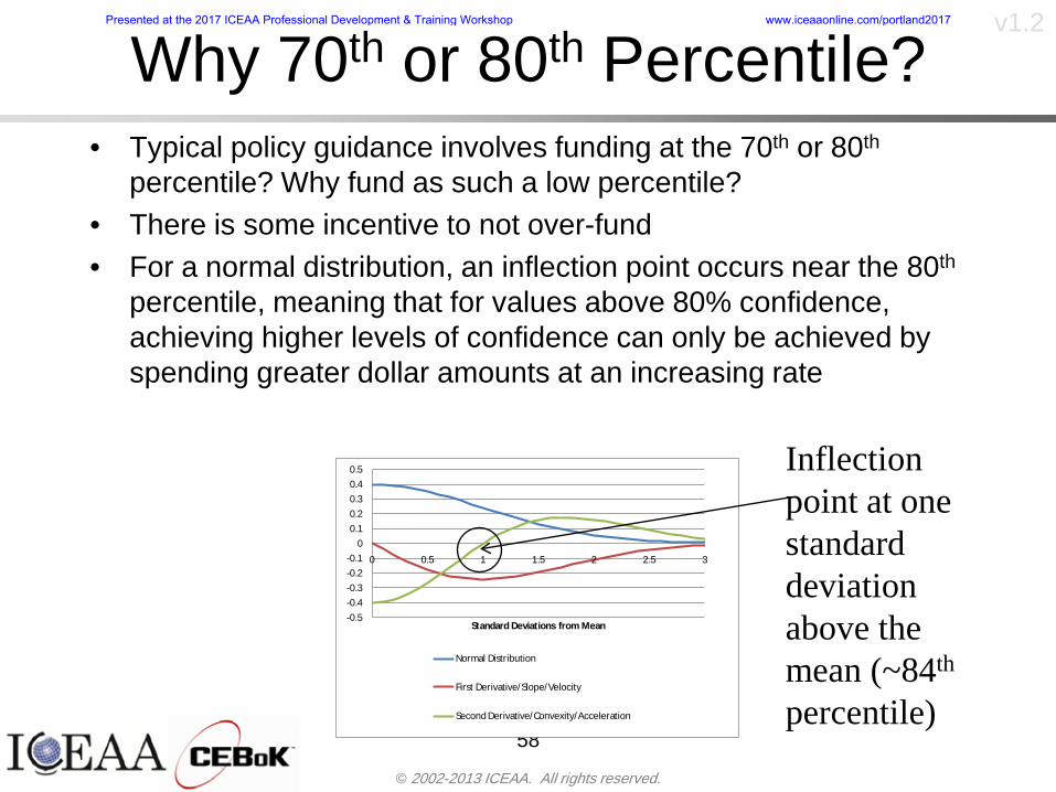
copy 2002-2013 ICEAA All rights reserved
v12
Why 70th or 80th Percentilebull Typical policy guidance involves funding at the 70th or 80th
percentile Why fund as such a low percentilebull There is some incentive to not over-fundbull For a normal distribution an inflection point occurs near the 80th
percentile meaning that for values above 80 confidence achieving higher levels of confidence can only be achieved by spending greater dollar amounts at an increasing rate
58
-05-04-03-02-01
00102030405
0 05 1 15 2 25 3
Standard Deviations from Mean
Normal Distribution
First DerivativeSlopeVelocity
Second DerivativeConvexityAcceleration
Inflection point at one standard deviation above the mean (~84th
percentile)
Presented at the 2017 ICEAA Professional Development amp Training Workshop wwwiceaaonlinecomportland2017
copy 2002-2013 ICEAA All rights reserved
v12
Funding Above Inflection Pointsbull As the percentile goes above the 80th percentile the amount
needed to achieve that higher level of confidence begins to increase at an increasing rate as is evident from the graph
59
0
10
20
30
40
50
60
70
50 55 60 65 70 75 80 85 90 95 100
$ Ab
ove
MEa
n to
Ach
ieve
Per
cent
ile
Percentile (Confidence Level)
Presented at the 2017 ICEAA Professional Development amp Training Workshop wwwiceaaonlinecomportland2017
copy 2002-2013 ICEAA All rights reserved
v12
Why Budget to the 70th or 80thbull Government projects are funded at the 70th or 80th percentilesbull Why not the 90th or 99th percentile Wonrsquot that help prevent
overrunsndash As we have seen percentiles do not add across programs
bull The sum of the 80th percentiles does NOT equal the total 80th percentile
ndash This is because the individual programs are riskier than the entire suite of missions
bull Known as the ldquoPortfolio effectrdquo (more or this later)
ndash Funding at the 80th gives confidence that the entire portfolio will be adequately funded
bull And since there is an inflection point near the 80th percentile funding above that level quickly becomes cost prohibitive
60
Presented at the 2017 ICEAA Professional Development amp Training Workshop wwwiceaaonlinecomportland2017
copy 2002-2013 ICEAA All rights reserved
v12
Inflection Points for Lognormalbull For a lognormal the inflection point
variesndash Coefficient of variation equal to 10 equates to an
inflection point at the 70th percentile
61
0
10
20
30
40
50
60
70
050 060 070 080 090 100
Coef
ficen
t of V
aria
tion
Percentile of the Inflection Point
Presented at the 2017 ICEAA Professional Development amp Training Workshop wwwiceaaonlinecomportland2017
copy 2002-2013 ICEAA All rights reserved
v12
Issues with Percentile Fundingbull However risk management does not stop at a
specific percentilendash What happens when the 70th percentile is exceeded
bull Any effective risk management policy should prescribe what happens after a bad event occursndash With VaR we only know when a bad event has occurred ndash Also funding at a relatively low level means we have no true
sense of the real risks that should be guarded against
62
Presented at the 2017 ICEAA Professional Development amp Training Workshop wwwiceaaonlinecomportland2017
copy 2002-2013 ICEAA All rights reserved
v12
ldquoHere There Be Dragonsrdquobull On old maps uncharted territory was often
marked with monsters or dragons
63
A section of the Carta Marina by Olaus Magnus 16th Century
Presented at the 2017 ICEAA Professional Development amp Training Workshop wwwiceaaonlinecomportland2017
copy 2002-2013 ICEAA All rights reserved
v12
Distribution Comparisonbull Four different distributions with the same 70th
percentile
bull Should we expect the tails to be similar
64
0
10
20
30
40
50
60
70
80
0 100 200 300 400 500 600
Perc
entil
eCo
nfid
ence
Lev
el
Triangular
Normal
Lognormal
Pareto
Presented at the 2017 ICEAA Professional Development amp Training Workshop wwwiceaaonlinecomportland2017
copy 2002-2013 ICEAA All rights reserved
v12Distribution Comparison Tail Behavior
bull The normal and triangular distributions have similar tails but the lognormal and Pareto have much fatter right tails
65
70
75
80
85
90
95
100
500 1500 2500 3500 4500 5500
Perc
entil
eCo
nfid
ence
Lev
el
Triangular
Normal
Lognormal
Pareto
Here There Be Dragons
Presented at the 2017 ICEAA Professional Development amp Training Workshop wwwiceaaonlinecomportland2017
copy 2002-2013 ICEAA All rights reserved
v12Distribution Comparison ndash Tail Behavior (Table)
bull There is significant tail risk for the lognormal and the Paretobull The 99th percentile for the Pareto is 1000 times greater than
the 70th percentilendash Risk seen in financial markets and in catastrophic risks like natural
disasters bull Four different projects follow the four different risk profiles seen
in this example should clearly have different risk management approaches but 70th percentile funding indicates the same risk management approach for all four
66
Percentile Triangular Normal Lognormal Pareto 70th $600 $600 $600 $600 80th $680 $660 $770 $1430 90th $770 $750 $1070 $5880 95th $840 $820 $1410 $23750 99th $930 $950 $2350 $600000
Presented at the 2017 ICEAA Professional Development amp Training Workshop wwwiceaaonlinecomportland2017
copy 2002-2013 ICEAA All rights reserved
v12Percentile Budgeting is Not Risk Management
bull Percentile budgeting ne effective risk management policybull Suppose that you are shopping for a new car You
mention that safety is your top concern The salesman says he has a great safe car available You ask about the air bags Do they work The salesman answers ldquoOf course Seventy percent of the time they work fine Only 30 of the time the air bags will fail to deployrdquo Would you buy such a car Hedge fund manager David Einhorn has stated ldquoRisk management is the air bag that must always work but only in the multi-sigma event where you have an accidentrdquo
67
Risk management is the air bag that must always work but only in the multi-sigma event where you
have an accident
Presented at the 2017 ICEAA Professional Development amp Training Workshop wwwiceaaonlinecomportland2017
copy 2002-2013 ICEAA All rights reserved
v12
Joint Confidence Level Analysisbull Schedules are risky toobull For 98 recent NASA missions average
schedule growth was 38ndash Not as high as cost growth but still significant
68
0
5
10
15
20
25
30
35
40
Schedule
Cost
Presented at the 2017 ICEAA Professional Development amp Training Workshop wwwiceaaonlinecomportland2017
copy 2002-2013 ICEAA All rights reserved
v12
Schedules Impact Costbull Changes in schedule can have enormous
impacts on cost ndash Schedule slips can lead to cost increases
bull Fixed programmatic costs must be paid on a regular basisndash Achieving schedule milestones early can result in cost
savings
bull Schedule is an important consideration in cost analysis including cost risk analysis
bull However we must be careful in correctly integrating cost and schedule riskndash Schedule is not simply an input but is dependent on many of
the same factors that drive cost
69
Presented at the 2017 ICEAA Professional Development amp Training Workshop wwwiceaaonlinecomportland2017
copy 2002-2013 ICEAA All rights reserved
v12
The Relationship of Cost to Schedulebull Cost and schedule are positively correlated
ndash A larger program with bigger scope with take longer to complete than a smaller simpler program
bull However longer schedules do not always equate to higher cost nor shorter schedules with lower costndash Highly compressed schedules relative to the
optimal schedule can lead to large overrunsbull Compressed schedules are commonplace for
many planetary missions
70
Presented at the 2017 ICEAA Professional Development amp Training Workshop wwwiceaaonlinecomportland2017
copy 2002-2013 ICEAA All rights reserved
v12The Impact of Schedule GrowthCompression on Cost
bull Compressed schedules lead to cost growth and based on existing research is actually more expensive than schedule slippages
71
0
20
40
60
80
100
120
140
160
-50 -25 0 25 50 75 100
Percentage Change in Schedule
Perc
enta
ge C
hang
e in
Cos
t due
to
Sche
dule
Cha
nge
Source Smart CB ldquoCost and Schedule Interrelationshipsrdquo 2007 NASA Cost Symposium
Presented at the 2017 ICEAA Professional Development amp Training Workshop wwwiceaaonlinecomportland2017
copy 2002-2013 ICEAA All rights reserved
v12Schedule as an Independent Variable
bull Why not simply add schedule as an input to cost-estimating relationships (CERs)
bull Schedule is often treated as an independent variable ndash schedules are often determined independently of cost considerationsndash Cost may not be considered explicitly although budgets and
schedules are determined based on scope and other common factors
bull In 2006 SAIC undertook a research task to determine the impact of schedule on cost and added schedule as an independent variable to the CERs in the NASAAir Force Cost Model (NAFCOM) to see if schedule provided any improvement in goodness of fit
72
Presented at the 2017 ICEAA Professional Development amp Training Workshop wwwiceaaonlinecomportland2017
copy 2002-2013 ICEAA All rights reserved
v12
Schedule is a Dependent Variablebull Since NAFCOM includes an exhaustive list of cost drivers the inclusion
of schedule should give an indication of whether there is any additional independent value added from schedule independent of the cost drivers
bull In the study schedule was added to 10 subsystem-level CERs
ndash In each case the addition of schedule did NOTimprove the goodness of fit and schedule was NOT found to be a statistically significant cost driver (given the presence of the other variables) for any of the 10 CERs
bull Standard errors for the CERs increased due to decrease in degrees of freedom
bull Thus schedule as an independent variable did not provide any additional explanation of variation in historical cost
bull This is because schedule is truly NOT an independent variable but a dependent variable and is a function of the same factors that drive cost
73
Presented at the 2017 ICEAA Professional Development amp Training Workshop wwwiceaaonlinecomportland2017
copy 2002-2013 ICEAA All rights reserved
v12
Incorporation of Schedule in Cost Risk
bull When using subjective methods care must be taken in applying schedule to cost risk analysis
bull Since schedule is a dependent variable treating it independently from other factors when assessing its impact on cost can lead to a double count of independent variables in the cost risk analysis
bull Direct inclusion of schedule in a cost risk analysis effectively doubles the influence of each cost driver
ndash Incorrectly leads to broader risk ranges
74
CostWeight
HeritageNewness
Technology Readiness Schedule
Presented at the 2017 ICEAA Professional Development amp Training Workshop wwwiceaaonlinecomportland2017
copy 2002-2013 ICEAA All rights reserved
v12Subjective Cost Risk Methods and Overinclusion of Risk Factors
bull Subjective methods are suitable when data are scarce or not availablebull However care must be taken not to treat correlated sources of risk
such as schedule as independent of each otherbull Example ndash a subjective risk analysis incorporated technology readiness
design risk requirements stability integration risk and schedule and treated each source of risk as independent
bull Risk triangle high value without schedule risk was 31 times the point estimate
bull Risk triangle high value with schedule risk added on top of other sources of risk treated independently was 34 times the point estimate
bull Risk triangle taking correlation between sources of risk into account in a rigorous statistical manner has a high value 15 times the point estimate less than half the effect when treating sources of risk as independent
75
Presented at the 2017 ICEAA Professional Development amp Training Workshop wwwiceaaonlinecomportland2017
copy 2002-2013 ICEAA All rights reserved
v12Fundamental Equation of Cost and Schedule Interrelationships
bull The Fundamental Equation of the Relationship Between Cost and Schedule is
Time = Moneybull This is a well known adage that time is money Your boss at
work may even mention this to you from time to time or if you are the boss you are all too aware of this iron law
bull Because time is money cost and schedule risk should be modeled jointly not with schedule as an independent cost driver
bull Note that cost and schedule are not perfectly correlatedndash Cost can sometimes ldquobuy downrdquo schedule extra money can be
spent to meet a deadline since in some cases additional effort to hasten the completion of a task
76
Presented at the 2017 ICEAA Professional Development amp Training Workshop wwwiceaaonlinecomportland2017
copy 2002-2013 ICEAA All rights reserved
v12How to (Correctly) Incorporate Schedule into Cost Risk Analysis
bull The best way to model cost and schedule risk is to develop a joint cost and schedule model based on the same data
bull Since such models are not currently available the next best approach is to model cost and schedule independently and then integrate cost and schedule risk analyses using joint probability distributions taking into account correlation between cost and schedulendash This approach pioneered by Paul Garvey and Steve Book is
considered industry best practicendash This is a practical method mathematically tractable and follows
naturally from the Fundamental Equation of Cost and Schedule Interrelationships
77
Book S A ldquoQuantifying the Relationship Between Cost and Schedulerdquo The Measurable News Winter 2007-2008 pp 11-15Garvey PR Probability Methods for Cost Uncertainty Analysis A Systems Engineering Perspective New York Marcel Dekker 2000 pp 308-335
Presented at the 2017 ICEAA Professional Development amp Training Workshop wwwiceaaonlinecomportland2017
copy 2002-2013 ICEAA All rights reserved
v12
Joint Lognormal and Normal Distributions
bull Cost and schedule are typically modeled as some combination of Normal and Lognormal probability distributionsndash Studies by The Aerospace Corporation the MITRE
Corporation Wyle Labs and SAIC have found that the Lognormal probability distribution almost always serves as a good model for both the schedule distribution and the cost distribution
ndash The Normal distribution may also be appropriate in some instances and depending upon the level of confidence at which budgets are set may even be more conservative and logically consistent than the Normal distribution
ndash Joint Lognormal and Normal distributions are defined by a pair of mean and standard deviations and a level of correlation between the two
78
Presented at the 2017 ICEAA Professional Development amp Training Workshop wwwiceaaonlinecomportland2017
copy 2002-2013 ICEAA All rights reserved
v12Modeling Cost and Schedule as a Bivariate Distribution
bull In the approach set forth by Book and Garvey cost risk is assessed and the top-level distribution is modeled as a Lognormal (or Normal) distribution schedule risk is assessed and the overall schedule risk is modeled as a Lognormal (or Normal) distribution
bull The two distributions are combined into a Bivariate distribution by assigning a correlation between the two and by treating the two distributions as the marginal distributions of a Bivariate Lognormal distributionndash Other combinations include a Bivariate Normal or a Bivariate
Normal-Lognormal
79
Presented at the 2017 ICEAA Professional Development amp Training Workshop wwwiceaaonlinecomportland2017
copy 2002-2013 ICEAA All rights reserved
v12Bivariate Lognormal Distribution for Cost and Schedule
bull Cost is often observed to be Lognormal when strong positive correlations are present among the systemrsquos WBS cost element costs
bull A systemrsquos schedule is often observed (from Monte Carlo simulations) to be Lognormal if it is the sum of many positively correlated schedule activities in an overall schedule network
bull If Lognormal distributions characterize a systemrsquos cost and schedule then the Bivariate Lognormal could serve as an assumed model of their joint distributionndash In this case the marginal distribution of each of cost and schedule is
Lognormalbull Other possibilities for modeling cost and schedule as a Bivariate
distribution include a Bivariate Normal or a Bivariate Normal-Lognormal distributionndash All these combinations are analytically tractable
80
Presented at the 2017 ICEAA Professional Development amp Training Workshop wwwiceaaonlinecomportland2017
copy 2002-2013 ICEAA All rights reserved
v12Bivariate Lognormal for Cost and Schedule
bull Contour Plots of a Bivariate Lognormal
81
Presented at the 2017 ICEAA Professional Development amp Training Workshop wwwiceaaonlinecomportland2017
copy 2002-2013 ICEAA All rights reserved
v12Correlation Between Cost and Schedule
bull Cost and schedule are positively correlated but not perfectly sondash For example it is possible to have a schedule underrun and a cost
overrunbull Based on cost and schedule growth data for 50 completed NASA
programs the correlation between development cost and development schedule is 70
82
00
200
400
600
800
1000
1200
-500 00 500 1000 1500 2000 2500Historical Cost Growth
Hist
oric
al S
ched
ule
Gro
wth
r = 715
Presented at the 2017 ICEAA Professional Development amp Training Workshop wwwiceaaonlinecomportland2017
copy 2002-2013 ICEAA All rights reserved
v12Correlation Between Cost and Schedule Caveats
bull Based on historical data recommended correlation between cost and schedule is 70 but this could be higher or lower depending upon program circumstancesndash If program is budget constrained cost and schedule will be
more highly correlated (go as you pay)ndash If program is schedule constrained cost and schedule will
have lower correlation perhaps even negative correlation ndash Smaller programs have smaller correlation between cost and
schedule riskbull Relatively easy to ldquohurry uprdquo and finish on time or even early if
needed
83
Presented at the 2017 ICEAA Professional Development amp Training Workshop wwwiceaaonlinecomportland2017
copy 2002-2013 ICEAA All rights reserved
v12
Conditional Confidence Levelsbull Given a programrsquos project schedule we can determine the cost
risk distribution conditional upon the given schedulebull Conditional cost S-curves are steeper than unconditional
(marginal) cost S-curves between some uncertainty has been removed because schedule is fixed
84
Presented at the 2017 ICEAA Professional Development amp Training Workshop wwwiceaaonlinecomportland2017
copy 2002-2013 ICEAA All rights reserved
v12
Joint Confidence Levelsbull Joint 65 confidence represents the probability of
achieving both 65 confidence in cost AND 65 confidence in schedulendash This is different than achieving 65 cost confidence alone
or achieving 65 schedule confidence alonebull Due to the imperfect correlation between cost and schedule it
is possible to achieve a 65 cost confidence with a lower level of schedule confidence
bull Restricting the schedule confidence thus requires additional $ to achieve a given level of confidence
85
X
Y
Possible Values for Which X gt a Possible Values for
Which X gt a and Y gt b
a
b
Presented at the 2017 ICEAA Professional Development amp Training Workshop wwwiceaaonlinecomportland2017
copy 2002-2013 ICEAA All rights reserved
v12Joint Confidence Levels Versus Cost Confidence Levels Only
bull Example of the differences between cost confidence schedule confidence conditional cost confidence and joint cost and schedule confidence
86
Joint Cost-Schedule Confidence Iso-Curves
Cost (RY$M)
Sche
dule
(Mon
ths)
65 Confidence
50 Confidence
70 Confidence
65 Cost Confidence AggressiveSchedule65 Cost ConfidenceScheduleGiven 65 Schedule ConfidenceUnconditional 65 CostConfidenceUnconditional 65 ScheduleConfidence
65 Cost Confidence 65 Joint Cost and Schedule
Confidence for 65 Schedule Confidence
Presented at the 2017 ICEAA Professional Development amp Training Workshop wwwiceaaonlinecomportland2017
copy 2002-2013 ICEAA All rights reserved
v12
Joint Cost and Schedule Confidence
bull Can examine pairs of cost and schedule that achieve a given level of confidence
bull Provides insights into the trade-offs between cost and schedule for a given level of confidencendash Possible to increase cost confidence by giving a
project more time in some instances or possible to ldquobuy downrdquo schedule
bull But these have limits and are shown in the iso-cost and schedule confidence curves
87
Presented at the 2017 ICEAA Professional Development amp Training Workshop wwwiceaaonlinecomportland2017
copy 2002-2013 ICEAA All rights reserved
v12Cost and Schedule Trade-offs for a Given Level of Joint Confidence
bull Hypothetical Example
88
Cost (RY$M)
Schedule (Months)
$100 48$99 48$89 49$87 50$85 51$85 52$84 53$83 55$83 55$83 56
Cost and Schedule 65 Confidence Iso-Curve
4748495051525354555657
$80 $82 $84 $86 $88 $90 $92 $94 $96 $98 $100
Cost (RY$ M)
Sche
dule
(Mon
ths)
Presented at the 2017 ICEAA Professional Development amp Training Workshop wwwiceaaonlinecomportland2017
copy 2002-2013 ICEAA All rights reserved
v12Policy Considerations for Confidence Levels
bull For large programs the difference between the amount of money needed to achieve 65 cost confidence independent of schedule and joint 65 cost and schedule confidence can represent hundreds of millions and even billions of dollars
89
Joint Cost-Schedule Confidence Iso-Curves
Cost (RY$M)
Sche
dule
(Mon
ths)
65 Confidence
65 Cost Confidence AggressiveSchedule
65 Cost ConfidenceScheduleGiven 65 Schedule Confidence
Unconditional 65 CostConfidence
Joint Cost and Schedule Confidence for 65 Cost Confidence and Program Baseline Schedule is Less Than 35
65 Cost Confidence Independent of Schedule Cost Needed to Achieve
Both 65 Joint Cost and Schedule Confidence for the Schedule with 65 Confidence
Presented at the 2017 ICEAA Professional Development amp Training Workshop wwwiceaaonlinecomportland2017
copy 2002-2013 ICEAA All rights reserved
v12
Copulasbull More generally any combination of distributions can
be used (more than just normal and lognormal)ndash Termed ldquocopulardquo from the Italian word for ldquocouplerdquondash Copulas are a way to combine marginal distributions of any
number and type into a joint distributionbull More formally a copula is a multivariate joint distribution defined
on the n-dimensional unit cube [0 1]n such that every marginal distribution is uniform on the interval [0 1]
bull (The bivariate form of) Sklarrsquos theorem states that for any bivariate distribution function H(x y) let F(x) = H(x infin) and G(y) = H(infin y) be the univariate marginal probability distribution functions Then there exists a copula C such that H(xy)=C(F(x)G(y))
ndash Copulas are widely used in risk management for investments and insurance
bull Considered industry best practice (Li 2000)bull Marketed as part of JP Morganrsquos CreditMetrics suite of tools
(Gupton et Al 1997)90
Presented at the 2017 ICEAA Professional Development amp Training Workshop wwwiceaaonlinecomportland2017
copy 2002-2013 ICEAA All rights reserved
v12Parametric Joint Cost and Schedule Analysis
bull A parametric model based on a consistent data set with a set of overlapping cost and schedule drivers is a cleaner way to model cost and schedule
91
CostWeight
HeritageNewness
Technology Readiness
Schedule
0
20
40
60
80
100
Confidence
Joint Cost and Schedule Confidence
Schedule
Cost
Lognormal Distribution PDF and CDF
0102030405060708090100
200 300 400 500 600 700 800 900 1000Cost $
Con
fiden
ce L
evel
0
00002
00004
00006
00008
0001
00012
00014
00016
Prob
abili
ty D
ensi
ty
CDFPDF
Lognormal Distribution PDF and CDF
0102030405060708090100
200 300 400 500 600 700 800 900 1000Cost $
Con
fiden
ce L
evel
0
00002
00004
00006
00008
0001
00012
00014
00016
Prob
abili
ty D
ensi
ty
CDFPDF
Presented at the 2017 ICEAA Professional Development amp Training Workshop wwwiceaaonlinecomportland2017
copy 2002-2013 ICEAA All rights reserved
v12Parametric Joint Cost and Schedule Analysis (2)
bull Joint cost and schedule risk analysis produced naturally by the integrated modelndash Addresses several issues with the copula
approachbull Tail dependencybull Correlation ndash no need to assign correlation
between cost and schedulebull Consistency of cost and schedule models
92
Presented at the 2017 ICEAA Professional Development amp Training Workshop wwwiceaaonlinecomportland2017
copy 2002-2013 ICEAA All rights reserved
v12
Resource-Loaded Schedulesbull Involves assigning cost and schedule risks to a resource-loaded schedule
networkbull Bottom-up approach
ndash More labor intensive than parametrics but can also provide more insight
ndash Can answer questions than parametric typically cannot such as how much do reserve requirements decrease if a specific risk is retired
bull Currently being implemented in Constellation programbull Has same issue as all bottom-up models hard to count all the risks and model
them discretely
ndash As a result there is a tendency to reflect less risk than indicated by history
ndash ldquoThere are more things in heaven and earth Horatio than are dreamt of in your philosophyrdquo William Shakespeare Hamlet Act I Scene V
93
Presented at the 2017 ICEAA Professional Development amp Training Workshop wwwiceaaonlinecomportland2017
copy 2002-2013 ICEAA All rights reserved
v12Resource-Loaded Schedules Vs Parametrics
bull Parametric most appropriate for early estimatesndash But also good for high-level checks as project progresses
bull As plans take shape lower level modeling may be more appropriate
94 1
CONCEPTUALDEVELOPMENT
PROJECTDEFINITION DESIGN DEVELOPMENT OPERATIONS
PARAMETRIC PARAMETRIC
ANALOGY
ENGINEERING (Bottoms Up)
$PARAMETRIC
DETAILED
$
Pre Phase A Phase B Phase CDPhase A Phase EPre Phase A Phase B Phase CDPhase A Phase E
Risk = f(Cost Estimating Relationship Inputs eg mass power data rate TRL new design etc)
Risk = f(cost and schedule variation of the analogous elements)
Risk = f(variation of detailed inputs eg labor hours rates materials etc)
Presented at the 2017 ICEAA Professional Development amp Training Workshop wwwiceaaonlinecomportland2017
copy 2002-2013 ICEAA All rights reserved
v12
Resource-Loaded Schedulesbull Methodology has been demonstrated in other
industriesndash Construction oil and gasndash Analysis has not been traditionally done on highly uncertain
complex development projects bull Methodology focuses on project baseline schedule
ndash In baseline schedule all tasks are resource loaded to represent a baseline schedule and cost standpoint
ndash Resource loaded schedule is ldquorolledrdquo up to a manageable level
ndash Based on the risk and uncertainties identified schedule distributions are applied to each rolled up task
ndash Cost uncertainties are also applied to rolled up tasksbull Uncertainties include labor rate man power etc
ndash A Monte Carlo simulation is run to develop joint cost-schedule distributions
95
Presented at the 2017 ICEAA Professional Development amp Training Workshop wwwiceaaonlinecomportland2017
copy 2002-2013 ICEAA All rights reserved
v12
Unit III - Module 9 96
Execution ndash Cross Checksbull Means The mean cost growth factor for WBS items
can be compared to history as a way to cross check results
bull CVs The CV of the cost growth factors for WBS items can be compared to history as a way to cross check results
bull Inputs Checks are performed on inputs or other parameters to see if historical values are in line with program assumptionsndash Example Historical risk scores can be compared to program
risk scores to see if risk assessors are being realistic and to see if the underlying database is representative of the program
11
Presented at the 2017 ICEAA Professional Development amp Training Workshop wwwiceaaonlinecomportland2017
- Cost and Schedule Risk Analysis Basic
- Acknowledgments
- Unit Index
- Risk Overview
- Agenda
- Introduction
- Risk Analysis Terms
- Are Our Costs Realistic
- Historical Cost Growth
- Sources of Cost Risk
- Point Estimates of Cost
- Types of Risk
- Point Estimates Vs Risk Estimates
- Cost Risk and Probability
- Probability Model ndash Distribution
- Probability Model ndash Distribution
- Probability ndash Top-Level Distribution
- S-Curves and Confidence Levels
- Example ndash Normal Distribution
- Confidence Levels
- Measuring Parametric Model Uncertainty
- Parametric Model Example
- Weight Uncertainty
- Estimating Uncertainty
- Estimating Uncertainty (2)
- Estimating Uncertainty (3)
- Aggregating Risk
- WBS Example
- WBS and Risk
- Aggregating Risk
- Percentiles Do Not Add
- Percentiles Do Not Add (2)
- Percentiles Do Not Add (3)
- Methods for Aggregating Risk
- Monte Carlo Simulationfor Risk Analysis
- Monte Carlo Simulation
- Using Random Numbers to Simulate Distributions
- Simulating a Triangular Distribution
- Simulating a Triangular Distribution (2)
- Monte Carlo and the WBS
- Number of Trials
- Number of Trials (2)
- Number of Trials (3)
- Number of Trials (4)
- Number of Trials (5)
- Number of Trials (6)
- Methods of Simulation
- Probability Model ndash Correlation
- Correlation And Causation
- The Importance of Correlation
- The Importance of Correlation (2)
- Measures of Correlation
- Pearson Correlation
- Spearman Correlation
- Functional Correlation
- Risk Measures
- Value at Risk (VaR)
- Why 70th or 80th Percentile
- Funding Above Inflection Points
- Why Budget to the 70th or 80th
- Inflection Points for Lognormal
- Issues with Percentile Funding
- ldquoHere There Be Dragonsrdquo
- Distribution Comparison
- Distribution Comparison Tail Behavior
- Distribution Comparison ndash Tail Behavior (Table)
- Percentile Budgeting is Not Risk Management
- Joint Confidence Level Analysis
- Schedules Impact Cost
- The Relationship of Cost to Schedule
- The Impact of Schedule GrowthCompression on Cost
- Schedule as an Independent Variable
- Schedule is a Dependent Variable
- Incorporation of Schedule in Cost Risk
- Subjective Cost Risk Methods and Overinclusion of Risk Factors
- Fundamental Equation of Cost and Schedule Interrelationships
- How to (Correctly) Incorporate Schedule into Cost Risk Analysis
- Joint Lognormal and Normal Distributions
- Modeling Cost and Schedule as a Bivariate Distribution
- Bivariate Lognormal Distribution for Cost and Schedule
- Bivariate Lognormal for Cost and Schedule
- Correlation Between Cost and Schedule
- Correlation Between Cost and Schedule Caveats
- Conditional Confidence Levels
- Joint Confidence Levels
- Joint Confidence Levels Versus Cost Confidence Levels Only
- Joint Cost and Schedule Confidence
- Cost and Schedule Trade-offs for a Given Level of Joint Confidence
- Policy Considerations for Confidence Levels
- Copulas
- Parametric Joint Cost and Schedule Analysis
- Parametric Joint Cost and Schedule Analysis (2)
- Resource-Loaded Schedules
- Resource-Loaded Schedules Vs Parametrics
- Resource-Loaded Schedules
- Execution ndash Cross Checks
-
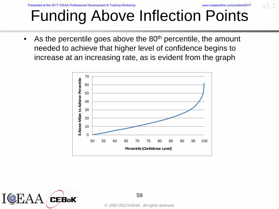
copy 2002-2013 ICEAA All rights reserved
v12
Funding Above Inflection Pointsbull As the percentile goes above the 80th percentile the amount
needed to achieve that higher level of confidence begins to increase at an increasing rate as is evident from the graph
59
0
10
20
30
40
50
60
70
50 55 60 65 70 75 80 85 90 95 100
$ Ab
ove
MEa
n to
Ach
ieve
Per
cent
ile
Percentile (Confidence Level)
Presented at the 2017 ICEAA Professional Development amp Training Workshop wwwiceaaonlinecomportland2017
copy 2002-2013 ICEAA All rights reserved
v12
Why Budget to the 70th or 80thbull Government projects are funded at the 70th or 80th percentilesbull Why not the 90th or 99th percentile Wonrsquot that help prevent
overrunsndash As we have seen percentiles do not add across programs
bull The sum of the 80th percentiles does NOT equal the total 80th percentile
ndash This is because the individual programs are riskier than the entire suite of missions
bull Known as the ldquoPortfolio effectrdquo (more or this later)
ndash Funding at the 80th gives confidence that the entire portfolio will be adequately funded
bull And since there is an inflection point near the 80th percentile funding above that level quickly becomes cost prohibitive
60
Presented at the 2017 ICEAA Professional Development amp Training Workshop wwwiceaaonlinecomportland2017
copy 2002-2013 ICEAA All rights reserved
v12
Inflection Points for Lognormalbull For a lognormal the inflection point
variesndash Coefficient of variation equal to 10 equates to an
inflection point at the 70th percentile
61
0
10
20
30
40
50
60
70
050 060 070 080 090 100
Coef
ficen
t of V
aria
tion
Percentile of the Inflection Point
Presented at the 2017 ICEAA Professional Development amp Training Workshop wwwiceaaonlinecomportland2017
copy 2002-2013 ICEAA All rights reserved
v12
Issues with Percentile Fundingbull However risk management does not stop at a
specific percentilendash What happens when the 70th percentile is exceeded
bull Any effective risk management policy should prescribe what happens after a bad event occursndash With VaR we only know when a bad event has occurred ndash Also funding at a relatively low level means we have no true
sense of the real risks that should be guarded against
62
Presented at the 2017 ICEAA Professional Development amp Training Workshop wwwiceaaonlinecomportland2017
copy 2002-2013 ICEAA All rights reserved
v12
ldquoHere There Be Dragonsrdquobull On old maps uncharted territory was often
marked with monsters or dragons
63
A section of the Carta Marina by Olaus Magnus 16th Century
Presented at the 2017 ICEAA Professional Development amp Training Workshop wwwiceaaonlinecomportland2017
copy 2002-2013 ICEAA All rights reserved
v12
Distribution Comparisonbull Four different distributions with the same 70th
percentile
bull Should we expect the tails to be similar
64
0
10
20
30
40
50
60
70
80
0 100 200 300 400 500 600
Perc
entil
eCo
nfid
ence
Lev
el
Triangular
Normal
Lognormal
Pareto
Presented at the 2017 ICEAA Professional Development amp Training Workshop wwwiceaaonlinecomportland2017
copy 2002-2013 ICEAA All rights reserved
v12Distribution Comparison Tail Behavior
bull The normal and triangular distributions have similar tails but the lognormal and Pareto have much fatter right tails
65
70
75
80
85
90
95
100
500 1500 2500 3500 4500 5500
Perc
entil
eCo
nfid
ence
Lev
el
Triangular
Normal
Lognormal
Pareto
Here There Be Dragons
Presented at the 2017 ICEAA Professional Development amp Training Workshop wwwiceaaonlinecomportland2017
copy 2002-2013 ICEAA All rights reserved
v12Distribution Comparison ndash Tail Behavior (Table)
bull There is significant tail risk for the lognormal and the Paretobull The 99th percentile for the Pareto is 1000 times greater than
the 70th percentilendash Risk seen in financial markets and in catastrophic risks like natural
disasters bull Four different projects follow the four different risk profiles seen
in this example should clearly have different risk management approaches but 70th percentile funding indicates the same risk management approach for all four
66
Percentile Triangular Normal Lognormal Pareto 70th $600 $600 $600 $600 80th $680 $660 $770 $1430 90th $770 $750 $1070 $5880 95th $840 $820 $1410 $23750 99th $930 $950 $2350 $600000
Presented at the 2017 ICEAA Professional Development amp Training Workshop wwwiceaaonlinecomportland2017
copy 2002-2013 ICEAA All rights reserved
v12Percentile Budgeting is Not Risk Management
bull Percentile budgeting ne effective risk management policybull Suppose that you are shopping for a new car You
mention that safety is your top concern The salesman says he has a great safe car available You ask about the air bags Do they work The salesman answers ldquoOf course Seventy percent of the time they work fine Only 30 of the time the air bags will fail to deployrdquo Would you buy such a car Hedge fund manager David Einhorn has stated ldquoRisk management is the air bag that must always work but only in the multi-sigma event where you have an accidentrdquo
67
Risk management is the air bag that must always work but only in the multi-sigma event where you
have an accident
Presented at the 2017 ICEAA Professional Development amp Training Workshop wwwiceaaonlinecomportland2017
copy 2002-2013 ICEAA All rights reserved
v12
Joint Confidence Level Analysisbull Schedules are risky toobull For 98 recent NASA missions average
schedule growth was 38ndash Not as high as cost growth but still significant
68
0
5
10
15
20
25
30
35
40
Schedule
Cost
Presented at the 2017 ICEAA Professional Development amp Training Workshop wwwiceaaonlinecomportland2017
copy 2002-2013 ICEAA All rights reserved
v12
Schedules Impact Costbull Changes in schedule can have enormous
impacts on cost ndash Schedule slips can lead to cost increases
bull Fixed programmatic costs must be paid on a regular basisndash Achieving schedule milestones early can result in cost
savings
bull Schedule is an important consideration in cost analysis including cost risk analysis
bull However we must be careful in correctly integrating cost and schedule riskndash Schedule is not simply an input but is dependent on many of
the same factors that drive cost
69
Presented at the 2017 ICEAA Professional Development amp Training Workshop wwwiceaaonlinecomportland2017
copy 2002-2013 ICEAA All rights reserved
v12
The Relationship of Cost to Schedulebull Cost and schedule are positively correlated
ndash A larger program with bigger scope with take longer to complete than a smaller simpler program
bull However longer schedules do not always equate to higher cost nor shorter schedules with lower costndash Highly compressed schedules relative to the
optimal schedule can lead to large overrunsbull Compressed schedules are commonplace for
many planetary missions
70
Presented at the 2017 ICEAA Professional Development amp Training Workshop wwwiceaaonlinecomportland2017
copy 2002-2013 ICEAA All rights reserved
v12The Impact of Schedule GrowthCompression on Cost
bull Compressed schedules lead to cost growth and based on existing research is actually more expensive than schedule slippages
71
0
20
40
60
80
100
120
140
160
-50 -25 0 25 50 75 100
Percentage Change in Schedule
Perc
enta
ge C
hang
e in
Cos
t due
to
Sche
dule
Cha
nge
Source Smart CB ldquoCost and Schedule Interrelationshipsrdquo 2007 NASA Cost Symposium
Presented at the 2017 ICEAA Professional Development amp Training Workshop wwwiceaaonlinecomportland2017
copy 2002-2013 ICEAA All rights reserved
v12Schedule as an Independent Variable
bull Why not simply add schedule as an input to cost-estimating relationships (CERs)
bull Schedule is often treated as an independent variable ndash schedules are often determined independently of cost considerationsndash Cost may not be considered explicitly although budgets and
schedules are determined based on scope and other common factors
bull In 2006 SAIC undertook a research task to determine the impact of schedule on cost and added schedule as an independent variable to the CERs in the NASAAir Force Cost Model (NAFCOM) to see if schedule provided any improvement in goodness of fit
72
Presented at the 2017 ICEAA Professional Development amp Training Workshop wwwiceaaonlinecomportland2017
copy 2002-2013 ICEAA All rights reserved
v12
Schedule is a Dependent Variablebull Since NAFCOM includes an exhaustive list of cost drivers the inclusion
of schedule should give an indication of whether there is any additional independent value added from schedule independent of the cost drivers
bull In the study schedule was added to 10 subsystem-level CERs
ndash In each case the addition of schedule did NOTimprove the goodness of fit and schedule was NOT found to be a statistically significant cost driver (given the presence of the other variables) for any of the 10 CERs
bull Standard errors for the CERs increased due to decrease in degrees of freedom
bull Thus schedule as an independent variable did not provide any additional explanation of variation in historical cost
bull This is because schedule is truly NOT an independent variable but a dependent variable and is a function of the same factors that drive cost
73
Presented at the 2017 ICEAA Professional Development amp Training Workshop wwwiceaaonlinecomportland2017
copy 2002-2013 ICEAA All rights reserved
v12
Incorporation of Schedule in Cost Risk
bull When using subjective methods care must be taken in applying schedule to cost risk analysis
bull Since schedule is a dependent variable treating it independently from other factors when assessing its impact on cost can lead to a double count of independent variables in the cost risk analysis
bull Direct inclusion of schedule in a cost risk analysis effectively doubles the influence of each cost driver
ndash Incorrectly leads to broader risk ranges
74
CostWeight
HeritageNewness
Technology Readiness Schedule
Presented at the 2017 ICEAA Professional Development amp Training Workshop wwwiceaaonlinecomportland2017
copy 2002-2013 ICEAA All rights reserved
v12Subjective Cost Risk Methods and Overinclusion of Risk Factors
bull Subjective methods are suitable when data are scarce or not availablebull However care must be taken not to treat correlated sources of risk
such as schedule as independent of each otherbull Example ndash a subjective risk analysis incorporated technology readiness
design risk requirements stability integration risk and schedule and treated each source of risk as independent
bull Risk triangle high value without schedule risk was 31 times the point estimate
bull Risk triangle high value with schedule risk added on top of other sources of risk treated independently was 34 times the point estimate
bull Risk triangle taking correlation between sources of risk into account in a rigorous statistical manner has a high value 15 times the point estimate less than half the effect when treating sources of risk as independent
75
Presented at the 2017 ICEAA Professional Development amp Training Workshop wwwiceaaonlinecomportland2017
copy 2002-2013 ICEAA All rights reserved
v12Fundamental Equation of Cost and Schedule Interrelationships
bull The Fundamental Equation of the Relationship Between Cost and Schedule is
Time = Moneybull This is a well known adage that time is money Your boss at
work may even mention this to you from time to time or if you are the boss you are all too aware of this iron law
bull Because time is money cost and schedule risk should be modeled jointly not with schedule as an independent cost driver
bull Note that cost and schedule are not perfectly correlatedndash Cost can sometimes ldquobuy downrdquo schedule extra money can be
spent to meet a deadline since in some cases additional effort to hasten the completion of a task
76
Presented at the 2017 ICEAA Professional Development amp Training Workshop wwwiceaaonlinecomportland2017
copy 2002-2013 ICEAA All rights reserved
v12How to (Correctly) Incorporate Schedule into Cost Risk Analysis
bull The best way to model cost and schedule risk is to develop a joint cost and schedule model based on the same data
bull Since such models are not currently available the next best approach is to model cost and schedule independently and then integrate cost and schedule risk analyses using joint probability distributions taking into account correlation between cost and schedulendash This approach pioneered by Paul Garvey and Steve Book is
considered industry best practicendash This is a practical method mathematically tractable and follows
naturally from the Fundamental Equation of Cost and Schedule Interrelationships
77
Book S A ldquoQuantifying the Relationship Between Cost and Schedulerdquo The Measurable News Winter 2007-2008 pp 11-15Garvey PR Probability Methods for Cost Uncertainty Analysis A Systems Engineering Perspective New York Marcel Dekker 2000 pp 308-335
Presented at the 2017 ICEAA Professional Development amp Training Workshop wwwiceaaonlinecomportland2017
copy 2002-2013 ICEAA All rights reserved
v12
Joint Lognormal and Normal Distributions
bull Cost and schedule are typically modeled as some combination of Normal and Lognormal probability distributionsndash Studies by The Aerospace Corporation the MITRE
Corporation Wyle Labs and SAIC have found that the Lognormal probability distribution almost always serves as a good model for both the schedule distribution and the cost distribution
ndash The Normal distribution may also be appropriate in some instances and depending upon the level of confidence at which budgets are set may even be more conservative and logically consistent than the Normal distribution
ndash Joint Lognormal and Normal distributions are defined by a pair of mean and standard deviations and a level of correlation between the two
78
Presented at the 2017 ICEAA Professional Development amp Training Workshop wwwiceaaonlinecomportland2017
copy 2002-2013 ICEAA All rights reserved
v12Modeling Cost and Schedule as a Bivariate Distribution
bull In the approach set forth by Book and Garvey cost risk is assessed and the top-level distribution is modeled as a Lognormal (or Normal) distribution schedule risk is assessed and the overall schedule risk is modeled as a Lognormal (or Normal) distribution
bull The two distributions are combined into a Bivariate distribution by assigning a correlation between the two and by treating the two distributions as the marginal distributions of a Bivariate Lognormal distributionndash Other combinations include a Bivariate Normal or a Bivariate
Normal-Lognormal
79
Presented at the 2017 ICEAA Professional Development amp Training Workshop wwwiceaaonlinecomportland2017
copy 2002-2013 ICEAA All rights reserved
v12Bivariate Lognormal Distribution for Cost and Schedule
bull Cost is often observed to be Lognormal when strong positive correlations are present among the systemrsquos WBS cost element costs
bull A systemrsquos schedule is often observed (from Monte Carlo simulations) to be Lognormal if it is the sum of many positively correlated schedule activities in an overall schedule network
bull If Lognormal distributions characterize a systemrsquos cost and schedule then the Bivariate Lognormal could serve as an assumed model of their joint distributionndash In this case the marginal distribution of each of cost and schedule is
Lognormalbull Other possibilities for modeling cost and schedule as a Bivariate
distribution include a Bivariate Normal or a Bivariate Normal-Lognormal distributionndash All these combinations are analytically tractable
80
Presented at the 2017 ICEAA Professional Development amp Training Workshop wwwiceaaonlinecomportland2017
copy 2002-2013 ICEAA All rights reserved
v12Bivariate Lognormal for Cost and Schedule
bull Contour Plots of a Bivariate Lognormal
81
Presented at the 2017 ICEAA Professional Development amp Training Workshop wwwiceaaonlinecomportland2017
copy 2002-2013 ICEAA All rights reserved
v12Correlation Between Cost and Schedule
bull Cost and schedule are positively correlated but not perfectly sondash For example it is possible to have a schedule underrun and a cost
overrunbull Based on cost and schedule growth data for 50 completed NASA
programs the correlation between development cost and development schedule is 70
82
00
200
400
600
800
1000
1200
-500 00 500 1000 1500 2000 2500Historical Cost Growth
Hist
oric
al S
ched
ule
Gro
wth
r = 715
Presented at the 2017 ICEAA Professional Development amp Training Workshop wwwiceaaonlinecomportland2017
copy 2002-2013 ICEAA All rights reserved
v12Correlation Between Cost and Schedule Caveats
bull Based on historical data recommended correlation between cost and schedule is 70 but this could be higher or lower depending upon program circumstancesndash If program is budget constrained cost and schedule will be
more highly correlated (go as you pay)ndash If program is schedule constrained cost and schedule will
have lower correlation perhaps even negative correlation ndash Smaller programs have smaller correlation between cost and
schedule riskbull Relatively easy to ldquohurry uprdquo and finish on time or even early if
needed
83
Presented at the 2017 ICEAA Professional Development amp Training Workshop wwwiceaaonlinecomportland2017
copy 2002-2013 ICEAA All rights reserved
v12
Conditional Confidence Levelsbull Given a programrsquos project schedule we can determine the cost
risk distribution conditional upon the given schedulebull Conditional cost S-curves are steeper than unconditional
(marginal) cost S-curves between some uncertainty has been removed because schedule is fixed
84
Presented at the 2017 ICEAA Professional Development amp Training Workshop wwwiceaaonlinecomportland2017
copy 2002-2013 ICEAA All rights reserved
v12
Joint Confidence Levelsbull Joint 65 confidence represents the probability of
achieving both 65 confidence in cost AND 65 confidence in schedulendash This is different than achieving 65 cost confidence alone
or achieving 65 schedule confidence alonebull Due to the imperfect correlation between cost and schedule it
is possible to achieve a 65 cost confidence with a lower level of schedule confidence
bull Restricting the schedule confidence thus requires additional $ to achieve a given level of confidence
85
X
Y
Possible Values for Which X gt a Possible Values for
Which X gt a and Y gt b
a
b
Presented at the 2017 ICEAA Professional Development amp Training Workshop wwwiceaaonlinecomportland2017
copy 2002-2013 ICEAA All rights reserved
v12Joint Confidence Levels Versus Cost Confidence Levels Only
bull Example of the differences between cost confidence schedule confidence conditional cost confidence and joint cost and schedule confidence
86
Joint Cost-Schedule Confidence Iso-Curves
Cost (RY$M)
Sche
dule
(Mon
ths)
65 Confidence
50 Confidence
70 Confidence
65 Cost Confidence AggressiveSchedule65 Cost ConfidenceScheduleGiven 65 Schedule ConfidenceUnconditional 65 CostConfidenceUnconditional 65 ScheduleConfidence
65 Cost Confidence 65 Joint Cost and Schedule
Confidence for 65 Schedule Confidence
Presented at the 2017 ICEAA Professional Development amp Training Workshop wwwiceaaonlinecomportland2017
copy 2002-2013 ICEAA All rights reserved
v12
Joint Cost and Schedule Confidence
bull Can examine pairs of cost and schedule that achieve a given level of confidence
bull Provides insights into the trade-offs between cost and schedule for a given level of confidencendash Possible to increase cost confidence by giving a
project more time in some instances or possible to ldquobuy downrdquo schedule
bull But these have limits and are shown in the iso-cost and schedule confidence curves
87
Presented at the 2017 ICEAA Professional Development amp Training Workshop wwwiceaaonlinecomportland2017
copy 2002-2013 ICEAA All rights reserved
v12Cost and Schedule Trade-offs for a Given Level of Joint Confidence
bull Hypothetical Example
88
Cost (RY$M)
Schedule (Months)
$100 48$99 48$89 49$87 50$85 51$85 52$84 53$83 55$83 55$83 56
Cost and Schedule 65 Confidence Iso-Curve
4748495051525354555657
$80 $82 $84 $86 $88 $90 $92 $94 $96 $98 $100
Cost (RY$ M)
Sche
dule
(Mon
ths)
Presented at the 2017 ICEAA Professional Development amp Training Workshop wwwiceaaonlinecomportland2017
copy 2002-2013 ICEAA All rights reserved
v12Policy Considerations for Confidence Levels
bull For large programs the difference between the amount of money needed to achieve 65 cost confidence independent of schedule and joint 65 cost and schedule confidence can represent hundreds of millions and even billions of dollars
89
Joint Cost-Schedule Confidence Iso-Curves
Cost (RY$M)
Sche
dule
(Mon
ths)
65 Confidence
65 Cost Confidence AggressiveSchedule
65 Cost ConfidenceScheduleGiven 65 Schedule Confidence
Unconditional 65 CostConfidence
Joint Cost and Schedule Confidence for 65 Cost Confidence and Program Baseline Schedule is Less Than 35
65 Cost Confidence Independent of Schedule Cost Needed to Achieve
Both 65 Joint Cost and Schedule Confidence for the Schedule with 65 Confidence
Presented at the 2017 ICEAA Professional Development amp Training Workshop wwwiceaaonlinecomportland2017
copy 2002-2013 ICEAA All rights reserved
v12
Copulasbull More generally any combination of distributions can
be used (more than just normal and lognormal)ndash Termed ldquocopulardquo from the Italian word for ldquocouplerdquondash Copulas are a way to combine marginal distributions of any
number and type into a joint distributionbull More formally a copula is a multivariate joint distribution defined
on the n-dimensional unit cube [0 1]n such that every marginal distribution is uniform on the interval [0 1]
bull (The bivariate form of) Sklarrsquos theorem states that for any bivariate distribution function H(x y) let F(x) = H(x infin) and G(y) = H(infin y) be the univariate marginal probability distribution functions Then there exists a copula C such that H(xy)=C(F(x)G(y))
ndash Copulas are widely used in risk management for investments and insurance
bull Considered industry best practice (Li 2000)bull Marketed as part of JP Morganrsquos CreditMetrics suite of tools
(Gupton et Al 1997)90
Presented at the 2017 ICEAA Professional Development amp Training Workshop wwwiceaaonlinecomportland2017
copy 2002-2013 ICEAA All rights reserved
v12Parametric Joint Cost and Schedule Analysis
bull A parametric model based on a consistent data set with a set of overlapping cost and schedule drivers is a cleaner way to model cost and schedule
91
CostWeight
HeritageNewness
Technology Readiness
Schedule
0
20
40
60
80
100
Confidence
Joint Cost and Schedule Confidence
Schedule
Cost
Lognormal Distribution PDF and CDF
0102030405060708090100
200 300 400 500 600 700 800 900 1000Cost $
Con
fiden
ce L
evel
0
00002
00004
00006
00008
0001
00012
00014
00016
Prob
abili
ty D
ensi
ty
CDFPDF
Lognormal Distribution PDF and CDF
0102030405060708090100
200 300 400 500 600 700 800 900 1000Cost $
Con
fiden
ce L
evel
0
00002
00004
00006
00008
0001
00012
00014
00016
Prob
abili
ty D
ensi
ty
CDFPDF
Presented at the 2017 ICEAA Professional Development amp Training Workshop wwwiceaaonlinecomportland2017
copy 2002-2013 ICEAA All rights reserved
v12Parametric Joint Cost and Schedule Analysis (2)
bull Joint cost and schedule risk analysis produced naturally by the integrated modelndash Addresses several issues with the copula
approachbull Tail dependencybull Correlation ndash no need to assign correlation
between cost and schedulebull Consistency of cost and schedule models
92
Presented at the 2017 ICEAA Professional Development amp Training Workshop wwwiceaaonlinecomportland2017
copy 2002-2013 ICEAA All rights reserved
v12
Resource-Loaded Schedulesbull Involves assigning cost and schedule risks to a resource-loaded schedule
networkbull Bottom-up approach
ndash More labor intensive than parametrics but can also provide more insight
ndash Can answer questions than parametric typically cannot such as how much do reserve requirements decrease if a specific risk is retired
bull Currently being implemented in Constellation programbull Has same issue as all bottom-up models hard to count all the risks and model
them discretely
ndash As a result there is a tendency to reflect less risk than indicated by history
ndash ldquoThere are more things in heaven and earth Horatio than are dreamt of in your philosophyrdquo William Shakespeare Hamlet Act I Scene V
93
Presented at the 2017 ICEAA Professional Development amp Training Workshop wwwiceaaonlinecomportland2017
copy 2002-2013 ICEAA All rights reserved
v12Resource-Loaded Schedules Vs Parametrics
bull Parametric most appropriate for early estimatesndash But also good for high-level checks as project progresses
bull As plans take shape lower level modeling may be more appropriate
94 1
CONCEPTUALDEVELOPMENT
PROJECTDEFINITION DESIGN DEVELOPMENT OPERATIONS
PARAMETRIC PARAMETRIC
ANALOGY
ENGINEERING (Bottoms Up)
$PARAMETRIC
DETAILED
$
Pre Phase A Phase B Phase CDPhase A Phase EPre Phase A Phase B Phase CDPhase A Phase E
Risk = f(Cost Estimating Relationship Inputs eg mass power data rate TRL new design etc)
Risk = f(cost and schedule variation of the analogous elements)
Risk = f(variation of detailed inputs eg labor hours rates materials etc)
Presented at the 2017 ICEAA Professional Development amp Training Workshop wwwiceaaonlinecomportland2017
copy 2002-2013 ICEAA All rights reserved
v12
Resource-Loaded Schedulesbull Methodology has been demonstrated in other
industriesndash Construction oil and gasndash Analysis has not been traditionally done on highly uncertain
complex development projects bull Methodology focuses on project baseline schedule
ndash In baseline schedule all tasks are resource loaded to represent a baseline schedule and cost standpoint
ndash Resource loaded schedule is ldquorolledrdquo up to a manageable level
ndash Based on the risk and uncertainties identified schedule distributions are applied to each rolled up task
ndash Cost uncertainties are also applied to rolled up tasksbull Uncertainties include labor rate man power etc
ndash A Monte Carlo simulation is run to develop joint cost-schedule distributions
95
Presented at the 2017 ICEAA Professional Development amp Training Workshop wwwiceaaonlinecomportland2017
copy 2002-2013 ICEAA All rights reserved
v12
Unit III - Module 9 96
Execution ndash Cross Checksbull Means The mean cost growth factor for WBS items
can be compared to history as a way to cross check results
bull CVs The CV of the cost growth factors for WBS items can be compared to history as a way to cross check results
bull Inputs Checks are performed on inputs or other parameters to see if historical values are in line with program assumptionsndash Example Historical risk scores can be compared to program
risk scores to see if risk assessors are being realistic and to see if the underlying database is representative of the program
11
Presented at the 2017 ICEAA Professional Development amp Training Workshop wwwiceaaonlinecomportland2017
- Cost and Schedule Risk Analysis Basic
- Acknowledgments
- Unit Index
- Risk Overview
- Agenda
- Introduction
- Risk Analysis Terms
- Are Our Costs Realistic
- Historical Cost Growth
- Sources of Cost Risk
- Point Estimates of Cost
- Types of Risk
- Point Estimates Vs Risk Estimates
- Cost Risk and Probability
- Probability Model ndash Distribution
- Probability Model ndash Distribution
- Probability ndash Top-Level Distribution
- S-Curves and Confidence Levels
- Example ndash Normal Distribution
- Confidence Levels
- Measuring Parametric Model Uncertainty
- Parametric Model Example
- Weight Uncertainty
- Estimating Uncertainty
- Estimating Uncertainty (2)
- Estimating Uncertainty (3)
- Aggregating Risk
- WBS Example
- WBS and Risk
- Aggregating Risk
- Percentiles Do Not Add
- Percentiles Do Not Add (2)
- Percentiles Do Not Add (3)
- Methods for Aggregating Risk
- Monte Carlo Simulationfor Risk Analysis
- Monte Carlo Simulation
- Using Random Numbers to Simulate Distributions
- Simulating a Triangular Distribution
- Simulating a Triangular Distribution (2)
- Monte Carlo and the WBS
- Number of Trials
- Number of Trials (2)
- Number of Trials (3)
- Number of Trials (4)
- Number of Trials (5)
- Number of Trials (6)
- Methods of Simulation
- Probability Model ndash Correlation
- Correlation And Causation
- The Importance of Correlation
- The Importance of Correlation (2)
- Measures of Correlation
- Pearson Correlation
- Spearman Correlation
- Functional Correlation
- Risk Measures
- Value at Risk (VaR)
- Why 70th or 80th Percentile
- Funding Above Inflection Points
- Why Budget to the 70th or 80th
- Inflection Points for Lognormal
- Issues with Percentile Funding
- ldquoHere There Be Dragonsrdquo
- Distribution Comparison
- Distribution Comparison Tail Behavior
- Distribution Comparison ndash Tail Behavior (Table)
- Percentile Budgeting is Not Risk Management
- Joint Confidence Level Analysis
- Schedules Impact Cost
- The Relationship of Cost to Schedule
- The Impact of Schedule GrowthCompression on Cost
- Schedule as an Independent Variable
- Schedule is a Dependent Variable
- Incorporation of Schedule in Cost Risk
- Subjective Cost Risk Methods and Overinclusion of Risk Factors
- Fundamental Equation of Cost and Schedule Interrelationships
- How to (Correctly) Incorporate Schedule into Cost Risk Analysis
- Joint Lognormal and Normal Distributions
- Modeling Cost and Schedule as a Bivariate Distribution
- Bivariate Lognormal Distribution for Cost and Schedule
- Bivariate Lognormal for Cost and Schedule
- Correlation Between Cost and Schedule
- Correlation Between Cost and Schedule Caveats
- Conditional Confidence Levels
- Joint Confidence Levels
- Joint Confidence Levels Versus Cost Confidence Levels Only
- Joint Cost and Schedule Confidence
- Cost and Schedule Trade-offs for a Given Level of Joint Confidence
- Policy Considerations for Confidence Levels
- Copulas
- Parametric Joint Cost and Schedule Analysis
- Parametric Joint Cost and Schedule Analysis (2)
- Resource-Loaded Schedules
- Resource-Loaded Schedules Vs Parametrics
- Resource-Loaded Schedules
- Execution ndash Cross Checks
-
copy 2002-2013 ICEAA All rights reserved
v12
Why Budget to the 70th or 80thbull Government projects are funded at the 70th or 80th percentilesbull Why not the 90th or 99th percentile Wonrsquot that help prevent
overrunsndash As we have seen percentiles do not add across programs
bull The sum of the 80th percentiles does NOT equal the total 80th percentile
ndash This is because the individual programs are riskier than the entire suite of missions
bull Known as the ldquoPortfolio effectrdquo (more or this later)
ndash Funding at the 80th gives confidence that the entire portfolio will be adequately funded
bull And since there is an inflection point near the 80th percentile funding above that level quickly becomes cost prohibitive
60
Presented at the 2017 ICEAA Professional Development amp Training Workshop wwwiceaaonlinecomportland2017
copy 2002-2013 ICEAA All rights reserved
v12
Inflection Points for Lognormalbull For a lognormal the inflection point
variesndash Coefficient of variation equal to 10 equates to an
inflection point at the 70th percentile
61
0
10
20
30
40
50
60
70
050 060 070 080 090 100
Coef
ficen
t of V
aria
tion
Percentile of the Inflection Point
Presented at the 2017 ICEAA Professional Development amp Training Workshop wwwiceaaonlinecomportland2017
copy 2002-2013 ICEAA All rights reserved
v12
Issues with Percentile Fundingbull However risk management does not stop at a
specific percentilendash What happens when the 70th percentile is exceeded
bull Any effective risk management policy should prescribe what happens after a bad event occursndash With VaR we only know when a bad event has occurred ndash Also funding at a relatively low level means we have no true
sense of the real risks that should be guarded against
62
Presented at the 2017 ICEAA Professional Development amp Training Workshop wwwiceaaonlinecomportland2017
copy 2002-2013 ICEAA All rights reserved
v12
ldquoHere There Be Dragonsrdquobull On old maps uncharted territory was often
marked with monsters or dragons
63
A section of the Carta Marina by Olaus Magnus 16th Century
Presented at the 2017 ICEAA Professional Development amp Training Workshop wwwiceaaonlinecomportland2017
copy 2002-2013 ICEAA All rights reserved
v12
Distribution Comparisonbull Four different distributions with the same 70th
percentile
bull Should we expect the tails to be similar
64
0
10
20
30
40
50
60
70
80
0 100 200 300 400 500 600
Perc
entil
eCo
nfid
ence
Lev
el
Triangular
Normal
Lognormal
Pareto
Presented at the 2017 ICEAA Professional Development amp Training Workshop wwwiceaaonlinecomportland2017
copy 2002-2013 ICEAA All rights reserved
v12Distribution Comparison Tail Behavior
bull The normal and triangular distributions have similar tails but the lognormal and Pareto have much fatter right tails
65
70
75
80
85
90
95
100
500 1500 2500 3500 4500 5500
Perc
entil
eCo
nfid
ence
Lev
el
Triangular
Normal
Lognormal
Pareto
Here There Be Dragons
Presented at the 2017 ICEAA Professional Development amp Training Workshop wwwiceaaonlinecomportland2017
copy 2002-2013 ICEAA All rights reserved
v12Distribution Comparison ndash Tail Behavior (Table)
bull There is significant tail risk for the lognormal and the Paretobull The 99th percentile for the Pareto is 1000 times greater than
the 70th percentilendash Risk seen in financial markets and in catastrophic risks like natural
disasters bull Four different projects follow the four different risk profiles seen
in this example should clearly have different risk management approaches but 70th percentile funding indicates the same risk management approach for all four
66
Percentile Triangular Normal Lognormal Pareto 70th $600 $600 $600 $600 80th $680 $660 $770 $1430 90th $770 $750 $1070 $5880 95th $840 $820 $1410 $23750 99th $930 $950 $2350 $600000
Presented at the 2017 ICEAA Professional Development amp Training Workshop wwwiceaaonlinecomportland2017
copy 2002-2013 ICEAA All rights reserved
v12Percentile Budgeting is Not Risk Management
bull Percentile budgeting ne effective risk management policybull Suppose that you are shopping for a new car You
mention that safety is your top concern The salesman says he has a great safe car available You ask about the air bags Do they work The salesman answers ldquoOf course Seventy percent of the time they work fine Only 30 of the time the air bags will fail to deployrdquo Would you buy such a car Hedge fund manager David Einhorn has stated ldquoRisk management is the air bag that must always work but only in the multi-sigma event where you have an accidentrdquo
67
Risk management is the air bag that must always work but only in the multi-sigma event where you
have an accident
Presented at the 2017 ICEAA Professional Development amp Training Workshop wwwiceaaonlinecomportland2017
copy 2002-2013 ICEAA All rights reserved
v12
Joint Confidence Level Analysisbull Schedules are risky toobull For 98 recent NASA missions average
schedule growth was 38ndash Not as high as cost growth but still significant
68
0
5
10
15
20
25
30
35
40
Schedule
Cost
Presented at the 2017 ICEAA Professional Development amp Training Workshop wwwiceaaonlinecomportland2017
copy 2002-2013 ICEAA All rights reserved
v12
Schedules Impact Costbull Changes in schedule can have enormous
impacts on cost ndash Schedule slips can lead to cost increases
bull Fixed programmatic costs must be paid on a regular basisndash Achieving schedule milestones early can result in cost
savings
bull Schedule is an important consideration in cost analysis including cost risk analysis
bull However we must be careful in correctly integrating cost and schedule riskndash Schedule is not simply an input but is dependent on many of
the same factors that drive cost
69
Presented at the 2017 ICEAA Professional Development amp Training Workshop wwwiceaaonlinecomportland2017
copy 2002-2013 ICEAA All rights reserved
v12
The Relationship of Cost to Schedulebull Cost and schedule are positively correlated
ndash A larger program with bigger scope with take longer to complete than a smaller simpler program
bull However longer schedules do not always equate to higher cost nor shorter schedules with lower costndash Highly compressed schedules relative to the
optimal schedule can lead to large overrunsbull Compressed schedules are commonplace for
many planetary missions
70
Presented at the 2017 ICEAA Professional Development amp Training Workshop wwwiceaaonlinecomportland2017
copy 2002-2013 ICEAA All rights reserved
v12The Impact of Schedule GrowthCompression on Cost
bull Compressed schedules lead to cost growth and based on existing research is actually more expensive than schedule slippages
71
0
20
40
60
80
100
120
140
160
-50 -25 0 25 50 75 100
Percentage Change in Schedule
Perc
enta
ge C
hang
e in
Cos
t due
to
Sche
dule
Cha
nge
Source Smart CB ldquoCost and Schedule Interrelationshipsrdquo 2007 NASA Cost Symposium
Presented at the 2017 ICEAA Professional Development amp Training Workshop wwwiceaaonlinecomportland2017
copy 2002-2013 ICEAA All rights reserved
v12Schedule as an Independent Variable
bull Why not simply add schedule as an input to cost-estimating relationships (CERs)
bull Schedule is often treated as an independent variable ndash schedules are often determined independently of cost considerationsndash Cost may not be considered explicitly although budgets and
schedules are determined based on scope and other common factors
bull In 2006 SAIC undertook a research task to determine the impact of schedule on cost and added schedule as an independent variable to the CERs in the NASAAir Force Cost Model (NAFCOM) to see if schedule provided any improvement in goodness of fit
72
Presented at the 2017 ICEAA Professional Development amp Training Workshop wwwiceaaonlinecomportland2017
copy 2002-2013 ICEAA All rights reserved
v12
Schedule is a Dependent Variablebull Since NAFCOM includes an exhaustive list of cost drivers the inclusion
of schedule should give an indication of whether there is any additional independent value added from schedule independent of the cost drivers
bull In the study schedule was added to 10 subsystem-level CERs
ndash In each case the addition of schedule did NOTimprove the goodness of fit and schedule was NOT found to be a statistically significant cost driver (given the presence of the other variables) for any of the 10 CERs
bull Standard errors for the CERs increased due to decrease in degrees of freedom
bull Thus schedule as an independent variable did not provide any additional explanation of variation in historical cost
bull This is because schedule is truly NOT an independent variable but a dependent variable and is a function of the same factors that drive cost
73
Presented at the 2017 ICEAA Professional Development amp Training Workshop wwwiceaaonlinecomportland2017
copy 2002-2013 ICEAA All rights reserved
v12
Incorporation of Schedule in Cost Risk
bull When using subjective methods care must be taken in applying schedule to cost risk analysis
bull Since schedule is a dependent variable treating it independently from other factors when assessing its impact on cost can lead to a double count of independent variables in the cost risk analysis
bull Direct inclusion of schedule in a cost risk analysis effectively doubles the influence of each cost driver
ndash Incorrectly leads to broader risk ranges
74
CostWeight
HeritageNewness
Technology Readiness Schedule
Presented at the 2017 ICEAA Professional Development amp Training Workshop wwwiceaaonlinecomportland2017
copy 2002-2013 ICEAA All rights reserved
v12Subjective Cost Risk Methods and Overinclusion of Risk Factors
bull Subjective methods are suitable when data are scarce or not availablebull However care must be taken not to treat correlated sources of risk
such as schedule as independent of each otherbull Example ndash a subjective risk analysis incorporated technology readiness
design risk requirements stability integration risk and schedule and treated each source of risk as independent
bull Risk triangle high value without schedule risk was 31 times the point estimate
bull Risk triangle high value with schedule risk added on top of other sources of risk treated independently was 34 times the point estimate
bull Risk triangle taking correlation between sources of risk into account in a rigorous statistical manner has a high value 15 times the point estimate less than half the effect when treating sources of risk as independent
75
Presented at the 2017 ICEAA Professional Development amp Training Workshop wwwiceaaonlinecomportland2017
copy 2002-2013 ICEAA All rights reserved
v12Fundamental Equation of Cost and Schedule Interrelationships
bull The Fundamental Equation of the Relationship Between Cost and Schedule is
Time = Moneybull This is a well known adage that time is money Your boss at
work may even mention this to you from time to time or if you are the boss you are all too aware of this iron law
bull Because time is money cost and schedule risk should be modeled jointly not with schedule as an independent cost driver
bull Note that cost and schedule are not perfectly correlatedndash Cost can sometimes ldquobuy downrdquo schedule extra money can be
spent to meet a deadline since in some cases additional effort to hasten the completion of a task
76
Presented at the 2017 ICEAA Professional Development amp Training Workshop wwwiceaaonlinecomportland2017
copy 2002-2013 ICEAA All rights reserved
v12How to (Correctly) Incorporate Schedule into Cost Risk Analysis
bull The best way to model cost and schedule risk is to develop a joint cost and schedule model based on the same data
bull Since such models are not currently available the next best approach is to model cost and schedule independently and then integrate cost and schedule risk analyses using joint probability distributions taking into account correlation between cost and schedulendash This approach pioneered by Paul Garvey and Steve Book is
considered industry best practicendash This is a practical method mathematically tractable and follows
naturally from the Fundamental Equation of Cost and Schedule Interrelationships
77
Book S A ldquoQuantifying the Relationship Between Cost and Schedulerdquo The Measurable News Winter 2007-2008 pp 11-15Garvey PR Probability Methods for Cost Uncertainty Analysis A Systems Engineering Perspective New York Marcel Dekker 2000 pp 308-335
Presented at the 2017 ICEAA Professional Development amp Training Workshop wwwiceaaonlinecomportland2017
copy 2002-2013 ICEAA All rights reserved
v12
Joint Lognormal and Normal Distributions
bull Cost and schedule are typically modeled as some combination of Normal and Lognormal probability distributionsndash Studies by The Aerospace Corporation the MITRE
Corporation Wyle Labs and SAIC have found that the Lognormal probability distribution almost always serves as a good model for both the schedule distribution and the cost distribution
ndash The Normal distribution may also be appropriate in some instances and depending upon the level of confidence at which budgets are set may even be more conservative and logically consistent than the Normal distribution
ndash Joint Lognormal and Normal distributions are defined by a pair of mean and standard deviations and a level of correlation between the two
78
Presented at the 2017 ICEAA Professional Development amp Training Workshop wwwiceaaonlinecomportland2017
copy 2002-2013 ICEAA All rights reserved
v12Modeling Cost and Schedule as a Bivariate Distribution
bull In the approach set forth by Book and Garvey cost risk is assessed and the top-level distribution is modeled as a Lognormal (or Normal) distribution schedule risk is assessed and the overall schedule risk is modeled as a Lognormal (or Normal) distribution
bull The two distributions are combined into a Bivariate distribution by assigning a correlation between the two and by treating the two distributions as the marginal distributions of a Bivariate Lognormal distributionndash Other combinations include a Bivariate Normal or a Bivariate
Normal-Lognormal
79
Presented at the 2017 ICEAA Professional Development amp Training Workshop wwwiceaaonlinecomportland2017
copy 2002-2013 ICEAA All rights reserved
v12Bivariate Lognormal Distribution for Cost and Schedule
bull Cost is often observed to be Lognormal when strong positive correlations are present among the systemrsquos WBS cost element costs
bull A systemrsquos schedule is often observed (from Monte Carlo simulations) to be Lognormal if it is the sum of many positively correlated schedule activities in an overall schedule network
bull If Lognormal distributions characterize a systemrsquos cost and schedule then the Bivariate Lognormal could serve as an assumed model of their joint distributionndash In this case the marginal distribution of each of cost and schedule is
Lognormalbull Other possibilities for modeling cost and schedule as a Bivariate
distribution include a Bivariate Normal or a Bivariate Normal-Lognormal distributionndash All these combinations are analytically tractable
80
Presented at the 2017 ICEAA Professional Development amp Training Workshop wwwiceaaonlinecomportland2017
copy 2002-2013 ICEAA All rights reserved
v12Bivariate Lognormal for Cost and Schedule
bull Contour Plots of a Bivariate Lognormal
81
Presented at the 2017 ICEAA Professional Development amp Training Workshop wwwiceaaonlinecomportland2017
copy 2002-2013 ICEAA All rights reserved
v12Correlation Between Cost and Schedule
bull Cost and schedule are positively correlated but not perfectly sondash For example it is possible to have a schedule underrun and a cost
overrunbull Based on cost and schedule growth data for 50 completed NASA
programs the correlation between development cost and development schedule is 70
82
00
200
400
600
800
1000
1200
-500 00 500 1000 1500 2000 2500Historical Cost Growth
Hist
oric
al S
ched
ule
Gro
wth
r = 715
Presented at the 2017 ICEAA Professional Development amp Training Workshop wwwiceaaonlinecomportland2017
copy 2002-2013 ICEAA All rights reserved
v12Correlation Between Cost and Schedule Caveats
bull Based on historical data recommended correlation between cost and schedule is 70 but this could be higher or lower depending upon program circumstancesndash If program is budget constrained cost and schedule will be
more highly correlated (go as you pay)ndash If program is schedule constrained cost and schedule will
have lower correlation perhaps even negative correlation ndash Smaller programs have smaller correlation between cost and
schedule riskbull Relatively easy to ldquohurry uprdquo and finish on time or even early if
needed
83
Presented at the 2017 ICEAA Professional Development amp Training Workshop wwwiceaaonlinecomportland2017
copy 2002-2013 ICEAA All rights reserved
v12
Conditional Confidence Levelsbull Given a programrsquos project schedule we can determine the cost
risk distribution conditional upon the given schedulebull Conditional cost S-curves are steeper than unconditional
(marginal) cost S-curves between some uncertainty has been removed because schedule is fixed
84
Presented at the 2017 ICEAA Professional Development amp Training Workshop wwwiceaaonlinecomportland2017
copy 2002-2013 ICEAA All rights reserved
v12
Joint Confidence Levelsbull Joint 65 confidence represents the probability of
achieving both 65 confidence in cost AND 65 confidence in schedulendash This is different than achieving 65 cost confidence alone
or achieving 65 schedule confidence alonebull Due to the imperfect correlation between cost and schedule it
is possible to achieve a 65 cost confidence with a lower level of schedule confidence
bull Restricting the schedule confidence thus requires additional $ to achieve a given level of confidence
85
X
Y
Possible Values for Which X gt a Possible Values for
Which X gt a and Y gt b
a
b
Presented at the 2017 ICEAA Professional Development amp Training Workshop wwwiceaaonlinecomportland2017
copy 2002-2013 ICEAA All rights reserved
v12Joint Confidence Levels Versus Cost Confidence Levels Only
bull Example of the differences between cost confidence schedule confidence conditional cost confidence and joint cost and schedule confidence
86
Joint Cost-Schedule Confidence Iso-Curves
Cost (RY$M)
Sche
dule
(Mon
ths)
65 Confidence
50 Confidence
70 Confidence
65 Cost Confidence AggressiveSchedule65 Cost ConfidenceScheduleGiven 65 Schedule ConfidenceUnconditional 65 CostConfidenceUnconditional 65 ScheduleConfidence
65 Cost Confidence 65 Joint Cost and Schedule
Confidence for 65 Schedule Confidence
Presented at the 2017 ICEAA Professional Development amp Training Workshop wwwiceaaonlinecomportland2017
copy 2002-2013 ICEAA All rights reserved
v12
Joint Cost and Schedule Confidence
bull Can examine pairs of cost and schedule that achieve a given level of confidence
bull Provides insights into the trade-offs between cost and schedule for a given level of confidencendash Possible to increase cost confidence by giving a
project more time in some instances or possible to ldquobuy downrdquo schedule
bull But these have limits and are shown in the iso-cost and schedule confidence curves
87
Presented at the 2017 ICEAA Professional Development amp Training Workshop wwwiceaaonlinecomportland2017
copy 2002-2013 ICEAA All rights reserved
v12Cost and Schedule Trade-offs for a Given Level of Joint Confidence
bull Hypothetical Example
88
Cost (RY$M)
Schedule (Months)
$100 48$99 48$89 49$87 50$85 51$85 52$84 53$83 55$83 55$83 56
Cost and Schedule 65 Confidence Iso-Curve
4748495051525354555657
$80 $82 $84 $86 $88 $90 $92 $94 $96 $98 $100
Cost (RY$ M)
Sche
dule
(Mon
ths)
Presented at the 2017 ICEAA Professional Development amp Training Workshop wwwiceaaonlinecomportland2017
copy 2002-2013 ICEAA All rights reserved
v12Policy Considerations for Confidence Levels
bull For large programs the difference between the amount of money needed to achieve 65 cost confidence independent of schedule and joint 65 cost and schedule confidence can represent hundreds of millions and even billions of dollars
89
Joint Cost-Schedule Confidence Iso-Curves
Cost (RY$M)
Sche
dule
(Mon
ths)
65 Confidence
65 Cost Confidence AggressiveSchedule
65 Cost ConfidenceScheduleGiven 65 Schedule Confidence
Unconditional 65 CostConfidence
Joint Cost and Schedule Confidence for 65 Cost Confidence and Program Baseline Schedule is Less Than 35
65 Cost Confidence Independent of Schedule Cost Needed to Achieve
Both 65 Joint Cost and Schedule Confidence for the Schedule with 65 Confidence
Presented at the 2017 ICEAA Professional Development amp Training Workshop wwwiceaaonlinecomportland2017
copy 2002-2013 ICEAA All rights reserved
v12
Copulasbull More generally any combination of distributions can
be used (more than just normal and lognormal)ndash Termed ldquocopulardquo from the Italian word for ldquocouplerdquondash Copulas are a way to combine marginal distributions of any
number and type into a joint distributionbull More formally a copula is a multivariate joint distribution defined
on the n-dimensional unit cube [0 1]n such that every marginal distribution is uniform on the interval [0 1]
bull (The bivariate form of) Sklarrsquos theorem states that for any bivariate distribution function H(x y) let F(x) = H(x infin) and G(y) = H(infin y) be the univariate marginal probability distribution functions Then there exists a copula C such that H(xy)=C(F(x)G(y))
ndash Copulas are widely used in risk management for investments and insurance
bull Considered industry best practice (Li 2000)bull Marketed as part of JP Morganrsquos CreditMetrics suite of tools
(Gupton et Al 1997)90
Presented at the 2017 ICEAA Professional Development amp Training Workshop wwwiceaaonlinecomportland2017
copy 2002-2013 ICEAA All rights reserved
v12Parametric Joint Cost and Schedule Analysis
bull A parametric model based on a consistent data set with a set of overlapping cost and schedule drivers is a cleaner way to model cost and schedule
91
CostWeight
HeritageNewness
Technology Readiness
Schedule
0
20
40
60
80
100
Confidence
Joint Cost and Schedule Confidence
Schedule
Cost
Lognormal Distribution PDF and CDF
0102030405060708090100
200 300 400 500 600 700 800 900 1000Cost $
Con
fiden
ce L
evel
0
00002
00004
00006
00008
0001
00012
00014
00016
Prob
abili
ty D
ensi
ty
CDFPDF
Lognormal Distribution PDF and CDF
0102030405060708090100
200 300 400 500 600 700 800 900 1000Cost $
Con
fiden
ce L
evel
0
00002
00004
00006
00008
0001
00012
00014
00016
Prob
abili
ty D
ensi
ty
CDFPDF
Presented at the 2017 ICEAA Professional Development amp Training Workshop wwwiceaaonlinecomportland2017
copy 2002-2013 ICEAA All rights reserved
v12Parametric Joint Cost and Schedule Analysis (2)
bull Joint cost and schedule risk analysis produced naturally by the integrated modelndash Addresses several issues with the copula
approachbull Tail dependencybull Correlation ndash no need to assign correlation
between cost and schedulebull Consistency of cost and schedule models
92
Presented at the 2017 ICEAA Professional Development amp Training Workshop wwwiceaaonlinecomportland2017
copy 2002-2013 ICEAA All rights reserved
v12
Resource-Loaded Schedulesbull Involves assigning cost and schedule risks to a resource-loaded schedule
networkbull Bottom-up approach
ndash More labor intensive than parametrics but can also provide more insight
ndash Can answer questions than parametric typically cannot such as how much do reserve requirements decrease if a specific risk is retired
bull Currently being implemented in Constellation programbull Has same issue as all bottom-up models hard to count all the risks and model
them discretely
ndash As a result there is a tendency to reflect less risk than indicated by history
ndash ldquoThere are more things in heaven and earth Horatio than are dreamt of in your philosophyrdquo William Shakespeare Hamlet Act I Scene V
93
Presented at the 2017 ICEAA Professional Development amp Training Workshop wwwiceaaonlinecomportland2017
copy 2002-2013 ICEAA All rights reserved
v12Resource-Loaded Schedules Vs Parametrics
bull Parametric most appropriate for early estimatesndash But also good for high-level checks as project progresses
bull As plans take shape lower level modeling may be more appropriate
94 1
CONCEPTUALDEVELOPMENT
PROJECTDEFINITION DESIGN DEVELOPMENT OPERATIONS
PARAMETRIC PARAMETRIC
ANALOGY
ENGINEERING (Bottoms Up)
$PARAMETRIC
DETAILED
$
Pre Phase A Phase B Phase CDPhase A Phase EPre Phase A Phase B Phase CDPhase A Phase E
Risk = f(Cost Estimating Relationship Inputs eg mass power data rate TRL new design etc)
Risk = f(cost and schedule variation of the analogous elements)
Risk = f(variation of detailed inputs eg labor hours rates materials etc)
Presented at the 2017 ICEAA Professional Development amp Training Workshop wwwiceaaonlinecomportland2017
copy 2002-2013 ICEAA All rights reserved
v12
Resource-Loaded Schedulesbull Methodology has been demonstrated in other
industriesndash Construction oil and gasndash Analysis has not been traditionally done on highly uncertain
complex development projects bull Methodology focuses on project baseline schedule
ndash In baseline schedule all tasks are resource loaded to represent a baseline schedule and cost standpoint
ndash Resource loaded schedule is ldquorolledrdquo up to a manageable level
ndash Based on the risk and uncertainties identified schedule distributions are applied to each rolled up task
ndash Cost uncertainties are also applied to rolled up tasksbull Uncertainties include labor rate man power etc
ndash A Monte Carlo simulation is run to develop joint cost-schedule distributions
95
Presented at the 2017 ICEAA Professional Development amp Training Workshop wwwiceaaonlinecomportland2017
copy 2002-2013 ICEAA All rights reserved
v12
Unit III - Module 9 96
Execution ndash Cross Checksbull Means The mean cost growth factor for WBS items
can be compared to history as a way to cross check results
bull CVs The CV of the cost growth factors for WBS items can be compared to history as a way to cross check results
bull Inputs Checks are performed on inputs or other parameters to see if historical values are in line with program assumptionsndash Example Historical risk scores can be compared to program
risk scores to see if risk assessors are being realistic and to see if the underlying database is representative of the program
11
Presented at the 2017 ICEAA Professional Development amp Training Workshop wwwiceaaonlinecomportland2017
- Cost and Schedule Risk Analysis Basic
- Acknowledgments
- Unit Index
- Risk Overview
- Agenda
- Introduction
- Risk Analysis Terms
- Are Our Costs Realistic
- Historical Cost Growth
- Sources of Cost Risk
- Point Estimates of Cost
- Types of Risk
- Point Estimates Vs Risk Estimates
- Cost Risk and Probability
- Probability Model ndash Distribution
- Probability Model ndash Distribution
- Probability ndash Top-Level Distribution
- S-Curves and Confidence Levels
- Example ndash Normal Distribution
- Confidence Levels
- Measuring Parametric Model Uncertainty
- Parametric Model Example
- Weight Uncertainty
- Estimating Uncertainty
- Estimating Uncertainty (2)
- Estimating Uncertainty (3)
- Aggregating Risk
- WBS Example
- WBS and Risk
- Aggregating Risk
- Percentiles Do Not Add
- Percentiles Do Not Add (2)
- Percentiles Do Not Add (3)
- Methods for Aggregating Risk
- Monte Carlo Simulationfor Risk Analysis
- Monte Carlo Simulation
- Using Random Numbers to Simulate Distributions
- Simulating a Triangular Distribution
- Simulating a Triangular Distribution (2)
- Monte Carlo and the WBS
- Number of Trials
- Number of Trials (2)
- Number of Trials (3)
- Number of Trials (4)
- Number of Trials (5)
- Number of Trials (6)
- Methods of Simulation
- Probability Model ndash Correlation
- Correlation And Causation
- The Importance of Correlation
- The Importance of Correlation (2)
- Measures of Correlation
- Pearson Correlation
- Spearman Correlation
- Functional Correlation
- Risk Measures
- Value at Risk (VaR)
- Why 70th or 80th Percentile
- Funding Above Inflection Points
- Why Budget to the 70th or 80th
- Inflection Points for Lognormal
- Issues with Percentile Funding
- ldquoHere There Be Dragonsrdquo
- Distribution Comparison
- Distribution Comparison Tail Behavior
- Distribution Comparison ndash Tail Behavior (Table)
- Percentile Budgeting is Not Risk Management
- Joint Confidence Level Analysis
- Schedules Impact Cost
- The Relationship of Cost to Schedule
- The Impact of Schedule GrowthCompression on Cost
- Schedule as an Independent Variable
- Schedule is a Dependent Variable
- Incorporation of Schedule in Cost Risk
- Subjective Cost Risk Methods and Overinclusion of Risk Factors
- Fundamental Equation of Cost and Schedule Interrelationships
- How to (Correctly) Incorporate Schedule into Cost Risk Analysis
- Joint Lognormal and Normal Distributions
- Modeling Cost and Schedule as a Bivariate Distribution
- Bivariate Lognormal Distribution for Cost and Schedule
- Bivariate Lognormal for Cost and Schedule
- Correlation Between Cost and Schedule
- Correlation Between Cost and Schedule Caveats
- Conditional Confidence Levels
- Joint Confidence Levels
- Joint Confidence Levels Versus Cost Confidence Levels Only
- Joint Cost and Schedule Confidence
- Cost and Schedule Trade-offs for a Given Level of Joint Confidence
- Policy Considerations for Confidence Levels
- Copulas
- Parametric Joint Cost and Schedule Analysis
- Parametric Joint Cost and Schedule Analysis (2)
- Resource-Loaded Schedules
- Resource-Loaded Schedules Vs Parametrics
- Resource-Loaded Schedules
- Execution ndash Cross Checks
-
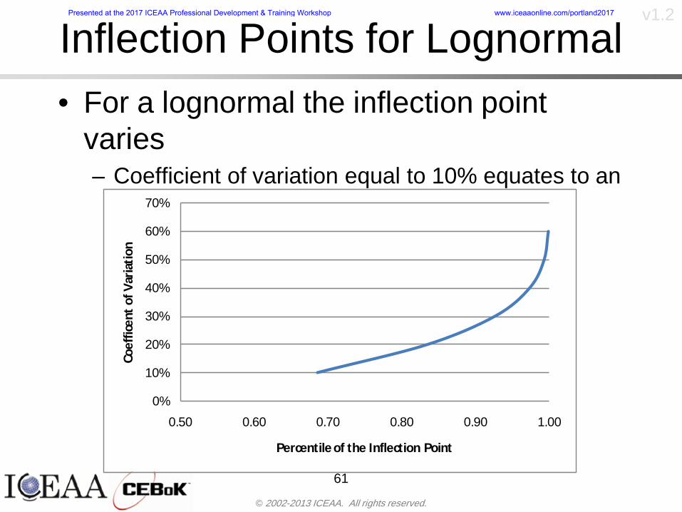
copy 2002-2013 ICEAA All rights reserved
v12
Inflection Points for Lognormalbull For a lognormal the inflection point
variesndash Coefficient of variation equal to 10 equates to an
inflection point at the 70th percentile
61
0
10
20
30
40
50
60
70
050 060 070 080 090 100
Coef
ficen
t of V
aria
tion
Percentile of the Inflection Point
Presented at the 2017 ICEAA Professional Development amp Training Workshop wwwiceaaonlinecomportland2017
copy 2002-2013 ICEAA All rights reserved
v12
Issues with Percentile Fundingbull However risk management does not stop at a
specific percentilendash What happens when the 70th percentile is exceeded
bull Any effective risk management policy should prescribe what happens after a bad event occursndash With VaR we only know when a bad event has occurred ndash Also funding at a relatively low level means we have no true
sense of the real risks that should be guarded against
62
Presented at the 2017 ICEAA Professional Development amp Training Workshop wwwiceaaonlinecomportland2017
copy 2002-2013 ICEAA All rights reserved
v12
ldquoHere There Be Dragonsrdquobull On old maps uncharted territory was often
marked with monsters or dragons
63
A section of the Carta Marina by Olaus Magnus 16th Century
Presented at the 2017 ICEAA Professional Development amp Training Workshop wwwiceaaonlinecomportland2017
copy 2002-2013 ICEAA All rights reserved
v12
Distribution Comparisonbull Four different distributions with the same 70th
percentile
bull Should we expect the tails to be similar
64
0
10
20
30
40
50
60
70
80
0 100 200 300 400 500 600
Perc
entil
eCo
nfid
ence
Lev
el
Triangular
Normal
Lognormal
Pareto
Presented at the 2017 ICEAA Professional Development amp Training Workshop wwwiceaaonlinecomportland2017
copy 2002-2013 ICEAA All rights reserved
v12Distribution Comparison Tail Behavior
bull The normal and triangular distributions have similar tails but the lognormal and Pareto have much fatter right tails
65
70
75
80
85
90
95
100
500 1500 2500 3500 4500 5500
Perc
entil
eCo
nfid
ence
Lev
el
Triangular
Normal
Lognormal
Pareto
Here There Be Dragons
Presented at the 2017 ICEAA Professional Development amp Training Workshop wwwiceaaonlinecomportland2017
copy 2002-2013 ICEAA All rights reserved
v12Distribution Comparison ndash Tail Behavior (Table)
bull There is significant tail risk for the lognormal and the Paretobull The 99th percentile for the Pareto is 1000 times greater than
the 70th percentilendash Risk seen in financial markets and in catastrophic risks like natural
disasters bull Four different projects follow the four different risk profiles seen
in this example should clearly have different risk management approaches but 70th percentile funding indicates the same risk management approach for all four
66
Percentile Triangular Normal Lognormal Pareto 70th $600 $600 $600 $600 80th $680 $660 $770 $1430 90th $770 $750 $1070 $5880 95th $840 $820 $1410 $23750 99th $930 $950 $2350 $600000
Presented at the 2017 ICEAA Professional Development amp Training Workshop wwwiceaaonlinecomportland2017
copy 2002-2013 ICEAA All rights reserved
v12Percentile Budgeting is Not Risk Management
bull Percentile budgeting ne effective risk management policybull Suppose that you are shopping for a new car You
mention that safety is your top concern The salesman says he has a great safe car available You ask about the air bags Do they work The salesman answers ldquoOf course Seventy percent of the time they work fine Only 30 of the time the air bags will fail to deployrdquo Would you buy such a car Hedge fund manager David Einhorn has stated ldquoRisk management is the air bag that must always work but only in the multi-sigma event where you have an accidentrdquo
67
Risk management is the air bag that must always work but only in the multi-sigma event where you
have an accident
Presented at the 2017 ICEAA Professional Development amp Training Workshop wwwiceaaonlinecomportland2017
copy 2002-2013 ICEAA All rights reserved
v12
Joint Confidence Level Analysisbull Schedules are risky toobull For 98 recent NASA missions average
schedule growth was 38ndash Not as high as cost growth but still significant
68
0
5
10
15
20
25
30
35
40
Schedule
Cost
Presented at the 2017 ICEAA Professional Development amp Training Workshop wwwiceaaonlinecomportland2017
copy 2002-2013 ICEAA All rights reserved
v12
Schedules Impact Costbull Changes in schedule can have enormous
impacts on cost ndash Schedule slips can lead to cost increases
bull Fixed programmatic costs must be paid on a regular basisndash Achieving schedule milestones early can result in cost
savings
bull Schedule is an important consideration in cost analysis including cost risk analysis
bull However we must be careful in correctly integrating cost and schedule riskndash Schedule is not simply an input but is dependent on many of
the same factors that drive cost
69
Presented at the 2017 ICEAA Professional Development amp Training Workshop wwwiceaaonlinecomportland2017
copy 2002-2013 ICEAA All rights reserved
v12
The Relationship of Cost to Schedulebull Cost and schedule are positively correlated
ndash A larger program with bigger scope with take longer to complete than a smaller simpler program
bull However longer schedules do not always equate to higher cost nor shorter schedules with lower costndash Highly compressed schedules relative to the
optimal schedule can lead to large overrunsbull Compressed schedules are commonplace for
many planetary missions
70
Presented at the 2017 ICEAA Professional Development amp Training Workshop wwwiceaaonlinecomportland2017
copy 2002-2013 ICEAA All rights reserved
v12The Impact of Schedule GrowthCompression on Cost
bull Compressed schedules lead to cost growth and based on existing research is actually more expensive than schedule slippages
71
0
20
40
60
80
100
120
140
160
-50 -25 0 25 50 75 100
Percentage Change in Schedule
Perc
enta
ge C
hang
e in
Cos
t due
to
Sche
dule
Cha
nge
Source Smart CB ldquoCost and Schedule Interrelationshipsrdquo 2007 NASA Cost Symposium
Presented at the 2017 ICEAA Professional Development amp Training Workshop wwwiceaaonlinecomportland2017
copy 2002-2013 ICEAA All rights reserved
v12Schedule as an Independent Variable
bull Why not simply add schedule as an input to cost-estimating relationships (CERs)
bull Schedule is often treated as an independent variable ndash schedules are often determined independently of cost considerationsndash Cost may not be considered explicitly although budgets and
schedules are determined based on scope and other common factors
bull In 2006 SAIC undertook a research task to determine the impact of schedule on cost and added schedule as an independent variable to the CERs in the NASAAir Force Cost Model (NAFCOM) to see if schedule provided any improvement in goodness of fit
72
Presented at the 2017 ICEAA Professional Development amp Training Workshop wwwiceaaonlinecomportland2017
copy 2002-2013 ICEAA All rights reserved
v12
Schedule is a Dependent Variablebull Since NAFCOM includes an exhaustive list of cost drivers the inclusion
of schedule should give an indication of whether there is any additional independent value added from schedule independent of the cost drivers
bull In the study schedule was added to 10 subsystem-level CERs
ndash In each case the addition of schedule did NOTimprove the goodness of fit and schedule was NOT found to be a statistically significant cost driver (given the presence of the other variables) for any of the 10 CERs
bull Standard errors for the CERs increased due to decrease in degrees of freedom
bull Thus schedule as an independent variable did not provide any additional explanation of variation in historical cost
bull This is because schedule is truly NOT an independent variable but a dependent variable and is a function of the same factors that drive cost
73
Presented at the 2017 ICEAA Professional Development amp Training Workshop wwwiceaaonlinecomportland2017
copy 2002-2013 ICEAA All rights reserved
v12
Incorporation of Schedule in Cost Risk
bull When using subjective methods care must be taken in applying schedule to cost risk analysis
bull Since schedule is a dependent variable treating it independently from other factors when assessing its impact on cost can lead to a double count of independent variables in the cost risk analysis
bull Direct inclusion of schedule in a cost risk analysis effectively doubles the influence of each cost driver
ndash Incorrectly leads to broader risk ranges
74
CostWeight
HeritageNewness
Technology Readiness Schedule
Presented at the 2017 ICEAA Professional Development amp Training Workshop wwwiceaaonlinecomportland2017
copy 2002-2013 ICEAA All rights reserved
v12Subjective Cost Risk Methods and Overinclusion of Risk Factors
bull Subjective methods are suitable when data are scarce or not availablebull However care must be taken not to treat correlated sources of risk
such as schedule as independent of each otherbull Example ndash a subjective risk analysis incorporated technology readiness
design risk requirements stability integration risk and schedule and treated each source of risk as independent
bull Risk triangle high value without schedule risk was 31 times the point estimate
bull Risk triangle high value with schedule risk added on top of other sources of risk treated independently was 34 times the point estimate
bull Risk triangle taking correlation between sources of risk into account in a rigorous statistical manner has a high value 15 times the point estimate less than half the effect when treating sources of risk as independent
75
Presented at the 2017 ICEAA Professional Development amp Training Workshop wwwiceaaonlinecomportland2017
copy 2002-2013 ICEAA All rights reserved
v12Fundamental Equation of Cost and Schedule Interrelationships
bull The Fundamental Equation of the Relationship Between Cost and Schedule is
Time = Moneybull This is a well known adage that time is money Your boss at
work may even mention this to you from time to time or if you are the boss you are all too aware of this iron law
bull Because time is money cost and schedule risk should be modeled jointly not with schedule as an independent cost driver
bull Note that cost and schedule are not perfectly correlatedndash Cost can sometimes ldquobuy downrdquo schedule extra money can be
spent to meet a deadline since in some cases additional effort to hasten the completion of a task
76
Presented at the 2017 ICEAA Professional Development amp Training Workshop wwwiceaaonlinecomportland2017
copy 2002-2013 ICEAA All rights reserved
v12How to (Correctly) Incorporate Schedule into Cost Risk Analysis
bull The best way to model cost and schedule risk is to develop a joint cost and schedule model based on the same data
bull Since such models are not currently available the next best approach is to model cost and schedule independently and then integrate cost and schedule risk analyses using joint probability distributions taking into account correlation between cost and schedulendash This approach pioneered by Paul Garvey and Steve Book is
considered industry best practicendash This is a practical method mathematically tractable and follows
naturally from the Fundamental Equation of Cost and Schedule Interrelationships
77
Book S A ldquoQuantifying the Relationship Between Cost and Schedulerdquo The Measurable News Winter 2007-2008 pp 11-15Garvey PR Probability Methods for Cost Uncertainty Analysis A Systems Engineering Perspective New York Marcel Dekker 2000 pp 308-335
Presented at the 2017 ICEAA Professional Development amp Training Workshop wwwiceaaonlinecomportland2017
copy 2002-2013 ICEAA All rights reserved
v12
Joint Lognormal and Normal Distributions
bull Cost and schedule are typically modeled as some combination of Normal and Lognormal probability distributionsndash Studies by The Aerospace Corporation the MITRE
Corporation Wyle Labs and SAIC have found that the Lognormal probability distribution almost always serves as a good model for both the schedule distribution and the cost distribution
ndash The Normal distribution may also be appropriate in some instances and depending upon the level of confidence at which budgets are set may even be more conservative and logically consistent than the Normal distribution
ndash Joint Lognormal and Normal distributions are defined by a pair of mean and standard deviations and a level of correlation between the two
78
Presented at the 2017 ICEAA Professional Development amp Training Workshop wwwiceaaonlinecomportland2017
copy 2002-2013 ICEAA All rights reserved
v12Modeling Cost and Schedule as a Bivariate Distribution
bull In the approach set forth by Book and Garvey cost risk is assessed and the top-level distribution is modeled as a Lognormal (or Normal) distribution schedule risk is assessed and the overall schedule risk is modeled as a Lognormal (or Normal) distribution
bull The two distributions are combined into a Bivariate distribution by assigning a correlation between the two and by treating the two distributions as the marginal distributions of a Bivariate Lognormal distributionndash Other combinations include a Bivariate Normal or a Bivariate
Normal-Lognormal
79
Presented at the 2017 ICEAA Professional Development amp Training Workshop wwwiceaaonlinecomportland2017
copy 2002-2013 ICEAA All rights reserved
v12Bivariate Lognormal Distribution for Cost and Schedule
bull Cost is often observed to be Lognormal when strong positive correlations are present among the systemrsquos WBS cost element costs
bull A systemrsquos schedule is often observed (from Monte Carlo simulations) to be Lognormal if it is the sum of many positively correlated schedule activities in an overall schedule network
bull If Lognormal distributions characterize a systemrsquos cost and schedule then the Bivariate Lognormal could serve as an assumed model of their joint distributionndash In this case the marginal distribution of each of cost and schedule is
Lognormalbull Other possibilities for modeling cost and schedule as a Bivariate
distribution include a Bivariate Normal or a Bivariate Normal-Lognormal distributionndash All these combinations are analytically tractable
80
Presented at the 2017 ICEAA Professional Development amp Training Workshop wwwiceaaonlinecomportland2017
copy 2002-2013 ICEAA All rights reserved
v12Bivariate Lognormal for Cost and Schedule
bull Contour Plots of a Bivariate Lognormal
81
Presented at the 2017 ICEAA Professional Development amp Training Workshop wwwiceaaonlinecomportland2017
copy 2002-2013 ICEAA All rights reserved
v12Correlation Between Cost and Schedule
bull Cost and schedule are positively correlated but not perfectly sondash For example it is possible to have a schedule underrun and a cost
overrunbull Based on cost and schedule growth data for 50 completed NASA
programs the correlation between development cost and development schedule is 70
82
00
200
400
600
800
1000
1200
-500 00 500 1000 1500 2000 2500Historical Cost Growth
Hist
oric
al S
ched
ule
Gro
wth
r = 715
Presented at the 2017 ICEAA Professional Development amp Training Workshop wwwiceaaonlinecomportland2017
copy 2002-2013 ICEAA All rights reserved
v12Correlation Between Cost and Schedule Caveats
bull Based on historical data recommended correlation between cost and schedule is 70 but this could be higher or lower depending upon program circumstancesndash If program is budget constrained cost and schedule will be
more highly correlated (go as you pay)ndash If program is schedule constrained cost and schedule will
have lower correlation perhaps even negative correlation ndash Smaller programs have smaller correlation between cost and
schedule riskbull Relatively easy to ldquohurry uprdquo and finish on time or even early if
needed
83
Presented at the 2017 ICEAA Professional Development amp Training Workshop wwwiceaaonlinecomportland2017
copy 2002-2013 ICEAA All rights reserved
v12
Conditional Confidence Levelsbull Given a programrsquos project schedule we can determine the cost
risk distribution conditional upon the given schedulebull Conditional cost S-curves are steeper than unconditional
(marginal) cost S-curves between some uncertainty has been removed because schedule is fixed
84
Presented at the 2017 ICEAA Professional Development amp Training Workshop wwwiceaaonlinecomportland2017
copy 2002-2013 ICEAA All rights reserved
v12
Joint Confidence Levelsbull Joint 65 confidence represents the probability of
achieving both 65 confidence in cost AND 65 confidence in schedulendash This is different than achieving 65 cost confidence alone
or achieving 65 schedule confidence alonebull Due to the imperfect correlation between cost and schedule it
is possible to achieve a 65 cost confidence with a lower level of schedule confidence
bull Restricting the schedule confidence thus requires additional $ to achieve a given level of confidence
85
X
Y
Possible Values for Which X gt a Possible Values for
Which X gt a and Y gt b
a
b
Presented at the 2017 ICEAA Professional Development amp Training Workshop wwwiceaaonlinecomportland2017
copy 2002-2013 ICEAA All rights reserved
v12Joint Confidence Levels Versus Cost Confidence Levels Only
bull Example of the differences between cost confidence schedule confidence conditional cost confidence and joint cost and schedule confidence
86
Joint Cost-Schedule Confidence Iso-Curves
Cost (RY$M)
Sche
dule
(Mon
ths)
65 Confidence
50 Confidence
70 Confidence
65 Cost Confidence AggressiveSchedule65 Cost ConfidenceScheduleGiven 65 Schedule ConfidenceUnconditional 65 CostConfidenceUnconditional 65 ScheduleConfidence
65 Cost Confidence 65 Joint Cost and Schedule
Confidence for 65 Schedule Confidence
Presented at the 2017 ICEAA Professional Development amp Training Workshop wwwiceaaonlinecomportland2017
copy 2002-2013 ICEAA All rights reserved
v12
Joint Cost and Schedule Confidence
bull Can examine pairs of cost and schedule that achieve a given level of confidence
bull Provides insights into the trade-offs between cost and schedule for a given level of confidencendash Possible to increase cost confidence by giving a
project more time in some instances or possible to ldquobuy downrdquo schedule
bull But these have limits and are shown in the iso-cost and schedule confidence curves
87
Presented at the 2017 ICEAA Professional Development amp Training Workshop wwwiceaaonlinecomportland2017
copy 2002-2013 ICEAA All rights reserved
v12Cost and Schedule Trade-offs for a Given Level of Joint Confidence
bull Hypothetical Example
88
Cost (RY$M)
Schedule (Months)
$100 48$99 48$89 49$87 50$85 51$85 52$84 53$83 55$83 55$83 56
Cost and Schedule 65 Confidence Iso-Curve
4748495051525354555657
$80 $82 $84 $86 $88 $90 $92 $94 $96 $98 $100
Cost (RY$ M)
Sche
dule
(Mon
ths)
Presented at the 2017 ICEAA Professional Development amp Training Workshop wwwiceaaonlinecomportland2017
copy 2002-2013 ICEAA All rights reserved
v12Policy Considerations for Confidence Levels
bull For large programs the difference between the amount of money needed to achieve 65 cost confidence independent of schedule and joint 65 cost and schedule confidence can represent hundreds of millions and even billions of dollars
89
Joint Cost-Schedule Confidence Iso-Curves
Cost (RY$M)
Sche
dule
(Mon
ths)
65 Confidence
65 Cost Confidence AggressiveSchedule
65 Cost ConfidenceScheduleGiven 65 Schedule Confidence
Unconditional 65 CostConfidence
Joint Cost and Schedule Confidence for 65 Cost Confidence and Program Baseline Schedule is Less Than 35
65 Cost Confidence Independent of Schedule Cost Needed to Achieve
Both 65 Joint Cost and Schedule Confidence for the Schedule with 65 Confidence
Presented at the 2017 ICEAA Professional Development amp Training Workshop wwwiceaaonlinecomportland2017
copy 2002-2013 ICEAA All rights reserved
v12
Copulasbull More generally any combination of distributions can
be used (more than just normal and lognormal)ndash Termed ldquocopulardquo from the Italian word for ldquocouplerdquondash Copulas are a way to combine marginal distributions of any
number and type into a joint distributionbull More formally a copula is a multivariate joint distribution defined
on the n-dimensional unit cube [0 1]n such that every marginal distribution is uniform on the interval [0 1]
bull (The bivariate form of) Sklarrsquos theorem states that for any bivariate distribution function H(x y) let F(x) = H(x infin) and G(y) = H(infin y) be the univariate marginal probability distribution functions Then there exists a copula C such that H(xy)=C(F(x)G(y))
ndash Copulas are widely used in risk management for investments and insurance
bull Considered industry best practice (Li 2000)bull Marketed as part of JP Morganrsquos CreditMetrics suite of tools
(Gupton et Al 1997)90
Presented at the 2017 ICEAA Professional Development amp Training Workshop wwwiceaaonlinecomportland2017
copy 2002-2013 ICEAA All rights reserved
v12Parametric Joint Cost and Schedule Analysis
bull A parametric model based on a consistent data set with a set of overlapping cost and schedule drivers is a cleaner way to model cost and schedule
91
CostWeight
HeritageNewness
Technology Readiness
Schedule
0
20
40
60
80
100
Confidence
Joint Cost and Schedule Confidence
Schedule
Cost
Lognormal Distribution PDF and CDF
0102030405060708090100
200 300 400 500 600 700 800 900 1000Cost $
Con
fiden
ce L
evel
0
00002
00004
00006
00008
0001
00012
00014
00016
Prob
abili
ty D
ensi
ty
CDFPDF
Lognormal Distribution PDF and CDF
0102030405060708090100
200 300 400 500 600 700 800 900 1000Cost $
Con
fiden
ce L
evel
0
00002
00004
00006
00008
0001
00012
00014
00016
Prob
abili
ty D
ensi
ty
CDFPDF
Presented at the 2017 ICEAA Professional Development amp Training Workshop wwwiceaaonlinecomportland2017
copy 2002-2013 ICEAA All rights reserved
v12Parametric Joint Cost and Schedule Analysis (2)
bull Joint cost and schedule risk analysis produced naturally by the integrated modelndash Addresses several issues with the copula
approachbull Tail dependencybull Correlation ndash no need to assign correlation
between cost and schedulebull Consistency of cost and schedule models
92
Presented at the 2017 ICEAA Professional Development amp Training Workshop wwwiceaaonlinecomportland2017
copy 2002-2013 ICEAA All rights reserved
v12
Resource-Loaded Schedulesbull Involves assigning cost and schedule risks to a resource-loaded schedule
networkbull Bottom-up approach
ndash More labor intensive than parametrics but can also provide more insight
ndash Can answer questions than parametric typically cannot such as how much do reserve requirements decrease if a specific risk is retired
bull Currently being implemented in Constellation programbull Has same issue as all bottom-up models hard to count all the risks and model
them discretely
ndash As a result there is a tendency to reflect less risk than indicated by history
ndash ldquoThere are more things in heaven and earth Horatio than are dreamt of in your philosophyrdquo William Shakespeare Hamlet Act I Scene V
93
Presented at the 2017 ICEAA Professional Development amp Training Workshop wwwiceaaonlinecomportland2017
copy 2002-2013 ICEAA All rights reserved
v12Resource-Loaded Schedules Vs Parametrics
bull Parametric most appropriate for early estimatesndash But also good for high-level checks as project progresses
bull As plans take shape lower level modeling may be more appropriate
94 1
CONCEPTUALDEVELOPMENT
PROJECTDEFINITION DESIGN DEVELOPMENT OPERATIONS
PARAMETRIC PARAMETRIC
ANALOGY
ENGINEERING (Bottoms Up)
$PARAMETRIC
DETAILED
$
Pre Phase A Phase B Phase CDPhase A Phase EPre Phase A Phase B Phase CDPhase A Phase E
Risk = f(Cost Estimating Relationship Inputs eg mass power data rate TRL new design etc)
Risk = f(cost and schedule variation of the analogous elements)
Risk = f(variation of detailed inputs eg labor hours rates materials etc)
Presented at the 2017 ICEAA Professional Development amp Training Workshop wwwiceaaonlinecomportland2017
copy 2002-2013 ICEAA All rights reserved
v12
Resource-Loaded Schedulesbull Methodology has been demonstrated in other
industriesndash Construction oil and gasndash Analysis has not been traditionally done on highly uncertain
complex development projects bull Methodology focuses on project baseline schedule
ndash In baseline schedule all tasks are resource loaded to represent a baseline schedule and cost standpoint
ndash Resource loaded schedule is ldquorolledrdquo up to a manageable level
ndash Based on the risk and uncertainties identified schedule distributions are applied to each rolled up task
ndash Cost uncertainties are also applied to rolled up tasksbull Uncertainties include labor rate man power etc
ndash A Monte Carlo simulation is run to develop joint cost-schedule distributions
95
Presented at the 2017 ICEAA Professional Development amp Training Workshop wwwiceaaonlinecomportland2017
copy 2002-2013 ICEAA All rights reserved
v12
Unit III - Module 9 96
Execution ndash Cross Checksbull Means The mean cost growth factor for WBS items
can be compared to history as a way to cross check results
bull CVs The CV of the cost growth factors for WBS items can be compared to history as a way to cross check results
bull Inputs Checks are performed on inputs or other parameters to see if historical values are in line with program assumptionsndash Example Historical risk scores can be compared to program
risk scores to see if risk assessors are being realistic and to see if the underlying database is representative of the program
11
Presented at the 2017 ICEAA Professional Development amp Training Workshop wwwiceaaonlinecomportland2017
- Cost and Schedule Risk Analysis Basic
- Acknowledgments
- Unit Index
- Risk Overview
- Agenda
- Introduction
- Risk Analysis Terms
- Are Our Costs Realistic
- Historical Cost Growth
- Sources of Cost Risk
- Point Estimates of Cost
- Types of Risk
- Point Estimates Vs Risk Estimates
- Cost Risk and Probability
- Probability Model ndash Distribution
- Probability Model ndash Distribution
- Probability ndash Top-Level Distribution
- S-Curves and Confidence Levels
- Example ndash Normal Distribution
- Confidence Levels
- Measuring Parametric Model Uncertainty
- Parametric Model Example
- Weight Uncertainty
- Estimating Uncertainty
- Estimating Uncertainty (2)
- Estimating Uncertainty (3)
- Aggregating Risk
- WBS Example
- WBS and Risk
- Aggregating Risk
- Percentiles Do Not Add
- Percentiles Do Not Add (2)
- Percentiles Do Not Add (3)
- Methods for Aggregating Risk
- Monte Carlo Simulationfor Risk Analysis
- Monte Carlo Simulation
- Using Random Numbers to Simulate Distributions
- Simulating a Triangular Distribution
- Simulating a Triangular Distribution (2)
- Monte Carlo and the WBS
- Number of Trials
- Number of Trials (2)
- Number of Trials (3)
- Number of Trials (4)
- Number of Trials (5)
- Number of Trials (6)
- Methods of Simulation
- Probability Model ndash Correlation
- Correlation And Causation
- The Importance of Correlation
- The Importance of Correlation (2)
- Measures of Correlation
- Pearson Correlation
- Spearman Correlation
- Functional Correlation
- Risk Measures
- Value at Risk (VaR)
- Why 70th or 80th Percentile
- Funding Above Inflection Points
- Why Budget to the 70th or 80th
- Inflection Points for Lognormal
- Issues with Percentile Funding
- ldquoHere There Be Dragonsrdquo
- Distribution Comparison
- Distribution Comparison Tail Behavior
- Distribution Comparison ndash Tail Behavior (Table)
- Percentile Budgeting is Not Risk Management
- Joint Confidence Level Analysis
- Schedules Impact Cost
- The Relationship of Cost to Schedule
- The Impact of Schedule GrowthCompression on Cost
- Schedule as an Independent Variable
- Schedule is a Dependent Variable
- Incorporation of Schedule in Cost Risk
- Subjective Cost Risk Methods and Overinclusion of Risk Factors
- Fundamental Equation of Cost and Schedule Interrelationships
- How to (Correctly) Incorporate Schedule into Cost Risk Analysis
- Joint Lognormal and Normal Distributions
- Modeling Cost and Schedule as a Bivariate Distribution
- Bivariate Lognormal Distribution for Cost and Schedule
- Bivariate Lognormal for Cost and Schedule
- Correlation Between Cost and Schedule
- Correlation Between Cost and Schedule Caveats
- Conditional Confidence Levels
- Joint Confidence Levels
- Joint Confidence Levels Versus Cost Confidence Levels Only
- Joint Cost and Schedule Confidence
- Cost and Schedule Trade-offs for a Given Level of Joint Confidence
- Policy Considerations for Confidence Levels
- Copulas
- Parametric Joint Cost and Schedule Analysis
- Parametric Joint Cost and Schedule Analysis (2)
- Resource-Loaded Schedules
- Resource-Loaded Schedules Vs Parametrics
- Resource-Loaded Schedules
- Execution ndash Cross Checks
-
copy 2002-2013 ICEAA All rights reserved
v12
Issues with Percentile Fundingbull However risk management does not stop at a
specific percentilendash What happens when the 70th percentile is exceeded
bull Any effective risk management policy should prescribe what happens after a bad event occursndash With VaR we only know when a bad event has occurred ndash Also funding at a relatively low level means we have no true
sense of the real risks that should be guarded against
62
Presented at the 2017 ICEAA Professional Development amp Training Workshop wwwiceaaonlinecomportland2017
copy 2002-2013 ICEAA All rights reserved
v12
ldquoHere There Be Dragonsrdquobull On old maps uncharted territory was often
marked with monsters or dragons
63
A section of the Carta Marina by Olaus Magnus 16th Century
Presented at the 2017 ICEAA Professional Development amp Training Workshop wwwiceaaonlinecomportland2017
copy 2002-2013 ICEAA All rights reserved
v12
Distribution Comparisonbull Four different distributions with the same 70th
percentile
bull Should we expect the tails to be similar
64
0
10
20
30
40
50
60
70
80
0 100 200 300 400 500 600
Perc
entil
eCo
nfid
ence
Lev
el
Triangular
Normal
Lognormal
Pareto
Presented at the 2017 ICEAA Professional Development amp Training Workshop wwwiceaaonlinecomportland2017
copy 2002-2013 ICEAA All rights reserved
v12Distribution Comparison Tail Behavior
bull The normal and triangular distributions have similar tails but the lognormal and Pareto have much fatter right tails
65
70
75
80
85
90
95
100
500 1500 2500 3500 4500 5500
Perc
entil
eCo
nfid
ence
Lev
el
Triangular
Normal
Lognormal
Pareto
Here There Be Dragons
Presented at the 2017 ICEAA Professional Development amp Training Workshop wwwiceaaonlinecomportland2017
copy 2002-2013 ICEAA All rights reserved
v12Distribution Comparison ndash Tail Behavior (Table)
bull There is significant tail risk for the lognormal and the Paretobull The 99th percentile for the Pareto is 1000 times greater than
the 70th percentilendash Risk seen in financial markets and in catastrophic risks like natural
disasters bull Four different projects follow the four different risk profiles seen
in this example should clearly have different risk management approaches but 70th percentile funding indicates the same risk management approach for all four
66
Percentile Triangular Normal Lognormal Pareto 70th $600 $600 $600 $600 80th $680 $660 $770 $1430 90th $770 $750 $1070 $5880 95th $840 $820 $1410 $23750 99th $930 $950 $2350 $600000
Presented at the 2017 ICEAA Professional Development amp Training Workshop wwwiceaaonlinecomportland2017
copy 2002-2013 ICEAA All rights reserved
v12Percentile Budgeting is Not Risk Management
bull Percentile budgeting ne effective risk management policybull Suppose that you are shopping for a new car You
mention that safety is your top concern The salesman says he has a great safe car available You ask about the air bags Do they work The salesman answers ldquoOf course Seventy percent of the time they work fine Only 30 of the time the air bags will fail to deployrdquo Would you buy such a car Hedge fund manager David Einhorn has stated ldquoRisk management is the air bag that must always work but only in the multi-sigma event where you have an accidentrdquo
67
Risk management is the air bag that must always work but only in the multi-sigma event where you
have an accident
Presented at the 2017 ICEAA Professional Development amp Training Workshop wwwiceaaonlinecomportland2017
copy 2002-2013 ICEAA All rights reserved
v12
Joint Confidence Level Analysisbull Schedules are risky toobull For 98 recent NASA missions average
schedule growth was 38ndash Not as high as cost growth but still significant
68
0
5
10
15
20
25
30
35
40
Schedule
Cost
Presented at the 2017 ICEAA Professional Development amp Training Workshop wwwiceaaonlinecomportland2017
copy 2002-2013 ICEAA All rights reserved
v12
Schedules Impact Costbull Changes in schedule can have enormous
impacts on cost ndash Schedule slips can lead to cost increases
bull Fixed programmatic costs must be paid on a regular basisndash Achieving schedule milestones early can result in cost
savings
bull Schedule is an important consideration in cost analysis including cost risk analysis
bull However we must be careful in correctly integrating cost and schedule riskndash Schedule is not simply an input but is dependent on many of
the same factors that drive cost
69
Presented at the 2017 ICEAA Professional Development amp Training Workshop wwwiceaaonlinecomportland2017
copy 2002-2013 ICEAA All rights reserved
v12
The Relationship of Cost to Schedulebull Cost and schedule are positively correlated
ndash A larger program with bigger scope with take longer to complete than a smaller simpler program
bull However longer schedules do not always equate to higher cost nor shorter schedules with lower costndash Highly compressed schedules relative to the
optimal schedule can lead to large overrunsbull Compressed schedules are commonplace for
many planetary missions
70
Presented at the 2017 ICEAA Professional Development amp Training Workshop wwwiceaaonlinecomportland2017
copy 2002-2013 ICEAA All rights reserved
v12The Impact of Schedule GrowthCompression on Cost
bull Compressed schedules lead to cost growth and based on existing research is actually more expensive than schedule slippages
71
0
20
40
60
80
100
120
140
160
-50 -25 0 25 50 75 100
Percentage Change in Schedule
Perc
enta
ge C
hang
e in
Cos
t due
to
Sche
dule
Cha
nge
Source Smart CB ldquoCost and Schedule Interrelationshipsrdquo 2007 NASA Cost Symposium
Presented at the 2017 ICEAA Professional Development amp Training Workshop wwwiceaaonlinecomportland2017
copy 2002-2013 ICEAA All rights reserved
v12Schedule as an Independent Variable
bull Why not simply add schedule as an input to cost-estimating relationships (CERs)
bull Schedule is often treated as an independent variable ndash schedules are often determined independently of cost considerationsndash Cost may not be considered explicitly although budgets and
schedules are determined based on scope and other common factors
bull In 2006 SAIC undertook a research task to determine the impact of schedule on cost and added schedule as an independent variable to the CERs in the NASAAir Force Cost Model (NAFCOM) to see if schedule provided any improvement in goodness of fit
72
Presented at the 2017 ICEAA Professional Development amp Training Workshop wwwiceaaonlinecomportland2017
copy 2002-2013 ICEAA All rights reserved
v12
Schedule is a Dependent Variablebull Since NAFCOM includes an exhaustive list of cost drivers the inclusion
of schedule should give an indication of whether there is any additional independent value added from schedule independent of the cost drivers
bull In the study schedule was added to 10 subsystem-level CERs
ndash In each case the addition of schedule did NOTimprove the goodness of fit and schedule was NOT found to be a statistically significant cost driver (given the presence of the other variables) for any of the 10 CERs
bull Standard errors for the CERs increased due to decrease in degrees of freedom
bull Thus schedule as an independent variable did not provide any additional explanation of variation in historical cost
bull This is because schedule is truly NOT an independent variable but a dependent variable and is a function of the same factors that drive cost
73
Presented at the 2017 ICEAA Professional Development amp Training Workshop wwwiceaaonlinecomportland2017
copy 2002-2013 ICEAA All rights reserved
v12
Incorporation of Schedule in Cost Risk
bull When using subjective methods care must be taken in applying schedule to cost risk analysis
bull Since schedule is a dependent variable treating it independently from other factors when assessing its impact on cost can lead to a double count of independent variables in the cost risk analysis
bull Direct inclusion of schedule in a cost risk analysis effectively doubles the influence of each cost driver
ndash Incorrectly leads to broader risk ranges
74
CostWeight
HeritageNewness
Technology Readiness Schedule
Presented at the 2017 ICEAA Professional Development amp Training Workshop wwwiceaaonlinecomportland2017
copy 2002-2013 ICEAA All rights reserved
v12Subjective Cost Risk Methods and Overinclusion of Risk Factors
bull Subjective methods are suitable when data are scarce or not availablebull However care must be taken not to treat correlated sources of risk
such as schedule as independent of each otherbull Example ndash a subjective risk analysis incorporated technology readiness
design risk requirements stability integration risk and schedule and treated each source of risk as independent
bull Risk triangle high value without schedule risk was 31 times the point estimate
bull Risk triangle high value with schedule risk added on top of other sources of risk treated independently was 34 times the point estimate
bull Risk triangle taking correlation between sources of risk into account in a rigorous statistical manner has a high value 15 times the point estimate less than half the effect when treating sources of risk as independent
75
Presented at the 2017 ICEAA Professional Development amp Training Workshop wwwiceaaonlinecomportland2017
copy 2002-2013 ICEAA All rights reserved
v12Fundamental Equation of Cost and Schedule Interrelationships
bull The Fundamental Equation of the Relationship Between Cost and Schedule is
Time = Moneybull This is a well known adage that time is money Your boss at
work may even mention this to you from time to time or if you are the boss you are all too aware of this iron law
bull Because time is money cost and schedule risk should be modeled jointly not with schedule as an independent cost driver
bull Note that cost and schedule are not perfectly correlatedndash Cost can sometimes ldquobuy downrdquo schedule extra money can be
spent to meet a deadline since in some cases additional effort to hasten the completion of a task
76
Presented at the 2017 ICEAA Professional Development amp Training Workshop wwwiceaaonlinecomportland2017
copy 2002-2013 ICEAA All rights reserved
v12How to (Correctly) Incorporate Schedule into Cost Risk Analysis
bull The best way to model cost and schedule risk is to develop a joint cost and schedule model based on the same data
bull Since such models are not currently available the next best approach is to model cost and schedule independently and then integrate cost and schedule risk analyses using joint probability distributions taking into account correlation between cost and schedulendash This approach pioneered by Paul Garvey and Steve Book is
considered industry best practicendash This is a practical method mathematically tractable and follows
naturally from the Fundamental Equation of Cost and Schedule Interrelationships
77
Book S A ldquoQuantifying the Relationship Between Cost and Schedulerdquo The Measurable News Winter 2007-2008 pp 11-15Garvey PR Probability Methods for Cost Uncertainty Analysis A Systems Engineering Perspective New York Marcel Dekker 2000 pp 308-335
Presented at the 2017 ICEAA Professional Development amp Training Workshop wwwiceaaonlinecomportland2017
copy 2002-2013 ICEAA All rights reserved
v12
Joint Lognormal and Normal Distributions
bull Cost and schedule are typically modeled as some combination of Normal and Lognormal probability distributionsndash Studies by The Aerospace Corporation the MITRE
Corporation Wyle Labs and SAIC have found that the Lognormal probability distribution almost always serves as a good model for both the schedule distribution and the cost distribution
ndash The Normal distribution may also be appropriate in some instances and depending upon the level of confidence at which budgets are set may even be more conservative and logically consistent than the Normal distribution
ndash Joint Lognormal and Normal distributions are defined by a pair of mean and standard deviations and a level of correlation between the two
78
Presented at the 2017 ICEAA Professional Development amp Training Workshop wwwiceaaonlinecomportland2017
copy 2002-2013 ICEAA All rights reserved
v12Modeling Cost and Schedule as a Bivariate Distribution
bull In the approach set forth by Book and Garvey cost risk is assessed and the top-level distribution is modeled as a Lognormal (or Normal) distribution schedule risk is assessed and the overall schedule risk is modeled as a Lognormal (or Normal) distribution
bull The two distributions are combined into a Bivariate distribution by assigning a correlation between the two and by treating the two distributions as the marginal distributions of a Bivariate Lognormal distributionndash Other combinations include a Bivariate Normal or a Bivariate
Normal-Lognormal
79
Presented at the 2017 ICEAA Professional Development amp Training Workshop wwwiceaaonlinecomportland2017
copy 2002-2013 ICEAA All rights reserved
v12Bivariate Lognormal Distribution for Cost and Schedule
bull Cost is often observed to be Lognormal when strong positive correlations are present among the systemrsquos WBS cost element costs
bull A systemrsquos schedule is often observed (from Monte Carlo simulations) to be Lognormal if it is the sum of many positively correlated schedule activities in an overall schedule network
bull If Lognormal distributions characterize a systemrsquos cost and schedule then the Bivariate Lognormal could serve as an assumed model of their joint distributionndash In this case the marginal distribution of each of cost and schedule is
Lognormalbull Other possibilities for modeling cost and schedule as a Bivariate
distribution include a Bivariate Normal or a Bivariate Normal-Lognormal distributionndash All these combinations are analytically tractable
80
Presented at the 2017 ICEAA Professional Development amp Training Workshop wwwiceaaonlinecomportland2017
copy 2002-2013 ICEAA All rights reserved
v12Bivariate Lognormal for Cost and Schedule
bull Contour Plots of a Bivariate Lognormal
81
Presented at the 2017 ICEAA Professional Development amp Training Workshop wwwiceaaonlinecomportland2017
copy 2002-2013 ICEAA All rights reserved
v12Correlation Between Cost and Schedule
bull Cost and schedule are positively correlated but not perfectly sondash For example it is possible to have a schedule underrun and a cost
overrunbull Based on cost and schedule growth data for 50 completed NASA
programs the correlation between development cost and development schedule is 70
82
00
200
400
600
800
1000
1200
-500 00 500 1000 1500 2000 2500Historical Cost Growth
Hist
oric
al S
ched
ule
Gro
wth
r = 715
Presented at the 2017 ICEAA Professional Development amp Training Workshop wwwiceaaonlinecomportland2017
copy 2002-2013 ICEAA All rights reserved
v12Correlation Between Cost and Schedule Caveats
bull Based on historical data recommended correlation between cost and schedule is 70 but this could be higher or lower depending upon program circumstancesndash If program is budget constrained cost and schedule will be
more highly correlated (go as you pay)ndash If program is schedule constrained cost and schedule will
have lower correlation perhaps even negative correlation ndash Smaller programs have smaller correlation between cost and
schedule riskbull Relatively easy to ldquohurry uprdquo and finish on time or even early if
needed
83
Presented at the 2017 ICEAA Professional Development amp Training Workshop wwwiceaaonlinecomportland2017
copy 2002-2013 ICEAA All rights reserved
v12
Conditional Confidence Levelsbull Given a programrsquos project schedule we can determine the cost
risk distribution conditional upon the given schedulebull Conditional cost S-curves are steeper than unconditional
(marginal) cost S-curves between some uncertainty has been removed because schedule is fixed
84
Presented at the 2017 ICEAA Professional Development amp Training Workshop wwwiceaaonlinecomportland2017
copy 2002-2013 ICEAA All rights reserved
v12
Joint Confidence Levelsbull Joint 65 confidence represents the probability of
achieving both 65 confidence in cost AND 65 confidence in schedulendash This is different than achieving 65 cost confidence alone
or achieving 65 schedule confidence alonebull Due to the imperfect correlation between cost and schedule it
is possible to achieve a 65 cost confidence with a lower level of schedule confidence
bull Restricting the schedule confidence thus requires additional $ to achieve a given level of confidence
85
X
Y
Possible Values for Which X gt a Possible Values for
Which X gt a and Y gt b
a
b
Presented at the 2017 ICEAA Professional Development amp Training Workshop wwwiceaaonlinecomportland2017
copy 2002-2013 ICEAA All rights reserved
v12Joint Confidence Levels Versus Cost Confidence Levels Only
bull Example of the differences between cost confidence schedule confidence conditional cost confidence and joint cost and schedule confidence
86
Joint Cost-Schedule Confidence Iso-Curves
Cost (RY$M)
Sche
dule
(Mon
ths)
65 Confidence
50 Confidence
70 Confidence
65 Cost Confidence AggressiveSchedule65 Cost ConfidenceScheduleGiven 65 Schedule ConfidenceUnconditional 65 CostConfidenceUnconditional 65 ScheduleConfidence
65 Cost Confidence 65 Joint Cost and Schedule
Confidence for 65 Schedule Confidence
Presented at the 2017 ICEAA Professional Development amp Training Workshop wwwiceaaonlinecomportland2017
copy 2002-2013 ICEAA All rights reserved
v12
Joint Cost and Schedule Confidence
bull Can examine pairs of cost and schedule that achieve a given level of confidence
bull Provides insights into the trade-offs between cost and schedule for a given level of confidencendash Possible to increase cost confidence by giving a
project more time in some instances or possible to ldquobuy downrdquo schedule
bull But these have limits and are shown in the iso-cost and schedule confidence curves
87
Presented at the 2017 ICEAA Professional Development amp Training Workshop wwwiceaaonlinecomportland2017
copy 2002-2013 ICEAA All rights reserved
v12Cost and Schedule Trade-offs for a Given Level of Joint Confidence
bull Hypothetical Example
88
Cost (RY$M)
Schedule (Months)
$100 48$99 48$89 49$87 50$85 51$85 52$84 53$83 55$83 55$83 56
Cost and Schedule 65 Confidence Iso-Curve
4748495051525354555657
$80 $82 $84 $86 $88 $90 $92 $94 $96 $98 $100
Cost (RY$ M)
Sche
dule
(Mon
ths)
Presented at the 2017 ICEAA Professional Development amp Training Workshop wwwiceaaonlinecomportland2017
copy 2002-2013 ICEAA All rights reserved
v12Policy Considerations for Confidence Levels
bull For large programs the difference between the amount of money needed to achieve 65 cost confidence independent of schedule and joint 65 cost and schedule confidence can represent hundreds of millions and even billions of dollars
89
Joint Cost-Schedule Confidence Iso-Curves
Cost (RY$M)
Sche
dule
(Mon
ths)
65 Confidence
65 Cost Confidence AggressiveSchedule
65 Cost ConfidenceScheduleGiven 65 Schedule Confidence
Unconditional 65 CostConfidence
Joint Cost and Schedule Confidence for 65 Cost Confidence and Program Baseline Schedule is Less Than 35
65 Cost Confidence Independent of Schedule Cost Needed to Achieve
Both 65 Joint Cost and Schedule Confidence for the Schedule with 65 Confidence
Presented at the 2017 ICEAA Professional Development amp Training Workshop wwwiceaaonlinecomportland2017
copy 2002-2013 ICEAA All rights reserved
v12
Copulasbull More generally any combination of distributions can
be used (more than just normal and lognormal)ndash Termed ldquocopulardquo from the Italian word for ldquocouplerdquondash Copulas are a way to combine marginal distributions of any
number and type into a joint distributionbull More formally a copula is a multivariate joint distribution defined
on the n-dimensional unit cube [0 1]n such that every marginal distribution is uniform on the interval [0 1]
bull (The bivariate form of) Sklarrsquos theorem states that for any bivariate distribution function H(x y) let F(x) = H(x infin) and G(y) = H(infin y) be the univariate marginal probability distribution functions Then there exists a copula C such that H(xy)=C(F(x)G(y))
ndash Copulas are widely used in risk management for investments and insurance
bull Considered industry best practice (Li 2000)bull Marketed as part of JP Morganrsquos CreditMetrics suite of tools
(Gupton et Al 1997)90
Presented at the 2017 ICEAA Professional Development amp Training Workshop wwwiceaaonlinecomportland2017
copy 2002-2013 ICEAA All rights reserved
v12Parametric Joint Cost and Schedule Analysis
bull A parametric model based on a consistent data set with a set of overlapping cost and schedule drivers is a cleaner way to model cost and schedule
91
CostWeight
HeritageNewness
Technology Readiness
Schedule
0
20
40
60
80
100
Confidence
Joint Cost and Schedule Confidence
Schedule
Cost
Lognormal Distribution PDF and CDF
0102030405060708090100
200 300 400 500 600 700 800 900 1000Cost $
Con
fiden
ce L
evel
0
00002
00004
00006
00008
0001
00012
00014
00016
Prob
abili
ty D
ensi
ty
CDFPDF
Lognormal Distribution PDF and CDF
0102030405060708090100
200 300 400 500 600 700 800 900 1000Cost $
Con
fiden
ce L
evel
0
00002
00004
00006
00008
0001
00012
00014
00016
Prob
abili
ty D
ensi
ty
CDFPDF
Presented at the 2017 ICEAA Professional Development amp Training Workshop wwwiceaaonlinecomportland2017
copy 2002-2013 ICEAA All rights reserved
v12Parametric Joint Cost and Schedule Analysis (2)
bull Joint cost and schedule risk analysis produced naturally by the integrated modelndash Addresses several issues with the copula
approachbull Tail dependencybull Correlation ndash no need to assign correlation
between cost and schedulebull Consistency of cost and schedule models
92
Presented at the 2017 ICEAA Professional Development amp Training Workshop wwwiceaaonlinecomportland2017
copy 2002-2013 ICEAA All rights reserved
v12
Resource-Loaded Schedulesbull Involves assigning cost and schedule risks to a resource-loaded schedule
networkbull Bottom-up approach
ndash More labor intensive than parametrics but can also provide more insight
ndash Can answer questions than parametric typically cannot such as how much do reserve requirements decrease if a specific risk is retired
bull Currently being implemented in Constellation programbull Has same issue as all bottom-up models hard to count all the risks and model
them discretely
ndash As a result there is a tendency to reflect less risk than indicated by history
ndash ldquoThere are more things in heaven and earth Horatio than are dreamt of in your philosophyrdquo William Shakespeare Hamlet Act I Scene V
93
Presented at the 2017 ICEAA Professional Development amp Training Workshop wwwiceaaonlinecomportland2017
copy 2002-2013 ICEAA All rights reserved
v12Resource-Loaded Schedules Vs Parametrics
bull Parametric most appropriate for early estimatesndash But also good for high-level checks as project progresses
bull As plans take shape lower level modeling may be more appropriate
94 1
CONCEPTUALDEVELOPMENT
PROJECTDEFINITION DESIGN DEVELOPMENT OPERATIONS
PARAMETRIC PARAMETRIC
ANALOGY
ENGINEERING (Bottoms Up)
$PARAMETRIC
DETAILED
$
Pre Phase A Phase B Phase CDPhase A Phase EPre Phase A Phase B Phase CDPhase A Phase E
Risk = f(Cost Estimating Relationship Inputs eg mass power data rate TRL new design etc)
Risk = f(cost and schedule variation of the analogous elements)
Risk = f(variation of detailed inputs eg labor hours rates materials etc)
Presented at the 2017 ICEAA Professional Development amp Training Workshop wwwiceaaonlinecomportland2017
copy 2002-2013 ICEAA All rights reserved
v12
Resource-Loaded Schedulesbull Methodology has been demonstrated in other
industriesndash Construction oil and gasndash Analysis has not been traditionally done on highly uncertain
complex development projects bull Methodology focuses on project baseline schedule
ndash In baseline schedule all tasks are resource loaded to represent a baseline schedule and cost standpoint
ndash Resource loaded schedule is ldquorolledrdquo up to a manageable level
ndash Based on the risk and uncertainties identified schedule distributions are applied to each rolled up task
ndash Cost uncertainties are also applied to rolled up tasksbull Uncertainties include labor rate man power etc
ndash A Monte Carlo simulation is run to develop joint cost-schedule distributions
95
Presented at the 2017 ICEAA Professional Development amp Training Workshop wwwiceaaonlinecomportland2017
copy 2002-2013 ICEAA All rights reserved
v12
Unit III - Module 9 96
Execution ndash Cross Checksbull Means The mean cost growth factor for WBS items
can be compared to history as a way to cross check results
bull CVs The CV of the cost growth factors for WBS items can be compared to history as a way to cross check results
bull Inputs Checks are performed on inputs or other parameters to see if historical values are in line with program assumptionsndash Example Historical risk scores can be compared to program
risk scores to see if risk assessors are being realistic and to see if the underlying database is representative of the program
11
Presented at the 2017 ICEAA Professional Development amp Training Workshop wwwiceaaonlinecomportland2017
- Cost and Schedule Risk Analysis Basic
- Acknowledgments
- Unit Index
- Risk Overview
- Agenda
- Introduction
- Risk Analysis Terms
- Are Our Costs Realistic
- Historical Cost Growth
- Sources of Cost Risk
- Point Estimates of Cost
- Types of Risk
- Point Estimates Vs Risk Estimates
- Cost Risk and Probability
- Probability Model ndash Distribution
- Probability Model ndash Distribution
- Probability ndash Top-Level Distribution
- S-Curves and Confidence Levels
- Example ndash Normal Distribution
- Confidence Levels
- Measuring Parametric Model Uncertainty
- Parametric Model Example
- Weight Uncertainty
- Estimating Uncertainty
- Estimating Uncertainty (2)
- Estimating Uncertainty (3)
- Aggregating Risk
- WBS Example
- WBS and Risk
- Aggregating Risk
- Percentiles Do Not Add
- Percentiles Do Not Add (2)
- Percentiles Do Not Add (3)
- Methods for Aggregating Risk
- Monte Carlo Simulationfor Risk Analysis
- Monte Carlo Simulation
- Using Random Numbers to Simulate Distributions
- Simulating a Triangular Distribution
- Simulating a Triangular Distribution (2)
- Monte Carlo and the WBS
- Number of Trials
- Number of Trials (2)
- Number of Trials (3)
- Number of Trials (4)
- Number of Trials (5)
- Number of Trials (6)
- Methods of Simulation
- Probability Model ndash Correlation
- Correlation And Causation
- The Importance of Correlation
- The Importance of Correlation (2)
- Measures of Correlation
- Pearson Correlation
- Spearman Correlation
- Functional Correlation
- Risk Measures
- Value at Risk (VaR)
- Why 70th or 80th Percentile
- Funding Above Inflection Points
- Why Budget to the 70th or 80th
- Inflection Points for Lognormal
- Issues with Percentile Funding
- ldquoHere There Be Dragonsrdquo
- Distribution Comparison
- Distribution Comparison Tail Behavior
- Distribution Comparison ndash Tail Behavior (Table)
- Percentile Budgeting is Not Risk Management
- Joint Confidence Level Analysis
- Schedules Impact Cost
- The Relationship of Cost to Schedule
- The Impact of Schedule GrowthCompression on Cost
- Schedule as an Independent Variable
- Schedule is a Dependent Variable
- Incorporation of Schedule in Cost Risk
- Subjective Cost Risk Methods and Overinclusion of Risk Factors
- Fundamental Equation of Cost and Schedule Interrelationships
- How to (Correctly) Incorporate Schedule into Cost Risk Analysis
- Joint Lognormal and Normal Distributions
- Modeling Cost and Schedule as a Bivariate Distribution
- Bivariate Lognormal Distribution for Cost and Schedule
- Bivariate Lognormal for Cost and Schedule
- Correlation Between Cost and Schedule
- Correlation Between Cost and Schedule Caveats
- Conditional Confidence Levels
- Joint Confidence Levels
- Joint Confidence Levels Versus Cost Confidence Levels Only
- Joint Cost and Schedule Confidence
- Cost and Schedule Trade-offs for a Given Level of Joint Confidence
- Policy Considerations for Confidence Levels
- Copulas
- Parametric Joint Cost and Schedule Analysis
- Parametric Joint Cost and Schedule Analysis (2)
- Resource-Loaded Schedules
- Resource-Loaded Schedules Vs Parametrics
- Resource-Loaded Schedules
- Execution ndash Cross Checks
-

copy 2002-2013 ICEAA All rights reserved
v12
ldquoHere There Be Dragonsrdquobull On old maps uncharted territory was often
marked with monsters or dragons
63
A section of the Carta Marina by Olaus Magnus 16th Century
Presented at the 2017 ICEAA Professional Development amp Training Workshop wwwiceaaonlinecomportland2017
copy 2002-2013 ICEAA All rights reserved
v12
Distribution Comparisonbull Four different distributions with the same 70th
percentile
bull Should we expect the tails to be similar
64
0
10
20
30
40
50
60
70
80
0 100 200 300 400 500 600
Perc
entil
eCo
nfid
ence
Lev
el
Triangular
Normal
Lognormal
Pareto
Presented at the 2017 ICEAA Professional Development amp Training Workshop wwwiceaaonlinecomportland2017
copy 2002-2013 ICEAA All rights reserved
v12Distribution Comparison Tail Behavior
bull The normal and triangular distributions have similar tails but the lognormal and Pareto have much fatter right tails
65
70
75
80
85
90
95
100
500 1500 2500 3500 4500 5500
Perc
entil
eCo
nfid
ence
Lev
el
Triangular
Normal
Lognormal
Pareto
Here There Be Dragons
Presented at the 2017 ICEAA Professional Development amp Training Workshop wwwiceaaonlinecomportland2017
copy 2002-2013 ICEAA All rights reserved
v12Distribution Comparison ndash Tail Behavior (Table)
bull There is significant tail risk for the lognormal and the Paretobull The 99th percentile for the Pareto is 1000 times greater than
the 70th percentilendash Risk seen in financial markets and in catastrophic risks like natural
disasters bull Four different projects follow the four different risk profiles seen
in this example should clearly have different risk management approaches but 70th percentile funding indicates the same risk management approach for all four
66
Percentile Triangular Normal Lognormal Pareto 70th $600 $600 $600 $600 80th $680 $660 $770 $1430 90th $770 $750 $1070 $5880 95th $840 $820 $1410 $23750 99th $930 $950 $2350 $600000
Presented at the 2017 ICEAA Professional Development amp Training Workshop wwwiceaaonlinecomportland2017
copy 2002-2013 ICEAA All rights reserved
v12Percentile Budgeting is Not Risk Management
bull Percentile budgeting ne effective risk management policybull Suppose that you are shopping for a new car You
mention that safety is your top concern The salesman says he has a great safe car available You ask about the air bags Do they work The salesman answers ldquoOf course Seventy percent of the time they work fine Only 30 of the time the air bags will fail to deployrdquo Would you buy such a car Hedge fund manager David Einhorn has stated ldquoRisk management is the air bag that must always work but only in the multi-sigma event where you have an accidentrdquo
67
Risk management is the air bag that must always work but only in the multi-sigma event where you
have an accident
Presented at the 2017 ICEAA Professional Development amp Training Workshop wwwiceaaonlinecomportland2017
copy 2002-2013 ICEAA All rights reserved
v12
Joint Confidence Level Analysisbull Schedules are risky toobull For 98 recent NASA missions average
schedule growth was 38ndash Not as high as cost growth but still significant
68
0
5
10
15
20
25
30
35
40
Schedule
Cost
Presented at the 2017 ICEAA Professional Development amp Training Workshop wwwiceaaonlinecomportland2017
copy 2002-2013 ICEAA All rights reserved
v12
Schedules Impact Costbull Changes in schedule can have enormous
impacts on cost ndash Schedule slips can lead to cost increases
bull Fixed programmatic costs must be paid on a regular basisndash Achieving schedule milestones early can result in cost
savings
bull Schedule is an important consideration in cost analysis including cost risk analysis
bull However we must be careful in correctly integrating cost and schedule riskndash Schedule is not simply an input but is dependent on many of
the same factors that drive cost
69
Presented at the 2017 ICEAA Professional Development amp Training Workshop wwwiceaaonlinecomportland2017
copy 2002-2013 ICEAA All rights reserved
v12
The Relationship of Cost to Schedulebull Cost and schedule are positively correlated
ndash A larger program with bigger scope with take longer to complete than a smaller simpler program
bull However longer schedules do not always equate to higher cost nor shorter schedules with lower costndash Highly compressed schedules relative to the
optimal schedule can lead to large overrunsbull Compressed schedules are commonplace for
many planetary missions
70
Presented at the 2017 ICEAA Professional Development amp Training Workshop wwwiceaaonlinecomportland2017
copy 2002-2013 ICEAA All rights reserved
v12The Impact of Schedule GrowthCompression on Cost
bull Compressed schedules lead to cost growth and based on existing research is actually more expensive than schedule slippages
71
0
20
40
60
80
100
120
140
160
-50 -25 0 25 50 75 100
Percentage Change in Schedule
Perc
enta
ge C
hang
e in
Cos
t due
to
Sche
dule
Cha
nge
Source Smart CB ldquoCost and Schedule Interrelationshipsrdquo 2007 NASA Cost Symposium
Presented at the 2017 ICEAA Professional Development amp Training Workshop wwwiceaaonlinecomportland2017
copy 2002-2013 ICEAA All rights reserved
v12Schedule as an Independent Variable
bull Why not simply add schedule as an input to cost-estimating relationships (CERs)
bull Schedule is often treated as an independent variable ndash schedules are often determined independently of cost considerationsndash Cost may not be considered explicitly although budgets and
schedules are determined based on scope and other common factors
bull In 2006 SAIC undertook a research task to determine the impact of schedule on cost and added schedule as an independent variable to the CERs in the NASAAir Force Cost Model (NAFCOM) to see if schedule provided any improvement in goodness of fit
72
Presented at the 2017 ICEAA Professional Development amp Training Workshop wwwiceaaonlinecomportland2017
copy 2002-2013 ICEAA All rights reserved
v12
Schedule is a Dependent Variablebull Since NAFCOM includes an exhaustive list of cost drivers the inclusion
of schedule should give an indication of whether there is any additional independent value added from schedule independent of the cost drivers
bull In the study schedule was added to 10 subsystem-level CERs
ndash In each case the addition of schedule did NOTimprove the goodness of fit and schedule was NOT found to be a statistically significant cost driver (given the presence of the other variables) for any of the 10 CERs
bull Standard errors for the CERs increased due to decrease in degrees of freedom
bull Thus schedule as an independent variable did not provide any additional explanation of variation in historical cost
bull This is because schedule is truly NOT an independent variable but a dependent variable and is a function of the same factors that drive cost
73
Presented at the 2017 ICEAA Professional Development amp Training Workshop wwwiceaaonlinecomportland2017
copy 2002-2013 ICEAA All rights reserved
v12
Incorporation of Schedule in Cost Risk
bull When using subjective methods care must be taken in applying schedule to cost risk analysis
bull Since schedule is a dependent variable treating it independently from other factors when assessing its impact on cost can lead to a double count of independent variables in the cost risk analysis
bull Direct inclusion of schedule in a cost risk analysis effectively doubles the influence of each cost driver
ndash Incorrectly leads to broader risk ranges
74
CostWeight
HeritageNewness
Technology Readiness Schedule
Presented at the 2017 ICEAA Professional Development amp Training Workshop wwwiceaaonlinecomportland2017
copy 2002-2013 ICEAA All rights reserved
v12Subjective Cost Risk Methods and Overinclusion of Risk Factors
bull Subjective methods are suitable when data are scarce or not availablebull However care must be taken not to treat correlated sources of risk
such as schedule as independent of each otherbull Example ndash a subjective risk analysis incorporated technology readiness
design risk requirements stability integration risk and schedule and treated each source of risk as independent
bull Risk triangle high value without schedule risk was 31 times the point estimate
bull Risk triangle high value with schedule risk added on top of other sources of risk treated independently was 34 times the point estimate
bull Risk triangle taking correlation between sources of risk into account in a rigorous statistical manner has a high value 15 times the point estimate less than half the effect when treating sources of risk as independent
75
Presented at the 2017 ICEAA Professional Development amp Training Workshop wwwiceaaonlinecomportland2017
copy 2002-2013 ICEAA All rights reserved
v12Fundamental Equation of Cost and Schedule Interrelationships
bull The Fundamental Equation of the Relationship Between Cost and Schedule is
Time = Moneybull This is a well known adage that time is money Your boss at
work may even mention this to you from time to time or if you are the boss you are all too aware of this iron law
bull Because time is money cost and schedule risk should be modeled jointly not with schedule as an independent cost driver
bull Note that cost and schedule are not perfectly correlatedndash Cost can sometimes ldquobuy downrdquo schedule extra money can be
spent to meet a deadline since in some cases additional effort to hasten the completion of a task
76
Presented at the 2017 ICEAA Professional Development amp Training Workshop wwwiceaaonlinecomportland2017
copy 2002-2013 ICEAA All rights reserved
v12How to (Correctly) Incorporate Schedule into Cost Risk Analysis
bull The best way to model cost and schedule risk is to develop a joint cost and schedule model based on the same data
bull Since such models are not currently available the next best approach is to model cost and schedule independently and then integrate cost and schedule risk analyses using joint probability distributions taking into account correlation between cost and schedulendash This approach pioneered by Paul Garvey and Steve Book is
considered industry best practicendash This is a practical method mathematically tractable and follows
naturally from the Fundamental Equation of Cost and Schedule Interrelationships
77
Book S A ldquoQuantifying the Relationship Between Cost and Schedulerdquo The Measurable News Winter 2007-2008 pp 11-15Garvey PR Probability Methods for Cost Uncertainty Analysis A Systems Engineering Perspective New York Marcel Dekker 2000 pp 308-335
Presented at the 2017 ICEAA Professional Development amp Training Workshop wwwiceaaonlinecomportland2017
copy 2002-2013 ICEAA All rights reserved
v12
Joint Lognormal and Normal Distributions
bull Cost and schedule are typically modeled as some combination of Normal and Lognormal probability distributionsndash Studies by The Aerospace Corporation the MITRE
Corporation Wyle Labs and SAIC have found that the Lognormal probability distribution almost always serves as a good model for both the schedule distribution and the cost distribution
ndash The Normal distribution may also be appropriate in some instances and depending upon the level of confidence at which budgets are set may even be more conservative and logically consistent than the Normal distribution
ndash Joint Lognormal and Normal distributions are defined by a pair of mean and standard deviations and a level of correlation between the two
78
Presented at the 2017 ICEAA Professional Development amp Training Workshop wwwiceaaonlinecomportland2017
copy 2002-2013 ICEAA All rights reserved
v12Modeling Cost and Schedule as a Bivariate Distribution
bull In the approach set forth by Book and Garvey cost risk is assessed and the top-level distribution is modeled as a Lognormal (or Normal) distribution schedule risk is assessed and the overall schedule risk is modeled as a Lognormal (or Normal) distribution
bull The two distributions are combined into a Bivariate distribution by assigning a correlation between the two and by treating the two distributions as the marginal distributions of a Bivariate Lognormal distributionndash Other combinations include a Bivariate Normal or a Bivariate
Normal-Lognormal
79
Presented at the 2017 ICEAA Professional Development amp Training Workshop wwwiceaaonlinecomportland2017
copy 2002-2013 ICEAA All rights reserved
v12Bivariate Lognormal Distribution for Cost and Schedule
bull Cost is often observed to be Lognormal when strong positive correlations are present among the systemrsquos WBS cost element costs
bull A systemrsquos schedule is often observed (from Monte Carlo simulations) to be Lognormal if it is the sum of many positively correlated schedule activities in an overall schedule network
bull If Lognormal distributions characterize a systemrsquos cost and schedule then the Bivariate Lognormal could serve as an assumed model of their joint distributionndash In this case the marginal distribution of each of cost and schedule is
Lognormalbull Other possibilities for modeling cost and schedule as a Bivariate
distribution include a Bivariate Normal or a Bivariate Normal-Lognormal distributionndash All these combinations are analytically tractable
80
Presented at the 2017 ICEAA Professional Development amp Training Workshop wwwiceaaonlinecomportland2017
copy 2002-2013 ICEAA All rights reserved
v12Bivariate Lognormal for Cost and Schedule
bull Contour Plots of a Bivariate Lognormal
81
Presented at the 2017 ICEAA Professional Development amp Training Workshop wwwiceaaonlinecomportland2017
copy 2002-2013 ICEAA All rights reserved
v12Correlation Between Cost and Schedule
bull Cost and schedule are positively correlated but not perfectly sondash For example it is possible to have a schedule underrun and a cost
overrunbull Based on cost and schedule growth data for 50 completed NASA
programs the correlation between development cost and development schedule is 70
82
00
200
400
600
800
1000
1200
-500 00 500 1000 1500 2000 2500Historical Cost Growth
Hist
oric
al S
ched
ule
Gro
wth
r = 715
Presented at the 2017 ICEAA Professional Development amp Training Workshop wwwiceaaonlinecomportland2017
copy 2002-2013 ICEAA All rights reserved
v12Correlation Between Cost and Schedule Caveats
bull Based on historical data recommended correlation between cost and schedule is 70 but this could be higher or lower depending upon program circumstancesndash If program is budget constrained cost and schedule will be
more highly correlated (go as you pay)ndash If program is schedule constrained cost and schedule will
have lower correlation perhaps even negative correlation ndash Smaller programs have smaller correlation between cost and
schedule riskbull Relatively easy to ldquohurry uprdquo and finish on time or even early if
needed
83
Presented at the 2017 ICEAA Professional Development amp Training Workshop wwwiceaaonlinecomportland2017
copy 2002-2013 ICEAA All rights reserved
v12
Conditional Confidence Levelsbull Given a programrsquos project schedule we can determine the cost
risk distribution conditional upon the given schedulebull Conditional cost S-curves are steeper than unconditional
(marginal) cost S-curves between some uncertainty has been removed because schedule is fixed
84
Presented at the 2017 ICEAA Professional Development amp Training Workshop wwwiceaaonlinecomportland2017
copy 2002-2013 ICEAA All rights reserved
v12
Joint Confidence Levelsbull Joint 65 confidence represents the probability of
achieving both 65 confidence in cost AND 65 confidence in schedulendash This is different than achieving 65 cost confidence alone
or achieving 65 schedule confidence alonebull Due to the imperfect correlation between cost and schedule it
is possible to achieve a 65 cost confidence with a lower level of schedule confidence
bull Restricting the schedule confidence thus requires additional $ to achieve a given level of confidence
85
X
Y
Possible Values for Which X gt a Possible Values for
Which X gt a and Y gt b
a
b
Presented at the 2017 ICEAA Professional Development amp Training Workshop wwwiceaaonlinecomportland2017
copy 2002-2013 ICEAA All rights reserved
v12Joint Confidence Levels Versus Cost Confidence Levels Only
bull Example of the differences between cost confidence schedule confidence conditional cost confidence and joint cost and schedule confidence
86
Joint Cost-Schedule Confidence Iso-Curves
Cost (RY$M)
Sche
dule
(Mon
ths)
65 Confidence
50 Confidence
70 Confidence
65 Cost Confidence AggressiveSchedule65 Cost ConfidenceScheduleGiven 65 Schedule ConfidenceUnconditional 65 CostConfidenceUnconditional 65 ScheduleConfidence
65 Cost Confidence 65 Joint Cost and Schedule
Confidence for 65 Schedule Confidence
Presented at the 2017 ICEAA Professional Development amp Training Workshop wwwiceaaonlinecomportland2017
copy 2002-2013 ICEAA All rights reserved
v12
Joint Cost and Schedule Confidence
bull Can examine pairs of cost and schedule that achieve a given level of confidence
bull Provides insights into the trade-offs between cost and schedule for a given level of confidencendash Possible to increase cost confidence by giving a
project more time in some instances or possible to ldquobuy downrdquo schedule
bull But these have limits and are shown in the iso-cost and schedule confidence curves
87
Presented at the 2017 ICEAA Professional Development amp Training Workshop wwwiceaaonlinecomportland2017
copy 2002-2013 ICEAA All rights reserved
v12Cost and Schedule Trade-offs for a Given Level of Joint Confidence
bull Hypothetical Example
88
Cost (RY$M)
Schedule (Months)
$100 48$99 48$89 49$87 50$85 51$85 52$84 53$83 55$83 55$83 56
Cost and Schedule 65 Confidence Iso-Curve
4748495051525354555657
$80 $82 $84 $86 $88 $90 $92 $94 $96 $98 $100
Cost (RY$ M)
Sche
dule
(Mon
ths)
Presented at the 2017 ICEAA Professional Development amp Training Workshop wwwiceaaonlinecomportland2017
copy 2002-2013 ICEAA All rights reserved
v12Policy Considerations for Confidence Levels
bull For large programs the difference between the amount of money needed to achieve 65 cost confidence independent of schedule and joint 65 cost and schedule confidence can represent hundreds of millions and even billions of dollars
89
Joint Cost-Schedule Confidence Iso-Curves
Cost (RY$M)
Sche
dule
(Mon
ths)
65 Confidence
65 Cost Confidence AggressiveSchedule
65 Cost ConfidenceScheduleGiven 65 Schedule Confidence
Unconditional 65 CostConfidence
Joint Cost and Schedule Confidence for 65 Cost Confidence and Program Baseline Schedule is Less Than 35
65 Cost Confidence Independent of Schedule Cost Needed to Achieve
Both 65 Joint Cost and Schedule Confidence for the Schedule with 65 Confidence
Presented at the 2017 ICEAA Professional Development amp Training Workshop wwwiceaaonlinecomportland2017
copy 2002-2013 ICEAA All rights reserved
v12
Copulasbull More generally any combination of distributions can
be used (more than just normal and lognormal)ndash Termed ldquocopulardquo from the Italian word for ldquocouplerdquondash Copulas are a way to combine marginal distributions of any
number and type into a joint distributionbull More formally a copula is a multivariate joint distribution defined
on the n-dimensional unit cube [0 1]n such that every marginal distribution is uniform on the interval [0 1]
bull (The bivariate form of) Sklarrsquos theorem states that for any bivariate distribution function H(x y) let F(x) = H(x infin) and G(y) = H(infin y) be the univariate marginal probability distribution functions Then there exists a copula C such that H(xy)=C(F(x)G(y))
ndash Copulas are widely used in risk management for investments and insurance
bull Considered industry best practice (Li 2000)bull Marketed as part of JP Morganrsquos CreditMetrics suite of tools
(Gupton et Al 1997)90
Presented at the 2017 ICEAA Professional Development amp Training Workshop wwwiceaaonlinecomportland2017
copy 2002-2013 ICEAA All rights reserved
v12Parametric Joint Cost and Schedule Analysis
bull A parametric model based on a consistent data set with a set of overlapping cost and schedule drivers is a cleaner way to model cost and schedule
91
CostWeight
HeritageNewness
Technology Readiness
Schedule
0
20
40
60
80
100
Confidence
Joint Cost and Schedule Confidence
Schedule
Cost
Lognormal Distribution PDF and CDF
0102030405060708090100
200 300 400 500 600 700 800 900 1000Cost $
Con
fiden
ce L
evel
0
00002
00004
00006
00008
0001
00012
00014
00016
Prob
abili
ty D
ensi
ty
CDFPDF
Lognormal Distribution PDF and CDF
0102030405060708090100
200 300 400 500 600 700 800 900 1000Cost $
Con
fiden
ce L
evel
0
00002
00004
00006
00008
0001
00012
00014
00016
Prob
abili
ty D
ensi
ty
CDFPDF
Presented at the 2017 ICEAA Professional Development amp Training Workshop wwwiceaaonlinecomportland2017
copy 2002-2013 ICEAA All rights reserved
v12Parametric Joint Cost and Schedule Analysis (2)
bull Joint cost and schedule risk analysis produced naturally by the integrated modelndash Addresses several issues with the copula
approachbull Tail dependencybull Correlation ndash no need to assign correlation
between cost and schedulebull Consistency of cost and schedule models
92
Presented at the 2017 ICEAA Professional Development amp Training Workshop wwwiceaaonlinecomportland2017
copy 2002-2013 ICEAA All rights reserved
v12
Resource-Loaded Schedulesbull Involves assigning cost and schedule risks to a resource-loaded schedule
networkbull Bottom-up approach
ndash More labor intensive than parametrics but can also provide more insight
ndash Can answer questions than parametric typically cannot such as how much do reserve requirements decrease if a specific risk is retired
bull Currently being implemented in Constellation programbull Has same issue as all bottom-up models hard to count all the risks and model
them discretely
ndash As a result there is a tendency to reflect less risk than indicated by history
ndash ldquoThere are more things in heaven and earth Horatio than are dreamt of in your philosophyrdquo William Shakespeare Hamlet Act I Scene V
93
Presented at the 2017 ICEAA Professional Development amp Training Workshop wwwiceaaonlinecomportland2017
copy 2002-2013 ICEAA All rights reserved
v12Resource-Loaded Schedules Vs Parametrics
bull Parametric most appropriate for early estimatesndash But also good for high-level checks as project progresses
bull As plans take shape lower level modeling may be more appropriate
94 1
CONCEPTUALDEVELOPMENT
PROJECTDEFINITION DESIGN DEVELOPMENT OPERATIONS
PARAMETRIC PARAMETRIC
ANALOGY
ENGINEERING (Bottoms Up)
$PARAMETRIC
DETAILED
$
Pre Phase A Phase B Phase CDPhase A Phase EPre Phase A Phase B Phase CDPhase A Phase E
Risk = f(Cost Estimating Relationship Inputs eg mass power data rate TRL new design etc)
Risk = f(cost and schedule variation of the analogous elements)
Risk = f(variation of detailed inputs eg labor hours rates materials etc)
Presented at the 2017 ICEAA Professional Development amp Training Workshop wwwiceaaonlinecomportland2017
copy 2002-2013 ICEAA All rights reserved
v12
Resource-Loaded Schedulesbull Methodology has been demonstrated in other
industriesndash Construction oil and gasndash Analysis has not been traditionally done on highly uncertain
complex development projects bull Methodology focuses on project baseline schedule
ndash In baseline schedule all tasks are resource loaded to represent a baseline schedule and cost standpoint
ndash Resource loaded schedule is ldquorolledrdquo up to a manageable level
ndash Based on the risk and uncertainties identified schedule distributions are applied to each rolled up task
ndash Cost uncertainties are also applied to rolled up tasksbull Uncertainties include labor rate man power etc
ndash A Monte Carlo simulation is run to develop joint cost-schedule distributions
95
Presented at the 2017 ICEAA Professional Development amp Training Workshop wwwiceaaonlinecomportland2017
copy 2002-2013 ICEAA All rights reserved
v12
Unit III - Module 9 96
Execution ndash Cross Checksbull Means The mean cost growth factor for WBS items
can be compared to history as a way to cross check results
bull CVs The CV of the cost growth factors for WBS items can be compared to history as a way to cross check results
bull Inputs Checks are performed on inputs or other parameters to see if historical values are in line with program assumptionsndash Example Historical risk scores can be compared to program
risk scores to see if risk assessors are being realistic and to see if the underlying database is representative of the program
11
Presented at the 2017 ICEAA Professional Development amp Training Workshop wwwiceaaonlinecomportland2017
- Cost and Schedule Risk Analysis Basic
- Acknowledgments
- Unit Index
- Risk Overview
- Agenda
- Introduction
- Risk Analysis Terms
- Are Our Costs Realistic
- Historical Cost Growth
- Sources of Cost Risk
- Point Estimates of Cost
- Types of Risk
- Point Estimates Vs Risk Estimates
- Cost Risk and Probability
- Probability Model ndash Distribution
- Probability Model ndash Distribution
- Probability ndash Top-Level Distribution
- S-Curves and Confidence Levels
- Example ndash Normal Distribution
- Confidence Levels
- Measuring Parametric Model Uncertainty
- Parametric Model Example
- Weight Uncertainty
- Estimating Uncertainty
- Estimating Uncertainty (2)
- Estimating Uncertainty (3)
- Aggregating Risk
- WBS Example
- WBS and Risk
- Aggregating Risk
- Percentiles Do Not Add
- Percentiles Do Not Add (2)
- Percentiles Do Not Add (3)
- Methods for Aggregating Risk
- Monte Carlo Simulationfor Risk Analysis
- Monte Carlo Simulation
- Using Random Numbers to Simulate Distributions
- Simulating a Triangular Distribution
- Simulating a Triangular Distribution (2)
- Monte Carlo and the WBS
- Number of Trials
- Number of Trials (2)
- Number of Trials (3)
- Number of Trials (4)
- Number of Trials (5)
- Number of Trials (6)
- Methods of Simulation
- Probability Model ndash Correlation
- Correlation And Causation
- The Importance of Correlation
- The Importance of Correlation (2)
- Measures of Correlation
- Pearson Correlation
- Spearman Correlation
- Functional Correlation
- Risk Measures
- Value at Risk (VaR)
- Why 70th or 80th Percentile
- Funding Above Inflection Points
- Why Budget to the 70th or 80th
- Inflection Points for Lognormal
- Issues with Percentile Funding
- ldquoHere There Be Dragonsrdquo
- Distribution Comparison
- Distribution Comparison Tail Behavior
- Distribution Comparison ndash Tail Behavior (Table)
- Percentile Budgeting is Not Risk Management
- Joint Confidence Level Analysis
- Schedules Impact Cost
- The Relationship of Cost to Schedule
- The Impact of Schedule GrowthCompression on Cost
- Schedule as an Independent Variable
- Schedule is a Dependent Variable
- Incorporation of Schedule in Cost Risk
- Subjective Cost Risk Methods and Overinclusion of Risk Factors
- Fundamental Equation of Cost and Schedule Interrelationships
- How to (Correctly) Incorporate Schedule into Cost Risk Analysis
- Joint Lognormal and Normal Distributions
- Modeling Cost and Schedule as a Bivariate Distribution
- Bivariate Lognormal Distribution for Cost and Schedule
- Bivariate Lognormal for Cost and Schedule
- Correlation Between Cost and Schedule
- Correlation Between Cost and Schedule Caveats
- Conditional Confidence Levels
- Joint Confidence Levels
- Joint Confidence Levels Versus Cost Confidence Levels Only
- Joint Cost and Schedule Confidence
- Cost and Schedule Trade-offs for a Given Level of Joint Confidence
- Policy Considerations for Confidence Levels
- Copulas
- Parametric Joint Cost and Schedule Analysis
- Parametric Joint Cost and Schedule Analysis (2)
- Resource-Loaded Schedules
- Resource-Loaded Schedules Vs Parametrics
- Resource-Loaded Schedules
- Execution ndash Cross Checks
-
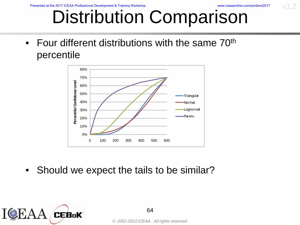
copy 2002-2013 ICEAA All rights reserved
v12
Distribution Comparisonbull Four different distributions with the same 70th
percentile
bull Should we expect the tails to be similar
64
0
10
20
30
40
50
60
70
80
0 100 200 300 400 500 600
Perc
entil
eCo
nfid
ence
Lev
el
Triangular
Normal
Lognormal
Pareto
Presented at the 2017 ICEAA Professional Development amp Training Workshop wwwiceaaonlinecomportland2017
copy 2002-2013 ICEAA All rights reserved
v12Distribution Comparison Tail Behavior
bull The normal and triangular distributions have similar tails but the lognormal and Pareto have much fatter right tails
65
70
75
80
85
90
95
100
500 1500 2500 3500 4500 5500
Perc
entil
eCo
nfid
ence
Lev
el
Triangular
Normal
Lognormal
Pareto
Here There Be Dragons
Presented at the 2017 ICEAA Professional Development amp Training Workshop wwwiceaaonlinecomportland2017
copy 2002-2013 ICEAA All rights reserved
v12Distribution Comparison ndash Tail Behavior (Table)
bull There is significant tail risk for the lognormal and the Paretobull The 99th percentile for the Pareto is 1000 times greater than
the 70th percentilendash Risk seen in financial markets and in catastrophic risks like natural
disasters bull Four different projects follow the four different risk profiles seen
in this example should clearly have different risk management approaches but 70th percentile funding indicates the same risk management approach for all four
66
Percentile Triangular Normal Lognormal Pareto 70th $600 $600 $600 $600 80th $680 $660 $770 $1430 90th $770 $750 $1070 $5880 95th $840 $820 $1410 $23750 99th $930 $950 $2350 $600000
Presented at the 2017 ICEAA Professional Development amp Training Workshop wwwiceaaonlinecomportland2017
copy 2002-2013 ICEAA All rights reserved
v12Percentile Budgeting is Not Risk Management
bull Percentile budgeting ne effective risk management policybull Suppose that you are shopping for a new car You
mention that safety is your top concern The salesman says he has a great safe car available You ask about the air bags Do they work The salesman answers ldquoOf course Seventy percent of the time they work fine Only 30 of the time the air bags will fail to deployrdquo Would you buy such a car Hedge fund manager David Einhorn has stated ldquoRisk management is the air bag that must always work but only in the multi-sigma event where you have an accidentrdquo
67
Risk management is the air bag that must always work but only in the multi-sigma event where you
have an accident
Presented at the 2017 ICEAA Professional Development amp Training Workshop wwwiceaaonlinecomportland2017
copy 2002-2013 ICEAA All rights reserved
v12
Joint Confidence Level Analysisbull Schedules are risky toobull For 98 recent NASA missions average
schedule growth was 38ndash Not as high as cost growth but still significant
68
0
5
10
15
20
25
30
35
40
Schedule
Cost
Presented at the 2017 ICEAA Professional Development amp Training Workshop wwwiceaaonlinecomportland2017
copy 2002-2013 ICEAA All rights reserved
v12
Schedules Impact Costbull Changes in schedule can have enormous
impacts on cost ndash Schedule slips can lead to cost increases
bull Fixed programmatic costs must be paid on a regular basisndash Achieving schedule milestones early can result in cost
savings
bull Schedule is an important consideration in cost analysis including cost risk analysis
bull However we must be careful in correctly integrating cost and schedule riskndash Schedule is not simply an input but is dependent on many of
the same factors that drive cost
69
Presented at the 2017 ICEAA Professional Development amp Training Workshop wwwiceaaonlinecomportland2017
copy 2002-2013 ICEAA All rights reserved
v12
The Relationship of Cost to Schedulebull Cost and schedule are positively correlated
ndash A larger program with bigger scope with take longer to complete than a smaller simpler program
bull However longer schedules do not always equate to higher cost nor shorter schedules with lower costndash Highly compressed schedules relative to the
optimal schedule can lead to large overrunsbull Compressed schedules are commonplace for
many planetary missions
70
Presented at the 2017 ICEAA Professional Development amp Training Workshop wwwiceaaonlinecomportland2017
copy 2002-2013 ICEAA All rights reserved
v12The Impact of Schedule GrowthCompression on Cost
bull Compressed schedules lead to cost growth and based on existing research is actually more expensive than schedule slippages
71
0
20
40
60
80
100
120
140
160
-50 -25 0 25 50 75 100
Percentage Change in Schedule
Perc
enta
ge C
hang
e in
Cos
t due
to
Sche
dule
Cha
nge
Source Smart CB ldquoCost and Schedule Interrelationshipsrdquo 2007 NASA Cost Symposium
Presented at the 2017 ICEAA Professional Development amp Training Workshop wwwiceaaonlinecomportland2017
copy 2002-2013 ICEAA All rights reserved
v12Schedule as an Independent Variable
bull Why not simply add schedule as an input to cost-estimating relationships (CERs)
bull Schedule is often treated as an independent variable ndash schedules are often determined independently of cost considerationsndash Cost may not be considered explicitly although budgets and
schedules are determined based on scope and other common factors
bull In 2006 SAIC undertook a research task to determine the impact of schedule on cost and added schedule as an independent variable to the CERs in the NASAAir Force Cost Model (NAFCOM) to see if schedule provided any improvement in goodness of fit
72
Presented at the 2017 ICEAA Professional Development amp Training Workshop wwwiceaaonlinecomportland2017
copy 2002-2013 ICEAA All rights reserved
v12
Schedule is a Dependent Variablebull Since NAFCOM includes an exhaustive list of cost drivers the inclusion
of schedule should give an indication of whether there is any additional independent value added from schedule independent of the cost drivers
bull In the study schedule was added to 10 subsystem-level CERs
ndash In each case the addition of schedule did NOTimprove the goodness of fit and schedule was NOT found to be a statistically significant cost driver (given the presence of the other variables) for any of the 10 CERs
bull Standard errors for the CERs increased due to decrease in degrees of freedom
bull Thus schedule as an independent variable did not provide any additional explanation of variation in historical cost
bull This is because schedule is truly NOT an independent variable but a dependent variable and is a function of the same factors that drive cost
73
Presented at the 2017 ICEAA Professional Development amp Training Workshop wwwiceaaonlinecomportland2017
copy 2002-2013 ICEAA All rights reserved
v12
Incorporation of Schedule in Cost Risk
bull When using subjective methods care must be taken in applying schedule to cost risk analysis
bull Since schedule is a dependent variable treating it independently from other factors when assessing its impact on cost can lead to a double count of independent variables in the cost risk analysis
bull Direct inclusion of schedule in a cost risk analysis effectively doubles the influence of each cost driver
ndash Incorrectly leads to broader risk ranges
74
CostWeight
HeritageNewness
Technology Readiness Schedule
Presented at the 2017 ICEAA Professional Development amp Training Workshop wwwiceaaonlinecomportland2017
copy 2002-2013 ICEAA All rights reserved
v12Subjective Cost Risk Methods and Overinclusion of Risk Factors
bull Subjective methods are suitable when data are scarce or not availablebull However care must be taken not to treat correlated sources of risk
such as schedule as independent of each otherbull Example ndash a subjective risk analysis incorporated technology readiness
design risk requirements stability integration risk and schedule and treated each source of risk as independent
bull Risk triangle high value without schedule risk was 31 times the point estimate
bull Risk triangle high value with schedule risk added on top of other sources of risk treated independently was 34 times the point estimate
bull Risk triangle taking correlation between sources of risk into account in a rigorous statistical manner has a high value 15 times the point estimate less than half the effect when treating sources of risk as independent
75
Presented at the 2017 ICEAA Professional Development amp Training Workshop wwwiceaaonlinecomportland2017
copy 2002-2013 ICEAA All rights reserved
v12Fundamental Equation of Cost and Schedule Interrelationships
bull The Fundamental Equation of the Relationship Between Cost and Schedule is
Time = Moneybull This is a well known adage that time is money Your boss at
work may even mention this to you from time to time or if you are the boss you are all too aware of this iron law
bull Because time is money cost and schedule risk should be modeled jointly not with schedule as an independent cost driver
bull Note that cost and schedule are not perfectly correlatedndash Cost can sometimes ldquobuy downrdquo schedule extra money can be
spent to meet a deadline since in some cases additional effort to hasten the completion of a task
76
Presented at the 2017 ICEAA Professional Development amp Training Workshop wwwiceaaonlinecomportland2017
copy 2002-2013 ICEAA All rights reserved
v12How to (Correctly) Incorporate Schedule into Cost Risk Analysis
bull The best way to model cost and schedule risk is to develop a joint cost and schedule model based on the same data
bull Since such models are not currently available the next best approach is to model cost and schedule independently and then integrate cost and schedule risk analyses using joint probability distributions taking into account correlation between cost and schedulendash This approach pioneered by Paul Garvey and Steve Book is
considered industry best practicendash This is a practical method mathematically tractable and follows
naturally from the Fundamental Equation of Cost and Schedule Interrelationships
77
Book S A ldquoQuantifying the Relationship Between Cost and Schedulerdquo The Measurable News Winter 2007-2008 pp 11-15Garvey PR Probability Methods for Cost Uncertainty Analysis A Systems Engineering Perspective New York Marcel Dekker 2000 pp 308-335
Presented at the 2017 ICEAA Professional Development amp Training Workshop wwwiceaaonlinecomportland2017
copy 2002-2013 ICEAA All rights reserved
v12
Joint Lognormal and Normal Distributions
bull Cost and schedule are typically modeled as some combination of Normal and Lognormal probability distributionsndash Studies by The Aerospace Corporation the MITRE
Corporation Wyle Labs and SAIC have found that the Lognormal probability distribution almost always serves as a good model for both the schedule distribution and the cost distribution
ndash The Normal distribution may also be appropriate in some instances and depending upon the level of confidence at which budgets are set may even be more conservative and logically consistent than the Normal distribution
ndash Joint Lognormal and Normal distributions are defined by a pair of mean and standard deviations and a level of correlation between the two
78
Presented at the 2017 ICEAA Professional Development amp Training Workshop wwwiceaaonlinecomportland2017
copy 2002-2013 ICEAA All rights reserved
v12Modeling Cost and Schedule as a Bivariate Distribution
bull In the approach set forth by Book and Garvey cost risk is assessed and the top-level distribution is modeled as a Lognormal (or Normal) distribution schedule risk is assessed and the overall schedule risk is modeled as a Lognormal (or Normal) distribution
bull The two distributions are combined into a Bivariate distribution by assigning a correlation between the two and by treating the two distributions as the marginal distributions of a Bivariate Lognormal distributionndash Other combinations include a Bivariate Normal or a Bivariate
Normal-Lognormal
79
Presented at the 2017 ICEAA Professional Development amp Training Workshop wwwiceaaonlinecomportland2017
copy 2002-2013 ICEAA All rights reserved
v12Bivariate Lognormal Distribution for Cost and Schedule
bull Cost is often observed to be Lognormal when strong positive correlations are present among the systemrsquos WBS cost element costs
bull A systemrsquos schedule is often observed (from Monte Carlo simulations) to be Lognormal if it is the sum of many positively correlated schedule activities in an overall schedule network
bull If Lognormal distributions characterize a systemrsquos cost and schedule then the Bivariate Lognormal could serve as an assumed model of their joint distributionndash In this case the marginal distribution of each of cost and schedule is
Lognormalbull Other possibilities for modeling cost and schedule as a Bivariate
distribution include a Bivariate Normal or a Bivariate Normal-Lognormal distributionndash All these combinations are analytically tractable
80
Presented at the 2017 ICEAA Professional Development amp Training Workshop wwwiceaaonlinecomportland2017
copy 2002-2013 ICEAA All rights reserved
v12Bivariate Lognormal for Cost and Schedule
bull Contour Plots of a Bivariate Lognormal
81
Presented at the 2017 ICEAA Professional Development amp Training Workshop wwwiceaaonlinecomportland2017
copy 2002-2013 ICEAA All rights reserved
v12Correlation Between Cost and Schedule
bull Cost and schedule are positively correlated but not perfectly sondash For example it is possible to have a schedule underrun and a cost
overrunbull Based on cost and schedule growth data for 50 completed NASA
programs the correlation between development cost and development schedule is 70
82
00
200
400
600
800
1000
1200
-500 00 500 1000 1500 2000 2500Historical Cost Growth
Hist
oric
al S
ched
ule
Gro
wth
r = 715
Presented at the 2017 ICEAA Professional Development amp Training Workshop wwwiceaaonlinecomportland2017
copy 2002-2013 ICEAA All rights reserved
v12Correlation Between Cost and Schedule Caveats
bull Based on historical data recommended correlation between cost and schedule is 70 but this could be higher or lower depending upon program circumstancesndash If program is budget constrained cost and schedule will be
more highly correlated (go as you pay)ndash If program is schedule constrained cost and schedule will
have lower correlation perhaps even negative correlation ndash Smaller programs have smaller correlation between cost and
schedule riskbull Relatively easy to ldquohurry uprdquo and finish on time or even early if
needed
83
Presented at the 2017 ICEAA Professional Development amp Training Workshop wwwiceaaonlinecomportland2017
copy 2002-2013 ICEAA All rights reserved
v12
Conditional Confidence Levelsbull Given a programrsquos project schedule we can determine the cost
risk distribution conditional upon the given schedulebull Conditional cost S-curves are steeper than unconditional
(marginal) cost S-curves between some uncertainty has been removed because schedule is fixed
84
Presented at the 2017 ICEAA Professional Development amp Training Workshop wwwiceaaonlinecomportland2017
copy 2002-2013 ICEAA All rights reserved
v12
Joint Confidence Levelsbull Joint 65 confidence represents the probability of
achieving both 65 confidence in cost AND 65 confidence in schedulendash This is different than achieving 65 cost confidence alone
or achieving 65 schedule confidence alonebull Due to the imperfect correlation between cost and schedule it
is possible to achieve a 65 cost confidence with a lower level of schedule confidence
bull Restricting the schedule confidence thus requires additional $ to achieve a given level of confidence
85
X
Y
Possible Values for Which X gt a Possible Values for
Which X gt a and Y gt b
a
b
Presented at the 2017 ICEAA Professional Development amp Training Workshop wwwiceaaonlinecomportland2017
copy 2002-2013 ICEAA All rights reserved
v12Joint Confidence Levels Versus Cost Confidence Levels Only
bull Example of the differences between cost confidence schedule confidence conditional cost confidence and joint cost and schedule confidence
86
Joint Cost-Schedule Confidence Iso-Curves
Cost (RY$M)
Sche
dule
(Mon
ths)
65 Confidence
50 Confidence
70 Confidence
65 Cost Confidence AggressiveSchedule65 Cost ConfidenceScheduleGiven 65 Schedule ConfidenceUnconditional 65 CostConfidenceUnconditional 65 ScheduleConfidence
65 Cost Confidence 65 Joint Cost and Schedule
Confidence for 65 Schedule Confidence
Presented at the 2017 ICEAA Professional Development amp Training Workshop wwwiceaaonlinecomportland2017
copy 2002-2013 ICEAA All rights reserved
v12
Joint Cost and Schedule Confidence
bull Can examine pairs of cost and schedule that achieve a given level of confidence
bull Provides insights into the trade-offs between cost and schedule for a given level of confidencendash Possible to increase cost confidence by giving a
project more time in some instances or possible to ldquobuy downrdquo schedule
bull But these have limits and are shown in the iso-cost and schedule confidence curves
87
Presented at the 2017 ICEAA Professional Development amp Training Workshop wwwiceaaonlinecomportland2017
copy 2002-2013 ICEAA All rights reserved
v12Cost and Schedule Trade-offs for a Given Level of Joint Confidence
bull Hypothetical Example
88
Cost (RY$M)
Schedule (Months)
$100 48$99 48$89 49$87 50$85 51$85 52$84 53$83 55$83 55$83 56
Cost and Schedule 65 Confidence Iso-Curve
4748495051525354555657
$80 $82 $84 $86 $88 $90 $92 $94 $96 $98 $100
Cost (RY$ M)
Sche
dule
(Mon
ths)
Presented at the 2017 ICEAA Professional Development amp Training Workshop wwwiceaaonlinecomportland2017
copy 2002-2013 ICEAA All rights reserved
v12Policy Considerations for Confidence Levels
bull For large programs the difference between the amount of money needed to achieve 65 cost confidence independent of schedule and joint 65 cost and schedule confidence can represent hundreds of millions and even billions of dollars
89
Joint Cost-Schedule Confidence Iso-Curves
Cost (RY$M)
Sche
dule
(Mon
ths)
65 Confidence
65 Cost Confidence AggressiveSchedule
65 Cost ConfidenceScheduleGiven 65 Schedule Confidence
Unconditional 65 CostConfidence
Joint Cost and Schedule Confidence for 65 Cost Confidence and Program Baseline Schedule is Less Than 35
65 Cost Confidence Independent of Schedule Cost Needed to Achieve
Both 65 Joint Cost and Schedule Confidence for the Schedule with 65 Confidence
Presented at the 2017 ICEAA Professional Development amp Training Workshop wwwiceaaonlinecomportland2017
copy 2002-2013 ICEAA All rights reserved
v12
Copulasbull More generally any combination of distributions can
be used (more than just normal and lognormal)ndash Termed ldquocopulardquo from the Italian word for ldquocouplerdquondash Copulas are a way to combine marginal distributions of any
number and type into a joint distributionbull More formally a copula is a multivariate joint distribution defined
on the n-dimensional unit cube [0 1]n such that every marginal distribution is uniform on the interval [0 1]
bull (The bivariate form of) Sklarrsquos theorem states that for any bivariate distribution function H(x y) let F(x) = H(x infin) and G(y) = H(infin y) be the univariate marginal probability distribution functions Then there exists a copula C such that H(xy)=C(F(x)G(y))
ndash Copulas are widely used in risk management for investments and insurance
bull Considered industry best practice (Li 2000)bull Marketed as part of JP Morganrsquos CreditMetrics suite of tools
(Gupton et Al 1997)90
Presented at the 2017 ICEAA Professional Development amp Training Workshop wwwiceaaonlinecomportland2017
copy 2002-2013 ICEAA All rights reserved
v12Parametric Joint Cost and Schedule Analysis
bull A parametric model based on a consistent data set with a set of overlapping cost and schedule drivers is a cleaner way to model cost and schedule
91
CostWeight
HeritageNewness
Technology Readiness
Schedule
0
20
40
60
80
100
Confidence
Joint Cost and Schedule Confidence
Schedule
Cost
Lognormal Distribution PDF and CDF
0102030405060708090100
200 300 400 500 600 700 800 900 1000Cost $
Con
fiden
ce L
evel
0
00002
00004
00006
00008
0001
00012
00014
00016
Prob
abili
ty D
ensi
ty
CDFPDF
Lognormal Distribution PDF and CDF
0102030405060708090100
200 300 400 500 600 700 800 900 1000Cost $
Con
fiden
ce L
evel
0
00002
00004
00006
00008
0001
00012
00014
00016
Prob
abili
ty D
ensi
ty
CDFPDF
Presented at the 2017 ICEAA Professional Development amp Training Workshop wwwiceaaonlinecomportland2017
copy 2002-2013 ICEAA All rights reserved
v12Parametric Joint Cost and Schedule Analysis (2)
bull Joint cost and schedule risk analysis produced naturally by the integrated modelndash Addresses several issues with the copula
approachbull Tail dependencybull Correlation ndash no need to assign correlation
between cost and schedulebull Consistency of cost and schedule models
92
Presented at the 2017 ICEAA Professional Development amp Training Workshop wwwiceaaonlinecomportland2017
copy 2002-2013 ICEAA All rights reserved
v12
Resource-Loaded Schedulesbull Involves assigning cost and schedule risks to a resource-loaded schedule
networkbull Bottom-up approach
ndash More labor intensive than parametrics but can also provide more insight
ndash Can answer questions than parametric typically cannot such as how much do reserve requirements decrease if a specific risk is retired
bull Currently being implemented in Constellation programbull Has same issue as all bottom-up models hard to count all the risks and model
them discretely
ndash As a result there is a tendency to reflect less risk than indicated by history
ndash ldquoThere are more things in heaven and earth Horatio than are dreamt of in your philosophyrdquo William Shakespeare Hamlet Act I Scene V
93
Presented at the 2017 ICEAA Professional Development amp Training Workshop wwwiceaaonlinecomportland2017
copy 2002-2013 ICEAA All rights reserved
v12Resource-Loaded Schedules Vs Parametrics
bull Parametric most appropriate for early estimatesndash But also good for high-level checks as project progresses
bull As plans take shape lower level modeling may be more appropriate
94 1
CONCEPTUALDEVELOPMENT
PROJECTDEFINITION DESIGN DEVELOPMENT OPERATIONS
PARAMETRIC PARAMETRIC
ANALOGY
ENGINEERING (Bottoms Up)
$PARAMETRIC
DETAILED
$
Pre Phase A Phase B Phase CDPhase A Phase EPre Phase A Phase B Phase CDPhase A Phase E
Risk = f(Cost Estimating Relationship Inputs eg mass power data rate TRL new design etc)
Risk = f(cost and schedule variation of the analogous elements)
Risk = f(variation of detailed inputs eg labor hours rates materials etc)
Presented at the 2017 ICEAA Professional Development amp Training Workshop wwwiceaaonlinecomportland2017
copy 2002-2013 ICEAA All rights reserved
v12
Resource-Loaded Schedulesbull Methodology has been demonstrated in other
industriesndash Construction oil and gasndash Analysis has not been traditionally done on highly uncertain
complex development projects bull Methodology focuses on project baseline schedule
ndash In baseline schedule all tasks are resource loaded to represent a baseline schedule and cost standpoint
ndash Resource loaded schedule is ldquorolledrdquo up to a manageable level
ndash Based on the risk and uncertainties identified schedule distributions are applied to each rolled up task
ndash Cost uncertainties are also applied to rolled up tasksbull Uncertainties include labor rate man power etc
ndash A Monte Carlo simulation is run to develop joint cost-schedule distributions
95
Presented at the 2017 ICEAA Professional Development amp Training Workshop wwwiceaaonlinecomportland2017
copy 2002-2013 ICEAA All rights reserved
v12
Unit III - Module 9 96
Execution ndash Cross Checksbull Means The mean cost growth factor for WBS items
can be compared to history as a way to cross check results
bull CVs The CV of the cost growth factors for WBS items can be compared to history as a way to cross check results
bull Inputs Checks are performed on inputs or other parameters to see if historical values are in line with program assumptionsndash Example Historical risk scores can be compared to program
risk scores to see if risk assessors are being realistic and to see if the underlying database is representative of the program
11
Presented at the 2017 ICEAA Professional Development amp Training Workshop wwwiceaaonlinecomportland2017
- Cost and Schedule Risk Analysis Basic
- Acknowledgments
- Unit Index
- Risk Overview
- Agenda
- Introduction
- Risk Analysis Terms
- Are Our Costs Realistic
- Historical Cost Growth
- Sources of Cost Risk
- Point Estimates of Cost
- Types of Risk
- Point Estimates Vs Risk Estimates
- Cost Risk and Probability
- Probability Model ndash Distribution
- Probability Model ndash Distribution
- Probability ndash Top-Level Distribution
- S-Curves and Confidence Levels
- Example ndash Normal Distribution
- Confidence Levels
- Measuring Parametric Model Uncertainty
- Parametric Model Example
- Weight Uncertainty
- Estimating Uncertainty
- Estimating Uncertainty (2)
- Estimating Uncertainty (3)
- Aggregating Risk
- WBS Example
- WBS and Risk
- Aggregating Risk
- Percentiles Do Not Add
- Percentiles Do Not Add (2)
- Percentiles Do Not Add (3)
- Methods for Aggregating Risk
- Monte Carlo Simulationfor Risk Analysis
- Monte Carlo Simulation
- Using Random Numbers to Simulate Distributions
- Simulating a Triangular Distribution
- Simulating a Triangular Distribution (2)
- Monte Carlo and the WBS
- Number of Trials
- Number of Trials (2)
- Number of Trials (3)
- Number of Trials (4)
- Number of Trials (5)
- Number of Trials (6)
- Methods of Simulation
- Probability Model ndash Correlation
- Correlation And Causation
- The Importance of Correlation
- The Importance of Correlation (2)
- Measures of Correlation
- Pearson Correlation
- Spearman Correlation
- Functional Correlation
- Risk Measures
- Value at Risk (VaR)
- Why 70th or 80th Percentile
- Funding Above Inflection Points
- Why Budget to the 70th or 80th
- Inflection Points for Lognormal
- Issues with Percentile Funding
- ldquoHere There Be Dragonsrdquo
- Distribution Comparison
- Distribution Comparison Tail Behavior
- Distribution Comparison ndash Tail Behavior (Table)
- Percentile Budgeting is Not Risk Management
- Joint Confidence Level Analysis
- Schedules Impact Cost
- The Relationship of Cost to Schedule
- The Impact of Schedule GrowthCompression on Cost
- Schedule as an Independent Variable
- Schedule is a Dependent Variable
- Incorporation of Schedule in Cost Risk
- Subjective Cost Risk Methods and Overinclusion of Risk Factors
- Fundamental Equation of Cost and Schedule Interrelationships
- How to (Correctly) Incorporate Schedule into Cost Risk Analysis
- Joint Lognormal and Normal Distributions
- Modeling Cost and Schedule as a Bivariate Distribution
- Bivariate Lognormal Distribution for Cost and Schedule
- Bivariate Lognormal for Cost and Schedule
- Correlation Between Cost and Schedule
- Correlation Between Cost and Schedule Caveats
- Conditional Confidence Levels
- Joint Confidence Levels
- Joint Confidence Levels Versus Cost Confidence Levels Only
- Joint Cost and Schedule Confidence
- Cost and Schedule Trade-offs for a Given Level of Joint Confidence
- Policy Considerations for Confidence Levels
- Copulas
- Parametric Joint Cost and Schedule Analysis
- Parametric Joint Cost and Schedule Analysis (2)
- Resource-Loaded Schedules
- Resource-Loaded Schedules Vs Parametrics
- Resource-Loaded Schedules
- Execution ndash Cross Checks
-
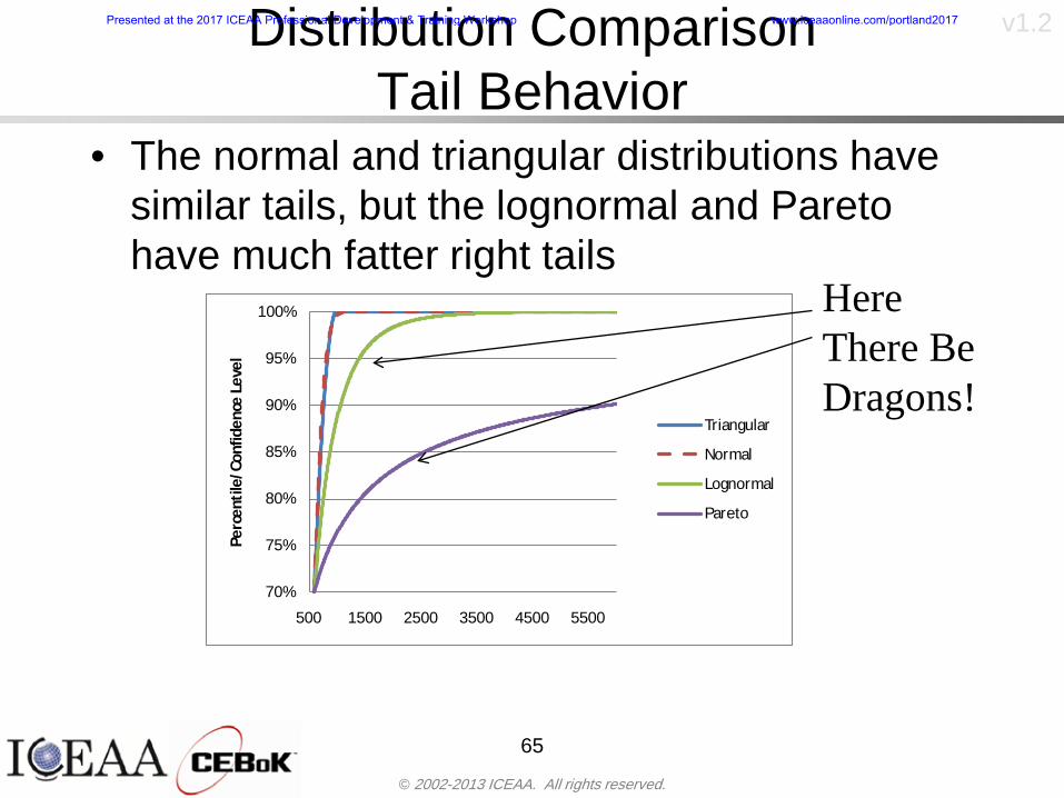
copy 2002-2013 ICEAA All rights reserved
v12Distribution Comparison Tail Behavior
bull The normal and triangular distributions have similar tails but the lognormal and Pareto have much fatter right tails
65
70
75
80
85
90
95
100
500 1500 2500 3500 4500 5500
Perc
entil
eCo
nfid
ence
Lev
el
Triangular
Normal
Lognormal
Pareto
Here There Be Dragons
Presented at the 2017 ICEAA Professional Development amp Training Workshop wwwiceaaonlinecomportland2017
copy 2002-2013 ICEAA All rights reserved
v12Distribution Comparison ndash Tail Behavior (Table)
bull There is significant tail risk for the lognormal and the Paretobull The 99th percentile for the Pareto is 1000 times greater than
the 70th percentilendash Risk seen in financial markets and in catastrophic risks like natural
disasters bull Four different projects follow the four different risk profiles seen
in this example should clearly have different risk management approaches but 70th percentile funding indicates the same risk management approach for all four
66
Percentile Triangular Normal Lognormal Pareto 70th $600 $600 $600 $600 80th $680 $660 $770 $1430 90th $770 $750 $1070 $5880 95th $840 $820 $1410 $23750 99th $930 $950 $2350 $600000
Presented at the 2017 ICEAA Professional Development amp Training Workshop wwwiceaaonlinecomportland2017
copy 2002-2013 ICEAA All rights reserved
v12Percentile Budgeting is Not Risk Management
bull Percentile budgeting ne effective risk management policybull Suppose that you are shopping for a new car You
mention that safety is your top concern The salesman says he has a great safe car available You ask about the air bags Do they work The salesman answers ldquoOf course Seventy percent of the time they work fine Only 30 of the time the air bags will fail to deployrdquo Would you buy such a car Hedge fund manager David Einhorn has stated ldquoRisk management is the air bag that must always work but only in the multi-sigma event where you have an accidentrdquo
67
Risk management is the air bag that must always work but only in the multi-sigma event where you
have an accident
Presented at the 2017 ICEAA Professional Development amp Training Workshop wwwiceaaonlinecomportland2017
copy 2002-2013 ICEAA All rights reserved
v12
Joint Confidence Level Analysisbull Schedules are risky toobull For 98 recent NASA missions average
schedule growth was 38ndash Not as high as cost growth but still significant
68
0
5
10
15
20
25
30
35
40
Schedule
Cost
Presented at the 2017 ICEAA Professional Development amp Training Workshop wwwiceaaonlinecomportland2017
copy 2002-2013 ICEAA All rights reserved
v12
Schedules Impact Costbull Changes in schedule can have enormous
impacts on cost ndash Schedule slips can lead to cost increases
bull Fixed programmatic costs must be paid on a regular basisndash Achieving schedule milestones early can result in cost
savings
bull Schedule is an important consideration in cost analysis including cost risk analysis
bull However we must be careful in correctly integrating cost and schedule riskndash Schedule is not simply an input but is dependent on many of
the same factors that drive cost
69
Presented at the 2017 ICEAA Professional Development amp Training Workshop wwwiceaaonlinecomportland2017
copy 2002-2013 ICEAA All rights reserved
v12
The Relationship of Cost to Schedulebull Cost and schedule are positively correlated
ndash A larger program with bigger scope with take longer to complete than a smaller simpler program
bull However longer schedules do not always equate to higher cost nor shorter schedules with lower costndash Highly compressed schedules relative to the
optimal schedule can lead to large overrunsbull Compressed schedules are commonplace for
many planetary missions
70
Presented at the 2017 ICEAA Professional Development amp Training Workshop wwwiceaaonlinecomportland2017
copy 2002-2013 ICEAA All rights reserved
v12The Impact of Schedule GrowthCompression on Cost
bull Compressed schedules lead to cost growth and based on existing research is actually more expensive than schedule slippages
71
0
20
40
60
80
100
120
140
160
-50 -25 0 25 50 75 100
Percentage Change in Schedule
Perc
enta
ge C
hang
e in
Cos
t due
to
Sche
dule
Cha
nge
Source Smart CB ldquoCost and Schedule Interrelationshipsrdquo 2007 NASA Cost Symposium
Presented at the 2017 ICEAA Professional Development amp Training Workshop wwwiceaaonlinecomportland2017
copy 2002-2013 ICEAA All rights reserved
v12Schedule as an Independent Variable
bull Why not simply add schedule as an input to cost-estimating relationships (CERs)
bull Schedule is often treated as an independent variable ndash schedules are often determined independently of cost considerationsndash Cost may not be considered explicitly although budgets and
schedules are determined based on scope and other common factors
bull In 2006 SAIC undertook a research task to determine the impact of schedule on cost and added schedule as an independent variable to the CERs in the NASAAir Force Cost Model (NAFCOM) to see if schedule provided any improvement in goodness of fit
72
Presented at the 2017 ICEAA Professional Development amp Training Workshop wwwiceaaonlinecomportland2017
copy 2002-2013 ICEAA All rights reserved
v12
Schedule is a Dependent Variablebull Since NAFCOM includes an exhaustive list of cost drivers the inclusion
of schedule should give an indication of whether there is any additional independent value added from schedule independent of the cost drivers
bull In the study schedule was added to 10 subsystem-level CERs
ndash In each case the addition of schedule did NOTimprove the goodness of fit and schedule was NOT found to be a statistically significant cost driver (given the presence of the other variables) for any of the 10 CERs
bull Standard errors for the CERs increased due to decrease in degrees of freedom
bull Thus schedule as an independent variable did not provide any additional explanation of variation in historical cost
bull This is because schedule is truly NOT an independent variable but a dependent variable and is a function of the same factors that drive cost
73
Presented at the 2017 ICEAA Professional Development amp Training Workshop wwwiceaaonlinecomportland2017
copy 2002-2013 ICEAA All rights reserved
v12
Incorporation of Schedule in Cost Risk
bull When using subjective methods care must be taken in applying schedule to cost risk analysis
bull Since schedule is a dependent variable treating it independently from other factors when assessing its impact on cost can lead to a double count of independent variables in the cost risk analysis
bull Direct inclusion of schedule in a cost risk analysis effectively doubles the influence of each cost driver
ndash Incorrectly leads to broader risk ranges
74
CostWeight
HeritageNewness
Technology Readiness Schedule
Presented at the 2017 ICEAA Professional Development amp Training Workshop wwwiceaaonlinecomportland2017
copy 2002-2013 ICEAA All rights reserved
v12Subjective Cost Risk Methods and Overinclusion of Risk Factors
bull Subjective methods are suitable when data are scarce or not availablebull However care must be taken not to treat correlated sources of risk
such as schedule as independent of each otherbull Example ndash a subjective risk analysis incorporated technology readiness
design risk requirements stability integration risk and schedule and treated each source of risk as independent
bull Risk triangle high value without schedule risk was 31 times the point estimate
bull Risk triangle high value with schedule risk added on top of other sources of risk treated independently was 34 times the point estimate
bull Risk triangle taking correlation between sources of risk into account in a rigorous statistical manner has a high value 15 times the point estimate less than half the effect when treating sources of risk as independent
75
Presented at the 2017 ICEAA Professional Development amp Training Workshop wwwiceaaonlinecomportland2017
copy 2002-2013 ICEAA All rights reserved
v12Fundamental Equation of Cost and Schedule Interrelationships
bull The Fundamental Equation of the Relationship Between Cost and Schedule is
Time = Moneybull This is a well known adage that time is money Your boss at
work may even mention this to you from time to time or if you are the boss you are all too aware of this iron law
bull Because time is money cost and schedule risk should be modeled jointly not with schedule as an independent cost driver
bull Note that cost and schedule are not perfectly correlatedndash Cost can sometimes ldquobuy downrdquo schedule extra money can be
spent to meet a deadline since in some cases additional effort to hasten the completion of a task
76
Presented at the 2017 ICEAA Professional Development amp Training Workshop wwwiceaaonlinecomportland2017
copy 2002-2013 ICEAA All rights reserved
v12How to (Correctly) Incorporate Schedule into Cost Risk Analysis
bull The best way to model cost and schedule risk is to develop a joint cost and schedule model based on the same data
bull Since such models are not currently available the next best approach is to model cost and schedule independently and then integrate cost and schedule risk analyses using joint probability distributions taking into account correlation between cost and schedulendash This approach pioneered by Paul Garvey and Steve Book is
considered industry best practicendash This is a practical method mathematically tractable and follows
naturally from the Fundamental Equation of Cost and Schedule Interrelationships
77
Book S A ldquoQuantifying the Relationship Between Cost and Schedulerdquo The Measurable News Winter 2007-2008 pp 11-15Garvey PR Probability Methods for Cost Uncertainty Analysis A Systems Engineering Perspective New York Marcel Dekker 2000 pp 308-335
Presented at the 2017 ICEAA Professional Development amp Training Workshop wwwiceaaonlinecomportland2017
copy 2002-2013 ICEAA All rights reserved
v12
Joint Lognormal and Normal Distributions
bull Cost and schedule are typically modeled as some combination of Normal and Lognormal probability distributionsndash Studies by The Aerospace Corporation the MITRE
Corporation Wyle Labs and SAIC have found that the Lognormal probability distribution almost always serves as a good model for both the schedule distribution and the cost distribution
ndash The Normal distribution may also be appropriate in some instances and depending upon the level of confidence at which budgets are set may even be more conservative and logically consistent than the Normal distribution
ndash Joint Lognormal and Normal distributions are defined by a pair of mean and standard deviations and a level of correlation between the two
78
Presented at the 2017 ICEAA Professional Development amp Training Workshop wwwiceaaonlinecomportland2017
copy 2002-2013 ICEAA All rights reserved
v12Modeling Cost and Schedule as a Bivariate Distribution
bull In the approach set forth by Book and Garvey cost risk is assessed and the top-level distribution is modeled as a Lognormal (or Normal) distribution schedule risk is assessed and the overall schedule risk is modeled as a Lognormal (or Normal) distribution
bull The two distributions are combined into a Bivariate distribution by assigning a correlation between the two and by treating the two distributions as the marginal distributions of a Bivariate Lognormal distributionndash Other combinations include a Bivariate Normal or a Bivariate
Normal-Lognormal
79
Presented at the 2017 ICEAA Professional Development amp Training Workshop wwwiceaaonlinecomportland2017
copy 2002-2013 ICEAA All rights reserved
v12Bivariate Lognormal Distribution for Cost and Schedule
bull Cost is often observed to be Lognormal when strong positive correlations are present among the systemrsquos WBS cost element costs
bull A systemrsquos schedule is often observed (from Monte Carlo simulations) to be Lognormal if it is the sum of many positively correlated schedule activities in an overall schedule network
bull If Lognormal distributions characterize a systemrsquos cost and schedule then the Bivariate Lognormal could serve as an assumed model of their joint distributionndash In this case the marginal distribution of each of cost and schedule is
Lognormalbull Other possibilities for modeling cost and schedule as a Bivariate
distribution include a Bivariate Normal or a Bivariate Normal-Lognormal distributionndash All these combinations are analytically tractable
80
Presented at the 2017 ICEAA Professional Development amp Training Workshop wwwiceaaonlinecomportland2017
copy 2002-2013 ICEAA All rights reserved
v12Bivariate Lognormal for Cost and Schedule
bull Contour Plots of a Bivariate Lognormal
81
Presented at the 2017 ICEAA Professional Development amp Training Workshop wwwiceaaonlinecomportland2017
copy 2002-2013 ICEAA All rights reserved
v12Correlation Between Cost and Schedule
bull Cost and schedule are positively correlated but not perfectly sondash For example it is possible to have a schedule underrun and a cost
overrunbull Based on cost and schedule growth data for 50 completed NASA
programs the correlation between development cost and development schedule is 70
82
00
200
400
600
800
1000
1200
-500 00 500 1000 1500 2000 2500Historical Cost Growth
Hist
oric
al S
ched
ule
Gro
wth
r = 715
Presented at the 2017 ICEAA Professional Development amp Training Workshop wwwiceaaonlinecomportland2017
copy 2002-2013 ICEAA All rights reserved
v12Correlation Between Cost and Schedule Caveats
bull Based on historical data recommended correlation between cost and schedule is 70 but this could be higher or lower depending upon program circumstancesndash If program is budget constrained cost and schedule will be
more highly correlated (go as you pay)ndash If program is schedule constrained cost and schedule will
have lower correlation perhaps even negative correlation ndash Smaller programs have smaller correlation between cost and
schedule riskbull Relatively easy to ldquohurry uprdquo and finish on time or even early if
needed
83
Presented at the 2017 ICEAA Professional Development amp Training Workshop wwwiceaaonlinecomportland2017
copy 2002-2013 ICEAA All rights reserved
v12
Conditional Confidence Levelsbull Given a programrsquos project schedule we can determine the cost
risk distribution conditional upon the given schedulebull Conditional cost S-curves are steeper than unconditional
(marginal) cost S-curves between some uncertainty has been removed because schedule is fixed
84
Presented at the 2017 ICEAA Professional Development amp Training Workshop wwwiceaaonlinecomportland2017
copy 2002-2013 ICEAA All rights reserved
v12
Joint Confidence Levelsbull Joint 65 confidence represents the probability of
achieving both 65 confidence in cost AND 65 confidence in schedulendash This is different than achieving 65 cost confidence alone
or achieving 65 schedule confidence alonebull Due to the imperfect correlation between cost and schedule it
is possible to achieve a 65 cost confidence with a lower level of schedule confidence
bull Restricting the schedule confidence thus requires additional $ to achieve a given level of confidence
85
X
Y
Possible Values for Which X gt a Possible Values for
Which X gt a and Y gt b
a
b
Presented at the 2017 ICEAA Professional Development amp Training Workshop wwwiceaaonlinecomportland2017
copy 2002-2013 ICEAA All rights reserved
v12Joint Confidence Levels Versus Cost Confidence Levels Only
bull Example of the differences between cost confidence schedule confidence conditional cost confidence and joint cost and schedule confidence
86
Joint Cost-Schedule Confidence Iso-Curves
Cost (RY$M)
Sche
dule
(Mon
ths)
65 Confidence
50 Confidence
70 Confidence
65 Cost Confidence AggressiveSchedule65 Cost ConfidenceScheduleGiven 65 Schedule ConfidenceUnconditional 65 CostConfidenceUnconditional 65 ScheduleConfidence
65 Cost Confidence 65 Joint Cost and Schedule
Confidence for 65 Schedule Confidence
Presented at the 2017 ICEAA Professional Development amp Training Workshop wwwiceaaonlinecomportland2017
copy 2002-2013 ICEAA All rights reserved
v12
Joint Cost and Schedule Confidence
bull Can examine pairs of cost and schedule that achieve a given level of confidence
bull Provides insights into the trade-offs between cost and schedule for a given level of confidencendash Possible to increase cost confidence by giving a
project more time in some instances or possible to ldquobuy downrdquo schedule
bull But these have limits and are shown in the iso-cost and schedule confidence curves
87
Presented at the 2017 ICEAA Professional Development amp Training Workshop wwwiceaaonlinecomportland2017
copy 2002-2013 ICEAA All rights reserved
v12Cost and Schedule Trade-offs for a Given Level of Joint Confidence
bull Hypothetical Example
88
Cost (RY$M)
Schedule (Months)
$100 48$99 48$89 49$87 50$85 51$85 52$84 53$83 55$83 55$83 56
Cost and Schedule 65 Confidence Iso-Curve
4748495051525354555657
$80 $82 $84 $86 $88 $90 $92 $94 $96 $98 $100
Cost (RY$ M)
Sche
dule
(Mon
ths)
Presented at the 2017 ICEAA Professional Development amp Training Workshop wwwiceaaonlinecomportland2017
copy 2002-2013 ICEAA All rights reserved
v12Policy Considerations for Confidence Levels
bull For large programs the difference between the amount of money needed to achieve 65 cost confidence independent of schedule and joint 65 cost and schedule confidence can represent hundreds of millions and even billions of dollars
89
Joint Cost-Schedule Confidence Iso-Curves
Cost (RY$M)
Sche
dule
(Mon
ths)
65 Confidence
65 Cost Confidence AggressiveSchedule
65 Cost ConfidenceScheduleGiven 65 Schedule Confidence
Unconditional 65 CostConfidence
Joint Cost and Schedule Confidence for 65 Cost Confidence and Program Baseline Schedule is Less Than 35
65 Cost Confidence Independent of Schedule Cost Needed to Achieve
Both 65 Joint Cost and Schedule Confidence for the Schedule with 65 Confidence
Presented at the 2017 ICEAA Professional Development amp Training Workshop wwwiceaaonlinecomportland2017
copy 2002-2013 ICEAA All rights reserved
v12
Copulasbull More generally any combination of distributions can
be used (more than just normal and lognormal)ndash Termed ldquocopulardquo from the Italian word for ldquocouplerdquondash Copulas are a way to combine marginal distributions of any
number and type into a joint distributionbull More formally a copula is a multivariate joint distribution defined
on the n-dimensional unit cube [0 1]n such that every marginal distribution is uniform on the interval [0 1]
bull (The bivariate form of) Sklarrsquos theorem states that for any bivariate distribution function H(x y) let F(x) = H(x infin) and G(y) = H(infin y) be the univariate marginal probability distribution functions Then there exists a copula C such that H(xy)=C(F(x)G(y))
ndash Copulas are widely used in risk management for investments and insurance
bull Considered industry best practice (Li 2000)bull Marketed as part of JP Morganrsquos CreditMetrics suite of tools
(Gupton et Al 1997)90
Presented at the 2017 ICEAA Professional Development amp Training Workshop wwwiceaaonlinecomportland2017
copy 2002-2013 ICEAA All rights reserved
v12Parametric Joint Cost and Schedule Analysis
bull A parametric model based on a consistent data set with a set of overlapping cost and schedule drivers is a cleaner way to model cost and schedule
91
CostWeight
HeritageNewness
Technology Readiness
Schedule
0
20
40
60
80
100
Confidence
Joint Cost and Schedule Confidence
Schedule
Cost
Lognormal Distribution PDF and CDF
0102030405060708090100
200 300 400 500 600 700 800 900 1000Cost $
Con
fiden
ce L
evel
0
00002
00004
00006
00008
0001
00012
00014
00016
Prob
abili
ty D
ensi
ty
CDFPDF
Lognormal Distribution PDF and CDF
0102030405060708090100
200 300 400 500 600 700 800 900 1000Cost $
Con
fiden
ce L
evel
0
00002
00004
00006
00008
0001
00012
00014
00016
Prob
abili
ty D
ensi
ty
CDFPDF
Presented at the 2017 ICEAA Professional Development amp Training Workshop wwwiceaaonlinecomportland2017
copy 2002-2013 ICEAA All rights reserved
v12Parametric Joint Cost and Schedule Analysis (2)
bull Joint cost and schedule risk analysis produced naturally by the integrated modelndash Addresses several issues with the copula
approachbull Tail dependencybull Correlation ndash no need to assign correlation
between cost and schedulebull Consistency of cost and schedule models
92
Presented at the 2017 ICEAA Professional Development amp Training Workshop wwwiceaaonlinecomportland2017
copy 2002-2013 ICEAA All rights reserved
v12
Resource-Loaded Schedulesbull Involves assigning cost and schedule risks to a resource-loaded schedule
networkbull Bottom-up approach
ndash More labor intensive than parametrics but can also provide more insight
ndash Can answer questions than parametric typically cannot such as how much do reserve requirements decrease if a specific risk is retired
bull Currently being implemented in Constellation programbull Has same issue as all bottom-up models hard to count all the risks and model
them discretely
ndash As a result there is a tendency to reflect less risk than indicated by history
ndash ldquoThere are more things in heaven and earth Horatio than are dreamt of in your philosophyrdquo William Shakespeare Hamlet Act I Scene V
93
Presented at the 2017 ICEAA Professional Development amp Training Workshop wwwiceaaonlinecomportland2017
copy 2002-2013 ICEAA All rights reserved
v12Resource-Loaded Schedules Vs Parametrics
bull Parametric most appropriate for early estimatesndash But also good for high-level checks as project progresses
bull As plans take shape lower level modeling may be more appropriate
94 1
CONCEPTUALDEVELOPMENT
PROJECTDEFINITION DESIGN DEVELOPMENT OPERATIONS
PARAMETRIC PARAMETRIC
ANALOGY
ENGINEERING (Bottoms Up)
$PARAMETRIC
DETAILED
$
Pre Phase A Phase B Phase CDPhase A Phase EPre Phase A Phase B Phase CDPhase A Phase E
Risk = f(Cost Estimating Relationship Inputs eg mass power data rate TRL new design etc)
Risk = f(cost and schedule variation of the analogous elements)
Risk = f(variation of detailed inputs eg labor hours rates materials etc)
Presented at the 2017 ICEAA Professional Development amp Training Workshop wwwiceaaonlinecomportland2017
copy 2002-2013 ICEAA All rights reserved
v12
Resource-Loaded Schedulesbull Methodology has been demonstrated in other
industriesndash Construction oil and gasndash Analysis has not been traditionally done on highly uncertain
complex development projects bull Methodology focuses on project baseline schedule
ndash In baseline schedule all tasks are resource loaded to represent a baseline schedule and cost standpoint
ndash Resource loaded schedule is ldquorolledrdquo up to a manageable level
ndash Based on the risk and uncertainties identified schedule distributions are applied to each rolled up task
ndash Cost uncertainties are also applied to rolled up tasksbull Uncertainties include labor rate man power etc
ndash A Monte Carlo simulation is run to develop joint cost-schedule distributions
95
Presented at the 2017 ICEAA Professional Development amp Training Workshop wwwiceaaonlinecomportland2017
copy 2002-2013 ICEAA All rights reserved
v12
Unit III - Module 9 96
Execution ndash Cross Checksbull Means The mean cost growth factor for WBS items
can be compared to history as a way to cross check results
bull CVs The CV of the cost growth factors for WBS items can be compared to history as a way to cross check results
bull Inputs Checks are performed on inputs or other parameters to see if historical values are in line with program assumptionsndash Example Historical risk scores can be compared to program
risk scores to see if risk assessors are being realistic and to see if the underlying database is representative of the program
11
Presented at the 2017 ICEAA Professional Development amp Training Workshop wwwiceaaonlinecomportland2017
- Cost and Schedule Risk Analysis Basic
- Acknowledgments
- Unit Index
- Risk Overview
- Agenda
- Introduction
- Risk Analysis Terms
- Are Our Costs Realistic
- Historical Cost Growth
- Sources of Cost Risk
- Point Estimates of Cost
- Types of Risk
- Point Estimates Vs Risk Estimates
- Cost Risk and Probability
- Probability Model ndash Distribution
- Probability Model ndash Distribution
- Probability ndash Top-Level Distribution
- S-Curves and Confidence Levels
- Example ndash Normal Distribution
- Confidence Levels
- Measuring Parametric Model Uncertainty
- Parametric Model Example
- Weight Uncertainty
- Estimating Uncertainty
- Estimating Uncertainty (2)
- Estimating Uncertainty (3)
- Aggregating Risk
- WBS Example
- WBS and Risk
- Aggregating Risk
- Percentiles Do Not Add
- Percentiles Do Not Add (2)
- Percentiles Do Not Add (3)
- Methods for Aggregating Risk
- Monte Carlo Simulationfor Risk Analysis
- Monte Carlo Simulation
- Using Random Numbers to Simulate Distributions
- Simulating a Triangular Distribution
- Simulating a Triangular Distribution (2)
- Monte Carlo and the WBS
- Number of Trials
- Number of Trials (2)
- Number of Trials (3)
- Number of Trials (4)
- Number of Trials (5)
- Number of Trials (6)
- Methods of Simulation
- Probability Model ndash Correlation
- Correlation And Causation
- The Importance of Correlation
- The Importance of Correlation (2)
- Measures of Correlation
- Pearson Correlation
- Spearman Correlation
- Functional Correlation
- Risk Measures
- Value at Risk (VaR)
- Why 70th or 80th Percentile
- Funding Above Inflection Points
- Why Budget to the 70th or 80th
- Inflection Points for Lognormal
- Issues with Percentile Funding
- ldquoHere There Be Dragonsrdquo
- Distribution Comparison
- Distribution Comparison Tail Behavior
- Distribution Comparison ndash Tail Behavior (Table)
- Percentile Budgeting is Not Risk Management
- Joint Confidence Level Analysis
- Schedules Impact Cost
- The Relationship of Cost to Schedule
- The Impact of Schedule GrowthCompression on Cost
- Schedule as an Independent Variable
- Schedule is a Dependent Variable
- Incorporation of Schedule in Cost Risk
- Subjective Cost Risk Methods and Overinclusion of Risk Factors
- Fundamental Equation of Cost and Schedule Interrelationships
- How to (Correctly) Incorporate Schedule into Cost Risk Analysis
- Joint Lognormal and Normal Distributions
- Modeling Cost and Schedule as a Bivariate Distribution
- Bivariate Lognormal Distribution for Cost and Schedule
- Bivariate Lognormal for Cost and Schedule
- Correlation Between Cost and Schedule
- Correlation Between Cost and Schedule Caveats
- Conditional Confidence Levels
- Joint Confidence Levels
- Joint Confidence Levels Versus Cost Confidence Levels Only
- Joint Cost and Schedule Confidence
- Cost and Schedule Trade-offs for a Given Level of Joint Confidence
- Policy Considerations for Confidence Levels
- Copulas
- Parametric Joint Cost and Schedule Analysis
- Parametric Joint Cost and Schedule Analysis (2)
- Resource-Loaded Schedules
- Resource-Loaded Schedules Vs Parametrics
- Resource-Loaded Schedules
- Execution ndash Cross Checks
-
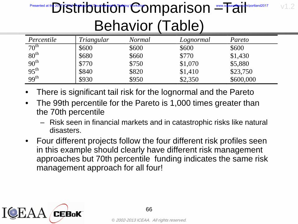
copy 2002-2013 ICEAA All rights reserved
v12Distribution Comparison ndash Tail Behavior (Table)
bull There is significant tail risk for the lognormal and the Paretobull The 99th percentile for the Pareto is 1000 times greater than
the 70th percentilendash Risk seen in financial markets and in catastrophic risks like natural
disasters bull Four different projects follow the four different risk profiles seen
in this example should clearly have different risk management approaches but 70th percentile funding indicates the same risk management approach for all four
66
Percentile Triangular Normal Lognormal Pareto 70th $600 $600 $600 $600 80th $680 $660 $770 $1430 90th $770 $750 $1070 $5880 95th $840 $820 $1410 $23750 99th $930 $950 $2350 $600000
Presented at the 2017 ICEAA Professional Development amp Training Workshop wwwiceaaonlinecomportland2017
copy 2002-2013 ICEAA All rights reserved
v12Percentile Budgeting is Not Risk Management
bull Percentile budgeting ne effective risk management policybull Suppose that you are shopping for a new car You
mention that safety is your top concern The salesman says he has a great safe car available You ask about the air bags Do they work The salesman answers ldquoOf course Seventy percent of the time they work fine Only 30 of the time the air bags will fail to deployrdquo Would you buy such a car Hedge fund manager David Einhorn has stated ldquoRisk management is the air bag that must always work but only in the multi-sigma event where you have an accidentrdquo
67
Risk management is the air bag that must always work but only in the multi-sigma event where you
have an accident
Presented at the 2017 ICEAA Professional Development amp Training Workshop wwwiceaaonlinecomportland2017
copy 2002-2013 ICEAA All rights reserved
v12
Joint Confidence Level Analysisbull Schedules are risky toobull For 98 recent NASA missions average
schedule growth was 38ndash Not as high as cost growth but still significant
68
0
5
10
15
20
25
30
35
40
Schedule
Cost
Presented at the 2017 ICEAA Professional Development amp Training Workshop wwwiceaaonlinecomportland2017
copy 2002-2013 ICEAA All rights reserved
v12
Schedules Impact Costbull Changes in schedule can have enormous
impacts on cost ndash Schedule slips can lead to cost increases
bull Fixed programmatic costs must be paid on a regular basisndash Achieving schedule milestones early can result in cost
savings
bull Schedule is an important consideration in cost analysis including cost risk analysis
bull However we must be careful in correctly integrating cost and schedule riskndash Schedule is not simply an input but is dependent on many of
the same factors that drive cost
69
Presented at the 2017 ICEAA Professional Development amp Training Workshop wwwiceaaonlinecomportland2017
copy 2002-2013 ICEAA All rights reserved
v12
The Relationship of Cost to Schedulebull Cost and schedule are positively correlated
ndash A larger program with bigger scope with take longer to complete than a smaller simpler program
bull However longer schedules do not always equate to higher cost nor shorter schedules with lower costndash Highly compressed schedules relative to the
optimal schedule can lead to large overrunsbull Compressed schedules are commonplace for
many planetary missions
70
Presented at the 2017 ICEAA Professional Development amp Training Workshop wwwiceaaonlinecomportland2017
copy 2002-2013 ICEAA All rights reserved
v12The Impact of Schedule GrowthCompression on Cost
bull Compressed schedules lead to cost growth and based on existing research is actually more expensive than schedule slippages
71
0
20
40
60
80
100
120
140
160
-50 -25 0 25 50 75 100
Percentage Change in Schedule
Perc
enta
ge C
hang
e in
Cos
t due
to
Sche
dule
Cha
nge
Source Smart CB ldquoCost and Schedule Interrelationshipsrdquo 2007 NASA Cost Symposium
Presented at the 2017 ICEAA Professional Development amp Training Workshop wwwiceaaonlinecomportland2017
copy 2002-2013 ICEAA All rights reserved
v12Schedule as an Independent Variable
bull Why not simply add schedule as an input to cost-estimating relationships (CERs)
bull Schedule is often treated as an independent variable ndash schedules are often determined independently of cost considerationsndash Cost may not be considered explicitly although budgets and
schedules are determined based on scope and other common factors
bull In 2006 SAIC undertook a research task to determine the impact of schedule on cost and added schedule as an independent variable to the CERs in the NASAAir Force Cost Model (NAFCOM) to see if schedule provided any improvement in goodness of fit
72
Presented at the 2017 ICEAA Professional Development amp Training Workshop wwwiceaaonlinecomportland2017
copy 2002-2013 ICEAA All rights reserved
v12
Schedule is a Dependent Variablebull Since NAFCOM includes an exhaustive list of cost drivers the inclusion
of schedule should give an indication of whether there is any additional independent value added from schedule independent of the cost drivers
bull In the study schedule was added to 10 subsystem-level CERs
ndash In each case the addition of schedule did NOTimprove the goodness of fit and schedule was NOT found to be a statistically significant cost driver (given the presence of the other variables) for any of the 10 CERs
bull Standard errors for the CERs increased due to decrease in degrees of freedom
bull Thus schedule as an independent variable did not provide any additional explanation of variation in historical cost
bull This is because schedule is truly NOT an independent variable but a dependent variable and is a function of the same factors that drive cost
73
Presented at the 2017 ICEAA Professional Development amp Training Workshop wwwiceaaonlinecomportland2017
copy 2002-2013 ICEAA All rights reserved
v12
Incorporation of Schedule in Cost Risk
bull When using subjective methods care must be taken in applying schedule to cost risk analysis
bull Since schedule is a dependent variable treating it independently from other factors when assessing its impact on cost can lead to a double count of independent variables in the cost risk analysis
bull Direct inclusion of schedule in a cost risk analysis effectively doubles the influence of each cost driver
ndash Incorrectly leads to broader risk ranges
74
CostWeight
HeritageNewness
Technology Readiness Schedule
Presented at the 2017 ICEAA Professional Development amp Training Workshop wwwiceaaonlinecomportland2017
copy 2002-2013 ICEAA All rights reserved
v12Subjective Cost Risk Methods and Overinclusion of Risk Factors
bull Subjective methods are suitable when data are scarce or not availablebull However care must be taken not to treat correlated sources of risk
such as schedule as independent of each otherbull Example ndash a subjective risk analysis incorporated technology readiness
design risk requirements stability integration risk and schedule and treated each source of risk as independent
bull Risk triangle high value without schedule risk was 31 times the point estimate
bull Risk triangle high value with schedule risk added on top of other sources of risk treated independently was 34 times the point estimate
bull Risk triangle taking correlation between sources of risk into account in a rigorous statistical manner has a high value 15 times the point estimate less than half the effect when treating sources of risk as independent
75
Presented at the 2017 ICEAA Professional Development amp Training Workshop wwwiceaaonlinecomportland2017
copy 2002-2013 ICEAA All rights reserved
v12Fundamental Equation of Cost and Schedule Interrelationships
bull The Fundamental Equation of the Relationship Between Cost and Schedule is
Time = Moneybull This is a well known adage that time is money Your boss at
work may even mention this to you from time to time or if you are the boss you are all too aware of this iron law
bull Because time is money cost and schedule risk should be modeled jointly not with schedule as an independent cost driver
bull Note that cost and schedule are not perfectly correlatedndash Cost can sometimes ldquobuy downrdquo schedule extra money can be
spent to meet a deadline since in some cases additional effort to hasten the completion of a task
76
Presented at the 2017 ICEAA Professional Development amp Training Workshop wwwiceaaonlinecomportland2017
copy 2002-2013 ICEAA All rights reserved
v12How to (Correctly) Incorporate Schedule into Cost Risk Analysis
bull The best way to model cost and schedule risk is to develop a joint cost and schedule model based on the same data
bull Since such models are not currently available the next best approach is to model cost and schedule independently and then integrate cost and schedule risk analyses using joint probability distributions taking into account correlation between cost and schedulendash This approach pioneered by Paul Garvey and Steve Book is
considered industry best practicendash This is a practical method mathematically tractable and follows
naturally from the Fundamental Equation of Cost and Schedule Interrelationships
77
Book S A ldquoQuantifying the Relationship Between Cost and Schedulerdquo The Measurable News Winter 2007-2008 pp 11-15Garvey PR Probability Methods for Cost Uncertainty Analysis A Systems Engineering Perspective New York Marcel Dekker 2000 pp 308-335
Presented at the 2017 ICEAA Professional Development amp Training Workshop wwwiceaaonlinecomportland2017
copy 2002-2013 ICEAA All rights reserved
v12
Joint Lognormal and Normal Distributions
bull Cost and schedule are typically modeled as some combination of Normal and Lognormal probability distributionsndash Studies by The Aerospace Corporation the MITRE
Corporation Wyle Labs and SAIC have found that the Lognormal probability distribution almost always serves as a good model for both the schedule distribution and the cost distribution
ndash The Normal distribution may also be appropriate in some instances and depending upon the level of confidence at which budgets are set may even be more conservative and logically consistent than the Normal distribution
ndash Joint Lognormal and Normal distributions are defined by a pair of mean and standard deviations and a level of correlation between the two
78
Presented at the 2017 ICEAA Professional Development amp Training Workshop wwwiceaaonlinecomportland2017
copy 2002-2013 ICEAA All rights reserved
v12Modeling Cost and Schedule as a Bivariate Distribution
bull In the approach set forth by Book and Garvey cost risk is assessed and the top-level distribution is modeled as a Lognormal (or Normal) distribution schedule risk is assessed and the overall schedule risk is modeled as a Lognormal (or Normal) distribution
bull The two distributions are combined into a Bivariate distribution by assigning a correlation between the two and by treating the two distributions as the marginal distributions of a Bivariate Lognormal distributionndash Other combinations include a Bivariate Normal or a Bivariate
Normal-Lognormal
79
Presented at the 2017 ICEAA Professional Development amp Training Workshop wwwiceaaonlinecomportland2017
copy 2002-2013 ICEAA All rights reserved
v12Bivariate Lognormal Distribution for Cost and Schedule
bull Cost is often observed to be Lognormal when strong positive correlations are present among the systemrsquos WBS cost element costs
bull A systemrsquos schedule is often observed (from Monte Carlo simulations) to be Lognormal if it is the sum of many positively correlated schedule activities in an overall schedule network
bull If Lognormal distributions characterize a systemrsquos cost and schedule then the Bivariate Lognormal could serve as an assumed model of their joint distributionndash In this case the marginal distribution of each of cost and schedule is
Lognormalbull Other possibilities for modeling cost and schedule as a Bivariate
distribution include a Bivariate Normal or a Bivariate Normal-Lognormal distributionndash All these combinations are analytically tractable
80
Presented at the 2017 ICEAA Professional Development amp Training Workshop wwwiceaaonlinecomportland2017
copy 2002-2013 ICEAA All rights reserved
v12Bivariate Lognormal for Cost and Schedule
bull Contour Plots of a Bivariate Lognormal
81
Presented at the 2017 ICEAA Professional Development amp Training Workshop wwwiceaaonlinecomportland2017
copy 2002-2013 ICEAA All rights reserved
v12Correlation Between Cost and Schedule
bull Cost and schedule are positively correlated but not perfectly sondash For example it is possible to have a schedule underrun and a cost
overrunbull Based on cost and schedule growth data for 50 completed NASA
programs the correlation between development cost and development schedule is 70
82
00
200
400
600
800
1000
1200
-500 00 500 1000 1500 2000 2500Historical Cost Growth
Hist
oric
al S
ched
ule
Gro
wth
r = 715
Presented at the 2017 ICEAA Professional Development amp Training Workshop wwwiceaaonlinecomportland2017
copy 2002-2013 ICEAA All rights reserved
v12Correlation Between Cost and Schedule Caveats
bull Based on historical data recommended correlation between cost and schedule is 70 but this could be higher or lower depending upon program circumstancesndash If program is budget constrained cost and schedule will be
more highly correlated (go as you pay)ndash If program is schedule constrained cost and schedule will
have lower correlation perhaps even negative correlation ndash Smaller programs have smaller correlation between cost and
schedule riskbull Relatively easy to ldquohurry uprdquo and finish on time or even early if
needed
83
Presented at the 2017 ICEAA Professional Development amp Training Workshop wwwiceaaonlinecomportland2017
copy 2002-2013 ICEAA All rights reserved
v12
Conditional Confidence Levelsbull Given a programrsquos project schedule we can determine the cost
risk distribution conditional upon the given schedulebull Conditional cost S-curves are steeper than unconditional
(marginal) cost S-curves between some uncertainty has been removed because schedule is fixed
84
Presented at the 2017 ICEAA Professional Development amp Training Workshop wwwiceaaonlinecomportland2017
copy 2002-2013 ICEAA All rights reserved
v12
Joint Confidence Levelsbull Joint 65 confidence represents the probability of
achieving both 65 confidence in cost AND 65 confidence in schedulendash This is different than achieving 65 cost confidence alone
or achieving 65 schedule confidence alonebull Due to the imperfect correlation between cost and schedule it
is possible to achieve a 65 cost confidence with a lower level of schedule confidence
bull Restricting the schedule confidence thus requires additional $ to achieve a given level of confidence
85
X
Y
Possible Values for Which X gt a Possible Values for
Which X gt a and Y gt b
a
b
Presented at the 2017 ICEAA Professional Development amp Training Workshop wwwiceaaonlinecomportland2017
copy 2002-2013 ICEAA All rights reserved
v12Joint Confidence Levels Versus Cost Confidence Levels Only
bull Example of the differences between cost confidence schedule confidence conditional cost confidence and joint cost and schedule confidence
86
Joint Cost-Schedule Confidence Iso-Curves
Cost (RY$M)
Sche
dule
(Mon
ths)
65 Confidence
50 Confidence
70 Confidence
65 Cost Confidence AggressiveSchedule65 Cost ConfidenceScheduleGiven 65 Schedule ConfidenceUnconditional 65 CostConfidenceUnconditional 65 ScheduleConfidence
65 Cost Confidence 65 Joint Cost and Schedule
Confidence for 65 Schedule Confidence
Presented at the 2017 ICEAA Professional Development amp Training Workshop wwwiceaaonlinecomportland2017
copy 2002-2013 ICEAA All rights reserved
v12
Joint Cost and Schedule Confidence
bull Can examine pairs of cost and schedule that achieve a given level of confidence
bull Provides insights into the trade-offs between cost and schedule for a given level of confidencendash Possible to increase cost confidence by giving a
project more time in some instances or possible to ldquobuy downrdquo schedule
bull But these have limits and are shown in the iso-cost and schedule confidence curves
87
Presented at the 2017 ICEAA Professional Development amp Training Workshop wwwiceaaonlinecomportland2017
copy 2002-2013 ICEAA All rights reserved
v12Cost and Schedule Trade-offs for a Given Level of Joint Confidence
bull Hypothetical Example
88
Cost (RY$M)
Schedule (Months)
$100 48$99 48$89 49$87 50$85 51$85 52$84 53$83 55$83 55$83 56
Cost and Schedule 65 Confidence Iso-Curve
4748495051525354555657
$80 $82 $84 $86 $88 $90 $92 $94 $96 $98 $100
Cost (RY$ M)
Sche
dule
(Mon
ths)
Presented at the 2017 ICEAA Professional Development amp Training Workshop wwwiceaaonlinecomportland2017
copy 2002-2013 ICEAA All rights reserved
v12Policy Considerations for Confidence Levels
bull For large programs the difference between the amount of money needed to achieve 65 cost confidence independent of schedule and joint 65 cost and schedule confidence can represent hundreds of millions and even billions of dollars
89
Joint Cost-Schedule Confidence Iso-Curves
Cost (RY$M)
Sche
dule
(Mon
ths)
65 Confidence
65 Cost Confidence AggressiveSchedule
65 Cost ConfidenceScheduleGiven 65 Schedule Confidence
Unconditional 65 CostConfidence
Joint Cost and Schedule Confidence for 65 Cost Confidence and Program Baseline Schedule is Less Than 35
65 Cost Confidence Independent of Schedule Cost Needed to Achieve
Both 65 Joint Cost and Schedule Confidence for the Schedule with 65 Confidence
Presented at the 2017 ICEAA Professional Development amp Training Workshop wwwiceaaonlinecomportland2017
copy 2002-2013 ICEAA All rights reserved
v12
Copulasbull More generally any combination of distributions can
be used (more than just normal and lognormal)ndash Termed ldquocopulardquo from the Italian word for ldquocouplerdquondash Copulas are a way to combine marginal distributions of any
number and type into a joint distributionbull More formally a copula is a multivariate joint distribution defined
on the n-dimensional unit cube [0 1]n such that every marginal distribution is uniform on the interval [0 1]
bull (The bivariate form of) Sklarrsquos theorem states that for any bivariate distribution function H(x y) let F(x) = H(x infin) and G(y) = H(infin y) be the univariate marginal probability distribution functions Then there exists a copula C such that H(xy)=C(F(x)G(y))
ndash Copulas are widely used in risk management for investments and insurance
bull Considered industry best practice (Li 2000)bull Marketed as part of JP Morganrsquos CreditMetrics suite of tools
(Gupton et Al 1997)90
Presented at the 2017 ICEAA Professional Development amp Training Workshop wwwiceaaonlinecomportland2017
copy 2002-2013 ICEAA All rights reserved
v12Parametric Joint Cost and Schedule Analysis
bull A parametric model based on a consistent data set with a set of overlapping cost and schedule drivers is a cleaner way to model cost and schedule
91
CostWeight
HeritageNewness
Technology Readiness
Schedule
0
20
40
60
80
100
Confidence
Joint Cost and Schedule Confidence
Schedule
Cost
Lognormal Distribution PDF and CDF
0102030405060708090100
200 300 400 500 600 700 800 900 1000Cost $
Con
fiden
ce L
evel
0
00002
00004
00006
00008
0001
00012
00014
00016
Prob
abili
ty D
ensi
ty
CDFPDF
Lognormal Distribution PDF and CDF
0102030405060708090100
200 300 400 500 600 700 800 900 1000Cost $
Con
fiden
ce L
evel
0
00002
00004
00006
00008
0001
00012
00014
00016
Prob
abili
ty D
ensi
ty
CDFPDF
Presented at the 2017 ICEAA Professional Development amp Training Workshop wwwiceaaonlinecomportland2017
copy 2002-2013 ICEAA All rights reserved
v12Parametric Joint Cost and Schedule Analysis (2)
bull Joint cost and schedule risk analysis produced naturally by the integrated modelndash Addresses several issues with the copula
approachbull Tail dependencybull Correlation ndash no need to assign correlation
between cost and schedulebull Consistency of cost and schedule models
92
Presented at the 2017 ICEAA Professional Development amp Training Workshop wwwiceaaonlinecomportland2017
copy 2002-2013 ICEAA All rights reserved
v12
Resource-Loaded Schedulesbull Involves assigning cost and schedule risks to a resource-loaded schedule
networkbull Bottom-up approach
ndash More labor intensive than parametrics but can also provide more insight
ndash Can answer questions than parametric typically cannot such as how much do reserve requirements decrease if a specific risk is retired
bull Currently being implemented in Constellation programbull Has same issue as all bottom-up models hard to count all the risks and model
them discretely
ndash As a result there is a tendency to reflect less risk than indicated by history
ndash ldquoThere are more things in heaven and earth Horatio than are dreamt of in your philosophyrdquo William Shakespeare Hamlet Act I Scene V
93
Presented at the 2017 ICEAA Professional Development amp Training Workshop wwwiceaaonlinecomportland2017
copy 2002-2013 ICEAA All rights reserved
v12Resource-Loaded Schedules Vs Parametrics
bull Parametric most appropriate for early estimatesndash But also good for high-level checks as project progresses
bull As plans take shape lower level modeling may be more appropriate
94 1
CONCEPTUALDEVELOPMENT
PROJECTDEFINITION DESIGN DEVELOPMENT OPERATIONS
PARAMETRIC PARAMETRIC
ANALOGY
ENGINEERING (Bottoms Up)
$PARAMETRIC
DETAILED
$
Pre Phase A Phase B Phase CDPhase A Phase EPre Phase A Phase B Phase CDPhase A Phase E
Risk = f(Cost Estimating Relationship Inputs eg mass power data rate TRL new design etc)
Risk = f(cost and schedule variation of the analogous elements)
Risk = f(variation of detailed inputs eg labor hours rates materials etc)
Presented at the 2017 ICEAA Professional Development amp Training Workshop wwwiceaaonlinecomportland2017
copy 2002-2013 ICEAA All rights reserved
v12
Resource-Loaded Schedulesbull Methodology has been demonstrated in other
industriesndash Construction oil and gasndash Analysis has not been traditionally done on highly uncertain
complex development projects bull Methodology focuses on project baseline schedule
ndash In baseline schedule all tasks are resource loaded to represent a baseline schedule and cost standpoint
ndash Resource loaded schedule is ldquorolledrdquo up to a manageable level
ndash Based on the risk and uncertainties identified schedule distributions are applied to each rolled up task
ndash Cost uncertainties are also applied to rolled up tasksbull Uncertainties include labor rate man power etc
ndash A Monte Carlo simulation is run to develop joint cost-schedule distributions
95
Presented at the 2017 ICEAA Professional Development amp Training Workshop wwwiceaaonlinecomportland2017
copy 2002-2013 ICEAA All rights reserved
v12
Unit III - Module 9 96
Execution ndash Cross Checksbull Means The mean cost growth factor for WBS items
can be compared to history as a way to cross check results
bull CVs The CV of the cost growth factors for WBS items can be compared to history as a way to cross check results
bull Inputs Checks are performed on inputs or other parameters to see if historical values are in line with program assumptionsndash Example Historical risk scores can be compared to program
risk scores to see if risk assessors are being realistic and to see if the underlying database is representative of the program
11
Presented at the 2017 ICEAA Professional Development amp Training Workshop wwwiceaaonlinecomportland2017
- Cost and Schedule Risk Analysis Basic
- Acknowledgments
- Unit Index
- Risk Overview
- Agenda
- Introduction
- Risk Analysis Terms
- Are Our Costs Realistic
- Historical Cost Growth
- Sources of Cost Risk
- Point Estimates of Cost
- Types of Risk
- Point Estimates Vs Risk Estimates
- Cost Risk and Probability
- Probability Model ndash Distribution
- Probability Model ndash Distribution
- Probability ndash Top-Level Distribution
- S-Curves and Confidence Levels
- Example ndash Normal Distribution
- Confidence Levels
- Measuring Parametric Model Uncertainty
- Parametric Model Example
- Weight Uncertainty
- Estimating Uncertainty
- Estimating Uncertainty (2)
- Estimating Uncertainty (3)
- Aggregating Risk
- WBS Example
- WBS and Risk
- Aggregating Risk
- Percentiles Do Not Add
- Percentiles Do Not Add (2)
- Percentiles Do Not Add (3)
- Methods for Aggregating Risk
- Monte Carlo Simulationfor Risk Analysis
- Monte Carlo Simulation
- Using Random Numbers to Simulate Distributions
- Simulating a Triangular Distribution
- Simulating a Triangular Distribution (2)
- Monte Carlo and the WBS
- Number of Trials
- Number of Trials (2)
- Number of Trials (3)
- Number of Trials (4)
- Number of Trials (5)
- Number of Trials (6)
- Methods of Simulation
- Probability Model ndash Correlation
- Correlation And Causation
- The Importance of Correlation
- The Importance of Correlation (2)
- Measures of Correlation
- Pearson Correlation
- Spearman Correlation
- Functional Correlation
- Risk Measures
- Value at Risk (VaR)
- Why 70th or 80th Percentile
- Funding Above Inflection Points
- Why Budget to the 70th or 80th
- Inflection Points for Lognormal
- Issues with Percentile Funding
- ldquoHere There Be Dragonsrdquo
- Distribution Comparison
- Distribution Comparison Tail Behavior
- Distribution Comparison ndash Tail Behavior (Table)
- Percentile Budgeting is Not Risk Management
- Joint Confidence Level Analysis
- Schedules Impact Cost
- The Relationship of Cost to Schedule
- The Impact of Schedule GrowthCompression on Cost
- Schedule as an Independent Variable
- Schedule is a Dependent Variable
- Incorporation of Schedule in Cost Risk
- Subjective Cost Risk Methods and Overinclusion of Risk Factors
- Fundamental Equation of Cost and Schedule Interrelationships
- How to (Correctly) Incorporate Schedule into Cost Risk Analysis
- Joint Lognormal and Normal Distributions
- Modeling Cost and Schedule as a Bivariate Distribution
- Bivariate Lognormal Distribution for Cost and Schedule
- Bivariate Lognormal for Cost and Schedule
- Correlation Between Cost and Schedule
- Correlation Between Cost and Schedule Caveats
- Conditional Confidence Levels
- Joint Confidence Levels
- Joint Confidence Levels Versus Cost Confidence Levels Only
- Joint Cost and Schedule Confidence
- Cost and Schedule Trade-offs for a Given Level of Joint Confidence
- Policy Considerations for Confidence Levels
- Copulas
- Parametric Joint Cost and Schedule Analysis
- Parametric Joint Cost and Schedule Analysis (2)
- Resource-Loaded Schedules
- Resource-Loaded Schedules Vs Parametrics
- Resource-Loaded Schedules
- Execution ndash Cross Checks
-
copy 2002-2013 ICEAA All rights reserved
v12Percentile Budgeting is Not Risk Management
bull Percentile budgeting ne effective risk management policybull Suppose that you are shopping for a new car You
mention that safety is your top concern The salesman says he has a great safe car available You ask about the air bags Do they work The salesman answers ldquoOf course Seventy percent of the time they work fine Only 30 of the time the air bags will fail to deployrdquo Would you buy such a car Hedge fund manager David Einhorn has stated ldquoRisk management is the air bag that must always work but only in the multi-sigma event where you have an accidentrdquo
67
Risk management is the air bag that must always work but only in the multi-sigma event where you
have an accident
Presented at the 2017 ICEAA Professional Development amp Training Workshop wwwiceaaonlinecomportland2017
copy 2002-2013 ICEAA All rights reserved
v12
Joint Confidence Level Analysisbull Schedules are risky toobull For 98 recent NASA missions average
schedule growth was 38ndash Not as high as cost growth but still significant
68
0
5
10
15
20
25
30
35
40
Schedule
Cost
Presented at the 2017 ICEAA Professional Development amp Training Workshop wwwiceaaonlinecomportland2017
copy 2002-2013 ICEAA All rights reserved
v12
Schedules Impact Costbull Changes in schedule can have enormous
impacts on cost ndash Schedule slips can lead to cost increases
bull Fixed programmatic costs must be paid on a regular basisndash Achieving schedule milestones early can result in cost
savings
bull Schedule is an important consideration in cost analysis including cost risk analysis
bull However we must be careful in correctly integrating cost and schedule riskndash Schedule is not simply an input but is dependent on many of
the same factors that drive cost
69
Presented at the 2017 ICEAA Professional Development amp Training Workshop wwwiceaaonlinecomportland2017
copy 2002-2013 ICEAA All rights reserved
v12
The Relationship of Cost to Schedulebull Cost and schedule are positively correlated
ndash A larger program with bigger scope with take longer to complete than a smaller simpler program
bull However longer schedules do not always equate to higher cost nor shorter schedules with lower costndash Highly compressed schedules relative to the
optimal schedule can lead to large overrunsbull Compressed schedules are commonplace for
many planetary missions
70
Presented at the 2017 ICEAA Professional Development amp Training Workshop wwwiceaaonlinecomportland2017
copy 2002-2013 ICEAA All rights reserved
v12The Impact of Schedule GrowthCompression on Cost
bull Compressed schedules lead to cost growth and based on existing research is actually more expensive than schedule slippages
71
0
20
40
60
80
100
120
140
160
-50 -25 0 25 50 75 100
Percentage Change in Schedule
Perc
enta
ge C
hang
e in
Cos
t due
to
Sche
dule
Cha
nge
Source Smart CB ldquoCost and Schedule Interrelationshipsrdquo 2007 NASA Cost Symposium
Presented at the 2017 ICEAA Professional Development amp Training Workshop wwwiceaaonlinecomportland2017
copy 2002-2013 ICEAA All rights reserved
v12Schedule as an Independent Variable
bull Why not simply add schedule as an input to cost-estimating relationships (CERs)
bull Schedule is often treated as an independent variable ndash schedules are often determined independently of cost considerationsndash Cost may not be considered explicitly although budgets and
schedules are determined based on scope and other common factors
bull In 2006 SAIC undertook a research task to determine the impact of schedule on cost and added schedule as an independent variable to the CERs in the NASAAir Force Cost Model (NAFCOM) to see if schedule provided any improvement in goodness of fit
72
Presented at the 2017 ICEAA Professional Development amp Training Workshop wwwiceaaonlinecomportland2017
copy 2002-2013 ICEAA All rights reserved
v12
Schedule is a Dependent Variablebull Since NAFCOM includes an exhaustive list of cost drivers the inclusion
of schedule should give an indication of whether there is any additional independent value added from schedule independent of the cost drivers
bull In the study schedule was added to 10 subsystem-level CERs
ndash In each case the addition of schedule did NOTimprove the goodness of fit and schedule was NOT found to be a statistically significant cost driver (given the presence of the other variables) for any of the 10 CERs
bull Standard errors for the CERs increased due to decrease in degrees of freedom
bull Thus schedule as an independent variable did not provide any additional explanation of variation in historical cost
bull This is because schedule is truly NOT an independent variable but a dependent variable and is a function of the same factors that drive cost
73
Presented at the 2017 ICEAA Professional Development amp Training Workshop wwwiceaaonlinecomportland2017
copy 2002-2013 ICEAA All rights reserved
v12
Incorporation of Schedule in Cost Risk
bull When using subjective methods care must be taken in applying schedule to cost risk analysis
bull Since schedule is a dependent variable treating it independently from other factors when assessing its impact on cost can lead to a double count of independent variables in the cost risk analysis
bull Direct inclusion of schedule in a cost risk analysis effectively doubles the influence of each cost driver
ndash Incorrectly leads to broader risk ranges
74
CostWeight
HeritageNewness
Technology Readiness Schedule
Presented at the 2017 ICEAA Professional Development amp Training Workshop wwwiceaaonlinecomportland2017
copy 2002-2013 ICEAA All rights reserved
v12Subjective Cost Risk Methods and Overinclusion of Risk Factors
bull Subjective methods are suitable when data are scarce or not availablebull However care must be taken not to treat correlated sources of risk
such as schedule as independent of each otherbull Example ndash a subjective risk analysis incorporated technology readiness
design risk requirements stability integration risk and schedule and treated each source of risk as independent
bull Risk triangle high value without schedule risk was 31 times the point estimate
bull Risk triangle high value with schedule risk added on top of other sources of risk treated independently was 34 times the point estimate
bull Risk triangle taking correlation between sources of risk into account in a rigorous statistical manner has a high value 15 times the point estimate less than half the effect when treating sources of risk as independent
75
Presented at the 2017 ICEAA Professional Development amp Training Workshop wwwiceaaonlinecomportland2017
copy 2002-2013 ICEAA All rights reserved
v12Fundamental Equation of Cost and Schedule Interrelationships
bull The Fundamental Equation of the Relationship Between Cost and Schedule is
Time = Moneybull This is a well known adage that time is money Your boss at
work may even mention this to you from time to time or if you are the boss you are all too aware of this iron law
bull Because time is money cost and schedule risk should be modeled jointly not with schedule as an independent cost driver
bull Note that cost and schedule are not perfectly correlatedndash Cost can sometimes ldquobuy downrdquo schedule extra money can be
spent to meet a deadline since in some cases additional effort to hasten the completion of a task
76
Presented at the 2017 ICEAA Professional Development amp Training Workshop wwwiceaaonlinecomportland2017
copy 2002-2013 ICEAA All rights reserved
v12How to (Correctly) Incorporate Schedule into Cost Risk Analysis
bull The best way to model cost and schedule risk is to develop a joint cost and schedule model based on the same data
bull Since such models are not currently available the next best approach is to model cost and schedule independently and then integrate cost and schedule risk analyses using joint probability distributions taking into account correlation between cost and schedulendash This approach pioneered by Paul Garvey and Steve Book is
considered industry best practicendash This is a practical method mathematically tractable and follows
naturally from the Fundamental Equation of Cost and Schedule Interrelationships
77
Book S A ldquoQuantifying the Relationship Between Cost and Schedulerdquo The Measurable News Winter 2007-2008 pp 11-15Garvey PR Probability Methods for Cost Uncertainty Analysis A Systems Engineering Perspective New York Marcel Dekker 2000 pp 308-335
Presented at the 2017 ICEAA Professional Development amp Training Workshop wwwiceaaonlinecomportland2017
copy 2002-2013 ICEAA All rights reserved
v12
Joint Lognormal and Normal Distributions
bull Cost and schedule are typically modeled as some combination of Normal and Lognormal probability distributionsndash Studies by The Aerospace Corporation the MITRE
Corporation Wyle Labs and SAIC have found that the Lognormal probability distribution almost always serves as a good model for both the schedule distribution and the cost distribution
ndash The Normal distribution may also be appropriate in some instances and depending upon the level of confidence at which budgets are set may even be more conservative and logically consistent than the Normal distribution
ndash Joint Lognormal and Normal distributions are defined by a pair of mean and standard deviations and a level of correlation between the two
78
Presented at the 2017 ICEAA Professional Development amp Training Workshop wwwiceaaonlinecomportland2017
copy 2002-2013 ICEAA All rights reserved
v12Modeling Cost and Schedule as a Bivariate Distribution
bull In the approach set forth by Book and Garvey cost risk is assessed and the top-level distribution is modeled as a Lognormal (or Normal) distribution schedule risk is assessed and the overall schedule risk is modeled as a Lognormal (or Normal) distribution
bull The two distributions are combined into a Bivariate distribution by assigning a correlation between the two and by treating the two distributions as the marginal distributions of a Bivariate Lognormal distributionndash Other combinations include a Bivariate Normal or a Bivariate
Normal-Lognormal
79
Presented at the 2017 ICEAA Professional Development amp Training Workshop wwwiceaaonlinecomportland2017
copy 2002-2013 ICEAA All rights reserved
v12Bivariate Lognormal Distribution for Cost and Schedule
bull Cost is often observed to be Lognormal when strong positive correlations are present among the systemrsquos WBS cost element costs
bull A systemrsquos schedule is often observed (from Monte Carlo simulations) to be Lognormal if it is the sum of many positively correlated schedule activities in an overall schedule network
bull If Lognormal distributions characterize a systemrsquos cost and schedule then the Bivariate Lognormal could serve as an assumed model of their joint distributionndash In this case the marginal distribution of each of cost and schedule is
Lognormalbull Other possibilities for modeling cost and schedule as a Bivariate
distribution include a Bivariate Normal or a Bivariate Normal-Lognormal distributionndash All these combinations are analytically tractable
80
Presented at the 2017 ICEAA Professional Development amp Training Workshop wwwiceaaonlinecomportland2017
copy 2002-2013 ICEAA All rights reserved
v12Bivariate Lognormal for Cost and Schedule
bull Contour Plots of a Bivariate Lognormal
81
Presented at the 2017 ICEAA Professional Development amp Training Workshop wwwiceaaonlinecomportland2017
copy 2002-2013 ICEAA All rights reserved
v12Correlation Between Cost and Schedule
bull Cost and schedule are positively correlated but not perfectly sondash For example it is possible to have a schedule underrun and a cost
overrunbull Based on cost and schedule growth data for 50 completed NASA
programs the correlation between development cost and development schedule is 70
82
00
200
400
600
800
1000
1200
-500 00 500 1000 1500 2000 2500Historical Cost Growth
Hist
oric
al S
ched
ule
Gro
wth
r = 715
Presented at the 2017 ICEAA Professional Development amp Training Workshop wwwiceaaonlinecomportland2017
copy 2002-2013 ICEAA All rights reserved
v12Correlation Between Cost and Schedule Caveats
bull Based on historical data recommended correlation between cost and schedule is 70 but this could be higher or lower depending upon program circumstancesndash If program is budget constrained cost and schedule will be
more highly correlated (go as you pay)ndash If program is schedule constrained cost and schedule will
have lower correlation perhaps even negative correlation ndash Smaller programs have smaller correlation between cost and
schedule riskbull Relatively easy to ldquohurry uprdquo and finish on time or even early if
needed
83
Presented at the 2017 ICEAA Professional Development amp Training Workshop wwwiceaaonlinecomportland2017
copy 2002-2013 ICEAA All rights reserved
v12
Conditional Confidence Levelsbull Given a programrsquos project schedule we can determine the cost
risk distribution conditional upon the given schedulebull Conditional cost S-curves are steeper than unconditional
(marginal) cost S-curves between some uncertainty has been removed because schedule is fixed
84
Presented at the 2017 ICEAA Professional Development amp Training Workshop wwwiceaaonlinecomportland2017
copy 2002-2013 ICEAA All rights reserved
v12
Joint Confidence Levelsbull Joint 65 confidence represents the probability of
achieving both 65 confidence in cost AND 65 confidence in schedulendash This is different than achieving 65 cost confidence alone
or achieving 65 schedule confidence alonebull Due to the imperfect correlation between cost and schedule it
is possible to achieve a 65 cost confidence with a lower level of schedule confidence
bull Restricting the schedule confidence thus requires additional $ to achieve a given level of confidence
85
X
Y
Possible Values for Which X gt a Possible Values for
Which X gt a and Y gt b
a
b
Presented at the 2017 ICEAA Professional Development amp Training Workshop wwwiceaaonlinecomportland2017
copy 2002-2013 ICEAA All rights reserved
v12Joint Confidence Levels Versus Cost Confidence Levels Only
bull Example of the differences between cost confidence schedule confidence conditional cost confidence and joint cost and schedule confidence
86
Joint Cost-Schedule Confidence Iso-Curves
Cost (RY$M)
Sche
dule
(Mon
ths)
65 Confidence
50 Confidence
70 Confidence
65 Cost Confidence AggressiveSchedule65 Cost ConfidenceScheduleGiven 65 Schedule ConfidenceUnconditional 65 CostConfidenceUnconditional 65 ScheduleConfidence
65 Cost Confidence 65 Joint Cost and Schedule
Confidence for 65 Schedule Confidence
Presented at the 2017 ICEAA Professional Development amp Training Workshop wwwiceaaonlinecomportland2017
copy 2002-2013 ICEAA All rights reserved
v12
Joint Cost and Schedule Confidence
bull Can examine pairs of cost and schedule that achieve a given level of confidence
bull Provides insights into the trade-offs between cost and schedule for a given level of confidencendash Possible to increase cost confidence by giving a
project more time in some instances or possible to ldquobuy downrdquo schedule
bull But these have limits and are shown in the iso-cost and schedule confidence curves
87
Presented at the 2017 ICEAA Professional Development amp Training Workshop wwwiceaaonlinecomportland2017
copy 2002-2013 ICEAA All rights reserved
v12Cost and Schedule Trade-offs for a Given Level of Joint Confidence
bull Hypothetical Example
88
Cost (RY$M)
Schedule (Months)
$100 48$99 48$89 49$87 50$85 51$85 52$84 53$83 55$83 55$83 56
Cost and Schedule 65 Confidence Iso-Curve
4748495051525354555657
$80 $82 $84 $86 $88 $90 $92 $94 $96 $98 $100
Cost (RY$ M)
Sche
dule
(Mon
ths)
Presented at the 2017 ICEAA Professional Development amp Training Workshop wwwiceaaonlinecomportland2017
copy 2002-2013 ICEAA All rights reserved
v12Policy Considerations for Confidence Levels
bull For large programs the difference between the amount of money needed to achieve 65 cost confidence independent of schedule and joint 65 cost and schedule confidence can represent hundreds of millions and even billions of dollars
89
Joint Cost-Schedule Confidence Iso-Curves
Cost (RY$M)
Sche
dule
(Mon
ths)
65 Confidence
65 Cost Confidence AggressiveSchedule
65 Cost ConfidenceScheduleGiven 65 Schedule Confidence
Unconditional 65 CostConfidence
Joint Cost and Schedule Confidence for 65 Cost Confidence and Program Baseline Schedule is Less Than 35
65 Cost Confidence Independent of Schedule Cost Needed to Achieve
Both 65 Joint Cost and Schedule Confidence for the Schedule with 65 Confidence
Presented at the 2017 ICEAA Professional Development amp Training Workshop wwwiceaaonlinecomportland2017
copy 2002-2013 ICEAA All rights reserved
v12
Copulasbull More generally any combination of distributions can
be used (more than just normal and lognormal)ndash Termed ldquocopulardquo from the Italian word for ldquocouplerdquondash Copulas are a way to combine marginal distributions of any
number and type into a joint distributionbull More formally a copula is a multivariate joint distribution defined
on the n-dimensional unit cube [0 1]n such that every marginal distribution is uniform on the interval [0 1]
bull (The bivariate form of) Sklarrsquos theorem states that for any bivariate distribution function H(x y) let F(x) = H(x infin) and G(y) = H(infin y) be the univariate marginal probability distribution functions Then there exists a copula C such that H(xy)=C(F(x)G(y))
ndash Copulas are widely used in risk management for investments and insurance
bull Considered industry best practice (Li 2000)bull Marketed as part of JP Morganrsquos CreditMetrics suite of tools
(Gupton et Al 1997)90
Presented at the 2017 ICEAA Professional Development amp Training Workshop wwwiceaaonlinecomportland2017
copy 2002-2013 ICEAA All rights reserved
v12Parametric Joint Cost and Schedule Analysis
bull A parametric model based on a consistent data set with a set of overlapping cost and schedule drivers is a cleaner way to model cost and schedule
91
CostWeight
HeritageNewness
Technology Readiness
Schedule
0
20
40
60
80
100
Confidence
Joint Cost and Schedule Confidence
Schedule
Cost
Lognormal Distribution PDF and CDF
0102030405060708090100
200 300 400 500 600 700 800 900 1000Cost $
Con
fiden
ce L
evel
0
00002
00004
00006
00008
0001
00012
00014
00016
Prob
abili
ty D
ensi
ty
CDFPDF
Lognormal Distribution PDF and CDF
0102030405060708090100
200 300 400 500 600 700 800 900 1000Cost $
Con
fiden
ce L
evel
0
00002
00004
00006
00008
0001
00012
00014
00016
Prob
abili
ty D
ensi
ty
CDFPDF
Presented at the 2017 ICEAA Professional Development amp Training Workshop wwwiceaaonlinecomportland2017
copy 2002-2013 ICEAA All rights reserved
v12Parametric Joint Cost and Schedule Analysis (2)
bull Joint cost and schedule risk analysis produced naturally by the integrated modelndash Addresses several issues with the copula
approachbull Tail dependencybull Correlation ndash no need to assign correlation
between cost and schedulebull Consistency of cost and schedule models
92
Presented at the 2017 ICEAA Professional Development amp Training Workshop wwwiceaaonlinecomportland2017
copy 2002-2013 ICEAA All rights reserved
v12
Resource-Loaded Schedulesbull Involves assigning cost and schedule risks to a resource-loaded schedule
networkbull Bottom-up approach
ndash More labor intensive than parametrics but can also provide more insight
ndash Can answer questions than parametric typically cannot such as how much do reserve requirements decrease if a specific risk is retired
bull Currently being implemented in Constellation programbull Has same issue as all bottom-up models hard to count all the risks and model
them discretely
ndash As a result there is a tendency to reflect less risk than indicated by history
ndash ldquoThere are more things in heaven and earth Horatio than are dreamt of in your philosophyrdquo William Shakespeare Hamlet Act I Scene V
93
Presented at the 2017 ICEAA Professional Development amp Training Workshop wwwiceaaonlinecomportland2017
copy 2002-2013 ICEAA All rights reserved
v12Resource-Loaded Schedules Vs Parametrics
bull Parametric most appropriate for early estimatesndash But also good for high-level checks as project progresses
bull As plans take shape lower level modeling may be more appropriate
94 1
CONCEPTUALDEVELOPMENT
PROJECTDEFINITION DESIGN DEVELOPMENT OPERATIONS
PARAMETRIC PARAMETRIC
ANALOGY
ENGINEERING (Bottoms Up)
$PARAMETRIC
DETAILED
$
Pre Phase A Phase B Phase CDPhase A Phase EPre Phase A Phase B Phase CDPhase A Phase E
Risk = f(Cost Estimating Relationship Inputs eg mass power data rate TRL new design etc)
Risk = f(cost and schedule variation of the analogous elements)
Risk = f(variation of detailed inputs eg labor hours rates materials etc)
Presented at the 2017 ICEAA Professional Development amp Training Workshop wwwiceaaonlinecomportland2017
copy 2002-2013 ICEAA All rights reserved
v12
Resource-Loaded Schedulesbull Methodology has been demonstrated in other
industriesndash Construction oil and gasndash Analysis has not been traditionally done on highly uncertain
complex development projects bull Methodology focuses on project baseline schedule
ndash In baseline schedule all tasks are resource loaded to represent a baseline schedule and cost standpoint
ndash Resource loaded schedule is ldquorolledrdquo up to a manageable level
ndash Based on the risk and uncertainties identified schedule distributions are applied to each rolled up task
ndash Cost uncertainties are also applied to rolled up tasksbull Uncertainties include labor rate man power etc
ndash A Monte Carlo simulation is run to develop joint cost-schedule distributions
95
Presented at the 2017 ICEAA Professional Development amp Training Workshop wwwiceaaonlinecomportland2017
copy 2002-2013 ICEAA All rights reserved
v12
Unit III - Module 9 96
Execution ndash Cross Checksbull Means The mean cost growth factor for WBS items
can be compared to history as a way to cross check results
bull CVs The CV of the cost growth factors for WBS items can be compared to history as a way to cross check results
bull Inputs Checks are performed on inputs or other parameters to see if historical values are in line with program assumptionsndash Example Historical risk scores can be compared to program
risk scores to see if risk assessors are being realistic and to see if the underlying database is representative of the program
11
Presented at the 2017 ICEAA Professional Development amp Training Workshop wwwiceaaonlinecomportland2017
- Cost and Schedule Risk Analysis Basic
- Acknowledgments
- Unit Index
- Risk Overview
- Agenda
- Introduction
- Risk Analysis Terms
- Are Our Costs Realistic
- Historical Cost Growth
- Sources of Cost Risk
- Point Estimates of Cost
- Types of Risk
- Point Estimates Vs Risk Estimates
- Cost Risk and Probability
- Probability Model ndash Distribution
- Probability Model ndash Distribution
- Probability ndash Top-Level Distribution
- S-Curves and Confidence Levels
- Example ndash Normal Distribution
- Confidence Levels
- Measuring Parametric Model Uncertainty
- Parametric Model Example
- Weight Uncertainty
- Estimating Uncertainty
- Estimating Uncertainty (2)
- Estimating Uncertainty (3)
- Aggregating Risk
- WBS Example
- WBS and Risk
- Aggregating Risk
- Percentiles Do Not Add
- Percentiles Do Not Add (2)
- Percentiles Do Not Add (3)
- Methods for Aggregating Risk
- Monte Carlo Simulationfor Risk Analysis
- Monte Carlo Simulation
- Using Random Numbers to Simulate Distributions
- Simulating a Triangular Distribution
- Simulating a Triangular Distribution (2)
- Monte Carlo and the WBS
- Number of Trials
- Number of Trials (2)
- Number of Trials (3)
- Number of Trials (4)
- Number of Trials (5)
- Number of Trials (6)
- Methods of Simulation
- Probability Model ndash Correlation
- Correlation And Causation
- The Importance of Correlation
- The Importance of Correlation (2)
- Measures of Correlation
- Pearson Correlation
- Spearman Correlation
- Functional Correlation
- Risk Measures
- Value at Risk (VaR)
- Why 70th or 80th Percentile
- Funding Above Inflection Points
- Why Budget to the 70th or 80th
- Inflection Points for Lognormal
- Issues with Percentile Funding
- ldquoHere There Be Dragonsrdquo
- Distribution Comparison
- Distribution Comparison Tail Behavior
- Distribution Comparison ndash Tail Behavior (Table)
- Percentile Budgeting is Not Risk Management
- Joint Confidence Level Analysis
- Schedules Impact Cost
- The Relationship of Cost to Schedule
- The Impact of Schedule GrowthCompression on Cost
- Schedule as an Independent Variable
- Schedule is a Dependent Variable
- Incorporation of Schedule in Cost Risk
- Subjective Cost Risk Methods and Overinclusion of Risk Factors
- Fundamental Equation of Cost and Schedule Interrelationships
- How to (Correctly) Incorporate Schedule into Cost Risk Analysis
- Joint Lognormal and Normal Distributions
- Modeling Cost and Schedule as a Bivariate Distribution
- Bivariate Lognormal Distribution for Cost and Schedule
- Bivariate Lognormal for Cost and Schedule
- Correlation Between Cost and Schedule
- Correlation Between Cost and Schedule Caveats
- Conditional Confidence Levels
- Joint Confidence Levels
- Joint Confidence Levels Versus Cost Confidence Levels Only
- Joint Cost and Schedule Confidence
- Cost and Schedule Trade-offs for a Given Level of Joint Confidence
- Policy Considerations for Confidence Levels
- Copulas
- Parametric Joint Cost and Schedule Analysis
- Parametric Joint Cost and Schedule Analysis (2)
- Resource-Loaded Schedules
- Resource-Loaded Schedules Vs Parametrics
- Resource-Loaded Schedules
- Execution ndash Cross Checks
-
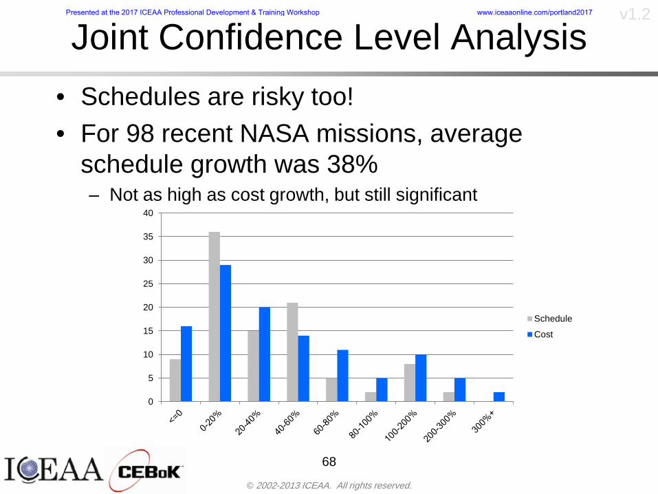
copy 2002-2013 ICEAA All rights reserved
v12
Joint Confidence Level Analysisbull Schedules are risky toobull For 98 recent NASA missions average
schedule growth was 38ndash Not as high as cost growth but still significant
68
0
5
10
15
20
25
30
35
40
Schedule
Cost
Presented at the 2017 ICEAA Professional Development amp Training Workshop wwwiceaaonlinecomportland2017
copy 2002-2013 ICEAA All rights reserved
v12
Schedules Impact Costbull Changes in schedule can have enormous
impacts on cost ndash Schedule slips can lead to cost increases
bull Fixed programmatic costs must be paid on a regular basisndash Achieving schedule milestones early can result in cost
savings
bull Schedule is an important consideration in cost analysis including cost risk analysis
bull However we must be careful in correctly integrating cost and schedule riskndash Schedule is not simply an input but is dependent on many of
the same factors that drive cost
69
Presented at the 2017 ICEAA Professional Development amp Training Workshop wwwiceaaonlinecomportland2017
copy 2002-2013 ICEAA All rights reserved
v12
The Relationship of Cost to Schedulebull Cost and schedule are positively correlated
ndash A larger program with bigger scope with take longer to complete than a smaller simpler program
bull However longer schedules do not always equate to higher cost nor shorter schedules with lower costndash Highly compressed schedules relative to the
optimal schedule can lead to large overrunsbull Compressed schedules are commonplace for
many planetary missions
70
Presented at the 2017 ICEAA Professional Development amp Training Workshop wwwiceaaonlinecomportland2017
copy 2002-2013 ICEAA All rights reserved
v12The Impact of Schedule GrowthCompression on Cost
bull Compressed schedules lead to cost growth and based on existing research is actually more expensive than schedule slippages
71
0
20
40
60
80
100
120
140
160
-50 -25 0 25 50 75 100
Percentage Change in Schedule
Perc
enta
ge C
hang
e in
Cos
t due
to
Sche
dule
Cha
nge
Source Smart CB ldquoCost and Schedule Interrelationshipsrdquo 2007 NASA Cost Symposium
Presented at the 2017 ICEAA Professional Development amp Training Workshop wwwiceaaonlinecomportland2017
copy 2002-2013 ICEAA All rights reserved
v12Schedule as an Independent Variable
bull Why not simply add schedule as an input to cost-estimating relationships (CERs)
bull Schedule is often treated as an independent variable ndash schedules are often determined independently of cost considerationsndash Cost may not be considered explicitly although budgets and
schedules are determined based on scope and other common factors
bull In 2006 SAIC undertook a research task to determine the impact of schedule on cost and added schedule as an independent variable to the CERs in the NASAAir Force Cost Model (NAFCOM) to see if schedule provided any improvement in goodness of fit
72
Presented at the 2017 ICEAA Professional Development amp Training Workshop wwwiceaaonlinecomportland2017
copy 2002-2013 ICEAA All rights reserved
v12
Schedule is a Dependent Variablebull Since NAFCOM includes an exhaustive list of cost drivers the inclusion
of schedule should give an indication of whether there is any additional independent value added from schedule independent of the cost drivers
bull In the study schedule was added to 10 subsystem-level CERs
ndash In each case the addition of schedule did NOTimprove the goodness of fit and schedule was NOT found to be a statistically significant cost driver (given the presence of the other variables) for any of the 10 CERs
bull Standard errors for the CERs increased due to decrease in degrees of freedom
bull Thus schedule as an independent variable did not provide any additional explanation of variation in historical cost
bull This is because schedule is truly NOT an independent variable but a dependent variable and is a function of the same factors that drive cost
73
Presented at the 2017 ICEAA Professional Development amp Training Workshop wwwiceaaonlinecomportland2017
copy 2002-2013 ICEAA All rights reserved
v12
Incorporation of Schedule in Cost Risk
bull When using subjective methods care must be taken in applying schedule to cost risk analysis
bull Since schedule is a dependent variable treating it independently from other factors when assessing its impact on cost can lead to a double count of independent variables in the cost risk analysis
bull Direct inclusion of schedule in a cost risk analysis effectively doubles the influence of each cost driver
ndash Incorrectly leads to broader risk ranges
74
CostWeight
HeritageNewness
Technology Readiness Schedule
Presented at the 2017 ICEAA Professional Development amp Training Workshop wwwiceaaonlinecomportland2017
copy 2002-2013 ICEAA All rights reserved
v12Subjective Cost Risk Methods and Overinclusion of Risk Factors
bull Subjective methods are suitable when data are scarce or not availablebull However care must be taken not to treat correlated sources of risk
such as schedule as independent of each otherbull Example ndash a subjective risk analysis incorporated technology readiness
design risk requirements stability integration risk and schedule and treated each source of risk as independent
bull Risk triangle high value without schedule risk was 31 times the point estimate
bull Risk triangle high value with schedule risk added on top of other sources of risk treated independently was 34 times the point estimate
bull Risk triangle taking correlation between sources of risk into account in a rigorous statistical manner has a high value 15 times the point estimate less than half the effect when treating sources of risk as independent
75
Presented at the 2017 ICEAA Professional Development amp Training Workshop wwwiceaaonlinecomportland2017
copy 2002-2013 ICEAA All rights reserved
v12Fundamental Equation of Cost and Schedule Interrelationships
bull The Fundamental Equation of the Relationship Between Cost and Schedule is
Time = Moneybull This is a well known adage that time is money Your boss at
work may even mention this to you from time to time or if you are the boss you are all too aware of this iron law
bull Because time is money cost and schedule risk should be modeled jointly not with schedule as an independent cost driver
bull Note that cost and schedule are not perfectly correlatedndash Cost can sometimes ldquobuy downrdquo schedule extra money can be
spent to meet a deadline since in some cases additional effort to hasten the completion of a task
76
Presented at the 2017 ICEAA Professional Development amp Training Workshop wwwiceaaonlinecomportland2017
copy 2002-2013 ICEAA All rights reserved
v12How to (Correctly) Incorporate Schedule into Cost Risk Analysis
bull The best way to model cost and schedule risk is to develop a joint cost and schedule model based on the same data
bull Since such models are not currently available the next best approach is to model cost and schedule independently and then integrate cost and schedule risk analyses using joint probability distributions taking into account correlation between cost and schedulendash This approach pioneered by Paul Garvey and Steve Book is
considered industry best practicendash This is a practical method mathematically tractable and follows
naturally from the Fundamental Equation of Cost and Schedule Interrelationships
77
Book S A ldquoQuantifying the Relationship Between Cost and Schedulerdquo The Measurable News Winter 2007-2008 pp 11-15Garvey PR Probability Methods for Cost Uncertainty Analysis A Systems Engineering Perspective New York Marcel Dekker 2000 pp 308-335
Presented at the 2017 ICEAA Professional Development amp Training Workshop wwwiceaaonlinecomportland2017
copy 2002-2013 ICEAA All rights reserved
v12
Joint Lognormal and Normal Distributions
bull Cost and schedule are typically modeled as some combination of Normal and Lognormal probability distributionsndash Studies by The Aerospace Corporation the MITRE
Corporation Wyle Labs and SAIC have found that the Lognormal probability distribution almost always serves as a good model for both the schedule distribution and the cost distribution
ndash The Normal distribution may also be appropriate in some instances and depending upon the level of confidence at which budgets are set may even be more conservative and logically consistent than the Normal distribution
ndash Joint Lognormal and Normal distributions are defined by a pair of mean and standard deviations and a level of correlation between the two
78
Presented at the 2017 ICEAA Professional Development amp Training Workshop wwwiceaaonlinecomportland2017
copy 2002-2013 ICEAA All rights reserved
v12Modeling Cost and Schedule as a Bivariate Distribution
bull In the approach set forth by Book and Garvey cost risk is assessed and the top-level distribution is modeled as a Lognormal (or Normal) distribution schedule risk is assessed and the overall schedule risk is modeled as a Lognormal (or Normal) distribution
bull The two distributions are combined into a Bivariate distribution by assigning a correlation between the two and by treating the two distributions as the marginal distributions of a Bivariate Lognormal distributionndash Other combinations include a Bivariate Normal or a Bivariate
Normal-Lognormal
79
Presented at the 2017 ICEAA Professional Development amp Training Workshop wwwiceaaonlinecomportland2017
copy 2002-2013 ICEAA All rights reserved
v12Bivariate Lognormal Distribution for Cost and Schedule
bull Cost is often observed to be Lognormal when strong positive correlations are present among the systemrsquos WBS cost element costs
bull A systemrsquos schedule is often observed (from Monte Carlo simulations) to be Lognormal if it is the sum of many positively correlated schedule activities in an overall schedule network
bull If Lognormal distributions characterize a systemrsquos cost and schedule then the Bivariate Lognormal could serve as an assumed model of their joint distributionndash In this case the marginal distribution of each of cost and schedule is
Lognormalbull Other possibilities for modeling cost and schedule as a Bivariate
distribution include a Bivariate Normal or a Bivariate Normal-Lognormal distributionndash All these combinations are analytically tractable
80
Presented at the 2017 ICEAA Professional Development amp Training Workshop wwwiceaaonlinecomportland2017
copy 2002-2013 ICEAA All rights reserved
v12Bivariate Lognormal for Cost and Schedule
bull Contour Plots of a Bivariate Lognormal
81
Presented at the 2017 ICEAA Professional Development amp Training Workshop wwwiceaaonlinecomportland2017
copy 2002-2013 ICEAA All rights reserved
v12Correlation Between Cost and Schedule
bull Cost and schedule are positively correlated but not perfectly sondash For example it is possible to have a schedule underrun and a cost
overrunbull Based on cost and schedule growth data for 50 completed NASA
programs the correlation between development cost and development schedule is 70
82
00
200
400
600
800
1000
1200
-500 00 500 1000 1500 2000 2500Historical Cost Growth
Hist
oric
al S
ched
ule
Gro
wth
r = 715
Presented at the 2017 ICEAA Professional Development amp Training Workshop wwwiceaaonlinecomportland2017
copy 2002-2013 ICEAA All rights reserved
v12Correlation Between Cost and Schedule Caveats
bull Based on historical data recommended correlation between cost and schedule is 70 but this could be higher or lower depending upon program circumstancesndash If program is budget constrained cost and schedule will be
more highly correlated (go as you pay)ndash If program is schedule constrained cost and schedule will
have lower correlation perhaps even negative correlation ndash Smaller programs have smaller correlation between cost and
schedule riskbull Relatively easy to ldquohurry uprdquo and finish on time or even early if
needed
83
Presented at the 2017 ICEAA Professional Development amp Training Workshop wwwiceaaonlinecomportland2017
copy 2002-2013 ICEAA All rights reserved
v12
Conditional Confidence Levelsbull Given a programrsquos project schedule we can determine the cost
risk distribution conditional upon the given schedulebull Conditional cost S-curves are steeper than unconditional
(marginal) cost S-curves between some uncertainty has been removed because schedule is fixed
84
Presented at the 2017 ICEAA Professional Development amp Training Workshop wwwiceaaonlinecomportland2017
copy 2002-2013 ICEAA All rights reserved
v12
Joint Confidence Levelsbull Joint 65 confidence represents the probability of
achieving both 65 confidence in cost AND 65 confidence in schedulendash This is different than achieving 65 cost confidence alone
or achieving 65 schedule confidence alonebull Due to the imperfect correlation between cost and schedule it
is possible to achieve a 65 cost confidence with a lower level of schedule confidence
bull Restricting the schedule confidence thus requires additional $ to achieve a given level of confidence
85
X
Y
Possible Values for Which X gt a Possible Values for
Which X gt a and Y gt b
a
b
Presented at the 2017 ICEAA Professional Development amp Training Workshop wwwiceaaonlinecomportland2017
copy 2002-2013 ICEAA All rights reserved
v12Joint Confidence Levels Versus Cost Confidence Levels Only
bull Example of the differences between cost confidence schedule confidence conditional cost confidence and joint cost and schedule confidence
86
Joint Cost-Schedule Confidence Iso-Curves
Cost (RY$M)
Sche
dule
(Mon
ths)
65 Confidence
50 Confidence
70 Confidence
65 Cost Confidence AggressiveSchedule65 Cost ConfidenceScheduleGiven 65 Schedule ConfidenceUnconditional 65 CostConfidenceUnconditional 65 ScheduleConfidence
65 Cost Confidence 65 Joint Cost and Schedule
Confidence for 65 Schedule Confidence
Presented at the 2017 ICEAA Professional Development amp Training Workshop wwwiceaaonlinecomportland2017
copy 2002-2013 ICEAA All rights reserved
v12
Joint Cost and Schedule Confidence
bull Can examine pairs of cost and schedule that achieve a given level of confidence
bull Provides insights into the trade-offs between cost and schedule for a given level of confidencendash Possible to increase cost confidence by giving a
project more time in some instances or possible to ldquobuy downrdquo schedule
bull But these have limits and are shown in the iso-cost and schedule confidence curves
87
Presented at the 2017 ICEAA Professional Development amp Training Workshop wwwiceaaonlinecomportland2017
copy 2002-2013 ICEAA All rights reserved
v12Cost and Schedule Trade-offs for a Given Level of Joint Confidence
bull Hypothetical Example
88
Cost (RY$M)
Schedule (Months)
$100 48$99 48$89 49$87 50$85 51$85 52$84 53$83 55$83 55$83 56
Cost and Schedule 65 Confidence Iso-Curve
4748495051525354555657
$80 $82 $84 $86 $88 $90 $92 $94 $96 $98 $100
Cost (RY$ M)
Sche
dule
(Mon
ths)
Presented at the 2017 ICEAA Professional Development amp Training Workshop wwwiceaaonlinecomportland2017
copy 2002-2013 ICEAA All rights reserved
v12Policy Considerations for Confidence Levels
bull For large programs the difference between the amount of money needed to achieve 65 cost confidence independent of schedule and joint 65 cost and schedule confidence can represent hundreds of millions and even billions of dollars
89
Joint Cost-Schedule Confidence Iso-Curves
Cost (RY$M)
Sche
dule
(Mon
ths)
65 Confidence
65 Cost Confidence AggressiveSchedule
65 Cost ConfidenceScheduleGiven 65 Schedule Confidence
Unconditional 65 CostConfidence
Joint Cost and Schedule Confidence for 65 Cost Confidence and Program Baseline Schedule is Less Than 35
65 Cost Confidence Independent of Schedule Cost Needed to Achieve
Both 65 Joint Cost and Schedule Confidence for the Schedule with 65 Confidence
Presented at the 2017 ICEAA Professional Development amp Training Workshop wwwiceaaonlinecomportland2017
copy 2002-2013 ICEAA All rights reserved
v12
Copulasbull More generally any combination of distributions can
be used (more than just normal and lognormal)ndash Termed ldquocopulardquo from the Italian word for ldquocouplerdquondash Copulas are a way to combine marginal distributions of any
number and type into a joint distributionbull More formally a copula is a multivariate joint distribution defined
on the n-dimensional unit cube [0 1]n such that every marginal distribution is uniform on the interval [0 1]
bull (The bivariate form of) Sklarrsquos theorem states that for any bivariate distribution function H(x y) let F(x) = H(x infin) and G(y) = H(infin y) be the univariate marginal probability distribution functions Then there exists a copula C such that H(xy)=C(F(x)G(y))
ndash Copulas are widely used in risk management for investments and insurance
bull Considered industry best practice (Li 2000)bull Marketed as part of JP Morganrsquos CreditMetrics suite of tools
(Gupton et Al 1997)90
Presented at the 2017 ICEAA Professional Development amp Training Workshop wwwiceaaonlinecomportland2017
copy 2002-2013 ICEAA All rights reserved
v12Parametric Joint Cost and Schedule Analysis
bull A parametric model based on a consistent data set with a set of overlapping cost and schedule drivers is a cleaner way to model cost and schedule
91
CostWeight
HeritageNewness
Technology Readiness
Schedule
0
20
40
60
80
100
Confidence
Joint Cost and Schedule Confidence
Schedule
Cost
Lognormal Distribution PDF and CDF
0102030405060708090100
200 300 400 500 600 700 800 900 1000Cost $
Con
fiden
ce L
evel
0
00002
00004
00006
00008
0001
00012
00014
00016
Prob
abili
ty D
ensi
ty
CDFPDF
Lognormal Distribution PDF and CDF
0102030405060708090100
200 300 400 500 600 700 800 900 1000Cost $
Con
fiden
ce L
evel
0
00002
00004
00006
00008
0001
00012
00014
00016
Prob
abili
ty D
ensi
ty
CDFPDF
Presented at the 2017 ICEAA Professional Development amp Training Workshop wwwiceaaonlinecomportland2017
copy 2002-2013 ICEAA All rights reserved
v12Parametric Joint Cost and Schedule Analysis (2)
bull Joint cost and schedule risk analysis produced naturally by the integrated modelndash Addresses several issues with the copula
approachbull Tail dependencybull Correlation ndash no need to assign correlation
between cost and schedulebull Consistency of cost and schedule models
92
Presented at the 2017 ICEAA Professional Development amp Training Workshop wwwiceaaonlinecomportland2017
copy 2002-2013 ICEAA All rights reserved
v12
Resource-Loaded Schedulesbull Involves assigning cost and schedule risks to a resource-loaded schedule
networkbull Bottom-up approach
ndash More labor intensive than parametrics but can also provide more insight
ndash Can answer questions than parametric typically cannot such as how much do reserve requirements decrease if a specific risk is retired
bull Currently being implemented in Constellation programbull Has same issue as all bottom-up models hard to count all the risks and model
them discretely
ndash As a result there is a tendency to reflect less risk than indicated by history
ndash ldquoThere are more things in heaven and earth Horatio than are dreamt of in your philosophyrdquo William Shakespeare Hamlet Act I Scene V
93
Presented at the 2017 ICEAA Professional Development amp Training Workshop wwwiceaaonlinecomportland2017
copy 2002-2013 ICEAA All rights reserved
v12Resource-Loaded Schedules Vs Parametrics
bull Parametric most appropriate for early estimatesndash But also good for high-level checks as project progresses
bull As plans take shape lower level modeling may be more appropriate
94 1
CONCEPTUALDEVELOPMENT
PROJECTDEFINITION DESIGN DEVELOPMENT OPERATIONS
PARAMETRIC PARAMETRIC
ANALOGY
ENGINEERING (Bottoms Up)
$PARAMETRIC
DETAILED
$
Pre Phase A Phase B Phase CDPhase A Phase EPre Phase A Phase B Phase CDPhase A Phase E
Risk = f(Cost Estimating Relationship Inputs eg mass power data rate TRL new design etc)
Risk = f(cost and schedule variation of the analogous elements)
Risk = f(variation of detailed inputs eg labor hours rates materials etc)
Presented at the 2017 ICEAA Professional Development amp Training Workshop wwwiceaaonlinecomportland2017
copy 2002-2013 ICEAA All rights reserved
v12
Resource-Loaded Schedulesbull Methodology has been demonstrated in other
industriesndash Construction oil and gasndash Analysis has not been traditionally done on highly uncertain
complex development projects bull Methodology focuses on project baseline schedule
ndash In baseline schedule all tasks are resource loaded to represent a baseline schedule and cost standpoint
ndash Resource loaded schedule is ldquorolledrdquo up to a manageable level
ndash Based on the risk and uncertainties identified schedule distributions are applied to each rolled up task
ndash Cost uncertainties are also applied to rolled up tasksbull Uncertainties include labor rate man power etc
ndash A Monte Carlo simulation is run to develop joint cost-schedule distributions
95
Presented at the 2017 ICEAA Professional Development amp Training Workshop wwwiceaaonlinecomportland2017
copy 2002-2013 ICEAA All rights reserved
v12
Unit III - Module 9 96
Execution ndash Cross Checksbull Means The mean cost growth factor for WBS items
can be compared to history as a way to cross check results
bull CVs The CV of the cost growth factors for WBS items can be compared to history as a way to cross check results
bull Inputs Checks are performed on inputs or other parameters to see if historical values are in line with program assumptionsndash Example Historical risk scores can be compared to program
risk scores to see if risk assessors are being realistic and to see if the underlying database is representative of the program
11
Presented at the 2017 ICEAA Professional Development amp Training Workshop wwwiceaaonlinecomportland2017
- Cost and Schedule Risk Analysis Basic
- Acknowledgments
- Unit Index
- Risk Overview
- Agenda
- Introduction
- Risk Analysis Terms
- Are Our Costs Realistic
- Historical Cost Growth
- Sources of Cost Risk
- Point Estimates of Cost
- Types of Risk
- Point Estimates Vs Risk Estimates
- Cost Risk and Probability
- Probability Model ndash Distribution
- Probability Model ndash Distribution
- Probability ndash Top-Level Distribution
- S-Curves and Confidence Levels
- Example ndash Normal Distribution
- Confidence Levels
- Measuring Parametric Model Uncertainty
- Parametric Model Example
- Weight Uncertainty
- Estimating Uncertainty
- Estimating Uncertainty (2)
- Estimating Uncertainty (3)
- Aggregating Risk
- WBS Example
- WBS and Risk
- Aggregating Risk
- Percentiles Do Not Add
- Percentiles Do Not Add (2)
- Percentiles Do Not Add (3)
- Methods for Aggregating Risk
- Monte Carlo Simulationfor Risk Analysis
- Monte Carlo Simulation
- Using Random Numbers to Simulate Distributions
- Simulating a Triangular Distribution
- Simulating a Triangular Distribution (2)
- Monte Carlo and the WBS
- Number of Trials
- Number of Trials (2)
- Number of Trials (3)
- Number of Trials (4)
- Number of Trials (5)
- Number of Trials (6)
- Methods of Simulation
- Probability Model ndash Correlation
- Correlation And Causation
- The Importance of Correlation
- The Importance of Correlation (2)
- Measures of Correlation
- Pearson Correlation
- Spearman Correlation
- Functional Correlation
- Risk Measures
- Value at Risk (VaR)
- Why 70th or 80th Percentile
- Funding Above Inflection Points
- Why Budget to the 70th or 80th
- Inflection Points for Lognormal
- Issues with Percentile Funding
- ldquoHere There Be Dragonsrdquo
- Distribution Comparison
- Distribution Comparison Tail Behavior
- Distribution Comparison ndash Tail Behavior (Table)
- Percentile Budgeting is Not Risk Management
- Joint Confidence Level Analysis
- Schedules Impact Cost
- The Relationship of Cost to Schedule
- The Impact of Schedule GrowthCompression on Cost
- Schedule as an Independent Variable
- Schedule is a Dependent Variable
- Incorporation of Schedule in Cost Risk
- Subjective Cost Risk Methods and Overinclusion of Risk Factors
- Fundamental Equation of Cost and Schedule Interrelationships
- How to (Correctly) Incorporate Schedule into Cost Risk Analysis
- Joint Lognormal and Normal Distributions
- Modeling Cost and Schedule as a Bivariate Distribution
- Bivariate Lognormal Distribution for Cost and Schedule
- Bivariate Lognormal for Cost and Schedule
- Correlation Between Cost and Schedule
- Correlation Between Cost and Schedule Caveats
- Conditional Confidence Levels
- Joint Confidence Levels
- Joint Confidence Levels Versus Cost Confidence Levels Only
- Joint Cost and Schedule Confidence
- Cost and Schedule Trade-offs for a Given Level of Joint Confidence
- Policy Considerations for Confidence Levels
- Copulas
- Parametric Joint Cost and Schedule Analysis
- Parametric Joint Cost and Schedule Analysis (2)
- Resource-Loaded Schedules
- Resource-Loaded Schedules Vs Parametrics
- Resource-Loaded Schedules
- Execution ndash Cross Checks
-
copy 2002-2013 ICEAA All rights reserved
v12
The Relationship of Cost to Schedulebull Cost and schedule are positively correlated
ndash A larger program with bigger scope with take longer to complete than a smaller simpler program
bull However longer schedules do not always equate to higher cost nor shorter schedules with lower costndash Highly compressed schedules relative to the
optimal schedule can lead to large overrunsbull Compressed schedules are commonplace for
many planetary missions
70
Presented at the 2017 ICEAA Professional Development amp Training Workshop wwwiceaaonlinecomportland2017
copy 2002-2013 ICEAA All rights reserved
v12The Impact of Schedule GrowthCompression on Cost
bull Compressed schedules lead to cost growth and based on existing research is actually more expensive than schedule slippages
71
0
20
40
60
80
100
120
140
160
-50 -25 0 25 50 75 100
Percentage Change in Schedule
Perc
enta
ge C
hang
e in
Cos
t due
to
Sche
dule
Cha
nge
Source Smart CB ldquoCost and Schedule Interrelationshipsrdquo 2007 NASA Cost Symposium
Presented at the 2017 ICEAA Professional Development amp Training Workshop wwwiceaaonlinecomportland2017
copy 2002-2013 ICEAA All rights reserved
v12Schedule as an Independent Variable
bull Why not simply add schedule as an input to cost-estimating relationships (CERs)
bull Schedule is often treated as an independent variable ndash schedules are often determined independently of cost considerationsndash Cost may not be considered explicitly although budgets and
schedules are determined based on scope and other common factors
bull In 2006 SAIC undertook a research task to determine the impact of schedule on cost and added schedule as an independent variable to the CERs in the NASAAir Force Cost Model (NAFCOM) to see if schedule provided any improvement in goodness of fit
72
Presented at the 2017 ICEAA Professional Development amp Training Workshop wwwiceaaonlinecomportland2017
copy 2002-2013 ICEAA All rights reserved
v12
Schedule is a Dependent Variablebull Since NAFCOM includes an exhaustive list of cost drivers the inclusion
of schedule should give an indication of whether there is any additional independent value added from schedule independent of the cost drivers
bull In the study schedule was added to 10 subsystem-level CERs
ndash In each case the addition of schedule did NOTimprove the goodness of fit and schedule was NOT found to be a statistically significant cost driver (given the presence of the other variables) for any of the 10 CERs
bull Standard errors for the CERs increased due to decrease in degrees of freedom
bull Thus schedule as an independent variable did not provide any additional explanation of variation in historical cost
bull This is because schedule is truly NOT an independent variable but a dependent variable and is a function of the same factors that drive cost
73
Presented at the 2017 ICEAA Professional Development amp Training Workshop wwwiceaaonlinecomportland2017
copy 2002-2013 ICEAA All rights reserved
v12
Incorporation of Schedule in Cost Risk
bull When using subjective methods care must be taken in applying schedule to cost risk analysis
bull Since schedule is a dependent variable treating it independently from other factors when assessing its impact on cost can lead to a double count of independent variables in the cost risk analysis
bull Direct inclusion of schedule in a cost risk analysis effectively doubles the influence of each cost driver
ndash Incorrectly leads to broader risk ranges
74
CostWeight
HeritageNewness
Technology Readiness Schedule
Presented at the 2017 ICEAA Professional Development amp Training Workshop wwwiceaaonlinecomportland2017
copy 2002-2013 ICEAA All rights reserved
v12Subjective Cost Risk Methods and Overinclusion of Risk Factors
bull Subjective methods are suitable when data are scarce or not availablebull However care must be taken not to treat correlated sources of risk
such as schedule as independent of each otherbull Example ndash a subjective risk analysis incorporated technology readiness
design risk requirements stability integration risk and schedule and treated each source of risk as independent
bull Risk triangle high value without schedule risk was 31 times the point estimate
bull Risk triangle high value with schedule risk added on top of other sources of risk treated independently was 34 times the point estimate
bull Risk triangle taking correlation between sources of risk into account in a rigorous statistical manner has a high value 15 times the point estimate less than half the effect when treating sources of risk as independent
75
Presented at the 2017 ICEAA Professional Development amp Training Workshop wwwiceaaonlinecomportland2017
copy 2002-2013 ICEAA All rights reserved
v12Fundamental Equation of Cost and Schedule Interrelationships
bull The Fundamental Equation of the Relationship Between Cost and Schedule is
Time = Moneybull This is a well known adage that time is money Your boss at
work may even mention this to you from time to time or if you are the boss you are all too aware of this iron law
bull Because time is money cost and schedule risk should be modeled jointly not with schedule as an independent cost driver
bull Note that cost and schedule are not perfectly correlatedndash Cost can sometimes ldquobuy downrdquo schedule extra money can be
spent to meet a deadline since in some cases additional effort to hasten the completion of a task
76
Presented at the 2017 ICEAA Professional Development amp Training Workshop wwwiceaaonlinecomportland2017
copy 2002-2013 ICEAA All rights reserved
v12How to (Correctly) Incorporate Schedule into Cost Risk Analysis
bull The best way to model cost and schedule risk is to develop a joint cost and schedule model based on the same data
bull Since such models are not currently available the next best approach is to model cost and schedule independently and then integrate cost and schedule risk analyses using joint probability distributions taking into account correlation between cost and schedulendash This approach pioneered by Paul Garvey and Steve Book is
considered industry best practicendash This is a practical method mathematically tractable and follows
naturally from the Fundamental Equation of Cost and Schedule Interrelationships
77
Book S A ldquoQuantifying the Relationship Between Cost and Schedulerdquo The Measurable News Winter 2007-2008 pp 11-15Garvey PR Probability Methods for Cost Uncertainty Analysis A Systems Engineering Perspective New York Marcel Dekker 2000 pp 308-335
Presented at the 2017 ICEAA Professional Development amp Training Workshop wwwiceaaonlinecomportland2017
copy 2002-2013 ICEAA All rights reserved
v12
Joint Lognormal and Normal Distributions
bull Cost and schedule are typically modeled as some combination of Normal and Lognormal probability distributionsndash Studies by The Aerospace Corporation the MITRE
Corporation Wyle Labs and SAIC have found that the Lognormal probability distribution almost always serves as a good model for both the schedule distribution and the cost distribution
ndash The Normal distribution may also be appropriate in some instances and depending upon the level of confidence at which budgets are set may even be more conservative and logically consistent than the Normal distribution
ndash Joint Lognormal and Normal distributions are defined by a pair of mean and standard deviations and a level of correlation between the two
78
Presented at the 2017 ICEAA Professional Development amp Training Workshop wwwiceaaonlinecomportland2017
copy 2002-2013 ICEAA All rights reserved
v12Modeling Cost and Schedule as a Bivariate Distribution
bull In the approach set forth by Book and Garvey cost risk is assessed and the top-level distribution is modeled as a Lognormal (or Normal) distribution schedule risk is assessed and the overall schedule risk is modeled as a Lognormal (or Normal) distribution
bull The two distributions are combined into a Bivariate distribution by assigning a correlation between the two and by treating the two distributions as the marginal distributions of a Bivariate Lognormal distributionndash Other combinations include a Bivariate Normal or a Bivariate
Normal-Lognormal
79
Presented at the 2017 ICEAA Professional Development amp Training Workshop wwwiceaaonlinecomportland2017
copy 2002-2013 ICEAA All rights reserved
v12Bivariate Lognormal Distribution for Cost and Schedule
bull Cost is often observed to be Lognormal when strong positive correlations are present among the systemrsquos WBS cost element costs
bull A systemrsquos schedule is often observed (from Monte Carlo simulations) to be Lognormal if it is the sum of many positively correlated schedule activities in an overall schedule network
bull If Lognormal distributions characterize a systemrsquos cost and schedule then the Bivariate Lognormal could serve as an assumed model of their joint distributionndash In this case the marginal distribution of each of cost and schedule is
Lognormalbull Other possibilities for modeling cost and schedule as a Bivariate
distribution include a Bivariate Normal or a Bivariate Normal-Lognormal distributionndash All these combinations are analytically tractable
80
Presented at the 2017 ICEAA Professional Development amp Training Workshop wwwiceaaonlinecomportland2017
copy 2002-2013 ICEAA All rights reserved
v12Bivariate Lognormal for Cost and Schedule
bull Contour Plots of a Bivariate Lognormal
81
Presented at the 2017 ICEAA Professional Development amp Training Workshop wwwiceaaonlinecomportland2017
copy 2002-2013 ICEAA All rights reserved
v12Correlation Between Cost and Schedule
bull Cost and schedule are positively correlated but not perfectly sondash For example it is possible to have a schedule underrun and a cost
overrunbull Based on cost and schedule growth data for 50 completed NASA
programs the correlation between development cost and development schedule is 70
82
00
200
400
600
800
1000
1200
-500 00 500 1000 1500 2000 2500Historical Cost Growth
Hist
oric
al S
ched
ule
Gro
wth
r = 715
Presented at the 2017 ICEAA Professional Development amp Training Workshop wwwiceaaonlinecomportland2017
copy 2002-2013 ICEAA All rights reserved
v12Correlation Between Cost and Schedule Caveats
bull Based on historical data recommended correlation between cost and schedule is 70 but this could be higher or lower depending upon program circumstancesndash If program is budget constrained cost and schedule will be
more highly correlated (go as you pay)ndash If program is schedule constrained cost and schedule will
have lower correlation perhaps even negative correlation ndash Smaller programs have smaller correlation between cost and
schedule riskbull Relatively easy to ldquohurry uprdquo and finish on time or even early if
needed
83
Presented at the 2017 ICEAA Professional Development amp Training Workshop wwwiceaaonlinecomportland2017
copy 2002-2013 ICEAA All rights reserved
v12
Conditional Confidence Levelsbull Given a programrsquos project schedule we can determine the cost
risk distribution conditional upon the given schedulebull Conditional cost S-curves are steeper than unconditional
(marginal) cost S-curves between some uncertainty has been removed because schedule is fixed
84
Presented at the 2017 ICEAA Professional Development amp Training Workshop wwwiceaaonlinecomportland2017
copy 2002-2013 ICEAA All rights reserved
v12
Joint Confidence Levelsbull Joint 65 confidence represents the probability of
achieving both 65 confidence in cost AND 65 confidence in schedulendash This is different than achieving 65 cost confidence alone
or achieving 65 schedule confidence alonebull Due to the imperfect correlation between cost and schedule it
is possible to achieve a 65 cost confidence with a lower level of schedule confidence
bull Restricting the schedule confidence thus requires additional $ to achieve a given level of confidence
85
X
Y
Possible Values for Which X gt a Possible Values for
Which X gt a and Y gt b
a
b
Presented at the 2017 ICEAA Professional Development amp Training Workshop wwwiceaaonlinecomportland2017
copy 2002-2013 ICEAA All rights reserved
v12Joint Confidence Levels Versus Cost Confidence Levels Only
bull Example of the differences between cost confidence schedule confidence conditional cost confidence and joint cost and schedule confidence
86
Joint Cost-Schedule Confidence Iso-Curves
Cost (RY$M)
Sche
dule
(Mon
ths)
65 Confidence
50 Confidence
70 Confidence
65 Cost Confidence AggressiveSchedule65 Cost ConfidenceScheduleGiven 65 Schedule ConfidenceUnconditional 65 CostConfidenceUnconditional 65 ScheduleConfidence
65 Cost Confidence 65 Joint Cost and Schedule
Confidence for 65 Schedule Confidence
Presented at the 2017 ICEAA Professional Development amp Training Workshop wwwiceaaonlinecomportland2017
copy 2002-2013 ICEAA All rights reserved
v12
Joint Cost and Schedule Confidence
bull Can examine pairs of cost and schedule that achieve a given level of confidence
bull Provides insights into the trade-offs between cost and schedule for a given level of confidencendash Possible to increase cost confidence by giving a
project more time in some instances or possible to ldquobuy downrdquo schedule
bull But these have limits and are shown in the iso-cost and schedule confidence curves
87
Presented at the 2017 ICEAA Professional Development amp Training Workshop wwwiceaaonlinecomportland2017
copy 2002-2013 ICEAA All rights reserved
v12Cost and Schedule Trade-offs for a Given Level of Joint Confidence
bull Hypothetical Example
88
Cost (RY$M)
Schedule (Months)
$100 48$99 48$89 49$87 50$85 51$85 52$84 53$83 55$83 55$83 56
Cost and Schedule 65 Confidence Iso-Curve
4748495051525354555657
$80 $82 $84 $86 $88 $90 $92 $94 $96 $98 $100
Cost (RY$ M)
Sche
dule
(Mon
ths)
Presented at the 2017 ICEAA Professional Development amp Training Workshop wwwiceaaonlinecomportland2017
copy 2002-2013 ICEAA All rights reserved
v12Policy Considerations for Confidence Levels
bull For large programs the difference between the amount of money needed to achieve 65 cost confidence independent of schedule and joint 65 cost and schedule confidence can represent hundreds of millions and even billions of dollars
89
Joint Cost-Schedule Confidence Iso-Curves
Cost (RY$M)
Sche
dule
(Mon
ths)
65 Confidence
65 Cost Confidence AggressiveSchedule
65 Cost ConfidenceScheduleGiven 65 Schedule Confidence
Unconditional 65 CostConfidence
Joint Cost and Schedule Confidence for 65 Cost Confidence and Program Baseline Schedule is Less Than 35
65 Cost Confidence Independent of Schedule Cost Needed to Achieve
Both 65 Joint Cost and Schedule Confidence for the Schedule with 65 Confidence
Presented at the 2017 ICEAA Professional Development amp Training Workshop wwwiceaaonlinecomportland2017
copy 2002-2013 ICEAA All rights reserved
v12
Copulasbull More generally any combination of distributions can
be used (more than just normal and lognormal)ndash Termed ldquocopulardquo from the Italian word for ldquocouplerdquondash Copulas are a way to combine marginal distributions of any
number and type into a joint distributionbull More formally a copula is a multivariate joint distribution defined
on the n-dimensional unit cube [0 1]n such that every marginal distribution is uniform on the interval [0 1]
bull (The bivariate form of) Sklarrsquos theorem states that for any bivariate distribution function H(x y) let F(x) = H(x infin) and G(y) = H(infin y) be the univariate marginal probability distribution functions Then there exists a copula C such that H(xy)=C(F(x)G(y))
ndash Copulas are widely used in risk management for investments and insurance
bull Considered industry best practice (Li 2000)bull Marketed as part of JP Morganrsquos CreditMetrics suite of tools
(Gupton et Al 1997)90
Presented at the 2017 ICEAA Professional Development amp Training Workshop wwwiceaaonlinecomportland2017
copy 2002-2013 ICEAA All rights reserved
v12Parametric Joint Cost and Schedule Analysis
bull A parametric model based on a consistent data set with a set of overlapping cost and schedule drivers is a cleaner way to model cost and schedule
91
CostWeight
HeritageNewness
Technology Readiness
Schedule
0
20
40
60
80
100
Confidence
Joint Cost and Schedule Confidence
Schedule
Cost
Lognormal Distribution PDF and CDF
0102030405060708090100
200 300 400 500 600 700 800 900 1000Cost $
Con
fiden
ce L
evel
0
00002
00004
00006
00008
0001
00012
00014
00016
Prob
abili
ty D
ensi
ty
CDFPDF
Lognormal Distribution PDF and CDF
0102030405060708090100
200 300 400 500 600 700 800 900 1000Cost $
Con
fiden
ce L
evel
0
00002
00004
00006
00008
0001
00012
00014
00016
Prob
abili
ty D
ensi
ty
CDFPDF
Presented at the 2017 ICEAA Professional Development amp Training Workshop wwwiceaaonlinecomportland2017
copy 2002-2013 ICEAA All rights reserved
v12Parametric Joint Cost and Schedule Analysis (2)
bull Joint cost and schedule risk analysis produced naturally by the integrated modelndash Addresses several issues with the copula
approachbull Tail dependencybull Correlation ndash no need to assign correlation
between cost and schedulebull Consistency of cost and schedule models
92
Presented at the 2017 ICEAA Professional Development amp Training Workshop wwwiceaaonlinecomportland2017
copy 2002-2013 ICEAA All rights reserved
v12
Resource-Loaded Schedulesbull Involves assigning cost and schedule risks to a resource-loaded schedule
networkbull Bottom-up approach
ndash More labor intensive than parametrics but can also provide more insight
ndash Can answer questions than parametric typically cannot such as how much do reserve requirements decrease if a specific risk is retired
bull Currently being implemented in Constellation programbull Has same issue as all bottom-up models hard to count all the risks and model
them discretely
ndash As a result there is a tendency to reflect less risk than indicated by history
ndash ldquoThere are more things in heaven and earth Horatio than are dreamt of in your philosophyrdquo William Shakespeare Hamlet Act I Scene V
93
Presented at the 2017 ICEAA Professional Development amp Training Workshop wwwiceaaonlinecomportland2017
copy 2002-2013 ICEAA All rights reserved
v12Resource-Loaded Schedules Vs Parametrics
bull Parametric most appropriate for early estimatesndash But also good for high-level checks as project progresses
bull As plans take shape lower level modeling may be more appropriate
94 1
CONCEPTUALDEVELOPMENT
PROJECTDEFINITION DESIGN DEVELOPMENT OPERATIONS
PARAMETRIC PARAMETRIC
ANALOGY
ENGINEERING (Bottoms Up)
$PARAMETRIC
DETAILED
$
Pre Phase A Phase B Phase CDPhase A Phase EPre Phase A Phase B Phase CDPhase A Phase E
Risk = f(Cost Estimating Relationship Inputs eg mass power data rate TRL new design etc)
Risk = f(cost and schedule variation of the analogous elements)
Risk = f(variation of detailed inputs eg labor hours rates materials etc)
Presented at the 2017 ICEAA Professional Development amp Training Workshop wwwiceaaonlinecomportland2017
copy 2002-2013 ICEAA All rights reserved
v12
Resource-Loaded Schedulesbull Methodology has been demonstrated in other
industriesndash Construction oil and gasndash Analysis has not been traditionally done on highly uncertain
complex development projects bull Methodology focuses on project baseline schedule
ndash In baseline schedule all tasks are resource loaded to represent a baseline schedule and cost standpoint
ndash Resource loaded schedule is ldquorolledrdquo up to a manageable level
ndash Based on the risk and uncertainties identified schedule distributions are applied to each rolled up task
ndash Cost uncertainties are also applied to rolled up tasksbull Uncertainties include labor rate man power etc
ndash A Monte Carlo simulation is run to develop joint cost-schedule distributions
95
Presented at the 2017 ICEAA Professional Development amp Training Workshop wwwiceaaonlinecomportland2017
copy 2002-2013 ICEAA All rights reserved
v12
Unit III - Module 9 96
Execution ndash Cross Checksbull Means The mean cost growth factor for WBS items
can be compared to history as a way to cross check results
bull CVs The CV of the cost growth factors for WBS items can be compared to history as a way to cross check results
bull Inputs Checks are performed on inputs or other parameters to see if historical values are in line with program assumptionsndash Example Historical risk scores can be compared to program
risk scores to see if risk assessors are being realistic and to see if the underlying database is representative of the program
11
Presented at the 2017 ICEAA Professional Development amp Training Workshop wwwiceaaonlinecomportland2017
- Cost and Schedule Risk Analysis Basic
- Acknowledgments
- Unit Index
- Risk Overview
- Agenda
- Introduction
- Risk Analysis Terms
- Are Our Costs Realistic
- Historical Cost Growth
- Sources of Cost Risk
- Point Estimates of Cost
- Types of Risk
- Point Estimates Vs Risk Estimates
- Cost Risk and Probability
- Probability Model ndash Distribution
- Probability Model ndash Distribution
- Probability ndash Top-Level Distribution
- S-Curves and Confidence Levels
- Example ndash Normal Distribution
- Confidence Levels
- Measuring Parametric Model Uncertainty
- Parametric Model Example
- Weight Uncertainty
- Estimating Uncertainty
- Estimating Uncertainty (2)
- Estimating Uncertainty (3)
- Aggregating Risk
- WBS Example
- WBS and Risk
- Aggregating Risk
- Percentiles Do Not Add
- Percentiles Do Not Add (2)
- Percentiles Do Not Add (3)
- Methods for Aggregating Risk
- Monte Carlo Simulationfor Risk Analysis
- Monte Carlo Simulation
- Using Random Numbers to Simulate Distributions
- Simulating a Triangular Distribution
- Simulating a Triangular Distribution (2)
- Monte Carlo and the WBS
- Number of Trials
- Number of Trials (2)
- Number of Trials (3)
- Number of Trials (4)
- Number of Trials (5)
- Number of Trials (6)
- Methods of Simulation
- Probability Model ndash Correlation
- Correlation And Causation
- The Importance of Correlation
- The Importance of Correlation (2)
- Measures of Correlation
- Pearson Correlation
- Spearman Correlation
- Functional Correlation
- Risk Measures
- Value at Risk (VaR)
- Why 70th or 80th Percentile
- Funding Above Inflection Points
- Why Budget to the 70th or 80th
- Inflection Points for Lognormal
- Issues with Percentile Funding
- ldquoHere There Be Dragonsrdquo
- Distribution Comparison
- Distribution Comparison Tail Behavior
- Distribution Comparison ndash Tail Behavior (Table)
- Percentile Budgeting is Not Risk Management
- Joint Confidence Level Analysis
- Schedules Impact Cost
- The Relationship of Cost to Schedule
- The Impact of Schedule GrowthCompression on Cost
- Schedule as an Independent Variable
- Schedule is a Dependent Variable
- Incorporation of Schedule in Cost Risk
- Subjective Cost Risk Methods and Overinclusion of Risk Factors
- Fundamental Equation of Cost and Schedule Interrelationships
- How to (Correctly) Incorporate Schedule into Cost Risk Analysis
- Joint Lognormal and Normal Distributions
- Modeling Cost and Schedule as a Bivariate Distribution
- Bivariate Lognormal Distribution for Cost and Schedule
- Bivariate Lognormal for Cost and Schedule
- Correlation Between Cost and Schedule
- Correlation Between Cost and Schedule Caveats
- Conditional Confidence Levels
- Joint Confidence Levels
- Joint Confidence Levels Versus Cost Confidence Levels Only
- Joint Cost and Schedule Confidence
- Cost and Schedule Trade-offs for a Given Level of Joint Confidence
- Policy Considerations for Confidence Levels
- Copulas
- Parametric Joint Cost and Schedule Analysis
- Parametric Joint Cost and Schedule Analysis (2)
- Resource-Loaded Schedules
- Resource-Loaded Schedules Vs Parametrics
- Resource-Loaded Schedules
- Execution ndash Cross Checks
-
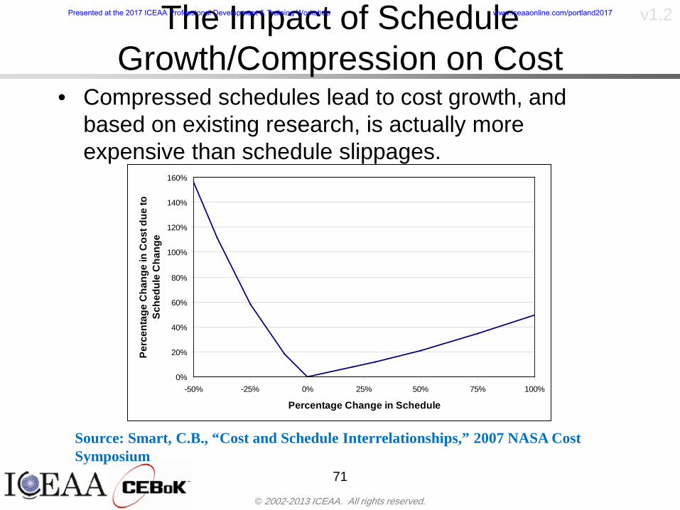
copy 2002-2013 ICEAA All rights reserved
v12The Impact of Schedule GrowthCompression on Cost
bull Compressed schedules lead to cost growth and based on existing research is actually more expensive than schedule slippages
71
0
20
40
60
80
100
120
140
160
-50 -25 0 25 50 75 100
Percentage Change in Schedule
Perc
enta
ge C
hang
e in
Cos
t due
to
Sche
dule
Cha
nge
Source Smart CB ldquoCost and Schedule Interrelationshipsrdquo 2007 NASA Cost Symposium
Presented at the 2017 ICEAA Professional Development amp Training Workshop wwwiceaaonlinecomportland2017
copy 2002-2013 ICEAA All rights reserved
v12Schedule as an Independent Variable
bull Why not simply add schedule as an input to cost-estimating relationships (CERs)
bull Schedule is often treated as an independent variable ndash schedules are often determined independently of cost considerationsndash Cost may not be considered explicitly although budgets and
schedules are determined based on scope and other common factors
bull In 2006 SAIC undertook a research task to determine the impact of schedule on cost and added schedule as an independent variable to the CERs in the NASAAir Force Cost Model (NAFCOM) to see if schedule provided any improvement in goodness of fit
72
Presented at the 2017 ICEAA Professional Development amp Training Workshop wwwiceaaonlinecomportland2017
copy 2002-2013 ICEAA All rights reserved
v12
Schedule is a Dependent Variablebull Since NAFCOM includes an exhaustive list of cost drivers the inclusion
of schedule should give an indication of whether there is any additional independent value added from schedule independent of the cost drivers
bull In the study schedule was added to 10 subsystem-level CERs
ndash In each case the addition of schedule did NOTimprove the goodness of fit and schedule was NOT found to be a statistically significant cost driver (given the presence of the other variables) for any of the 10 CERs
bull Standard errors for the CERs increased due to decrease in degrees of freedom
bull Thus schedule as an independent variable did not provide any additional explanation of variation in historical cost
bull This is because schedule is truly NOT an independent variable but a dependent variable and is a function of the same factors that drive cost
73
Presented at the 2017 ICEAA Professional Development amp Training Workshop wwwiceaaonlinecomportland2017
copy 2002-2013 ICEAA All rights reserved
v12
Incorporation of Schedule in Cost Risk
bull When using subjective methods care must be taken in applying schedule to cost risk analysis
bull Since schedule is a dependent variable treating it independently from other factors when assessing its impact on cost can lead to a double count of independent variables in the cost risk analysis
bull Direct inclusion of schedule in a cost risk analysis effectively doubles the influence of each cost driver
ndash Incorrectly leads to broader risk ranges
74
CostWeight
HeritageNewness
Technology Readiness Schedule
Presented at the 2017 ICEAA Professional Development amp Training Workshop wwwiceaaonlinecomportland2017
copy 2002-2013 ICEAA All rights reserved
v12Subjective Cost Risk Methods and Overinclusion of Risk Factors
bull Subjective methods are suitable when data are scarce or not availablebull However care must be taken not to treat correlated sources of risk
such as schedule as independent of each otherbull Example ndash a subjective risk analysis incorporated technology readiness
design risk requirements stability integration risk and schedule and treated each source of risk as independent
bull Risk triangle high value without schedule risk was 31 times the point estimate
bull Risk triangle high value with schedule risk added on top of other sources of risk treated independently was 34 times the point estimate
bull Risk triangle taking correlation between sources of risk into account in a rigorous statistical manner has a high value 15 times the point estimate less than half the effect when treating sources of risk as independent
75
Presented at the 2017 ICEAA Professional Development amp Training Workshop wwwiceaaonlinecomportland2017
copy 2002-2013 ICEAA All rights reserved
v12Fundamental Equation of Cost and Schedule Interrelationships
bull The Fundamental Equation of the Relationship Between Cost and Schedule is
Time = Moneybull This is a well known adage that time is money Your boss at
work may even mention this to you from time to time or if you are the boss you are all too aware of this iron law
bull Because time is money cost and schedule risk should be modeled jointly not with schedule as an independent cost driver
bull Note that cost and schedule are not perfectly correlatedndash Cost can sometimes ldquobuy downrdquo schedule extra money can be
spent to meet a deadline since in some cases additional effort to hasten the completion of a task
76
Presented at the 2017 ICEAA Professional Development amp Training Workshop wwwiceaaonlinecomportland2017
copy 2002-2013 ICEAA All rights reserved
v12How to (Correctly) Incorporate Schedule into Cost Risk Analysis
bull The best way to model cost and schedule risk is to develop a joint cost and schedule model based on the same data
bull Since such models are not currently available the next best approach is to model cost and schedule independently and then integrate cost and schedule risk analyses using joint probability distributions taking into account correlation between cost and schedulendash This approach pioneered by Paul Garvey and Steve Book is
considered industry best practicendash This is a practical method mathematically tractable and follows
naturally from the Fundamental Equation of Cost and Schedule Interrelationships
77
Book S A ldquoQuantifying the Relationship Between Cost and Schedulerdquo The Measurable News Winter 2007-2008 pp 11-15Garvey PR Probability Methods for Cost Uncertainty Analysis A Systems Engineering Perspective New York Marcel Dekker 2000 pp 308-335
Presented at the 2017 ICEAA Professional Development amp Training Workshop wwwiceaaonlinecomportland2017
copy 2002-2013 ICEAA All rights reserved
v12
Joint Lognormal and Normal Distributions
bull Cost and schedule are typically modeled as some combination of Normal and Lognormal probability distributionsndash Studies by The Aerospace Corporation the MITRE
Corporation Wyle Labs and SAIC have found that the Lognormal probability distribution almost always serves as a good model for both the schedule distribution and the cost distribution
ndash The Normal distribution may also be appropriate in some instances and depending upon the level of confidence at which budgets are set may even be more conservative and logically consistent than the Normal distribution
ndash Joint Lognormal and Normal distributions are defined by a pair of mean and standard deviations and a level of correlation between the two
78
Presented at the 2017 ICEAA Professional Development amp Training Workshop wwwiceaaonlinecomportland2017
copy 2002-2013 ICEAA All rights reserved
v12Modeling Cost and Schedule as a Bivariate Distribution
bull In the approach set forth by Book and Garvey cost risk is assessed and the top-level distribution is modeled as a Lognormal (or Normal) distribution schedule risk is assessed and the overall schedule risk is modeled as a Lognormal (or Normal) distribution
bull The two distributions are combined into a Bivariate distribution by assigning a correlation between the two and by treating the two distributions as the marginal distributions of a Bivariate Lognormal distributionndash Other combinations include a Bivariate Normal or a Bivariate
Normal-Lognormal
79
Presented at the 2017 ICEAA Professional Development amp Training Workshop wwwiceaaonlinecomportland2017
copy 2002-2013 ICEAA All rights reserved
v12Bivariate Lognormal Distribution for Cost and Schedule
bull Cost is often observed to be Lognormal when strong positive correlations are present among the systemrsquos WBS cost element costs
bull A systemrsquos schedule is often observed (from Monte Carlo simulations) to be Lognormal if it is the sum of many positively correlated schedule activities in an overall schedule network
bull If Lognormal distributions characterize a systemrsquos cost and schedule then the Bivariate Lognormal could serve as an assumed model of their joint distributionndash In this case the marginal distribution of each of cost and schedule is
Lognormalbull Other possibilities for modeling cost and schedule as a Bivariate
distribution include a Bivariate Normal or a Bivariate Normal-Lognormal distributionndash All these combinations are analytically tractable
80
Presented at the 2017 ICEAA Professional Development amp Training Workshop wwwiceaaonlinecomportland2017
copy 2002-2013 ICEAA All rights reserved
v12Bivariate Lognormal for Cost and Schedule
bull Contour Plots of a Bivariate Lognormal
81
Presented at the 2017 ICEAA Professional Development amp Training Workshop wwwiceaaonlinecomportland2017
copy 2002-2013 ICEAA All rights reserved
v12Correlation Between Cost and Schedule
bull Cost and schedule are positively correlated but not perfectly sondash For example it is possible to have a schedule underrun and a cost
overrunbull Based on cost and schedule growth data for 50 completed NASA
programs the correlation between development cost and development schedule is 70
82
00
200
400
600
800
1000
1200
-500 00 500 1000 1500 2000 2500Historical Cost Growth
Hist
oric
al S
ched
ule
Gro
wth
r = 715
Presented at the 2017 ICEAA Professional Development amp Training Workshop wwwiceaaonlinecomportland2017
copy 2002-2013 ICEAA All rights reserved
v12Correlation Between Cost and Schedule Caveats
bull Based on historical data recommended correlation between cost and schedule is 70 but this could be higher or lower depending upon program circumstancesndash If program is budget constrained cost and schedule will be
more highly correlated (go as you pay)ndash If program is schedule constrained cost and schedule will
have lower correlation perhaps even negative correlation ndash Smaller programs have smaller correlation between cost and
schedule riskbull Relatively easy to ldquohurry uprdquo and finish on time or even early if
needed
83
Presented at the 2017 ICEAA Professional Development amp Training Workshop wwwiceaaonlinecomportland2017
copy 2002-2013 ICEAA All rights reserved
v12
Conditional Confidence Levelsbull Given a programrsquos project schedule we can determine the cost
risk distribution conditional upon the given schedulebull Conditional cost S-curves are steeper than unconditional
(marginal) cost S-curves between some uncertainty has been removed because schedule is fixed
84
Presented at the 2017 ICEAA Professional Development amp Training Workshop wwwiceaaonlinecomportland2017
copy 2002-2013 ICEAA All rights reserved
v12
Joint Confidence Levelsbull Joint 65 confidence represents the probability of
achieving both 65 confidence in cost AND 65 confidence in schedulendash This is different than achieving 65 cost confidence alone
or achieving 65 schedule confidence alonebull Due to the imperfect correlation between cost and schedule it
is possible to achieve a 65 cost confidence with a lower level of schedule confidence
bull Restricting the schedule confidence thus requires additional $ to achieve a given level of confidence
85
X
Y
Possible Values for Which X gt a Possible Values for
Which X gt a and Y gt b
a
b
Presented at the 2017 ICEAA Professional Development amp Training Workshop wwwiceaaonlinecomportland2017
copy 2002-2013 ICEAA All rights reserved
v12Joint Confidence Levels Versus Cost Confidence Levels Only
bull Example of the differences between cost confidence schedule confidence conditional cost confidence and joint cost and schedule confidence
86
Joint Cost-Schedule Confidence Iso-Curves
Cost (RY$M)
Sche
dule
(Mon
ths)
65 Confidence
50 Confidence
70 Confidence
65 Cost Confidence AggressiveSchedule65 Cost ConfidenceScheduleGiven 65 Schedule ConfidenceUnconditional 65 CostConfidenceUnconditional 65 ScheduleConfidence
65 Cost Confidence 65 Joint Cost and Schedule
Confidence for 65 Schedule Confidence
Presented at the 2017 ICEAA Professional Development amp Training Workshop wwwiceaaonlinecomportland2017
copy 2002-2013 ICEAA All rights reserved
v12
Joint Cost and Schedule Confidence
bull Can examine pairs of cost and schedule that achieve a given level of confidence
bull Provides insights into the trade-offs between cost and schedule for a given level of confidencendash Possible to increase cost confidence by giving a
project more time in some instances or possible to ldquobuy downrdquo schedule
bull But these have limits and are shown in the iso-cost and schedule confidence curves
87
Presented at the 2017 ICEAA Professional Development amp Training Workshop wwwiceaaonlinecomportland2017
copy 2002-2013 ICEAA All rights reserved
v12Cost and Schedule Trade-offs for a Given Level of Joint Confidence
bull Hypothetical Example
88
Cost (RY$M)
Schedule (Months)
$100 48$99 48$89 49$87 50$85 51$85 52$84 53$83 55$83 55$83 56
Cost and Schedule 65 Confidence Iso-Curve
4748495051525354555657
$80 $82 $84 $86 $88 $90 $92 $94 $96 $98 $100
Cost (RY$ M)
Sche
dule
(Mon
ths)
Presented at the 2017 ICEAA Professional Development amp Training Workshop wwwiceaaonlinecomportland2017
copy 2002-2013 ICEAA All rights reserved
v12Policy Considerations for Confidence Levels
bull For large programs the difference between the amount of money needed to achieve 65 cost confidence independent of schedule and joint 65 cost and schedule confidence can represent hundreds of millions and even billions of dollars
89
Joint Cost-Schedule Confidence Iso-Curves
Cost (RY$M)
Sche
dule
(Mon
ths)
65 Confidence
65 Cost Confidence AggressiveSchedule
65 Cost ConfidenceScheduleGiven 65 Schedule Confidence
Unconditional 65 CostConfidence
Joint Cost and Schedule Confidence for 65 Cost Confidence and Program Baseline Schedule is Less Than 35
65 Cost Confidence Independent of Schedule Cost Needed to Achieve
Both 65 Joint Cost and Schedule Confidence for the Schedule with 65 Confidence
Presented at the 2017 ICEAA Professional Development amp Training Workshop wwwiceaaonlinecomportland2017
copy 2002-2013 ICEAA All rights reserved
v12
Copulasbull More generally any combination of distributions can
be used (more than just normal and lognormal)ndash Termed ldquocopulardquo from the Italian word for ldquocouplerdquondash Copulas are a way to combine marginal distributions of any
number and type into a joint distributionbull More formally a copula is a multivariate joint distribution defined
on the n-dimensional unit cube [0 1]n such that every marginal distribution is uniform on the interval [0 1]
bull (The bivariate form of) Sklarrsquos theorem states that for any bivariate distribution function H(x y) let F(x) = H(x infin) and G(y) = H(infin y) be the univariate marginal probability distribution functions Then there exists a copula C such that H(xy)=C(F(x)G(y))
ndash Copulas are widely used in risk management for investments and insurance
bull Considered industry best practice (Li 2000)bull Marketed as part of JP Morganrsquos CreditMetrics suite of tools
(Gupton et Al 1997)90
Presented at the 2017 ICEAA Professional Development amp Training Workshop wwwiceaaonlinecomportland2017
copy 2002-2013 ICEAA All rights reserved
v12Parametric Joint Cost and Schedule Analysis
bull A parametric model based on a consistent data set with a set of overlapping cost and schedule drivers is a cleaner way to model cost and schedule
91
CostWeight
HeritageNewness
Technology Readiness
Schedule
0
20
40
60
80
100
Confidence
Joint Cost and Schedule Confidence
Schedule
Cost
Lognormal Distribution PDF and CDF
0102030405060708090100
200 300 400 500 600 700 800 900 1000Cost $
Con
fiden
ce L
evel
0
00002
00004
00006
00008
0001
00012
00014
00016
Prob
abili
ty D
ensi
ty
CDFPDF
Lognormal Distribution PDF and CDF
0102030405060708090100
200 300 400 500 600 700 800 900 1000Cost $
Con
fiden
ce L
evel
0
00002
00004
00006
00008
0001
00012
00014
00016
Prob
abili
ty D
ensi
ty
CDFPDF
Presented at the 2017 ICEAA Professional Development amp Training Workshop wwwiceaaonlinecomportland2017
copy 2002-2013 ICEAA All rights reserved
v12Parametric Joint Cost and Schedule Analysis (2)
bull Joint cost and schedule risk analysis produced naturally by the integrated modelndash Addresses several issues with the copula
approachbull Tail dependencybull Correlation ndash no need to assign correlation
between cost and schedulebull Consistency of cost and schedule models
92
Presented at the 2017 ICEAA Professional Development amp Training Workshop wwwiceaaonlinecomportland2017
copy 2002-2013 ICEAA All rights reserved
v12
Resource-Loaded Schedulesbull Involves assigning cost and schedule risks to a resource-loaded schedule
networkbull Bottom-up approach
ndash More labor intensive than parametrics but can also provide more insight
ndash Can answer questions than parametric typically cannot such as how much do reserve requirements decrease if a specific risk is retired
bull Currently being implemented in Constellation programbull Has same issue as all bottom-up models hard to count all the risks and model
them discretely
ndash As a result there is a tendency to reflect less risk than indicated by history
ndash ldquoThere are more things in heaven and earth Horatio than are dreamt of in your philosophyrdquo William Shakespeare Hamlet Act I Scene V
93
Presented at the 2017 ICEAA Professional Development amp Training Workshop wwwiceaaonlinecomportland2017
copy 2002-2013 ICEAA All rights reserved
v12Resource-Loaded Schedules Vs Parametrics
bull Parametric most appropriate for early estimatesndash But also good for high-level checks as project progresses
bull As plans take shape lower level modeling may be more appropriate
94 1
CONCEPTUALDEVELOPMENT
PROJECTDEFINITION DESIGN DEVELOPMENT OPERATIONS
PARAMETRIC PARAMETRIC
ANALOGY
ENGINEERING (Bottoms Up)
$PARAMETRIC
DETAILED
$
Pre Phase A Phase B Phase CDPhase A Phase EPre Phase A Phase B Phase CDPhase A Phase E
Risk = f(Cost Estimating Relationship Inputs eg mass power data rate TRL new design etc)
Risk = f(cost and schedule variation of the analogous elements)
Risk = f(variation of detailed inputs eg labor hours rates materials etc)
Presented at the 2017 ICEAA Professional Development amp Training Workshop wwwiceaaonlinecomportland2017
copy 2002-2013 ICEAA All rights reserved
v12
Resource-Loaded Schedulesbull Methodology has been demonstrated in other
industriesndash Construction oil and gasndash Analysis has not been traditionally done on highly uncertain
complex development projects bull Methodology focuses on project baseline schedule
ndash In baseline schedule all tasks are resource loaded to represent a baseline schedule and cost standpoint
ndash Resource loaded schedule is ldquorolledrdquo up to a manageable level
ndash Based on the risk and uncertainties identified schedule distributions are applied to each rolled up task
ndash Cost uncertainties are also applied to rolled up tasksbull Uncertainties include labor rate man power etc
ndash A Monte Carlo simulation is run to develop joint cost-schedule distributions
95
Presented at the 2017 ICEAA Professional Development amp Training Workshop wwwiceaaonlinecomportland2017
copy 2002-2013 ICEAA All rights reserved
v12
Unit III - Module 9 96
Execution ndash Cross Checksbull Means The mean cost growth factor for WBS items
can be compared to history as a way to cross check results
bull CVs The CV of the cost growth factors for WBS items can be compared to history as a way to cross check results
bull Inputs Checks are performed on inputs or other parameters to see if historical values are in line with program assumptionsndash Example Historical risk scores can be compared to program
risk scores to see if risk assessors are being realistic and to see if the underlying database is representative of the program
11
Presented at the 2017 ICEAA Professional Development amp Training Workshop wwwiceaaonlinecomportland2017
- Cost and Schedule Risk Analysis Basic
- Acknowledgments
- Unit Index
- Risk Overview
- Agenda
- Introduction
- Risk Analysis Terms
- Are Our Costs Realistic
- Historical Cost Growth
- Sources of Cost Risk
- Point Estimates of Cost
- Types of Risk
- Point Estimates Vs Risk Estimates
- Cost Risk and Probability
- Probability Model ndash Distribution
- Probability Model ndash Distribution
- Probability ndash Top-Level Distribution
- S-Curves and Confidence Levels
- Example ndash Normal Distribution
- Confidence Levels
- Measuring Parametric Model Uncertainty
- Parametric Model Example
- Weight Uncertainty
- Estimating Uncertainty
- Estimating Uncertainty (2)
- Estimating Uncertainty (3)
- Aggregating Risk
- WBS Example
- WBS and Risk
- Aggregating Risk
- Percentiles Do Not Add
- Percentiles Do Not Add (2)
- Percentiles Do Not Add (3)
- Methods for Aggregating Risk
- Monte Carlo Simulationfor Risk Analysis
- Monte Carlo Simulation
- Using Random Numbers to Simulate Distributions
- Simulating a Triangular Distribution
- Simulating a Triangular Distribution (2)
- Monte Carlo and the WBS
- Number of Trials
- Number of Trials (2)
- Number of Trials (3)
- Number of Trials (4)
- Number of Trials (5)
- Number of Trials (6)
- Methods of Simulation
- Probability Model ndash Correlation
- Correlation And Causation
- The Importance of Correlation
- The Importance of Correlation (2)
- Measures of Correlation
- Pearson Correlation
- Spearman Correlation
- Functional Correlation
- Risk Measures
- Value at Risk (VaR)
- Why 70th or 80th Percentile
- Funding Above Inflection Points
- Why Budget to the 70th or 80th
- Inflection Points for Lognormal
- Issues with Percentile Funding
- ldquoHere There Be Dragonsrdquo
- Distribution Comparison
- Distribution Comparison Tail Behavior
- Distribution Comparison ndash Tail Behavior (Table)
- Percentile Budgeting is Not Risk Management
- Joint Confidence Level Analysis
- Schedules Impact Cost
- The Relationship of Cost to Schedule
- The Impact of Schedule GrowthCompression on Cost
- Schedule as an Independent Variable
- Schedule is a Dependent Variable
- Incorporation of Schedule in Cost Risk
- Subjective Cost Risk Methods and Overinclusion of Risk Factors
- Fundamental Equation of Cost and Schedule Interrelationships
- How to (Correctly) Incorporate Schedule into Cost Risk Analysis
- Joint Lognormal and Normal Distributions
- Modeling Cost and Schedule as a Bivariate Distribution
- Bivariate Lognormal Distribution for Cost and Schedule
- Bivariate Lognormal for Cost and Schedule
- Correlation Between Cost and Schedule
- Correlation Between Cost and Schedule Caveats
- Conditional Confidence Levels
- Joint Confidence Levels
- Joint Confidence Levels Versus Cost Confidence Levels Only
- Joint Cost and Schedule Confidence
- Cost and Schedule Trade-offs for a Given Level of Joint Confidence
- Policy Considerations for Confidence Levels
- Copulas
- Parametric Joint Cost and Schedule Analysis
- Parametric Joint Cost and Schedule Analysis (2)
- Resource-Loaded Schedules
- Resource-Loaded Schedules Vs Parametrics
- Resource-Loaded Schedules
- Execution ndash Cross Checks
-
copy 2002-2013 ICEAA All rights reserved
v12
Schedule is a Dependent Variablebull Since NAFCOM includes an exhaustive list of cost drivers the inclusion
of schedule should give an indication of whether there is any additional independent value added from schedule independent of the cost drivers
bull In the study schedule was added to 10 subsystem-level CERs
ndash In each case the addition of schedule did NOTimprove the goodness of fit and schedule was NOT found to be a statistically significant cost driver (given the presence of the other variables) for any of the 10 CERs
bull Standard errors for the CERs increased due to decrease in degrees of freedom
bull Thus schedule as an independent variable did not provide any additional explanation of variation in historical cost
bull This is because schedule is truly NOT an independent variable but a dependent variable and is a function of the same factors that drive cost
73
Presented at the 2017 ICEAA Professional Development amp Training Workshop wwwiceaaonlinecomportland2017
copy 2002-2013 ICEAA All rights reserved
v12
Incorporation of Schedule in Cost Risk
bull When using subjective methods care must be taken in applying schedule to cost risk analysis
bull Since schedule is a dependent variable treating it independently from other factors when assessing its impact on cost can lead to a double count of independent variables in the cost risk analysis
bull Direct inclusion of schedule in a cost risk analysis effectively doubles the influence of each cost driver
ndash Incorrectly leads to broader risk ranges
74
CostWeight
HeritageNewness
Technology Readiness Schedule
Presented at the 2017 ICEAA Professional Development amp Training Workshop wwwiceaaonlinecomportland2017
copy 2002-2013 ICEAA All rights reserved
v12Subjective Cost Risk Methods and Overinclusion of Risk Factors
bull Subjective methods are suitable when data are scarce or not availablebull However care must be taken not to treat correlated sources of risk
such as schedule as independent of each otherbull Example ndash a subjective risk analysis incorporated technology readiness
design risk requirements stability integration risk and schedule and treated each source of risk as independent
bull Risk triangle high value without schedule risk was 31 times the point estimate
bull Risk triangle high value with schedule risk added on top of other sources of risk treated independently was 34 times the point estimate
bull Risk triangle taking correlation between sources of risk into account in a rigorous statistical manner has a high value 15 times the point estimate less than half the effect when treating sources of risk as independent
75
Presented at the 2017 ICEAA Professional Development amp Training Workshop wwwiceaaonlinecomportland2017
copy 2002-2013 ICEAA All rights reserved
v12Fundamental Equation of Cost and Schedule Interrelationships
bull The Fundamental Equation of the Relationship Between Cost and Schedule is
Time = Moneybull This is a well known adage that time is money Your boss at
work may even mention this to you from time to time or if you are the boss you are all too aware of this iron law
bull Because time is money cost and schedule risk should be modeled jointly not with schedule as an independent cost driver
bull Note that cost and schedule are not perfectly correlatedndash Cost can sometimes ldquobuy downrdquo schedule extra money can be
spent to meet a deadline since in some cases additional effort to hasten the completion of a task
76
Presented at the 2017 ICEAA Professional Development amp Training Workshop wwwiceaaonlinecomportland2017
copy 2002-2013 ICEAA All rights reserved
v12How to (Correctly) Incorporate Schedule into Cost Risk Analysis
bull The best way to model cost and schedule risk is to develop a joint cost and schedule model based on the same data
bull Since such models are not currently available the next best approach is to model cost and schedule independently and then integrate cost and schedule risk analyses using joint probability distributions taking into account correlation between cost and schedulendash This approach pioneered by Paul Garvey and Steve Book is
considered industry best practicendash This is a practical method mathematically tractable and follows
naturally from the Fundamental Equation of Cost and Schedule Interrelationships
77
Book S A ldquoQuantifying the Relationship Between Cost and Schedulerdquo The Measurable News Winter 2007-2008 pp 11-15Garvey PR Probability Methods for Cost Uncertainty Analysis A Systems Engineering Perspective New York Marcel Dekker 2000 pp 308-335
Presented at the 2017 ICEAA Professional Development amp Training Workshop wwwiceaaonlinecomportland2017
copy 2002-2013 ICEAA All rights reserved
v12
Joint Lognormal and Normal Distributions
bull Cost and schedule are typically modeled as some combination of Normal and Lognormal probability distributionsndash Studies by The Aerospace Corporation the MITRE
Corporation Wyle Labs and SAIC have found that the Lognormal probability distribution almost always serves as a good model for both the schedule distribution and the cost distribution
ndash The Normal distribution may also be appropriate in some instances and depending upon the level of confidence at which budgets are set may even be more conservative and logically consistent than the Normal distribution
ndash Joint Lognormal and Normal distributions are defined by a pair of mean and standard deviations and a level of correlation between the two
78
Presented at the 2017 ICEAA Professional Development amp Training Workshop wwwiceaaonlinecomportland2017
copy 2002-2013 ICEAA All rights reserved
v12Modeling Cost and Schedule as a Bivariate Distribution
bull In the approach set forth by Book and Garvey cost risk is assessed and the top-level distribution is modeled as a Lognormal (or Normal) distribution schedule risk is assessed and the overall schedule risk is modeled as a Lognormal (or Normal) distribution
bull The two distributions are combined into a Bivariate distribution by assigning a correlation between the two and by treating the two distributions as the marginal distributions of a Bivariate Lognormal distributionndash Other combinations include a Bivariate Normal or a Bivariate
Normal-Lognormal
79
Presented at the 2017 ICEAA Professional Development amp Training Workshop wwwiceaaonlinecomportland2017
copy 2002-2013 ICEAA All rights reserved
v12Bivariate Lognormal Distribution for Cost and Schedule
bull Cost is often observed to be Lognormal when strong positive correlations are present among the systemrsquos WBS cost element costs
bull A systemrsquos schedule is often observed (from Monte Carlo simulations) to be Lognormal if it is the sum of many positively correlated schedule activities in an overall schedule network
bull If Lognormal distributions characterize a systemrsquos cost and schedule then the Bivariate Lognormal could serve as an assumed model of their joint distributionndash In this case the marginal distribution of each of cost and schedule is
Lognormalbull Other possibilities for modeling cost and schedule as a Bivariate
distribution include a Bivariate Normal or a Bivariate Normal-Lognormal distributionndash All these combinations are analytically tractable
80
Presented at the 2017 ICEAA Professional Development amp Training Workshop wwwiceaaonlinecomportland2017
copy 2002-2013 ICEAA All rights reserved
v12Bivariate Lognormal for Cost and Schedule
bull Contour Plots of a Bivariate Lognormal
81
Presented at the 2017 ICEAA Professional Development amp Training Workshop wwwiceaaonlinecomportland2017
copy 2002-2013 ICEAA All rights reserved
v12Correlation Between Cost and Schedule
bull Cost and schedule are positively correlated but not perfectly sondash For example it is possible to have a schedule underrun and a cost
overrunbull Based on cost and schedule growth data for 50 completed NASA
programs the correlation between development cost and development schedule is 70
82
00
200
400
600
800
1000
1200
-500 00 500 1000 1500 2000 2500Historical Cost Growth
Hist
oric
al S
ched
ule
Gro
wth
r = 715
Presented at the 2017 ICEAA Professional Development amp Training Workshop wwwiceaaonlinecomportland2017
copy 2002-2013 ICEAA All rights reserved
v12Correlation Between Cost and Schedule Caveats
bull Based on historical data recommended correlation between cost and schedule is 70 but this could be higher or lower depending upon program circumstancesndash If program is budget constrained cost and schedule will be
more highly correlated (go as you pay)ndash If program is schedule constrained cost and schedule will
have lower correlation perhaps even negative correlation ndash Smaller programs have smaller correlation between cost and
schedule riskbull Relatively easy to ldquohurry uprdquo and finish on time or even early if
needed
83
Presented at the 2017 ICEAA Professional Development amp Training Workshop wwwiceaaonlinecomportland2017
copy 2002-2013 ICEAA All rights reserved
v12
Conditional Confidence Levelsbull Given a programrsquos project schedule we can determine the cost
risk distribution conditional upon the given schedulebull Conditional cost S-curves are steeper than unconditional
(marginal) cost S-curves between some uncertainty has been removed because schedule is fixed
84
Presented at the 2017 ICEAA Professional Development amp Training Workshop wwwiceaaonlinecomportland2017
copy 2002-2013 ICEAA All rights reserved
v12
Joint Confidence Levelsbull Joint 65 confidence represents the probability of
achieving both 65 confidence in cost AND 65 confidence in schedulendash This is different than achieving 65 cost confidence alone
or achieving 65 schedule confidence alonebull Due to the imperfect correlation between cost and schedule it
is possible to achieve a 65 cost confidence with a lower level of schedule confidence
bull Restricting the schedule confidence thus requires additional $ to achieve a given level of confidence
85
X
Y
Possible Values for Which X gt a Possible Values for
Which X gt a and Y gt b
a
b
Presented at the 2017 ICEAA Professional Development amp Training Workshop wwwiceaaonlinecomportland2017
copy 2002-2013 ICEAA All rights reserved
v12Joint Confidence Levels Versus Cost Confidence Levels Only
bull Example of the differences between cost confidence schedule confidence conditional cost confidence and joint cost and schedule confidence
86
Joint Cost-Schedule Confidence Iso-Curves
Cost (RY$M)
Sche
dule
(Mon
ths)
65 Confidence
50 Confidence
70 Confidence
65 Cost Confidence AggressiveSchedule65 Cost ConfidenceScheduleGiven 65 Schedule ConfidenceUnconditional 65 CostConfidenceUnconditional 65 ScheduleConfidence
65 Cost Confidence 65 Joint Cost and Schedule
Confidence for 65 Schedule Confidence
Presented at the 2017 ICEAA Professional Development amp Training Workshop wwwiceaaonlinecomportland2017
copy 2002-2013 ICEAA All rights reserved
v12
Joint Cost and Schedule Confidence
bull Can examine pairs of cost and schedule that achieve a given level of confidence
bull Provides insights into the trade-offs between cost and schedule for a given level of confidencendash Possible to increase cost confidence by giving a
project more time in some instances or possible to ldquobuy downrdquo schedule
bull But these have limits and are shown in the iso-cost and schedule confidence curves
87
Presented at the 2017 ICEAA Professional Development amp Training Workshop wwwiceaaonlinecomportland2017
copy 2002-2013 ICEAA All rights reserved
v12Cost and Schedule Trade-offs for a Given Level of Joint Confidence
bull Hypothetical Example
88
Cost (RY$M)
Schedule (Months)
$100 48$99 48$89 49$87 50$85 51$85 52$84 53$83 55$83 55$83 56
Cost and Schedule 65 Confidence Iso-Curve
4748495051525354555657
$80 $82 $84 $86 $88 $90 $92 $94 $96 $98 $100
Cost (RY$ M)
Sche
dule
(Mon
ths)
Presented at the 2017 ICEAA Professional Development amp Training Workshop wwwiceaaonlinecomportland2017
copy 2002-2013 ICEAA All rights reserved
v12Policy Considerations for Confidence Levels
bull For large programs the difference between the amount of money needed to achieve 65 cost confidence independent of schedule and joint 65 cost and schedule confidence can represent hundreds of millions and even billions of dollars
89
Joint Cost-Schedule Confidence Iso-Curves
Cost (RY$M)
Sche
dule
(Mon
ths)
65 Confidence
65 Cost Confidence AggressiveSchedule
65 Cost ConfidenceScheduleGiven 65 Schedule Confidence
Unconditional 65 CostConfidence
Joint Cost and Schedule Confidence for 65 Cost Confidence and Program Baseline Schedule is Less Than 35
65 Cost Confidence Independent of Schedule Cost Needed to Achieve
Both 65 Joint Cost and Schedule Confidence for the Schedule with 65 Confidence
Presented at the 2017 ICEAA Professional Development amp Training Workshop wwwiceaaonlinecomportland2017
copy 2002-2013 ICEAA All rights reserved
v12
Copulasbull More generally any combination of distributions can
be used (more than just normal and lognormal)ndash Termed ldquocopulardquo from the Italian word for ldquocouplerdquondash Copulas are a way to combine marginal distributions of any
number and type into a joint distributionbull More formally a copula is a multivariate joint distribution defined
on the n-dimensional unit cube [0 1]n such that every marginal distribution is uniform on the interval [0 1]
bull (The bivariate form of) Sklarrsquos theorem states that for any bivariate distribution function H(x y) let F(x) = H(x infin) and G(y) = H(infin y) be the univariate marginal probability distribution functions Then there exists a copula C such that H(xy)=C(F(x)G(y))
ndash Copulas are widely used in risk management for investments and insurance
bull Considered industry best practice (Li 2000)bull Marketed as part of JP Morganrsquos CreditMetrics suite of tools
(Gupton et Al 1997)90
Presented at the 2017 ICEAA Professional Development amp Training Workshop wwwiceaaonlinecomportland2017
copy 2002-2013 ICEAA All rights reserved
v12Parametric Joint Cost and Schedule Analysis
bull A parametric model based on a consistent data set with a set of overlapping cost and schedule drivers is a cleaner way to model cost and schedule
91
CostWeight
HeritageNewness
Technology Readiness
Schedule
0
20
40
60
80
100
Confidence
Joint Cost and Schedule Confidence
Schedule
Cost
Lognormal Distribution PDF and CDF
0102030405060708090100
200 300 400 500 600 700 800 900 1000Cost $
Con
fiden
ce L
evel
0
00002
00004
00006
00008
0001
00012
00014
00016
Prob
abili
ty D
ensi
ty
CDFPDF
Lognormal Distribution PDF and CDF
0102030405060708090100
200 300 400 500 600 700 800 900 1000Cost $
Con
fiden
ce L
evel
0
00002
00004
00006
00008
0001
00012
00014
00016
Prob
abili
ty D
ensi
ty
CDFPDF
Presented at the 2017 ICEAA Professional Development amp Training Workshop wwwiceaaonlinecomportland2017
copy 2002-2013 ICEAA All rights reserved
v12Parametric Joint Cost and Schedule Analysis (2)
bull Joint cost and schedule risk analysis produced naturally by the integrated modelndash Addresses several issues with the copula
approachbull Tail dependencybull Correlation ndash no need to assign correlation
between cost and schedulebull Consistency of cost and schedule models
92
Presented at the 2017 ICEAA Professional Development amp Training Workshop wwwiceaaonlinecomportland2017
copy 2002-2013 ICEAA All rights reserved
v12
Resource-Loaded Schedulesbull Involves assigning cost and schedule risks to a resource-loaded schedule
networkbull Bottom-up approach
ndash More labor intensive than parametrics but can also provide more insight
ndash Can answer questions than parametric typically cannot such as how much do reserve requirements decrease if a specific risk is retired
bull Currently being implemented in Constellation programbull Has same issue as all bottom-up models hard to count all the risks and model
them discretely
ndash As a result there is a tendency to reflect less risk than indicated by history
ndash ldquoThere are more things in heaven and earth Horatio than are dreamt of in your philosophyrdquo William Shakespeare Hamlet Act I Scene V
93
Presented at the 2017 ICEAA Professional Development amp Training Workshop wwwiceaaonlinecomportland2017
copy 2002-2013 ICEAA All rights reserved
v12Resource-Loaded Schedules Vs Parametrics
bull Parametric most appropriate for early estimatesndash But also good for high-level checks as project progresses
bull As plans take shape lower level modeling may be more appropriate
94 1
CONCEPTUALDEVELOPMENT
PROJECTDEFINITION DESIGN DEVELOPMENT OPERATIONS
PARAMETRIC PARAMETRIC
ANALOGY
ENGINEERING (Bottoms Up)
$PARAMETRIC
DETAILED
$
Pre Phase A Phase B Phase CDPhase A Phase EPre Phase A Phase B Phase CDPhase A Phase E
Risk = f(Cost Estimating Relationship Inputs eg mass power data rate TRL new design etc)
Risk = f(cost and schedule variation of the analogous elements)
Risk = f(variation of detailed inputs eg labor hours rates materials etc)
Presented at the 2017 ICEAA Professional Development amp Training Workshop wwwiceaaonlinecomportland2017
copy 2002-2013 ICEAA All rights reserved
v12
Resource-Loaded Schedulesbull Methodology has been demonstrated in other
industriesndash Construction oil and gasndash Analysis has not been traditionally done on highly uncertain
complex development projects bull Methodology focuses on project baseline schedule
ndash In baseline schedule all tasks are resource loaded to represent a baseline schedule and cost standpoint
ndash Resource loaded schedule is ldquorolledrdquo up to a manageable level
ndash Based on the risk and uncertainties identified schedule distributions are applied to each rolled up task
ndash Cost uncertainties are also applied to rolled up tasksbull Uncertainties include labor rate man power etc
ndash A Monte Carlo simulation is run to develop joint cost-schedule distributions
95
Presented at the 2017 ICEAA Professional Development amp Training Workshop wwwiceaaonlinecomportland2017
copy 2002-2013 ICEAA All rights reserved
v12
Unit III - Module 9 96
Execution ndash Cross Checksbull Means The mean cost growth factor for WBS items
can be compared to history as a way to cross check results
bull CVs The CV of the cost growth factors for WBS items can be compared to history as a way to cross check results
bull Inputs Checks are performed on inputs or other parameters to see if historical values are in line with program assumptionsndash Example Historical risk scores can be compared to program
risk scores to see if risk assessors are being realistic and to see if the underlying database is representative of the program
11
Presented at the 2017 ICEAA Professional Development amp Training Workshop wwwiceaaonlinecomportland2017
- Cost and Schedule Risk Analysis Basic
- Acknowledgments
- Unit Index
- Risk Overview
- Agenda
- Introduction
- Risk Analysis Terms
- Are Our Costs Realistic
- Historical Cost Growth
- Sources of Cost Risk
- Point Estimates of Cost
- Types of Risk
- Point Estimates Vs Risk Estimates
- Cost Risk and Probability
- Probability Model ndash Distribution
- Probability Model ndash Distribution
- Probability ndash Top-Level Distribution
- S-Curves and Confidence Levels
- Example ndash Normal Distribution
- Confidence Levels
- Measuring Parametric Model Uncertainty
- Parametric Model Example
- Weight Uncertainty
- Estimating Uncertainty
- Estimating Uncertainty (2)
- Estimating Uncertainty (3)
- Aggregating Risk
- WBS Example
- WBS and Risk
- Aggregating Risk
- Percentiles Do Not Add
- Percentiles Do Not Add (2)
- Percentiles Do Not Add (3)
- Methods for Aggregating Risk
- Monte Carlo Simulationfor Risk Analysis
- Monte Carlo Simulation
- Using Random Numbers to Simulate Distributions
- Simulating a Triangular Distribution
- Simulating a Triangular Distribution (2)
- Monte Carlo and the WBS
- Number of Trials
- Number of Trials (2)
- Number of Trials (3)
- Number of Trials (4)
- Number of Trials (5)
- Number of Trials (6)
- Methods of Simulation
- Probability Model ndash Correlation
- Correlation And Causation
- The Importance of Correlation
- The Importance of Correlation (2)
- Measures of Correlation
- Pearson Correlation
- Spearman Correlation
- Functional Correlation
- Risk Measures
- Value at Risk (VaR)
- Why 70th or 80th Percentile
- Funding Above Inflection Points
- Why Budget to the 70th or 80th
- Inflection Points for Lognormal
- Issues with Percentile Funding
- ldquoHere There Be Dragonsrdquo
- Distribution Comparison
- Distribution Comparison Tail Behavior
- Distribution Comparison ndash Tail Behavior (Table)
- Percentile Budgeting is Not Risk Management
- Joint Confidence Level Analysis
- Schedules Impact Cost
- The Relationship of Cost to Schedule
- The Impact of Schedule GrowthCompression on Cost
- Schedule as an Independent Variable
- Schedule is a Dependent Variable
- Incorporation of Schedule in Cost Risk
- Subjective Cost Risk Methods and Overinclusion of Risk Factors
- Fundamental Equation of Cost and Schedule Interrelationships
- How to (Correctly) Incorporate Schedule into Cost Risk Analysis
- Joint Lognormal and Normal Distributions
- Modeling Cost and Schedule as a Bivariate Distribution
- Bivariate Lognormal Distribution for Cost and Schedule
- Bivariate Lognormal for Cost and Schedule
- Correlation Between Cost and Schedule
- Correlation Between Cost and Schedule Caveats
- Conditional Confidence Levels
- Joint Confidence Levels
- Joint Confidence Levels Versus Cost Confidence Levels Only
- Joint Cost and Schedule Confidence
- Cost and Schedule Trade-offs for a Given Level of Joint Confidence
- Policy Considerations for Confidence Levels
- Copulas
- Parametric Joint Cost and Schedule Analysis
- Parametric Joint Cost and Schedule Analysis (2)
- Resource-Loaded Schedules
- Resource-Loaded Schedules Vs Parametrics
- Resource-Loaded Schedules
- Execution ndash Cross Checks
-
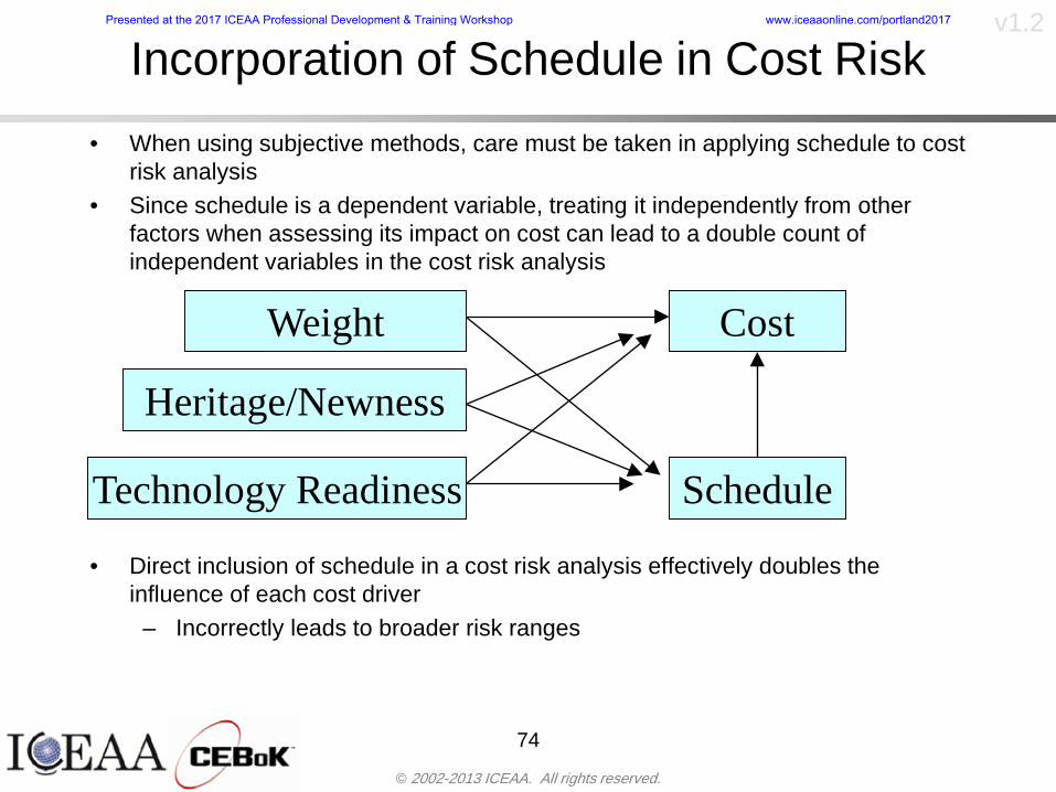
copy 2002-2013 ICEAA All rights reserved
v12
Incorporation of Schedule in Cost Risk
bull When using subjective methods care must be taken in applying schedule to cost risk analysis
bull Since schedule is a dependent variable treating it independently from other factors when assessing its impact on cost can lead to a double count of independent variables in the cost risk analysis
bull Direct inclusion of schedule in a cost risk analysis effectively doubles the influence of each cost driver
ndash Incorrectly leads to broader risk ranges
74
CostWeight
HeritageNewness
Technology Readiness Schedule
Presented at the 2017 ICEAA Professional Development amp Training Workshop wwwiceaaonlinecomportland2017
copy 2002-2013 ICEAA All rights reserved
v12Subjective Cost Risk Methods and Overinclusion of Risk Factors
bull Subjective methods are suitable when data are scarce or not availablebull However care must be taken not to treat correlated sources of risk
such as schedule as independent of each otherbull Example ndash a subjective risk analysis incorporated technology readiness
design risk requirements stability integration risk and schedule and treated each source of risk as independent
bull Risk triangle high value without schedule risk was 31 times the point estimate
bull Risk triangle high value with schedule risk added on top of other sources of risk treated independently was 34 times the point estimate
bull Risk triangle taking correlation between sources of risk into account in a rigorous statistical manner has a high value 15 times the point estimate less than half the effect when treating sources of risk as independent
75
Presented at the 2017 ICEAA Professional Development amp Training Workshop wwwiceaaonlinecomportland2017
copy 2002-2013 ICEAA All rights reserved
v12Fundamental Equation of Cost and Schedule Interrelationships
bull The Fundamental Equation of the Relationship Between Cost and Schedule is
Time = Moneybull This is a well known adage that time is money Your boss at
work may even mention this to you from time to time or if you are the boss you are all too aware of this iron law
bull Because time is money cost and schedule risk should be modeled jointly not with schedule as an independent cost driver
bull Note that cost and schedule are not perfectly correlatedndash Cost can sometimes ldquobuy downrdquo schedule extra money can be
spent to meet a deadline since in some cases additional effort to hasten the completion of a task
76
Presented at the 2017 ICEAA Professional Development amp Training Workshop wwwiceaaonlinecomportland2017
copy 2002-2013 ICEAA All rights reserved
v12How to (Correctly) Incorporate Schedule into Cost Risk Analysis
bull The best way to model cost and schedule risk is to develop a joint cost and schedule model based on the same data
bull Since such models are not currently available the next best approach is to model cost and schedule independently and then integrate cost and schedule risk analyses using joint probability distributions taking into account correlation between cost and schedulendash This approach pioneered by Paul Garvey and Steve Book is
considered industry best practicendash This is a practical method mathematically tractable and follows
naturally from the Fundamental Equation of Cost and Schedule Interrelationships
77
Book S A ldquoQuantifying the Relationship Between Cost and Schedulerdquo The Measurable News Winter 2007-2008 pp 11-15Garvey PR Probability Methods for Cost Uncertainty Analysis A Systems Engineering Perspective New York Marcel Dekker 2000 pp 308-335
Presented at the 2017 ICEAA Professional Development amp Training Workshop wwwiceaaonlinecomportland2017
copy 2002-2013 ICEAA All rights reserved
v12
Joint Lognormal and Normal Distributions
bull Cost and schedule are typically modeled as some combination of Normal and Lognormal probability distributionsndash Studies by The Aerospace Corporation the MITRE
Corporation Wyle Labs and SAIC have found that the Lognormal probability distribution almost always serves as a good model for both the schedule distribution and the cost distribution
ndash The Normal distribution may also be appropriate in some instances and depending upon the level of confidence at which budgets are set may even be more conservative and logically consistent than the Normal distribution
ndash Joint Lognormal and Normal distributions are defined by a pair of mean and standard deviations and a level of correlation between the two
78
Presented at the 2017 ICEAA Professional Development amp Training Workshop wwwiceaaonlinecomportland2017
copy 2002-2013 ICEAA All rights reserved
v12Modeling Cost and Schedule as a Bivariate Distribution
bull In the approach set forth by Book and Garvey cost risk is assessed and the top-level distribution is modeled as a Lognormal (or Normal) distribution schedule risk is assessed and the overall schedule risk is modeled as a Lognormal (or Normal) distribution
bull The two distributions are combined into a Bivariate distribution by assigning a correlation between the two and by treating the two distributions as the marginal distributions of a Bivariate Lognormal distributionndash Other combinations include a Bivariate Normal or a Bivariate
Normal-Lognormal
79
Presented at the 2017 ICEAA Professional Development amp Training Workshop wwwiceaaonlinecomportland2017
copy 2002-2013 ICEAA All rights reserved
v12Bivariate Lognormal Distribution for Cost and Schedule
bull Cost is often observed to be Lognormal when strong positive correlations are present among the systemrsquos WBS cost element costs
bull A systemrsquos schedule is often observed (from Monte Carlo simulations) to be Lognormal if it is the sum of many positively correlated schedule activities in an overall schedule network
bull If Lognormal distributions characterize a systemrsquos cost and schedule then the Bivariate Lognormal could serve as an assumed model of their joint distributionndash In this case the marginal distribution of each of cost and schedule is
Lognormalbull Other possibilities for modeling cost and schedule as a Bivariate
distribution include a Bivariate Normal or a Bivariate Normal-Lognormal distributionndash All these combinations are analytically tractable
80
Presented at the 2017 ICEAA Professional Development amp Training Workshop wwwiceaaonlinecomportland2017
copy 2002-2013 ICEAA All rights reserved
v12Bivariate Lognormal for Cost and Schedule
bull Contour Plots of a Bivariate Lognormal
81
Presented at the 2017 ICEAA Professional Development amp Training Workshop wwwiceaaonlinecomportland2017
copy 2002-2013 ICEAA All rights reserved
v12Correlation Between Cost and Schedule
bull Cost and schedule are positively correlated but not perfectly sondash For example it is possible to have a schedule underrun and a cost
overrunbull Based on cost and schedule growth data for 50 completed NASA
programs the correlation between development cost and development schedule is 70
82
00
200
400
600
800
1000
1200
-500 00 500 1000 1500 2000 2500Historical Cost Growth
Hist
oric
al S
ched
ule
Gro
wth
r = 715
Presented at the 2017 ICEAA Professional Development amp Training Workshop wwwiceaaonlinecomportland2017
copy 2002-2013 ICEAA All rights reserved
v12Correlation Between Cost and Schedule Caveats
bull Based on historical data recommended correlation between cost and schedule is 70 but this could be higher or lower depending upon program circumstancesndash If program is budget constrained cost and schedule will be
more highly correlated (go as you pay)ndash If program is schedule constrained cost and schedule will
have lower correlation perhaps even negative correlation ndash Smaller programs have smaller correlation between cost and
schedule riskbull Relatively easy to ldquohurry uprdquo and finish on time or even early if
needed
83
Presented at the 2017 ICEAA Professional Development amp Training Workshop wwwiceaaonlinecomportland2017
copy 2002-2013 ICEAA All rights reserved
v12
Conditional Confidence Levelsbull Given a programrsquos project schedule we can determine the cost
risk distribution conditional upon the given schedulebull Conditional cost S-curves are steeper than unconditional
(marginal) cost S-curves between some uncertainty has been removed because schedule is fixed
84
Presented at the 2017 ICEAA Professional Development amp Training Workshop wwwiceaaonlinecomportland2017
copy 2002-2013 ICEAA All rights reserved
v12
Joint Confidence Levelsbull Joint 65 confidence represents the probability of
achieving both 65 confidence in cost AND 65 confidence in schedulendash This is different than achieving 65 cost confidence alone
or achieving 65 schedule confidence alonebull Due to the imperfect correlation between cost and schedule it
is possible to achieve a 65 cost confidence with a lower level of schedule confidence
bull Restricting the schedule confidence thus requires additional $ to achieve a given level of confidence
85
X
Y
Possible Values for Which X gt a Possible Values for
Which X gt a and Y gt b
a
b
Presented at the 2017 ICEAA Professional Development amp Training Workshop wwwiceaaonlinecomportland2017
copy 2002-2013 ICEAA All rights reserved
v12Joint Confidence Levels Versus Cost Confidence Levels Only
bull Example of the differences between cost confidence schedule confidence conditional cost confidence and joint cost and schedule confidence
86
Joint Cost-Schedule Confidence Iso-Curves
Cost (RY$M)
Sche
dule
(Mon
ths)
65 Confidence
50 Confidence
70 Confidence
65 Cost Confidence AggressiveSchedule65 Cost ConfidenceScheduleGiven 65 Schedule ConfidenceUnconditional 65 CostConfidenceUnconditional 65 ScheduleConfidence
65 Cost Confidence 65 Joint Cost and Schedule
Confidence for 65 Schedule Confidence
Presented at the 2017 ICEAA Professional Development amp Training Workshop wwwiceaaonlinecomportland2017
copy 2002-2013 ICEAA All rights reserved
v12
Joint Cost and Schedule Confidence
bull Can examine pairs of cost and schedule that achieve a given level of confidence
bull Provides insights into the trade-offs between cost and schedule for a given level of confidencendash Possible to increase cost confidence by giving a
project more time in some instances or possible to ldquobuy downrdquo schedule
bull But these have limits and are shown in the iso-cost and schedule confidence curves
87
Presented at the 2017 ICEAA Professional Development amp Training Workshop wwwiceaaonlinecomportland2017
copy 2002-2013 ICEAA All rights reserved
v12Cost and Schedule Trade-offs for a Given Level of Joint Confidence
bull Hypothetical Example
88
Cost (RY$M)
Schedule (Months)
$100 48$99 48$89 49$87 50$85 51$85 52$84 53$83 55$83 55$83 56
Cost and Schedule 65 Confidence Iso-Curve
4748495051525354555657
$80 $82 $84 $86 $88 $90 $92 $94 $96 $98 $100
Cost (RY$ M)
Sche
dule
(Mon
ths)
Presented at the 2017 ICEAA Professional Development amp Training Workshop wwwiceaaonlinecomportland2017
copy 2002-2013 ICEAA All rights reserved
v12Policy Considerations for Confidence Levels
bull For large programs the difference between the amount of money needed to achieve 65 cost confidence independent of schedule and joint 65 cost and schedule confidence can represent hundreds of millions and even billions of dollars
89
Joint Cost-Schedule Confidence Iso-Curves
Cost (RY$M)
Sche
dule
(Mon
ths)
65 Confidence
65 Cost Confidence AggressiveSchedule
65 Cost ConfidenceScheduleGiven 65 Schedule Confidence
Unconditional 65 CostConfidence
Joint Cost and Schedule Confidence for 65 Cost Confidence and Program Baseline Schedule is Less Than 35
65 Cost Confidence Independent of Schedule Cost Needed to Achieve
Both 65 Joint Cost and Schedule Confidence for the Schedule with 65 Confidence
Presented at the 2017 ICEAA Professional Development amp Training Workshop wwwiceaaonlinecomportland2017
copy 2002-2013 ICEAA All rights reserved
v12
Copulasbull More generally any combination of distributions can
be used (more than just normal and lognormal)ndash Termed ldquocopulardquo from the Italian word for ldquocouplerdquondash Copulas are a way to combine marginal distributions of any
number and type into a joint distributionbull More formally a copula is a multivariate joint distribution defined
on the n-dimensional unit cube [0 1]n such that every marginal distribution is uniform on the interval [0 1]
bull (The bivariate form of) Sklarrsquos theorem states that for any bivariate distribution function H(x y) let F(x) = H(x infin) and G(y) = H(infin y) be the univariate marginal probability distribution functions Then there exists a copula C such that H(xy)=C(F(x)G(y))
ndash Copulas are widely used in risk management for investments and insurance
bull Considered industry best practice (Li 2000)bull Marketed as part of JP Morganrsquos CreditMetrics suite of tools
(Gupton et Al 1997)90
Presented at the 2017 ICEAA Professional Development amp Training Workshop wwwiceaaonlinecomportland2017
copy 2002-2013 ICEAA All rights reserved
v12Parametric Joint Cost and Schedule Analysis
bull A parametric model based on a consistent data set with a set of overlapping cost and schedule drivers is a cleaner way to model cost and schedule
91
CostWeight
HeritageNewness
Technology Readiness
Schedule
0
20
40
60
80
100
Confidence
Joint Cost and Schedule Confidence
Schedule
Cost
Lognormal Distribution PDF and CDF
0102030405060708090100
200 300 400 500 600 700 800 900 1000Cost $
Con
fiden
ce L
evel
0
00002
00004
00006
00008
0001
00012
00014
00016
Prob
abili
ty D
ensi
ty
CDFPDF
Lognormal Distribution PDF and CDF
0102030405060708090100
200 300 400 500 600 700 800 900 1000Cost $
Con
fiden
ce L
evel
0
00002
00004
00006
00008
0001
00012
00014
00016
Prob
abili
ty D
ensi
ty
CDFPDF
Presented at the 2017 ICEAA Professional Development amp Training Workshop wwwiceaaonlinecomportland2017
copy 2002-2013 ICEAA All rights reserved
v12Parametric Joint Cost and Schedule Analysis (2)
bull Joint cost and schedule risk analysis produced naturally by the integrated modelndash Addresses several issues with the copula
approachbull Tail dependencybull Correlation ndash no need to assign correlation
between cost and schedulebull Consistency of cost and schedule models
92
Presented at the 2017 ICEAA Professional Development amp Training Workshop wwwiceaaonlinecomportland2017
copy 2002-2013 ICEAA All rights reserved
v12
Resource-Loaded Schedulesbull Involves assigning cost and schedule risks to a resource-loaded schedule
networkbull Bottom-up approach
ndash More labor intensive than parametrics but can also provide more insight
ndash Can answer questions than parametric typically cannot such as how much do reserve requirements decrease if a specific risk is retired
bull Currently being implemented in Constellation programbull Has same issue as all bottom-up models hard to count all the risks and model
them discretely
ndash As a result there is a tendency to reflect less risk than indicated by history
ndash ldquoThere are more things in heaven and earth Horatio than are dreamt of in your philosophyrdquo William Shakespeare Hamlet Act I Scene V
93
Presented at the 2017 ICEAA Professional Development amp Training Workshop wwwiceaaonlinecomportland2017
copy 2002-2013 ICEAA All rights reserved
v12Resource-Loaded Schedules Vs Parametrics
bull Parametric most appropriate for early estimatesndash But also good for high-level checks as project progresses
bull As plans take shape lower level modeling may be more appropriate
94 1
CONCEPTUALDEVELOPMENT
PROJECTDEFINITION DESIGN DEVELOPMENT OPERATIONS
PARAMETRIC PARAMETRIC
ANALOGY
ENGINEERING (Bottoms Up)
$PARAMETRIC
DETAILED
$
Pre Phase A Phase B Phase CDPhase A Phase EPre Phase A Phase B Phase CDPhase A Phase E
Risk = f(Cost Estimating Relationship Inputs eg mass power data rate TRL new design etc)
Risk = f(cost and schedule variation of the analogous elements)
Risk = f(variation of detailed inputs eg labor hours rates materials etc)
Presented at the 2017 ICEAA Professional Development amp Training Workshop wwwiceaaonlinecomportland2017
copy 2002-2013 ICEAA All rights reserved
v12
Resource-Loaded Schedulesbull Methodology has been demonstrated in other
industriesndash Construction oil and gasndash Analysis has not been traditionally done on highly uncertain
complex development projects bull Methodology focuses on project baseline schedule
ndash In baseline schedule all tasks are resource loaded to represent a baseline schedule and cost standpoint
ndash Resource loaded schedule is ldquorolledrdquo up to a manageable level
ndash Based on the risk and uncertainties identified schedule distributions are applied to each rolled up task
ndash Cost uncertainties are also applied to rolled up tasksbull Uncertainties include labor rate man power etc
ndash A Monte Carlo simulation is run to develop joint cost-schedule distributions
95
Presented at the 2017 ICEAA Professional Development amp Training Workshop wwwiceaaonlinecomportland2017
copy 2002-2013 ICEAA All rights reserved
v12
Unit III - Module 9 96
Execution ndash Cross Checksbull Means The mean cost growth factor for WBS items
can be compared to history as a way to cross check results
bull CVs The CV of the cost growth factors for WBS items can be compared to history as a way to cross check results
bull Inputs Checks are performed on inputs or other parameters to see if historical values are in line with program assumptionsndash Example Historical risk scores can be compared to program
risk scores to see if risk assessors are being realistic and to see if the underlying database is representative of the program
11
Presented at the 2017 ICEAA Professional Development amp Training Workshop wwwiceaaonlinecomportland2017
- Cost and Schedule Risk Analysis Basic
- Acknowledgments
- Unit Index
- Risk Overview
- Agenda
- Introduction
- Risk Analysis Terms
- Are Our Costs Realistic
- Historical Cost Growth
- Sources of Cost Risk
- Point Estimates of Cost
- Types of Risk
- Point Estimates Vs Risk Estimates
- Cost Risk and Probability
- Probability Model ndash Distribution
- Probability Model ndash Distribution
- Probability ndash Top-Level Distribution
- S-Curves and Confidence Levels
- Example ndash Normal Distribution
- Confidence Levels
- Measuring Parametric Model Uncertainty
- Parametric Model Example
- Weight Uncertainty
- Estimating Uncertainty
- Estimating Uncertainty (2)
- Estimating Uncertainty (3)
- Aggregating Risk
- WBS Example
- WBS and Risk
- Aggregating Risk
- Percentiles Do Not Add
- Percentiles Do Not Add (2)
- Percentiles Do Not Add (3)
- Methods for Aggregating Risk
- Monte Carlo Simulationfor Risk Analysis
- Monte Carlo Simulation
- Using Random Numbers to Simulate Distributions
- Simulating a Triangular Distribution
- Simulating a Triangular Distribution (2)
- Monte Carlo and the WBS
- Number of Trials
- Number of Trials (2)
- Number of Trials (3)
- Number of Trials (4)
- Number of Trials (5)
- Number of Trials (6)
- Methods of Simulation
- Probability Model ndash Correlation
- Correlation And Causation
- The Importance of Correlation
- The Importance of Correlation (2)
- Measures of Correlation
- Pearson Correlation
- Spearman Correlation
- Functional Correlation
- Risk Measures
- Value at Risk (VaR)
- Why 70th or 80th Percentile
- Funding Above Inflection Points
- Why Budget to the 70th or 80th
- Inflection Points for Lognormal
- Issues with Percentile Funding
- ldquoHere There Be Dragonsrdquo
- Distribution Comparison
- Distribution Comparison Tail Behavior
- Distribution Comparison ndash Tail Behavior (Table)
- Percentile Budgeting is Not Risk Management
- Joint Confidence Level Analysis
- Schedules Impact Cost
- The Relationship of Cost to Schedule
- The Impact of Schedule GrowthCompression on Cost
- Schedule as an Independent Variable
- Schedule is a Dependent Variable
- Incorporation of Schedule in Cost Risk
- Subjective Cost Risk Methods and Overinclusion of Risk Factors
- Fundamental Equation of Cost and Schedule Interrelationships
- How to (Correctly) Incorporate Schedule into Cost Risk Analysis
- Joint Lognormal and Normal Distributions
- Modeling Cost and Schedule as a Bivariate Distribution
- Bivariate Lognormal Distribution for Cost and Schedule
- Bivariate Lognormal for Cost and Schedule
- Correlation Between Cost and Schedule
- Correlation Between Cost and Schedule Caveats
- Conditional Confidence Levels
- Joint Confidence Levels
- Joint Confidence Levels Versus Cost Confidence Levels Only
- Joint Cost and Schedule Confidence
- Cost and Schedule Trade-offs for a Given Level of Joint Confidence
- Policy Considerations for Confidence Levels
- Copulas
- Parametric Joint Cost and Schedule Analysis
- Parametric Joint Cost and Schedule Analysis (2)
- Resource-Loaded Schedules
- Resource-Loaded Schedules Vs Parametrics
- Resource-Loaded Schedules
- Execution ndash Cross Checks
-
copy 2002-2013 ICEAA All rights reserved
v12
Joint Lognormal and Normal Distributions
bull Cost and schedule are typically modeled as some combination of Normal and Lognormal probability distributionsndash Studies by The Aerospace Corporation the MITRE
Corporation Wyle Labs and SAIC have found that the Lognormal probability distribution almost always serves as a good model for both the schedule distribution and the cost distribution
ndash The Normal distribution may also be appropriate in some instances and depending upon the level of confidence at which budgets are set may even be more conservative and logically consistent than the Normal distribution
ndash Joint Lognormal and Normal distributions are defined by a pair of mean and standard deviations and a level of correlation between the two
78
Presented at the 2017 ICEAA Professional Development amp Training Workshop wwwiceaaonlinecomportland2017
copy 2002-2013 ICEAA All rights reserved
v12Modeling Cost and Schedule as a Bivariate Distribution
bull In the approach set forth by Book and Garvey cost risk is assessed and the top-level distribution is modeled as a Lognormal (or Normal) distribution schedule risk is assessed and the overall schedule risk is modeled as a Lognormal (or Normal) distribution
bull The two distributions are combined into a Bivariate distribution by assigning a correlation between the two and by treating the two distributions as the marginal distributions of a Bivariate Lognormal distributionndash Other combinations include a Bivariate Normal or a Bivariate
Normal-Lognormal
79
Presented at the 2017 ICEAA Professional Development amp Training Workshop wwwiceaaonlinecomportland2017
copy 2002-2013 ICEAA All rights reserved
v12Bivariate Lognormal Distribution for Cost and Schedule
bull Cost is often observed to be Lognormal when strong positive correlations are present among the systemrsquos WBS cost element costs
bull A systemrsquos schedule is often observed (from Monte Carlo simulations) to be Lognormal if it is the sum of many positively correlated schedule activities in an overall schedule network
bull If Lognormal distributions characterize a systemrsquos cost and schedule then the Bivariate Lognormal could serve as an assumed model of their joint distributionndash In this case the marginal distribution of each of cost and schedule is
Lognormalbull Other possibilities for modeling cost and schedule as a Bivariate
distribution include a Bivariate Normal or a Bivariate Normal-Lognormal distributionndash All these combinations are analytically tractable
80
Presented at the 2017 ICEAA Professional Development amp Training Workshop wwwiceaaonlinecomportland2017
copy 2002-2013 ICEAA All rights reserved
v12Bivariate Lognormal for Cost and Schedule
bull Contour Plots of a Bivariate Lognormal
81
Presented at the 2017 ICEAA Professional Development amp Training Workshop wwwiceaaonlinecomportland2017
copy 2002-2013 ICEAA All rights reserved
v12Correlation Between Cost and Schedule
bull Cost and schedule are positively correlated but not perfectly sondash For example it is possible to have a schedule underrun and a cost
overrunbull Based on cost and schedule growth data for 50 completed NASA
programs the correlation between development cost and development schedule is 70
82
00
200
400
600
800
1000
1200
-500 00 500 1000 1500 2000 2500Historical Cost Growth
Hist
oric
al S
ched
ule
Gro
wth
r = 715
Presented at the 2017 ICEAA Professional Development amp Training Workshop wwwiceaaonlinecomportland2017
copy 2002-2013 ICEAA All rights reserved
v12Correlation Between Cost and Schedule Caveats
bull Based on historical data recommended correlation between cost and schedule is 70 but this could be higher or lower depending upon program circumstancesndash If program is budget constrained cost and schedule will be
more highly correlated (go as you pay)ndash If program is schedule constrained cost and schedule will
have lower correlation perhaps even negative correlation ndash Smaller programs have smaller correlation between cost and
schedule riskbull Relatively easy to ldquohurry uprdquo and finish on time or even early if
needed
83
Presented at the 2017 ICEAA Professional Development amp Training Workshop wwwiceaaonlinecomportland2017
copy 2002-2013 ICEAA All rights reserved
v12
Conditional Confidence Levelsbull Given a programrsquos project schedule we can determine the cost
risk distribution conditional upon the given schedulebull Conditional cost S-curves are steeper than unconditional
(marginal) cost S-curves between some uncertainty has been removed because schedule is fixed
84
Presented at the 2017 ICEAA Professional Development amp Training Workshop wwwiceaaonlinecomportland2017
copy 2002-2013 ICEAA All rights reserved
v12
Joint Confidence Levelsbull Joint 65 confidence represents the probability of
achieving both 65 confidence in cost AND 65 confidence in schedulendash This is different than achieving 65 cost confidence alone
or achieving 65 schedule confidence alonebull Due to the imperfect correlation between cost and schedule it
is possible to achieve a 65 cost confidence with a lower level of schedule confidence
bull Restricting the schedule confidence thus requires additional $ to achieve a given level of confidence
85
X
Y
Possible Values for Which X gt a Possible Values for
Which X gt a and Y gt b
a
b
Presented at the 2017 ICEAA Professional Development amp Training Workshop wwwiceaaonlinecomportland2017
copy 2002-2013 ICEAA All rights reserved
v12Joint Confidence Levels Versus Cost Confidence Levels Only
bull Example of the differences between cost confidence schedule confidence conditional cost confidence and joint cost and schedule confidence
86
Joint Cost-Schedule Confidence Iso-Curves
Cost (RY$M)
Sche
dule
(Mon
ths)
65 Confidence
50 Confidence
70 Confidence
65 Cost Confidence AggressiveSchedule65 Cost ConfidenceScheduleGiven 65 Schedule ConfidenceUnconditional 65 CostConfidenceUnconditional 65 ScheduleConfidence
65 Cost Confidence 65 Joint Cost and Schedule
Confidence for 65 Schedule Confidence
Presented at the 2017 ICEAA Professional Development amp Training Workshop wwwiceaaonlinecomportland2017
copy 2002-2013 ICEAA All rights reserved
v12
Joint Cost and Schedule Confidence
bull Can examine pairs of cost and schedule that achieve a given level of confidence
bull Provides insights into the trade-offs between cost and schedule for a given level of confidencendash Possible to increase cost confidence by giving a
project more time in some instances or possible to ldquobuy downrdquo schedule
bull But these have limits and are shown in the iso-cost and schedule confidence curves
87
Presented at the 2017 ICEAA Professional Development amp Training Workshop wwwiceaaonlinecomportland2017
copy 2002-2013 ICEAA All rights reserved
v12Cost and Schedule Trade-offs for a Given Level of Joint Confidence
bull Hypothetical Example
88
Cost (RY$M)
Schedule (Months)
$100 48$99 48$89 49$87 50$85 51$85 52$84 53$83 55$83 55$83 56
Cost and Schedule 65 Confidence Iso-Curve
4748495051525354555657
$80 $82 $84 $86 $88 $90 $92 $94 $96 $98 $100
Cost (RY$ M)
Sche
dule
(Mon
ths)
Presented at the 2017 ICEAA Professional Development amp Training Workshop wwwiceaaonlinecomportland2017
copy 2002-2013 ICEAA All rights reserved
v12Policy Considerations for Confidence Levels
bull For large programs the difference between the amount of money needed to achieve 65 cost confidence independent of schedule and joint 65 cost and schedule confidence can represent hundreds of millions and even billions of dollars
89
Joint Cost-Schedule Confidence Iso-Curves
Cost (RY$M)
Sche
dule
(Mon
ths)
65 Confidence
65 Cost Confidence AggressiveSchedule
65 Cost ConfidenceScheduleGiven 65 Schedule Confidence
Unconditional 65 CostConfidence
Joint Cost and Schedule Confidence for 65 Cost Confidence and Program Baseline Schedule is Less Than 35
65 Cost Confidence Independent of Schedule Cost Needed to Achieve
Both 65 Joint Cost and Schedule Confidence for the Schedule with 65 Confidence
Presented at the 2017 ICEAA Professional Development amp Training Workshop wwwiceaaonlinecomportland2017
copy 2002-2013 ICEAA All rights reserved
v12
Copulasbull More generally any combination of distributions can
be used (more than just normal and lognormal)ndash Termed ldquocopulardquo from the Italian word for ldquocouplerdquondash Copulas are a way to combine marginal distributions of any
number and type into a joint distributionbull More formally a copula is a multivariate joint distribution defined
on the n-dimensional unit cube [0 1]n such that every marginal distribution is uniform on the interval [0 1]
bull (The bivariate form of) Sklarrsquos theorem states that for any bivariate distribution function H(x y) let F(x) = H(x infin) and G(y) = H(infin y) be the univariate marginal probability distribution functions Then there exists a copula C such that H(xy)=C(F(x)G(y))
ndash Copulas are widely used in risk management for investments and insurance
bull Considered industry best practice (Li 2000)bull Marketed as part of JP Morganrsquos CreditMetrics suite of tools
(Gupton et Al 1997)90
Presented at the 2017 ICEAA Professional Development amp Training Workshop wwwiceaaonlinecomportland2017
copy 2002-2013 ICEAA All rights reserved
v12Parametric Joint Cost and Schedule Analysis
bull A parametric model based on a consistent data set with a set of overlapping cost and schedule drivers is a cleaner way to model cost and schedule
91
CostWeight
HeritageNewness
Technology Readiness
Schedule
0
20
40
60
80
100
Confidence
Joint Cost and Schedule Confidence
Schedule
Cost
Lognormal Distribution PDF and CDF
0102030405060708090100
200 300 400 500 600 700 800 900 1000Cost $
Con
fiden
ce L
evel
0
00002
00004
00006
00008
0001
00012
00014
00016
Prob
abili
ty D
ensi
ty
CDFPDF
Lognormal Distribution PDF and CDF
0102030405060708090100
200 300 400 500 600 700 800 900 1000Cost $
Con
fiden
ce L
evel
0
00002
00004
00006
00008
0001
00012
00014
00016
Prob
abili
ty D
ensi
ty
CDFPDF
Presented at the 2017 ICEAA Professional Development amp Training Workshop wwwiceaaonlinecomportland2017
copy 2002-2013 ICEAA All rights reserved
v12Parametric Joint Cost and Schedule Analysis (2)
bull Joint cost and schedule risk analysis produced naturally by the integrated modelndash Addresses several issues with the copula
approachbull Tail dependencybull Correlation ndash no need to assign correlation
between cost and schedulebull Consistency of cost and schedule models
92
Presented at the 2017 ICEAA Professional Development amp Training Workshop wwwiceaaonlinecomportland2017
copy 2002-2013 ICEAA All rights reserved
v12
Resource-Loaded Schedulesbull Involves assigning cost and schedule risks to a resource-loaded schedule
networkbull Bottom-up approach
ndash More labor intensive than parametrics but can also provide more insight
ndash Can answer questions than parametric typically cannot such as how much do reserve requirements decrease if a specific risk is retired
bull Currently being implemented in Constellation programbull Has same issue as all bottom-up models hard to count all the risks and model
them discretely
ndash As a result there is a tendency to reflect less risk than indicated by history
ndash ldquoThere are more things in heaven and earth Horatio than are dreamt of in your philosophyrdquo William Shakespeare Hamlet Act I Scene V
93
Presented at the 2017 ICEAA Professional Development amp Training Workshop wwwiceaaonlinecomportland2017
copy 2002-2013 ICEAA All rights reserved
v12Resource-Loaded Schedules Vs Parametrics
bull Parametric most appropriate for early estimatesndash But also good for high-level checks as project progresses
bull As plans take shape lower level modeling may be more appropriate
94 1
CONCEPTUALDEVELOPMENT
PROJECTDEFINITION DESIGN DEVELOPMENT OPERATIONS
PARAMETRIC PARAMETRIC
ANALOGY
ENGINEERING (Bottoms Up)
$PARAMETRIC
DETAILED
$
Pre Phase A Phase B Phase CDPhase A Phase EPre Phase A Phase B Phase CDPhase A Phase E
Risk = f(Cost Estimating Relationship Inputs eg mass power data rate TRL new design etc)
Risk = f(cost and schedule variation of the analogous elements)
Risk = f(variation of detailed inputs eg labor hours rates materials etc)
Presented at the 2017 ICEAA Professional Development amp Training Workshop wwwiceaaonlinecomportland2017
copy 2002-2013 ICEAA All rights reserved
v12
Resource-Loaded Schedulesbull Methodology has been demonstrated in other
industriesndash Construction oil and gasndash Analysis has not been traditionally done on highly uncertain
complex development projects bull Methodology focuses on project baseline schedule
ndash In baseline schedule all tasks are resource loaded to represent a baseline schedule and cost standpoint
ndash Resource loaded schedule is ldquorolledrdquo up to a manageable level
ndash Based on the risk and uncertainties identified schedule distributions are applied to each rolled up task
ndash Cost uncertainties are also applied to rolled up tasksbull Uncertainties include labor rate man power etc
ndash A Monte Carlo simulation is run to develop joint cost-schedule distributions
95
Presented at the 2017 ICEAA Professional Development amp Training Workshop wwwiceaaonlinecomportland2017
copy 2002-2013 ICEAA All rights reserved
v12
Unit III - Module 9 96
Execution ndash Cross Checksbull Means The mean cost growth factor for WBS items
can be compared to history as a way to cross check results
bull CVs The CV of the cost growth factors for WBS items can be compared to history as a way to cross check results
bull Inputs Checks are performed on inputs or other parameters to see if historical values are in line with program assumptionsndash Example Historical risk scores can be compared to program
risk scores to see if risk assessors are being realistic and to see if the underlying database is representative of the program
11
Presented at the 2017 ICEAA Professional Development amp Training Workshop wwwiceaaonlinecomportland2017
- Cost and Schedule Risk Analysis Basic
- Acknowledgments
- Unit Index
- Risk Overview
- Agenda
- Introduction
- Risk Analysis Terms
- Are Our Costs Realistic
- Historical Cost Growth
- Sources of Cost Risk
- Point Estimates of Cost
- Types of Risk
- Point Estimates Vs Risk Estimates
- Cost Risk and Probability
- Probability Model ndash Distribution
- Probability Model ndash Distribution
- Probability ndash Top-Level Distribution
- S-Curves and Confidence Levels
- Example ndash Normal Distribution
- Confidence Levels
- Measuring Parametric Model Uncertainty
- Parametric Model Example
- Weight Uncertainty
- Estimating Uncertainty
- Estimating Uncertainty (2)
- Estimating Uncertainty (3)
- Aggregating Risk
- WBS Example
- WBS and Risk
- Aggregating Risk
- Percentiles Do Not Add
- Percentiles Do Not Add (2)
- Percentiles Do Not Add (3)
- Methods for Aggregating Risk
- Monte Carlo Simulationfor Risk Analysis
- Monte Carlo Simulation
- Using Random Numbers to Simulate Distributions
- Simulating a Triangular Distribution
- Simulating a Triangular Distribution (2)
- Monte Carlo and the WBS
- Number of Trials
- Number of Trials (2)
- Number of Trials (3)
- Number of Trials (4)
- Number of Trials (5)
- Number of Trials (6)
- Methods of Simulation
- Probability Model ndash Correlation
- Correlation And Causation
- The Importance of Correlation
- The Importance of Correlation (2)
- Measures of Correlation
- Pearson Correlation
- Spearman Correlation
- Functional Correlation
- Risk Measures
- Value at Risk (VaR)
- Why 70th or 80th Percentile
- Funding Above Inflection Points
- Why Budget to the 70th or 80th
- Inflection Points for Lognormal
- Issues with Percentile Funding
- ldquoHere There Be Dragonsrdquo
- Distribution Comparison
- Distribution Comparison Tail Behavior
- Distribution Comparison ndash Tail Behavior (Table)
- Percentile Budgeting is Not Risk Management
- Joint Confidence Level Analysis
- Schedules Impact Cost
- The Relationship of Cost to Schedule
- The Impact of Schedule GrowthCompression on Cost
- Schedule as an Independent Variable
- Schedule is a Dependent Variable
- Incorporation of Schedule in Cost Risk
- Subjective Cost Risk Methods and Overinclusion of Risk Factors
- Fundamental Equation of Cost and Schedule Interrelationships
- How to (Correctly) Incorporate Schedule into Cost Risk Analysis
- Joint Lognormal and Normal Distributions
- Modeling Cost and Schedule as a Bivariate Distribution
- Bivariate Lognormal Distribution for Cost and Schedule
- Bivariate Lognormal for Cost and Schedule
- Correlation Between Cost and Schedule
- Correlation Between Cost and Schedule Caveats
- Conditional Confidence Levels
- Joint Confidence Levels
- Joint Confidence Levels Versus Cost Confidence Levels Only
- Joint Cost and Schedule Confidence
- Cost and Schedule Trade-offs for a Given Level of Joint Confidence
- Policy Considerations for Confidence Levels
- Copulas
- Parametric Joint Cost and Schedule Analysis
- Parametric Joint Cost and Schedule Analysis (2)
- Resource-Loaded Schedules
- Resource-Loaded Schedules Vs Parametrics
- Resource-Loaded Schedules
- Execution ndash Cross Checks
-

copy 2002-2013 ICEAA All rights reserved
v12Modeling Cost and Schedule as a Bivariate Distribution
bull In the approach set forth by Book and Garvey cost risk is assessed and the top-level distribution is modeled as a Lognormal (or Normal) distribution schedule risk is assessed and the overall schedule risk is modeled as a Lognormal (or Normal) distribution
bull The two distributions are combined into a Bivariate distribution by assigning a correlation between the two and by treating the two distributions as the marginal distributions of a Bivariate Lognormal distributionndash Other combinations include a Bivariate Normal or a Bivariate
Normal-Lognormal
79
Presented at the 2017 ICEAA Professional Development amp Training Workshop wwwiceaaonlinecomportland2017
copy 2002-2013 ICEAA All rights reserved
v12Bivariate Lognormal Distribution for Cost and Schedule
bull Cost is often observed to be Lognormal when strong positive correlations are present among the systemrsquos WBS cost element costs
bull A systemrsquos schedule is often observed (from Monte Carlo simulations) to be Lognormal if it is the sum of many positively correlated schedule activities in an overall schedule network
bull If Lognormal distributions characterize a systemrsquos cost and schedule then the Bivariate Lognormal could serve as an assumed model of their joint distributionndash In this case the marginal distribution of each of cost and schedule is
Lognormalbull Other possibilities for modeling cost and schedule as a Bivariate
distribution include a Bivariate Normal or a Bivariate Normal-Lognormal distributionndash All these combinations are analytically tractable
80
Presented at the 2017 ICEAA Professional Development amp Training Workshop wwwiceaaonlinecomportland2017
copy 2002-2013 ICEAA All rights reserved
v12Bivariate Lognormal for Cost and Schedule
bull Contour Plots of a Bivariate Lognormal
81
Presented at the 2017 ICEAA Professional Development amp Training Workshop wwwiceaaonlinecomportland2017
copy 2002-2013 ICEAA All rights reserved
v12Correlation Between Cost and Schedule
bull Cost and schedule are positively correlated but not perfectly sondash For example it is possible to have a schedule underrun and a cost
overrunbull Based on cost and schedule growth data for 50 completed NASA
programs the correlation between development cost and development schedule is 70
82
00
200
400
600
800
1000
1200
-500 00 500 1000 1500 2000 2500Historical Cost Growth
Hist
oric
al S
ched
ule
Gro
wth
r = 715
Presented at the 2017 ICEAA Professional Development amp Training Workshop wwwiceaaonlinecomportland2017
copy 2002-2013 ICEAA All rights reserved
v12Correlation Between Cost and Schedule Caveats
bull Based on historical data recommended correlation between cost and schedule is 70 but this could be higher or lower depending upon program circumstancesndash If program is budget constrained cost and schedule will be
more highly correlated (go as you pay)ndash If program is schedule constrained cost and schedule will
have lower correlation perhaps even negative correlation ndash Smaller programs have smaller correlation between cost and
schedule riskbull Relatively easy to ldquohurry uprdquo and finish on time or even early if
needed
83
Presented at the 2017 ICEAA Professional Development amp Training Workshop wwwiceaaonlinecomportland2017
copy 2002-2013 ICEAA All rights reserved
v12
Conditional Confidence Levelsbull Given a programrsquos project schedule we can determine the cost
risk distribution conditional upon the given schedulebull Conditional cost S-curves are steeper than unconditional
(marginal) cost S-curves between some uncertainty has been removed because schedule is fixed
84
Presented at the 2017 ICEAA Professional Development amp Training Workshop wwwiceaaonlinecomportland2017
copy 2002-2013 ICEAA All rights reserved
v12
Joint Confidence Levelsbull Joint 65 confidence represents the probability of
achieving both 65 confidence in cost AND 65 confidence in schedulendash This is different than achieving 65 cost confidence alone
or achieving 65 schedule confidence alonebull Due to the imperfect correlation between cost and schedule it
is possible to achieve a 65 cost confidence with a lower level of schedule confidence
bull Restricting the schedule confidence thus requires additional $ to achieve a given level of confidence
85
X
Y
Possible Values for Which X gt a Possible Values for
Which X gt a and Y gt b
a
b
Presented at the 2017 ICEAA Professional Development amp Training Workshop wwwiceaaonlinecomportland2017
copy 2002-2013 ICEAA All rights reserved
v12Joint Confidence Levels Versus Cost Confidence Levels Only
bull Example of the differences between cost confidence schedule confidence conditional cost confidence and joint cost and schedule confidence
86
Joint Cost-Schedule Confidence Iso-Curves
Cost (RY$M)
Sche
dule
(Mon
ths)
65 Confidence
50 Confidence
70 Confidence
65 Cost Confidence AggressiveSchedule65 Cost ConfidenceScheduleGiven 65 Schedule ConfidenceUnconditional 65 CostConfidenceUnconditional 65 ScheduleConfidence
65 Cost Confidence 65 Joint Cost and Schedule
Confidence for 65 Schedule Confidence
Presented at the 2017 ICEAA Professional Development amp Training Workshop wwwiceaaonlinecomportland2017
copy 2002-2013 ICEAA All rights reserved
v12
Joint Cost and Schedule Confidence
bull Can examine pairs of cost and schedule that achieve a given level of confidence
bull Provides insights into the trade-offs between cost and schedule for a given level of confidencendash Possible to increase cost confidence by giving a
project more time in some instances or possible to ldquobuy downrdquo schedule
bull But these have limits and are shown in the iso-cost and schedule confidence curves
87
Presented at the 2017 ICEAA Professional Development amp Training Workshop wwwiceaaonlinecomportland2017
copy 2002-2013 ICEAA All rights reserved
v12Cost and Schedule Trade-offs for a Given Level of Joint Confidence
bull Hypothetical Example
88
Cost (RY$M)
Schedule (Months)
$100 48$99 48$89 49$87 50$85 51$85 52$84 53$83 55$83 55$83 56
Cost and Schedule 65 Confidence Iso-Curve
4748495051525354555657
$80 $82 $84 $86 $88 $90 $92 $94 $96 $98 $100
Cost (RY$ M)
Sche
dule
(Mon
ths)
Presented at the 2017 ICEAA Professional Development amp Training Workshop wwwiceaaonlinecomportland2017
copy 2002-2013 ICEAA All rights reserved
v12Policy Considerations for Confidence Levels
bull For large programs the difference between the amount of money needed to achieve 65 cost confidence independent of schedule and joint 65 cost and schedule confidence can represent hundreds of millions and even billions of dollars
89
Joint Cost-Schedule Confidence Iso-Curves
Cost (RY$M)
Sche
dule
(Mon
ths)
65 Confidence
65 Cost Confidence AggressiveSchedule
65 Cost ConfidenceScheduleGiven 65 Schedule Confidence
Unconditional 65 CostConfidence
Joint Cost and Schedule Confidence for 65 Cost Confidence and Program Baseline Schedule is Less Than 35
65 Cost Confidence Independent of Schedule Cost Needed to Achieve
Both 65 Joint Cost and Schedule Confidence for the Schedule with 65 Confidence
Presented at the 2017 ICEAA Professional Development amp Training Workshop wwwiceaaonlinecomportland2017
copy 2002-2013 ICEAA All rights reserved
v12
Copulasbull More generally any combination of distributions can
be used (more than just normal and lognormal)ndash Termed ldquocopulardquo from the Italian word for ldquocouplerdquondash Copulas are a way to combine marginal distributions of any
number and type into a joint distributionbull More formally a copula is a multivariate joint distribution defined
on the n-dimensional unit cube [0 1]n such that every marginal distribution is uniform on the interval [0 1]
bull (The bivariate form of) Sklarrsquos theorem states that for any bivariate distribution function H(x y) let F(x) = H(x infin) and G(y) = H(infin y) be the univariate marginal probability distribution functions Then there exists a copula C such that H(xy)=C(F(x)G(y))
ndash Copulas are widely used in risk management for investments and insurance
bull Considered industry best practice (Li 2000)bull Marketed as part of JP Morganrsquos CreditMetrics suite of tools
(Gupton et Al 1997)90
Presented at the 2017 ICEAA Professional Development amp Training Workshop wwwiceaaonlinecomportland2017
copy 2002-2013 ICEAA All rights reserved
v12Parametric Joint Cost and Schedule Analysis
bull A parametric model based on a consistent data set with a set of overlapping cost and schedule drivers is a cleaner way to model cost and schedule
91
CostWeight
HeritageNewness
Technology Readiness
Schedule
0
20
40
60
80
100
Confidence
Joint Cost and Schedule Confidence
Schedule
Cost
Lognormal Distribution PDF and CDF
0102030405060708090100
200 300 400 500 600 700 800 900 1000Cost $
Con
fiden
ce L
evel
0
00002
00004
00006
00008
0001
00012
00014
00016
Prob
abili
ty D
ensi
ty
CDFPDF
Lognormal Distribution PDF and CDF
0102030405060708090100
200 300 400 500 600 700 800 900 1000Cost $
Con
fiden
ce L
evel
0
00002
00004
00006
00008
0001
00012
00014
00016
Prob
abili
ty D
ensi
ty
CDFPDF
Presented at the 2017 ICEAA Professional Development amp Training Workshop wwwiceaaonlinecomportland2017
copy 2002-2013 ICEAA All rights reserved
v12Parametric Joint Cost and Schedule Analysis (2)
bull Joint cost and schedule risk analysis produced naturally by the integrated modelndash Addresses several issues with the copula
approachbull Tail dependencybull Correlation ndash no need to assign correlation
between cost and schedulebull Consistency of cost and schedule models
92
Presented at the 2017 ICEAA Professional Development amp Training Workshop wwwiceaaonlinecomportland2017
copy 2002-2013 ICEAA All rights reserved
v12
Resource-Loaded Schedulesbull Involves assigning cost and schedule risks to a resource-loaded schedule
networkbull Bottom-up approach
ndash More labor intensive than parametrics but can also provide more insight
ndash Can answer questions than parametric typically cannot such as how much do reserve requirements decrease if a specific risk is retired
bull Currently being implemented in Constellation programbull Has same issue as all bottom-up models hard to count all the risks and model
them discretely
ndash As a result there is a tendency to reflect less risk than indicated by history
ndash ldquoThere are more things in heaven and earth Horatio than are dreamt of in your philosophyrdquo William Shakespeare Hamlet Act I Scene V
93
Presented at the 2017 ICEAA Professional Development amp Training Workshop wwwiceaaonlinecomportland2017
copy 2002-2013 ICEAA All rights reserved
v12Resource-Loaded Schedules Vs Parametrics
bull Parametric most appropriate for early estimatesndash But also good for high-level checks as project progresses
bull As plans take shape lower level modeling may be more appropriate
94 1
CONCEPTUALDEVELOPMENT
PROJECTDEFINITION DESIGN DEVELOPMENT OPERATIONS
PARAMETRIC PARAMETRIC
ANALOGY
ENGINEERING (Bottoms Up)
$PARAMETRIC
DETAILED
$
Pre Phase A Phase B Phase CDPhase A Phase EPre Phase A Phase B Phase CDPhase A Phase E
Risk = f(Cost Estimating Relationship Inputs eg mass power data rate TRL new design etc)
Risk = f(cost and schedule variation of the analogous elements)
Risk = f(variation of detailed inputs eg labor hours rates materials etc)
Presented at the 2017 ICEAA Professional Development amp Training Workshop wwwiceaaonlinecomportland2017
copy 2002-2013 ICEAA All rights reserved
v12
Resource-Loaded Schedulesbull Methodology has been demonstrated in other
industriesndash Construction oil and gasndash Analysis has not been traditionally done on highly uncertain
complex development projects bull Methodology focuses on project baseline schedule
ndash In baseline schedule all tasks are resource loaded to represent a baseline schedule and cost standpoint
ndash Resource loaded schedule is ldquorolledrdquo up to a manageable level
ndash Based on the risk and uncertainties identified schedule distributions are applied to each rolled up task
ndash Cost uncertainties are also applied to rolled up tasksbull Uncertainties include labor rate man power etc
ndash A Monte Carlo simulation is run to develop joint cost-schedule distributions
95
Presented at the 2017 ICEAA Professional Development amp Training Workshop wwwiceaaonlinecomportland2017
copy 2002-2013 ICEAA All rights reserved
v12
Unit III - Module 9 96
Execution ndash Cross Checksbull Means The mean cost growth factor for WBS items
can be compared to history as a way to cross check results
bull CVs The CV of the cost growth factors for WBS items can be compared to history as a way to cross check results
bull Inputs Checks are performed on inputs or other parameters to see if historical values are in line with program assumptionsndash Example Historical risk scores can be compared to program
risk scores to see if risk assessors are being realistic and to see if the underlying database is representative of the program
11
Presented at the 2017 ICEAA Professional Development amp Training Workshop wwwiceaaonlinecomportland2017
- Cost and Schedule Risk Analysis Basic
- Acknowledgments
- Unit Index
- Risk Overview
- Agenda
- Introduction
- Risk Analysis Terms
- Are Our Costs Realistic
- Historical Cost Growth
- Sources of Cost Risk
- Point Estimates of Cost
- Types of Risk
- Point Estimates Vs Risk Estimates
- Cost Risk and Probability
- Probability Model ndash Distribution
- Probability Model ndash Distribution
- Probability ndash Top-Level Distribution
- S-Curves and Confidence Levels
- Example ndash Normal Distribution
- Confidence Levels
- Measuring Parametric Model Uncertainty
- Parametric Model Example
- Weight Uncertainty
- Estimating Uncertainty
- Estimating Uncertainty (2)
- Estimating Uncertainty (3)
- Aggregating Risk
- WBS Example
- WBS and Risk
- Aggregating Risk
- Percentiles Do Not Add
- Percentiles Do Not Add (2)
- Percentiles Do Not Add (3)
- Methods for Aggregating Risk
- Monte Carlo Simulationfor Risk Analysis
- Monte Carlo Simulation
- Using Random Numbers to Simulate Distributions
- Simulating a Triangular Distribution
- Simulating a Triangular Distribution (2)
- Monte Carlo and the WBS
- Number of Trials
- Number of Trials (2)
- Number of Trials (3)
- Number of Trials (4)
- Number of Trials (5)
- Number of Trials (6)
- Methods of Simulation
- Probability Model ndash Correlation
- Correlation And Causation
- The Importance of Correlation
- The Importance of Correlation (2)
- Measures of Correlation
- Pearson Correlation
- Spearman Correlation
- Functional Correlation
- Risk Measures
- Value at Risk (VaR)
- Why 70th or 80th Percentile
- Funding Above Inflection Points
- Why Budget to the 70th or 80th
- Inflection Points for Lognormal
- Issues with Percentile Funding
- ldquoHere There Be Dragonsrdquo
- Distribution Comparison
- Distribution Comparison Tail Behavior
- Distribution Comparison ndash Tail Behavior (Table)
- Percentile Budgeting is Not Risk Management
- Joint Confidence Level Analysis
- Schedules Impact Cost
- The Relationship of Cost to Schedule
- The Impact of Schedule GrowthCompression on Cost
- Schedule as an Independent Variable
- Schedule is a Dependent Variable
- Incorporation of Schedule in Cost Risk
- Subjective Cost Risk Methods and Overinclusion of Risk Factors
- Fundamental Equation of Cost and Schedule Interrelationships
- How to (Correctly) Incorporate Schedule into Cost Risk Analysis
- Joint Lognormal and Normal Distributions
- Modeling Cost and Schedule as a Bivariate Distribution
- Bivariate Lognormal Distribution for Cost and Schedule
- Bivariate Lognormal for Cost and Schedule
- Correlation Between Cost and Schedule
- Correlation Between Cost and Schedule Caveats
- Conditional Confidence Levels
- Joint Confidence Levels
- Joint Confidence Levels Versus Cost Confidence Levels Only
- Joint Cost and Schedule Confidence
- Cost and Schedule Trade-offs for a Given Level of Joint Confidence
- Policy Considerations for Confidence Levels
- Copulas
- Parametric Joint Cost and Schedule Analysis
- Parametric Joint Cost and Schedule Analysis (2)
- Resource-Loaded Schedules
- Resource-Loaded Schedules Vs Parametrics
- Resource-Loaded Schedules
- Execution ndash Cross Checks
-
copy 2002-2013 ICEAA All rights reserved
v12Bivariate Lognormal Distribution for Cost and Schedule
bull Cost is often observed to be Lognormal when strong positive correlations are present among the systemrsquos WBS cost element costs
bull A systemrsquos schedule is often observed (from Monte Carlo simulations) to be Lognormal if it is the sum of many positively correlated schedule activities in an overall schedule network
bull If Lognormal distributions characterize a systemrsquos cost and schedule then the Bivariate Lognormal could serve as an assumed model of their joint distributionndash In this case the marginal distribution of each of cost and schedule is
Lognormalbull Other possibilities for modeling cost and schedule as a Bivariate
distribution include a Bivariate Normal or a Bivariate Normal-Lognormal distributionndash All these combinations are analytically tractable
80
Presented at the 2017 ICEAA Professional Development amp Training Workshop wwwiceaaonlinecomportland2017
copy 2002-2013 ICEAA All rights reserved
v12Bivariate Lognormal for Cost and Schedule
bull Contour Plots of a Bivariate Lognormal
81
Presented at the 2017 ICEAA Professional Development amp Training Workshop wwwiceaaonlinecomportland2017
copy 2002-2013 ICEAA All rights reserved
v12Correlation Between Cost and Schedule
bull Cost and schedule are positively correlated but not perfectly sondash For example it is possible to have a schedule underrun and a cost
overrunbull Based on cost and schedule growth data for 50 completed NASA
programs the correlation between development cost and development schedule is 70
82
00
200
400
600
800
1000
1200
-500 00 500 1000 1500 2000 2500Historical Cost Growth
Hist
oric
al S
ched
ule
Gro
wth
r = 715
Presented at the 2017 ICEAA Professional Development amp Training Workshop wwwiceaaonlinecomportland2017
copy 2002-2013 ICEAA All rights reserved
v12Correlation Between Cost and Schedule Caveats
bull Based on historical data recommended correlation between cost and schedule is 70 but this could be higher or lower depending upon program circumstancesndash If program is budget constrained cost and schedule will be
more highly correlated (go as you pay)ndash If program is schedule constrained cost and schedule will
have lower correlation perhaps even negative correlation ndash Smaller programs have smaller correlation between cost and
schedule riskbull Relatively easy to ldquohurry uprdquo and finish on time or even early if
needed
83
Presented at the 2017 ICEAA Professional Development amp Training Workshop wwwiceaaonlinecomportland2017
copy 2002-2013 ICEAA All rights reserved
v12
Conditional Confidence Levelsbull Given a programrsquos project schedule we can determine the cost
risk distribution conditional upon the given schedulebull Conditional cost S-curves are steeper than unconditional
(marginal) cost S-curves between some uncertainty has been removed because schedule is fixed
84
Presented at the 2017 ICEAA Professional Development amp Training Workshop wwwiceaaonlinecomportland2017
copy 2002-2013 ICEAA All rights reserved
v12
Joint Confidence Levelsbull Joint 65 confidence represents the probability of
achieving both 65 confidence in cost AND 65 confidence in schedulendash This is different than achieving 65 cost confidence alone
or achieving 65 schedule confidence alonebull Due to the imperfect correlation between cost and schedule it
is possible to achieve a 65 cost confidence with a lower level of schedule confidence
bull Restricting the schedule confidence thus requires additional $ to achieve a given level of confidence
85
X
Y
Possible Values for Which X gt a Possible Values for
Which X gt a and Y gt b
a
b
Presented at the 2017 ICEAA Professional Development amp Training Workshop wwwiceaaonlinecomportland2017
copy 2002-2013 ICEAA All rights reserved
v12Joint Confidence Levels Versus Cost Confidence Levels Only
bull Example of the differences between cost confidence schedule confidence conditional cost confidence and joint cost and schedule confidence
86
Joint Cost-Schedule Confidence Iso-Curves
Cost (RY$M)
Sche
dule
(Mon
ths)
65 Confidence
50 Confidence
70 Confidence
65 Cost Confidence AggressiveSchedule65 Cost ConfidenceScheduleGiven 65 Schedule ConfidenceUnconditional 65 CostConfidenceUnconditional 65 ScheduleConfidence
65 Cost Confidence 65 Joint Cost and Schedule
Confidence for 65 Schedule Confidence
Presented at the 2017 ICEAA Professional Development amp Training Workshop wwwiceaaonlinecomportland2017
copy 2002-2013 ICEAA All rights reserved
v12
Joint Cost and Schedule Confidence
bull Can examine pairs of cost and schedule that achieve a given level of confidence
bull Provides insights into the trade-offs between cost and schedule for a given level of confidencendash Possible to increase cost confidence by giving a
project more time in some instances or possible to ldquobuy downrdquo schedule
bull But these have limits and are shown in the iso-cost and schedule confidence curves
87
Presented at the 2017 ICEAA Professional Development amp Training Workshop wwwiceaaonlinecomportland2017
copy 2002-2013 ICEAA All rights reserved
v12Cost and Schedule Trade-offs for a Given Level of Joint Confidence
bull Hypothetical Example
88
Cost (RY$M)
Schedule (Months)
$100 48$99 48$89 49$87 50$85 51$85 52$84 53$83 55$83 55$83 56
Cost and Schedule 65 Confidence Iso-Curve
4748495051525354555657
$80 $82 $84 $86 $88 $90 $92 $94 $96 $98 $100
Cost (RY$ M)
Sche
dule
(Mon
ths)
Presented at the 2017 ICEAA Professional Development amp Training Workshop wwwiceaaonlinecomportland2017
copy 2002-2013 ICEAA All rights reserved
v12Policy Considerations for Confidence Levels
bull For large programs the difference between the amount of money needed to achieve 65 cost confidence independent of schedule and joint 65 cost and schedule confidence can represent hundreds of millions and even billions of dollars
89
Joint Cost-Schedule Confidence Iso-Curves
Cost (RY$M)
Sche
dule
(Mon
ths)
65 Confidence
65 Cost Confidence AggressiveSchedule
65 Cost ConfidenceScheduleGiven 65 Schedule Confidence
Unconditional 65 CostConfidence
Joint Cost and Schedule Confidence for 65 Cost Confidence and Program Baseline Schedule is Less Than 35
65 Cost Confidence Independent of Schedule Cost Needed to Achieve
Both 65 Joint Cost and Schedule Confidence for the Schedule with 65 Confidence
Presented at the 2017 ICEAA Professional Development amp Training Workshop wwwiceaaonlinecomportland2017
copy 2002-2013 ICEAA All rights reserved
v12
Copulasbull More generally any combination of distributions can
be used (more than just normal and lognormal)ndash Termed ldquocopulardquo from the Italian word for ldquocouplerdquondash Copulas are a way to combine marginal distributions of any
number and type into a joint distributionbull More formally a copula is a multivariate joint distribution defined
on the n-dimensional unit cube [0 1]n such that every marginal distribution is uniform on the interval [0 1]
bull (The bivariate form of) Sklarrsquos theorem states that for any bivariate distribution function H(x y) let F(x) = H(x infin) and G(y) = H(infin y) be the univariate marginal probability distribution functions Then there exists a copula C such that H(xy)=C(F(x)G(y))
ndash Copulas are widely used in risk management for investments and insurance
bull Considered industry best practice (Li 2000)bull Marketed as part of JP Morganrsquos CreditMetrics suite of tools
(Gupton et Al 1997)90
Presented at the 2017 ICEAA Professional Development amp Training Workshop wwwiceaaonlinecomportland2017
copy 2002-2013 ICEAA All rights reserved
v12Parametric Joint Cost and Schedule Analysis
bull A parametric model based on a consistent data set with a set of overlapping cost and schedule drivers is a cleaner way to model cost and schedule
91
CostWeight
HeritageNewness
Technology Readiness
Schedule
0
20
40
60
80
100
Confidence
Joint Cost and Schedule Confidence
Schedule
Cost
Lognormal Distribution PDF and CDF
0102030405060708090100
200 300 400 500 600 700 800 900 1000Cost $
Con
fiden
ce L
evel
0
00002
00004
00006
00008
0001
00012
00014
00016
Prob
abili
ty D
ensi
ty
CDFPDF
Lognormal Distribution PDF and CDF
0102030405060708090100
200 300 400 500 600 700 800 900 1000Cost $
Con
fiden
ce L
evel
0
00002
00004
00006
00008
0001
00012
00014
00016
Prob
abili
ty D
ensi
ty
CDFPDF
Presented at the 2017 ICEAA Professional Development amp Training Workshop wwwiceaaonlinecomportland2017
copy 2002-2013 ICEAA All rights reserved
v12Parametric Joint Cost and Schedule Analysis (2)
bull Joint cost and schedule risk analysis produced naturally by the integrated modelndash Addresses several issues with the copula
approachbull Tail dependencybull Correlation ndash no need to assign correlation
between cost and schedulebull Consistency of cost and schedule models
92
Presented at the 2017 ICEAA Professional Development amp Training Workshop wwwiceaaonlinecomportland2017
copy 2002-2013 ICEAA All rights reserved
v12
Resource-Loaded Schedulesbull Involves assigning cost and schedule risks to a resource-loaded schedule
networkbull Bottom-up approach
ndash More labor intensive than parametrics but can also provide more insight
ndash Can answer questions than parametric typically cannot such as how much do reserve requirements decrease if a specific risk is retired
bull Currently being implemented in Constellation programbull Has same issue as all bottom-up models hard to count all the risks and model
them discretely
ndash As a result there is a tendency to reflect less risk than indicated by history
ndash ldquoThere are more things in heaven and earth Horatio than are dreamt of in your philosophyrdquo William Shakespeare Hamlet Act I Scene V
93
Presented at the 2017 ICEAA Professional Development amp Training Workshop wwwiceaaonlinecomportland2017
copy 2002-2013 ICEAA All rights reserved
v12Resource-Loaded Schedules Vs Parametrics
bull Parametric most appropriate for early estimatesndash But also good for high-level checks as project progresses
bull As plans take shape lower level modeling may be more appropriate
94 1
CONCEPTUALDEVELOPMENT
PROJECTDEFINITION DESIGN DEVELOPMENT OPERATIONS
PARAMETRIC PARAMETRIC
ANALOGY
ENGINEERING (Bottoms Up)
$PARAMETRIC
DETAILED
$
Pre Phase A Phase B Phase CDPhase A Phase EPre Phase A Phase B Phase CDPhase A Phase E
Risk = f(Cost Estimating Relationship Inputs eg mass power data rate TRL new design etc)
Risk = f(cost and schedule variation of the analogous elements)
Risk = f(variation of detailed inputs eg labor hours rates materials etc)
Presented at the 2017 ICEAA Professional Development amp Training Workshop wwwiceaaonlinecomportland2017
copy 2002-2013 ICEAA All rights reserved
v12
Resource-Loaded Schedulesbull Methodology has been demonstrated in other
industriesndash Construction oil and gasndash Analysis has not been traditionally done on highly uncertain
complex development projects bull Methodology focuses on project baseline schedule
ndash In baseline schedule all tasks are resource loaded to represent a baseline schedule and cost standpoint
ndash Resource loaded schedule is ldquorolledrdquo up to a manageable level
ndash Based on the risk and uncertainties identified schedule distributions are applied to each rolled up task
ndash Cost uncertainties are also applied to rolled up tasksbull Uncertainties include labor rate man power etc
ndash A Monte Carlo simulation is run to develop joint cost-schedule distributions
95
Presented at the 2017 ICEAA Professional Development amp Training Workshop wwwiceaaonlinecomportland2017
copy 2002-2013 ICEAA All rights reserved
v12
Unit III - Module 9 96
Execution ndash Cross Checksbull Means The mean cost growth factor for WBS items
can be compared to history as a way to cross check results
bull CVs The CV of the cost growth factors for WBS items can be compared to history as a way to cross check results
bull Inputs Checks are performed on inputs or other parameters to see if historical values are in line with program assumptionsndash Example Historical risk scores can be compared to program
risk scores to see if risk assessors are being realistic and to see if the underlying database is representative of the program
11
Presented at the 2017 ICEAA Professional Development amp Training Workshop wwwiceaaonlinecomportland2017
- Cost and Schedule Risk Analysis Basic
- Acknowledgments
- Unit Index
- Risk Overview
- Agenda
- Introduction
- Risk Analysis Terms
- Are Our Costs Realistic
- Historical Cost Growth
- Sources of Cost Risk
- Point Estimates of Cost
- Types of Risk
- Point Estimates Vs Risk Estimates
- Cost Risk and Probability
- Probability Model ndash Distribution
- Probability Model ndash Distribution
- Probability ndash Top-Level Distribution
- S-Curves and Confidence Levels
- Example ndash Normal Distribution
- Confidence Levels
- Measuring Parametric Model Uncertainty
- Parametric Model Example
- Weight Uncertainty
- Estimating Uncertainty
- Estimating Uncertainty (2)
- Estimating Uncertainty (3)
- Aggregating Risk
- WBS Example
- WBS and Risk
- Aggregating Risk
- Percentiles Do Not Add
- Percentiles Do Not Add (2)
- Percentiles Do Not Add (3)
- Methods for Aggregating Risk
- Monte Carlo Simulationfor Risk Analysis
- Monte Carlo Simulation
- Using Random Numbers to Simulate Distributions
- Simulating a Triangular Distribution
- Simulating a Triangular Distribution (2)
- Monte Carlo and the WBS
- Number of Trials
- Number of Trials (2)
- Number of Trials (3)
- Number of Trials (4)
- Number of Trials (5)
- Number of Trials (6)
- Methods of Simulation
- Probability Model ndash Correlation
- Correlation And Causation
- The Importance of Correlation
- The Importance of Correlation (2)
- Measures of Correlation
- Pearson Correlation
- Spearman Correlation
- Functional Correlation
- Risk Measures
- Value at Risk (VaR)
- Why 70th or 80th Percentile
- Funding Above Inflection Points
- Why Budget to the 70th or 80th
- Inflection Points for Lognormal
- Issues with Percentile Funding
- ldquoHere There Be Dragonsrdquo
- Distribution Comparison
- Distribution Comparison Tail Behavior
- Distribution Comparison ndash Tail Behavior (Table)
- Percentile Budgeting is Not Risk Management
- Joint Confidence Level Analysis
- Schedules Impact Cost
- The Relationship of Cost to Schedule
- The Impact of Schedule GrowthCompression on Cost
- Schedule as an Independent Variable
- Schedule is a Dependent Variable
- Incorporation of Schedule in Cost Risk
- Subjective Cost Risk Methods and Overinclusion of Risk Factors
- Fundamental Equation of Cost and Schedule Interrelationships
- How to (Correctly) Incorporate Schedule into Cost Risk Analysis
- Joint Lognormal and Normal Distributions
- Modeling Cost and Schedule as a Bivariate Distribution
- Bivariate Lognormal Distribution for Cost and Schedule
- Bivariate Lognormal for Cost and Schedule
- Correlation Between Cost and Schedule
- Correlation Between Cost and Schedule Caveats
- Conditional Confidence Levels
- Joint Confidence Levels
- Joint Confidence Levels Versus Cost Confidence Levels Only
- Joint Cost and Schedule Confidence
- Cost and Schedule Trade-offs for a Given Level of Joint Confidence
- Policy Considerations for Confidence Levels
- Copulas
- Parametric Joint Cost and Schedule Analysis
- Parametric Joint Cost and Schedule Analysis (2)
- Resource-Loaded Schedules
- Resource-Loaded Schedules Vs Parametrics
- Resource-Loaded Schedules
- Execution ndash Cross Checks
-
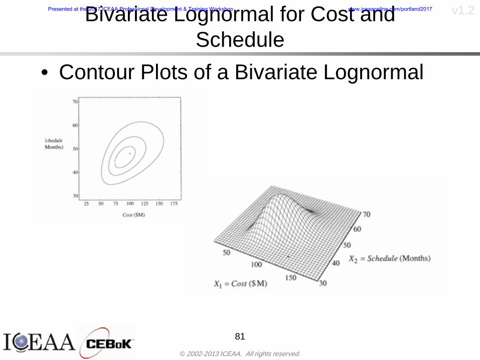
copy 2002-2013 ICEAA All rights reserved
v12Bivariate Lognormal for Cost and Schedule
bull Contour Plots of a Bivariate Lognormal
81
Presented at the 2017 ICEAA Professional Development amp Training Workshop wwwiceaaonlinecomportland2017
copy 2002-2013 ICEAA All rights reserved
v12Correlation Between Cost and Schedule
bull Cost and schedule are positively correlated but not perfectly sondash For example it is possible to have a schedule underrun and a cost
overrunbull Based on cost and schedule growth data for 50 completed NASA
programs the correlation between development cost and development schedule is 70
82
00
200
400
600
800
1000
1200
-500 00 500 1000 1500 2000 2500Historical Cost Growth
Hist
oric
al S
ched
ule
Gro
wth
r = 715
Presented at the 2017 ICEAA Professional Development amp Training Workshop wwwiceaaonlinecomportland2017
copy 2002-2013 ICEAA All rights reserved
v12Correlation Between Cost and Schedule Caveats
bull Based on historical data recommended correlation between cost and schedule is 70 but this could be higher or lower depending upon program circumstancesndash If program is budget constrained cost and schedule will be
more highly correlated (go as you pay)ndash If program is schedule constrained cost and schedule will
have lower correlation perhaps even negative correlation ndash Smaller programs have smaller correlation between cost and
schedule riskbull Relatively easy to ldquohurry uprdquo and finish on time or even early if
needed
83
Presented at the 2017 ICEAA Professional Development amp Training Workshop wwwiceaaonlinecomportland2017
copy 2002-2013 ICEAA All rights reserved
v12
Conditional Confidence Levelsbull Given a programrsquos project schedule we can determine the cost
risk distribution conditional upon the given schedulebull Conditional cost S-curves are steeper than unconditional
(marginal) cost S-curves between some uncertainty has been removed because schedule is fixed
84
Presented at the 2017 ICEAA Professional Development amp Training Workshop wwwiceaaonlinecomportland2017
copy 2002-2013 ICEAA All rights reserved
v12
Joint Confidence Levelsbull Joint 65 confidence represents the probability of
achieving both 65 confidence in cost AND 65 confidence in schedulendash This is different than achieving 65 cost confidence alone
or achieving 65 schedule confidence alonebull Due to the imperfect correlation between cost and schedule it
is possible to achieve a 65 cost confidence with a lower level of schedule confidence
bull Restricting the schedule confidence thus requires additional $ to achieve a given level of confidence
85
X
Y
Possible Values for Which X gt a Possible Values for
Which X gt a and Y gt b
a
b
Presented at the 2017 ICEAA Professional Development amp Training Workshop wwwiceaaonlinecomportland2017
copy 2002-2013 ICEAA All rights reserved
v12Joint Confidence Levels Versus Cost Confidence Levels Only
bull Example of the differences between cost confidence schedule confidence conditional cost confidence and joint cost and schedule confidence
86
Joint Cost-Schedule Confidence Iso-Curves
Cost (RY$M)
Sche
dule
(Mon
ths)
65 Confidence
50 Confidence
70 Confidence
65 Cost Confidence AggressiveSchedule65 Cost ConfidenceScheduleGiven 65 Schedule ConfidenceUnconditional 65 CostConfidenceUnconditional 65 ScheduleConfidence
65 Cost Confidence 65 Joint Cost and Schedule
Confidence for 65 Schedule Confidence
Presented at the 2017 ICEAA Professional Development amp Training Workshop wwwiceaaonlinecomportland2017
copy 2002-2013 ICEAA All rights reserved
v12
Joint Cost and Schedule Confidence
bull Can examine pairs of cost and schedule that achieve a given level of confidence
bull Provides insights into the trade-offs between cost and schedule for a given level of confidencendash Possible to increase cost confidence by giving a
project more time in some instances or possible to ldquobuy downrdquo schedule
bull But these have limits and are shown in the iso-cost and schedule confidence curves
87
Presented at the 2017 ICEAA Professional Development amp Training Workshop wwwiceaaonlinecomportland2017
copy 2002-2013 ICEAA All rights reserved
v12Cost and Schedule Trade-offs for a Given Level of Joint Confidence
bull Hypothetical Example
88
Cost (RY$M)
Schedule (Months)
$100 48$99 48$89 49$87 50$85 51$85 52$84 53$83 55$83 55$83 56
Cost and Schedule 65 Confidence Iso-Curve
4748495051525354555657
$80 $82 $84 $86 $88 $90 $92 $94 $96 $98 $100
Cost (RY$ M)
Sche
dule
(Mon
ths)
Presented at the 2017 ICEAA Professional Development amp Training Workshop wwwiceaaonlinecomportland2017
copy 2002-2013 ICEAA All rights reserved
v12Policy Considerations for Confidence Levels
bull For large programs the difference between the amount of money needed to achieve 65 cost confidence independent of schedule and joint 65 cost and schedule confidence can represent hundreds of millions and even billions of dollars
89
Joint Cost-Schedule Confidence Iso-Curves
Cost (RY$M)
Sche
dule
(Mon
ths)
65 Confidence
65 Cost Confidence AggressiveSchedule
65 Cost ConfidenceScheduleGiven 65 Schedule Confidence
Unconditional 65 CostConfidence
Joint Cost and Schedule Confidence for 65 Cost Confidence and Program Baseline Schedule is Less Than 35
65 Cost Confidence Independent of Schedule Cost Needed to Achieve
Both 65 Joint Cost and Schedule Confidence for the Schedule with 65 Confidence
Presented at the 2017 ICEAA Professional Development amp Training Workshop wwwiceaaonlinecomportland2017
copy 2002-2013 ICEAA All rights reserved
v12
Copulasbull More generally any combination of distributions can
be used (more than just normal and lognormal)ndash Termed ldquocopulardquo from the Italian word for ldquocouplerdquondash Copulas are a way to combine marginal distributions of any
number and type into a joint distributionbull More formally a copula is a multivariate joint distribution defined
on the n-dimensional unit cube [0 1]n such that every marginal distribution is uniform on the interval [0 1]
bull (The bivariate form of) Sklarrsquos theorem states that for any bivariate distribution function H(x y) let F(x) = H(x infin) and G(y) = H(infin y) be the univariate marginal probability distribution functions Then there exists a copula C such that H(xy)=C(F(x)G(y))
ndash Copulas are widely used in risk management for investments and insurance
bull Considered industry best practice (Li 2000)bull Marketed as part of JP Morganrsquos CreditMetrics suite of tools
(Gupton et Al 1997)90
Presented at the 2017 ICEAA Professional Development amp Training Workshop wwwiceaaonlinecomportland2017
copy 2002-2013 ICEAA All rights reserved
v12Parametric Joint Cost and Schedule Analysis
bull A parametric model based on a consistent data set with a set of overlapping cost and schedule drivers is a cleaner way to model cost and schedule
91
CostWeight
HeritageNewness
Technology Readiness
Schedule
0
20
40
60
80
100
Confidence
Joint Cost and Schedule Confidence
Schedule
Cost
Lognormal Distribution PDF and CDF
0102030405060708090100
200 300 400 500 600 700 800 900 1000Cost $
Con
fiden
ce L
evel
0
00002
00004
00006
00008
0001
00012
00014
00016
Prob
abili
ty D
ensi
ty
CDFPDF
Lognormal Distribution PDF and CDF
0102030405060708090100
200 300 400 500 600 700 800 900 1000Cost $
Con
fiden
ce L
evel
0
00002
00004
00006
00008
0001
00012
00014
00016
Prob
abili
ty D
ensi
ty
CDFPDF
Presented at the 2017 ICEAA Professional Development amp Training Workshop wwwiceaaonlinecomportland2017
copy 2002-2013 ICEAA All rights reserved
v12Parametric Joint Cost and Schedule Analysis (2)
bull Joint cost and schedule risk analysis produced naturally by the integrated modelndash Addresses several issues with the copula
approachbull Tail dependencybull Correlation ndash no need to assign correlation
between cost and schedulebull Consistency of cost and schedule models
92
Presented at the 2017 ICEAA Professional Development amp Training Workshop wwwiceaaonlinecomportland2017
copy 2002-2013 ICEAA All rights reserved
v12
Resource-Loaded Schedulesbull Involves assigning cost and schedule risks to a resource-loaded schedule
networkbull Bottom-up approach
ndash More labor intensive than parametrics but can also provide more insight
ndash Can answer questions than parametric typically cannot such as how much do reserve requirements decrease if a specific risk is retired
bull Currently being implemented in Constellation programbull Has same issue as all bottom-up models hard to count all the risks and model
them discretely
ndash As a result there is a tendency to reflect less risk than indicated by history
ndash ldquoThere are more things in heaven and earth Horatio than are dreamt of in your philosophyrdquo William Shakespeare Hamlet Act I Scene V
93
Presented at the 2017 ICEAA Professional Development amp Training Workshop wwwiceaaonlinecomportland2017
copy 2002-2013 ICEAA All rights reserved
v12Resource-Loaded Schedules Vs Parametrics
bull Parametric most appropriate for early estimatesndash But also good for high-level checks as project progresses
bull As plans take shape lower level modeling may be more appropriate
94 1
CONCEPTUALDEVELOPMENT
PROJECTDEFINITION DESIGN DEVELOPMENT OPERATIONS
PARAMETRIC PARAMETRIC
ANALOGY
ENGINEERING (Bottoms Up)
$PARAMETRIC
DETAILED
$
Pre Phase A Phase B Phase CDPhase A Phase EPre Phase A Phase B Phase CDPhase A Phase E
Risk = f(Cost Estimating Relationship Inputs eg mass power data rate TRL new design etc)
Risk = f(cost and schedule variation of the analogous elements)
Risk = f(variation of detailed inputs eg labor hours rates materials etc)
Presented at the 2017 ICEAA Professional Development amp Training Workshop wwwiceaaonlinecomportland2017
copy 2002-2013 ICEAA All rights reserved
v12
Resource-Loaded Schedulesbull Methodology has been demonstrated in other
industriesndash Construction oil and gasndash Analysis has not been traditionally done on highly uncertain
complex development projects bull Methodology focuses on project baseline schedule
ndash In baseline schedule all tasks are resource loaded to represent a baseline schedule and cost standpoint
ndash Resource loaded schedule is ldquorolledrdquo up to a manageable level
ndash Based on the risk and uncertainties identified schedule distributions are applied to each rolled up task
ndash Cost uncertainties are also applied to rolled up tasksbull Uncertainties include labor rate man power etc
ndash A Monte Carlo simulation is run to develop joint cost-schedule distributions
95
Presented at the 2017 ICEAA Professional Development amp Training Workshop wwwiceaaonlinecomportland2017
copy 2002-2013 ICEAA All rights reserved
v12
Unit III - Module 9 96
Execution ndash Cross Checksbull Means The mean cost growth factor for WBS items
can be compared to history as a way to cross check results
bull CVs The CV of the cost growth factors for WBS items can be compared to history as a way to cross check results
bull Inputs Checks are performed on inputs or other parameters to see if historical values are in line with program assumptionsndash Example Historical risk scores can be compared to program
risk scores to see if risk assessors are being realistic and to see if the underlying database is representative of the program
11
Presented at the 2017 ICEAA Professional Development amp Training Workshop wwwiceaaonlinecomportland2017
- Cost and Schedule Risk Analysis Basic
- Acknowledgments
- Unit Index
- Risk Overview
- Agenda
- Introduction
- Risk Analysis Terms
- Are Our Costs Realistic
- Historical Cost Growth
- Sources of Cost Risk
- Point Estimates of Cost
- Types of Risk
- Point Estimates Vs Risk Estimates
- Cost Risk and Probability
- Probability Model ndash Distribution
- Probability Model ndash Distribution
- Probability ndash Top-Level Distribution
- S-Curves and Confidence Levels
- Example ndash Normal Distribution
- Confidence Levels
- Measuring Parametric Model Uncertainty
- Parametric Model Example
- Weight Uncertainty
- Estimating Uncertainty
- Estimating Uncertainty (2)
- Estimating Uncertainty (3)
- Aggregating Risk
- WBS Example
- WBS and Risk
- Aggregating Risk
- Percentiles Do Not Add
- Percentiles Do Not Add (2)
- Percentiles Do Not Add (3)
- Methods for Aggregating Risk
- Monte Carlo Simulationfor Risk Analysis
- Monte Carlo Simulation
- Using Random Numbers to Simulate Distributions
- Simulating a Triangular Distribution
- Simulating a Triangular Distribution (2)
- Monte Carlo and the WBS
- Number of Trials
- Number of Trials (2)
- Number of Trials (3)
- Number of Trials (4)
- Number of Trials (5)
- Number of Trials (6)
- Methods of Simulation
- Probability Model ndash Correlation
- Correlation And Causation
- The Importance of Correlation
- The Importance of Correlation (2)
- Measures of Correlation
- Pearson Correlation
- Spearman Correlation
- Functional Correlation
- Risk Measures
- Value at Risk (VaR)
- Why 70th or 80th Percentile
- Funding Above Inflection Points
- Why Budget to the 70th or 80th
- Inflection Points for Lognormal
- Issues with Percentile Funding
- ldquoHere There Be Dragonsrdquo
- Distribution Comparison
- Distribution Comparison Tail Behavior
- Distribution Comparison ndash Tail Behavior (Table)
- Percentile Budgeting is Not Risk Management
- Joint Confidence Level Analysis
- Schedules Impact Cost
- The Relationship of Cost to Schedule
- The Impact of Schedule GrowthCompression on Cost
- Schedule as an Independent Variable
- Schedule is a Dependent Variable
- Incorporation of Schedule in Cost Risk
- Subjective Cost Risk Methods and Overinclusion of Risk Factors
- Fundamental Equation of Cost and Schedule Interrelationships
- How to (Correctly) Incorporate Schedule into Cost Risk Analysis
- Joint Lognormal and Normal Distributions
- Modeling Cost and Schedule as a Bivariate Distribution
- Bivariate Lognormal Distribution for Cost and Schedule
- Bivariate Lognormal for Cost and Schedule
- Correlation Between Cost and Schedule
- Correlation Between Cost and Schedule Caveats
- Conditional Confidence Levels
- Joint Confidence Levels
- Joint Confidence Levels Versus Cost Confidence Levels Only
- Joint Cost and Schedule Confidence
- Cost and Schedule Trade-offs for a Given Level of Joint Confidence
- Policy Considerations for Confidence Levels
- Copulas
- Parametric Joint Cost and Schedule Analysis
- Parametric Joint Cost and Schedule Analysis (2)
- Resource-Loaded Schedules
- Resource-Loaded Schedules Vs Parametrics
- Resource-Loaded Schedules
- Execution ndash Cross Checks
-
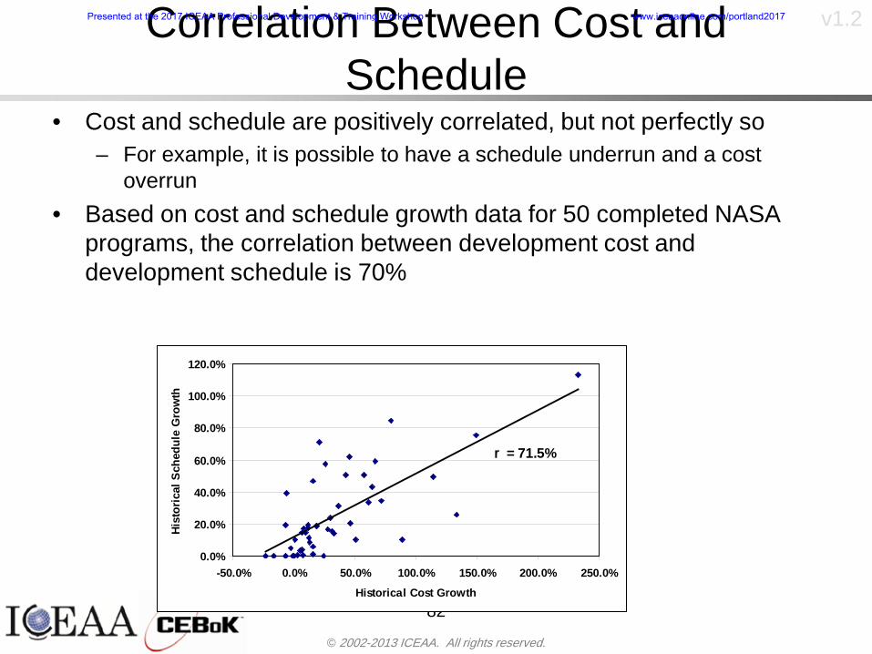
copy 2002-2013 ICEAA All rights reserved
v12Correlation Between Cost and Schedule
bull Cost and schedule are positively correlated but not perfectly sondash For example it is possible to have a schedule underrun and a cost
overrunbull Based on cost and schedule growth data for 50 completed NASA
programs the correlation between development cost and development schedule is 70
82
00
200
400
600
800
1000
1200
-500 00 500 1000 1500 2000 2500Historical Cost Growth
Hist
oric
al S
ched
ule
Gro
wth
r = 715
Presented at the 2017 ICEAA Professional Development amp Training Workshop wwwiceaaonlinecomportland2017
copy 2002-2013 ICEAA All rights reserved
v12Correlation Between Cost and Schedule Caveats
bull Based on historical data recommended correlation between cost and schedule is 70 but this could be higher or lower depending upon program circumstancesndash If program is budget constrained cost and schedule will be
more highly correlated (go as you pay)ndash If program is schedule constrained cost and schedule will
have lower correlation perhaps even negative correlation ndash Smaller programs have smaller correlation between cost and
schedule riskbull Relatively easy to ldquohurry uprdquo and finish on time or even early if
needed
83
Presented at the 2017 ICEAA Professional Development amp Training Workshop wwwiceaaonlinecomportland2017
copy 2002-2013 ICEAA All rights reserved
v12
Conditional Confidence Levelsbull Given a programrsquos project schedule we can determine the cost
risk distribution conditional upon the given schedulebull Conditional cost S-curves are steeper than unconditional
(marginal) cost S-curves between some uncertainty has been removed because schedule is fixed
84
Presented at the 2017 ICEAA Professional Development amp Training Workshop wwwiceaaonlinecomportland2017
copy 2002-2013 ICEAA All rights reserved
v12
Joint Confidence Levelsbull Joint 65 confidence represents the probability of
achieving both 65 confidence in cost AND 65 confidence in schedulendash This is different than achieving 65 cost confidence alone
or achieving 65 schedule confidence alonebull Due to the imperfect correlation between cost and schedule it
is possible to achieve a 65 cost confidence with a lower level of schedule confidence
bull Restricting the schedule confidence thus requires additional $ to achieve a given level of confidence
85
X
Y
Possible Values for Which X gt a Possible Values for
Which X gt a and Y gt b
a
b
Presented at the 2017 ICEAA Professional Development amp Training Workshop wwwiceaaonlinecomportland2017
copy 2002-2013 ICEAA All rights reserved
v12Joint Confidence Levels Versus Cost Confidence Levels Only
bull Example of the differences between cost confidence schedule confidence conditional cost confidence and joint cost and schedule confidence
86
Joint Cost-Schedule Confidence Iso-Curves
Cost (RY$M)
Sche
dule
(Mon
ths)
65 Confidence
50 Confidence
70 Confidence
65 Cost Confidence AggressiveSchedule65 Cost ConfidenceScheduleGiven 65 Schedule ConfidenceUnconditional 65 CostConfidenceUnconditional 65 ScheduleConfidence
65 Cost Confidence 65 Joint Cost and Schedule
Confidence for 65 Schedule Confidence
Presented at the 2017 ICEAA Professional Development amp Training Workshop wwwiceaaonlinecomportland2017
copy 2002-2013 ICEAA All rights reserved
v12
Joint Cost and Schedule Confidence
bull Can examine pairs of cost and schedule that achieve a given level of confidence
bull Provides insights into the trade-offs between cost and schedule for a given level of confidencendash Possible to increase cost confidence by giving a
project more time in some instances or possible to ldquobuy downrdquo schedule
bull But these have limits and are shown in the iso-cost and schedule confidence curves
87
Presented at the 2017 ICEAA Professional Development amp Training Workshop wwwiceaaonlinecomportland2017
copy 2002-2013 ICEAA All rights reserved
v12Cost and Schedule Trade-offs for a Given Level of Joint Confidence
bull Hypothetical Example
88
Cost (RY$M)
Schedule (Months)
$100 48$99 48$89 49$87 50$85 51$85 52$84 53$83 55$83 55$83 56
Cost and Schedule 65 Confidence Iso-Curve
4748495051525354555657
$80 $82 $84 $86 $88 $90 $92 $94 $96 $98 $100
Cost (RY$ M)
Sche
dule
(Mon
ths)
Presented at the 2017 ICEAA Professional Development amp Training Workshop wwwiceaaonlinecomportland2017
copy 2002-2013 ICEAA All rights reserved
v12Policy Considerations for Confidence Levels
bull For large programs the difference between the amount of money needed to achieve 65 cost confidence independent of schedule and joint 65 cost and schedule confidence can represent hundreds of millions and even billions of dollars
89
Joint Cost-Schedule Confidence Iso-Curves
Cost (RY$M)
Sche
dule
(Mon
ths)
65 Confidence
65 Cost Confidence AggressiveSchedule
65 Cost ConfidenceScheduleGiven 65 Schedule Confidence
Unconditional 65 CostConfidence
Joint Cost and Schedule Confidence for 65 Cost Confidence and Program Baseline Schedule is Less Than 35
65 Cost Confidence Independent of Schedule Cost Needed to Achieve
Both 65 Joint Cost and Schedule Confidence for the Schedule with 65 Confidence
Presented at the 2017 ICEAA Professional Development amp Training Workshop wwwiceaaonlinecomportland2017
copy 2002-2013 ICEAA All rights reserved
v12
Copulasbull More generally any combination of distributions can
be used (more than just normal and lognormal)ndash Termed ldquocopulardquo from the Italian word for ldquocouplerdquondash Copulas are a way to combine marginal distributions of any
number and type into a joint distributionbull More formally a copula is a multivariate joint distribution defined
on the n-dimensional unit cube [0 1]n such that every marginal distribution is uniform on the interval [0 1]
bull (The bivariate form of) Sklarrsquos theorem states that for any bivariate distribution function H(x y) let F(x) = H(x infin) and G(y) = H(infin y) be the univariate marginal probability distribution functions Then there exists a copula C such that H(xy)=C(F(x)G(y))
ndash Copulas are widely used in risk management for investments and insurance
bull Considered industry best practice (Li 2000)bull Marketed as part of JP Morganrsquos CreditMetrics suite of tools
(Gupton et Al 1997)90
Presented at the 2017 ICEAA Professional Development amp Training Workshop wwwiceaaonlinecomportland2017
copy 2002-2013 ICEAA All rights reserved
v12Parametric Joint Cost and Schedule Analysis
bull A parametric model based on a consistent data set with a set of overlapping cost and schedule drivers is a cleaner way to model cost and schedule
91
CostWeight
HeritageNewness
Technology Readiness
Schedule
0
20
40
60
80
100
Confidence
Joint Cost and Schedule Confidence
Schedule
Cost
Lognormal Distribution PDF and CDF
0102030405060708090100
200 300 400 500 600 700 800 900 1000Cost $
Con
fiden
ce L
evel
0
00002
00004
00006
00008
0001
00012
00014
00016
Prob
abili
ty D
ensi
ty
CDFPDF
Lognormal Distribution PDF and CDF
0102030405060708090100
200 300 400 500 600 700 800 900 1000Cost $
Con
fiden
ce L
evel
0
00002
00004
00006
00008
0001
00012
00014
00016
Prob
abili
ty D
ensi
ty
CDFPDF
Presented at the 2017 ICEAA Professional Development amp Training Workshop wwwiceaaonlinecomportland2017
copy 2002-2013 ICEAA All rights reserved
v12Parametric Joint Cost and Schedule Analysis (2)
bull Joint cost and schedule risk analysis produced naturally by the integrated modelndash Addresses several issues with the copula
approachbull Tail dependencybull Correlation ndash no need to assign correlation
between cost and schedulebull Consistency of cost and schedule models
92
Presented at the 2017 ICEAA Professional Development amp Training Workshop wwwiceaaonlinecomportland2017
copy 2002-2013 ICEAA All rights reserved
v12
Resource-Loaded Schedulesbull Involves assigning cost and schedule risks to a resource-loaded schedule
networkbull Bottom-up approach
ndash More labor intensive than parametrics but can also provide more insight
ndash Can answer questions than parametric typically cannot such as how much do reserve requirements decrease if a specific risk is retired
bull Currently being implemented in Constellation programbull Has same issue as all bottom-up models hard to count all the risks and model
them discretely
ndash As a result there is a tendency to reflect less risk than indicated by history
ndash ldquoThere are more things in heaven and earth Horatio than are dreamt of in your philosophyrdquo William Shakespeare Hamlet Act I Scene V
93
Presented at the 2017 ICEAA Professional Development amp Training Workshop wwwiceaaonlinecomportland2017
copy 2002-2013 ICEAA All rights reserved
v12Resource-Loaded Schedules Vs Parametrics
bull Parametric most appropriate for early estimatesndash But also good for high-level checks as project progresses
bull As plans take shape lower level modeling may be more appropriate
94 1
CONCEPTUALDEVELOPMENT
PROJECTDEFINITION DESIGN DEVELOPMENT OPERATIONS
PARAMETRIC PARAMETRIC
ANALOGY
ENGINEERING (Bottoms Up)
$PARAMETRIC
DETAILED
$
Pre Phase A Phase B Phase CDPhase A Phase EPre Phase A Phase B Phase CDPhase A Phase E
Risk = f(Cost Estimating Relationship Inputs eg mass power data rate TRL new design etc)
Risk = f(cost and schedule variation of the analogous elements)
Risk = f(variation of detailed inputs eg labor hours rates materials etc)
Presented at the 2017 ICEAA Professional Development amp Training Workshop wwwiceaaonlinecomportland2017
copy 2002-2013 ICEAA All rights reserved
v12
Resource-Loaded Schedulesbull Methodology has been demonstrated in other
industriesndash Construction oil and gasndash Analysis has not been traditionally done on highly uncertain
complex development projects bull Methodology focuses on project baseline schedule
ndash In baseline schedule all tasks are resource loaded to represent a baseline schedule and cost standpoint
ndash Resource loaded schedule is ldquorolledrdquo up to a manageable level
ndash Based on the risk and uncertainties identified schedule distributions are applied to each rolled up task
ndash Cost uncertainties are also applied to rolled up tasksbull Uncertainties include labor rate man power etc
ndash A Monte Carlo simulation is run to develop joint cost-schedule distributions
95
Presented at the 2017 ICEAA Professional Development amp Training Workshop wwwiceaaonlinecomportland2017
copy 2002-2013 ICEAA All rights reserved
v12
Unit III - Module 9 96
Execution ndash Cross Checksbull Means The mean cost growth factor for WBS items
can be compared to history as a way to cross check results
bull CVs The CV of the cost growth factors for WBS items can be compared to history as a way to cross check results
bull Inputs Checks are performed on inputs or other parameters to see if historical values are in line with program assumptionsndash Example Historical risk scores can be compared to program
risk scores to see if risk assessors are being realistic and to see if the underlying database is representative of the program
11
Presented at the 2017 ICEAA Professional Development amp Training Workshop wwwiceaaonlinecomportland2017
- Cost and Schedule Risk Analysis Basic
- Acknowledgments
- Unit Index
- Risk Overview
- Agenda
- Introduction
- Risk Analysis Terms
- Are Our Costs Realistic
- Historical Cost Growth
- Sources of Cost Risk
- Point Estimates of Cost
- Types of Risk
- Point Estimates Vs Risk Estimates
- Cost Risk and Probability
- Probability Model ndash Distribution
- Probability Model ndash Distribution
- Probability ndash Top-Level Distribution
- S-Curves and Confidence Levels
- Example ndash Normal Distribution
- Confidence Levels
- Measuring Parametric Model Uncertainty
- Parametric Model Example
- Weight Uncertainty
- Estimating Uncertainty
- Estimating Uncertainty (2)
- Estimating Uncertainty (3)
- Aggregating Risk
- WBS Example
- WBS and Risk
- Aggregating Risk
- Percentiles Do Not Add
- Percentiles Do Not Add (2)
- Percentiles Do Not Add (3)
- Methods for Aggregating Risk
- Monte Carlo Simulationfor Risk Analysis
- Monte Carlo Simulation
- Using Random Numbers to Simulate Distributions
- Simulating a Triangular Distribution
- Simulating a Triangular Distribution (2)
- Monte Carlo and the WBS
- Number of Trials
- Number of Trials (2)
- Number of Trials (3)
- Number of Trials (4)
- Number of Trials (5)
- Number of Trials (6)
- Methods of Simulation
- Probability Model ndash Correlation
- Correlation And Causation
- The Importance of Correlation
- The Importance of Correlation (2)
- Measures of Correlation
- Pearson Correlation
- Spearman Correlation
- Functional Correlation
- Risk Measures
- Value at Risk (VaR)
- Why 70th or 80th Percentile
- Funding Above Inflection Points
- Why Budget to the 70th or 80th
- Inflection Points for Lognormal
- Issues with Percentile Funding
- ldquoHere There Be Dragonsrdquo
- Distribution Comparison
- Distribution Comparison Tail Behavior
- Distribution Comparison ndash Tail Behavior (Table)
- Percentile Budgeting is Not Risk Management
- Joint Confidence Level Analysis
- Schedules Impact Cost
- The Relationship of Cost to Schedule
- The Impact of Schedule GrowthCompression on Cost
- Schedule as an Independent Variable
- Schedule is a Dependent Variable
- Incorporation of Schedule in Cost Risk
- Subjective Cost Risk Methods and Overinclusion of Risk Factors
- Fundamental Equation of Cost and Schedule Interrelationships
- How to (Correctly) Incorporate Schedule into Cost Risk Analysis
- Joint Lognormal and Normal Distributions
- Modeling Cost and Schedule as a Bivariate Distribution
- Bivariate Lognormal Distribution for Cost and Schedule
- Bivariate Lognormal for Cost and Schedule
- Correlation Between Cost and Schedule
- Correlation Between Cost and Schedule Caveats
- Conditional Confidence Levels
- Joint Confidence Levels
- Joint Confidence Levels Versus Cost Confidence Levels Only
- Joint Cost and Schedule Confidence
- Cost and Schedule Trade-offs for a Given Level of Joint Confidence
- Policy Considerations for Confidence Levels
- Copulas
- Parametric Joint Cost and Schedule Analysis
- Parametric Joint Cost and Schedule Analysis (2)
- Resource-Loaded Schedules
- Resource-Loaded Schedules Vs Parametrics
- Resource-Loaded Schedules
- Execution ndash Cross Checks
-
copy 2002-2013 ICEAA All rights reserved
v12Correlation Between Cost and Schedule Caveats
bull Based on historical data recommended correlation between cost and schedule is 70 but this could be higher or lower depending upon program circumstancesndash If program is budget constrained cost and schedule will be
more highly correlated (go as you pay)ndash If program is schedule constrained cost and schedule will
have lower correlation perhaps even negative correlation ndash Smaller programs have smaller correlation between cost and
schedule riskbull Relatively easy to ldquohurry uprdquo and finish on time or even early if
needed
83
Presented at the 2017 ICEAA Professional Development amp Training Workshop wwwiceaaonlinecomportland2017
copy 2002-2013 ICEAA All rights reserved
v12
Conditional Confidence Levelsbull Given a programrsquos project schedule we can determine the cost
risk distribution conditional upon the given schedulebull Conditional cost S-curves are steeper than unconditional
(marginal) cost S-curves between some uncertainty has been removed because schedule is fixed
84
Presented at the 2017 ICEAA Professional Development amp Training Workshop wwwiceaaonlinecomportland2017
copy 2002-2013 ICEAA All rights reserved
v12
Joint Confidence Levelsbull Joint 65 confidence represents the probability of
achieving both 65 confidence in cost AND 65 confidence in schedulendash This is different than achieving 65 cost confidence alone
or achieving 65 schedule confidence alonebull Due to the imperfect correlation between cost and schedule it
is possible to achieve a 65 cost confidence with a lower level of schedule confidence
bull Restricting the schedule confidence thus requires additional $ to achieve a given level of confidence
85
X
Y
Possible Values for Which X gt a Possible Values for
Which X gt a and Y gt b
a
b
Presented at the 2017 ICEAA Professional Development amp Training Workshop wwwiceaaonlinecomportland2017
copy 2002-2013 ICEAA All rights reserved
v12Joint Confidence Levels Versus Cost Confidence Levels Only
bull Example of the differences between cost confidence schedule confidence conditional cost confidence and joint cost and schedule confidence
86
Joint Cost-Schedule Confidence Iso-Curves
Cost (RY$M)
Sche
dule
(Mon
ths)
65 Confidence
50 Confidence
70 Confidence
65 Cost Confidence AggressiveSchedule65 Cost ConfidenceScheduleGiven 65 Schedule ConfidenceUnconditional 65 CostConfidenceUnconditional 65 ScheduleConfidence
65 Cost Confidence 65 Joint Cost and Schedule
Confidence for 65 Schedule Confidence
Presented at the 2017 ICEAA Professional Development amp Training Workshop wwwiceaaonlinecomportland2017
copy 2002-2013 ICEAA All rights reserved
v12
Joint Cost and Schedule Confidence
bull Can examine pairs of cost and schedule that achieve a given level of confidence
bull Provides insights into the trade-offs between cost and schedule for a given level of confidencendash Possible to increase cost confidence by giving a
project more time in some instances or possible to ldquobuy downrdquo schedule
bull But these have limits and are shown in the iso-cost and schedule confidence curves
87
Presented at the 2017 ICEAA Professional Development amp Training Workshop wwwiceaaonlinecomportland2017
copy 2002-2013 ICEAA All rights reserved
v12Cost and Schedule Trade-offs for a Given Level of Joint Confidence
bull Hypothetical Example
88
Cost (RY$M)
Schedule (Months)
$100 48$99 48$89 49$87 50$85 51$85 52$84 53$83 55$83 55$83 56
Cost and Schedule 65 Confidence Iso-Curve
4748495051525354555657
$80 $82 $84 $86 $88 $90 $92 $94 $96 $98 $100
Cost (RY$ M)
Sche
dule
(Mon
ths)
Presented at the 2017 ICEAA Professional Development amp Training Workshop wwwiceaaonlinecomportland2017
copy 2002-2013 ICEAA All rights reserved
v12Policy Considerations for Confidence Levels
bull For large programs the difference between the amount of money needed to achieve 65 cost confidence independent of schedule and joint 65 cost and schedule confidence can represent hundreds of millions and even billions of dollars
89
Joint Cost-Schedule Confidence Iso-Curves
Cost (RY$M)
Sche
dule
(Mon
ths)
65 Confidence
65 Cost Confidence AggressiveSchedule
65 Cost ConfidenceScheduleGiven 65 Schedule Confidence
Unconditional 65 CostConfidence
Joint Cost and Schedule Confidence for 65 Cost Confidence and Program Baseline Schedule is Less Than 35
65 Cost Confidence Independent of Schedule Cost Needed to Achieve
Both 65 Joint Cost and Schedule Confidence for the Schedule with 65 Confidence
Presented at the 2017 ICEAA Professional Development amp Training Workshop wwwiceaaonlinecomportland2017
copy 2002-2013 ICEAA All rights reserved
v12
Copulasbull More generally any combination of distributions can
be used (more than just normal and lognormal)ndash Termed ldquocopulardquo from the Italian word for ldquocouplerdquondash Copulas are a way to combine marginal distributions of any
number and type into a joint distributionbull More formally a copula is a multivariate joint distribution defined
on the n-dimensional unit cube [0 1]n such that every marginal distribution is uniform on the interval [0 1]
bull (The bivariate form of) Sklarrsquos theorem states that for any bivariate distribution function H(x y) let F(x) = H(x infin) and G(y) = H(infin y) be the univariate marginal probability distribution functions Then there exists a copula C such that H(xy)=C(F(x)G(y))
ndash Copulas are widely used in risk management for investments and insurance
bull Considered industry best practice (Li 2000)bull Marketed as part of JP Morganrsquos CreditMetrics suite of tools
(Gupton et Al 1997)90
Presented at the 2017 ICEAA Professional Development amp Training Workshop wwwiceaaonlinecomportland2017
copy 2002-2013 ICEAA All rights reserved
v12Parametric Joint Cost and Schedule Analysis
bull A parametric model based on a consistent data set with a set of overlapping cost and schedule drivers is a cleaner way to model cost and schedule
91
CostWeight
HeritageNewness
Technology Readiness
Schedule
0
20
40
60
80
100
Confidence
Joint Cost and Schedule Confidence
Schedule
Cost
Lognormal Distribution PDF and CDF
0102030405060708090100
200 300 400 500 600 700 800 900 1000Cost $
Con
fiden
ce L
evel
0
00002
00004
00006
00008
0001
00012
00014
00016
Prob
abili
ty D
ensi
ty
CDFPDF
Lognormal Distribution PDF and CDF
0102030405060708090100
200 300 400 500 600 700 800 900 1000Cost $
Con
fiden
ce L
evel
0
00002
00004
00006
00008
0001
00012
00014
00016
Prob
abili
ty D
ensi
ty
CDFPDF
Presented at the 2017 ICEAA Professional Development amp Training Workshop wwwiceaaonlinecomportland2017
copy 2002-2013 ICEAA All rights reserved
v12Parametric Joint Cost and Schedule Analysis (2)
bull Joint cost and schedule risk analysis produced naturally by the integrated modelndash Addresses several issues with the copula
approachbull Tail dependencybull Correlation ndash no need to assign correlation
between cost and schedulebull Consistency of cost and schedule models
92
Presented at the 2017 ICEAA Professional Development amp Training Workshop wwwiceaaonlinecomportland2017
copy 2002-2013 ICEAA All rights reserved
v12
Resource-Loaded Schedulesbull Involves assigning cost and schedule risks to a resource-loaded schedule
networkbull Bottom-up approach
ndash More labor intensive than parametrics but can also provide more insight
ndash Can answer questions than parametric typically cannot such as how much do reserve requirements decrease if a specific risk is retired
bull Currently being implemented in Constellation programbull Has same issue as all bottom-up models hard to count all the risks and model
them discretely
ndash As a result there is a tendency to reflect less risk than indicated by history
ndash ldquoThere are more things in heaven and earth Horatio than are dreamt of in your philosophyrdquo William Shakespeare Hamlet Act I Scene V
93
Presented at the 2017 ICEAA Professional Development amp Training Workshop wwwiceaaonlinecomportland2017
copy 2002-2013 ICEAA All rights reserved
v12Resource-Loaded Schedules Vs Parametrics
bull Parametric most appropriate for early estimatesndash But also good for high-level checks as project progresses
bull As plans take shape lower level modeling may be more appropriate
94 1
CONCEPTUALDEVELOPMENT
PROJECTDEFINITION DESIGN DEVELOPMENT OPERATIONS
PARAMETRIC PARAMETRIC
ANALOGY
ENGINEERING (Bottoms Up)
$PARAMETRIC
DETAILED
$
Pre Phase A Phase B Phase CDPhase A Phase EPre Phase A Phase B Phase CDPhase A Phase E
Risk = f(Cost Estimating Relationship Inputs eg mass power data rate TRL new design etc)
Risk = f(cost and schedule variation of the analogous elements)
Risk = f(variation of detailed inputs eg labor hours rates materials etc)
Presented at the 2017 ICEAA Professional Development amp Training Workshop wwwiceaaonlinecomportland2017
copy 2002-2013 ICEAA All rights reserved
v12
Resource-Loaded Schedulesbull Methodology has been demonstrated in other
industriesndash Construction oil and gasndash Analysis has not been traditionally done on highly uncertain
complex development projects bull Methodology focuses on project baseline schedule
ndash In baseline schedule all tasks are resource loaded to represent a baseline schedule and cost standpoint
ndash Resource loaded schedule is ldquorolledrdquo up to a manageable level
ndash Based on the risk and uncertainties identified schedule distributions are applied to each rolled up task
ndash Cost uncertainties are also applied to rolled up tasksbull Uncertainties include labor rate man power etc
ndash A Monte Carlo simulation is run to develop joint cost-schedule distributions
95
Presented at the 2017 ICEAA Professional Development amp Training Workshop wwwiceaaonlinecomportland2017
copy 2002-2013 ICEAA All rights reserved
v12
Unit III - Module 9 96
Execution ndash Cross Checksbull Means The mean cost growth factor for WBS items
can be compared to history as a way to cross check results
bull CVs The CV of the cost growth factors for WBS items can be compared to history as a way to cross check results
bull Inputs Checks are performed on inputs or other parameters to see if historical values are in line with program assumptionsndash Example Historical risk scores can be compared to program
risk scores to see if risk assessors are being realistic and to see if the underlying database is representative of the program
11
Presented at the 2017 ICEAA Professional Development amp Training Workshop wwwiceaaonlinecomportland2017
- Cost and Schedule Risk Analysis Basic
- Acknowledgments
- Unit Index
- Risk Overview
- Agenda
- Introduction
- Risk Analysis Terms
- Are Our Costs Realistic
- Historical Cost Growth
- Sources of Cost Risk
- Point Estimates of Cost
- Types of Risk
- Point Estimates Vs Risk Estimates
- Cost Risk and Probability
- Probability Model ndash Distribution
- Probability Model ndash Distribution
- Probability ndash Top-Level Distribution
- S-Curves and Confidence Levels
- Example ndash Normal Distribution
- Confidence Levels
- Measuring Parametric Model Uncertainty
- Parametric Model Example
- Weight Uncertainty
- Estimating Uncertainty
- Estimating Uncertainty (2)
- Estimating Uncertainty (3)
- Aggregating Risk
- WBS Example
- WBS and Risk
- Aggregating Risk
- Percentiles Do Not Add
- Percentiles Do Not Add (2)
- Percentiles Do Not Add (3)
- Methods for Aggregating Risk
- Monte Carlo Simulationfor Risk Analysis
- Monte Carlo Simulation
- Using Random Numbers to Simulate Distributions
- Simulating a Triangular Distribution
- Simulating a Triangular Distribution (2)
- Monte Carlo and the WBS
- Number of Trials
- Number of Trials (2)
- Number of Trials (3)
- Number of Trials (4)
- Number of Trials (5)
- Number of Trials (6)
- Methods of Simulation
- Probability Model ndash Correlation
- Correlation And Causation
- The Importance of Correlation
- The Importance of Correlation (2)
- Measures of Correlation
- Pearson Correlation
- Spearman Correlation
- Functional Correlation
- Risk Measures
- Value at Risk (VaR)
- Why 70th or 80th Percentile
- Funding Above Inflection Points
- Why Budget to the 70th or 80th
- Inflection Points for Lognormal
- Issues with Percentile Funding
- ldquoHere There Be Dragonsrdquo
- Distribution Comparison
- Distribution Comparison Tail Behavior
- Distribution Comparison ndash Tail Behavior (Table)
- Percentile Budgeting is Not Risk Management
- Joint Confidence Level Analysis
- Schedules Impact Cost
- The Relationship of Cost to Schedule
- The Impact of Schedule GrowthCompression on Cost
- Schedule as an Independent Variable
- Schedule is a Dependent Variable
- Incorporation of Schedule in Cost Risk
- Subjective Cost Risk Methods and Overinclusion of Risk Factors
- Fundamental Equation of Cost and Schedule Interrelationships
- How to (Correctly) Incorporate Schedule into Cost Risk Analysis
- Joint Lognormal and Normal Distributions
- Modeling Cost and Schedule as a Bivariate Distribution
- Bivariate Lognormal Distribution for Cost and Schedule
- Bivariate Lognormal for Cost and Schedule
- Correlation Between Cost and Schedule
- Correlation Between Cost and Schedule Caveats
- Conditional Confidence Levels
- Joint Confidence Levels
- Joint Confidence Levels Versus Cost Confidence Levels Only
- Joint Cost and Schedule Confidence
- Cost and Schedule Trade-offs for a Given Level of Joint Confidence
- Policy Considerations for Confidence Levels
- Copulas
- Parametric Joint Cost and Schedule Analysis
- Parametric Joint Cost and Schedule Analysis (2)
- Resource-Loaded Schedules
- Resource-Loaded Schedules Vs Parametrics
- Resource-Loaded Schedules
- Execution ndash Cross Checks
-
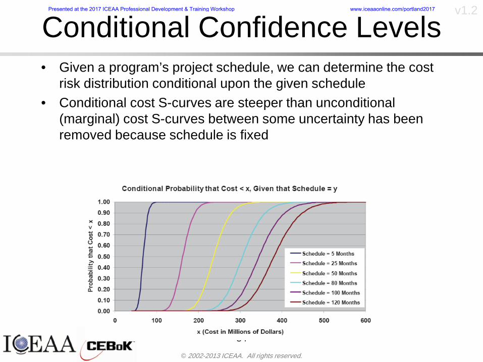
copy 2002-2013 ICEAA All rights reserved
v12
Conditional Confidence Levelsbull Given a programrsquos project schedule we can determine the cost
risk distribution conditional upon the given schedulebull Conditional cost S-curves are steeper than unconditional
(marginal) cost S-curves between some uncertainty has been removed because schedule is fixed
84
Presented at the 2017 ICEAA Professional Development amp Training Workshop wwwiceaaonlinecomportland2017
copy 2002-2013 ICEAA All rights reserved
v12
Joint Confidence Levelsbull Joint 65 confidence represents the probability of
achieving both 65 confidence in cost AND 65 confidence in schedulendash This is different than achieving 65 cost confidence alone
or achieving 65 schedule confidence alonebull Due to the imperfect correlation between cost and schedule it
is possible to achieve a 65 cost confidence with a lower level of schedule confidence
bull Restricting the schedule confidence thus requires additional $ to achieve a given level of confidence
85
X
Y
Possible Values for Which X gt a Possible Values for
Which X gt a and Y gt b
a
b
Presented at the 2017 ICEAA Professional Development amp Training Workshop wwwiceaaonlinecomportland2017
copy 2002-2013 ICEAA All rights reserved
v12Joint Confidence Levels Versus Cost Confidence Levels Only
bull Example of the differences between cost confidence schedule confidence conditional cost confidence and joint cost and schedule confidence
86
Joint Cost-Schedule Confidence Iso-Curves
Cost (RY$M)
Sche
dule
(Mon
ths)
65 Confidence
50 Confidence
70 Confidence
65 Cost Confidence AggressiveSchedule65 Cost ConfidenceScheduleGiven 65 Schedule ConfidenceUnconditional 65 CostConfidenceUnconditional 65 ScheduleConfidence
65 Cost Confidence 65 Joint Cost and Schedule
Confidence for 65 Schedule Confidence
Presented at the 2017 ICEAA Professional Development amp Training Workshop wwwiceaaonlinecomportland2017
copy 2002-2013 ICEAA All rights reserved
v12
Joint Cost and Schedule Confidence
bull Can examine pairs of cost and schedule that achieve a given level of confidence
bull Provides insights into the trade-offs between cost and schedule for a given level of confidencendash Possible to increase cost confidence by giving a
project more time in some instances or possible to ldquobuy downrdquo schedule
bull But these have limits and are shown in the iso-cost and schedule confidence curves
87
Presented at the 2017 ICEAA Professional Development amp Training Workshop wwwiceaaonlinecomportland2017
copy 2002-2013 ICEAA All rights reserved
v12Cost and Schedule Trade-offs for a Given Level of Joint Confidence
bull Hypothetical Example
88
Cost (RY$M)
Schedule (Months)
$100 48$99 48$89 49$87 50$85 51$85 52$84 53$83 55$83 55$83 56
Cost and Schedule 65 Confidence Iso-Curve
4748495051525354555657
$80 $82 $84 $86 $88 $90 $92 $94 $96 $98 $100
Cost (RY$ M)
Sche
dule
(Mon
ths)
Presented at the 2017 ICEAA Professional Development amp Training Workshop wwwiceaaonlinecomportland2017
copy 2002-2013 ICEAA All rights reserved
v12Policy Considerations for Confidence Levels
bull For large programs the difference between the amount of money needed to achieve 65 cost confidence independent of schedule and joint 65 cost and schedule confidence can represent hundreds of millions and even billions of dollars
89
Joint Cost-Schedule Confidence Iso-Curves
Cost (RY$M)
Sche
dule
(Mon
ths)
65 Confidence
65 Cost Confidence AggressiveSchedule
65 Cost ConfidenceScheduleGiven 65 Schedule Confidence
Unconditional 65 CostConfidence
Joint Cost and Schedule Confidence for 65 Cost Confidence and Program Baseline Schedule is Less Than 35
65 Cost Confidence Independent of Schedule Cost Needed to Achieve
Both 65 Joint Cost and Schedule Confidence for the Schedule with 65 Confidence
Presented at the 2017 ICEAA Professional Development amp Training Workshop wwwiceaaonlinecomportland2017
copy 2002-2013 ICEAA All rights reserved
v12
Copulasbull More generally any combination of distributions can
be used (more than just normal and lognormal)ndash Termed ldquocopulardquo from the Italian word for ldquocouplerdquondash Copulas are a way to combine marginal distributions of any
number and type into a joint distributionbull More formally a copula is a multivariate joint distribution defined
on the n-dimensional unit cube [0 1]n such that every marginal distribution is uniform on the interval [0 1]
bull (The bivariate form of) Sklarrsquos theorem states that for any bivariate distribution function H(x y) let F(x) = H(x infin) and G(y) = H(infin y) be the univariate marginal probability distribution functions Then there exists a copula C such that H(xy)=C(F(x)G(y))
ndash Copulas are widely used in risk management for investments and insurance
bull Considered industry best practice (Li 2000)bull Marketed as part of JP Morganrsquos CreditMetrics suite of tools
(Gupton et Al 1997)90
Presented at the 2017 ICEAA Professional Development amp Training Workshop wwwiceaaonlinecomportland2017
copy 2002-2013 ICEAA All rights reserved
v12Parametric Joint Cost and Schedule Analysis
bull A parametric model based on a consistent data set with a set of overlapping cost and schedule drivers is a cleaner way to model cost and schedule
91
CostWeight
HeritageNewness
Technology Readiness
Schedule
0
20
40
60
80
100
Confidence
Joint Cost and Schedule Confidence
Schedule
Cost
Lognormal Distribution PDF and CDF
0102030405060708090100
200 300 400 500 600 700 800 900 1000Cost $
Con
fiden
ce L
evel
0
00002
00004
00006
00008
0001
00012
00014
00016
Prob
abili
ty D
ensi
ty
CDFPDF
Lognormal Distribution PDF and CDF
0102030405060708090100
200 300 400 500 600 700 800 900 1000Cost $
Con
fiden
ce L
evel
0
00002
00004
00006
00008
0001
00012
00014
00016
Prob
abili
ty D
ensi
ty
CDFPDF
Presented at the 2017 ICEAA Professional Development amp Training Workshop wwwiceaaonlinecomportland2017
copy 2002-2013 ICEAA All rights reserved
v12Parametric Joint Cost and Schedule Analysis (2)
bull Joint cost and schedule risk analysis produced naturally by the integrated modelndash Addresses several issues with the copula
approachbull Tail dependencybull Correlation ndash no need to assign correlation
between cost and schedulebull Consistency of cost and schedule models
92
Presented at the 2017 ICEAA Professional Development amp Training Workshop wwwiceaaonlinecomportland2017
copy 2002-2013 ICEAA All rights reserved
v12
Resource-Loaded Schedulesbull Involves assigning cost and schedule risks to a resource-loaded schedule
networkbull Bottom-up approach
ndash More labor intensive than parametrics but can also provide more insight
ndash Can answer questions than parametric typically cannot such as how much do reserve requirements decrease if a specific risk is retired
bull Currently being implemented in Constellation programbull Has same issue as all bottom-up models hard to count all the risks and model
them discretely
ndash As a result there is a tendency to reflect less risk than indicated by history
ndash ldquoThere are more things in heaven and earth Horatio than are dreamt of in your philosophyrdquo William Shakespeare Hamlet Act I Scene V
93
Presented at the 2017 ICEAA Professional Development amp Training Workshop wwwiceaaonlinecomportland2017
copy 2002-2013 ICEAA All rights reserved
v12Resource-Loaded Schedules Vs Parametrics
bull Parametric most appropriate for early estimatesndash But also good for high-level checks as project progresses
bull As plans take shape lower level modeling may be more appropriate
94 1
CONCEPTUALDEVELOPMENT
PROJECTDEFINITION DESIGN DEVELOPMENT OPERATIONS
PARAMETRIC PARAMETRIC
ANALOGY
ENGINEERING (Bottoms Up)
$PARAMETRIC
DETAILED
$
Pre Phase A Phase B Phase CDPhase A Phase EPre Phase A Phase B Phase CDPhase A Phase E
Risk = f(Cost Estimating Relationship Inputs eg mass power data rate TRL new design etc)
Risk = f(cost and schedule variation of the analogous elements)
Risk = f(variation of detailed inputs eg labor hours rates materials etc)
Presented at the 2017 ICEAA Professional Development amp Training Workshop wwwiceaaonlinecomportland2017
copy 2002-2013 ICEAA All rights reserved
v12
Resource-Loaded Schedulesbull Methodology has been demonstrated in other
industriesndash Construction oil and gasndash Analysis has not been traditionally done on highly uncertain
complex development projects bull Methodology focuses on project baseline schedule
ndash In baseline schedule all tasks are resource loaded to represent a baseline schedule and cost standpoint
ndash Resource loaded schedule is ldquorolledrdquo up to a manageable level
ndash Based on the risk and uncertainties identified schedule distributions are applied to each rolled up task
ndash Cost uncertainties are also applied to rolled up tasksbull Uncertainties include labor rate man power etc
ndash A Monte Carlo simulation is run to develop joint cost-schedule distributions
95
Presented at the 2017 ICEAA Professional Development amp Training Workshop wwwiceaaonlinecomportland2017
copy 2002-2013 ICEAA All rights reserved
v12
Unit III - Module 9 96
Execution ndash Cross Checksbull Means The mean cost growth factor for WBS items
can be compared to history as a way to cross check results
bull CVs The CV of the cost growth factors for WBS items can be compared to history as a way to cross check results
bull Inputs Checks are performed on inputs or other parameters to see if historical values are in line with program assumptionsndash Example Historical risk scores can be compared to program
risk scores to see if risk assessors are being realistic and to see if the underlying database is representative of the program
11
Presented at the 2017 ICEAA Professional Development amp Training Workshop wwwiceaaonlinecomportland2017
- Cost and Schedule Risk Analysis Basic
- Acknowledgments
- Unit Index
- Risk Overview
- Agenda
- Introduction
- Risk Analysis Terms
- Are Our Costs Realistic
- Historical Cost Growth
- Sources of Cost Risk
- Point Estimates of Cost
- Types of Risk
- Point Estimates Vs Risk Estimates
- Cost Risk and Probability
- Probability Model ndash Distribution
- Probability Model ndash Distribution
- Probability ndash Top-Level Distribution
- S-Curves and Confidence Levels
- Example ndash Normal Distribution
- Confidence Levels
- Measuring Parametric Model Uncertainty
- Parametric Model Example
- Weight Uncertainty
- Estimating Uncertainty
- Estimating Uncertainty (2)
- Estimating Uncertainty (3)
- Aggregating Risk
- WBS Example
- WBS and Risk
- Aggregating Risk
- Percentiles Do Not Add
- Percentiles Do Not Add (2)
- Percentiles Do Not Add (3)
- Methods for Aggregating Risk
- Monte Carlo Simulationfor Risk Analysis
- Monte Carlo Simulation
- Using Random Numbers to Simulate Distributions
- Simulating a Triangular Distribution
- Simulating a Triangular Distribution (2)
- Monte Carlo and the WBS
- Number of Trials
- Number of Trials (2)
- Number of Trials (3)
- Number of Trials (4)
- Number of Trials (5)
- Number of Trials (6)
- Methods of Simulation
- Probability Model ndash Correlation
- Correlation And Causation
- The Importance of Correlation
- The Importance of Correlation (2)
- Measures of Correlation
- Pearson Correlation
- Spearman Correlation
- Functional Correlation
- Risk Measures
- Value at Risk (VaR)
- Why 70th or 80th Percentile
- Funding Above Inflection Points
- Why Budget to the 70th or 80th
- Inflection Points for Lognormal
- Issues with Percentile Funding
- ldquoHere There Be Dragonsrdquo
- Distribution Comparison
- Distribution Comparison Tail Behavior
- Distribution Comparison ndash Tail Behavior (Table)
- Percentile Budgeting is Not Risk Management
- Joint Confidence Level Analysis
- Schedules Impact Cost
- The Relationship of Cost to Schedule
- The Impact of Schedule GrowthCompression on Cost
- Schedule as an Independent Variable
- Schedule is a Dependent Variable
- Incorporation of Schedule in Cost Risk
- Subjective Cost Risk Methods and Overinclusion of Risk Factors
- Fundamental Equation of Cost and Schedule Interrelationships
- How to (Correctly) Incorporate Schedule into Cost Risk Analysis
- Joint Lognormal and Normal Distributions
- Modeling Cost and Schedule as a Bivariate Distribution
- Bivariate Lognormal Distribution for Cost and Schedule
- Bivariate Lognormal for Cost and Schedule
- Correlation Between Cost and Schedule
- Correlation Between Cost and Schedule Caveats
- Conditional Confidence Levels
- Joint Confidence Levels
- Joint Confidence Levels Versus Cost Confidence Levels Only
- Joint Cost and Schedule Confidence
- Cost and Schedule Trade-offs for a Given Level of Joint Confidence
- Policy Considerations for Confidence Levels
- Copulas
- Parametric Joint Cost and Schedule Analysis
- Parametric Joint Cost and Schedule Analysis (2)
- Resource-Loaded Schedules
- Resource-Loaded Schedules Vs Parametrics
- Resource-Loaded Schedules
- Execution ndash Cross Checks
-
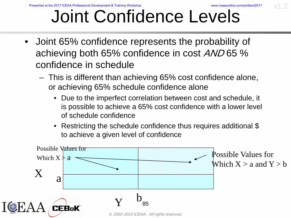
copy 2002-2013 ICEAA All rights reserved
v12
Joint Confidence Levelsbull Joint 65 confidence represents the probability of
achieving both 65 confidence in cost AND 65 confidence in schedulendash This is different than achieving 65 cost confidence alone
or achieving 65 schedule confidence alonebull Due to the imperfect correlation between cost and schedule it
is possible to achieve a 65 cost confidence with a lower level of schedule confidence
bull Restricting the schedule confidence thus requires additional $ to achieve a given level of confidence
85
X
Y
Possible Values for Which X gt a Possible Values for
Which X gt a and Y gt b
a
b
Presented at the 2017 ICEAA Professional Development amp Training Workshop wwwiceaaonlinecomportland2017
copy 2002-2013 ICEAA All rights reserved
v12Joint Confidence Levels Versus Cost Confidence Levels Only
bull Example of the differences between cost confidence schedule confidence conditional cost confidence and joint cost and schedule confidence
86
Joint Cost-Schedule Confidence Iso-Curves
Cost (RY$M)
Sche
dule
(Mon
ths)
65 Confidence
50 Confidence
70 Confidence
65 Cost Confidence AggressiveSchedule65 Cost ConfidenceScheduleGiven 65 Schedule ConfidenceUnconditional 65 CostConfidenceUnconditional 65 ScheduleConfidence
65 Cost Confidence 65 Joint Cost and Schedule
Confidence for 65 Schedule Confidence
Presented at the 2017 ICEAA Professional Development amp Training Workshop wwwiceaaonlinecomportland2017
copy 2002-2013 ICEAA All rights reserved
v12
Joint Cost and Schedule Confidence
bull Can examine pairs of cost and schedule that achieve a given level of confidence
bull Provides insights into the trade-offs between cost and schedule for a given level of confidencendash Possible to increase cost confidence by giving a
project more time in some instances or possible to ldquobuy downrdquo schedule
bull But these have limits and are shown in the iso-cost and schedule confidence curves
87
Presented at the 2017 ICEAA Professional Development amp Training Workshop wwwiceaaonlinecomportland2017
copy 2002-2013 ICEAA All rights reserved
v12Cost and Schedule Trade-offs for a Given Level of Joint Confidence
bull Hypothetical Example
88
Cost (RY$M)
Schedule (Months)
$100 48$99 48$89 49$87 50$85 51$85 52$84 53$83 55$83 55$83 56
Cost and Schedule 65 Confidence Iso-Curve
4748495051525354555657
$80 $82 $84 $86 $88 $90 $92 $94 $96 $98 $100
Cost (RY$ M)
Sche
dule
(Mon
ths)
Presented at the 2017 ICEAA Professional Development amp Training Workshop wwwiceaaonlinecomportland2017
copy 2002-2013 ICEAA All rights reserved
v12Policy Considerations for Confidence Levels
bull For large programs the difference between the amount of money needed to achieve 65 cost confidence independent of schedule and joint 65 cost and schedule confidence can represent hundreds of millions and even billions of dollars
89
Joint Cost-Schedule Confidence Iso-Curves
Cost (RY$M)
Sche
dule
(Mon
ths)
65 Confidence
65 Cost Confidence AggressiveSchedule
65 Cost ConfidenceScheduleGiven 65 Schedule Confidence
Unconditional 65 CostConfidence
Joint Cost and Schedule Confidence for 65 Cost Confidence and Program Baseline Schedule is Less Than 35
65 Cost Confidence Independent of Schedule Cost Needed to Achieve
Both 65 Joint Cost and Schedule Confidence for the Schedule with 65 Confidence
Presented at the 2017 ICEAA Professional Development amp Training Workshop wwwiceaaonlinecomportland2017
copy 2002-2013 ICEAA All rights reserved
v12
Copulasbull More generally any combination of distributions can
be used (more than just normal and lognormal)ndash Termed ldquocopulardquo from the Italian word for ldquocouplerdquondash Copulas are a way to combine marginal distributions of any
number and type into a joint distributionbull More formally a copula is a multivariate joint distribution defined
on the n-dimensional unit cube [0 1]n such that every marginal distribution is uniform on the interval [0 1]
bull (The bivariate form of) Sklarrsquos theorem states that for any bivariate distribution function H(x y) let F(x) = H(x infin) and G(y) = H(infin y) be the univariate marginal probability distribution functions Then there exists a copula C such that H(xy)=C(F(x)G(y))
ndash Copulas are widely used in risk management for investments and insurance
bull Considered industry best practice (Li 2000)bull Marketed as part of JP Morganrsquos CreditMetrics suite of tools
(Gupton et Al 1997)90
Presented at the 2017 ICEAA Professional Development amp Training Workshop wwwiceaaonlinecomportland2017
copy 2002-2013 ICEAA All rights reserved
v12Parametric Joint Cost and Schedule Analysis
bull A parametric model based on a consistent data set with a set of overlapping cost and schedule drivers is a cleaner way to model cost and schedule
91
CostWeight
HeritageNewness
Technology Readiness
Schedule
0
20
40
60
80
100
Confidence
Joint Cost and Schedule Confidence
Schedule
Cost
Lognormal Distribution PDF and CDF
0102030405060708090100
200 300 400 500 600 700 800 900 1000Cost $
Con
fiden
ce L
evel
0
00002
00004
00006
00008
0001
00012
00014
00016
Prob
abili
ty D
ensi
ty
CDFPDF
Lognormal Distribution PDF and CDF
0102030405060708090100
200 300 400 500 600 700 800 900 1000Cost $
Con
fiden
ce L
evel
0
00002
00004
00006
00008
0001
00012
00014
00016
Prob
abili
ty D
ensi
ty
CDFPDF
Presented at the 2017 ICEAA Professional Development amp Training Workshop wwwiceaaonlinecomportland2017
copy 2002-2013 ICEAA All rights reserved
v12Parametric Joint Cost and Schedule Analysis (2)
bull Joint cost and schedule risk analysis produced naturally by the integrated modelndash Addresses several issues with the copula
approachbull Tail dependencybull Correlation ndash no need to assign correlation
between cost and schedulebull Consistency of cost and schedule models
92
Presented at the 2017 ICEAA Professional Development amp Training Workshop wwwiceaaonlinecomportland2017
copy 2002-2013 ICEAA All rights reserved
v12
Resource-Loaded Schedulesbull Involves assigning cost and schedule risks to a resource-loaded schedule
networkbull Bottom-up approach
ndash More labor intensive than parametrics but can also provide more insight
ndash Can answer questions than parametric typically cannot such as how much do reserve requirements decrease if a specific risk is retired
bull Currently being implemented in Constellation programbull Has same issue as all bottom-up models hard to count all the risks and model
them discretely
ndash As a result there is a tendency to reflect less risk than indicated by history
ndash ldquoThere are more things in heaven and earth Horatio than are dreamt of in your philosophyrdquo William Shakespeare Hamlet Act I Scene V
93
Presented at the 2017 ICEAA Professional Development amp Training Workshop wwwiceaaonlinecomportland2017
copy 2002-2013 ICEAA All rights reserved
v12Resource-Loaded Schedules Vs Parametrics
bull Parametric most appropriate for early estimatesndash But also good for high-level checks as project progresses
bull As plans take shape lower level modeling may be more appropriate
94 1
CONCEPTUALDEVELOPMENT
PROJECTDEFINITION DESIGN DEVELOPMENT OPERATIONS
PARAMETRIC PARAMETRIC
ANALOGY
ENGINEERING (Bottoms Up)
$PARAMETRIC
DETAILED
$
Pre Phase A Phase B Phase CDPhase A Phase EPre Phase A Phase B Phase CDPhase A Phase E
Risk = f(Cost Estimating Relationship Inputs eg mass power data rate TRL new design etc)
Risk = f(cost and schedule variation of the analogous elements)
Risk = f(variation of detailed inputs eg labor hours rates materials etc)
Presented at the 2017 ICEAA Professional Development amp Training Workshop wwwiceaaonlinecomportland2017
copy 2002-2013 ICEAA All rights reserved
v12
Resource-Loaded Schedulesbull Methodology has been demonstrated in other
industriesndash Construction oil and gasndash Analysis has not been traditionally done on highly uncertain
complex development projects bull Methodology focuses on project baseline schedule
ndash In baseline schedule all tasks are resource loaded to represent a baseline schedule and cost standpoint
ndash Resource loaded schedule is ldquorolledrdquo up to a manageable level
ndash Based on the risk and uncertainties identified schedule distributions are applied to each rolled up task
ndash Cost uncertainties are also applied to rolled up tasksbull Uncertainties include labor rate man power etc
ndash A Monte Carlo simulation is run to develop joint cost-schedule distributions
95
Presented at the 2017 ICEAA Professional Development amp Training Workshop wwwiceaaonlinecomportland2017
copy 2002-2013 ICEAA All rights reserved
v12
Unit III - Module 9 96
Execution ndash Cross Checksbull Means The mean cost growth factor for WBS items
can be compared to history as a way to cross check results
bull CVs The CV of the cost growth factors for WBS items can be compared to history as a way to cross check results
bull Inputs Checks are performed on inputs or other parameters to see if historical values are in line with program assumptionsndash Example Historical risk scores can be compared to program
risk scores to see if risk assessors are being realistic and to see if the underlying database is representative of the program
11
Presented at the 2017 ICEAA Professional Development amp Training Workshop wwwiceaaonlinecomportland2017
- Cost and Schedule Risk Analysis Basic
- Acknowledgments
- Unit Index
- Risk Overview
- Agenda
- Introduction
- Risk Analysis Terms
- Are Our Costs Realistic
- Historical Cost Growth
- Sources of Cost Risk
- Point Estimates of Cost
- Types of Risk
- Point Estimates Vs Risk Estimates
- Cost Risk and Probability
- Probability Model ndash Distribution
- Probability Model ndash Distribution
- Probability ndash Top-Level Distribution
- S-Curves and Confidence Levels
- Example ndash Normal Distribution
- Confidence Levels
- Measuring Parametric Model Uncertainty
- Parametric Model Example
- Weight Uncertainty
- Estimating Uncertainty
- Estimating Uncertainty (2)
- Estimating Uncertainty (3)
- Aggregating Risk
- WBS Example
- WBS and Risk
- Aggregating Risk
- Percentiles Do Not Add
- Percentiles Do Not Add (2)
- Percentiles Do Not Add (3)
- Methods for Aggregating Risk
- Monte Carlo Simulationfor Risk Analysis
- Monte Carlo Simulation
- Using Random Numbers to Simulate Distributions
- Simulating a Triangular Distribution
- Simulating a Triangular Distribution (2)
- Monte Carlo and the WBS
- Number of Trials
- Number of Trials (2)
- Number of Trials (3)
- Number of Trials (4)
- Number of Trials (5)
- Number of Trials (6)
- Methods of Simulation
- Probability Model ndash Correlation
- Correlation And Causation
- The Importance of Correlation
- The Importance of Correlation (2)
- Measures of Correlation
- Pearson Correlation
- Spearman Correlation
- Functional Correlation
- Risk Measures
- Value at Risk (VaR)
- Why 70th or 80th Percentile
- Funding Above Inflection Points
- Why Budget to the 70th or 80th
- Inflection Points for Lognormal
- Issues with Percentile Funding
- ldquoHere There Be Dragonsrdquo
- Distribution Comparison
- Distribution Comparison Tail Behavior
- Distribution Comparison ndash Tail Behavior (Table)
- Percentile Budgeting is Not Risk Management
- Joint Confidence Level Analysis
- Schedules Impact Cost
- The Relationship of Cost to Schedule
- The Impact of Schedule GrowthCompression on Cost
- Schedule as an Independent Variable
- Schedule is a Dependent Variable
- Incorporation of Schedule in Cost Risk
- Subjective Cost Risk Methods and Overinclusion of Risk Factors
- Fundamental Equation of Cost and Schedule Interrelationships
- How to (Correctly) Incorporate Schedule into Cost Risk Analysis
- Joint Lognormal and Normal Distributions
- Modeling Cost and Schedule as a Bivariate Distribution
- Bivariate Lognormal Distribution for Cost and Schedule
- Bivariate Lognormal for Cost and Schedule
- Correlation Between Cost and Schedule
- Correlation Between Cost and Schedule Caveats
- Conditional Confidence Levels
- Joint Confidence Levels
- Joint Confidence Levels Versus Cost Confidence Levels Only
- Joint Cost and Schedule Confidence
- Cost and Schedule Trade-offs for a Given Level of Joint Confidence
- Policy Considerations for Confidence Levels
- Copulas
- Parametric Joint Cost and Schedule Analysis
- Parametric Joint Cost and Schedule Analysis (2)
- Resource-Loaded Schedules
- Resource-Loaded Schedules Vs Parametrics
- Resource-Loaded Schedules
- Execution ndash Cross Checks
-
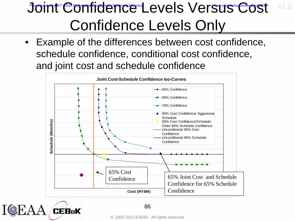
copy 2002-2013 ICEAA All rights reserved
v12Joint Confidence Levels Versus Cost Confidence Levels Only
bull Example of the differences between cost confidence schedule confidence conditional cost confidence and joint cost and schedule confidence
86
Joint Cost-Schedule Confidence Iso-Curves
Cost (RY$M)
Sche
dule
(Mon
ths)
65 Confidence
50 Confidence
70 Confidence
65 Cost Confidence AggressiveSchedule65 Cost ConfidenceScheduleGiven 65 Schedule ConfidenceUnconditional 65 CostConfidenceUnconditional 65 ScheduleConfidence
65 Cost Confidence 65 Joint Cost and Schedule
Confidence for 65 Schedule Confidence
Presented at the 2017 ICEAA Professional Development amp Training Workshop wwwiceaaonlinecomportland2017
copy 2002-2013 ICEAA All rights reserved
v12
Joint Cost and Schedule Confidence
bull Can examine pairs of cost and schedule that achieve a given level of confidence
bull Provides insights into the trade-offs between cost and schedule for a given level of confidencendash Possible to increase cost confidence by giving a
project more time in some instances or possible to ldquobuy downrdquo schedule
bull But these have limits and are shown in the iso-cost and schedule confidence curves
87
Presented at the 2017 ICEAA Professional Development amp Training Workshop wwwiceaaonlinecomportland2017
copy 2002-2013 ICEAA All rights reserved
v12Cost and Schedule Trade-offs for a Given Level of Joint Confidence
bull Hypothetical Example
88
Cost (RY$M)
Schedule (Months)
$100 48$99 48$89 49$87 50$85 51$85 52$84 53$83 55$83 55$83 56
Cost and Schedule 65 Confidence Iso-Curve
4748495051525354555657
$80 $82 $84 $86 $88 $90 $92 $94 $96 $98 $100
Cost (RY$ M)
Sche
dule
(Mon
ths)
Presented at the 2017 ICEAA Professional Development amp Training Workshop wwwiceaaonlinecomportland2017
copy 2002-2013 ICEAA All rights reserved
v12Policy Considerations for Confidence Levels
bull For large programs the difference between the amount of money needed to achieve 65 cost confidence independent of schedule and joint 65 cost and schedule confidence can represent hundreds of millions and even billions of dollars
89
Joint Cost-Schedule Confidence Iso-Curves
Cost (RY$M)
Sche
dule
(Mon
ths)
65 Confidence
65 Cost Confidence AggressiveSchedule
65 Cost ConfidenceScheduleGiven 65 Schedule Confidence
Unconditional 65 CostConfidence
Joint Cost and Schedule Confidence for 65 Cost Confidence and Program Baseline Schedule is Less Than 35
65 Cost Confidence Independent of Schedule Cost Needed to Achieve
Both 65 Joint Cost and Schedule Confidence for the Schedule with 65 Confidence
Presented at the 2017 ICEAA Professional Development amp Training Workshop wwwiceaaonlinecomportland2017
copy 2002-2013 ICEAA All rights reserved
v12
Copulasbull More generally any combination of distributions can
be used (more than just normal and lognormal)ndash Termed ldquocopulardquo from the Italian word for ldquocouplerdquondash Copulas are a way to combine marginal distributions of any
number and type into a joint distributionbull More formally a copula is a multivariate joint distribution defined
on the n-dimensional unit cube [0 1]n such that every marginal distribution is uniform on the interval [0 1]
bull (The bivariate form of) Sklarrsquos theorem states that for any bivariate distribution function H(x y) let F(x) = H(x infin) and G(y) = H(infin y) be the univariate marginal probability distribution functions Then there exists a copula C such that H(xy)=C(F(x)G(y))
ndash Copulas are widely used in risk management for investments and insurance
bull Considered industry best practice (Li 2000)bull Marketed as part of JP Morganrsquos CreditMetrics suite of tools
(Gupton et Al 1997)90
Presented at the 2017 ICEAA Professional Development amp Training Workshop wwwiceaaonlinecomportland2017
copy 2002-2013 ICEAA All rights reserved
v12Parametric Joint Cost and Schedule Analysis
bull A parametric model based on a consistent data set with a set of overlapping cost and schedule drivers is a cleaner way to model cost and schedule
91
CostWeight
HeritageNewness
Technology Readiness
Schedule
0
20
40
60
80
100
Confidence
Joint Cost and Schedule Confidence
Schedule
Cost
Lognormal Distribution PDF and CDF
0102030405060708090100
200 300 400 500 600 700 800 900 1000Cost $
Con
fiden
ce L
evel
0
00002
00004
00006
00008
0001
00012
00014
00016
Prob
abili
ty D
ensi
ty
CDFPDF
Lognormal Distribution PDF and CDF
0102030405060708090100
200 300 400 500 600 700 800 900 1000Cost $
Con
fiden
ce L
evel
0
00002
00004
00006
00008
0001
00012
00014
00016
Prob
abili
ty D
ensi
ty
CDFPDF
Presented at the 2017 ICEAA Professional Development amp Training Workshop wwwiceaaonlinecomportland2017
copy 2002-2013 ICEAA All rights reserved
v12Parametric Joint Cost and Schedule Analysis (2)
bull Joint cost and schedule risk analysis produced naturally by the integrated modelndash Addresses several issues with the copula
approachbull Tail dependencybull Correlation ndash no need to assign correlation
between cost and schedulebull Consistency of cost and schedule models
92
Presented at the 2017 ICEAA Professional Development amp Training Workshop wwwiceaaonlinecomportland2017
copy 2002-2013 ICEAA All rights reserved
v12
Resource-Loaded Schedulesbull Involves assigning cost and schedule risks to a resource-loaded schedule
networkbull Bottom-up approach
ndash More labor intensive than parametrics but can also provide more insight
ndash Can answer questions than parametric typically cannot such as how much do reserve requirements decrease if a specific risk is retired
bull Currently being implemented in Constellation programbull Has same issue as all bottom-up models hard to count all the risks and model
them discretely
ndash As a result there is a tendency to reflect less risk than indicated by history
ndash ldquoThere are more things in heaven and earth Horatio than are dreamt of in your philosophyrdquo William Shakespeare Hamlet Act I Scene V
93
Presented at the 2017 ICEAA Professional Development amp Training Workshop wwwiceaaonlinecomportland2017
copy 2002-2013 ICEAA All rights reserved
v12Resource-Loaded Schedules Vs Parametrics
bull Parametric most appropriate for early estimatesndash But also good for high-level checks as project progresses
bull As plans take shape lower level modeling may be more appropriate
94 1
CONCEPTUALDEVELOPMENT
PROJECTDEFINITION DESIGN DEVELOPMENT OPERATIONS
PARAMETRIC PARAMETRIC
ANALOGY
ENGINEERING (Bottoms Up)
$PARAMETRIC
DETAILED
$
Pre Phase A Phase B Phase CDPhase A Phase EPre Phase A Phase B Phase CDPhase A Phase E
Risk = f(Cost Estimating Relationship Inputs eg mass power data rate TRL new design etc)
Risk = f(cost and schedule variation of the analogous elements)
Risk = f(variation of detailed inputs eg labor hours rates materials etc)
Presented at the 2017 ICEAA Professional Development amp Training Workshop wwwiceaaonlinecomportland2017
copy 2002-2013 ICEAA All rights reserved
v12
Resource-Loaded Schedulesbull Methodology has been demonstrated in other
industriesndash Construction oil and gasndash Analysis has not been traditionally done on highly uncertain
complex development projects bull Methodology focuses on project baseline schedule
ndash In baseline schedule all tasks are resource loaded to represent a baseline schedule and cost standpoint
ndash Resource loaded schedule is ldquorolledrdquo up to a manageable level
ndash Based on the risk and uncertainties identified schedule distributions are applied to each rolled up task
ndash Cost uncertainties are also applied to rolled up tasksbull Uncertainties include labor rate man power etc
ndash A Monte Carlo simulation is run to develop joint cost-schedule distributions
95
Presented at the 2017 ICEAA Professional Development amp Training Workshop wwwiceaaonlinecomportland2017
copy 2002-2013 ICEAA All rights reserved
v12
Unit III - Module 9 96
Execution ndash Cross Checksbull Means The mean cost growth factor for WBS items
can be compared to history as a way to cross check results
bull CVs The CV of the cost growth factors for WBS items can be compared to history as a way to cross check results
bull Inputs Checks are performed on inputs or other parameters to see if historical values are in line with program assumptionsndash Example Historical risk scores can be compared to program
risk scores to see if risk assessors are being realistic and to see if the underlying database is representative of the program
11
Presented at the 2017 ICEAA Professional Development amp Training Workshop wwwiceaaonlinecomportland2017
- Cost and Schedule Risk Analysis Basic
- Acknowledgments
- Unit Index
- Risk Overview
- Agenda
- Introduction
- Risk Analysis Terms
- Are Our Costs Realistic
- Historical Cost Growth
- Sources of Cost Risk
- Point Estimates of Cost
- Types of Risk
- Point Estimates Vs Risk Estimates
- Cost Risk and Probability
- Probability Model ndash Distribution
- Probability Model ndash Distribution
- Probability ndash Top-Level Distribution
- S-Curves and Confidence Levels
- Example ndash Normal Distribution
- Confidence Levels
- Measuring Parametric Model Uncertainty
- Parametric Model Example
- Weight Uncertainty
- Estimating Uncertainty
- Estimating Uncertainty (2)
- Estimating Uncertainty (3)
- Aggregating Risk
- WBS Example
- WBS and Risk
- Aggregating Risk
- Percentiles Do Not Add
- Percentiles Do Not Add (2)
- Percentiles Do Not Add (3)
- Methods for Aggregating Risk
- Monte Carlo Simulationfor Risk Analysis
- Monte Carlo Simulation
- Using Random Numbers to Simulate Distributions
- Simulating a Triangular Distribution
- Simulating a Triangular Distribution (2)
- Monte Carlo and the WBS
- Number of Trials
- Number of Trials (2)
- Number of Trials (3)
- Number of Trials (4)
- Number of Trials (5)
- Number of Trials (6)
- Methods of Simulation
- Probability Model ndash Correlation
- Correlation And Causation
- The Importance of Correlation
- The Importance of Correlation (2)
- Measures of Correlation
- Pearson Correlation
- Spearman Correlation
- Functional Correlation
- Risk Measures
- Value at Risk (VaR)
- Why 70th or 80th Percentile
- Funding Above Inflection Points
- Why Budget to the 70th or 80th
- Inflection Points for Lognormal
- Issues with Percentile Funding
- ldquoHere There Be Dragonsrdquo
- Distribution Comparison
- Distribution Comparison Tail Behavior
- Distribution Comparison ndash Tail Behavior (Table)
- Percentile Budgeting is Not Risk Management
- Joint Confidence Level Analysis
- Schedules Impact Cost
- The Relationship of Cost to Schedule
- The Impact of Schedule GrowthCompression on Cost
- Schedule as an Independent Variable
- Schedule is a Dependent Variable
- Incorporation of Schedule in Cost Risk
- Subjective Cost Risk Methods and Overinclusion of Risk Factors
- Fundamental Equation of Cost and Schedule Interrelationships
- How to (Correctly) Incorporate Schedule into Cost Risk Analysis
- Joint Lognormal and Normal Distributions
- Modeling Cost and Schedule as a Bivariate Distribution
- Bivariate Lognormal Distribution for Cost and Schedule
- Bivariate Lognormal for Cost and Schedule
- Correlation Between Cost and Schedule
- Correlation Between Cost and Schedule Caveats
- Conditional Confidence Levels
- Joint Confidence Levels
- Joint Confidence Levels Versus Cost Confidence Levels Only
- Joint Cost and Schedule Confidence
- Cost and Schedule Trade-offs for a Given Level of Joint Confidence
- Policy Considerations for Confidence Levels
- Copulas
- Parametric Joint Cost and Schedule Analysis
- Parametric Joint Cost and Schedule Analysis (2)
- Resource-Loaded Schedules
- Resource-Loaded Schedules Vs Parametrics
- Resource-Loaded Schedules
- Execution ndash Cross Checks
-
copy 2002-2013 ICEAA All rights reserved
v12
Joint Cost and Schedule Confidence
bull Can examine pairs of cost and schedule that achieve a given level of confidence
bull Provides insights into the trade-offs between cost and schedule for a given level of confidencendash Possible to increase cost confidence by giving a
project more time in some instances or possible to ldquobuy downrdquo schedule
bull But these have limits and are shown in the iso-cost and schedule confidence curves
87
Presented at the 2017 ICEAA Professional Development amp Training Workshop wwwiceaaonlinecomportland2017
copy 2002-2013 ICEAA All rights reserved
v12Cost and Schedule Trade-offs for a Given Level of Joint Confidence
bull Hypothetical Example
88
Cost (RY$M)
Schedule (Months)
$100 48$99 48$89 49$87 50$85 51$85 52$84 53$83 55$83 55$83 56
Cost and Schedule 65 Confidence Iso-Curve
4748495051525354555657
$80 $82 $84 $86 $88 $90 $92 $94 $96 $98 $100
Cost (RY$ M)
Sche
dule
(Mon
ths)
Presented at the 2017 ICEAA Professional Development amp Training Workshop wwwiceaaonlinecomportland2017
copy 2002-2013 ICEAA All rights reserved
v12Policy Considerations for Confidence Levels
bull For large programs the difference between the amount of money needed to achieve 65 cost confidence independent of schedule and joint 65 cost and schedule confidence can represent hundreds of millions and even billions of dollars
89
Joint Cost-Schedule Confidence Iso-Curves
Cost (RY$M)
Sche
dule
(Mon
ths)
65 Confidence
65 Cost Confidence AggressiveSchedule
65 Cost ConfidenceScheduleGiven 65 Schedule Confidence
Unconditional 65 CostConfidence
Joint Cost and Schedule Confidence for 65 Cost Confidence and Program Baseline Schedule is Less Than 35
65 Cost Confidence Independent of Schedule Cost Needed to Achieve
Both 65 Joint Cost and Schedule Confidence for the Schedule with 65 Confidence
Presented at the 2017 ICEAA Professional Development amp Training Workshop wwwiceaaonlinecomportland2017
copy 2002-2013 ICEAA All rights reserved
v12
Copulasbull More generally any combination of distributions can
be used (more than just normal and lognormal)ndash Termed ldquocopulardquo from the Italian word for ldquocouplerdquondash Copulas are a way to combine marginal distributions of any
number and type into a joint distributionbull More formally a copula is a multivariate joint distribution defined
on the n-dimensional unit cube [0 1]n such that every marginal distribution is uniform on the interval [0 1]
bull (The bivariate form of) Sklarrsquos theorem states that for any bivariate distribution function H(x y) let F(x) = H(x infin) and G(y) = H(infin y) be the univariate marginal probability distribution functions Then there exists a copula C such that H(xy)=C(F(x)G(y))
ndash Copulas are widely used in risk management for investments and insurance
bull Considered industry best practice (Li 2000)bull Marketed as part of JP Morganrsquos CreditMetrics suite of tools
(Gupton et Al 1997)90
Presented at the 2017 ICEAA Professional Development amp Training Workshop wwwiceaaonlinecomportland2017
copy 2002-2013 ICEAA All rights reserved
v12Parametric Joint Cost and Schedule Analysis
bull A parametric model based on a consistent data set with a set of overlapping cost and schedule drivers is a cleaner way to model cost and schedule
91
CostWeight
HeritageNewness
Technology Readiness
Schedule
0
20
40
60
80
100
Confidence
Joint Cost and Schedule Confidence
Schedule
Cost
Lognormal Distribution PDF and CDF
0102030405060708090100
200 300 400 500 600 700 800 900 1000Cost $
Con
fiden
ce L
evel
0
00002
00004
00006
00008
0001
00012
00014
00016
Prob
abili
ty D
ensi
ty
CDFPDF
Lognormal Distribution PDF and CDF
0102030405060708090100
200 300 400 500 600 700 800 900 1000Cost $
Con
fiden
ce L
evel
0
00002
00004
00006
00008
0001
00012
00014
00016
Prob
abili
ty D
ensi
ty
CDFPDF
Presented at the 2017 ICEAA Professional Development amp Training Workshop wwwiceaaonlinecomportland2017
copy 2002-2013 ICEAA All rights reserved
v12Parametric Joint Cost and Schedule Analysis (2)
bull Joint cost and schedule risk analysis produced naturally by the integrated modelndash Addresses several issues with the copula
approachbull Tail dependencybull Correlation ndash no need to assign correlation
between cost and schedulebull Consistency of cost and schedule models
92
Presented at the 2017 ICEAA Professional Development amp Training Workshop wwwiceaaonlinecomportland2017
copy 2002-2013 ICEAA All rights reserved
v12
Resource-Loaded Schedulesbull Involves assigning cost and schedule risks to a resource-loaded schedule
networkbull Bottom-up approach
ndash More labor intensive than parametrics but can also provide more insight
ndash Can answer questions than parametric typically cannot such as how much do reserve requirements decrease if a specific risk is retired
bull Currently being implemented in Constellation programbull Has same issue as all bottom-up models hard to count all the risks and model
them discretely
ndash As a result there is a tendency to reflect less risk than indicated by history
ndash ldquoThere are more things in heaven and earth Horatio than are dreamt of in your philosophyrdquo William Shakespeare Hamlet Act I Scene V
93
Presented at the 2017 ICEAA Professional Development amp Training Workshop wwwiceaaonlinecomportland2017
copy 2002-2013 ICEAA All rights reserved
v12Resource-Loaded Schedules Vs Parametrics
bull Parametric most appropriate for early estimatesndash But also good for high-level checks as project progresses
bull As plans take shape lower level modeling may be more appropriate
94 1
CONCEPTUALDEVELOPMENT
PROJECTDEFINITION DESIGN DEVELOPMENT OPERATIONS
PARAMETRIC PARAMETRIC
ANALOGY
ENGINEERING (Bottoms Up)
$PARAMETRIC
DETAILED
$
Pre Phase A Phase B Phase CDPhase A Phase EPre Phase A Phase B Phase CDPhase A Phase E
Risk = f(Cost Estimating Relationship Inputs eg mass power data rate TRL new design etc)
Risk = f(cost and schedule variation of the analogous elements)
Risk = f(variation of detailed inputs eg labor hours rates materials etc)
Presented at the 2017 ICEAA Professional Development amp Training Workshop wwwiceaaonlinecomportland2017
copy 2002-2013 ICEAA All rights reserved
v12
Resource-Loaded Schedulesbull Methodology has been demonstrated in other
industriesndash Construction oil and gasndash Analysis has not been traditionally done on highly uncertain
complex development projects bull Methodology focuses on project baseline schedule
ndash In baseline schedule all tasks are resource loaded to represent a baseline schedule and cost standpoint
ndash Resource loaded schedule is ldquorolledrdquo up to a manageable level
ndash Based on the risk and uncertainties identified schedule distributions are applied to each rolled up task
ndash Cost uncertainties are also applied to rolled up tasksbull Uncertainties include labor rate man power etc
ndash A Monte Carlo simulation is run to develop joint cost-schedule distributions
95
Presented at the 2017 ICEAA Professional Development amp Training Workshop wwwiceaaonlinecomportland2017
copy 2002-2013 ICEAA All rights reserved
v12
Unit III - Module 9 96
Execution ndash Cross Checksbull Means The mean cost growth factor for WBS items
can be compared to history as a way to cross check results
bull CVs The CV of the cost growth factors for WBS items can be compared to history as a way to cross check results
bull Inputs Checks are performed on inputs or other parameters to see if historical values are in line with program assumptionsndash Example Historical risk scores can be compared to program
risk scores to see if risk assessors are being realistic and to see if the underlying database is representative of the program
11
Presented at the 2017 ICEAA Professional Development amp Training Workshop wwwiceaaonlinecomportland2017
- Cost and Schedule Risk Analysis Basic
- Acknowledgments
- Unit Index
- Risk Overview
- Agenda
- Introduction
- Risk Analysis Terms
- Are Our Costs Realistic
- Historical Cost Growth
- Sources of Cost Risk
- Point Estimates of Cost
- Types of Risk
- Point Estimates Vs Risk Estimates
- Cost Risk and Probability
- Probability Model ndash Distribution
- Probability Model ndash Distribution
- Probability ndash Top-Level Distribution
- S-Curves and Confidence Levels
- Example ndash Normal Distribution
- Confidence Levels
- Measuring Parametric Model Uncertainty
- Parametric Model Example
- Weight Uncertainty
- Estimating Uncertainty
- Estimating Uncertainty (2)
- Estimating Uncertainty (3)
- Aggregating Risk
- WBS Example
- WBS and Risk
- Aggregating Risk
- Percentiles Do Not Add
- Percentiles Do Not Add (2)
- Percentiles Do Not Add (3)
- Methods for Aggregating Risk
- Monte Carlo Simulationfor Risk Analysis
- Monte Carlo Simulation
- Using Random Numbers to Simulate Distributions
- Simulating a Triangular Distribution
- Simulating a Triangular Distribution (2)
- Monte Carlo and the WBS
- Number of Trials
- Number of Trials (2)
- Number of Trials (3)
- Number of Trials (4)
- Number of Trials (5)
- Number of Trials (6)
- Methods of Simulation
- Probability Model ndash Correlation
- Correlation And Causation
- The Importance of Correlation
- The Importance of Correlation (2)
- Measures of Correlation
- Pearson Correlation
- Spearman Correlation
- Functional Correlation
- Risk Measures
- Value at Risk (VaR)
- Why 70th or 80th Percentile
- Funding Above Inflection Points
- Why Budget to the 70th or 80th
- Inflection Points for Lognormal
- Issues with Percentile Funding
- ldquoHere There Be Dragonsrdquo
- Distribution Comparison
- Distribution Comparison Tail Behavior
- Distribution Comparison ndash Tail Behavior (Table)
- Percentile Budgeting is Not Risk Management
- Joint Confidence Level Analysis
- Schedules Impact Cost
- The Relationship of Cost to Schedule
- The Impact of Schedule GrowthCompression on Cost
- Schedule as an Independent Variable
- Schedule is a Dependent Variable
- Incorporation of Schedule in Cost Risk
- Subjective Cost Risk Methods and Overinclusion of Risk Factors
- Fundamental Equation of Cost and Schedule Interrelationships
- How to (Correctly) Incorporate Schedule into Cost Risk Analysis
- Joint Lognormal and Normal Distributions
- Modeling Cost and Schedule as a Bivariate Distribution
- Bivariate Lognormal Distribution for Cost and Schedule
- Bivariate Lognormal for Cost and Schedule
- Correlation Between Cost and Schedule
- Correlation Between Cost and Schedule Caveats
- Conditional Confidence Levels
- Joint Confidence Levels
- Joint Confidence Levels Versus Cost Confidence Levels Only
- Joint Cost and Schedule Confidence
- Cost and Schedule Trade-offs for a Given Level of Joint Confidence
- Policy Considerations for Confidence Levels
- Copulas
- Parametric Joint Cost and Schedule Analysis
- Parametric Joint Cost and Schedule Analysis (2)
- Resource-Loaded Schedules
- Resource-Loaded Schedules Vs Parametrics
- Resource-Loaded Schedules
- Execution ndash Cross Checks
-
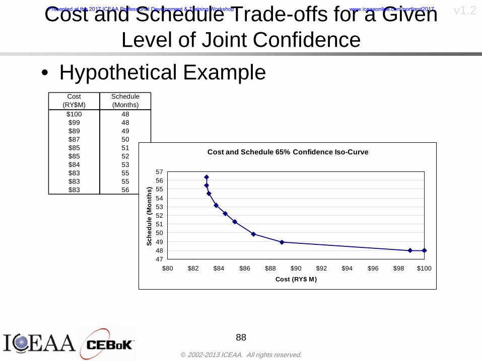
copy 2002-2013 ICEAA All rights reserved
v12Cost and Schedule Trade-offs for a Given Level of Joint Confidence
bull Hypothetical Example
88
Cost (RY$M)
Schedule (Months)
$100 48$99 48$89 49$87 50$85 51$85 52$84 53$83 55$83 55$83 56
Cost and Schedule 65 Confidence Iso-Curve
4748495051525354555657
$80 $82 $84 $86 $88 $90 $92 $94 $96 $98 $100
Cost (RY$ M)
Sche
dule
(Mon
ths)
Presented at the 2017 ICEAA Professional Development amp Training Workshop wwwiceaaonlinecomportland2017
copy 2002-2013 ICEAA All rights reserved
v12Policy Considerations for Confidence Levels
bull For large programs the difference between the amount of money needed to achieve 65 cost confidence independent of schedule and joint 65 cost and schedule confidence can represent hundreds of millions and even billions of dollars
89
Joint Cost-Schedule Confidence Iso-Curves
Cost (RY$M)
Sche
dule
(Mon
ths)
65 Confidence
65 Cost Confidence AggressiveSchedule
65 Cost ConfidenceScheduleGiven 65 Schedule Confidence
Unconditional 65 CostConfidence
Joint Cost and Schedule Confidence for 65 Cost Confidence and Program Baseline Schedule is Less Than 35
65 Cost Confidence Independent of Schedule Cost Needed to Achieve
Both 65 Joint Cost and Schedule Confidence for the Schedule with 65 Confidence
Presented at the 2017 ICEAA Professional Development amp Training Workshop wwwiceaaonlinecomportland2017
copy 2002-2013 ICEAA All rights reserved
v12
Copulasbull More generally any combination of distributions can
be used (more than just normal and lognormal)ndash Termed ldquocopulardquo from the Italian word for ldquocouplerdquondash Copulas are a way to combine marginal distributions of any
number and type into a joint distributionbull More formally a copula is a multivariate joint distribution defined
on the n-dimensional unit cube [0 1]n such that every marginal distribution is uniform on the interval [0 1]
bull (The bivariate form of) Sklarrsquos theorem states that for any bivariate distribution function H(x y) let F(x) = H(x infin) and G(y) = H(infin y) be the univariate marginal probability distribution functions Then there exists a copula C such that H(xy)=C(F(x)G(y))
ndash Copulas are widely used in risk management for investments and insurance
bull Considered industry best practice (Li 2000)bull Marketed as part of JP Morganrsquos CreditMetrics suite of tools
(Gupton et Al 1997)90
Presented at the 2017 ICEAA Professional Development amp Training Workshop wwwiceaaonlinecomportland2017
copy 2002-2013 ICEAA All rights reserved
v12Parametric Joint Cost and Schedule Analysis
bull A parametric model based on a consistent data set with a set of overlapping cost and schedule drivers is a cleaner way to model cost and schedule
91
CostWeight
HeritageNewness
Technology Readiness
Schedule
0
20
40
60
80
100
Confidence
Joint Cost and Schedule Confidence
Schedule
Cost
Lognormal Distribution PDF and CDF
0102030405060708090100
200 300 400 500 600 700 800 900 1000Cost $
Con
fiden
ce L
evel
0
00002
00004
00006
00008
0001
00012
00014
00016
Prob
abili
ty D
ensi
ty
CDFPDF
Lognormal Distribution PDF and CDF
0102030405060708090100
200 300 400 500 600 700 800 900 1000Cost $
Con
fiden
ce L
evel
0
00002
00004
00006
00008
0001
00012
00014
00016
Prob
abili
ty D
ensi
ty
CDFPDF
Presented at the 2017 ICEAA Professional Development amp Training Workshop wwwiceaaonlinecomportland2017
copy 2002-2013 ICEAA All rights reserved
v12Parametric Joint Cost and Schedule Analysis (2)
bull Joint cost and schedule risk analysis produced naturally by the integrated modelndash Addresses several issues with the copula
approachbull Tail dependencybull Correlation ndash no need to assign correlation
between cost and schedulebull Consistency of cost and schedule models
92
Presented at the 2017 ICEAA Professional Development amp Training Workshop wwwiceaaonlinecomportland2017
copy 2002-2013 ICEAA All rights reserved
v12
Resource-Loaded Schedulesbull Involves assigning cost and schedule risks to a resource-loaded schedule
networkbull Bottom-up approach
ndash More labor intensive than parametrics but can also provide more insight
ndash Can answer questions than parametric typically cannot such as how much do reserve requirements decrease if a specific risk is retired
bull Currently being implemented in Constellation programbull Has same issue as all bottom-up models hard to count all the risks and model
them discretely
ndash As a result there is a tendency to reflect less risk than indicated by history
ndash ldquoThere are more things in heaven and earth Horatio than are dreamt of in your philosophyrdquo William Shakespeare Hamlet Act I Scene V
93
Presented at the 2017 ICEAA Professional Development amp Training Workshop wwwiceaaonlinecomportland2017
copy 2002-2013 ICEAA All rights reserved
v12Resource-Loaded Schedules Vs Parametrics
bull Parametric most appropriate for early estimatesndash But also good for high-level checks as project progresses
bull As plans take shape lower level modeling may be more appropriate
94 1
CONCEPTUALDEVELOPMENT
PROJECTDEFINITION DESIGN DEVELOPMENT OPERATIONS
PARAMETRIC PARAMETRIC
ANALOGY
ENGINEERING (Bottoms Up)
$PARAMETRIC
DETAILED
$
Pre Phase A Phase B Phase CDPhase A Phase EPre Phase A Phase B Phase CDPhase A Phase E
Risk = f(Cost Estimating Relationship Inputs eg mass power data rate TRL new design etc)
Risk = f(cost and schedule variation of the analogous elements)
Risk = f(variation of detailed inputs eg labor hours rates materials etc)
Presented at the 2017 ICEAA Professional Development amp Training Workshop wwwiceaaonlinecomportland2017
copy 2002-2013 ICEAA All rights reserved
v12
Resource-Loaded Schedulesbull Methodology has been demonstrated in other
industriesndash Construction oil and gasndash Analysis has not been traditionally done on highly uncertain
complex development projects bull Methodology focuses on project baseline schedule
ndash In baseline schedule all tasks are resource loaded to represent a baseline schedule and cost standpoint
ndash Resource loaded schedule is ldquorolledrdquo up to a manageable level
ndash Based on the risk and uncertainties identified schedule distributions are applied to each rolled up task
ndash Cost uncertainties are also applied to rolled up tasksbull Uncertainties include labor rate man power etc
ndash A Monte Carlo simulation is run to develop joint cost-schedule distributions
95
Presented at the 2017 ICEAA Professional Development amp Training Workshop wwwiceaaonlinecomportland2017
copy 2002-2013 ICEAA All rights reserved
v12
Unit III - Module 9 96
Execution ndash Cross Checksbull Means The mean cost growth factor for WBS items
can be compared to history as a way to cross check results
bull CVs The CV of the cost growth factors for WBS items can be compared to history as a way to cross check results
bull Inputs Checks are performed on inputs or other parameters to see if historical values are in line with program assumptionsndash Example Historical risk scores can be compared to program
risk scores to see if risk assessors are being realistic and to see if the underlying database is representative of the program
11
Presented at the 2017 ICEAA Professional Development amp Training Workshop wwwiceaaonlinecomportland2017
- Cost and Schedule Risk Analysis Basic
- Acknowledgments
- Unit Index
- Risk Overview
- Agenda
- Introduction
- Risk Analysis Terms
- Are Our Costs Realistic
- Historical Cost Growth
- Sources of Cost Risk
- Point Estimates of Cost
- Types of Risk
- Point Estimates Vs Risk Estimates
- Cost Risk and Probability
- Probability Model ndash Distribution
- Probability Model ndash Distribution
- Probability ndash Top-Level Distribution
- S-Curves and Confidence Levels
- Example ndash Normal Distribution
- Confidence Levels
- Measuring Parametric Model Uncertainty
- Parametric Model Example
- Weight Uncertainty
- Estimating Uncertainty
- Estimating Uncertainty (2)
- Estimating Uncertainty (3)
- Aggregating Risk
- WBS Example
- WBS and Risk
- Aggregating Risk
- Percentiles Do Not Add
- Percentiles Do Not Add (2)
- Percentiles Do Not Add (3)
- Methods for Aggregating Risk
- Monte Carlo Simulationfor Risk Analysis
- Monte Carlo Simulation
- Using Random Numbers to Simulate Distributions
- Simulating a Triangular Distribution
- Simulating a Triangular Distribution (2)
- Monte Carlo and the WBS
- Number of Trials
- Number of Trials (2)
- Number of Trials (3)
- Number of Trials (4)
- Number of Trials (5)
- Number of Trials (6)
- Methods of Simulation
- Probability Model ndash Correlation
- Correlation And Causation
- The Importance of Correlation
- The Importance of Correlation (2)
- Measures of Correlation
- Pearson Correlation
- Spearman Correlation
- Functional Correlation
- Risk Measures
- Value at Risk (VaR)
- Why 70th or 80th Percentile
- Funding Above Inflection Points
- Why Budget to the 70th or 80th
- Inflection Points for Lognormal
- Issues with Percentile Funding
- ldquoHere There Be Dragonsrdquo
- Distribution Comparison
- Distribution Comparison Tail Behavior
- Distribution Comparison ndash Tail Behavior (Table)
- Percentile Budgeting is Not Risk Management
- Joint Confidence Level Analysis
- Schedules Impact Cost
- The Relationship of Cost to Schedule
- The Impact of Schedule GrowthCompression on Cost
- Schedule as an Independent Variable
- Schedule is a Dependent Variable
- Incorporation of Schedule in Cost Risk
- Subjective Cost Risk Methods and Overinclusion of Risk Factors
- Fundamental Equation of Cost and Schedule Interrelationships
- How to (Correctly) Incorporate Schedule into Cost Risk Analysis
- Joint Lognormal and Normal Distributions
- Modeling Cost and Schedule as a Bivariate Distribution
- Bivariate Lognormal Distribution for Cost and Schedule
- Bivariate Lognormal for Cost and Schedule
- Correlation Between Cost and Schedule
- Correlation Between Cost and Schedule Caveats
- Conditional Confidence Levels
- Joint Confidence Levels
- Joint Confidence Levels Versus Cost Confidence Levels Only
- Joint Cost and Schedule Confidence
- Cost and Schedule Trade-offs for a Given Level of Joint Confidence
- Policy Considerations for Confidence Levels
- Copulas
- Parametric Joint Cost and Schedule Analysis
- Parametric Joint Cost and Schedule Analysis (2)
- Resource-Loaded Schedules
- Resource-Loaded Schedules Vs Parametrics
- Resource-Loaded Schedules
- Execution ndash Cross Checks
-
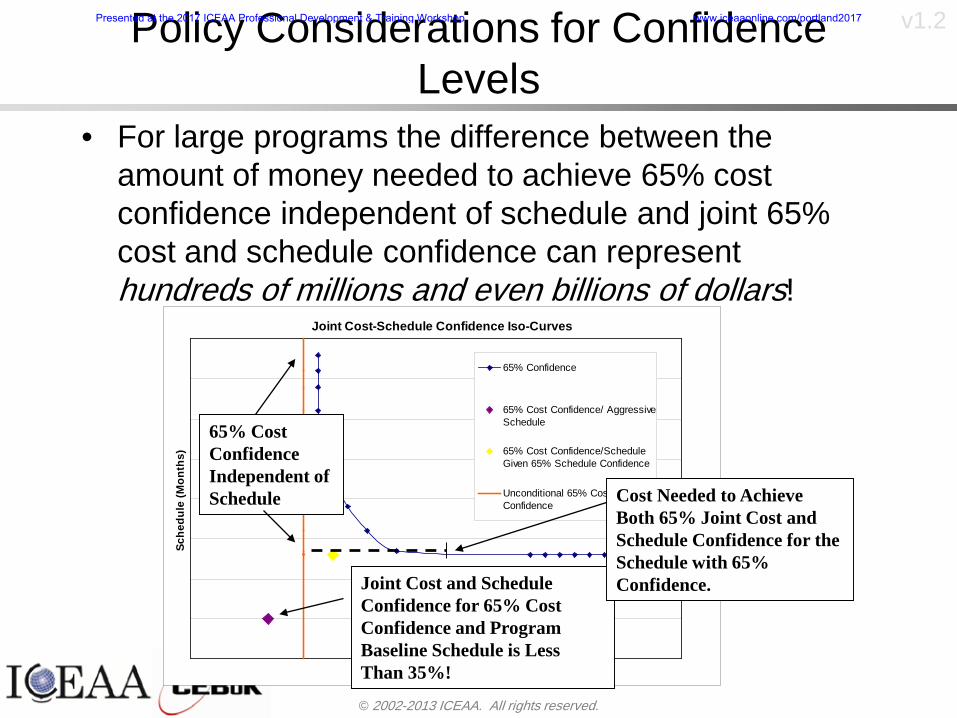
copy 2002-2013 ICEAA All rights reserved
v12Policy Considerations for Confidence Levels
bull For large programs the difference between the amount of money needed to achieve 65 cost confidence independent of schedule and joint 65 cost and schedule confidence can represent hundreds of millions and even billions of dollars
89
Joint Cost-Schedule Confidence Iso-Curves
Cost (RY$M)
Sche
dule
(Mon
ths)
65 Confidence
65 Cost Confidence AggressiveSchedule
65 Cost ConfidenceScheduleGiven 65 Schedule Confidence
Unconditional 65 CostConfidence
Joint Cost and Schedule Confidence for 65 Cost Confidence and Program Baseline Schedule is Less Than 35
65 Cost Confidence Independent of Schedule Cost Needed to Achieve
Both 65 Joint Cost and Schedule Confidence for the Schedule with 65 Confidence
Presented at the 2017 ICEAA Professional Development amp Training Workshop wwwiceaaonlinecomportland2017
copy 2002-2013 ICEAA All rights reserved
v12
Copulasbull More generally any combination of distributions can
be used (more than just normal and lognormal)ndash Termed ldquocopulardquo from the Italian word for ldquocouplerdquondash Copulas are a way to combine marginal distributions of any
number and type into a joint distributionbull More formally a copula is a multivariate joint distribution defined
on the n-dimensional unit cube [0 1]n such that every marginal distribution is uniform on the interval [0 1]
bull (The bivariate form of) Sklarrsquos theorem states that for any bivariate distribution function H(x y) let F(x) = H(x infin) and G(y) = H(infin y) be the univariate marginal probability distribution functions Then there exists a copula C such that H(xy)=C(F(x)G(y))
ndash Copulas are widely used in risk management for investments and insurance
bull Considered industry best practice (Li 2000)bull Marketed as part of JP Morganrsquos CreditMetrics suite of tools
(Gupton et Al 1997)90
Presented at the 2017 ICEAA Professional Development amp Training Workshop wwwiceaaonlinecomportland2017
copy 2002-2013 ICEAA All rights reserved
v12Parametric Joint Cost and Schedule Analysis
bull A parametric model based on a consistent data set with a set of overlapping cost and schedule drivers is a cleaner way to model cost and schedule
91
CostWeight
HeritageNewness
Technology Readiness
Schedule
0
20
40
60
80
100
Confidence
Joint Cost and Schedule Confidence
Schedule
Cost
Lognormal Distribution PDF and CDF
0102030405060708090100
200 300 400 500 600 700 800 900 1000Cost $
Con
fiden
ce L
evel
0
00002
00004
00006
00008
0001
00012
00014
00016
Prob
abili
ty D
ensi
ty
CDFPDF
Lognormal Distribution PDF and CDF
0102030405060708090100
200 300 400 500 600 700 800 900 1000Cost $
Con
fiden
ce L
evel
0
00002
00004
00006
00008
0001
00012
00014
00016
Prob
abili
ty D
ensi
ty
CDFPDF
Presented at the 2017 ICEAA Professional Development amp Training Workshop wwwiceaaonlinecomportland2017
copy 2002-2013 ICEAA All rights reserved
v12Parametric Joint Cost and Schedule Analysis (2)
bull Joint cost and schedule risk analysis produced naturally by the integrated modelndash Addresses several issues with the copula
approachbull Tail dependencybull Correlation ndash no need to assign correlation
between cost and schedulebull Consistency of cost and schedule models
92
Presented at the 2017 ICEAA Professional Development amp Training Workshop wwwiceaaonlinecomportland2017
copy 2002-2013 ICEAA All rights reserved
v12
Resource-Loaded Schedulesbull Involves assigning cost and schedule risks to a resource-loaded schedule
networkbull Bottom-up approach
ndash More labor intensive than parametrics but can also provide more insight
ndash Can answer questions than parametric typically cannot such as how much do reserve requirements decrease if a specific risk is retired
bull Currently being implemented in Constellation programbull Has same issue as all bottom-up models hard to count all the risks and model
them discretely
ndash As a result there is a tendency to reflect less risk than indicated by history
ndash ldquoThere are more things in heaven and earth Horatio than are dreamt of in your philosophyrdquo William Shakespeare Hamlet Act I Scene V
93
Presented at the 2017 ICEAA Professional Development amp Training Workshop wwwiceaaonlinecomportland2017
copy 2002-2013 ICEAA All rights reserved
v12Resource-Loaded Schedules Vs Parametrics
bull Parametric most appropriate for early estimatesndash But also good for high-level checks as project progresses
bull As plans take shape lower level modeling may be more appropriate
94 1
CONCEPTUALDEVELOPMENT
PROJECTDEFINITION DESIGN DEVELOPMENT OPERATIONS
PARAMETRIC PARAMETRIC
ANALOGY
ENGINEERING (Bottoms Up)
$PARAMETRIC
DETAILED
$
Pre Phase A Phase B Phase CDPhase A Phase EPre Phase A Phase B Phase CDPhase A Phase E
Risk = f(Cost Estimating Relationship Inputs eg mass power data rate TRL new design etc)
Risk = f(cost and schedule variation of the analogous elements)
Risk = f(variation of detailed inputs eg labor hours rates materials etc)
Presented at the 2017 ICEAA Professional Development amp Training Workshop wwwiceaaonlinecomportland2017
copy 2002-2013 ICEAA All rights reserved
v12
Resource-Loaded Schedulesbull Methodology has been demonstrated in other
industriesndash Construction oil and gasndash Analysis has not been traditionally done on highly uncertain
complex development projects bull Methodology focuses on project baseline schedule
ndash In baseline schedule all tasks are resource loaded to represent a baseline schedule and cost standpoint
ndash Resource loaded schedule is ldquorolledrdquo up to a manageable level
ndash Based on the risk and uncertainties identified schedule distributions are applied to each rolled up task
ndash Cost uncertainties are also applied to rolled up tasksbull Uncertainties include labor rate man power etc
ndash A Monte Carlo simulation is run to develop joint cost-schedule distributions
95
Presented at the 2017 ICEAA Professional Development amp Training Workshop wwwiceaaonlinecomportland2017
copy 2002-2013 ICEAA All rights reserved
v12
Unit III - Module 9 96
Execution ndash Cross Checksbull Means The mean cost growth factor for WBS items
can be compared to history as a way to cross check results
bull CVs The CV of the cost growth factors for WBS items can be compared to history as a way to cross check results
bull Inputs Checks are performed on inputs or other parameters to see if historical values are in line with program assumptionsndash Example Historical risk scores can be compared to program
risk scores to see if risk assessors are being realistic and to see if the underlying database is representative of the program
11
Presented at the 2017 ICEAA Professional Development amp Training Workshop wwwiceaaonlinecomportland2017
- Cost and Schedule Risk Analysis Basic
- Acknowledgments
- Unit Index
- Risk Overview
- Agenda
- Introduction
- Risk Analysis Terms
- Are Our Costs Realistic
- Historical Cost Growth
- Sources of Cost Risk
- Point Estimates of Cost
- Types of Risk
- Point Estimates Vs Risk Estimates
- Cost Risk and Probability
- Probability Model ndash Distribution
- Probability Model ndash Distribution
- Probability ndash Top-Level Distribution
- S-Curves and Confidence Levels
- Example ndash Normal Distribution
- Confidence Levels
- Measuring Parametric Model Uncertainty
- Parametric Model Example
- Weight Uncertainty
- Estimating Uncertainty
- Estimating Uncertainty (2)
- Estimating Uncertainty (3)
- Aggregating Risk
- WBS Example
- WBS and Risk
- Aggregating Risk
- Percentiles Do Not Add
- Percentiles Do Not Add (2)
- Percentiles Do Not Add (3)
- Methods for Aggregating Risk
- Monte Carlo Simulationfor Risk Analysis
- Monte Carlo Simulation
- Using Random Numbers to Simulate Distributions
- Simulating a Triangular Distribution
- Simulating a Triangular Distribution (2)
- Monte Carlo and the WBS
- Number of Trials
- Number of Trials (2)
- Number of Trials (3)
- Number of Trials (4)
- Number of Trials (5)
- Number of Trials (6)
- Methods of Simulation
- Probability Model ndash Correlation
- Correlation And Causation
- The Importance of Correlation
- The Importance of Correlation (2)
- Measures of Correlation
- Pearson Correlation
- Spearman Correlation
- Functional Correlation
- Risk Measures
- Value at Risk (VaR)
- Why 70th or 80th Percentile
- Funding Above Inflection Points
- Why Budget to the 70th or 80th
- Inflection Points for Lognormal
- Issues with Percentile Funding
- ldquoHere There Be Dragonsrdquo
- Distribution Comparison
- Distribution Comparison Tail Behavior
- Distribution Comparison ndash Tail Behavior (Table)
- Percentile Budgeting is Not Risk Management
- Joint Confidence Level Analysis
- Schedules Impact Cost
- The Relationship of Cost to Schedule
- The Impact of Schedule GrowthCompression on Cost
- Schedule as an Independent Variable
- Schedule is a Dependent Variable
- Incorporation of Schedule in Cost Risk
- Subjective Cost Risk Methods and Overinclusion of Risk Factors
- Fundamental Equation of Cost and Schedule Interrelationships
- How to (Correctly) Incorporate Schedule into Cost Risk Analysis
- Joint Lognormal and Normal Distributions
- Modeling Cost and Schedule as a Bivariate Distribution
- Bivariate Lognormal Distribution for Cost and Schedule
- Bivariate Lognormal for Cost and Schedule
- Correlation Between Cost and Schedule
- Correlation Between Cost and Schedule Caveats
- Conditional Confidence Levels
- Joint Confidence Levels
- Joint Confidence Levels Versus Cost Confidence Levels Only
- Joint Cost and Schedule Confidence
- Cost and Schedule Trade-offs for a Given Level of Joint Confidence
- Policy Considerations for Confidence Levels
- Copulas
- Parametric Joint Cost and Schedule Analysis
- Parametric Joint Cost and Schedule Analysis (2)
- Resource-Loaded Schedules
- Resource-Loaded Schedules Vs Parametrics
- Resource-Loaded Schedules
- Execution ndash Cross Checks
-
copy 2002-2013 ICEAA All rights reserved
v12
Copulasbull More generally any combination of distributions can
be used (more than just normal and lognormal)ndash Termed ldquocopulardquo from the Italian word for ldquocouplerdquondash Copulas are a way to combine marginal distributions of any
number and type into a joint distributionbull More formally a copula is a multivariate joint distribution defined
on the n-dimensional unit cube [0 1]n such that every marginal distribution is uniform on the interval [0 1]
bull (The bivariate form of) Sklarrsquos theorem states that for any bivariate distribution function H(x y) let F(x) = H(x infin) and G(y) = H(infin y) be the univariate marginal probability distribution functions Then there exists a copula C such that H(xy)=C(F(x)G(y))
ndash Copulas are widely used in risk management for investments and insurance
bull Considered industry best practice (Li 2000)bull Marketed as part of JP Morganrsquos CreditMetrics suite of tools
(Gupton et Al 1997)90
Presented at the 2017 ICEAA Professional Development amp Training Workshop wwwiceaaonlinecomportland2017
copy 2002-2013 ICEAA All rights reserved
v12Parametric Joint Cost and Schedule Analysis
bull A parametric model based on a consistent data set with a set of overlapping cost and schedule drivers is a cleaner way to model cost and schedule
91
CostWeight
HeritageNewness
Technology Readiness
Schedule
0
20
40
60
80
100
Confidence
Joint Cost and Schedule Confidence
Schedule
Cost
Lognormal Distribution PDF and CDF
0102030405060708090100
200 300 400 500 600 700 800 900 1000Cost $
Con
fiden
ce L
evel
0
00002
00004
00006
00008
0001
00012
00014
00016
Prob
abili
ty D
ensi
ty
CDFPDF
Lognormal Distribution PDF and CDF
0102030405060708090100
200 300 400 500 600 700 800 900 1000Cost $
Con
fiden
ce L
evel
0
00002
00004
00006
00008
0001
00012
00014
00016
Prob
abili
ty D
ensi
ty
CDFPDF
Presented at the 2017 ICEAA Professional Development amp Training Workshop wwwiceaaonlinecomportland2017
copy 2002-2013 ICEAA All rights reserved
v12Parametric Joint Cost and Schedule Analysis (2)
bull Joint cost and schedule risk analysis produced naturally by the integrated modelndash Addresses several issues with the copula
approachbull Tail dependencybull Correlation ndash no need to assign correlation
between cost and schedulebull Consistency of cost and schedule models
92
Presented at the 2017 ICEAA Professional Development amp Training Workshop wwwiceaaonlinecomportland2017
copy 2002-2013 ICEAA All rights reserved
v12
Resource-Loaded Schedulesbull Involves assigning cost and schedule risks to a resource-loaded schedule
networkbull Bottom-up approach
ndash More labor intensive than parametrics but can also provide more insight
ndash Can answer questions than parametric typically cannot such as how much do reserve requirements decrease if a specific risk is retired
bull Currently being implemented in Constellation programbull Has same issue as all bottom-up models hard to count all the risks and model
them discretely
ndash As a result there is a tendency to reflect less risk than indicated by history
ndash ldquoThere are more things in heaven and earth Horatio than are dreamt of in your philosophyrdquo William Shakespeare Hamlet Act I Scene V
93
Presented at the 2017 ICEAA Professional Development amp Training Workshop wwwiceaaonlinecomportland2017
copy 2002-2013 ICEAA All rights reserved
v12Resource-Loaded Schedules Vs Parametrics
bull Parametric most appropriate for early estimatesndash But also good for high-level checks as project progresses
bull As plans take shape lower level modeling may be more appropriate
94 1
CONCEPTUALDEVELOPMENT
PROJECTDEFINITION DESIGN DEVELOPMENT OPERATIONS
PARAMETRIC PARAMETRIC
ANALOGY
ENGINEERING (Bottoms Up)
$PARAMETRIC
DETAILED
$
Pre Phase A Phase B Phase CDPhase A Phase EPre Phase A Phase B Phase CDPhase A Phase E
Risk = f(Cost Estimating Relationship Inputs eg mass power data rate TRL new design etc)
Risk = f(cost and schedule variation of the analogous elements)
Risk = f(variation of detailed inputs eg labor hours rates materials etc)
Presented at the 2017 ICEAA Professional Development amp Training Workshop wwwiceaaonlinecomportland2017
copy 2002-2013 ICEAA All rights reserved
v12
Resource-Loaded Schedulesbull Methodology has been demonstrated in other
industriesndash Construction oil and gasndash Analysis has not been traditionally done on highly uncertain
complex development projects bull Methodology focuses on project baseline schedule
ndash In baseline schedule all tasks are resource loaded to represent a baseline schedule and cost standpoint
ndash Resource loaded schedule is ldquorolledrdquo up to a manageable level
ndash Based on the risk and uncertainties identified schedule distributions are applied to each rolled up task
ndash Cost uncertainties are also applied to rolled up tasksbull Uncertainties include labor rate man power etc
ndash A Monte Carlo simulation is run to develop joint cost-schedule distributions
95
Presented at the 2017 ICEAA Professional Development amp Training Workshop wwwiceaaonlinecomportland2017
copy 2002-2013 ICEAA All rights reserved
v12
Unit III - Module 9 96
Execution ndash Cross Checksbull Means The mean cost growth factor for WBS items
can be compared to history as a way to cross check results
bull CVs The CV of the cost growth factors for WBS items can be compared to history as a way to cross check results
bull Inputs Checks are performed on inputs or other parameters to see if historical values are in line with program assumptionsndash Example Historical risk scores can be compared to program
risk scores to see if risk assessors are being realistic and to see if the underlying database is representative of the program
11
Presented at the 2017 ICEAA Professional Development amp Training Workshop wwwiceaaonlinecomportland2017
- Cost and Schedule Risk Analysis Basic
- Acknowledgments
- Unit Index
- Risk Overview
- Agenda
- Introduction
- Risk Analysis Terms
- Are Our Costs Realistic
- Historical Cost Growth
- Sources of Cost Risk
- Point Estimates of Cost
- Types of Risk
- Point Estimates Vs Risk Estimates
- Cost Risk and Probability
- Probability Model ndash Distribution
- Probability Model ndash Distribution
- Probability ndash Top-Level Distribution
- S-Curves and Confidence Levels
- Example ndash Normal Distribution
- Confidence Levels
- Measuring Parametric Model Uncertainty
- Parametric Model Example
- Weight Uncertainty
- Estimating Uncertainty
- Estimating Uncertainty (2)
- Estimating Uncertainty (3)
- Aggregating Risk
- WBS Example
- WBS and Risk
- Aggregating Risk
- Percentiles Do Not Add
- Percentiles Do Not Add (2)
- Percentiles Do Not Add (3)
- Methods for Aggregating Risk
- Monte Carlo Simulationfor Risk Analysis
- Monte Carlo Simulation
- Using Random Numbers to Simulate Distributions
- Simulating a Triangular Distribution
- Simulating a Triangular Distribution (2)
- Monte Carlo and the WBS
- Number of Trials
- Number of Trials (2)
- Number of Trials (3)
- Number of Trials (4)
- Number of Trials (5)
- Number of Trials (6)
- Methods of Simulation
- Probability Model ndash Correlation
- Correlation And Causation
- The Importance of Correlation
- The Importance of Correlation (2)
- Measures of Correlation
- Pearson Correlation
- Spearman Correlation
- Functional Correlation
- Risk Measures
- Value at Risk (VaR)
- Why 70th or 80th Percentile
- Funding Above Inflection Points
- Why Budget to the 70th or 80th
- Inflection Points for Lognormal
- Issues with Percentile Funding
- ldquoHere There Be Dragonsrdquo
- Distribution Comparison
- Distribution Comparison Tail Behavior
- Distribution Comparison ndash Tail Behavior (Table)
- Percentile Budgeting is Not Risk Management
- Joint Confidence Level Analysis
- Schedules Impact Cost
- The Relationship of Cost to Schedule
- The Impact of Schedule GrowthCompression on Cost
- Schedule as an Independent Variable
- Schedule is a Dependent Variable
- Incorporation of Schedule in Cost Risk
- Subjective Cost Risk Methods and Overinclusion of Risk Factors
- Fundamental Equation of Cost and Schedule Interrelationships
- How to (Correctly) Incorporate Schedule into Cost Risk Analysis
- Joint Lognormal and Normal Distributions
- Modeling Cost and Schedule as a Bivariate Distribution
- Bivariate Lognormal Distribution for Cost and Schedule
- Bivariate Lognormal for Cost and Schedule
- Correlation Between Cost and Schedule
- Correlation Between Cost and Schedule Caveats
- Conditional Confidence Levels
- Joint Confidence Levels
- Joint Confidence Levels Versus Cost Confidence Levels Only
- Joint Cost and Schedule Confidence
- Cost and Schedule Trade-offs for a Given Level of Joint Confidence
- Policy Considerations for Confidence Levels
- Copulas
- Parametric Joint Cost and Schedule Analysis
- Parametric Joint Cost and Schedule Analysis (2)
- Resource-Loaded Schedules
- Resource-Loaded Schedules Vs Parametrics
- Resource-Loaded Schedules
- Execution ndash Cross Checks
-
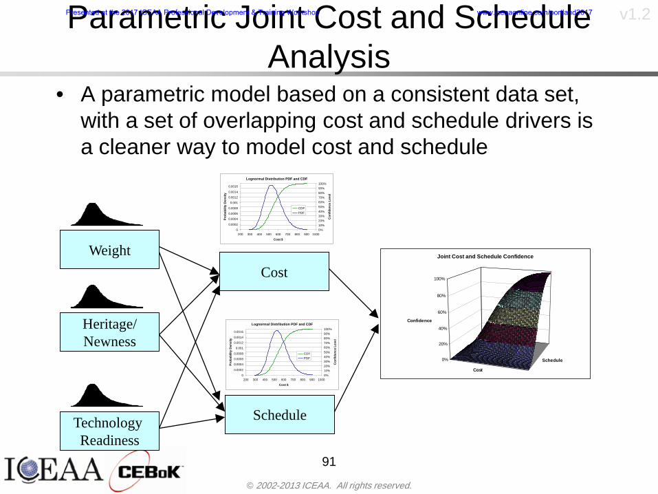
copy 2002-2013 ICEAA All rights reserved
v12Parametric Joint Cost and Schedule Analysis
bull A parametric model based on a consistent data set with a set of overlapping cost and schedule drivers is a cleaner way to model cost and schedule
91
CostWeight
HeritageNewness
Technology Readiness
Schedule
0
20
40
60
80
100
Confidence
Joint Cost and Schedule Confidence
Schedule
Cost
Lognormal Distribution PDF and CDF
0102030405060708090100
200 300 400 500 600 700 800 900 1000Cost $
Con
fiden
ce L
evel
0
00002
00004
00006
00008
0001
00012
00014
00016
Prob
abili
ty D
ensi
ty
CDFPDF
Lognormal Distribution PDF and CDF
0102030405060708090100
200 300 400 500 600 700 800 900 1000Cost $
Con
fiden
ce L
evel
0
00002
00004
00006
00008
0001
00012
00014
00016
Prob
abili
ty D
ensi
ty
CDFPDF
Presented at the 2017 ICEAA Professional Development amp Training Workshop wwwiceaaonlinecomportland2017
copy 2002-2013 ICEAA All rights reserved
v12Parametric Joint Cost and Schedule Analysis (2)
bull Joint cost and schedule risk analysis produced naturally by the integrated modelndash Addresses several issues with the copula
approachbull Tail dependencybull Correlation ndash no need to assign correlation
between cost and schedulebull Consistency of cost and schedule models
92
Presented at the 2017 ICEAA Professional Development amp Training Workshop wwwiceaaonlinecomportland2017
copy 2002-2013 ICEAA All rights reserved
v12
Resource-Loaded Schedulesbull Involves assigning cost and schedule risks to a resource-loaded schedule
networkbull Bottom-up approach
ndash More labor intensive than parametrics but can also provide more insight
ndash Can answer questions than parametric typically cannot such as how much do reserve requirements decrease if a specific risk is retired
bull Currently being implemented in Constellation programbull Has same issue as all bottom-up models hard to count all the risks and model
them discretely
ndash As a result there is a tendency to reflect less risk than indicated by history
ndash ldquoThere are more things in heaven and earth Horatio than are dreamt of in your philosophyrdquo William Shakespeare Hamlet Act I Scene V
93
Presented at the 2017 ICEAA Professional Development amp Training Workshop wwwiceaaonlinecomportland2017
copy 2002-2013 ICEAA All rights reserved
v12Resource-Loaded Schedules Vs Parametrics
bull Parametric most appropriate for early estimatesndash But also good for high-level checks as project progresses
bull As plans take shape lower level modeling may be more appropriate
94 1
CONCEPTUALDEVELOPMENT
PROJECTDEFINITION DESIGN DEVELOPMENT OPERATIONS
PARAMETRIC PARAMETRIC
ANALOGY
ENGINEERING (Bottoms Up)
$PARAMETRIC
DETAILED
$
Pre Phase A Phase B Phase CDPhase A Phase EPre Phase A Phase B Phase CDPhase A Phase E
Risk = f(Cost Estimating Relationship Inputs eg mass power data rate TRL new design etc)
Risk = f(cost and schedule variation of the analogous elements)
Risk = f(variation of detailed inputs eg labor hours rates materials etc)
Presented at the 2017 ICEAA Professional Development amp Training Workshop wwwiceaaonlinecomportland2017
copy 2002-2013 ICEAA All rights reserved
v12
Resource-Loaded Schedulesbull Methodology has been demonstrated in other
industriesndash Construction oil and gasndash Analysis has not been traditionally done on highly uncertain
complex development projects bull Methodology focuses on project baseline schedule
ndash In baseline schedule all tasks are resource loaded to represent a baseline schedule and cost standpoint
ndash Resource loaded schedule is ldquorolledrdquo up to a manageable level
ndash Based on the risk and uncertainties identified schedule distributions are applied to each rolled up task
ndash Cost uncertainties are also applied to rolled up tasksbull Uncertainties include labor rate man power etc
ndash A Monte Carlo simulation is run to develop joint cost-schedule distributions
95
Presented at the 2017 ICEAA Professional Development amp Training Workshop wwwiceaaonlinecomportland2017
copy 2002-2013 ICEAA All rights reserved
v12
Unit III - Module 9 96
Execution ndash Cross Checksbull Means The mean cost growth factor for WBS items
can be compared to history as a way to cross check results
bull CVs The CV of the cost growth factors for WBS items can be compared to history as a way to cross check results
bull Inputs Checks are performed on inputs or other parameters to see if historical values are in line with program assumptionsndash Example Historical risk scores can be compared to program
risk scores to see if risk assessors are being realistic and to see if the underlying database is representative of the program
11
Presented at the 2017 ICEAA Professional Development amp Training Workshop wwwiceaaonlinecomportland2017
- Cost and Schedule Risk Analysis Basic
- Acknowledgments
- Unit Index
- Risk Overview
- Agenda
- Introduction
- Risk Analysis Terms
- Are Our Costs Realistic
- Historical Cost Growth
- Sources of Cost Risk
- Point Estimates of Cost
- Types of Risk
- Point Estimates Vs Risk Estimates
- Cost Risk and Probability
- Probability Model ndash Distribution
- Probability Model ndash Distribution
- Probability ndash Top-Level Distribution
- S-Curves and Confidence Levels
- Example ndash Normal Distribution
- Confidence Levels
- Measuring Parametric Model Uncertainty
- Parametric Model Example
- Weight Uncertainty
- Estimating Uncertainty
- Estimating Uncertainty (2)
- Estimating Uncertainty (3)
- Aggregating Risk
- WBS Example
- WBS and Risk
- Aggregating Risk
- Percentiles Do Not Add
- Percentiles Do Not Add (2)
- Percentiles Do Not Add (3)
- Methods for Aggregating Risk
- Monte Carlo Simulationfor Risk Analysis
- Monte Carlo Simulation
- Using Random Numbers to Simulate Distributions
- Simulating a Triangular Distribution
- Simulating a Triangular Distribution (2)
- Monte Carlo and the WBS
- Number of Trials
- Number of Trials (2)
- Number of Trials (3)
- Number of Trials (4)
- Number of Trials (5)
- Number of Trials (6)
- Methods of Simulation
- Probability Model ndash Correlation
- Correlation And Causation
- The Importance of Correlation
- The Importance of Correlation (2)
- Measures of Correlation
- Pearson Correlation
- Spearman Correlation
- Functional Correlation
- Risk Measures
- Value at Risk (VaR)
- Why 70th or 80th Percentile
- Funding Above Inflection Points
- Why Budget to the 70th or 80th
- Inflection Points for Lognormal
- Issues with Percentile Funding
- ldquoHere There Be Dragonsrdquo
- Distribution Comparison
- Distribution Comparison Tail Behavior
- Distribution Comparison ndash Tail Behavior (Table)
- Percentile Budgeting is Not Risk Management
- Joint Confidence Level Analysis
- Schedules Impact Cost
- The Relationship of Cost to Schedule
- The Impact of Schedule GrowthCompression on Cost
- Schedule as an Independent Variable
- Schedule is a Dependent Variable
- Incorporation of Schedule in Cost Risk
- Subjective Cost Risk Methods and Overinclusion of Risk Factors
- Fundamental Equation of Cost and Schedule Interrelationships
- How to (Correctly) Incorporate Schedule into Cost Risk Analysis
- Joint Lognormal and Normal Distributions
- Modeling Cost and Schedule as a Bivariate Distribution
- Bivariate Lognormal Distribution for Cost and Schedule
- Bivariate Lognormal for Cost and Schedule
- Correlation Between Cost and Schedule
- Correlation Between Cost and Schedule Caveats
- Conditional Confidence Levels
- Joint Confidence Levels
- Joint Confidence Levels Versus Cost Confidence Levels Only
- Joint Cost and Schedule Confidence
- Cost and Schedule Trade-offs for a Given Level of Joint Confidence
- Policy Considerations for Confidence Levels
- Copulas
- Parametric Joint Cost and Schedule Analysis
- Parametric Joint Cost and Schedule Analysis (2)
- Resource-Loaded Schedules
- Resource-Loaded Schedules Vs Parametrics
- Resource-Loaded Schedules
- Execution ndash Cross Checks
-
copy 2002-2013 ICEAA All rights reserved
v12
Resource-Loaded Schedulesbull Involves assigning cost and schedule risks to a resource-loaded schedule
networkbull Bottom-up approach
ndash More labor intensive than parametrics but can also provide more insight
ndash Can answer questions than parametric typically cannot such as how much do reserve requirements decrease if a specific risk is retired
bull Currently being implemented in Constellation programbull Has same issue as all bottom-up models hard to count all the risks and model
them discretely
ndash As a result there is a tendency to reflect less risk than indicated by history
ndash ldquoThere are more things in heaven and earth Horatio than are dreamt of in your philosophyrdquo William Shakespeare Hamlet Act I Scene V
93
Presented at the 2017 ICEAA Professional Development amp Training Workshop wwwiceaaonlinecomportland2017
copy 2002-2013 ICEAA All rights reserved
v12Resource-Loaded Schedules Vs Parametrics
bull Parametric most appropriate for early estimatesndash But also good for high-level checks as project progresses
bull As plans take shape lower level modeling may be more appropriate
94 1
CONCEPTUALDEVELOPMENT
PROJECTDEFINITION DESIGN DEVELOPMENT OPERATIONS
PARAMETRIC PARAMETRIC
ANALOGY
ENGINEERING (Bottoms Up)
$PARAMETRIC
DETAILED
$
Pre Phase A Phase B Phase CDPhase A Phase EPre Phase A Phase B Phase CDPhase A Phase E
Risk = f(Cost Estimating Relationship Inputs eg mass power data rate TRL new design etc)
Risk = f(cost and schedule variation of the analogous elements)
Risk = f(variation of detailed inputs eg labor hours rates materials etc)
Presented at the 2017 ICEAA Professional Development amp Training Workshop wwwiceaaonlinecomportland2017
copy 2002-2013 ICEAA All rights reserved
v12
Resource-Loaded Schedulesbull Methodology has been demonstrated in other
industriesndash Construction oil and gasndash Analysis has not been traditionally done on highly uncertain
complex development projects bull Methodology focuses on project baseline schedule
ndash In baseline schedule all tasks are resource loaded to represent a baseline schedule and cost standpoint
ndash Resource loaded schedule is ldquorolledrdquo up to a manageable level
ndash Based on the risk and uncertainties identified schedule distributions are applied to each rolled up task
ndash Cost uncertainties are also applied to rolled up tasksbull Uncertainties include labor rate man power etc
ndash A Monte Carlo simulation is run to develop joint cost-schedule distributions
95
Presented at the 2017 ICEAA Professional Development amp Training Workshop wwwiceaaonlinecomportland2017
copy 2002-2013 ICEAA All rights reserved
v12
Unit III - Module 9 96
Execution ndash Cross Checksbull Means The mean cost growth factor for WBS items
can be compared to history as a way to cross check results
bull CVs The CV of the cost growth factors for WBS items can be compared to history as a way to cross check results
bull Inputs Checks are performed on inputs or other parameters to see if historical values are in line with program assumptionsndash Example Historical risk scores can be compared to program
risk scores to see if risk assessors are being realistic and to see if the underlying database is representative of the program
11
Presented at the 2017 ICEAA Professional Development amp Training Workshop wwwiceaaonlinecomportland2017
- Cost and Schedule Risk Analysis Basic
- Acknowledgments
- Unit Index
- Risk Overview
- Agenda
- Introduction
- Risk Analysis Terms
- Are Our Costs Realistic
- Historical Cost Growth
- Sources of Cost Risk
- Point Estimates of Cost
- Types of Risk
- Point Estimates Vs Risk Estimates
- Cost Risk and Probability
- Probability Model ndash Distribution
- Probability Model ndash Distribution
- Probability ndash Top-Level Distribution
- S-Curves and Confidence Levels
- Example ndash Normal Distribution
- Confidence Levels
- Measuring Parametric Model Uncertainty
- Parametric Model Example
- Weight Uncertainty
- Estimating Uncertainty
- Estimating Uncertainty (2)
- Estimating Uncertainty (3)
- Aggregating Risk
- WBS Example
- WBS and Risk
- Aggregating Risk
- Percentiles Do Not Add
- Percentiles Do Not Add (2)
- Percentiles Do Not Add (3)
- Methods for Aggregating Risk
- Monte Carlo Simulationfor Risk Analysis
- Monte Carlo Simulation
- Using Random Numbers to Simulate Distributions
- Simulating a Triangular Distribution
- Simulating a Triangular Distribution (2)
- Monte Carlo and the WBS
- Number of Trials
- Number of Trials (2)
- Number of Trials (3)
- Number of Trials (4)
- Number of Trials (5)
- Number of Trials (6)
- Methods of Simulation
- Probability Model ndash Correlation
- Correlation And Causation
- The Importance of Correlation
- The Importance of Correlation (2)
- Measures of Correlation
- Pearson Correlation
- Spearman Correlation
- Functional Correlation
- Risk Measures
- Value at Risk (VaR)
- Why 70th or 80th Percentile
- Funding Above Inflection Points
- Why Budget to the 70th or 80th
- Inflection Points for Lognormal
- Issues with Percentile Funding
- ldquoHere There Be Dragonsrdquo
- Distribution Comparison
- Distribution Comparison Tail Behavior
- Distribution Comparison ndash Tail Behavior (Table)
- Percentile Budgeting is Not Risk Management
- Joint Confidence Level Analysis
- Schedules Impact Cost
- The Relationship of Cost to Schedule
- The Impact of Schedule GrowthCompression on Cost
- Schedule as an Independent Variable
- Schedule is a Dependent Variable
- Incorporation of Schedule in Cost Risk
- Subjective Cost Risk Methods and Overinclusion of Risk Factors
- Fundamental Equation of Cost and Schedule Interrelationships
- How to (Correctly) Incorporate Schedule into Cost Risk Analysis
- Joint Lognormal and Normal Distributions
- Modeling Cost and Schedule as a Bivariate Distribution
- Bivariate Lognormal Distribution for Cost and Schedule
- Bivariate Lognormal for Cost and Schedule
- Correlation Between Cost and Schedule
- Correlation Between Cost and Schedule Caveats
- Conditional Confidence Levels
- Joint Confidence Levels
- Joint Confidence Levels Versus Cost Confidence Levels Only
- Joint Cost and Schedule Confidence
- Cost and Schedule Trade-offs for a Given Level of Joint Confidence
- Policy Considerations for Confidence Levels
- Copulas
- Parametric Joint Cost and Schedule Analysis
- Parametric Joint Cost and Schedule Analysis (2)
- Resource-Loaded Schedules
- Resource-Loaded Schedules Vs Parametrics
- Resource-Loaded Schedules
- Execution ndash Cross Checks
-
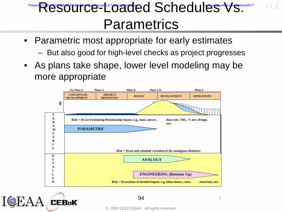
copy 2002-2013 ICEAA All rights reserved
v12Resource-Loaded Schedules Vs Parametrics
bull Parametric most appropriate for early estimatesndash But also good for high-level checks as project progresses
bull As plans take shape lower level modeling may be more appropriate
94 1
CONCEPTUALDEVELOPMENT
PROJECTDEFINITION DESIGN DEVELOPMENT OPERATIONS
PARAMETRIC PARAMETRIC
ANALOGY
ENGINEERING (Bottoms Up)
$PARAMETRIC
DETAILED
$
Pre Phase A Phase B Phase CDPhase A Phase EPre Phase A Phase B Phase CDPhase A Phase E
Risk = f(Cost Estimating Relationship Inputs eg mass power data rate TRL new design etc)
Risk = f(cost and schedule variation of the analogous elements)
Risk = f(variation of detailed inputs eg labor hours rates materials etc)
Presented at the 2017 ICEAA Professional Development amp Training Workshop wwwiceaaonlinecomportland2017
copy 2002-2013 ICEAA All rights reserved
v12
Resource-Loaded Schedulesbull Methodology has been demonstrated in other
industriesndash Construction oil and gasndash Analysis has not been traditionally done on highly uncertain
complex development projects bull Methodology focuses on project baseline schedule
ndash In baseline schedule all tasks are resource loaded to represent a baseline schedule and cost standpoint
ndash Resource loaded schedule is ldquorolledrdquo up to a manageable level
ndash Based on the risk and uncertainties identified schedule distributions are applied to each rolled up task
ndash Cost uncertainties are also applied to rolled up tasksbull Uncertainties include labor rate man power etc
ndash A Monte Carlo simulation is run to develop joint cost-schedule distributions
95
Presented at the 2017 ICEAA Professional Development amp Training Workshop wwwiceaaonlinecomportland2017
copy 2002-2013 ICEAA All rights reserved
v12
Unit III - Module 9 96
Execution ndash Cross Checksbull Means The mean cost growth factor for WBS items
can be compared to history as a way to cross check results
bull CVs The CV of the cost growth factors for WBS items can be compared to history as a way to cross check results
bull Inputs Checks are performed on inputs or other parameters to see if historical values are in line with program assumptionsndash Example Historical risk scores can be compared to program
risk scores to see if risk assessors are being realistic and to see if the underlying database is representative of the program
11
Presented at the 2017 ICEAA Professional Development amp Training Workshop wwwiceaaonlinecomportland2017
- Cost and Schedule Risk Analysis Basic
- Acknowledgments
- Unit Index
- Risk Overview
- Agenda
- Introduction
- Risk Analysis Terms
- Are Our Costs Realistic
- Historical Cost Growth
- Sources of Cost Risk
- Point Estimates of Cost
- Types of Risk
- Point Estimates Vs Risk Estimates
- Cost Risk and Probability
- Probability Model ndash Distribution
- Probability Model ndash Distribution
- Probability ndash Top-Level Distribution
- S-Curves and Confidence Levels
- Example ndash Normal Distribution
- Confidence Levels
- Measuring Parametric Model Uncertainty
- Parametric Model Example
- Weight Uncertainty
- Estimating Uncertainty
- Estimating Uncertainty (2)
- Estimating Uncertainty (3)
- Aggregating Risk
- WBS Example
- WBS and Risk
- Aggregating Risk
- Percentiles Do Not Add
- Percentiles Do Not Add (2)
- Percentiles Do Not Add (3)
- Methods for Aggregating Risk
- Monte Carlo Simulationfor Risk Analysis
- Monte Carlo Simulation
- Using Random Numbers to Simulate Distributions
- Simulating a Triangular Distribution
- Simulating a Triangular Distribution (2)
- Monte Carlo and the WBS
- Number of Trials
- Number of Trials (2)
- Number of Trials (3)
- Number of Trials (4)
- Number of Trials (5)
- Number of Trials (6)
- Methods of Simulation
- Probability Model ndash Correlation
- Correlation And Causation
- The Importance of Correlation
- The Importance of Correlation (2)
- Measures of Correlation
- Pearson Correlation
- Spearman Correlation
- Functional Correlation
- Risk Measures
- Value at Risk (VaR)
- Why 70th or 80th Percentile
- Funding Above Inflection Points
- Why Budget to the 70th or 80th
- Inflection Points for Lognormal
- Issues with Percentile Funding
- ldquoHere There Be Dragonsrdquo
- Distribution Comparison
- Distribution Comparison Tail Behavior
- Distribution Comparison ndash Tail Behavior (Table)
- Percentile Budgeting is Not Risk Management
- Joint Confidence Level Analysis
- Schedules Impact Cost
- The Relationship of Cost to Schedule
- The Impact of Schedule GrowthCompression on Cost
- Schedule as an Independent Variable
- Schedule is a Dependent Variable
- Incorporation of Schedule in Cost Risk
- Subjective Cost Risk Methods and Overinclusion of Risk Factors
- Fundamental Equation of Cost and Schedule Interrelationships
- How to (Correctly) Incorporate Schedule into Cost Risk Analysis
- Joint Lognormal and Normal Distributions
- Modeling Cost and Schedule as a Bivariate Distribution
- Bivariate Lognormal Distribution for Cost and Schedule
- Bivariate Lognormal for Cost and Schedule
- Correlation Between Cost and Schedule
- Correlation Between Cost and Schedule Caveats
- Conditional Confidence Levels
- Joint Confidence Levels
- Joint Confidence Levels Versus Cost Confidence Levels Only
- Joint Cost and Schedule Confidence
- Cost and Schedule Trade-offs for a Given Level of Joint Confidence
- Policy Considerations for Confidence Levels
- Copulas
- Parametric Joint Cost and Schedule Analysis
- Parametric Joint Cost and Schedule Analysis (2)
- Resource-Loaded Schedules
- Resource-Loaded Schedules Vs Parametrics
- Resource-Loaded Schedules
- Execution ndash Cross Checks
-
copy 2002-2013 ICEAA All rights reserved
v12
Resource-Loaded Schedulesbull Methodology has been demonstrated in other
industriesndash Construction oil and gasndash Analysis has not been traditionally done on highly uncertain
complex development projects bull Methodology focuses on project baseline schedule
ndash In baseline schedule all tasks are resource loaded to represent a baseline schedule and cost standpoint
ndash Resource loaded schedule is ldquorolledrdquo up to a manageable level
ndash Based on the risk and uncertainties identified schedule distributions are applied to each rolled up task
ndash Cost uncertainties are also applied to rolled up tasksbull Uncertainties include labor rate man power etc
ndash A Monte Carlo simulation is run to develop joint cost-schedule distributions
95
Presented at the 2017 ICEAA Professional Development amp Training Workshop wwwiceaaonlinecomportland2017
copy 2002-2013 ICEAA All rights reserved
v12
Unit III - Module 9 96
Execution ndash Cross Checksbull Means The mean cost growth factor for WBS items
can be compared to history as a way to cross check results
bull CVs The CV of the cost growth factors for WBS items can be compared to history as a way to cross check results
bull Inputs Checks are performed on inputs or other parameters to see if historical values are in line with program assumptionsndash Example Historical risk scores can be compared to program
risk scores to see if risk assessors are being realistic and to see if the underlying database is representative of the program
11
Presented at the 2017 ICEAA Professional Development amp Training Workshop wwwiceaaonlinecomportland2017
- Cost and Schedule Risk Analysis Basic
- Acknowledgments
- Unit Index
- Risk Overview
- Agenda
- Introduction
- Risk Analysis Terms
- Are Our Costs Realistic
- Historical Cost Growth
- Sources of Cost Risk
- Point Estimates of Cost
- Types of Risk
- Point Estimates Vs Risk Estimates
- Cost Risk and Probability
- Probability Model ndash Distribution
- Probability Model ndash Distribution
- Probability ndash Top-Level Distribution
- S-Curves and Confidence Levels
- Example ndash Normal Distribution
- Confidence Levels
- Measuring Parametric Model Uncertainty
- Parametric Model Example
- Weight Uncertainty
- Estimating Uncertainty
- Estimating Uncertainty (2)
- Estimating Uncertainty (3)
- Aggregating Risk
- WBS Example
- WBS and Risk
- Aggregating Risk
- Percentiles Do Not Add
- Percentiles Do Not Add (2)
- Percentiles Do Not Add (3)
- Methods for Aggregating Risk
- Monte Carlo Simulationfor Risk Analysis
- Monte Carlo Simulation
- Using Random Numbers to Simulate Distributions
- Simulating a Triangular Distribution
- Simulating a Triangular Distribution (2)
- Monte Carlo and the WBS
- Number of Trials
- Number of Trials (2)
- Number of Trials (3)
- Number of Trials (4)
- Number of Trials (5)
- Number of Trials (6)
- Methods of Simulation
- Probability Model ndash Correlation
- Correlation And Causation
- The Importance of Correlation
- The Importance of Correlation (2)
- Measures of Correlation
- Pearson Correlation
- Spearman Correlation
- Functional Correlation
- Risk Measures
- Value at Risk (VaR)
- Why 70th or 80th Percentile
- Funding Above Inflection Points
- Why Budget to the 70th or 80th
- Inflection Points for Lognormal
- Issues with Percentile Funding
- ldquoHere There Be Dragonsrdquo
- Distribution Comparison
- Distribution Comparison Tail Behavior
- Distribution Comparison ndash Tail Behavior (Table)
- Percentile Budgeting is Not Risk Management
- Joint Confidence Level Analysis
- Schedules Impact Cost
- The Relationship of Cost to Schedule
- The Impact of Schedule GrowthCompression on Cost
- Schedule as an Independent Variable
- Schedule is a Dependent Variable
- Incorporation of Schedule in Cost Risk
- Subjective Cost Risk Methods and Overinclusion of Risk Factors
- Fundamental Equation of Cost and Schedule Interrelationships
- How to (Correctly) Incorporate Schedule into Cost Risk Analysis
- Joint Lognormal and Normal Distributions
- Modeling Cost and Schedule as a Bivariate Distribution
- Bivariate Lognormal Distribution for Cost and Schedule
- Bivariate Lognormal for Cost and Schedule
- Correlation Between Cost and Schedule
- Correlation Between Cost and Schedule Caveats
- Conditional Confidence Levels
- Joint Confidence Levels
- Joint Confidence Levels Versus Cost Confidence Levels Only
- Joint Cost and Schedule Confidence
- Cost and Schedule Trade-offs for a Given Level of Joint Confidence
- Policy Considerations for Confidence Levels
- Copulas
- Parametric Joint Cost and Schedule Analysis
- Parametric Joint Cost and Schedule Analysis (2)
- Resource-Loaded Schedules
- Resource-Loaded Schedules Vs Parametrics
- Resource-Loaded Schedules
- Execution ndash Cross Checks
-
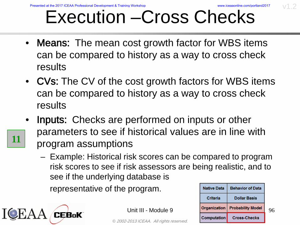