GRETHA UMR CNRS 5113 Université Montesquieu Bordeaux IV

Avenue Léon Duguit - 33608 PESSAC - FRANCE Tel : +33 (0)5.56.84.25.75 - Fax : +33 (0)5.56.84.86.47 - www.gretha.fr

Learning the optimal buffer-stock consumption rule of Carroll

Murat YILDIZOGLU

GREQAM, CNRS, UMR 6579

Université Paul Cézanne, Aix-Marseille 3

Marc-Alexandre SENEGAS

Isabelle SALLE

Martin ZUMPE

GREThA, CNRS, UMR 5113

Université de Bordeaux

Cahiers du GREThA n°2011-11

Cahiers du GREThA 2011 – 11

GRETHA UMR CNRS 5113 Univers i té Montesquieu Bordeaux IV

Avenue Léon Dugui t - 33608 PESSAC - FRANCE Tel : +33 (0)5 .56 .84 .25.75 - Fax : +33 (0)5 .56 .84 .86 .47 - www.gretha.f r

Mécanismes d’apprentissage et règle de consommation de Carroll : les apports d’une modélisation à base d’agents.

Résumé

Cette contribution vise à reconsidérer les conclusions relativement pessimistes tirées par Allen et Carroll (2001) à propos de la capacité d’apprentissage des agents en matière de comportement de consommation optimal (caractérisé par l’adoption de la règle étudiée par Carroll (1992) et dite « buffer-stock »). Dans cette optique, nous développons un modèle à base d’agents dans lequel différents mécanismes d’apprentissage sont envisagés et comparés sur la base des comportements de consommation qu’ils font émerger. Nous montrons que ni un simple mécanisme d’apprentissage adaptatif individuel, ni un mode d’apprentissage social fondé sur l’imitation ne peuvent faire émerger des comportements de consommation satisfaisants. Par contre, si les agents peuvent former des anticipations adaptatives sur la base d’un modèle mental qui de surcroît évolue en fonction des modifications de l’environnement de l’agent, leur comportement devient beaucoup plus intéressant que ce soit sur le plan de sa régularité que de la capacité qu’ont les agents à améliorer leurs performances de consommation au cours du temps (ce qui est une manifestation claire de l’apprentissage). Ce faisant, nos résultats indiquent que les hypothèses de rationalité limitée et d’anticipations adaptatives sont compatibles avec des comportements économiques robustes et réalistes qui peuvent même, dans certains cas, converger vers la solution optimale. Elles peuvent donc constituer un cadre d’analyse intéressant pour développer des modèles macroéconomiques fondés sur des dynamiques (adaptatives) d’apprentissage.

Mots-clés : consommation, apprentissage, anticipations, comportement adaptatif, économie computationnelle

Learning the optimal buffer-stock consumption rule of Carroll

Abstract

This article questions the rather pessimistic conclusions of Allen et Carroll (2001) about the ability of consumer to learn the optimal buffer-stock based consumption rule. To this aim, we develop an agent based model where alternative learning schemes can be compared in terms of the consumption behaviour that they yield. We show that neither purely adaptive learning, nor social learning based on imitation can ensure satisfactory consumption behaviours. By contrast, if the agents can form adaptive expectations, based on an evolving individual mental model, their behaviour becomes much more interesting in terms of its regularity, and its ability to improve performance (which is as a clear manifestation of learning). Our results indicate that assumptions on bounded rationality, and on adaptive expectations are perfectly compatible with sound and realistic economic behaviour, which, in some cases, can even converge to the optimal solution. This framework may therefore be used to develop macroeconomic models with adaptive dynamics.

Keywords: Consumption decisions; Learning; Expectations; Adaptive behaviour, Computational economics

JEL: E21; D91; D83; D84

Reference to this paper: YILDIZOGLU Murat, SENEGAS Marc-Alexandre, SALLE Isabelle, ZUMPE Martin, “Learning the optimal buffer-stock consumption rule of Carroll”, Cahiers du GREThA, n°2011-11, http://ideas.repec.org/p/grt/wpegrt/2011-11.html

1 Introduction

Recent developments of the standard approach to individual and aggregate consumption behavior in thelast two decades1 have been mainly driven by the quest for a better matching with the stylized factsobserved in this field. In an extensive set of influential studies provided in this respect, Carroll (Carroll,1992, 1997, 2001) shows that an amended version of the Life Cycle / Permanent Income Hypothesismodel is able to deliver outcomes which are, in a broader sense, consistent with the main features of therelated empirical evidence and, in any case, far more consistent than those stemming from the traditionalmodelling frameworks which have been called upon beforehand: like the perfect certainty model withconstant relative risk aversion utility or the certainty equivalent model. In his version of the consumptionmodel, Carroll shows that, under quite mild conditions - regarding consumer behavior under uncertainty-, the solution to the optimal consumption problem does exhibit the properties of a ”buffer stock” rule,according to which the individual consumer behaves as if she had a target level for a stock of financialassets in mind, and used it to smooth her consumption in the face of an uncertain, periodic incomestream2. With this consumption rule at hand, the model is able to explain at least three empiricalpuzzles that cannot be solved under the alternative, aforementioned settings: the ”consumption/incomeparallel”, the ”consumption/income” divergence, and the stability of the ”household age/wealth profile”3.Moreover, according to Carroll, the buffer-stock model provides a reliable framework to formalise theFriedmanian conception of the permanent income hypothesis, by explicitly acknowledging the importanceof precautionary saving induced by uncertainty on future labor income.

One of the main purposes of Carroll’s investigations is to try to reconcile the predictions of one modelof individual consumption behavior based on intertemporal optimisation and rational expectations withwhat we do observe in terms of actual consumption and savings patterns. Whether such a frameworkmay be plausibly assumed to underlie the consumption behavior of real-life consumers remains an openquestion however. As Carroll himself recognises, ”the sophisticated mathematical apparatus [that is]required to solve [numerically] the optimal consumption problem” (Carroll, 2001, page 41) seems toplay as a sufficient impediment for considering that consumers could be endowed with such numericalcapabilities in reality. Indeed, despite its intuitive interpretation and heuristic simplicity, the exactsolution to the optimization problem takes the form of a complex nonlinear consumption rule withoutany explicit analytical formula. Yet, as Allen and Carroll show (Allen and Carroll, 2001), this optimalstrategy may be approximated by a linear rule whose adoption generates utility streams that are onlyslightly lower than those associated with the exact and fully nonlinear solution. This rule recasts thenonlinear optimisation problem into a two-dimensional framework which has an intuitive interpretation:the intercept of the rule formula determines the target of wealth and the slope the speed with which theconsumer tries to get back to the latter when away from it. As such, this rule may in turn provide aplausible candidate for learning, and a relevant basis for testing whether consumers are able to adopta nearly optimal (intertemporal) consumption behavior in real-life. Allen and Carroll (2001) address

1see Deaton (1991, 1992) for a overview of the state of the art at the beginning of the nineties.2see Carroll (1997) for a thorough examination of those properties and Carroll (2001) for a didactic presentation and

comparative analysis.3see Carroll (1997) for a detailed documentation of those puzzles

2

this issue by considering a set of consumers which engage into a process of trial and error regardingalternative linear consumption rules, and select them according to their welfare properties. On the basisof their simulations, they observe that ”the simplified linear [nearly optimal] consumption function isenormously difficult to find by trial and error (...) it takes about a million "years"of model time to finda reasonably good consumption rule by trial and error”. Hence, their conclusion: while the ”empiricalevidence suggests that typical households engage in buffer-stock saving behavior”, the ”question remainsof how consumers come by their consumption rules”.

In this paper, we reassess the case for learning regarding the linear buffer-stock rule of Allen andCarroll by considering alternative assumptions about the learning process followed by consumers. Bydoing so, we aim to investigate which features of learning may be key in this context for pushing theconsumption behavior close to the optimal solution. The conclusion of Allen and Carroll seems to indicatethat no matter the length of the trial and the number of repetitions (at least for plausible values of theircombination), one simple (but systematic) exploration of the strategy space (which obviously includes thelinear approximate of the fully optimal solution) proves to be a rather inefficient process for selecting therelevant rule. Other forms of learning processes which, by contrast, do embed feedbacks from experienceto the (dynamic) choice of strategies by the individual consumer may however lead to more efficientresults. In the following we will analyze three of them, that are usually considered in the learningliterature: purely individual adaptive learning based on combination of discovered strategies and randomexperimenting (Arifovic, 1994; Vriend, 2000; Yildizoglu, 2002; Vallée and Yıldızoğlu, 2009); social learningbased on imitation (Arifovic, 1994; Vriend, 2000); adaptive individual learning where the strategies arechosen on the basis of adaptive expectations formed by the agents, as a consequence of their experiencein the economy (Yildizoglu, 2001).

The first mechanism relies on the adaptation of agents’ behaviour through both random experiment-ing, and combining already discovered strategies. Arifovic (1994) provides one of the first analysis ofthis approach in an economic context. What is modeled here is the capacity of the agents to refine apopulation of strategies as a consequence of the performance they obtain with these strategies in theirenvironment, as well as their capacity to adapt their strategies to the evolution of this environment, ina dynamic context. The formalization of this approach usually corresponds to a particular adaptationof the Genetic Algorithms (GA) introduced by Holland (1992). Many applications of this approach ineconomics take the form of a social learning process, combining random experimentation by individualagents with imitation of strategies between agents. The originality of our approach is the adoption of aframework that includes purely individual learning in the first place. We nevertheless also analyze thepotential role of the social dimension of learning, by introducing an imitation process between agents.This social dimension corresponds to the second mechanism we analyze. Hence, we echo the suggestion ofAllen and Carroll according to which ”there may be more hope of consumers finding reasonably good rulesin a "social learning" context in which one can benefit from the experience of others” (Allen and Carroll,2001). Moreover, Vriend (2000) indicates that social and individual learning can yield very contrastedresults (see also Vallée and Yıldızoğlu, 2009).

With the third learning scheme, we introduce a richer framework that aims to overcome the mainshortcoming of the preceding schemes: the absence of a forward looking behaviour by the agents. Looking

3

forward is important when the agents compare different strategies, before choosing one of them for thecurrent period. If they do not form any expectations, they can only base that decision on the performancesthat they have observed in the past. And, to this aim, they can only compare the strategies they haveactually used in the past (and, moreover in specific economic contexts). In order to assess the potentialperformances of these strategies in the current context (which can be completely new to them), or toassess how the strategies they have recently discovered would perform, even if they have not yet usedthem, they must be able to generalize from past observations. Such a generalization requires that theagents develop a representation of their environment and the connection between their decisions andperformance. With rational expectations, agents are supposed to know and use the real model of theeconomy, while in a purely adaptive context this assumption is not relevant. In this respect, the approachwe introduce is original, since it adopts a framework where the agents are able to build a representation oftheir environment (a mental model, Holland et al., 1989a), but only on the basis of their past experience.Moreover, this representation evolves as a consequence of this experience.

In order to analyze the ability of consumers to learn through these mechanisms, we develop a simplecomputational agent based model (ABM) directly inspired by the original setup of Allen and Carroll(2001). First, we introduce in this model adaptive learning without expectations, including also a socialcomponent that we modulate through a dedicated parameter. In a second stage, learning with adaptiveexpectations is introduced by endowing each consumer with an artificial neural network (ANN) thatcaptures her mental model of the economy. To our knowledge, this is the first article that considers sucha learning process in this setup4.

Two articles tackling the same question as our’s may be contrasted with the approach adopted here.They are both based on a specific scheme of learning: reinforcement learning. Reinforcement learningcorresponds to the selection of an action rule in a set of rules, with a probability that increases withthe relative success observed in the past for each rule (Sutton and Barto, 1998). Howitt and Özak(2009) consider such a reinforcement learning process, and show that consumers can discover optimalconsumption strategies. But to obtain this result, they need to enhance reinforcement learning with avery sophisticated adjustment mechanism. This latter feature is rather difficult to accept under boundedrationality assumptions, even if the complete learning process is parsimonious in terms of informationused by the consumer. Lettau and Uhlig (1999) introduce a much simpler learning framework: a classifiersystem reduced to its reinforcement learning component. In this setting, agents choose, in each period,the consumption strategy that has obtained the highest average performance in the past. They observethat this mechanism introduces a bias in favour of strategies that yield high performances in periodswith high incomes. These strategies are adopted instead of the optimal one, which is introduced inthe population from the start. However, the authors disregard the most interesting dimension of theclassifier systems (Holland and Miller, 1991; Holland et al., 1989b), i.e. their ability to generalize usinga flexible correspondence between the states of the environment and chosen strategies. It ensues thatLettau and Uhlig use a reinforcement mechanism that is exclusively dependent on the past performancesof the strategies. By contrast, we aim to build a framework that is perfectly compatible with boundedrationality, and in which agents can form adaptive expectations by generalizing from their past experience.

4see Yildizoglu (2001) for an example of this approach in industrial economics.

4

In what follows, we proceed through numerical simulations, and analyze our results through standardstatistical and econometric methods. Another innovation of this article is the methodology used to conductthe sensitivity analysis in these simulations. Instead of the commonly used Monte Carlo approach, weadopt a Design of Experiments (DOE) method based on Nearly Orthogonal Latin Hypercubes (NOLH).This method is very promising in simulation studies, because it allows the exploration of the parameterspace in a very parsimonious way. The structure of the ABM and our methodology are presented indedicated sections.

Two main insights may be drawn from our analysis. First, the social dimension of learning doesnot appear to significantly improve the ability of consumers to discover (and adopt) a nearly optimalconsumption behavior. Endowing the consumer with the capacity to imitate the best strategy which hasbeen used in the previous period does only marginally add to the performances associated with a purelyindividual learning scheme. This result suggests that sharing rules corresponding to different contexts (interms of incomes and wealths) does not yield a more efficient learning, when consumers face heterogeneousincome shocks. Therefore, contrary to what Allen and Carroll (2001) expect5, the social learning processmay not lead, in such an environment, to a quicker convergence onto the optimal strategy.

What seems crucial (and this is the second insight) for learning better consumption rules, is theability of the consumer to build, with the help of her experience, a structured representation of herenvironment. Assuming the existence of this mental representation ensures a much better outcome interms of convergence towards the optimal rule, than the one which would obtain when the strategy spaceis explored in an unstructured manner, through random experimenting and some simple combination ofalready discovered strategies. Moreover, giving to the consumer the ability to look forward over severalperiods using this representation (i.e. forming expectations about the intertemporal consequences of hercurrent decisions), enhances the convergence process.

Finally, our results show that the genuinely adaptive learning process that we have considered yieldsrather realistic behaviors for the agents (stability of behaviour and increasing performance over time).In the simple setup of Allen and Carroll (2001), we furthermore observe that such a process may evenconverge towards the optimal solution, and that, without assuming that the consumers possess rationalexpectations beforehand. This feature looks promising for studying adaptive macroeconomic dynamicswith learning agents.

We proceed as follows. The next section introduces the original setting of Allen and Carroll (2001)and the buffer-stock rule for consumption, as well as the numerical experiments carried out by theseauthors. The learning mechanisms explored in our article are presented in the third section. We firstquickly present learning without expectations and follow with a more detailed presentation of learningwith adaptive expectations. Our simulation protocol and methods of analysis are introduced in the fourthsection. Our results are discussed in the fifth section. We first show that purely adaptive individualand social learning do not yield satisfactory consumption behaviours. Only a learning process directed

5Carroll is however skeptical about the added value of considering social learning with respect to the problem at hand:”even the social learning model will probably take considerable time to converge on optimal behavior, so this model providesno reason to suppose that consumers will react optimally in the short or medium run to the introduction of new elements intotheir environment” Carroll (2001, p. 42).

5

by adaptive expectations gives rise to economically sound consumption behaviours. The last sectionconcludes and discusses our results.

2 The original problem

Following Allen and Carroll (2001), let consider the intertemporal consumption problem of an individualagent. The consumer aims to maximize discounted utility from consumption over the remainder of a(possibly infinite) lifetime

max{Cs}∞t

Et

[ ∞∑s=t

βs−tu(Cs)], (1)

in a setting characterized by the following equations:

As = Xs − Cs (2)

Xs+1 = Rs+1 ·As + Ys+1 (3)

Cs ≤ Xs ∀s (4)

and where the variables are

β − time discount factor

Xs − resources available for consumption (‘cash-on-hand’)

As − assets after all actions have been taken in period s

Cs − consumption in period s

Rs − interest factor (1 + r)from period s− 1to s.

u(C) − utility derived from consumption.

Ys − noncapital income in period s

Allen and Carroll (2001) adopt some more specific assumptions with respect to this general setting.First, they specify the utility function as u(C) ≡ C1−ρ/(1− ρ), with ρ = 3, implying

u (C) = − 12C2 < 0, C 6= 0 (5)

Furthermore, they set R = 1 and β = 0.95. Finally, they consider a three point distribution forincome:

Y 0.7 1 1.3Probability 0.2 0.6 0.2

with E [Y ] = 1.

In this framework, Carroll (2004) shows that C∗ (Xt) may be rewritten6 as C∗ (Xt) = 1+f(Xt −X

∗)for some functional form f (.) with specific properties (but no analytical expression), and with X∗ a target

6This equivalence is only valid under the impatience condition that writes as Rβ1/ρ < G, with G the income growthfactor. In the case we consider G = 1, and the condition is satisfied.

6

level for cash-on-hand (that is assumed to be larger than 1 for the latter expression to be valid)7. Thena linear (Taylor) expansion of C∗ (Xt) can be obtained around the point Xt = X

∗, and writes as8:

C∗ (Xt) ' 1 + γ∗ ·(Xt −X

∗)This expression gives the linear ”optimal” buffer-stock rule. Allen and Carroll then consider the family

of functions Cθ (Xt) which are indexed by θ ≡{γθ, Xθ

}and write as:

Cθ (Xt) =

1 + γθ(X −Xθ

)if γθ

(X −Xθ

)≤ Xθ

X if γθ(X −Xθ

)> Xθ

. (6)

Each consumption strategy of the agent can then be represented by a vector: θ =(γθ, Xθ

). By

construction, when θ = θ∗ ≡(γ∗, X

∗), Cθ∗ (Xt) corresponds to the Taylor approximation of C∗ (Xt)around Xt = X

∗.In their numerical analysis, Allen and Carroll (2001) adopt the following search space of consumption

strategies:

γ ∈ ]0.05, 1] ,∆γ = 0.05

X ∈ [1, 2.9] ,∆X = 0.1

This setup corresponds to 20 steps for each component, generating a complete strategy space of 400combinations to explore. Let Θ be the complete set of these strategies.

Given the steps used for constructing the search space, the element of Θ that is the closest one to theoptimal strategy is:

θ∗ =(γ∗, X

∗) = (0.25, 1.2) (7)

⇒ C∗ (X) = 1 + 0.25 (X − 1.2) (8)

Allen and Carroll (2001) test whether consumers can discover this optimal strategy through a sys-tematic exploration of the strategy space, and an estimation of their infinite horizon utility flow. Eachconsumer tests all the possible 400 strategies by using each of them to decide on her consumption dur-ing n periods, starting with a given initial cash-on-hand S0. In order to estimate the expected utilityflow over all possible random income flows, this n period consumption process is repeated m times. Thestrategy that gives the highest estimation for the utility flow is then selected by each consumer. Allen andCarroll use the numerical approximation of the value function for evaluating the distance to the optimalvalue flow observed with this best strategy, and they call this distance the sacrifice value. They considerthis process for 1000 consumers for each combination (S0, n,m) and compute the average sacrifice value

7This target level is a key element of the buffer-stock savings model of Carroll. The proof of its existence is set up inCarroll (1997).

8by construction, γ∗ ≡ f ′ (0)

7

over this population to assess how close this process can get to the optimal utility for the correspondingcombination. They show that a sufficiently small sacrifice can only be obtained for a very high number ofconsumption decisions (in the most extreme case, n = 50, m = 200, each consumer taking 10000 effectiveconsumption decisions with each strategy).

Their results indicate that it is not easy for individual consumers to get sufficiently close to the infinitehorizon optimum without explicitly solving the full optimization problem, even if one assumes that theyuse the more parsimonious buffer-stock rule:

[· · · ] even when the goal is to learn only this simple approximation, pure trial-and-errorlearning requires an enormous amount of experience to allow consumers to distinguish goodrules from bad ones—far more experience than any one consumer would have over the courseof a single lifetime. (p.268, Allen and Carroll, 2001)

The aim of the following sections is to show that alternative learning schemes could yield more interestingoutcomes.

3 Three learning schemes

We now present three different learning schemes that we analyze in the context of the buffer-stock model.The first learning scheme we study is a simple one, based on random experimenting by the agents and thecombination of the already discovered strategies. We also allow a possibility for imitation of the strategiesbetween consumers (see the next paragraph).

3.1 Purely adaptive learning without expectations

The economy is composed of n consumers, each using an evolving population Θi ⊂ Θ of m strategies oftype θ =

(γ,X

). At the initial period, these strategies are randomly drawn from Θ, each with a random

fitness f ∈ [0, 1].In each period, each consumer either imitates the behaviour of another consumer or uses the strategy

for which the highest performance (fitness) has been observed in the past (this maximal fitness is justrandom in the initial period). This performance is computed using the utility obtained with this strategy,the last time the consumer has used it:

f (θ) = exp (u(C (θ)) (9)

When the consumer uses a strategy in a period, she updates its fitness using the utility obtained withthat strategy.

Moreover, every GArate periods, each consumer revises her strategy population through the followingthree steps:

1. Reconducting the strategies for the next experimentation period, through a roulette-wheel basedon the relative performance of the strategies: this selection operator creates a new population ofstrategies, where the probability of each strategy to be reproduced is proportional to its relativeperformance

(fl/∑j fj

).

8

2. Combining the already discovered strategies (crossover): each strategy in the population can becombined, with a probability pC , with another strategy. If strategies θi and θj are chosen, they arereplaced by two new strategies: θk =

(γi, Xj

)and θl =

(γj , Xi

).

3. Random experimenting (mutation): with a probability pm one component of each strategy (Xj orγj) can be modified by drawing a new value from the corresponding strategy space.

In each period, we measure the distance between the observed consumption and corresponding utility levelson the one hand, and the optimal values we would observe with the behaviours given by equations 7, onthe other hand (see section 4.2 for more details on these indicators).

The complete structure of the model (its pseudo code) is given in Figure 1.

Initialization1. Create n consumers, each consumer i using a population Θi ⊂ Θ of m strategies of type θil =

(γil, Xil

)l=1...m

2. randomly draw the initial strategy population of each consumer and the corresponding fitness values3. draw randomly an element of Θi as the initial strategy of the consumer4. compute the consumption of each consumer with this strategy given the common initial resources X0 ∈ {0, 1, 2, 3}

C0 = min{

1 + γ0(X0 −X0

), X0

}5. compute the initial utility of each consumer u0 = U (C0)6. compute the consumption level and the utility performance that the consumer would have attained using the optimal

strategy θ∗C∗0 = min

{1 + γ∗

(X0 −X

∗), X0

}, u∗0 = U (C∗)

7. compute the distances to these optimal levels with the following indicators:

∆Z ≡ Z∗ − Z, Z = X, γ,C,X, u

8. compute the new cash-on-hand of the consumer X1 = X0 − C0 and the one which would have resulted from the useof the optimal strategy X∗1 = X0 − C∗0 .

9. compute other individual and global indicators10. for t ≤ T , (T is the length of each run)

(a) draw a new income for each consumer and compute the new cash in hand Xt = Xt−1 − Ct−1 + Yt and thecorresponding optimal flow X∗t = Xt−1 − C∗t−1 + Yt

(b) select a strategy for each consumer:

i. with a probability pI the consumer imitates the best strategy observed in t−1, in the population of agents,and the imitated strategy replaces the strategy with the lowest fitness

ii. with a probability(1− pI

)the consumer uses the best strategy in Θi

(c) execute steps (4)− (9) using the selected strategy and Xt(d) if t mod GARate = 0, the strategy population is updated using selection, crossover, mutation operators.

Figure 1: Pseudo code of the learning without expectations model

3.2 Social dimension of learning: imitating successful consumers

With a probability pI each consumer can imitate the strategy used in the preceding period by the consumerwho has obtained the highest utility. Allen and Carroll evoke a potentially positive role for social learning,in the search of the optimal consumption strategy. Imitation is indeed the simplest way of introducingthe diffusion good strategies within the population of consumers.

9

Simulations Decision Internal Model

Effective result of the

decision

If Result differs from Simulation

Update model

Figure 2: Dynamics of the mental model of the agents

We will analyze together the outcomes related to these two learning processes.

3.3 Learning with adaptive expectations

The previous learning schemes are based on the use of the discovered best strategy by the consumer.She chooses a particular strategy on the basis of the performance observed the last time she used thisstrategy, even if this performance has been obtained under specific circumstances (resulting mainly fromthe past income shocks and consumption decisions). But, this is not necessarily a very relevant basisfor assessing the performance of this strategy under current conditions. In other terms, these learningschemes are purely adaptive, and the decisions are not based on the projection of past performances onthe future circumstances. Such a projection would require a capacity of the agents to «generalize» orform «expectations» . This generalization would in turn entail that the agent develops a representationof her environment (mental model, Holland et al., 1989a). We consider now consumers who are able todevelop such a representation as a result from their past experience.

The mental model of each agent summarizes the state of the agent’s knowledge and evolves as aconsequence of evolution of this knowledge. It guides the decision process since it enables the agent totest the connections between the alternatives of choice and their consequences. The presence of suchan internal model can reflect the intentionality of decisions. Obviously, in this context, the concept of”model” must be understood in a very loose sense. More than a mathematical construction, it consists in arepresentation of the agent’s perception of the environment: “In (. . . ) situations [that are not sufficientlysimple as to be transparent to human mind], we must expect that the mind will use such imperfectinformation as it has, will simplify and represent the situation as it can, and make such calculations asare within its powers” (Simon, 1976, p.144). These calculations are “As if” experiments that enable theagent to evaluate the possible consequences of her decisions. In other words, before making a decision,the agent simulates the potential outcomes of different decisions by using her internal model. The outputof these simulations provides the expectations of the agent. The agent takes a decision on the basis ofthese expectations. This decision yields an effective outcome, which can be compared with the expectedone resulting from the simulations. Discrepancies between those outcomes may lead to an update of themental model. Hence, we have a dynamic structure which evolves as depicted by Figure 2 (Yildizoglu,2001).

10

Income

Expected utility flow

Inputs Output(s)

Cash on hand

Strategies:

aij

O

Hjbj

Ii

γl

X l

Figure 3: A feed forward ANN with one hidden layer

While this line of thought is quite obvious, its integration into economic models is problematic. This isthe reason why purely adaptive models (see the preceding section) generally neglect the dynamic processof expectation formation. This representation of learning, as the product of an evolutionary algorithm,does enable the elaboration of better decision rules, but only through trial and error. In this case, theagent can only judge decisions which have been used before. On the contrary, the vision based on thedynamics of the internal model admits that agents can have a relatively precise (if not perfect) perceptionof the value of their decisions, even if they have never been used before. This is made possible by meansof simulations using the internal model.

The standard way of formalizing such a model is to rely upon the subjective probabilities approachof Savage. In this case, the internal model of the agent corresponds to a set of conditional probabilitydistributions. The update of this model can be imagined through successive least square estimations orapplications of Bayes’ rule. The Bayesian approach has the advantage of not assuming any particularstructure for the internal model. But it is very demanding in terms of agents’ rationality. Moreover,”there is substantial evidence that Bayes’ theorem lacks empirical relevance and hence its proceduraljustification is weak” (Salmon, 1995, p.245).

Recursive least square estimations have been used, in this perspective, albeit at the aggregate level,by the recent macroeconomic learning literature (Evans and Honkapohja, 2001). However, this methodrelies upon a specific functional structure for the internal model. We adopt, here, a more flexible tool.Our approach is independent of the structure and the parametrization of the internal model, in order toincorporate only its most primitive dimensions: its existence and its influence on the decisions of agents.In this respect, an artificial neural network (ANN) is a good candidate for representing the role of theinternal model, and its adaptive nature. With only minimal structural assumptions, namely the list ofendogenous and explicative variables, and the structure of the hidden layer, it can represent the factthat the agent adjusts her internal model to the flow of experience. For many practical problems, even avery simple feed forward ANN with one hidden layer of few hidden nodes gives quite robust results (seeMasters (1993), for the discussion of properties of ANNs).

More particularly, an ANN provides a time varying flexible functional form that delivers an approxim-ation of the connections between the inputs and the output of the internal model. This approximation isobtained by the calibration of the parameters of the ANN (aij and bj in Figure 3) according to the series

11

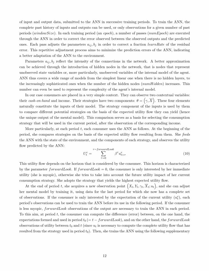
of input and output data, submitted to the ANN in successive training periods. To train the ANN, thecomplete past history of inputs and outputs can be used, or only observations for a given number of pastperiods (windowSize). In each training period (an epoch), a number of passes (numEpoch) are executedthrough the ANN in order to correct the error observed between the observed outputs and the predictedones. Each pass adjusts the parameters aij , bj in order to correct a fraction learnRate of the residualerror. This repetitive adjustment process aims to minimize the prediction errors of the ANN, indicatinga better adaptation of the ANN to the environment.

Parameters aij , bj reflect the intensity of the connections in the network. A better approximationcan be achieved through the introduction of hidden nodes in the network, that is nodes that representunobserved state variables or, more particularly, unobserved variables of the internal model of the agent.ANN thus covers a wide range of models from the simplest linear one when there is no hidden layers, tothe increasingly sophisticated ones when the number of the hidden nodes (numHidden) increases. Thisnumber can even be used to represent the complexity of the agent’s internal model.

In our case consumers are placed in a very simple context. They can observe two contextual variables:their cash-on-hand and income. Their strategies have two components: θ =

(γ,X

). These four elements

naturally constitute the inputs of their model. The strategy component of the inputs is used by themto compare different potential strategies on the basis of the expected utility flow they can yield (hencethe unique output of the mental model). This comparison serves as a basis for selecting the consumptionstrategy that will be used in the current period, after the observation of the corresponding income.

More particularly, at each period t, each consumer uses the ANN as follows. At the beginning of theperiod, she compares strategies on the basis of the expected utility flow resulting from them. She feedsthe ANN with the state of the environment, and the components of each strategy, and observes the utilityflow predicted by the ANN:

U et =τ=forwardLook∑

τ=0βτuet+τ (10)

This utility flow depends on the horizon that is considered by the consumer. This horizon is characterizedby the parameter forwardLook. If forwardLook = 0, the consumer is only interested by her immediateutility (she is myopic), otherwise she tries to take into account the future utility impact of her currentconsumption strategy. She adopts the strategy that yields the highest expected utility flow.

At the end of period t, she acquires a new observation point(Xt, Yt, γt, Xt;ut

), and she can adjust

her mental model by training it, using data for the last period for which she now has a complete setof observations. If the consumer is only interested by the expectation of the current utility (uet ), eachperiod’s observations can be used to train the ANN before its use in the following period. If the consumeris less myopic, forwardLook observations of the output are necessary to train the ANN in each period.To this aim, at period t, the consumer can compute the difference (error) between, on the one hand, theexpectations formed and used in period t0 (= t− forwardLook), and on the other hand, the forwardLookobservations of utility between t0 and t (since ut is necessary to compute the complete utility flow that hasresulted from the strategy used in period t0). Then, she trains the ANN using the following supplementary

12

inputs and output: (Xt−forwardLook, Yt−forwardLook, γt−forwardLook, Xt−forwardLook;

)→ Ut−forwardLook =

τ=forwardLook∑τ=0

βτut−forwardLook+τ (11)

As a consequence, in our model, the role of forwardLook is twofold: at the one hand, a longer horizonyields less myopic decisions, at the other, it imposes on the agent the use of a more out-of-date mentalmodel for forming her expectations.

The pseudo code of the model is summarized in Figure 4.

Initialization1. Create n consumers, each consumer i using a population Θi ⊂ Θ of m strategies of type θil =

(γil, Xil

)l=1...m

;

2. γ and X belong to the original strategy space of Allen and Carroll (2001)3. randomly draw the initial strategy population of each consumer4. randomly initialize the ANN of each consumer5. draw randomly an element of Θi as the initial strategy of the consumer6. compute the consumption of each consumer with this strategy given the common initial resources X0 ∈ {0, 1, 2, 3}

C0 = min{

1 + γ0(X0 −X0

), X0

}7. compute the initial utility of each consumer u0 = U (C0)8. compute the behaviour and performance that the consumer would have using the optimal strategy θ∗

C∗0 = min{

1 + γ∗(X0 −X

∗), X0

}, u∗0 = U (C∗)

9. compute the distances to the optimal behaviour and results

∆Z ≡ Z∗ − Z, Z = X, γ,C,X, u

10. compute other individual and global indicators11. compute the new cash-on-hand of the consumer X1 = X0−C0 and the one she would have using the optimal strategy

X∗1 = X0 − C∗0 .12. for t ≤ T , (T is the length of each run)

(a) draw a new income for each consumer and compute the new cash in hand Xt = Xt−1 − Ct−1 + Yt and thecorresponding optimal flow X∗t = Xt−1 − C∗t−1 + Yt

(b) Selection of the strategy:

i. with a probability pI the consumer imitates the best strategy observed in t−1, in the population of agents,and the imitated strategy replaces the strategy with the lowest fitness

ii. with a probability(1− pI

)and if t > forwardLook the consumer chooses a new strategy from her strategy

population using her expectations given by her mental model; if t ≤ forwardLook, consumers choosesrandomly a strategy Θit

(c) execute steps (6)− (10) using the selected strategy and Xt(d) if t > forwardLook, train the ANN with the observation corresponding to the period t− forwardLook(e) if t mod GARate = 0, the strategy population is updated using selection, crossover, mutation operators and the

expected fitness of the elements of the new population is updated using the actual state of the ANN(f) compute individual and global indicators.

Figure 4: Pseudo code of the learning with expectations model

13

As we have noted, several parameters condition the learning capacity of the ANN: the number ofhidden nodes (numHidden); the data window used for the training (windowSize); the error correctionrate in each epoch of training (learnRate); the number of passes used in each training epoch (numEpoch).The names and explored values of these parameter are given in the Appendix. Except in extreme cases,their values do not play a major role in our results.

4 Simulation protocol and methods of analysis

4.1 Experimentation protocol

Large sampling methods such as Monte Carlo simulations come at a computational cost if there arenumerous parameters with large experiment domains.

We would indeed need to implement a very large number of simulations ion order to obtain a represen-tative sample of all parameter configurations. In this context, Design of experiments (DOE) approach9

allows us to minimize the sample size under constraint of representativity. This method provides a sample,namely a design, of the whole set of parameters’ (or factors) values. The chosen configurations are calleddesign points. Some properties of the design are useful. Uniform designs (see for example Fang et al.(2000)), such as Latin Hypercubes, typically have good space-filling properties, i.e. they correctly coverthe whole parameters space.10 Moreover Latin Hypercubes ensure that linear effects of the factors arenon correlated and they are widely used in computer simulations (Ye, 1998; Butler, 2001). Nevertheless,this orthogonality comes at the cost of deteriorated space-filling properties. Accordingly, Cioppa (2002)proposes a Nearly Orthogonal (NOLH) design which offers an efficient trade-off between orthogonalityand space-filling properties (see also Cioppa and Lucas, 2007; Kleijnen et al., 2005).

For each version of the model, we use the same NOLH design to sample the parameters space usingSanchez (2005). Up to 11 factors, the resulting NOLH design provides 33 design points (see Sanchez(2005) for further details, and Table 1 in the Appendix, for the values of the parameters used in theexperiments). We launch 20 replications of each experiment, with a duration of T = 1250 periods in orderto take into account the diversity of the random draws. This set-up corresponds to 660 runs in total andwe sample the results every 50 periods during each run. We have n = 20 consumers and each consumeris given a strategy population of size m = 20.

9See for example Goupy and Creighton (2007) for a pedagogical statement. This method is widely used in areas suchas industry, chemistry, computer science, biology, etc. To our knowledge, Oeffner (2008) and Happe (2005) are the onlyapplications to an economic agent-based model.

10They also respect the non-collapsing criteria which ensures that each point is uniquely tested.

14

4.2 Indicators and analysis of results

The main indicators that we use in the analysis are dedicated to measure the distance to optimal beha-viours and performances, as indicated in the step 9 of Figure 4:

sumDistCons =∑i=ni=1 |C∗i − Ci|

sumDistUtility =∑i=ni=1 |U∗i − Ui|

sumDistGamma =∑i=ni=1 |γ∗ − γi|

sumDistX =∑i=ni=1 |X∗ −Xi|

(12)

Using absolute values gives a full assessment of the distance, because we eliminate all possible compens-ation between the distances of the consumers. We also consider the variances of these absolute distances,in order to check if individual consumers’ behaviours converge. We use simple time plots and boxplotsto study the evolution of these distances in time and their distributions between different configurations.Boxplots give the four quartiles of the distribution, and the median corresponds to the middle bar. Weuse R-project (R Development Core Team, 2003) and the ggplot2 library(Wickham, 2009) for conductingthis analysis.

5 Results

5.1 Individual learning

Figure 5 shows that the agents are able to somewhat learn the optimal consumption levels and we observethat the variance of the consumption levels is also decreasing in time. But, their performance in terms ofutility is not satisfactory at all. Even in the latest periods they remain collectively far from the optimumand a very high discrepancy exists between their individual performances. Figure 6 shows that even ifthey are able to converge towards X∗, the distance to γ∗ increases and remains high until the end of thesimulations.

5.2 Social dimension of learning

Different social learning profiles are pooled together in the preceding results. If we distinguish config-urations where imitation is frequent from the ones where it is rarer, we can observe the role played bysocial learning. Figure 7 distinguishes results in different configurations according to the correspondingintervals of pI values. It exhibits an intermediate range of imitation probability that minimizes the totaldistance to optimal consumption levels. Figure 8 confirms this result from the point of view of the totalutility sacrifice: it is minimal for the same configurations: pI ∈ (0.19, 0.22], but still remains high.

5.3 Individual learning with expectations

By contrast with the preceding outcomes, learning with expectations corresponds to a continuous im-provement in the performances of the consumers. Figure 9 shows that the total distance to optimalconsumption and to optimal level of utility decreases in time, as well as the distance between consumers.

15

sumDistCons

Periods

sum

Dis

tCon

s

5.7

5.8

5.9

6.0

6.1

6.2

●

●

●

●

●

●

●

●

●●

●

●

●

●

●

●●

●

●

●

●

●

●

●

●

200 400 600 800 1000 1200

varConsumption

Periods

varC

onsu

mpt

ion

0.190

0.195

0.200

0.205●

●

●●

●

●

●

●

● ●

●

●

●

●

●

● ●

●

●

● ●

●

●

●

●

200 400 600 800 1000 1200

sumDistUtility

Periods

sum

Dis

tUtil

ity

3600

3800

4000

4200

4400

●

●

●

●

●

●

●

●

●

●

●

●

●

●

●

●

●●

●

●

●

●

●

●

●

200 400 600 800 1000 1200

varDistUtility

Periods

varD

istU

tility

850000

900000

950000

1000000

1050000

●

●

●

●

●

●

●

●

●

●

●

●

●

●

●

●

●●

●

●

●

●

●

●

●

200 400 600 800 1000 1200

Figure 5: Individual learning and convergence to the optimal strategy (average of each indicator, in eachperiod, over all experiments and all runs)

sumDistCons

Periods

sum

Dis

tCon

s

5.7

5.8

5.9

6.0

6.1

6.2

●

●

●

●

●

●

●

●

●●

●

●

●

●

●

●●

●

●

●

●

●

●

●

●

200 400 600 800 1000 1200

sumDistX

Periods

sum

Dis

tX

8.0

8.5

9.0

9.5

●

●

●

● ●

● ●

● ●

●

●

●

●

●

●●

●●

●

●

●

●

●

●

●

200 400 600 800 1000 1200

sumDistGamma

Periods

sum

Dis

tGam

ma

8.4

8.6

8.8

9.0

9.2

9.4

●

●

●

●

●

●●

● ●

●●

●

●●

● ●

●● ●

●

● ●●

●●

200 400 600 800 1000 1200

Figure 6: Learning without expectations : Convergence in time on optimal consumption, but not reallyon its components (average of each indicator, in each period, over all experiments and all runs)

16

Distribution of sumDistCons: Role of probImitate (t>T/2)

Intervals of probImitate

sum

Dis

tCon

s

2

4

6

8

10

12

●

●

●

●

●

●

●

●

●

●

●

●

●

●

●

●

●

●

●

●

●

●

●

●

●

●

●

●

●

●

●

●

●

●

●

●

●

●

●

●

●

●

●

●

●

●

●

●

●

●

●

●

●

●

●

●

●

●

●

●

●

●

●

●

●

●

[0.05,0.078] (0.078,0.11] (0.11,0.13] (0.13,0.16] (0.16,0.19] (0.19,0.22] (0.22,0.24] (0.24,0.27] (0.27,0.3]

Figure 7: Individual learning and the role of imitation (distribution of sumDistCons over the correspondingexperiments and all runs, for t > T/2)

Distribution of sumDistUtility: Role of probImitate (t>T/2)

Intervals of probImitate

sum

Dis

tUtil

ity

0

2000

4000

6000

8000

10000

12000

14000●

●

●

● ● ●●

●

[0.05,0.078] (0.078,0.11] (0.11,0.13] (0.13,0.16] (0.16,0.19] (0.19,0.22] (0.22,0.24] (0.24,0.27] (0.27,0.3]

Figure 8: Role of imitation regarding utility sacrifice (distribution of sumDistUtility over the correspon-ding experiments and all runs, for t > T/2)

17

sumDistCons

Periods

sum

Dis

tCon

s

2.0

2.5

3.0

3.5

4.0

4.5

●

●

●

●

●

●

●

●

● ●●

● ●

● ●● ●

● ● ● ● ●● ● ●

200 400 600 800 1000 1200

varConsumption

Periods

varC

onsu

mpt

ion

0.05

0.10

0.15

0.20●

●

●

●

●●

●

●

● ●

●● ●

● ●● ● ● ● ●

● ●● ● ●

200 400 600 800 1000 1200

sumDistUtility

Periods

sum

Dis

tUtil

ity

0

1000

2000

3000

4000●

●

●●

●

●

●

● ●●

●

● ●●

●

● ●●

●● ● ● ● ● ●

200 400 600 800 1000 1200

varDistUtility

Periods

varD

istU

tility

0e+00

2e+05

4e+05

6e+05

8e+05

●

●

●

●

●

●

●

● ●●

●

● ●●

●

● ●● ●

● ● ● ● ● ●

200 400 600 800 1000 1200

Figure 9: Learning with expectations (average of each indicator, in each period, over all experiments andall runs)

These results can clearly be distinguished from the ones obtained above. Forming adaptive expectationsallows consumers to better discover consumption strategies that improve their utility.

We should also remark that, a total distance of 2 corresponds to an average individual distance of 0.1from the optimal consumption level for each consumers. This is a remarkable performance if we considerthat these consumers are not supposed to solve an infinite horizon optimization problem.

Moreover, Figure 10 shows that they can now better converge towards the optimal consumptionstrategy θ∗, even if, again, discovering γ∗ is more difficult for them.

The role of forward looking can also be analyzed from the same point of view. First, Figure 11 showsthat, even with myopic forward looking (forwardLook = 0), the total distance to optimal consumptionis significantly lower than the one observed with the previous learning scheme. Second, giving to theconsumer the ability to look forward over several periods (forwardLook > 0) enhances the convergenceprocess. We indeed observe in the graphic an intermediate zone where the distance is minimal, but, fromforwardLook = 8 on, it begins to increase again. With a long horizon, the agent uses a more out-of-datemental mode to form her expectations. As a consequence, looking very far is not necessarily preferablewith this adaptive behaviour. Figure 12 confirms these results in terms of utility sacrifice.

18

sumDistCons

Periods

sum

Dis

tCon

s

2.0

2.5

3.0

3.5

4.0

4.5

●

●

●

●

●

●

●

●

● ●●

● ●

● ●● ●

● ● ● ● ●● ● ●

200 400 600 800 1000 1200

sumDistX

Periods

sum

Dis

tX

6

8

10

12

14

16

●

●

●

●

●

●

●

●●

●●

●●

● ● ● ●● ●

● ● ● ● ●●

200 400 600 800 1000 1200

sumDistGamma

Periods

sum

Dis

tGam

ma

8.5

9.0

9.5

●

●

● ●

● ●

● ●

● ●●

●

●

●

●●

●●

● ●

●●

●●

●

200 400 600 800 1000 1200

Figure 10: Learning with expectations : Convergence in time on the optimal consumption strategy andits components (average of each indicator, in each period, over all experiments and all runs)

Distribution of sumDistCons: Role of forwardLook (t>T/2)

forwardLook

sum

Dis

tCon

s

0

1

2

3

4

●

●

●

●

●

●

●

●

●

●

●

●

●

●

●

●

●

●

●

●

●

●

●

●

●

●

●

●

●

●

●

●

●

●

●

●

●

●

●

●

●

●

●

●

●

●

●

●

●

●

●

●

●

●

●

●

●

●

●

●

●

●

●

●

●

●

●

●

●

●

●

●

●

●

●

●

●

●

●

●

●

●

●

●

●

●

●

●

●

●

●

●

●

●

●

●

●

●

●

●

●

●

●

●

●

●

●

●

●

●

●

●

●

●

●

●

●

●

●

●

●

●

●

●

●

●

●

●

●

●

●

●

●

●

●

●

●

●

●

●

●

●

●

●

●

●

●

●

●

●

●

●

●

●

●

●

●

●

●

●

●

●

●

●

●●

●

●

●

●

●

●

●

●

●

●

●

●

●

●

●

●

●

●

●

●

●

●

●

●

●

●

●

●

●

●

●

●

●

●

●

●

●

●

●

●

●

●

●

●

●

●

●

●

●

●

●

●

●

●

●

●

●

●

●

●

●●

●

●

●

0 1 2 3 4 5 6 7 8 9 10 11 12

Figure 11: Learning with expectations and looking forward (distribution of sumDistCons over the corres-ponding experiments and all runs, for t > T/2)

Distribution of sumDistUtility: Role of forwardLook (t>T/2)

forwardLook

sum

Dis

tUtil

ity

0

1

2

3

4●

●

●

●

●

●

●

●

●

●

●

●

●

●

●

●

●

●

●

●

●

●

●

● ●

●

●

●

●

●

●

●

●

●

●

●

● ●

●

●

●

●

●

●

●

●

●

●

●

●

●

●

●

●

●

●

●

●

●

●

●

●

●

●

●

●

●

●

●

●

●

●

●

●

●

●

●

●

●

●

●

●

●

●

●

●

●

●

●

●

●

●

●

●

●

●

●

●

●

0 1 2 3 4 5 6 7 8 9 10 11 12

Figure 12: Learning with expectations and looking forward : utility sacrifice (distribution of sumDistUtilityover the corresponding experiments and all runs, for t > T/2)

19

6 Conclusion

In this article, we develop an computational agent based model (ABM) to reassess the case for learningregarding the linear buffer-stock rule of Allen and Carroll (2001), and by considering alternative assump-tions about the learning process of consumers. By doing so, we try to investigate which features of learningmay be key in this context for pushing the consumption behavior close to the optimal solution obtainedin a rational expectations intertemporal setting.

In this ABM we consider three learning mechanisms: purely adaptive learning based on randomexperimenting and combinations of already discovered consumption strategies; social learning based onimitation of strategies between consumers; adaptive learning guided by adaptive expectations. The firsttwo mechanisms are modeled using a framework similar to genetic algorithms. The last mechanismcombines this kind of learning with adaptive expectations formed by the agents on the basis of theirmental model of the economy. This mental model is represented as a personal artificial neural networkused by each consumer to build her representation of the economy from her experience in this economy. Weshow that only the last approach yields economically sound consumption behaviour. Consumers developa consumption behaviour preserved from unrealistic erratic fluctuations (a common shortcoming of purelyadaptive learning schemes), while attaining performances that increase in time. This corresponds to theemergence of an effective learning on their side. The ability to look forward helps them in this processand an intermediate expectation horizon yields the best results.

These results look promising in the perspective of building macro economic models based on adaptivelearning dynamics. Agent based modeling would be a natural framework for such investigations, as itwould enable the understanding of the aggregate outcomes resulting from coordination problems betweenagents endowed with bounded rationality. For example, the authors are developing an ABM inspiredby the canonical NK model, in order to analyze the effects of different monetary rules à la Taylor withlearning agents.

20

Appendix

A Model parameters and simulation experiments

Table 1 gives the values of the parameters explored in the simulations. These values have been generatedusing Sanchez (2005). For other parameters, we have adopted the following assumptions:

• n = 20: number of consumers;

• m = 40: number of elements in the strategy population of each agent;

• T = 1250 : number of simulation periods in each run;

• β = 0.95;

• ρ = 3;

• windowSize = 150: the training of the ANN uses observations from the last 150 periods.

• u (c ≤ 0.01) ≡ −5000: truncation of utility computation, in order to avoid buffer overflow problemsresulting from the utility function adopted by Allen and Carroll (2001).

21

Parameter initialWealth probCrossOver probMutate probImitate forwardLook gaRate numeEpoch learnRate nbHidden

Min 0 0.05 0.05 0.05 0 1 20 0.01 2

Max 3 0.4 0.4 0.3 12 10 50 0.1 6

Experiments

0 3 0.08 0.2 0.1 11 7 41 0.05 6

1 3 0.4 0.09 0.14 6 3 43 0.04 6

2 3 0.2 0.37 0.09 0 6 42 0.01 3

3 2 0.36 0.4 0.15 11 2 44 0.02 4

4 3 0.06 0.21 0.1 8 7 32 0.06 2

5 3 0.38 0.16 0.12 5 3 25 0.09 2

6 2 0.21 0.39 0.11 0 7 31 0.09 6

7 2 0.29 0.38 0.14 11 3 27 0.1 4

8 2 0.14 0.13 0.18 9 4 20 0.03 4

9 2 0.28 0.15 0.22 3 6 23 0.04 5

10 2 0.13 0.31 0.29 4 2 24 0.02 4

11 2 0.3 0.28 0.28 9 10 34 0.05 3

12 2 0.1 0.12 0.19 7 2 49 0.08 3

13 3 0.26 0.18 0.27 2 6 48 0.07 3

14 2 0.12 0.35 0.28 5 1 40 0.08 5

15 2 0.27 0.26 0.3 10 9 37 0.07 5

16 2 0.23 0.23 0.18 6 6 35 0.06 4

17 0 0.37 0.25 0.25 2 4 29 0.06 2

18 0 0.05 0.36 0.21 6 8 28 0.07 2

19 0 0.25 0.08 0.26 12 5 28 0.1 5

20 1 0.09 0.05 0.2 1 9 26 0.09 4

21 0 0.39 0.24 0.25 4 4 38 0.05 6

22 0 0.07 0.29 0.23 7 8 45 0.02 6

23 1 0.24 0.06 0.24 12 4 39 0.02 3

24 1 0.16 0.07 0.21 1 8 43 0.01 4

25 1 0.31 0.32 0.17 3 7 50 0.08 4

26 1 0.17 0.3 0.13 9 5 47 0.07 3

27 1 0.32 0.14 0.06 8 9 46 0.09 5

28 1 0.15 0.17 0.07 3 1 36 0.06 5

29 1 0.35 0.33 0.16 5 9 21 0.03 5

30 0 0.19 0.27 0.08 10 5 22 0.04 5

31 1 0.33 0.1 0.07 8 10 30 0.03 3

32 1 0.18 0.19 0.05 2 2 33 0.04 3

Table 1: Experiments

22

References

Todd W. Allen and Christopher D. Carroll. Individual learning about consumption. Macoreconomicdynamics, 5:255–271, 2001.

J. Arifovic. Genetic Algorithm Learning and the Cobweb Model. Journal of Economic Dynamics andControl, 18:3–28, 1994.

N.A. Butler. Optimal and orthogonal latin hypercube designs for computer experiments. Biometrika, 88(3):847–857, 2001.

Christopher D. Carroll. The buffer-stock theory of saving: Some macroeconomic evidence. BrookingsPapers on Economic Activity, (2):61–156, 1992.

Christopher D. Carroll. Buffer stock saving and the life cycle/permanent income hypothesis. QuarterlyJournal of Economics, CXII(1):1–56, 1997.

Christopher D. Carroll. A theory of the consumption function, with and without liquidity constraints.Journal of Economic Perspectives, 15(3):23–46, 2001.

Christopher D. Carroll. Theoretical foundations of buffer stock saving. Working Paper 10867, NBER,2004.

Thomas M. Cioppa and Thomas W Lucas. Efficient nearly orthogonal and space-filling latin hypercubes.Technometrics, 49(1):45–55, 2007.

T.M. Cioppa. Efficient Nearly Orthogonal And Space-Filling Experimental Designs For High-DimensionalComplex Models. Doctoral dissertation in philosophy in operations research, Naval Postgraduate School,Monterey:CA, 2002.

Angus Deaton. Saving and liquidity constraints. Econometrica, 59(5):1221–1248, 1991.

Angus Deaton. Understanding Consumption. Oxford University Press, New York, 1992.

G. W. Evans and S. Honkapohja. Learning and Expectations in Macroeconomics. Princeton UniversityPress, Princeton, 2001.

K.T. Fang, D.K.J. Lin, P. Winker, and Y. Zhang. Uniform design: Theory and application. Technometrics,42(3):237–248, 2000.

J. Goupy and L. Creighton. Introduction to Design of Experiments with JMP Examples, Third Edition.SAS Institute Inc., Cary, NC, USA, 2007.

K. Happe. Agent-based modelling and sensitivity analysis by experimental design and metamodelling: anapplication to modelling regional structural change. Paper prepared for the XIth International Congressof the European Association of Agricultural Economists, 2005.

23

J. Holland and J. H. Miller. Artificial adaptive agents in economic theory. American Economic ReviewPapers and Procedings, 81(2):363–370, 1991.

J. H. Holland, K. J. Holyoak, R. E. Nisbett, and P. R. Thagard. Induction. Processes of Inference,Learning and Discoverey. MIT Press, 1989a.

John H. Holland. Adaptation in Natural and Artificial Systems: An Introductory Analysis with Applica-tions to Biology, Control, and Artificial Intelligence. MIT Press, Cambridge, MA, 1992.

John H. Holland, Keith J Holyoak, and Paul R. Thagard. Induction. Processes of Inference, Learning,and Discovery. MIT Press, Cambridge:MA, 1989b.

Peter Howitt and Ömer Özak. Adaptive consumption behavior. Working Paper 15427, NBER, 2009.

Jack P. C. Kleijnen, Susan M. Sanchez, Thomas W. Lucas, and Thomas M. Cioppa. A user’s guide tothe brave new world of designing simulation experiments. INFORMS Journal on Computing, 17(3):263–289, 2005.

Martin Lettau and Harald Uhlig. Rules of thumb versus dynamic programming. The American EconomicReview, 89(1):148–174, 1999.

Timothy Masters. Practical Neural Network recipes in C++. Academic Press, New York, 1993.

M. Oeffner. Agent - Based Keynesian Macroeconomics – An Evolutionary Model Embedded In An Agent- Based Computer Simulation. Doctoral dissertation, Bayerische Julius - Maximilians Universitat„Wurzburg, 2008.

R Development Core Team. R: A Language and Environment for Statistical Computing, volumehttp://www.r-project.org/. R Foundation for Statistical Computing, Vienna, 2003.

Mark Salmon. Bounded rationality and learning: Procedural learning. In Mark Kirman, Alan; Salmon,editor, Learning and Rationality in Economics, pages 236–275. Blackwell, Oxford, 1995.

S. M. Sanchez. Nolhdesigns spreadsheet. Software available online viahttp://diana.cs.nps.navy.mil/SeedLab/, 2005.

Herbert A. Simon. From substantial to procedural rationality. In S. J. Latsis, editor, Method and Appraisalin Economics, pages 129–148. Cambridge University Press, Cambridge, 1976.

Richard S. Sutton and Andrew G. Barto. Reinforcement Learning: an Introduction. MIT Press, Cam-bridge, MA, 1998.

Thomas Vallée and Murat Yıldızoğlu. Convergence in the finite cournot oligopoly with social and indi-vidual learning. Journal of Economic Behaviour and Organization, (72):670–690, 2009.

Nicolaas Vriend. An illustration of the essential difference between individual and social learning, andits consequences for computational analyses. Journal of Economic Dynamics and Control, 24(1):1–19,2000.

24

Hardley Wickham. ggplot2 Elegant Graphics for Data Analysis. Springer, Dordrecht, 2009.

K.Q. Ye. Orthogonal column latin hypercubes and their application in computer experiments. Journalof the American Statistical Association, 93(444):1430–1439, 1998.

Murat Yildizoglu. Connecting adaptive behaviour and expectations in models of innovation: The potentialrole of artificial neural networks. European Journal of Economics and Social Systems, 15(3):203–220,2001.

Murat Yildizoglu. Competing R&D strategies in an evolutionary industry model. Computational Eco-nomics, 19:52–65, 2002.

25

Cahiers du GREThA Working papers of GREThA

GREThA UMR CNRS 5113

Université Montesquieu Bordeaux IV Avenue Léon Duguit

33608 PESSAC - FRANCE Tel : +33 (0)5.56.84.25.75 Fax : +33 (0)5.56.84.86.47

www.gretha.fr

Cahiers du GREThA (derniers numéros)

2010-16 : CHANTELOT Sébastien, PERES Stéphanie, VIROL Stéphane, The geography of French creative class: An exploratory spatial data analysis

2010-17 : FRIGANT Vincent, LAYAN Jean-Bernard, Une analyse comparée du commerce international de composants automobiles entre la France et l’Allemagne : croiser un point de vue d’économie internationale et d’économie industrielle

2010-18 : BECUWE Stéphane, MABROUK Fatma, Migration internationale et commerce extérieur : quelles correspondances ?

2010-19 : BONIN Hubert, French investment banks and the earthquake of post-war shocks (1944-1946)

2010-20 : BONIN Hubert, Les banques savoyardes enracinées dans l’économie régionale (1860-1980s)

2011-01 : PEREAU Jean-Christophe, DOYEN Luc, LITTLE Rich, THEBAUD Olivier, The triple bottom line: Meeting ecological, economic and social goals with Individual Transferable Quotas

2011-02 : PEREAU Jean-Christophe, ROUILLON Sébastien, How to negotiate with Coase? 2011-03 : MARTIN Jean-Christophe, POINT Patrick, Economic impacts of development of road

transport for Aquitaine region for the period 2007-2013 subject to a climate plan 2011-04 : BERR Eric, Pouvoir et domination dans les politiques de développement 2011-05 : MARTIN Jean-Christophe, POINT Patrick, Construction of linkage indicators of

greenhouse gas emissions for Aquitaine region 2011-06 : TALBOT Damien, Institutions, organisations et espace : les formes de la proximité 2011-07 : DACHARY-BERNARD Jeanne, GASCHET Frédéric, LYSER Sandrine, POUYANNE

Guillaume, VIROL Stéphane, L’impact de la littoralisation sur les valeurs foncières et immobilières: une lecture différenciée des marchés agricoles et résidentiels

2011-08 : BAZEN Stephen, MOYES Patrick, Elitism and Stochastic Dominance 2011-09 : CLEMENT Matthieu, Remittances and household expenditure patterns in Tajikistan: A

propensity score matching analysis 2011-10 : RAHMOUNI Mohieddine, YILDIZOGLU Murat, Motivations et déterminants de

l’innovation technologique : Un survol des théories modernes 2011-11 : YILDIZOGLU Murat, SENEGAS Marc-Alexandre, SALLE Isabelle, ZUMPE Martin,

Learning the optimal buffer-stock consumption rule of Carroll

La coordination scientifique des Cahiers du GREThA est assurée par Sylvie FERRARI et Vincent

FRIGANT. La mise en page est assurée par Dominique REBOLLO.