Learning from Multiple Sources

Koby Crammer, Michael Kearns, Jennifer WortmanDepartment of Computer and Information Science

University of PennsylvaniaPhiladelphia, PA 19104

Abstract

We consider the problem of learning accurate models from multiple sources of“nearby” data. Given distinct samples from multiple data sources and estimatesof the dissimilarities between these sources, we provide a general theory of whichsamples should be used to learn models for each source. This theory is applicablein a broad decision-theoretic learning framework, and yields results for classifi-cation and regression generally, and for density estimation within the exponentialfamily. A key component of our approach is the development of approximatetriangle inequalities for expected loss, which may be of independent interest.

1 Introduction

We introduce and analyze a theoretical model for the problem of learning from multiple sources of“nearby” data. As a hypothetical example of where such problems might arise, consider the follow-ing scenario: For each web user in a large population, we wish to learn a classifier for what sitesthat user is likely to find “interesting.” Assuming we have at least a small amount of labeled data foreach user (as might be obtained either through direct feedback, or via indirect means such as click-throughs following a search), one approach would be to apply standard learning algorithms to eachuser’s data in isolation. However, if there are natural and accessible measures of similarity betweenthe interests of pairs of users (as might be obtained through their mutual labelings of common websites), an appealing alternative is to aggregate the data of “nearby” users when learning a classifierfor each particular user. This alternative is intuitively subject to a trade-off between the increasedsample size and how different the aggregated users are.

We treat this problem in some generality and provide a bound addressing the aforementioned trade-off. In our model there are K unknown data sources, with source i generating a distinct sample Si

of ni observations. We assume we are given only the samples Si, and a disparity1 matrix D whoseentry D(i, j) bounds the difference between source i and source j. Given these inputs, we wish todecide which subset of the samples Sj will result in the best model for each source i. Our frame-work includes settings in which the sources produce data for classification, regression, and densityestimation (and more generally any additive-loss learning problem obeying certain conditions).

Our main result is a general theorem establishing a bound on the expected loss incurred by using alldata sources within a given disparity of the target source. Optimization of this bound then yields arecommended subset of the data to be used in learning a model of each source. Our bound clearlyexpresses a trade-off between three quantities: the sample size used (which increases as we includedata from more distant models), a weighted average of the disparities of the sources whose data isused, and a model complexity term. It can be applied to any learning setting in which the underlyingloss function obeys an approximate triangle inequality, and in which the class of hypothesis mod-els under consideration obeys uniform convergence of empirical estimates of loss to expectations.

1We avoid using the term distance since our results include settings in which the underlying loss measuresmay not be formal distances.

For classification problems, the standard triangle inequality holds. For regression we prove a 2-approximation to the triangle inequality, and for density estimation for members of the exponentialfamily, we apply Bregman divergence techniques to provide approximate triangle inequalities. Webelieve these approximations may find independent applications within machine learning. Uniformconvergence bounds for the settings we consider may be obtained via standard data-independentmodel complexity measures such as VC dimension and pseudo-dimension, or via more recent data-dependent approaches such as Rademacher complexity.

The research described here grew out of an earlier paper by the same authors [1] which examinedthe considerably more limited problem of learning a model when all data sources are corruptedversions of a single, fixed source, for instance when each data source provides noisy samples of afixed binary function, but with varying levels of noise. In the current work, each source may beentirely unrelated to all others except as constrained by the bounds on disparities, requiring us todevelop new techniques. Wu and Dietterich studied similar problems experimentally in the contextof SVMs [2]. The framework examined here can also be viewed as a type of transfer learning [3, 4].

In Section 2 we introduce a decision-theoretic framework for probabilistic learning that includesclassification, regression, density estimation and many other settings as special cases, and then giveour multiple source generalization of this model. In Section 3 we provide our main result, which isa general bound on the expected loss incurred by using all data within a given disparity of a targetsource. Section 4 then applies this bound to a variety of specific learning problems. In Section 5 webriefly examine data-dependent applications of our general theory using Rademacher complexity.

2 Learning models

Before detailing our multiple-source learning model, we first introduce a standard decision-theoreticlearning framework in which our goal is to find a model minimizing a generalized notion of empiricalloss [5]. Let the hypothesis class H be a set of models (which might be classifiers, real-valuedfunctions, densities, etc.), and let f be the target model, which may or may not lie in the classH. Let z be a (generalized) data point or observation. For instance, in (noise-free) classificationand regression, z will consist of a pair 〈x, y〉 where y = f(x). In density estimation, z is theobserved value x. We assume that the target model f induces some underlying distribution Pf overobservations z. In the case of classification or regression, Pf is induced by drawing the inputs xaccording to some underlying distribution P, and then setting y = f(x) (possibly corrupted bynoise). In the case of density estimation f simply defines a distribution Pf over observations x.

Each setting we consider has an associated loss function L(h, z). For example, in classification wetypically consider the 0/1 loss: L(h, 〈x, y〉) = 0 if h(x) = y, and 1 otherwise. In regression wemight consider the squared loss function L(h, 〈x, y〉) = (y−h(x))2. In density estimation we mightconsider the log loss L(h, x) = log(1/h(x)). In each case, we are interested in the expected loss ofa model g2 on target g1, e(g1, g2) = Ez∼Pg1

[L(g2, z)]. Expected loss is not necessarily symmetric.

In our multiple source model, we are presented with K distinct samples or piles of data S1, ..., SK ,and a symmetric K × K matrix D. Each pile Si contains ni observations that are generated from afixed and unknown model fi, and D satisfies e(fi, fj), e(fj , fi) ≤ D(i, j). 2 Our goal is to decidewhich piles Sj to use in order to learn the best approximation (in terms of expected loss) to each fi.

While we are interested in accomplishing this goal for each fi, it suffices and is convenient toexamine the problem from the perspective of a fixed fi. Thus without loss of generality let ussuppose that we are given piles S1, ..., SK of size n1, . . . , nK from models f1, . . . , fK such thatε1 ≡ D(1, 1) ≤ ε2 ≡ D(1, 2) ≤ · · · ≤ εK ≡ D(1,K), and our goal is to learn f1. Here we havesimply taken the problem in the preceding paragraph, focused on the problem for f1, and reorderedthe other models according to their proximity to f1. To highlight the distinguished role of the targetf1 we shall denote it f . We denote the observations in Sj byzj

1, . . . , zjnj

. In all cases we will

analyze, for any k ≤ K, the hypothesis hk minimizing the empirical loss ek(h) on the first k pilesS1, . . . , Sk, i.e.

2While it may seem restrictive to assume that D is given, notice that D(i, j) can be often be estimated fromdata, for example in a classification setting in which common instances labeled by both fi and fj are available.

hk = argminh∈H

ek(h) = argminh∈H

1n1:k

k∑j=1

nj∑i=1

L(h, zji )

where n1:k = n1 + · · · + nk. We also denote the expected error of function h with respect to thefirst k piles of data as

ek(h) = E [ek(h)] =k∑

i=1

(ni

n1:k

)e(fi, h).

3 General theory

In this section we provide the first of our main results: a general bound on the expected loss of themodel minimizing the empirical loss on the nearest k piles. Optimization of this bound leads to arecommended number of piles to incorporate when learning f = f1. The key ingredients needed toapply this bound are an approximate triangle inequality and a uniform convergence bound, whichwe define below. In the subsequent sections we demonstrate that these ingredients can indeed beprovided for a variety of natural learning problems.

Definition 1 For α ≥ 1, we say that the α-triangle inequality holds for a class of models F andexpected loss function e if for all g1, g2, g3 ∈ F we have

e(g1, g2) ≤ α(e(g1, g3) + e(g3, g2)).

The parameter α ≥ 1 is a constant that depends on F and e.

The choice α = 1 yields the standard triangle inequality. We note that the restriction to models inthe class F may in some cases be quite weak — for instance, when F is all possible classifiers orreal-valued functions with bounded range — or stronger, as in densities from the exponential family.Our results will require only that the unknown source models f1, . . . , fK lie in F , even when ourhypothesis models are chosen from some possibly much more restricted class H ⊆ F . For now wesimply leave F as a parameter of the definition.

Definition 2 A uniform convergence bound for a hypothesis space H and loss function L is abound that states that for any 0 < δ < 1, with probability at least 1 − δ for any h ∈ H

|e(h) − e(h)| ≤ β(n, δ)

where e(h) = 1n

∑ni=1 L(h, zi) for n observations z1, . . . , zn generated independently according to

distributions P1, . . . Pn, and e(h) = E [e(h)] where the expectation is taken over z1, . . . , zn. β is afunction of the number of observations n and the confidence δ, and depends on H and L.

This definition simply asserts that for every model in H, its empirical loss on a sample of size nand the expectation of this loss will be “close.” In general the function β will incorporate stan-dard measures of the complexity of H, and will be a decreasing function of the sample size n, asin the classical O(

√d/n) bounds of VC theory. Our bounds will be derived from the rich litera-

ture on uniform convergence. The only twist to our setting is the fact that the observations are nolonger necessarily identically distributed, since they are generated from multiple sources. However,generalizing the standard uniform convergence results to this setting is straightforward.

We are now ready to present our general bound.

Theorem 1 Let e be the expected loss function for loss L, and let F be a class of models for whichthe α-triangle inequality holds with respect to e. Let H ⊆ F be a class of hypothesis models forwhich there is a uniform convergence bound β for L. Let K ∈ N, f = f1, f2, . . . , fK ∈ F , {εi}K

i=1,{ni}K

i=1, and hk be as defined above. For any δ such that 0 < δ < 1, with probability at least 1− δ,for any k ∈ {1, . . . , K}

e(f, hk) ≤ (α + α2)k∑

i=1

(ni

n1:k

)εi + 2αβ(n1:k, δ/2K) + α2 min

h∈H{e(f, h)}

Before providing the proof, let us examine the bound of Theorem 1, which expresses a natural andintuitive trade-off. The first term in the bound is a weighted sum of the disparities of the k ≤ Kmodels whose data is used with respect to the target model f = f1. We expect this term to increaseas we increase k to include more distant piles. The second term is determined by the uniformconvergence bound. We expect this term to decrease with added piles due to the increased samplesize. The final term is what is typically called the approximation error — the residual loss that weincur simply by limiting our hypothesis model to fall in the restricted class H. All three terms areinfluenced by the strength of the approximate triangle inequality that we have, as quantified by α.

The bounds given in Theorem 1 can be loose, but provide an upper bound necessary for optimizationand suggest a natural choice for the number of piles k∗ to use to estimate the target f :

k∗ = argmink

((α + α2)

k∑i=1

(ni

n1:k

)εi + 2αβ(n1:k, δ/2K)

).

Theorem 1 and this optimization make the implicit assumption that the best subset of piles to usewill be a prefix of the piles — that is, that we should not “skip” a nearby pile in favor of more distantones. This assumption will generally be true for typical data-independent uniform convergence suchas VC dimension bounds, and true on average for data-dependent bounds, where we expect uniformconvergence bounds to improve with increased sample size. We now give the proof of Theorem 1.

Proof: (Theorem 1) By Definition 1, for any h ∈ H, any k ∈ {1, . . . K}, and any i ∈ {1, . . . , k},(ni

n1:k

)e(f, h) ≤

(ni

n1:k

)(αe(f, fi) + αe(fi, h))

Summing over all i ∈ {1, . . . , k}, we find

e(f, h) ≤k∑

i=1

(ni

n1:k

)(αe(f, fi) + αe(fi, h))

= αk∑

i=1

(ni

n1:k

)e(f, fi) + α

k∑i=1

(ni

n1:k

)e(fi, h) ≤ α

k∑i=1

(ni

n1:k

)εi + αek(h)

In the first line above we have used the α-triangle inequality to deliberately introduce a weightedsummation involving the fi. In the second line, we have broken up the summation. Notice that thefirst summation is a weighted average of the expected loss of each fi, while the second summationis the expected loss of h on the data. Using the uniform convergence bound, we may assert that withhigh probability ek(h) ≤ ek(h) + β(n1:k, δ/2K), and with high probability

ek(hk) = minh∈H

{ek(h)} ≤ minh∈H

{k∑

i=1

(ni

n1:k

)e(fi, h) + β(n1:k, δ/2K)

}

Putting these pieces together, we find that with high probability

e(f, hk) ≤ α

k∑i=1

(ni

n1:k

)εi + 2αβ(n1:k, δ/2K) + α min

h∈H

{k∑

i=1

(ni

n1:k

)e(fi, h)

}

≤ α

k∑i=1

(ni

n1:k

)εi + 2αβ(n1:k, δ/2K)

+ α minh∈H

{k∑

i=1

(ni

n1:k

)αe(fi, f) +

k∑i=1

(ni

n1:k

)αe(f, h)

}

= (α + α2)k∑

i=1

(ni

n1:k

)εi + 2αβ(n1:k, δ/2K) + α2 min

h∈H{e(f, h)}

0 0.1 0.2 0.3 0.4 0.5 0.6 0.7 0.8 0.9 10

0.1

0.2

0.3

0.4

0.5

0.6

0.7

0.8

0.9

1

MAX DATAMAX DATAMAX DATAMAX DATAMAX DATAMAX DATAMAX DATAMAX DATAMAX DATAMAX DATAMAX DATAMAX DATAMAX DATAMAX DATAMAX DATAMAX DATAMAX DATAMAX DATAMAX DATAMAX DATAMAX DATAMAX DATAMAX DATAMAX DATAMAX DATAMAX DATAMAX DATAMAX DATAMAX DATAMAX DATAMAX DATAMAX DATAMAX DATAMAX DATAMAX DATAMAX DATAMAX DATAMAX DATAMAX DATAMAX DATAMAX DATAMAX DATAMAX DATAMAX DATAMAX DATAMAX DATAMAX DATAMAX DATAMAX DATAMAX DATAMAX DATAMAX DATAMAX DATAMAX DATAMAX DATAMAX DATAMAX DATAMAX DATAMAX DATAMAX DATAMAX DATAMAX DATAMAX DATAMAX DATAMAX DATAMAX DATAMAX DATAMAX DATAMAX DATAMAX DATAMAX DATAMAX DATAMAX DATAMAX DATAMAX DATAMAX DATAMAX DATAMAX DATAMAX DATAMAX DATAMAX DATAMAX DATAMAX DATAMAX DATAMAX DATAMAX DATAMAX DATAMAX DATAMAX DATAMAX DATAMAX DATAMAX DATAMAX DATAMAX DATAMAX DATAMAX DATAMAX DATAMAX DATAMAX DATAMAX DATA

0

0.2

0.4

0.6

0.8

1

0

20

40

60

80

100

120

140

sam

ple

size

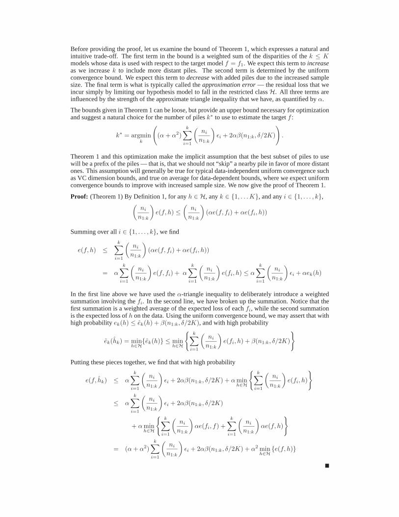
Figure 1: Visual demonstration of Theorem 2. In this problem there are K = 100 classifiers, each defined by2 parameters represented by a point fi in the unit square, such that the expected disagreement rate between twosuch classifiers equals the L1 distance between their parameters. (It is easy to create simple input distributionsand classifiers that generate exactly this geometry.) We chose the 100 parameter vectors fi uniformly at randomfrom the unit square (the circles in the left panel). To generate varying pile sizes, we let ni decrease with thedistance of fi from a chosen “central” point at (0.75, 0.75) (marked “MAX DATA” in the left panel); theresulting pile sizes for each model are shown in the bar plot in the right panel, where the origin (0, 0) is in thenear corner, (1, 1) in the far corner, and the pile sizes clearly peak near (0.75, 0.75). Given these fi, ni andthe pairwise distances, the undirected graph on the left includes an edge between fi and fj if and only if thedata from fj is used to learn fi and/or the converse when Theorem 2 is used to optimize the distance of thedata used. The graph simultaneously displays the geometry implicit in Theorem 2 as well as its adaptivity tolocal circumstances. Near the central point the graph is quite sparse and the edges quite short, correspondingto the fact that for such models we have enough direct data that it is not advantageous to include data fromdistant models. Far from the central point the graph becomes dense and the edges long, as we are required toaggregate a larger neighborhood to learn the optimal model. In addition, decisions are affected locally by howmany models are “nearby” a given model.

4 Applications to standard learning settings

In this section we demonstrate the applicability of the general theory given by Theorem 1 to severalstandard learning settings. We begin with the most straightforward application, classification.

4.1 Binary classification

In binary classification, we assume that our target model is a fixed, unknown and arbitrary functionf from some input set X to {0, 1}, and that there is a fixed and unknown distribution P over the X .Note that the distribution P over input does not depend on the target function f . The observations areof the form z = 〈x, y〉 where y ∈ {0, 1}. The loss function L(h, 〈x, y〉) is defined as 0 if y = h(x)and 1 otherwise, and the corresponding expected loss is e(g1, g2) = E〈x,y〉∼Pg1

[L(g2, 〈x, y〉)] =Prx∼P [g1(x) �= g2(x)]. For 0/1 loss it is well-known and easy to see that the (standard) 1-triangleinequality holds, and classical VC theory [6] provides us with uniform convergence. The conditionsof Theorem 1 are thus easily satisfied, yielding the following.

Theorem 2 Let F be the set of all functions from an input set X into {0,1} and let d be the VCdimension of H ⊆ F . Let e be the expected 0/1 loss. Let K ∈ N, f = f1, f2, . . . , fK ∈ F ,{εi}K

i=1, {ni}Ki=1, and hk be as defined above in the multi-source learning model. For any δ such

that 0 < δ < 1, with probability at least 1 − δ, for any k ∈ {1, . . . , K}

e(f, hk) ≤ 2k∑

i=1

(ni

n1:k

)εi + min

h∈H{e(f, h)} + 2

√d log (2en1:k/d) + log (16K/δ)

8n1:k

In Figure 1 we provide a visual demonstration of the behavior of Theorem 1 applied to a simpleclassification problem.

4.2 Regression

We now turn to regression with squared loss. Here our target model f is any function from an inputclass X into some bounded subset of R. (Frequently we will have X ⊆ R

d, but this is not required.)We again assume a fixed but unknown distribution P (that does not depend on f ) on the inputs. Ourobservations are of the form z = 〈x, y〉. Our loss function is L(h, 〈x, y〉) = (y − h(x))2, and theexpected loss is thus e(g1, g2) = E〈x,y〉∼Pg1

[L(g2, 〈x, y〉)] = Ex∼P

[(g1(x) − g2(x))2

].

For regression it is known that the standard 1-triangle inequality does not hold. However, a 2-triangleinequality does hold and is stated in the following lemma. The proof is given in Appendix A.

Lemma 1 Given any three functions g1, g2, g3 : X → R, a fixed and unknown distribution P onthe inputs X , and the expected loss e(g1, g2) = Ex∼P

[(g1(x) − g2(x))2

],

e(g1, g2) ≤ 2 (e(g1, g3) + e(g3, g1)) .

The other required ingredient is a uniform convergence bound for regression with squared loss.There is a rich literature on such bounds and their corresponding complexity measures for the modelclass H, including the fat-shattering generalization of VC dimension [7], ε-nets and entropy [6] andthe combinatorial and pseudo-dimension approaches beautifully surveyed in [5]. For concretenesshere we adopt the latter approach, since it serves well in the following section on density estimation.

While a detailed exposition of the pseudo-dimension dim(H) of a class H of real-valued functionsexceeds both our space limitations and scope, it suffices to say that it generalizes the VC dimensionfor binary functions and plays a similar role in uniform convergence bounds. More precisely, in thesame way that the VC dimension measures the largest set of points on which a set of classifiers canexhibit “arbitrary” behavior (by achieving all possible labelings of the points), dim(H) measuresthe largest set of points on which the output values induced by H are “full” or “space-filling.”(Technically we ask whether {〈h(x1), . . . , h(xd)〉 : h ∈ H} intersects all orthants of R

d withrespect to some chosen origin.) Ignoring constant and logarithmic factors, uniform convergencebounds can be derived in which the complexity penalty is

√dim(H)/n. As with the VC dimension,

dim(H) is ordinarily closely related to the number of free parameters defining H. Thus for linearfunctions in R

d it is O(d) and for neural networks with W weights it is O(W ), and so on.

Careful application of pseudo-dimension results from [5] along with Lemma 1 and Theorem 1 yieldsthe following. A sketch of the proof appears in Appendix A.

Theorem 3 Let F be the set of functions from X into [−B,B] and let d be the pseudo-dimension ofH ⊆ F under squared loss. Let e be the expected squared loss. Let K ∈ N, f = f1, f2, . . . , fK ∈F , {εi}K

i=1, {ni}Ki=1, and hk be as defined in the multi-source learning model. Assume that n1 ≥

d/16e. For any δ such that 0 < δ < 1, with probability at least 1 − δ, for any k ∈ {1, . . . , K}

e(f, hk) ≤ 6k∑

i=1

(ni

n1:k

)εi+4 min

h∈H{e(f, h)}+128B2

√ d

n1:k+

√ln(16K/δ)

n1:k

(√ln

16e2n1:k

d

)

4.3 Density estimation

We turn to the more complex application to density estimation. Here our models are no longer func-tions, but densities P . The loss function for an observation x is the log loss L(P, x) = log (1/P (x)).The expected loss is then e(P1, P2) = Ex∼P1 [L(P2, x)] = Ex∼P1 [log(1/P2(x))].

As we are not aware of an α-triangle inequality that holds simultaneously for all density func-tions, we provide general mathematical tools to derive specialized α-triangle inequalities for specificclasses of distributions. We focus on the exponential family of distributions, which is quite generaland has nice properties which allow us to derive the necessary machinery to apply Theorem 1. Westart by defining the exponential family and explaining some of its properties. We proceed by de-riving an α-triangle inequality for Kullback-Liebler divergence in exponential families that impliesan α-triangle inequality for our expected loss function. This inequality and a uniform convergencebound based on pseudo-dimension yield a general method for deriving error bounds in the multiplesource setting which we illustrate using the example of multinomial distributions.

Let x ∈ X be a random variable, in either a continuous space (e.g. X ⊆ Rd) or a discrete space

(e.g. X ⊆ Zd). We define the exponential family of distributions in terms of the following compo-

nents. First, we have a vector function of the sufficient statistics needed to compute the distribution,denoted Ψ : R

d → Rd′

. Associated with Ψ is a vector of expectation parameters µ ∈ Rd′

which pa-rameterizes a particular distribution. Next we have a convex vector function F : R

d′ → R (definedbelow) which is unique for each family of exponential distributions, and a normalization functionP0(x). Using this notation we define a probability distribution (in the expectation parameters) to be

PF (x |µ) = e∇F (µ)·(Ψ(x)−µ)+F (µ)P0(x) . (1)

For all distributions we consider it will hold that Ex∼PF (·|µ) [Ψ(x)] = µ. Using this fact and the lin-earity of expectation, we can derive the Kullback-Liebler (KL) divergence between two distributionsof the same family (which use the same functions F and Ψ) and obtain

KL (PF (x |µ1) ‖ PF (x |µ2)) = F (µ1) − [F (µ2) + ∇F (µ2) · (µ1 − µ2)] . (2)

We define the quantity on the right to be the Bregman divergence between the two (parameter) vec-tors µ1 and µ2, denoted BF (µ1 ‖ µ2). The Bregman divergence measures the difference betweenF and its first-order Taylor expansion about µ2 evaluated at µ1. Eq. (2) states that the KL divergencebetween two members of the exponential family is equal to the Bregman divergence between the twocorresponding expectation parameters. We refer the reader to [8] for more details about Bregmandivergences and to [9] for more information about exponential families.

We will use the above relation between the KL divergence for exponential families and Bregmandivergences to derive a triangle inequality as required by our theory. The following lemma showsthat if we can provide a triangle inequality for the KL function, we can do so for expected log loss.

Lemma 2 Let e be the expected log loss, i.e. e(P1, P2) = Ex∼P1 [log(1/P2(x))]. For any threeprobability distributions P1, P2, and P3, if KL (P1 ‖ P2) ≤ α(KL (P1 ‖ P3) + KL (P3 ‖ P2)) forsome α ≥ 1 then e(P1, P2) ≤ α(e(P1, P3) + e(P3, P2)).

The proof is given in Appendix B. The next lemma gives an approximate triangle inequality for theKL divergence. We assume that there exists a closed set P = {µ} which contains all the parametervectors. The proof (again see Appendix B) uses Taylor’s Theorem to derive upper and lower boundson the Bregman divergence and then uses Eq. (2) to relate these bounds to the KL divergence.

Lemma 3 Let P1, P2, and P3 be distributions from an exponential family with parameters µ andfunction F . Then

KL (P1 ‖ P2) ≤ α (KL (P1 ‖ P3) + KL (P3 ‖ P2))where α = 2 supξ∈P λ1(H(F (ξ)))/ infξ∈P λd′(H(F (ξ))). Here λ1(·) and λd′(·) are the highestand lowest eigenvalues of a given matrix, and H(·) is the Hessian matrix.

The following theorem, which states bounds for multinomial distributions in the multi-source set-ting, is provided to illustrate the type of results that can be obtained using the machinery described inthis section. More details on the application to the multinomial distribution are given in Appendix B.

Theorem 4 Let F ≡ H be the set of multinomial distributions over N values with the probabilityof each value bounded from below by γ for some γ > 0, and let α = 2/γ. Let d be the pseudo-dimension of H under log loss, and let e be the expected log loss. Let K ∈ N, f = f1, f2, . . . , fK ∈F , {εi}K

i=1, 3 {n}Ki=1, and hk be as defined above in the multi-source learning model. Assume that

n1 ≥ d/16e. For any 0 < δ < 1, with probability at least 1 − δ for any k ∈ {1, . . . ,K},

e(f, hk) ≤ (α + α2)k∑

i=1

(ni

n1:k

)εi + α min

h∈H{e(f, h)}

+ 128 log2(α

2

)√ d

n1:k+

√ln(16K/δ)

n1:k

(√ln

16e2n1:k

d

)

3Here we can actually make the weaker assumption that the εi bound the KL divergences rather than theexpected log loss, which avoids our needing upper bounds on the entropy of each source distribution.

5 Data-dependent bounds

Given the interest in data-dependent convergence methods (such as maximum margin, PAC-Bayes,and others) in recent years, it is natural to ask how our multi-source theory can exploit these modernbounds. We examine one specific case for classification here using Rademacher complexity [10, 11];analogs can be derived in a similar manner for other learning problems.

If H is a class of functions mapping from a set X to R, we define the empirical Rademacher com-plexity of H on a fixed set of observations x1, . . . , xn as

Rn(H) = E

[suph∈H

∣∣∣∣∣ 2nn∑

i=1

σih(xi)

∣∣∣∣∣∣∣∣∣∣x1, . . . , xn

]

where the expectation is taken over independent uniform {±1}-valued random variables σ1, . . . , σn.

The Rademacher complexity for n observations is then defined as Rn(H) = E[Rn(H)

]where the

expectation is over x1, . . . , xn.

We can apply Rademacher-based convergence bounds to obtain a data-dependent multi-sourcebound for classification. A proof sketch using techniques and theorems of [10] is in Appendix C.

Theorem 5 Let F be the set of all functions from an input set X into {-1,1} and let Rn1:k be theempirical Rademacher complexity of H ⊆ F on the first k piles of data. Let e be the expected 0/1loss. Let K ∈ N, f = f1, f2, . . . , fK ∈ F , {εi}K

i=1, {ni}Ki=1, and hk be as defined in the multi-

source learning model. Assume that n1 ≥ d/16e. For any δ such that 0 < δ < 1, with probabilityat least 1 − δ, for any k ∈ {1, . . . , K}

e(f, hk) ≤ 2k∑

i=1

(ni

n1:k

)εi + min

h∈H{e(f, h)} + Rn1:k(H) + 4

√2 ln(4K/δ)

n1:k

While the use of data-dependent complexity measures can be expected to yield more accurate boundsand thus better decisions about the number k∗ of piles to use, it is not without its costs in comparisonto the more standard data-independent approaches. In particular, in principle the optimization ofthe bound of Theorem 5 to choose k∗ may actually involve running the learning algorithm on allpossible prefixes of the piles, since we cannot know the data-dependent complexity term for eachprefix without doing so. In contrast, the data-independent bounds can be computed and optimizedfor k∗ without examining the data at all, and the learning performed only once on the first k∗ piles.

References

[1] K. Crammer, M. Kearns, and J. Wortman. Learning from data of variable quality. In NIPS 18, 2006.

[2] P. Wu and T. Dietterich. Improving SVM accuracy by training on auxiliary data sources. In ICML, 2004.

[3] J. Baxter. Learning internal representations. In COLT, 1995.

[4] S. Ben-David. Exploiting task relatedness for multiple task learning. In COLT, 2003.

[5] D. Haussler. Decision theoretic generalizations of the PAC model for neural net and other learning appli-cations. Information and Computation, 1992.

[6] V. N. Vapnik. Statistical Learning Theory. Wiley, 1998.

[7] M. Kearns and R. Schapire. Efficient distribution-free learning of probabilistic concepts. JCSS, 1994.

[8] Y. Censor and S.A. Zenios. Parallel Optimization: Theory, Algorithms, and Applications. Oxford Uni-versity Press, New York, NY, USA, 1997.

[9] M. J. Wainwright and M. I. Jordan. Graphical models, exponential families, and variational inference.Technical Report 649, Department of Statistics, University of California, Berkeley, 2003.

[10] P. L. Bartlett and S. Mendelson. Rademacher and Gaussian complexities: Risk bounds and structuralresults. Journal of Machine Learning Research, 2002.

[11] V. Koltchinskii. Rademacher penalties and structural risk minimization. IEEE Trans. Info. Theory, 2001.

A Details of the Application to Regression

A.1 Proof of Lemma 1

For any x ∈ X|g1(x) − g2(x)| = |g1(x) − g3(x) + g3(x) − g2(x)| ≤ |g1(x) − g3(x)| + |g3(x) − g2(x)|.

Since both sides of this equation are nonnegative, we have

(|g1(x) − g2(x)|)2 ≤ (|g1(x) − g3(x)| + |g3(x) − g2(x)|)2

and

e(g1, g2) = E[(g1(x) − g2(x))2

] ≤ E[(|g1(x) − g3(x)| + |g3(x) − g2(x)|)2

]= E

[(g1(x) − g3(x))2 + (g3(x) − g2(x))2 + 2 |(g1(x) − g3(x))(g3(x) − g2(x))|]

= e(g1, g3) + e(g3, g2) + 2E [|(g1(x) − g3(x))(g3(x) − g2(x))|]≤ e(g1, g3) + e(g3, g2) + E

[(g1(x) − g3(x))2 + (g3(x) − g2(x))2

]= 2e(g1, g3) + 2e(g3, g2)

where all expectations are taken over x. The second inequality follows from the fact that for anyreal numbers y and z we have 0 ≤ (y − z)2 = y2 + z2 − 2yz and thus yz ≤ 1

2 (y2 + z2).

A.2 Proof Sketch of Theorem 3

The following lemma is similar to Corollary 2 of [5] and is thus stated without proof.

Lemma 4 Let H be a hypothesis class such that for each h ∈ H there exists a loss function L(h, ·)from a set Z into [0,M ]. Let d be the pseudo-dimension of these loss functions with 1 ≤ d < ∞.For any ε such that 0 < ε ≤ M

Pr [∃h ∈ H : |e(h) − e(h)| ≥ ε] ≤ 8(

32eMε

ln32eM

ε

)d

e−ε2n/64M2

where e(h) = 1n

∑ni=1 L(h, zi) for observations z1, . . . , zn drawn from the target distribution, and

e(h) = E [e(h)] where the expectation is taken over z1, . . . , zn.

We set

δ ≥ 8(

32eMε

ln32eM

ε

)d

e−ε2n/64M2

and find that when n > d/16e, a valid solution for ε in is given by

ε = 8M

(√d

n+

√ln(8/δ)

n

)(√ln

16e2n

d

).

Noting that the squared loss function applied to a class of functions with output in [−B,B] isbounded by 4B2, this yields the following result.

Lemma 5 Let H be a class of functions from an input set X to [−B,B]. Let L(h, 〈x, y〉) = (y −h(x))2 be the squared loss function with pseudo-dimension d when applied to H. The followingfunction β is a uniform convergence bound for H and L when n > d/16e.

β(n, δ) = 32B2

(√d

n+

√ln(8/δ)

n

)(√ln

16e2n

d

)

Theorem 3 is then a direct application of Theorem 1 using Lemmas 1 and 5.

B Details of the Application to Density Estimation

B.1 Proof of Lemma 2

Let H(P ) denote the entropy of the distribution P . Recall that H(P ) ≥ 0 and note that e(P1, P2) =KL (P1 ‖ P2) + H(P1). Assuming KL (P1 ‖ P2) ≤ α(KL (P1 ‖ P3) + KL (P3 ‖ P2)), we have

e(P1, P2) = KL (P1 ‖ P2) + H(P1) ≤ α(KL (P1 ‖ P3) + KL (P3 ‖ P2)) + H(P1)= α(e(P1, P3) − H(P1) + e(P3, P2) − H(P3)) + H(P1)= α(e(P1, P3) + e(P3, P2)) − (α − 1)H(P1) − αH(P3)≤ α(e(P1, P3) + e(P3, P2)) .

B.2 Proof of Lemma 3

We remind the reader that F is convex and thus its Hessian matrix H(F ) is positive semi-definite.By definition,

BF (µ1 ‖ µ2) = F (µ1) − [F (µ2) + ∇F (µ2) · (µ1 − µ2)] .

Recall that P = {µ} is the set of all parameter vectors. By Taylor’s Theorem, there exists a ξ∗ ∈ Psuch that

BF (µ1 ‖ µ2) =12(µ1 − µ2)T H(F (ξ∗))(µ1 − µ2) .

We can use the last equality to derive both upper and lower bounds on the Bregman divergence. Letλ1(·) and λd′(·) be the highest and lowest eigenvalues of a matrix respectively. Then

BF (µ1 ‖ µ2) ≤ 12‖µ1 − µ2‖2 sup

ξ∈Pλ1(H(F (ξ))) . (3)

and

BF (µ1 ‖ µ2) ≥ 12‖µ1 − µ2‖2 inf

ξ∈Pλd′(H(F (ξ)))

‖µ1 − µ2‖2 ≤ 2(

BF (µ1 ‖ µ2)infξ∈P λd′(H(F (ξ)))

)(4)

An application of a generalization of Lemma 1 for vectors to Eq. (3) followed by two applicationsof Eq. (4) yields

BF (µ1 ‖ µ2) ≤ (‖µ1 − µ3‖2 + ‖µ3 − µ2‖2)supξ∈P

λ1(H(F (ξ)))

≤ 2(

supξ∈P λ1(H(F (ξ)))infξ∈P λd′(H(F (ξ)))

)(BF (µ1 ‖ µ3) + BF (µ3 ‖ µ2))

= α (BF (µ1 ‖ µ3) + BF (µ3 ‖ µ2)) .

By the definition of Bregman divergence and Eq. (2), we have

KL (P1 ‖ P2) ≤ α (KL (P1 ‖ P3) + KL (P3 ‖ P2)) .

B.3 Proof Sketch of Theorem 4

Consider the case of multinomial distributions. The probability space consists of N distinct events{1, ..., N}. We assign to the ith event the ith standard vector Ei, where Ei(j) = 1 if i = j andzero otherwise. In this example, the ith element of µ ∈ R

d′equals the probability of getting the ith

element in the probability space. Clearly, we have that∑

i µi = 1.

The sufficient statistics are the N indicators for each of the N possible atomic states of the space,that is Ψ(x) = x. The Bregman function is given by F (x) =

∑i xi log(xi) − xi, and its first

derivative is ∇F (x) = (... log(xi)...). The normalization function is P0(x) = e. Plugging theabove definitions in Eq. (1) we get

PF (i |µ) = eP

j log(µj)(Ei(j)−µj)+µj log(µj)−µj e

= eP

j log(µj)Ei(j)−P

j µj e = ΠjµEi(j)j e−1e = µi

as required. We compute the second derivative of F and get a diagonal matrix, where the value ofthe ith element of the diagonal is 1/µi.

We can bound infξ∈P λd′(H(F (ξ))) = 1 as we need for Lemma 3. In order to compute the match-ing sup bound, we restrict the set of multinomial distributions we consider and enforce a lowerbound of γ > 0 over the probability of each atomic event. The new set of parameter vectors be-comes Pγ = {µ : µi ≥ γ}. We then have, supξ∈Pγ

λ1(H(F (ξ))) = 1/γ, and the constant inLemma 3 becomes 2/γ = α.

We can apply the pseudo-dimension results from [5] along with Lemma 3 and Theorem 1 to derivethe proof of Theorem 4.

C Details of the Data-Dependent Bounds

C.1 Proof Sketch of Theorem 5

The following data-dependent uniform convergence bound for binary classification is adopted withonly minor modifications from [10] and as such is stated here without proof.

Lemma 6 Let F be a set of {±1}-valued functions defined on X and let L be the 0/1 loss function.The following function β is a uniform convergence bound for F and L.

β(n, δ) =Rn(F)

2+

√ln(2/δ)

2n.

The following lemma, which relates the true Rademacher complexity of a function class with itsempirical Rademacher complexity, follows immediately from Theorem 11 of [10].

Lemma 7 Let H be a class of functions mapping to [−1, 1]. For any integer n, for any 0 < δ < 1,with probability 1 − δ, ∣∣∣Rn(H) − Rn(H)

∣∣∣ ≤√

8 ln(2/δ)n

.

Theorem 5 then follows from the application of Theorem 1 using the 1-triangle inequality and Lem-mas 6 and 7.