Learning and the Great Moderation

James Bullard�Federal Reserve Bank of St. Louis

Aarti Singh†

Washington University in St. Louis

25 June 2007‡

AbstractWe study a stylized theory of the volatility reduction in the U.S.

after 1984—the Great Moderation—which attributes part of the stabi-lization to less volatile shocks and another part to more difficult infer-ence on the part of Bayesian households attempting to learn the latentstate of the economy. We use a standard equilibrium business cyclemodel with technology following an unobserved regime-switchingprocess. After 1984, according to Kim and Nelson (1999a), the vari-ance of U.S. macroeconomic aggregates declined because boom andrecession regimes moved closer together, keeping conditional vari-ance unchanged. In our model this makes the signal extraction prob-lem more difficult for Bayesian households, and in response they mod-erate their behavior, reinforcing the effect of the less volatile stochas-tic technology and contributing an extra measure of moderation tothe economy. We construct example economies in which this learn-ing effect accounts for about 30 percent of a volatility reduction of themagnitude observed in the postwar U.S. data. Keywords: Bayesianlearning, information, business cycles, regime switching. JEL codes:E3, D8.

�Email: bullard@stls.frb.org. Any views expressed are those of the authors and do notnecessarily reflect the views of the Federal Reserve Bank of St. Louis or the Federal ReserveSystem.

†Email: asingha@artsci.wustl.edu‡We thank Yunjong Eo, Kyu Ho Kang, and James Morley for helpful discussions dur-

ing the initial stages of this research. We also thank numerous very helpful seminar andworkshop participants for their comments. In addition, we thank S. Boragan Aruoba, Je-sus Fernandez-Villaverde, and Juan Rubio-Ramirez for providing their Mathematica codeconcerning perturbation methods.

1 Introduction

1.1 Overview

The U.S. economy experienced a significant decline in volatility—on the

order of fifty percent for many key macroeconomic variables—sometime

during the mid-1980s. This phenomenon, sometimes called the Great Mod-eration, has been the subject of a large and expanding literature. The main

question in the literature has been the nature and causes of the volatility

reduction. In some of the research, better counter-cyclical monetary policy

has been promoted as the main contributor to the low volatility outcomes.

In other strands, the lower volatility is attributed primarily or entirely to

good luck, in the sense that the shocks buffeting the economy have gener-

ally been less frequent and smaller than those from the high volatility 1970s

era. In fact, the good luck story is probably the leading explanation in the

literature to date. Yet, the pure good luck explanation strains credulity as

the full amount of the volatility reduction is simply due to smaller shocks.

Why should shocks suddenly be 50 percent less volatile?

In this paper, we study a version of the good luck story, but one which

we think is more credible. In our version, the economy is indeed buffeted

by smaller shocks after the mid-1980s, but this lessened volatility is coupled

with changed equilibrium behavior of the private sector in response to the

smaller shocks. The changed behavior comes from a learning effect which

is central to the paper. The learning effect reduces overall volatility of the

economy still further in response to the smaller shock volatility. Thus, in

our version of the good luck story, the Great Moderation is due partly to

less volatile shocks and partly to a learning effect, so that the shocks do not

have to account for the entire volatility reduction. Quantifying the magni-

tude of this effect in an equilibrium setting is the primary purpose of the

paper.

1

1.2 What we do

There have been many attempts to quantify the volatility reduction in the

U.S. macroeconomic data. In this paper we follow the regime-switching

approach to this question, as that will facilitate our learning analysis. The

regimes can be thought of as expansions and recessions. According to Kim

and Nelson (1999a), expansion and recession states moved closer to one

another after 1984, but in a way that kept conditional, within-regime vari-

ance unchanged. These results imply that recessions and expansions were

relatively distinct phases and hence easily distinguishable in the pre-1984

era. In contrast, during the post-1984 era, the two phases were much less

distinct.

The Kim and Nelson (1999a) study is a purely empirical exercise. We

want to take their core finding as a primitive for our quantitative-theoretic

model: Regimes moved closer together, but conditional variance remained

constant. The economies we study and compare will all be in the context of

this idea.

We assume that the two phases are driven by an unobservable vari-

able, and that economic agents must learn about this variable by observing

other macroeconomic data, such as real output. Agents learn about the un-

observable state via Bayesian updating.1 When the two states are closer

together, agents find it harder to infer whether the economy is in a reces-

sion or in an expansion based on observable data since the two phases of

the business cycle are less distinct. Therefore, learning becomes more dif-

ficult and leads to an additional change in the behavior of households. In

particular, volatility in macroeconomic aggregates will be moderated since

the households are more uncertain which regime they are in at any point in

time.

We wish to study this phenomenon in a model which can provide a

well-known benchmark. Accordingly, we use a simple equilibrium busi-

1Learning as a signal extraction problem is a distinct issue from expectational stabilityas described by Evans and Honkapohja (2001). We do not study expectational stability inthis paper.

2

ness cycle model in which the level of productivity depends in part on a

first-order, two-state Markov process. The complete information version of

this model is known to be very close to linear, so that a reduction in the vari-

ance of the driving shock process translates one-for-one into a reduction in

the variance of endogenous variables in equilibrium. The incomplete in-

formation, Bayesian learning version of the model is nonlinear. Reductions

in driving shock variance result in more than a one-for-one reduction in

the variance of endogenous variables. The difference between what one

observes in the complete information case and what one observes in the in-

complete information, Bayesian learning case is the learning effect we wish

to focus upon. We solve the model using perturbation methods.

1.3 Main findings

We begin by establishing that the baseline model with regime switching

behaves nearly identically to standard models in this class under complete

information when we use a suitable calibration that keeps driving shock

variance and persistence at standard values. We then use the incomplete

information, Bayesian learning version of this model as a laboratory to at-

tempt to better understand the learning effect in which we are interested.

We report results for a comparison of economies in which both uncondi-

tional and conditional variances of the shock process are held constant, but

where the distance between the two regimes is altered.2 These economies

have nearly identical driving shock processes when viewed from an AR (1)perspective. The economies differ only to the degree that the two regimes

are closer to each other or farther apart. We establish that this alone creates

a learning effect—private sector behavior is substantially altered and en-

dogenous variables are less volatile when the two regimes are closer. We at-

tribute this result to the increased difficulty of the inference problem when

the two regimes are closer together.

We then extend these first findings, allowing unconditional variance to

2There are clear limits to how well this task can be accomplished.

3

rise as regimes are moved farther apart, still keeping conditional variance

constant. We then compare the resulting volatility of endogenous variables

to a complete information benchmark. The complete information model

is close to linear, and so the volatility of endogenous variables relative to

the volatility of the shock is a constant. For the incomplete information,

Bayesian learning economies, endogenous variable volatility rises with the

volatility of the shock. This ratio begins to approach the complete informa-

tion constant for sufficiently high shock variance. Thus the incomplete in-

formation economies begin to behave like complete information economies

when the two regimes are sufficiently distinct. This is because the inference

problem is simplified as the regimes move apart, and thus agent behavior

is moderated less.

Finally, we compare incomplete information economies in which ob-

served volatility in macroeconomic variables is substantially different, with

one economy enjoying on the order of 50 percent lower output volatility

than the other. This volatility difference is then decomposed into a portion

due to lower shock variance—“good luck” as it is known in the literature—

and another portion due to more difficult inference, the learning effect in

which we are interested. We find that the learning effect accounts for about

30 percent of the volatility reduction, and the good luck portion accounts

for about 70 percent. This suggests that learning effects may help account

for a substantial fraction of observed volatility reduction in more elaborate

economies which can confront more aspects of observed macroeconomic

data.

1.4 Recent related literature

Broadly speaking, there are two strands of literature concerning the Great

Moderation. One focuses on dating the Great Moderation and the other

looks into the causes that led to it. The dating literature, including Kim and

Nelson (1999a), McConnell and Perez-Quiros (2000), and Stock and Watson

(2003) typically assumes that the date when the structural break occurred is

unknown and then identifies it using either classical or Bayesian methods.

4

According to the other strand, there are three broad causes of the sudden

reduction in volatility—better monetary policy, structural change, or good

luck. Clarida, Gali and Gertler (2000) argued that better monetary policy in

the Volker-Greenspan era led to lower volatility, but Sims and Zha (2006)

and Primiceri (2005) conclude that switching monetary policy regimes were

insufficient to explain the Great Moderation and so favor a version of the

good luck story. The proponents of the structural change argument mainly

emphasize one of two reasons for reduced volatility: a rising share of ser-

vices in total production, which is typically less volatile than goods sector

production (Burns (1960), Moore and Zarnowitz (1986)), and better inven-

tory management (Kahn, McConnell, and Perez-Quiros (2002)).3 A num-

ber of authors, including Ahmed, Levin, and Wilson (2004), Arias, Hansen,

and Ohanian (2006), and Stock and Watson (2003) have compared compet-

ing hypotheses and concluded that in recent years the U.S. economy has to

a large extent simply been hit by smaller shocks.4

In the literature, learning has often been used to help explain fluctua-

tions in endogenous macroeconomic variables. In Cagetti, Hansen, Sargent

and Williams (2002) agents solve a filtering problem since they are uncer-

tain about the drift of the technology. In Van Nieuwerburgh and Veldkamp

(2006) agents solve a problem similar to the one posed in this paper. They

use their model to help explain business cycle asymmetries. In their paper

learning asymmetries arise due to an endogenously varying rate of infor-

mation flow. Andolfatto and Gomme (2003) also incorporate learning in a

dynamic stochastic general equilibrium model. Here agents learn about the

monetary policy regime, instead of technology, and learning is used to help

explain why real and nominal variables may be highly persistent following

a regime change. In an empirical paper, Milani (2007) uses Bayesian meth-

3Kim, Nelson, and Piger (2004) argue that the time series evidence does not support theidea that the volatility reduction is driven by sector specific factors.

4Owyang, Piger, and Wall (2007) use state-level employment data and document signif-icant heterogeneity in volatility reductions by state. They suggest that the disaggregateddata is inconsistent with the inventory management hypothesis or less volatile aggregateshocks, and instead favors the improved monetary policy hypothesis.

5

ods to estimate the impact of learning in a DSGE New Keynesian model. In

his model, recursive learning contributes to the endogenous generation of

time-varying volatility similar to that observed in the U.S. postwar period.5

Arias, Hansen and Ohanian (2006) employ a standard equilibrium busi-

ness cycle model as we do, but with complete information. They conclude

that the Great Moderation is most likely due to a reduction in the volatil-

ity of technology shocks. Our explanation does rely on a reduction in the

volatility of technology shocks but that reduction accounts for only a frac-

tion of the moderation according to the model in this paper.

1.5 Organization

In the next section we present our model. In the following section we cal-

ibrate and solve the model using perturbation methods. We then turn to

results.

2 Environment

2.1 Overview

We study a version of an equilibrium business cycle model with exoge-

nous growth. We think of this model as a laboratory to study the effects

in which we are interested. Time is discrete and denoted by t = 0, 1, ....∞.

The economy consists of an infinitely-lived representative household that

derives utility from consumption of goods and leisure. Aggregate output

is produced by competitive firms that use labor and capital.

2.2 Households

The representative household is endowed with 1 unit of time each period

which it must divide between labor, `t, and leisure, (1� `t). In addition,

5Two additional empirical papers, Justiniano and Primiceri (2006) and Fernandez-Villaverde and Rubio-Ramirez (2007), introduce stochastic volatility into DSGE settings,but without learning, and conclude that volatilities have changed substantially during thesample period.

6

the household owns an initial stock of capital k0 which it rents to firms and

may augment through investment, it. Household utility is defined over a

stochastic sequence of consumption ct and leisure (1� `t) such that

U = E0

∞

∑t=0

βtu(ct, `t), (1)

where β 2 (0, 1) is the discount factor, E0 is the conditional expectations

operator and period utility function u is given by

u(ct, `t) =[cθ

t (1� `t)1�θ ]1�τ

1� τ. (2)

The parameter τ governs the elasticity of intertemporal substitution for

bundles of consumption and leisure, and θ controls the intratemporal elas-

ticity of substitution between consumption and leisure. At the end of each

period t the household receives wage income and interest income which

is used to buy consumption goods and to invest. Thus the household’s

end-of-period budget constraint is6

ct + it = wt`t + rtkt, (3)

where it is investment, wt is the wage rate, and rt is the interest rate. The

law of motion for the capital stock is given by

kt+1 = (1� δ)kt + it, (4)

where δ is the net depreciation rate of capital.

2.3 Firms

Competitive firms produce output yt according to the constant returns to

scale technology

yt = ezt f (kt, `t) = ezt kαt `

1�αt , (5)

where kt is aggregate capital stock, `t is the aggregate labor input and zt is

a stochastic process representing the level of technology relative to a bal-

anced growth trend.6We stress ”end of period” since in the begining of the period the agent has only expec-

tations about the wage and the interest rate.

7

2.4 Shock process

We assume that the level of technology is dependent on a latent variable.

Accordingly, we let zt follow the stochastic process

zt = (aH + aL)(st + ςηt)� aL, (6)

with

zt =

�aH + (aH + aL)ςηt if st = 1�aL + (aH + aL)ςηt if st = 0

, (7)

where aH � 0, aL � 0, ηt � i.i.d. N(0, 1), and ς > 0 is a weighting parame-

ter. The variable st is the latent state of the economy where st = 0 denotes a

“recession” state, and st = 1 denotes an “expansion” state. We assume that

st follows a first-order Markov process with transition probabilities given

by

Π =

�q 1� q

1� p p

�, (8)

where q = Pr(st = 0jst�1 = 0) and p = Pr(st = 1jst�1 = 1). Hamil-

ton (1989) shows that the stochastic process for st is stationary and has an

AR(1) specification such that

st = λ0 + λ1st�1 + vt, (9)

where λ0 = (1� q), λ1 = (p+ q� 1), and vt has the following conditional

probability distribution: If st�1 = 1, vt = (1� p) with probability p and

vt = �p with probability (1� p); and, vt = �(1� q) with probability qand vt = q with probability (1� q) conditional on st�1 = 0. Thus

zt = ξ0 + ξ1zt�1 + σεt, (10)

where ξ0 = (aH + aL) λ0 + λ1aL � aL, ξ1 = λ1, σ = (aH + aL), and

εt = vt + ςηt � λ1ςηt�1. (11)

The stochastic process for zt, equation (10), has the same AR (1) form

as in a standard equilibrium business cycle model even though we have

8

incorporated regime-switching. In our quantitative work, we use σ as the

perturbation parameter in order to approximate a second-order solution to

the equilibrium of the economy. We sometimes call σ the “regime distance”

as it measures the distance between the conditional expectation of the level

of technology relative to trend, z, in the high state, aH, and the low state,

�aL. The distribution of ε is nonstandard, being the sum of discrete and

continuous random variables. Since η is i.i.d., v and η are uncorrelated.

The mean of εt is zero and the variance is given by

σ2ε = p (1� p)

λ0

1� λ1+ q (1� q)

�1� λ0

1� λ1

�+ ς2

�1+ λ2

1

�. (12)

We draw from this distribution when solving the model. The variance is in

part a function of ς, which will play a role in the analysis below.

2.5 Information structure

2.5.1 Overview

In any period t, the agent enters the period with an expectation of the level

of technology, zet . The latent state, st, as well as the two shocks ηt and vt, are

all unobservable by the agent. First, households and firms make decisions

based on the expected wage and the expected interest rate. Next, shocks are

realized and output is produced. We let actual consumption equal planned

consumption and require investment to absorb any difference between ex-

pected output and actual output. At the end of the period, the level of

technology zt can be inferred based on the amount of inputs used and the

realized output, since zt = log yt � log kαt `

1�αt . This zt is then used to calcu-

late next period’s expected latent state, set+1, using Bayes’ rule, and then the

expected level of technology for the next period, zet+1. Period t ends and

the agent enters the next period with zet+1. The details of these calculations

are given below. Given this timing, the information available to the agent

at the time decisions are made is Ft = fyt�1, ct�1, zt�1, it�1, kt, `t�1, wt�1,

rt�1g. Here at = fa0, a1, ...atg represents the history of any series a.

9

2.5.2 Beliefs

We follow Kim and Nelson (1999b) in the following discussion of the evo-

lution of beliefs. At date t, agents forecast st�1 given information available

at date t. Letting bt = P(st�1 = 0jFt),

bt = ∑st�2=0,1

P(st�1 = 0, st�2jFt)

= P(st�1 = 0, st�2 = 0jFt) + P(st�1 = 0, st�2 = 1jFt), (13)

where the joint probability that the economy was in a recession in the last

two periods is given by

P(st�1 = 0, st�2 = 0jFt) = P(st�1 = 0, st�2 = 0jzt�1, Ft�1)

=φ(zt�1, st�1 = 0, st�2 = 0jFt�1)

φ(zt�1jFt�1)

=φL(zt�1jst�1 = 0, st�2 = 0, Ft�1)

φ(zt�1jFt�1)�

P(st�1 = 0jst�2 = 0, Ft�1)P(st�2 = 0jFt�1), (14)

where φi denotes the density function under regime i 2 fL, Hg, and φ(zt�1

j Ft�1) = Σst�1 Σst�2 φ(zt�1, st�1, st�2jFt�1). Similarly,

P(st�1 = 0, st�2 = 1jFt) =

φL(zt�1jst�1 = 0, st�2 = 1, Ft�1)P(st�1 = 0jst�2 = 1, Ft�1)P(st�2 = 1jFt�1)

φ(zt�1jFt�1).

(15)

Using the transition probabilities define gL and gH as

gL = φL(zt�1jst�1 = 0, st�2 = 0, Ft�1)qbt�1

+ φL(zt�1jst�1 = 0, st�2 = 1, Ft�1)(1� p)(1� bt�1), (16)

and

gH = φH(zt�1jst�1 = 1, st�2 = 0, Ft�1)(1� q)bt�1

+ φH(zt�1jst�1 = 1, st�2 = 1, Ft�1)p(1� bt�1). (17)

10

Since zt�1 = ξ0 + ξ1zt�2 + σ(vt�1 + ςηt�1 � λ1ςηt�2), then conditional

on vt, zt has a normal distribution. Letting st�1 = 0 and st�2 = 0, then

vt�1 = �(1� q) and zt�2 = �aL + σςηt�2, and so, if in the last two periods

the economy was in a recession, zt�1 = ξ0 + ξ1(�aL)� σ(1� q) + σςηt�1.

We can therefore write the conditional density function as

φL00 = φL(zt�1jst�1 = 0, st�2 = 0, Ft�1)

=1p

2πσ2ς2exp

�� (zt�1 � ξ0 � ξ1(�aL) + σ(1� q))2

2σ2ς2

�. (18)

When st�1 = 0 and st�2 = 1, then vt�1 = �p and zt�2 = aH + σςηt�2, and

the density function is

φL10 = φL(zt�1jst�1 = 0, st�2 = 1, Ft�1)

=1p

2πσ2ς2exp

�� (zt�1 � ξ0 � ξ1(aH) + σp)2

2σ2ς2

�. (19)

Similarly

φH01 = φH(zt�1jst�1 = 1, st�2 = 0, Ft�1)

=1p

2πσ2ς2exp

�� (zt�1 � ξ0 � ξ1(�aL)� σq)2

2σ2ς2

�, (20)

and

φH11 = φH(zt�1jst�1 = 1, st�2 = 1, Ft�1)

=1p

2πσ2ς2exp

�� (zt�1 � ξ0 � ξ1(aH)� σ(1� p))2

2σ2ς2

�. (21)

Thus we can write bt as

bt =gL

gL + gH. (22)

2.5.3 Expectations

Since bt is the probability that the economy was in a recession and (1� bt)

is the probability that the economy was in an expansion in the last period,

11

we determine the probability distribution of the current state by allowing

for the possibility of state change. In particular,

[P(st = 0jFt), P(st = 1jFt)]

= [P(st�1 = 0jFt), P(st�1 = 1jFt)]

�q 1� q

1� p p

�(23)

which can be rewritten as

[P(st = 0jFt), P(st = 1jFt)] = [bt, (1� bt)]

�q 1� q

1� p p

�. (24)

Given that P(st = 0jFt) = btq+ (1� bt)(1� p) and P(st = 1jFt) = bt(1�q) + (1� bt)p, the current expected state is given by

set = bt(1� q) + (1� bt)p, (25)

and the expected technology at date t is given by

zet = (aH + aL)se

t + (�aL). (26)

Equivalently

zet = [bt(1� q) + (1� bt)p] aH � [btq+ (1� bt)(1� p)] aL. (27)

We stress that the expectation of the level of technology can be written

in a recursive way. First, solve equation (27) for bt to obtain

bt =(aH + aL) p� aL � ze

t(aH + aL) (p+ q� 1)

. (28)

Also from equation (27), next period’s value of ze is

zet+1 = [bt+1(1� q) + (1� bt+1)p] aH � [bt+1q+ (1� bt+1)(1� p)] aL. (29)

The value of bt+1 in this equation can be written in terms of updated (t+ 1)

values of gL and gH defined in equations (16) and (17), which will depend

on bt, and, through the definitions of the conditional densities (18), (19),

12

(20), and (21), on zt as well. Using equation (28) to eliminate bt we conclude

that we can write

zet+1 = f (ze

t , zt) (30)

where f is a complicated function of zet and zt. Of course, zt is itself a func-

tion of endogenous variables such as yt, kt, and `t. The fact that zet+1 has

a recursive aspect plays a substantive role in some of our findings below.

When the agent observes a value for zt at the end of the period, that value

is not the only input into next period’s expected value, as zet also plays a

role.

2.6 The household’s problem

The household’s decision problem is to choose a sequence of fct, `tg for

t � 0 that maximizes (1) subject to (3) and (4) given a stochastic process for

fwt, rtg for t � 0, interiority constraints ct � 0, 0 � `t � 1, and given k0.

Expectations are formed rationally given the assumed information struc-

ture.

Assuming an interior solution, the optimality conditions imply that

u`(ct, `t)

uc(ct, `t)= Et[wt] (31)

Before the shocks are realized, households make their consumption and

labor decisions based on expected wages and interest rates. In this model

investment is a residual and absorbs unexpected shocks to income. The

Euler equation is

uc(ct, `t) = βEt [uc(ct+1, `t+1)(rt+1 + (1� δ))] . (32)

2.7 The firm’s problem

Firms produce a final good by choosing capital kt and labor `t such that

they maximize their expected profits. The firms period t problem is then

maxkt,`t

Et[ezt kαt `

1�αt � wt`t � rtkt] 8t. (33)

13

The first order conditions for the firm are

rt = Et[ezt fk(kt, `t)] (34)

wt = Et[ezt f`(kt, `t)] (35)

These conditions differ from the standard condition because technology

level zt is not observable when decisions are made.

2.8 Second-order approximation

We follow Van Nieuwerburgh and Veldkamp (2006) and study a passive

learning problem.7 As a result, the timing and informational constraints

faced by the planner are the same as in the decentralized economy, and

the competitive equilibrium and the planning problem are equivalent. The

planner’s problem is to maximize household utility (1) subject to the re-

source constraint

ct + kt+1 = ezt kαt `

1�αt + (1� δ) kt (36)

and the evolution of beliefs given by equations (22) and (27). The solu-

tion to this problem is characterized by (31), (32), (36), and the exogenous

stochastic process (10).

The perturbation methods we use are standard and are described in

Aruoba, Fernandez-Villaverde, and Rubio-Ramirez (2006). To solve the

problem we find three policy functions or decision rules, one each for con-

sumption, labor supply, and next period’s capital, as a function of the two

states and a perturbation parameter σ. Our regime distance parameter

σ = aH + aL plays the role of σ in Aruoba, et al. (2006). This is possible

because the regime switching process for the level of technology can be

written as an AR (1) process, as in equation (10). We use and modify the

Mathematica code provided by Aruoba, et al., (2006). That code is written

for a standard normal random variable εt in (10), whereas εt follows the

7The planner does not take into account the effect of consumption and labor choices onthe evolution of beliefs.

14

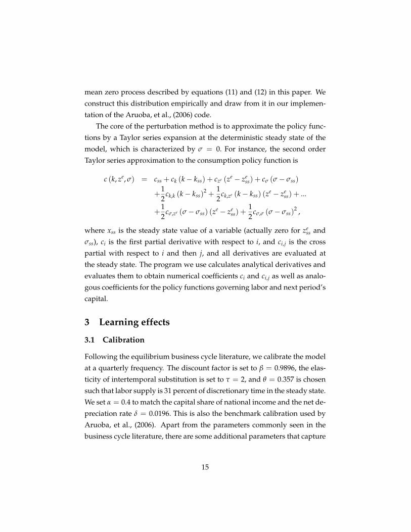
mean zero process described by equations (11) and (12) in this paper. We

construct this distribution empirically and draw from it in our implemen-

tation of the Aruoba, et al., (2006) code.

The core of the perturbation method is to approximate the policy func-

tions by a Taylor series expansion at the deterministic steady state of the

model, which is characterized by σ = 0. For instance, the second order

Taylor series approximation to the consumption policy function is

c (k, ze, σ) = css + ck (k� kss) + cze (ze � zess) + cσ (σ� σss)

+12

ck,k (k� kss)2 +

12

ck,ze (k� kss) (ze � zess) + ...

+12

cσ,ze (σ� σss) (ze � zess) +

12

cσ,σ (σ� σss)2 ,

where xss is the steady state value of a variable (actually zero for zess and

σss), ci is the first partial derivative with respect to i, and ci,j is the cross

partial with respect to i and then j, and all derivatives are evaluated at

the steady state. The program we use calculates analytical derivatives and

evaluates them to obtain numerical coefficients ci and ci,j as well as analo-

gous coefficients for the policy functions governing labor and next period’s

capital.

3 Learning effects

3.1 Calibration

Following the equilibrium business cycle literature, we calibrate the model

at a quarterly frequency. The discount factor is set to β = 0.9896, the elas-

ticity of intertemporal substitution is set to τ = 2, and θ = 0.357 is chosen

such that labor supply is 31 percent of discretionary time in the steady state.

We set α = 0.4 to match the capital share of national income and the net de-

preciation rate δ = 0.0196. This is also the benchmark calibration used by

Aruoba, et al., (2006). Apart from the parameters commonly seen in the

business cycle literature, there are some additional parameters that capture

15

the regime switching process. In particular, the parameters �aL and aH re-

flect the level of technology zt relative to trend in recessions and expansions

respectively. We also have the transition probabilities p and q as well as a

weighting parameter ς.

To obtain a baseline economy that can be compared to the benchmark

calibration of Aruoba, et al., (2006), (AFR), we use equation (10), repro-

duced here for convenience

zt = ξ0 + ξ1zt�1 + σεt. (37)

We wish to choose the values of p, q, aH, aL and ς such that ξ0 = 0, ξ1 =

0.95, σ = 0.007, and σ2ε = 1, the standard equilibrium business cycle values

and the ones used in the benchmark calibration of AFR. To remain compa-

rable to AFR, we would like εt to be close to a standard normal random

variable, with σ = aH + aL = 0.007. To meet this latter requirement, we

choose symmetric regimes by setting aH = aL = 0.0035. Since

ξ1 = λ1 = (p+ q� 1),

we set p = q = 0.975, yielding ξ1 = 0.95. These values imply ξ0 =

(aH + aL) λ0 + λ1aL � aL = 0. This leaves the mean and variance of εt. The

mean is zero, but to get the variance

σ2ε = p (1� p)

λ0

1� λ1+ q (1� q)

�1� λ0

1� λ1

�+ ς2

�1+ λ2

1

�equal to one, we set the remaining parameter ς = 0.719.8 Thus the uncon-

ditional standard deviation of the shock process, σσε, is 0.007 as desired,

and the conditional standard deviation, σςση = σς is 0.005 (since ση = 1

by assumption). For this calibration, the nonstochastic steady state values

are given by: zess = zss = 0, kss = 23.141, css = 1.288, `ss = 0.311, and

yss = 1.742.

8We chose the positive value for ς that met this requirement.

16

TABLE 1.Benchmark comparison.

Variable AFR ModelOutput 1.2418 1.2398Consumption 0.4335 0.4323Hours 0.5714 0.5706Investment 3.6005 3.5953Capital 0.2490 0.2466

Table 1: A comparison of standard deviations of key endogenous variablesfor a standard equilibrium business cycle model (AFR) and the complete in-formation version of the present model with regime switching, calibratedto mimic the standard case. The addition of regime switching does notchange the standard deviations appreciably. In both cases, each simulationhas 200 observations. For each simulation we compute the standard devia-tions for percentage deviations from Hodrick-Prescott filter with λ = 1600and then average over 250 simulations.

3.2 A complete information benchmark comparison

The benchmark calibration involves choosing parameters for the regime

switching economy such that the economy is as close as possible to a stan-

dard equilibrium business cycle model. We now investigate whether the

benchmark equilibrium is comparable to the equilibrium of a standard

model. For this purpose we endow the agents with complete information.

Table 1 shows that the regime switching economy with complete informa-

tion and the baseline calibration delivers results almost identical to a stan-

dard equilibrium business cycle model, that is, the same results as AFR.

Since we use perturbation methods to solve our model, it seems natural

then to compare our model with AFR.

This shows that despite the addition of regime switching, the complete

information economy calibrated to look like the standard case delivers re-

sults very similar to the standard case. We now turn to incomplete infor-

mation economies with Bayesian learning.

17

3.3 Allowing only regime distance to change

We ideally would like to keep economies as similar as possible while chang-

ing the distance between expansionary and recessionary regimes. Our intu-

ition is that, keeping conditional (within regime) variance constant, regimes

which are closer together pose a more difficult inference problem for agents.

The agents then take actions which are not as extreme as they would be un-

der complete information. The result is a moderating force in the economy.

To investigate this hypothesis in similar economies we proceed as fol-

lows. Except for aH, aL, ς, and σε, all parameters are the same as in the

baseline economy. Our goal is to move the values of aH and aL farther

apart but keep the standard deviation of the shock, σσε, equal to 0.007, and

simultaneously keep the conditional standard deviation σς = 0.005. If we

achieve this, then the shock processes for each of these economies will look

the same from an AR (1) perspective.

The conditional standard deviation requires

σς = (aH + aL) ς = 0.005. (38)

The unconditional standard deviation requires

σσε = (aH + aL)hκ + ς2

�1+ λ2

1

�i 12= 0.007 (39)

where κ = p (1� p) λ01�λ1

+ q (1� q)�

1� λ01�λ1

�. With p = q, then κ =

p (1� p) = 0.024375. Also, 1+ λ21 = 1.9025. These considerations indicate

that there is only one available parameter, ς, that can be calibrated to match

both targets. We can write

0.005033ς

�0.024375+ ς2 (1.9025)

� 12 = 0.007. (40)

Taking the positive value of ς that solves this equation yields ς = 0.87435,

so that aH + aL = 0.005756.

Attempts to move the regimes farther apart or closer together than aH +

aL = 0.005756 will cause us to miss on either the unconditional or the con-

ditional standard deviation target. However, the deterioration is not too

18

Figure 1: Shock distributions for economies A, B, and C are very similar, but theregimes for economy B are twice as far apart as those for economy A. For economyC, the regimes are three times as far apart. Figures are drawn for 10, 000 drawsfrom each distribution.

dramatic for values of σ = aH + aL as low as 0.0035 or as high as 0.0105.

These are convenient values as the former is one half of the benchmark

calibration value, and the latter is three times the former. Thus we set

aH = aL = 0.0035 for economy A, aH = aL = 0.007 for economy B, and

aH = aL = 0.0105 for economy C. In each case we set ς to keep the condi-

tional standard deviation equal to 0.005.

In terms of the equation for the shock process

zt = ξ0 + ξ1zt�1 + σεt,

these economies are all very similar. In each case, ξ0 = 0, ξ1 = 0.95,

and the standard deviation of the shock is not too far from 0.007. From

the perspective of the AR (1) process describing the stochastic technology,

the economies are nearly the same. The distribution of σε for the three

economies, A, B, and C is depicted in Figure 1.

Even though these economies have similar AR (1) processes for the sto-

chastic technology, they differ in σ = aH + aL, the distance between the

recession and expansion states. In economy A the two states are not very

distinct relative to economies B and C, and in economy C the states are the

most distinguishable. Because conditional variance is constant, we expect

the inference problem of the agents to be relatively difficult in economy

19

TABLE 2. INCREASING σEconomy

A B CParameter values

aH 0.0035 0.0070 0.0105aL 0.0035 0.0070 0.0105σ 0.0070 0.0140 0.0210σσε 0.0070 0.0073 0.0077σς 0.0050 0.0050 0.0050

Volatility, in percent s.d.Output 0.9300 1.0100 1.1060Consumption 0.1450 0.1730 0.2050Hours 0.1240 0.2850 0.4450Investment 3.5580 3.8040 4.1060Capital 0.2430 0.2640 0.28701T ∑(se � s)2 0.3900 0.3680 0.2970

Table 2: The three economies have differing regime distances but are cali-brated in a way such that the AR(1) process for the stochastic technologyis almost identical, having the same persistence as well as the same condi-tional and nearly the same unconditional standard deviation.

A, leading to moderated behavior, and relatively easy in economy C, lead-

ing to more volatile behavior. Table 2 illustrates how this difference in the

distance between the regimes is enough to induce differences in aggregate

volatility.

Table 2 illustrates a learning effect across economies that appear to be

nearly identical when looking at the nature of the stochastic productivity

process driving the economy. The inference problem is more severe in some

cases, leading agents to make different decisions and changing the nature

of the equilibrium. In economy A, the regime distance is one-half that of

economy B and one-third that of economy C. This makes the inference

problem harder in economy A and agents experience greater uncertainty

about the true state in this economy. The result is that standard deviation

of output falls by almost 19 percent in economy A relative to economy C.

The volatility of other endogenous variables also falls precipitously.

20

Our hypothesis is that this occurs because the inference problem is more

severe in economy A. For each economy A, B, and C we compute the av-

erage sum of squared deviations of the expected latent state from the true

latent state. This statistic is one measure of the confusion faced by agents

in their respective economies. From the last row of Table 2 we can see that

as the states become more and more distinguishable, that is, as we move

from economy A to economy C, the confusion as measured by this statistic

decreases.

Table 2 also indicates that σσε increases somewhat as we move from

economy A to economy C, so that these economies are not exactly the same

in terms of unconditional volatility. As discussed above, we can only keep

either unconditional volatility or conditional volatility completely constant

while still meeting other calibration goals, but not both. Still, according to

the Table, output volatility increases by 19 percent moving from economy

A to economy C, while the unconditional standard deviation increases by

only 10 percent (that is, 0.007 versus 0.0077) for the same economies. This

suggests a fairly substantial learning effect for economies that, on the face

of it, would appear to be very similar. We now turn to another set of exper-

iments to explore this finding more systematically.

3.4 Incomplete approaches complete information

In this subsection we abandon the attempt to keep all aspects of the economies

the same as we move regimes farther apart or closer together. Instead, in

this subsection we allow the standard deviation of σε to vary when we

change σ = aH + aL, but we hold conditional (within regime) variance con-

stant using the parameter ς. This means that the economies we compare

in this subsection will have substantially different unconditional variances,

different levels of volatility coming directly from the driving shock process

in the economy. We then need a benchmark against which we can compare

these economies. The benchmark we choose is the counterpart, complete

information version of these economies.

Standard equilibrium business cycle models are known to be very close

21

to linear when there is complete information. In these economies, the stan-

dard deviation of key endogenous variables increases one-for-one with in-

creases in σσε. We expect that our regime switching model with complete

information is also very close to linear with respect to the unconditional

standard deviation, σσε. The only difference between this case and the

economies we study is the addition of incomplete information and Bayesian

learning. The latter economies are nonlinear, so that the standard deviation

of key endogenous variables no longer increases one-for-one with increases

in σσε. By comparing the complete and incomplete information versions of

the same economies, we can infer the size of the learning effect in which

we are interested. In addition, we expect the inference problem to become

less severe as regimes move farther apart. The economies with learning

should begin to look more like complete information economies as regimes

become more distinct.

In Figure 2 we plot the unconditional standard deviation on the hori-

zontal axis. On the vertical axis, we plot the standard deviation of output

relative to the unconditional standard deviation. In our version of the stan-

dard “RBC” equilibrium business cycle model (no regime switching, com-

plete information), the standard deviation of output is 1.2418 percent and

the standard deviation of the shock is 0.7 percent. Thus the ratio of stan-

dard deviation of output relative to the standard deviation of the shock

process is 1.77. Because of linearity, this ratio does not change as the un-

conditional variance of the shock increases. This is depicted by the hori-

zontal dotted line in Figure 2. We also know that our complete information

model with regime switching delivers results close to the standard equilib-

rium business cycle model for certain parameter values (see Table 1). Thus

we expect the ratio of standard deviations of output and shocks to be con-

stant for this case as well. This turns out to be verified in the Figure, as the

solid line indicates only minor deviations from the standard equilibrium

business cycle model.9

9Each point in this figure is computed by simulating 200 quarters for the given economy,and averaging results over 250 such economies. We calculate 13 such points and connect

22

The linear relationship between σσε and the standard deviation of en-

dogenous variables breaks down in a model with incomplete information.

When the states become less distinct, moving from the right to the left along

the horizontal axis in Figure 2, the agents have to learn about the state of

the economy and the learning effect moderates the behavior of all endoge-

nous variables. But when states are distinct, toward the right in the Figure,

the standard deviation of output rises more than one-for-one. Agents are

more able to discern the true state when the states are more distinct.

Figure 2 shows that learning has a pronounced effect on private sector

equilibrium behavior. Moreover, it shows that the learning effect becomes

larger as regimes move closer together, keeping conditional variance un-

changed. This makes sense as the inference problem becomes more diffi-

cult for agents. The agents base behavior in part on the expected regime,

which, because of increased confusion, more often takes on intermediate

values instead of extreme values. This leads the agents to take actions mid-

way between the ones they would take if they were sure they were in one

regime or the other. This provides a clear moderating force in the economy

above and beyond the reduction in unconditional variance. We now turn

to a quantitative assessment of the size of this moderating force.

3.5 Comparing economies with observed moderation

In this subsection we compare two economies, both of which have incom-

plete information and Bayesian learning. The first economy has higher

volatility than the second. We choose parameters so that the volatility of

output in the second economy is on the order of 50 percent of the corre-

sponding volatility in the first economy. Thus the second economy has

greatly moderated endogenous variable volatility relative to the first. Some

of this reduced volatility is due to reduced volatility of the shocks, but some

is due to the learning effect. The main idea in this subsection is to under-

stand whether this learning effect could be large enough to be a significant

them for each line in the figure.

23

Figure 2

1.0

1.1

1.2

1.3

1.4

1.5

1.6

1.7

1.8

1.9

2.0

0.699 0.725 0.766 0.831 0.903 0.988 1.082

unconditional standard deviation

stand

ard 

devi

atio

n of

 out

put r

elat

ive 

to th

esta

ndar

d de

viat

ion 

of sh

ock

1.0

1.1

1.2

1.3

1.4

1.5

1.6

1.7

1.8

1.9

2.0

Complete Information RBC Incomplete Information

Figure 2: The complete information economy, like the RBC model, has volatil-ity which is proportional to the volatility of the shock. This is indicated by thehorizontal line in the Figure. In the incomplete information economy, this is nolonger true because of the inference problem. This problem becomes less severemoving to the right in the Figure, and the incomplete information case approachesthe complete information case.

24

TABLE 3. MODERATION.Economy

High volatility Low volatilityParameter Values

aH 0.0265 0.0025aL 0.0265 0.0025σ 0.053 0.005σσε 0.0108 0.007σς 0.005 0.005

Volatility, in percent s.d.Output 1.816 0.908Consumption 0.390 0.138Hours 1.141 0.082Investment 6.504 3.487Capital 0.451 0.2381T ∑(se � s)2 0.125 0.415

Table 3: Comparison high and low volatility incomplete informationeconomies. The volatility reduction in output is about 50 percent, but thevolatility reduction in the unconditional variance is only 35 percent. Learn-ing accounts for on the order of 30 percent of the volatility reduction inoutput.

contributor to an output moderation of this magnitude in a general equi-

librium setting, or whether it would be trivially small and hence unlikely

to provide much of an impact.

The empirical literature on the Great Moderation, including Kim and

Nelson (1999a), McConnell and Perez-Quiros (2000), and Stock and Watson

(2003), has documented the large decline in output volatility after 1984. As

an example, we calculated the Hodrick-Prescott-filtered standard deviation

of U.S. output for 1962-1983 and 1984-2005. These values are 1.90 and 0.99,

and so the volatility reduction by this measure is 0.99/1.90 � 0.52 or ap-

proximately 50 percent. In this subsection we want to choose parameters

so as to compare economies in which the endogenous variables exhibit a

volatility reduction of this magnitude. From there, we want to decompose

the sources of the volatility reduction.

25

For this purpose, we set aH = aL = 0.0265 in the high volatility econ-

omy and aH = aL = 0.0025 in the low volatility economy. This implies

σ = 0.053 in the former case and σ = 0.005 in the latter case. We again

choose ς to keep the conditional standard deviation σς constant at 0.005.

These parameter choices imply that σσε, the unconditional standard devia-

tion of the productivity shock, is 1.08 percent in the high volatility economy

and 0.7 percent in the low volatility economy. We view these as plausible

values. These parameter choices are described in the top panel of Table 3.

With these parameter values, the endogenous output standard deviation in

the high volatility economy is 1.816, whereas the corresponding standard

deviation in the low volatility economy is 0.908, a reduction of 50 percent.

Moreover, all endogenous variables are considerably less volatile. This is

documented in the lower panel of Table 3.

If these were complete information economies, the volatility reduction

would be proportional to the decline in the unconditional standard devia-

tion of the productivity shock εt. If that was the case, the endogenous vari-

ables in the low volatility economy would be about 65 percent as volatile� 0.0070.0108

�as those in the high volatility economy—this would be a volatility

reduction of 35 percent. The actual volatility reduction is 50 percent, and

the extra 15 percentage points of volatility reduction can be attributed to

the learning effect described in the previous subsection. Thus we conclude

that for these two economies, the good luck part of the volatility reduction

accounts for 35/50 or 70 percent of the total volatility reduction, and the

learning effect accounts for 15/50 or 30 percent of the volatility reduction.

We think this calculation, while far from definitive, clearly demonstrates

that learning could play a substantial role in the observed volatility reduc-

tion in the U.S. economy, with a contribution that may have been on the

order of 30 percent of the total. This is fairly substantial, and it suggests

that it may be fruitful to analyze the hypothesis of this paper in more elab-

orate models which can confront the data on more dimensions.

The shock processes driving these two economies are displayed in Fig-

ure 3. The two economies are perhaps not too different from this perspec-

26

Figure 3: Shock distributions for the high volatility economy, on the left, and thelow volatility economy, on the right. Figures are drawn for 10, 000 draws fromeach distribution.

tive, but the higher volatility economy clearly has more tail events and is

less like a normally distributed random variable than the one driving the

low volatility economy. The inference problem clearly becomes more se-

vere in the low volatility economy. Our measure of confusion is given in

the last line of Table 3. This measure increases substantially as the economy

becomes less volatile.10

Figures 4 and 5 show more detail on the nature of this confusion. In

these figures, we plot time series on the latent state st and the agent’s ex-

pectations of that state at each date. The state st is either 0 or 1 and is

indicated by solid diamonds at 0 and 1 in the figures. The expectation is

indicated by the gray triangles and is never exactly zero or one but is often

close. These figures also show the evolution of output for each economy.

The log of output is measured on the right scale in the figures and is shown

as a dashed line. The logarithm of the steady state of output is 0.55 and

is shown as a solid line; we can therefore refer to output above or below

10See Campbell (2007) for a discussion of the increased magnitude of forecast errors inthe post-moderation era among professional forecasters. One might also view the well-documented increase in lags in business cycle dating in the post-moderation era as an indi-cation of increased confusion between boom and recession states.

27

0

0.1

0.2

0.3

0.4

0.5

0.6

0.7

0.8

0.9

1

1 101 201 301 4010.4

0.45

0.5

0.55

0.6

0.65

0.7

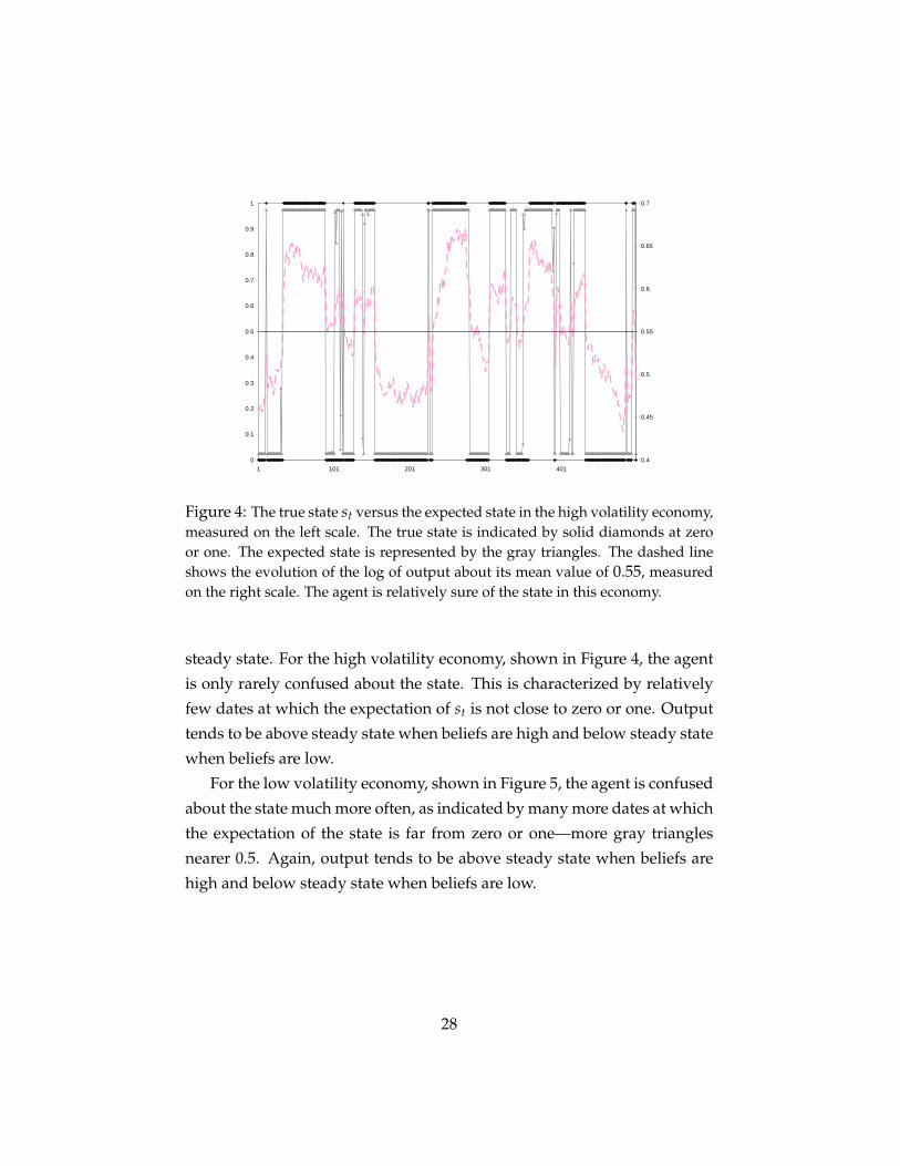
Figure 4: The true state st versus the expected state in the high volatility economy,measured on the left scale. The true state is indicated by solid diamonds at zeroor one. The expected state is represented by the gray triangles. The dashed lineshows the evolution of the log of output about its mean value of 0.55, measuredon the right scale. The agent is relatively sure of the state in this economy.

steady state. For the high volatility economy, shown in Figure 4, the agent

is only rarely confused about the state. This is characterized by relatively

few dates at which the expectation of st is not close to zero or one. Output

tends to be above steady state when beliefs are high and below steady state

when beliefs are low.

For the low volatility economy, shown in Figure 5, the agent is confused

about the state much more often, as indicated by many more dates at which

the expectation of the state is far from zero or one—more gray triangles

nearer 0.5. Again, output tends to be above steady state when beliefs are

high and below steady state when beliefs are low.

28

0

0.1

0.2

0.3

0.4

0.5

0.6

0.7

0.8

0.9

1

1 101 201 301 4010.4

0.45

0.5

0.55

0.6

0.65

0.7

Figure 5: The true state versus the expected state in the low volatility economy,along with the evolution of log output about its steady state value. The agent isrelatively confused about the true state, causing moderated behavior.

3.6 A surprise

Confusion about the latent state st leads to some surprising behavior which

we did not expect to find. This behavior is illustrated in Figure 5. In par-

ticular, the agent sometimes believes in recession or expansion states when

in fact the opposite is true. This occurs, for instance, in the time period

around t = 250 in this simulation. Here the true state is low, but the agent

believes the state is high. Interestingly, output remains above steady state

for this entire period. The beliefs are driving the consumption, investment,

and labor supply behavior of the agent in the economy, such that belief in

the high regime is causing output to boom.

How does this belief-driven behavior come about? At the end of each

period, agents can observe labor, capital, and output and therefore can in-

fer a value for zt. Let’s suppose the agent observes a high level of labor

input and a high level of output. The agent may infer that the current la-

tent state st is high and construct next period’s expectation of the level of

29

technology based on the expectation that st+1 is also likely to be high (since

the latent state is very persistent). But the high level of labor input may also

itself have been due to an expectation of a high level of technology in the

past period. The agent may therefore propagate the expectation of a high

state forward. Labor input in the current period would then again be high,

output would again be high, and the agent may again infer that the state

st is high and construct next period’s expectation of the level of technology

based on the expectation that st is high. In this way beliefs can influence the

equilibrium of the economy, and this effect is more pronounced as regimes

move closer together.

Another way to gain intuition for the nature of the belief-driven behav-

ior is to consider equation (30), which is derived earlier and reproduced

here:

zet+1 = f (ze

t , zt) . (41)

The expected level of technology is a state variable in this system. The agent

is able to calculate a value for zt at the end of each period after production

has occurred based on observed values of yt, kt, and `t, and this provides

an input, but not the only input, into the next period’s expected level of

technology. This is because the decisions taken today that produced today’s

output depend in part on the belief that was in place at the beginning of

the period, zet . The true state is not fully revealed by the zt calculated at the

end of the period. Nevertheless, when regimes are far apart, the evidence

is fairly clear regarding which state the economy is in and so zt provides

most of the information needed to form an accurate expectation zet+1. When

regimes are closer together, zt is not nearly as informative and the previous

expectation zet can play a large role in shaping ze

t+1.

4 Conclusions

We have investigated the idea that learning may have contributed to the

great moderation in a stylized regime-switching economy. The main point

is that direct econometric estimates may overstate the degree of “good

30

luck” or moderation in the shock processes driving the economy. This is

because the changes in the nature of the shock process with incomplete in-

formation can also change private sector behavior and hence the nature of

the equilibrium. Our complete information model has provided a bench-

mark in which it is well known that equilibrium volatility is linear in the

volatility of the shock process, such that doubling the volatility of the shock

process will double the equilibrium volatility of the endogenous variables.

Against this background, we have demonstrated that learning introduced

a pronounced nonlinear effect, in which private sector behavior changes

markedly in response to a changed stochastic driving process for the econ-

omy with incomplete information. We have found, in a benchmark calcu-

lation, that such an effect can account for about 30 percent of a change in

observed volatility. We think this is substantial and is worth investigating

in more elaborate models that can confront the data on more dimensions.

References

[1] Ahmed, S., A. Levin and B. Wilson. 2004. “Recent U.S. Macroeconomic

Stability: Good Luck, Good Policies, or Good Practices?” Review ofEconomics and Statistics 86(3): 824-32.

[2] Andolfatto, D. and P. Gomme. 2003. “Monetary Policy Regimes and

Beliefs.” International Economic Review 44: 1-30.

[3] Arias, A., G. Hansen, and L. Ohanian. 2006. “Why Have Business Cy-

cle Fluctuations Become Less Volatile?” NBER Working Paper #12079.

[4] Aruoba, S.B., J. Fernandez-Villaverde, and J.F. Rubio-Ramirez. 2006.

“Comparing Solution Methods for Dynamic Equilibrium Economies.”

Journal of Economic Dynamics and Control, 30(12): 2477-2508.

[5] Burns, A. 1960. “Progress Towards Economic Stability.” American Eco-nomic Review 50(1).

31

[6] Cagetti, M., L. Hansen, T. Sargent and N. Williams. 2002. “Robustness

and Pricing with Uncertain Growth.” Review of Financial Studies 15(2):

363-404.

[7] Campbell, S. 2007. “Macroeconomic Volatility, Predictability, and Un-

certainty in the Great Moderation: Evidence from the Survey of Pro-

fessional Forecasters.” Journal of Business and Economic Statistics 25(2):

191-200.

[8] Clarida, R., J. Gali, and M. Gertler. 2000. “Monetary Policy Rules and

Macroeconomic Stability: Evidence and Some Theory.” Quarterly Jour-nal of Economics, February, 147-180.

[9] Evans, G., and S. Honkapohja. 2001. Learning and Expectations in Macro-economics. Princeton University Press.

[10] Fernandez-Villaverde, J., and J. Rubio-Ramirez. 2007. “Estimating

Macroeconomic Models: A Likelihood Approach.” Review of EconomicStudies, forthcoming.

[11] Hamilton, J. 1989. “A New Approach to the Economic Analysis

of Nonstationary Time Series and the Business Cycle.” Econometrica57(2): 357-384.

[12] Justiniano, A., and G. Primiceri. 2006. “The Time-Varying Volatility of

Macroeconomic Fluctuations.” NBER Working Paper #12022.

[13] Kahn, J., M. McConnell, and G. Perez-Quiros. 2002. “The Reduced

Volatility of the U.S. Economy: Policy or Progress?” Manuscript, FRB-

New York.

[14] Kim, C.-J., and C. Nelson. 1999a. “Has the U.S. Economy become more

Stable? A Bayesian Approach Based on a Markov-Switching Model of

the Business Cycle.” The Review of Economics and Statistics 81(4): 608-

616.

32

[15] Kim, C.-J., and C. Nelson. 1999b. State Space Models with Regime Switch-ing. MIT Press, Cambridge, MA.

[16] Kim, C.-J., C. Nelson, and J. Piger. 2004. “The Less-Volatile U.S. Econ-

omy: A Bayesian Investigation of Timing, Breadth, and Potential Ex-

planations.” Journal of Business and Economic Statistics 22(1): 80-93.

[17] McConnell, M., and G. Perez-Quiros. 2000. “Output Fluctuations in

the United States: What Has Changed Since the Early 1980s?” Ameri-can Economic Review 90(5): 1464-1476.

[18] Milani, F. 2007. “Learning and Time-Varying Macroeconomic Volatil-

ity.” Manuscript, UC-Irvine.

[19] Moore, G.H. and V. Zarnowitz. 1986. “The Development and Role of

the NBER’s Business Cycle Chronologies.” In: Robert J. Gordon, ed.,

The American Business Cycle: Continuity and Change. Chicago: Univer-

sity of Chicago Press.

[20] Owyang, M., J. Piger, and H. Wall. 2007. “A State-Level Analysis of the

Great Moderation.” Working paper 2007-003B, Federal Reserve Bank

of St. Louis.

[21] Primiceri, G. 2005. “Time-Varying Structural Vector Autoregressions

and Monetary Policy.” Review of Economic Studies 72(3): 821-852.

[22] Van Nieuwerburgh, S. and L. Veldkamp. 2006. “Learning Asymme-

tries in Real Business Cycles.” Journal of Monetary Economics 53(4): 753-

772.

[23] Sims, C., and T. Zha. 2006. “Were There Regime Switches in U.S. Mon-

etary Policy?” American Economic Review 96(1): 54-81.

[24] Stock, J., and M. Watson. 2003. “Has the Business Cycle Changed and

Why?” NBER Macroeconomics Annual 2002 17: 159-218.

33