Learning and Discovery in Dynamical Systems with Hidden State

Milena Scaccia

Supervised by Prakash Panangaden, Joelle Pineau, and Doina Precup

August 15, 2007

Abstract

We consider the problem of learning in dynamical systems with hidden state. This problem is deemedchallenging due to the fact that the state is not completely visible to an outside observer. We explore acandidate algorithm, which we call the Merge-Split algorithm, for learning deterministic automata withobservations. This is based on the work of Gavalda et al(2006) which approximates a given HiddenMarkov Model (HMM) with a learned Probabilistic Deterministic Finite Automaton (PDFA).

1 Introduction

Learning and planning under uncertainty is one of the main aspects of modern AI research. This problemhas a considerable application in the field of robotics since robots must cope with environments that arepartially observable, stochastic, dynamic and continuous. In order for a robot to reason correctly about itsenvironment, it must be provided with a good internal representation of it. Learning the internal representa-tion of a partially observable system is deemed difficult due to the state being hidden to an outside observer.Instead, there are observables that partly identify the state. From information we are able to retrieve, giventhe observables, we want to learn a model that approximates the partially observable system and that willenable us to make good predictions on future action effects.

A good representation should contain enough information for the robot to make the right decisions and itsinternal state variables should correspond to the natural state variables of the physical world. In the AIliterature, there is much discussion about choosing a good state representation to work with. In robotics,for example, standard notions are the x,y position of a robot at any given time, or the angle of its joints(in the case of an arm robot). This choice of representation is not something that is set in stone, but it iswondered whether the obvious choice is always the best choice.

The problem of learning a good internal representation has received a lot of attention in recent research butcurrent solutions are suboptimal. This paper presents an attempt to find an algorithm that constructs anautomaton that best represents data generated by a partially observable system.

We explore a candidate algorithm, which we call the Merge-Split algorithm, for learning deterministic au-tomata with observations. This is based on Gavalda’s et al.’s GKPP algorithm(2006) which approximates aHidden Markov Model (HMM) with a Probabilistic Deterministic Finite Automaton (PDFA).

We demonstrate how the algorithm works with different inputs and explore the limitations of the algorithmas well as the advantages it may have over other learning algorithms. For now, we only consider the Merge-Split algorithm in the deterministic case, but we are primarily interested in finding a solution for inferringhidden state in probabilistic environments such as Partially Observable Probabilistic Automata (POPA).We wish to extend Merge-Split to work in such stochastic environments. This will better apply to real-worldproblems since the real world is essentially a probabilistic environment.

1

2 Background

In this section, we review the definitions of various types of partially observable systems.

2.1 Partially Observable Systems

We use the flip automaton in Mealy form [2] to illustrate three types of partially observable systems: De-terministic Kripke Automata (DKA), Deterministic Automata with Stochastic Observations (DASOs), andPartially Observable Probabilistic Automata (POPAs).

Definition 2.1 A deterministic Kripke automaton (DKA) is a quintuple

K = {S,A,O, δ : S × A → S, γ : S → 2O}.

where S is a set of states, A is a set of actions, O is a set of observations, δ is a deterministic transitionfunction and γ is an deterministic observation function associated with the states.

Figure 1: Deterministic Kripke Flip Automaton

Definition 2.2 A deterministic automaton with stochastic observations (DASO) is a quintuple

J = (S,A,O, δ : S × A → S, γ : S × O → [0, 1])

where S is a set of states, A is a set of actions, O is a set of observations, δ is a deterministic transitionfunction and γ is an observation function such that γ(s, ω) is the probability of observing ω in state s.

Figure 2: Deterministic Flip Automaton with Stochastic Observations

2

Definition 2.3 A partially observable probabilistic automaton (POPA) is a quintuple

H = (S,A,O, τ : S × A × S → [0, 1], γ : S × O → [0, 1])

where S is a set of states, A is a set of actions, O is a set of observations, τ(s, a, ·) defines a probabilitydistribution on possible final states and γ(s, ω) is the probability of observing ω in state s.

Figure 3: Partially Observable Probabilistic Flip Automaton

Most of the work we have done revolved around the DKA, but we wish to extend results to probabilisticsystems such as DASOs and POPAs since the real world is essentially a probabilistic world.

2.2 HMMs and PDFAs

In this section, we define two systems used in the GKPP algorithm. Recall that the GKPP algorithm learnsa Probabilistic Deterministic Finite Automaton that can approximate a Hidden Markov Model.

Definition 2.4 A Probabilistic Deterministic Finite Automaton (PDFA) is a tuple (S,Σ, T,O, s0)where S is a finite set of states, Σ is a finite set of observations, T : S × Σ → S is the transition function,O : S × Σ → [0, 1] defines the emission probability of each observation on each state, O(s, σ) = P (σt =σ|st = s) and so ∈ S is the initial state. Note that we do not work with actions, but only with observationsin PDFAs. Observations are what allow for transitions from one state to the other. Once an observationhad been selected, the transition to a new state, s′, is deterministic and given by T (s, σ).

In a probabilistic nondeterministic finite automaton(PNFA), the transition function is stochastic:T : S × σ × S → [0, 1], and T (s, σ, s′) = P (st+1 = s′|st = s, σt = σ).

In both PDFAs and PNFAs, a special symbol marks the end of a string.

Definition 2.5 A Hidden Markov Model (HMM) is a tuple (S,Σ, T,O, b0) where S is a finite setof states, Σ is a finite set of observations, T (s, s′) = P (st+1 = s′|st = s) is the transition probability,O(s, σ) = P (σt = σ|st = s) is the emission probability of each observation on each state, and finally,b0(s) = P (s0 = s) is the initial state distribution. Given an observation trajectory σ1, ...σk, emitted bya known HMM, we can recursively estimate the probability distribution over states at any time bt+1, byBayesian updating as follows: bt+1(s) =

∑s′∈S bt(s

′)O(s′, σt)t(s′, s).

In the paper PAC-Learning of Markov Models with Hidden State, Gavalda et al. demonstrated that everyHMM can be transformed into an equivalent PNFA which can in turn be approximated by a PDFA. (Notethat all the systems are finite.) This shows that finite-size approximation of an HMM by a PDFA is alwayspossible. This can be used in the context of PAC-learning where the goal of learning is to find a model thatapproximates the true probability distribution over observation trajectories.

3

Ron at al.(2005) proposed that PAC-learning of PDFAs is possible if we restrict to the class of PDFAs thatare acyclic and have distinguishability criterion between states.

Definition 2.6 A PDFA has distinguishability µ if for any two states s and s′, the probability distributionsover observation trajectories starting at s and s′, Ps and Ps′ , differ by at least µ : m(Ps,Ps′) ≥ µ,∀s, s′ ∈ S,where m is a measure of the difference between two probability distributions.

3 GKPP Algorithm

Given sequences of observations, σ1, ...σn. the GKPP algorithm constructs an automaton which can generatethis data with high probability. The algorithm maintains a list of “safe states” and “candidate states”, thesafe states being states we decide to include in the graph constructed.

Let D denote the set of training trajectories (sequences of observations). The algorithm works as fol-lows:

It takes as input the parameters δ, n and µ, where δ is the desired confidence, n is the upper bound on thenumber of states desired in the model, and µ is a lower bound on the distinguishability between any twostates.

We begin by initializing a single safe state S = {s0} representing the initial state of the target machine. Wealso initialize a set of candidate states s0σ ∀σ ∈ Σ. Also, a multiset Ds, or Dsσ is associated with each safeand candidate state, respectively. The multiset of a state will contain the suffixes of all training trajectoriesthat pass through it.

For each sequence of observations, d = σ0, ...σk, we traverse the graph by matching each observation to astate until we reach a candidate state sσ or until we have exhausted all observations in d, in which case weproceed to the next sequence of observations. Note that in the case where we find a candidate state sσi

(which occurs when all transitions up to σi−1 lead to a safe state s and there is no transition out of s withobservation σi), we add the sub-trajectory {σi+1, ...σk} to the multiset Dsσi

.

In the induction step, the algorithm will either:

1. Promote a candidate state to a safe state• if the training data suggests that there is a significant difference between the probability distributionover trajectories observed from the candidate state and any safe state, then the candidate state willbe promoted.

2. Merge a candidate state with an existing safe state• If there is not a significant difference between the probability distributions over trajectories observedfrom the candidate state and a safe state, then the candidate state will be merged with the existingsafe state.

3. Retain it as a candidate state.• If there is not enough information to decide, then we retain the state as a candidate state.

The algorithm first judges whether there is enough information to promote or merge a candidate statecorrectly. A candidate state will not be retained when it is declared large.

Definition 3.1 A candidate state sσ is declared large when:

|Dsσ| ≥3(1 + µ/4)

(µ/4)ln

2

δ′(2)

where δ′ = δµ2(n|Σ|+2)

4

This is what we call the largeness condition.

Let |Ds(σ)| denote the number of trajectories starting with observation σ in multiset Ds and note that|Ds(σ)|/|Ds| can be regarded as an empirical approximation of the probability that trajectory d will beobserved starting from state s.

If the candidate state is not retained, and if there exists a safe state s′ such that for every trajectory d,

||Dsσ(d)|

|Dsσ|−

|Ds′(d)|

Ds′

| ≤ µ/2, (3)

then we merge sσ and s′. In this case, candidate state sσ is removed and a σ transition from s tos′ is added.In addition, |Ds(d)| is increased by |Dsσ(d)|.

On the other hand, if for every s′, there exists a d such that

||Dsσ(d)|

|Dsσ|−

|Ds′(d)|

|Ds′ || > µ/2 (4),

then sσ is promoted to a new safe state. In this case, we add a σ transition from s to sσ, and add candidatestates sσσ′ for every observation σ′ ∈ Σ. All trajectories in Dsσ are distributed appropriately to the newcandidate states.

The final step of the algorithm entails transforming the constructed graph into a PDFA. Every safe statewill become a state of the automaton, the set of observations Σ remains the same, and the probabilisticobservation function is computed as follows:

O(s, σ) =|Ds′(σ)|

∑σ′∈Σ |Ds(σ′)|

(1 − (|Σ| + 1)γ) + γ, (5)

where γ < 1|Σ|+1 .

Finally, we take care of any remaining candidate state sσ by looking for a safe state s′ that is the mostsimilar to it, add a σ transition from s to s′ (the transition function is T (s, σ) = sσ), and we compute theobservation probability as defined above.

The resulting automaton will be a PDFA that can be used to approximately compute the probabilities ofdifferent trajectories in the HMM.

4 The Merge-Split Algorithm

The Merge-Split algorithm is a derivation of the GKPP algorithm. It uses the same concept as GKPP: ituses both state splitting and merging operations. Unlike GKPP, it works with observations and actions,and it works in deterministic environments. It does not consider the distinguishability parameter, which isspecific to a probability distribution.

The basic idea of the Merge-Split algorithm is as follows:• Two nodes are merged is their sets of possible future transitions are identical• If a node cannot be merged with any other existing node, it will be further expanded (split).

5

4.1 Flip Automaton Example

We revisit the flip automaton which we use to demonstrate a step-by-step sample run of the Merge-Splitalgorithm.

Flip Automaton (as seen in Figure 1)

Step 1: The Merge-Split algorithm begins by initializing a single null state, from which one is allowed totake any action/observation sequence. (Note that the set of numbers next to a node in the graph indicatethe possible states we can be in at this point. In this case we can be in either state 1 or state 2, since thenull node indicates no actions were taken yet).

Figure 4: Step 1 of the Merge-Split Algorithm initializes a single null state

6

Step 2: For every possible transition, create a child node.

Figure 5: Merge-Split creates a child node for every possible transition from the null state.

Step 3: Merge nodes whose sets of future possible transitions are identical. For example, taking an L0 actionis the same as taking an L1 action. Both actions will take us to state 1. The future trajectories of nodes L0and L1 will thus be identical, so the two nodes are merged.

Figure 6: Merge-Split merges redundant nodes

Step 4: Nodes that did not get merged with other existing nodes will be expanded an additional step.

7

Figure 7: Merge-Split expands nodes which did not previously get merged

Step 5: The following is the final automaton learned by the Merge-Split algorithm.

Figure 8: Merge-Split merges redundant nodes (as in Figure 6)

We can clean up our diagram of the learned automaton by removing crossed out nodes and adding appropriatelabels and transition arrows to the remaining nodes:

8

Figure 9: The final automaton learned by the Merge-Split algorithm w.r.t. the Flip Automaton

The resulting automaton closely resembles the original machine, and allows us to correctly predict futureaction effects!

4.2 Additional Examples

While Merge-Split learned a model that closely resembled the original machine in the flip-automaton, thereexist examples where Merge-Split may learn a model that resembles the minimal representation of the originalmachine.

The following is a 6-state DKA [3], in Mealy form.

9

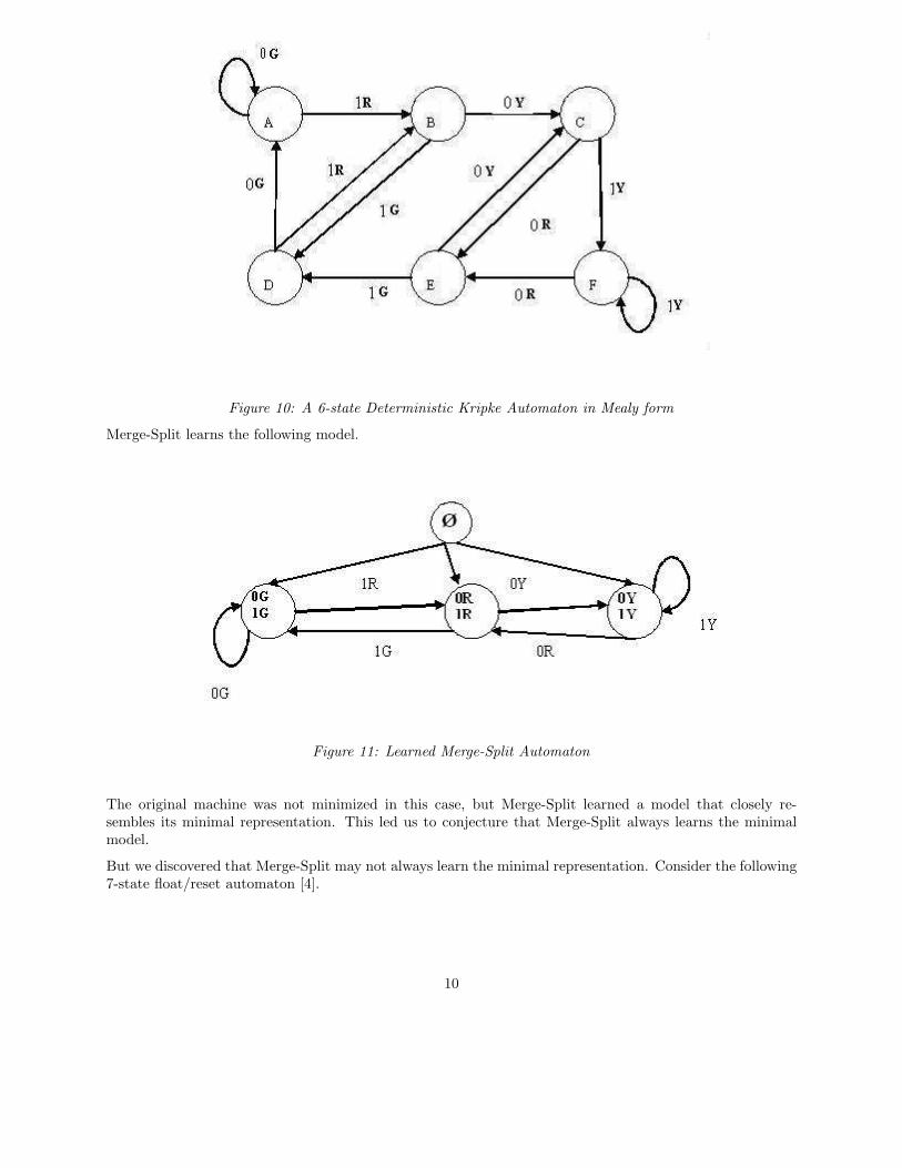
Figure 10: A 6-state Deterministic Kripke Automaton in Mealy form

Merge-Split learns the following model.

Figure 11: Learned Merge-Split Automaton

The original machine was not minimized in this case, but Merge-Split learned a model that closely re-sembles its minimal representation. This led us to conjecture that Merge-Split always learns the minimalmodel.

But we discovered that Merge-Split may not always learn the minimal representation. Consider the following7-state float/reset automaton [4].

10

Figure 12: 7-state Float/Reset Automaton

The Merge-Split algorithm will learn a 28-state model, which is well over the number of states in the originalautomaton.

11

Figure 13: The Merge-Split Learned Automaton w.r.t. the 7-state Float-Reset Automaton

Merge-Split works by looking at the set of future transitions of a node. The reason the algorithm repeatedlyexpands nodes in the float/reset case is because it identifies differences in the futures of the nodes. Forinstance, starting from the B0 node, if we look at a 5-step extension of the node, i.e. B0B0B0B0B0B0,wenote that our future possible transitions are {B0, A1, C0}, whereas up to a 4-step extension will give us thetransition set {B0, A0, A1, C0}. Hence we cannot merge B0B0, B0B0B0, B0B0B0B0, or B0B0B0B0B0 withthe node B0, because this would not reflect the difference in future transitions encountered.

12

4.3 Deterministic Case vs. Stochastic Case

There are several differences in the difficulties that may arise when learning the structure of a deterministicsystem versus that of a probabilistic system. In fact, there is much discussion devoted to which of the twocases is more difficult to handle. Intuitively, one would gather that it is easier to deal with the deterministiccase, but the following demonstrates why it may be quite challenging.

What is particular about the deterministic case is that we cannot assign distributions to the transitions, andwe cannot determine with what probability the machine can satisfy an experiment. We can only determinewhat transitions are possible.

Figure 14 illustrates the challenges faced when learning the structure of a deterministic system. If the currentdata suggests that our model should satisfy the sequences a1, b0a1 and b0b0a1, then at this point, we donot know whether we should create additional states to satisfy the data, or whether our model should loopon action b0 (i.e. merge the nodes that satisfy b0). Both looping and non-looping models fit the currentdata.

Learning the structure of a deterministic transition system involves more than producing a model that merelymemorizes the current data (as in Figure 14(b)). A model that merely memorizes what was seen so far willbe “shafted” by any longer sequence. Notice that the model in Figure 14(b) will require modifications if thedata suggests that the sequence b0b0b0a1 should also be satisfied. This is why it is a good idea to generalizethe model.

(a) Simple two-state model

(b) A model that memorizes the data

Figure 14: Models (a) and (b) both satisfy a1, b0a1, b0b0a1, but (a) can satisfy b0b0b0a1, while (b) cannot.

Our Merge-Split algorithm overcomes this difficulty by exploring the sets of all possible future transitions ofeach node. In the Float-Reset automaton example (Figure 12), Merge-Split was able to recognize that thelearned model (Figure 13) should not merge all the nodes satisfying B0. It was able to detect a differencebetween the 4th and 5th-step extensions of the B0 node.

13

Given that Merge-Split works efficiently in the deterministic case, we aim to extend it to the stochastic caseand hope for comparable results.

GKPP can in a certain sense be thought of as the probabilistic version of Merge-Split. Unlike GKPP,Merge-Split works with transition systems consisting of actions and observations whereas GKPP works forHMMs, in which case we do not have actions but only observations that account for transitions betweenstates. We want to generalize GKPP to work for the case of actions in order to be able to infer hidden statein probabilistic environments such as POPAs.

To extend the Merge-Split algorithm to the stochastic case, we must reintroduce the largeness conditionand the distinguishability parameter in order to determine if there is a significant difference between theprobability distributions over trajectories observed from any two states. The trajectories will now consistof both actions and observations, hence it is necessary to adjust the largeness condition to take actions intoconsideration. This was not yet worked on, but we do not expect it to be a difficult task.

5 Future Work

Although our Merge-Split algorithm allows us to correctly predict future action effects in deterministicenvironments, the constructed automaton is not minimal. We wish to refine Merge-Split so that it learns theminimal representation of a given partially observable system. We want to do this in order to connect it withthe notion of the double-dual representation [3]. The double-dual representation is the minimal version ofthe original machine with deterministic transition structure and no hidden state. Its states can be thought ofas “bundles” of predictions for experiments, making this representation hold the promise of better learningand planning algorithms.

As described, we also aim to extend the Merge-Split algorithm to work in probabilistic environments in orderto better apply it to real-world problems. Achieving these goals will bring us a step closer to reaching ourlong-term goal of finding an algorithm that learns the most succinct automaton consistent with the dataproduced by a partially observable system.

6 References

[1] R.Gavalda, P.Keller, J.Pineau, D.Precup. “PAC-Learning of Markov Models with Hidden State” In Pro-ceedings of ECML, 2006.

[2] M.P.Holmes, C.L.Isbell. “Looping Suffix Tree-Based Inference of Partially Observable Hidden State”. InProceedings of ICML, 2006.

[3]C.Hundt, P.Panangaden, J.Pineau, D.Precup, M.Dinculescu. “Duality of State and Observations”. Re-search supported by NSERC and CFI, 2006.

[4] M.L.Littman, R.S. Sutton, S.Singh. “Predictive Representations of State”. AT&T Labs–Research,2001.

14