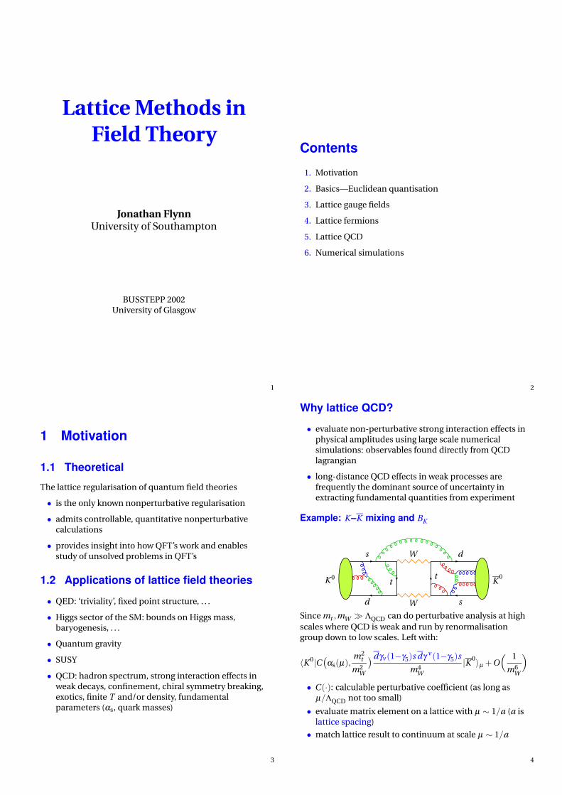
Lattice Methods in

Field Theory

Jonathan FlynnUniversity of Southampton

BUSSTEPP 2002University of Glasgow

1

Contents1. Motivation

2. Basics—Euclidean quantisation

3. Lattice gauge fields

4. Lattice fermions

5. Lattice QCD

6. Numerical simulations

2

1 Motivation

1.1 TheoreticalThe lattice regularisation of quantum field theories

• is the only known nonperturbative regularisation

• admits controllable, quantitative nonperturbativecalculations

• provides insight into how QFT’s work and enablesstudy of unsolved problems in QFT’s

1.2 Applications of lattice field theories• QED: ‘triviality’, fixed point structure, . . .

• Higgs sector of the SM: bounds on Higgs mass,baryogenesis, . . .

• Quantum gravity

• SUSY

• QCD: hadron spectrum, strong interaction effects inweak decays, confinement, chiral symmetry breaking,exotics, finite T and/or density, fundamentalparameters (αs, quark masses)

3

Why lattice QCD?• evaluate non-perturbative strong interaction effects in

physical amplitudes using large scale numericalsimulations: observables found directly from QCDlagrangian

• long-distance QCD effects in weak processes arefrequently the dominant source of uncertainty inextracting fundamental quantities from experiment

Example: K –K mixing and BK

K 0K

0

W

W

d

s

s

d

tt

Since mt ,mW ΛQCD can do perturbative analysis at high

scales where QCD is weak and run by renormalisationgroup down to low scales. Left with:

〈K 0|C(

αs(µ),m2

t

m2W

)dγν (1−γ5)s dγ ν (1−γ5)s

m4W

|K 0〉µ +O

( 1

m6W

)

• C (·): calculable perturbative coefficient (as long asµ/ΛQCD not too small)

• evaluate matrix element on a lattice with µ ∼ 1/a (a islattice spacing)

• match lattice result to continuum at scale µ ∼ 1/a

4

CKM matrix and unitarity triangle(

Vud Vus VubVcd Vcs VcbVt d Vt s Vt b

)

=

(

1−λ2/2 λ Aλ3(ρ − i η)

−λ 1−λ2/2 Aλ2

Aλ3(1−ρ − i η) −Aλ2 1

)

+ O(λ4)

Unitarity: VudV ∗ub +VcdV ∗cb +Vt dV ∗t b = 0

VudV ∗ub = Aλ3(ρ + i η)+ O(λ7)

VcdV ∗cb = −Aλ3 + O(λ7)

Vt dV ∗t b = Aλ3(1−ρ− i η)+ O(λ7)

where ρ = ρ(1−λ2/2) and η = η(1−λ2/2).

(0,0) (1,0)

(ρ,η)

ρ + i η 1−ρ − i η

γ β

α

5

Unitarity triangle

VudV ∗ub +VcdV ∗cb +Vt dV ∗t b = 0

0

0.2

0.4

0.6

0.8

1

-1 -0.5 0 0.5 1

sin 2βWA

∆md∆ms & ∆md

|εK|

|εK|

|Vub/Vcb|

ρ

η

C K Mf i t t e r

Measurement VCKM×other Constraint

b→ u

b→ c

∣

∣

∣

∣

Vub

Vcb

∣

∣

∣

∣

2

ρ2 + η2

∆Md |Vt d |2 f 2

Bd

BBdf (mt ) (1−ρ)2 + η2

∆Md

∆Ms

∣

∣

∣

∣

Vt d

Vt s

∣

∣

∣

∣

2 f 2Bd

BBd

f 2Bs

BBs

(1−ρ)2 + η2

εK f (A,η,ρ,BK ) ∝ η(1−ρ)

(CKMfitter Spring 2002: H Hocker et al, hep-ph/0104062;

http://ckmfitter.in2p3.fr/)

6

. . . with sin 2β from BaBar and Belle, Standard Model is ingood shape. Errors in the nonperturbative parameters arenow the limiting factor in more precise testing to look foreffects from New Physics.

There is also a rich upcoming experimental programme inthe next few years which will need or test lattice results:

• B-factories: constraining unitarity triangle, rare decays

• Tevatron Run II: ∆MBs, ∆ΓBs

, b-hadron lifetimes, . . .

• CLEOc: leptonic and semileptonic D decays, masses ofquarkonia, hybrids, glueballs

• LHC: . . .

7

2 Basics: Euclidean quantisationLattice embedded in d-dimensional Euclidean spacetime

Las

Tat

at

as

as ,at lattice spacings

Las length in spatial dimension(s)

Tat length in temporal dimension

Matter fields live on lattice sites x . Example: scalar field

φ(x) withx j = nas , n = 0, . . . ,L−1

x0 = mat , m =, . . . ,T−1

8

2.1 Lattice as a regulatorFourier transform of a lattice scalar field in one dimension:x = na, n = 0, . . . ,L−1, with periodic boundary conditions:

φ(p) = aL−1

∑n=0

e−ipnaφ(x)

φ(x + La) = φ(x)

• discretisation implies

• φ(p) periodic with period 2π/a

• momenta lie in first Brillouin zone

−πa

< p ≤πa

• have introduced a momentum cutoff;

Λ =πa

• spatial periodicity implies momentum p quantised inunits of 2π/La

• gauge invariance and gauge fields, fermions: later

Lattice provides both UV and IR cutoffs. Ultimately wantinfinite volume (L,T →∞) and continuum (a → 0) limits.Most effort devoted to continuum limit.

9

2.2 Euclidean quantisation on the latticePath integral well-defined in Euclidean space

MinkowskiWick

rotationEuclidean

iε prescription avoids poles

Procedure1. Continuum classical Euclidean field theory

2. Discretisation−→ lattice action

3. Quantisation−→ functional integral

10

Step 1Euclidean fields φ(x) obtained formally from analyticcontinuation

t →−ix0, φ(x,t )→ φ(x)

Action:

SE [φ ] =

∫

d4x

1

2(∂µ φ)2 +V (φ)

where µ = 0,1,2,3 and

V (φ) =1

2m2φ 2 +

λ4!

φ 4

Minkowski ←→ Euclidean

Lorentz symmetry O(4) symmetry

t 2− x2 invariant (x 0)2 + x2 invariant

+

−−−

+

+

+

+

11

Step 2: DiscretisationIntroduce a hypercubic lattice ΛE with at = as = a.

ΛE =

x ∈ aZ4∣

∣

∣

x0

a= 0, . . . ,T−1;

x1,2,3

a= 0, . . . ,L−1

• L3T lattice sites

• finite volume

• finite number d.o.f.

Lattice action:

SE [φ ] = a4 ∑x∈ΛE

1

2∇µ φ(x)∇µφ(x)+V (φ)

with forward and backward lattice derivatives

∇µ φ(x) ≡1

a

(

φ(x+aµ)− φ(x))

∇∗µ φ(x) ≡1

a

(

φ(x)− φ(x−aµ))

Lattice Laplacian:

∆φ(x) ≡3

∑µ=0

(∇∗µ ∇µ)φ(x)

=1

a2

3

∑µ=0

(

φ(x+aµ)+ φ(x−aµ)− 2φ(x))

12

Lattice action for a free scalar field:

SE [φ ] = a4 ∑x∈ΛE

−1

2φ(x)∆φ(x)+V (φ)

Remarks• Discretisation is not unique. Can use different

definitions for ∇(∗)µ and/or V (φ) as long as they become

the same in the naive continuum limit, a → 0.

∗ Universality: discretisations fall into classes, eachmember of which has the same continuum limit

∗ Improvement: optimise choice of lattice action fora faster approach to the continuum limit

• O(4) (eventually Lorentz symmetry) is not preserved.Have cubic symmetry instead; recover O(4) symmetryas a→ 0.

13

Step 3: Quantisation—functional integral

ZE ≡∫

D [φ ]e−SE [φ ]

D [φ ] is the measure, eg:

D [φ ] = ∏x∈ΛE

dφ(x)

• finite number of integrations

Correlation functions

〈φ(x1) · · ·φ(xn)〉 ≡1

ZE

∫

D [φ ]φ(x1) · · ·φ(xn)e−SE [φ ]

• 〈·〉 is shorthand for 〈0|T · |0〉, time-ordered vacuumexpectation value

• well-defined if SE [φ ] > 0

• particle spectrum implicitly determined by correlationfunctions

• analytically continue to Minkowski space and getS-matrix elements (= physics) via LSZ

14

2.3 Generating functionalScalar product on space F of fields φ over ΛE :

(φ1,φ2) = a4 ∑x∈ΛE

φ1(x)φ2(x)

Action for free scalar field:

SE [φ ] =1

2(φ ,K φ), K = −∇∗µ ∇µ +m2

K is a linear operator on F .

Let J(x) be an external field (source) on ΛE , J ∈F , anddefine the generating functional W [J ] through,

eW [J ] ≡ 〈e(J ,φ)〉

=1

ZE

∫

∏x∈ΛE

dφ(x)e−SE [φ ]e(J ,φ)

Correlation functions found by differentiating w.r.t. J(x):

∂∂ J(x)

eW [J ] = a4〈φ(x)e(J ,φ)〉

∂ 2

∂ J(x1)∂ J(x2)eW [J ]

∣

∣

∣

∣

J=0

= (a4)2〈φ(x1)φ(x2)〉

15

Lattice propagatorRelation between W [J ] and K :

eW [J ] =1

ZE

∫

∏x∈ΛE

dφ(x)e−SE [φ ]e(J ,φ) = e12 (J ,K−1J)

Diagonalise K through Fourier transform:

J(p) = a4 ∑y∈ΛE

e−ip·y J(y ), J(x) =1

a4L3T∑

p∈Λ∗E

eip·x J(p)

Λ∗E is the dual lattice (or set of momentum points in theBrillouin zone):

Λ∗E =

p

∣

∣

∣p0 =

2πTa

n0, p1,2,3 =2πLa

n1,2,3;

n0 = 0, . . . ,T−1, n1,2,3 = 0, . . . ,L−1

aL

aL

aT

2π/a

2π/a

2π/a

ΛE Λ∗E

16

Propagator (continued)Find:

(K−1J)(x) = a4 ∑y∈ΛE

G(x − y )J(y )

G(x−y ) is the Green function for K :

G(x − y ) =1

a4L3T∑

p∈Λ∗E

eip·(x−y)

p2 +m2

with

p2 =3

∑µ=0

pµpµ , pµ =2

asin

(apµ

2

)

eW [J ] = exp

1

2a8 ∑

x ,y∈ΛE

J(x)G(x − y )J(y )

Therefore the propagator is:

〈φ(x)φ(y )〉=1

a8

∂ 2

∂ J(x)∂ J(y )eW [J ]

∣

∣

∣

∣

J=0

= G(x − y )

17

Remarks• As a→ 0 (and L,T →∞), G(x − y ) becomes the

Euclidean Feynman propagator:

G(x − y )a→0−→

∫

d4p

(2π)4

eip·(x−y)

p2 +m2

using p2 = p2 + O(a2).

• Particle masses defined through poles of the

propagator, here poles of (p2 +m2)−1, which isperiodic in each component of p with period 2π/a.

p2 =4

a2

3

∑µ=0

sin2(apµ

2

)

Unique mass spectrum inside first Brillouin zone,pµ ∈ (−π/a,π/a].

18

Free Scalar Two-point Correlator inPosition Space

C (x0) = a3 ∑x

〈φ(x0,x)φ(0)〉= a3 ∑x

G(x0,x)

• Create a particle at the origin; propagate it to anyspatial point at time x0

• ∑x · projects onto zero 3-momentum ( ∑x eip·x·wouldproject on momentum p).

• Can evaluate explicitly for free scalar field (exercise)

C (x0) =e−m|x0|

2m(1 +m2a2/4)1/2

with ‘physical mass’ (position of pole in propagator forp = 0) m, satisfying

sinh

(

am

2

)

=am

2

• Fitting exponential decay of a lattice 2-point functionlets you extract masses. Works more generally, seelater.

19

QCD LoreConfinement:

• gluons confine quarks and antiquarks into coloursinglets

qq qqq

mesons baryons

• gluons confine gluons into glueballs

• no free quarks or gluons as asymptotic states

Lattice QCD: a non-perturbative regulator which preservesgauge symmetry−→ allows us to study these questions

20

3 Nonabelian lattice gauge fieldsPerform steps 1–3 for Yang-Mills

Step 1Classical continuum Euclidean Yang-Mills action

SE [A] = −1

2g 20

∫

d4x Tr(

Fµν (x)Fµν(x))

g0 is the bare gauge coupling

SU (N) gauge fields in R4 (N colours):

Aµ (x) x ∈ R4, µ = 0, . . . ,3

Aµ = Aaµ T a Aµ ∈ su(N) (Lie algebra)

T a a = 1, . . . ,N 2− 1. Generators

Aaµ real vector field

[T a ,T b] = f abc T c Structure constants f abc

A†µ = −Aµ (antihermitian)

Dµ = ∂µ + Aµ

Field strength:

Fµν = ∂µ Aν − ∂ν Aµ +[Aµ ,Aν ]

Gauge transformations:

Aµ (x) → g (x)Aµ(x)g−1(x)+ g (x)∂µg−1(x)

Fµν → g (x)Fµν g−1(x)

21

Step 2: DiscretisationFor the discretised gauge field, Aµ (x), x ∈ ΛE , thetransformation law

Aµ (x)→ g (x)Aµ(x)g−1(x)+ g (x)∇µg−1(x)

is inconsistent with group multiplication for nonabeliangroups (Exercise).

• naive discretisation of classical Y-M action fails

• need a different concept to discretise pure gaugetheory

• use parallel transport on lattice

22

3.1 Defining lattice gauge fields

Continuum

x

y

C

Curve C from y to x parametrisedby:

z(t ), 0 ≤ t ≤ 1

z(0) = y, z(1) = x

Parallel transport along C :

d

dt+ z µ Aµ (z)

v(t ) = 0

Solution

v(1) = PO exp

−∫ x

ydz µ Aµ (z)

v(0)

Parallel transporter from y to x along C is,

U C(x ,y ) = PO exp

−∫ x

ydz µ Aµ (z)

Lattice

Choose C ’s connecting neighbouring lattice sites.

x x + aµ

U (x ,x + aµ) ≡Uµ (x) ∈ SU (N)

U (x + aµ ,x) = U−1(x ,x + aµ) = U−1µ (x)

23

Definition

A lattice gauge field is a set of SU (N) matrices Uµ(x),x ∈ ΛE , µ = 0,1,2,3. Uµ(x) is called a link variable.

Remarks

• Where is the gauge potential Aµ (x)? Can define alattice potential Aµ via

Uµ(x) = eaAµ (x)

but this is not unique. If Actmµ (x) is a given continuum

gauge potential, one can use a link variable toapproximate it for small a:

lima→0

1

a

(

Uµ (x)− 1)

= Actmµ (x)

• Gauge transformations on the lattice. Letg (x) ∈ SU (N) for x ∈ ΛE .

Uµ (x)→ g (x)Uµ(x)g−1(x + aµ)

By inspection, if C is a closed loop of link variablesthen

W (C ) = TrU C(x ,x)

is gauge-invariant. This is called a Wilson loop.

• Approximate locally gauge invariant continuum fieldsby gauge invariant combinations of link variables (seefollowing example . . . ).

24

Exercise

Tr(

F ctmµν (x)F ctm

µν (x))

F ctmµν is a field strength defined in terms of a given

continuum gauge potential Actmµ .

Consider the plaquette:

Pµν (x) ≡

x

x + aν x + aµ + aν

x + aµ

Show that

Tr Pµν (x) = Tr

Uµ(x)Uν (x+aµ)U−1µ (x+aν)U−1

ν (x)

a→0= N +

a4

2Tr(

F ctmµν (x)F ctm

µν (x))

+ O(a5)

25

3.2 Wilson plaquette actionReturn to Step 2: discretise the continuum action:

SE [A] = −1

2g 20

∫

d4x Tr(

Fµν (x)Fµν(x))

Consider

SE [U ] =1

g 20

∑x∈ΛE

∑µ,ν

Tr(

1−Pµν (x))

=1

g 20

∑x∈ΛE

∑µ,ν

(

−a4

2Tr(

Fµν (x)Fµν(x))

+ O(a5)

)

a→0→ −1

2g 20

∫

d4x Tr(

Fµν (x)Fµν(x))

Rewrite as

SE [U ] =N

g 20

∑x∈ΛE

∑µ,ν

µ<ν

(

2−1

NTr(Pµν + P †

µν )

)

=2N

g 20

∑x∈ΛE

∑µ,ν

µ<ν

(

1−1

NRe Tr Pµν (x)

)

= β ∑2

(

1−1

NRe Tr P

2

)

• ∑2

is sum over all oriented plaquettes

• β ≡2N

g 20

is the lattice coupling

• Last line is the Wilson plaquette action

26

SE [U ] =N

g 20

∑x∈ΛE

∑µ,ν

µ<ν

(

2−1

NTr(Pµν + P †

µν )

)

=2N

g 20

∑x∈ΛE

∑µ,ν

µ<ν

(

1−1

NRe Tr Pµν (x)

)

= β ∑2

(

1−1

NRe Tr P

2

)

• ∑2

is sum over all oriented plaquettes

• no Aµ fields: degrees of freedom are SU (3) matrices

• β ≡2N

g 20

is the lattice coupling

• Last line is the Wilson plaquette action

• not obligatory to use simple plaquette: all traces ofclosed Wilson loops are proportional to F ·F as a→ 0,allowing other choices for lattice gauge action

27

Step 3: QuantisationDefine a functional integral:

Z =

∫

D [U ]e−SE [U ] =

∫

∏x∈ΛE

3

∏µ=0

dUµ(x)e−SE [U ]

dUµ(x): invariant group measure for compact Lie group,eg SU (N)

Uµ (x)→U gµ (x) = g (x)Uµ(x)g−1(x + aµ)

dU gµ (x) = dUµ(x) so that D [U g ] = D [U ]

Measure can be normalised, since SU (N) compact:∫

SU (N)dU = 1

Not true for∫

dAµ , Aµ ∈ su(N)

• Functional integral well-defined: finite number ofvariables integrated over compact domain

• No gauge fixing required in lattice gauge theory (ingeneral: but becomes necessary if you want to do aperturbative evaluation of the integral because of zeromodes in the quadratic part of the action)

28

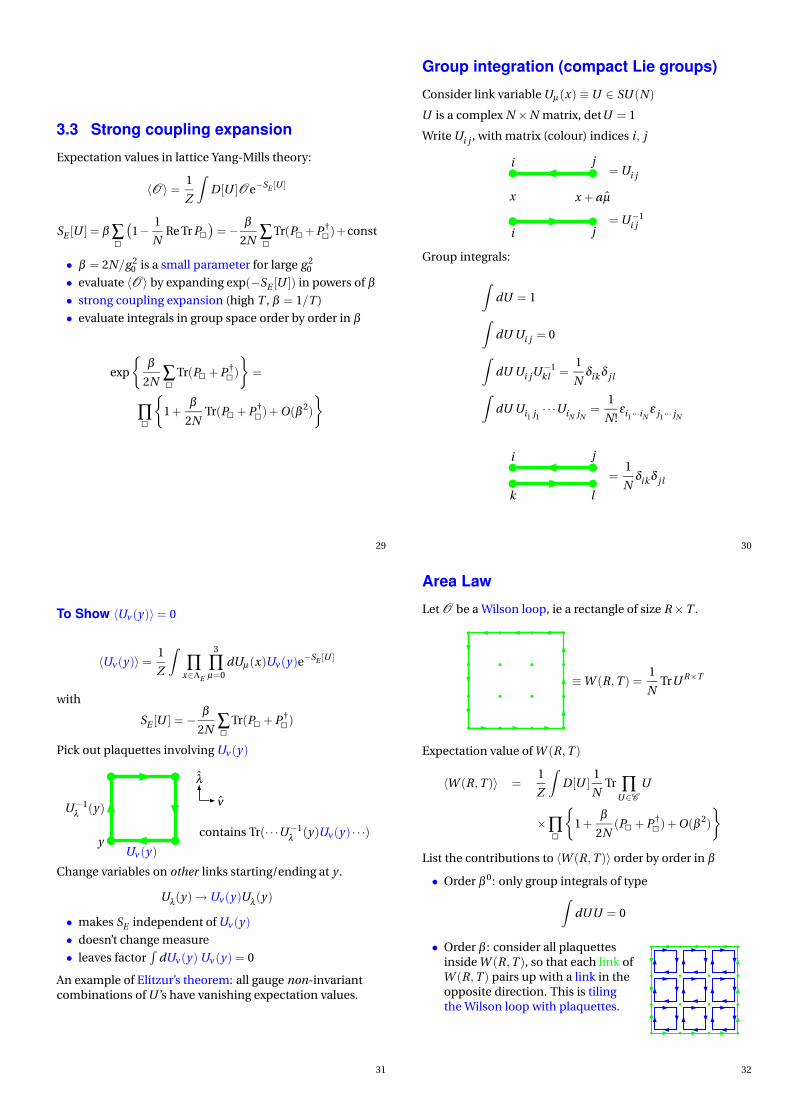
3.3 Strong coupling expansionExpectation values in lattice Yang-Mills theory:

〈O〉 =1

Z

∫

D [U ]Oe−SE [U ]

SE [U ] = β ∑2

(

1−1

NRe Tr P

2

)

=−β

2N∑2

Tr(P2

+P †2

)+const

• β = 2N/g 20 is a small parameter for large g 2

0

• evaluate 〈O〉 by expanding exp(−SE [U ]) in powers of β• strong coupling expansion (high T , β = 1/T )

• evaluate integrals in group space order by order in β

exp

β2N

∑2

Tr(P2

+ P †2

)

=

∏2

1 +β

2NTr(P

2+ P †

2)+ O(β 2)

29

Group integration (compact Lie groups)Consider link variable Uµ (x) ≡U ∈ SU (N)

U is a complex N ×N matrix, detU = 1

Write Ui j , with matrix (colour) indices i, j

x x + aµ

i

i

j

j

= Ui j

= U−1i j

Group integrals:

∫

dU = 1

∫

dU Ui j = 0

∫

dU Ui jU−1

kl =1

Nδik δ jl

∫

dU Ui1 j1· · ·UiN jN

=1

N !εi1···iN

ε j1··· jN

i

k

j

l

=1

Nδikδ jl

30

To Show 〈Uν (y )〉= 0

〈Uν (y )〉 =1

Z

∫

∏x∈ΛE

3

∏µ=0

dUµ(x)Uν(y )e−SE [U ]

with

SE [U ] = −β

2N∑2

Tr(P2

+ P †2

)

Pick out plaquettes involving Uν (y )

U−1λ (y )

yUν (y )

ν

λ

contains Tr(· · ·U−1λ (y )Uν(y ) · · ·)

Change variables on other links starting/ending at y .

Uλ(y )→Uν (y )Uλ(y )

• makes SE independent of Uν (y )

• doesn’t change measure

• leaves factor∫

dUν (y ) Uν (y ) = 0

An example of Elitzur’s theorem: all gauge non-invariantcombinations of U ’s have vanishing expectation values.

31

Area LawLet O be a Wilson loop, ie a rectangle of size R×T .

≡W (R,T ) =1

NTrU R×T

Expectation value of W (R,T )

〈W (R,T )〉 =1

Z

∫

D [U ]1

NTr ∏

U∈CU

×∏2

1 +β

2N(P

2+ P †

2)+ O(β 2)

List the contributions to 〈W (R,T )〉 order by order in β

• Order β 0: only group integrals of type∫

dUU = 0

• Order β : consider all plaquettesinside W (R,T ), so that each link ofW (R,T ) pairs up with a link in theopposite direction. This is tilingthe Wilson loop with plaquettes.

32

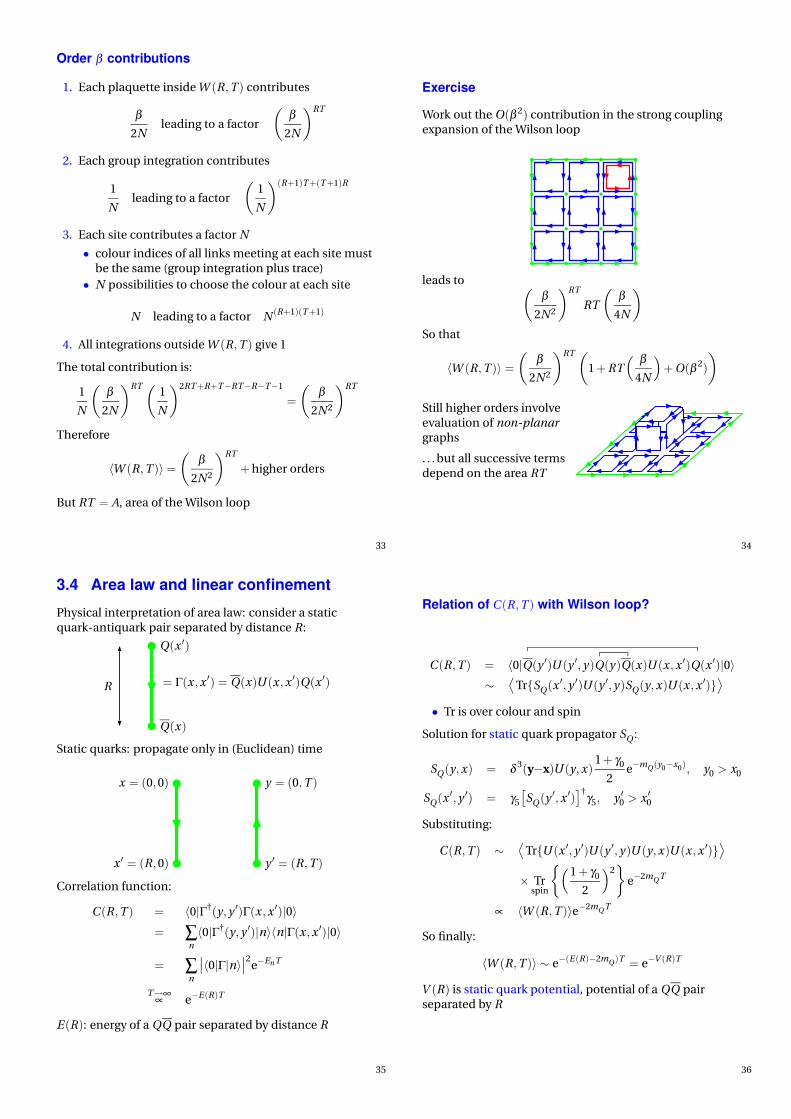
Order β contributions

1. Each plaquette inside W (R,T ) contributes

β2N

leading to a factor

(

β2N

)RT

2. Each group integration contributes

1

Nleading to a factor

(

1

N

)(R+1)T +(T +1)R

3. Each site contributes a factor N

• colour indices of all links meeting at each site mustbe the same (group integration plus trace)

• N possibilities to choose the colour at each site

N leading to a factor N (R+1)(T +1)

4. All integrations outside W (R,T ) give 1

The total contribution is:

1

N

(

β2N

)RT (1

N

)2RT +R+T−RT−R−T−1

=

(

β2N2

)RT

Therefore

〈W (R,T )〉 =(

β2N2

)RT

+ higher orders

But RT = A, area of the Wilson loop

33

Exercise

Work out the O(β 2) contribution in the strong couplingexpansion of the Wilson loop

leads to(

β2N2

)RT

RT

(

β4N

)

So that

〈W (R,T )〉 =(

β2N2

)RT (

1 + RT

( β4N

)

+ O(β 2)

)

Still higher orders involveevaluation of non-planargraphs

. . . but all successive termsdepend on the area RT

34

3.4 Area law and linear confinementPhysical interpretation of area law: consider a staticquark-antiquark pair separated by distance R:

R

Q(x ′)

Q(x)

= Γ(x ,x ′) = Q(x)U (x ,x ′)Q(x ′)

Static quarks: propagate only in (Euclidean) time

x ′ = (R,0)

x = (0,0)

y ′ = (R,T )

y = (0,T )

Correlation function:

C (R,T ) = 〈0|Γ†(y,y ′)Γ(x ,x ′)|0〉= ∑

n

〈0|Γ†(y,y ′)|n〉〈n|Γ(x ,x ′)|0〉

= ∑n

∣

∣〈0|Γ|n〉∣

∣

2e−EnT

T→∞∝ e−E(R)T

E (R): energy of a QQ pair separated by distance R

35

Relation of C (R,T ) with Wilson loop?

C (R,T ) = 〈0|Q(y ′)U (y ′,y )Q(y )Q(x)U (x ,x ′)Q(x ′)|0〉∼

⟨

TrSQ(x ′,y ′)U (y ′,y )SQ(y,x)U (x ,x ′)⟩

• Tr is over colour and spin

Solution for static quark propagator SQ :

SQ(y,x) = δ 3(y−x)U (y,x)1 + γ0

2e−mQ (y0−x0), y0 > x0

SQ(x ′,y ′) = γ5

[

SQ(y ′,x ′)]†γ5, y ′0 > x ′0

Substituting:

C (R,T ) ∼⟨

TrU (x ′,y ′)U (y ′,y )U (y,x)U (x ,x ′)⟩

× Trspin

(

1 + γ0

2

)2

e−2mQ T

∝ 〈W (R,T )〉e−2mQ T

So finally:

〈W (R,T )〉 ∼ e−(E(R)−2mQ)T = e−V (R)T

V (R) is static quark potential, potential of a QQ pairseparated by R

36

Linear confinement

Use strong coupling expansion for 〈W (R,T )〉 to computeV (R):

〈W (R,T )〉 =(

β2N2

)RT

= eln(β/2N2)RT

Write r = Ra, t = Ta

〈W (R,T )〉 = ea−2 ln(β/2N2)rt = e−V (r)t

V (r) = −a−2 ln(β/2N2)r ≡ σr

• area law implies linearly rising potential V (r)

• need infinite energy to separate Q and Q entirely

• linear confinement

• σ is called the string tension

Result suggestive: strong coupling is opposite ofcontinuum limit. Should supplement result withnumerical studies extrapolated to continuum limit toconfirm. Nonetheless, see a characteristic behaviour ofstrong-coupling gauge theories.

37

Static quark potential

• Strong coupling expansion yields V (r) ∼ σr

• Expect to see Coulomb part, V (r) ∼ 1/r , for small r

• General functional form of V (r):

V (r) = V0 + σr −e

rσ string tension

e ‘charge’

• Determine V (r) via numerical simulation by‘measuring’ Wilson loops (UKQCD hep-lat/0107021)

• e = π/12 in bosonic string model (Luscher 1981):confirmed numerically (Luscher and Weisz,

hep-lat/0207003)

0 1 2r/r0

−2.5

−1.5

−0.5

0.5

1.5

2.5

[V(r)

−V(r0

)]*r0

5.93 Quenched, 6235.29, c=1.92, k=0.134005.26, c=1.95, k=0.134505.20, c=2.02, k=0.135005.20, c=2.02, k=0.135505.20, c=2.02, k=0.13565 Model

38

3.5 Plaquette-plaquette correlationCorrelator of two plaquettes at same spatial position,different times. Smallest linking surface is a 1× 1 tubejoining the plaquettes

t

t1,x t2,x

〈Tr(U1)Tr(U2)〉 ∼ e−mt

with

m = −4 ln β + · · ·Dynamical mass generation in pure Yang-Mills (glueballmass)

39

4 Lattice Fermi fields

Step 1:Classical continuum Euclidean action for free fermions:

S[ψ ,ψ ] =

∫

d4x ψ(x)(γµ∂µ +m0)ψ(x)

ψ , ψ Grassmann valued

Recall in Minkowski spacetime: γ Mµ , γ M

ν = 2gµν . Now

define Euclidean Hermitian γ -matrices by:

γ0 = γ M0

γ j = −iγ Mj

so γµ , γν = 2δµν , γ †µ = γµ

Step 2: discretisation

S[ψ ,ψ ] = a4 ∑x∈ΛE

ψ(x)(

γµ1

2(∇µ + ∇∗µ)+m0

)

ψ(x)

= a4 ∑x∈ΛE

ψ(x)Qψ(x)

where

Q =1

2(∇µ + ∇∗µ)γµ +m0

is the ‘naive’ lattice Dirac operator

40

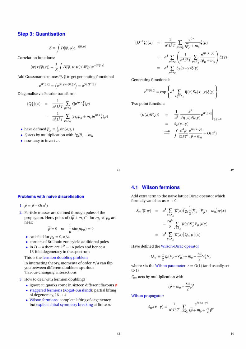
Step 3: Quantisation

Z ≡∫

D [ψ ,ψ ]e−S[ψ,ψ ]

Correlation functions:

〈ψ(x)ψ(y )〉=1

Z

∫

D [ψ ,ψ ]ψ(x)ψ(y )e−S[ψ,ψ ]

Add Grassmann sources η , ξ to get generating functional

eW [η,ξ ] =⟨

e(η,ψ)+(ψ,ξ )⟩

= e(η,Q−1ξ )

Diagonalise via Fourier transform:

(Qξ )(x) =1

a4L3T∑

p∈Λ∗E

Qeip·x ξ (p)

=1

a4L3T∑

p∈Λ∗E

(iγµpµ +m0)eip·x ξ (p)

• have defined pµ ≡ 1a

sin(apµ)

• Q acts by multiplication with iγµpµ +m0

• now easy to invert . . .

41

(Q−1ξ )(x) =1

a4L3T∑

p∈Λ∗E

eip·x

i /pµ +m0

ξ (p)

= a4 ∑y∈ΛE

(

1

a4L3T∑

p∈Λ∗E

eip·(x−y)

i /pµ +m0

)

ξ (y )

≡ a4 ∑y∈ΛE

SF (x−y )ξ (y )

Generating functional:

eW [η,ξ ] = exp

a4 ∑x ,y∈ΛE

η(x)SF (x−y )ξ (y )

Two point function:

〈ψ(x)ψ(y )〉 =1

a8

∂ 2

∂ η(x)∂ ξ (y )eW [η,ξ ]

∣

∣

∣

∣

η,ξ=0

= SF (x−y )

a→0−→∫

d4p

(2π)4

eip·(x−y)

i /p +m0

+ O(a2)

42

Problems with naive discretisation

1. /p = /p + O(a2)

2. Particle masses are defined through poles of the

propagator. Here, poles of (i /p +m0)−1 for m0 pµ are

near:

/p = 0 or1

asin(apµ) = 0

• satisfied for pµ = 0,π/a

• corners of Brillouin zone yield additional poles

• in D = 4 there are 2D = 16 poles and hence a16-fold degeneracy in the spectrum

This is the fermion doubling problem

In interacting theory, momenta of order π/a can flipyou between different doublers: spurious‘flavour-changing’ interactions

3. How to deal with fermion doubling?

• ignore it: quarks come in sixteen different flavours X• staggered fermions (Kogut-Susskind): partial lifting

of degeneracy, 16→ 4.

• Wilson fermions: complete lifting of degeneracybut explicit chiral symmetry breaking at finite a.

43

4.1 Wilson fermionsAdd extra term to the naive lattice Dirac operator whichformally vanishes as a→ 0:

SW [ψ ,ψ ] = a4 ∑x∈ΛE

ψ(x)(

γµ1

2(∇µ+∇∗µ)+m0

)

ψ(x)

−ra5

2∑

x∈ΛE

ψ(x)∇∗µ∇µ ψ(x)

= a4 ∑x∈ΛE

ψ(x)[

QW ψ]

(x)

Have defined the Wilson-Dirac operator

QW ≡1

2γµ (∇µ+∇∗µ)+m0−

ra

2∇∗µ ∇µ

where r is the Wilson parameter, r = O(1) (and usually setto 1)

QW acts by multiplication with

i /p +m0 +ra

2p2

Wilson propagator:

SW (x−y ) =1

a4L3T∑

p∈Λ∗E

eip·(x−y)

i /p +m0 + ra2

p2

44

Adding the Wilson term,−(ra/2)ψ(x)∆ψ(x), modifies thedispersion relation:

m0 →m0 +ra

2p2

Term proportional to the Wilson parameter r vanishes inthe classical continuum limit a → 0 and we recover thecontinuum Euclidean fermion propagator.

After adding the Wilson term, mass terms near corners ofBZ are:

pµ mass multiplicity

(0,0,0,0) m0 1

( πa,0,0,0) m0 + 2

r

a4

( πa, π

a,0,0) m0 + 4

r

a6

( πa, π

a, π

a,0) m0 + 6

r

a4

( πa, π

a, π

a, π

a) m0 + 8

r

a1

Choose r = 1: states associated with corners of BZ receivemasses of order 1/a, ie of order the cutoff scale

• these states are removed from the spectrum

• one fermion species survives in the continuum limit

45

Wilson fermion dispersion relation for momentum (k,0,0)with−π < ka ≤ π , ma = 0.2 and r = 0,0.2,0.4,0.6,0.8,1.

ka

E a

ππ/20−π/2−π

1.2

1

0.8

0.6

0.4

0.2

0

46

Explicit form of the Wilson action:

SW [ψ ,ψ ] = a4 ∑x∈ΛE

1

2a∑µ

[

ψ(x)(γµ−r)ψ(x + aµ)

−ψ(x + aµ)(γµ+r)ψ(x)]

+(

m0 +4r

a

)

ψ(x)ψ(x)

Set r = 1: ‘project out’ components of Dirac spinor

through appearance of 12(1± γµ) to lift the degeneracy.

Problem: for m0 = 0, SW [ψ ,ψ ] is no longer invariant underchiral transformations

ψ(x)→ eiaγ5 ψ(x)

• chiral symmetry is broken explicitly by theregularisation procedure

∗ only restored as a→ 0: chiral and continuum limitsare bound together for Wilson fermions

∗ lack of chiral symmetry makes operator mixingmore complicated in lattice case than in continuum

∗ possible to show that explicit chiral symmetrybreaking by Wilson term appears in chiral Wardidentities and becomes the anomaly term as a→ 0

47

4.2 Chiral symmetry on the latticeConsider massless free fermions on the lattice with alattice Dirac operator Q = Q(x−y )

S[ψ ,ψ ] = a4 ∑x ,y∈ΛE

ψ(x)Q(x−y)ψ(y )

Desirable properties of Q:

1. Q(x−y ) is local

2. Q(p) = iγµpµ + O(ap2)

3. Q(p) is invertible for p 6= 0

4. γ5Q + Qγ5 = 0

Nielsen-Ninomiya no-go theorem (1981): 1–4 do not holdsimultaneously

−→ either left with doublers or chiral symmetry isexplicitly broken

Ginsparg-Wilson relation

You can realise exact chiral symmetry on the lattice byreplacing 4 with

γ5Q + Qγ5 = aQγ5Q

(P Ginsparg and KG Wilson PRD 25 (1982) 2649, M Luscher

hep-lat/9802011, 1998)

48

More on N-N conditions

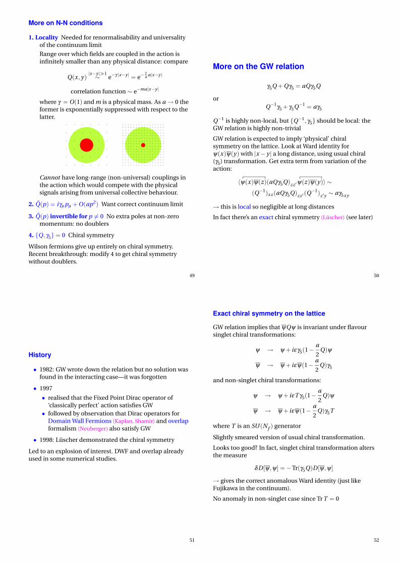
1. Locality Needed for renormalisability and universalityof the continuum limit

Range over which fields are coupled in the action isinfinitely smaller than any physical distance: compare

Q(x ,y )|x−y |1∼ e−γ |x−y | = e−

γa a|x−y |

correlation function ∼ e−ma|x−y |

where γ = O(1) and m is a physical mass. As a→ 0 theformer is exponentially suppressed with respect to thelatter.

Cannot have long-range (non-universal) couplings inthe action which would compete with the physicalsignals arising from universal collective behaviour.

2. Q(p) = iγµpµ + O(ap2) Want correct continuum limit

3. Q(p) invertible for p 6= 0 No extra poles at non-zeromomentum: no doublers

4. Q, γ5 = 0 Chiral symmetry

Wilson fermions give up entirely on chiral symmetry.Recent breakthrough: modify 4 to get chiral symmetrywithout doublers.

49

More on the GW relation

γ5Q + Qγ5 = aQγ5Q

or

Q−1γ5 + γ5Q−1 = aγ5

Q−1 is highly non-local, but Q−1, γ5 should be local: theGW relation is highly non-trivial

GW relation is expected to imply ‘physical’ chiralsymmetry on the lattice. Look at Ward identity forψ(x)ψ(y ) with |x − y | a long distance, using usual chiral(γ5) transformation. Get extra term from variation of theaction:

〈ψ(x)ψ(z)(aQγ5Q)zz ′ψ(z)ψ(y )〉 ∼

(Q−1)xz (aQγ5Q)zz ′(Q−1)

z ′y ∼ aγ5xy

→ this is local so negligible at long distances

In fact there’s an exact chiral symmetry (Luscher) (see later)

50

History

• 1982: GW wrote down the relation but no solution wasfound in the interacting case—it was forgotten

• 1997

• realised that the Fixed Point Dirac operator of‘classically perfect’ action satisfies GW

• followed by observation that Dirac operators forDomain Wall Fermions (Kaplan, Shamir) and overlapformalism (Neuberger) also satisfy GW

• 1998: Luscher demonstrated the chiral symmetry

Led to an explosion of interest. DWF and overlap alreadyused in some numerical studies.

51

Exact chiral symmetry on the lattice

GW relation implies that ψQψ is invariant under flavoursinglet chiral transformations:

ψ → ψ + iεγ5(1−a

2Q)ψ

ψ → ψ + iεψ(1−a

2Q)γ5

and non-singlet chiral transformations:

ψ → ψ + iεT γ5(1−a

2Q)ψ

ψ → ψ + iεψ(1−a

2Q)γ5T

where T is an SU (N f ) generator

Slightly smeared version of usual chiral transformation.

Looks too good? In fact, singlet chiral transformation altersthe measure

δ D [ψ,ψ ] = −Tr(γ5Q)D [ψ,ψ ]

→ gives the correct anomalous Ward identity (just likeFujikawa in the continuum).

No anomaly in non-singlet case since Tr T = 0

52

Anomaly in LGT with GW relation

Expectation value of some fermion operator

〈O〉 =1

Z

∫

D [ψ ,ψ ]Oe−S

Apply chiral transformation as change of variable,remembering that S is invariant:

δ ψ = εγ5(1−1

2aQ)ψ δ ψ = εψ(1−

1

2aQ)γ5

〈O〉 =1

Z

∫

D [ψ ′,ψ ′]O ′e−S =1

Z

∫

D [ψ ,ψ ]J(O + εδO)e−S

with Jacobian factor J =

∣

∣

∣

∂ (ψ ′,ψ ′)∂ (ψ ,ψ)

∣

∣

∣.

∂ ψ ′x∂ ψy

= δxy + εγ5(1−1

2aQxy )

∂ ψ ′x∂ ψy

= δxy + ε(1−1

2aQxy )γ5

J = det

(

1 + εγ5(1− 12

aQ) 0

0 1 + ε(1− 12

aQ)γ5

)

= det(1 + εX )det(1 + εY )

= 1 + ε tr(X +Y ) = 1− εa tr(γ5Q)

where X = γ5(1− 12

aQ), Y = (1− 12

aQ)γ5) and used

det = exp tr ln, tr γ5 = 0.

53

Combining:

〈O〉 =1

Z

∫

D [ψ ,ψ ](

1− εa tr(γ5Q))

(O + εδO)e−S

To order ε∫

D [ψ ,ψ ](

δO −a tr(γ5Q))

e−S = 0

. . . giving the correct anomalous Ward identity for a globalflavour-singlet axial transformation.

(Note: tr(γ5Q) vanishes in the free case, but it’s non-zero inthe presence of gauge fields.)

54

LH and RH chiral fermions

If have chiral symmetry expect to decompose

ψQψ = ψ+Qψ+ + ψ−Qψ−

It’s really possible:

ψ− = P−ψ ψ+ = P+ψψ− = ψP+ ψ+ = ψP−

where P± = 12(1± γ5) as usual and

P± =1

2(1± γ5)

γ5 is a ‘smeared’ γ5:

γ5 = γ5(1−aQ)

γ5γ5 = 1

γ5Q = −Q γ5

‘Left’ and ‘right’ become gauge-dependent ideas

55

Neuberger’s operator

An operator Q satisfying the GW relation can be defined asfollows. Let

QW =1

2

(

γµ(∇µ+∇∗µ)−a∇∗µ∇µ)

be the massless free Wilson-Dirac operator. Neuberger’soperator is defined (in its simplest form) as:

QN =1

a

(

1−A(A†A)−1/2)

where

A = 1−aQW

Exercise

Show that QN satisfies the GW relation

56

4.3 Domain Wall Fermions

Dirac fermion in 5 dimensions

D5 = γµ ∂µ + γ5∂s − φ(s)

γ5 = −γ0γ1γ2γ3, µ = 0,1,2,3

s: extra spatial coordinate

φ is a given potentialrepresenting a domain wallwith height and width set bya scale M , e.g.φ(s) = M tanh(M s), butexact form not needed.

s

φ(s)M

1/M

Planewave solutions

D5χ(x , s) = 0 with χ(x , s) = eip·x u(s)

p = (iE ,p) physical 4-momentum

m2 = E 2−p2 mass of the mode

Allowed m2 determined from:[

γ5∂s − φ(s)]

u(s) = −iγµpµu(s)

Multiply on left by iγµpµ[

− ∂ 2s +V (s)

]

u(s) = m2u(s)

with V (s) = γ5∂sφ(s)+ φ 2(s).

57

[

− ∂ 2s +V (s)

]

u(s) = m2u(s)

Assume eigenfunctions havedefinite chirality since

−∂ 2s +V (s) commutes with

γ5. Three cases:s

V (s)γ5 = +1

γ5 = −1

1. Continuous spectrum

V (s)|s|→∞−→ M 2 leads to eigenvalues with m2 ≥M 2

2. Discrete spectrum

eigenfunctions with m2 < M 2 decay exponentially−→discrete spectrum. All non-zero masses are of order M(only scale). No negative masses since

−∂ 2s +V (s) = (−γ5∂s + φ)†(−γ5∂s + φ).

3. Massless modes

(−γ5∂s + φ)u(s) = 0, γµpµu(s) = 0

with solutions

u(s) = exp

±∫ s

0φ(t )dt

v,

P±v = vγµpµv = 0

Only LH solution isnormalisable. Masslessmode bound to the wall s

u(s)

58

Summary

• all but one mode have mass m ≥ O(M )

• massless mode: left-handed and bound to domain wall

• at energies E M , theory describes a left-handedfermion in 4-dimensions

Domain Wall Fermions

Mechanism is stable against changes in setup:

• domain wall−→Dirichlet boundary condition

• Dirac fields χ(x , s) in s ≥ 0 with

D5 = D4 + γ5∂s −M

satisfying

D5χ(x , s) = 0, P+χ(x , s)|s=0 = 0

• −→massless mode as before

• 5-dim fermion propagator satisfies

D5G(x , s; y,t )∣

∣

s,t≥0= δ (x − y )δ (s− t )

P+G(x , s; y,t )∣

∣

s=0= 0

59

• on the boundary you find:

G(x ,0; y,0) = 2M P−S(x ,y )P+

where S(x ,y ) is the 4-dimensional propagator of theoperator

D ≡ M +(D4−M )[

1− (D4/M )2]−1/2

= D4(1−D4/2M + · · ·)

D describes a massless 4-dim fermion, reduces to D4

as M →∞.

• D satisfies a Ginsparg-Wilson relation

γ5D + Dγ5 =1

MDγ5D

• (Kaplan 1992) The construction also works

∗ in the presence of gauge fields (no s-dependence)

∗ and on the lattice: M → 1/a, D4 → QW (masslessWilson-Dirac)

D =1

a

(

1− (1−aQW )[

(1−aQW )†(1−aQW )]−1/2

)

=1

a

(

1−A(A†A)−1/2)

where A = 1−aQW

• use a finite 5th-dimension: can have one chiralityexponentially bound to one wall, other chirality onother wall

60

5 Lattice QCDFormulate a lattice theory of quarks and gluons.

Lattice action:

SQC D [U ,ψ ,ψ ] = SG [U ]+ SF [U ,ψ,ψ ]

SG [U ] Wilson plaquette action

SF [U ,ψ,ψ ] Wilson fermion action

Define a covariant derivative:

Dµ ψ(x) =1

a

(

Uµ (x)ψ(x + aµ)−ψ(x))

D∗µ ψ(x) =1

a

(

ψ(x)−U †µ (x −aµ)ψ(x −aµ)

)

For the Wilson-Dirac operator:

1

2γµ(∇µ+∇∗µ)+m0−

ra

2∇∗µ ∇µ

→1

2γµ (Dµ+D∗µ )+m0−

ra

2D∗µ Dµ

Set:r = 1

a = 1 express all quantities in units of a

61

5.1 Fermion action in LQCD

SF [U ,ψ,ψ ] = ∑x∈ΛE

−1

2

3

∑µ=0

[

ψ(x)(1−γµ)Uµ(x)ψ(x+µ)

+ ψ(x+µ)(1+γµ )U †µ ψ(x)

]

+ ψ(x)(

m0 + 4)

ψ(x)

Rescale ψ and ψ by

ψ(x)→√

2κ ψ(x), ψ(x)→ ψ(x)√

2κ

and fix κ by requiring (m0 + 4)2κ = 1

Lattice action for QCD with Wilson fermions becomes:

SQCD[U ,ψ,ψ ] = β ∑2

(

1−1

3Re Tr P

2

)

+ ∑x∈ΛE

−κ3

∑µ=0

[

ψ(x)(1−γµ)Uµ(x)ψ(x+µ)

+ ψ(x+µ)(1+γµ )U †µ ψ(x)

]

+ ψ(x)ψ(x)

We have traded parameters: (g0,m0) 7→ (β ,κ), with:

β =6

g 20

, κ =1

2m0 + 8(hopping parameter)

62

5.2 Effective gauge actionRewrite fermionic piece of LQCD action:

SF [U ,ψ,ψ ] = ∑x∈ΛE

ψ(x)[QW ψ ](x)

≡ ∑x ,y∈ΛE

ψ(x)Qxy ψ(y )

Qxy is Wilson-Dirac operator in matrix notation (‘quarkmatrix’)

Qxy = δxy −κ3

∑µ=0

δy,x+µ(1−γµ)Uµ(x)

+ δy,x−µ(1+γµ )U †

µ (x)

Functional integral:

Z =

∫

D [U ,ψ,ψ ]e−SG [U ]−SF [U ,ψ,ψ ]

Integrate out fermions:

Z =

∫

D [U ]e−SG [U ] det Q[U ]

Exercise

Show that det Q[U ] is real.

63

Introduce the effective gauge action, using

det X = elog det X = eTr log X

so that

Z =

∫

D [U ]e−Seff[U ], Seff[U ] ≡ SG [U ]−Tr log Q[U ]

Quark propagator:

〈ψ(y )ψ(x)〉 =1

Z

∫

D [U ]Q−1y x [U ]e−Seff[U ]

Now examine the fermionic contribution to Seff[U ] ingreater detail. Split:

Q[U ] = Q(0)−V [U ]

Q(0) describes free Wilson fermions:

Q(0)xy = δxy −κ

3

∑µ=0

[

δy,x+µ(1−γµ)+ δ

y,x−µ(1+γµ)]

Q(0)−1 ≡ S(0)W

(free Wilson propagator)

while V is the interaction term:

Vxy [U ] = κ3

∑µ=0

[

δy,x+µ(1−γµ)

(

Uµ (x)− 1)

+ δy,x−µ(1+γµ )

(

U †µ (y )− 1

)

]

64

Now write

Q[U ] = Q(0)Q(0)−1Q[U ] = Q(0)

(

1−Q(0)−1V [U ]

)

The effective gauge action becomes

Seff[U ] = SG [U ]− log det Q[U ]

= SG [U ]−Tr log(

1−Q(0)−1V [U ]

)

+ const

= SG [U ]+∞∑j=1

1

jTr(

S(0)W

V [U ]) j

• Trace here is over all quark indices: Dirac, colour, site

• each term is a closed loop of j free quark propagatorsand j vertices

• the sum contributes closed quark loops to the effectiveaction

+1

2+

1

3+ · · ·

65

5.3 The quenched approximationThere is phenomenological evidence that quark loops haveonly small effects on hadronic physics.

Zweig’s (OZI) rule: φ → 3π is suppressed relative toφ → K +K−

φ π−

π 0

π+

s

s

d

du

d

du

φ

K−

K +

s

s

s

u

u

s

This motivates the quenched approximation whichcorresponds to setting

det Q[U ] = 1, ie Seff[U ] = SG [U ]

• det Q[U ] = 1 corresponds to setting κ = 0 for internalquarks (in loops)

κ = 0 ⇔ mq = ∞−→ infinitely heavy quarks in loops contributing to theeffective gluon interaction

• quenching is an enormous simplification fornumerical simulations:

cost of full QCD

cost of quenched QCD> 10 000

66

6 Numerical simulationsReturn to the problem of computing observables in QCD(restrict to SU (3) gauge group)

〈O〉 =1

Z

∫

D [U ]Oe−Seff[U ]

=1

Z

∫

∏x∈ΛE

3

∏µ=0

dUµ(x)Oe−Seff[U ]

• strong coupling expansions have a small radius ofconvergence

• weak coupling expansion is asymptotic

• . . . and the two don’t overlap

• exact evaluation of 〈O〉 or Z on a computer is notpractical (although possible in principle)

• instead use stochastic methods to evaluate 〈O〉 or Z

• Monte Carlo integration: evaluate the observable on afinite number of ‘typical’ field configurations

Field configuration

Assignment of an SU (3) matrix Uµ (x) to every link (x , µ)on the lattice:

C =

Uµ(x)∣

∣x ∈ ΛE , µ = 0,1,2,3

, C = U

67

6.1 Monte Carlo integrationIntegrand is strongly peaked around configurations C withlarge values of

W (C ) ≡ e−Seff

[C ] = e−Seff

[U ]

W (C ) :Boltzmann factor or statisticalweight of configuration C

Monte Carlo procedure

• generate a sample or ensemble of gauge fieldconfigurations, Ci , i = 1, . . . ,Ncfg, with statistical

weights W (Ci)

• sample comprises predominantly configurations withlarge W (Ci)

• importance sampling: design an algorithm whichgenerates a configuration C with likelihood W (C )

• common algorithms

• Metropolis

• heat bath (for SU (N) gauge theory, scalar fieldtheories, spin systems)

• cluster algorithms (Swendsen-Wang, Wolff) (forspin systems, O(N) models, not gauge theories)

• hybrid Monte Carlo (HMC) or multibosonalgorithms (for QCD with dynamical fermions)

68

• quenched QCD: use W (C ) = e−SG [C ] = e−SG [U ] asprobability measure

• ‘full’ QCD: use W (C ) = det Q[U ]e−SG [U ] as measure

• det Q[U ] is real but not positive definite

• use det(Q†Q)e−SG , corresponding to two flavours ofdynamical quark

• hard to simulate odd numbers of fermions

• evaluate observables on each configuration in theensemble, O [Ci ], i = 1, . . . ,Ncfg, giving Ncfg

‘measurements’

• sample average of observable

O =1

Ncfg

Ncfg

∑i=1

O [Ci ]

• expectation value

〈O〉 = limNcfg→∞

O

• results from Monte Carlo integration have statisticalerror ∝ 1/

√

Ncfg

69

6.2 Hadronic correlation functionsRecall spectral decomposition of two-point function:

〈A(x)B(y )〉= ∑n,pn

〈0|A(0,x)|n〉e−(En−E0)(x0−y0)〈n|B(0,y)|0〉

Now consider the pion two-point function:

Cπ (t ) ≡∑x

〈0|P(t ,x)P †(0)|0〉

• P(x) = ψ(x)γ5ψ(x) is an interpolating operator

between the pion state and the vacuum. P † = −P

• ∑x projects onto zero momentum: states |n〉 at rest

• states |n〉 in sum have same quantum numbers as

pion, J P = 0−

Cπ (t ) = ∑n

〈0|P(0)|np=0〉〈np=0|P †(0)|0〉2M (π)

n

e−M (π)n t

= ∑n

∣

∣〈0|P |n〉∣

∣

2

2M (π)n

e−M (π)n t

• For large Euclidean times t the state with the lowestmass dominates, call it Mπ

70

Numerical calculation of 2pt correlator

Let

P (x) = ψ1(x)γ5ψ2(x)

P †(x) = −ψ2(x)γ5ψ1(x)

1,2 label distinct quark flavours: limits the contractionsappearing; different choices of 1,2 let you study mπ ,mK , . . .The correlator:

Cπ (t ) =∑x

〈0|T P(t ,x)P †(0)|0〉

=∑x

−〈0|T ψ1(x)γ5ψ2(x)ψ2(0)γ5ψ1(0)|0〉

=∑x

1

Z

∫

∏x∈ΛE

µ=0,...,3

dUµ(x)e−Seff

[U ] Tr(

γ5Q−12 [U ]x0γ5Q−1

1 [U ]0x

)

=∑x

⟨

Tr(

γ5Q−12 [U ]x0γ5Q−1

1 [U ]0x

)⟩

=∑x

t ,x 0

21

γ5 γ5

Sample average

Cπ (t ) =1

Ncfg

Ncfg

∑i=1

∑x

Tr(

γ5SCiW,2

(x ,0)γ5SCiW,1

(0,x))

where SCiW, j

(y,x) is propagator for quark type j from x to y

on the ith configuration Ci .

71

Calculating propagators

• SW (x ,y )ab,µν has site, spin and colour indices and

depends on the gauge field and the quark mass (κ)

• on a given configuration the propagator for quark typej (with mass fixed by κ j ) solves

QCizx SCi

W, j(x ,y ) = δx ,y

suppressing colour and spin indices

• impractical to solve for the whole matrix: instead, fixy = 0:

QCizx SCi

W, j(x ,0) = δx ,0

∗ solve matrix equation Q ·X = b for vector X

∗ repeat for each configuration i

−→ gives propagator from 0 to any x

• correlation function also contains SW (0,x).

∗ since Q = γ5Q†γ5, then SW = γ5S†W γ5

∗ −→ get SW (0,x) from SW (x ,0)

−→ have all propagators needed

• now just evaluate the trace with γ5’s using propagatorsevaluated on each gauge configuration

72

• On a finite lattice withperiodic temporalboundary conditionsCπ (t ) is symmetric fort → T − t

0

t

T − t

Cπ (t )0tT→

1

2Mπ

∣

∣〈0|P |π〉∣

∣

2(e−Mπ t + e−Mπ (T−t ))

=1

Mπ

∣

∣〈0|P |π〉∣

∣

2e−Mπ T /2 cosh

(

Mπ (T /2− t ))

• Obtain Mπ and the matrix element Z = 〈0|P |π〉 ∝ fπ byfitting Cπ (t ) to the above cosh formula

t

Cπ (t )

302520151050

1

0.01

10−4

10−6

Example: Quenched, β = 6, κ = 0.1337, 323× 64 lattice.

Fitted curve has aMπ = 0.3609+12−13, Z = 0.1553+39

−41. (D Lin,

APE data)

73

Effective mass plot

Plot

M effπ (t ) = ln

[

Cπ (t )+√

C 2π (t )−C 2

π (T /2)

Cπ (t +1)+√

C 2π (t +1)−C 2

π (T /2)

]

0tT≈ Mπ

0 10 20 30t

0.20

0.30

0.40

0.50

0.60

mes

on m

ass

fitted curve

Quenched β = 6.0, κ = 0.1337

a MP = 0.3609+0.0012−0.0013ZP = 0.1553+0.0039−0.0041

(D Lin, APE data)

Simpler: if T →∞, then Cπ (t ) ∝ e−Mπ t and plot

ln(

Cπ (t )/Cπ (t +1))

≈Mπ

Differs only at right hand end of above plot

74

• By choosing appropriate interpolating operators for:

vector mesons ρ,K ∗,φ , . . .

octet baryons N ,Σ,Λ,Ξ, . . .

decuplet baryons ∆,Σ∗,Ξ∗,Ω

one can extract the hadron spectrum from fits to thecorrelation functions

75

6.3 Elimination of bare parametersHadron masses obtained from correlation functionsdepend implicitly on the input bare parameters, β and κ .Moreover, you determine dimensionless quantities, likeaMπ and have to fix a afterwards.

Eliminate bare parameters by matching lattice hadronmasses to experiment.

Can study quark mass dependence of hadrons on thelattice by computing aMhad for several values of κ at fixedβ . From leading order chiral perturbation theory:

M 2π = B(mu +md)

M 2K± = B(mu +ms)

Mρ = A +C (mu +md)

MK ∗ = A +C (mu +ms)

−→ information on quark mass dependence resides inparameters A, B and C

Motivates ansatz for quark mass dependence of latticedata:

(aMPS)2 = (aB)(amq1

+ amq2)

aMV = (aA)+C (amq1+ amq2

)

= (aA)+C

(aB)(aMPS)

2

76

To first approximation, assume mu = md = 0, so that one

expects M 2π = 0 (in real life: M 2

π = 0.018 GeV2 compared to

M 2ρ = 0.59 GeV2).

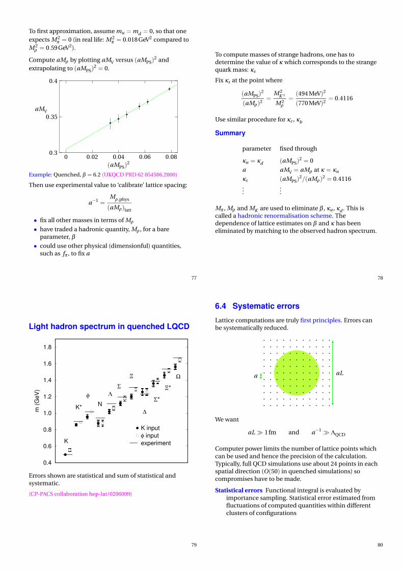
Compute aMρ by plotting aMV versus (aMPS)2 and

extrapolating to (aMPS)2 = 0.

(aMPS)2

aMV

0.080.060.040.020

0.4

0.35

0.3

Example: Quenched, β = 6.2 (UKQCD PRD 62 054506,2000)

Then use experimental value to ‘calibrate’ lattice spacing:

a−1 =Mρ,phys

(aMρ)latt

• fix all other masses in terms of Mρ

• have traded a hadronic quantity, Mρ , for a bareparameter, β• could use other physical (dimensionful) quantities,

such as fπ , to fix a

77

To compute masses of strange hadrons, one has todetermine the value of κ which corresponds to the strangequark mass: κs

Fix κs at the point where

(aMPS)2

(aMρ)2=

M 2K±

M 2ρ

=(494 MeV)2

(770 MeV)2= 0.4116

Use similar procedure for κc , κb

Summary

parameter fixed through

κu = κd (aMPS)2 = 0

a aMV = aMρ at κ = κu

κs (aMPS)2/(aMρ)2 = 0.4116

......

Mπ , Mρ and MK are used to eliminate β , κu , κd . This iscalled a hadronic renormalisation scheme. Thedependence of lattice estimates on β and κ has beeneliminated by matching to the observed hadron spectrum.

78

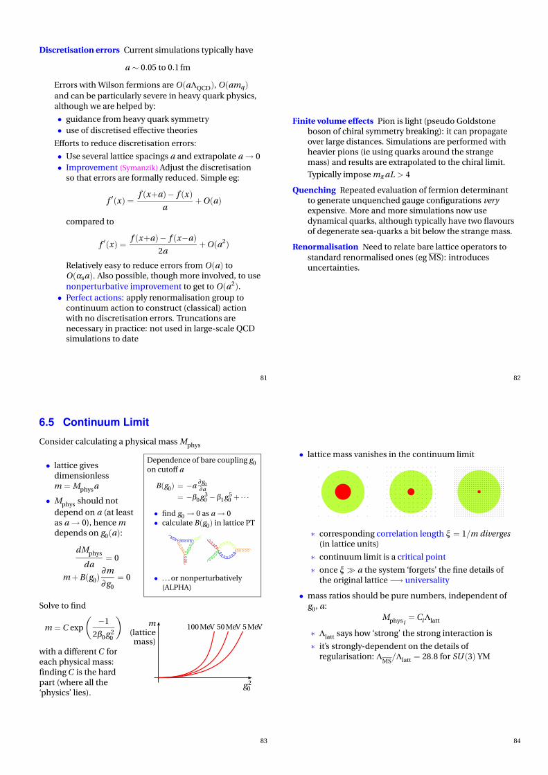
Light hadron spectrum in quenched LQCD

0.4

0.6

0.8

1.0

1.2

1.4

1.6

1.8

m (G

eV)

K inputφ inputexperimentK

K*

φN

ΛΣ

Ξ

∆

Σ*

Ξ*

Ω

Errors shown are statistical and sum of statistical andsystematic.

(CP-PACS collaboration hep-lat/0206009)

79

6.4 Systematic errorsLattice computations are truly first principles. Errors canbe systematically reduced.

a aL

We want

aL 1 fm and a−1 ΛQCD

Computer power limits the number of lattice points whichcan be used and hence the precision of the calculation.Typically, full QCD simulations use about 24 points in eachspatial direction (O(50) in quenched simulations) socompromises have to be made.

Statistical errors Functional integral is evaluated byimportance sampling. Statistical error estimated fromfluctuations of computed quantities within differentclusters of configurations

80

Discretisation errors Current simulations typically have

a ∼ 0.05 to 0.1 fm

Errors with Wilson fermions are O(aΛQCD), O(amq)

and can be particularly severe in heavy quark physics,although we are helped by:

• guidance from heavy quark symmetry

• use of discretised effective theories

Efforts to reduce discretisation errors:

• Use several lattice spacings a and extrapolate a → 0

• Improvement (Symanzik) Adjust the discretisationso that errors are formally reduced. Simple eg:

f ′(x) =f (x+a)− f (x)

a+ O(a)

compared to

f ′(x) =f (x+a)− f (x−a)

2a+ O(a2)

Relatively easy to reduce errors from O(a) toO(αsa). Also possible, though more involved, to use

nonperturbative improvement to get to O(a2).

• Perfect actions: apply renormalisation group tocontinuum action to construct (classical) actionwith no discretisation errors. Truncations arenecessary in practice: not used in large-scale QCDsimulations to date

81

Finite volume effects Pion is light (pseudo Goldstoneboson of chiral symmetry breaking): it can propagateover large distances. Simulations are performed withheavier pions (ie using quarks around the strangemass) and results are extrapolated to the chiral limit.

Typically impose mπ aL > 4

Quenching Repeated evaluation of fermion determinantto generate unquenched gauge configurations veryexpensive. More and more simulations now usedynamical quarks, although typically have two flavoursof degenerate sea-quarks a bit below the strange mass.

Renormalisation Need to relate bare lattice operators to

standard renormalised ones (eg MS): introducesuncertainties.

82

6.5 Continuum LimitConsider calculating a physical mass Mphys

• lattice givesdimensionlessm = Mphysa

• Mphys should not

depend on a (at leastas a→ 0), hence mdepends on g0(a):

dMphys

da= 0

m + B(g0)∂m

∂ g0

= 0

Dependence of bare coupling g0on cutoff a

B(g0) = −a∂ g0

∂ a

= −β0g 30 −β1g 5

0 + · · ·

• find g0 → 0 as a→ 0

• calculate B(g0) in lattice PT

• . . . or nonperturbatively

(ALPHA)

Solve to find

m = C exp

(

−1

2β0g 20

)

with a different C foreach physical mass:finding C is the hardpart (where all the‘physics’ lies).

g 20

m(lattice

mass)

100 MeV 50 MeV 5 MeV

83

• lattice mass vanishes in the continuum limit

∗ corresponding correlation length ξ = 1/m diverges(in lattice units)

∗ continuum limit is a critical point

∗ once ξ a the system ‘forgets’ the fine details ofthe original lattice−→ universality

• mass ratios should be pure numbers, independent ofg0, a:

Mphysi= CiΛlatt

∗ Λlatt says how ‘strong’ the strong interaction is

∗ it’s strongly-dependent on the details ofregularisation: Λ

MS/Λlatt = 28.8 for SU (3) YM

84

Scaling

• calibrate a from mρ , fπ , σ , . . .• further calculations yield mass ratios mi/m0

• if close enough to ctm limit, mi/m0 is constant asβ • this is scaling

Asymptotic Scaling

• PT in g 20 should work for large enough β = 2N/g 2

0

• observe scaling according to the β -function (1-loop)

Mphysa ∝ exp

( −1

2β0g 20

)

• this is asymptotic scaling

85

6.6 Renormalisation of Lattice OperatorsTypically (ignoring operator mixing):

Oren(µ) = Z

O(µa,g )O latt(a)

• if a−1 ΛQCD and µ ΛQCD can use PT to relate

• ZO

depends on short-distance physics

• IR physics common to matrix elements of O ren,latt

Example: axial vector current in Wilson LQCD

Alattµ = ψ(x)γµ γ5ψ(x)

Use this in a 2-point correlation function:

C (t ) = ∑x

〈0|T Alatt0 (x,t )Alatt

0

†(0)|0〉

large t >0=

∣

∣〈π(p = 0)|Alatt0

†(0)|0〉

∣

∣

2

2mπe−mπ t

But

Arenµ = ZAAlatt

µ and 〈π(p = 0)|Aren0

†(0)|0〉 = fπmπ

so that

fπ =ZA

∣

∣〈π |Alatt0

†|0〉∣

∣

mπ

. . . you need ZA to get the physical fπ .

86

Perturbative renormalisation

Calculate matrix element of quark bilinear O between, say,the same quark states and fix Z

Oby demanding agreement

(ZO

is a property of O so use any convenient states).

ZO

=

∣

∣

∣

∣

ctm∣

∣

∣

∣

∣

∣

latt

ZO

= 1 +αs

4π

(

γ ln(µa)+ c)

+ · · ·

For axial current with µa = 1

ZA = 1− 15.8αs

4πCF

15.8 is a large coefficient. . .

• αMSs /α latt

s ≈ 2.7: α latts is a poor expansion parameter

• related to tadpoles: extra vertices in lattice PT from

expanding exp(

aAµ (x))

• turn to nonperturbative renormalisation. . .

87

Nonperturbative renormalisation

Impose a physical condition to fix ZO

• Example 1: local Wilson vector current

Vµ = ψ(x)γµψ(x)

not conserved−→ ZV 6= 1

Possible to define a conserved lattice vector currentV C

µ , which has Z = 1. Hence, fix ZV using

ZV =〈π(p)|V C

µ (0)|π(p)〉〈π(p)|Vµ(0)|π(p)〉

• Example 2: Use Ward Identities to relate Z ’s of differentoperators. For example, impose continuum axialcurrent WID

〈∂µ AµO〉 = 2m〈PO〉

with O arbitrary operator

m renormalised quark mass

P pseudoscalar density

88