Lattice Simulations of Nonperturbative Quantum Field Theories

Lattice Simulationsof Nonperturbative

Quantum Field Theories

David SchaichAdvisor: Prof. Loinaz

Final Thesis TalkAmherst College

2 May 2006

David Schaich Final Thesis Talk – 2 May 2006 2

Outline

Lattice simulationsWe did this last time

Quantum field theoryA very very very brief introduction

Phase transitionsPicking up where we left off in December

SolitonsTime permitting


Lattice Simulations


Lattice Simulations

We did this last time


Lattice Simulations

We did this last time

So we'll take it for granted that we have (Markov chain Monte Carlo) algorithms that will reliably and efficiently reproduce the Boltzmann distribution

Allowing us to simulate statistical systems on the computer


Quantum Field Theory(in five minutes) (or less)



Combination of special relativity and quantum mechanics

Free particle Schrödinger equation:

Relativistic analog is the KleinGordon equation:

E= p2

2mE i ∂

∂ tp i ∇

i ∂∂ t

=−12m

∇ 2

E2= p2m2 ∂2

∂ t 2− ∇2m2=∂2m2=0



KleinGordon equation only really makes sense if is treated as a field

Otherwise there are unbounded negativeenergy solutions, and negative probability densities

For example,

x=∫ d4 k

24[a k e−ik⋅xa†k eik⋅x ]


4 Quantum Field Theory

Lagrangian:

Equation of motion:Same form as KleinGordon equation, only nonlinear

Obvious constant solutions:

L=12∂2−1

2022−

44

∂202=−3

=0 =±−02


4 Quantum Field Theory Phases

Lagrangian:

Equation of motion:Same form as KleinGordon equation, only nonlinear

Two phases:

Symmetric phase Broken phase

L=12∂2−1

2022−

44

∂202=−3

⟨⟩=0 ⟨⟩=±−02



Going from symmetric phase to broken phase breaks symmetry:

In symmetric phase values of are randomly +/(“updown symmetry”)

In broken phase, values are either all + or all

Symmetric phase Broken phase

⟨⟩=0 ⟨⟩=±−02



So there's a phase transition!

Let's put some lattice simulations on the cluster to calculate the critical point!

✓Symmetricphase

Brokenphase


4 Theory Simulations

Wait, are we perhaps being a bit glib?



Wait, are we perhaps being a bit glib?

Well, yes, but we don't need to be

There exists a rigorous mapping from quantum field theories to classical statistical mechanics, through Wick rotation,

t=x0−ix4

∣x∣2=x02−x2−x 2x4

2=−∣x E∣2

∂2= ∂2

∂ x02−

∇ 2− ∇ 2− ∂2

∂ x 42=−∂E

2

d 4 x=d x0d3 x−i d 3 x dx4=−i d

4 x E

L=12∂2−1

2022−

44−1

2∂E 2−1

2022−

44=−LE



Minkowski spacetime converted into fourdimensional Euclidean space

The Euclidean Lagrangian LE has the form of

an energy density

The action SE then has the form of an energy

And the Feynman path integral behaves just like a thermodynamic partition function

LE=12∂E

212022

44

S E=∫ d 4 xE LE

∫D xei S=∫D xei∫d4 x L∫D xe−∫d

4 xE LE=∫D x e−S E



So we can investigate the 4 quantum field theory by simulating the corresponding statistical system using the techniques discussed when last we met

The discretized lattice action SE is

where μ20L

and λL depend on the lattice

spacing a

S E=−∑⟨ij ⟩

i j∑n

[d0L2

2n

2L4n4]

0L2 =0

2a2

L=a2


4 Theory Phases

Since, we're interested in the continuum theory (a0), we have a slight problem:

which we solve by considering the critical coupling constant

lima0 0L2 =lima0 0

2a2=0lima0L=lima0 a

2=0

S E=−∑⟨ij ⟩

i j∑n

[d0L2

2n

2L4n4]

[/2]crit=lima0 [L/L2 ]crit


Preliminary Phase Results

Published Results:

W. Loinaz & R. S. Willey, Phys. Rev. D. 58, 076003 (1998).

[/2]crit=10.26−.04.08

[/2]crit=10.27−.05.06


Final Phase ResultsMore data confirms higher-order effects:

Regression includes λlog[λ] and λ2log[λ] terms, reflecting some mixture of higher-order loop corrections and systematic effects introduced by approximations made during the discretization procedure


Final Phase ResultsMore data confirms higher-order effects:

[/2]crit=10.85−.08.03


4 Theory Solitons

Recall equation of motion:

Nonlinearity allows for some even more interesting solutions

These 'kink' solutions continuously connect two degenerate ground states in broken phase:

∂202=−3

=±−02

tanh [ x−0

2

2 ]


4 Theory Solitons

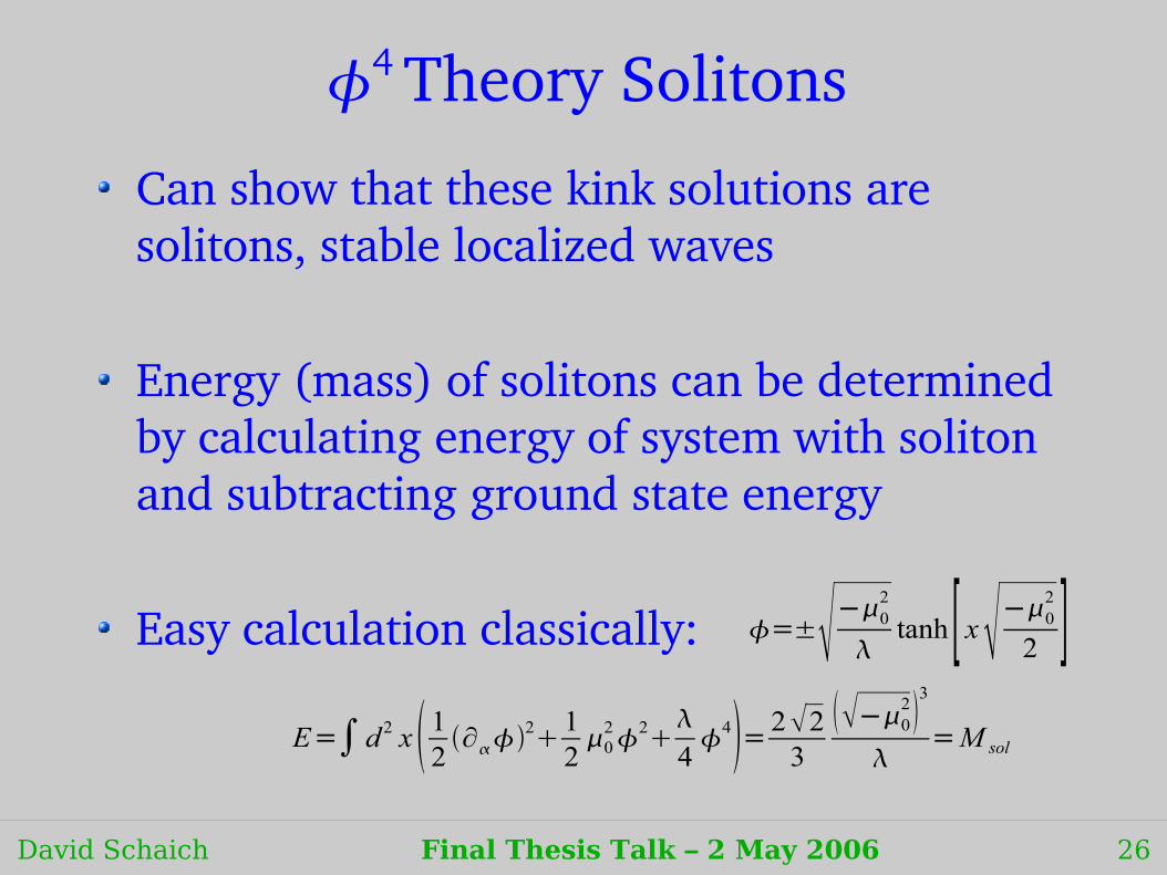
Can show that these kink solutions are solitons, stable localized waves

Energy (mass) of solitons can be determined by calculating energy of system with soliton and subtracting ground state energy

Easy calculation classically:

E=∫d 2 x 12 ∂2 12022

44= 223 −0

2 3

=M sol

=±−02

tanh [ x−0

2

2 ]


4 Theory Solitons

Classically,

Must take quantum effects into account.Firstorder (in ħ, zerothorder in λ) approximation:

What do the simulations say?

M sol=223

−02 3

M sol=223

−02 3

−0

2 16 23− 32 O


Classicallimit

Classicallimit

r=−02

=1


Acknowledgments

National Science FoundationThis work was partially funded by NSF grant 0521169,

as well as an Amherst Faculty Research Award Program (FRAP) grant

Prof. Loinaz

Prof. Kaplan

Chris Bednarzyk '01

Lattice Simulations of Nonperturbative Quantum Field Theories

Documents

Transcript of Lattice Simulations of Nonperturbative Quantum Field Theories