arX

iv:h

ep-t

h/94

0115

3v1

28

Jan

1994

Nonperturbative QCD: A Weak-Coupling Treatment on the Light Front

Kenneth G. Wilsona, Timothy S. Walhouta, Avaroth Harindranatha,

Wei-Min Zhang∗a, Robert J. Perrya, and Stanis law D. G lazekb

aDepartment of Physics, The Ohio State University, Columbus, Ohio 43210-1106, USAbInstitute of Theoretical Physics, Warsaw University, ul. Hoza 69, 00-861 Warsaw, Poland

(February 1, 2008)

In this work the determination of low-energy bound states in Quantum Chromodynamics is recast so that itis linked to a weak-coupling problem. This allows one to approach the solution with the same techniques whichsolve Quantum Electrodynamics: namely, a combination of weak-coupling diagrams and many-body quantummechanics. The key to eliminating necessarily nonperturbative effects is the use of a bare Hamiltonian in whichquarks and gluons have nonzero constituent masses rather than the zero masses of the current picture. The useof constituent masses cuts off the growth of the running coupling constant and makes it possible that the runningcoupling never leaves the perturbative domain. For stabilization purposes an artificial potential is added to theHamiltonian, but with a coefficient that vanishes at the physical value of the coupling constant. The weak-couplingapproach potentially reconciles the simplicity of the Constituent Quark Model with the complexities of QuantumChromodynamics. The penalty for achieving this perturbative picture is the necessity of formulating the dynamicsof QCD in light-front coordinates and of dealing with the complexities of renormalization which such a formulationentails. We describe the renormalization process first using a qualitative phase space cell analysis, and we thenset up a precise similarity renormalization scheme with cutoffs on constituent momenta and exhibit calculations tosecond order. We outline further computations that remain to be carried out. There is an initial nonperturbativebut nonrelativistic calculation of the hadronic masses that determines the artificial potential, with binding energiesrequired to be fourth order in the coupling as in QED. Next there is a calculation of the leading radiative correctionsto these masses, which requires our renormalization program. Then the real struggle of finding the right extensionsto perturbation theory to study the strong-coupling behavior of bound states can begin.

PACS numbers: 11.10.Ef, 11.10.Gh, 12.38.Bx

I. INTRODUCTION

The only truly successful approach to bound states in field theory has been Quantum Electrodynamics (QED),with its combination of nonrelativistic quantum mechanics to handle bound states and perturbation theory to handlerelativistic effects. Lattice Gauge Theory is maturing but has yet to rival QED’s comprehensive success. Thereare four barriers which prohibit an approach to Quantum Chromodynamics (QCD) that is analogous to QED. Thebarriers are: (1) the unlimited growth of the running coupling constant g in the infrared region, which invalidatesperturbation theory; (2) confinement, which requires potentials that diverge at long distances as opposed to theCoulombic potentials of perturbation theory; (3) spontaneous chiral symmetry breaking, which does not occur inperturbation theory; and (4) the nonperturbative structure of the QCD vacuum. Contrasting the gloomy picture ofthe strong interaction in QCD, however, is that of the Constituent Quark Model (CQM), where only the minimumnumber of constituents required by the symmetries are used to build each hadron and where Zweig’s rule leaves littlerole for production of extra constituents. Instead, rearrangement of pre-existing constituents dominates the physics.Yet the CQM has never been reconciled with QCD — not even qualitatively. Ever since the work of Feynman, though,it has been clear that the best hope of reconciliation is offered by infinite momentum frame (IMF) dynamics.

In this paper, a framework closely related to the IMF will be employed, namely, light-front quantization. Thepurpose of this paper is to provide arguments that all the barriers to a perturbative starting point for solving QCDcan be overcome, at least in principle, when a light-front framework is used. We present the basic formulation forsuch an approach. Coupled to the choice of coordinates are the introduction of nonzero masses for both quarks andgluons, the use of cutoffs on constituent momenta which eliminate vacuum degrees of freedom, and the addition ofan artificial stabilizing and confining potential which vanishes at the relativistic value of the renormalized couplingbut nowhere else. One result of these unconventional modifications is a theory with a trivial vacuum. However, the

∗Present Address: Institute of Physics, Academia Sinica, Taipei 11529, Taiwan, ROC.

1

theory has extra terms in the Hamiltonian which are induced by the elimination of vacuum degrees of freedom, whichaccount for spontaneous chiral symmetry breaking, yet can be treated perturbatively. It is a theory where a second-order treatment of renormalization effects should closely resemble the phenomenological CQM, while a fourth-ordertreatment — if all goes well — should begin to replace phenomenology by true results of QCD. We have not carriedout these computations but will outline them to show that they are indeed perturbative ones.

Our basic aim, then, is to tailor an approach to QCD which is based on the phenomenologically successful approachof the CQM. Central to our formulation is to start with nonzero masses for both quarks and gluons and to thenconsider the case of an arbitrary coupling constant g which is small even at the quark-gluon mass scale — a runningcoupling which is then small everywhere because below this scale it cannot run anymore. This means sacrificingmanifest gauge invariance and Lorentz covariance, with these symmetries only being implicitly restored (if at all)when the renormalized coupling is increased to its relativistic value, which we call gs. The value gs is a fixed numberbecause it is measured at the hadron mass scale, and by asymptotic freedom arguments such a coupling has a fixedvalue. For smaller values of g our theory lacks full covariance and is not expected to have the predictive power ofQCD, but it allows phenomenology to guide renormalization and is defined to maximize the ease of perturbativecomputations and extrapolation to gs.

Some key new ideas in this paper have previously been reported only in unpublished notes [1–5]. Some have beenpresented in a condensed form in Ref. [6]. These ideas underly two main parts of this paper. The first part is aqualitative power counting analysis of divergences in light-front QCD (LFQCD), which provides a vital basis for thenew cutoff scheme and renormalization framework we develop in the second part. More broadly, this paper draws ona range of previous research efforts by the authors and colleagues: the QCD calculations presented in this paper arelargely based on the standard gauge-fixed LFQCD Hamiltonian [7], and the specific diagrammatic rules used here aredefined with examples in Refs. [8–10] following earlier work [11]. This paper follows recent work on QCD [8–10,12,13]and the similarity renormalization scheme [14,15]; and it is also the outgrowth of a line of research that covers theTamm-Dancoff approximation [16], light-front QED [17], and light-front renormalization [18]. The relation of thispaper to the entire field of light-front field theory will be outlined in section II.

The plan of the paper is as follows. As our formulation is quite different not only from previous approachesto QCD but also to previous studies of light-front dynamics, we start in Section II with a general overview andmotivation of our approach. We discuss the apparent contradictions between QCD and its precursor, the CQM. Thenwe outline why a light-front approach can bridge the gap between QCD and the CQM and discuss in turn how eachof the equal-time barriers to a weak-coupling treatment of QCD may be overcome. In Sections III-V, the first majorpart of the paper, we motivate and discuss the light-front power-counting analysis, describe the canonical LFQCDHamiltonian, and use a qualitative phase space cell analysis to classify the possible counterterms for ultraviolet andinfrared divergences in LFQCD needed for renormalization. Light-front power counting can determine the operatorstructure of the LFQCD Hamiltonian [2], and we rely on the derivation from the QCD Lagrangian to determinedetails such as color factors. This canonical LFQCD Hamiltonian will be treated as a Hamiltonian in the many-bodyspace of finite numbers of quark and gluon constituents, a Hamiltonian which with regularization gives finite answersin this many-body space. Three terms in the canonical Hamiltonian itself require infrared counterterms because oflinear infrared divergences, and we proceed to construct them. We explain the absence of finite parts to many of thesecounterterms because kinematical longitudinal boost invariance is a scale invariance. Because of this kinematicalconstraint, only counterterms for logarithmic infrared divergences are allowed to contain finite parts, which as part ofthe renormalization process must be tuned to reproduce physical results. Counterterms to canonical terms are primecandidates for bringing in phenomena associated with true confinement and with the spontaneously broken vacuumof normal rest frames. We distinguish true confinement in the exact theory from the artificial confinement which weintroduce by hand in the weak-coupling starting point.

This leads to the second major part of the paper, where in Sections VI-X we set up an explicit quantitative schemefor renormalization of the LFQCD Hamiltonian. First, a momentum space cutoff procedure is introduced whichregulates the Hamiltonian itself rather than the individual terms of perturbation theory [3]. This cutoff schemedepends on the use of massive constituents and is chosen to ensure that each state has only a finite number ofconstituents. Both gauge invariance and Lorentz covariance are violated by these cutoffs, and a range of countertermsis needed to enable a finite limit as the cutoffs are removed. Restoration of the violated symmetries can only beestablished by examining the solution to the theory at the relativistic limit gs (or good approximations to thissolution). This is the price we must pay for achieving the new framework. We proceed to the construction of theeffective Hamiltonian. We begin by discussing a novel perturbation theory formalism due to G lazek and Wilson[14,15] designed to transform a cutoff Hamiltonian to band-diagonal form while avoiding small energy denominatorsthat plague other approaches [19]. This is called the “similarity renormalization scheme.” The end product of thescheme is a band-diagonal effective Hamiltonian in which dependence on the original cutoffs has been removed to anydesired order of perturbation theory. As an example we determine in detail the gluon mass counterterms necessaryto remove second-order divergences generated by two-gluon intermediate states. We then proceed to construct order

2

g2 light-front infrared counterterms, and we identify finite counterterms that may be necessary to compensate forthe removal of zero longitudinal momentum modes from the cutoff theory. The next step is to analyze the role of anartificial potential in the model. We use it to maintain the qualitative structure of bound states for small g, exceptfor an overall scale factor g4. We argue our theory is closely analogous to a CQM if the band-diagonal Hamiltonianis computed only to order g2. Our hope is that higher-order computations for the effective Hamiltonian will beinvaluable preparation for study of the limit g → gs.

II. MOTIVATION AND OVERVIEW

A key ingredient in the constituent picture of hadrons, starting with the parton model and then moving to the quarkparton model with constituent quarks and gluons, is the infinite momentum frame. The field theoretic realization ofthe intuitive ideas from the IMF is provided by the light-front dynamics of field theories. Recently there has beenrenewed interest in LFQCD because of its potential advantages over the normal equal-time formulation, especiallydue to the triviality of the light-front vacuum in the cutoff theory. However, a basic puzzle has remained — namely,how do confinement, chiral symmetry breaking, and other nonperturbative aspects of QCD emerge from LFQCD?

Since Dirac’s formulation of Hamiltonian systems in light-front coordinates [20] and the development of the infinitemomentum frame limit of equal-time field theory [21], there has been intermittent progress in this area, initially drivenby the recognition of its importance for current algebra [22] and the parton model [23], but later slowed by the manyrenormalization problems inherent to Hamiltonian field theory. After early progress towards understanding light-frontfield theory [24], theorists began to consider light-front QCD [7]. No clearly successful approach to nonperturbativeQCD emerged, so some theorists tried to make progress on technically simpler problems such as 1+1 dimensionalfield theory [25] and bound states in QED and the Yukawa model in 3+1 dimensions [26]. More recently there hasalso been much work on the light-front zero mode problem [27], primarily by theorists who advocate a differentapproach to the vacuum problem than that developed in this paper — the relationship between most of this work andours is at present obscure. Unfortunately, the barriers that are discussed in this paper have hindered theorists fromattacking nonperturbative QCD in 3+1 dimensions; and so recent work on light-front field theory has not focused onthe light-front problem that is of greatest practical interest.

In this paper we establish a new framework for studying QCD in light-front coordinates by building from anunconventional choice of the bare cutoff Hamiltonian. The basic question we try to answer is the following: canone set up QCD to be renormalized and solved by the same techniques that solve QED; namely, a combination ofweak-coupling perturbation theory and many-body quantum mechanics? The changes from the standard approach inQED we introduce are: a) the use of light-front dynamics; b) the use of nonzero masses for both quarks and gluons;c) the need to handle relativistic effects which give rise to, for example, asymptotic freedom in QCD, which in turnleads to a fairly strong renormalized coupling constant and hence relativistic binding energies; d) the presence ofartificial stabilizing and confining potentials which vanish at relativistic values of the coupling constant but nowhereelse; and e) the concerns about light-front longitudinal infrared divergences, which cancel perturbatively in QEDbecause of gauge invariance. Our theory is not gauge-invariant order by order because we use a non-zero gluon mass.Moreover, we propose that these non-cancelling divergences are necessarily the sources of true confining potentialsand chiral symmetry breaking in QCD. With the cutoff Hamiltonian we have a trivial vacuum. Furthermore, thefree part of the cutoff Hamiltonian exhibits exact chiral symmetry despite the existence of a quark mass. (In thecanonical light-front Hamiltonian, chiral symmetry is explicitly broken only by the helicity flip part of the quark-gluon interaction. The free Hamiltonian itself only breaks chiral symmetry if zero mode quarks are included.) Weexpect light-front infrared divergences to be sources of confinement and chiral symmetry breaking because these areboth vacuum effects in QCD, and we show that vacuum effects can enter the light-front theory through light-frontlongitudinal infrared effects. Because of the unconventional scaling properties of the light-front Hamiltonian, theseeffects include renormalization counterterms with whole functions to be determined by the renormalization process.

The basic motivation for our approach is physical rather than mathematical. Physically, one’s unperturbed orstarting Hamiltonian is supposed to model the physics one is after, at least roughly. A Hamiltonian with nonzero(constituent) quark and gluon masses and confining potentials is closer to the physics of strong interactions thana Hamiltonian with zero mass constituents and no confining potentials. Then, in the spirit of QED, we analyzerenormalization effects with the confining potential itself treated perturbatively, but only to generate an effectivefew-body Hamiltonian which can be solved nonperturbatively.

3

A. Constituent quarks versus QCD

Prior to the establishment of QCD as the underlying theory of strong interactions, there arose the Constituent QuarkModel [28] and Feynman’s Parton Model [23]. The CQM provides an intuitive understanding of many low-energyobservables. The Parton Model provides an intuitive understanding of many high-energy phenomena. Then QCDcame along, and along with it came the commonly accepted notion that the vacuum of QCD is a very complicatedmedium. Unfortunately, this is the source of a contradiction between the constituent quark picture and QCD; andtwenty years of study of QCD have done little to weaken that contradiction.

The complicated vacuum of QCD plays a crucial role in invalidating any perturbative picture of isolated quarks andgluons. One important function of the vacuum is to produce confining interactions among quarks and gluons at largedistances, thus overturning the non-confining gluon exchange potential of perturbation theory. Another importantfunction of the vacuum is to provide the spontaneous breaking of chiral symmetry. The equal-time QCD vacuum is aninfinite sea of quarks and gluons, and baryons and mesons arise as excitations on this sea. Unfortunately, individualquarks and gluons are lost in this infinite sea.

According to the CQM, however, a meson is a simple quark-antiquark bound state and a baryon is a bound stateof three quarks; and Zweig’s rule suppresses particle production in favor of rearrangement of constituents. But howcan the hadrons be simply a quark-antiquark or a three quark bound state if they are excitations over a complicatedvacuum state? One may hope that the effects of quarks and gluons in the vacuum may be treated via weak-couplingperturbation theory. Unfortunately, the coupling of quarks and gluons in the vacuum grows in strength as the averagemomentum of these constituents decreases as a result of asymptotic freedom. Thus one expects the density of low-momentum constituents in the vacuum to be quite large, thereby invalidating any perturbative treatment of vacuumeffects.

The CQM, as we conceive it, requires that both quarks and gluons have sizable masses. For gluons, this violatesthe gauge invariance of QCD. For quarks, this violates the rule that chiral symmetry is not explicitly broken only formassless quarks.

On the other hand, many high-energy phenomena are most naturally described in the language of the Parton Model.The constituent picture and the probabilistic interpretation of distribution functions are essential for the validity ofthe Parton Model. But it is not at all easy to reconcile the probabilistic picture with the notion of a nontrivial vacuumin the equal-time framework. Thus both the Constituent Quark Model and the Parton Model are put in peril byQCD with a complicated vacuum structure.

At first glance, the blame for the contradiction rests with the naivete of the constituent picture. Equal-time QCDseems to clearly indicate that any few-body, perturbative approach to hadron bound states is unfounded. However,in light-front dynamics we argue that the CQM and QCD can be reconciled so that the apparent contradictionsdisappear.

B. Why the light front and massive constituents?

A constituent picture of hadrons is certainly very natural in a nonrelativistic context. However, particle creationand destruction need to be a part of any realistic picture of relativistic bound states. Is it possible to build a relativisticconstituent picture of hadrons based on nonrelativistic, few-body intuitions?

As pointed out long ago, the most serious obstacles to this goal are overcome by changing to light-front coordinates(the “front-form” in Dirac’s original work [20]), or moving to the IMF [23,24,21]. In light-front quantization onequantizes on a surface at fixed light-front time, x+ = t + z (see Fig. 1), and evolves the system using a light-frontHamiltonian P−, which is the momentum conjugate to x+. A longitudinal spatial coordinate, x− = t− z, arises, withits conjugate longitudinal momentum being P+.

The possibility of building a constituent picture in light-front field theory rests on a simple observation. All physicaltrajectories lie in or on the forward light cone. This means that all physical trajectories lie in the first quadrant ofthe light-front coordinate system, so that all longitudinal momenta satisfy the constraint,

k+ ≥ 0. (2.1)

By implementing any cutoff that removes degrees of freedom with identically zero longitudinal momentum, one forcesthe vacuum to be trivial because it can carry no longitudinal momentum.

For a free massive particle on shell (k2 = m2), the light-front energy is

k− =k2⊥ +m2

k+, (2.2)

4

where k⊥ is the transverse momentum. This means that the zero-momentum states we must remove to create a trivialvacuum in theories with positive m2, have infinite energy unless k⊥ = 0 and m = 0. This makes it sensible to replacethe zero-momentum modes with effective interactions, since this is exactly the strategy used when renormalizingdivergences from high energy degrees of freedom in equal-time field theory. However, such a starting point may befar removed from the canonical field theory.

When field theories simpler than QCD are analyzed in light-front coordinates, it becomes apparent that the as-sumption of a trivial vacuum can be misleading. If m2 < 0 because of spontaneous or dynamical symmetry breaking,constituents may have exactly zero longitudinal momentum (known as “zero modes”) and still have finite energy.In this case the physical vacuum is free to contain an arbitrarily large number of zero longitudinal momentum con-stituents. The importance of zero modes is most simply illustrated in models with spontaneous symmetry breakingsuch as the sigma model. In the case of the sigma model, however, using power-counting arguments and demandingcurrent conservation (see Appendix A) one can easily determine the counterterms needed to preserve the physics —at least on the canonical or tree level — for a theory in which zero modes are removed. We compare and contrast thesigma model with and without the zero modes removed. Both are reasonable theories, but the phenomena of the twotheories must be described with different languages. The discussion of Appendix A indicates that an alternative wayto realize the dynamics of spontaneous symmetry breaking on the light-front is to force the vacuum to be trivial andto include counterterms in the Hamiltonian which are based on power counting and explicitly break chiral symmetry.In Appendix A it is shown that current conservation can be used to fix these counterterms. It has also been shown inRef. [32] that in some cases one can use the renormalization group and coupling coherence, which is discussed below,to fix such counterterms.

The analysis of QCD is far more complicated than that of the sigma model. In QCD, the signal of spontaneoussymmetry breaking is still a vanishing pion mass, but the pion is now a composite state. For the weak-couplingstarting point, we require all hadrons including the pion to have masses that are close to the sum of their constituentquark masses. One might imagine other limiting procedures, but we require our starting point to be perturbativeand the pion cannot be massless initially with this criterion. As the coupling increases, the pion mass must decreasetoward zero if spontaneous chiral symmetry breaking is to be recovered as g → gs. The pion mass should be acontinuous function of the coupling, so it cannot reach zero until the coupling reaches its physical value gs; and it doesso only after the inclusion of renormalization effects. In contrast, the sigma model illustrates spontaneous symmetrybreaking even for arbitrarily small coupling. Thus the complete determination of the terms necessary to counter theelimination of zero modes in QCD will not be simple.

But the major problem in LFQCD is not the question of zero modes. To even address the role of zero modes we needa reliable, practical calculational framework. LFQCD has severe infrared divergences arising from small longitudinalmomenta when we eliminate the zero modes [7,12,8–10]. These infrared divergences are separate from and in additionto the infrared problems of equal-time QCD. In equal-time QCD, infrared problems arise due to both zero quark andgluon masses and to the growth of the running coupling constant in the infrared domain. In LFQCD the same infraredproblems also exist, but they are divergences associated with small transverse momenta, which are the only momentathat combine directly with masses. The longitudinal infrared divergences are special to LFQCD and for this reason itis normally presumed that they will cancel out if treated properly. An essential part of this supposed cancellation isthe maintenance of gauge invariance. To preserve manifest gauge invariance in QCD in perturbation theory one needsmassless gluons and carefully chosen regularization schemes. With massless gluons, however, the running couplingconstant increases without bound when the energy scale is of the order of hadronic bound state energies. Thus oneneeds all orders of perturbation theory to compute observables in the hadronic bound state range. But all orders ofperturbation theory involve arbitrary numbers of quarks and gluons as intermediate states, thus contradicting thenotion that hadrons are mostly a quark–antiquark or three-quark bound state. It is this problem that has caused usto abandon manifest gauge invariance in favor of a weak-coupling picture in which gluons have mass.

Suppose we consider a light-front Hamiltonian whose free part corresponds to that of massive quarks and gluons.What is the justification for taking massive gluons in the free part of the Hamiltonian? As is always the case, thedivision of the Hamiltonian into a free part and an interaction part is arbitrary; however, it is also true that theconvergence of a perturbative expansion depends crucially on how this choice is made. We are free to take advantageof this arbitrariness; we choose the free gluon part of the bare cutoff Hamiltonian to be that of massive gluons. (InQED, in contrast, where electrons and photons appear as free particles in asymptotic scattering states, it would bemore difficult to exercise this freedom.) Furthermore, as we show in Section XIII, the cutoffs we employ inevitablyintroduce quadratic mass renormalization for quarks and gluons; thus the bare quark and gluon masses are tunableparameters. Of course, the crucial question is what the renormalized masses used for the bound state computationswill be: these might be of the order that phenomenology assigns to constituent quarks and gluons. (In QED, onewould tune the bare masses to reproduce physical masses; in QCD, we must tune to fit bound state properties.)

The fact that we are giving the gluon a mass should not create any contradiction with asymptotic freedom when gachieves its relativistic value gs. The reason is that gs is a running coupling constant, gΛ, at a scale where Λ is of the

5

same magnitude as hadronic masses, Λ ∼ ΛQCD. gΛ is small at extremely large momentum scales, and the running

scale is Λ ≈ ΛQCDec/g2

Λ for small running gΛ, where c is a positive constant. But changes to amplitudes due to masses

can be treated perturbatively at such scales and behave as powers of ΛQCD/Λ ≈ e−c/g2Λ , which vanishes to all orders

in a perturbative expansion in powers of gΛ.Once we assume the free part to consist of massive gluons, what are the consequences? A gluon mass automatically

prevents unbounded growth of the running coupling constant below the gluon mass scale and provides kinematicbarriers to unlimited gluon emission. It eliminates any equal-time type infrared problems. With nonzero quark andgluon masses it is also possible to develop a cutoff procedure for the Hamiltonian such that if the cutoffs are imposedin a specific frame, a large number of states (the upper limit of whose invariant masses are guaranteed to be abovea large cutoff) are still available for study even in boosted frames. Another consequence of nonzero gluon mass isthat the long-range gluon exchange potential between a pair of quarks is too small in transverse directions, falling offexponentially. Hence an artificial potential must be added to provide a full strength potential to yield realistic boundstates for small g.

C. Light-front infrared divergences

Our basic objective is to establish a weak-coupling framework for studying QCD bound states, so that one cansmoothly approach the strong-coupling limit and use bound state phenomenology to guide renormalization. We haveargued that the choice of light-front dynamics, massive quarks and gluons, and a particular cutoff scheme eliminatesthe traditional barriers to a perturbative treatment of QCD. The first step, then, is the construction of a bareHamiltonian which incorporates confining potentials, massive quarks and gluons, and a trivial vacuum. The cutoffswill violate Lorentz and gauge symmetries, forcing the bare Hamiltonian to contain a larger than normal suite ofcounterterms to enable a finite limit as the cutoffs are removed.

Now in the equal-time theory, the QCD vacuum is thought to be a complicated medium which presumably providesboth confinement and the spontaneous breaking of chiral symmetry. But in the light-front theory with a suitablycutoff Hamiltonian, we have asserted that the vacuum is trivial. So we have to find other sources for confinement andspontaneous chiral symmetry breaking in the cutoff theory. A natural place to look for them is in the divergencesassociated with light-front infrared singularities.

Explicitly, suppose we regulate infrared divergences (where k+i → 0) by cutting off the longitudinal momentum of

each constituent i so that k+i > ǫ, with ǫ a small but finite positive constant. (We will also need to regulate ultraviolet

divergences by cutting off large transverse momenta, for example via k2⊥ < Λ2, but this is not important for the present

discussion.) Because the total longitudinal momentum P+ of a state is just the sum of the longitudinal momentaof its constituents, P+ =

∑

i k+i , it follows immediately that the vacuum of the cutoff theory (for which P+ = 0)

contains no constituents; that is, the vacuum is trivial. Moreover, any state with finite P+ can contain at mostP+/ǫ constituents. Therefore, effects which in an equal-time formulation are due to infinite numbers of constituents— in particular, confinement and chiral symmetry breaking — must have other sources in the cutoff theory on thelight-front. The obvious candidates are the counterterms which must be introduced in the effective Hamiltonian inorder to eliminate the dependence of observables on the infrared cutoff ǫ. Of special interest are counterterms thatreflect consequences of zero modes (namely, modes with k+ = 0) in the full theory (see discussions in Sections IV.Band XI).

Now in the canonical Hamiltonian, one particular term of interest is the instantaneous interaction in the longitudinaldirection between color charge densities, which provides a potential which is linear in the longitudinal separationbetween two constituents that have the same transverse positions. In the absence of a gluon mass term, this interactionis precisely cancelled by the emission and absorption of longitudinal gluons. The presence of a gluon mass term meansthat this cancellation becomes incomplete. But what is still lacking is the source of transverse confining interactions.

According to power-counting arguments, the counterterms for longitudinal light-front infrared divergences maycontain functions of transverse momenta [2]; and there exists the possibility that the a priori unknown functionsin the finite parts of these counterterms will include confining interactions in the transverse direction. The g → gs

limit may then be smooth if such confining functions are actually required to restore full covariance to the theory. Inthe absence of a gluon mass term, the light-front singularities are supposed to cancel among each other in physicalamplitudes. This has been verified to order g2 explicitly in perturbative amplitudes for quarks and gluons rather thanphysical states, to order g3 for the quark-gluon vertex [12,10], and to order g4 in the gluon four-point function [33].A gluon mass term in the free part of the Hamiltonian, however, spoils this cancellation. What are the consequences?

The light-front infrared singularities give rise to both linear and logarithmic divergences. The linear divergences,however, contain the inverse of the longitudinal cutoff 1

ǫ , which violates longitudinal boost invariance; and hence theinfinite parts of the counterterms for these divergences also violate longitudinal boost invariance. Thus finite parts

6

for these counterterms are prohibited by longitudinal boost invariance, which is a kinematical symmetry. So we haveto analyze logarithmic infrared divergences in order to get candidates for transverse confinement.

There is a specific problem that the complexity of the counterterms creates. In covariant perturbation theoryevery coupling or mass introduced by renormalization becomes an independent parameter. One might worry that theappearance of whole functions as counterterms could destroy the predictive power of the theory because functionsinclude an infinite number of parameters and may seem to destroy the renormalizability of the theory. We discussthe resolution of this problem at the end of Section V.

D. Zero modes and chiral symmetry breaking

How does chiral symmetry breaking arise in the light-front theory with the zero modes removed? The removal ofthe zero modes has two important consequences for chiral symmetry in LFQCD — namely, the vacuum is trivial, andchiral symmetry is exact for free quarks of any mass. The consequence of a trivial vacuum is that, as with the sigmamodel, the mechanism for effects associated with spontaneous chiral symmetry breaking in the equal-time theorywill be far different in LFQCD. The consequence of chiral symmetry being exact for massive constituents meansthat the mechanism for effects associated with explicit chiral symmetry breaking in equal-time will also be quitedifferent in LFQCD. We discuss these points further in this subsection but leave most details of the light-front chiraltransformation to Appendix B. We just note here for the discussion which follows that the fermion field naturallyseparates into two-component fields ψ = ψ+ + ψ− on the light-front, where ψ+ is dynamical and ψ− is constrained.The light-front chiral transformation applies freely only to the two-component field ψ+ [34], because the constraintequations are inconsistent with the chiral transformation rules when explicit breaking is present.

In light-front dynamics chiral symmetry is exact for free quarks of any mass once zero modes have been removed.This is because chiral charge conservation is simply the conservation of light-front helicity, which is a fundamentalproperty of free quarks in light front dynamics in the absence of zero modes (see Appendix B). Despite the conservationof chiral charge, the local chiral current is not conserved. The divergence of the chiral current remains 2imF ψγ5ψ.How does one reconcile the conservation of light-front chiral charge with the non-conservation of the axial current?From the chiral current divergence equation, the light-front time derivative of the chiral charge is proportional to∫dx−d2x⊥ψγ5ψ. When the fields in this integral are expanded in terms of momentum eigenstates, the diagonal terms

b†b and d†d — where b and d are the quark and antiquark annihilation operators — vanish, namely the matrix elementsmultiplying them vanish. Moreover, the off-diagonal terms b†d†, and bd vanish if the zero modes are absent. Thus itis the absence of zero modes which makes it possible for the light-front chiral charge to be conserved irrespective ofthe non-conservation of the axial current for free massive fermions. The light-front time derivative of the chiral chargecan avoid vanishing only if “zero mode quarks and antiquarks” (quarks and antiquarks with exactly zero longitudinalmomentum) are permitted to exist. But the cutoffs we use prevent this possibility, and hence chiral symmetry isexact for all free quarks in the cutoff theory.

In normal reference frames, the absence of a mass term implies conservation of the axial vector current and hencea conserved axial charge. Given a conserved axial current, there are two possibilities: a) the axial charge annihilatesthe vacuum, in which case as a consequence of Coleman’s theorem (“invariance of the vacuum is the invariance of theworld”) the symmetry is reflected in the spectrum of the Hamiltonian — that is, we expect degenerate parity doubletsin the spectrum; or b) the axial charge does not annihilate the vacuum, in which case one talks about the spontaneousbreaking of chiral symmetry, as a consequence of which massless Nambu-Goldstone bosons should exist. In the realworld, the pion — the Goldstone boson — is very light, and the second possibility is thought to be realized. Thenonzero mass of the pion is thought to arise from the explicit symmetry breaking terms in the Lagrangian, namely,the small current quark masses.

On the light-front, in the absence of interactions, massive quarks in the cutoff theory do not violate the chiralsymmetry of the light-front Hamiltonian thanks to the cutoffs. Now consider interactions in the gauge theory. Thereremains one explicit chiral breaking term in the canonical Hamiltonian (see Section IV),

gmF

∫

dx−d2x⊥ψ†+σ⊥ ·

(

A⊥1

∂+ψ+ − 1

∂+(A⊥ψ+)

)

. (2.3)

This term, which involves gluon emission and absorption, is linear in the quark mass and couples the transverse gluonfield A⊥ to the Dirac matrix γ⊥ (actually, the Pauli matrix σ⊥ in the two-component notation above), which causesa helicity flip. In the free quark Hamiltonian, γ⊥ does not appear, and the quark mass appears only squared. Nowthe bare cutoff Hamiltonian has canonical terms and counterterms. The chiral charge still annihilates the vacuumstate, which is just a kinematical property of the cutoff theory, despite the fact that the chiral charge no longercommutes with even the canonical cutoff Hamiltonian. Thus the vacuum annihilation property of the chiral charge in

7

the cutoff theory has nothing to do with the symmetry of the Hamiltonian and does not appear to have any dynamicalconsequences. The concept of spontaneous symmetry breaking seems to have lost its relevance in the cutoff theory.

But the pion should emerge as an almost massless particle. How does this become possible on the light-front withoutzero modes? We may take a hint from the sigma model with the zero modes removed, as discussed in Appendix A. Inthat model terms which explicitly violate the symmetry must be added to the Hamiltonian to yield a conserved chiralcurrent, and at the same time the pion must be held massless. In QCD, the elimination of these modes directly resultsin effective interactions. The effective interactions (the counterterms in the cutoff theory) can explicitly violate chiralsymmetry yet still persist in the limit of zero quark mass. Since spontaneous breaking of chiral symmetry in normalframes is a vacuum effect, we look for interaction terms that are sensitive to zero mode quarks and antiquarks. Thereis a term in the canonical Hamiltonian of the form

g2

∫

dx−d2x⊥ψ†+σ⊥ · A⊥

1

i∂+

(

σ⊥ · A⊥ψ+

)

, (2.4)

which contains an instantaneous fermion. Some of the interactions which correspond to this term are shown dia-grammatically in Fig. 2. These interactions by themselves do not violate chiral symmetry. However, since they aresensitive to fermion zero modes, the counterterms for these interactions need not be restricted by chiral symmetryconsiderations. The only requirement we can impose is that they obey light-front power counting criteria.

We show later that there are explicit chiral symmetry breaking terms which satisfy the power counting restriction.We add such terms to our Hamiltonian. As a result of renormalization, in addition to the emergence of non-canonicalexplicit symmetry violating terms, the canonical symmetry violating term of Eq. (2.3) is also renormalized. Becauseof the effects of explicit chiral symmetry breaking terms on this renormalization, the coefficient mF of this symmetryviolating term in the cutoff Hamiltonian need not be zero, even when the full relativistic theory has only spontaneousbreaking of chiral symmetry. In fact, in the limit in which chiral symmetry is broken only spontaneously, the sameconstituent mass scale may appear in both the kinetic energy and the symmetry breaking interactions. This allows thequark constituent mass to set the scale for most hadron masses, and yet enables chiral symmetry breaking interactionsto be sufficiently strong to make the pion massless. Thus light-front power counting criteria and renormalization allowus to introduce effective interactions which explicitly break chiral symmetry and yet may still ensure a massless pionin the relativistic limit g → gs.

E. The Artificial Potential

The task of solving the light-front Hamiltonian at the relativistic value of g is far too difficult to attempt at thepresent time. Instead the goal of this paper is to define a plausible sequence of simpler computations that can builda knowledge base which enables studies of the full light-front Hamiltonian to be fruitful at some future date.

A crucial step in simplifying the computation is the introduction of an artificial potential in the Hamiltonian.A primary rule for the artificial potential is that it should vanish at the relativistic limit. For example, the artificial

potential might have an overall factor (1 − g2/g2s) to ensure its vanishing at g = gs. This rule leaves total flexibility

in the choice of the artificial potential since no relativistic physics is affected by it.The first role we propose for the artificial potential is that it ensure that the bound state structure of the theory at

very small g is similar to the actual structure seen in nature. However, we also want the weak-coupling behavior ofthe theory to be similar to QED in weak coupling. This will ensure that methods of computation already developedfor QED will be applicable. To ensure these connections we propose to structure the artificial potential so that boundstate energies all scale as g4 for small g, just as QED bound state energies scale as e4. We then demand a reasonablematch to experiment when the scale factor g4 is set to g4

s , even when higher order corrections (of order g6, g8, etc.)are neglected.

The second role of the artificial potential is to remove unfortunate consequences of the nonzero gluon mass from thegluon exchange potential. Due to the nonzero mass, the gluon exchange potential falls off too rapidly in the transversedirection, while being too strong in the longitudinal direction. In the longitudinal direction there is an instantaneouslinear potential of order g2 which normally would be completely cancelled by the one-gluon exchange; but due to thenonzero mass, the cancellation is incomplete. Without the artificial potential there are even instabilities that preventthe existence of stable bound states at weak coupling. More details on these instabilities are given in Section X.B.

The third role we assign to the artificial potential is to give the weak-coupling theory a structure close to the CQMso that past experience with the quark model can be used to determine the precise form of this potential and to fit itto experimental data. To ensure this we will define an initial calculation which involves QCD complications only ina very minimal form.

The final role of the artificial potential is to incorporate a linear potential in both the longitudinal and transversedirections to ensure quark confinement for any g. This is important for phenomenology. It is also needed for studying

8

the roles of a linear potential and where it might originate, especially in the relativistic limit where the artificialpotential vanishes.

Only broad principles will be laid down here for the artificial potential. Its construction in detail will require acollaboration between specialists in the CQM and in QCD perturbation theory.

The basic need is to incorporate the qualitative phenomenology of QCD bound states into the artificial potential.This qualitative phenomenology comes from three sources: kinetic energy, Coulomb-like potentials, and linear poten-tials. We propose that all three terms should be present in the weak-coupling Hamiltonian and all should have thesame overall scaling behavior with g in bound state computations, namely g4. The kinetic and Coulomb-like termscan be constructed directly from the canonical Hamiltonian combined with a one-gluon exchange term, the latterobtained for the case of zero gluon mass. The Coulomb term, if represented in position space, has the usual formg2/r, except that the definition of r we propose is

r =

√

(p+δx−)2

m2c

+ δx2⊥ (2.5)

and there actually are two terms which are added:

VC = g2 1

2

[ mc

p+r+

m′c

p′+r′

]

, (2.6)

where δx− is the light-front longitudinal separation of two constituents, δx⊥ the transverse separation, mc the con-stituent mass, and p+ the constituent longitudinal momentum. The prime refers to the second of the two constituents.The p+/mc in the definition of r ensures that the dimensions match. The positive or negative SU(3) charges mustalso be inserted. See Appendix C for details.

A few comments regarding the form of the Coulomb potential are in order here. Our nonrelativistic limit is g → 0and not the mc → ∞ limit studied earlier in Ref. [35]. In this limit p+ is held fixed while δx− scales as 1

g2 . In

light-front coordinates, the factor p+ is necessary for dimensions as already stated and in the nonrelativistic limitp+ is proportional to the center of mass momentum of the bound state independent of the relative coordinate δx−.Relativistically, r will need a careful definition to avoid possible disastrous behavior when p+

1 << p+3 or vice versa;

this problem has not been studied. Also in the relativistic case, p+ does not commute with δx−, so p+δx− must besymmetrized to preserve Hermiticity.

Finally, we need a linear potential term — terms proportional to r and r′. In Coulomb bound states, both are oforder 1/g2. Hence to achieve an energy of order g4, the linear potential must have a coefficient of order g6. Thus thelinear potential term, in position space, would be proportional to g6r. To be precise, and get dimensions straight, itsform is

VL = g6β[m3

cr

p++m′3

c r′

p′+

]

, (2.7)

with β a numerical constant.The linear potential needs to exist between all possible pairs of constituents: qq, qq, qq, qg, qg, and gg, where q, q

and g stand for quark, antiquark and gluon respectively. The linear potential must always be positive (confining)rather than negative (destabilizing). We show in Section X.B. that it cannot involve products of SU(3) charges asthe Coulomb term does. The Coulomb term could be given a Yukawa structure rather than the pure g2/r term. Allof the potential has to be Fourier transformed to momentum space and then restricted to the allowed range of bothlongitudinal and transverse momentum after all cutoffs have been imposed.

The artificial potential must also contain counterterms that remove the unwanted components of the one-gluon-exchange and instantaneous-gluon terms. Thus in addition to the order g6 linear potential, linear in both the longi-tudinal and transverse directions, there is a subtraction to remove the order g2 linear potential in the longitudinaldirection. The potential removed is the potential that remains after the incomplete cancellation of the instantaneouspotential in the canonical Hamiltonian by one-gluon-exchange terms.

To ensure that the artificial potential vanishes at gs without destroying its weak-coupling features, the subtractionterm has to be treated with care. We suggest the subtracted linear potential be multiplied by (1− g6/g6

s) so that thesubtraction begins to be negated only in order g8, which is smaller for small g than the artificial g6 linear potentialthat needs to be dominant. All other terms in the artificial potential can be multiplied by (1 − g2/g2

s) instead.To ensure that the Coulomb term shows Coulomb behavior, at least roughly, at typical bound state sizes, it is

important that the mass used in any Yukawa-type modification of the Coulomb term scale as g2 rather than being aconstant mass.

9

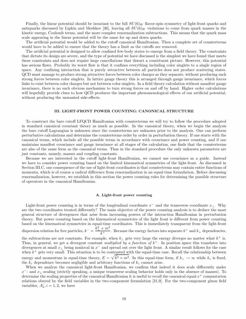
Finally, the linear potential should be invariant to the full SU(6)W flavor-spin symmetry of light-front quarks andantiquarks discussed by Lipkin and Meshkov [36], leaving all SU(6)W violations to come from quark masses in thekinetic energy, Coulomb terms, and the more complex renormalization subtractions. This means that the quark massscale appearing in the linear potential will be the same for up and down quarks.

The artificial potential would be added to the cutoff canonical Hamiltonian. Then a complete set of countertermswould have to be added to ensure that the theory has a limit as the cutoffs are removed.

The artificial potential is designed to allow confined few-body states to emerge from a field theory. The constraintsthat dictate its design are severe, and the type of potential we have discussed is the simplest we have found that meetsthese constraints and does not require large cancellations that thwart a constituent picture. However, this potentialhas serious flaws. Probably its worst flaw is that it confines everything including color singlets to a single region ofspace. Any confining interaction that is purely attractive between all particles does not produce scattering states.QCD must manage to produce strong attractive forces between color charges as they separate, without producing suchstrong forces between color singlets. In lattice gauge theory this is arranged through gauge invariance, which forceslinks to exist between color charges but not between color singlets. In a field theory calculation without manifest gaugeinvariance, there is no such obvious mechanism to turn strong forces on and off by hand. Higher order calculationswill hopefully provide clues to how QCD produces the important phenomenological effects of our artificial potential,without producing the unwanted side-effects.

III. LIGHT-FRONT POWER COUNTING: CANONICAL STRUCTURE

To construct the bare cutoff LFQCD Hamiltonian with counterterms we will try to follow the procedure adoptedin standard canonical covariant theory as much as possible. In the canonical theory, when we begin the analysisthe bare cutoff Lagrangian is unknown since the counterterms are unknown prior to the analysis. One can performperturbative calculations and determine the counterterms order by order in perturbation theory. If one starts with thecanonical terms, which include all the possible terms in accordance with covariance and power counting, and if onemaintains manifest covariance and gauge invariance at all stages of the calculation, one finds that the countertermsare also of the same form as the canonical terms. Thus in the standard procedure the only unknown parameters arejust constants, namely, masses and coupling constants.

Because we are interested in the cutoff light-front Hamiltonian, we cannot use covariance as a guide. Insteadwe have to consider power counting based on the limited kinematical symmetries of the light-front. As discussed inSection III.C, one consequence of the use of light-front coordinates is that counterterms may contain entire functions ofmomenta, which is of course a radical difference from renormalization in an equal-time formulation. Before discussingrenormalization, however, we establish in this section the power counting rules for determining the possible structureof operators in the canonical Hamiltonian.

A. Light-front power counting

Light-front power counting is in terms of the longitudinal coordinate x− and the transverse coordinate x⊥. Whyare the two coordinates treated differently? The main objective of the power counting analysis is to deduce the mostgeneral structure of divergences that arise from increasing powers of the interaction Hamiltonian in perturbationtheory. But power counting based on the kinematical symmetries of the light front is different from power countingbased on the kinematical symmetries in equal-time coordinates. This is immediately transparent from the light-front

dispersion relation for free particles, k− =k2⊥ +m2

k+ . Because the energy factors into separate k+ and k⊥ dependencies,

the subtractions are not constants. For example, when k⊥ gets very large the energy diverges no matter what k+ is.Thus, in general, we get a divergent constant multiplied by a function of k+. In position space this translates intodivergences at small x⊥ being nonlocal in x− and spread out over the light front. A similar result follows for the casewhen k+ gets very small. This situation is to be contrasted with the equal-time case. Recall the relationship between

energy and momentum in equal-time theory, E =√~k2 +m2. In this equal-time form, if k⊥ → ∞ while kz is fixed,

the kz dependence becomes negligible and arbitrary functions of kz cannot arise.When we analyze the canonical light-front Hamiltonian, we confirm that indeed it does scale differently under

x−- and x⊥-scaling (strictly speaking, a unique transverse scaling behavior holds only in the absence of masses). Todetermine the scaling properties of the canonical Hamiltonian it is useful to recall the canonical equal-x+ commutationrelations obeyed by the field variables in the two-component formulation [31,9]. For the two-component gluon fieldvariables, Ai

a, i = 1, 2, we have

10

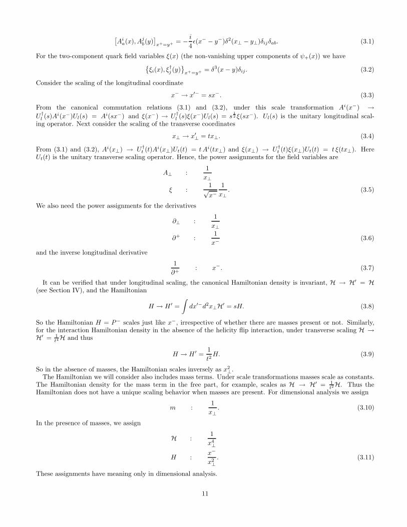
[Ai

a(x), Ajb(y)

]

x+=y+ = − i

4ǫ(x− − y−)δ2(x⊥ − y⊥)δijδab. (3.1)

For the two-component quark field variables ξ(x) (the non-vanishing upper components of ψ+(x)) we have{ξi(x), ξ†j (y)

}

x+=y+ = δ3(x − y)δij . (3.2)

Consider the scaling of the longitudinal coordinate

x− → x′− = sx−. (3.3)

From the canonical commutation relations (3.1) and (3.2), under this scale transformation Ai(x−) →U †

l (s)Ai(x−)Ul(s) = Ai(sx−) and ξ(x−) → U †l (s)ξ(x−)Ul(s) = s

12 ξ(sx−). Ul(s) is the unitary longitudinal scal-

ing operator. Next consider the scaling of the transverse coordinates

x⊥ → x′⊥ = tx⊥. (3.4)

From (3.1) and (3.2), Ai(x⊥) → U †t (t)Ai(x⊥)Ut(t) = t Ai(tx⊥) and ξ(x⊥) → U †

t (t)ξ(x⊥)Ut(t) = t ξ(tx⊥). HereUt(t) is the unitary transverse scaling operator. Hence, the power assignments for the field variables are

A⊥ :1

x⊥

ξ :1√x−

1

x⊥. (3.5)

We also need the power assignments for the derivatives

∂⊥ :1

x⊥

∂+ :1

x−(3.6)

and the inverse longitudinal derivative

1

∂+: x−. (3.7)

It can be verified that under longitudinal scaling, the canonical Hamiltonian density is invariant, H → H′ = H(see Section IV), and the Hamiltonian

H → H ′ =

∫

dx′−d2x⊥H′ = sH. (3.8)

So the Hamiltonian H = P− scales just like x−, irrespective of whether there are masses present or not. Similarly,for the interaction Hamiltonian density in the absence of the helicity flip interaction, under transverse scaling H →H′ = 1

t4H and thus

H → H ′ =1

t2H. (3.9)

So in the absence of masses, the Hamiltonian scales inversely as x2⊥.

The Hamiltonian we will consider also includes mass terms. Under scale transformations masses scale as constants.The Hamiltonian density for the mass term in the free part, for example, scales as H → H′ = 1

t2H. Thus theHamiltonian does not have a unique scaling behavior when masses are present. For dimensional analysis we assign

m :1

x⊥. (3.10)

In the presence of masses, we assign

H :1

x4⊥

H :x−

x2⊥. (3.11)

These assignments have meaning only in dimensional analysis.

11

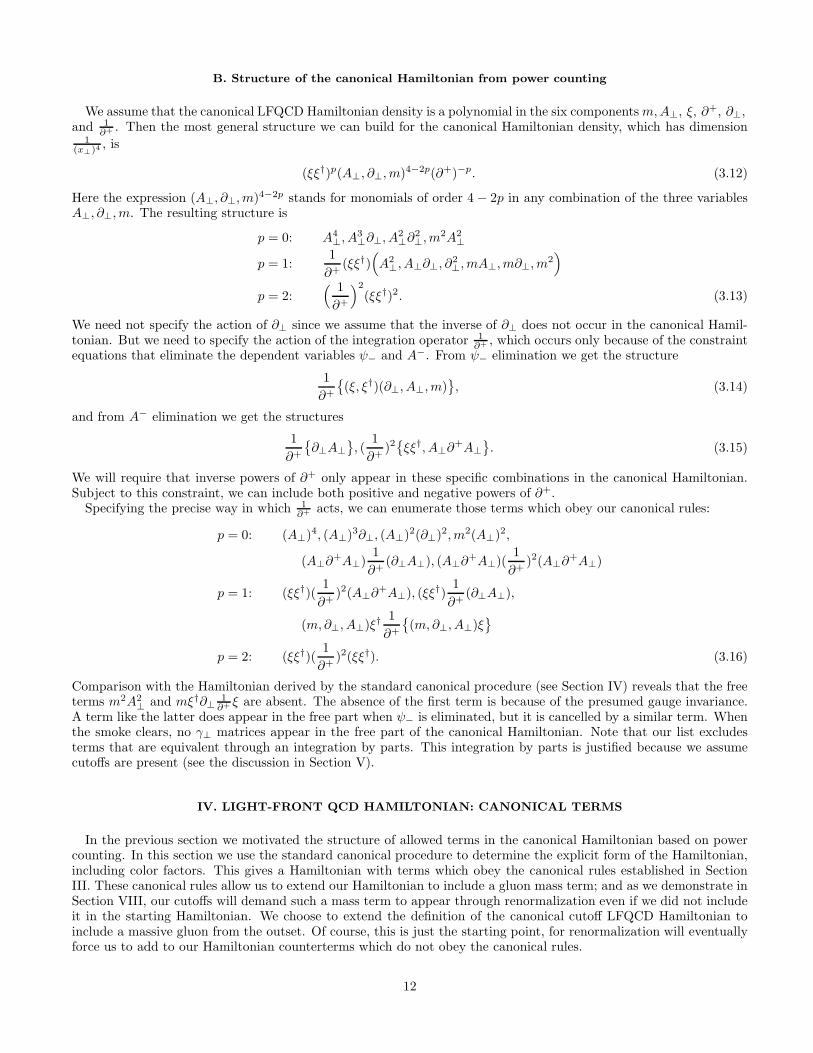
B. Structure of the canonical Hamiltonian from power counting

We assume that the canonical LFQCD Hamiltonian density is a polynomial in the six componentsm,A⊥, ξ, ∂+, ∂⊥,

and 1∂+ . Then the most general structure we can build for the canonical Hamiltonian density, which has dimension

1(x⊥)4 , is

(ξξ†)p(A⊥, ∂⊥,m)4−2p(∂+)−p. (3.12)

Here the expression (A⊥, ∂⊥,m)4−2p stands for monomials of order 4 − 2p in any combination of the three variablesA⊥, ∂⊥,m. The resulting structure is

p = 0: A4⊥, A

3⊥∂⊥, A

2⊥∂

2⊥,m

2A2⊥

p = 1:1

∂+(ξξ†)

(

A2⊥, A⊥∂⊥, ∂

2⊥,mA⊥,m∂⊥,m

2)

p = 2:( 1

∂+

)2

(ξξ†)2. (3.13)

We need not specify the action of ∂⊥ since we assume that the inverse of ∂⊥ does not occur in the canonical Hamil-tonian. But we need to specify the action of the integration operator 1

∂+ , which occurs only because of the constraintequations that eliminate the dependent variables ψ− and A−. From ψ− elimination we get the structure

1

∂+

{(ξ, ξ†)(∂⊥, A⊥,m)

}, (3.14)

and from A− elimination we get the structures

1

∂+

{∂⊥A⊥

}, (

1

∂+)2

{ξξ†, A⊥∂

+A⊥}. (3.15)

We will require that inverse powers of ∂+ only appear in these specific combinations in the canonical Hamiltonian.Subject to this constraint, we can include both positive and negative powers of ∂+.

Specifying the precise way in which 1∂+ acts, we can enumerate those terms which obey our canonical rules:

p = 0: (A⊥)4, (A⊥)3∂⊥, (A⊥)2(∂⊥)2,m2(A⊥)2,

(A⊥∂+A⊥)

1

∂+(∂⊥A⊥), (A⊥∂

+A⊥)(1

∂+)2(A⊥∂

+A⊥)

p = 1: (ξξ†)(1

∂+)2(A⊥∂

+A⊥), (ξξ†)1

∂+(∂⊥A⊥),

(m, ∂⊥, A⊥)ξ†1

∂+

{(m, ∂⊥, A⊥)ξ

}

p = 2: (ξξ†)(1

∂+)2(ξξ†). (3.16)

Comparison with the Hamiltonian derived by the standard canonical procedure (see Section IV) reveals that the freeterms m2A2

⊥ and mξ†∂⊥1

∂+ ξ are absent. The absence of the first term is because of the presumed gauge invariance.A term like the latter does appear in the free part when ψ− is eliminated, but it is cancelled by a similar term. Whenthe smoke clears, no γ⊥ matrices appear in the free part of the canonical Hamiltonian. Note that our list excludesterms that are equivalent through an integration by parts. This integration by parts is justified because we assumecutoffs are present (see the discussion in Section V).

IV. LIGHT-FRONT QCD HAMILTONIAN: CANONICAL TERMS

In the previous section we motivated the structure of allowed terms in the canonical Hamiltonian based on powercounting. In this section we use the standard canonical procedure to determine the explicit form of the Hamiltonian,including color factors. This gives a Hamiltonian with terms which obey the canonical rules established in SectionIII. These canonical rules allow us to extend our Hamiltonian to include a gluon mass term; and as we demonstrate inSection VIII, our cutoffs will demand such a mass term to appear through renormalization even if we did not includeit in the starting Hamiltonian. We choose to extend the definition of the canonical cutoff LFQCD Hamiltonian toinclude a massive gluon from the outset. Of course, this is just the starting point, for renormalization will eventuallyforce us to add to our Hamiltonian counterterms which do not obey the canonical rules.

12

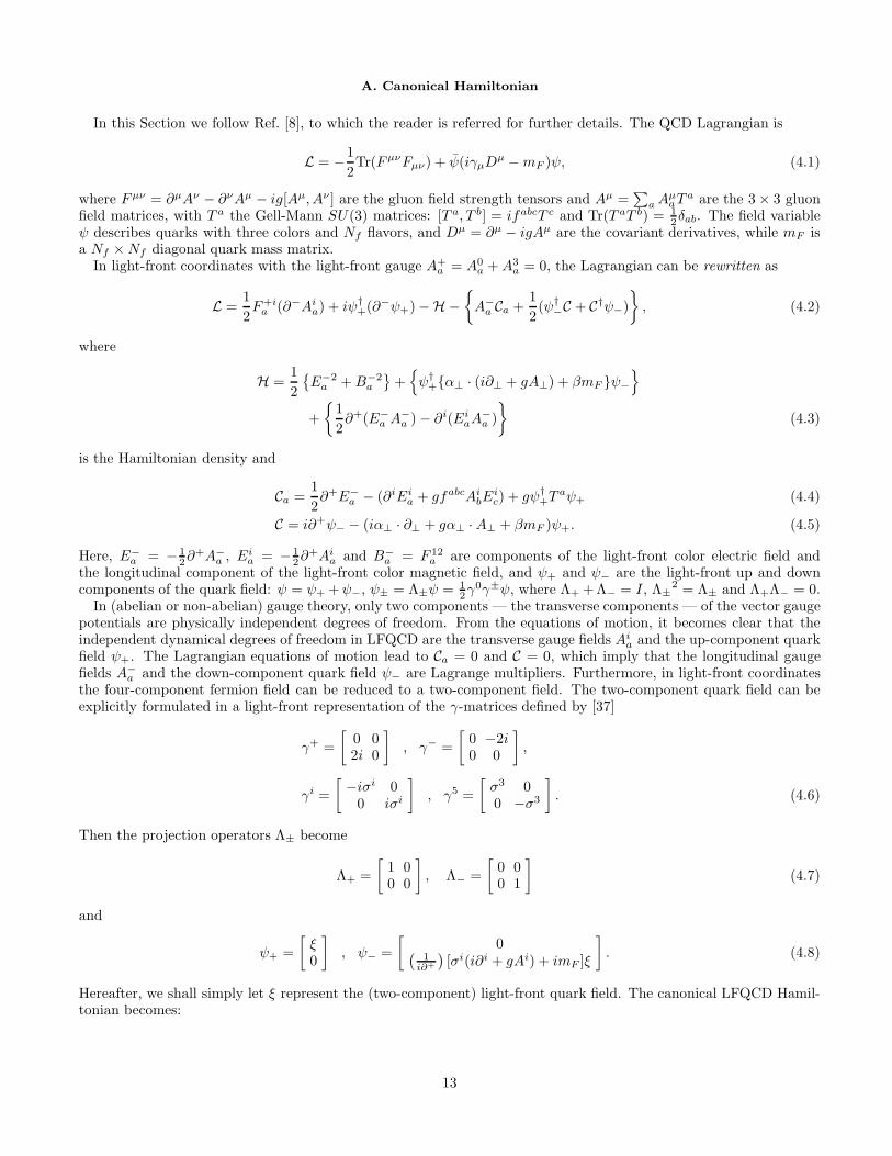
A. Canonical Hamiltonian

In this Section we follow Ref. [8], to which the reader is referred for further details. The QCD Lagrangian is

L = −1

2Tr(FµνFµν) + ψ(iγµD

µ −mF )ψ, (4.1)

where Fµν = ∂µAν − ∂νAµ − ig[Aµ, Aν ] are the gluon field strength tensors and Aµ =∑

aAµaT

a are the 3 × 3 gluonfield matrices, with T a the Gell-Mann SU(3) matrices: [T a, T b] = ifabcT c and Tr(T aT b) = 1

2δab. The field variableψ describes quarks with three colors and Nf flavors, and Dµ = ∂µ − igAµ are the covariant derivatives, while mF isa Nf ×Nf diagonal quark mass matrix.

In light-front coordinates with the light-front gauge A+a = A0

a +A3a = 0, the Lagrangian can be rewritten as

L =1

2F+i

a (∂−Aia) + iψ†

+(∂−ψ+) −H −{

A−a Ca +

1

2(ψ†

−C + C†ψ−)

}

, (4.2)

where

H =1

2

{E−2

a +B−2a

}+

{

ψ†+{α⊥ · (i∂⊥ + gA⊥) + βmF }ψ−

}

+

{1

2∂+(E−

a A−a ) − ∂i(Ei

aA−a )

}

(4.3)

is the Hamiltonian density and

Ca =1

2∂+E−

a − (∂iEia + gfabcAi

bEic) + gψ†

+Taψ+ (4.4)

C = i∂+ψ− − (iα⊥ · ∂⊥ + gα⊥ ·A⊥ + βmF )ψ+. (4.5)

Here, E−a = − 1

2∂+A−

a , Eia = − 1

2∂+Ai

a and B−a = F 12

a are components of the light-front color electric field andthe longitudinal component of the light-front color magnetic field, and ψ+ and ψ− are the light-front up and downcomponents of the quark field: ψ = ψ+ +ψ−, ψ± = Λ±ψ = 1

2γ0γ±ψ, where Λ+ + Λ− = I, Λ±

2 = Λ± and Λ+Λ− = 0.In (abelian or non-abelian) gauge theory, only two components — the transverse components — of the vector gauge

potentials are physically independent degrees of freedom. From the equations of motion, it becomes clear that theindependent dynamical degrees of freedom in LFQCD are the transverse gauge fields Ai

a and the up-component quarkfield ψ+. The Lagrangian equations of motion lead to Ca = 0 and C = 0, which imply that the longitudinal gaugefields A−

a and the down-component quark field ψ− are Lagrange multipliers. Furthermore, in light-front coordinatesthe four-component fermion field can be reduced to a two-component field. The two-component quark field can beexplicitly formulated in a light-front representation of the γ-matrices defined by [37]

γ+ =

[0 02i 0

]

, γ− =

[0 −2i0 0

]

,

γi =

[−iσi 0

0 iσi

]

, γ5 =

[σ3 00 −σ3

]

. (4.6)

Then the projection operators Λ± become

Λ+ =

[1 00 0

]

, Λ− =

[0 00 1

]

(4.7)

and

ψ+ =

[ξ0

]

, ψ− =

[0

(1

i∂+

)[σi(i∂i + gAi) + imF ]ξ

]

. (4.8)

Hereafter, we shall simply let ξ represent the (two-component) light-front quark field. The canonical LFQCD Hamil-tonian becomes:

13

H =

∫

dx−d2x⊥

{1

2(∂iAj

a)2 + gfabcAiaA

jb∂

iAjc

+g2

4fabcfadeAi

bAjcA

idA

je

+

[

ξ†{σ⊥ · (i∂⊥ + gA⊥) − imF}

×(

1

i∂+

)

{σ⊥ · (i∂⊥ + gA⊥) + imF }ξ]

+ g∂iAia

(1

∂+

)

(fabcAjb∂

+Ajc + 2ξ†T aξ)

+g2

2

(1

∂+

)

(fabcAib∂

+Aic + 2ξ†T aξ)

×(

1

∂+

)

(fadeAjd∂

+Aje + 2ξ†T aξ)

}

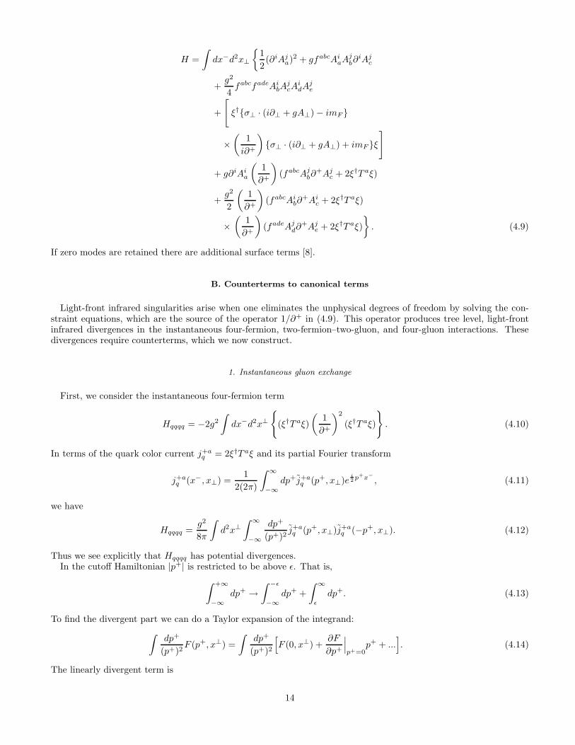
. (4.9)

If zero modes are retained there are additional surface terms [8].

B. Counterterms to canonical terms

Light-front infrared singularities arise when one eliminates the unphysical degrees of freedom by solving the con-straint equations, which are the source of the operator 1/∂+ in (4.9). This operator produces tree level, light-frontinfrared divergences in the instantaneous four-fermion, two-fermion–two-gluon, and four-gluon interactions. Thesedivergences require counterterms, which we now construct.

1. Instantaneous gluon exchange

First, we consider the instantaneous four-fermion term

Hqqqq = −2g2

∫

dx−d2x⊥

{

(ξ†T aξ)

(1

∂+

)2

(ξ†T aξ)

}

. (4.10)

In terms of the quark color current j+aq = 2ξ†T aξ and its partial Fourier transform

j+aq (x−, x⊥) =

1

2(2π)

∫ ∞

−∞dp+j+a

q (p+, x⊥)ei2

p+x−

, (4.11)

we have

Hqqqq =g2

8π

∫

d2x⊥∫ ∞

−∞

dp+

(p+)2j+aq (p+, x⊥)j+a

q (−p+, x⊥). (4.12)

Thus we see explicitly that Hqqqq has potential divergences.In the cutoff Hamiltonian |p+| is restricted to be above ǫ. That is,

∫ +∞

−∞dp+ →

∫ −ǫ

−∞dp+ +

∫ ∞

ǫ

dp+. (4.13)

To find the divergent part we can do a Taylor expansion of the integrand:

∫dp+

(p+)2F (p+, x⊥) =

∫dp+

(p+)2

[

F (0, x⊥) +∂F

∂p+

∣∣∣p+=0

p+ + ...]

. (4.14)

The linearly divergent term is

14

g2

8π

2

ǫ

∫

d2x⊥j+aq (0, x⊥)j+a

q (0, x⊥). (4.15)

The logarithmically divergent term vanishes because of the symmetric cutoff. Let us suppose we had used separatecutoffs ǫ+ and ǫ− for small positive and negative p+, respectively. Then the potentially logarithmically divergent termis

ig2

8πln

(ǫ+ǫ−

) ∫

d2x⊥

∫

dx−∫

dy−j+aq (x−, x⊥)(x− − y−)j+a

q (y−, x⊥), (4.16)

which is finite if we choose ǫ+ = µǫ−, with µ some number. This particular operator vanishes because of symmetryunder x− → y− exchange, but it forces us to reconsider our original neglect of zero modes in the solution of theconstraint equations.

We are finding a potentially divergent sensitivity of the Hamiltonian to modes with small longitudinal momentum,and we regard this as a signal that finite zero mode effects may arise. The potential divergence arises from theconstraint equations and reflects contributions from A− close to zero longitudinal momentum. It is extremely naiveto suppose that the canonical constraint equation for A− reproduces the nonperturbative effects of a zero mode inany simple manner. We discuss the divergences that arise from the exchange of small longitudinal momentum gluonswith physical polarization below, but even here we can think of the counterterms produced by the constraint equationas arising from the exchange of small longitudinal momentum gluons with unphysical polarization. Once one realizesthat an exchange is involved and that the divergence is independent of transverse coordinates, it becomes clear thateven the assumption that these counterterms will be local in the transverse direction is naive. We therefore allowterms in the Hamiltonian of the form

ig2

8π

∫

d2x⊥dx−

∫

dy−d2y⊥j+aq (x−, x⊥)(x− − y−)OG(x⊥ − y⊥)j+a

q (y−, y⊥). (4.17)

OG is a function of the transverse variables and is restricted by dimensional analysis, kinematical boost invariance,translational invariance, and invariance under rotations about the longitudinal axis. OG must be odd under x⊥ → y⊥to keep (4.17) from vanishing, and this is not possible here because gluon exchange gives only an even number ofpolarization vectors ǫiλ with which to contract the transverse indices. Thus there is indeed no finite countertermassociated with logarithmic divergences in Hqqqq , and our discussion serves only to illustrate one way candidatevacuum interactions can be identified.

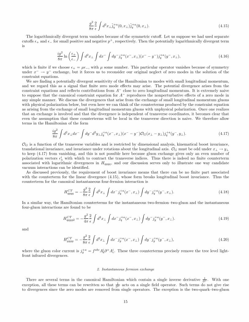
As discussed previously, the requirement of boost invariance means that there can be no finite part associatedwith the counterterm for the linear divergence (4.15), whose form breaks longitudinal boost invariance. Thus thecounterterm for the canonical instantaneous four-fermion interaction is

HCTqqqq = − g2

8π

2

ǫ

∫

d2x⊥

∫

dx−j+aq (x−, x⊥)

∫

dy−j+aq (y−, x⊥). (4.18)

In a similar way, the Hamiltonian counterterms for the instantaneous two-fermion–two-gluon and the instantaneousfour-gluon interactions are found to be

HCTqqgg2 = − g2

4π

2

ǫ

∫

d2x⊥

∫

dx−j+aq (x−, x⊥)

∫

dy−j+ag (y−, x⊥). (4.19)

and

HCTgggg = − g2

8π

2

ǫ

∫

d2x⊥

∫

dx−j+ag (x−, x⊥)

∫

dy−j+ag (y−, x⊥), (4.20)

where the gluon color current is j+ag = fabcAi

b∂+Ai

c. These three counterterms precisely remove the tree level light-front infrared divergences.

2. Instantaneous fermion exchange

There are several terms in the canonical Hamiltonian which contain a single inverse derivative 1∂+ . With one

exception, all these terms can be rewritten so that 1∂+ acts on a single field operator. Such terms do not give rise

to divergences since the zero modes are removed from single operators. The exception is the two-quark–two-gluon

15

interaction involving an instantaneous fermion exchange Hqqgg1 . Here 1∂+ acts on a product of field operators and

hence can give rise to a logarithmic divergence (see also Section V).Denoting σ⊥ ·A⊥(x−, x⊥) ξ(x−, x⊥) by f(x−, x⊥), we have

Hqqgg1 = g2

∫

dx−d2x⊥f†(x−, x⊥)

1

i∂+f(x−, x⊥). (4.21)

Introducing the partial Fourier transform as before

f(p+, x⊥) =

∫ ∞

−∞dx−e

i2

p+x−

f(x−, x⊥), (4.22)

we find

Hqqgg1 =g2

4π

∫

d2x⊥

∫ ∞

−∞

dp+

p+f †(p+, x⊥)f(−p+, x⊥). (4.23)

A potential logarithmic divergence disappears if we use a symmetric cutoff.Once again, though, we must be careful with this logarithmic divergence. While there is no divergent dependence

on the symmetric longitudinal infrared cutoff ǫ since the divergence due to small p+ is cancelled by the divergencedue to small −p+, we still have to worry about non-vanishing contributions from states with exactly p+ = 0 — thatis, from exchange of zero-mode fermions. Once an infrared cutoff is employed, we have eliminated the possibility ofcomputing this contribution; and so we should include in the Hamiltonian terms which can counter the effects of thisexclusion. Such counterterms have the form

HCTqqgg1 = g2

∫

dx−d2x⊥

∫

dy−d2y⊥f†(x−, x⊥)OF (x⊥ − y⊥)f(y−, y⊥), (4.24)

where dimensional analysis reveals that OF scales as 1. Since this term comes from zero-mode fermion exchange, OF

is a function of transverse variables and the Pauli matrices σ⊥. Since this term arises from vacuum effects, it is notrestricted to have a polynomial dependence on transverse variables and the renormalized constituent mass. Thus aterm like OF ∼ m−1

F σ⊥ · ∂⊥ is allowed and should be included in the Hamiltonian. Such a term explicitly violateschiral symmetry and need not be small in the relativistic limit.

This is then the first point at which an arbitrary function enters the Hamiltonian. At the simplest level, thefunction OF (x⊥, y⊥) must be determined phenomenologically by fitting bound state properties. It is an open questionwhether theoretical techniques such as coupling coherence will determine it a priori, whether the requirement ofrelativistic invariance will determine it completely a posteriori, or whether phenomenology will still be necessarywhen renormalization is done at higher orders.

C. Canonical Hamiltonian: free plus interaction terms

Now we add explicitly the gluon mass term to the LFQCD canonical Hamiltonian together with the countertermsfor instantaneous interactions. The Hamiltonian is written as a free term plus interactions

H =

∫

dx−d2x⊥(H0 + Hint), (4.25)

with

H0 =1

2(∂iAj

a)(∂iAja) +

1

2m2

GAjaA

ja + ξ†

(−∂2⊥ +m2

F

i∂+

)

ξ

Hint = VA + Hqqg + Hggg + Hqqgg + Hqqqq + Hgggg . (4.26)

Here VA is the artificial potential, and

Hqqg = gξ†{

−2

(1

∂+

)

(∂⊥ · A⊥)

+ σ⊥ ·A⊥

(1

∂+

)

(σ⊥ · ∂⊥ +mF )

16

+

(1

∂+

)

(σ⊥ · ∂⊥ −mF )σ⊥ · A⊥

}

ξ (4.27)

Hggg = gfabc

{

∂iAjaA

ibA

jc + (∂iAi

a)

(1

∂+

)

(Ajb∂

+Ajc)

}

(4.28)

Hqqgg = g2

{

ξ†σ⊥ ·A⊥

(1

i∂+

)

σ⊥ · A⊥ξ

}

− 2g2

{

(fabcAib∂

+Aic)

(1

∂+

)2

(ξ†T aξ)

}

+HCTqqgg1 +HCT

qqgg2

= Hqqgg1 + Hqqgg2 (4.29)

Hqqqq = −2g2

{

(ξ†T aξ)

(1

∂+

)2

(ξ†T aξ)

}

+HCTqqqq (4.30)

Hgggg =g2

4fabcfade

{

AibA

jcA

idA

je

−2(Aib∂

+Aic)

(1

∂+

)2

(Ajd∂

+Aje)

}

+HCTgggg

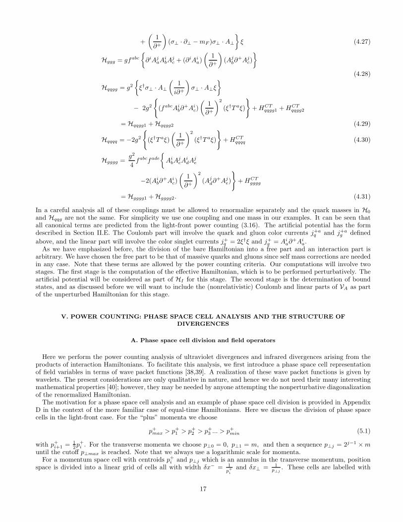
= Hgggg1 + Hgggg2. (4.31)

In a careful analysis all of these couplings must be allowed to renormalize separately and the quark masses in H0

and Hqqg are not the same. For simplicity we use one coupling and one mass in our examples. It can be seen thatall canonical terms are predicted from the light-front power counting (3.16). The artificial potential has the formdescribed in Section II.E. The Coulomb part will involve the quark and gluon color currents j+a

q and j+ag defined

above, and the linear part will involve the color singlet currents j+q = 2ξ†ξ and j+g = Aia∂

+Aia.

As we have emphasized before, the division of the bare Hamiltonian into a free part and an interaction part isarbitrary. We have chosen the free part to be that of massive quarks and gluons since self mass corrections are neededin any case. Note that these terms are allowed by the power counting criteria. Our computations will involve twostages. The first stage is the computation of the effective Hamiltonian, which is to be performed perturbatively. Theartificial potential will be considered as part of HI for this stage. The second stage is the determination of boundstates, and as discussed before we will want to include the (nonrelativistic) Coulomb and linear parts of VA as partof the unperturbed Hamiltonian for this stage.

V. POWER COUNTING: PHASE SPACE CELL ANALYSIS AND THE STRUCTURE OF

DIVERGENCES

A. Phase space cell division and field operators

Here we perform the power counting analysis of ultraviolet divergences and infrared divergences arising from theproducts of interaction Hamiltonians. To facilitate this analysis, we first introduce a phase space cell representationof field variables in terms of wave packet functions [38,39]. A realization of these wave packet functions is given bywavelets. The present considerations are only qualitative in nature, and hence we do not need their many interestingmathematical properties [40]; however, they may be needed by anyone attempting the nonperturbative diagonalizationof the renormalized Hamiltonian.

The motivation for a phase space cell analysis and an example of phase space cell division is provided in AppendixD in the context of the more familiar case of equal-time Hamiltonians. Here we discuss the division of phase spacecells in the light-front case. For the “plus” momenta we choose

p+max > p+

1 > p+2 > p+

3 ... > p+min (5.1)

with p+i+1 = 1

2p+i . For the transverse momenta we choose p⊥0 = 0, p⊥1 = m, and then a sequence p⊥j = 2j−1 ×m

until the cutoff p⊥max is reached. Note that we always use a logarithmic scale for momenta.For a momentum space cell with centroids p+

i and p⊥j which is an annulus in the transverse momentum, positionspace is divided into a linear grid of cells all with width δx− = 1

p+

i

and δx⊥ = 1p⊥j

. These cells are labelled with

17

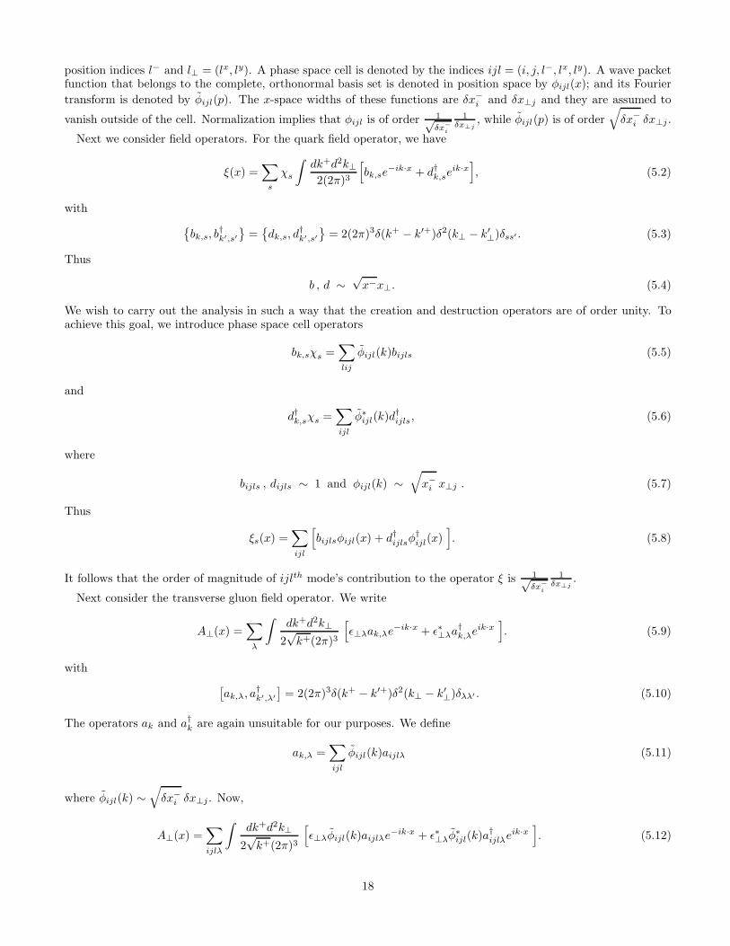
position indices l− and l⊥ = (lx, ly). A phase space cell is denoted by the indices ijl = (i, j, l−, lx, ly). A wave packetfunction that belongs to the complete, orthonormal basis set is denoted in position space by φijl(x); and its Fourier

transform is denoted by φijl(p). The x-space widths of these functions are δx−i and δx⊥j and they are assumed to

vanish outside of the cell. Normalization implies that φijl is of order 1√δx−

i

1δx⊥j

, while φijl(p) is of order√

δx−i δx⊥j .

Next we consider field operators. For the quark field operator, we have

ξ(x) =∑

s

χs

∫dk+d2k⊥2(2π)3

[

bk,se−ik·x + d†k,se

ik·x]

, (5.2)

with

{bk,s, b

†k′,s′

}=

{dk,s, d

†k′,s′

}= 2(2π)3δ(k+ − k′+)δ2(k⊥ − k′⊥)δss′ . (5.3)

Thus

b , d ∼√x−x⊥. (5.4)

We wish to carry out the analysis in such a way that the creation and destruction operators are of order unity. Toachieve this goal, we introduce phase space cell operators

bk,sχs =∑

lij

φijl(k)bijls (5.5)

and

d†k,sχs =∑

ijl

φ∗ijl(k)d†ijls, (5.6)

where

bijls , dijls ∼ 1 and φijl(k) ∼√

x−i x⊥j . (5.7)

Thus

ξs(x) =∑

ijl

[

bijlsφijl(x) + d†ijlsφ†ijl(x)

]

. (5.8)

It follows that the order of magnitude of ijlth mode’s contribution to the operator ξ is 1√δx−

i

1δx⊥j

.

Next consider the transverse gluon field operator. We write

A⊥(x) =∑

λ

∫dk+d2k⊥

2√k+(2π)3

[

ǫ⊥λak,λe−ik·x + ǫ∗⊥λa

†k,λe

ik·x]

. (5.9)

with

[ak,λ, a

†k′,λ′

]= 2(2π)3δ(k+ − k′+)δ2(k⊥ − k′⊥)δλλ′ . (5.10)

The operators ak and a†k are again unsuitable for our purposes. We define

ak,λ =∑

ijl

φijl(k)aijlλ (5.11)

where φijl(k) ∼√

δx−i δx⊥j . Now,

A⊥(x) =∑

ijlλ

∫dk+d2k⊥

2√k+(2π)3

[

ǫ⊥λφijl(k)aijlλe−ik·x + ǫ∗⊥λφ

∗ijl(k)a†ijlλe

ik·x]

. (5.12)

18

The order of magnitude of ijlth mode’s contribution to A⊥(x) is 1δx⊥j

.

Because of the cutoffs we impose, the wave packet functions φijl(x) do not have zero modes; that is,∫dxφijl(x) = 0.

We must also specify the order of magnitude of ∂⊥, ∂+, and (∂+)−1 when acting on a specified subset of waveletsin an operator product. For qualitative purposes each gradient needs to be applied only to the most rapidly changingwavelet in the subset, so that ∂⊥ is of order (δx⊥)−1, where δx⊥ is the smallest width in the subset. A similar resultholds for ∂+. The effect of the inverse operator (∂+)−1 — which involves an integration — is also determined by thesmallest width δx− in the product. Qualitatively, it amounts to multiplication of the subset by the width δx−, forthe other, broader widths act as constants over this width. However, there is a special case we must note.

To see this, consider the action of (∂+)−1 on a product of field operators. Now the wave packet functions associatedwith destruction operators have positive k+ only, and the wave packet functions associated with creation operatorshave negative k+ only. If the product contains only creation operators or only destruction operators, then the operationof (∂+)−1 qualitatively amounts to multiplication by the smaller width among the product in accord with the ruleabove. But if the product contains at least one creation and one destruction operator, then wavelets with Fouriermodes of positive k+ and wavelets with Fourier modes of negative k+ will both occur in the product. When theyhave the same mean value of k+, the product acquires a zero mode and then (∂+)−1 no longer produces a localizedfunction but rather one which covers the whole space. Thus the action of a single ( 1

∂+ ) can lead to a logarithmic

infrared divergence and the action of ( 1∂+ )2 can lead to both linear and logarithmic infrared divergences already in

the canonical terms. We have discussed these divergences and the counterterms which remove them in Section IV.B.

B. Ultraviolet divergences and counterterms

Consider ultraviolet divergences arising from the products of interaction Hamiltonians. Each term in the interactionHamiltonian involves an integral over the product of three or four field operators. Each field operator is expanded interms of wave packet functions. First, we consider the ultraviolet divergences arising from a product of two interactionHamiltonians. We shall consider the special case of just two wave packet sectors, one being fixed and the other beingarbitrarily large. This corresponds to a single divergent loop integral in the familiar language. The fixed wave packetwidth corresponds to the fixed external momenta in the loop diagram, and the varying wave packet width correspondsto the diverging loop momenta.

We denote the widths of the fixed and varying wave packet sectors by (δx−, δx⊥) and (δy−, δy⊥), respectively.

The energy of the varying wave packet sector scales as δy−

δy2⊥

. The energy diverges as δy⊥ → 0, corresponding to

the traditional type of short-distance ultraviolet divergence, which we consider in this section. The divergences asδy− → ∞ are light-front infrared divergences, which we consider in the next section. Consider ultraviolet divergenceswhich occur when δy⊥ ≪ δx⊥. We set δx− = δy−. The interaction Hamiltonian contains only cubic and quarticterms in the field operators ξ†, ξ, and Ai. We now observe that, as a consequence of momentum conservation at thevertices, to produce an ultraviolet divergence at least two of the three or four operators have to refer to a y-sector.We also note that a transverse gradient will yield 1

δy⊥

unless it applies to a product of x-sectors only.

Now consider the terms in the interaction Hamiltonian. If all operators refer to y-sectors, each term scales as δy−

δy2⊥

except for the mass term (the helicity-flip interaction), which scales as δy−

δy⊥

. But if some operators refer to x-sectors,

there will be additional factors of δy⊥

δx⊥

. For each field operator (ξ†, ξ, A⊥) belonging to an x-sector and for each

derivative ∂⊥ acting on only x-sectors, there is a factor of δy⊥

δx⊥

. This gives the contribution from a single sector with

width δy−, δy⊥ as δy⊥ gets small. But many wavelets with different δy⊥ can contribute, namely, all wavelets withdifferent centers that overlap a given x-wavelet (see Fig. 13). Since the transverse space has dimension two, thenumber of independent wavelets of linear size δy⊥ that overlap with the wavelet of size δx⊥ is of order (δx⊥/δy⊥)2.

Next consider the second-order perturbation theory formula

HI1

E.DHI , (5.13)

where E.D denotes the energy denominator. For qualitative purposes, we can replace the energy denominator by the

energy of the y-sector, namely, δy−

δy2⊥

. Thus the contribution in second order of a given term to the effective Hamiltonian

resulting from wave packet functions of a given width δy⊥ scales as

(δy−

δy2⊥

)

×( δy2

⊥δy−

)

×(δy−

δy2⊥

)

×(δx⊥δy⊥

)2

×( δy⊥δx⊥

)n

(5.14)

19

where n counts the number of ξ†, ξ, A⊥, and ∂⊥ factors that refer to x-sectors. If n is greater than 4 there is nodivergence, while for n less than or equal to four a divergence arises. When n is equal to 4, the contribution fromthe sector of a given size δy⊥ is a constant. Now we have to sum over all scale sizes δy⊥. The scale sizes δy⊥ allowedare inverse powers of 2 all the way down to a minimum size 1

Λ . A sum over all scale sizes down to 1Λ yields a term of

order (lnΛ /ln2), which gives a logarithmic divergence as Λ → ∞.Thus the power counting rule for ultraviolet counterterms is the same (in δx⊥) as for the canonical Hamiltonian;

namely, that there can be at most four operators scaling as δx−1⊥ . Even though we did the analysis for two HI ’s, it

holds for any number of HI ’s, where the first HI creates one or more y-type constituents, intermediate HI ’s maintainat least one y-type constituent, and the last HI destroys all the remaining y-type constituents. (We are ignoringcontributions “disconnected in y” — that is, products which contain an HI with only x-sector constituents. Thesediagrams have already acquired counterterms.) Each energy denominator may be replaced by the energy of the y-

sector δy−

δy2⊥

since each intermediate state contains at least one y-type constituent by assumption. If there are m factors

HI , there are m− 1 factorsδy2

⊥

δy− . Each HI scales like δy−

δy2⊥

times powers of (δy⊥/δx⊥). An overall factor (δx⊥/δy⊥)2,

counts the number of y-type wave packet functions that overlap with a single x-type wave packet function. Thus thefinal rule for the scaling versus δx⊥ and δy⊥ is identical for m HI ’s as for 2 HI ’s — namely, divergences occur forproducts in the effective Hamiltonian of x-operators up to fourth order in ξ†, ξ, A⊥, and∂⊥.

C. Infrared divergence and counterterms

Light-front infrared divergences are large-energy divergences as can be seen from the light-front dispersion relation

p− =p2⊥

+m2

p+ , which blows up as p+ → 0. We have already discussed the counterterms for light-front infrared

divergences that arise in the instantaneous interactions in the Hamiltonian. In this section we discuss the infrareddivergences which arise in products of the interaction Hamiltonian.

As in the analysis of ultraviolet divergences we will separate out the divergences caused by a specific y-type wavepacket function from the operator structure associated with an x-type wavelet. Let us discuss the differences from

the analysis of ultraviolet divergences. First of all, the y-wavelet energy scale δy−

y2⊥

is blowing up because δy− is

approaching ∞. Thus it will be assumed that δy− ≫ δx−, while to avoid confusion with ultraviolet problems weassume δy⊥ is of order δx⊥. In contrast to the ultraviolet case, light-front infrared divergences are caused by a singley-type wavelet with a width δy−. The reason for this is that only one y-type wavelet overlaps with a given x-typewavelet, since δy− is much wider than δx−. In this case momentum conservation at the vertices implies that toproduce a light-front infrared divergence at least two operators in HI have to be x-type. Each term in HI scales asδy−

δy2⊥

times a factor: a) ( δy−

δx− )12 for each ξ or ξ† referring to an x-type, b) ( δy−

δx− ) for every ∂+ acting on an x-type

operator and a reciprocal factor ( δx−

δy− ) for every (∂+)−1 operator when applied to a product including at least one

x-type operator, and c) ( δx−

δy− ) arising from the range of integration in each HI involving an x-type operator. As in

the case of ultraviolet divergences, in the effective Hamiltonian a term with no factor ( δx−

δy− ) diverges logarithmically

due to a sum over different widths δy−. However, exceptions to the above rules occur for terms in the canonicalHamiltonian involving ( 1

∂+ ) or ( 1∂+ )2 operators, which we will note below.

Let us now catalogue the factors associated with the scaling behavior of various terms in the interaction Hamiltonian.

If we ignore ∂+ or 1∂+ factors, then the rules are simple: an x-type ξ produces a factor ( ∂y−

∂x− )1/2, an x-type A⊥ produces

no factor, and the presence of any x-type operator in HI produces ( δx−

δy− ) as result of the change of integration width.

Thus, ignoring ∂+ and 1∂+ factors, we can compute the impact of any product of x-type operators on the scaling

behavior of HI :

ξξ : no factor

A⊥ξ : (δx−/δy−)12

A⊥ξξ : no factor

A⊥A⊥ : (δx−/δy−)

A⊥A⊥ξ : (δx−/δy−)12

A⊥A⊥ξξ : no factor

ξξξ : (δy−/δx−)12

20

ξξξξ : (δy−/δx−). (5.15)

Next we classify again the possible x-type operators in HI by the degree of divergence in HI that results, when theeffects of ∂+ and 1

∂+ factors are included. Here it is assumed that ∂+ or (1/∂+) is applied to a product that containsat least one x-type operator. It is useful to recall the structure of terms in the canonical Hamiltonian (see SectionIV), which we consider one by one in the following.

When all the operators in the Hamiltonian refer to the y-sector, the Hamiltonian scales as δy−. We have todetermine the scale factor that arises as a result of replacing two or more y-type operators by x-type operators. Let usfirst consider some specific examples. In the following we denote the operators that belong to the x-type by a subscript(x) and those belonging to the y-type by a subscript (y) respectively. Now consider the term in the Hamiltonian∫dz−d2z⊥ξ

†A⊥1

∂+ ξ. Here we write the integration variable as z in order to distinguish dz from the widths δx andδy.

1. For the case∫dz−d2z⊥(A⊥)(y)ξ

†(x)

1∂+ ξ(x), from our rules we get δy− × ( δy−

δx− ) (for two ξ′s) × ( δx−

δy− ) (for 1∂+ ) ×

( δx−

δy− ) (arising from the range of integration). Thus the scaling behavior is like δx− which we write as δy− ×( δx−

δy− ). Hence the scale factor is ( δx−

δy− ).

2. For the case∫dz−d2z⊥(A⊥ξ

†)(x)1

∂+ ξ(y) we get from our rules δy− × ( δy−

δx− )12 (for ξ†) × ( δx−

δy− ) ( arising from

the range of integration) . Thus the scaling behavior is like (δx− δy−)12 which we write as δy− × ( δx−

δy− )12 .

Hence the scale factor is ( δx−

δy− )12 .

Now there may be exceptions to these rules when (∂+)−1 or (∂+)−2 acts on a product of operators, for then it wouldpick out a zero mode as described above. However, we have eliminated this possibility by imposing a longitudinalcutoff ǫ on such terms and then adding a counterterm to remove the ǫ-dependence. Because of this, integration byparts is allowed and can be used to determine the order of magnitude of (∂+)−1 or (∂+)−2. The exception to theusual rule occurs, then, when there are not x-sector wavelets on each side of the inverse gradient, for integration byparts allows us to re-write the product so that the inverse operator acts entirely on y-type wavelets. Then it picksout a y-sector width and so does not produce the factor (δx−/δy−) or (δx−/δy−)2 expected from the above rules.Thus, for example, consider the term

∫dz−d2z⊥(ξ†A⊥)(y)

1∂+ (ξA⊥)(x). With the zero mode eliminated, we are free

to interchange the operation of 1∂+ to get

∫dz−d2z⊥

1∂+

((ξ†A⊥)(y)

)(A⊥ξ)(x). Thus the scaling is δy− × ( δy−

δx− )12

(from ξ) × ( δx−

δy− ) (arising from the range of integration). Hence the scaling behavior is (δx− δy−)12 , which we write

as δy− × ( δx−

δy− )12 ; and so the scale factor is ( δx−

δy− )12 .

In the following we determine the scale factor for various terms in the interaction Hamiltonian when two or moreoperators in them are replaced by x-type operators, the remaining operators being of y-type. Each 1

∂+ may apply

to y operators too, e.g, 1∂+ ξ might mean 1

∂+ (A⊥ξ) with A⊥ of y-type. The scale factor is unchanged by any suchembedded y operators.Products of ξ and ξ :

ξξ : no factor

(∂+)−2(ξξ) : no factor (exception applies)

ξ(∂+)−1ξ : (δx−/δy−)

ξ(∂+)−2ξ : (δx−/δy−)2. (5.16)

Products of A⊥ and ξ :

A⊥ξ : (δx−/δy−)12

(∂+)−1(A⊥ξ) : (δx−/δy−)12 (exception applies)

ξ(∂+)−2

(∂+A⊥) : (δx−/δy−)32

(∂+A⊥)(∂+)−2ξ : (δx−/δy−)32

ξ(∂+)−2A⊥ : (δx−/δy−)

52

A⊥(∂+)−2ξ : (δx−/δy−)

52

ξ(∂+)−1A⊥ : (δx−/δy−)

32 . (5.17)

21

Products of ξ, ξ, and A⊥ :

ξ2(∂+)−2A⊥ : (δx−/δy−)2

ξ2(∂+)−2∂+A⊥ : (δx−/δy−)

A⊥(∂+)−2ξ2 : (δx−/δy−)2

(∂+A⊥)(∂+)−2ξ2 : (δx−/δy−)

ξ2(∂+)−1A⊥ : (δx−/δy−)

ξ(∂+)−1A⊥ξ : (δx−/δy−)

ξA⊥(∂+)−1ξ : (δx−/δy−). (5.18)

Products of A⊥ and A⊥ :

A⊥A⊥ : (δx−/δy−)

A⊥(∂+)−2A⊥ : (δx−/δy−)3

A⊥(∂+)−2∂+A⊥ : (δx−/δy−)2

(∂+A⊥)(∂+)−2∂+A⊥ : (δx−/δy−)

(∂+)−2(A⊥∂+A⊥) : no factor (exception applies)

A⊥∂+A⊥ : no factor

A⊥1

∂+A⊥ : (δx−/δy−)2. (5.19)

Products of ξ, A⊥, and A⊥ :

ξ(∂+)−2A⊥∂+A⊥ : (δx−/δy−)

32

A⊥ξ(∂+)−1A⊥ : (δx−/δy−)

32

A⊥(∂+)−1ξA⊥ : (δx−/δy−)32 . (5.20)

Products of ξ, ξ, and ξ :

ξ(∂+)−2ξ2 : (δx−/δy−)32

ξ2(∂+)−2ξ : (δx−/δy−)32 . (5.21)

The above list splits into four types: a) Products which contain no δx−

δy− factors. They are all components of the color

charge density, either the quark or the gluon component. These products can occur in any number of HI ’s withoutreducing the divergence of the overall product. If these products are the only source of x-type operators, the overalldivergence behaves as δy−, that is, linearly. b) Products which contain a factor of (δx−/δy−)

12 . These products

involve a single ξ. Since only an even number of ξ’s can appear in the effective Hamiltonian, two such productsare required from two separate HI ’s; and the result is to generate a factor (δx−/δy−), which implies a logarithmicdivergence. If more than two such products occur there is no longer any divergence. c) Products which generate afactor (δx−/δy−). If any such product occurs once, a linear divergence is converted to a logarithmic divergence; andif they occur more than once, there is no divergence. Finally, d) products that scale as a higher than linear power of(δx−/δy−). Such products cancel any divergence — even if present linearly.

As we have already explained, counterterms for linear divergences cannot have finite parts. Thus we are interestedin logarithmic divergences. Even in this class, the power-counting analysis may be an overestimate since, for example,as seen in Section III.B, a logarithmic divergence may disappear when a symmetric cutoff is used.

D. Examples

Now we provide examples of the determination of the divergence structure in perturbation theory using the quali-tative phase space cell analysis described above. We consider the second-order shift in the energy of a gluon comingfrom a two-gluon intermediate state.

As candidates for HI , we take

22

HI(1) = gfabc

∫

dz−d2z⊥∂iAj

aAibA

jc, (5.22)

HI(2) = −gfabc

∫

dz−d2z⊥

( 1

∂+∂iAi

a

)

Ajb∂

+Ajc. (5.23)

We separate the field operators into low-momentum parts which contain wavelets of width δx⊥, δx− and high-

momentum parts which contain wavelets of width δy⊥, δy− . In the discussion below we drop factors of g and color

factors.

1. Ultraviolet divergence

To avoid confusion with infrared divergences, we set δx− = δy−. For a candidate HI , we choose HI(1). Rememberthat to produce an ultraviolet divergence at least two operators have to belong to the high sector.

a) Consider HI(1) ≈∫dz−d2z⊥(∂iAjAi)(y)A

j(x) and the energy shift ∆E ≈ HI(1)

1E.DHI(1). Referring back to the

scaling formula (5.14), n = 2. Hence the scaling behavior of the energy shift is 1(δy⊥)2 × (δy⊥)2 × 1

(δy⊥)2 × ( δx⊥

δy⊥

)2 ×( δy⊥

δx⊥

)2, that is, ∆E ≈ 1(δy⊥)2 , a quadratic ultraviolet divergence.

b) Consider HI(1) ≈∫dz−d2z⊥∂

iAj(x)(A

iAj)(y) and the energy shift ∆E ≈ HI(1)1

E.DHI(1). In this case n = 4 and

hence the scaling behavior of the energy shift is 1(δy⊥)2 × (δy⊥)2 × 1

(δy⊥)2 × ( δx⊥

δy⊥

)2 × ( δy⊥

δx⊥

)4, that is, ∆E ≈ 1(δx⊥)2 ,

a logarithmic ultraviolet divergence.

2. Infrared divergence

To avoid confusion we set δx⊥ = δy⊥. Remember that to produce an infrared divergence at least two operatorshave to belong to the low sector. Thus, for example, we may take

HI(1) ≈∫

dz−d2z⊥∂iAj

(y)(AiAj)(x), (5.24)

HI(2) ≈∫

dz−d2z⊥

( 1

∂+∂iAi

(y)

)

(Aj∂+Aj)(x). (5.25)

a) Consider the energy shift ∆E ≈ HI(2)1

E.DHI(2). According to our rules, HI(2) scales like δy−. The energy

denominator produces a factor 1δy− . Another HI(2) produces a factor δy−. Thus ∆E ≈ δy−, which results in a linear

infrared divergence.

b) Consider the energy shift ∆E ≈ HI(2)1

E.DHI(1). According to our rules, HI(1) scales like δy− × ( δx−

δy− ). The

energy denominator produces a factor 1δy− . HI(2) produces a factor δy−. Thus ∆E ≈ δx−, which results in a

logarithmic infrared divergence.To complete the analysis one must determine what happens when δy⊥ ≪ δx⊥ and simultaneously δy− ≫ δx−,

as well as other double orderings involving drastically different transverse and longitudinal widths. We have notcompleted analyses for all such cases.

E. The structure of counterterms: summary

We have found that the power counting rule for ultraviolet counterterms is the same (in δx⊥) as for the canonicalHamiltonian, that there can be at most four operators scaling as 1

δx⊥

. However, the counterterm has a complexnonlocality in the longitudinal coordinates. The reason for this is that the longitudinal distance scales for x-type andy-type wavelets overlap even when ultraviolet transverse divergences are produced. Thus the ultraviolet countertermsare built out of products up to fourth order in ξ, ξ†, A⊥, and ∂⊥ (see Eq. (3.16)) and have completely arbitrarylongitudinal structure. As a result of the constraint from longitudinal boost invariance only vertex counterterms caninvolve a priori unknown functions of longitudinal variables.

23

The counterterms for infrared divergences, on the other hand, involve arbitrary numbers of quark and gluonoperators. They have a complex nonlocality in the transverse variables. This is in contrast to the divergent countertermfor the canonical instantaneous four-fermion interaction which is local in the transverse direction. If we identify thecounterterms arising from infrared gluons (small longitudinal momentum) as the source of transverse confinement,then the unknown nonlocal transverse behavior would have to include confining effects at large transverse separation.

From a physical point of view the appearance of long-range many-body interactions involving arbitrary numbersof quarks and gluons is inevitable if one allows a confining two-body interaction. It has long been appreciated in theCQM that if one uses confining two-body interactions, unphysical long-range van der Waals forces inevitably ariseabove 1+1 dimensions [41]. In the CQM various schemes allow the potential to distinguish between colored objectsin different hadrons, but we have no such operators at our disposal in a field theory. Therefore the only way to cancelthe residual long-range multipole interactions between color singlets is with long-range many-body interactions. Itwould be a failure of our approach if such operators were not allowed by the same arguments that lead to a confiningtwo-body interaction. The possible impact such operators have on the predictive power of the theory is not knownyet.

There is a question of whether the artificial potential will drastically alter the analysis of infrared divergences. Wedo not study this problem here.

As mentioned in Section II, one might worry that the appearance of functions of momenta in the counterterms coulddestroy the predictive power of the theory and lead to non-renormalizability. However, these functions are needed torestore Lorentz covariance and gauge invariance as g → gs, and without such counterterms physical quantities willnot even approach finite limits as cutoffs are removed for any coupling.

We do not expect any new parameters to appear in the properly renormalized theory; so all new counterterms mustactually be determined by the finite set of canonical free parameters. This problem has been studied in Ref. [32],where a set of relationships called “coupling coherence” [42] were used to fix this relationship. Coupling coherencerests on the observation that only canonical variables should run independently with the cutoffs in renormalizationgroup equations. To lowest orders in perturbation theory it has been explicitly demonstrated that coupling coherencefixes the bare Hamiltonian in scalar field theory, and that Lorentz covariance is restored by the resultant counterterms[19]. Whether coupling coherence helps solve the infrared problem has yet to be demonstrated, but it is at least ableto deal with spontaneous symmetry breaking [32].

VI. A CUTOFF SCHEME FOR THE HAMILTONIAN

In the previous sections we presented a qualitative analysis of divergences based on wavelets. Now we set upa precise momentum space framework for renormalization of the LFQCD Hamiltonian. We employ the “similarityrenormalization scheme” [14,15], which allows one to avoid the difficulties often encountered in traditional perturbationrenormalization schemes when using plane wave states to study the structures of divergences. Thus, although we useplane wave states to determine the form of the effective Hamiltonian, we may still set up the renormalization tofollow the qualitative wavelet analysis of Section V. Of course, the assumption here is that the artificial Coulomb andlinear potentials will not affect the structure of the divergences. As we have seen, the canonical Hamiltonian alreadyleads to divergences at the tree level due to k+ getting small. Beyond tree level, products of Hamiltonians also leadto divergences both due to k+ getting small and k⊥ getting large. We need to introduce a regulator before we caninvestigate these divergences and construct the corresponding counterterms. This is done here.

A. Cutoffs on constituents

Since the final step of the renormalization process involves the nonperturbative diagonalization of the Hamiltonian,we need to develop a cutoff procedure that is applicable to the Hamiltonian as a whole instead of just to perturbativecalculations order by order. One way to accomplish this is to cut off the single particle momenta appearing in the fieldvariables themselves. Cutoffs on the constituent momenta k+ and k⊥, which we call “constituent cutoffs”, obviouslyviolate the longitudinal and transverse boost symmetries of the light front. What does this violation mean? Thedirect effect of the cutoff is to eliminate states that would be present without the cutoff. For a given center of massmomentum, a key parameter is the lowest mass state that is not eliminated by the cutoff. This lowest mass dependson the center of mass momentum chosen, and is degraded if P⊥ increases or P+ decreases.

If constituent cutoffs destroy light-front boost invariance except for a limited range of center of mass momenta,then, why do we want to use such cutoffs? One could instead employ — as has been suggested elsewhere, see e.g.,[19,35,43,44] — cutoffs which preserve both transverse and longitudinal boost invariance. We shall call such cutoffs

24

“Jacobi cutoffs” for they act on the Jacobi or internal momenta of a constituent, which are defined relative to thecenter of mass momenta. Unfortunately, Jacobi cutoffs inevitably refer to extensive quantities of a state and therebyintroduce nonlocalities in the Hamiltonian. If the cutoff on constituent i depends on the total momentum of the state,then a dependence on all spectators j will be introduced in any matrix element. Thus any counterterm may changewhen another spectator is included, which greatly complicates the renormalization process [19]. So there is a stiffprice to pay for insisting on a regulator which preserves explicit boost symmetry.

We prefer to employ a constituent cutoff scheme because of the conceptual simplicity of its implementation. Thisis especially important for LFQCD, where the final diagonalization of the Hamiltonian will be done on a computer.In addition, we will be encountering nonlocal effective potentials which result from the similarity renormalizationscheme, and it will be important to avoid nonlocalities from the regulator itself. Choosing constituent cutoffs ensuresthere is a limited possibility of confusing between different sources of nonlocalities. Moreover, as we show below, onecan choose constituent cutoffs which would allow boost invariance to be maintained to a good approximation withina large domain of center of mass momenta. In the next section, we discuss the details of the cutoff scheme and mapout the center of mass domain (the values of P+ and P⊥) in which when a cutoff constituent appears in a state, theinternal mass of that state is guaranteed to be above an effective cutoff Λ2.

B. Details of the cutoff scheme

We start with the formula for the total mass of an eigenstate of H0 (where H0 is the free part of the Hamiltonian)of n constituents with momenta (k+

i , ki⊥) and masses mi:

M2 = P+∑

i

m2i + k2

i⊥k+

i

− P 2⊥, (6.1)

where P+ =∑

i k+i and P⊥ =

∑

i ki⊥. If we introduce the internal or Jacobi momenta xi =k+

i

P+ and qi⊥ = ki⊥−xiP⊥,then

M2 =∑

i

m2i + q2i⊥xi

. (6.2)

Thus the square of the total mass of the system is simply a sum of internal mass terms, which is a manifestation ofthe kinematical boost symmetries.

We need to prove that the partial sums of internal mass terms can always be lowered by replacing two constituentsby a single constituent with the same total q⊥ and x and the lower of the constituent masses; that is,

m21 + q21⊥x1

+m2

2 + q22⊥x2

≥ (m1 +m2)2 + (q1⊥ + q2⊥)2

x1 + x2. (6.3)

Let ξ1 = x1

x1+x2, ξ2 = x2

x1+x2= 1 − ξ1, q1⊥ = r⊥ + ξ1q⊥, q2⊥ = −r⊥ + ξ2q

⊥, where q⊥ = q1⊥ + q2⊥. Then

m21 + q21⊥x1

+m2

2 + q22⊥x2

=1

x1 + x2

[m2

1 + r2⊥ξ1

+m2

2 + r2⊥ξ2

+ q2⊥

]

≥ 1

x1 + x2

[m2

1ξ2 +m22ξ1

ξ1ξ2+ q2⊥

]

. (6.4)

But the minimum value ofm2

1

ξ1+

m22

ξ2is (m1 +m2)2. Hence

m21 + q21⊥x1

+m2

2 + q22⊥x2

≥ (m1 +m2)2 + (q1⊥ + q2⊥)2

x1 + x2≥ m2 + (q1⊥ + q2⊥)2

x1 + x2, (6.5)

where m is the lower of the constituent masses. It follows then that any multi-constituent state with a given total xand q⊥ must have an invariant mass which is greater than or equal to that of the state containing just two constituentsof lowest mass m and having the same total q⊥ and x.

We set constituent momentum cutoffs such that for states of center of mass momentum (P+0 , P⊥ = 0) the cutoff

momenta first appear in states when the (mass)2 is 2Λ2 and then evaluate the range of center of mass momenta(P+, P⊥) for which cutoff momentum constituents first appear at a (mass)2 of Λ2 or higher. Thus all states with

25

(mass)2 < 2Λ2 and total momentum (P+0 , 0) are kept; and we must then restrict the range of (P+, P⊥) so as to ensure

that no state with this total momentum and (mass)2 < Λ2 has a constituent beyond the cutoff boundary. This givesus a large domain to test whether covariance can be restored to good approximation with appropriate counterterms.

By our theorem, if a constituent of momentum (k+1 , k1⊥) and mass m1 appears in a state of center of mass

momentum (P+0 , 0), then the state of minimum total mass containing this constituent contains a second constituent

with momentum (k+2 , k2⊥), where k+

2 = P+0 − k+

1 and k1⊥ = −k2⊥, and mass m, the minimum of the constituentmasses. The mass of this state is

(mass)2 =m2

1 + k21⊥

x1+m2 + k2

1⊥1 − x1

(6.6)

with x1 =k+

1

P+

0

, x2 =k+

2

P+

0

. We therefore need to characterize the boundary curve in x1, k1⊥ space on which

m21 + k2

1⊥x1

+m2 + k2

1⊥1 − x1

=m2

1

x1+

m2

1 − x1+

k21⊥

x1(1 − x1)= 2Λ2. (6.7)

Solving this equation for k21⊥ we have

k21⊥ = 2Λ2x1(1 − x1) −m2

1(1 − x1) −m2x1. (6.8)

For Λ2 ≫ m21, we find k2

1⊥ achieves its maximum value very close to Λ2

2 , when x1 = 12 . To ensure no deterioration in

the cutoff for momenta P+ > P+0 , we define the cutoff boundary curve to be

k21⊥ =

Λ2

2−m2 for x1 =

k+1

P+0

>1

2(including x1 > 1), (6.9)

while for x1 <12

k21⊥ = 2Λ2x1(1 − x1) −m2, (6.10)

which applies only in the domain x1 >m2

2Λ2 + O(m4

Λ4 ) for which k21⊥ ≥ 0. We will ignore corrections to the bound on

x that are O(m4

Λ4 ), but a careful analysis must retain these. x1 <m2

2Λ2 is not allowed. Note that x1 is defined in terms

of P+0 , even for P+ 6= P+

0 .The reader may at first feel somewhat uneasy about the statement “including x1 > 1.” Consider for simplicity a

two-body system of equal-mass particles. First consider the frame P+ = P+0 and P⊥ = 0. The internal mass of the

state is

M2 =

(m2 + k2

1⊥k+1

+m2 + k2

2⊥k+2

)

P+0 . (6.11)

Define x1 =k+

1

P+

0

and x2 =k+

2

P+

0

. Thus in the frame P+ = P+0 , 0 < x1 < 1, where we have dropped terms of order

m2/Λ2. Next consider the frame P+ = P+. Let c = P+

P+

0

. Thus in this frame 0 < x1 < c and c is greater than 1

if P+ > P+0 . We also have x2 = c − x1 and 0 < x2 < c. If we did not extend the boundary as exhibited in (6.9),

however, the xi’s would be limited as 0 < xi < 1; and one could not have a two constituent state with P+ > 2P+0 .

Such a cutoff would likely be too restrictive.We next determine the boundary curve in P+ and P⊥ space for which the cutoff mass is Λ2, namely, constituents

on the cutoff boundary occur only in states of (mass)2 = Λ2 or higher. If the center of mass momentum of a stateis (P+, P⊥) and we consider one constituent (k+

1 , k1⊥) on the cutoff boundary (6.9 − 6.10) with x1 = k+1 /P

+0 , then

from our theorem above we know that the invariant mass of this state must be at least

M2 =m2 + (k1⊥ − ξ1P⊥)2

ξ1+m2 + (k2⊥ − ξ2P⊥)2

ξ2=m2 + (k1⊥ − ξ1P⊥)2

ξ1(1 − ξ1), (6.12)

where ξ1 = k+1 /P

+, ξ2 = k+2 /P

+, and the second equality follows from the relations k+2 = P+−k+

1 and k2⊥ = P⊥−k1⊥.We ask, what must (P+, P⊥) be to ensure that the minimum of this mass over all allowed values of k+

1 , with k21⊥ on

the boundary, is Λ2?

26

First, note that M2 is a minimum when k1⊥ and P⊥ are in the same direction. Let γ = P+/P+0 , so that ξ1 = x1/γ.

Using (6.12) and the requirement that M2 be greater than Λ2, we find

x21P

2⊥ − 2x1γ | k1⊥ | | P⊥ |≥ Λ2x1(γ − x1) − γ2

(k21⊥ +m2

). (6.13)

Dropping the solution which excludes P⊥ = 0, we have

0 ≤| P⊥ |≤ 1

x1

[

γ | k1⊥ | −(Λ2x1(γ − x1) − γ2m2

)1/2]

. (6.14)

Substituting for k1⊥ from (6.9-6.10), dropping terms of order m2/Λ2, and minimizing the right-hand side with respectto x1, we find

0 ≤| P⊥ |≤ Λ [(1 − γ)(2γ − 1)]1/2

for 1/2 ≤ γ ≤ 3/4. (6.15)

and

0 ≤| P⊥ |≤ Λ

2√

2for γ ≥ 3/4, (6.16)

Using the definition of γ, this implies that only states with P+ ≥ P+0 /2 are allowed.

C. Cutoffs and field operators

To summarize the results of the previous section, the cutoff boundary on each constituent’s momenta (k+i , ki⊥) is

specified by

k2i⊥ = 2Λ2 k

+i

P+0

(1 − k+i

P+0

) −m2 form2

2Λ2P+

0 < k+i <

P+0

2(6.17)

and

k2i⊥ =

Λ2

2−m2 for

P+0

2< k+

i , (6.18)

where m is the lowest of the constituent masses. Then, in a considerable range of center of mass domain (P⊥ =

0, P+ =P+

0

2 to P⊥ = Λ2√

2, P+ ≥ 3P+

0

4 ), when a cutoff constituent appears in a state, the internal mass of the state is

guaranteed to be at least Λ2. This domain for physics with cutoff (mass)2 ≥ Λ2 is shown in Fig. 4.At all stages of the calculation we will also want to provide a buffer zone outside this constituent momentum cutoff

boundary extending k2i⊥ roughly a factor of 2 and k+

i a factor of 1/2. We can accomplish this by setting the outsideof the buffer zone at

k2i⊥ = 4Λ2 k

+i

P+0

(1 − k+i

P+0

) −m2 form2

4Λ2P+

0 < k+i <

P+0

2(6.19)

and

k2i⊥ = Λ2 −m2 for

P+0

2< k+

i . (6.20)

The buffer zone allows the use of a smoothing cutoff in order to let interactions die gradually. In (6.17-6.20), thecutoff Λ eliminates both ultraviolet transverse and infrared longitudinal degrees of freedom. In order to define such aconstituent cutoff which still limits the invariant mass of a state, however, we are forced to introduce a longitudinalmomentum scale P+

0 . Dependence on this scale must also be eliminated as part of the renormalization process.We now have the boundary on the degrees of freedom kept in k⊥ and k+. This is shown in Fig. 5. These cutoff

boundaries are to be employed in the integrals over momenta in the momentum-space expansion of the field operators.The quark field operator is

ξ(x) =∑

s

χs

∫

c

dk+d2k⊥16π3

[bs(k)e−ik·x + d†s(k)eik·x]

, (6.21)

27

and the gluon field operator is

Ai(x) =∑

λ

∫

c

dk+d2k⊥

16π3√k+

[

ǫiλaλ(k)e−ik·x + ǫi∗λ a†λ(k)eik·x

]

, (6.22)

where color indices have been suppressed. If we choose sharp momentum cutoffs, the momentum integrals may beexplicitly written as

∫

c

dk+d2k⊥≡∫ P+

0/2

k+

min

dk+

∫

d2k⊥θ(2Λ2x(1 − x) −m2 − k2⊥)

+

∫ ∞

P+

0/2

dk+

∫

d2k⊥θ(Λ2

2−m2 − k2

⊥), (6.23)

where now k+min = m2

2Λ2P+0 .

With sharp momentum cutoffs it is possible to develop non-analyticities in the structure of counterterms. Weillustrate this with the following example.

Consider the type of transverse momentum integration that occurs in the gluon self-mass. In its simplest form thisintegral is

I=

∫

d2k1⊥d2k2⊥ δ

2(P⊥ − k1⊥ − k2⊥) θ(Λ2 − k2

1⊥)θ(Λ2 − k2

2⊥), (6.24)

=

∫

d2k1⊥ θ(Λ2 − k2

1⊥)θ(Λ2 − (P⊥ − k2⊥)2

), (6.25)

with Λ a very large parameter. Introducing the variable κ⊥ by k1⊥ = κ⊥ + 12P⊥, k2⊥ = −κ⊥ + 1

2P⊥,

I =1

2

∫ 2π

0

dφ κ2max, (6.26)

with (for P⊥ << Λ)

κmax ≃Minimum[Λ − 1

2| P⊥ | cosφ,Λ +

1

2| P⊥ | cosφ

]. (6.27)

Then,

Idivergent = πΛ2 − 2Λ | P⊥ | . (6.28)

The sharp cutoff has given rise to a non-analytic divergence. To avoid such non-analyticities in the structure ofcounterterms, analytic cutoff functions are preferred. For example, the momentum integrals can be cutoff as

∫

c

dk+d2k⊥ ≡∫ ∞

0

dk+

∫

d2k⊥C( k2

⊥ +m2

k2⊥ + m2 + 4Λ2x/(1 + 4x)

)

, (6.29)

where x = k+/P+0 . C(y) is a cutoff function which equals 1 for y = 0 and decreases analytically to 0 for y = 1. The

integration over longitudinal momentum is thus cutoff at a minimum k+min = m2

2Λ2P+0 . As long as C is analytic the

self-mass will have to be analytic in P⊥; the | P⊥ | divergence will disappear.

VII. SIMILARITY RENORMALIZATION SCHEME

The bare cutoff Hamiltonian will be solved in two stages. The first stage is a renormalization stage in which effectsat relativistic momenta are computed using perturbation theory. These effects are computed to a specified order in gin perturbation theory. For the simplest computation the renormalization calculation is limited to second-order termsin g. To study the next level of complexity, the similarity renormalization program can be carried out to fourth orderin g, but that is not attempted here.

The output of the renormalization stage is an effective Hamiltonian which is dominated in weak coupling bynonrelativistic relative momenta. The bound states of the effective Hamiltonian in weak coupling are pure qq, pure

28

qqq, or pure gg states, exactly as predicted in the CQM. All major effects of gluon emission and absorption — or morecomplex processes — are absorbed into the effective Hamiltonian for these states. Once the effective Hamiltonian isconstructed, the computation of bound state energies involves readily executed numerical computations.

A new procedure for the renormalization of Hamiltonians has been developed by G lazek and Wilson to best meetthe needs of light-front computations [14,15]. The new procedure is needed to simplify qualitative calculations leadingto the effective Hamiltonian. Of especial importance is an ability to handle linear potentials correctly. The problemwith a linear potential is that even if it has a small coefficient (even of order g6), the linear potential becomes oforder 1 or even larger simply by going to large enough distances. But once a linear potential has become large enoughit can no longer be treated perturbatively and must instead be incorporated into an unperturbed Hamiltonian, foreither qualitative or quantitative analysis. Since a crucial question is how linear potentials do or do not develop, aprocedure which handles them sensibly is of critical importance.

Another requirement for the new renormalization procedure is that no small energy denominators should arise inany order of perturbation theory. That is, energy denominators of the form 1/(E−E′) should never arise with |E−E′|being far smaller that either E or E′. Normal perturbative treatments of field theoretic Hamiltonians lead constantlyto such small energy denominators. But for exploring the complex phenomena of light-front renormalization, whichwill require crude and qualitative analyses, it is desirable to avoid encountering the possibly large effects resultingfrom such small denominators. Such large effects are very difficult to estimate using qualitative arguments. Largeeffects arise in particular when kinematic constraints force E − E′ to have a single sign yet allow it to be small. Atypical example is collinear emission of gluons at large transverse momenta. In this case, the incoming and outgoingconstituents all have large light-front energies due to their large momenta. Nevertheless, the final state energy is onlyslightly above the initial state energy, yet cannot ever be lower than the initial state energy.

The third requirement we place on the new renormalization procedure is that the effective Hamiltonian should havea Jacobi-type cutoff severely restricting internal momenta while the center of mass momenta are restricted only bythe original bare cutoff. This will allow us to verify the restoration of longitudinal and transverse boost invariance inthe effective Hamiltonian itself.

The first stage computation also identifies all cutoff dependencies in the bare Hamiltonian, and therefore can be usedto identify all needed counterterms to eliminate the cutoff dependence in perturbation theory, including dependenciesthat violate as well as conserve boost invariance.

A. The similarity transformation of Hamiltonians

For now our discussion will be valid for any Hamiltonian with non-negative eigenvalues. Specialization to thelight-front case occurs below in Section VII.B. The basic idea of the “similarity renormalization scheme” is to developa sequence of infinitesimal unitary transformations that transform the initial bare Hamiltonian HB to an effectiveHamiltonian Hσ, where σ is an arbitrarily chosen energy scale. When the 0 transformations are multiplied together,one arrives at a transformation Sσ:

Hσ = SσHBS†σ. (7.1)

The basic goal for the transformation Sσ is that Hσ should be in band-diagonal form relative to the scale σ. Whatthis means, qualitatively, is that matrix elements of Hσ involving energy jumps much larger than σ (other than jumpsbetween two large but nearby energies) will all be zero, while matrix elements involving smaller jumps or two nearbyenergies remain in Hσ.

We require that for σ → ∞, Hσ → HB and Sσ → 1. The effective Hamiltonian we seek involves Hσ with σ of orderthe quark or gluon mass. The similarity operator Sσ may be expressed in terms of the anti-Hermitian generator ofinfinitesimal changes of scale Tσ as

Sσ = T exp(

∫ ∞

σ

dσ′ Tσ′), (7.2)

where T puts operators in order of increasing σ. Clearly, this satisfies the above limit condition. Using

Tσ = SσdS†

σ

dσ= −dSσ

dσS†

σ, (7.3)

the differential form of (7.1) is

dHσ

dσ= [Hσ, Tσ], (7.4)

29

which is subject to the boundary condition limσ→∞Hσ = HB from above. We shall never need to explicitly constructthe similarity operator Sσ in what follows.

We need to specify the action of Tσ. We write HB = H0 + HBI , Hσ = H0 + HIσ, let Ei and Ej be eigenvalues of

H0, and denote any given matrix element of Hσ as Hσij . The differential equations of the similarity renormalizationscheme [15] that determine both Hσ and Tσ are,

dHσij

dσ= fσij [HIσ, Tσ]ij +

d

dσ(ln fσij)Hσij , (7.5)

Tσij =1

Ej − Ei

{

(1 − fσij)[HIσ, Tσ]ij −d

dσ(ln fσij)Hσij

}

,

where fσij = f(xσij) with

xσij =|Ei − Ej |Ei + Ej + σ

. (7.6)

These equations are consistent with (7.4). The function f(x) should be chosen as follows:

0 ≤ x ≤ 1

3, f(x) = 1 (near diagonal region);

1

3≤ x ≤ 2

3, f(x) drops from 1 to 0 (transition region); (7.7)

2

3≤ x ≤ 1, f(x) = 0 (far off diagonal region).

f(x) is to be infinitely differentiable throughout 0 ≤ x ≤ 1, including the transition points 1/3 and 2/3.It will be shown that with these definitions Hσij is zero in the far off-diagonal region and Tσij is zero in the near-

diagonal region. The second claim is immediately obvious from the form of Tσij in (7.5), for 1−f and dσ(ln f) vanishwhen 0 ≤ x ≤ 1/3. To see that Hσij vanishes when x ≥ 2/3, we first note that since H0 is diagonal, dσ(ln f)H0ij

vanishes identically (f is 1 and dσf is 0 for x = 0); and from this result we can indeed declare that the unperturbedpart H0 of Hσ does not vary with σ, with Tσ being of order HI or higher. Now we can re-write the equations (7.5) as

d

dσ

{1

fσijHIσij

}

= [HIσ, Tσ]ij , (7.8)

Tσij =1

Ej − Ei

{

(1 − fσij)[HIσ, Tσ]ij − (dfσij

dσ)

1

fσijHIσij

}

.

We will see below that HI/f remains finite even when f = 0. Solving the first equation with the stated boundarycondition at σ → ∞ gives

HIσij = fσij

{

HBIij −

∫ ∞

σ

dσ′[HIσ′ , Tσ′ ]ij

}

. (7.9)

Since f(x) vanishes when |x| ≥ 2/3, we find that Hσij does indeed vanish in the far off-diagonal region.That Tσij is zero in the near-diagonal region means that a perturbative solution to Hσij in terms of HB

Iij will neverinvolve vanishing energy denominators, which are a potential source of large errors in other perturbative renormal-ization schemes. That Hσij is zero in the far off-diagonal region will help identify divergent terms and determine theform of counterterms necessary to remove these divergences. In LFQCD, we are considering cutoffs which severelybreak the symmetries of the canonical theory. The renormalization process is therefore sure to be quite complicated,and the advantage of the similarity renormalization procedure is that it allows a clean identification and separationof divergences.

Finally, we have to discuss renormalization conditions. The bare LFQCD Hamiltonian has a limited structure— canonical terms, an artificial potential, and renormalization terms. The renormalization counterterms are tobe determined by fixing outputs: both physical masses and renormalized coupling constants defined in terms ofmeasurable parameters, and a subset of the constraints of Lorentz covariance. These outputs are to be obtainedperturbatively by solving the Hamiltonian bound state problem. But for now we mainly want the functional form ofthe counterterms, which has to precede determination of their strengths. The main requirement for counterterms inHB is that they remove divergences in the integral over the commutator [HIσ′ , Tσ′ ].

30

We can summarize the equations for HIσ and Tσ as

HIσ = HBIσ + [HIσ′ , Tσ′ ]

︸ ︷︷ ︸R

, (7.10)

where HBIσij = fσijH

BIij and the linear operation R is

Xσ′ij︸ ︷︷ ︸R

= −fσij

∫ ∞

σ

dσ′Xσ′ij . (7.11)

Using the equation for HIσ allows us to write

Tσ = HBIσT + [HIσ′ , Tσ′ ]

︸ ︷︷ ︸T

, (7.12)

where

HBIσTij = − 1

Ej − Ei

(d

dσfσij

)

HBIij (7.13)

and

Xσ′ij︸ ︷︷ ︸

T

= − 1

Ej − Ei

(d

dσfσij

) ∫ ∞

σ

dσ′Xσ′ij +1

Ej − Ei(1 − fσij)Xσij . (7.14)

This equation structure saves us from writing the solution for Tσ separately because it is obtained by substitutionfrom the equation for HIσ; namely, HB

Iσ → HBIσT , and all higher order terms have the substitution ...

︸︷︷︸R→T. So we

can start writing the iterated solution for HIσ:

HIσ = HBIσ + [HB

Iσ′ , HBIσ′T ]

︸ ︷︷ ︸R

(7.15)

+[[HBIσ′′ , HB

Iσ′′T ]︸ ︷︷ ︸R′

, HBIσ′T ]

︸ ︷︷ ︸R

,

+[HBIσ′ , [HB

Iσ′′ , HBIσ′′T ]

︸ ︷︷ ︸T ′

]

︸ ︷︷ ︸R

+ . . .

The counterterms in HBI must be chosen to cancel the divergences which occur in integrals over intermediate states

at higher order in HBI , and such counterterms must also then be included in higher-order iterations. If a limit to this

process exists, the Hamiltonian is said to be renormalizable.

B. Discussion of the scheme

Now we may discuss the similarity renormalization scheme in more detail. The ultimate aim of this scheme isto transform the Hamiltonian HB into a manageable, band-diagonal form Hσ. HB is the bare cutoff Hamiltonian,forced to be finite by the imposition of some cutoff Λ. The differential transformation framework produces a set ofHamiltonians Hσ′ , where σ′ ranges from O(Λ) down to some scale σ and thereby dresses the Hamiltonian. One stepin this process is the determination of the form of the counterterms which must be included in HB so that each ofthe matrix elements of the transformed Hamiltonian Hσij has no large dependence on Λ. This is the renormalizationprocess: as we send Λ → ∞, we get a renormalized, scale-dependent effective Hamiltonian HR

σ . This does not finishthe renormalization of the Hamiltonian, however, for the finite parts of the counterterms in HB will produce in HR

σ

unknown constants and functions of momenta which must be adjusted to reproduce physical observables and to restorethe symmetries which were broken by the cutoff Λ. These quantities are to be fixed, then, by solving HR

σ ; and oneshould be able to do this with a combination of few-body Hamiltonian methods and weak-coupling diagrams.

We show this renormalization scheme pictorially in Fig. 6. The grey area is the region where σ is large enough sothat Hσ is equivalent to the bare Hamiltonian HB . The necessary condition is that |xσij | ≤ 1/3 for all i and j, whichis true for

σ ≥ Λ

2− 5µ

2, (7.16)

31

where Λ is the maximum and µ is the minimum energy of the free states of the cutoff Hamiltonian HB. By loweringthe scale σ below this region for a given Λ, we start transforming HB — eventually producing a band-diagonalHamiltonian at some sufficiently low scale. Thus we form a new “Triangle of Renormalization,” as shown in Fig.6. First, we eliminate degrees of freedom by fixing the cutoff at some value Λ1, and we denote the correspondingbare Hamiltonian as H1

B . Now we perform the unitary similarity transformation to bring the Hamiltonian to a band-diagonal form characterized by some scale σ0, which we denote as H1

0 in the figure. Next, we increase the cutoff tosome value Λ2 to get H2

B and then transform via σ to get H20 , defined at the same similarity scale σ0 as was H1

0 .As we increase ΛN in this way, we end up with a sequence of band-diagonal Hamiltonians HN

0 . The renormalizedHamiltonian at scale σ0 is the limit of this sequence, HR

0 = limN→∞HN0 .

Of course, we could use the similarity transformation to bring the effective Hamiltonian to any scale σn and obtaina set of sequences {HN

n }. As we change σ, we change the characteristic scale; but the physics is invariant with respectto this change for large enough ΛN . The utility of the similarity renormalization scheme is that the transformationis invertible, as indicated by the double-arrowed lines in Fig. 6. Thus, if we find a Hamiltonian that is finite and Λ-independent for any one scale σn, the differential similarity framework guarantees that we can obtain a Hamiltonianthat is finite and cutoff independent for all σ. Note that we require that each matrix element of Hσ be cutoffindependent for external momenta which are small in comparison to the cutoff, which is more restrictive than justrequiring this of the eigenvalues of Hσ.

We now discuss the choice of counterterms. We start with the bare cutoff Hamiltonian HB, which consists of thecanonical Hamiltonian with cutoff Λ plus a set of counterterms which have an explicit Λ-dependence arranged so thatphysical observables obtained from HB are Λ-independent. These counterterms are at the outset undetermined. Aswe perform the similarity transformation, we get an effective Hamiltonian Hσ, where the scale σ replaces Λ. Thisis done through a precise differential framework. Qualitatively, we are separating high-energy degrees of freedom (oforder Λ) from low-energy degrees of freedom (of order σ). In the language of the phase space cell analysis of SectionV, we have Λ ∼ transverse (longitudinal) widths (δy⊥)−1(δy−) respectively and σ ∼ transverse (longitudinal) widths(δx⊥)−1(δx−) respectively. Thus by varying Λ, we determine which divergences have to be eliminated from Hσ. Thecounterterms which eliminate these divergences must be added to HB, and so can have no dependence on σ. Thestructure of each counterterm HCT

Bij is limited by the structure of the divergence it must cancel — namely, by theexternal legs associated with states i and j. Along with the diverging part of each counterterm, we may in principleassociate an unknown finite piece, whose precise form is to be determined by fitting data and restoring symmetries.These terms must be restricted so that a piece which removes an ultraviolet divergence, for example, will have a precisebehavior with respect to external transverse momenta, but may have a finite piece associated with it which containsan unknown function of the external longitudinal momenta — provided that function does not break boost invariance.A similar rule applies to counterterms for infrared divergences. However, remember that the individual constituentsassociated with external momenta do not correspond to physical states, and so we cannot include counterterms forapparent infrared divergences which would be eliminated upon integration with a test function.

Finally, we need to fill in some details in order to match the general presentation of the similarity scheme givenhere to the particular choices of light-front coordinates and the cutoffs on constituent momenta described in SectionVI. The bare LFQCD Hamiltonian has a cutoff Λ which has the dimensions of transverse momentum. The cutoffΛ of Section VI is designed to simultaneously eliminate constituents with large light-front energies due to eitherlarge transverse or small longitudinal momenta. We want to define the light-front similarity scale to have the samedimensions as Λ and to be a true invariant mass scale. The scale σ is defined through (7.6), which we now re-definefor the light-front as

xσij =|P−

j − P−i |

P−i + P−

j + P−σ. (7.17)

Here, P−i and P−

j are the (off-mass-shell) light-front free energies of the states i and j (namely, sums over the states’

constituents’ light-front free energies); and

P−σ ≡ −2P 2

⊥ + σ2

P+. (7.18)

Since (P+, P⊥) is conserved in any process — that is, Hij ∝ δ(P+i − P+

j )δ2(Pi⊥ − Pj⊥) — we see that xσij as given

in (7.18) is independent of the total longitudinal momentum P+ and transverse momentum P⊥. Defined in this way,the light-front similarity scale σ′ interpolates from a mass scale O(Λ) down to some final scale σ, which sets the massscale of the bound states of the effective Hamiltonian. Moreover, from (6.1) and (6.2) we see that (7.17) reduces to

xσij =|M2

j −M2i |

M2i +M2

j + σ2, (7.19)

32

with Mi and Mj the total masses of the states i and j. So the similarity transformation replaces the cutoff Λ, whichexplicitly breaks boost invariance, with a boost invariant mass scale σ.

VIII. EXAMPLE CALCULATION: SECOND-ORDER GLUON MASS CORRECTION

In this section we provide an example of the application of the new regulator scheme and the similarity transfor-mation perturbation theory to second order in the coupling constant. We calculate the correction to the gluon masscoming from intermediate two-gluon states, which is depicted in Fig. 7. This correction contains severe divergences.

First, we need to find the explicit form for H(2) in (7.15). After substitution from the previous equations and useof the Hermiticity of HB

I , we find

H(2)Iσij = [HB

Iσ′ , HBIσ′T ]ij

︸ ︷︷ ︸R

=∑

k

HBIikH

BIkj

{

gσjik

P−i − P−

k

+gσijk

P−j − P−

k

}

, (8.1)

where the sum over intermediate states k includes an integration over momenta. The function g is

gσijk = fσij

∫ ∞

σ

dσ′fσ′ikd

dσ′ fσ′jk, (8.2)

and it serves to keep i and j in the near-diagonal and transition regions (xσij < 2/3) and j and k in the transitionand far off-diagonal regions (xσjk > 1/3). The identity fσij = fσji and integration by parts give

gσijk + gσjik = fσij(1 − fσikfσjk), (8.3)

so that we can write

gσjik

P−i − P−

k

+gσijk

P−j − P−

k

=1

2fσij(1 − fσikfσjk)

{

1

P−i − P−

k

+1

P−j − P−

k

}

(8.4)

−P−

i − P−j

2(P−i − P−

k )(P−j − P−

k )(gσijk − gσjik).

The first term is the same as that obtained in the Bloch renormalization scheme [19], but now modified so that theenergy denominators never get small. The second term in (8.4) vanishes as P−

i → P−j . Divergences occur when P−

k

is much greater than P−i and P−

j , in which case the first term in (8.4) will give the dominant contribution to (8.1).For the gluon mass correction, the initial and final states have the same momenta, so that

H(2)Iσij =

∑

k

HBIikH

BIkj

1 − f2σik

P−i − P−

k

. (8.5)

We denote the single gluon state as |i〉 = |P, a, λ〉, where P = (P+, P⊥), a, and λ are its momentum, color index, andhelicity index. Using the diagrammatic rules for the canonical vertices [9], we have:

H(2)Iσij= 〈P, b, λ′|H(2)

Iσ |P, a, λ〉

= −1

2

1

P+g2(facdf bdc)

∫

c

dk+1 d

2k1⊥16π3

dk+2 d

2k2⊥16π3

θ(k+1 )

k+1

θ(k+2 )

k+2

16π3δ3(P − k1 − k2)

P−i − P−

k

[1 − f2(xσik)

]

ǫ∗i4λ′

{

δi3i2

[

(ki42 − ki4

1 ) − P i4

P+(k+

2 − k+1 )

]

+ δi2i4

[

− (ki32 + P i3) +

ki31

k+1

(k+2 + P+)

]

+ δi4i3

[

(P i2 + ki21 ) − ki2

2

k+2

(P+ + k+1 )

]}

×{

δi2i3

[

(ki12 − ki1

1 ) − P i1

P+(k+

2 − k+1 )

]

+ δi1i3

[

(ki21 + P i2) − ki2

2

k+2

(k+1 + P+)

]

33

+ δi1i2

[

− (P i3 + ki32 ) +

ki31

k+1

(P+ + k+2 )

]}

ǫi1λ

=g2CA

2P+16π3δab

∫

c

dk+1 d

2k1⊥dk+2 d

2k2⊥δ3(P − k1 − k2)M2λλ′ (P, k1, k2)

(1 − f2

σik

)(8.6)

where the factor 12 is the symmetry factor, P−

i =m2

G+(P⊥)2

P+ , P−k = k−1 + k−2 =

m2G+k2

1⊥

k+

1

+m2

G+k22⊥

k+

2

, fσik = f(xσik)

with f given by (7.7) and xσik given by (7.17-19), CAδab = facdf bcd = Nδab, and M2λλ′ denotes the two vertices

with the energy denominator.To find the mass correction, we set P⊥ = 0 and define

H(2)Iσii|P⊥=0 ≡ δm2

G

P+δλλ′δab, (8.7)

where the mass shift is δm2G = δm2

GΛ + δm2Gσ.

Integration over k2 and the cutoff scheme of Section VI lead to

δm2Gδλλ′ = − g2N

16π3

∫

dk+1 d

2k1⊥θΛǫ (k1)θΛǫ (P − k1)M2λλ′ (P, k1, P − k1)

(1 − f2

σik

), (8.8)

where

M2λλ′(P, k1, P − k1) =1

k+1

1

P+ − k+1

[k21⊥ +m2

G

k+1

+k21⊥ +m2

G

P+ − k+1

− m2G

P+

]−1

×4(

k21⊥

[(P+

k+1

)2+

( P+

P+ − k+1

)2]

δλλ′ + 2k1⊥.ǫ∗λ′k1⊥.ǫλ

)

(8.9)

and the cutoff function θΛǫ (k) is defined via (6.23) as

θΛǫ (k)≡ θ(k+ − ǫ)[

θ(P+

0

2− k+

)

θ(

2Λ2 k+

P+0

(

1 − k+

P+0

)

−m2 − k2⊥

)

+ θ(

k+ − P+0

2

)

θ(Λ2

2−m2 − k2

⊥

)]

, (8.10)

with ǫ ≃ m2P+

0

2Λ2 , Λ the bare cutoff, and m the smaller of mG and mF . We use sharp cutoffs here only for the purposeof illustration. We stress that smooth cutoffs are preferred so as to avoid non-analyticities.

We write

δm2Gδλλ′ = −g

2N

4π3Iλλ′ , (8.11)

with

Iλλ′ =

∫

dxd2k1⊥θΛǫ

(xP+, k1⊥

)θΛǫ

((1 − x)P+,−k1⊥

)

(

2k1⊥.ǫ∗λ′k1⊥.ǫλ +

( 1

x2+

1

(1 − x)2)k21⊥δλλ′

)

1

k21⊥ +m2

G[1 − x+ x2]

[

1 − f2(xσik)]

, (8.12)

with

x =k+1

P+and xσik =

k21⊥ +m2

G(1 − x+ x2)

k21⊥ +m2

G(1 + x− x2) + σ2. (8.13)

So we see that the external (total) momentum P+ enters only through the cutoffs. The term independent of fσik

in (8.12) gives rise to divergent contributions as the cutoff Λ becomes large, as well as finite contributions, and thesecond term involving f2

σik is a finite, σ-dependent contribution (fσik cuts off the integration before it reaches thebare cutoff Λ).

34

Evaluating I for the case P+ > P+0 , for example, the divergent part of the mass shift is

δm2GΛ = −N g2

4π2

(F1 + F2 + F3 + F4

). (8.14)

F1 is the quadratic ultraviolet divergent part,

F1 = Λ2[1

2− P+

0

6P+− 4P+

P+0

− 4P+

P+0

(2P+

P+0

− 1)

ln2P+ − P+

0

2P+

]

. (8.15)

F2 is the logarithmic ultraviolet divergent part,

F2 = −m2G ln Λ2

[

5

6− 2 ln

P+

P+0

]

. (8.16)

F3 is the mixed ultraviolet and infrared divergent part,

F3 = 4Λ2P+

P+0

lnP+

0

2ǫ− 2m2

G

[P+

ǫ− ln

P+0

ǫ

]

ln Λ2. (8.17)

F4 is the pure infrared divergent part,

F4= 2m2G

P+

ǫlnP+

0

ǫ− 2

(

m2 +m2G +m2

G ln2

m2G

)P+

ǫ

−m2G ln2 P

+0

ǫ− 2m2

G

(

1 − P+

P+0

− ln2

m2G

)

lnP+

0

ǫ. (8.18)

Note that the mass shift is negative, as it must be in second-order perturbation theory.The coefficients of the ultraviolet quadratic and logarithmic divergences are multiplied by functions of longitudinal

momenta which are in accord with the power counting rules but which are not boost invariant. We have to subtractthem entirely, and the finite parts of these counterterms are just arbitrary constants since an arbitrary functionof longitudinal momenta violates longitudinal boost invariance. The divergences arising from small longitudinalmomenta also violate longitudinal boost invariance because of the cutoff scheme, and so these divergences are also tobe subtracted away, leaving room for only an arbitrary constant.

The evaluation of the second term in (8.12) depends explicitly on the choice of the function f . For qualitativepurposes, we may choose a step function, namely,

f(x) = θ(1

2− x) (8.19)

which results in the effective cutoffs for the Jacobi momenta

κ2⊥max = (σ2 + 3m2

G)x(1 − x) −m2G ,

m2G

(σ2 + 3m2G)

≤ x ≤ 1 − m2G

σ2 + 3m2G

. (8.20)

These yield a result bounded by σ and finite as Λ → ∞.Thus, with the cutoff theory, even if we set the bare gluon mass to zero, the gluon mass correction δm2

G does notvanish. After subtracting the infinite mass correction, there remains a finite contribution which depends on the massscale parameter σ. This dependence is altered by spectators because xσij changes when spectator energies change.

IX. INFRARED COUNTERTERMS IN LOWEST-ORDER PERTURBATION THEORY

In Section IV we discussed the infrared counterterms in the canonical Hamiltonian itself. Products of the interactionHamiltonian lead to light-front infrared (small k+) divergences in addition to the ultraviolet (large k⊥) divergences.Note that we do not have the conventional infrared divergence (small k⊥) since gluons are massive. As we havepointed out there is a crucial difference between these infrared divergences and ultraviolet divergences.

In constructing counterterms for the infrared divergences in the products of the interaction Hamiltonian, we findstrong cutoff dependence already in tree level amplitudes — for example, in the O(g2) quark–antiquark scattering

35

amplitude. Here, what one has in fact are infrared singularities. When we diagonalize the Hamiltonian, theseamplitudes are integrated with wave packet functions, and nonintegrable singularities in the amplitudes give riseto energy divergences. Thus to find the infrared counterterm it is not enough just to isolate the infrared singularamplitudes; we have to integrate the amplitude over the external leg with a wave packet function. For QED, incontrast, where the external legs correspond to physical particles, all tree level singularities have to cancel. No suchcancellations will be assumed here.

In this section we outline the construction of infrared (small k+) counterterms up to order g2. The infrareddivergences arise from either an exchanged infrared gluon or an exchanged infrared fermion in the intermediatestate. The counterterms arising from infrared gluons are of interest when looking for the origin of confinement, andthe counterterms arising from infrared fermions are of interest when looking for the origin of spontaneous chiralsymmetry breaking.

A. Counterterms from infrared gluons

1. Counterterms in the quark–antiquark sector

The interaction Hamiltonian Hqqg gives rise to an effective Hamiltonian in second order whose matrix element forthe qq states |i〉 = |p1, s1, α1; p2,−s2, α2〉 and |j〉 = |p3, s3, α3; p4,−s4, α4〉 (see Fig. 8) is given by

H(2)Iσij= −g2 T a

α3α1T a

α4α2M2ij

[

F2 fσij (1 − fσikfσjk) + O((P−

k )−3)]

, (9.1)

where pn, sn, αn are the momentum, helicity and color index of the nth quark,

M2ij= χ†s3

[

2pi11 − pi1

3

p+1 − p+

3

− imF

( 1

p+1

− 1

p+3

)

σi1 −(

σi1σ⊥ · p1⊥

p+1

+σ⊥ · p3⊥

p+3

σi1)]

χs1

× χ†−s2

[

2pi14 − pi1

2

p+4 − p+

2

− imF

( 1

p+4

− 1

p+2

)

σi1 −(

σi1σ⊥ · p4⊥

p+4

+σ⊥ · p2⊥

p+2

σi1)]

χ−s4, (9.2)

F2=θΛǫ (p1 − p3)

p+1 − p+

3

1

2

[ 1

p−1 − p−3 − q−+

1

p−4 − p−2 − q−

]

+θΛǫ (p3 − p1)

p+3 − p+

1

1

2

[ 1

p−2 − p−4 + q−+

1

p−3 − p−1 + q−

]

, (9.3)

and

fσij = f(xσij) with xσij =| P+P−

j − P+P−i |

P+P−j + P+P−

i − 2P 2⊥ + σ2

. (9.4)

The function θΛǫ (k), which arises from the cutoffs on the intermediate gluon, is defined in Section VII:

θΛǫ (k)≡ θ(k+ − ǫ)[

θ(P+

0

2− k+

)

θ(

2Λ2 k+

P+0

(

1 − k+

P+0

)

−m2 − k2⊥

)

+ θ(

k+ − P+0

2

)

θ(Λ2

2−m2 − k2

⊥

)]

, (9.5)

with ǫ =m2P+

0

2Λ2 , Λ the bare cutoff, and m the smaller of mG and mF . Here we have also defined

p− =m2

F + p2⊥

p+, q− =

m2G + (p1⊥ − p3⊥)2

p+1 − p+

3

, (9.6)

P−k denotes the intermediate state energy:

P−k = p−3 + q− + p−2 for p+

1 > p+3 and P−

k = p−1 − q− + p−4 for p+1 < p+

3 . (9.7)

36

The expression for F2 can be further simplified,

F2=θΛǫ (p1 − p3) + θΛǫ (p3 − p1)

p+1 − p+

3

1

2

[ 1

p−1 − p−3 − q−+

1

p−4 − p−2 − q−

]

. (9.8)

To identify the infrared counterterms, we look for singular terms. We have, explicitly,

P−i = p−1 + p−2 , P

−j = p−3 + p−4 . (9.9)

The intermediate state energy is dominated by that of the infrared gluon, namely,

P−k ≈ q− for p+

1 > p+3 , P−

k ≈ −q− for p+3 > p+

1 . (9.10)

As the gluon longitudinal momentum fraction reaches ǫ, both xσik and xσjk become greater than 23 ; and as a

consequence 1 − fσikfσjk → 1. The leading singular term is

4g2T aα3α1

T aα4α2

δs1s3δs2s4

(

1 − m2G

(p1⊥ − p3⊥)2 +m2G

) fσij

(p+1 − p+

3 )2

×[

θΛǫ (p1 − p3) + θΛǫ (p3 − p1)]

. (9.11)

To find the infrared divergence we integrate over p3 with a test function φ(p+3 , p3⊥), which we may assume is nonzero

only in the range where fσij = 1. This evaluation is complicated by the cutoff function. Using the definition of θΛǫ in(9.5), we find a divergent piece

I ≡∫ P+

0/2

ǫ

dk+

(k+)2

∫

d2k⊥φ(p+ k)θ(m2

ǫk+

(1 − k+

P+0

)−m2 − k2

⊥

) k2⊥

k2⊥ +m2

G

, (9.12)

where k = p3−p1; and a similar piece for p+1 −p+

3 > ǫ, which is the same as (9.12) except that φ(p+k) → φ(p−k). Tofind the small-ǫ dependence in I, we write k+ = ǫx, switch the order of integration, and expand in ǫ. The divergencehas the form

2m2

ǫ

∫

d2k⊥k2⊥

(k2⊥ + m2)(k2

⊥ +m2G)φ(p+

1 , p1⊥ + k⊥). (9.13)

Hence we need to include a counterterm for this linear divergence in HB:

4g2T aα3α1

T aα4α2

δs1s3δs2s4

2m2

ǫ

(p1⊥ − p3⊥)2(

(p1⊥ − p3⊥)2 +m2)(

(p1⊥ − p3⊥)2 +m2G

)δ(p+1 − p+

3 ). (9.14)

Without our cutoffs and for zero gluon mass we would find exactly the same counterterm but with the opposite signas the counterterm for the instantaneous four-fermion interaction in the canonical Hamiltonian, and hence no O(g2)counterterm would be necessary for the linear infrared divergence. But our cutoff scheme, which is dependent on thechoice of massive constituents and thereby eliminates zero modes, does not allow complete cancellation to occur.

There are also 1q+ type singularities which lead to logarithmic infrared divergences. But these divergences are

cancelled from the two θ-functions in (9.8). Thus there is no counterterm necessary to remove a logarithmic infrareddivergence in qq scattering to second order [45]. However, as discussed in Section IV.B for the canonical Hamiltoniancounterterms, the use of a symmetric cutoff to ensure the cancellation of divergences from small positive and neg-ative longitudinal momenta excludes any possibility of finite contributions from exact zero modes. To counter thiselimination of zero modes, we can include a finite term analogous to (4.17). Here the transverse structure in M2 —for example, the product of the first and last terms in (9.2) — may keep such terms from vanishing, in contrast toterms corresponding to instantaneous zero-mode gluon exchange. The finite counterterms also involve a product oftwo fermion color charges as one needs to start building true confining potentials. True confining potentials confineonly non-zero color charge states as opposed to the artificial potential which confines all states.

37

2. Counterterms in the quark–gluon sector

Now we consider the qg states. The effective Hamiltonian in second order (see Fig. 9) is given by

H(2)Iσij= ig2fabc T b

α2α1M2ij

[

F2 fσij (1 − fσikfσjk) + O((P−

k )−3)]

, (9.15)

for the states |i〉 = |k1, λ1, a; p1, s1, α1〉 and |j〉 = |k2, λ2, c; p2, s2, α2〉, where

M2ij= ǫ∗i2λ2

[

δi1i3(

(k1 + q)i2 − ki22

k+2

(q+ + k+1 )

)

+ δi2i3(

(k2 − q)i1 − ki11

k+1

(k+2 − q+)

)

+δi1i2(

− (k1 + k2)i3 +qi3

q+(k+

1 + k+2 )

)]

ǫi1λ1

×χ†s2

[2qi3

q+− imF

( 1

p+1

− 1

p+2

)

σi3 −(

σi3σ⊥ · p1⊥

p+1

+σ⊥ · p2⊥

p+2

σi3)]

χs1, (9.16)

F2=θΛǫ (p1 − P3) + θΛǫ (p3 − p1)

k+1 − k+

2

1

2

[ 1

k−1 − k−2 − q−+

1

p−2 − p−1 − q−

]

, (9.17)

and

k−n =m2

G + k2n⊥

k+n

, q− =m2

G + (k1⊥ − k2⊥)2

k+1 − k+

2

. (9.18)

Again, to identify the infrared counterterms, we look for singular terms. As in the case of the quark–antiquarksector, the intermediate state energy is dominated by the infrared gluon and the factor (1 − fσikfσjk) is replaced by1. The most singular term (leaving out the factor fσij) is

2ig2fabcT bα2α1

δi1i2δλ1λ2δs1s2

(k+1 + k+

2 )

(k+1 − k+

2 )2

(

1 − m2G

m2G + (k1⊥ − k2⊥)2

)

×[

θΛǫ (p1 − p3) + θΛǫ (p3 − p1)]

. (9.19)

To find the divergence we must again integrate over k2 with a test function, which again yields a linearly divergentterm as above. Here also the cutoffs and nonzero gluon mass spoil any complete cancellation of this divergence withthe counterterm for the two quark–two gluon instantaneous interaction.

After the subtraction of the linear divergence, a linearly singular term (proportional to m2G) survives; but as in

the case of the qq scattering amplitude, there is no divergence after integrating the amplitude with a test function.There are also other 1/q+ terms in (9.18), but the logarithmic divergences they produce are cancelled from the twoθΛǫ -functions. However, as with the qq sector, even though the logarithmic divergence for small q+ is cancelled bythat for small −q+, we need to include a counterterm to account for the possibility of finite effects from exchange ofgluons with exactly q+ = 0.

B. Counterterms from infrared fermions

In this subsection, we consider the contributions to the matrix elements of the effective Hamiltonian in the quark-gluon sector arising from quark exchange. First, we discuss the contribution from an intermediate one-quark–two-gluonstate, as is shown in Fig. 10a. The matrix element is given by

H(2)Iσij= g2 (T aT b)α2α1

M2ij

[

F2 fσij (1 − fσikfσjk) + O((P−

k )−3))]

, (9.20)

where

M2ij= χ†s2ǫ∗⊥λ2

·[

2k1⊥

k+1

+ imF

( 1

p+2

− 1

p+3

)

σ⊥ −(

σ⊥σ⊥ · p3⊥

p+3

+σ⊥ · p2⊥

p+2

σ⊥

)]

×[

2k2⊥

k+2

+ imF

( 1

p+3

− 1

p+1

)

σ⊥ −(

σ⊥σ⊥ · p1⊥

p+1

+σ⊥ · p3⊥

p+3

σ⊥

)]

· ǫ⊥λ1χs1

, (9.21)

38

F2= θΛǫ (p+1 − k+

2 )1

2

[ 1

p−1 − p−3 − k−2+

1

p−2 − p−3 − k−1

]

, (9.22)

with p+3 = p+

1 − k+2 , p3⊥ = p1⊥ − k2⊥ .

In the limit p+3 → 0, we have

H(2)Iσ ≈ −g2T aT bχ†(σ⊥ · ǫ∗⊥)(σ⊥ · ǫ⊥)χ

θΛǫ (p+1 − k+

2 )

p+1 − k+

2

(9.23)

which leads to a logarithmic divergence when we integrate the effective Hamiltonian with wave packet functions whichare functions of external momenta.

Next we consider the contributions to the matrix elements of the effective Hamiltonian in the quark-gluon sectorarising from antiquark exchange, that is, from an intermediate two-quark–one-antiquark state, as is shown in Fig.10b. The matrix element is given by

H(2)Iσij= −g2 (T aT b)α2α1

M2ij

[

F2 fσij (1 − fσikfσjk) + O((P−

k )−3)]

, (9.24)

where

M2ij= χ†s2ǫ∗⊥λ2

·[

2k1⊥

k+1

+ imF

( 1

p+2

+1

p+3

)

σ⊥ −(

σ⊥σ⊥ · p3⊥

p+3

+σ⊥ · p2⊥

p+2

σ⊥

)]

×[

2k2⊥

k+2

− imF

( 1

p+3

+1

p+1

)

σ⊥ −(

σ⊥σ⊥ · p1⊥

p+1

+σ⊥ · p3⊥

p+3

σ⊥

)]

· ǫ⊥λ1χs1

, (9.25)

F2= θΛǫ (k+2 − p+

1 )1

2

[ 1

k−1 − p−2 − p−3+

1

k−1 − p−1 − p−3

]

(9.26)

with p+3 = k+

2 − p+1 , p3⊥ = k2⊥ − p1⊥ .

In the limit p+3 → 0, we have

H(2)Iσij ≈ g2T aT bχ†(σ⊥ · ǫ∗⊥)(σ⊥ · ǫ⊥)χ

θΛǫ (k+2 − p+

1 )

k+2 − p+

1

(9.27)

which leads to a logarithmic divergence when we integrate the effective Hamiltonian with wave packet functions whichare functions of external momenta.

Note that if we keep both types of intermediate states, the singularity acquires a principal value prescription sincethe θ-functions sum to one, and thus no counterterm is needed. This is because the singularity occurs when theintermediate state energy is dominated by the exchanged quark or antiquark, in which case it does not matter if theother particles in the intermediate state are quarks or gluons. However, it is clear that the finite part of these diagramswill be affected differently, for the function 1 − fσikfσjk in (9.23) will now cut off the two diagrams differently sincethe intermediate state energies are different when the exchanged quark and antiquark have finite energy. Thus weexpect that at higher order there will be diagrams which contain quark or antiquark exchange of finite energy andhave divergences associated with another process. Counterterms for these diagrams will have a different dependencefor the intermediate qgg and qqq states and so a logarithmic divergence will not acquire a principal value prescriptionas here in second order. The counterterms necessary to remove such higher-order divergences will provide a possiblesource for explicit chiral symmetry breaking terms in the renormalized Hamiltonian.

Moreover, as with gluon exchange above, despite the cancellation of near-zero k+ logarithmic divergences, we mustinclude a finite term which might restore any physics lost by the elimination of exact zero modes. As discussedin Section IV.B, there are finite non-canonical terms which have the structure of these logarithmic divergences andwhich satisfy the requirements of power counting and boost invariance yet break chiral symmetry. Since such termsnecessarily contain the effects normally associated with the vacuum, it is no surprise that they provide a source forchiral symmetry breaking (see the discussion of the sigma model in Appendix A).

Finally, a similar result applies for the matrix element describing quark–antiquark annihilation into two gluons,which involves the quark exchange shown in Fig. 11a and a similar diagram with an intermediate antiquark. Weshould here include a finite term so as to counter the removal of zero-mode fermion exchange, and this may include apiece which explicitly breaks chiral symmetry. It follows that the chiral symmetry violating term in the qqg couplingwill have an arbitrary size due to renormalization from such a qqgg counterterm, as is depicted in Fig. 11b. Thisterm then need not vanish in the limit of only spontaneous chiral symmetry breaking.

39

C. Many-body infrared counterterms

While we provide no thorough discussion of higher-order counterterms, we need to clarify one qualitatively newfeature that arises beyond second order. In Section IX.A we showed that the matrix elements for gluon exchangeinclude pieces that diverge like 1/(q+)2, where q+ is the longitudinal momentum exchange. This leads to divergenceseven at tree level. These divergences require counterterms, and we have argued that the finite part of such countertermsmay contain confining interactions unless boost invariance precludes this.

One example should adequately illustrate what happens at higher orders. In Fig. 12a we show a fourth order treediagram in which two gluons are exchanged between three quarks. To evaluate the matrix elements that arise in theeffective Hamiltonian we must integrate over small q+. Keeping only the most singular parts of the matrix elements,we encounter longitudinal integrals of the form

∫

ǫ

dq+1q+1

∫

ǫ

dq+2q+2

(1

q+1

)2(1

q+2

)2

q+1 q+2

(M2

1

q+1+M2

2

q+2

)−1

. (9.28)

The entire product of matrix elements is relatively complicated, but this integral is easily analyzed. There is alog2(ǫM2

1 /M22 ) divergence, and a log2(ǫM2

2 /M21 ) divergence. There is actually a nested divergence in this diagram,

which would be subtracted if one adds the appropriate third order diagram; however, even after this subtraction oneis left with log2(ǫ) divergences.

Another simple example is shown in Fig. 12b, in which there is a gluon exchanged between two quarks while onequark interacts through an instantaneous potential with a spectator. Regardless of the form of the instantaneousinteraction, this diagram diverges logarithmically unless a symmetric cutoff on longitudinal momenta is used. Asargued above, the presence of this potential logarithmic divergence indicates that the elimination of zero modes mayproduce an interaction with the operator structure in Figure 11b. This three-body interaction may be long range inthe transverse direction, and it may be as strong as the two-body confining interactions. As we pointed out earlier,such long-range many-body interactions are required to cancel unphysical van der Waals forces if there is a confiningtwo-body interaction [41].

X. LFQCD BOUND STATE COMPUTATIONS

Consider how bound states are handled in QED [46]. There one includes in the unperturbed Hamiltonian aninstantaneous potential whose form is obtained from the general two-fermion four-point function. The precise choiceof the potential to include in the unperturbed part is a matter of some art, since one must weigh the competingdemands of making the unperturbed calculation as simple as possible while at the same time including a large partof the relevant physics and ensuring that perturbative corrections are small. Invariably, the bound state calculationreduces to the usual nonrelativistic Schrodinger equation in the appropriate limit, and the corresponding nonrelativisticstates are used in the perturbative expansion. The precise details of any particular calculation will vary, and the mostefficient methods can only be arrived at after some experience.

We want to take the same approach to bound states here, but we know from phenomenological constituent quarkmodels that the confining potentials we need for the bound state calculation are far different from the Coulomb-likepotentials that arise at low order in the usual relativistic perturbation theory. We expect counterterms for the light-front infrared divergences to be the ultimate source of the needed potentials. For artificially small coupling, however,the artificial potential is the dominant confinement mechanism. The similarity renormalization scheme and massiveconstituents with cutoffs allow us to treat this confining potential in a weak coupling framework.

In this section, we outline the construction of the effective LFQCD Hamiltonian for low-energy hadrons and discussthe increasing levels of complexity in the LFQCD bound state computations in this formulation.

A. The effective LFQCD Hamiltonian and bound states

In the similarity renormalization scheme, the effective LFQCD Hamiltonian that will be used to compute thehadronic bound states is

Hσij = LimΛ→∞ fσij

[

HBij +

∑

k

1

2HB

IikHBIkj

( gσijk

P−j − P−

k

+gσjik

P−i − P−

k

)

+ · · ·]

. (10.1)

40

Hσ causes transitions only between states staying “close to the diagonal” due to the factor fσij , and the effectsof transitions to and from intermediate states which are “far off-diagonal” have explicitly appeared in the effectiveHamiltonian Hσ as a perturbative expansion.

Recall that HBij has the cutoff Λ which violates both longitudinal and transverse boost invariance. First we identify

the counterterms that must be included in HB so that the matrix elements of the effective Hamiltonian Hσij have nodivergent dependence on Λ. Then we send Λ → ∞ so that cutoff dependence is removed from the effective HamiltonianHσ. As in standard perturbative renormalization theory, Λ dependence will be removed order by order in gσ, wheregσ is the running coupling constant at the similarity scale in Hamiltonian matrix elements. This avoids having tosolve the nonperturbative bound state problem to identify and remove Λ dependence.

There is a question whether Hσij satisfies boost invariance after Λ → ∞. There can be finite terms in Hσ whichviolate boost invariance yet cannot justifiably be subtracted. Such terms might result, for example, as a byproduct

of divergent terms of the form ln Λ2

P 2⊥

f(P+), where P⊥ and P+ are external momenta. The ln Λ2 divergence must

be subtracted. But the finite term ln P 2⊥ f(P+) cannot be subtracted because no arguments exist that would justify

such a non-analytic P⊥ dependence resulting from the effects of states above the cutoff. In this case violations ofboost invariance can only disappear at special values of g where the coefficient of the boost violating terms vanish.Clearly one such special value has to be g = gs, as part of the restoration of covariance at gs.

In the following it is assumed that the effective Hamiltonian Hσ has boost invariance simply as a result of takingthe Λ → ∞ limit. Hσ is generated as the first step in solving the bare cutoff Hamiltonian HB. The second step is toconstruct bound states from Hσ. We may write the bound state equation as

∑

j

HσijψNσj = ENψNσi, (10.2)

where the sum over j includes a sum over Fock space sectors and integrals over momenta. The light-front energy ofthe Nth eigenstate is

EN = (M2N + P 2

N⊥)/P+N , (10.3)

where P+N and PN⊥ are the total longitudinal and transverse momenta of the eigenstate and MN is its mass.

We will solve this field theoretic bound state problem in the standard fashion, using bound state perturbationtheory. This requires us to identify a part of Hσ, Hσ0, which is treated nonperturbatively to produce bound states.The essential simplification that makes further calculation possible is that Hσ0 does not contain any interactionsthat change particle number, so that the methods of few-body quantum mechanics can be used to solve this initialnonperturbative problem. All field theoretic corrections that arise from particle creation and annihilation will then betreated perturbatively, as in QED. The potentials that appear in Hσ0 must be chosen to make it possible for boundstate perturbation theory to converge; and as stated above, this requires some art even in QED.

The bare cutoff Hamiltonian is divided as HB = HB0 +HB

I . For the determination of the effective Hamiltonian Hσ,the unperturbed part of the bare Hamiltonian HB

0 is chosen to be that of free massive quarks and gluons with thestandard relativistic dispersion relation in light-front kinematics. The interaction part HB

I then contains the canonicalinteraction terms Hint, renormalization counterterms HCT

B , and the artificial potential VA. The artificial potentialis itself separated as VA = V0 + V CT

A , with Coulomb and linear parts, V0 = VC + VL, and counterterms V CTA which

remove unphysical effects resulting from the choice of a massive gluon. For the bound state calculation, we want tochoose the starting Hamiltonian to contain as much of the physics in as simple a form as possible. So we define

Hσ0ij = fσij

(HB

0ij + V0ij

), (10.4)

and write the unperturbed bound state solutions as ψ(0)Nσj . These bound states will be pure qq, pure qqq, or pure gg,

as in the CQM.The starting Hamiltonian is determined from the the Fourier transforms of

HB0 =

∫

dx−d2x⊥

{1

2(∂iAj

a)2 +m2GA

i2a + ξ†

(−∂2⊥ +m2

F

i∂+

)

ξ}

, (10.5)

V0=

∫

dx−d2x⊥dy−d2y⊥

{

− 1

4πj+a(x)VC(x, y)j+a(y)

+ j+(x)VL(x, y)j+(y)}

, (10.6)

where VC and VL are given by Eqs.(2.6) and (2.7), j+a = j+aq +j+a

g is the color vector charge density, and j+ = j+q +j+gis the color singlet charge density. This starting Hamiltonian determines the spectrum to order g4

σ and produces thezeroth order bound states that are used to analyze radiative corrections starting at order g6

σ.

41

The interaction part of the effective Hamiltonian can now be analyzed perturbatively, and it includes effectivepotentials that contain the effects of interactions involving far off-diagonal states as well as renormalization countert-erms, which are determined order by order. Consider the effective Hamiltonian Hσ generated to second order in therenormalized coupling constant. The counterterms HCT

B up to this order have been discussed in the Sections IV.B,VIII, and IX. They are the counterterms for the canonical instantaneous interactions, which can be combined as

HCTB2 = − g2

4πǫ

∫

d2x⊥

(∫

dx−j+a(x−, x⊥))2

, (10.7)

and the counterterms from one-gluon exchange given in momentum space in (9.14) and (9.19), plus a similar term inthe gluon-gluon sector. There are also quark and gluon mass counterterms, some of which we have given explicitly inSection VIII. The effect of these counterterms is to completely cancel the leading radiative corrections from instanta-neous gluon exchange, all of which diverge or produce pathologies. In addition, as has been discussed in Sections IVand IX, we need to include terms which counter the elimination of zero modes, like (4.24):

HBc3 = g2

∫

dx−d2x⊥dy−d2y⊥ξ

†(σ⊥ ·A⊥)OF (x, y)(σ⊥ ·A⊥)ξ. (10.8)

Such a counterterm can break chiral symmetry, for example, if OF ∼ m−1F (σ⊥ · ∂⊥). At this order, OF must be

determined phenomenologically; it remains to be seen whether coupling coherence and/or the restoration of Lorentzcovariance will completely determine it at higher orders and as one lets g → gs. As discussed in Section IX, theremay be many more such counterterms resulting from the elimination of zero modes. We have not written them downexplicitly, but this must be done to compute order g6

σ shifts in the hadron spectrum.What is the dependence of this effective Hamiltonian Hσ on the scale σ? Suppose we restrict the states to only a qq

pair. Then only number conserving (potential-like) terms in Hσ contribute. Now if we let the scale σ approach a verylarge number, only the original interactions in HB survive since the factor (1−fσikfσjk) → 0. Thus the canonical four-fermion interaction together with all counterterms survive, whereas the transversely smeared four-fermion interactiondiminishes in strength. In the limit σ → ∞ we are recovering HB which is no surprise. In this limit the effects ofhigher Fock sectors (for example qqg) can be recovered only by including them explicitly, and so it clearly becomes apoor approximation to include only the qq sector when σ becomes too large.

By lowering the similarity scale σ, we reduce the allowed range of gluon momenta which can contribute, for example,to the binding of a quark and antiquark in a meson. These effects must appear elsewhere; and we see that throughthe similarity transformation they are added directly to the Hamiltonian via the second and higher order terms inHB in (10.1). Thus by lowering σ, we put the bare gluon exchange effects of HB into a qq potential in the effectiveHamiltonian Hσ perturbatively. This clearly changes the character of the bound state calculation. It changes froma field theoretic computation with arbitrary numbers of constituents to a computation dominated by an effective qqpotential. If we choose the similarity scale σ to be just above the hadronic mass scale, the major effects come fromthe qq sector. The resulting nonrelativistic calculation will not see the scale σ in first approximation, since only statesclose to the diagonal — for which fσij = 1 in (10.4) — will contribute.

Consider Coulombic bound states with a Hamiltonian of the form H = p2

m − g2

r . p ∼ 1r and the energy of the bound

state scales like g4. Since r scales like 1g2 , if we add to the Hamiltonian a linear potential of the form α r and insist

that the energy still scales like g4 we infer that α ∼ g6.The bound state equation for the unperturbed effective Hamiltonian Hσ0 can be written as

{[ 1

p+p2 +

1

p′+p′2

]− g2

4π

[mF

p+r+

mF

p′+r′

]

+( g2

4π

)3β[m3

F r

p++m3

F r′

p′+

]}

Ψ =4mFEP+

Ψ, (10.9)

where P+ is the center of mass longitudinal momentum. Using p+ ∼ 12P

+ and p′+ ∼ 12P

+, the fully nonrelativisticbound state energy is

E =⟨ p2

mF− g2

4πr+ β

( g2

4π

)3m2

F r⟩

. (10.10)

Now as expected, the uncertainty principle shows that E is minimized when r is of order 1g2 , and p is of order g2 and

hence E is of order g4. Numerical computations can easily give precise results.

42

B. Potential instability problem

As we have argued in Section II.E, we add an artificial potential to our effective Hamiltonian to ensure that thebound state structure is similar to that of the CQM. An additional benefit of including an artificial potential is thatit allows the removal of a potential resulting from the choice of a massive gluon which might otherwise cause aninstability in the bound state calculations.

We have shown in the previous sections that the introduction of a nonzero gluon mass leads to the incompletecancellation of the linear interaction in the longitudinal direction between the canonical instantaneous interactionand the interaction arising from one-gluon exchange. The resulting interaction between the color charge densities isproportional to

g2T aT a m2G

m2G + (p1⊥ − p3⊥)2

1

(p+1 − p+

3 )2. (10.11)

In the nonrelativistic limit, the transverse momentum difference in the denominator can be neglected in comparisonto m2

G, and this part of the effective Hamiltonian reduces to a pure linear interaction in the longitudinal direction.This linear interaction may cause an instability in the bound states when they are expanded to include higher Fockspace sectors. Taking the expectation value of this term in a color singlet state consisting of a quark and an antiquark,

namely, |s2〉 = bi†d†i |0〉, we obtain the linear potential contribution to the energy. But the expectation value of the

same interaction in a color singlet state consisting of a quark, an antiquark and gluon, namely, |s3〉 =[T a

]j

ibi†d†ja

a†|0〉,is the same as the previous case except that it is multiplied by the factor − 1

2CA + CF = − 16 for SU(3). This results

in an linear potential which gives a negative contribution to the energy. This negative contribution leads to a possibleinstability for many-body bound states.

To remove the above instabilities in hadronic bound states, we need to subtract this linear interaction, as discussedin Section II.E. We add this subtraction to the artificial potential with the form

g2

4

(

1 − g6

g6s

)∫

d2x⊥dx−dy− j+a(x−, x⊥)|x− − y−|j+a(y−, x⊥) (10.12)

Here we multiply by a coefficient (1 − g6/g6s) rather than (1 − g2/g2

s) to ensure that the order-g6 linear artificialpotential in (10.7) is always dominant for weak coupling. The introduction of an artificial linear potential in boththe longitudinal and transverse directions then stabilizes the bound states for small running coupling constant g. Itis not known yet whether this instability recurs for g near gs and if so how to counter it.

C. Sources of Complexity in the QCD computations

A basic goal of this paper is to structure a sequence of computations in LFQCD with growing levels of complexity.The major sources of the complexity will be reviewed here.

All computations envisioned here have two stages. The first stage is a computation of an effective HamiltonianHσ. We have defined σ to be a mass cutoff parameter, a mass above which states diminish in importance for furthercomputations. The goal of the first stage is to compute Hσ with σ being just above the hadronic mass scale. In thesimplest computation, Hσ consists of a truncated version of the canonical Hamiltonian (namely HB

Iσ) combined withfurther corrections (from the commutator in (7.10)) computed only to order g2, as in (10.1). From this, then, boundstate energies are to be computed only to order g4. This is a straightforward computation with the main concern tofix free parameters through a comparison with physical spectra after setting g4 equal to g4

s . The fit at this stage isextremely crude.

At this point the results are analogous to those for positronium with only a Coulomb interaction. There areadditional terms in Hσ coming from one gluon exchange that are order g2, but because of their dependence on rthey do not correct the energy until order g6 or higher. They produce spin and orbital splittings, but before thesesplittings can be fully computed one must determine corrections to the kinetic energy of order g2, corrections to theCoulomb interaction of order g4, and one must allow corrections to the artificial linear potential of order g8 in Hσ.Just as in QED, operators must be classified both on the basis of explicit powers of g multiplying them and on theirimplicit dependence on g arising from the fact that r scales like 1/g2 in the bound states. At each stage one mustconsistently retain all terms in Hσ that produce corrections of the same order in g after both explicit and implicitdependence on g is determined. This is standard bound state perturbation theory, with a linear potential addedand forced to contribute at the same leading order as a Coulomb interaction, and with the underlying field theoryproducing additional interactions.

43

Actually there is an important subtlety here. One gluon exchange falls exponentially fast at large r because of thegluon mass. To obtain an order g6 spin splitting the gluon mass in the exchange interaction must be of order g2 orzero, not of order one. We allow the artificial potential to contain spin-dependent interactions at weak coupling thatvanish as g → gs, with a range governed by a mass that is order g2. At no point do we allow the introduction ofunphysically light constituents to obtain mass splittings, because there is no mechanism to prevent copious productionof such light constituents in all hadrons as g → gs, and there is no evidence for the proliferation of light hadrons suchconstituents would necessitate even at weak coupling.

The calculation of all the terms in Hσ required to compute binding energies to order g6 is complicated becauseof the large number of perturbative diagrams involved and the complexity of the cutoffs. However, there is a veryinteresting question that arises. The question is whether longitudinal boost invariance will be irretrievably violatedby the fourth-order results. If the fourth-order results include logarithmic divergences due to the infrared cutoff,divergences which also have non-trivial dependencies on transverse momentum, then there will be a boost invarianceviolation. The reason is that the logarithm will involve a ratio of an external longitudinal momentum divided bythe cutoff momentum. While the cutoff dependence can legitimately be subtracted, the finite part of the logarithmcannot, and so results in a violation of longitudinal boost invariance. This violation would be similar to the violationof scale invariance of canonical equal-time QCD at zero mass. The scale invariance violation is never eliminated, itinstead results in asymptotic freedom. A violation of boost invariance would likewise be irretrievable in weak coupling,and could only go away at a special value of g. Clearly, this special value would have to be gs.

In addition, if the fourth-order computations turn up such logarithmic longitudinal divergences, then there wouldhave to be finite subtractions accompanying the subtractions of the logarithmic cutoff-dependent divergences. Thesefinite subtractions would involve arbitrary functions of transverse momentum — functions that could conceivably bethe source of transverse linear potentials. Certainly, these finite subtractions would be direct reflections of vacuumeffects, which means linear potentials would not be a surprise.

However, the most challenging problem to resolve is the computation of the effective Hamiltonian Hσ beyondfourth-order. The major concern is the computation of higher-order corrections caused by removal of “wee parton”states. By “wee parton” states we mean states of high mass due to the presence of constituents in the infrared regionand without large transverse momentum. The simplest example is a state with two equal mass constituents but onehaving a far smaller longitudinal momentum (smaller x in Feynman’s language) than the other. Their transversemomentum will be set to p⊥ and −p⊥, respectively. If one constituent has longitudinal momentum p+, the other has

momentum xp+, with x small, then the states mass squared is aboutm2+p2

⊥

x , where m is the constituent mass. Theproblem is that when p⊥ is small, masses count, which means there can be major corrections associated with actualvalues for bound state masses. This is a problem once the binding energies are themselves of order the constituentmasses, namely, when g is near its relativistic value gs.

This challenge will not be resolved easily. It is unlikely that it can even be seriously addressed until after thefourth-order computations are complete, and one can start estimating higher-order terms and determine the extentto which strong binding energies result in large higher-order terms in Hσ. This challenge is further enhanced by theproblem of avoiding instabilities in Hσ itself for g near gs.

XI. CONCLUSION

We have presented a framework for the computation of bound states in QCD that is based on Hamiltonian methods.The essential ingredients of our formulation are the use of light-front coordinates, nonzero quark and gluon masses,severe cutoffs on constituent momenta, and the similarity renormalization scheme. We have argued that this formu-lation of the theory removes all barriers to a treatment of hadrons in QCD which is analogous to that of bound statesin QED. In particular, we have shown that in our formulation it is natural to choose a starting Hamiltonian whichcontains many characteristics of the Constituent Quark Model, and therefore we expect that we may fashion thisunperturbed Hamiltonian to model the basic physics well already at the outset. We take the view that the generalprinciples of the CQM are true and propose to proceed from there. To achieve our perturbative starting point wemust introduce artificial stabilizing and confining potentials to reproduce the necessary physics at small values of thecoupling g, and we must extrapolate to the relativistic value of the renormalized coupling gs. At gs, the artificialpotential must vanish, and the true dynamics will appear. The essential point to realize is that our formulation allowsthe possibility that this true dynamics may be discovered perturbatively.

Thus the price we pay for our new formulation — renormalization problems from severe light-front infrared di-vergences and the breaking of both gauge and Lorentz covariance — may eventually turn out to be relatively smallin comparison to what we gain: both confinement and chiral symmetry breaking may be studied with bound stateperturbation theory. Moreover, the eventual restoration of Lorentz covariance — which requires the calculation of

44

physical observables so as to complete the renormalization process — will be made easier by the expectation thatbound states will be well-approximated by nonrelativistic, few-body wave functions. The most daring aspect of thisapproach is the assignment of zero-mode contributions to counterterms for infrared divergences. There is no precedentfor our analysis, and its worth can only be proven by obtaining satisfactory and relativistic results as g → gs.

The possibility of combining phenomenology and field theory at weak coupling opens a wide range of interestingcomputations. One feature essential for the feasibility of the entire enterprise is our contention that a massive gluonprevents the unlimited growth of the running coupling constant in the infrared domain. For this to happen all purelight-front infrared divergences (due to k+ getting small) need to be cancelled in the coupling constant renormalizationcalculation. This needs to be demonstrated. Then there is the computation of bound states and hadronic observables.The use of an artificial potential and massive quarks and gluons makes this possible to leading order in a perturbativeexpansion, with more and more of the true physics being included as one moves to higher orders. As discussed in thecontext of Lattice Gauge Theory by Lepage and Mackenzie [47], we must extrapolate to the relativistic value of therenormalized coupling in order to make the perturbative expansion legitimate. One can also readily conceive otherinstructive calculations which would not involve all the complications of low-energy QCD, such as the application ofthe framework developed here to the study of scalar field theory, QED, and especially heavy quark systems.

The possibility of constructing low-energy bound states in QCD through a combination of relativistic perturbationtheory and many-body quantum mechanics defines a start-up phase with a wide range of new and tractable calcula-tions. We have tried to emphasize those computations which are most immediately relevant and to define how thesecalculations can be carried out. The final demonstration of the feasibility of our approach awaits these computations.

ACKNOWLEDGMENTS

We acknowledge many helpful discussions over several years with D. Mustaki, S. Pinsky, and J. Shigemitsu. Wewould also like to acknowledge our useful interactions with S. Brodsky, M. Burkardt, D. H. Feng, R. Furnstahl, X. Ji,P. Lepage, and G.A. Miller. This research is supported in part by the National Science Foundation under Grant Nos.PHY-8858250, PHY-91029022, PHY-9203145, and PHY-9207889, and by Komitet Badan Naukowych under GrantNo. KBN 2 P302 031 05. Some of the figures in this paper were constructed using the package “FEYNMAN: A LATEXRoutine for Generating Feynman Diagrams,” by Michael Levine, Cavendish-HEP 88/11.

APPENDIX A: SIGMA MODEL WITH AND WITHOUT ZERO MODES

We will work only at the canonical or tree level here. The Lagrangian for the sigma model is

L =1

2(∂µσ)2 +

1

2(∂µπ)2 − V (σ2 + π2), (A1)

where

V (σ2 + π2) = −1

2µ2(σ2 + π2) +

λ

4(σ2 + π2)2. (A2)

This Lagrangian has a continuous symmetry corresponding to the transformation

σ → σ′= σ cosα + π sinα,

π → π′= −σ sin α + π cos α. (A3)

The extremum of the potential V is determined by

δV

δσ= σ[−µ2 + λ(σ2 + π2)] = 0,

δV

δπ= π[−µ2 + λ(σ2 + π2)] = 0. (A4)

For µ2 > 0, the minimum of the potential is at σ2 +π2 = σ2v = µ2

λ . There are an infinite number of degenerate vacuua.We can pick any one of them to be the true vacuum. For example, we can pick

< 0 | σ | 0 >= σv 6= 0, < 0 | π | 0 >= 0. (A5)

45

Then the symmetry is said to be spontaneously broken.The conserved current associated with the symmetry of the Lagrangian is

Jµ = σ∂µπ − π∂µσ. (A6)

The associated charge is

Q =1

2

∫

dx−d2x⊥[σ∂+π − π∂+σ]. (A7)

From the canonical commutation relations for σ and π fields, namely,

[σ(x), σ(y)

]|x+=y+= − i

4ǫ(x− − y−)δ2(x⊥ − y⊥), (A8)

[π(x), π(y)

]|x+=y+= − i

4ǫ(x− − y−)δ2(x⊥ − y⊥), (A9)

we have

[Q, π(0)

]= −iσ(0),

[Q, σ(0)

]= iπ(0). (A10)

Thus we have

< 0 | [Q, π(0)] | 0 >= −iσv 6= 0. (A11)

Starting from ∂µJµ = 0, we have,

dQ

dx+= 0. (A12)

From (A11) it is also easy to verify Goldstone’s theorem and assert the existence of a massless pion.In the theory we have considered, zero modes are present; and as a result

• there is spontaneous symmetry breaking,

• the vacuum is nontrivial, < 0 | σ(0) | 0 > 6= 0,

• a massless pion is predicted.

Next we discuss the σ model with the zero modes removed. To construct the effective Hamiltonian we cannot usethe symmetry (A3) as a guide but can rely on power counting and locality. The Hamiltonian is

P− =

∫

dx−d2x⊥[1

2(∂⊥φ · ∂⊥φ+ ∂⊥π · ∂⊥π) + V ]. (A13)

Since the symmetry is broken only in the σ sector, we insist that V is even in the π-field so that the symmetry underπ → −π remains. Thus, since no inverse powers of mass are allowed, we can write

V =1

2m2

φφ2 +

1

2m2

ππ2 + λ1φ

4 + λ2π4 + λ3φ

2π2 + λ4φ3 + λ5π

2φ. (A14)

Since there are no zero modes, a term of the form λ6φ vanishes upon integration in (A13) and so is not included.The equations of motion are

− ∂+∂−π + ∂2⊥π= m2

ππ + 4λ2π3 + 2λ3φ

2π + 2λ5πφ,

−∂+∂−φ+ ∂2⊥φ= m2

φφ+ 4λ1φ3 + 2λ3π

2φ+ 3λ4φ2 + λ5π

2. (A15)

Next we construct the covariant current operator Jµ. First we determine the canonical dimensions of the componentsJ+, J− and J⊥. Since the charge Q (= 1

2

∫dx−d2x⊥J

+) is dimensionless, the canonical dimension of J+ is J+ ∼

46

1x−

1(x⊥)2 . Since each term in ∂µJµ (= 1

2 (∂−J+ + ∂+J−) − ∂⊥ · J⊥) should have the same dimensions, the canonical

dimensions of the other components are

J⊥ ∼ 1

(x⊥)3, J− ∼ x−

(x⊥)4. (A16)

The components of Jµ are to be constructed from the operators π, φ, ∂+, ∂−, and ∂⊥ and constants. The constantsare allowed to have dimensions of negative power of x⊥ (as masses do) but no power of x−. Since the operator 1

∂+

does not appear in the canonical scalar field theory, we do not allow the operator 1∂+ to appear in the canonical

current operator. We also implement the symmetry that Jµ has to change sign under π → −π. Then the allowedstructure of components of Jµ is

J+= a1∂+π + a2(∂+π)φ+ a3(∂+φ)π,

J⊥= b1∂⊥π + b2(∂⊥φ)π + b3(∂⊥π)φ,

J−= c1∂−π + c2(∂−π)φ+ c3(∂−φ)π. (A17)

Next we compute ∂µJµ and set the coefficients of terms involving derivatives which cannot be replaced by theequation of motion to be zero. Then we get

a2 = −c3, a3 = −c2, b2 = −b3. (A18)

Further, from the structure of the equations of motion, we also have

b1 =a1 + c1

2, b2 = −a2 + c2

2. (A19)

Since the zero modes are dropped, we have the charge

Q =1

2

∫

dx−d2x⊥[a2φ∂+π + a3π∂

+φ]. (A20)

Insisting that Q generates the correct transformation laws (A10), we arrive at

a3 = −a2. (A21)

Without loss of generality we set a2 = 1, so

J+= a1∂+π + φ∂+π − π∂+φ, (A22)

J−= c1∂−π + φ∂−π − π∂−φ, (A23)

J⊥=1

2(a1 + c1)∂⊥π + φ∂⊥π − π∂⊥φ. (A24)

Further, if J+ and J− are to transform as components of a covariant four-vector, we also have to set c1 = a1. Then

Jµ = φ∂µπ − π∂µφ+ a1∂µπ. (A25)

Since our effective Hamiltonian (even with explicit symmetry breaking) is supposed to give rise to the same physicsas that of spontaneous symmetry breaking, we demand that the current is conserved. Using the equations of motion(A15),

∂µJµ= −(φ+ a1)(m2ππ + 4λ2π

3 + 2λ3φ2π + 2λ5πφ)

+π(m2φφ+ 4λ1φ

3 + 2λ3π2φ+ 3λ4φ

2 + λ5π2) = 0. (A26)

Setting the coefficients of the different combinations of field operators separately to zero, we have

m2πa1 = 0, m2

π −m2φ + 2λ5a1 = 0, 4λ2 − 2λ3 = 0, 4λ1 − 2λ3 = 0,

2λ5 − 3λ4 + 2a1λ3 = 0, −λ5 + 4λ2a1 = 0. (A27)

The solutions are

47

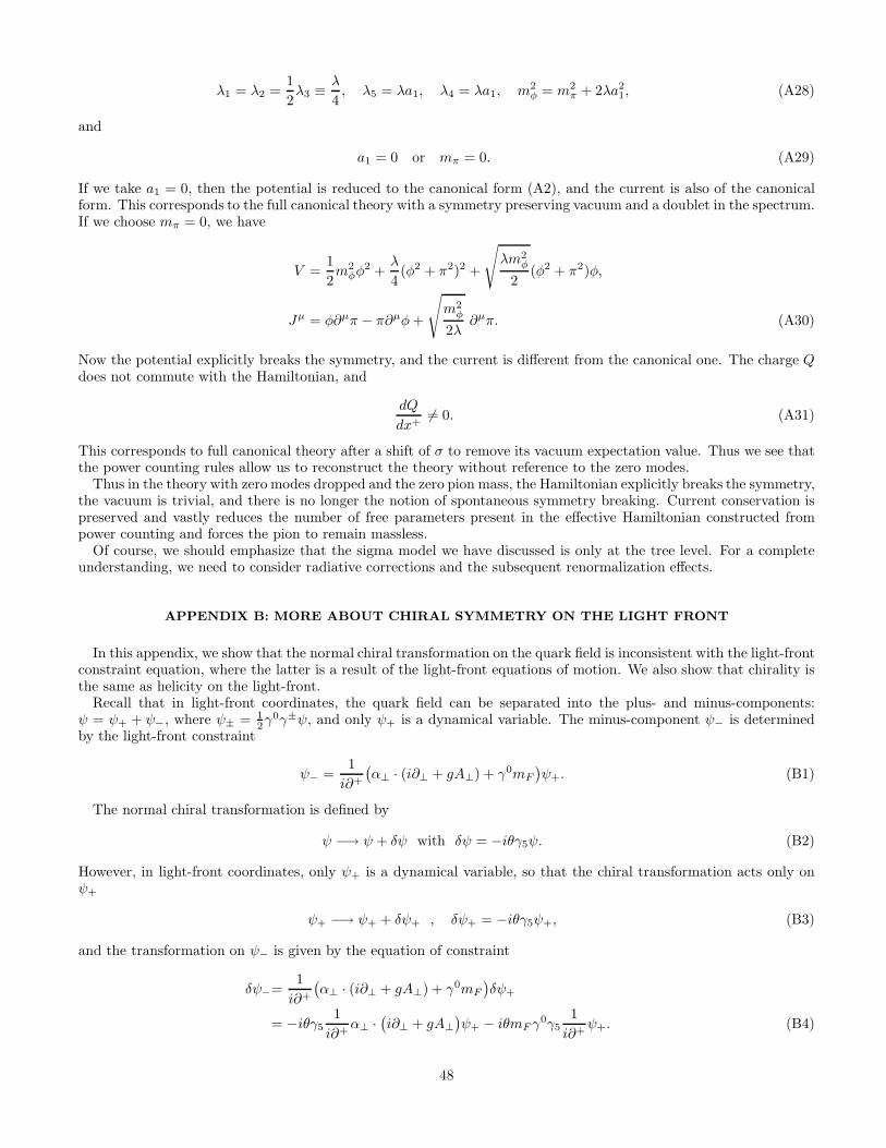
λ1 = λ2 =1

2λ3 ≡ λ

4, λ5 = λa1, λ4 = λa1, m2

φ = m2π + 2λa2

1, (A28)

and

a1 = 0 or mπ = 0. (A29)

If we take a1 = 0, then the potential is reduced to the canonical form (A2), and the current is also of the canonicalform. This corresponds to the full canonical theory with a symmetry preserving vacuum and a doublet in the spectrum.If we choose mπ = 0, we have

V =1

2m2

φφ2 +

λ

4(φ2 + π2)2 +

√

λm2φ

2(φ2 + π2)φ,

Jµ = φ∂µπ − π∂µφ+

√

m2φ

2λ∂µπ. (A30)

Now the potential explicitly breaks the symmetry, and the current is different from the canonical one. The charge Qdoes not commute with the Hamiltonian, and

dQ

dx+6= 0. (A31)

This corresponds to full canonical theory after a shift of σ to remove its vacuum expectation value. Thus we see thatthe power counting rules allow us to reconstruct the theory without reference to the zero modes.

Thus in the theory with zero modes dropped and the zero pion mass, the Hamiltonian explicitly breaks the symmetry,the vacuum is trivial, and there is no longer the notion of spontaneous symmetry breaking. Current conservation ispreserved and vastly reduces the number of free parameters present in the effective Hamiltonian constructed frompower counting and forces the pion to remain massless.

Of course, we should emphasize that the sigma model we have discussed is only at the tree level. For a completeunderstanding, we need to consider radiative corrections and the subsequent renormalization effects.

APPENDIX B: MORE ABOUT CHIRAL SYMMETRY ON THE LIGHT FRONT

In this appendix, we show that the normal chiral transformation on the quark field is inconsistent with the light-frontconstraint equation, where the latter is a result of the light-front equations of motion. We also show that chirality isthe same as helicity on the light-front.

Recall that in light-front coordinates, the quark field can be separated into the plus- and minus-components:ψ = ψ+ + ψ−, where ψ± = 1

2γ0γ±ψ, and only ψ+ is a dynamical variable. The minus-component ψ− is determined

by the light-front constraint

ψ− =1

i∂+

(α⊥ · (i∂⊥ + gA⊥) + γ0mF

)ψ+. (B1)

The normal chiral transformation is defined by

ψ −→ ψ + δψ with δψ = −iθγ5ψ. (B2)

However, in light-front coordinates, only ψ+ is a dynamical variable, so that the chiral transformation acts only onψ+

ψ+ −→ ψ+ + δψ+ , δψ+ = −iθγ5ψ+, (B3)

and the transformation on ψ− is given by the equation of constraint

δψ−=1

i∂+

(α⊥ · (i∂⊥ + gA⊥) + γ0mF

)δψ+

= −iθγ51

i∂+α⊥ ·

(i∂⊥ + gA⊥

)ψ+ − iθmFγ

0γ51

i∂+ψ+. (B4)

48

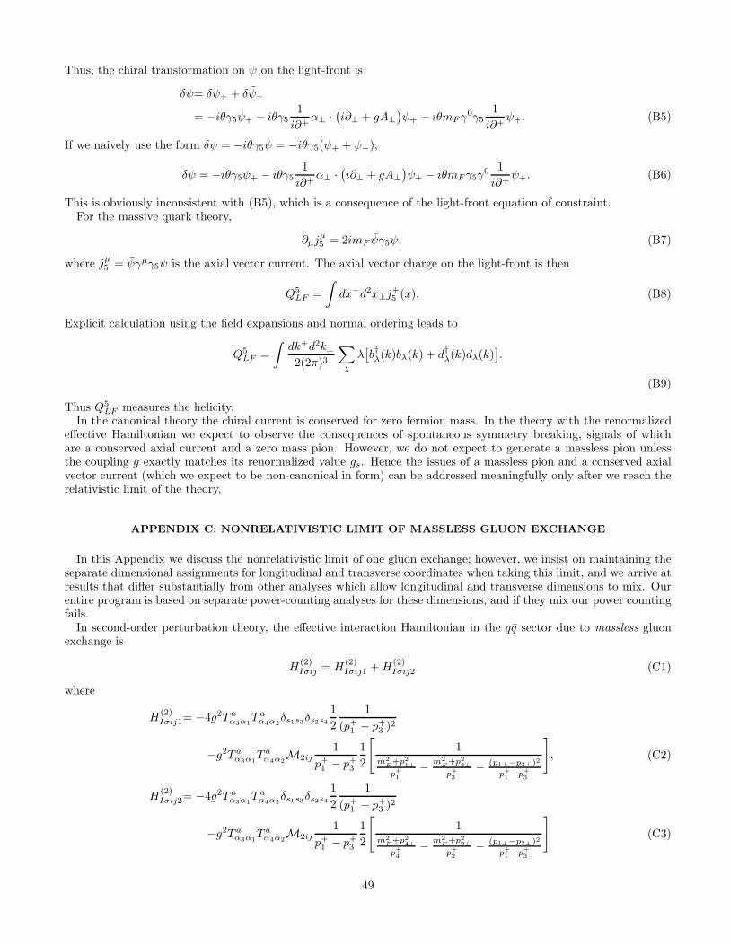
Thus, the chiral transformation on ψ on the light-front is

δψ= δψ+ + δψ−

= −iθγ5ψ+ − iθγ51

i∂+α⊥ ·

(i∂⊥ + gA⊥

)ψ+ − iθmFγ

0γ51

i∂+ψ+. (B5)

If we naively use the form δψ = −iθγ5ψ = −iθγ5(ψ+ + ψ−),

δψ = −iθγ5ψ+ − iθγ51

i∂+α⊥ ·

(i∂⊥ + gA⊥

)ψ+ − iθmFγ5γ

0 1

i∂+ψ+. (B6)

This is obviously inconsistent with (B5), which is a consequence of the light-front equation of constraint.For the massive quark theory,

∂µjµ5 = 2imF ψγ5ψ, (B7)

where jµ5 = ψγµγ5ψ is the axial vector current. The axial vector charge on the light-front is then

Q5LF =

∫

dx−d2x⊥j+5 (x). (B8)

Explicit calculation using the field expansions and normal ordering leads to

Q5LF =

∫dk+d2k⊥2(2π)3

∑

λ

λ[b†λ(k)bλ(k) + d†λ(k)dλ(k)

].

(B9)

Thus Q5LF measures the helicity.

In the canonical theory the chiral current is conserved for zero fermion mass. In the theory with the renormalizedeffective Hamiltonian we expect to observe the consequences of spontaneous symmetry breaking, signals of whichare a conserved axial current and a zero mass pion. However, we do not expect to generate a massless pion unlessthe coupling g exactly matches its renormalized value gs. Hence the issues of a massless pion and a conserved axialvector current (which we expect to be non-canonical in form) can be addressed meaningfully only after we reach therelativistic limit of the theory.

APPENDIX C: NONRELATIVISTIC LIMIT OF MASSLESS GLUON EXCHANGE

In this Appendix we discuss the nonrelativistic limit of one gluon exchange; however, we insist on maintaining theseparate dimensional assignments for longitudinal and transverse coordinates when taking this limit, and we arrive atresults that differ substantially from other analyses which allow longitudinal and transverse dimensions to mix. Ourentire program is based on separate power-counting analyses for these dimensions, and if they mix our power countingfails.

In second-order perturbation theory, the effective interaction Hamiltonian in the qq sector due to massless gluonexchange is

H(2)Iσij = H

(2)Iσij1 +H

(2)Iσij2 (C1)

where

H(2)Iσij1= −4g2T a

α3α1T a

α4α2δs1s3

δs2s4

1

2

1

(p+1 − p+

3 )2

−g2T aα3α1

T aα4α2

M2ij1

p+1 − p+

3

1

2

[

1m2

F+p2

1⊥

p+

1

− m2F

+p23⊥

p+

3

− (p1⊥−p3⊥)2

p+

1−p+

3

]

, (C2)

H(2)Iσij2= −4g2T a

α3α1T a

α4α2δs1s3

δs2s4

1

2

1

(p+1 − p+

3 )2

−g2T aα3α1

T aα4α2

M2ij1

p+1 − p+

3

1

2

[

1m2

F+p2

4⊥

p+

4

− m2F

+p22⊥

p+

2

− (p1⊥−p3⊥)2

p+

1−p+

3

]

(C3)

49

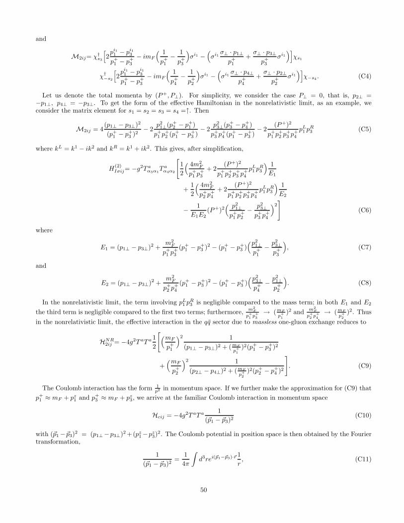
and

M2ij= χ†s3

[

2pi11 − pi1

3

p+1 − p+

3

− imF

( 1

p+1

− 1

p+3

)

σi1 −(

σi1σ⊥ · p1⊥

p+1

+σ⊥ · p3⊥

p+3

σi1)]

χs1

χ†−s2

[

2pi11 − pi1

3

p+1 − p+

3

− imF

( 1

p+4

− 1

p+2

)

σi1 −(

σi1σ⊥ · p4⊥

p+4

+σ⊥ · p2⊥

p+2

σi1)]

χ−s4. (C4)

Let us denote the total momenta by (P+, P⊥). For simplicity, we consider the case P⊥ = 0, that is, p2⊥ =−p1⊥, p4⊥ = −p3⊥. To get the form of the effective Hamiltonian in the nonrelativistic limit, as an example, weconsider the matrix element for s1 = s2 = s3 = s4 =↑. Then

M2ij = 4(p1⊥ − p3⊥)2

(p+1 − p+

3 )2− 2

p21⊥(p+

2 − p+1 )

p+1 p

+2 (p+

1 − p+3 )

− 2p23⊥(p+

3 − p+4 )

p+3 p

+4 (p+

1 − p+3 )

− 2(P+)2

p+1 p

+2 p

+3 p

+4

pL1 p

R3 (C5)

where kL = k1 − ik2 and kR = k1 + ik2. This gives, after simplification,

H(2)Iσij= −g2T a

α3α1T a

α4α2

[

1

2

( 4m2F

p+1 p

+3

+ 2(P+)2

p+1 p

+2 p

+3 p

+4

pL1 p

R3

) 1

E1

+1

2

( 4m2F

p+2 p

+4

+ 2(P+)2

p+1 p

+2 p

+3 p

+4

pL1 p

R3

) 1

E2

− 1

E1E2(P+)2

( p21⊥

p+1 p

+2

− p23⊥

p+3 p

+4

)2]

(C6)

where

E1 = (p1⊥ − p3⊥)2 +m2

F

p+1 p

+3

(p+1 − p+

3 )2 − (p+1 − p+

3 )(p2

1⊥p+1

− p23⊥p+3

)

, (C7)

and

E2 = (p1⊥ − p3⊥)2 +m2

F

p+2 p

+4

(p+1 − p+

3 )2 − (p+1 − p+

3 )(p2

3⊥p+4

− p21⊥p+2

)

. (C8)

In the nonrelativistic limit, the term involving pL1 p

R3 is negligible compared to the mass term; in both E1 and E2

the third term is negligible compared to the first two terms; furthermore,m2

F

p+

1p+

3

→ (mF

p+

1

)2 andm2

F

p+

2p+

4

→ (mF

p+

2

)2. Thus

in the nonrelativistic limit, the effective interaction in the qq sector due to massless one-gluon exchange reduces to

HNR2ij = −4g2T aT a 1

2

[(mF

p+1

)2 1

(p1⊥ − p3⊥)2 + (mF

p+

1

)2(p+1 − p+

3 )2

+(mF

p+2

)2 1

(p2⊥ − p4⊥)2 + (mF

p+

2

)2(p+2 − p+

4 )2

]

. (C9)

The Coulomb interaction has the form 1p2 in momentum space. If we further make the approximation for (C9) that

p+1 ≈ mF + pz

1 and p+3 ≈ mF + pz

3, we arrive at the familiar Coulomb interaction in momentum space

Hcij = −4g2T aT a 1

(~p1 − ~p3)2(C10)

with (~p1−~p3)2 = (p1⊥−p3⊥)2 +(pz1−pz

3)2. The Coulomb potential in position space is then obtained by the Fouriertransformation,

1

(~p1 − ~p3)2=

1

4π

∫

d3rei(~p1−~p3)·~r 1

r, (C11)

50

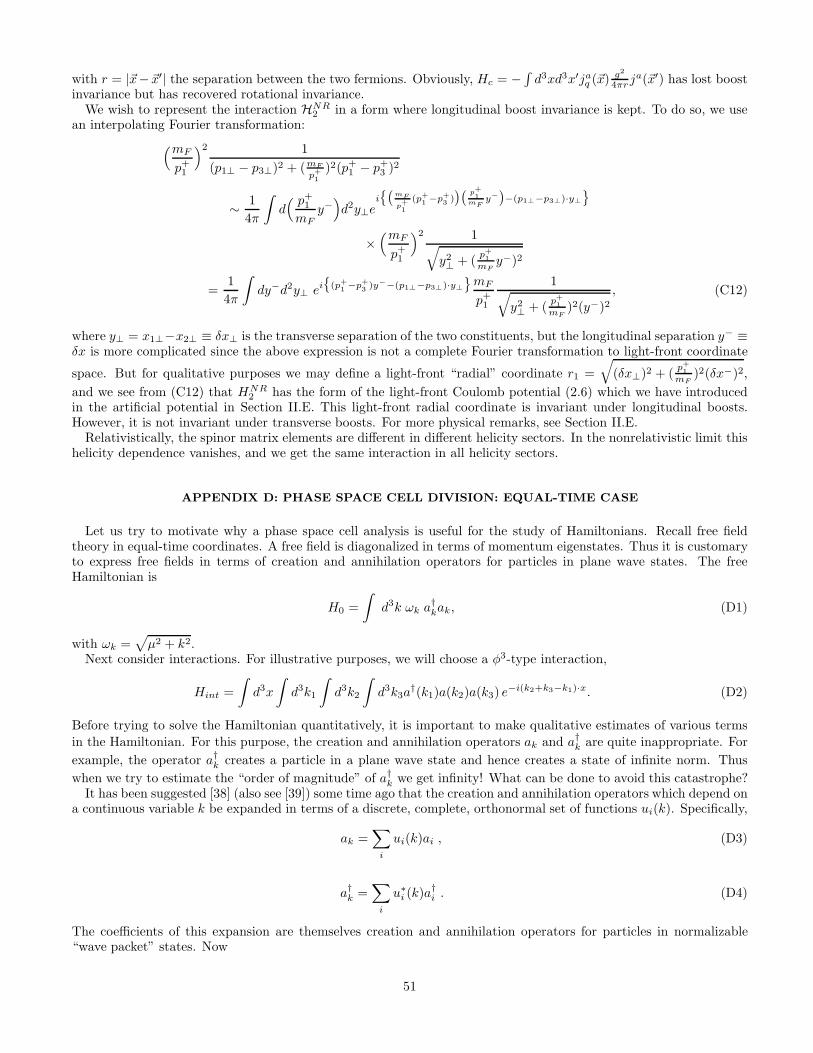
with r = |~x−~x′| the separation between the two fermions. Obviously, Hc = −∫d3xd3x′ja

q (~x) g2

4πr ja(~x′) has lost boost

invariance but has recovered rotational invariance.We wish to represent the interaction HNR

2 in a form where longitudinal boost invariance is kept. To do so, we usean interpolating Fourier transformation:

(mF

p+1

)2 1

(p1⊥ − p3⊥)2 + (mF

p+

1

)2(p+1 − p+

3 )2

∼ 1

4π

∫

d( p+

1

mFy−

)

d2y⊥ei{(

mF

p+

1

(p+

1−p+

3))(

p+

1mF

y−

)−(p1⊥−p3⊥)·y⊥

}

×(mF

p+1

)2 1√

y2⊥ + (

p+

1

mFy−)2

=1

4π

∫

dy−d2y⊥ ei{

(p+

1−p+

3)y−−(p1⊥−p3⊥)·y⊥

}mF

p+1

1√

y2⊥ + (

p+

1

mF)2(y−)2

, (C12)

where y⊥ = x1⊥−x2⊥ ≡ δx⊥ is the transverse separation of the two constituents, but the longitudinal separation y− ≡δx is more complicated since the above expression is not a complete Fourier transformation to light-front coordinate

space. But for qualitative purposes we may define a light-front “radial” coordinate r1 =

√

(δx⊥)2 + (p+

1

mF)2(δx−)2,

and we see from (C12) that HNR2 has the form of the light-front Coulomb potential (2.6) which we have introduced

in the artificial potential in Section II.E. This light-front radial coordinate is invariant under longitudinal boosts.However, it is not invariant under transverse boosts. For more physical remarks, see Section II.E.

Relativistically, the spinor matrix elements are different in different helicity sectors. In the nonrelativistic limit thishelicity dependence vanishes, and we get the same interaction in all helicity sectors.

APPENDIX D: PHASE SPACE CELL DIVISION: EQUAL-TIME CASE

Let us try to motivate why a phase space cell analysis is useful for the study of Hamiltonians. Recall free fieldtheory in equal-time coordinates. A free field is diagonalized in terms of momentum eigenstates. Thus it is customaryto express free fields in terms of creation and annihilation operators for particles in plane wave states. The freeHamiltonian is

H0 =

∫

d3k ωk a†kak, (D1)

with ωk =√

µ2 + k2.Next consider interactions. For illustrative purposes, we will choose a φ3-type interaction,

Hint =

∫

d3x

∫

d3k1

∫

d3k2

∫

d3k3a†(k1)a(k2)a(k3) e−i(k2+k3−k1)·x. (D2)

Before trying to solve the Hamiltonian quantitatively, it is important to make qualitative estimates of various terms

in the Hamiltonian. For this purpose, the creation and annihilation operators ak and a†k are quite inappropriate. For

example, the operator a†k creates a particle in a plane wave state and hence creates a state of infinite norm. Thus

when we try to estimate the “order of magnitude” of a†k we get infinity! What can be done to avoid this catastrophe?It has been suggested [38] (also see [39]) some time ago that the creation and annihilation operators which depend on

a continuous variable k be expanded in terms of a discrete, complete, orthonormal set of functions ui(k). Specifically,

ak =∑

i

ui(k)ai , (D3)

a†k =∑

i

u∗i (k)a†i . (D4)

The coefficients of this expansion are themselves creation and annihilation operators for particles in normalizable“wave packet” states. Now

51

H0 =∑

i1i2

Ci1i2 a†i1ai2 , (D5)

where

Ci1i2 =

∫

d3k ωk u∗i1(k)ui2(k) . (D6)

H0 is now the Hamiltonian of an infinite number of oscillators coupled to each other (no longer diagonal). Nowmaking H0 diagonal means making self-interactions of the individual oscillators more important than interactionsbetween different oscillators. Consider the matrix C. If the ul’s are orthogonal, C would be diagonal except forthe factor ωk. Even with the factor ωk, one should be able to keep the off-diagonal elements small. If the ui’s are“properly chosen” (that is, as localized in momentum space as possible) then for distinct momentum shells i1 andi2, the functions ui1 and ui2 do not overlap very much. If ui1 and ui2 are in the same momentum shell but differentspatial cells, this fact will be reflected in a rapid phase variation of u∗i1ui2 as a function of k, which again makes theintegral small. Thus with a properly chosen set of ui’s, for order of magnitude estimates we need to consider onlydiagonal elements Ci1i1 of C.

The interaction Hamiltonian in terms of wave packet states is

Hint =∑

i1i2i3

a†i1ai2ai3Di1i2i3 (D7)

with

Di1i2i3=

∫

d3x

∫

d3k1

∫

d3k2

∫

d3k3u∗i1(k1)ui2(k2)ui3(k3) e−i(k2+k3−k1).x

=

∫

d3xv∗i1 (x)vi2 (x)vi3 (x). (D8)

If the u’s are as localized as possible in momentum space, then the v’s are as spread out as possible in coordinate spaceand hence the off-diagonal elements of D are as big as the diagonal elements of D. Thus if we want to approximateD by its diagonal elements for order of magnitude estimates, we need v’s to be as localized in coordinate space aspossible. Thus we clearly have to satisfy almost mutually exclusive requirements, which means that we have to settlefor a compromise.

A qualitative implementation of the compromise is as follows. We choose ui(k) such that if ∆ki is the momentumwidth of the function ui(k) and ∆xi is the width of the Fourier transform vi(x) of ui(k), then the product ∆ki∆xi isnear the lower limit set by the uncertainty principle, that is,

∆ki∆xi ≈1

2. (D9)

The set of functions {ui} is chosen to be complete and orthonormal. What does this mean? Think of ui as occupyinga cell of unit volume in phase space. Completeness means that the total volume occupied by the ui’s must fill allspace. Orthogonality means that the regions occupied by different ui’s do not overlap.

How are we going to divide the phase space into cells? Consider one dimensional example for visualization. Dividethe momentum space into an infinite number of cells, the ith cell being

2−i < k < 2−i+1 . (D10)

For each momentum cell separately, divide the position space linearly into cells of the appropriate size. The positionspace coordinate is chosen to be l ≤ 2−ix ≤ l + 1.

Let us give some examples. Consider i = 0. Then 1 < k < 2, and the length of the momentum cell is Lk = 1. Theposition cell division is l ≤ x ≤ l + 1. Thus the position space coordinates are, for example,

l = −1 −1 < x < 0, (D11)

l = 0 0 < x < 1,

l = +1 1 < x < 2,

and so on, so that each position space cell has length Lx = 1. Thus the “ volume” of each phase space cell is LkLx = 1.

52

Consider i = 1. Then 12 < k < 1, and the length of the momentum cell is Lk = 1

2 . The position cell division is

l ≤ 12x ≤ l + 1. Thus the position space coordinates are, for example,

l = −1 −2 < x < 0, (D12)

l = 0 0 < x < 2,

l = +1 2 < x < 4,

and so on, so that each position space cell has length Lx = 2. Thus the “volume” of each phase space cell is againLkLx = 1.

One can label each phase space cell by (l, i). An illustration of the division of phase space into cells is given in Fig.13.

Why have we chosen a logarithmic scale for momentum cells? One would like to have each momentum cell correspondto a distinct energy scale so that order of magnitude estimates become meaningful. A linear choice obviously failsfor this purpose, while a logarithmic choice is the most obvious one that fulfills it. Note that there is nothing sacredabout the factor of 2; for a specific example where the factor of 2 appears as the optimum choice, see Ref. [39].

[1] K. G. Wilson, “Initial Draft”, (1989).[2] K. G. Wilson, “Light-front QCD”, OSU internal report (1990).[3] K. G. Wilson, “QCD: a weak coupling treatment on light fronts”, unpublished notes (July, 1993).[4] K. G. Wilson, “Renormalization of QCD weak coupling model”, unpublished notes (July, 1993).[5] R. J. Perry and K.G. Wilson, “Toward a Solution of QCD on the Light Front,” unpublished (1991).[6] T. S. Walhout, “Light-Front Hamiltonian Approach to Quantum Chromodynamics,” to appear in the Proceedings of

PANIC ’93, (World Scientific, 1993).[7] E. Tomboulis, Phys. Rev. D8, 2736 (1973);

A. Casher, Phys. Rev. D14, 452 (1976);W. A. Bardeen and R. B. Pearson, Phys. Rev. D13, 547 (1976);C. B. Thorn, Phys. Rev. D19, 639; D20, 1934 (1979);W. A. Bardeen, R. B. Pearson, E. Rabinovici, Phys. Rev. D21, 1037 (1980);G.P. Lepage and S.J. Brodsky, Phys. Rev. D22, 2157 (1980);V. A. Franke, Y. V. Novozhilov, and E. V. Prokhvatilov, Lett. Math. Phys. 5, 239; 437 (1981);G.P. Lepage, S.J. Brodsky, T. Huang and P. B. Mackenzie, in Particles and Fields 2, edited by A. Z. Capri and A. N.Kamal (Plenum, New York, 1983);St. D. G lazek, Phys. Rev. D38, 3277 (1988);S. J. Brodsky and G. P. Lepage, in Perturbative Quantum Chromodynamics ed. A. H. Mueller, (World Scientific, Singapore,1989);E. V. Prokhvatilov and V. A. Franke, Sov. J. Nucl Phys. 49, 688 (1989);P. A. Griffin, Nucl. Phys. B372, 270 (1992).

[8] W. M. Zhang and A. Harindranath, Phys. Rev. D48, 4868 (1993).[9] W. M. Zhang and A. Harindranath, Phys. Rev. D48, 4881 (1993).

[10] A. Harindranath and W. M. Zhang, Phys. Rev. D48, 4903 (1993).[11] A. Casher, and G.P. Lepage and S.J. Brodsky, in [7].[12] R. J. Perry, Phys. Lett. 300B, 8 (1993).[13] W. M. Zhang and A. Harindranath, Phys. Lett. 314B, 223 (1993).[14] St. D. G lazek and K.G. Wilson, Phys. Rev. D48, 5863 (1993).[15] St. D. G lazek and K.G. Wilson, “Perturbative Renormalization Group for Extensive Hamiltonians,” submitted to Phys.

Rev. D (1993).[16] R. J. Perry, A. Harindranath and K. G. Wilson, Phys. Rev. Lett. 65, 2959 (1990);

A. Harindranath and R. J. Perry, Phys. Rev. D43, 492 (1991);R. J. Perry and A. Harindranath, Phys. Rev. D43, 4051 (1991);St. D. G lazek and R.J. Perry, Phys. Rev. D45, 3740 (1992);A. Harindranath, R. J. Perry, and J. Shigemitsu, Phys. Rev. D46, 4580 (1992);S. G lazek, A. Harindranath, S. Pinsky, J. Shigemitsu, and K. G. Wilson, Phys. Rev. D47, 1599 (1993);Y. Mo and R. J. Perry, J. Comp. Phys. 108, 159 (1993);A. Harindranath, J. Shigemitsu, W. M. Zhang, “Study of Utilizing Basis Functions to Solve Simple Light-Front Equations

53

in 3+1 Dimensions”, OSU report (1992);M. Brisudova and St. D. G lazek, “Relativistic scattering and bound-state properties in a special Hamiltonian model,”unpublished (1993).

[17] D. Mustaki, S. Pinsky, J. Shigemitsu, and K. Wilson, Phys. Rev. D43, 3411 (1991).[18] St. D. G lazek and R.J. Perry, Phys. Rev. D45, 3734 (1992);

B. van de Sande and S. S. Pinsky, Phys. Rev. D46, 5479 (1992);St. D. G lazek and K. G. Wilson, Phys. Rev. D47, 4657 (1993);St. D. G lazek, Acta Phys. Polonica B24, 1315 (1993);R. J. Perry and K. G. Wilson, Nucl. Phys. B403, 587 (1993);R. J. Perry, “A renormalization group approach to Hamiltonian light-front field theory”, OSU preprint OSU-NT-93-117,to appear in Ann. Phys. (1993).

[19] Perry, in [18].[20] P. A. M. Dirac, Rev. Mod. Phys. 21, 392 (1949).[21] S. Weinberg, Phys. Rev. 150, 1313 (1966).[22] S. Fubini and G, Furlan, Physics 1, 229 (1965);

R. Dashen and M. Gell-Mann, Phys. Rev. Lett. 17, 340 (1966);An initial light-front formulation of QCD inspired from the properties of light-front current algebra is H. Fritzsch and M.Gell-Mann, in Proc. XVI Int. Conf. on High Energy Physics, edited by J. D. Jackson and A. Roberts. (Fermilab, 1972)Vol. 2, p. 135;For more discussion on light-front current algebra, also see: R. Jackiw, Springer Tracts in Mod. Phys. 62 1972; V. DeAlfaro, S. Fubini, G. Furlan, and G. Rossetti, Currents in Hadron Physics, (North-Holland, Amsterdam , 1973); E. Eichten,F. Feinberg, and J. F. Willemen, Phys. Rev. D8, 1204 (1973); H. J. Melosh, Phys. Rev. D9, 1095 (1974).

[23] R. P. Feynman, Phys. Rev. Lett. 23, 1415 (1969);J. D. Bjorken and E. A. Paschos, Phys. Rev. 185, 1975 (1969);R. P. Feynman, Photon-hadron interactions, Benjamin, Reading, Massachusetts (1972);J. B. Kogut and L. Susskind, Phys. Rep.C8, 75 (1973).Early work on the field theoretic realization of the parton model is: S. D. Drell, D. J. Levy and T. M. Yan, Phys. Rev.181, 2159 (1969); Phys. Rev. D1, 1035; 1617 (1970); and J. D. Bjorken, J. B. Kogut, and D.E. Soper, Phys. Rev. D3,1382 (1971).

[24] K. Bardacki and M. B. Halpern, Phys. Rev. 176, 1686 (1968);L. Susskind, Phys. Rev., 165, 1535 (1968); and in Lectures in Theoretical Physics, Vol. XI-D, edited by K. T. Mahanthappaand E. E. Brittin, (Gordon and Breach Sci. Pub., New York, 1969) p.135;S.-J. Chang and S.-K. Ma, Phys. Rev. 180, 1506 (1969);J. B. Kogut and D. E. Soper, Phys. Rev. D1, 2901 (1970);H. Leutwyler, J. R. Klauder and L. Streit, Nuo. Cim. Vol. LXVIA, No.3 (1970);F. Rohrlich, Acta. Phys. Austr. 32, 87 (1970);R. A. Neville and F. Rohrlich, Nov. Cim. A1, 625 (1971);S.-J. Chang, R. G. Root and T.-M. Yan, Phys. Rev. D7, 1133 (1973);S.-J. Chang and T.-M. Yan, Phys. Rev. D7, 1147 (1973);T.-M. Yan, Phys. Rev. D7, 1760; 1780 (1973);S. J. Brodsky, R. Roskies and R. Suaya, Phys. Rev. D8, 4574 (1973);J. M. Namyslowski, Prog. in Part. Nucl. Phys. Vol. 14, edited by A. Faessler (Pergamon Press, 1985);A. Langnau and M. Burkardt, Phys. Rev. D47, 3452 (1993).

[25] G. t’Hooft, Nucl. Phys. B75, 461 (1974);H. Bergknoff, Nucl. Phys. B122, 215 (1977);H. C. Pauli and S. J. Brodsky, Phys. Rev. D32, 1993; 2001 (1985);A. Harindranath and J. Vary, Phys. Rev. D36, 1141 (1987); D37, 1064; 3010 (1988);M. Sawicki and L. Mankiewicz, Phys. Rev. D37, 421 (1988); D40, 3415 (1990);T. Eller, H. C. Pauli, and S. J. Brodsky, Phys. Rev. D35, 1493 (1987);M. Burkardt, Nucl. Phys. A504, 762 (1989);K. Hornbostel, S. J. Brodsky, and H. C. Pauli, Phys. Rev. D41, 3814 (1990);M. Burkardt, Nucl. Phys. B373, 613 (1992);S. Dalley and I. R. Klebanov, “String Spectrum of 1+1 Dimensional Large N QCD with Adjoint Matter,” Princeton Univ.preprint PUPT-1342 (1993);and also see most of the references in [16].

[26] S. I. Nagornyi, et al, Sov. J. Nucl. Phys. 49, 465 (1989);A. C. Tang, S. J. Brodsky, and H. C. Pauli, Phys. Rev. D44, 1842 (1991);M. Burkardt, Nucl. Phys. B373, 371 (1992);M. Kaluza and H. C. Pauli, Phys. Rev. D45, 2968 (1992);M. Kaluza and H.-J. Pirner, Phys. Rev. D47, 1620 (1993);

54

M. Krautgartner, H. C. Pauli, and F. Wolz, Phys. Rev. D45, 3755 (1992);G lazek and Perry, in [16];G lazek, Harindranath, Shigemitsu, Pinsky and Wilson, in [16];P. M. Wort, Phys. Rev. D47, 608 (1993).

[27] T. Maskawa and K. Yamawaki, Prog. Theor. Phys. 56, 1649 (1976);A. Harindranath and J. P. Vary, Phys. Rev. D37, 421 (1988);G. McCartor, Z. Phys. C41, 271 (1988);Th. Heinzl, St. Krusche, and E. Werner, Z. Phys. A334, 443 (1989);Prokhvatilov and Franke in [7];G. McCartor, Z. Phys. C52, 611 (1991);F. Lenz, M. Thies, S. Levit, and K. Yazaki, Ann. Phys. (NY) 208 1 (1991);P. P. Srivastava, Light-Front Quantized Field Theory: (An Introduction), Lecture delivered at XIV Encontro Nacional deParticulas e Campos, Caxambu, MG, September 1993 (CBPF-NF- 075/93) and references therein;G. McCartor and D. G. Robertson, Z. Phys. C53 679 (1992);D. G. Robertson, Phys. Rev. D47, 2549 (1993);M. Burkardt, Phys. Rev. D47, 4628 (1993).

[28] For the development of the CQM, see: M. Gell-Mann, Phys. Lett. 8, 214 (1964);G. Zweig, CERN Reports Th. 401 and 412 (1964), and in Proc. Int. School of Phys. “Ettore Majorana”, Erice, Italy (1964),ed. A. Zichichi, p.192 (Academic, New York, 1965);H. J. Lipkin, Phys. Rep. 8 C, 173 (1973);O. W. Greenberg, Ann. Rev. Nucl. Sci. 28, 327 (1978).For quark model reviews, see: J.J.J. Kokkedee, The Quark Model, Benjamin, New York (1969);F.E. Close, Quarks and Partons, Academic Press, London (1979);A. Pickering, Constructing Quarks, Univ. of Chicago Press, Chicago (1984). This reference contains a carefully researchedhistory of the quark hypothesis, and a complete bibliography;W. Lucha, F. F. Schoberl, and D. Gromes, Phys. Rep. 200, 127 (1991).

[29] Susskind, in [24].[30] Bardacki and Halpern, in [24].[31] J. D. Bjorken, J. B. Kogut, and D.E. Soper, in [23].[32] Perry and Wilson, in [18].[33] Thorn, in [7].[34] The details of chiral transformation in light-front coordinates for free fermion theory is discussed in D. Mustaki, “Chiral

Symmetry and the Constituent Quark Model: A Null-Plane Point of View”, Bowling Green State University Preprint,1994.

[35] G lazek and Perry in [18].[36] H.J. Lipkin and S. Meshkov, Phys. Rev. 143 1269 (1966). Also see Close in [28].[37] J. D. Bjorken, J. B. Kogut, and D.E. Soper, in [23]; also see W.M. Zhang and A. Harindranath, in [9].[38] K.G. Wilson, Phys. Rev. 140, B445 (1965).[39] K.G. Wilson, Phys. Rev. B4, 3184 (1971).[40] See, for examples, I. Daubechies, Ten Lectures on Wavelets, CBMS/NSF Series in Applied Mathematics, #61, (SIAM

Publ., 1992);Wavelets and Their Applications, edited by M.B. Ruskai, et al., (Jones and Bartlett, Boston, 1992);Chui, C.K, An Introduction to Wavelets, (Academic Press, Boston, 1992);Wavelets, a Tutorial in Theory and Applications, edited by C. K. Chui, (Academic Press, Boston, 1992).

[41] R. S. Willey, Phys. Rev. D18, 270 (1978);G. McCartor, Phys. Rev. D18, 3873 (1978);M. B. Gavela, A. LeYaouanc, L. Oliver, et al., Phys. Lett. 82B, 431 (1979);G. Feinberg and J. Sucher, Phys. Rev. D20, 1717 (1979);O. W. Greenberg and H. J. Lipkin, Nucl. Phys. A370, 349 (1981).

[42] R. Oehme and W. Zimmerman, Commun. Math. Phys. 97, 569 (1985);R. Oheme, K. Sibold, and W. Zimmerman, Phys. lett. B147, 115 (1984);W. Zimmerman, Commun. Math. Phys. 97, 211 (1985).

[43] Lepage and Brodsky, in [7].[44] Drell, Levy and Yan, in [23].[45] G lazek, in [18].[46] See, for example, G.T. Bodwin and D.R. Yennie, Phys. Rep. 43C, 267 (1978);

G.T. Bodwin, D.R. Yennie, and M.A. Gregorio, Rev. Mod. Phy. 57, 723 (1985);W.E. Caswell and G.P. Lepage, Phys. Rev. A18, 810 (1978);J.R. Sapirstein, E.A. Terray, and D.R. Yennie, Phys. Rev. D29, 2990 (1984).

[47] G.P. Lepage and P.B. Mackenzie, Phys. Rev. D48, 2250 (1993).

55

List of Figures

1. Light-front coordinate system.

2. Examples of instantaneous interactions sensitive to fermion zero modes.

3. Instantaneous four-fermion and two-fermion–two-gluon interactions.

4. Cutoff region of center of mass momenta.

5. Cutoff region of constituent momenta.

6. Triangle of renormalization.

7. Gluon mass correction from two-gluon intermediate states.

8. Contribution to quark–antiquark scattering amplitude from gluon exchange.

9. Contribution to quark–gluon scattering amplitude from gluon exchange.

10. Contribution to quark-gluon scattering amplitude from quark exchange.

11. Quark-antiquark annihilation and contribution to qqg vertex renormalization.

12. Higher-order multifermion processes requiring counterterms.

13. Example of phase space cell division in one dimension.

56

This figure "fig1-1.png" is available in "png" format from:

http://arXiv.org/ps/hep-th/9401153v1

This figure "fig2-1.png" is available in "png" format from:

http://arXiv.org/ps/hep-th/9401153v1

This figure "fig1-2.png" is available in "png" format from:

http://arXiv.org/ps/hep-th/9401153v1

This figure "fig2-2.png" is available in "png" format from:

http://arXiv.org/ps/hep-th/9401153v1

This figure "fig1-3.png" is available in "png" format from:

http://arXiv.org/ps/hep-th/9401153v1

This figure "fig2-3.png" is available in "png" format from:

http://arXiv.org/ps/hep-th/9401153v1

This figure "fig1-4.png" is available in "png" format from:

http://arXiv.org/ps/hep-th/9401153v1

This figure "fig2-4.png" is available in "png" format from:

http://arXiv.org/ps/hep-th/9401153v1

This figure "fig1-5.png" is available in "png" format from:

http://arXiv.org/ps/hep-th/9401153v1

This figure "fig2-5.png" is available in "png" format from:

http://arXiv.org/ps/hep-th/9401153v1

This figure "fig1-6.png" is available in "png" format from:

http://arXiv.org/ps/hep-th/9401153v1

This figure "fig2-6.png" is available in "png" format from:

http://arXiv.org/ps/hep-th/9401153v1

This figure "fig2-7.png" is available in "png" format from:

http://arXiv.org/ps/hep-th/9401153v1