Exploring Surface Texture - University of Southampton

Exploring Surface Texture

A fundamental guide to the measurement of surface finish

7th Edition



A fundamental guide to the measurement of surface finish

i

PUBLISHED BY

Taylor Hobson Limited2 New Star Road

Leicester LE4 9JQEngland

www.taylor-hobson.com

Edited in 2003 by Taylor Hobson LimitedFirst published March 19802nd edition November 1986

3rd edition March 19984th edition June 20035th edition May 2006

6th edition January 20097th edition November 2011

List No. 600-14/03

© Taylor Hobson LtdCopyright and translation rights reserved

PRINTED IN GREAT BRITAIN

CONTENTS

PREFACE iv

Note to the 4th edition iv

CHAPTER 1 - Introduction 2

The Rough and the Smooth 3

Why Measure Surface Texture? 3

What is Surface Texture? 7

CHAPTER 2 - The Surface 12

The Cause of Surface Texture 14

Roughness, Waviness and Form 15

CHAPTER 3 - Measuring the Surface 21

Stylus 24

Mechanics and Electronics 28

Digitization 29

Calibration 32

Arcuate Correction 33

Form removal 33

Filters - General 34

Lambda S (λs) Filtering 36

Roughness or Waviness? 37

Choosing A Roughness Cut-Off 38

Waviness (λs’) Filtering 44

Short Surfaces 45

Non-Contact Measuring Systems 46

3D or Areal Measurements 47

CHAPTER 4 - Putting a Number To It 53

Roughness Average (Ra) 54

ii

iii

RMS value (Rq) 57

Peak and Valley Heights 57

Material ratio (Bearing ratio) 61

Peak Counting (Ppc) 63

Amplitude Distribution, Skew (Rsk) and Kurtosis (Rku) 65

R & W 68

Waviness Parameters 69

Surface Texture at the Design Stage 69

3D Parameters 70

A Final Word on Parameters 72

CHAPTER 5 - Instrumentation 74

The Stylus Instrument 74

The Talysurf 74

Gauge 76

Independent Datum 83

Instrument Accuracy 84

Curved Surfaces 85

Form and Contour Measurement 87

3D Measurements With Stylus Instruments 88

Non-contact Surface Measurement 88

SUPPLEMENTAL INFORMATION 93

Recommended Further Reading 93

Glossary 93

Roughness Parameters Defined in ISO 4287 96

Selected List of International Standards Applicable to Surface Texture Measurement 97

INDEX 98

PREFACE

This book is intended to give the reader an insight into the basics of surface texture and its measurement.

To make this book as practically useful as possible we will concentrate on the one, almost universal, method of measurement - by means of stylus instruments. These can be found throughout the world: in the laboratory, standards room and workshop - you even have one yourself in the form of a fingernail!

The principles of stylus measurement will be dealt with in some detail while other methods will be described briefly, chiefly for their interest and the way that certain properties of surface texture are utilized for measurement.

Note to the 4th edition

Since the first publication of this book over 20 years ago the technologies to produce and measure surfaces have evolved significantly. Nevertheless, the “fundamentals” remain true, and that is what we seek to cover here. Many non-contact and 3D measurement techniques are now widely used, and this edition includes some detail of these areas. However, without apology, the main analysis remains based on stylus instruments as this provides a fundamental understanding that can be applied universally.

This edition has been updated significantly in relation to the technology of the stylus instrument. Virtually every instrument available today is digital, using a microprocessor or PC to analyze the data. If you have an older, analog instrument you may find some of the terminology different, though references are included to historical standards and obsolete technologies.

iv

CHAPTER 1 - Introduction "There shall be standard measures of wine, ale and corn (the London quarter), throughout the kingdom. There shall be also be a standard width of dyed cloth, russett and haberject, namely two ells within the selvedges. Weights are to be standardized similarly." (Magna Carta, clause 35, AD 1215)

"At one time the terms ‘rough machine’, ‘medium machine’ and ‘fine machine’, or equivalent symbols, were used on drawings, leaving the surface to be controlled by limitations of the machining process involved and arbitrary opinions of operator and inspector which all too often did not coincide.

Most of the uncertainties of specifying surface requirements have been eliminated by the development of instruments for the measurement of surface texture on a numerical basis and by the issue of various national standards. . . " (British Standard 1134 part 2, 1972)

Both the above documents are dealing with the same problem, although differing in time by several centuries. They both address the problem of measurement by laying down standards and specifying ways of measuring.

It is obviously very important to standardize the common weights and measures used in everyday life in order to allow manufacturers to be confident that, for instance, a round shaft made in Japan and having a diameter of 25.62mm when measured with a British micrometer will be exactly the same as one made in China, having a diameter of 25.62mm when measured with a micrometer made in the U.S.A.

This book is designed to help the reader understand what surface texture measurement is and how it fits into the pattern of engineering production. Please do not expect that it is the complete answer to all measuring problems relating to surface finish. That would require a much larger and more detailed treatise.

2

The Rough and the Smooth

The differences between rough and smooth surfaces can be distinguished by both touch and appearance. The problem is that these differences are subjective and no two observers will have the same opinion as to the value of these differences.

To one inspector a surface may be "fairly smooth" while to another it may be "smooth". These difficulties become even more apparent when the two surfaces are produced by different methods, such as turning and grinding. In the field of engineering, the exact degree of roughness or smoothness can be of considerable importance, affecting the function of a component or its cost.

The dimensions which we shall be dealing with are usually very small, being expressed in microns (a millionth of a meter, symbol µm). Older texts refer to microinches (a millionth of an inch, symbol µin): the relationship between the two is 39.37 microinches = 1 micron, but it is generally accepted to be 40µin to 1µm.

Why Measure Surface Texture?

Consider the history of a manufactured component (Figure 1). First comes the production process (manufacture). If the part has been produced correctly it can be put into use along with any other parts of the same design. However, as we are aware, processes do not remain constant, and have to be monitored to detect changes that could affect performance. So an intermediate step has to be added to the process: this is the measurement sequence. This step must detect all changes from the design data that are likely to affect the performance. So size, shape, hardness and smoothness must all be checked.

3

4

Figure 1: Stages in the life of a manufactured component

Process ControlHaving made a measurement, it is not enough to simply scrap the one piece which fails and continue production; the cause must be identified and corrected, thus preventing more scrap in later work.

Changes in production processes can affect surface texture in many ways. Tool wear, strains in the material and incorrect machining conditions can leave their mark on the surface. Surface texture is the fingerprint of manufacture and as it comes at the end of the production line it is an important method of control.

PerformanceThis, in the sense which we are using it in here, is not just a mechanical function. The component must not only work correctly, it must also look good, last a long time and, importantly, be capable of being produced economically.

Once a part is found to perform well, the surface texture must be controlled within certain limits to produce parts with similar, if not identical, specifications. Measurement on subsequent components is then a method of confirming that they will perform well.

FunctionIn many applications surface texture is closely allied to function, for instance where two surfaces are in close moving contact with each other their surface textures will affect their sealing or wear properties. This might suggest that it is a case of "the smoother the better", but this is not always true as other factors may be involved. Where lubrication is involved it has been found that roughness valleys are required to hold oil. Also, the financial aspect has to be considered: it costs a lot of money to produce very smooth surfaces and the expense of this exercise can add to the bill considerably without gaining a great deal of performance.

However well two surfaces in relative motion (e.g. a shaft and its bearing) are lubricated, some wear will occur. If the surfaces are rough they will soon become smoother as the peaks wear away. Since this removes metal there will be a quicker change in the fit of the two parts than if the finish was at the optimum from the start. On the other hand some parts such as clamping devices or a pin with an “interference fit” depend on friction for their functionality.

Another application where surface finish can have an influence on performance is the use of lip seals to prevent the escape of hydraulic fluids. If the finish is too smooth it is difficult to maintain a fluid film between the shaft and the seal. If the finish is too rough it can cause abrasion and consequent breakdown, leading to failure.

Inspection of the texture left on a component after machining will often reveal tool defects, incorrect tool settings or wrong tool speeds and feeds. Figure 2 shows examples of ground surfaces affected by improper wheel dressing, feed errors and tool chatter.

The appearance of a surface can be of some importance. For instance sheet steel used for motor car bodies must have a finish which will allow paint to bond to the surface without any "orange peel" effect and with an even appearance. Anybody who has tried to paint onto a glass surface will appreciate the difficulty in getting a firm bonded finish. Metallic parts are not the only components to require control; both paper and plastic parts need the same degree of repeatability.

5

6

Figure 2(A) Ground surface showing improper wheel dressing(B) Ground surface showing errors of feed(C) Ground surface showing tool chatter or vibration marks

A

B

C

Components formed by rolling, extruding or drawing through dies will tend to repeat any imperfections such as roughness, scratches or wear marks which may be on the original tool.

It is hoped these few examples just given will show that exploring surface texture has a very practical significance. It can be seen that some thought must be given to surface texture at the design stage, with the designer specifying the texture required to give the correct performance. It follows that the production engineer must use the correct machine tools to obtain that finish and advise the operator of the tolerances allowed.

Surface texture measurement has now become such a routine task that users of these systems often overlook the basis on which the assessment has been made, but an understanding of this can lead to a more intelligent use of any surface texture instrument.

What is Surface Texture?Up to now we have skimmed over the subject, mentioning roughness and smoothness. We will now look at the subject in more detail to determine what we mean by the term. Consider a theoretical perfectly smooth flat surface 150mm long, (Figure 3a). If it had a hollow 15µm deep in the middle, but was otherwise the same, (Figure 3b), we would say that it was smooth but slightly curved. The curvature represents an error from the true (expected) form. If the spacing of the high points was halved (Figure 3c) it would be considered as wavy. If the spacing were to be reduced further (Figure 3d) then it would still be classed as wavy. However if the spacing were to be reduced even further (Figure 3e) then the surface would be considered to be flat but rough.

7

Figure 3: Surfaces having the same irregularities but different spacings

To summarize, a surface having a height of 15µm can be regarded as curved, wavy or rough according to the spacing of these irregularities.

Many surfaces exhibit both roughness and waviness (Figure 4), and often these are combined with form error (Figure 5).

8

9

Figure 4: Roughness and waviness, the constituents of Surface Texture

Figure 5: Many surfaces exhibit both roughness and waviness (A) and some also have some form error (B)

Exploring the SurfaceThe surfaces that we have used as examples have irregularities which are perfectly regular. However, in real life, this would not be the case as even a surface with a pattern will not be as regular as our illustrations.

Since the individual roughness irregularities are too small to see with the naked eye, some form of magnifying device is needed. First thoughts turn naturally to a microscope, but while this will reveal the spacing of the horizontal pattern, it will not pick up the peaks and valleys clearly as these are perpendicular to the surface and the relative heights are not revealed. Instead we may use the imaginary instrument shown in Figure 6. In principle, the majority of surface measuring instruments use the same techniques to obtain a picture of the surface.

A very sharp stylus is drawn across the surface at a constant speed for a set distance. An electrical signal is obtained and amplified to produce a much enlarged vertical magnification. This signal may be displayed on both graph and screen outputs, together with numerical values that characterize the surface texture.

Figure 6: Diagram showing the basic principle of a surface texture instrument

Putting a Number to itAlthough there is a whole chapter later in this book devoted to quantifying the results, we should talk a little about the subject now. Profile traces of different surfaces can be com-pared visually but the interpretation is subjective. Ideally we need a single number which we can give to a surface to characterize the factors that affect performance.

No single method will cover all the information obtained by a single trace; however, we can quantify one characteristic at a time. The most commonly used parameter is Ra or Roughness Average. It also used to be called CLA (Center Line Average) and AA (Arithmetical Average). This parameter was the first attempt to solve the problem that the roughness heights in any surface differ significantly and an average value is considered to be the safest method of assessment.

Figure 7: Typical profile plot

10

Figure 8: Typical roughness values obtainable by different finishing processes

11

Figure 8 gives typical Ra values in microns obtained from various finishes. The higher the value the rougher the finish. With this knowledge it is possible to specify the texture, or at least one characteristic of it, by quoting an Ra number. It should be recognized that as the Ra value of a surface is generated by averaging the roughness height of the surface profile, there can be a number of components with very different peak spacings that have the same Ra value (see “CHAPTER 4 - Putting a Number To It” for examples).

CHAPTER 2 - The Surface

We should start our examination of surface texture by firstly considering what the surface is. Most processes will produce a repetitive finish of some description and now that instruments allow easy access to a variety of parameters it is essential that we ask the right questions: does the Ra value quantify the surface characteristic which is necessary for control? Are we measuring in the correct manner? To answer this we need to consider what a surface comprises.

“Surface” is defined as the boundary between the material and air. Texture produced by a machining process covers the whole surface, so ideally it should be assessed over the total area. Most measuring instruments use a single line trace, so how can this be representative of the entire part? Fortunately, most surfaces which are produced in common processes have a texture which is fairly even over a large area. So a trace taken at one place will differ only marginally from another taken at a different location providing that it is taken parallel to the first trace. This is due to the fact that a number of parts have a distinct texture pattern (the lay). This will be discussed later in the chapter.

Although experience has shown that a trace taken along a single track is usually adequate to obtain the required information, it is sometimes necessary to check the texture over an area. The more sophisticated stylus instruments can now achieve this method of meas-urement, but until recently the time required ruled it out for normal inspection. Areal devices are now becoming available to allow areas to be mapped in a matter of sec-onds (see Taylor Hobson Talysurf CCI gauge on page 92).

Random scratches or marks may be present on any surface even if not part of the manufacturing process; these could be caused by bad control of swarf or handling afterwards. Certain parameters (such as Ra) have an averaging effect, reducing the importance of these features.

12

Figure 9: Parallel traces across a turned surface

Change of Texture with UseAs soon as one surface comes into contact with another, wear will take place. However, the designer will, either from experience or actual tests, know that a part having certain surface characteristics will perform satisfactorily. Because of this, measurements made at the production stage can also be validly used to assess future performance.

Surface Texture is ComplexSurface characteristics can be complex. As you can see in Figure 12, roughness, waviness and form can exist in combination. In addition to the finish produced by the finishing process, there is an inherent structure in the material. Very few surfaces are molecularly smooth, mica and quartz being possible exceptions (though only over small areas). In metals, grain areas will produce troughs and ridges in the order of 0.01µm. These irregularities are extremely fine compared with texture from machining and some instruments with lesser sensitivity will not detect them.

13

Figure 10: Parallel traces across a ground surface

Figure 11: Consecutive closely spaced traces can give a detailed picture - in this case of rough mild steel

This complex texture is the main reason why so many parameters have been proposed to quantify the various features. Care must be taken to ensure that the correct parameter is selected; it is useless to expect a parameter based on amplitude height such as Ra to correlate with performance if such performance depends on irregular spacing.

Figure 12: Milled surface showing:

(A) roughness marks left by the cutter

(B) waviness, chatter marks which may be formed by the metal springing

as each tooth contacts the part

(C) form error, which may be due to bad alignment of tool or slide

The Cause of Surface TextureWhen a part is machined, a particle is detached by the process, leaving on the component a scratch which is actually a minute groove. The formation of these grooves by the tool as it passes across the part produces the surface finish. Within each groove, the texture is determined by the manner in which the material is detached from the solid material. If the tool is perfectly set up and guided, then the particles will be of equal size and depth and the part will form a flat plane. If this is not the case then the component will form an undulating surface.

14

Roughness, Waviness and FormA question sometimes asked is "At what point does roughness become waviness?" This is almost impossible to answer. The change from the concept of roughness to that of waviness often depends on the size of the workpiece. For example, the irregular spacing which would be regarded as roughness on a machine spindle would be regarded as waviness on a watch staff. The number of waves in the functional length also has some influence on how we classify the irregularities. One wave on a watch staff might be considered as curvature, but a larger number of waves on a longer shaft may be accepted as waviness. It is better to separate roughness, waviness and form according to their cause, as this also relates to the performance factors.

So, we can define as follows:

Roughness the irregularities which are inherent in the production process (e.g. cutting tool or abrasive grit)

Waviness that part of the texture on which roughness is superimposed. It may result from vibrations, chatter or work deflections and strains in the material.

It is also impossible to specify precisely where waviness stops and the shape becomes part of the general form of the part, but using the same criterion we say that:

Form the general shape of the surface, ignoring variations due to roughness and waviness.

These distinctions are therefore qualitative not quantitative, yet are of considerable importance as defining them this way is well established and functionally sound.

Roughness is produced only by the method of manufacture resulting from the process rather than the machine. Marks can be left by the tool or grit itself: these will be of a periodic nature for some processes and more random in others. There is also a finer structure formed by tearing of the part during machining, the build up of debris at the edge and small blemishes in the tool tip. Waviness, however, is attributed to the individual machine, imbalance in the grinding wheel, lead screw inaccuracy and lack of rigidity. Form errors are often caused by the part not being held firmly enough or a slideway not being straight, or heat generated during the process that can cause a surface to bend.

15

It should be emphasized that these three characteristics are never found in isolation. Most surfaces are the result of a combination of the effects of roughness, waviness and form. It is still necessary to analyze them separately as in Figure 13.

Figure 13: A surface profile represents the combined effects of roughness, waviness and form

Are Peaks and Valleys Equally Important?Certain parameters take into account both peaks and valleys (Ra being one of them). However, others are designed purely to look at the number and spacing of the departures from the center line in either an upward or downward direction.

LayMany machined surfaces will have a distinct directional characteristic that is called lay and can be classified into the types which are illustrated in Figure 14.

The measured trace should usually be taken at right angles to the direction of lay, unless specified otherwise, and it is good practice to ensure that the surface be examined closely to determine the optimum direction to use. If a trace is taken at right angles over a part with a distinct lay then the peaks will be more closely spaced than one made in line with the lay.

16

In fact, in extreme cases there could be no peaks in the latter measurement. For surfaces with a crossed lay then the trace should be taken at 45º, this will average out the effect of the two surfaces. On multi-lay surfaces or ones where the lay is not obvious it is customary to take a number of traces in different directions and accept the one with the highest value. It is sometimes necessary, if the lay is functionally important, to specify on drawings the direction or type of lay, the symbols for this are shown in Figure 14.

17

Figure 14: Lay and symbols used in drawings

Parallel

Perpendicular

Crossed

Multi-directional

Particulate

Circular

Radial

=

X

M

P

C

R

Granular SurfacesA common group of surfaces encountered are granular in make up and can be difficult to measure meaningfully. This group includes cast iron and sintered materials that are commonly used in bearing manufacture as they have useful lubrication properties.

Typically, the surface, when formed, is fairly rough and symmetrical with high peaks and deep valleys. When the material is honed, the peaks are reduced to give a smooth bearing surface, leaving the valleys as the predominant feature. It is obvious that a parameter such as Ra would be very misleading on this type of surface.

When granular surfaces show signs of re-entrant features, they will probably be impossible to trace correctly with a stylus, although computer aided analysis will be able to eliminate most of the valleys which will have little effect on an Ra value.

Cast ReplicasWhen it is impracticable to measure a component due to inaccessibility to a stylus, then a replica of the surface can be made. Typical of these replicas is the Taylor Hobson Kit which is a powder and liquid which when mixed is poured onto the surface. When hardened, it can be removed and measurements made on the replica. Typically, the accuracy is within 4% of the real value, although some smooth surfaces will be shown as slightly rougher than the original and some rough surfaces will appear to be slightly smoother. It must be remembered that the surface, being a replica, will be inverted; the peaks appearing to be valleys and vice versa (unless the instrument has the capability to invert the profile). This will not affect the Ra value as this is an averaging parameter.

Surface FeaturesTo illustrate the complexity of surface characteristics and the factors to be considered, we now show some photographs (Figure 15 & Figure 16) and traces of a number of different materials and processes. In each case the horizontal scale of the profile is at the same magnification as the photograph.

18

Figure 15: Photographs and profiles of typical surfaces (A-C)

19

Figure 16: Photographs and profiles of typical surfaces (D-G)

20

CHAPTER 3 - Measuring the Surface

The first step in quantifying the texture of a surface is to obtain a digital representation of the surface being considered. The resultant data can then be processed to produce the parameters we are interested in, as described in CHAPTER 4 - Putting a Number To It.

We shall begin by considering the simplest case: a stylus instrument taking a single trace of the surface - this is referred to as “the profile”. To properly understand the data we end up with, we need to consider the steps in the process as summarized in Figure 17. Filtering is a critical and complex part of the process, and will be discussed at some length.

Finally, we will broaden the simple case to look at some of the issues around 3D measurement and the use of non-contact gauges.

Older instruments did not have digital analysis, and had to calculate parameters “on the fly” or simply record the profile onto a chart for later manual processing. Nevertheless, the principles are the same, simply implemented with analog electronics rather than digital processing.

The Profile is not a Magnified Cross Section of the SurfaceThe heights of roughness irregularities are very small compared with their spacing, for example 3µm and 50µm respectively. Since it is normal to take an average of several measurements made over consecutive sampling lengths, the ratio of roughness height to total profile length is seen to be very small (Figure 18). A graphical recording of surface irregularities must be magnified to show the peaks and valleys clearly. For example, if a profile is magnified to X10,000, it would give a vertical displacement of 30mm on a graph. At the same magnification the irregularity spacing would be 500mm and a 5mm measurement would be 50m in length!

This is clearly impractical and rules out graphs having the same vertical and horizontal scales. Instead, we select the scales independently to show the height and spacing of the profile more clearly. Typically the analysis program will auto scale any graphical presenta-tion to give the optimum visualization of the profile.

21

Affect

Loss of fine detail and distortion of peaks and valleys

Potential distortion of data, loss of high frequency information and injection of noise

Sample surface

Data correction for some repeatable instrument errors

Data correction for arcuate motion of stylus

Least squares mean line fit

Primary profile

Roughness profile

Waviness profile

This data is used to calculate surface parameters

Influenced by

Stylus tip geometry

Quality of instrument

ADC linearity, range, resolution, sampling frequency

Calibration method, quality of calibration artifact

Software algorithm

Software algorithm

Software algorithm

Software algorithm

Software algorithm

Figure 17: Factors that may influence conversion of the actual surface into a digital representation

22

Factor

Stylus

Mechanics and Electronics

Digitization

Calibration

Arcuate correction

Form removal

λs filter

λc filter

λs’ filter

Factors that may influence conversion of theactual surface into a digital representation

There are occasions where it is a requirement for the horizontal and vertical scales to be the same. This is usually where the shape of the surface, as opposed to the surface texture, is being analysed. There are various instruments available for contour measurement, with varying degrees of complexity and sophistication.

Figure 18: Typical relative surface dimensions (not to scale)

Peak and Valley Shapes

Although the different scales used in vertical and horizontal directions will distort the visual shape of the profile, it is important to note that any measurements scaled from the graph are correct. This can be demonstrated with reference to the peak angles of the profile as described below.

As the horizontal magnification of the profile is increased, the length is expanded and the peaks appear to be flatter. Increase the horizontal magnification even further until the vertical and horizontal magnifications are equal and the same peaks appear to be much flatter.

We must therefore realize that it is the spiky appearance of the peaks and valleys that causes so much misunderstanding when making visual studies of profiles. It is only the much greater magnification in the vertical direction that produces this problem; in fact the peaks on the surface are really quite low and blunt.

23

StylusThe stylus is the only active contact between the instrument and the surface; it is therefore a very important part of the system and its dimensions and shape are factors which, in certain conditions, can have a marked influence on the information which the instrument gathers.

24

Figure 19: Diagram illustrating how the profile shapes vary as the horizontal scale is reduced

i) Surface profile with same scale in both directions and very little detail shown

ii) Profile with height magnified x 5 more than the length

iii) Profile graph showing height magnified x 50 more than the length, much more detail of the surface is shown

The ISO standard for roughness measurements is a 60° or 90° conical stylus with a spherical tip of 2µm radius. However, this is quite a delicate stylus, and needs an instrument with excellent mechanical properties to fully exploit it. Many users therefore prefer to use a 5µm stylus, although it should be noted that this is non-standard for most typical measure-ments and is greater than the size permitted within the bandwidth criteria (see Table 1). Because of its hardness and low coefficient of friction, diamond is the preferred stylus material.

Table 1: Recommended cut-offs and stylus tip size

The stylus tip acts as a mechanical filter. Figure 20A shows an actual surface with a tip of 2µm radius. It is clear that the stylus will not penetrate all the surface features. Figure 20B shows the surface as it would be displayed on an instrument: one might think that a stylus would not be able to penetrate any of the valleys. However, when the stylus is displayed on the same scales as the profile its shape becomes almost indistinguishable from a thin line and it is easy to see that the stylus can penetrate into apparently quite narrow valleys.

25

lc ls Bandwidth Rtip (max) Max sampling (upper cut-off) (lower cut-off) (lc / ls ratio) (stylus tip radius) spacing [mm] [µm] [µm] [µm] 0.08 2.5 30:1 2 0.5 0.25 2.5 100:1 2 0.5 0.8 2.5 300:1 2 0.5 2.5 8.0 300:1 5 1.5 8.0 25 300:1 10 5

26

Figure 20: (A) Relative sizes of stylus and surface (B) Relative size of stylus compared with a profile graph made at Vv=x5000, Vh=x100

Unsurprisingly, a smaller stylus will penetrate narrower valleys than one of a larger radi-us, as shown in Figure 21.

Figure 21: Showing how a larger radius tip reduces apparent amplitude of closely spaced irregularities

The distortion of the measured result compared to the actual surface is clearly shown in Figure 22. The dotted line is the path of the center of the spherical section of the stylus, and can be seen to deviate from the solid line which is the actual surface being measured. The valley has been reduced in both width and depth, while the peak has been widened and flattened. Note, however, that the height of the peak is correctly recorded. The larger the feature with respect to the stylus, the less will be the effect of the stylus mechanical filter.Taylor Hobson instruments include an algorithm to compensate for this problem.

Figure 22: Effect of stylus radius. The curvature tended to round off peaks although the peak height was not

affected. This no longer applies when using the Taylor Hobson algorithm. The depth of the valleys will still be reduced.

When using a parameter such as Ra the result is not much affected as it is an averaging parameter and the omission of the finest texture does not affect the value very much. However, a larger effect comes when using a parameter that depends on an accurate calculation of the valleys for its results (for example Rv). The results then are dependent on the angle of the valleys and the tip radius of the stylus. It is thus important that, as a metrologist, you select a stylus tip diameter that is suitable for the measurement you are making.

Another effect of the geometry of the stylus is “flanking”. If the slope of the roughness exceeds the angle of the conisphere the stylus will no longer contact on the spherical tip portion, but on the straight edge. This is most clearly evident when measuring a step, as illustrated in Figure 23. Typically the profile will exhibit a radius followed by an angle that corresponds to the stylus “flank” angle. This is rarely a problem in roughness measurement, but needs to be considered when, for example, measuring the roughness at the bottom of a sharp sided depression or when measuring form error.

27

Figure 23: Stylus Flanking

The Effect of Stylus ContactThe question is sometimes asked - what effect has a stylus on a polished surface? The answer depends on the part being measured. Experience has proved that functional failure due to marks caused by surface marking is practically non-existent. The only concrete fact is that sometimes a mark can be seen, so the part may be rejected for cosmetic reasons. Most of the damage occurs when the stylus is reversed across the surface (e.g. while setting up or when using auto-return) rather than during measurement.

When measuring softer materials, such as plastic lenses or electroless nickel, it is possible to use alternative stylus materials that will not damage the surface.

Mechanics and ElectronicsIn a contact profilometer the mechanical structure of interest is the cantilevered beam with the stylus on one end and the moving part of the transducer on the other (Figure 24). This structure needs as low a moment of inertia as possible to allow the stylus to trace the surface without losing contact when passing over peaks. The stylus force, which can be applied by a spring or the weight of the beam, should be kept to a minimum and should be in keeping with the radius of the tip. The blunter the tip the more force can be applied. Fine tips and styli that have sharper than normal cone angles (e.g. 60º) should ideally have a stylus force of 3mN or less.

The movement of the armature is converted to an electrical signal in the transducer coil (see CHAPTER 5 - Instrumentation for more detail of how this is accomplished). This signal is processed and amplified in analog electronics before being passed for digitization. The bandwidth of these electronics must be sufficient to accommodate all the surface features being measured, and of good linearity and signal to noise ratio to do so without distortion.

28

29

Figure 24: Stylus, beam and armature form the mechanical structure of interest when considering frequency response.

Frequency ResponseThe frequency of the signal produced by a surface tracing instrument will depend on the traverse speed and the spacing of the surface features being measured. Figure 25 demonstrates the relationship between the spacing, traverse speed and signal frequency.

The frequency response of the instrument must be high enough to record all the information available, and must do so without distortion. Two distinct mechanisms are relevant: the mechanical response of the system and the bandwidth of the gauge and electronics.

DigitizationAll surface instruments manufactured today process data digitally. In a few cases the transducer in the gauge produces digital output directly. In most cases there is an analog output that must be digitized. There are a number of aspects of this digitization process that must be understood to correctly interpret the data that is available from your instrument. Clearly the digitizer must be linear over its range, and have negligible introduced noise, so as not to distort the signal. However, the two factors that we need to look at in more detail here are the range-to-resolution, and the sampling rate.

30

Figure 25: Signal frequency depends on irregularity spacing (compare A & B) and traverse speed (compare A,C and D). Traverse speeds A=1mm/sec B=1mm/sec C= 0.5mm/sec D=2mm/sec.

Range to resolution is the ratio of the smallest feature that can be measured by the system (the resolution) to the range over which the gauge will operate. Simple instruments may use a 12 bit analog to digital converter (ADC) which allows a range to resolution of 4,000:1 whereas the most sophisticated, such as the Taylor Hobson PGI gauge, have 24 bits giving a range to resolution of over 16 million:1.

This is important as the resolution effectively sets the smoothest surface that can be measured. As a rule of thumb an instrument cannot give a reasonable estimate of roughness on a surface when Ra is less than twice the resolution. As an example, if an instrument has a resolution of 0.1µm the smoothest surface it can be used on is one with an Ra of 0.2µm. If this instrument had a 12 bit ADC then the largest feature it could cope with is 400µm: while this may sound a lot it effectively limits the use to flat samples with little waviness. Larger range to resolution ratios allow measurements to be taken over samples with a lot of form - for instance a ball.

Sampling rate refers to how often a data point is taken along the direction of traverse: this determines the maximum spatial frequency of surface features that can be measured (equivalent to the minimum distance between features). Figure 26 shows how too low a data sampling rate can fail to properly resolve the higher frequency elements of a surface. The technical term for this is “aliasing”.

For those readers familiar with “Nyquist”s Sampling Theory” you will appreciate that the shortest λ that can be resolved is twice the data logging spacing. In the measurement of surfaces ISO 3274 specifies that the minimum surface feature spacing is five times the data logging spacing, and is referred to as λs - see the next section for more detail.

At first glance, the reader might assume that the highest possible data logging frequency is desirable. But that is to forget that the surface has already been “filtered” by the stylus. In practice it is not useful to sample much more frequently than one tenth of the radius of the stylus spherical tip. For example, for an instrument with a 2µm conisphere stylus sampling more frequently than about every 0.2µm simply generates over-large data files with negligible additional information.

Another factor which should be noted is that if the data logging is controlled on a temporal basis (i.e. time interval rather than spacing interval) then even with sufficient data spacing, aliasing can still occur as a result of speed fluctuations in the traverse mechanism (Figure 27).

31

Figure 26: Aliasing effects of insufficient data density

32

Figure 27: Aliasing as a result of speed fluctuations with temporal datalogging

The ideal method of data logging is to sample at fixed distance of travel, as determined by a high accuracy scale on the traverse unit.

CalibrationA surface texture measuring instrument should have a means of checking its accuracy and repeatability. To achieve this confidence level the instrument is normally supplied with a calibration standard which is either a step of known height or a short surface which has a known Ra value.

Where the measuring system has a wide range and an arcuately moving stylus, it is more common to provide a ball calibration standard. The ball provides an excellent means of calibrating the displacement of the gauge and also (and perhaps more importantly) allows the correction factors necessary for the arcuate correction to be derived.

TraceabilityA calibration can never be better than the standard against which the instrument is calibrated. Standards are issued by most instrument manufacturers to confirm accuracy of their instruments. These are measured in a laboratory that has an even higher accuracy standard, which in itself has been checked against a standard in the National Standards Laboratory of the country of origin.

Without such traceability a calibration standard is virtually worthless, as its accuracy cannot be documented or proven.

Arcuate CorrectionThe design of all stylus instruments involves the stylus being mounted on a pivot arm. As such an arm moves up and down in the Z direction it also moves back and forth in X: (Figure 28).

Arcuate movement must be corrected for if surface parameters are to be correctly measured. The effects on form measurement (see below) are even more significant. In theory, arcuate correction can be addressed mathematically through simple trigonometry. In practice it is not possible to know the lengths involved to sufficient accuracy to do this, so the movement must be calibrated out of the system using known artifacts.

Form removalWe have now arrived at the stage in the process where we have a string of digital data providing a “true” representation of the actual surface, the “trueness” being limited by the various issues covered so far in this chapter.

33

Figure 28 Arcuate correction

The reader is referred back to Figure 13 to be reminded that this “true” profile contains not only roughness data, but also waviness, form error and nominal form. To perform meaningful analysis these different aspects must be separated, and the first step is the elimination of the “nominal form”.

The “nominal form” of the surface is the intended underlying shape. In many circumstances this will be a straight line (for a flat surface) or an arc (for a circular or spherical component). However any shape is allowed and the only practical limitation is the flexibility of the analysis software. The nominal form is removed by the “least squares method” which produces a unique fit. (Older methods such as minimum area fit did not always produce a unique solution.) In the least squares method a reference line matching the nominal form is positioned so that the sum of the squares of the deviations from the line is at a minimum. Figure 29 illustrates the method for a straight line (flat surface).

Figure 29: The least squares mean line is positioned such that the sum of a2+b2+c2.......+n2 is a minimum

Filters - GeneralThe use of filters in surface analysis is very important. It is therefore explained here at some length and the reader is encouraged to fully understand the principles, as misapplication of filters can lead to wildly incorrect interpretation of surface parameters.

Why are filters so important? The answer is because we use them to separate roughness, waviness and form error. The reader is referred back to earlier sections, particularly Figure 3 and Figure 13. Any surface is a combination of these three features, and to analyze them separately (which is required as they affect different properties of the workpiece) the trace of the surface recorded by the instrument must be filtered to separate these different elements.

34

Let us start with some definitions. In general parlance, a filter acts to alter the frequency response of a system, and is usually defined as low pass (attenuate high frequencies/short wavelengths), high pass (attenuate low frequencies/long wavelengths) or band pass (allow through only a specified range of frequencies). In surface analysis filter parameters are always in terms of wavelength rather than frequency .

An ideal filter allows through 100% of the passed wavelengths and 0% of the attenuated ones. In real life this is not possible. Real filters attenuate more or pass more, depending on how far the input wavelength is from the cut-off wavelength (λc). Figure 30 shows this graphically. The rate at which the attenuation varies as the wavelength moves away from λc is called the “roll-off”.

Figure 30: Filter quality

In surface instruments a digital filter called a “Gaussian” is used. The Gaussian filter has good roll-off capability and introduces low distortion and phase shift to the data. The filter function is defined to have a transmission of 50% at the cut-off wavelength.

Older analog instruments had to implement their filters in electronics, and used filters known as ISO 2CR or 2CR PC. Digital equivalents of these are available in more comprehensive surface analysis software packages (such as Taylor Hobson Ultra software). These filters should only be used to provide backward compatibility with older measurements.

35

The extreme ends of any data collection are potentially subjected to distortion by filtering because there is a requirement to allow for filter charging and settling (even digital filters). To minimize this problem, after filtering has taken place, some of the data collected is discarded. The amount of data discarded and its location, is dependent on the filter used, as follows:

Gaussian - half of the first sample length and half of the last sample length are discardedISO 2CR - the first two sample lengths are discarded2CR PC - the first and last sample lengths are discarded

The reader is referred back to Figure 13 to be reminded of the difference between roughness, waviness and form. Filtering is used in surface texture analysis to separate out these features so that they can be measured independently of each other. A spatial frequency is chosen as the boundary between the roughness and waviness: this is known as the “Cut-off” or “Lambda C” (λc). The choice of cut-off is fundamental to the correct interpretation of surface data, and is discussed at some length below.

Lambda S (λs) FilteringLambda S is a short wavelength (high frequency) cut off filter that is applied to roughness measurements. It was introduced into the ISO standards in 1996, principally to address the differences between surface measuring instruments. For instance, an instrument with a 5µm stylus sampling every 1µm will have much less short wavelength information than one with a 2µm stylus sampling every 0.25µm.

The smallest Lambda S allowed is five times the data sampling spacing: thus if an instrument samples every 0.25µm the smallest Lambda S permitted is 1.25µm. Roughness filtering has thus now become a “band pass filter” as defined in an earlier section.

For instance a bandwidth of 100:1 will attenuate any wavelength that is shorter than one hundredth of the cut-off length. Several bandwidths are usually available but the recommendation is that 300:1 should be adopted unless the cut-off selected does not have enough data points in its traverse length.

36

Recent developments within the German automotive industry have required the option of suppressing λs filtering, and this is generally permitted in instrument configuration software. As a user, you must be sure that the inclusion or exclusion of a λs filter is clearly reported with your results, as it may significantly affect your surface measurement results.

Roughness or Waviness?The prime purpose of assessing surface finish is that of ensuring that the part is “fit for purpose” and that it will meet or exceed its stated performance criteria and life expectancy. From this point of view the designer and inspector must work together to ensure that the ideal filter and parameters are chosen based on the desired performance characteristics.

The designer must clearly articulate the key features of the surface which are “ideal” in terms of ensuring good performance (e.g. sufficient deep narrow grooves for oil retention on a cylinder liner). In addition those features deemed “unacceptable” must also be articulated (e.g. deep narrow grooves would be a disaster on fillet radii of crankshafts due to high stresses and are the likely points of crack propagation and failure emanating from the deep narrow groove).

Ideally a good surface finish specification will use filters and parameters that will clearly identify unacceptable defects as well as confirm that the surface is generally acceptable. This may often mean the use of averaging parameters (e.g. Ra, Rq, Rpm etc.) for confirmation of general surface quality and the use of peak parameters (e.g. Rp, Rv, Rt etc.) for the identification of potential defects (see next chapter for definitions of these parameters).

When choosing the filter a similar choice needs to be taken by the process control engineer. Some parameter/filter combinations may act as a good control of the primary condition of the machining process. It may be possible to detect degradation in cutting tool and/or lubricant just by observing the change in roughness. Similarly it may be possible to observe changes in the basic condition of the machine tool itself by measuring a component’s waviness.

It is often good practice when designing a new part to write down the “favorable” surface finish features as well as those features which might be deemed “unfavorable”. If possible draw a sketch of the profile feature(s) in each category. From these sketches determine if the features of interest are closely spaced (in which case a roughness filter would be used) or widely spaced (in which case a waviness filter would be used).

37

Choosing A Roughness Cut-OffThe profile shown in Figure 31A has both waviness and roughness characteristics and both patterns are relatively repetitive. So the roughness at A could be considered to be typical of the roughness of the whole surface, differing only in minor detail from that at B over a similar length. However if the shorter distance T is chosen, the patterns C and D are not the same and give a misleading picture of the profile.

When the roughness has been filtered out of the profile (Figure 31B), the decision as to the correct length for waviness becomes very clear. The profile becomes repetitive over the distance U but when the length is reduced to V then the waviness measured at E and F are radically different.

It should be apparent that it is very important to select the correct sample length to suit the surface being measured. The length should be the length over which the parameter being measured will have statistical significance without being long enough to include irrelevant details.

Fortunately ISO 4288: 1996 gives a strong guideline on the selection of the appropriate cut-off for roughness filters. This coupled with a pragmatic empirical approach should cover the majority of applications (see later in this chapter).

38

Figure 31: Effects of different sampling (cut-off) lengths

The choice of cut-off can be made by using Table 2 as a guideline. The RSm parameter is used as the means of selecting which cut-off should be chosen. The RSm parameter will closely match the feed rate on single point machining operations.

39

Table 2: Recommended Cut-off selection

In many cases the RSm parameter may not be known or may not be measurable. In such circumstances how can the correct filter be chosen?

Using an empirical approach can often be the easiest way of determining the correct filter and filter cut-off. The technique can be used equally for waviness parameters as it can for roughness parameters. For this reason only its use with roughness filters will be discussed.

Start by taking an Unfiltered (unmodified) profile. Observe the profile and then progressively apply a roughness filter starting with the longest cut-off available (e.g. 8mm) and finishing with the shortest cut-off available (e.g. 0.08mm). Typically there will be a point at which the surface features of interest are highlighted best in that the waviness has been suppressed to a minimal amount. As the cut-off gets shorter the roughness itself will start to be suppressed and the features of interest will become less prominent.

The 8mm Cut-off (Figure 32) still shows areas of waviness and while they may indicate some potential errors in the machine (e.g. poor straightness), the waviness itself may not affect performance of the part. Note that the Ra value is calculated with the waviness included and as such is artificially high for the pure roughness content of the part.

40

Recommended Cut-off (ISO 4288-1996) Periodic

Non-Periodic Profiles

Cut-off Roughness Roughness

Profiles Sampling Evaluation Length Length Spacing Distance Rz (µm) Ra (µm) lc(mm) lr (mm) ln (mm) RSm (mm)

0.013 - 0.04 To 0.1 To 0.02 0.08 0.08 0.4

0.04 - 0.13 0.1 - 0.5 0.02 - 0.1 0.25 0.25 1.25

0.13 - 0.4 0.5 - 10 0.1 - 2.0 0.8 0.8 4.0

0.4 - 1.3 10 - 50 2 - 10 2.5 2.5 12.5

1.3 - 4.0 50 10 8 8 40.0

Figure 32: 8.0mm Gaussian Roughness Filter

The 2.5mm Cut-off (Figure 33) reduces the waviness but does not eradicate it altogether. Again the inclusion of some of the residual waviness gives a slightly higher Ra value.


The 0.8mm Cut-off (Figure 34) has now rem oved all the waviness and just the core roughness remains. The Ra value of 0.0268µm is the correct value of roughness in this example.

41


As the filter cut-off is shortened even the roughness will start to be filtered and the amplitude will decrease. Note that the Ra value with a 0.25mm Cut-off (Figure 35) has now reduced to 0.0261µm.


Reducing the cut-off again (to 0.08mm) further reduces the Ra value to 0.0241µm (Figure 36).

42


Note on Choosing A Cut-OffContrary to popular belief the choice of filter is not the role of the instrument operator or the inspector. The design engineer is actually responsible for the choice of filter(s) and the parameters, since it is the design drawing that states exactly where, how and with what filter (and parameters) a part should be measured (see Figure 37 regarding the surface finish designation on drawings).

In reality the responsibility tends to vary between the designer, the inspector and the process control engineer, since the measurement of surface finish can be used not only to control part performance but also aid in controlling manufacturing performance.

43

Waviness (λs’) FilteringWaviness is assessed by removing all the wavelengths associated with roughness. Under the ISO definitions, this is achieved by selecting a longer λs, in practice assumed to be the same as the λc chosen for roughness analysis. Clearly, longer sample lengths and evaluation lengths should be selected for waviness analysis to include the full waviness bandwidth. The ISO definition of waviness includes a long wavelength filter (λc) to exclude form error from the calculation. In practice, such filters are seldom employed as use of even a moderate bandwidth (e.g. 100:1) is often impractical because of the evaluation length required.

Measuring LengthsTable 2 refers to “Cut-off”, “Sample Length” and “Evaluation Length”. These terms need explanation, along with “Traverse Length” and “Measurement Length” (Figure 38).

Sampling length (lr) This is the length of the surface over which a single assessment of a parameter (such as Ra) is made. For convenience it is normally the same as the cut-off length (lc), although this need not be the case. However, few instruments provide the means to select a different cut-off value from the sample length.

44

Figure 37: Specifying parameter values on drawings

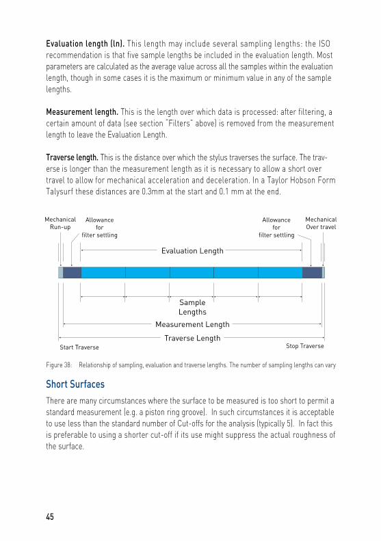
Evaluation length (ln). This length may include several sampling lengths: the ISO recommendation is that five sample lengths be included in the evaluation length. Most parameters are calculated as the average value across all the samples within the evaluation length, though in some cases it is the maximum or minimum value in any of the sample lengths.

Measurement length. This is the length over which data is processed: after filtering, a certain amount of data (see section “Filters” above) is removed from the measurement length to leave the Evaluation Length.

Traverse length. This is the distance over which the stylus traverses the surface. The trav-erse is longer than the measurement length as it is necessary to allow a short over travel to allow for mechanical acceleration and deceleration. In a Taylor Hobson Form Talysurf these distances are 0.3mm at the start and 0.1 mm at the end.

Short SurfacesThere are many circumstances where the surface to be measured is too short to permit a standard measurement (e.g. a piston ring groove). In such circumstances it is acceptable to use less than the standard number of Cut-offs for the analysis (typically 5). In fact this is preferable to using a shorter cut-off if its use might suppress the actual roughness of the surface.

45

Figure 38: Relationship of sampling, evaluation and traverse lengths. The number of sampling lengths can vary

If there is still insufficient surface to use a cut-off then using a Primary profile (a profile that is filtered only by the short wavelength filter, λs) is also acceptable. In the majority of cases a short surface will not exhibit much waviness and therefore will not significantly affect the roughness value.

Non-contact Measuring SystemsSo far we have restricted our discussion to the issues around measuring a surface with a contact stylus instrument. This has provided a good case study for metrology fundamentals, which generally apply across all measurement technologies.

However, it is worth considering briefly the differences that might pertain when using a non-contact measurement system. Some of the technologies available are outlined in CHAPTER 5 - Instrumentation.

Non-contact instruments offer several advantages over contact systems including the elimination of surface damage and increased measuring speed. Perhaps surprisingly, non-contact systems are rarely more accurate than a good stylus-based contact instrument. Disadvantages include not being able to measure into small bores or traverse across widely changing shapes as easily as a standard diamond stylus could do. The optical gauge also will not be able to “sweep aside” dirt in the same way that a diamond tip stylus tends to do.

Clearly, no light based system can measure completely black or totally transparent surfaces. On the other hand they can measure through transparent intermediate layers to assess bottom surfaces or intermediate interfaces

So where do the principal differences lie?Lateral resolution The majority of non contact systems use a beam of light focused onto the surface. It is very difficult to focus such a spot to less than about 5µm across with 10-15µm being typical. Within this spot the illumination can vary significantly, therefore, it is difficult to know exactly what point is being measured, and it can vary with reflectivity. Also, it is difficult to focus throughout a significant vertical range, therefore the spot size may vary depending on how high or low the sample is at that point.

Not all systems use focused spots: some image the surface onto a detector such as a CCD. Here the Rayleigh limits of lens aperture and diffraction effects limit the lateral resolution to about 0.5µm.

46

Electromagnetic surface Light is reflected at the “electromagnetic surface” not the physical surface. For homogeneous surfaces this makes little difference, especially for roughness measurements. However, absolute height measurements, and any measurement across material boundaries can be significantly affected.

Phase change There can be a phase change at the point of reflection, and this is dependent on the material of the surface. For a homogeneous surface this is not a problem. However, for instruments that are sensitive to phase, significant apparent steps in measured data can be introduced at a material boundary. This may occur for inclusions in metals or for different materials deposited on a semiconductor, for example.

Another annoying physical factor inherent in optical methods is the tendency of sharp points to act as secondary sources of light. It appears that if a radius of curvature of a part of the surface is smaller than about 10µm, diffraction effects appear which tend to enhance the edge. This is not serious at large values but is crucial in fine surfaces. This suggests that it could be the reason that very often the optical instrument produces higher values on finer surfaces.

For these reasons, it is virtually impossible to get an absolutely consistent measurement of roughness between contact and non-contact methods. However, there are strong correlations, and non-contact metrology is very useful in many process control applications and is therefore widely used in both research and industry. Subject to the above caveats the principles already learned by the reader in this chapter can be applied to both contact and non-contact surface metrology solutions.

3D or Areal MeasurementsOur considerations of surface measurements have so far been limited to a 2D trace (traditionally defined as the X axis being the horizontal movement of the gauge traversing the surface and the Z axis being the vertical displacement of the gauge due to surface features). However, a more complete picture of the surface would be available from a 3D representation.

Such measurements are becoming ever more common, driven by three factors:

• Increased computing power is now available at a cost that allows the very large data sets produced in 3D measurement to be processed in a reasonable time.

• Non contact metrology methods can produce the data much more quickly.

• The complex and very highly controlled surfaces being produced today need this detailed level of analysis for good quality control.

47

3D Surface measurement is often also referred to as “3D Topographic” or “Areal” measurement. Topographic clearly originates from topography (i.e., the study or detailed description of the surface features of a region), however the term “areal” is perhaps not so intuitive. The term “areal” basically means that the measurement is derived from an area of the surface, rather than a single line scan (2D).

Figure 39: MEMS Surface

Figure 39 shows an example of a highly engineered surface. It would be virtually impossible to get meaningful data from this surface with a 2D instrument as you would not be able to control whether the stylus (or non-contact point sensor) passed over some of the intentional features, or not. This would render any roughness analysis worthless. With a 3D measurement as shown here, and modern analysis software, the exact line or area to be assessed can be chosen so that meaningful data is produced (Figure 40 - Figure 42)

48

Another benefit of 3D systems is their ability to visualize surfaces to emphasize the surface features. Figure 43 shows four views of the same surface measurement of a cylinder liner with cross-hatch honing. The images are generated from the same measurement data using software to form the different views. On-screen they can be rotated and scaled to optimize the view.

49

Figure 40: Profile taken randomly across MEMS surface

Figure 41: Profile taken across a single line of peaks on MEMS Surface

Figure 42: Profile taken in valleys of MEMS surface

Figure 43: Four views of the same 3D surface image (A) raw data (B) raw data after form removal (C) photo simulation image of the data (D) axonometric map of groove detail

50

A

B

C

D

3D data is acquired in one of two ways: a point sensor is raster scanned over a surface, or a multipoint image is produced in a single shot using a camera-like CCD or similar device (Refer to CHAPTER 5 for additional information on instrumentation).

Raster scanning is slower than single shot systems, but is more flexible in terms of area examined, data density and dynamic range. It is also usually cheaper. As there are now two moving axes (the gauge being the third axis) several further effects must be considered when analysing the data. First there is the issue of having an accurate start point for each traverse. A variable start position will give rise to a distorted picture of the surface (Figure 44 & Figure 45). Also, the two moving axes must be exactly orthogonal to one another and to the gauge movement, otherwise a skew will be introduced into the result.

Figure 44: 3D Measurement with good start position control

Figure 45: 3D Measurement with poor start position control relative to one another

51

52

Figure 46: This image, produced by a Talysurf CCI instrument using coherence correlation interferometry, illustrates the significant possibilities available with 3D measuring techniques. An array of more than 1 million data points in X and Y makes possible high graphical resolution and reliable calculation of area, volume and lateral distances. The nanotechnology based device shown is less than 6um in height.

183µm

183µm

5.9µm

CHAPTER 4 - Putting a Number To It

If every different surface could be given a unique number, a number that completely characterized its roughness, then we would have succeeded in converting roughness assessment from a subjective to an objective process. Unfortunately, no single parameter will cope with the complexity of most surfaces. We therefore require a series of parameters to give us a guide to accurate assessment of performance. In this chapter we shall explore some of the parameters which express roughness numerically and the conditions for specifying their values.

Most parameters were originally developed nationally to suit the individual country’s requirements and consequently there has been some duplication of certain methods of assessment. These have largely been standardized and a list of the relevant papers can be found in the Appendix to this book.

The main criteria for selecting a surface texture parameter are: can it be related to performance or the production process it controls? Does the parameter value change rapidly or slowly with the function it is monitoring? To illustrate the point, Figure 47 shows how some parameters change with surface wear. It can be seen that parameters with predominant peaks change most during wear and, as would be expected, those which are influenced by valley depth are affected least.

Profile parameters fall into three groups depending on the characteristics of the profile they quantify:

Amplitude parameters which are determined solely by peak or valley heights, or both, irrespective of horizontal spacing (e.g. Ra).

Spacing parameters which are determined solely by the spacing of irregularities along the surface (e.g. RSm).

Hybrid parameters which are determined by amplitude and spacing in combination (e.g. Rdq).

In the following sections we discuss the parameters that are used to quantify certain aspects of surface finish. These parameters can be calculated for Primary profiles, Roughness profiles or Waviness profiles, as indicated by the prefix letter (P, R or W respectively). For convenience we have referred to the Roughness analysis, and consequently the parameters are shown with the prefix R.

53

Figure 47: Chart showing variation of parameters with wear

Roughness Average (Ra)This is the most commonly used parameter in surface texture analysis. (In the past it has been called the Center Line Average [CLA] or Arithmetic Average [AA] in the United States.) We, therefore, should devote some considerable time to this parameter.

Figure 48 illustrates the derivation of Ra. The area of the profile below the center line in illustration A is inverted and placed above the line in illustration B. Ra is then the mean height of the resulting profile. Mathematically, Ra is the arithmetic average value of the absolute (or modulus of the) departure of the profile from the reference line throughout the sampling length (Figure 49).

Notes:i) The Ra value over one sampling length represents the average roughness so the effect of a non typical peak or valley will be averaged out and will not have a significant influence on the results.

ii) Most National and International Standards suggest that assessments are made over five consecutive sampling lengths and then the data averaged out. This ensures that the Ra value is typical of the surface.

54

iii) The Ra value is meaningless unless the cut-off length is known. Where not otherwise stated lc is assumed to be 0.8mm and the bandwidth 300:1.

iv) Where not otherwise indicated, measurements should be made at right angles to the direction of lay.

v) Ra will give no information regarding the shape of the irregularities. Figure 50 illustrates this point.

vi) No distinction is made between peaks and valleys.

vii) Ra units are length, typically microns.

ix) Figure 51 shows how parameters are specified on drawings.

Figure 48: Graphical derivation of Ra

(A) Profile with center line

(B) Lower portions of profile inverted

(C) Ra is the mean of the profile.

55

Figure 49: Mathematical derivation of Ra

56

Figure 50: Profiles having the same Ra value but with different shapes and different peak to valley values.

57

Figure 51: Specifying parameter values on drawings

Some countries use different symbols to denote roughness values. For details see the relevant National Standard.

RMS value (Rq)Another method of calculating an average roughness value is known as the root mean square (rms). This is obtained by squaring each value and taking the square root of the mean of these values.

Why is it necessary to have two averaging parameters? The answer is chiefly historical. Ra is the easier to determine graphically and was therefore adopted initially before digital roughness measuring instruments became available.

Rq values are more meaningful than Ra figures when used in statistical work.

Peak and Valley HeightsIt is sometimes useful to specify the maximum peak to valley height rather than the mean height that Ra gives. This parameter is termed Rt and is the distance between the highest and lowest points of the profile within the evaluation length.

58

Figure 52: Derivation of some peak parameters

Zpvi = The maximum peak to valley height within the sampling length, i

Zpi = Height of the highest point of the profile above the center line within the sampling length, i

Zvi = Depth of the lowest point of the profile below the center line within the sampling length, i

Rt = The vertical height between the highest and lowest points of the profile within the evaluation length

With reference to Figure 52, Rp, Rv and Rz are the average values of Zpi, Zvi and Zpvi over all sampling lengths. The values Zpi, Zvi and Zpvi are used here for explanatory purposes only, and are not ISO parameters.

Historically, there have been many attempts to define parameters by many national standard authorities and some confusion still remains as to the relationship of, for instance, ISO and DIN definitions. We will therefore use the ISO definitions here and ask the reader to check their relationship with other standards where necessary.

The majority of instruments are now digital rather than analog in their operation. This allows the data to be processed using computers and alleviates the operator from having to perform leveling and analytical tasks. Where an assessment is still made from a graph, then any manual measurement of peaks or valleys must be made perpendicular to the chart ordinates. This is because of the use of different scaling for the Z and X axes.

Figure 53: Graph recorded: (A) generally parallel to the chart (B) sloping across the chart

In both cases the height of the peak is only correct if measured perpendicular to the base line.

The valley is similarly measured.

Ten Point Height (also RzJIS)The Rz parameter has had a very confusing history which leads to problems if you do not know exactly which version is being used. Rz has now been standardized to two basic types: Rz and RzJIS (JIS: Japanese Institute of Standards). Rz is the parameter described in the section above. RzJIS is the "Ten Point Height" parameter described below.

59

A

B

As a guide, the following equivalents have been adopted by most metrology institutions and equipment manufacturers:

Original Description Adopted Equivalent

RzDIN 1974 Rz with a 2CR filter RzISO 1984 RzJIS with a 2CR filter RzISO 1996 Rz with gaussian filter RzJIS 1982 RzJIS with 2CR filter RzJIS 1994 RzJIS with gaussian filter

The RzJIS parameter is particularly useful when measuring very small lengths and is based on ten points within the sampling length. The five highest peaks and the five deepest valleys are assessed and the result is the mean height of these ten points.

The center line is only used as a reference direction. Although the measurements shown in Figure 54 are being made from the center line it makes no difference where the line is set. The same result is obtained if the peaks and valleys are measured from any line inside or outside the profile as long as the line is parallel to the center line. This parameter is particularly suited to assessments made from graphs, requiring only ten linear calculations.

It must be stressed that this parameter must not be confused with the DIN Standard definition of peak and valley calculation which is also called Rz but is normally known as Rtm in ISO and British Standards.

60

Figure 54: Derivation of RzJIS and RSm (mean spacing)

P1 + P2 + P3 + P4 + P5 + V1 + V2 + V3 + V4 + P5

10Rz JIS =

S1 + S2 + S3 + .......... + Sn

nRSm =

Mean Width of Profile Elements, R SmThe parameter Sm is used to describe the average spacing of profile elements (peaks and valleys) measured along the measurement direction. Its derivation is shown in Figure 54. The peaks and valleys are found using both horizontal and vertical discrimination criteria (not shown).

Material Ratio (Bearing Ratio)One of the most common uses of an engineering surface is to provide a bearing surface for another component moving relative to it. This results in wear, and the bearing ratio parameter, which simulates the effect of this wear, is widely used. Imagine a lapping plate resting on the highest peak of a profile (Figure 55). As the peaks wear and the bearing line descends down the profile, the length of the bearing line (the length of the profile in contact with the lapping plate) increases. Material ratio, symbol Rmr, is the ratio (expressed as a percentage) of the length of the bearing surface at any specified depth in the profile to the profile length.

61

Figure 55: Illustration showing the derivation of material ratio

This parameter, although it simulates the effect of wear, cannot take the place of running in tests because:

i) Material ratio is a fraction of a length not an area of a surface.

ii) It is determined from a relatively short trace and ignores the effect of waviness or form.

iii) In practice two contacting surfaces are involved, both of which have a part in causing wear.

a + b + c + d + e + f + g + hRmr = L

In spite of this, Rmr is a parameter that can be usefully correlated with performance. The converse of the parameter can also be used, namely the depth at which a certain bearing area is found. Thus if a material ratio of 60%, for example, is found to be correct for an application, the depth P at which the crests must be truncated can be determined.

Material Ratio Curve (Abbott Firestone or Bearing Ratio Curve)By plotting the material ratio at a range of depths in the profile (Figure 56), a material ratio curve can be plotted to provide a means of distinguishing different shapes of profile.

62

Figure 56: Derivation of the material ratio curve (Abbot-Firestone or bearing ratio curve)

What Constitutes A Peak?As soon as we begin to measure Rz from a profile trace, or to count the number of peaks (e.g. Rpc) within a sampling length, a question that arises is what constitutes a peak or valley? Consider Figure 57. Areas A (between points C and D) and B (between E and F) can be called profile peaks. Note that to be considered as a peak the trace has to pass through the mean line twice. So in Figure 57 the peaks are A and B. The smaller apparent peaks which do not reach the mean line do not qualify.

It is likely that when the surface is put into use a considerable number of the very small local peaks will disappear before they have an effect on performance.

Profile valleys are similarly defined.

63

Figure 57: Profile peaks and valleys

Peak Counting (Rpc)The spacing of roughness peaks can be of considerable importance in the manufacture of sheet steel where control of a surface is necessary to lubricate the sheet when pressing, to avoid scoring and to prevent the texture showing through the paint on the finished product. By controlling the peak spacing it is also possible to obtain better bonding and uniformity of finishes of plating and paintwork. Peak spacing is also of importance in the performance of friction surfaces such as brake discs.

Peak count is assessed by the number of peaks which pass through a selectable band centered about the mean line and the results are given in peaks per cm (or per inch). It is advisable to measure this parameter over the greatest evaluation length possible.

In Figure 58 only two peaks are counted. To constitute a complete peak (i.e., Peak 1), the profile must pass from below the lower reference line [point a] to above the upper reference line [point b] and then below the lower reference line once again [point c]. Likewise, the profile passing through points d, e and f will constitute Peak 2. Note however, that minor peaks A, B, C, D and E would not be counted because their adjacent valleys did not pass through the lower reference level.

64

Figure 58: Peak counting

High Spot Count (RHSC)This is the number of complete peaks which project above a reference line parallel to the mean line.This line can be set at a selected depth below the highest peak,a height above the lowest valley or a selected distance above or below the mean line. In Figure 58 Peak 1, peaks A and C and Peak 2 constitute complete peaks (the profile passes through the upper reference level both upwards and downwards) and would be included in High Spot Count. The minor peaks B, D and E would not be included.

Slope (Rda and Rdq)The slope of the profile is the angle (in terms of gradient) that it makes with a line parallel with the center line. The mean of the absolute value of slope calculated at each of the points in the profile within the sampling length is known as the average slope (symbol Rda for the arithmetical mean and Rdq for the rms value).

The slope is calculated using the assessment length and the developed or actual profile length, that is: the length occupied if all the peaks and valleys were stretched out in a straight line (Figure 59).

The steeper the average slope, the longer the actual length of the surface compared to its nominal length. This is a very useful guide for painting and plating operations where the length of surface available for coating is important.

Average slope is useful in assessing certain properties of engineering surfaces:

Contact The parameter can be related to hardness and elasticity and can be an indication of the crushability of the surface.

Optical If Rda or Rdq (RΔa or RΔq) is small, the surface is a good reflector often looking cosmetically good. Since the average slope depends on both amplitude and spacing, it is a hybrid parameter. Friction The higher the Rda or Rdq (RΔa or RΔq) then typically the higher the friction exhibited by the surface and visa versa.

65

Figure 59: Profile length

Amplitude Distribution (Skew [Rsk] and Kurtosis [Rku])The amplitude distribution curve illustrates the relative total lengths over which the profile graph attains any selected range of heights above or below the center line. This is shown in Figure 60.

The horizontal lengths of profile included within a narrow band of width dz at a mean height y, are a, b, c, d and e. By expressing the sum of these lengths as a percentage of the evaluation length, we obtain a measure of the relative amount of the profile graph at height y:

a + b + c + d + e x100% L

The way in which the amplitude density is distributed over the whole profile can be seen by plotting the density against the height (y). The shape of the curve can be very informative. A profile which has a regular shape gives an amplitude distribution which is symmetrical about the center line, but an unsymmetrical profile gives a skewed curve (Figure 61). The direction of skew depends on whether the bulk of the material is above the mean line (negative skew) or below it (positive skew). This curve, therefore, gives us a method of distinguishing between two surfaces with the same Ra but having different shapes. Skewness is given a numerical value and is denoted by the parameter Rsk.

A porous, sintered or cast iron surface typically has a large value of skew. If it exceeds ±2, alternative parameters should be used as Ra is unlikely to provide useful information. A surface with negative skew would probably be right for a bearing surface having a few spikes that would quickly wear away. A surface with positive skew would be useful for painting or plating, having more spikes to cling on to.

Skew cannot detect if the spikes are uniformly distributed about the mean line whereas Kurtosis can. Kurtosis (symbol Rku) provides a measure of the sharpness of the surface, a "spiky" surface having a high Kurtosis value and a "bumpy" surface having a low Kurtosis value.

66

Figure 60: Derivation of amplitude distribution curve

A comparison of Figure 56 and Figure 60 shows a close connection between the amplitude distribution curve and the bearing ratio curve. In fact one can be obtained from the other by the simple graphical procedure illustrated in Figure 62.

67

Figure 62: Method of obtaining material ratio curve (Abbot-Firestone or bearing ratio) from amplitude distribution curve

Figure 61: Skew (Rsk) will distinguish between profiles of different shapes

R & W (French Motif)Two parameters, R (roughness) and W (waviness) together with Aw (average waviness) are extensively used in the French automobile industry. They were devised to provide a subjective assessment of the profile graph - a means of quantifying the profile in a practical manner by drawing on a graph an envelope which encloses the profile, touching the highest peaks and lowest valleys but smoothing out the roughness irregularities (Figure 63). Any peaks or valleys determined by the analysis to be exceptional are removed from the result. This envelope is an attempt to show the general form of the surface with less detail than the actual graph.

68

Figure 63: Three profiles are used in the R&W analysis:

1) The unfiltered profile with slope correction (i.e. out of level has been removed with respect to a least squares straight line), gathered by traversing the stylus, skidless, over the workpiece.

2) The corrected roughness envelope (superimposed on the unfiltered profile)

3) The waviness envelope (superimposed on the unfiltered profile)

Waviness ParametersWaviness parameters have not received much attention in this book for the simple reason that most of the roughness parameters have a waviness counterpart. As demonstrated earlier, the difference between roughness and waviness is chiefly one of scale, although their cause and function are dissimilar.

The cut-off length at which waviness is assessed refers to the length below which the irregularities are suppressed. The sampling length must therefore be greater than the cut-off. This is of course the opposite of the purpose of the cut-off as applied to the roughness measurement. The distinction is important and must be remembered when selecting the cut-off to be used in waviness measurement. The upper limit is normally set by the maxi-mum traverse length available, not the need to exclude form deviations.

Relationship of ParametersIn the past there has been much talk about the value of various parameters in relation to Ra. Experience has shown that there is no fixed relationship between the majority of param-eters as the ratio depends entirely on the shape of the profile. With the rapid increase of computer aided instruments this problem is largely overcome and all guesswork can now be taken out of converting results.

Surface Texture at the Design StageAlthough it is important to consider the surface texture requirements at the design stage, it must be pointed out that surface texture should not be controlled unless close control is essential to looks or performance. Imposition of close control will always mean higher costs, sometimes unnecessarily.

69

70

Figure 64: The relative cost, in production time, necessary to produce finishes by different processes

3D ParametersParameters for 3D areal assessment are still under discussion by ISO and other standards organizations and at the time of publication there are no formally approved parameters defined. However, it is most likely that at least 18 parameters will be adopted as currently defined in “EUR 15178EN Provisional” and as shown in Table 3.

Table 3: Proposed 3D Parameters

Description Comment Sq Root mean square deviation Used to discriminate between different surfaces of the surface based on height informationand to monitor manufacturing stability

Ssk Skewness of the surface Indicates aspects of load carrying capacity/lubrication

Sku Kurtosis of the surface Indicates ‘spikiness’ of the surface

Sp Highest peak Largest peak height within the definition area

Sv Lowest valley Largest valley depth within the definition area

Sz Ten point height of the surface Used to evaluate extreme surface height deviations

Sa Average absolute deviation of Non-preferred parameter the surface

Sds Density of summits of the Used to evaluate the density of peaks surface and pits in the surface

Str Texture aspect ratio of the surface Measures the isotropy of a surface

Sal Fastest decay autocorrelation Describes the most significant length length component of texture Std Texture direction of the surface Indicates the direction of the significant lay of the surface

Sdq Root mean square slope of Evaluates contact or optical properties the surface Ssc Arithmetic mean summit Measures the openness or closeness of curvature the texture

Sdr Developed surface area ratio Understanding of deformation of surface regions

Functional Parameters (characterizing bearing and oil retention properties)

Vvc Core void volume Difference in void volume per unit area measured at 10% and 80% material ratio

Vvv Valley void volume Volume of the voids per unit area at 80% material ratio

Vmp Peak material volume Material volume per unit area at 10% material ratio Vmc Core material volume Difference in material volume per unit area measured at 10% and 80% material ratio

71

Hybrid Parameters

Spatial Parameters

Amplitude Parameters

As 3D areal measurement becomes more practicable in terms of measurement cycle time and equipment availability, increased development will go into determining new analysis techniques that allow the function of the part to be better controlled. One such method is the Contour map with Critical Points, Ridges and Course Lines plotted (Figure 65).

72

Figure 65: Contour, Critical Point, Ridge and Course plot

Such a plot uses geographical analysis techniques to identify critical points on the surface (such as Summits, Peaks and Valleys) and then from such critical points Ridges and Course lines will be determined. If the course lines inter-connect then it is likely that the surface will allow fluids to pass along them and hence be a source of leakage. Similarly if they do not connect then the surface may be considered a good lubricating surface if the volume of the valleys is sufficient.

While the ability to derive numbers from such a methodology is still being developed, it is clear that the focus is on better control of the “functionality” of the surface rather than discrete parameters that are not inter-related.

A Final Word on ParametersResearch continues into improving traditional manufacturing processes and therefore the search for new parameters to adequately express surface features by number will continue. The parameters mentioned in this book are not a complete list: for further explanations of the current parameters and definitions it is recommended that the reader consults the surface texture parameter card currently supplied by Taylor Hobson Ltd at the address shown at the front of this publication or look in the glossary under the FAQ section of the website at www.taylor-hobson.com.

Summary

Before passing on to explore a different aspect of surface texture measurement it will be useful to summarize some of the more important things which we have discovered.

i) The most important feature of surface texture assessment is - the SURFACE.

ii) Any assessment, whether qualitative or quantitative, must be interpreted in relation to the surface - its method of production, its lay and its function.

iii) Roughness, waviness and form are three ways in which a surface can depart from perfect smoothness and flatness. Although always found in combination, the effects on performance are different and by choosing the appropriate sampling length can often be separately assessed.

iv) The profile trace, although visually distorted, is an accurately scaled representation of the surface along the path taken by the stylus. Surface features can be accurately measured from it by taking into account the different vertical and horizontal magnifications.

73

CHAPTER 5 - Instrumentation

74

Figure 66: The first Talysurf instrument

The Stylus InstrumentElectrical stylus type instruments are to be found wherever surface finish is measured: in the workshop, inspection area, standards room, research laboratory and technical college, so we should explore their construction in some detail.

The TalysurfIn 1935, R. E. Reason of Taylor, Taylor & Hobson started a major research project into the nature and measurement of surface finish. During this project he evolved the geometric standards and mathematical basis for instrumenting the measurements. The result was the first of a long and continuing line of Talysurf instruments. Dr Reason’s work laid the foundation for standardizing surface texture measurement, both nationally and internationally. Talysurfs went into commercial production in 1942 (Figure 66), this first instrument incorporating many of the basic features of subsequent instruments.

The basic components of these first instruments are depicted schematically in Figure 67. The stylus was traversed across the surface and the pickup converted its vertical movements into an electrical signal which was amplified and used to operate a recorder. From this filtered signal was derived an Ra value which was displayed on a pointer or analog meter. Later instruments have extra facilities including computer analysis and programming for automatic measurement, but in principle the operation remains the same.

75

Figure 67: Diagram showing the chief constituents of a stylus type surface texture measuring instrument

Figure 68: Form Talysurf PGI Instrument

In this chapter we will examine each of the basic components in some detail, but firstly we must emphasize one basic feature of most of the surface finish measuring instruments which are currently being used - namely that the profile is traced by movement across the surface, the sampling of consecutive points of the profile being spaced in either time or distance. Modern systems will utilize true distance measurement capability (using gratings or lasers) rather than time for datalogging.

This is necessary for greater accuracy and is essential where form error or contouring applications are required. Where systems use time as the basis for datalogging then errors in spatial parameters can occur (due to speed fluctuations in the traverse mechanism) and the true measurement of form is almost impossible.

Note: Some specialized applications such as measurement of surface texture of small balls, require an instrument capable of rotating the ball under a fixed stylus. The attachment for this facility is part of Taylor Hobson’s current range (Figure 81).

GaugeThe function of the gauge is to convert the vertical movements of the stylus into proportional variations of an electrical signal. The sensitivity required of the gauge is such that it should respond to a stylus movement of less than 0.01µm. Although the output is very small, high resolution systems can accurately assess the deviations. However, for the operator to visualize the profile the displacements are amplified by a factor of up to X2,000,000 (although X50,000 or less is more typical).

a) Analog Transducers

For surface metrology gauges these transducers can be further divided into two groups, depending on their principle of operation:

i) Position sensitive: These give a signal proportional to the displacement, even when the stylus is stationary. The output is dependent on the distance that the stylus is displaced and is related only to the position of the stylus within its range of vertical movement. The advantage of this type of pick-up is that it enables a true recording of waviness and form.

ii) Motion sensitive: Gauges in this group produce an output only when the stylus is moving, the output being related to the speed at which the stylus is displaced and dropping to zero when the pick-up is stationary. When the displacement is very slow, for example due to widely spaced waviness or form change, the output is extremely small and for practical purposes is zero. This type of pick-up is therefore most commonly used in skidded instruments.

Many analog systems have multiple range settings: this allows a small portion of the gauge range to be used with very high resolution, or the full gauge range at a lower resolution.

76

b) Digital Transducers

As the stylus moves, pulses corresponding to multiples of the transducer resolution are fed to an up-down electronic counter which displays the gauge displacement. The range is determined by the physical constraints of the gauge.

Typical range to resolution ratios are in the order of 700,000:1. There is no need for range switching, therefore the maximum resolution is available with the maximum range.

The displayed displacement is relative to the stylus position where the counter is zeroed. Therefore every time the electronics are switched off and on again the counter has to be re-zeroed at a particular stylus datum position. If a certain maximum stylus speed is exceeded the counter may lose count, requiring zeroing at the datum position again.

Gauges with Analog Position Sensitive TransducersThe gauge with a variable inductance transducer, used in many models of measuring instruments, is of this type (Figure 69).

77

Figure 69: Variable inductance gauge

Figure 70: Schematic diagram of modulated carrier system

The stylus is carried at one end of a beam pivoted at the fulcrum on knife edges. The far end carries an armature which moves between two coils, changing their relative inductance. The coils are connected in an AC bridge circuit (Figure 70) such that when the armature is central between the bridge it is balanced and gives no output. Movement of the armature unbalances the bridge which produces an output proportional to the displacement, the relative phase of the signal depending on the direction of the movement. The signal is amplified and compared with that of the oscillator to determine in which direction it has moved from the central (zero) position. The use of an oscillator to produce a constant AC output is necessary because the pick-up, unlike a motion-sensitive pick-up, does not generate any output, it merely serves to modify the carrier. The stylus is held in contact with the surface and with the knife edges by means of a weak spring acting on the beam. The ligaments prevent movement of the beam in a horizontal plane, with the result that the stylus is only free to move vertically.

These gauges are also used in the newer types of measuring instruments, where the range to resolution ratio has increased from approx 1,000:1 to better than 64,000:1. Modern electronics have allowed this to happen, obviating the need for a skid. Precise pivot bearings have replaced the knife edge pivot shown in Figure 69.

Gauges with Motion Sensitive TransducersThis type of gauge includes a piezoelectric crystal which has the property of developing a voltage across electrodes when the crystal is deformed. It is not used very often other than in low cost entry-level systems.

Gauges with Digital TransducersTwo gauges that are currently used in Taylor Hobson instruments are based on interferometery. Interferometry basically uses the principle of counting the light and dark “fringes” caused when two light beams interfere. Often the signal is interpolated to give a finer resolution.

78

Figure 71: Interference fringes

Figure 71 shows how, when 2 spots of light are superimposed, interference occurs to create light and dark sections which can be counted and used as a means of precise measurement.

a) Laser Interferometric Gauge

On the end of the pivoted stylus arm is positioned an end reflector, which acts as the moving arm of a miniature Michelson laser interferometer. The laser wavelength (632.8nm) provides the measurement reference. The interference fringe pattern is detected by four photodiodes enabling the output signal to be interpolated to give a basic resolution of 10nm. The range of 6mm is limited by the size of the end reflector.

b) Phase Grating Interferometric (PGI) Gauge (Figure 72)

The PGI gauge was developed to offer a greater range than the laser interferometric gauge and a reduction in physical size by using a laser diode instead of a gas (HeNe) laser. In the PGI gauge a curved phase grating is positioned on the end of the pivoted stylus arm, which is the moving element in the interferometer. The grating wavelength provides the measurement reference: this is a crucial difference as the measurement is now independent of the laser wavelength, which can vary significantly with environmental conditions. The interference fringe pattern is detected by four photodiodes, enabling the output signal to be interpolated to give a basic resolution of 0.8nm and a range of 12.5mm.

79

Figure 72: Schematic diagram of the phase grating Interferometric (PGI) gauge

Gauge DatumHaving dealt with the mechanism of the gauge we must see how it is used to measure surface irregularities. The electrical output represents the combined displacement of the stylus and the gauge body relative to the general level of the surface; the gauge must, therefore, traverse along a line accurately parallel to the surface if the electrical output is to be a true representation of the traced profile.

This can be achieved in two ways; by using an independent datum or by use of a skid. More sophisticated instruments are fitted with a datum bar in the traverse unit that is of sufficient straightness accuracy that it can generally be discounted in any calculations. Instruments with datum bars can measure waviness and form as well as roughness. Less sophisticated instruments will not be fitted with a datum bar: instead they have a “skid”.

SkidWhen a skid is fitted the gauge is hinged to the traverse drive shaft at one end, the other end is supported by a curved surface of a larger radius projecting below the stylus and in contact with the surface (Figure 73). Providing the radius of the skid is considerably larger than the spacing of the peaks, then the line of movement will be almost a straight line (Figure 74), the up and down movement as the skid moves from crest to crest will be normally insignificant. The ISO standards recommend that the skid radius should be greater than 50 times lc.

80

As the crests become more widely spaced the skid will sink more deeply into the valleys and will no longer provide a straight datum. A longer datum such as a shoe skid (Figure 76) will then be required to bridge the more widely spaced crests.

Figure 73: Gauge supported by a skid

Figure 74: A skid supporting the pick-up giving an almost straight line movement across the surface

Figure 75: A rounded skid does not provide a serviceable datum if the surface irregularities are too widely spaced

81

Figure 76: A flat shoe will solve the above problems

Ideally the skid and the stylus should be coincident, but for practical reasons the skid is usually placed slightly in front or behind the stylus; this offset can lead to errors on some surfaces. Figure 77 shows one effect which causes distortion on a display or printout - the amount depends on the waviness spacing. If this spacing is the same as the skid/stylus spacing then the skid will rise on one crest while the stylus rises on the next one, a condition which will entirely suppress the peak. This effect is reduced when two skids are used, one on each side of the stylus or one in front and one behind the pick-up.

To sum up, the skid is a filter which modifies the profile to a greater or lesser extent. Its radius must, therefore, be suitably chosen. For general purposes a skid radius of 50mm is usually suitable.

The use of skids is no longer recommended by the ISO standards.

Figure 77: Phase effects when using a skid

82

Independent DatumThe most common independent datum is a shaft built into the traverse unit. This is normally straight to within 0.1µm over 100mm, so for all normal measurements the errors can be discounted. The gauge is fixed rigidly to the datum, but may be hinged in order to allow the user to fit a skid to the gauge.

The use of an independent datum allows all the irregularities on the surface - those of waviness and form as well as roughness - to be measured (Figure 78). With the wide range available in modern gauges this allows the user to assess certain other geometric shapes such as radii and angles. This in turn leads to the use of such instruments in assessing the form (or contour) of a component

Figure 78: An independent datum provides a straight reference for the gauge traverse

Electronics & Data ProcessingWhen an analog gauge is used, the signal must be amplified before passing to the digitization process. The analog to digital converter (ADC) then digitizes the signal. This whole process must achieve suitable bandwidth, linearity and noise suppression for the application: clearly, lower specification instruments are more tolerant of poorer electronics than more accurate ones.

The output of the ADC (or a digital gauge directly) is passed to the digital processing system. This is typically microcontroller based for low-end instruments (such as the Taylor Hobson Surtronic Duo) where limited menus allow the user to measure a single or a few parameters.

In more sophisticated instruments data analysis is typically performed in a PC. Powerful programs allow a huge variety of analyses to be performed: the range and scope of these are beyond this book. However, a word of warning: with the huge variety of parameters and variables that can be altered in these systems it is easy to produce a wrong, but apparently correct, answer.

83

If you understand and follow the principles of this book you will be well placed to make a good assessment.

Instrument AccuracyThe “accuracy” of an instrument measuring surface texture is the combination of a number of features, and is often hard to calculate from instrument specifications. GUM (an overview "Guide to the Expression of Uncertainty in Measurement" issued by ISO) provides an introduction to the calculation of errors.

It is often said that a chain is only as strong as its weakest link: in many ways the performance of an instrument is the same in that any one poor area of performance will limit the overall capability. For example, however good the gauge mechanics, transducer and electronics, if the digitizer introduces a non-linearity the system will not read correctly. In the opposite sense, if an instrument has a fantastic headline feature, such as very high resolution, the rest of the system must be of sufficient quality for this feature to be of any use.

A well-designed instrument has a balance of performance in all areas to give the best possible overall capability. Often, the only practical way to properly assess an instrument is to make measurements of known parts under a variety of conditions, and analyze the results.

What’s the difference between accuracy, resolution and repeatability?Accuracy is, in a nutshell, how close a result is to the real value. In terms of dimensional measurement this is referred to how close the result is to the nationally or internationally recognized value.

Resolution represents the “fineness” to which you know your result - no matter how accurate the result is. As an example, person A could measure the length of a 100mm bar with a resolution of 0.1µm, but their results might always read 98mm - so their resolution is 0.1µm, but their accuracy is only 2mm - 20,000 times worse than their resolution. Person B might measure the same bar with a set of callipers and have a resolution of only 0.1mm, but consistently measures 99.5mm. Their accuracy is then 4X better than person A’s, even though their resolution is a thousand times worse.

Repeatability is a measure of how closely a result can be reproduced under controlled conditions. In the example above, person A might make a number of measurements with a spread from 97.9912mm to 98.0086mm. The spread of the results is 0.0174mm, and this is a measure of the repeatability of the result. Usually this is referred back to the standard deviation in the results. In this example, the resolution of the result is 0.0001mm, the repeatability 0.0174mm and the accuracy 2mm!

84

Instrument set-upHowever good the instrument and calibration standards, a badly installed, located or used instrument will give the wrong answer! It is beyond the scope of this book to deal with all these issues, but a few guidelines will assist the reader. It should be remembered that the greater the accuracy you wish to achieve, the more strictly these guidelines need to be followed.

Metrology environment The instrument must be kept at constant temperature and free from vibration and excessive air movement.

Sample preparation The sample must be clear of all surface debris, grease, cutting fluids etc. It should be stabilized at the same temperature as the instrument.

Sample set-up The sample must be held firmly in position so that it cannot be moved during the measurement process. It should be leveled and measured around the center of the gauge range. Good leveling can take some time, and a wider gauge range makes this less important, saving on set-up time.

Metrologist skill A good metrologist can get more consistent results from the same instrument compared to a lay person. Training in both the instrument and general metrology are important.

Curved SurfacesAll the surfaces mentioned so far have been nominally flat. However, we also have a need to measure surface texture of curved surfaces such as balls, rollers, gear teeth and the fillet radii of crankshafts.

Before wide range pick-ups were produced with sufficient resolution to assess surface texture as well as form, it was necessary to find a way of measuring in such a manner that the shape did not influence the surface texture too much.

With large radii the problem could be overcome by using a short cut-off length and a skid fitted to the pick-up. The skid does cause problems if fitted in front or behind the stylus as shown in Figure 79, but the displacement can be reduced by introducing a skid which surrounds the stylus, the tip of the stylus projecting through the skid (Figure 80).

85

Some other solutions to the problem of curved surface measurement are:

i) The gauge is guided by a curved datum instead of a straight one.

ii) The gauge is held stationary and the component rotated under it.

iii) The gauge is traversed circumferentially round the surface.

iv) A wide range gauge such as the one fitted to Form Talysurf is used.

Figure 79: Effect of a curved surface. The displacement of the stylus due solely to the curvature is d1 + d2.

Figure 80: Side skid gauge in which the skid takes the form of a cylindrical surface through which the stylus projects.

Rotating WorkpieceIn this method the component - a ball or roller for instance - is rotated in a conical seating against the stylus of a pick-up built into the seat housing (Figure 81). The advantages of this system include the fact that the tip of the stylus is always in line with the center of the component and the possibility of the tip flanking on the part is eliminated.

86

Figure 81: Principle of rotating workpiece instrument (Ball Unit)

Form and Contour MeasurementAlthough form deviations are not part of surface texture, they are closely connected with it: like roughness and waviness they are surface irregularities and can be assessed with similar instruments.

The requirement for form checking is to determine the comparatively small deviations from a nominally straight or arcuate surface, or to measure the profile of a shaped surface. It is a single traverse measurement of the surface profile and is often referred to as a form or contour measurement. The deviations from a straight surface can easily be checked using a surface measuring instrument providing it is fitted with a straightness datum. For this type of measurement it is advised that a longer traverse is used in order to ensure that the greater spacing of the deviations is assessed.

Form measurement requires a much larger gauge range than for straightness checking. Taylor Hobson has been in the forefront of developments to increase the range of the gauge without significantly reducing its resolution. They have, with their Form Talysurf Series instruments, been able to produce gauges which will measure over a range in excess of 12mm and still have sufficient resolution to measure surface finish correctly. This has allowed form measurement to be carried out on a large proportion of components using a standard surface measuring instrument. The assessment can be computed and the radii, angles etc. can be displayed and printed out through a standard inkjet or laser printer. Importantly, the surface finish can also be calculated during the same pass over the component.

In circumstances where a much larger gauge range is required then a dedicated contour instrument is offered and many of the assessment facilities used in Form Talysurf are still available. However, the surface texture analysis capability is not possible.

87

3D Measurements With Stylus InstrumentsWhere stylus instruments are used for 3D surface mapping it is essential that they possess an independent datum. The use of a skidded instrument would suppress the natural surface contours in all planes of measurement and could significantly distort the results.

88

Figure 82: Basic “stepping” method used by stylus systems

Such systems can offer a high degree of spatial resolution and can have a fixed resolution in both X & Y directions. Their disadvantage is that they are slow, and as a result can be prone to suffering from environmental effects such as drift and vibration.

Non-contact Surface MeasurementThere are a number of non-contact gauges on the market that can be mounted on standard surface measuring instrumentation.

Capacitance systemsThe most basic form of areal surface measurement is a capacitance gauge. Such systems use the surface as one plate of the capacitor. The air between the surface and the capacitance probe acts as the dielectric. The overall surface roughness of the surface then causes a change in the capacitance level.

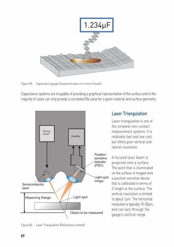
89

Figure 84: Laser Triangulation (Reflectance method)

Laser TriangulationLaser triangulation is one of the simplest non-contact measurement systems. It is relatively fast and low cost, but offers poor vertical and lateral resolution.

A focused laser beam is projected onto a surface. The point that is illuminated on the surface is imaged onto a position sensitive device that is calibrated in terms of Z height at the surface. The vertical resolution is limited to about 1µm. The horizontal resolution is typically 10-20µm, and can vary through the gauge’s vertical range.

Figure 83: Capacitance gauge (measured value is in micro Farads)

Capacitance systems are incapable of providing a graphical representation of the surface and in the majority of cases can only provide a correlated Ra value for a given material and surface geometry.

Atomic Force MicroscopyStrictly speaking, Atomic Force Microscopes (AFMs) are contact measurement devices but, due to the very low stylus force involved, are usually considered non-contact for practical purposes. AFMs offer a very high resolution 3D measurement capability: in the limit AFMs can resolve individual atoms. They are often used by semiconductor companies and in materials research. While very versatile in their measurement capabilities it should be remembered that they can only measure over a small area (circa 100µm x 100µm) and over a small height (circa 5µm) and produce very small data sets. AFMs are notoriously difficult to calibrate and are better used for qualitative imaging of a surface rather than for quantitative analysis.

Another key factor which should not be ignored is that the primary measurement is based on force and not displacement. It is therefore possible to introduce distortions to the surface as a result of material interactions between the surface and the probe, which affect the force on the stylus rather than its displacement.

90

The AFM stylus is made out of silicon using MEMS etching technology. The cantilever is about 50µm long and the stylus tip as small as 1nm diameter. The cantilever arm is moved up and down using piezo electric activators built into the silicon, and deflection of the arm is measured by noting the deflection of a light beam reflected off the top of it, near the stylus. Horizontal actuators allow a scanning motion of the stylus.

Figure 85: Atomic Force Microscope

Confocal MicroscopyIn confocal microscopy a rotating disc is used with a series of optical pin holes arranged in a spiral. This creates a series of images that progressively spiral outwards to give an overall picture of an area. As the disc spins a voice coil motor is used to bring each new image into focus. Since the distance the voice coil has moved is known the height of the surface at the focus point can be determined, hence building a 3D image of the surface.

A Confocal microscope can deliver very high resolutions and a relatively fast measurement, however it tends to be limited to small areas and has a limited height range.

Scanning InterferometerA scanning interferometer uses conventional white light as its light source. A piezo drive system is used to “scan” the objective lens about a focal point. The sample to be measured is usually positioned on a precision X/Y stage. As the imaging system is “traversed” through its range by the piezo drive system the focal point is noted for each pixel in the CCD array. The major benefit of such a measurement system is that large numbers of points (typically 1024x1024) can be measured with very high lateral resolution (circa 0.3 microns) and vertical resolution (typically less than 0.1nm) in just a few seconds.

91

Figure 87: Scanning Interferometer

Figure 86: Confocal Microscope

By changing the magnification of the objective lens, larger areas can be assessed in a single measurement. It should be noted that in this case the lateral resolution is reduced proportionally: for an instrument with a 1 megapixel CCD measuring an area of 5mm by 5mm the lateral resolution will be 5 microns.

An example of this type of gauge is Taylor Hobson’s Talysurf CCI instrument which can achieve Z resolutions of 0.1Å ( 1 Angstrom = 0.1nm ) and Ra repeatability of better than 3pm ( 1,000 picometers = 1 nanometer ).

92

Figure 88: Taylor Hobson Talysurf CCI Scanning White Light Interferometer

SUPPLEMENTAL INFORMATION

Recommended Further Reading"Surfaces and Their Measurement" by Professor David Whitehouse (available from the Taylor Hobson e-commerce website at http://esales.taylor-hobson.com).

David Whitehouse’s book is the accepted worldwide reference text on surface texture measurement. It is not an entry level text, but the author has managed to keep the mathematics to a minimum in order to optimize the flow of useful information.

GlossaryAccuracy The amount by which the result of a measurement departs from the true value of the measurement.

ADC An analog to digital converter.

Analog instrument One that operates with a signal that can vary continuously. Anisotropic surface A surface with a directional lay.

Areal To do with an area, rather than a line. "Areal measurement" is also known as 3D Topographic, or simply 3D.

Assessment length The length of surface over which measurements are calculated

Center line A reference line parallel to the general direction of a profile, which divides the profile into two equal parts.

Contour The nominal form (profile) of the surface, excluding roughness and waviness irregularities.

Cut off wavelength Wavelength at which a sinewave at the same wavelength is attenuated by a stated amount, usually 50%. A choice of cut offs is normally given in the measurement software.

Digital instrument One in which at least some of the circuits operate with a signal that varies step wise.

Filter An operation that modifies the relative amplitudes of different wavelengths present in a signal.

Filtered profile (Sometimes termed the modified profile). The profile representation after passing through a filter.

Form The general shape of the surface.

Functional surface Surface of a component (e.g. a bearing surface) which is essential to the functioning of that component. 93

Gauge (Sometimes called pick up or probe) Component which contains the tracing element with the stylus tip and the transducer. Independent datum Guiding means for the gauge, independent of the surface. Isotropic surface A surface having no directional lay. Lay The direction of predominant surface pattern. Local peak That part of a profile flanked by a valley on either side, the crest being the point where the tangent changes sign. Local valley That part of a profile flanked by a peak on either side, the bottom being the point where the tangent changes sign. Magnification The scale of enlargement: Vertical (Vv) - in a direction normal to the surface; Horizontal (Vh) - along the surface.

Mean line Another term for center line. Measured profile The profile (or its equivalent waveform) obtained by a measuring instrument.

Parameter The numerical description of the feature being measured.

Particulate surface A surface devoid of a directional lay.

Pick up (Sometimes called probe or gauge). Component which contains the tracing element with the stylus tip and the transducer. Profile The outline of a section normal to the surface or its representation (e.g. a graph). Profile peak That portion of a profile above the reference line, between adjacent intersections of the profile with that line. Profile valley That portion of a profile below the reference line, between adjacent intersections of the profile with that line.

Range The maximum distance that can be measured. Real profile The profile of the surface.

Repeatability The precision with which repeat measurements of the same profile give the same value.

Resolution The smallest distance between adjacent details that can be measured with a particular instrument .

Roughness The irregularities in the surface texture which are inherent in the production process, excluding waviness and form errors.

94

Sampling length The length of surface selected for making a single assessment of a parameter.

Sensitivity The instrument’s magnification. Skid Guiding means for the gauge such that the surface forms a datum.

Stylus That part of the instrument which contacts the surface being. measured and traces the profile.

Surface texture Those roughness and waviness irregularities which tend to form a pattern or texture on the surface.

Tactile assessment Assessing the surface by its feel.

Traverse length The length of surface traversed by the stylus during a measurement.

Uncertainty of Parameter, associated with the result of a measurement, that Measurement characterizes the dispersion of the values that could reasonably be attributed to the object under analysis.

Wavelength The distance between corresponding features of a substantially repetitive profile.

Waviness That component of surface texture upon which roughness is superimposed.

95

APPENDIX A

Roughness Parameters Defined in ISO 4287 1984 1997 D Profile peak density Rp Rp Maximum profile peak height Rm Rv Maximum profile valley depth Ry Rz Maximum peak to valley height Re Rc Mean height - Rt Total height Ra Ra Average deviation Rq Rq Root mean square deviation λa - Average wavelength λq Rλq, Rlq Root mean square wavelength S - Mean spacing of local peaks in the profile Sm RSm Mean width of the profile elements Sk Rsk Skewness - Rku Kurtosis Δa - Average slope Δq RΔq, Rdq Root mean square slope tp Rmr Material ratio (expressed as %) - Rmr(c) Material ratio of the profile at a given level (%) - Rδc, Rdc Profile section height difference Rz See page 57RzJIS See page 57 l lp, lr, lw Sampling length. The sampling lengths for the three different profiles are named: lp (primary profile), lw (waviness profile), lr (roughness profile). Ln ln Evaluation lengthL0 - Developed profile length Note: ISO 1997 parameters above which are written as Rxx are the parameters calculatedfrom the roughness profile. Equivalent parameters exist calculated from the primary profile and the waviness profile, designated Pxx and Wxx respectively. As an example, Ra (roughness profile) has equivalent parameters written Pa (primary profile) and Wa (waviness profile).

96

APPENDIX B

Selected List of International Standards Applicable to Surface Texture Measurement

ISO 1302 Geometrical Product Specifications (GPS) - Indication of surface2002 texture in technical product documentation

ISO 3274 Geometrical Product Specifications (GPS) - Surface Texture:1996 Profile method - Nominal Characteristics of contact (stylus) instruments

ISO 4287 Geometrical Product Specifications (GPS) - Surface Texture: 1997 Profile method -Terms, definitions and surface texture parameters ISO 4288 Geometrical Product Specifications (GPS) - Surface Texture: 1996 Profile method -Rules and procedures for the assessment of surface texture ISO 5436-1 Geometrical Product Specifications (GPS) - Surface Texture:

2000 Profile method; Measurement standards - Part 1: Material measures

ISO 5436-2 Geometrical Product Specifications (GPS) - Surface Texture: 2001 Profile method; Measurement standards - Part 2: Software measurement standards

ISO 11562 Geometrical Product Specifications (GPS) - Surface Texture: 1996 Profile method - Metrological characteristics of phase correct filters ISO 12085 Geometrical Product Specifications (GPS) - Surface Texture: 1996 Profile method - Motif parameters

ISO 12179 Geometrical Product Specifications (GPS) - Surface Texture: 2000 Profile method - Calibration of contact (stylus) instruments ISO 13565-1 Geometrical Product Specifications (GPS) - Surface Texture: 1996 Profile method - Surfaces having stratified functional properties - Part 1: Filtering and general measurement conditions

ISO 13565-2 Geometrical Product Specifications (GPS) - Surface Texture: 1996 Profile method - Surfaces having stratified functional properties - Part 2: Height characterization using the linear material ratio curve ISO 13565-3 Geometrical Product Specifications (GPS) - Surface Texture: 1998 Profile method - Surfaces having stratified functional properties - Part 3: Height characterization using the material probability curve

97

33D Parameters .............................. 70

A

Abbott Firestone curve ..................... 62Amplifier ...................................... 78, 83Amplitude distribution ................ 65, 67Amplitude parameters ..................... 53Atomic Force Microscopy ................. 90Average slope ................................... 64Average waviness ............................. 68

B

Balls measurement of ........................... 85Bearing ratio ..................................... 61Bearing ratio curve ........................... 62Brake drums ..................................... 63

C

Calibration standard ......................... 32Capacitance systems .................. 88, 89Cast iron ............................................ 18Center line ......................................... 10Confocal microscopy ......................... 91Contact .............................................. 65Contour measurement ..................... 87Cosmetic appearance ....................... 65Cosmetic effect of texture ............ 5, 28Cost of machining ............................. 69Crushability ........................................ 65Curved surfaces ................................ 85Cut-off .......................................... 35, 69

D

Datum ............................................... 80 skid ............................................... 80 independent .................................. 83DIN standard .................................... 58

E

Elasticity ............................................ 65Evaluation length .............................. 43

F

Fillet radii measurement of ........................... 85Filters ................................................ 34Form definition of ................................... 15 measurement of ........................... 87Form Talysurf .............................. 75, 87Frequency response ........................ 29Friction .............................................. 65

G

Gauge ..................................... 76, 77, 78Laser interferometric ....................... 79Phase grating interferometric ......... 79Gaussian filter .................................. 35Gear teeth measurement of ........................... 85Granular surfaces ............................. 18

H

Hardness ........................................... 65High spot count ................................ 64

98

INDEX

I

Instrument accuracy ........................ 84

K

Kurtosis ....................................... 65, 66

L

Lay ................................................ 12, 16Lubrication .......................................... 5

M

Magnification horizontal (vh) ............................... 21 vertical (vv) .................................... 21Manufacture control of ......................................... 3Material ratio .................................... 61Material ratio curve .......................... 62Motion sensitive gauges ............. 76, 78

O

Optical characteristics ...................... 65Optical gauge .................................... 46

P

Parameters .................................. 53-73 Aw .................................................. 68 CLA ................................................ 54 on drawings .................................. 57 R&W .............................................. 68 Ra - definition ............................... 54 relationship of ............................... 70 Rku ................................................ 66

Rmr ........................................ 62, 96 Rpc ............................................... 63 Rq (Rms) .................................. 58, 96 Rsk .............................. 65, 66, 67, 96 Rz JIS ...................................... 59, 60 typical values ................................ .11 waviness parameters ................... 69Peak count ....................................... 63Peaks angles of ....................................... 23 local peaks ................................... 63 profile peaks ................................. 62Position sensitive gauges ........... 76, 77

R

R & W ................................................ 68Re-entrant profile ............................. 18Replicas ............................................. 18Rollers measurement of ........................... 85Root mean square ................ 57, 71, 96Roughness average (CLA) .......... 10, 54

S

Sampling length ................................ 44Scanning Interferometer .................. 91Seals checking of .................................... 5Sintered materials ...................... 18, 66Skew .................................................. 65Skid ............................ 80-83, 85, 86, 95Spacing parameters ......................... 53Standards .............. 2, 32, 54, 60, 74, 97Stylus effect of shape .............................. 26 tracking ......................................... 28Stylus instruments ........................... 88Surface characteristics ............... 12, 18

99

Surface texture as a means of control ......... 4, 63, 69 cause of ......................................... 14 characteristics of ........................... 3 constituents of .................... 7, 15, 37

T

Talysurf ........................................ 74, 87Ten point height .......................... 59, 71

Three dimensional ...................... 12, 47Tool marks .................................... 7, 14Traceability ........................................ 32Traverse length ........................... 44, 96

V

Valleys as opposed to peaks ............... 16, 63 effect of .......................................... 18

W

Waviness definition of ................................ 7, 95 parameters ................................... 69Wear measurement of ........... 5, 13, 53, 61

100

Taylor Hobson UK (Global Headquarters)

PO Box 36, 2 New Star RoadLeicester, LE4 9JQ, England

Tel: +44 116 276 3771 Fax: +44 116 246 0579 [email protected]

www.taylor-hobson.com

Taylor Hobson FranceRond Point de l’Epine Champs

Batiment D, 78990 Elancourt, FranceTel: +33 130 68 89 30 Fax: +33 130 68 89 39

[email protected]

Taylor Hobson GermanyPostfach 4827, Kreuzberger Ring 6

65205 Wiesbaden, GermanyTel: +49 611 973040 Fax: +49 611 97304600

[email protected]

Taylor Hobson India1st Floor, Prestige Featherlite Tech Park

148, EPIP II Phase, Whitefield, Bangalore – 560 006Tel: +91 1860 2662 468 Fax: +91 80 6782 3232

[email protected]

Taylor Hobson ItalyVia De Barzi

20087 Robecco sul Naviglio, Milan, ItalyTel: +39 02 946 93401 Fax: +39 02 946 93450

[email protected]

Taylor Hobson Japan3F Shiba NBF Tower, 1-1-30, Shiba Daimon Minato-ku

Tokyo 105-0012, JapanTel: +81 (0) 3 6809-2406 Fax: +81 (0) 3 6809-2410

[email protected]

Taylor Hobson Korea#310, Gyeonggi R&DB Center, 906-5, lui-dong

Yeongtong-gu, Suwon, Gyeonggi, 443-766, KoreaTel: +82 31 888 5255 Fax: +82 31 888 5256

[email protected]

Taylor Hobson China Beijing OfficeWestern Section, 2nd Floor,

Jing Dong Fang Building (B10), No.10, Jiu Xian Qiao Road, Chaoyang District, Beijing, 100015, China

Tel: +86 10 8526 2111 Fax: +86 10 8526 [email protected]

Taylor Hobson China Shanghai OfficePart A, 1st Floor, No. 460 North Fute Road

Waigaoqiao Free Trade Zone, Shanghai, 200131, ChinaTel: +86 21 5868 5111-110 Fax: +86 21 5866 0969-110

[email protected]

Taylor Hobson SingaporeAMETEK Singapore, 10 Ang Mo Kio Street 65

No. 05-12 Techpoint, Singapore 569059Tel: +65 6484 2388 Ext 120 Fax: +65 6484 2388 Ext 120

[email protected]

Taylor Hobson USA1725 Western Drive

West Chicago, Illinois 60185, USATel: +1 630 621 3099 Fax: +1 630 231 1739

[email protected]

© DiskArt™ 1988


Serving a global marketTaylor Hobson is world renowned as a manufacturer of precision measuring instruments used for inspection in research and production facilities. Our equipment performs at nanometric levels of resolution and accuracy.

To complement our precision manufacturing capability we also offer a host of metrology support services to provide our customers with complete solutions to their measuring needs and total confidence in their results.

Contracted Services from Taylor Hobson

• Inspection services measurement of your production parts by skilled technicians using industry leading instruments in accord with ISO standards

• Metrology training practical, hands-on training courses for roundness and surface finish conducted by experienced metrologists • Operator training on-site instruction will lead to greater proficiency and higher productivity • UKAS Calibration and Testing certification for artifacts or instruments in our laboratory or at customer’s site

For the above services, contact our Center of Excellence:email: [email protected] or call: +44 116 276 3779

• Design engineering special purpose, dedicated metrology systems for demanding applications

• Precision manufacturing contract machining services for high precision applications and industries

• Preventative maintenance protect your metrology investment with a Talycare service cover plan

For the above services, contact our Sales Department:email: [email protected] or call: +44 116 246 2034

Exploring Surface Texture - University of Southampton

Documents

Transcript of Exploring Surface Texture - University of Southampton