�����������������

Citation: Brontowiyono, W.; Asmara,

A.A.; Jana, R.; Yulianto, A.;

Rahmawati, S. Land-Use Impact on

Water Quality of the Opak

Sub-Watershed, Yogyakarta,

Indonesia. Sustainability 2022, 14,

4346. https://doi.org/10.3390/

su14074346

Academic Editor: Mohammad

Hossein Ahmadi

Received: 22 March 2022

Accepted: 1 April 2022

Published: 6 April 2022

Publisher’s Note: MDPI stays neutral

with regard to jurisdictional claims in

published maps and institutional affil-

iations.

Copyright: © 2022 by the authors.

Licensee MDPI, Basel, Switzerland.

This article is an open access article

distributed under the terms and

conditions of the Creative Commons

Attribution (CC BY) license (https://

creativecommons.org/licenses/by/

4.0/).

sustainability

Article

Land-Use Impact on Water Quality of the Opak Sub-Watershed,Yogyakarta, IndonesiaWidodo Brontowiyono 1,2, Adelia Anju Asmara 1,2,* , Raudatun Jana 3, Andik Yulianto 1,4

and Suphia Rahmawati 1,4

1 Environmental Engineering Department, Universitas Islam Indonesia, Yogyakarta 55584, Indonesia;widodo.bronto@uii.ac.id (W.B.); andik.yulianto@uii.ac.id (A.Y.); suphia.rahmawati@uii.ac.id (S.R.)

2 Center for Environmental Studies, Universitas Islam Indonesia, Yogyakarta 55584, Indonesia3 Water Quality Laboratory, Universitas Islam Indonesia, Yogyakarta 55584, Indonesia;

raudatunjanaa@gmail.com4 Risk Assessment Analysis Laboratory, Universitas Islam Indonesia, Yogyakarta 55584, Indonesia* Correspondence: adelia.anju@uii.ac.id

Abstract: The integrated monitoring system of water quality is eminently reliant on water qualitytrend data. This study aims to obtain water quality patterns related to land-use change over aperiodic observation in the Opak sub-watershed, Indonesia, both from a seasonal and spatial point ofview. Landsat image data from 2013 to 2020 and water quality data comprising 25 parameters werecompiled and analyzed. This study observed that land use remarkably correlated to water quality,especially the building area representing the dense population and various anthropogenic activities, topollute the water sources. Three types of pollutant sources were identified using principal componentanalysis (PCA), including domestic, industrial, and agricultural activities, which all influenced thevariance in river water quality. The use of spatiotemporal-based and multivariate analysis was tointerpret water quality trend data, which can help the stakeholders to monitor pollution and takecontrol in the Opak sub-watershed. The results investigated 17 out of 25 water quality parameters,which showed an increasing trend from upstream to downstream during the observation time.The concentration of biological oxygen demand over five days (BOD5), chemical oxygen demand(COD), nitrite, sulfide, phenol, phosphate, oil and grease, lead, Escherichia coli (E. coli), and total coli,surpassed the water quality standard through spatial analysis.

Keywords: Escherichia coli; land use; spatial; temporal; water quality

1. Introduction

Rapid and vast land-use change generated environmental carrying capacity deteriora-tion, thereby significantly decreasing water quality along with the watershed. Accordingto some studies, green space and agricultural areas have changed extensively to becomesettlement and industrial areas in many big cities of Indonesia. For the last three decadesin the primary watershed, which covered Jakarta, Bogor, Depok, Tangerang, and Bekasi(Jabodetabek), the building area grew more than 12 times and up to 30% of natural veg-etation was lost [1]. Agricultural land in Kartamantul (Sleman, Yogyakarta and Bantul),Yogyakarta was converted into settlement area for 1.19%/year from 1994–2000 [2]. Accord-ing to Statistics of D.I. Yogyakarta, from 2012 to 2014, 1149 Ha of agricultural land wasconverted to serve non-agricultural purposes in 3 regions of the Winongo River [3]. Theupstream of the Brantas sub-watershed reported a drastic increase in the resident area from2520.74 Ha to 4830.62 Ha in 7 years (2006–2013) [4]. As the change of land cover and landuse related to quality and quantity of river water occurred, the Ministry of Environmentand Forestry of Indonesia identified that more than 68% of water quality in all regions ofIndonesia have been heavily polluted [5]. On the other hand, the Brantas Watershed has421 fountains, which fell to 57 fountains in less than 5 years [6] and about 119 wellsprings

Sustainability 2022, 14, 4346. https://doi.org/10.3390/su14074346 https://www.mdpi.com/journal/sustainability

Sustainability 2022, 14, 4346 2 of 21

in Kulonprogo. Yogyakarta has been identified as being critical and in an endangeredstatus [7], and there are around 160 natural water sources in Bandung City, only 67 of whichproduce water [8]. Declining water quality encourages other serious problems associatedwith decreased water quality and public health risks.

Land cover and land use are critical components of water quality. Both point and non-point pollution sources from land use are pivotal issues to monitor watershed managementand planning. Different contaminant sources run into nearby water bodies. For instance,ground and surface water aggravate water quality itself. Much research has been conductedto investigate the correlation between the effect of land use and water quality. Camara et al.found that 87% of urban land use was a significant source of water pollution [9].

In comparison, 82% identified agricultural land use, 77% forest land use and 44% otherland uses. The correlation revealed that the related activity of agriculture and forest had amore significant impact on water quality due to their physical and chemical water qualityindicators. At the same time, urban development activities are more affected due to changesin hydrological processes, such as runoff and erosion. Using satellite images from 2007 until2017, Tahiru et al. found the impact of land use and land cover changes on water qualityparameters, such as turbidity, ammonia, and total coliform counts [8]. Remote sensing andstatistical analysis were employed to divide three ‘effluents’ of built-up areas, agricultureareas, and open space [10]. These groups significantly correlated to declining water quality,including Total Suspended Solids (TSS), Biochemical Oxygen Demand (BOD5), ChemicalOxygen Demand (COD), E. coli, and several metals. Another interesting finding was thatof E. coli and sediment parameters in changing land use land cover using water qualityindex and modelling water discharge [11]. Over eight years, E. coli data was collected,and Landsat data between 2001 and 2018 was used and showed a negative correlationbetween E. coli loading and expanded land use land cover. In addition, the higher the waterdischarge, the more sediment loading is possible in the sub-basin.

Several approaches are utilized to investigate other relations between land use andvarious water contaminants, such as the pairing of spatial and multivariate statistical anal-ysis. By understanding and observing numerous water quality parameters simultaneouslyand their related factors, principal component analysis (PCA) is applicable to support aninterpretation of the results. Tripathi and Singal [12] applied PCA to represent 9 out of28 water quality parameters that possessed significant results and less bias to determineWater Quality Index (WQI) in the Ganga River. Furthermore, Lee et al. [13] examinedthe correlation with a significant level (p < 0.05) and PCA on water quality parametersregarding land use covered. Each source positively associates with specific parameters;examples for the residential area are BOD5, COD, NH3, and PO4 while for agricultural land,examples are TSS, NO3, and PO4; as well as BOD5, COD, NH3, and NO3 for livestock. Theintegrated method by PCA/FA (principal component analysis/factor analysis), analysis ofvariance (ANOVA), and cluster analysis (CA) were employed to identify source pollutiondue to land-use changes in northern Iran [14]. Another particular result shows that mostinorganic ions and land-use characteristics are examined for small river basins in centralJapan [15]. The urban development and residential area showed a significant positivecorrelation to farmland-exposed, noticeable ions of pollutants.

Previous research has analyzed the relationship between land use and water qualitymeasures in Indonesia. A study using the pollution index method in Semarang Cityindicated that the water pollution index was above government regulation standard [16].Another study conducted by Nugraha [17] simulated the influence of land use on waterquality via the QUAL2E model and pollution index in Central Java. Unfortunately, detailedspatial land-use data did not support that research. Moreover, research conducted byIndriyani et al. [18] exposed where BOD5 and COD loading from the residential arearesulted in the worst water quality on the Ciracab River. Inversely, the forest area hadopposite conditions. However, the land-use data were supported by GIS-based analysisdata, only after being investigated for a few water parameters and lack of statistical analysis.In Yogyakarta, some investigations were done by combining spatial and multivariate

Sustainability 2022, 14, 4346 3 of 21

analysis. Suharyo [19] and Hamid [20] studied the water quality of the Opak watershed.They found a positive correlation between chemical and microbial parameters and landuse, although the multivariate analysis was not significant (r ≤ 0.5) due to limited temporaldata. Munawar [21] and Pratama [22] did comprehensive and multi-analysis research onthe Code River. The initial study explained not only the spatial data and water qualityanalysis but also economic analysis. Then, the later study coupled LULC (land use landchange) and multivariate analysis.

Although many researchers have analyzed the relationship between land use andwater quality, only a few of them utilized principal component analysis (PCA) in Indonesia.In addition, PCA analysis is an appropriate data representation technique to imagine andrecognize the kind of pollutants in the Opak sub-watershed [23,24]. In the current study, aspatiotemporal analysis is applied on the water quality of the Opak sub-watershed focusedon the Winongo River and its land use for the period of 2013–2020. PCA further analyzedthe critical and selected data out of 25 water quality parameters at 8 sampling points toidentify the possible pollution sources. Subsequently, the seven-year water quality trenddata were analyzed by multivariate statistical correlation with land use.

2. Materials and Methods2.1. Study Area

Opak watershed, located in Yogyakarta Province, Indonesia, has a length of 65 kmand a catchment area of ±1398.18 km2. The watershed consists of the Tambakbayan, Code,Winongo, Gajahwong, and Oyo sub-watersheds. One of the biggest sub-watersheds thatcrosses three regions in Yogyakarta is the Winongo sub-watershed [25]. The WinongoRiver has a total coverage area of 47.83 km2. It has a length of 23.49 km, flowing from theupstream located on Sleman Regency and through the middle stream on Yogyakarta City,finishing downstream in Bantul Regency. The width of the surface rivers is averaged toabout 10.2 m, while the width of the bottom is ranged around 8.5 m [26]. The WinongoRiver is a pivotal river for three regions of Yogyakarta, i.e., Sleman Regency, YogyakartaCity, and Bantul Regency, used for water drinking resources, irrigation, household cleaning,fish-farming, dams, sand quarries, and as a tourist destination.

The catchment area of the Winongo River of the Opak sub-watershed tends to decline,starting from 112 km2 (2002) [27], then decreasing to 88.12 km2 (2012) [28], and finally47.83 km2 (2021). The average annual rainfall is 1466.55 mm/year and shows a droughtindex from 24.56% to 36.87% (mid to heavy drought), with a basin coefficient of 0.875 [29].Statistics of D.I. Yogyakarta reported the average annual temperature to be about 26 ◦C;the maximum temperature in August is 34.8 ◦C and the minimum temperature in Julyis 18.40 ◦C. Furthermore, annual relative humidity is measured at ±86% [30]. Besides,urbanization and rapid population growth without proper control and management trig-gered many citizens to build their residence along the riverbank. In addition to comingfrom inside Yogyakarta, such as Wonosari and Kulon Progo, nonnative people came toYogyakarta from Wonigiri, Solo, and Madura. This resulted in many issues that othercities in Indonesia also faced, such as heavily polluted rivers, high sedimentation, fasterosion level, and flooding [31–33]. Furthermore, the middle stream flows through thetight urban population and home industries caused various water contaminants to enterthe sub-watershed [34–36]. Also, numerous fishery activities generate algae bloomingphenomenoa in several river flow components [37,38].

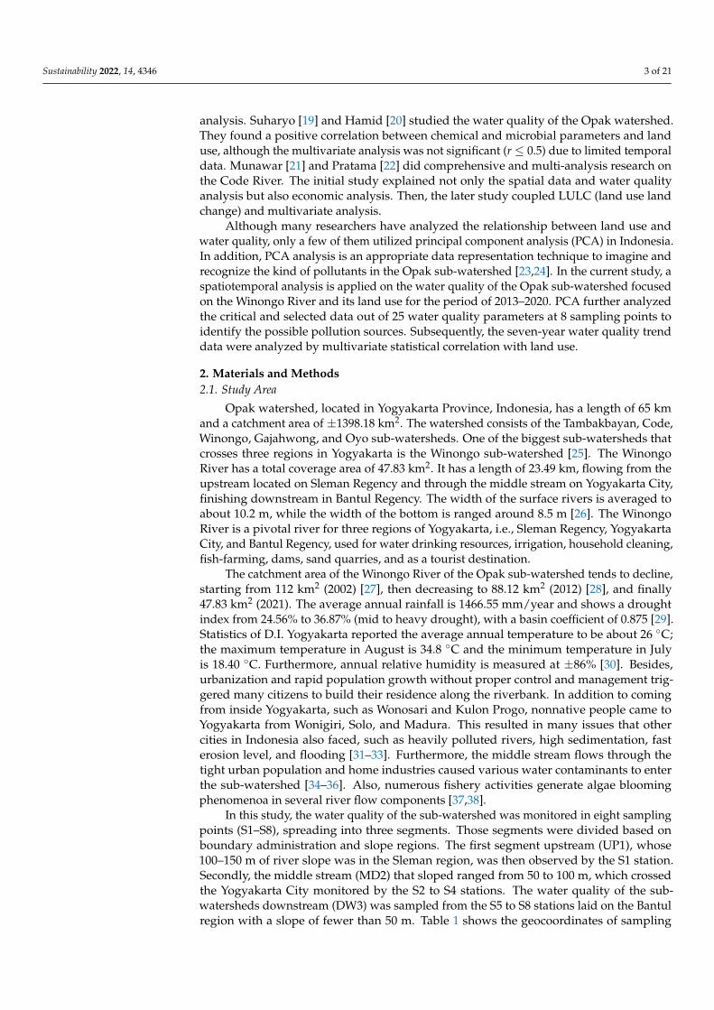
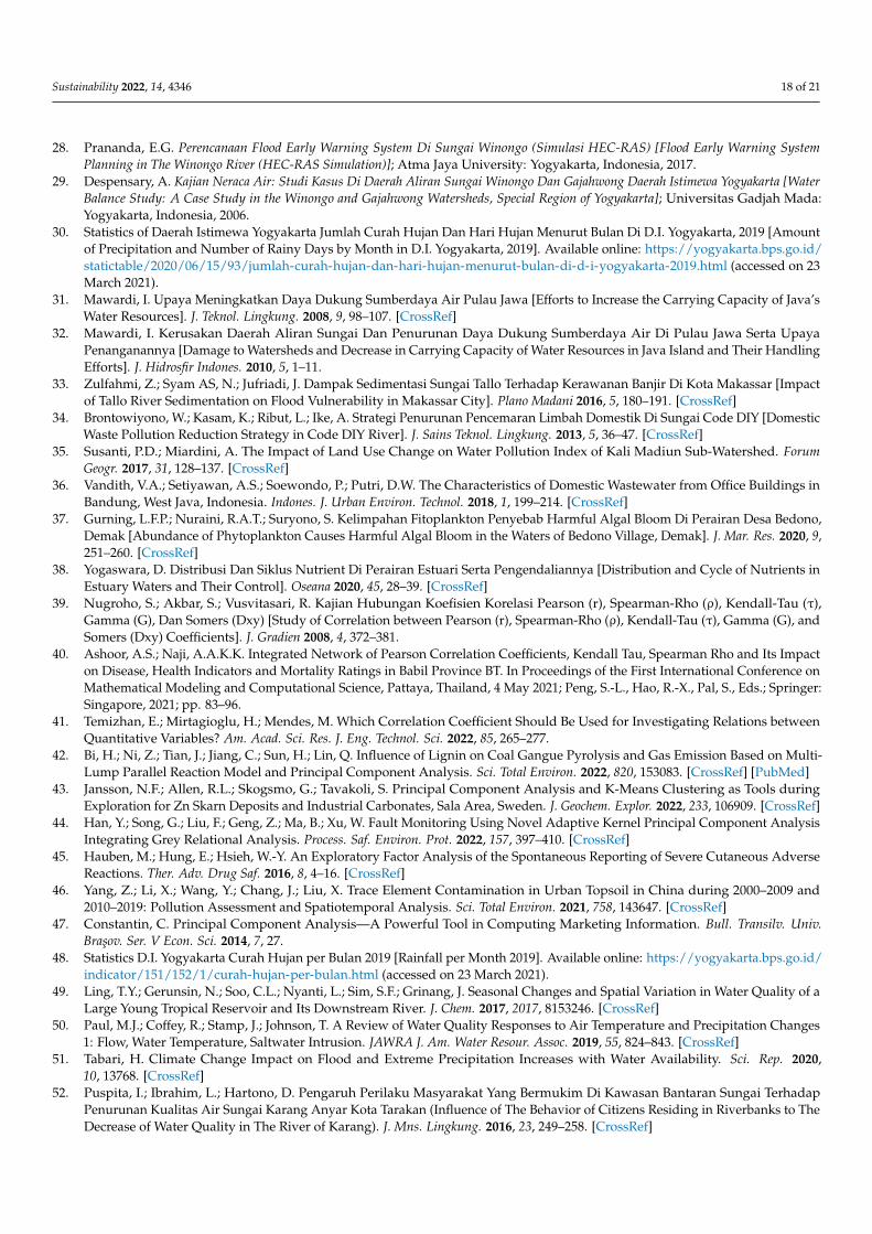
In this study, the water quality of the sub-watershed was monitored in eight samplingpoints (S1–S8), spreading into three segments. Those segments were divided based onboundary administration and slope regions. The first segment upstream (UP1), whose100–150 m of river slope was in the Sleman region, was then observed by the S1 station.Secondly, the middle stream (MD2) that sloped ranged from 50 to 100 m, which crossedthe Yogyakarta City monitored by the S2 to S4 stations. The water quality of the sub-watersheds downstream (DW3) was sampled from the S5 to S8 stations laid on the Bantulregion with a slope of fewer than 50 m. Table 1 shows the geocoordinates of sampling

Sustainability 2022, 14, 4346 4 of 21

points. Furthermore, all the sampling locations and those segments were visualized inFigure 1.

Table 1. Sampling Coordinates.

Points Latitude Longitude

Point 1 −7.886111111 110.5116667Point 2 −7.677833333 110.3763056Point 3 −7.776944444 110.3573889Point 4 −7.789777778 110.3573889Point 5 −7.808361111 110.3537222Point 6 −7.840333333 110.3403333Point 7 −7.912755555 110.3470278Point 8 −7.978722222 110.3134167

Sustainability 2022, 14, x FOR PEER REVIEW 4 of 23

region with a slope of fewer than 50 m. Table 1 shows the geocoordinates of sampling

points. Furthermore, all the sampling locations and those segments were visualized in

Figure 1.

Table 1. Sampling Coordinates.

Points Latitude Longitude

Point 1 −7.886111111 110.5116667

Point 2 −7.677833333 110.3763056

Point 3 −7.776944444 110.3573889

Point 4 −7.789777778 110.3573889

Point 5 −7.808361111 110.3537222

Point 6 −7.840333333 110.3403333

Point 7 −7.912755555 110.3470278

Point 8 −7.978722222 110.3134167

Figure 1. Sampling points of Opak sub-watershed.

Figure 1. Sampling points of Opak sub-watershed.

Sustainability 2022, 14, 4346 5 of 21

2.2. Water Quality and Geographic Information

The water quality data of the sub-watershed was taken from the EnvironmentalAgency of Yogyakarta Province from 2013 to 2020. The data was collected three times ayear from the eight sampling stations explained before (S1–S8). Every monitoring datapoint consists of 25 parameters, which were physical parameters: temperature, pH, TotalDissolved Solids (TDS), Total Suspended Solids (TSS), and color; chemical parameters:Dissolved Oxygen (DO), Biochemical Oxygen Demand (BOD5), Chemical Oxygen Demand(COD), Chlorine (Cl2), nitrate (NO2), nitrite (NO3), ammonium (NH4), detergent, phenol,phosphate (PO4), oil and fat, iron (Fe), manganese (Mn), cadmium (Cd), lead (Pb), zinc(Zn), and copper (Cu); and biological parameters: Total coliform and E. coli.

For spatial processing data, two types of satellite images were used. First, landuse classification data was extracted from Landsat data collected by the United StatesGeological Survey (USGS) from 2013 to 2020. Second, to determine the sub-watershedboundary, the satellite data was delineated and extracted by a mask manually using ArcGIS10.8. Exact steps were defined for deciding river segments (upstream, middle stream, anddownstream). The shapefile images were gathered from the Environmental Agency ofYogyakarta Province.

2.3. Land-Use Classification

ArcGIS 10.8 extracted and processed each satellite image of USGS from 2013 to 2020and broken into layers. The land-use classification was based on the most similar images oftraining sample drawing tools, conducted by interactive supervised classification. Afterthe final conversion, land uses were categorized and divided into the National StandardIndonesia (SNI 7645-1:2014) three main cover types, namely building (BU), agriculture(AG), and VA (Vegetation). Those categories were considered according to the dominantcoverage area in three representative regions.

2.4. Statistical Analysis

Pearson correlation analysis was used to assess the close link between the data vari-ables of water quality parameter in each sub-watershed and the quantity of land use utilized.To determine correlation coefficients, a correlation matrix was created by calculating thecoefficients of different pairings of parameters, and the correlation was then checked forsignificance using the p valve. The significance was assessed at the 0.05 level (2-tailedanalysis). If p < 0.05, the differences were substantial, and if p > 0.05, they were not. ThePearson correlation coefficient was appropriate for normally distributed data, whereasSpearman-rho (ρ) and Kendall-tau (σ) were not regularly distributed [39–41]. Besides thePearson correlation, this study also applied principal component analysis (PCA) so thatmultivariate normal data could be obtained. The first stage in the PCA approach was todetermine factor analysis and identify the original variables among sub-watershed waterqualities. PCA analysis has initial eigenvalues greater than 1 supported by the rotationmatrix method, containing the number of factors to be selected from the variable [42–44].By following and interpreting, the rotation outcome factor was going to reveal factors andvariables regarding the water quality in the Opak sub-watershed. Moreover, to validate, thePCA analysis was assessed by preliminary tests, such as the Kaiser–Meyer–Oklin (KMO)Test, Bartlett Test, anti-image, and scree plot. The KMO test was considered appropriate touse after reaching a value of one. The Bartlett and anti-image significant tests might be lessthan 0.5 [45,46]. Finally, the scree plot was evaluated to identify the number of elements orcategories retrieved in a matrix [47].

3. Results and Discussion3.1. Temporal Analysis of the Opak Sub-Watershed’s Water Quality

The temporal trend of the Opak sub-watershed was classified based on the seasonfrom 2013 to 2020. As explained by the Meteorological, Climatological, and GeophysicalAgency (BMKG) of Yogyakarta Province [30,48], in Table 2, the wet season (or rainy season)

Sustainability 2022, 14, 4346 6 of 21

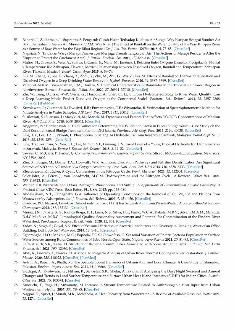
peaked in February/March and the peak of the dry season was in September/October.Furthermore, water quality parameters were clustered into a gradual decline and rising inmedian parameters from the wet to dry season. The trend of decreasing median parametersfrom wet season to dry season includes temperature, pH, TDS, DO, chlorine, nitrate, sulfide,detergent, phenol, phosphate, Fe, Mn, Cd, Cu, Pb, colour, E. coli, and Total Coliform. Onthe other hand, there is the increasing concentration of water quality parameters, such asTSS, BOD5, COD, nitrite, ammonia, oil and grease, and zinc (Zn).

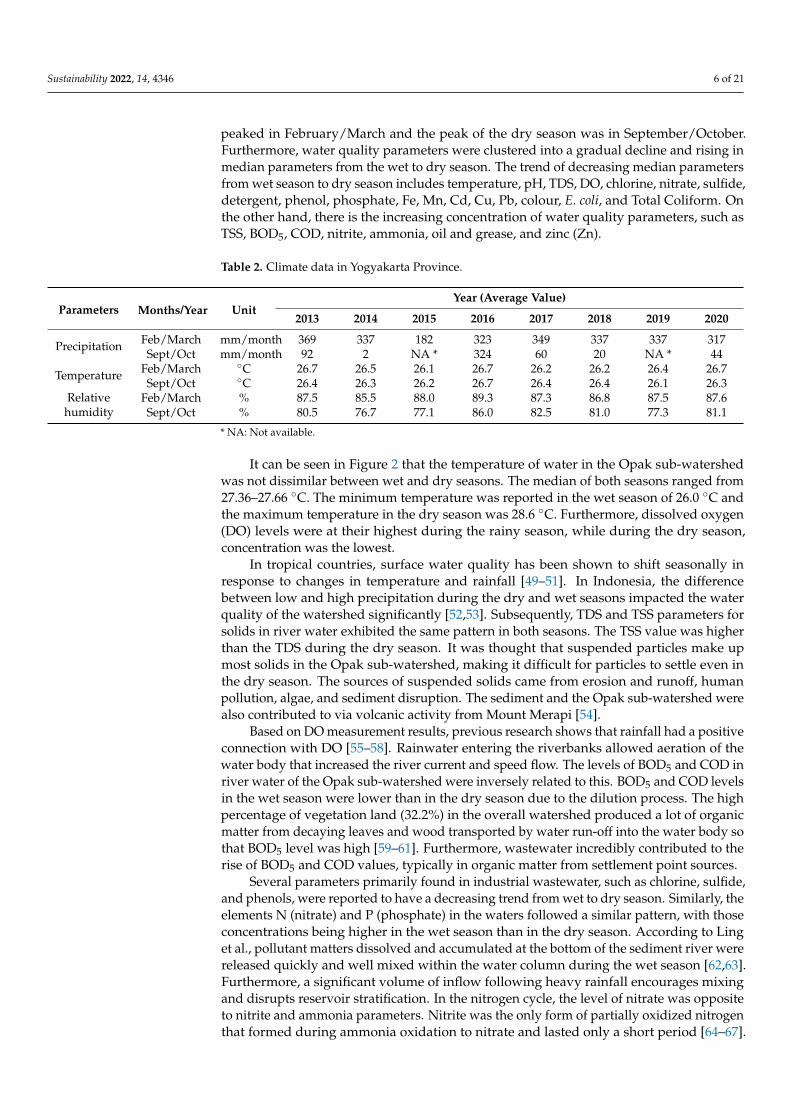
Table 2. Climate data in Yogyakarta Province.

Parameters Months/Year UnitYear (Average Value)

2013 2014 2015 2016 2017 2018 2019 2020

Precipitation Feb/March mm/month 369 337 182 323 349 337 337 317Sept/Oct mm/month 92 2 NA * 324 60 20 NA * 44

Temperature Feb/March ◦C 26.7 26.5 26.1 26.7 26.2 26.2 26.4 26.7Sept/Oct ◦C 26.4 26.3 26.2 26.7 26.4 26.4 26.1 26.3

Relativehumidity

Feb/March % 87.5 85.5 88.0 89.3 87.3 86.8 87.5 87.6Sept/Oct % 80.5 76.7 77.1 86.0 82.5 81.0 77.3 81.1

* NA: Not available.

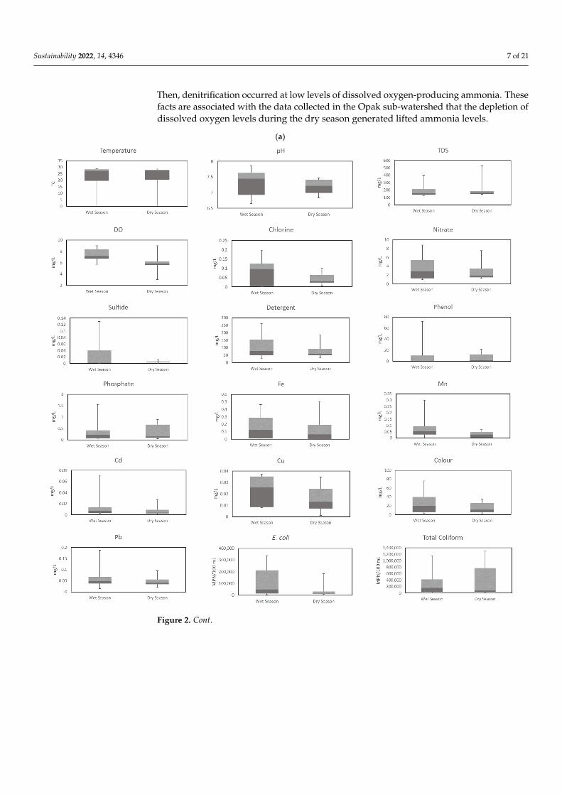
It can be seen in Figure 2 that the temperature of water in the Opak sub-watershedwas not dissimilar between wet and dry seasons. The median of both seasons ranged from27.36–27.66 ◦C. The minimum temperature was reported in the wet season of 26.0 ◦C andthe maximum temperature in the dry season was 28.6 ◦C. Furthermore, dissolved oxygen(DO) levels were at their highest during the rainy season, while during the dry season,concentration was the lowest.

In tropical countries, surface water quality has been shown to shift seasonally inresponse to changes in temperature and rainfall [49–51]. In Indonesia, the differencebetween low and high precipitation during the dry and wet seasons impacted the waterquality of the watershed significantly [52,53]. Subsequently, TDS and TSS parameters forsolids in river water exhibited the same pattern in both seasons. The TSS value was higherthan the TDS during the dry season. It was thought that suspended particles make upmost solids in the Opak sub-watershed, making it difficult for particles to settle even inthe dry season. The sources of suspended solids came from erosion and runoff, humanpollution, algae, and sediment disruption. The sediment and the Opak sub-watershed werealso contributed to via volcanic activity from Mount Merapi [54].

Based on DO measurement results, previous research shows that rainfall had a positiveconnection with DO [55–58]. Rainwater entering the riverbanks allowed aeration of thewater body that increased the river current and speed flow. The levels of BOD5 and COD inriver water of the Opak sub-watershed were inversely related to this. BOD5 and COD levelsin the wet season were lower than in the dry season due to the dilution process. The highpercentage of vegetation land (32.2%) in the overall watershed produced a lot of organicmatter from decaying leaves and wood transported by water run-off into the water body sothat BOD5 level was high [59–61]. Furthermore, wastewater incredibly contributed to therise of BOD5 and COD values, typically in organic matter from settlement point sources.

Several parameters primarily found in industrial wastewater, such as chlorine, sulfide,and phenols, were reported to have a decreasing trend from wet to dry season. Similarly, theelements N (nitrate) and P (phosphate) in the waters followed a similar pattern, with thoseconcentrations being higher in the wet season than in the dry season. According to Linget al., pollutant matters dissolved and accumulated at the bottom of the sediment river werereleased quickly and well mixed within the water column during the wet season [62,63].Furthermore, a significant volume of inflow following heavy rainfall encourages mixingand disrupts reservoir stratification. In the nitrogen cycle, the level of nitrate was oppositeto nitrite and ammonia parameters. Nitrite was the only form of partially oxidized nitrogenthat formed during ammonia oxidation to nitrate and lasted only a short period [64–67].

Sustainability 2022, 14, 4346 7 of 21

Then, denitrification occurred at low levels of dissolved oxygen-producing ammonia. Thesefacts are associated with the data collected in the Opak sub-watershed that the depletion ofdissolved oxygen levels during the dry season generated lifted ammonia levels.

Sustainability 2022, 14, x FOR PEER REVIEW 7 of 23

(a)

Figure 2. Cont.

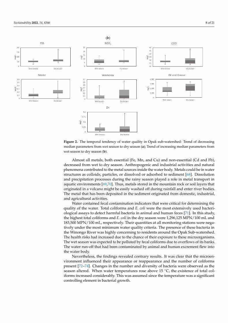
Sustainability 2022, 14, 4346 8 of 21Sustainability 2022, 14, x FOR PEER REVIEW 8 of 23

(b)

Figure 2. The temporal tendency of water quality in Opak sub-watershed: Trend of decreasing me-

dian parameters from wet season to dry season (a); Trend of increasing median parameters from

wet season to dry season (b).

In tropical countries, surface water quality has been shown to shift seasonally in re-

sponse to changes in temperature and rainfall [49–51]. In Indonesia, the difference be-

tween low and high precipitation during the dry and wet seasons impacted the water

quality of the watershed significantly [52,53]. Subsequently, TDS and TSS parameters for

solids in river water exhibited the same pattern in both seasons. The TSS value was higher

than the TDS during the dry season. It was thought that suspended particles make up

most solids in the Opak sub-watershed, making it difficult for particles to settle even in

the dry season. The sources of suspended solids came from erosion and runoff, human

pollution, algae, and sediment disruption. The sediment and the Opak sub-watershed

were also contributed to via volcanic activity from Mount Merapi [54].

Based on DO measurement results, previous research shows that rainfall had a posi-

tive connection with DO [55–58]. Rainwater entering the riverbanks allowed aeration of

the water body that increased the river current and speed flow. The levels of BOD5 and

COD in river water of the Opak sub-watershed were inversely related to this. BOD5 and

COD levels in the wet season were lower than in the dry season due to the dilution pro-

cess. The high percentage of vegetation land (32.2%) in the overall watershed produced a

lot of organic matter from decaying leaves and wood transported by water run-off into

the water body so that BOD5 level was high [59–61]. Furthermore, wastewater incredibly

contributed to the rise of BOD5 and COD values, typically in organic matter from settle-

ment point sources.

Several parameters primarily found in industrial wastewater, such as chlorine, sul-

fide, and phenols, were reported to have a decreasing trend from wet to dry season. Sim-

ilarly, the elements N (nitrate) and P (phosphate) in the waters followed a similar pattern,

with those concentrations being higher in the wet season than in the dry season. Accord-

ing to Ling et al., pollutant matters dissolved and accumulated at the bottom of the sedi-

ment river were released quickly and well mixed within the water column during the wet

season [62,63]. Furthermore, a significant volume of inflow following heavy rainfall en-

courages mixing and disrupts reservoir stratification. In the nitrogen cycle, the level of

nitrate was opposite to nitrite and ammonia parameters. Nitrite was the only form of

Figure 2. The temporal tendency of water quality in Opak sub-watershed: Trend of decreasingmedian parameters from wet season to dry season (a); Trend of increasing median parameters fromwet season to dry season (b).

Almost all metals, both essential (Fe, Mn, and Cu) and non-essential (Cd and Fb),decreased from wet to dry season. Anthropogenic and industrial activities and naturalphenomena contributed to the metal sources inside the water body. Metals could be in waterstructures as colloids, particles, or dissolved or adsorbed to sediment [68]. Dissolutionand precipitation processes during the rainy season played a role in metal transport inaquatic environments [69,70]. Thus, metals stored in the mountain rock or soil layers thatoriginated in a volcano might be easily washed off during rainfall and enter river bodies.The metal that has been deposited in the sediment originated from domestic, industrial,and agricultural activities.

Water contained fecal contamination indicators that were critical for determining thequality of the water. Total coliforms and E. coli were the most extensively used bacteri-ological assays to detect harmful bacteria in animal and human feces [71]. In this study,the highest total coliforms and E. coli in the dry season were 1,296,125 MPN/100 mL and183,500 MPN/100 mL, respectively. Their quantities at all monitoring stations were nega-tively under the most minimum water quality criteria. The presence of these bacteria inthe Winongo River was highly concerning to residents around the Opak Sub-watershed.The health risks had increased due to the chance of their exposure to these microorganisms.The wet season was expected to be polluted by fecal coliforms due to overflows of its banks.The water run-off that had been contaminated by animal and human excrement flew intothe water body.

Nevertheless, the findings revealed contrary results. It was clear that the microen-vironment influenced their appearance or reappearance and the number of coliformspresent [72–74]. Changes in the number and diversity of bacteria were observed as theseason altered. When water temperatures rose above 15 ◦C, the existence of total col-iforms increased considerably. This was assumed since the temperature was a significantcontrolling element in bacterial growth.

Sustainability 2022, 14, 4346 9 of 21

3.2. Spatial Analysis of the Opak Sub-Watershed’s Water Quality

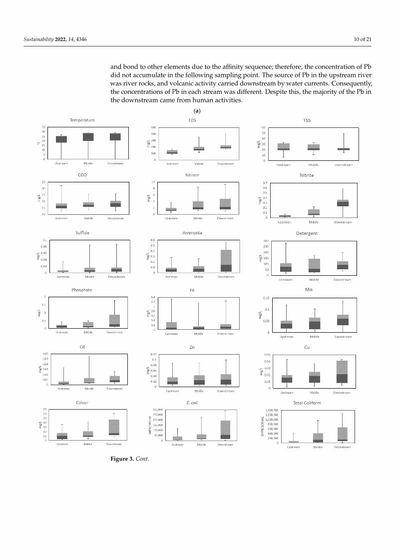
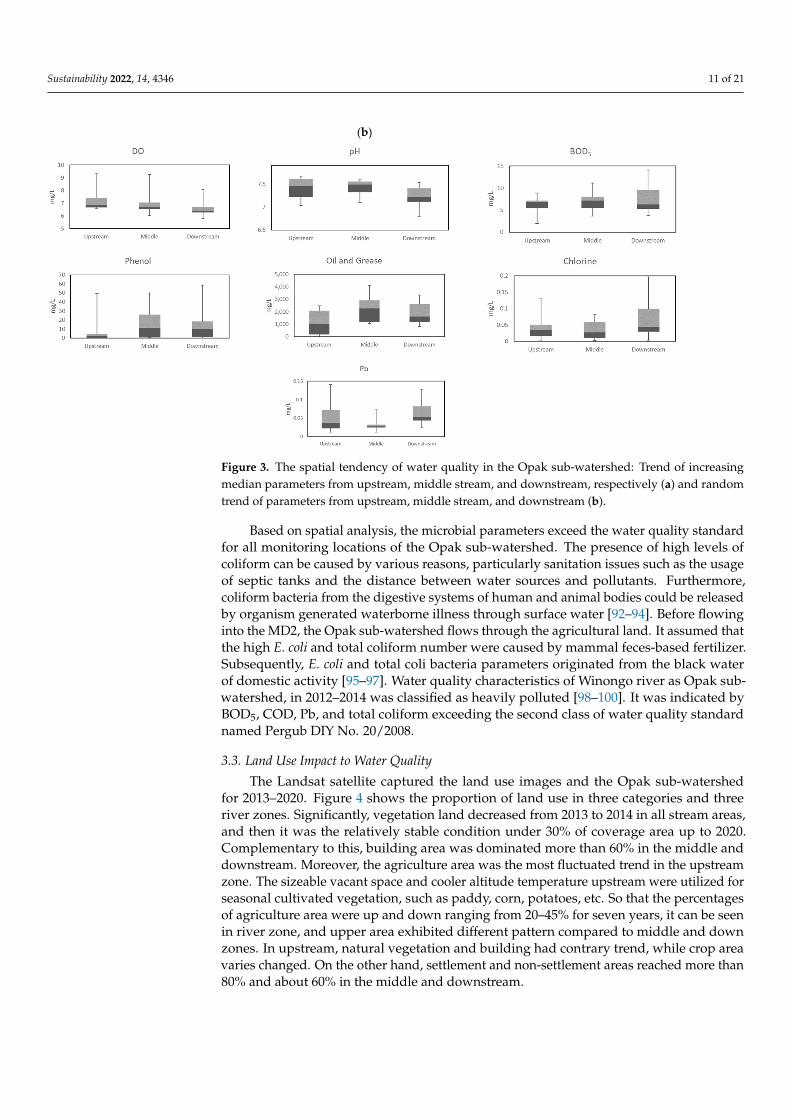
In the spatial analysis data, water quality parameters are divided into two groups, i.e.,the trend of increasing and random median parameters from upstream, middle stream,and downstream, respectively. Random trends sometimes mean the highest concentrationaccumulated on the middle stream, and occasionally they fluctuated among three samplingpoints. Overall, water parameters in the Opak sub-watershed climbed up from upstreamto downstream, such as temperature, TDS, TSS, COD, nitrate, nitrite, sulfide, ammonia,detergent, phosphate, Fe, Mn, Cd, Zn, Cu, colour, E. coli, and total coliform. That aside,pH, BOD5, phenol, oil and grease reached the largest concentration in the middle stream.Chlorine and Pb levels shifted for every observation point. Then, dissolved oxygen (DO)concentration steadily decreased from upstream to downstream.

As shown in Figure 3, the temperature between the middle stream (MD2) and down-stream (DW3) is invariable, around 28 ◦C. Moreover, TDS gradually climbed up to thethird monitoring station, whereas the TSS value remained stable. Furthermore, severalparameters showed a random trend, such as chlorine, phenol, Pb, oil, and grease. Thechlorine and Pb levels peaked in the last stream while phenol, oil, and grease surged in thesecond stream of the Opak sub-watershed.

The upstream (UP1) is 3 ◦C cooler than the others, which is different from the two sitesbefore. The temperature of the surrounding air had a significant impact on the temperatureof the river water. Warmer urban surfaces caused temperature surges in streams. Accordingto the landscape of the study area, MD2 and DW3 is located in the tight, densely populationarea. Land-use changes linked to urbanization lead to changes in the temperature regime ofthe air in cities, resulting in urban heat islands [75–77]. Furthermore, domestic residentialwastewater was a pivotal contributor to rising river water temperatures [78–80].

The sources of solids inside the water column were dominated by outside factors, suchas erosion, run-off, flooding, etc. In UP1, the riverbanks’ vegetation could hold the soil, soit was not be carried away by the water flow. The combined impacts of leaves, stems, roots,and litter allowed plants to intercept rainfall and control surface run-off, thus fulfilling thefunction of soil and water conservation [10,81–84]. Furthermore, TSS concentration wasinfluenced by the material derived from land carried by river flows [85–87].

By comparing BOD5 and COD, the median of BOD5 rose from UP1 to MD2, then fellas it entered DW3. Generally, the DO level is constantly depleted in the three monitoringpoints. On the contrary, BOD5 and COD increased. A similar phenomenon happenedfor other parameters, such as NO2, NO3, NH3, PO4 and detergent. A lot of dissolvedoxygen is used inside the water body. The oxidation process of those matters rapidlyoccurs and generates a high concentration of not only BOD5 and COD but also N and Pelements. Commonly, organic matters originated from settlements and industrial activities.In addition, the MD2 and DW3 were circled by several kinds of home industries, such astofu industries. Previous research shows that approximately five tofu home industries didnot treat their wastewater and discharged it directly into the river [88]. Through observingaround the study area, the numerous sewer pipes flew directly to the water body of theWinongo river.

The presence of phenolics in water could be attributed to the deterioration or de-composition of natural organic materials in the water and the discharge of industrial andresidential wastewater and runoff from agricultural lands [89]. On the other hand, chlorinewas also used in wastewater treatment plants and swimming pools as a disinfectant, asa bleaching agent in textile manufacturers and paper mills, and as an element in manylaundry bleaches [90,91]. Both phenol and chlorine were poisonous to aquatic organismseven at deficient levels.

Furthermore, as one of the heavy metals, Pb possessed a bizarre phenomenon in thisstudy. All the metals concentration, substantial and non-substantial, steadily increasingfrom UP1 to DW3, except Pb. The level of Pb was high in two monitoring locations,upstream and downstream, 0.03 and 0.05 ppm, respectively. In the middle stream, Pbconcentration jumped down to 0.02 ppm. It was assumed that Pb metal was easier to settle

Sustainability 2022, 14, 4346 10 of 21

and bond to other elements due to the affinity sequence; therefore, the concentration of Pbdid not accumulate in the following sampling point. The source of Pb in the upstream riverwas river rocks, and volcanic activity carried downstream by water currents. Consequently,the concentrations of Pb in each stream was different. Despite this, the majority of the Pb inthe downstream came from human activities.

Sustainability 2022, 14, x FOR PEER REVIEW 10 of 23

(a)

Figure 3. Cont.

Sustainability 2022, 14, 4346 11 of 21Sustainability 2022, 14, x FOR PEER REVIEW 11 of 23

(b)

Figure 3. The spatial tendency of water quality in the Opak sub-watershed: Trend of increasing

median parameters from upstream, middle stream, and downstream, respectively (a) and random

trend of parameters from upstream, middle stream, and downstream (b).

The upstream (UP1) is 3 °C cooler than the others, which is different from the two

sites before. The temperature of the surrounding air had a significant impact on the tem-

perature of the river water. Warmer urban surfaces caused temperature surges in streams.

According to the landscape of the study area, MD2 and DW3 is located in the tight,

densely population area. Land-use changes linked to urbanization lead to changes in the

temperature regime of the air in cities, resulting in urban heat islands [75–77]. Further-

more, domestic residential wastewater was a pivotal contributor to rising river water tem-

peratures [78–80].

The sources of solids inside the water column were dominated by outside factors,

such as erosion, run-off, flooding, etc. In UP1, the riverbanks’ vegetation could hold the

soil, so it was not be carried away by the water flow. The combined impacts of leaves,

stems, roots, and litter allowed plants to intercept rainfall and control surface run-off, thus

fulfilling the function of soil and water conservation [10,81–84]. Furthermore, TSS concen-

tration was influenced by the material derived from land carried by river flows [85–87].

By comparing BOD5 and COD, the median of BOD5 rose from UP1 to MD2, then fell

as it entered DW3. Generally, the DO level is constantly depleted in the three monitoring

points. On the contrary, BOD5 and COD increased. A similar phenomenon happened for

other parameters, such as NO2, NO3, NH3, PO4 and detergent. A lot of dissolved oxygen

is used inside the water body. The oxidation process of those matters rapidly occurs and

generates a high concentration of not only BOD5 and COD but also N and P elements.

Commonly, organic matters originated from settlements and industrial activities. In ad-

dition, the MD2 and DW3 were circled by several kinds of home industries, such as tofu

industries. Previous research shows that approximately five tofu home industries did not

treat their wastewater and discharged it directly into the river [88]. Through observing

around the study area, the numerous sewer pipes flew directly to the water body of the

Winongo river.

The presence of phenolics in water could be attributed to the deterioration or decom-

position of natural organic materials in the water and the discharge of industrial and res-

idential wastewater and runoff from agricultural lands [89]. On the other hand, chlorine

was also used in wastewater treatment plants and swimming pools as a disinfectant, as a

Figure 3. The spatial tendency of water quality in the Opak sub-watershed: Trend of increasingmedian parameters from upstream, middle stream, and downstream, respectively (a) and randomtrend of parameters from upstream, middle stream, and downstream (b).

Based on spatial analysis, the microbial parameters exceed the water quality standardfor all monitoring locations of the Opak sub-watershed. The presence of high levels ofcoliform can be caused by various reasons, particularly sanitation issues such as the usageof septic tanks and the distance between water sources and pollutants. Furthermore,coliform bacteria from the digestive systems of human and animal bodies could be releasedby organism generated waterborne illness through surface water [92–94]. Before flowinginto the MD2, the Opak sub-watershed flows through the agricultural land. It assumed thatthe high E. coli and total coliform number were caused by mammal feces-based fertilizer.Subsequently, E. coli and total coli bacteria parameters originated from the black waterof domestic activity [95–97]. Water quality characteristics of Winongo river as Opak sub-watershed, in 2012–2014 was classified as heavily polluted [98–100]. It was indicated byBOD5, COD, Pb, and total coliform exceeding the second class of water quality standardnamed Pergub DIY No. 20/2008.

3.3. Land Use Impact to Water Quality

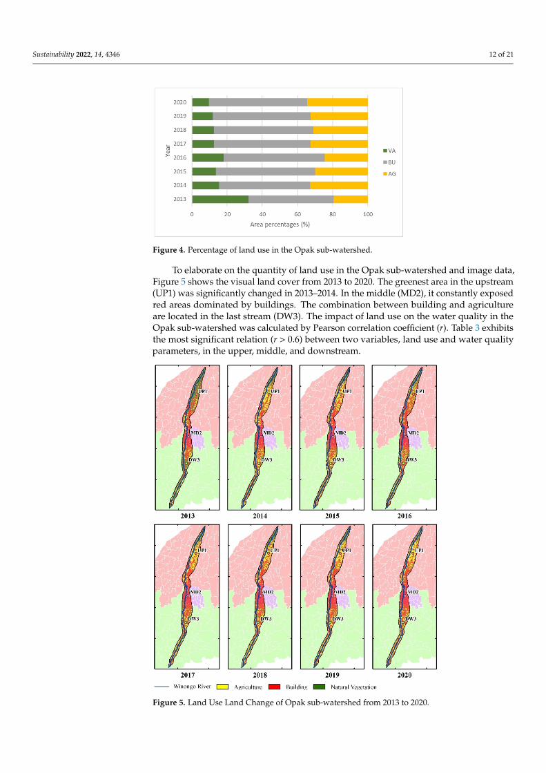
The Landsat satellite captured the land use images and the Opak sub-watershedfor 2013–2020. Figure 4 shows the proportion of land use in three categories and threeriver zones. Significantly, vegetation land decreased from 2013 to 2014 in all stream areas,and then it was the relatively stable condition under 30% of coverage area up to 2020.Complementary to this, building area was dominated more than 60% in the middle anddownstream. Moreover, the agriculture area was the most fluctuated trend in the upstreamzone. The sizeable vacant space and cooler altitude temperature upstream were utilized forseasonal cultivated vegetation, such as paddy, corn, potatoes, etc. So that the percentagesof agriculture area were up and down ranging from 20–45% for seven years, it can be seenin river zone, and upper area exhibited different pattern compared to middle and downzones. In upstream, natural vegetation and building had contrary trend, while crop areavaries changed. On the other hand, settlement and non-settlement areas reached more than80% and about 60% in the middle and downstream.

Sustainability 2022, 14, 4346 12 of 21Sustainability 2022, 14, x FOR PEER REVIEW 13 of 23

Figure 4. Percentage of land use in the Opak sub-watershed.

To elaborate on the quantity of land use in the Opak sub-watershed and image data,

Figure 5 shows the visual land cover from 2013 to 2020. The greenest area in the upstream

(UP1) was significantly changed in 2013–2014. In the middle (MD2), it constantly exposed

red areas dominated by buildings. The combination between building and agriculture are

located in the last stream (DW3). The impact of land use on the water quality in the Opak

sub-watershed was calculated by Pearson correlation coefficient (r). Table 3 exhibits the

most significant relation (r > 0.6) between two variables, land use and water quality pa-

rameters, in the upper, middle, and downstream.

Figure 5. Land Use Land Change of Opak sub-watershed from 2013 to 2020.

Figure 4. Percentage of land use in the Opak sub-watershed.

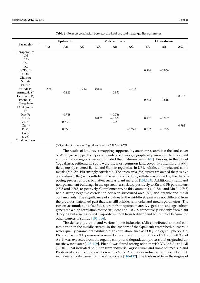
To elaborate on the quantity of land use in the Opak sub-watershed and image data,Figure 5 shows the visual land cover from 2013 to 2020. The greenest area in the upstream(UP1) was significantly changed in 2013–2014. In the middle (MD2), it constantly exposedred areas dominated by buildings. The combination between building and agricultureare located in the last stream (DW3). The impact of land use on the water quality in theOpak sub-watershed was calculated by Pearson correlation coefficient (r). Table 3 exhibitsthe most significant relation (r > 0.6) between two variables, land use and water qualityparameters, in the upper, middle, and downstream.

Sustainability 2022, 14, x FOR PEER REVIEW 13 of 23

Figure 4. Percentage of land use in the Opak sub-watershed.

To elaborate on the quantity of land use in the Opak sub-watershed and image data,

Figure 5 shows the visual land cover from 2013 to 2020. The greenest area in the upstream

(UP1) was significantly changed in 2013–2014. In the middle (MD2), it constantly exposed

red areas dominated by buildings. The combination between building and agriculture are

located in the last stream (DW3). The impact of land use on the water quality in the Opak

sub-watershed was calculated by Pearson correlation coefficient (r). Table 3 exhibits the

most significant relation (r > 0.6) between two variables, land use and water quality pa-

rameters, in the upper, middle, and downstream.

Figure 5. Land Use Land Change of Opak sub-watershed from 2013 to 2020.

Figure 5. Land Use Land Change of Opak sub-watershed from 2013 to 2020.

Sustainability 2022, 14, 4346 13 of 21

Table 3. Pearson correlation between the land use and water quality parameter.

ParameterUpstream Middle Stream Downstream

VA AB AG VA AB AG VA AB AG

TemperaturepHTDSTSSDO

BOD5 (*) 0.886 −0.936COD

ChlorineNitrateNitrite

Sulfide (*) 0.876 −0.742 0.865 −0.718Ammonia (*) −0.821 −0.871Detergent (*) −0.712

Phenol (*) 0.713 −0.816Phosphate

Oil & greaseFe

Mn (*) −0.748 −0.766Cd (*) 0.807 −0.833 0.837 −0.907Zn (*) 0.738 0.723Cu (*) −0.792Pb (*) 0.765 −0.748 0.752 −0.775ColorE. coli

Total coliform

(*) Significant correlation Significant area: <−0.707 or >0.707.

The results of land cover mapping supported by another research that the land coverof Winongo river, part of Opak sub-watershed, was geographically variable. The woodlandand plantation regions were dominated the upstream basin [101]. Besides, in the city ofYogyakarta, settlements spots were the most common land cover. Furthermore, Paddyfields mostly covered Bantul and Sleman regencies. In UP1, sulfide, ammonia, and somemetals (Mn, Zn, Pb) strongly correlated. The green area (VA) upstream owned the positivecorrelation (0.876) with sulfide. In the natural condition, sulfide was formed by the decom-posing process of organic matter, such as plant material [102,103]. Additionally, semi andnon-permanent buildings in the upstream associated positively to Zn and Pb parameters,0.738 and 0.765, respectively. Complementary to this, ammonia (−0.821) and Mn (−0.748)had a strong negative correlation between structured area (AB) and organic and metalcontaminants. The significance of r values in the middle stream was not different fromthe previous watershed part that was still sulfide, ammonia, and metals parameters. Therun-off accumulation of sulfide sources from upstream areas, vegetation, and agriculturegenerated a high correlation coefficient, 0.865 and −0.718, respectively. Not only from plantdecaying but also dissolved evaporite mineral from fertilizer and soil sulfates become theother sources of sulfide [104–106].

The dense population and various home industries (AB) contributed to metal con-tamination in the middle stream. In the last part of the Opak sub-watershed, numerouswater quality parameters exhibited high correlation, such as BOD5, detergent, phenol, Cd,Pb, and Cu. BOD5 possessed a remarkable correlation up to 0.886 of VA and −0.936 ofAB. It was expected from the organic compound degradation process that originated do-mestic wastewater [107–109]. Phenol was found strong relation with VA (0.713) and AB(−0.816) that indicated pollution from industrial, agricultural, and home sources. Cd andPb showed a significant correlation with VA and AB. Besides industrial sources, Cd and Pbin the water body came from the atmosphere [110–112]. The fuels used from the engine of

Sustainability 2022, 14, 4346 14 of 21

transportation emitted to the atmosphere, and during the rainy season was dropped intosurface water and was expected through run-off from open space.

More importantly, an unexpected correlation was found, for example, between Cdand Pb and vegetation (0.837 and 0.752, respectively). Such strong correlation was notfound in previous research [22] so that further investigations are required to explain theassociation between heavy metal and vegetation. Another essential point, the determinationof VA (vegetation area), is needed to be clarified. It was supported by previous findingthat cadmium became an issue combining phosphorus fertilizers [113]. Replanting orrevegetation in such blank areas using fertilizer could contribute heavy metal sourcesthrough run-off into riverbanks.

3.4. Principal Component Analysis (PCA) of Pollution Source

Principal component analysis (PCA) was used to determine the pollution sources in theOpak sub-watershed. To validate the statistical requirement of PCA analysis, preliminarytests, such as KMO, Bartlett, and anti-image matric tests, were done. Four out of 25 waterquality parameters, i.e., TSS, chlorine, COD, and sulfide, were eliminated from the analysisdue to over 0.5 anti-image correlation. Subsequently, six components were obtained fromthe total variance calculation. The eigenvalue of those components should be more than 1.0.The sampling adequacy of the Kaiser-Meyer-Oikin (KMO) test showed a value of 0.628 tocontinue the analysis. Furthermore, by calculating the next step of the rotated componentmatrix, BOD5 was ineligible (<0.5) so that the twenty remaining parameters are re-extractedand displayed in Table 4.

Table 4. Six components (Co) extracted from 20 parameters of water quality.

Parameter Co1 Co2 Co3 Co4 Co5 Co6

Temperature −0.707pH −0.718TDS 0.742DO −0.556

Nitrate 0.828Nitrite 0.818

Ammonia −0.806Detergent 0.511

Phenol 0.560Phosphate 0.742

Oil and grease 0.536Fe 0.567Mn 0.837Cd 0.589Zn −0.628Cu 0.864Pb 0.815

Color 0.724E. coli 0.765

Total coliform 0.788

Eigenvalue 4.279 3.162 2.094 1.734 1.439 1.156%Variance explained 21.393 15.809 10.468 8.671 7.194 5.778

The source of pollution was represented by six extracted components with a totalvariance of 69.313% (Table 3). The first component, 21.393% of the total variance, consistingof temperature, TDS, detergent, E. coli, and total coliform, described domestic activities andhuman fecal contamination. As identical sub-watershed in Yogyakarta Province, Code Rivershowed a different pattern with the present study that COD and BOD5 [21] classified themain organic compounds. The second, fourth, and sixth components, 15.809%, 8.671%, and5.778% of the total variance, respectively, defined an industrial characteristic regarding Mn,Cd, Zn, Fe, Pb, Cu, pH, phenol, and oil and grease. Additionally, the third (10.468%) and

Sustainability 2022, 14, 4346 15 of 21

fifth (7.194%) components portrayed the contaminant from agriculture activities correlatingwith nitrate, nitrite, phosphate, ammonia, and DO parameters.

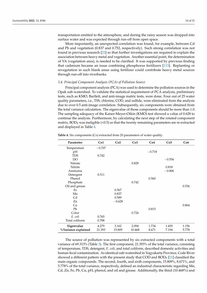
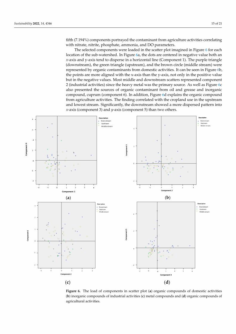
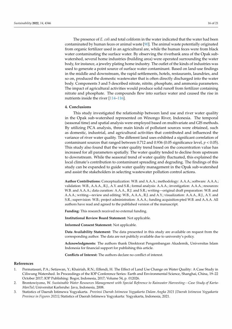
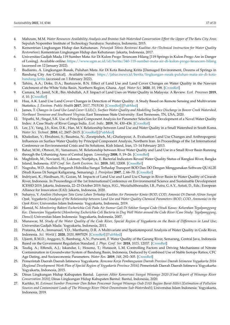
The selected components were loaded in the scatter plot imagined in Figure 6 for eachlocation of the sub-watershed. In Figure 6a, the dots are centered in negative value both anx-axis and y-axis tend to disperse in a horizontal line (Component 1). The purple triangle(downstream), the green triangle (upstream), and the brown circle (middle stream) wererepresented by organic contaminants from domestic activities. It can be seen in Figure 6b,the points are more aligned with the x-axis than the y-axis, not only in the positive valuebut in the negative values. Most middle and downstream scatters represented component2 (industrial activities) since the heavy metal was the primary source. As well as Figure 6calso presented the sources of organic contaminant from oil and grease and inorganiccompound, cuprum (component 6). In addition, Figure 6d explains the organic compoundfrom agriculture activities. The finding correlated with the cropland use in the upstreamand lowest stream. Significantly, the downstream showed a more dispersed pattern intox-axis (component 3) and y-axis (component 5) than two others.

Sustainability 2022, 14, x FOR PEER REVIEW 16 of 23

The source of pollution was represented by six extracted components with a total

variance of 69.313% (Table 3). The first component, 21.393% of the total variance, consist-

ing of temperature, TDS, detergent, E. coli, and total coliform, described domestic activi-

ties and human fecal contamination. As identical sub-watershed in Yogyakarta Province,

Code River showed a different pattern with the present study that COD and BOD5 [21]

classified the main organic compounds. The second, fourth, and sixth components, 15.809%,

8.671%, and 5.778% of the total variance, respectively, defined an industrial characteristic

regarding Mn, Cd, Zn, Fe, Pb, Cu, pH, phenol, and oil and grease. Additionally, the third

(10.468%) and fifth (7.194%) components portrayed the contaminant from agriculture activ-

ities correlating with nitrate, nitrite, phosphate, ammonia, and DO parameters.

The selected components were loaded in the scatter plot imagined in Figure 6 for

each location of the sub-watershed. In Figure 6a, the dots are centered in negative value

both an x-axis and y-axis tend to disperse in a horizontal line (Component 1). The purple

triangle (downstream), the green triangle (upstream), and the brown circle (middle

stream) were represented by organic contaminants from domestic activities. It can be seen

in Figure 6b, the points are more aligned with the x-axis than the y-axis, not only in the

positive value but in the negative values. Most middle and downstream scatters repre-

sented component 2 (industrial activities) since the heavy metal was the primary source.

As well as Figure 6c also presented the sources of organic contaminant from oil and grease

and inorganic compound, cuprum (component 6). In addition, Figure 6d explains the or-

ganic compound from agriculture activities. The finding correlated with the cropland use

in the upstream and lowest stream. Significantly, the downstream showed a more dis-

persed pattern into x-axis (component 3) and y-axis (component 5) than two others.

(a) (b)

Sustainability 2022, 14, x FOR PEER REVIEW 17 of 23

(c)

(d)

Figure 6. The load of components in scatter plot (a) organic compounds of domestic activities (b)

inorganic compounds of industrial activities (c) metal compounds and (d) organic compounds of

agricultural activities.

The presence of E. coli and total coliform in the water indicated that the water had been con-

taminated by human feces or animal waste [90]. The animal waste potentially originated from

organic fertilizer used in an agricultural are, while the human feces were from black water con-

taminating the surface water. By observing the riverbank area of the Opak sub-watershed, several

home industries (building area) were operated surrounding the water body, for instance, a jewelry

plating home industry. The outlet of the kinds of industries was used to generate a point source of

surface water contaminant. Based on land-use findings in the middle and downstream, the rapid

settlements, hotels, restaurants, laundries, and so on, produced the domestic wastewater that is

often directly discharged into the water body. Components 3 and 5 described nitrate, nitrite, phos-

phate, and ammonia parameters. The impact of agricultural activities would produce solid runoff

from fertilizer containing nitrate and phosphate. The compounds flew into surface water and

caused the rise in nutrients inside the river [114–116].

4. Conclusions

This study investigated the relationship between land use and river water quality in

the Opak sub-watershed represented on Winongo River, Indonesia. The temporal (sea-

sonal time) and spatial analysis were employed based on multivariate and GIS methods.

By utilizing PCA analysis, three main kinds of pollutant sources were obtained, such as

domestic, industrial, and agricultural activities that contributed and influenced the vari-

ance of river water quality. The different land uses exhibited a significant correlation of

contaminant sources that ranged between 0.712 and 0.936 (0.05 significance level, p < 0.05).

This study also found that the water quality trend based on the concentration value has

increased for all parameters spatially. The water quality tended to decline from upstream

to downstream. While the seasonal trend of water quality fluctuated, this explained the

local climate’s contribution to contaminant spreading and degrading. The findings of this

study can be expanded to guide water quality management in the Opak sub-watershed

and assist the stakeholders in selecting wastewater pollution control actions.

Author Contributions: Conceptualization: W.B. and A.A.A.; methodology: A.A.A.; software:

A.AA.; validation: W.B., A.A.A., R.J., A.Y. and S.R.; formal analysis: A.A.A.; investigation: A.A.A.;

resources: W.B. and A.A.A.; data curation: A.A.A., R.J., and S.R.; writing—original draft prepara-

tion: W.B. and A.A.A.; writing—review and editing: W.B., A.A.A., R.J., and A.Y.; visualization: A.A.A.,

R.J., A.Y., and S.R.; supervision: W.B.; project administration: A.A.A.; funding acquisition:pted W.B.

and A.A.A. All authors have read and agreed to the published version of the manuscript.

Funding: This research received no external funding.

Figure 6. The load of components in scatter plot (a) organic compounds of domestic activities(b) inorganic compounds of industrial activities (c) metal compounds and (d) organic compounds ofagricultural activities.

Sustainability 2022, 14, 4346 16 of 21

The presence of E. coli and total coliform in the water indicated that the water had beencontaminated by human feces or animal waste [90]. The animal waste potentially originatedfrom organic fertilizer used in an agricultural are, while the human feces were from blackwater contaminating the surface water. By observing the riverbank area of the Opak sub-watershed, several home industries (building area) were operated surrounding the waterbody, for instance, a jewelry plating home industry. The outlet of the kinds of industries wasused to generate a point source of surface water contaminant. Based on land-use findingsin the middle and downstream, the rapid settlements, hotels, restaurants, laundries, andso on, produced the domestic wastewater that is often directly discharged into the waterbody. Components 3 and 5 described nitrate, nitrite, phosphate, and ammonia parameters.The impact of agricultural activities would produce solid runoff from fertilizer containingnitrate and phosphate. The compounds flew into surface water and caused the rise innutrients inside the river [114–116].

4. Conclusions

This study investigated the relationship between land use and river water qualityin the Opak sub-watershed represented on Winongo River, Indonesia. The temporal(seasonal time) and spatial analysis were employed based on multivariate and GIS methods.By utilizing PCA analysis, three main kinds of pollutant sources were obtained, suchas domestic, industrial, and agricultural activities that contributed and influenced thevariance of river water quality. The different land uses exhibited a significant correlation ofcontaminant sources that ranged between 0.712 and 0.936 (0.05 significance level, p < 0.05).This study also found that the water quality trend based on the concentration value hasincreased for all parameters spatially. The water quality tended to decline from upstreamto downstream. While the seasonal trend of water quality fluctuated, this explained thelocal climate’s contribution to contaminant spreading and degrading. The findings of thisstudy can be expanded to guide water quality management in the Opak sub-watershedand assist the stakeholders in selecting wastewater pollution control actions.

Author Contributions: Conceptualization: W.B. and A.A.A.; methodology: A.A.A.; software: A.A.A.;validation: W.B., A.A.A., R.J., A.Y. and S.R.; formal analysis: A.A.A.; investigation: A.A.A.; resources:W.B. and A.A.A.; data curation: A.A.A., R.J. and S.R.; writing—original draft preparation: W.B. andA.A.A.; writing—review and editing: W.B., A.A.A., R.J. and A.Y.; visualization: A.A.A., R.J., A.Y. andS.R.; supervision: W.B.; project administration: A.A.A.; funding acquisition:pted W.B. and A.A.A. Allauthors have read and agreed to the published version of the manuscript.

Funding: This research received no external funding.

Institutional Review Board Statement: Not applicable.

Informed Consent Statement: Not applicable.

Data Availability Statement: The data presented in this study are available on request from thecorresponding author. The data are not publicly available due to university’s policy.

Acknowledgments: The authors thank Direktorat Pengembangan Akademik, Universitas IslamIndonesia for financial support for publishing this article.

Conflicts of Interest: The authors declare no conflict of interest.

References1. Permatasari, P.A.; Setiawan, Y.; Khairiah, R.N.; Effendi, H. The Effect of Land Use Change on Water Quality: A Case Study in

Ciliwung Watershed. In Proceedings of the IOP Conference Series: Earth and Environmental Science, Shanghai, China, 19–22October 2017; IOP Publishing: Bogor, Indonesia, 2017; Volume 54, p. 012026.

2. Brontowiyono, W. Sustainable Water Resources Management with Special Reference to Rainwater Harvesting—Case Study of Karta-ManTul; Universitat Karlsruhe: Java, Indonesia, 2008.

3. Statistics of Daerah Istimewa Yogyakarta. Provinsi Daerah Istimewa Yogyakarta Dalam Angka 2021 [Daerah Istimewa YogyakartaProvince in Figures 2021]; Statistics of Daerah Istimewa Yogyakarta: Yogyakarta, Indonesia, 2021.

Sustainability 2022, 14, 4346 17 of 21

4. Mahzum, M.M. Water Resources Availability Analysis and Brantas Sub-Watershed Conservation Effort the Upper of The Batu City Area;Sepuluh Nopember Institute of Technology Surabaya: Surabaya, Indonesia, 2015.

5. Kementrian Lingkungan Hidup dan Kehutanan. Petunjuk Teknis Restorasi Kualitas Air (Technical Instruction for Water QualityRestoration); Kementrian Lingkungan Hidup dan Kehutanan: Jakarta, Indonesia, 2017.

6. Universitas Gadjah Mada 119 Sumber Mata Air Di Kulon Progo Terancam Hilang [119 Springs in Kulon Progo Are in Dangerof Losing]. Available online: https://www.ugm.ac.id/id/berita/340-119-sumber-mata-air-di-kulon-progo-terancam-hilang(accessed on 12 January 2022).

7. Budianto, A. Lingkungan Rusak, Puluhan Mata Air Di Kota Bandung Kritis [Damaged Environment, Dozens of Springs inBandung City Are Critical]. Available online: https://jabar.inews.id/berita/lingkungan-rusak-puluhan-mata-air-di-kota-bandung-kritis (accessed on 1 February 2022).

8. Tahiru, A.A.; Doke, D.A.; Baatuuwie, B.N. Effect of Land Use and Land Cover Changes on Water Quality in the NawuniCatchment of the White Volta Basin, Northern Region, Ghana. Appl. Water Sci. 2020, 10, 198. [CrossRef]

9. Camara, M.; Jamil, N.R.; Bin Abdullah, A.F. Impact of Land Uses on Water Quality in Malaysia: A Review. Ecol. Processes 2019,8, 10. [CrossRef]

10. Hua, A.K. Land Use Land Cover Changes in Detection of Water Quality: A Study Based on Remote Sensing and MultivariateStatistics. J. Environ. Public Health 2017, 2017, 7515130. [CrossRef] [PubMed]

11. James, T. Changes in Land Use Land Cover (LULC), Surface Water Quality and Modelling Surface Discharge in Beaver Creek Watershed,Northeast Tennessee and Southwest Virginia; East Tennessee State University: East Tennessee, TN, USA, 2020.

12. Tripathi, M.; Singal, S.K. Use of Principal Component Analysis for Parameter Selection for Development of a Novel Water QualityIndex: A Case Study of River Ganga India. Ecol. Indic. 2019, 96, 430–436. [CrossRef]

13. Lee, J.Y.; Yang, J.S.; Kim, D.K.; Han, M.Y. Relationship between Land Use and Water Quality in a Small Watershed in South Korea.Water Sci. Technol. 2010, 62, 2607–2615. [CrossRef] [PubMed]

14. Khaledian, Y.; Ebrahimi, S.; Basatnia, N.; Zeratpisheh, M.; Ghafarpour, A. Evaluation Land Use Changes and AnthropogenicInfluences on Surface Water Quality by Principal Component Analysis, Northern Iran. In Proceedings of the 1st InternationalConference on Environmental Crisis and Its Solutions, Kish Island, Iran, 13–14 February 2013.

15. Bahar, M.M.; Ohmori, H.; Yamamuro, M. Relationship between River Water Quality and Land Use in a Small River Basin Runningthrough the Urbanizing Area of Central Japan. Limnology 2008, 9, 19–26. [CrossRef]

16. Maghfiroh, M.; Novianti, H.; Lukman; Nurtjahya, E. Bacterial Indicators Reveal Water Quality Status of Rangkui River, BangkaIsland, Indonesia. IOP Conf. Ser. Earth Environ. Sci. 2019, 380, 12008. [CrossRef]

17. Nugraha, W.D. Analisis Pengaruh Hidrolika Sungai Terhadap Transport BOD Dan DO Dengan Menggunakan Software QUAL2E(Studi Kasus Di Sungai Kaligarang, Semarang). J. Presipitasi 2007, 2, 66–70. [CrossRef]

18. Indriyani, K.; Hasibuan, H.; Gozan, M. Impacts of Land Use and Land Use Change in River Basin to Water Quality of CirarabRiver, Indonesia. In Proceedings of the 1st International Conference on Environmental Science and Sustainable DevelopmentICESSD 2019, Jakarta, Indonesia, 22–23 October 2019; Saiya, H.G., WeziaSulthonudin, I.B., Putra, G.A.Y., Astuti, D., Eds.; EuropeanAlliance for Innovation (EAI): Jakarta, Indonesia, 2020.

19. Suharyo, Y. Analisis Hubungan Tata Guna Lahan Terhadap Kualitas Air Parameter Kimia (BOD, COD, Amonia) Di Daerah Aliran SungaiOpak, Yogyakarta [Analysis of the Relationship between Land Use and Water Quality Chemical Parameters (BOD, COD, Ammonia) in theOpak River; Universitas Islam Indonesia: Yogyakarta, Indonesia, 2019.

20. Hamid, N. Monitoring Bakteri Escherichia Coli Pada Air Sumur Gali Di Sekitar Sungai Code (Studi Kasus: Kelurahan TegalpanggungKec. Danurejan Yogyakarta) [Monitoring Escherichia Coli Bacteria in Dug Well Water around the Code River (Case Study: Tegalpanggung,Danu)]; Universitas Islam Indonesia: Yogyakarta, Indonesia, 2007.

21. Munawar, M. Study of the Water Quality of the Code River, Special Region of Yogyakarta on the Basis of Differences in Land Use;Universitas Gadjah Mada: Yogyakarta, Indonesia, 2011.

22. Pratama, M.A.; Immanuel, Y.D.; Marthanty, D.R. A Multivariate and Spatiotemporal Analysis of Water Quality in Code River,Indonesia. Sci. World J. 2020, 2020, 8897029. [CrossRef] [PubMed]

23. Ujianti, R.M.D.; Anggoro, S.; Bambang, A.N.; Purwanti, F. Water Quality of the Garang River, Semarang, Central Java, IndonesiaBased on the Government Regulation Standard. J. Phys. Conf. Ser. 2018, 1025, 12037. [CrossRef]

24. Taufiq, A.; Effendi, A.J.; Iskandar, I.; Hosono, T.; Hutasoit, L.M. Controlling Factors and Driving Mechanisms of NitrateContamination in Groundwater System of Bandung Basin, Indonesia, Deduced by Combined Use of Stable Isotope Ratios, CFCAge Dating, and Socioeconomic Parameters. Water Res. 2019, 148, 292–305. [CrossRef]

25. Pemerintah Daerah Daerah Istimewa Yogyakarta. Rencana Kerja Pembangunan Daerah Provinsi Daerah Istimewa Yogyakarta 2016[Regional Development Work Plan of Special Region of Yogyakarta Province 2016]; Pemerintah Daerah Daerah Istimewa Yogyakarta:Yogyakarta, Indonesia, 2015.

26. Dinas Lingkungan Hidup Kabupaten Bantul. Laporan Akhir Konservasi Sungai Winongo 2020 [Final Report of Winongo RiverConservation 2020]; Dinas Lingkungan Hidup Kabupaten Bantul: Bantul, Indonesia, 2020.

27. Kartiko, H. Estimasi Sumber Pencemar Dan Beban Pencemar Sungai Winongo (Sub DAS Bagian Barat-Hilir) [Estimation of PollutionSources and Contaminant Loads of The Winongo River (West-Downstream Sub-Watershed)]; Universitas Islam Indonesia: Yogyakarta,Indonesia, 2019.

Sustainability 2022, 14, 4346 18 of 21

28. Prananda, E.G. Perencanaan Flood Early Warning System Di Sungai Winongo (Simulasi HEC-RAS) [Flood Early Warning SystemPlanning in The Winongo River (HEC-RAS Simulation)]; Atma Jaya University: Yogyakarta, Indonesia, 2017.

29. Despensary, A. Kajian Neraca Air: Studi Kasus Di Daerah Aliran Sungai Winongo Dan Gajahwong Daerah Istimewa Yogyakarta [WaterBalance Study: A Case Study in the Winongo and Gajahwong Watersheds, Special Region of Yogyakarta]; Universitas Gadjah Mada:Yogyakarta, Indonesia, 2006.

30. Statistics of Daerah Istimewa Yogyakarta Jumlah Curah Hujan Dan Hari Hujan Menurut Bulan Di D.I. Yogyakarta, 2019 [Amountof Precipitation and Number of Rainy Days by Month in D.I. Yogyakarta, 2019]. Available online: https://yogyakarta.bps.go.id/statictable/2020/06/15/93/jumlah-curah-hujan-dan-hari-hujan-menurut-bulan-di-d-i-yogyakarta-2019.html (accessed on 23March 2021).

31. Mawardi, I. Upaya Meningkatkan Daya Dukung Sumberdaya Air Pulau Jawa [Efforts to Increase the Carrying Capacity of Java’sWater Resources]. J. Teknol. Lingkung. 2008, 9, 98–107. [CrossRef]

32. Mawardi, I. Kerusakan Daerah Aliran Sungai Dan Penurunan Daya Dukung Sumberdaya Air Di Pulau Jawa Serta UpayaPenanganannya [Damage to Watersheds and Decrease in Carrying Capacity of Water Resources in Java Island and Their HandlingEfforts]. J. Hidrosfir Indones. 2010, 5, 1–11.

33. Zulfahmi, Z.; Syam AS, N.; Jufriadi, J. Dampak Sedimentasi Sungai Tallo Terhadap Kerawanan Banjir Di Kota Makassar [Impactof Tallo River Sedimentation on Flood Vulnerability in Makassar City]. Plano Madani 2016, 5, 180–191. [CrossRef]

34. Brontowiyono, W.; Kasam, K.; Ribut, L.; Ike, A. Strategi Penurunan Pencemaran Limbah Domestik Di Sungai Code DIY [DomesticWaste Pollution Reduction Strategy in Code DIY River]. J. Sains Teknol. Lingkung. 2013, 5, 36–47. [CrossRef]

35. Susanti, P.D.; Miardini, A. The Impact of Land Use Change on Water Pollution Index of Kali Madiun Sub-Watershed. ForumGeogr. 2017, 31, 128–137. [CrossRef]

36. Vandith, V.A.; Setiyawan, A.S.; Soewondo, P.; Putri, D.W. The Characteristics of Domestic Wastewater from Office Buildings inBandung, West Java, Indonesia. Indones. J. Urban Environ. Technol. 2018, 1, 199–214. [CrossRef]

37. Gurning, L.F.P.; Nuraini, R.A.T.; Suryono, S. Kelimpahan Fitoplankton Penyebab Harmful Algal Bloom Di Perairan Desa Bedono,Demak [Abundance of Phytoplankton Causes Harmful Algal Bloom in the Waters of Bedono Village, Demak]. J. Mar. Res. 2020, 9,251–260. [CrossRef]

38. Yogaswara, D. Distribusi Dan Siklus Nutrient Di Perairan Estuari Serta Pengendaliannya [Distribution and Cycle of Nutrients inEstuary Waters and Their Control]. Oseana 2020, 45, 28–39. [CrossRef]

39. Nugroho, S.; Akbar, S.; Vusvitasari, R. Kajian Hubungan Koefisien Korelasi Pearson (r), Spearman-Rho (ρ), Kendall-Tau (τ),Gamma (G), Dan Somers (Dxy) [Study of Correlation between Pearson (r), Spearman-Rho (ρ), Kendall-Tau (τ), Gamma (G), andSomers (Dxy) Coefficients]. J. Gradien 2008, 4, 372–381.

40. Ashoor, A.S.; Naji, A.A.K.K. Integrated Network of Pearson Correlation Coefficients, Kendall Tau, Spearman Rho and Its Impacton Disease, Health Indicators and Mortality Ratings in Babil Province BT. In Proceedings of the First International Conference onMathematical Modeling and Computational Science, Pattaya, Thailand, 4 May 2021; Peng, S.-L., Hao, R.-X., Pal, S., Eds.; Springer:Singapore, 2021; pp. 83–96.

41. Temizhan, E.; Mirtagioglu, H.; Mendes, M. Which Correlation Coefficient Should Be Used for Investigating Relations betweenQuantitative Variables? Am. Acad. Sci. Res. J. Eng. Technol. Sci. 2022, 85, 265–277.

42. Bi, H.; Ni, Z.; Tian, J.; Jiang, C.; Sun, H.; Lin, Q. Influence of Lignin on Coal Gangue Pyrolysis and Gas Emission Based on Multi-Lump Parallel Reaction Model and Principal Component Analysis. Sci. Total Environ. 2022, 820, 153083. [CrossRef] [PubMed]

43. Jansson, N.F.; Allen, R.L.; Skogsmo, G.; Tavakoli, S. Principal Component Analysis and K-Means Clustering as Tools duringExploration for Zn Skarn Deposits and Industrial Carbonates, Sala Area, Sweden. J. Geochem. Explor. 2022, 233, 106909. [CrossRef]

44. Han, Y.; Song, G.; Liu, F.; Geng, Z.; Ma, B.; Xu, W. Fault Monitoring Using Novel Adaptive Kernel Principal Component AnalysisIntegrating Grey Relational Analysis. Process. Saf. Environ. Prot. 2022, 157, 397–410. [CrossRef]

45. Hauben, M.; Hung, E.; Hsieh, W.-Y. An Exploratory Factor Analysis of the Spontaneous Reporting of Severe Cutaneous AdverseReactions. Ther. Adv. Drug Saf. 2016, 8, 4–16. [CrossRef]

46. Yang, Z.; Li, X.; Wang, Y.; Chang, J.; Liu, X. Trace Element Contamination in Urban Topsoil in China during 2000–2009 and2010–2019: Pollution Assessment and Spatiotemporal Analysis. Sci. Total Environ. 2021, 758, 143647. [CrossRef]

47. Constantin, C. Principal Component Analysis—A Powerful Tool in Computing Marketing Information. Bull. Transilv. Univ.Brasov. Ser. V Econ. Sci. 2014, 7, 27.

48. Statistics D.I. Yogyakarta Curah Hujan per Bulan 2019 [Rainfall per Month 2019]. Available online: https://yogyakarta.bps.go.id/indicator/151/152/1/curah-hujan-per-bulan.html (accessed on 23 March 2021).

49. Ling, T.Y.; Gerunsin, N.; Soo, C.L.; Nyanti, L.; Sim, S.F.; Grinang, J. Seasonal Changes and Spatial Variation in Water Quality of aLarge Young Tropical Reservoir and Its Downstream River. J. Chem. 2017, 2017, 8153246. [CrossRef]

50. Paul, M.J.; Coffey, R.; Stamp, J.; Johnson, T. A Review of Water Quality Responses to Air Temperature and Precipitation Changes1: Flow, Water Temperature, Saltwater Intrusion. JAWRA J. Am. Water Resour. Assoc. 2019, 55, 824–843. [CrossRef]

51. Tabari, H. Climate Change Impact on Flood and Extreme Precipitation Increases with Water Availability. Sci. Rep. 2020,10, 13768. [CrossRef]

52. Puspita, I.; Ibrahim, L.; Hartono, D. Pengaruh Perilaku Masyarakat Yang Bermukim Di Kawasan Bantaran Sungai TerhadapPenurunan Kualitas Air Sungai Karang Anyar Kota Tarakan (Influence of The Behavior of Citizens Residing in Riverbanks to TheDecrease of Water Quality in The River of Karang). J. Mns. Lingkung. 2016, 23, 249–258. [CrossRef]

Sustainability 2022, 14, 4346 19 of 21

53. Raharjo, I.; Zulkarnain, I.; Suprapto, S. Pengaruh Curah Hujan Terhadap Kualitas Air Sungai Way Kuripan Sebagai Sumber AirBaku Perusahaan Daerah Air Minum (PDAM) Way Rilau [The Effect of Rainfall on the Water Quality of the Way Kuripan Riveras a Source of Raw Water for the Way Rilau Regional Dr. J. Ilm. Tek. Pertan.-TekTan 2018, 5, 77–85. [CrossRef]

54. Napsiah, N. Tindakan Warga Merapi Pascaerupsi Menjaga Daerah Tangkapan Air [The Actions of Merapi Residents After theEruption to Protect the Catchment Area]. J. Penelit. Kesejaht. Sos. 2016, 15, 329–336. [CrossRef]

55. Muñoz, H.; Orozco, S.; Vera, A.; Suárez, J.; García, E.; Neria, M.; Jiménez, J. Relación Entre Oxígeno Disuelto, Precipitación Pluvialy Temperatura: Río Zahuapan, Tlaxcala, México [Relationship between Dissolved Oxygen, Rainfall and Temperature: ZahuapanRiver, Tlaxcala, Mexico]. Tecnol. Cienc. Agua 2015, 6, 59–74.

56. Liu, M.; Zhang, Y.; Shi, K.; Zhang, Y.; Zhou, Y.; Zhu, M.; Zhu, G.; Wu, Z.; Liu, M. Effects of Rainfall on Thermal Stratification andDissolved Oxygen in a Deep Drinking Water Reservoir. Hydrol. Processes 2020, 34, 3387–3399. [CrossRef]

57. Valappil, N.K.M.; Viswanathan, P.M.; Hamza, V. Chemical Characteristics of Rainwater in the Tropical Rainforest Region inNorthwestern Borneo. Environ. Sci. Pollut. Res. 2020, 27, 36994–37010. [CrossRef]

58. Zhi, W.; Feng, D.; Tsai, W.-P.; Sterle, G.; Harpold, A.; Shen, C.; Li, L. From Hydrometeorology to River Water Quality: Cana Deep Learning Model Predict Dissolved Oxygen at the Continental Scale? Environ. Sci. Technol. 2021, 55, 2357–2368.[CrossRef] [PubMed]

59. Kurniawati, P.; Gusrianti, R.; Dwisiwi, B.B.; Purbaningtias, T.E.; Wiyantoko, B. Verification of Spectrophotometric Method forNitrate Analysis in Water Samples. AIP Conf. Proc. 2017, 1911, 20012. [CrossRef]

60. Susilowati, S.; Sutrisno, J.; Masykuri, M.; Maridi, M. Dynamics and Factors That Affects DO-BOD Concentrations of MadiunRiver. AIP Conf. Proc. 2018, 2049, 20052. [CrossRef]

61. Anggraini, N.; Herdiansyah, H. COD Values for Determining BOD5 Dilution Factor in Faecal Sludge Waste—Case Study on theDuri Kosambi Faecal Sludge Treatment Plant in DKI Jakarta Province. AIP Conf. Proc. 2019, 2120, 40038. [CrossRef]

62. Ling, T.Y.; Lee, T.Z.E.; Nyanti, L. Phosphorus in Batang Ai Hydroelectric Dam Reservoir, Sarawak, Malaysia. World Appl. Sci. J.2013, 28, 1348–1354. [CrossRef]

63. Ling, T.Y.; Gerunsin, N.; Soo, C.L.; Lee, N.; Sim, S.F.; Grinang, J. Nutrient Level of a Young Tropical Hydroelectric Dam Reservoirin Sarawak, Malaysia. Borneo J. Resour. Sci. Technol. 2018, 8, 14–22. [CrossRef]

64. Sawyer, C.; McCarty, P.; Parkin, G. Chemistry for Environmental Engineering and Science, 5th ed.; McGraw-Hill Education: New York,NY, USA, 2002.

65. Zhu, X.; Burger, M.; Doane, T.A.; Horwath, W.R. Ammonia Oxidation Pathways and Nitrifier Denitrification Are SignificantSources of N2O and NO under Low Oxygen Availability. Proc. Natl. Acad. Sci. USA 2013, 110, 6328–6333. [CrossRef]

66. Kleerebezem, R.; Lücker, S. Cyclic Conversions in the Nitrogen Cycle. Front. Microbiol. 2021, 12, 622504. [CrossRef]67. Soler-Jofra, A.; Pérez, J.; van Loosdrecht, M.C.M. Hydroxylamine and the Nitrogen Cycle: A Review. Water Res. 2021,

190, 116723. [CrossRef]68. Weiner, E.R. Nutrients and Odors: Nitrogen, Phosphorus, and Sulfur. In Applications of Environmental Aquatic Chemistry: A

Practical Guide; CRC Press: Boca Raton, FL, USA, 2013; pp. 133–180.69. Abdel-Ghani, N.T.; Elchaghaby, G.A. Influence of Operating Conditions on the Removal of Cu, Zn, Cd and Pb Ions from

Wastewater by Adsorption. Int. J. Environ. Sci. Technol. 2007, 4, 451–456. [CrossRef]70. Oladoye, P.O. Natural, Low-Cost Adsorbents for Toxic Pb(II) Ion Sequestration from (Waste)Water: A State-of-the-Art Review.

Chemosphere 2022, 287, 132130. [CrossRef]71. Muniz, J.N.; Duarte, K.G.; Ramos Braga, F.H.; Lima, N.S.; Silva, D.F.; Firmo, W.C.A.; Batista, M.R.V.; Silva, F.M.A.M.; Miranda,

R.d.C.M.; Silva, M.R.C. Limnological Quality: Seasonality Assessment and Potential for Contamination of the Pindaré RiverWatershed, Pre-Amazon Region, Brazil. Water 2020, 12, 851. [CrossRef]

72. Yadav, N.; Singh, S.; Goyal, S.K. Effect of Seasonal Variation on Bacterial Inhabitants and Diversity in Drinking Water of an OfficeBuilding, Delhi. Air Soil Water Res. 2019, 12, 1–10. [CrossRef]

73. Egberongbe, H.O.; Bankole, M.O.; Popoola, T.O.S.; Olowofeso, O. Seasonal Variation of Enteric Bacteria Population in SurfaceWater Sources among Rural Communities of Ijebu North, Ogun State, Nigeria. Agro-Science 2021, 20, 81–85. [CrossRef]

74. Lafta Alzurfi, S.K.; Katia, I.I. Structure of Bacterial Communities Associated with Some Aquatic Plants. IOP Conf. Ser. EarthEnviron. Sci. 2021, 790, 12030. [CrossRef]

75. Abdi, R.; Endreny, T.; Nowak, D. A Model to Integrate Analysis of Urban River Thermal Cooling in River Restoration. J. Environ.Manag. 2020, 258, 110023. [CrossRef] [PubMed]

76. Aslam, A.; Rana, I.A.; Bhatti, S.S. The Spatiotemporal Dynamics of Urbanisation and Local Climate: A Case Study of Islamabad,Pakistan. Environ. Impact Assess. Rev. 2021, 91, 106666. [CrossRef]

77. Siddiqui, A.; Kushwaha, G.; Nikam, B.; Srivastav, S.K.; Shelar, A.; Kumar, P. Analysing the Day/Night Seasonal and AnnualChanges and Trends in Land Surface Temperature and Surface Urban Heat Island Intensity (SUHII) for Indian Cities. Sustain.Cities Soc. 2021, 75, 103374. [CrossRef]

78. Kinouchi, T.; Yagi, H.; Miyamoto, M. Increase in Stream Temperature Related to Anthropogenic Heat Input from UrbanWastewater. J. Hydrol. 2007, 335, 78–88. [CrossRef]

79. Nagpal, H.; Spriet, J.; Murali, M.K.; McNabola, A. Heat Recovery from Wastewater—A Review of Available Resource. Water 2021,13, 1274. [CrossRef]

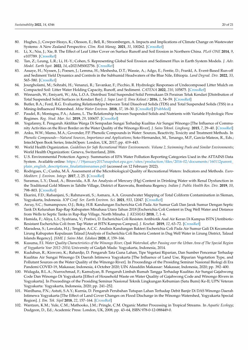
Sustainability 2022, 14, 4346 20 of 21

80. Hughes, J.; Cowper-Heays, K.; Olesson, E.; Bell, R.; Stroombergen, A. Impacts and Implications of Climate Change on WastewaterSystems: A New Zealand Perspective. Clim. Risk Manag. 2021, 31, 100262. [CrossRef]

81. Li, X.; Niu, J.; Xie, B. The Effect of Leaf Litter Cover on Surface Runoff and Soil Erosion in Northern China. PLoS ONE 2014, 9,e107789. [CrossRef]

82. Tan, Z.; Leung, L.R.; Li, H.-Y.; Cohen, S. Representing Global Soil Erosion and Sediment Flux in Earth System Models. J. Adv.Model. Earth Syst. 2022, 14, e2021MS002756. [CrossRef]

83. Assaye, H.; Nyssen, J.; Poesen, J.; Lemma, H.; Meshesha, D.T.; Wassie, A.; Adgo, E.; Fentie, D.; Frankl, A. Event-Based Run-offand Sediment Yield Dynamics and Controls in the Subhumid Headwaters of the Blue Nile, Ethiopia. Land Degrad. Dev. 2022, 33,565–580. [CrossRef]

84. Jourgholami, M.; Sohrabi, H.; Venanzi, R.; Tavankar, F.; Picchio, R. Hydrologic Responses of Undecomposed Litter Mulch onCompacted Soil: Litter Water Holding Capacity, Runoff, and Sediment. CATENA 2022, 210, 105875. [CrossRef]

85. Winnarsih, W.; Emiyarti, W.; Afu, L.O.A. Distribusi Total Suspended Solid Permukaan Di Perairan Teluk Kendari [Distribution ofTotal Suspended Solid Surfaces in Kendari Bay]. J. Sapa Laut (J. Ilmu Kelaut.) 2016, 1, 54–59. [CrossRef]

86. Butler, B.A.; Ford, R.G. Evaluating Relationships between Total Dissolved Solids (TDS) and Total Suspended Solids (TSS) in aMining-Influenced Watershed. Mine Water Environ. 2018, 37, 18–30. [CrossRef] [PubMed]

87. Paudel, B.; Montagna, P.A.; Adams, L. The Relationship between Suspended Solids and Nutrients with Variable Hydrologic FlowRegimes. Reg. Stud. Mar. Sci. 2019, 29, 100657. [CrossRef]

88. Yogafanny, E. Pengaruh Aktifitas Warga Di Sempadan Sungai Terhadap Kualitas Air Sungai Winongo [The Influence of Commu-nity Activities on the River Border on the Water Quality of the Winongo River]. J. Sains Teknol. Lingkung. 2015, 7, 29–40. [CrossRef]

89. Anku, W.W.; Mamo, M.A.; Govender, P.P. Phenolic Compounds in Water: Sources, Reactivity, Toxicity and Treatment Methods. InPhenolic Compounds—Natural Sources, Importance and Applications; Soto-Hernandez, M., Tenango, M.P., García-Mateos, R., Eds.;IntechOpen Book Series; IntechOpen: London, UK, 2017; pp. 419–443.

90. World Health Organization. Guidelines for Safe Recreational Water Environments. Volume 2, Swimming Pools and Similar Environments;World Health Organization: Geneva, Switzerland, 2006.

91. U.S. Environmental Protection Agency. Summaries of EPA Water Pollution Reporting Categories Used in the ATTAINS DataSystem. Available online: https://19january2017snapshot.epa.gov/sites/production/files/2016-02/documents/160112parent_plain_english_descriptions_finalattainsnames.pdf (accessed on 12 February 2022).

92. Rodrigues, C.; Cunha, M.Â. Assessment of the Microbiological Quality of Recreational Waters: Indicators and Methods. Euro-Mediterr. J. Environ. Integr. 2017, 2, 25. [CrossRef]

93. Suramas, L.Y.; Daud, A.; Birawida, A.B. An Analysis of Mercury (Hg) Content in Drinking Water with Renal Dysfunction inthe Traditional Gold Miners in TahiIte Village, District of Rarowatu, Bombana Regency. Indian J. Public Health Res. Dev. 2019, 10,798–803. [CrossRef]

94. Ekarini, F.D.; Rafsanjani, S.; Rahmawati, S.; Asmara, A.A. Groundwater Mapping of Total Coliform Contamination in Sleman,Yogyakarta, Indonesia. IOP Conf. Ser. Earth Environ. Sci. 2021, 933, 12047. [CrossRef]

95. Awuy, S.C.; Sumampouw, O.J.; Boky, H.B. Kandungan Escherichia Coli Pada Air Sumur Gali Dan Jarak Sumur Dengan SepticTank Di Kelurahan Rap-Rap Kabupaten Minahasa Utara Tahun 2018 [Escherichia Coli Content in Dug Well Water and Distancefrom Wells to Septic Tanks in Rap-Rap Village, North Minaha. J. KESMAS 2018, 7, 1–6.

96. Hamida, F.; Aliya, L.S.; Syafriana, V.; Pratiwi, D. Escherichia Coli Resisten Antibiotik Asal Air Keran Di Kampus ISTN [Antibiotic-Resistant Escherichia Coli from Tap Water at ISTN Kampus Campus]. J. Kesehat. 2019, 12, 63–72. [CrossRef]

97. Maradesa, S.; Lawalata, H.J.; Tengker, A.C.C. Analisis Kandungan Bakteri Escherichia Coli Pada Air Sumur Gali Di KecamatanLirung Kabupaten Kepulauan Talaud [Analysis of Escherichia Coli Bacteria Content in Dug Well Water in Lirung District, TalaudIslands Regency]. JSME J. Sains Mat. Edukasi 2020, 8, 159–166.

98. Kusuma, F.I. Water Quality Characteristics of the Winongo River, Opak Watershed, after Passing over the Urban Area of The Special Regionof Yogyakarta Year 2012–2014; University of Gadjah Mada: Yogyakarta, Indonesia, 2014.

99. Kudubun, R.; Kisworo, K.; Rahardjo, D. Pengaruh Tata Guna Lahan, Tipe Vegetasi Riparian, Dan Sumber Pencemar TerhadapKualitas Air Sungai Winongo Di Daerah Istimewa Yogyakarta [The Influence of Land Use, Riparian Vegetation Type, andPollutant Sources on the Water Quality of the Winongo River]. In Proceedings of the Prosiding Seminar Nasional Biologi di EraPandemi COVID-19, Makassar, Indonesia, 4 October 2020; UIN Alauddin Makassar: Makassar, Indonesia, 2020; pp. 392–400.

100. Widagda, B.L.A.; Nurrochmad, F.; Kamulyan, B. Pengaruh Limbah Rumah Tangga Terhadap Kualitas Air Sungai GajahwongCode Dan Winongo Di Yogyakarta [Effect of Household Waste on Water Quality of Gajahwong Code and Winongo Rivers inYogyakarta]. In Proceedings of the Prosiding Seminar Nasional Teknik Lingkungan Kebumian (Satu Bumi) Ke-II; UPN VeteranYogyakarta: Yogyakarta, Indonesia, 2020; pp. 241–252.

101. Wardhana, P.N.; Astuti, S.A.Y.; Kurnia, D. Pengaruh Perubahan Tutupan Lahan Terhadap Debit Banjir Di DAS Winongo DaerahIstimewa Yogyakarta [The Effect of Land Cover Changes on Flood Discharge in the Winongo Watershed, Yogyakarta SpecialRegion]. J. Ilm. Tek. Sipil 2018, 22, 157–164. [CrossRef]

102. Wantzen, K.M.; Yule, C.M.; Mathooko, J.M.; Pringle, C.M. Organic Matter Processing in Tropical Streams. In Aquatic Ecology;Dudgeon, D., Ed.; Academic Press: London, UK, 2008; pp. 43–64, ISBN 978-0-12-088449-0.

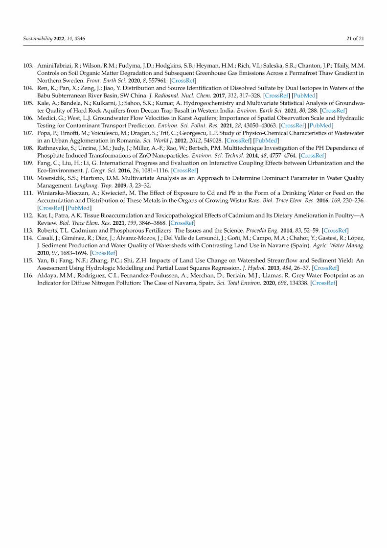
Sustainability 2022, 14, 4346 21 of 21

103. AminiTabrizi, R.; Wilson, R.M.; Fudyma, J.D.; Hodgkins, S.B.; Heyman, H.M.; Rich, V.I.; Saleska, S.R.; Chanton, J.P.; Tfaily, M.M.Controls on Soil Organic Matter Degradation and Subsequent Greenhouse Gas Emissions Across a Permafrost Thaw Gradient inNorthern Sweden. Front. Earth Sci. 2020, 8, 557961. [CrossRef]

104. Ren, K.; Pan, X.; Zeng, J.; Jiao, Y. Distribution and Source Identification of Dissolved Sulfate by Dual Isotopes in Waters of theBabu Subterranean River Basin, SW China. J. Radioanal. Nucl. Chem. 2017, 312, 317–328. [CrossRef] [PubMed]

105. Kale, A.; Bandela, N.; Kulkarni, J.; Sahoo, S.K.; Kumar, A. Hydrogeochemistry and Multivariate Statistical Analysis of Groundwa-ter Quality of Hard Rock Aquifers from Deccan Trap Basalt in Western India. Environ. Earth Sci. 2021, 80, 288. [CrossRef]

106. Medici, G.; West, L.J. Groundwater Flow Velocities in Karst Aquifers; Importance of Spatial Observation Scale and HydraulicTesting for Contaminant Transport Prediction. Environ. Sci. Pollut. Res. 2021, 28, 43050–43063. [CrossRef] [PubMed]

107. Popa, P.; Timofti, M.; Voiculescu, M.; Dragan, S.; Trif, C.; Georgescu, L.P. Study of Physico-Chemical Characteristics of Wastewaterin an Urban Agglomeration in Romania. Sci. World J. 2012, 2012, 549028. [CrossRef] [PubMed]

108. Rathnayake, S.; Unrine, J.M.; Judy, J.; Miller, A.-F.; Rao, W.; Bertsch, P.M. Multitechnique Investigation of the PH Dependence ofPhosphate Induced Transformations of ZnO Nanoparticles. Environ. Sci. Technol. 2014, 48, 4757–4764. [CrossRef]

109. Fang, C.; Liu, H.; Li, G. International Progress and Evaluation on Interactive Coupling Effects between Urbanization and theEco-Environment. J. Geogr. Sci. 2016, 26, 1081–1116. [CrossRef]

110. Moersidik, S.S.; Hartono, D.M. Multivariate Analysis as an Approach to Determine Dominant Parameter in Water QualityManagement. Lingkung. Trop. 2009, 3, 23–32.

111. Winiarska-Mieczan, A.; Kwiecien, M. The Effect of Exposure to Cd and Pb in the Form of a Drinking Water or Feed on theAccumulation and Distribution of These Metals in the Organs of Growing Wistar Rats. Biol. Trace Elem. Res. 2016, 169, 230–236.[CrossRef] [PubMed]

112. Kar, I.; Patra, A.K. Tissue Bioaccumulation and Toxicopathological Effects of Cadmium and Its Dietary Amelioration in Poultry—AReview. Biol. Trace Elem. Res. 2021, 199, 3846–3868. [CrossRef]

113. Roberts, T.L. Cadmium and Phosphorous Fertilizers: The Issues and the Science. Procedia Eng. 2014, 83, 52–59. [CrossRef]114. Casalí, J.; Giménez, R.; Díez, J.; Álvarez-Mozos, J.; Del Valle de Lersundi, J.; Goñi, M.; Campo, M.A.; Chahor, Y.; Gastesi, R.; López,

J. Sediment Production and Water Quality of Watersheds with Contrasting Land Use in Navarre (Spain). Agric. Water Manag.2010, 97, 1683–1694. [CrossRef]

115. Yan, B.; Fang, N.F.; Zhang, P.C.; Shi, Z.H. Impacts of Land Use Change on Watershed Streamflow and Sediment Yield: AnAssessment Using Hydrologic Modelling and Partial Least Squares Regression. J. Hydrol. 2013, 484, 26–37. [CrossRef]

116. Aldaya, M.M.; Rodriguez, C.I.; Fernandez-Poulussen, A.; Merchan, D.; Beriain, M.J.; Llamas, R. Grey Water Footprint as anIndicator for Diffuse Nitrogen Pollution: The Case of Navarra, Spain. Sci. Total Environ. 2020, 698, 134338. [CrossRef]