Journal Identification = JAG Article Identification = 416 Date: May 30, 2011 Time: 10:4 pm

En

Sa

b

a

ARA

KNCTS

1

afitscetta

o

Cf

0d

International Journal of Applied Earth Observation and Geoinformation 13 (2011) 657–667

Contents lists available at ScienceDirect

International Journal of Applied Earth Observation andGeoinformation

jo u r n al hom epage: www.elsev ier .com/ locate / jag

fficient collection of training data for sub-pixel land cover classification usingeural networks

tien Heremansa,∗, Bert Bossynsa,b, Herman Eerensb, Jos Van Orshovena

Department of Earth and Environmental Sciences, Katholieke Universiteit Leuven, Celestijnenlaan 200E, B-3001 Leuven, BelgiumVlaamse Instelling voor Technologisch Onderzoek (VITO), Boeretang 200, B-2400 Mol, Belgium

r t i c l e i n f o

rticle history:eceived 5 May 2010ccepted 26 March 2011

eywords:eural networksrop area estimationraining dataampling

a b s t r a c t

Artificial neural networks (ANNs) are a popular class of techniques for performing soft classificationsof satellite images. They have successfully been applied for estimating crop areas through sub-pixelclassification of medium to low resolution images. Before a network can be used for classification andestimation, however, it has to be trained. The collection of the reference area fractions needed to trainan ANN is often both time-consuming and expensive. This study focuses on strategies for decreasing theefforts needed to collect the necessary reference data, without compromising the accuracy of the resultingarea estimates. Two aspects were studied: the spatial sampling scheme (i) and the possibility for reusingtrained networks in multiple consecutive seasons (ii). Belgium was chosen as the study area becauseof the vast amount of reference data available. Time series of monthly NDVI composites for both SPOT-VGT and MODIS were used as the network inputs. The results showed that accurate regional crop areaestimation (R2 > 80%) is possible using only 1% of the entire area for network training, provided that thetraining samples used are representative for the land use variability present in the study area. Limiting thetraining samples to a specific subset of the population, either geographically or thematically, significantly

decreased the accuracy of the estimates. The results also indicate that the use of ANNs trained with datafrom one season to estimate area fractions in another season is not to be recommended. The interannualvariability observed in the endmembers’ spectral signatures underlines the importance of using up-to-date training samples. It can thus be concluded that the representativeness of the training samples, bothregarding the spatial and the temporal aspects, is an important issue in crop area estimation using ANNsthat should not easily be ignored.

. Introduction

The collection of national or regional crop area statistics is usu-lly organized as a combination of farmer inquiries and targetedeld surveys. This is a costly and time-consuming approach andhe results are mostly not available before the end of the growingeason. However, a diverse range of stakeholders requires accuraterop area statistics as early in the growing season as possible (Slazart al., 2007). Remotely sensed images can contribute significantlyo the timely estimation of the areas occupied by different cropypes through land cover classification with a special focus on the

gricultural land (Sedano et al., 2005).

In the area of land cover classification, the focus has long beenn high resolution sensors like Landsat TM/ETM and SPOT HRV(IR)

∗ Corresponding author at: K.U. Leuven, Division Forest, Nature and Landscape,elestijnenlaan 200E-2411, B-3001 Leuven, Belgium. Tel.: +32 16 329745;

ax: +32 16 329760.E-mail address: stien.heremans@ees.kuleuven.be (S. Heremans).

303-2434/$ – see front matter © 2011 Elsevier B.V. All rights reserved.oi:10.1016/j.jag.2011.03.008

© 2011 Elsevier B.V. All rights reserved.

(Dawbin and Evans, 1988; Fuller et al., 1994; Tsiligirides, 1998).These sensors outperform their lower resolution counterparts interms of spatial detail, but spatial resolution is not the sole factorto be considered. The sensor’s scene width and temporal res-olution also have to be taken into account. Sensors with shortrevisiting times are able to capture information about phenolog-ical changes, which facilitates the discrimination of different croptypes (Murakami et al., 2001; Murthy et al., 2003; Wardlow et al.,2007). High temporal resolution sensors also allow for the creationof time composites, which have proven effective for the reductionof cloud contamination (Dennison et al., 2007).

Medium and low resolution sensors like SPOT-VEGETATIONand MODIS (Moderate Resolution Imaging Spectrometer) combinelarge scenes, high temporal resolutions and low prices; an excellentcombination for operational crop classifications. Due to their lowspatial resolution, however, the images exhibit a high probability

of mixed pixels (Fisher, 1997). Mixed pixels are pixels containingmore than one land cover class on the ground (Cracknell, 1998). Theabundance of mixed pixels in medium and low resolution imagescalls for the use of sub-pixel or soft image classification techniques;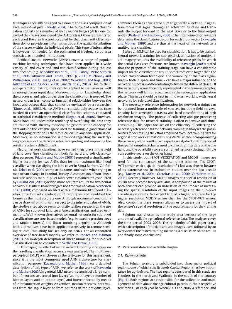

Journal Identification = JAG Article Identification = 416 Date: May 30, 2011 Time: 10:4 pm

6 arth O

teceetois

mvteWAnatni(ntAadtMir

othcnmmbnesfctomcabio(c

tpssdabhou

58 S. Heremans et al. / International Journal of Applied E

echniques specially designed to estimate the class composition ofach individual pixel (Foody, 2004). The output of a soft classifi-ation consists of a number of Area Fraction Images (AFIs), one forach of the classes considered. The AFI for class k then represents forach pixel the area fraction occupied by that class. Soft classifica-ions do not provide any information about the spatial distributionf the classes within the individual pixels. This type of informations however not needed for the estimation of (regional) crop areatatistics, as intended in this paper.

Artificial neural networks (ANNs) cover a range of popularachine learning techniques that have been applied in a wide

ariety of land cover and land use classifications during the lastwo decades (e.g. Benediktsson et al., 1990; Foody, 1996; Serpicot al., 1996; Atkinson and Tatnall, 1997; Ji, 2000; Muchoney andilliamson, 2001; Huang et al., 2002; Venkatesh and Raja, 2003;

itkenhead and Aalders, 2008; Lunetta et al., 2010). Due to theiron-parametric nature, they can be applied to Gaussian as wells non-gaussian input data. Moreover, no prior knowledge abouthe processes and rules underlying the classification is needed. Theetworks can learn complex functional relationships between the

nput and output data that cannot be envisaged by a researcherKimes et al., 1998). Hence, ANNs can considerably reduce the timeeeded to create an operational classification scheme, comparedo statistical classification methods (Rogan et al., 2008). However,NNs have the undesirable tendency of overfitting the data theyre trained with, thereby reducing the generalisation capacity forata outside the variable space used for training. A good choice ofhe stopping criterion is therefore crucial in any ANN application.

oreover, as no information is provided regarding the underly-ng processes or the decision rules, interpreting and improving theesults is often a difficult task.

Neural network classifiers have earned their place in the fieldf land cover/use classification, both for hard and soft classifica-ion purposes. Frizelle and Moody (2001) reported a significantlyigher accuracy for two ANNs than for the maximum likelihoodlassifier when classifying the land cover in Santa Barbara, Califor-ia. Erbek et al. (2004) came to the same conclusion when trying toap urban change in Istanbul, Turkey. A comparison of non-linearixture models for sub-pixel land cover classification conducted

y Liu and Wu (2005) yielded more accurate results for two neuraletwork classifiers than for regression tree classification. Verbeirent al. (2008) compared an ANN with a maximum likelihood clas-ifier for sub-pixel classification of crop types and identified theormer as the most accurate one. Although no general conclusionsan be drawn from this with respect to the inherent value of ANNs,he studies cited above seem to justify further research on the usef ANNs for sub-pixel land cover/use classifications and area esti-ations. Well-known alternatives to neural networks for sub-pixel

lassifications are tree-based models (e.g. boosted regression treesnd random forests) and linear unmixing algorithms. Althoughoth alternatives have been applied extensively in remote sens-

ng studies, this study focuses only on ANNs. For an elaboratedverview of tree-based models, we refer to Rodach and Maimon2008). An in-depth description of linear unmixing for sub-pixellassification can be consulted in Settle and Drake (1993).

In this paper, the effect of neural network training strategies onhe resulting classification accuracy was analysed. The multilayererceptron (MLP) was chosen as the test-case for this assessment,ince it is the most commonly used ANN architecture for clas-ification purposes (Kavzoglu and Mather, 1999). For a detailedescription of this type of ANN, we refer to the work of Kavzoglund Mather (2003). In general, MLP networks consist of a large num-

er of neurons structured into layers (an input layer, a number ofidden layers and an output layer) and interconnected by meansf interconnection weights. An artificial neuron receives input val-es from the input layer or from neurons in the previous layer,

bservation and Geoinformation 13 (2011) 657–667

combines them as a weighted sum to generate a ‘net’ input signal,transforms that signal through an activation function and trans-mits the output forward to the next layer or to the final outputnodes (Basheer and Hajmeer, 2000). The interconnection weightsdetermine the classification output for each input vector (Kavzogluand Mather, 1999) and are thus at the heart of the network as amultivariate classifier.

Before an MLP can be used for classification, it has to be trained.Neural network training for sub-pixel classification of multivari-ate imagery requires the availability of reference pixels for whichthe actual class area fractions are known. Kavzoglu (2009) statedthat the properties of the training stage can have a considerableimpact on the classification result, sometimes even larger than thechoice classification technique. The variability of the class signa-tures – both in space and time – can have a major influence on thenetwork’s success in differentiating between the different classes. Ifthis variability is insufficiently represented in the training samples,the network will fail to recognize it in the subsequent applicationphase. This issue should be kept in mind when working with neuralnetworks for sub-pixel classifications.

The necessary reference information for network training canbe obtained from a multitude of sources, including field surveys,existing land cover/use datasets and hard classifications of highresolution imagery. The process of collecting and pre-processingreference data for network training is often expensive and time-consuming. This paper focuses on the efficiency of collecting thenecessary reference data for network training. It analyses the possi-bilities for decreasing the efforts required to collect training data forregional crop area estimations using ANNs, without compromisingthe accuracy of the results. Two aspects are studied: optimization ofthe spatial sampling scheme used to collect training data on the onehand and the possibility to reuse a trained network during multipleconsecutive years on the other hand.

In this study, both SPOT-VEGETATION and MODIS images areused for the comparison of the sampling schemes. The SPOT-VGT sensor with a spatial resolution of 1 km was chosen becauseof its extensive use in estimation studies over the last decade(e.g. Tansey et al., 2004; Carreiras et al., 2006; Verbeiren et al.,2008). Recently however, MODIS images at a spatial resolution of250 m have become freely available. A comparison of the results ofboth sensors can provide an indication of the impact of increas-ing the spatial resolution of the input images on the sub-pixelclassification results. We expect to find a higher accuracy for thehigher resolution MODIS sensor than for the SPOT-VGT sensor.Also, combining these sensors allows us to assess the impact ofthe sensor’s spatial resolution on the requirements for the trainingdata.

Belgium was chosen as the study area because of the largeamount of available agricultural reference data. The analyses coverthe time period 2003–2006. The remainder of this paper startswith a description of the datasets and images used, followed by anoverview of the tested training methods, a discussion of the resultsand finally some conclusions.

2. Reference data and satellite images

2.1. Reference data

The Belgian territory is subdivided into three major politicalregions, one of which (the Brussels Capital Region) has low impor-tance for agriculture. The two regions considered in this study are

Flanders in the north and Wallonia in the south of the country(Fig. 1). Both regions are responsible for the collection and man-agement of data about the agricultural parcels in their respectiveterritories. For each year between 2003 and 2006, a reference land

Journal Identification = JAG Article Identification = 416 Date: May 30, 2011 Time: 10:4 pm

S. Heremans et al. / International Journal of Applied Earth Observation and Geoinformation 13 (2011) 657–667 659

F northI s (mea

uc

–

–

–

tti

classes and the areas they occupy in the Belgian territory can befound in Table 1.

Table 1The aggregated land use classes present in the reference land use geodataset andtheir respective areas. For the non-agricultural classes, the area remains constantthroughout the years. For the agricultural classes, the range over the four years usedin this study is provided.

Class name Explanation Area (km2)

WGR Winter grain 2316–2785MAI Maize 2503–2964POT Potato 795–916SUG Sugar beet 519–759GRA Grassland (permanent,

temporary and natural)7298

ig. 1. The Belgian territory is subdivided into three major regions: Flanders in thet contains 589 municipalities (mean size of 52 km2) and 26 agro-statistical district

se database including the location of the major crop types wasonstructed by merging the following three geodatasets:

The parcel geodataset of the Integrated Administration and Con-trol System (IACS) for the Walloon region. This annually updateddataset contains information on most agricultural parcels presentin the region (field boundaries, crop type, owner, etc.). The IACSinitiative was started in 1992, as a means to control the area-based subsidies claimed by farmers. It was developed in theframework of the EU Common Agricultural Policy (CAP).

The MESTBANK geodataset for the Flemish region. This agri-cultural parcel dataset serves as a tool for monitoring theimplementation of the nitrate directive. The MESTBANK datasetcan be considered as the Flemish counterpart of IACS and is alsoannually updated. The MESTBANK parcel datasets have a the-matic accuracy exceeding 97% with an average error on the parcelarea of less than 2%.

The CORINE land use/cover dataset of the year 2000 (CLC2000),covering the entire Belgian territory. This dataset is used to fillthe voids in the IACS and MESTBANK datasets related to the non-agricultural land use classes. For the CLC2000 dataset, a thematicaccuracy higher than 85% and a geometric accuracy better than100 m was demonstrated (Maucha and Büttner, 2006). The accu-racies mentioned are however only valid for the reference year2000. When using the dataset in later years, as done in this paper,the accuracy will decrease as a result of land cover/use changedthat might have occurred since the reference year 2000.

The three vectorial datasets listed above were combined in awo-step procedure. The first step consisted of a spatial merge ofhe agricultural parcel datasets (IACS and MESTBANK). Due to thedentical legends and the seamless boundary connections between

(grey), Wallonia in the south (white) and the Brussels capital region in the centre.n size of 1174 km2).

both datasets, no difficulties were encountered during this mergingprocedure. The resulting crop field dataset was superimposed onthe CORINE land cover/use dataset, replacing the coinciding areasof CORINE with the more detailed parcel data. It is important torealize that while the IACS and MESTBANK datasets are dynamic,the CLC2000 dataset is a static one, valid for the reference year 2000.The overlay thus results in a dataset with fixed land use vectors forthe non-agricultural classes, while the field shape and crop typeis dynamic throughout the subsequent years for the areas coveredby crops. The 128-class legend resulting from the overlay was sim-plified through thematic aggregation into 8 broad land use classes.These classes reflect the four major crop classes of Belgium and thefour major non-agricultural land use classes. An overview of the

FOR Forest (deciduous,coniferous and mixed)

5616

URB Urban area 5279OTH Other 5639

Journal Identification = JAG Article Identification = 416 Date: May 30, 2011 Time: 10:4 pm

6 arth O

2

fV(Idub

adfciiDbpeTctmft

3

3

cwcsroA

wcg(sciaSidag

3

twmtwpt

60 S. Heremans et al. / International Journal of Applied E

.2. Satellite imagery

Daily NDVI images for the period April–October were obtainedor each year between 2003 and 2006 from both the SPOT-EGETATION (1 km resolution) sensor and the TERRA-MODIS

250 m resolution) sensor. The Normalized Difference Vegetationndex (NDVI) is a commonly used index to measure vegetationensity and vigor (Tucker et al., 1985). Time series of NDVI val-es, reflecting crop phenology, are commonly used to discriminateetween crop types (Wardlow et al., 2007).

After preprocessing, the daily NDVI images were subjected to temporal compositing procedure, generating time series of 10-aily composites ranging from April to October for each of theour successive years (2003–2006). This period (April–October)overs most of the growing season for the major crops grownn Belgium and the NDVI composites were used as the primarynput for the neural network classifications described in this paper.etails on the Maximum Value Compositing technique used cane found in Eerens et al. (2007). The resulting SPOT-VGT com-osites were cleaned at VITO (Vlaams Instituut voor Technologien Onderzoek), resulting in nearly cloud-free composite images.he MODIS composites on the other hand were not cleaned, butlouded pixels were masked and excluded from the selection ofraining and validation samples. For the years 2004–2006, only

onthly composites of SPOT-VGT images were available. There-ore, the temporal extrapolation study was only carried out forhese composites.

. Methods

.1. Creation of reference area fraction images

The vectorial reference datasets described in Section 2.1 are notompatible with the low resolution NDVI images. Therefore, theyere transformed into four sets of eight (one for each considered

lass) reference AFIs, one set for each of the growing seasons con-idered (2003–2006). The reference AFI value of a pixel for class kepresents the fraction of this class present in the ground coveragef the low resolution pixel. For each pixel, the values of all referenceFIs sum up to unity.

The reference AFIs used for network training and validationere extracted from the vectorial land use datasets using the pro-

edure applied by Verbeiren et al. (2008). First, a low resolutionrid with the same spatial characteristics as the input NDVI imagesprojection, resolution, framing) was created. This grid was thenuperimposed on the vectorial land use datasets. For each gridell, the fraction occupied by class k was determined and storedn the reference AFI for class k. The resulting AFIs are co-aligned tond share the spatial resolution of the input images: 1 km for thePOT-VGT images and 250 m for the MODIS images. As explainedn Section 2.1, the areas covered by crops are dynamic resulting inifferent area fractions for the different growing seasons. The non-gricultural areas, derived from the CLC2000 dataset, are stable andive rise to identical area fractions for all growing seasons.

.2. Neural network training

Two strategies were examined for their potential to increasehe efficiency of reference data collection and use for ANN trainingithout compromising the accuracy of the resulting crop area esti-ates: the optimization of the spatial sampling scheme (i) and the

emporal reuse of trained networks (ii). The spatial sampling aspectas studied through a comparison of 11 procedures for the sam-ling of reference pixels within the study area (Section 3.2.1). Theemporal aspect was studied through the application of networks

bservation and Geoinformation 13 (2011) 657–667

trained in one year on input data from subsequent years (Section3.2.2).

3.2.1. Spatial training data configurationsThe available reference AFIs cover the entire Belgian territory

(Fig. 1). These datasets represents the population of reference pix-els from which training samples can be drawn. In this paper, 11different schemes for collecting the training samples are compared(Table 2). They can be assigned to three different sampling types:

• Simple random sampling: In sampling schemes of this type, apredefined number of training pixels are extracted from the pop-ulation purely at random. Each element of the population has anequal probability of being selected. The population is not subdi-vided or stratified and the feasibility of collecting the samples isnot taken into account.

• Systematic sampling: For this type of sampling, samples are drawnat predefined regular intervals (distance, pixel number, etc.) witha randomly selected starting point.

• Non-probability sampling: This sampling scheme selects pixelsbased on some external properties defined a priori. No underly-ing statistical assumptions, like selection probabilities, are takeninto account.

Simple random and systematic sampling are both examplesof probability-based sampling designs. In probability sampling, asopposed to non-probability sampling, each unit of the populationhas a non-zero chance of being included (Ripley, 2004). Probabil-ity sampling is applied in schemes S2 to S6 (Table 2). SchemesS7 to S10 are examples of the non-probability sampling type, astraining pixels are concentrated in one geographical region, thedistrict of Tournai (see Fig. 1). Pixels outside this district have azero probability of being sampled, hence these schemes do not ful-fil the requirements of probability sampling. In scheme S7, all pixelswithin the district of Tournai are used for training. Scheme S8 rep-resents a random selection of training pixels, but only pixels in theTournai district can be selected. In scheme s9, training pixels areagain selected randomly, but only pixel from the region of Tournaiin which no class exceeds a 50% area fraction qualify for selection.S10 is also a random scheme, but only pixels in the Tournai dis-trict that contain at least four of the eight land cover classes canbe selected. The district of Tournai was chosen for the geograph-ical limitation of the training pixels because it was considered asthe most representative district for the entire study area. All landcover classes present in the entire study area are present in this dis-trict. Sampling scheme S11 is also an example of a non-probabilityscheme, since only pixels where one class covers >50% of the areaqualify for inclusion. In scheme S1, no sampling is applied, as theentire population is used for training. In schemes S9 to S11, train-ing pixels are selected based on their homo- or heterogeneity. Asthis may have an impact on the classification success of the trainednetworks, these schemes were added to the list.

An important issue when comparing sampling schemes is thefeasibility of the reference data collection. In this study, referenceAFIs were available for the entire study area. In most operationalapplications however, these data have to be collected by field sur-veys or by photo-interpretation. Then, the sampling scheme hasa significant impact on the collection efforts. To take this intoaccount, the 11 sampling schemes were ranked according to theirfeasibility and provided with a ranking score, ranging from 1 formost feasible scheme to 11 for the least feasible scheme. The fea-

sibility ranking of the sampling schemes was defined according tothree rules of thumb:

• The feasibility decreases with sample size;

Journal Identification = JAG Article Identification = 416 Date: May 30, 2011 Time: 10:4 pm

S. Heremans et al. / International Journal of Applied Earth Observation and Geoinformation 13 (2011) 657–667 661

Table 2Sampling schemes used to select pixels for network training from the population and their associated feasibility ranking scores (1 = most feasible, 11 = least feasible). Thesampling types are subdivided into systematic (S), simple random (R) and non-probability (NP) sampling.

Scheme number Description Sampling type % of pixels from thepopulation selected

Feasibility rankingscore

S1 Entire population NA 100 10S2 Regular grid containing every 3rd pixel in rows and columns S 11 8S3 Regular grid containing every 10th pixel in rows and columns S 1 6S4 Random 11% of the population R 11 9S5 Random 1% of the population R 1 7S6 3 × 3 cell blocks selected in each 30 × 30 pixels window S 1 5S7 All pixels in the region of Tournai NP 4 2S8 Random sampling of 11% of the pixels in Tournai NP/R 0.4 1S9 Random sampling of 11% of pixels in the region of Tournai in

which no class exceeds 50% area fractionNP 0.4 3

han 4

rea

•

•

rtsTato

w

p((obchltpybtns

3

ncasvSyi1tawnw

S10 All pixels within the region of Tournai containing more tdifferent classes

S11 All pixels where one class covers more than 50% of the a

The feasibility is larger for spatially concentrated sampling thanfor scattered sampling;Systematic sampling schemes are more feasible than randomsampling schemes.

For schemes S9 and S10, information about all pixels in theegion of Tournai has to be collected and analysed to identifyhe correct pixels. Therefore, these schemes are less feasible thancheme S7, where all pixels in the region of Tournai are selected.he same holds for scheme S11. This scheme requires informationbout the area fractions in the entire study area in order to be ableo select only those pixels in which one class covers more than 50%f the area.

An overview of the sampling schemes used in this paper, alongith their feasibility scores, is provided in Table 2.

To assess the impact of the sampling scheme on the networkerformance, MLP networks were trained for all combinations ofi) SPOT-VGT or MODIS sensor, (ii) short (March–May) or longMarch–October) NDVI time series for the year 2003 and (iii) eachf the eleven sampling schemes, resulting in a total of 44 com-inations. The networks were specified with one hidden layerontaining eight nodes, a tan-sigmoid activation function for theidden nodes, a sigmoid activation function for the output nodes, a

earning rate equal to 0.0001, a maximum of 50,000 iterations andhe Mean Absolute Deviation <1% as the stopping criterion. Thearameter choices were based on the results of a sensitivity anal-sis of MLP networks for agricultural area estimation carried outy Doyen (2006). Since all classes were estimated simultaneously,he output layer consisted of 8 output nodes. The number of inputodes is set equal to the number of input variables, being 9 for thehort time series and 21 for the long time series.

.2.2. Extrapolation of trained networks in timeAnother strategy for reducing the sampling efforts is to reuse

etworks trained for one specific agricultural season to estimaterop area fractions in subsequent seasons. However, this strategyssumes sufficiently stable temporal NDVI signatures for each con-idered land use class throughout successive seasons. To test thealidity of this assumption for Flanders, networks trained withPOT-VGT monthly NDVI time series for each of four successiveears (2003–2006) were used to estimate crop areas in the yeart was trained for, as well as in the other three years. Thus, all6 possible combinations of training and application years wereested. For each of these combinations, a short (March–May) and

long (March–October) time series of monthly NDVI compositesas offered to the network, resulting in a total number of 32etwork applications. Training pixels for the calibration of the net-orks were selected according to sampling scheme S2 (Table 2),

NP 3 4

NP 9 11

systematically selecting every 3rd pixel in rows and columns.The classifications were performed with a simple 3-layer back-propagation neural network (NN), with 3 and 8 input nodes forthe short and the long time series respectively, 8 output nodes and8 nodes in the hidden layer. The activation function used for thehidden nodes was tan-sigmoid, for the output nodes a sigmoid acti-vation function was used. The learning rate was set equal to 0.0001,with a maximum of 50,000 iterations and the Mean Absolute Error<1% as the stopping criterion.

3.3. Validation

The neural networks described above were applied to estimatearea fractions at the pixel level, resulting in one estimated AFI perland use class for each network. The estimated area fractions werevalidated at three different levels of aggregation: the pixel level,the municipality level and the district level (Fig. 1). To obtain thearea fractions at higher levels of spatial aggregation, the per-pixelarea fractions were averaged per municipality or district. For thevalidation, all pixels, municipalities or districts were used, includ-ing the ones used for training, since the objective was to identifythe sampling scheme that produces the best area fraction estimatesfor the entire territory. We acknowledge that for the evaluation ofthe classification method used, cross-validation or an independenttest set would have been necessary. However, this study does notexplicitly aim to assess the accuracy of the classifier used.

All neural networks were validated using the simple linearregression approach, given by:

Xref = a + b × Xest

where Xref represents the reference area fraction and Xest the esti-mated fraction. The values a and b respectively represent theintercept and the slope of the regression equation. Perfect estima-tion assumes an intercept equal to 0 and a slope equal to 1. Foreach linear regression equation, the corresponding coefficient ofdetermination (R2) was also calculated. The higher the value of thiscoefficient, the stronger the (linear) relation between the estimatedand the reference area fractions. All the R2 values reported in thispaper refer to ‘pooled’ R2 values, which means that they are basedon the linear relation between the reference and the estimated areafractions for all classes combined. In other words, they reflect theoverall agreement between the reference and estimated fraction,without any distinction between the individual classes.

The coefficients of determination (R2) were used to evaluate the

performance of the spatial sampling schemes. These schemes wereranked according to their associated collection feasibility. From theviewpoint of sampling optimization, we want to select the schemewith the highest feasibility and the highest accuracy. However,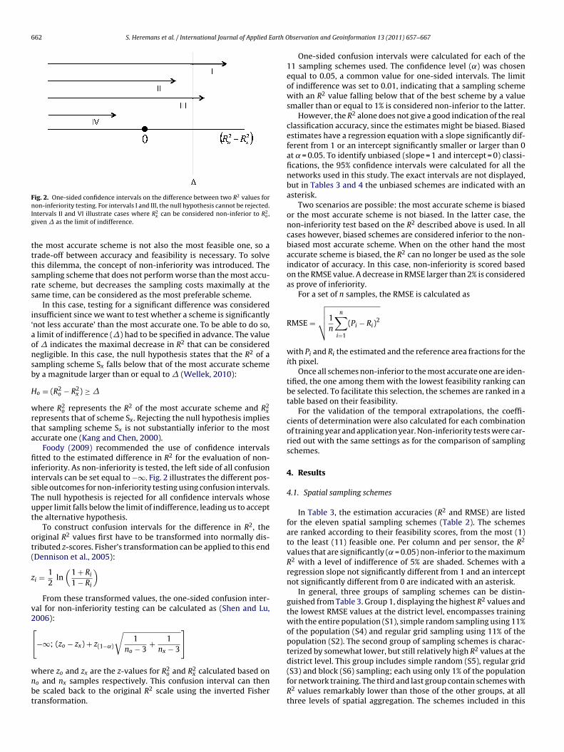

Journal Identification = JAG Article Identification = 416 Date: May 30, 2011 Time: 10:4 pm

662 S. Heremans et al. / International Journal of Applied Earth O

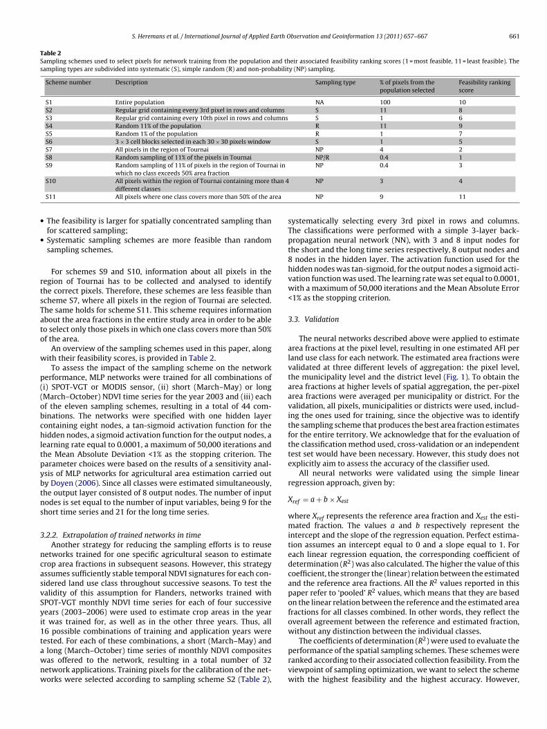
Fig. 2. One-sided confidence intervals on the difference between two R2 values fornIg

tttsrs

i‘aonsb

H

wrta

fiiisTut

ot(

z

v2[

wnbt

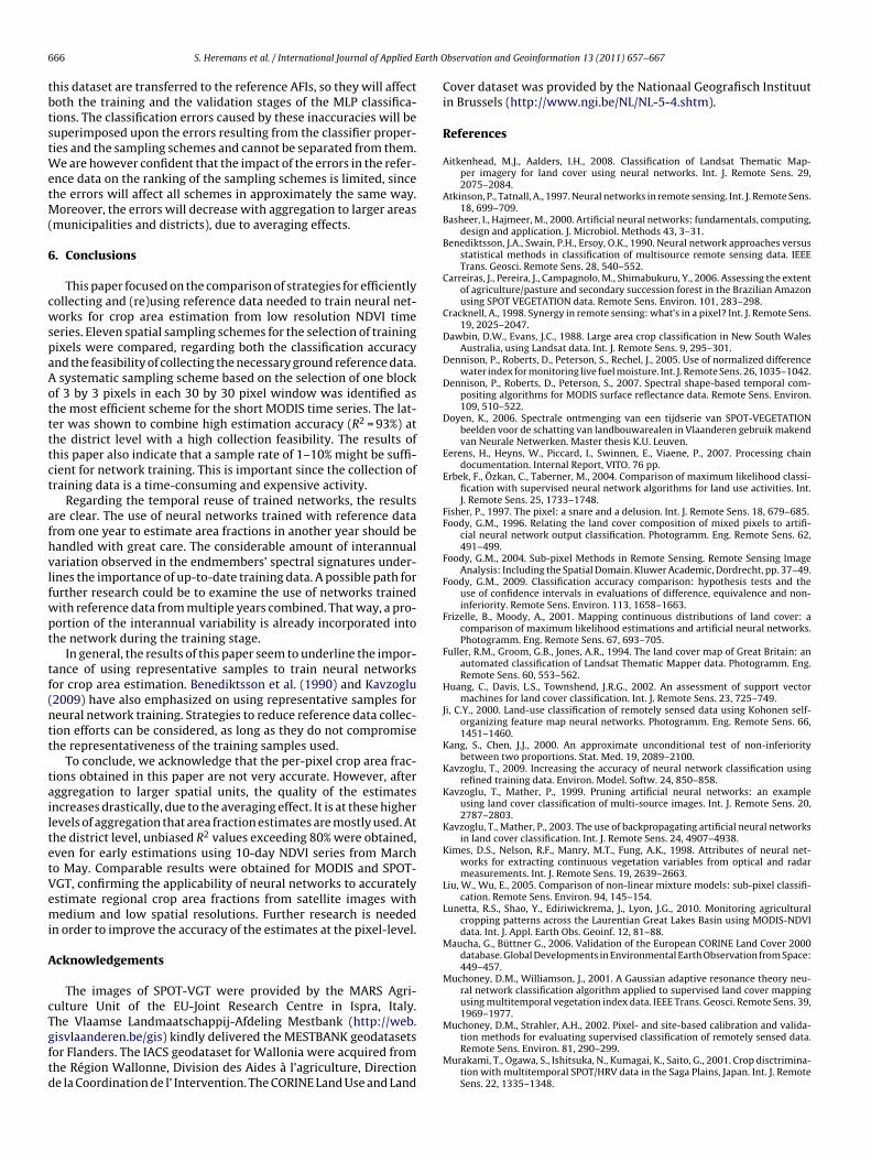
on-inferiority testing. For intervals I and III, the null hypothesis cannot be rejected.ntervals II and VI illustrate cases where R2

x can be considered non-inferior to R2o ,

iven � as the limit of indifference.

he most accurate scheme is not also the most feasible one, so arade-off between accuracy and feasibility is necessary. To solvehis dilemma, the concept of non-inferiority was introduced. Theampling scheme that does not perform worse than the most accu-ate scheme, but decreases the sampling costs maximally at theame time, can be considered as the most preferable scheme.

In this case, testing for a significant difference was considerednsufficient since we want to test whether a scheme is significantlynot less accurate’ than the most accurate one. To be able to do so,

limit of indifference (�) had to be specified in advance. The valuef � indicates the maximal decrease in R2 that can be consideredegligible. In this case, the null hypothesis states that the R2 of aampling scheme Sx falls below that of the most accurate schemey a magnitude larger than or equal to � (Wellek, 2010):

o = (R2o − R2

x ) ≥ �

here R2o represents the R2 of the most accurate scheme and R2

xepresents that of scheme Sx. Rejecting the null hypothesis implieshat sampling scheme Sx is not substantially inferior to the mostccurate one (Kang and Chen, 2000).

Foody (2009) recommended the use of confidence intervalstted to the estimated difference in R2 for the evaluation of non-

nferiority. As non-inferiority is tested, the left side of all confusionntervals can be set equal to −∞. Fig. 2 illustrates the different pos-ible outcomes for non-inferiority testing using confusion intervals.he null hypothesis is rejected for all confidence intervals whosepper limit falls below the limit of indifference, leading us to accepthe alternative hypothesis.

To construct confusion intervals for the difference in R2, theriginal R2 values first have to be transformed into normally dis-ributed z-scores. Fisher’s transformation can be applied to this endDennison et al., 2005):

i = 12

ln(

1 + Ri

1 − Ri

)From these transformed values, the one-sided confusion inter-

al for non-inferiority testing can be calculated as (Shen and Lu,006):

−∞; (zo − zx) + z(1−˛)

√1

no − 3+ 1

nx − 3

]

here zo and zx are the z-values for R2o and R2

x calculated based ono and nx samples respectively. This confusion interval can thene scaled back to the original R2 scale using the inverted Fisherransformation.

bservation and Geoinformation 13 (2011) 657–667

One-sided confusion intervals were calculated for each of the11 sampling schemes used. The confidence level (˛) was chosenequal to 0.05, a common value for one-sided intervals. The limitof indifference was set to 0.01, indicating that a sampling schemewith an R2 value falling below that of the best scheme by a valuesmaller than or equal to 1% is considered non-inferior to the latter.

However, the R2 alone does not give a good indication of the realclassification accuracy, since the estimates might be biased. Biasedestimates have a regression equation with a slope significantly dif-ferent from 1 or an intercept significantly smaller or larger than 0at ̨ = 0.05. To identify unbiased (slope = 1 and intercept = 0) classi-fications, the 95% confidence intervals were calculated for all thenetworks used in this study. The exact intervals are not displayed,but in Tables 3 and 4 the unbiased schemes are indicated with anasterisk.

Two scenarios are possible: the most accurate scheme is biasedor the most accurate scheme is not biased. In the latter case, thenon-inferiority test based on the R2 described above is used. In allcases however, biased schemes are considered inferior to the non-biased most accurate scheme. When on the other hand the mostaccurate scheme is biased, the R2 can no longer be used as the soleindicator of accuracy. In this case, non-inferiority is scored basedon the RMSE value. A decrease in RMSE larger than 2% is consideredas prove of inferiority.

For a set of n samples, the RMSE is calculated as

RMSE =

√√√√1n

n∑i=1

(Pi − Ri)2

with Pi and Ri the estimated and the reference area fractions for theith pixel.

Once all schemes non-inferior to the most accurate one are iden-tified, the one among them with the lowest feasibility ranking canbe selected. To facilitate this selection, the schemes are ranked in atable based on their feasibility.

For the validation of the temporal extrapolations, the coeffi-cients of determination were also calculated for each combinationof training year and application year. Non-inferiority tests were car-ried out with the same settings as for the comparison of samplingschemes.

4. Results

4.1. Spatial sampling schemes

In Table 3, the estimation accuracies (R2 and RMSE) are listedfor the eleven spatial sampling schemes (Table 2). The schemesare ranked according to their feasibility scores, from the most (1)to the least (11) feasible one. Per column and per sensor, the R2

values that are significantly ( ̨ = 0.05) non-inferior to the maximumR2 with a level of indifference of 5% are shaded. Schemes with aregression slope not significantly different from 1 and an interceptnot significantly different from 0 are indicated with an asterisk.

In general, three groups of sampling schemes can be distin-guished from Table 3. Group 1, displaying the highest R2 values andthe lowest RMSE values at the district level, encompasses trainingwith the entire population (S1), simple random sampling using 11%of the population (S4) and regular grid sampling using 11% of thepopulation (S2). The second group of sampling schemes is charac-terized by somewhat lower, but still relatively high R2 values at thedistrict level. This group includes simple random (S5), regular grid

(S3) and block (S6) sampling; each using only 1% of the populationfor network training. The third and last group contain schemes withR2 values remarkably lower than those of the other groups, at allthree levels of spatial aggregation. The schemes included in this

Journal Identification = JAG Article Identification = 416 Date: May 30, 2011 Time: 10:4 pm

S. Heremans et al. / International Journal of Applied Earth Observation and Geoinformation 13 (2011) 657–667 663

Table 3Coefficients of determination and RMSE for all spatial sampling schemes at the three levels of spatial aggregation. The schemes are ranked by their feasibility scores (FS)(SS = sampling scheme).

MODIS Short series (March–May) Long series (March–October)

Pixel Municip District Pixel Municip District

FB SS % pixels R2 (%) RMSE R2 (%) RMSE R2 (%) RMSE R2 (%) RMSE R2 (%) RMSE R2 (%) RMSE

1 S8 0.4 4 19.3 5 13.9 7 12.3 8 18.8 12 13.1 15 10.92 S7 4.0 22 17.3 37 11.1 54 7.8 41 15.1 65 8.5 77 6.03 S9 0.4 4 19.2 8 13.4 11 11.9 10 18.3 21 12.1 18 10.64 S10 0.4 7 18.8 13 13 19 10.8 22 17.4 38 11.1 36 9.55 S6 1.0 32 15.9 52 9.5 77 5.9 47 14.2 64 8.4 83 5.16 S3 1.0 31 16.0 51 9.7 69 6.9 46 14.4 67 8.1 84 5.07 S5 1.0 34 15.7 53 9.4 77 5.7 46 14.2 65 8.2 83 4.88 S2 11.1 40 15.0 61 8.6 82(*) 5.2 57 12.7 79 6.3 92(*) 3.49 S4 10.0 41 14.8 65 8.1 83(*) 4.9 58 12.6 79 6.4 93(*) 3.210 S1 100.0 43 14.6 69 7.7 85(*) 4.6 61 12.0 85 5.4 100(*) 2.611 S11 9.4 38 15.0 61 8.4 81 5.1 55 12.8 79 6.1 92(*) 3.4

MODIS Short series (March–May) Long series (March–October)

Pixel Municip District Pixel Municip District

FB SS % pixels R2 (%) RMSE R2 (%) RMSE R2 (%) RMSE R2 (%) RMSE R2 (%) RMSE R2 (%) RMSE

1 S8 0.4 12 23.4 34 11.1 48 8.2 38 19.8 75 7.6 85 5.22 S7 4.0 13 23.5 38 10.9 47 8.2 42 19.2 78 7.0 86 4.93 S9 0.2 6 24.4 11 13.1 15 11.1 22 22.2 32 11.3 37 9.24 S10 0.4 2 24.9 5 13.6 5 12.5 7 24.1 12 12.8 8 11.45 S6 1.0 35 20.1 71 7.6 83 4.8 53 17.2 84(*) 5.6 93(*) 3.26 S3 1.0 35 20.1 46 10.4 80 5.4 54 17.1 85(*) 5.4 93 3.27 S5 1.0 35 20.2 69 7.7 81 5.1 53 17.1 84 5.6 93 3.28 S2 11.1 37 19.9 49 10.1 82 5.0 55 16.7 86(*) 5.2 94(*) 3.09 S4 10.0 37 19.9 73 7.4 84(*) 4.8 55 16.7 86(*) 5.2 94(*) 2.910 S1 100.0 37 19.8 71 7.5 84(*) 4.7 56 16.5 87(*) 5.0 94(*) 2.811 S11 8.7 24 21.9 50 9.6 52 8.0 46 18.3 66 8.7 70 6.7

T h a limi dicate

gpoewsduog

TVT

Cf

he R2 values that are significantly non-inferior to the maximum R2 at ̨ = 0.05, witntercept non-significantly different from 1 and 0) at the 5% significance level are in

roup (S7, S8, S9 and S10) are all examples of non-probability sam-ling. In this sampling type, the decision to include a pixel is basedn prior knowledge about the properties of the pixels. Some pix-ls therefore have a zero chance of being included in the sample,hile others have an inclusion probability equal to one. Sampling

cheme S11 cannot unequivocally be assigned to one of the groups2

escribed above, since its R value depends largely on the sensor

sed. For the VGT sensor, the R2 of scheme S11 lies between thatf group 1 and that of group 2. For MODIS, it is situated betweenroup 2 and group 3. Although training pixels are selected from the

able 4alidation results (R2) for networks trained in one year and applied in another. Results at

he maximal R2 value for each application year is indicated in bold.

Training year Short time series (March–May)

Application year

2003 2004 2005 20

Pixel2003 45 33 37 352004 26 44 35 262005 29 34 46 262006 38 28 33 44Municip2003 77 57 62 662004 49 75 62 492005 54 61 77 482006 64 45 53 76District2003 92(*) 68(*) 73 742004 60(*) 89(*) 77(*) 562005 57 67(*) 90(*) 442006 80(*) 56 62 91

ombinations significantly non-inferior to the maximum in the same application year are srom 1 and 0) at the 5% significance level are indicated with an asterisk (*).

it of indifference equal to 5% are shaded. Unbiased classifications (with slope andd with an asterisk (*).

entire study area, scheme S11 is also an example of non-probabilitysampling. Pixels in which one class occupies more than 50% of thearea have a chance of being included equal to one, the other pixels’inclusion chance is zero.

For most sampling schemes, only small differences in accuracybetween the SPOT-VEGETATION and the MODIS sensor were found.

The exception is scheme S8, randomly selecting 11% of the pixelsin the region of Tournai. For the long time series, the MODIS sensorgives an R2 of 85%, opposed to only 15% for the SPOT-VEGETATIONsensor.

the pixel level (top), the municipality level (middle) and the district level (bottom).

Long time series (March–October)

Application year

06 2003 2004 2005 2006

51 39 39 34 31 49 41 33 32 39 50 33

32 37 36 48

82 65 64 59 53 80 68 57 57 69 80 60

56 61 58 78

95(*) 72 73 64 56(*) 92(*) 79 62 55(*) 75 93(*) 58(*) 64(*) 70 68 93(*)

haded. Unbiased classifications (with slope and intercept non-significantly different

Journal Identification = JAG Article Identification = 416 Date: May 30, 2011 Time: 10:4 pm

664 S. Heremans et al. / International Journal of Applied Earth Observation and Geoinformation 13 (2011) 657–667

00.10.20.30.40.50.60.70.80.9

121110987654321N

DV

I

Months

POTATO

2003200420052006

0

0.2

0.4

0.6

0.8

1

121110987654321

ND

VI

Months

WINTER GRAIN

2003200420052006

0

0.2

0.4

0.6

0.8

1

1.2

13121110987654321

ND

VI

MAIZE

2003200420052006

00.10.20.30.40.50.60.70.80.9

121110987654321

ND

VI

SUGAR BEET

2003200420052006

Months Months

00.10.20.30.40.50.60.70.8

121110987654321

ND

VI

Months

GRASSLAND

2003200420052006

00.10.20.30.40.50.60.70.80.9

121110987654321

ND

VI

Months

FOREST

2003200420052006

0

0.1

0.2

0.3

0.4

0.5

0.6

0.7

121110987654321

ND

VI

URBAN

2003200420052006

00.10.20.30.40.50.60.70.8

121110987654321

ND

VI

OTHER

2003200420052006

ility fo

etsoimrcc0egitbi

s

Months

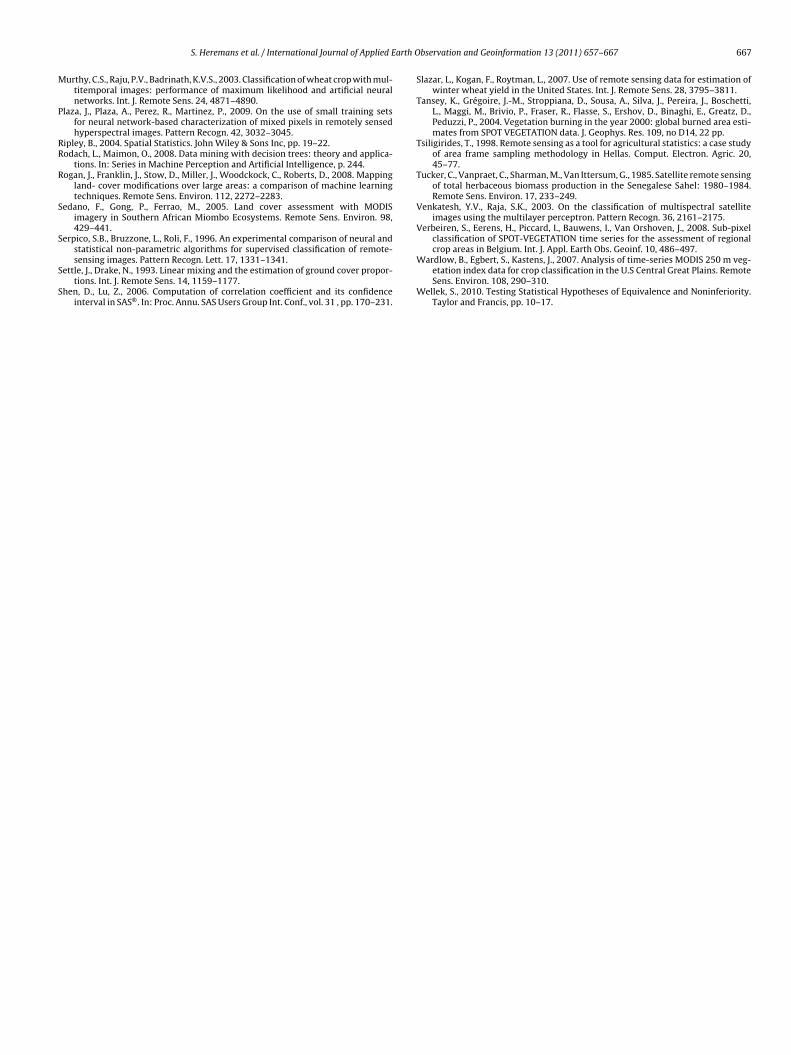
Fig. 3. Endmember spectrum variab

From the viewpoint of optimization, the scheme with the high-st feasibility that has an accuracy significantly non-inferior tohat of the most accurate one is considered as the most preferablecheme. In this study, the R2 value was used as the main indicatorf accuracy. All sampling schemes with an R2 significantly non-nferior to the highest R2, for the same sensor and time series, were

arked. From these schemes, the one with the lowest feasibilityank was identified as the most preferable one. However, mostlassifications display a regression equation with a slope signifi-antly different from 1 or an intercept significantly different from

at ̨ = 0.05. In other words, they are biased. For all time seriesxcept the long MODIS series, even the scheme using all pixels (S1)ives rise to biased estimates, rendering the R2 useless for inferior-ty testing. In all cases, biased estimates were considered inferioro unbiased estimates. When the most accurate scheme was also

iased, non-inferiority was tested on the RMSE values. A decrease

n RMSE larger than 2% was considered as prove of inferiority.According to these rules, sampling scheme S6 with a feasibility

core of 5, was identified as the most optimal scheme for the short

Months

r all crops in the period 2003–2006.

MODIS time series, both at the municipality and at the district level.In this sampling scheme, the training pixels are spatially arrangedas one block of 3 by 3 pixels per window of 30 by 30 pixels. Itshould be pointed out that S6 needs only 1% of the population fornetwork training for achieving an R2 non-inferior to the R2 achievedwhen using the entire population for training. For the long MODISseries, scheme S2 – a regular grid using 11% of the population fortraining – was identified as the most optimal sampling scheme atall levels of spatial aggregation. For this series, the R2 of schemeS6 was not proven to be non-inferior to the maximal R2. For theSPOT-VGT time series, none of the alternative schemes was provento be non-inferior to scheme S1.

4.2. Extrapolation of trained networks in time

In Table 4, the overall R2 values at the pixel, municipality anddistrict level for all combinations of training and application yearsare displayed. This table shows markedly higher R2 values for appli-cation of the networks in the year of training than for application

Journal Identification = JAG Article Identification = 416 Date: May 30, 2011 Time: 10:4 pm

arth O

inRcwTafytaec

cbtbrtssv

5

tctIs(irlsesng

cSrosifim

stTgyrdpcFws1

S. Heremans et al. / International Journal of Applied E

n non-training years. At none of the aggregation levels, an R2 for aon-training year was found to be significantly non-inferior to the2 in the respective training year. Moreover, the estimates for appli-ation in the training year were all non-biased at the district level,hile some other combinations lead to biased estimates. From

able 4, a marked increase of the R2 values with the level of spatialggregation is again observed. At the same time however, the dif-erences between the R2 values for training years and non-trainingears rise considerably with the level of aggregation. For the shortime series, the accuracy of the combination of training year 2003nd application year 2006 and the reverse combination is consid-rably higher than that of all other combinations. This observationan however not be extended to the long time series.

The importance of using season-specific networks becomeslear when inspecting the temporal NDVI profiles of the endmem-ers, extracted using a fully constrained linear unmixing model. Inhis type of unmixing model, the sum of the area fractions muste equal to 1 and none of the fractions can be smaller than 0. Theesulting endmember profiles for the four successive years used inhis study (2003–2006) are plotted in Fig. 3. All land use classeshow a considerable variability between the reflectance profiles ofuccessive years, although some classes (potato, maize) are moreariable than others (winter grain, forest, urban).

. Discussion

For the implementation of food security policies and to supportrading of agricultural products, accurate estimates of the areasovered by the most prevalent crops are needed. The earlier inhe growing season these area estimates are available, the better.n this study, a large number of neural networks were trained forhort and long time series of NDVI composites. The short time seriesMarch–May) correspond roughly to area estimates obtained earlyn the growing season, while the long series (March–October) cor-espond to late estimates. Table 3 shows that early estimates areess accurate than late estimates, for all the training strategies con-idered. At the district level however, unbiased R2 values for thearly estimates exceeding 80% are obtained. This confirms the pos-ibility to generate usable regional crop area estimates with neuraletworks using only 1% of the area for training, even as early in therowing season as early June.

Food insecure regions are often data-poor as well. Sampling effi-iency is thus an important topic for these regions. The results ofection 4.1 indicate the possibility for Belgium to obtaining accu-ate crop area estimates using ANNs trained with a limited amountf training samples using MODIS NDVI time series, as long as theseamples are representative for the entire study area. This clearlyllustrates the potential applicability of artificial neural networksor crop area estimation in data-poor regions. Mixed cropping andrregular cropping calendars as practiced in many tropical regions

ay however compromise this applicability to some extent.Besides increasing the sampling efficiency, another possible

trategy for dealing with data-poor circumstances is to reuserained networks during multiple years. However, the results ofable 4 show that this is not a recommended strategy for Bel-ian circumstances. When using neural networks trained in oneear to estimate crop areas for another year, the estimation accu-acy decreased significantly. A most plausible explanation for thisecrease can be found in the interannual variability of the tem-oral endmember profiles in relation to variations in weatheronditions and market-driven agricultural management decisions.

or the temporal extrapolations, monthly SPOT-VGT compositesere used as opposed to 10-daily composites for the sampling

cheme comparison. This is due to the lack of availability of the0-daily composites for the years 2004–2006. Using 10-daily com-

bservation and Geoinformation 13 (2011) 657–667 665

posites could have resulted in more accurate classification results.However, the decrease in accuracy when extrapolating to non-training years might also have been larger for 10-daily compositesas the number of potential differences in the endmember spectraincreases with the temporal resolution.

The results of Table 3 show that limiting the training sam-ples geographically (S7, S8, S9, S10) and/or thematically (S9, S10,S11), largely decreases the accuracy of the resulting networks. Thisunderlines the importance of including as much of the variabil-ity present in the study area as possible into the training samples.Benediktsson et al. (1990) have already stated that the performanceof ANNs for classification depends largely on using representativetraining samples, since their learning is completely data-driven.They can in other words only apply what they have learned dur-ing training. Kavzoglu (2009) also recognizes the key importanceof representative training samples for accurate classification.

Although Plaza et al. (2009) emphasize on the importance ofusing informative training samples composed of highly mixed pix-els in multilayer perceptron training, this is not confirmed by ourresults. The selection of mixed pixels was favored in schemes S9and S10, but does not seem to generate more accurate classificationresults. Sampling scheme S9 randomly selects pixels in the regionof Tournai in which no class exceeds 50% area fraction. Scheme S10uses all pixels in Tournai containing more than 4 different classes.When comparing the results of scheme S9 to those of scheme S8 – asimple random selection of the same number of pixels in the sameregion – the latter displays slightly lower RMSE values. The effectis more pronounced for the comparison of scheme S10 and schemeS7, the latter using all pixels in the Tournai region. Although schemeS10 favors the selection of mixed pixels, its classification results aremarkedly less accurate than those of scheme S7, for both sensorsat all three levels of spatial aggregation.

From Table 3, it is also clear that simple random samplingschemes are slightly more accurate than regular grid and blocksampling, when an equal amount of training samples is used. Thesuperiority of the random sampling schemes can be explained bytheir higher efficiency of capturing the variability present in theentire study area (Kavzoglu, 2009). Moreover, the collection of indi-vidual, non-grouped pixels may provide a higher variance in thetraining samples and avoid autocorrelation effects (Muchoney andStrahler, 2002).

The results of this study also indicate the impact of spatialaggregation on the accuracy of crop area estimation using neuralnetworks. As the level of spatial aggregation increases from thepixel to the district level, the R2 values increase with more than40% for the most efficient training strategies. The R2 values foundhere are concordant with the results obtained by Verbeiren et al.(2008). They also found a marked increase of the R2-values whenaggregating the estimates to higher regional levels, with R2 valuesat the district level between, 83 and 95% for crop area estimation.However, Verbeiren et al. (2008) obtained these results using 50%of the area for training and the other 50% for validation. The resultsof the current study indicate that a systematic sampling strategyselecting only 1–10% of the area for network training can sufficefor usable and feasible crop area estimation at the district level.

There is however a high probability that the optimal samplingscheme depends on the characteristics of the study area. Furtherresearch is needed to analyze the interactions between the charac-teristics (homogeneity, fragmentation, etc.) of the study area andthe appropriateness of different sampling schemes. The results ofthis paper can stimulate researchers in the field of sub-pixel classi-fication to reflect on the impact of sampling issues before starting

the actual collection procedures.

As mentioned in Section 2.1, the CORINE land use/cover datasetused in the creation of the reference area fraction images (AFIs) hasa thematic accuracy of approximately 85%. The errors present in

Journal Identification = JAG Article Identification = 416 Date: May 30, 2011 Time: 10:4 pm

6 arth O

tbtstWetM(

6

cwspaAottttct

afhvlfwpt

tf(ntt

tailtetVemi

A

cTgftd

66 S. Heremans et al. / International Journal of Applied E

his dataset are transferred to the reference AFIs, so they will affectoth the training and the validation stages of the MLP classifica-ions. The classification errors caused by these inaccuracies will beuperimposed upon the errors resulting from the classifier proper-ies and the sampling schemes and cannot be separated from them.

e are however confident that the impact of the errors in the refer-nce data on the ranking of the sampling schemes is limited, sincehe errors will affect all schemes in approximately the same way.

oreover, the errors will decrease with aggregation to larger areasmunicipalities and districts), due to averaging effects.

. Conclusions

This paper focused on the comparison of strategies for efficientlyollecting and (re)using reference data needed to train neural net-orks for crop area estimation from low resolution NDVI time

eries. Eleven spatial sampling schemes for the selection of trainingixels were compared, regarding both the classification accuracynd the feasibility of collecting the necessary ground reference data.

systematic sampling scheme based on the selection of one blockf 3 by 3 pixels in each 30 by 30 pixel window was identified ashe most efficient scheme for the short MODIS time series. The lat-er was shown to combine high estimation accuracy (R2 = 93%) athe district level with a high collection feasibility. The results ofhis paper also indicate that a sample rate of 1–10% might be suffi-ient for network training. This is important since the collection ofraining data is a time-consuming and expensive activity.

Regarding the temporal reuse of trained networks, the resultsre clear. The use of neural networks trained with reference datarom one year to estimate area fractions in another year should beandled with great care. The considerable amount of interannualariation observed in the endmembers’ spectral signatures under-ines the importance of up-to-date training data. A possible path forurther research could be to examine the use of networks trainedith reference data from multiple years combined. That way, a pro-ortion of the interannual variability is already incorporated intohe network during the training stage.

In general, the results of this paper seem to underline the impor-ance of using representative samples to train neural networksor crop area estimation. Benediktsson et al. (1990) and Kavzoglu2009) have also emphasized on using representative samples foreural network training. Strategies to reduce reference data collec-ion efforts can be considered, as long as they do not compromisehe representativeness of the training samples used.

To conclude, we acknowledge that the per-pixel crop area frac-ions obtained in this paper are not very accurate. However, afterggregation to larger spatial units, the quality of the estimatesncreases drastically, due to the averaging effect. It is at these higherevels of aggregation that area fraction estimates are mostly used. Athe district level, unbiased R2 values exceeding 80% were obtained,ven for early estimations using 10-day NDVI series from Marcho May. Comparable results were obtained for MODIS and SPOT-GT, confirming the applicability of neural networks to accuratelystimate regional crop area fractions from satellite images withedium and low spatial resolutions. Further research is needed

n order to improve the accuracy of the estimates at the pixel-level.

cknowledgements

The images of SPOT-VGT were provided by the MARS Agri-ulture Unit of the EU-Joint Research Centre in Ispra, Italy.he Vlaamse Landmaatschappij-Afdeling Mestbank (http://web.

isvlaanderen.be/gis) kindly delivered the MESTBANK geodatasetsor Flanders. The IACS geodataset for Wallonia were acquired fromhe Région Wallonne, Division des Aides à l’agriculture, Directione la Coordination de l’ Intervention. The CORINE Land Use and Land

bservation and Geoinformation 13 (2011) 657–667

Cover dataset was provided by the Nationaal Geografisch Instituutin Brussels (http://www.ngi.be/NL/NL-5-4.shtm).

References

Aitkenhead, M.J., Aalders, I.H., 2008. Classification of Landsat Thematic Map-per imagery for land cover using neural networks. Int. J. Remote Sens. 29,2075–2084.

Atkinson, P., Tatnall, A., 1997. Neural networks in remote sensing. Int. J. Remote Sens.18, 699–709.

Basheer, I., Hajmeer, M., 2000. Artificial neural networks: fundamentals, computing,design and application. J. Microbiol. Methods 43, 3–31.

Benediktsson, J.A., Swain, P.H., Ersoy, O.K., 1990. Neural network approaches versusstatistical methods in classification of multisource remote sensing data. IEEETrans. Geosci. Remote Sens. 28, 540–552.

Carreiras, J., Pereira, J., Campagnolo, M., Shimabukuru, Y., 2006. Assessing the extentof agriculture/pasture and secondary succession forest in the Brazilian Amazonusing SPOT VEGETATION data. Remote Sens. Environ. 101, 283–298.

Cracknell, A., 1998. Synergy in remote sensing: what’s in a pixel? Int. J. Remote Sens.19, 2025–2047.

Dawbin, D.W., Evans, J.C., 1988. Large area crop classification in New South WalesAustralia, using Landsat data. Int. J. Remote Sens. 9, 295–301.

Dennison, P., Roberts, D., Peterson, S., Rechel, J., 2005. Use of normalized differencewater index for monitoring live fuel moisture. Int. J. Remote Sens. 26, 1035–1042.

Dennison, P., Roberts, D., Peterson, S., 2007. Spectral shape-based temporal com-positing algorithms for MODIS surface reflectance data. Remote Sens. Environ.109, 510–522.

Doyen, K., 2006. Spectrale ontmenging van een tijdserie van SPOT-VEGETATIONbeelden voor de schatting van landbouwarealen in Vlaanderen gebruik makendvan Neurale Netwerken. Master thesis K.U. Leuven.

Eerens, H., Heyns, W., Piccard, I., Swinnen, E., Viaene, P., 2007. Processing chaindocumentation. Internal Report, VITO. 76 pp.

Erbek, F., Özkan, C., Taberner, M., 2004. Comparison of maximum likelihood classi-fication with supervised neural network algorithms for land use activities. Int.J. Remote Sens. 25, 1733–1748.

Fisher, P., 1997. The pixel: a snare and a delusion. Int. J. Remote Sens. 18, 679–685.Foody, G.M., 1996. Relating the land cover composition of mixed pixels to artifi-

cial neural network output classification. Photogramm. Eng. Remote Sens. 62,491–499.

Foody, G.M., 2004. Sub-pixel Methods in Remote Sensing. Remote Sensing ImageAnalysis: Including the Spatial Domain. Kluwer Academic, Dordrecht, pp. 37–49.

Foody, G.M., 2009. Classification accuracy comparison: hypothesis tests and theuse of confidence intervals in evaluations of difference, equivalence and non-inferiority. Remote Sens. Environ. 113, 1658–1663.

Frizelle, B., Moody, A., 2001. Mapping continuous distributions of land cover: acomparison of maximum likelihood estimations and artificial neural networks.Photogramm. Eng. Remote Sens. 67, 693–705.

Fuller, R.M., Groom, G.B., Jones, A.R., 1994. The land cover map of Great Britain: anautomated classification of Landsat Thematic Mapper data. Photogramm. Eng.Remote Sens. 60, 553–562.

Huang, C., Davis, L.S., Townshend, J.R.G., 2002. An assessment of support vectormachines for land cover classification. Int. J. Remote Sens. 23, 725–749.

Ji, C.Y., 2000. Land-use classification of remotely sensed data using Kohonen self-organizing feature map neural networks. Photogramm. Eng. Remote Sens. 66,1451–1460.

Kang, S., Chen, J.J., 2000. An approximate unconditional test of non-inferioritybetween two proportions. Stat. Med. 19, 2089–2100.

Kavzoglu, T., 2009. Increasing the accuracy of neural network classification usingrefined training data. Environ. Model. Softw. 24, 850–858.

Kavzoglu, T., Mather, P., 1999. Pruning artificial neural networks: an exampleusing land cover classification of multi-source images. Int. J. Remote Sens. 20,2787–2803.

Kavzoglu, T., Mather, P., 2003. The use of backpropagating artificial neural networksin land cover classification. Int. J. Remote Sens. 24, 4907–4938.

Kimes, D.S., Nelson, R.F., Manry, M.T., Fung, A.K., 1998. Attributes of neural net-works for extracting continuous vegetation variables from optical and radarmeasurements. Int. J. Remote Sens. 19, 2639–2663.

Liu, W., Wu, E., 2005. Comparison of non-linear mixture models: sub-pixel classifi-cation. Remote Sens. Environ. 94, 145–154.

Lunetta, R.S., Shao, Y., Ediriwickrema, J., Lyon, J.G., 2010. Monitoring agriculturalcropping patterns across the Laurentian Great Lakes Basin using MODIS-NDVIdata. Int. J. Appl. Earth Obs. Geoinf. 12, 81–88.

Maucha, G., Büttner G., 2006. Validation of the European CORINE Land Cover 2000database. Global Developments in Environmental Earth Observation from Space:449–457.

Muchoney, D.M., Williamson, J., 2001. A Gaussian adaptive resonance theory neu-ral network classification algorithm applied to supervised land cover mappingusing multitemporal vegetation index data. IEEE Trans. Geosci. Remote Sens. 39,1969–1977.

Muchoney, D.M., Strahler, A.H., 2002. Pixel- and site-based calibration and valida-

tion methods for evaluating supervised classification of remotely sensed data.Remote Sens. Environ. 81, 290–299.

Murakami, T., Ogawa, S., Ishitsuka, N., Kumagai, K., Saito, G., 2001. Crop disctrimina-tion with multitemporal SPOT/HRV data in the Saga Plains, Japan. Int. J. RemoteSens. 22, 1335–1348.

Journal Identification = JAG Article Identification = 416 Date: May 30, 2011 Time: 10:4 pm

arth O

M

P

RR

R

S

S

S

S

S. Heremans et al. / International Journal of Applied E

urthy, C.S., Raju, P.V., Badrinath, K.V.S., 2003. Classification of wheat crop with mul-titemporal images: performance of maximum likelihood and artificial neuralnetworks. Int. J. Remote Sens. 24, 4871–4890.

laza, J., Plaza, A., Perez, R., Martinez, P., 2009. On the use of small training setsfor neural network-based characterization of mixed pixels in remotely sensedhyperspectral images. Pattern Recogn. 42, 3032–3045.

ipley, B., 2004. Spatial Statistics. John Wiley & Sons Inc, pp. 19–22.odach, L., Maimon, O., 2008. Data mining with decision trees: theory and applica-

tions. In: Series in Machine Perception and Artificial Intelligence, p. 244.ogan, J., Franklin, J., Stow, D., Miller, J., Woodckock, C., Roberts, D., 2008. Mapping

land- cover modifications over large areas: a comparison of machine learningtechniques. Remote Sens. Environ. 112, 2272–2283.

edano, F., Gong, P., Ferrao, M., 2005. Land cover assessment with MODISimagery in Southern African Miombo Ecosystems. Remote Sens. Environ. 98,429–441.

erpico, S.B., Bruzzone, L., Roli, F., 1996. An experimental comparison of neural andstatistical non-parametric algorithms for supervised classification of remote-

sensing images. Pattern Recogn. Lett. 17, 1331–1341.

ettle, J., Drake, N., 1993. Linear mixing and the estimation of ground cover propor-tions. Int. J. Remote Sens. 14, 1159–1177.

hen, D., Lu, Z., 2006. Computation of correlation coefficient and its confidenceinterval in SAS® . In: Proc. Annu. SAS Users Group Int. Conf., vol. 31 , pp. 170–231.

bservation and Geoinformation 13 (2011) 657–667 667

Slazar, L., Kogan, F., Roytman, L., 2007. Use of remote sensing data for estimation ofwinter wheat yield in the United States. Int. J. Remote Sens. 28, 3795–3811.

Tansey, K., Grégoire, J.-M., Stroppiana, D., Sousa, A., Silva, J., Pereira, J., Boschetti,L., Maggi, M., Brivio, P., Fraser, R., Flasse, S., Ershov, D., Binaghi, E., Greatz, D.,Peduzzi, P., 2004. Vegetation burning in the year 2000: global burned area esti-mates from SPOT VEGETATION data. J. Geophys. Res. 109, no D14, 22 pp.

Tsiligirides, T., 1998. Remote sensing as a tool for agricultural statistics: a case studyof area frame sampling methodology in Hellas. Comput. Electron. Agric. 20,45–77.

Tucker, C., Vanpraet, C., Sharman, M., Van Ittersum, G., 1985. Satellite remote sensingof total herbaceous biomass production in the Senegalese Sahel: 1980–1984.Remote Sens. Environ. 17, 233–249.

Venkatesh, Y.V., Raja, S.K., 2003. On the classification of multispectral satelliteimages using the multilayer perceptron. Pattern Recogn. 36, 2161–2175.

Verbeiren, S., Eerens, H., Piccard, I., Bauwens, I., Van Orshoven, J., 2008. Sub-pixelclassification of SPOT-VEGETATION time series for the assessment of regionalcrop areas in Belgium. Int. J. Appl. Earth Obs. Geoinf. 10, 486–497.

Wardlow, B., Egbert, S., Kastens, J., 2007. Analysis of time-series MODIS 250 m veg-etation index data for crop classification in the U.S Central Great Plains. RemoteSens. Environ. 108, 290–310.

Wellek, S., 2010. Testing Statistical Hypotheses of Equivalence and Noninferiority.Taylor and Francis, pp. 10–17.