Labour Market Effects of Fixed-Term Employment Contracts

Labour Market Effects of Fixed-Term Employment Contracts – Microeconometric Analyses

for West Germany

Inaugural-Dissertation zur Erlangung des Doktorgrades

des Fachbereichs Wirtschaftswissenschaften der Johann Wolfgang Goethe-Universität

Frankfurt am Main

Tobias Hagen

Kelkheim

2004

3

Contents

1 Introduction 13

2 Fixed-Term Employment Contracts in Germany: Definition, Institutional

Background, and Empirical Relevance 17

2.1 Definition of Fixed-Term versus Permanent Employment Contracts 17

2.2 Institutional Background in Germany 18

2.3 Empirical Relevance of Fixed-Term Contracts in West Germany 21

3 Methodological Background: Identification of the Effects of Institutions and

Policy Interventions 29

3.1 Introduction: Estimation of Causal Effects of Binary Treatments Using Microeconometric Methods 29

3.2 Basics 30

3.2.1 The Evaluation Problem in General and the Parameters of Interest 30

3.2.2 Regression: Homogeneous Versus Heterogeneous Effects and Sources of Selection Bias 32

3.2.3 Social Experiments 35

3.2.4 Natural Experiments 35

3.2.5 SUTVA: Possible General Equilibrium Effects and Indirect Effects of Fixed-Term Contracts 36

3.2.6 Basic Approaches for the Generation of Control Groups 37

3.3 Evaluation Methods Requiring Cross Sectional Data 38

3.3.1 Propensity Score Matching 38

3.3.2 Parametric Regression Methods Versus Matching 45

3.3.3 Instrumental Variable Approaches and Selection Models 46

3.4 Evaluation Methods Requiring Panel Data 47

3.4.1 Before-After Estimator 47

3.4.2 Difference-in-Differences Estimator 49

3.5 Pre-Program Test 50

3.6 Summary 51

4

4 The Role of Fixed-Term Contracts in Labour Demand 52

4.1 Overview: Why Do Firms Use Fixed-Term Contracts? 52

4.2 Theoretical Considerations 55

4.2.1 Introduction 55

4.2.2 Protection Against Dismissal in Economic Theory and Structure of Adjustment Costs in Labour Demand 56

4.2.3 Dynamic Labour Demand with Firing Costs and Availability of Fixed-Term Contracts 57

4.2.4 Matching and Equilibrium Labour Market Models with Fixed-Term Contracts 61

4.2.5 Further Considerations on Institutional Reasons for Using Fixed-Term Contracts 66

4.2.6 Summary and Conclusions from the Theoretical Considerations 68

4.3 Previous Empirical Results on the Effects of Dismissal Protection and Fixed-Term Contracts 69

4.4 Why do Employers Use Fixed-Term Contracts? Evaluating the Effects of Firing Costs of Permanent Work on the Use of Atypical Work 76


4.4.2 Dataset, Model Specification, and Estimation Technique 77

4.4.3 Estimation Results 86

4.4.4 Summary of the Empirical Analysis of the Firms’ Use of Atypical Work 91

4.5 Empirical Analysis of the Role of Fixed-Term Contracts in Worker and Job Flows 92


4.5.2 Methodology 94

4.5.3 Dataset and Weighting 99

4.5.4 Results 100

4.5.5 Summary of the Empirical Analysis of the Role of Fixed-Term Contracts in Worker and Job Flows 110

4.6 Conclusions 111

5 Do Temporary Workers Receive Risk Premiums? – Effects of Fixed-Term

Contracts on Working Conditions and Wages in the Short-Run 112

5.1 Introduction 112


5.2.1 Compensating Wage Differential for Workers on Fixed-Term Contracts 113

5.2.2 Wage Penalty for Workers on Fixed-Term Contracts 114

5.2.3 Worker Preferences for Fixed-Term Contracts 119

5.2.4 Heterogeneity of Fixed-Term Contract Jobs 119

5

5.2.5 Use of Subjective Outcome Variables in Economic Analysis 120

5.3 Previous Empirical Results 121

5.4 Data Base, Estimation Sample, and Descriptive Statistics 124

5.5 Econometric Approach 137

5.5.1 Characterising the Selection Problem 137

5.5.2 Attempts to Account for Selection on Unobservables 137

5.5.3 Choice of Conditioning Variables 139

5.5.4 Further Specification Issues: Other Selection Problems 141

5.5.5 Implementation of the Propensity Score Matching Estimator 141

5.6 Determinants of the Type of Contract: Estimation of the Propensity Score 143

5.6.1 Model A: Using only Pre-Treatment Variables 143

5.6.2 Model C: Accounting for Job and Employer Attributes 149

5.7 Effects of Fixed-Term Contracts: Results of the Matching Estimator 156

5.7.1 Choice of the Matching Estimator and Checks on the Balancing Property 156

5.7.2 Effects of Fixed-Term Contracts for Men 161

5.7.3 Effects of Fixed-Term Contracts for Women 169

5.8 Summary and Conclusions 173

6 Do Fixed-Term Contracts Increase the Long-Term Employment

Opportunities of the Unemployed? 175

6.1 Overview: Are Fixed-Term Contracts Stepping Stones for the Unemployed or Dead-Ends? 175


6.2.1 Basic Concepts: Job Search Theory and Determinants of Unemployment Duration 176

6.2.2 Under Which Conditions Do Job Searchers Enter into Fixed-Term Contract Jobs? 178

6.2.3 Why Should Fixed-Term Contracts be Stepping Stones Towards Permanent Positions? 181

6.3 Fixed-Term Contracts and the Re-Employment Probabilities of the Unemployed 183


6.3.2 Previous Results: Unemployment Duration Analyses Distinguishing Between Employment Contracts 184

6.3.3 Modelling Framework: Discrete Competing Risks Hazard Rate Model 186

6.3.4 Data Base and Variables 188

6.3.5 Estimation Results of the Competing Risks Hazard Rate Model 193

6.3.6 Summary: Fixed-Term Contracts and the Re-Employment Probabilities of the Unemployed 199

6

6.4 Effects of Entering into Fixed-Term Contract Jobs: Are Fixed-Term Contracts Stepping Stones? 200


6.4.2 Previous Studies: Causal Effects of Fixed-Term Contracts on Future Employment Prospects 200

6.4.3 Econometric Approach 202

6.4.3.1 The Counterfactuals of Interest and the Policy Questions 202

6.4.3.2 Implementation of the Propensity Score Matching Estimator 207

6.4.4 Definition of the Outcome Variables 210

6.4.5 Estimation Results of the Propensity Score Equation (Discrete Hazard Rate Model) 212

6.4.6 Estimation Results of the Matching Estimator 214

6.4.6.1 Matching Quality 215

6.4.6.2 Mean Effects of Fixed-Term Contracts 218

6.4.6.3 Heterogeneous Effects of Fixed-Term Contracts 224

6.4.7 Summary: Effects of Entering into Fixed-Term Contracts on the Long-Term Employment Opportunities of the Unemployed 231

6.5 Conclusions 233

7 Summary and Conclusions 235

8 Appendix 239

9 References 253

7

List of Figures

Figure 1: Proportion of FTCs in Total Dependent Employment in West Germany.................... 23

Figure 2: Index of Permanent Contract and FTC Employment (1995=100%) ........................... 24

Figure 3: Kernel Density Estimation of the Hourly Wage (€) Distribution of Men by Type

of Contract – Unrestricted Tenure ................................................................................... 133

Figure 4: Kernel Density Estimation of the Hourly Wage (€) Distribution of Men by Type

of Contract – Tenure ≤2................................................................................................... 133

Figure 5: Kernel Density Estimation of the Hourly Wage (€) Distribution of Women by

Type of Contract – Unrestricted Tenure .......................................................................... 134

Figure 6: Kernel Density Estimation of the Hourly Wage (€) Distribution of Women by

Type of Contract – Tenure ≤2.......................................................................................... 134

Figure 7: Employment Effects – DEF.1.................................................................................... 219

Figure 8: Employment Effects – DEF.2.................................................................................... 219

Figure 9: Unemployment Effects – DEF.1................................................................................ 220

Figure 10: Unemployment Effects – DEF.2.............................................................................. 220

Figure 11: Out-of-labour-force Effect – DEF.1 ........................................................................ 221

Figure 12: Out-of-Labour-Force Effect – DEF.2 ...................................................................... 222

Figure 13: Employment Effects – Women (DEF.2).................................................................. 225

Figure 14: Unemployment Effects – Women (DEF.2) ............................................................. 226

Figure 15: Out-of-Labour-Force Effect – Women (DEF.2)...................................................... 226

Figure 16: Employment Effects – Age ≥32 (DEF.2) ............................................................... 228

Figure 17: Unemployment Effects – Age ≥ 32 (DEF.2) ........................................................... 228

Figure 18: Out-of-Labour-Force Effects – Age ≥32 (DEF.2) ................................................... 229

Figure 19: Employment Effects – Workers With Formal Qualification (DEF.2)....................... 230

Figure 20: Unemployment Effects – Workers With Formal Qualification (DEF.2)................... 230

Figure 21: Out-of-Labour-Force Effects – Workers With Formal Qualification (DEF.2).......... 231

List of Tables

Table 1: Duration of FTCs in 1998 ............................................................................................. 25

Table 2: Proportion of FTCs in Total Dependent Employment in 1998/99................................ 27

Table 3: Overview of Matching and Equilibrium Models with FTCs ........................................64

Table 4: Share of Establishments Using Atypical Work............................................................. 83

Table 5: Share of Establishments Employing Atypical Workers by

Number of Employees and Industry .................................................................................. 84

Table 6: Means of Adjustment to Expected or Unexpected Demand Changes During the

Year in West Germany in 1996 ......................................................................................... 84

Table 7: Means of Adjustment to Increasing and Decreasing Demand in West Germany in

1993 ................................................................................................................................... 85

Table 8: Determinants of Employing FTC, FL, or TWA Workers............................................. 88

8

Table 9: Effects of the Increase in the Minimum Employment Threshold Level

for the Protection Against Dismissal Law in October 1996 ..............................................90

Table 10: Means of Job and Worker Flow Rates for Total Employment ................................. 101

Table 11: Means of Job and Worker Flow Rates by Employment Trend................................. 102

Table 12: Means of Job and Worker Flows by Type of Contract ............................................. 103

Table 13: Means of Job and Worker Flow Rates by Type of Contract and

Employment Trend .......................................................................................................... 105

Table 14: Decomposition of Worker Flows by Type of Contract............................................. 106

Table 15: Share of FTCs in Total Worker Flows...................................................................... 107

Table 16: Worker Flows by Contract Type and Industry.......................................................... 109

Table 17: Sample Means of Explanatory Variables.................................................................. 125

Table 18: Number and Proportion of FTCs by Ongoing Job Tenure........................................ 127

Table 19: Means of Usual Weekly Hours of Work by Type of Contract.................................. 128

Table 20: Two-Sample Wilcoxon Rank-Sum Test for Differences in the

Distribution of Usual Weekly Hours of Work by Type of Contract................................ 129

Table 21: Earnings Distribution by Type of Contract............................................................... 130

Table 22: Means of Hourly Wage by Type of Contract............................................................ 131

Table 23: Two-sample Wilcoxon Rank-Sum Test for Differences in the

Distribution of Hourly Wage in € by Type of Contract................................................. 132

Table 24: Subjective Assessment of Job Insecurity Distribution by Type of Contract............. 136

Table 25: Subjective Assessment of Career Opportunities by Type of Contract...................... 136

Table 26: Propensity Score – Men (Model A)........................................................................... 145

Table 27: Propensity Score – Women (Model A)...................................................................... 147

Table 28: Propensity Score – Men (Model C)........................................................................... 150

Table 29: Propensity Score – Women (Model C) ..................................................................... 153

Table 30: Matching Quality – Men (Model A).......................................................................... 158

Table 31: Matching Quality – Women (Model A) .................................................................... 158

Table 32: Means of Important Conditioning Variables (X) Before and

After Kernel-Based Matching – Men (Model A) ............................................................. 159

Table 33: Means of Important Conditioning Variables (X) Before and

After Kernel-Based Matching – Women (Model A)........................................................ 160

Table 34: Wage Effects of FTCs – Men (Model A) .................................................................. 162

Table 35: Wage Effects of FTCs – Men (Model B) .................................................................. 162

Table 36: Wage Effects of FTCs – Men (Model C) .................................................................. 162

Table 37: Effects of FTCs on Job Insecurity – Men (Model A) ................................................ 164

Table 38: Effects of FTCs on Job Insecurity – Men (Model B) ................................................ 164

Table 39: Effects of FTCs on Job Insecurity – Men (Model C )............................................... 164

Table 40: Effects of FTCs on Career Opportunities – Men (Model A) ..................................... 165

Table 41: Effects of FTCs on Career Opportunities – Men (Model B) ..................................... 166

Table 42: Effects of FTCs on Career Opportunities – Men (Model C)..................................... 166

Table 43: Heterogeneous Wage Effects of FTCs – Men (Model A) ......................................... 168

Table 44: Wage Effects of FTCs – Women (Model A ) ............................................................ 169

Table 45: Wage Effects of FTCs – Women (Model B)............................................................. 170

9

Table 46: Wage Effects of FTCs – Women (Model C)............................................................. 170

Table 47: Effects of FTCs on Job Insecurity – Women (Model A)........................................... 171

Table 48: Effects of FTCs on Career Opportunities – Women (Model A)................................ 171

Table 49: Heterogeneous Wage Effects of FTCs – Women (Model A) .................................... 172

Table 50: Duration of Completed Unemployment Spells by Kind of Transition ..................... 190

Table 51: Explanatory Variables............................................................................................... 192

Table 52: Model Choice on the Basis of Information Criteria.................................................. 193

Table 53: Estimation Results of the (Multinomial Logistic) Competing Risks

Hazard Rate Model With All Exit States......................................................................... 197

Table 54: Definitions of the ‘Non-Treatment’ State and the Counterfactual............................ 205

Table 55: Definition of Treated and Untreated Individuals ...................................................... 207

Table 56: Definition of the Outcome Variables ........................................................................ 211

Table 57: Logistic Hazard Rate Model (Propensity Score Estimation) ....................................213

Table 58: Loss of Treated Observations due to Common Support Requirement and

Lack of Similar Untreated Within the Caliper (NN-Matching, Outcome 2)................... 216

Table 59: Means of Important Pre-Treatment Variables (X) Before and

After NN-Matching (DEF.1)........................................................................................... 216

Table 60: Means of Important Pre-Treatment Variables (X) Before and

After NN-Matching (DEF.2)........................................................................................... 217

Table 61: Probability of Being Employed on a Permanent Contract – DEF.1.......................... 223

Table 62: Probability of Being Employed on a Permanent Contract – DEF.2.......................... 223

Table 63: Probability of Being Employed on a FTC – DEF.2 .................................................. 224

Table 64: Probabilities of Being Employed on a Permanent Contract versus FTC –

Women (DEF.2) .............................................................................................................. 227


Age ≥ 32 (DEF.2) ........................................................................................................... 229


Workers With Formal Qualification (DEF.2).................................................................... 231

Table 67: Descriptive Statistics for the Estimation Sample – Dependent Variables................. 240

Table 68: Descriptive Statistics for the Estimation Sample – Independent Variables ............. 240

Table 69: Probability of Being Employed on FTC (Omitting Federal State Dummies)........... 241

Table 70: Effects of FTCs on Mean Weekly Hours of Work – Men (Model A ) ...................... 242

Table 71: Effects of FTCs on Working Part-time – Men (Model A)......................................... 242

Table 72: Effects of FTCs on Mean Weekly Hours of Work – Women (Model A).................. 242

Table 73: Effects of FTCs on Working Part-time – Women (Model A) ................................... 242

Table 74: Effects of FTCs on Job Insecurity – Men (Model A) ................................................ 243

Table 75: Effects of FTCs on Career Opportunities – Men (Model A) ..................................... 244

Table 76: Effects of FTCs on Job Insecurity – Women (Model A)........................................... 245

Table 77: Effects of FTCs on Career Opportunities – Women (Model A)................................ 246

Table 78: Duration of Continuous Employment Spells After the Transition from

Unemployment to FTCs and Permanent Contracts in Months ........................................ 247

Table 79: Means of Explanatory Variables by Kind of Transition ........................................... 247

10

Table 80: Estimation Results of the Multinomial Logistic Duration Model with Two

Destination States ............................................................................................................ 249

Table 81: Estimation Results of the Multinomial Logistic Duration Model with Four

Destination States ............................................................................................................ 251

List of Symbols

{ }0,1C ∈ treatment dummy

tCA adjustment costs

CR churning rate

tE employment level in the current period t *

tE desired level of employment

( )E Y X expectation of Y conditional on X

( )( )R

i iF w t cumulated wage offer distribution

( )G ⋅ kernel function

HR hiring rate

iIN linear index JCR job creation rate

JDR job destruction rate

N employment stock

1N , 0N , CN number of treated, number of untreated, number of controls

( )Pr ⋅ probability

( )ie� neighbourhood as a function of the propensity score

RR rotation rate

SR separation rate

TFR transformation (of fixed-term into permanent contracts) rate

itU , 1itU , 0itU unobserved error terms in case of treatment (1) or non-treatment (0) in the out-

come equations

iV unobserved error term in the participation equation

WTR worker turnover rate

X vector of explanatory (conditioning) variables

tY output

Y observed outcome

Y1 outcome in the treatment state

Y0 outcome in the non-treatment state

Z vector of explanatory variables *Z instrumental variable

ia time-invariant individual-specific effect

( )e X , e propensity score (participation probability conditional on X)

( )1g X , ( )0

g X functions of X in the group of treated (1) and controls (0)

h bandwidth parameter

( )ih t hazard rate of individual i after unemployment duration t

11

i individual, establishment, treated individual

t period of time, period of time before treatment

t´ period of time after treatment

( )R

iw t reservation wage

( ),w i j weight associated to the members j of the control group for treated i

z , 'z two values of *Z

( )tα baseline hazard

itε classical error term

iξ job offer rate

tθ common macroeconomic time effect

λ speed of adjustment

Ψ interval (caliper)

Φ cumulative normal distribution

jω number of times an untreated person is used as a control

⊥ statistical independence

List of Abbreviations

AIC Akaike information criterion

ATE average treatment effect

ATT average treatment effect on the treated

ATU average treatment effect on the untreated

BetrVG Betriebsverfassungsgesetz

BIBB Bundesinstitut für Berufsbildung

BIC Bayesian criterion

Coeff. coefficient

DIW Deutsches Institut für Wirtschaftsforschung

e.g. for example

Eq. equation

FL freelance

FTC fixed-term contract

GSOEP German Socio-Economic Panel

HQIC Hannan-Quin criterion

i.e. that is

IAB Institut für Arbeitsmarkt- und Berufsforschung

IIA independence of irrelevant alternatives

IV instrumental variable

KschG Kündigungsschutzgesetz

Marg. eff. marginal effect

NN nearest neighbour obs. observations

PER permanent contract

Std.err. standard error

12

SUTVA stable unit-treatment value assumption

TWA temporary work agency

TzBfG Teilzeit- und Befristungsgesetz

ZEW Zentrum für Europäische Wirtschaftsforschung

13

1 Introduction

An important feature of the German labour market is the coexistence of perma-nent contracts which are associated with high institutional firing costs due to dismissal protection legislation and fixed-term contracts (FTCs) which establish employment relationships for a limited duration of time. FTCs expire automati-cally without dismissal at the end of the agreed term. The employment relation-ship is either terminated or the employer can decide to offer the worker a perma-nent position or, under certain circumstances, another FTC. Obviously, the avail-ability of FTCs leads to a substantial alteration of the framework in which the optimisation behaviour of actors in the labour market takes place.

This is all the more likely as the importance of FTCs in the West German la-bour market has been underestimated not only in the political discussion, but also by economists so far. The reason may be that many studies have focussed on ag-gregate employment stocks, which conceal most of the employment dynamics. In West German private sector establishments FTCs constitute only 6–7% of all jobs, but about 30% of all hirings and separations are based on them (see Sub-chapter 4.5). This discrepancy indicates the necessity to look at micro data, i.e., information on the individual behaviour of workers and firms. Furthermore, the magnitude of FTC employment suggests that the usual assumption of a rigid la-bour market in Germany, which is contrasted with a flexible U.S. labour market, seems to be an oversimplification. Besides the obvious policy relevance, this may be one reason why the labour market effects of flexible employment contracts have become an important and prolific field of research in labour economics in recent years.1

FTCs were liberalised in Germany by the Employment Promotion Act in 1985 as a reaction to the unemployment crisis. Besides, temporary work agencies have been liberalised for several times since 1985. Recently, both types of atypical work have been further facilitated by the so-called “Hartz Reform”. Therefore, Germany is a typical example of a partial deregulation of the dismissal protection legislation (BLANCHARD and LANDIER, 2002), being observed in many European countries, where kinds of temporary work such as FTCs were introduced, while keeping institutional firing restrictions on permanent contracts constant.

Of course, the aim of the reforms was to alleviate the unemployment problem (or to increase employment), which has increasingly become a problem of low-qualified workers being affected by international trade („globalisation“) and technological change.2 The government’s official objectives of the liberalisation have been expressed in a number of communiques (see JAHN, 2002).

1 See, for example, the symposium on temporary work in the Economic Journal 112, June 2002. 2 See EISEN (2001) for a discussion of both sources of unemployment of low-qualified workers.

FITZENBERGER (1999) provides an empirical analysis of this issue.

14

Before 1985, the objective of the permission to conclude FTCs was to give firms the possibility of dealing with unexpected events and short-term peaks in labour demand. The objectives of the reform in 1985 can be summarised as fol-lows (see JAHN, 2002). FTCs should (1.) increase the overall flexibility of the labour market, (2.) increase the individual employment opportunities of workers, especially of those who are protected by special dismissal protection rules (e.g., disabled workers), (3.) lead to a reduction of long-term unemployment, and (4.) reduce the amount of overtime work. An “unofficial” objective of the govern-ment has always been to avoid an extensive reform of the dismissal protection legislation for permanent contracts despite the unemployment crisis3, which can, obviously, be explained by political factors.4 All the intended effects of FTCs except point (4.) are at least partly evaluated throughout this study.

Although a number of extensive German studies including research on the la-bour market effects of FTCs already exists5, there is still a lack of empirical and in particular econometric analyses attempting to shed light on causal relation-ships.

Chapter 2 starts with a definition of fixed-term versus permanent contracts and provides a brief overview of the institutional background with respect to dis-missal protection for permanent contracts, the regulation of FTCs, and the role of works councils and collective wage agreements. Afterwards, the potentials as well as the limitations of the individual level and establishment level datasets used in the subsequent chapters are discussed. Subchapter 2.3 provides a first view on the empirical picture of FTCs in West Germany by presenting some de-scriptive statistics on the incidence of FTCs in demographic groups and along the business cycle as well as information on the duration of FTCs.

In the course of the study, microeconometric analyses attempting to identify causal relationships are presented. In Chapter 3 it is stressed that the underlying questions are in many cases comparable and can be analysed within the frame-work of the so-called potential-outcome approach to causality (see ROY, 1951; RUBIN, 1974), which has particularly been applied to the evaluation of active la-bour market programmes so far. The microeconometric methods applied in this study are presented and their assumptions and limitations are discussed.

Chapter 4 provides theoretical as well as empirical analyses of the role of FTCs in labour demand and makes attempts to reveal whether and to what extent FTCs increase the overall flexibility of the labour market as intended by the reform of 3 This statement is based on a verbal information from a ministry official at the Federal Ministry of

Economics and Employment. 4 The political economy of partial versus general labour market reforms is beyond the scope of this

study. A theoretical model formalising this argument is provided by CAHUC and POSTEL-V INAY (2002). DOLADO, GARCÍA-SERRANO, and JIMENO (2002) apply some of the arguments to the Spanish case. SAINT-PAUL (2000) provides an extensive discussion of the political economy of (partial) labour market reforms.

5 See, for example, LINNE (1991), WALWEI (1991), BIELENSKI, KOHLER, and SCHREIBER-K ITTL (1994), ZIMMERMANN (1997), SCHÖMANN, ROGOWSKI, and KRUPPE (1998), and JAHN (2002).

15

1985. From an employer’s point of view, the most relevant differences between FTCs and permanent contracts are the lower institutional firing costs of FTCs and the higher turnover rate of FTC workers. By presenting dynamic labour de-mand and matching models it is shown that there are three categories of reasons for firms to use FTCs. Firstly, FTCs may be used as ‘buffer stock’, that is, as an adjustment instrument to cope with demand or productivity shocks. Secondly, FTCs may be used as a screening device (prolonged probationary period) in presence of asymmetric information on the workers’ ability (or productivity). Thirdly, FTCs are used to substitute a certain proportion of permanent workers by FTC workers if job positions that are inherently permanent are (repeatedly) filled by FTC workers.

These three categories of reasons for using FTCs have different welfare impli-cations (see VAREJÃO and PORTUGAL, 2003). For example, if FTCs are exclu-sively used as buffer stock, they facilitate firing in downturn, reduce labour hoarding, and thus foster productivity. However, as FTC workers have a lower job stability, the use of FTCs as buffer stock also hampers learning and training on-the-job. Furthermore, the use of FTCs as buffer stock may also raise the wage pressure of the permanent contract workers (see Section 5.2.1). The effects on the chances of unemployed workers to get a job offer (either FTC or permanent) are ambiguous in theoretical models (see Subchapter 4.2). If FTCs are used as screening devices, they may lead to better job matches and therefore more stable employer-employee relationships. Furthermore, unemployed workers with ad-verse signals may have the chance to enter into a permanent contract by using an initial FTC as stepping stone (see Chapter 6). If FTCs are used as substitute for permanent workers on inherently permanent jobs, they may have adverse effects on productivity growth, again because they reduce investments in training, and because otherwise good matches are terminated and replaced by matches of un-certain values (see Subchapter 5.2). Substitution, as long as it is not based on deputising an absent permanent worker, is obviously the main point in which policy makers and the public are most concerned about.

Subchapter 4.4 provides an empirical analysis of the firms’ reasons for using FTCs focussing on the econometric identification of the link between dismissal protection for permanent contract workers and the firms’ use of FTCs. Further-more, a comparison with the determinants of the use of two other types of atypi-cal work (freelance workers and workers from temporary work agencies) is pro-vided. Subchapter 4.5 includes an analysis of the role of FTCs in worker flows (inflows into and outflows from establishments) since, as discussed in the course of Chapter 4, dismissal protection legislation and FTCs may be more relevant for worker flows than for changes in employment stocks. The analysis reveals the proportion of FTCs transformed into permanent contracts within establishments and thus gives a first impression of the role of FTCs as screening devices and stepping stones towards permanent contracts. Furthermore, it is investigated to what extent FTC workers are hired and fired without changing the number of the

16

establishments’ employees and thus the relevance of the role of FTCs as a substi-tute is revealed.

Chapter 5 evaluates the short-run causal effect of being employed on a FTC (compared to a permanent contract) on workers’ subjective assessments of work-ing conditions as well as wages. One theoretical prediction discussed in the chap-ter is that FTC workers should be compensated for the lower employment stabil-ity by higher wages, given the assumptions of a perfect labour market hold. An-other strand of the literature introduces asymmetric information and workers maximising their lifetime utility or earnings. This introduces the possibility of FTCs being investments from the workers’ point of view, and probationary peri-ods or incentive schemes from the employers’ point of view. The econometric analysis is based on a large cross-sectional dataset of German employees allow-ing to perform separate analyses for different sub-groups of workers.

Chapter 6 provides the most important analyses of this study as two important policy goals of FTCs are touched, that is, whether taking up a FTC increases the individual employment opportunities in the long-run (stepping stone effect) and whether FTCs affect the job-finding behaviour of unemployed job searchers. Chapter 6 consists of three parts. In Subchapter 6.2 the conditions for unem-ployed job searchers to enter into a FTC job instead of a permanent contract job are derived mainly within the framework of the job search theory. Furthermore, it is discussed under which conditions FTCs may be stepping stones towards per-manent contracts. From a theoretical point of view, the result that FTCs are step-ping stones towards permanent jobs is far from being ambiguous. The issue is complicated by the fact that one has to ask counterfactual questions. For exam-ple, if an unemployed job searcher had kept on searching instead of entering into a FTC, she or he had possibly got a permanent contract job with better working conditions and career opportunities. Furthermore, there are theoretical models even suggesting that the partial deregulation in European countries is not a rem-edy, but part of the unemployment problem. Subchapter 6.3 provides a micro-econometric unemployment duration analysis distinguishing between both types of contracts as destination states when leaving unemployment. This analysis re-veals whether FTCs and permanent contracts are behaviourally distinct states with respect to the job searchers’ characteristics and regional labour market con-ditions. It is focused on the effect of unemployment duration (duration depend-ence) as well as adverse worker characteristics on the transition to FTCs versus permanent contract. Finally, Subchapter 6.4 analyses the effects of entering into FTCs from unemployment on future employment opportunities. Are FTCs step-ping stones for the unemployed or are FTCs dead ends leading to recurrent peri-ods of temporary jobs and unemployment? The econometric analysis is again based on a potential-outcome approach to causality attempting to account for the sequential problem job searchers face when deciding to take up a FTC job.

All chapters include a summary and conclusion. Chapter 7 provides an overall summary and conclusion of the study containing hints for future research.

17

2 Fixed-Term Employment Contracts in Germany: Defini-tion, Institutional Background, and Empirical Relevance

2.1 Definition of Fixed-Term versus Permanent Employment Contracts

First of all, the terms ‘fixed-term contract’ (synonym: ‘temporary contract’ or ‘limited term contract’) and ‘permanent contract’ (synonym: ‘indefinite term contract’ or ‘unlimited term contract’) have to be defined. Fixed-term contracts (FTCs) define temporary employment relationships, which expire automatically without dismissal at the end of the agreed term, after the completion of a speci-fied task, or the occurrence of a specified event (see WALWEI, 1990). After the expiration of the contract, the employment relationship is terminated, or the em-ployer can decide to offer the worker a permanent position or, under certain cir-cumstances, another FTC.

FTC work has to be distinguished from other kinds of temporary and atypical work, such as temporary work agencies (TWAs), freelancers (FLs), trainees, or other types of subcontracting.6 In contrast, permanent contracts end either through dismissal by the employer, quit of the worker, a dissolution contract (‘Aufhebungsvertrag’), the transition to retirement, or due to the death of the worker.

It should be kept in mind that a permanent contract does not automatically im-ply a long-term employment relationship and that a FTC does not necessarily imply a temporary one. These institutional terms may be used for a large number of very heterogeneous employment relationships. It is not unlikely that some specific worker-job matches based on FTCs are more stable than other matches based on permanent contracts. Furthermore, it is an empirical question to which extent a FTC makes an employment relationship more unstable. If, for example, institutional restrictions are far less important than economic factors for the sta-bility of matches, it is at least a theoretically admissible possibility that the type of employment contract does not matter for the duration of an employment rela-tionship. Furthermore, a FTC does not necessarily need to be associated with a higher unemployment risk than a permanent contract as rational FTC workers are likely to be more engaged in on-the-job search.

6 For definitions of temporary work see POLIVKA and NARDONE (1989), ATKINSON (1984), or KELLER

and SEIFERT (1995). A definition of temporary work agency employment can be found in BROSE, SCHULZE-BÖING, and MEYER (1990) as well as in MAURER (1995). The distinction between free-lancers and other self-employed workers on the one hand, and dependent employment on the other is discussed in DIETRICH (1999).

18

2.2 Institutional Background in Germany

The institutional background relevant for the subsequent analyses consists of the protection against dismissal legislation and the regulation of FTCs between 1991 and 2001. Furthermore, it is necessary to describe the legal rights and the influence capabilities of works councils and of collective wage agreements for the analyses in Chapter 4.

Dismissal Protection

German protection against dismissal legislation is based on legal regulations as well as on decisions of labour courts. Collective wage agreements sometimes contain additional clauses in favour of employees. These regulations make indi-vidual or collective dismissals costly either in terms of time, money or procedural complexity (HUNT, 2000).

In general, it is distinguished between ordinary and extraordinary dismissals (‘ordentliche’ versus ‘außerordentliche Kündigung’). Extraordinary dismissals (§626 German Civil Code; ‘Bürgerliches Gesetzbuch’, BGB) are legal, for ex-ample, in case of criminal offences. Ordinary dismissals are associated with peri-ods of notice depending on age and job tenure of the worker to be dismissed. In absence of individual or collective agreements, the period of notice is one month for two years of job tenure and goes up to 20 months for 20 years of job tenure (§622 German Civil Code). In addition, the Protection Against Dismissal Law (‘Kündigungschutzgesetz’, KschG) stipulates conditions under which a dismissal is socially unjustified. A worker who has been dismissed unfairly is entitled to severance payments. These depend on age, job tenure, and earnings and amount to a maximum of 12 monthly earnings or up to 18 monthly earnings if the dis-missed employee is at least 55 years old and has been employed in the firm for at least 20 years. In addition, there is a special protection against dismissal (‘spe-zieller Kündigungsschutz’) for some groups of workers. Inter alia, members of the works council, disabled persons, and pregnant women are specially protected.

Before the second Improvement of Employment Opportunities Act came into force in October 1996, all permanent employees with an employment duration of at least 6 months in establishments with 6 or more employees covered by social security (threshold level) were within the scope of the Protection Against Dis-missal Law. The second Improvement of Employment Opportunities Act raised the threshold level for the application of the Protection Against Dismissal Law to 11 employees. However, employees which had been covered by the Protection Against Dismissal Law in September 1996 retained their coverage under the old

19

regulation for three years (until September 1999). In December 1998, the new German government lowered the threshold level back to 6 employees.7

According to the Workplace Labour Relations Act (‘Betriebsverfassungsge-setz’, BetrVG), the works council (‘Betriebsrat’) must be consulted before an employee can be dismissed. If the works council disagrees, the worker may ap-peal to the labour court. In case of mass dismissals the consultation with the works council is more extensive and the regional employment office (‘Landesar-beitsamt’) must be informed. The employment office can decide that the em-ployer has to wait for up to 2 months (normally 1 month) before proceeding with redundancies. Establishments with at least 20 employees have to negotiate a so-cial plan (‘Sozialplan’) with the works council, including redundancy payment and payment of re-training measures.

In establishments with at least 20 employees, works councils also have to agree on the recruitment of new employees (§ 99 BetrVG). The works council can re-fuse to agree if the recruitment leads to dismissals or is otherwise detrimental for the current staff. In this case, the employer can appeal to a labour court for an approval of the recruitment. Thus although works councils cannot ultimately pre-vent the employer from hiring new workers, they can increase the procedural complexities and the costs of hiring. Apart from these general provisions, the Workplace Labour Relations Act does not provide works councils with a man-date to negotiate with employers over the use of atypical employment.8

In international comparisons, e.g., provided by the OECD (1999), the German system of protection against dismissal legislation for permanent contract workers is assessed as being relatively strict: In the late 1980s, Germany is on position 13 out of 20 OCED countries, with the first place being the country with the less strict protection against dismissal (U.S.). In the late 1990s, Germany is assessed to be on position 21 out of 27 OECD countries.

Fixed-Term Contracts

The most important restrictions on the use of FTC work are the objective rea-sons which must be given for employing workers on FTCs, the maximum num-ber of renewals of FTCs, and finally, the maximum cumulated duration of these contracts with one employer.

The first legal basis for the use of FTCs is the German Civil Code. Employers have to justify the use of FTCs by objective reasons and can conclude a FTC with a maximum duration of 6 months. Accepted objective reasons are, inter alia,

7 This variation (interpreted as ‘natural experiment’; see Section 3.2.4) in dismissal protection legisla-

tion allows to assess the effect of firing costs of permanent contract work on the use of FTC work in Subchapter 4.4.

8 The Law on Part-Time and Fixed-Term Employment Contracts of 2001 (see the next paragraph) introduced the right of the works council to be informed about the number and proportion of employ-ees with fixed-term contracts (§20). However, no right of co-determination concerning the type of contract offered is included in the law.

20

seasonal fluctuations in demand, temporary high volumes of work, deputising a person, carrying out special tasks, on-the-job-training, public employment meas-ures, probationary periods, and a FTC at the request of the employee (see WAL-

WEI, 1990). The public sector as well as particular categories of occupations have special regulations which facilitate the use of FTCs. This is relevant, among oth-ers, for scientists and executive employees as well as for research and education positions. According to the Civil Code there are no restrictions with regard to repeated use. Thus workers can be repeatedly employed on FTCs lasting at most 6 months at the same employer, provided that the employer proves objective rea-sons. Objective reasons were not explicitly stated in the law until January 2001, when the Act on Part-Time and Fixed-Term Employment Relationships came into force.9

Until 1985 the Civil Code was the only regulation for the use of FTCs. The use of FTCs was liberalised by the first Improvement of Employment Opportunities Act (‘Beschäftigungsförderungsgesetz’, BeschFG) in May 1985 (see Box 1 for an overview). From 1985 on, employers were free to hire new employees on FTCs without objective reasons for a duration of up to 18 months. The same was true for workers directly after the completion of their apprenticeship. For start-up businesses, the maximum duration was extended to 24 months. However, under this Act a FTC had to be converted into a permanent contract if the worker was to be retained after expiration of the contract. To prevent conversions of perma-nent into temporary employment contracts, FTCs were not allowed if the worker had been employed by the same employer (on either type of contract) during a period of four months prior to the commencement of the FTC.

This regulation is of practical relevance for FTCs with a duration of more than six months in establishments with at least 6 employees as only these establish-ments and employees are within the scope of the Protection Against Dismissal Law (see WALWEI, 1990).

When the second Improvement of Employment Opportunities Act came into force in October 1996, the maximum duration of FTCs was extended to 24 months, and a maximum of three contract renewals were allowed. In January 2001, the Act on Part-Time and Fixed-Term Employment Relationships (‘Teil-zeit- und Befristungsgesetz’, TzBfG) came into effect, replacing the Improve-ment of Employment Opportunities Act. FTCs without objective reasons are now only allowed in case of hiring new employees (i.e., employees who have never before worked for the employer). The law explicitly states that the maximum du-ration of FTCs and the number of renewals can be regulated by collective agree-ments, even in the case they should be less restrictive than the law.

Already before 2001, some collective wage agreements regulated the conditions under which FTCs were permitted, the maximum duration of FTCs, and the pre-

9 The objective reasons were developed by case law. WALWEI (1990) provides a historical view.

21

conditions for the repeated use of FTCs (see WALWEI , 1990; ZIMMERMANN , 1997).

The relevance of the legal grounds for the use of FTC work can be evaluated analysing the IAB establishment panel for 2001. According to my own calcula-tions based on the IAB Establishment Panel for Baden-Wuerttemberg, 5% of all FTC workers are participants in public employment measures, 54% are on FTCs justified by objective reasons, and about 41% without objective reasons.

Box 1: Regulations of FTCs in Germany – Overview

§620 Civil Code (BGB) - use of FTCs has to be justified by objective reasons

- maximum duration of 6 months

- repeated use of more than one FTC at the same employer possible (if justified by objective

reasons) Improvement of Employment Opportunities Act (01 Mai 1985)

- coexistent with the Civil Code regulations

- legalisation of one nonrecurring FTC without necessity of justification by objective rea-

sons

- maximum duration of FTCs: 18 months (24 months for business start-ups)

- only newly hired workers or former trainees if no permanent position is available Second Improvement of Employment Opportunities Act (01 October 1996)

- coexistent with the Civil Code regulations

- maximum duration of FTCs: 24 months

- three renewals within the maximum duration of 24 months possible

- no limitations on the use of FTCs for employees being at least 60 years old

- former trainees can be hired on FTCs even if permanent positions are available Act on Part-Time and Fixed-Term Employment Relationships (01 January 2001)

- inclusion of objective reasons in the law: objective reasons are now statutory defined

- no limitations on the use of FTCs for employees being at least 58 years old Sources: WALWEI (1990), RUDOLPH (2000), OBERTHÜR and LENZE (2001), JAHN (2002).

2.3 Empirical Relevance of Fixed-Term Contracts in West Germany

As this is an empirical study, the reliability of the results crucially depends on the quality of the underlying datasets. The following microeconomic datasets are used: the German Microcensus, the BIBB/IAB dataset 1998/99 (see Subchapter 5.4), the IAB Establishment Panel (see the Sections 4.4.2 and 4.5.3), and the German Socio-Economic Panel (see Section 6.3.4).

Information on the type of the contract (FTC versus permanent contract) is available in a number of micro datasets, however, the underlying definitions are

22

often different.10 For example, the German Microcensus and the IAB Establish-ment Panel do not allow to distinguish between regular unsubsidised FTCs and participants in public employment measures. This problem may not be too severe since public employment measures are far less important in West Germany than in East Germany as already indicated by the numbers in the previous subsec-tion.11 Trainees in the German apprenticeship system hold, by definition, FTCs. However, these should obviously not be mixed-up with other FTC employment relationships.

Another fundamental problem common to every survey is that the interviewee can interpret the question in two ways: either she or he understands it in the sense of the contractual arrangement “fixed-term employment contract” or, rather fac-tual, as her or his employment relationship being temporary or permanent. The latter possibility cannot be ruled out in many cases.

A further issue is the definition of the samples. It would be useful to define the samples used in different analyses in a way that they always represent one spe-cific underlying population, for example, the labour force in West Germany in 1995–2000, without participants in public employment measures, without per-sons in vocational training and without the public sector etc. This is not possible here due to various reasons. First of all, the underlying populations of the surveys are often different. For example, the population of the IAB Establishment Panel consists of all West German Establishments with at least one employee covered by social security. The definition of the term “establishment” (in contrast to “company”) will be presented in Section 4.4.2. In contrast, the population of the BIBB/IAB dataset consists of all employees aged between 16 and 65. Perhaps more relevant than the underlying population is the definition of the sample, which is driven by restrictions due to the sample size as well as particularities of some variables. For example, in Chapter 6 a sample of persons entering into un-employment during the period 1991–2000 is defined, but the public sector is not excluded since the sample would otherwise become too small. In the empirical analysis for the second half of the 1990s in Subchapter 4.4, not only the public sector is excluded but also financial institutions and insurance companies since they do not report sales as a measure for their business activity.

All empirical analyses of this study are restricted to West Germany. The most important reason is that the particularities of the East German labour market would require separate analyses in either case.12 10 For a discussion of the measurement of FTC work in Germany see BIELENSKI (1998). 11 For example, the absolute number of FTC workers (only blue- and white collar workers including

public employment measures) in April 1999 in West Germany was according to the Microcensus about 1.59 million. According to the public employment office, the stock of participants in public employment measures in West Germany was 71,608 persons in this month, which is a proportion of less than 5%.

12 An open question is whether to include West Berlin in the analyses, since it has evolved with respect to its labour market problems more into East German conditions after the unification. Nevertheless, as there is rather a shortage of observations and since West Berlin can still be distinguished from East

23

The different sample designs imply that the analyses of this study cannot be compared on a one-to-one basis but must be interpreted as “jigsaw pieces” which hopefully coalesce into general insights into the labour market effects of FTCs.

How important are FTCs in the German labour market in general and for dif-ferent groups of workers? The aim of this subsection is to provide a first view on the empirical relevance of FTCs in West Germany. More detailed descriptive analyses are presented in the subsequent chapters.

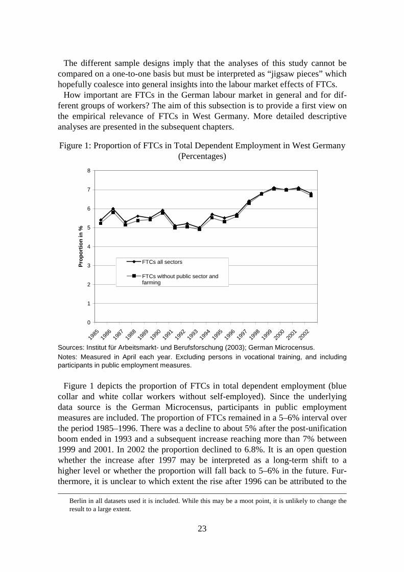
Figure 1: Proportion of FTCs in Total Dependent Employment in West Germany (Percentages)

Sources: Institut für Arbeitsmarkt- und Berufsforschung (2003); German Microcensus. Notes: Measured in April each year. Excluding persons in vocational training, and including participants in public employment measures.

Figure 1 depicts the proportion of FTCs in total dependent employment (blue

collar and white collar workers without self-employed). Since the underlying data source is the German Microcensus, participants in public employment measures are included. The proportion of FTCs remained in a 5–6% interval over the period 1985–1996. There was a decline to about 5% after the post-unification boom ended in 1993 and a subsequent increase reaching more than 7% between 1999 and 2001. In 2002 the proportion declined to 6.8%. It is an open question whether the increase after 1997 may be interpreted as a long-term shift to a higher level or whether the proportion will fall back to 5–6% in the future. Fur-thermore, it is unclear to which extent the rise after 1996 can be attributed to the

Berlin in all datasets used it is included. While this may be a moot point, it is unlikely to change the result to a large extent.

0

1

2

3

4

5

6

7

8

1985

1986

1987

1988

1989

1990

1991

1992

1993

1994

1995

1996

1997

1998

1999

2000

2001

2002

Pro

port

ion

in %

FTCs all sectors

FTCs without public sector andfarming

24

deregulation by the second Improvement of Employment Opportunities Act (see Box 1). Moreover, illustrates that omitting the public sector (where many public employment measures are implemented) as well as the farming and fishing in-dustry does not affect the overall picture of the evolution of FTCs.

Figure 2: Index of Permanent Contract and FTC Employment in West Germany– Excluding the Public Sector as well as Farming and Fishing (1995=100%)

Source: INSTITUT FÜR ARBEITSMARKT- UND BERUFSFORSCHUNG (2003); German Microcensus. Notes: Measured in April each year. Excluding persons in vocational training, and including participants in public employment measures.

Figure 2 depicts the evolution of FTC and permanent contract employment

(without public sector as well as farming and fishing) as an index with the re-spective type of employment defined as 100% in 1985. Besides the impressions (already found in ) that the increase after 1997 could be a general shift out of the range of 100–130% (corresponding to 5–6% in ) there are some basic findings with regard to the behaviour along the business cycle: FTC employment is more volatile than permanent contract employment. Focussing on the years around the German unification in 1990, there is an interesting pattern which has similarly been observed for Sweden (see HOLMLUND and STORRIE, 2002): FTC employ-ment increases earlier than permanent employment during the starting economic upturn (1985–1989), it decreases when the first indications of the end of the boom are revealed (1991–1992) and increases in the economic downturn (1993–1995) while permanent employment decreases.

The major problem with this interpretation of the figure is that the period under observation includes three law changes (May 1985, October 1996, January 2001). Hence, economic forces may be superposed by institutional changes. Un-

80

90

100

110

120

130

140

150

160

170

1985

1986

1987

1989

1990

1991

1992

1993

1994

1995

1996

1997

1998

1999

2000

2001

2002

Inde

x in

% (

1995

=100

)

PERM employmentFTC employment

25

fortunately, there is no dataset for Germany available which starts before the first law change came into force in 1985.

The German Microcensus is the only German dataset containing information on the duration of FTCs. Employees holding FTCs are asked about the duration of their current FTCs. Note that this information is fundamentally different from information on the elapsed duration of ongoing employment relationships (job tenure).13

A general methodological problem results from the fact that the distribution of ongoing spells (for example job tenure, unemployment, etc.) measured at a point in time is subject to two off-setting biases, which may either over- or underesti-mate the true distribution of the spells (SALANT , 1977 and FARBER, 1999): (1.) Spell truncation means that the observed duration of a spell is a lower bound for the completed duration because the spell has not ended at the date of the survey interview. (2.) Length-bias means that spells of short duration are less likely to be observed on any given date than longer spells, so that the observed average dura-tion of the observed spells is longer than the average duration of all spells.14

Table 1: Duration of FTCs in 1998 (Percentages) – Excluding the Public Sector as well as Farming and Fishing

Men Women Duration in

months Proportion Cumulated

Proportion Proportion Cumulated

Proportion 1 1.2 1.2 1.2 1.2 2 1.6 2.8 1.3 2.4 3 5.8 8.5 4.4 6.9 4 1.6 10.1 2.0 8.9 5 1.3 11.4 1.3 10.1

6 17.2 28.6 15.8 26.0 7–9 5.4 34.1 4.6 30.6

10–12 29.5 63.6 31.6 62.2 13–15 1.3 64.9 1.7 63.9 16–18 4.6 69.4 5.1 69.0 19–21 0.3 69.8 1.1 70.0 22–24 13.6 83.3 12.2 82.3 25–29 0.4 83.8 0.7 83.0 30–36 6.2 90.0 8.8 91.8

≥ 37 10.0 100.0 8.2 100.0

Source: German Microcensus 1998; own calculations. Notes: Measured in April 1998. Excluding persons in vocational training, and including participants in public employment measures. Weighted figures are obtained using the individual weights (inflation factors) included in the German Microcenus.

The contract duration information from the German Microcensus 1998 is not

subject to spell-truncation since persons are not asked about the elapsed duration of their job, but on the duration which is specified in their contract. Since only length-bias is relevant in this case, the following statistics should be interpreted

13 The latter is analysed in Subchapter 5.4. 14 Both types of bias will be relevant in the context of different analyses in the subsequent chapters.

26

as an upper bound for the true duration distribution of FTCs (see Table 1). Put differently, the proportion of short FTCs is relatively underestimated and the proportion of long FTCs is relatively overestimated. Table 1 indicates that there seem to be no clear-cut differences between men and women. More than 25% of all FTCs are not longer than 6 months, more than 60% of all FTCs are 12 months at most, and approximately 83% are not longer than 24 months. The remainder of about 17% of FTCs being longer than 24 months must be in accordance to spe-cial regulations for certain occupations (see Subchapter 2.2) or it is based on measurement errors since neither the Civil Code nor the Improvement of Em-ployment Opportunities Act permit FTCs to be longer than 24 months in general.

Some further descriptive statistics on the proportion of FTCs in different groups of employees are depicted in Table 2. The underlying dataset is the BIBB/IAB survey for 1998/99, which allows to distinguish between FTC workers and par-ticipants in public employment measures (see Subchapter 5.4).15 First of all, it is worthwhile noting that the proportion of FTCs according to the BIBB/IAB data-set (men: 5.2%, women: 6.7%) is very similar to what can be found with the German Microcensus for 1998 (which includes participants in public employ-ment measures) using a comparable sample definition (5.5% and 6.6%).

In the first column of Table 2 (unrestricted tenure) the proportion of FTC workers in total dependent employment is depicted. Since the probability to ob-serve workers on FTCs decreases with job tenure (Table 1 indicates that 78% of all FTCs are not longer than 2 years), it may be misleading to use this sample. FTC workers have on average a much shorter job tenure than permanent contract workers.16 Therefore, the analysis is restricted to workers with a job tenure of 2 years at most (tenure ≤2 years) in the right column of Table 2. Thus the left col-umn depicts all jobs, and the right column includes “new” jobs only.

While the proportion of FTCs seem to be almost monotonically declining with age in the unrestricted sample, the sample for tenure ≤2 years indicates no clear relationship. It suggests, very different from what is usually stated in the litera-ture (see, e.g., JAHN, 2002; OECD, 2002), that FTC employment is not a phe-nomenon which is prevalent to the youth labour market: More than 23% of male workers aged between 42 and 65 and a job tenure of 2 years at most are em-ployed on FTCs. Put differently, older male workers seem not to have a lower risk of holding a FTC when taking up a new job than younger workers. The dis-crepancy can be explained by the obvious fact that on the one hand older workers have a longer job tenure on average, and that on the other hand FTCs are usually only permitted at the start of an employment relationship. However, the fact that the common legal limitations on the use of FTCs are not applied to employees of

15 Participants in public employment measures, persons younger than 18 or older than 65 years, em-

ployees in the public sector or in the farming and fishing sector, persons in mini-jobs, persons in mili-tary or civilian service, trainees, pupils, students and pensioners are excluded (see Subchapter 5.4 for a detailed description).

16 This issue will be discussed in greater detail in Chapter 5.

27

at least 60 years during the period under observation (1998/99) is not reflected in the numbers.17 The upward shift in the proportion of FTCs for women from the age group ‘34–37’ to the age group ‘38–41’ is remarkable. This may result from women returning to work after career interruptions, e.g., due to parental leave.

Table 2: Proportion of FTCs in Total Dependent Employment in 1998/99 (Percentages)

Unrestricted tenure Tenure ≤≤≤≤ 2 years

Group of employees Men Women Both Men Women Both

All 5.2 6.7 5.8 19.4 19.7 19.5

Age group 18–21 20.8 22.1 21.3 22.9 33.0 27.0 22–25 14.6 13.5 14.1 23.6 23.8 23.7 26–29 8.2 8.4 8.3 17.1 18.6 17.7 30–33 5.1 7.3 5.9 14.2 20.0 16.5 34–37 4.1 5.9 4.7 17.7 14.5 16.4 38–41 4.6 6.9 5.5 20.0 22.9 21.4 42–45 3.6 5.8 4.4 23.5 14.8 19.1 46–49 3.8 4.8 4.2 23.8 20.9 22.2 50–53 2.8 5.0 3.7 23.5 15.4 19.5 54–65 2.5 2.8 2.6 23.7 9.2 16.7

Formal qualification

Without 10.7 10.1 10.4 24.2 26.6 25.4 Vocational training 4.7 6.0 5.2 18.2 17.6 17.9 Master craftsman 2.7 2.4 2.6 17.0 12.4 15.8

Polytechnic 4.4 5.3 4.6 15.9 12.9 15.2 University 5.1 7.7 5.8 23.3 26.7 24.5

Nationality Foreigner 9.7 10.0 9.8 23.1 22.8 23.0

German 4.9 6.5 5.5 19.0 19.5 19.2 Hours of work Part-time job 8.9 7.0 7.2 23.5 16.9 17.7 Full-time job 5.1 6.5 5.5 19.2 23.0 20.2

Kind of establishment Industry 5.6 8.5 6.3 23.9 29.0 25.4

Craft 5.9 6.3 6.0 15.7 16.5 15.9 Trade 6.7 7.7 7.3 18.9 20.1 19.6

Others (services) 7.7 6.5 7.0 17.5 16.7 17.1 Numb. of observations 11,420 7,522 18,942 1,725 1,408 3,133

Source: BIBB/IAB dataset 1998/99; own calculations. Notes: Sample as described in the text and in Chapter 5 but age 18-65. Weighted figures are obtained using the individual weights (inflation factors) included in the BIBB/IAB dataset. Part-time is defined as ≤30 hours of work per week.

In the sample for tenure ≤2 years the proportion of FTCs declines with formal

qualification with the exception of employees holding a university degree. Work-ers holding a university degree have almost the same probability to be employed on FTCs as workers without any formal qualification. In the sample with unre-stricted tenure the proportion of FTCs among workers holding a university de- 17 Due to the sample size it is not feasible to show the results for the age group of workers being at least

60 years old.

28

gree is about half the proportion of FTCs among the workers without a formal qualification. One possible explanation of the discrepancy between the samples may be that workers holding a university degree may have shorter FTC spells and may have a higher probability of getting their FTCs converted into a perma-nent one than workers without qualification.

The incidence of FTCs by nationality again depends on the sample chosen: while the sample with unrestricted tenure clearly indicates that foreigners are much more likely to be employed on FTCs, this result is less clear-cut for the tenure ≤2 years sample. This could be caused by German workers holding shorter FTCs and having a higher probability to enter into permanent contracts afterwards.

There is no clear-cut positive association between FTCs and part-time work: For women in the sample for tenure ≤2 years the proportion of FTCs among part-timers is even lower (16.9%) than among the full-timers (23.0%).18

In the BIBB/IAB survey workers are asked in quite general terms about the sec-tor of their establishment. Some numbers are shown in Table 2. A more detailed analysis on differences by industry sectors, with more reliable and detailed sector information, is presented in Subchapter 4.5. For both men and women in the sample for tenure ≤2 years the highest proportion of FTCs is in the establish-ments of the ‘industry’ sector. Approximately 25% of all workers in new jobs (tenure ≤2 years) are employed on FTCs.

Even though this is a purely descriptive analysis, which does not allow to ex-tract any causal statements, one important finding is that it may be quite mislead-ing simply to compare mean characteristics of all FTC workers with all perma-nent workers without considering the effect of differences in job tenure. This is an important result since this issue is not taken into account in most national as well as international descriptive studies on the incidence of FTC work (see, e.g., OECD, 2002).

18 In the causal analysis of Subchapter 5.7 it is, however, found that FTCs have either no significant

effect (for women) or only a moderately negative effect (for men) on working hours.

29

3 Methodological Background: Identification of the Effects of Institutions and Policy Interventions

3.1 Introduction: Estimation of Causal Effects of Binary Treatments Using Microeconometric Methods

The objective of this chapter is to provide an overview of some of the econo-metric methods used in the analyses of the subsequent chapters.19 It is shown that the underlying econometric problems are comparable and can be tackled within the same framework. In the subsequent chapters, the following questions are ana-lysed: (1.) What is the effect of the Protection Against Dismissal Law for permanent workers on the use of FTC workers (Subchapter 4.4)? (2.) What is the effect of FTCs on wages and subjective assessments of working conditions (Chapter 5)? (3.) What effect do FTCs have on employment opportunities of those unem-ployed entering into FTCs (Subchapter 6.4)?

What these questions have in common is that all institutions, policy interven-tions, or regulations which are to be analysed may be interpreted as so-called treatments (see WOOLDRIDGE, 2002: Chapter 18) implying that the so-called po-tential-outcome approach to causality may be applied (see ROY, 1951; RUBIN, 1974).20 The questions require the comparison of ‘treated’ individuals or firms with an unobserved counterfactual, i.e., a hypothetical state of the world in which the same individual or firm is unaffected by the institution, regulation, or policy intervention of interest.21 The counterfactual framework clarifies the dis-tinction between associations and causal effects. Thus the questions can be re-phrased as follows: (1.) How does firms’ use of FTCs change due to the fact that they are acting within the scope of a law leading to higher firing costs for permanent workers compared to the counterfactual situation the same firms would be outside the scope of this law? (2.) How do the workers’ wages and assessments of working conditions change due to the fact that they are employed on a fixed-term basis in comparison to be-ing employed on a permanent basis?

19 Parts of this chapter are a based on HAGEN and FITZENBERGER (2004) discussing the applicability of

microeconometric methods for the evaluation of the “Hartz Reform”. 20 Following the literature, which is strongly linked to statistics and biometrics, the terms “treatment”,

“programme”, “policy”, and “participation” are used interchangeably throughout this study. 21 Note that the approach is not limited to persons but it can also be applied to firms, regions, or indus-

tries. Nevertheless, the terms “individual” and “person” are used throughout this chapter.

30

(3.) How do employment opportunities of the unemployed change due to the fact that they enter into FTCs instead of continue searching for a job?

In recent years, the development of econometrics of evaluation of active labour market policy (ALMP) has made important contributions to methods dealing with these and similar questions.22 What follows is a presentation of methods applied in the econometric analyses of the subsequent chapters.

3.2 Basics

3.2.1 The Evaluation Problem in General and the Parameters of Interest

Besides the exact definition of what the ‘treatment’ actually is, implying the definition of the counterfactual and the choice of untreated individuals as a source of potential control groups, one has to be aware of the parameter of inter-est which is to be estimated (see HECKMAN, LALONDE, and SMITH , 1999: Sub-chapter 3.2 for a general discussion). In the evaluation literature various parame-ters are estimated. The parameter of interest in most evaluation studies is the av-erage effect of the treatment on the treated (ATT) representing the mean effect for those who actually participate in the treatment. Another parameter often esti-mated is the average treatment effect (ATE), which is the expected effect of treatment on a randomly drawn person from the population. The average effect of treatment on the untreated (ATU) measures the expected treatment effect for an individual drawn from the population of non-participants. If one finds that ATT>ATU, one can conclude that the participants are those individuals who gain the most with respect to their outcome variable.23 In the context of the method of instrumental variable estimation (see Section 3.3.3) there is another parameter in the presence of heterogeneous effects, the so-called local average treatment ef-fect (LATE). The LATE is the average treatment effect induced by variation of the instrument. Since this parameter is not relevant for the empirical analyses in the subsequent chapters, it is not discussed any further.24

What is the causal effect of a treatment 1, relative to another treatment 0, or non-treatment respectively, on an outcome variable of interest Y ?

Let Y1 be the outcome that would result if an individual was exposed to treat-ment 1, and Y0 the outcome that would result if the same individual received no

22 The starting point of the econometric literature may be the seminal work by LALONDE (1986). For

methodological surveys see HECKMAN, LALONDE, and SMITH (1999); BLUNDELL and COSTA DIAS (2002); ANGRIST and KRUEGER (1999); SMITH and TODD (2003); HUJER and CALIENDO (2001). A survey on the practical experiences with the evaluation of ALMP in Germany is provided by FITZEN-

BERGER and HUJER (2002). 23 Note that ATT>ATU implies ATT > ATE > ATU. Hence, if ATT<ATU, then also ATT < ATE < ATU.

This holds since the ATE is a weighted average of the ATT and the ATU. 24 Recently it has been shown by HECKMAN and VYTLACIL (2001) that all parameters used in the

evaluation literature are weighted versions of one parameter, the so-called Marginal Treatment Effect. This parameter is also not discussed any further.

31

treatment. { }0,1C∈ is a dummy variable indicating, whether the treatment is ac-

tually received, i.e., C=1 in case of participation. For an individual i, the actually observed employment probability is

( )0 1 0i i i i iY Y C Y Y= + − . However, the individual causal effect 1 0i iY Y− cannot be es-

timated, since an individual i can never be observed in two different states

( )1 0,i iY Y at the same point in time. Put differently, the counterfactuals ( )1 , 0i iY C =

as well as ( )0 , 1i iY C = are not observable. While estimating the causal effect for

an individual ( )1 0i iY Y− is never possible, it is possible for the mean (or other

quantities) in samples of the population (see LECHNER, 1999). As mentioned above, the parameter of interest in most evaluation studies is the

average effect of the treatment on the treated

( ) ( ) ( )1 0 1 01 1 1ATT E Y Y C E Y C E Y C= − = = = − = , (1)

which is the average effect on those who actually receive the treatment. In the application of Subchapter 6.4, for example, the ATT measures the change in the future employment prospects of unemployed individuals entering into FTCs which is caused by the fact that they actually entered into FTCs (C =1). The last term in Eq. (1) describes the hypothetical average employment probability, if the FTC workers had stayed unemployed. Of course, this term is not observable and has to be estimated using a control group of unemployed workers. Therefore, the evaluation problem can also be interpreted as a missing data problem. However, the average future employment probability of a randomly chosen unemployed worker is typically unsuitable since unemployed persons entering into FTCs and unemployed persons not entering into FTCs differ in characteristics which affect their future employment probability

( ) ( )0 01 0E Y C E Y C= ≠ = . (2)

Eq. (2) states that using the (future) outcome variable of an untreated individual as an estimate for the hypothetical situation in which a treated individual had not participated is in general not valid. The groups differ due to observable and un-observable characteristics giving rise to selection bias: the workers entering into FTCs are not a random sample of the population, but they may select themselves or may be selected on the basis of characteristics which influence their outcome (e.g., their future employment prospects).

Accordingly, the average effect of treatment on the untreated (ATU) is ( ) ( ) ( )1 0 1 00 0 0= − = = = − =ATU E Y Y C E Y C E Y C , (3)

which is the average treatment effect for an individual drawn from the population of non-participants. Obviously, the unknown counterfactual in Eq. (3) is

( )1 0=E Y C , that is, the average outcome of non-participants if they had partici-

pated. The ATE is simply the weighted average of the ATT and the ATU ( ) ( ) ( ) ( ) ( )1 0 1 0 1 0Pr 1 1 Pr 0 0ATE E Y Y C E Y Y C C E Y Y C= − = = ⋅ − = + = ⋅ − = , (4)

32

and denotes the average outcome of a person randomly drawn from the popula-tion, which is treated with the probability ( )Pr 1=C and untreated with the prob-ability ( )Pr 0C = . In the following, the estimation techniques are mainly dis-cussed for the ATT, since the estimation procedures for the ATU and the ATE are quite similar.

3.2.2 Regression: Homogeneous Versus Heterogeneous Effects and Sources of Selection Bias

In this section, the evaluation problem is illustrated in terms of regression func-tions for the more general case that panel data are available.25 For this purpose general outcome equations (invoking additive separability of the error terms) are assumed, with the individual denoted by i and the time period by t:

( )1 1 1it it itY g X U= + (5)

( )0 0 0it it itY g X U= + .

The two potential outcomes 1Y and 0Y are explained through the functions ( )1g ⋅ and ( )0g ⋅ by the vector of observable variables itX . The unobserved error terms

1itU and 0itU are independently distributed across individuals and are uncorrelated with X and ( )1 0itE U = and ( )0 0itE U = .

Furthermore, it is assumed that an individual’s decision to participate in a measure (or, for example, to take up a FTC job), can be parameterised as follows. For each individual i there is an index iIN , which is explained through a function

( )f ⋅ by observable variables iZ ( )i i iIN f Z V= + (6) with iV denoting an unobserved error term. Participation occurs if the index is larger than zero, that is,

1 if 0

0 otherwise.i i

i

C IN

C

= >=

For some methods presented in the following sections Eq. (6) is estimated by a probability model for ( )Pr 1C Z= . This is termed propensity score, selection

equation, or control function, depending on the method used and the assumptions imposed.

As described in the previous section, the observed individual outcome variable is ( )1 01it i it i itY C Y C Y= + − . Taking Eq. (5) into account this can be written as

( ) ( )*0 0 it it it it i itY g X X C Uα= + + (7)

with ( )*it itXα denoting the individual-specific treatment impact for individual i

given her or his characteristics itX :

( ) ( ) ( ) [ ]*1 0 1 0 1 0it it it it it it it itX Y Y g X g X U Uα = − = − + − . (8)

25 This section is mainly based on BLUNDELL and COSTA DIAS (2002) as well as HECKMAN (2001). The

special case of linear outcome equations is discussed in HECKMAN and ROBB (1985).

33

Eq. (8) states that the individual treatment effect is determined through ( ) ( )1 0it itg X g X− by observable differences itX as well as by differences in

unobservable variables [ ]1 0−it itU U . Since the treatment impact varies across in-

dividuals (that is, their observable and unoberservable characteristics), this is called heterogeneous treatment effect. Hence, it can be distinguished between heterogeneity of the effect with respect to observable variables (characteristics) and heterogeneity of the effect with respect to unobserved variables (characteris-tics).

The treatment effect is homogeneous, leading to the common effect model, if the following conditions are simultaneously satisfied: – There are no differences in the impact of unobserved variables (individuals’

characteristics) between the treated and untreated persons, that is,

1 0it it itU U U= = (no heterogeneity with respect to unobservables);

– ( ) ( )1 0it itg X g X− is constant with respect to itX , that is, individuals with dif-

ferent observable characteristics (old vs. young, women vs. men etc.) have the same individual-specific treatment effect.

The homogeneous (common) effect model implies that the treatment effect is the same for every individual and, therefore, ATT = ATE = ATU and the outcome Eq. (7) simplifies to ( ) *

0= + +it it it i itY g X C Uα .

Selection bias, as defined in Eq. (2) for the general case, is relevant in the re-gression model (5), if ( ) 0it iE U C ≠ , that is, the participation dummy is correlated with the error term in the outcome equation. This, in turn, can be attributed to two reasons which are not mutually exclusive (see HECKMAN, ICHIMURA, SMITH , and TODD, 1998: 1029): First, the dependency between the error term ( )1 0,it itU U in Eq. (5) and the observable variables iZ in Eq. (6), given the identity of iZ and

itX in Eq. (5) and Eq. (6), being termed selection on observables. Second, the dependency between the error terms ( )1 0,it itU U and iV , being termed selection on unobservables.

More generally, three sources for an inconsistent estimation of the treatment ef-fect can be identified:

First, there may be (as already mentioned) differences in the distribution of X variables among participants and non-participants (selection on observables). In the extreme case, for particular values or ranges of observable variables neither participants nor non-participants do exist. This is termed lack of common sup-port. For some nonexperimental approaches, such as the propensity score match-ing estimator, the common support condition is crucial: a person with particular observable X variables can be participant as well as nonparticipant with a prob-ability strictly larger than zero and smaller than 100%, that is, ( )0 Pr 1 1< = <C X .

In empirical (labour) economics many examples for lack of common support can be found:

34

– in case of the evaluation of the employment effects of a training measure for unemployed workers without formal qualification it is obviously difficult to define a reliable control group of non-participants if all unemployed persons without qualification within a particular local labour market participate in this measure;

– when estimating the productivity effects of further training on productivity at the firm level it turns out that there are hardly any larger firms which do not offer further training. Thus without further (parametric) assumptions, it may be impossible to generate a reliable control group for larger firms.

Lack of common support does not imply that treatment effects cannot be identi-fied in general. Some methods (difference-in-differences, see Section 3.4.2 and the so-called regression discontinuity design) are based on the fact that an exoge-nous policy variation (so-called natural experiments, see Section 3.2.4) induces that some persons are participants or non-participants in a measure with a prob-ability of (almost) 100%.

Even if one decides to compare treated and untreated persons only within the common support, both groups may still be different with respect to the distribu-tion of their X variables. Assuming that there are also non-participants from the training measure for unemployed in above example, participants may be younger on average, and thus may have better labour market prospects.

Second, there may be selection bias due to (unobserved) variables which are not included in the vector X, but which affect participation as well as outcome (selec-tion on unobservables).26 These variables may be unobserved since they are ei-ther not included in the dataset, or it is generally impossible or difficult to collect these variables. For example, important variables such as a person’s ability or motivation are usually not directly measurable. Taking up the example from above, one may assume that it is possible to generate a control group for the par-ticipants in training, which has, on average, the same observable characteristics (age, sex, health status, place of residence etc.) as the group of participants. Nev-ertheless, participants may be more motivated to take up a job on average and therefore more willing to invest in human capital by participating in a training measure. This example demonstrates that selection on unobservables is likely in practice. Therefore, when applying methods based on the assumption that selec-tion on unobservables is not relevant, a justification based on theoretical consid-erations is necessary.

Third, the treatment effect may be inconsistently estimated in case of specifica-tion errors in the participation Eq. (6) and/or the outcome Eq. (5). This is espe-cially relevant in case of parametric (regression) approaches. For example, cer-tain assumptions with regard to the (joint) distribution of the error terms could be incorrect. Assumptions with regard to the functional form of the equations could

26 This corresponds to the classical selection problem as addressed in the models by HECKMAN (1978,

1979).

35

be wrong, that is, the imposed ( )itg X may not correspond to the true relationship. Particularly, the heterogeneity of the effects requires a corresponding interaction of effects in parametric approaches, which may be mistakenly omitted by the re-searcher.

3.2.3 Social Experiments

Social experiments randomly choose participants from a group of people who are potential participants. This implies that the assignment to treatment is com-pletely independent of the possible outcome or the treatment effect. The group of untreated is statistically equivalent to the treated group in all dimensions except for the treatment status. Even though social experiments are not relevant for the subsequent analyses they are an interesting benchmark for non-experimental econometric approaches. First of all, the performance of non-experimental esti-mators has been checked by using experimental data.27 Second and more impor-tant, non-experimental estimators attempt to simulate experimental situations (“quasi-experimental methods”). Social experiments should not be mixed up with natural experiments, which are discussed in the following section.

3.2.4 Natural Experiments

A natural experiment is an exogenous source of (policy) variation, which causes a randomly chosen subpopulation to participate in a measure or to be within the scope of a regulation or reform, while other subpopulations do not par-ticipate or are not within the scope of the regulation or reform. The central as-sumption states that the assignment to the groups is exogenous with respect to the outcome variable (policy exogeneity). ‘Group’ may mean age-group or other demographic characteristics, region, or (as in Subchapter 4.4) establishment-size-group. By definition, the common support assumption is not given as the prob-ability of participation of non-participants equals zero. Thus methods being based on the common support condition such as propensity score matching are not suit-able in this case.

In empirical economics there are various examples for policy changes being in-terpreted as natural experiments in order to estimate causal (treatment) effects: – In the eighties, entitlement to unemployment benefit was extended for older

workers in Germany. This has been used in a couple of studies, starting with HUNT (1995), to identify the effect of unemployment benefit entitlement on unemployment duration (see Section 3.4.2).

– AUTOR (2003) assesses whether there is a causal relation between the increase of dismissal protection (in terms of decline of “employment-at-will”28) in

27 See, for example, SMITH and TODD (2003). 28 The common law doctrine of employment-at-will, which has been recognised throughout the U.S.

since 1953, rules that employers and employees have unlimited discretion to terminate their employ-

36

some federal states of the U.S. and the growth of temporary work agency em-ployment. Using the state level variation as a natural experiment within a dif-ference-in-differences framework (see Section 3.4.2), the result is obtained that the increase in firing costs explains as much as 20% of the growth of temporary employment between 1973 and 1995.

In Subchapter 4.4, a change of the employment threshold for the application of the Protection Against Dismissal Law is used to estimate the effect of firing costs for permanent workers on the establishments’ use of FTC work.

If the policy exogeneity assumption is fulfilled, natural experiments can be used straightforward by difference-in-differences estimators (see Section 3.4.2) for the estimation of treatment effects.

However, exogenous policy variations do not always generate clearly defined groups of treated and untreated individuals. Instead it may only increase the probability of participation for certain groups while the participation is also af-fected by other factors (see MEYER, 1995). In this case, natural experiments can be used within an instrumental variable approach.

3.2.5 SUTVA: Possible General Equilibrium Effects and Indirect Effects of Fixed-Term Contracts

A fundamental requirement for the validity of empirical studies based on partial equilibrium estimators is the stable unit-treatment value assumption (SUTVA; see RUBIN, 1980b and WOOLDRIDGE, 2002): there is no interference between indi-viduals leading to different outcomes depending on treatments other individuals received. In particular, the labour market situations of the control group (consist-ing of non-participants) must not be affected by the participating individuals. If the SUTVA is violated, the causal effect estimated by the partial analysis at the microeconomic level is not informative with regard to the impact on the econ-omy at large.29 In the context of the evaluation of ALMP these effects on non-participants are called indirect effects of the treatment. HECKMAN, LALONDE, and SMITH (1999: Subchapter 9.1) cite the following indirect effects: displacement effects, i.e. jobs created by one programme are at the expense of other jobs; sub-stitution effects, i.e. jobs created for a certain category of workers replace jobs for other categories because relative wage costs have changed; deadweight effects, i.e. subsidising hiring that would have occurred in the absence of the programme; tax effects, i.e. effects of taxation required to finance the programmes on the be-haviour of everyone in the society.

What does this assumption mean for the analyses at hand and what may be indi-rect effects in the context of FTCs? Obviously, the SUTVA is very likely to be

ment relationships at any time for any reason unless explicitly contracted otherwise (see AUTOR, 2003).

29 Put differently, if the SUTVA is violated the “no-treatment” benchmark is contaminated by the treatment (see HECKMAN, LALONDE, and SMITH , 1999: 2035).

37

violated in reality, a statement which is also predicted by theoretical models ex-plaining the macroeconomic impact of FTCs.30 Nevertheless, in line with previ-ous literature, the microeconometric analysis is regarded here as a complemen-tary starting-point for further analyses using other (macroeconomic or general equilibrium) methods. Nonetheless, the plausibility of the SUTVA and possible implications of its violation are discussed in the context of the analyses in the respective chapters.

3.2.6 Basic Approaches for the Generation of Control Groups

Depending on the dataset used, there are generally two different possibilities to generate the counterfactual outcome by a control group: the control group con-sists of participants prior to entering the programme or the control group consists of persons who (at least) do not participate during the treatment under observa-tion. Given these possibilities, there are three general approaches to estimate the mean counterfactual situation ( )0 1E Y C= : (1.) before-after, (2.) cross-section, or

(3.) difference-in-differences estimators (see HECKMAN, LALONDE, and SMITH , 1999). All estimators presented in the following sections belong to one of these approaches.

The applicability of the methods presented in the next sections depends on the availability of panel data or cross-section data, on the relevance of the different components of the selection bias (as previously discussed), and finally, on the researcher’s willingness to impose assumptions with respect to functional forms, distribution of error terms, and exogeneity of variables.

In Section 3.4.1, it is discussed that the before-after estimator, which in princi-ple means to compare treated persons with themselves before the treatment (treated persons serve as their own control group), is based on assumptions which may not be realistic in many cases. Therefore, one usually tries to generate the control group of untreated persons in order to apply a cross-section or a differ-ence-in-differences estimator. However, it is not necessary to impose that an un-treated person is a person that never participates. For example, it suffices to de-fine a control group in such a manner that a control individual is not treated be-fore calendar period t+1, given that the corresponding treated person participates in period t (see Subchapter 6.4).31

30 For example, BOERI (1999) predicts that re-employment chances of the unemployed are reduced by

the fact that they have to compete with FTC workers on vacancies; BENTOLILA and SAINT-PAUL (1992) indicate that FTCs increase employment stability of permanent workers; and BENTOLILA and DOLADO (1994) point to positive effects of FTCs on aggregate wages (see Subchapter 4.2).

31 To the best of my knowledge, this approach was proposed for the first time by SIANESI (2004). Ru-diments can already be found in LECHNER (1999) and BRODATY, CÉPON, and FOUGÈRE (2001). Re-cently this approach has been formalised by FREDRISKSSON and JOHANSSON (2003). LECHNER and M IQUEL (2002) show that the approach may be included in the framework of dynamic treatments and derive the identifying assumptions.

38

3.3 Evaluation Methods Requiring Cross Sectional Data

The methods presented in the following sections can be applied to the case of treated and untreated individuals being observed only for one time period. This does not imply that they are not applicable to panel data.

3.3.1 Propensity Score Matching

In recent years, propensity score matching has probably become the most popu-lar approach to the evaluation of labour market programmes.32 It is, furthermore, increasingly applied to other topics as well.33 The basic idea of matching is to match a (group of) untreated individual(s) with similar characteristics to every treated individual. The resulting control group is used to estimate the counterfac-tual outcome. In Chapter 5 propensity score matching is applied to estimate the ATT of FTCs on wages and subjective assessments of the working conditions, using a control group of permanent workers. In Subchapter 6.4, the ATT of enter-ing into FTCs from unemployment on long-term employment prospects is esti-mated using a control group of unemployed persons who do not enter into FTCs in the same months.

Basic Assumptions

In this subsection, only the estimation of the ATT is discussed in detail. The es-timation of the ATE and ATU is analogous in many respects. Whenever the esti-mation of the ATE requires further assumptions, it is mentioned explicitly.

Let X again be a vector of (pre-treatment) conditioning variables that are unaf-fected by the treatment, such as sex, age, and qualification. The statistical match-ing estimator may solve the problem of selection bias (due to differences in ob-servable characteristics) by imposing the Conditional Independence Assumption (CIA)

0 ⊥Y C X (for ATT) (9)

1 0, ⊥Y Y C X (for ATE) (10)

where ⊥ denotes independence.34 Assumption (9) for the ATT states that the out-come of the untreated individuals is independent of the participation status C, after controlling for observable variables X (see LECHNER, 1998). Assumption (10) states that the estimation of the ATE requires that the outcome variable is in both states independent of the participation status, after conditioning on X.35 The 32 See, e.g., HUJER and CALIENDO (2001). 33 For example, BLACK and SMITH (2003) estimate the effects of college quality on earnings. LECHNER

and VAZQUEZ-ALVAREZ (2003) use matching to identify the effect of disabilities on labour market outcomes.

34 The CIA is also termed ‘ignorability of treatment’ or ‘selection on observables’. 35 It actually suffices to impose the conditional mean independence assumption if one only wants to

estimate the mean ATT. This assumption is weaker than the CIA since it requires only the mean out-comes to be independent of the treatment conditional on X (see WOOLDRIDGE 2002: Subchapter

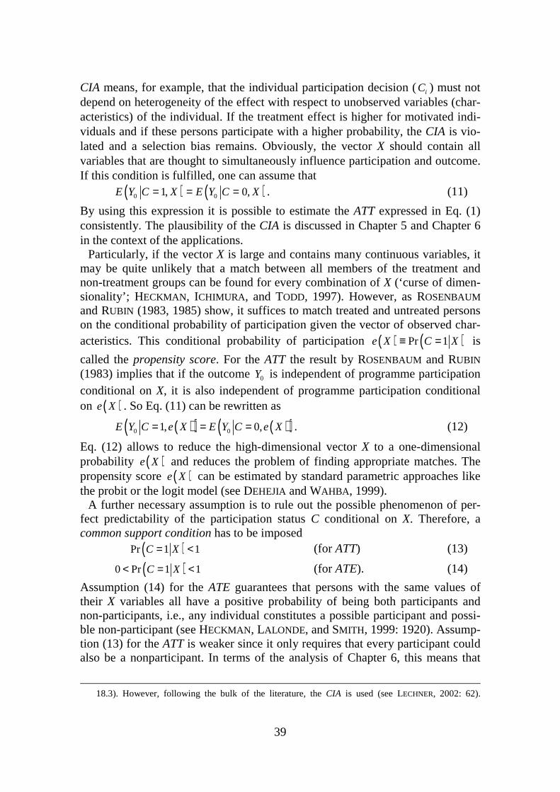
39

CIA means, for example, that the individual participation decision ( iC ) must not depend on heterogeneity of the effect with respect to unobserved variables (char-acteristics) of the individual. If the treatment effect is higher for motivated indi-viduals and if these persons participate with a higher probability, the CIA is vio-lated and a selection bias remains. Obviously, the vector X should contain all variables that are thought to simultaneously influence participation and outcome. If this condition is fulfilled, one can assume that

( ) ( )0 01, 0,= = =E Y C X E Y C X . (11)

By using this expression it is possible to estimate the ATT expressed in Eq. (1) consistently. The plausibility of the CIA is discussed in Chapter 5 and Chapter 6 in the context of the applications.

Particularly, if the vector X is large and contains many continuous variables, it may be quite unlikely that a match between all members of the treatment and non-treatment groups can be found for every combination of X (‘curse of dimen-sionality’; HECKMAN, ICHIMURA, and TODD, 1997). However, as ROSENBAUM and RUBIN (1983, 1985) show, it suffices to match treated and untreated persons on the conditional probability of participation given the vector of observed char-acteristics. This conditional probability of participation ( ) ( )Pr 1e X C X≡ = is

called the propensity score. For the ATT the result by ROSENBAUM and RUBIN (1983) implies that if the outcome 0Y is independent of programme participation conditional on X, it is also independent of programme participation conditional on ( )e X . So Eq. (11) can be rewritten as

( )( ) ( )( )0 01, 0,E Y C e X E Y C e X= = = . (12)

Eq. (12) allows to reduce the high-dimensional vector X to a one-dimensional probability ( )e X and reduces the problem of finding appropriate matches. The propensity score ( )e X can be estimated by standard parametric approaches like the probit or the logit model (see DEHEJIA and WAHBA , 1999).

A further necessary assumption is to rule out the possible phenomenon of per-fect predictability of the participation status C conditional on X. Therefore, a common support condition has to be imposed

( )Pr 1 1C X= < (for ATT) (13)

( )0 Pr 1 1C X< = < (for ATE). (14)

Assumption (14) for the ATE guarantees that persons with the same values of their X variables all have a positive probability of being both participants and non-participants, i.e., any individual constitutes a possible participant and possi-ble non-participant (see HECKMAN, LALONDE, and SMITH , 1999: 1920). Assump-tion (13) for the ATT is weaker since it only requires that every participant could also be a nonparticipant. In terms of the analysis of Chapter 6, this means that

18.3). However, following the bulk of the literature, the CIA is used (see LECHNER, 2002: 62).

40

every individual entering into a FTC could, given her or his characteristics, in general also have stayed unemployed in order to keep on searching. In Chapter 5, this means that every FTC worker could in principle also hold a permanent con-tract.

In concrete terms, propensity score matching estimators work as follows. In the first step, a probability model is used to explain the participation status C by the vector X (possibly including interaction terms and polynomials of X). Subse-quently, for each person (that is, for treated and untreated persons) the propensity score ( )e X is predicted using the estimated equation from the first step. Follow-

ing the literature, the predicted linear index rather than the predicted conditional probability is used in both analyses of Chapter 5 and Chapter 6 (see LECHNER, 1998). The reason for this is that individuals in the tails of the distribution can be distinguished more exactly. Nevertheless, to simplify matters the term ‘propen-sity score’ is also used for the predicted linear index in the following. In the third step, for each person i from the treatment group, a (group of) comparable un-treated person(s) is matched. Matches are constructed on the basis of a neighbourhood ( )ie� , where ie is the estimated propensity score for a treated

person i. Let 0N denote the number of observations in the subsample of the un-treated, and 1N the number of observations in the subsample of the treated. Then the individuals in the untreated subsample who are neighbours to i, are individu-

als { }0j C∈ = for whom ( )j ie e∈� , i.e., the set of persons ( ){ }i j iA j e e= ∈� .

The effect of the treatment for each observation i in the treatment group is esti-mated by subtracting the weighted average of the outcome of the untreated group observations from the outcome of the treatment observation i (see HECKMAN, LALONDE, and SMITH , 1999). Hence, the ATT is estimated by

( )01

1 01 11

1,

NN

i ji j

Y w i j YN = =

−

∑ ∑ . (15)

Different matching estimators differ in the weights ( ) [ ], 0,1w i j ∈ (with

( )0

1

, 1N

j

w i j=

=∑ ), which are associated to the members of the control group and in

the way the neighbourhood is defined. Basically, there is a negative association between ( ),w i j and i je e− . The more dissimilar j is to i, in terms of the esti-

mated propensity scores, the smaller is the associated weight ( ),w i j of the con-

trol individual j. The extreme case is nearest neighbour matching (see next sub-section), where only one nearest neighbour in terms of the estimated propensity score is used as a control for one treated person, that is, ( ),w i j is either 1 or 0.

Asymptotically all matching estimators produce the same results, because in an arbitrarily large sample they all compare only exact matches (see BLACK and SMITH , 2003). “In finite samples, different matching estimators produce different estimates because of systematic differences between them in which observations

41

they assign positive weight, how much weight they assign them, and how they handle (implicitly) the support problem.” (BLACK and SMITH , 2003: 17). This is also found here: In the application of Subchapter 6.4, nearest-neighbour matching seems to generate the most reliable results, while the analyses in Chapter 5 seem to be in favour of kernel-based matching.

Nearest-Neighbour Matching

Nearest-neighbour matching (NN-matching) defines the neighbourhood iA of the treated individual i in such a way, that only the untreated j is selected as a control individual that is closest to i in terms of ie and je :

{ }{ }01,...,

mini i jj N

A j e e∈

= − , (16)

where is a metric measuring the distance between ie and je . Eq. (16) states that the unemployed worker j with the value of je that is nearest to ie , is selected as a match and is defined as a control for the treated (FTC worker) i. The weight

( ),w i j =1 is attached to this selected control, i.e., there is only one control per treated individual.

NN-matching can either be performed with or without replacement. With re-placement means that each untreated individual can serve as a control for more than one treated individual. This can improve the matching quality, but it in-creases the related standard error of the estimated effect, which has to be consid-ered when estimating the standard errors (see the subsection below for the calcu-lation of the standard errors). In order to reduce the risk of ‘bad matches’, a modified version of NN-matching, called ‘caliper matching’, can be used (see COCHRAN and RUBIN, 1973). For a pre-specified level of tolerance 0Ψ > (cali-per), the treated individual i is matched to the untreated individual j so that:

i je e− < Ψ . (17)

If none of the untreated persons is within the interval (caliper) Ψ around the treated individual i, the individual i is left unmatched and is not used for the es-timation. This is one possible method for imposing the common support condi-tion (see subsection below for a discussion of this issue).

Kernel-Based Matching Approaches

Simple NN-matching uses only a fraction of the information on the untreated individuals, as only one untreated individual is matched to one treated individual. Therefore, it is associated with a loss of efficiency (see FRÖLICH, 2004). In the extreme case, kernel-based matching estimators construct matches by calculating weighted averages of the outcomes of all individuals in the sample of untreated (within the common support), with the weights depending on the similarity of the treated and the untreated individuals in terms of distance between ie and je . Thus the variance of the estimate is reduced (efficiency gain), which may, however, be associated with an increased bias (imbalance in observable characteristics). In

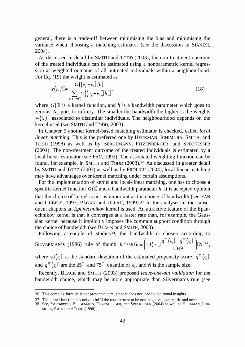
42

general, there is a trade-off between minimising the bias and minimising the variance when choosing a matching estimator (see the discussion in SIANESI, 2004).

As discussed in detail by SMITH and TODD (2003), the non-treatment outcome of the treated individuals can be estimated using a nonparametric kernel regres-sion as weighted outcome of all untreated individuals within a neighbourhood. For Eq. (15) the weight is estimated as

( )( )( )

( )( )( )0

,j i

j ik C

G e e hw i j

G e e h∈ =

−=

−∑ , (18)

where ( )G ⋅ is a kernel function, and h is a bandwidth parameter which goes to zero as 0N goes to infinity. The smaller the bandwidth the higher is the weights

( ),w i j associated to dissimilar individuals. The neighbourhood depends on the kernel used (see SMITH and TODD, 2003).

In Chapter 5 another kernel-based matching estimator is checked, called local linear matching. This is the preferred one by HECKMAN, ICHIMURA, SMITH , and TODD (1998) as well as by BERGEMANN, FITZENBERGER, and SPECKESSER (2004). The non-treatment outcome of the treated individuals is estimated by a local linear estimator (see FAN, 1992). The associated weighting function can be found, for example, in SMITH and TODD (2003).36 As discussed in greater detail by SMITH and TODD (2003) as well as by FRÖLICH (2004), local linear matching may have advantages over kernel matching under certain assumptions.

For the implementation of kernel and local-linear matching, one has to choose a specific kernel function ( )G ⋅ and a bandwidth parameter h. It is accepted opinion

that the choice of kernel is not as important as the choice of bandwidth (see FAN and GIJBELS, 1997; PAGAN and ULLAH , 1999).37 In the analyses of the subse-quent chapters an Epanechnikov kernel is used. An attractive feature of the Epan-echnikov kernel is that it converges at a faster rate than, for example, the Gaus-sian kernel because it implicitly imposes the common support condition through the choice of bandwidth (see BLACK and SMITH , 2003).

Following a couple of studies38, the bandwidth is chosen according to

SILVERMAN ’s (1986) rule of thumb ( ) ( ) ( )25 750.20.9 min sd ,

1.349i i

i

q e q eh e N− −

= ⋅ ⋅

,

where ( )sd ie is the standard deviation of the estimated propensity score, ( )25iq e

and ( )75iq e are the 25th and 75th quantile of ie , and N is the sample size.

Recently, BLACK and SMITH (2003) proposed leave-one-out validation for the bandwidth choice, which may be more appropriate than Silverman’s rule (see

36 This complex formula is not presented here, since it does not lead to additional insights.

37 The kernel function has only to fulfil the requirement to be non-negative, symmetric and unimodal. 38 See, for example, BERGEMANN, FITZENBERGER, and SPECKESSER (2004) as well as HECKMAN, ICHI-

MURA, SMITH , and TODD (1998).

43

also FRÖLICH, 2004). The basic idea of leave-one-out validation is to leave an untreated observation out and to minimise the forecast error in out-of-sample predictions of the untreated observation left out (see PAGAN and ULLAH , 1999). In Chapter 5, this approach turns out to be not feasible due to computational rea-sons.

Mahalanobis Distance

In previous empirical research the so-called Mahalanobis distance has fre-quently been used as a method of matching on additional variables besides the predicted propensity score (see, for example, LECHNER, 1999; HUJER, MAURER, and WELLNER, 1998). Using variables (a subset of conditioning variables in-cluded in X which are assumed to be important) in addition to the predicted pro-pensity score may decrease the selection bias, and may function as an additional protection against any impact due to inconsistent estimation of the propensity score. The propensity score in combination with the additional variables is termed balancing score ( )b X (see ROSENBAUM and RUBIN, 1983). Matching on the balancing score is performed using the Mahalanobis distance (see RUBIN, 1980a), which is again a method of obtaining a one-dimensional measure of simi-larity. Again, NN-matching as well as different kernel-based matching estimators are applicable.

Imposing the Common Support Condition

Unlike parametric estimators, the consistency of matching crucially depends on the common support condition. In case of propensity score matching the condi-tion requires the distribution of the estimated propensity of the treated 1e to be entirely overlapped by the distribution of the propensity score of the untreated

0e . For example, in case of the analyses of Chapter 6, this means that for every unemployed person entering into a FTC a sufficiently similar person (in terms of the estimated propensity score) staying unemployed in the same calendar month has to be available.

Usually there are two approaches to the problem of lacking common support (see LECHNER, 2001a): Either matching is performed only for the sub-population within the common support, or the problem is simply ignored. In case of NN-matching the latter may imply using untreated neighbours who are very different from the treated individuals. This approach can obviously lead to biased esti-mates due to ‘bad matches’. Although the first approach is appropriate for obtain-ing a consistent estimate for the region of common support (i.e., the region of the distribution in which each treated individual is juxtaposed to a sufficiently simi-lar untreated individual in terms of the propensity score), it may be misleading: “When treatment effects are heterogeneous inside and outside the common sup-port, then the estimated effect does no longer correspond to the original parame-ter of interest.” (L ECHNER, 2001a: 21). Otherwise, if the treatment effect is ho-

44

mogeneous at least within the treatment group, no additional problems appear besides the loss of information and thus loss of efficiency of the estimator (see BLUNDELL and COSTA DIAS, 2000).

In concrete terms, the following approaches are used to impose the common support condition represented in Eq. (13) and Eq. (14): – The treatment observations whose estimated propensity score is higher than

the maximum or less than the minimum estimated propensity score of the controls are dropped.

– Using caliper matching: Imposing a caliper, that is, dropping treated observa-tions for which no sufficiently similar controls can be found, is a way of im-posing the common support.

– Choosing a kernel which does not have a positive density over the whole real line, that is, a kernel which is zero outside a neighbourhood of the origin. This is true for the Epanechnikov and the Triangle kernel but not for the Normal kernel.

Further approaches, not being applied in this study, can be found in LECHNER

(2001a) and HECKMAN, ICHIMURA, SMITH , and TODD (1998).

Obtaining Standard Errors

In order to test the statistical significance of the estimated treatment effects, standard errors have to be computed. A potential difficulty arises from the fact that the estimated variance of the treatment effect should also include the vari-ance due to the estimation of the propensity score and the imposition of the common support. A possible solution to the problem is calculating the variance based on bootstrapping (see LECHNER, 2002).39 Each bootstrap draw includes a re-estimation of the propensity score, imposing the common support, and (in case of kernel-based matching) the re-calculation of the optimal bandwidth.

The method of bootstrapping is a popular re-sampling method used to estimate, inter alia, standard errors in case analytical estimates are biased or even unavail-able. The basic idea can be described for a sample mean as follows (see BROWN-

STONE and VALLETTA , 2001): The mean of an observed sample typically differs from the mean of the underlying population due to sampling errors. The sampling distribution (including the standard error) summarises how the sample means would vary, if a large number of samples were drawn from this population. Now, the essential idea is to assume that the observed sample is the population and to draw (bootstrap) samples from this approximate population (which is actually the sample) to estimate the sampling distribution. The bootstrap samples are drawn from the observed dataset (sample) with replacement, and the mean is computed for each boostrap sample. Thus drawing N bootstrap samples leads to N esti-

39 For kernel matching estimators, HECKMAN, ICHIMURA, and TODD (1998) present analytical formulae

for the estimation of the variance. To the best of my knowledge, this has not been used in applied work so far, possibly due to complexity.

45

mated means. The distribution of these means approximates the sampling distri-bution (and thus the standard error) of the population mean. In case of kernel-based matching estimators of Chapter 5, this bootstrap approach is adopted.

The obvious practical problem is that bootstrapping is very time-consuming. In case of 500 draws (which seems to be rather a lower limit in the literature), all estimation steps described above have to be repeated 500 times. Therefore, in the analysis of Subchapter 6.4 boostrapping turns out to be infeasible. For the esti-mated ATT by NN-matching, the following formula may be applied (see HUJER, CALIENDO, and THOMSEN, 2003 as well as LECHNER, 2001b):

( ) ( )( )

( )

02

11 02

1 1

11 0

N

jjVar ATT Var Y C Var Y C

N N

ω== = + =∑

, (19)

which takes into account that matching with replacement is performed, i.e., an untreated individual can serve for more than one treated individual as a control.

jω denotes the number of times an untreated person is used as a control. As men-

tioned above, the variance increases with ω . When using Eq. (19), independent observations, fixed weights, and homoskedasticity of the outcome variable within the treated and the control group have to be assumed. Furthermore, the variance is assumed not to depend on the fact that the propensity score is estimated and that the estimated probabilities are applied to a reduced sample due to the com-mon support condition. Using Eq. (19) may be justified by the result that there seems to be little difference between the bootstrapped variance and the variance calculated using this formula (see LECHNER, 2002).

Estimating Heterogeneous Effects Using Propensity Score Matching

It is quite straightforward to estimate heterogeneous treatment effects with re-spect to observable variables X. Note that this corresponds to simple interactions between X variables and the treatment dummy within a regression approach. In general, there are three different valid approaches used in applied studies: (1.) one may perform the whole analysis (the estimation of the propensity score as well as the matching) completely separate for each subgroup (applied in Chapter 5); (2.) one may use the whole sample, but may include subgroup dummies in the mahalanobis distance and thus imposing that only individuals within the same group are matched (applied in Subsection 6.4.6.3); (3.) one may first do the whole analysis for the whole sample and afterwards estimate regressions with interaction effects on the matched sample.

3.3.2 Parametric Regression Methods Versus Matching

As indicated in Section 3.2.2, using parametric methods may be associated with some drawbacks in comparison to propensity score matching methods (see, e.g., BLACK and SMITH , 2003):

46

(1.) regression models often impose the assumption of a linear functional form and linear additive (common) effects; (2.) regression models can be estimated in areas without common support by their functional form assumptions. Put differently, parametric models conceal the common support problem and may lead to results which are not justified by the underlying data; (3.) estimating regression equations requires ( ), 0E U X C = , while matching only

needs ( ) ( )1 0, 1 , 0E U X C E U X C= = = .

However, arguments (1.) and (2.) are not conclusive against regression meth-ods. A linear model can approximate non-linear functional forms to a large de-gree by using higher order and interaction terms (see WOOLDRIDGE, 2002: 612). Furthermore, the estimation could be restricted to the common support. The area of common support is, however, harder to be defined without a propensity score.

Point (3.) is a remaining advantage of matching methods over regression analy-ses: The dependency of C (and X) with the error term U does not have to be zero as in regression analysis, but it has to be the same in the treatment and control group. Put differently, matching does not require the absence of selection bias (selection on unobservables), but the selection bias to be balanced in the treat-ment and the control group conditional on X. Furthermore, assuming that the de-pendency between X and U is balanced in the treatment and the control group by the matching estimator, one can use conditioning variables which would be cor-related with the error term in a parametric regression model (see LECHNER, 1998). In Chapter 5 and Subchapter 6.4, this property is repeatedly used to justify the CIA and the application of propensity score matching.

3.3.3 Instrumental Variable Approaches and Selection Models

The approaches addressed in the following may eliminate bias due to selection on unobservables without the necessity of panel data to be available. In ex-change, exogeneity assumptions and/or assumptions on the (joint) distribution of error terms have to be imposed, which are partly untestable. Since the application of these approaches does not yield reasonable and presentable results in Chap-ter 5, only the basic idea is presented.

All Instrumental Variable (IV) approaches (and selection models, see below), are based on the assumption that there is at least one IV *Z , which affects par-ticipation (C), but has no direct effect on the outcome (Y). There is an analogy between IVs and experiments: As flipping a coin in case of an experiment deter-mines participation but not the outcome, an IV affects C but not Y. For the exam-ple of a linear model, the following two conditions are prerequisites for a variable

*Z to be a suitable IV:

( ) ( )* *Pr 1 , Pr 1 , 'C X Z z C X Z z= = ≠ = = (20)

47

where z and 'z are two values of *Z . The assumption of Eq. (20) simply states that changes in the value of *Z (which must have at least two values z and 'z ) must affect the conditional participation probability. The condition

( ) ( )*, , ,E U X Z C E U X C= , (21)

requires that *Z is unrelated to the error term in the outcome equation(s), condi-tional on the included observable variables X. Thus the only way *Z is allowed to affect the outcomes is through the participation status (exclusion restriction). In practice, it turns out that it is often difficult or even impossible to find reliable exclusion restrictions. In case of the analyses of Chapter 5, one needs an IV af-fecting the probability of holding a FTC (instead of a permanent contract) but not wages. Recent literature states that valid IVs are generated by natural experi-ments (see ANGRIST and KRUEGER, 2001). In Chapter 5, the reverse direction of the reform of the Protection Against Dismissal Law (lowering the employment threshold) as discussed above, is used as an IV (which, however, turns out to be not suitable as it is not sufficiently correlated with the endogenous variable).

Selection models and switching regression models are akin to IV methods. An important result is found by VYTLACIL (2002). He shows that the non-parametric identification of selection models and instrumental variable models require ex-actly the same assumptions and, hence, both models identify the same causal ef-fect. Non-parametric selection models and instrumental variable models are iden-tical.

3.4 Evaluation Methods Requiring Panel Data

If longitudinal data are available, that is, individuals are observed for at least one period before and one period after the treatment, there are more possibilities to estimate the hypothetical outcome of non-treatment for the treated. Assuming that the error term can be additively decomposed into a (time invariant) individ-ual-specific effect ia , a common macroeconomic time effect tθ , and a random individual effect itε (classical error term), Eq. (5) can be re-written as

( ) ( ) ( )1 01it i it i it i t itY C g X C g X a θ ε= + − + + + . (22)

3.4.1 Before-After Estimator

The basic principle of this approach is to use the pre-treatment outcome as an estimate for the unobserved counterfactual outcome of the participants in case of nonparticipation by differencing out the unobserved individual effects ia . The approach can be interpreted as a fixed-effects estimator. To simplify matters, only two time periods are assumed in the following: t´ denotes the period before and t the period after the treatment.40 The identifying assumption is (see HECKMAN, LALONDE, and SMITH , 1999: 1892)

40 A generalisation is straightforward and does not lead to additional insights.

48

( )0 0 1 0t tE Y Y C′− = = . (23)

If this is valid, the before-after estimator is given by

( )1 0 1t t CY Y ′ =

− (24)

where C=1 means, that only individuals are taken into account which participate between t´ and t, and the bar denotes sample means. The individual treatment effect for every individual i may be written as ( ) ( )1 0 1 0 0 0it it it it it itY Y Y Y Y Y′ ′− = − + − . (25)

The last term ( )0 0it itY Y′ − is the bias of the estimated individual effect, which

stems from the fact that one assumes ( ) ( )0 01 1t tE Y C E Y C′= = = . The assumption

is valid, if the expected value of ( )0 0it itY Y′ − is zero. The assumption is not ful-

filled, if macroeconomic conditions affecting Y change between t´ and t (that is, if there is a time-specific intercept tθ ), or if the participation (which takes place

between t´ and t) already affects 0tY ′ (anticipatory effects).

The following example highlights a situation in which the before-after estima-tor leads to biased results. Assume one wants to evaluate the effects of FTCs on the workers’ subjective assessments of their career opportunities. Assume, fur-thermore, that workers hold permanent positions in t´ and FTCs in t. If macro-economic conditions get worse between and t´ and t (which negatively affects career opportunities), the career opportunities in t´ are obviously not a valid esti-mate of the counterfactual of the career opportunities in t.

Anticipatory effects are relevant for the before-after estimator as well as the dif-ference-in-differences estimator, described in the next section. It has been ob-served in a number of studies, that, shortly before participating in a certain train-ing programme, earnings and employment situations of the future participants deteriorate, which has been termed “Ashenfelter’s Dip” (see HECKMAN and SMITH 1999; FITZENBERGER and PREY 2000; BERGEMANN, FITZENBERGER, and SPECKESSER 2004).41 Usually, this transitory decline in employment probabili-ties and wages of participants is explained by anticipatory effects: In expectation of participation, search activities are reduced, leading on average to reduced em-ployment probabilities and wages. In either case, this implies that the outcome of the treated in t´ is (even conditional on X) not a valid estimate of the hypothetical outcome in t in case of non-participation, that is, ( ) ( )0 0, 1 , 1t tE Y X C E Y X C′= ≠ = .

Not only are anticipatory effects relevant in case of ALMP measures, but also for policy changes in general. For example, rational employers may try to take an-nounced changes of dismissal protection legislation into account by adjusting their hiring and firing decisions. A possible solution is to define t´ in a way, that the period of time between t´ and the start of the treatment is longer (see BERGE-

MANN , FITZENBERGER, and SPECKESSER, 2004).

41 This phenomenon was observed for the first time by ASHENFELTER (1978) for the earnings effects of

a training programme.

49

Although the before-after estimator is not reliable in many situations, it has some advantages: non-participants are not required since it suffices to have in-formation on participants and their pre-participation histories, implying that the common support condition has not to be fulfilled in a strict sense.

3.4.2 Difference-in-Differences Estimator

The difference-in-differences (DiD) estimator is based on panel data, and can be applied without invoking strong assumptions, if there are exogenous policy changes (natural experiments, see Section 3.2.4). The DiD estimator can again be applied as a simple difference in means, but also within a regression framework. Furthermore, propensity score matching may be combined with the DiD estima-tor. The DiD approach estimates the treatment effect as the difference between the change of the outcome variables of the treated over time and the change of the outcome variable of the untreated over time. Here, only the more relevant DiD estimator is presented, which conditions on X. Assuming that, conditional on X, the change in the non-treatment outcome of the treated equals the change of the non-treatment outcome

( ) ( )0 0 0 0, 1 , 0t t t tE Y Y X C E Y Y X C′ ′− = = − = , (26)

the ATT can be estimated as ( ) ( ) ( ) ( )1 1 1 0| 1, | 1, | 0, | 0,t t t tE Y C X E Y C X E Y C X E Y C X′ ′ = − = − = − = . (27)

This is also true in presence of (time invariant) unobserved heterogeneity and all kinds of heterogeneity of the treatment effect.

The assumption in Eq. (26) is less restrictive as in case of the before-after-estimator since also (macroeconomic) time effects tθ , equally affecting the out-come of both groups, can be differenced out. Hence, the DiD estimator elimi-nates both unobserved fixed individual effects ia as well as unobserved fixed time effects tθ .

The DiD approach can also be used within (parametric) regression models (see MEYER, 1995).42 A seminal example for the application of the DiD approach within a hazard rate model for the analysis of unemployment duration is the study by HUNT (1995).43 She analyses the effects of unemployment benefit on unemployment duration by interpreting the extension of unemployment benefit entitlement for older workers in the eighties as a natural experiment. The group of untreated individuals are younger unemployed which are not (directly) af-fected by the reform. The effect is the difference in the change of the hazard rate over time between treated and untreated unemployed persons. The hazard rate from unemployment ( )tλ is (represented in a simplified way) specified as

42 Note that this may be interpreted as a reduced form IV approach (see ANGRIST and KRUEGER, 2001). 43 This study was an impetus for more microeconometric research on the effects of the unemployment

insurance in Germany (see, for example, STEINER, 1997; HUJER and SCHNEIDER; 1996, 1998). A hazard rate model for the analysis of unemployment duration will be presented in Subchapter 6.3.

50

( ) ( ) [ ]0 1 2 3 4exp tt t X after C after Cλ λ β β β β= + + + × (28)

where after is a dummy variable which is one after the reform and zero other-wise. The participation dummy C is one for the age group of older unemployed affected by the reform, after C× is an interaction effect, and X are characteristics of the unemployed and further explanatory variables. Since the analysis results in a significantly negative estimate of 4β , one may conclude that the reform has led to a lower hazard rate and, therefore, a longer unemployment duration for the older unemployed. Of course, the simplified parametric specification in Eq. (28) may lead to biased results as the heterogeneity of the effect is not taken into ac-count.44

In case the analysis is not based on a natural experiment, that is, the assignment to the treatment or non-treatment group is not exogenous, the DiD approach is only valid, if conditioning on X eliminates the bias due to selection on observ-ables. Furthermore, selection on unobservable must be time constant and linear-additive in order to be differenced out.

The DiD approach is inconsistent if, – 0tY ′ is affected by anticipatory effects (Ashenfelter’s Dip; see previous sec-

tion); – treated and untreated individuals are affected in a different way by (unob-

served) macroeconomic shocks tθ .45 For example, the hazard rate of older

unemployed may be affected by the business cycle in a different way as younger unemployed;

– the policy is endogenous.46

3.5 Pre-Program Test

If the pre-treatment values of the outcome variable ( )1 0,′ ′t tY Y are available in the

dataset, it is possible to test to which extent the approach used is able to eliminate selection bias. The “Pre-Program test”, proposed by HECKMAN and HOTZ (1989), is based on the consideration that, if there is no selection bias left, there are no significant differences between the mean outcome variables of the group of treated and the group of controls before the start of the treatment (t´). Put dif-ferently, the ATT (or the treatment effect in general) before the treatment should be zero. In case of matching methods, one can test the null hypothesis that

44 Further critique of HUNT’s (1995) study with respect to the policy exogeneity has been expressed by

EISEN (1997). 45 BLUNDELL and COSTA DIAS (2002: 29) propose an adjustment method for this case. 46 Further reasons for inconsistency are presented in MEYER (1995) as well as BLUNDELL and COSTA

DIAS (2002).

51

( ) ( )1 0| 1, | 1,′ ′= = =t tE Y C X E Y C X , that is, � ( ) 0′ =tATT X .47 However, this test is

obviously unsuitable, if anticipatory effects are relevant. Not all studies are based on panel data or have information on the pre-

programme outcome variable (see, for example, BLACK and SMITH , 2003). In this case, however, evaluating programmes or interventions by non-experimental econometric techniques based on untestable assumptions, such as the CIA, is “an act of faith” (HECKMAN, 2001: 718), since there is no possibility to get an idea of the reliability of the assumptions. This problem has to be faced in Chapter 5.

3.6 Summary

The empirical questions raised in the introduction to this chapter are addressed in the following analyses. Subchapter 4.4 analyses whether there is a causal rela-tionship between firing costs for permanent positions and the firms’ use of FTC workers (and other types of atypical work) by using the change in the threshold level for the application of the Protection Against Dismissal Law as a natural ex-periment within a difference-in-differences framework.

Chapter 5 applies (mainly kernel-based) propensity score matching estimators to estimate the causal effects of FTCs on wages and subjective assessment of working conditions by using a control group of permanent workers as an estimate of the counterfactual. Furthermore, some attempts are made taking selection on unobservables into account by using a further change in the Protection Against Dismissal Law as an instrumental variable. This, however, turns out to be unsuc-cessful.

Subchapter 6.4 uses NN-matching estimators to identify the causal effects of entering into a FTC from unemployment on future employment prospects (in permanent jobs), by generating a control group of unemployed who have not yet entered into a FTC. The corresponding propensity score is estimated by a hazard rate model for the transition from unemployment to FTC jobs.

47 In case of regression methods the test can be performed by including a dummy variable, which is one

for treated individuals before the treatment and zero otherwise. The estimated coefficient can be in-terpreted as remaining selection bias.

52

4 The Role of Fixed-Term Contracts in Labour Demand

4.1 Overview: Why Do Firms Use Fixed-Term Contracts?

In this chapter, the role of FTCs in firms’ labour demand decisions is analysed. From the employers’ point of view, the most relevant differences between fixed-term and permanent contracts are not only the lower firing costs, but also the higher turnover rate of FTC workers. The latter may stem from the fact that many FTCs are not converted into permanent contracts, and hence imply worker out-flows as well as a higher quit rate of FTC workers, as they anticipate their higher unemployment risk. Thus using FTCs forces firms to engage in search for new workers more often, creating costs that have to be weighed against the advantage of low firing costs (see HOLMLUND and STORRIE, 2002).

In the course of this chapter, it is emphasised that it is essential to differentiate between job flows (or job turnover, respectively) on the one hand and worker flows (or worker turnover, respectively) on the other hand. Job flows refer to changes in the number of filled jobs within a firm reflecting expansions and con-tractions. Worker flows refer to the flow of workers through those jobs.

In the literature, several reasons have been identified that may render FTC work and other types of temporary work profitable for firms. Following VAREJÃO and PORTUGAL (2003), all these reasons can be, at least loosely, attributed to one of the following three roles: – FTCs are used as a buffer stock, that is, as an adjustment instrument to cope

with demand or productivity shocks; – FTCs are used as a screening device (prolonged probationary period), in pres-

ence of asymmetric information on the worker’s ability (productivity); – FTCs are used as a substitute for a certain proportion of permanent workers.

Job positions that are inherently permanent are (repeatedly) filled by FTC workers. Jobs are inherently permanent, if they are filled with permanent con-tract workers in the (unobserved) hypothetical situation in which no FTC workers are available.48

The reasons can be summarised as follows. They are discussed in greater detail in subsequent sections and chapters. (1.) Firms can use temporary employment to adjust more efficiently to tempo-rary demand fluctuations. Similar to overtime work, temporary workers are used more frequently during booms and fewer during recessions (see Section 4.2.3). Furthermore, if employers are uncertain about whether a rise in demand is tem-

48 VAREJÃO and PORTUGAL (2003) use the term “churning” for substitution. Since the term churning is

used in Subchapter 4.5 in a related but not identical meaning, the term “substitution” is preferred throughout this study.

53

porary or permanent, they may be reluctant to increase the number of permanent workers, but rather rely on temporary workers until the economic outlook be-comes more certain. Temporary work serves as a buffer stock or means of ad-justment. (2.) By employing temporary work, firms may insulate their permanent work-force from the effects of changing product demand conditions. This insulation may help firms to reduce firing costs and secure firm-specific human capital. It may also be used to obtain wage and work rule concessions from permanent workers in exchange for greater employment stability (see BÜRKLE, 2004; BEN-

TOLILA and DOLADO, 1994). Again, temporary work serves as a buffer stock. (3.) If asymmetric information on the ability (and therefore productivity) of applicants and workers is relevant, and matches are experience goods (JOVANO-

VIC, 1979), firms may use a temporary job as a prolonged probationary period for screening prospective permanent employees. The effect of asymmetric infor-mation on workers’ and applicants’ productivity is discussed in greater detail Subchapter 5.2. (4.) It may be an optimal equilibrium phenomenon to have a substitution strat-egy, that is, to substitute a certain proportion of permanent workers by FTC workers, independent of the business development (see VAREJÃO and PORTU-

GAL, 2003). Job positions that are inherently permanent (for example, cashiers) are repeatedly filled by FTC workers in order to reduce labour costs, given that wages for temporary workers are lower (see Chapter 5), or that wages (or fringe benefits, or days of holiday entitlements) rise automatically with age or job ten-ure (such as in the public sector). This incentive is enhanced by the fact that peri-ods of notice also depend on age and job tenure (see Subchapter 2.2). However, such a substitution strategy by the firm can obviously only be optimal in case of jobs with sufficiently low hiring costs and jobs with low requirements for firm-specific human capital. (5.) According to empirical findings, search costs borne by the employer in-crease with labour market tightness (see, e.g., BURGESS, 1988). Furthermore, job-to-job worker mobility increases with a better state of the labour market. A tighter labour market makes it relatively more advantageous to hire workers on permanent contracts since permanent contracts avoid to some extent worker quits that are more costly when workers are more difficult to find (see WASMER, 1999; HOLMLUND and STORRIE, 2002). (6.) Assuming imperfect information on the workers’ effort, shirking can be avoided by paying efficiency wages to permanent workers and by relating the probability of conversion or renewal of FTCs to the productivity of FTC workers (see GÜELL, 2000 and Subchapter 5.2). Again, it may be an optimal equilibrium strategy to fill permanent positions by temporary workers. Furthermore, if work-ers exhibit career concerns, they may increase their effort and thus their output (given their wages) in order to get their contract renewed (see Subchapter 5.2). Even if employers were not interested in finding out the true ability of the work-

54

ers, initial FTCs may increase productivity since workers on FTCs are willing to spend more effort. (7.) Again, assuming asymmetric information on ability, workers on FTCs may deter from asserting their rights, such as parental leave, since taking up their claims may be interpreted as low ability by the employer which, in turn, leads to a lower conversion probability. The reason is that a loss of work experience due to parental leave affects wages of high-ability workers relatively more than wages of low-ability workers. Hence, loss of work experience is associated with higher opportunity costs for high-ability workers.49 To my knowledge, this ar-gument has never been brought forward yet, but it may be an explanation why FTCs seem to have an adverse effect on fertility in Spain (see DOLADO, GARCÍA-SERRANO, and JIMENO, 2002). Again, it may be optimal to fill existing perma-nent jobs by FTC workers. (8.) Temporary work may be used in case of temporary absences of permanent employees due to illness, holidays, or parental leave (see Section 4.2.5). (9.) The previous point is related to the following situation, described in the literature (see LINNE, 1991). A particular worker is to be hired on a permanent job. However, there is a temporal mismatch in the sense that this worker can take up the job only later. In the meantime the position is filled by a temporary worker. If the hiring process is very time-consuming (e.g., due to skill mismatch in the local labour market), the situation is similar. The job may be filled by a temporary worker until a more suitable person is found.

There are two further arguments. However, these seem to be less relevant for FTC workers than for workers from temporary work agencies (TWAs in the fol-lowing) and freelance work (FL in the following): It may be cost-effective for small- or medium-sized firms to hire FL or TWA workers instead of permanent workers for particular tasks. ABRAHAM and TAYLOR (1996) cite the example of computer support activities inside smaller firms often being carried out by FL workers. Finally, using FL workers instead of permanent employees may be ad-vantageous for firms in order to avoid paying social security contributions.

The chapter is structured as follows. In the next section, theoretical models are described explaining the role of FTCs in labour demand. Subchapter 4.3 summa-rises findings from previous empirical studies which are complementary to the empirical analyses in this chapter. In Subchapter 4.4, firms’ reasons for using FTCs are empirically analysed and compared with the use of TWA and FL work. This comparison may reveal the role of flexible forms of work and the extent to which they are substitutes for permanent labour better than an exclusive analysis of FTCs. Subchapter 4.4 focuses on the econometric investigation of the link be-

49 To the best of my knowledge, there is no empirical evidence on the link between ability and wage

effects of the loss of work experience. There are, however, results available that are related to formal qualification, which is usually assumed to be correlated with ability (see BEBLO and WOLF, 2002): Estimation results for German women suggest that any deviation from full-time employment is asso-ciated with significant wage cuts. The wage cuts are relatively higher for highly qualified women.

55

tween dismissal protection for permanent contract workers and the firms’ use of FTCs. Subchapter 4.5 provides an analysis of the role of FTCs in worker flows (inflows into and outflows from establishments) since, as discussed in the follow-ing, dismissal protection legislation and FTCs may be more relevant for worker flows than for changes in employment stocks.

4.2 Theoretical Considerations

4.2.1 Introduction

The objective of this section is to provide insights into some theoretical models describing how the existence of FTCs may affect firms’ labour demand deci-sions. As pointed out by DOLADO, GARCÍA-SERRANO, and JIMENO (2002), exist-ing models dealing with the labour market effects of FTCs can be classified as one of the following four types of models. First, there are dynamic labour de-mand models. Second, there are equilibrium matching and search models. Third, there are efficiency wage models. Fourth, there are wage bargaining models. This chapter focuses on labour demand and matching models. Efficiency wage and search models, considering the workers’ perspectives, are discussed in Sub-chapter 5.2 and Subchapter 6.2. Wage bargaining is picked up in Subchapter 5.2 as well. Section 4.2.2 briefly summarises how protection against dismissal legis-lation is usually modelled in economic theory. Afterwards, Section 4.2.3 pro-vides an overview of recent theoretical models on labour demand with firing costs taking into account FTCs. Section 4.2.4 presents the results of several equi-librium and matching models taking labour supply and, particularly, asymmetric information as well as worker mobility into account. Finally, Section 4.2.5 pro-vides an overview of theoretical arguments describing the possible impacts of German institutions, such as collective wage agreements and works councils.

Note that a duality of the labour force, as predicted by older segmented labour market theories (see, e.g., CHAIN , 1976; TAUBMAN and WACHTER, 1986), is de-rived in the following approaches within a neo-classical framework (augmented by information asymmetries or institutional features), without the necessity to give up the basic assumption of rational individuals and firms maximising their utility and profit (see, e.g., ERKE, 1993; SAINT-PAUL, 1996).50 For this reason, ‘traditional’ segmented labour market theories are not discussed.

50 As stated by TAUBMAN and WACHTER (1986: 1184), one main feature of ‘traditional’ segmented

labour market theories is that “... labor market problems are viewed in a dynamic context, where maximizing behavior, to the extent that it does exist, is unimportant for the market outcomes...”

56

4.2.2 Protection Against Dismissal in Economic Theory and Structure of Adjustment Costs in Labour Demand

In economic models protection against dismissal is generally interpreted as fir-ing costs, i.e., adjustment costs in labour demand which are incurred by dismiss-als of workers by employers (see BLAU and KAHN, 1999; ADDISON and TEIXEIRA, 2001).51 It is distinguished between direct effects on employment via firms’ incentives to hire and fire workers, and the indirect effects on wage setting behaviour, worker mobility, and further macroeconomic factors (see BLAU and KAHN, 1999).

With regard to the direct effects, LAZEAR (1990) argues that the effects of firing costs could be completely offset by an efficient contract charging an entry fee to newly employed workers, that is, by lower starting wages. More general, a trans-fer from the worker to the employer could completely compensate for the firing costs. In this case, severance payments would not have any allocative effects.

However, in practice such transfers from workers to firms are not seen as feasi-ble for many reasons (see BLAU and KAHN, 1999). It is more reasonable to inter-pret institutional firing costs to be lost resources, if one defines them as time, money, or procedural complexity for the employer (see HUNT, 2000). All theo-retical models presented in the following assume that dismissal protection is not associated with an according compensation by transfers from workers to employ-ers (see BLANCHARD and LANDIER, 2002). This seems to be not too far from re-ality in the German labour market (see FRANZ, 2003: 416).

Before turning to labour demand models, the dimensions by which the structure of adjustment costs can be characterised have to be outlined (see HAMERMESH, 1993; KÖLLING, 1998). First, it can be distinguished between adjustment costs resulting from economic, technological, or institutional reasons (see FRANZ, 2003). For the analysis at hand, institutional reasons are obviously most relevant, i.e., firing costs due to dismissal protection. Furthermore, economic reasons (e.g., initial skill adoption training or search costs) may also be relevant for the firms’ decisions to perform a ‘high-worker-turnover strategy’ using FTCs.

Second, an important distinction is the one between net costs and gross costs of adjustment (see HAMERMESH, 1995). Gross costs are incurred when a worker is dismissed or hired. They are independent of the impact of these worker flows on the level of employment. Net costs of adjustment are incurred, if the level of em-ployment changes. They reflect changes in the number of jobs rather than the flows of workers. Hence, gross costs arise from worker flows and net costs arise from net employment changes. For economic models this distinction is impor-tant, if labour is heterogeneous, or if there are worker quits in case of homogene-ous labour. Otherwise, net costs and gross costs are identical. Since dismissal costs are obviously related to worker (out-)flows and since two types of work 51 For an overview of adjustment costs in factor demand see HAMERMESH and PFANN (1996) as well as

KÖLLING (1998).

57

(FTCs versus permanent contracts) shall be considered, gross costs of adjust-ments are clearly more relevant for the question at hand.

A third distinction is the one between symmetric and asymmetric adjustment costs. Only for tractability reasons, traditional economic and econometric models assume symmetric adjustment costs, that is, hiring a number of workers (increas-ing total employment by a number of jobs) incurs the same costs as firing the same number of workers (decreasing total employment by the same number of jobs). This assumption has been rejected by many empirical analyses (see, e.g., PFANN and PALM , 1993), and is obviously not well-suited for analysing the ef-fects of two types of work differing in their firing costs, if there are no good rea-sons to assume that labour with high firing costs is also associated with high hir-ing costs.

A fourth dimension is the functional form of the adjustment costs (see HAMER-

MESH and PFANN, 1996). Again, due to its simplicity in econometric models, symmetric convex (quadratic) adjustment costs have been assumed in many em-pirical applications. The underlying assumption is that hiring and firing costs per worker increase with the total number of hirings and firings. In more recent theo-retical models linear adjustment costs are assumed, with the costs proportionally increasing with the number of workers hired or fired. Indeed, linear firing costs seem to be a reasonable approach to model the effects of protection against dis-missal legislation (see BERTOLA, 1990). Lumpy costs are a further alternative: they occur independently of the size of the employment change. Note that differ-ent adjustment costs imply different optimal patterns of adjustment for the firm (see NICKELL, 1986; HAMERMESH, 1993). For example, in case of convex ad-justment costs, it is optimal to smooth the dynamic time path of employment over time in order to avoid increasing marginal costs of adjustment. In contrast, a firm facing linear adjustment costs has no advantage of postponing adjustment into the future and may change employment within one period, however, possi-bly not complete to the new equilibrium. As shown, for example, in the model by BENTOLILA and SAINT-PAUL (1994), discussed in the section below, it may even be optimal not to change employment at all, if the shock falls within an inaction range.

4.2.3 Dynamic Labour Demand with Firing Costs and Availability of Fixed-Term Contracts

Available theoretical models can be distinguished by the assumptions whether they only take direct effects of firing costs on labour demand into account or also indirect effects, and whether demand or productivity changes are stochastic or deterministic. The models analyse effects on steady state employment levels (av-erage employment over the business cycle) and employment adjustment along the business cycle or as reactions to shocks.

58

Models without Fixed-Term Contracts

The well-known “traditional” model of dynamic labour demand (see SARGENT, 1978; NICKELL, 1978, 1988) comes to the conclusion that adjustment costs not only reduce labour fluctuation over the cycle, but also average employment (see ADDISON and TEIXERIA, 2003). The reason is that, in steady states, adjustment costs drive a wedge between the wage and the marginal productivity of labour. During periods of declining product demand, adjustment costs lead to fewer fir-ings or job destruction (labour hoarding). During periods of increasing demand, the firm may not only take wage costs, but also expected future firing costs into account. These firing costs increase the present value of the costs of a recruitment and, therefore, reduce hirings.

More recent studies show that direct effects of firing costs on average employ-ment are ambiguous and depend on the type of shock, the functional form of the labour demand schedule52, the discount rate (with which future adjustment costs are discounted), and worker quits, which do (by definition) not incur any institu-tional firing costs (see BERTOLA, 1999). Worker quits are, however, assumed to be exogenous since labour supply is not modelled, resulting from the partial equi-librium character of the models.

In a discrete-time dynamic labour demand model with uncertainty about busi-ness conditions53, BERTOLA (1990) shows that (asymmetric) linear hiring and firing costs do not bias labour demand towards lower average employment at given wages. Even though adjustment costs decrease the firm’s operating prof-its54, average employment does not need to be lower because adjustment costs lower employment within a good business environment, but increase it in bad times. The underlying mechanism is that the firm’s current hiring decision not only depends on current wages and hiring costs, but also on (expected) future firing costs. Since future firing costs are discounted, their effect on current hiring decisions is small. The effect of firing costs on the current firing decision is lar-ger, since the current firing costs are certain in cases of dismissals and they are not discounted. In the same manner, the firm’s current firing decisions depend on future hiring costs. The negative effect of future firing costs on current hiring increases with the probability that a good state comes to an end.

Thus firing costs have an ambiguous effect on average employment, but unam-biguously decrease employment variability. In contrast, hiring costs do never increase employment in this context.

52 BLAU and KAHN (1999) illustrate the effect of the functional form of the labour demand schedule

during intervals of high and low employment. If the slope of the demand curve is flat during reces-sions and steep during booms, firing costs may raise average employment.

53 Business conditions can only be in two states, that is, ‘good’ or ‘bad’ (two-state Markov process). 54 It is a standard result in dynamic labour demand models that firing costs reduce the firm’s profit (see

DOLADO, GARCÍA-SERRANO, and JIMENO, 2002). This implies that including an investment decision into the model may lead to the result that firing costs reduce investments, which, in turn decreases la-bour demand.

59

Imposing slightly different assumptions about the nature of the shocks and us-ing continuous-time instead of discrete-time models, BENTOLILA and BERTOLA (1990)55, BENTOLILA and SAINT-PAUL (1994)56, and BERTOLA (1992)57 yield comparable results.58

Models with Fixed-Term Contracts

BENTOLILA and SAINT-PAUL (1992) augment the model by BERTOLA (1990) outlined above by introducing two types of workers (on FTCs versus permanent contracts). The workers differ in their productivity, wages, and firing costs. As pointed out by the authors and discussed in detail in Chapter 5, there are theoreti-cal (as well as empirical) reasons to assume that the wage paid to permanent workers is higher than the wage paid to FTC workers. Additionally, the produc-tivity of FTC workers is assumed to be lower. The first reason stated is that per-manent workers may receive more training (see Section 5.2.2 for an extensive discussion). The second reason stems from an efficiency wage argument (see again Section 5.2.2): It may be profitable to pay efficiency wages to permanent contract workers, while monitoring FTC workers (leading to lower wages) or letting FTC workers shirk (leading to lower productivity). Moreover, BENTOLILA and SAINT-PAUL (1992) assume that dismissing permanent workers is associated with firing costs in contrast to FTC workers. Two firing strategies are possible in the model: Either the firm uses mass dismissals which are associated with fixed costs per worker (linear firing costs), or the firm uses a gradual strategy which is associated with quadratic firing costs. The introduction of FTCs leads to a duality of the workforce within the firm, with FTC workers being used to deal with fluc-tuation in product demand. In detail the model yields the following results: (1.) With respect to average employment, the introduction of FTCs is equivalent to a reduction in firing costs in homogeneous labour demand models: Firms in a good business state hire more workers since the marginal worker holds a FTC which is

55 BENTOLILA and BERTOLA (1990) use a continuous-time model with stochastic but permanent (ran-

dom-walk) shocks. Again, firing costs reduce the variability of employment along the business cycle. The overall effect of firing costs on employment is small but positive.

56 The results in the discrete-time model by BENTOLILA and SAINT-PAUL (1994) are slightly different: (1.) rising firing costs reduce firm’s willingness to hire and fire; (2.) more surprising, average steady-state labour demand decreases with firing costs if firing costs are small, but increases when they are high enough; (3.) for small firing costs a decreasing quit rate increases the negative effect of firing costs on average labour demand, and for large firing costs a decreasing quit rate decreases the nega-tive effect on average employment; (4.) higher uncertainty in output causes average labour demand to rise but lowers it in comparison to the case of no adjustment costs.

57 The model by BERTOLA (1992) yields additional insights even though it is non-stochastic. Again, higher firing costs reduce the variability of employment along the business cycle, while the effect on average employment is ambiguous, depending on the form of the labour demand function, on the dis-count rates, the quit rates, and on the relative size of hiring and firing costs. If discount rates and quit rates are positive, firing costs can again increase average employment.

58 There are also several general equilibrium analyses on the effects of firing costs. LJUNGQVIST (2002) provides a survey and an evaluation of different approaches.

60

associated with a lower shadow marginal cost than a permanent worker, who will incur firing costs in a future recession with a positive probability. Therefore, the firm hires less permanent contract workers compared to the situation in which FTCs are not available. This effect may be interpreted as a kind of substitution. On the other hand, all FTC workers are fired, if the firm is in a recession. To-gether with the mechanism of less permanent workers being hired during boom-ing periods due to substitution, there is even a slightly negative effect on average overall employment. (2.) Analogously to a reduction in firing costs in a homoge-neous labour demand model, the availability of FTCs increases the fluctuation of employment along the business cycle and decreases the persistence of the short-term employment effects of shocks, that is, it increases the speed of employment adjustment. (3.) The introduction of FTCs increases the employment stability of permanent contract workers, even though the labour market is more flexible from an aggregate point of view. Workers on FTCs bear the burden of employment adjustment and face even less employment stability than in case of uniformly reduced firing costs. Put differently, FTCs generate a dual labour market and serve as buffer stock. However, the model neglects the possibility of conversions of FTCs into permanent ones.

Comparable results are generated in the model by SAINT-PAUL (1991). How-ever, in his model duality within firms arises endogenously due to efficiency wages. Workers are assumed to be homogeneous. Institutional firing costs and FTCs do not exist. He shows that it may be optimal for the firm to have a dual structure, with a stable pool of permanent workers who are paid efficiency wages and a fluctuating pool of temporary workers being monitored, even though all workers are homogeneous. An increase in the volatility of demand implies a par-tial substitution of permanent by temporary workers.

BOOTH, FRANCESCONI, and FRANK (2003) obtain a similar result based on the behaviour of the firm to train only some workers and to use the other (temporary workers) as buffer stock (see Section 5.2.2). Again, duality arises endogenously, even if all workers are ex ante identical.

NUNZIATA and STAFFOLANI (2002) extend the model by BENTOLILA and BER-

TOLA (1990) by introducing FTCs and legal quota constraints on the use of FTC workers. FTC and permanent contract workers are close substitutes, but not per-fect ones. All new workers are assumed to be hired on FTCs. According to the firms’ needs, FTCs are transformed into permanent contracts. In every period the number of FTC workers is assumed to suffice to cover the expected increase in permanent employment in the following period. Dismissing permanent workers is associated with linear firing costs. A further central assumption is that the pro-ductivity of FTC workers positively depends on the share of permanent (experi-enced) workers in total employment. This mechanism ensures that not all perma-nent workers are substituted by FTC workers. NUNZIATA and STAFFOLANI’s (2002) model yields the following results: Higher firing costs of permanent workers induce

61

– a reduction of permanent employment in good states and an increase in bad states, implying an increase of the employment stability of permanent work-ers;

– a rise in FTC work in good states and a reduction in bad states, that is, an in-crease in the variability of FTC work;

– an increase in total employment in bad states and a decrease in good states with an ambiguous average employment effect.

In addition, results are derived for the case that the firm is constrained in its use of FTC work. It is assumed that the government or a collective wage agreement defines a maximum FTC proportion in the firm’s total employment. If the con-straint is binding, an increase in firing costs reduces permanent, FTC, and total employment in good states and increases them in bad states. If the constraint is strengthened (i.e., the legal maximum proportion of FTCs is reduced), FTC em-ployment decreases, permanent employment increases, and total employment decreases. Put differently, restrictions on the use of FTCs reduce overall em-ployment compared to the situation that no restrictions are imposed.

The basic theoretical model by ABRAHAM (1988) shows that an increase in the uncertainty in product demand (formalised as dispersion of demand) raises the expected ratio of FTC to permanent work.

DOLADO, GARCÍA-SERRANO, and JIMENO (2002) provide a general model of dynamic labour demand along the lines of BENTOLILA and SAINT-PAUL (1992). The model explains the average steady state proportion of FTCs in total em-ployment. The proportion of FTC jobs increases with (1.) the productivity of FTC relative to permanent contract workers, (2.) the elasticity of substitution be-tween both types of work, (3.) the wage of permanent contract relative to FTC workers, (4.) firing costs of permanent contract relative to FTC workers, (5.) hir-ing costs of permanent contract relative to FTC workers, and (6.) the volatility of business conditions.

4.2.4 Matching and Equilibrium Labour Market Models with Fixed-Term Contracts

So far, only partial equilibrium (labour demand) models have been presented. Possible approaches to integrate labour demand, labour supply, and particularly job-to-job mobility and asymmetric information into dynamic analyses are matching models.59 The key element of matching models is the matching process of workers and firms under uncertainty, where productivity is specific to a worker-job match. Matching models allow to account for (frictional) unemploy-ment as well as wage formation.

An important basic model is the one proposed by JOVANOVIC (1979), explain-ing worker mobility caused by incomplete information on the value of a specific worker-job match. The only possibility of workers and employers to learn about 59 For a general overview of matching models see MORTENSEN and PISSARIDES (1999).

62

the value of a specific match is to enter the employment relationship and to ex-perience it. Hence, employment relationships are experience goods.60 The model predicts that workers remain in jobs in which their productivity turns out to be relatively high, and that they select themselves out of jobs in which their produc-tivity is revealed to be low.

A synopsis of equilibrium and matching models taking account of FTCs can be found in Table 3. BOERI (1999) proposes a matching model with exogenous crea-tion and destruction of jobs and on-the-job search. His major assumption is that FTC jobs and periods of notice (due to dismissal protection) are basically the same, in the sense that both definitely lead to a termination of the employment relationship. Hence, FTC jobs are assumed to be really inherently temporary, that is, they are destroyed after the contract expires.61 Thus the possible role of FTCs as screening device is neglected. The motivation of the model is the empirical finding that annual job turnover rates (sum of job creation and destruction rela-tive to the stock of employment) in high-firing-cost European countries are not lower than in the low-firing-cost U.S. labour market (see Subchapter 4.3). How-ever, more in line with theory, there are lower inflows into and outflows from unemployment. BOERI’s (1999) model predicts that the relatively high job turn-over rates in high-firing-cost European countries result from the partial deregula-tion: The job turnover is linked to job-to-job transitions of FTC workers, who change their jobs without an intervening unemployment spell (and thus without inflows into and outflows from unemployment). While job movers from perma-nent jobs lead to vacancies which may be filled by unemployed persons, FTC jobs are destroyed at the end of the period. Workers on FTCs are forced to search on-the-job in order to avoid becoming unemployed in the next period. If their on-the-job search is successful, and they leave their firm before their job is de-stroyed, they are not replaced, so that no ‘vacancy chain’ is set in motion.62 Therefore, workers on FTCs compete with the unemployed for jobs (BOERI, 1999). On the other hand, job-to-job mobility of permanent workers declines due to the existence of FTCs. Thus periods of notice and FTCs increase unemploy-ment duration, decrease the probability of dismissals and quits of permanent workers, and hence strengthen the duality of the labour market.

VAREJÃO and PORTUGAL (2003) propose a two period matching model with in-complete information on the worker productivity that highlights the roles of sub-stitution and screening, but neglects the buffer stock function. Firms do not de-cide on the level of their workforce (which is given as the product demand is cer-tain and constant), but on the structure with respect to the types of contracts. Permanent and FTC workers receive the same wages, but permanent workers

60 “…the only way to determine the quality of a specific match is to form the match and ‘experience it’.”

(JOVANOVIC, 1979: 973) 61 The analogy of periods of notice and FTCs in their effect on on-the-job search is also stressed by

GARIBALDI (2002). See also SWAIM and PODGURSKY (1990). 62 Vacancy chains are discussed, e.g., by AKERLOF, ROSE, and YELLEN (1988).

63

have a higher expected productivity, higher firing as well as higher hiring costs.63 FTCs last for one period. All workers are hired at the beginning of the first pe-riod. At the end of the first period firms have revealed the workers’ productivity and decide whether to employ the workers for a second period. Those workers who do not meet the critical match value are fired. The firm faces three (interde-pendent) decisions: At the beginning of the first period the firm makes a decision to which extent existing vacancies are filled by FTC or permanent contract work-ers; at the end of the first period the firm decides whether to keep or replace per-manent workers, and whether to keep or to replace FTC workers. The latter deci-sion is related to the question under which conditions FTCs lead to permanent contracts (screening device) and when jobs are repeatedly filled by new FTC workers (substitution). The results can be summarised as follows: (1.) The expected productivity of a permanent match within the following two periods must be high enough to compensate for the additional hiring and firing costs permanent matches incur relative to FTC matches. (2.) Permanent matches are retained for the second period, if their true productiv-ity exceeds the expected productivity of a new match plus the incurred hiring and firing costs. (3.) For the decision whether to retain FTC workers, one can distinguish between two cases. If conversion clauses (a worker on a FTC can only be retained for an-other period, if her or his contract is converted into a permanent one) do not ap-ply, the decision is essentially the same as for permanent workers in (2.). If con-version clauses apply, the firm has to take the additional firing costs in case of the conversion into a permanent contract into account. Given a certain expected productivity of a new FTC match, replacement of a FTC match is more likely, if hiring and firing costs of FTCs are low, and the relative costs of firing a perma-nent worker are high.

63 The higher hiring costs of permanent workers are motivated by the assumption that permanent work-

ers enter the firm through a more demanding pre-hiring screening process as they are more costly to dismiss, which seems to be reasonable (see the study by GOUX, MAURIN, and PAUCHET, 2001 de-scribed in Section 4.5.1). The pre-hiring screening process also explains the higher mean productivity of permanent workers.

64

Table 3: Overview of Matching and Equilibrium Models with FTCs

Features / Assump-tions

BOERI (1999) VAREJÃO and PORTUGAL (2003)

MAURIN (2000) CAHUC and POSTAL-V INAY (2002)

BLANCHARD and LANDIER (2002)

Job creation / Job destruction

exogenous no

endogenous

endogenous; type of contract is partly exogenous

endogenous

Product market shocks no no productivity shocks to the firm (‘good’ and ‘bad’ state)

match-specific productivity shocks

match-specific productivity shocks

Wage formation no no flexible wages that adapt to productivity; however, minimum wage

bargaining between firm and worker; FTC workers have the same power

Nash bargaining with con-tinuous renegotiations both in FTC and permanent jobs

FTC versus PERM work-ers

FC(PERM) > FC(FTC) W (PERM)> W (FTC)

HC(PERM) > HC(FTC) FC(PERM) > FC(FTC) W (PERM)= W (FTC) Y(PERM)>Y(FTC)

HC(PERM)=HC(FTC)=0 FC(PERM) > FC(FTC)

HC(PERM)=HC(FTC) FC(PERM) > FC(FTC)

HC(PERM)=HC(FTC)=0 FC(PERM) > FC(FTC) W (PERM)> W (FTC) Y(PERM)>Y(FTC)

Asymmetric information on productivity of future job-worker match

on productivity of job-worker match

no on productivity of job-worker match

on productivity of job-worker match

Dismissal initiated by the employer

exogenous yes yes yes permanent employment relationships end with re-tirement; permanent workers are never dismissed

Endogenous on-the-job search and mobility

yes no yes no no

Conversions of FTCs into permanent contracts at the same employer

no yes yes yes yes

Further essential assump-tions

FTC � period of notice � intermediate and transitory labour market state between employment and unemploy-ment

two period model; no unemployed (job search-ers)

FTCs are preferred by firms and workers; any FTC must be exoge-nously approved by the government, otherwise it is immediately converted into a permanent contract

job searchers can enter em-ployment only through FTCs; permanent jobs can only be entered through FTC jobs;

65

Table 3 continued.... Main Effects of FTCs on

BOERI (1999) VAREJÃO and PORTUGAL (2003)

MAURIN (2000) CAHUC and POSTAL-V INAY (2002)

BLANCHARD and LANDIER (2002)

Unemployed persons increase duration of UE not modelled re-employment probability increase

if firing costs for permanent workers are high, FTCs increase UE inflows and UE level

decrease duration of UE; increase the UE probability of FTC workers

Employed persons increase stability of perma-nent jobs; permanent work-ers reduce quits; workers on FTCs are more engaged in on-the-job search

increase stability of perma-nent jobs

decrease stability of perma-nent jobs

decrease probability of get-ting a permanent contract; even if a FTC match is pro-ductive, the firm may in many cases not transform the FTC into a permanent one

Further findings unemployed have to compete with FTC workers engaged in on-the-job search on existing vacancies

FTCs are used as a substitute (and not as probationary period), if relative hiring and firing costs of FTCs are low

decrease quit rates and in-crease dismissal rates

the higher the firing costs for permanent workers, the lower the share of FTCs being transformed into per-manent contracts

increase the bargaining position of permanent work-ers

Notes: HC = hiring costs; FC = hiring costs; JC= job creation; Y=output per worker (productivity); UE = unemployment.

66

MAURIN (2000) proposes a competitive equilibrium model with worker mobil-ity and the restriction that employers cannot renew FTCs after one period, but have to convert the contracts into permanent ones, if they want to retain the workers. The predictions of the model can be summarised as follows: FTCs re-duce the average duration of both unemployment and employment spells. FTCs increase the employment prospects of unemployed workers and decrease the em-ployment stability of permanent contract workers. This contradicts the result of the labour demand and matching models that FTCs create dual labour markets. The overall impact of FTCs on average employment depends on the parameter constellation. For most realistic parameter values, the average employment effect is positive.

BLANCHARD and LANDIER (2002) propose a matching model with wage bar-gaining and the assumption that workers can enter (permanent) employment only by taking up a FTC job (entry-level job). Again, the aim of the model is to dem-onstrate the effect of a partial reform (being typical for European countries such as Germany ) consisting of lowering firing costs for entry-level jobs (FTCs) while keeping them constant for permanent jobs. BLANCHARD and LANDIER (2002) show that such a partial reform may have adverse effects: It makes firms more willing to hire workers by using the entry-level FTC job as probationary period. However, the reform renders firms reluctant to convert FTCs into perma-nent contracts. Even if a job-worker match turns out to be productive, the firm may still prefer not to convert the FTC into a permanent one (that is, to fire the FTC worker), and to hire a new worker on FTC. Workers may be worse-off as they experience multiple spells of unemployment and FTC employment before getting a permanent job. In contrast to other models, FTC work cannot lead to high job stability as permanent workers are dismissed with a zero probability (all permanent workers leave the firm due to retirement). However, FTCs lead to higher wages for permanent contract workers.

CAHUC and POSTAL-VINAY (2002) obtain comparable results. If firing costs for permanent workers are high, FTCs increase unemployment inflows and the un-employment level. The higher the firing costs for permanent workers, the lower is the share of FTCs being transformed into permanent contracts. 64

4.2.5 Further Considerations on Institutional Reasons for Using Fixed-Term Contracts

If wages of permanent contract workers were perfectly flexible, quantitative ad-justments of firms’ workforces, such as the employment of temporary workers, would not be necessary as a response to changing demand and supply conditions (see BENTOLIA and ROGERSON, 1997). In reality, wage rigidities are prevalent, as

64 Another matching model, which is not taken into account, is proposed by WASMER (1999). The

model explains the rising proportion of temporary work in Europe by macroeconomic factors. It pre-dicts that a slowdown in the growth of labour productivity can lead to an increase in FTC work.

67

several studies confirm (see, e.g., FRANZ and PFEIFFER, 2003). One explanation of wage rigidities at the firm level is the presence of industry-wide collective agreements. Thus adjustments may be made by changing quantities rather than (input) prices.

The advantages and disadvantages of employing temporary labour rather than using other quantitative adjustment instruments depend on economic and institu-tional factors. Alternative instruments of adjustment are, in particular, adapting the number of employees or the number of working hours, or making use of in-ventories. The latter is not considered in the following.

In Germany, several institutional arrangements may influence the use of atypi-cal work. On the one hand, there are legal limits on the use of FTCs, TWA, and FL employment.65 However, there are indirect effects of collective wage agree-ments and works councils which influence firms’ decisions to offer permanent or atypical contracts.

Firstly, as many collective wage agreements restrict the amount of overtime work or fix overtime premiums, establishments which apply collective agree-ments may have higher costs of changing working hours. They may also have greater difficulties in adjusting the number of permanent employees, since collec-tive wage agreements often contain clauses regarding employment protection rules, in particular clauses which protect specific groups of workers, such as sen-ior employees (see KAISER and PFEIFFER, 2001). Thus these establishments may have a higher probability of using atypical labour.

Secondly, since works councils have to agree to the introduction of overtime, companies with works councils may be prevented from using overtime as an in-strument of adjustment. In addition, works councils can increase the firing costs of permanent workers by increasing the procedural complexity of individual dismissals or of mass redundancies (see Subchapter 2.2). Firms which have works councils may thus exhibit a higher propensity to adjust through the use of temporary work.

On the other hand, collective agreements and works councils may also provide an obstacle to the use of atypical work. Since unions mobilise against the use of atypical labour, its use may be lower in firms which adhere to collective agree-ments.

One might also presume that the probability of using atypical workers is lower in firms with works councils, since hiring decisions fall within the scope of co-determination, and works councils must specifically be heard on the issue of em-ploying atypical workers.66

65 The institutional background for FTCs is described in Subchapter 2.2, and the regulation on TWA

work is summarised in Box 5 in the Appendix. 66 An extensive discussion on the effects of works councils on the use of FTCs can be found in

BOOCKMANN and HAGEN (2003).

68

Further reasons for employing temporary workers are illness or other unex-pected absences of employees (due to parental leave etc.). In a theoretical model, ABRAHAM (1988) formalises the notion that stochastic absence time of employ-ees is a reason both for overstaffing and employing temporary workers. Since the number of absence workers varies from period to period, it is not possible to hire exactly the number of permanent workers additionally needed in each period. The use of temporary work becomes more likely, if the variability of the firm’s absenteeism rate rises.

4.2.6 Summary and Conclusions from the Theoretical Considerations

Section 4.2.3 has described labour demand models considering FTCs. All mod-els come to the conclusion that the introduction of FTCs increases the overall variability of employment (job turnover). This increased variability results, how-ever, only from a higher turnover in FTC work, while the job turnover of perma-nent work declines, that is, employment stability of permanent workers increases. This corresponds to the buffer stock role of FTCs. Since permanent employment decreases to a certain extent in equilibrium (in comparison to a world without FTCs), also substitution prevails.

Section 4.2.4 has presented models taking two further crucial aspects of em-ployment relationships into account: ex ante, the productivity of the worker-job match is (possibly for both contracting parties) unknown and has to be experi-enced. This gives rise to on-the-job search and worker mobility. Furthermore, it creates an additional decision problem for employers, that is, whether to fire a worker after her or his contract is terminated, or to give her or him a permanent job, if her or his productivity turns out to be high enough. Two of the models presented highlight the following mechanism. A FTC job may be a probationary period that may serve as a stepping stone to a permanent job, if firing costs of permanent workers are not ‘too high’, and if relative hiring and firing costs of FTCs are not ‘too low’. Put differently, if it is much easier for a job searcher to get a FTC job than a permanent contract job, the FTC job serves less likely as a stepping stone.67 A further result is that FTC workers are likely to be more en-gaged in on-the-job search. If FTC workers are exclusively employed at inher-ently temporary jobs, their on-the-job search might negatively affect the re-employment chances of unemployed job searchers (see BOERI, 1999).

Even if the results of the models differ somehow, the majority of them con-cludes that the introduction of FTCs is associated with adverse labour market effects.

Section 4.2.5 has discussed institutional reasons (works councils and collective wage agreements) for the use of FTCs. Collective wage agreements (unions) and works councils may affect the use of temporary work through four channels: (1.)

67 The role of asymmetric information and the stepping stone effect is discussed in greater detail in

Chapter 5 and Chapter 6.

69

direct effect, i.e. possible opposition of unions and employee representatives against the use of FTCs; (2.) indirect effect, i.e. increase in firing costs of perma-nent workers; (3.) indirect effect, i.e. raising the costs of overtime work as an alternative adjustment instrument; (4.) wage rigidities (from collective wage agreements) increasing the necessity of numerical adjustments.

4.3 Previous Empirical Results on the Effects of Dismissal Protection and Fixed-Term Contracts

What follows is a summary of empirical findings that may be complementary to the empirical analysis in Subchapter 4.4 and Subchapter 4.5 and may, therefore, be important for drawing conclusions.

Summary of the Empirical Findings on the Labour Market Effects of Dis-missal Protection for Permanent Contract Workers

The empirical findings on the effects of dismissal protection legislation have al-ready been discussed in a number of studies.68 Therefore, the results are only briefly summarised here.

The following effects of dismissal protection legislation for permanent con-tracts seem to have become widely accepted: (1.) if there is an expansive effect on the level of unemployment, it is probably weak; (2.) the average duration of unemployment increases, the risk of becoming unemployed decreases, and aver-age job tenure increases. This means lower worker turnover (hirings and separa-tions relative to total employment) and reallocation of workers between jobs and other labour market states; (3.) the structure of the pool of the employed and the unemployed is affected: the relative employment chances of youths and women decrease; (4.) the use of overtime increases; (5.) the use of forms of temporary work and (spurious) self-employment increases.

The effects on overall employment are controversial, reflecting the theoretical ambiguity. While NICKELL and LAYARD (1999) state that there are no significant effects, ADDISON and TEIXEIRA (2003) do find negative effects.

A further issue of interest is the observation that annual job creation and job destruction rates (created and destroyed jobs relative to total employment) are not lower in many (high firing-costs) European countries than in the (low-firing costs) U.S. labour market. For example, NICKELL and LAYARD (1999: Table 19) report annual job turnover rates (sum of the rates of job creation and job destruc-tion) in continuing establishments of 12.1% for Germany and of 7.7% for the U.S. Four interpretations of this puzzle have been put forward:

68 See OECD (1999); NICKELL and LAYARD (1999); JAHN (2002) as well as ADDISON and TEIXEIRA

(2003).

70

(1.) Protection against dismissal does not affect job creation and destruction and thus changes in net-employment, since, at least in the long-run, economic forces prevail institutional rigidities, or since firms and workers make arrangements to offset the regulations (e.g., in the sense of LAZEAR’S, 1990 model mentioned in Section 4.2.2). (2.) While protection against dismissal legislation hampers job creation and de-struction in Europe, the stronger wage inflexibility at the establishment level (preventing employers from wage adjustments) promotes it (see BERTOLA and ROGERSON, 1997). (3.) Coexistence of permanent and temporary employment relationships in Europe: an average job turnover rate may be the result of high job turnover of temporary work and low job turnover of permanent contract work. BOERI (1999) provides a similar explanation: the job turnover in Europe is linked to job-to-job transitions of workers on FTCs who change their job without an intervening un-employment spell (see Section 4.2.4). (4.) BLANCHARD and PORTUGAL (2001) point to the following issue: while (in the example of the Portuguese and the U.S. labour market) there are no signifi-cant differences in annual job creation and destruction rates, there are consider-able differences when looking at quarterly rates. The authors explain this dis-crepancy by decomposing the firm’s desired employment level into a transitory and a permanent component. The higher the adjustment costs, the more a firm may smooth the transitory component, while the firm cannot smooth the perma-nent component. The lower the frequency of data on employment changes, the more important is the permanent component relative to the transitory component, and thus the smaller may be the effect of dismissal costs on the measured em-ployment movements.

Fixed-Term Contracts and the Speed of Employment Adjustment

One strand of the literature measures employment flexibility in the framework of traditional dynamic labour demand models, assuming that net employment changes cause adjustment costs. In order to estimate the effects of FTCs on the flexibility of the employment stock, before-after (the deregulation of FTCs) comparisons are applied.

The traditional dynamic labour demand equation (also termed ‘partial adjust-ment model’) can be described as follows (for a formal derivation see NICKELL, 1986; SARGENT, 1978; KÖLLING, 1998). Although this model has been criticised in many points, it is widely used in empirical research because of its simplicity.

Adjustment costs tCA take the adaptively-separable quadratic form

( )2

10.5t t tCA b E E−= − ,

with b being assumed to be a positive constant, and tE denoting the employment level in the current period t. A representative firm maximises the expected pre-sent value of its stream of future profits. There are some exogenous variables

71

(such as product demand) affecting the firm’s demand for tE . The firm is a risk-neutral decision maker with rational expectations about the paths of shocks. Un-der certain assumptions about the process generating (product demand) shocks, the closed form solution of the firm’s optimisation problem at time t is given by

( ) *1 1 ,t t tE E Eλ λ−= + − (29)

where *tE is the desired level of employment, and λ captures the speed of ad-

justment. *tE is based on rational expectations about future wages, product de-

mand, and further determinants. After some rearranging and further assumptions (see NICKELL, 1986 and KÖL-

LING, 1998) an estimation equation derived from Eq. (29) can be written as ( )1ln lnt t t tE E L X eλ β− ′= + + , (30)

where ln tE is the natural logarithm of employment in period t, L is a lag opera-tor, X is a vector of explanatory variables, β ′ is a vector of coefficients to be es-timated, and te is an error term. The parameter of interest is the adjustment pa-rameter λ . λ is close to 1, if the costs of adjustment are much higher than the costs of being in disequilibrium. The lower the parameter λ , the higher is the adjustment speed towards the desired level of employment.

The vector X may include a constant α , output tY , wage costs, and other cost components, a time trend t, and further explanatory variables affecting employ-ment. If panel data are used, the error term te may consist of firm- (or industry-) specific (fixed) effects ci, time-specific effects τt, and a classical error term εit. From the estimated coefficients λ̂ , it is possible to calculate the median length of the adjustment lag, i.e., the time it takes the establishment to move halfway to the new equilibrium in response to a shock (see HAMERMESH, 1993: 248).

This framework is used in the following empirical studies for Germany to as-sess the impact of the deregulation of FTCs on employment adjustment at the industry level, without observing the actual amount of FTC employment.

ABRAHAM and HOUSEMAN (1994) analyse the effect of the Employment Pro-motion Act which liberalised the use of FTCs in Germany (see Subchapter 2.2) by estimating the equation 2

1 1 1 1 1 1 2ln ln ln ln lnt t t t t tE aft E E aft Y Y aft t tα α λ λ β β δ δ ε− −= + + + ⋅ + + ⋅ + + + , (31)

with aft denoting a dummy variable, taking the value of one from the first quar-ter of 1985 onwards (after the use of FTCs was liberalised) and a value of zero before this date. If employment becomes more responsive after the law change, the estimated 1λ should be statistically significant negative. ABRAHAM and HOUSEMAN (1994) use quarterly industry level data for the period 1970–1990 for West Germany. Neither for the manufacturing industry as a whole, nor for any of the eight industries, a significantly negative 1λ can be found.

KRAFT (1993) uses a modified version of Eq. (30), which may be interpreted as a simplified error correction model. His analysis is based on a panel of annual

72

data for the period 1970–1987 on 21 German manufacturing industries. The re-sults even suggest a reduction in adjustment speed during the period 1985–1987.

HUNT (2000) uses monthly industry level data for 201 industries over the pe-riod 1977–1992. A panel data estimation technique is applied to a modified ver-sion of Eq. (30) allowing the adjustment pattern to be different in upturns and downturns. A random coefficients model is used, which means that some coeffi-cients may be industry-specific. Again, a before-after comparison in the fashion of Eq. (31) is applied. Well in line with ABRAHAM and HOUSEMAN (1994) and KRAFT (1993), no evidence in favour of employment adjustment being faster af-ter 1985 is found.

Aggregate data, as used in the presented studies, may conceal the firms’ ad-justment processes and may therefore lead to an underestimation of the effects of FTCs. For this reason, I took up an approach proposed by BENTOLILA and SAINT-PAUL (1992) for Spain in a previous study, to identify the role of FTCs for net employment adjustment in West Germany using a large panel of establishment level data (see HAGEN, 2003). The crucial assumption is that it is possible to make inference about the differences in adjustment speed between FTC and per-manent contract employment by comparing the estimated adjustment coefficients of dynamic labour demand equations for total employment TOTALλ and for per-manent contract employment PERλ , respectively.69 Eq. (30) is estimated sepa-rately for total and permanent employment by a dynamic panel data estimator for the period 1997–2000.70 The analysis is based on the IAB Establishment Panel (see Section 4.4.2). In all specifications the estimated TOTALλ is smaller than the estimated PERλ . In the preferred specification the estimated TOTALλ is 0.20 and the estimated PERλ is 0.26, implying a median adjustment lag of 5.1 months (to-tal employment) versus 6.1 months (permanent contract employment).

The study by BENTOLILA and SAINT-PAUL (1992), using Spanish firm level data for the period 1985–1988, also leads to the result that the adjustment of total employment is faster than the adjustment of permanent employment. Moreover, in contrast to the results for Germany, cyclical response of Spanish employment is larger after FTCs have been deregulated.

HOLMLUND and STORRIE (2002) provide a macroeconometric model describing the role of FTC and permanent contract employment along the business cycle in the Swedish labour market. Based on aggregate quarterly data for the period 1987–2000, they simulate the response of permanent and FTC employment to a transitional negative output shock. The negative output shock lasts for 5 years

69 Permanent employment is simply defined as the total number of the establishments’ employees less

FTC employees. 70 The analysis is performed with the ARELLANO and BOND (1991) Generalized Method of Moments

dynamic panel data estimator. This estimator controls for establishment fixed-effects ci by first dif-ferentiating the equations. Establishment fixed-effects may include time constant variables such as industry affiliation, region, or inter-firm differences in technology (see NICKELL and WHADHWANI , 1991).

73

and its maximum is reached after 2.5 years with -3% GDP. The evolution of both types of employment is as follows: When the recession starts, there is an initial steep fall in FTC employment. From the trough and onwards, FTC work rises steeply, being above its initial level by the end of the recession (overshooting). After the end of the recession FTC employment gradually falls back to its initial level. In contrast, the decline in permanent work during the downturn starts later and is much less pronounced. Permanent employment starts to rise after the end of the recession, without overshooting.

Considering BENTOLILA and SAINT-PAUL ’s (1992) result that the introduction of FTCs has increased adjustment speed in Spain, the question arises how the results for Germany are to be interpreted. Three German studies using aggregate (industry level) data could not find evidence for the introduction of FTCs to in-crease the overall speed of adjustment. HUNT’s (2000) interpretation for the re-sult is that either institutional firing costs are less important than commonly thought, or that works councils and unions were able to convince employers of converting more FTCs into permanent ones than employers actually wanted. As already mentioned, the results for Germany may also be based on a methodical problem, as aggregate data may conceal the firms’ adjustment processes.

Another possible explanation is based on the prediction of the majority of the theoretical models described above: The use of FTC workers may reduce the turnover of permanent contract workers by decreasing their probability of being dismissed and their propensity to quit. Hence, the impact of the availability of FTCs on the adjustment speed of total employment may be smaller than ex-pected. This explanation does not contradict my previous result that adjustment speed of total employment is faster than adjustment speed of permanent em-ployment (HAGEN, 2003). However, the liberalisation of FTCs has not increased overall employment flexibility since the stability of permanent contract employ-ment has increased, because FTC work serves as buffer stock.71

Of course, there are reasons to assume that the presented estimation results are biased. Convex and symmetric adjustment costs may be a poor approximation to the true structure of the adjustment costs. Even more important, net adjustment costs may not be the relevant category to describe differences in firing costs be-tween FTCs and permanent contracts.

So the question about the role of FTC work in firms’ hiring and firing decisions arises. This can only be analysed using worker flow data. Subchapter 4.5 presents an empirical analysis based on worker flows for West Germany.

71 Somehow related to this issue is the ongoing debate about whether job stability has changed in West

Germany during the past decades (see BERGEMANN and SCHNEIDER, 1998; BERGEMANN and MERTENS, 2000; SCHASSE, 1991 as well as WINKELMANN and ZIMMERMANN , 1998).

74

Aggregate Employment Effects of Fixed-Term Contracts

There is only sparse empirical evidence on the effect of FTCs on total employ-ment at the firm level or at the macroeconomic level, i.e., whether FTCs lead to an increase in total employment independent of the business cycle. The main rea-son is that such approaches have to be based on quite restrictive assumptions and small datasets. The major underlying identifying problem is that there are no counterfactuals for the existence of FTCs available within countries. Hence, within countries the best that can be done is to use before-after estimators (see Section 3.4.1).

An alternative approach is to use aggregate data of (EU or OECD) countries. The OECD (1999) uses data for 19 countries for 2 periods (1985–1990 and 1992–1997) and cannot find any significant effect of the strictness of the regula-tion of FTCs on the levels of unemployment and employment.

NUNZIATA and STAFFOLANI (2002) test the hypothesis derived from their theo-retical model, described in Section 4.2.3, by using a panel of aggregate annual data of 15 European countries for the period 1983–1998. They use time-varying indicators for the strictness of labour market regulations on dismissal protection for permanent contracts as well as FTCs and temporary work agencies.72 The employment-population ratio (permanent and total) is regressed within a static fixed-effects specification on a vector of employment regulation indicators, a vector of control variables for other labour market institutions (union density, bargaining co-ordination, tax wedge etc.), a vector of interaction terms between institutions, and a set of time dummies. The results can be summarised as fol-lows: – Temporary Employment (that is, FTC as well as TWA work) is positively cor-

related with permanent employment protection. Furthermore, temporary em-ployment is negatively correlated with the strength of FTC regulation. There is, furthermore, an interaction effect: the stricter the dismissal protection for permanent contracts, the larger the impact of the strictness of regulation of FTCs and TWAs.

– Permanent employment is negatively affected by the strictness of the regula-tions of FTCs. The authors interpret this result as evidence in favour of the hypothesis that FTCs serve as stepping stones towards permanent jobs.

This type of studies is associated with some methodological problems which hamper a causal interpretation. Besides the problem of the small sample size, the static specification, and the common-effect assumption (see Subchapter 3.2), po-tential endogeneity of institutions are fundamental problems (see, e.g., CALIENDO, HAGEN, and HUJER, 2004).

KRAFT (1996) analyses the employment effects of the Employment Opportu-nity Act which came into effect in 1985 (see Subchapter 2.2). He explains the 72 The use of time-varying indicators for labour market regulation is the distinguishing feature of this

empirical study.

75

relative change in total employment in a panel of firms for 1987 (after) to 1985 (before) by the proportion of hirings into FTCs based on the Employment Oppor-tunity Act (without justification by objective reasons) and further variables. He finds a positive effect on labour demand and estimates a positive overall em-ployment effect of 70,000-80,000 employees in West Germany. The major re-striction of this study is the assumption that the use of first differences rules out the endogeneity of the hiring decision.

76

4.4 Why do Employers Use Fixed-Term Contracts? Evaluating the Ef-fects of Firing Costs of Permanent Work on the Use of Atypical Work

4.4.1 Introduction

In this section, panel data for West German establishments are used to uncover the conditions under which atypical work is used. By analysing FTCs as well as TWA and FL work it will be revealed what makes FTCs different from other types of atypical work.73

Apart from economic factors, the data also allows to assess the impact of insti-tutional factors, such as dismissal protection legislation, works councils, and col-lective agreements. In particular, the change of the employment threshold for the application of the Protection Against Dismissal Law in 1996 is used to identify the effect of institutional firing costs of permanent contract workers on the use of atypical workers within a difference-in-differences framework.

Most available empirical studies on the reasons for firms’ use of atypical work are available for the U.S. The empirical study by ABRAHAM (1988) shows that firms subject to high seasonal or year-to-year variations in demand make greater use of temporary workers than other firms. ABRAHAM and TAYLOR (1996) find that a firm’s decision to use FL work rather than its own employees is influenced by wage and benefit savings, the volatility of its output demand, and the avail-ability of specialised skills possessed by FL workers. If FL workers are employed in low-skilled activities, the decision is motivated mainly by savings in wage costs. GRAMM and SCHNELL (2001) find that the higher the share of employees with union representation, the lower the propensity to use flexible types of con-tracts. Firms having a “low-cost producer strategy” are more likely to rely on TWA workers. The hypothesis that temporary work is used to increase the job stability of the permanent workforce is investigated by CAPPELLI and NEUMARK (2001). The results indicate that firms using temporary work have significantly higher dismissal rates also for the permanent staff, i.e., the hypothesis is rejected. VAREJÃO and PORTUGAL (2003) provide an empirical analysis for Portugal. Their main conclusion is that screening (and not substitution or adjustment) is the major motivation for employing workers on FTCs.

Using a dataset of German firms from the service sector, KAISER and PFEIFFER (2001) investigate under which conditions firms use FTC and FL work as a means of adjustment. The probability of using FTCs increases with the size of the firm, the significance of demand changes, and the share of low-skilled work-ers. Furthermore, if a firm is bound to a collective wage agreement, the prob-ability of using FTC workers increases as well. Contrary to these results, FL 73 The regulation of TWA work is summarised in Box 5 in the Appendix.

77

work is used with a lower intensity, if the firm applies a collective wage agree-ment. The use of FL work increases with the share of high-skilled workers.

BOOCKMANN and HAGEN (2003) analyse the role of works councils in the de-mand for FTC employment using the IAB Establishment Panel for West Ger-many. Works councils may have a direct and various indirect effects on the use of atypical work (see Section 4.2.5). The empirical results reflect this ambiguity: the existence of a works council has a significantly positive effect on the prob-ability of employing at least one FTC worker, but not on the proportion of FTC workers. A further result is that the regional unemployment rate increases the use oft FTCs, which may be interpreted as evidence that job searchers are forced to enter FTCs in regional labour markets with high unemployment. Furthermore, since hiring costs increase with labour market tightness (that is, a low unem-ployment rate), firms may prefer a low turnover strategy using permanent work-ers in regional labour markets with low unemployment rates. Further empirical results, compatible with both hypotheses, are presented in Chapter 5 and 6.

This Subchapter is structured as follows. The following section introduces the dataset and describes the specification of the econometric model. Section 4.4.3 presents the estimation results. Section 4.4.4 provides a summary.

4.4.2 Dataset, Model Specification, and Estimation Technique

Sample

The empirical analysis is based on five waves of the IAB Establishment Panel from 1994 until 1998 for West Germany, which contains over 4000 usable inter-views per year.74 The same data base is used in Subchapter 4.5 for an analysis of FTC versus permanent contract worker flows. The unit of observation of the data is not the company, but the establishment. “Establishment” refers to “the local unit in which the activities of a company, that is, the production of goods or ser-vices, are actually carried out” (K ÖLLING, 2000: 293). Since the scope of the German Protection Against Dismissal Law differs according to establishment size, this principle of data collection is well suited for the analysis. The popula-tion of the panel consists of establishments with at least one employee covered by social security. Therefore, establishments with no employees covered by so-cial security are excluded, particularly those establishments with only self-employed persons in the definition of the social security system (farmers, artists, publicists) as well as public sector offices exclusively employing civil servants.

The IAB Establishment Panel is a stratified random sample of establishments. Larger establishments have a higher probability of being selected into the sample

74 Due to data confidentiality laws in Germany, it is not possible for researchers outside the Federal

Labour Service to directly access the data. For this reason, all data operations were carried out with the help of the IAB Establishment Panel Data Service at the Federal Labour Service Offices.

78

than smaller ones. 75 In addition, the probability of being selected into the sample differs across industries (see KÖLLING, 2000). In each year, the establishments taking part in the survey are interviewed on the number and structure of their employees as of June 30th. Except for 1995, the interviews contained questions regarding the number of FTC workers; however, due to further data limitations only information for the three years from 1996 to 1998 could be used for the analysis of FTC work. Complete information on TWA and FL workers is avail-able for the years from 1994 to 1998. The way of questioning in the interviews should rule out to a large extent trainees to be counted as FTC workers or as free-lancers. However, it cannot be ruled out that participants in public employment measures are included. Since non-profit organisations, the government sector, public social security institutions, and agricultural enterprises are excluded, this is probably a minor problem. Financial institutions and insurance companies also cannot be used in the analyses, since they do not report sales as a measure of their business volume.

To the extent that they report sales as a measure for their business volume, es-tablishments from the sector ‘education, research, and publication’ are included. Even though this sector is likely to contain also some public sector establish-ments, the sector is not excluded, since it may be of particular interest due to spe-cial regulations (see Subchapter 2.2).

Hypotheses and Explanatory Variables

The objective is to estimate a reduced-form model of the demand for FTC, TWA, and FL employment in West German establishments. The dependent vari-ables are dummies indicating whether the respective types of labour are used (that is, if there is at least one worker holding the particular type of contract) by the establishment at the time of the interview.

The reason for estimating a reduced-form approach, instead of a heterogeneous labour demand function with different types of labour and further input factors, is that no information on input prices (i.e., wages for permanent contract, FTC, FL, and TWA work) is available. Therefore, one has to assume that, by controlling for a rich set of explanatory variables as well as unobserved establishment-specific effects, an omitted variable bias is avoided.

The reason for not analysing the proportion or the absolute number of atypical workers in the establishment results from methodological problems. Usually one would estimate a censored regression model (e.g., a tobit model) to deal with the fact that many establishments do not use the particular type of atypical work at the time of the interview. However, the tobit model is based on the assumption that the decision to employ at least one FTC worker is determined by the same

75 This stratified sampling is necessary to ensure that a sufficient number of larger establishments is

included in the dataset. In case of random sampling, it could happen (due to the finiteness of the sam-ple) that there is not any larger establishment drawn.

79

stochastic process as the decision of how many FTC workers to employ (see GREENE, 2003: Chapter 22). As only 38% of all establishments in the unweighted sample use FTCs (the numbers for FL and TWA work are even smaller), this as-sumption seems quite unrealistic. Alternatively, one could use a sample selection model (also termed “tobit type II” model) which allows both stages (the decision to employ at least one FTC worker and the proportion of FTC workers condi-tional on employing at least one) to differ. However, sample selection models require an exclusion restriction, that is, at least one variable which affects the decision to employ at least one FTC worker and not the proportion of FTC work-ers in order to avoid that identification solely relies on functional form assump-tions.76 Unfortunately, it turned out that there is no reliable exclusion restriction for a sample selection model. Thus only the probability of employing at least one FTC (or FL or TWA) worker can be analysed.

To test whether atypical work is used as a means of adjustment to changing demand conditions, the management’s assessment of expected change in sales for the current year (given at June 30th of each year) as a measure for expected changes in product demand are included. Using the actual changes in sales ap-pears less sensible, since the amount of sales refers to the whole year, whereas employment (and the use of atypical work) is measured in June. Moreover, it is not feasible to subtract the material inputs in order to obtain a measure for ex-pected change in value added due to many missing answers with regard to mate-rial inputs. Since expected sales are included as first differences in the regres-sions and it is controlled for unobserved heterogeneity, this is possibly a minor issue. Expected sales are deflated with the price index of net output from national account data for different industries provided by the Federal Statistical Office (Statistisches Bundesamt).

A dummy variable indicating whether there are seasonal fluctuations in the de-mand for the establishment’s product, using the management’s subjective as-sessment contained in the 1993 and 1996 surveys, is included.77 This variable is used to check whether establishments subject to recurrent changes in demand conditions rely more heavily on atypical work as an adjustment mechanism, as the labour demand models, presented in Subchapter 4.2, suggest.

Apart from variables relating to demand changes, it is controlled for a number of establishment characteristics. A set of establishment size dummies (defined according to total employment) is included in order to control for the fact that the probability of using atypical work is higher, if the workforce is greater. To con-trol for the industrial relations practices in the establishment, dummy variables indicating whether the establishment is bound to an industry level or a firm level collective wage agreement and whether a works council exists are used.

76 Note that this is similar to the requirements of instrumental variables (see Section 3.3.3). 77 In alternative specifications the coefficient of variation of the output for every firm was included as

an additional explanatory variable. The results were far from being significant.

80

The role of the capital stock and technological change has not been addressed so far. New technologies often require further training. Since employers’ and employees’ incentives to engage in job-specific training increase with the ex-pected duration of the employment contract, a firm may not hire temporary workers for tasks linked with new technologies (see BOOTH, FRANCESCONI, and FRANK, 2003; AUTOR, 2003 as well as Subchapter 5.2). One would, therefore, expect the probability of employing temporary workers to decline with the tech-nological level of the production technology. On the other hand, SEGAL and SULLIVAN (1997) stress that the trend towards open standards, such as those that allow for different kinds of computer hardware and software to be used together, leads organisations to avoid solutions that are highly firm-specific which, in turn, facilitates the use of temporary work (see also NEUMARK and REED, 2004). Two variables capture the effect of the technology used in the establishment on the probability of employing atypical work. As a measure for capital input and tech-nological change firms’ own assessment of the state of their capital stock com-pared to other establishments in the same industry in the previous year is used (possible answers range from “state of the art” to “obsolete”). Besides, indicators for the kinds of investments undertaken in the previous year are included. One dummy variable indicates investment into information and communication tech-nologies (ICT), another represents ‘other investments’, mainly investment into real estate as well as office and traffic equipment.

In most theoretical models it is assumed that permanent and atypical workers are substitutes in production, which is the case only if their skills are not too dif-ferent. If atypical and permanent employees have different skill levels and thus may be complementary, the dynamic properties of labour demand are likely to be significantly altered. As in the German labour market many TWA and FTC workers have lower qualifications, only firms with low-qualified permanent workers may use atypical workers as substitutes or for screening purposes. Among the characteristics of the workforce included is the proportion of workers with formal qualification. The expected sign of the coefficient of this variable is theoretically ambiguous: On the one hand, one might expect the variable to have a negative effect, if it describes the skill-requirements of the usual tasks in the firm. On the other hand, firms might want to use temporary work to insulate their qualified workers from changing demand conditions. A further control variable is the proportion of women in the workforce.

In the IAB survey, establishments are asked whether they expect problems with the workforce to arise due to sickness or parental leave within the next two years. Two dummy varaiables are created accordingly and their one-year-lagged values are added as explanatory variables. Sickness or other unexpected absences of employees (due to parental leave etc.) are often seen as important reasons for employing TWA workers, and they are also legally accepted reasons for employ-ing FTC workers in Germany (see Subchapter 2.2 and Section 4.2.5). The dum-mies may serve as proxies for actual absenteeism.

81

Among the variables relating to labour market institutions, dummy variables for the existence of a works council in the establishment and for the application of industry level or firm level collective wage agreements are included.

Variation of the Protection Against Dismissal Law as a Natural Experiment

The variation of the minimum employment threshold level for the application of the Protection Against Dismissal Law in 1996 (see Subchapter 2.2) may be used to evaluate the effect of institutional firing costs for permanent workers on the use of atypical employees.78 The hypothesis of interest is that after October 1996 establishments with 6 to 10 employees use atypical employment with a lower probability than before this date. The protection of confidence for employ-ees which had been covered by the Protection Against Dismissal Law in Septem-ber 1996 seems to be no serious limitation, since the decision whether to use FTCs is only relevant for new employees. Furthermore, the law change may af-fect the number of FTC workers getting their contracts transformed into perma-nent ones. Unfortunately, the use of FTC work was liberalised at the same date: the maximum duration was prolonged to 24 months and the legal number of re-newals was increased to three (see Subchapter 2.2). To the extent that this has a common and additive effect on all establishments, it is captured by time fixed-effects.

The policy change is interpreted as a natural experiment within a difference-in-differences (DiD) framework (see Section 3.4.2). Thus the group of establish-ments with 6 to 10 employees are interpreted as “treatment group”. The other establishments, which are not within the scope of the policy change, form the control group. The DiD estimator for this problem can be written as

( ) ( )1 1 0 2 3Pr 1 ,fit it i it it it it it it iE X X after C before C after aα β δ β β≥ = Φ + + × + × + , (32)

with { }FTC, TWA, FLf ∈ ,

where ftE is the number of atypical workers of type f, itX is a vector of explana-

tory variables (including the sub-vector 1itX , as well as time and treatment dum-mies), and ia is an unobserved establishment-specific effect which is modelled as a random effect.79 Φ denotes the cumulative normal distribution (leading to a probit model), before is a time dummy being one before the law change, after is a time dummy equalling one after the law change, and itC is the treatment dummy being one for the establishments in the treatment group (6-10 employees) and zero otherwise. The causal effect of the treatment is estimated as 3 2

ˆ ˆβ β− . If this

78 Since data for the years 1999 and 2000 was not available at the time this research was performed, it

was not possible to also take the second reform into account when the minimum employment thresh-old level was set back to its pre-1996 reform level (see Subchapter 2.2 and Subchapter 5.5).

79 For a further example of a difference-in-differences approach within a random effects probit model see MADRIAN (1994).

82

difference is significantly negative, a reduction in institutional firing costs for permanent workers indeed reduces the probability of using flexible workers.80

As a kind of sensitivity check, Eq. (32) is augmented by further interacted dummy variables. The establishment size dummies neighbouring to the size of the treatment group, that is, establishments with 1-5 employees and establish-ments with 11–19 employees, are also interacted with before and after dummy variables. If for these groups the interacted before and after dummies are not sta-tistically significantly different, this may be interpreted as evidence in favour of the assumption that controlling for observable and unobservable variables helps to isolate the law change effect.

As discussed in detail in Section 3.4.2, this approach identifies the causal effect, if the following assumptions hold. Firstly, the change in regulation has to be ex-ogenous, i.e., not affected by the use of atypical work. This assumption would, for example, be violated, if the government had increased the threshold level (lowered the firing costs for the treatment group establishments) in order to re-duce the number of establishments using atypical work. This seems to be unlikely since the use of FTCs was liberalised at the same time.

Secondly, one has to assume that this law change was unexpected, since antici-pation would have led to altered behaviour even before the law change. A possi-ble anticipatory effect of establishments in the treatment group would be to post-pone hirings of permanent workers to the period after the law change takes place as there is protection of confidence for employees which were hired before. This behaviour, which may bias the result, cannot be ruled out.

What does the SUTVA mean for the analysis at hand (see Section 3.2.5)? One has to assume that establishments which were not within the scope of the change of the Protection Against Dismissal Law are not affected in a way which influ-ences their demand for FTCs. This seems to be realistic.

Descriptive statistics for the variables used in the unweighted estimation sample can be found in Table 67 and Table 68 in the Appendix.

Descriptive Evidence

The share of establishments using atypical workers based on weighted data in the sample can be seen from Table 4. The numbers in Table 4 are likely to be downward biased due to the stock sampling problem, as discussed in Subchapter 2.3. Comparable magnitudes can be found, for example, in BÜCHTEMANN (1993). One explanation of the small numbers is the high proportion of small es-tablishments which may employ (by pure chance) not any atypical worker at the time of the interview. Note that the proportion of firms using atypical workers is much larger in the unweighted estimation sample (see Table 67 in the Appendix).

80 Note that Eq. (32) is completely analogous to the form presented in Eq. (28) in Section 3.4.2 and can

easily be rearranged in that form.

83

A breakdown of firms using atypical work by establishment size and by indus-try is provided in Table 5. As expected, the proportion of establishments employ-ing atypical workers increases with the total number of employees. However, the size effect is stronger for FTC and TWA employees than for FL work. A reason could be that small and medium-sized firms use FL workers for very specialised tasks of intermittent nature for which hiring permanent or FTC employees does not pay. The table also shows that TWA employment is used predominantly by establishments in the supply of energy and water, as well as in the basic and in-vestment goods industry. FTCs are frequent in the same industries, but also in some of the service sectors. Establishments using FL work, by contrast, are con-centrated in industries which provide human capital intensive services, such as education and business related services.

The role of flexible working contracts can be gathered from assessments of the establishments’ managements. In the 1996 survey of the IAB Establishment Panel, establishments were asked whether they had experienced expected or un-expected fluctuations in demand and production during the year and which in-struments of adjustment they had used. The results can be seen in Table 6. FTCs are much more frequently mentioned than TWA employment, particularly amongst companies affected by expected demand changes. Only 3% of these companies used TWA employment as a means of adjustment, while TWAs were used by 6% of the establishments affected by unforeseen demand changes. This difference may be explained by lower search costs (hiring costs), but higher overall labour costs for TWA workers (due to charges in favour of the agency) in comparison to FTC workers. A firm which needs to react quickly to an unex-pected positive shock in the very short run may have no time to search for new employees on the labour market, while a firm which has more time for adjust-ment may engage in search activities in order to avoid TWA charges.

Table 4: Share of Establishments Using Atypical Work (Percentages)

1994 1995 1996 1997 1998 Average

FTC workers 6.7 7.8 8.4 7.6

TWA workers 2.1 2.3 1.4 1.9 2.3 2.1

FL workers 4.4 4.8 3.6 4.4 4.7 4.4

Notes: Weighted by the inverse of the sampling probability as inflation factor. As in the estimation sample, establishments which did not report their sales as revenues (finan-cial institutions, insurance companies, non-profit organisations, the government sector, public social security institutions, and agricultural enterprises) are excluded. Source: Own estimations based on the IAB Establishment Panel for West Germany (1994–1998).

84

Table 5: Share of Establishments Using Atypical Workers by Number of Em-ployees and Industry (Percentages)

FTC workers 1996–1998

TWA workers 1994–1998

FL workers 1994–1998

Number of employees 1–5 2.4 0.9 3.4 6–10 6.8 1.5 3.8 11–19 11.9 1.8 5.2 20–49 24.0 5.3 8.3 50–99 36.6 11.2 11.4 100–199 56.6 24.9 11.7 200–499 69.8 30.2 17.2 500–999 80.0 31.6 21.3 1000–4999 80.0 43.1 25.0 5000 and more * 49.1 24.1 Industry Mining, electricity, water supply 24.0 7.2 2.7 Basic industry 12.8 8.6 3.4 Investment goods industry 11.0 5.5 3.9 Consumer goods 8.2 1.7 1.9 Construction 5.7 4.9 3.5 Wholesale, retail 7.4 1.1 2.5 Transport, telecommunication 9.9 1.4 3.6 Hotels, restaurants 8.9 0.5 0.8 Education, research, publication 6.9 * 14.8 Health services 7.4 0.4 2.7 Business related services 5.5 1.5 13.8 Other services 9.3 2.9 8.8 Total 7.6 2.1 4.4

Notes: * denotes inadequate number of observations. Weighted by the inverse of the sampling probability as inflation factor. As in the estimation sample, establishments which did not report their sales as revenues (financial institutions, insurance companies, non-profit organisations, the government sector, public social security institutions, and agricultural enterprises) are excluded. Source: Own estimations based on the IAB Establishment Panel for West Germany (1994–1998).

Table 6: Means of Adjustment to Expected or Unexpected Demand Changes During the Year in West Germany in 1996 (Percentages)

Kind of prevailing demand changes Expected Unexpected Inventories 12 12 Overtimes hours / extra-shifts 35 31 Shifting of holiday or free-time periods 43 37 Short-time working 2 5 Additional FTC workers 20 15 Additional TWA workers 3 6 Hiring / firing of staff 10 15

Notes: Weighted by the inverse of the sampling probability as inflation factor. Source: Own Estimations based on the IAB Establishment Panel for West Germany (1996).

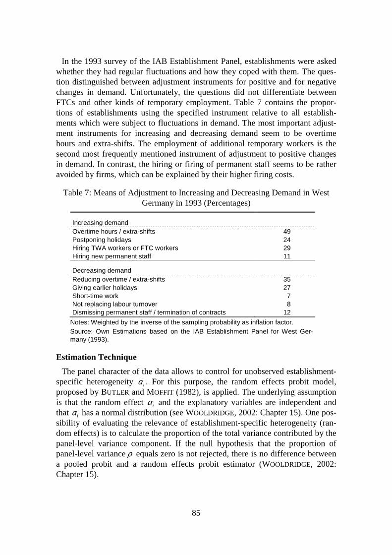
85

In the 1993 survey of the IAB Establishment Panel, establishments were asked whether they had regular fluctuations and how they coped with them. The ques-tion distinguished between adjustment instruments for positive and for negative changes in demand. Unfortunately, the questions did not differentiate between FTCs and other kinds of temporary employment. Table 7 contains the propor-tions of establishments using the specified instrument relative to all establish-ments which were subject to fluctuations in demand. The most important adjust-ment instruments for increasing and decreasing demand seem to be overtime hours and extra-shifts. The employment of additional temporary workers is the second most frequently mentioned instrument of adjustment to positive changes in demand. In contrast, the hiring or firing of permanent staff seems to be rather avoided by firms, which can be explained by their higher firing costs.

Table 7: Means of Adjustment to Increasing and Decreasing Demand in West Germany in 1993 (Percentages)

Increasing demand Overtime hours / extra-shifts 49 Postponing holidays 24 Hiring TWA workers or FTC workers 29 Hiring new permanent staff 11

Decreasing demand Reducing overtime / extra-shifts 35 Giving earlier holidays 27 Short-time work 7 Not replacing labour turnover 8 Dismissing permanent staff / termination of contracts 12

Notes: Weighted by the inverse of the sampling probability as inflation factor. Source: Own Estimations based on the IAB Establishment Panel for West Ger-many (1993).

Estimation Technique

The panel character of the data allows to control for unobserved establishment-specific heterogeneity iα . For this purpose, the random effects probit model, proposed by BUTLER and MOFFIT (1982), is applied. The underlying assumption is that the random effect iα and the explanatory variables are independent and that iα has a normal distribution (see WOOLDRIDGE, 2002: Chapter 15). One pos-sibility of evaluating the relevance of establishment-specific heterogeneity (ran-dom effects) is to calculate the proportion of the total variance contributed by the panel-level variance component. If the null hypothesis that the proportion of panel-level varianceρ equals zero is not rejected, there is no difference between a pooled probit and a random effects probit estimator (WOOLDRIDGE, 2002: Chapter 15).

86

A potential drawback of the random effects probit model is that it is calculated using Gauss-Hermite quadrature as an approximation for the high-dimensional integral that is part of the likelihood function (see GREENE, 2003: Appendix E.5.4). This requires the integrated function to be well-approximated by a poly-nomial. The approximation is appropriate, if changing the number of quadrature points does not affect the results. The estimation results turn out to be robust concerning the number of quadrature points.81 Therefore, one can conclude that the Gauss-Hermite quadrature method is appropriate and the random-effects pro-bit is applicable.

4.4.3 Estimation Results

Note that all estimated coefficients presented in the following are informative only with regard to the sign and statistical significance of the effects, but not with regard to the magnitudes. The reason is that the estimated coefficients do not correspond to marginal effects on the probability (see WOOLDRIDGE, 2002: 458). Even if it is generally possible to estimate the corresponding marginal ef-fects, these time-consuming calculations could not be performed here due to time-restrictions at the federal employment office.

The estimation results are depicted in Table 8. It is ex ante unclear whether the demand for atypical workers reacts symmetrically to increases and decreases in output. Therefore, likelihood ratio tests are used to find out whether the estima-tion of separate coefficients for positive and negative output changes (the unre-stricted model) or a common coefficient for output changes (the restricted model) is appropriate. Only in the case of FL workers the likelihood-ratio test indicates that the unrestricted model should be preferred: positive expected output changes have a significantly positive effect on the use of FL work, whereas negative out-put changes have no effect.

The result that the use of FTC work is not significantly affected by expected output changes may be explained by two opposite effects: On the one hand, an output increase may make it more necessary to use FTCs in order to adjust to a temporary positive demand shock. On the other hand, if the shock turns out to last longer, firms may start to convert FTCs into permanent contracts. Note that if there was indeed no effect of demand changes on the use of FTCs, then this would render it more possible that FTCs are only used for substitution of perma-nent workers or for screening purposes. However, in a comparable study we find a positive effect of actual output increases on the use of FTCs (see BOOCKMANN and HAGEN, 2003). Thus the use of FTCs as a means of adjustment should not be rejected from this finding.

For TWA work expected output changes have a significantly positive effect, which may indicate that TWA work is indeed used for adjustment purposes. Ex-

81 This is simply checked by comparing the results using different number of quadrature points. The

results are hardly affected.

87

pected positive output changes increase the use of FL work. The result of nega-tive output changes not reducing the use of FL work may indicate that firms may outsource permanent jobs by using FL workers during economic downturns.

The qualitative indicators for the state of capital stock as well as the sum of in-vestments in the previous year are found to have no significant effect in all speci-fications. Therefore, these variables are not included in the specifications de-picted in Table 8. By contrast, the coefficient of the dummy variable indicating ICT investment in the previous year is significantly positive for all three kinds of atypical employment. This may be a confirmation of the specialisation argument, particularly in the case of FL workers: for many smaller firms it may be profit-able to contract out services associated with the establishment’s own ICT equip-ment (see Section 4.4.2).

The existence of collective wage agreements has no significant effect on the probability of using FTC or TWA work. An interpretation is that the negative direct and the countervailing positive indirect effects described in Section 4.2.5 are balanced. By contrast, collective wage agreements (particularly, those con-cluded at the industry level) have a significantly negative effect on the probabil-ity of employing FL workers. KAISER and PFEIFFER (2001) obtain similar results for the German service sector. This may be explained by the fact that FL workers are often covered by collective wage agreements. In establishments which apply collective agreements, the cost advantage of FL work may therefore be lower.

The estimated coefficient for the existence of works councils is in line with the preponderance of the indirect effect (see Section 4.2.5). It suggests that estab-lishments with works councils tend to use FTCs more frequently. The main ex-planation may be that works councils increase firing costs for permanent work-ers, which decreases the relative firing costs of FTC workers. All theoretical models presented in Section 4.2.5 predict a positive link between firing costs of permanent workers and the use of FTC work. However, works councils do not seem to influence the use of the other two types of atypical work. When inter-preting the results one should, however, keep in mind that the existence of a works council is assumed to be strictly exogenous conditional on the other ex-planatory variables. Recent studies on the effects of works councils on firm per-formance have cast doubt on this exogeneity assumption (see, e.g., ADDISON et al., 2004). In this application it is conceivable that FTC workers are less inter-ested in co-determination than permanent workers. This would make the exis-tence of works councils in establishments using FTCs less likely. This form of endogeneity would exert a downward bias on the estimated impact of works councils on FTC employment.

88

Table 8: Determinants of Employing FTC, FL, or TWA Workers

FTC (1996–1998)

FL (1994–1998)

TWA (1994–1998)

Coeff. Std.err. Coeff. Std.err. Coeff. Std.err. Expected output increase 0.558 *** 0.197 Expected output decrease 0.487 0.449 Expected output change 0.299 0.188 0.457 *** 0.170

Seasonal fluctuations 0.150 * 0.085 -0.074 0.084 -0.061 0.634 Collective wage: firm level industry level

-0.117 -0.158

0.141 0.106

-0.246 -0.543

* ***

0.139 0.115

-0.053 -0.074

0.305 0.524

Works council 0.325 *** 0.107 -0.052 0.128 0.214 0.147 Share of workers with qualification -0.039 0.133 0.575 *** 0.145 0.166 0.992 Share of women -0.225 0.169 -0.213 0.187 -1.226 *** 0.242

ICT investments (t-1) 0.200 *** 0.067 0.621 *** 0.104 0.314 *** 0.114 Other investments (t-1) 0.101 0.073 0.326 *** 0.114 0.156 0.121 Problems due to parental leave (t-1) 0.361 *** 0.124 -0.122 0.115 -0.252 ** 0.126 Problems due to sickness (t-1) -0.017 0.091 -0.154 * 0.087 0.059 0.503 Wave 1995 0.091 0.003 0.106 Wave 1996 0.097 -0.049 0.112 Wave 1997 0.014 0.075 0.015 0.099 0.131 0.113 Wave 1998 0.378 *** 0.082 0.113 0.100 0.432 *** 0.116 Reference: ≥ 5000 employees 1– 5 employees x before -5.127 *** 0.727 -2.446 0.376 -2.504 *** 0.479 1– 5 employees x after -4.853 *** 0.668 -2.190 0.380 -3.226 *** 0.556 6– 10 employees x before -3.834 *** 0.666 -1.915 0.371 -2.560 *** 0.515 6– 10 employees x after -4.352 *** 0.661 -2.282 0.406 -2.628 *** 0.490 11–19 employees x before -3.397 *** 0.652 -1.889 0.370 -1.952 *** 0.421 11–19 employees x after -3.575 *** 0.641 -1.776 0.380 -2.140 *** 0.433 20–49 employees -3.142 *** 0.626 -1.561 *** 0.331 -1.619 *** 0.348 50–99 employees -2.819 *** 0.624 -1.218 *** 0.327 -1.077 *** 0.337 100–199 employees -2.068 *** 0.617 -0.839 *** 0.315 -0.174 0.321 200–499 employees -1.558 ** 0.612 -0.567 * 0.304 -0.042 0.313 500–999 employees -1.246 ** 0.618 0.026 0.308 0.096 0.320 1000–4999 employees -0.932 0.614 -0.061 0.299 0.281 0.310 Reference: Construction Mining, electricity, water supply 0.399 0.306 -0.584 * 0.327 -0.053 0.343 Basic industry 0.619 *** 0.176 -0.317 * 0.192 0.770 *** 0.214 Investment goods industry 0.783 *** 0.163 0.143 0.171 0.945 *** 0.201 Consumer goods 0.406 ** 0.175 -0.110 0.198 0.214 0.938 Wholesale, retail 0.420 ** 0.167 -0.154 0.188 0.018 0.230 Transport, telecommunication 0.120 *** 0.210 -0.247 0.247 -0.020 0.278 Hotels, restaurants 0.774 *** 0.213 -0.123 0.257 -0.467 0.381 Education, research, publication 1.016 *** 0.331 1.354 *** 0.292 0.025 0.440 Health services 1.024 *** 0.278 0.309 0.282 0.620 0.378 Business related services 0.342 * 0.206 1.033 *** 0.206 0.337 0.278 Other services 0.245 0.262 0.148 0.294 0.211 0.359

89

Table 8 continued... FTC FL TWA Coeff. Std.err. Coeff. Std.err. Coeff. Std.err. Reference: Bavaria Berlin West 0.422 ** 0.221 0.066 0.194 0.422 * 0.221 Schleswig-Holstein 0.151 *** 0.295 -0.047 0.254 0.151 0.295 Hamburg 1.060 0.256 0.431 ** 0.216 1.060 *** 0.256 Lower Saxony -0.275 0.184 -0.362 ** 0.160 -0.275 0.184 Bremen 0.173 0.368 -0.183 0.329 0.173 0.368 North Rhine-Westphalia 0.184 0.140 -0.057 0.124 0.184 0.140 Hesse 0.194 0.184 -0.053 0.165 0.194 0.184 Rhineland-Palatinate -0.175 0.213 -0.281 0.190 -0.175 0.213 Baden-Wuerttemberg 0.041 0.152 0.106 0.131 0.041 0.152 Constant -1.191 ** 0.438 0.270 0.133 -1.191 *** 0.438 Std. err. of random effects 0.868 *** 0.088 1.154 *** 0.076 1.286 *** 0.081 ρ 0.430 *** 0.050 0.567 *** 0.032 0.623 *** 0.030 LR-Tests for joint significance Industry dummies 43.07 *** 0.000 87.73 *** 0.000 64.16 *** 0.000 Wave dummies 26.4 *** 0.000 4.160 0.385 27.66 *** 0.000 Firm size dummies 250.07 *** 0.000 131.00 *** 0.000 155.99 *** 0.000 Federal state dummies 19.74 ** 0.030 17.42 ** 0.045 29.88 *** 0.000 Number of observations 3,735 6,303 7,207 Number of establishments 2,344 2,928 2,843

Notes: *** (**,*) denotes significant at the 1 (5, 10) percent level. Source: Own Estimations based on the IAB Establishment Panel for West Germany (1994–1998).

The proportion of employees with a formal qualification has a positive effect on

the probability of using FL workers. This may indicate that FL workers are used more often in establishments with tasks that require a qualification. In addition, it may reflect the finding that adjustment costs for qualified permanent workers are generally higher than for unskilled permanent workers (see, e.g., HAMERMESH, 1993). Ceteris paribus, an increase in adjustment costs for permanent workers raises the probability of using temporary workers, if both are substitutes in pro-duction.

The effect of the indicator variable for problems with parental leave is highly significant in the case of FTC workers, which is in line with the hypothesis posed. However, for FL workers and TWA workers the results reject the hy-pothesis.

As the descriptive tables already indicated, the highest probability of using TWA workers is found among establishments in the basic and investment goods industry. In contrast, FL workers are used with a higher probability in the busi-ness-related service sector, which seems to be plausible. Furthermore, they are frequently used in the education, research, and publication sector. The highest probability of establishments to use FTC workers is in the health services sector, in the education, research, and publication sector, in the investment goods indus-try, and in hotels and restaurants.

90

Another interesting result are the significant differences between the federal state dummies. In the city states of West Berlin and Hamburg, establishments employ TWA workers with a significantly higher probability than in the base category (Bavaria), which is a territorial state. This may reflect supply restric-tions as it seems plausible that the density of temporary work agencies increases with urbanity. An exception is Bremen which does not have significantly more establishments employing atypical workers than Bavaria. Comparable results are not found for FL and FTC work, which rely on bilateral contracts between firms and worker without the use of an agency as intermediary.

Table 9 describes the estimated effects of the increase in the minimum em-ployment threshold level for the Protection Against Dismissal Law in October 1996 on the probability of using atypical work. The table reports the coefficients of the interaction terms and Wald tests with the null hypothesis that the differ-ences in the coefficients are zero. The specifications are the same as in Table 8.

Table 9: Effects of the Increase in the Minimum Employment Threshold Level for the Protection Against Dismissal Law in October 1996

FTC FL TWA Numb. of em-ployees

Coeff. (Std.err.) before

Coeff. (Std.err.)

after

Wald test p-value


Coeff. (Std.err.)

after

Wald test p-value


Coeff. (Std.err.)

after

Wald test p-value

1–5 -5.13 (0.73)

-4.85 (0.67)

0.46 -2.45 (0.38)

-2.19 (0.38)

0.29 -2.50 (0.48)

-3.23 (0.56)

0.17

6–10 -3.83 (0.67)

-4.35 (0.66)

0.05 -1.92 (0.37)

-2.28 (0.41)

0.20 -2.56 (0.52)

-2.63 (0.49)

0.60

11–19 -3.40 (0.65)

-3.56 (0.64)

0.43 -1.89 (0.37)

-1.18 (0.38)

0.67 -1.95 (0.42)

-2.14 (0.43)

0.13

Notes: Estimation results from Table 8.

The probability of using TWA workers decreases in all three firm size groups,

but the differences are not statistically significant. In the case of FL workers, the probability decreases only in establishments with 6-10 employees, which con-forms with the expectation. However, the differences are not statistically signifi-cantly different from zero.

Most interesting is the result for the probability of using FTC workers: The in-crease in the minimum employment threshold for the application of the Protec-tion Against Dismissal Law significantly lowers the probability of using FTC workers for establishments with 6-10 employees, while there are no significant changes in the two contiguous establishment size groups. This may suggest that firing costs of permanent contract employees are more important as a reason for using FTC workers than for using TWA or FL workers. Indeed, it appears plau-sible that FTC workers are closer substitutes for permanent employees in produc-tion than TWA or FL workers.

91

4.4.4 Summary of the Empirical Analysis of the Firms’ Use of Atypical Work

Using a change in dismissal protection legislation as a natural experiment, some evidence is found that the stringency of dismissal protection for permanent work-ers has a positive effect on the probability of using FTC workers. This indicates that firms do indeed use FTC workers as a more flexible alternative to permanent employment. By contrast, a similar effect for TWA and FL workers cannot be identified, which may indicate that permanent and FTC workers are closer substi-tutes than permanent workers and TWA and FL workers.

This result should, however, be interpreted with care: it is (in case of FTCs) based on data given only one year before and two years after the policy change. Furthermore, one cannot rule out that anticipatory effects are relevant, i.e., that the hiring behaviour changed already before the law change was implemented. Nevertheless, to the best of my knowledge, this is the first microeconometric study that can reveal this association between firing costs and FTCs at the firm level.82 Other studies have either used country level or regional data to attempt to identify this relationship (see NUNZIATA and STAFFOLANI, 2002 and AUTOR, 2003).

Works councils may also raise firing costs of permanent employees in Ger-many. In accordance with this hypothesis, the probability of employing FTC workers is influenced positively by the existence of a works council. Collective wage agreements as another potential institutional source of firing costs do not influence the probability of employing FTC and TWA workers. Supposably, the direct effect (unions opposing against the use of atypical work) outweighs the indirect effects (unions increasing firing costs of permanent workers; raising the costs of overtime; increasing wage rigidities).

Furthermore, establishments facing problems due to parental leave use FTCs more often. This has been interpreted as evidence in favour of the hypothesis that FTCs are used in case of stochastic absence time of permanent contract workers.

82 Furthermore, it is the first study using this policy variation in Germany as a natural experiment. This

variation could be used for a number of related questions.

92

4.5 Empirical Analysis of the Role of Fixed-Term Contracts in Worker and Job Flows

4.5.1 Introduction

The analysis of the previous section was based on an employment stock ap-proach, since not inflows (hirings) and outflows (separations) of FTC workers were explained, but the existence of FTC jobs. However, the difference in firing costs between FTC and permanent contract workers refers to worker flows.

Therefore, this subchapter takes a step back to a simple descriptive analysis of worker flows and job flows based on the IAB Establishment Panel.83 Again, it is not possible to evaluate whether FTCs increase employment flexibility or even the employment level. However, avoiding unrealistic assumptions as imposed in econometric studies, cited in Subchapter 4.3, such as symmetrical and convex adjustment costs, it is possible to gain some insights into the role of FTCs in dy-namic labour demand.

There is a growing literature on the “flow approach to labour markets” (BLANCHARD and DIAMOND , 1992) and especially on worker flows at the firm level (see, e.g., BURGESS, LANE, and STEVENS, 2001). The fundamental reason for focussing on worker flows is the well-known result that most employers are simultaneously hiring and facing separations, that declining firms continue to hire, and that growing firms continue to lose workers. Furthermore, workers mostly enter jobs which already existed before the contract is signed and which will not be destroyed when the worker quits or is dismissed. The phenomenon of worker turnover exceeding job turnover is termed ‘rotation’ or ‘churning’ (see, e.g., SERRANO, 1998; BURGESS, LANE, and STEVENS, 2001). The role of FTCs in these dynamic processes is almost unknown for Germany. This subchapter aug-ments the framework of the worker turnover and job turnover literature (see, e.g., DAVIS and HALTIWANGER, 1999, SCHETTKAT, 1996 as well as BURDA and WY-

PLOSZ, 1994) by taking FTCs versus permanent contracts into account. Churning is a matter of particular interest in the analysis of this subchapter as it

is linked to the three categories of reasons for the use of FTCs (buffer stock, screening, and substitution): if the churning rate (the proportion of worker turn-over that is not associated with job creation and destruction) of FTCs is close to 100%, then this may be interpreted as evidence for the hypothesis that an existing FTC job is inherently permanent, but repeatedly filled by FTC workers. Even though it is not possible to directly conclude from this result that this reflects the underlying role of FTCs as a substitute for permanent contracts (as there can still

83 Throughout this Subchapter the terms “inflows”, “recruitments”, and “hirings” as well as “outflows”,

“separations”, and “firings” are used interchangeably. Formally, it is incorrect to term all worker out-flows from establishments as firing, since also quits, retirements etc. are included.

93

be a constant number of probationary period jobs), this would indicate that FTC workers are not used for adjustment purposes (buffer stock). A churning rate for FTC work of zero would indicate that every inflowing FTC worker occupies a newly created job and every outflowing FTC worker represents a destroyed FTC job. In this case FTC work would be exclusively used for adjustment purposes. However, since there may be a simultaneous creation of one type of jobs (e.g., FTC jobs) and destruction of the other type (e.g., permanent contract jobs), this simple concept has to be augmented in the course of this subchapter.

In detail, the aim of the following descriptive analysis is to shed light on the following questions.84 How widespread is FTC employment in West Germany? The descriptive analyses in Subchapter 2.3 and in the previous subchapter could only reveal the proportion of FTC jobs and the proportion of establishments us-ing FTCs measured at a certain date. Hence, how large is the proportion of FTCs in worker flows? Which fraction of an establishment’s FTCs is converted into permanent contracts? The larger this proportion, the more important is obviously the role of FTCs as screening device. How big is the fluctuation within the group of fixed-term employees and the group of permanent employees within estab-lishments? To which extent do inflows into and outflows from establishments occur simultaneously, and to which extent do inflows and outflows lead to job creation and destruction? Are simultaneous outflows of permanent workers and inflows of FTC workers observable?

So far, empirical evidence on the significance of FTCs in worker flows at the firm level is only available for France, Spain, and Portugal.85

For France, ABOWD, CORBEL, and KRAMARZ (1999) show that during the pe-riod 1987–1990 about 70% of all hirings are on FTCs, whereby this share is even larger in establishments with decreasing employment. More than half of the total outflows is due to expired FTCs. The separation rate of FTCs (outflows of FTCs relative to FTC employment) is even higher in growing businesses. About one third of all fixed-term contracts are converted into permanent ones.

SERRANO (1998) finds similar results for Spanish companies with more than 500 employees during the period 1993–1994. Accordingly, 85% of all firms’ in-flows and 79% of all outflows are based on FTCs. While about 3% of all em-ployees with permanent contracts are hired or fired by a company (worker turn-over) during each quarter, this ratio is about 57% for the group of FTC workers. This high FTC worker turnover results to a large extent from churning.

For the Portuguese labour market during the period 1991–1998, VAREJÃO and PORTUGAL (2003) find that the proportion of FTCs in the employment stock is on average about 14%. However, the proportion of FTCs in hirings is about 62% and in firings about 43%. The quarterly worker turnover rate is about 31%, indi-

84 Of course, these questions should not be interpreted as causal in the sense defined in Chapter 3. 85 For Germany worker flows on the basis of establishment level data are analysed by BELLMANN and

BOERI (1998). However, they do not take the role of FTCs into account.

94

cating that approximately one in three FTC workers either joins or leaves her or his employer every quarter. In contrast, the worker turnover rate for permanent workers is about 5%.

The econometric study by GOUX, MAURIN, and PAUCHET (2001) interprets FTC and permanent work as two different factors in production. This is possible since their panel dataset for French firms for the period 1988–1992 provides in-formation on wage costs of both types of work. Furthermore, the authors are able to make inference on the structure of gross adjustment costs, since they have data on inflows and outflows of permanent contract and FTC workers. The results can be summarised as follows: it is more costly to adjust permanent contract workers than FTC workers, firing permanent workers is much more expensive than hiring them, hiring costs of FTC workers are slightly lower than hiring costs of perma-nent workers, and the transformation of FTCs into permanent contracts is a means of permanent (long-term) labour adjustment.86

This subchapter is structured as follows. The next section introduces measures describing job and worker flows by type of contract. Section 4.5.3 describes the dataset and explains how the data can be weighted in order to be estimates either for the population of establishments or for the population of employees in West Germany. The results are presented in Section 4.5.4. A summary of the findings is provided in Section 4.5.5.

4.5.2 Methodology

Terminology87

To simplify matters, assume one establishment i. The hiring rate HRit and the separation rate SRit of the establishment i for the period between dates t-1 and t is given by

it

itit N

HHR = ,

it

itit N

SSR = , (33)

with Hit denoting the number of hirings during this period, Sit is the number of separations, and Nit is the stock of total employment in the establishment. Total employment Nit is defined as the average of the employment stocks Li at the dates t-1 and t, that is, ( )ititit LLN += −12

1 .

The (worker) turnover rate itWTR is the sum of the hiring rate ( itHR ) and the separation rate ( itSR ) in the respective establishment88, that is,

86 The lower hiring costs for FTCs may be interpreted as evidence in favour of a less demanding pre-

hiring screening process, as FTC workers can be screened on-the-job. 87 The definitions and the terminology in this Subchapter follow the literature to a large extent (see

DAVIS and HALTIWANGER, 1999). 88 Note that, under certain assumptions, there is a simple negative connection between the average dura-

tion of an employment relationship and the worker turnover rate (see CRAMER and KOLLER, 1988).

95

it it itWTR HR SR= + . (34)

Worker turnover can be decomposed into two components. The first component consists of hirings and separations which are associated with job creation or job destruction, that is, net changes in total employment of the establishment. This can be expressed in terms of the job creation rate itJCR and the job destruction rate itJDR

ititit SRHRJCR −= for 1it itL L − >− 0 and 0 otherwise, (35)

ititit SRHRJDR +−= for 1it itL L − <− 0 and 0 otherwise. (36)

By using this concept, it is assumed that job creation and destruction is reflected in a net employment change within the establishment. Following the literature, simultaneous creation and destruction of job positions within the establishment has to be neglected (see, e.g., SERRANO, 1998). Put differently, if one job posi-tion (e.g., with low skill requirements) is destroyed, and one job position (e.g., with high skill requirements) is created within the same establishment (as sug-gested by the literature on technological change), this is not counted as creation or destruction of jobs.

Job creation and job destruction rates are associated with the rate of net em-ployment change. The absolute value of the growth rate of the employment stock is given by 89 it it it it itGR HR SR JCR JDR= − = − . (37)

The job turnover rate is not depicted in the following analyses. However, it can simply be computed as the sum of the job creation and destruction rates.

The second component of worker turnover consists of hirings and separations which are not related to a net change in employment. This phenomenon is de-noted as rotation or churning. Rotation or churning may result either from worker mobility between job positions at different employers (e.g., due to per-sonal factors, low job satisfaction, higher career opportunities at other employ-ers), or from the decision of the employer (workers are exchanged at a given job position because the match turns out to be poor, there is technological or organ-isational change, or churning is a cost-minimising equilibrium strategy).90 The rotation rate itRR is the part of the turnover rate that is not associated with a net employment change, i.e.,

it it it it it it it it it itRR WTR GR WTR JCR JDR HR SR HR SR= − = − − = + − − . (38)

89 This rate corresponds to the absolute value of (Lit -Lit-1) / 0.5·(Lit+L it-1) which is a growth rate in dis-

crete time. 90 Remember again, that a simultaneous creation and destruction of job positions which is not associ-

ated with net employment changes within an establishment is treated as churning or rotation even if there is destruction of old jobs and creation of new jobs. Thus rotation or churning is likely to be overestimated.

96

Relating the rotation rate to the turnover rate leads to the so-called churning rate91

it it itCR RR WTR= . (39)

The churning rate itCR indicates the proportion of worker turnover that cannot be attributed to net changes in employment. Obviously, itCR is not defined for a single establishment that neither has worker inflows nor outflows during the pe-riod ( 0itWTR = ). An itCR close to 100% means that almost all hirings and separa-tions are associated with replacements of workers on existing jobs, for example, since all employment relationships turn out to be mismatches (from the worker’s or the employer’s point of view).

Two Types of Contracts

The concept is now defined separately for FTC and permanent contract (PER) work (an overview is provided in Box 2).92 For example, the hiring rate of FTC work FTC

itHR indicates the number of hirings on FTCs relative to the stock of FTC employees in the establishment. After the termination of a FTC, two destination states can be distinguished. Either the employee leaves the establishment due to the expiration of her or his FTC (included in the separation rate FTC

itSR of FTCs), or the FTC is transformed into a permanent contract. This is expressed in the transformation rate, which is defined as

itit FTC

it

TFTFR

N= , (40)

where itTF denotes the number of transformations from FTCs into permanent contracts within the establishment.

A problem arises due to the fact that, although there is information on worker quits and retiring, it cannot be identified whether these belong to FTC or perma-nent contract workers. Since economic theory predicts that the quit rate of FTC workers is higher than the quit rate of permanent contract workers, this may be a serious limitation. Due to the lack of reasonable alternatives, the number of sepa-rations of permanent workers is simply defined as PER FTC

it it itS S S= − , with FTCitS

consisting only of FTC worker outflows due to the termination of their FTCs. Hence, all quits and retirings are counted as permanent worker separations, im-plying that PER

itSR overestimates the true permanent worker separation rate, and FTCitSR underestimates the true FTC worker separation rate.93

91 Note that the literature suggests different definitions of the churning rate. However, all definitions

have comparable meanings (see BURGESS, LANE, and STEVENS, 2001). Here the definition proposed by BELLMANN and BOERI (1998) is applied.

92 In the following, the superscripts FTC and PER stand for fixed-term and permanent contracts, respec-tively.

93 Note that most firm level data are associated with similar problems. SERRANO (1998) faces exactly the same problem and seems to use a comparable definition.

97

The respective rotation rates of fixed-term and permanent contract work can be defined analogously to Eq. (38) as

FTC FTC FTC FTC FTC FTC FTCit it it it it it itRR HR SR HR SR WTR GR= + − − = − , (41) PER PER PER PER PER PER PERit it it it it it itRR HR SR HR SR WTR GR= + − − = − .

Note that these rotation rates do not include transformations of FTCs into perma-nent contracts. This flow is taken into account by another measure introduced below.

The churning rates for the two types of contracts can be analogously to Eq. (39) defined as

FTC FTC FTCit it itCR RR WTR= , PER PER PERit it itCR RR WTR= .

The rotation rates of FTC and permanent contract employment defined in Eq. (41) do not sum up to the rotation rate of total employment in Eq. (38), since the denominators are different (they are either FTC

itN or PERitN ). Additionally, it is not

taken into account that there may be outflows from one type of contract, but in-flows into the other type of contract within the establishment. Given the assump-tion discussed above, this may be interpreted as substitution and, therefore, as an additional kind of rotation or churning. In order to account for this, the flows for each type of contract are related to total employment itN . One receives the fol-lowing alternative rotation rates for both types of contracts

kit

kit

kit

kit

kit SRRHRRSRRHRRRRR −−+= , { },k FTC PER∈ , (42)

where k kit it itHRR H N= and k k

it it itSRR S N= . The additional ‘R’ at the variables in-dicates that the flows are related to total employment instead of contract-specific employment. Similarly, the transformation rate itTFRR is defined by relating itTF

to itN .

The difference between total rotation in the establishment as defined in Eq. (38) and the sum of the rotation within the two types of contracts in Eq. (42) leads to the cross rotation rate:

cross FTC PERit it it itRRR RR RRR RRR= − − . (43)

The cross rotation rate crossitRRR is zero, if FTC employment as well as permanent

contract employment increases, or if FTC employment as well as permanent con-tract employment decreases. The cross rotation rate is calculated as

0 if > >

0 if

FTC FTC PER PER

it it it it

cross

it i

H S H S

RRR H=

∧

( )< <

2 min , otherwise.

FTC FTC PER PER

t it it it

FTC FTC PER PER

it it it it

S H S

HRR SRR HRR SRR⋅ − −

∧

(44)

The cross rotation rate can be interpreted as follows: It is the part of turnover of the establishment’s total workforce which emerges from the fact that under one type of contract employment is created, while at the same time employment is

98

reduced under the other type. For example, if an establishment has outflows of permanent staff and replaces it by FTC employees without changing its total em-ployment, this is neither rotation of FTC employment ( FTC

itRR ), nor rotation of

permanent employment ( PERitRRR ), but cross rotation ( cross

itRRR ).94 Note that cross rotation is a new concept which has not been introduced to the literature so far.

Box 2: Measures to Describe Worker and Job Flows

Name Notation Variable in numerator

Denominator: Stock of employed of contract type { },k FTC PER∈

Hiring rate kHR hiring on contract type k

Separation rate kSR outflow from the establishment from employment with contract type k

Worker turnover rate kWTR sum of hiring rate and separation rate for contract type k

Job creation rate kJCR created job positions for contract type k

Job destruction rate kJDR destroyed job positions for contract type k

Rotation rate kRR turnover rate of contract type k less hirings on and separa-tions from contract type k which are associated with crea-tion or destruction of jobs of contract type k

Churning rate kCR rotation rate in relation to turnover rate

Transformation rate TFR transitions from FTC in permanent contracts within the establishment

Denominator: Stock of total employment

Hiring rate kHRR analogous to HR

Separation rate kSRR analogous to SR

worker turnover rate kWTRR analogous to TR

Rotation rate kRRR analogous to RR

Cross Rotation rate crossRRR Part of total turnover which is associated with a simultane-ous reduction in the workforce of one type of contract, and an increase in the workforce of the other type of contract

Transformation rate TFRR analogous to TFR

Note: If the superscript k is not used, the corresponding measure is for total employment without distinguishing between the type of contract.

94 Cross rotation can be further split up according to whether permanent employees are replaced by FTC

employees or vice versa. However, it complicates the analysis without enhancing the understanding of the issue.

99

4.5.3 Dataset and Weighting

For the empirical analysis again the IAB Establishment Panel (already intro-duced in Section 4.4.2) for the years 1997–1999 as well as 2000 is used. The farming and fishing industry as well as the public sector are again excluded from the analysis. Using the sampling weights (or the inflation factors, respectively) it is possible to estimate statistics of the measures previously introduced describing the population, i.e., an average establishment in West Germany or total employ-ment in West Germany. Weighting is necessary because the dataset is a stratified sample with large establishments and certain sectors being overrepresented (see KÖLLING, 2000). For an unbiased estimation of the corresponding standard er-rors, the sample design (stratification and clustering) is taken into account (see, e.g., DEATON, 1997). The number of missing observations due to item non-response is very low. Therefore, this issue is not further addressed.

Box 3: Two Concepts of Representativeness (Example: Hiring Rate)

Average rate (representative of the popu-lation of establishments)

Aggregate rate (representative of the population of employees)

The average hiring rate of all establishments in the population (establishments in West Germany) is the weighted average of itHR

over all 1,...,i J= establishments in the sample with the weight being the inflation factor iw :

1i it

i

HR w HRJ

= ⋅∑

HR is the estimated hiring rate of an aver-age establishment in West Germany

The aggregate hiring rate is the weighted aver-age of itHR over all 1,...,i J= establishments,

with the weight consisting of the inflation fac-tor iw and the proportion of employees in es-

tablishment i in total employment ( / )it tN N :

⋅ ⋅= ⋅ ⋅ = =

⋅

∑ ∑∑

∑

i it i itit i i

i iti t i it t

i

w H w HN

HR w HRN w N N

.

HR is the estimated hiring rate of total em-ployment in West Germany, given by the ratio of the estimated hirings in the population and the estimated total employment in the popula-tion.

Notes: The sample consists of 1,...,i J= establishments, with 1 iw denoting the probability that

an establishment from the population (West Germany) is sampled, implying an inflation factor of

iw as included in the IAB Establishment Panel. The total employment stock in an establishment

i is itN . The aggregate total employment in the population tN (estimated total employment in

West Germany) is given by the weighted sum of the employment itN over all 1,...,i J= estab-

lishments, that is, t i iti

N w N= ⋅∑ .

Weighting the introduced measures by inflation factors allows to draw infer-

ence about two different populations (see the overview in Box 3). It is possible to estimate average rates over all establishments in West Germany, which de-

100

scribe the expected value of a rate of an establishment randomly drawn from the population of all establishments in West Germany. However, these average rates over all establishments are not informative with regard to their impact on total employment. Aggregate rates take this aspect into account. Aggregate rates are calculated by weighting the single establishment rates by the inflation factor as well as the proportion of the establishment’s employment in total employment.

Average rates which are estimated to draw inference about the population of es-tablishments are denoted by HR, SR, etc. Aggregate rates which are estimated to draw inference about the population of employees are denoted by HR, SR, etc.

Using the IAB Establishment Panel for the period 1997–1999 is associated with at least two fundamental caveats. The inflows as well as the outflows always re-late to the first six months of each calendar year only. In contrast, the employ-ment stocks itL (as well as FTC

itL , PERitL ) are measured at the end of June each year,

that is, at the end of the six months period in which the worker flows are meas-ured. The average employment between dates t-1 and t, is determined as

( )1, 12it i t itN L L−= + . Thus itL as well as , 1i tL − are necessary. The first best solution

would be to define , 1i tL − to be the stock of employment at the beginning of the

year (January) using the identities

itititti SHLL +−=−1, , (45)

and

, 1FTC FTC FTC FTCi t it it it itL L H S TF− = − + + . (46)

Unfortunately, itTF is only available for the year 2000, but not for 1997–1999.95

For this reason, the stock of total employment in January , 1i tL − is estimated as the

average of total employment in June and total employment in June of the previ-ous year. For , 1

FTCi tL − and , 1

PERi tL − this approximation is used in an analogous way. This

approach implies that Eq. (45) and (46) hold only approximately. Furthermore, due to possible seasonal effects, the calculated measures always have to be inter-preted keeping in mind that they refer to the first half of the calendar year.

4.5.4 Results

Total Employment

Table 10 presents the means of the rates for total employment, that is, without distinguishing between the type of contract. The aggregate rates depicted in the first row suggest that during the first half of the years 1997–1999 more employ-ees were hired than separations took place (HR > SR). Accordingly, more jobs were created than destroyed (JCR > JDR). However, one should take into ac-count that this net employment increase refers to the first six months and is,

95 On the other hand, this year does not include information on FTC hirings and thus cannot be used for

the other questions posed.

101

therefore, likely to be overestimated due to seasonal effects (see Eq. (35) and (36)). The worker turnover rate WTR indicates that during a six-months period 12.6%

of all workers enter into or leave an establishment. The difference between the net change in employment and the WTR leads to the rotation rate: RR indicates that 5.9% of the employees are affected by worker flows that are not associated with the creation or destruction of jobs. Relating rotation to turnover results in a churning rate CR of 47%. Put differently, almost half of the turnover serves for the exchange of employees on a constant number of job positions without being associated with creation or destruction of jobs within a six-months period.

Table 10: Means of Job and Worker Flow Rates for Total Employment (Percentages, Standard Errors in Parentheses)

Aggregate rates

HR SR JCR JDR WTR RR CR Obs. 6.44

(0.18) 6.19

(0.16) 3.47

(0.13) 3.22

(0.12) 12.62 (0.29)

5.93 (0.22)

47.00 (1.08)

7,631

Average rates

HR SR JCR JDR WTR RR CR

Obs. 5.95

(0.27) 7.07

(0.35) 3.75

(0.23) 4.88

(0.32) 13.02 (0.47)

4.39 (0.30)

27.44 (1.18)

7,631

Source: Own estimations based on the IAB Establishment Panel for West Germany (1997–1999)

The second row of Table 10 depicts the estimated results of the averages rates

(representative of the population of establishments) which do not take the size of the establishments’ workforces into account. It can be seen that the results are now reversed, that is, now JCR JDR< and HR SR< . The discrepancy to the ag-gregate numbers could be explained by differences in the development of smaller and larger establishments: In the aggregate rates the larger establishments (which increase employment) outweigh the smaller establishments (which reduce em-ployment). The difference in the churning rates (CR >CR) indicates a greater importance of churning within large establishments.96 Following the literature, Table 11 differentiates between growing ( , 1it i tL L −> ),

contracting ( , 1it i tL L −< ), and establishments with stable employment ( , 1it i tL L −= ), measured as the change in employment in the first half of each year.97 The well-

96 However, creation or destruction of jobs that is spuriously counted as churning is also more likely in

large firms. 97 One may argue that defining the evolution of establishments by more long-term employment growth

measures, such as employment changes within a two-year period, would be more suitable. However, using the presented definitions of employment evolution ensures that some properties of the concept are fulfilled making the results easier to interpret. For example, the definition used here leads to the result that for establishments with stable employment JCR=JDR=0% and CR=100% hold.

102

known result that contracting establishments still hire workers and that growing establishments still have outflows is confirmed.98 It can even be seen that grow-ing establishments have a slightly higher SR than establishments with stable em-ployment. This phenomenon is discussed in greater detail below where it is dis-tinguished between FTCs and permanent contracts. It is not surprising that grow-ing and contracting firms have a much higher WTR than firms with stable em-ployment. The proportion of rotation in total turnover (the churning rate CR) is not much lower in contracting establishments than in growing establishments. Possibly, firms try to create better job-worker matches in times of shrinking business development, or workers increase their job-to-job mobility in case of the threat of a future dismissal. Of course, FTCs may be important in this process. In line with the definition in Eq. (39), the CR has to be 100%, if , 1it i tL L −= , that is, WTR equals RR: Since neither new jobs are created, nor old ones are destroyed (JCR = JDR = 0), all recruitments and separations serve for churning.

Table 11: Means of Job and Worker Flow Rates by Employment Trend (Percentages, Standard Errors in Parentheses)

Aggregate rates

HR SR JCR JDR WTR RR CR Obs.

, 1it i tL L −> 15.22 (0.44)

4.00 (0.25)

11.23 (0.36)

0.00 (0.00)

19.22 (0.62)

7.99 (0.49)

41.58 (1.66)

2,139

, 1it i tL L −= 2.49 (0.15)

2.49 (0.15)

0.00 (0.00)

0.00 (0.00)

4.98 (0.30)

4.98 (0.30)

100.00 (0.00)

3,140

, 1it i tL L −< 2.52 (0.17)

12.36 (0.39)

0.00 (0.00)

9.84 (0.34)

14.89 (0.62)

5.05 (0.35)

33.91 (1.68)

2,352

Average rates

HR SR JCR JDR WTR RR CR Obs.

, 1it i tL L −> 24.20 (0.76)

2.57 (0.31)

21.64 (0.73)

0.00 (0.00)

26.77 (0.91)

5.13 (0.62)

14.45 (1.03)

2,139

, 1it i tL L −= 2.21 (0.20)

2.21 (0.20)

0.00 (0.00)

0.00 (0.00)

4.43 (0.40)

4.43 (0.41)

100.00 (0.00)

3,140

, 1it i tL L −< 1.74 (0.22)

30.35 (1.31)

0.00 (0.00)

28.61 (1.30)

32.10 (1.35)

3.48 (0.44)

8.85 (0.69)

2,352

Source: Own estimations based on the IAB Establishment Panel for West Germany (1997–1999).

98 When comparing establishments with growing, contracting, and stable employment, it should be

noted that small establishments are overrepresented among establishments with stable employment, as for them Lit=Li,t-1 holds with a higher probability.

103

Permanent Versus Fixed-Term Contracts

In this subsection, the results of Table 10 and Table 11 are differentiated be-tween fixed-term and permanent contracts. For reasons of clarity, only the aggre-gate rates are presented in the following.99 As expected, hiring and separation rates are much higher for FTC employment than for permanent employment ( FTC PERHR HR> and FTC PERSR SR> ). There are about 44 hirings on FTCs per 100 FTC employees within the first six months of each year (Column 1, Table 12), whereas there are only 3.9 hirings on permanent contracts per 100 permanent workers. The turnover rate of FTC work ( FTCWTR ) of 62.4% is much larger than the turnover rate for permanent workers of 9.3%. This difference reflects the much lower average job tenure of FTC work when the match is dissolved. Note that the result is in line with the predictions of the theoretical models presented in Subchapter 4.2: As FTC workers are associated with lower firing costs than per-manent workers, they are more often hired and fired (that is, not getting their contract renewed or transformed into a permanent one).

Table 12: Means of Job and Worker Flows by Type of Contract (Percentages, Standard Errors in Parentheses)

FTCHR

FTCSR FTCWTR

FTCJCR

FTCJDR

TFR (2000)

FTCRR FTCCR Obs.

(2000)

FTC 44.21 (1.47)

18.16 (1.25)

62.37 (2.03)

32.28 (1.47)

6.24 (0.93)

9.07 (1.01)

23.85 (1.84)

38.24 (2.23)

7,484 (3,131)

PERHR

PERSR PERWTR

PERJCR

PERJDR

PERRR PERCR Obs.

PER 3.88

(0.14) 5.39

(0.15) 9.28

(0.23) 2.15

(0.11) 3.66

(0.12) 3.47

(0.17) 37.36 (1.27)

7,484

Source: Own estimations based on the IAB Establishment Panel for West Germany (1997–1999 and 2000).

Is this higher flexibility in terms of higher FTC worker flows associated with

higher flexibility in terms of FTC job flows? The results in Table 12 indicate much larger job creation and job destruction (job turnover) within FTC employ-ment ( FTC PERJCR JCR> and FTC PERJDR JDR> ). This result is in line with my pre-vious econometric dynamic labour demand study, where I find evidence that the speed of adjustment is faster for the total employment stock (including FTC work) than for the permanent contract employment stock (see Subchapter 4.3 and HAGEN, 2003). As already discussed in Subchapter 4.3, this does not necessarily mean that overall job turnover increases since most theoretical models presented in Subchapter 4.2 predict that the employment stability of permanent workers increases with the use of FTCs.

99 Considering the average rates does not lead to additional insights.

104

Both worker flow and job flow rates indicate a net increase in FTC employment ( FTC FTCHR SR> and FTC FTCJCR JDR> ), while permanent contract employment rates suggest a decrease. However, one should keep the following issues in mind: Firstly, it may simply be explained by the seasonal effect already mentioned above since JCR and JDR are calculated by hirings and separations during the first six months of each year. Secondly, transformations from FTCs into perma-nent contracts may take place, which are not considered by the worker flow and job flow rates. According to the transformation rate (TFR), 9.1% of all employ-ees with FTCs get their contracts transformed into a permanent one during the first six months of the year 2000. Assuming that the amount of transformations of contracts has not significantly changed between 1997–1999 and 2000100, one may conclude (by considering that FTCSR = 18.2%) that approximately one third of all FTCs lead to permanent contracts within the same establishment, and two thirds of FTC workers leave the establishment with the expiration of their con-tracts.101

To which extent are FTC and permanent contract worker flows used for the re-placement of workers? The rotation rate FTCRR of approximately 24% indicates that, at a given number of FTC jobs, almost one in four FTC workers is replaced by another FTC worker within six months. The churning rate for FTC work

FTCCR of 38% equals approximately the churning rate of permanent employment PERCR . However, it should be kept in mind that the proportion of FTC employees

being replaced by other FTC employees is far greater in absolute numbers than in the group of permanent staff ( FTC PERRR RR> ). Furthermore, the discrepancy be-tween the churning rates within the two types of contracts ( FTCCR , PERCR , Table 12) and the much higher total churning rate of 47% (CR, Table 10) can be ex-plained by the fact that cross rotation only affects CR, but not FTCCR and PERCR . Put differently, in addition to churning or rotation within the two types of work, there is churning between these types, leading to the concept of cross rotation. This issue is discussed in greater detail in the subsection below.

In Table 13 the results of Table 12 are again differentiated between growing, shrinking, and establishments with stable employment. An interesting result is the hiring rate of fixed-term contracts ( FTCHR ) in contracting firms, which stays at the high level of approximately 23% in establishments with stable employ-ment. At the same time the separation rate of FTCs FTCSR in shrinking firms is far higher than elsewhere. Taking into account that PERHR is only about 1.3% in shrinking establishments and that in Table 15 it is depicted that more than 50% of all hirings are on FTCs in shrinking establishments, a reasonable explanation is that vacancies are to a large extent filled by FTC workers as their future de-struction probability is high. This is also in line with the finding for shrinking

100 At least, it can be shown that the SRFTC has not changed significantly: With 18.9% for 2000 it almost

equals the number for 1997–1999. 101 This corresponds to the magnitude found by ABOWD, CORBEL, and KRAMARZ (1999) for France.

105

establishments that the PERJCR is not statistically significantly different from zero, while the FTCJCR is still about 7.4%. According to the FTCJDR , 18.4% of all FTC jobs are destroyed within six months in shrinking establishments. The hy-pothesis that existing permanent job vacancies in shrinking establishments (and therefore jobs with an increased probability to be destroyed in near future) are filled by FTC workers is also in line with the relatively high values of FTCRR and

FTCCR indicating substitution.

Table 13: Means of Job and Worker Flow Rates by Type of Contract and Em-ployment Trend (Percentages, Standard Errors in Parentheses)

FTC FTCHR FTCSR FTCWTR FTCJCR FTCJDR TFR (2000)

FTCRR FTCCR Obs. (2000)

, 1it i tL L −>

63.90 (2.20)

12.52 (1.46)

76.42 (2.62)

51.59 (2.66)

0.21 (0.06)

7.70 (1.20)

24.62 (2.92)

32.22 (3.36)

2,063 (793)

, 1it i tL L −=

23.21 (2.49)

6.95 (1.53)

30.16 (3.31)

18.50 (2.26)

2.24 (0.92)

16.70 (4.45)

9.42 (2.54)

31.23 (6.54)

3,110 (1,399)

, 1it i tL L −<

22.58 (1.62)

33.52 (3.06)

56.10 (3.40)

7.44 (0.87)

18.38 (2.77)

7.31 (12.54)

30.28 (2.87)

54.00 (3.73)

2,311 (939)

PER PERHR PERSR

PERWTR

PERJCR PERJDR PERRR PERCR

Obs.

, 1it i tL L −>

9.62 (0.38)

3.03 (0.18)

12.65 (0.49)

7.31 (0.33)

0.71 (0.06)

4.62 (0.36)

36.54 (1.97)

2,063

, 1it i tL L −=

1.78 (0.13)

2.24 (0.14)

4.02 (0.27)

0.06 (0.03)

0.53 (0.07)

3.42 (0.26)

85.15 (1.79)

3,110

, 1it i tL L −<

1.26 (0.14)

11.11 (0.36)

12.36 (0.43)

0.01 (0.00)

9.86 (0.32)

2.49 (0.27)

20.17 (1.78)

2,311

Source: Own estimations based on the IAB Establishment Panel for West Germany (1997–1999 and 2000)

One would expect growing firms to transform more FTCs into permanent con-

tracts. Surprisingly, the transformation rate TFR is significantly lower among growing establishments than among establishments with stable employment. This holds when looking at the ratio / FTCTFR SR : the highest ratio can be found among establishments with stable employment, the lowest among shrinking establish-ments. The latter seems to be more in line with what one would expect. The find-ing of less FTCs being transformed (relative to FTC separations) in growing es-tablishments than in establishments with stable employment may be explained by considering the much higher FTCWTR in growing establishments:

106

– some of the growing establishments may interpret the employment increase as a temporary positive shock, e.g., due to a seasonal effect. If the maximum du-ration of a FTC is reached, employers terminate the contract and prefer to hire a new worker on the FTC job. Theoretical models suggest that the negative effect of future firing costs on a current FTC conversion (which is analogous to a hiring on a permanent contract) increases with the probability that good business conditions come to an end (see Subchapter 4.2);

– some fast-growing establishments may omit an expansive and time-consuming pre-hiring screening process for permanent workers by hiring workers on FTCs. This may, in turn, lead to many unproductive matches and thus separations.

Both hypotheses may explain why almost 25% of the FTC worker turnover ( FTCRR ) is not associated with a change in the number of FTC jobs in growing establishments.

Fixed-Term and Permanent Contracts in Relation to Total Employment

Some of the figures in Table 12 are now reproduced in Table 14, which relates the flows to total employment. For example, the number of hirings into FTCs ( FTCH ) is related to total employment N and not only to FTC employment and is denoted by HRR. As discussed in Section 4.5.2, this may help to reveal the role of both types of contracts in total worker turnover and provides a possibility to decompose total rotation into a within (type of contract) component and a be-tween component.

Table 14: Decomposition of Worker Flows by Type of Contract (Percentages, Standard Errors in Parentheses)

HRR SRR WTRR RRR TFRR

(2000)

Obs.

(2000)

Total 6.36

(0.18) 6.19

(0.16) 12.55 (0.29)

5.84 (0.22)

7,484 (3,131)

FTC 2.73 (0.13)

1.12 (0.09)

3.85 (0.20)

1.47 (0.14)

0.59 (0.05)

PERM 3.66 (0.14)

5.05 (0.14)

8.71 (0.23)

3.24 (0.15)

CROSS

1.13 (0.07)


107

The first row of Table 14 (approximately) equals the first row of Table 10.102 The second row indicates that, on average, hirings on FTCs equal 2.73% of the total employment stock and the third row shows that hirings on permanent con-tract are 3.66% of total employment (HRR). Table 14 provides a decomposition of the rotation rate ( RRR) into rotation rates

for both types of contracts ( FTCRRR and PERRRR ) and the cross rotation rate CROSSRRR . The largest part of rotation is within permanent contract employment: PERRRR equals 3.25%. Hence, the proportion of permanent rotation in total rota-

tion is approximately 55%. The FTCRRR of 1.47% indicates that about 25% of total rotation is due to cases in which FTCs terminate or new workers are hired on FTCs without changing the number of FTC jobs in the establishment. This seems to be quite high as the proportion of FTC workers in the employment stock is only about 6.1% (see Table 15). The remainder of the RRR of nearly 20% is cross-rotation crossRRR , i.e., the simultaneous creation of jobs for one type of contract type and destruction of jobs of the other type of contract.

Table 15: Share of FTCs in Total Worker Flows (Percentages, Standard Errors in Parentheses)

FTCN N FTCH H FTCS S FTCWT WT Obs.

Total 6.08 (0.23)

42.79 (1.49)

18.19 (1.34)

30.68 (1.22)

7,484

, 1it i tL L −> 10.25 (0.57)

43.92 (1.86)

32.76 (3.63)

41.61 (1.99)

2,063

, 1it i tL L −= 2.78 (0.20)

27.31 (2.74)

8.56 (1.84)

17.93 (1.87)

3,110

, 1it i tL L −< 5.84 (0.40)

52.77 (3.44)

15.88 (1.58)

22.10 (1.71)

2,311

Source: Own estimations based on the IAB Establishment Panel for West Germany (1997–1999 and 2000)

Table 15 relates the flows of FTC employment to those of total employment.

The first column additionally presents the proportion of the FTC employment stock in the total employment stock (FTCN N ). The proportion of FTCs in the stock of employees approximately corresponds to what has been found in Sub-chapter 2.3 based on individual level data. Although only 6.1% of all employees hold FTCs, the proportion of FTCs among hirings (FTCH H ) is 42.3%.103 About 102 The small differences result from a slightly reduced sample (Table 10: 7,631 establishments and

Table 14: 7,484 establishments) using only establishments for which information on the type of con-tract in worker stocks and flows are complete. A comparison between Table 10 and Table 14 reveals that the results are only slightly affected.

103 This result is above the one of BIELENSKI, KOHLER, and SCHREIBER-K ITTL (1994) who find about one third of all hirings to be on FTCs. Their study is based on a representative survey among private en-terprises with at least five employees in 1992.

108

18.2% of all separations are due to expiring FTCs (FTCS S). The proportion of FTC turnover in total worker turnover ( FTCWT WT) is about 31%. In the next rows, the results are again differentiated between growing, shrink-

ing, and establishments with stable employment. As expected from the previous results in this section, the proportion of FTCs in employment stocks is lower in establishments with stable employment. The proportion of FTCs in hirings (FTCH H ) is larger in shrinking establish-

ments than in growing establishments. This is again in line with the hypothesis that a shrinking establishment may hesitate to hire a worker on a permanent con-tract, if it has to fill a vacancy of a permanent position, which will be destroyed with a high probability in the near future.

The fact that FTCS S is larger in growing than in shrinking establishments can simply be explained by the finding from Table 11: Growing establishments have a much smaller overall separation rate than shrinking establishments (4.0% vs. 12.4%). Hence, as many FTCs are not transformed into permanent contracts, growing establishments have, given their high FTCHR of 64% (Table 13), a large value of FTCS S.

Finally, Table 16 depicts some of the worker flow and job flow rates for differ-ent industries. It can be seen that there is a considerable heterogeneity. Results of particular interest are: – with 21.2% the ‘education, research, and publication’ sector is by far the one

with the highest proportion of FTCs in the employment stock. Likewise above-average rates can be found in ‘other services’ (9.7%) as well as in ‘construction’ (7.2%);

– high worker turnover rates of FTCs (and thus on average short FTC employ-ment spells) can be found in ‘other services’, ‘hotels, restaurants’, ‘construc-tion’ and ‘basic industry’. Low worker turnover rates of FTCs (on average long FTCs relationships) can be found in the ‘banking’, ‘mining, electricity, water supply’, ‘health services’, and ‘education, research, publication’;

– ‘education, research, publication’ is the only sector where a high average sta-bility of permanent workers (a small value of PERWTR ) is associated with a high proportion of FTCs in total employment stock as predicted by most theo-retical models, presented in Subchapter 4.2;

– a relatively high proportion of contract transformation (measured as the ratio of TFR and FTCSR ) can be found in ‘transport, telecommunication’, in the ‘health service’ as well as ‘hotels, restaurants’. The latter may simply be ex-plained by the fact that many hotels and restaurants are possibly not large enough to be within the scope of the Protection Against Dismissal Law and thus there is in fact no a large difference between FTC and permanent con-tract workers in terms of firing costs. In contrast, a low proportion of trans-formation of FTCs into permanent contracts can be observed in ‘education, research, publication’ as well as ‘other services’.

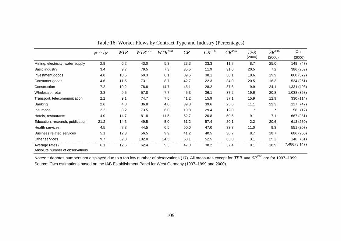
109

Table 16: Worker Flows by Contract Type and Industry (Percentages)

FTCN N WTR

FTCWTR PERWTR

CR FTCCR

PERCR TFR

(2000)

FTCSR (2000)

Obs.

(2000)

Mining, electricity, water supply 2.9 6.2 43.0 5.3 23.3 23.3 11.8 8.7 25.0 149 (47)

Basic industry 3.4 9.7 79.5 7.3 35.5 11.9 31.6 20.5 7.2 386 (259)

Investment goods 4.8 10.6 60.3 8.1 39.5 38.1 30.1 18.6 19.9 880 (572)

Consumer goods 4.6 11.5 73.1 8.7 42.7 22.3 34.0 20.5 16.3 534 (261)

Construction 7.2 19.2 78.8 14.7 45.1 28.2 37.6 9.9 24.1 1,331 (493)

Wholesale, retail 3.3 9.5 57.8 7.7 45.3 36.1 37.2 19.6 20.8 1,038 (368)

Transport, telecommunication 2.2 9.1 74.7 7.5 41.2 15.9 37.1 15.9 12.9 330 (114)

Banking 2.6 4.8 36.8 4.0 39.3 39.6 25.6 11.1 22.3 117 (47)

Insurance 2.2 8.2 73.5 6.0 19.8 29.4 12.0 * * 58 (17)

Hotels, restaurants 4.0 14.7 81.8 11.5 52.7 20.8 50.5 9.1 7.1 667 (231)

Education, research, publication 21.2 14.3 49.5 5.0 61.2 57.4 30.1 2.2 20.6 613 (230)

Health services 4.5 8.3 44.5 6.5 50.0 47.0 33.3 11.0 9.3 551 (207)

Business related services 5.1 12.3 56.5 9.9 41.2 40.5 30.7 8.7 18.7 686 (250)

Other services 9.7 32.3 102.0 24.5 63.1 52.5 63.0 3.1 25.2 146 (51)

Average rates / Absolute number of observations

6.1 12.6 62.4 9.3 47.0 38.2 37.4 9.1 18.9 7,486 (3,147)

Notes: * denotes numbers not displayed due to a too low number of observations (17). All measures except for TFR and FTCSR are for 1997–1999.


110

4.5.5 Summary of the Empirical Analysis of the Role of Fixed-Term Con-tracts in Worker and Job Flows

The possibly most important result of this Subachpter is the finding that FTCs are much more important for gross employment dynamics in the German labour market than previously found in the literature, being based on employment stocks. According to the IAB Establishment Panel, on average only 6.1% of all employees (except those of the public sector, agriculture and forestry) work on the basis of a FTC in West Germany in the period 1997–1999. However, almost 43% of all hirings are based on FTCs. This reflects the substantial worker turn-over of this type of employment which is hidden behind the low stock of FTC employment. The turnover of FTC workers accounts for almost 31% of the total worker turnover. One explanation for this surprising magnitude, which should be kept in mind, is that the flows are observed only for the first six months of each year, that is, they may be affected by seasonal effects.

As expected, FTCs are used in growing firms. The proportion of FTCs in em-ployment stock is more than 10%. The proportion of FTCs in worker turnover is about 40%, indicating that 4 in 10 hirings and separations are based on FTCs in growing establishments. These results are in line with the labour demand models predicting that FTCs are used during economic upturns.

More surprising is the amount of FTC work in shrinking establishments. The share of fixed-term employment in total employment in shrinking firms is 5.8%, with 52.8% of all hirings being based on FTCs. The widespread use of FTCs in shrinking establishments may be explained by the consideration that shrinking establishments hesitate to hire workers on permanent contracts, if a permanent position has to be filled (e.g., due to worker quits) since the future destruction probability of the job is high and so are the expected firing cost. Hence, this find-ing is insofar in line with theoretical models in Subchapter 4.2 as they predict that the negative effect of future firing costs on current hiring decisions increases with the probability that the respective job is destroyed in the future. The empirical findings cannot reject any of the three categories of reasons for

using FTCs introduced in Subchapter 4.2 (buffer stock, screening, substitution): (1.) Obviously, FTC jobs serve for adjustment purposes (buffer stock) as the job turnover rate of FTCs (sum of job creation and destruction rates) is approxi-mately six times larger than the job turnover rate of permanent workers. Whether and to what extent FTCs increase the stability of permanent contract jobs cannot be evaluated. A comparison between sectors in Table 16 does not indicate evi-dence in favour of this hypothesis. (2.) The overall rotation rate indicates that about 5.8% of all hirings and separa-tions are not associated with net employment changes. One quarter of this rota-tion is based on FTCs, although the proportion of FTCs in total employment stock is only 6.1%. Thus many hirings and firings of FTCs are not associated

111

with net employment changes and, hence, FTCs may be frequently used as sub-stitutes for permanent workers to fill permanent positions. (3.) One third of all FTC workers get their contract converted into a permanent one within the same establishment and two thirds of FTC workers leave the es-tablishment. Although this result does not state anything about causal relation-ships, the hypothesis of FTCs as a screening device (prolonged probationary pe-riod) cannot be rejected. Hence, the hypothesis of FTCs exclusively being dead ends, as they are exclusively used as buffer stock or for substitution purposes, can clearly be rejected.

4.6 Conclusions

This chapter has analysed the role of FTCs in labour demand. In addition to ad-justment purposes (buffer stock) and screening (probationary period) it has been discussed that another reason for using FTCs may be a substitution strategy: In-herently permanent jobs are repeatedly filled by FTC workers.

It has been empirically shown that firing costs for permanent workers matter for the use of FTCs, and that FTCs and permanent contract work may be closer sub-stitutes than permanent workers on the one hand and TWA and FL work on the other. Furthermore, the empirical results indicate that none of the three categories of reasons for the use of FTCs can be rejected. However, the idea of FTCs exclu-sively being dead ends can clearly be rejected.

A final conclusion is that firms seem to be interested in long-term employment relationships, otherwise all hirings would be on FTCs and no conversions of FTCs into permanent contracts would occur.104 The firm has to trade-off a high-worker-turnover strategy associated with low firing costs but high total hiring costs as well as possibly lower worker productivity and wages against a low-worker-turnover strategy associated with high firing costs but lower total hiring costs as well as possibly higher productivity and wages. The optimal solution appears to be a mixture of both and depends, inter alia, on the specific tasks in the job and the firm’s business environment. This may to some extent explain the large differences found between industry sectors.

104 It is beyond the scope of this study to discuss all the pros and cons of long-term employment relation-

ships from the employers’ point of view. Overviews can be found, e.g., in SCHASSE (1991) and FAR-

BER (1999).

112

5 Do Temporary Workers Receive Risk Premiums? – Effects of Fixed-Term Contracts on Working Conditions and Wages in the Short-Run

5.1 Introduction

Even though it would be incorrect to equate FTCs with temporary jobs and permanent contracts with long-term employment relationships, it seems plausible to expect FTC workers to bear on average a higher risk of unemployment and discontinuity than permanent workers (see Subchapter 2.1). Descriptive evidence in favour of lower objective stability of FTC jobs has been presented in Subchap-ter 4.5 (in terms of higher worker turnover) and is presented in the Appendix (Table 78). In this chapter, it is shown that lower job stability and poorer career opportunities are also perceived by FTC workers in terms of subjective assess-ments of their jobs.

What effects do FTCs have on individual wages? The well-known theory of compensating differentials states that disadvantages among work activities are equalised by wage differentials (see ROSEN, 1986). Therefore, higher risk of un-employment or generally uncertain prospects for the future working life due to a FTC may be compensated for by higher wages in a competitive labour market.105 For example, a worker holding a FTC may receive a higher wage that equalises the loss of the expected value of the redundancy payment (see BOOTH, FRANCESCONI, and FRANK, 2002).

On the other hand, there are also reasons for expecting FTCs to have negative effects on wages. For example, some economic models, presented in the previous chapter, predict that groups of workers with higher turnover (low expected job tenure) are paid less. FTCs may also serve as probationary period with lower wages at the beginning of an employment relationship, or as an incentive mecha-nism to avoid shirking during an initial period.

While available studies find some evidence for compensating wage differentials for jobs with a higher unemployment risk in the U.S. (see ROSEN, 1986), only negative effects of FTCs on wages have been found so far. Before analysing compensating differentials it should be tested whether and to what extent FTC jobs are associated with attributes decreasing the utility of FTC workers, in com-parison to the hypothetical situation in which the same worker holds a permanent contract. Even though it is obvious that the objective stability of FTC jobs is

105 It seems to be common practice to cite Adam Smith in this context. He writes about wages and job

stability: “The wages in different occupations vary with constancy or inconstancy of employment. ... The high wages of those workmen, therefore, are not so much the recompense of their skill, as the compensation of the inconstancy of their employment.” (SMITH , 1776, Vol I: 120).

113

lower, it is ex ante unclear that this aspect is associated with ‘psychological costs’ and thus a reduction of the workers’ utilities. Since the theory of compen-sating differentials is based on the assumption that workers maximise their util-ity, subjective assessments may be even more relevant than objective outcomes. Therefore, the effects of FTCs on two subjective outcome variables are esti-mated: (1.) the worker’s assessment of the risk of dismissal or termination of the contract, respectively, and (2.) the worker’s job satisfaction with regard to career opportunities.

The subsequent Subchapter presents some theoretical approaches to the wage effects of FTCs and discusses the use of subjective outcome variables. Subchap-ter 5.3 gives an overview of previous empirical studies. An introduction to the dataset and detailed descriptive statistics are provided in Subchapter 5.4. Sub-chapter 5.5 leads to the empirical analysis by discussing the econometric ap-proach. The estimated determinants for holding a FTC are presented in Subchap-ter 5.6. Subchapter 5.7 contains the econometric analysis of the short-run effects of FTCs on wages and subjective assessment of working conditions using a pro-pensity score matching estimator. A summary and conclusions can be found in Subchapter 5.8.


5.2.1 Compensating Wage Differential for Workers on Fixed-Term Con-tracts

The theory of compensating differentials assumes a competitive market. The most important assumptions are (see ROSEN, 1986): (1.) Workers seek to maxi-mise their utility, which not only depends on income, but also on other utility-related aspects of the job. (2.) Workers form expectations about the relative risks and attributes of different jobs, i.e., they are sufficiently informed. (3.) Workers have a range of job offers from which to choose. The latter may result from high occupational or regional mobility of workers.

The influential theoretical study by ABOWD and ASHENFELTER (1981) models the competitive equilibrium wage rate under the assumption that job offers vary according to the amount of (1.) anticipated unemployment and (2.) unemploy-ment risk.

(1.) Unemployment is modelled as a predictable constraint in the hours of work (for example within one year), which prevents workers from working the number of hours they would like to work. For example, FTCs may be used for seasonal jobs, so that workers can work less than they would like to within a year. If workers had the choice, they would always prefer the unconstrained job to the constrained job with the same wage rate. In a perfect labour market the compen-

114

sating wage differential for anticipated unemployment is simply an increase in the wage rate eliminating the utility differences.

(2.) Unemployment risk is modelled by the assumption that the hours constraint is not known with certainty, but is a random draw from a known hours distribu-tion and, therefore, a known mean hours constraint. Sign and magnitude of the compensating differential for the risk depends on the worker’s attitude towards risk. Imposing the assumption that workers are risk averse, that is, their utility function is convex due to diminishing marginal utility of income, there must be a positive differential. Thus an equilibrium requires the wage rate to compensate for the mean constraint in hours worked as well as for the risk of fluctuation in hours worked.

BOOTH, FRANCESCONI, and FRANK (2002) argue that workers on FTCs, given the assumption of the theory of compensating differentials, may receive a higher wage that offsets the loss of the expected value of the redundancy payment.106 The compensating differential depends on the probability of the worker receiving a permanent contract afterwards (or the probability of losing the job, respec-tively), the worker’s attitude towards risk, and the features of the unemployment insurance system.

5.2.2 Wage Penalty for Workers on Fixed-Term Contracts

There is a number of reasons why workers holding FTCs may not receive a compensating differential, but even (contemporaneously) lower wages.107

First of all, the problems employers face in their hiring decision and in the ini-tial period of the employment relationship after the match is formed are summa-rised. In principle, all models are based on this framework, albeit some aspects may be omitted in the respective model (see GIBBONS and WALDMAN , 1999). Generally, it is assumed that the output (or productivity) of a worker in a given job is a function of her or his observable characteristics (qualification, age, etc.), her or his ability (which is unobservable to the employer), and her or his effort (possibly also unobservable to the employer). Effort is associated with individual costs for the worker. The employer can assess the applicant and the employed worker only by her or his observable characteristics, her or his signals, and her or his output. The employer has to decide whether to hire a particular applicant, whether to retain her or him after an initial period (or recurrently in every pe-riod), and how to provide appropriate incentives for the worker (see GIBBONS

106 This is familiar with the model of LAZEAR (1990) outlined in Section 4.2.2. Lazear’s model predicts

the neutrality of firing costs, since in efficient bargaining models legally mandated severance pay-ments may be entirely offset by payments from workers to firms. Payments from firms to workers (as a compensating differential) in case of FTCs obviously are the other side of the same coin. Lazear’s model differs, however, with respect to one important assumption from the theory of equalising dif-ferences: workers do not maximise their utility but earnings.

107 Some of these issues will be discussed in greater detail in Chapter 6 in the context of the long-term employment effects of FTCs.

115

and WALDMAN , 1999). In general, the underlying problems can be characterised as follows:

Before hiring: Applicants have some characteristics which are observable for the employer and some which are unobservable (e.g. ability). Hence, ex ante, the match-specific productivity is to a certain extent unknown and has to be experi-enced by forming the match (see JOVANOVIC, 1979), or it is revealed by a sorting mechanism (see WEISS, 1995). Employers try to learn something about the unob-servable characteristics (ability) of the applicants by interpreting their labour market history. For example, if there are two applicants with otherwise identical observable characteristics, employers may decide to hire the one with the shorter unemployment spell (see BLANCHARD and DIAMOND , 1994), or the one who has not been dismissed by one of her or his previous employers (see GIBBONS and KATZ, 1991).

After hiring: During an initial period (which may be a probationary period) em-ployers are still uncertain about the true ability of the new worker and try to learn something by assessing the output or productivity of the worker (screening).

Workers try to signal their ability, e.g., by entering or not entering specific jobs (see the discussion on probationary periods below). After the match has been formed workers may try to signal high productivity by increasing their output through choosing their level of effort. However, since exerting effort is associ-ated with costs for workers, it may also be optimal for the worker to shirk (see GIBBONS and WALDMAN , 1999).

A number of efficiency wage models, based on the moral hazard problem asso-ciated with shirking, explain how duality of the workforce may arise inside firms. For example, in the tradition of the SHAPIRO and STIGLITZ (1984) efficiency wage model, REBITZER and TAYLOR (1991) show that wages paid to permanent workers exceed those paid to temporary workers, if one assumes monitoring of workers to be costly, and product demand to be uncertain. It is profitable for the firm to pay efficiency wages to permanent workers, while monitoring temporary workers, which leads to lower wages, although both are perfect substitutes. The efficiency wage model by SAINT-PAUL (1991), already presented in Subchapter 4.2, yields the same results. An interesting feature of this model is that the duality within firms arises endogenously without the existence of two types of contracts. However, both models have the drawback that the possibility of FTC workers becoming permanent workers within the same firm is neglected.

GÜELL (2000) provides an efficiency wage model in which the possibility to convert a FTC into a permanent contract is used by employers as an incentive mechanism. While shirking of permanent contract workers is prevented by effi-ciency wages, this is unnecessary for FTC workers since their conversion prob-ability is positively linked to their productivity and hence their effort. During the FTC job, wages provide no incentive for effort. Therefore, wages can be reduced in comparison to permanent workers.

116

Another strand of the theoretical literature views an initial FTC as a probation-ary period providing the employer with the possibility of learning about the worker’s ability without incurring institutional firing costs in case the match is resolved (see BOOTH, FRANCESCONI, and FRANK, 2002 as well as Subchapter 4.2). As pointed out by LOH (1994), probationary periods with lower wages may induce self-selection of workers with higher abilities because they have a higher probability of obtaining permanent contracts afterwards. FTCs with lower initial wages may therefore function as a sorting device implemented by firms since low wages during the FTC period will be compensated for by higher future wages at the same employer. Hence, high-ability workers may select themselves into low-paid FTC jobs.

In Subsection 6.2.2, it is discussed in greater detail that a worker’s labour mar-ket history may be interpreted as a signal by potential employers in the presence of incomplete information on the ability of job searchers (or applicants). If a job searcher’s employment history involves adverse signals, employers may hesitate to offer her or him a permanent contract, but prefer to offer a FTC first. Hence, if adverse signals are indeed correlated with unobservables (such as ability), it is possible that low-ability workers have to enter into FTCs as they receive perma-nent contract job offers only with a low probability. Note that this statement is contrary to the prediction of LOH’s (1994) model.

In presence of asymmetric information on ability and so-called career concerns of workers, another phenomenon may occur which highlights the investment na-ture of a job’s initial period (see GIBBONS and MURPHY, 1992). It is assumed that an employer cannot distinguish between a worker’s ability and effort. Therefore, the employer has to assess the worker by her or his output. In general, career concerns arise, if the internal or external labour market uses a worker’s current output to update its belief about the worker’s ability, and bases decisions on fu-ture wages on these beliefs. The worker has an incentive to invest in effort to in-crease her or his output in order to influence the market’s (employer’s) belief. In equilibrium, however, the market anticipates this incentive and draws correct inference about the worker’s ability from the observed output. The model has some interesting implications: At the beginning of her or his career a worker has more incentives to invest in additional effort because a longer prospective career increases the return to changing the market’s belief. In an optimal incentive con-tract, current pay is most sensitive to current performance for workers close to retirement and for workers with low career opportunities. Put differently, for workers with career opportunities (such as a possible conversion from a FTC into a permanent contract) additional output related pay is less necessary than for workers with no career opportunities (such as permanent contract workers near retirement). Although GIBBONS and MURPHY (1992) do not take probationary

117

periods or FTCs explicitly into account, their result is in line with lower wages during FTC periods due to the workers’ willingness to invest in effort.108

A further explanation of lower wages of FTC workers can be derived from a human capital argument. Expected job tenure of permanent contract workers is higher. Hence, permanent workers and their firms have more incentives to invest in human capital than FTC workers and their employers due to the well-known hold-up problem109. This may lead to higher wages. BOOTH, FRANCESCONI, and FRANK (2003) develop a simple labour demand model with stochastic product demand in which dualism inside firms arises endogenously due to human capital investment decisions and temporary workers serving as buffer stock (see Sub-chapter 4.2). The distinction between temporary and permanent work arises by the decision of firms to train some of their employees. After the training, trained (permanent) and untrained (temporary) workers are treated differently in terms of wages and firing probability. The wage differential is caused by the fact that training always incorporates a specific as well as a general component of human capital. Untrained temporary workers may have fewer outside opportunities, and hence may be paid lower wages. The model implies that, even if all workers are ex ante identical, it is optimal for the firm to offer relatively stable employment relationships with high training to some of its new employees, and to offer unsta-ble employment with low training to others. Hence, trained permanent workers gain rents in the model: although they do not contribute to the cost of training their wages are higher since firms pay more in order to avoid quits.

Another reason for negative wage effects may be relevant, if FTC workers are more frequently employed in low unionised sectors or firms (see SEGAL and SULLIVAN , 1998). However, in Subchapter 4.4 no significant effect of collective wage agreements on the firms’ use of FTCs has been found. Therefore, this is probably a minor issue in practice.

Finally, FTC workers may be outsiders in the wage bargaining process. The augmented insider-outsider model proposed by BENTOLILA and DOLADO (1994) shows that, if unions represent mainly the interests of workers on permanent con-tracts, but set wages for all workers, the existence of FTCs increases the unions’ bargaining power. If FTC employment serves as a buffer against the negative effects of wage rises on the employment probability of permanent contract work-ers, the aggregate wage level may be higher, the higher the proportion of FTCs is. If firms can pay lower wages to FTC workers, this may compensate the firms for the wage rise, and the firms’ overall labour costs may not change or may de-

108 The application of GIBBONS and MURPHY’s (1992) model to FTCs has been proposed by

ENGELLANDT and RIPHAN (2003). 109 See GIBBONS and WALDMAN (1999) for a survey of the hold-up problem. See AUTOR (2003) for a

theoretical model describing the impact of firing costs on investments in specific human capital.

118

crease in the proportion of FTCs (see DOLADO, GARCÍA-SERRANO, and JIMENO, 2002).110

Recapitulating the theoretical arguments, there are four reasons for paying a worker less because she or he holds a FTC instead of a permanent contract: (1.) in case of insider power of permanent contract workers and the firm’s possi-bility to pay FTC workers lower wages; (2.) in case of hold-up problems caused by human capital investments for perma-nent workers; (3.) in the presence of incomplete information on the ability of job applicants, FTCs are used as a screening device with lower wages, which may lead to a sort-ing effect and higher effort during the FTC jobs. The initial FTC job may even be a regular part of the career path;111 (4.) in the presence of hidden actions (shirking), permanent workers receive effi-ciency wages, while FTC workers do not so, since (a) they are monitored or (b) the probability of conversion into a permanent contract is related to their effort.

The last two points lead to the insight that it may be quite misleading to focus exclusively on contemporaneous wages and utility during a FTC job, instead of looking at expected lifetime wages and utility. Workers may enter into low-paid FTC jobs since this is an investment with returns in future periods. If the theo-retical models are relevant and FTCs are nothing but probationary periods lead-ing to a sorting mechanism, there should not be a strong negative effect of hold-ing a FTC on job satisfaction with regard to the career opportunities.112

A remaining issue is how employers in practice pay FTC workers lower wages than permanent workers. There is anecdotal evidence that FTC workers are not discriminated on given positions by circumventing the standards fixed in collec-tive agreements or standards which are common in the firm (see LINNE, 1991). A more likely way may be to assign FTC workers to a lower pay scale group (‘Tarifgruppe’) with the prospect of an advancement in case the contract is con-verted into a permanent one, after the initial FTC period (see LINNE, 1991). Fur-thermore, there may be the possibility to vary the amount of bonus payments which are not stipulated by collective wage agreements.

110 On the other hand, there may be a disciplinary effect: Due to their lower employment stability, FTC

workers are wary of engaging themselves in strikes led by the insiders (permanent workers). Thus permanent workers fear to be replaced by FTC workers in case of strikes. Hence, the power of per-manent workers erodes as the proportion of FTC workers increases (see DOLADO, GARCÍA-SERRANO, and JIMENO, 2002).

111 As stressed by MCGINNITY and MERTENS (2003), for some professional careers, such as teachers, researchers, and doctors, FTC jobs are an important part of acquiring further experience before finally reaching a permanent position.

112 The obvious problem is, that it is unclear what “strong negative effect” means in terms of magnitude.

119

5.2.3 Worker Preferences for Fixed-Term Contracts

A FTC at the request of the employee is a legally accepted reason for the justi-fication of the use of FTCs by objective reasons in Germany (see Subchapter 2.2). Assuming that there is no compensating wage differential and that the in-vestment and screening character of FTCs, as described in the previous section, is not given: Are there any reasons for a worker to choose a FTC, if she or he can also get a permanent contract, with otherwise identical job attributes, with the same employer?113

The analysis of ABOWD and ASHENFELTER (1981) introduced above can be ap-plied to highlight the conditions under which workers may prefer FTCs. Remem-ber that unemployment is modelled as a predictable constraint in the hours of work. If the hours constraint refers to one year, it is obvious that some workers may prefer a seasonal full-time job for some months to a part-time job for the whole year, given they prefer less than one year full-time. However, the seasonal work schedule of the job does not need to be implemented by a FTC job. The same seasonal job could be stipulated in a permanent contract, which would pro-vide the worker with a higher security for getting the same seasonal job again in the subsequent year. Put differently, individuals do not prefer the FTC, but the associated arrangement with regard to the hours of work. If it was possible to have the same arrangement within a permanent contract, workers would again prefer the permanent contract to the FTC. The same is true for workers preferring a temporary job because they want to take up another job at a later date, want to start an apprenticeship, or study at a university. Workers can quit a (permanent) job any time (considering a certain notice period) to take up another activity (see LINNE, 1991).

There may be one reason for workers to prefer FTCs resulting from an incen-tive created by the German unemployment insurance system: If workers really prefer a job to be temporary (due to the reasons previously mentioned), they are better-off when becoming unemployed due to the termination of a FTC in com-parison to quitting the job. The reason is that quitting one’s job leads to a period of exclusion (‘Sperrzeit’) from unemployment compensation (see LINNE, 1991).

5.2.4 Heterogeneity of Fixed-Term Contract Jobs

The discussion has already suggested that there may be important differences in the effects of FTCs on working conditions and wages, which may depend on the type of job as well as on the characteristics of the workers. There may be ‘bad FTC jobs’ which are used solely for adjustment and substitution purposes (see Subchapter 4.2) and ‘good FTC jobs’ which serve as extended probationary pe-

113 See HOLMLUND and STORRIE (2002) for a comparable discussion on the relevance of workers’ pref-

erences for FTCs in the Swedish labour market.

120

riod, or are even a common part of the career path. MCGINNITY and MERTENS (2003) term this idea “two-tier labour market for FTCs”.114

It seems reasonable to assume that ‘bad FTC jobs’, requiring only low human capital endowment of the workers, are more likely to be affected by ‘dual labour market effects’ (i.e., low wages, low career opportunities, and low job stability) than ‘good FTC jobs’ for highly qualified workers (see MCGINNITY and MERTENS, 2003).

However, with respect to the wage effects the predictions are ambiguous. If a FTC serves as probationary period, it may be associated with a low initial wage level but a high wage growth (see WANG and WEISS, 1998; MCGINNITY and MERTENS, 2003).115 Especially persons with career concerns may be more will-ing to accept low initial wages in FTC jobs in exchange for career opportunities. It seems reasonable to assume that young individuals with high formal qualifica-tion are more likely to be concerned about their career. In contrast, if a FTC worker is used only for substitution or as a means of adjustment, and thus the conversion probability is rather low, workers may not be willing to accept lower wages. This may, for example, be more relevant for workers with low qualifica-tion. More general, the higher the transformation probability, the lower the com-pensation FTC workers demand. Hence, it is an empirical question how the wage effects of FTCs differ between groups of persons. If a FTC serves as a probation-ary period for one group of persons (e.g., highly qualified workers) more than for another group of persons (e.g., low-qualified workers), then the wage effect should be more negative.

5.2.5 Use of Subjective Outcome Variables in Economic Analysis

As mentioned in the introduction, besides the wage level, also two subjective outcome variables (assessment of the risk of dismissal or termination of the con-tract, and job satisfaction with regard to career opportunities) are used.

The main reason for using subjective outcome variables is that they may be more strongly correlated with utility than ‘objective’ job attributes.116 As docu-mented in an ongoing discussion, subjective variables are likely to be noisy due to various reasons (see, e.g., FREEMAN, 1978; CLARK; 1997, 2001; HAMERMESH, 2001; CLARK ET AL., 2004).117 Since picking up the whole discussion would be beyond the scope of this chapter, only some crucial issues are mentioned. As

114 MCGINNITY and MERTENS (2003) assume that the heterogeneity may be taken into account by esti-

mating the wage effect for different quantiles of the wage distribution. 115 Unfortunately, analysing wage growth is not possible within the analysis of this chapter since the

underlying dataset is a single cross-section. 116 See FREY and STUTZER (2002) for a general discussion on the use of subjective variables (especially

about subjective well-being) in economic analyses. 117 FREEMAN (1978: 135): “... while there are good reasons to treat subjective variables gingerly, the

answers to questions about how people feel toward their job are not meaningless but rather convey useful information about economic life that should not be ignored.”

121

suggested by CLARK (1997), one source of bias, which may be particularly rele-vant for between group comparisons of subjective variables, is that utility (and thus job satisfaction) may be determined by relative values and expectations. He analyses the phenomenon of women usually reporting a higher level of job satis-faction than men, even though their jobs are worse in terms of objective stan-dards. He finds evidence in favour of the hypothesis that satisfaction is deter-mined by a comparison of the present situation to a comparison level, which is mainly given by the workers’ own experiences in the past. Hence, the higher job satisfaction of women is explained by their lower expectations resulting from worse experiences in the past.

This issue may also be relevant for the analysis at hand. For example, univer-sity graduates may have a higher demand for career opportunities than workers without formal qualification. Hence, at a given job the former are more likely to be dissatisfied than the latter. Since FTC workers are only compared with a con-trol group with on average similar observable characteristics, this issue may not be relevant here. Furthermore, one can assume that, if expectations are generated by labour market experiences, using a control group of workers with on average similar labour market experiences, balances differences in expectations between FTC workers and the control group of permanent workers.

A more difficult problem arises, if the type of contract itself affects the com-parison level, that is, if FTC workers only compare their situation with other FTC workers but not with all workers. For example, if FTC workers have lower ex-pectations with regard to their career opportunities and job security due to the fact that they hold FTCs, this would systematically bias the (expected negative) treatment effects on job security and career opportunities towards zero. As the majority of workers still holds permanent contracts and since permanent con-tracts are still the standard type of employment relationship in the public percep-tion, this bias is unlikely.

A remaining problem is that comparisons of the estimated effects of FTCs on subjective outcome variables between different groups of workers (men versus women; young versus old etc.) may be meaningless. Different groups of workers have different expectations and hence comparison levels. Therefore, the effects of FTCs on subjective outcome variables of different groups of workers are esti-mated and presented, but not compared between groups.

5.3 Previous Empirical Results

Empirical studies may be classified by whether they are static or dynamic. Static in this context means that contemporaneous or short-term effects of FTCs in comparison to permanent contract jobs are analysed. The underlying counter-factual is the hypothetical situation of the FTC workers holding permanent con-tracts. Dynamic means that also long-term (especially wage) effects of having

122

been in a FTC job in the past on future outcome variables are analysed in com-parison to having been in a permanent job in the past.

Starting with contemporaneous wage effects, BOOTH, FRANCESCONI, and FRANK (2002) find that FTC workers in the UK earn less than permanent work-ers (men -8.9% and women -6%).

In a previous study, I found that FTC workers earn 5% less than comparable permanent contract workers using the method of propensity score matching based on a cross-section of the German Socio-Economic Panel (GSOEP) for West Germany in 1999 (see HAGEN, 2002). A comparable magnitude is found by SCHÖMANN and KRUPPE (1994) for West Germany using parametric regressions. MCGINNITY and MERTENS (2002) using the GSOEP do not find significantly negative wage effects for West Germany when applying an instrumental variable approach, that is, when also taking selection on unobservables into account (see Section 3.3.3). In order to reveal more about the distribution of the wage effect, MERTENS and MCGINNITY (2003) apply quantile regression techniques, that is, the effects are estimated for different quantiles of the wage distribution. It turns out that workers in the upper quantiles earn only slightly less than their perma-nent counterparts, whereas workers in the lowest quantile earn considerably less.

BROWN and SESSIONS (2003) use a switching regression approach and find a negative earnings effect of 13% for the UK. Furthermore, they apply an Oaxaca-Decomposition of the earnings differential (see, e.g., GREENE, 2003 for a intro-duction to this method). The purpose is to decompose the wage differential into an endowment component (characteristics of the workers such as qualification, experiences, and sex) and a price component (how this endowment is valued by the market in terms of earnings). It turns out that 70% of the earnings differential is due to a price component, that is, the endowment of the FTC workers is less valued in terms of earnings than the endowment of permanent workers (e.g., a human capital investment has a lower return in FTC jobs than in permanent jobs). The authors interpret the results as evidence for discrimination on the part of employers. However, this result is also in line with the idea of a FTC as a kind of investment.

As mentioned in Section 5.2.2, one reason for lower wages may be lower in-vestment in human capital in combination with the hold-up problem. Indeed ARULAMPALAM and BOOTH (1998) show for the UK that men on FTCs are 16% and women are 12% less likely to receive work-related training. This result has been confirmed by BOOTH, FRANCESCONI, and FRANK (2002) finding for men a 12% and for women a 7% lower probability of work-related training.

BARDASI and FRANCESCONI (2003) analyse the effects of FTCs on self-reported subjective wellbeing for the UK in the 1990s. They find no significant effect of FTCs on health. Only for women there is a significantly negative effect on life satisfaction. The study by BOOTH, FRANCESCONI, and FRANK (2002) finds a strong negative effect of FTCs on different aspects of job satisfaction for the UK. For both men and women there are no significant effects on overall job satisfac-

123

tion, but negative effects on satisfaction with career opportunities and job secu-rity.

For Spain, there are two empirical studies highlighting another utility-related aspect of FTCs: Their effects on work accidents and injuries as well as illness rates. According to GUADALUPE (2003), there are two theoretical reasons for expecting FTCs to raise work accidents: (1.) lower investments in human capital, (2.) higher effort of FTC workers in order to increase the conversion probability. Using a panel of aggregate industry data, GUADALUPE (2003) finds that FTCs increase the probability of work accidents to happen by 5 percentage points. She concludes that the use of FTCs is associated with higher social costs and a pro-ductivity loss. Using individual level data AMUEDO-DORANTES (2002) finds the opposite: Controlling for working conditions FTCs lead to a lower probability of work injuries and illness. However, GUADALUPE (2003) argues that this result may be biased by a number of factors, such as differences in reporting of work injuries between FTC and permanent workers.

Absence from work (due to illness, accidents, and family matters) as well as unpaid overtime are interpreted by ENGELLANDT and RIPHAN (2003) as proxy variables for worker’s effort in an empirical analysis for Switzerland. The hy-pothesis is that FTC workers have an incentive to signal their effort in order to increase the probability of getting their contract transformed into a permanent one, as suggested by the model of GIBBONS and MURPHY (1992) discussed above. They find that FTC workers have a 60% higher probability of working unpaid overtime. Workers in positions with the potential for upward mobility have an even higher probability. However, ENGELLANDT and RIPHAN (2003) find no significant effect on the probability of absence from work.118 My interpreta-tion is that the latter finding may result from two opposed effects: FTCs increase illness and accidents on the one hand, but workers do not dare to be absent from work on the other.

Note that the finding of ENGELLANDT and RIPHAN (2003) is in line with the hypothesis of a FTC job as an investment in lifetime earnings or utility, while the results with regard to the negative effects on satisfaction with career opportuni-ties and job security as well as the negative effects on training opportunities seem to be more in line with the use of FTCs as a means of adjustment or substitution, and hence, adverse long-term effects on the individual career path.

There are only few dynamic studies comparing the situation of having entered into a FTC job with the counterfactual situation of having entered into a perma-nent job on future wages. The study for the UK by BOOTH, FRANCESCONI, and FRANK (2002), shows that workers holding a FTC job in the first period of their employment spell and getting a permanent contract later, start with a lower wage

118 ICHINO and RIPHAN (2001) find a strong increase in absenteeism after the probationary period (when

protection against dismissal comes into effect) among Italian bank employees. RIPHAN and THALMEIER (2001) obtain a similar result for Germany.

124

level (men -8.9% and women -6%), but have a higher wage growth than compa-rable permanent workers. After ten years, women who had been employed in FTC jobs, receive the same wage as those who started with permanent contracts. In contrast, men are not able to catch up and still receive a wage penalty of -5% after ten years of employment. For West Germany, MCGINNITY and MERTENS (2002) also find that an initial FTC increases wage growth.

Note that the results are again in line with idea of a FTC as an investment pe-riod or as a probationary period. On the other hand, the result by BOOTH, FRANCESCONI, and FRANK (2002), that men who had a FTC ten years ago still have lower wages, seems to be contradictory.

5.4 Data Base, Estimation Sample, and Descriptive Statistics

Data Base and Estimation Sample

In order to evaluate the effects of FTCs on individual wages and subjective as-sessments of working conditions, the BIBB/IAB dataset, a representative sample of 0.1% of all individuals employed in Germany, is used.119 The survey is im-plemented every seven years, but cannot be used as a panel. Here, the latest wave from the survey in 1998/99 is used. It includes more than 34,000 employees who were interviewed between October 1998 and March 1999. This cross-sectional dataset contains detailed information on the qualification and professional career of each employee, the organisational and technological environment of jobs, in-formation about the employer as well as a variety of assessments of working conditions with regard to different job attributes.

Starting with a sample of 27,634 employees living in West Germany the fol-lowing persons are excluded: participants in public employment measures, per-sons younger than 21 or older than 57, employees in the public sector or in the farming sector, persons in mini-jobs120, persons in military or civilian service, trainees and apprentices, pupils, students, and pensioners. Furthermore, only workers in their main jobs are included since the earnings information is avail-able only for this group. Finally, approximately 12,800 persons are used in the econometric analysis.

Specifically, the following variables are used. The central question defining the treatment status is: “Are you presently in a fixed-term or an undefined term em-ployment relationship?” A dummy variable is created accordingly. The variable containing information on job tenure (in years), that is, the elapsed duration of

119 The BIBB/IAB “Qualification and Career Survey” dataset is jointly collected by the Research Insti-

tute of the Federal Labor Office (Institut für Arbeitsmarkt- und Berufsforschung, IAB Nuremberg) and the Federal Institute for Vocational Training (Bundesinstitut für Berufsbildung, BIBB Berlin).

120 That is, persons in jobs not covered by social security (630-DM-Job).

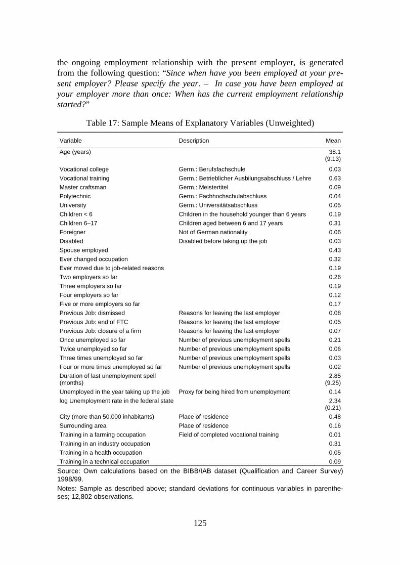
125

the ongoing employment relationship with the present employer, is generated from the following question: “Since when have you been employed at your pre-sent employer? Please specify the year. – In case you have been employed at your employer more than once: When has the current employment relationship started?”

Table 17: Sample Means of Explanatory Variables (Unweighted)

Variable Description Mean

Age (years) 38.1 (9.13)

Vocational college Germ.: Berufsfachschule 0.03

Vocational training Germ.: Betrieblicher Ausbilungsabschluss / Lehre 0.63

Master craftsman Germ.: Meistertitel 0.09

Polytechnic Germ.: Fachhochschulabschluss 0.04

University Germ.: Universitätsabschluss 0.05

Children < 6 Children in the household younger than 6 years 0.19

Children 6–17 Children aged between 6 and 17 years 0.31

Foreigner Not of German nationality 0.06

Disabled Disabled before taking up the job 0.03

Spouse employed 0.43

Ever changed occupation 0.32

Ever moved due to job-related reasons 0.19

Two employers so far 0.26

Three employers so far 0.19

Four employers so far 0.12

Five or more employers so far 0.17

Previous Job: dismissed Reasons for leaving the last employer 0.08

Previous Job: end of FTC Reasons for leaving the last employer 0.05

Previous Job: closure of a firm Reasons for leaving the last employer 0.07

Once unemployed so far Number of previous unemployment spells 0.21

Twice unemployed so far Number of previous unemployment spells 0.06

Three times unemployed so far Number of previous unemployment spells 0.03

Four or more times unemployed so far Number of previous unemployment spells 0.02

Duration of last unemployment spell (months)

2.85 (9.25)

Unemployed in the year taking up the job Proxy for being hired from unemployment 0.14

log Unemployment rate in the federal state 2.34 (0.21)

City (more than 50.000 inhabitants) Place of residence 0.48

Surrounding area Place of residence 0.16

Training in a farming occupation Field of completed vocational training 0.01

Training in an industry occupation 0.31

Training in a health occupation 0.05

Training in a technical occupation 0.09

Source: Own calculations based on the BIBB/IAB dataset (Qualification and Career Survey) 1998/99. Notes: Sample as described above; standard deviations for continuous variables in parenthe-ses; 12,802 observations.

126

The following outcome variables are used. Hourly wages are calculated from earnings (including overtime) and actual weekly hours of work. The exact word-ing of the question about earnings is: “How much are your monthly gross earn-ings from your main activity? If your earnings fluctuate very much, please report your average earnings”. One problem arises due to the fact that the earnings variable is collected not as a continuos number but in bracket form with 19 brackets. Following DINARDO and PISCHKE (1997) as well as FITZENBERGER and SPITZ (2004), the approach chosen here is to assign the midpoint to every bracket. For the highest category which is not bound above, the lower bound (15,000 DM; 7,669 Euro) is assumed.121 It has been shown, among others, by KUCKULENZ and ZWICK (2003) that the point estimates of coefficients in a Min-cer-type earnings equation do not substantially differ between OLS using the generate earnings variable and maximum likelihood interval regression models using the bracket form. For calculating hourly wages the information on the usual weekly hours of work is used.

The second outcome variable is subjective assessment of job security. Persons are asked the following question: “How do you assess the danger of being dis-missed by your employer in the near future? / failing to get your contract re-newed?” Possible answers are “very high danger”, “ high danger”, “ rather low danger”, and “no danger at all”. Four dummy variables are generated accord-ingly.

The third outcome variable is satisfaction with career opportunities at the pre-sent job. Possible answers are “very satisfied”, “ by and large satisfied”, “ rather dissatisfied”, and “very dissatisfied”. Again, four dummy variables are generated for these answers.

Table 17 provides a description of the explanatory variables (including German notions for formal qualifications) used in the econometric analyses and some de-scriptive statistics. More descriptive statistics are presented in the next subsec-tion.

Descriptive Statistics

In Table 18 the proportion of FTCs in different parts of the job tenure distribu-tion of all workers is depicted. It is differentiated between unweighted sample means and weighted statistics being estimates for the means in the population (West German employees). It can be seen that the weighted and unweighted means differ only slightly.

However, as mentioned in Subchapter 2.3, the presented means are unsuitable for assessing the duration distribution of FTCs due to spell truncation and length bias. Nevertheless, Table 18 exposes at least one important fact for the further analyses. Almost 60% of all ongoing FTC employment spells are shorter than 2

121 This is very unlikely to bias the results since only 48 individuals in the sample (0.37%) report earn-

ings in this category.

127

years.122 This corresponds to the maximum duration stipulated by the Employ-ment Promotion Act, which is in force for the period under observation. Thus FTC jobs with a duration of more than 2 years must be based on the regulations according to the Civil Code. More than 90% of ongoing FTC employment rela-tionships are not longer than 10 years. The median duration of ongoing FTC spells is 2 years and of permanent contract spells is 8 years (this holds for the unweighted and the weighted sample).

An important finding from this analysis is that it may be quite misleading sim-ply to compare mean characteristics of all FTC workers with all permanent workers, since there are very few FTC workers in the right tail of the tenure dis-tribution (see also Subchapter 2.3). Put differently, since the probability to hold a FTC after being employed at the same employer for more than 10 years goes to zero, it does not make much sense to use permanent workers with more than 10 years of job tenure for the estimation of the relevant counterfactual situation of FTC jobs. Therefore, in the econometric as well as the descriptive analyses, sam-ples restricted to job tenure ≤10 years and job tenure ≤2 years are defined. Note that this is a first attempt to impose common support (see Section 3.3.1).

Table 18: Number and Proportion of FTCs by Ongoing Job Tenure – Weighted and Unweighted Sample Means (Percentages)

Men Women Tenure (years)

number

un-weighted

proportion

un-weighted

cumulated proportion

un-weighted

proportion

weighted

number

un-weighted

proportion

un-weighted

cumulated proportion

un-weighted

proportion

weighted

0 32 29.09 6.02 28.59 23 27.38 5.35 25.57

1 206 22.34 44.74 22.11 155 20.83 41.4 21.74

2 82 13.16 60.15 12.91 72 14.40 58.14 15.12

3 34 6.83 66.54 6.64 32 6.79 65.58 6.27

4 24 4.73 71.05 4.61 30 7.08 72.56 7.50

5 28 6.18 76.31 6.73 11 3.15 75.12 2.88

6 18 4.36 79.69 4.20 17 5.04 79.07 6.31

7-8 34 4.12 86.08 4.67 29 4.52 85.82 4.33

9-10 23 2.66 90.40 2.20 27 4.32 92.10 4.96

≥ 11 51 1.44 100.00 1.40 34 1.92 100.00 2.03

Total 532 6.07 5.88 430 7.23 7.28

Source: Own calculations based on the BIBB/IAB dataset 1998/99. Notes: Sample as described in the previous subsection. Weighted figures are obtained using the individual weights (inflation factors) included in the BIBB/IAB dataset.

122 In Subchapter 2.3, using a question from the German Microcensus which is not subject to spell trun-

cation, it turns out that approximately 83% of all FTCs are not longer than 24 months. Note, however, that in this chapter employment spell durations are analysed, while Subchapter 2.3 analyses durations of FTCs as stipulated in the contracts.

128

Assuming that actual (in contrast to stipulated) hours of work reflect workers’ effort as suggested by ENGELLANDT and RIPHAN (2003), and that FTC workers invest more in effort, one would expect on average longer hours of work in FTC jobs. Of course, since the analysis in this subsection is a descriptive one, this hy-pothesis cannot be tested in causal sense.123 Table 19 depicts the average usual weekly hours of work. For men the result is fairly clear: Permanent contract jobs are associated with significantly more working hours than FTC jobs. For women the results are different: Depending on the samples, the average weekly hours of work of female FTC workers are even larger. In the sample with tenure ≤2 years female FTC workers work 2.67 hours more per week than female permanent workers do (see Subchapter 2.3 for a complementary analysis).

Table 19: Means of Usual Weekly Hours of Work by Type of Contract (Standard Errors in Parentheses)


FTC PERM t-test (p-value)


unrestricted 40.11 (0.42)

42.71 (0.11)

-6.03 (0.00)

29.94 (0.61)

31.03 (30.70)

-1.73 (0.08)

≤10 39.93 (0.48)

41.29 (0.12)

-2.77 (0.01)

30.37 (0.65)

30.00 (0.21)

0.55 (0.59)

≤2 40.33 (0.64)

41.75 (0.25)

-2.08 (0.04)

30.54 (0.82)

27.87 (0.42)

2.88 (0.00)

Source: Own calculations based on the BIBB/IAB dataset 1998/99. Notes: Sample as described in the previous subsection. Weighted figures are obtained using the individual weights (expansion factors) included in the BIBB/IAB dataset.

So far only the means of the weekly hours of work have been considered. In the

following the whole distribution is taken into account. In Table 20 the null hy-pothesis that the hours distribution of FTCs and the hours distribution of perma-nent contracts are from populations with equal distributions is tested by perform-ing a Wilcoxon ranksum test (also known as the Mann-Whitney two-sample sta-tistic; see CONOVER, 1999). Furthermore, an estimate of the probability of the value of the working hours in permanent contract jobs being larger than the value of working hours in FTC jobs is presented (Pr(PERM>FTC)). In principle, this is a test for whether the hours distribution of permanent contract jobs is in the right of the hours distribution of FTC jobs. The results indicate for men that FTC and permanent jobs have significantly different distributions of hours of work, with evidence in favour of longer hours of work in permanent jobs. For women only the results for the unrestricted sample indicate that the FTC and the permanent contract hours distribution is significantly different at the 5% level. For tenure ≤2

123 A causal analysis of this issue is presented in Subchapter 5.7.

129

years the results are even more in favour of longer working hours in FTC jobs, as already found in Table 19.

Table 20: Two-Sample Wilcoxon Rank-Sum Test for Differences in the Distribu-tion of Usual Weekly Hours of Work by Type of Contract

(p-Values and Estimated Probabilities)

Tenure (years)

Men Women

unrestricted H0: FTC=PERM 0.000 0.019

Pr(PERM>FTC) 0.574 0.533

≤10 H0:FTC = PERM 0.000 0.636

Pr(PERM = FTC) 0.564 0.507

≤2 H0:FTC=PERM 0.000 0.303

Pr(PERM>FTC) 0.582 0.479

The distribution of monthly earnings can be found in Table 21. The tendency

that not only the mean (see the last row) but the whole distribution of permanent contract workers’ earnings is in the right of the FTC workers’ earnings distribu-tion seems to be obvious. Even though monthly earnings are not continuously measured, the Wilcoxon rank-sum test is again applicable since the test requires at least an ordinal scale (see CONOVER, 1999). The differences in the earnings distribution is only for women with tenure ≤ 2 years not statistically significant.

130

Table 21: Earnings Distribution by Type of Contract (Percentages)

Men Women Tenure (years) Unrestricted Tenure ≤10 Tenure ≤2 Unrestricted Tenure ≤10 Tenure ≤2

Monthly Earnings Y in € FTC PERM FTC PERM FTC PERM FTC PERM FTC PERM FTC PERM Y < 307 1.13 0.20 1.34 0.24 1.82 0.47 5.12 3.80 4.93 4.75 6.50 7.22 307 ≤ Y < 511 0.83 0.51 0.99 0.73 1.29 1.18 12.00 10.80 12.38 13.53 12.75 20.85 511 ≤ Y < 767 1.37 0.73 1.62 0.96 2.48 0.86 11.60 7.06 11.64 7.44 8.02 7.44 767 ≤ Y < 1,023 2.56 1.35 2.03 1.91 2.13 3.31 17.32 12.09 17.29 12.75 18.30 12.05 1,023 ≤ Y < 1,278 10.00 4.01 10.84 5.74 10.38 7.08 16.99 16.17 15.90 15.19 20.16 14.29 1,278 ≤ Y < 1,534 19.49 7.83 18.76 10.08 20.69 11.74 13.91 14.55 15.05 14.42 10.71 12.71 1,534 ≤ Y < 1,790 19.54 12.44 19.18 14.83 15.59 17.55 12.85 12.12 12.58 11.88 12.04 8.89 1,790 ≤ Y < 2,045 16.76 14.77 16.66 16.08 12.83 13.94 2.53 7.81 2.93 6.89 2.99 5.32 2,045 ≤ Y < 2,301 9.24 15.57 9.58 14.06 11.15 12.05 1.91 5.31 1.88 4.61 2.77 3.06 2,301 ≤ Y < 2,556 5.74 12.43 5.73 10.85 7.18 9.44 1.52 3.58 1.54 2.85 2.46 2.26 2,556 ≤ Y < 2,812 3.66 7.68 3.92 6.59 4.78 5.68 1.72 2.03 1.99 1.78 1.49 1.72 2,812 ≤ Y < 3,068 2.43 6.71 2.41 5.22 2.94 5.18 0.44 1.74 0.51 1.39 0.25 1.44 3,068 ≤ Y < 3,579 2.27 6.57 2.17 5.04 2.19 4.97 1.17 1.17 0.97 1.02 1.33 1.06 3,579 ≤ Y < 4,090 1.63 3.12 1.51 2.57 1.88 2.18 0.13 0.62 0.15 0.46 0.00 0.62 4,090 ≤ Y < 4,602 1.69 2.13 1.79 1.82 1.85 1.23 0.11 0.49 0.13 0.48 0.21 0.19 4,602 ≤ Y < 5,113 0.53 1.17 0.25 0.84 0.38 0.77 0.00 0.09 0.00 0.11 0.00 0.08 5,113 ≤ Y < 7,663 1.02 2.14 1.07 1.88 0.44 1.85 0.68 0.51 0.14 0.41 0.00 0.80 Y ≥7,663 0.12 0.64 0.14 0.55 0.00 0.51 0.00 0.07 0.00 0.07 0.00 0.00 Rank-sum test p-value for H0: PERM = FTC 0.00 0.00 0.00 0.00 0.00 0.55 Pr (PERM>FTC) 0.68 0.63 0.58 0.59 0.56 0.51 Mean of constructed earnings in € (standard error)

1,605 (50.56)

1,729 (16.53)

1,588 (55.48)

1,939 (208.4)

1,580 (63.89)

1,870 (39.88)

1,017 (43.57)

1,077 (12.67)

992 (36.62)

1,128 (15.78)

994 (50.14)

1,021 (30.34)

t-test on differences in mean earnings (p-value)

-2.32 (0.020)

-5.92 (0.000)

-3.85 (0.000)

-1.32 (0.185)

-3.20 (0.001)

-0.44 (0.664)

Source: Own estimations based on the BIBB/IAB dataset 1998/99. Notes: The odd earning categories stem from the fact that earnings are collected in Deutsche Mark in the survey. Mean earnings are constructed, as described in Subchapter 5.4. Weighted figures are obtained using the individual weights (inflation factors) included in the BIBB/IAB dataset.

131

Table 22 presents the mean hourly wage by type of contract and different sam-ples. In the unrestricted sample the average hourly wage of male permanent workers is about 13.0 € and the mean hourly wage of male FTC workers is about 10.5 €. The difference is statistically significant at the 1% level. Women in per-manent jobs earn 10.2 € per hour and women in FTC jobs are paid an average wage of 9.5 € per hour. This difference is not statistically significant at the 10% level. The difference is, however, significant for women in the restricted samples. For women with job tenure ≤10 years the mean wage in FTC jobs is even higher than in permanent contract jobs.

Table 22: Means of Hourly Wage by Type of Contract (Standard Errors in Parentheses)




Unrestricted 10.52 (0.25)

12.98 (0.08)

9.50 (0.000)

9.48 (0.74)

10.16 (0.13)

0.91 (0.363)

≤10 10.52 (0.28)

12.07 (0.10)

5.21 (0.000)

9.64 (0.30)

8.71 (0.30)

2.78 (0.005)

≤2 10.20 (0.29)

11.39 (0.22)

3.26 (0.001)

8.72 (0.30)

9.59 (0.14)

2.78 (0.005)


From Figure 3 to Figure 6 the empirical distributions of hourly wages are de-

picted for the unrestricted sample and the sample with tenure ≤2 years124 esti-mated by kernel density estimators.125

Here the wage distribution functions are estimated by a so-called adaptive two-stage kernel density estimator using the Epanechnikov kernel (see PAGAN and ULLAH , 1999). As discussed in BURKHAUSER et al. (1999), it has some advantage over the more common fixed (or global) bandwidth approaches, which tend to

124 Since it does not lead to more insights, the figures for the sample with tenure ≤10 years are not pre-

sented. 125 Kernel density estimation is an often applied nonparametric method for the estimation of the distribu-

tion of a variable without the necessity of an ex ante specification of the form of the distribution (such as the normal or the exponential distribution). The histogram can be interpreted as a crude density es-timator. In contrast, kernel density estimators smooth the estimated distribution shape. An extensive representation is provided, for example, by PAGAN and ULLAH (1999). As stressed by BURKHAUSER et al. (1999), the method of kernel density estimation has some advantages in characterising distribu-tions over other traditional summary measures such as the Gini coefficient or the coefficient of varia-tion. It provides a picture of the whole distribution of wages. It captures absolute (descriptive) wage differentials between FTC and permanent workers as well as men and women via shifts in the density functions to the right or to the left.

132

oversmoothing in areas with many observations and undersmoothing in areas with only sparse observations (in the tails of the distribution).126

It can be seen from Figure 3 and Figure 4 that the wage distribution of male FTC workers seems to be shifted to the left from the wage distribution of male permanent workers. This result is confirmed in Table 23 which indicates that the null hypothesis of FTC and permanent contract wage distributions stemming from populations with equal distributions is clearly rejected for men. Further-more, the result in Table 23 that Pr(PERM>FTC) > 0.5 is in line with the visual find-ing that the wage distribution of FTC workers is shifted to the left.

For women the difference in the wage distribution by type of contract is less clear-cut (Figure 5 and Figure 6), though the rank sum test (Table 23) indicates again a rejection of the null hypothesis of equal distributions and again the FTC wage distribution is shifted to the left (Pr(PERM>FTC)>0.5). Nevertheless, the dif-ferences in the wage distribution between FTCs and permanent contracts seem to be larger for men than for women.

Table 23: Two-Sample Wilcoxon Rank-Sum Test for Differences in the Distribu-tion of Hourly Wages in € by Type of Contract

(p-Values and Estimated Probabilities)

Tenure (years)

Men Women

Unrestricted H0: FTC=PERM 0.000 0.000

Pr(PERM>FTC) 0.674 0.594

≤10 H0: FTC=PERM 0.000 0.000

Pr(PERM>FTC) 0.619 0.577

≤2 H0:FTC=PERM 0.003 0.011

Pr(PERM>FTC) 0.559 0.555

126 In concrete terms, in the first stage a fixed-bandwidth (using Sliverman’s rule of thumb; see Section

3.3.1) density estimate is computed. In the second stage this estimate is used to adapt the size of the bandwidth for every data point. A formal representation can be found in BURKHAUSER et al. (1999).

133

Figure 3: Kernel Density Estimation of the Hourly Wage (€) Distribution of Men by Type of Contract – Unrestricted Tenure

Source: Own estimations based on the BIBB/IAB dataset 1998/99. Notes: Adaptive kernel density estimations (varying bandwidths) using the inverse sam-pling weights as inflation factors. The estimation contains the whole distribution of the sample, but the figure is truncated at >30 € for the sake of clarity.

Figure 4: Kernel Density Estimation of the Hourly Wage (€) Distribution of Men by Type of Contract – Tenure ≤2 Years

For source and notes see Figure 3.

0.00

0.01

0.02

0.03

0.04

0.05

0.06

0.07

0.08

0 5 10 15 20 25 30

Hourly Wages

FTCPERM

0

0.01

0.02

0.03

0.04

0.05

0.06

0.07

0.08

0 5 10 15 20 25 30

Hourly Wages

FTCPERM

134

Figure 5: Kernel Density Estimation of the Hourly Wage (€) Distribution of Women by Type of Contract – Unrestricted Tenure


Figure 6: Kernel Density Estimation of the Hourly Wage (€) Distribution of Women by Type of Contract – Tenure ≤2 Years


0

0.01

0.02

0.03

0.04

0.05

0.06

0.07

0.08

0 5 10 15 20 25 30

Hourly Wages

FTCPERM

0

0.01

0.02

0.03

0.04

0.05

0.06

0.07

0.08

0 5 10 15 20 25 30

Hourly Wages

FTCPERM

135

Finally, Table 24 and Table 25 depict the distributions of the two other outcome variables, that is, subjective assessment of job security as well as satisfaction with career opportunities at the present job. The numbers in Table 24 correspond to the expectations: (1.) FTC workers always assess their jobs as significantly more unstable, (2.) all in all, subjective job insecurity decreases with job tenure127, (3.) there is a high proportion of FTC workers assessing the instability of their FTC jobs as rather low or even perceiving no danger at all. 54.7% of all men and 53.6% of all women in FTC jobs with job tenure ≤2 years see a rather low or no danger at all of not getting their contract renewed, that is, losing their job in the near future. This high amount may indicate that FTC holders are aware of the high conversion probability within the same establishment of approximately one third, as found in Subchapter 4.5.

The numbers for men in Table 25 are in line with the hypothesis that the career opportunities are less satisfactory in FTC jobs. However, it is worth noting that the differences in three highest categories are not too large. Even more striking are the numbers for women: Focussing on tenure ≤2 years there are no significant differences between FTC and permanent jobs in two categories.

It remains to be answered in the econometric analyses of the next subchapter, whether and to what extent the presented associations between the outcome vari-ables and the type of contract are causal relationships, and for which groups of workers the wage effects of FTCs are more or less relevant.

127 It is a well-known result that objective job stability increases with elapsed job tenure (see FARBER,

1994).

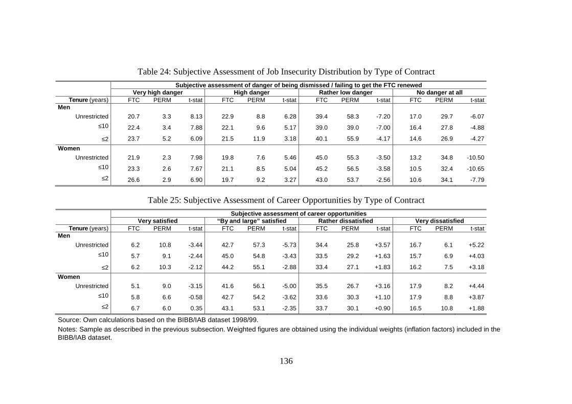
136

Table 24: Subjective Assessment of Job Insecurity Distribution by Type of Contract

Subjective assessment of danger of being dismissed / failing to get the FTC renewed Very high danger High danger Rather low danger No d anger at all

Tenure (years) FTC PERM t-stat FTC PERM t-stat FTC PERM t-stat FTC PERM t-stat Men

Unrestricted 20.7 3.3 8.13 22.9 8.8 6.28 39.4 58.3 -7.20 17.0 29.7 -6.07

≤10 22.4 3.4 7.88 22.1 9.6 5.17 39.0 39.0 -7.00 16.4 27.8 -4.88

≤2 23.7 5.2 6.09 21.5 11.9 3.18 40.1 55.9 -4.17 14.6 26.9 -4.27

Women

Unrestricted 21.9 2.3 7.98 19.8 7.6 5.46 45.0 55.3 -3.50 13.2 34.8 -10.50

≤10 23.3 2.6 7.67 21.1 8.5 5.04 45.2 56.5 -3.58 10.5 32.4 -10.65

≤2 26.6 2.9 6.90 19.7 9.2 3.27 43.0 53.7 -2.56 10.6 34.1 -7.79

Table 25: Subjective Assessment of Career Opportunities by Type of Contract

Subjective assessment of career opportunities Very satisfied “By and large” satisfied Rather di ssatisfied Very dissatisfied

Tenure (years) FTC PERM t-stat FTC PERM t-stat FTC PERM t-stat FTC PERM t-stat Men

Unrestricted 6.2 10.8 -3.44 42.7 57.3 -5.73 34.4 25.8 +3.57 16.7 6.1 +5.22

≤10 5.7 9.1 -2.44 45.0 54.8 -3.43 33.5 29.2 +1.63 15.7 6.9 +4.03

≤2 6.2 10.3 -2.12 44.2 55.1 -2.88 33.4 27.1 +1.83 16.2 7.5 +3.18

Women

Unrestricted 5.1 9.0 -3.15 41.6 56.1 -5.00 35.5 26.7 +3.16 17.9 8.2 +4.44

≤10 5.8 6.6 -0.58 42.7 54.2 -3.62 33.6 30.3 +1.10 17.9 8.8 +3.87

≤2 6.7 6.0 0.35 43.1 53.1 -2.35 33.7 30.1 +0.90 16.5 10.8 +1.88


137

5.5 Econometric Approach

The methodological discussion in this subchapter focuses on the estimation of the wage effects of FTCs. For both the other outcome variables the econometric approach is analogous.

5.5.1 Characterising the Selection Problem

First of all, what exactly is the treatment in this chapter? Of course, the treat-ment is ‘being employed on a FTC instead of a permanent contract’. This in-cludes in fact two decisions: (1.) the decision to enter into a FTC, and (2.) the decision to still hold a FTC at the time of the interview. The average treatment effect on the treated (ATT) is obviously the mean effect of being employed on FTC on wages (and subjective working conditions) of FTC workers in compari-son to the hypothetical situation the same workers would be employed on perma-nent contracts.

Assume that the outcome Eq. (5) in Section 3.2.2 is a (Mincer-type) wage equa-tion with itY denoting the hourly wage128 of individual i, and itX being a vector of conditioning variables. Since only one period of time is considered, the index t can be dropped. As discussed in detail in Section 3.2.2, the selection problem occurs in Eq. (5), if the treatment dummy iC is correlated with the error term iU , that is, ( ) 0i iE U C ≠ , which may be caused by selection on observables or selec-tion on unobservables.

If the Conditional Independence Assumption (CIA) holds (if solely selection on observables is relevant), the mean outcome of a control group of permanent con-tract workers with similar mean values of X-variables is a valid estimate of the counterfactual (see Section 3.3.1). As discussed in greater detail in subsequent sections, the counterfactual outcome is estimated by a propensity matching esti-mator (see Section 3.3.1)

If selection on unobservables is relevant, the analysis becomes much more complicated. For example, selection on unobservables would imply in case of the theoretical model by LOH (1994), that high-ability workers enter into FTCs with a higher probability. The attempts to account for selection on unobservables are presented in the following section.

5.5.2 Attempts to Account for Selection on Unobservables

As only a cross-sectional dataset is available, an instrumental variable (IV) is necessary for identification, that is, a variable affecting wages only through the treatment status (type of contract) but not directly (exclusion restriction; see Sec-tion 3.3.3). Since the necessary statistical properties of an IV, as described in Section 3.3.3, are usually untestable, the choice of an IV should be justified by

128 Using hourly wages instead of monthly earnings as outcome variable avoids the potential bias due to

differences in working hours (see FRANZ and STEINER, 2000).

138

theoretical considerations. The most plausible solution would be to find an ex-ogenous variation generated by a policy change, that is, a natural experiment (see Section 3.2.4).

One possible exogenous variation is the following: After having been increased to 11 employees on 01 October 1996, the employment threshold level for the ap-plication of the Protection Against Dismissal Law was reduced to 6 employees per establishment on 01 December 1998. Assuming that the number of employ-ees per establishment can be treated as exogenous with respect to the worker’s decision on the type of contract129, the hypothesis is that the probability of being employed on a FTC basis increases in establishments which came into the scope of the law on 01 December 1998, that is, establishment with 6-10 employees. There should be, ceteris paribus, no significant changes over time in the behav-iour of the other establishments. Thus the hypothesis is complementary to the hypothesis tested in Subchapter 4.4, where establishment level data are used.

I used this variation to explain the workers’ probabilities of being employed on FTCs by a probit model:

( ) ( )1 1 0 2 3Pr 1 5 _ 9 5 _ 9C X X after size size afterβ δ β β= = Φ + + + × , (47)

where after is a dummy variable, which is one, if a person is interviewed after 01 December 1998 and zero otherwise.130 5 _ 9size is a dummy variable for estab-lishments with 5-9 employees at the time of the interview since this is the nearest available category in the dataset.131 5 _ 9size after× is an interaction effect which serves as IV and1X is a vector of further explanatory variables including the other establishment size dummies. Basically, 5 _ 9size after× is a valid IV, if it affects (conditional on the other explanatory variables in Eq. (47)) the worker’s probability of being employed on FTC, and if it does not affect wages directly (exclusion restriction; see Section 3.3.3).

I estimated the basic Eq. (47) in several ways. A first approach was to assume that only new hirings were affected by the policy change, that is, only employees who were hired in 1998 or 1999. The interaction effect 5 _ 9size after× turned out to be weakly positively correlated with C, but the corresponding estimated coef-ficient in Eq. (47) was far from statistical significance. The most obvious reason is that only 43 workers are observed in the sample which are hired from estab-lishments with 5-9 employees after the reform (11 of these employees are hired on FTCs). In a second approach I included all workers (with job tenure ≤10 years), assuming that the law does not only alter the hiring decision with respect to the type of contract but also the decision whether or not to convert a FTC into a permanent contract. Again, the interaction term (IV) 5 _ 9size after× had no sig-nificant effect when estimating Eq. (47).

129 As discussed in the subsequent section, this assumption may not be realistic since the type of contract

is likely to be simultaneously determined with establishment size. 130 Remember that the interviews were conducted between October 1998 and March 1999. 131 Obviously, size5_9 serves only as a proxy variable for establishments with 6-10 employees.

139

I tried further IVs, which are, however, less convincing from a theoretical point of view. The aggregated labour force participation rates by age, qualification, and sex generated in a first step by the German Microcensus for 1998, were used. These turned out to be insufficiently correlated with the FTC dummy. Also the labour force participation rates by age, region (federal state), and sex had no sig-nificant effect on the type of contract.132

Due to the lack of a suitable IV, it is assumed that there is no selection on unob-servables or that some of the observable conditioning variables serve as proxy variables for unoberservables (see the section on the implementation of the matching estimator below).

5.5.3 Choice of Conditioning Variables

As stated in Section 3.3.1, the vector of conditioning variables in the propensity score equation should contain all variables simultaneously affecting the participa-tion decision as well as the outcome variables. From previous research and eco-nomic theory it is not obvious which variables to choose and, particularly, which variables are admissible. EHRENBERG and SMITH (1991: 263) state that compen-sating differentials are to be measured as follows: “The prediction is that, holding worker characteristics constant, employees in bad jobs receive higher wages than those working under more pleasant conditions.” Hence, theory demands the worker characteristics to be held constant, i.e., to be used as conditioning vari-ables.

The empirical literature on compensating wage differentials is quite vague about whether and to what extent one should, additionally to worker characteris-tics, condition on employer and job attributes, such as industry, firm size, job position etc.133 There are good reasons to take all possible factors into account: This ensures that FTC workers are compared only with permanent contract workers in equivalent situations and surroundings.

However, the underlying problem is that, given worker characteristics, wages and all job and employer attributes are determined simultaneously. This is ex-actly one crucial prediction of the theory of compensating wage differentials: A job is characterised by a bunch of attributes which may have positive or negative implications for a worker’s utility. An unfavourable attribute of the job (such as a FTC) may not be compensated for by a higher wage but, for example, by a higher position, more training opportunities, or a larger firm size (which provides a large internal labour market).

132 Also further variables from the BIBB/IAB dataset, such as having lost the last job due to firm closure

or having been in military service, turn out to be not suitable. They have either no significant effect on the probability of being employed on FTCs or have a significant effect on wages.

133 For example, while BOOTH, FRANCESCONI, and FRANK (2002) as well as WOLF (2002) control for all available job characteristics, ABOWD and ASHENFELTER (1981) do not control for job characteristics at all. BROWN and SESSIONS (2003) condition in addition to worker characteristics only on three dif-ferent occupation classes.

140

While the empirical literature on compensating wage differentials is ambiguous in this respect, precise guidelines can be found in the evaluation literature. LECHNER (1998) terms this issue the admissibility problem: A variable is admis-sible as a conditioning variable, if its potential values do not depend on the treatment status. Put differently, an admissible conditioning variable is a pre-treatment variable. Obviously, all job and employer attributes (industry, firm size, job position etc.) are simultaneously determined with the type of contract, and are therefore not admissible to be included in the set of conditioning vari-ables.

A further challenge is how to deal with the information on job tenure, which has turned out to be crucial in the descriptive analyses (Subchapter 2.3 and 5.4). The object is to distinguish the job tenure effect from the FTC effect. From an econometric point of view the following issues have to be considered: (1.) Job tenure may capture the effects of the accumulation of firm-specific human capital (see TOPEL, 1991) as well as employers’ and workers’ learning about the quality of the match (see FARBER, 1999). However, it is well-known that job tenure is endogenous with respect to wages, since workers’ mobility decisions are based on current wages; (2.) job tenure is obviously directly determined by the type of contract. Put differently, job tenure is endogenous with respect to the type of con-tract.

A possible approach to the first point is to assume that the endogeneity of ten-ure with respect to wages is cancelled out in the matching approach, if the prop-erty ( ) ( )1 0, 1 , 0E U X C E U X C= = = holds (see Section 3.3.2). The second point

seems to be more critical: Job tenure is obviously not an admissible conditioning variable since it is directly determined by the type of contract.

The approach chosen here to deal with the issue of admissibility of conditioning variables (and especially of job tenure) is to check the sensitivity of the results with regard to the inclusion of these variables. In concrete terms the following specifications are used:

Model A: Only admissible pre-treatment variables (worker characteristics) are included in the estimation equation of the propensity score.134

Model B: Job tenure is included in the balancing score besides the propensity score (using the Mahalanobis distance, see Section 3.3.1) in order to impose that only persons with exactly the same value of job tenure are matched.

134 The only set of variables which may be job-related are federal state dummies and unemployment

rates at the federal state level, both referring to the place of residence and not the place of work. Here is an obvious trade-off: On the one hand the place of residence is likely to be determined simultane-ously with the job and its characteristics. On the other hand, HECKMAN, ICHIMURA, and TODD (1997) emphasise the importance of comparing individuals within the same regional labour market. The nec-essary assumption is that the federal state is not simultaneously determined with the type of contract. An example for the violation of this assumption is the following. A worker chooses a FTC job (in-stead of a permanent job) because the permanent job requires that she or he has to move to another federal state.

141

Model C : In addition, variables on the job and the employer are included in the propensity score equation. Job tenure is still part of the balancing score. Hence, the goal of this specification is to compare FTC workers with a control group of permanent workers with, on average, similar worker characteristics, job and em-ployer related attributes, and the same distribution of job tenure.

A further approach to the problem of admissibility is to truncate the distribution for the sample with regard to job tenure from the right, such as there are up to 5 different samples (tenure ≤10, tenure ≤8 down to tenure ≤2 years), and to esti-mate the effects for each sub-sample. Further reasons for doing this is to impose common support (see Section 3.3.1 and Subchapter 5.4), and to check the robust-ness of the results with respect to an increasing proportion of FTCs which are justified by the Civil Code and not by the Employment Promotion Act.

5.5.4 Further Specification Issues: Other Selection Problems

In order to estimate the effect of FTCs on wages and subjective employment conditions consistently, it may be necessary to take another source of selection bias into account: The type of contract as well as wages can be observed only for those individuals who are actually employed. This corresponds to the classical sample selection problem, which is basically a problem of selection on unobserv-ables (see HECKMAN, 1979). There may be unobserved factors influencing the decision whether to be employed as well as wages and the type of contract. This may bias the results, especially for women, who are much more likely to be non-employed.135

The major drawback of the dataset used is that it includes only employed indi-viduals. Thus the problem cannot be taken into account.136 However, using a matching estimator one can again assume that the condition

( ) ( )1 0, 1 , 0E U X C E U X C= = = holds: By conditioning on a rich set of X variables

(including previous labour market experiences) also the unobservables are bal-anced between treated and control individuals. Nevertheless, it should be kept in mind that especially the results for women may be biased, if the condition is not fulfilled.

5.5.5 Implementation of the Propensity Score Matching Estimator

Three different matching estimators are compared137: (1.) NN-matching (with caliper and with replacement), (2.) kernel matching using an Epanechnikov ker-

135 To be exact, there is one more step (individual’s decision) to be taken into account: First, whether to

be in the labour force, second whether to be employed, and third which type of contract to enter. 136 In the previous study already described above, I used the GSOEP to estimate the impact of FTCs and,

thus I could test the significance of the problem (see HAGEN, 2002). I found that neither the effect of FTCs on wages nor the probability model for the type of contract is affected by a sample selection bias.

137 The analysis is performed using a modified version of “psmatch2” for STATA 8.0 implemented by LEUVEN and SIANESI (2003).

142

nel, and (3.) matching based on nonparametric local linear regression using also an Epanechnikov kernel. Nonparametric (kernel and local linear regression) matching estimators may be better suited for the analysis at hand than NN-matching since the ratio of treated to untreated workers is relatively large, imply-ing that it may be often impossible to find sufficiently similar nearest neighbours.

For the kernel-based matching estimators the bandwidth is chosen by Silver-man’s rule of thumb (see Section 3.3.1).138 The standard errors are calculated by a bootstrap procedure using 500 replications (see Section 3.3.1). Each bootstrap includes re-estimation of the propensity score and the re-calculation of the opti-mal bandwidth for the bootstrap sample. Thus the bootstrap procedure does not only take the variance due to the estimation of the propensity score into account, but also the variance due to the choice of the bandwidth (see Section 3.3.1).

Since both the ATT as well as the Average Treatment Effect on the Untreated (ATU) are estimated, the stricter version of the CIA and the common support condition are necessary, that is, ( )0 Pr 1 1C X< = < as well as ( )1 0,Y Y C e X⊥ (see

Chapter 3.3.1). The heterogeneity of the effects of FTCs is taken into account by estimating the ATT for different groups of workers and performing all the estima-tion steps described for the pre-defined subsamples (see Section 3.3.1).

Can the CIA assumed to be fulfilled? It would obviously be naive to assume that all variables that simultaneously affect participation (the probability to be employed on a FTC) as well as wages (and subjective assessment of working conditions) are observed in the dataset, and could be included in the conditioning set. Variables which may be missing (unobserved) are ability and motivation. Furthermore, the workers’ attitudes towards risk may, according to the theoreti-cal considerations, influence the acceptability of a FTC job. There is insufficient information available describing the hiring process, the firms’ decisions to use FTCs, and the workers’ decisions to accept FTCs. Therefore, it has to be as-sumed, that the rich set of variables describing workers’ labour market history may serve as proxies for unobserved variables. For example, the dummy vari-ables ‘ever changed occupation’ and ‘ever moved due to job-related reasons’ may be correlated with the (unobserved) attitude towards mobility and may therefore also include information on motivation. The same is obviously true for the number of previous employment and unemployment spells as well as the du-ration of the last unemployment spell. Hence, the underlying untestable assump-tion is again that by controlling for various employment history variables also selection on unobservables is balanced. Again, ( ) ( )1 0, 1 , 0E U X C E U X C= = = is

assumed to hold.

138 Choosing the bandwidth by leave-one-out validation (see Section 3.3.1) turns out be computationally

infeasible since the optimal bandwidth has to be calculated at every bootstrapping draw and, hence, the number of simulations gets too large.

143

5.6 Determinants of the Type of Contract: Estimation of the Propensity Score

In this Subchapter, the determinants of holding a FTC are analysed by estimat-ing probit models. In the subsequent section these estimated equations are used for predicting the propensity score for every worker. For the search of specifica-tion the so-called balancing score property of the estimated propensity score is used. For this purpose, the proposition

( )i i iX C e X⊥ if ( )ie X is the propensity score, (48)

by ROSENBAUM and RUBIN (1983) is applied (see also DEHEJIA and WAHBA , 1999). Conditional on the propensity score ( )e X , the conditioning variables X are independent of the type of contract C, implying that for individuals with the same propensity score (probability to hold a FTC), the distribution of X should be the same in the groups of treated and untreated individuals.

As described by DEHEJIA and WAHBA (1999), proposition (48) can also be used before performing the actual matching to assess the balancing score property of the estimated propensity score. For a given specification, observations are grouped into strata of the estimated propensity score. Within each stratum it is tested whether the average propensity scores of treated and controls differ. If there is a significant difference, the stratum is again split until there are no sig-nificant differences left. Then t-tests on differences in the means of the covariates X are performed within each stratum. If there are significant differences between the groups, then higher-order terms and interaction terms of X variables are in-cluded in the propensity score equation until there are no significant differences in the tests.

The balancing score property turns out to be satisfied with a quite parsimonious specification, that is, without any interaction effects. Hence, a more flexible specification seems to be unnecessary. Note that this test does not reveal any-thing about the validity of the CIA.

In Section 5.6.1 the results of the propensity score equation for Model A (only pre-treatment variables), and in Section 5.6.2 for Model C (including also job and employer attributes) is presented.

5.6.1 Model A: Using only Pre-Treatment Variables

Table 26 depicts the estimation results of the probit models for the probability of holding a FTC for men, and Table 27 provides the results for women, both for the samples with tenure ≤10 years as well as the sample with tenure ≤2 years.139 Furthermore, corresponding marginal effects are depicted.140

139 Among others, a dummy variable indicating if the person has ever been self-employed (which may be

a proxy for risk aversion), and a dummy indicating if the person was unemployed directly after voca-tional training have been included but turned out to be statistically insignificant in all specifications.

140 The calculation of marginal effects in the probit model is described in GREENE (2003: 668).

144

Starting with the results for men in Table 26, it can be seen that in the sample with tenure ≤ 10 years, age is modelled as a set of dummy variables. The results for the age dummies confirm the result from the descriptive analysis in Subchap-ter 2.3, that there is no clear-cut negative relationship between age and the prob-ability of being employed on FTC. Since age specified as a polynomial of third degree leads to a better property of the estimated propensity score (in terms of the balancing property in Eq. (48)), only the polynomial specification is used in the following.

In addition to the federal state dummies the unemployment rate of the federal state is included. The reason for including both is simply that, when it is not pos-sible to match individuals within the same federal state, including the unem-ployment rate ensures that individuals in different federal states but with similar unemployment rates have more similar predicted probabilities of holding a FTC (propensity scores). Note that the estimated negative coefficient of the federal state unemployment rate is the result of multicollinearity resulting from the low variation. If federal state dummies are excluded, the estimated coefficient of the unemployment rate becomes positive (see Table 69 in the Appendix), i.e., the higher the unemployment rate the higher the probability of being employed on FTC. Various theoretical explanations are available for this result (see also Sub-chapter 4.2 and Section 6.3.5). One is that workers are more willing to accept FTCs in bad labour market conditions. A second one is that firms may prefer a low turnover strategy using permanent workers in regional labour markets with low unemployment rates as hiring costs increase with labour market tightness.

As the unemployed job searchers’ determinants of entering into FTCs are dis-cussed in greater in detail in Subchapter 6.3, only some of the results are briefly summarised. Among others, the following variables have a positive effect on the probability of being employed on FTC for male workers (Table 26):

Having been unemployed in the year taking up the job increases the probability of holding a FTC. Furthermore, workers whose last job ended because of dis-missal or end of FTC (instead of quit) have a higher probability of holding a FTC. These results indicate that workers with adverse signals or with adverse unobservable characteristics enter into FTC jobs with a higher probability. Being disabled increases the probability of holding a FTC for men in the sample with tenure ≤10 years, albeit the level of statistical significance is low. The incentive to hire disabled persons on FTCs is likely to be enforced by the special dismissal protection for these persons (see Subchapter 2.2). More results in line with this hypothesis are presented in Subchapter 6.3.

In Table 27 it can be seen that many results are similar for women. Exceptions are the statistically insignificant coefficients for being disabled and for end of previous job due to dismissal. Furthermore, for women the probability of being employed on a FTC decreases, if the spouse is employed. A possible interpreta-tion stems from a reservation wage argument: If a woman has an employed spouse, she can afford to search for a permanent job for a longer period of time.

145

Table 26: Propensity Score – Men (Model A)

Men Tenure ≤≤≤≤10 years tenure ≤≤≤≤2 years Coeff. t-stat Marg. eff. X Coeff. t-stat Marg. eff. X

Age (years) -0.605 -2.71 -0.151 33.98 Age2 / 1,000 16.423 2.66 4.095 1.222 Age3 / 100,000 -14.427 -2.62 -3.597 0.465 Age group (reference: 21-23 years) 24-26 -0.245 -1.86 -0.029 0.09 27-29 -0.316 -2.44 -0.036 0.12 30-32 -0.599 -4.35 -0.060 0.15 33-35 -0.644 -4.53 -0.064 0.15 36-38 -0.690 -4.50 -0.064 0.12 39-41 -0.571 -3.69 -0.055 0.10 42-45 -0.581 -3.66 -0.056 0.09 46-49 -0.586 -3.47 -0.055 0.06 50-53 -0.544 -2.92 -0.051 0.04 54-57 -0.816 -3.54 -0.062 0.02 Qualification (reference: no formal qualification) Vocational training -0.086 -0.89 -0.012 0.59 -0.119 -0.85 -0.030 0.53 Vocational college 0.280 1.72 0.046 0.03 0.363 1.56 0.105 0.03 Master craftsman -0.180 -1.39 -0.022 0.11 -0.128 -0.72 -0.030 0.11 Polytechnic -0.010 -0.06 -0.001 0.05 -0.068 -0.30 -0.016 0.06 University 0.200 1.47 0.031 0.07 0.161 0.84 0.043 0.09 Children < 6 -0.300 -3.95 -0.037 0.25 -0.305 -2.78 -0.070 0.21 Children 6– 17 0.074 0.99 0.010 0.26 0.042 0.37 0.010 0.23 Foreigner 0.167 1.72 0.025 0.09 0.026 0.19 0.007 0.10 Disabled 0.257 1.71 0.042 0.03 0.132 0.59 0.035 0.03 Spouse employed -0.056 -0.86 -0.007 0.29 0.077 0.80 0.019 0.25 Employment history Ever changed occupation 0.134 2.14 0.019 0.37 0.241 2.76 0.061 0.42 Ever moved due to job-related reasons -0.017 -0.25 -0.002 0.25 -0.027 -0.28 -0.007 0.26 Two employers so far 0.021 0.21 0.003 0.25 -0.329 -2.05 -0.075 0.21 Three employers so far 0.016 0.14 0.002 0.22 -0.270 -1.58 -0.062 0.22 Four employers so far 0.096 0.79 0.014 0.14 -0.039 -0.21 -0.010 0.14 Five or more employers so far 0.169 1.42 0.025 0.23 -0.128 -0.72 -0.031 0.32 Previous job: dismissed 0.258 2.92 0.041 0.11 0.048 0.40 0.012 0.17 Previous job: end of FTC 0.511 5.14 0.095 0.06 0.546 4.04 0.164 0.09 Previous job: closure of a firm 0.083 0.83 0.012 0.10 0.001 0.01 0.000 0.11

146

Table 26 continued... Men Tenure ≤≤≤≤10 years Tenure ≤≤≤≤2 years

Coeff. t-stat Marg. eff. X Coeff. t-stat Marg. eff. X Once unemployed so far -0.046 -0.56 -0.006 0.24 -0.069 -0.59 -0.017 0.29 Twice unemployed so far 0.064 0.58 0.009 0.09 -0.035 -0.23 -0.009 0.12 Three times unemployed so far -0.047 -0.32 -0.006 0.04 -0.015 -0.08 -0.004 0.06 Four or more times unemployed so far 0.395 2.94 0.069 0.04 0.302 1.67 0.084 0.07 Duration of previous unemployment spell in months 0.002 0.77 0.000 3.29 0.003 0.69 0.001 4.32 Unemployed in the year taking up the job 0.265 3.30 0.041 0.17 0.387 3.60 0.105 0.27 Regional (place of residence) variables log unemployment rate of the federal state -0.738 -1.61 -0.101 2.34 -0.791 -1.19 -0.197 2.35 Hamburg 0.089 0.44 0.013 0.02 -0.105 -0.34 -0.025 0.02 Lower Saxony 0.279 2.09 0.044 0.12 0.246 1.20 0.067 0.12 Bremen 0.487 2.12 0.092 0.02 0.459 1.52 0.138 0.02 North Rhine-Westphalia -0.073 -0.54 -0.010 0.28 -0.099 -0.47 -0.024 0.29 Hesse -0.150 -0.77 -0.019 0.09 -0.154 -0.51 -0.036 0.09 Rhineland-Palatinate -0.413 -1.74 -0.043 0.05 -0.366 -1.02 -0.077 0.04 Baden-Wuerttemberg -0.439 -1.61 -0.048 0.15 -0.500 -1.21 -0.104 0.15 Bavaria -0.415 -1.56 -0.047 0.17 -0.453 -1.12 -0.097 0.17 Saarland 0.012 0.04 0.002 0.01 -0.248 -0.54 -0.055 0.01 City (more than 50.000 inhabitants) 0.085 1.25 0.012 0.49 0.198 1.98 0.049 0.52 Surrounding area -0.192 -2.01 -0.024 0.15 -0.050 -0.37 -0.012 0.14 Field of occupational qualification Training in farming occupation -0.283 -1.01 -0.031 0.01 -0.234 -0.60 -0.052 0.01 Training in industry occupation -0.141 -1.86 -0.019 0.45 -0.020 -0.17 -0.005 0.41 Training in health occupation 0.294 1.21 0.049 0.01 -0.090 -0.24 -0.022 0.01 Training in technical occupation -0.031 -0.29 -0.004 0.12 -0.003 -0.02 -0.001 0.12 Constant 0.838 0.70 8.170 2.63 Log-Likelihood -1207.2603 -622.56071 Likelihood ratio test (p-value) χ2 (51) = 240.43 (0.0000) χ2 (44) = 125.08 (0.0000) No. of observations 4,435 1,421

Notes: The marginal effects are calculated at the mean values of continuous variables and for discrete changes of dummy variables from 0 to 1. Base category: 21-23 years old (specification with tenure ≤10 years), no formal qualification, no children, German nationality, not disabled, spouse not employed, never changed occupation, never moved due to job-related reasons, only one employer so far, quit previous job, never unemployed so far, not unemployed in the year taking up the job, living in West Berlin or Schleswig-Holstein, living in a rural area, field of occu-pational qualification: no occupational qualification or occupational qualification in the service sector. Source: Own estimations based on the BIBB/IAB dataset 1998/99.

147

Table 27: Propensity Score – Women (Model A)

Women Tenure ≤≤≤≤10 years Tenure ≤≤≤≤2 years Coeff. t-stat Marg. eff. X Coeff. t-stat Marg. eff. X

Age (years) -0.187 -0.72 -0.048 34.86 Age2 / 1,000 5.850 0.81 1.497 1.29 Age3 / 100,000 -6.003 -0.92 -1.536 0.51 Age group (reference: 21-23 years) 24-26 -0.181 -1.35 -0.024 0.10 27-29 -0.252 -1.86 -0.032 0.11 30-32 -0.428 -2.93 -0.050 0.12 33-35 -0.306 -2.06 -0.038 0.11 36-38 -0.403 -2.55 -0.047 0.11 39-41 -0.426 -2.64 -0.049 0.10 42-45 -0.486 -3.02 -0.054 0.10 46-49 -0.535 -3.26 -0.057 0.09 50-53 -0.573 -3.08 -0.058 0.06 54-57 -0.706 -3.04 -0.064 0.03 Qualification (reference: no formal qualification) Vocational training -0.312 -3.74 -0.050 0.67 -0.216 -1.76 -0.056 0.61 Vocational college -0.073 -0.46 -0.010 0.04 0.044 0.21 0.012 0.05 Master craftsman -0.517 -3.05 -0.055 0.06 -0.262 -1.10 -0.060 0.05 Polytechnic -0.436 -1.96 -0.048 0.03 -0.782 -2.04 -0.134 0.02 University 0.217 1.43 0.037 0.04 0.177 0.83 0.049 0.06 Children < 6 -0.020 -0.22 -0.003 0.16 0.089 0.71 0.023 0.18 Children 6– 17 0.104 1.28 0.016 0.33 0.008 0.07 0.002 0.35 Foreigner 0.022 0.16 0.003 0.05 -0.011 -0.06 -0.003 0.07 Disabled 0.072 0.28 0.011 0.02 0.340 0.91 0.100 0.01 Spouse employed -0.116 -1.77 -0.017 0.55 -0.161 -1.65 -0.041 0.49 Employment history Ever changed occupation -0.027 -0.39 -0.004 0.34 -0.066 -0.67 -0.017 0.40 Ever moved due to job-related reasons 0.102 1.25 0.016 0.17 0.005 0.04 0.001 0.20 Two employers so far -0.135 -1.35 -0.019 0.27 -0.433 -2.74 -0.099 0.25 Three employers so far -0.164 -1.46 -0.023 0.21 -0.586 -3.38 -0.126 0.21 Four employers so far -0.220 -1.70 -0.029 0.14 -0.455 -2.43 -0.100 0.16 Five or more employers so far 0.142 1.15 0.022 0.19 -0.168 -0.93 -0.041 0.26 Previous job: dismissed -0.032 -0.29 -0.005 0.09 -0.154 -1.04 -0.037 0.13 Previous job: end of FTC 0.440 3.65 0.084 0.05 0.415 2.45 0.123 0.07 Previous job: closure of a firm 0.006 0.05 0.001 0.07 0.112 0.62 0.030 0.08

148

Table 27 continued... Women Tenure ≤≤≤≤10 years Tenure ≤≤≤≤2 years

Coeff. t-stat Marg. eff. X Coeff. t-stat Marg. eff. X Once unemployed so far -0.001 -0.01 0.000 0.26 -0.085 -0.67 -0.021 0.30 Twice unemployed so far 0.142 1.13 0.023 0.08 0.040 0.24 0.010 0.12 Three times unemployed so far 0.088 0.50 0.014 0.03 -0.167 -0.71 -0.040 0.05 Four or more times unemployed so far 0.202 0.90 0.034 0.02 0.125 0.45 0.034 0.03 Duration of previous unemployment spell in months 0.009 3.65 0.001 3.93 0.004 1.14 0.001 5.15 Unemployed in the year taking up the job 0.140 1.44 0.022 0.14 0.295 2.24 0.082 0.21 Regional (place of residence) variables log unemployment rate of the federal state -1.121 -2.50 -0.165 2.34 -1.874 -2.48 -0.480 2.33 Hamburg -0.395 -2.00 -0.045 0.04 -0.278 -0.94 -0.063 0.04 Lower Saxony 0.104 0.81 0.016 0.12 -0.012 -0.05 -0.003 0.11 Bremen 0.413 1.66 0.079 0.02 0.377 0.98 0.112 0.02 North Rhine-Westphalia -0.315 -2.45 -0.042 0.26 -0.336 -1.49 -0.080 0.28 Hesse -0.650 -3.34 -0.065 0.09 -0.792 -2.38 -0.142 0.08 Rhineland-Palatinate -0.791 -3.22 -0.069 0.04 -0.825 -2.10 -0.140 0.04 Baden-Wuerttemberg -0.860 -3.34 -0.085 0.16 -1.164 -2.59 -0.198 0.16 Bavaria -0.973 -3.87 -0.095 0.18 -1.266 -2.88 -0.218 0.19 Saarland -0.512 -1.57 -0.052 0.01 -0.803 -1.60 -0.134 0.01 City (more than 50.000 inhabitants) -0.115 -1.53 -0.017 0.49 -0.102 -0.91 -0.026 0.50 Surrounding area -0.143 -1.48 -0.020 0.15 -0.079 -0.55 -0.020 0.15 Field of occupational qualification Training in farming occupation 0.224 0.95 0.038 0.01 0.320 0.86 0.094 0.01 Training in industry occupation 0.234 2.13 0.039 0.08 0.359 2.26 0.104 0.09 Training in health occupation -0.068 -0.63 -0.010 0.10 -0.068 -0.41 -0.017 0.09 Training in technical occupation -0.205 -1.05 -0.026 0.03 -0.332 -1.17 -0.073 0.04 Constant 2.382 2.05 6.609 1.89 Log-Likelihood -1032.6939 -514.39375 Likelihood ratio test (p-value) χ2 (51) =197.39 (0.0000) χ2 (44) = 86.73 (0.0000) No. of observations 3,589 1,140

Notes and Source: See Table 26.

149

5.6.2 Model C: Accounting for Job and Employer Attributes

Table 28 and Table 29 depict the estimated coefficients of the determinants of

holding a FTC using job and employer attributes as additional explanatory vari-ables. The following additional results are of interest. The worker assessment of a good or very good business situation of the establishment reduces the probabil-ity of being on FTC for men and women. This is well in line with the theoretical and empirical findings of Chapter 4 that an employer hesitates to hire a person on a permanent contract, if the job is likely to be destroyed in the near future.

Male workers in job positions with simple tasks (labourer or blue-collar worker with simple tasks) have a higher probability of holding FTCs. This result may be explained by lower on-the-job training requirements in these job positions. Only for women there seems to be a positive relationship between the establishment size and the probability of holding a FTC. A positive relationship may be ex-plained by institutional firing costs (due to dismissal protection or co-determination rights) increasing with establishment size.

150

Table 28: Propensity Score – Men (Model C)

Men Tenure ≤≤≤≤10 years Tenure ≤≤≤≤2 years Coeff. t-stat Marg. eff. X Coeff. t-stat Marg. eff. X Age (years) -0.636 -4.00 -0.08 35.07 -0.557 -2.41 -0.13 33.98 Age2 / 1,000 14.693 3.58 1.89 1.29 14.82 2.38 3.52 1.22 Age3 / 100,000 -11.823 -3.26 -1.52 0.50 -13.04 -2.37 -3.10 0.47 Qualification (Reference: no formal qualification) Vocational training 0.155 1.44 0.02 0.59 0.119 0.75 0.03 0.53 Vocational college 0.558 3.27 0.10 0.03 0.625 2.52 0.19 0.03 Master craftsman 0.142 0.97 0.02 0.11 0.136 0.66 0.03 0.11 Polytechnic 0.338 1.89 0.05 0.05 0.272 1.10 0.07 0.06 University 0.604 3.87 0.11 0.07 0.543 2.47 0.16 0.09 Children < 6 -0.289 -3.73 -0.03 0.25 -0.294 -2.61 -0.06 0.21 Children 6– 17 0.060 0.78 0.01 0.26 0.004 0.04 0.00 0.23 Foreigner 0.113 1.15 0.02 0.09 -0.007 -0.05 0.00 0.10 Disabled 0.269 1.75 0.04 0.03 0.197 0.85 0.05 0.03 Spouse employed -0.012 -0.17 0.00 0.29 0.132 1.32 0.03 0.25 Employment history Ever changed occupation 0.063 0.95 0.01 0.37 0.129 1.37 0.03 0.42 Ever moved due to job-related reasons -0.002 -0.03 0.00 0.25 -0.006 -0.06 0.00 0.26 Two employers so far 0.083 0.80 0.01 0.25 -0.328 -1.99 -0.07 0.21 Three employers so far 0.085 0.74 0.01 0.22 -0.259 -1.47 -0.06 0.22 Four employers so far 0.176 1.39 0.02 0.14 -0.011 -0.06 0.00 0.14 Five or more employers so far 0.236 1.91 0.03 0.23 -0.126 -0.68 -0.03 0.32 Previous job: dismissed 0.237 2.62 0.03 0.11 0.038 0.31 0.01 0.17 Previous job: end of FTC 0.474 4.65 0.08 0.06 0.515 3.68 0.15 0.09 Previous job: closure of a firm 0.074 0.72 0.01 0.10 -0.014 -0.09 0.00 0.11 Once unemployed so far -0.047 -0.56 -0.01 0.24 -0.042 -0.34 -0.01 0.29 Twice unemployed so far 0.089 0.79 0.01 0.09 0.019 0.13 0.00 0.12 Three times unemployed so far -0.040 -0.27 0.00 0.04 -0.037 -0.18 -0.01 0.06 Four or more times unemployed so far 0.405 2.94 0.07 0.04 0.240 1.29 0.06 0.07 Duration of previous unemployment spell in months 0.001 0.22 0.00 3.29 0.001 0.17 0.00 4.32 Unemployed in the year taking up the job 0.234 2.86 0.03 0.17 0.348 3.12 0.09 0.27

151

Table 28 continued... Men Tenure ≤≤≤≤10 years Tenure ≤≤≤≤2 years Coeff. t-stat Marg. eff. X Coeff. t-stat Marg. eff. X Regional (place of residence) variables log unemployment rate of the federal state -0.855 -1.81 -0.11 2.34 -0.911 -1.35 -0.21 2.35 Hamburg 0.133 0.64 0.02 0.02 -0.153 -0.48 -0.03 0.02 Lower Saxony 0.278 2.03 0.04 0.12 0.148 0.69 0.04 0.12 Bremen 0.469 1.99 0.08 0.02 0.376 1.22 0.10 0.02 North Rhine-Westphalia -0.083 -0.60 -0.01 0.28 -0.189 -0.88 -0.04 0.29 Hesse -0.179 -0.88 -0.02 0.09 -0.261 -0.85 -0.05 0.09 Rhineland-Palatinate -0.436 -1.78 -0.04 0.05 -0.459 -1.24 -0.09 0.04 Baden-Wuerttemberg -0.523 -1.85 -0.05 0.15 -0.642 -1.50 -0.12 0.15 Bavaria -0.473 -1.73 -0.05 0.17 -0.616 -1.48 -0.12 0.17 Saarland -0.048 -0.16 -0.01 0.01 -0.428 -0.89 -0.08 0.01 City (more than 50.000 inhabitants) 0.116 1.64 0.01 0.49 0.217 2.07 0.05 0.52 Surrounding area -0.164 -1.67 -0.02 0.15 -0.035 -0.25 -0.01 0.14 Field of occupational qualification Professional Training in Farming occupation -0.438 -1.50 -0.04 0.01 -0.469 -1.13 -0.09 0.01 Professional Training in industry occupation -0.232 -2.62 -0.03 0.45 -0.217 -1.62 -0.05 0.41 Professional Training in health occupation 0.040 0.14 0.01 0.01 -0.340 -0.78 -0.07 0.01 Professional Training in technical occupation -0.061 -0.54 -0.01 0.12 -0.051 -0.32 -0.01 0.12 Job Position (reference labourer) craftsman -0.222 -2.44 -0.03 0.26 -0.090 -0.68 -0.02 0.22 foreman -0.763 -2.88 -0.06 0.03 -0.697 -1.72 -0.11 0.02 blue-collar master craftsman -0.381 -1.04 -0.04 0.01 -0.295 -0.63 -0.06 0.01 white-collar master craftsman -0.313 -1.03 -0.03 0.01 -0.053 -0.13 -0.01 0.01 blue-collar worker with simple tasks 0.247 1.62 0.04 0.03 -0.576 -2.20 -0.10 0.03 blue-collar worker with difficult tasks -0.029 -0.23 0.00 0.05 -0.089 -0.47 -0.02 0.06 blue-collar worker working autonomously -0.527 -4.54 -0.05 0.14 -0.616 -3.71 -0.11 0.14 blue-collar worker with executive functions -0.551 -4.88 -0.05 0.19 -0.729 -4.52 -0.14 0.20

152

Table 28 continued... Men Tenure ≤≤≤≤10 years Tenure ≤≤≤≤2 years Coeff. t-stat Marg. eff. X Coef t-value M.E. X Industrial sector (Reference: other services) Craft -0.213 -2.59 -0.03 0.28 -0.296 -2.48 -0.07 0.29 Trade -0.177 -1.92 -0.02 0.15 -0.041 -0.32 -0.01 0.16 Media 0.189 0.65 0.03 0.01 0.351 0.87 0.10 0.01 Logistic -0.243 -1.47 -0.03 0.03 -0.351 -1.53 -0.07 0.04 Telecommunication -0.205 -0.61 -0.02 0.01 -0.065 -0.16 -0.01 0.01 Financial intermediation -0.056 -0.30 -0.01 0.03 -0.219 -0.71 -0.05 0.03 Health and social work 0.321 1.33 0.05 0.01 0.450 1.39 0.13 0.02 Electricity, gas and water supply 0.281 0.68 0.04 0.00 1.353 1.53 0.48 0.00 Establishment size (Reference: 1-4 employees) 5-9 employees -0.002 -0.02 0.00 0.13 -0.055 -0.32 -0.01 0.16 10-49 employees -0.148 -1.37 -0.02 0.30 -0.054 -0.36 -0.01 0.31 50-99 employees 0.060 0.49 0.01 0.12 0.165 0.95 0.04 0.12 100-499 employees -0.201 -1.67 -0.02 0.19 -0.028 -0.16 -0.01 0.16 500-999 employees -0.080 -0.52 -0.01 0.06 0.153 0.69 0.04 0.05 ≥ 1000 employees 0.063 0.48 0.01 0.11 0.318 1.67 0.08 0.09 Business situation of the establishment is good or very good -0.156 -2.36 -0.02 0.76 -0.174 -1.77 -0.04 0.75 Constant 9.340 4.15 8.320 2.60 Log-Likelihood -1171.5664 -594.14334 Likelihood ratio test (p-value) χ2 (59) = 311.82 χ2 (59) = 181.91 No. of observations 4,435 1,421

Notes: The marginal effects are calculated at the mean values of continuous variables and for discrete changes of dummy variables from 0 to 1. Base category: 21-23 years old (specification with tenure ≤10 years), no formal qualification, no children, German nationality, not disabled, spouse not employed, never changed occupation, never moved due to job-related reasons, only one employer so far, quit previous job, never unemployed so far, not unemployed in the year taking up the job, living in West Berlin or Schleswig-Holstein, living in a rural area, field of occu-pational qualification: no occupational qualification or occupational qualification in the service sector, Job position: labourer, industrial sector: other services, establishment size: 1-4 employees. Source: Own estimations based on the BIBB/IAB dataset 1998/99.

153

Table 29: Propensity Score – Women (Model C)

Women Tenure ≤≤≤≤10 years Tenure ≤≤≤≤2 years Coeff. t-stat Marg. eff. X Coeff. t-stat Marg. eff. X Age (years) -0.193 -1.18 -0.03 35.90 -0.102 -0.38 -0.03 34.86 Age2 / 1,000 4.321 0.97 0.62 1.37 4.193 0.47 1.05 1.29 Age3 / 100,000 -3.442 -0.86 -0.50 0.55 -4.578 -0.60 -1.15 0.51 Qualification (Reference: no formal qualification) Vocational training -0.229 -2.47 -0.03 0.67 -0.170 -1.24 -0.04 0.61 Vocational college 0.014 0.08 0.00 0.04 0.096 0.42 0.02 0.05 Master craftsman -0.385 -2.13 -0.04 0.06 -0.198 -0.77 -0.04 0.05 Polytechnic -0.264 -1.12 -0.03 0.03 -0.717 -1.74 -0.12 0.02 University 0.474 2.84 0.09 0.04 0.320 1.33 0.09 0.06 Children < 6 0.007 0.07 0.00 0.16 0.117 0.90 0.03 0.18 Children 6– 17 0.100 1.25 0.01 0.33 0.024 0.20 0.01 0.35 Foreigner 0.003 0.02 0.00 0.05 -0.046 -0.24 -0.01 0.07 Disabled 0.067 0.26 0.01 0.02 0.413 1.08 0.12 0.01 Spouse employed -0.123 -1.86 -0.02 0.55 -0.198 -1.98 -0.05 0.49 Employment history Ever changed occupation? -0.053 -0.74 -0.01 0.34 -0.067 -0.65 -0.02 0.40 Ever moved due to job-related reasons? 0.120 1.43 0.02 0.17 -0.006 -0.05 0.00 0.20 Two employers so far -0.149 -1.47 -0.02 0.27 -0.502 -3.08 -0.11 0.25 Three employers so far -0.163 -1.42 -0.02 0.21 -0.643 -3.62 -0.13 0.21 Four employers so far -0.189 -1.44 -0.02 0.14 -0.470 -2.44 -0.10 0.16 Five or more employers so far 0.158 1.27 0.02 0.19 -0.254 -1.37 -0.06 0.26 Previous Job: Dismissed -0.011 -0.10 0.00 0.09 -0.122 -0.79 -0.03 0.13 Previous Job: End of FTC 0.443 3.63 0.08 0.05 0.480 2.76 0.14 0.07 Previous Job: Closure of a firm -0.006 -0.05 0.00 0.07 0.101 0.54 0.03 0.08 Once unemployed so far -0.035 -0.39 0.00 0.26 -0.089 -0.69 -0.02 0.30 Twice unemployed so far 0.104 0.82 0.02 0.08 0.037 0.22 0.01 0.12 Three times unemployed so far 0.055 0.31 0.01 0.03 -0.141 -0.58 -0.03 0.05 Four or more times unemployed so far 0.120 0.53 0.02 0.02 0.049 0.17 0.01 0.03 Duration of last unemployment spell in months 0.009 3.83 0.00 3.93 0.005 1.38 0.00 5.15 Unemployed in the year taking up the job 0.132 1.33 0.02 0.14 0.252 1.86 0.07 0.21

154

Table 29 continued... Women Tenure ≤≤≤≤10 years Tenure ≤≤≤≤2 years Coeff. t-stat Marg. eff. X Coeff. t-stat Marg. eff. X Regional (place of residence) variables log unemployment rate of the federal state -1.219 -2.67 -0.17 2.34 -2.020 -2.63 -0.50 2.33 Hamburg -0.330 -1.65 -0.04 0.04 -0.057 -0.19 -0.01 0.04 Lower Saxony 0.138 1.05 0.02 0.12 0.122 0.51 0.03 0.11 Bremen 0.476 1.87 0.09 0.02 0.497 1.26 0.15 0.02 North Rhine-Westphalia -0.277 -2.12 -0.04 0.26 -0.212 -0.91 -0.05 0.28 Hesse -0.627 -3.17 -0.06 0.09 -0.737 -2.14 -0.13 0.08 Rhineland-Palatinate -0.771 -3.08 -0.06 0.04 -0.800 -1.98 -0.13 0.04 Baden-Wuerttemberg -0.886 -3.38 -0.08 0.16 -1.110 -2.42 -0.18 0.16 Bavaria -0.988 -3.85 -0.09 0.18 -1.258 -2.80 -0.21 0.19 Saarland -0.497 -1.49 -0.05 0.01 -0.647 -1.26 -0.11 0.01 City (more than 50.000 inhabitants) -0.127 -1.66 -0.02 0.49 -0.110 -0.95 -0.03 0.50 Surrounding area -0.127 -1.29 -0.02 0.15 -0.029 -0.19 -0.01 0.15 Field of occupational qualification Training in farming occupation 0.253 1.04 0.04 0.01 0.334 0.87 0.10 0.01 Training in industry occupation 0.260 2.24 0.04 0.08 0.411 2.45 0.12 0.09 Training in health occupation -0.024 -0.18 0.00 0.10 -0.156 -0.79 -0.04 0.09 Training in technical occupation -0.206 -1.03 -0.03 0.03 -0.359 -1.22 -0.07 0.04 Job Position (reference labourer) Craftsman -0.186 -0.98 -0.02 0.04 0.002 0.01 0.00 0.03 Blue-collar worker with simple tasks 0.107 0.85 0.02 0.09 -0.023 -0.12 -0.01 0.08 Blue-collar worker with difficult tasks -0.007 -0.07 0.00 0.24 -0.058 -0.39 -0.01 0.24 Blue-collar worker working autonomously -0.116 -1.07 -0.02 0.27 -0.053 -0.34 -0.01 0.27 Blue-collar worker with executive functions -0.377 -2.85 -0.04 0.15 -0.258 -1.37 -0.06 0.14

155

Table 29 continued... Women Tenure ≤≤≤≤10 years Tenure ≤≤≤≤2 years Coeff. t-stat Marg. eff. X Coeff. t-stat Marg. eff. X Industrial sector (Reference: other services) Craft -0.030 -0.26 0.00 0.12 -0.015 -0.09 0.00 0.12 Trade 0.109 1.37 0.02 0.34 0.224 1.89 0.06 0.33 Media -0.226 -0.77 -0.03 0.01 -0.462 -0.98 -0.09 0.02 Logistic -0.013 -0.05 0.00 0.02 -0.043 -0.12 -0.01 0.02 Financial intermediation -0.228 -1.14 -0.03 0.04 -0.266 -0.80 -0.06 0.03 Health and social work 0.034 0.25 0.00 0.11 0.297 1.59 0.08 0.10 Establishment size (Reference: 1-4 employees) 5-9 employees 0.102 1.00 0.01 0.21 0.203 1.40 0.05 0.21 10-49 employees 0.114 1.19 0.02 0.28 0.135 0.98 0.03 0.28 50-99 employees 0.222 1.75 0.04 0.09 0.290 1.60 0.08 0.09 100-499 employees 0.331 3.02 0.06 0.13 0.654 3.99 0.20 0.11 500-999 employees 0.613 3.64 0.13 0.03 0.926 3.38 0.31 0.03 ≥ 1000 employees 0.154 0.94 0.02 0.05 0.635 2.48 0.20 0.04 Business situation of the establishment is good or very good -0.188 -2.71 -0.03 0.74 -0.277 -2.76 -0.07 0.68 Constant 5.084 2.27 5.827 1.63 Log-Likelihood -1026.2121 -501.64542 Likelihood ratio test (p-value) χ2 (54) = 210.36 χ2 (54) = 112.22 No. of observations 3,589 1,140

Notes and Source: See Table 28.

156

5.7 Effects of Fixed-Term Contracts: Results of the Matching Estimator

In this subchapter, the estimated effects of FTCs are presented. First of all, in the next section evidence on the performance of different matching estimators with respect to their ability to balance differences in the conditioning variables are presented.

5.7.1 Choice of the Matching Estimator and Checks on the Balancing Property

As mentioned in Subchapter 5.5, three different matching estimators are com-pared.141 The estimations are separately performed by sex and for different parts of the job tenure distribution, which is truncated from the right as described in Subchapter 5.5. Only Model A is used. The NN-matching approach is performed imposing a caliper (set to 0.001) which leads to a substantial loss of treated indi-viduals (FTC workers).142

As mentioned in Subchapter 3.5, a useful check on the matching quality is to test whether there are any significant differences in the outcome variables of treated and control group before the treatment (pre-program test). Since the data-set consists only of one cross-section, no information on the outcome variables before the treatment is available. A possibility to obtain insights into the per-formance of different matching estimators with respect to their ability to balance differences in the conditioning variables, is to compare the (unweighted) means of the standardised differences of all conditioning variables (see, for example, HUJER, CALIENDO, and THOMSEN, 2003).143 Note again that this is not a test on the validity of the CIA, but on the balancing property of the propensity score as presented in Eq. (48) above.

The first and most important result of this exercise is that kernel-based match-ing outperforms both the other approaches in terms of the mean standardised dif-ferences (see Table 30 and Table 31).144 Altogether, the better matching quality of the kernel-based matching estimator is quite convincing. The bad performance of the NN-matching estimator (which has the worst performance in the sample for men) may be explained by the fact that there are not many untreated individu-

141 As mentioned in Section 3.3.1, all those matching estimators produce asymptotically the same esti-

mate (see BLACK and SMITH , 2003). 142 Otherwise the performance is relatively poor.

143 The standardised difference of a variable x is defined as

( ) ( )( )( )1 0 1 1 0 02 ,x Var x Var xx − +

with Var1 and Var0 denoting the variance of x in the treated (1) and untreated (0) subsamples. The unweighted mean of the standardised difference is the average over the standardised differences of all conditioning variables X.

144 Advice on the choice of the matching estimator can be found in FRÖLICH (2004) as well as BLACK and SMITH (2003).

157

als (relative to treated) implying that often no sufficiently similar nearest neighbour is available. This is confirmed when looking at the effect of the trunca-tion of the sample with respect to tenure (from tenure ≤10 to tenure ≤2 years): With increasing N1/N0 also the bias (mean standardised difference) increases. The fact that NN-matching with replacement is performed can be seen from the num-ber of control persons NC in the tables: there are less control persons than treated persons resulting from control persons being used more than once. Given these findings, only the kernel-based matching estimator is applied for the analysis.

The detailed findings on the balancing property of the kernel-based matching estimator (Model A) are presented in Table 32 for men and in Table 33 for women. For most variables the standardised difference is strongly reduced in the matched samples.

158

Table 30: Matching Quality (Unweighted Mean of Standardised Differences) – Men (Model A)

Before Matching After Matching

NN-Matching (with caliper) Kernel Matching Local linear regression matching

Tenure (years) N1 N0 Mean std. diff. %

NT NC Mean std. diff. %



Unrestricted 526 8,051 54.00 474 433 10.10 523 8,051 2.52 523 8,051 6.28

≤ 10 453 4,457 26.43 407 357 4.23 451 4,457 3.40 451 4,457 5.11

≤ 8 433 3,663 21.20 389 345 9.95 431 3,663 1.83 431 3,663 7.41

≤ 6 409 2,886 20.06 364 321 8.38 408 2,886 2.26 408 2,886 9.14

≤ 4 362 2,130 19.89 305 265 15.03 359 2,130 2.23 359 2,130 13.32

≤ 2 294 1,245 17.32 207 176 11.05 291 1,245 2.04 291 1,245 5.32

Table 31: Matching Quality (Unweighted Mean of Standardised Differences) – Women (Model A)

Before Matching After Matching

NN-Matching (with caliper) Kernel Matching Local linear regression matching

Tenure (years) N1 N0 Mean std. diff. %




Unrestricted 443 5,789 52.15 401 369 13.66 441 5,789 3.31 441 5,789 13.07

≤ 10 392 3,776 38.83 353 319 8.73 390 3,776 5.44 390 3,776 14.80

≤ 8 368 3,169 35.56 333 296 3.60 366 3,169 3.01 366 3,169 5.49

≤ 6 338 2,548 33.03 286 251 6.33 336 2,548 4.73 336 2,548 15.60

≤ 4 301 1,870 31.15 246 224 11.96 299 1,870 1.24 299 1,870 13.98

≤ 2 238 1,053 21.66 171 147 10.29 238 1,053 2.37 238 1,053 6.33

159

Table 32: Means of Important Conditioning Variables (X) Before and After Kernel-Based Matching – Men (Model A)

Tenure ≤≤≤≤ 10 years Tenure ≤≤≤≤ 2 years

Before Matching After Matching Before Matching After Matching

Variable Treated Un-treated

std. diff. %

Treated Controls std. diff. %

Treated Un-treated

std. diff. %


Age 34.038 35.169 13.4 34.090 34.054 0.4 34.045 33.966 0.9 34.038 33.907 1.6 Vocational training 0.524 0.593 13.9 0.528 0.531 0.7 0.485 0.545 11.9 0.489 0.489 0.1 Vocational college 0.051 0.028 11.8 0.049 0.047 0.8 0.060 0.027 16.4 0.053 0.057 2.0 Master craftsman 0.076 0.110 11.5 0.077 0.077 0.1 0.094 0.112 5.8 0.095 0.098 1.2 Polytechnic 0.041 0.051 5.0 0.041 0.039 0.9 0.049 0.063 6.2 0.049 0.044 2.2 University 0.087 0.074 4.7 0.087 0.089 0.5 0.090 0.086 1.6 0.091 0.103 4.2 Children < 6 0.155 0.254 24.7 0.156 0.157 0.2 0.154 0.229 19.0 0.155 0.157 0.5 Children 6-17 0.247 0.258 2.5 0.249 0.240 2.0 0.248 0.226 5.2 0.246 0.231 3.6 Foreigner 0.117 0.083 11.5 0.118 0.122 1.5 0.109 0.098 3.7 0.110 0.112 0.7 Disabled 0.043 0.026 9.2 0.044 0.045 0.6 0.041 0.027 8.0 0.042 0.049 4.1 Spouse employed 0.260 0.297 8.3 0.262 0.260 0.2 0.263 0.250 3.0 0.265 0.245 4.6 Ever changed occupation 0.438 0.358 16.3 0.436 0.434 0.4 0.511 0.397 23.2 0.508 0.525 3.6 Ever moved due to job-related reasons 0.252 0.249 0.6 0.251 0.251 0.1 0.259 0.261 0.5 0.261 0.270 2.0 Two employers so far 0.206 0.250 10.4 0.208 0.217 2.1 0.154 0.227 18.6 0.155 0.162 1.7 Three employers so far 0.183 0.221 9.5 0.185 0.188 0.7 0.169 0.228 14.7 0.170 0.182 2.9 Four employers so far 0.135 0.139 1.1 0.136 0.137 0.2 0.158 0.137 5.9 0.159 0.148 3.3 Five or more employers so far 0.310 0.217 21.2 0.305 0.291 3.2 0.395 0.303 19.3 0.390 0.379 2.4 Previous job: dismissed 0.168 0.103 19.0 0.169 0.170 0.3 0.180 0.162 4.9 0.182 0.174 2.0 Previous job: end of FTC 0.150 0.055 31.6 0.144 0.139 1.4 0.177 0.070 32.8 0.170 0.172 0.4 Previous job: closure of a firm 0.104 0.098 2.0 0.105 0.107 0.5 0.113 0.113 0.2 0.114 0.106 2.5 Once unemployed so far 0.247 0.243 0.9 0.249 0.265 3.8 0.274 0.291 3.7 0.277 0.297 4.5 Twice unemployed so far 0.117 0.084 11.0 0.118 0.116 0.6 0.147 0.119 8.3 0.144 0.145 0.2 Three times unemployed so far 0.056 0.042 6.7 0.056 0.058 0.8 0.071 0.056 6.2 0.072 0.072 0.2 Four or more times unemployed so far 0.109 0.037 28.2 0.103 0.097 2.2 0.143 0.058 28.5 0.140 0.137 1.1 Durat. of last unemployment spell in months 4.756 3.142 16.4 4.756 4.927 1.7 5.658 4.008 16.4 5.655 5.702 0.5 Unemployed in the year taking up the job 0.300 0.162 33.2 0.295 0.296 0.4 0.414 0.240 37.6 0.409 0.412 0.6 log regional unemployment rate 2.371 2.335 17.7 2.371 2.372 0.5 2.378 2.338 18.5 2.377 2.373 1.8 City (more than 50.000 inhabitants) 0.560 0.482 15.6 0.559 0.552 1.4 0.590 0.500 18.1 0.587 0.578 1.9 Surrounding area 0.102 0.158 16.8 0.103 0.107 1.3 0.109 0.147 11.4 0.110 0.115 1.6 Training in farming occupation 0.010 0.014 3.4 0.010 0.009 1.5 0.011 0.016 3.7 0.011 0.008 2.8 Training in industry occupation 0.379 0.452 14.9 0.382 0.378 0.9 0.387 0.419 6.5 0.390 0.384 1.2 Training in health occupation 0.018 0.009 7.5 0.018 0.019 0.5 0.011 0.013 1.6 0.011 0.013 1.7 Training in technical occupation 0.102 0.120 5.9 0.103 0.106 1.0 0.113 0.126 3.9 0.114 0.128 4.4

160

Table 33: Means of Important Conditioning Variables (X) Before and After Kernel-Based Matching – Women (Model A)

Tenure ≤≤≤≤ 10 years Tenure ≤≤≤≤ 2 years

Before Matching After Matching Before Matching After Matching

Variable Treated Untreated std. diff. %


Treated Un-treated

std. diff. %


Age 34.045 33.966 0.9 34.038 33.907 1.6 34.105 36.100 22.2 34.065 34.207 1.6 Vocational training 0.485 0.545 11.9 0.489 0.489 0.1 0.580 0.675 19.8 0.581 0.582 0.2 Vocational college 0.060 0.027 16.4 0.053 0.057 2.0 0.050 0.038 5.5 0.047 0.054 3.2 Master craftsman 0.094 0.112 5.8 0.095 0.098 1.2 0.032 0.058 12.6 0.032 0.032 0.3 Polytechnic 0.049 0.063 6.2 0.049 0.044 2.2 0.017 0.027 6.3 0.018 0.019 0.6 University 0.090 0.086 1.6 0.091 0.103 4.2 0.073 0.042 13.5 0.074 0.073 0.5 Children < 6 0.154 0.229 19.0 0.155 0.157 0.5 0.152 0.160 2.2 0.150 0.154 1.0 Children 6-17 0.248 0.226 5.2 0.246 0.231 3.6 0.332 0.335 0.5 0.330 0.325 1.2 Foreigner 0.109 0.098 3.7 0.110 0.112 0.7 0.061 0.049 5.4 0.062 0.065 1.2 Disabled 0.041 0.027 8.0 0.042 0.049 4.1 0.017 0.015 2.1 0.018 0.014 2.6 Spouse employed 0.263 0.250 3.0 0.265 0.245 4.6 0.464 0.556 18.6 0.466 0.466 0.0 Ever changed occupation 0.511 0.397 23.2 0.508 0.525 3.6 0.341 0.343 0.5 0.342 0.348 1.3 Ever moved due to job-related reasons 0.259 0.261 0.5 0.261 0.270 2.0 0.207 0.161 11.8 0.206 0.194 3.2 Two employers so far 0.154 0.227 18.6 0.155 0.162 1.7 0.233 0.277 10.0 0.233 0.227 1.3 Three employers so far 0.169 0.228 14.7 0.170 0.182 2.9 0.166 0.214 12.2 0.162 0.161 0.3 Four employers so far 0.158 0.137 5.9 0.159 0.148 3.3 0.111 0.145 10.2 0.112 0.117 1.4 Five or more employers so far 0.395 0.303 19.3 0.390 0.379 2.4 0.254 0.180 17.9 0.254 0.260 1.5 Previous job: dismissed 0.180 0.162 4.9 0.182 0.174 2.0 0.090 0.088 0.9 0.091 0.093 0.4 Previous job: end of FTC 0.177 0.070 32.8 0.170 0.172 0.4 0.108 0.044 24.2 0.103 0.103 0.1 Previous job: closure of a firm 0.113 0.113 0.2 0.114 0.106 2.5 0.058 0.066 3.2 0.059 0.059 0.1 Once unemployed so far 0.274 0.291 3.7 0.277 0.297 4.5 0.274 0.255 4.4 0.271 0.263 1.8 Twice unemployed so far 0.147 0.119 8.3 0.144 0.145 0.2 0.105 0.074 10.9 0.100 0.106 2.1 Three times unemployed so far 0.071 0.056 6.2 0.072 0.072 0.2 0.055 0.028 13.5 0.056 0.058 1.1 Four or more times unemployed so far 0.143 0.058 28.5 0.140 0.137 1.1 0.032 0.014 12.4 0.032 0.037 2.9 Durat. of last unemployment spell in months 5.658 4.008 16.4 5.655 5.702 0.5 7.636 3.538 25.6 6.496 6.581 0.5 Unemployed in the year taking up the job 0.414 0.240 37.6 0.409 0.412 0.6 0.216 0.132 22.1 0.212 0.210 0.7 log regional unemployment rate 2.378 2.338 18.5 2.377 2.373 1.8 2.379 2.334 21.4 2.379 2.380 0.4 City (more than 50.000 inhabitants) 0.590 0.500 18.1 0.587 0.578 1.9 0.469 0.489 3.8 0.469 0.469 0.0 Surrounding area 0.109 0.147 11.4 0.110 0.115 1.6 0.134 0.153 5.4 0.133 0.136 1.0 Training in farming occupation 0.011 0.016 3.7 0.011 0.008 2.8 0.020 0.014 5.3 0.018 0.019 0.7 Training in industry occupation 0.387 0.419 6.5 0.390 0.384 1.2 0.105 0.076 9.9 0.100 0.099 0.6 Training in health occupation 0.011 0.013 1.6 0.011 0.013 1.7 0.087 0.106 6.4 0.088 0.084 1.4 Training in technical occupation 0.113 0.126 3.9 0.114 0.128 4.4 0.023 0.036 7.5 0.024 0.022 0.7

161

5.7.2 Effects of Fixed-Term Contracts for Men

The estimated effects of FTCs on wages, subjective employment stability, and

subjective career opportunities are presented in this section. Furthermore, the results of Model A, B, and C are compared for different subsamples with respect to maximum job tenure.

Homogeneous Effects for Men

First of all, a comparison of the results can reveal whether and to what extent the estimated effects depend on the model specification (Model A, B, C), that is, the choice of the conditioning variables. Table 34 depicts the estimated ATT and ATU (measured in € and in percentages) on wages for different samples with a decreasing maximum tenure for Model A. The ATT is the difference between the average wage of FTC workers and the average estimated counterfactual wage. The ATU is the average wage loss permanent workers would have, if they were employed on FTCs instead.

All wage effects estimated by Model A are negative, but in case of the sample with tenure ≤2 years not statistically significant (see Table 34). The insignifi-cance of the effects for the sample with tenure ≤2 years results from the large standard errors which are likely to be caused by the reduced sample. The ATT ranges from -0.5 € (-4.6%) to -0.9 € (-7.5%). Including tenure into the balancing score (Model B), that is, imposing that the control group has (exactly) the same distribution of job tenure, leads to stronger (statistically significant) negative wage effects but otherwise comparable patterns (see Table 35). The wage effects are now between -0.9 € (-8.0%) and -1.1 € (-9.8%). The same is true for Model C which additionally conditions on job and employer attributes. Now, the ATT is around -1.0 € (-9.5% to -7.9%, see Table 36).

Thus different sets of conditioning variables lead to different results. However, these differences are not large and not statistically significant. Therefore, Model A is the preferred specification in the following since it is based on admissible conditional variables only (see the discussion in Subchapters 5.5).

A further interesting finding from all models is that the estimated ATT is more negative, the longer the maximum job tenure is. Hence, the wage-tenure profile in permanent jobs is steeper than in comparable FTC jobs. This finding is in line with economic theory: FTC workers and their employers have less incentives to invest in firm-specific human capital during the FTC (see the discussion in Sec-tion 5.2.2). Note that this is not a rejection of the hypothesis of FTCs as proba-tionary periods as the underlying theory predicts a stronger wage increase after the FTC.

162

In most cases the estimated ATT is larger than the estimated ATU. This result indicates that those workers enter into FTCs, whose contemporaneous wage loss from doing so, is lower on average.

Table 34: Wage Effects of FTCs – Men (Model A) (Standard Errors in Parentheses)

Mean Wages in €

Tenure (years)

ATT (€) ATT (%) ATU (€) ATU (%) NT

≤ 10 -0.86 (0.28)

*** -7.5 -1.29 (0.41)

*** -10.6 390

≤ 8 -0.76 (0.30)

** -6.7 -1.02 (-0.41)

** -8.5 371

≤ 6 -0.68 (0.31)

** -6.0 -0.94 (0.43)

** -7.9 351

≤ 4 -0.62 (0.33)

* -5.6 -0.74 (0.44)

* -6.4 315

≤ 2 -0.51 (0.41)

-4.7 -0.55 (0.47)

-4.8 264

Notes: *** (**,*) denotes significance at the 1 (5, 10) percent level.

Table 35: Wage Effects of FTCs – Men (Model B) (Standard Errors in Parentheses)

Mean Wages in €

Tenure (years)


≤ 10 -1.14 (0.28)

*** -9.8 -1.45 (0.39)

*** -11.9 392

≤ 2 -0.91 (0.32)

*** -8.0 -0.92 (0.32)

*** -8.1 265


Table 36: Wage Effects of FTCs – Men (Model C) (Standard Errors in Parentheses)

Mean Wages in €

Tenure (years)


≤ 10 -1.10 (0.28)

*** -9.5 -1.42 (0.36)

*** -11.7 391

≤ 2 -0.89 (0.33)

*** -7.9 -0.88 (0.35)

** -7.7 263


163

In Table 70 and Table 71 in the Appendix the ATT (Model A) of FTCs on usual weekly working hours and the probability of working part-time are depicted for men. On average, FTC jobs are associated with slightly shorter working hours and have no effect on the probability of working part-time. Thus the result by ENGELLANDT and RIPHAN (2003) for Switzerland (see Subchapter 5.3) cannot be replicated for Germany. Furthermore, the findings indicate that the negative wage effect of FTCs does not result from longer working hours at given monthly earn-ings.

Table 37 (Model A), Table 38 (Model B), and Table 39 (Model C) depict the es-timated effects on subjective assessment of danger of being dismissed / failing to get the FTC renewed . In the following discussion, I focus on the first and the fourth category (very high danger, no danger at all) for the most part, in order to keep the interpretations simple.

There are again no fundamental differences between the three models. The es-timated ATT indicates that FTCs indeed lead to a higher subjective assessment of losing one’s job by approximately 20 percentage points. The ATT on the prob-ability of perceiving no danger at all is about -12 percentage points. The follow-ing discussion focuses on Model A (Table 37): While subjective job insecurity of permanent workers seems to decline with increasing job tenure (see Table 24 in Subchapter 5.4), the ATT of holding a FTC in the highest category (very high danger) and the lowest category (no danger at all) is hardly affected by the choice of the sample with regard to tenure, that is, the ATT is almost constant. In the second category (high danger) there seems to be a tendency towards an in-creasing ATT with increasing maximum tenure.

164

Table 37: Effects of FTCs on Job Insecurity – Men (Model A) (Standard Errors in Parentheses)

Subjective assessment of danger of being dismissed / failing to get the FTC renewed

Very high danger

High danger Rather low danger

No danger at all

Tenure (years)

ATT (%-points)

ATT (%-points)

ATT (%-points)

ATT (%-points)

≤10 20.1 (2.4)

*** 11.2 (2.3)

*** -18.8 (2.8)

*** -12.5 (2.2)

***

≤ 8 20.4 (2.2)

*** 10.5 (2.6)

*** -18.5 (3.0)

*** -12.4 (2.2)

***

≤ 6 20.8 (2.6)

*** 10.2 (2.7)

*** -18.7 (3.3)

*** -12.3 (2.5)

***

≤ 4 20.8 (2.9)

*** 9.3 (3.0)

*** -15.7 (3.5)

*** -14.4 (2.4)

***

≤ 2 20.3 (3.1)

*** 8.1 (3.5)

** -16.5 (4.3)

*** -11.9 (2.9)

***


Table 38: Effects of FTCs on Job Insecurity – Men (Model B) (Standard Errors in Parentheses)


Very high danger


No danger at all

Tenure (years)

ATT (%-points)

ATT (%-points)

ATT (%-points)

ATT (%-points)

≤10 19.1 (2.5)

*** 10.8 (2.5)

*** -17.9 (3.1)

*** -12.0 (2.4)

***

≤ 2 20.2 (3.1)

*** 9.3 (3.5)

*** -18.7 (4.4)

*** -10.8 (3.0)

***


Table 39: Effects of FTCs on Job Insecurity – Men (Model C ) (Standard Errors in Parentheses)


Very high danger


No danger at all

Tenure (years)

ATT (%-points)

ATT (%-points)

ATT (%-points)

ATT (%-points)

≤10 19.6 (2.5)

*** 9.0 (2.8)

*** -18.6 (3.4)

*** -9.9 (2.4)

***

≤ 2 20.3 (3.0)

*** 6.9 (3.9)

* -17.3 (4.2)

*** -10.0 ( 2.9)

***


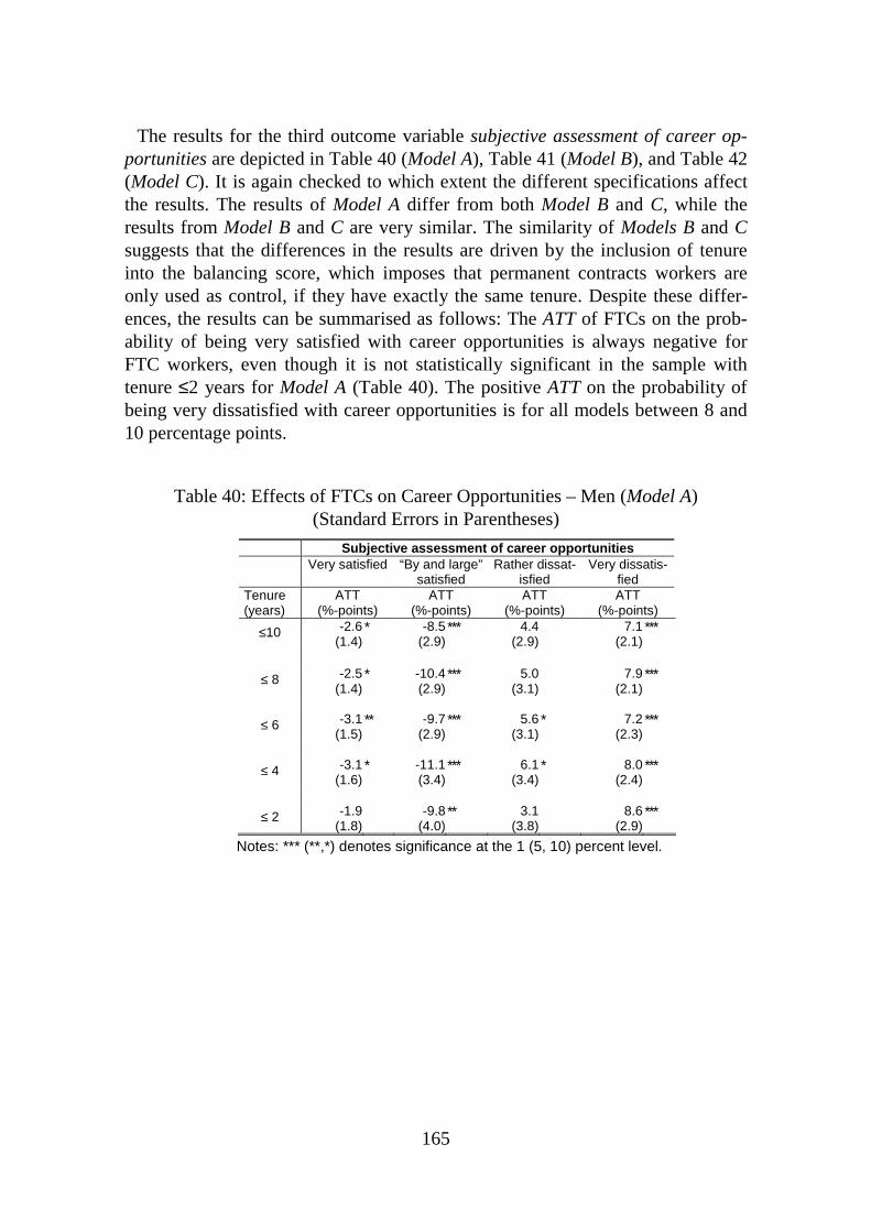
165

The results for the third outcome variable subjective assessment of career op-portunities are depicted in Table 40 (Model A), Table 41 (Model B), and Table 42 (Model C). It is again checked to which extent the different specifications affect the results. The results of Model A differ from both Model B and C, while the results from Model B and C are very similar. The similarity of Models B and C suggests that the differences in the results are driven by the inclusion of tenure into the balancing score, which imposes that permanent contracts workers are only used as control, if they have exactly the same tenure. Despite these differ-ences, the results can be summarised as follows: The ATT of FTCs on the prob-ability of being very satisfied with career opportunities is always negative for FTC workers, even though it is not statistically significant in the sample with tenure ≤2 years for Model A (Table 40). The positive ATT on the probability of being very dissatisfied with career opportunities is for all models between 8 and 10 percentage points.

Table 40: Effects of FTCs on Career Opportunities – Men (Model A) (Standard Errors in Parentheses)

Subjective assessment of career opportunities Very satisfied “By and large”

satisfied Rather dissat-

isfied Very dissatis-

fied Tenure (years)

ATT (%-points)

ATT (%-points)

ATT (%-points)

ATT (%-points)

≤10 -2.6 (1.4)

* -8.5 (2.9)

*** 4.4 (2.9)

7.1 (2.1)

***

≤ 8 -2.5 (1.4)

* -10.4 (2.9)

*** 5.0 (3.1)

7.9 (2.1)

***

≤ 6 -3.1 (1.5)

** -9.7 (2.9)

*** 5.6 (3.1)

* 7.2 (2.3)

***

≤ 4 -3.1 (1.6)

* -11.1 (3.4)

*** 6.1 (3.4)

* 8.0 (2.4)

***

≤ 2 -1.9 (1.8)

-9.8 (4.0)

** 3.1 (3.8)

8.6 (2.9)

***


166

Table 41: Effects of FTCs on Career Opportunities – Men (Model B) (Standard Errors in Parentheses)




fied Tenure (years)

ATT (%-points)

ATT (%-points)

ATT (%-points)

ATT (%-points)

≤10 -3.9 (1.4)

*** -13.1 (2.8)

*** 8.3 (2.3)

*** 8.6 (2.0)

***

≤ 2 -3.9 (1.9)

** -13.8 (3.5)

* 7.7 (3.3)

** 9.9 (2.5)

***


Table 42: Effects of FTCs on Career Opportunities – Men (Model C) (Standard Errors in Parentheses)




fied Tenure (years)

ATT (%-points)

ATT (%-points)

ATT (%-points)

ATT (%-points)

≤10 -3.6 (1.4)

*** -13.1 (2.9)

*** 8.0 (2.6)

*** 8.7 (2.0)

***

≤ 2 -3.5 (1.8)

* -13.5 (3.5)

*** 7.2 (3.4)

** 9.8 (2.7)

***


Summarising the results, it may be concluded that a FTC, on average, increases

the probability that a worker regards his job as unstable and as a ‘dead end’, in comparison to a permanent contract worker with similar characteristics (Model A) in a similar job (Model C). Assuming that these subjective assessments are sufficiently correlated with the utility from the job, one can conclude that FTC jobs are ceteris paribus associated with lower utility than comparable permanent jobs. This utility loss is not simultaneously compensated for by higher wages. All specifications have shown that FTCs have no significant positive or even statisti-cally significant negative effects on wages of about -5% up to -10%.

Of course, the utility loss may in the long-run be compensated for by higher lifetime earnings (or utilities) or by other job-related factors (large internal labour market etc.). The latter is, however, less probable since Model C, which led to very similar results already conditions on a number of job and employer attrib-utes. The question to be answered in the next subsection is how the estimated short-run wage effects differ between groups of workers.

167

Heterogeneous Effects for Men

In this subsection, heterogeneous ATTs with respect to important observable characteristics are estimated by Model A for the sample with tenure ≤10 years. In order to secure a sufficient number of observations to be available focussing on this relatively large sample is necessary. Nevertheless, the results should be in-terpreted with caution as the number of observations becomes quite small.

The results for the wage effects are depicted in Table 43. In order to provide an impression of the wage level in the respective subgroup, mean FTC wages are depicted in the first column. The ATT of FTCs on wages is more negative in large establishments in terms of absolute values (-1.34 € versus -0.78 €) as well as in percentages (-10.6% versus -7.3%). The result that there is no significant ATT on wages in the industry sector but in the trade sector seems to be puzz-ling.145 One possible explanation may be that unions and works councils, pre-venting employers to pay lower wages to FTC workers, play a more important role in the industry sector (see DANIEL and SOFER, 1998).

With respect to formal qualification, the results are different compared to what has previously been found in other studies: there is no significantly negative ATT of FTCs on wages of workers without formal qualifications. All in all, there is a positive relationship between the wage penalty to FTCs and the level of formal qualification. For workers with university degree there is a significantly negative wage effect of -2.7 € (-17.2%), which is the most negative ATT found among the subgroups. Note that this result is quite stable and can also be obtained from Model B and Model C. To some extent, this result contradicts the finding by MERTENS and MCGINNITY (2003) that the lowest wage penalty to FTCs is in the upper quantiles of the wage distribution (see Subchapter 5.3).

A possible interpretation is in line with the hypothesis posed in Section 5.2.4: Workers with university degree are more concerned about their careers and they have a sufficiently high probability of getting their contract transformed into permanent ones. Hence, they are willing to earn less than comparable permanent contract workers, since they will be compensated for with a sufficiently high probability in the future.

The wage effects for different age groups indicate that workers younger than 32 years face no significant wage penalty to FTCs. The results indicate that a sig-nificantly negative wage effect can only be found for FTC workers being at least 32 years old. This result is opposed to the prediction derived from the model by GIBBONS and MURPHY (1992), presented in Section 5.2.4.

145 This industry definition of sectors results from the way of data collection in the interview. Persons are

first asked to state whether their employer belongs to the ‘industry’, ‘craft’, ‘trade’, or ‘miscellane-ous’ sector.

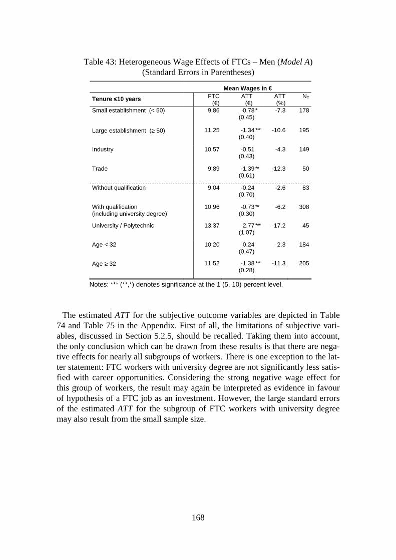
168

Table 43: Heterogeneous Wage Effects of FTCs – Men (Model A) (Standard Errors in Parentheses)

Mean Wages in €

Tenure ≤≤≤≤10 years FTC (€)

ATT (€)

ATT (%)

NT

Small establishment (< 50) 9.86 -0.78 (0.45)

* -7.3 178

Large establishment (≥ 50) 11.25 -1.34 (0.40)

*** -10.6 195

Industry 10.57 -0.51 (0.43)

-4.3 149

Trade 9.89 -1.39 (0.61)

** -12.3 50

Without qualification 9.04 -0.24 (0.70)

-2.6 83

With qualification (including university degree)

10.96 -0.73 (0.30)

** -6.2 308

University / Polytechnic 13.37 -2.77 (1.07)

*** -17.2 45

Age < 32 10.20 -0.24 (0.47)

-2.3 184

Age ≥ 32 11.52 -1.38 (0.28)

*** -11.3 205


The estimated ATT for the subjective outcome variables are depicted in Table

74 and Table 75 in the Appendix. First of all, the limitations of subjective vari-ables, discussed in Section 5.2.5, should be recalled. Taking them into account, the only conclusion which can be drawn from these results is that there are nega-tive effects for nearly all subgroups of workers. There is one exception to the lat-ter statement: FTC workers with university degree are not significantly less satis-fied with career opportunities. Considering the strong negative wage effect for this group of workers, the result may again be interpreted as evidence in favour of hypothesis of a FTC job as an investment. However, the large standard errors of the estimated ATT for the subgroup of FTC workers with university degree may also result from the small sample size.

169

5.7.3 Effects of Fixed-Term Contracts for Women

Homogeneous Effects for Women

The estimated wage effects of FTCs for women are in many respects compara-ble to the findings for men (see Table 44 for Model A, Table 45 for Model B, and Table 46 for Model C). Again, there are no substantial differences between the effects estimated by the different specifications. The ATT from Model A is in the range of -0.67€ up to -0.93€, corresponding to -7% up to -9.7% compared to the control group of permanent workers. Hence, the negative wage effect for women is stronger than the effect found for men in the previous section. In Table 44 it can be seen that there is a tendency for a decreasing negative ATT with increasing maximum job tenure. This is in contrast to the results for men in the previous section, where results that are more in favour of a positive relationship have been found. Just like the results for men, in most cases ATT >ATU, albeit not statisti-cally significant.

Again, the ATT (Model A) of FTCs on usual weekly working hours and the probability of working part-time are estimated (see Table 72 and Table 73 in the Appendix). On average, for women FTC jobs are neither associated with shorter working hours nor with a higher probability of working part-time, which contra-dicts the findings from the descriptive analysis in Subchapter 5.4.

Table 44: Wage Effects of FTCs – Women (Model A) (Standard Errors in Parentheses)

Mean Wages in €

Tenure (years)


≤10 -0.67 (0.30)

*** -7.0 -0.79 (0.40)

** -8.3 339

≤8 -0.67 (0.30)

*** -7.1 -0.73 (0.39)

* -7.4 316

≤6 -0.67 (0.35)

* -7.1 -0.72 (0.39)

* -8.2 293

≤4 -0.80 (0.32)

*** -8.5 -0.61 (0.44)

-6.4 267

≤2 -0.93 (0.49)

* -9.7 -0.99 (0.53)

* -10.1 218


170

Table 45: Wage Effects of FTCs – Women (Model B) (Standard Errors in Parentheses)

Mean Wages in €

Tenure (years)


≤10 -0.95 (0.35)

*** -9.7 -0.82 (0.35)

** -8.3 341

≤2 -1.16 (0.48)

*** -11.9 -1.18 (0.45)

*** -12.1 218


Table 46: Wage Effects of FTCs – Women (Model C) (Standard Errors in Parentheses)

Mean Wages in €

Tenure (years)


≤10 -0.94 (0.32)

*** -9.6 -0.83 (0.33)

*** -8.4 338

≤2 -1.07 (0.51)

** -11.0 -2.14 (0.49)

*** -21.9 216


Table 47 depicts that FTCs have very strong and statistically significant effects on the subjective assessment of job security. Since Model B and Model C again do not lead to different results than Model A, they are not depicted. The probabil-ity of perceiving very high danger of losing ones job increases by 24.5 percent-age points due to holding a FTC instead of a permanent contract. The probability of perceiving that there is no danger at all decreases by 25 percentage points due to holding a FTC. Hence, the ATT seems to be stronger for women than for men, although a between group comparison is of limited use as discussed above.

From Table 48 it becomes obvious that there are many statistically insignificant effects of FTCs on the assement of career opportunities. This is in contrast to the strongly negative results found for men. A possible explanation, besides the gen-eral limitation of subjective indicators (see Section 5.2.5), is that for women FTCs seem to be stepping stones more often and, consequently, FTCs are to a less extent associated with a loss of career opportunities: In Subchapter 6.4, a slightly more positive (stepping stone) effect of entering into a FTC on the future employment opportunities is found for female unemployed.

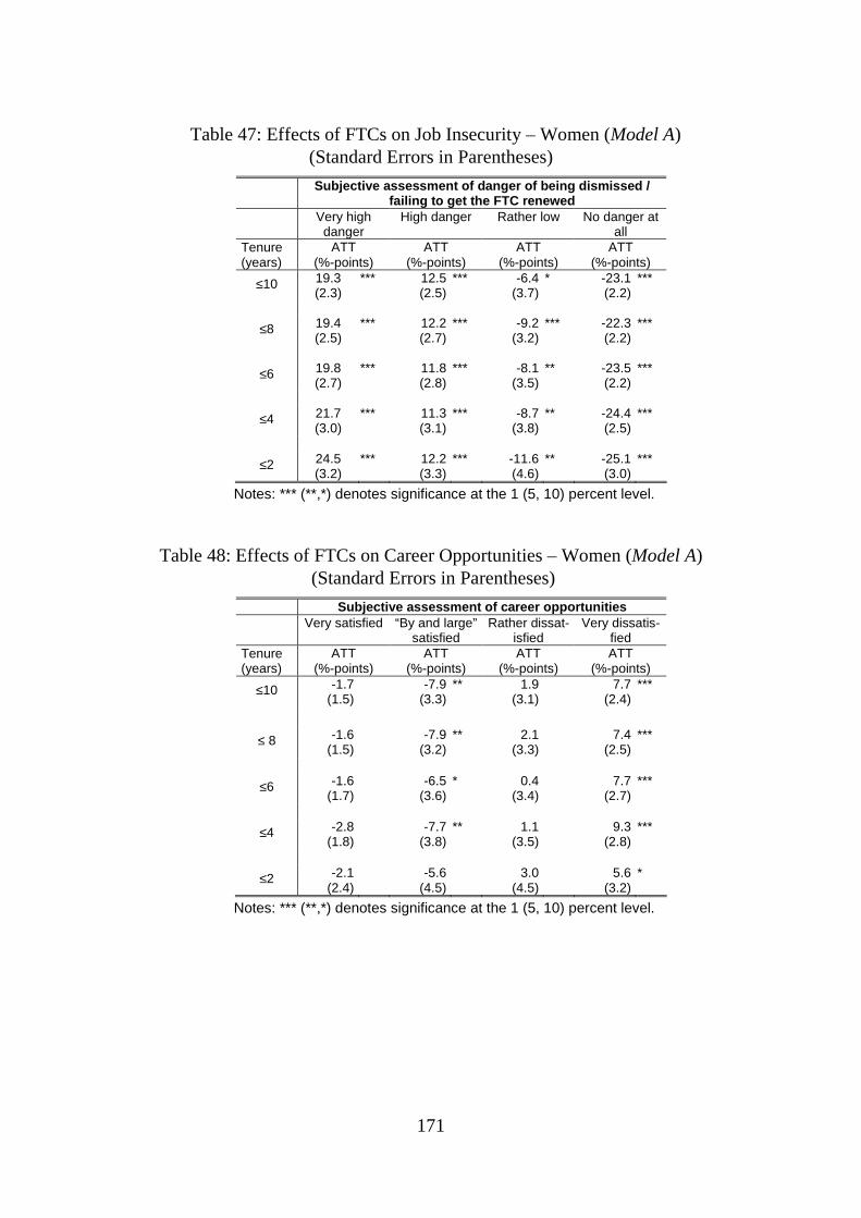
171

Table 47: Effects of FTCs on Job Insecurity – Women (Model A) (Standard Errors in Parentheses)


Very high danger

High danger Rather low No danger at all

Tenure (years)

ATT (%-points)

ATT (%-points)

ATT (%-points)

ATT (%-points)

≤10 19.3 (2.3)

*** 12.5 (2.5)

*** -6.4 (3.7)

* -23.1 (2.2)

***

≤8 19.4 (2.5)

*** 12.2 (2.7)

*** -9.2 (3.2)

*** -22.3 (2.2)

***

≤6 19.8 (2.7)

*** 11.8 (2.8)

*** -8.1 (3.5)

** -23.5 (2.2)

***

≤4 21.7 (3.0)

*** 11.3 (3.1)

*** -8.7 (3.8)

** -24.4 (2.5)

***

≤2 24.5 (3.2)

*** 12.2 (3.3)

*** -11.6 (4.6)

** -25.1 (3.0)

***


Table 48: Effects of FTCs on Career Opportunities – Women (Model A) (Standard Errors in Parentheses)




fied Tenure (years)

ATT (%-points)

ATT (%-points)

ATT (%-points)

ATT (%-points)

≤10 -1.7 (1.5)

-7.9 (3.3)

** 1.9 (3.1)

7.7 (2.4)

***

≤ 8 -1.6 (1.5)

-7.9 (3.2)

** 2.1 (3.3)

7.4 (2.5)

***

≤6 -1.6 (1.7)

-6.5 (3.6)

* 0.4 (3.4)

7.7 (2.7)

***

≤4 -2.8 (1.8)

-7.7 (3.8)

** 1.1 (3.5)

9.3 (2.8)

***

≤2 -2.1 (2.4)

-5.6 (4.5)

3.0 (4.5)

5.6 (3.2)

*


172

Heterogeneous Effects for Women

Table 49 displays the estimated effects of FTCs on wages for different sub-groups of female workers. First of all, one should consider the small number of treated workers depicted in the last column. All in all, the results are very similar to those found for men. The largest absolute and relative negative ATT on wages is found again for workers with university degree. With -2.9 € it corresponds to a wage penalty of more than 20% compared to the control group of permanent workers. In line with the results for men, there is no significant negative effect of FTCs on workers without qualification.

The heterogeneous effects of FTCs on the subjective outcome variables are de-picted in Table 76 and Table 77 in the Appendix. All groups of female FTC workers perceive a higher job insecurity. Again, there are only few statistically significant effects on perceived career opportunities in different subgroups of female workers.

Table 49: Heterogeneous Wage Effects of FTCs – Women (Model A) (Standard Errors in Parentheses)

Mean Wages in €

Tenure ≤≤≤≤10 years FTC (€)

ATT (€)

ATT (%)

NT

Small establishment (<50 employees)

8.60 -0.58 (0.50)

-6.3 193

Large firm (≥50 employees)

9.33 -1.33 (0.38)

*** -12.5 126

Industry 9.11 -0.78 (0.57)

-7.9 68

Trade 8.90 -0.42 (0.87)

-4.5 118

Without qualification 8.41 0.15 (0.74)

-1.8 80

With qualification (including university degree)

9.05 -0.82 (0.36)

** -8.3 257


** -20.6 27

Age < 32 years 8.48 -0.59 (0.53)

-6.5 143

Age ≥ 32 years 9.14 -0.82 (0.47)

* -8.2 194


173

5.8 Summary and Conclusions

The objective of this chapter has been to analyse the short-run effects of FTCs on the workers’ subjective assessment of working conditions and especially on wages. The underlying theoretical question is whether and to what extent work-ers are compensated for the lower employment stability and lower career oppor-tunities in FTC jobs by higher wages. If the assumptions of a perfect labour mar-ket were fulfilled, one would expect, ceteris paribus, higher wages for FTCs. On the other hand, in the presence of asymmetric information on workers’ ability, hidden actions of workers, or career concerns there may be a contemporaneous wage loss which is compensated for in the long-run. Hence, the simple theory of compensating differentials, as presented in Subchapter 5.2, may be too restrictive since two important features of the labour market are not taken into account: asymmetric information and workers’ maximisation of lifetime utility or earn-ings.

The reasons for analysing the effects of FTCs on two subjective outcome vari-ables (subjective assessment of the danger of losing one’s job and subjective as-sessment of career opportunities) are threefold: First, it should be tested whether FTCs are really associated with drawbacks that are perceived by workers. Sec-ond, subjective variables may be more strongly correlated with utility than objec-tive measures. Third, job satisfaction has been found in other studies to be one of the main determinants of worker mobility and thus on-the-job search.

The econometric analysis has been performed by interpreting a FTC as a treat-ment (compared to the non-treatment state of holding a permanent contract) and by applying the potential-outcome approach, presented in Chapter 3. Estimating the effects of FTCs is associated with a further methodological problem which has rarely been addressed in the empirical literature on compensating differen-tials: Many of the important variables determining wages can not be interpreted as admissible pre-treatment variables since they are determined simultaneously with the contract type, such as industry, firm size, and job position. In addition, job tenure is endogenous with respect to the type of contract. What has been done in this chapter, is to check the robustness of the results with respect to the inclu-sion of tenure and other job-related covariates. Furthermore, the effect has been estimated for different subsamples of maximum job tenure.

The results turn out to be quite robust with respect to the choice of conditioning variables and can be summarised as follows: (1.) FTCs raise the probability of workers to expect losing their job; (2.) FTCs decrease the probability of being (very) satisfied with career opportunities and increase the probability of being (very) dissatisfied with career opportunities; (3.) FTCs are not associated with

174

compensating wage differentials but the results are more in favour of a wage penalty to FTCs.146

Depending on the specification, the wage effects of FTCs for men are between -4.7% and -9.8%, and for women between -7.0% and -11.9%. Interestingly, there is a negative relationship between the wage penalty to FTCs and the level of formal qualification. In particular, workers with a university degree have a much stronger negative wage effect, while there is no significantly negative effect for persons without a formal qualification. As workers with university degree may, in general, have better outside options, this result may be interpreted as evidence in favour of a prolonged probationary or, more general, investment period lead-ing to higher wages in the long-run. Obviously, this has to be analysed by a lon-gitudinal (dynamic) study in further research.

It should again be stressed that this has been a microeconomic study ruling out general equilibrium effects (SUTVA, see Section 3.2.5). Hence, possible negative wage effects at the individual level should not be mixed up with negative effects of FTCs on aggregate wages at the macroeconomic level (being associated with positive employment effects). The augmented insider-outsider model by BENTO-

LILA and DOLADO (1994) shows that the opposite may be true (see Section 5.2.2), that is, FTCs may increase the aggregate wage level.

146 Compensation differentials also could not be found for other negative job-related aspects in Germany

(see, for example, SCHMIDT and ZIMMERMANN , 1991).

175

6 Do Fixed-Term Contracts Increase the Long-Term Employment Opportunities of the Unemployed?

6.1 Overview: Are Fixed-Term Contracts Stepping Stones for the Un-employed or Dead-Ends?

One important political goal of the liberalisation of FTCs in the 1980s was that dismissal protection legislation was thought to reduce the re-employment prob-abilities of the unemployed, particularly of those with adverse signals and those within the scope of the special protection against dismissal (see Subchapter 2.2). Thus FTCs, or temporary work in general, may increase the employment oppor-tunities of the unemployed which are harmed by the firing costs due to employ-ment protection for permanent workers. The rationale is simple: employers may be more willing to hire if they can fire easily (see ADDISON and TEIXEIRA, 2003 and Subchapter 4.2).

However, objections are raised to this view. FTC work may create a segmented labour market where the employment stability of permanent contract workers is raised by firms’ using temporary workers as a kind of buffer against transitory changes in the business environment. For some workers this may imply to be ‘trapped’ in a cycle of recurrent periods of unemployment and FTC jobs (see BLANCHARD and LANDIER, 2002 and Subchapter 4.2). The temporary nature of the employment relationship could become the cause of subsequent unemploy-ment periods and new FTC jobs (see TAUBMAN and WACHTER, 1986). This phe-nomenon may be fostered by inferior access to training and lower career oppor-tunities in FTC jobs (see BOOTH, FRANCESCONI, and FRANK, 2002, 2003 as well as Chapter 5). Thus the central issue is whether or not FTC work really increases the long-run employment opportunities of the unemployed entering into FTC jobs in terms of future permanent employment relationships or employment in general. Put differently, should unemployed job searchers take up FTC jobs or should they keep on searching for permanent positions? Are FTC jobs ‘stepping stones’ for the unemployed or ‘dead ends’ (BOOTH, FRANCESCONI, and FRANK, 2002)? While this topic has been touched on in Chapter 5 within a static frame-work, this chapter analyses the dynamic aspect and focuses on the group of un-employed job searchers.

Here, the aim is to investigate the employment effects of FTCs for the unem-ployed by using matching methods, which have been described in detail in Sec-tion 3.3.1 and already applied in Chapter 5. The methodological contribution of the following econometric analysis is to estimate the propensity score by a dis-

176

crete hazard rate model, which has been done only rarely so far.147 I will argue that this may have some advantages – at least in this application.

The structure of this chapter is as follows. The next subchapter provides some considerations on the theoretical framework. The empirical analysis is divided into two parts: Subchapter 6.3 analyses the differences in the determinants of transitions from unemployment to FTC and permanent jobs by hazard rate mod-els. The hazard rate model for the transition to FTC jobs is used to estimate the propensity score in Subchapter 6.4, and the results are used evaluate the long-term employment effects of entering into FTCs by a matching estimator. Sub-chapter 6.5 draws conclusions.


First, some basic concepts related to job search theory and unemployment dura-tion analysis are introduced. Using these concepts and taking the empirical re-sults of Chapter 5 into account, it is discussed under which conditions unem-ployed job searchers may be willing to accept FTC job offers. Finally, the theo-retical literature is reviewed with respect to suggestions under which conditions FTCs may serve as stepping stones to permanent employment.

6.2.1 Basic Concepts: Job Search Theory and Determinants of Unem-ployment Duration

A framework for analysing the determinants of unemployment duration is the job search theory. This is also applied to describe the conditions for accepting FTC job offers. The probability of an unemployed worker i leaving unemploy-ment to a specific job after a certain unemployment duration t is the hazard rate

( )ih t . The hazard rate can be expressed in terms of the probability of receiving a

specific job offer iξ times the probability that the offer is acceptable

( )( )1 R

i iF w t− , where ( )( )R

i iF w t is the cumulated wage offer distribution and

( )R

iw t is the reservation wage (see MORTENSEN, 1986: 862).148

In steady states an unambiguous relationship between the hazard rate and the proportion of long-term unemployed (or other unemployment durations) occurs. As shown by MACHIN and MANNING (1999), the proportion of long-term unem-

147 To the best of my knowledge, there are only two studies using hazard rate models for the estimation

of the propensity score (see BRODATY, CRÉPON, and FOUGÈRE, 2001 and SIANESI, 2004). Recently this approach has been formally justified by FREDRIKSSON and JOHANSSON (2003).

148 This arrival rate of job offers in standard search models can be further decomposed into the flow of vacancies times the probability that the worker becomes aware of a vacancy times the probability that the worker actually is offered the job.

177

ployed in total unemployment in steady-states149 is (1.) negatively affected by the average hazard rate from unemployment at any duration of unemployment and (2.) positively affected by the degree of negative duration dependence. Point (1.) means that if it is possible to increase the hazard rate from unemployment at any duration of unemployment (for example for the short-term unemployed), the proportion of long-term unemployed decreases.150 Point (2.) highlights the im-portance of the effect of the duration of the current unemployment spell on the individual hazard rate. If the individual hazard rate (after controlling for ob-served and unobserved heterogeneity) depends on the unemployment duration, there is duration dependence in the hazard rate. Negative (positive) duration de-pendence means that the hazard rate decreases (increases) with unemployment duration. Based on empirical evidence the focus of the debate has concentrated on negative duration dependence.

As derived by MACHIN and MANNING (1999), negative duration dependence of an individual hazard rate ( )ih t may stem from the following (partly interdepend-ent) factors (see also STEINER, 2001): – the job offer arrival rate iξ decreases with the unemployment duration t;

– the wage offer distribution ( )( )R

i iF w t shifts to the left with increasing unem-

ployment duration; – the worker’s search intensity decreases with unemployment duration; – the decline in the reservation wage ( )R

iw t is too low to balance the three

points mentioned above. The job offer arrival rate may decline with unemployment duration either due

to a deterioration of human capital (see PISSARIDES, 1992) or due to stigma effects of unemployment duration (see LOCKWOOD, 1991 and the following sec-tion). Even if the reservation wage falls with unemployment duration, it can be shown that the negative effect is not equalised for the most common assumptions on the wage offer distribution (see MACHIN and MANNING, 1999).151 If the wage offer distribution is more reduced with unemployment duration than the reserva-tion wage, the hazard rate declines.

If the search intensity of the unemployed is reduced with unemployment dura-tion, the job offer arrival rate also declines with duration. The reason most often

149 Here, steady state means that the inflow rates into unemployment and the outflow rates out of unem-

ployment are constant. If one does not impose this assumption, two further basic results appear: The proportion of long-term unemployed is lower if the inflow into unemployment was particularly high in the recent past, and the proportion of long-term unemployed is higher if the outflow rate was par-ticularly low in the recent past.

150 Of course, also the overall level of unemployment decreases. It is well-known that the unemployment rate is determined at a given constant unemployment level by the average risk of becoming unem-ployed times the average unemployment duration times the average number of individual unemploy-ment spells (see FRANZ, 2003: 353).

151 There are various reasons to assume the reservation wage to be decreasing in unemployment dura-tion, for example, due to ageing within a finite time horizon model (see FRANZ, 2003: 213).

178

mentioned for the decline in the search intensity in the literature are discourage-ment effects (see FRANZ, 2003: Chapter 7).

6.2.2 Under Which Conditions Do Job Searchers Enter into Fixed-Term Contract Jobs?

The results of Chapter 5 are in line with the hypothesis that workers entering into FTC jobs perceive their unemployment risk to be higher than comparable workers entering into permanent contract jobs. Furthermore, one can argue that temporary employment relationships are associated with a loss of returns to job seniority.152 Descriptive statistics on the duration of employment spells after the transition from unemployment to FTCs or permanent contracts respectively, be-ing also in line with this statement, are provided in Table 78 in the Appendix.

Available empirical studies and the results of Chapter 5 suggest that FTC work-ers do not receive wage premiums to compensate for these risks but even lower wages. As discussed in detail in Subchapter 5.2, these empirical results do not conflict with economic theory if departures from the assumptions of a perfect market are considered.

The question arises when and under which conditions unemployed job search-ers are willing to enter into FTCs instead of continue searching for a permanent job. To the best of my knowledge, there is no job search model explicitly taking FTC and permanent contract jobs into account. Nevertheless, some basic job search models can be discussed in order to gain some insights into the underlying behaviour and to obtain theory-based hypotheses.

BURDETT and MORTENSEN (1980) augment the standard sequential job search model with a job-specific random dismissal probability without explicitly taking FTCs and permanent contracts into account. If one assumes that failing to get the contract renewed is associated with an adverse signal for potential future em-ployers (for example, if non-renewal due to unfavourable business development or due to low worker’s ability is not distinguishable), the reservation wage is in-creasing with the dismissal probability.153 Therefore, the reservation wage with regard to FTC jobs is, ceteris paribus, higher than the reservation wage with re-gard to permanent contract jobs (see GROOT, 1990; BOVER and GÓMEZ, 2003). The reservation wage with regard to FTC jobs decreases, however, with the ex-pected probability that the contract is transformed into a permanent one by the employer. Nevertheless, the acceptability of FTC job offers is, ceteris paribus, lower than the acceptability of permanent contract job offers.

152 A result often found in wage regressions is that job seniority has a significantly positive effect on

wages. One explanation for this result is the accumulation of firm specific human capital during em-ployment (see PISSARIDES, 1994).

153 BURDETT and MORTENSEN’s (1980) general proposition is that the reservation wage is increasing in the dismissal probability if the return to search after being dismissed from the job is less than the ex-pected return to search before the job was taken up. A general proof that the reservation wage de-pends on the type of job (offer) can be found in WEITZMAN (1979).

179

If the reservation wage decreases with unemployment duration, the probability of a FTC job to be acceptable increases with unemployment duration as well. Note that there may be further reasons for job searchers to reduce their reserva-tion wages and accept FTC job offers. They may, for example, have to meet tem-porary declines in family income, particularly when other family members have lost their jobs. This highlights that the acceptability of jobs is not only influenced by individual characteristics (and labour market conditions) but also by factors related to the general household situation.

Within the job search framework unemployment compensation is interpreted as a reduction of the opportunity costs of unemployment (see MORTENSEN, 1986). By increasing the reservation wage unemployment compensation reduces the acceptability of job offers. Given the assumptions about the reservation wages with regard to FTCs and permanent contracts, the probability of accepting a FTC job offer is more reduced than the probability of accepting a permanent contract job offer (see BOVER and GÓMEZ, 2003). Put differently, given a certain prob-ability of permanent contract job offers, unemployed without unemployment compensation are more willing to accept FTCs than unemployed receiving un-employment compensation.154

Outside the framework of job search theory this result can also be derived from the model by VAN DE KLUNDERT (1990). In his model, unemployment results from the assumption that queuing for a ‘primary’ job is preferred to a ‘secondary’ job, if the utility derived from unemployment compensation, combined with the status of searching for a proper, that is, primary job, exceeds the utility derived from a secondary job. Besides the effects of subjective factors such as ‘status in the labour market’, the model highlights the effects of unemployment compensa-tion: If the amount of benefit is relatively high and depends on the previous wage rate, unemployed persons may prefer to wait for a suitable primary job. Hence, previous high-wage primary (permanent) jobs increase unemployment duration and decrease the probability of entering into low-wage secondary (temporary) jobs. In particular, as entrants into the labour market (younger workers or women after maternity leave) are often not entitled to unemployment compensation and have no determined idea about their ‘labour market status’, they are more likely to enter into FTCs. Unemployed who were previously employed on a permanent basis may hesitate to accept a FTC job offer. This may lead to various types of state dependence.

In Subchapter 5.2 the role of asymmetric information on workers’ ability is de-scribed in detail. If incomplete information plays an important role, the employ-ment histories of job searchers may serve as signals. References from previous employers and the reputation of previous jobs may reveal information on the ability (or further unobservable characteristics) of the worker. If the employment

154 According to this argumentation, unemployment compensation could be interpreted as a subsidy for

the search for ‘good’ (permanent) jobs.

180

history involves adverse signals, employers with permanent contract vacancies may hesitate to offer permanent jobs to these job-searchers (see PEETERS, 1999). If the unemployment duration is an adverse signal155, then, within the job search framework, the offer rate for permanent contract jobs may decrease relative to the offer rate for FTC jobs with increasing unemployment duration. Given that the relative FTC job offer rate and the relative acceptability of FTC offers in-crease with unemployment duration, the duration dependence of the FTC hazard rate should be empirically more positive (or less negative) than the duration de-pendence of the permanent contract hazard rate (see GROOT, 1990).

Particularly, older dual labour market theories predict that the temporary nature of an employment relationship is the cause of subsequent unemployment and temporary jobs (see TAUBMANN and WACHTER, 1986). Thus interpreting FTC jobs as ‘secondary’ and permanent contract jobs as ‘primary’ implies that having been employed on a FTC in the past may be an adverse signal for future employ-ers, at least if the jobs are associated with unfavourable attributes.156 This state-ment is also compatible with more recent theoretical models on signalling effects (see MA and WEISS, 1993; MCCORMICK, 1990). Hence, workers who previously held a FTC job have a higher probability of re-entering into a FTC job as they receive fewer permanent contract job offers.

However, the matching model by CANZIANI and PETRONGOLO (2001) high-lights that the stigma attached to being dismissed increases in firing costs. Since the information on the worker’s productivity is imperfect, the firm’s hiring deci-sion also depends on the worker’s employment history including the reasons for the end of the previous job. Hence, having been dismissed (despite high firing costs) decreases the re-employment prospects. Since the termination of a FTC is not associated with firing costs, entering into unemployment after a FTC job is a less adverse signal.

The availability of job offers increases with a job searcher’s regional mobility and the acceptability of commuting time. Obviously, both should be lower for mothers with young children. Therefore, they may be more inclined to accept FTC job offers.

So far, the possibility of on-the-job search has been neglected. As repeatedly mentioned in the previous chapters, it is likely that FTCs promote on-the-job search in comparison to permanent contract jobs since rational workers anticipate the higher risk of job losses (see BOERI, 1999). If one, furthermore, assumes that FTCs increase the arrival rate of job offers (due to networking etc., see next sec-tion) or improves the wage offer distribution by enhancing human capital (see

155 LOCKWOOD’S (1991) theoretical model shows that if it is costly for employers to test workers, they

may use unemployment duration as a signal on which the employment decision is based. 156 “...secondary employment may be regarded as a kind of stigma that bars access to the primary sec-

tor.” (MCDONALD and SOLOW, 1985: 1124).

181

next section), entering into a FTC job may be an optimal search strategy.157 On-the-job search may also render re-entering into FTCs after a previous FTC and a subsequent unemployment spell as an optimal strategy.

Nevertheless, it seems reasonable to assume that in most cases job searchers accept FTC job offers after having failed to get a permanent job, and if they ex-pect a permanent job offer only with a sufficiently low probability. Hence, the decision to accept a FTC offer is sequential over time.

The most realistic view seems to be to interpret FTC jobs (similar to training) as a kind of investment under uncertainty for the unemployed workers. The in-vestment consists of the lower contemporaneous utility during the job in com-parison to the hypothetical situation of the individual finding a permanent job in the next period. The returns of this investment depend on the expected stream of future earnings or utility (including unemployment benefit), that is, expected life-time earnings or utility. Furthermore, the profitability of the investment depends on the counterfactual transition rate to permanent jobs and the counterfactual stream of future earnings or utility from permanent jobs.

6.2.3 Why Should Fixed-Term Contracts be Stepping Stones Towards Permanent Positions?

Why and under which conditions may FTCs be stepping stones towards perma-nent positions, that is, increase the long-term employment opportunities of those entering into FTCs?

During FTC jobs there may be more investments in (general and specific) hu-man capital (in comparison to the hypothetical situation that the person had stayed unemployed), even if there is no formal training. This may raise the worker’s employment opportunities at the same or other employers. The latter is associated with a shift in the wage offer distribution to the right. However, firms may invest less in FTC workers than in permanent contract workers since they recognise the shorter expected job tenure (see BOOTH, FRANCESCONI, and FRANK, 2003 and Chapter 5). Therefore, the opposite effect may also be possible: If the unemployed person had not accepted the FTC job offer in a certain period, she or he might have got a permanent contract job offer in the next period with better training and career opportunities.

As discussed in detail in Chapter 5, FTCs may be used as a prolonged proba-tionary period in order to overcome the problem of asymmetric information. Thus FTCs may serve as a screening device. This may help unemployed persons with adverse signals, who would otherwise get permanent contract job offers only with a low probability (see PEETERS, 1999). After the expiration of the FTC and after sufficient information on the worker’s ability is collected, the worker may get a permanent contract job offer from the same employer. This may be

157 The argument is based on HECKMAN, LALONDE, and SMITH (1999), who present a model which in-

terprets public sponsored labour market training as an optimal form of job search.

182

especially true if FTCs induce a sorting mechanism as shown in the model by LOH (1994) described in Subchapter 5.2.

FTC jobs may promote on-the-job search (see BOERI, 1999). So it seems plau-sible to state that the job search intensity may not be much lower than during un-employment and strictly higher than in permanent contract jobs. If, however, search intensity was lower than during unemployment, FTCs could decrease the probability of receiving permanent contract job offers compared to unemploy-ment.

FTC workers may be able to enlarge their social network within the firm or even the industry in which they are employed (see VAN DEN BERG, HOLM, and VAN OURS, 2002). This may increase the workers’ knowledge of (future) vacan-cies and may again help other employers to collect (otherwise unobserved) in-formation on the workers’ productivity.

For on-the-job-searchers a FTC job may also be a positive signal to other em-ployers, again in comparison to the situation in which the person had stayed un-employed and thus had possibly been affected by negative ‘stigma effects’ due to unemployment. However, in order to be a credible positive signal the cost of finding a FTC jobs must be higher (in the broad sense of search costs) for low ability workers (see GERFIN, LECHNER, and STEIGER, 2002). The harder it is to get a FTC job, the better is the signal to potential future employers. But again, entering into a FTC job may have the opposite effect, that is, it may signal that the person did not receive any offers for permanent contract jobs. This may be especially true for recurrent FTC spells. Hence, temporary jobs may be ‘stigma-tised’ (see MA and WEISS, 1993). Given that FTCs are associated with a negative wage differential, they may be an adverse signal especially for highly qualified workers (see MCCORMICK, 1990).

The matching and labour demand modes discussed in Subchapter 4.2, also de-scribe the determinants of FTCs being stepping stones. A FTC job may be a stepping stone to a permanent job, if firing costs of permanent workers are not too high, and if relative hiring and firing costs of FTCs are not too low. Put dif-ferently, if it is much easier for a job searcher to get a FTC than a permanent con-tract, the FTC job is less likely to be a stepping stone.

183

6.3 Fixed-Term Contracts and the Re-Employment Probabilities of the Unemployed

6.3.1 Introduction

One objective of the liberalisation of FTCs was to increase the re-employment probabilities of the unemployed, especially those with adverse signals and those who are within the scope of the special protection against dismissal (see Sub-chapter 2.2). If this assumption is true, personal characteristics which are known to increase unemployment duration should affect the probability of getting low-firing-cost FTC jobs (the FTC hazard rate) less than the probability of getting high-firing-cost permanent contract jobs (the permanent contract hazard rate).

There is, however, no empirical evidence on the determinants of contract-specific hazard rates for Germany available yet. Thus it has not been revealed what makes FTC and permanent jobs different from an unemployed job searcher’s point of view.

This Subchapter analyses the role of individual unemployment duration and personal characteristics for the transitions from unemployment to FTC jobs ver-sus permanent contract jobs within a competing risks hazard rate model. This is the starting point for the estimation of the propensity score in Subchapter 6.4.

Distinguishing jobs by their type of contract is associated with some benefits. Firstly, it provides insights into the behaviour of job searchers and employers in the presence of contracts which differ in their firing costs. Secondly, pooling dif-ferent types of jobs and contracts, what is usually done in hazard rate analyses, may induce a spurious negative duration dependence effect (see GROOT, 1990). Generally speaking, spurious negative duration dependence is usually attributed to omitted variables (unobserved heterogeneity). Distinguishing between jobs may capture heterogeneity by allowing coefficients to vary across different groups of individuals.158

To the best of my knowledge, this is the first empirical attempt to distinguish between the destination states of FTCs and permanent contracts in unemploy-ment duration analyses for Germany. It is shown that permanent contract jobs and FTC jobs are indeed behaviourally distinct states with respect to the search-ers’ characteristics and regional labour market conditions.

158 A further reason why this analysis may be useful is stressed by ATKINSON and MICKLEWRIGHT

(1991). They highlight the importance of distinguishing between ‘regular’ and ‘marginal’ jobs in the analysis of the effects of unemployment compensation on the transition between unemployment and employment. It seems reasonable to expect unemployment compensation to have a different effect on the transition to FTC jobs than on the transition to permanent jobs. Unemployment compensation may be interpreted as a subsidy for the search for ‘good jobs’, i.e., regular jobs (see Section 6.2.2). Unfortunately, due to data restrictions it is not possible to model unemployment compensation in an adequate way within the econometric hazard rate model in this Chapter.

184

6.3.2 Previous Results: Unemployment Duration Analyses Distinguishing Between Employment Contracts

The literature on unemployment duration has always recognised unemployment and inactivity to be behaviourally distinct states, but has generally failed to dis-tinguish between different types of employment other than full-time and part-time jobs (see PORTUGAL and ADDISON, 2003). To the best of my knowledge, there are only three studies which distinguish between FTC and permanent con-tract jobs as destination states.

For the Netherlands, GROOT (1990) estimates a continuous time competing risks model distinguishing between permanent contract and FTC jobs. He finds higher educated and younger unemployed to enter FTCs with a higher probabil-ity. The author explains the former with the assumption that individuals with higher human capital are less risk averse due to their better labour market pros-pects. He finds no significant duration dependence effect, for neither the FTC hazard nor the permanent contract hazard.

For Portugal, PORTUGAL and ADDISON (2003) estimate a discrete time compet-ing risks model for six different exit states (full-time permanent contract jobs, full-time FTC jobs, part-time work, public employment jobs, self-employment, and out-of-labour force), taking unobserved heterogeneity into account by a gamma distribution. The analysis focuses on the impacts of unemployment bene-fits. The authors find strong disincentive effects of unemployment benefit for FTC as well as for permanent contract jobs, which are not significantly different between these two states. The authors conclude that being entitled to unemploy-ment benefit does not help job searchers to find permanent jobs (otherwise the negative effect on the FTC hazard would have been stronger). Labour market entrants, workers having already been employed on FTCs in the past, and work-ers who have had a large number of jobs, exit into FTCs with a higher probabil-ity. A further result is that the permanent contract hazard rate is negatively asso-ciated with the regional unemployment rate, while the unemployment rate seems to have no effect on the FTC hazard. Moreover, the duration dependence of the permanent contract hazard rate is much more negative than the duration depend-ence of the FTC hazard rate. The interpretation suggested by the authors is that jobs searchers, initially looking for permanent jobs, switch to FTCs after a period of unsuccessful search. Note that this is in line with the theoretical predictions of Subchapter 6.2 that the decision to take up a FTC job is sequential over time.

BOVER and GÓMEZ (2003) use a discrete logistic hazard rate model without controlling for unobserved heterogeneity and distinguish between transitions to FTC and permanent contracts in an analysis for Spain. They also find stronger negative duration dependence for the FTC hazard rate than for the permanent contract hazard rate which is again compatible with the hypothesis mentioned.

Even though the following studies do not analyse the transitions from unem-ployment to FTC jobs, their results may be of particular importance. DEKKER

185

(2000) analyses the effects of entering into unemployment from FTCs (versus permanent contracts) on unemployment duration by a discrete hazard rate model for Germany and the UK (without distinguishing between the type of contract after unemployment). If workers on FTCs were more active in on-the-job search than permanent contract workers, FTC workers should experience shorter spells of unemployment compared to permanent contract workers when losing their job. He finds evidence for a decreasing effect of previous FTCs on unemployment duration, which is in line with this hypothesis.

In order to test the hypothesis from their theoretical model (see Section 6.2.2), CANZIANI and PETRONGOLO (2001) distinguish between different causes for un-employment (end of non-seasonal FTC, end of seasonal FTC, quit, and dis-missal) in a discrete hazard rate analysis (again without distinguishing between FTC and permanent contracts jobs as destination states) for the UK. To the extent that lower firing costs indeed lower the stigma attached to adverse employment histories, the authors would expect unemployment spells to be shorter after the termination of a FTC in comparison to the case of dismissal from a permanent position. They find that unemployed who terminated a FTC or quit their previous job experience significantly shorter unemployment spells than those who were dismissed. The negative effect of dismissal on unemployment duration seems to be stronger for older workers. The additional finding that unemployed who pre-viously held a seasonal FTC (which is an inherently temporary job) have shorter unemployment spells than those who previously held a non-seasonal FTC, is in-terpreted by CANZIANI and PETRONGOLO (2001) as evidence for the hypothesis that the failure to get a non-seasonal FTC renewed or converted into a permanent contract implies a negative signal, even though a less negative signal than being dismissed.

GÜELL (2000) analyses the effects of the introduction of FTCs in Spain in the mid 1980s on the duration dependence of the hazard rate from unemployment to employment. This is done by comparing estimation results for the periods before and after the introduction of FTCs using a proportional hazard rate model with-out controlling for unobserved heterogeneity. The results indicate that for short unemployment durations (up to 5 months) the probability of leaving unemploy-ment has increased since the introduction of FTCs. In contrast, for long-term un-employed the probability of leaving unemployment has been reduced. Put differ-ently, the availability of FTCs has increased the re-employment probability of short-term unemployed and has decreased the re-employment probabilities of long-term unemployed. Assuming that the reduction in the hazard rate for long-term unemployed is really caused by the introduction of FTCs159, this result may be explained by the theoretical matching model by BOERI (1999), which predicts that the reemployment chances of the unemployed are reduced by on-the-job-

159 As discussed in Section 3.4.1, before-after estimators are based on relatively restrictive identifying

assumptions.

186

search of FTC workers (see Subchapter 4.2). A further result is that unemployed who have become unemployed because their FTCs were terminated have shorter unemployment durations than those who lost their jobs due to other reasons. This is in line with the results of DEKKER (2000) as well as CANZIANI and PETRON-

GOLO (2001).

6.3.3 Modelling Framework: Discrete Competing Risks Hazard Rate Model

The central concept of duration analysis is the hazard rate. The hazard rate is the probability that an individual leaves unemployment at a certain time given that the individual has stayed unemployed until that time. Since unemployment spells are measured on a monthly basis in the underlying dataset (GSOEP, see Section 6.3.4), a discrete time hazard rate model instead of a continuous time hazard rate model is specified.160 It can be shown that the two approaches yield similar results (see NARENDRANATHAN and STEWART, 1993). Different destina-tion states are distinguished, i.e., an independent competing risks model is esti-mated. Four destination (exit) states are taken into account: FTC jobs, permanent contract jobs (including self-employment)161, on-the-job training (including ap-prenticeship), and out-of-labour force (including school and university).

The amount of time spent in unemployment before a transition to another state or right-censoring occurs is denoted by T.162 Let unemployment duration be grouped into t discrete intervals. T = t if the transition occurs during the interval [ )1,t tI I− and T>t if the spell is (right-)censored (see STEINER, 2001).

ikT denotes the time (number of months) an individual i (with { }1...i N∈ ) has

spent in her or his k-th unemployment spell (with { }1... ik K∈ ) before the transi-

tion to another state or right-censoring occurs. The destination-specific hazard rate j

ikh is the probability that an individual i leaves her or his k-th unemployment

spell for state j (with { }1,2,3,4j ∈ ) during [ )1,t tI I− , given that the spell has lasted

until the beginning of t-1, and given a vector of observable explanatory variables ( )ikx t either measured at the beginning of the interval or being time-constant.

Furthermore, there may be unobserved variables iε , which are discussed below.

160 For other examples of discrete time hazard rate models for unemployment duration analysis using the

GSOEP see HUJER and SCHNEIDER (1996); HUJER, MAURER, and WELLNER (1999); LAUER (2003); and STEINER (2001). See LANCASTER (1990); DEVINE and KIEFER (1991); and VAN DEN BERG (2001) for a presentation of continuous models.

161 Due to the sample size a further differentiation between self-employment and paid employment is not feasible. For an analysis of the hazard rate into self-employment in West Germany see REIZE (2004). Furthermore, the distinction between the types of contracts implies that a differentiation between full-time and part-time work is not feasible due to the limited sample size.

162 Right-censoring means that during the period in which the individual is observed, the transition out of the current state does not occur (the spell end date is unknown), so that the total length of time be-tween entry into and exit from the state is unknown.

187

The destination-specific hazard rate can be written as (see FAHRMEIR and TUTZ, 2001; STEINER, 2001; LAUER, 2003)

( )( ) ( )( ), Pr , , ,jik ik i ik ik ik ih t x t T t D j T t x tε ε= = = ≥

(49)

with 1 if transition to FTC occurs;

2 if transition to permanent contract occurs;

3 if transition to training occurs;

4 if transition to out-of-labour force occurs.

D

=

In the next step, a functional form for the hazard rate has to be specified. Fol-

lowing a couple of studies using discrete time models, a logistic hazard rate model (also called proportional odds model) is used. Modelling all destination states simultaneously leads to the multinomial logit model with random effects (see STEINER, 2001; FAHRMEIR and TUTZ, 2001; BOVER and GÓMEZ, 2003; LAUER, 2003): 163

( )( ) ( ) ( )( )( ) ( )( )

4

1

exp,

1 exp

j j ik ijik ik i

l l ik il

t x th t x t

t x t

α β εε

α β ε=

′+ +=

′+ + +∑, (50)

The vectors of destination-specific parameters to be estimated are denoted by jβ ′ .

The so-called baseline hazard ( )j tα describes the effect of unemployment dura-

tion on the transitions to the destination states j. An important issue is how to model the duration dependence of the hazard rate, i.e., the functional form of the baseline hazard ( )j tα . Following recent studies, a functional form assumption is

avoided by specifying the baseline hazard with dummy variables (see STEINER, 2001; BOVER, ARELLANO, and BENTOLIA, 2002). Since it is, due to the sample size, not possible to use a single dummy variable for each month, a so-called piecewise constant specification is used in which durations of unemployment are grouped together into seven categories and the hazard is assumed to be constant within those categories (see MACHIN and MANNING, 1999: 3112). The dummy variable specification of the baseline hazard allows the hazard rate to be non-monotonic and have spikes at some durations.

As shown by NARENDRANATHAN and STEWART (1993) as well as by BOVER and GÓMEZ (2003), the parameters ( )j tα and jβ ′ in Eq. (50) can also be sepa-rately estimated by four binary logit models for each destination state keeping the other states as right-censored.164 In principle, this is an implication of the In-dependence of Irrelevant Alternatives (IIA) assumption of the multinomial logit

163 A formal derivation of the likelihood function, being based on the method proposed by JENKINS

(1995), can be found in LAUER (2003). 164 Of course, it is also possible to estimate a multinomial logit hazard rate model for two destination

states (FTC and permanent contract) keeping the other states (training, out-of-labour force) as right-censored.

188

model (see Section 6.3.5). Both methods provide consistent estimates of the pa-rameters, although the joint estimation by a multinomial logit is asymptotically more efficient.165 A possible advantage of separate estimations is that the pa-rameters estimated for one of the alternatives are not affected by specification errors in the equations of the other alternatives (see BOVER and GÓMEZ, 2003). Besides the computational advantage (separate estimation is faster), this is the main reason to estimate the propensity score in Subchapter 6.4 by a single logis-tic hazard rate model for the transition to FTC jobs. The results, presented in Sec-tion 6.3.5, are estimated by the multinomial logit specification presented in Eq. (50). As expected, both approaches produce very similar results.

It is well-known that omitting unobserved heterogeneity iε may bias the esti-mated coefficients, particularly of the baseline hazard. This typically leads to the wrong impression of negative duration dependence (see MACHIN and MANNING, 1999; LANCASTER, 1990; STEINER, 2001). In contrast, other coefficients seem not to be affected to a large extent (see HAM and HAUSMAN, 1990; MEYER 1990).

HECKMAN and SINGER (1984) show that estimates from hazard rate models are sensitive to the assumed distribution of unobserved heterogeneity. To address this concern, they propose a nonparametric method to account for unobserved heterogeneity using a discrete probability distribution (see POWERS and XIE, 2000: 195). This approach assumes that iε is an additive heterogeneity term and

follows an m-point discrete distribution with masspoints 1ε ,…, mε and associated

probabilities ( )Pr qε , where

( )1Pr 1

m

qqε

==∑ , ( )1

Pr 0m

q qqε ε

==∑ , ( )( ) 0q iE x tε = , ( ) 1,...,q q m∀ = .

The probabilities ( )Pr qε of the masspoints can be interpreted as the proportion

of the population falling into the q-th heterogeneity group. In practical imple-mentation one begins with a few points and increases m until the fit of the model (evaluated by certain information criteria) fails to improve (see BAKER and MELINO, 2000).

Due to the limited sample size, the analysis is performed for men and women together, which is a serious restriction given the well-known substantial differ-ences in labour force behaviour. However, differences are taken into account as far as possible by allowing important variables to have a sex-specific impact, through corresponding interaction effects.

6.3.4 Data Base and Variables

The data base for the analysis in this Subchapter as well as Subchapter 6.4 is the German Socio-Economic Panel (GSOEP) for the period 1991–2001. The GSOEP is a representative household survey of the German population, con-

165 See also the discussion in REIZE (2004: Subchapter 6.2).

189

ducted annually.166 A useful feature of the GSOEP is the availability of monthly information between annual interviews (so-called calendar). Different employ-ment states are covered. This information is gathered through a retrospective questioning about what happened during particular months within the year pre-ceding the interview.

Unfortunately, the type of contract is not collected on a monthly basis in the GSOEP. The survey only asks for the type of contract in the current job at the date of the interview. The exact wording is: “Do you have an a priori temporary employment relationship or do you have a permanent employment contract?”167 It is possible to generate monthly information, taking the regulation of FTCs into account: Employers are usually not allowed to employ a person with a FTC after having employed the same person with a permanent contract.168 Thus while it is allowed to transform a fixed-term contract into a permanent one, it is not allowed the other way around. Hence, if a person is currently employed with a FTC at her or his present employer, she or he was already hired on a fixed-term basis.

Using this information, the type of contract is not defined for about 30% of all transitions from unemployment to employment. These undefined transitions are obviously more often short-term (that is the reason why they are not being ob-served at the months of the interview), so it is likely that FTC spells are missing disproportionally often, which may induce a selection problem.169

It is possible to reduce the amount of undefined transitions to about 18% by us-ing another variable in the dataset including the reason for the end of the last em-ployment spell (due to the expiration of a FTC or an apprenticeship contract). However, using this information one identifies “unsuccessful” FTCs with a higher probability, i.e., those FTCs which do not lead to a long-term employment relationship with the same employer. For this reason, the latter information is not used for the definition of employment spells. Following ZIJL, HEYMA , and VAN

166 Details on the GSOEP can be obtained from the web-server of the German Institute of Economic

Research (DIW) in Berlin (http://www.diw-berlin.de/soep/). 167 Until 1995 only employees who reported job changes were asked this question. This is no problem

for the definition of the transition from unemployment to FTC jobs (see also the discussion in Section 6.4.4).

168 Exceptions to this rule are FTCs which are justified by the objective reason ‘at the request of the employee’ (see Subchapter 2.2).

169 To check the significance of this problem, a maximum-likelihood probit model with sample selection was estimated (see VAN DE VEN and VAN PRAGG, 1981). In the first probit equation, the transition to any type of employment (including undefined spells) is analysed, in the second probit equation the FTC hazard rate. The error terms of both equations are assumed to be jointly normally distributed. If the correlation of the error terms is not zero, a separate estimation of the FTC hazard rate leads to bi-ased results. This is checked by performing LR-tests. Various estimations with different exclusion re-strictions were performed. Since all LR-tests in all specifications showed that the correlation of the error terms is not significantly different from zero, it may be concluded that the estimated FTC haz-ard rate model is probably not biased by the sampling scheme since the selection effects are either captured by observable variables, or there is no selection bias at all.

190

DEN BERG (2004), unemployment spells ending in employment spells with unde-fined type of employment contract are simply excluded from the analysis.

For the interpretation of the results one should keep in mind that very short FTC spells are likely to be underrepresented. These short-term spells may, on the one hand, be ‘precarious’ FTC jobs in the sense that they are associated with a short contract duration. On the other hand, there may be short FTC spells leading to permanent positions at the same employer after a short time which are mis-classified as jobs starting with a permanent contract.

The estimation sample consists of individuals registered as unemployed for at least one month between January 1991 and December 2000. In order to obtain an inflow sample only spells are used which start after January 1991, i.e., left-censored spells are excluded (see HUJER, MAURER, and WELLNER, 1999). Since several formal and informal early-retirement measures exist in Germany, only persons not older than 58 years are included. The minimum age for being in the sample is 18 years. One may argue that this is, given the comparatively long pe-riod of education in Germany, too young to ensure that only unemployed persons are included who are really job searchers. However, it is interesting to include younger workers since temporary jobs may be important for the transition from school or apprenticeship to work (see RYAN , 2001). Due to the limited sample size the public sector is not excluded.

In order to distinguish regular FTCs from public employment measures, the lat-ter are defined as unemployment spells in the analyses. This definition seems to be reasonable as a certain duration of unemployment usually is a necessary con-dition for participation. Table 50 displays the number of transitions and the aver-age duration of the unemployment spells.

Table 50: Duration of Completed Unemployment Spells by Kind of Transition

Transition to Mean Standard Deviation

25 percen-tile

Median 75 per-centile

No.

FTC 8.766 9.078 3 6 11 349 Permanent contract 8.087 7.891 3 6 10 767

Training 8.936 9.027 3 6 11 235 Out-of-labour-force 12.589 12.486 4 9 15 597

Note: The figures are based on the estimation sample of the duration models estimated in this Subchapter. Source: Own estimations based on the GSOEP.

An overview of the explanatory variables being mostly time varying is de-

picted in Table 51. In addition to demographic characteristics (age, sex, national-ity, disabilities, marital status), variables on formal qualification and previous labour market experience are included, which may be important signals for em-ployers and which are likely to capture individual heterogeneity of the unem-ployed job searchers. The duration of the last employment and unemployment spell is included (accounting for possible lagged duration dependence, see

191

HECKMAN and BORJAS, 1980). Furthermore, the number of previous unemploy-ment spells is included in order to control for ‘occurrence dependence’. For checking whether or not there is state dependence in the type of the employment contract, a dummy variable indicating if the person has ever held a FTC before and dummy variables describing the reason for the end of the last employment contract (‘due to end of a FTC or apprenticeship contract’ and ‘due to dismissal’) are included.

The monthly federal state unemployment rate is included to control for regional labour market conditions.170 Further regional differences should be captured by regional dummies. However, they turn out to be insignificant in all specifications and are dropped. Furthermore, fixed time effects (annual dummy variables) as well as seasonal effects (quarterly dummy variables) are included. Descriptive statistics of the explanatory variables can be found in Table 79 in the Appendix.

The German system of unemployment compensation consisted of two parts during the period under observation, unemployment benefit (‘Arbeitslosengeld’) and unemployment assistance (‘Arbeitslosenhilfe’). A problem arises due to the fact that exact monthly income information (and therefore also unemployment benefit and assistance) is only available for the time before 1996. From 1996 on people were only asked whether or not they had received unemployment com-pensation in the preceding calendar year and how much the monthly amount was. Thus there is a trade-off between the omission of important variables on the one hand, and significant measurement errors on the other. I decided to include only dummy variables indicating if an unemployed person receives no unemployment benefit or no unemployment assistance in the year of the unemployment spell. This is obviously a very crude measure. Furthermore, it neglects the fact that not the actual receipt but the potential benefit entitlement to unemployment compen-sation is relevant for the reservation wage and the decision to accept a job offer (see HUNT, 1995).171 Variables affecting potential benefit entitlement (previous employment history) are directly included.

The amount of unemployment benefit and assistance is also not directly mod-elled since it is again not available on a monthly scale. Hence, the net income of the household (which is again collected for the preceding year) including unem-ployment compensation but excluding earnings of the individual is included.172

170 Obviously, it would be more suitable to use regional units, which approximate regional labour mar-

kets more accurate (for example travel-to-work-areas). Unfortunately, the necessary information is not included in the GSOEP.

171 STEINER (1997) calculates the potential benefit entitlement by combining monthly calendar data and retrospectively collected employment information. This approach is not adopted in the subsequent analysis in order to avoid measurement errors.

172 In other studies dealing with unemployment duration analysis more sophisticated approaches for the treatment of the unemployment compensation are applied (see, for example, STEINER, 2001 or REIZE, 2004).

192

Table 51: Explanatory Variables

Variable Definition

Baseline hazard (unemploy-

ment duration)

7 categories:

1 month (base category), 2-3 months, 4-6 months, 7-9 months, 10-12

months, 13-18 months, ≥19 months

Formal qualification Highest formal qualification:

no occupational qualification (ohne Berufsausbildung)

vocational qualification (Berufsausbildung / Lehre) (base category)

master craftsman (Meister)

university graduate (including polytechnic) (Uni- oder FH-Abschluss)

Marital status, household com-

position

Cohabitating couple (Base category)

married

no partner

children < 16 (dummy variable indicating children under age 16)

Reason for end of previous job quit last job (base category)

end of FTC or apprenticeship contract

dismissed

Previous labour market state employed (base category)

out-of-labour-force

training or school

Duration of previous employ-

ment spell

6 categories:

1–2 months (base category), 3–5 months, 6–8 months, 9–11 months,

12–20 months, ≥ 21 months

Previous unemployment

experiences

duration of previous unemployment spell (months)

number of previous unemployment spells

number of previous unemployment spells (squared)

Already a FTC before dummy variable indicating if the individual has ever been employed on

a FTC before

Public sector before dummy variables indicating if the individual was previously employed in

the public sector

Log net household income natural logarithm of the present net income of the household (collected

for the preceding year) including unemployment benefit and unem-

ployment assistance but excluding earned income by the individual

No unemployment benefit

No unemployment assistance

not in receipt of any unemployment benefit (‘Arbeitslosengeld’) / assis-

tance (‘Arbeitslosenhilfe’) in the current year

Log regional unemployment

rate

natural logarithm of the unemployment rate in the federal state (place

of residence) on a monthly basis reported by the Federal Employment

Office

193

6.3.5 Estimation Results of the Competing Risks Hazard Rate Model

Note that the choice and specification of the included explanatory variables is rather motivated by the purpose to fulfil the CIA than by considerations concern-ing the clarity of the results. For example, while the duration of the previous un-employment spell is included as a continuous variable as a second order polyno-mial, the duration of the previous employment spell is included as dummy vari-ables. The decisions concerning the specification of explanatory variables result from specification tests (fit statistics, LR-tests), balancing property tests as al-ready applied in Chapter 5, and pre-program tests (see Subchapter 3.5).

The model is estimated both without unobserved individual heterogeneity (iε is restricted to be zero) and with unobserved heterogeneity as a kind of robustness check.173 However, in case of the specification with unobserved heterogeneity the simultaneous estimation of a model containing all destination states by maximum likelihood proved to be infeasible due to the amount of computing time. Therefore, in order to test the significance of unobserved heterogeneity, only two destination states are explicitly modelled in a first step, that is, the tran-sition to FTC and permanent jobs, defining the other states as right-censored.

The question arises how many mass points are appropriate for a correct specifi-cation. Since the likelihood ratio test for the existence of unobserved individual heterogeneity is not applicable under the null hypothesis of no heterogeneity, the model with the highest Information Criterion is chosen (see BAKER and MELINO, 2000; REIZE, 2004), defined as

AIC = ln likelihood – number of parameters BIC = ln likelihood – number of parameters x ln(N)/2 HQIC = ln likelihood – number of parameters x ln(ln(N))

with N denoting the number of observations.174

Table 52: Model Choice on the Basis of Information Criteria

Number of parameters ln likelihood AIC BIC HQIC

No heterogeneity 110 -4522.521 -4632.521 -5073.333 -4775.97

2 mass points 112 -4520.232 -4634.232 -5091.073 -4782.89

Notes: Based on the estimations in Table 80. Source: Own estimations based on the GSOEP.

Table 52 depicts that omitting the mass points maximises the information crite-

ria, i.e., controlling for unobserved heterogeneity does not lead to a better fit. The estimation results depicted in Table 80 in the Appendix document that control-

173 I thank my former colleague Frank Reize for putting his STATA programms for the HECKMAN and

SINGER (1984) estimator at my disposal (see REIZE, 2004). 174 AIC refers to Akaike Information Criterion, HQIC denotes the Hannan-Quin Criterion, and BIC is the

Bayesian Criterion.

194

ling for unobserved heterogeneity does not alter the results. Focussing on the baseline hazard one can see that the level of the estimated coefficients is affected, but not the pattern. Given these results it is not controlled for unobserved hetero-geneity in the following.

In contrast, STEINER (2001) finds that three mass points for men and two mass points for women lead to the best fit. However, he does only take one exit state for men (employment) and two for women (employment and out-of-labour force) into account. Thus increasing the number of exit states may decrease the amount of omitted heterogeneity and, therefore, the necessity to model unobserved het-erogeneity (see GROOT, 1990). A further explanation may be that various vari-ables on previous labour market experiences are used in this analysis, which may capture unobserved heterogeneity as well.

The estimation result of the multinomial logistic hazard rate model (with four destination states and without controlling for unobserved heterogeneity) are de-picted in Table 81 in the Appendix. The log-likelihood ratio test proposed by CRAMER and RIDDER (1991) confirms that the differences in the destination-specific regression coefficients are statistically significant at the 1% level. Hence, FTC and permanent contract jobs are indeed behaviourally distinct states. Fur-thermore, a Hausman test on the IIA assumption of the multinomial logit is per-formed (see HAUSMAN and MCFADDEN, 1984).175 The null hypothesis of inde-pendence cannot be rejected at the 1% level, which suggests the applicability of the multinomial logit model.

A further issue is the interpretation of the estimated coefficients. It is well-known (and can be seen from differentiating Eq. (50) with respect to ( )ikx t ) that the coefficients estimated by multinomial logit models cannot be interpreted as marginal effects and that even the direction of the effects is not determined by the estimated coefficients (see WOOLDRIDGE, 2002). Therefore, relative risk ratios (odds ratios) are estimated defining exit into permanent contracts as base cate-gory. These are depicted besides estimated marginal effects of the estimated co-efficients (evaluated at the means of the X covariates and expressed as percent-ages) in Table 53.176

The following results seems to be of particular interest (Table 53): There is no clear-cut pattern of duration dependence in the transition to FTCs and permanent contracts (see the baseline hazard). If one focuses on long-term unemployed (at least 13 months), there is a tendency for positive duration de-pendence in the FTC hazard rate and negative duration dependence in the perma-

175 IIA means “Independence from Irrelevant Alternatives” assumption, which is the major restriction to

multinomial logit models. The IIA implies that the ratio of the choice probabilities of any two alterna-tives is entirely unaffected by changing the characteristics of any other alternative or adding another alternative (see WOOLDRDIGE, 2002: Section 15.9.2).

176 Due to the very time consuming calculations it turned out to be infeasible to calculate standard errors for the marginal effects. Therefore, the t-values of the corresponding coefficients (Table 81 in the Appendix) are reported.

195

nent contract hazard rate. This result is in line with the theoretical considerations of Section 6.2.2: Unemployed job-searchers enter into FTC jobs after having failed to get a permanent job or after not expecting to receive a permanent job offer with a sufficiently high probability any more.

The variables end of previous job due to expiration of a FTC or apprenticeship contract and already a FTC before have significantly positive effects on the tran-sition to FTCs, but not on the transition to permanent contracts. This result seems to be of particular relevance as DEKKER (2000) finds that having held a FTC be-fore the unemployment spell increases the hazard rate and interprets this as evi-dence in favour of more on-the-job search activities (see Section 6.3.2). CAN-

ZIANI and PETRONGOLO (2001) find that losing ones job due to the expiration of a FTC increases the hazard rate and interpret this as evidence in favour of their hypothesis that the termination of a FTC employment relationship is less stigma-tised than being dismissed from a permanent contract job. However, the results depicted in Table 53 suggest that only the FTC hazard but not the permanent contract hazard rate increases.

In the same way, end of previous job due to dismissal has a positive effect and end of previous job due to expiration of a FTC or apprenticeship contract has a negative effect on the permanent contract hazard rate. The results are more in line with theories predicting that FTCs are associated with an adverse signal, forcing workers to enter again into a FTC (see Section 6.2.2). There is, however, an al-ternative interpretation: individuals who did not pass the transition from appren-ticeship (which may also be interpreted as a kind of probationary period) to per-manent contract employment within a firm have to enter into an additional proba-tionary period, that is, a FTC (see RYAN , 2001).177

The negative effect of the variable end of previous job due to dismissal on the relative risk of entering into a FTC job instead of a permanent contract job is also in line with prediction of the theoretical model by VAN DE KLUNDERT (1990), described in Section 6.2.2.

Typical characteristics having been found to prolong unemployment duration in other studies, such as disabilities, being a foreigner, being mother with young children,178 do not affect the FTC hazard rate, but have a significantly negative effect on the permanent contract hazard rate. Put differently, the relative risk of entering into a FTC instead of a permanent contract is 2.0 for disabled persons (relative to persons without disabilities), 1.5 for foreigners (relative to Germans) and 1.9 for women with children (relative to men without children). The incen-tive to hire disabled job searchers on FTCs (instead of on permanent contracts) is likely to be enforced by the special dismissal protection for these persons (see Subchapter 2.2). Furthermore, unemployed who previously were out of the la-

177 See MCGINNITY and MERTENS (2003) for a general discussion of the role of FTCs for the entry into

the labour market for younger workers. 178 See, for example, HUJER and SCHNEIDER (1996) as well as STEINER (2001).

196

bour force or employed in the public sector enter into FTCs with a higher prob-ability.

The regional (monthly) unemployment rate affects the permanent job hazard rate more negatively than the FTC job hazard rate. The same is found by PORTU-

GAL and ADDISON (2003) for Portugal (see Section 6.3.2). Assuming that the unemployment rate serves as a proxy for regional labour demand, the result for the FTC hazard may be interpreted as the sum of two opposed effects: (1.) lower labour demand is associated with less job offers and thus a lower FTC hazard rate; (2.) given the lower labour demand (associated with less permanent job of-fers) job searchers are more likely to accept FTC job offers. Assuming further-more that the unemployment rate also serves as a proxy for the regional business conditions an interpretation in line with the empirical results of Subchapter 4.5 would be that firms hire more workers on FTCs during economic downturn. Fi-nally, firms may prefer a low turnover strategy using permanent workers in re-gional labour markets with low unemployment rates in order to minimise search costs (see Subchapter 4.2).

As previously mentioned, the estimated positive coefficients of the dummy variables for not receiving unemployment benefit and assistance should not be interpreted as causal effects. However, the estimated baseline hazard may also be interpreted as being affected by an entitlement effect: There is a strong increase in the FTC hazard during months 10–12 of unemployment duration which is not associated with a similar increase in the permanent contract hazard rate (see the odds ratios for months 7–9 and months 10–12 in Table 53). As unemployment benefit is not controlled on a monthly basis, the unemployment benefit effect may partly be captured by the baseline hazard. For many individuals the entitle-ment period for the receipt of unemployment benefit expires after having re-ceived it for 12 months (see STEINER, 1997). This is in line with the hypothesis that job searchers are more willing to accept FTC job offers once they are not entitled to unemployment benefit any more. Put differently, if the search subsidy (unemployment benefit) for good (permanent) jobs expires, job searchers are willing to accept bad (FTC) job offers. However, this conclusion may be too far-reaching given that the baseline hazard is likely to capture a number of unob-served variables.

197

Table 53: Estimation Results of the (Multinomial Logistic) Competing Risks Hazard Rate Model With All Exit States

– Marginal Effects and Relative Risk Ratios

X

Exit into FTC

Exit into PERM

Relative Risk of entering into FTC versus

PERM Marg. eff.

x 100 “t-

stat” Marg. eff

x 100 “t-

stat” Odds ratio

t-stat

Baseline hazard

Month 2 – 3 0.153 0.539 3.39 2.424 8.04 0.680 -1.91

Month 4 – 6 0.168 0.481 3.01 1.802 6.15 0.775 -1.20

Month 7 – 9 0.121 0.286 1.65 2.225 6.29 0.584 -2.12

Month 10 – 12 0.086 0.933 3.88 2.270 5.51 0.948 -0.19

Month 13 – 18 0.106 0.544 2.43 2.833 6.57 0.628 -1.62

Month ≥ 19 0.169 0.853 3.50 1.688 4.08 1.068 0.22

Age 39.212 -0.129 -0.76 -0.278 -1.09 0.996 -0.02

Age2 / 1,000 17.092 0.520 1.10 1.084 1.55 1.038 0.05

Age3 / 100,000 80.778 -0.067 -1.60 -0.137 -2.23 0.993 -0.11

No occupational qualification 0.421 -0.317 -2.96 -0.782 -4.73 1.045 0.27

Master craftsman 0.045 -0.127 -0.58 0.311 0.90 0.729 -0.97

University graduate 0.064 0.487 2.61 0.538 1.89 1.234 0.95

Female 0.492 -0.019 -0.06 0.215 0.54 0.871 -0.35

Disabled 0.117 0.093 0.54 -0.895 -3.36 2.004 2.63

Foreigner 0.365 0.063 0.44 -0.630 -3.78 1.527 2.61

Married 0.633 0.188 0.94 -0.072 -0.25 1.306 0.95

Married x female 0.311 -0.297 -1.13 -0.121 -0.27 0.734 -0.80

No partner 0.299 -0.198 -1.10 -0.539 -1.96 1.061 0.22

No partner x female 0.147 0.537 1.65 0.629 1.38 1.249 0.58

Children < 16 0.398 -0.082 -0.56 0.007 -0.02 0.903 -0.46

Children x female 0.217 0.003 0.01 -0.983 -3.51 1.855 2.06

Prev. job: end of FTC or apprenticeship 0.104 0.819 3.60 0.472 1.49 1.625 1.89

Prev. job: end of FTC or appr. x female 0.053 -0.352 -1.86 -0.340 -0.91 0.725 -0.89

Prev Job: dismissed 0.260 0.217 1.31 1.391 5.41 0.680 -1.74

Prev Job: dismissed x female 0.119 -0.044 -0.19 -0.471 -1.61 1.253 0.70

Out-of-labour-force before 0.196 0.526 1.93 -0.247 -0.59 1.936 1.91

Out-of-labour-force before x female 0.128 -0.420 -1.82 -0.716 -1.67 0.845 -0.39

Training or school before 0.127 0.449 2.39 0.414 1.62 1.274 1.06

Duration of prev. unemployment spell 3.300 -0.015 -1.68 -0.018 -1.46 0.992 -0.62

198

... Table 53 continued X

Exit into FTC

Exit into PERM

Relative Risk of entering into FTC versus

PERM Marg. eff

x 100 “t-

stat” Marg. eff.

x 100 “t-

stat” odds ratio

t-stat

Prev. employment spell 3–5 months 0.047 0.953 3.43 0.822 2.27 1.500 1.43

Prev. employment spell 6–8 months 0.055 0.642 2.53 -0.206 -0.51 2.002 2.32

Prev. employment spell 9–11 months 0.029 0.282 1.09 2.055 4.44 0.631 -1.38

Prev. employment spell 12–20 months 0.047 0.241 1.05 0.874 2.43 0.875 -0.45

Prev. employment spell ≥ 21 months 0.182 0.199 1.30 0.756 3.35 0.870 -0.69

Already a FTC before 0.115 0.403 2.69 -0.280 -1.34 1.757 3.02

Public sector before 0.102 0.358 2.25 -0.128 -0.53 1.544 2.13

Number of prev. unemployment spells 0.818 -0.057 -0.78 -0.033 -0.28 0.952 -0.50

Number of prev. unemployment spells2 2.602 0.017 1.90 0.031 2.20 1.003 0.28

Log net household income 7.253 -0.049 -2.65 -0.042 -1.38 0.965 -1.35

No unemployment benefit 0.449 0.256 2.62 0.874 5.59 0.857 -1.04

No unemployment assistance 0.808 0.619 5.19 1.690 8.40 0.744 -1.22

Log regional unemployment rate 2.222 -0.046 -0.28 -1.108 -3.65 1.709 1.88

Spell started in first quarter 0.347 -0.517 -4.46 -0.870 -4.69 0.845 -0.92

Spell started in second quarter 0.273 -0.454 -3.88 -0.690 -3.77 0.813 -1.09

Spell started in third quarter 0.209 -0.269 -2.27 -0.270 -1.39 0.819 -1.07

1992 0.069 0.044 0.13 0.310 0.65 0.902 -0.19

1993 0.104 -0.008 -0.00 -0.339 -0.72 1.203 0.34

1994 0.134 0.415 0.94 0.058 0.16 1.472 0.75

1995 0.135 0.237 0.58 -0.031 -0.02 1.312 0.52

1996 0.141 0.214 0.50 -0.360 -0.78 1.549 0.83

1997 0.139 0.196 0.48 0.214 0.45 1.110 0.20

1998 0.116 0.894 1.71 0.042 0.16 2.108 1.42

1999 0.088 0.751 1.51 0.967 1.79 1.265 0.45

2000 0.048 1.924 2.93 3.254 4.56 1.209 0.37

Note: X denotes means of explanatory variables. The marginal effects are calculated at the mean values of continuous variables and for discrete changes of dummy variables from 0 to 1. The “t-stat” stems from the corresponding coefficients in Table 81 in the Appendix. The odds ratio is the exponential of the corresponding coefficient defining “exit into permanent contracts” as base category. Reference category: men, cohabiting with a partner, vocational training, no children, not dis-abled, German nationality, previous job quit, never a FTC job before, previous employment spell 1-2 months, not out-of-labour before, not in training or school before, receives unemployment benefit or assistance, unemployment spell started in fourth quarter, calendar year is 1991, un-employed for only 1 month.

Source: Own estimations based on the GSOEP (see Table 81 in the Appendix).

199

6.3.6 Summary: Fixed-Term Contracts and the Re-Employment Prob-abilities of the Unemployed

The empirical findings of the competing risks hazard rate model can be summa-rised as follows. Typical characteristics which have been found to prolong un-employment duration in other studies, such as disabilities, being a foreigner, or being a mother with young children, do not affect the FTC hazard rate, but have a negative effect on the permanent contract hazard. Furthermore, the distinction between types of contracts has allowed to show that the duration dependence of the FTC hazard is rather positive (after 13 months of unemployment), whereas the duration dependence of the permanent contract hazard is rather negative. This is in line with the hypothesis in Subchapter 6.2 that job searchers enter into FTC jobs after having failed to receive permanent job offers. Thus FTCs may be ‘en-try jobs’ for unemployed job searchers with low employment chances. However, it should be kept in mind that the analysis in this subchapter has not been based on a comparison with a counterfactual situation, that is, a world in which FTCs are not available. Such a counterfactual is not observable in the period under ob-servation since all unemployed job searchers can enter into FTCs. Put differently, it is possible that the same workers would enter into permanent contracts, if FTCs were not available. In the same way, it is not possible to infer from the re-sults anything about the effect of FTCs on duration dependence of the overall hazard rate.179 Hence, it is not possible to draw the conclusion that the existence of FTCs reduces unemployment duration. At most, the results can be interpreted as a first hint.

Previous studies have found that having been employed on a FTC in the previ-ous job decreases unemployment duration by increasing the transition rate from unemployment to employment (see Section 6.3.2). The theoretical interpretation of these results is either higher on-the-job search during FTC jobs, or reduced stigma in comparison to being dismissed from a permanent job. The distinction between types of contracts in the hazard rate analysis of this subchapter has re-vealed that the positive effect on the hazard rate is only statistically significant for transitions to FTC jobs. Put differently, having previously been employed on a FTC decreases only the unemployment duration of those individuals who enter into a FTC again. This seems not to be compatible with the hypothesis of stigma due to firing costs of permanent contracts as suggested by CANZIANI and PETRONGOLO (2001). This result is more in line with the predictions of dual la-bour market theories, such as the model by VAN DE KLUNDERT (1990), discussed in Section 6.2.2.

179 This is analysed by GÜELL (2000) for Spain using a before-after (the introduction of FTCs) approach

within a hazard rate model (see Section 6.3.2).

200

6.4 Effects of Entering into Fixed-Term Contract Jobs: Are Fixed-Term Contracts Stepping Stones?

6.4.1 Introduction

After having analysed what makes an unemployed entering into a FTC (instead of a permanent contract), this subchapter evaluates whether and to what extent FTCs serve as stepping stones. The subchapter is structured as follows. The next section summarises studies estimating the causal effect of entering into tempo-rary jobs on future employment opportunities. Section 6.4.3 discusses the econometric approach and particularly how a propensity score matching estima-tor has to be augmented in order to fit into the application at hand. Section 6.4.5 presents the estimation results of the propensity score and Section 6.4.6 presents the estimated effects of entering into FTCs on future employment prospects for the total sample and different subsamples of workers. A summary and discussion is provided in Section 6.4.7.

6.4.2 Previous Studies: Causal Effects of Fixed-Term Contracts on Future Employment Prospects

Currently, there are only few empirical studies attempting to identify the causal effects of entering into FTCs on future employment opportunities of job search-ers. On the one hand, there are studies evaluating the employment effects of sub-sidised temporary employment relationships which are promoted by public em-ployment offices (see LECHNER et al. 2001; GERFIN, LECHNER, and STEIGER, 2002). On the other hand, there are studies analysing the determinants of the du-ration of unsubsidised180 temporary employment relationships (see, e.g., GÜELL

and PETRONGOLO, 2003) and the determinants of the transition to other labour market states (see, e.g., ALBA-RAMÌREZ, 1998; GIESECKE and GROß, 2002; AMUEDO-DORANTES, 2000). Although the latter studies may shed light on the determinants of a temporary employment relationship to be successful in terms of the transition to a permanent contract job, they are not informative with respect to the question whether it is beneficial for an unemployed job searcher to take up a temporary job (in terms of the subsequent employment probability). In most studies there is no comparison with a suitable counterfactual to holding a FTC and thus causal statements are not possible.

To the best of my knowledge, there are only five studies analysing the causal effects of unsubsidised FTC jobs on future employment opportunities. The study by BRODATY, CRÉPON, and FOUGÈRE (2001) compares the employment effects of youth employment programmes with FTCs in France by matching estimators.

180 Here unsubsidised means that temporary jobs are not active labour market programmes in the sense

that they are sponsored by the public employment office.

201

It turns out that FTC jobs are more effective than employment programmes. However, the study does not make a comparison to unemployed who do not par-ticipate in any programme or who do not enter into FTCs, respectively.

All the other studies apply multivariate hazard rate models comparing the direct transitions from unemployment to permanent contracts with indirect transitions via a FTC job. Selection on unobservables is taken into account by estimating a simultaneous model for all transitions and allowing the errors terms of the transi-tions to be correlated. The multivariate hazard rate approaches, such as the one proposed by ABBRING and VAN DEN BERG (2003), have the advantage that the estimated effect is allowed to vary with the duration of the treatment (FTC job). This may lead to additional insights (see VAN DEN BERG, HOLM, and VAN OURS, 2002): Given an overall positive treatment effect, an effect increasing with elapsed duration of the FTC can be interpreted as the result of accumulation of human capital or increasing net-working. If the treatment effect decreases with elapsed duration of the treatment, this may indicate a prevailing stigma effect.

VAN DEN BERG, HOLM, and VAN OURS (2002) analyse a special kind of tempo-rary job scheme in the Netherlands which is open for medical students searching for trainee positions to get work experience. The question is if these temporary jobs help students to get a position as a trainee more quickly. In order to deal with selection on unobervables, all possible transitions between the three states (searching, temporary job, and trainee position) are simultaneously estimated by a multivariate duration model. The temporary job is found to help students to get a trainee position faster. As there is evidence in favour of negative duration de-pendence of the transition rate from the tempory job to the trainee position, the overall positve treatment effect is explained by positive signals for potential em-ployers and not by human capital accumulation or networking.

The same estimation approach is adopted by ZIJL, HEYMA , and VAN DEN BERG (2004) for the question whether FTCs are stepping stones for the unemployed in the Netherlands. Three destination states (unemployment, temporary jobs, per-manent jobs) are taken into account and all possible transitions between them are modelled, again allowing the error terms to be correlated. It again turns out that FTCs are indeed stepping stones: unemployed find permanent positions more quickly than without the intermediate FTC jobs. Since it is found that the transi-tion from a FTC job to regular employment increases with job tenure, the authors conclude that the accumulation of human capital and the increasing size of the network may be relevant.

CHALMERS and KALB (2000) analyse for Australia whether taking up a casual job (which is a broader definition than a FTC job) increases the probability of getting a permanent job. They apply the approach of VAN DEN BERG, HOLM, and VAN OURS (2002) and find stepping stone effects. The positive effect is greater for men and for less educated. Furthermore, in line with the studies already men-tioned, they find that the positive effect is positively associated with the duration of the casual job.

202

A multivariate hazard rate model is also applied by BONNAL, FOUGÈRE, and SÉRANDON (1997) for unemployed youth in France. It turns out that entering into a FTC job increases the probability of holding a permanent contract in the future.

The results of the empirical studies can be summarised as follows: All studies using a clear-cut counterfactual (that is, a control group of untreated) find a step-ping stone effect. Interestingly, the conclusion that FTCs lead to a segmented labour market is found only in studies which do not make use of a well-defined control group as an estimate for the counterfactual situation.

6.4.3 Econometric Approach

The previous subchapter has analysed the determinants of the transition from unemployment to FTC jobs. These estimates are used as a starting point for the estimation of the propensity score for the matching estimator. The question is: What effect do FTCs have on employment opportunities of the former unem-ployed? This question can be restated: How do the employment opportunities of unemployed persons change due to the fact they enter into FTCs instead of con-tinue searching? As discussed in detail in Chapter 3, one can apply matching methods in order to answer this question. Here, propensity score matching using a discrete hazard rate model for the estimation of the propensity score is applied. In the following subsections it is discussed why this is a reasonable approach.

First of all, it is necessary to carefully define the treatment. In this analysis the treatment is defined as transition from unemployment to a FTC job. Hence, fur-ther attributes of the FTC job, such as the duration of the contract, the wage, or the working conditions, are not taken into account, i.e., many very heterogeneous jobs are pooled into one treatment.181

6.4.3.1 The Counterfactuals of Interest and the Policy Questions

To apply the matching methods, described in Section 3.3.1, to the evaluation of the effects of FTCs one has to take the following features of the dataset into ac-count (see Section 6.3.4 for a description of the dataset used): (1.) If an unemployed person does not enter into a FTC job after a certain unem-

ployment duration, she or he can enter into a FTC job in a later month, or in a following unemployment spell. Thus a person may function as a potential

181 Note that focusing on previously unemployed individuals already reduces the heterogeneity in com-

parison to other studies dealing with the effects of FTCs. Furthermore, also in studies which evaluate different labour market programmes it is common to pool at least some measures into one category, since it is, for example, in case of training programmes impossible to interpret every type and topic of training as a separate treatment. Within an extension of the methodological framework used it would be possible to differentiate between different types of FTC jobs, for example, between jobs with long and short FTCs or jobs with low or high skill requirements (see LECHNER, 2001b for the foundation of the so-called multiple treatments approach). The scale of the dataset is, however, too small for the application of the multiple treatments approach.

203

control after a particular duration of unemployment as well as a treated per-son at a later point in time.

(2.) The starting date of the treatment is not unique, i.e., FTC jobs can be entered in each month between 1991 and 2000.

(3.) The date of the inflow into unemployment is not unique. Hence, not only the starting date of the treatment differs but also the unemployment duration be-fore the treatment.

(4.) There is not only one possible treatment per person, but persons can enter into FTCs more than once (after becoming unemployed again).

(5.) Due to the fact that an unemployed person who has entered into a FTC (and is therefore a treated person) can become unemployed again, she or he can also become a control for another treated person.

The implications of these issues are discussed in the subsequent paragraphs. It is explained why the application of hazard rate models for the estimation of the propensity score may be a suitable approach.

Definition of the Counterfactual and the ‘Non-Treatment’ State

After having defined the treatment as transition from unemployment to a FTC job the question arises what the appropriate counterfactual is. Point (1.) and Point (5.) mentioned above illustrate the necessity of having a clear-cut counterfactual. In general, one can think of two different counterfactuals linked to the decisions of job searchers, implying different policy questions (see the summary in Table 54).182

A first possible job searcher’s decision may be (depending on the characteris-tics of the individual and the attributes of the desired job offers) never to enter into a FTC job. This would imply a non-treatment group of unemployed indi-viduals who never enter into FTCs. This definition is in line with the design in most evaluation studies in which the control group consists of people who never participate in the evaluated programme (during the period under observation). The corresponding policy question is, whether the existence of the institution ‘fixed-term contract’ helps unemployed to find stable (permanent contract) em-ployment relationships. This kind of non-treatment definition is referred to as Definition 1 (DEF.1) in the following. Untreated individuals according to DEF.1 are individuals who never enter into FTCs within the whole period of time they are observed in the dataset used.

A second possible behaviour of job searchers, which is more in line with the concept of sequential job search discussed in Subchapter 6.2, may be to enter into FTCs after having failed to find a permanent contract job for several months of unemployment, and when expecting a permanent job offer only with a suffi-ciently low probability. This means that an untreated person with a particular un-employment duration can become a treated person at a later point of time in his 182 See HECKMAN, LALONDE, and SMITH (1999: Subchapter 3.2) for a general discussion on this issue.

204

or her unemployment spell and can therefore be a treated person as well as a con-trol person. SIANESI (2004) proposed this definition of non-treatment in the con-text of the evaluation of active labour market policy in Sweden. The methodo-logical problem is that almost every unemployed person in Sweden participates in a programme sooner or later, so the non-treatment DEF.1 seems not to be a reasonable concept. She states that the reason for an unemployed individual not to participate in a programme is that she or he has found a job before. Therefore, the participation decision is sequential over time. This, however, implies that in-dividuals who have never participated are those who were successful in finding a (permanent) job before. Non-treatment DEF.1 may, therefore, bias the estimated treatment effect towards negative values since it implicitly conditions on the out-come variable (see FREDRIKSSON and JOHANSSON, 2003).183

The idea of a sequential participation decision can be applied to the evaluation of the effects of FTCs. Assuming a unique inflow date into unemployment for all individuals and letting 1T denote the duration of an unemployment spell before an individual exits into a FTC, the underlying question can be formulated as fol-lows: Is it beneficial (in terms of future employment opportunities) to enter into a FTC after a certain duration of unemployment 1T in comparison to continue searching for a permanent position? Throughout this subchapter, this definition of the non-treatment state and untreated persons are referred to as Definition 2 (DEF.2). According to this definition untreated persons can be control persons after a particular unemployment duration as well as treated persons in later months or in a later unemployment spell.184 Hence, the only requirement an un-employed has to fulfil to be a potential control person for a person entering into a FTC in 1T , is not to enter into a FTC if t ≤ 1T . If t > 1T , she or he may enter into a FTC job, or a permanent contract job, or may drop out of the labour force. It can be seen in Table 54 that DEF.2 implies an increased number of untreated (i.e., potential control) unemployment spells in comparison to DEF.1.

The obvious drawback of DEF.2 is that it renders the definition of the ATT: It is not only the effect of entering into a FTC on those who enter into the FTC, but in addition the effect of entering into a FTC early (with respect to the unemploy-ment duration) (see SIANESI, 2004).

183 FREDRIKSSON and JOHANSSON (2003: 3) state about non-treatment DEF.1: “By defining the compari-

son group in this way one is implicitly conditioning on the outcome variable since those who do not enter in future time periods to a large extent consist of those who have had the luck of finding a job. Therefore, the conditional independence assumptions (…) do not hold and studies that define the comparison group in this way will generate estimates that are biased towards finding negative treat-ment effects when, in fact, none exist.”

184 A justification can be found in HECKMAN, LALONDE, and SMITH (1999: 83): “The same individual may be in both groups if that person is treated at one time and untreated at another.”

205

Table 54: Definitions of the ‘Non-Treatment’ State and the Counterfactual

Untreated persons Counterfactual of

interest Number of untreated

Policy question

DEF.1 Unemployed who do never enter into FTC jobs

World without FTCs for individual i

Spells: 1,271

Persons: 1,041

Does the existence of FTC jobs increase the long-term employment prospects of those unemployed who enter into FTCs?

DEF.2 Unemployed who do not enter into FTC jobs, if unem-ployment duration

1t T≤

World without FTC jobs up to the unem-ployment duration

1t T> for individual i

Spells: 1,826

Persons: 1,447

Do unemployed persons taking the first opportunity (accepting a FTC job offer) enhance their future em-ployment prospects in comparison to those who continue searching (for permanent contract jobs)?

Note: The number of untreated refers to spells (and persons) with non-missing explanatory vari-ables in the estimation of the propensity score during the period 1991–2000 which do not end in transitions to FTCs.

Unknown Start of ‘Non-Treatment’

A problem in every evaluation study using longitudinal data is that important time varying variables such as the unemployment duration prior to the treatment are not defined for the group of untreated individuals (see LECHNER, 2002 and HUJER, MAURER, and WELLNER, 1998). The unemployment duration prior to entering into the treatment (FTC) is by definition an unobserved counterfactual for untreated individuals.185 Thus it is not possible to simply include this variable in the propensity score equation (see SIANESI, 2004 and LECHNER, 2002).

Estimating the propensity score by a hazard rate model is a simple solution to this problem. The hazard rate can be interpreted as the transition probability from unemployment to the treatment, conditional on having stayed unemployed for a number of months 1T .186 Hence, by matching on the predicted hazard rate also the differences in the unemployment duration between treated and controls are balanced.

185 Let T0i denote the hypothetical unemployment duration of an untreated individual i before entering

into the treatment. Obviously, the counterfactuals (T1i, Ci=0) and (T0i, Ci=1) are not observable. 186 To the best of my knowledge, there are only two papers estimating the propensity score by a hazard

rate model (see SIANESI, 2004 as well as BRODATY, CRÉPON, and FOUGÈRE, 2001). To be exact, SIANESI (2004) estimates for every period a probit conditional on having reached an unemployment duration, which corresponds to the period. “This approach is equivalent to a discrete hazard model, with all the estimated parameters allowed to be duration-specific” SIANESI (2004: 17).

206

Repeated Treatments (Transitions from Unemployment to FTCs)

As mentioned in point (4.) above, a person may enter into a FTC more than once.187 In the analyses it is not considered whether a treatment is the person’s first one or not. A repeated treatment is interpreted as if the person had never en-tered into a FTC job from unemployment before. An alternative approach is to model repeated participation explicitly and to allow the repeated participation to have a different effect.188

Since repeated transitions from unemployment to FTCs are rare events, it is not possible to perform separate analyses for repeated treatments. There are 349 treatments (transitions to FTCs) observed in the dataset. 295 of them are by per-sons who enter into a FTC only once, 25 persons enter twice, and one person takes up four FTCs.

A second alternative approach, which seems to be common practice, is to focus on the first treatment and to exclude a repeated treatment from the analysis or to include only those individuals who participate only once. This, however, may induce a selection bias since ‘unsuccessful’ FTC jobs (in terms of repeated tran-sitions from unemployment to FTCs and vice versa) are systematically excluded. A similar line of argument applies to the untreated: using only the first unem-ployment spell leads to sample selection towards ‘above average’ controls (see HAM and LALONDE, 1996: 184).

Illustration of the Non-Treatment Definitions

Table 55 depicts examples illustrating the considerations of the previous para-graphs. A monthly time scale, corresponding to a certain calendar time, is as-sumed.189

Person 1 becomes unemployed (U) in month 2, after having been employed in period 1 (E). In month 7 the person is treated (), i.e., she or he enters into a FTC.190 The person is employed (without taking the type of contract into ac-count) until month 13 and becomes unemployed again in month 14. In month 17 she or he enters into a FTC again, i.e., she or he is treated. As stated in the previ-ous paragraph, a person can be part of the treatment group more than once.191

Person 2 is not in the sample (or the survey, respectively) until month 6, when she or he is employed. After having been unemployed for two months she or he

187 This is called ‘dynamic treatments’ in the literature. Dynamic treatments are addressed in LECHNER

and MIQUEL (2002). 188 This is done, for example, by BERGEMANN, FITZENBERGER, and SPECKESSER (2004) for labour mar-

ket programmes in East Germany. 189 For example, month 1 may be January 1991. 190 Remember that treatment is defined as entering into a FTC from unemployment but not being em-

ployed on a FTC. 191 The person is then considered as another person. This implies that it is equivalent for the analysis

whether one observes two unemployed persons which each enter into a FTC once or whether one ob-serves one person who enters into FTCs twice (after being unemployed again).

207

enters into a FTC in month 9. Person 2 is a potential member of the control group for the first treatment of person 1, assuming non-treatment DEF.2. The estimated propensity scores may, however, be too different since the unemployment dura-tions of both persons are very different in month 7.

Person 3 is a potential control person for the first treatment of person 1. She or he can be used as an untreated person in terms of both definitions of non-treatment since she or he never enters into a FTC. Finally, person 4 is a potential control group member for the second treatment of person 1 if DEF.2 is applied.

Table 55: Definition of Treated and Untreated Individuals

Month 1 2 3 4 5 6 7 8 9 10 11 12 13 14 15 16 17 18 19 20

Person 1 E U U U U U E E E E E E U U U E E E

Person 2 ⋅⋅⋅⋅ ⋅⋅⋅⋅ ⋅⋅⋅⋅ ⋅⋅⋅⋅ ⋅⋅⋅⋅ E U U E E E E E E E E E E E

Person 3 E U U U U U U P E E E E E E E E E E E E

Person 4 E E E U U U U U P E E E E U U U U U E

Note: E = employed; U = unemployed ; = entering into a FTC (treatment); P = entering into a permanent contract; ⋅⋅⋅⋅ = missing observation.

6.4.3.2 Implementation of the Propensity Score Matching Estimator

The main modification of the standard propensity score matching approach is to estimate the propensity score by a discrete time hazard rate model. Thus treated and untreated individuals are matched on the basis of the predicted transition probabilities from unemployment to FTCs, conditional on having stayed unem-ployed for a certain number of months192

( )( ) ( )( )Pr , 1 ,FTCk k ke t X t T t C X t T t≡ = = ≥ .

The notation corresponds to the one introduced in Section 6.3.3. In order to keep the notation simple, the propensity score is again denoted by e.

The propensity score is estimated by a simple logistic model (without control-ling for unobserved heterogeneity). The probability of leaving unemployment is estimated separately for the transition to FTCs, keeping the other exit states as right-censored at the time of completion (see Section 6.3.3). Variables which have no statistically significant effects on the FTC hazard rate are excluded from the equation. Remember that the CIA requires the vector X to contain all the vari-ables that are thought to simultaneously influence participation and outcome (see Section 3.3.1). Additionally to matching on the estimated propensity score (which is the predicted hazard rate for every individual), it is imposed that indi-viduals are matched only within the same calendar month τ, ensuring that treated

192 Further discussions on this approach can be found in SIANESI (2004) as well as FREDRIKSSON and

JOHANSSON (2003).

208

and controls face the same economic environment. Hence, every single control person is in exactly the same calendar month as her or his corresponding treated person, and on average treated and control persons have a very similar unem-ployment duration, given that the matching estimator balances out differences in the baseline hazard (unemployment duration). In the following, some further is-sues are discussed in detail.

As discussed in Section 6.3.4, it is likely that transitions to FTCs are systemati-cally underrepresented in comparison to the population, since FTC employment spells are more often short-term and therefore more likely to be not defined. This may be interpreted as choice-based sampling. In general, the problem of choice-based sampling occurs, if in the data used the probability of sampling a treated individual does not correspond to the population probability that an individual is a treated. What does choice-based sampling imply for propensity score matching estimation? If there is choice-based sampling, weights are required to estimate the propensity score consistently and thus the causal effect (see SMITH and TODD, 2003). When the weights are unknown it can be shown that propensity score matching methods can still be applied by transforming the estimated pro-pensity scores e to odds ratios ( )1e e− or log odds ratios, respectively, and by matching on these instead.193 In case of NN-matching choice-based sampling does not seem to be a severe problem: It does not matter whether matching is performed on the odds ratio or on the propensity score, because the ranking of the observations is the same and therefore the same neighbours are selected (see SMITH and TODD, 2003).194 However, for methods using the absolute distance between observations, such as kernel-based matching, it does matter.

The relevance of the common support condition for matching estimators is ex-tensively discussed in Section 3.3.1. In this chapter, the common support condi-tion is imposed for every single calendar month τ. In concrete terms, for every month between 1991 and 2000 it is checked whether there is an overlap in the distribution of the estimated propensity score of treated and untreated persons. Following HECKMAN, ICHIMURA, and TODD (1997), treated persons outside the range of the distribution of the propensity score of untreated persons are ex-cluded. Furthermore, the caliper is an additional approach to impose common support.

The estimation of standard errors of the ATT is discussed in detail in Section 3.3.1. Following LECHNER (2002) as well as HUJER, CALIENDO, and THOMSEN (2003), the standard errors are calculated using Eq. (19) in Section 3.3.1 since a bootstrapping approach turns out to be infeasible due to the calculation time.

193 Ignoring choice-based sampling in the estimation of the propensity score is consistent since the odds

ratio estimated using the incorrect weights (or no weights, respectively) is a scalar multiple of the true odds ratio, which is itself a monotonic transformation of the propensity score.

194 Any transformation of the propensity score which preserves the order of the observations does not affect consistency of the NN-matching estimator (see LECHNER, 1998).

209

Since matching with replacement is applied195, the number of times an untreated person is used as a control is taken into account in the calculation of the standard errors.

Anticipatory effects are discussed in context of the before-after estimator in Subchapter 3.4. However, it is also relevant for the case that the propensity score is estimated by a hazard rate model, i.e., the transition rates to FTCs (or other jobs) may be affected by anticipatory effects. Several months before the actual transition occurs many job searchers know that they will take up a job soon and some may already have signed the employment contract. Anticipatory effects lead, ceteris paribus, to reduced FTC hazard rates during the months before the transition occurs. Thus it is likely that control persons with too low estimated propensity scores are matched. For example, if one assumes that persons with higher FTC hazard rates are those with more favourable characteristics (causing better employment opportunities), the estimated effect of FTCs (on future em-ployment opportunities) is biased upwards, since the group of control persons has less favourable characteristics on average. Since the treatment affects pre-treatment variables, the CIA is violated.

There is no clear-cut solution to this problem. One straightforward but arbitrary approach is to match treated and untreated persons on the basis of the estimated propensity score not by the month of transition, but some months earlier.196 Al-though I could not find any evidence for a decline in the employment probability before the treatment, I try to avoid the violation of the CIA by assuming that an-ticipatory effects do not start earlier than two months before the transition to the FTCs. Thus treated and control persons are matched two months before the treatment occurs. If anticipatory effects are strong and start earlier, this is obvi-ously only an incomplete solution to the problem. However, the results turn out to be quite robust with respect to different specifications concerning the month of matching.

What does the SUTVA (see Section 3.2.5) imply for the analysis at hand? The fact that some individuals enter into FTCs must not affect the labour market situation of those individuals who do not so. For example, if entering into FTCs increases the individuals’ labour market chances, this should not be at the ex-pense of those who do not enter into FTCs. However, this exactly corresponds to the predictions of the matching model by BOERI (1999), presented in Section 4.2.4: Re-employment probabilities of the unemployed are reduced, since they have to compete with FTC workers on existing vacancies. Furthermore, the whole range of possibilities of how permanent contract jobs are substituted by FTC jobs and the impacts on wage formation are not taken into account (see Subchapter 4.2 and Section 5.2.2).

195 Matching with replacement means that an untreated person can be used as a control for more than one

treated person (see in Section 3.3.1). 196 This approach is in line with interpretation of anticipatory effects as an earlier start of the treatment.

210

Thus it is conceivable that a positive effect for participants estimated at the mi-croeconomic level is based solely on redistribution of employment chances be-tween treated and untreated individuals. While it is quite obvious that indirect and general equilibrium effects are relevant, it is ambiguous in which direction they affect the results from a macroeconomic point of view.

6.4.4 Definition of the Outcome Variables

An overview of the outcome variables used in the analysis can be found in Table 56. The first and probably most important outcome is the future probability of being employed on a permanent contract. Since the type of contract is only observed at the time of interview in the raw data (see Section 6.3.4), this outcome variable is measured annually. Thus the estimated ATT is the mean difference in the probability of being employed on a permanent contract between the treated and control group in the year following the next. The year of the interview fol-lowing the transition is not taken into account because it is exactly the informa-tion which is used to define the start of the employment spell as a FTC job or a permanent contract job in many cases. A further problem arises due to the fact that the question whether the present employment contract is temporary or per-manent is not available for all waves of the panel study. Until 1995 only those persons were asked about the type of their contract who reported job changes. From 1995 onwards all necessary information is available. This is not a problem for the identification of transitions to FTCs or permanent contracts, that is, the estimation of the propensity score. It implies, however, that the first outcome variable is only measured from 1996 until 2001 (at least one year after the transi-tion to the FTC).

The second outcome measure is derived from the monthly calendar. The effect is the difference in the employment probability between treated and controls within each of the 36 months ensuing the treatment. Monthly data are only avail-able until December 2000 (the monthly information is collected retrospectively) so that the monthly outcome variables are only available up to this date. Em-ployment is now broadly defined as FTC and permanent contract employment as well as self-employment but not as training on-the-job. The third outcome vari-able is again derived from the monthly calendar. The effect is the difference in the probability of registered unemployment between treated and controls within each of the 36 months following the treatment. The fourth outcome variable is the probability of being out-of-labour-force. Finally, the fifth outcome variable is the probability of being employed on a FTC in the year following the next. Note that this is an annually measured variable comparable with Outcome 1. Further-more, Outcome 5 is not defined for non-treatment DEF.1, since DEF.1 requires that untreated individuals never enter into a FTC, i.e., the mean Outcome 5 of the untreated is fixed at zero.

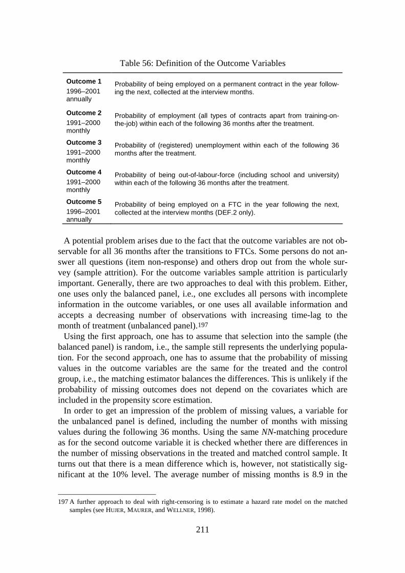
211

Table 56: Definition of the Outcome Variables

Outcome 1 1996–2001 annually

Probability of being employed on a permanent contract in the year follow-ing the next, collected at the interview months.

Outcome 2 1991–2000 monthly

Probability of employment (all types of contracts apart from training-on-the-job) within each of the following 36 months after the treatment.


Probability of (registered) unemployment within each of the following 36 months after the treatment.


Probability of being out-of-labour-force (including school and university) within each of the following 36 months after the treatment.

Outcome 5 1996–2001 annually

Probability of being employed on a FTC in the year following the next, collected at the interview months (DEF.2 only).

A potential problem arises due to the fact that the outcome variables are not ob-

servable for all 36 months after the transitions to FTCs. Some persons do not an-swer all questions (item non-response) and others drop out from the whole sur-vey (sample attrition). For the outcome variables sample attrition is particularly important. Generally, there are two approaches to deal with this problem. Either, one uses only the balanced panel, i.e., one excludes all persons with incomplete information in the outcome variables, or one uses all available information and accepts a decreasing number of observations with increasing time-lag to the month of treatment (unbalanced panel).197

Using the first approach, one has to assume that selection into the sample (the balanced panel) is random, i.e., the sample still represents the underlying popula-tion. For the second approach, one has to assume that the probability of missing values in the outcome variables are the same for the treated and the control group, i.e., the matching estimator balances the differences. This is unlikely if the probability of missing outcomes does not depend on the covariates which are included in the propensity score estimation.

In order to get an impression of the problem of missing values, a variable for the unbalanced panel is defined, including the number of months with missing values during the following 36 months. Using the same NN-matching procedure as for the second outcome variable it is checked whether there are differences in the number of missing observations in the treated and matched control sample. It turns out that there is a mean difference which is, however, not statistically sig-nificant at the 10% level. The average number of missing months is 8.9 in the

197 A further approach to deal with right-censoring is to estimate a hazard rate model on the matched

samples (see HUJER, MAURER, and WELLNER, 1998).

212

treated sample and 8.3 in the control sample. The corresponding t-statistic of 0.59 indicates that the difference is not statistically significantly different from zero. One can conclude that there is sample attrition, but no strong evidence in favour of induced sample selection bias. Thus the unbalanced panel approach is pursued since the bias generated by simply dropping incomplete data may be worse than the bias due to a declining number of observations with an increasing time-lag to the treatment. Furthermore, using the unbalanced panel ensures a sufficient sam-ple size.

6.4.5 Estimation Results of the Propensity Score Equation (Discrete Haz-ard Rate Model)

Is it plausible to assume the CIA to be fulfilled? Of course, it seems unrealistic to assume that all variables simultaneously affecting the FTC hazard and out-come variables are included in the propensity score. Nevertheless, one may argue again that the variables relating to the individuals’ previous labour market ex-periences may capture unobserved characteristics of the unemployed. Hence, again it is assumed that by balancing differences in X variables which are likely to be correlated with unobservables, also differences in unobservables are bal-anced.

The criterion finally used to find a specification of the propensity score is the pre-program test, i.e., the ability of the approach to balance out pre-treatment differences in the outcome variables (see Subchapter 3.5). The results of the pro-pensity score estimation are depicted in Table 57. Since the results are basically the same as the results in Section 6.3.5, they are not discussed any further.

213

Table 57: Logistic Hazard Rate Model (Propensity Score Estimation)

Transition to FTC

Coeff. t-stat.

Baseline hazard

Month 2–3 0.475 2.82

Month 4–6 0.429 2.46

Month 7–9 0.231 1.08

Month 10–12 0.710 3.20

Month 13–18 0.420 1.74

Month ≥ 19 0.691 3.00

Age -0.188 -0.92

Age2 / 1.000 0.730 1.29

Age3 / 100.000 -0.090 -1.80

No occupational qualification -0.329 -2.51

Master craftsman -0.165 -0.58

University graduate 0.460 2.59

Female 0.294 1.61

Married 0.327 2.01

Married x female -0.698 -3.06

Prev job: end of FTC or Apprenticeship 0.554 2.97

Prev job: end of FTC or Apprenticeship x female -0.457 -1.69

Out-of-labour-force before 0.612 2.28

Out-of-labour-force before x female -0.725 -2.16

Training or school before 0.445 2.38

Duration of prev. unemployment spell -0.016 -1.54

Prev. employment spell 3–5 months 0.763 3.31




Prev. employment spell ≥ 21 months 0.247 1.41

Already a FTC before 0.495 3.38

Public sector before 0.393 2.48

Number of prev. unemployment spells -0.048 -0.59

Number of prev. unemployment spells2 0.015 1.48

Log net household income -0.058 -2.71

No unemployment benefit 0.281 2.31

No unemployment assistance 0.935 4.93

214

Table 57 continued... Coeff. t-stat.

Log regional unemployment rate 0.117 0.57

Spell started in first quarter -0.684 -4.48

Spell started in second quarter -0.645 -4.01

Spell started in third quarter -0.402 -2.58

Constant -3.523 -1.46

Numb. of Spells 349

Numb. of Persons 321

Numb. of Observations (person months) 23,151

Log-likelihood -1645.004

χ2 (37) 330.62

Notes: See Table 53. Sources: Own estimations based on the GSOEP.

6.4.6 Estimation Results of the Matching Estimator

For both definitions of untreated individuals (DEF.1 and DEF.2), simple NN-matching (with caliper) is performed (see Box 4).198 The command ‘psmatch’ implemented by SIANESI (2001) in STATA 7.0 is used in a modified form, which imposes the common support condition for every calendar month and which al-lows the propensity score to be estimated by a hazard rate model. Following LECHNER (1998), not the estimated probability but the linear index is predicted. The caliper is chosen by considering the trade-off between reducing the bias, on the one hand, and minimising the loss of (treated) observations, on the other. The caliper is set in most cases to 0.03Ψ = , which turned out to be a reasonable com-promise.

In Subsection 6.4.6.2 the mean effects are reported, while Subsection 6.4.6.3 presents the effects for subgroups of individuals. The next subsection presents some evidence on the matching quality.

198 Furthermore, several kernel-based matching estimators have been checked (see Section 3.3.1 and

Subchapter 5.5). It turns out, that NN-matching seems to be more suitable than different types of ker-nel-based matching procedures for generating appropriate control groups in the sense of a pre-program test (see Subchapter 3.5). Therefore, the results of the kernel-based estimators are not pre-sented and discussed as they do not lead to any additional insights.

215

Box 4: Implementation of the Propensity Score Matching Estimation

Step 1 Estimate a discrete (logistic) hazard rate model for the transition from unem-

ployment to FTCs (independent competing risks) by maximum likelihood. In-

clude all covariates X and a non-parametric (piece-wise constant) specification

for the baseline hazard.

Step 2 Predict the propensity score

( )( )Pr , 1 ,k ke T t C X t T t≡ = = ≥ for every individual,

with T denoting the duration of the unemployment spell and k the number of

the unemployment spell of the individual.

Step 3 For non-treatment DEF.1: Exclude individuals from the pool of untreated per-

sons who are treated at any time during the period under observation.

Step 4 Impose common support for every month: Drop observations outside the sup-

port and the caliper.

Step 5 NN-Matching: For every calendar month τ, match the untreated person j with

the closest propensity score i je e− to each treated person i, 2 months be-

fore the actual transition to FTC occurs. Untreated person j can be used as a control more than once (with replacement).

Step 6 The ATT is the difference in the (weighted) mean outcomes of both groups.

6.4.6.1 Matching Quality

As mentioned above, the common support condition requires that for every un-employed individual entering into a FTC a sufficiently similar untreated person in terms of the predicted propensity score should be available for each single month. The latter is necessary since matching is conditioned on the same calen-dar month, i.e., treated and control persons are matched only within the same cal-endar month. If there is no sufficiently similar untreated person available for a treated person, she or he cannot be used in the analysis and is excluded. Unfortu-nately, this procedure leads to a significant loss of observations (see Table 58). A further substantial reduction of observations is a result of imposing the untreated to be within the caliper. As expected, less observations are lost in case of DEF.2. The difference of the samples of DEF.1 and DEF.2 implies that a comparison of the effects with regard to the untreated definition is possibly not meaningful (see Section 3.3.1 for a discussion).

216

Table 58: Loss of Treated Observations due to Common Support Requirement and Lack of Similar Untreated Within the Caliper (NN-Matching, Outcome 2)

Number of treatments (transitions to FTCs) DEF.1 DEF.2

Before matching 349 349

Within common support 304 339

Within the caliper (after NN- matching) 239 282

Table 59: Means of Important Pre-Treatment Variables (X) Before and After NN-Matching (DEF.1)

Before matching After matching

1x 0x p-vala std.

diff. %b

1x 0x p-vala std. diff. %b

Propensity score -3.695 -5.055 0.000 132.47 -3.998 -3.998 0.994 0.04

Dur. of unemployment (baseline) 8.799 12.392 0.000 32.02 9.703 10.226 0.598 4.66

Female 0.453 0.512 0.028 11.92 0.477 0.498 0.648 4.19

Married 0.507 0.668 0.000 33.08 0.519 0.523 0.927 0.86

Married × female 0.206 0.335 0.000 29.36 0.222 0.238 0.665 3.80

Age 32.673 41.650 0.000 76.53 32.979 32.971 0.993 0.07

Prev. job: end of FTC or appren-ticeship

0.244 0.055 0.000 54.67 0.172 0.134 0.253 10.94

Prev. job: end of FTC or appren-ticeship × female

0.097 0.033 0.000 26.35 0.092 0.075 0.510 6.83

Dur. of previous unempl. spell 2.739 3.207 0.310 6.30 3.285 2.707 0.367 7.78

Dur. of previous empl. spell 13.146 16.579 0.091 10.43 13.431 15.489 0.473 6.25

Out-of-labour-force before 0.129 0.225 0.000 25.42 0.146 0.197 0.146 13.25

Training or school before 0.192 0.115 0.000 21.49 0.176 0.205 0.416 8.17

Public service before 0.206 0.073 0.000 38.89 0.172 0.106 0.018 19.42

University degree 0.163 0.042 0.000 40.83 0.084 0.059 0.287 8.44

No occupational qualification 0.301 0.439 0.000 28.84 0.360 0.377 0.705 3.50

Log household net income 6.793 7.302 0.000 20.48 7.008 6.939 0.765 2.77

No unemployment benefit 0.476 0.439 0.175 7.30 0.444 0.531 0.055 17.64

No unemployment assistance 0.883 0.815 0.001 18.87 0.849 0.870 0.511 5.86

Log unemployment rate 2.256 2.205 0.006 18.82 2.257 2.236 0.318 7.99

Number of observations 349 16,120 239 239

Note: The 16,120 observations in the untreated group before matching correspond to 1,271 spells and 1,041 individuals. aTwo-sample t-test with unequal variance: H0: 1 0x x− =0. bStan-

dardised difference defined as ( ) ( )( )( )1 0 1 1 0 02x Var x Var xx − + with x denoting the re-

spective conditioning variable.

217

Table 60: Means of Important Pre-Treatment Variables (X) Before and After NN-Matching (DEF.2)

Before matching After matching

1x 0x p-vala std.

diff. %b

1x 0x p-vala std. diff. %b

Propensity score -3.695 -4.759 0.000 103.08 -3.871 -3.871 0.990 0.07

Dur. of unemployment (baseline) 8.799 11.301 0.001 23.40 9.521 9.007 0.547 4.81

Female 0.453 0.493 0.139 8.00 0.475 0.464 0.801 2.13

Married 0.507 0.636 0.000 26.20 0.521 0.535 0.736 2.89

Married × female 0.206 0.313 0.000 24.48 0.223 0.238 0.690 3.26

Age 32.673 39.33 0.000 57.93 32.69 32.31 0.636 3.33

Prev. job: end of FTC or appren-ticeship

0.244 0.101 0.000 38.25 0.199 0.213 0.678 3.82

Prev. job: end of FTC or appren-ticeship × female

0.097 0.052 0.002 17.24 0.089 0.106 0.489 6.75

Dur. of previous unempl. spell 2.739 3.313 0.188 8.01 3.089 3.145 0.923 0.79

Dur. of previous empl. spell 13.146 15.77 0.168 8.32 12.73 15.53 0.259 8.89

Out-of-labour-force before 0.129 0.198 0.001 18.80 0.142 0.138 0.904 0.96


Public service before 0.206 0.100 0.000 29.71 0.159 0.198 0.228 10.94

University degree 0.163 0.062 0.000 32.45 0.110 0.092 0.486 5.66

No occupational qualification 0.301 0.423 0.000 25.56 0.344 0.351 0.860 1.49

Log household net income 6.793 7.264 0.001 18.98 7.033 6.919 0.590 4.60



Log unemployment rate 2.256 2.222 0.020 12.76 2.273 2.275 0.907 0.97

Number of observations 349 22,743 282 282

Note: The 22,743 observations in the untreated group before matching correspond to 1,826 unemployment spells and 1,447 individuals. aTwo-sample t-test as defined in the note of Table 59. bStandardised differences as defined in the note of Table 59.

Does the NN-matching estimator balance pre-treatment differences in observ-

able variables X between the group of treated and the control group of untreated? To what extent is the balancing property of the propensity score matching esti-mator fulfilled?199 In order to answer this question some statistics are presented in detail. Means of pre-treatment variables of treated 1x and untreated workers

0x , as well as the matched FTCs and controls are depicted in Table 59 (for DEF.1) and Table 60 (for DEF.2). t-tests indicate that the differences in the means of nearly all conditioning variables X are not significantly different from zero in the matched sample, while there are important differences before match-ing. This is also confirmed by the observation that the standardised differences of nearly all variables decline.

199 See Subchapter 5.6 for a discussion of the balancing property of the propensity score.

218

Differences between Table 59 (for DEF.1) and Table 60 (for DEF.2) are also of interest: It turns out that pre-treatment differences are balanced better in case of DEF.2. The obvious reason is that there are more potential control individuals available in case of DEF.2. Another reason may be that untreated persons accord-ing to DEF.1 differ more from the treated since they do never participate. This hypothesis is in line with the finding that standardised differences before match-ing are larger in Table 59 (for DEF.1) than in Table 60 (for DEF.2).

Another important finding from Table 59 (for DEF.1) which is worthwhile to be mentioned is the fact that the sample of treated individuals after matching seems to be different from treated before matching with respect to the mean of its X variables. This is an unattractive implication of the common support condition (see Section 3.3.1).

As discussed in Subchapter 3.5, the pre-program test consists of t-tests on the differences in the outcome variables between the group of treated and the group of control persons before the treatment (the transition to the FTC). This is tested up to 24 months before the treatment for the monthly measured outcome vari-ables, and up to 3 years for the annually measured outcome variables. The results are depicted in the following subsection.

6.4.6.2 Mean Effects of Fixed-Term Contracts

In this subsection, the estimated ATTs for all outcome variables and for both definitions of non-treatment are reported. First of all, effects on the monthly measured outcome variables (2, 3, and 4) are discussed. Since it turns out that the estimated ATTs under DEF.1 and DEF.2 differ less than expected, it does not seem to be necessary to consider the fact that DEF.2 renders the definition of the ATT when interpreting the results (see Subsection 6.4.3.1).

Outcome 2 – Employment Probability (1991–2000)

Figure 7 (DEF.1) and Figure 8 (DEF.2) present the differences in employment probabilities between treated and control persons including a 95% confidence interval. Note that employment includes permanent contract jobs and FTC jobs, but excludes training. Zero on the time axis represents the month in which the treatment occurs, i.e., the transition from unemployment to a FTC job.

The fact that the confidence intervals overlap the abscissas before the treatment (-24 up to -3 months) indicates that the pre-treatment differences in the employ-ment probabilities are not statistically significant. Hence, the matching approach balances pre-treatment differences in the employment status to a large extent (pre-program test). Similar to the result found in the previous subsection, the per-formance of the matching estimator seems to be slightly better in case of DEF.2.

The figures for both definitions suggest that entering into FTC jobs increases the employment probability for up to 36 months after the transition. Of course, it is not surprising that there is a positive ATT in the first months after the treat-ment. The result that there is still a significantly positive effect between 24 up 36

219

months seems to be more relevant, given that most FTCs are not longer than 24 months (see Subchapters 2.3 and 5.4). The similarities of the results in Figure 7 (DEF.1) and Figure 8 (DEF.2) are surprising, given the dissimilarity of the con-cepts. The effects in case of DEF.2 seem to be slightly more positive. To which extent the estimated positive employment effect is based on FTC or permanent contract jobs is assessed in a subsequent paragraph.

Figure 7: Employment Effects – DEF.1

Figure 8: Employment Effects – DEF.2

-0.4

-0.2

0

0.2

0.4

0.6

0.8

1

-24

-21

-18

-15

-12 -9 -6 -3 0 3 6 9 12 15 18 21 24 27 30 33 36

Months before and after treatment

Em

ploy

men

t pro

babi

lity

Effect

95 % Significance

-0.4

-0.2

0

0.2

0.4

0.6

0.8

1

-24

-21

-18

-15

-12 -9 -6 -3 0 3 6 9 12 15 18 21 24 27 30 33 36


Em

ploy

men

t pro

babi

lity

Effect95 % Significance

220

Outcome 3 – Unemployment Probability (1991–2000)

Again, it can be seen in Figure 9 and Figure 10 that there are almost no signifi-cant differences in the pre-treatment probabilities of being registered unemployed in the matched samples for both non-treatment definitions. It seems to be puzz-ling that approximately 17 months after the transition there are no significantly negative effects on the unemployment probability anymore, while Figure 7 and Figure 8 indicate that there are positive employment effects. The explanation ob-viously has to be found in the effects on the probability of being out-of-labour-force (see next paragraph).

Figure 9: Unemployment Effects – DEF.1

Figure 10: Unemployment Effects – DEF.2

-1

-0.8

-0.6

-0.4

-0.2

0

0.2

-24

-21

-18

-15

-12 -9 -6 -3 0 3 6 9 12 15 18 21 24 27 30 33 36


Une

mpl

oym

ent p

roba

bilit

y


-1

-0.8

-0.6

-0.4

-0.2

0

0.2

-24

-21

-18

-15

-12 -9 -6 -3 0 3 6 9 12 15 18 21 24 27 30 33 36


Une

mpl

oym

ent p

roba

bilit

y


221

Outcome 4 – Probability of Being Out-of-Labour-Force (1991–2000)

As Figure 11 and Figure 12 indicate, entering into a FTC reduces the probabil-ity of being out-of-labour-force within the ensuing 36 months. Therefore, one can conclude that the positive employment effect (Outcome 2) is not accompanied by a lower probability of registered unemployment in the long-run, but by a reduced probability of being-out-of labour-force. This effect is likely to be driven by women, younger or elderly workers. FTCs may successfully be used by people (re-)entering the labour market.200 If they become unemployed after the expira-tion of the contract, they are more strongly attached to the labour market since they have qualified for unemployment compensation and have possibly enhanced their employment prospects (through human capital investments), which reduces the probability of leaving the labour force. The effect seems to be larger in case of DEF.1. However, the differences between DEF.1 and DEF.2 are not statisti-cally significant.

Figure 11: Out-of-labour-force Effect – DEF.1

200 A result in Subchapter 6.3 is that unemployed job searchers who were previously out of labour force

have a higher relative probability of entering into FTCs instead of entering into permanent contracts.

-0.3

-0.2

-0.1

0

0.1

-24

-21

-18

-15

-12 -9 -6 -3 0 3 6 9 12 15 18 21 24 27 30 33 36


Out

-of-

labo

ur fo

rce

prob

abili

ty


222

Figure 12: Out-of-Labour-Force Effect – DEF.2

Outcome 1 – Probability of Holding a Permanent Contract (1996–2001)

So far, it has only been revealed that entering from unemployment into a FTC increases the overall employment probability in the future without taking the type of employment contract into account. Now the question must be answered to what extent this higher future employment probability consists of permanent con-tract jobs. The estimated ATT on the probability of holding a permanent contract for non-treatment DEF.1 is depicted in Table 61. The first column of Table 61 depicts the development of the probability of holding a permanent contract of treated individuals before and after entering into a FTC. It indicates that almost 45% of all employed individuals entering into a FTC hold a permanent contract 2 years later.

The estimated ATTs before the treatment (year -3 until year -1) indicate that even after matching there are some pre-treatment differences in the probability of holding a permanent contract between the treated and the control group, which are, however, not statistically significant.

Up to 3 years after the transition to a FTC, the formerly unemployed raise their chances of holding a permanent contract. But only the positive effect of 11 per-centage points 3 years after entering into the FTC is statistically significant. The effect 4 years after the transition is reported but should be interpreted with high-est caution due to the substantial loss of observations.

-0.3

-0.2

-0.1

0

0.1

-24

-21

-18

-15

-12 -9 -6 -3 0 3 6 9 12 15 18 21 24 27 30 33 36


Out

-of-

labo

ur-f

orce

pro

babi

lity


223

Table 61: Probability of Being Employed on a Permanent Contract – DEF.1

All persons

Year Mean treated Mean control ATT t-stat Pairs

- 3 0.439 0.426 0.012 0.156 82

- 2 0.333 0.433 -0.100 -1.574 120

- 1 0.194 0.250 -0.056 -1.199 160

+ 2 0.448 0.437 0.011 0.214 174

+ 3 0.578 0.468 0.110 1.926 154

+ 4 0.575 0.500 0.075 1.090 106

Note: Ψ = 0.03.

In Table 62 the estimated effects based on DEF.2 are reported. Again, there are

some minor pre-treatment differences in the probability of holding a permanent contract, which are, however, smaller than in case of DEF.1. The effect is now more clear-cut: After 3 years 59.7% of all unemployed who had entered into FTCs hold permanent contracts. Only 43.5% of unemployed who had not entered into FTCs in a certain month (but possibly later) hold permanent contracts. The difference (ATT) of 16.1 percentage points is highly significant. 4 years after tak-ing up a FTC job, the effect is still significantly positive at the 5% level.

Table 62: Probability of Being Employed on a Permanent Contract – DEF.2

All persons


- 3 0.377 0.349 0.028 0.424 106

- 2 0.312 0.347 -0.035 -0.619 144

- 1 0.194 0.246 -0.052 -1.230 191

+ 2 0.441 0.412 0.028 0.587 211

+ 3 0.597 0.435 0.161 3.119 186

+ 4 0.603 0.481 0.122 1.976 131

Note: Ψ = 0.03.

Outcome 5 – Probability of Being Employed on a FTC (1996–2001)

Outcome 5 (the probability of holding a FTC) is the counterpart to Out-come 1.201 The matching procedure is able to balance out pre-treatment differ-ences in the outcome variable to a large extent (see Table 63). It can be seen that entering into a FTC not only increases the probability of holding a permanent contract in the future, but also to hold a FTC again.

Note that in the third and fourth year after the treatment the effect on the prob-ability of holding a permanent contract (Table 62) is higher than the probability

201 Remember that Outcome 5 is only defined for untreated DEF.2 (see Section 6.4.4).

224

of holding a FTC (Table 63). The sum of the two effects (probability of holding a FTC and probability of holding a permanent contract) corresponds approximately to the overall employment effect depicted in Figure 8.

This explains why there is no positive ATT with respect to the probability of holding a permanent contract 2 years after entering into a FTC in Table 62: While control persons may enter into a permanent job directly from unemploy-ment, many treated individuals are still in their FTC jobs, for example, waiting to get their FTC transformed into a permanent one at the present employer. A very familiar mechanism is termed ‘lock-in effect’ in the literature on the evaluation of active labour market policy (see, e.g., VAN OURS, 2004).

Table 63: Probability of Being Employed on a FTC – DEF.2

All Persons


- 3 0.104 0.075 0.028 0.715 106

- 2 0.118 0.083 0.035 0.969 144

- 1 0.136 0.115 0.021 0.614 191

+ 2 0.313 0.142 0.171 4.239 211

+ 3 0.134 0.097 0.037 1.123 186

+ 4 0.137 0.061 0.076 2.060 131

Note: Ψ = 0.03.

6.4.6.3 Heterogeneous Effects of Fixed-Term Contracts

Although it is not necessary for the application of matching estimators to as-sume the ATT to be homogeneous across all individuals (see Subchapter 3.3), so far only mean effects have been presented. Therefore, sub-samples are imposed by including a dummy variable for the corresponding subgroups into the Maha-lanobis distance, and the matching estimator described above are performed on these samples (see Section 3.3.1 for the methodological background). For many sub-samples, this approach turns out to be not suitable as the number of untreated individuals per month becomes too small leading to a poor performance in terms of the pre-program test. Thus only a differentiation by one single characteristic is possible. The effects for women, individuals with formal qualification, and indi-viduals who are at least 32 years old are presented.

Only non-treatment DEF.2 is used in order to ensure a sufficient number of un-treated individuals, which may be justified by the fact that there have not been great differences in the mean effects between the two definitions of non-treatment. Nevertheless, the number of pairs becomes quite small as many treated persons have to be dropped since no suitable untreated individuals could be found within the common support and the caliper. For this reason, the results should be interpreted with greatest caution and only as a “tendency”.

225

Women

It can be seen in Figure 13 that the observed pre-treatment employment prob-ability of women entering into FTCs is always between 2 and 10 percentage points higher than the control group, but not statistically significant. Neverthe-less, one can conclude that women entering into FTCs have unobservable charac-teristics which lead to slightly higher employment probabilities on average, and hence the CIA may be violated. Keeping this caveat in mind and comparing Figure 13 with Figure 8, it may be concluded that the employment effects are slightly higher for women than for the whole sample. Whether the same can be stated for the unemployment effects (Figure 14) remains unclear.

A matter of particular interest are the effects on the probability of being out-of-labour force. Comparing Figure 15 with Figure 12 and taking only the point es-timates into account, one may conclude that the reduction of the probability of being out-of-labour force is at least temporarily stronger for women. The same seems to be true for the probability of holding a permanent contract: While for the whole sample the effect is 16 percentage points after 3 years (Table 62), the corresponding effect for women is approximately 22 percentage points (Table 64).

Figure 13: Employment Effects – Women (DEF.2)

-0.2

0

0.2

0.4

0.6

0.8

1

-24

-21

-18

-15

-12 -9 -6 -3 0 3 6 9 12 15 18 21 24 27 30 33 36


Em

ploy

men

t pro

babi

lity Effect

95 % Significance

226

Figure 14: Unemployment Effects – Women (DEF.2)

Figure 15: Out-of-Labour Force Effect – Women (DEF.2)

-1

-0.8

-0.6

-0.4

-0.2

0

0.2

-24

-21

-18

-15

-12 -9 -6 -3 0 3 6 9 12 15 18 21 24 27 30 33 36


Une

mpl

oym

ent p

roba

bilit

y


-0.4

-0.3

-0.2

-0.1

0

0.1

0.2

-24

-21

-18

-15

-12 -9 -6 -3 0 3 6 9 12 15 18 21 24 27 30 33 36


Out

-of-

labo

ur fo

rce

prob

abili

ty


227

Table 64: Probabilities of Being Employed on a Permanent Contract versus FTC – Women (DEF.2)

Women

Outcome 1: Permanent contract Outcome 5: FTC

Year Mean treated

Mean control

ATT t-stat Mean treated

Mean control

ATT t-stat Pairs

- 3 0.290 0.258 0.032 0.274 0.097 0.065 0.032 0.451 31

- 2 0.266 0.267 0.000 0.000 0.200 0.067 0.133 1.859 45

- 1 0.161 0.194 -0.032 -0.467 0.210 0.048 0.161 0.058 62

+ 2 0.537 0.373 0.164 1.903 0.194 0.030 0.164 3.087 67

+ 3 0.563 0.333 0.229 2.295 0.125 0.042 0.083 1.479 48

+ 4 0.600 0.429 0.171 1.435 0.114 0.029 0.086 1.392 35

Note: Ψ = 0.03.

Age ≥≥≥≥ 32

It would be of particular interest to evaluate the effects of entering into a FTC on the employment opportunities of workers older than 58 years since they can be hired on FTCs without legal limitations (see Subchapter 2.2). Unfortunately, there are not enough observations available since the mean age of unemployed entering into FTCs is about 32 years. Therefore, only workers who are at least 32 years old are used in the analysis. The results in comparison to the whole sample can be summarised as follows.

The point estimates of the employment effects seem to be similar to the point estimates of effects for the whole sample (Figure 16 and Figure 8), even though the estimated effects are often not significant, which may result from the small sample size. The effects on the probability of being unemployed (Figure 17 and Figure 10) and the probability of being out-of-labour force look very similar (Figure 18 and Figure 12), but again are not statistically significant. There are some differences with respect to the effects on the probability of holding perma-nent contracts (Table 65 and Table 62) as well as the probability of holding FTCs (Table 65 and Table 63). It seems, however, not possible to derive any reliable and clear-cut conclusion from this comparison.

228

Figure 16: Employment Effects – Age ≥32 (DEF.2)

Figure 17: Unemployment Effects – Age ≥ 32 (DEF.2)

-0.4

-0.2

0

0.2

0.4

0.6

0.8

1

-24

-21

-18

-15

-12 -9 -6 -3 0 3 6 9 12 15 18 21 24 27 30 33 36


Em

ploy

men

t pro

babi

lity


-1

-0.8

-0.6

-0.4

-0.2

0

0.2

-24

-21

-18

-15

-12 -9 -6 -3 0 3 6 9 12 15 18 21 24 27 30 33 36


Une

mpl

oym

ent p

roba

bilit

y


229

Figure 18: Out-of-Labour-Force Effects – Age ≥32 (DEF.2)

Table 65: Probabilities of Being Employed on a Permanent Contract versus FTC – Age ≥ 32 (DEF.2)

Age ≥ 32


Year Mean treated

Mean control


Mean control

ATT t-stat Pairs

- 3 0.551 0.367 0.184 1.837 0.082 0.082 0.000 0.000 49

- 2 0.452 0.339 0.113 1.284 0.081 0.065 0.016 0.343 62

- 1 0.238 0.250 -0.013 -0.183 0.075 0.05 0.025 0.650 80

+ 2 0.533 0.373 0.160 1.981 0.147 0.067 0.080 1.589 75

+ 3 0.517 0.466 0.052 0.553 0.138 0.052 0.086 1.588 58

+ 4 0.541 0.405 0.135 1.159 0.108 0.054 0.054 0.844 37

Note: Ψ = 0.03.

With Formal Qualification

In this paragraph, only individuals are analysed which have completed at least a vocational training. This amounts to approximately 70% of all individuals enter-ing into FTCs. Due to the number of observations, it is unfortunately not possible to focus on workers without formal qualification, which would be more interest-ing from a policy-orientated point of view.

-0.3

-0.2

-0.1

0

0.1

-24

-21

-18

-15

-12 -9 -6 -3 0 3 6 9 12 15 18 21 24 27 30 33 36


Out

-of-

labo

ur-f

orce

pro

babi

lity


230

Comparing again the point estimates of the monthly measured outcome vari-ables (Figure 19 with Figure 8, Figure 20 with Figure 10, and Figure 21 with Figure 12), one may conclude that the effect for the sub-sample is slightly better in terms of enhancing employment prospects. Again, it is unclear which conclu-sions can be drawn from a comparison of the ATTs with respect to Outcome 1 and 5 (see Table 66): One insight may be that the stepping stone effect occurs earlier but is less lasting for workers with formal qualification.

Figure 19: Employment Effects – Workers With Formal Qualification (DEF.2)

Figure 20: Unemployment Effects – Workers With Formal Qualification (DEF.2)

-0.4

-0.2

0

0.2

0.4

0.6

0.8

1

-24

-21

-18

-15

-12 -9 -6 -3 0 3 6 9 12 15 18 21 24 27 30 33 36


Em

ploy

men

t pro

babi

lity

Effect

95 % Significance

-1

-0.8

-0.6

-0.4

-0.2

0

0.2

-24

-21

-18

-15

-12 -9 -6 -3 0 3 6 9 12 15 18 21 24 27 30 33 36


Une

mpl

oym

ent p

roba

bilit

y


231

Figure 21: Out-of-Labour-Force Effects – Workers With Formal Qualification (DEF.2)

Table 66: Probabilities of Being Employed on a Permanent Contract versus FTC – Workers With Formal Qualification (DEF.2)

Workers With Formal Qualification


Year Mean treated

Mean control


Mean control

ATT t-stat Pairs

- 3 0.400 0.400 0.000 0.000 0.100 0.100 0.000 0.000 40

- 2 0.328 0.466 -0.138 -1.520 0.086 0.052 0.034 0.728 58

- 1 0.203 0.278 -0.076 -1.098 0.114 0.114 0.000 0.000 79

+ 2 0.599 0.401 0.198 3.624 0.138 0.060 0.078 2.363 167

+ 3 0.585 0.492 0.093 1.424 0.136 0.059 0.076 1.967 118

+ 4 0.533 0.453 0.080 0.976 0.147 0.004 0.106 2.268 75

Note: Ψ = 0.016.

6.4.7 Summary: Effects of Entering into Fixed-Term Contracts on the Long-Term Employment Opportunities of the Unemployed

Subchapter 6.4 has investigated the effects of the transition from unemploy-ment to FTC jobs on the individuals’ future employment opportunities in the West German labour market.

First, it has been discussed in Subsection 6.4.3.1 that there are at least two rea-sonable counterfactuals for individuals entering into FTC jobs after a certain un-

-0.3

-0.2

-0.1

0

0.1

-24

-21

-18

-15

-12 -9 -6 -3 0 3 6 9 12 15 18 21 24 27 30 33 36


Out

-of-

labo

ur fo

rce

prob

abili

ty


232

employment duration. One counterfactual, most commonly applied in evaluation studies, is to compare a ‘world with FTCs’ with a ‘world without FTCs’ and de-fine untreated persons as unemployed who never enter into FTCs during the pe-riod under observation (termed DEF.1). A second counterfactual, which may be more in line with the idea of sequential job search (unemployed enter into FTCs after having failed to find a permanent job), is not to enter into a FTC up to a cer-tain duration of unemployment, but possibly in a later month. This implies a comparison of unemployed entering into FTCs in a particular month of unem-ployment duration with those unemployed who do not enter into FTCs up to the end of this month (termed DEF.2). Both definitions have been analysed in this Subchapter. Contrary to expectation, the estimation results differ only slightly between DEF.1 and DEF.2, which may, however, be driven by the small sample size. Therefore, the differences in the definitions are not emphasised when inter-preting the results.

Second, it has been discussed in Section 6.4.3 and shown in Section 6.4.6.1 that the estimation of the propensity score by a hazard rate model is a suitable ap-proach since it seems to be more in the spirit of the sequential job search theory than the commonly used ‘static’ propensity score, and it is able to balance pre-treatment differences between treated and untreated individuals in most cases.

Third, it has been argued in Section 6.4.3, that the SUTVA is likely to be vio-lated, since general equilibrium and indirect effects of unknown sign and magni-tude are probable. One empirical study for Spain is in line with the hypothesis that FTC workers reduce re-employment chances of long-term unemployed through on-the-job search (see Section 6.4.2). These indirect and general equilib-rium effects may imply that the estimated effects are not informative with regard to the economy as a whole.

Fourth, it has been discussed in Section 6.3.4 that the sample used may lead to biased estimates caused by the way the information on the type of contract is col-lected in the GSOEP. Short FTC employment spells are likely to be underrepre-sented. While NN-matching is robust against the general case that treated indi-viduals are over- or underrepresented in comparison to untreated individuals with regard to the underlying population (choice-based sampling), the results may still be biased by the selectivity with regard to the fact that shorter FTC spells are more likely to be excluded.

Fifth, it has been shown in Subsection 6.4.6.1 that imposing the common sup-port condition leads to a substantial loss of observations. This may imply that the estimated results are not informative with regard to the underlying population under certain conditions.

Keeping these caveats in mind the results can be summarised as follows: Enter-ing from unemployment into FTC jobs – increases the future overall employment probability by 15–20 percentage

points at least within the ensuing 36 months,

233

– increases the probability of holding a permanent contract 3 years later by 16 percentage points,

– has only a negative effect on the risk of unemployment in the short-run (up to 18 months),

– reduces the probability of leaving the labour force by 10 percentage points at least within the ensuing 36 months.

Analyses for sub-groups (women, workers older than 32 years, workers with formal qualification) have revealed that unemployed women may benefit more from entering into FTCs than unemployed men. Slightly more positive effects have also been found for unemployed with formal qualification. These results should, however, be interpreted with caution since the samples for the analyses have been quite small. Probably, the most important finding of these analyses for sub-groups is that no result is contradictory to the estimated mean effects sum-marised above. More detailed analyses would obviously be useful. To the best of my knowledge, there is, however, no larger panel dataset for Germany available including information on the type of contract.

6.5 Conclusions

The competing risks hazard rate model shows that typical characteristics which have been found to prolong unemployment duration in other studies, such as dis-abilities, being a foreigner, being mother with young children, do not affect the FTC hazard rate, but have a negative effect on the permanent contract hazard. Moreover, while the probability to enter into permanent contract jobs decreases for long-term unemployed, long-term unemployment has no negative effect on the probability to take up a FTC. Thus FTCs may serve as entry jobs for job searchers with low employment chances, which would exactly correspond to one of the political goals of the liberalisation of FTCs. However, as previously men-tioned, this statement should not be interpreted in the sense that FTCs reduce overall unemployment duration.

Using a propensity score matching estimator it has been revealed that entering into a FTC increases the individual future employment probability (including FTC and permanent contract jobs) and the probability of holding a permanent contract job, and decreases the probability of leaving the labour force. These findings are compatible with the hypothesis that FTCs are stepping stones to-wards permanent contract jobs.

Some results of the hazard rate model and the matching approach are, however, also in line with dual labour market theories: Having held a FTC increases the probability of entering into a FTC and holding a FTC in the future. Entering into a FTC has no long-term negative effect on the unemployment probability, i.e., the effect vanishes after 18 months.

234

Nevertheless, taking all the results together and considering that for no sub-group a negative effect on labour market prospects could be detected, my conclu-sion is that the stepping stone hypothesis cannot be rejected, at least at the micro-economic level. This is also in line with the results found in other empirical stud-ies discussed in Section 6.4.2. As mentioned there, all available empirical studies using a causal approach (that is, a control group of nonparticipants) find a step-ping stone effect. The conclusion that FTCs lead to a segmented labour market is only found in empirical studies which do not ask counterfactual questions.

235

7 Summary and Conclusions

In this study I have analysed the labour market effects of fixed-term contracts (FTCs) in West Germany. The study consists of empirical analyses using indi-vidual level as well as establishment level datasets but also theoretical considera-tions and discussions of previous empirical research. Except for the descriptive analysis in Subchapter 4.5, the empirical parts of the study have attempted to identify causal effects by microeconometric methods described in Chapter 3.

The role of FTCs in labour demand has been analysed in Chapter 4. Economic theory suggests three categories of reasons why firms use FTCs. FTCs serve as buffer stock, that is, as an adjustment instrument to cope with demand or produc-tivity shocks that may insulate the firms’ permanent workforce. FTCs are used as a screening device (prolonged probationary period) to overcome the problem of asymmetric information when hiring new employees. FTCs are used as a substi-tute for permanent workers, that is, job positions that are inherently permanent are repeatedly filled by FTC workers.

The empirical analysis could not reject any of these hypotheses. First of all, it has been found that FTCs are much more important for the German labour mar-ket as commonly thought when focussing on aggregate employment stocks. Moreover, the descriptive evidence seems to be in favour of the hypothesis that FTCs increase the overall flexibility of the labour market. Almost 43% of all hir-ings are based on FTCs. The turnover of FTC workers accounts for almost 31% of the total worker turnover. FTCs are extensively used as an adjustment instru-ment, which is reflected in the job turnover rate of FTCs being approximately six times larger than the job turnover rate of permanent workers.

Even though the numbers are based on a descriptive analysis, and even though the hypothesis of the liberalisation of FTCs in 1985 having raised overall labour market flexibility (in terms of the adjustment speed of employment stocks) has been rejected by econometric analyses so far, I would deliberately conclude that FTCs are likely to increase labour market flexibility. The reasons for drawing this conclusion are twofold. Firstly, the previous econometric studies for Ger-many discussed in Subchapter 4.3 are based on aggregate employment stock data, which are likely to conceal most of the dynamics at the firm level. Sec-ondly, if FTC work was not increasing overall employment flexibility (e.g., in terms of worker flows or job flows at the firm level), this could only be driven by a decrease of the flexibility (increase in job stability) of permanent contract work which fully outweighs the increase in flexibility caused by FTCs. Although most theoretical models predict a certain increase in the job stability of permanent work due to the use of FTCs (see Subchapter 4.3), to the best of my knowledge, clear-cut empirical evidence in favour of this relationship has not been been found so far.

236

A large proportion (40%) of hirings on FTCs and terminations of FTCs are not associated with net employment changes and, hence, FTCs may be used as sub-stitutes for permanent workers to fill permanent positions. This conclusion is un-derlined by the empirical result of a positive relationship between firing costs for permanent contract workers and the use of FTCs (see Subchapter 4.4). This rela-tionship could not be found for the two other types of temporary work analysed.

As one third of all FTC workers get their contract converted into a permanent one within the same establishment, the hypothesis of FTCs serving as prolonged probationary period cannot be rejected. Hence, the hypothesis of FTCs exclu-sively being dead ends can clearly be rejected already at this stage.

In Chapter 5 I have analysed the short-term effects of FTCs on workers’ sub-jective assessments of career opportunities and of job security as well as wages. The results can be summarised as follows: (1.) FTCs raise the subjective job in-security; (2.) FTCs decrease satisfaction with career opportunities; (3.) FTC workers do not receive a wage differential compensating for these disadvantages, but even a wage penalty. The first conclusion from these results is that FTC workers are indeed worse-off in the short-run compared to the situation they held permanent contracts. However, considering theoretical arguments as well as the heterogeneity of estimated effects with regard to formal qualification this conclu-sion has to be recapitulated. For workers without qualification no significantly negative wage effect of FTCs could be detected, whereas workers with university degree have much lower wages when holding a FTC, but at the same time they do not assess their career opportunities as significantly worse than the control group of similar permanent contract workers. This underlines the idea that enter-ing into a FTC job may be an investment in lifetime earnings or utility for several groups. In contrast, persons without a formal qualification may not be willing to accept FTC jobs with lower wages as they are less likely to serve as stepping stones for them. This conclusion is in line with the tendency found in Subchapter 6.4 that the stepping stone effect for persons with qualification seems to be stronger. To some extent these results contradict the results of older segmented labour market theories predicting low-qualified workers to be more negatively affected in terms of wages by a segmentation by the type of employment con-tract. Further research has to analyse this issue of long-run compensation and maximisation of lifetime earnings by a longitudinal (dynamic) approach using panel data. The main reason for using a cross sectional dataset instead of the German Socio-Economic Panel (which is the only individual level panel dataset available including information on the type of contract) for the analysis in Chap-ter 5 is that it is large enough to allow reliable estimates of effects for subgroups of individuals.

The results of the analyses of Chapter 6 are possibly the most important ones since two central policy goals of FTCs are touched. Typical characteristics which are known to prolong unemployment duration, such as disabilities, being a for-eigner, or being mother with young children, do not affect the FTC hazard rate

237

negatively. In contrast, these characteristics decrease the transition probability to permanent contract jobs. Hence, it is easier to get a FTC job than a permanent contract job for unemployed job searchers. More important: Having entered a FTC increases the probability of being employed in a permanent job later on. Hence, FTCs serve as stepping stones towards permanent jobs. This is in line with empirical studies for other countries using a causal approach. Interestingly, the result of FTCs leading to a segmented labour market, as predicted by many theoretical models, is only found in studies which do not make use of well-defined control groups to estimate the counterfactual outcome.

Of course, these positive conclusions with respect to a stepping-stone effect have to be set off against possible adverse effects of FTCs. In this study only some negative short-run effects of FTCs at the micro level have been empirically revealed, that is, on wages, subjective job security, and subjective career oppor-tunities. However, other microeconometric studies (especially for Spain) have found further adverse effects, such as lower productivity and human capital in-vestments, more work related accidents, and even some evidence in favour of negative effects on fertility (see DOLADO, GARCÍA-SERRANO, and JIMENO, 2002).

Given the results of the theoretical models discussed, in addition to negative ef-fects at the micro level there may be effects at the macro level, which are more likely to be negative than positive. During the course of this study I have high-lighted the caveats of the empirical methods used. It has again to be stressed that the analyses have been of partial-analytical nature. All causal analyses presented are based on the assumption that the control units are not affected by the treat-ments. It is however likely that substantial effects occur at the macroeconomic level. Many of the theoretical papers discussed take general equilibrium effects into account and come to negative results. Most indicate that the introduction of FTCs (a partial deregulation) has a number of adverse labour market effects (see Subchapter 4.2), so that the overall employment effect may even be negative.

This leads to the central question that could not be addressed in this study: Is the liberalisation of types of temporary work (a partial deregulation) an alterna-tive to an extensive reform of protection against dismissal legislation? The prob-lem at the microeconomic level is that there is no counterfactual for the availabil-ity of FTCs observable within countries. Hence, studies based on aggregate data or general equilibrium models would be useful to gain further insight into the labour market effects of FTCs and the question on the effects of the partial de-regulation.

A promising approach at the micro-level, which may lead to additional insights, is a difference-in-differences estimator based on a natural experiment (see Sec-tion 3.2.4). The so-called “Hartz Reform” induced the following variation: The age threshold for hiring a person on a FTC without limitations was lowered from 58 to 52 years in January 2003. This age group may be large enough for estimat-ing the effects of the liberalisation of FTCs for the specific group on their em-

238

ployment chances in comparison to the counterfactual FTCs were not liberalised, which can be estimated by the adjacent age groups not being within the scope of this reform. Analysing the effects of the reform is, however, left for future re-search.

239

8 Appendix

Box 5: Institutional Background on Temporary Work Agency Work (until 1999)

Until 1967, the supply of temporary workers by Temporary Work Agencies (TWAs) was

forbidden, because the German Federal Employment Service had a monopoly on job place-

ment services. In 1967, a judgement of the Federal Constitutional Court repealed this regula-

tion in view of the constitutional right of freedom of occupation. The supply of workers by

private agencies was subsequently regulated by the Act on the Supply of Workers by Tempo-

rary Employment Agencies of 1972. The main principle of the law is still valid today: the

TWA has all the duties of an employer. With this provision, the legislator aimed at bringing

the relation between the TWA and its employees onto the same level as the relation between

a regular employer and its employees. To prevent the TWA from working as a job placement

agency, additional conditions were included in the law. First, the employment contract be-

tween the TWA and the temporary worker has to be of unlimited duration. This stipulation

was later given more concrete meaning by the Federal Employment Service. It required the

contract between the worker and the TWA to be at least 25% or one day longer than the du-

ration of the first commission to a user enterprise. A second legal constraint for TWAs is the

limit to the duration a worker is allowed to be commissioned to a user company. In the origi-

nal law, the maximum duration had been 3 months. With the Improvement of Employment

Opportunities Act of 1985, the maximum duration was extended to 6 months. In 1994, the

new Improvement of Employment Opportunities Act further increased this limitation to 9

months. In addition, the Federal Employment Service’s monopoly of job placement was

repealed in that year. Since then, TWAs have had the possibility both to supply temporary

workers and to provide job placement services. Finally, the maximum cumulated duration

was increased to 12 months by the Act on the Supply of Workers by Temporary Employ-

ment Agencies of 1997. The works council of the user establishment has to agree to the em-

ployment of TWA workers in the same way as in the case of recruitment of permanent work-

ers (§ 99 of the Works Constitution Act).

Source: RUDOLPH and SCHRÖDER (1997) as well as JAHN (2002).

240

Table 67: Descriptive Statistics for the Estimation Sample – Dependent Variables

Variable Data Mean Std. Dev. Observations

TWA Workers overall 0.176 0.381 N 7,207

(Dummy) between 0.342 I 2,843

within 0.193 iT

2.731

FTC Workers overall 0.377 0.485 N 4,873


within 0.232 iT

2.277

FL Workers overall 0.114 0.317 N 6,303


within 0.185 iT

2.728

Notes: N is the overall number of used observations, I is the number of establishments and iT is the average number of times an establishment is observed in the sample. The between data are generated by calculating the means over time by establishment

ix . The within data are de-

fined as it ix x x− + , where the overall mean x is added to equate the mean of all data (overall,

between and within). Source: IAB Establishment Panel for West Germany 1993–1998.

Table 68: Descriptive Statistics for the Estimation Sample – Independent Variables

Variable Mean Std. Dev.

Min. Max.

Expected output change 0.027 0.220 -1.000 5.000 Seasonal fluctuations (dummy) 0.292 Collective wage agreement industry level (dummy) 0.693 Collective wage agreement firm level (dummy) 0.093 Works council (dummy) 0.462 ICT investments (dummy) 0.521 Other Investments (dummy) 0.258 Share of workers with qualification 0.599 0.294 0.000 1.000 Share of women 0.348 0.286 0.000 1.000 Problems due to parental leave (dummy) 0.092 Problems due to sickness (dummy) 0.177

Notes: See previous table. All statistics are from the estimation samples. Source: IAB Establishment Panel for West Germany 1993–1998.

241

Table 69: Probability of Being Employed on FTC (Omitting Federal State Dummies), Tenure≤ 10 Years, Marginal Effects

Men Women Marg. eff. t-stat X Marg. eff. t-stat X Age (years) -0.083 -3.87 35.1 -0.034 -1.42 35.9 Age2 / 1,000 1.891 3.44 1.29 0.622 1.21 1.37 Age3 / 100,000 -1.520 -3.11 0.50 -0.508 -1.11 0.55 Qualification (reference: no formal qualification) Vocational training -0.009 -0.65 0.59 -0.047 -3.54 0.67 Vocational college 0.045 1.66 0.03 -0.010 -0.42 0.04 Master craftsman -0.020 -1.26 0.11 -0.054 -2.90 0.06 Polytechnic 0.001 0.05 0.05 -0.046 -1.79 0.03 University 0.037 1.71 0.07 0.030 1.17 0.04 Children < 6 -0.037 -3.96 0.25 -0.007 -0.55 0.16 Children 6–17 0.012 1.11 0.26 0.016 1.34 0.33 Foreigner 0.023 1.59 0.09 0.002 0.12 0.05 Disabled 0.042 1.70 0.03 0.006 0.16 0.02 Spouse employed -0.006 -0.65 0.29 -0.016 -1.61 0.55 Employment history Ever changed occupation 0.021 2.39 0.37 -0.006 -0.60 0.34 Ever moved due to job-related reasons 0.000 0.05 0.25 0.019 1.50 0.17 Two employers so far 0.005 0.36 0.25 -0.020 -1.38 0.27 Three employers so far 0.004 0.26 0.22 -0.023 -1.45 0.21 Four employers so far 0.018 0.99 0.14 -0.028 -1.63 0.14 Five or more employers so far 0.027 1.53 0.23 0.021 1.07 0.19 Previous Job: Dismissed 0.044 3.09 0.11 -0.006 -0.38 0.09 Previous Job: End of FTC 0.098 5.26 0.06 0.082 3.56 0.05 Previous Job: Closure of a firm 0.013 0.92 0.10 0.002 0.10 0.07 Once unemployed so far -0.005 -0.44 0.24 -0.002 -0.12 0.26 Twice unemployed so far 0.009 0.58 0.09 0.023 1.15 0.08 Three times unemployed so far -0.003 -0.13 0.04 0.019 0.66 0.03 Four or more times unemployed so far 0.075 3.14 0.04 0.036 0.93 0.02 Duration of last unemployment spell in months 0.000 0.81 3.29 0.002 4.12 3.93 Unemployed in the year taking up the job 0.042 3.34 0.17 0.021 1.33 0.14 Regional (place of residence) variables log unemployment rate of the federal state 0.043 2.26 2.34 0.092 4.09 2.34 City (more than 50.000 inhabitants) 0.006 0.64 0.49 -0.032 -2.98 0.49 Surrounding area -0.022 -1.83 0.15 -0.022 -1.65 0.15 Field of occupational qualification Training in Farming occupation etc. -0.033 -1.05 0.01 0.042 1.00 0.01 Training in industry occupation -0.021 -2.00 0.45 0.037 1.97 0.08 Training in health occupation 0.049 1.19 0.01 -0.011 -0.70 0.10 Training in technical occupation -0.006 -0.43 0.12 -0.028 -1.09 0.03 Log-Likelihood -1215.7468 -1050.6032 Likelihood ratio χ2 (35) = 223.45 χ2 (35) = 161.57 No. of observations 4,350 3,589

242

Table 70: Effects of FTCs on Mean Weekly Hours of Work – Men (Model A ) (Standard Errors in Parentheses)

Mean Weekly Working Hours

Tenure (years)

ATT (hours) NT

≤10 -1.05 (0.49)

** 390

≤2 -1.15 (0.64)

* 264

Table 71: Effects of FTCs on Working Part-time – Men (Model A) (Standard Errors in Parentheses)

Part-time (%) Tenure (years)

ATT (%-points)

NT

≤10 1.21 (1.34)

390

≤2 0.54 (2.08)

264

Table 72: Effects of FTCs on Mean Weekly Hours of Work – Women (Model A) (Standard Errors in Parentheses)

Mean Weekly Working Hours

Tenure (years)

ATT (hours) NT

≤10 -0.73 (0.57)

339

≤2 0.88 (0.93)

218

Table 73: Effects of FTCs on Working Part-time – Women (Model A) (Standard Errors in Parentheses)

Part-time (%) Tenure (years)

ATT (%-points)

NT

≤10 3.67 (2.65)

339

≤2 -1.27 (3.70)

218

243

Table 74: Effects of FTCs on Job Insecurity – Men (Model A) (Standard Errors in Parentheses)


Very high danger High danger Rather low danger

No danger at all

Tenure ≤≤≤≤10 years FTC (%)

ATT (%-points)

FTC (%)

ATT (%-points)

FTC (%)

ATT (%-points)

FTC (%)

ATT (%-points)

Small establishment (< 50)

24.9 18.7 (3.9)

*** 26.1 15.3 (3.9)

*** 34.4 -21.4 (5.1)

*** 14.6 -12.6 (3.9)

***

Large establishment (≥50) 21.2 17.7 (3.1)

*** 20.5 9.9 (3.5)

*** 44.7 -14.0 (4.6)

*** 13.5 -13.6 (3.3)

***

Industry 26.5 23.0 (3.6)

*** 21.1 5.6 (4.5)

40.6 -16.8 (5.4)

*** 11.8 -11.8 (3.8)

***

Trade 23.3 19.2 (7,2)

*** 13.9 1,8 (6.2)

48.9 -7,1 (9.9)

13.9 -13.9 (7.8)

*


*** 26.9 10.2 (7.0)

29.8 -28.4 (8.0)

*** 10.5 -7.6 (4.9)

With qualification 22.5 18.8 (2.7)

*** 21.9 12.0 (2.8)

*** 41.1 -17.9 (3.3)

*** 15.0 -12.9 (2.6)

***

University / Polytechnic 16.3 14.5 (6.2)

** 20.9 14.5 (7.7)

** 39.6 -17.1 (9.7)

* 23.3 -11.8 (10.5)

Age < 32 years 23.0 19.1 (3.3)

*** 17.2 4.7 (3.9)

44.6 -13.2 (5.2)

** 15.3 -10.5 (3.8)

***

Age ≥ 32 years 26.1 21.3 (3.3)

*** 27.2 15.8 (3.3)

*** 34.4 -24.4 (3.9)

*** 12.5 -12.6 (3.1)

***

Notes: FTC (%) denotes the proportion of FTC workers choosing the respective category. *** (**,*) denotes significance at the 1 (5, 10) percent level.

244

Table 75: Effects of FTCs on Career Opportunities – Men (Model A) (Standard Errors in Parentheses)

Subjective assessment of career opportunities

Tenure ≤≤≤≤10 years Very satisfied “By and large” satisfied

Rather dissatis-fied

Very dissatisfied

FTC (%)

ATT (%-points)

FTC (%)

ATT (%-points)

FTC (%)

ATT (%-points)

FTC (%)

ATT (%-points)


3.5 -4.5 (1.8)

** 38.7 -13.3 (4.5)

*** 40.4 8.3 (4.3)

* 17.4 9.5 (3.2)

***

Large establishment (≥50) 6.2 -2.6 (2.4)

46 -2.5 (4.3)

35.0 0.5 (4.4)

12.9 4.6 (2.9)

Industry 6.6 -0.9 (2.5)

37.1 -12.8 (4.8)

*** 44.1 10.5 (5.0)

** 13.2 3.2 (3.5)

Trade 8.3 0.5 (5.0)

47.9 0.5 (9.1)

*** 27.3 -7.7 (9.6)

16.7 6.8 (7.7)


33.3 -11.5 (6.9)

* 39.8 -0.7 (7.1)

21.8 9.9 (5.6)

*

With qualification 5.5 -3.2 (1.5)

** 43.8 -7.8 (3.3)

** 36.3 4.6 (3.2)

14.9 6.9 (2.3)

***


51.1 -3.0 (5.4)

28.6 5.0 (8.8)

7.1 1.1 (4.9)

Age < 32 years 5.6 -3.3 (2.2)

42.1 -6.1 (4.7)

37.1 2.4 (4.3)

15.1 6.9 (3.0)

**

Age ≥ 32 years 5.3 -2.1 (1.8)

41.3 -10.2 (4.6)

* 37.2 5.4 (4.0)

16.2 6.9 (3.1)

**


245

Table 76: Effects of FTCs on Job Insecurity – Women (Model A) (Standard Errors in Parentheses)


Tenure ≤≤≤≤10 years Very high danger High danger Rather low dan-ger

No danger at all

FTC (%)

ATT (%-points)

FTC (%)

ATT (%-points)

FTC (%)

ATT (%-points)

FTC (%)

ATT (%-points)


26.1 21.7 (12.3

)

* 8.7 2.2 (9.5)

60.8 17.1 (16.5

)

4.3 -41.0 (11.9

)

***

Large establishment (≥50) 22.5 19.5 (4.1)

*** 21.7 13.1 (4.3)

*** 45.9 -11.7 (5.7)

** 8.9 -19.9 (7.1)

***

Industry 27.9 23.5 (6.5)

*** 24.6 11.1 (7.2)

36.0 -22.4 (8.2)

*** 11.5 -12.2 (6.5)

*

Trade 23.3 19.2 (6.4)

*** 13.9 1.8 (7.1)

48.9 -7.1 (10.4)

13.9 -13.9 (8.1)

*


*** 25.7 11.0 (6.1)

* 40.5 -10.7 (8.2)

5.4 -23.2 (5.5)

***

With qualification 20.9 18.6 (2.9)

*** 21.4 13.8 (3.0)

*** 47.8 -8.3 (3.5)

** 9.8 -24.2 (2.6)

***


* 8.7 2.2 (9.8)

60.8 17.1 (15.9)

4.3 -41.0 (12.5)

***

Age < 32 years 20.0 17.6 (3.7)

*** 20.8 10.9 (3.8)

*** 50.0 -6.9 (5.2)

9.3 -21.6 (3.8)

***

Age ≥ 32 years 24.2 20.4 (3.3)

*** 22.5 13.0 (3.1)

*** 44.4 -8.8 (4.0)

** 9.0 -24.5 (2.9)

***


246

Table 77: Effects of FTCs on Career Opportunities – Women (Model A) (Standard Errors in Parentheses)

Subjective assessment of career opportunities

Tenure ≤≤≤≤10 years Very satisfied “By and large” satisfied

Rather dissatis-fied

Very dissatisfied

FTC (%)

ATT (%-points)

FTC (%)

ATT (%-points)

FTC (%)

ATT (%-points)

FTC (%)

ATT (%-points)

Small establishments (< 50)

5.6 -1.2 (2.0)

41.8 -10.1 (4.2)

*** 36.1 5.1 (4.1)

16.4 6.2 (3.2)

*

Large establishment (≥50) 3.5 -4.2 (2.6)

46.5 -1.0 (5.9)

34.3 -1.0 (5.9)

15.8 6.3 (4.0)

Industry 3.4 -1.6 (3.5)

45.7 -0.6 (9.5)

33.9 -1.4 (9.0)

17.0 3.6 (7.1)

Trade 4.6 -0.9 (2.7)

41.2 -8.1 (5.9)

35.5 2.0 (5.8)

18.7 7.0 (4.6)

Without qualification 1.5 -4.0 (2.7)

39.4 -1.8 (8.3)

37.7 -1.7 (8.6)

21.2 7.5 (6.3)

With qualification 6.3 -1.4 (1.7)

42.5 -10.2 (3.5)

*** 34.0 3.3 (3.8)

17.2 8.4 (2.5)

***


29.2 -7.9 (15.6)

45.9 7.2 (16.6)

8.3 0.4 (9.0)

Age < 32 years 3.0 -7.8 (2.4)

*** 45.1 -3.6 (4.9)

36.1 4.7 (5.3)

15.8 6.7 (3.4)

**

Age ≥ 32 years 6.8 2.4 (2.0)

39.7 -12.0 (4.3)

*** 34.7 0.4 (4.0)

18.8 9.2 (3.1)

***


247

Table 78: Duration of Continuous Employment Spells After the Transition from Unemployment to FTCs and Permanent Contracts in Months

Employment spell starts with

Mean Min. Max. Standard Deviation

25 per-centile

Median 75 per-centile

FTC 9.5 1 89 9.6 5 7 11 Permanent contract 18.1 1 107 19.7 5 10 23

Note: The employment spells may include FTC and permanent contracts at different employers. The figures are based on the estimation sample of the duration models in Subchapters 6.3. Right-censoring is not taken into account biasing the results towards zero.

Table 79: Means of Explanatory Variables by Kind of Transition

Variables Right-censored unemploy-ment spell

Exit into FTC

Exit into PERM

Exit into Training

Exit into out-of-labour-force

Baseline hazard

Month 2 – 3 0.235 0.224 0.260 0.191 0.142

Month 4 – 6 0.115 0.198 0.196 0.221 0.176

Month 7 – 9 0.090 0.099 0.134 0.157 0.131

Month 10 – 12 0.038 0.093 0.081 0.089 0.144

Month 13 – 18 0.051 0.074 0.094 0.072 0.119

Month ≥ 19 0.056 0.105 0.066 0.094 0.174

Age 36.205 (10.436)

32.654 (9.562)

33.541 (10.103)

32.183 (9.988)

35.871 (0.463)

No occupational qualification 0.338 0.300 0.290 0.332 0.429

Master craftsman 0.047 0.040 0.065 0.064 0.018

University graduate 0.073 0.164 0.105 0.089 0.049

Female 0.397 0.456 0.437 0.498 0.621

Disabled 0.038 0.088 0.051 0.119 0.139

Foreigner 0.261 0.314 0.264 0.179 0.310

Married 0.620 0.504 0.528 0.426 0.600

Married x female 0.261 0.204 0.224 0.238 0.439

No partner 0.316 0.408 0.360 0.519 0.322

No partner x female 0.111 0.210 0.160 0.247 0.132

Children < 16 0.551 0.453 0.403 0.353 0.430

Children x female 0.244 0.218 0.152 0.213 0.327

248

… Table 79 continued

Variables Right-censored unemploy-ment spell

Exit into FTC

Exit into PERM

Exit into Training

Exit into out-of-labour-force

Prev job: end of FTC or apprenticeship 0.103 0.242 0.142 0.136 0.112

Prev job: end of FTC or apprenticeship x female

0.073 0.097 0.068 0.068 0.054

Prev Job: dismissed 0.256 0.245 0.366 0.255 0.159

Prev Job: dismissed x female 0.077 0.103 0.136 0.123 0.104

Out-of-labour-force before 0.043 0.127 0.087 0.140 0.300

Out-of-labour-force before x female 0.030 0.071 0.049 0.098 0.219

Training or school before 0.081 0.190 0.170 0.302 0.161

Duration of prev. unemployment spell 2.560 (6.348)

2.711 (6.042)

2.666 (6.293)

2.732 (6.404)

3.104 (8.496)

Prev. employment spell 3–5 months 0.056 0.085 0.064 0.051 0.062




Prev. employment spell ≥ 21 months 0.218 0.181 0.237 0.149 0.129

Already a FTC before 0.150 0.269 0.151 0.115 0.102

Public sector before 0.085 0.204 0.108 0.089 0.118

Numb. of prev. unemployment spells 1.650 (2.408)

1.031 (1.714)

0.971 (1.680)

0.864 (1.320)

0.692 (1.156)

Log net household income 6.379 (2.987)

6.801 (2.703)

7.005 (2.471)

7.401 (2.016)

7.545 (1.961)

No unemployment benefit 0.449 0.473 0.445 0.468 0.628

No unemployment assistance 0.910 0.884 0.925 0.898 0.930

Log regional unemployment rate 2.217 (0.271)

2.252 (0.271)

2.193 (0.284)

2.242 (0.294)

2.228 (0.270)

Spell started in first quarter 0.269 0.261 0.263 0.260 0.397

Spell started in second quarter 0.217 0.215 0.261 0.187 0.240

Spell started in third quarter 0.215 0.241 0.242 0.370 0.191

Number of transitions 234 349 767 235 597

Number of persons 219 321 683 214 533

Note: The figures are based on the estimation sample of the duration models in Subchapter 6.3. Standard deviations of metric variables are in parentheses.

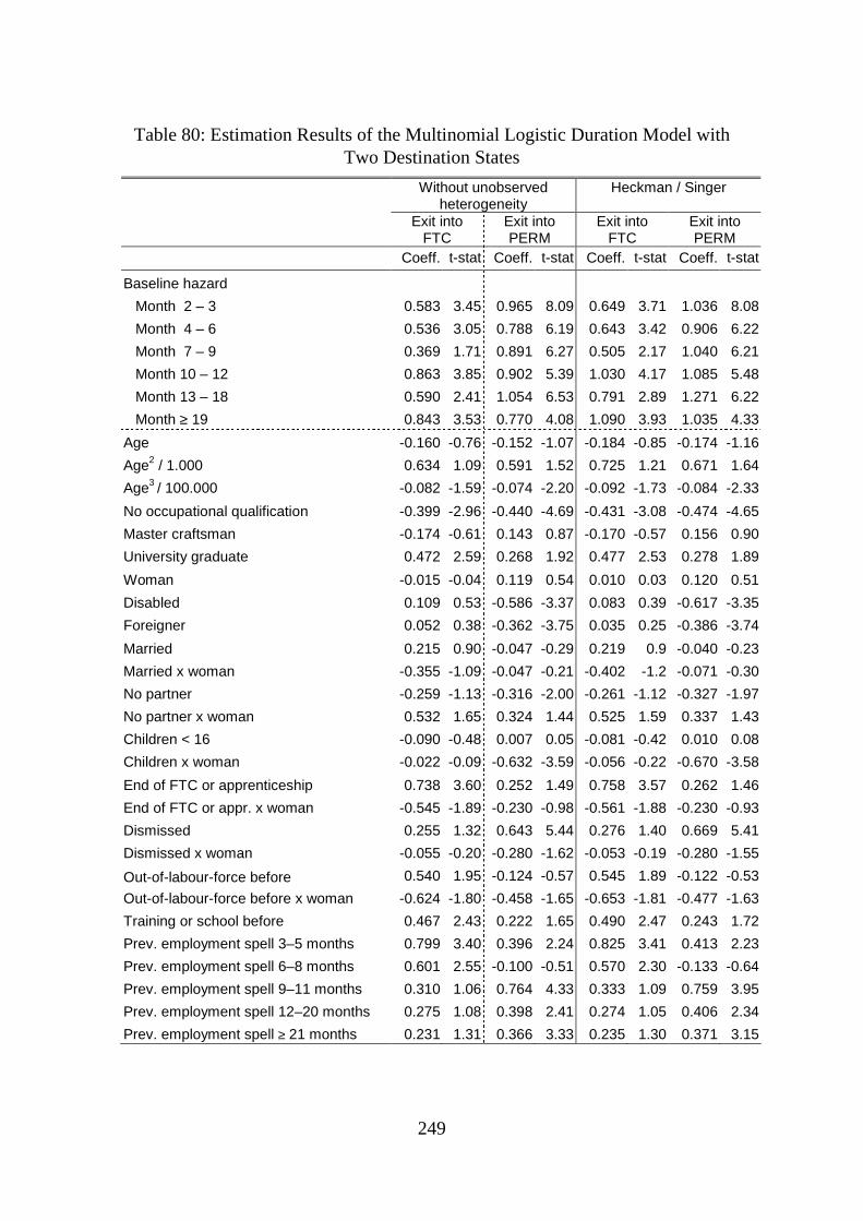
249

Table 80: Estimation Results of the Multinomial Logistic Duration Model with Two Destination States

Without unobserved heterogeneity

Heckman / Singer

Exit into FTC

Exit into PERM

Exit into FTC

Exit into PERM

Coeff. t-stat Coeff. t-stat Coeff. t-stat Coeff. t-stat

Baseline hazard

Month 2 – 3 0.583 3.45 0.965 8.09 0.649 3.71 1.036 8.08

Month 4 – 6 0.536 3.05 0.788 6.19 0.643 3.42 0.906 6.22

Month 7 – 9 0.369 1.71 0.891 6.27 0.505 2.17 1.040 6.21

Month 10 – 12 0.863 3.85 0.902 5.39 1.030 4.17 1.085 5.48

Month 13 – 18 0.590 2.41 1.054 6.53 0.791 2.89 1.271 6.22

Month ≥ 19 0.843 3.53 0.770 4.08 1.090 3.93 1.035 4.33

Age -0.160 -0.76 -0.152 -1.07 -0.184 -0.85 -0.174 -1.16

Age2 / 1.000 0.634 1.09 0.591 1.52 0.725 1.21 0.671 1.64

Age3 / 100.000 -0.082 -1.59 -0.074 -2.20 -0.092 -1.73 -0.084 -2.33

No occupational qualification -0.399 -2.96 -0.440 -4.69 -0.431 -3.08 -0.474 -4.65

Master craftsman -0.174 -0.61 0.143 0.87 -0.170 -0.57 0.156 0.90

University graduate 0.472 2.59 0.268 1.92 0.477 2.53 0.278 1.89

Woman -0.015 -0.04 0.119 0.54 0.010 0.03 0.120 0.51

Disabled 0.109 0.53 -0.586 -3.37 0.083 0.39 -0.617 -3.35

Foreigner 0.052 0.38 -0.362 -3.75 0.035 0.25 -0.386 -3.74

Married 0.215 0.90 -0.047 -0.29 0.219 0.9 -0.040 -0.23

Married x woman -0.355 -1.09 -0.047 -0.21 -0.402 -1.2 -0.071 -0.30

No partner -0.259 -1.13 -0.316 -2.00 -0.261 -1.12 -0.327 -1.97

No partner x woman 0.532 1.65 0.324 1.44 0.525 1.59 0.337 1.43

Children < 16 -0.090 -0.48 0.007 0.05 -0.081 -0.42 0.010 0.08

Children x woman -0.022 -0.09 -0.632 -3.59 -0.056 -0.22 -0.670 -3.58

End of FTC or apprenticeship 0.738 3.60 0.252 1.49 0.758 3.57 0.262 1.46

End of FTC or appr. x woman -0.545 -1.89 -0.230 -0.98 -0.561 -1.88 -0.230 -0.93

Dismissed 0.255 1.32 0.643 5.44 0.276 1.40 0.669 5.41

Dismissed x woman -0.055 -0.20 -0.280 -1.62 -0.053 -0.19 -0.280 -1.55

Out-of-labour-force before 0.540 1.95 -0.124 -0.57 0.545 1.89 -0.122 -0.53

Out-of-labour-force before x woman -0.624 -1.80 -0.458 -1.65 -0.653 -1.81 -0.477 -1.63


Prev. employment spell 3–5 months 0.799 3.40 0.396 2.24 0.825 3.41 0.413 2.23

Prev. employment spell 6–8 months 0.601 2.55 -0.100 -0.51 0.570 2.30 -0.133 -0.64



Prev. employment spell ≥ 21 months 0.231 1.31 0.366 3.33 0.235 1.30 0.371 3.15

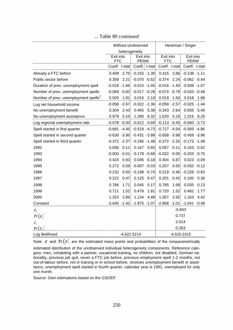
250

... Table 80 continued

Without unobserved

heterogeneity

Heckman / Singer

Exit into FTC

Exit into PERM

Exit into FTC

Exit into PERM

Coeff. t-stat Coeff. t-stat Coeff. t-stat Coeff. t-stat

Already a FTC before 0.408 2.70 -0.155 -1.30 0.415 2.66 -0.138 -1.11

Public sector before 0.359 2.21 -0.070 -0.52 0.374 2.24 -0.062 -0.44

Duration of prev. unemployment spell -0.018 -1.66 -0.010 -1.45 -0.016 -1.40 -0.008 -1.07

Number of prev. unemployment spells -0.069 -0.82 -0.017 -0.28 -0.074 -0.79 -0.033 -0.48

Number of prev. unemployment spells2 0.020 1.91 0.016 2.19 0.019 1.50 0.018 1.89

Log net household income -0.058 -2.67 -0.022 -1.36 -0.059 -2.57 -0.025 -1.44



Log regional unemployment rate -0.078 -0.33 -0.612 -3.69 -0.113 -0.45 -0.660 -3.73

Spell started in first quarter -0.681 -4.45 -0.519 -4.73 -0.717 -4.54 -0.565 -4.86

Spell started in second quarter -0.630 -3.90 -0.431 -3.88 -0.658 -3.98 -0.459 -3.96

Spell started in third quarter -0.372 -2.37 -0.166 -1.48 -0.372 -2.32 -0.173 -1.48

1992 0.056 0.11 0.167 0.65 0.057 0.11 0.163 0.62

1993 -0.003 -0.01 -0.178 -0.68 -0.022 -0.05 -0.203 -0.75

1994 0.424 0.93 0.046 0.18 0.404 0.87 0.023 0.09

1995 0.272 0.59 -0.007 -0.03 0.257 0.55 -0.032 -0.12

1996 0.232 0.50 -0.198 -0.74 0.219 0.46 -0.228 -0.83

1997 0.222 0.47 0.125 0.47 0.201 0.42 0.100 0.36

1998 0.786 1.71 0.045 0.17 0.785 1.68 0.035 0.13

1999 0.711 1.52 0.478 1.81 0.720 1.52 0.482 1.77

2000 1.323 2.89 1.134 4.48 1.357 2.92 1.163 4.42

Constant -3.645 -1.42 -1.875 -1.07 -2.868 -1.01 -1.041 -0.49

1ε -0.843

( )1Pr ε 0.737

2ε 2.614

( )2Pr ε 0.263

Log likelihood -4,522.5214 -4,520.2315

Note: ε and ( )Pr ε are the estimated mass points and probabilities of the nonparametrically

estimated distribution of the unobserved individual heterogeneity components. Reference cate-gory: men, cohabiting with a partner, vocational training, no children, not disabled, German na-tionality, previous job quit, never a FTC job before, previous employment spell 1-2 months, not out-of-labour before, not in training or in school before, receives unemployment benefit or assis-tance, unemployment spell started in fourth quarter, calendar year is 1991, unemployed for only one month.

Source: Own estimations based on the GSOEP.

251

Table 81: Estimation Results of the Multinomial Logistic Duration Model with Four Destination States

Exit into FTC

Exit into PERM

Exit into Training

Exit into out-of-labour-

force Coeff. t-stat. Coeff. t-stat. Coeff. t-stat. Coeff. t-stat.

Baseline hazard

Month 2 – 3 0.573 3.39 0.958 8.04 0.603 2.74 0.600 3.60

Month 4 – 6 0.527 3.01 0.782 6.15 0.790 3.66 0.780 4.85

Month 7 – 9 0.355 1.65 0.893 6.29 0.964 4.05 0.875 5.05

Month 10 – 12 0.869 3.88 0.922 5.51 0.916 3.25 1.453 8.38

Month 13 – 18 0.593 2.43 1.059 6.57 0.613 2.01 1.211 6.65

Month ≥19 0.835 3.50 0.770 4.08 0.808 2.67 1.320 7.36

Age -0.160 -0.76 -0.156 -1.09 -0.423 -1.73 -0.101 -0.70

Age2 / 1.000 0.639 1.10 0.602 1.55 1.403 2.04 0.067 0.17

Age3 / 100.000 -0.083 -1.60 -0.076 -2.23 -0.151 -2.45 0.005 0.14

No occupational qualification -0.399 -2.96 -0.444 -4.73 -0.362 -2.21 -0.148 -1.55

Master craftsman -0.168 -0.58 0.147 0.90 0.228 0.79 -0.863 -2.76

University graduate 0.474 2.61 0.263 1.89 0.155 0.60 -0.246 -1.18

Female -0.017 -0.06 0.119 0.54 -0.651 -1.61 0.345 1.24

Disabled 0.111 0.54 -0.584 -3.36 0.461 2.08 0.527 3.92

Foreigner 0.060 0.44 -0.364 -3.78 -0.696 -3.74 -0.320 -3.13

Married 0.226 0.94 -0.041 -0.25 -0.125 -0.43 -0.202 -0.92

Married x female -0.370 -1.13 -0.060 -0.27 0.386 0.95 0.371 1.33

No partner -0.252 -1.10 -0.310 -1.96 0.024 0.09 0.058 0.24

No partner x female 0.532 1.65 0.310 1.38 0.816 2.09 -0.559 -1.94

Children < 16 -0.104 -0.56 -0.003 -0.02 -0.494 -2.02 -0.206 -1.23

Children x female 0.002 0.01 -0.616 -3.51 0.197 0.63 0.365 1.83

Prev job: end of FTC or apprenticeship 0.738 3.60 0.252 1.49 0.020 0.07 0.478 2.29

Prev job: end of FTC or appr. x female -0.535 -1.86 -0.213 -0.91 -0.194 -0.47 -0.626 -2.18

Prev Job: dismissed 0.252 1.31 0.638 5.41 0.049 0.21 -0.430 -2.10

Prev Job: dismissed x female -0.053 -0.19 -0.279 -1.61 0.153 0.47 0.232 0.93

Out-of-labour-force before 0.536 1.93 -0.128 -0.59 -0.262 -0.70 0.400 2.02

Out-of-labour-force before x female -0.631 -1.82 -0.462 -1.67 0.033 0.08 -0.281 -1.29


252

… Table 81 continued

Exit into FTC

Exit into PERM

Exit into Training

Exit into out-of-labour-

force Coeff. t-stat. Coeff. t-stat. Coeff. t-stat. Coeff. t-stat.

Duration of prev. unemployment spell -0.018 -1.68 -0.010 -1.46 -0.020 -1.57 -0.015 -2.41


Prev. employment spell 6–8 months 0.595 2.53 -0.099 -0.51 -0.363 -0.91 0.598 2.91



Prev. employment spell ≥ 21 months 0.229 1.30 0.368 3.35 -0.018 -0.08 0.027 0.18

Already ever FTC before 0.405 2.69 -0.159 -1.34 -0.333 -1.44 -0.039 -0.25

Public sector before 0.363 2.25 -0.071 -0.53 -0.397 -1.57 -0.109 -0.77

Number of prev. unemployment spells -0.066 -0.78 -0.016 -0.28 0.216 1.58 0.090 1.02

Number of prev. unemployment spells2 0.020 1.90 0.016 2.20 -0.028 -1.09 -0.009 -0.56

Log net household income -0.058 -2.65 -0.022 -1.38 0.050 1.40 0.046 2.01



Log regional unemployment rate -0.068 -0.28 -0.604 -3.65 -0.044 -0.15 -0.104 -0.56

Spell started in first quarter -0.682 -4.46 -0.514 -4.69 -0.318 -1.57 -0.172 -1.36

Spell started in second quarter -0.625 -3.88 -0.418 -3.77 -0.378 -1.75 -0.253 -1.87

Spell started in third quarter -0.356 -2.27 -0.155 -1.39 0.512 2.69 -0.169 -1.20

1992 0.065 0.13 0.168 0.65 0.369 0.75 0.398 0.99

1993 -0.002 -0.00 -0.186 -0.72 -0.978 -1.76 0.680 1.75

1994 0.428 0.94 0.041 0.16 -0.031 -0.06 0.301 0.76

1995 0.266 0.58 -0.006 -0.02 0.140 0.29 0.408 1.04

1996 0.231 0.50 -0.207 -0.78 -0.230 -0.47 0.053 0.13

1997 0.226 0.48 0.121 0.45 0.031 0.06 0.379 0.94

1998 0.789 1.71 0.043 0.16 0.117 0.24 0.522 1.30

1999 0.706 1.51 0.471 1.79 0.582 1.20 0.838 2.11

2000 1.342 2.93 1.152 4.56 1.366 2.93 1.381 3.49

Constant -3.719 -1.45 -1.874 -1.07 -1.501 -0.50 -4.663 -2.55

Numb. of Transition 349 767 235 597

Numb. of Persons 321 683 214 533

Numb. of Observations 23,151

Log-likelihood -8166.4056

χ2 (216) 2096.67

Source and Notes: see Table 80.

253

9 References

ABBRING, J. H. and G. J. VAN DEN BERG (2003), The Nonparametric Identification of Treatment Effects in Duration Models, Econometrica 71(5), 1491-1517.

ABOWD, J. M. and O. C. ASHENFELTER (1981), Anticipated Unemployment, Temporary Lay-offs, and Compensating Wage Differentials, in: S. Rosen (ed.), Studies in Labor Markets, Chicago: University of Chicago Press, 141-170.

ABOWD, J. M., P. CORBEL, and F. KRAMARZ (1999), The Entry and Exit of Workers and the Growth of Employment: An Analysis of French Establishments, The Review of Economics and Statistics 81(2), 170-187.

ABRAHAM , K. G. (1988), Flexible Staffing Arrangements and Employers’ Short-Term Adjust-ment Strategies, in: R. A. Hart (ed.), Employment, Unemployment and Labor Utilization, Boston, MA: Unwin Hyman Press, 288-311.

ABRAHAM , K. G. and S. N. HOUSEMAN (1994), Does Employment Protection Inhibit Labor Market Flexibility? Lessons from Germany, France and Belgium, in: R. M. Blank (ed.), So-cial Protection Versus Economic Flexibility: Is There a Trade-off?, Chicago: University of Chicago Press, 59-93.

ABRAHAM , K. G. AND S. K. TAYLOR (1996), Firms’ Use of Outside Contractors: Theory and Evidence, Journal of Labor Economics 14(3), 394-424.

ADDISON, J. T., L. BELLMANN , C. SCHNABEL, and J. WAGNER (2004), The Reform of the Ger-man Works Constitution Act: A Critical Assessment, Industrial Relations 43(2), 392-420

ADDISON, J. T. and P. TEIXEIRA (2003), The Economics of Employment Protection, Journal of Labor Research 24(1), 85-129.

AKERLOF, G. A., A. K. ROSE, and J. L. YELLEN (1988), Job Switching and Job Satisfaction in the U.S. Labor Market, Brookings Papers on Economic Activity 1988(2), 495-582.

ALBA RAMÍREZ, A. (1998), How Temporary is Temporary Employment in Spain?, Journal of Labor Research 19(4), 695-710.

AMUEDO-DORANTES, C. (2000), Work Transitions into and out of Involuntary Temporary Em-ployment in a Segmented Market: Evidence from Spain, Industrial and Labor Relations Re-view 53(2), 309-325.

AMUEDO-DORANTES, C. (2002), Work Safety in the Context of Temporary Employment: The Spanish Experience, Industrial and Labor Relations Review 55(2), 262-272.

ANGRIST, J. D. and A. B. KRUEGER (1999), Chapter 23: Empirical Strategies in Labor Econom-ics, in: O. C. Ashenfelter and D. Card (eds.), Handbook of Labor Economics Vol. 3A, Am-sterdam: North-Holland, 1277-1366.

ANGRIST, J. D. and A. B. KRUEGER (2001), Instrumental Variables and the Search for Identifi-cation: From Supply and Demand to Natural Experiments, Journal of Economic Perspec-tives 15(4), 69-85.

ARELLANO, M. and S. R. BOND (1991), Some Tests of Specification for Panel Data: Monte Carlo Evidence and an Application to Employment Equations, Review of Economics Studies 58(2), 277-297.

ARULAMPALAM , W. and A. L. BOOTH (1998), Training and Labour Market Flexibility: Is There a Trade-Off?, British Journal of Industrial Relations 36(4), 521-536.

ASHENFELTER, O. C. (1978), Estimating the Effect of Training Programs on Earnings, The Re-view of Economics and Statistics 60(1), 47-57.

ATKINSON, J. (1984), Manpower Strategies for Flexible Organisations, Personnel Management 16(8), 28-31.

ATKINSON, A. B. and J. MICKLEWRIGHT (1991), Unemployment Compensation and Labor Mar-ket Transitions: A Critical Review, Journal of Economic Literature 29(4), 1679-1727.

AUTOR, D. H. (2003), Outsourcing at Will: The Contribution of Unjust Dismissal Doctrine to the Growth of Employment Outsourcing, Journal of Labor Economics 21(1), 1-42.

254

BAKER, M. and A. MELINO (2000), Duration Dependence and Nonparametric Heterogeneity: A Monte Carlo Study, Journal of Econometrics 96(2), 357-393.

BARDASI, E. and M. FRANCESCONI (2003), The Impact of Atypical Employment on Individual Wellbeing: Evidence from a Panel of British Workers, ISER Working Paper No. 2003-02, Institute for Social and Economic Research (ISER), University of Essex.

BEBLO, M. and E. WOLF (2002), How Much Does a Year Off Cost? Estimating the Wage Ef-fects of Employment Breaks and Part-Time Periods, Cahiers Économiques de Bruxelles 45(2), 191-218.

BELLMANN , L. and T. BOERI (1998), Internal and External Adjustment to New Technologies, Economics of Innovation and New Technology 5(2-4), 325-343.

BENTOLILA, S. and G. BERTOLA (1990), Firing Costs and Labour Demand: How Bad is Euroes-clerosis?, Review of Economic Studies 57(3), 381-402.

BENTOLILA, S. and J. J. DOLADO (1994), Labour Flexibility and Wages: Lessons from Spain, Economic Policy 9(18), 53-99.

BENTOLILA, S. and G. SAINT-PAUL (1992), The Macroeconomic Impact of Flexible Labour Contracts, with an Application to Spain, European Economic Review 36(5), 1013-1053.

BENTOLILA, S. and G. SAINT-PAUL (1994), A Model of Labor Demand with Linear Adjustment Costs, Labour Economics 1(3-4), 303-326.

BERGEMANN, A., B. FITZENBERGER, and S. SPECKESSER (2004), Evaluating the Dynamic Em-ployment Effects of Training Programs in East Germany Using Conditional Difference-in-Difference, ZEW Discussion Paper No. 04-41, Mannheim.

BERGEMANN, A. and A. MERTENS (2000), Job Stability Trends, Layoffs and Quits: An Empiri-cal Analysis for West Germany, SFB 373 Discussion Paper No. 102-2001, Humboldt Uni-versity Berlin.

BERGEMANN, A. and H. SCHNEIDER (1998), Ist der deutsche Arbeitsmarkt beweglicher gewor-den? Eine Analyse anhand der Unternehmenszugehörigkeitsdauer in Westdeutschland, IWH Wirtschaft im Wandel 11/98, 15-21.

BERTOLA, G. (1990), Job Security, Employment and Wages, European Economic Review 34(4), 851-886.

BERTOLA, G. (1992), Labor Turnover Costs and Average Labor Demand, Journal of Labor Economics 10(4), 389-411.

BERTOLA, G. (1999), CHAPTER 45: Microeconomic Perspectives on Aggregate Labor Markets, in: O. C. Ashenfelter and D. Card (eds.), Handbook of Labor Economics Vol. 3C, Amster-dam: North-Holland, 2985-3028.

BERTOLA, G. and R. ROGERSON (1997), Institutions and Labour Reallocation, European Eco-nomic Review 41(6), 1147-71.

BIELENSKI, H. (1998), Befristete Beschäftigung, in: J. Schupp, F. Büchel, M. Diewald, and R. Habich (eds.), Arbeitsmarktstatistik zwischen Realität und Fiktion, Berlin: Edition Sigma, 167-181.

BIELENSKI, H., B. KOHLER, and M. SCHREIBER-KITTL (1994), Befristete Beschäftigung und Arbeitsmarkt. Empirische Untersuchung über befristete Arbeitsverträge nach BeschFG 1985/1990, Forschungsbericht des Bundesministeriums für Arbeit und Sozialordnung No. 242, Bonn.

BLACK , D. A. and J. A. SMITH (2004), How Robust is the Evidence on the Effects of College Quality? Evidence from Matching, Journal of Econometrics 121(1-2), 99-124.

BLANCHARD, O. J. and P. A. DIAMOND (1992), The Flow Approach to Labor Markets, American Economic Review 82(2), 345-359.

BLANCHARD, O. J. and P. A. DIAMOND (1994), Ranking, Unemployment Duration, and Wages, Review of Economic Studies 61(3), 417-434.

BLANCHARD, O. J. and A. LANDIER (2002), The Perverse Effects of Partial Labor Market Re-form: Fixed Duration Contracts in France, The Economic Journal 112(480), F214-F244.

255

BLANCHARD, O. J. and P. PORTUGAL (2001), What Hides Behind an Unemployment Rate: Comparing Portuguese and U.S. Labor Markets, American Economic Review 91(1), 187-207.

BLAU , F. D. and L. M. KAHN (1999), Chapter 25: Institutions and Laws in the Labor Market, in: O. C. Ashenfelter and D. Card (eds.), Handbook of Labor Economics Vol. 3A, Amsterdam: North-Holland, 1399-1461.

BLUNDELL, R. and M. COSTA DIAS (2000), Evaluation Methods for Non-Experimental Data, Fiscal Studies 21(4), 427-468.

BLUNDELL, R. and M. COSTA-DIAS (2002), Alternative Approaches to Evaluation in Empirical Microeconomics, CeMMAP Working Paper CWP 10/02, Centre for Microdata Methods and Practice (CeMMAP), London.

BOERI, T. (1999), Enforcement of Employment Security Regulations, On-The-Job Search and Unemployment Duration, European Economic Review 43(1), 65-89.

BONNAL, L., D. FOUGÈRE, and A. SÉRANDON (1997), Evaluating the Impact of French Em-ployment Policies on Individual Labour Market Histories, Review of Economic Studies 64(4), 683-713.

BOOCKMANN, B. and T. HAGEN (2003), Works Councils and Fixed-Term Employment: Evi-dence from West German Establishments, Schmollers Jahrbuch 123(3), 359-382.

BOOCKMAN, B. and T. HAGEN (2004), Role of Fixed-Term Employment Contracts in Worker and Job Flows at the Establishment Level: An Empirical Analysis for West Germany, mimeo, Centre for European Economic Research (ZEW), Mannheim.

BOOTH, A. L., M. FRANCESCONI, and J. FRANK (2002), Temporary Jobs: Stepping Stones or Dead Ends?, The Economic Journal 112(480), F189-F213.

BOOTH, A. L., M. FRANCESCONI, and J. FRANK (2003), Labour as a Buffer: Do Temporary Workers Suffer?, in: G. Fagan, F. P. Mongelli, and J. Morgan (eds.), Institutions and Wage Formation in the New Europe, Cheltenham: Edward Elgar Publishing, 53-68.

BOVER, O., M. ARELLANO, and S. BENTOLILA (2002), Unemployment Duration, Benefit Dura-tion and the Business Cycle, The Economic Journal 112(479), 223-265.

BOVER, O. and R. GÓMEZ (2004), Another Look at Unemployment Duration: Exit to a Perma-nent vs. a Temporary Job, Investigaciones Económicas 28(2), 285-314.

BRODATY, T., B. CRÉPON, and D. FOUGÈRE (2001), Using Matching Estimators to Evaluate Alternative Youth Employment Programs: Evidence from France, 1986-1988, in: M. Lechner and F. Pfeiffer (eds.), Econometric Evaluation of Labour Market Policies, Heidel-berg: Physica-Verlag, 85-120.

BROSE, H.-G., M. SCHULZE-BÖING, and W. MEYER (1990), Arbeit auf Zeit: Zur Karriere ei-nes“ neuen“ Beschäftigungsverhältnisses, Opladen: Leske & Budrich.

BROWN, S. and J. G. SESSIONS (2003), Earnings, Education, and Fixed-Term Contracts, Scottish Journal of Political Economy 50(4), 492-506.

BROWNSTONE, D. and R. VALLETTA (2001), The Bootstrap and Multiple Imputations: Harness-ing Increased Computing Power for Improved Statistical Tests, Journal of Economic Per-spectives 15(4), 129-141.

BÜCHTEMANN, C. F. (1993), Employment Security and Deregulation: The West German Ex-perience, in: C. F. Büchtemann (ed.), Employment Security and Labor Market Behavior: In-terdisciplinary Approaches and International Evidence, Ithaca, NY: ILR Press, 272-296.

BÜRKLE, T. (2004), Beschäftigungssicherheit als konstituierendes Element interner Arbeits-märkte, München: Hampp, Mering.

BURDA, M. and C. WYPLOSZ (1994), Gross Worker and Job Flows in Europe, European Eco-nomic Review 38(6), 1287-1315.

BURDETT, K. and D. T. MORTENSEN (1980), Search, Layoffs, and Labor Market Equilibrium, Journal of Political Economy 88(4), 652-672.

BURGESS, S. M. (1988), Employment Adjustment in UK Manufacturing, The Economic Journal 98(389), 81-103.

256

BURGESS, S. M., J. LANE, and D. STEVENS (2001), Churning Dynamics: An Analysis of Hires and Separations at the Employer Level, Labour Economics 8(1), 1-14.

BURKHAUSER, R. V., A. CREWS CUTTS, M. C. DALY , and S. P. JENKINS (1999), Testing the Significance of Income Distribution Changes Over the 1980s Business Cycle: A Cross-National Comparison, Journal of Applied Econometrics 14(3), 253-272.

BUTLER, J. S. and R. MOFFITT (1982), A Computationally Efficient Quadrature Procedure for the One-Factor Multinomial Probit Model, Econometrica 50(3), 761-764.

CAHUC, P. and F. POSTEL-VINAY (2002), Temporary Jobs, Employment Protection and Labor Market Performance, Labour Economics 9(1), 63-91.

CAIN , G. G. (1976), The Challenge of Segmented Labor Market Theories to Orthodox Theory: A Survey, Journal of Economic Literature 14(4), 1215-1257.

CALIENDO, M., T. HAGEN, and R. HUJER (2004), Makroökonomische Methoden auf Basis von Regionaldaten, in: T. Hagen and A. Spermann, Hartz Gesetze – Methodische Ansätze zu ei-ner Evaluierung, (ZEW Wirtschaftsanalysen Vol. 74), Baden-Baden: Nomos Verlagsgesell-schaft (unter Mitarbeit von: M. Arntz, A. Ammermüller, M. Beblo, M. Biewen, B. Boock-mann, M. Caliendo, B. Fitzenberger, N. Gürtzgen, R. Hujer, P. Jacobebbinghaus, F. Pfeiffer, A. Weber, R. Wilke, H. Winterhager, E. Wolf, G. Wunderlich), 84-97.

CANZIANI , P. and B. PETRONGOLO (2001), Firing Costs and Stigma: A Theoretical Analysis and Evidence from Microdata, European Economic Review 45(10), 1877-1906.

CAPPELLI, P. and D. NEUMARK (2001), External Job Churning and Internal Job Flexibility, NBER Working Paper No. 8111, National Bureau of Economic Research (NBER), Cam-bridge, MA.

CHALMERS, J. and G. KALB (2000), The Transition from Unemployment to Work: Are Casual Jobs a Short Cut to Permanent Employment?, SPRC Discussion Paper No. 109, Social Pol-icy Research Centre (SPRC), University of New South Wales, Sydney.

CLARK , A. E. (1997), Job Satisfaction and Gender: Why are Women so Happy at Work?, La-bour Economics 4(4), 341-372.

CLARK , A. E. (2001), What Really Matters in a Job? Hedonic Measurement Using Quit Data, Labour Economics 8(2), 223-242.

CLARK , A. E., F. ETILÉ, F. POSTEL-VINAY , C. SENIK, and K. VAN DER STRAETEN (2004), Het-erogeneity in Reported Well-Being: Evidence from Twelve European Countries, DELTA Working Paper No. 2004-01, Département et Laboratoire d'Economie Théorique Appliquée (DELTA), École Normale Supérieure, Paris.

COCHRAN, W. G. and D. B. RUBIN (1973), Controlling Bias in Observational Studies, Sankyha 35(4), 417-446.

CONOVER, W. J. (1999), Practical Nonparametric Statistics, 3rd Edition, New York: Wiley. CRAMER, U. and M. KOLLER (1988): Gewinne und Verluste von Arbeitsplätzen in Betrieben –

der „Job-Turnover“-Ansatz, Mitteilungen aus der Arbeitsmarkt- und Berufsforschung 21(3), 361-377.

CRAMER, J. S. and G. RIDDER (1991), Pooling States in the Multinomial Logit Model, Journal of Econometrics 47(2-3), 267-272.

DANIEL, C. and C. SOFER (1998), Bargaining, Compensating Wage Differentials, and Dualism of the Labor Market: Theory and Evidence for France, Journal of Labor Economics 16(3), 546-575.

DAVIS, S. and J. C. HALTIWANGER (1999), Chapter 41: Gross Job Flows, in: O. C. Ashenfelter and D. Card (eds.), Handbook of Labor Economics Vol. 3B, Amsterdam: North-Holland, 2711-2805.

DEATON, A. (1997), The Analysis of Household Surveys: A Microeconometric Approach to Development Policy, Baltimore: Johns Hopkins University Press.

DEHEJIA, R. H. and S. WAHBA (1999), Causal Effects in Non-Experimental Studies: Re-Evaluating the Evaluation of Training Programs, Journal of the American Statistical Asso-ciation 94(448), 1053-1062.

257

DEKKER, R. (2000), Unemployment Durations in a “Flexible” Career: Evidence for the UK, paper presented at the European Society of Population Economics Conference 2000, Insti-tute for the Study of Labor (IZA), Bonn.

DEVINE, T. J. and N. M. KIEFER (1991), Empirical Labor Economics: The Search Approach, New York: Oxford University Press.

DIETRICH, H. (1999), Freelance and Contract Workers in Germany – Enterprise Perspectives from the IAB Establishment, in: J. Merz and M. Ehling (eds.), Time Use – Research, Data and Policy: Contributions from the International Conference on Time Use (ICTU), Univer-sity of Lüneburg, April 22-25, 1998, Baden-Baden: Nomos Verlagsgesellschaft, 227-240.

DINARDO J. E. and J.-S. PISCHKE (1997), The Returns To Computer Use Revisited: Have Pen-cils Changed The Wage Structure Too?, Quarterly Journal of Economics 112(1), 291-303.

DOLADO, J. J., C. GARCÍA-SERRANO, and J. F. JIMENO (2002), Drawing Lessons from the Boom of Temporary Jobs in Spain, The Economic Journal 112(721), F270-F295.

EHRENBERG, R. G. and R. S. SMITH (1991), Modern Labor Economics: Theory and Public Pol-icy, 4th Edition, New York: Harper & Collins.

EISEN, R. (1997), Reformüberlegungen zur Arbeitslosenversicherung, in: R. Hauser (ed.), Re-form des Sozialstaats I: Arbeitsmarkt, soziale Sicherung und soziale Dienstleistungen, Ber-lin: Duncker & Humblot, 45-76.

EISEN, R. (2001), Globalisierung, Arbeitslosigkeit und die Reform des Sozialstaats: Prolegome-na zu einer Theorie der Sozialreform, in: I. Becker, N. Ott, and G. Rolf (eds.), Soziale Siche-rung in einer dynamischen Gesellschaft: Festschrift für Richard Hauser zum 65. Geburt-stag, Frankfurt: Campus-Verlag, 63-86.

ENGELLANDT, A. and R. T. RIPHAN (2003), Temporary Contracts and Employee Effort, IZA Discussion Paper No. 780, Institute for the Study of Labor (IZA), Bonn.

ERKE, B. (1993), Arbeitslosigkeit und Konjunktur auf segmentierten Arbeitsmärkten: eine mak-roökonomische Analyse auf der Grundlage der Effizienzlohntheorie, Heidelberg: Physica-Verlag.

FAHRMEIR, L. and G. TUTZ (2001), Multivariate Statistical Modelling Based on Generalized Linear Models, New York: Springer.

FAN, J. (1992), Design-Adaptive Nonparametric Regression, Journal of the American Statistical Association 87(4), 998-1004.

FAN, J. and I. GIJBELS (1997), Local Polynomial Modelling and Its Applications, London: Chapman & Hall.

FARBER, H. S. (1994), The Analysis of Interfirm Worker Mobility, Journal of Labor Economics 12(4), 554-593.

FARBER, H. S. (1999), Chapter 37: Mobility and Stability: The Dynamics of Job Change in La-bor Markets, in: O. C. Ashenfelter and D. Card (eds.), Handbook of Labor Economics Vol. 3B, Amsterdam: North-Holland, 2439-2483.

FITZENBERGER, B. (1999), Wages and Employment Across Skill Groups: An Analysis for West Germany, Heidelberg: Physica-Verlag.

FITZENBERGER, B. and H. PREY (2000), Evaluating Public Sector Sponsored Training in East Germany, Oxford Economic Papers 52(3), 497-520.

FITZENBERGER, B. and A. SPITZ (2004), Die Anatomie des Berufswechsels: Eine empirische Bestandsaufnahme auf Basis der BIBB/IAB-Daten 1998/1999, ZEW Discussion Paper No. 04-05, Centre for European Economic Research (ZEW), Mannheim.

FRANZ, W. (2003), Arbeitsmarktökonomik, 5th Edition, Berlin: Springer. FRANZ, W. and F. PFEIFFER (2003), Zur ökonomischen Rationalität von Lohnrigiditäten aus der

Sicht von Unternehmen, Jahrbücher für Nationalökonomie und Statistik 223(1), 23-57. FRANZ, W. and V. STEINER (2000), Wages in the East German Transition Process: Facts and

Explanations, German Economic Review 1(3), 241-269. FREDRIKSSON, P. and P. JOHANSSON (2003), Program Evaluation and Random Program Starts,

IFAU Working Paper No. 2003:1, Institute for Labour Market Policy Evaluation (IFAU), Uppsala.

258

FREEMAN, R. B. (1978), Job Satisfaction as an Economic Variable, American Economic Review 68(2), 135-141.

FREY, B. S. and A. STUTZER (2002), What Can Economists Learn from Happiness Research?, Journal of Economic Literature 40(2), 402-435.

FRÖLICH, M. (2004), Finite Sample Properties of Propensity-Score Matching and Weighting Estimators, The Review of Economics and Statistics 86(1), 77-90.

GARIBALDI , P. (2002), Search Unemployment with Advance Notice, Discussion Paper, Bocconi University, Milan.

GERFIN, M., M. LECHNER, and H. STEIGER (2002), Does Subsidised Temporary Employment Get the Unemployed Back to Work? An Econometric Analysis of Two Different Schemes, IZA Discussion Paper No. 606, Institute for the Study of Labor (IZA), Bonn.

GIBBONS, R. and L. F. KATZ (1991), Layoffs and Lemons, Journal of Labor Economics 9(4), 351-380.

GIBBONS, R. and K. J. MURPHY (1992), Optimal Incentive Contracts in the Presence of Career Concerns: Theory and Evidence, Journal of Political Economy 100(3), 468-505.

GIBBONS, R. and M. WALDMAN (1999), Chapter 36: Careers in Organizations: Theory and Evi-dence, in: O. C. Ashenfelter and D. Card (eds.), Handbook of Labor Economics Vol. 3B, Amsterdam: North-Holland, 2373-2437.

GIESECKE, J. and M. GROß (2002), Befristete Beschäftigung: Chance oder Risiko?, Kölner Zeit-schrift für Soziologie und Sozialpsychologie 54(1), 85-108.

GOUX, D., E. MAURIN, and M. PAUCHET (2001), Fixed-Term Contracts and the Dynamics of Labour Demand, European Economic Review 45(3), 533-552.

GRAMM , C. L., and J. F. SCHNELL (2001), The Use of Flexible Staffing Arrangements in Core Production Jobs, Industrial and Labor Relations Review 54(2), 245-258.

GREENE, W. H. (2003), Econometric Analysis, 5th Edition, Upper Saddle River, NJ: Prentice Hall.

GROOT, W. (1990), Heterogeneous Jobs and Re-Employment Probabilities, Oxford Bulletin of Economics and Statistics 52(3), 253-267.

GUADALUPE, M. (2003), The Hidden Costs of Fixed Term Contracts: The Impact on Work Ac-cidents, Labour Economics 10(3), 339-357

GÜELL, M. (2000), Fixed-Term Contracts and Unemployment: An Efficiency Wage Analysis, Working Paper No. 433, Princeton University, Department of Economics, Industrial Rela-tions Sections.

GÜELL, M. and B. PETRONGOLO (2003), How Binding are Legal Limits? Transitions from Tem-porary to Permanent Work in Spain, CEPR Discussion Paper No. 3931, Centre for Eco-nomic Policy Research (CEPR), London.

HAGEN, T. (2002), Do Temporary Workers Receive Risk Premiums? Assessing the Wage Ef-fects of Fixed-Term Contracts in West Germany by a Matching Estimator Compared with Parametric Approaches, LABOUR: Review of Labour Economics and Industrial Relations 16(4), 667-705.

HAGEN, T. (2003), Does Fixed-Term Contract Employment Raise Firms’ Adjustment Speed? Evidence from an Establishment Panel for West Germany, Jahrbücher für Nationalökono-mie und Statistik 223(4), 403-421.

HAGEN, T. and B. FITZENBERGER (2004), Mikroökonometrische Methoden zur Ex-post-Evaluation, in: T. Hagen and A. Spermann, Hartz Gesetze – Methodische Ansätze zu einer Evaluierung, (ZEW Wirtschaftsanalysen Vol. 74), Baden-Baden: Nomos Verlagsgesell-schaft (unter Mitarbeit von: M. Arntz, A. Ammermüller, M. Beblo, M. Biewen, B. Boock-mann, M. Caliendo, B. Fitzenberger, N. Gürtzgen, R. Hujer, P. Jacobebbinghaus, F. Pfeiffer, A. Weber, R. Wilke, H. Winterhager, E. Wolf, G. Wunderlich), 45-72.

HAM , J. C. and R. J. LALONDE (1996), The Effect of Sample Selection and Initial Conditions in Duration Models: Evidence from Experimental Data on Training, Econometrica 64(1), 175-205.

HAMERMESH, D. S. (1993), Labor Demand, Princeton, NJ: Princeton University Press.

259

HAMERMESH, D. S. (1995), Labour Demand and the Source of Adjustment Costs, The Economic Journal 105(430), 620-634.

HAMERMESH, D. S. (2001), The Changing Distribution of Job Satisfaction, Journal of Human Resources 36(1), 1-30.

HAMERMESH, D. S. and G. A. PFANN (1996), Adjustment Costs in Factor Demand, Journal of Economic Literature 34(3), 1264-1292.

HAN, A. and J. A. HAUSMAN (1990), Flexible Parametric Estimation of Duration and Compet-ing Risk Models, Journal of Applied Econometrics 5(1), 1-28.

HAUSMAN, J. A. and D. L. MCFADDEN (1984), Specification Tests for the Multinomial Logit Model, Econometrica 52(5), 1219-1240.

HECKMAN, J. J. (1979), Sample Selection Bias as a Specification Error, Econometrica 47(1), 153-161.

HECKMAN, J. J. (2001), Micro Data, Heterogeneity, and the Evaluation of Public Policy: Nobel Lecture, Journal of Political Economy 109(4), 673-748

HECKMAN, J. J. and G. J. BORJAS (1980), Does Unemployment Cause Future Unemployment? Definitions, Questions and Answers from a Continuous Time Model of Heterogeneity and State Dependence, Economica 47(187), 247-283.

HECKMAN, J. J. and V. J. HOTZ (1989), Choosing Among Nonexperimental Methods for Esti-mating the Impact of Social Programs: The Case of Manpower Training, Journal of the American Statistical Association 84(408), 862-874.

HECKMAN, J. J, H. ICHIMURA, J. SMITH , and P. E. TODD (1998), Characterizing Selection Bias Using Experimental Data, Econometrica 66(5), 1017-98.

HECKMAN, J. J., H. ICHIMURA, and P. E. TODD (1997), Matching as an Econometric Evaluation Estimator: Evidence from Evaluating a Job Training Programme, Review of Economic Stud-ies 64(4), 605-654.

HECKMAN, J. J., H. ICHIMURA, and P. E. TODD (1998), Matching as an Econometric Evaluation Estimator, Review of Economic Studies 65(2), 261-294.

HECKMAN, J. J., R. J. LALONDE, and J. A. SMITH (1999), Chapter 31: The Economics and Econometrics of Active Labor Market Programs, in: O. C. Ashenfelter and D. Card (eds.), Handbook of Labor Economics Vol. 3B, Amsterdam: North-Holland, 1865-2097.

HECKMAN, J. J and R. ROBB (1985), Alternative Methods for Evaluating the Impact of Interven-tions, in: J. J. Heckman and B. L. Singer (eds.), Longitudinal Analysis of Labor Market Data, Cambridge, MA: Cambridge University Press, 156-246.

HECKMAN, J. J. and B. L. SINGER (1984), A Method for Minimizing the Impact of Distributional Assumptions in Econometric Models for Duration Data, Econometrica 52(2), 271-320.

HECKMAN, J. J. and E. VYTLACIL (2001), Policy – Relevant Treatment Effects, American Eco-nomic Review 91(2), 107-111.

HOLMLUND , B. and D. STORRIE (2002), Temporary Work in Turbulent Times: The Swedish Experience, The Economic Journal 112(480), F245-F269.

HUJER, R. and M. CALIENDO (2001), Evaluation of Active Labour Market Policy – Methodo-logical Concepts and Empirical Estimates, in: I. Becker, N. Ott, and G. Rolf (eds.): Soziale Sicherung in einer dynamischen Gesellschaft: Festschrift für Richard Hauser zum 65. Ge-burtstag, Frankfurt: Campus-Verlag, 583-617.

HUJER, R., M. CALIENDO, and D. RADIC (2001), Nobody knows… How Do Different Evalua-tion Estimators Perform in a Simulated Labour Market Experiment?, Working Paper, Jo-hann Wolfgang Goethe-University Frankfurt, Faculty of Economics and Business Admini-stration.

HUJER, R., M. CALIENDO, and S. THOMSEN (2003), New Evidence on the Effects of Job Crea-tion Schemes in Germany – A Matching Approach with Threefold Heterogeneity, Working Paper, Johann Wolfgang Goethe-University Frankfurt, Faculty of Economics and Business Administration.

HUJER, R., and B. FITZENBERGER (2002), Stand und Perspektiven der Evaluation der Aktiven Arbeitsmarktpolitik in Deutschland, Perspektiven der Wirtschaftspolitik 3(2), 139-158.

260

HUJER, R., K.-O. MAURER, and M. WELLNER (1998), Kurz- und langfristige Effekte von Wei-terbildungsmaßnahmen auf die Arbeitslosigkeitsdauer in Westdeutschland, in: F. Pfeiffer und W. Pohlmeier (eds.), Qualifikation, Weiterbildung und Arbeitsmarkterfolg, (ZEW Wirt-schaftsanalysen Vol. 31), Baden-Baden: Nomos Verlagsgesellschaft, 197-222.

HUJER, R., K.-O. MAURER, and M. WELLNER (1999): Estimating the Effect of Vocational Training on Unemployment Duration in West Germany – A Discrete Hazard Rate Model with Instrumental Variables, Jahrbücher für Nationalökonomie und Statistik 218(1), 619-646.

HUJER, R. and H. SCHNEIDER (1989), The Analysis of Labor Market Mobility Using Panel Data, European Economic Review 33, 530-536.

HUJER, R. and H. SCHNEIDER (1996), Institutionelle und strukturelle Determinanten der Ar-beitslosigkeit in Westdeutschland – Eine mikroökonometrische Analyse mit Paneldaten, in: B. Gahlen, H. Hesse, and H.-J. Ramser (eds.), Arbeitslosigkeit und Möglichkeiten ihrer Ü-berwindung, Tübingen: Mohr, 53-76.

HUJER, R. and H. SCHNEIDER (1998), Initial- und Verlaufseffekte der „Replacement Ratio“ auf die individuelle Arbeitslosigkeitsdauer, in: H. P. Galler and G. Wagner (eds.), Empirische Forschung und wirtschaftspolitische Beratung: Festschrift für Hans-Jürgen Krupp zum 65. Geburtstag, Frankfurt: Campus-Verlag, 184-199.

HUNT, J. (1995), The Effect of Unemployment Compensation on Unemployment Duration in Germany, Journal of Labour Economics 13(1), 88-120.

HUNT, J. (2000), Firing Costs, Employment Fluctuations and Average Employment: An Exami-nation of Germany, Economica 67(266), 177-202.

ICHINO, A., F. MEALLI , and T. NANNICINI (2004), Temporary Work Agencies in Italy: A Springboard Toward Permanent Employment?, paper in progress, European University In-stitute, Florence.

ICHINO, A. and R. T. RIPHAN (2001), The Effect of Employment Protection on Worker Effort. A Comparison of Absenteeism During and After Probation, IZA Discussion Paper No. 385, Institute for the Study of Labor (IZA), Bonn.

INSTITUT FÜR ARBEITSMARKT- UND BERUFSFORSCHUNG (2003): Zahlen-Fibel – Ergebnisse der Arbeitsmarkt- und Berufsforschung, Beiträge zur Arbeitsmarkt- und Berufsforschung No. 101, Nürnberg.

JAHN, E. J. (2002), Zur ökonomischen Theorie des Kündigungsschutzes: Volatilität der Arbeits-nachfrage und duale Arbeitsmärkte, Berlin: Duncker & Humblot.

JENKINS, S. P. (1995), Easy Estimation Methods for Discrete-Time Duration Models, Oxford Bulletin of Economics and Statistics 57(1), 129-138.

JOVANOVIC, B. (1979), Job Matching and the Theory of Turnover, Journal of Political Econ-omy 87(5), 972-990.

KAISER, U. and F. PFEIFFER (2001), Collective Wage Agreements and Firms’ Employment Policies, LABOUR: Review of Labour Economics and Industrial Relations 15(2), 317-341.

KELLER, B. and H. SEIFERT (eds.) (1995), Atypische Beschäftigung: Verbieten oder gestalten?, Köln: Bund-Verlag.

KIEFER, N. M. (1988), Economic Duration Data and Hazard Functions, Journal of Economic Literature 26(2), 646-679.

KÖLLING, A. (1998), Anpassungen auf dem Arbeitsmarkt – eine Analyse der dynamischen Ar-beitsnachfrage in der Bundesrepublik Deutschland, Beiträge zur Arbeitsmarkt- und Berufs-forschung No. 217, Nürnberg.

KÖLLING, A. (2000), The IAB-Establishment Panel, Schmollers Jahrbuch 120(2), 291-300. KRAFT, K. (1993), Eurosclerosis Reconsidered: Employment Protection and Work Force Ad-

justment in West Germany, in: C. F. Büchtemann (ed.), Employment Security and Labor Market Behavior: Interdisciplinary Approaches and International Evidence, Ithaca, NY: ILR Press, 297-301.

KRAFT, K. (1996), Die Auswirkungen des Beschäftigungsförderungsgesetzes, Jahrbuch für Wirtschaftswissenschaften 47, 264-281.

261

KUCKULENZ, A. and T. ZWICK (2003), The Impact of Training on Earnings – Differences Be-tween Participant Groups and Training Forms, ZEW Discussion Paper No. 03-57, Centre for European Economic Research (ZEW), Mannheim.

LALONDE, R. J. (1986), Evaluating the Econometric Evaluations of Training Programs with Experimental Data, American Economic Review 76(4), 604-620.

LANCASTER, T. (1990), The Econometric Analysis of Transition Data, Cambridge, MA: Cam-bridge University Press.

LAUER, C. (2003), Education and Unemployment: A French-German Comparison, ZEW Dis-cussion Paper No. 03-34, Centre for European Economic Research (ZEW), Mannheim.

LAZEAR, E. P. (1990), Job Security Provisions and Employment, Quarterly Journal of Econom-ics 105(3), 699-726.

LECHNER, M. (1998), Training the East German Labour Force: Microeconometric Evaluations of Continuous Vocational Training after Unification, Heidelberg: Physica-Verlag.

LECHNER, M. (1999), Earnings and Employment Effects of Continuous Off-The-Job Training in East Germany after Unification, Journal of Business and Economic Statistics 17(1), 74-90.

LECHNER, M. (2001a), A Note on the Common Support Problem in Applied Evaluation Studies, Discussion Paper No. 2001-01, University of St. Gallen, Department of Economics.

LECHNER, M. (2001b), Identification and Estimation of Causal Effects of Multiple Treatments Under the Conditional Independence Assumption, in: M. Lechner, M. and F. Pfeiffer (eds.), Econometric Evaluation of Labour Market Policies, Heidelberg: Physica-Verlag, 43-58.

LECHNER, M. (2002), Some Practical Issues in the Evaluation of Heterogeneous Labour Market Programmes by Matching Methods, Journal of the Royal Statistical Society – Series A, 165(1), 59-82.

LECHNER, M. and R. MIQUEL (2002), Identification of Effects of Dynamic Treatments by Se-quential Conditional Independence Assumptions, Discussion Paper, revised version March 2002, University of St. Gallen, Department of Economics.

LECHNER, M., F. PFEIFFER, H. SPENGLER, and M. ALMUS (2001), The Impact of Non-Profit Temping Agencies on Individual Success, in: M. Lechner and F. Pfeiffer (eds.), Economet-ric Evaluation of Labour Market Policies, Heidelberg: Physica-Verlag, 211-242.

LECHNER M. and R. VAZQUEZ-ALVAREZ (2003), The Effect of Disability on Labour Market Outcomes in Germany: Evidence from Matching, IZA Discussion Paper No. 967, Institute for the Study of Labor (IZA), Bonn.

LEUVEN, E. and B. SIANESI (2003), PSMATCH2: Stata Module to Perform Full Mahalanobis and Propensity Score Matching, Common Support Graphing, and Covariate Imbalance Test-ing, Statistical Software Component No. S432001, Boston College, Department of Econom-ics, downloadable on http://ideas.repec.org/c/boc/bocode/s432001.html

LINNE, G. (1991), Personalpolitische Funktionen, betriebspolitische und soziale Folgen befris-teter Arbeitsverträge: Eine empirische Untersuchung und ihre Verwendung in der politi-schen Diskussion um das Beschäftigungsförderungsgesetz 1990, doctoral dissertation, Uni-versity Göttingen.

LJUNGQVIST, L. (2002), How Do Layoff Costs Affect Employment?, The Economic Journal 112(482), 829-853.

LOCKWOOD, B. (1991), Information Externalities in the Labour Market and the Duration of Unemployment, Review of Economic Studies 58(4), 733-753.

LOH, E. S. (1994), Employment Probation as a Sorting Mechanism, Industrial and Labor Rela-tions Review 47(3), 471-486.

MA, C. A. and A. M. WEISS (1993), A Signalling Theory of Unemployment, European Eco-nomic Review 37(1), 135-157.

MACHIN, S. and A. MANNING (1999), Chapter 47: The Causes and Consequences of Long-Term Unemployment, in: O. C. Ashenfelter and D. Card (eds.), Handbook of Labor Eco-nomics Vol. 3C, Amsterdam: North-Holland, 3085-3139.

MADRIAN , B. C. (1994), Employment-Based Health Insurance and Job Mobility: Is There Evi-dence of Job-Lock?, Quarterly Journal of Economics 109(1), 27-54.

262

MAURER, R. (1995), Temporary Work Contracting: An Economic Analysis of Short-Term Labor Trading Applying the New Institutional Approach, with Reference to the Regulation of Tem-porary Work in France and Germany, doctoral dissertation, Saarland University, Saar-brücken.

MAURIN, E. (2000), The European Paradox: Do flexible Contracts Create Rigid Labour Mar-kets?, Document de travail No. 2000-07, Centre de Recherche en Economie et Statistique (CREST), Paris.

MCCORMICK, B. (1990), A Theory of Signalling During Job Search, Employment Efficiency, and “Stigmatised” Jobs, Review of Economic Studies 57(2), 299-313.

MCDONALD, I. M. and R. M. SOLOW (1985), Wages and Employment in a Segmented Labour Market, Quarterly Journal of Economics 100(4), 1115-1141.

MCGINNITY , F. and A. MERTENS (2002), Fixed-Term Contracts in East and West Germany: Low Wages, Poor Prospects?, SFB 373 Discussion Paper No. 72-2002, Humboldt Univer-sity Berlin.

MCGINNITY , F. and A. MERTENS (2003), Befristete Verträge und Berufseinstieg, unpublished manuscript, Max Planck Institute for Human Development, Berlin.

MERTENS, A. and F. MCGINNITY (2003), A “Two-Tier” Labour Market for Fixed-Term Jobs? Evaluating Evidence from West Germany Using Quantile Regression, Working Paper No. 1 of the Project Employment Relationships at Risk, Max Planck Institute for Human Devel-opment, Berlin.

MEYER, B. D. (1990), Unemployment Insurance and Unemployment Spells, Econometrica 58(4), 757-782.

MEYER, B. D. (1995), Natural and Quasi-Experiments in Economics, Journal of Business and Economic Statistics 13(2), 151-161.

MORTENSEN, D. T. (1986), Chapter 15: Job Search and Labor Market Analysis, in: O. C Ashen-felter and R. Layard (eds.), Handbook of Labor Economics Vol. 2, Amsterdam: North Hol-land, 849-920.

MORTENSEN, D. T. and C. A. PISSARIDES (1999), Chapter 39: New Developments in Models of Search in the Labor Market, in: O. C. Ashenfelter and D. Card (eds.), Handbook of Labor Economics Vol. 3B, Amsterdam: North-Holland, 2567-2627.

NARENDRANATHAN, W. and M. B. STEWART (1993), Modelling the Probability of Leaving Unemployment: Competing Risks Models with Flexible Baseline Hazards, Applied Statis-tics 42(1), 63-83.

NEUMARK, D. and D. REED (2004), Employment Relationships in the New Economy, Labour Economics 11(1), 1-31.

NICKELL, S. J. (1978), Fixed-Costs, Employment and Labour Demand Over the Cycle, Economica 45(180), 329-345.

NICKELL, S. J. (1986), Chapter 9: Dynamic Models of Labour Demand, in: O. C. Ashenfelter and R. Layard (eds.), Handbook of Labor Economics Vol. 1, Amsterdam: North-Holland, 473-522.

NICKELL, S. J. and R. LAYARD (1999), Chapter 46: Labor Market Institutions and Economic Performance, in: O. C. Ashenfelter and D. Card (eds.), Handbook of Labor Economics Vol. 3C, Amsterdam: North-Holland, 3029-84.

NICKELL, S. J. and S. B. WADHWANI (1991), Employment Determination in British Industry: Investigations Using Micro-Data, Review of Economic Studies 58(5), 955-969.

NUNZIATA , L. and S. STAFFOLANI (2002), The Employment Effects of Short-Term Contracts Regulations in Europe, Nuffield College, Oxford.

OBERTHÜR, N. and S. LENZE (2001), Das neue Gesetz über Teilzeitarbeit und befristete Arbeits-verträge: eine Darstellung der gesetzlichen Neuregelung unter Berücksichtigung der bishe-rigen Rechtslage, Köln: Praktikerforum für Arbeits- und Wirtschaftsrecht (PfA).

OECD (1999), Employment Outlook 1999, Paris. OECD (2002), Employment Outlook 2002, Paris.

263

PAGAN, A. R. and A. ULLAH (1999), Nonparametric Econometrics, Cambridge, MA: Cam-bridge University Press.

PEETERS, A. (1999), Labour Turnover Costs, Employment and Temporary Work, doctoral dis-sertation, Catholic University of Leuven.

PFANN, G. A. and F. C. PALM (1993), Asymmetric Adjustment Costs in Non-Linear Labour Demand Models for the Netherlands and U.K. Manufacturing Sectors, Review of Economic Studies 60(2), 397-412.

PISSARIDES, C. A. (1992), Loss of Skill During Unemployment and the Persistence of Employ-ment Shocks, Quarterly Journal of Economics 107(4), 1371-1391.

PISSARIDES, C. A. (1994), Search Unemployment with On-The-Job Search, Review of Eco-nomic Studies 61(3), 457-475.

POLIVKA , A. E. and T. NARDONE (1989), On the Definition of “Contingent Work”, Monthly Labour Review 112(12), 9-16.

PORTUGAL, P. and J. T. ADDISON (2003), Six Ways to Leave Unemployment, IZA Discussion Paper No. 954, Institute for the Study of Labor (IZA), Bonn.

POWERS, D. A. and Y. XIE (2000), Statistical Methods for Categorical Data Analysis, San Di-ego, Calif.: Academic Press.

REBITZER, J. B. and L. J. TAYLOR (1991), A Model of Dual Labor Markets When Product De-mand is Uncertain, Quarterly Journal of Economics 106(4), 1373-1383.

REIZE, F. (2004), Leaving Unemployment for Self-Employment: An Empirical Study, (ZEW Economic Studies Vol. 25), Heidelberg: Physica-Verlag.

RIPHAN, R. T. and A. THALMEIER (2001), Behavioral Effects of Probation Periods: An Analysis of Worker Absenteeism, Jahrbücher für Nationalökonomie und Statistik 221(2), 179-201.

ROSEN, S. (1986), Chapter 12: The Theory of Equalizing Differences, in: O. C. Ashenfelter and R. Layard (eds.), Handbook of Labor Economics Vol. 1, Amsterdam: North Holland, 641-692.

ROSENBAUM, P. R. and D. B. RUBIN (1983), The Central Role of the Propensity Score in Ob-servational Studies for Causal Effects, Biometrika 70(1), 41-55.

ROSENBAUM, P. R. and D. B. RUBIN (1985), Constructing a Control Group Using Multivariate Matched Sampling Methods that Incorporate the Propensity Score, The American Statisti-cian 39(1), 33-38.

ROY, A. (1951), Some Thoughts on the Distribution of Earnings, Oxford Economic Papers 3(2), 135-145.

RUBIN, D. B. (1974), Estimating Causal Effects of Treatments in Randomised and Non-Randomised Studies, Journal of Educational Psychology 66(5), 688-701.

RUBIN, D. B. (1980a), Bias Reduction Using Mahalanobis-Metric Matching, Biometrics 36(2), 293-298.

RUBIN, D. B. (1980b), Discussion of “Randomization Analysis of Experimental Data: The Fisher Randomization Test” (by. D. Basu), Journal of the American Statistical Association 75, 591-593.

RUDOLPH, H. (2000), Arbeitsmarktpolitik: Befristete Arbeitsverträge sind bald neu zu regeln, IAB-Kurzbericht No. 12/2000, Nürnberg.

RUDOLPH, H. and E. SCHRÖDER (1997), Arbeitnehmerüberlassung: Trends und Einsatzlogik, Mitteilungen aus der Arbeitsmarkt- und Berufsforschung 30(1), 102-126.

RYAN , P. (2001), The School-to-Work Transition: A Cross-National Perspective, Journal of Economic Literature 39(1), 34-92.

SAINT-PAUL, G. (1991), Dynamic Labor Demand with Dual Labor Markets, Economic Letters 36(2), 219-222.

SAINT-PAUL, G. (1996), Dual Labor Markets: A Macroeconomic Perspective, Cambridge, MA: MIT Press.

SAINT-PAUL, G. (2000), The Political Economy of Labour Market Institutions, Oxford: Oxford University Press.

264

SALANT , S. W. (1977), Search Theory and Duration Data: A Theory of Sorts, Quarterly Journal of Economics 91(1), 39-57.

SARGENT, T. J. (1978), Estimation of Dynamic Labor Demand Schedules under Rational Expec-tations, Journal of Political Economy 86(6), 1009-1044.

SCHASSE, U. (1991), Betriebszugehörigkeitsdauer und Mobilität: Eine empirische Untersu-chung zur Stabilität von Beschäftigungsverhältnissen, Frankfurt: Campus-Verlag.

SCHETTKAT, R. (1996), The Flow Analysis of Labour Markets, London: Routledge. SCHÖMANN, K. and T. KRUPPE (1994), Who Enters Fixed-Term Contracts: Evidence from East

and West Germany, DIW Vierterljahreshefte zur Wirtschaftsforschung 63(1-2), 69-74. SCHÖMANN, K., R. ROGOWSKI, and T. Kruppe (1998), Labour Market Efficiency in the Euro-

pean Union: Employment Protection and Fixed-Term Contracts, London: Routledge. SEGAL, L. M. and D. G. SULLIVAN (1997), The Growth of Temporary Services Work, Journal

of Economic Perspectives 11(2), 117-136. SEGAL, L. M. and D. G. SULLIVAN (1998), Wage Differentials for Temporary Service Work:

Evidence from Administrative Data, Working Paper No. 98-23, Federal Reserve Bank of Chicago, Research Department.

SERRANO, C. G. (1998), Worker Turnover and Job Reallocation: The Role of Fixed-Term Con-tracts, Oxford Economic Papers 50(4), 709-725.

SHAPIRO, C. and J. E. STIGLITZ (1984), Equilibrium Unemployment as a Worker Discipline Device, American Economic Review 74(3), 433-444.

SIANESI, B. (2001), Implementing Propensity Score Matching Estimators with STATA, paper prepared for UK Stata Users Group, VII Meeting, May 2001, London.

SIANESI, B. (2004), An Evaluation of the Swedish System of Active Labour Market Programs in the 1990s, The Review of Economics and Statistics 86(1), 133-155.

SILVERMAN , B. W. (1986), Density Estimation for Statistics and Data Analysis, London: Chapman & Hall.

SMITH , A. (1776), An Inquiry into the Nature and Causes of the Wealth of Nations, 1976 Edi-tion, Oxford: Oxford University Press.

SMITH , J. and P. E. TODD (2004), Does Matching Overcome LaLonde’s Critique of Nonex-perimental Estimators?, Journal of Econometrics, forthcoming.

STEINER, V. (2001), Unemployment Persistence in the West German Labour Market: Negative Duration Dependence or Sorting?, Oxford Bulletin of Economics and Statistics 63(1), 91-113.

SWAIM , P. and M. PODGURSKY (1990), Advance Notice and Job Search: The Value of an Early Start, Journal of Human Resources 25(2), 147-178.

TAUBMAN , P. and M. WACHTER (1986), Chapter 21: Segmented Labour Markets, in: O. C. Ashenfelter and R. Layard (eds.), Handbook of Labour Economics Vol. 2, Amsterdam: North-Holland, 1183-1203.

TOPEL, R. H. (1984), Equilibrium Earnings, Turnover, and Unemployment: New Evidence, Journal of Labor Economics 2(4), 500-522.

TOPEL, R. H. (1991), Specific Capital, Mobility, and Wages: Wages Rise with Job Seniority, Journal of Political Economy 99(1), 145-176.

VAN DE KLUNDERT, T. (1990), On Socioeconomic Causes of “Wait Unemployment”, European Economic Review 34(5), 1011-1022.

VAN DE VEN, W. P. M. M. and B. M. S. VAN PRAAG (1981), The Demand for Deductibles in Private Health Insurance: A Probit Model with Sample Selection, Journal of Econometrics 17(2), 229-252.

VAN DEN BERG, G. J. (2001), Chapter 55: Duration Models: Specification, Identification and Multiple Durations, in: J. J. Heckman and E. E. Leamer (eds.), Handbook of Econometrics Vol. 5, Amsterdam: North-Holland, 3381-3460.

VAN DEN BERG, G. J., A. HOLM, and J. C. VAN OURS (2002), Do Stepping-Stone Jobs Exist? Early Career Paths in the Medical Profession, Journal of Population Economics 15(4), 647-665.

265

VAN OURS, J. C. (2004), The Locking-in Effect of Subsidized Jobs, Journal of Comparative Economics, 32(1), 37-55.

VAREJÃO, J. and P. PORTUGAL (2003): Why do Firms Use Fixed-Term Contracts?, Discussion Paper DP 2003-10, Research Center on Industrial, Labour and Managerial Economics, Uni-versity of Porto.

VYTLACIL , E. (2002), Independence, Monotonicity, and Latent Index Models: An Equivalence Result, Econometrica 70(1), 331-341.

WALWEI , U. (1990), Ökonomisch-rechtliche Analyse befristeter Arbeitsverhältnisse, Beiträge zur Arbeitsmarkt- und Berufsforschung No. 139, Nürnberg.

WANG, R. and A. M. WEISS (1998), Probation, Layoffs, and Wage-Tenure Profiles: A Sorting Explanation, Labour Economics 5(3), 359-383.

WASMER, E. (1999), Competition for Jobs in a Growing Economy and the Emergence of Dual-ism, The Economic Journal 109(457), 349-371.

WEISS, A. M. (1995), Human Capital vs. Signalling Explanations of Wages, Journal of Eco-nomic Perspectives 9(4), 133-154.

WEITZMAN , M. L. (1979), Optimal Search for the Best Alternative, Econometrica 47(3), 641-654.

WINKELMANN , R. and K. F. ZIMMERMANN (1998), Is Job Stability Declining in Germany? Evi-dence from Count Data Models, Applied Economics 30(11), 1413-1420.

WOLF, E. (2002), Lower Wage Rates for Fewer Hours? A Simultaneous Wage-Hours Model for Germany, Labour Economics 9(5), 643-663.

WOOLDRIDGE, J. M. (2002), Econometric Analysis of Cross Section and Panel Data, Cam-bridge, MA: MIT Press.

ZIJL, M., G. J. VAN DEN BERG, and A. HEYMA (2004), Stepping-Stones for the Unemployed: The Effect of Temporary Jobs on the Duration until Regular Work, IZA Discussion Paper No. 1241, Institute for the Study of Labor (IZA), Bonn.

ZIMMERMANN , H. (1997), Befristete versus unbefristete Arbeitsverträge: Eine theoretische und empirische Untersuchung zur Anwendung unterschiedlicher Beschäftigungsformen in pri-vatwirtschaftlichen Unternehmen, Frankfurt: Lang.

266

Curriculum Vitae

Dipl.-Volkswirt Tobias Hagen

Personal details 31 March 1974 Born in Kelkheim, Germany

marital status Unmarried

nationality German

Education 1993 A-levels (Abitur)

October 1993 Student of economics, Johann Wolfgang Goethe-University,

– November 1999 Franfurt/Main, Germany

Specialisations:

Public finance (Prof. Dr. Dieter Biehl)

Monetary theory (Prof. Dr. Gerhard Illing) and international

trade (Prof. Dr. Malcolm Dunn)

Social policy (Prof. Dr. Dr. h.c. Roland Eisen, Prof. Dr. Richard

Hauser)

Topic of master thesis (Diplomarbeit): “Change of unions, employers’

associations, and collective wage bargaining processes accounting for

the requirements of the EMU” (“Strukturwandel der Ar-

beitsmarktparteien und der Tarifverhandlungsprozesse unter besonderer

Berücksichtigung der Anpassungsnotwendigkeit im Hinblick auf die

EWU”),

supervisor: Prof. Dr. Richard Hauser, grade: 1.0

November 1999 Diploma in economics (Diplom-Volkswirt), grade: 1.7

November 1999 Ph.D. Student, Johann Wolfgang Goethe-University, Frankfurt/Main,

– June 2005 Germany, supervisor: Prof. Dr. Dr. h.c. Roland Eisen

Academic positions September 1999 Research fellow, Centre for European Economic Research

– October 2004 (ZEW) Mannheim, Germany, Department of Labour Economics, Hu-

man Resources and Social Policy

October 2002 Marie Curie short stay fellowship, Institute for Social and Economic

– December 2002 Research (ISER), University of Essex, United Kingdom,

supervisor: Prof. Dr. Stephen P. Jenkins

Labour Market Effects of Fixed-Term Employment Contracts

Documents

Transcript of Labour Market Effects of Fixed-Term Employment Contracts