La Niche Ecologique: Concepts, Modèles, Applications (PhD Thesis)

ECOLE NORMALE SUPERIEUREECOLE DOCTORALE FRONTIERES DU VIVANT

Thèse en vue d'obtenir le grade de DocteurSciences de la Vie et de la Terre

LA NICHE ÉCOLOGIQUE

CONCEPTS, MODÈLES, APPLICATIONS

soutenue le 15 décembre 2010 par

Arnaud Pocheville

devant le jury composé de

Pr. Régis Ferrière Directeur de thèseDr. Philippe Huneman CodirecteurDr. Sébastien Barot RapporteurPr. Frédéric Bouchard RapporteurDr. Minus van Baalen ExaminateurPr. Etienne Danchin ExaminateurDr. François Munoz Examinateur

Table des matières

Remerciements...........................................................................................................................5Résumé........................................................................................................................................7Summary.....................................................................................................................................7Introduction................................................................................................................................8

La niche écologique: histoire et controverses récentes1. Histoire du concept de niche....................................................................................................9

1.1 Le concept avant la lettre..................................................................................................91.2 Grinnell et Elton, la nucléation du concept....................................................................101.3 George Hutchinson et le principe d’exclusion compétitive...........................................111.4 L’âge d’or : la théorie de la niche ...................................................................................141.5 Les années 1980 : le déclin .............................................................................................151.6 Chase et Leibold, la rénovation......................................................................................161.7 La théorie de la construction de niche et la niche des cellules souches.........................17

2. Le concept de niche et les théories de la coexistence............................................................183 La théorie neutraliste et son bouquet de controverses............................................................21

3.1 La théorie neutre avant la lettre......................................................................................213.2 Caractéristiques des modèles neutres.............................................................................223.3 Domaine de performance de la théorie neutre................................................................23

3.3.1 Qualité des hypothèses...........................................................................................233.3.2 Qualité des prédictions...........................................................................................24

3.4 Nature de l’opposition entre théorie neutre et théorie de la niche.................................273.4.1 Statut de la stochasticité.........................................................................................273.4.2 La théorie neutre : une hypothèse nulle ? ...............................................................283.4.3 Dimensionnalité des modèles.................................................................................28

4 Conclusions.............................................................................................................................294.1 Acceptions du concept....................................................................................................294.2 Niche et neutralité...........................................................................................................30

Références bibliographiques......................................................................................................32

What niche construction is (not)Introduction................................................................................................................................391. Our verbal formalism.............................................................................................................40

1.1 Explanation and the many scales of biology..................................................................401.2 The war raging between the inside and the outside.......................................................42

2. The selectionist scheme(s) in biology....................................................................................432.1 The scheme.....................................................................................................................432.2 Historical perspectives....................................................................................................44

The substrate of heritability............................................................................................44

1

The object of selection....................................................................................................462.3 The selectionist scheme revisited...................................................................................49

Heredity and replication..................................................................................................49Phenotypes of replicators (development)........................................................................50Variations in fitness (evolution)......................................................................................51

2.4 A note on maps...............................................................................................................532.5 A note on spatial extension.............................................................................................542.6 Concluding discussion on the selectionist scheme.........................................................55

The necessary invariance................................................................................................55Timescale separations....................................................................................................55Externalism and internalism ...........................................................................................56Historical roots and leafs.................................................................................................57

3. What niche construction is.....................................................................................................573.1 Construction in living systems.......................................................................................57

Examples.........................................................................................................................57Definitions.......................................................................................................................57Generalisation : niche interaction....................................................................................58

3.2 The (non)universality of construction...........................................................................59The thermodynamic (dis)proof.......................................................................................59The correlationpropagation (dis)proof...........................................................................60

3.3 The many scales of niche construction: development, ecology, (micro and macro)evolution...............................................................................................................................613.4 The many meanings of niche construction.....................................................................61

OLF's dichotomies...........................................................................................................61The degree of selection : mere effects vs adaptations....................................................62Auto vs alloniche construction (or narrow vs broad sense)..........................................62

3.5 What the focal living system is (organisms vs genes)...................................................643.6 What selection pressures are: variables or invariants?...................................................66

Selection pressures as local explanans............................................................................66Selection pressures as global explanans..........................................................................66Selections pressures in niche construction......................................................................67Selective environment and natural selection...................................................................68

3.7 OLF's review of past theory...........................................................................................69Coevolution.....................................................................................................................69Habitat selection..............................................................................................................71Evolution in spatially heterogeneous environments.......................................................72Other approaches.............................................................................................................72

3.8 To build, or not to build?................................................................................................73Niche construction or extended phenotype?...................................................................74

3.9 Niche construction and extended phenotype..................................................................74The relationship between genes and niche construction.................................................75The “reciprocal causation” between construction and selection....................................76Conclusion on extended phenotypes...............................................................................77

3.10 Niche construction and posthumous phenotypes.........................................................77

2

Niche construction and feedback....................................................................................77Niche construction rephrased..........................................................................................78Examples of posthumous phenotypes.............................................................................79Posthumous phenotypes and scale separability..............................................................80Scale (non) separability by example...............................................................................81Rescaling: some formalism.............................................................................................83Conclusion on posthumous phenotypes..........................................................................84

3.11 Relaxing the invariance of the phenotypefitness map................................................853.12 A note on evolutionary self and nonself.....................................................................863.13 Concluding discussion on what niche construction is..................................................87

Niche construction revisited : definitions and invariants................................................87Other constructionist tracks.............................................................................................88Environment or phenotype..............................................................................................89Space vs time...................................................................................................................89

4. Problems of niche construction : adaptation, externalism.....................................................904.1 Adaptation.......................................................................................................................90

Concepts of adaptation....................................................................................................91Construction towards fit ?...............................................................................................92

4.2 Back to the basics : is selectionism an externalism ?.....................................................95Historical perspectives....................................................................................................95Selective laws and selective forces.................................................................................96Back to Lewontin's equations..........................................................................................98Constitutive vs causal construction.................................................................................99Conclusion on externalism............................................................................................100

5. Other alternative evolutionary biologies and niche construction........................................1025.1 The “new” explanandum..............................................................................................1025.2 The multiple entanglements..........................................................................................1025.3 The importance of (not so) rare events.........................................................................1055.4 Bringing a new theory of macroevolution....................................................................1065.5 Epistasis and the rugged fitness landscape...................................................................107

6. Conclusion............................................................................................................................107Main point................................................................................................................................109Glossary....................................................................................................................................110References................................................................................................................................113

L'écologie intraorganisme: thérapie génique et construction de nicheI. Modèle de la démographie cellulaire....................................................................................125

1. Modèle d'ordre 1.............................................................................................................1252. Modèle d'ordre 2.............................................................................................................126

Analogie avec la physique.............................................................................................127Différences entre les dynamiques inertielle et non inertielle: mortalité accélérée,overshoot.......................................................................................................................127Friction, antifriction......................................................................................................128

3. Modèles à plusieurs espèces...........................................................................................129

3

Modèle d'ordre 1............................................................................................................129Modèle d'ordre 2............................................................................................................130Modèle d'ordre 2 avec friction......................................................................................130

4. Discussion.......................................................................................................................131II. Modèle écologique de la thérapie génique d'une déficience enzymatique ........................133

1. Modèle biologique..........................................................................................................1342. Modèle d'ordre 1.............................................................................................................135

Oscillations....................................................................................................................1373. Modèle d'ordre 2.............................................................................................................137

Friction..........................................................................................................................1374. Discussion.......................................................................................................................138

Perspectives thérapeutiques..........................................................................................138Autres perspectives thérapeutiques...............................................................................139Importance de l'inertie démographique.........................................................................140Perspectives de modélisation........................................................................................141Perspectives conceptuelles............................................................................................142

Figures......................................................................................................................................143Annexes....................................................................................................................................150

1. Limitation de la vitesse de croissance par une vitesse maximale (rmax)......................1502. Linéarisation du système d'ordre 1 avec une espèce......................................................1513. Linéarisation du système d'ordre 2 avec une espèce......................................................1514. Linéarisation du système d'ordre 1 avec deux espèces..................................................1525. Linéarisation du système d'ordre 2 avec deux espèces (sans friction) ..........................1536. Linéarisation du système d'ordre 2 avec deux espèces (avec friction)..........................1537. Linéarisation du système d'ordre 1, avec deux espèces et construction d'enzyme........1548. Linéarisation du système d'ordre 2 avec deux espèces, construction d'enzyme, etséparation d'échelle sur la dynamique de l'enzyme............................................................154

Références................................................................................................................................156

Conclusions.............................................................................................................................163

4

Remerciements

Cette thèse est née de la fusion de deux projets, l'un de Michel Morange et Régis Ferrière surla question des modèles en biologie, l'autre de Michel Loreau et Régis Ferrière sur lamodélisation de la construction de niche. C'est à Michel Morange que je dois, en particulier,l'orientation initiale vers ce projet, et c'est à Régis Ferrière et Philippe Huneman que je dois saréalisation. Tous deux m'ont beaucoup été à circonscrire et explorer ce sujet très vaste, à lacroisée de l'écologie, de la biologie évolutive, de la philosophie de la biologie, de lamodélisation, et de la médecine.Cette thèse n'aurait pas pu être effectuée dans une autre école doctorale que l'EDinterdisciplinaire Frontières du Vivant (474), dont je tiens à remercier ici vivement lesfondateurs, en particulier François Taddéi, Samuel Bottani, Ariel Lindner, les représentantsdes étudiants, les secrétaires Laura Ciriani, Céline Garrigues et Véronique Waquet, ainsi quela fondation BettencourtSchueller pour son soutien financier. Le métissage scientifique,l'imagination et l'ambition comme valeurs premières, l'excellence des cours et del'environnement de travail, l'indispensable convivialité des interactions, enfin, font de cetteécole un haut lieu de l'activité universitaire française, que je continuerai à fréquenter avec leplus grand plaisir. Parmi les nombreux clubs de l'ED dans lesquels j'ai picoré, deux clubsnotamment ont donné lieu à des discussions décisives: le club évolution (avec TimothéeFlutre, Laurent Arnoult, François Blanquart, François Mallard, Livio RiboliSasco, MaëlMontévil, Johannes Martens, Antonine Nicoglou) en 2007, et le club flux (avec StéphaneDouady, encore Livio, encore Maël, Sophie Heinrich, Bernard Hennion) en 2008.Cette thèse a également bénéficié de l'environnement d'exception du Laboratoire Ecologie etEvolution (UMR 7625). Je tiens à remercier en particulier tous les membres de l'équipeEcologie & Evolution Mathématiques pour leur disponibilité et la qualité de leurs conseils.Parmi eux, Sébastien Ballesteros m'a nourri d'une bibliographie précieuse, avant d'être ravi àl'équipe par une soutenance de thèse trop précoce quoique très brillante. Je lui dois beaucoup.Frantz Depaulis, en plus de s'être bien occupé de la Passiflora edulis du bureau, et RobinAguilée, Faustine Zoveda, Anton Camacho, Sandrine Adiba, François Mallard, pour ne citerque les plus jeunes, ont fait de ces journées de laboratoire un vrai plaisir social en plus descientifique.Je tiens à remercier les organisatrices du séminaire de philosophie de la biologie de l'Institutd'Histoire et de Philosophie des Sciences et des Techniques, MarieClaude Lorne, FrancescaMerlin et Antonine Nicoglou. Cette thèse aurait été toute autre sans les discussions lors duséminaire et des groupes de lecture. Dans le groupe, outre les organisatrices du séminaire,Johannes Martens, Thomas Pradeu, Hugo Viciana, Maël Montévil, Matteo Mossio, etPhilippe Huneman bien sûr, ont toujours eu des arguments pointus.De nombreuses personnes ont régulièrement contribué à réenchanter la science pendant cettethèse. Parmi elles, citons les organisateurs, notamment Annick Lesne, et les participants, del'école de Berder, qui ont à chaque fois nourri ma curiosité et mon imagination. L'école d'étéde San Sebastian, organisée par Matteo Mossio, et l'école de printemps de Cargèse, organiséepar Philippe Huneman, ont aussi été des moments importants d'ouverture scientifique. C'est à

5

Stéphane Douady que je dois, alors que j'étais profondément enfoncé dans les forêts duconcept, d'avoir retrouvé le goût que j'ignorais avoir perdu d'interroger la vie qui croît au coindes rues. Enfin, deux personnes en particulier, par leur imagination, leur humour et leurrigueur scientifique, ont été des phares pendant la rédaction: Philippe Huneman et FrédéricBouchard. Je souhaite à bien des étudiants de croiser leur route.Le chapitre I n'aurait pu voir le jour sans l'équipe éditoriale des Mondes Darwiniens (MarcSilberstein, Thomas Heams, Philippe Huneman, et Guillaume Lecointre). Je remercieFrançois Munoz de l'avoir revu avec autant de précision. Le chapitre II a bénéficié dediscussions intenses avec Clive Jones sur les rapports entre construction de niche,coévolution, et ingénierie de l'écosystème, ainsi que de discussions avec Stéphane Douady surles présupposés d'une écriture en termes de systèmes dynamiques invariants. Deuxprésentations de Frédéric Bouchard sur le concept de fitness nonreproductive appliqué aupeuplier fauxtremble ont nourri mon inspiration. Ce chapitre porte également la marquediscrète mais profonde d'un travail avec Evelyn Fox Keller en 2006 sur le conceptd'héritabilité et l'importance des glissements verbaux. Le chapitre sur l'écologie intraorganisme doit beaucoup à une présentation de Michel Morange à l'IHPST sur le concept deniche cellulaire, et aux discussions avec Pierre Sonigo sur la vision écologique del'immunologie. Une partie du travail de cette thèse, non exposée ici, a porté sur lesimplications d'une modifiabilité épigénétique des réseaux géniques inférés par des méthodes àhaut débit au sein d'un projet porté par Laurent Vallat, avec qui les rendezvous seronttoujours d'intenses moments d'excitation scientifique. Pour ce projet, Laurent et moi avonsbénéficié de discussions très enrichissantes avec Annick Lesne sur la façon de faire de labiologie systémique. Enfin, l'ensemble de la thèse est le fruit de discussions nourries avecMaël Montévil, à qui cette thèse doit plus que beaucoup, si l'on me pardonne cette litote.Mes deux tuteurs, Sara Franceschelli et Guillaume Beslon, m'ont donné des conseils décisifsquant à la rédaction de la thèse. J'en répète deux ici textuellement, à l'attention des futursthésards qui auraient la chance de les lire. Sara: “Tu ne comprends vraiment la littérature quequand tu écris.”, et Guillaume: “Ce n'est qu'une thèse.” (!). Sans ces deux conseils, je seraisvraisemblablement encore en train d'essayer d'écrire la première phrase.Alors que la recherche est faite de doutes, j'ai pu compter sur le soutien infaillible de mesproches. Mes parents et grandsparents, frère, oncle, amis (Antoine Collin Marie Couvreur àl'appareil Antoine Ermakoff Camille Danzon Elsa Ollivier et puis Maël Montévil pour ne citerque les plus célèbres), sans oublier Dame Aliénor, ont été le continent argilocalcaire surlequel j'ai pu faire croître le petit arbre de cette thèse.Enfin, je tiens à remercier très vivement tous ceux sans qui cette soutenance n'aurait pas étépossible. Parmi eux, les membres de la scolarité de l'ENS, en particulier Marline Francis,Martine Bretheau, et Pascale Vitorge, ont été d'une aide très précieuse. Je garderai unexcellent souvenir de l'attention portée par l'ENS à ses étudiants, par la voix de sa scolarité.Michel Volovitch, également, a toujours été très disponible.Toute ma gratitude va aux membres du jury, qui ont su se libérer malgré le délaid'organisation très court: Sébastien Barot, Frédéric Bouchard, Etienne Danchin, FrançoisMunoz, Minus Van Baalen, et bien sûr mes deux directeurs Régis Ferrière et PhilippeHuneman qui pendant toute la durée de cette thèse ont été d'un soutien inestimable.

6

RésuméCette thèse est une enquête sur le concept de niche et quelques grands cadres théoriques qui ysont apparentés: la théorie de la niche et la théorie neutraliste en écologie, la théorie de laconstruction de niche en biologie évolutive, et la niche des cellules souches en écologie intraorganisme.Le premier chapitre retrace l'histoire du concept de niche et confronte la théorie de la niche àune théorie concurrente, la théorie neutraliste. Le concept de niche apparaît comme devantêtre un explanans de la diversité des espèces et de la structure des écosystèmes.Le deuxième chapitre confronte la théorie évolutive standard à la théorie de la construction deniche, dans laquelle un organisme peut modifier son environnement et ainsi influer sur lasélection à venir. Nous montrons comment caractériser cette confrontation en termesd'échelles temporelles des processus en jeu, ce qui nous permet d'identifier le domaine devalidité véritablement propre à la théorie de la construction de niche plus explicitement qu'ilne l'a été par le passé.Le troisième chapitre développe les recherches des deux chapitres précédents dans le cadre dela modélisation d'une thérapie génique comme un processus écologique de compétition et deconstruction de niche par les cellules. Nous présentons une famille de modèles appliqués àdifférentes échelles temporelles de la dynamique cellulaire, entre lesquelles le modélisateurprécautionneux ne saurait choisir sans résultats expérimentaux spécifiques.Nous concluons sur les conceptions de la relation entre un organisme et son environnementattachées aux diverses facettes du concept.

SummaryThis thesis is an investigation of the niche concept and of some related major theoreticalframeworks: the niche theory and neutral theory in ecology, the niche construction theory inevolutionary biology, and stem cell niche in intraorganism ecology.The first chapter traces the history of the niche concept and compares the niche theory to acompeting theory, the neutral theory. The niche concept appears to be an explanans of speciesdiversity and ecosystem structure.The second chapter compares the standard evolutionary theory to the theory of nicheconstruction, in which an organism can affect its environment and thus influence the selectionto come. We show how to characterize this confrontation in terms of time scales of processesinvolved, which allows us to identify the range of validity truly unique to the theory of nicheconstruction more explicitly than it has been in the past.The third chapter develops the research of the previous two chapters in the modeling of a genetherapy as a process of competition and ecological niche construction by cells. We present afamily of models applied to different time scales of cellular dynamics, among which thecareful modeler can not choose without specific experimental results.We conclude on the conceptions of the relationship between an organism and its environmentattached to the various facets of the concept.

7

IntroductionCette thèse est une enquête sur le concept de niche et quelques grands cadres théoriques qui ysont apparentés: la théorie de la niche et la théorie neutraliste en écologie (chapitre 1), lathéorie de la construction de niche en biologie évolutive (chapitre 2), la niche des cellulessouches en écologie intraorganisme (chapitre 3). Le projet à long terme dans lequel s'inscritce travail, est une recherche du ou des cadres idoines pour interroger le vivant, définir lesobjets de la biologie, et dégager les invariants correspondants.Le premier chapitre sera introductif, nous y retracerons tout d'abord l'histoire du concept deniche. Nous verrons combien profondément ce concept est enraciné dans la conceptionDarwinienne de la lutte pour la survie, et comment il a été fait appel à lui pour expliquer ladiversité et la coexistence des espèces. Puis nous nous intéresserons à la confrontation de lathéorie de la niche à une théorie concurrente, la théorie neutraliste1, pour conclure sur ledomaine de validité attendu de chaque théorie.Dans le deuxième chapitre, nous transposerons notre questionnement à l'échelle évolutive:nous nous intéresserons à une théorie concurrente de la théorie évolutive standard, la théoriede la construction de niche. Alors que la théorie standard explique l'adaptation des organismesà leur environnement par le fait de la sélection naturelle, la théorie de la construction de nichesuppose qu'une telle adaptation peut être également atteinte par le fait de la modification deleur milieu par les organismes. Nous verrons à quel point la théorie de la construction deniche peut se réduire à la théorie standard, mais également que la détermination de cetteréduction est une question empirique sur les échelles de temps caractéristiques des objets enquestion (gènes, phénotypes, etc).Dans le troisième chapitre, nous transposerons notre questionnement à l'échelle intraorganisme, afin d'étudier une thérapie génique d'un point de vue écologique. La question deséchelles de temps des processus démographiques et de la construction de leur environnementpar les cellules (dans notre cas, une enzyme thérapeutique) nous conduira tout d'abord à nousinterroger sur le sens d'adopter des équations du premier ou du deuxième ordre pour ladynamique des populations, avant de développer un modèle écologique (à l'ordre 1 et à l'ordre2) d'une thérapie génique. Nous discuterons les perspectives thérapeutiques soulevées par lesmodèles de chaque ordre.En conclusion, nous reviendrons sur les résultats de notre enquête et les perspectivesassociées.

1 Ces théories sont protéiformes, et mieux caractérisées par leurs modèles respectifs que par une appellationsommaire. Nous entrerons dans les détails dans le corps du texte.

8

La niche écologique: histoire et controversesrécentes.1

Le concept de niche imprègne l’écologie. Comme le concept de fitness en biologie évolutive,c’est un concept central, au sens parfois peu explicité, apte à subir des glissements, jusqu’àfinalement pouvoir être qualifié de tautologique (Griesemer 1992). Comme définitionpréliminaire, disons, sans préciser davantage, que la niche est ce qui décrit l’écologie d’uneespèce, ce qui peut signifier son rôle dans l’écosystème, son habitat, etc. Le concept, inspirépar la biologie darwinienne, a connu une fortune croissante au cours du 20e siècle, à la croiséedes disciplines écologiques en développement, avant de tomber en disgrâce dans les années1980 (Chase & Leibold 2003). Dans une première partie, nous retraçons l’histoire du conceptet de ses sens, de ses diverses fortunes et infortunes. Dans une deuxième partie, nousexaminons plus précisément les rapports que le concept entretient avec les explications de lacoexistence et de la diversité. Dans une troisième partie, nous exposons la récente controverseentre la théorie basée sur le concept de niche et la théorie neutre, et discutons son bienfondé.En conclusion, nous revenons sur les vertus et difficultés des différents sens du concept.

1. Histoire du concept de niche

1.1 Le concept avant la lettre

L’idée qu’une espèce ait un habitat ou un rôle a précédé de beaucoup les travaux de labiologie postdarwinienne, et court à travers l’histoire, sans que la filiation entre ses diversesincarnations ne soit d’ailleurs toujours évidente.Nombre de mythes religieux, notamment, en Occident, la Genèse, attribuent à chaque espèceune place au sein d’un système harmonieux. Par ailleurs, dès l’Antiquité on trouve chez lesphilosophes et naturalistes grecs des explications de la multiplicité des formes de vie et desdescriptions très précises de ce que nous appellerions aujourd’hui « l’écologie » des organismes, incluant leur régime alimentaire, leur habitat, leur comportement, l’influence dela saisonnalité, leur distribution, etc. (e.g. Aristote, 4e s. av. JC, 1883). Au 18e siècle, Linné(1744, 1972) réunit l’harmonie divine de la Genèse et les travaux des naturalistescontemporains dans sa définition de « l’économie de la nature », dans laquelle les êtres naturels sont complémentaires et tendent à une fin commune.Les idées du rapport à l’environnement et de l’interdépendance des éléments du systèmenaturel se lisent dans les écrits des naturalistes du 19e siècle, sous diverses formes telles que ladéfinition des types de relations biotiques (parasitisme, commensalisme, mutualisme), leconcept de biocœnose, l’examen quantifié des chaînes trophiques, l’étude des successionsvégétales et des rétroactions entre sol et plantes, ou encore la notion de facteur limitant(McIntosh 1986). Darwin apporte, en sus, l’idée que les êtres vivants occupent une place dans

1 Chapitre 27 du livre collectif   Les Mondes darwiniens. L’évolution de l’évolution, sous la direction deThomas Heams, Philippe Huneman, Guillaume Lecointre, Marc Silberstein, Paris, Syllepse, 2009.

9

l’économie de la nature à laquelle ils sont adaptés par sélection naturelle : c’est ce qu’il appelle explicitement la « line of life », de la même façon que la « line of work » réfère chez les anglosaxons à la profession d’une personne (e.g. Darwin 1859 : 303, Stauffer 1975 : 349, 379). Pour les successeurs de Darwin, l’« économie de la nature » est laïcisée et on doit lui rechercher des causes mécaniques (Haeckel 1874 : 637).

1.2 Grinnell et Elton, la nucléation du concept

La première utilisation du mot « niche » dans le sens de la place occupée par une espèce dans l’environnement est probablement due à Roswell Johnson (1910 : 87) ; mais c’est à Joseph Grinnell (1913 : 91) que l’on doit d’avoir le premier inséré le concept dans un programme de recherche, en décrivant explicitement les niches de certaines espèces. Grinnell s’intéresse àl’influence de l’environnement sur la distribution des populations et leur évolution, suivant encela les traditions de la biogéographie, de la systématique et de l’évolution darwinienne(Grinnell 1917). Par « niche », Grinnell entend tout ce qui conditionne l’existence d’une espèce à un endroit donné, ce qui inclut des facteurs abiotiques comme la température,l’humidité, les précipitations et des facteurs biotiques comme la présence de nourriture, decompétiteurs, de prédateurs, d’abris, etc. En fait, son concept de niche est étroitement lié à sonidée de l’exclusion compétitive (Grinnell 1904), plus volontiers attribuée à Gause (1934),quoique déjà très prégnante chez Darwin (1872 : 85) : la niche est un complexe de facteurs écologiques, une place, en raison de laquelle les espèces évoluent et s’excluent.Ainsi, pour expliquer la répartition et les propriétés des espèces, Grinnell développe unehiérarchie écologique parallèle à la hiérarchie systématique. Tandis que la hiérarchiesystématique subdivise le vivant depuis les règnes jusqu’aux sousespèces (et au delà), lahiérarchie écologique subdivise la répartition des facteurs biotiques et abiotiques enroyaumes, régions, zones de vie, aires fauniques, associations végétales et niches écologiquesou environnementales (Grinnell 1924). Les niveaux supérieurs, comme les royaumes, régions,zones de vie, ont une connotation géographique explicite et sont plutôt associés aux facteursabiotiques. À l’inverse, les niveaux inférieurs, dont la niche, sont plutôt associés aux facteursbiotiques et n’ont pas de connotation géographique explicite. Dans ce contexte, la niche estvue comme l’unité ultime d’association entre espèces (1913) ou de distribution (1928), et ilest axiomatique qu’elle soit propre, dans une zone géographique donnée, à chaque espèce(1917).Par ailleurs, en comparant les communautés de différentes régions, Grinnell imagine quecertaines niches occupées dans une région peuvent être vacantes dans une autre, à cause deslimitations à la dispersion dues aux barrières géographiques. La comparaison descommunautés l’amène également à porter son attention sur les équivalents écologiques, qui,par convergence évolutive, sont conduits à occuper des niches similaires dans des zonesgéographiques différentes (1924).Charles Elton (1927 : chap. V), perçu comme l’autre père du concept de niche, se focalise aussi sur les équivalents écologiques, mais au sein d’un programme de recherche différent.Elton recherche les invariances de structures des communautés via quatre axes d’étude quimettent l’accent sur les relations trophiques : les chaînes trophiques qui se combinent pour former un cycle trophique, la relation entre la taille d’un organisme et la taille de sa

10

nourriture, la niche d’un organisme, et la « pyramide des nombres », les organismes à la base des chaînes trophiques étant plus abondants selon un certain ordre de grandeur que lesorganismes en fin de chaîne. La niche est définie principalement par la place dans les chaînestrophiques, comme carnivore, herbivore, etc.; quoique d’autres facteurs comme le microhabitat puissent aussi être inclus. Elton donne de nombreux exemples d’organismes occupantdes niches similaires, comme le renard arctique qui se nourrit d’œufs de guillemots et derestes de phoques tués par les ours polaires, et la hyène tachetée qui se nourrit d’œufsd’autruches et de restes de zèbres tués par les lions.Bien que certains commentateurs ultérieurs (e.g. Whittaker et al. 1973), notamment ceux desmanuels (Ricklefs 1979:242, Krebs 1994:245, Begon et al. 2006:31), aient forcé la distinctionentre le concept de Grinnell et celui d’Elton, en les renommant respectivement « niche d’habitat » et « niche fonctionnelle », les deux concepts apparaissent très proches 1. Si proches, qu’il a pusembler discutable qu’ils aient été formulés indépendamment (Schoener 1986:88).Le mot « niche » est d’ailleurs utilisé par des contemporains en écologie animale dans un sens semblable à celui de Grinnell et Elton2. En écologie végétale, des concepts proches mais habilléssouvent d’une terminologie différente sont développés dans des travaux qui précèdent deplusieurs dizaines d’années des études similaires sur la niche3, mais qui seront par la suiteignorés par les écologistes (Chase & Leibold 2003).

1 Chez les deux auteurs : (1) les équivalents écologiques sont la raison d’être du concept, comme une preuve que des niches semblables existent, (2) la niche est vue comme une place qui existe indépendamment deson occupant, (3) la nourriture est une composante majeure de la niche mais celleci n’y est pas restreinte,incluant aussi les facteurs du microhabitat et la relation aux prédateurs. En revanche, la définition d’Eltonétant plus floue, il est possible que plusieurs espèces partagent la même niche. De plus, Elton exclutexplicitement les facteurs de macrohabitat, ce qui n’est pas le cas de Grinnell. (Cf. Schoener 1986:8687pour une discussion détaillée de la parenté de ces deux concepts.)

Griesemer (1992) remarque que plutôt que de s’attacher aux différences entre certaines de leurs définitionsrespectives, il vaut mieux distinguer les deux concepts en regard des programmes de recherche danslesquels ils sont insérés : Grinnell se focalise sur l’environnement pour expliquer la spéciation, tandis qu’Elton se focalise sur la structure des communautés.

2 Schoener (1986:85) mentionne en particulier la précédence de Johnson (1910), déjà soulignée,historiquement, par Gaffney (1973). Johnson utilise le mot dans un sens proche du concept de Grinnell : différentes espèces doivent occuper différentes niches dans une région, à cause de l’importance de lacompétition dans la théorie darwinienne. Il observe cependant que les coccinelles qu’il étudie ne semblentpas montrer de nette distinction de niche – une observation, note Schoener, répétée de nombreuses fois surles arthropodes par la suite. Hutchinson (1978), qui a étudié les livres à la disposition de Grinnell entre1910 et 1914, n’y a pas trouvé le traité de Johnson.

Schoener (1986:84) rapporte également les travaux d'un autre contemporain, Taylor (1916), qui a travailléavec Grinnell, et qui se focalise lui aussi sur les équivalents écologiques. Cependant, plutôt que d'imaginerque c'est la répétition de radiations adaptatives locales à des niches semblables entre localités différentesqui va conduire à des convergences, Taylor propose que ce soit le même groupe d'organismes qui varemplir, en l'absence de barrières à la dispersion, la même niche dans différentes zones géographiques.

3 Dans leur introduction historique, Chase & Leibold (2003:78) brossent un rapide et édifiant portrait detelles études en écologie végétale : « Par exemple, Tansley (1917) a mené des expériences sur lacompétition et la coexistence des espèces, dans un sens qui évoque l’espace de niche partagé (« sharedniche space »). Il a également différencié explicitement les conditions dans lesquelles une espèce pourrait exister et celles dans lesquelles elle existe effectivement, ce qui rappelle la discussion d’Hutchinson (1957)sur la niche fondamentale et la niche réalisée. Salisbury (1929) a approfondi la distinction, et suggéré quel’intensité de la compétition entre des espèces était fortement corrélée à leur similarité. »

11

1.3 George Hutchinson et le principe d’exclusion compétitive

Dans les années 1930, Georgyi Gause réalise une série d’études empiriques sur lesdynamiques de populations de paramécies en compétition ou subissant la prédation deDidinium, destinées à tester les prédictions des équations différentielles de Vito Volterra(1926) et Alfred Lotka (1924). Il identifie la niche d’Elton aux coefficients de compétition dumodèle de LotkaVolterra (Gause 1934 : chap. III) et conclut que deux espèces occupant lamême niche dans un environnement homogène ne peuvent coexister, l’une excluant l’autre(ibid. : chap. V). Des expériences apparentées sont menées par Thomas Park (1948) sur des coléoptères et mènent à des conclusions similaires. Ce faisant, la niche est phagocytée par ladynamique des population, car elle est vue comme le déterminant des exclusions compétitives– dont on a évacué l’intégration à une vision évolutionniste à la Grinnell (Griesemer 1992 : 237).À la suite de ces études, l’impossibilité de la coexistence de plusieurs espèces sur une même niche,qui était auparavant perçue comme un principe qualitatif trop évident pour être intéressant,apparaît renforcé comme un principe découlant d’une généralisation empirique (Hutchinson1957)1. Ce principe sera ultérieurement désigné, entre autres, principe de Gause ou principed’exclusion compétitive. Bien qu’ayant posé des difficultés et rencontré des résistances (Hardin1960), il demeure encore fondamental aujourd’hui (e.g. Meszéna et al. 2005).En 1957, Hutchinson provoque un glissement supplémentaire en formalisant le concept deniche comme un attribut de l’espèce, et non plus de l’environnement. La niche est décrite dansun espace de variables environnementales, biotiques et abiotiques, dont certaines valeursreprésentent les limites de viabilité de l’espèce2. La région incluse entre ces valeurs limites, oùl’espèce peut exister indéfiniment, est nommée niche fondamentale (fig.1). La nicheréellement occupée par l’espèce, restreinte aux régions de la niche fondamentale où l’espècen’est pas exclue par ses compétiteurs, est quant à elle nommée niche réalisée. À l’inverse dela niche fondamentale, la niche réalisée est contingente à un ensemble de compétiteurs donné.Tandis que Grinnell et Elton mettaient l’accent sur la similarité des niches occupées par deséquivalents écologiques dans des zones géographiques différentes, Hutchinson met l’accentsur la similarité des niches des espèces dans une même localité, et sur la façon dont ellesentrent en compétition, quoique d’autres facteurs soient considérés, comme la prédation et lavariabilité environnementale. Chez Hutchinson, la compétition (pour des ressources) peutmodifier la niche d’une espèce – dans le sens d’une réduction de la similarité. Les auteurs

1 En France, Teissier et L’Héritier (1935), qui réalisent des expériences sur la coexistence de deux espècesde drosophiles, parviennent (en accord avec certains resultats experimentaux de Gause 1934), à l’inverse, àla conclusion que « deux espèces vivant au dépens d’un même milieu et l’exploitant de manière apparemment identique peuvent subsister côte à côte dans un état d’équilibre approximatif ». (Cf. Gayon & Veuille 2001 : 88.) Sur le statut du principe d’exclusion compétitive, considéré comme un principe a prioriet, partant, irréfutable, cf. Hardin (1960).

2 La première formulation de ce concept de niche par Hutchinson se trouve dans une note de bas de paged'un article de limnologie (Hutchinson 1944). Schoener (1986:91) signale une formulation extrêmementsimilaire dans un livre de Kostitzin (1935:43) : « Imaginons un espace symbolique à plusieurs dimensionsreprésentant les facteurs vitaux : p = pression, T = température, l = éclairage, etc. Dans cet espace chaqueêtre vivant à un moment donné occupe un point, une espèce peut être représentée par un ensemble depoints. » Hutchinson (1978:158) reconnaît avoir eu connaissance du travail de Kostitzin dans les années1940, sans s'en être toutefois souvenu au moment de formuler sa définition en 1944.

12

suivants se concentreront sur la compétition pour les ressources1 et associeront les deux mots,niche et compétition, dans des combinaisons de plus en plus intimes.

Le glissement opéré par Hutchinson, depuis la niche offerte par l’environnement à la niched’une espèce, sera parfois qualifié de révolutionnaire (Schoener 1986). Il sera cristallisé par ladistinction entre la niche environnementale et la niche populationnelle (Colwell 1992). Enfait, il peut sembler naturel de glisser, au moins verbalement, entre « la niche occupée par telle espèce » et « la niche de telle espèce ». Hutchinson luimême semble revenir à la niche environnementale quand il discute le problème de la saturation d’un biotope, et dit avoirseulement formalisé le concept en usage (1957). Par cette « simple » formalisation cependant, le concept permet d’envisager des quantifications et des théories prédictives ; il présente toutefois encore quelques difficultés opératoires2.

1 La prédation sera également laissée de côté dans le développement de la théorie neutre.2 Les difficultés opératoires du concept d’Hutchinson tiennent au formalisme (binaire) de la théorie des

ensembles qu’il emploie. Tous les points de la niche fondamentale impliquent une probabilité égale depersistance de la population, et tous les points hors de la niche représentent une probabilité nulle depersistance. Or pour l'écologiste, la performance d'une espèce ne se réduit pas à une donnée binaire. Malgrécette simplification, une difficulté majeure est de déterminer empiriquement les états environnementaux quipermettent à la population de survivre, car la survie d’une population est difficile à estimer – surtout sur leterrain. De même, il est matériellement impossible de mesurer la survie d’une population à un point desvaleurs environnementales, et des mesures plus grossières risquent de laisser de côté la mesure de l’impactdes espèces compétitrices sur la niche réalisée. Hutchinson (1978) a proposé d’utiliser plutôt la valeurmoyenne, mais cette solution manque à la fois de pertinence biologique (une même moyenne peutreprésenter des réalités biologiques très différentes) et de pertinence concernant la limite de similarité (lalargeur de la niche et le chevauchement ne sont plus représentés).

Une autre difficulté concerne la nature des variables environnementales considérées : à proprement parler, c’est l’occurrence d’un facteur (par exemple, la fréquence des graines d’une certaine taille) qui constitue unaxe de la niche, et non la mesure de ce facteur (la taille des graines) (cf. Hutchinson 1957 : 421, fig. 1 reproduite ciplus haut : les axes sont respectivement « temperature » et « size of food »). Ce problème seretrouve dans le concept de niche d’utilisation, qui utilise également la mesure du facteur et non la mesurede son occurrence.

13

Fig.1: Illustration originale du concept de niche d'Hutchinson (1957:fig.1) : « Deuxniches fondamentales définies par un couple de variables dans un espace de niche àdeux dimensions. Seulement l'une des deux espèces est supposée pouvoir persisterdans la région d'intersection. Les lignes joignant les points équivalents dans l'espacede niche et dans l'espace de biotope indiquent la relation entre les deux espaces. Ladistribution des deux espèces impliquées est montrée dans le panneau de droite enrelation avec une courbe habituelle de la température en fonction de la profondeurdans un lac en été. »

En 1959, en s’interrogeant plus précisément sur les causes du nombre d’espèces dans unbiotope et de leur degré de similarité, Hutchinson remarque que lorsque deux espècessimilaires coexistent, le ratio moyen de la taille de la plus grande sur la plus petite estapproximativement 4/3. Le ratio, bientôt connue comme le ratio de Hutchinson, consumerapendant de nombreuses années une grande partie des élans théoriques et expérimentaux enécologie, ouvrant la voie à des recherches florissantes sur les causes et les conséquences de ladiversité (Chase & Leibold 2003).

1.4 L’âge d’or : la théorie de la niche

Dans les années 1960, Robert MacArthur, Richard Levins et leurs collègues étendentl’approche d’Hutchinson et refondent le concept de niche une fois encore (MacArthur &Levins 1967). Au concept d’Hutchinson – la gamme des états environnementaux, propres àune espèce, qui permettent son existence – est substitué le concept de distribution d’utilisationdes ressources. La niche, définie pour une population particulière, revient à la fréquenced’utilisation d’une ressource ordonnée sur une ou plusieurs dimensions et peut êtrereprésentée simplement par un histogramme. Les axes de la niche peuvent être très variés,incluant notamment la nourriture (fréquence de consommation d’items classés selon leur taillepar exemple), l’espace et le temps (fréquences d’occurrence ou d’activité suivant les lieuxet/ou les rythmes circadiens, saisonniers, etc.).La niche comme distribution d’utilisation est une grandeur éminemment opératoire. Facile àmesurer par rapport aux niches des auteurs antérieurs, elle est rapidement utilisée dans ungrand nombre d’études empiriques et nuclée une famille bientôt foisonnante de modèles,maintenant connue sous le nom de théorie de la niche (Vandermeer 1972). La théorie de laniche ne traite pratiquement que de compétition. Elle vise à expliquer les règles d’assemblageet de coexistence des communautés, leur degré de saturation ou d’invasibilité, le nombre,l’abondance et le degré de similarité des espèces qui les composent. Via ce programme, leconcept se niche fermement dans la plupart des problématiques écologiques, même si certainsécologistes trouvent le concept confus (Root 1967), à éviter (Williamson 1972) ou encoreappelé à disparaître (Margalef 1968)1.

Les difficultés exposées cidessus sont en partie déjà évoquées par Hutchinson (1957:417) et discutées parSchoener (1986:93).

1 Schoener (1986:103) mentionne par ailleurs la dissidence de certains botanistes à l'égard de la théorie de laniche, considérée comme inappropriée ou d’un domaine d’utilité restreint pour les plantes : tous lesautotrophes requièrent de la lumière, de l’eau et des minéraux similaires, et un partitionnement conséquentdes ressources semble impossible (mais cf. section 3.4.3).

En particulier, Grubb (1977) défend une définition étendue de la niche, incluant la niche d'habitat, la forme devie (lifeform), la niche phénologique (c’estàdire la répartition dans le temps des phénomènes périodiquescaractéristiques des organismes), et la niche de régénération (c'estàdire le pattern de remplacement d'unindividu mort par un conspécifique). Comme le remarque Schoener, l’habitat et la phénologie sontcompatibles avec le concept de niche d’utilisation, ainsi que la forme de vie, que la plupart des zoologistesinterpréteraient comme les propriétés morphologiques qui reflètent les types d’utilisations. La niche derégénération représente quant à elle la différenciation éventuelle des espèces dans leurs patterns deproduction moyenne des diaspores, de variabilité temporelle de cette production, de dispersion dansl'espace et dans le temps, de germination, de croissance, etc. Selon Grubb, la niche régénérative estparticulièrement importante pour les végétaux, qui requièrent un espace de fixation et dont les capacités dereproduction débordent largement l’espace libre. Des travaux de modélisation (Fageström & Agren 1979)ont montré que des différences dans la niche de régénération permettent la coexistence d’espèces qui

14

Les modèles de la théorie de la niche sont basés sur les équations de LotkaVolerra. Desdéveloppements ultérieurs montreront que des descriptions plus mécanistes de la dynamiquedes ressources produisent des comportements semblables, dans un cas limite, à ceux deséquations de LotkaVolterra (Tilman 1982). Les modèles reposent sur l’hypothèse crucialeque le chevauchement des niches d’utilisation permet de calculer les coefficients decompétition. Les valeurs limites des coefficients qui permettent la coexistence donnent lasimilarité limite des espèces. La similarité limite peut aussi être mesurée par le rapport entrela largeur de la niche, définie comme la variété des ressources utilisées par l’espèce (parexemple, l’écarttype de la distribution) et la distance entre les modes des distributions dechaque espèce.Dans les modèles écologiques, les niches des espèces n’évoluent pas (au sens d’une évolutionpar sélection naturelle sur le temps long). Ces modèles ont pour but de déterminer, pour unecommunauté à l’équilibre donnée, si une espèce peut envahir, voire persister, et de formulerainsi les règles de coexistence et d’assemblage.Dans les modèles d’évolution des niches à l'inverse, la niche est définie au niveau desorganismes et ces niches d’organismes sont variables au sein d’une espèce. La niche d’uneespèce devient un nuage de points ou une densité de probabilités d’utilisation, qui peut êtrescindée en composantes « intra » et « inter » organismes ( e.g. Rougharden 1972, Ackerman &Doebeli 2004). Ces modèles s’intéressent à l’évolution des propriétés de la niche comme salargeur et la position du mode, au rapport distance/largeur à l’équilibre évolutif, c’estàdireau déplacement et à la divergence/convergence des caractères – par exemple les ratios detaille (Roughgarden 1972, 1976, Case 1982)1.Au départ, la théorie est généralement appliquée à des jeux de données préexistants, mais ellestimule également de nouvelles études empiriques chez les écologistes de terrain. Lasimilarité limite est un pan de ces investigations, délicat car la théorie n’en prédit pas devaleur unique, encore moins pour la similarité limite réalisée. Après la publicationd’Hutchinson sur les ratios de taille de 4/3, de nombreuses recherches empiriques sont menéespour tenter de déterminer si, sur cette dimension, les niches sont espacées de façon nonaléatoire – avec des résultats tantôt positifs, tantôt négatifs. Certaines études empiriquesciblent des prédictions particulières de la théorie, comme la coévolution de la taille parmidifférentes espèces, ou le chevauchement attendu en fonction du grain de l’habitat considéré(Schoener 1986).

1.5 Les années 1980 : le déclin

À l’engouement pour la théorie de la niche centrée sur la compétition, succède un contrecoupdans les années 1980. En particulier, Simberloff (1978) et Strong (1980) montrent que lesnombreuses études sur les patterns de compétition ne faisaient pas appel à des hypothèsesnulles adéquates, mettant ainsi en doute leur validité et l’importance de la théorie. Le débatsur la forme des modèles nuls générera des tensions et reste conflictuel aujourd’hui. Ladifficulté de devoir d’abord montrer la présence de la compétition, ou de falsifier son absence,

autrement s’exclueraient (Schoener 1986:103).Cette dissidence des botanistes à l'égard de la théorie de la niche se retrouve dans la formulation de la théorie

neutre (section 3), élaborée au départ sur des systèmes forestiers (Hubbell 1979).1 Pour des travaux plus récents, voir e.g. Loeuille & Loreau 2005

15

entre en résonance avec la charge menée par Gould & Lewontin (1979), en biologie évolutive,contre les programmes adaptationnistes « durs » 1, et l'émergence de la théorie neutre engénétique des populations (Kimura 1968, 1983).La théorie de la niche est également affaiblie par ses propres développements : chaque nouveau traitement semble produire des résultats nouveaux et inattendus, ne convergeant pasvers une théorie générale ou utilisable. Parallèlement, l’accent mis sur la compétition décroît àmesure que se développe une vision plus pluraliste de la coexistence, avec des modèlesprenant en compte la prédation, les stress2 abiotiques, le mutualisme, ou encorel’hétérogénéité spatiotemporelle extrinsèque et intrinsèque. Ceci marque un retour auxpremières conceptions de Grinnell et Elton, mais n’empêche pas le concept de niche de rester,globalement, étroitement lié à la compétition (Colwell 1992, Chase & Leibold 2003).Cependant, ces développements de la théorie ne sont pas intimement connectés aux travauxempiriques, dont le nombre décroît par ailleurs. Les écologistes empiristes sont désormaissceptiques quant à l’utilité de la théorie et se concentrent sur des tests d’hypothèses trèssimples avec des modèles nuls rigoureux, sur la présence ou l’absence d’interactions entreespèces – principalement la compétition. Cette attitude empirique va de pair avec la percée dela rigueur statistique et expérimentale en écologie. Les études de la diversité, de l’abondance,de la distribution aux larges échelles sont délaissées au profit d’études sur les interactionslocales, plus propres aux manipulations. Et parmi ceux qui s’intéressent aux larges échellesspatiales, Hubbell (1979) évite quant à lui explicitement de faire appel à des différences deniche pour expliquer les motifs de distribution (cf. section 3).

1.6 Chase et Leibold, la rénovation

Suite à cette perte de vitesse du concept dans la littérature, Matthew Leibold (1995) etJonathan Chase, qui lui destinent un rôle utile et synthétique en écologie, proposent uneultime refonte basée sur le formalisme mécaniste de Tilman (1982). Ils montrent qu’il fautdistinguer dans l’écologie d’un organisme les impacts d’un facteur écologique sur cetorganisme, c’estàdire sa réponse au facteur – en particulier ses besoins –, et les impacts del’organisme sur le facteur écologique (Chase & Leibold 2003). La niche est définie comme laréunion de ce qui décrit les réponses de l’organisme et ses impacts3 (fig. 2). Dans ceformalisme, Chase et Leibold présentent un bestiaire de facteurs écologiques suivant les typesd’impacts, positifs, nuls ou négatifs, de et sur l’organisme. Ils mettent l’accent en particuliersur les ressources, les prédateurs et les stress. Les axes de la niche doivent être des mesuresquantitatives de l’occurrence des facteurs écologiques, et pas simplement des mesures desfacteurs comme dans la niche de distribution d’utilisation. Chase et Leibold produisent ainsiune synthèse élégante d’un siècle d’histoire.Chase et Leibold incorporent leur nouveau concept dans un programme de recherche inclusifqui vise à libérer la théorie de la niche de l’accent mis sur la compétition et sur les interactionslocales. Rompre l’association avec la compétition doit permettre de sauver la terminologie de

1 Sur l’adaptation, cf. Grandcolas, ainsi que Downes, ce volume. (NdÉ.)2 Stress : facteur ayant un impact négatif sur l’organisme et sur lequel l’organisme n’a pas d’impact. 3 Pour être exact, Leibold (1995) et Chase & Leibold (2003) parlent de la réunion des besoins et des impacts

de l’organisme. La généralisation de la définition aux réponses de l’organisme paraît naturelle (cf. e.g.Meszena et al. 2005).

16

la niche de son remplacement par des synonymes à vertu cosmétique, et d’améliorer lalisibilité des études antérieures par les écologistes contemporains, moins friands de l’histoirede leur discipline que leurs collègues évolutionnistes (Griesemer 1992). Mettre en avantl'insertion du concept dans l’exploration des processus hétérogènes multiéchelles doitrépondre aux défis de l’écologie contemporaine comme la dégradation des habitats, lesextinctions, les invasions, etc. À ce stade, la refonte de Chase et Leibold n’est pas directementinterprétable empiriquement. Il s’agit, de l’aveu même des auteurs, d’une charpente pourconstruire des hypothèses plus particulières. L’avenir de ce programme de recherche reste àécrire.

Fig.2: Théorie de la niche selon Chase & Leibold (2003, adaptée de Tilman 1982:chap.2) : ce diagramme illustre les réponses et impacts deux espèces 1 et 2 à deuxressources substituables A et B. Flèches: vecteurs synthétisant l'impact de chaqueespèce sur A et B. Droites : courbes d'annulation du taux de croissance de chaqueespèce en fonction des valeurs des ressources A et B (courbes dites isoclines decroissance nulle, ou ZNGI: zero net growth isoclines). Dans cet exemple, le taux decroissance est négatif sous la ZNGI et positif au dessus, le demiplan au dessus de laZNGI représente donc la zone de viabilité de l'espèce. Enfin, chaque espèce a d'autantplus besoin d'une ressource que le point d'intersection de la ZNGI avec l'axe de laressource est élevé. A gauche: 1 a plus besoin de B et diminue le plus B, inversement2 a le plus besoin de A et diminue le plus A ; la direction des vecteurs d'impacts et lepoint d'intersection des isoclines définissent une zone de coexistence. A droite, lesvecteurs d'impacts ont été inversés: la zone de coexistence s'est muée en zoned'exclusion. L'intervalle des valeurs environnementales dont les espèces fontl'expérience dépend des caractéristiques des espèces, mais aussi de la dynamiqueintrinsèque de l'environnement, comme le taux de renouvellement des ressources.

1.7 La théorie de la construction de niche et la niche des cellules souches

Le concept de niche a connu récemment deux prolongements : la construction de niche en biologie évolutive, et la niche des cellules souches en biologie cellulaire.Le programme de recherche de la construction de niche naît d’une opposition au programmeexternaliste en évolution, où le paysage adaptatif est conçu comme une entité non modifiable(Lewontin 1983). Les tenants du programme constructionniste soulignent, à l’inverse, que parleurs activités (construction de terriers, sécrétion de substances chimiques, consommation de

17

ZNGI 1

Ressource A

Ressource B

ZNGI 2

Impacts 2

Impacts 1

coexistence

espèce 1seule

espèce 2seule

Ressource A

Ressource B

ZNGI 2

Impacts 1

Impacts 2

espèce 1 ou espèce 2

espèce 1seule

espèce 2seule

ZNGI 1

proies, etc.), les organismes modifient leur environnement, d’une façon telle que les pressions desélection qu’ils subissent en retour puissent être modifiées. La niche est définie comme l’ensembledes pressions évolutives, et la construction se réfère à leur modification (OdlingSmee et al. 2003).Le programme se présente comme une généralisation de modèles déjà existants en biologieévolutive, tels que les modèles de coévolution, de sélection fréquencedépendante et d’effetsmaternels. En écologie, une branche du programme plaide pour l’accroissement de la prise encompte de l’ingénierie de l’écosystème dans les modèles.La difficulté épistémologique majeure de ce programme est de présenter avec insistance laconstruction comme un processus évolutif symétrique à la sélection naturelle, l’une n’étant pasinféodée à l’autre (e.g. OdlingSmee et al. 2003, Day et al. 2003). Dans le principe, c’est unedifférence révolutionnaire avec les approches précédentes. Pourtant, à notre connaissance, lesmodèles et les exemples de construction de niche donnés par ces auteurs font toujours appel à uneentité invariante qui peut être considérée comme la pression de sélection (par exemple, la matricede gains dans un jeu), les autres entités pouvant être considérées comme des variables (parexemple, les fréquences des stratégies). Dès lors, la perspective externaliste du phénotype étendu,considérant des pressions de sélection non modifiables pouvant agir sur des phénotypes aussibien extérieurs (comme des activités) qu’intérieurs à l’organisme, ne semble pas dépassée(Dawkins 1982, 2004).En biologie cellulaire, le concept de niche écologique a été importé pour expliquer l’immortalitéapparente de certaines cellules souches1 (Schoffield 1978, 1983). La niche y est définie comme lemicroenvironnement tissulaire requis pour que des cellules acquièrent ou conservent leurscaractéristiques de cellules souches, et qui contrôle leur nombre. C’est l’unité basique de laphysiologie (Scadden 2006). En cas de vacance, la niche peut contraindre des cellulesdifférenciées à adopter des caractéristiques de cellules souches. Réciproquement, des cellulessouches peuvent induire la formation de niches. La niche est localisée dans l’espace, c’est unestructure tridimensionnelle constituée d’autres cellules et de leurs signaux, de matériauxextracellulaires, elle est la cible de signaux provenant du système nerveux et est associée ausystème circulatoire. Elle a une dimension fonctionnelle. Du fait de son impact sur le tissu quil’environne, la niche est considérée comme une cible thérapeutique prometteuse (Li & Xie 2005,Scadden 2006). Le vocable « niche » est également employé en cancérologie, par analogie avec la biologie des cellules souches : d’une part, l’altération de la niche d’une cellule souche est envisagée comme étiologie possible du cancer, d’autre part, les cellules cancéreuses aussi peuventinduire la formation de niches dites prémétastatiques (environnements modifiés favorisantl’établissement des cellules tumorales2) et métastatiques (via par exemple le développement desvaisseaux sanguins à proximité) (Psaila & Lyden 2009)3.

1 Une cellule souche est une cellule ayant une capacité d’autorenouvellement illimité ou prolongé, et quipeut donner au moins un type de descendant hautement différencié. Habituellement, entre la cellule soucheet les cellules différenciées, il existe une population de cellules (parfois appelées cellules d’amplificationtransitoire) à capacité proliférative et à potentiel de différenciation limités (Watt & Hogan 2000).

2 Il a été montré que des cellules tumorales peuvent mobiliser des cellules normales de la moelle osseuse, lesfaire migrer vers des régions particulières et changer l’environnement local de telle sorte que celuici attireet supporte le développement d’une métastase (Steeg 2005).

3 Les travaux sur la niche cellulaire font explicitement référence au concept de niche écologique (e.g. Powell2005). Les travaux sur la « construction de niche » par les cellules, en revanche, ne semblent pas inspirés par le programme d’OdlingSmee et ses collègues.

18

2. Le concept de niche et les théories de la coexistence

Dès Grinnell, la niche est un explanans de la diversité : diverses espèces coexistent parce que chacune occupe sa propre niche. Nous montrons dans cette section comment le concept estintégré aux explications actuelles de la coexistence1, ce qui nous permettra de mieuxcomprendre la controverse générée par la théorie neutre (section 3).Tout d’abord, soulignons que les explications de la diversité invoquées varient suivant que lacoexistence de différentes espèces dans une même localité est supposée instable ou stable. Ilexiste de nombreux concepts de stabilité, dont l’examen ne peut entrer dans le cadre de cechapitre (e.g. Ives & Carpenter 2007). Comme définition sommaire, disons que la coexistenceest instable lorsque les populations ne sont pas chacune maintenues sur le long terme. Àl’inverse, la coexistence est stable lorsque la fréquence ou la densité de chaque population nemontrent pas de tendance sur le long terme ou, au moins, que les populations tendent à ne pasêtre perdues (Chesson 2000, Meszéna et al. 2005).Les « mécanismes 2 » qui favorisent la coexistence peuvent avoir des effets égalisants oustabilisants. Les mécanismes sont égalisants lorsqu’ils amoindrissent les différences de fitnessmoyenne3 entre populations. Les mécanismes sont stabilisants lorsqu’ils mettent en jeu desboucles de rétroaction négatives sur les fréquences4. De telles boucles existent quand lesinteractions intraspécifiques (compétition directe ou apparente par exemple) sont « plus négatives » que les interactions interspécifiques. Les mécanismes égalisants et les mécanismes stabilisants, conjointement, augmentent la probabilité ou la durabilité de la coexistence ; tenter d’explorer leur contribution relative à la coexistence (e.g. Adler et al. 2007) n’a pas toujoursde sens : suivant les définitions, ils peuvent être incommensurables 5. L’égalité des fitness6 etl’absence de mécanismes stabilisants sont le cœur de la théorie neutre (fig.3, cf. aussi section3).

1 Cf. Delord, ce volume. (NdÉ.)2 Nous employons ici le mot « mécanisme » dans le sens, très large, dans lequel il est employé en écologie :

pratiquement, toute voie de génération d’un motif (pattern) est un mécanisme. Par exemple, l’intensité dela compétition dans un modèle de LotkaVolterra peut être vue comme un mécanisme de l’exclusion dedeux espèces, et la consommation d’une même ressource dans un modèle de Tilman peut être vue commeun mécanisme, parmi d’autres possibles, de l’intensité de la compétition. C’est dans ce sens que l’on diraqu’un modèle de Tilman est « plus mécaniste » qu’un modèle de LotkaVolterra, qualifié quant à lui de « plus phénoménologique ».

3 La fitness ici est moyennée non pas sur le temps mais sur les différentes valeurs de la disponibilité desressources (Chesson 2000) ou la fréquence relative (Adler et al. 2007).

4 Fréquencedépendance négative : les populations les plus fréquentes sont désavantagées. Densité dépendance négative : pour chaque population le taux de croissance per capita augmente quand la densitédiminue. La plupart des fréquencesdépendances négatives émergent de densitésdépendances négatives(par exemple, quand chaque espèce a une niche propre pouvant soutenir une densité maximale donnée),mais la densitédépendance n’est pas suffisante pour générer une fréquencedépendance : il faut en sus quechaque espèce diminue plus sa propre croissance que celle des autres.

5 Les facteurs égalisants se mesurent en différences de fitness moyenne (fitness moyennée ici par rapport àl'abondance : fréquence ou densité). Leur dimension est donc en fitness. Les facteurs stabilisants semesurent généralement en différences de fitness par différence d'abondance (fréquence ou densité), leurdimension est donc en fitness/abondance (e.g. Adler et al. 2007, cf. fig. 3). Une fréquence étant un nombresans dimension, quand les facteurs stabilisants sont définis par rapport à la fréquence, ils sontcommensurables aux facteurs égalisants.

6 Dans la théorie neutre l'égalité des fitness est définie au niveau individuel (quelle que soit l'espèce), ce quiimplique l'égalité au niveau populationnel (l'inverse n'étant pas vrai).

19

Le partage des niches est propre à créer des rétroactions négatives, stabilisantes, quand lesimpacts de chaque espèce sont opposés à ses réponses à chaque facteur, comparativement auxautres espèces. C’est le cas par exemple, quand des espèces sont limitées par diverses ressourceset que chaque espèce diminue le plus (impact négatif) la disponibilité de la ressource dont elle ale plus besoin (réponse positive). C’est aussi le cas quand des espèces subissent la prédation deplusieurs prédateurs/parasites et que chaque espèce augmente le plus (impact positif) lapopulation du prédateur/parasite qui la limite le plus (réponse négative). En ce qui concerne lesfacteurs de rétroactions négatives (par exemple, des facteurs limitants), plus le chevauchementdes niches est faible, c’estàdire plus les réponses sont opposées aux impacts et propres à chaqueespèce, plus le partage des niches est stabilisant. Rappelons que la limite de la similarité quipermet la coexistence stable dépend des mécanismes égalisants qui existent par ailleurs (Chesson2000) et de la robustesse de la stabilité recherchée (Meszéna 2005). La similarité limite et ladiversité limite peuvent aussi être affectées par le minimum de viabilité d’une population : une niche d’autant plus similaire à celle d’un compétiteur ou d’autant plus restreinte supporte, touteschoses égales par ailleurs, une population d’autant plus faible, donc d’autant plus sujette auxeffets Allee1 ou aux extinctions stochastiques.Le partage des niches n’est pas le seul mécanisme stabilisant possible. Par exemple lesprédateurs et les parasitoïdes stabilisent la coexistence des proies quand ils ont des réponsesfréquencedépendantes, c’estàdire quand ils affectent le dominant quel qu’il soit, même sitoutes les espèces proies sont écologiquement semblables par ailleurs.

Fig.3: Diagramme illustrant les hypothèses typiques de la théorie de la niche (àgauche) et de la théorie neutre (à droite) ; pour la théorie neutre, cf. section 3. Agauche: les espèces ont des fitness moyennes différentes (traits pointillés) maischacune subit une fréquencedépendance négative (trait plein), ce qui stabilise lacoexistence (l'angle de la droite représente l'intensité de la stabilisation). A droite:les espèces ne présentent aucune fréquencedépendance, mais ont des fitnessmoyennes égales. (Modifié d'après Adler et al. 2007)

Divers mécanismes peuvent affecter le partage des niches, et la compétition interspécifiquen’est que l’un d’entre eux (cf. Rohde 2005). Celleci conduit à une ségrégation des niches :

1 Une population est sujette à un effet Allee quand, aux faibles densités, le taux de croissance est d’autantplus bas que la densité est faible. Cet effet peut être expliqué par la difficulté à trouver des partenairesreproducteurs, ou par la nécessité pour un groupe d’atteindre une masse critique pour pouvoir exploiter uneressource.

20

fitness

espèce j

espèce i

fréquence fréquence

fitness

espèce j

espèce i

même quand aucune espèce n’est exclue, chacune voit son utilisation des zones dechevauchement réduite par la présence de compétiteurs interspécifiques. Ainsi, si lechevauchement augmente ceteris paribus la compétition, la compétition quant à elle diminue,ceteris paribus, le chevauchement (sur le temps écologique par la modification des nichesréalisées, sur le temps évolutif par la modification des niches fondamentales). Du fait de cetterétroaction négative de la compétition sur ellemême via son impact sur le chevauchement etde la multiplicité des mécanismes qui peuvent par ailleurs affecter le partage des niches,l’évaluation de l’importance de la compétition dans le partage de niches est ardue et sujette àcontroverse (Looijen 1998 : chap. XIII).

3 La théorie neutraliste et son bouquet de controverses

Hubbell (2001) a récemment développé une remise en question drastique du concept de niche,en proposant une théorie neutraliste de la diversité (au sens de la distribution et del’abondance des espèces), dans laquelle les espèces ont la même niche, et où les individus ontla même fitness quelle que soit l'espèce. La dynamique de la communauté est aléatoire et nedépend pas de sa composition. Cette théorie neutre propose donc, en écologie, rien de moinsque la négation de l’approche darwinienne, dans laquelle ce sont les patterns de compétitionentre espèces qui déterminent l’assemblage d'une communauté ; cet assemblage est supposé,par ailleurs, reproductible (e.g. Darwin 1859 : 7475), à un point tel que les communautés ont pu être vues comme des superorganismes (Clements 1916).Les succès de la théorie sur les cas étudiés par Hubbell et ses collègues, notamment les forêtstropicales humides très diversifiées, ont mis le concept de niche en sérieuse difficulté.Néanmoins, nous verrons que la théorie neutre et la théorie de la niche1 ne s’opposent pas dela manière la plus évidente : la vigueur de la controverse qui en a découlé peut être imputée, en partie, à cette négation des intuitions sélectionnistes (section 3.2), mais aussi à l’ambiguïtédu statut du débat, qui oscille entre la difficulté de distinguer les prédictions des modèlesneutres de celles des modèles de niche (section 3.3), et des questions épistémologiquescomme par exemple la nature de l’aléatoire (section 3.4).

3.1 La théorie neutre avant la lettre

La théorie neutraliste de Hubbell consiste en une synthèse d’idées et de données publiées dansles années 19601980. Le débat entre forces stochastiques et forces déterministes (dont nousquestionnons la nature plus loin) comme explications de la diversité est lancé dès deuxarticles classiques de Hutchinson (1959, 1961). MacArthur et Wilson euxmêmes (1967),dans la théorie de la biogéographie des îles, expliquent des motifs de distribution à largeéchelle en supposant que les espèces subissent des aléas (suivant une distribution deprobabilité) de colonisation et d’extinction. Paradoxalement, MacArthur ne semble pas avoircherché à expliciter un éventuel lien entre la théorie biogéographique et la théorie de la niche.En génétique des populations, Kimura (1968, 1983), inspiré par les calculs de coût de la

1 Par commodité, nous désignons dans cette section par « théorie de la niche », au sens large, le corpus des modèles basés sur le concept de niche et non, au sens strict, le programme de recherche de MacArthur etLevins évoqué dans la section 1.4.

21

sélection de Haldane (1957) et les travaux sur la dérive1 génétique de Wright (1931), proposeune théorie neutre d’évolution des fréquences alléliques où les allèles ont tous la mêmefitness, les seules causes du changement étant la mutation, la migration et la stochasticitédémographique. Kimura propose ainsi une hypothèse nulle, dont l'alternative serait laprésence de sélection naturelle à l’échelle d’un génome. Ces travaux sont transposés enécologie (Watterson 1974, Caswell 1976), en considérant les abondances des espèces au lieudes fréquences alléliques. Hubbell (1979) enrichit ces modèles de l’intuition que la dispersionlimitée, en plus de la dérive, est un facteur majeur dans l’assemblage des communautés2, quiexplique la distribution agglutinée des arbres conspécifiques dans sa forêt d’étude de BarroColorado. Par ailleurs, parallèlement au déclin du concept de niche, le principe d’exclusioncompétitive est miné par des travaux qui montrent que la limitation de la dispersion, enécologie spatiale, peut retarder ad infinitum l’exclusion d'une espèce par une autre, et cemême en l’absence de tradeoffs3 (Hurtt & Pacala 1995). Hubbell trouve ses intuitionsconfortées par ces travaux, étant de ceux qui considèrent que l’exclusion compétitive n’est passuffisamment documentée dans la littérature empirique (Hubbell 2005). Hubbell élabore alorsune refonte des modèles neutralistes dans une monographie, The Unified Neutral Theory ofBiodiversity and Biogeography (2001), qui devient rapidement un « bestseller » (Leigh 2007) et génère une abondante controverse.

3.2 Caractéristiques des modèles neutres

Un modèle neutre décrit une communauté d'individus (appartenant à des génotypes / desespèces), au comportement symétrique (voir cidessous), soumise à une apparition denouveaux types (par mutation / spéciation) et une perte de types par dérive stochastique. Ladiversité des réplicateurs représente un équilibre dynamique entre l’extinction des résidents etl’apparition des nouveaux types. Des interactions complexes sont possibles entre lesindividus, du moment qu’elles sont symétriques, c’estàdire que le type d’un individu (parexemple l’espèce chez Hubbell) n’a pas d’effet sur le « destin » de l'individu, ni sur celui desautres individus de la communauté. Typiquement, dans la théorie neutre, la communauté estdéfinie comme un ensemble d’espèces de niveau trophique similaire et les individus sont encompétition symétrique les uns avec les autres. La compétition s’effectue le plus souvent parle biais d’un maintien supposé de la communauté à un effectif donné (jeu à somme nulle). Lesrelations trophiques, qui sont asymétriques, et le mutualisme (asymétrique ou symétrique) nesont pas traités.La symétrie (encore appelée équivalence ou égalité) est source de confusion dans les débatsniche/neutralité. La symétrie peut se définir à plusieurs niveaux : niveau intraspécifique (Kimura), niveau interspécifique (Hubbell), etc. L’asymétrie à un niveau est compatible, enprincipe, avec la symétrie à un autre niveau4. De plus, la symétrie peut se définir pour

1 Dérive : variation d'une fréquence (ici, fréquence allélique) en raison d'un échantillonnage aléatoire d'unepopulation : la population d'allèles descendants représente un échantillon (fini) de la population d'allèlesparentaux. L'échantillon est, statistiquement, d'autant moins représentatif (et la population dérive d'autantplus) qu'il comporte peu d'individus.

2 La migration avait déjà été étudiée en génétique des populations, mais n’avait jamais eu un statut centralcomme dans la théorie de Hubbell (cf. Alonso et al. 2006).

3 Tradeoff: compromis4 C'est notamment le cas si deux espèces sont exactement semblables (même fréquences génétiques par

22

différentes propriétés : l’équivalence écologique (ici : l’inexistence de mécanismes stabilisants1) n’est pas synonyme d’équivalence des fitness moyennes2 (existence demécanismes égalisants), malgré la confusion entretenue par la terminologie de Hubbell quiutilise indifféremment équivalence écologique, fonctionnelle ou démographique, et certainsde ses arguments sur la convergence des niches où il ignore (plus ou moins sciemment) leprincipe d’exclusion compétitive (e.g. Hubbell 2005 : 169). Les modèles neutres sont des modèles à chevauchement de niche complet et à fitness symétriques.L’une des forces de la théorie neutre est de proposer des modèles spatiaux implicites etexplicites, dans lesquels l’assemblage est déterminé par la dispersion, et non l’adaptation à unenvironnement local. Les modèles spatiaux implicites considèrent des communautés locales,qui échangent des individus, selon un certain taux de migration, avec une communautéglobale (certes peu identifiable empiriquement). Ces modèles décrivent les communautéslocales comme des échantillons de la communauté globale, ce qui permet une confrontationdirecte avec des données d’échantillonnage d’une communauté. Les modèles spatiauxexplicites spécifient les dynamiques démographiques et de dispersion dans un espaceexplicite, ce qui génère des distributions autocorrélées dans l’espace et dans le temps, c’estàdire des motifs non aléatoires (pour une revue des modèles neutres, notamment concernantleur modélisation de l'espace, voir Beeravolu et al. 2009). Ces modèles se distinguentnotablement des « modèles nuls » antérieurs, basés sur la génération de motifs de distributionaléatoires – la présence d’autocorrélations dans les données était alors interprétée comme uneffet de l’hétérogénéité de l’environnement (Bell 2001).

3.3 Domaine de performance de la théorie neutre

3.3.1 Qualité des hypothèses

C’est un truisme de l’activité scientifique que de considérer que les hypothèses d’une théorie sont,du fait de leur caractère idéal, à proprement parler fausses. La théorie neutre n’échappe pas à larègle, et sa capacité à décrire les distributions d’abondance malgré l’hypothèse de chevauchementdes niches et l’hypothèse d’équivalence des fitness moyennes, a conduit à s’interroger sur lanécessité de la théorie de la niche pour expliquer d’autres types d’observations.Concernant l’hypothèse d’équivalence des niches, l’existence de différences de niches paraîtdifficilement discutable même aux ténors de la neutralité (e.g. Engelbrecht et al. 2007) – ceuxci

exemple) et seulement noninterfécondes : il y aura alors sélection intraspécifique mais pas interspécifique.Hubbell (2006) propose (apparemment à son insu) un modèle de ce type pour « expliquer » la neutralité auniveau interspéficique.

Le cas inverse consiste en deux espèces chacune homogène (pas de variabilité intraspécifique en fitness),mais de fitness différentes (variabilité interspécifique) : il y aura sélection interspécifique mais pasintraspécifique.

1 Bell (2000) propose une définition différente : une communauté est composée d’espèces écologiquement équivalentes quand aucun membre n’a d’interaction positive avec un autre (communauté d’espèces encompétition, amensalisme ou interaction nulle).

2 La théorie neutre considère plutôt l'équivalence des fitness individuelles, qui implique l'équivalence desfitness moyennes des populations. Nous utilisons ici la formule « fitness moyennes » pour mieux faireressortir les connexions avec la théorie de la niche d'une part, et d'autre part ne pas égarer le lecteur sur cequi détermine (en l'occurence la fitness moyenne) les patterns d'abondance d'espèces, que nous discutonsplus loin. (Voir aussi la note 27 discutant les divers niveaux possibles d'équivalence en fitness.)

23

insistent en revanche sur le fait que les différences phénotypiques ou de distribution ne reflètentpas toutes des différences de niches. Au nombre des observations qui appellent une explicationen termes de niche (cf. Bell et al. 2006 et Leigh 2007, pour une revue), mentionnonsnotamment : (1) les réponses différentes, et consistantes, d’espèces différentes aux changements environnementaux dans l’espace et dans le temps ; (2) l’ overyielding1 observé dans les mélangesd’espèces par rapport aux monocultures en laboratoire ou sur le terrain, employé dans lespolycultures dès le MoyenÂge (Derville 1999), et qui est interprété comme unecomplémentarité dans l’exploitation des ressources – notons que l’overyielding tombe en dehorsdu champ de la théorie neutre dans la mesure où il n’y a pas, par définition, d’impact de ladiversité sur l’effectif de la communauté (par ailleurs supposé constant dans la plupart desmodèles actuels) ; (3) la stabilité de la composition des communautés, point que nous détaillons dans la section 3.3.2.Concernant l’hypothèse d’équivalence des fitness moyennes, en l’absence de mécanismesstabilisants, de très légers écarts à cette hypothèse conduisent à des prédictions complètementdifférentes, avec dominance monospécifique, conformément au principe d’exclusioncompétitive. La durée de l’exclusion est de l’ordre, en nombre de générations, de l’inverse dela différence en fitness, c’estàdire 1/|r

i r

j| générations (100 générations par exemple pour

une différence de 1 %).Les paramètres peuvent être difficiles à interpréter empiriquement et, partant, difficiles àmesurer a priori – ce qui permettrait pourtant d’enrichir la famille des prédictions de lathéorie. Les modèles spatiaux implicites (e.g. Hubbell 2001 : chap. 5), par exemple, ne sont pas vraiment éclairants sur ce que représente le taux de migration, d’ailleurs peu mesuré2. Demême, l’hypothèse selon laquelle chaque arbre a une probabilité donnée d’être une nouvelleespèce dérange certains écologistes, qui concèdent qu’elle puisse être opératoire dans le casde petites populations isolées. Enfin, la valeur estimée des paramètres peut varier suivant lesméthodes d’estimation pour un même jeu de données sans que la raison n'en soit très claire, etparfois, varier de plusieurs ordres de grandeur suivant les études, ce qui chiffonne l’intuition : par exemple le taux de spéciation estimé a posteriori pour le Panama est 1 300 fois celui obtenu pour la forêt d’Yasuni (Amazonie, Équateur) et 2,6 millions de fois celui de la forêt deManu (Amazonie du SudEst, Pérou) (Leigh 2007)3.Du fait de ces limitations, l’une des préoccupations concerne la qualité des prédictions de lathéorie neutre et de ses extrapolations, qui pourraient être limitées à une certaine zone devaleurs de paramètres qui puissent paraître hautement improbables et requérir, au moins, unevérification (Zhang & Lin 1997). Cette inquiétude est importante quant à l’application de lathéorie à la biologie de la conservation – qui est pourtant l’un des moteurs du travaild’Hubbell (2001).

1 Overyielding : Corrélation positive entre la productivité d’une communauté et sa diversité.2 Leigh (2007), mais cf. Alonso et al. (2006) pour une sensibilité opposée.3 Munoz et al. (2007) ont proposé une approche relaxant les modalités de spéciation et n'impliquant pas

d'estimation du paramètre de spéciation. L'estimation de la spéciation semble très peu fiable de manièregénérale, à l'inverse de l'estimation du paramètre de migration qui semble plus robuste (sur l'estimation desparamètres, voir aussi Beeravolu et al. 2009).

24

3.3.2 Qualité des prédictions

La théorie neutre a été conçue initialement pour décrire les distributions d’abondanced’espèces sur une parcelle (SAD : species abundance distributions, cf. fig.4). Le domained’application s’est étendu aux relations aire/diversité, aux relations aire derépartition/abondance locale, à l’interprétation des motifs spatiaux (autocorrélations spatiales)et temporels (autocorrélations dans le temps des motifs spatiaux, de la composition et de ladiversité d’une communauté).Le succès remarquable de la théorie neutre sur la prédiction des SAD a provoquél’étonnement : pourquoi, malgré ses hypothèses, réussitelle si bien ? Ce point a été central dans la controverse, bien que concernant des propriétés agrégées comme les SAD, la théorieneutre et la théorie de la niche soient peu ou prou exaequo. La théorie neutre interprète lesdistributions d’abondance en termes d’individus de nouveau type (spéciation/migration) àchaque génération, tandis que la théorie de la niche suppose que les distributions d’abondancesont déterminées par la distribution des niches (Bell et al. 2006). Faisant écho au scepticismehistorique envers la pertinence des SAD pour juger des mécanismes sousjacents, Puyeo et al.(2007) ont récemment montré que la SAD générée par un modèle est une logsérie quand lemodèle ne contient aucune information à propos des abondances des espèces : c’est le cas d’un modèle neutre strict (où les abondances résultent d’un processus démographiquealéatoire), mais aussi d’un modèle de niches idiosyncratiques (où les abondances résultentd’un processus d’attribution aléatoire de niches). Les modèles qui dévient de cette informationnulle génèrent des SAD en lois puissance ou lognormale. Le modèle de Hubbell, enparticulier, qui génère une lognormale pour la communauté locale, introduit de l’informationau niveau de l’aire caractéristique de la communauté locale, ce qui n’est pas un mécanismeforcément plus général que d’autres (le modèle de Hubbell génère une logsérie pour lacommunauté globale). Malgré cette égalité qualitative, la qualité descriptive de la théorieneutre sur les SAD et sa simplicité d’implémentation peuvent la faire apparaître comme lameilleure méthode actuelle d’interpolation pour estimer la diversité d’une parcelle (e.g.Hubbell et al. 2008).Un autre objectif de la théorie neutre est d’expliquer la répartition agglutinée d’organismesconspécifiques (autocorrélations spatiales). L’interprétation traditionnelle en termes de nichesconsistait à poser que la répartition non aléatoire des organismes dans l’espace reflétaitl’adaptation locale à des facteurs environnementaux répartis euxmêmes de façon nonaléatoire, des sites éloignés ayant plus de chances d’être différents. À l’inverse, la théorieneutre suppose que la répartition agglutinée s’explique en termes de dispersion locale, dessites plus éloignés échangeant moins de migrants. Qualitativement, les modèles neutresspatiaux explicites peuvent générer tout motif en utilisant des valeurs idoines pour leursparamètres, notamment le taux de migration1. La question se pose alors de déterminer à quelpoint la composition des communautés est explicable par des adaptations locales ou lalimitation de la dispersion. Une solution intuitive est de rechercher des corrélations entrefacteurs environnementaux et répartition des espèces. Cette solution peut être peu probantecar (1) d’une part, l’absence de corrélation peut simplement signifier que les facteurs

1 Cf. par exemple Chave & Leigh (2002), ainsi que Chave (2004) concernant l'échec de la théorie neutreseulement aux très petites et très grandes échelles spatiales ou temporelles.

25

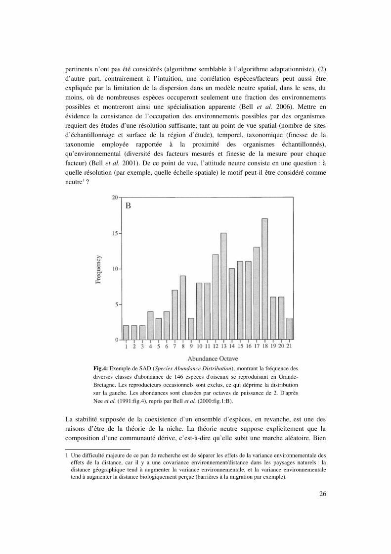
pertinents n’ont pas été considérés (algorithme semblable à l’algorithme adaptationniste), (2)d’autre part, contrairement à l’intuition, une corrélation espèces/facteurs peut aussi êtreexpliquée par la limitation de la dispersion dans un modèle neutre spatial, dans le sens, dumoins, où de nombreuses espèces occuperont seulement une fraction des environnementspossibles et montreront ainsi une spécialisation apparente (Bell et al. 2006). Mettre enévidence la consistance de l’occupation des environnements possibles par des organismesrequiert des études d’une résolution suffisante, tant au point de vue spatial (nombre de sitesd’échantillonnage et surface de la région d’étude), temporel, taxonomique (finesse de lataxonomie employée rapportée à la proximité des organismes échantillonnés),qu’environnemental (diversité des facteurs mesurés et finesse de la mesure pour chaquefacteur) (Bell et al. 2001). De ce point de vue, l’attitude neutre consiste en une question : à quelle résolution (par exemple, quelle échelle spatiale) le motif peutil être considéré commeneutre1 ?

La stabilité supposée de la coexistence d’un ensemble d’espèces, en revanche, est une desraisons d’être de la théorie de la niche. La théorie neutre suppose explicitement que lacomposition d’une communauté dérive, c’estàdire qu’elle subit une marche aléatoire. Bien

1 Une difficulté majeure de ce pan de recherche est de séparer les effets de la variance environnementale deseffets de la distance, car il y a une covariance environnement/distance dans les paysages naturels : la distance géographique tend à augmenter la variance environnementale, et la variance environnementaletend à augmenter la distance biologiquement perçue (barrières à la migration par exemple).

26

Fig.4: Exemple de SAD (Species Abundance Distribution), montrant la fréquence desdiverses classes d'abondance de 146 espèces d'oiseaux se reproduisant en GrandeBretagne. Les reproducteurs occasionnels sont exclus, ce qui déprime la distributionsur la gauche. Les abondances sont classées par octaves de puissance de 2. D'aprèsNee et al. (1991:fig.4), repris par Bell et al. (2000:fig.1:B).

que caractérisée, du fait des dynamiques démographiques, par des autocorrélationstemporelles, la composition d’une communauté neutre ne présente donc aucun équilibre, et,encore moins de résilience. Notons qu’à l’inverse, sa diversité tend vers un équilibredynamique spéciation/dérive1. Cet aspect de la théorie en fait une hypothèse nulle intéressantepour tester les écarts à la dérive, au sein d’une communauté ou entre communautés (section3.4.2). La stabilité et la résilience de la composition après une perturbation, les tempsd’extinction trop courts pour être neutres dans les registres fossiles, les explosionsdémographiques des espèces invasives, plaident, à cet égard, pour des explications en termesde niches (Bell et al. 2006).Ce concept de dérive des communautés a été appliqué à l'étude de la divergence decommunautés isolées. Si les communautés sont isolées, la théorie neutre prédit que ladiversité sommée des communautés croit linéairement au cours du temps (jusqu'à néanmoinsune diversité sommée maximale où les communautés n'ont plus aucune espèce en commun etont atteint chacune l'équilibre spéciation/extinction), tandis que la théorie de la niche préditque les compositions de communautés semblables doivent rester, du moins sur le tempsécologique, semblables (du fait de mécanismes stabilisants). Malheureusement, même ensituation neutre, un seul migrant par génération et par communauté suffit à homogénéiser lescompositions de chaque communauté, ce qui rend, une fois encore, les prédictionsindiscernables (Bell et al. 2006).

3.4 Nature de l’opposition entre théorie neutre et théorie de la niche

La difficulté à départager les théories était déjà présente dans la controverse entre neutralismeet sélectionnisme en génétique des populations. Elle y a été contournée par le développementd’un modèle synthétique, dit quasineutre, qui prend en compte les effets de la dérive et de lasélection (Ohta 1973). Un tel modèle a été élaboré également en écologie des communautés(Zhou & Zhang 2008), mais qui n’élude pas la difficulté de déterminer l’origine (sélection oudérive) des patterns observés, ni la difficulté du statut de la stochasticité.

3.4.1 Statut de la stochasticité

Le statut de la stochasticité (sensu aléatoire) a sans doute généré une confusion importantedans le débat, qui peut être illustrée par l’emploi d’une terminologie malheureuse : celle de forces stochastiques, ou forces neutres (stochasticité démographique par exemple) paropposition aux forces déterministes (sélection par exemple). Sans nous prononcer sur laprésence, irréductible ou non, de l’aléatoire en biologie2, remarquons que le syntagme forcestochastique tient de l’oxymore : la stochasticité est justement ce qui n’est pas directionnel3.En fait, les termes stochastiques d’un modèle représentent des mécanismes inconnus oulaissés de côté (ou considérés, dans la théorie, comme intrinsèquement aléatoires, par exemple

1 En d'autres termes si la composition d'une communauté neutre ne présente aucun équilibre ni résilience, cen'est pas le cas des caractéristiques de cette composition (nombre d'espèces, fréquences relatives etc).

2 Cf. Malaterre & Merlin, ce volume. (NdÉ.)3 Nous entendons ici « directionnel » au sens d'une direction dans l'évolution des fréquences (des allèles ou

des espèces par exemple), ou dans la répartition des espèces (ou des allèles) sur un paysage donné. Ladérive, à l'inverse, peut être considérée comme un bruit : elle « explique » dans quelle mesure on ne peutpas connaître la direction de l'évolution.

27

en physique quantique). Autrement dit, les termes stochastiques représentent la partd’information absente du modèle, et n’ont pas d’autre vertu explicative que la part d’inconnudans le résultat. Abandonner certains termes déterministes au profit de termes stochastiquesne doit pas se faire uniquement dans le but de gagner en parcimonie, mais aussi en vérifiantque l’explanandum d’intérêt n’est pas abandonné. Par exemple, la théorie neutre laisse de côtéun explanandum notable : elle ne permet pas, du fait de la symétrie, de prédire quelles espèces vont être rares ou fréquentes. À ce titre, le continuum de plus en plus consensuel (e.g. Gewin2006) entre déterminisme et stochasticité, interprété comme un continuum de causalité(chaque force pouvant déterminer la dynamique à divers degrés) est à apprécier plutôt commeun continuum de la quantité d’information introduite dans un modèle (cf. Clark et al. 2007,2009).

3.4.2 La théorie neutre : une hypothèse nulle ?

La théorie neutre a montré la nonnécessité de la théorie de la niche quant à l’explication, aumoins au niveau qualitatif, des motifs de répartition spatiale ou des motifs de diversité – sauf,il est vrai, en cas de sélection forte ou aux grandes échelles spatiales (Bell 2006). De ce fait, età cause de sa parcimonie, la théorie neutre est souvent considérée comme une hypothèse nulleà, éventuellement, réfuter (e.g. Leigh 2007)1.Typiquement, les modèles de la théorie neutre font appel à deux hypothèses : (1) une double hypothèse d’équivalence des espèces : aux niveaux écologique (pas de stabilisation) et compétitif (fitness moyennes égales), (2) pour les modèles spatiaux (explicites ou implicites),une hypothèse de limitation de la dispersion.Une hypothèse alternative de (1) est une hypothèse selon laquelle les espèces ne sont paséquivalentes, au niveau compétitif et/ou écologique ; c’est l’hypothèse que posent les modèles de coexistence basés sur le concept de niche. À ce titre, le test de la dérive dans le temps de lacomposition d’une communauté revêt bien un caractère de test d’hypothèse nulle par rapportaux modèles de niche.Le cas spatial est plus ambigu. L’hypothèse (2) est une hypothèse de connectivité de l’espace.Son hypothèse alternative, à première vue, est une absence de connectivité (c’estàdire unedispersion illimitée), et non l’hypothèse d’hétérogénéité des écologies des espèces et des facteursécologiques dans l’espace, que posent les modèles de répartition basés sur la niche. La difficulté àrejeter un modèle neutre ou de niche par l’examen de motifs spatiaux invite également à préférer,plutôt qu’un test d’hypothèse nulle, une approche de sélection de modèles, dans laquelle leshypothèses concurrentes sont confrontées simultanément aux données, et classées selon descritères tels que la vraisemblance, la parcimonie, etc. (cf. Johnson & Omland 2004, Clark 2007).

3.4.3 Dimensionnalité des modèles

Clark et al. (2004, 2007, 2009) ont apporté un éclairage intéressant sur l’opposition entre

1 La théorie neutre n’a pas été toujours perçue comme une hypothèse nulle. Bell (2001 : 2418) distingue ainsi deux versions de la théorie : (1) la version faible, selon laquelle la théorie est certes capable de générer des motifs semblables à ceux trouvés dans les données, mais qui ne suppose pas que la théorie identifie lesprincipaux mécanismes sousjacents aux motifs d’abondance et de diversité, (2) la version forte, selonlaquelle la théorie neutre connaît un tel succès prédictif précisément parce qu’elle a identifié cesmécanismes.

28

modèles neutres et modèles de niche. Selon eux, chaque type de modèle échoue à expliquer ladiversité : les modèles de niche, parce qu’on observe trop peu de tradeoffs et deschevauchements trop importants sur le terrain par rapport aux réquisits des modèles, et lesmodèles neutres, parce qu’ils n’expliquent pas la stabilité et la résilience observées dans lescommunautés. Cette faillite épistémique serait due à la basse dimensionnalité de ces modèles,même en théorie de la niche. Selon Clark et al., la basse dimensionnalité est favorisée enécologie pour plusieurs raisons : les modèles doivent être solubles, peu d’axes de ressources et de tradeoffs seulement sont perçus empiriquement, enfin, les critères de sélection de modèlesqui s’appuient sur la parcimonie et éliminent tous les effets non significatifs, ainsi que le fit derelations déterministes avec un bruit résiduel, font apparaître des relations à bassedimensionnalité. Clark et al. proposent une alternative : explorer explicitement les processus mal représentés ou mis de côté et envisager des modèles complexes. À l’aide d’une techniqued’inférence (modèle hiérarchisé bayesien), ils révèlent des différences de niches de hautedimensionnalité chez deux espèces d’arbres en apparence écologiquement équivalentes. Cetappel à des explications de haute dimensionnalité fait écho à un article fondateur deHutchinson (1961) sur le même sujet. Du point de vue de la structure, les modèles neutres etde niche classiques appartiennent à la même famille de modèles (basse dimensionnalité) etsont à opposer aux modèles de haute dimensionnalité. En revanche, les modèles de niche debasse et de haute dimensionnalités visent le même explanandum : déterminer l’abondance de certaines espèces, ou les issues de situations de compétition par exemple.

4 Conclusions

4.1 Acceptions du concept

Même si le mot « niche » en écologie a substantiellement changé d’acception en un siècle d’existence, ses multiples sens gravitent tous autour de la vision darwinienne d’écosystèmesstructurés par la lutte pour la survie. À l’origine, le mot signifie une place dans l’écosystème,au sens d’une relation aux ressources, aux prédateurs et à l’habitat. Grinnell et Elton, encomparant des communautés, en viennent à s’intéresser aux équivalents écologiques, c’estàdire à des espèces ayant une niche similaire dans des localités ou des écosystèmes différents : le mot « niche » se teinte d’une connotation d’invariant de la structure des écosystèmes. L’idée selon laquelle deux espèces qui coexistent au même endroit doivent occuper des nichesdifférentes, déjà présente chez Darwin et ses successeurs, dont Grinnell, et plus tarddénommée principe d’exclusion compétitive, fournit le cadre de la redéfinition de Hutchinson.Hutchinson formalise la niche d’une espèce comme le volume, dans l’espace des variablesenvironnementales, où l’espèce peut survivre indéfiniment (niche fondamentale), ou bien levolume, restreint du fait des interactions avec les compétiteurs présents, où l’espèce surviteffectivement (niche réalisée). La niche est propre à chaque espèce, l’invariance de lastructure de l'écosystème n’est plus présupposée. Par cette formalisation, Hutchinson ouvre lavoie à la quantification des différences de niche qui permettent la coexistence et dessimilarités qui conduisent à l’exclusion, une préoccupation déjà présente chez Darwin (1859 : 320). Il est notable qu’au cours de l’histoire des recherches sur l’exclusion compétitive, et enparticulier dans l’article fondateur de Hutchinson (1957 : 417418), le statut du principe

29

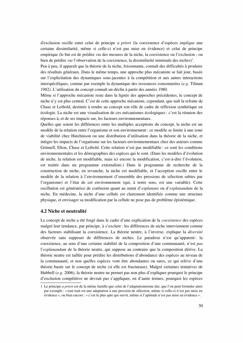
d'exclusion oscille entre celui de principe a priori (la coexistence d’espèces implique unecertaine dissimilarité, même si celleci n’est pas mise en évidence) et celui de principeempirique (le but est de prédire via des mesures de la niche, la coexistence ou l’exclusion ; oubien de prédire via l’observation de la coexistence, la dissimilarité minimale des niches)1.Peu à peu, il apparaît que la théorie de la niche, foisonnante, connaît des difficultés à produiredes résultats généraux. Dans le même temps, une approche plus mécaniste se fait jour, baséesur l’explicitation des dynamiques sousjacentes à la compétition et aux autres interactionsinterspécifiques, comme par exemple la dynamique des ressources consommées (e.g. Tilman1982). L’utilisation du concept connaît un déclin à partir des années 1980.Même si l’approche mécaniste reste dans la lignée des approches précédentes, le concept deniche n’y est plus central. C’est de cette approche mécaniste, cependant, que naît la refonte deChase et Leibold, destinée à rendre au concept son rôle de cadre de réflexion synthétique enécologie. La niche est une visualisation de ces mécanismes écologiques : c’est la réunion des réponses à, et de ses impacts sur, les facteurs environnementaux.Quelles que soient les différences entre les multiples acceptions du concept, la niche est unmodèle de la relation entre l’organisme et son environnement : ce modèle se limite à une zone de viabilité chez Hutchinson ou une distribution d’utilisation dans la théorie de la niche, etintègre les impacts de l’organisme sur les facteurs environnementaux chez des auteurs commeGrinnell, Elton, Chase et Leibold. Cette relation n’est pas modifiable : ce sont les conditions environnementales et les démographies des espèces qui le sont. (Dans les modèles d’évolutionde niche, la relation est modifiable, mais ici encore la modification, c’estàdire l’évolution,est traitée dans un programme externaliste.) Dans le programme de recherche de laconstruction de niche, en revanche, la niche est modifiable, et l’acception oscille entre lemodèle de la relation à l’environnement (l’ensemble des pressions de sélection subies parl’organisme) et l’état de cet environnement (qui, à notre sens, est une variable). Cetteoscillation est génératrice de confusion quant au statut d’explanans ou d’explanandum de laniche. En médecine, la niche d’une cellule est clairement identifiée comme une structurephysique, et envisager sa modification par la cellule ne pose pas de problème épistémique.

4.2 Niche et neutralité

Le concept de niche a été forgé dans le cadre d’une explication de la coexistence des espècesmalgré leur tendance, par principe, à s’exclure : les différences de niche interviennent comme des facteurs stabilisant la coexistence. La théorie neutre, à l’inverse, explique la diversitéobservée sans supposer de différences de niches. Le paradoxe n’est qu’apparent : la coexistence, au sens d’une certaine stabilité de la composition d’une communauté, n’est pasl’explanandum de la théorie neutre, qui suppose au contraire que la composition dérive. Lathéorie neutre est taillée pour prédire les distributions d’abondance des espèces au niveau dela communauté, et non quelles espèces vont être abondantes ou rares, ce qui relève d’unethéorie basée sur le concept de niche (si elle est fructueuse). Malgré certaines tentatives deHubbell (e.g. 2006), la théorie neutre ne permet pas non plus d’expliquer pourquoi le principed’exclusion compétitive ne devrait pas s’appliquer, en d’autre termes, pourquoi les espèces

1 Le principe a priori est de la même famille que celui de l’adaptationnisme dur, que l’on peut formuler ainsipar exemple : « tout trait est une adaptation à une pression de sélection, même si celleci n’est pas mise en évidence », ou bien encore : « c’est le plus apte qui survit, même si l’aptitude n’est pas mise en évidence ».

30

devraient évoluer vers des fitness égales. Nous avons vu que les motifs de diversité ne sont la plupart du temps pas discriminants quantaux hypothèses d’une stabilisation des communautés ou d’une équivalence des espèces – ce quisignifie que ces motifs ne peuvent pas être interprétés comme des indices favorisant l’une oul’autre hypothèse. À ce titre, la théorie neutre a élargi la famille des modèles aptes à expliquerles motifs de diversité, ce qui permet en retour de mieux cerner les hypothèses non nécessaires àl’explication de ces motifs.La plupart des critiques se sont concentrées sur l’hypothèse d’équivalence des fitness, qui paraîthautement improbable, tandis que l’hypothèse de stabilisation est bien documentée tant du pointde vue théorique (Chesson 2000) qu’empirique (Bell 2006). Cette hypothèse d’équivalence seprésente cependant comme une approximation opératoire pour dériver une certaine famille derésultats dans l’étude de la diversité, quoiqu’elle puisse diminuer la robustesse de la théorie. Lesapports de la théorie neutre ne se limitent pas aux hypothèses d’équivalence (écologique et defitness moyenne) : les accents mis sur la limitation de la dispersion, sur la stochasticité (c’està dire la part d’inconnu) et les effets d’échantillonnage sont tout à fait détachables des hypothèsesd’équivalence et intégrables à une théorie mécaniste (Alonso et al. 2006). La théorie neutrereprésente ainsi une première entrée dans des domaines théoriques difficiles, comme les solutionsanalytiques de modèles spatialement explicites (Bramson 1996, 1998). L’hypothèsed’équivalence des fitness, centrale à l’origine, ne devrait plus apparaître que comme un caslimite1.

1 Nous tenons à remercier Frédéric Bouchard, Antoine Collin, Régis Ferrière, Jean Gayon, Philippe Huneman, MaëlMontévil, Michel Morange, François Munoz, Aurélien Pocheville et Marc Silberstein, dont les suggestions ont permisd’améliorer considérablement les versions précédentes du manuscrit.

31

Références bibliographiques

ACKERMANN M. & DOEBELI M. (2004), “Evolution of niche width and adaptive diversification”,Evolution, 58(12) : 25992612. ADLER P.B., JANNEKE H.L & LEVINE J.M. (2007), “A niche for neutrality”, Ecology Letters, 10 : 95104.ALONSO D., ETIENNE R.S. & MCKANE A.J. (2006), “The merits of neutral theory”, 21(8) : 451 457.ARISTOTE (1883), Histoire des animaux, trad. J. BarthélémySaint Hilaire, Paris, Hachette.

<http://remacle.org/bloodwolf/philosophes/Aristote/tableanimaux.htm>.BEGON M.,TOWNSEND C. R., HARPER J. L. (2006), Ecology: from individuals to ecosystems,Oxford, Blackwell Publishing Ltd.BELL G. (2000), “The Distribution of Abundance in Neutral Communities”, The AmericanNaturalist, 155(5) : 606617. BELL G. (2001), “Neutral Macroecology”, Science, 293 : 24132418. BELL G., LECHOWICZ M.J. & WATERWAY M.J. (2001), “The scale of local adaptation in forestplants”, in J. Silvertown & J. Antonovics (eds.), Integrating Ecology and Evolution in aSpatial Context, Special Symposium of the British Ecological Society, Oxford, BlackwellScience.BELL G., LECHOWICZ Martin J. & WATERWAY Marcia J. (2006), “The comparative evidencerelating to functional and neutral interpretations of biological communities”, Ecology, 87(6) : 13781386.BEERAVOLU C. R., COUTERON P., PÉLISSIER R. & MUNOZ F. (2009), “Studying ecologicalcommunities from a neutral standpoint:A review of models’ structure and parameterestimation”, Ecological Modelling,220(20):26032610 BERSHAD A.K., FUENTES M.A. & KRAKAUER D.C. (2008), “Developmental autonomy andsomatic niche construction promotes robust cell fate decisions”, Journal of TheoreticalBiology, 254(2) : 408416. BRAMSON M., COX J.T. & DURRETT R. (1996), “Spatial models for species area curves”, Annalsof Probability, 24 : 17271751. BRAMSON M., COX J.T. & DURRETT R. (1998), “A spatial model for the abundance of species”,Annals of Probability, 28 : 658709. CADOTTE M.W. (2004), “Book Review. Ecological Niches : Linking Classical and Contemporary Approaches”, Biodiversity and Conservation, 13 : 17911793. CASE T.J. (1982), “Coevolution in resourcelimited competition communities”, TheoreticalPopulation Biology, 21 : 6991. CASWELL H. (1976), “Community structure : a neutral model analysis”, EcologicalMonographs, 46 : 327354. CHASE J.M. & LEIBOLD M.A. (2003), Ecological Niches : Linking Classical and Contemporary Approaches, Chicago, University of Chicago Press.CHAVE J. (2004), Neutral theory and community ecology., Ecology Letters, 7:241253. CHAVE J. & LEIGH E. G. (2002), A spatiallyexplicit neutral model of betadiversity in tropicalforests., Theoretical Population Biology, 62:153168.

32

CHESSON P. (2000), “Mechanisms of maintenance of species diversity”, Annual Review ofEcology, Evolution and Systematics, 31 : 343366. CHESSON P. & REES M. (2007), “Commentary on Clark et al. (2007) : Resolving the biodiversity paradox”, Ecology Letters, 10(8) : 659661. CLARK J.S. (2007), Models for Ecological Data : An Introduction , Princeton, Princeton UP.CLARK J.S. (2009), “Beyond neutral science”, Trends in Ecology & Evolution, 24(1) : 815. CLARK J.S., DIETZE M., CHAKRABORTY S., AGARWAL P.K., IBANEZ I., LADEAU S. & WOLOSIN M.(2007), “Resolving the biodiversity paradox”, Ecology Letters, 10(8) : 647659. CLEMENTS F.E. (1916), Plant Succession: An Analysis of the Development of Vegetation,Washington D.C., Carnegie Institution of Washington.COLWELL R.K. (1992), “Niche : A Bifurcation in the Conceptual Lineage of the Term”, in E.F.Keller & E.A. Lloyd (eds.), Keywords in Evolutionary Biology, Cambridge, Harvard UP.DARWIN C.R. (1859), On the origin of species by means of natural selection, or thepreservation of favoured races in the struggle for life, London, John Murray, 1st ed., 1st issue.

<http://darwinonline.org.uk>.DARWIN C.R. (1872), The origin of species by means of natural selection, or the preservationof favoured races in the struggle for life, London, John Murray, 6th ed.

<http://darwinonline.org.uk>.DAWKINS R. (1982), The Extended Phenotype, Oxford, WH Freeman.DAWKINS R. (2004), “Extended Phenotype – But Not Too Extended. A Reply to Laland, Turnerand Jablonka”, Biology and Philosophy, 19 : 377396. DAY R.L., LALAND K.N. & ODLINGSMEE J. (2003), “Rethinking Adaptation – The nicheconstruction perspective”, Perspectives in Biology and Medicine, 46(1) : 8095. DERVILLE A. (1999), L’agriculture du Nord au Moyen Âge, Presses Universitaires duSeptentrion.DOAK D.F., BIGGER D., HARDING E.K., MARVIER M.A., O’MALLEY R.E. & THOMSON D. (1998),“The Statistical Inevitability of StabilityDiversity Relationships in Community Ecology”,The American Naturalist, 151(3) : 264276. DODGE Y. (2004), Statistique : dictionnaire encyclopédique, Paris, Springer Verlag.DORMANN C.F. (2008), “On community matrix theory in experimental plant ecology”, WebEcology, 8 : 108115. ELTON C.S. (1927), Animal Ecology, New York, Macmillan Co.

<www.archive.org/details/animalecology00elto>.ENGELBRECHT B.M.J. et al. (2007), “Drought sensitivity shapes species distribution patterns intropical forests”, Nature, 447 : 8082. GAFFNEY B.M. (1973), Roots of the niche concept, American Naturalist, 109:490GAUSE G.F. (1934), The Struggle for Existence, Baltimore, Williams and Wilkins.

<www.ggause.com/Contgau.htm>.GAYON J. & VEUILLE M. (2001), “The genetics of experimental populations : L’Héritier and Teissier’s population cages (19321954)”, in R. Singh et al. (eds.), Thinking about Evolution : Historical, Philosophical and Political Perspectives, Cambridge, Cambridge UP : 77102. GEWIN V. (2006), “Beyond Neutrality – Ecology Finds Its Niche”, PloS, 41(8) : e278. GOULD S.J. & LEWONTIN R.C. (1979), “The sprandels of San Marco and the Panglossianparadigm : a critique of the adaptationist programme”, Proceedings of the Royal Society of

33

http://darwin-online.org.uk/

http://www.ggause.com/Contgau.htm

http://www.archive.org/details/animalecology00elto

http://darwin-online.org.uk/

London, Series B, Biological Sciences, 205 : 581598. GRIESEMER J. (1992), “Niche : Historical Perspectives”, in E.F. Keller & E.A. Lloyd (eds.),Keywords in Evolutionary Biology, Cambridge, Harvard UP.GRINNELL J. (1904), “The origin and distribution of the chestnutbacked chickadee”, The Auk,21 : 364379. GRINNELL J. (1917), “The nicherelationships of the California trasher”, The Auk, 34 : 427433. <http://artifex.org/~ecoreaders/lit/Grinnell1917.pdf >. GRINNELL J. (1928), “Presence and absence of animals”, University of California Chronicle,30 : 429450. Repris in J. Grinnell, Joseph Grinnell’s Philosophy of Nature, Berkeley & LosAngeles, University of California Press, 1943.GRINNELL J. & SWARTH H.S. (1913), “An account of the birds and mammals of the San Jacintoarea of Southern California”, University of California Publications in Zoology, 10 : 197406. GRUBB P.J. (1977), “The maintenance of speciesrichness in plant communities : the importance of the regeneration niche”, Biological Reviews, 52 : 107145. HAECKEL E. (1874), Histoire de la création des êtres organisés d’après les lois naturelles,Paris, Reinwald.HALDANE J.B.S. (1957), “The cost of natural selection”, Journal of Genetics, 55 : 511524. HARDIN G. (1960), “The Competitive Exclusion Principle”, Science, 131 : 12921297. HUBBELL S.P (1979), “Tree dispersion, abundance and diversity in a tropical dry forest”,Science, 203 : 12991309. HUBBELL S.P. (2001), The Unified Neutral Theory of Species Abundance and Diversity,Princeton, Princeton UP.HUBBELL S.P. (2005), “Neutral theory in community ecology and the hypothesis of functionalequivalence”, Functional Ecology, 19 : 166172. HUBBELL S.P. (2006), “Neutral Theory and the Evolution of Ecological Equivalence”, Ecology,87(6) : 13871398. HUBBELL S.P. et al. (2008), “How many tree species are there in the Amazon and how many ofthem will go extinct ?”, PNAS USA, 105 (suppl.1) : 1149811504. HURTT G.C. & PACALA S.W. (1995), “The consequences of recruitment limitation. Reconcilingchance, history, and competitive differences between plants”, Journal of Theoretical Biology,176 : 112. HUTCHINSON G.E. (1944), “Limnological studies in Connecticut. VII. A critical examination ofthe supposed relationship between phytoplankton periodicity and chemical changes in lakewaters”, Ecology, 26 : 326. HUTCHINSON G.E. (1957), “Concluding remarks”, Cold Spring Harbor Symposia onQuantitative Biology, 22 (2) : 415427 .<http://artifex.org/~ecoreaders/lit/Hutchinson1957.pdf>.HUTCHINSON G.E. (1959), “Homage to Santa Rosalia or Why Are There So Many Kinds ofAnimals ?”, The American Naturalist, 93 : 145. HUTCHINSON G.E. (1961), “The paradox of the plankton”, The American Naturalist, 95 : 137 145.HUTCHINSON G.E. (1978), An Introduction to Population Ecology, New Haven, Yale UP.IVES A.R. & CARPENTER S.R. (2007), “Stability and Diversity of Ecosystems”, Science, 317 : 5862.

34

http://artifex.org/~ecoreaders/lit/Hutchinson1957.pdf

http://artifex.org/~ecoreaders/lit/Grinnell1917.pdf

JOHNSON R.H. (1910), Determinate Evolution in the color pattern of the Ladybeetles,Washington, Carnegie Institution of Washington.JOHNSON J.B. & OMLAND K.S. (2004), “Model selection in ecology and evolution”, Trends inEcology & Evolution, 19(2) : 101108. KELLY C., BOWLER M.G., PYBUS O. & HARVEY P.H. (2008), “Phylogeny, niches, and relativeabundance in natural communities”, Ecology, 89 : 962970. KIMURA M. (1968), “Evolutionary Rate at the Molecular Level”, Nature, 217 : 624626. KIMURA M. (1983), The Neutral Theory of Molecular Evolution, Cambridge, Cambridge UP.KOSTITZIN V.A. (1935), Evolution de l’atmosphère, Exposés de biométrie et de statistiquebiologique, VIII, Paris, Hermann, cité par T.W. Schoener, “The Ecological Niche”, in J.M.Cherrett (ed.), Ecological Concepts : The Contribution of Ecology to an Understanding of theNatural World, Cambridge, Blackwell, 1989.KREBS, C.J. (1994), Ecology : The Experimental Analysis of Distribution and Abundances, 6th

edition, HarperCollins College PublishersLACK D. (1947), Darwin’s Finches, Cambridge, Cambridge UP.LEIBOLD M.A. (1995), “The niche concept revisited: mechanistic models and communitycontext”, Ecology, 76 : 13711382. LEHMAN C. & TILMAN D. (2000), “Biodiversity, Stability, and Productivity in CompetitiveCommunities”, The American Naturalist, 156 : 534552. LEIGH E.G. Jr (2007), “Neutral theory : a historical perspective”, Journal of EvolutionaryBiology, 20 : 20752091. LEWONTIN R.C. (1983), “Gene, organism, and environment”, in D.S. Bendall, Evolution frommolecules to men, Cambridge, Cambridge UP.LI L. & XIE T. (2005), “Stem Cell Niche : Structure and Function”, Annual Review of Cell andDevelopmental Biology, 21 : 605631. LINNÉ C. von (1972), L’économie de la nature [1744], trad. B. Jasmin, Paris, Vrin.LOEUILLE, N. & LOREAU, M., (2005). Evolutionary emergence of sizestructured food webs.

Proceedings of the National Academy of Sciences of the United States of America,102(16), p.57615766.

LOOIJEN R.C. (1998), Holism and reductionism in biology and ecology. The mutualdependence of higher and lower level research programs, Rijksuniversiteit Groningen.

<http://dissertations.ub.rug.nl/faculties/fil/1998/r.c.looijen/.LOREAU M. (2000), “Biodiveristy and ecosystem functioning: recent theoretical advances”,Oikos, 91 : 317. LOTKA A.J. (1924), Elements of physical biology, Baltimore, Williams and Wilkins.MACARTHUR R. H. & LEVINS R. (1967), “The limiting similarity, convergence and divergenceof coexisting species”, American Naturalist, 101 : 377385. MACLEAN C.R. & BELL G. (2002), “Experimental adaptive radiation in Pseudomonas”, TheAmerican Naturalist, 160 : 569581. MARGALEF R. (1968), Perspectives in Ecological Theory, Chicago, University of ChicagoPress.MCINTOSH R.P. (1986), The Background of Ecology : Concept and Theory , Cambridge,Cambridge UP.MESZÉNA G., GYLLENBERG M., PASZTOR L. & METZ J.A.J. (2005), “Competitive exclusion and

35

limiting similarity: A unified theory”, Theoretical Population Biology, 69 : 6887. MIKKELSON G.M. (2005), “NicheBased vs. Neutral Models of Ecological Communities”,Biology and Philosophy, 20 : 557566. MUNOZ F., COUTERON P., RAMESH B.R. & RAMPAL E.S. (2007), “Estimating parameters of neutralcommunities : from one single large to several small samples”, Ecology, 88(10) : 24822488. NEE, S., HARVEY P. H., MAY R. (1991), “Lifting the veil on abundance and diversity.”,Proceedings of the Royal Society of London B, Biological Sciences, 243:161163ODLINGSMEE J., LALAND K. & FELDMAN M. (2003), Niche Construction: The Neglected Processin Evolution, Princeton UP.OHTA T. (1973), “Slightly Deleterious Mutant Substitutions in Evolution”, Nature, 246(5428) : 9698.PARK T. (1948), “Experimental studies of interspecific competition. I. Comptition betweenpopulations of the flour beetles, Tribolium confusum Duval and Tribolium castaneaumHerbst”, Ecological Monographs, 18 : 265307. PARK T. (1954), “Experimental studies of interspecific competition. II. Temperature, humidity,and competition in two species of tribolium”, Physiological Zoology, 27 : 177238. PSAILA B. & LYDEN D. (2009), “The metastatic niche: adapting the foreign soil”, NatureReviews Cancer, 9(4) : 285293. POWELL K. (2005), “It’s the ecology, stupid !”, Nature, 435 : 268270. PUEYO S., HE F. & ZILLIO T. (2007), “The maximum entropy formalism and the idiosyncratictheory of biodiversity”, Ecology Letters, 10 : 10171028. RICKLEFS, R.E. (1979), Ecology, 2nd edition, New York, Chiron.ROHDE K. (2005), Nonequilibrium Ecology, Cambridge, Cambridge UP.ROOT R.B. (1967), “The niche exploitation pattern of the bluegrey gnatcatcher”, EcologicalMonographs, 37 : 317349. ROUGHGARDEN J. (1972), “Evolution of niche width”, American Naturalist, 103 : 683719. ROUGHGARDEN J. (1976), “Resource partitioning among competing species – a coevolutionaryapproach”, Theoretical Population Biology, 9 : 388424. SALISBURY E.J. (1929), “The biological equipment of species in relation to competition”,Journal of Ecology, 17 : 197222. SCADDEN D.T. (2006), “The stemcell niche as an entity of action”, Nature, 41 : 10751079. SCHOENER T.W. (1989), “The Ecological Niche”, in J.M. Cherrett (ed.), Ecological Concepts : The Contribution of Ecology to an Understanding of the Natural World, Cambridge,Blackwell.SCHOFIELD R. (1978), “The relationship between the spleen colonyforming cell and thehaemopoietic stem cell”, Blood Cells, 4(12) : 725. SCHOFIELD R. (1983), “The stem cell system”, Biomedicine & Pharmacotherapy, 37(8) : 375 380.SEMPER K. (1881), The Natural Conditions Of Existence As They Affect Animal Life, London,C. Kegan Paul & Co.SIMBERLOFF D. S. (1978), “Using island biogeographic distributions to determine ifcolonization is stochastic“, The American Naturalist, 112 : 713726. STAUFFER R.C. (ed.) (1975), Charles Darwin’s Natural Selection; being the second part of hisbig species book written from 1856 to 1858, Cambridge, Cambridge UP.

36

STEEG P.S. (2005), “Emissaries set up new sites”, Nature, 438 : 750751. STRONG D.R. (1980), “Null hypothesis in Ecology”, Synthese, 43 : 271285. TANSLEY A.G. (1917), “On competition between Galium saxatile L. (G. hercynicum Weig.)and Galium sylvestre Poll. (G. asperum Schreb.) on different types of soil”, Journal ofEcology, 5 : 173179. TAYLOR P. (1916), “The status of the beavers of Western North America, with a considerationof the factors in their speciation”, University of California Publications in Zoology, 12 : 413 495, cité par G.E. Hutchinson, An Introduction to Population Ecology, New Haven, Yale UP,1978 : 156157. TEISSIER G. & L’HÉRITIER P. (1935), « Recherches sur la concurrence vitale. Étude depopulations mixtes de Drosophila melanogaster et de Drosophila funibris », C. R. Soc. Biol.,t. 118 : 13961398. TILMAN D. (1982), Resource Competition and Community Structure., Princeton, Princeton UP.TILMAN D., LEHMAN C.L. & BRISTOW C.E. (1998), “DiversityStability Relationships : Statistical Inevitability or Ecological Consequence ?”, The American Naturalist, 151(3) : 277282. VANDERMEER J.H. (1972), “Niche Theory”, Annual Review of Ecology, Evolution andSystematics, 3 : 107132. VOLTERRA V. (1926), “Fluctuations in the abundance of a species considered mathematically”,Nature, 118 : 558560. WATT F.M. & HOGAN B.L.M. (2000), “Out of Eden : Stem Cells and Their Niches”, Science,287 : 14271430. WATTERSON G.A. (1974), “Models for the logarithmic species abundance distributions”,Theoretical Population Biology, 6 : 217250. WHITTAKER R.H., LEVINS S.A. & ROOT R.B. (1973), “Niche, habitat and ecotope”, AmericanNaturalist, 107 : 321338. WILLIAMSON M.H. (1972), The analysis of biological populations, London, Edward Arnold.WRIGHT S. (1931), “Evolution in Mendelian Populations”, Genetics, 16 : 97158. ZHANG D.Y. & LIN K. (1997), “The Effects of Competitive Asymmetry on the Rate ofCompetitive Displacement : How Robust is Hubbell’s Community Drift Model ?”, Journal oftheoretical biology, 188 : 361367. ZHOU S.R. & ZHANG D.Y. (2008), “A Nearly Neutral Model of Biodiversity”, Ecology,89(1) : 248258.

37

What niche construction is (not)

Introduction

The theory of evolution by natural selection can be traced back to Darwin and Wallace (1858)and Darwin (1859) – though of course, depending on one's taste for historical analogies, morevenerable predecessors can be found (e.g. Empedocles, Vth c. BC (Fairbanks 1898), or morerecently Sebright 1809, Matthew 1831, Thompson 1839). The theory was a charge against theimmutability of species and an argument for the descent with modification, as well as anargument for taking natural selection as “the main but not exclusive means of modification”(Darwin 1859:6). Moreover, throughout Darwin's book it is clear that “above all, Darwin'smechanism of natural selection was intended to explain that which British natural theologyfound so significant : adaptation.” (Ruse 1992:78). Ever since, the history of Darwin's (and Wallace's) theory has been rich (extended accounts ofthe story can be found in e.g. Mayr 1982, Sloan 2008). Two historical turns will beparticularly important for us : the synthesis between genetic gradualism and natural selectionas achieved by population genetics (Fisher 1930), and the synthesis between populationgenetics and taxonomy (Dobzhansky 1937), that would initiate the Evolutionary Synthesis inthe 40's (Mayr and Provine 19801998:xii). The Synthesis in turn would grant the divorcebetween evolutionary biology and embryology, despite some good times in common of thesedisciplines in the past (see Amundson 2005). Most of the current debates, including the placeof niche construction in evolutionary theory that we will study in details, are rooted in thisstory. We will come back to light historical accounts below to enlighten these roots more.For the two or three past decades (Lewontin 1983, OldingSmee 1988), evolutionary theoryhas delivered a growing movement “that has sought a reconceptualization of adaptation byplacing emphasis on niche construction” (Laland 2004:316). Niche construction is the processwhereby organisms, through their metabolism, activities, choices etc, modify the selectionpressures to which their or other's populations are exposed (OdlingSmee, Laland & Feldman,hereafter OLF 2003:419). Thus to the proponents of this movement, « there are in fact twologically distinct routes to the evolving match between organisms and their environments:either the organism changes to suit the environment, or the environment is changed to suit theorganism.” (OLF 2003:18). “Match” here, sounds like the “adaptations” to be explainedsolely by natural selection in Darwin's project as summarized by Ruse's quote above. Nicheconstruction is presented “not as just a product of evolution, but as a cocontributor, withnatural selection, to the evolutionary process itself.” (OLF 2003:370). Taking nicheconstruction into account should lead to a new, extended, evolutionary theory (OLF2003:370385).In this paper, we will investigate the organismenvironment symmetry introduced by nicheconstruction, in particular as regards adaptation, and how niche construction theory introducesnovelty in evolutionary biology. Most arguments will deal with verbal formalizations andsometimes, we will have to to investigate the meaning of a single word. Verbal formalizationsare versatile means to account for intricate phenomena. They help us to make sense of models

39

(in particular mathematical models), and probably guide, or rather constrain, our empiricaland theoretical explorations. Thus, indepth treatments of verbal formalizations are anecessary evil (see notably Fox Keller 2002, e.g.:138). They allow to escape verbal traps, ofwhich authors cited here are fully aware, but that could confuse naive readers. We will(briefly) see that figures or equations, that is, translations in other languages, can help but arenot sufficient for our questions.First, we will give some verbal formalism to lay the foundations for our questions (section 1).Then, we will present standard, if any standard, natural selection theory (section 2). Then, wewill present and discuss niche construction theory (section 3), in particular as regardsadaptation and evolutionary explanations (section 4). Finally, we will discuss its place in“alternative” evolutionary biologies (section 5), before concluding and summing up the mainpoint (section 6).

Note: To ease reading, numerous footnotes specify details while lightening the main text. Aglossary and a summary are given at the end of the text.

1. Our verbal formalism

1.1 Explanation and the many scales of biology

To start with, let us consider that an explanation consists of an invariant link betweendifferent (at least two) states of a system, e.g. some initial conditions and some outcome(Woodward 1997, 2001). Investigating the diverse possible forms of the invariant link fallsout the reach of this paper, let us just notice that for the explanation to be relevant, theinvariant must usually link as few outcomes as possible to given input variables1, for somecost in parsimony. In this paper, we will consider that the invariant is the explanans, i.e. thepart of the explanation that explains, and that the states are the explanandum, i.e. the part thatis explained2. Building the explanation consists in particular to define which part of thesystem belongs either to the invariant or to the state, for both the explanans and theexplanandum will change if some part of the invariant becomes a variable or vice versa. Thus,there is a fundamental asymmetry between the invariant and the set of states, deeply rooted inwhat an explanation is. This question will turn out to be crucial in the next parts.Except in the case of a theory of everything, explanations are local3 : they have a limited

1 For instance, the case where every possible outcome are linked to every possible input variables is atautology. In our opinion tautologies are not considered as explanatory, even in everyday life.

2 One could argue that the explanans contains also the initial conditions, and that the explanandum containsonly the output state. There can be reasons not to do so (in particular when it is desirable to keep anexplanatory symmetry between initial and final states, e.g. when the invariant is a bijection). Moregenerally, the rationale for equating invariance and explanans, is to consider that the invariant structures(makes sense of) the set of states. Anyway, this consideration does not affect the argument here.

3 Here we mean local in a similar sense than Van Frasen means abstraction below. In particular in VanFrasen's example about Caesar's death, the abstraction is valid relatively to a given timescale.

“The description of some account as an explanation of a given fact or event, is incomplete. It can only be anexplanation with respect to a certain relevance relation and a certain contrastclass. These are contextualfactors, in that they are determined neither by the totality of accepted scientific theories, nor by the event

40

range of validity (that is a limited range of definition and, if locally defined, of sufficientaccuracy). The range can be defined in terms of scales on given dimensions (spatial, temporal,etc), and/or of objects of study (microtubules, microorganisms, etc), or else. Assessing therange of validity of an explanation is a matter of betting (sensu GodfreySmith 1998:53),because knowing the range would require to know that everything is known, though it iscrucial to rumble where the explanation holds and where it does not. The biological explanations we will be concerned with in this paper deal with dynamicalsystems and are timescale dependent. The invariant in a dynamical system is the law oftransformation that enables one to predict, given some state, a later state (or retrodict aprevious state). The invariant includes parameters and everything else in the explanation thatdoes not depend on time. On the other hand, the state of the system is the set of the timedependent variables, at a given time. However, the invariant generally varies beyond, or below, some timescale. The usual way tosimplify the problem is to deliberately limit the range of the explanation by assessing a timescale separation between, say, fast and slow processes, and to consider that processes beyondor below the scale of study are invariant (for instance the laws of physics are invariant on thehuman time scale even if at the scale of the universe, they may have changed). Thus, differentdisciplines working each on a different scale will usually produce different explanations,which can in turn help them segregate into separate fields. This is the drama played by theexplanations considered in this paper.Here, we will consider several biological processes : mutation (very briefly), ontogeny,ecology, and (micro and macro) evolution. These processes are each usually associated with acorresponding timescale, and, as we shall see, these timescales are usually assumed to beseparated. It is worth noticing that time, here, does not mean the physical time, but rathersome biological time : generally the metrics involves the generation1. As different livingsystems typically have different generationlength, a given intrageneration explanation aboutsome system (e.g. some vertebrate) may well deal with physical durations that represent intergenerational term for other systems (e.g. some gut microbes). Thus, the expressions “smalltimescale” or “long timescale” have here to be understood relatively to a given system.

or fact for which an explanation is requested. It is sometimes said that an Omniscient Being would have acomplete explanation, whereas these contextual factors only bespeak our limitations due to which we canonly grasp one part or aspect of the complete explanation at any given time. But this is a mistake. If theOmniscient Being has no specific interests (legal, medical, economic; or just an interest in optics orthermodynamics rather than chemistry) and does not abstract (so that he never thinks of Caesar's deathqua multiple stabbing, or qua assassination), then no whyquestions ever arise for him in any way at all—and he does not have any explanation in the sense that we have explanations. If he does have interests,and does abstract from individual peculiarities in his thinking about the world, then his whyquestions areas essentially contextdependent as ours. In either case, his advantage is that he always has all theinformation needed to answer any specific explanation request. But that information is, in and by itself,not an explanation; just as a person cannot be said to be older, or a neighbour, except in relation toothers.” (Van Fraasen 1980:130).

1 For a thoughtprovoking, deeply worked out, work on biological time, see Bailly et al. (forthcoming).Bailly et al. propose to account for all intrinsically cyclic biological processes by adding to the physicaltime t, a 2nd time dimension (Ө?, the “biological time”), which would be, roughly speaking, kind of acircle.

41

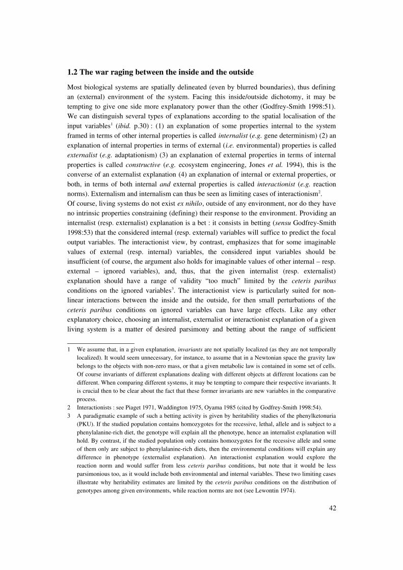
1.2 The war raging between the inside and the outside

Most biological systems are spatially delineated (even by blurred boundaries), thus definingan (external) environment of the system. Facing this inside/outside dichotomy, it may betempting to give one side more explanatory power than the other (GodfreySmith 1998:51).We can distinguish several types of explanations according to the spatial localisation of theinput variables1 (ibid. p.30) : (1) an explanation of some properties internal to the systemframed in terms of other internal properties is called internalist (e.g. gene determinism) (2) anexplanation of internal properties in terms of external (i.e. environmental) properties is calledexternalist (e.g. adaptationism) (3) an explanation of external properties in terms of internalproperties is called constructive (e.g. ecosystem engineering, Jones et al. 1994), this is theconverse of an externalist explanation (4) an explanation of internal or external properties, orboth, in terms of both internal and external properties is called interactionist (e.g. reactionnorms). Externalism and internalism can thus be seen as limiting cases of interactionism2. Of course, living systems do not exist ex nihilo, outside of any environment, nor do they haveno intrinsic properties constraining (defining) their response to the environment. Providing aninternalist (resp. externalist) explanation is a bet : it consists in betting (sensu GodfreySmith1998:53) that the considered internal (resp. external) variables will suffice to predict the focaloutput variables. The interactionist view, by contrast, emphasizes that for some imaginablevalues of external (resp. internal) variables, the considered input variables should beinsufficient (of course, the argument also holds for imaginable values of other internal – resp.external – ignored variables), and, thus, that the given internalist (resp. externalist)explanation should have a range of validity “too much” limited by the ceteris paribusconditions on the ignored variables3. The interactionist view is particularly suited for nonlinear interactions between the inside and the outside, for then small perturbations of theceteris paribus conditions on ignored variables can have large effects. Like any otherexplanatory choice, choosing an internalist, externalist or interactionist explanation of a givenliving system is a matter of desired parsimony and betting about the range of sufficient

1 We assume that, in a given explanation, invariants are not spatially localized (as they are not temporallylocalized). It would seem unnecessary, for instance, to assume that in a Newtonian space the gravity lawbelongs to the objects with nonzero mass, or that a given metabolic law is contained in some set of cells.Of course invariants of different explanations dealing with different objects at different locations can bedifferent. When comparing different systems, it may be tempting to compare their respective invariants. Itis crucial then to be clear about the fact that these former invariants are new variables in the comparativeprocess.

2 Interactionists : see Piaget 1971, Waddington 1975, Oyama 1985 (cited by GodfreySmith 1998:54).3 A paradigmatic example of such a betting activity is given by heritability studies of the phenylketonuria

(PKU). If the studied population contains homozygotes for the recessive, lethal, allele and is subject to aphenylalaninerich diet, the genotype will explain all the phenotype, hence an internalist explanation willhold. By contrast, if the studied population only contains homozygotes for the recessive allele and someof them only are subject to phenylalaninerich diets, then the environmental conditions will explain anydifference in phenotype (externalist explanation). An interactionist explanation would explore thereaction norm and would suffer from less ceteris paribus conditions, but note that it would be lessparsimonious too, as it would include both environmental and internal variables. These two limiting casesillustrate why heritability estimates are limited by the ceteris paribus conditions on the distribution ofgenotypes among given environments, while reaction norms are not (see Lewontin 1974).

42

accuracy (and definition), of the supposed type of interactions and, last but not least, of thekind of internal or external variability that is available in the given living system to explain1.Turning back to the dynamical biological systems, why is the internalist/externalist distinctionimportant ? Because, to state it generally, living systems are dynamical systems that engageinto diachronic interactions with their environment. When dealing with such an interaction, one obvious intuition is to consider that theenvironment is large compared to the system, and thus (please notice that this is an intuitiveand somewhat weak “thus”), that the environmental rate of change is slow compared with thesystem's rate of change. In particular, if the system is expected to exert some force on itsenvironment, the effects on the environment are supposed to be small and negligible.Thereby, this intuition leads to consider that there is a timescale separation between the fastinternal processes, and the slow environmental processes2. For instance, when studying plantgrowth, we consider Earth's effects on amyloplasts distribution in statocytes, which leads togravitropism (Wise & Hoober 2007:515), but we do not consider the effects of individualplant growth on the distribution of mass at the surface of the Earth. This amounts to considerthat environmental variables may be input variables (or not, if the environment is heldconstant3), but not output variables, in other terms, this intuition leads to provide nonconstructive explanations. In the next sections, we will examine the avatars and consequencesof such an intuition. Now, keeping this formalism in mind, we are going to discuss theselectionist scheme in evolutionary biology.

2. The selectionist scheme(s) in biology

This sections does not aim at providing a full account of the structure of evolutionary theory,nor at reviewing extensively the family of models built in it. Rather, the goal here is tohighlight several salient features of the selectionist scheme4.

2.1 The scheme

The selectionist scheme can be sketched as the fulfilment of the following two conditions5: (1)

1 The trick here is that the available variability is investigated regarding the bet on it. If a researchersupposes that a genetic explanation will be the most appropriate for some trait (for instance,developmental clocks), he will be inclined to try to produce genetic variants for this trait, thus reinforcingthe available internal variability.

2 This intuition may be reinforced in biology by the feeling that abiota is somehow inert, by contrast withliving systems.

3 We mean here “constant” over the whole range of the considered objects to explain. In particular, whendealing with several biological samples, if the environment is variable from one sample to another (evenif it is held constant for each sample), the environment can well be an input variable when aiming atcomparing the samples (e.g. in studies on evolutionary convergence).

4 We purposely avoid the term “Darwinian scheme” here, fully agreeing with Lewontin (1974) : “… theessential nature of the Darwinian revolution was neither the introduction of evolutionism as a world view(since historically that is not the case) nor the emphasis on natural selection as the main motive force inevolution (since empirically that may not be the case), but rather the replacement of a metaphysical viewof variation among organisms by a materialistic view.”. Fisher (1930, vii) made the same point.

5 This sketch is drawn from Lewontin (1970), though Lewontin's account is slightly different : “1. Differentindividuals in a population have different morphologies, physiologies, and behaviors (phenotypic

43

the existence of some heritable phenotypic variability among the individuals (whatever“individual” means) in the population (2) a determined relation (at a given point in time)between the considered phenotypic differences and some differences in fitness.A population fulfilling these conditions is expected to undergo natural selection. The twokeywords here, which will be at the centre of the argument, are heritability and fitness (orselection). Sketching their stories quickly will help to understand which historicalassumptions some current theorists would like to relax.

2.2 Historical perspectives

The substrate of heritability

Heritability has been historically central to Darwinism. The principle of “unity of descent”,independently from any natural selection principle, has been used by Darwin to explain the“unity of type”, that is, the resemblance of structure between organisms (Darwin 1859:206),which had been a critical issue for palaeontology and comparative anatomy during the XIX th

century (Sloan 2008).Heritability has here to be understood sensu Galton (1869), as any correlation1 acrossgenerations (heritability thus entails variability : there is no correlation if there is novariation), and not in terms of any specified mechanism of inheritance. However, part of thestory of biology during the XXth century has precisely been to look for the mechanisms ofinheritance in living systems (see Maienschein 1992), as well as to specify in which cases theinherited materials could lead to inherited differences in traits (see Wade 1992).For Darwin, inheritance could be a blending process involving entities (named gemmules) «

variation). 2. Different phenotypes have different rates of survival and reproduction in differentenvironments (differential fitness). 3. There is a correlation between parents and offspring in thecontribution of each to future generations (fitness is heritable).”

Lewontin puts the emphasis on heritability of fitness differences, while we put the emphasis on heritability ofphenotypic differences, provided that fitness is defined at each generation. Lewontin's goal in focusing onfitness here is to dismiss neutral phenotypes as irrelevant for the scheme. Lewontin does not specify thekind of the relationship between phenotype and fitness here (loose correlation, strict bijection, etc),neither do we. For the sake of exactness, if these relations are correlations, it is worth emphasizing thatcorrelations are not transitive (that is, “A correlated to B & B correlated to C” does not imply “Acorrelated to C”). Thus heritable phenotypic differences which would be themselves correlated todifferences in fitness would not entail heritable differences in fitness.

1 It has often be stressed (e.g. Hull 1988 :404) that “correlation is not strong enough for heritability. Thecorrelations must be causal.”. Without entering into details here, we do not see anything else in“causation” than robust correlations (for instance : robust against different background conditions ordifferent conditionals). However, unless when heritability is defined as the response to selection(breeder's equation : H² = R/S), the condition on inheritance is actually necessary but not sufficient, forthe effects of selection to be conserved across generations (because of the nontransitivity of correlations,see section 3.2). Unfortunately, when inheritance is defined as the response to selection, the conditionturns into a tautology (“effects of selection are conserved if there is response to selection”) – unless, ofcourse, we are provided with past measures of the response to selection that we can extrapolate. Forreviews of classical concepts of heritability, see Wade (1992), Feldman (1992), and Visscher et al.(2008), for a discussion of inclusive heritability (combining genetic and nongenetic inheritance) seeDanchin and Wagner (2010).

44

collected from all parts of the system to constitute the sexual elements” (1868:374). However,since the work of Hugo de Vries and Carl Correns in the early 1900 rediscovering Mendel'slaws of inheritance (1866), the substrate of inheritance has been supposed to be nonblendingentities, separate units of heredity that were named genes (after Johannsen 1909). (Here, wegloss over essential, but innumerable, historical complexities, such that the arguments ofPearson's school (1904) on the means to obtain discontinuous inheritance from blendingentities.) Implicitly, Mendel's laws required a separation between the processes of inheritanceon the one hand, and the ontogenetic processes on the other hand (Lewontin 1992), aseparation that has been achieved in the semantic domain by Johannsen (1911), coining theterms genotype and phenotype for the first and second processes respectively. Morgan (1917)then hypothesized that genes resided at particular locations on chromosomes, and Avery et al.(1944) showed that (some) genes were made up of DNA, specifying a little bit more thephysical substrate of inheritance. Crick (1957) postulated some years later that information,equated here as a precise sequence of bases or amino acids1, could only be transferred fromnucleic acid (to other nucleic acids or to proteins), but not from proteins (to other proteins orto nucleic acids)2. And as genes were supposed to be the only substrate for inheritance andwere thought to be effectively made up of amino acids, Crick's postulate offered a support toWeismann's principle (1889:392409) that acquired phenotypic characteristics could not beinherited (a principle, as mentioned earlier, already latent in Mendel's laws). Historically, thisprinciple has been important to dismiss the still ongoing Lamarckism (see Bowler 1992, Sloan2008).The roadstory of the gene concept did not end up here, and had many avatars, particularly inmolecular biology (reviewed in Gerstein et al. 2007). Interestingly, current molecularbiologists seem to no longer explicitly mention inheritance in their gene concept(s), ratherdefined in terms of a functional unit, which can be distributed throughout the genome 3 4 (seealso Fox Keller 2000).Thereby, part of the history of biology during the last century has been to investigate a (timescale) separation between the dynamics, here meant as the individual dynamics of one entity,of long lasting hereditary entities (the genes), assumed to remain unchanged throughoutgenerations except by supposedly rare accidents (mutations), and short lasting, mortal, entities(the phenotypes), whose individual dynamics, also named ontogenesis, were supposed to letthe long lasting hereditary entities virtually unchanged.

1 “Information means here the precise determination of sequence, either of bases in the nucleic acid or ofamino acid residues in the protein.” (Crick 1957, quoted in Judson 1979)

2 If information is to mean anything (for the sake of the argument, let's suppose it does), the fact thatnucleic acids bear information requires itself an explanation. The classical view (see e.g. Laland 2004) isthat populations of genes get informed through natural selection at the intergenerational scale. Thus thetransfer of information to genes is possible in the selectionist framework, but at another level than theindividual sequence.

3 See for instance the definition proposed by Gerstein et al. (2007) : “A gene is a union of genomicsequences encoding a coherent set of potentially overlapping functional products.”

4 By contrast, Kitcher (1992) has argued that we do not need to specify a priori segmentation rules fornucleic acids, dropping talk of genes and studying instead the properties of regions of nucleic acid aslong as, for evolutionary studies, the segments retained obey the rules of population genetics. Thisposition resonates with Dawkins' (1976) and Williams' (1966).

45

The object of selection

In parallel with the development of genetics, Fisher (1930) provided the first synthesis ofDarwinian selection and Mendelian genetics, giving birth to what is now known as populationgenetics. Fisher (e.g. 1918) was mainly interested in additive genetic effects on phenotype,which were heritable1 and could respond to selection, by contrast with dominance andepistatic genetic effects2, which were compared to environmental noise by Fisher (Fisher1930:xiii, Wade 1992, Okasha 2008). Wright (e.g. 1921, 1930, 1932) developed similarapproaches, but put an emphasis on epistasis and ruggedness of adaptive landscapes.Moreover, focusing on additivity of genetic effects somehow sustained gradualism (e.g.Fisher 1930:373), the view according to which major evolutionary changes, described bypalaeontology, can be explained by accumulation of small evolutionary changes, described bypopulation genetics. Gradualism had already been embraced by Darwin (1859, but see1866:132 for a “saltationist” hypothesis4) and had been a major subject of contention betweenBiometrical and Mendelian schools at the beginning of the century (Sloan 2008). Gradualismwould turn out to be one of the main points of the socalled Modern Synthesis of the 30's40'sbetween Mendelian and population genetics, cytology, ecology, systematics and paleontology(Mayr & Provine 1998).Notably, embryology had not been included in the Modern Synthesis, despite someembryological works of the founding fathers (Huxley 1932, Huxley and de Beer 1934, Wright1934), and despite the fact that the founding fathers were well aware of its importance (e.g.Huxley 1942:8, Mayr 1970:108). Reciprocally, embryologists of the early XXth century didnot care much about evolution, rather focusing on mechanisms of development (for a reviewon the (non)relation between the Synthesis and embryology, see Hamburger 1998). Theseparation between development and evolution culminated particularly in Mayr's dichotomybetween two biologies (1961, 1982:67) : the biology studying proximate (developmental)causes and the biology studying ultimate (evolutionary) causes : “Proximate causes have to dowith the decoding of the program of a given individual ; evolutionary causes have to do withthe changes of genetic programs through time, and with the reasons for these changes” (Mayr1982:68). To Mayr, the two biologies were both “remarkably self contained” (1982:68) andnecessarily complementary (1982:72,131), but the two kinds of causation were not to beconfused (1982:11,455,834). Noteworthily, this dichotomy was implicitly posed in terms oftimescale separation.At that time, for most population geneticists and supporters of the Modern Synthesis,

1 See “narrow sense heritability” in Lewontin (1974)2 See “broad sense heritability” in Lewontin (1974)3 The famous quote is : “Evolutionary changes are generally recognized as producing progressively higher

organization in the organic world.” (Fisher 1930:37)4 “But I must here remark that I do not suppose that the process ever goes on so regularly as is represented

in the diagram, though in itself made somewhat irregular, nor that it goes on continuously; it is far moreprobable that each form remains for long periods unaltered, and then again undergoes modification. Nordo I suppose that the most divergent varieties are invariably preserved: a medium form may often longendure, and may or may not produce more than one modified descendant; for natural selection willalways act according to the nature of the places which are either unoccupied or not perfectly occupied byother beings; and this will depend on infinitely complex relations.” (Darwin 1866:132). This sentenceappears in this (i.e. fourth) edition of The Origin.

46

theorizing evolution would imply to focus on genes frequencies (e.g. Dobzhansky 1937:11,defined evolution as a change in gene ratios, a view still dominating (Rosenberg andBouchard 20022008)). The genecentred perspective gained much interest a few decadeslater, with the “unit of selection” debate between geneselectionists (e.g. Williams 1966,Dawkins 1976), claiming that genes were the genuine units of selection, and organism (orgroup or species) selectionists, claiming that organisms, groups or species were the relevantunits to consider for selection studies (e.g. Lewontin 1970, 1974, Gould 1977, for speciesselection see Vrba 1984, Jablonski 1986).The debate could be quickly sketched as follow1 (here we give only a rough account of thedebate to put our section 3.5 in perspective ; we have to ignore primary but dense historicalsubtelties, interested readers can refer to e.g. Okasha 2006, Huneman 2010:348351). Geneselectionists claimed that no matter how much and how complicated interactions betweenloci, it would always be possible to identify a mean effect of any given gene substitution at agiven locus, on fitness at the population level (Williams 1966:57). Moreover, selection at ahigher level than the gene (e.g. selection for altruistic traits in a group) would suffer fromdynamical impediments, because evolutionary dynamics at lower levels (e.g. genes) werethought to be in general so much faster than dynamics at higher levels (e.g. groups), that theywould prevent most of the selection processes to be relevant at higher levels (Williams 1966,

1 The two positions are illustrated by this two following quotes :The first : “Obviously it is unrealistic to believe that a gene actually exists in its own world with no

complications other than abstract selection coefficients and mutation rates. The unity of the genotype andthe functional subordination of the individual genes to each other and to their surroundings would seem,at first sight, to invalidate the onelocus model of natural selection. Actually these considerations do notbear on the basic postulates of the theory. No matter how functionally dependent a gene may be, and nomatter how complicated its interactions with other genes and environmental factors, it must always betrue that a given gene substitution will have an arithmetic mean effect on fitness in any population. Oneallele can always be regarded as having a certain selection coefficient relative to another at the same locusat any given point in time. Such coefficients are numbers that can be treated algebraically, andconclusions inferred for one locus can bi iterated over all loci. Adaptation can thus be attributed to theeffect of selection acting independently at each locus. Although this theory is conceptually simple andlogically complete, it is seldom simple in practice and seldom provides complete answers to biologicalproblems. Not only do gene interactions and the processes of producing phenotypic effects offer auniverse of problems for physiological geneticists, but the environment itself is a complex and varyingsystem. Selection coefficients can be expected to change continually in all but the most stableenvironments, and to do so independently at each locus.” (Williams 1966:5657).

The second : “It must be remembered that each locus is not subject to selection separate from the others, sothat thousands of selective processes would be summed as if they were individual events. The entireindividual organism, not the chromosomal locus, it the unit of selection, and the alleles at different lociinteract in complex ways to yield the final product.” (Ayala 1978:64 quoted by Hull 1988:217).

Here, Williams argues that at the population level a selective effect, no matter how small, will take place oneach locus, while Ayala remarks that if selection is a screening process, the holes must have the size oforganisms, not genes. But this does not contradict Williams arguing about processes at the populationlevel.

The contradiction would rather come from nonrepeatability of selection events if the interactions betweenloci, and environmental changes, were too strong and the population too small : selection coefficientwould be inconsistent throughout generations and the dynamics, even if highly selective, would look likedrift (here with a high variance in offspring between individuals). Or, at the level of empirical sufficiency,the contradiction could come from the possible nonusability of the theory (see Lewontin 1974:9).

47

Lewontin 1970, but for selection at the species level see Jablonski 1986). The claim of geneselectionists was that reducing evolution to gene dynamics should be successful (Hull1988:422, GodfreySmith 2000:4). By contrast, organismselectionists highlighted that“selection does not see genes” but for instance whole organisms, and that interactionsbetween elements at all levels (mostly between loci in a genome, but also between organisms,groups, etc) were evolutionarily significant (the debate still goes on : the above, now quitecolloquial, quote on selection has been found in Minelli 2009:207). Most notably, Darwinhimself had not been sharp on this issue, endlessly speaking of the evolution of variations(e.g. 1859:12, 84), but in the meantime speaking of nature selecting variations for “the goodof” the individual (e.g. 1859:84), the group (e.g. 1859:202) or the species (e.g. 1859:201)1.As Hull (1980:313, 1988:217) has pointed out, most of the (bloody) debate arose because ofan ambiguity in the phrase “unit of selection” : gene selectionists actually meant that geneswere units of replication, fully aware (at least officially : Hull 1988:422) that selectioncoefficients should come from phenotypic effects (e.g. Williams 1966:57)2, while organismselectionists meant that organisms were units of interaction with the world (sensu Hull1980:318), most of them fully agreeing that genes were the units of replication (Mameli2004:37, see e.g. Lewontin 1970:143). A posteriori, the debate could seem pointless, butwords matter : for gene selectionists proposed to frame evolutionary theories without anyreference to interactions, focusing in particular on the bookkeeping of gene frequencies(Williams 1985), while organism selectionists urged not to evacuate from evolutionarybiology development and/or causal mechanisms leading to selection (Mayr 1978, Gould andLewontin 1979, Hull 1988:218, 422). As for developmental mechanisms, in the meantimeevolutionary developmental biology (evodevo) (re)emerged as a distinct field of research inthe 80's – partly as a resurgence of the earlier developmental genetics of Morgan(1926:510) and Goldschmidt 1940 (for a thoughtprovoking review on the historicalrelationships between embryology and evolutionary biology, see Amundson 2005). We willreturn to the issue of evodevo later.In conclusion, XXth century evolutionary biology has been stretched between an inclination toconsider development as a black box and separate it, at least temporarily (that is, for somedecades), from evolution, as did the Modern Synthesis and in particular geneselectionists 4,and an inclination to do the converse.

1 We let to reader's discretion the interpretation of Darwin's writings in terms of replicators (the variations)and interactors (individuals and groups).

2 Indeed, population genetics alone is insufficient to determine the values of particular selectioncoefficients, or to provide explanations that developmental studies could provide (e.g. the fact thatdevelopmental constraints could lead to evolutionary stasis, see e.g. Gould and Lewontin 1979).

3 Even when dealing with the theoretical possibility of selection at the level of the population, Lewontinframes the debate in genetic terms : “In this case the genetic composition of the species is a result of themore or less equal interaction of powerful selection at three levels.” (1970:14). The three levels here are :organelle, individual, and deme.

4 Being a supporter of the Synthesis does not imply to be geneselectionist. For instance, Mayr was far tobe a geneselectionist : « By the 1980s the geneticists had given up their endorsement of the gene as theobject of selection, and the synthesis can be considered fully completed only now.” (Mayr & Provine1998:xiii).

48

2.3 The selectionist scheme revisited

Historical accounts above have left us with several dichotomies that we will find useful to castthe problem, and specify the selectionist scheme in the dominant view. (These dichotomies,among others, have been critically reviewed in Amundson 2005 and Laland et al. 2008, butthese critics should not affect the presentation here. Besides, we will discuss thesedichotomies ourselves throughout the presentation.)

Heredity and replication

For the scheme to be applied across generations, (variable) longlasting, i.e. hereditary acrossgenerations, entities must be exhibited. With analogy to Weismann's separation between the(potentially immortal) germen and the (always mortal) soma of metazoans, such entities hasbeen qualified germline (Dawkins 19762006:172,258).Following Darwin (1859:Chap.III) evolutionary biologists focused on entities (mainlyorganisms and, later, genes) having geometrical rates of increase (in absence of any limitingfactor), that is, entities having somehow autocatalytic qualities. Indeed, geometrical dynamicsfavour competition and replacement of some variants by others, thus enhancing the relevanceof considering such autocatalytic entities to explain a given state of the living world1. Suchautocatalytic entities, faithfully reproducing (some of) their own variations, have been namedreplicators (Dawkins 19762006:Chap.2, 1978).Genes have been considered as the most paradigmatic units of heredity (as Mendeliancharacters) or of replication (as strands of nucleic acids). Because of mutation andrecombination that can break up a given sequence, the smallest unit of replication can be asingle nucleic base, but larger strands can also be considered provided that they aresufficiently variable, and sufficiently stably transmitted and/or sufficiently affected byselection to overcome the degradation dynamics caused by mutation and recombination(Williams 1966:24, Dawkins 19762006:36, Kitcher 1992). By contrast, organisms (orgroups) are considered too ephemeral and unable to pass on changes in their individualstructure, to play a role as replicators. Asexual organisms (sensu organisms reproducingasexually) seem to be a notable exception to this account, but they should not, if their nongenetic materials have faster enough (degradation) dynamics compared to the evolutionarydynamics described in terms of longlasting entities.It is worth noticing that, even if the replicator concept has been designed to generalize theproperties of genes, anything else eligible to be a replicator can be included into evolutionarystudies, including cultural entities (Dawkins 1979, 2004) : the selectionist scheme (but notparticular models) is at first sight left unchanged whatever the selected object is.

1 “Replacement” occurs even in a world with no limiting factors. This is because two lineages should neverhave exactly the same geometrical rate of increase (axiom of inequality, Hardin 1960), and because thedifference between two exponential growths is itself an exponential. Thus, one lineage will exclude theother in the space of frequencies (which is actually a limiting space).

By geometrical dynamics, we mean also differential mortality (even without any reproduction), or growth oforganisms or of parts of organisms.

49

Phenotypes of replicators (development)

For the replicators to be relevant, they must exert an influence on the world : that is, they musthave phenotypes (they must be active germline replicators, Dawkins 1982:47). Besides, thesephenotypes must be relevant to us and (sufficiently) knowable. A phenotype is the response ofa gene to the environment. Generally speaking, a phenotype must be understood as a part ofthe reaction norm plotted on environmental dimensions (Lewontin 19742006):p=g , E

where p is the phenotype of a gene g in an environment E given by an ontogenesis function o.(Noteworthily, the reaction norm can be refined by explicitly showing developmental noiserather than averaging it.) The environment here should include other replicators, competitorsor not (e.g. other genes of the same genome, Dawkins 19762006:ix) and could be highlymultidimensional because of nonadditive effects, which forbid easy ceteris paribus averagingon environmental dimensions. Thus, if the “environment” varies through time (on a intra orintergenerational time scale, see section 3.10), the net effect of the replicator on the world willtypically depend on the selected time window.However, because investigating reaction norms implies to empirically set and replicate allconsidered variable environmental conditions (including the rest of the genetic background),and because theoretical investigation of complex development can quickly becomeintractable, there is a temptation to rather consider the environment (at least the rest of thegenome) as constant, irrelevant, or averaged over (i.e. treated as random noise with no meaneffect). This averaging actually relies on the assumption that organisms, and living systems ingeneral, can be “atomized into partial phenotypes and partial genotypes” (Lewontin1992:140), while, in parallel, the environment can be atomized into “an array of factors”(Bock 1980).We already mentioned above Williams' thinking of selection in terms of differences inaverage effect on fitness (1966:57). A close thinking is exemplified with regard todevelopment by, for example, this quote of Dawkins : “Expressions like 'gene for longlegs' [should be understood as] a single gene which, other things being equal, tends to makelegs longer than they would have been under the influence of the gene's allele” (19762006:37, Dawkins' emphasis). Elsewhere, Dawkins (2004:392) explicitly calls for usinganalysis of variance to sort out differential effects from complex developmental interactions.Unfortunately exhibiting such a genotypephenotype mapping is impossible except in veryspecial cases (Lewontin 1992). Analysis of variance is a method of description which is notrobust enough against usual ceteris paribus relaxations on environmental and geneticbackgrounds to serve as a predictive method of effects of gene substitutions in anevolutionary process (Lewontin 1974, 19742006). For the sake of argument, let's suppose forthe moment that the genotypephenotype pathway is well defined and accessible toknowledge (but see section 3.11 and 5.5).It should be noticed that here, “phenotype” means any effect on the environment of a gene (ormore generally a replicator) that is attributable to the given gene, and not effects that would becontained below organism's boundaries1. Phenotypes can be indefinitely extended spatially

1 For clarity, we however exclude replicating events as phenotypic effets. They would seem eligible (theyindeed are events on the world), but the conceptual distinction between the genotype and the phenotype

50

provided that the considered environmental modification can be attributed to the presence of agiven gene (Dawkins 1978, 1982), whatever the importance of boundaries in particularevolutionary processes. (Here, we do not follow Sterelny's argument (2005), who restrictsextended phenotypes to such environmental features that are systematically and pervasivelycontrolled, and that are “central to the organism's life history”. We prefer not to presume whatkind of environmental modifications will be evolutionarily relevant, in particular becauserelevance here depends on the timescales of interest.) Besides, because they are effects on theworld of an entity, phenotypes are always spatially extended with regard to this entity (even ifthis spatial extension is at the molecular scale, as with transposons). Spatial extension will befurther discussed (section 2.4, 3.9, 3.13).

Variations in fitness (evolution)

For phenotypes to undergo a selective process, they must have different fitnesses1. Severalaccounts of what fitness should mean have emerged (discussed e.g. in Endler 1986:3350,Beatty 1992, Paul 1992, Fox Keller 1992, Ariew & Lewontin 2004, Bouchard 2008,Rosenberg & Bouchard 20022008, Huneman in prep.). Examining them in detail falls out ofthe scope of this study, because the question here will be less about what fitness means thanabout what determines fitness, and what fitness determines. However, to avoid confusing thereader by using undefined keywords, we will nevertheless specify the interpretation wechoose. Besides, this issue is closely related to the issue of adaptation (section 4.1). The keyhere, is that fitness should have an explanatory value of dynamical trends in the selectionistscheme, by contrast with mere byproducts of incidental dynamics2 (see Bouchard 2008).

Preliminary note : We will not specify whether fitness is given at the individual level (fitness ofan individual with regard to the considered phenotype) or at some population level (mean fitnessof a given phenotype). Indeed, this question is orthogonal to ours here : we will deal with trends,not with noise – whatever, besides, the importance of noise in evolutionary processes. To state itquickly, given a selective trend, we can go from an infinite population of identical individuals(identical here with regard to a given measured phenotype) to a population reduced to a singleindividual by decreasing the number of sampled individuals, without modifying the selective trend(let aside, of course, densitydependent selective trends).

To get an intuitive idea of what an explanatory concept of fitness should be, we can cast the

make it hard (though not impossible) to see offspring replicators as phenotypes of the parent replicator.1 Actually, a comparable account would hold if there were no variation. Of course, there is no “selection” if

a (population of a) single variant is involved, but we may still be interested in some comparable trends(absolute growth or subsistence for instance). Darwin himself considered the two cases, competitionbetween variants and (lonely) subsistence (1859:62) :

“Two canine animals in a time of dearth, may be truly said to struggle with each other which shall get foodand live. But a plant on the edge of a desert is said to struggle for life against the drought, though moreproperly it should be said to be dependent on the moisture.”

2 The concept exposed here belongs to the family of socalled “ecological fitness” concepts, dealing withinteraction properties of the phenotype ; by contrast with definitions of fitness in terms of observed pastsuccess.

51

fitness concept into solving/problems terms. On this view, Bouchard1 (2008:561) gives : “a isfitter than b in E = a's traits result in its solving the design problems set by E more fully thanb's traits”2. To remain consistent with our previous terminology, we just have to cast thedefinition in terms of phenotypes3. And as we deal with dynamical trajectories, we have tospecify the timeinterval on which the definition is applied. Thus we obtain : “a phenotype ais fitter than a phenotype b in E if it solves the design problems set by E on a time interval Tmore fully than b”. The designproblems set by E possibly include an interaction between aand b. To include the timeinterval is vital here, because the selective trends will generallydepend on it (Sober 2001:4)4. Typically, population genetics defines fitness relatively to onesingle, complete, generation – though, most empirical studies actually deal withintragenerational intervals (on this issue see Endler 1986:12,40,49,84,206). For the moment,we will follow population geneticists and consider the timeinterval T to be of one generation.Noteworthily, for the scheme to be physical and not metaphysical, the fitness must beapproximately measurable ; for the moment, we will assume it is. Assessing fitnesses ofphenotypes results in a phenotypefitness map5. It is usually assumed that fitness depends onthe environment : indeed one of the primary aims of the selectionist scheme is precisely toexplain why organisms fit their environment (e.g. Endler 1986:32). Thus generally speaking,the dimensions of the phenotypefitness map will include environmental conditions, and thefitness of a given phenotype will be comparable to a reaction norm against everyenvironmental conditions to be considered:w=s p , E

where w stands for the fitness of a phenotype p in an environment E, as a result of theselective function s. The “environment” here, can include other phenotypes and in particularthe competing variants. (That the number of different environmental conditions to considercould go to infinity is a problem to implement the scheme on real cases, but let's assume forthe moment that the biologist will be able to extract a limited set of relevant environmentalconditions.)As we mentioned earlier, a striking aspect of the selectionist scheme is that it typicallyinvolves geometrical dynamics, proper to lead to rapid exclusion/replacement of variants (andaccumulation of changes in a gradualist view). The effect of fitness we will be interested in, is

1 This is a slight modification of Dennett's definition (1996). It corresponds to adaptedness sensu Endler(1986:40:table 2.1).

2 Can we specify more the fitness concept, for instance, the dimensionality of this quantity ? As for thesedimensions (we mean, the types of solutions to environmental problems), they will most of the time varywith the environment, and the relevant environment will most of the time vary with the biological study.Therefore, we cannot specify these dimensions here.

3 It is only fair to notice that casting the problem of fitness in terms of individual phenotypes instead ofindividual's traits is not trivial, for any integration of the traits together into the individual would be lost.We are obliged to do this, however, since we describe here the geneselectionist scheme.

4 Of course if a study deals with only one timeinterval, not specifying the timeinterval is tempting.5 It will not escape reader's attention that fitness here is a phenotypic property and that it could be

considered as part of the phenotype. The reason to keep the concept, is to help distinguishing between“raw” phenotypic properties, and those very phenotypic properties which are relevant for a givenselectionist study. The same holds for the growth rate : it could be considered as part of the phenotypetoo. Here again, we artificially split the concept between phenotype, fitness and growth rate to helpdistinguishing the parts of the gene effects that “explain” the dynamics accross generations.

52

the rate of increase or decrease (in absolute or relative numbers), on a given timeinterval, ofthe quantity of the causing gene. Increase or decrease result from replication and survival ofthe gene: a gene's phenotype is fitter, i.e. it solves better an environmental problem on a giventime interval, if the gene increases in quantity on this time interval1. The rationale for trackingthe gene's quantity is the bet that it will enable us to explain the phenotypes populationdynamics2.For the moment, we only considered selective processes occurring during a single, completegeneration3. What about longer trends of selection ? Notice that if the developmentalenvironment varies across generations the same gene could have different phenotypes,displaying to selection hidden parts of its reaction norm4. This is typically the case withfrequencydependent development. To extrapolate, stochasticity let aside, unigenerationalselective processes to multigenerational selective processes, we thus have to make theassumption that the developmental environment does not significantly vary, otherwise, wehave to track its dynamics and to know the reaction norms. Of course if the selectiveenvironment (sensu Brandon 1992) varies we have to track it too. Only if the relevantdevelopmental environment is held constant on the considered evolutionary timescale, willthe dynamics of the phenotypes population follow the genes population dynamics ; and only ifthe genotypephenotype map is known, will the genes population dynamics explain thephenotypes population dynamics – which is, we assume, our primary explanandum (Lewontin1974).

2.4 A note on maps

If the timeintervals used to define each map (genopheno and phenofitness) are identical(and they should be, as we shall see), we can concatenate the genotypephenotype and thephenotypefitness maps into a single genotypefitness map: knowing p=o g ,E o and

w=s p , E s we can write w=s o g , Eo , E s= g ,E o , s where o is the geno

1 Here we depart from the measure of fitness sensu Endler (1986:40:table 2.1): fitness is “measured by theaverage contribution to the breeding population by a phenotype, or a class of phenotypes, relative to thecontributions of other phenotypes.”. This stems from our concept of phenotype, which is attributed to agene: p=o(g,E). (Of course two genes can have the same phenotype.)

On the other hand, our approach is compatible, in our view, with Lehman's models (2007, 2009) onposthumous phenotypes. In these models, we would consider that the environmental problem to solveinvolves intergenerational processes (see 3.10).

2 This account supposes that each gene has approximately the same per capita impact on the world, or atleast that the impacts have no geometrical dynamics. It could be the case that some genes haveexponentially growing impacts without any replication nor survival of the gene, for instance, if theirphenotype “grows” which is the case in particular if the phenotype is a replicator (Brown et al. 2008). Inthis case the fitness sensu “replication + survival of the gene” is insufficient to describe the phenotypesdynamics. In his thesis, RiboliSasco (2010) has explored the explanatory importance of the ratio betweenthe per capita impact and the number of replicators.

3 That is, phenotypic selection sensu Endler (1986:12).4 It is important not to get distracted by selection on developmental plasticity here. “Plasticity” is a kind of

phenotype for which the developmental environment can be considered as constant even if the resultingtrait varies (accordingly to the some environmental features) : the trait “plasticity” is constant, theresulting trait varies.

53

pheno map, s is the phenofitness map, σ the genofitness map, and Ei the relevantenvironment for process i (i.e. ontogenesis and/or selection)1. For the rest of the argument, wewill suppose that such a concatenated map is defined2.The two maps (genopheno and phenofitness) or the single concatenated genotypefitnessmap are invariants in our evolutionary explanations (the genopheno map is also an invariantin developmental explanations). Their dimensions include variable conditions, typicallyenvironmental ones, that allow to explain given cases3. These maps are defined with regard togiven timeintervals (when the timeintervals tend to zero we talk about instantaneousphenotype and instantaneous fitness). Moreover, it is assumed that development and evolutionare first order Markov processes (Lewontin 1983:279). Thus the instantaneous fitness of aninstantaneous phenotype depends on the current state of the system, and in particular,possibly on the state of the phenotypes population (this is even more obvious for fitnessdifferences). As the phenotypes population and the rest of the environment can vary throughtime, instantaneous fitness and instantaneous phenotype of a given gene are usually notinvariant under translations in time. Only the maps are.

2.5 A note on spatial extension

Recall that we want to attribute environmental modifications to given genes (or replicators).Intuitively, we make the assumption that the further the spatial extension, the more thedilution of a gene's effect. And the more the dilution, the less the effect is expected to berelevant (beyond a given limit, we assume that the gene has a null effect). Moreover, ceterisparibus, the further the extension, the slower the selective feedback ; and the slower thefeedback, the less the temporal covariance between selective events and the original gene (i.e.the less the effect on fitness). In this respect, physical boundaries do matter : because theyavoid dilution of phenotypic effects. Noteworthily, “positive” phenotypic effects tend to bebounded, whereas “negative” (such as waste) tend not to be.This invites our intuition to separate temporally the phenotypic effects extending beyond agiven scale, from those extending above (typically the scale is given by the organism'sboundary), and to consider those extending too far as both too weak and too slow to matter on

1 On experimental determination of these maps using RNA as a biological model, see Schuster et al. 1994,Huynen et al. 1996, Reidys et al. 1997.

2 This concatenation assumes that the maps are not mere correlations, for correlations are not transitive (seesection 3.2). The concatenation can only be made assuming ceteris paribus conditions with respect to theenvironments of genes. For instance, if a gene is rather rare and always associated with a lethal gene, itwill have a low fitness even if its “phenotype” is, otherwise, invaluable. To concatenate the maps, wehave to assume that this kind of associations are negligible.

3 One more time, because we distinguished earlier between the genotype and the phenotype, we did notconsider replication, survival, etc, in brief, evolutionary events, as phenotypes but as parts of the genes'evolutionary dynamics. However, there is nothing conceptually wrong considering death andreproduction as developmental events. But, we assumed a timescale separation to distinguish betweendevelopmental processes and evolutionary processes. This forces us in turn to consider a separationbetween developmental and selective environments : the parts of the environment that influence thephenotype are developmental, and the parts that lead to selective events (death etc) belongs to theselective environment. These distinctions are more than widespread, but explaining their contingency ismore than welcome.

54

our timescale of interest. This is reinforced by the desire to separate developmental andevolutionary timescales : considering too slow phenotypic effects would not allow it.Our argument, here, is that spatial extension in itself is not what primarily matters : whatmatters is the timescale separation between phenotypic effects that we judge relevant, andthose that we do not. Of course, “relevance” depends on the case of study.

2.6 Concluding discussion on the selectionist scheme

The necessary invariance

As any explanatory device, the selectionist scheme relies on an unavoidable separationbetween an invariant, and a set of states. The separation between the invariant and thevariables, in dynamical systems, relies on an implicit timescale separation between thedynamics of the invariant (supposed to be close to zero on the considered timescale) and thedynamics of the variables. In the selectionist scheme, we deal with several separations.

Timescale separations

First, we separate hereditary (long lasting) from nonhereditary (short lasting) entities. Weshowed that this entails to assume non(genetic)inheritance1 of acquired characteristics. Thedynamics of an individual hereditary entity (typically a germline gene sequence2) is supposedto be invariant with regard to the dynamics of the surrounding world (let aside cases wherethe environment is mutagenic). From this separation stems the distinction between thephenotype, and the genotype that causes, ceteris paribus, the phenotype in the surroundingworld.From this geno/pheno distinction stems another distinction, the distinction betweendevelopment and evolution. Indeed, though replication (in the broadest sense) is an effect of agene on its environment and could thus be considered as a phenotype, we will typically notconsider gene copies as part of a parental gene's phenotype (which would be still developingafter the parent's death), but as part of an evolving genotypic lineage. Development is thedynamics of a single phenotype. Selection is the geometrical dynamics of genotypiclineage(s). Besides, because phenotypes are assumed not to replicate3, they are not included inthe bookkeeping of evolution. Only genes are units of bookkeeping.From the distinction between development and evolution, it is tempting to posit a timescaleseparation between developmental, and evolutionary processes. This timescale separation isnot embedded in the conceptual distinction between development and evolution. Whenseparated, developmental and evolutionary processes would be the scope of respectively shortterm and long term explanations. This temptation comes partly from the geometricallygrowing explanatory power of geometrical dynamics with time, which promotes longterm

1 Or, more exactly, nonlong lastinginheritance. The question then is how much we can segregate betweenlong and short lasting inheritance.

2 The evoked dynamics of an individual gene sequence can be considered as the ontogenesis of the gene(and not of the phenotype).

3 If phenotypes replicate, the selectionist will consider them as replicators, and will look for... theirphenotypes (see e.g. Dawkins 2004). See our brief discussion of this case in section 5.2.

55

explanations, partly from the supposition that development lasts only one generation, andpartly from the possibility to consider long lasting, faithfully replicating, hereditary entities.Positing a timescale separation entails that individual phenotypic dynamics will be invariantwith regard to evolutionary dynamics of genotypic lineages and vice versa. In other terms,ontogenesis can be considered as instantaneous at the evolutionary timescale and evolutioncan be considered as null at the ontogenesis timescale1. Interestingly, a similar timescaleseparation is also usually assumed between ecology and evolution (discussed in OLF2003:231235). The simplest case of selection happens when the relevant developmental environment doesnot vary on an evolutionary timescale (i.e. that if it varies, it can be averaged), such that theportion of the reactionnorm exposed to selection remains approximately constant on thelongterm. Then, the genopheno map is more precise (i.e. more averaged!), linking a givengenotype to fewer phenotypes than it would if the developmental environment should vary.Thus, the genopheno invariant is more stringent. If, in addition, the selective environment isinvariant, then the fitness of a given gene is invariant under translations in time. In the mostgeneral case however, the fitness of a gene (even absolute fitness) is not invariant undertranslation in time.There are no organisms in this scheme. Organisms do not faithfully replicate on the long term,thus they are not units of bookkeeping. Neither are they, because of sex in the most generalsense, units of phenotype. Whatever their functional integration, they are let aside. This has,among other connotations, an important implication : the “environments” considered in thisscheme are environments of genes, not of organisms ; phenotypes are always environmentalmodifications.In summary, the selectionist scheme relies on the following invariants : the genotypicinvariance (the long lasting hereditary entities), the genotypephenotype map (thedevelopmental rules), the phenotypefitness map (the selective rules). It can include, or not,some invariant environmental features, in particular developmental or selective ones. As forthe state of the evolutionary system, it includes the current population of genes (or otherreplicators), the current population of phenotypes, and the current fitness of each phenotype.It can include, or not, some variable environmental features (developmental or selective).Moreover, the selectionist scheme classically contains an additional assumption : thatontogenesis is timeseparable from selection.

Externalism and internalism

Such a dichotomy between ontogeny and selection in the selectionist scheme has already beennoticed by Lewontin (1983:274), though in somewhat different terms : “The essence ofDarwin's account of evolution was the separation of causes of ontogenetic variation, ascoming from internal factors, and causes of phylogenetic variation, as being imposed from theexternal environment by way of internal selection.”. Subsequently, the selectionist scheme hasbeen described as externalist (GodfreySmith 1998:142). In our view though, the dichotomyhas to be set primarily in terms of timescale separations, which may in turn entail (or not)

1 This timescale separation does not imply that the developmental environment is constant on theevolutionary timescale, for ontogenesis could still be considered as instantaneous in the case of avariable developmental environment on the evolutionary time scale.

56

some spaceseparations of the variables. (See section 4.2 for a discussion of externalism inevolutionary biology.)

Historical roots and leafs

Interestingly, all the distinctions we listed above can be anachronistically traced back toDarwin (1859), stemming from its original scheme – let aside the pangenesis, which is “attotal variance” with the scheme (Lewontin 1983:274, but see Jablonka and Lamb 2005:15),and the fact that organisms were central to Darwin (Lennox 2010, Huneman 2010). Theoriginal scheme was a longterm explanatory scheme, dealing with “an almost infinite numberof generations” as for both inheritance (Darwin 1859:466), and accumulation of variationsthrough selection (Darwin 1859:481). In practice though, biological systems are far frominfinite. So what does “long term” precisely mean here ? Is there any term long enough toenable the evoked timescale separations ? What is the scope of the selectionist scheme ?Precisely these are the questions that the “constructionists” ask.

3. What niche construction is

In this section we will expose what the niche construction processes are, and why theconstructionists (Lewontin, OdlingSmee, Laland, Feldman and others) want to take them intoaccount in evolutionary biology. We will have to specify some of the various meanings ofniche construction. Then, we will examine the theoretical consequences of the nicheconstruction processes, and in particular the relationship between the obtained nicheconstruction theory and the selectionist scheme exposed above1.

3.1 Construction in living systems

Examples

We cannot expose the rationale for niche construction better than OLF (2003:1) did in the firstparagraph of their book :“Organisms play two roles in evolution. The first consists of carrying genes, organismssurvive and reproduce according to chance and natural selection pressures in theirenvironments. This role is the basis for most evolutionary theory (...). However, organismsalso interact with environments, take energy and resources from environments make microand macrohabitat choices (…), constructs artifacts, emit detritus and die in environments, andby doing all these things, modify at least some of the natural selection pressures present intheir own, and in each other's, local environments. This second role for phenotypes inevolution is not well described (…) by evolutionary biologists (…). We call it “nicheconstruction” (OdlingSmee 1988).”This presentation has been repeated without substantive modifications in other papers of theteam (e.g. Laland et al. 2003:117, Day et al. 2003:84, Laland 2004:316, Laland & Sterelny2006:1751), we can thus take it for representative of the framework.

1 The niche construction theory is often called “extended evolutionary theory” and the selectionist scheme“standard evolutionary theory” by OLF (2003).

57

Definitions

The “niche” here is defined as “the sum of all the natural selection pressures to which thepopulation is exposed” ; while “niche construction” is defined as “the process wherebyorganisms (...) modify their own and/or each other's niche” (OLF 2003:419), that is, theselection pressures to which their or others' populations are exposed. Please note that this is aparticular meaning in the family of concepts reviewed in the first chapter of this thesis.Definitions have to end somewhere, and “selection pressures” is let undefined. This is becauseOLF give a “glossary of new terms” (2003:419), not of old ones, but this is somewhatunfortunate because one major theme of their book is precisely to compare the old and newtheories (OLF 2003:Chap.10). It will turn out that this very phrase of “selection pressures”,bearing all its colloquial and lax meanings, is central to the claim (in the title of the book!)that niche construction is the neglected process in evolution.

Generalisation : niche interaction

Actually, niche construction does not deal only with evolution. Rather, the key is the rejectionof the dichotomy between processes that are internal vs external to the organism (Laland et al.2003:117), and consequently the rejection of externalism (especially, of course, in evolution).Sometimes, niche construction has been understood simply as any modification of theenvironment (e.g. Laland et al. 1999:10242). Elsewhere, though, this meaning has beenexplicitly rejected, and niche construction has been defined as, rather, the “organismdriven(...) modification of the relationship between an organism and its relative niche” (Laland et al.2006:1751, see also OdlingSmee 1988:89100). In this respect, constructionists put a specialemphasis on the interactions between organisms and their environments and would be bettercalled interactionists1.This interactionist view explicitly traces back to Lewontin (1983:282). Lewontin proposes tocharacterize adaptationism (any other externalist explanation of an organism's dynamicswould fit this characterization) as a pair of differential equations “describing the changes inorganisms O as a function of organism and environment E (…) and the autonomous change ofenvironment”. He gets :dOdt

= f O , E

dEdt

=g E

By contrast, he proposes the constructionist view in which organisms and environments are“each a function of the other” :dOdt

= f O , E

dEdt

=g O , E

These metaphorical equations are repeated by constructionists as a banner for their view (e.g.OdlingSmee 1988:76, OLF 2003:1619). We will come back to these equations in section 4.2

1 Indeed, they aim at subsuming niche construction (organismdriven modification) and natural selection(environment driven modification) into a single theory of the organismenvironment relationship.

58

(see also section 6).Before discussing the importance of niche construction in evolutionary theory, we have todiscuss the many scales and meanings of niche construction. This will give the opportunity toquestion the formulation of the theory in terms of organisms, rather than genes.

3.2 The (non)universality of construction

The thermodynamic (dis)proof

First, OLF deduce the universality of niche construction from a thermodynamic observation :“A basic feature of living organisms is that they take in and assimilate materials for growthand maintenance and eliminate or excrete waste products. It follows that, merely by existing,organisms must change their local environments to some degree. Niche construction is not theexclusive prerogative of large populations, keystone species, or clever animals ; it is a fact oflife.” (OLF 2003:36, my emphasis)Farther, they are more precise :“In the language of thermodynamics, organisms are open, dissipative systems that can onlymaintain their farfromequilibrium states relative to their environments by constantlyexchanging energy and matter with their local environments. (...) Twoways interactions (...)do permit organisms to stay alive without violating the second law [of thermodynamics, A/N].These twoway interactions account for the origins of obligate niche construction.”(2003:168). Again : “Niche construction is connected to thermodynamics by the fact that it iswork.” (Laland et al 2005:49, their emphasis). The argument here is quite strange becausethere is probably nothing (or almost nothing) easier than finding externalist models of opendissipative systems. The key is, indeed, to delineate the relevant open system (see section4.2).Though, they temperate their claim : “Sometimes no practical consequences of any kind arisefrom these interactions with the environment and they can safely be ignored” (2003:169, seealso e.g. 2003:8). But note that this is at variance with their previous (and repeated) claim thatniche construction is an “obligate” “fact of life”.Now, we are properly armed to rephrase OLF's claim and compare it with the “standard”view : OLF claim that the effects of the organisms on the environment cannot be timeseparated from the effects of the environment on the organism ; thus, they coevolve in thebroadest sense. This is far from a trivial claim. The standard view would be the opposite : thatthe environment is big enough, and organisms' effects diluted enough, to neglect them on ourusual timescales. Actually, this is an empirical question. We cannot prove or disprove nicheconstruction, reject or accept externalism, only by general considerations onthermodynamics1.

1 Interestingly, Sterelny (2005) uses thermodynamical arguments for a different issue : that is, showing thatbarriers do matter in life : “Every organism is a system far from thermodynamic equilibrium, and ismaintained at its farfromequilibrium condition only by the expenditure of energy and by a barrier to thefree flow of energy and material from the organism to the environment.”.

Here the argument is quite strange, because there seems to be an infinity of (self)organized, farfromequilibrium, systems which do not exhibit any obvious barrier to the flow : convection cells, BelousovZhabotinsky reactions, running sand dunes (Andreotti et al. 2002), to name just a few. Certainly, they

59

To make this central point clear, a comparison can be useful here. All living systems havesome mass. Thus, by their growth, movements, etc, they must influence the gravitational fieldof Earth in some way. Gravitational construction is a fact of life. However, we do not takegravitational construction into account to compute the trajectory of Earth. This is because weimplicitly posit a (time)scale separation between the two processes: the effects of life ongravitational fields are (for the moment) so small that it would take them more than the solarsystem's lifetime to be significant for us. This comparison shows how a timescale separationcan break a possible symmetry between two processes.

The correlationpropagation (dis)proof

One paper (Laland & Sterelny 2006:1757) contains another argument aiming at “deducing”the universality of niche construction from already known facts. It is worth discussing too,because it contains an attractive flaw:“If there were no correlation between nicheconstructing activities and environmental states,there could be no extended phenotypes. If there were no correlation between thoseenvironmental states that are sources of selection and (recipient) genes, there would be nodirectional selection. Provided nicheconstructing byproducts are consistently generated,modify selection pressures, and precipitate a genetic response, niche changing will becorrelated with, and prior to, genetic change.”1

Though intuitive, this argument does not withstand scrutiny (here we will focus on the twofirst sentences, the third is, strictly speaking, logically decoupled, and we give it here only toenlighten their point). The reason is that, despite intuition, correlations are not transitive(sensu transitivity of binary relations). If A is correlated to B, and B to C, this does not implyany correlation between A and C. Even if A is positively (resp. negatively) correlated to B, andB positively (resp. negatively) correlated to C, is not implied any correlation between A and C:they can be positively, negatively, or uncorrelated2. For instance, there is a positive

seem less organized than the simplest organisms – granted an intuitive metrics of organization, which isfar from obtained (but see the attempt by Bailly & Longo 2009). But this does not entail that effectsextending outside the organism's barrier cannot be somewhat organized.

1 This argument is found also in OLF (2003:8) : “It is difficult to see how organisms can avoid doing this[modifying their own, and others' selective environments, A/N]. Environmental change modifies naturalselection pressures (Endler 1986), while organisms are a known source of environmental change inecology (Jones et al. 1997).” This time, OLF immediately give an amendment : “However, in order forniche construction to be a significant evolutionary process, it is not sufficient for nicheconstructingorganisms to modify one or more natural selection pressures in their local environments temporarily,because whatever selection pressures they do modify must also persist in their modified form for longenough, and with enough local consistency, to be able to have an evolutionary effect.” This amendment isdiscussed later.

2 The reasoning is more obvious when considering long or infinite chains of correlations, for instance: Acorr. to B, B corr. to C, C corr. to D, etc... Y corr. to Z. We would not bet on the positivity, negativity, orabsence, of any correlation between A and Z.

The intuition of transitivity comes from the fact that in everyday life, correlations appear to be transitive“most of the time”. Sometimes, it is possible to derive obligate transitivity for some sets of correlations,depending on the strengh of the correlations and the number of samples for each correlation. As for thestrength, the limiting case is when R²=1 for each correlation, where correlations are all transitive. Thenumber of samples is important to be known, when the number differs from one correlation (e.g. A to B)

60

correlation between youth and life expectancy, and a positive correlation between lifeexpectancy and IQ (e.g. Whalley & Deary 2001), but there seems to be hardly any positivecorrelation between youth and IQ (we suppose our readers are adults).In Laland & Sterelny's argument above, it may well be the case that the parts of theenvironmental states that are modified by the organisms are not sources of selection1. It is,besides, precisely the externalist claim. Yet all the correlations evoked in their argument hold.

3.3 The many scales of niche construction: development, ecology, (micro andmacro) evolution

The same line of reasoning holds for thermodynamics and for development, ecology,evolution etc. Niche construction is the nonnegligible modification by a living system of theenvironment acting on it, in such a way that there is a rough symmetry, i.e. an interplay,between their dynamics (on a given timescale)2. Thus, developmental niche construction canbe defined as the nonnegligible modification by an organism (or a litter of siblings) of itsdevelopmental environment, ecological niche construction as the nonnegligible modificationby an organism (or a group/population) of its ecological environment, and evolutionary nicheconstruction as the nonnegligible modification by an organism (or a clone/species) of itsselective environment.In this paper, we will treat only evolutionary niche construction in details. Parallel accountswould hold for other scales of reasoning. Besides, it is important to notice that nicheconstruction at one scale, does not imply niche construction at another scale. Thus, even if wehad a perfectly interactionist model of the exchanges of matter and energy between anorganism and its environment on a given thermodynamic scale, this would not imply that theorganism modifies the local (or global) selection pressures on a given evolutionary timescale3.

3.4 The many meanings of niche construction

Probably because of the programmatic nature of the niche construction framework (e.g. OLF2003:304, Laland et al. 2005:53), the niche construction concept is protean, having manyavatars with regard to the local questions. In addition to classifications according to the scalesof study (mostly ecological vs evolutionary niche construction, OLF 2003:40,194), severaldichotomies have been proposed

and another (B to C): for instance, if BtoC has few samples compared to AtoB, it could be the case thatall the samples of BtoC are outsiders of AtoB. Thus these correlations would not be transitive even ifeach is very strong and has relatively few outsiders.

1 We will specify later what “sources of selection” can mean (section 4.2).2 Here we gloss over the desire of OLF to be inclusive and include modifications of others' environment. If

there is no feedback on the focal living system on the considered timescale, there is no symmetrybetween the living system and its environment.

3 We are indebted to Johannes Martens for having drawn our attention to this point. Here we gloss overperfectly closed organismenvironment systems, which would remain perfectly closed at all scales.

61

OLF's dichotomies

OLF themselves distinguish :(1) relocational vs perturbational niche construction, depending on whether the

organisms move in, or physically change, their environment,(2) inceptive vs counteractive niche construction, depending on whether organisms

introduce change or neutralize autonomous change in the environment,(3) positive vs negative niche construction, depending on the average effect on fitness

(Okasha 2005 points to the fact that here, it must be specified whether the effect is onabsolute or relative fitness)

(see OLF 2003:47 for a presentation of these concepts and 419420 for the definitions).

The degree of selection : mere effects vs adaptations

Sterelny (2005) proposes in addition to distinguish between:(4) individual and collective niche construction, and closely links this distinction to a

dichotomy between:(5) adaptation and mere effects.

Indeed, in Sterelny's view individual niche constructing effects can be selected for (oragainst), eventually leading to adaptations, while collective effects, though of tantamountbiological relevance, cannot be selected because of a lack of covariation between the activityand the selection feedback at the individual level. Actually, there is more than a continuumbetween individual and collective effects (a continuum already noticed by Laland et al.2005:39) and the individual/collective dichotomy does not directly relate to evolutionaryeffects. We will thus rather speak in terms of degree of selection (on, once again, a giventimescale), directly stemming from the rate of the selective feedback at the individual level.Dawkins (2004) makes a similar point, distinguishing niche change (i.e. mere effects) fromniche construction (i.e. extended phenotype, in his view), for similar concerns about thecovariation between a niche constructing activity, and a benefit in fitness. The distinctionbetween adaptation and effects can be traced back to Williams (1966:3) and, as always, toDarwin (1859:46). It turns out to be of primary relevance to disentangle OLF's claims,frequently slipping between individual and collective levels (Sterelny 2005). It is only fair to mention Laland et al. (2005) reaction to Sterelny's (or Dawkins', or Williams')distinction between adaptations and effects : “[T]here may well be a useful qualitativedistinction between nicheconstructing adaptations and effects, but the latter are every bit asconsequential as the former. We strongly dispute any suggestion that only the former categorymatters in evolution. » (:51), “One of our major points is that certain important forms offeedback in evolution are consistently neglected because the conventional perspectivediscourages their consideration. (…) Sterelny’s use of the adjective ‘‘mere’’ to describe‘‘effects’’ is common within evolutionary biology, and a good illustration of the current habitof dismissing the feedback from effects as inconsequential.” (:41). We will examine later howeffects can be included in evolutionary analysis despite their tendency to escape directselection.

62

Auto vs alloniche construction (or narrow vs broad sense)

Finally, there is a last dichotomy that will be useful in our discussion : the distinction betweenliving systems changing their own vs others' environments. This dichotomy is implicit inOLF's definition of niche construction (2003:419, quoted above). We propose the terms of,respectively, autoniche construction vs alloniche construction. In this vein, Okasha (2005:4)proposes to distinguish construction in the narrow sense (modification of ones' ownenvironment) vs in the broad sense (including modification of others' environment), but thisterminology is a little too neutral and can be misleading (for instance, it has already been usedin a different sense by GodfreySmith 1998:148). According to Okasha (2005:2), the languageof “construction” applies when living systems modify their own environment. This is atvariance however with OLF's (2003:371) appeal to GodfreySmith's (1996:51,131) meaningof construction (section 1.2). There is a subtle tempting slippage here. An environment beingdefined with respect to a living system, when we talk about an organism modifying itsenvironment, we intuitively expect that this will lead to some feedback on the organism itself(on a given scale of time), though the idea of feedback is not embedded in GodfreySmithterminology1.Laland et al. (2005:38) suggest that the terminology should not be given too muchimportance, and that if construction is not the appropriate term, then we should change theterm rather than the argument. But words matter : some of their arguments precisely rely onslippages in their terminology (see sections 4.1 & 4.2). In particular, their central claim thatorganism and environment “coevolve” (e.g. OLF 2003:50), or that there is a symmetrybetween natural selection and niche construction (e.g. OLF 2003:14, Laland et al. 2005:41,Laland et al. 2006:1751), in a word, that niche construction is a new theory (OLF 2003:370385), cannot be understood in terms of alloniche construction. For alloniche construction isa fundamentally asymmetrical process : it is nothing more than classical, asymmetrical,natural selection, where the selection pressures undergone by a living system stem fromenvironmental features that are modified by an other, independent, living system. In this view,Laland et al. 1999 seminal paper does not actually deal with niche construction, but withclassical natural selection2.

1 GodfreySmith counts as “literal construction of the environment” the fact that “organisms alter theexternal world as they interact with it” (referring to Lewontin 1983).

2 The model is as follows: we consider an isolated population of randomly mating, diploid individuals,defined at two diallelic loci (with alleles E and e for the first, and alleles A and a for the second). Therelative fitness of A depends on the presence of a given resource R whose renewal rate depends on thefrequency of E. If there is no linkage disequilibrium, the evolution of the frequency of A depends on anexternal source of selection (that is E, through its effects on R), and the evolution of E does not depend onits own “niche constructing” effects.

Laland et al. (1999) do not explore the situation with linkage disequilibrium, because it had already beenaddressed in Laland et al. 1996 (with a similar model). Unfortunately Laland et al. (1996) do not dwell onthe dynamical implications of linkage. Thus, the claims on Laland et al. (1999) on the dynamicalimplications of niche construction (generating inertia and momentum) do not illustrate autonicheconstruction. OLF (2003:chap. 3) sum up Laland et al. (1996, 1999).

Here are the genotypic fitnesses (Laland et al. 1999:table 1), where it can be seen that E's fitness does notdepend on R, and thus that construction does not feed back on itself. α and β represent selectionindependent of R.

63

Though Laland et al. (2005:41) claim that “throughout our studies on niche construction wehave been consistent in utilising the broad definition” (broad here sensu Okasha 2005, i.e.auto and/or alloniche construction in our terminology), we must confess that they were not.The central figure of their book for instance is cast in terms of organisms modifying their ownenvironment, not others' (OLF 2003:14 fig.1.3, reproduced below).For all these reasons, for the rest of the chapter we will restrict niche construction to autoniche construction, where living systems modify their own environment (however, to save inkwe will not specify “auto” every time)1.

3.5 What the focal living system is (organisms vs genes)

Until now, we have been neutral with regard to the living systems in question and theirrelative environments (except cases where we borrowed others terminology, i.e. “organism”,for clarity in discussing their quotes). This is because we mostly discussed niche constructionin the general sense, not only evolutionary niche construction, and because the living systemto consider depends on the considered type of construction. Now, we will specifically focuson evolutionary niche construction : the modification, by a living system, of the selectionpressures acting on it. It is time to reap the fruits of our discussion of the object of selection(section 2.2 & 2.3).One striking aspect of niche construction theory is the discrepancy between the verbalaccounts of the theory, framed in terms of organisms2 both transmitting their genes andmodifying their environments (e.g. OLF 2003:1, 14:fig.1.3), and the mathematical models ofthe theory, framed in terms of genes having phenotypes (OLF 2003:387410), or, for culturalevolution, in terms of phenogenotypes3 (OLF 2003:411418). Laland (2004:324) himself, in aprogrammatic conclusion, oscillates: “In my terms, there are two processes in evolution,natural selection and niche construction. There is a power and utility to regarding the gene asthe unit of selection, but equally there is value to seeing the organism as the unit of nicheconstruction.”

EE Ee eeAA α1α2 + Rε α2 + Rε β1α2 + RεAa α1 + √(R(1R))ε 1+ √(R(1R))ε β1 + √(R(1R))εaa α1β2 + (1R)ε β2 + (1R)ε β1β2 + (1R)εAs for the dynamics of the resource, it is of the type: Rt = f(Rt1,pE t), where pE is the frequency of E.1 It is hard for us to make sense of the following argument, so in order not to ignore it we give it to the

reader : “Third, Okasha claims that ‘‘some of OLF’s own arguments seem to presuppose the narrowerrather than the broader notion of nicheconstruction’’, suggesting that our perturbationrelocation andinceptivecounteractive dichotomies only makes sense relative to the constructor. We think a more usefuldistinction here is between ‘phenotype’ and ‘extended phenotype’ (Dawkins 1982). The constructingactivity (phenotype) can be described as perturbatory or relocatory, inceptive or counteractive, but thechange in the environment (extended phenotype) cannot. To the extent that other organisms typicallyexperience the change rather than the act of changing then, as Okasha says, these subcategories of nicheconstruction do not pertain to the modified environment of other organisms. However, neither do theyrelate to the modified environment of the constructor. The distinction is between constructing andconstruction, not between feedback to self or other.” (Laland et al 2005:40)

2 The verbal theory is framed in terms of organisms, but with the notable exception of the discussion ofEMGAs (environmentally mediated genotypic associations) for ecological studies (OLF 2003:217224)

3 Phenogenotype: specified combination of a genotype and a variant for a cultural trait (OLF 2003:420)

64

This discrepancy traces back to Lewontin (1983) and comes from the underlying interactionistview of biology, which does not favor qualitative or causal separations between involvedliving entities: “Genes, organisms, and environments are in reciprocal interaction with eachother in such a way that each is both cause and effect in a quite complex, although perfectlyanalyzable, way.” (1983:276).Even when putting the standard evolutionary view in a nutshell, Lewontin himself oscillates:first, he sketches adaptationism in terms of organisms “The organism proposes; theenvironment disposes.” (1983:276), and traces this view back to Darwin (Lewontin1983:273). This is at variance with Williams' (1966) and Dawkins' (1976) genecentred views,which could have been considered as the most classical externalist evolutionary perspectivesat that time (by now, each clan claims to have won the war, see e.g. Dawkins 19762006:xvand Mayr & Provine 1998:xiii). But farther, Lewontin changes his tune: “Norms of reactioncross each other so that no genotype gives a phenotype unconditionally larger, smaller, faster,slower, more or less different than another. These wellknown facts seem, however, to havemade no impact on evolutionary theorists who continue to speak about selection for acharacter and about genes that are selected because they produce that character.” (1983:278).Thus he criticizes the mainstream theorists for being genecentrists.Then he proposes his own interactionist view: “Organisms do not adapt to their environments:they construct them out of the bits and pieces of the external world.” (1983:280). And thisview is again framed in terms of organisms (this quote is repeated in OLF 2003:17, see alsothe pair of differential equations given above).Words matter. Semantic slippages are the brownian motion giving rise to philosophical heat.(For scientific heat, we enjoy in addition slippages in the interpretation of models'parameters.) If Lewontin (and followers) opposes to the externalism of classical genecentrism by arguing the interactionism of an organismcentered view, the two views are verylikely to talk past each other. Not the same environments, not the same invariants, arediscussed.Indeed, if Lewontin and followers are right, that is, if uncoupling organism and environmentis illicit on (for instance) the evolutionary time scale, there is still a way to rescue externalism:that is to consider that the organism/environment pair is not the right couple to consider forevolutionary studies. Two declinations of this idea have already been explored, one shrinkingthe organism, the other extending it.The first one, that we exposed at some length in section 2.2, is to consider that the units ofselection are not organisms but genes (sensu nucleic acids), both because genes are supposedto be units of replication, and because it is supposed possible to determine a relevant averagephenotypic effect of a gene, giving rise to selection (Dawkins 1976, 1982). Here,modifications of the (intra or extra organism) environment are gene's (always extended)phenotype.The second one, is to consider that the boundary we draw around an organism is somehowarbitrary, and that, for instance, “the edifices constructed by animals are properly externalorgans of physiology” belonging to an “extended organism” (Turner 2000:ix). Here,modifications of the environment are organism's extended phenotype. As we saw in section2.2 & 2.3, framing the selectionist scheme in terms of organisms is complicated, becauseorganisms (when identified) generally do not breed truly enough for our desired explanations

65

of intergenerational dynamics. Thus we will not explore the extended organism perspectivehere. The same arguments than those we will give would hold for organisms provided thatthey fulfill the requirements of the selectionist scheme.For the above reasons, from then on we will discuss only genetic evolutionary (auto) nicheconstruction1 : that is, the process whereby genes modify their own selection pressures. Wenow have to clarify the notion of selection pressures.

3.6 What selection pressures are: variables or invariants?

The most explicit definition of selection pressure according to OLF is to be found in theirdiscussion of the evolutionary niche (2003:40): “In principle, it would be possible to relateeach selectionpressure dimension to a specific utilization distribution, such that the resourcefrequency corresponds to the intensity of selection that would be acting on the population.”Farther, in a caption (2003:49:fig 2.1) they seem to assume a selection pressure as “arisingfrom an environmental factor”. OdlingSmee (2007) himself “provisionally assume[s] thatthese selection pressures are themselves derived from energy and matter resources in theenvironments of organisms.” These quotes deserve clarification (see also section 4.2).More generally, we have found in the literature two classes of meanings of “selectionpressure” with regard to the timescale of the evolutionary explanation: (1) the local and (2)the global explanans of a dynamics (here local and global mean in time).

Selection pressures as local explanans

To the first class belongs the interpretation of selection pressures in terms of current selectioncoefficients (that is, differences in current fitness values) in population genetics orquantitative genetics, or selection gradient (that is, invasion fitness) in adaptive dynamics.(For uses in population genetics, see e.g. Staff 1977, Durham 1991:121 fig.3.4, Kimura1994:288, Ehrentreich 2008:155, Stephens 2010:133. For uses in adaptive dynamics, see e.g.Clobert et al. 2001:76, 88, 138, 271.) When selection is frequencydependent (which is theparadigmatic case in adaptive dynamics), current selection coefficients/gradients suffered bygiven genotypes vary through time accordingly to the population's composition, and theycannot provide robust insights on the selective dynamics at timescales exceeding one (or notmuch more) generation. In this case it will be easier to think of them as variables of thedynamical system. Whenever selection is not frequencydependent (which is the paradigmaticcase in population genetics), selection coefficients are invariant under modifications of thepopulation composition (and in particular, modifications of his composition through time) andcan thus be said to belong to class (2) as well (below).

1 Here we tune OLF's definitions into genetic terms in accord with their mathematical models and restrictourself to autoniche construction sensu modification of selection pressures in accord with their big(verbal) theoretical view. Just the other perspective would be to consider organisms rather than genes, inaccord with the big theoretical view, and niche construction sensu mere environmental modification, inaccord with their mathematical models. The obtained theory would reduce to ecosystem engineering(Jones et al 1994).

66

Selection pressures as global explanans

To the class (2) belongs the interpretation of selection pressures in terms of long terminvariants driving the long term (selection) dynamics of the population. This is wellexemplified in the following quote by Sterelny (2005). Discussing frequencydependentselection of sneak vs guard strategies in fishes populations, Sterelny writes: “Moreimportantly, even if an agent’s choice makes a difference to the local ratio, there is animportant sense in which this does not change the selective environment. It does not changethe equilibrium ratio of sneaks to guards. (…) On the assumption that evolutionary agents areindividual organisms, the per capita effect of each agents action is typically not niche altering.It will not usually change the local ratio, and it will not change the equilibrium ratios thatdetermine the longrun dynamics of the population.” (See also e.g. Mayr 1988:409, Sober2000:59, Grene and Depew 2004:272, Sober and Lewontin 2009:305, Cummins and Roth2009:84 for other similar understandings.)

Selections pressures in niche construction

Note that the explanandum depends on the explanans. With local explanans (class 1), wefocus on current, transient, aspects of the dynamics. With global explanans (class 2), we aremore inclined to deal with steady states (possible ESSs1, for instance). That Sterelny supposesthat there will ever exist an equilibrium ratio of sneaks over guards is a good illustration. Thetwo interpretations are compatible, in the sense that selection coefficients can vary throughtime (in the paradigmatic case of frequencydependence) according to a longterm invariant,which would be in our case the payoff matrix (which is frequency independent). But this isnot the same to say that genes have an impact (say by construction) on the current payoffthey experience (which is the usual role for phenotypes) and to say that they modify the payoff matrix (which is more unusual).The clues given by OLF do not allow to decide between the two interpretations as for theselection pressures that should be modified by niche construction. In fact, we think theyoscillate.On the one hand there are some reasons for understanding niche construction as an avatar offrequencydependence. For instance in the quote given above (OLF 2003:40), if selectionpressures have to be understood as resource distribution, and phenotype as utilizationdistribution, and if the impact of utilization on the dynamics of the resource is significant(only) at the timescale of one generation, we obtain classical frequencydependence. Besides,OLF (e.g. 2003:120121) consider frequency and densitydependence as cases of nicheconstruction (following Lewontin 1983:282)2.On the other hand, when OLF argue for a symmetry between niche construction and naturalselection in evolutionary dynamics (e.g. Laland et al. 2006:1751, OLF 2003:14:fig.1.3), theymust imply that niche construction is the modification, by the selected living system, of the

1 ESS : evolutionarily stable strategy : “a strategy such that, if all the members of a population adopt it,then no mutant strategy could invade the population under the influence of natural selection” (MaynardSmith 1982:10)

2 However, OLF (2003:123) regret that models exploring frequencydependence rarely consider themodification of fitness on other loci.

67

long term selective invariants (e.g. the payoff matrix in frequencydependence). For,otherwise, there would be no such long term symmetry : natural selection would “win” on thelong term (natural selection here sensu the invariant determining who, given a context,invades). And this long term symmetry between natural selection and niche constructionseems dear to their heart, as they endlessly repeat that niche construction is not subservient tonatural selection, that natural selection never preceded niche construction, even when we lookback at the origins of life (e.g. OLF 2003:19). We will come back later to the issue ofreciprocal causation (or cyclical causation) and symmetry between natural selection and nicheconstruction.For the moment, we have to remain neutral as for the meaning of selection pressure in OLF'swritings. To avoid confusing the discussion, we will avoid this term whenever possible(except when discussing others' quotes). We will rather speak in terms of selectioncoefficients (possibly frequencydependent) and of (implicitly long term) selective invariant(frequency independent)1. The selective invariant is invariant with respect to the phenotypesbeing selected2 and can be treated as the phenotypefitness map. This means that phenotypesare variables in the selective process3. Using our previous formalism, we can characterize selection pressures sensu selectioncoefficients c(t) as differences in fitness at time t:c t =w1 t −w2t = p1, E t − p2, E t

Assuming a genotypephenotype mapping, we can transform the definition :c t =g1, E t ,E t − g2, E t ,E t = g1, E t −g 2, E t

Frequencydependence is a special case where E(t) = f(G(t)), where G stands for thepopulation of genes. Niche construction is a more general case where E(t) = f(G(t'), t' ≤ t).A special case occurs when E(t) is invariant, that is E(t)=E. In this case we can drop E in theselective invariant and write:c= E g1− E g2

The selective invariant σ actually always depends on implicit environmental invariants (bywriting σE ,we specify only one implicit environmental invariant here). Niche constructionhypothesis is that such previously assumed environmental invariants are actually variables(see 3.10).The shift of emphasis from genotypes (in population genetics colloquial meanings of selectionpressures) to phenotypes (in our terminology) is more exact with regard to the selectiveprocess, and will turn out to be necessary to clarify what niche construction is (recall that wedefined phenotypes as effects of genes on the world). Fitness and selective invariant are, asalways, defined with respect to a given timeinterval, but they are by construction defined on

1 Given the current population's distribution and the environmental state, the selective invariant determinesthe selection coefficients. The case where the selection coefficients are equal to the long term selectiveinvariant is a limit case where these variables (the selection coefficients) are held constant throughout theselective process.

2 This means that whatever the phenotypic composition of the population, the selective invariant willremain the same.

3 A similar invariance holds for the developmental invariant, which is invariant with regard to theconsidered genes : genes are variables in the developmental process.

68

the same timeinterval1. Moreover, the selective invariant is invariant through translations intime (in the extent of a given timescale), while fitnesses and selective coefficients are notnecessarily. We will discuss this notion of “time interval” at length later.

Selective environment and natural selection

Sometimes OLF use “selective environment” or “natural selection” (e.g. OLF 2003:19,376quoted below) instead of “(natural) selection pressure”. “Selective environment” and “naturalselection” are not included in the definitions of the theory (2003:419), so to avoid endlessexegeses we will provisionally consider them as synonyms (or misnomers) for “selectionpressure”. In section 4.2, we will come back to the notion of “pressures” stemming from the“environment”. For the moment, the point with these terms remains the same, that is, thequestion of knowing whether OLF mean an invariant or a variable of the selectionist scheme,when they invoke selective environment or natural selection.

3.7 OLF's review of past theory

Before continuing the conceptual analysis of what niche construction can be, we must make adetour with a discussion of past theory. This discussion will help identify what is at stakeconcerning the novelty of the theory and its relationships with already existing theory.OLF aknowledge that “In the ecology and evolution literatures there is a considerable body offormal theory that models aspects of niche construction and its consequences” (2003:117).They give several examples that they aim at interpreting as preniche construction studies(2003:117133): resource depletion in ecology (we will not discuss it here, as it relates toecological niche construction), frequency and densitydependent selection (we just discussedthe issue of frequencydependence, roughly the same reasoning would hold for densitydependence), coevolution, habitat selection, maternal effects (see section 3.10),environmentally mediated epistasis (briefly discussed in section 5.5, it relates todevelopmental niche construction), geneculture coevolution (to be discussed in future work),evolution in spatially heterogenous environments, and “other approaches” (listed below). Intheir view, these bodies of theories investigate some cases of niche construction but in adisparate and nonsystematic manner (2003:132).However, these examples are understandable within the “classical” selectionist scheme, as wehave seen or will see. Words matter here, because if niche construction theory reduces torephrasing classical theory into new terms, it cannot be said to be a new theory, only acosmetic. However, we believe that niche construction theory contains intrinsic novelties thatcould account for relevant empirical facts (section 3.10).

Coevolution

OLF (2003:67115) collate a large number of evolutionary cases of niche construction thatfall into the categories of intra or intergenomic coevolution: “There is also a substantialbody of circumstantial evidence that the niche construction of organisms has modifiedselection pressures and generated selection for alternative traits. This includes selection for

1 Time interval: that is, Δt or dt in dynamical systems.

69

anatomical and behavioral adaptations that enhance the efficiency of their niche construction,adaptations to relocation, selection favoring elaboration and regulation of the constructedresource, and selection for modified courtship, mating, and parental behavior. Although it isnot clear that all of these adaptations are actually evolutionary responses to priori nicheconstruction, it is likely that many of them are.” (2003:112113).For instance, moles (e.g. Talpa europea) both dig burrows and display digging legs and pooreyesight (2003:77:table 2.3) ; fungusgrowing termites build mound where “ventilationsystem of vertical channels in thick outer walls utilizes metabolic heat of fungus to power airconditioning and gas exchange” (2003:80:table.2.4) ; these termites also “cultivate fungi onwhich they are nutritionally dependent in specially constructed chambers”(2003:89:table2.5) ; some birds (e.g. Sula dactylatra) have vestigial, though elaborated, neststhat function “as a courtship ritual promoting pair formation” (OLF 2003:98:table2.6). As formultispecies interactions, let's mention for instance, “in plants, the evolution of flowers andother adaptations for attracting insects and facilitating pollination” (2003:106:table2.7).(These examples are, in our view, representative of OLF's tables.)Hence, any behavioral aspect of any living system should count as niche construction, even ifthey can be explained by the classical scheme, as soon as some part of the externalenvironment (of the organism) is involved. Though we agree that an extended evolutionarytheory should include classical natural selection as well as niche construction, we think thatlabelling any “external” behavior as a niche constructing one obscures the novelty of nicheconstruction theory.As for organisms adapting (or more neutrally, responding) to their own niche construction onthe evolutionary time, Turner (2000) shows how external adaptations can be thought asexternal organs of an organism. Thus, OLF's examples will be more easily understood asintragenomic coevolution1, comparable to the evolution of physiological adjustments (if any)of classical organs. As for organisms responding to others' niche construction, Darwin himselfalready acknowledged the importance of the codependence of living systems : “I shouldpremise that I use the term Struggle for Existence in a large and metaphorical sense, includingdependence of one being on another.” (1859:62, see also e.g. 3, 60, 75, 109, 132 ; for anextensive work on coevolution, see Darwin 1862).OLF are perfectly aware that their examples involve coevolution (e.g. 2003:113, 124125) butto them, coevolution is an instance of niche construction : “Models of coevolution of two ormore species implicitly or explicitly take account of the fact that the niche construction of onepopulation can affect the selection on another.” (2003:124)However, coevolution between species or between locus can be thought as frequencydependent evolution (for interspecific frequencydependent coevolution, see Seger 1992). Aslong as (we insist: as long as) there is no modification (sensu construction) of the payoffmatrix on the considered time scale, we have natural selection, not niche construction.Intriguingly, this is not what scares OLF : “One possible criticism of our argument that nicheconstruction plays a central role in evolution is that, in some of the examples we have given,genetic variation for the recipient trait may not have been present at the time the nicheconstructing trait evolved, [thus] the traits [could not] be said to coevolve, and the evolution

1 Except, of course, cases where the extended organism contains several genomes, in which case thecoevolutionary process would be intergenomic.

70

of each trait could be treated separately.” (2003:113). Well, the question they respond to hereseems to be whether niche construction played the role of initial conditions (a role stressed byOLF elsewhere, though not in these terms, see section 5.3), or of a concomitant process. OLFrespond to this criticism that empirical evidence makes it improbable that the traits did noteffectively coevolve1. Unfortunately, this question relates to the relevance of takingcoevolution into account, not directly to the relevance of revising the asymmetry betweenphenotypes and selection in the selectionist scheme.This issue is of primary importance because of OLF's claim (e.g. 2003:290, see also Laland2004:321, Laland et al. 2005:41, Laland & Sterelny 2005:1759, and section 4.1) that nicheconstruction adds, in addition to classical natural selection, a second route to the adaptation ofan organism to its environment, relies on cases of intragenomic coevolution between “genesfor” classical organs and “genes for” external organs (sensu Turner 2000). What OLF presentas cases of organisms modifying their selection pressures can thus be reinterpreted, at firstsight, as cases of coevolving genes, some of them having extended phenotypes2. We willdiscuss the issue of adaptation at some length in section 4.1.

1 They also give two other responses (OLF 2003:113114) : “niche construction can be dependent uponlearning” without involving any genetic variation (we already discussed this point) ; “the consequences ofniche are likely to be far more profound than just trait coevolution.” (we will discuss this with regards tophenotypes extended in time). We do not mention these responses in the main text because they seem tous a little off topic with regards to the original criticism.

2 The reader might wonder why OLF limit niche construction to modifications of the external environment,and not of the internal environment : if most of niche construction is actually intragenomic coevolution,why not considering also coevolution between genes having nonextended (sensu below organism'sboundaries) phenotypes ? Actually, they do not limit niche construction to external modifications, as thequotes below show. For the time being however, the concept of “internal niche construction” is ratheranecdotal in the literature, and seems to relate to developmental niche construction, not evolutionaryniche construction of internal features. The underlying rationale of putting the emphasis on externalmodifications for evolutionary niche construction is, in our view, the intuition that external modificationscan survive more easily the death of the agent. See also the discussion of the selectionist scheme as anexternalism (section 4.2). Here are two illustrative quotes :

“Updating Waddington (1953), Schwenk and Wagner (2004) attempt to solve the paradox of developmentalconstraints by proposing that natural selection is resolvable into ‘‘external’’ and ‘‘internal’’ components.By external selection they mean the conventional sorting between variant organisms in populations. Byinternal natural selection they mean selection derived from the contemporary internal dynamics of adeveloping organism, that is, ‘‘the characters interaction with other characters of a system within theinternal milieu’’ (p 395). (…) In theory, niche construction too is resolvable into external and internalcomponents. Conceivably, it may be useful to consider the expression of transcription factors by genes inthe internal environments of developing organisms as consistent with the logic of ‘‘internal nicheconstruction,’’ whether or not this is the best label to use. ” (Laland et al. 2008:559).

And :“Is there anything in common between “internal niche construction” in developing organisms, and “external

niche construction” by populations in ecosystems ?” (OdlingSmee 2009, in Barberousse et al. 2009)

71

Habitat selection

“Habitat selection refers to cases where individuals with a particular genotype are able tochoose the habitat in which their fitness is greatest (Rosenzweig 1991). It is, therefore, a formof relocational niche construction (…).” (OLF 2003:123). Laland et al. (2007:53) go further :“… niche construction subsumes habitat selection, dispersal and migration.”Rather, we would consider that habitat selection is a case of intragenomic coevolution andthat invoking niche construction is superfluous (if not argued) : habitat selection that“channel[s] the direction of adaptive evolution” (OLF 2003:124) and subsequent (if any)adaptation to the chosen habitat are similar to other cases of coevolution where one locuschannels another locus' evolution. Thus the account on coevolution given above holds.By contrast, by counting habitat selection as a case of niche construction, OLF implicitlymean that there is a dynamical symmetry between habitat choice and selection by habitat.This symmetry is an empirical claim on the timescales of the processes, that cannot beproven with mere verbal rephrasing.

Evolution in spatially heterogeneous environments

OLF (2003:129130), following Holt and Gaines (1992) remark that in a spatiallyheterogeneous environment, “evolution can be channelled (…) toward adaptation to thoseregions of niche space in which abundance is greatest, rather than to other regions.”. This isbecause a variant enhancing fitness in a patch or a niche with an initially higher abundancethan in other patches has a selective advantage : if invaded, the patch will “water” the otherpatches by dispersal more than these patches will do. Holt and Gaines (1992) conclude thatnatural selection should be conservative with regards to the fundamental niche, whereabundance is expected to be higher. The fact that demographical increase is favourable toselection was already present in Darwin (e.g. 1859:41), as well as the positive feedbackbetween demographical increase (i.e. adaptability) and adaptation (e.g. 1859:125).As regards niche construction, OLF (2003:130) point to the fact that “[i]f adaptation to a localenvironment increases population size there, then the importance of that environment relativeto other local environments over the species distribution as a whole will be increased. Oneconsequence of this is that niche construction in a particular local environment that leads to anincrease in population size there automatically biases selection toward further adaptation inthat environment (…).” Ceteris paribus, the reasoning is indeed right, whatever niche construction means. It does notshow, however, that we cannot understand this kind of facts within the classical selectionistscheme. Here, we can consider that positive niche construction is an adaptation like any otheradaptation, and that, following Darwin, it enhances adaptability (here “positive” and“adaptation” are to be understood in terms of absolute fitness).

Other approaches

OLF (2003:130132) cite three other previous approaches that seem close to nicheconstruction : dynamic selective environments, sensu selection coefficients (OLF 2003:130)(e.g. Kimura 1954, Haldane and Jayakar 1963, Lewontin and Cohen 1969, Gillepsie 1973,

72

Van Valen 1973, Karlin and Liberman 1974, OLF's citations1), feedback loops in evolution(Roberston 1991), and the extended phenotype (Dawkins 1982) (we will discuss this issue atlength below). OLF argue that in previous approaches of dynamic selective environments, thedynamics were autonomous, not “respond[ing] to the activities of the organisms under study”(2003:131). This is at variance however with their position on coevolution as a case of nicheconstruction (given above), because Van Valen's Red Queen principle (1973) states that “Foran evolutionary system, continuing development is needed just in order to maintain its fitnessrelative to the systems it is coevolving with.”. Robertson's approach, though elegantlyabstract, is also based on coevolution (1991:470).We thus have two kinds of previous approaches listed here (in addition to the extendedphenotype, discussed right below) : autonomous dynamics of selection coefficient, andcoevolution. The first is obviously classical, asymmetrical, natural selection. The second hasalready been discussed. None of them involve or imply niche construction, which pleads fortheoretical novelty of the construction framework, if founded, but pleads against a particularfoundation of niche construction in these approaches.

3.8 To build, or not to build?

Now that we have worked out the definition of niche construction and confronted it to pasttheory to specify what niche construction is not, we are going to tackle what is, in our view,truly new in niche construction. This novelty stems from a deep, intrinsic, thoughtprovocative, paradox nested in niche construction: in the selectionist scheme, modifications ofthe environment by a living system are usually thought as parts of its phenotype, not part ofthe selective process the living system undergoes: living systems are selected according totheir phenotypes. There is a separation, thus, between the selection and the phenotype. Inniche construction, there seems to be no such separation: genes modify the environment, andthese modifications can be considered either as impacted by selection (as phenotypes) or asimpacting selection (as construction). This stems directly from OLF's definition of nicheconstruction (2003:419, quoted above). Laland (2004:320) puts the paradox in a nutshell : “...some extended phenotypes are ‘heritable’. Organisms not only acquire genes from theirancestors but also an ecological inheritance, that is, a legacy of natural selection pressuresthat have been modified by the niche construction of their genetic or ecological ancestors(OdlingSmee 1988)” (my emphasis). Thus, phenotypes have the status of selection pressureson themselves2!The paradox is nested in the lax meaning of selection pressure. It is a paradox because at firstsight, to make sense of any selectionist scheme, there must be an asymmetry between whatselects and what is selected: the first seems to be a process (or an invariant function, indynamical systems), the second seems to be a variable. Depending on the meaning of“selection pressure” (variable selection coefficient or selective invariant), this asymmetry

1 OLF also cite Hartl & Cook 1973, Balanced polymorphism of quasineutral alleles, Theoretical PopulationBiology, 4:163172. We have not been able to find this paper, thus we do not cite it in the main text.

2 Or, to be precise, on (reiterations of) themselves later in time. We will examine later phenotypes extendedin time. The reader might find the claim to be trivially true for frequencydependence, but it is no longertrivially true if we do not limit its range to frequencydependence. Here, we remain neutral as forfrequencydependence, not to trivialize a priori niche construction theory.

73

might seem to be relaxed by niche construction (it is relaxed when the former selectiveinvariant becomes modifiable and thus, becomes a variable). Thus, on the one hand, OLF aimat integrating natural selection and niche construction into a unified extended evolutionarytheory (OLF 2003:chap.10, Laland et al. 2005:531). On the other hand, the theoreticalextension precisely consists in relaxing the intrinsic asymmetry of selection by enabling genes(or organisms) to modify the “selection pressures” through their phenotypes.We are going to discuss this issue at some length. It will appear deeply related to therelationship between niche construction and extended phenotype, that we discuss right below.Just after, we will discuss particular cases of extended phenotypes: that is, phenotypesextended in time, or posthumous phenotypes. This discussion will provide us with a redefinition of niche construction. In the following discussions, we will suppose that thephenotypefitness map2, that is, what we call the selective invariant, is never modified(remember that it contains environmental variables, such that the dynamics of the selectiveenvironment modifies only the current fitness, not the map). Niche construction theory willnot necessarily vanish. We will then relax the assumption of invariance of the phenotypefitness map, but this will not be for the good of niche construction: rather, natural selectionwill vanish.

Niche construction or extended phenotype?

As niche construction is (sometimes by definition: e.g. Laland et al. 1999:10242) livingsystem driven environmental modifications, the immediate intuition is to think of them asextended phenotypes (Dawkins 1982), and thus to reduce niche construction to classicalnatural selection. Dawkins exemplifies such a reduction: “... niche construction ... confusestwo very different impacts that organisms might have on their environments ... mere effectsand engineering [of their] own environment3... Niche construction is a suitable name only forthe second of these two (and it is a special case of the extended phenotype).” (2004:379).Yet, the extended phenotype theory does not assume the modification of the selectionpressures. Besides, it is genecentred, not organismcentered as niche construction theory, butthe organism is probably not the relevant unit here (sections 2.2, 2.3, 3.5, and 4.2). This pointis acknowledged, though not conceded, by OLF (2003:131132).OLF take (great) pains to clarify that we should not perform such a reduction. To them, incontrast, “Dawkins' (1982) extended phenotype [is] one theoretical construct that captures

1 See e.g. Laland et al. (2005:53): “For example, it grants phenotypes a limited capacity to codirect thegenetic evolution of their populations by recruiting ontogenetic processes to modify natural selection.That raises philosophical issues that are more often associated with ‘‘Lamarckism’’. However, nicheconstruction is not Lamarckian, It is Darwinian. It only modifies orthodox Darwinian selection.”

2 As well as the genotypephenotype map, which is not in question here (it concerns developmental nicheconstruction).

3 This quote actually contains a quote of Sterelny that we cut for clarity of the main text. Here is the entirequote : “The problem I have with niche construction is that it confuses two very different impacts thatorganisms might have on their environments. As Sterelny (2000) put it, Some of these impacts are mereeffects; they are byproducts of the organisms’s way of life. But sometimes we should see the impact oforganism on environment as the organism engineering its own environment: the environment is altered inways that are adaptive for the engineering organism. Niche construction is a suitable name only for thesecond of these two (and it is a special case of the extended phenotype).” (Dawkins 2004)

74

some, but not all, of the consequences of niche construction.” (OLF 2003:1311). In a numberof papers, they give and repeat several reasons. We will examine their arguments below, butfor the most part, we will not agree. Rather, we will show a subtle manner to reconcile bothOLF and Dawkins.

3.9 Niche construction and extended phenotype

OLF (or rather, Laland et al., see the following references) see several reasons not to considerniche construction as an avatar of phenotypic extension: (1) “the relationship between genesand niche construction” (Laland & Sterelny 2006:1756, repeated in Laland et al. 2007:54,Laland et al. 2009:199, see also OdlingSmee 1988:85) (2) the “reciprocal causation” betweenconstruction and selection (OLF 2003:19, repeated in Day et al. 2003:83, Laland & Sterelny2006:1757, Laland et al. 2007:54, Laland et al. 2009:199) (3) the evolutionary importance offeedbacks and in particular feedbacks stemming from “mere effects” (Laland et al. 2005:53,repeated in Laland et al. 2007:55) (4) their “desire to focus on the symmetry betweenorganism and environment” (Laland et al. 2005:53) (5) their desire to “bring a freshperspective” and “develop [it] into a viable empirical programme of research” (Laland et al.2005:53). Here, for presentation convenience we will discuss only (1) and (2) ; (3) will bediscussed just in the following section (3.10), we already discussed (4), (5) will be examinedlater (sections 3.13 and 5).

The relationship between genes and niche construction

Laland and Sterelny (2006:1756) state their argument as follows: “First, it is just not true thatall evolutionarily consequential niche construction is under genetic control. This is wellillustrated by the example of the coevolution of dairy farming and lactose absorption. (...)There are no ‘‘genes for’’ dairy farming (sensu Dawkins 1976), and it is not an adaptation(sensu Williams 1966). The difference between the cultures that farm cattle and those that donot are not explained by genetic differences between the two types of populations. In thisexample, niche construction is not reducible to the prior natural selection of genes controllingnicheconstructing behavior, yet this activity has generated stable selection favoring genes forlactose absorption. (...) Thus, human cultural niche construction must be recognized as asignificant cause of human evolution.”Then, they give many other examples of such cultural niche constructions that are in theirview not reducible to prior natural selection. If niche construction can be nongenetic inorigin, then our framing of niche construction in genetic terms is in trouble. But is this reallythe case?Let's dwell on this example. It is a famous example of niche construction (see also e.g. OLF2003:343, Laland 2004:322323, Laland & Brown 2006:97, Laland et al. 2007:55, Laland etal. 2008:551, Laland et al. 2009:198), but it is perfectly reducible to classical naturalselection.We are facing different human groups that are supposed to be genetically homogeneous withrespect to dairy farming, but culturally heterogeneous (again with respect to dairy farming).

1 The original quote is the other way around : “One theoretical construct that captures some, but not all, ofthe consequences of niche construction is Dawkins' (1982) extended phenotype.”

75

There are two ways of accommodating cultural heterogeneity in a genecentrist view: eitheryou include parental cultural practices into the dimensions of the offspring developmentalenvironment, and you treat cultural heterogeneity as a reaction norm ; or you just treat cultureas a developmental noise at the level of the group (groups randomly “fall”, or even do not fall,into different cultural gaps). The first line of reasoning supposes that there are “genes for”culture (sensu Dawkins 19762006:37), and that their corresponding adaptation, if any, is “thecapacity to learn” (OLF 2003:21, Laland & Sterelny 2006:1756, see also Sterelny 2005:13).The second line of reasoning supposes that there are no such genes and that to espouse or notculture is, from a genetic point of view, a matter of chance. In any case, what we observe hereis not niche construction1, but either classical (one way, here) coevolution between “genesfor” culture and “genes for” digestion (section 3.7), or classical natural selection of “genesfor” digestion driven by external events (here cultural ones).Culture might seem too central and too vast to us to be treated as a reaction norm or as adevelopmental noise. We might want to think it as a very process in evolution, as for instancein cultural evolutionary studies. This possibility exists, but it is a matter of explanatoryemphasis2, not of breaking any explanatory asymmetry between natural selection and nicheconstruction in the selectionist scheme, as we just showed above (we temperate this claim insection 4.2).

The “reciprocal causation” between construction and selection

Here is one arguments of OLF against an explanatory hierarchy between natural selection andniche construction (explanatory hierarchy sensu: selection would explain construction but notthe other way around), for which our framework of timescale separations will show relevant:“Yet the standard view is that niche construction should not be regarded as a process inevolution because it is determined by prior natural selection. The unstated assumption is thatthe environmental source of the prior natural selection is independent of the organism (...).However, in reality, the argument that niche construction can be disregarded because it ispartly a product of natural selection makes no more sense than the proposition that naturalselection can be disregarded because it is partly a product of niche construction. One cannotassume that the ultimate cause of niche construction is the environments that selected fornicheconstructing traits, if prior niche construction had partly caused the state of the selectiveenvironment (...). Ultimately, such recursions would regress back to the beginning of life, andas niche construction is one of the defining features of life (...) there is no stage at which wecould say natural selection preceded niche construction (...).” (OLF 2003:1819,375, repeatedin Day et al. 2003:83, Laland 2004:319, Laland et al. 2009:200; close arguments are found inOdlingSmee 2007:282 and Laland et al. 2008:552)3.

1 Sensu autoniche construction, for alloniche construction is, as we explained earlier, classical naturalselection.

2 Explanatory emphasis : we mean here that in this example, the theoretician can focus on cases where the“genes for” culture are at an evolutionary steady state while “genes for” digestion and “culture for” dairyfarming are evolving. Thus the theoretician would probably like not to invoke any selection on “genesfor” culture.

3 Elsewhere, the authors adopt a more temperate view : “[W]e are proposing a mix of externalist andconstructivist explanations, according to which natural selection is partly dependent on the niche

76

Though intuitive, this argument does not support close examination. For the question is notwhether we can trace some factual “dialog” between selection and construction back to theorigin of life, but whether we need to trace this dialog in our explanations. In other terms, thequestion is whether, at a time (in the history of life), some invariants enabling to apply anexternalist selectionist scheme at some interesting timescale emerged. In our case, the firstlong lasting, faithfully, differentially, replicating entities set the stage for selection. (They didnot, however, rule out the possibility of construction, as we will see in section 3.10.)Of course niche construction can (have) set some initial conditions. So did the origin of thesolar system, the big bang (if any), and so on. But initial conditions do not have the samestatus than processes in dynamical systems.

Conclusion on extended phenotypes

Extended phenotypes, sensu phenotypes extended in space, belong gloriously to the cohort ofcases that an externalist, genecentrist, selectionism aims at explaining. The same would holdfor extended phenotypes of organisms (Turner 2000) in an organismcentered view if theorganisms are faithful enough units of replication. Certainly do the phenotypes extend beyondthe organism's boundaries, but Dawkins (1982) shows that it does not matter much for theselectionist scheme. Rather, he shows that genes' phenotypes are always somewhat extended,and that the fact that the phenotypes are extended does not prevent us to identify independentselection pressures (this fact is acknowledged by OLF 2003:131). If phenotypes extended inspace pertain to the most orthodox externalism, as they seem to be, there is no reason to makethem a case of niche construction, nor to reduce niche construction to extended phenotype.Thus, if niche construction is founded, this part of the Dawkinsian scheme should not captureany of the consequences of niche construction (here we do agree with OLF 2003:131).Actually, the spatial extension of the constructed environments is not what primarily matters(see sections 3.10, and 2.5).

3.10 Niche construction and posthumous phenotypes1

Apart from the spatial extension of environmental modifications, another idea pervades nicheconstruction theory : the idea of evolutionary feedback. As we shall see, spatial extension ofphenotypes should not be seen as anything else than a mean to cause evolutionary feedbackon our timescales of interest. We will claim here that feedback, not spatial extension, is whattruly distinguishes niche construction theory from the selectionist scheme.

Niche construction and feedback

In their concluding chapter, OLF put their view in a nutshell. It is worth quoting at length :“… Consider the differences it makes if natural selection stems from autonomous components

constructing activities of organisms, and niche construction is largely dependent on prior natural selectionpressures, including those that are, or have been, biotically modified.” (OLF 2003:373). The spiritremains the same : the claim that niche construction is not the mere product of natural selection, but anevolutionary process in itself (e.g. OLF 2003:370).

1 Among all other parts of the text, the section 3.10 has benefited from invaluable discussions with MaëlMontévil.

77

of environments or from nicheconstructed components of environments. The difference canbe summed up in one word : feedback. If organisms evolve in response to selection pressuresmodified by their ancestors, there is feedback in the system. (…) It is well established thatsystems with feedback behave quite differently from systems without feedback (Robertson1991), and by neglecting this feedback, the standard evolutionary perspective must at leastsometimes misrepresent how evolution works. (…) For example, [models show that] feedbackfrom niche construction can cause evolutionary inertia or momentum, lead to the fixation ofotherwise deleterious alleles, support stable polymorphisms where none are expected,eliminate what would otherwise be stable polymorphisms, and influence linkagedisequilibrium.” (OLF 2003:376. This corresponds to argument (3) listed in section 3.9. Thisargument is also found e.g. in Laland et al. 1999:10242, Day et al. 2003:88, Laland 2004:320,Laland et al. 2005:53, Laland & Sterelny 2006:1754, Laland & Brown 2006:96, Laland et al.2007:56, Laland et al. 2008:202. For an extensive, gene centered, adaptive dynamicsmodelling of phenotypes extended in space and time, see Lehmann 2007.)Above (section 3.8), we made the assumption that niche construction could not stem from amodification of the phenotypefitness map (the selective invariant) by the phenotypes,because such a dependence of the selector on the selected would hardly allow to make senseof any “selection”. Thus, we consider that the selective invariant is “autonomous” 1. There isanother way to make sense of niche construction, however.

Niche construction rephrased

Niche construction, being an effect of a gene on its environment, is a phenotype. As aphenotype, the dynamics of the construction can be thought of as an ontogenesis2. If the

1 As OLF use the term “selective environment”, which is let undefined in their book (though they citeBrandon & Antonovics 1996, but for another purpose, OLF 2003:30), the two views are not necessarilycontradictory (see sections 3.13, 4.2 and glossary).

2 To our knowledge, the fact that standard theory ignores development and that niche construction precisely“arises from development” (OLF 2003:381), has been only lately pointed out by Laland et al. (2008:549).For instance, we have not been able to find any mention of the term “EvoDevo” in their book, though thetwo views appear very similar. There is a notable exception however, to be found in the summary of the4th chapter :

“It is only because ontogenetic processes can be semantically informed by natural selection that individualorganisms can survive and reproduce and contribute to the next generation of their populations. Thus,niche construction fuels the evolutionary process as a consequence of the interactions of individualorganisms with their environments, while natural selection informs the evolutionary process by selectingfor “fit” genotypes. The result is an intimate interplay between phylogenetic and ontogenetic processes inevolution. Neither process on its own suffices to account for either the evolution of populations or thedevelopment of individuals. Together hey help to account for both.” (OLF 2003:193, the paragraph isrepeated p.381)

Here, “intimate interplay” really looks like “entangled timescales” (in our terminology).By contrast, most of the time we find arguments like this one :“The effects of genes on a phenotype, whether the phenotype is the carrier of the genes or another individual,

are mediated by developmental (including environmental) processes, and to leapfrog those processes istantamount to denying that development exerts any meaningful influence on the phenotype.” (OLF2003:372).

Note that this is not what classical selectionism denies : it denies that developmental dynamics exerts anymeaningful influence on evolution (or rather selection). In another instance we find the argument properly

78

dynamics of the constructed environment has to be taken into account in a selection process,this means that the ontogenesis dynamics is not separable from the selection dynamics. Inother terms, ontogenesis lasts “too long” to be separated from selection.Now we can rephrase niche construction theory into a single sentence : ontogenesis is notseparable from selection1. From the analytical perspective we adopted, this is the centralclaim of OLF ; beside, it stems directly from Lewontin's works (1983). We were not able,however, to find it obviously stated2. We are going to examine this claim in details.How is it possible that ontogenesis lasts too long comparatively to the focal selectiveprocess ? There are two (compatible) possibilities :(1) our timewindow of interest is too small : for instance, we are studying selection at anintragenerational scale, where ontogenesis dynamics is primary (this case is rather obviousand we will not study it here, though, as we evoked above, most empirical works deal withsuch timescales, see Endler 1986)(2) the phenotypes extend in time on several generations : this is particularly the casewith “posthumous phenotypes” (Lehman 2007). In some cases though, it will be possible toapply the classical selectionist scheme (sensu the selectionist scheme separating ontogenesisfrom selection) on niche constructing activities with a suitable change in the variables (andsometimes a rescaling of our time window of interest) : we will not consider selection ongenes, but on lineages. Lineages are genealogical chains of genes, they extend on severalgenerations of genes ; how many is precisely the question to answer.First, we will give several examples of niche construction extending in time, then we willdiscuss the notion of posthumous phenotype and its relationship to evolutionary feedback.

Examples of posthumous phenotypes

The simplest cases of phenotypes extending in time are probably maternal effects. As statedby OLF (citing Mousseau and Fox 1998, see also Wolf & Wade 2009), “maternal effectsoccur when a mother's phenotype influences her offspring's phenotype independently of thefemale's genetic contributions to her offspring.” (2003:125, see also the discussions pp.911,

stated :“For instance, Dawkins’ approach neglects niche construction resulting from byproducts and other non

adaptations, which can equally be consequential. Also, once we recognize that there is a second route bywhich phenotypes play a role in evolution, and a second form of feedback from nicheconstructingeffects, it opens the door for a multitude of developmental processes, acquired characters, social learningand culture to be instrumental in the evolutionary process, through their influence on niche construction.For example, it grants phenotypes a limited capacity to codirect the genetic evolution of their populationsby recruiting ontogenetic processes to modify natural selection.” (Laland et al. 2005:53)

1 Niche construction theory, strictly speaking, is a particular case of nonseparability, where the nonseparability stems from the nonseparable effects of ontogenesis on the selective dynamic. Indeed,theoretically, selection can be nonseparable from ontogenesis because of a selective environment varying“autonomously” at the same pace than ontogenesis. “Selective environment”, however, is a fuzzyconcept. We could as well consider that any (non neutral) phenotype is a modification of the selectiveenvironment (see right below) and thus, that whenever ontogenesis is not separable from selection, theselective environment cannot be said to be totally autonomous (see also section 4.2).

2 For instance, see this statement of Laland et al. (2005:39) : “[The fact that] instances of nicheconstruction that are neither deliberate nor obviously beneficial to the constructor can nevertheless directits subsequent evolution (...) is our major focus ”

79

125127, 161 ; for a taste of the dynamical effects at the population dynamics scale seeGinzburg & Collyvan 2004:4963). Thus, the parental phenotype lasts in the descent. Thisimplies that, if we are seeking any evolutionary explanation of maternal effects, the righttimeinterval of phenotypic expression to consider is not one generation, but (at least) acouple of generations. The wrong way to tackle the issue would be to consider the costs (orbenefits) of a mother's strategy without considering also the impacts on offspring. Thus, the“unit of selection” here, lasts (at least) two generations.An example of a phenotype “more posthumous” than a maternal effect can be found in thebeaver dam. Beaver dams can last for decades or even centuries (Ruedemann & Schoonmaker1938, Neff 1957, Meentemeyer & Butler 1995, cited in Martell et al. 2006), with a generationlength of approximately five years (Millar and Zammuto 1983). Though, a selectionistaccount of dam building can be provided : “For Dawkins (…) when beavers build dams theyensure the propagation of ‘genes for’ dam building, and that is all. Linear causation ismaintained.” (Laland 2003:3171). Indeed, beavers directly benefit from their dam. Butprobably, dams can be inherited (Laland et al. 2003:119), and beavers can benefit from theirancestors' dams, which leads to kin selection in time. Here too, if we were to explain anytendency for beavers to produce long lasting dams, the evolutionary explanation could gainfrom being stated in terms of multigenerational units of selection.The effects of earthworms on land can last even more than beavers' (in numbers ofgenerations). As Laland et al. (2005:39) put it, “… each worm directly benefits from its own[burrowing] activities” but “their impact on the soil accumulates over many generations”. Inparticular, earthworms “weaken soil matric potentials, allowing the organism to draw waterinto its body, thereby preventing desiccation (Turner 2000).” This might explain whyearthworms seem so poorly adapted to life on dry land (Turner 2000). This is one of OLF'sfavourite examples (see also e.g. OLF 2003:11,160,291,375, Laland 2004:319321, Laland &Brown 2006:99, Laland & Sterelny 2006:1754,17581760, Laland et al. 2008:552,554,560,Laland et al 2009:199). Here, we can notice that the covariation between a parental impact onthe environment (say, the soil matric potentials) and the effect on offspring's fitness seemsweaker than with the beaver dam, where the covariation seemed weaker than with maternaleffects. Then, we have another paradigmatic case : the production of oxygen. “When photosynthesisfirst evolved in bacteria (…) a novel form of oxygen production was created. The contributionof these ancestral organisms to the earth's 21% oxygen atmosphere must have occurred overbillions of years, and it must have take innumerable generations of photosynthesizingorganisms to achieve. It is highly likely that modified natural selection pressures, stemmingfrom the earth's changed atmosphere, played an enormous role in subsequent biologicalevolution.” (OLF 2003:12). Here, we have an environmental impact that is so small at the percapita level, that it will take (thousands of) billions of generations to be evolutionarilysignificant. The “feedback” is so slow that there seems to be no feedback.

1 We are quoting out of context here because Laland regrets that Dawkins does not consider impacts ofdam building genes on other loci, which is, in his view, a new scope for niche construction. However,Dawkins (1982) gives many examples of intra and intergenomic coevolution, thus we are not sure to getLaland's contention.

80

Posthumous phenotypes and scale separability

Now we can specify the notion of posthumous phenotype. This is necessary if we want tounderstand the difference between saying that genes have posthumous phenotypes, and sayingthat genes modify the “selection pressures” (a difference not highlighted in Laland's quoteabove, section 3.8). A phenotype is a modification in the environment that can be attributed toa gene. At first sight, there is nothing wrong with the idea that this environmentalmodification can last longer than its constructing gene (sensu nucleic acid), as there seems tobe nothing wrong with the idea that a phenotype can extend beyond gene's boundaries. Thus,posthumous phenotypes are to time what extended phenotypes are to space. There is adifference, however : time is the reference dimension for dynamical systems.Classical phenotypes (or rather phenotypes in classical studies) are environmentalmodifications whose dynamics are thought to be separable from the selective process'dynamics : they are brief enough to be considered as instantaneous. Posthumous phenotypes,however, persist in time, and as persistent entities, they can impact the selective dynamics: itis, at first sight, no longer separable from ontogenesis. Is it still possible to apply the“classical” selectionist scheme separating ontogenesis from selection ? There are fourpossibilities here :(1) the posthumous phenotype has fast enough a dynamics (short lifetime) compared tothe selective process' dynamics it undergoes (i.e. weak selection1)(2) the posthumous phenotype has a dynamics comparable to that of the selective process(3) the posthumous phenotype has slow enough a dynamics compared to the selectiveprocess' dynamics (i.e. “weak phenotype”)(4) the posthumous phenotype has no characteristic timescale.Moreover, these comparisons are made on our timescale of interest (except for 4). Here forsimplicity, we do not consider the characteristic timescale of genes (modified by mutation2),but it should be included into a complete analysis (we discuss it briefly in section 5.2). Thecharacteristic timescale of the selective process depends on fitness differences (with neutralphenotypes, i.e. “mere effects”, the selective timescale is infinite). The fact that the currentfitness differences might depend on the selective process itself (e.g. in frequencydependence)leads to the interesting possibility that a focal case can jump from one class (1, 2 or 3) toanother during the selective process. This is, of course, also true with classical onegenerational phenotypes.In cases (1) and (3), the two dynamics are separable and the classical selectionist schemeapplies. In case (2) and (4), we have what we could call, now, true niche construction. Let'stake a look at our examples one more time.

Scale (non) separability by example

Maternal effects and beaver dams would belong to case (1) (let's assume it for the sake ofargument, even if we do not a priori know the dynamics of the selective process involved).

1 On weak selection, see Wu et al. 2010.2 For a n bases gene, with a probability of µ mutations per generation per base, the characteristic timescale

is approximately 1/(nµ) generations (of course, the characteristic time depends on our criterion for geneticidentity).

81

They involve kin selection in time, as extended phenotypes can involve kin selection in space.The probability that a “gene for” a posthumous phenotype invades depends on its posthumouseffects on its descent's fitness, this amounts to track the kin selection pressure at severalgenerations in the descent (Lehman 2007:6,10). This approach is particularly suited underweak selection and additive gene action (Lehman 2007:14). This is the first way to understandthe evolution of posthumous phenotypes within the classical selectionist scheme. Anotherway is to consider selection on rescaled (i.e. multigenerational) lineages having rescaledphenotypes. The rationale for rescaling is that probably, the one generation timeinterval orthe one individual spaceinterval are not the most suited to understand every biological cases.We give it here as a theoretical possibility, without entering into mathematical details thatwould depend on focal cases. For posthumous phenotypes, we rescale in time ; for extendedphenotypes, in space (for space, see Van Baalen & Rand 1998). The less we have to rescale toget a consistent picture of what is going on in the selective process, the smaller our unit ofselection (in space or time)1. When rescaling (in space or time, but it is time that mattershere), we define our genotypephenotype and phenotypefitness maps on broader intervalsthan the usual ones (actually, for the first map, we would rather speak in terms of lineagephenotype map). The lineage has to be defined with respect to a number of generations (agenotype is a one generation lineage) : it is the set of the gene copies on the given timeinterval. The lineage has an ontogenesis across generations, as a genotype has an ontogenesisacross a single generation (sometimes we could consider even smaller timeintervals) : thelineage's phenotype is the set of gene copies' phenotypes on the given timeinterval, includingpossible interactions in time. As long as the rescaled hereditary entities and theircorresponding phenotypes have dynamics that are separable from that of the rescaled selectiveprocess, the classical selectionist scheme separating ontogenesis from selection applies.Rescaling is particularly suited for cases where genes have non additive posthumous effectsand when lineages have somewhat identifiable beginning and end, though time boundaries arenot, in our view, necessary2. We propose a slightly formalized account to clarify this pointbelow.Photosynthesis would belong (quite undoubtedly this time) to case (3). As we mentionedabove, atmospheric enrichment in oxygen is “too slow” and seems at first sight negligible aswell. Let's note, however, that “slow” here depends on our timescale of interest : if we aredealing with selection extending on thousands of billions of generations, then the selectiveprocess can indeed be affected by construction on our timescale of interest. Unless we are

1 This does not mean that the phenotypes do not extend beyond the spatial or time unit. The spatial or timeunits of selection are special cases of classical units of selection (Lewontin 1970), which can be obtainedin mean field situations (defining groups of entities does not imply any spatial arrangement of theseentities).

2 With unbounded in time lineages, the spirit of rescaling is to take enough generations in the cutting to beable to neglect the remaining posthumous phenotype of the lineage. Neglecting the remainingposthumous phenotype is what we do when we neglect maternal effects at onegenerational scale (thoughmaternal effects are, except spontaneous generation, ubiquitous). An example of such quasiunbounded intime but evolving lineage can be found in the quaking aspen (Populus tremuloides) (Bouchard 2008). Inthis case, assuming weak selection, we can derive Hamilton's rule (see below) either for invasion of thetree by some of its parts or for invasion of an area by a tree (tree here means the whole “forest” oframets).

82

dealing with billions of generations however, we cannot think of lineages of photosyntheticorganisms being selected for enriching the atmosphere : on timescales smaller than billionsof generations there is no selective feedback on atmosphere enrichment, and atmosphereenrichment is “a mere effect”. This does not mean, of course, that there will necessarily be aselective feedback on longer timescales : O²rich atmospheres can be neutral with regard tophotosynthetic organisms (or “genes for” photosynthesis). In between, let's say we have earthworms, exemplifying case (2) (once again, let's assume itfor the sake of argument, even if we do not really know the involved timescales). The case ismore difficult. We cannot rescale our system to separate a selective process and anontogenetic process, even a multigenerational one, as the two processes have the same timescale. If we try some rescaling, either we will assess phenotypic values and fitnesses on therelevant ontogenetic timescale (that is close to that of the selective process), and selectionwill not have enough time to occur ; or we will assess phenotypic and fitness values on smallenough timescales for selection to occur, but we will ignore some evolutionarily relevantparts of the ontogenetic process. Facing this difficulty, the first solution is to modify our timewindow of interest : to shorten or expand it. Shortening the window enables, hopefully, toneglect some long term aspects of the phenotypes. This is what we do intuitively when weconsider the evolution of photosynthesis: we do not consider, at first sight, the possiblefeedback of O² enrichment occurring on a billions of generations timescale ; we focus onshorter timewindows. Widening the window enables, hopefully, to identify a longer selectiveprocess and to perform a rescaling as described above. This is what we would intuitively doif, for instance, we were studying selection on photosynthesis on cosmic timescales (which isan approach that deserves respect), where O² enrichment can be an evolutionarily relevantaspect of the photosynthetic lineage(s)'s phenotype. Instead of rescaling the window ofinterest, the second solution is to give up the primacy of selection in our explanations, and tostudy the interplay between ontogenesis and selection. This is what we should intuitively dowhen considering selection at an intragenerational timescale, where the trends in thephenotypic distribution cannot, hopelessly, be given by selection alone. The “interplay”between ontogenesis and selection here does not mean that the phenotypefitness map variesthroughout ontogenesis, but that the phenotype varies throughout the selective process (inother terms, the genotypephenotype map is a dynamic map, not an instantaneous one,compared to the selective process). To conclude, the selectionist scheme does apply (if theconditions of inheritance and differences in fitness are met), but it is insufficient (sensudynamical insufficiency, Lewontin 1974).In case (4), the phenotype has no characteristic timescale. This means that it continues tohave significant effects (variations or fluctuations), that is, it continues to “last”, on all timescales. This is given here as a theoretical possibility (we cannot give any biological exampleof such a case, which does not mean that there is none). It has to be treated as case (2), exceptthat we cannot enjoy the possibility to rescale our timewindow of interest, because thephenotype will have significant effects on the same timescale than any rescaled selectiveprocess. We cannot identify any unit of selection in time even on infinite timescales. Theselectionist scheme will apply (if the conditions are met) but will always be insufficient. (Let'squickly note that, even if we do not consider this issue here, the same reasoning would holdfor extended phenotypes having no characteristic spacescale. In this case, we would not be

83

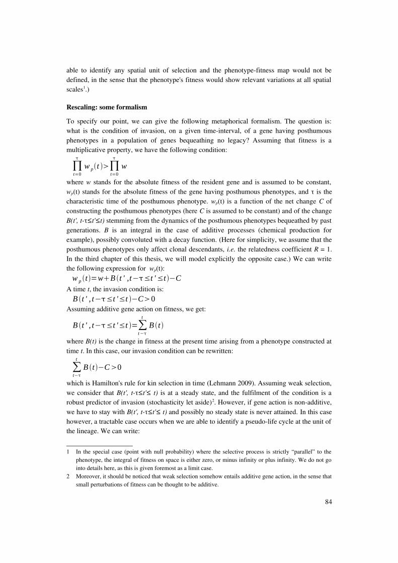
able to identify any spatial unit of selection and the phenotypefitness map would not bedefined, in the sense that the phenotype's fitness would show relevant variations at all spatialscales1.)

Rescaling: some formalism

To specify our point, we can give the following metaphorical formalism. The question is:what is the condition of invasion, on a given timeinterval, of a gene having posthumousphenotypes in a population of genes bequeathing no legacy? Assuming that fitness is amultiplicative property, we have the following condition:

∏t=0

w pt ∏t=0

w

where w stands for the absolute fitness of the resident gene and is assumed to be constant,wp(t) stands for the absolute fitness of the gene having posthumous phenotypes, and τ is thecharacteristic time of the posthumous phenotype. wp(t) is a function of the net change C ofconstructing the posthumous phenotypes (here C is assumed to be constant) and of the changeB(t', tτ≤t'≤t) stemming from the dynamics of the posthumous phenotypes bequeathed by pastgenerations. B is an integral in the case of additive processes (chemical production forexample), possibly convoluted with a decay function. (Here for simplicity, we assume that theposthumous phenotypes only affect clonal descendants, i.e. the relatedness coefficient R = 1.In the third chapter of this thesis, we will model explicitly the opposite case.) We can writethe following expression for wp(t):w p t =wB t ' ,t−≤t '≤t −C

A time t, the invasion condition is:B t ' , t−≤t '≤t −C0

Assuming additive gene action on fitness, we get:

B t ' , t−≤t '≤t =∑t−

t

B t

where B(t) is the change in fitness at the present time arising from a phenotype constructed attime t. In this case, our invasion condition can be rewritten:

∑t−

t

B t −C0

which is Hamilton's rule for kin selection in time (Lehmann 2009). Assuming weak selection,we consider that B(t', tτ≤t'≤ t) is at a steady state, and the fulfilment of the condition is arobust predictor of invasion (stochasticity let aside)2. However, if gene action is nonadditive,we have to stay with B(t', tτ≤t'≤ t) and possibly no steady state is never attained. In this casehowever, a tractable case occurs when we are able to identify a pseudolife cycle at the unit ofthe lineage. We can write:

1 In the special case (point with null probability) where the selective process is strictly “parallel” to thephenotype, the integral of fitness on space is either zero, or minus infinity or plus infinity. We do not gointo details here, as this is given foremost as a limit case.

2 Moreover, it should be noticed that weak selection somehow entails additive gene action, in the sense thatsmall perturbations of fitness can be thought to be additive.

84

W p=∏t=0

w pt

where Wp stands for the rescaled fitness of the lineage, and wp(t) for the fitness of its units.wp(t) is still untractable but now we can identify a rescaled selective process:W p=S G p , E

where Gp is the focal piece of lineage and E the relevant environment for the lineage.

Conclusion on posthumous phenotypes

OLF's argument against an explanatory hierarchy between natural selection and nicheconstruction (the “reciprocal causation” issue examined above, section 3.10) requires thatliving systems are in case (4), or in case (2) with a phenotype's characteristic time comparableeither to the duration from the origin of life or to the gene's characteristic time (these twoconditions ensure that we cannot resize our timewindow to identify an autonomous selectiveprocess). The central figure of niche construction theory (OLF 2003:14:fig.1.3, reproduced asfig.1 below) has to be understood in the same way.

Fig.1: The tragedy of arrows. It is a truism that like other models, pictures are misleading when crucialhypotheses are, consciously or not, not made explicit. OLF give the following caption for their figure :« [Left] : Standard evolutionary perspective : Organisms transmit genes from generation t to generation t +1with natural selection acting on phenotypes. [Right] : With niche construction : Organisms also modify theirlocal environment (E), as depicted by the arrow labeled “niche construction.” Each generation inherits fromancestral organisms both genes and a legacy of modified selection pressures, described as “ecologicalinehritance.”. » As the reader will guess, niche construction theory (right) is founded only if the processesdescribed by parallel arrows have the same timescale (and interact). To give empirical evidences for suchadditional arrows is insufficient to support the theory if the timescales and characteristic times are notspecified. (After OLF 2003:14:fig.1.3)

To conclude, as for posthumous phenotypes, we evoked two ideas. The first is the question ofseparating the ontogenesis of a phenotype, possibly a rescaled one, from the selective processit undergoes. The second is the question of the size of our timewindow of interest, that isdirectly linked to the scales of the observable processes, and that should be mentioned in

85

debates (implicitly) relating to the nonseparability of some processes.How much of evolutionary biology conforms to dynamics such as (1), (2), (3), or (4) is anempirical issue. Not an easy one, of course. To our knowledge, none of the empiricalexamples given by OLF (mostly in 2003:chap.2) has been shown to conform to case (2) or (4)where ontogenesis is not negligible. If we are right in rephrasing niche construction theory asthe nonseparability of ontogenesis and selection, this means that there is, to date, no knownexample of true niche construction (or at least that they are not given by OLF). Only better :niche construction may be the hidden face of the darwinian moon.

3.11 Relaxing the invariance of the phenotypefitness map

Theoretically, we can relax the assumption that the phenotypefitness map is invariant withrespect to time on our timescale of interest. This is in particular the case if we make it dependon catastrophic events. This means that condition (2) in the selectionist scheme (section 2.1)is not met : even given all relevant environmental conditions, a phenotype does not have anyfitness. In this case, fitness as an evolutionary currency is illdefined1. A comparison can bemade with economy, where price can also be undefined, in which case there is no trade orcrisis (e.g. Green & Zhou 2004:8, Walter & Brian 2007, Mandelbrot & Hudson 2009). Wewould not get any robust insight of what is “selected” for “the good of” what. Naturalselection, and the selectionist scheme as an explanatory scheme, would vanish. Other theories,neutral theory for instance, would take over (of course such other theories can also be relevantwhen fitness is defined).If constructionists want to integrate natural selection to an extended theory (including nicheconstruction), they should be clear that the phenotypefitness map, i.e. the selective invariant,is not modified by niche construction. There could be another way to consider the relationship between natural selection and nicheconstruction, however. Constructionists could consider that natural selection, sensu invarianceof the phenotypefitness map, is a limit case of “extended evolution” including nicheconstruction as a more general invariant, as Newtonian mechanics can be considered as a limitcase of relativity (Rivadula 2004, see Lewontin 1983:275 for a similar comparison). We donot explore this issue here, but in both ways, the invariants of the extended evolutionarytheory should be specified.

3.12 A note on evolutionary self and nonself

Niche construction is framed in terms of self and nonself (see also our discussion of autoand alloniche construction in section 3.4) : niche construction is “the process wherebyorganisms (…) modify their own and/or each other's niches. Niche construction may result inchanges in one or more natural selection pressures in the external environment of populations.(...)” (OLF 2003:419). Debaters should be careful in agreeing on what “own” or “other” mean(here we will discuss only “own”, or rather self, letting to reader's discretion the completionby the reciprocal). Depending on the timescale of the modification of the niche, there are twomeanings of “self” in niche construction claims:

1 As evoked above, a similar problem arises if we consider the theoretical possibility of extendedphenotypes having no characteristic spatial scale.

86

(1) “self” refers to the individual bounded by classical generations (a given organism, ifidentified, or a given piece of germinal nucleic acids)(2) “self” means one's descent (i.e. the individual is a lineage). If “self” refers to the individual, modifying its own niche can be thought of as a classical,possibly extended, phenotype. If “self” refers to one's descent, then the account given insection 3.10 holds. It should be noticed that rescaling, when possible, consists precisely inshifting from one meaning of “self” to another. This point is important, to appreciate howsynonymous it can be to say that an organism (or a gene) bequeaths modified “selectionpressures” to its descent (that is, to itself later in time), and to say that a lineage has aphenotype1. Whenever we rescale (even implicitly), we have synonymy.Note : here we did not come back on the oscillation between individuals and populationscontained in the definition, but it may be worth being looked after too (see sections 2.3 and3.4).

3.13 Concluding discussion on what niche construction is

Niche construction revisited : definitions and invariants

Niche construction is defined as “the process whereby organisms (…) modify their ownand/or each other's (…) selection pressures » (OLF 2003:419). We have seen that thisdefinition is problematic, though not meaningless, in several respects : (1) the meaning of“organism” (2) the meaning of “selection pressure” (3) the meaning of “self” (4) and the(unspecified) timescales of interest.As for (1), we have argued that we should rephrase niche construction in genetic terms. Thismakes most cases of organisms modifying their “selective environments” reducing to cases ofgenes having extended phenotypes (extended sensu beyond organism's boundaries). As for(2), we have stressed the necessity to clarify whether one understands selective pressures as aselective invariant (the phenotypefitness map) or a variable (the selection coefficients) of theselective process (see also section 4.2). If we consider selection pressures as variable selectioncoefficient, niche construction theory is somehow trivialized as a particular case (possibly oftantamount importance, but already described by standard theory) of natural selection. If weconsider them as the long term selective invariant, we argued that we still should not considerthat they are modified, but that, instead, the phenotype is dynamic. As for (3), we havestressed the necessity to be clear about the level (in time) of construction (e.g. individual orlineage). As for (4), we have examined at length the embedded implications of choosing atimescale of interest and to slip from one to another (i.e. to possibly implicitly,unconsciously, rescale the problem when debating).We rephrased evolutionary niche construction theory into a single sentence : “ontogenesis is

1 Recall Laland's quote (2004:320): “... some extended phenotypes are ‘heritable’. Organisms not onlyacquire genes from their ancestors but also an ecological inheritance, that is, a legacy of natural selectionpressures that have been modified by the niche construction of their genetic or ecological ancestors(OdlingSmee 1988)”.

The same reasoning holds when we want to compare the claim (encountered sometimes) that organisms orgenes bequeath modified “selection pressures” to themselves (as individuals) later in time, and the claimthat they have phenotypes on their whole lifetime.

87

not separable from selection”. Ontogenesis is the process whereby a gene modifies itsenvironment ; thus, phenotypes are always extended. Ontogenesis is defined by the genotypephenotype map. Selection is the process whereby a phenotype awards fitness to the gene (orthe lineage) that produces it. It is defined by the phenotypefitness map. In our view, the twomaps are invariants even in niche construction theory, but when ontogenesis is not separablefrom selection the genotypephenotype map is dynamic, and this dynamics has to be takeninto account. If we conflate the two maps however, the point that natural selection is notmodified is obscured.We proposed that for some cases, non negligible posthumous modifications of theenvironment could be accounted for within a classical selectionist way with a proper rescalingin time of the considered lineages, phenotypes, and selective processes. Under weak (i.e.slow) selection and additive gene action, rescaling is unnecessary, and we can apply a kinselection in time approach (Lehman 2007, 2009). However, we have emphasized thatrescaling is not, from a theoretical point of view, always possible. Thus truly new dynamicsare possible. We have seen that all (but one : the notable argument on feedback) arguments of OLF infavour of niche construction theory do not hold, and that none of their empirical examplestruly exemplify it, in the sense that a priori, they can be as well explained by the classicalselectionist scheme (by the way, these examples are given as absolute numbers, not relativenumbers, which would weaken the claim on pervasiveness of niche construction if theseexamples exemplified it1). Throughout the presentation, we have put a special emphasis onthe fact that claims about the timescales of processes are empirical claims, and that to ourknowledge no data, for the moment, justifies an entanglement of ontogenesis and selection.We should limit our invocation of niche construction to those cases where construction isprobable, not just possible.Notably, OLF (2003:Chap.7) propose empirical methods for detecting evolutionary nicheconstruction in the wild. We did not review this program here, but in our view, it reducesunfortunately to seeking for evidences of evolution of extended phenotypes or intragenomiccoevolution, notably the following method: “Step 1 : Search for a correlation between someorganismal structure and environmental factors. Step 2 : If no relationship is found,investigate whether the organism exhibits niche construction that might compensate for pooradaptation of the structural trait. Step 3 : Investigate whether there is evidence for organismdriven modification of the selective environment. Step 4 : If so, search for evidence forevolutionary feedback in the form of structural or functional adaptation to the constructedenvironment.” (OLF 2003:292). In our view the method can be rephrased as follows : “Step1 : unchanged, Step 2 : search for adaptation in the form of extended phenotypes. Step 3 :unchanged. Step 4 : search for intragenomic coevolution.”However, niche construction theory, properly rephrased, is a theoretically valid extension ofstandard evolutionary theory (where ontogenesis is separated from selection), and we feel thatit is worth investigating. This entails that the invariants of the extended evolutionary theoryshould be explicit (we proposed general invariants above), and that the empirical facts shouldbe gathered with respect to these posited invariants.

1 E.g., in addition to OLF 2003:chap.2, Laland & Sterelny 2006:1756, Laland et al. 2007:57, Laland et al.2008:551, Laland et al. 2009:203.

88

Other constructionist tracks

Here, we have dealt with only one timescale separation (ontogenesis from selection) but theniche construction perspective can apply to other dichotomies as well : (1) the genotypephenotype distinction (2) the separation between development and the developmentalenvironment (on developmental or evolutionary timescales), etc. As for (1), if the phenotypehas a characteristic time comparable to that of the genotype (on a given time scale of interest),the genotypephenotype separation no longer holds. This can be the case for instance inevolutionary cultural studies, where cultural variants (e.g. dairy farming) can last formillennia, letting enough time for “genes for” culture (not genes for digestion here) to evolveas well, or in the case of oxygen enrichment examined above. As for (2), if, say, ontogenesismodifies the developmental environment on an evolutionary timescale, we have one moreway in which ontogenesis can influence evolution (and possibly selection).

Environment or phenotype

The analytic difficulty when comparing selection and niche construction, is that there is nodifference in nature between a phenotype and a selective environment : a phenotype is amodification of the environment that awards some fitness to a gene, thus this modified part ofthe environment impacts the selective process undergone by the gene:w=s p , E

where the phenotype p is environmental in nature (s is the selective function). If the selectiveenvironment was defined as everything in the environment that affects the (differential)replication of the gene, ontogenesis, if not neutral, could always be seen as a modification ofthe selective environment. This is as true within the classical selectionist scheme (even withfrequencyindependence), as within niche construction theory1.The difference between the phenotype and the socalled selective environment lies only in thetimescales we usually attribute to the phenotype's dynamics (i.e. gene's effects on theenvironment) as compared to the selective environment's dynamics (i.e. environment's effectson gene's fitness) : in classical selectionism we assume that these dynamics are separated.Actually, one of the main endeavours of the selectionist theorist consists in delineating aphenotype/environment boundary that enables her to apply this timescale separation: ratherthan everything in the environment that differentially affects the replication of the gene, the“autonomous” selective environment is this specific part that is not affected by theontogeneses in presence (for instance, the “autonomous” selective environment is that part ofthe environment which determines the payoff matrix in frequencydependent selection).Because of these ambiguities, we avoided to cast the problem in terms of (modified)environments and rather used a timescale separation criterion to distinguish the classicalselectionist scheme from niche construction theory. We will come back on the issue of“selective environment” in section 4.2.

1 Our account departs from Brandon's account. In his definition, Brandon shortcuts ontogenesis: “Theselective environment is measured in terms of the relative actualized fitnesses of different genotypesacross time or space.” (Brandon 1990, 1992, Brandon & Antonovics 1996:chap.10). “Selection occurswhen differential adaptedness to a common selective environment leads to differential reproductivesuccess.” (Brandon 1992).

89

Space vs time

In our view, niche construction can be a valid theory even in mean field situations. Space isnot intrinsic to the theory (the word “environment” appears more than hundred times in OLF'sbook1, but “environment” is a spatial concept only in the sense that it invites us to presume aseparation between individual's internal and external compartments, not in the sense of anydistance between individuals). Though not intrinsic, space is of primary importance, however.Here, we mean space as limited dispersal, which leads to viscous populations. It can bethought in parallel as limited diffusion of the extended and posthumous phenotypes. Limiteddispersal results in lineages being correlated (through time) with particular places (Lehman2009:139). (This in turn results in spatial autocorrelations of genes, which can enhance kinselection, see Van Baalen and Rand 1998.) If interactions between individuals and with theenvironment have limited spatial ranges, an individual that locally modifies the environmentcan, ceteris paribus, more easily differentially affect the fitness of its descent (Lehman2007:2), than in mean field situations. The geometry of space is decisive here : fractalgeometry, for instance, leads to more confined interactions (e.g. Wiens and Miles 1989,Sugihara and May 1990). Space, thus, (and it was somehow expected) is of primaryimportance for the evolution of the spatial but also temporal extensions of phenotypes. In thisrespect space can influence the timescale separations of the considered processes, as it hasbeen shown, in ecology, by infinitely delayed competitive exclusion in viscous populations(Hurt & Paccala 1995, cf. this thesis, chap.1:3.1).

4. Problems of niche construction : adaptation, externalism

Now that we have discussed what niche construction is, we are going to examinetwo constructionist issues : the redefinition of adaptation (to an environment) by theconstructionists, and in which way the niche constructionism departs from the selectionistexternalism.

4.1 Adaptation

One main goal of the constructionist framework is to “rethink adaptation” (Day et al. 2003,see also e.g. OLF 2003:1619,374376, Laland 2004:316). This is ambitious, as adaptation isprobably one of the most central concepts of evolutionary biology. Here we discussadaptation sensu the fact that an entity is adapted (to the environment), and not the dynamicalprocess of getting adapted.

Concepts of adaptation

Classical selectionism recognizes two different kinds of features that can possibly enhance thefitness of organisms (or rather phenotypes) : (1) features that have been shaped by selectionthroughout the history of the lineage, and (2) features that have not been shaped by selection.Darwin (1859:197) and Williams (1966:v,4), for instance, considered only the first asadaptations, the second being referred to by Williams as (sometimes incidental) effects

1 This represents, by the way, an occurrence 30 % greater than for the word “organism” (ca. 73occurrences), and 10 % greater than for the word “gene” (ca. 88 occurrences).

90

(1966:v,13). By contrast, Bock (1979:39) considered that both were to be counted asadaptations, following the vernacular intuition of the word that something is adapted to a roleif it fulfils its role, whatever the origin of this fit (Endler 1986:47 1). This is also the“currentist” concept of fitness defended by Reeve and Sherman (1993), who argued that theusual “historical” concept of adaptation, equating it with direct effect of selection, misses thewhole research program of behavioural ecology. Throughout his book, Williams (1966) hasbeen very severe with regard to the conflation of the first and second meanings. His bookstarts with these words : “Evolutionary adaptation is a special and onerous concept that shouldnot be used unnecessarily, and an effect should not be called a function unless it is clearlyproduced by design and not by chance.” (1966:v, see also e.g. 4,89). Williams refers tochance, here, because Lamarckism is dismissed, and no other process than natural selection issupposed to enhance fitness. To clarify the debate, Gould and Vrba (1982:6) proposed to stillname adaptations the features shaped by selection, and to coin a new word, exaptation, for“unselected, but useful” features.Thus, classical selectionism recognizes two different ways towards the “fit” of an organism(or phenotype) to its conditions of life : natural selection (adaptation), and chance(exaptation)2. The “fit” is measured in terms of (absolute) fitness3.In niche construction, the vocabulary is somewhat richer. Following Bock (1980), OdlingSmee (1988:98) calls a “synerg” the matching condition between a organismal feature and anenvironmental factor (see also OLF 2003:41,43, Laland et al. 2003:118). In some instances,we find the terms “synergic match” (Day et al. 2003:82), “synergistic relationships” (OLF2003:43), “handinglove fit” (Laland and Sterelny 2006:1758), “dynamic complementarymatch” (Day et al. 2003:93, or only one of these two adjectives : OLF 2003:50,164,240),“dynamic adaptive match” (OLF 2003:3,376), “evolving match” (OLF 2003:18), “evolvingcomplementary match” (Day et al. 2003:80), or just “match” (OLF 2003:4849:fig.2.1,290,Laland 2004:321,322, Laland and Sterelny 2006:1758, Laland et al. 2008:198), to describethe match between an organism and its environment. We gave some details on theoccurrences, here, to show that this terminology is not anecdotal. We find the

1 We do not follow Gould and Vrba's (1982:4) account here, to whom the vernacular meaning refers to “ad+ aptus, or towards a fit (for a particular role). When we adapt a tool for a new role, we change its designconsciously so that i will work well in its appointed task.”. It seems to us that it is only one side of thevernacular coin.

2 Our argument here is different from OdlingSmee's finding (1988:82) : “The synthetic theory currentlyassigns a dual role to the environment. One role is explicit, pragmatic, and obvious. It is assumed that theenvironment is the sole source of natural selection. Its second role is implicit, philosophical, and far lessobvious. Natural selection is assumed to be the only force capable of altering gene frequenciesnonrandomly, and therefore to be capabe of directing evolutionary descent down nonrandom paths.”.

In our view, natural selection is not the only “force” capable of directing gene frequencies (as mutationpressure could be considered too), but the only “force” capable of directing gene frequencies with respectto fit (see section 4.2 for a discussion of natural selection as a force).

3 As regards adaptation, frequencydependence is a complicated issue, because the selective process makesthe selective environment vary at the same pace than does the population. Strategies are not alwayslinearly ordered in terms of success : A might win on B, B on C, and C on A (for such rockpaperscissorgames in the field see e.g. Sinervo and Lively 1996). Here, we can rescue the concept of adaptation bynarrowing the timewindow on which we investigate whether, given similar environments, absolutefitness has increased in the population.

91

term “adaptation” too, and it refers, sometimes explicitly, to Williams' sense (e.g. OLF2003:41,49,370, Laland and Sterelny 2006:1756), though we found it used in the sense of“fit” rarely (e.g. OLF 2003:3,284)1.

Construction towards fit ?

The niche construction perspective on fit is rather unusual : “[T]here are two routes to the fitbetween organisms and their environments: (1) organisms may, as a result of naturalselection, evolve characteristics that render them wellsuited to their environments; or (2)nicheconstructing organisms may change their environments to suit their currentcharacteristics.” (Day et al. 2003:81, my emphasis on the problematic “to” ; see also e.g. OLF2003:18,43,240,290,375,376, Laland 2004:321, Laland and Sterelny 2006:1758,1759, Lalandand Brown 2006:95). Or, in a nutshell : “Adaptation depends on both natural selection andniche construction” (OLF 2003:3:fig.1.1). Here “adaptation” is probably a misnomer for “fit”,as the authors are coherent using Williams' (1966) sense in the rest of their book (OLF 2003).This perspective stems from Lewontin's emblematic sentence : “Organisms do not adapt totheir environments, they construct them out of the bits and pieces of the external world.”(1983:280, quoted in OLF 2003:17, we find a similar sentence in Lewontin's commentary onthe cover of the book). To OLF, indeed, the way classical selectionism looks at adaptation is a“problem” and a “deficiency” (2003:375). Lewontin himself proposed to replace the“metaphor of adaptation” (1983:280) by the “metaphor of construction” (1983:282). So, isniche construction a third2 way toward fit, in addition to chance and natural selection, or is itreducible to one of them ?Let's take a look again on OLF's (and Lewontin's) examples of organismenvironment fitspossibly attained by construction. We find : spiders adapting to their webs or constructingwebs suited to them (OLF 2003:17), earthworms “weakening [soil] matrix potentials andmak[ing] it easier for them to draw water into their bodies” rather than undergoing adaptationto life on land of, for instance, their “freshwater” kidneys (OLF 2003:374376), and probablymost of the examples of the OLF's Chapter 2 (OLF 2003:50115), some of them havingalready been given above (section 3.7). As for Lewontin's examples, we get : “ants mak[ing]fungus farms, trees spread[ing] out leaves to catch sunlight, (…) beavers rais[ing] the waterlevel of a pond, (…) white pine (...) creat[ing] a dense shade that prevents its own reseeding”

1 The ambiguity of the niche construction framework about adaptation is exemplified by this quote :“In summary, if ‘‘adaptation’’ means the asymmetric accommodation of a lineage to its environment, then

niche construction does not cause adaptations (sensu Williams 1966) in the nicheconstructing lineage.(Niche construction may cause adaptations in this sense in other lineages: domestic mice are adapted tohumancaused changes in their environment.) But although niche construction may not explainadaptations in this narrow sense, it does explain organismenvironment matches.” (Laland et Sterelny2006:1759)

First, we can notice that niche construction does not cause adaptation of mice to humancaused changes :selection does. Second, the “organismenvironment match” is not, in our view, proven by the paragraphspreceding the quote.

2 A third route, and not a “second route”, as OLF put it (e.g. 2003 :43,240,290,376). Of course it could beargued that chance is not a route, but a drift. This issue is not very important here, what matters is not toforget chance, and not to award niche construction fits that are due to chance.

92

(1983:2811) (in the last example we have negative niche construction).As we already mentioned (section 3.7) the given examples can be interpreted in terms of intraor intergenomic coevolution, which is acknowledged by OLF : “Although it is not clear thatall of these adaptations are actually evolutionary responses to prior niche construction, it islikely that many of them are. This means that it may frequently be appropriate to considerevolution as a process in which environmentaltering traits coevolve with traits whose fitnessdepends on alterable sources of natural selection in environments.” (2003:113). According tothis interpretation, niche construction is not at all a supplementary route towards fit, but aphenotypic part of a classical selective process. Thus, rephrased in genetic terms, the nicheconstruction perspective on fit (given above) reads : “There are two routes to the fit between agene and its environment: (1) the gene may, as a result of natural selection, evolve a classicalphenotype (sensu internal to the organism, if any) or (2) the gene may evolve an extendedphenotype.”. Well. This is much less unusual.Even if we consider the particular case where the niche construction phenotypes at the originof the subsequent selective process have not been shaped themselves by prior natural selection(OLF 2003:19,372, section 3.9), the classical selectionism applies2 : there is indeed noimpossibility of coevolution between traits that are effects (sensu Williams 1996:v) and otherselected traits. Here the coevolution would be asymmetrical as effects are by definition nonselected traits, but we still do not have any new route to fit. What about nongenetic niche construction (if any) ? Even in this case, we do not get anyinsight that niche construction, and not classical adaptation or chance, leads to fit. If nicheconstruction arises from developmental noise (OLF 2003:372), it has to be shown how noisecan lead, except by chance, to fit. If niche construction arises from acquired characteristics,from instance from learned behaviours (e.g. OLF 2003:21,372), it has to be shown how theseacquired characteristics enhance fit, without the capacity of acquiring such capacities (e.g. thecapacity to learn) having been itself shaped by natural selection (Sterelny 2005) (section 3.9).OLF themselves seem to accept that the path towards fit through acquired characteristics isdue to natural selection, as they write : “Niche construction (…) must be directed by semanticinformation whose structure and content is the result of prior natural selection.”(2003:176:table 4.1)3.We can work out the earthworm example to give a dichotomous key of what is at stake here.Earthworm is a famous example of niche construction (see e.g. OLF 2003:11,160,291,375,Laland 2004:319321, Laland & Brown 2006:99, Laland & Sterelny 2006:1754,17581760,Laland et al 2009:199, Laland et al. 2008:552,554,560), it deserves a famous discussion.First, we observe that earthworms modify the edaphic environment and make it more“aqueous”. Only better : this suits the worm (Darwin 1881:310, Turner 2000). Has there beenany selection for modifying the soil and making it more aqueous, for instance, by mucus

1 Here we give only examples of organisms altering the external world, but Lewontin sees three otherroutes towards construction : to “determine what is relevant, (…) [to] transduce the physical signals of theexternal world, (...) [to] create statistical patterns of environment different from the patterns in theexternal world” (1983:281). See section 4.2.

2 If, of course, ontogeny and selection are not entangled.3 OLF would probably deny that this sentence pleads for a supremacy of natural selection, given their

argument on reciprocal causation. We already examined this argument (section 3.9).

93

secretion ? If yes : we have a case of classical natural selection (Williams 1966:191). If not,the constructing activity is a “mere effect” ; then, was there any other reason (than the alreadydiscarded natural selection) to expect that this constructing “mere effect” would be beneficialto the worm ? If not : fitness enhancement results from mere chance (for instance, it is usuallyassumed that mutations are random with regard to fitness, in the sense that knowing thefitness of a trait is supposed to tell us nothing about the probability of the correspondingmutation(s), if any2). If yes : the new way towards fit has to be worked out, because it sets thestage for a scientific revolution.3

Unfortunately, we have not been able to find a single clue that niche construction leads to fitby other ways than natural selection and chance in OLF's writings. By the way, OLFthemselves consider that niche construction can be positive (enhancing fitness), but alsonegative (decreasing fitness), thus niche construction sometimes generates a mismatchbetween the organism and the environment (OLF 2003:4750). Niche construction shouldthus be a route towards nonfit as well. One more time, we do not know of any process thatcan give us an expectation of the sign of a new niche construction activity, and thus anexpectation of the impact of niche construction on fit once selection is discarded (we considerchance does not give any expectation of the sign). If we use our rephrasing of nicheconstruction in terms of timescale separations, we can say that we have no clue that the nonseparability of ontogenesis and selection should lead to fit (recall that fitness is still defined inthis case)4. Neither do we have any clue that, when ontogenesis is separable from selection,

1 In this section, Williams discusses the level of selection : individual or populational.2 To be precise, we can imagine nonrandom mutations with regard to the phenotypic dynamics (hence

inheritance of acquired characteristics), which could nevertheless be random with regard to fitness (hencenonLamarckism).

3 In the following quote Laland et al (2005:41) offer a subtle discussion of the distinction between effectsand adaptation :

“If the only feedback to an organism from a nicheconstructing activity were due to effects on selection of thegenes that underpin the activity, then whether the character is an adaptation or effect is of paramountimportance, since the difference between these impinges on survival value and reproductive benefits ofthe character. But, as all three commentators seem to accept, this is not the only form of feedback fromniche construction. Such activity frequently also modifies selection pressures acting on other aspects ofthe phenotype, in the same or in descendent populations; for this second kind of feedback the distinctionbetween adaptation and effect is irrelevant. One of the contributions of the nicheconstruction perspectiveis to focus on the symmetry between these rather that their sequential nature, which is the old way ofthinking about evolution (Lewontin 1983).”

By contrast, we consider that for this second kind of feedback, there is, first, no feedback (since the modifiedpressures act on other aspects of the phenotype, that is, given the first sentence of the quote, on othergenes). Second, the distinction between adaptation and effect is still relevant, and activities of this kindare, indeed, effects.

4 The claim is quite explicit here : “The focus [of ecological developmental biology] is the ability ofdeveloping organism to sense cues from its environment and to modify its development to become morefit in a particular habitat.” (Laland et al. 2008:549). We strongly doubt that such examples of this “abilityto sense cues” are not due to chance or natural selection. Gould and Vrba (1982:592), for instance, givesome examples of fit without selection : “Many sedentary marine organisms, sponges and corals inparticular, are well adapted to the flow regimes in which they live. A wide spectrum of 'good design' maybe purely phenotypic in origin, largely induced by the current itself.”. Here, it can be argued that eitherthere has not been selection for the response to the current (or there cannot be, in which case fitness is

94

extended or posthumous phenotypes should lead to fit, except by chance or selection.In conclusion, the claim that niche construction is a new route to fit should be entirelyavoided, or clearly labelled as pure speculation. (This is not pejorative.)

Note :As for history, even Julian Huxley was, contrary to Darwin, insensitive to adaptation, sensu fit(Ruse 1992:79). As for us, we remain a priori agnostic : unless a proper metric is defined for the“match”, enabling to compare possible and realized states, we do not see why we should considerthat organisms match or do not match their environment1.Throughout our discussion, we have considered that fit is given in terms of fitness. This is inaccord with OLF's use of “match”, also referring to fitness (e.g. 2003:4750). We could imagine,however, other currencies, maybe better suited for constructionist or interactionist views. Forinstance, the minimization of some energy would give the degree of match between a livingsystem and its environment by the degree of minimization of the interaction's energy (indevelopment or evolution). Theories of this kind could or could not relate much to Darwin's work.We mention this perspective only as a theoretical possibility : until a proper state phase is definedto compute the considered energy, the perspective remains metaphorical (Van Valen 1991 goes inthis direction, see also Bouchard 2007).

4.2 Back to the basics : is selectionism an externalism ?

OLF (2003:18) following Lewontin (1983:282) oppose the selectionist scheme as anexternalism involving unmodifiable selection pressures imposed by the “externalenvironment” (e.g. 2003:10,131,419, “external” means here external to the organism).Lewontin's metaphorical equations (given above in section 3.1, repeated in section 4.2), forinstance, characterizing the selectionist scheme, have organism and environment as variables.Here we aim at specifying in which sense the selectionist scheme is externalist, and in whichsense constructionists or interactionists views depart from it (if ever they do).

Historical perspectives

Darwin himself did not state clearly his scheme in an externalist way2. We have not been ableto find the word “environment” a single time in the diverse editions of The Origin (18591876). Neither did we find the phrases “selection pressure” or “selection force”, which do not,to our knowledge, exist in his writings. What we found, by contrast, are the concepts oforganisms “adapting to” (e.g. 1859:82) (or being modified by, e.g. 1859:4,10) their“conditions of life” or “existence”, of “places in the economy of nature” to be “filled up”(1859:81), of organisms being “fitted for their places in nature” (1859:88, 199) or “fitted for

irrelevant), and fit, if any, is due to chance, or there has been selection.1 Subjectivity is important here, because if we lack imagination, we will not envisage other possible

organismenvironment relationships where the match could be much, much, higher.2 This is somehow acknowledged by Laland et al. (2008:554) : “Although Darwin recognized organisms as

constructors of their environment, and championed some marvelous examples of niche construction (e.g.earthworms, coral), his postsynthesis legacy became a view of organisms as passive objects molded bythe external force of selection.”

We are not sure, however, that Darwin would have been a constructionist in his time.

95

(...) different habits of life” (1859:183). Significantly, Darwin's work is mostly stated in termsof “laws” (e.g. 1859:vx, 489490), the highest, in his view, being “the law [of] Conditions ofExistence (...), fully embraced by the principle of natural selection” (1859:206). “Conditionsof existence” might seem close, though not synonymous, to our concept of environment1, butother concepts such as “habits of life” seem a bit less environmental. Spencer, now famous mostly for having coined the sentence “survival of the fittest” todescribe natural selection (1864:444) but who has been more influential in his time, is bycontrast, according to GodfreySmith (1998:68), a great externalist. Spencer, indeed, speaksof selection in terms of “fit” of organisms to their “environments” (1886:42). He specifies,however, that fit is “a figure of speech” that has not to be understood as the fit of “a glove [to]a hand” but in terms of what he, and we, now call fitness (1886:42). In his view, theenvironment is constituted of “universallypresent” “matters and forces” (1886:47).Today, it is commonplace to consider that selective “forces” or “pressures”, whatever theymean, stem from environmental factors. To GodfreySmith for instance, “In adaptationism 2

the externalist pattern of explanation is displayed more clearly than it is anywhere else.Adaptationims seeks to explain the structure and behavior of biological systems in terms ofpressures and requirements imposed by the system's environment. Biological structure, orsome very significant portion of it, is understood as an adaptive response to environmentalconditions.” (1998:32, see also 1998:142, or e.g. Williams 1992:484). Following Lewontin(1983), the constructionists regret that in the standard view, “The adaptations of organisms aretreated as consequences of independent natural selection pressures moulding organisms to fitpreestablished environmental templates.” (OdlingSmee 2009:70, see also e.g. Day et al.2003:81, Laland 2004:315, Laland et al. 2007:54, Laland et al. 2008:554, Laland et al.2008:197).So, what is the “environment” here? How is it “external” to the organism, or, more generally,to the living system? Where do the “selective forces” come from?

Selective laws and selective forces

Selective “forces” or “pressures” are metaphors borrowed from physics. In physics, matterand energy, and the resulting forces (or potentials), are variables, they are spatialized, that is,they have spatial coordinates. By contrast, laws and other invariants are, by definition,

1 Darwin aims here at combining both Geoffroy's and Cuvier's theories into a single theory: Geoffroy'sidea of the unity of type was, in Darwin's view, to be understood by common descent, and Cuvier'sprinciple of conditions of existence was to be understood by natural selection (Darwin 1859:206,Ovspovat 19811995:150). The following quote of Cuvier helps to see the link between the “conditions ofexistence” and the environment:

“L'histoire naturelle a cependant aussi un principe rationel qui lui est particulier, et qu'elle emploie avecavantage en beaucoup d'occasions; c'est celui des conditions d'existence, vulgairement nommé des causesfinales. Comme rien ne peut exister s'il ne réunit les conditions qui rendent son existence possible, lesdifférentes parties de chaque être doivent être coordonnées de manière à rendre possible l'être total, nonseulement en luimême, mais dans ses rapports avec ceux qui l'entourent, et l'analyse de ces conditionsconduit souvent à des lois générales tout aussi démontrées que celles qui dérivent du calcul, ou del'expérience.” (1817:6, Cuvier's emphasis ; on this subject see Huneman 2006, 2008:341363).

2 GodfreySmith speaks in terms of “adaptationism” rather than “selectionist scheme”, but this does notmatter if we consider selection as the only way towards adaptation.

96

invariant under translations in space (at a given scale), and do not have such spatialcoordinates. Thus, if there were such selective forces, they could have spatial coordinates andstem “from the outside” of a living system (e.g. Spencer 1886:481), by contrast with thecorresponding selective laws (i.e. the selective invariant in our terminology) that could not.Actually, Endler has shown how misleading these metaphors can be (1986:2933): forinstance, if the selective forces were to be applied on gene frequencies, it would seem hard, atfirst sight, to make sense of what the corresponding “mass” of the set of frequencies wouldbe. It is, in our view, easier to think in terms of invariants (labelled as “selective” if there is aselective process) and variables, that can be either environmental or biotic variables.Selective invariants, such as the socalled “selection pressures” which can be seen, sensuselection coefficients, as short term invariants, are neither “pressures” nor “forces”, they arelaws that describe the interactions between living systems and their environment. They haveno spatial coordinates, and strictly speaking, they are neither internal, nor external to a livingsystem. They are “external” to the living system only in the sense that they are invariants,while the living system is a variable. Here we come back to Darwin, following Cuvier's use ofthe word “principle” and Whewell's appeal to “general laws” (Darwin 1859:ii), who castsevolutionism in terms of laws. (Lewontin's concept of constraints, in the quote given below,seems similar, though the invariant could be different.)On the other hand, the invariants, that describe the interactions between the variables, candescribe asymmetric forcings between variables. If some environmental variables haveautonomous dynamics, that is, if their dynamics are not influenced by biotic variables ( i.e. theeffects of the biotic variables on environmental variables are timeseparated from theenvironmental variables' dynamics), the intuition that some part of the external environmentexerts a “force” on the living matter, but not the other way around, is legitimate (though it isnot, strictly speaking, a force but rather a forcing). For instance, we classically consider thatEarth exerts a gravitational force on living matter, but we seldom consider the reciprocal.Now, classical selectionism assumes a separation between ontogenesis and selection, that is,in particular, that phenotypes do not modify the selective environment. Hence, the selectiveenvironment forces the living's dynamics, and classical selectionism is an externalism. Herewe come back to Spencer's intuition that evolution is forced by, or undergoes a “force” from,

1 “Obviously the most general trait is the greater amount of change wrought on the outer surface than onthe inner mass. In so far as the matters of which the medium is composed come into play, the unavoidableimplication is that they act more on the parts directly exposed to them than on the parts sheltered fromthem. And in so far as the forces pervading the medium come into play, it is manifest that, excludinggravity, which affects outer and inner parts indiscriminately, the outer parts have to bear larger shares oftheir actions. If it is a question of heat, then the exterior must lose it or gain it faster than the interior; andin a medium which is now warmer and now colder, the two must habitually differ in temperature to someextent – at least where the size is considerable. If it is a question of light, then in all but absolutelytransparent masses, the outer parts must undergo more of any change producible by it than the inner parts– supposing other things equal; by which I mean, supposing the case is not complicated by any suchconvexities of the outer surface as produce internal concentrations of rays. Hence then, speakinggenerally, the necessity is that the primary and almost universal effect of the converse between the bodyand its medium, is to differentiate its outside from its inside. I say almost universal, because where thebody is both mechanically and chemically stable, like, for instance, a quartz crystal, the medium may failto work either inner or outer change.” (Spencer 1886:48)

97

the environment (e.g. Spencer 1886:491)2.In conclusion, selectionism is externalist in the sense that there is an asymmetry in reciprocalinfluence between environmental variables and biotic variables, which entails nonconstructionist explanations. Environment here has to be defined as a set of variables that“can be described independently of the properties of the organic system” (GodfreySmith1998:151). By contrast, selective invariants are neither environmental nor internal to livingsystems. This is why, in section 1.2, we defined the different explanatory regimes (internalismetc) according to the localization of input variables.

Back to Lewontin's equations

As we already noticed (section 3.1) Lewontin proposed to characterize externalistexplanations as a pair of differential equations “describing the changes in organisms O as afunction of organism and environment E (…) and the autonomous change of environment”(1983:282). Externalism is given by :dOdt

= f O , E

dEdt

=g E

while, by contrast, constructionism is given by :dOdt

= f O , E

dEdt

=g O , E

These metaphorical equations are a bit insufficient to characterize his view, however, in thesense that constructionist explanations, thus defined, can be externalist in some respects.Indeed, when writing dE/dt=g(O,E), Lewontin does not specify whether there is or not anautonomous forcing (see glossary) in the dynamics of E (such as an autonomous supply rate)that is not modifiable by O. If these equations are to describe dissipative systems (for

1 “If, now, inorganic masses, relatively so stable in composition, thus have their outer parts differentiatedfrom their inner parts, what must we say of organic masses, characterized by such extreme chemicalinstability?—instability so great that their essential material is named protein, to indicate the readinesswith which it passes from one isomeric form to another.” (Spencer 1886:49)

2 There is a another, close but not identical, way to consider that evolutionism (not selectionism) is anexternalism (or not). It comes from the consideration of evolution of different lineages put in similarenvironments (and the possible evolutionary convergences), and from the consideration of radiations of asingle lineage in different environments (and the possible evolutionary divergences) (see the section onGrinnell and Elton, this thesis, chap.1). If the lineages never constrain evolution under natural selectionwhile environments do (for instance if mutation is nonlimiting), selectionism will be thought of as anexternalism. However, lineages sometimes do constrain evolution: for instance, depending on theirlocation in the adaptive landscape, lineages will not always climb the same adaptive peak (if any), or mayeven not climb any peak at all (selective stasis) because of developmental constraints (sensu Gould andLewontin 1979:594597). Here, we would have former lineage properties that would (partially or totally)explain current lineage properties. Thus, depending on focal cases, evolutionism could be sometimesinternalist. Dismissing such internalist explanations amounts to considering that biotic variables exertnegligible influence on their own dynamics compared to the influence of environmental variables.

98

instance, if O has any death rate), such an external forcing is expected to take place for thesystem to somehow maintain. Thus, the apparent causal closure between O and E in themetaphorical equations will be broken in real equations, contrary to OLF's intuition onthermodynamics discussed above (section 3.2).Then, Lewontin gives a thoughtprovoking account on evolution under construction, which isworth quoting entirely: “The error is to suppose that because organisms construct theirenvironments they can construct them arbitrarily in the manner of a science fiction writerconstructing an imaginary world. The coupled equations of coevolution of organism andenvironment are not unconstrained (...) Some pathways through the organismenvironmentspace are more probable than others, precisely because there are real physical relations in theexternal world that constrain change. Where there is strong convergence is in certainmarsupialplacental pairs, and this should be taken as evidence about the nature of constraintson development and physical relations, rather than as evidence for preexisting niches.”(1983:283).Here, we get Darwin's intuition of evolutionary laws, contra Spencer's intuition of externalforcing.Certainly, the key is to know what O and E should mean here. Theoretically, in some cases itwill be possible to change O and E in Lewontin's equations to get an understandableexternalist account (i.e. extended phenotype perspective), where the effects of one variable onthe other will be ignored (that is, separated), and Lewontin's “constraints” will reduce toempty niches forcing selection. In other cases, such change of variables will not be possibleand tracking the interaction will show necessary (i.e. niche construction perspective).

Constitutive vs causal construction

Lewontin sees several ways for organisms to construct their world: “Organisms determinewhat is relevant. (…) Organisms alter the external world as they interact with it. (...)Organisms transduce the physical signals of the external world. (...) Organisms createstatistical patterns of environment different from the patterns in the external world.”(1983:280281). To GodfreySmith (1998:144151), Lewontin conflates two different sensesof construction: a “literal causal sense, and a constitutive or ontological sense” (1998:144). Inthe causal sense, organisms alter their external environments, they construct their world byintervening on it. In the ontological sense, organisms define what their relevant or perceivedenvironments are; they modify their perceived world by undergoing internal change(1998:146).As for evolution, GodfreySmith's distinction holds as long as we consider somehow boundedorganisms, but vanishes as soon as we embrace a genecentrist perspective (with alwaysextended phenotypes). For in a genecentrist perspective, we have, say, the gene's sequence onthe one hand (for the sake of argument let's suppose the sequence is sufficient as far asevolution matters), and the phenotype on the other hand (we limit ourselves to “active”replicators here). Apart from synonymous mutations, any “constitutive” construction (changein the sequence) will result in a “causal” construction (change in the phenotype), and apartfrom stochastic events, any causal construction will result from gene's constitution 1. Genetic

1 In our view, the most similar distinction between the two kinds of construction is between traveling in a

99

mutation always entails both constitutive and (change in) causal construction. Gene :constitution, phenotype: construction. From the gene's point of view, Lewontin's quote abovereduces to: “Genes have phenotypes.”However, there is an intuition that is worth emphasizing in Lewontin's concept ofconstruction, the intuition of codefinition between the living system and its environment: “Tomake the metaphor of adaptation work, environments or ecological niches must exist beforethe organisms that fill them. (...) But what laws of the physical universe can be used to pickout the possible environments waiting to be filled? In fact, we only recognize an 'environment'when we see the organism whose environment it is.” (Lewontin 1983:280). This is both trueand untrue. (Here, we gloss over the organism/environment terminology and switch back interms of genes and selective invariants.) Usually for microevolution studies, we consider thatwe are able to define a (local) selective invariant describing the interactions betweensufficiently close variants, even if we did not observe every variants and their interactions inthe field. We assume that small mutations will not qualitatively change the interactions. Localextrapolation enables to recognize empty places in the economy of nature even if we do notsee directly any pen pusher filling them. Hence in this case, we can define absolute, notrelative, environments. Extrapolation is probably less reliable for macroevolution studies.Here Lewontin is right, and selectionism fails: we discover the adaptive landscape (sensuselective invariant) as and when the variants travel through it. (See, however, the discussionby Arnold et al. (2001:23,26): while they agree that global landscapes are mainly imaginary,they argue that adaptive landscapes can provide extrapolations of micro to macroevolution.See also the discussion of macroevolution right below.)

Conclusion on externalism

Dynamical invariants describe the interaction between a living system and its environment.They are neither internal, nor external to the system. However, if the living system is the onlyvariable that is modified by the interaction, the environment remaining unchanged, then theenvironment “forces” the dynamics of the living system, and the environmental variables“explain” biotic variables dynamics (and not the other way around). Classical selectionism, byassuming a decoupling of ontogenesis and selection, supposes that the effects of the bioticvariables on environmental variables (i.e. phenotypes) vanish between generations1. Selection,

reaction norm (changing the phenotype without changing the gene), and traveling in an adaptivelandscape (changing the gene). But as far as selection is concerned, there is no qualitative differencebetween displaying a reaction norm and displaying a particular phenotypic value (which is just a constantreaction norm on usual environmental conditions). Thus, even this distinction does not seem very relevantto us.

1 We depart slightly from GodfreySmith here, for whom game theory cannot be said “asymmetricallyexternalist” (1998:1367), that is, game theory cannot be said to involve an explicit or implicit denial ofan effect of the organic system on its environment (1998:135). In our view, either the “organic system” isthe population, and then, it has no “environment” in the dynamical system, and game theory is purelyinternalist. Or the “organic system” is a given individual. Then, if we assume that development andevolution are two different processes (that is, that copying oneself or dying are not phenotypes), wecannot consider that modifications of the environment happening “merely” by evolution of the populationcount as individual modifications of the environment, hence the individual environment is never modifiedby individuals and game theory is purely externalist (this does not hold if we do not distinguish

100

the result of the interaction of the living system with its environment, is “forced” throughgenerations by the environment. In this sense, classical selectionism is an externalism.By contrast niche construction, sensu ontogenesisselection entanglement, entails that themodifications of the environment have a timescale comparable to that of the selectiveprocess, and thus, that on the selective timescale, the environment is modified. Wheneverthere is environmental selective forcing, it does not have enough time to act upon the living'sdynamics.Two concepts of environment have been met : the absolute concept (that is, the environmentis defined without respect to the system, let apart boundaries), and the relative concept (theconverse). In our view (and GodfreySmith's 1998:152), only the absolute concept enables tocommensurate different living system's environments, their modifications, their influence onthe living system, etc. Moreover, the environment should have the same nature than the livingsystem, that is a – possibly constant – variable, and not an invariant.A strategy to save externalism is to delineate the living systems in such a way that they are theonly variables modified by the interactions with the environment (GodfreySmith 1998:48)1.The extended phenotype perspective illustrates this strategy with respect to development : thephenotype encompasses all the features modified by the interaction between a gene and itsenvironment. The posthumous phenotype perspective extends the extended phenotype ontimescales longer than single generations, possibly selective timescales. There is a strong similarity between organismcentered construction and genecentredextended phenotypes: both tend to scuttle the organism/environment delineation. Bothrecognize the same fact: organisms' environments are modified. There is a strong dissimilaritybetween the two perspectives however. The extended perspective assumes that taking as muchenvironment as possible to save externalism will not matter much as for the dynamics, whilethe organismcentered constructionist perspective does not. The fact that externalconstructions do not have the same dynamics than internal construction (as for death, decay,etc) pleads for the constructionist perspective. Even if in this paper we have been arguing thatwe should not give up the externalist genecentred perspective for wrong reasons (such as“astonishing” examples of intra or intergenomic coevolution), it is very well possible, in ourview, that the genecentred perspective can show insufficient. In the same way that the firstreplicating entities set the stage for selection, it is possible that the first organisms set thestage for new dynamics (here we come back to Laland's intuition in the quote given in section3.52). By new dynamics, we mean possibly not only new selective dynamics, like the selectivedynamics at the gene level described in Laland et al.'s 1999 selectionist model, or likepossible selective dynamics involving inheritance and selection at the organism level (orabove: Bouchard 2008). What these dynamics can be, we leave it to reader's imagination. (Forthe moment.)

development and evolution).1 The environment is codefined, here, in the sense of the delineation between the inside and the outside

(not so much in the sense of factors that are relevant).2 “In my terms, there are two processes in evolution, natural selection and niche construction. There is a

power and utility to regarding the gene as the unit of selection, but equally there is value to seeing theorganism as the unit of niche construction.” Laland (2004:324).

101

5. Other alternative evolutionary biologies and niche construction

Apart from the revision of the selectionist scheme and of the concept of adaptation that weexamined at length, niche construction theorists have assigned to niche construction severalother implications on evolutionary biology. Here we aim at reviewing them in a condensedway.

5.1 The “new” explanandum

The most obvious implication of niche construction is to change the explanandum ofevolutionary biology: now environmental states, as well as genes or strategies, are variables toexplain (e.g. OLF 2003:171, Lehman 2007). Of course, from the gene's point of view, there isnot much difference between investigating the phenotypic state and the environmentalmodification's state1. But by putting an emphasis on an explicit description of the dynamics ofthe interaction between a gene (or an organism, in their view) and its environment, nicheconstructionists depart from the tendency to dismiss ontogenesis in evolutionary studies.Moreover, as many examples of niche construction phenotypes are in fact plastic phenotypes(such as learned behaviors), the emphasis put on ontogenesis resonates with the recent trendto take phenotypic plasticity into account in ecology and evolution (e.g. WestEberhard 2003,Pigliucci 2005, Miner et al. 2005, Donohue 2005).In this respect, and when there is no ontogenyselection entanglement, the niche constructionframework can be seen not so much as a new theory, but as a plea to take phenotypes,extended or not, into account (though the constructionists put their emphasis in terms oftaking organisms into account, e.g. Laland and Sterelny 2006:1752).

5.2 The multiple entanglements

Another implication is to envisage the possibility of multiple channels of inheritance inaddition to genetic inheritance, each with its own characteristic time. The mechanisms ofnongenetic inheritance range from DNA methylations, cytoplasmic and somatic factors,nutrients provided in egg, to habitat quality and influences of parental behavior on offspringdevelopment (these mechanisms are reviewed in Bonduriansky & Day 2009:105:table 1,Jablonka & Lamb 2005, for an analysis framework of inclusive heritability see Danchin &Wagner 2010). Notably, the recent momentum gained by nongenetic (or nonnucleic)inheritance can be seen as a resurgence of a question which is a century old (Sapp 1987).

1 For instance : “(…) by directing so much attention to the adaptations of organisms, and so little attentionto the changes caused in environments by nicheconstructing organisms, standard evolutionary theoryalso plays down the consequences of evolution for environments. Environmental change is seldomregarded as another aspect of the expression of biological evolution itself, and is therefore seldomincluded as part of evolutionary theory. Exceptions occur when environments are artificially restricted toother biota, as in populationcommunity ecology where, for instance, coevolutionary models can beapplied. However, as soon as abiotic environmental components are also included, as in processfunctional ecology, it becomes difficult for the standard theory to describe environmental change inevolutionary terms.” (OLF 2003 :171).

This can be read, without any loss in generality, as a plea to take extended and posthumous phenotypes intoaccount.

102

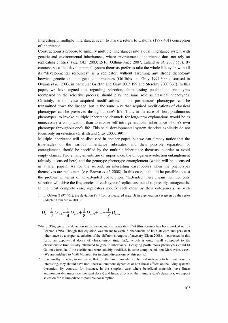
Interestingly, multiple inheritances seem to mark a return to Galton's (1897:401) conceptionof inheritance1.Constructionists propose to simplify multiple inheritances into a dual inheritance system withgenetic and environmental inheritances, where environmental inheritance does not rely onreplicating entities2 (e.g. OLF 2003:1216, OdlingSmee 2007, Laland et al. 2008:553). Bycontrast, socalled developmental system theorists prefer to take the whole life cycle with allits “developmental resources” as a replicator, without assuming any strong dichotomybetween genetic and nongenetic inheritances (Griffiths and Gray 1994:300, discussed inOyama et al. 2003, in particular Griffith and Gray 2003:199 and Sterelny 2003:337). In thispaper, we have argued that regarding selection, short lasting posthumous phenotypes(compared to the selective process) should play the same role as classical phenotypes.Certainly, in this case acquired modifications of the posthumous phenotypes can betransmitted down the lineage, but in the same way that acquired modifications of classicalphenotypes can be preserved throughout one's life. Thus, in the case of short posthumousphenotypes, to invoke multiple inheritance channels for longterm explanations would be asunnecessary a complication, than to invoke self intragenerational inheritance of one's ownphenotype throughout one's life. This said, developmental system theorists explicitly do notfocus only on selection (Griffith and Gray 2003:199).Multiple inheritance will be discussed in another paper, but we can already notice that thetimescales of the various inheritance substrates, and their possible separation orentanglement, should be specified by the multiple inheritance theorists in order to avoidempty claims. Two entanglements are of importance: the ontogenesisselection entanglement(already discussed here) and the genotypephenotype entanglement (which will be discussedin a later paper). As for the second, an interesting case occurs when the phenotypesthemselves are replicators (e.g. Brown et al. 2008). In this case, it should be possible to castthe problem in terms of an extended coevolution. “Extended” here means that not onlyselection will drive the frequencies of each type of replicators, but also, possibly, ontogenesis.In the most complete case, replicators modify each other by their ontogenesis, as with

1 In Galton (1897:401), the deviation D(t) from a measured mean M in a generation t is given by the series(adapted from Sloan 2008) :

Dt=12Dt−1

14D t−2

18D t−3...

1

2nDt−n

Where D(ti) gives the deviation in the ascendancy at generation (ti) (this formula has been worked out byPearson 1898). Though this equation was meant to explain phenomena of both atavism and persistentinheritance by a proper calculation of the different strengths of ancestry (Sloan 2008), it expresses, in thisform, an exponential decay of characteristic time ln(2), which is quite small compared to thecharacteristic time usually attributed to genetic inheritance. Decaying posthumous phenotypes could fitGalton's formula, if the coefficients were suitably modified, in some complicated, nonMarkovian, cases.(We are indebted to Maël Montévil for indepth discussions on this point.)

2 It is worthy of note, in our view, that for the environmentally inherited materials to be evolutionarilyinteresting, they should have nonlinear autonomous dynamics or nonlinear effects on the living system'sdynamics. By contrast, for instance, in the simplest case where beneficial materials have linearautonomous dynamics (e.g. constant decay) and linear effects on the living system's dynamics, we expectselection for as immediate as possible consumption.

103

transcription and reverse transtription for instance. How much of biology conforms to thisinclusive picture is still to be shown1.There is still another entanglement at stake. With posthumous phenotypes, the selectiveprocess, ceteris paribus, takes more time. This is a supplementary reason, ceteris paribus, forthis process not to complete its course on a given timeinterval. In particular, new mutationscan arise in the population before a given posthumous phenotype get entirely selected ordeselected. Advent of new variants can modify selection coefficients. This means that nicheconstruction (sensu posthumous phenotypes) can favor an entanglement between ecological(selective process) and evolutionary (new mutations) timescales. Evolution could be a

1 GodfreySmith (2000) remarks that such reverse transcriptions, if probably rare in organic processes, areubiquitous in cultural processes. He actually speaks in terms of reverse translation, but this does notmatter much for culture where there is, at first sight, no separation between transcription and translation.The entire thought experiment is worth quoting :

“I will illustrate the relevant phenomena with a hypothetical example. Hull dislikes fanciful thoughtexperiments, but I hope he will forgive this one, as it illustrates not just the space of possibilities but alsosome real cases. Imagine there is reverse translation, from protein primary structure to nucleic acidsequence, as well as forward translation. Then we can imagine an organism in which the genetic materialinitially contributed by parents is in the form of DNA, but once the new individual has used these genesto manufacture proteins, the DNA is broken down. (The proteins regulate their own activities during thismiddle stage.) At the end of the cycle, new genes for the next generation are made by reversetranslating(and reversetranscribing) from protein to nucleic acid. In this case, any "allele" exists in two physicallydifferent forms through the life cycle – first as nucleic acid base sequence and then as amino acidsequence. Mutations in either form will be passed on.

(…)Does any of this matter? Reverse translation does not exist. Is there any reason to think about strange cases in

which discrete replicators get lost in a sea of causal complexity? Yes, because aside from the need toexplore the space of possibilities, these complicated translations and reversetranslations are ubiquitous incultural transmission.

(...)Even simpler cultural replicators often exhibit changes of form similar to those in the hypothetical case

outlined above. Suppose a bird learns its song from a parent or from other local adult birds. Then the songpattern takes two distinct forms in this process. The young bird acquires its song by picking up soundwaves. This results in the formation of neural structures, which persist when the song is not being sung.The song is passed to new birds in the form of sound waves again. We have a causal channel throughwhich the inheritance of variation is possible, but any replicator variant must exists in two physicallydifferent forms during the cycle. A mutation at either stage can be passed on. Birdsongs of this kind arenot as unproblematic replicators as genes, but they are still good candidates, even though they are of thecomplicated type illustrated by my hypothetical "reversetranslation" case.

(…)To the extent that cultural transmission involves a lineage of structures, distinct to some extent from the

causal sea surrounding them, where earlier members of the lineage can be causally involved in theproduction of similar later members, in a way causally responsible for the similarity between them, wehave replicators. To the extent that no lineage can be isolated because of constant blending, and to theextent that the similarities between cultural products over time result from a network of dispersed andinteracting causal factors, in which all the quirks of human preference and flexibility are involved, we donot have replicators. These are reasons to be skeptical about general replicator based theories of culturalchange, of the type advanced by Dawkins (1976), Hull (1988) and Dennett (1995). » (GodfreySmith2000).

Here, in our view, GodfreySmith does not illustrate well his thought experiment, as neural structures are not,

104

runaway from selection, the loose material of living flowing, never quite stable, never quitefree, like pillow lavas in an ocean of forms.As for entanglements, concepts are laid to seek for unexpected or not sought trajectories1.Empirical implementations of the “entanglementist” research program should give birth tonew concepts also, provided that the invariants and their timescales are made explicit orexplicitly questioned.

5.3 The importance of (not so) rare events

The constructionists put a special emphasis on the role of rare events in evolution: “Even asingle isolated nicheconstructing event can be evolutionarily consequential. Considerdispersal into a new environment, where descendants of the dispersing organisms will, formultiple generations, “inherit”2 modified selection.” (Laland et al. 2008:552, see also, as faras we can merge their views, Griffith and Gray 1994:288). Emergence of a new culture wouldbe a similar example (section 3.9). The constructionists call such events “niche constructing”events because they do not necessarily involve alteration of the genetic materials.“Epigenetic” events or epigenetic mutations could be more general expressions, butepigenetics has a rich story already and Waddington's (1942) original term bears hasunderwent a shift in the XXth century (Haig 2004). Let's be neutral and call them nongenetic.Nongenetic mutations can accelerate evolution and enable living systems to “overcome someof the limitations of genetic inheritance” (Bonduriansky and Day 2009:111). This is, after all,a well known role of learning, where successful behavioral variants are kept in mind, to dealwith small timescale problems (see Danchin et al. 2008:129), or of some maternal effectsthat can complement environmental cues to determine behaviors such as, for instance,diapauses in insects (Mousseau and Dingle 1991:514).However, theoretically such “rare” (or not so rare), sporadic, events can not only act as (nongenetic) novelty inducers, but also change the phase space of development and/or selection.That is, new dimensions in the phase space get relevant and some get irrelevant as for thedynamics ; phase space shifting is a way of expressing a radical change in the

as far as we know, germline replicators (sensu Dawkins 19762006) – by contrast with songs. In thisrespect, neural structures will be more easily thought of as phenotypes of the songs, which are the onlyreplicators at play. A different situation, however, occurs with substrates of human cultural objects :digital objects can be seen as germline replicators, as well as the cultural objets that they record. But inthis case, it can be argued that mutations in digital objects (such as crashdisks during thesis redaction)are probably not a driving force of cultural evolution, compared to, say, behavioural mutations. Thiscomes from the fact that digital objects are, for the moment, rather reliable replicators with very lowmutation rates. Better examples of such reversetranslation couples could maybe be found in economy,though we did not investigate this way much.

Finally, we quoted also one of the conclusive paragraphs, which does not relate much to the problem ofreversetranslation, to show that this thought experiment was not GodfreySmith's main point here.

1 We gloss over the “new” trajectories of Laland et al.'s (1999) seminal model and its descent in OLF's(2003) book, which result merely from changing the type of natural selection. Something moreunexpected can probably be derived from niche construction.

2 The quotation marks are of importance here. The descent inherits the new environment only if wecompare two populations in different environments, otherwise, there is no variability and thus, noheritability.

105

developmental/selective process1. In this category could fall some of the “dispersal mutations”and “cultural mutations” mentioned above. From the genetic point of view, new parts of thereaction norms get exposed to evolution. This, of course, can favor the nonseparability ofecology and evolution, if phasespace shifting is rendered more frequent by nicheconstruction.Phase space shifting already occurs, however, with classical environmental changes. Thereason to invoke niche construction (sensu extended or posthumous phenotypes) here, wouldbe to show that such nongenetic mutations are nonnegligible phasespace modifiers in thecourse of evolution. This cannot be done by exhibiting isolated examples, but by integratingthem into an “entanglementist” theory. For instance, ideally, a theory of nongeneticmutations would give probability distributions of the expected mutations2.

5.4 Bringing a new theory of macroevolution

Close to the idea of phasespace transitions, we find the idea of macroevolution. We candefine microevolution as the selective process occurring in a given phase space (of traits),while macroevolution occurs when the system changes of phase space, either because ofchanges in developmental and/or selective environments, or simply in the course of thedynamics, because of critical points in the phase space where (unexpected) pleiotropy occursor new traits get (surprisingly) evolutionarily relevant.Changes in phase space, and definitions of the relevant phase space of traits, are questionstackled by the evodevo framework (see Minelli 2009). Also, as niche construction can lead tochanges in the developmental and/or selective environments, it can favour (or not, ifcounteractive) macroevolution. This is how we read Laland et al.'s plea (2008:551) to buildbridges between evodevo and niche construction, to provide evolutionary biology with atheory of macroevolution (partly based on niche construction). By the way, the fact that nicheconstruction deals with the entanglement of ontogenesis and selection makes de facto nicheconstruction theory a (new) part of the evodevo framework. As for now, the theory is in itsembryonic stages, that is, the collect of empirical examples – though in evodevo, sometheoretical advances have been met (reviewed in Müller 2007).

1 Of course, a change in the phase space can be subsumed into a broader phase space. The point here is thatnot all, but not always the same, developmental or selective dimensions are relevant. The question ofqualifying or not a given mutation as a “change in the phasespace” or “a move in the same phase space”is a matter of taste and, notably, of theoretical lightness (in particular of dimensional parsimony).

2 This would be also true, of course, of an ideal theory of genetic mutations. This idea comes from thefollowing quote: “This means that, in addition to chance and natural selection, there is a third explicitlyrecognized source of evolutionary innovation, which occurs when geneinformed, directed, nonrandom,yet novel, acts of niche construction bring about consistent changes in environments” (Laland et al.2008:561). Here we gloss over the fact that natural selection is not, as far as we know, an explicitlyrecognized source of innovation, and concentrate on the claim that the niche constructing mutationswould be both “novel” and “nonrandom”. The question is: nonrandom in which respect? A theory ofepigenetic mutations should answer this question, and in particular the question of (non)randomness withregards to fitness, if any.

106

5.5 Epistasis and the rugged fitness landscape

Some genetic interactions (such as underdominance and epistasis) can make the fitnesslandscape more rugged (Wright 1932:3), that is, with multiple fitness peaks more or lessseparated by fitness valleys (the impossibility to prove the nonexistence of ridges connectingthe peaks justifies the fuzzy “more or less” here ; see Whitlock et al. 1995:622). Here thelandscape is drawn as a genotypefitness map or a phenotypefitness map (Whitlock et al.1995:603, for epistasis in genotypephenotype maps see the review by Phillips 2008:856859). This issue is closely connected to macroevolution : such ruggedness of the fitnesslandscape will cause moves in the phase space of traits (or genes), and thus, possibly,(unexpected) changes of the phase space when one dimension of the landscape gets(ir)relevant.Eventually, too rugged a landscape could prevent consistent evolution under selection. Thetopology of the genes (sensu their structural similarity) and the topology of their fitnesseswould not be similar enough to apply gradualism (Huneman 2010). Certainly, selectionismdoes not require gradualism, but gradualism enhances the relevance of selectionism. Realoccurrences of this theoretical possibility, however, are expected to be reduced by thesmoothing effect of individual landscape averaging at the population al level, which makeslandscapes less rugged (Arnold et al. 2001:18,23)Niche construction (sensu extended or posthumous phenotypes) can also lead, as any otherphenotype, to epistasis – at least theoretically (OLF 2003:127). Because of phenotypicextension, niche constructing phenotypes can be, probably, more easily influenced by genes inother organisms (conspecific or not) than classical phenotypes. Here too, the possible effectson the fitness landscapes are an entirely new field of investigation.

6. Conclusion

Selectionism involves one necessary and sufficient cardinal condition : a criterion of selectionof phenotypes, that is in our case differences in fitness (survival and/or reproduction). Thisdefines a phenotypefitness map. For the effects of selection on phenotypes abundance at aparticular date to be propagated in time, selectionism requires a second condition : heritabilityof the selected phenotypes (as heritability entails variability, we do not need the classical butredundant condition on variability here). This condition is fulfilled in particular when theselected phenotypes are defined as effects of long lasting hereditary entities (the genes) on theworld. This defines a genotypephenotype map1. Last, for the selective process to be the onlyprocess at play, selectionism requires another condition : that ontogenesis be timeseparatedfrom selection2.

1 There is a slight, but notable, slippage here, between defining heritable phenotypes as “entities under thepartial control of hereditary entities (the genes)”, and as “the very effects of genes on the world” (i.e. totalcontrol).

2 Moreover, for the dynamics of the phenotypes abundances to be consistent (i.e. self similar) through time,selectionism requires another condition : that ontogenesis and selection be consistent, if not invariant,through time (we gloss over the theoretical possibility that both ontogenesis and selection be inconsistentbut compensate each other). This is achieved when both developmental and selective environments arethemselves consistent through time (recall that the other variables in the system, the long lastinghereditary entities, are already supposed to be individually invariant in time). Relaxing this condition is

107

Niche construction theory, as for its evolutionary part, consists in relaxing the last condition :ontogenesis is no more separable from selection. The relaxation comes from the considerationthat genes can have long lasting (posthumous) phenotypes. Tracking the ontogenesis ofposthumous phenotypes is the way to incorporate “mere effects” in the selective processes.Niche construction theory, however, is still an instance of the selectionist scheme, as it is builton the two conditions of fitness and heritability1. The “symmetry” between construction andselection has to be understood, in our view, in the sense of a timescale entanglement of thesetwo processes. Niche construction is a “constructionism” in the sense that the environmentdoes not alone force the phenotypic dynamics through selective events, as in classicalselectionism, but also does the gene through ontogenetic events (this might seem ratherobvious a posteriori, but it was not so obvious, in our view, in earlier formulations of thetheory)2. As for niche construction qua an instance of evodevo, coming back to theimportance of the relationships between ontogenesis and evolution can be seen as aresurgence of XIXth century preoccupations (e.g. Haeckel 1866, 1895, Sloan 2008, Amundson2005).Other relaxations, such as relaxing the timescale separation between genotype andphenotype, could lead to even more complex pictures, if found in the field. It is a truism to saythat timeseparations are crucial in dynamical systems, but it is a truism worthy of note. In ourview, some hot debates (about the unit of selection, the negligibility of ontogenesis, the needfor internalist explanations, to name just those we discussed) could gain from being stated interms of timescale separations, because identified claims are easier to discuss, and becausethey become empirical rather than conceptual issues.Even though we gave some support to the theoretical possibility of a “symmetry” betweenconstruction and selection, we were not able, by contrast, to find any support for the view thatconstruction should lead to fit. In our view, OLF's claim on the two routes (selection andconstruction, in addition to chance) towards fit should be entirely avoided. This claimobscures what niche construction theory is about, that is, timescale entanglement, and notany organismenvironment match.Despite remarkable efforts of the founding fathers, empirical evidences are still to be found toget a taste of the evolutionary implications of true niche construction. The examples that havebeen gathered so far can be interpreted in the classical selectionist scheme, for the most partas intra or intergenomic coevolutive events, as could be interpreted the examples that mightbe gathered by field researchers following OLF's method for detecting niche construction inthe wild (2003:292). To give niche construction theory some support, a special attentionshould thus be given, in our view, to the empirical investigation of the timescales ofontogenesis and selection. Given the difficulty to detect natural selection in the wild (Endler1986:chap.4), it is not clear whether we will ever be able to detect timescale entanglement, as

common in evolutionary biology, notably because of varying selective environments, such as infrequencydependence.

1 Here we consider only the part of niche construction theory that is embedded in the definition of nicheconstruction (OLF 2003:419). We gloss over other interesting parts of the theory, such as the definition ofcouples {organism, environment} as new explanda (e.g. OdlingSmee 2007, in our view). This will bediscussed in a following paper.

2 Here we mean “construction” sensu OLF(2003:419) as rephrased by us, where the feedback is primary,and not sensu GodfreySmith (1998) where there is no such requisite.

108

it would suppose to first detect the selective process, if any, at play. Empirical detectionwould be necessary however, to build a true physical theory from niche construction intuitivepremisses.

Main point

Ontogenesis is the process whereby a gene modifies its environment. Selection is the processwhereby an environment modifies a gene's fitness (i.e. its geometrical rate of increase). Thedistinction between ontogenesis and selection stems from the distinction between phenotypeand replication. Embryology is internalist (sensu nonexternalist constructivist, section 1.2) ifthe gene “forces” the environment without being itself modified (nongenetic inheritance ofacquired characteristics). Selectionism is externalist (sensu non constructivist) if theenvironment “forces” the gene's fitness.For clarity, we can split Lewontin's system into two systems describing each ontogenesis (o)and selection (s). Thereafter, g means the population vector of individual genes and E thevector of individual environments1. We get:Ontogenesis:E t t=og t ,E t

g t t=g t

Selection:g t t=s g t , E t

E t t= f E t

Here the selective function s and the ontogenetic function o are invariant in the dynamics (f isany function describing autonomous environmental dynamics). Moreover, we assume thatgenes are left unchanged throughout ontogenesis, and that the environment has anautonomous dynamics throughout selection. We intentionally do not distinguish betweendevelopmental and selective environments here, in order to avoid any reactivating of the idea(somehow stemming from the usual timescale separation between ontogeny and evolution)that development and selection occur in two different worlds.Lewontin's constructivist claim, worked out by OdlingSmee, Laland, Feldman and others,amounts to claim that the two systems are not separable (i.e. same E and g, and similar Δt).Without time separation, we get the following constructive system:E t t=og t ,E t 1

g t t=s g t , E t

where forcings have been removed (but partial forcings can remain, hidden in themetaphorical equations, see section 4.2)2.

1 The two systems can be both read at the individual or populational level, but the sense of the systemchanges depending on the level. Intuitively, we would prefer the individual level for ontogenesis, where gstands for an individual nucleic acid, and populational level for selection, where g stands for thepopulation vector of genes. However, to compare the two systems requires to interpret them at the samelevel.

2 The metaphor of information processing in biology (i.e. populations of genes are informed by naturalselection, and individual genes express this information throughout ontogenesis, e.g. OLF 2003:174)comes, in our view, from the supposed forcings described by our two systems of equations: what forces,

109

Frequency dependence is a particular case of selection where E=g. Thus for frequencydependence, we get:E t t=sg t 2

Comparing (1) and (2) helps to distinguish between “selective construction” (that is, amodification of the selective environment through the selective process itself, without anyentanglement with ontogenesis: equation 2) and “ontogenetic construction” (modification ofthe selective environment through the ontogenetic process: equation 1). We called the lastniche construction here.

Glossary

Here we aim at specifying in which idiosyncratic sense we (and sometimes authors cited here)take some of the words discussed in the main text (the corresponding sections where theconcepts are discussed are given).

Adaptation: in this chapter, adaptation means fit (section 4.1).Classical selectionist scheme: the selectionist scheme where ontogenesis as a dynamicalprocess is neglected (sections 2.1 & 2.6).Entanglement: non separability of scales1.Environment: “the surrounginds of a given organism or population, including all the contentsof this regions” (GodfreySmith 1998:152). Here GodfreySmith reduces Brandon's threeconcepts of environment into one (see selective environment below).Gene: active, faithfully replicating, piece of nucleic acid (section 2.2).Genotype: class to which a gene belongs (given its sequence or its reaction norm)2.Genotypephenotype map: see norm of reaction (section 2.3).Fit: adaptedness (to given constraints) (section 4.1).Fitness: adaptedness or expected geometrical rate of increase on a given timescale (includingrate of nondecrease by mere survival) given adaptedness on this timescale3 (section 2.4).Forcing: any structure imposed onto a system, or, in particular, onto the dynamics of avariable. Forcing entails the absence of retroaction4.Invariant : figure that is symmetric with respect to a specified set of transformations. In thispaper, the transformations are mostly translations in time. The invariant here is a set ofdynamical equations, including the set of constant parameters (section 1.1).5

informs.1 Our use of this term departs from its strict meaning in quantum mechanics.2 We draw the reader's attention to the fact that this definition departs from the usual definition, where a

genotype stands for a class to which an gene or organism belongs based upon “the postulated state of itsinternal hereditary factors, the genes” (Lewontin 1992).

3 Here we use the socalled propensity concept. The timescale criterion is meant to subsume, as far aspossible with so few words, both concepts of “long term fitness” (Thoday 1953) and of “expected time toextinction” (Cooper 1984), while remaining neutral as for the relevant timescale (for instance, one mightbe interested in transient events).

4 Here we do not limit forcing to the temporal structures, in contrast with traditionnal meaning of the wordin the field of classical mechanics.

5 Our use of this concept here is rather liberal. For an indepth discussion of symmetry and invariance, see

110

Natural selection: the process described by the selectionist scheme (section 2.1)1.Niche (OLF's sense): “the sum of all the natural selection pressures to which the population isexposed. A population O's niche is specified at time t by a “niche function” N(t) whereN(t)=h(O,E). O is the population of organisms, and E is O's environment, both specified attime t. The temporal dynamics of N(t), equivalent to niche evolution, are driven by both O'snicheconstructing acts, and selection from sources in E that have previously been modifiedby O's nicheconstructing acts, as well as by the dynamics of E that are independent of O'sniche construction.” (OLF 2003:419). Note that this definition departs from those used inecology (this thesis, chap.1).Niche construction (OLF's sense): “the process whereby organisms, through theirmetabolism, their activities, and their choices, modify their own and/or each other's niches.Niche construction may restul in changes in one or more natural selection pressures in theexternal environment of populations. Nicheconstructing organisms may alter the naturalselection pressures of their own population, of other populations, or of both.” (OLF2003:419). Niche construction (our sense): ontogenesis which is not separable from selection.Norm of reaction : “the function that maps the space of environmental sequences into thespace of phenotypic outcomes for a given genotype. (…) Of course, in practice, these arespecified as the mapping of partial environment (e.g., temperature) into partial phenotype(e.g., body weight) for a partial genotype.” (Lewontin 1992:141, the concept is due toWolterreck 1909:135, see Sarkar 2006:80).Ontogenesis: the process whereby a gene (or any other replicator) modifies its environment.Phenotype: effect of a gene on the world. The phenotype of x is that part Ex of theenvironment E for which P(Ex / x & y) = P(Ex / x) ≠ P(Ex / y), where y stands for any othergenotypic entity in the system2.Phenotypefitness map: selective invariant. As the reaction norm, the selective invariantincludes environmental dimensions (section 2.3).Replication (broad sense): growth and persistence, multiplication and survivalSelection: the process whereby an environment modifies a gene's fitness.Selection (or selective) pressure: short term selective invariant: selection coefficients orselection gradients (i.e. differences in fitness3), or long term selective invariant: e.g. payoffmatrix (section 3.6).Selective environment: the environment “measured in terms of the relative actualizedfitnesses of different genotypes across time or space” (Brandon 1992). Brandon defines the

Brading & Castellani (2008).1 As Hodge (1992) remarked, Darwin did not explicitly define this term. For conceptual accounts see e.g.

Endler (1986:4 gives a similar definition, 1992), Brandon (2008).2 We draw the reader's attention to the fact that this definition departs from the usual definition, where a

phenotype is a class to which an organism belongs based upon “the observable physical qualities of theorganism, including its morphology, physiology, and behavior at all levels of description” (Lewontin1992).

3 Endler (1986:xii) lists at least two meanings of selection gradient: (1) geographic gradient in naturalselection (2) the rate of change of fitness with trait value (Lande & Arnold 1983). Here we use the secondsense.

111

selective environment in contrast with the external environment (“the sum of total of factors,both biotic and abiotic, external to the organisms of interest”) and the ecological environment(“those features of the external environment that affect the organisms' contributions topopulation growth”). (It should be noticed that OLF do not cite Brandon, thus we cannotconclude that their use of the word conforms to the definition given here.)State: set of variables, at a given point on the dimension of reference. In our case, thereference dimension is time (section 1.1).Time scale: characteristic time of a process (e.g. mean lifetime or halflife time).Time scale separation: the theoretical procedure whereby, when dealing with a particulardynamical process, one ignores other possibly relevant processes because they are either fastenough or slow enough. When two dynamical processes are time separated, their dynamicsare invariant with regards to each other.

112

References

Allis, C.D., Jenuwein, T. & Reinberg, D., 2007. Epigenetics, CSHL Press.ÁlvarezCastro, J.M., Kopp, M. & Hermisson, J., 2009. Effects of epistasis and the evolution

of genetic architecture: exact results for a 2locus model. Theoretical populationbiology, 75(23), p.109–122.

Amundson, R., 2005. The changing role of the embryo in evolutionary thought: roots of evodevo, Cambridge University Press.

Andreotti, B., Claudin, P. & Douady, S., 2002. Selection of dune shapes and velocities Part 2: A twodimensional modelling. The European Physical Journal B, 28(3), p.12.

Ariew, A. & Lewontin, R.C., 2004. The Confusions of Fitness. The British Journal for thePhilosophy of Science, 55(2), p.347 363.

Arnold, S.J., Pfrender, M.E. & Jones, A.G., 2001. The adaptive landscape as a conceptualbridge between microand macroevolution. Genetica, 112(1), p.9–32.

Arthur, W.B., 1999. Complexity and the economy. Science, 284(5411), p.107.Avery, O.T., MacLeod, C.M. & McCarty, M., 1944. Studies on the Chemical Nature of the

Substance Inducing Transformation of Pneumococcal Types: Induction ofTransformation by a Desoxyribonucleic Acid Fraction Isolated from PneumococcusType III. Journal of Experimental Medicine, 79(2), p.137158.

Ayala, F.J., 1978. Mechanisms of Evolution. Scientific American, 239(3), p.56&.Ayala, F.J. & Arp, R., 2009. Contemporary Debates in Philosophy of Biology, John Wiley

and Sons.Bailly, F. & Longo, G., 2009. Biological Organization and AntiEntropy. Journal of

Biological Systems, 17(1), p.6396.Bailly, F., Longo, G. & Montévil, M., A 2dimensional Geometry for Biological Time.Barberousse, A., 2009. Mapping the future of biology: evolving concepts and theories,

Springer.Beatty, J., 1992. Fitness: Theoretical Contexts. Dans Keywords in evolutionary biology.

Harvard University Press, p. 115119.Bendall, D.S., 1986. Evolution from molecules to men, CUP Archive.Bock, W., A synthetic explanation of macroevolutionary change a reductionistic approach.

Bull. Carnegie Mus. Nat. Hist., 13, p.2069.Bock, W.J., 1980. The Definition and Recognition of Biological Adaptation. American

Zoologist, 20(1), p.217 227.Bonduriansky, R. & Day, T., 2009. Nongenetic inheritance and its evolutionary implications.

Annual Review of Ecology, Evolution, and Systematics, 40, p.103–125.Boogert, N.J., Paterson, D.M. & Laland, K.N., 2006. The implications of niche construction

and ecosystem engineering for conservation biology. BioScience, 56(7), p.570–578.Bouchard, F., 2008. Causal processes, fitness, and the differential persistence of lineages.

Philosophy of Science, 75(5), p.560–570.Bouchard, F., 2007. Moving beyond the influence of molecular genetics on the debate about

reductionism in philosophy of biology. Dans The Influence of Genetics onContemporary Thinking. Dordrecht: Springer Netherlands.

113

Bowler, P.J., 1992. Lamarckism. Dans Keywords in evolutionary biology. Harvard UniversityPress, p. 188193.

Brandon, R., 2008. Natural Selection. Available at: http://plato.stanford.edu/entries/naturalselection/ [Accédé Novembre 9, 2010].

Brandon, R.N., 1990. Adaptation and environment, Princeton University Press.Brandon, R.N., 1996. Concepts and methods in evolutionary biology, Cambridge University

Press.Brandon, R.N., 1992. Environment. Dans Keywords in evolutionary biology. Harvard

University Press, p. 8791.Brown, S., Le Chat, L. & Taddei, F., 2008. Evolution of virulence: triggering host

inflammation allows invading pathogens to exclude competitors. ECOLOGYLETTERS, 11(1), p.4451.

Bub, J., 2001. Quantum Entanglement and Information. Available at:http://plato.stanford.edu/entries/qtentangle/ [Accédé Novembre 13, 2010].

Burian, R.M., 1992. Adaptation: Historical Perspectives. Dans Keywords in evolutionarybiology. Harvard University Press, p. 712.

Carroll, S.B., 2008. Evodevo and an expanding evolutionary synthesis: a genetic theory ofmorphological evolution. Cell, 134(1), p.25–36.

Champagnat, N., Ferrière, R. & Méléard, S., 2006. Unifying evolutionary dynamics: Fromindividual stochastic processes to macroscopic models. Theoretical PopulationBiology, 69(3), p.297321.

Clobert, J., 2001. Dispersal, Oxford University Press.Cooper, W.S., 1984. Expected time to extinction and the concept of fundamental fitness.

Journal of Theoretical Biology, 107(4), p.603629.Crick, F., 1958. On Protein Synthesis Academic Press., New York.Cummins, R. & Roth, M., 2009. Traits have not evolved to function the way they do because

of a past advantage. Dans Contemporary Debates in Philosophy of Biology. JohnWiley and Sons.

Cuvier, G., 1817. Le règne animal distribué d'après son organisation: pour servir de base àl'histoire naturelle des animaux et d'introduction à l'anatomie comparée.L'introduction, les mammifères et les oiseaux, Deterville.

Danchin, É. & Wagner, R.H., 2010. Inclusive heritability: combining genetic and nongeneticinformation to study animal behavior and culture. Oikos, 119(2), p.210–218.

Danchin, É., Giraldeau, L. & Cézilly, F., 2008. Behavioural ecology, Oxford University Press.Darwin, C., 1862. On the various contrivances by which British and foreign orchids are

fertilised by insects, and on the good effects of intercrossing. 1er éd., London: JohnMurray. Available at: http://darwinonline.org.uk/

Darwin, C.R., 1881. The formation of vegetable mould, through the action of worms, withobservations on their habits., London: John Murray.

Darwin, C.R., 1868. The variation of animals and plants under domestication. 1er éd.,London: John Murray. Available at: http://darwinonline.org.uk

Darwin, C.R., 1859. On the origin of species by means of natural selection, or thepreservation of favoured races in the struggle for life. 1er éd., London: John Murray.

Darwin, C.R., 1860a. On the origin of species by means of natural selection, or the

114

preservation of favoured races in the struggle for life. 2 éd., London: John Murray.Darwin, C.R., 1860b. On the origin of species by means of natural selection, or the

preservation of favoured races in the struggle for life. 1er éd., New York: D.Appleton.

Darwin, C.R., 1861. On the origin of species by means of natural selection, or thepreservation of favoured races in the struggle for life. 3 éd., London: John Murray.





Darwin, C.R. & Wallace, A., 1858. On the tendency of species to form varieties; and on theperpetuation of varieties and species by natural means of selection. Dans Journal ofthe Proceedings of the Linnean Society of London. Zoology, p. 4650. Available at:http://darwinonline.org.uk/

Dawkins, R., 1978. Replicator selection and the extended phenotype. Zeitschrift FürTierpsychologie, 47(1), p.6176.

Dawkins, R., 2004. Extended phenotype–but not too extended. A reply to Laland, Turner andJablonka. Biology and Philosophy, 19(3), p.377–396.

Dawkins, R., 1976. The selfish gene, Oxford University Press.Dennett, D.C., 1996. Darwin's dangerous idea: evolution and the meanings of life, Simon &

Schuster.Dickins, T. & Dickins, B., 2008. Mother nature's tolerant ways: Why nongenetic inheritance

has nothing to do with evolution. NEW IDEAS IN PSYCHOLOGY, 26(1), p.4154.Dobzhansky, T., 1937. Genetics and the Origin of Species Reissue., Columbia University

Press.Donohue, K., 2005. Niche construction through phenological plasticity: life history dynamics

and ecological consequences. New Phytologist, 166(1), p.8392.Durham, W.H., 1992. Coevolution: Genes, Culture, and Human Diversity, Stanford

University Press.Ehrentreich, N., Fe, S.F.I.(. & N.M.), 2008. Agentbased modeling: the Santa Fe Institute

artificial stock market model revisited, Springer.Endler, J.A., 1992. Natural Selection: Current Usages. Dans Keywords in evolutionary

biology. Harvard University Press, p. 220224.Fairbanks, A., 1898. Empedocles Fragments and Commentary. Dans The First Philosophers

of Greece. London: K. Paul, Trench, Trubner, p. 157234. Available at:http://history.hanover.edu/texts/presoc/emp.htm.

Feldman, M.W., 1992. Heritability: Some Theoretical Ambiguities. Dans Keywords inevolutionary biology. Harvard University Press, p. 151157.

Ferrière, R. & Le Galliard, J., 2001. Invasion fitness and adaptive dynamics in spatialpopulation models. Dans Dispersal. Oxford University Press.

115

Fisher, S.R.A., 1918. The Correlation Between Relatives on the Supposition of MendelianInheritance. Philosophical Transactions of the Royal Society of Edinburgh, 52,p.399433.

Fisher, S.R.A. & Bennett, J.H., 1930. The genetical theory of natural selection: a completevariorum edition, Oxford University Press.

Fox Keller, E., 1992. Fitness: Reproductive Ambiguities. Dans Keywords in evolutionarybiology. Harvard University Press, p. 120121.

Galton, F., 1897. The Average Contribution of Each Several Ancestor to the Total Heritage ofthe Offspring. Proceedings of the Royal Society of London, 91, p.401413.

Galton, F., 1869. Hereditary Genius, London: Macmillan and Co.Gerstein, M.B. et al., 2007. What is a gene, postENCODE? History and updated definition.

Genome research, 17(6), p.669.Gillespie, J.H., 1973. Natural Selection with Varying Selection Coefficients ? a Haploid

Model. Genetics Research, 21(02), p.115120.Gingerich, P.D., 2009. Rates of Evolution. Annual Review of Ecology, Evolution, and

Systematics, 40, p.657–675.Ginzburg, L.R. & Colyvan, M., 2004. Ecological orbits: how planets move and populations

grow, Oxford University Press.GodfreySmith, P., 2000. The replicator in retrospect. Biology and Philosophy, 15(3), p.403–

423.GodfreySmith, P., 1998. Complexity and the Function of Mind in Nature, Cambridge

University Press.Goldschmidt, R.B., 1940. The material basis of evolution, Yale University Press.Goodman, C. & Coughlin, B., 2000. The evolution of evodevo biology. PROCEEDINGS OF

THE NATIONAL ACADEMY OF SCIENCES OF THE UNITED STATES OFAMERICA, 97(9), p.44244425.

Gould, S.J., 1977. Eternal metaphors of paleontology. Dans Patterns of Evolution asIllustrated by the Fossil Record. Amsterdam: Elsevier.

Gould, S.J. & Lewontin, R.C., 1979. Spandrels of Sanmarco and the Panglossian Paradigm A Critique of the Adaptationist Program. Proceedings of the Royal Society of LondonSeries BBiological Sciences, 205(1161), p.581598.

Gould, S.J. & Vrba, E.S., 1982. Exaptation A Missing Term in the Science of Form.Paleobiology, 8(1), p.415.

Green, E.J. & Zhou, R., 2005. Money as a Mechanism in a Bewley Economy. InternationalEconomic Review, 46(2), p.351–371.

Grene, M.G., Grene, M. & Depew, D.J., 2004. The philosophy of biology: an episodic history,Cambridge University Press.

Gros, P.A., Le Nagard, H. & Tenaillon, O., 2009. The evolution of epistasis and its links withgenetic robustness, complexity and drift in a phenotypic model of adaptation.Genetics, 182(1), p.277.

Haeckel, E., 1866. Generelle Morphologie der Organismen: allgemeine Grundzüge derorganischen FormenWissenschaft, mechanisch begründet durch die von CharlesDarwin reformirte DescendenzTheorie. Allgemeine Entwickelungsgeschichte derOrganismen, Reimer.

116

Haeckel, E., 1895. The Riddle of the Universe at the Close of the Nineteenth Century, ReadBooks.

Haig, D., 2004. The (Dual) Origin of Epigenetics. Dans Epigenetics. CSHL Press.Haldane, J.B.S. & Jayakar, S.D., 1963. Polymorphism due to selection of varying direction.

Journal of Genetics, 58(2), p.237242.Hamburger, V., 1998. Embryology and the Modern Synthesis in Evolutionary Theory. Dans

The evolutionary synthesis: perspectives on the unification of biology. Cambridge,Massachusetts: Harvard University Press.

Hodge, M.J.S., 1992. Natural Selection: Historical Perspectives. Dans Keywords inevolutionary biology. Harvard University Press, p. 212219.

Holt, R. & Gaines, M., 1992. Analysis of Adaptation in Heterogenous Landscapes Implications for the Evolution of Fundamental Niches. Evolutionary Ecology, 6(5),p.433447.

Hubbell, S.P., 2006. Neutral theory and the evolution of ecological equivalence. Ecology,87(6), p.1387–1398.

Huggett, R.J., 2004. Fundamentals of biogeography, Routledge.Hull, D. & Wilkins, J.S., 2001. Replication. Available at:

http://plato.stanford.edu/entries/replication/ [Accédé Novembre 9, 2010].Hull, D.L., 1980. Individuality and Selection. Annual Review of Ecology and Systematics, 11,

p.311332.Hull, D.L., 1988. Science as a process: an evolutionary account of the social and conceptual

development of science, University of Chicago Press.Huneman, P., 2006. Naturalising purpose: From comparative anatomy to the 'adventure of

reason' [An article from: Studies in History and Philosophy of Biol & Biomed Sci],Elsevier.

Huneman, P., 2010. Assessing the Prospects for a Return of Organisms in EvolutionaryBiology. Hist. Phil. Life Sci., 32(341372).

Huneman, P., 2008. Métaphysique et biologie: Kant et la constitution du conceptd'organisme, KIME.

Hurtt, G. & Pacala, S., 1995. The consequences of Recruitment Limitation ReconcilingChance, History and Competitive Differences Between Plants. Journal of TheoreticalBiology, 176(1), p.112.

Huxley, J.S., 1942. Evolution: the modern synthesis, London: Allen and Unwin.Huxley, J.S., 1932. Problems of relative growth, London: Methuen.Huxley, J.S. & de Beer, G.R., 1934. The elements of experimental embryology, Cambridge:

Cambridge University Press.Huynen, M.A., Stadler, P.F. & Fontana, W., 1996. Smoothness within ruggedness: the role of

neutrality in adaptation. Proceedings of the National Academy of Sciences of theUnited States of America, 93(1), p.397 401.

Jablonka, E. & Lamb, M.J., 2005. Evolution in four dimensions: genetic, epigenetic,behavioral, and symbolic variation in the history of life, MIT Press.

Jablonski, D., 1989. The Biology of Mass Extinction: A Palaeontological View.Philosophical Transactions of the Royal Society of London. Series B, BiologicalSciences, 325(1228), p.357368.

117

Johannsen, W., 1909. Elemente der exakten Erblichkeitslehre, Jena: Gustav Fischer.Available at: http://caliban.mpizkoeln.mpg.de/johannsen/elemente/index.html.

Johannsen, W., 1911. The Genotype Conception of Heredity. The American Naturalist,45(531), p.129159.

Jones, C., Lawton, J. & Shachak, M., 1994. Organisms as Ecosystem Engineers. Oikos, 69(3),p.373386.

Judson, H.F., 1979. The Eighth Day of Creation, London: Jonathan Cape Press.Karlin, S. & Liberman, U., 1974. Random temporal variation in selection intensities:Case of

large population size. Theoretical Population Biology, 6, p.355382.Keller, E.F., 2002. The century of the gene, Harvard University Press.Keller, E.F. & Lloyd, E.A., 1992. Keywords in evolutionary biology 4 éd., Harvard University

Press.Kimura, M., 1994. Population genetics, molecular evolution, and the neutral theory: selected

papers, University of Chicago Press.Kimura, M., 1954. Process Leading to QuasiFixation of Genes in Natural Populations Due to

Random Fluctuation of Selection Intensities. Genetics, 39(3), p.280295.Kitcher, P., 1992. Gene: Current Usages. Dans Keywords in evolutionary biology. Harvard

University Press, p. 128131.Kylafis, G. & Loreau, M., 2008. Ecological and evolutionary consequences of niche

construction for its agent. Ecology letters, 11(10), p.1072–1081.Laland, K.N., OdlingSmee, J.F. & Feldman, M.W., 2003. Niche Construction, Ecological

Inheritance, and Cycles of Contingency in Evolution. Dans Cycles of Contingency:Developmental Systems and Evolution. MIT Press.

Laland, K.N., 2004. Extending the extended phenotype. Biology and Philosophy, 19(3),p.313–325.

Laland, K.N. & Brown, G.R., 2006. Niche construction, human behavior, and the adaptivelaghypothesis. Evolutionary Anthropology: Issues, News, and Reviews, 15(3), p.95–104.

Laland, K.N., Kendal, J.R. & Brown, G.R., 2007. The niche construction perspective. Journalof Evolutionary Psychology, 5(1), p.51–66.

Laland, K.N., OdlingSmee, J. & Feldman, M.W., 2005. On the breadth and significance ofniche construction: a reply to Griffiths, Okasha and Sterelny. Biology andPhilosophy, 20(1), p.37–55.

Laland, K.N. et al., 2009. Conceptual barriers to progress within evolutionary biology.Foundations of science, 14(3), p.195–216.

Laland, K.N., OdlingSmee, J. & Gilbert, S.F., 2008. EvoDevo and niche construction:building bridges. Journal of Experimental Zoology Part B: Molecular andDevelopmental Evolution, 310(7), p.549–566.

Laland, K.N. & Sterelny, K., 2006. Perspective: seven reasons (not) to neglect nicheconstruction. Evolution, 60(9), p.1751–1762.

Laland, K.N., OdlingSmee, F.J. & Feldman, M.W., 1999. Evolutionary consequences ofniche construction and their implications for ecology. Proceedings of the NationalAcademy of Sciences of the United States of America, 96(18), p.10242.

Laland, K.N., OdlingSmee, F.J. & Feldman, M.W., 1996. The evolutionary consequences ofniche construction: a theoretical investigation using twolocus theory. Journal of

118

Evolutionary Biology, 9(3), p.293316.Lande, R. & Arnold, S., 1983. The Measurement of Selection on Correlated Characters.

Evolution, 37(6), p.12101226.Lehmann, L., 2008. The adaptive dynamics of niche constructing traits in spatially subdivided

populations: evolving posthumous extended phenotypes. Evolution, 62(3), p.549–566.

Lehmann, L. 2009, SpaceTime Relatedness and Hamilton's Rule for LongLasting Behaviorsin Viscous Populations. The American Naturalist, 175(1), p.136143.

Lehmann, L., Ravigné, V. & Keller, L., 2008. Population viscosity can promote the evolutionof altruistic sterile helpers and eusociality. Proceedings of the Royal Society B:Biological Sciences, 275(1645), p.1887 1895.

Lennox, J., 2004. Darwinism. Available at: http://plato.stanford.edu/entries/darwinism/[Accédé Novembre 9, 2010].

Lewens, T., 2008. Seven types of adaptationism. Biology & Philosophy, 24(2), p.161182.Lewens, T., 2010. The Natures of Selection. The British Journal for the Philosophy of

Science, 61(2), p.313 333.Lewontin, R., 2006. Commentary: Statistical analysis or biological analysis as tools for

understanding biological causes. International Journal of Epidemiology, 35(3),p.536537.

Lewontin, R.C., 1974. The analysis of variance and the analysis of causes. InternationalJournal of Epidemiology, 35(3), p.520 525.

Lewontin, R.C., 1970. The units of selection. Annual Review of Ecology and Systematics, 1,p.1–18.

Lewontin, R.C., 2006. The analysis of variance and the analysis of causes. InternationalJournal of Epidemiology, 35(3), p.520.

Lewontin, R.C. & Cohen, D., 1969. On Population Growth in a Randomly VaryingEnvironment. Proceedings of the National Academy of Sciences of the United Statesof America, 62(4), p.1056 1060.

Lewontin, R.C., 1986. Gene, organism and environment. Dans Evolution from molecules tomen. Bendall D.S.

Lewontin, R.C., 1992. Genotype and Phenotype. Dans Keywords in evolutionary biology.Harvard University Press, p. 137144.

Lewontin, R.C., 1974. The Genetic Basis of Evolutionary Change, New York: ColumbiaUniversity Press.

Lloyd, E.A., 1992. Unit of Selection. Dans Keywords in evolutionary biology. HarvardUniversity Press, p. 334340.

Loeuille, N. & Loreau, M., 2005. Evolutionary emergence of sizestructured food webs.Proceedings of the National Academy of Sciences of the United States of America ,102(16), p.57615766.

Maienschein, J., 1992. Gene: Historical Perspectives. Dans Keywords in evolutionary biology.Harvard University Press, p. 122127.

Mameli, M., 2004. Nongenetic selection and nongenetic inheritance. The British Journal forthe Philosophy of Science, 55(1), p.35.

Mandelbrot, B. & Hudson, R.L., 2009. Une approche fractale des marchés: risquer, perdre et

119

gagner, Odile Jacob.Matthew, P., 1831. On Naval Timber and Arboriculture, London: Longmans.Mayr, E., 1961. Cause and effect in biology. Science, 134, p.15011506.Mayr, E., 1978. Origin and History of Some Terms in Systematic and Evolutionary Biology.

Systematic Biology, 27(1), p.83 88.Mayr, E., 1970. Populations, species, and evolution, Cambridge, Massachusetts: Harvard

University Press.Mayr, E., 1982. The growth of biological thought: diversity, evolution, and inheritance ,

Harvard University Press.Mayr, E., 1988. Toward a new philosophy of biology: observations of an evolutionist,

Harvard University Press.Mayr, E. & Provine, W.B., 1998. The evolutionary synthesis: perspectives on the unification

of biology, Harvard University Press.McGrawHill, 1977. McGrawHill encyclopedia of science and technology: an international

reference work in fifteen volumes including an index, McGrawHill.Mendel, G., 1865. Experiments in plant hybridization (1865). Dans Read at the meetings of

February 8th, and March 8th. Available at:http://www.esp.org/foundations/genetics/classical/gm65a.pdf.

Mendel, G.J., 1866. Versuche über Pflanzenhybriden. Dans Verhandlungen desnaturforschenden Vereines in Brünn, Bd. IV für das Jahr, 1865. p. 347. Available at:http://www.esp.org/foundations/genetics/classical/gm65.pdf.

Mesoudi, A., Whiten, A. & Laland, K.N., 2006. Towards a unified science of culturalevolution. Behavioral and Brain Sciences, 29(04), p.329–347.

Millar, J.S. & Zammuto, R.M., 1983. Life histories of mammals: an analysis of life tables.Ecology, 64(4), p.631–635.

Minelli, A., 2006. The changing role of the embryo in evolutionary thought: roots of EvoDevo. Heredity, 96(5), p.419–420.

Minelli, A., 2009. Forms of becoming: the evolutionary biology of development, PrincetonUniversity Press.

Miner, B.G. et al., 2005. Ecological consequences of phenotypic plasticity. Trends in Ecology& Evolution, 20(12), p.685–692.

Morgan, T.H., 1926. Genetics and the Physiology of Development. The American Naturalist,60(671), p.489515.

Morgan, T.H., 1917. The Theory of the Gene. The American Naturalist, 51(609), p.513544.Mousseau, T. & Dingle, H., 1991. Maternal effects in insect life histories. Annual Review of

Entomology, 36, p.511534.Mousseau, T.A. & Fox, C.W., 1998. The adaptive significance of maternal effects. Trends in

Ecology & Evolution, 13(10), p.403407.Müller, G.B., 2007. Evo–devo: extending the evolutionary synthesis. Nature Reviews

Genetics, 8(12), p.943–949.OdlingSmee, F.J., Laland, K.N. & Feldman, M.W., 2003. Niche construction: the neglected

process in evolution, Princeton University Press.OdlingSmee, J., 2007. Niche inheritance: a possible basis for classifying multiple inheritance

systems in evolution. Biological Theory, 2(3), p.276–289.

120

OdlingSmee, J.F., 1988. NicheConstructing Phenotypes. Dans The Role of behavior inevolution. Plotkin, Henry C.

OdlingSmee, J.F., 2009. Niche Construction in Evolution, Ecosystems and DevelopmentalBiology. Dans Mapping the future of biology: evolving concepts and theories.Springer.

Okasha, S., 2006. Evolution and the levels of selection, Oxford University Press.Okasha, S., 2005. On Niche Construction and Extended Evolutionary Theory. Biology &

Philosophy, 20(1), p.110.Orzack, S.H. & Forber, P., 2010. Adaptationism. Available at:

http://plato.stanford.edu/entries/adaptationism/ [Accédé Novembre 9, 2010].Ospovat, D., 1981. The development of Darwin's theory: natural history, natural theology,

and natural selection, 18381859, Cambridge University Press.Oyama, S., 1985. The ontogeny of information: developmental systems and evolution, Duke

University Press.Oyama, S., Griffiths, P.E. & Gray, R.D., 2003. Cycles of Contingency: Developmental

Systems and Evolution, MIT Press.Paul, D., 1992. Fitness: Historical Perspectives. Dans Keywords in evolutionary biology.

Harvard University Press, p. 112114.Pearson, K., 1898. Mathematical Contributions to the Theory of Evolution: On the Law of

Ancestral Heredity. Proceedings of the Royal Society of London, 92, p.386412.Pearson, K., 1904. Mathematical Contributions to the Theory of Evolution.—XII: On a

Generalised Theory of Alternative Inheritance, with Special Reference to Mendel'sLaws. , 203A, p.5386.

Phillips, P.C., 2008. Epistasis—the essential role of gene interactions in the structure andevolution of genetic systems. Nature Reviews Genetics, 9(11), p.855–867.

Piaget, J., 1971. Biologie et connaissance: essai sur les relations entre les régulationsorganiques et les processus cognitifs, Delachaux et Niestlé.

Pigliucci, M., 2005. Evolution of phenotypic plasticity: where are we going now? Trends inEcology & Evolution, 20(9), p.481–486.

Plotkin, H.C., 1988. The Role of behavior in evolution, MIT Press.Provine, W.B., 2001. The origins of theoretical population genetics, University of Chicago

Press.Reeve, H. & Sherman, P., 1993. Adaptation and the goals of evolutionary research. Quarterly

Review of Biology, 68(1), p.132.Reichard, M., Smith, C. & Jordan, W.C., 2004. Genetic evidence reveals densitydependent

mediated success of alternative mating behaviours in the European bitterling(Rhodeus sericeus). Molecular Ecology, 13(6), p.1569–1578.

Reidys, C., Stadler, P.F. & Schuster, P., 1997. Generic properties of combinatory maps:Neutral networks of RNA secondary structures. Bulletin of Mathematical Biology,59(2), p.339397.

RiboliSasco, L., 2010. Evolving information in living systems, a pathwayfor the understanding of cooperation and other majortransitions. Paris Descartes.

Rivadulla, A., 2004. The Newtonian Limit of Relativity Theory and the Rationality of Theory

121

Change. Synthese, 141(3), p.417–429.Robertson, D.S., 1991. Feedback theory and Darwinian evolution. Journal of theoretical

biology, 152(4), p.469–484.Rosenberg, A. & Arp, R., 2009. Philosophy of biology: an anthology, WileyBlackwell.Rosenberg, A. & Bouchard, F., 2002. Fitness. Available at:

http://plato.stanford.edu/entries/fitness/ [Accédé Novembre 9, 2010].Ruse, M., 1992. Darwinism. Dans Keywords in evolutionary biology. Harvard University

Press, p. 7480.Sansom, R. & Brandon, R.N., 2007. Integrating evolution and development: from theory to

practice, MIT Press.Sapp, J., 1987. Beyond the gene: cytoplasmic inheritance and the struggle for authority in

genetics, Oxford University Press.Sarkar, S., 2006. From genes as determinants to DNA as resource. Historical Notes on

Development and Genetics. Dans Genes in development: rereading the molecularparadigm. Duke University Press.

Sarkar, S. & Plutynski, A., 2010. A Companion to the Philosophy of Biology, John Wiley andSons.

Scheffer, M. & Van Nes, E.H., 2006. Selforganized similarity, the evolutionary emergence ofgroups of similar species. , 103(16), p.62306235.

Schmalhausen, I.I., 1949. Factors of Evolution: The Theory of Stabilizing Selection,Philadelphia: Blakiston.

Schuster, P. et al., 1994. From Sequences to Shapes and Back: A Case Study in RNASecondary Structures. Proceedings: Biological Sciences, 255(1344), p.279284.

Sebright, J.S., 1809. The Art of Improving the Breeds of Domestic Animals., London.Seger, J., 1992. Evolution of exploitervictim relationships. Dans Natural enemies: the

population biology of predators, parasites and diseases. Oxford, UK: Blackwell.Sinervo, B. & Lively, C., 1996. The rockpaperscissors game and the evolution of alternative

male strategies. Nature, 380(6571), p.240243.Sloan, P., 2005. Evolution. Available at: http://plato.stanford.edu/entries/evolution/ [Accédé

Novembre 9, 2010].Smith, J.M., 1982. Evolution and the theory of games, Cambridge University Press.Sober, E. & Lewontin, R.C., 2009. Artifact, cause and genic selection. Dans Philosophy of

biology: an anthology. WileyBlackwell.Sober, E., 2000. Philosophy of biology, Westview Press.Spencer, H., 18862008. The Factors of Organic Evolution, BiblioBazaar, LLC.Spencer, H., 1864. The principles of biology, Williams and Norgate.Stephens, C., 2010. Population Genetics. Dans A Companion to the Philosophy of Biology.

John Wiley and Sons.Sterelny, K., 2005. Made By Each Other: Organisms and Their Environment. Biology &

Philosophy, 20(1), p.2136.Stillman, B. & Stewart, D., 2004. Epigenetics, CSHL Press.Thoday, J.M., 1953. Components of fitness. Symposia of the Society for Experimental

Biology, 7, p.96113.Thompson, A., 1839. Generation. Dans The Cyclopaedia of Anatomy and Physiology.

122

London: R. B. Todd.Turner, J.S., 2000. The extended organism: the physiology of animalbuilt structures, Harvard

University Press.Van Baalen, M. & Rand, D.A., 1998. The unit of selection in viscous populations and the

evolution of altruism. Journal of Theoretical Biology, 193, p.631–648.Van Fraassen, B.C., 1980. The scientific image, Oxford University Press.Van Valen, L., 1973. A new evolutionary law. Evolutionary Theory, 1, p.130.Van Valen, L., 1991. Biotal evolution: a manifesto. Evolutionary Theory, 10, p.113.Vrba, E.S., 1984. Why species selection? Systematic Zoology, 33, p.318328.Waddington, C.H., 1975. The evolution of an evolutionist, Edinburgh University Press.Wade, M.J., 1992. Epistasis. Dans Keywords in evolutionary biology. Harvard University

Press, p. 8791.Wade, M.J., 1994. Heritability: Historical Perspectives. Dans Keywords in evolutionary

biology. Harvard University Press, p. 149150.Wagner, R.H. & Danchin, É., 2010. A taxonomy of biological information. Oikos, 119(2),

p.203–209.Walter, C. & Brian, É., 2007. Critique de la valeur fondamentale, Springer Verlag France.Walter, C. & Pracontal, M.D., 2009. Le virus B: Crise financière et mathématiques, Seuil.Weismann, A., 1889. Essays Upon Heredity, Oxford: Clarendon Press. Available at:

http://www.esp.org/books/weismann/essays/facsimile/.WestEberhard, M.J., 1994. Adaptation: Current Usages. Dans Keywords in evolutionary

biology. Harvard University Press, p. 1318.WestEberhard, M.J., 2003. Developmental plasticity and evolution, Oxford University Press.Whalley, L.J. & Deary, I.J., 2001. Longitudinal cohort study of childhood IQ and survival up

to age 76. Bmj, 322(7290), p.819.Whitlock, M. et al., 1995. Multiple fitness peaks and epistasis. Annual Review of Ecology and

Systematics, 26, p.601629.Wiens, J.A. & Milne, B.T., 1989. Scaling of ‘landscapes’ in landscape ecology, or, landscape

ecology from a beetle’s perspective. Landscape Ecology, 3(2), p.8796.Williams, G.C., 1996. Adaptation and natural selection: a critique of some current

evolutionary thought, Princeton University Press.Williams, G.C., 1992. Gaia, Nature Worship and Biocentric Fallacies. The Quarterly Review

of Biology, 67(4), p.479486.Williams, G.C., 1985. A defense of reductionism in evolutionary biology. Oxford Surveys in

Evolutionary Biology, 2, p.127.Wise, R.R. & Hoober, J.K., 2007. The Structure and Function of Plastids, Springer.Wolf, J. & Wade, M., 2009. What are maternal effects (and what are they not)? Philosophical

Transactions of the Royal Society BBiological Sciences, 364(1520), p.11071115.Woodward, J., 2003. Scientific Explanation. Available at:

http://plato.stanford.edu/entries/scientificexplanation/ [Accédé Novembre 19, 2010].Woodward, J., 1997. Explanation, Invariance, and Intervention. Philosophy of Science, 64,

p.S26S41.Woodward, J., 2001. Law and Explanation in Biology: Invariance Is the Kind of Stability

That Matters. Philosophy of Science, 68(1), p.120.

123

Wright, S.G., 1934. Genetics of abnormal growth in the guinea pig. Cold Spring HarborSymposium on Quantitative Biology, 2, p.137147.

Wright, S.G., 1921. Systems of Mating. IV. Genetics, (6), p.111178.Wright, S.G., 1930. The Genetical Theory of Natural Selection: A Review. Journal of

Heredity, 21, p.349356.Wright, S.G., 1932. The roles of mutation, inbreeding, crossbreeding and selection in

evolution. Dans Proceedings of the Sixth International Congress of Genetics. p. 356366.

Wu, B. et al., 2010. Universality of weak selection. Physical Review E, 82(4), p.046106.

124

L'écologie intraorganisme: thérapie génique etconstruction de niche(chapitre coécrit avec Maël Montévil)

Dans ce chapitre, nous étudions une famille de modèles écologiques décrivant desdynamiques de populations de cellules dans un organisme. Dans une première partie, nousexposons la famille de modèles concernant la compétition intra et interspécifique. Dans uneseconde partie, nous étudions l'impact sur la dynamique, d'une modification del'environnement écologique des cellules par les cellules ellesmêmes. Ce modèle a pour butl'étude d'une thérapie génique du point de vue de l'écologie intraorganisme.Cette étude s'inscrit dans une perspective plus générale dont le but est de montrer : (1)l'implémentation des concepts écologiques en biologie cellulaire, (2) l'importance deshypothèses sur les échelles de temps des processus en question, (3) l'enrichissement desquestions écologiques par l'extension à la biologie cellulaire, et (4) de proposer des questionsempiriques et de nouveaux mesurables au praticien et à l'expérimentateur.

I. Modèle de la démographie cellulaire

Nous considérons que la démographie cellulaire est sous dépendance directe d'un flux limitant(t)φ de nutriments (ou d'autres facteurs, tels que des facteurs de croissance). Dans les modèles

suivants, nous ne préciserons pas la dynamique de (t),φ en particulier nous ferons l'hypothèseque (t)φ n'est pas modifié par les populations cellulaires (i.e. pas de dynamique de stock ni deconsommation), et qu'il est sous la dépendance de facteurs externes à l'organe considéré : (t)φforce1 la dynamique. Cette hypothèse peut être relaxée en modélisant l'interaction avec (t)φcomme un système de type prédateurproie, mais cette généralisation n'est pas nécessaire à cestade.

1. Modèle d'ordre 1

Nous considérons que le flux (t)φ est instantanément équitablement réparti entre les cellules.Cette hypothèse est comparable à la ratiodépendance dans les modèles prédateurproie(Arditi & Ginzburg 1989, Akçakaya et al. 1995). Le modèle n'est valide que lorsque lenombre N de cellules est assez grand ; autrement dit, le modèle est valide lorsque le flux estlimitant. Le taux de croissance per capita augmente instantanément, linéairement avec laquantité de flux disponible par cellule : nous nous plaçons donc dans une situation où doublerà la fois le flux et la population ne change pas le taux de croissance par cellule. En l'absencede flux, les cellules subissent une mortalité intrinsèque constante m :

1 Nous entendons forçage au sens d'une variable qui impose une certaine dynamique à une autre variable,sans être ellemême affectée par l'intéraction.

125

1dNN dt

=r=a

N−m

où a est une constante d'échelle.L'équation (1) admet deux équilibres:

N ∗=0

et :

N ∗ =a

mN* = 0 est instable du point de vue du système dynamique, mais stable du point de vuebiologique si l'on exclut toute migration – c'est une limitation intrinsèque à ce formalisme,développé à l'origine pour des problèmes physiques où les « petites fluctuations » ont toujoursun sens (Jacobs & Metz 2003). N*= a (t)/mφ est stable du point de vue de la dynamique et dupoint de vue de nos hypothèses biologiques. Le système relaxe vers l'équilibre avec un tempscaractéristique =1/m (cf. fig.1).τCet équilibre requiert que (t)φ ait une dynamique suffisamment lente pour que l'on puisseconsidérer localement le flux comme constant. On peut alors considérer à l'échelle desvariations de (t) φ que le système suit sa valeur d'équilibre en fonction de (t)φ :

N t ≃at

mPar la suite, nous nous plaçons dans le cas où (t)φ est constant à l'échelle des variations deN(t), et afin d'alléger la lecture, nous le noterons .φ


Dans ce modèle, nous suivons les travaux de Ginzburg (Ginzburg & Colyvan 2004) surl'inertie démographique. Nous considérons que le taux de croissance per capita a une certaineinertie (comparable à l'inertie en physique Newtonienne) perceptible à l'échelle de ladynamique démographique. En d'autres termes, nous ne séparons pas la dynamique du taux decroissance per capita de la dynamique de la population.Biologiquement, une telle inertie du taux de croissance per capita peut provenir de ladynamique de la qualité des cellules (stock énergétique ou qualité de l'organisation, sensuBailly & Longo 2009) : si les conditions de vie se dégradent, chaque cellule dispose deréserves qui introduisent un délai dans la réponse démographique ; inversement si lesconditions s'améliorent les cellules doivent refaire leurs réserves et adapter leurs organisationsavant que leurs paramètres démographiques (division et mortalité) ne soient affectés. Laqualité peut également être transmise à la descendance (effets maternels). Dans ce modèle, la variation du taux de croissance per capita dépend du flux de nutrimentsper capita, à une constante de proportionnalité près (notée encore a). Les cellules ont unmétabolisme basal: en l'absence de flux de nutriments, le taux de croissance per capitadécroît. Nous notons ce métabolisme m pour aider à l'identification d'analogies structurellesentre les modèles, mais il ne faut pas l'entendre comme une mortalité instantanée. Nousobtenons l'équation de l'accélération démographique:

126

2drdt

=a

N−m

Cette équation admet les mêmes équilibres que l'équation (1).

Analogie avec la physique

Dans ce modèle, les facteurs démographiques ( φ et m) agissent sur l'accélération dr/dt et nonla vitesse r. Si =m=φ 01, la population croît à une vitesse constante, ce qui est analogue aumouvement rectiligne uniforme d'un mobile sur lequel ne s'exerce aucune force en physiqueNewtonienne. En revanche, dans le modèle non inertiel, comparable à la physiqueAristotélicienne (équation 1), l'absence de facteurs modifiant la dynamique se traduit par unevitesse nulle (stase démographique).Notre interprétation de l'inertie démographique s'écarte de celle de Ginzburg (Ginzburg &Colyvan 2004:chap.6), qui considère que la situation “par défaut” de la dynamique estl'absence de facteurs limitants (i.e. r = rmax). Sous l'interprétation de Ginzburg, la dynamique“par défaut” (l'équivalent du mouvement rectiligne uniforme) dépend d'une propriétébiologique (rmax), et non de conditions initiales comme dans le cas du mouvement rectiligneuniforme, où le mouvement dépend de la vitesse initiale v(0) et non des propriétés du mobile(sa masse par exemple). Cette interprétation de ce que doit être la dynamique par défaut d'unepopulation rejoint le cas par défaut sous l'équation de Lotka (19252), qui est d'ordre 1, oùquand N ~ 0 les facteurs limitants n'influent pas la dynamique et la vitesse dN/Ndt est donnéepar le taux de croissance per capita maximal du système biologique.A l'inverse, à notre sens dans le cas biologique, le métabolisme m fait partie des facteurs quiagissent sur la vitesse r (tout comme la surface d'un mobile peut être plus ou moins propice àla friction), et il faut accepter d'ignorer le métabolisme dans une idéalisation inspirée del'idéalisation Newtonienne. Dans ce cas la dynamique idéale est donnée par la conditioninitiale r(0) et non la propriété rmax.La définition du cas idéal est importante d'un point de vue théorique, si l'on considère que lepropos de l'écologie est de décrire les déviations au cas idéal.

Différences entre les dynamiques inertielle et non inertielle: mortalité accélérée,overshoot

Dans le modèle inertiel (équation 2), la mortalité est accélérée en l'absence de flux : le taux decroissance per capita décroît potentiellement jusqu'à ∞ (c'estàdire que la mort est subite).En revanche, en l'absence de flux r est constant avec le modèle non inertiel (équation 1: = φ 0implique r = m) (fig.2). Au niveau des populations d'organismes, l'accélération de lamortalité est observée empiriquement (Akçakaya et al. 1988, Ginzburg et al. 1988).

1 L'absence de métabolisme inclut l'absence de perte de qualité (partage des ressources) lors des divisions.Cette idéalisation s'entend mieux soit à court terme (peu d'effet des divisions), soit dans le cas dedivisions asymétriques (Saccharomyces cerevisiae par exemple).

2 C'estàdire : dNNdt

=r 1− NK

127

D'autre part, une dynamique inertielle permet l'overshoot, c'estàdire le dépassement de lavaleur d'équilibre démographique par la population (fig.3, fig. 4). L'overshoot entraîne desoscillations démographiques autour de la valeur d'équilibre d'une pulsation √(m), soit unepériode T=2 /√(m) (calculs en annexes). En d'autres termes, le métabolisme accélère laπpulsation, ce qui peut être interprété comme une accélération du temps biologique (Bailly etal. forth.).

Friction, antifriction

Dans ce modèle (équation 2), les oscillations autour de la valeur d'équilibre ne sont niamorties, ni amplifiées. Un tel comportement est structurellement instable : de petitesmodifications du modèle conduisent à la convergence vers des équilibres stables ou à ladivergence (Nowak & May 2004).Biologiquement, les oscillations sont amorties quand, lorsque r > 0 (individus de bonnequalité), la croissance de r en fonction du flux est amoindrie (l'individu dilapide sesressources) et/ou quand, lorsque r < 0, la croissance de r en fonction du flux est augmentée(l'individu économise ses ressources). A l'inverse, les oscillations sont amplifiées quand,lorsque r > 0 (individus de bonne qualité), la croissance de r en fonction du flux estaugmentée (l'individu est plus efficace dans l'utilisation des ressources) et/ou quand, lorsque r< 0, la croissance de r en fonction du flux est amoindrie (l'individu est moins efficace).D'autres raisons que les raisons intuitives données entre parenthèses peuvent influer surl'amortissement ou l'amplification des oscillations, notamment des effets environnementauxde friction, de forçage ou de résonance. Nous pouvons capturer ce comportement dynamiqueaux causes multiples avec une fonction phénoménologique simple pour représenter la friction(f > 0) ou l'antifriction (f < 0):

3drdt

=a

N−m− f r

L'équation 3 s'annule en particulier si r =r* :

r ∗=

1f a

N−m

r* correspond à la vitesse limite due à la friction (f > 0, r* décrit un “équilibre” stable) ou àl'antifriction (f < 0, r* décrit un “équilibre” instable).En particulier, dans le cas d'une chute libre (N = ∞ ou = φ 0) avec friction (f > 0), r atteintune valeur maximale : r* = m / f. Dans ce cas, le taux de croissance per capita est donné pardeux propriétés intrinsèques aux cellules, le métabolisme et la friction. Cette vitesse limite estanalogue à la vitesse limite d'un mobile en chute libre dans un milieu de viscosité nonnulle.Ginzburg & Colyvan (2004:90) ont également modélisé la dynamique démographique par uneéquation du second ordre (c'estàdire en dr/dt) avec un terme phénoménologique de friction.Cependant, la vitesse limite (per capita) d'une chute libre dans le modèle de Ginzburg &Colyvan est proportionnelle au ratio N/N*, qui n'est pas une propriété des cellules,

128

contrairement à l'intuition.Autour de l'équilibre, le système avec friction (f > 0) peut adopter trois régimes différents enfonction du signe de ∆ = f ² / 4 – m (fig.5 & 6, calculs en annexes):(1) régime pseudopériodique avec oscillations amorties (∆ < 0): la pulsation est donnée par :ω

=m−f²4

La période est donnée par T = 2 / . Le temps de relaxation est donné par :π ω τ

=2f

(2) régime critique (∆=0): le système n'a pas d'oscillations, et relaxe avec un tempscaractéristique = 2/τ f.(3) régime apériodique (∆>0): le système retourne à l'équilibre avec un temps de relaxation :τ

=2

f −2 f²4

−m

Notons que la relaxation est plus lente que dans le régime d'oscillations amorties: dans ce casla friction s'oppose au retour à l'équilibre.Nous verrons que d'un point de vue théorique, l'existence ou non d'une friction dans lesdynamiques cellulaires intraorganismes a des implications thérapeutiques.

3. Modèles à plusieurs espèces

Dans cette section nous dérivons les modèles mentionnés en I.1, I.2 dans le cas d'uneinteraction entre deux espèces. Nous utiliserons ces modèles dans la partie suivante. Quoiquenous décrivions ici les dynamiques d'un point de vue général (en ne faisant aucune hypothèsed'équivalence des deux espèces en présence sur tel ou tel point particulier), nous seronsautorisés à diminuer drastiquement le nombre de paramètres dans la partie suivante en faisantcertaines hypothèses de symétrie entre les lignées.

Modèle d'ordre 1

Nous supposons que les deux espèces interagissent de façon compétitive via leur dépendanceau flux φ. Nous décrivons l'interaction en faisant une hypothèse de superposition comparableà celle du modèle de compétition interspécifique de type LotkaVolterra.

1.1dN 1

N 1dt=

a1

N 1q21 N 2

−m1

1.2dN 2

N 2dt=

a2

N 2q1 2N 1

−m2

qij décrit l'effet per capita de i sur j. L'équation n'a de sens que si q ≥ 0. En effet si q < 0,l'interaction correspond à de la facilitation, et l'hypothèse de superposition n'est plus adéquate(il faudrait introduire un terme de saturation réciproque entre N1 et N2).Le système a quatre équilibres: trois équilibres correspondent à la disparition d'au moins une

129

espèce et se réduisent donc au cas monospécifique, et un équilibre correspond à la coexistencedes populations 1 et 2:(a) N1 = N2 = 0 ; ou N1 = 0 et N2 =a2φ/m2 ; ou N2= 0 et N1= a1φ/m1

(b) l'équilibre correspondant à la coexistence est donné par le couple {N1 *, N2 *}, lorsqueq21q12 ≠ 1:

N 1∗= 1

1−q21 q12 a1

m1

−q21

a2

m2

N 2∗= 1

1−q21q12 a2

m 2

−q12

a1

m1

L'équilibre définit une coexistence ssi N1 * > 0 et N2* > 0. Il n'y a jamais coexistence si q21q12

= 1, sauf dans le cas particulier où a1/m1=q21a2/m2. Dans ce cas particulier, la coexistence estneutre et l'équilibre est indifférent à la répartition relative entre 1 et 2, dans la mesure oùl'équation N1 + q21N2 = a1 /mφ 1 est vérifiée.Le comportement du système dans l'espace des paramètres est résumé en fig. 7.

Modèle d'ordre 2

Nous partons du modèle décrit en section I.2 et l'étendons au cas à deux espèces en faisant lesmêmes hypothèses que cidessus (I.3) concernant l'interaction compétitive entre 1 et 2:

2.1dr 1

dt=

a1

N 1q21N 2

−m1

2.2dr2

dt=

a2

N 2q12 N 1

−m2

Le système {2.1,2.2} a les mêmes équilibres que le système {1.1,1.2}. La stabilité del'équilibre est donnée par le signe de la valeur propre la plus élevée (notée , l'autre valeurνpropre est notée µ, cf. annexes). Quand ν > 0 le point fixe {N1

*, N2*} est instable et l'une des

deux populations est éliminée. Si ν < 0, alors N1 et N2 suivent des oscillations superposées(indépendantes) de pulsations √(µ) et √(ν). Le système ne montre pas d'oscillations couplées(fig. 8).

Modèle d'ordre 2 avec friction

Nous généralisons l'équation 3 au cas à 2 espèces:

3.3dr 1

dt=

a1

N 1q21N 2

−m1− f 1 r1

3.4dr2

dt=

a2

N 2q1 2N 1

−m2− f 2 r2

Par la suite, nous nous intéresserons uniquement au cas où f1 = f2 = f. Dans ce cas, on peutmontrer que les conditions de stabilité locale ne sont pas affectées par le frottement (cf.annexes). Dans le cas stable, la dynamique du système correspond à la superposition desdynamiques de deux populations suivant l'équation 3, avec donc les mêmes types de

130

comportements.

4. Discussion

Un modèle de la dynamique d'une population devrait exhiber trois comportements essentiels :la mortalité en l'absence de ressources, la croissance en situation nonlimitante (rmax)1, etl'existence éventuelle d'un N* dû à des facteurs limitants (nutriments ou espace). Ces troiscomportements peuvent être biologiquement liés : par exemple, une surmortalité due à desprélèvements peut affecter à la fois rmax et N*. A l'inverse, ils peuvent être biologiquementindépendants : par exemple, si N* est dû à un espace limitant, augmenter les nutrimentsdisponibles peut augmenter rmax

sans affecter N*. Il n'est pas possible de représenter troiscomportements potentiellement indépendants avec seulement deux paramètres (p.ex. a et φ mdans notre modèle, r et K dans LotkaVolterra), et il n'est pas possible de représenter un N*

indépendant de rmax avec des équations du premier ordre (Ginzburg 1992), quoique l'on puisses'approcher d'une telle indépendance (Watkinson 1992, Getz 1996, cf. aussi annexes).Sous ces contraintes, et afin de privilégier une certaine parcimonie essentielle à notreapplication à la thérapie génique (section suivante), nous avons choisi de sacrifier lecomportement de la population loin du N* (i.e. de ne pas introduire de rmax). Un modèleconcurrent aurait été l'équation logistique dans la version de Verhulst (1838) :

dNNdt

=a−bN

ou sa réécriture par Lotka (1925) :

dNNdt

=r 1−NK

Nous n'avons pas utilisé ce modèle pour les raisons suivantes:(1) la difficulté d'interprétation des paramètres (Olson 1992, Miller et al. 2002): a, ou r, àla fois représentent rmax et ont un impact sur la densité dépendance (N*=a/b dans l'équation deVerhulst, et le paramètre de densité dépendance est r/K dans l'équation de Lotka) ; d'autrepart, K ne doit pas être interprété comme la capacité limite du milieu mais comme une valeurd'équilibre (Berryman 1992). Dit autrement, dans l'équation logistique le point d'inflexion estun point de symétrie (entre la croissance loin de l'équilibre et la croissance près de l'équilibre)qui ne paraît pas avoir de fondement biologique évident (Gompertz 1932).(2) la forme irréaliste de la densité dépendance (Getz 1996), quand N << N* (McCarthy1997, Courchamp et al. 1999, Etienne et al. 2002, Kent et al. 2003), mais aussi quand N >>N* : dans ce cas la mortalité per capita est proportionnelle au ratio N/N*, et non à unepropriété du système biologique en l'absence de ressources (mortalité par famine parexemple). Ce comportement vient du fait que l'équation de Verhulst est un développement deTaylor, et se retrouve dans le modèle inertiel de Ginzburg & Colyvan (2004:90), qui a lamême forme (mais à l'ordre 2). A l'inverse, nous avons choisi de modéliser la dynamique pour des situations où N n'est pastrès inférieur à N*. Cette hypothèse se justifie par l'application de ce modèle (section suivante)à des cas où N n'est jamais petit devant N*. Nous avons privilégié une densité dépendance

1 Ici nous entendons r au sens de dN/Ndt, et non au sens du paramètre de l'équation de Lotka donnée plusbas. rmax signifie donc (dN/Ndt)max.

131

moins abrupte (sensu Getz 1996) que celle de l'équation logistique quand N>>N*, enparticulier nous avons privilégié une vitesse de chute libre qui soit une propriété desindividus, et non une fonction de la distance entre N et N*. L'attention portée à la forme de ladensitédépendance, en particulier dans le cas de la chute libre, se justifie en partie par uneperspective de notre travail (non présentée dans cette thèse), où la modification du N* parconstruction ou destruction de niche est le comportement focal. Dans ce contexte, il sera trèsinstructif d'étudier empiriquement la forme de densitédépendance la plus adaptée aux diverstypes de contraintes en écologie intraorganisme: les contraintes chimiques (ressources,signaux, toxines) donnentelles lieu à une densitédépendance moins abrupte que lescontraintes physiques (contraintes mécaniques et espace limitant)? En d'autres termes, cesformes de densitédépendance ontelles les mêmes échelles de temps, ou bien les contraintesspatiales agissentelles plutôt à l'ordre 1, et les contraintes chimiques à l'ordre 21? Dans ce travail, nous nous sommes limités à la dimension écologique de la niche cellulaire,c'estàdire à l'impact de la densité sur la compétition. Cependant en écologie intraorganismela densitédépendance a des effets inconnus en écologie des organismes. Les contraintesphysiques, en particulier, sont connues pour affecter la différentiation des cellules souchesdans certaines niches (GerechtNir et al. 2004, Mohr et al. 2006, Johnston et al. 2007) ainsique pour affecter le phénotype malin et la réponse aux traitements dans le cas du cancer(Ingber & Jamieson 1985, Huang & Ingber 2005, Paszek et al. 2005, Schwartz 2005:chap.15).C'est un comportement nouveau par rapport à l'écologie des organismes, où lescomportements les plus proches seraient à la fois la migration et la métamorphose2. Enfin,N*=0 n'est pas un équilibre stable même sans migration pour une population de cellulessouches: en cas de vacance, la niche cellulaire peut contraindre des cellules différenciées àadopter des caractéristiques de cellules souches (Lie & Xie 2005, c.f. cette thèse, chap.1).Le modèle étant simple et décrivant avant tout une relaxation vers un équilibre (à l'ordre 1, ouà l'ordre 2 avec friction), une certaine homologie structurelle est attendue avec les modèles dela littérature. On notera, ainsi, l'homologie structurelle (partielle, sauf dans la version où nousintroduisons un rmax, cf. annexes) du modèle d'ordre 1 avec le modèle en temps discret deBeverton & Holt (1957, MaynardSmith & Slatkin 1973, Getz & Kaitala 1989, Getz 1996).Cette homologie explique en particulier l'analogie des résultats qualitatifs du système d'ordre1 à deux espèces en compétition, avec un système de type LotkaVolterra.Dans ce travail, nous nous sommes intéressés à la stabilité structurelle de notre modélisation,en introduisant une fonction phénoménologique de friction. Une forte friction fait tendre lesystème vers un comportement d'ordre 1: l'inertie perd de son importance dynamique. Dansces modèles, la friction affecte la relaxation mais pas la stabilité des équilibres. Ce ne seraplus le cas dans la partie suivante.Notre modèle présente l'avantage d'avoir des paramètres interprétables à la fois à l'ordre 1 et àl'ordre 2 (quoique le sens et la dimensionnalité des paramètres changent suivant l'ordre). Al'ordre 1, le système décrit la croissance d'un organe, ou dans le cas à deux espèces,

1 Sur cette question voir en particulier Ingber & Jamieson 1985.2 A ce sujet, il est intéressant de noter une véritable homologie entre la dédifférentiation des cellules

souches (Niwa et al. 2000, Fu et al. 2001, Brawley & Matunis 2004) et la transdifférenciation des cellulesdifférenciées (Shen et al. 2000) au niveau intraorganisme, et la transdifférenciation entraînant laréversion d'un stade reproducteur à juvénile chez le cnidaire Turritopsis nutricula (Piraino et al. 1996).

132

l'éventuelle invasion d'un organe par une lignée cellulaire. A l'ordre 2, notre modèle eststructurellement identique à celui de Ginzburg & Colyvan (2004:44) modélisant la dynamiquede la qualité des individus. Cette propriété permet, avec une même structure, d'étudierl'importance des séparations d'échelles sur les dynamiques obtenues. La difficulté du choix apriori entre les modèles d'ordre 1 et 2 vient de la diversité des résultats empiriques. Lesrésultats qualitatifs du modèle à l'ordre 1 sont en accord avec les résultats empiriques en cequi concerne respectivement la croissance d'un organe ou de la qualité d'une cellule (cf. resp.Kooijman 2000:33:fig.2.5 et 2:fig.1.1), mais aussi à l'ordre 2 en ce qui concerne lesoscillations démographiques amorties, amplifiées, ou non, en écologie des organismes (cf. larevue de Ginzburg & Colyvan 2004:9293) ou intraorganisme (cf. partie suivante).

II. Modèle écologique de la thérapie génique d'une déficienceenzymatique

L'organisme peut être vu comme un biome, composée d'organes qui sont autant d'écosystèmesoù se jouent des drames écologiques et évolutifs (Kupiec & Sonigo 2003).Cette perspective a déjà montré sa valeur heuristique par le passé. En ce qui concerne latransdisciplinarité de la perspective évolutionniste, Cairns (1975) par exemple, décrit lerenouvellement cellulaire d'un organisme comme un processus évolutif, où des cellulespeuvent muter et être sélectionnées. Cette perspective l'amène à prédire l'existence demécanismes de protection de l'organisme contre l'invasion par des cellules à plus grandefitness (en l'occurrence des cellules cancéreuses), comme par exemple le mode de division descellules souches (cf. aussi Nowak et al. 2003). La perspective du cancer comme processusévolutif permet également à Nowell (1976) de prédire, lors d'un cancer, la sélection etl'expansion clonale de phénotypes résistants aux interventions thérapeutiques. Quant auxapplications de la perspective écologiste, Schofield (1978, 1983) par exemple, emprunte leconcept de niche écologique pour expliquer l'immortalité apparente de certaines cellulessouches par leurs relations avec l'environnement cellulaire (cf. ce mémoire, chap.1 section1.7). Enfin, l'application de la perspective écoévolutive à la biologie intraorganisme arécemment pris de l'ampleur, notamment dans l'étude des dynamiques intrahôtes desmaladies infectieuses décrites par des interactions de type prédateurproie entre virus etsystème immunitaire (Nowak & May 20001), dans l'étude du cancer (Merlo et al. 2006), ouencore dans l'application de la théorie neutre aux communautés de la flore intestinale ou de la

1 Parmi ces travaux, citons les suivants pour donner un aperçu de l'application de cette perspective. Phillips(1996), en utilisant un modèle de dynamique des populations de virions et de lymphocytes, parvient àexpliquer qu'une diminution de la charge virale d'une personne infectée par le VIH ne provient pasforcément d'une réponse immunitaire de l'organisme, contrairement à ce qui était supposé jusqu'à alors.Alizon & Van Baalen (2008), produisent un modèle emboîté qui décrit à la fois la dynamique intrahôted'une infection multiple et la dynamique épidémiologique dans la population d'hôtes, et prédit ainsil'émergence de stratégies parasitaires hypervirulentes – une telle prédiction aurait été impossible ens'épargnant la description de la dynamique intrahôte et en faisant l'hypothèse classique de tradeoff entretransmission et virulence (Alizon et al. 2008). Brown et al. (2008) marient le concept de construction deniche et des modèles épidémiologiques pour modéliser la dynamique de la flore intestinale. Cairns et al.(2009) appliquent le concept de relations proieprédateur aux dynamiques bactériophagesbactéries dansle champ de recherche des « phage therapies ».

133

peau (e.g. Turnbaugh et al. 2007, Roth & James 1988, 2008).Ce chapitre s'inscrit dans cette perspective. La question qui nous intéresse est l'étude d'unethérapie génique. La thérapie génique vise la correction d'un dysfonctionnementphysiologique dont l'origine est l'expression inadéquate d'un gène défectueux. Dans lapratique, des cellules du patient sont génétiquement modifiées in vitro par l'insertion d'ungène puis réinjectées au patient, dans le but que ces cellules modifiées remplacent les cellulesrésidentes, ou au moins persistent durablement dans le corps du patient : c'est la « prise » de lagreffe (Aiuti et al. 2003, CavazzanoCalvo 2005). D'un point de vue écologique, leremplacement éventuel d'une lignée cellulaire par une autre s'apparente a priori à uneexclusion compétitive (ou à une dérive), tandis que la modification de l'environnementcellulaire par les cellules génétiquement modifiées, par exemple par la production d'uneenzyme qui faisait défaut, s'apparente à de l'ingénierie de l'écosystème (Jones et al. 1994), ouen d'autres termes, à de la construction de niche écologique (sensu OdlingSmee et al.2003:chap.5)1. La prise ou non de la greffe dépend des détails de l'interaction écologique(Gonzalez et al. 2008). Le but de ce travail est de déterminer les conditions de prise de lagreffe.

1. Modèle biologique

Notre modèle biologique est une maladie monogénique rare (entre 1:300 000 et 1:1 000 000),la déficience en adénosine deaminase (ADA) (CavazzanaCalvo et al. 2004, 2005). Du pointde vue biochimique, la déficience en ADA cause un trouble du métabolisme des purinescaractérisée par l'accumulation de métabolites dans les compartiments intra et intercellulaires, qui entraîne en particulier une apoptose prématurée des lymphocytes (CavazzanaCalvo et al. 2004). L'anomalie des lymphocytes n'est pas complètement élucidée (Gaspar etal. 2009). Cette déficience se traduit par des anomalies sévères du système immunitaire(SCID: severe combined immunodeficiency), ainsi que par d'autres problèmes systémiques, etsans traitement la maladie est fatale dans la première année. Trois traitements sont possibles:la transplantation de cellules souches hématopoïétiques (HSCT: hematopoietic stem celltransplantation), l'injection d'enzyme, et la thérapie génique. La transplantation de cellulessouches hématopoïétiques représente une bonne option si et seulement si un donneurapparenté et compatible est disponible (88% de survie après un an, contre entre 29% et 67%dans les cas de donneur noncompatible et/ou nonapparenté). L'injection hebdomadaire oubihebdomadaire d'enzyme (ADA bovine pegylée) permet de maintenir un niveau élevéd'ADA plasmatique, mais la restauration de la fonction immunitaire est suboptimale à longterme. Enfin la thérapie génique permet de restaurer la fonction immunitaire et métabolique,

1 Des travaux de modélisation concernant les thérapies géniques existent dans la littérature, mais ceuxciadoptent plutôt une perspective moléculaire comme, par exemple, l'optimisation des vecteurs detransgénèse (e.g. Tayi et al. 2010), le traitement multiéchelle de l'angiogénèse (Billy et al. 2009,Gabhann et al. 2010), ou la thérapie génique antiHIV (Murray et al. 2009). Les modèles les plus prochesd'une perspective écologique concernent le traitement du cancer par des virus oncolytiques: par exempleNovozhilov et al. (2006) appliquent un modèle prédateurproie ratiodépendant (Arditi & Ginzburg 1989)pour décrire la destruction d'une tumeur par des virus oncolytiques – un résultat qui ne peut être prédit,d'ailleurs, par des modèles plus classiques nonratiodépendants. Cf. aussi par exemple Bach et al. (2001),Dingli et al. (2009) pour des approches écoévolutives du traitement du cancer.

134

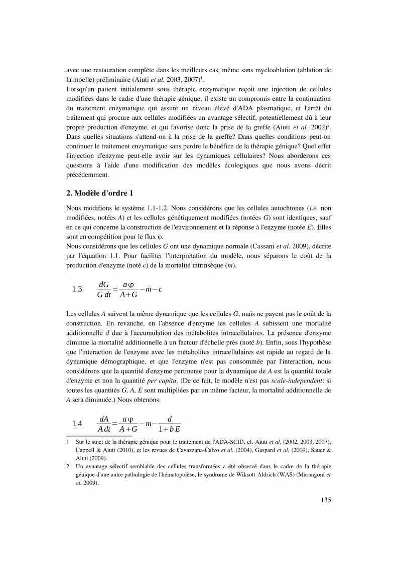
avec une restauration complète dans les meilleurs cas, même sans myeloablation (ablation dela moelle) préliminaire (Aiuti et al. 2003, 2007)1.Lorsqu'un patient initialement sous thérapie enzymatique reçoit une injection de cellulesmodifiées dans le cadre d'une thérapie génique, il existe un compromis entre la continuationdu traitement enzymatique qui assure un niveau élevé d'ADA plasmatique, et l'arrêt dutraitement qui procure aux cellules modifiées un avantage sélectif, potentiellement dû à leurpropre production d'enzyme, et qui favorise donc la prise de la greffe (Aiuti et al. 2002)2.Dans quelles situations s'attendon à la prise de la greffe? Dans quelles conditions peutoncontinuer le traitement enzymatique sans perdre le bénéfice de la thérapie génique? Quel effetl'injection d'enzyme peutelle avoir sur les dynamiques cellulaires? Nous aborderons cesquestions à l'aide d'une modification des modèles écologiques que nous avons décritprécédemment.


Nous modifions le système 1.11.2. Nous considérons que les cellules autochtones (i.e. nonmodifiées, notées A) et les cellules génétiquement modifiées (notées G) sont identiques, saufen ce qui concerne la construction de l'environnement et la réponse à l'enzyme (notée E). Ellessont en compétition pour le flux .φNous considérons que les cellules G ont une dynamique normale (Cassani et al. 2009), décritepar l'équation 1.1. Pour faciliter l'interprétation du modèle, nous séparons le coût de laproduction d'enzyme (noté c) de la mortalité intrinsèque (m).

1.3dGG dt

=a

AG−m−c

Les cellules A suivent la même dynamique que les cellules G, mais ne payent pas le coût de laconstruction. En revanche, en l'absence d'enzyme les cellules A subissent une mortalitéadditionnelle d due à l'accumulation des métabolites intracellulaires. La présence d'enzymediminue la mortalité additionnelle à un facteur d'échelle près (noté b). Enfin, sous l'hypothèseque l'interaction de l'enzyme avec les métabolites intracellulaires est rapide au regard de ladynamique démographique, et que l'enzyme n'est pas consommée par l'interaction, nousconsidérons que la quantité d'enzyme pertinente pour la dynamique de A est la quantité totaled'enzyme et non la quantité per capita. (De ce fait, le modèle n'est pas scaleindependent: sitoutes les quantités G, A, E sont multipliées par un même facteur, la mortalité additionnelle deA sera diminuée.) Nous obtenons:

1.4dAAdt

=a

AG−m−

d1b E

1 Sur le sujet de la thérapie génique pour le traitement de l'ADASCID, cf. Aiuti et al. (2002, 2003, 2007),Cappell & Aiuti (2010), et les revues de CavazzanaCalvo et al. (2004), Gaspard et al. (2009), Sauer &Aiuti (2009).

2 Un avantage sélectif semblable des cellules transformées a été observé dans le cadre de la thérapiegénique d'une autre pathologie de l'hématopoïèse, le syndrome de WiksottAldrich (WAS) (Marangoni etal. 2009).

135

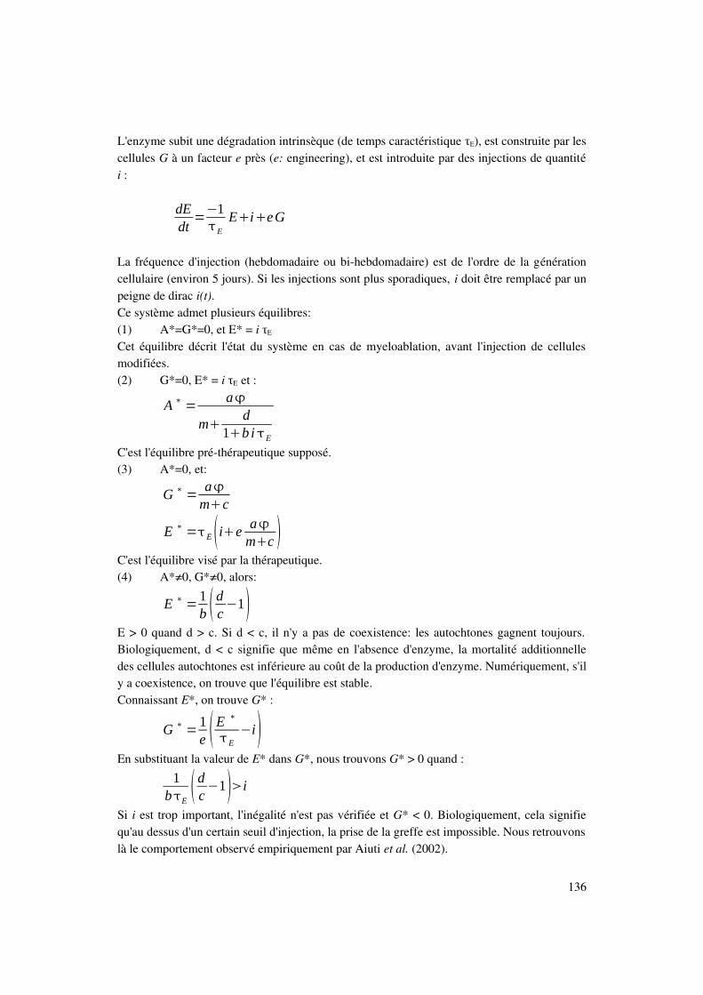
L'enzyme subit une dégradation intrinsèque (de temps caractéristique τE), est construite par lescellules G à un facteur e près (e: engineering), et est introduite par des injections de quantitéi :

dEdt

=−1E

EieG

La fréquence d'injection (hebdomadaire ou bihebdomadaire) est de l'ordre de la générationcellulaire (environ 5 jours). Si les injections sont plus sporadiques, i doit être remplacé par unpeigne de dirac i(t).Ce système admet plusieurs équilibres:(1) A*=G*=0, et E* = i τE

Cet équilibre décrit l'état du système en cas de myeloablation, avant l'injection de cellulesmodifiées.(2) G*=0, E* = i τE et :

A ∗=

a

md

1b iE

C'est l'équilibre préthérapeutique supposé.(3) A*=0, et:

G ∗=

a

mc

E ∗ =E iea

mc C'est l'équilibre visé par la thérapeutique.(4) A*≠0, G*≠0, alors:

E ∗ =1b dc−1

E > 0 quand d > c. Si d < c, il n'y a pas de coexistence: les autochtones gagnent toujours.Biologiquement, d < c signifie que même en l'absence d'enzyme, la mortalité additionnelledes cellules autochtones est inférieure au coût de la production d'enzyme. Numériquement, s'ily a coexistence, on trouve que l'équilibre est stable.Connaissant E*, on trouve G* :

G ∗=

1e E

∗

E−i

En substituant la valeur de E* dans G*, nous trouvons G* > 0 quand :

1bE

dc−1i

Si i est trop important, l'inégalité n'est pas vérifiée et G* < 0. Biologiquement, cela signifiequ'au dessus d'un certain seuil d'injection, la prise de la greffe est impossible. Nous retrouvonslà le comportement observé empiriquement par Aiuti et al. (2002).

136

Connaissant G*, on trouve A*:

A ∗=

amc

−G ∗

A* > 0 quand aφ/(m+c) > G* : la coexistence de A et G n'est pas indépendante de l'échelle.Nous pouvons remarquer que dans cet équilibre, la valeur de E* ne dépend pas de la constanted'injection i : l'injection d'enzyme a pour seul effet de diminuer G*, du fait de la compétitionavec les cellules A. Nous retrouvons là également un comportement observé par Aiuti et al.(2002). Du point de vue thérapeutique, l'injection est donc contreproductive à l'équilibre.

Oscillations

En situation de coexistence, le système suit un régime de relaxation exponentielle, ou unrégime pseudopériodique d'oscillations amorties (fig. 9), ou est instable (cf. annexes). Cesoscillations proviennent du couplage des populations A et G par le compartimentenzymatique, qui a luimême une certaine inertie, de temps caractéristique τE.


Dans cette section, nous transformons le modèle d'ordre 1 en modèle d'ordre 2 en suivant lesarguments exposés en I.2, afin d'étudier l'impact en termes thérapeutiques de la nonséparabilité éventuelle de la dynamique du taux de croissance per capita et de la dynamiquedémographique. Nous obtenons :

2.3dr A

dt=

a

AG−m−

d1b E

2.4drG

dt=

a

AG−m−c

En conservant la même équation pour la dynamique de l'enzyme:dEdt

=−1E

EieG

Ce système admet les mêmes équilibres que le système {1.3,1.4}, mais le comportementdynamique au voisinage des équilibres est modifié.Si la dynamique de l'enzyme est rapide par rapport à la dynamique démographique, on peutapproximer E par τE(i+eG)1. Le système a les mêmes équilibres. En linéarisant le système prèsde l'équilibre, il apparaît que le système peut soit osciller autour de l'équilibre, soit divergeravec des oscillations amplifiées (cf. annexes). La quantité d'injection i peut déstabiliser lesystème quand d(m+c) < 4c². En considérant que la coexistence intervient si d>c, et qu'apriori m>>c (c'estàdire que la construction de l'enzyme n'est qu'une petite partie du travailmétabolique d'une cellule G), la déstabilisation éventuelle du système par l'injection d'enzymen'est pas attendue, sauf valeur extrême des paramètres.

Friction

Une fois encore, nous nous interrogeons sur la stabilité structurelle du modèle d'ordre 2 en

1 Cette hypothèse de séparation d'échelles signifie que les cellules G n'ont pas de phénotype posthume (c.f.Chap.2:3.10)

137

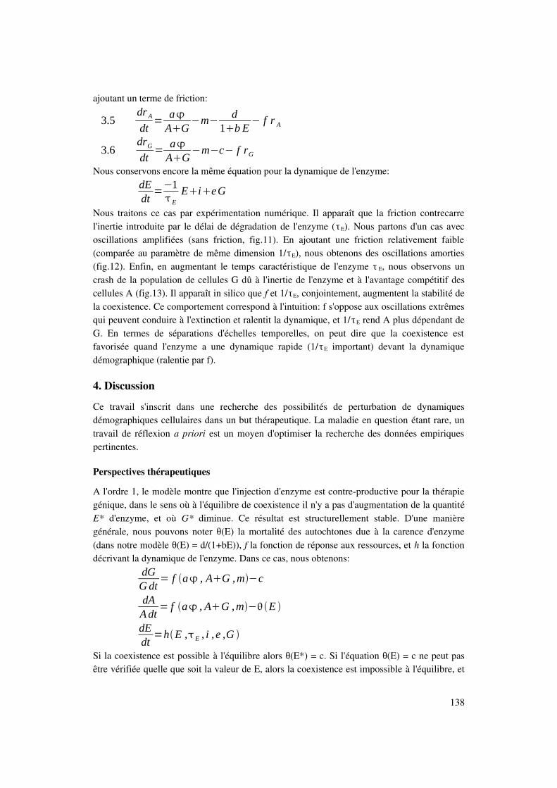
ajoutant un terme de friction:

3.5dr A

dt=

a

AG−m−

d1b E

− f r A

3.6drGdt

=a

AG−m−c− f rG

Nous conservons encore la même équation pour la dynamique de l'enzyme:dEdt

=−1E

EieG

Nous traitons ce cas par expérimentation numérique. Il apparaît que la friction contrecarrel'inertie introduite par le délai de dégradation de l'enzyme (τE). Nous partons d'un cas avecoscillations amplifiées (sans friction, fig.11). En ajoutant une friction relativement faible(comparée au paramètre de même dimension 1/τE), nous obtenons des oscillations amorties(fig.12). Enfin, en augmentant le temps caractéristique de l'enzyme τ E, nous observons uncrash de la population de cellules G dû à l'inertie de l'enzyme et à l'avantage compétitif descellules A (fig.13). Il apparaît in silico que f et 1/τE, conjointement, augmentent la stabilité dela coexistence. Ce comportement correspond à l'intuition: f s'oppose aux oscillations extrêmesqui peuvent conduire à l'extinction et ralentit la dynamique, et 1/τ E rend A plus dépendant deG. En termes de séparations d'échelles temporelles, on peut dire que la coexistence estfavorisée quand l'enzyme a une dynamique rapide (1/τE important) devant la dynamiquedémographique (ralentie par f).

4. Discussion

Ce travail s'inscrit dans une recherche des possibilités de perturbation de dynamiquesdémographiques cellulaires dans un but thérapeutique. La maladie en question étant rare, untravail de réflexion a priori est un moyen d'optimiser la recherche des données empiriquespertinentes.

Perspectives thérapeutiques

A l'ordre 1, le modèle montre que l'injection d'enzyme est contreproductive pour la thérapiegénique, dans le sens où à l'équilibre de coexistence il n'y a pas d'augmentation de la quantitéE* d'enzyme, et où G* diminue. Ce résultat est structurellement stable. D'une manièregénérale, nous pouvons noter θ(E) la mortalité des autochtones due à la carence d'enzyme(dans notre modèle θ(E) = d/(1+bE)), f la fonction de réponse aux ressources, et h la fonctiondécrivant la dynamique de l'enzyme. Dans ce cas, nous obtenons:

dGGdt

= f a , AG ,m−c

dAAdt

= f a , AG ,m−E

dEdt

=hE ,E , i , e ,G

Si la coexistence est possible à l'équilibre alors θ(E*) = c. Si l'équation θ(E) = c ne peut pasêtre vérifiée quelle que soit la valeur de E, alors la coexistence est impossible à l'équilibre, et

138

A gagne quand θ(E) < c, G gagne quand (E) > cθ . L'équilibre est stable seulement quanddθ(E)/dE < 0. Cette condition signifie que pour que l'équilibre soit stable, la surmortalité parcarence d'enzyme doit diminuer quand la quantité d'enzyme augmente (cette condition estréalisée dans notre modèle). Dans la situation de coexistence, θ(E*) détermine E*, qui nedépend donc pas de i. E* détermine G* via la fonction h(E,τE,i, e, G). Or, si h est croissanteen fonction de i et croissante également en fonction de G* (ce qui est naturel a priori), G*(i)est décroissante, et peut éventuellement devenir négative1. Biologiquement, cela signifie qu'audessus d'un certain seuil d'injection, la prise de la greffe est impossible, et les injections fontdiminuer la quantité d'enzyme construite par les cellules G. Ces deux comportements sontobservés empiriquement par Aiuti et al. (2002).Il est important de noter que ce raisonnement vaut à l'équilibre seulement (et s'il y acoexistence, ce qui semble être le cas sur plusieurs années). D'un point de vue thérapeutique,il peut être inévitable d'avoir à recourir à des injections sporadiques d'enzyme quand larestauration fonctionnelle n'est pas complète par thérapie génique, en particulier quand lepatient est en mauvaise condition (Aiuti et al. 2002), afin d'augmenter temporairement leniveau de l'enzyme au dessus de son niveau d'équilibre. Cependant, les injections doivent sefaire sur une période aussi courte que possible: en environ un mois, l'enzyme plasmatiquesemble retrouver son niveau d'équilibre préinjections malgré les injections (Aiuti et al.2002:fig.1). Outre la diminution observée de la population des cellules constructrices, il n'estpas exclu que la présence d'enzyme active une boucle de rétroaction négative sur laconstruction par les cellules G.

Autres perspectives thérapeutiques

Dans ce travail, nous nous sommes concentrés sur une thérapie génique pérenne. Cependant,une piste des thérapies géniques concerne les thérapies transitoires. Par exemple, en cas defracture, il est possible de modifier des cellules de sorte qu'elles produisent des facteurs decroissance ostéogénique et améliorent l'union des fragments osseux. Ce type de thérapiepermet un traitement plus ciblé spatialement qu'une injection de protéine exogène (Baltzer &Lieberman 2004). Dans ce cas, le but n'est pas l'invasion d'un tissu par des cellules G, mais aucontraire leur élimination par les cellules A: le transitoire d'intérêt est le temps de relaxationdu tissu. En suivant le même modèle, nous pourrions écrire:

dAAdt

= f a , AG ,m

dGGdt

= f a , AG ,m−c

où il apparaît que le temps de relaxation est de l'ordre de 1/c, où c est le coût de laconstruction des facteurs de croissance par la cellule.

1 Plus précisément, on fixe E* et tous les paramètres de h sauf i et G*. Alors:

dE ∗

dt=0=

∂ h∂ i

di∂ h

∂G ∗dG ∗ , donc :

dG ∗

di=

−∂ h∂ i

∂ h

∂G ∗

Comme h/i et h/G* > 0 d'après nos hypothèses biologiques, il apparaît que dG*/di < 0.

139

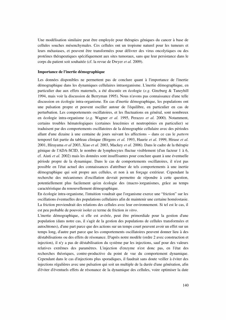
Une modélisation similaire peut être employée pour thérapies géniques du cancer à base decellules souches mésenchymales. Ces cellules ont un tropisme naturel pour les tumeurs etleurs métastases, et peuvent être transformées pour délivrer des virus oncolytiques ou desprotéines thérapeutiques spécifiquement aux sites tumoraux, sans que leur persistance dans lecorps du patient soit souhaitée (cf. la revue de Dwyer et al. 2009).

Importance de l'inertie démographique

Les données disponibles ne permettent pas de conclure quant à l'importance de l'inertiedémographique dans les dynamiques cellulaires intraorganisme. L'inertie démographique, enparticulier due aux effets maternels, a été discutée en écologie (e.g. Ginzburg & Taneyhill1994, mais voir la discussion de Berryman 1995). Nous n'avons pas connaissance d'une tellediscussion en écologie intraorganisme. En cas d'inertie démographique, les populations ontune pulsation propre et peuvent osciller autour de l'équilibre, en particulier en cas deperturbation. Les comportements oscillatoires, et les fluctuations en général, sont nombreuxen écologie intraorganisme (e.g. Wagner et al. 1995, Perazzo et al. 2000). Notamment,certains troubles hématologiques (certaines leucémies et neutropénies en particulier) setraduisent par des comportements oscillatoires de la démographie cellulaire avec des périodesallant d'une dizaine à une centaine de jours suivant les affections – dans ce cas le patterntemporel fait partie du tableau clinique (Birgens et al. 1993, Haurie et al. 1999, Hirase et al.2001, Hirayama et al 2003, Xiao et al. 2003, Mackey et al. 2006). Dans le cadre de la thérapiegénique de l'ADASCID, le nombre de lymphocytes fluctue visiblement (d'un facteur 1 à 6,cf. Aiuti et al. 2002) mais les données sont insuffisantes pour conclure quant à une éventuellepériode propre de la dynamique. Dans le cas de comportements oscillatoires, il n'est paspossible en l'état actuel des connaissances d'attribuer de tels comportements à une inertiedémographique qui soit propre aux cellules, et non à un forçage extérieur. Cependant larecherche des mécanismes d'oscillation devrait permettre de répondre à cette question,potentiellement plus facilement qu'en écologie des (macro)organismes, grâce au tempscaractéristique du renouvellement démographique.En écologie intraorganisme, l'intuition voudrait que l'organisme exerce une “friction” sur lesoscillations éventuelles des populations cellulaires afin de maintenir une certaine homéostasie.La friction proviendrait des relations des cellules avec leur environnement. Si tel est le cas, ilest peu probable de pouvoir isoler ce terme de friction in vitro.L'inertie démographique, si elle est avérée, peut être primordiale pour la gestion d'unepopulation (dans notre cas, il s'agit de la gestion des populations de cellules transformées etautochtones), d'une part parce que des actions sur un temps court peuvent avoir un effet sur untemps long, d'autre part parce que les comportements oscillatoires peuvent donner lieu à desdéstabilisations ou des effets de résonance. D'après notre modèle (ordre 2 avec construction etinjection), il n'y a pas de déstabilisation du système par les injections, sauf pour des valeursrelatives extrêmes des paramètres. L'injection d'enzyme n'est donc pas, en l'état desrecherches théoriques, contreproductive du point de vue du comportement dynamique.Cependant dans le cas d'injections plus sporadiques, il faudrait sans doute veiller à éviter desinjections régulières avec une pulsation qui soit un multiple de la durée d'une génération, afind'éviter d'éventuels effets de résonance de la dynamique des cellules, voire optimiser la date

140

d'injection en fonction de la dynamique démographique cellulaire. En revanche, même sansinjection d'enzyme, il apparaît que l'inertie démographique peut être une sourcesupplémentaire d'instabilité conduisant à l'échec d'une greffe1.Du point de vue dynamique, la niche peut être une source d'inertie démographique (dans notremodèle, à cause du temps caractéristique de l'enzyme τE), et la construction de niche est unfacteur écologique pouvant introduire une amplification des oscillations démographiques ouau contraire une friction. Afin de percevoir l'origine structurelle de cet effet, nous pouvonsdériver une seconde fois l'équation de la dynamique enzymatique. Nous obtenons:

d²Edt²

=−1E

dEdt

edGdt

En notant rE la vitesse dE/dt pour aider à l'identification des homologies structurelles, nouspouvons réécrire l'équation de l'accélération d²E/dt² :

d²Edt²

=−1E

r EeG rG

Il apparaît que rE / τE se comporte comme une friction visàvis de l'accélération d²E/dt². Leterme GrG représente une nonlinéarité qui explique la complexité de certains comportementsdécrits précédemment. Plus généralement, la dynamique de l'enzyme introduit dans l'étude dusystème linéarisé des termes en X, caractéristiques de la friction et de l'antifriction (sansfriction et sans construction de niche le polynôme caractéristique est de la forme P(X²)).

Perspectives de modélisation

Concernant l'effet de l'enzyme sur la dynamique, nous avons choisi le modèle le plus simple:les cellules G ne sont pas affectées par la concentration d'enzyme (sous l'hypothèse quel'enzyme construite intracellulaire est saturante), et la mortalité additionnelle (ou le coûtmétabolique additionnel dans le modèle d'ordre 2) des cellules A est additive à leurdynamique. Un travail est en cours pour généraliser cette famille de modèles aux cas où larestauration de la fonction cellulaire n'est pas complète par thérapie génique, et/ou où l'effetde l'enzyme n'est pas additif par rapport à la dynamique d'ordre 1 (c'estàdire que f a Ecomme variable). Dans ce cas, la dynamique des cellules G dépend de E, mais trèsprobablement, les cellules G ont un accès privilégié à l'enzyme construite par ellesmêmes, enparticulier avant que l'enzyme ne sorte du compartiment intracellulaire. Une façon simple deprendre en compte l'intuition de cet avantage compétitif (Aiuti et al. 2003) sans décrireexplicitement l'espace où se jouent les interactions (une description spatiale impliqued'employer des équations aux dérivées partielles plus difficilement solvables, de plus nousignorons la géométrie exacte de l'espace concerné), est de modéliser l'enzyme comme étantconstruite dans un compartiment intracellulaire (Ec, accessible uniquement aux cellules G) eten transit vers un compartiment intercellulaire, ici le plasma sanguin (E, qui dépend aussi desinjections), où elle est accessible aux cellules A et G.D'autre part, nous avons choisi pour la population des cellulessouches un modèle minimal(population non structurée). Cependant, les populations d'intérêt (lignées lymphocytaires) sontdes métapopulations structurées en populations sourcespuits du fait de la différentiation

1 L'importance de la dynamique dans la thérapeutique n'est pas nouvelle, en particulier en ce qui concernele cancer (e.g. Netti et al. 1995, Sangalli et al. 2001).

141

cellulaire, qui est également corrélée à l'âge des cellules (e.g. cellule souche → progéniteurlymphoïdes lymphoblaste prolymphocyte lymphocyte Tlymphocyte, pour ne→ → → →donner qu'une lignée). Très vraisemblablement, une telle structuration doit avoir des effetsdynamiques majeurs. L'extension du domaine de l'écologie à de telles populations est, denotre point de vue, une perspective prometteuse.

Perspectives conceptuelles

Dans cette section, nous nous sommes intéressés à l'impact de la construction d'une enzymedont la dynamique ne serait pas séparable de celle des populations cellulaires. Nous avonsporté notre attention en particulier sur l'importance des transitoires (oscillations, temps derelaxation) dus à l'inertie de la niche et à l'inertie démographique. Nous avons discutél'importance médicale de tels transitoires.Deux perspectives différentes émergent suivant que l'on considère les interactions écologiquescomme devant être décrites par des systèmes d'ordre 1 ou d'ordre 2. A l'ordre 1, la dynamiquedémographique est directement affectée par les facteurs démographiques (ressources,mortalité) tandis qu'à l'ordre 2, la dynamique démographique est affectée indirectement, àtravers l'équilibre au niveau individuel entre le métabolisme et l'acquisition de ressources. Al'ordre 2, les facteurs démographiques sont analogues aux forces de la mécaniqueNewtonienne, qui agissent sur l'accélération d'un mouvement et non sur la vitesse. En termesmathématiques, une dimension dynamique supplémentaire est ajoutée à la définition de laniche.Ginzburg et Colyvan (2004:102103), dans une conclusion programmatique, enjoignent auxécologistes d'identifier les “forces” écologiques, force étant à entendre au sens d'une causeinduisant une modification de l'état énergétique des individus ou du taux de croissancecorrespondant. Au nombre de ces forces, Ginzburg et Colyvan comptent l'énergétique, leseffets maternels, et les relations proieprédateur. La niche comme substrat de l'inertiedémographique, et la construction de niche comme force écologique, peuvent être ajoutées àce programme.1

1 Remerciements: ce chapitre s'inscrit dans la continuation d'un projet au CEMRACS 2004, dont lesparticipants étaient: Antonio Cappucio, Etienne Couturier, Michel de Lara, Regis Ferrière, Olivier Sester,Pierre Sonigo, Christian et Carlo.

142

Figures

143

Fig.1: Relaxation vers l'équilibre dans le modèle de vitessedémographique. Abscisses: temps. Ordonnées: N. a =1,φm=0.5, N(0)=0.1 (unités arbitraires).

Fig.2: Comparaison entre les mortalités exponentielle etaccélérée. Abscisses: temps. Ordonnées: ln(N). Courbe verte:modèle d'ordre 1 (équation 1). Courbe bleue: modèle d'ordre 2(équation 2). Le flux est mis à zéro à t=10. La mortalité estexponentielle (linéaire en ln(N)) dans le modèle d'ordre 1, etaccélérée (c'estàdire plus rapide qu'une exponentielle) dansle modèle d'ordre 2. a =10, m=0.5, n0=10 (unités arbitraires).φ

144

Fig.3: Dynamique démographique dans le modèle d'ordre 2(équation 2). Courbe bleue: N. Courbe verte: dN/dt. Lesystème suit des oscillations non amorties. aφ=1, m=0.5,N(0)=1.5, dn/dt(0)=0.1 (unités arbitraires).

Fig 4: Trajectoires du modèle d'ordre 2 (équation 2) dansl'espace de phase N, dN/dt. Bassin d'attraction du pointd'équilibre stable. Abscisses: N, ordonnées: dn/dt. Lestrajectoires commencent à gauche et terminent à droite. Lacourbe rouge et la courbe verte se rapprochent du point fixe.La courbe bleue s'éloigne, ce qui signifie que le bassind'attraction est limité. Cependant, il faut garder à l'esprit que lemodèle perd son sens quand N devient petit devant a . φ a =1φm=0.5 dn/dt(0)=0 , n(0)=1;1.2;1.4;1.6;1.8 (unités arbitraires).

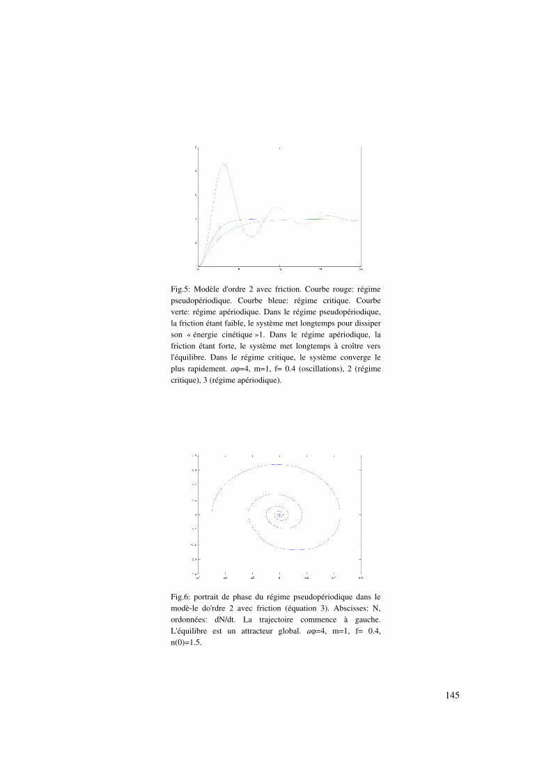
145

Fig.5: Modèle d'ordre 2 avec friction. Courbe rouge: régimepseudopériodique. Courbe bleue: régime critique. Courbeverte: régime apériodique. Dans le régime pseudopériodique,la friction étant faible, le système met longtemps pour dissiperson « énergie cinétique »1. Dans le régime apériodique, lafriction étant forte, le système met longtemps à croître versl'équilibre. Dans le régime critique, le système converge leplus rapidement. a =4, m=1, f= 0.4 (oscillations), 2 (régimeφcritique), 3 (régime apériodique).

Fig.6: portrait de phase du régime pseudopériodique dans lemodèle do'rdre 2 avec friction (équation 3). Abscisses: N,ordonnées: dN/dt. La trajectoire commence à gauche.L'équilibre est un attracteur global. a =4, m=1, f= 0.4,φn(0)=1.5.

146

Fig.7: issues de la compétition dans l'espace des paramètres.Afin d'alléger la lecture, nous posons A1=a1 /mφ 1 et A2=a2 /mφ 2.La zone de coexistence correspond au domaine de moindrecompétition entre 1 et 2.

Fig.8: oscillations superposées dans le modèle d'ordre 2 à deuxespèces. a =1.5, m=0.5, qφ 21=0.8 q12=0.9, n1(0)=1.2,dn1/dt(0)=0, n2(0)=1.2, dn2/dt(0)=0.3.

147

Fig.9: modèle de construction de niche d'ordre 1, en régimed'oscillations amorties. Courbe verte: cellules G, courberouge: enzyme, courbe bleue: cellules A. d=6; b=2; c=0.5;e=1; τE=5; i=0; a =10; m=0.5; A(0)=5; G(0)=0.5; E(0)=0.φ

Fig.10: modèle de construction de niche d'ordre 2 avecséparation temporelle sur l'enzyme. A(0)=9, dA/dt=0.1,G(0)=4, dG/dt=0, a =30; c=0.5; m=2; b=10, d=20, i=0, e=1,φτE=1.

148

Fig.11: modèle de construction de niche d'ordre 2 sansfriction. Les oscillations sont amplifiées. d=5; b=2; c=0.5;e=2; i=0; a =30; m=1; φ τE=0.2; f=0.

Fig. 12: modèle de construction de niche d'ordre 2 avecfriction. Ici la friction est faible mais les oscillations sontamorties. f=0.1 (autres paramètres: id.).

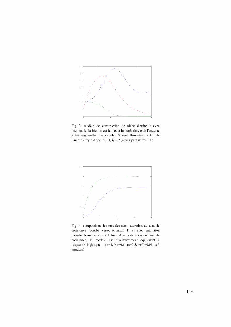
149

Fig.13: modèle de construction de niche d'ordre 2 avecfriction. Ici la friction est faible, et la durée de vie de l'enzymea été augmentée. Les cellules G sont éliminées du fait del'inertie enzymatique. f=0.1, τE = 2 (autres paramètres: id.).

Fig.14: comparaison des modèles sans saturation du taux decroissance (courbe verte, équation 1) et avec saturation(courbe bleue, équation 1 bis). Avec saturation du taux decroissance, le modèle est qualitativement équivalent àl'équation logistique. a =1, b =0.5, m=0.5, n(0)=0.01. (cf.φ φannexes)

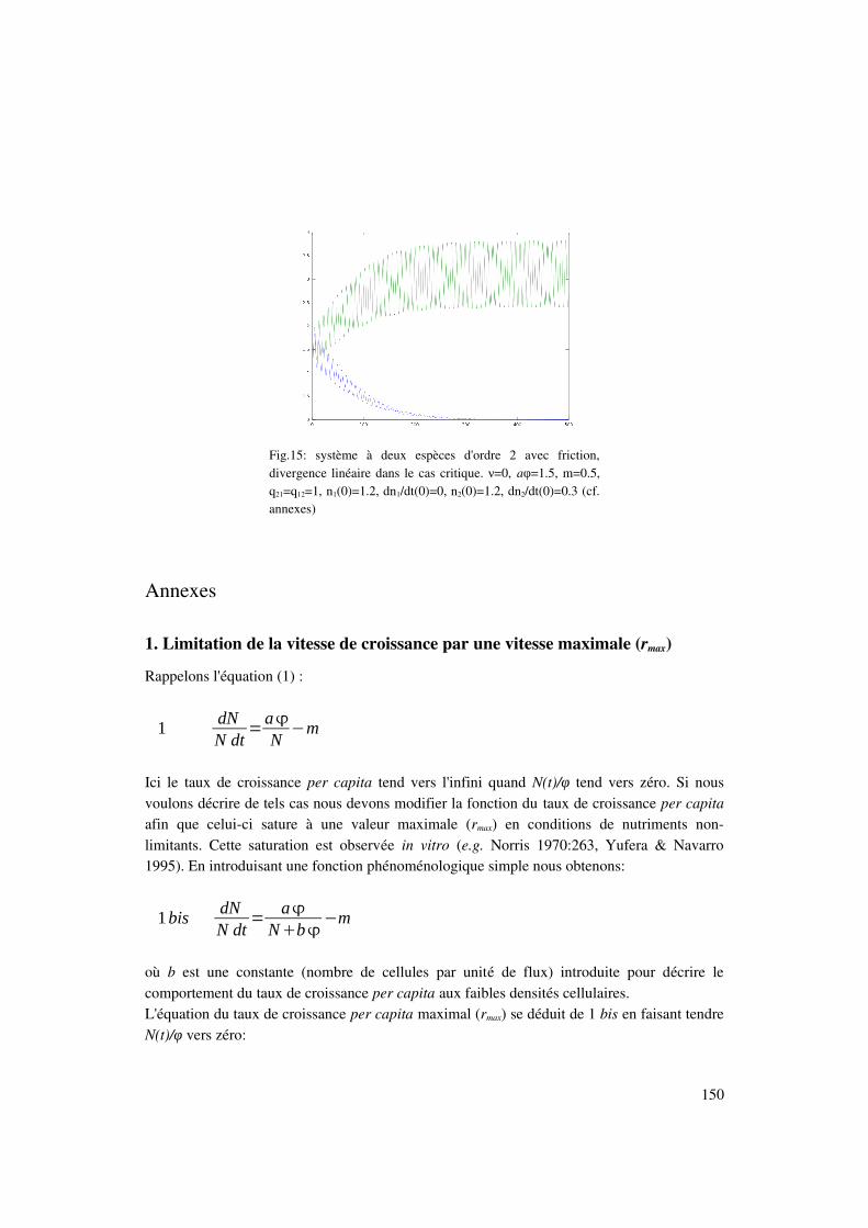
Annexes

1. Limitation de la vitesse de croissance par une vitesse maximale (rmax)

Rappelons l'équation (1) :

1dNN dt

=a

N−m

Ici le taux de croissance per capita tend vers l'infini quand N(t)/φ tend vers zéro. Si nousvoulons décrire de tels cas nous devons modifier la fonction du taux de croissance per capitaafin que celuici sature à une valeur maximale (rmax) en conditions de nutriments nonlimitants. Cette saturation est observée in vitro (e.g. Norris 1970:263, Yufera & Navarro1995). En introduisant une fonction phénoménologique simple nous obtenons:

1bisdNN dt

=a

Nb−m

où b est une constante (nombre de cellules par unité de flux) introduite pour décrire lecomportement du taux de croissance per capita aux faibles densités cellulaires.L'équation du taux de croissance per capita maximal (rmax) se déduit de 1 bis en faisant tendreN(t)/φ vers zéro:

150

Fig.15: système à deux espèces d'ordre 2 avec friction,divergence linéaire dans le cas critique. =0, ν a =1.5, m=0.5,φq21=q12=1, n1(0)=1.2, dn1/dt(0)=0, n2(0)=1.2, dn2/dt(0)=0.3 (cf.annexes)

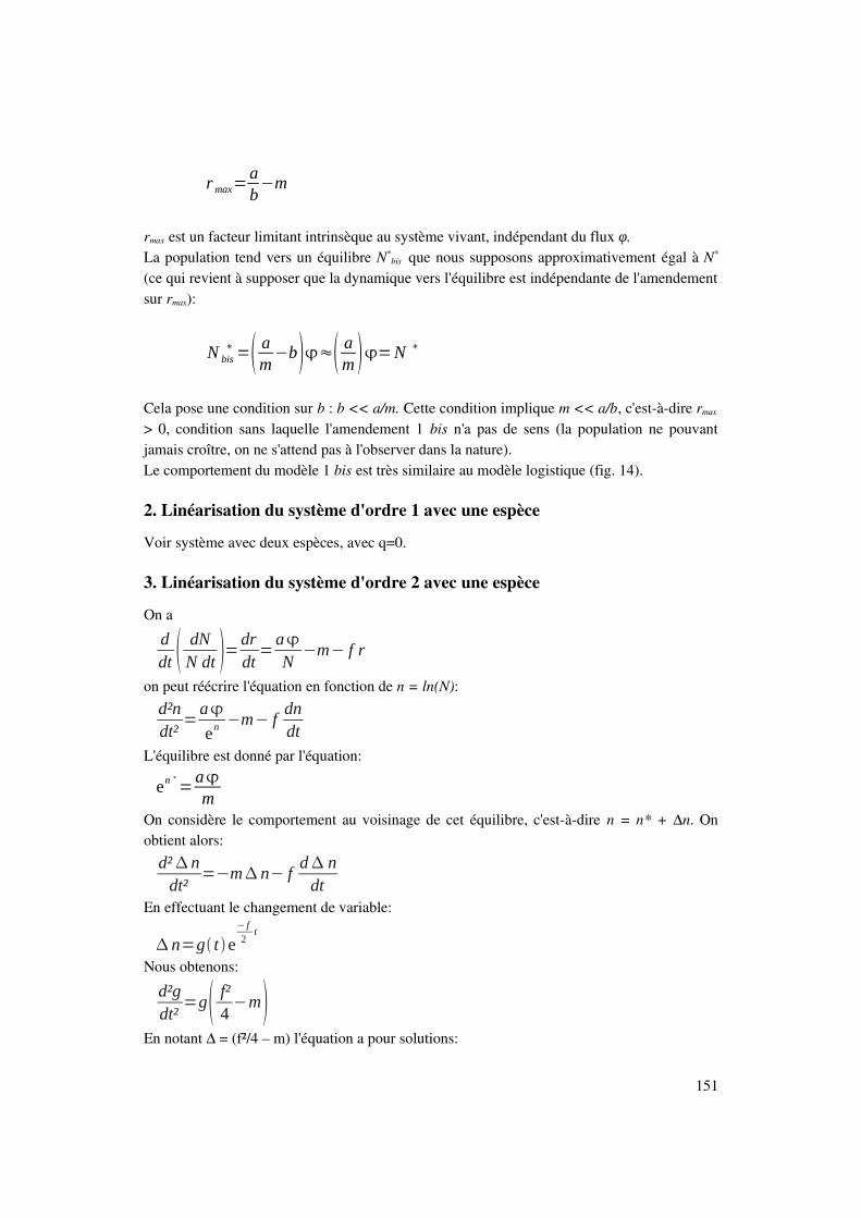
rmax=ab−m

rmax est un facteur limitant intrinsèque au système vivant, indépendant du flux .φ La population tend vers un équilibre N*

bis que nous supposons approximativement égal à N*

(ce qui revient à supposer que la dynamique vers l'équilibre est indépendante de l'amendementsur rmax):

N bis∗ = am−b≈ am =N ∗

Cela pose une condition sur b : b << a/m. Cette condition implique m << a/b, c'estàdire rmax

> 0, condition sans laquelle l'amendement 1 bis n'a pas de sens (la population ne pouvantjamais croître, on ne s'attend pas à l'observer dans la nature).Le comportement du modèle 1 bis est très similaire au modèle logistique (fig. 14).

2. Linéarisation du système d'ordre 1 avec une espèce

Voir système avec deux espèces, avec q=0.

3. Linéarisation du système d'ordre 2 avec une espèce

On a

ddt dN

N dt =drdt

=a

N−m− f r

on peut réécrire l'équation en fonction de n = ln(N):

d²ndt²

=a

en −m− fdndt

L'équilibre est donné par l'équation:

en ∗

=a

mOn considère le comportement au voisinage de cet équilibre, c'estàdire n = n* + ∆n. Onobtient alors:

d² ndt²

=−m n− fd ndt

En effectuant le changement de variable:

n=g t e− f2

t

Nous obtenons:

d²gdt²

=g f²4

−mEn notant ∆ = (f²/4 – m) l'équation a pour solutions:

151

si ∆ < 0:

g=A cos t−B sin t −

n=e− f2

t

Acos t −B sint −si ∆ = 0g=A tB

n=e− f2

t

AtBsi ∆ > 0

g=A cosh tB sinh t

n=e− f2

t

Acosh t B sinht =O e− f

2tt

La pulsation est donnée par √∆ et le temps de relaxation par l'inverse de f/2

4. Linéarisation du système d'ordre 1 avec deux espèces

dN 1

N 1dt=

a1

N 1q21 N 2

−m1

dN 2

N 2dt=

a2

N 2q12 N 1

−m2

Au voisinage de l'équilibre, on pose : n = ln(N) et n = n* + ∆(n).

N 1=en1=en1∗

n1=en1∗1 n1

N 2=en2=en2∗ n2=en2

∗1n 2

On obtient alors:d n1

dt=

a1

exp n1∗

1 n1q21exp n2∗1 n2

−m1

En réarrangeant on obtient :

d n1

dt=−

exp n1∗ n1q21exp n2

∗ n2

a1 m1

2

On obtient de même :

d n2

dt=−

q12exp n1∗ n1exp n2

∗ n2

a2m2

2

Nous cherchons les valeurs propres de ce système.Elles sont racines du polynôme caractéristique X² TX + DOn pose :

152

B1=m1

2

a1 exp n1

∗

B2=m2

2

a2exp n2

∗

Avec ces paramètres, nous obtenons :T=−B1B2

D=B1 B21−q21 q12

Le déterminant du polynôme caractéristique ∆ est donné par :=B1B2 ²−4 B1B21−q21 q12

donc :=B1−B2 ²4 B1B2q21q12

Donc ∆ > 0.Les valeurs propres sont donc :

µ=−B1B2−

2et

=−B1B2

2

=−B1B2B1B2 ²−4 B1 B21−q21 q12

2Il apparaît que ν < 0 quand (1 – q21q12) > 0 et ν > 0 quand (1 – q21q12 ) < 0.Quand ν > 0 le point fixe est instable. Biologiquement, cela signifie que la compétition esttrop importante et que l'une des deux populations est éliminée, dépendamment des conditionsinitiales.Si ν < 0 alors le point fixe est stable et le temps de relaxation est donné par 1/ .νSi = 0, alors qν 21q12=1, ce qui est exclu car N1

* et N2* ne sont pas définis.

Dans le cas où q21q12 =1, nous avons trois situations différentes, en fonction du signe de a1 /mφ 1 a2 /(mφ 2q12) : si ce terme est positif l'espèce 1 gagne, s'il est négatif l'espèce 2 gagne,s'il est nul, alors la coexistence est indifférente.

5. Linéarisation du système d'ordre 2 avec deux espèces (sans friction)

Le calcul est identique au système d'ordre 1, mais l'interprétation diffère.Quand ν > 0 le point fixe est instable et l'une des deux populations est éliminée.Si ν < 0, alors ∆n1 et ∆n2 sont des superpositions d'oscillations indépendantes de pulsations √(µ) et √(ν).

6. Linéarisation du système d'ordre 2 avec deux espèces (avec friction)

Nous considérons le cas où f1=f2=f. Alors le comportement du système est donné par les Z telque:X =Z² f Z

153

où X = µ ou ν.Z est donc donné par:

Z=12

− f ± f²4X

Si ν > 0, on a un Z > 0 donc le système est instable.Si ν < 0, le système est stable. Il y a alors plusieurs régimes possibles: si X < f²/4, lacomposante associée à X sera pseudopériodique. Si X = f²/4, alors cette composante seracritique. Si X > f²/4, la composante sera apériodique. Le comportement de ∆n1 et ∆n2 seradonné par une superposition des comportements associés aux deux valeurs propres.Si ν = 0, le système est instable et diverge linéairement, avec en plus une composanteoscillatoire (fig.15).

7. Linéarisation du système d'ordre 1, avec deux espèces et constructiond'enzyme

Après linéarisation, nous cherchons les valeurs propres du système (de dimension 3). Cellesci sont racines du polynôme caractéristique:

X³X² M1E X

ME

Bec² bd

où M = m+c et

B=M²a a

M−G ∗

On en conclut que dans le cas où il y a coexistence, 2 scénarios sont possibles:(1) soit le polynôme a trois racines négatives: dans ce cas le système convergeexponentiellement vers l'équilibre(2) soit le polynôme a une racine négative et deux solutions complexes conjuguées: dansce cas le système est stable ou instable suivant le signe de la partie réelle de ces racines. Dansle cas où le système est stable, le régime est pseudopériodique avec oscillations amorties.La résolution littérale du polynôme a été réalisée, mais l'expression littérale des solutions esttrop complexe pour être informative.

8. Linéarisation du système d'ordre 2 avec deux espèces, constructiond'enzyme, et séparation d'échelle sur la dynamique de l'enzyme

On trouve comme polynôme caractéristique:

X²MX Bc²d

où M = m+c et:

B=M²a a

M−G ∗

et :

G ∗ =1

beE dc −1−b iE

154

Le discriminant du polynôme est ∆:

=M²−4 Bc²d

Donc

=M² 1−4c²

d a a

M−G ∗

Si ∆ > 0, alors :

X =−M±

2S'il y a coexistence alors on a aφ/M – G* > 0, alors ces deux racines sont négatives et lesystème a des oscillations au voisinage de l'équilibre.Si ∆ < 0, alors :

X =−M± j

2; où j²=1.

Dans ce cas, les vecteurs propres ont une dynamique en exp(Z t), avec Z²=X. Or la partieréelle des racines est négative, donc pour chaque racine l'un des Z a une partie réelle positiveet l'équilibre est instable. Le système diverge avec des oscillations amplifiées.Quand la quantité d'injections i augmente, G* diminue donc ∆ diminue. Augmenter irapproche de l'instabilité. Si 1 < 4c²/ (dM), alors augmenter i déstabilise le système. On ne saitpas alors laquelle des deux populations va survivre, ce qui dépend en particulier desconditions initiales.

155

Références

Abraham, E. & Singer, M., 2007. Mechanisms of sepsisinduced organ dysfunction. CriticalCare Medicine, 35(10), p.24082416.

Aiuti, A., 2002. Advances in gene therapy for ADAdeficient SCID. Current Opinion inMolecular Therapeutics, 4(5), p.515522.

Aiuti, A., 2004. Gene therapy for adenosinedeaminasedeficient severe combinedimmunodeficiency. Best Practice & Research Clinical Haematology, 17(3), p.505516.

Aiuti, A. et al., 2007. Multilineage hematopoietic reconstitution without clonal selection inADASCID patients treated with stem cell gene therapy. Journal of ClinicalInvestigation, 117(8), p.22332240.

Aiuti, A. et al., 2009. Gene Therapy for Immunodeficiency Due to Adenosine DeaminaseDeficiency. New England Journal of Medicine, 360(5), p.447458.

Aiuti, A. et al., 2002. Immune reconstitution in ADASCID after PBL gene therapy anddiscontinuation of enzyme replacement. Nature Medicine, 8(5), p.423425.

Aiuti, A. et al., 2002. Correction of ADASCID by Stem Cell Gene Therapy Combined withNonmyeloablative Conditioning. Science, 296(5577), p.24102413.

Aiuti, F. & Giovannetti, A., 2003. Structured interruptions of therapy: looking for the bestprotocol. AIDS, 17(15), p.22572258.

Akçakaya, H., Arditi, R. & Ginzburg, L., 1995. Ratiodependent predation an abstractionthat works. Ecology, 76(3), p.9951004.

Akçakaya, H. et al., 1988. The Theory of Population Dynamics 2. Physiological Delays.Bulletin of Mathematical Biology, 50(5), p.503515.

Alizon, S. et al., 2009. Virulence evolution and the tradeoff hypothesis: history, current stateof affairs and the future. Journal of Evolutionary Biology, 22(2), p.245259.

Alizon, S. & van Baalen, M., 2008. Multiple infections, immune dynamics, and the evolutionof virulence. The American Naturalist, 172(4), p.E150168.

Arditi, R. & Ginzburg, L., 1989. Coupling in predator prey dynamics Ratiodependence.Journal of Theoretical Biology, 139(3), p.311326.

Bach, L. et al., 2001. An evolutionarygame model of tumourcell interactions: possiblerelevance to gene therapy. European Journal of Cancer, 37(16), p.21162120.

Baeten, L. et al., 2010. Unexpected understorey community development after 30 years inancient and postagricultural forests. Journal of Ecology, 98(6), p.14471453.

Bailly, F., Longo, G. & Montévil, M., A 2dimensional Geometry for Biological Time.Baltzer, A. & Lieberman, J., 2004. Regional gene therapy to enhance bone repair. Gene

Therapy, 11(4), p.344350.Bellows, T.S., 1981a. The Descriptive Properties of Some Models for Density Dependence.

Journal of Animal Ecology, 50(1), p.139156.Bellows, T.S., 1981b. The Descriptive Properties of Some Models for Density Dependence.

Journal of Animal Ecology, 50(1), p.139156.Bernard, S., Belair, J. & Mackey, M., 2004. Bifurcations in a whitebloodcell production

156

model. Comptes Rendus Biologies, 327(3), p.201210.Berryman, A.A., 1995. Population Cycles: A Critique of the Maternal and Allometric

Hypotheses. Journal of Animal Ecology, 64(2), p.290293.Beverton, R.J.H. & Holt, S.J., 1957. On the dynamics of exploited fish populations. Fisheries

Investigation Series, 2(19).Billy, F. et al., 2009. A pharmacologically based multiscale mathematical model of

angiogenesis and its use in investigating the efficacy of a new cancer treatmentstrategy. Journal of Theoretical Biology, 260(4), p.545562.

Birgens, H. & Karle, H., 1993. Reversible AdultOnset Cyclic Hematopoiesis with a CycleLength of 100 Days. British Journal of Haematology, 83(2), p.181186.

Booth, C. et al., 2007. Management options for adenosine deaminase deficiency; proceedingsof the EBMT satellite workshop (Hamburg, March 2006). Clinical Immunology,123(2), p.139147.

Buis, R. & Luck, J., 2006. The notion of the internal and external limitations of monotonicgrowth functions. A reformulation of the logistic equation. Comptes RendusBiologies, 329(11), p.880891.

Cairns, B.J. et al., 2009. Quantitative Models of In Vitro Bacteriophage–Host Dynamics andTheir Application to Phage Therapy. PLoS Pathog, 5(1), p.e1000253.

Cairns, J., 1975. Mutation Selection and Natural History of Cancer. Nature, 255(5505), p.197200.

Calder, W.A., 1996. Size, function, and life history, Courier Dover Publications.Cappell, B. & Aiuti, A., 2010a. Gene Therapy for Adenosine Deaminase Deficiency.

Immunology and Allergy Clinics of North America, 30(2), p.249+.Cappell, B. & Aiuti, A., 2010b. Gene Therapy for Adenosine Deaminase Deficiency.

Immunology and Allergy Clinics of North America, 30(2), p.249+.Cassani, B. et al., 2008. Altered intracellular and extracellular signaling leads to impaired T

cell functions in ADASCID patients. Blood, 111(8), p.42094219.Cassani, B. et al., 2009. Integration of retroviral vectors induces minor changes in the

transcriptional activity of T cells from ADASCID patients treated with gene therapy.Blood, 114(17), p.35463556.

CavazzanaCalvo, M. et al., 2005. Gene Therapy for Severe Combined Immunodeficiency.Annual Review of Medicine, 56(1), p.585602.

CavazzanaCalvo, M. et al., 2010. Transfusion independence and HMGA2 activation aftergene therapy of human [bgr]thalassaemia. Nature, 467(7313), p.318322.

CavazzanaCalvo, M., Thrasher, A. & Mavilio, F., 2004. The future of gene therapy. Nature,427(6977), p.779781.

Colijn, C. & Mackey, M., 2005. A mathematical model of hematopoiesis I. Periodic chronicmyelogenous leukemia. Journal of Theoretical Biology, 237(2), p.117132.

Courchamp, CluttonBrock & Grenfell, 1999. Inverse density dependence and the Alleeeffect. Trends in Ecology & Evolution (Personal Edition), 14(10), p.405410.

Deasy, B.M. et al., 2003. Modeling Stem Cell Population Growth: Incorporating Terms forProliferative Heterogeneity. Stem Cells, 21(5), p.536545.

Dingli, D. et al., 2009. Dynamics of multiple myeloma tumor therapy with a recombinantmeasles virus. Cancer Gene Therapy, 16(12), p.873882.

157

Dunlop, E.S., Heino, M. & Dieckmann, U., 2009. Ecogenetic modeling of contemporary lifehistory evolution. Ecological Applications, 19(7), p.18151834.

Dupre, L. et al., 2003. Functional correction of T cells from WiskottAldrich syndromepatients by retroviral and lentiviral vectormediated gene transfer. MolecularTherapy, 7(5), p.1062.

Dwyer, R.M. et al., 2010. Advances in mesenchymal stem cellmediated gene therapy forcancer. Stem Cell Research & Therapy, 1(3), p.25.

Etienne, R. et al., 2002. The interaction between dispersal, the Allee effect and scramblecompetition affects population dynamics. Ecological Modelling, 148(2), p.153168.

Fu, X. et al., 2001. Dedifferentiation of epidermal cells to stem cells in vivo. The Lancet,358(9287), p.10671068.

Gabriel, J., Saucy, F. & Bersier, L., 2005. Paradoxes in the logistic equation? EcologicalModelling, 185(1), p.147151.

Gaspar, H. et al., 2009. How I treat ADA deficiency. Blood, 114(17), p.35243532.GerechtNir, S. et al., 2004. Threedimensional porous alginate scaffolds provide a conducive

environment for generation of wellvascularized embryoid bodies from humanembryonic stem cells. Biotechnology and Bioengineering, 88(3), p.313320.

Getz, W.M., 1996. A Hypothesis Regarding the Abruptness of Density Dependence and theGrowth Rate of Populations. Ecology, 77(7), p.20142026.

Getz, W.M. & Kaitala, V., 1989. Ecogenetic models, competition, and heteropatry.Theoretical Population Biology, 36(1), p.3458.

Ginzburg, L.R. et al., 1988. Balanced growth rates vs. balanced accelerations as causes ofecological equilibria. Dans Biomathematics and Related Computational Problems.The Netherlands: Kluwer Academic Publishers, p. 165175.

Ginzburg, L.R. & Colyvan, M., 2004. Ecological orbits: how planets move and populationsgrow, Oxford University Press.

Ginzburg, L.R. & Taneyhill, D.E., 1994. Population Cycles of Forest Lepidoptera: AMaternal Effect Hypothesis. Journal of Animal Ecology, 63(1), p.7992.

Gonzalez, A., Lambert, A. & Ricciardi, A., 2008. When does ecosystem engineering causeinvasion and species replacement? Oikos, 117(8), p.12471257.

Griffith, T., Parthimos, D. & Edwards, D., 2006. Nonlinear analysis and modelling of thecellular mechanisms that regulate arterial vasomotion. Proceedings of the Institutionof Mechanical Engineers Part CJournal of Mechanical Engineering, 220(3), p.367383.

Gyllenberg, M., Jacobs, F. & Metz, J., 2003. On the concept of attractor for communitydynamical processes II: the case of structured populations. Journal of MathematicalBiology, 47(3), p.235248.

Hamada, H. et al., 2005. Mesenchymal stem cells (MSC) as therapeutic cytoreagents for genetherapy. Cancer Science, 96(3), p.149156.

Haurie, C., Dale, D. & Mackey, M., 1999. Occurrence of periodic oscillations in thedifferential blood counts of congenital, idiopathic, and cyclical neutropenic patientsbefore and during treatment with GCSF. Experimental Hematology, 27(3), p.401409.

Hirase, N. et al., 2001. Autoimmune neutropenia with cyclic oscillation of neutrophil count

158

after steroid administration. International Journal of Hematology, 73(3), p.346350.Hirayama, Y. et al., 2003. Cyclic platelet and leukocyte count oscillation in chronic

myelocytic leukemia regulated by the negative feedback of transforming growthfactor beta. International Journal of Hematology, 77(1), p.7174.

Huang, S. & Ingber, D.E., 2005. Cell tension, matrix mechanics, and cancer development.Cancer Cell, 8(3), p.175176.

Hung, S. et al., 2005. Mesenchymal Stem Cell Targeting of Microscopic Tumors and TumorStroma Development Monitored by Noninvasive In vivo Positron EmissionTomography Imaging. Clinical Cancer Research, 11(21), p.7749 7756.

Ingber, D.E. & Jamieson, J.D., 1985. Cells as tensegrity structures: architectural regulation ofhistodifferentiation by physical forces transduced over basement membrane. DansGene expression during normal and malignant differentiation. Academic Press.

Jacobs, F. & Metz, J., 2003. On the concept of attractor for communitydynamical processesI: the case of unstructured populations. Journal of Mathematical Biology, 47(3),p.222234.

Kent, A., Patrick Doncaster, C. & Sluckin, T., 2003. Consequences for predators of rescueand Allee effects on prey. Ecological Modelling, 162(3), p.233245.

Kooijman, S.A.L.M., 2000. Dynamic energy and mass budgets in biological systems,Cambridge University Press.

Kupiec, J. & Sonigo, P., 2003. Ni Dieu ni gène: pour une autre théorie de l'hérédité, Seuil.Lewin, B. & Sanlaville, C., 1998. Gènes VI, De Boeck Université.Li, L. & Xie, T., 2005. Stem cell niche: Structure and function. Annual Review of Cell and

Developmental Biology, 21, p.605631.Mac Gabhann, F., Annex, B. & Popel, A., 2010. Gene therapy from the perspective of

systems biology. Current Opinion in Molecular Therapeutics, 12(5), p.570577.Mackey, M. et al., 2006. Periodic oscillations of blood cell populations in chronic

myelogenous leukemia. Siam Journal on Mathematical Analysis, 38(1), p.166187.Marangoni, F. et al., 2009a. Evidence for Longterm Efficacy and Safety of Gene Therapy for

WiskottAldrich Syndrome in Preclinical Models. Molecular Therapy, 17(6), p.10731082.

Marangoni, F. et al., 2009b. Evidence for Longterm Efficacy and Safety of Gene Therapy forWiskottAldrich Syndrome in Preclinical Models. Molecular Therapy, 17(6), p.10731082.

Maynard Smith, J. & Slatkin, M., 1973. The Stability of PredatorPrey Systems. Ecology,54(2), p.384391.

McCarthy, M., 1997. The Allee effect, finding mates and theoretical models. EcologicalModelling, 103(1), p.99102.

Merlo, L.M. et al., 2006. Cancer as an evolutionary and ecological process. Nat Rev Cancer,6(12), p.924935.

Miller, D.H., Jensen, A.L. & Hammill, J.H., 2002. Density dependent matrix model for graywolf population projection. Ecological Modelling, 151(23), p.271278.

Mohr, J.C., de Pablo, J.J. & Palecek, S.P., 2006. 3D microwell culture of human embryonicstem cells. Biomaterials, 27(36), p.60326042.

Murray, J. et al., 2009. Mathematical modelling of the impact of haematopoietic stem cell

159

delivered gene therapy for HIV. Journal of gene medicine, 11(12), p.10771086.Netti, P.A. et al., 1995. Timedependent Behavior of Interstitial Fluid Pressure in Solid

Tumors: Implications for Drug Delivery. Cancer Research, 55(22), p.5451 5458.Niwa, H., Miyazaki, J. & Smith, A.G., 2000. Quantitative expression of Oct3/4 defines

differentiation, dedifferentiation or selfrenewal of ES cells. Nat Genet, 24(4), p.372376.

Norris, J., 1970. Methods in microbiology, Academic Press.Nowak, M.A. & May, R.M., 2000. Virus dynamics: mathematical principles of immunology

and virology, Oxford University Press.Nowak, M.A., Michor, F. & Iwasa, Y., 2003. The linear process of somatic evolution.

Proceedings of the National Academy of Sciences of the United States of America ,100(25), p.14966 14969.

Ozawa, K. et al., 2008. Cell and gene therapy using mesenchymal stem cells (MSCs). Journalof Autoimmunity, 30(3), p.121127.

Paszek, M.J. et al., 2005. Tensional homeostasis and the malignant phenotype. Cancer Cell,8(3), p.241254.

Phillips, A.N., 1996. Reduction of HIV Concentration During Acute Infection: Independencefrom a Specific Immune Response. Science, 271(5248), p.497499.

Piraino, S. et al., 1996. Reversing the Life Cycle: Medusae Transforming into Polyps and CellTransdifferentiation in Turritopsis nutricula (Cnidaria, Hydrozoa). Biol Bull, 190(3),p.302312.

Roth, R.R. & James, W.D., 1988. Microbial Ecology of the Skin. Annual Review ofMicrobiology, 42(1), p.441464.

Roth, R.R. & James, W.D., 1989. Microbiology of the skin: Resident flora, ecology, infection.Journal of the American Academy of Dermatology, 20(3), p.367390.

Rudnicki, R., 2009. Chaoticity of the blood cell production system. Chaos: AnInterdisciplinary Journal of Nonlinear Science, 19(4), p.043112.

Sangalli, M.E. et al., 2001. In vitro and in vivo evaluation of an oral system for time and/orsitespecific drug delivery. Journal of Controlled Release, 73(1), p.103110.

Sauer, A. & Aiuti, A., 2009a. New insights into the pathogenesis of adenosine deaminasesevere combined immunodeficiency and progress in gene therapy. Current Opinionin Allergy and Clinical Immunology, 9(6), p.496502.

Sauer, A. & Aiuti, A., 2009b. New insights into the pathogenesis of adenosine deaminasesevere combined immunodeficiency and progress in gene therapy. Current Opinionin Allergy and Clinical Immunology, 9(6), p.496502.

Sauer, A. et al., 2009. ADAdeficient SCID is associated with a specific microenvironmentand bone phenotype characterized by RANKL/OPG imbalance and osteoblastinsufficiency. Blood, 114(15), p.32163226.

Schofield, R., 1978. The relationship between the spleen colonyforming cell and thehaemopoietic stem cell. Blood Cells, 4(12), p.725.

Schofield, R., 1983. The stem cell system. Biomedicine & Pharmacotherapy = Biomédecine& Pharmacothérapie, 37(8), p.375380.

Schwartz, L., 2004. Cancer: between glycolysis and physical constraint, Springer.Shen, C., Slack, J.M.W. & Tosh, D., 2000. Molecular basis of transdifferentiation of pancreas

160

to liver. Nat Cell Biol, 2(12), p.879887.Sloan, W.T. et al., 2006. Quantifying the roles of immigration and chance in shaping

prokaryote community structure. Environmental Microbiology, 8(4), p.732740.Studeny, M. et al., 2002. Bone Marrowderived Mesenchymal Stem Cells as Vehicles for

Interferon Delivery into Tumors. β Cancer Research, 62(13), p.3603 3608.Tayi, V., Bowen, B. & Piret, J., 2010. Mathematical Model of the RateLimiting Steps for

RetrovirusMediated Gene Transfer Into Mammalian Cells. Biotechnology andBioengineering, 105(1), p.195209.

Turchin, P., 2003. Complex population dynamics: a theoretical/empirical synthesis, PrincetonUniversity Press.

Turnbaugh, P.J. et al., 2007. The Human Microbiome Project. Nature, 449(7164), p.804810.Verhulst, P., 1838. Notice sur la loi que la population poursuit dans son accroissement.

Correspondance mathématique et physique, 10, p.113121.Wagner, C., Nafz, B. & Persson, P., 1996. Chaos in blood pressure control. Cardiovascular

Research, 31(3), p.380 387.Winsor, C., The Gompertz curve as a growth curve. Proceedings of the National Academy of

Sciences of the United States of America, 18(1), p.1.Woodcock, S. et al., 2007. Neutral assembly of bacterial communities. FEMS Microbiology

Ecology, 62(2), p.171180.Xiao, Z. et al., 2003. Periodic oscillation of blood leukocytes, platelets, and hemoglobin in a

patient with chronic eosinophilic leukemia. Leukemia Research, 27(1), p.8991.Yufera, M. & Navarro, N., 1995. Population growth dynamics of the rotifer Brachionus

plicatilis cultured in nonlimiting food condition. Hydrobiologia, 313, p.399405.

161

Conclusions

Dans le premier chapitre, nous avons vu comment le concept de niche prend ses racines dansla vision darwinienne d'écosystèmes structurés par la lutte pour la survie. A l'origine, sensuGrinnell, la niche est une place dans l'écosystème, et les populations s'excluent (ou les espècesévoluent) en fonction de leur ajustement, ou adaptation, à la niche en question. L'observationde structures invariantes dans les écosystèmes (les équivalents écologiques) est interprétéecomme la marque de l'existence de niches invariantes sousjacentes. Hutchinson, et avec luiles pères du concept de niche de distribution d'utilisation, en posant la niche comme lapropriété d'une espèce et non d'une structure écosystémique préexistante, produisent unerefonte du concept où l'invariance structurelle n'est plus présupposée, mais éventuellementexplicable par le principe d'exclusion compétitive et la coévolution des espèces (cf. e.g. leratio de Hutchinson). Cependant le concept, qui se veut opératoire d'un point de vueempirique, souffre d'une définition mal fondée, car les dimensions de la niche sont desfacteurs écologiques euxmêmes hautement multidimensionnels qui ne renseignent pasnécessairement sur l'intensité de la compétition en jeu: celleci ne peut en effet être évaluéeque grâce à la connaissance concomitante des réponses et des impacts de chaque espèce surchaque dimension de chaque facteur écologique1. La théorie de la niche connaît des difficultésà produire des résultats généraux. Parallèlement, les modèles de la famille neutraliste, baséssur les effets d'échantillonnage et la viscosité spatiale, montrent que de nombreux patternsspatiotemporels ou de biodiversité ne requièrent pas d'explications en termes de niches. Laquestion de l'échelle (spatiale ou temporelle) à laquelle la théorie de la niche s'appliquedevient une question cruciale.Dans le deuxième chapitre, nous avons vu comment la notion d'échelle, en particulierd'échelle temporelle, est centrale à la définition des objets et des explications de la biologieévolutive. Le schème sélectionniste suppose une séparation d'échelle temporelle entre leseffets d'un système vivant sur son environnement et les effets de cet environnement sur lesystème vivant. L'environnement “explique” le système vivant au sens où il lui impose desconditions limites et force la dynamique évolutive. La théorie de la construction de niche, àl'inverse, ne suppose pas cette séparation d'échelles. Le système vivant est en intéraction avecle processus sélectif. Les invariants écosystémiques découlent de ces intéractions, et non plusd'un forçage par des niches préexistantes. Dans ce cadre, la notion d'adaptation a une nichepourrait être redéfinie. Nous avons vu que, cependant, la théorie de la construction de niches'appuie toujours sur la notion darwinienne de fitness, et qu'elle n'offre aucune raison depenser que la construction conduise au fit. Enfin, la question de la séparabilité des échelles estune question autant théorique qu'empirique. La théorie de la construction de niche devrait, ànotre sens, être développée à partir des cas empiriques qui échappent à la séparationd'échelles.Dans le troisième chapitre, nous avons transféré les résultats de nos recherches antérieures au

1 Par exemple, si un facteur écologique est la taille des graines, la fréquence des graines de chaque taille estune dimension écologique en soi, sur laquelle sont définis les réponses et impacts d'une espèce (cf.chap.1).

162

domaine de la biologie intraorganisme, pour étudier une thérapie génique d'un point de vueécologique. Nous avons porté notre attention en particulier sur l'importance d'une éventuelleinertie démographique, c'estàdire la nonséparabilité des dynamiques démographiques et del'organisation interne des cellules. Dans ce cadre, la niche cellulaire et la construction de nichepeuvent être perçues respectivement comme un substrat de l'inertie démographique et une“force” écologique (sensu Ginzburg & Colyvan 2004), tandis que les interventionsthérapeutiques représentent des forçages externes, c'estàdire des variables sur lesquelles lesystème des deux populations ne rétroagit pas, au niveau écologique. Cette perspective esttestable empiriquement: des forçages périodiques1 permettraient de révéler des périodespropres aux populations en question. Ces périodes propres pourraient être prises en comptedans le développement de thérapeutiques visant à gérer des populations cellulaires. Ce travailnous a amené à porter notre réflexion sur la singularité physique du vivant (sensu Bailly &Longo 20062): de notre point de vue, l'organisation interne des organismes vivants peutconduire à une dynamique démographique ayant plus de degrés de liberté (ce qui légitime unformalisme d'ordre supérieur) que la dynamique d'une réaction chimique, qui dépendessentiellement des probabilités de rencontre entre les réactifs, c'estàdire de leursconcentrations (ce qui légitime un formalisme d'ordre 1).Enfin, parce que la question de la compétition et de la fitness a soustendu l'ensemble de nosrecherches, nos travaux nous ont conduit à considérer, en perspective, la possibilité d'une nondéfinition de la fitness (nondéfinition étant à entendre ici au sens d'une grandeur non définie).Il nous semble que si la structure des fluctuations de la dynamique de l'environnement sélectifest rugueuse la fitness n'est plus définie, au sens où elle dépend d'une échelle temporelle (oujauge) d'évaluation arbitraire. L'objectivité de la notion de fitness dépend en effet d'unehypothèse qui n'est pas évidente sur la géométrie des trajectoires évolutives, c'estàdire sur letype de hasard, lisse ou rugueux, sousjacent. Dans nos travaux à venir, nous nousinterrogerons encore, longtemps sans doute, sur la “géométrie” du vivant.3

1 Dans notre modèle, il s'agirait de donner à φ(t) un caractère ondulatoire. “Forçage” ici retrouve son senstraditionnel en physique, c'estàdire le fait d'imposer une structure temporelle à un système.

2 Bailly, F. & Longo, G., 2006. Mathématiques et sciences de la nature : la singularité physique du vivant,Hermann. C.f. aussi Lesne, A. (2003:167172), Approches multiéchelles en physique et biologie,mémoire d'habilitation à diriger les recherches, Université Pierre et Marie Curie.

3 Comme bien d'autres parties de cette thèse, ces conclusions ont bénéficié de discussions inestimablesavec Maël Montévil, à qui je tiens au moment de clore ce mémoire, à exprimer une fois encore toute magratitude.

163

La Niche Ecologique: Concepts, Modèles, Applications (PhD Thesis)

Documents

Transcript of La Niche Ecologique: Concepts, Modèles, Applications (PhD Thesis)