Knowledge and Development A Cross-Section Approach

Derek H. C. Chen and Carl J. Dahlman *

The World Bank

Washington DC 20433

Abstract This paper assesses the effects of knowledge on economic growth. By using an

array of indicators, each of which represents an aspect of knowledge, as independent variables in cross-section regressions that span 92 countries for the period 1960 to 2000, the paper shows that knowledge is a significant determinant of long-term economic growth. In particular, we find that the stock of human capital, the level of domestic innovation and technological adaptation, and the level of information and communications technologies (ICT) infrastructure all exert statistically significant positive effects on long-term economic growth. More specifically with regard to the growth effects of the human capital stock, we find that an increase of 20 percent in the average years of schooling of a population tends to increase the average annual economic growth by 0.15 percentage point. In terms of innovation, we find that a 20 percent increase in the annual number of USPTO patents granted is associated with an increase of 3.8 percentage points in annual economic growth. Lastly, when the ICT infrastructure, measured by the number of phones per 1,000 persons, is increased by 20 percent, we find that annual economic growth tends to increase by 0.11 percentage point. World Bank Policy Research Working Paper 3366, August 2004 The Policy Research Working Paper Series disseminates the findings of work in progress to encourage the exchange of ideas about development issues. An objective of the series is to get the findings out quickly, even if the presentations are less than fully polished. The papers carry the names of the authors and should be cited accordingly. The findings, interpretations, and conclusions expressed in this paper are entirely those of the authors. They do not necessarily represent the view of the World Bank, its Executive Directors, or the countries they represent. Policy Research Working Papers are available online at http://econ.worldbank.org.

*The Knowledge for Development Program of the World Bank Institute.

Pub

lic D

iscl

osur

e A

utho

rized

Pub

lic D

iscl

osur

e A

utho

rized

Pub

lic D

iscl

osur

e A

utho

rized

Pub

lic D

iscl

osur

e A

utho

rized

2

Table of Contents 1. Introduction and Motivation 2. The Sources of Economic Growth 2.1 The Determinants of Total Factor Productivity 3. Knowledge and Economic Development 4. Measuring the Knowledge Economy

4.1 Human Capital and Education 4.2 Innovation and Technological Adoption 4.3 Infrastructure Level of Information and Communication Technologies 4.4 Economic and Institutional Regime

5. Empirical Methodology 6. Other Factors of Economic Growth 7. Results

7.1 Human Capital Stock / Education Pillar 7.2 Innovation Pillar 7.3 Information and Communication Technologies (ICT) Pillar 7.4 Economic and Institutional Regime

8. Summary and Conclusion Tables Appendix A: Generation of Aggregate Capital Stock

3

Appendix B: Complete Regression Results B.1 Education / Human Capital Stock Variables B.2 Innovation Variables B.3 Information and Communication Technologies

Infrastructure Variables B.4 Economic and Institutional Regime Variables Appendix C: Sources of Raw Data Tables for Appendices References

4

1. Introduction and Motivation In the past decade or so, much research has been conducted on productivity-led economic growth and its determinants. A major reason is the widespread belief that economic growth due to rapid factor accumulation is subject to diminishing returns, and hence is not sustainable. Recently, there has been a growing interest in the contribution of knowledge to total factor productivity growth, and consequently to sustainable long-term economic development. Economic research on knowledge comes in various forms. For example, there has been much research on the importance of human capital, in terms of education and/or skills, to economic growth. Similarly, research has been conducted on innovation and research and development (R&D) that lead to new technology, which ultimately leads to increases in output per capita. In addition, there has been some focus on the effects of information and communication technologies (ICTs) on the flow of knowledge and information and its ultimate effect on economic growth. In view of the above, this paper seeks to empirically determine the effects of various aspects of knowledge on economic growth, and by doing so, it dwells on the concept of the knowledge economy, an economy in which knowledge acts as the main engine of growth. We postulate that there exist four preconditions that lead to knowledge becoming an effective engine of growth. These four preconditions, or four pillars of the knowledge economy, are: · An economic and institutional regime to provide incentives for the efficient use of

existing and new knowledge and the flourishing of entrepreneurship. · An educated and skilled population to create, share, and use knowledge well. · A dynamic information infrastructure to facilitate the effective communication,

dissemination, and processing of information. · An efficient innovation system of firms, research centers, universities,

consultants, and other organizations to tap into the growing stock of global knowledge, assimilate and adapt it to local needs, and create new technology.

In essence, we postulate that the amount of knowledge and how it is used are key

determinants of total factor productivity. Strengthening the above four pillars of the knowledge economy will lead to an increase in the quantity and quality of the pool of knowledge available for economic production. This will consequently increase productivity and thus economic growth.

This paper is organized as follows: Section 2 lays down the analytical framework that will detail how knowledge is postulated to affect economic growth. Section 3 provides a brief review of the relevant literature, thus lending existing empirical evidence

5

to the structure of our analytical framework. Section 4 describes in detail the indicators we propose to use to measure the various aspects of the knowledge economy. Section 5 presents details regarding the underlying the empirical methodology for the econometric estimation. Section 6 briefly mentions the other determinants of economic growth that will be accounted for in our econometric estimation. Following this, the results of the various regressions are described in detail in Section 7, while Section 8 highlights the key conclusions of the paper along with the various extensions that we intend to carry out. 2. The Sources of Economic Growth Assume that there exists an economy aggregate production function

( )LKAFY ,= (1) where Y is the level of aggregate output K is the level of the capital stock L is the size of the labor force A is total factor productivity (a measure of the current level of technology) A typical example of an explicit form of equation (1) is that of the Cobb Douglas specification,

LK LKAY αα= (2) where αK is the elasticity of output to capital αL is the elasticity of output to labor From equation (2) it can be seen that

AA

LL

KK

YY

LK∆

+∆

+∆

=∆ αα (3)

Note that the term of the left hand side is growth rate of aggregate output, or more simply, economic growth. As such, the equation above implies that there are three sources of economic growth: growth in the amount of capital (the contribution of capital),

6

growth in the amount of labor (the contribution of labor) and growth in total factor productivity (TFP). From equation (2), with the additional assumption of constant returns to scale, it can be shown that

( ) ( )AA

LK

LK

LY

LY

K∆

+∆

=∆

α (4)

Equation (4) is simply the per worker specification of Equation (3). It states that the growth rate of per worker output is dependent on the grow rate of capital per worker and the growth rate of total factor productivity.

Traditional economic theory emphasizes the existence of diminishing returns to increases in aggregate output due to factor accumulation (increases in capital and/or labor). As such, increases in TFP are seen as the key to long-term economic growth and we turn to the determinants of TFP growth in the next section. 2.1 The Determinants of Total Factor Productivity Despite a long history of research on the determinants of total factor productivity, there is still much debate on what are the key determinants of total factor productivity (TFP). Solow (1956)1 simply postulated that the level of productivity depended on time

),().( LKFtAY = where t is time. Romer (19862, 19903) and Lucas (19884) proceeded further by arguing that TFP levels depended on the stock of knowledge or human capital. The aggregate production function can be therefore be represented as 1 Solow, Robert (1956). “A Contribution to the Theory of Economic Growth.” Quarterly Journal of Economic Growth.” Quarterly Journal of Economics. Vol. 50, pp. 65-94. 2 Romer, Paul M. (1986). “Increasing Returns and Long-Run Growth.” Journal of Political Economy. Vol. 94, pp. 1002-37, October. 3 Romer, Paul M. (1990). “Human Capital and Growth: Theory and Evidence.” Carnegie-Rochester Conference Series on Public Policy.. Vol. 32, No. 0, pp. 251-86. 4 Lucas, Robert E., Jr. (1988). “On the Mechanics of Economic Development.” Journal of Monetary Economics. Vol. 22, pp. 3-42.

7

),().( LKFhAY =

where h is the stock of human capital.

Grossman and Helpman (1991)5 introduced growth theory into an open-economy setting and argued that goods embody technological know-how and therefore countries can acquire foreign technology through imports. Thus, increases in imports tend to lead to increases in TFP:

),().,,( LKFmerAY = where r is the level of domestic R&D e is the level of education m is the quantity of imports from other countries.

Continuing with economic growth in an open-economy setting, Coe and Helpman (1995)6 found that for a sample of developed countries that both domestic and ‘foreign’ R&D had significant impact on total factor productivity (TFP), and that the latter increased with the general degree of openness of the economy and with openness toward the larger R&D producing countries. As such, their interpretation of the aggregate production function can be represented as:

),().*,,( LKFmrerAY F= where r represents country’s domestic R&D efforts e is the level of education rF represents the R&D efforts of the country’s trading partners m is the quantity of imports from other countries.

The knowledge economy framework, in agreement with the existing literature, postulates that total factor productivity is affected by the education level of the workforce/population and also the level of innovation that occurs within the economy. However, the framework takes a more holistic approach and further postulates that the economic and institutional regime and the level of information and communications

5 Grossman, Gene M., and Elhanan Helpman (1991). Innovation and Growth in the Global Economy. Cambridge, Mass and London: MIT Press. 6 Coe, D. T. and E. Helpman (1995). “International R&D Spillovers.” European Economic Review. Vol. 39, pp. 859-87.

8

technologies (ICTs) present in the economy are also important determinants of TFP. In essence, the aggregate production function has the specification of

),().,,,( LKFiregAY = (5) where g represents institutional and economic regime of the economy e represents education and training r represents country’s level of domestic innovation (includes both creating new

technology and technology adaptation) i represents country’s information and communication infrastructure.

In the following sections, we will briefly review the literature on the postulated effects of institutions, education or human capital accumulation, innovation and the information and communication technologies infrastructure on growth of total factor productivity and economic growth. We will also discuss in detail the different indicators available to measure each of the quantities of each of the pillars. 3. Knowledge and Economic Development

In this section, we provide a review of the literature that provides empirical evidence indicating that the various aspects of knowledge economy exert positive effects on economic growth. Given that a detailed review is provided in Chen and Dahlman (2004), only a brief synopsis of the more recent evidence will be presented here. An Educated and Skilled Population A well-educated and skilled population is essential to the efficient creation, acquisition, dissemination and utilization of relevant knowledge, which tends to increase total factor productivity and hence economic growth.

Basic education is necessary to increase peoples’ capacity to learn and to use information. On the other hand, technical secondary-level education, and higher education in engineering and scientific areas is necessary for technological innovation. Note that the production of new knowledge and its adaptation to a particular economic setting is generally associated with higher-level teaching and research. For example, in the industrial economies, university research accounts for a large share of domestic R&D. Technical secondary-level education is also required for the process of technological

9

adaptation of foreign technologies for use in domestic production processes. Such training is necessary to monitor technological trends, assess what is relevant for the firm or economy, and assimilate new technologies. A more educated population also tends to be relatively more technologically sophisticated. This generates local quality sensitive demand for advanced goods, which in turns tends to stimulate local firms to innovate and design technologically sophisticated goods and production techniques.

Most empirical cross-country studies of long-run growth now include some

measure of human capital and recent studies of international differences in output per worker7 and economic growth rates have focused the role of human capital in economic development8. Regardless of the underlying model, it is a fairly robust finding that a country’s human capital is almost always identified as an essential ingredient for achieving growth9. For example, Barro (1991), using cross-section data for 98 countries for the period 1960 to 1985 and the 1960 values of school enrollment rates at the secondary and primary levels as proxies for initial human capital, found that both school enrollment rates had statistically significant positive effects on growth of per capita real GDP. Similarly, Cohen and Soto (2001), using cross-country time-series data on educational attainment or average years of school, finds statistically significant positive effects of education on economic growth. Hanushek and Kimko (2000) take an alternative approach by focusing on the effects of educational quality on economic growth. Using international test scores as a proxy for the quality of educational systems, they find that educational quality does exert positive effects on economic growth10. An Effective Innovation System Economic theory (Solow, 1957; Romer, 1986, 1990b) indicates that technical progress is a major source of productivity growth and an effective innovation system is key for such technical advancement. An innovation system refers to the network of institutions, rules and procedures that influences the way by which a country acquires, creates, disseminates and uses knowledge. Institutions in the innovation system include universities, public and private research centers and policy think tanks. Non-governmental organizations and the government are also part of the innovation system to the extent that they also produce new knowledge.

7 See Temple (1999), Krueger and Lindal (2000). 8 See Mankiw et al. (1992), Benhabib and Spiegel (1994), Hall and Jones (1999). 9 However, the quantitative impact of human capital on growth has not been precisely estimated up to now (See Gundlach et al., 2001). 10 Cohen and Soto (2001) and Hanushek and Kimko (2000) will be discussed in greater detail below.

10

An effective innovation system provides an environment that nurtures research and development (R&D), which results in new goods, new processes and new knowledge, and hence is a major source of technical progress. The OECD (OECD, 1993) defined R&D to “comprise of creative work undertaken on a systemic basis in order to increase the stock of knowledge and the use of this stock of knowledge to devise new applications”.

There have been a number of studies that show that innovation or the generation

of technical knowledge has substantial positive effects on economic growth or productivity growth. For example, Lederman and Maloney (2003), using regressions with data panels of five-year averages between 1975 to 2000 over 53 countries, finds that a one-percentage point increase in the ratio of total R&D expenditure to GDP increases the growth rate of GDP by 0.78 percentage points. Guellec and van Pottelsberghe (2001) investigated the long-term effects of various types of R&D on multifactor productivity growth using panel data for the OECD over the period 1980-98. They find that business, public11 and foreign12 R&D all have statistically significant positive effects on productivity growth. Adams (1990), using the number count of academic scientific papers of various scientific fields13 to proxy for the stock of knowledge, finds that technical knowledge contributed significantly to the total factor productivity growth of U.S. manufacturing industries for the period 1953-1980.

Currently, the majority of technical knowledge is produced in the developed

countries: more than 70 percent of patenting and production of scientific and technical papers are accredited to researchers in industrialized countries. The disparity in the production of technical knowledge per capita between developed and developing countries is even greater than the disparity in income. However, note that domestic technological innovation is not the sole source of generation of technical knowledge. There are many ways for developing countries to avoid reinventing the wheel and tap into, adopt and adapt technical knowledge that was created in other developed countries. Therefore, a key element of a developing country’s innovation strategy is to find the best ways to tap into the growing global knowledge base and to decide where and how to deploy its domestic R&D capability. One factor that affects the magnitude to which an economy is able to tap into the global knowledge base is the economy’s openness to international trade and foreign direct investment. Numerous studies have indicated that imports and foreign direct

11 Guellec and van Pottelsberghe (2001) define public R&D as R&D performed by government and higher education sectors. 12 Guellec and van Pottelsberghe (2001) define foreign R&D as business R&D performed in other 15 OECD countries. 13 Adams used worldwide annual counts of publications in nine sciences: agriculture, biology, chemistry, computer science, engineering, geology, mathematics and statistics, medicine, and physics.

11

investments are important channels via which developing countries are able to gain access to foreign technologies. As such, we also look to the import and FDI shares out of GDP as indicators of the strength of the innovation pillar, as will be seen when we discuss the various indicators that are used in this paper. An Adequate Information Infrastructure Information and communications technologies (ICTs) are the backbone of the knowledge economy and in recent years have been recognized as an effective tool for promoting economic growth and sustainable development. With relatively low usage costs and the ability to overcome distance, ICTs have revolutionized the transfer of information and knowledge around the world.

ICT infrastructure in an economy refers to the accessibility, reliability and efficiency of computers, phones, television and radio sets, and the various networks that link them. The World Bank Group defines ICT to consist of hardware, software, networks, and media for collection, storage, processing transmission, and presentation of information in the form of voice, data, text, and images. They range from the telephone, radio and television to the Internet (World Bank, 2003a and 2003b). On the other hand, the OECD defines ICT sectors as a combination of manufacturing and service industries that capture, transmit and display data and information electronically. Table 1 lists the ICT producing sectors under the OECD definition.

Over the past decade, there has been a series of studies that show that both ICT production and ICT usage have contributed to economic growth14. ICT producing sectors have experienced major technological advancements, which have showed up as large gains in total factor productivity at the level of the economy. As for the non-ICT producing sectors, investment in ICT has resulted in capital deepening, and hence increases in labor productivity. More importantly, various studies have produced empirical evidence suggesting that substantial productivity gains have been experienced from ICT usage15. 14 See Pilat and Lee (2001), Jorgenson and Stiroh (2000), Oliner and Sichel (2000), Whelan (2000), and Schreyer (2000). 15 Some national studies point to the use of ICT as an important factor in improved TFP growth. For the United States, the Economic Report of the President (Council of Economic Advisors, 2000, 2001), Whelan (2000), Oliner and Sichel (2000) and Jorgenson and Stiroh (2000) attribute a considerable part of the increase in TFP growth to ICT-using sectors of the economy that do not produce ICT. For Australia, there is evidence that increased productivity has been accompanied by greater technology use, which includes use of ICT (Productivity Commission, 1999). There are also sectoral and firm studies that suggest that ICT investment has had positive impact on TFP. For examples in the distribution sector, see Readon et al. (1996), and Broersma and McGuckin (1999), while Brynjolfsson and Kemerer (1996) and Gandal et al. (1999) indicate the existence of spillover benefits from ICT capital at the firm level.

12

One of the most obvious benefits associated with ICT usage is the increased flow of information and knowledge. Because ICTs allow information to be transmitted relatively inexpensively and efficiently (in terms of cost), ICT usage tends to reduce uncertainty and transactions costs of participating in economic transactions. This, in turn, tends to lead to an increase in the volume of transactions leading to a higher level of output and productivity. Moreover, with the increased flow of information, technologies can be acquired and adapted more easily again leading to increased innovation and productivity. Apart from increasing the supply of information and knowledge, ICTs are able to overcome geographic boundaries. Therefore, international buyers and sellers are increasingly able to share information, reduce uncertainty, reduce transactions costs, and increase competitiveness across borders, all of which results in a more efficient global marketplace. Also, production processes can be outsourced, based on comparative advantage, across national boundaries resulting in further global efficiency gains. Market access and coverage also tend to expand, along with increased access to global supply chains. With the increased information flows, ICT availability and usage tends to allow greater transparency, accountability and accessibility in the delivery of public services. In addition, the public becomes informed of their rights and increases their awareness of political and development processes that influence their lives. The informed constituency is thus able to pressure policymakers to be responsive to their interests and demands. Also, better institutions and governance have been shown to be a substantial factor in increasing long-term economic growth.

The level of ICT infrastructure does not only affect the performance of manufacturers, consumers and governments, but also affects individuals in the way they work, acquire knowledge and communicate. As knowledge becomes a more important element of competitiveness, the use of ICTs will reduce transaction costs and barriers of time and space. Their use will also enable the mass production of customized goods and services, reducing the need to depend on the scarce traditional factors of production. A Conductive Economic and Institutional Regime The final pillar of the knowledge economy framework, but by no means the least, is the economic and institutional regime of the economy. The economic and institutional regime of an economy needs to be such that economic agents have incentives for the efficient use and creation of knowledge, and thus should have well-grounded and transparent macroeconomic, competition and regulatory policies.

13

A “knowledge-conducive” economic regime should be in general one that has the minimal number of the price distortions. For example, it should be open to international trade and be free from various protectionist policies in order to foster competition, which in turn will encourage entrepreneurship16. Government expenditures and budget deficits should be sustainable, and inflation should be stable and low17. Domestic prices should also be largely free from controls and the exchange rate should be stable and reflect the true value of the currency. The financial system should be one that is able to allocate resources to sound investment opportunities and redeploy assets from failed enterprises to more promising ones.18

Features of a conducive institutional regime include an effective, accountable and corrupt-free government and a legal system that supports and enforces the basic rules of commerce and protects property rights. Intellectually property rights should be also protected and strongly enforced. If intellectual property rights are not adequately protected and enforced, then researchers/scientists will have less incentive to create new technological knowledge and even in the event that knowledge is created, the lack of intellectual property rights protection will greatly hamper dissemination of such new knowledge.19 4. Indicators of the Knowledge Economy 4.1 Human Capital and Education Adult Literacy Rate20

One measure or proxy of human capital stock that has been commonly used in the literature is the adult literacy rate21. Literacy is conventionally defined as the ability to read and write, with understanding, a simple statement related to everyday life. The adult literacy rate is defined as the number of literate adults (persons who are of age 15 years or more) as a percentage of the adult population.

16 See Sachs and Warner (1995) and Bosworth and Collins (2003). 17 See Barro (1991). 18 See Levine et al., 2000. 19 See Knack and Keefer (1995) and Kaufmann et al. (2002, 2003) 20 The following discussion on adult literacy rates and school enrollment ratios is borrowed from Woessmann (2000). 21 See Azariadis and Drazen (1990) and Romer (1990b).

14

While there has been some criticism regarding the international comparability of the adult literacy rate because of the difficulty of ensuring that it is applied systematically, it does certainly reflect a component of the relevant stock of human capital. However, the measure fails to account for most, if not all, of the investments made in human capital beyond basic literacy. More specifically, any educational or training investment that occurs over and beyond that of basic literacy, such as the acquisition of numeracy, of logical and analytical reasoning, and of scientific and technical knowledge, is neglected. Hence, using adult literacy rates as a proxy for the stock of human capital implicitly implies the implausible assumption that none of these additional investments adds directly to the productivity of the labor force. Therefore, the adult literacy rate is commonly seen as an inaccurate measure of human capital. School Enrollment Ratios Another commonly used set of measures of human capital is school enrollment ratios, either primary, secondary or tertiary22. Gross enrollment ratios are defined as the ratio of the number of students enrolled at a grade level relative to the total population of the corresponding age group. Alternatively, net enrollment ratios are defined as ratios of the number of children of the official school age (as defined by the national education system) who are enrolled in school to the population of the corresponding official school age. Although some researchers interpret enrollment ratios as proxies for human capital stocks, they may be an inappropriate measure of the stock of human capital for current economic production for several reasons. First, enrollment ratios are flow variables, which implies that they can be at best proxies for changes in the human capital stock, which are the human capital investment flows, and not the stock itself. Given that it is the human stock that contributes to economic production, we are interested in measuring the entire productive stock and not just the human capital investment flows.

Second, students enrolled in schools are typically not part of the labor force, so the human capital that they acquire is not yet being used for production. As such, enrollment ratios in fact do not even measure the inflow of investment into the economically productive human capital stock, but the inflow of human capital investment that may become productive sometime in the future23. Moreover, enrollment ratios may not even accurately account for future human capital inflows as the current students may drop out and not graduate, or become graduates but not participate in the labor force.

22 For example, see Barro (1991), Mankiw et al. (1992), Levine and Renelt (1992). 23This occurs when current students, who are currently acquiring education, joins the economic active labor force in the future.

15

There is another reason that would tend to lead to enrollment ratios being seen as imperfect proxies even for changes in the human capital stock. Note that the stock of human capital is affected by net additions to the labor force, which is the difference between human capital embodied in the labor force entrants (inflows) and the human capital embodied in those who retire from the labor force (outflows). In other words, net human capital investment flows are the proper relevant measure of human capital investment flows. It should be clear that enrollment ratios are gross investment measures and that they proxy only for human capital inflows but not human capital outflows. In light of the above, current school enrollment ratios are unlikely to have a contemporaneous and stable relationship to the stock of human capital embodied in the current productive labor force of an economy. As such, they would tend to be poor indicators of the human capital stock that exist within an economy. Average Years of Schooling

The above-mentioned deficiencies render the adult literacy rate and school enrollment ratios as inappropriate proxies for the economically productive human capital stock. As a result, the literature in recent years has turned to using the average years of schooling of the adult population as the most common measurement for the human capital stock24. Average years of schooling, or equivalently average educational attainment, is clearly a stock measure and actually reflects the accumulated educational investment embodied in the current labor force. Thus, in accord with the current literature, we use the average years of schooling as our basic indicator for the current productive human capital stock25.

There are two main global data sets on educational attainment. The first and probably more widely used data set is that of Barro and Lee (1993, 2000). This data set contains information on educational attainment for persons aged 15 years or older for many countries spanning the period 1960 to 2000 on a 5-year basis. There are 142 countries with at least one observation and 107 countries with complete information. Their data set is based on school attainment figures obtained from UNESCO and they estimate missing values using data on school enrollment rates and the structure of the population by age groups. More specifically, their fill-in procedure uses the gross enrollment rate, adjusted for repeaters. Barro and Lee claim that this measure reflects the inflows of new school graduates to existing educational stock more accurately than the

24For example, see Barro and Sala-i-Martin (1995), Barro (1997, 1999), Benhabib and Spiegel (1994), Gundlach (1995), Isham (1995), Krueger and Lindahl (2000), O’Neill (1995) and Temple (1999b). 25Note that the measure of the average years of schooling as a proxy for the productive human capital stock is not without its own deficiencies. It will be seen later that our actual measure of the human capital stock attempts to account for some of these deficiencies.

16

traditional gross or net enrollment ratios. Their most recent version of the data set also takes into account changes in school duration over time within countries. The second global data set for average years of schooling is that of Cohen and Soto (2001), which covers 95 countries and spans the period 1960 to 2000 on a decade basis. This data set uses 3 main sources of data. They are the OECD database on education, national censuses or surveys published by UNESCO’s Statistical Yearbook and censuses obtained directly from national statistical agencies’ web pages. Based on reports from its members and other non-member countries, the OECD has published detailed information on educational attainment, beginning at the end of the 1980s. This information refers to the population aged 15 to 64 broken up in different age groups and this is the cornerstone of the Cohen-Soto data set for high-income countries. The main advantage of the OECD data set is that the information is presented in a standardized form across countries. Cohen and Soto extend the study performed by the OECD to missing periods and countries.

One key difference between the Cohen-Soto dataset is in the methodology for extrapolating the missing data. Barro and Lee extrapolate missing data for the whole population either backwards or forwards to obtain educational attainment for missing years. As opposed to using the whole population, Cohen and Soto utilize estimates for age-specific groups, which they argue tend to result in more reliable estimates. Cohen and Soto also claim that for some countries, they had more recent census information than that used by Barro and Lee.

In order to obtain the broadest coverage of countries for data on educational

attainment, we combined the information from the Barro-Lee and Cohen-Soto data sets to obtain the resultant data set that covers 144 countries for the period 1960 to 2000. If educational attainment data on a specific country is contained in both data sets, then we follow Bosworth and Collins (2003) and take the simple average of two data values to obtain our final measure of the average years of schooling.

Even though average years of schooling or average educational attainment is by far the most commonly used proxy of the human capital stock, there are still deficiencies with the unweighted sum of schooling years as a measure of the economically productive human capital stock. First, average educational attainment assumes that each additional year of schooling increases the human capital stock by the same magnitude, regardless of the amount of education already attained. This implies that a year of primary education tends to increase the human capital stock by the same amount as a year of tertiary education. Second, average educational attainment does not account for quality differences in the different education systems in the world. As such, it assumes that a year of education in a less developed country increases the human capital stock as much as a year of education in a developed country. Therefore, the following section focuses

17

on implementing adjustments to the basic average years of schooling to account for the above-mentioned deficiencies to obtain a better proxy for the human capital stock. Accounting for Rates of Return to Education To transform a measure of the average years of schooling into a human capital stock variable, we follow the specification used by Woessmann (2000):

rseh = (6) where h is the average per worker human capital stock r is the Mincerian rate of return to an additional year of schooling s is the number of years of schooling. Mincer (1974) proposed a method to estimate the market rates of return to education and this method is currently known as the “basic” earnings function method. This method involves fitting a semi-log ordinary least squares regression with the natural logarithm of earnings as the dependent variable, and the years of schooling and years of labor market experience and the square of years of labor market experience as independent variables. In this semi-log earnings function specification the coefficient on years of schooling can be interpreted as the average private rate of return to one additional year of education26.

Country specific data on Mincerian rates of return to schooling were obtained from Psacharopoulos (1994) and Bils and Klenow (2000). The former provides estimates on the returns to schooling for 62 countries for different years, while the latter has estimates for 52 countries for different years. In order to have the widest global coverage, we incorporate both data sets, which results in estimates for 64 countries for different years27. Given that there are more than 200 countries in the world, having Mincerian rates of return for just 64 countries would drastically reduce the potential number of

26 Note that the Mincerian rate of return does not take into account the educational level at which this additional year of schooling take place. Due to current data constraints, we were not able to incorporate educational rates of return that varied by educational level into our human capital stock computations. We will take up this challenge in the near future. 27 By “different years”, we mean that the year of the observation depends on the specific country. For example, the estimate for Argentina was only available for 1989 while that of Sweden is available only 1981.

18

observations in our cross-section regressions. For this reason, we employed a relatively crude method of filling in missing Mincerian rates for countries for which we have no available data. The logic underlying this method is based on the patterns that Psacharopoulos (1994) observed in his data set, which is that Mincerian rates tend to decline with increasing levels of per capita income. As such, countries in Sub-Saharan Africa experienced rates that were relatively higher than countries in the OECD. In this light, we further increase the coverage of our data set on Mincerian rates of return to education by using the simple average of the specific country’s regional and income-group means of the Mincerian rates to fill in missing values. For example, to obtain an estimate of the Mincerian rate of return to education for Uganda, we took the simple mean of the regional average for Sub-Saharan African countries and the average of the low-income countries. We term this series our extended series on Mincerian rates of return to education. Accounting for Educational Quality

As mentioned above, average years of schooling as the measure of educational attainment does not incorporate any adjustment for variations in quality. In recent years, there has been an increasing amount of evidence indicating that educational quality is a significant determinant of long-term economic growth. For example, Barro (2001) on including test scores into his regressions, showed that both science and mathematics test scores have a statistically significantly positive effect on growth28. Similarly, Hanushek and Kimko (2000), using their constructed indices for 31 countries for 1960-1990, do find that educational quality tends to have a statistically significant positive influence on economic growth. This positive influence on growth is still observed after controlling for effects of educational attainment, in terms of average number of years of schooling, on economic growth. Bosworth and Collins (2003) also note that failing to account for cross-country differences in educational quality is likely to be a much more serious problem for international comparisons of the correlation between incomes and education than for microeconomic studies since the quality of education within a country is likely to be relatively homogeneous.

There are two methods for accounting for the quality of education. The first

utilizes measures of schooling inputs, such as education expenditures, teacher salaries, total years of schooling of the adult population (a proxy for the education of parents),

28 Barro (2001) also had male upper-level educational attainment as one of the independent variables. He found that when test scores were excluded from the regressions, the estimated coefficient of the educational attainment variable was positive and highly significant. However, on the inclusion of test scores into the regression, while the estimated coefficient of the educational attainment variable still remained positive, it became only marginally significant. Thus Barro concluded that his results suggests that the quality and quantity of schooling both matter for growth, but that quality is much more important.

19

pupil-teacher ratios, and school dropout rates29. The second focuses on measures of cognitive skills of individuals. Using measures of cognitive skills has the clear advantage of allowing for differences in quality that result from sources other than the formal education system. On the other hand, using measures of school inputs becomes preferable if there are economically relevant aspects of human capital that are not captured by cognitive tests.

One extensive data set using the latter method is that of Hanushek and Kimko (2000), who developed indices of educational quality for 38 countries based 6 voluntary international tests of academic performance in mathematics and science for the years 1965 to 1991. The International Association for the Evaluation of Educational Achievement (IEA) administered four of the tests, while the remaining two were administered by the International Assessment of Educational Progress (IAEP). The focus on mathematics and science is in line with the theoretical emphasis on the importance of research and development as the source of growth30. They argue that students with a good understanding of mathematics and science form the future pool of engineers and scientists. Bishop (1992) finds that, at least for the United States, the grasp of mathematics is important in determining one’s productivity and income. To develop a single measure of educational quality, Hanushek and Kimko combined test scores from 26 available performance series, each reflecting different ages, subtest scores, years, and sets of countries, all with different mean percent correct31. Two approaches were taken to combining the separate tests available for each country. The first summary method uses a multiplicative transformation to convert each performance series to a mean of 50. The second method uses scores from the National Assessment of Education Progress (NAEP) tests for U.S. students to adjust the scores of the international tests so that they are comparable across countries and time32. In order to extend their educational quality measures to a larger set of countries Hanushek and Kimko associated their educational quality indices with other correlates of

29 For example, see Barro (2001). 30 For example, see Romer (1990a). 31 The international math and science tests are given at different points in time, suggesting that it could be possible to look at changes in quality over the 30 year period considered. Hanushek and Kimko, note however that this approach is impractical because their emphasis was on the quality of the labor force and not the quality of the students. A change in observed test performance of current students might indicate future growth effects but not contemporaneous effects, because the achievement change would not have propagated through the labor force. 32 At varying times from 1969 to the present, U.S. students aged 9, 13 and 17 have taken NAEP tests in both mathematics and science. These NAEP tests are constructed on a consistent basis to provide comparisons over time and thus the NAEP scores provide a benchmark of performance to which U.S. scores on international tests can be keyed. The mean for each international test series is allowed to drift in accordance to U.S. NAEP score drift and the mean U.S. performance on each international comparison.

20

educational performance. Thus using the 30 directly-measured countries, they estimated a statistical relationship between their educational quality indices and schooling inputs such as primary school enrollment, average years of schooling, total expenditure on education (as a share of GDP), annual population growth and regional dummies. These schooling inputs were able to account for more that 65 percent of the cross-country observed variation in educational quality33. The resulting estimates were used to generate predicted values for an additional 52 countries. Bosworth and Collins (2003) also constructed an alternative series on educational quality. They produced this series by re-estimating the Hanushek-Kimko relationship between the quality of education and the set of schooling inputs with updated data obtained from the World Development Indicators. In addition, they modified the estimating equation to include a measure of the quality of government institutions as one of the independent variables. The quality of institutions measure substantially improves the statistical fit and the reduced the role of several other variables. As with our data series on the Mincerian rates of return to education, we seek to increase the number of usable observations on educational quality by filling in missing values in the Hanushek-Kimko series. We employ the identical procedure of filling in missing values as before by using the simple average of a specific country’s regional and income group average of available educational quality observations. We term this series as our extended series on educational quality. Using Country-Specific Rate of Return to Education to Account for Difference in Educational Quality Some argue that qualitative differences in schooling can be accounted for by the use of country-specific rates of return to education that were mentioned above. For country specific rates of return to accurately reflect quality differences in the stock of human capital, three assumptions are required to hold. First, global labor markets need to be perfectly competitive. Second, labor is required to be perfectly mobile internationally, and lastly, employers need to be perfectly informed about the human capital quality of workers. It should be obvious that the probability that all 3 assumptions actually hold in the real world is relatively low. We know that labor markets are not very competitive in many countries, especially given the widespread existence of collective bargaining

33 It was be seen later that we intend to include both educational attainment as well as the Hanushek-Kimko measure of educational quality as separate regressors in our own cross section regressions on economic growth. We acknowledge that these two variables may be highly collinear as both measures are based, in part or in whole, on the average years of schooling.

21

mechanisms and uniform wage setting. Labor is also frequently highly immobile across countries, and it is very difficult or expensive for employers to be perfectly informed about the acquired skills of potential employees. At the same time, there is empirical evidence indicating that rates of return to education are not able to reflect cross-country quality differences in education. For example, data on rates of return collected by Psacharopoulos (1994) show that rates of return to education tend to decline with higher per capita income. For example, the returns to any level of education are highest in Africa and lowest in the industrial countries. As such, if rates of return did accurately reflect quality differences in education, then the data would imply that the quality of education is generally higher in the developing countries as compared to the developed countries, which is very unlikely34. Consequently, qualitative differences in education are probably not well captured by the available data on country-specific rates of return to education. 4.2. Measuring Innovation and Technology Adaptation USPTO Patent Counts

One of the most basic measures of the level of domestic innovative activity taking

place within an economy that bears commercial value is the annual number of U.S. patents filed by residents of the country. According to the U.S. Patent and Trademark Office (USPTO) website, a U.S. patent for an invention is the grant of a property right to the inventor(s), issued by the USPTO. The right conferred by the patent grant is, in the language of the statute and of the grant itself, "the right to exclude others from making, using, offering for sale, or selling" the invention in the United States or "importing" the invention into the United States. Note that while there are several patenting offices in the world, we have chosen to only use U.S. patent data. This is because different patenting agencies have different criteria as to what constitutes a novel and original innovation. By using only U.S. patent data, we are adhering to a consistent set of minimum standards for an innovation.

The data set, which we obtained from the USPTO website, provides information

on the number of U.S. patents distributed by the country of origin, which is determined by the residence of the inventor listed first on the patent application. The patent data set

34 Psacharopoulos (1985) attributes the observed inversely relationship between the rate of returns to education and per capita income to the relative scarcity of human-to-physical capital within each group of countries.

22

covers utility patents35 and other types of U.S. documents, such as design patents36, plant patents37, reissues, defensive publications, and statutory inventions registrations granted between 1977 and 2001 and is aggregated by year and country of the first named inventor.

U.S. patents and patents in general have long been recognized as a very rich and potentially fruitful source of data for the study of innovation and technical change38. One key reason for this recognition is because each patent contains highly detailed information on the innovation itself, the technological area to which it belongs, the inventors (e.g., their country of residence), etc. Also, the number of U.S. patents granted to foreign inventors has consistently been increasing during the last three decades. More specifically, the percentage of U.S. patents awarded to foreign inventors has risen from about 20 percent in the early 1960s to about 46 percent in 2001. In addition, inventors from 106 foreign countries were granted USPTO patents in 2001. Hence, U.S. patents increasingly reflect not only inventive activity in the U.S. itself, but also around the world. Lastly, the number of patents potentially available for research is enormous. The stock of patents is currently in excess of 6 million, and the flow comprises over 150,000 patents per year (as of 1999-2000). In addition, patents have been granted in the U.S. continuously since the late 18th century. The current numbering and reporting system dates to the 1870s, which means that there are (in principle) over 100 years of consistently reported data (Hall, Jaffe and Trajtenberg (2002)).

However, the use of patent data to measure the level innovation activity is not without problems. The most obvious limitation is that not all inventions are patented and hence not all innovation activity is captured. One of the reasons for innovation not being patented is that not all inventions meet the criteria set by the U.S. Patent and Trademark Office (USPTO). USPTO requires that the invention be novel, nontrivial and have commercial application. Another reason for non-patented inventions is simply that the inventor did not take the initiative to apply for a patent, and may have decided to rely on secrecy to prevent duplication of the invention by competitors. Given that there is no known available data on inventions that are not patented, little is known of the extent to which patents are representative of the entire population of inventions. 35 Utility patents may be granted to anyone who invents or discovers any new and useful process, machine, article of manufacture, or compositions of matters, or any new useful improvement thereof. 36 Design patents may be granted to anyone who invents a new, original, and ornamental design for an article of manufacture. 37 Plant patents may be granted to anyone who invents or discovers and asexually reproduces any distinct and new variety of plant. 38 See Griliches (1990) for a survey of research using patent data.

23

USPTO Utility Patent Counts An alternative patent data set is that of Hall, Jaffe and Trajtenberg (2001), which

covers all utility patents that were granted between January 1963 and December 1999. Utility patents are patents that are granted to persons who invent or discover any new and useful process, machine, article of manufacture, or compositions of matters, or any new useful improvement thereof. Thus this data set focuses on only one category of patents but provides data with a substantially longer time dimension. Also note that utility patents are the largest category of patents. In 1999, the number of utility patents granted reached 153,486 versus a total number of patents of 169,134. Hence, utility patents constitute more than 90 percent of all patents. As with the total patent count, we use the annual number of utility patents granted by the USPTO for a country as a measure of the level of domestic innovation activity existing within that country. USPTO Utility Patent Citations Received

It is widely accepted that innovations tend to vary enormously in terms of their

technological and economic importance, significance, or commercial value. While the patenting process requires innovations to be assessed for their novelty and commercial value, patented innovations still tend to exhibit a large variance in terms of quality and economic importance. One method of accounting for the large difference in the quality and value of patents is to use patent citation data that are included in the details of each patent. These citations are to previous patents and to the scientific literature, and they enable the tracing of multiple linkages between inventions, inventors, firms, geographical locations, etc. In particular, citations received may be telling of the importance of the cited patent and thus the number of citations an individual patent receives acts as a simple indicator of the significance of cited patents, this allowing one to capture the enormous heterogeneity in the value of patents. The idea of using patent citations to control for the quality of patented innovations has been affirmed by the USTPO: “If a single document is cited in numerous patents, the technology revealed in that document is apparently involved in many developmental efforts. Thus, the number of times a patent document is cited may be a measure of its technological significance.” (Office of technology Assessment and Forecast, USPTO, 1976, p. 167; as quoted in Hall, Jaffe and Trajtenberg (2001)).

One inherent shortcoming with patent citation data is the truncation problem.

More specifically, given that patents receive citations from subsequent ones over a long period of time (up to several decades), at any given point in time when the data are

24

collected, we observe only a fraction of the citations that the patents will eventually receive. Older patents clearly would have less of a truncation problem, namely because they would have had the opportunity to receive a higher fraction of the total number of eventual citations, whereas the truncation problem is more severe for the more recent patents. Another possible source of bias with patent citation data is that the number of citations received by any one patent tends to increase or decrease with the total number of new patents being granted. In the case of utility patents, the number of patents granted has been steadily increasing since the late 1970s, and there is even a sharp increase toward the end of the 1990s. This would imply that the number of patent citations received would tend to be larger the more recent the specific year we are looking at.

Our data on the annual number of patent citations received by USPTO utility patents were constructed from data on individual utility patents obtained from Hall, Jaffe and Trajtenberg (2002). It spans the period 1975 and 1999. Published Scientific and Technical Journal Articles

Another measure of domestic innovation is the annual number of scientific and technical journal articles published by the residents of a specific country. The scientific and technical fields include the following: physics, biology, chemistry, mathematics, clinical medicine, biomedical research, engineering and technology, and earth and space sciences. While this indicator does measure domestic innovative activity, its does not focus only those innovations that have commercial value and thus economic production. Data on scientific and technical journal articles were obtained from the World Bank World Development Indicators. Royalty Payments and Receipts

Royalty and license fees are payments and receipts between residents and nonresidents for the authorized use of intangible, nonproduced, nonfinancial assets and proprietary rights (such as patents, copyrights, trademarks, industrial processes, and franchises) and for the use, through licensing agreements, of produced originals of prototypes (such as manuscripts and films). As such, the amount of royalty and license fees an economy receives from the rest of the world can be used as a measure of domestic innovation. In fact, apart from being indicative of the amount of innovative activity taking place within the economy, royalty receipts also show the value of the innovation that is exported or sold abroad.

On the other hand, royalty and license fee payments measure the amount

innovation or technology that an economy imports from aboard. Indeed, royalty and license fee payments are our only measure that focuses exclusively on technological

25

adoption from abroad. Data for both royalty and license fee payments and receipts are obtained from the World Bank World Development Indicators and are in current U.S. dollars. Gross Foreign Direct Investment

Gross foreign direct investment is the sum of the absolute values of inflows and

outflows of foreign direct investment recorded in the balance of payments financial account. It includes equity capital, reinvestment of earnings, other long-term capital, and short-term capital. This indicator differs from the standard measure of foreign direct investment, which captures only inward investment. The indicator is calculated as a ratio to GDP in U.S. dollars and was obtained from the World Bank World Development Indicators. Manufacturing Trade Share

Two papers, namely Lee (1995) and Mazumdar (2001), show that imported machinery or capital goods tend to have a statistically significant positive effect on growth of per capita income across countries. They both interpreted their results as evidence of the positive effects of technological adoption from abroad on long-term economic growth. In light of the above, we attempt to capture the effects of imported capital goods by using the manufacturing trade share, which is defined as the ratio of the sum of manufacturing imports and exports to GDP. Note that manufacturing trade share also contains the amount of manufacturing exports, which we consider to be an indicator for international competitiveness.

Annual data for manufactures imports (as a share of merchandise imports), manufactures39 exports (as a share of merchandise exports), merchandise imports40, merchandise exports41 and GDP were obtained from the World Bank World Development Indicators. The manufacturing trade share was computed as the ratio of the sum of manufactures imports and exports in current U.S. dollars to GDP in current U.S. dollars.

39 Manufactures comprise the commodities in SITC sections 5 (chemicals), 6 (basic manufactures), 7 (machinery and transport equipment), and 8 (miscellaneous manufactured goods), excluding division 68 (nonferrous metals). 40 Merchandise imports show the c.i.f. value of goods received from the rest of the world valued in U.S. dollars. Data are in current U.S. dollars. 41 Merchandise exports show the f.o.b. value of goods provided to the rest of the world valued in U.S. dollars. Data are in current U.S. dollars.

26

4.3 Measuring the Level of Infrastructure in Information and Communications Technologies Empirical assessments of the effects of ICTs on aggregate output and economic growth typically entails distinguishing the economy-wide capital stock into ICT and non-ICT capital stock. However, due to the current non-availability of data to construct figures for the ICT capital stock, it will be seen in the empirical methodology section that we take an alternative approach. The approach entails including as a separate regressor a proxy for the stock of ICTs currently available in the economy, in addition to the aggregate capital stock variable as dictated by the assumption of the aggregate Cobb-Douglas production function. By this estimation methodology, we are implicitly testing for additional effects of ICTs on economic growth over and beyond that of its contribution as a “normal” component of the economy-wide capital stock. We will now consider the various indicators that we will use as proxies for the stock of ICTs available in the economy. Number of Computers (per 1,000 persons)

Personal computers per 1,000 population refers to the number of self-contained

computers designed to be used by a single individual and is an indicator of personal computer penetration and use of relatively new technology for information processing. The data series was obtained from the World Bank World Development Indicators. Number of Internet Users (per 1,000 persons)

Internet users are people with access to the worldwide network. The data series

was obtained from the World Bank World Development Indicators. Number of Internet Hosts (per 10,000 persons)

Internet hosts per 10,000 population refers to the number of computers with active

Internet Protocol (IP) addresses connected to the Internet. All hosts without a country code identification are assumed to be located in the United States. It is used as an indication of how well a population has advanced to the level of adapting and using advanced communication channels (Internet) to serve its priorities. The data series was obtained from the World Bank World Development Indicators.

27

Number of Phones (per 1,000 persons) Telephone mainlines are telephone lines connecting a customer's equipment to the

public switched telephone network. Data are presented per 1,000 people for the entire country. Mobile phones refers to users of portable telephones subscribing to an automatic public mobile telephone service using cellular technology that provides access to the public switched telephone network, per 1,000 people. Telephones per 1,000 population is the sum of telephone mainlines and mobile phones and provides a better indicator of connectivity than either in isolation. Data for the number telephone mainlines and mobile phones (per 1,000 persons) were obtained from the World Bank World Development Indicators. Number of Television Sets (per 1,000 persons)

Television sets refer to those in use, per 1,000 people. The data series was

obtained from the World Bank World Development Indicators. Number of Radios

Radios refer to radio receivers in use for broadcasts to the general public, per

1,000 people. The data series was obtained from the World Bank World Development Indicators. Number of Newspapers

Daily newspapers refer to those published at least four times a week, per 1,000

people. The data series was obtained from the World Bank World Development Indicators. 4.4 Indicators of Economic Regime and Institutional Quality In this paper, we employ the Sachs and Warner (1995) index of trade openness to serve as a broad indicator of the type of economic regime that prevails within a country. Similarly, to proxy for the quality of institutions, we use the Knack and Keefer (1995) index of the degree of property rights protection.

28

Economic Regime Sachs and Warner (1995) developed a zero-one indicator of trade openness for

about 80 developed and developing countries over the period 1960 to 1992. They considered a country to have an open trade policy for a specific year if it had none of the following characteristics during the year:

1. Nontariff barriers (NTBs) covering 40 percent or more of trade 2. Average tariff rates of 40 percent or more 3. A black market exchange rate that depreciated by 20 percent or more relative

to the official exchange rate, on average during the 1970s or 1980s 4. A socialist economic system (as defined by Kornai, 1992) 5. A state monopoly on major exports.

The five criteria were chosen in an effort to include all major types of trade

restrictions. Tariff and nontariff barriers are the most common and traditional of trade restrictions. Sachs and Warner argue that the black market premium (BMP) is indicative of the presence of exchange rate control and that a large BMP is evidence of the rationing of foreign exchange, which tends to serve as a form of import control. The socialist classification is included as an indicator for the centrally planned imposed trade restrictions such as those of Poland and Hungary. Export controls have the same effects as import controls in terms of closing the economy to trade.

Trade has been widely regarded as a strong engine of economic growth. The direct effects of trade liberalization typically include increased specialization, reduced rent-seeking, enhanced efficiency in resource allocation according to comparative advantage, more widespread diffusion of international knowledge, and heightened domestic competition as a result of international competition. In addition, the endogenous growth literature has emphasized the existence of various mechanisms through which trade openness may lead to an increase in the economy’s rate of growth in the long run. In particular, it has been argued that trade openness may facilitate the acquisition of less expensive or higher quality intermediate goods, and improved technologies, which enhance the overall productivity of the economy. Empirical studies such as Frankel and Romer (1999), Gallup, Radelet and Warner (1999), Irwin and Tervio (2002), and Dollar and Kraay (2001) have shown that countries that are more open to trade indeed also tend to have higher rates of economic growth. Similarly, Sachs and Warner (1995), using the above openness index in cross-section regressions over the period 1970-1989 for 79 developed and developing countries, finds that trade openness, on average, increases economic growth by 2.45 percentage points.

While trade openness is undoubtedly a desired feature of a knowledge economy,

we are also interested in the other features of a healthy economy, such as macroeconomic balance and reliance on the private sector as the main engine of growth. However, Sachs

29

and Warner note that trade reform is usually just one part of a government’s overall reform plan for integrating an economy with the world systems. They argue that trade liberalization is usually accompanied by a much broader range of reforms, such as price liberalization, budget restructuring, extensive privatization, deregulation and attempting to achieve macroeconomic stability. This has been especially clear in the post-communist countries. In almost all cases, trade reform has been merely part of the overall institutional harmonization with the advanced market economies. As such, to some degree, the Sachs and Warner measure of openness serves as a proxy for an entire array of features that are characteristic of a healthy economic regime, and hence is an appropriate measure for use in our regressions in explaining economic growth. Institutional Quality Knack and Keefer (1995) examines the effects of property rights on economic growth and find that property rights were able to explain about 8 to 10 percentage points of the observed variation in cross-country growth rates for the period 1974 to 1989. As proxies for the levels of property rights in countries, they used indicators provided by two private international investment risk services who evaluate country risk to potential foreign investors. More specifically, the data were obtained from the Business Environmental Risk Intelligence (BERI) and the International Country Risk Guide (ICRG). ICRG data were generally taken for the year 1982 and focused on expropriation risk, rule of law, repudiation of contracts by the government, corruption in government and the quality of the bureaucracy. On the other hand, BERI data were generally for the year 1972 and include indicators for bureaucratic delays, nationalization potential, contract enforceability and infrastructure quality. For this paper, we use the simple average of the ICRG indicators as a measure of institutional quality. Expropriation Risk and the Rule of Law

Both of these measures are proxies for the security of property and contract rights. The former measures the risk of expropriation while the latter measures whether there are established peaceful mechanisms for adjudicating disputes. Low scores on these dimensions are likely to imply that investor risk is high and investors may lose proceeds from the investment, or the entire investment itself. Such situations tend to induce potential investors reduce their investment and channel their resources to activities that are more secure from the threat of expropriation, leaving such countries with low investment levels and hence lower economic growth rates. Repudiation of Contracts by the Government

This is another indicator of contract enforcement and also of government credibility. Knack and Keefer argue that it is likely that if the government does not respect and recognize the contracts it has with private agents, then the government cannot be relied on to enforce contracts between two private parties. Hence, in the absence of

30

impartial state enforcement, only “self-enforcing” economic transactions, namely only those transactions where the benefits of compliance exceed the gains from cheating or reneging, will be occurring between private agents. This constraint would severely limit the number of economic transactions that would otherwise take place and hence such countries would tend to experience lower GDP levels and economic growth rates.

Repudiation is also an indicator of government credibility – regimes in which officials have the power unilaterally to modify or to repudiate contractual agreements will likely be unconstrained in numerous other areas that impinge on economic activity. In particular, entrepreneurs are likely to be suspicious about the institutional or other barriers on state officials that keep them from pursuing policies of confiscatory taxation or outright expropriation. Corruption in Government and Quality of Bureaucracy

These are proxies for the general efficiency with which government services are provided, and for the extent and damage of rent-seeking behavior. When countries score poorly on these dimensions, it is a strong indication that a bureaucracy lacks procedural clarity or technical competence and it is likely to introduce criteria other than efficiency into the determination of government policies or the allocation of public goods. In particular, the bureaucracy is likely to award contracts, business and trade licenses, police protection and so forth on the basis of criteria other than those of allocative and technical efficiency. In addition, bureaucracies where corruption is higher or competence is low are less likely to provide a strong bulwark against infringement on property rights. The resulting distortions in investment and trade may reduce the quantity and efficiency of capital investment and foreign technology introduced into the country. 5. Empirical Methodology Recall that we have shown that the growth rate of total factor productivity is one of the three key sources of economic growth. Our research objective focuses on demonstrating empirical evidence that the knowledge economy variables are significant determinants of economic growth (via their effects on the growth rate of TFP). To test our hypotheses, we will therefore replace the growth rate of TFP with measures of the human capital stock, innovation and information and communications infrastructure as our regressors of interest in our regression specifications for economic growth. Mathematically, by combining Equations (3) and (5), we obtain our estimating equation for the specification for the growth rate of real GDP:

31

IREGLL

KK

YY

IREGLK ββββαα ++++∆

+∆

=∆

(7)

where βi is the estimated coefficient of knowledge economy variable i. Similarly, by combining Equations (4) and (5), we obtain our estimating equation for the specification for the growth rate of real GDP per worker:

( ) ( )IREG

LK

LK

LY

LY

IREGK ββββα ++++∆

=∆

(8)

Simple averages over the relevant time periods were taken for each of the independent and dependent variables, resulting in each country having at most one observation in the cross-section regression. For example, annual observations for real GDP growth for a specific country were averaged over the years 1960 to 2000 to produce one observation for the 1960-2000 cross-section regressions. The regressions are estimated with White robust standard errors to account for the possibility of heteroskedasticity. 6. Other Factors of Economic Growth Rates of

Countries

Growth Rate of Capital / Growth Rate of Capital Per Worker It can be seen from equations (7) and (8) that we are employing a semi-structural regression specification by estimating the parameters of the assumed economy-wide aggregate production function, and we therefore include the growth rate of capital and labor as regressors. Estimating this semi-structural or semi reduced-form growth regression follows the estimation methodology of several recent studies such as Benhabib and Spiegel (1994), and Bosworth and Collins (2003).

Traditional empirical growth studies employ complete or fully reduced form regression specifications with the level of investment as a proxy for the growth rate of capital. One key reason for our choice of using the semi-structural specification is the intuitive appeal of linking our estimating equations to the theoretical model of the economy that was derived in Section 2. This results in the specifications of our

32

regressions being based on an explicit theoretical foundation, and is thus relatively less ad hoc than a fully reduced-form growth regression. Another important reason for choosing the semi-reduced form specification is the documented robustness of the highly statistically significant positive effects of the growth rate of capital on economic growth. This is compared to that of the investment rate, which does not generate such robust results. Given that capital is one of the two inputs into aggregate output, it is important to properly account for its role in the production process before we are able to correctly examine the roles played by the knowledge economy in economic development. If we are estimating equation (7), we see that the estimated coefficient of the growth rate of capital will simply be the elasticity of aggregate output with respect to capital. On the other hand, if we were estimating the per-worker specification as seen in equation (8) then the estimated coefficient of the growth of capital per worker would represent the elasticity of output per worker to the capital-labor ratio. A detailed account for the generation of the capital stock data is given in Appendix A.

Growth Rate of Labor The growth rate of labor only appears as a regressor when we are estimating equation (7). As in the case of capital, the estimated coefficient of the growth rate of labor is the elasticity of aggregate output with respect to labor.

Data for the total labor force used in this paper are comprised of people who meet the International Labour Organization definition of the economically active population: all people who supply labor for the production of goods and services during a specified period. It includes both the employed and the unemployed. While national practices vary in the treatment of such groups as the armed forces and seasonal or part-time workers, in general the labor force includes the armed forces, the unemployed, and first-time job-seekers, but excludes homemakers and other unpaid caregivers and workers in the informal sector. Initial Income

One of the key implications of the neoclassical growth model is that, all else being equal, poorer countries should grow faster than richer countries. For example, if two countries have the same long-run potential level of income, the country with lower current income should grow faster than the richer country. Poor countries tend to have a smaller capital stock (i.e. fewer machines, factories and roads) than rich countries. Since capital is relatively scarce, the rate of return on new investments tends to be higher, leading to faster growth. Poor countries also have the advantage of being able to borrow new technologies and best management practices from richer countries without paying

33

the costs of research and development. Many studies on economic growth have shown that once differences in other important structural and policy variables are taken into account, poor countries do indeed tend to grow faster than rich countries (e.g. Barro (1991); Sachs and Warner (1995). This outcome is known as conditional convergence, since the income levels of countries converge over time, conditional on having similar policies, resource endowments, etc. For this paper, we follow Bosworth and Collins (2003) by constructing the initial income variable to be the ratio of a specific country’s GDP per capita in 1960 to that of the U.S. in 1960, both measured in PPP terms. 7. Results This section presents the results of selected regressions in which various indicators of the knowledge economy were utilized to explain economic growth. We will first focus on various measures of human capital or education, followed by proxies for domestic innovation and technological adaptation, and then followed by measures of the level of infrastructure of information and communications technologies. Note that the complete range of regression results, which include as independent regressors every knowledge economy variable that we attempted to use to explain economic growth, will be discussed in Appendix B. 7.1 Human Capital Stock / Education Pillar Tables 1 and 1a present the regression results where the indicators or measures of the human capital stock were varied. Regressions in Table 1 were estimating the specification in Equation (7) in which constant returns to scale of the economy-wide aggregate production function was not assumed. Hence, the dependent variable in this set of regressions is the growth rate of real GDP. On the other hand, the regressions in Table 1a were estimating the specification in Equation (8), which assumes a constant returns to scale technology, and therefore has the growth rate of real GDP per worker as the dependent variable.

Notice that all regressions in Table 1 include the following as regressors: the growth rate of capital stock, the growth rate of the labor force, initial GDP per capita in 1960, the logarithm of the number of patents granted and the number of phones (per 1,000 persons and in logs) and a constant term. The set of regressors for the regressions in Table 1a are similar with the exception that the growth rate of the capital stock per

34

worker replaced the growth rate of the capital stock and the growth rate of labor was dropped (in accordance with Equation (8)). Even though this section focuses only on the education or human capital stock variables, we include the patent and the phone variables as regressors to account for the innovation and ICT pillars of the knowledge economy, respectively, thereby reducing the possibility of biases resulting from omitted variables. As will be seen, the results from both sets of regressions (per worker and non-per worker) are qualitatively very similar.

In Reg 1.1 (in Table 1) and Reg 1a.1 (in Table 1a), we use as a measurement of the human capital stock the exponentially compounded product of the average years of schooling of persons, at 15 and older, and the global average Mincerian rate of return of 9.5 percent (HC15). This is mathematically represented in Equation (9). Note that time subscripts have been omitted for simplicity.

isi eHC 095.015 = (9)

where HC15 is the average per worker human capital stock 0.095 is the global average Mincerian rate of return to an additional year of schooling si is the average number of years of schooling of persons aged 15 and older in

country i.

In Regs 1.1 and 1a.1, in addition to the human capital stock variable, we also included two other human capital variables as independent regressors. First is the square of the human capital stock, to account for diminishing returns to human capital accumulation42. The second additional variable is the educational quality variable, taken from Hanushek and Kimko (2000) and Bosworth and Collins (2003), to account for differences in the quality of the education systems in different countries.

Turning to the actual statistical results, we see that all of the estimated coefficients

of the independent variables have the theoretically expected signs and are generally statistically significant. The control, human capital, innovation and ICT variables together account for about 60 percent of the cross-country variation in economic growth rates. With regard to the estimated coefficients of the growth of capital and labor, we see 42 It will be seen in Appendix B that on its own, all our measures of the human capital stock consistently exhibit estimated coefficients that are positive but not statistically significant. However, once the square of the human capital stock is included as an additional regressor, or equivalently, once diminishing returns to human capital accumulation is accounted for, the estimated coefficient of the human capital stock measure turns statistically significant. Whenever included, the coefficient of the quadratic human capital stock variable is negative and statistically significant implying the robust evidence of diminishing returns.

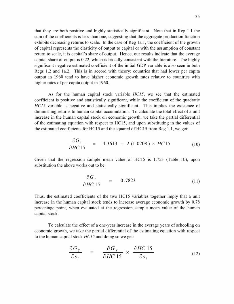
35

that they are both positive and highly statistically significant. Note that in Reg 1.1 the sum of the coefficients is less than one, suggesting that the aggregate production function exhibits decreasing returns to scale. In the case of Reg 1a.1, the coefficient of the growth of capital represents the elasticity of output to capital or with the assumption of constant return to scale, it is capital’s share of output. Hence, our results indicate that the average capital share of output is 0.22, which is broadly consistent with the literature. The highly significant negative estimated coefficient of the initial GDP variable is also seen in both Regs 1.2 and 1a.2. This is in accord with theory: countries that had lower per capita output in 1960 tend to have higher economic growth rates relative to countries with higher rates of per capita output in 1960.

As for the human capital stock variable HC15, we see that the estimated coefficient is positive and statistically significant, while the coefficient of the quadratic HC15 variable is negative and statistically significant. This implies the existence of diminishing returns to human capital accumulation. To calculate the total effect of a unit increase in the human capital stock on economic growth, we take the partial differential of the estimating equation with respect to HC15, and upon substituting in the values of the estimated coefficients for HC15 and the squared of HC15 from Reg 1.1, we get:

15)0208.1(23613.415

HCHC

GY ×−=∂∂

(10)

Given that the regression sample mean value of HC15 is 1.753 (Table 1b), upon substitution the above works out to be:

7823.015

=∂∂HC

G Y (11)

Thus, the estimated coefficients of the two HC15 variables together imply that a unit increase in the human capital stock tends to increase average economic growth by 0.78 percentage point, when evaluated at the regression sample mean value of the human capital stock.

To calculate the effect of a one-year increase in the average years of schooling on economic growth, we take the partial differential of the estimating equation with respect to the human capital stock HC15 and doing so we get:

i

Y

i

Y

sHC

HCG

sG

∂∂

×∂∂

=∂∂ 15

15 (12)

36

From equation (9), we know that the partial differential of the human capital stock to the average years of schooling is

is

i

es

HC *095.0095.015×=

∂∂

(13)

Substituting (11) and (13) into (12), we get

is

i

Y es

G *095.0095.07823.0 ××=∂∂

(14)

Noting that the final term on the right hand side of equation (14) is simply HC15 and substituting the regression sample mean value of HC15 of 1.753, we get

1303.0=∂∂

i

Y

sG

(15)

Thus a one-year increase in the average years of schooling, ceteris paribus, tends to increase average economic growth by 0.13 percentage point, when evaluated at the sample mean of HC15. Equivalently, if the average years of schooling were to increase by 20 percent, which is approximately an increase of 1.18 years, it would tend to increase economic growth by 0.15 percentage point per year. In the same fashion, by using the estimated coefficients from Reg 1a.1, we see that a one-year increase in the average years of schooling, ceteris paribus, tends to increase the average growth rate of output per worker by 0.10 percentage point. With regard to the effects of educational quality on economic growth, we see that while the estimated coefficient of the educational quality term is positive, it is not statistically significant. Nevertheless, the coefficient in Reg 1.1 implies that a one percent increase in educational quality tends to increase the average economic growth by 0.29 percent. With regard to domestic innovation, the estimated coefficient of the patents variable is positive and highly statistically significant. The value of the estimated coefficient of the patents variable in Reg 1.1 suggests that a one percent increase in the number of patents granted by the USPTO is associated with an increase in average economic growth of 0.19 percent. Similarly, the statistically significant positive coefficient of the ‘phones’ variable indicates that a doubling of the number of phones per

37

capita tends to increase average economic growth by 0.55 percentage point43. Notice that the estimated coefficients of the per-worker specification in Reg 1a.1 are very similar.

Next, we seek to improve our estimates by accounting for country differences in Mincerian rates of return to education. As such, we employ the human capital stock measure that again uses exponential compounding of the average years of schooling, but multiplied by country specific rates of return (Equation 16).

ii sri eHC =15 (16)

where HC15i is the average per worker human capital stock of country i ri is the Mincerian rate of return to an additional year of schooling for county i si is the number of years of schooling. Recall that we mentioned above that actual estimates of country specific Mincerian rates of return to education are relatively scarce and that to increase the number of usable observations in our regressions, we constructed an extended series of Mincerian rates of return to education by filling in missing data with the simple average of the specific country’s regional and income-group means of the Mincerian rates. Using the same crude methodology, we also constructed an extended series of educational quality. The regression results where both these series were used as regressors are presented in Regs 1.2 and 1a.244. We see that the results are qualitatively and quantitatively very similar to those of Reg 1.1 and 1a.1. All of the estimated coefficients are of the correct signs and are generally statistically significant. Also, all of the independent variables account for about 60 percent of the cross-country variation in economic growth rates. In particular, the positive coefficient of the human capital term and the negative coefficient of the quadratic human capital term again imply the presence of diminishing returns to human capital accumulation. The coefficient values in Reg 1.2 imply that a one-year increase in the average years of schooling increases average economic growth by 0.11 percentage point, while those in Reg 1a.2 suggest a corresponding increase of 0.11 percentage point in average output per worker. The estimated coefficient of the educational quality variable continues to be positive but insignificant.

43 Note from Table 1b that the regression sample mean value of phones per 1,000 persons is 167. Hence, doubling of the mean value implies an additional 167 phones and when this number is multiplied with the estimated coefficient of 0.0033. 44 Regression results where the human capital stock is constructed with the (non-extended) Mincerian rates of return are presented in Appendix B.

38

In Regs 1.3 and 1a.3, we employ the educational quality measure constructed by Bosworth and Collins (2003) that includes the quality of government institutions as an additional schooling input. We see that with this measure of educational quality, the estimated coefficient of the educational quality variable is positive and turns statistically significant (in Reg 1.3 only). The coefficient value in Reg 1.3 indicates that a one percent increase in educational quality tends to increase the average rate of long-term economic growth by 0.24 percentage point. As for the other independent variables, they continue to exhibit statistically significant estimated coefficients that are of the correct signs. Lastly, note that in both Reg 1.3 and Reg 1a.3 there is a substantial increase in the R-squared value of more than 16 percentage points when the Bosworth-Collins educational quality variable is used. The statistical significance of the Bosworth-Collins educational quality variable and the large jump in the R-squared value tend to suggest that the quality of government institutions may indeed be an important determinant of educational quality and/or of economic growth itself. In Regs 1.4 through 1.6 and Regs 1a.4 through 1a.6, we re-estimated the regressions but instead using the average years of schooling of persons aged 25 years and older. The key result remains unchanged, with human capital stock having a significant positive effect on growth of real GDP and output per worker while showing strong evidence of diminishing returns to capital accumulation. The resultant estimated effects of increases in educational attainment are slightly smaller than those regressions where the educational attainment of the population 15 years and older was used, which is intuitively consistent given that it is likely that persons aged 25 years and older are likely to form a smaller subset of the labor force than persons aged 15 and older. The coefficient values in Reg 1.4 imply that a one-year increase in the average years of schooling increases average economic growth by 0.11 percentage point, while those in Reg 1a.4 suggest a corresponding increase of 0.08 percentage point in average output per worker.

As for the educational quality variable, its estimated coefficient continues to be positive but statistically insignificant. However, when we employ the Bosworth-Collins measure of educational quality, the coefficient again becomes statistically significant in the non-per-worker specification. As before, there were also significant increases in the R-squared values of both per-worker (Reg 1a.6) and non-per worker (Reg 1.6) regressions with the use of the Bosworth-Collins measure of educational quality. 7.2 Innovation Pillar This section examines regression results where we employ different indicators of domestic innovation or technological adaptation to represent the innovation pillar of the knowledge economy. More specifically, we will look at whether the number of patents, utility patents, published scientific and technical journal articles, and the amount royalty

39

payments and receipts provide empirical evidence that domestic innovation and/or technological adaptation is important for long-term economic growth45. The results of the above mentioned regressions are presented in Tables 2 and 2a. Table 2b presents the summary statistics of the innovation variables, while Table 2c is the table of correlation coefficients between the innovation variables. Looking at the estimated coefficients of the growth of capital and labor in Table 2, we see they are positive and highly statistically significant. In addition, as seen in the previous section, the sum of the coefficients is consistently around 0.8, indicating aggregate production function with decreasing returns to scale technology. If we assume constant returns to scale, then the capital share of national income is estimated be 20 percent as seen from the estimated coefficients of the growth of capital per worker in Table 2a. As noted above, there is recurring evidence of diminishing returns to human capital accumulation as indicated by the significant positive coefficient of the human capital stock variable HC15, and the significant negative coefficient of the square of HC15. Also, the positive but statistically insignificant coefficient of the educational quality variable also emerges in both sets of regressions. With regard to the ICT variable ‘phone’, the estimated coefficient is consistently positive and highly statistically significant.

The first innovation variable that we consider is the logarithm of the annual

number of patents granted by the USPTO to a resident of a specific country (Reg 2.1 and Reg 2a.1). As we saw earlier, the estimated coefficient of the patents variable is positive and highly statistically significant. The results indicate that a one percent increase in the number of USPTO patents tends to increase average annual economic growth by 0.19 percentage point, and increase output per worker by 0.20 percentage point. We obtain similar results by using the logarithm of the annual number of utility patents granted by the USPTO to a resident of a specific country to represent domestic innovation. The statistically significant positive coefficient of 0.18 indicates that a one percent increase in the number of utility patents is associated with a 0.18 percentage point increase in annual growth of real GDP and also growth of output per worker. It is shown in Appendix B that we attempted to account for the differences in the quality of patents by using utility patent citation data available from Jaffe and Trajtenberg (2002). However, we obtained results that were theoretically implausible and have decided to exploit the information contained in the citation data at a later date.

The next domestic innovation variable that we examine is the logarithm of the annual number of published scientific and technical journal articles (Reg 2.3 and Reg 2a.3). We see that the estimated coefficient is positive and statistically significant and the value of 0.22 indicates that a one percent increase in the number of journal article tends

45 We also take a look at two other indicators, namely log of the ratio of gross foreign direct investment to GDP, and log of the manufactures trade share in GDP. However, as presented in Appendix B, the estimated coefficients for these 2 variables were statistically not significant.

40

to be associated with a 0.22 percentage point increase in annual economic growth or growth of output per capita. In Regs 2.4 and 2a.4, we turn to royalty payments and receipts as measures of technological adaptation and domestic innovation, respectively. We see that the estimated coefficient of the logarithm of royalty payments variable exhibits a negative sign, which is theoretically unexpected, and is statistically not significant. On the other hand, the logarithm of royalty receipts variable is positive and statistically significant. We note from Table 2c that the correlation coefficient between the royalty payments and the royalty receipts variable are not exceptionally high, therefore the theoretically inconsistent results is unlikely to be due multicollinearity. Given the unsatisfactory results with separate royalty payments and receipts variables, we combine the effects of domestic innovation and technological adaptation by using the logarithm of the sum of royalty payments and receipts as a single innovation pillar independent variable. The results of which are shown in Regs 2.5 and 2a.5, and this variable does produce estimated coefficients that are positive and statistically significant. A one percent increase in royalty payments or receipts tends to lead to an increase in economic growth and /or output per worker growth of 0.03 percentage point. In Regs 2.6, 2.7, 2a.6 and 2a.7, we re-estimate the regressions with royalty payments and receipts but instead of the logarithmic form we use the per capita form. We see that in the regressions with separate royalty payment and receipts regressors (Regs 2.6 and 2a.6), the estimated coefficients for that of royalty payments are now positive and highly statistically significant. On the other hand, the estimated coefficients for that of royalty receipts are still positive but no longer statistically significant. When the royalty payments and receipts are summed up to become the ‘royalties’ variable in Regs 2.7 and 2a.7, the estimated coefficient is positive and highly statistically significant. However, according to the coefficient values with the regression sample mean of $20,524 (See Table 2c), a doubling of royalty payments and receipts tends to lead to approximately 0.08 percentage point increase in the average rate of economic growth or 0.10 percentage point increase in the average growth rate of output per worker. This effect on economic growth and output per worker growth is significantly smaller than what was estimated with the logarithm case46. 7.3 Information and Communications Technologies (ICT) Pillar We now examine whether various proxies for the ICT infrastructure level are able to produce statistical evidence suggesting that ICT infrastructure is an important 46 In Appendix B, we also estimated regressions where the innovation pillar was represented by royalty payments and receipts as ratios of GDP. The results are qualitatively very similar with those where the royalty payments and receipts were in the ‘per capita’ form. More specifically, when estimated as separate regressors, royalty payments exhibited positive and statistically significant coefficients, while royalty receipts coefficients exhibited statistically insignificant ones. When summed together royalties as a share of GDP had coefficients that were positive and statistically significant.

41

determinant of long-term economic growth. Tables 3 and 3a present the regression results where we used ICT indicators such as the number of computers, the number of internet users (per 1,000 persons), the number of computer hosts (per 10,000 persons) and the number of phones (per 1,000 persons) were used to resent the ICT pillar47. We see that all of the ICT indicators produced estimated coefficients that are positive and statistically significant (generally at the 1 percent level of significance). All of the other independent variables also produced estimated coefficients with the correct signs and are statistically significant, with the single exception of the educational quality variable, which as we have repeatedly seen above, has the correct positive sign but is not statistically significant. Firstly in Regs 3.1 and 3a.1, we used the number of computers per 1,000 persons to represent the level of ICT infrastructure within an economy. With estimated coefficient values of 0.0082 and 0.0084, and a regression sample mean value of 65.85 (Table 3b), the results suggests that a 100 percent increase in the number of computers would lead to an increase in the average annual economic growth rate of 0.54 percentage point and an increase of 0.57 percentage point in the growth of output per worker, respectively. As for the estimated coefficients when the number of internet users per 1,000 persons is used to represent the ICT pillar (Regs 3.2 and 3a.2), given that the regression sample mean value is 33.48, a 100 percent increase in the number of internet users would lead to a 0.27 percentage point increase in the annual rate of economic growth and 0.28 percentage point increase in the growth of output per worker. Regs 3.3 and 3a.3 use the number of internet hosts per 10,000 persons to represent the level of ICT infrastructure within the economy. Given the estimated coefficients of 0.0017 and the regression sample mean value of 77.25, a doubling of the of the number of computer hosts tend to increase economic growth and output per worker growth by 0.13. Finally in Regs 3.4 and 3a.4, given that the regression mean value is 165.52, when the number of phones per 1,000 persons, which include both mainlines and cell phone lines, is doubled, the estimated coefficients suggest that the long-term annual economic growth would increase by 0.55 percentage point and growth in output per worker would increase by 0.66 percentage point. In summary, we have presented evidence suggesting that the level of ICT infrastructure is an important in explaining difference in long-term economic growth rates. The estimated effects are largest when the number of phones or the number of computers represents the ICT infrastructure. This is followed by the number of internet users and lastly by the number of internet hosts.

47 Note that we also attempted to use the number televisions, radio and newspapers (all per 1,000 persons) as ICT variables, however these indicators produced estimated coefficients that were either of the incorrect sign and/or were statistically not significant. The results of these regressions are examined in detail in Appendix B.

42

7.4 Economic and Institutional Regime Lastly, we turn to examine the effects of the economic and institutional regime, in addition to the rest of the knowledge variables, on economic growth. Tables 4 and 4a present the results of regressions where we included as additional regressors the Sachs- Warner (1995) index of economic openness and the institutional quality index from Bosworth and Collins (2003). As in the previous sections, Table 4 presents the results when the non-per-worker specification (Equation 7) is estimated and Table 4a presents the results when the per-worker specification (Equation 8) is estimated. The economic openness and institutional quality variables are included as additional regressors in Regs 4.2 through 4.11 and Regs 4a.2 through 4a.11. For convenient comparison, Regs 4.1 and 4a.1 present the results of regressions where the economic and institutional variables were not included, which we have already examined in detail in the preceding sections. Regs 4.2 through 4.6 and Regs 4a.2 through 4a.6 employ the human capital stock measures based on the population aged 15 years or older with various innovation and ICT indicators. Regs 4.7 through 4.11and Regs 4a.7 through 4a.11 re-estimates the regressions with the human capital based on average educational attainment of persons 25 years and older.

Firstly, we note that all of our ‘new’ regressions exhibit R-squared values that are around 20 percentage points higher than our control regressions. This does strongly suggest that economic and openness and institutional quality do play large role in determining rates of economic growth. Next, we notice that the institutions variable consistently produces estimated coefficients that are positive, which is theoretically consistent, and highly statistically significant. Similarly, the economic openness variable consistently returns an estimated coefficient that is positive and statistically significant.

The next striking observation is that upon the inclusion of the economic openness

and institutional quality variables as regressors, many of knowledge indicators, which had produce highly statistically significant estimated coefficients before, are now statistically not significant. More specifically, we see that our human capital stock variables, while maintaining their theoretically expected signs, are generally not statistically significant. The situation is similar with our ICT variables, with the exception that many of the ICT coefficients actually return coefficients with negative signs. This result, where controlling for economic openness and institutional quality eliminates prior present independent roles of other regressors of interest, is consistent with other studies that have included institutional quality in cross-country growth regressions48. However, there are a few innovation variables that have coefficients that managed to maintain their statistical significance. In particular, the innovation variables, 48 For example, Bosworth and Collins (2003) found that with the inclusion of an institution quality variable, their human capital stock / education variables became statistically insignificant.

43

‘journals’ (Regs 4.3 and 4a.3) and ‘royalties per capita’ (Regs 4.4 and 4a.4) exhibit positive and statistically significant coefficients. One reason for the sharp reduction in statistical significance of the estimated coefficients of the knowledge indicators on economic growth on the inclusion of the openness and institution variables could be because of substantial multicollinearity between the openness and institution variables and the other knowledge variables. Table 4b shows the correlation matrix between all of the knowledge variables used in the regressions in Tables 4 and 4a. We see that institutional quality is indeed highly correlated with many of the other knowledge variables. More specifically, note that the correlation between institutions and the human capital stock, patent and the ICT variables are greater than 0.8. On referring back to Tables 4 and 4a, we see that these are precisely the knowledge variables whose independent effects on economic growth were ‘eliminated’. On the other hand, we see that the correlation between institutions and the ‘journals’ and ‘royalties per capita’ are relatively lower, and these are precisely the innovation variables that managed to maintain their statistically significant positive effects on economic growth. Thus, the correlation table suggests that the reason why quite a few of the estimated coefficients of our knowledge indicators ‘lost’ their statistical significance is because they are highly correlated with institutional quality.49 8. Summary and Conclusion

Economic theory postulates that knowledge leads to increases in total factor productivity and hence economic growth. However, unlike traditional factors of production, knowledge is not subject to diminishing returns. If true, the increased creation, use, adoption and flow of knowledge in various forms will significantly improve the prospects of sustainable long-term economic development for many countries. In this light, this paper focuses on empirically assessing the effects of knowledge on economic growth.

We argue that knowledge can become the main engine of growth if the economy

satisfies certain preconditions. These preconditions include a sufficiently high level of quality human capital stock, a high intensity of domestic innovation and technological adoption, the information and communications infrastructure is well established, and the overall economic and institutional regime is conducive for knowledge to propagate and

49 One possible reason for this high correlation between institutional quality and the other knowledge variables could be because a good institutional quality environment is a pre-requisite for investment in education or human capital stock accumulation and ICT infrastructure to take place. We will defer to analysis the determinants of investment in education and ICT infrastructure to a future study.

44

become the driving force behind productivity and economic growth. By using an array of indicators, each of which represents an aspect of knowledge, as independent variables in cross-section regressions that span 92 countries for the period 1960 to 2000, this paper provides empirical evidence indicating that knowledge is a significant determinant of long-term economic growth. In other words, we find that the stock of human capital, the level of domestic innovation and technological adaptation, and the level of information and communications technologies infrastructure all exert statistically significant positive effects on long-term economic growth. More specifically with regard to the growth effects of the human capital stock, we find that an increase of 20 percent in the average years of schooling of a population tends to increase the average annual economic growth by 0.15 percentage point. In terms of innovation, we find that a 20 percent increase in the annual number of USPTO patents granted is associated with an increase of 3.8 percentage points in annual economic growth. Lastly, when the ICT infrastructure is measured by the number of phones per 1,000 persons is increased by 20 percent, we find that annual economic growth tends to increase by 0.11 percentage point. In line with existing literature, our results also show that the overall health of the economy and quality of institutions are important determinants of economic growth. However, the inclusion of such variables renders many of the human capital and ICT variables to have estimated coefficients that are no longer statistically significant. In contrast, the majority of our innovation variables produce coefficients that retain the positive sign and statistical significance. The relative robustness of the innovation variables may suggest that innovation and technological adoption may be the dominant facet of knowledge for economic development. Further research will be required to verify this point. A worthy extension of this research effort would be to transform our existing cross-country data set into one that would enable the estimation of panel regressions, as opposed to the current cross-section regressions. Apart from the obvious benefit of a significant increase in the number of observations, panel regressions would also allow instrumental variable estimation with the lagged independent variables acting as instruments. We will undertake this panel regression approach to the assessment of the effects of knowledge on development in the near future.

45

Years : 1960 - 2000 Reg 1.1 Reg 1.2 Reg 1.3 Reg 1.4 Reg 1.5 Reg 1.6

Growth of Capital 0.2128*** 0.2166*** 0.2511*** 0.2118*** 0.2194*** 0.2521***(0.0442) (0.0467) (0.0363) (0.0456) (0.0484) (0.0386)

Growth of Labor 0.5694*** 0.6831*** 0.3312*** 0.5867*** 0.6799*** 0.3416***(0.1335) (0.1690) (0.1189) (0.1320) (0.1688) (0.1207)

Initial GDP (1960) -3.8747*** -3.8616*** -3.6792*** -3.8384*** -3.8537*** -3.7460***(0.8375) (0.7987) (0.8213) (0.8858) (0.8217) (0.8543)

HC15 4.3613** 3.7613**(1.9441) (1.6161)

Sq of HC15 -1.0208** -0.7590*(0.4654) (0.3870)

HC15 with extended 1.6161*educational returns (0.8253)

Sq (HC15 with -0.2688**Extended (0.1264)Educational Returns)

HC25 3.7916* 3.6325**(1.9726) (1.5986)

Sq of HC25 -0.9286** -0.7321*(0.4662) (0.3787)

HC25 with extended 1.6068*educational returns (0.9558)

Sq (HC25 with -0.2960*Extended (0.1575)Educational Returns)

Log (Educational 0.2933 0.3671Quality) (0.5121) (0.5149)

Log (Educational 0.3256 0.3574Quality Extended) (0.5488) (0.5429)

Log (Educational 0.2405* 0.2528*Quality) - (0.1277) (0.1305)Bosworth & Collins

Log (Patents) 0.1909*** 0.1838** 0.1102** 0.1955*** 0.1867** 0.1085**(0.0728) (0.0785) (0.0516) (0.0738) (0.0774) (0.0524)

Phones 0.0033*** 0.0041*** 0.0024** 0.0035*** 0.0040*** 0.0023**(0.0010) (0.0011) (0.0010) (0.0011) (0.0011) (0.0010)

Constant -3.6660* -1.8984 -2.5109 -3.2783 -1.8733 -2.3360(2.1096) (1.7103) (1.7300) (2.0957) (1.6959) (1.6934)

R squared 0.6137 0.5967 0.7621 0.6078 0.5933 0.7596Number of Countries 85 92 73 84 90 72

*, **, *** denotes significance at the 90, 95 and 99 percent confidence level respectivelyRobust standard errors obtained using W hite's correction for heteroscedasticity.

Table 1Dependent Variable: Growth Rate of Real GDP

Educational Pillar Indicators

46

Years : 1960 - 2000 Reg 1a.1 Reg 1a.2 Reg 1a.3 Reg 1a.4 Reg 1a.5 Reg 1a.6

Growth of Capital 0.2119*** 0.2116*** 0.2464*** 0.2095*** 0.2128*** 0.2455***per worker (0.0424) (0.0451) (0.0375) (0.0436) (0.0464) (0.0398)

Initial GDP (1960) -3.7103*** -3.9131*** -3.5760*** -3.7197*** -3.9317*** -3.6712***(0.8717) (0.7780) (0.9164) (0.9234) (0.8032) (0.9496)

HC15 4.4661** 4.5116***(1.9854) (1.5779)

Sq of HC15 -1.0965** -1.0374***(0.4726) (0.3752)

HC15 with extended 1.5718**educational returns (0.7644)

Sq (HC15 with -0.2617**Extended (0.1139)Educational Returns)

HC25 3.8946* 4.3664***(2.0153) (1.5611)

Sq of HC25 -0.9925** -0.9995***(0.4738) (0.3638)

HC25 with extended 1.5373*educational returns (0.8991)

Sq (HC25 with -0.2845*Extended (0.1446)Educational Returns)

Log (Educational 0.3719 0.4324Quality) (0.5412) (0.5411)

Log (Educational 0.3877 0.4288Quality Extended) (0.5730) (0.5654)

Log (Educational 0.1743 0.1913Quality) - (0.1110) (0.1148)Bosworth & Collins

Log (Patents) 0.1956*** 0.1847** 0.1373** 0.1984*** 0.1873** 0.1331**(0.0701) (0.0788) (0.0534) (0.0714) (0.0774) (0.0543)

Phones 0.0040*** 0.0044*** 0.0039*** 0.0040*** 0.0043*** 0.0039***(0.0011) (0.0012) (0.0018) (0.0011) (0.0012) (0.0012)

Constant -4.5304** -2.3031 -3.9558** -4.066* -2.2720 -3.7559**(2.2424) (1.8845) (1.7167) (2.2225) (1.8833) (1.6724)

R squared 0.5912 0.5607 0.7240 0.5842 0.5578 0.7213Number of Countries 85 92 73 84 90 72

*, **, *** denotes significance at the 90, 95 and 99 percent confidence level respectivelyRobust standard errors obtained using White's correction for heteroscedasticity.

Table 1aDependent Variable: Growth Rate of Real GDP Per Worker

Educational Pillar Indicators

47

Obs Mean Std. Dev. Min Max

Growth of Capital 84 5.3917 3.3044 -0.0968 17.2024

Growth of Labor 84 2.2056 0.8845 0.2877 4.5267

Initial GDP (1960) 84 0.3105 0.2694 0.0341 1.2204

HC15 84 1.7530 0.4492 1.0581 2.8472

Square of HC15 84 3.3147 1.7509 1.1205 8.2040

HC15 extended 84 1.7315 0.4965 1.0693 4.7060

Square of HC15 extended 84 3.3172 2.6991 1.1445 24.2639

HC25 84 1.6892 0.4574 1.0433 2.8800

Square of HC25 84 3.1051 1.7545 1.0891 8.4101

HC25 extended 84 1.6579 0.4683 1.0515 4.2994

Square of HC25 extended 84 3.0363 2.3272 1.1066 20.2922

Log (Educational Quality) 84 3.7544 0.3076 2.9047 4.2785

Log (Patents) 84 2.4327 2.7420 0.0000 10.9275

Phones 84 167.4538 198.0019 0.8461 717.4805

Table 1bSummary Statistics:

Control and Human Capital Indpendent Variables

48

Years : 1960 - 2000 Reg 2.1 Reg 2.2 Reg 2.3 Reg 2.4 Reg 2.5 Reg 2.6 Reg 2.7

Growth of Capital 0.2128*** 0.2157*** 0.2252*** 0.2128*** 0.2033*** 0.2127*** 0.2141***(0.0442) (0.0451) (0.0394) (0.0513) (0.0494) (0.0504) (0.0504)

Growth of Labor 0.5694*** 0.5775*** 0.5948*** 0.5996*** 0.5703*** 0.5948*** 0.5933***(0.1335) (0.1392) (0.1259) (0.1485) (0.1500) (0.1519) (0.1509)

Initial GDP (1960) -3.8747*** -3.9019*** -3.6842*** -3.6173*** -3.8133*** -3.6136*** -3.6067***(0.8375) (0.8201) (0.7789) (0.7132) (0.7348) (0.7204) (0.7254)

HC15 4.3613** 4.5361** 3.9374** 2.8637* 2.2266 2.8002* 2.8968*(1.9441) (1.9274) (1.8746) (1.6399) (1.6457) (1.5394) (1.5483)

Sq of HC15 -1.0208** -1.0544** -0.9253** -0.6367* -0.4574 -0.5983* -0.6273*(0.4654) (0.4616) (0.4465) (0.3682) (0.3744) (0.3656) (0.3665)

Log (Educational 0.2933 0.3338 0.4639 0.2820 0.4720 0.3959 0.3980Quality) (0.5121) (0.5253) (0.4799) (0.5296) (0.5142) (0.5563) (0.5516)

Log (Patents) 0.1909***(0.0728)

Log (Utility Patents) 0.1759**(0.0741)

Log (Journals) 0.2254***(0.0500)

Log (Royalty Payments) -0.0040(0.0188)

Log (Royalty Receipts) 0.0336**(0.0166)

Log (Royalties) 0.0253*(0.0136)

Royalty Payments 0.000004***per capita (0.000001)

Royalty Receipts 0.000001per capita (0.000006)

Royalties per capita 0.000004***(0.000001)

Phones 0.0033*** 0.0036*** 0.0032*** 0.0046*** 0.0046*** 0.0044*** 0.0044***(0.0010) (0.0010) (0.0009) (0.0012) (0.0012) (0.0012) (0.0012)

Constant -3.6660* -4.0111* -4.7967** -2.4010 -2.4736 -2.5903 -2.5903(2.1096) (2.1394) (2.0922) (1.8850) (1.8782) (2.0501) (2.0318)

R squared 0.6137 0.6071 0.646 0.6410 0.6318 0.6320 0.6320Number of Countries 85 85 85 84 84 84 84

*, **, *** denotes significance at the 90, 95 and 99 percent confidence level respectivelyRobust standard errors obtained using White's correction for heteroscedasticity.

Table 2Dependent Variable: Growth Rate of Real GDP

Innovation Pillar Indicators

49

Years : 1960 - 2000 Reg 2a.1 Reg 2a.2 Reg 2a.3 Reg 2a.4 Reg 2a.5 Reg 2a.6 Reg 2a.7

Growth of Capital 0.2119*** 0.2147*** 0.2251*** 0.2118*** 0.2020*** 0.2136*** 0.2150***Per Worker (0.0424) (0.0434) (0.0385) (0.0499) (0.0473) (0.0492) (0.0492)

Initial GDP (1960) -3.7103*** -3.7533*** -3.5395*** -3.4598*** -3.6375*** -3.4116*** -3.4059***(0.8717) (0.8494) (0.8143) (0.7319) (0.7667) (0.7518) (0.7565)

HC15 4.4661** 4.6428** 4.0179** 2.9314* 2.2785 2.8552* 2.9533*(1.9854) (1.9699) (1.9165) (1.6963) (1.7155) (1.5822) (1.5961)

Sq of HC15 -1.0965** -1.1303** -0.9878** -0.7006* -0.5215 -0.6638* -0.6932*(0.4726) (0.4686) (0.4544) (0.3843) (0.3967) (0.3805) (0.3846)

Log (Educational 0.3719 0.4121 0.5337 0.3454 0.5610 0.4735 0.4750Quality) (0.5412) (0.5533) (0.5009) (0.5542) (0.5460) (0.5881) (0.5830)

Log (Patents) 0.1956***(0.0701)

Log (Utility Patents) 0.1839**(0.0706)

Log (Journals) 0.2295***(0.0494)

Log (Royalty Payments) -0.0047(0.0195)

Log (Royalty Receipts) 0.0369**(0.0175)

Log (Royalties) 0.0268**(0.0134)

Royalty Payments 0.000005***per capita (0.000001)

Royalty Receipts 0.000002per capita (0.000006)

Royalties per capita 0.000005***(0.000001)

Phones 0.0040*** 0.0041*** 0.0037*** 0.0051*** 0.0052*** 0.0049*** 0.0049***(0.0011) (0.0011) (0.0009) (0.0011) (0.0011) (0.0011) (0.0011)

Constant -4.5304** -4.8463** -5.5338** -3.1130 -3.3607 -3.3407 -3.4270(2.2424) (2.2722) (2.1996) (2.0799) (2.0756) (2.2176) (2.2023)

R squared 0.5912 0.5854 0.6248 0.6126 0.5999 0.6045 0.6042Number of Countries 85 85 85 84 84 84 84

*, **, *** denotes significance at the 90, 95 and 99 percent confidence level respectivelyRobust standard errors obtained using White's correction for heteroscedasticity.

Table 2aDependent Variable: Growth Rate of Real GDP Per Worker

Innovation Pillar Indicators

50

Obs Mean Std. Dev. Min Max

Log (Patents) 84 3.9213 1.6027 -0.3456 9.4527

Log (Utility Patents) 84 5.3917 3.3044 -0.0968 17.2024

Log (Journals) 84 2.2056 0.8845 0.2877 4.5267

Log (Royalty Payments) 84 0.3105 0.2694 0.0341 1.2204

Log (Royalty Receipts) 84 1.7530 0.4492 1.0581 2.8472

Log (Royalties) 84 3.3147 1.7509 1.1205 8.2040

Royalty Payments 84 1.7315 0.4965 1.0693 4.7060per capita

84 3.3172 2.6991 1.1445 24.2639Royalty Receiptsper capita 84 1.6892 0.4574 1.0433 2.8800

Royalties per capita 84 1.6579 0.4683 1.0515 4.2994

Table 2bSummary Statistics:

Innovation Indpendent Variables

51

Log (Patents)

Log (Utility

Patents)

Log (Journals)

Log (Royalty Payments)

Log (Royalty

Receipts)

Log (Royalties)

Royalty Payments Per Capita

Royalty Receipts

Per Capita

Royalties per capita

Log (Patents) 1.0000

Log (Utility 0.9948 1.0000Patents)

Log (Journals) 0.9090 0.9003 1.0000

Log (Royalty 0.4832 0.4697 0.5051 1.0000Payments)

Log (Royalty 0.6216 0.6089 0.6302 0.7738 1.0000Receipts)

Log (Royalties) 0.5131 0.4997 0.5004 0.9404 0.8362 1.0000

Royalty 0.3324 0.3206 0.2868 0.2989 0.3225 0.3026 1.0000Paymentsper capita

Royalty 0.7013 0.7174 0.5854 0.4091 0.5279 0.4416 0.4332 1.0000Receiptsper capita

Royalties 0.4626 0.4664 0.3947 0.3594 0.4125 0.3720 0.9747 0.6231 1.0000per capita

Table 2cTable of Correlation Coefficients:Innovation Indpendent Variables

52

Years : 1960 - 2000 Reg 3.1 Reg 3.2 Reg 3.3 Reg 3.4

Growth of Capital 0.2264*** 0.2251*** 0.2310*** 0.2128***(0.0530) (0.0440) (0.0464) (0.0442)

Growth of Labor 0.4614*** 0.4617*** 0.4521*** 0.5694***(0.1395) (0.1297) (0.1366) (0.1335)

Initial GDP (1960) -4.0288*** -3.4424*** -3.4300*** -3.8747***(0.7963) (0.8767) (0.8381) (0.8375)

HC15 3.7100*** 4.9953** 5.4972*** 4.3613**(1.3920) (1.9402) (1.9854) (1.9441)

Sq of HC15 -0.9508*** -1.1712** -1.2625** -1.0208**(0.3397) (0.4821) (0.4920) (0.4654)

Log (Educational 0.3848 0.3147 0.4798* 0.2933Quality) (0.5157) (0.4825) (0.4936) (0.5121)

Log (Patents) 0.2252*** 0.2366*** 0.2411*** 0.1909***(0.0706) (0.0688) (0.0711) (0.0728)

Computers 0.0082***(0.0020)

Internet Users 0.0082***(0.0023)

Hosts 0.0017**(0.0007)

Phones 0.0033***(0.0010)

Constant -2.8603 -4.1496** -5.2290*** -3.666*(1.7706) (1.9661) (1.9915) (2.1096)

R squared 0.6646 0.6114 0.6034 0.6137Number of Countries 81 85 85 85

*, **, *** denotes significance at the 90, 95 and 99 percent confidence level respectivelyRobust standard errors obtained using White's correction for heteroscedasticity.

Table 3Dependent Variable: Growth Rate of Real GDP

Information and CommunicationsTechnologies (ICT) Pillar Indicators

53

Years : 1960 - 2000 Reg 3.1 Reg 3.2 Reg 3.3 Reg 3.4

Growth of Capital 0.2293*** 0.2298*** 0.2360*** 0.2119***per worker (0.0507) (0.0419) (0.0444) (0.0424)

Initial GDP (1960) -3.5813*** -2.9514*** -2.9244*** -3.7103***(0.8771) (0.8905) (0.8668) (0.8717)

HC15 3.9910*** 5.2399** 5.7432*** 4.4661**(1.4484) (2.0078) (2.0243) (1.9854)

Sq of HC15 -1.0697*** -1.2780** -1.3677*** -1.0965**(0.3554) (0.4985) (0.4947) (0.4726)

Log (Educational 0.5363 0.4788 0.6516 0.3719Quality) (0.5569) (0.0633) (0.5336) (0.5412)

Log (Patents) 0.2474*** 0.2586*** 0.2636*** 0.1956***(0.0640) (0.0633) (0.0649) (0.0701)

Computers 0.0086***(0.0024)

Internet Users 0.0084***(0.0024)

Hosts 0.0017***(0.0006)

Phones 0.0040***(0.0011)

Constant -4.4327** -5.7535*** -6.8771*** -4.5304**(1.8692) (2.0604) (2.0484) (2.2424)

R squared 0.6165 0.5779 0.5687 0.5912Number of Countries 81 85 85 85

*, **, *** denotes significance at the 90, 95 and 99 percent confidence level respectivelyRobust standard errors obtained using White's correction for heteroscedasticity.

Table 3aDependent Variable: Growth Rate of Real GDP Per Worker

Information and CommunicationsTechnologies (ICT) Pillar Indicators

54

Obs Mean Std. Dev. Min Max

Computers 84 65.8529 82.4577 0.7364 301.6487(per 1,000 persons)

Internet Users 84 33.4844 48.7937 0.0153 215.5891(per 1,000 persons)

Hosts 84 77.2506 167.8352 0.0000 858.8547(per 10,000 persons)

Phones 84 165.5167 197.6284 0.8461 717.4805(per 1,000 persons)

Table 3bSummary Statistics:

Information and CommunicationsTechnologies (ICT) Independent Variables

55

Years : 1960 - 2000 Reg 4.1 Reg 4.2 Reg 4.3 Reg 4.4 Reg 4.5 Reg 4.6 Reg 4.7 Reg 4.8 Reg 4.9 Reg 4.10 Reg 4.11

Growth of Capital 0.2128*** 0.2384*** 0.2380*** 0.2510*** 0.2348*** 0.2344*** 0.2366*** 0.2358*** 0.2487*** 0.2318*** 0.2321***(0.0442) (0.0347) (0.0313) (0.0366) (0.0352) (0.0336) (0.0362) (0.0329) (0.0380) (0.0363) (0.0348)

Growth of Labor 0.5694*** 0.3999*** 0.4411*** 0.4059*** 0.4293*** 0.4315*** 0.4126*** 0.4533*** 0.4177*** 0.4418*** 0.4452***(0.1335) (0.1111) (0.1033) (0.1186) (0.0947) (0.0945) (0.1124) (0.1028) (0.1198) (0.0960) (0.0956)

Initial GDP (1960) -3.8747*** -3.6513*** -3.4613*** -3.4498*** -3.8702*** -3.8524*** -3.7380*** -3.5526*** -3.5551*** -3.9390*** -3.9599***(0.8375) (0.7642) (0.7073) (0.7222) (0.7564) (0.7509) (0.7934) (0.7482) (0.7622) (0.7865) (0.7868)

Economic 0.4979** 0.6255** 0.4578* 0.4189* 0.4595* 0.5021** 0.6281*** 0.4649* 0.4239* 0.4624*Openness (0.2337) (0.2395) (0.2468) (0.2405) (0.2354) (0.2310) (0.2373) (0.2438) (0.2392) (0.2337)

Institutions 3.6920*** 2.6259** 3.8409*** 3.0583*** 3.6058*** 3.7844*** 2.6916** 3.9367*** 3.1816*** 3.7142***(0.9857) (1.0632) (0.9294) (0.9658) (0.9153) (0.9833) (1.0651) (0.9266) (0.9663) (0.9134)

Education Variables

HC15 4.3613** 1.7563 1.7059 1.8216 1.7856 1.6176(1.9441) (1.7665) (1.5988) (1.8584) (1.7912) (1.7979)

Sq of HC15 -1.0208** -0.2906 -0.3056 -0.2981 -0.3561 -0.2435(0.4654) (0.4195) (0.3844) (0.4460) (0.4301) (0.4365)

HC25 1.6475 1.6450 1.6850 1.5373 1.4689(1.7405) (1.5670) (1.8370) (1.7828) (1.7790)

Sq of HC25 -0.2665 -0.2917 -0.2643 -0.3018 -0.2055(0.4157) (0.3765) (0.4468) (0.4338) (0.4376)

Log (Educational 0.2933 0.6176 0.7633* 0.6182 0.6166 0.6348 0.6324 0.7730* 0.6329 0.6414 0.6559Quality) (0.5121) (0.4461) (0.4129) (0.4654) (0.4741) (0.4643) (0.4550) (0.4191) (0.4724) (0.4858) (0.4752)

Innovation Variables

Log (Patents) 0.1909*** 0.0703 0.0723 0.0600 0.0683 0.0703 0.0574(0.0728) (0.0556) (0.0548) (0.0569) (0.0559) (0.0551) (0.0571)

Log (Journals) 0.1431*** 0.1439***(0.0497) (0.0503)

Royalties per 0.000002* 0.000002capita (0.000001) (0.000001)

ICT Variables

Phones 0.0033*** -0.0011 -0.0009 -0.0008 -0.0011 -0.0009 -0.0008(0.0010) (0.0010) (0.0010) (0.0011) (0.0010) (0.0010) (0.0011)

Computers 0.0012 0.0010(0.0018) (0.0018)

Internet Users -0.0027 -0.0029(0.0018) (0.0019)

Constant -3.6660* -4.0649** -4.6608*** -4.2734** -3.6728* -4.0212** -3.9997 -4.6183*** -4.1809** -3.5298* -3.9533**(2.1096) (1.9485) (1.7335) (2.1077) (1.9450) (1.9303) (1.8666) (1.6672) (2.0268) (1.8741) (1.8473)

R squared 0.6137 0.8194 0.8387 0.8185 0.8220 0.8192 0.8189 0.8388 0.8179 0.8216 0.8187No. of Countries 85 72 72 72 70 72 71 71 71 69 71

*, **, *** denotes significance at the 90, 95 and 99 percent confidence level respectivelyRobust standard errors in parentheses obtained using White's correction for heteroscedasticity.

Table 4Dependent Variable: Growth Rate of Real GDP

Regressions with Economic Openness and Institutions

56

Years : 1960 - 2000 Reg 4a.1 Reg 4a.2 Reg 4a.3 Reg 4a.4 Reg 4a.5 Reg 4a.6 Reg 4a.7 Reg 4a.8 Reg 4a.9 Reg 4a.10 Reg 4a.11

Growth of Capital 0.2119*** 0.2304*** 0.2317*** 0.2486*** 0.2322*** 0.2304*** 0.2269*** 0.2279*** 0.2442*** 0.2279*** 0.2268***per worker (0.0424) (0.0351) (0.0327) (0.0359) (0.0359) (0.0343) (0.0364) (0.0342) (0.0372) (0.0369) (0.0355)

Initial GDP (1960) -3.7103*** -3.4913*** -3.2936*** -3.2002*** -3.4618*** -3.4694*** -3.6157*** -3.4212*** -3.3430*** -3.5954*** -3.6358***(0.8717) (0.8094) (0.7716) (0.7625) (0.7824) (0.7527) (0.8452) (0.8176) (0.8037) (0.8147) (0.7976)

Economic 0.5622* 0.6986** 0.5128* 0.5783* 0.6223** 0.5568* 0.6910** 0.5144* 0.5649* 0.6085**Openness (0.2877) (0.3046) (0.2989) (0.2953) (0.2980) (0.2826) (0.3001) (0.2938) (0.2902) (0.2925)

Institutions 3.7204*** 2.5559** 3.7322*** 3.5433*** 4.0038*** 3.8455*** 2.6595** 3.8591*** 3.6842*** 4.1288***(1.0280) (1.1212) (0.9542) (0.9983) (0.9674) (1.0282) (1.1177) (0.9539) (1.0056) (0.9705)

Education Variables

HC15 4.4661** 2.2976 2.1616 2.3235 1.9538 1.8594(1.9854) (1.7346) (1.6186) (1.7967) (1.8472) (1.8214)

Sq of HC15 -1.0965** -0.5218 -0.5091 -0.5264 -0.4551 -0.3699(0.4726) (0.4066) (0.3830) (0.4299) (0.4524) (0.4433)

HC25 2.2058 2.1148 2.1651 1.8159 1.7918(1.7022) (1.5813) (1.7655) (1.7992) (1.7699)

Sq of HC25 -0.4941 -0.4920 -0.4810 -0.4138 -0.3393(0.4005) (0.3736) (0.4285) (0.4458) (0.4374)

Log (Educational 0.3719 0.7383 0.8826* 0.7408 0.7875 0.7930 0.7366 0.8761* 0.7416 0.7924 0.7959Quality) (0.5412) (0.5078) (0.4570) (0.5302) (0.5238) (0.5169) (0.5132) (0.4610) (0.5337) (0.5316) (0.5238)

Innovation Variables

Log (Patents) 0.1956*** 0.0719 0.0791 0.0696 0.0678 0.0739 0.0640(0.0701) (0.0572) (0.0573) (0.0587) (0.0579) (0.0581) (0.0595)

Log (Journals) 0.1543*** 0.1532***(0.0542) (0.0544)

Royalties per 0.000003*** 0.000003**capita (0.000001) (0.000001)

ICT Variables

Phones 0.0040*** 0.0003 0.0003 0.0005 0.0002 0.0002 0.0004(0.0011) (0.0011) (0.0011) (0.0011) (0.0011) (0.0011) (0.0011)

Computers 0.0008 0.0007(0.0025) (0.0025)

Internet Users -0.0025 -0.0027(0.0022) (0.0023)

Constant -4.5304** -5.7956*** -6.2132*** -5.8668*** -5.5098*** -5.8155*** -5.6831*** -6.1191 -5.7045*** -5.3951*** -5.7482***(2.2424) (1.9647) (1.7433) (2.0972) (1.9072) (1.8802) (1.8802) (1.6752) (2.0064) (1.8095) (1.7808)

R squared 0.5912 0.7980 0.8202 0.8023 0.8006 0.7990 0.7979 0.8205 0.8017 0.8005 0.7992No. of Countries 85 72 72 72 70 72 71 71 71 69 71

*, **, *** denotes significance at the 90, 95 and 99 percent confidence level respectivelyRobust standard errors in parentheses obtained using White's correction for heteroscedasticity.

Table 4aDependent Variable: Growth Rate of Real GDP Per Worker

Regressions with Economic Openness and Institutions

57

Openness Institutions HC15 Square of HC15 HC25 Square

of HC25

Log (Educational

Quality)

Log (Patents)

Log (Journals)

Royalties per capita Phones Computers Internet

Users

Openness 1.0000

Institutions 0.7308 1.0000

HC15 0.6538 0.8372 1.0000

Square of HC15 0.6315 0.8304 0.9931 1.0000

HC25 0.6527 0.8450 0.9974 0.9937 1.0000

Square of HC25 0.6310 0.8360 0.9875 0.9974 0.9931 1.0000

Log (Educational 0.5743 0.6663 0.6609 0.6410 0.6582 0.6346 1.0000Quality)

Log (Patents) 0.6152 0.8468 0.8245 0.8252 0.8333 0.8311 0.5984 1.0000

Log (Journals) 0.5048 0.7948 0.7056 0.7049 0.7106 0.7084 0.4856 0.9044 1.0000

Royalties 0.3851 0.4940 0.4525 0.4451 0.4593 0.4476 0.3002 0.4396 0.3750 1.0000per capita

Phones 0.7408 0.9099 0.8889 0.8927 0.9004 0.9011 0.6728 0.8483 0.7391 0.4495 1.0000

Computers 0.6452 0.8660 0.8651 0.8799 0.8783 0.8908 0.6466 0.7648 0.6416 0.4867 0.9219 1.0000

Internet Users 0.6638 0.8243 0.8443 0.8601 0.8520 0.8659 0.6417 0.7410 0.6186 0.4267 0.9087 0.9279 1.0000

Table 4bTable of Correlation Coefficients:Knowledge Economy Variables

58

Appendix A: Generation of Aggregate Capital Stock

Annual values of the country specific capital stock were generated from gross investment data using the perpetual inventory method:

ittiit IKK +−= − )1(1, δ where Kit is the level of the aggregate capital stock for country i in year t δ is the depreciation rate, which is assumed to be have the same value for all

countries for all time periods Iit is the level of gross investment for country i in year t Data on gross investment were obtained from the World Bank SIMA database as gross capital formation50 in constant local currency units. We assumed a depreciation rate of 5 percent for all countries and all time periods, which implies that δ was set equal to 0.05. Note that before any capital stock series can be constructed, the initial value of the capital stock is required. To obtain these initial capital stock values, we employed the constant initial investment growth specification, detailed in Young (1995). Specifically, assume the period t is the first period in which gross investment data for a country is available and also that g is the value of the average growth rate of gross investment for the next 4 periods, that is periods t+1 through t+4. If we further assume that the capital stock had been growing at the same growth rate g for infinite number of periods before period t, then we are able to use the mathematical result for the sum of an infinite geometric series and thus it can be shown that the value of the initial capital stock (value of the capital stock in period 1) is given by:

1110

11

1

011

<+−

>+

=

+−

= ∑∞

=

gandgif

gI

gIK

i

s

sii

δδ

δ

Note that 111

<+−

gδ is necessary in order to ensure that the convergence of the capital

stock (infinite geometric) series

50 Gross capital formation (formerly gross domestic investment) consists of outlays on additions to the fixed assets of the economy plus net changes in the level of inventories. Fixed assets include land improvements (fences, ditches, drains, and so on); plant, machinery, and equipment purchases; and the construction of roads, railways, and the like, including schools, offices, hospitals, private residential dwellings, and commercial and industrial buildings. Inventories are stocks of goods held by firms to meet temporary or unexpected fluctuations in production or sales, and "work in progress." According to the 1993 SNA, net acquisitions of valuables are also considered capital formation.

59

Appendix B: Complete Regression Results

In this appendix, we present the regression results of the complete set of knowledge economy variables that we attempted to use to explain long-term economic growth. We will first discuss the various human capital or education variables that we examined, followed by the innovation or technological adaptation variables. Variables representing the level of information and communications technologies (ICT) infrastructure will be presented in the final section of this appendix. B.1 Educational / Human Capital Stock Variables Tables A1 and A1a present the regression results where different indicators or measures of the human capital stock were used. Regressions in Table A1 were estimating the specification in Equation (7) with the growth rate of real GDP as the dependent variable, while those in Table A1a were estimating the specification in Equation (8) and therefore had the growth rate of real GDP per worker as the dependent variable.

Notice that all regressions in Table A1 include the following as regressors: the growth rate of capital stock, the growth rate of the labor force, initial GDP per capita in 1960, the number of patents granted (in logs) and the number of phones (per 1,000 persons and in logs) and a constant term. The set of regressors for the regressions in Table A1a are similar with exception that the growth rate of the capital stock per worker replaced the growth rate of the capital stock and the growth rate of labor was dropped (in accordance with Equation (8)). Even though this section focuses only on the education or human capital stock variables, we include the patent and the phone variables as regressors to account for the innovation and ICT pillars of the knowledge economy, thereby reducing the possibility of biases resulting from omitted variables. As it will be seen, the results from the both sets of regressions (per worker and non-per worker) are qualitatively very similar. With reference to Reg A1.1 in Table A1, we see that the estimated coefficients of all regressors possess the theoretically expected sign and are statistically significant (at least at the 10 percent level). Together capital, labor, initial GDP, the number of patents and phones account for about 62 percent of the cross-country variation in the real GDP growth rates from 1960 to 2000. Similar results are obtained in the per worker specification of the regression as demonstrated in Reg A1a.1 of Table A1a.

60

In Reg A1.2 and Reg A1a.2, we include the human capital stock measured using the exponentially compounded by the product of the average years of schooling of persons, at 15 and older, with the global average Mincerian rate of return of 9.5 percent (See Equation 9).

We see that the estimated coefficients of human capital variables are positive, which is theoretically consistent, but are statistically not significant. These results are consistent with earlier papers that attempted to assess the effects of human capital on economic growth. The estimated coefficients of the control variables continue to possess their theoretical expected signs and be statistically significant. However, note that the R squared values of the regressions actually fall with the inclusion of these educational attainment variables. We mentioned above that proper construction of the human capital stock requires accounting for differences in the quality of the education systems in different countries. As such, we include educational quality as an additional regressor in regressions Reg A1.3 and Reg A1a.3. As mentioned above, our educational quality variable is taken from Hanushek and Kimko (2000) and Bosworth and Collins (2003). We see that in both cases, the estimated coefficient of the educational quality variable is positive, but is not statistically significant. Also, the human capital measure remains positive and not statistically significant.

For the next pair of regressions, Reg A1.4 and A1a.4, we include a quadratic term for the human capital variable to capture the possible existence of strong diminishing returns to human capital accumulation. We see that the estimated coefficient of the squared human capital variable is negative and statistically significant, indicating evidence of diminishing returns. In addition, the estimated coefficient of the human capital variable remains positive but turns statistically significant. Hence, accounting for second-order effects leads to results that suggest that human capital accumulation is a significant determinant of economic growth. Note that the educational quality variable still positive but not statistically significant. However, this could be due to the data not being able to accurately measure quality differences, rather than educational quality not being important in explaining differences in long-term economic growth across countries51. As such, we continue to include the educational quality variable as an educational pillar regressor, even though it is not statistically significant. Next, we seek to improve our estimates by accounting for country differences in Mincerian rates of return to education. As such, we employ the human capital stock measure that again uses exponential compounding of the average years of schooling, but multiplied by country specific rates of return (See Equation 16). 51 Recall that more than 50 percent of the data from Hanushek and Kimko (2000) on educational quality were in fact predicted values from a regression with various schooling inputs as the independent variables.

61

The results of these regressions are presented as Reg A1.5 through Reg A1.7 and

Reg A1a.5 through Reg A1a.7. Given that data on these country specific rates are relatively scarce, the number of observations in these regressions decreases to 53 as compared to 85 in the previous regressions. As can be seen, a theoretically inconsistent negative sign for the estimated coefficient of the human capital measure results for the regressions with human capital variable alone, as well as for the regressions where the educational quality variable is included. In Reg A1.7, we see that with the inclusion of the quadratic term for this modified human capital variable, the estimated coefficient of the human capital variable turns positive, and becomes statistically significant. The estimated coefficient of the squared human capital variable also displays the theoretically expected negative sign and is statistically significant. The significance of the human capital and square human capital variable is not observed in the corresponding per worker regression in Reg A1a.7. The educational variable is not statistically significant throughout. Also note that the R-squared values of the regressions with the country-specific educational returns are significantly higher than those that utilize the global average Mincerian rate of return. However, the higher R-square value could be solely due to the few number of observations being used by the regressions. We mentioned above that to increase the number of usable observations in our regressions with human capital measure with country specific Mincerian rates of return, we constructed an extended series of Mincerian rates of return to education. We constructed this series by filling in missing data with the simple average of the specific country’s regional and income-group means of the Mincerian rates. The results of the regressions using this extended series of Mincerian rates are presented in Reg A1.8 through Reg A1.12 and Reg A1a.8 through Reg A1a.12. We see that on its own, this measure of human capital returns an estimated coefficient that is positive but not statistically significant. The qualitative nature of this result remains unchanged when the educational quality variable is included as an additional regressor, which also has an estimated coefficient that is positive, but not significant. However, as with other measures of the human capital stock, the estimated coefficient of our extended human capital stock measure turns statistically significant once we include the square of the extended human capital stock as an additional regressor. The coefficient of the square variable itself is negative and statistically significant indicating substantial diminishing returns to human capital accumulation.

Also, note that in Reg A1.11, A1.12, A1a.11 and Reg A1a.12 we utilized our extended series on educational quality, which was constructed in an identical fashion as our extended series of Mincerian rates of return to education. Namely, missing data for educational quality were filled in with the simple average of the specific country’s regional and income-group means. The key result remains unchanged, with educational attainment producing a significant positive estimated coefficient only when the quadratic educational attainment term is included as an additional regressor.

62

As a further robustness check, we re-estimate the above regressions using the educational attainment measure of average years of schooling of persons 25 years and older, instead of 15 years and older. The results of which are presented in Tables A1b and A1c, where the regressions presented in the former follow the specification in Equation (7), while those in the latter follow the (per worker) specification in Equation (8). We see that the results are largely qualitatively similar to those in Tables A1 and A1a. The estimated coefficient of the human capital stock variable is positive and statistically significant only when the square of the human capital stock variable is included as an independent variable. The educational quality variable is positive, but consistently fails to achieve statistical significance. B.2 Innovation Variables

We now turn to examine the results of the set of regressions in which we vary the indicators or measures of domestic innovation and technology adaptation. Table A2 presents the results where the non-per-worker specification was used, while Table A2a presents the results when the per-worker specification was used. Given that we postulate that innovation and technological adaptation tend to increase long-term economic growth, we would expect measures of innovation and technological adaptation to have positive estimated coefficients.

Firstly in Reg A2.1, we regressed the growth rate of real GDP on the control,

education and ICT variables, omitting any independent variable representing innovation. We see that the estimated coefficients of these variables are all of the correct sign and are statistically significant52, and together they account for 58 percent of the cross-country variation in growth rates. Very similar results were obtained using the per-worker specification, as seen in Reg A2a.1.

In Reg A2.2 and A2a.2, we include the logarithm of the number of patents

granted by the USPTO as the innovation measure. The patent count in these regressions includes all types of patents. We see that the estimated coefficient on this patent variable bears the theoretically expected positive sign and is highly statistically significant in both specifications. As such, there is some evidence that an increase in the average number of USPTO patents tends to increase economic growth in the long run.

Next, we proceed to attempt to control for the quality of patents by using the

average number of patent citations a specific country’s patents received. As mentioned 52 Only the coefficient of the educational quality variable is positive and statistically insignificant, which we have seen in the previous section to be a robust result.

63

above, we only managed to obtain citation data on USPTO utility patents, from Jaffe and Trajtenberg (2002). While utility patents constitute only a potion of total patents, they are likely to be the largest portion. Therefore, even though the patent count variable includes all types of patents, we include the logarithm of the utility patent citations as a separate regressor in order to account for the differences in the quality of patents. The results of the regressions that account for patent quality are presented in Regs A2.3 and A2a.3. We see that the citations variable returns an estimated coefficient that is negative, which is theoretically inconsistent, and is not statistically significant. The estimated coefficient of the patent count variable remains positive and highly statistically significant. In addition, note that in both regressions, there is a substantial jump in the R-square of more than 13 percentage points when the citation variable is included as an additional regressor. This leads us to believe that the inclusion of the citations variable does account for the quality of innovation, but the variable may be an inaccurate measure of innovation quality. In Reg A2.4 and Reg A2a.4, we account for possible interaction effects between the total patent count and the number of utility patent citations received. The coefficient of this interaction variable is negative, again theoretically inconsistent and not statistically significant. Also, the magnitude of the coefficient is extremely small. Note that the inclusion of the interaction variable has no effect on the qualitative nature of the rest of the variables.

For the next set of regressions, Regs A2.5 through A2.7 and Regs A2a.5 through

A2a.7, instead of using the total patent count as the basic patent variable, we used the number of USPTO utility patents granted. The results are largely similar as before. The utility patent variable coefficient consistently bears the positive sign and is statistically significant, while both the citations and interaction variables have coefficients that are of the incorrect negative sign and are not statistically significant. However, as in the case when using total patent counts, we see a large increase in the R-square when the citations variable is added as an additional regressor.

The next innovation indicator we used was the number of published scientific and

technical journal articles, the regression results of which are shown in Reg A2.8 and A2a.8. We see that the estimated coefficient of the journals variable is positive and highly statistically significant. In Regs A2.9 through A2.12 and Regs A2a.9 through A2a.12, we turned to using royalty receipts and payments as measures of domestic innovation and technological adaptation, respectively. Note that the royalty payments variable, unlike the rest of the innovation variables, is our only explicit measure of technological adaptation. We see that when the logarithm of the royalty payments is included as the sole innovation variable, it produced a coefficient that is positive and statistically significant. This would suggest that technological adaptation is an important determinant of long-term economic growth. Similarly, when the logarithm of the royalty receipts is included as the sole innovation variable, it produced a coefficient that is positive and highly statistically significant. In Reg A2.11 and Reg A2a.11, we included both royalty payments and receipts as separate explanatory variables in the regression

64

specifications. We see that the estimated coefficients of the royalty payments variable turned negative and statistically insignificant. On the other hand, the royalty receipts variable remained positive and statistically significant. In our final set regressions with royalty variables, we took the simple sum of royalty payments and receipts to get a new innovation variable called “royalties”. We see that this variable returns estimated coefficients that are positive and statistically significant.

For the final pair of innovation pillar regressions, we used two broader measures

of technological flows to proxy the amount technical knowledge that is being imported and exported. In Reg A2.13 and Reg A2a.13, we used the amount of gross foreign direct investment, which is the sum of inward and outward foreign direct investment, as a share of GDP. On the other hand, in Reg A2.13 and Reg A2a.13, we used the GDP share of manufactures trade, which is the sum of manufactures imports and exports, as the indicator for technological flows. We see that in both cases, the technological flow variable produces estimated coefficients that are positive but not statistically significant. Apart from having the innovation variables enter the regressions in the logarithmic form, we also scaled them by total population so that each of the variables entered the regressions in the per capita form. The results of these regressions are presented in Tables A2b and A2c. Firstly in Reg A2b.2 and A2c.2, we see that when the variable ‘patents per capita’ is used to represent the level of domestic innovation, there is no evidence that innovation is an important determinant of economic growth. The estimated coefficient of the patents variable is positive but is not statistically significant. Accounting for the quality of the patents by having the number of citations per capita as a separate independent variable worsens the result in the sense that the estimated coefficient of the patents variable becomes negative but remains not statistically significant. In addition, the estimated coefficients of the citations variable are negative, which is theoretically inconsistent, and are even generally statistically significant, most notably when interaction terms between patents and citations are introduced into the regressions (See Regs A2b.3, A2b.4, A2c.3, A2c.4). Very similar results are obtained when the number of USPTO utility patents per capita is used to proxy the level of domestic innovation as seen in Regs A2b.5 through A2b.7 and Regs A2c.5 through A2c.7. Recall that the log of the number of published scientific and technical journal articles produced coefficients that were positive and highly statistically significant. However, when journal articles per capita were used, the estimated coefficients were positive but not significant (Regs A2b.8 and A2c.8). For Regs A2b.9 through A2b.16 and Regs A2c.9 through A2c.16, we used various forms of royalty payments and receipts as measures of domestic innovation and technological adaptation. We see that royalty payments, either as a ratio over total population or GDP, always produces coefficients that are positive and highly statistically significant. On the other hand, the estimated

65

coefficients of royalty receipts, either as a ratio over total population or GDP, are consistently positive but not statistically significant. When we take the sum of royalty payments and receipts as a ratio over total population or GDP, we see that the estimate coefficient is positive and statistically significant. B.3 Information and Communications Technologies

Infrastructure Variables In this section of this Appendix, we focus on the effects of the ICT pillar on economic growth. In Tables A3 and A3a, we present the results of regressions in which various measures were used in turn to proxy for the level of ICT infrastructure.

In Regs A3.1 and A3a.1, we see that the all of the independent variables are of the correct sign and are statistically significant, with the except of the educational quality variable. In addition, we see that the control, education and innovation variables account for about 55 to 59 percent of the variation in cross-country growth rates. With the inclusion of the computers (per 1000 persons) as an additional regressor in Regs A3.2 and A3a.2, we see that in both cases the estimated coefficient is positive, which is theoretically expected and is highly statistically significant. Also note that the R-square increases by more that 6 percentage points with the addition of the computer variable.

Regs A3.3 and A3a.3 and Regs A3.4 and A3a.4 substitute the number of internet

users (per 1,000 persons) and the number of internet hosts (per 10,000 persons) for the number of computers. The results are largely similar, with the estimated coefficients being positive and highly statistically significant. Similarly, the qualitative nature of the results does not change when the number of phones (per 1000 persons) is used to represent the ICT pillar. We see that the number of phones have a positive and statistically significant effect on long-term economic growth. However, when the number of televisions and the number of newspapers (both per 1,000 persons) were used to proxy for the level of ICT infrastructure, the respective estimated coefficients were still positive but is no longer statistically significant (Regs A3.6 and A3a.6 and Regs A3.8 and A3a.8). Lastly, when the number of radios was used, the estimated coefficient of the radio variable was negative, which is theoretically inconsistent, and statistically significant at the 10 percent level of significance.

Note that regressions were also estimated with the various ICT variables in the

logarithmic form. While the estimated ICT coefficients in this series of regressions were generally positive and statistically significant, the estimated coefficients of the human capital / education variables generally became statistically insignificant. For this reason we will be using the non-logarithmic form of the ICT variables for our key results.

66

B.4 Economic and Institutional Regime Variables In section 7.4 we have seen that when economic openness and institutional quality variables, together with education, innovation and ICT variables, are included as regressors, the majority of the knowledge variables produce estimated coefficients that are statistically not significant. In this section, we allow economic openness and institutional quality to enter separately into the regressions so as to assess the individual effects of economic openness and institutional quality on economic growth, as well as their effects on the explanatory power of the rest of the knowledge variables. Economic Regime Only Tables A4 and A4a presents the regression results in which the growth rate of real GDP and real GDP per worker are regressed against variables indicating economic openness, education, innovation and ICT infrastructure. As in the previous sections, Table A4 presents the results when the non-per-worker specification (Equation 7) is estimated and Table A4a presents the results when the per-worker specification (Equation 8) is estimated. The economic openness variable is included as an additional regressor in Regs A4.2 through A4.11 and Regs A4a.2 through A4a.11. For convenient comparison, Regs A4.1 and A4a.1 present the results of regressions where economic openness variable was not included, which we have already examined in detail in the preceding sections. Regs A4.2 through A4.6 and Regs A4a.2 through A4a.6 employ the human capital stock measures based on the population aged 15 years or older with various innovation and ICT indicators. Regs A4.7 through A4.11 and Regs A4a.7 through A4a.11 re-estimates the regressions with the human capital based on average educational attainment of persons 25 years and older. With the inclusion of the economic openness variable as an additional regressor, we see that the R squared value increases by less than 2 percentage points. Also, we note that the estimated coefficient of the economic openness variable is consistently positive and statistically significant. In addition, it can be seen that with the inclusion of the openness variable, a number of the knowledge indicators have estimated coefficients that are no longer statistically significant. For example, all of the estimated coefficients education or human capital variables, while still positive, are no longer statistically significant. Similarly, the ICT variables phones and Internet users also have estimated coefficients that in most cases are not statistically significant. On the other hand, all of the coefficients of the innovation variables maintain their positive signs and statistical significance, indicating that innovation variables are perhaps the most robust of all of the knowledge indicators.

67

Institutional Quality Only

Lastly, we turn to examine the effects of the quality of institutions, in addition to the rest of the knowledge variables, on economic growth. Tables A5 and A5a present the results of regressions where we included as an additional regressor the institutional quality index from Bosworth and Collins (2003), instead of the Sachs and Warner economic openness variable.

Firstly, we note that all of our ‘new’ regressions exhibit R-squared values that are around 20 percentage points higher than our control regressions. This does strongly suggest that institutional quality does play a large role in determining rates economic growth. Next, we notice that the institutions variable consistently produced estimated coefficients that are positive, which is theoretically consistent, and highly statistically significant. The magnitude of the effect of institutions on economic growth is also considerably large. Take for example Reg A5.2 and A5a.2, which includes patents and phones representing the innovation and ICT pillars, respectively. With the estimated coefficient value of 3.9258 and the regression sample mean of 0.6527 (Table A5b), it can be shown that a 20 percent increase in the quality of institutions tends to increase annual economic growth and output per worker by around 0.5 percentage point.

The next striking observation is that upon the inclusion of the institutional quality variable as a regressor, many of knowledge indicators, which had produce highly statistically significant estimated coefficients before, are now statistically not significant. More specifically, we see that our human capital stock variables, while maintaining their theoretically expected signs, are generally not statistically significant. The situation is similar with our ICT variables, with the exception that some of the ICT coefficients actually return coefficients with negative signs (see Regs A5.2, A5.4, A5.6, A5.7, A5.9, A5.11, A5a.6 and A5a.11). This result, where controlling for institutional quality eliminates prior present independent roles of other regressors of interest, is consistent with other studies that have included institutional quality in cross-country growth regressions53. However, there are a few variables that have coefficients that managed to maintain their statistical significance. In particular, the innovation variables, ‘journals’ (Regs A5.3 and A5a.3) and ‘royalties per capita’ (Regs A5.4 and A5a.4) exhibit positive and statistically significant coefficients. This again suggests that positive effects of innovation variables on economic growth tend to be relatively more robust of the knowledge variables.

53 For example, Bosworth and Collins (2003) found that with the inclusion of an institution quality variable, their human capital stock / education variables became statistically insignificant.

68

Years : 1960 - 2000 Reg A1.1 Reg A1.2 Reg A1.3 Reg A1.4 Reg A1.5 Reg A1.6 Reg A1.7 Reg A1.8 Reg A1.9 Reg A1.10 Reg A1.11 Reg A1.12

Growth of Capital 0.2875*** 0.2308*** 0.2053*** 0.2128*** 0.2886*** 0.2519*** 0.2266*** 0.2339*** 0.2077*** 0.1966*** 0.2259*** 0.2166***

Growth of Labor 0.5356*** 0.7011*** 0.5463*** 0.5694*** 0.2605* 0.3057** 0.2852** 0.7035*** 0.5711*** 0.5301*** 0.7204*** 0.6831***

Initial GDP (1960) -2.2136*** -3.8888*** -4.3984*** -3.8747*** -3.5343*** -3.5656*** -3.9854*** -3.6189*** -3.9607*** -4.2980*** -3.5562*** -3.8616***

HC15 0.6736 0.6887 4.3613**

HC15 with -0.0402 -0.1326 1.3566*educational returns

HC15 with extended 0.2384 0.0447 1.4302* 0.1817 1.6161*educational returns

Sq of HC15 -1.0208**

Sq of (HC15 with -0.2610**educational returns)

Sq (HC15 with -0.2546** -0.2688**ExtendedEducational Returns)

Log (Educational 0.5051 0.2933 1.0499 1.1254 0.6900 0.5596Quality)

Log (Educational 0.4594 0.3256Quality Extended)

Log (Patents) 0.1479** 0.1894** 0.1790** 0.1909*** 0.1194 0.1095 0.0812 0.2059*** 0.1981*** 0.1823** 0.2030*** 0.1838**

Phones 0.0034*** 0.0038*** 0.0031*** 0.0033*** 0.0032*** 0.0023** 0.0026* 0.0045*** 0.0036*** 0.0038*** 0.0040*** 0.0041***

Constant 0.9257* -0.0184 -1.0921 -3.6660* 2.3902*** -1.0898 -2.7500 0.4861 -0.9909 -1.7828 -1.0755 -1.8984

R squared 0.6194 0.5809 0.5987 0.6137 0.6941 0.7100 0.7251 0.5784 0.5932 0.6071 0.5818 0.5967Number of Countries 107 92 85 85 53 53 53 92 85 85 92 92

*, **, *** denotes significance at the 90, 95 and 99 percent confidence level respectivelyRobust standard errors obtained using White's correction for heteroscedasticity.

Table A1Dependent Variable: Growth Rate of Real GDP

Educational Pillar Indicators

69

Years : 1960 - 2000 Reg A1a.1 Reg A1a.2 Reg A1a.3 Reg A1a.4 Reg A1a.5 Reg A1a.6 Reg A1a.7 Reg A1a.8 Reg A1a.9 Reg A1a.10 Reg A1a.11 Reg A1a.12

Growth of Capital 0.2772*** 0.2264*** 0.2033*** 0.2119*** 0.2704*** 0.2289*** 0.2089*** 0.2298*** 0.2048*** 0.1965*** 0.2208*** 0.2116***Per Worker

Initial GDP (1960) -2.3912*** -3.9762*** -4.2581*** -3.7103*** -3.6477*** -3.6847*** -4.0017*** -3.6856*** -3.9437*** -4.1992*** -3.6147*** -3.9131***

HC15 0.7106 0.5009 4.4661**

HC15 with -0.0031 -0.1073 1.0498educational returns

HC15 with extended 0.2398 0.0287 1.1449 0.1777 1.5718**educational returns

Sq of HC15 -1.0965**

Sq of (HC15 with -0.2023educational returns)

Sq (HC15 with -0.2052* -0.2617**extendededucational returns)

Log (Educational 0.6115 0.3719 1.1725 1.2351 0.7464 0.6449Quality)

Log (Educational 0.5066 0.3877Quality Extended)

Log (Patents) 0.1524** 0.1889** 0.1833** 0.1956*** 0.1232 0.1126 0.0906 0.2067*** 0.1973*** 0.1845** 0.2034*** 0.1847**

Phones 0.0041*** 0.0039*** 0.0038*** 0.0040*** 0.0047*** 0.0037*** 0.0040*** 0.0047*** 0.0042*** 0.0044*** 0.0042*** 0.0044***

Constant 0.5058** -0.2149 -1.8680 -4.5304** 1.1210** -2.7365 -4.1423 0.3499 -1.7359 -2.5023 -1.3481 -2.3031

R squared 0.6148 0.5444 0.5736 0.5912 0.6356 0.6557 0.6652 0.5410 0.5706 0.5801 0.5453 0.5607Number of Countries 107 92 85 85 53 53 53 92 85 85 92 92

*, **, *** denotes significance at the 90, 95 and 99 percent confidence level respectivelyRobust standard errors obtained using White's correction for heteroscedasticity.

Table A1aDependent Variable: Growth Rate of Real GDP Per Worker

Educational Pillar Indicators

70

Years : 1960 - 2000 Reg A1b.1 Reg A1b.2 Reg A1b.3 Reg A1b.4 Reg A1b.5 Reg A1b.6 Reg A1b.7 Reg A1b.8 Reg A1b.9 Reg A1b.10 Reg A1b.11 Reg A1b.12

Growth of Capital 0.2875*** 0.2335*** 0.2035*** 0.2118*** 0.2820*** 0.2381*** 0.2195*** 0.2355*** 0.2047*** 0.1956*** 0.2265*** 0.2194***

Growth of Labor 0.5356*** 0.6874*** 0.5648*** 0.5867*** 0.2662* 0.3181** 0.3043** 0.6845*** 0.5751*** 0.5438*** 0.7019*** 0.6799***

Initial GDP (1960) -2.2136*** -3.8021*** -4.3319*** -3.8384*** -3.6178*** -3.7009*** -4.0798*** -3.6342*** -3.9829*** -4.3185*** -3.5668*** -3.8537***

HC25 0.4127 0.4763 3.7916*

HC25 with -0.0648 -0.1836 1.3407*educational returns

HC25 with extended 0.1915 0.0047 1.5053* 0.1238 1.6068*educational returns

Sq of HC25 -0.9286**

Sq of (HC25 with -0.2858**educational returns)

Sq (HC25 with extended -0.2950** -0.2960*educational returns)

Log (Educational Quality) 0.5926 0.3671 1.1302 1.1645* 0.7218 0.5857

Log (Educational Quality 0.4920 0.3574extended)

Educational Quality (BC)

Log (Patents) 0.1479** 0.1981*** 0.1854** 0.1955*** 0.1200 0.1100 0.0864 0.2057*** 0.1987*** 0.1847** 0.2027*** 0.1867**

Phones 0.0034*** 0.0040*** 0.0033*** 0.0035*** 0.0033*** 0.0023** 0.0026** 0.0044*** 0.0036*** 0.0037*** 0.0040*** 0.0040***

Constant 0.9257* 0.3989 -1.1135 -3.2783 2.4733*** -1.2193 -2.7443 0.6366 -1.0248 -1.8668 -1.0260 -1.8733

R squared 0.6194 0.5777 0.5952 0.6078 0.6936 0.7116 0.7236 0.5778 0.5928 0.6049 0.5817 0.5933Number of Countries 107 90 84 84 52 52 52 90 84 84 90 90

*, **, *** denotes significance at the 90, 95 and 99 percent confidence level respectivelyRobust standard errors obtained using White's correction for heteroscedasticity.

Table A1bDependent Variable: Growth Rate of Real GDP

Educational Pillar Indicators

71

Years : 1960 - 2000 Reg A1c.1 Reg A1c.2 Reg A1c.3 Reg A1c.4 Reg A1c.5 Reg A1c.6 Reg A1c.7 Reg A1c.8 Reg A1c.9 Reg A1c.10 Reg A1c.11 Reg A1c.12

Growth of Capital 0.2772*** 0.2277*** 0.2003*** 0.2095*** 0.2624*** 0.2131*** 0.1981*** 0.2298*** 0.2010*** 0.1940*** 0.2197*** 0.2128***Per Worker

Initial GDP (1960) -2.3912*** -3.9242*** -4.2335*** -3.7197*** -3.7624*** -3.8508*** -4.1472*** -3.7342*** -3.9820*** -4.2469*** -3.6560*** -3.9317***

HC25 0.4463 0.3377 3.8946*

HC25 with -0.0175 -0.1512 1.0705educational returns

HC25 with extended 0.1877 -0.0081 1.2305 0.1115 1.5373*educational returns

Sq of HC25 -0.9925**

Sq of (HC25 with -0.2284educational returns)

Sq (HC25 with extended -0.2433* -0.2845*educational returns)

Log (Educational Quality) 0.6822 0.4324 1.263* 1.2928 0.7790 0.6691

Log (Educational Quality 0.5522 0.4288extended)

Educational Quality (BC)

Log (Patents) 0.1524** 0.1973*** 0.1880** 0.1984*** 0.1229 0.1122 0.0932 0.2062*** 0.1977*** 0.1860** 0.2028*** 0.1873**

Phones 0.0041*** 0.0042*** 0.0040*** 0.0040*** 0.0048*** 0.0037*** 0.0040*** 0.0047*** 0.0042*** 0.0043*** 0.0041*** 0.0043***

Constant 0.5058** 0.1965 -1.8520 -4.066* 1.2033** -2.8994 -4.2047 0.4789 -1.7686 -2.5648 -1.3626 -2.2720

R squared 0.6148 0.5414 0.5695 0.5842 0.6317 0.6548 0.6629 0.5411 0.5683 0.5768 0.5462 0.5578Number of Countries 107 90 84 84 52 52 52 90 84 84 90 90

*, **, *** denotes significance at the 90, 95 and 99 percent confidence level respectivelyRobust standard errors obtained using White's correction for heteroscedasticity.

Table A1cDependent Variable: Growth Rate of Real GDP Per Worker

Educational Pillar Indicators

72

Years : 1960 - 2000 Reg A2.1 Reg A2.2 Reg A2.3 Reg A2.4 Reg A2.5 Reg A2.6 Reg A2.7 Reg A2.8 Reg A2.9 Reg A2.10 Reg A2.11 Reg A2.12 Reg A2.13 Reg A2.14

Growth of Capital 0.2128*** 0.2128*** 0.2155*** 0.2030*** 0.2157*** 0.2193*** 0.2199*** 0.2252*** 0.2043*** 0.2122*** 0.2128*** 0.2033*** 0.2039*** 0.2093***

Growth of Labor 0.5514*** 0.5694*** 0.4801*** 0.4865*** 0.5775*** 0.4886*** 0.4889*** 0.5948*** 0.5756*** 0.5993*** 0.5996*** 0.5703*** 0.5340*** 0.4920***

Initial GDP (1960) -3.7443***-3.8747***-3.7109*** -3.9624*** -3.9019***-3.7300*** -3.7419*** -3.6842***-3.7938*** -3.6225*** -3.6173*** -3.8133*** -3.9376*** -3.2554***

HC15 4.2926** 4.3613** 1.6143 1.3979 4.5361** 1.8244 1.6783 3.9374** 2.3010 2.7693* 2.8637* 2.2266 2.4840 3.8180**

Log (Educational 0.2869 0.2933 0.7598 0.7664 0.3338 0.8214 0.8046 0.4639 0.4795 0.3056 0.2820 0.4720 0.1364 0.3769Quality)

Sq (HC15) -0.8941* -1.0208** -0.4121 -0.3206 -1.0544** -0.4503* -0.4068 -0.9253** -0.4651 -0.6136* -0.6367* -0.4574 -0.4861 -0.7779*

Log (Patents) 0.1909*** 0.2041*** 0.2074***

Patents * Citations -0.000001

Log (Utility Patents) 0.1759** 0.1832** 0.1898**

Utility Patents * -0.000001Citations

Log (Citations) -0.2904 -0.3884 -0.2664 -0.2642

Log (Journals) 0.2254***

Log (Royalty 0.0241* -0.0040Payments)

Log (Royalty 0.0309*** 0.0336**Receipts)

Log (Royalties) 0.0253*

Log (Gross FDI 0.1701/ GDP)

Log (Manufactures 0.2641Trade Share)

Phones 0.0045*** 0.0033*** 0.0030*** 0.0028*** 0.0036*** 0.0031*** 0.0031*** 0.0032*** 0.0045*** 0.0046*** 0.0046*** 0.0046*** 0.0046*** 0.0035**

Constant -3.6701** -3.6660* -2.0323 -1.6941 -4.0111* -2.5206 -2.3516 -4.7967** -2.6067 -2.4198 -2.4010 -2.4736 -1.2057 -4.2969**

R squared 0.5838 0.6137 0.7527 0.7683 0.6071 0.7412 0.7415 0.6460 0.6302 0.6409 0.6410 0.6318 0.6330 0.6551Number of Countries 85 85 75 72 85 75 75 85 84 84 84 84 84 83

*, **, *** denotes significance at the 90, 95 and 99 percent confidence level respectivelyRobust standard errors obtained using White's correction for heteroscedasticity.

Table A2Dependent Variable: Growth Rate of Real GDP

Innovation Pillar Indicators

73

Years : 1960 - 2000 Reg A2a.1 Reg A2a.2 Reg A2a.3 Reg A2a.4 Reg A2a.5 Reg A2a.6 Reg A2a.7 Reg A2a.8 Reg A2a.9 Reg A2a.10 Reg A2a.11 Reg A2a.12 Reg A2a.13 Reg A2a.14

Growth of Capital 0.2117*** 0.2119*** 0.2084*** 0.1973*** 0.2147*** 0.2126*** 0.2133*** 0.2251*** 0.2031*** 0.2111*** 0.2118*** 0.2020*** 0.2027*** 0.2088***Per Worker

Initial GDP (1960) -3.5651*** -3.7103*** -3.5568*** -3.8061*** -3.7533*** -3.5929*** -3.6067*** -3.5395*** -3.6165*** -3.4645*** -3.4598*** -3.6375*** -3.7376*** -3.0540***

HC15 4.4076** 4.4661** 2.2944 2.4694 4.6428** 2.5014 2.3396 4.0179** 2.3258 2.8198* 2.9314* 2.2785 2.6361 4.0967**

Log (Educational 0.3702 0.3719 0.8628 0.8223 0.4121 0.9246* 0.9059 0.5337 0.5712 0.3736 0.3454 0.5610 0.2392 0.4817Quality)

Sq (HC15) -0.9730** -1.0965** -0.6301* -0.6259 -1.1303** -0.6686* -0.6203 -0.9878** -0.5221 -0.6735* -0.7006* -0.5215 -0.5778 -0.9107**

Log (Patents) 0.1956*** 0.2130*** 0.2178***

Patents * Citations -0.000001

Log (Utility Patents) 0.1839** 0.1977*** 0.2048***

Utility Patents * -0.000001Citations

Log (Citations) -0.3042 -0.4284 -0.2836 -0.2813

Log (Journals) 0.2295***

Log (Royalty 0.0265** -0.0047Payments)

Log (Royalty 0.0338*** 0.0369**Receipts)

Log (Royalties) 0.0268**

Log (Gross FDI / 0.1609GDP)

Log (Manufactures 0.2213Trade Share)

Phones 0.0052*** 0.0040*** 0.0037*** 0.0037*** 0.0041*** 0.0039*** 0.0039*** 0.0037*** 0.0051*** 0.0051*** 0.0051*** 0.0052*** 0.0054*** 0.0045**

Constant -4.6058* -4.5304** -3.7439** -3.6273* -4.8463** -4.1920** -4.0014* -5.5338** -3.4742* -3.1395 -3.1130 -3.3607 -2.3097 -5.4836**

R squared 0.5596 0.5912 0.7221 0.7329 0.5854 0.7124 0.7127 0.6248 0.5990 0.6124 0.6126 0.5999 0.5982 0.6349Number of Countries 85 85 75 72 85 75 75 85 84 84 84 84 84 83

*, **, *** denotes significance at the 90, 95 and 99 percent confidence level respectivelyRobust standard errors obtained using White's correction for heteroscedasticity.

Table A2aDependent Variable: Growth Rate of Real GDP Per Worker

Innovation Pillar Indicators

74

Years : 1960 - 2000 Reg A2b.1 Reg A2b.2 Reg A2b.3 Reg A2b.4 Reg A2b.5 Reg A2b.6 Reg A2b.7 Reg A2b.8 Reg A2b.9 Reg A2b.10 Reg A2b.11 Reg A2b.12 Reg A2b.13 Reg A2b.14 Reg A2b.15 Reg A2b.16

Growth of Capital 0.2128*** 0.2123*** 0.2810*** 0.2764*** 0.2116*** 0.2797*** 0.2848*** 0.2160*** 0.2121*** 0.2074*** 0.2127*** 0.2141*** 0.2096*** 0.2035*** 0.2098*** 0.2074***

Growth of Labor 0.5514*** 0.5516*** 0.3750*** 0.3468*** 0.5531*** 0.3774*** 0.3099** 0.5390*** 0.5946*** 0.5589*** 0.5948*** 0.5933*** 0.6013*** 0.5551*** 0.6008*** 0.5939***

Initial GDP (1960) -3.7443*** -3.7700*** -3.0571*** -3.5223*** -3.8378*** -3.1009*** -3.4758*** -3.8309*** -3.6208*** -3.8491*** -3.6136*** -3.6067*** -3.6486*** -3.9177*** -3.6443*** -3.7444***

HC15 4.2926** 4.6019** 4.4415* 5.1836 4.7537** 4.7219* 4.5505* 4.6700** 2.7673* 3.1484** 2.8002* 2.8968* 2.4467 2.9903* 2.4448 2.5983*

Log (Educational 0.2869 0.3023 0.6869 0.6625 0.3130 0.7063 0.7587* 0.2812 0.3937 0.3833 0.3959 0.3980 0.4074 0.3684 0.4082 0.3886Quality)

Sq (HC15) -0.8941* -0.9890** -0.9861 -1.0756 -1.0327** -1.0700* -0.9321 -1.0052** -0.5875 -0.6544* -0.5983* -0.6273* -0.5201 -0.5983* -0.5188 -0.5188

Patents per capita 1.6747 -0.7966 -2.3916

Patents per capita * 8651.307Citations per capita

Utility Patents 2.7882 0.7730 -1.3946per cap

Utility Patents 8139.016**per cap * citationsper cap

Citations per cap -96.4275 -169.8344*** -95.4051*** -190.8698***

Journals per cap 0.5091

Royalty Payments 0.000004*** 0.000004***per capita

Royalty Receipts 0.000005 0.000001per capita

Royalties 0.000004***per capita

Royalty Payments 0.0754*** 0.0757***/ GDP

Royalty Receipts 0.0088 -0.0066/ GDP

Royalties / GDP 0.5517*

Phones 0.0045*** 0.0043*** 0.0037*** 0.0030*** 0.0044*** 0.0037*** 0.0028*** 0.0041*** 0.0045*** 0.0049*** 0.0044*** 0.0044*** 0.0046*** 0.0047*** 0.0046*** 0.0047***

Constant -3.6701** -3.9566* -5.0102* -5.5362* -4.1098* -5.2945** 5.2182** -3.9168* -2.5544 -2.7621 -2.5903 -2.6770 -2.3207 -2.5664 -2.3227 -2.3595

R squared 0.5838 0.5844 0.7254 0.7449 0.5852 0.7254 0.7373 0.5847 0.6319 0.6214 0.6320 0.6317 0.6311 0.6202 0.6311 0.6283Number of Countries 85 85 76 73 85 76 76 85 84 84 84 84 84 84 84 84

Table A2bDependent Variable: Growth Rate of Real GDP

Innovation Pillar Indicators

75

Years : 1960 - 2000 Reg A2c.1 Reg A2c.2 Reg A2c.3 Reg A2c.4 Reg A2c.5 Reg A2c.6 Reg A2c.7 Reg A2c.8 Reg A2c.9 Reg A2c.10 Reg A2c.11 Reg A2c.12 Reg A2c.13 Reg A2c.14 Reg A2c.15 Reg A2c.16

Growth of Capital 0.2117*** 0.2113*** 0.2728*** 0.2695*** 0.2105*** 0.2714*** 0.2735*** 0.2134*** 0.2127*** 0.2075*** 0.2136*** 0.2150*** 0.2096*** 0.2023*** 0.2097*** 0.2069***per worker

Initial GDP (1960) -3.5651*** -3.5906*** -2.8785*** -3.1817*** -3.6623*** -2.9336*** -3.1333*** -3.6059*** -3.4225*** -3.6515*** -3.4116*** -3.4059*** -3.4595*** -3.7373*** -3.4572*** -3.5622***

HC15 4.4076** 4.7240** 5.1897** 6.3619** 4.8883** 5.4951** 5.4677** 4.6065** 2.7981* 3.3095** 2.8552* 2.9533* 2.4012 3.0995* 2.4004 2.5781

Log (Educational 0.3702 0.3859 0.7941 0.7144 0.3973 0.8157 0.8539 0.3680 0.4700 0.4713 0.4735 0.4750 0.4865 0.4529 0.4869 0.4671Quality)

Sq (HC15) -0.9730** -1.0700** -1.2265** -1.4448** -1.1174** -1.3173** -1.2604** -1.0322** -0.6453* -0.7502* -0.6638* -0.6932* -0.5608 -0.6780* -0.5602 -0.6010

Patents per capita 1.7120 -0.5807 -1.2706

Patents per capita * 5065.565Citations per capita

Utility Patents 2.9109 1.1679 -0.0525per cap

Utility Patents 4707.501**per cap * citationsper cap

Citations per cap -96.4275*** -137.5006*** -92.8677*** -147.621***

Journals per cap 0.2621

Royalty Payments 0.000005*** 0.000005***per capita

Royalty Receipts 0.000007 0.000002per capita

Royalties per capita 0.000005***

Royalty Payments 0.0911*** 0.0913***/ GDP

Royalty Receipts 0.0176 -0.0033/ GDP

Royalties / GDP 0.6844**

Phones 0.0052*** 0.0051*** 0.0048*** 0.0043*** 0.0051*** 0.0047*** 0.0043*** 0.0050*** 0.0050*** 0.0051*** 0.0049*** 0.0049*** 0.0052*** 0.0054*** 0.0052*** 0.0053***

Constant -4.6058* -4.8997** -6.9039** -7.7460*** -5.0626** -7.2119*** -7.3507*** -4.7511** -3.2830 -3.7433* -3.3407 -3.4270 -2.9786 -3.5130 -2.9802 -3.0587

R squared 0.5596 0.5603 0.6998 0.7108 0.5611 0.7000 0.7041 0.5599 0.6044 0.5888 0.6045 0.6042 0.6037 0.5866 0.6037 0.5997Number of Countries 85 85 76 73 85 76 76 85 84 84 84 84 84 84 84 84

*, **, *** denotes significance at the 90, 95 and 99 percent confidence level respectivelyRobust standard errors obtained using White's correction for heteroscedasticity.

Table A2cDependent Variable: Growth Rate of Real GDP Per Worker

Innovation Pillar Indicators

76

Years : 1960 - 2000 Reg A3.1 Reg A3.2 Reg A3.3 Reg A3.4 Reg A3.5 Reg A3.6 Reg A3.7 Reg A3.8

Growth of Capital 0.2301*** 0.2264*** 0.2251*** 0.2310*** 0.2128*** 0.2285*** 0.2300*** 0.2275***

Growth of Labor 0.4506*** 0.4614*** 0.4617*** 0.4521*** 0.5694*** 0.5181*** 0.4435*** 0.4545***

Initial GDP (1960) -3.0532*** -4.0288*** -3.4424*** -3.4300*** -3.8747*** -3.4484*** -2.8316*** -3.1124***

HC15 4.4180*** 3.7100*** 4.9953** 5.4972*** 4.3613** 4.0428** 4.1537** 4.3220**

Log (Educational Quality) 0.5299 0.3848 0.3147 0.4798* 0.2933 0.4761 0.5010 0.4420

Sq (HC15) -0.9259* -0.9508*** -1.1712** -1.2625** -1.0208** -0.8913* -0.7351 -0.9313*

Log (Patents) 0.2413*** 0.2252*** 0.2366*** 0.2411*** 0.1909*** 0.1877** 0.2667*** 0.2288***

Computers 0.0082***

Internet Users 0.0082***

Hosts 0.0017**

Phones 0.0033***

TV 0.0023

Radio -0.0011*

News 0.0009

Constant -4.6162** -2.8603* -4.1496** -5.2290*** -3.6660* -4.1642** -4.3658** -4.1638*

R squared 0.5907 0.6646 0.6114 0.6034 0.6137 0.5958 0.6017 0.5936Number of Countries 85 81 85 85 85 85 85 85

*, **, *** denotes significance at the 90, 95 and 99 percent confidence level respectivelyRobust standard errors obtained using White's correction for heteroscedasticity.

Table A3Dependent Variable: Growth Rate of Real GDP

Information and Communications Technologies (ICT) Pillar Indicators

77

Years : 1960 - 2000 Reg A3a.1 Reg A3a.2 Reg A3a.3 Reg A3a.4 Reg A3a.5 Reg A3a.6 Reg A3a.7 Reg A3a.8

Growth of Capital 0.2350*** 0.2293*** 0.2298*** 0.2360*** 0.2119*** 0.2298*** 0.2354*** 0.2324***per worker

Initial GDP (1960) -2.5410*** -3.5813*** -2.9514*** -2.9244*** -3.7103*** -3.3504*** -2.3082*** -2.6036***

HC15 4.6508** 3.9910*** 5.2399** 5.7432*** 4.4661** 3.9538* 4.3988** 4.5494**

Log (Educational Quality) 0.7044 0.5363 0.4788 0.6516 0.3719 0.5727 0.6775 0.6134

Sq (HC15) -1.0271** -1.0697*** -1.2780** -1.3677*** -1.0965** -0.9356* -0.8424 -1.0317**

Log (Patents) 0.2640*** 0.2474*** 0.2586*** 0.2636*** 0.1956*** 0.1707* 0.2894*** 0.2510***

Computers 0.0086***

Internet Users 0.0084***

Hosts 0.0017***

Phones 0.0040***

TV 0.0037*

Radio -0.0011*

News 0.0010

Constant -6.2701*** -4.4327** -5.7535*** -6.8771*** -4.5304** -5.0121** -6.0569*** -5.7971***

R squared 0.5556 0.6165 0.5779 0.5687 0.5912 0.5712 0.5663 0.5587Number of Countries 85 81 85 85 85 85 85 85

*, **, *** denotes significance at the 90, 95 and 99 percent confidence level respectivelyRobust standard errors obtained using White's correction for heteroscedasticity.

Table A3aDependent Variable: Growth Rate of Real GDP Per Worker

Information and Communications Technologies (ICT) Pillar Indicators

78

Years : 1960 - 2000 Reg A4.1 Reg A4.2 Reg A4.3 Reg A4.4 Reg A4.5 Reg A4.6 Reg A4.7 Reg A4.8 Reg A4.9 Reg A4.10 Reg A4.11

Growth of Capital 0.2128*** 0.2100*** 0.2171*** 0.2152*** 0.2029*** 0.2181*** 0.2109*** 0.2161*** 0.2141*** 0.2011*** 0.2199***

Growth of Labor 0.5694*** 0.5810*** 0.6170*** 0.6148*** 0.5496*** 0.5425*** 0.5948*** 0.6316*** 0.6283*** 0.5575*** 0.5539***

Initial GDP (1960) -3.8747*** -3.4415*** -3.2582*** -3.1453*** -3.9135*** -3.1928*** -3.3176*** -3.1794*** -3.0907*** -3.7969*** -3.0297***

Economic 0.9307** 1.0236** 0.8193* 0.8615** 0.9364** 0.9767** 1.0575** 0.8473* 0.8994** 0.9845**Openness

Education Variables

HC15 4.3613** 2.9926 2.3752 2.0142 2.2126 3.5653

Sq of HC15 -1.0208** -0.6858 -0.5468 -0.4342 -0.5976 -0.8715

HC25 2.5797 2.0147 1.6447 1.8078 3.1898

Sq of HC25 -0.6375 -0.5030 -0.3800 -0.5535 -0.8414

Log (Educational 0.2933 0.3596 0.5140 0.4745 0.3881 0.3052 0.4147 0.5703 0.5313 0.4414 0.3461Quality)

Innovation Variables

Log (Patents) 0.1909*** 0.1921** 0.2029** 0.2013** 0.1966** 0.2082** 0.2059**

Log (Journals) 0.2351*** 0.2394***

Royalties per 0.000003*** 0.000003***capita

ICT Variables

Phones 0.0033*** 0.0013 0.0010 0.0028* 0.0013 0.0010 0.0029

Computers 0.0061*** 0.0063***

Internet Users 0.0055 0.0058

Constant -3.6660* -2.8202 -3.7620* -2.3008 -1.7087 -3.0310 -2.5466 -3.5633 -2.0873 -1.4304 -2.7282

R squared 0.6137 0.6311 0.6665 0.6512 0.6889 0.6338 0.6277 0.6645 0.6487 0.6883 0.6309No. of Countries 85 81 81 80 78 81 80 80 79 77 80

*, **, *** denotes significance at the 90, 95 and 99 percent confidence level respectivelyRobust standard errors in parentheses obtained using White's correction for heteroscedasticity.

Table A4Dependent Variable: Growth Rate of Real GDP

Regressions with Economic Openness

79

Years : 1960 - 2000 Reg A4a.1 Reg A4a.2 Reg A4a.3 Reg A4a.4 Reg A4a.5 Reg A4a.6 Reg A4a.7 Reg A4a.8 Reg A4a.9 Reg A4a.10 Reg A4a.11

Growth of Capital 0.2119*** 0.2042*** 0.2127*** 0.2118*** 0.2001*** 0.2141*** 0.2035*** 0.2105*** 0.2091*** 0.1972*** 0.2143***per worker

Initial GDP (1960) -3.7103*** -3.2636*** -3.1095*** -2.9651*** -3.5286*** -2.8308*** -3.1840*** -3.0670*** -2.9476*** -3.4596*** -2.7276***

Economic 1.0153** 1.1014** 0.8914* 1.0327** 1.1106 1.0534** 1.1284** 0.9147* 1.0579** 1.1446**Openness

Education Variables

HC15 4.4661** 3.0962 2.4333 2.0483 2.2036 3.5601

Sq of HC15 -1.0965** -0.7656 -0.6074 -0.4950 -0.6414 -0.9150

HC25 2.6911 2.0693 1.6596 1.8891 3.2435

Sq of HC25 -0.7097 -0.5551 -0.4286 -0.6078 -0.8872

Log (Educational 0.3719 0.4252 0.5709 0.5377 0.5128 0.4228 0.4705 0.6198 0.5882 0.5478 0.4481Quality)

Innovation Variables

Log (Patents) 0.1956*** 0.1890*** 0.2106*** 0.2091** 0.1925** 0.2140*** 0.2119**

Log (Journals) 0.2356*** 0.2393***

Royalties per 0.000004*** 0.000004***capita

ICT Variables

Phones 0.0040*** 0.0019 0.0014 0.0032** 0.0019 0.0014 0.0032**

Computers 0.0061** 0.0063**

Internet Users 0.0055 0.0058

Constant -4.5304** -3.6029 -4.3760* -2.9169 -2.7535 -4.0324* -3.2739 -4.1202* -2.6418 -2.4924 -3.7067

R squared 0.5912 0.6084 0.6457 0.6240 0.6528 0.6082 0.6039 06426 0.6199 0.6506 0.6041No. of Countries 85 81 81 80 78 81 80 80 79 77 80

*, **, *** denotes significance at the 90, 95 and 99 percent confidence level respectivelyRobust standard errors in parentheses obtained using White's correction for heteroscedasticity.

Table A4aDependent Variable: Growth Rate of Real GDP Per Worker

Regressions with Economic Openness

80

Years : 1960 - 2000 Reg A5.1 Reg A5.2 Reg A5.3 Reg A5.4 Reg A5.5 Reg A5.6 Reg A5.7 Reg A5.8 Reg A5.9 Reg A5.10 Reg A5.11

Growth of Capital 0.2128*** 0.2425*** 0.2434*** 0.2547*** 0.2411*** 0.2419*** 0.2399*** 0.2401*** 0.2517*** 0.2376*** 0.2391***

Growth of Labor 0.5694*** 0.3898*** 0.4290*** 0.3891*** 0.3974*** 0.4002*** 0.4038*** 0.4436*** 0.4024*** 0.4121*** 0.4163***

Initial GDP (1960) -3.8747*** -3.9271*** -3.7960*** -3.7156*** -4.0433*** -3.9622*** -4.0523*** -3.9262*** -3.8621*** -4.1495*** -4.1011***

Institutions 3.9258*** 3.1138*** 4.0278*** 3.4075*** 4.0090*** 4.0586*** 3.2284*** 4.1619*** 3.5735*** 4.1571***

HC15 4.3613** 2.4353 2.5856 2.3433 2.2624 2.3275

Sq of HC15 -1.0208** -0.4398 -0.5081 -0.4026 -0.4420 -0.4039

HC25 2.2012 2.3613 2.0960 1.9131 2.0787

Sq of HC25 -0.3826 -0.4542 -0.3392 -0.3571 -0.3398

Log (Educational 0.2933 0.6307 0.7476* 0.6395 0.6416 0.6423 0.6514 0.7640* 0.6606 0.6744 0.6662Quality)

Log (Patents) 0.1909*** 0.0645 0.0739 0.0567 0.0618 0.0703 0.0526

Log (Journals) 0.1226*** 0.1232**

Royalties per 0.000001* 0.000002*capita

Phones 0.0033*** -0.0003 0.0001 -0.0002 -0.0003 0.0001 -0.0003

Computers 0.0014 0.0012

Internet Users -0.0014 -0.0016

Constant -3.6660* -4.7680** -5.4597*** -4.8398** -4.2867** -4.7880** -4.6085** -5.2881*** -4.6688** -4.0900** -4.6414**

R squared 0.6137 0.8113 0.8263 0.8111 0.8155 0.8118 0.8105 0.8261 0.8102 0.8111 0.8111No. of Countries 85 74 74 74 72 74 73 73 73 73 73

*, **, *** denotes significance at the 90, 95 and 99 percent confidence level respectivelyRobust standard errors obtained using White's correction for heteroscedasticity.

Table A5Dependent Variable: Growth Rate of Real GDP

Regressions with Institutions

81

Years : 1960 - 2000 Reg A5a.1 Reg A5a.2 Reg A5a.3 Reg A5a.4 Reg A5a.5 Reg A5a.6 Reg A5a.7 Reg A5a.8 Reg A5a.9 Reg A5a.10 Reg A5a.11

Growth of Capital 0.2119*** 0.2330*** 0.2367*** 0.2526*** 0.2392*** 0.2384*** 0.2286*** 0.2316*** 0.2471*** 0.2338*** 0.2338***per worker

Initial GDP (1960) -3.7103*** -3.8461*** -3.6899*** -3.5075*** -3.6970*** -3.6529*** -4.0116*** -3.8621*** -3.7000*** -3.8801*** -3.8673***

Institutions 3.9795*** 3.0796*** 4.0017*** 4.0743*** 4.6475*** 4.1509*** 3.2376*** 4.1720*** 4.2608*** 4.8122***

HC15 4.4661** 2.8568* 2.9652* 2.7237 2.5302 2.6163

Sq of HC15 -1.0965** -0.6290 -0.6791* -0.5859 -0.5547 -0.5234

HC25 2.6073 2.7239* 2.4351 2.2220 2.3954

Sq of HC25 -0.5589 -0.6127 -0.5045 -0.4635 -0.4518

Log (Educational 0.3719 0.7744 0.8912* 0.7831 0.8438 0.8389* 0.7802 0.8921* 0.7915 0.8563 0.8431*Quality)

Log (Patents) 0.1956*** 0.0815 0.0887 0.0726 0.0762 0.0808 0.0642

Log (Journals) 0.1414*** 0.1397***

Royalties per 0.000003*** 0.000003*capita

Phones 0.0040*** 0.0009 0.0012 0.0009 0.0008 0.0011 0.0008

Computers 0.0010 0.0007

Internet Users -0.0017 -0.0021

Constant -4.5304** -6.5086*** -7.1021*** -6.4873*** -6.4777*** -6.9488*** -6.2809*** -6.8520*** -6.2340*** -6.2399*** -6.7406***

R squared 0.5912 0.7858 0.8045 0.7903 0.7871 0.7852 0.7858 0.8050 0.7896 0.7875 0.7859No. of Countries 85 74 74 74 72 74 73 73 73 71 73

*, **, *** denotes significance at the 90, 95 and 99 percent confidence level respectivelyRobust standard errors obtained using White's correction for heteroscedasticity.

Table A5aDependent Variable: Growth Rate of Real GDP Per Worker

Regressions with Institutions

82

Appendix C: Sources of Raw Data

Variable Source

GDP (constant LCU) W orld Bank W orld Development Indicators (W DI)

GDP is the sum of gross value added by all resident producers in the economy plus any product taxes and minus any subsidies not included in the value of the products. It is calculated without making deductions for depreciation of fabricated assets or for depletion and degradation of natural resources. Data are in constant local currency.

GDP per capita (constant LCU) W DI

GDP per capita is gross domestic product divided by m idyear population. GDP is the sum of gross value added by all resident producers in the economy plus any product taxes and minus any subsidies not included in the value of the products. It is calculated without making deductions for depreciation of fabricated assets or for depletion and degradation of natural resources. Data are in

Population, total W DI

Total population is based on the de facto definition of population, which counts all residents regardless of legal status or citizenship--except for refugees not permanently settled in the country of asylum, who are generally considered part of the population of their country of origin.

Average Years of Schooling of Population 15 years and older Barro and Lee (1993, 2000); Cohen and Soto (2001)

Average Years of Schooling of Population 25 years and older Barro and Lee (1993, 2000); Cohen and Soto (2001)

Rates of Return to Education Psacharopoulos (1994); Bils and Klenow (2000)

Educational Quality Hanushek and Kimko (2000)

USPTO Patent Counts USPTO website

USPTO Utility Patent Counts Hall, Jaffe and Trajtenberg (2001)

USPTO Utility Patent Citations Hall, Jaffe and Trajtenberg (2001)

Scientific and Technical Journal Articles W DI

Royalty and license fees, payments (BoP, current US$) W DI

Royalty and license fees, receipts (BoP, current US$) W DI

Gross Foreign Direct Investment (% of GDP) W DI

Manufactures imports (% of merchandise imports) W DI

Merchandise imports (current US$) W DI

Manufactures exports (% of merchandise imports) W DI

Merchandise exports (current US$) W DI

Personal computers (per 1,000 people) W DI

Internet users (per 1,000 people) W DI

Internet hosts (per 10,000 people) W DI

Telephone mainlines (per 1,000 people) W DI

Mobile phones (per 1,000 people) W DI

Television sets (per 1,000 people) W DI

Radios (per 1,000 people) W DI

Daily newspapers (per 1,000 people) W DI

Economic Openness Index Sachs and W arner (1995)

Institutional Quality Index Knack and Keefer (1995)

83

References:

Adams, James D. (1990). “Fundamental Stocks of Knowledge and Productivity Growth.” Journal of Political Economy. Vol. 98, No. 4, pp. 673-702.

Azariadis, Costa and Allan Drazen (1990). “Threshold Externalities in Economic Development.” Quarterly Journal of Economics. Vol. 105, No. 2, pp. 501-526.

Barro, Robert J. (1991). “Economic Growth in a Cross-Section of Countries.” Quarterly Journal of Economics. Vol. 106, No. 2, pp. 407-443.

Barro, Robert J. (1997). Determinants of Economic Growth: Across-Country Empirical Study. Cambridge, Mass.: MIT Press.

Barro, Robert J. (1999). “Human Capital and Growth in Cross-Country Regressions.” Swedish Economic Policy Review. Vol. 6, No. 2, pp. 237-277.

Barro, Robert and Jong-Wha Lee (1993). “International comparisons of educational attainment.” Journal of Monetary Economics. Vol. 32, pp. 363-394.

Barro, Robert J. and Jong-Wha Lee (2001). “International data on educational attainment: updates and implications.” Oxford Economic Papers, Vol. 3, pp. 541-563.

Barro, Robert J., and Xavier Sala-I-Martin (1995). Economic Growth. New York: McGraw-Hill.

Benhabib, Jess and Mark M. Spiegel (1994). “The Role of Human Capital in Economic Development: Evidence from Aggregate Cross-Country and Regional US Data.” Journal of Monetary Economics. Vol. 34, pp. 143-173.

Bils, Mark and Peter J. Klenow (2000). “Does Schooling Cause Growth?” American Economic Review. Vol. 90, No. 5 (December), pp. 1160-1183.

Bishop, John (1992). “The Impact of Academic Competencies of Wage, Unemployment, and Job Performance.” Carnegie-Rochester Conference Series on Public Policy. Vol. 37, pp. 127-194.

Bosworth, Barry and Susan M. Collins (2003). “The Empirics of Growth: An Update.” Economics of Developing Countries Paper, The Brookings Institution.

Broersma, Lourens and Robert H. McGuckin (1999). “The Impact of Computer on Productivity in the Trade Sector: Explorations with Dutch Microdata.” Research Memorandum GD-45, Groningen Growth and Development Centre, October.

84

Brynjolfsson, Erik and Chris F. Kemerer (1996). “Network Externalities in Microcomputer Software: An Econometric Analysis of the Spreadsheet Market.” Management Science. Vol. 42, No. 4, pp. 1627-47.

Chen, Derek H. C. and Carl J. Dahlman (2004). “Knowledge and Development: Global Trends and a Literature Survey”. (forthcoming).

Cohen, Daniel and Marcelo Soto (2001). “Growth and Human Capital: Good Data, Good Results.” Technical Papers No. 179, OECD Development Centre, September.

Council of Economic Advisors (2000). Economic Report of the President. United States Government Printing Office.

Council of Economic Advisors (2001). Economic Report of the President. United States Government Printing Office.

Dollar, David and Edward N. Wolf (1997). “Convergence of Industry Labor Productivity among Advanced Economies, 1963-1982.” Review of Economics and Statistics. Vol. LXX, No. 4 (November), pp. 549-558.

Dollar, David and Aart Kraay (2001). “Trade, Growth, and Poverty.” Policy Research Working Paper 2615, The World Bank, June.

Frankel, Jeffrey. A., and David Romer. “Does Trade Cause Growth.” The

American Economic Review. Vol. 89, No. 3, June 1999, pp. 379-399.

Gallup, John Luke, Steven Radelet and Andrew Warner (1999). “Economic Growth and the Income of the Poor.” Consulting Assistance on Economic Reform II (CAER II) Discussion Paper No. 36. Harvard Institute for International Development, January.

Gandal, Neil, Shane Greenstein and David Salant (1999). “Adoptions and Orphans in the Early Microcomputer Market.” Journal of Industrial Economics. Vol. 47, pp. 97-116.

Griliches, Zvi (1990). “Patent Statistics as Economic Statistics.” Journal of Economic Literature. Vol. 28. pp. 1661-1707.

Guellec, Dominique and Bruno van Pottelsberghe de la Potterie (2001). “R&D and Productivity Growth: Panel Data Analysis of 16 OECD Countries.” STI Working Papers 2001/3. Organisation for Economic Co-operation and Development.

85

Gundlach, Erich (1995). “The Role of Human Capital in Economic Growth: New results and Alternative Interpretations.” Weltwirtschaftliches Archiv. Vol. 131, No. 2, pp. 383-402.

Hall, Bronwyn H., Adam B. Jaffe, and Manuel Trajtenberg (2002). “The NBER Patent-Citations Data File: Lessons, Insights, and Methodological Tools.” In Patents, Citations and Innovation: A Window on the Knowledge Economy. Jaffe, Adam B. and Manuel Trajtenberg (eds). The MIT Press, Cambridge Massachusetts, USA.

Hall, B. H., A. B. Jaffe, and M. Tratjenberg (2001). "The NBER Patent Citation Data File: Lessons, Insights and Methodological Tools." NBER Working Paper 8498.

Hall, Robert E. and Charles I. Jones (1999). “Why Do Some Countries Produce So Much More Output per Worker than Others ?” Quarterly Journal of Economics. Vol. 114, February, pp. 83-116.

Hanushek, Eric A. and Dennis D. Kimko (2000). “Schooling, Labor-Force Quality, and the Growth of Nations.” American Economic Review. Vol. 90, No. 5 (December), pp. 1184-1208.

Irwin, Douglas A. and Marko Tervio (2002). “Does Trade Raise Income? Evidence from the Twentieth Century.” Journal of International Economics. Vol. 58, pp. 1-18.

Islam, Nazrul (1995). “Growth Empirics: A Panel Data Approach.” Quarterly Journal of Economics. Vol. 110, Vol. 4, pp. 1127-1170.

Jaffe, Adam B. and Manuel Trajtenberg (2002). Patents, Citations and Innovation: A Window on the Knowledge Economy. The MIT Press, Cambridge Massachusetts, USA.

Jong-Wha Lee (1995). “Capital Goods Imports and Long-Run Growth.” Journal of Development Economics. Vol. 48, pp. 91-110.

Jorgenson, Dale W. and Kevin Stiroh (2000). “Raising the Speed Limit: U.S. Economic Growth in the Information Age.” Brookings Papers on Economic Activity. Vol. 1, pp. 125-211.

Joy, Mazumdar (2001). “Imported Machinery and Growth in LDCs.” Journal of Development Economics. Vol. 65, pp. 209-224.

Kaufmann, Daniel, Aart Kraay and Pablo Zoido-Lobaton (2002). “Governance Matters II: Updated Indicators for 2000/01.” Policy Research Working Paper Series. No. 2772. The World Bank. January.

86

Kaufmann, Daniel, Aart Kraay and Massimo Mastruzzi (2003). “Governance Matters III: Governance Indicators for 1996-2002.” Policy Research Working Paper Series. No. 3106. The World Bank. July.

Kornai, Janos (1992). The Socialist System: The Political Economy of Communism. Princeton, N.J.: Princeton University Press.

Knack, Stephen and Philip Keefer (1995). “Institutions and Economic Performance: Cross Country Tests Using Alternative Institutional Measures.” Economics and Politics. Vol. 7, No. 3, pp. 207-227.

Krueger, Allan B. and Mikael Lindahl (2000). “Education for Growth: Why and For Whom?” National Bureau of Economic Research Working Paper No. 7591.

Lederman, Daniel and William F. Maloney (2003). “R&D and Development.” Policy Research Working Paper No. 3024, The World Bank.

Levine, Ross E. and David Renelt (1992). “A Sensitivity Analysis of Cross-Country Growth Regressions.” American Economic Review. Vol. 82, No. 4, pp. 942-963.

Levine, Ross, Norman Loayza and Thorsten Beck. “Financial Intermediation and Growth: Causality and Causes.” Journal of Monetary Economics. Vol. 46, 2000, pp. 31-77.

Mankiw, N. Gregory, David Romer and David N. Weil (1992). “A Contribution to the Empirics of Economic Growth.” Quarterly Journal of Economics. Vol. 107, No. 2 (May), pp. 407-437.

OECD (1993). The Measurement of Scientific and Technological Activities: Standard Practice for Surveys of Research and Experimental Development – Frascati Manual 1993. Organisation for Economic Co-operation and Development. France.

Oliner, Stephen D. and Sichel, Daniel E. (2000). “The Resurgence of Growth in the Late 1990s: Is Information Technology the Story?” Journal of Economic Perspectives. Vol. 14, No. 4 (Fall), pp. 3-22.

Pilat, Dirk and Frank C. Lee (2001). “Productivity Growth in ICT producing and ICT-Using Industries: A Source of Growth Differentials in the OECD?” STI Working Paper 2001/4, Organisation for Economic Co-operation and Development.

Productivity Commission (1999). Microeconomic Reform and Australian Productivity: Exploring the Links. Research Paper, AusInfo, Canberra.

87

Psacharopoulos, George (1985). “Returns to Education: A Further International Update and Implications.” The Journal of Human Resources. Vol. 20, No. 4, pp. 583-604.

Psacharopoulos, George (1994). “Returns to Investment in Education: A Global Update.” World Development. Vol. 22, No. 9, pp. 1325-1343.

Reardon, James, Ron Hasty and Barbara Coe (1996). “The Effect of Information Technology on Productivity in Retailing.” Journal of Retailing. Vol. 72, No. 4, pp. 445-461.

Romer, Paul M. (1986). “Increasing Returns and Long-Run Growth.” Journal of Political Economy. Vol. 94, pp. 1002-37, October.

Romer, Paul M. (1990a). “Endogenous Technical Change.” Journal of Political Economy. Vol. 98, pp. S71-S102.

Romer, Paul M. (1990b). “Human Capital and Growth: Theory and Evidence.” Carnegie-Rochester Conference Series on Public Policy. Vol. 32, No. 0, pp. 251-86.

Sachs, Jeffrey D. and Andrew M. Warner (1995). “Economic Reform and the Process of Global Integration.” Brookings Papers on Economic Activity. Vol. 1 (August), pp. 1-118.

Schreyer, Paul (2000). “The Contribution of Information and Communication Technology to Output Growth: A Study of the G7 Countries.” STI Working Paper 2000/2, Organisation for Economic Co-operation and Development, Paris.

Solow, Robert M. (1956). “A Contribution to the Theory of Economic Growth.” Quarterly Journal of Economics. Vol. 70 (February), pp. 65-94.

Solow, Robert M. (1957). “Technical Change and the Aggregate Production Function.” Review of Economics and Statistics. Vol. 39, pp. 312-320.

Temple, Jonathan (1999a). “The New Growth Evidence.” Journal of Economic Literature. Vol. 37, March, pp. 112-156.

Temple, Jonathan (1999b). “A Positive Effect of Human Capital on Growth.” Economics Letters. Vol. 65, pp. 131-134.

Whelan, Karl (2000). “Computers, Obsolescence, and Productivity.” Finance and Economics Discussion Series. 2000-6, Federal Reserve Board, Washington, DC.

World Bank (2003a). Engendering ICT: Ensuring Gender Equality in ICT for Development. Washington, D.C., September.

88

World Bank (2003b). ICT and MDGs: A World Bank Group Perspective. Washington, D.C., December.

Woessmann, Ludger (2000). “Specifying Human Capital: A Review, Some Extensions and Development Effects.” Kiel Institute of World Economics, Working Paper 1007. Kiel, Germany.