Coastal Dynamics 2009

1

EMPIRICAL RELATIONSHIPS BETWEEN INLET CROSS-SECTION AND TIDAL PRISM: A REVIEW

Marcel J.F. Stive1, J. van de Kreeke2, Nghiem T. Lam3 and Tran T. Tung4 and Roshanka Ranasinghe5,6

Abstract The well-known empirical relationship between the equilibrium cross-sectional area of tidal inlet entrances (A) and the tidal prism (P), first developed by O’Brien (1931), has been extensively reviewed. A theoretical investigation indicates that a unique A-P relationship should only be expected for clusters of inlets that are phenomenologically similar (i.e. fairly similar hydrodynamic and morphological conditions), and that the exponent q in the A-P relation should be larger than 1. However, the relevant published data available to date do not clearly support this theoretical finding. A re-analysis of the available data sets indicates that they may not be sufficiently reliable to verify our theoretical finding with regard to q>1 due to the violation of the condition of phenomenological similarity, and possibly also due to violating the initial definitions given by O’Brien (1931) in estimating the tidal prism. The resolution of this issue is important because slightly different values of q result in significantly variable values for the equilibrium cross-sectional area of the tidal entrance. This may have significant implications in determining the true stable equilibrium entrance cross-sectional area. We advocate a careful re-scrutiny of the datasets available as a necessary first step in evaluating the robustness of the theoretical considerations presented herein. Key words: inlet hydrodynamics, inlet morphodynamics, tidal prism, equilibrium cross-section, Escoffier diagram,

equilibrium velocity curve 1. Introduction Tidal inlet and estuary entrances around the world that are in a stable morphological equilibrium state appear to obey a consistent relationship between their gorge cross-sectional area and a characteristic gorge flow parameter. Probably, the first relevant reference in this context is LeConte (1905), who, based on observations of a small number of inlet entrances and harbours on the Pacific coast of the US, found an empirical relationship between the inlet cross-sectional area and the tidal prism. The pioneering work of LeConte (1905) was then followed up by O'Brien (1931), O'Brien (1969) and Jarrett (1976). The general form of the empirical relationship for the equilibrium cross-section based on the tidal prism is as follows:

qCPA = (1) where A (m2) is the cross-sectional area (relative to mean sea level) and P (m3) is generally the spring tidal prism. C (generally dimensional!) and q (always dimensionless!) are empirical parameters obtained from observational data. As in the above references we limit our review to inlets that are scoured in a sandy environment, are filled in by littoral sand transport and have negligible freshwater inflow. 1Faculty of Civil Engineering & Geosciences, Delft University of Technology, Stevinweg 1, 2628 CN Delft, NL,

m.j.f.stive@tudelft.nl 2Rosenstiel School of Marine and Atmospheric Science, University of Miami, 4600 Rickenbacker Causeway. Miami,

33149 USA, jvandekreeke@rsmas.miami.edu

3Faculty of Civil Engineering & Geosciences, Delft University of Technology, Stevinweg 1, 2628 CN Delft, NL, tlnghiem@yahoo.com

4Faculty of Civil Engineering & Geosciences, Delft University of Technology, Stevinweg 1, 2628 CN Delft, NL, t.tranthanh@tudelft.nl

5Faculty of Civil Engineering & Geosciences, Delft University of Technology, Stevinweg 1, 2628 CN Delft, NL 6Department of Water Engineering, UNESCO-IHE, 2601 DA Delft, NL, r.ranasinghe@unesco-ihe.org

Coastal Dynamics 2009

2

A selected overview of currently available literature presenting values for the empirical parameters C and q include O'Brien (1969), Jarrett (1976), Van de Kreeke (1992), Powell et al. (2006) for US inlets, Shigemura (1980) for Japanese inlets, Dieckmann et al.(1988) for Wadden Sea inlets, Gerritsen et al. (1990) and Van de Kreeke (1998) for Dutch inlets and Hume and Herdendorf (1993) for New Zealand inlets. As we will argue later, we object to the clustering of data as done in several of these references for inlets that are not in similar tidal, wave and morphological environments. Our arguments are based on our overview of the literature in the next section that suggests a theoretical background for the empirical relationship (equation (1)). In section 3 we will then review and comment upon the observations. The last section presents our conclusions (section 4). 2. Theoretical derivations of the A-P relationship More recently, after the pioneering, largely empirical work of LeConte (1905) and O’Brien (1931, 1969), theoretical backgrounds of the empirical A-P relationship have been suggested in the literature. The Escoffier diagram (1940) enters this discussion, although this is not obvious. We will review a range of theoretical approaches and use the Escoffier diagram as a starting point, because of its didactic value, i.e. this author introduces the concept of morphological equilibrium.

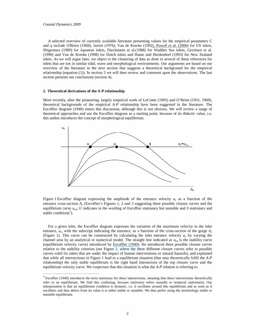
Figure 1 Escoffier diagram expressing the amplitude of the entrance velocity ue as a function of the entrance cross-section Ae (Escoffier’s Figures 1, 2 and 3 suggesting three possible closure curves and the equilibrium curve ueq; U indicates in the wording of Escoffier stationary but unstable and S stationary and stable conditions5).

For a given inlet, the Escoffier diagram expresses the variation of the maximum velocity in the inlet entrance, ue, with the subscript indicating the entrance, as a function of the cross-section of the gorge Ae (Figure 1). This curve can be constructed by calculating the inlet entrance velocity ue by varying the channel area by an analytical or numerical model. The straight line indicated as ueq is the stability curve (equilibrium velocity curve) introduced by Escoffier (1940). He introduced three possible closure curves relative to the stability criterion (see Figure 1, where the three different closure curves refer to possible curves valid for inlets that are under the impact of human interventions or natural hazards), and explained that while all intersections in Figure 1 lead to a equilibrium situation (that may theoretically fulfil the A-P relationship) the only stable equilibrium is the right hand intersection of the top closure curve and the equilibrium velocity curve. We conjecture that this situation is what the A-P relation is referring to.

5 Escoffier (1940) introduces the term stationary for these intersections, meaning that these intersections theoretically refer to an equilibrium. We find this confusing, because stationary refers ususally to temporal stationarity. Our interpretation is that an equilibrium condition is dynamic, i.e. it oscillates around this equilibrium and as soon as it oscillates and thus defers from its value it is either stable or unstable. We thus prefer using the terminology stable or unstable equilibrium.

Coastal Dynamics 2009

3

The stability curve (equilibrium velocity curve) that Escoffier introduced assumes that the equilibrium velocity, ueq, is a constant that depends only on the sediment diameter, and suggests that a good approximation of the velocity is 3 feet/second (0.9 m/s). His assumption has the following consequence. If as a first approximation we assume a sinusoidal tidal motion, we can relate the maximum entrance velocity to the tidal prism (this can be achieved by using an analytical or numerical model, the outcome of which may vary somewhat dependent on the degree of schematization adopted by such model):

e

Pu

AT

π= (2)

with T being the tidal period. For equilibrium conditions, ue = ueq = constant this implies that in equation (1) q=1. Furthermore, assuming a semi-diurnal tide with T = 44,700 s, ueq = 0.9 m/s results in C =7.8 10-5 (m-1). This is the order of magnitude value for C found empirically for the A-P relationship when q=1 (see next section).

However, we have strong evidence from literature (cf. Van de Kreeke, 1985, 1990) to claim that ue is a function of Ae, implying that q is not equal to 1 (and we will show that this has large consequences for the theoretical equilibrium cross-section). This arises when we adopt the often-posed and physically well-based concept that the equilibrium area of an inlet is determined by the balance between the transporting ebb-tidal capacity of the entrance flow and the littoral or alongshore transport. We reference here LeConte (1905), O’Brien (1931 and 1969), Riedel and Gourlay (1980), Hume and Herdendorf (1990), Van de Kreeke (1992), Kraus (1998) and Van de Kreeke (2004). The latter reference contains the essentials of most relevant earlier references and we will follow the argumentations here.

The sediment that is transported to the inlet entrance by wave-induced alongshore currents is carried to the inlet by the flood tidal currents. When the inlet is in equilibrium, this sediment is transported back in seaward direction by the ebb-tidal currents. The annual mean flux of sand entering the inlet on the flood is M (m3/s). M is assumed a constant fraction of the annual mean alongshore sediment transport and is assumed to remain constant in time. The remaining fraction is assumed to bypass the inlet via the ebb-tidal delta. When in equilibrium, the annual mean flux M equals the annual mean ebb-tidal sediment flux.

The ebb-tidal sediment transport in the entrance TR is taken proportional to the power n of the velocity amplitude and the power m of a length dimension of the cross-section l:

mne lkuTR = (3)

The subscript e refers to the entrance section. The coefficient k is a constant and its value is dependent

on the sediment characteristics. The values of n and m depend on the adopted sediment transport formulation, where n is in the range 3 to 6 and m of order 1 and the length scale l is either the annually averaged width or depth, the final choice depending on the way sediment enters and leaves the inlet entrance (Van de Kreeke, 1992; van de Kreeke, 2004). In the following we will adopt the assumption that for a given offshore tide ue is a unique function of the entrance cross-sectional area Ae.

After a change in the entrance cross-sectional area, the shape of the cross-section is assumed to remain geometrically similar. This allows expressing the length scale as a constant α times the square root of the annual mean cross-sectional area Ae:

eAl α= (4)

The value of α depends on the shape of the cross-section and the definition of l. Substituting the

expression (4) for l results in an expression for the annual mean ebb tidal sediment transport as function of the cross-sectional area:

2/me

ne

m AukTR α= (5)

In this equation ue is a function of Ae. When the cross-section is in equilibrium:

MTR = (6)

Coastal Dynamics 2009

4

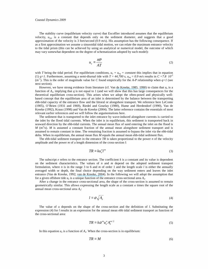
The shapes of the functions, which are independent for realistic values of the parameters k, α and m,

represented by equations (5) and (6) are plotted in Figure 2a. In general, there will be two values of the cross-sectional area for which the annual mean ebb tidal transport equals the mean annual influx of sediment M (Aeq1 and Aeq2).

A difficulty in determining the value of Aeq1 and Aeq2 from equations (5) and (6) is ascertaining the values k, n, m and α for a given inlet situation with a given mean annual influx of sediment M. Kraus (1998) undertakes such an approach and arrives at an A-P relationship with a power q of 0.9 and the coefficient a function of the mentioned parameters but also of the width and the depth of the inlet entrance. This implies that the coefficient is a function of Ae, so that the power q is not 0.9 when we remove the dependence of Ae, as is assumed commonly. We will further discuss this below.

An elegant way to circumvent ascertaining the parameters was followed by Van de Kreeke (2004) who uses the cross-sectional area versus tidal prism relationship (equation 2) for inlets at equilibrium. From equations (2), (5) and (6) it follows that for inlets at equilibrium:

eqe AA = (7)

with q

e CPA =

and

−

=

nm

nm

n

k

MTC

2

2

πα

2/mn

nq

−=

Equation (7) implies that for a set of inlets in equilibrium that have the same values of M, T, k, α, m and

n values of C and q theoretically should be the same. We will address this further in the next section.

Figure 2 Equilibrium cross-sectional areas (top: equations (5) and (6), bottom: equations: (8) and (9))

We now reintroduce Escoffier’s equilibrium velocity ueq. Eliminating P between equations (2) and (7)

Coastal Dynamics 2009

5

for inlets at equilibrium

eqe uu = (8)

with 1/11/1 −+−−= TACu q

eq

eq π

With values of q close to 1, ueq is a weak function of Ae. The relationship between velocity amplitude

and entrance cross-sectional area can be formally expressed as

),,,,,;()( TFLAAfAu oebeee ηα= (9)

with the parameters Ab = basin surface area, Le = length of entrance section, F = friction factor, η0 = ocean tide amplitude and T = tidal period.

The general shape of equations (8) and (9) is presented in Figure 2b. In plotting equation (8), it is assumed that q>1. For q>1, equation (8) implies that ueq is a decreasing function of Aeq. This is a direct consequence of equation (1) in which it is assumed that the ebb-tidal transport increases with a length dimension of the inlet, e.g. the width and thus the cross-sectional area, which we assume is physically most realistic. The larger the entrance is, the easier it is to flush out the sediment. For q=1 ueq is a straight line and for q<1 ueq increases monotonously. The roots Aeq1 and Aeq2 of equations (8) and (9) are the same as those of equations (5) and (6) and equations (7) and (9). The root Aeq2 is, following Escoffier (1940), the stable equilibrium cross-section which the A-P relationship corresponds to.

Starting from physical principles, several investigators have attempted to derive the value of the exponent q from theory. Our analysis of the literature suggests that three approaches are sound and exemplary for other attempts. Yanez (1989) as summarized by Van de Kreeke (1992) took the ebb tidal sediment transport proportional to the power n of the velocity amplitude and the width of the entrance section, w:

wkuTR ne= (10)

Comparing to equation (3), it follows l=w and m=1. Substituting m=1 in the expression for q (equation

7) and varying n between 3 and 5, the value of q varies between 1.11 and 1.20. Kraus (1998) took the ebb-tidal transport proportional to the amplitude of the bottom shear stress to the

power n/2 and the width of the entrance section, w. Based on Manning’s equation, the bottom shear stress was taken proportional to the velocity squared divided by the one third power of the hydraulic radius R (which is close to the water depth). The resulting expression for the transport is:

wRkuTR nne

6/−= (11)

Making use of equation (4) it follows:

2

6/1 n

ene AkuTR

−

= (12)

where the shape factor α is incorporated in k.

Comparing to equation (5), it follows m=1-n/6. Substituting in the expression for q, it follows that for n between 3 and 5, q varies between 1.03 and 1.20.

Suprijo and Mano (2004) assuming a rectangular cross-section with width w and depth h took

6/55 / hwkuTR e= (13)

Making use of equation (4) we derive:

Coastal Dynamics 2009

6

12/15 −= ee AkuTR (14)

Comparing to equation (5), it follows n = 5, while m = 1/6. Substituting in the expression for q, q = 1.02.

In conclusion, we state that the A-P relationship should only refer to inlets that are in a stable equilibrium. For a given inlet, this corresponds to the stable equilibrium point in the Escoffier diagram. The equilibrium velocity curve is a monotonously decreasing function of Ae, such that the coefficient q in the A-P relationship is larger than 1. We stress that it is important to assess the value of q, because, as we will show in the next section, the stable equilibrium cross-sectional area shows appreciable variation for different values of q and accordingly of C. 3. Observations of the A-P relationship Upfront we state that we object to the clustering of data as done in several of the following references for inlets that are not in similar tidal and morphological environments. Data sets used to determine the constants C and q in equation (1) should ideally consist of inlets that show phenomenological similarity (i.e., have similar values for k, n, m and α for a given inlet situation with mean annual influx of sediment M), implying that the datasets should be clustered while ensuring:

• similar wave driven littoral drift; • similar tide characteristics (form number, amplitude); • similar grain size and grain density; • similar shape of the cross-section.

However, since we are making a review of the A-P relationship we cannot ignore the widely referenced observations, and will provide these with our comments.

Early basic, well-referenced observations presented in literature are those of O’Brien (1969) and Jarrett (1976). These observations are amply used but do not or not completely fulfil the conditions that we conclude as essential for a reliable conclusion. After reviewing these references we will highlight and comment on observations made since then.

O'Brien (1931) originally determined a relationship between minimum gorge cross-sectional area of an inlet below mean tide level and the tidal prism at spring tide. This relationship was derived from observation of 9 inlets on the Atlantic coast, 18 others on the Pacific coast and one inlet on the Gulf coast in the US. According to O'Brien (1969) the relationship is predominantly valid for Pacific coastal inlets, where a mixed tidal pattern is observed and where typically a strong ebb flow exists between higher-high water and lower-low water. O’Brien (1969) showed that for these 28 US entrances, C=4.69 10-4 and q=0.85 are best-fit values applicable to all entrances when P is measured in cubic meters (m3) and A in square meters (m2), but when limited to 8 non-jettied entrances he derived C=1.08 10-4 and q=1 as best-fit values. Obviously, O’Brien’s data set of 28 inlets does not satisfy the requirement of same littoral drift and tide conditions, and we doubt whether this is the case for the 8 non-jettied entrances.

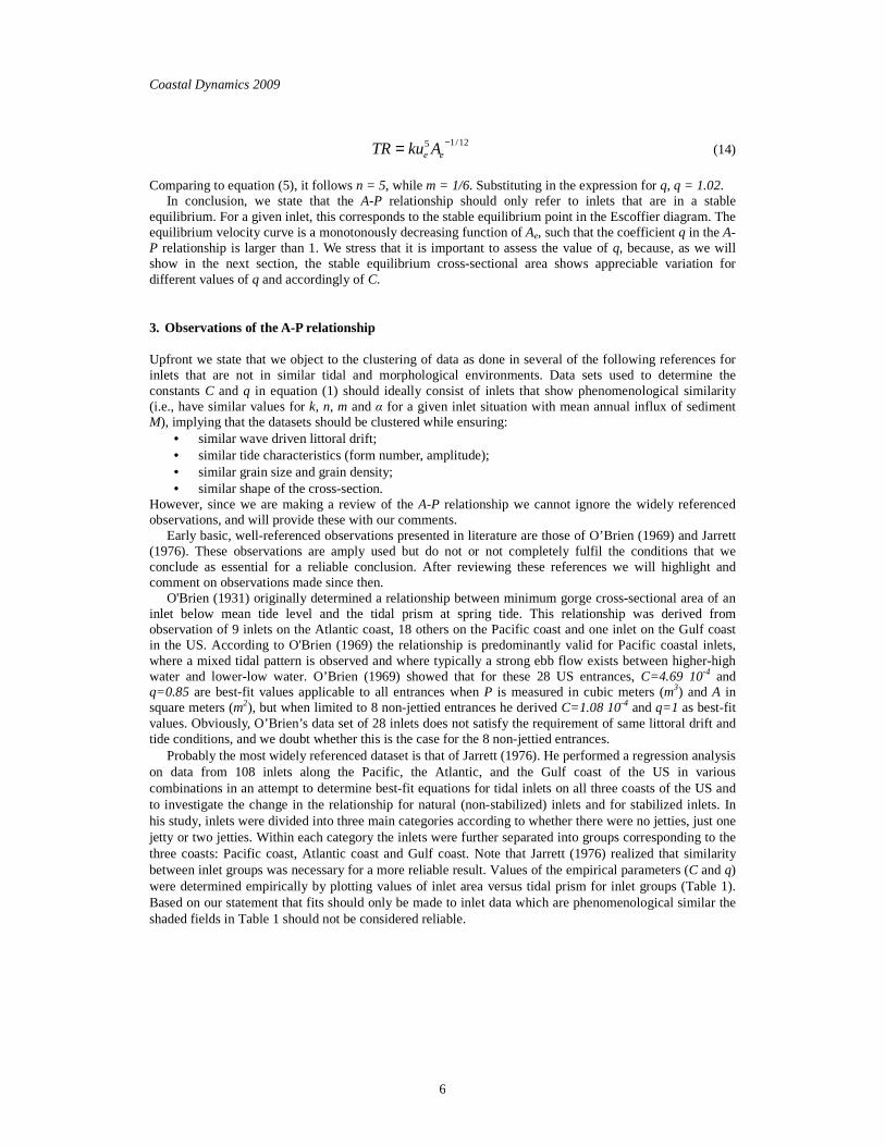
Probably the most widely referenced dataset is that of Jarrett (1976). He performed a regression analysis on data from 108 inlets along the Pacific, the Atlantic, and the Gulf coast of the US in various combinations in an attempt to determine best-fit equations for tidal inlets on all three coasts of the US and to investigate the change in the relationship for natural (non-stabilized) inlets and for stabilized inlets. In his study, inlets were divided into three main categories according to whether there were no jetties, just one jetty or two jetties. Within each category the inlets were further separated into groups corresponding to the three coasts: Pacific coast, Atlantic coast and Gulf coast. Note that Jarrett (1976) realized that similarity between inlet groups was necessary for a more reliable result. Values of the empirical parameters (C and q) were determined empirically by plotting values of inlet area versus tidal prism for inlet groups (Table 1). Based on our statement that fits should only be made to inlet data which are phenomenological similar the shaded fields in Table 1 should not be considered reliable.

Coastal Dynamics 2009

7

Location All inlets No jetty or one jetty Two jetties C q C Q C q All inlets 2.41 10-4 0.93 3.65 10-5 1.04 1.48 10-3 0.83 Atlantic coast

6.04 10-5 1.02 1.98 10-5 1.08 6.70 10-4 0.87

Gulf coast 9.30 10-4 0.84 6.94 10-4 0.86 1.43 10-3 0.81 Pacific coast 4.75 10-4 0.88 8.83 10-6 1.10 1.88 10-3 0.82 Table 1a. Empirical parameters of the A-P relationship for tidal inlets on US coasts in metric units, where the results in the shaded boxes are not fulfilling our recommendations (data derived and reprocessed from Jarrett, 1976) Location All inlets No jetty or one jetty Two jetties # of inlets r2 # of inlets r2 # of inlets r2 All inlets 108 0.90 71 0.92 37 0.88 Atlantic coast

59 0.92 40 0.94 19 0.81

Gulf coast 24 0.87 21 0.87 3 0.88 Pacific coast 25 0.92 10 0.97 15 0.93 Table 1b. Number of inlets and correlations for the datasets for tidal inlets on US coasts related to Table 1a, where the results in the shaded boxes are not fulfilling our recommendations (data derived and reprocessed from Jarrett, 1976)

Since the publication of the O’Brien (1969) and Jarrett (1976) datasets many studies published findings for the coefficients C and q for groups of other inlet entrances. We have made an initial scrutiny of these datasets and come to the disappointing conclusion that there exist only two studies that are close to fulfilling our phenomenological similarity condition, viz. Dieckmann et al. (1988), who studied the entrances of the Dutch and German Wadden Sea and Van de Kreeke (1998) who studied the entrances of the Dutch Wadden Sea, It should be stressed here that both these evaluations of the A-P relationship departed somewhat from the original O’Brien definition in that their estimates were based on the mean tidal prism instead of the spring tidal prism. An overview of the fits to these datasets is summarized in Table 2.

Source Location (# of inlets) C q r2 Dieckmann et al. (1988) Dutch and German Wadden Sea

(37) 3.72 105 0.92 ?

Van de Kreeke (1998) Dutch Wadden Sea (5) 3.45 10-4 0.81 0.96 Van de Kreeke (1998) Dutch Wadden Sea (5) 6.80 10-5 1 0.99 Table 2 Comparison of further findings for comparable inlet situations

From these results we conclude that optimal fits lead to q values that are in a range between 0.81 and 1, which is in clear contrast with our theoretical finding that q should be larger than 1. If we include the Jarrett (unshaded) dataset this range is between 0.81 and 1.10, which is more promising but still does not conform to our theoretical findings. We conclude that this is an issue that needs to be resolved and suggest that careful scrutiny of the data sets to check whether they fulfill the phenomenological similarity condition is a first and necessary step towards achieving this.

To illustrate what these results mean for a stability analysis, an example is presented for Midnight Pass on the south-west coast of Florida. The analysis was carried out as part of a study by Erickson consulting engineers on the reopening of the pass. To arrive at an A-P relationship for this location, Powell’s data were

Coastal Dynamics 2009

8

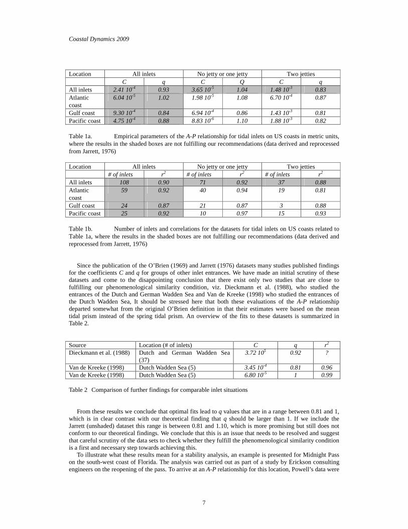
reanalyzed by selecting only the south-west (Gulf) inlets (data source: Powell, (2003), Tables A5 and A6). Inlets 29 -50 excluding inlets 40 and 44, since A and P values of inlets 40 and 44 are an order of magnitude larger than for the other inlets, were selected. This resulted in a total of 20 inlets, with mixed tides where the tidal prism pertains to the diurnal tide. In the subject area, this tide has a range of 0.7 m and a period T=89,640 sec. The gross littoral drift is in the range of 50,000-100,000 m3/yr. Hence, these data should be close or at least closer to fulfilling our conditions. Two correlation functions are used to derive an optimal fit, equation (1) with C and q as variables and equation (1) with q=1 and C as the only variable. The first gives C= 5.27 10-4 and q = 0.86 with r2 = 0.92 (which corresponds well with Jarrett’s subset for the Gulf Coast), the second results in C = 4.74 10-5 (q=1) with r2 = 0.90. We conclude that the practical result is that for nearly similar correlations for the Florida dataset either q can be 0.86 or 1 so that making use of equation (2) ue = 0.214 A0.16 (increasing line in figure 3) or ue = 0.74 m/s (straight line in figure 3). The closure curve was calculated using a 2-D model forced by a diurnal ocean tide. A trapezoidal shape for the cross-section was assumed. Note that the result is that there is a considerable difference in the values of the stable cross-sectional areas for the two correlation functions.

Figure 3. Escoffier closure curve and equilibrium velocity curves for different values of q (Midnight Pass on the south-west coast of Florida)

In summary, we have to conclude that on average all findings point at a value for the exponent q both smaller and larger than one, but the average for findings for inlets in similar hydrodynamic and morphological conditions seems to be around q= 1. We doubt that the data sets available are sufficiently reliable to support this conclusion. As argued in the theoretical section, a value larger than one is what we expect and we consider this an unresolved issue at this stage.

Why do we think this is a crucial issue to be resolved? When one fits the empirical relationship equation (1) to data with a different exponent q, significantly different values for the equilibrium cross-section are found, while the correlation coefficient is very similar. Obviously, this is of large consequence for establishment of the true equilibrium entrance cross-sectional area. 4. Conclusions We have reviewed the well-known empirical relationship (equation 1) expressing the equilibrium cross-sectional area of tidal inlet entrances as a function of the tidal prism P under forcing of the littoral drift. Reviewing the most promising theoretical approaches we find that theoretically the exponent q of equation

Coastal Dynamics 2009

9

(1) should be larger than 1. However, if we consider the literature presenting data we must conclude that the empirical findings do not clearly support the theoretical finding. We doubt that the data sets available are sufficiently reliable to support this conclusion, since we infer, based on our theoretical evaluations, that these datasets should fulfil the condition of phenomenological similarity, viz. they should pertain to fairly similar hydrodynamic and morphological conditions. The resolution of this issue is important because slightly different values of q in equation (1) result in significantly variable values for the equilibrium cross-sectional value of the tidal entrance. This may have significant implications in determining the true stable equilibrium entrance cross-sectional area. We advocate a careful re-scrutiny of the datasets available as a necessary first step in evaluating the robustness of the theoretical considerations presented herein. Acknowledgements The second author acknowledges the collaboration with Erickson Consulting Engineers on the data and modeling acquired for Midnight Pass. The third and fourth authors acknowledge the support from the cooperation project on coastal engineering between Delft University of Technology and Hanoi Water Resources University sponsored by the Netherlands Embassy in Hanoi. References Dieckmann, R., Osterhun, M., Partenscky, H.W., 1988. A comparison between German and North American tidal inlets.

Proceedings of the 21st International Conference on Coastal Engineering, ASCE, 2681-2691 Escoffier, F.F., 1940. The stability of tidal inlets. Shore and Beach 8 (4), 111 – 114 Gerritsen, F., and Louters, T, 1990. Morphological stability of inlets and channels in the Western Wadden sea.

Rijkswaterstaat, Report GWAO-90.019. Hume, T.M. and Herdendorf, C. E., 1990. Morphologic and Hydrologic Characteristics of Tidal Inlets on a Headland

Dominated, Low Littoral Drift Coast, Northeastern New Zea1and, Proceedings Skagen Symposium (2-5 Sep. 1990), Journal of Coastal Research Special Issue 9: 527-563.

Hume, T.M., Herdendorf, C., 1993. On the use of empirical stability relationships for characterising estuaries. Journal of Coastal Research 9 (2), 413– 422.

Jarrett, J.T., 1976. Tidal prism - inlet area relationships. GITI report no. 3. Coastal Engineering Research Center, US Army Corps of Engineers, Fort Belvoir, VA, USA

Kraus, N.C., 1998. Inlet cross-section area calculated by process-based model. Proceedings International Conference on Coastal Engineering. ASCE, Reston, VA, pp 3265—3278

LeConte, L.J., 1905. Discussion on the paper, “Notes on the improvement of river and harbor outlets in the United States” by D. A. Watt, paper no. 1009. Trans. ASCE 55 (December): 306—308

O’Brien, M.P., 1931. Estuary and Tidal Prisms Related to Entrance Areas. Civil Eng. 1 (8): 738-739. O’Brien, M.P., 1969. Equilibrium flow areas of inlets on sandy coasts. J Waterway Port Coast Ocean Eng 95 (l): 43—

52 Powell, M.A., R.J. Thieke and A.J. Mehta, 2006. Morphodynamic relataionships for ebb and flood delta volumes at

Florida’s entrances. Ocean Dynamics 56: 295-307. Powell M.A., 2003. Ebb shoal and flood shoal volumes on the coasts of Florida: St Marys entrance to Pensacola Pass.

Masters theses University of Florida. Riedel, H.P., and Gourlay, M.R., 1980. Inlets/Estuaries Discharging into Sheltered Waters. Proceedings International

Conference on Coastal Engineering, ASCE Press, NY, 2550-2562. Shigemura, T., 1980. Tidal prism – throat area relationships of the bays of Japan. Shore and Beach, 48 (3): 30-35 Suprijo, T. and Mano A., 2004. Dimenisonless parameters to describe topographical equilibrium of coastal inlets.

Proc .29th ICCE, ASCE: 2531-2543 Van de Kreeke, J., 1985. Stability of tidal inlets; Pass Cavallo, Texas. Estuarine Coastal Shelf Science, 21:33-43 Van de Kreeke, J., 1990. Stability of a two-inlet bay system. Coastal Engineering, 14: 481-497 Van de Kreeke, J., 1992. Stability of tidal inlets; Escoffier’s analysis. Shore and Beach , 60 (1): 9-12 Van de Kreeke, J., 1998. Adaptation of the Frisian inlet to a reduction in basin area with special reference to the cross-

sectional area of the inlet channel. In Dronkers, J. and Scheffers , M.B.A.M. (Eds). Proc. PECS conference: 355-362

Van de Kreeke, J., 2004. Equilibrium and cross-sectional stability of tidal inlets: application to the Frisian Inlet before and after basin reduction. Coastal Engineering, 51: 337-350

Coastal Dynamics 2009

10

Yanez, M. A., 1989. Stability of a double –inlet bay system; Marco Island, Fla. Masters thesis, RSMAS, University of Miami,. pp 67