Kink instability of flux ropes anchored at one

end and free at the other

Giovanni Lapenta,1,2 Ivo Furno,3 Thomas Intrator,2 and Gian Luca Delzanno2

Received 20 June 2006; revised 22 September 2006; accepted 3 October 2006; published 16 December 2006.

[1] The kink instability of a magnetized plasma column (flux rope) is a fundamentalprocess observed in laboratory and in natural plasmas. Previous theoretical, experimental,and observational work has focused either on the case of periodic (infinite) ropes (relevantto toroidal systems) or on finite ropes with both ends tied to a specified boundary(relevant to coronal ropes tied at the photosphere). However, in the Sun’s corona and inastrophysical systems there is an abundant presence of finite flux ropes tied at one endbut free at the other. Motivated by recent experiments conducted on the RSX device(Furno et al., 2006) and by recent theoretical work (Ryutov et al., 2006), the present paperinvestigates by simulation the linear and nonlinear evolution of free-ended flux ropes.The approach is based on comparing the classic case of a periodic flux rope with thecase of a rope tied at one end and free at the other. In the linear phase, periodic and freeropes behave radically differently. A simulation analysis of the linear phase confirms theexperimental and phenomenological findings relative to an increased instability of a freerope: the new stability limit is shown to be just half of the classic limit for periodic ropes. Inthe nonlinear phase, reconnection is observed to be a fundamental enabler to reach theeventual steady state. The mechanism for saturation of a flux rope is investigated andcompared with the classic theory (the so-called bubble state model) by Rosenbluth et al.(1976). A remarkable agreement is found for the classic periodic case. The case of a free ropeis again very different. The saturated state is observed to present a outwardly spiralingconfiguration with the displacement of the plasma column increasing progressively andmonotonically from the tied end to the free end. The maximum displacement is observed atthe free end where it is consistent with the displacement observed in a periodic rope.The key distinction is that in a periodic rope the same displacement is observed throughoutthe whole rope to form a helix with constant radius.

Citation: Lapenta, G., I. Furno, T. Intrator, and G. L. Delzanno (2006), Kink instability of flux ropes anchored at one end and free at

the other, J. Geophys. Res., 111, A12S06, doi:10.1029/2006JA011932.

1. Introduction

[2] The kink instability is a classic problem in plasmaphysics. It is a crucial consideration in the stability of fusiondevices [Wesson, 2004] and it is a common occurrence inspace and solar physics. For example, flux ropes observedin the solar corona and in the magnetosphere can beunstable to the kink mode and such instability has beenobserved and studied widely in the literature [Priest andForbes, 2000]. Figure 1 shows an examples of a solarcorona image where multiple flux tubes are observed.Movies are available of satellite observations showing thedynamic behavior of such coronal loops.

[3] Similarly, astrophysical observations show the pres-ence of magnetized jets emitted from accreting objects. Forexample, Figure 2 shows one of such jets emitted from thegalaxy M87, observed here in the radio frequency range atVLA.[4] The kink instability has been studied extensively in

previous literature. Section 4 reviews the previous work ofinterest to the present study, but the kink mode is a classictextbook plasma physics instability [see, e.g., Goedbloedand Poedts, 2004]. The vast majority of the previous workreferred to the case of a periodic rope as appropriate for atoroidal plasma where a plasma column closes on itself.[5] In the solar physics community, flux ropes tied to the

solar corona have been also considered [see, e.g., Hood andPriest, 1979]. In that case the photosphere is assumed to beso much heavier to hold fixed the ends of flux ropes linkedto it. However, as can be observed in Figure 1, some fluxropes become detached from the photosphere at one end(see upper left corner of Figure 1). This situation iscommon in coronal holes where the field lines are openand one end extends into the solar system. However, free-

JOURNAL OF GEOPHYSICAL RESEARCH, VOL. 111, A12S06, doi:10.1029/2006JA011932, 2006ClickHere

for

FullArticle

1Centre for Plasma Astrophysics, Departement Wiskunde, KatholiekeUniversiteit Leuven, Heverlee, Belgium.

2Los Alamos National Laboratory, Los Alamos, New Mexico, USA.3Ecole Polytechnique Federale de Lausanne (EPFL), Centre de

Recherches en Physique des Plasmas, Association EURATOM-Confedera-tion Suisse, Lausanne, Switzerland.

Copyright 2006 by the American Geophysical Union.0148-0227/06/2006JA011932$09.00

A12S06 1 of 19

ended ropes may become in existence even in regions ofnormally closed field lines, during the dynamical evolutionof the corona where reconnection can lead to the breakup offield lines that get detached from the corona at one end,thereby releasing energy from the corona outward into thesolar system. Such processes are for example part of themechanisms believed to be behind the so-called coronalmass ejections [Priest and Forbes, 2000].[6] Similarly, in the case of astrophysical jets, the tying

of the rope is working at one end only, at the end attachedto the object creating the jet [Blandford, 2002], but theother end of the jet is clearly free. In the example in Figure 2the jet is believed to be created in an accretion disk arounda black hole present in the center of galaxy M87 (anelliptical galaxy also known as NGC 4486 and Virgo A).[7] The primary novelty of the present paper is in

investigating with nonlinear numerical simulations the kinkinstability for free ended systems. Our analysis reaches twomain conclusions.

[8] First, we confirm the predictions of a previousphenomenological linear theory [Ryutov et al., 2006] vianumerical simulations. Our numerical simulations showthat indeed a system where the field lines are tied at oneend but free at the other is more unstable than thecorresponding periodic (or toroidal) system. This latterconfiguration is in itself more unstable than a systemline-tied at both ends, making the free-ended system moreunstable than all systems previously considered. Periodicsystems are unstable when the current exceeds the Kruskal-Shafranov (KS) limit [Goedbloed and Poedts, 2004],corresponding to the situation when a surface exists insidethe plasma where the safety factor q = 1. In the system line-tied at one end and free at the other, the kink instabilityappears as soon as q < 2 within the plasma. Note that a ropeline-tied at both ends is more stable than a periodic ropeonly when a conducting wall is close enough to the rope. Inthe case of a far conducting wall, the instability threshold isthe same for both cases [Ryutov et al., 2004].[9] Second, we investigate the saturation mechanism for

the instability. We observe that the instability grows on aAlfvenic timescale until the plasma region reaches themode resonant surface. The evolution afterwards requirethe process of reconnection. Eventually, the flux ropereaches saturation at a surface that can be well predictedusing the so-called bubble-state model introduced byRosenbluth et al. [1976] for periodic systems. A free-endedrope evolves through the same stages as a periodic rope, butits saturation state shows an outward spiraling where theouter radius of the rope is progressively displaced, fromzero displacement at the tied end to a maximum displace-ment at the free end. The maximum displacement of thefree end is still consistent with the model by Rosenbluth etal. [1976].[10] The paper is organized as follows. Section 2

describes the specific setting used in the present paper todescribe the evolution of flux ropes. The configurationconsidered is specific to the RSX device [Furno et al.,2003] where flux ropes can be studied directly experimen-tally. Section 3 describes the simulation method used tostudy the evolution.

Figure 1. Image of Active Region 9373 (rotated counter-clockwise over 90 degrees), taken by TRACE [Schrijver et

al., 1999] in its 171 A pass band on 2001-3-21.

Figure 2. Jet ejected from galaxy M87. Radio intensity at 14.435 GHz observed at VLA on 1994-5-2[Owen et al., 1989]. On the left side, a flux rope tied at one end and free at the other is shown to formduring the course of an eruption.

A12S06 LAPENTA ET AL.: KINK INSTABILITY OF FLUX TIED/FREE ROPES

2 of 19

A12S06

[11] Section 4 focuses on the linear stability comparingprevious predictions and experimental observations at RSXwith numerical simulations. The conclusion, as notedabove, is that the most unstable case is that of flux ropeswith one free end, followed by periodic ropes. Line-tied fluxropes, instead, are shown to be more stable than both.[12] Nonlinear evolution and saturation are described in

sections 5 and 6. Section 5 focuses on the reference case ofa periodic rope where previous theories can be validated.Section 6 deals with the case of a rope free at one end andtied at the other. Comparison between the two cases ismade. A qualitative agreement with experimental observation isalso provided. Conclusions are drawn in section 7.

2. Description of the System Under Consideration

[13] The Reconnection Scaling Experiment (RSX) atLos Alamos National Laboratory is described by Furnoet al. [2003, 2005] and takes advantage of recentlydeveloped plasma gun technology [Fiksel et al., 1996] tocreate a flux rope that is initially linear but supports fullythree-dimensional (3-D) evolution. One key attribute ofRSX is the ability to continuously adjust the axial guidefield (B0z = 0–2 kGauss) and ion gyro radius independentlyof the plasma and current density, providing scans ofplasma b. RSX is one of a few devices [Hansen et al.,2004; Gekelman et al., 1992] that have ever been used tostudy flux 3-D rope dynamics.[14] Typical plasma parameters are density ne � 3 �

1013 cm�3, electron temperature Te � 3–12eV, B0z = 100 G,Bq � 10 G, b � 0.5. Typical current rope radius is 2.5 cm.The Alfven time is of few ms, while the resistive diffusiontime is of the order of 100 ms. For the experimental data

shown here, the flux rope current Irope ramps up with aselected e-folding time, and instability grows and saturatesfor 100 A < Irope < 400 A. Figure 3 shows the typicalprofiles observed in RSX.[15] The RSX has a cylindrical vacuum chamber (4 m

length � 0.2 m radius) much larger than the flux ropedimension (0.5–1.5 m length � 0.03 m radius). For theexperiments relevant to the present work, one plasma gun[Fiksel et al., 1996] was radially inserted from the top asshown in Figure 4. The plasma gun contains a miniaturizedplasma source with a circular 0.4 cm radius nozzle aperturein which a hydrogen plasma is produced by an arcdischarge. The arc plasma is maintained for �10 ms by apulse forming network from which a current is drawnduring a �1.5 ms pulse that biases the external anodepositive relative the floating gun arc. The external anodelocation along the z axis determines the flux rope length.The constant, uniform, axial (in the z direction) back-ground magnetic field B0z, can be varied within the range0–2 kGauss.[16] To describe the plasma in RSX, we rely on a simple

model that captures qualitatively the main features of theplasma generated in RSX but thanks to its simplicity andgenerality can be easily related to configurations relevant tospace and astrophysical systems. We consider a simplemathematical model of a flux rope based on the textbookscrew pinch [Freidberg, 1987]. The magnetic field expres-sion in cylindrical (r, q, z) coordinates is

Bq ¼B0r

r2 þ w2

Bz ¼ 1

Br ¼ 0

ð1Þ

Figure 3. Experimental data from a typical plasma shot.From to bottom profiles of the plasma properties are shown:(a) electron temperature, (b) parallel resistivity, (c) densityand pressure, and (d) tangential magnetic field and current.SI units are used.

Figure 4. Artist’s rendition of the experimental config-uration simulated in the present paper. One plasma gunproduces a flux rope in a cylindrical vessel with a axialmagnetic field generated by outside coils. The ropegenerates its own tangential field and can be unstable tothe kink instability, as shown. The position and view angleof the camera are shown.

A12S06 LAPENTA ET AL.: KINK INSTABILITY OF FLUX TIED/FREE ROPES

3 of 19

A12S06

representing an helical magnetic field with helical pitchdetermined by the amplitude of the q component (i.e., byB0).[17] The magnetic field is not force free and is in balance

with a plasma pressure:

p ¼ B20w

2

2m0 r2 þ w2ð Þ2ð2Þ

Since the pressure is equal to p = rkT, the freedom in therelative choice of the density and temperature is used to bestrepresent the plasma in RSX, where the temperature anddensity have a similar profile: r = kT =

ffiffiffip

p. In some

reference runs below a uniform density r0 is alsoconsidered.[18] Figure 5 shows the initial pressure and poloidal

magnetic field profile for the case B0 = 1. The surfaceq = 1 is completely external to the bulk of the plasmaresulting in a configuration suitable to study external kinkmodes. The configuration described above represents areasonable qualitative model of a flux rope in RSX. Theapproximate scale is determined by comparing the wallradius and the temperature profile (directly linked to theSpitzer resistivity): one unit of the simulations correspondsto 4 cm in the real device. Below, we study the stabilityproperties of such a flux rope in conditions valid andapplicable to all the cases just listed.

3. Simulation Approach

[19] All simulations are carried out using the FLIP3D-MHD code [Brackbill, 1991] based on the standard

viscoresistive MHD model. The viscoresistive MHDmodel, written in the Lagrangian frame, is summarizedby mass continuity,

drdt

¼ �rr � v; ð3Þ

Faraday’s law,

d

dt

B

r

� �¼ B

r� rv� 1

rr� hJ½ ; ð4Þ

where a resistive Ohm’s law is assumed,

E ¼ hJ� V� B; ð5Þ

momentum conservation,

rdv

dt¼ �r pþ r þ B2

2

� �þr � BB; ð6Þ

internal energy equation

rdI

dt¼ �pr � vþ h J � Jð Þ: ð7Þ

and by Ampere’s law,

r� B ¼ m0J ð8Þ

[20] The flow variables are the mass density, r, themagnetic field, B, the current density, J, the fluid velocity, v,

Figure 5. Initial magnetic field Bq (solid), pressure (dashed) and safety factor q (dash-dotted) profile fora case with B0 = 1.

A12S06 LAPENTA ET AL.: KINK INSTABILITY OF FLUX TIED/FREE ROPES

4 of 19

A12S06

the specific internal energy, I, and the plasma pressure p.Here m0 is the magnetic permeability, h is the resistivity.The pressure is given by an ideal gas equation of state, p =(g � 1)rI. The viscous term, r, is given by the Navier-Stokes formula [Brackbill, 1991], where n is the scalarviscosity.[21] The resistivity is chosen either uniform (h = h0) or

according to Spitzer’s resistivity law [Spitzer, 1956]:

h ¼ h0T�3=2 ð9Þ

where the temperature is defined as usual: T = p/kn. Notethat the Spitzer resistivity model typically provides aninsufficient description of the actual resistivity in space andastrophysical plasmas, and even in fusion experimentaldevices, where anomalous effects dominate. However, inmany lower temperature experimental devices (includingRSX), the Spitzer resistivity model provides a reasonablefirst-order model of the relatively collisional plasma present[Trintchouk et al., 2003; Furno et al., 2005]. To express thereference resistivity, we use the Lundquist number definedas S = vAw/h0, and to express the uniform viscosity, we usethe Reynolds number defined as Re = vsw/n, where vs is thesound speed.[22] FLIP3D-MHD is based on the fluid particle in cell

(PIC) method [Brackbill, 1991] that uses particles to modelthe fluid advection but uses a computational grid to solvethe evolution equations for the fluid quantities written inLagrangian form. The time discretization is implicit toallow larger time steps [Brackbill, 1991]. The approachin FLIP3D-MHD is distinct from the SPH method[Monaghan, 1992] that uses particles and interactionkernels also to solve for the fluid quantities. Also, it isdistinct also from grid-based methods that discretize theadvection term on the grid as well. The condition r � B = 0is imposed at each time step. Space is scaled to thecharacteristic length of the initial equilibrium w, density isnormalized to the uniform reference value r0 and time isscaled by the Alfven time, t = L/vA, where vA is the Alfvenspeed. The magnetic permeability m0 is unitary.[23] FLIP3D-MHD has been previously used and applied

in a number of studies [Brackbill and Knoll, 2001; Lapentaand Knoll, 2004, 2005; Lapenta and Kronberg, 2005]. Thecoordinate system chosen in the code is cartesian. Thisdiffers significantly from the typical plasma physics codethat uses cylindrical coordinates. Here the system is repre-sented by a parallelepipedal domain of size Lx = Ly = 10wand Lz = 20w. The actual circular wall of the device isdescribed with the immersed boundary method.[24] The immersed boundary method [Peskin, 2002]

allows the description of arbitrarily (and even changing)boundaries or interfaces between materials. The method isextremely powerful, especially when combined with non-uniform or adaptive grids and has been applied successfullyto numerous applications [Peskin, 2002]. However, the caseat hand is very simple and the immersed boundary methodbecomes straightforward. The interface is a circle embeddedin a uniform cartesian grid. The metal vessel of RSX isrepresented by assigning material particles everywhereoutside a circle corresponding to radius R = 5w. The plasmainside the vessel is then represented by regular computa-tional particles that represent Lagrangian markers evolving

according to the MHD equations. The computationalparticles outside the circle are stationary and represent amaterial with zero resistivity (for an ideal wall, easilygeneralizable to resistive walls).[25] The immersed boundary method correctly represents

the response of a metal wall: it imposes no radial plasmavelocity at the wall and it imposes the correct boundaryconditions on the magnetic field. The use of the immersedboundary method in a PIC description of fluid equations ofany type results in an effective replacement of a sharpboundary with a diffuse transition with a thicknessequivalent to the size of the computational particle [Lapentaand Brackbill, 1996; Lapenta et al., 1995]. In FLIP3D-MHD the particle size is chosen to be in each directionequal to the corresponding grid spacing. The interfacesbecome transition regions of thickness equal to the cell size.The effect of the finite transition introduces a discretizationerror of the same order as the error already introduced bydiscretizing the operators. Except for special circumstances,there is no reason for imposing exact boundary conditionsto operators discretized with a certain truncation error.However, it is crucial that the discretization error be keptof the same order as the truncation error on the interiordomain to prevent the solution from being dominated byboundary errors. We have used the approach in previouspublications [Lapenta and Brackbill, 1996; Lapenta et al.,1995; Lapenta, 1999, 2002] and we have further tested theapproach here recovering the vacuum field solution withinthe expected truncation error and we have verified aposteriori that the boundary conditions are indeed correctlyimposed on the boundary.[26] The boundary conditions at the end walls (z = 0 and

z = Lz) are chosen in three different ways to representdifferent experimental or natural situations. First, periodicboundary conditions are applied to represent conditionstypical of toroidal devices or closed ropes. In this casethe actual toroidal rope is represented as a straight periodiccylinder.[27] Second, to represent conditions believed to be

typical of solar coronal plasmas line tying is applied atboth ends of the flux rope. For such a case the velocity fieldis chosen to be zero at both ends by applying Diricheletboundary conditions.[28] Finally, in some parts of the solar corona, e.g., in the

coronal holes and in some active regions (see Figure 1) ofthe corona, flux ropes are present anchored at one end onthe solar surface but free at the other. The same configu-ration is prevalent in astrophysical jets (see Figure 2). Asnoted above, the flux ropes produced in RSX are anchoredat the plasma gun but different conditions can be chosen atthe other end, ranging from nearly free motion to line tying,depending on the choice of the end electrode.[29] For the free boundary condition, we follow the

prevalent choice in the literature, i.e., the application ofNeumann boundary conditions [Zwingmann, 1987]:

@v

@z

����z¼Lz

¼ 0 ð10Þ

often used in solar and astrophysical simulation to representan open boundary. Similar expressions hold for all otherfields.

A12S06 LAPENTA ET AL.: KINK INSTABILITY OF FLUX TIED/FREE ROPES

5 of 19

A12S06

[30] For RSX this is a reasonable approximation of theplasma behavior at the end cathode where a sheath forms.Previous studies of such sheath [Ryutov et al., 2006] showsthat the correct condition to apply is

@v

@z

����z¼Lz

¼ kv ð11Þ

The two conditions above are extreme cases of thiscondition, Dirichelet conditions corresponding to k ! 1and Neumann conditions corresponding to k = 0.Intermediate values of k would result in intermediate resultsbetween the two cases considered here.[31] In the results below the simulation box has dimen-

sions [�Lx, Lx], [�Ly, Ly] and [0, Lz] with Lx = Ly = 5 andLz = 20. The system is discretized using a regular grid of75 � 75 � 150 Lagrangian markers (particles), with27 particles per cell in a 25 � 25 � 50 grid with a timestep Dt/tA = 0.1.

4. Stability of the Kink Mode

[32] The initial configuration described in section 2 isliable to become unstable to the kink instability [Kadomtsev,1992; Wesson, 2004; White, 2001]. The stability of aplasma with arbitrary shape needs to be computed numer-ically [Wesson, 2004], but for simple configurations withflat current profiles surrounded by vacuum and by idealwalls can be computed analytically [Goedbloed and Poedts,2004; Kadomtsev, 1992; White, 2001]. Previous resultshave indicated that the stability of kink modes dependsstrongly on the applied boundary conditions.[33] The system under investigation is surrounded in the

radial direction by a circular metal wall that could providestabilization. This configuration is clearly suitable to theexperiment RSX but it introduces a significant deviationfrom the reality of space and astrophysical systems. Theeffect of the surrounding walls, including their finiteresistivity, is one of the most active areas of research infusion plasmas [Wesson, 2004] and will not be addressedhere.[34] In the present work the attention is focused on the

effects of the boundary conditions imposed in the axialdirection. The axial conditions are directly linked with themechanisms creating and sustaining a flux rope. As notedabove, we consider periodic, open, and line tying condi-tions suitable for different natural and manmade plasmas.Below, the previously published conclusions are summa-rized limiting the scope to the previous results of interest tothe present discussion.[35] Most of the analysis of kink modes has been focused

on the application to toroidal plasmas where periodicboundary conditions are appropriate in the straight-cylinderapproximation. In this case a flux rope becomes unstable tothe kink mode when the current exceed the so-calledKruskal-Shafranov (KS) limit [Goedbloed and Poedts,2004]:

IKS ¼ 2pað Þ2Bz

m0Lð12Þ

where L is the length of the rope, a is its radius, and Bz is theaxial magnetic field, assumed uniform. Although, the KS

limit is most easily derived for uniform current profiles, itsvalidity is more general [Goedbloed and Poedts, 2004].[36] An alternative formulation of the KS limit, very

popular in the fusion literature, is based on introducingthe so-called safety factor:

q rð Þ ¼ 2prBz

Bq rð ÞL ð13Þ

that has the geometrical meaning of inverse of the pitchangle of the magnetic field lines, with q = 1 meaning thatthe field lines close upon themselves after one turn (in aperiodic rope) [Goedbloed and Poedts, 2004]. The stabilitylimit of the kink mode can be easily formulated in terms ofthe safety factor by the statement that q > 1 everywhere inthe domain for the plasma to be stable.[37] Previous work has shown that when the axial

boundary conditions are changed the stability of a fluxrope to the kink mode is modified. As can be imagined,flux ropes free at one end are more unstable, while fluxropes tied at both ends are more stable.[38] Line tying at both ends of a flux rope has been

addressed primarily in the solar physics community. Themain conclusion of relevance here is twofold. First, linetying increases the stability of a flux rope by increasing thelimit current beyond the KS limit [Hood and Priest, 1981;Einaudi and Van Hoven, 1983; Ryutov et al., 2004;Evstatiev et al., 2006]. The eigenfunctions are no longerharmonic functions (with displacement forced to remainzero at the line-tied ends). Second, the nonlinear saturationlevel is reduced because the flux ropes remain anchored andcannot move in the region close to the ends [Baty et al.,1998; Lionello et al., 1998b], changing the nonlinearevolution and leading to localized current sheet formation[Lionello et al., 1998a].[39] In the present paper the periodic and line-tied cases

are primarily used as comparison for the case of a flux ropeline-tied at one end and free at the other. As noted above,this situation is typical of jets in astrophysical systems andfor open field lines in the solar corona, anchored on thephotosphere at one end only.[40] The case of open boundary conditions has been

considered in a previous work directed specifically at theconditions prevalent in RSX [Ryutov et al., 2006; Furno etal., 2006]. In that case the end electrode forms a sheathwhere the flux rope is nearly free to roam. A linear theorybased on a model of the sheath leads to the conclusion thatflux ropes tied at one end and free at the other are moreunstable than periodic or line-tied ropes. Indeed, it wasshown that the current for the instability limit drops to justhalf of the KS limit. In terms of the safety factor, a free-ended rope is stable if q > 2 everywhere in the domain. Wenote that in the previous work by Ryutov et al. [2006] theboundary conditions represent the sheath in RSX, whilehere the focus is on Neumann boundary conditions torepresent a completely free-ended flux rope.[41] The increased susceptibility to the kink instability of

a rope free at one end and tied at the other is not a foregoneconclusion. The tying tends to stabilize the rope and theopen boundary condition allows the release of energy at theopen boundary, possibly reducing the availability of freeenergy for the instability. Yet, previous theoretical work[Ryutov et al., 2006] has proposed that a reduced KS limit

A12S06 LAPENTA ET AL.: KINK INSTABILITY OF FLUX TIED/FREE ROPES

6 of 19

A12S06

applies and recently, experimental evidence has confirmedthis suggestion [Furno et al., 2006]. Below, the effect onthe kink instability of allowing one free end in a flux rope isinvestigated by simulation.

4.1. Periodic (Infinite) Flux Ropes

[42] The periodic case is repeated here for reference andto provide a validation of the simulation code used here. Asystem with B0 = 1, uniform density and uniform resistivity(corresponding to S = 103) is considered. The radialdependence of the safety factor is shown in Figure 5.[43] The minimum value of q occurs in the center and is

q = p/10, corresponding to a severely unstable periodicconfiguration. Table 1 reports the unstable m = 1 and m = 2modes computed with a stability linear code and from asimulation conducted using the FLIP3D-MHD code withthe approach described above (section 3). The modes aredefined by a Fourier series analysis where the quantumnumber m refers to the q angular (poloidal) direction and nto the axial (toroidal) direction.[44] The results of the linear theory are obtained by an

independent stability code. Some details of the implemen-tation of the reference linear code used here are describedby Evstatiev et al. [2006]. In summary the equations ofviscoresistive MHD, equations (3)–(8), are linearized withrespect to a given equilibrium and the temporal and q, zdependence of the unknowns is assumed of the formexp[i(wt + mq + 2pnz/Lz)] (where m and n are the poloidaland axial wave number, respectively, and w is the frequencyof the perturbation). The equations, which are now onlydependent upon radius, are then discretized with finitedifference techniques on a uniform computational grid inthe radial direction, for fixed m and n. The problem isfinally cast as an eigenvalue problem for w and standardroot-finding techniques are used to compute the stability ofthe system. The results presented here have been obtainedwith Nr = 5000 discretization points which are enough toinsure the convergence of the eigenvalue on the third digit.[45] The simulation is conducted without any initial

perturbation and a multitude of modes is excited by theinitial discretization error. Figure 6 shows the results of theFourier analysis of the tangential component of the velocityfield (vq) for the m = ±1, n = 1, 2, 3 modes. The m = 1 andm = �1 modes are excited to a different degree, dependingon the initial perturbation provided by the use of a cartesiangrid to represent a cylindrically symmetric state. Suchperturbation is uncontrolled but can be reduced by refining

Table 1. Benchmark of the Linear Growth of the Kink Instability

in a Periodic Plasma Columna

m n Linear Theory gtA Simulation gtAm = 1 n = 1 0.080 0.05 ± 0.02m = 1 n = 2 0.121 0.13 ± 0.02m = 1 n = 3 0.029 0.04 ± 0.02m = 2 n = 2 0.0017 0.03 ± 0.02m = 2 n = 3 0.0326 0.04 ± 0.02m = 2 n = 4 0.0787 0.06 ± 0.02m = 2 n = 5 0.0730 0.05 ± 0.02m = 2 n = 6 0.0119 0.02 ± 0.02

aThree unstable m = 1 modes are present with different axial numbers n =1, 2, 3 and five with m = 2 and n = 2, 3, 4, 5, 6.

Figure 6. Evolution of the amplitude of the three unstablem = 1 (solid) and m = �1 (dashed) modes in a periodicsystem. Run with uniform viscosity (Reynolds numberRe = 103) and resistivity (Lundquist number S = 103).

A12S06 LAPENTA ET AL.: KINK INSTABILITY OF FLUX TIED/FREE ROPES

7 of 19

A12S06

the discretization. The unstable modes present a clear andextended linear phase followed by a nonlinear coupling ofthe different Fourier components. The growth rate in thelinear phase can be compared with the linear theory.[46] Table 1 compares linear theory and simulation results

for the unstable m = 1, 2 modes. Agreement is within theuncertainty of the detection algorithm. The uncertainty iscomputed by Fourier analyzing different field componentsfor different time intervals and measuring the spread. Thisuncertainty does not include the contribution of the discre-tization error, but a covergence study is conducted in timeand space demonstrating that the discretization error is lowerthan the uncertainty in the detection algorithm. For compar-ison, the same Fourier analysis is repeated for the same casebut with Spitzer resistivity (still with S = 103), and densitygiven by n =

ffiffiffip

p, showing similar results and comparable

growth rates (see Figure 7).[47] Besides the growth rate, the eigenfunction of each

mode can be compared with the results of the linear theory.Figure 8 shows the three eigenfunctions of the threecomponents of the velocity from linear theory and fromthe simulation, both with uniform resistivity. The eigen-functions have the correct parity and the general shape isrecovered well in the simulation for all three components.The eigenfunctions are obtained directly from the simula-tion results at a time when the (m = 1, n = 1) modedominates but are still contaminated by contributions ofother modes and in particular by Alfven waves propagatingin the outer regions (shown as wiggles in the velocity field).

4.2. Finite Flux Ropes

[48] When the same case considered above (B0 = 1 withSpitzer resistivity) is repeated using either line-tying at bothends or line-tying at one end and free boundary at the other,the results change very significantly. When nonperiodicboundary conditions are used, the Fourier analysis looses itsability to detected the modes in the system. The eigenfunc-tions of nonperiodic systems are no longer simple harmonicfunctions of z and couple different Fourier modes [Einaudiand Van Hoven, 1983; Ryutov et al., 2004]. A bettermeasure of the growth of the kink mode is provided byanalyzing the energies: a consequence of the kink instabilityis the conversion of magnetic energy into kinetic andthermal energy. Overall energy conservation is valid onlyin the case of periodic systems, while other boundaryconditions may allow outflow of energy from the system.In particular, the open boundary case allows energy andmomentum to leak out of the open boundary making thiscase fundamentally different from either line-tied orperiodic cases.[49] The growth of the kinetic energy in the system is

shown in Figure 9 for three cases: periodic rope (Figure 9a),rope tied at both ends (Figure 9b), and rope tied at one endand free at the other (Figure 9c). The case considered here isviolently unstable in the periodic case, with the kineticenergy increasing form its initial perturbation level (due tothe use of a Cartesian grid to represent a cylindricallysymmetric state) by two orders of magnitude.[50] The free-ended case is more unstable and shows a

faster initial growth of the kinetic energy. However, theenergy in the free-ended case can leave the system from theaxial ends and tends to accumulate to a lower level than in

Figure 7. Evolution of the amplitude of the three unstablem = 1 (solid) and m = �1 (dashed) modes in a periodicsystem. Run with Spitzer resistivity with reference S = 103

and uniform viscosity corresponding to Re = 103.

A12S06 LAPENTA ET AL.: KINK INSTABILITY OF FLUX TIED/FREE ROPES

8 of 19

A12S06

the periodic case. Furthermore, the tied end cannot move,reducing the total displacement possible and further reduc-ing the saturation energy. The line-tied case, instead, isstable even for this relatively strongly unstable case (forperiodic ropes).[51] To confirm the relative stability of the three types of

systems, another configuration is chosen. If B0 is reduced,the safety factor increases to levels where the KS limit is nolonger exceeded and the rope remains stable in the periodiccase. Figure 10 shows the case with B0 = 1/5 where theminimum value of the safety factor is q = p/2 largely abovethe stability limit for periodic systems (q > 1) but below thestability limit for free-ended systems (q < 2). Clearly,the periodic and line-tied runs remain stable where, instead,the free-ended rope remains violently unstable.[52] The simulation results above confirm previous

experimental and theoretical works [Ryutov et al., 2006;Furno et al., 2006] that suggested that free-ended ropes aremore susceptible to the kink instability. It is worth remarkingthat while previous models were limited to the slender-ropeapproximation, here the results are computed for a realisticmodel of flux ropes including Spitzer resistivity, as appro-priate for the accurate description of the RSX device.

5. Saturation of the Kink Instability

[53] The case of periodic ropes is considered first, tomake a direct link with previous theoretical work, primarilywith the theory of the bubble state model by Rosenbluth etal. [1976]. The mechanism of saturation of the kinkinstability in the present circumstances is illustrated inFigure 11–14. The results are for a simulation with periodicboundary conditions, with B0 = 1, n =

ffiffiffip

pand resistivity

given by the Spitzer formula. The figures show a 2-D crosssection of a 3-D simulation at four different times duringthe evolution. The quantities shown are the density r, theaxial current, the temperature, and the so-called helical flux.In the limit of reduced MHD [Biskamp, 1993], the helicalflux is

y ¼ yp �n

m

B0zpr2

Lð14Þ

where n and m are the mode numbers and yp is the poloidalflux. Each set of mode quantum numbers leads to a differenthelical flux. In the present case the most interesting is m = 2,n = 1, for reasons that will become apparent below. Thefigures also report two lines: the black line is theintersection of the mode resonant surface q = 2 withthe plane of the figures, the magenta line is the radius ofsaturation predicted by the bubble state model byRosenbluth et al. [1976].[54] The overall evolution entices the progressive dis-

placement of the plasma column (its kink, giving theinstability its name) until the surface of the dominantresonant mode is reached. The displacement can beobserved for all quantities plotted. In the present case therelevant surface where the displacements stalls turns out tobe q = 2 (depicted in black, see Figure 13). The fact that therelevant mode resonant surface is q = 2 is in itself not aforegone conclusion and it is not related to the linearstability or the fastest growing mode. Below, a model is

Figure 8. Eigenfunctions for the velocity field of them = 1,n = 1 mode. Results from the simulation code are shown asstars, results from linear theory are shown as a solid lines. Theratios between the peak value of each component are:uq/ur = 1.74, uz/ur = 2.64, from linear theory and uq/ur =1.56, uz/ur = 2.78, from the simulation results.

A12S06 LAPENTA ET AL.: KINK INSTABILITY OF FLUX TIED/FREE ROPES

9 of 19

A12S06

provided to explain why that is the important mode reso-nant surface and to predict it based on an analytical model.[55] Once the plasma reaches the mode resonant surface,

further motion is impeded by the need to pass the resonantsurface seen by the plasma as a wall. Until this time, the

evolution of the mode is ideal, but once the resonant surfaceis reached, nonideal effects become important. At earlystages before the plasma reaches the mode resonant surface,helical surfaces can cross the lines because resistivity ishigh (the temperature is low). However, as the plasma

Figure 10. Evolution of the kinetic energy for a flux rope with B0 = 1/5 for periodic boundaryconditions, for line-tying at both ends and for a case with line-tying at one end and open at the other(labeled as open).

Figure 9. Evolution of the kinetic energy for a flux rope with B0 = 1 for periodic boundary conditions,for line-tying at both ends and for a case with line-tying at one end and open at the other (labeled asopen).

A12S06 LAPENTA ET AL.: KINK INSTABILITY OF FLUX TIED/FREE ROPES

10 of 19

A12S06

approaches the mode resonant surface, the temperatureincreases and resistivity drops, slowing the process of fluxsurfaces crossing the mode resonant surface. Yet the evo-lution does not stop here. The plasma still evolves moreslowly, filling the region circled by the magenta line. To doso, it must cross the mode resonant surface q = 2 (blackline) at speeds determined by the reconnection processrequired to cross the surface. Evidence of reconnection isseen in the break up and reconnection of the helical fluxsurfaces leading to the progressive erosion of the island ofinitially centrally located helical flux (see Figure 13 andcompare with the corresponding figures for previous times,Figures 11–12). By the end time, the island has completelydisappeared (see Figure 14). Reconnection is also accom-panied by the formation of a ribbon of current [Gerrard andHood, 2003] evident in Figure 13 as the narrow region ofinverted (blue) current near the q = 2 surface (black line).The link between inverted currents and reconnection in fluxropes is also supported by experimental evidence [Furno etal., 2005].[56] Furthermore, the reconnection process is accompa-

nied by heating of the plasma visible in Figure 13 as areasof higher temperature in the regions formed on the separa-trix around the magnetic island. Note that Figures 11–14are 2-D cuts of a 3-D system and island and x-point are to

be regarded as extending out of the plane in a helicallysymmetric way.[57] The eventual steady state is characterized by a

completely displaced plasma column that has reached themaximum displacement radius (the magenta line). Thehelical flux no longer presents any remnant of the initiallycentrally located island but is monotonically decreasingaway from its maximum located in proximity of themagenta line. The current and the temperature, instead,remain primarily localized within the dominant resonantsurface at q = 2.[58] Note that the region between the dominant mode

resonant surface (black line) and the eventual saturationradius (magenta line) does not show any of the traces ofreconnection mentioned above: there is no island formationat the saturation radius, there is no heating of the plasma andthere is no inverted current forming. The only quantity thatclearly shows that the plasma has reached its saturated levelis the density. Note in particular how the plasma densitytends to spread along the saturation radius. The saturatedmagenta line is a purely theoretical line based on the theoryby Rosenbluth et al. [1976] but with no direct physicalidentity, yet the plasma density runs against it and spreadsalong it as if it was water flowing against a physical wall.This is a remarkable indication that the saturation line is

Figure 11. Run with periodic boundary conditions, B0 = 1 at time t/tA = 24.6, during the linear phase.False color representation of four significant quantities in two-dimensional (2-D) a section of the 3-Dsimulation at z = Lz/2. Quantities shown: (a) Density, (b) axial current, (c) helical flux (for mode numbersm = 2, n = 1), (d) temperature. In each panel the thick black line is the intersection of the q = 2 surfacewith the plane of the figure and the magenta line is the line corresponding to the saturation radiuspredicted by the bubble state theory [Rosenbluth et al., 1976] (see text).

A12S06 LAPENTA ET AL.: KINK INSTABILITY OF FLUX TIED/FREE ROPES

11 of 19

A12S06

Figure 12. Run with periodic boundary conditions, same as Figure 11 but at time t/tA = 50.1, near theend of the linear phase.

Figure 13. Run with periodic boundary conditions, same as Figure 11 but at time t/tA = 66.7, during thefirst nonlinear phase, where the plasma column reconnects and passes through the mode resonant surfaceq = 2 (black line).

A12S06 LAPENTA ET AL.: KINK INSTABILITY OF FLUX TIED/FREE ROPES

12 of 19

A12S06

really predicted correctly by the theory due to Rosenbluth etal. [1976] and summarized below.

5.1. Bubble State Model of the Saturation Mechanism

[59] The overall phenomenological description above canbe made quantitative by introducing a mathematical modelbased on the so-called reduced MHD picture (also known asStrauss model in America and Kadomtsev-Pogutse in theformer Soviet Union) [Kadomtsev and Pogutse, 1973;Strauss, 1976; Kadomtsev, 1992]. The model predicts whatis the dominant resonant mode (and correspondingly what isthe mode resonant surface, black line) and what is theeventual saturation circle (magenta curve). Below, themodel is summarized and its results are compared quanti-tatively with the simulation results.[60] The reduced MHD model can be based on the

assumption that the plasma is immersed in a large externalfield. In the present work the rope is produced in a vacuumchamber with a strong uniform axial field B0 = Bzbz.[61] The magnetic field and velocity field are both

assumed to be divergence free (obvious for B, but anapproximation for v):

B ¼ Bzbzþ bz�r?yp ð15Þ

v ¼ vzbzþ bz�r?f ð16Þ

where bz is the unit vector in the z direction and r? is thegradient operator in the plane normal to z, in cylindricalcoordinates: r? = br@r + (bq/r)@q. The new functions are

called poloidal flux function yp and stream function f,respectively.[62] The equations for reduced MHD follow from an

asymptotic expansion in the inverse aspect ratio � = w/Lz.The ensuing equations are [Biskamp, 1993]

r@x@t

þ v? � r?x� �

¼ B � rjz þ mrr2x

@yp

@tþ v? � r?yp ¼ Bz

@f@z

þ hr2yp

ð17Þ

where dimensionless quantities (as described in section 3)are used. The axial current is computed from

jz ¼ r2?yp ð18Þ

and the axial component of the vorticity is computed as

x ¼ r2?f ð19Þ

Note that the axial velocity vz is decoupled from the otherequations and need not be assumed constant or zero.However, for the present purposes it can be neglected[White, 2001].[63] A crucial property of the reduced MHD equations (17)

is that of admitting an energy integral of motion. For thepurpose of deriving a simplified model for the saturation ofthe external kink mode observed in the simulations, asimplified configuration is considered of a simply connected

Figure 14. Run with periodic boundary conditions, same as Figure 11 but at time t/tA = 88.1corresponding to the saturated state.

A12S06 LAPENTA ET AL.: KINK INSTABILITY OF FLUX TIED/FREE ROPES

13 of 19

A12S06

plasma region surrounded by vacuum and further sur-rounded by a circular wall. Moreover, a single helicitymode is assumed where all quantities depend on the axialand angular direction harmonically, e.g.,

yp r; q; z; tð Þ ¼ yp r; tð Þe�i2pnz=Lz�imq ð20Þ

where the same symbol is used for the whole quantity andits harmonic component.[64] Under these circumstances an energy integral can be

derived by multiplying scalarly the first of equation (17)with v?:

Eb ¼1

2

Zpla

r rfð Þ2þ ryð Þ2h i

dV � 1

2

Zvac

ryð Þ2 þ 2pyw ð21Þ

where the helical flux y has been used. The first integral iscomputed within the plasma region and the second withinthe vacuum region. The integral above is a constant ofmotion under the hypothesis that the helical flux at the wall,yw, is held constant, as appropriate for an ideal wall.[65] The configuration under investigation does not

exactly fit this model. The plasma density and current fallsoff rapidly from the center, but it is not quite a sharptransition between vacuum and plasma. The choice of acontinuous profile in the simulations is dictated by the needto represent the plasma in RSX with fidelity. Nevertheless,the initial configuration can be represented reasonably wellby a plasma column of radius approximately a = w carryingthe whole current in the system, surrounded by vacuum andby a wall at radius b = 5. The model is accurate in twoways. First, the total current is a crucial parameter for thekink instability and is preserved. Second, the outer region inthe simulations and in RSX is not quite vacuum but it hasthe main property of vacuum from the perspective ofstudying the kink instability; it has a very large resistivity(thanks to a lower temperature and the use of Spitzerresistivity). This latter point is what characterizes thepresent configuration as an external kink mode rather than

an internal kink mode where magnetic field surfaces mixand reconnect within the plasma.[66] On the basis of these approximations, the integral of

motion Eb can be used [Rosenbluth et al., 1976] to deter-mine the lowest energy state and to pose the question if thatis indeed the relaxed state of the plasma column aftersaturation of the kink mode. To analyze this point, theconcept of ‘‘bubble state’’ is introduced. A bubble state isdefined as a state where a (uniform in density and current)plasma is displaced radially to form a shell (of inner radius

rb and outer radius rs =ffiffiffiffiffiffiffiffiffiffiffiffiffiffiffir2b þ a2

q) circling a vacuum bubble

and further surrounded by more vacuum and eventually bythe wall. Figure 15 shows the concept. Note that theconfiguration of a bubble state is a single helicity state,with a specific m and n. The radial dependence shown inFigure 15 is further modulated by the angular harmonicdependence with mode number m and axial dependencewith mode number n.[67] The integral Eb can be computed analytically in this

case and the resulting energy is

Eb ¼ pr2s a

2

2� pln rs=bð Þ

b2 � r2s2

þ yw

� �2

ð22Þ

where yw = n(a2 � b2)/m � (a2/qa)ln(a/b). The plasma isassumed to have a uniform current and its safety factor iscorrespondingly uniform (within the plasma) and equal toqa.[68] Equation (22) provides a theoretical prediction of

what is the dominant mode and the radius of saturation forthe kinked rope. The equilibrium relaxed state is predictedto be the bubble state of minimum energy. Depending on theplasma radius, a, the wall radius, b, the plasma safety factorqa, and the ratio of the quantum numbers m/n of a kinkmode, the energy Eb of a bubble state of radius rs can belower or higher than the unperturbed state given by the roperemaining on axis. Note that the existence of a bubble stateof energy lower than the unperturbed state is not logicallydirectly linked to the stability of a rope. The stability orinstability implied by the nonexistence or existence of alower-energy bubble state is a nonlinear stability concept,not directly linked to linear stability.

Figure 16. Energy of the bubble state for different outerradii Rs. Modem/n = 2 is shown as a solid line, modem/n = 3is shown as a dashed line.

Figure 15. Schematical representation of a bubble state.

A12S06 LAPENTA ET AL.: KINK INSTABILITY OF FLUX TIED/FREE ROPES

14 of 19

A12S06

5.2. Comparison of the Bubble State Model WithSimulation Results

[69] For the case under consideration (B0 = 1), the modeldescribed above is analyzed assuming a = w = 1 and b/w = 5,with a uniform current inside the plasma equal to the totalcurrent in the simulation. Figure 16 shows the energy ofmodes m/n = 2 and m/n = 3. All other modes do not presenta lower energy bubble state. Note that the bubble state withm/n = 2 has a slightly lower energy than modes m/n = 3.Note also that the minimum energy for modes m/n = 3 is soclose to the wall to interfere with the immersed boundarymethod description of the wall, which becomes a cell-widetransition region, reaching r = 4.6.[70] On the basis of the model of bubble states, the

prediction is that the plasma column should reach a relaxedstate at rs/w = 3.23 and that at saturation mode numberm = 2,n = 1 should dominate. Note that the prediction is based onthe somewhat arbitrary decision to consider the position ofthe plasma/vacuum interface in the initial state equal to w.Figure 17 investigates the sensitivity of the prediction to thischoice. As can be observed, even a drastic change in theplasma radius used for the bubble state calculation onlychanges the radius of relaxation by small values.[71] Figure 14 shows the final relaxed state and depicts

(in magenta) the radius corresponding to the predictedrelaxation radius rs/w = 3.23. The agreement is remarkable.Furthermore, as noted above, in the intermediate phase ofrelaxation when the plasma surpasses the mode resonantsurface, it is the surface corresponding to q = m/n = 2 that isrelevant, confirming that the dominant mode for the non-linear relaxation is indeed mode (m = 2, n = 1).[72] Finally, yet another confirmation that the dominant

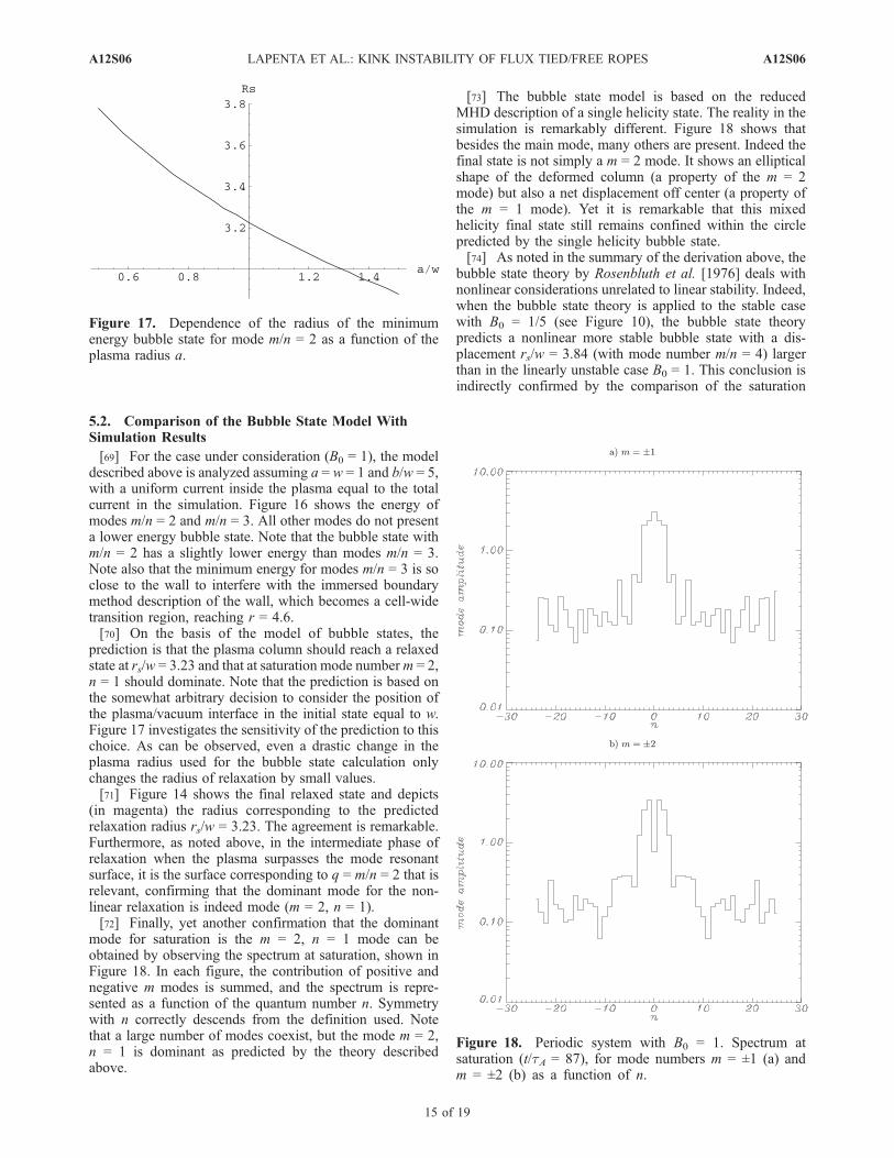
mode for saturation is the m = 2, n = 1 mode can beobtained by observing the spectrum at saturation, shown inFigure 18. In each figure, the contribution of positive andnegative m modes is summed, and the spectrum is repre-sented as a function of the quantum number n. Symmetrywith n correctly descends from the definition used. Notethat a large number of modes coexist, but the mode m = 2,n = 1 is dominant as predicted by the theory describedabove.

[73] The bubble state model is based on the reducedMHD description of a single helicity state. The reality in thesimulation is remarkably different. Figure 18 shows thatbesides the main mode, many others are present. Indeed thefinal state is not simply a m = 2 mode. It shows an ellipticalshape of the deformed column (a property of the m = 2mode) but also a net displacement off center (a property ofthe m = 1 mode). Yet it is remarkable that this mixedhelicity final state still remains confined within the circlepredicted by the single helicity bubble state.[74] As noted in the summary of the derivation above, the

bubble state theory by Rosenbluth et al. [1976] deals withnonlinear considerations unrelated to linear stability. Indeed,when the bubble state theory is applied to the stable casewith B0 = 1/5 (see Figure 10), the bubble state theorypredicts a nonlinear more stable bubble state with a dis-placement rs/w = 3.84 (with mode number m/n = 4) largerthan in the linearly unstable case B0 = 1. This conclusion isindirectly confirmed by the comparison of the saturation

Figure 18. Periodic system with B0 = 1. Spectrum atsaturation (t/tA = 87), for mode numbers m = ±1 (a) andm = ±2 (b) as a function of n.

Figure 17. Dependence of the radius of the minimumenergy bubble state for mode m/n = 2 as a function of theplasma radius a.

A12S06 LAPENTA ET AL.: KINK INSTABILITY OF FLUX TIED/FREE ROPES

15 of 19

A12S06

Figure 19. Run with free/line-tied boundary conditions, B0 = 1. False color representation of foursignificant quantities near the end of the linear phase in 2-D a section of the 3-D simulation at z = Lz:(a) Density, (b) axial current, (c) helical flux (for mode numbers m = 2, n = 1), (d) temperature. The blackand magenta line have the same meaning as in Figure 11.

Figure 20. Run with free/line-tied boundary conditions, same as Figure 19 but at time t/tA = 120.6.

A12S06 LAPENTA ET AL.: KINK INSTABILITY OF FLUX TIED/FREE ROPES

16 of 19

A12S06

level for the kinetic energy as shown in Figures 9–10 forthe free-ended ropes where both cases are linearly unstable.The saturation level for the more linearly unstable case B0 = 1is lower than that for B0 = 1/5, in accord with the bubblestate prediction (even though the bubble state prediction

applies strictly only to the periodic case). This result,however, is only suggestive as it might also be affectedby the indirect relationship between the displacement andthe saturation level of the kinetic energy, affected also by the

Figure 21. Magnetic flux tubes within a rope tied at one end and free at the other. Two times are shown:initial state (a) and at saturation, t/tA = 120.6. (b) The color shows the height along the z axis.

A12S06 LAPENTA ET AL.: KINK INSTABILITY OF FLUX TIED/FREE ROPES

17 of 19

A12S06

outflow of energy from the open boundary of the simulationbox.

6. Saturated State of a Free/Tied Flux Rope

[75] The analysis reported above is valid for a periodicsystem, and the study of the bubble states assumes theexistence of modes with defined helicity in a periodicsystem. For the case with line-tying at one end and freeboundary conditions at the other, the analysis cannot beapplied directly.[76] However, Figures 19–20 show the configuration of a

free-ended rope for the same parameters considered in theprevious section (B0 = 1, Spitzer resistivity with S = 103).As can be observed the intermediate nonlinear phase is stilldominated by the surface q = 2. Furthermore, the finalrelaxed state is still determined by rs/w = 3.23 as in theperiodic case.[77] There is, however, a fundamental difference. Figures

19–20 show a cross section of the plasma rope at z = Lz.Closer to the line-tied end, the rope is less displaced up tono displacement at all at the tied end. Figure 21 shows a 3-Drepresentation of the flux rope in its initial configuration andits relaxed state. Note how the line-tied end (closer to thereader) remains fixed, while the free end moves away. Acircle in pink is shown for reference to remind of the initialposition of the rope.[78] The simulations shown here are but a qualitative

representation of the real system in RSX. Future experi-

mental work will have to test the observations made in thesimulations regarding the saturation level and the propertiesof the saturated state. The experiments available thus farprovide already a confirmation to one of the conclusionsdescribed above regarding the saturated state of a rope freeat one end and tied at the other. Figure 22 shows foursubsequent figures taken from the camera angle along theplasma rope shown in Figure 4. The subsequent shotsprovide evidence of the increasing kinking of the initiallystraight rope. The final state is clearly still tied to the plasmagun generating the rope and is progressively more dis-placed, spiraling outward as observed in the simulations.Future work will be needed to make a quantitative connec-tion between the relaxed maximum displacement observedin the simulations, predicted by the bubble state model ofRosenbluth et al. [1976] and experiments.

7. Conclusions

[79] The results above can be summarized into twofindings. First, the ranking of ropes according to theirliability to the kink instability is free-ended flux ropes arethe most unstable, with their stability needing q > 2,periodic ropes come next, with the classic KS limit todetermine their stability. The most stable are line-tied fluxropes. This finding is of significance to solar and astro-physical flux ropes where the case of free-ended ropes maybe relevant and their reduced stability limit needs to betaken into account.

Figure 22. Sequence of images taken from a camera with a oblique view angle along the axial direction(see Figure 4). Four subsequent times are shown illustrating the progressive kink and its saturation to astate line-tied at the plasma gun but free at the free end. The largest displacement is at the free end.

A12S06 LAPENTA ET AL.: KINK INSTABILITY OF FLUX TIED/FREE ROPES

18 of 19

A12S06

[80] Second, the mechanism for nonlinear evolution pro-gresses in two steps. The first onsets when the plasmacolumn reaches the dominant mode resonant surface. Here,reconnection is needed for the plasma to progress further.The actual rate of reconnection is beyond the scope of thepresent paper. Spitzer resistivity is used within the regularresistive model; in real systems the situation is morecomplicated because of the presence of other nonidealmechanisms besides just collisional resistivity. The laststage of the evolution is the formation of a bubble statewhere the plasma reaches the radius predicted by a simplemodel due to Rosenbluth et al. [1976]. A significantdistinction needs to be made between the tied/free-endedand the periodic case. The tied end has zero displacement atsaturation, while the displacement spirals out away from thetied end. The maximum displacement is at the free end andit is the same as in the periodic case.[81] The conclusions reached above can be compared

with experiments conducted on RSX. The decreased stabil-ity of free flux ropes has indeed been observed in experi-ments [Furno et al., 2006]. The typical saturated columnhas the spiral structure observed here [Furno et al., 2006,2005]. The key prediction above about the ability of thebubble-state mode to predict the saturation level needs yetto be investigated experimentally.

[82] Acknowledgments. The authors gratefully acknowledge usefuldiscussions with Amitava Bhattacharjee, Daniele Bonfiglio, SusannaCappello, Dominique Escande, John Finn, Roberto Lionello, DimitriRyutov, and Dalton Schnack. This research is supported by the LDRDprogram at the Los Alamos National Laboratory and by the Office ofFusion Energy Science at the Office of Science of the United StatesDepartment of Energy. Work conducted under the auspices of the UnitedStates Department of Energy contract W-7405-ENG-36.[83] Amitava Bhattacharjee thanks the reviewers for their assistance in

evaluating this paper.

ReferencesBaty, H., G. Einaudi, R. Lionello, and M. Velli (1998), Ideal kink instabil-ities in line-tied coronal loops, Astron. Astrophys., 333, 313.

Biskamp, D. (1993), Nonlinear Magnetohydrodynamics, Cambridge Univ.Press, New York.

Blandford, R. (2002), Blood out of a stone, Science, 295, 1653.Brackbill, J. (1991), FLIP MHD: A particle-in-cell method for magnetohy-drodynamics, J. Comput. Phys., 96, 163.

Brackbill, J., and D. Knoll (2001), Transient magnetic reconnection andunstable shear layers, Phys. Rev. Lett., 86, 2329–2332.

Einaudi, G., and G. Van Hoven (1983), The stability of coronal loops:Finite-length and pressure-profile limits, Sol. Phys., 88, 163.

Evstatiev, E., G. Delzanno, and J. Finn (2006), A new method for analyzingline-tied kink modes in cylindrical geometry, Phys. Plasmas, 13, 072,902.

Fiksel, G., A. Almagri, D. Craig, M. Iida, S. Prager, and J. Sarff (1996),High current plasma electron emitter, Plasma Sources Sci. Technol., 5,78–83.

Freidberg, J. (1987), Ideal Magnetohydrodynamics, Springer, New York.Furno, I., et al. (2003), Reconnection scaling experiment: A new device forthree-dimensional magnetic reconnection studies, Rev. Sci. Instrum.,74(4), 2324.

Furno, I., T. P. Intrator, E. W. Hemsing, S. C. Hsu, P. Ricci, and G. Lapenta(2005), Coalescence of two magnetic flux ropes via collisional magneticreconnection, Phys. Plasmas, 12(5), 055, 702.

Furno, I., T. Intrator, D. Ryutov, S. Abbate, T. Madziwa-Nussinov, A. Light,L. Dorf, and G. Lapenta (2006), Current driven rotating kink mode in aplasma column with a non-line-tied free end, Phys. Rev. Lett., 97,015,002.

Gekelman, W., J. E. Maggs, and H. Pfister (1992), Experiments on theinteraction of current channels in a laboratory plasma: Relaxation tothe force-free state, IEEE Trans. Plasma Sci., 20(6), 614.

Gerrard, C., and A. Hood (2003), Kink unstable coronal loops: Currentsheets, current saturation and magnetic reconnection, Sol. Phys., 214, 151.

Goedbloed, H., and S. Poedts (2004), Principles of Magnetohydrody-namics, Cambridge Univ. Press, New York.

Hansen, J. F., S. K. P. Tripathi, and P. M. Bellan (2004), Co- and counter-helicity interaction between two adjacent laboratory prominences, Phys.Plasmas, 11(6), 3177.

Hood, A., and E. Priest (1979), Kink instability of solar coronal loops as thecause of solar flares, Sol. Phys., 64, 303.

Hood, A., and E. Priest (1981), Critical conditions for magnetic instabilitiesin forcefree coronal loops, Geophys. Astrophys. Fluid Dyn., 17, 297.

Kadomtsev, B. (1992), Tokamak Plasma: A Complex Physical System, Inst.of Phys. Publ., Philadelphia, Pa.

Kadomtsev, B., and O. Pogutse (1973), Nonlinear helical plasma perturba-tions in the tokamak, Sov. Phys. JETP, 38, 283.

Lapenta, G. (1999), Simulation of charging and shielding of dust particlesin drifting plasmas, Phys. Plasmas, 6, 1442.

Lapenta, G. (2002), Particle rezoning for multidimensional kinetic particle-in-cell simulations, J. Comput. Phys., 181, 317.

Lapenta, G., and J. Brackbill (1996), Immersed boundary method for plas-ma simulation in complex geometries, IEEE Trans. Plasma Sci., 24, 105.

Lapenta, G., and D. Knoll (2004), Reconnection in the solar corona: Role ofthe kelvinhelmholtz instability, Solar Phys., 214, 107.

Lapenta, G., and D. Knoll (2005), Effect of a converging flow at thestreamer cusp on the genesis of the slow solar wind, Astrophys. J.,624, 1049–1056.

Lapenta, G., and P. Kronberg (2005), Simulation of astrophysical jets:Collimation and expansion into radio lobes, Astrophys. J., 625, 37–50.

Lapenta, G., F. Iinoya, and J. Brackbill (1995), Particle-in-cell simulation ofglow discharges in complex geometries, IEEE Trans. Plasma Sci., 23,769.

Lionello, R., D. Schnack, G. Einaudi, and M. Velli (1998a), Current sheetformation due to nonlinear kink modes in periodic and line-tied config-urations, Phys. Plasmas, 5, 3722.

Lionello, R., M. Velli, G. Einaudi, and Z. Mikic (1998b), Nonlinear mag-netohydrodynamic evolution of line-tied coronal loops, Astrophys. J.,494, 840.

Monaghan, J. J. (1992), Smoothed particle hydrodynamics, Annu. Rev.Astron. Astrophys., 30, 543.

Owen, F., P. Hardee, and T. Cornwell (1989), High-resolution high dynamicrange VLA images of the M87 jet at 2 centimeters, Astrophys. J., 340,698.

Peskin, C. (2002), The immersed boundary method, Acta Numer., 11, 479.Priest, E., and T. Forbes (2000), Magnetic Reconnection: MHD Theory andApplications, Cambridge Univ. Press, New York.

Rosenbluth, M., D. Monticello, H. Strauss, and R. White (1976), Numericalstudies of nonlinear evolution of kink modes in tokamaks, Phys. Fluids,19, 1987.

Ryutov, D. D., R. H. Cohen, and L. D. Pearlstein (2004), Stability of afinite-length screw pinch revisited, Phys. Plasmas, 11, 4740.

Ryutov, D. D., I. Furno, T. P. Intrator, S. Abbate, and T. Madziwa-Nussinov(2006), Phenomenological theory of the kink instability in a slenderplasma column, Phys. Plasmas, 13, 032, 105.

Schrijver, C., et al. (1999), A new view of the solar outer atmosphere by thetransition region and coronal explorer, Solar Phys., 187, 261.

Spitzer, L. (1956), Physics of Fully Ionized Gases, Wiley-Interscience,Hoboken, N. J.

Strauss, H. (1976), Non-linear three dimensional dynamics of noncirculartokamaks, Phys. Fluids, 19, 134.

Trintchouk, F., M. Yamada, H. Ji, R. M. Kulsrud, and T. A. Carter (2003),Measurement of the transverse Spitzer resistivity during collisional mag-netic reconnection, Phys. Plasmas, 10, 319.

Wesson, J. (2004), Tokamak, Oxford Univ. Press, New York.White, R. (2001), The Theory of Toroidally Confined Plasmas, ImperialColl. Press, London.

Zwingmann, W. (1987), Theoretical study of onset conditions for solareruptive processes, Solar Phys., 111, 309.

�����������������������G. L. Delzanno and T. Intrator, Los Alamos National Laboratory, Los

Alamos, NM 87545, USA.I. Furno, Ecole Polytechnique Federale de Lausanne (EPFL), Centre de

Recherches en Physique des Plasmas, Association EURATOM-Confederation Suisse, CH-1015 Lausanne, Switzerland.G. Lapenta, Centre for Plasma Astrophysics, Departement Wiskunde,

Katholieke Universiteit Leuven, Celestijnenlaan 200B, BE-3001 Heverlee,Belgium. (giovanni.lapenta@wis.kuleuven.be)

A12S06 LAPENTA ET AL.: KINK INSTABILITY OF FLUX TIED/FREE ROPES

19 of 19

A12S06