kinematics of two link manipulator in matlab/simulink and msc ...

MM SCIENCE JOURNAL I 2021 I OCTOBER

4749

KINEMATICS OF TWO LINK MANIPULATOR IN

MATLAB/SIMULINK AND MSC ADAMS/VIEW

SOFTWARE

DARINA HRONCOVA1, ĽUBICA MIKOVA1,

IVAN VIRGALA1, ERIK PRADA1 1Technical University of Kosice, Faculty of Mechanical

Engineering, Kosice, Slovak Republic

DOI: 10.17973/MMSJ.2021_10_2021025

[email protected]

The paper deals with the kinematic analysis of a manipulator mechanism. The matrix method of kinematic analysis is used for the solution. The robot's mechanism is an open kinematic chain. The vector of position, velocity and acceleration is determined. The problem is solved using Matlab and MSC Adams / View. The Matlab program is used to solve kinematics equations in symbolic form. Computer software reduces the design time and also brings economic benefits. Conditions are being created for faster research and the creation of new mechanical systems gradually appearing in the production area. Computer simulation can also serve an educational purpose and giving additional information about the mechanical systems through simulation and kinematic analysis.

KEYWORDS

Matlab, Simulink, computer simulation, kinematics, symbolic form, matrix method

1 INTRODUCTION

The objective of the kinematic analysis of bound mechanical systems is to determine the relationship between the coordinates of the driven kinematic pairs and the coordinates of the drives. to determine the appropriate velocities and accelerations and to investigate the motion of its significant points and members of the analyzed system. Mechanisms of industrial robots and manipulators are composed of bodies which form different kinds of kinematic chains. In most cases these mechanisms represent open or mixed kinematic chains. Two bodies of a kinematic chain mutually interconnected so that their mobility to each other is limited, form a kinematic pair. According to kind of kinematic bond in a kinematic pair the kinematic chains are composed of translational or rotational kinematic pairs. This subject is addressed by authors in papers [Delyova 2014, Frankovsky 2013, Gmiterko 2010, Hroncova 2012, 2014, Xiong 2018, Serrano 2015]. We use analytical, graphical, and experimental methods in kinematic analysis of mechanisms. Many analytical methods are based on different areas of mathematics. They provide the best accuracy in determination of the investigated parameters at each instant of the operation of the mechanism. The intensive progress of computers extends the application of analytical methods [Bozek 2014, Kelemenova 2016] and the use of computers in presenting the results of the calculation visually on

a screen or paper largely eliminates the shortcomings of analytical methods resulting from the lack of clarity of obtained results.

2 ANALYTICAL METHODS

Analytical methods are based on the use of methods of analytical geometry, tensor and matrix calculus, complex variables and other areas of mathematics. These methods are connected with coordinate systems and lead to scalar equations for the investigated quantities [Brat 1981, Garcia 2015, Stejskal 1996]. One of the methods used in the kinematic analysis of mechanisms is the vector method, which allows solving problems in an explicit form, which eliminates the need to solve algebraic equations of high degrees. The method describes the kinematic scheme of the mechanism by vector polygons. From these we can compile equations that solve the problem of position. Subsequently, we can get the equations to determine velocity and acceleration. The position of individual members is expressed with vectors. The beginning and end of the vector is in the kinematic bonds. The vector shapes that characterize the mechanism change with motion but remain closed. The condition of closure, formulated by vectors, allows by suitable projection into the coordinate axes obtain the necessary scalar geometric relations between the coordinates of individual members. Equations for velocity are obtained as their time derivations. The equation for acceleration is obtained by further derivation. If we want to investigate the motion of a point of a member of the mechanism, we express its position vector as the sum of the position vectors of the members that enclose this vector pattern. Graphical methods are based on the direct geometric construction of the paths of motion of the most characteristic points of the members of plane mechanisms and their kinematic quantities. The drawing shows the shape of these paths, the angles between the members and the configuration of the mechanism at a certain instant, the relationships between velocities and accelerations of different points (of course with errors, inherent in geometric construction). Graphical methods make possible to visualize the movement of members of planar mechanisms and their significant points. They are used to solve spatial mechanisms less frequently. Experimental methods are based on the measurement of various motion parameters during the operation of real mechanisms or their models. The combination of computer technology with measuring instruments expands the possibilities of application of experimental methods in kinematics. It makes possible the measurement of rapidly changing motion parameters and increases the accuracy of the measurements [Kurylo 2018, Papacz 2018]. Matrix methods are often the most efficient for compilation of general algorithms for analysis of kinematic and force quantities of mechanisms of different configuration. Matrix notation is compact, illustrative, it is suitable for use in a computer environment. It allows an easy transition from symbolic equations to scalar equations and is suitable for numerical methods used on a computer. The theory of simple open kinematic chains has a direct application in the kinematic analysis of various manipulators and robots, which are often formed by these chains. We decompose the motion of two members bound by a lower kinematic pair into a finite number


4750

of basic motions [Abramov 2014]. The kinematic diagram of one of these manipulators is shown in Fig. 1 [Brat 1981].

3 MODEL OF A TWO-MEMBER RR MANIPULATOR

The mechanical system of the two-member manipulator representing the open kinematic chain is composed of two members 1 and 2 and a base 0 according to Fig. 1.

Figure 1. Two-member robotic arm on mobile chassis

The two-member robotic arm is considered in the shape shown in Fig.2.

Figure 2. Two-member robotic arm on fixed frame

The member 1 of length l1 rotates around the axis z0 ≡ z1 by an angle φ1 and the member 2 of length l2 rotates around the axis z2 by an angle φ2 (Fig.3). It is necessary to investigate the absolute motion of the member 2 and its point M and to determine the position vector r0M, the position of the point M with respect to the base 0, to express the velocity v0M and the acceleration a0M of the point M with respect to the base 0 using the matrix method of basic motions.

Figure 3. R-R mechanical system with 2° of freedom

We introduce the coordinate systems in individual members according to Fig. 3. Movement of member 1 with respect to base 0 is only rotational, coordinate system O1,x1,y1,z1 of member 1 is rotated with respect to coordinate system of the base O0,x0,y0,z0 by angle φ1 around axis z0 ≡ z1, where φ1=φ1(t). The coordinate system O2,x2,y2,z2 of member 2 is shifted by the value l1 in the

direction of the axis x1 and rotated by an angle φ2 around the axis z2. The length of member 2 is l2 and we investigate the absolute motion of point M, which is located at its end with respect to base 0. The generalized coordinate of the rotational motion of member 1 is q1= φ1 and the generalized coordinate of the rotational motion of member 2 is q2= φ2. We express the motion of member 2 by basic decomposition to the reference point M. In general, we express it in the form:

n:1= n : (n -1)+ (n -1) : (n -2) +…+2:1,

where n - denotes the number of members.

4 MATRIX METHOD

We look for the position, velocity and acceleration of the point M of member 2. Then the frame motion of this member is determined by the motion of point M and is expressed by the basic decomposition to the reference point M and described by the equation:

𝑟0𝑀 = ∏ 𝑇𝑖,𝑖+11𝑖=0 . 𝑟2𝑀 (1)

Relative spherical motion is described by a transformation matrix:

𝑇02 = ∏ 𝑇𝑖,𝑖+11𝑖=0 (2)

We denote the transformation matrices between individual coordinate systems in kinematic pairs using transformation matrices of basic motions. Matrix equation of the trajectory of the point M with respect to the coordinate system of the base 0:

𝑟0𝑀 = 𝑇02. 𝑟2𝑀 (3)

where matrix T02:

𝑇02 = 𝑇01. 𝑇12 (4)

The transformation between the coordinate system of member 1 and the base 0 is described by matrix T01:

𝑇01 = 𝑇𝑍6(𝜑1) (5)

The transformation between the coordinate system of member 2 and member 1 is described by matrix T12:

𝑇12 = 𝑇𝑍6(𝜑2)𝑇𝑍1(𝑙1) (6)

Extended vector of position of point M in body space 2:

𝑟2𝑀 = [

𝑙2

001

] (7)

The shape of the matrices results from the type of bond:

𝑇𝑍6(𝜙1) = [

𝑐𝜑1 −𝑠𝜑1 0 0𝑠𝜑1 𝑐𝜑1 0 0

0 0 1 00 0 0 1

] (8)

𝑇𝑍6(𝜙2) = [

𝑐𝜑2 −𝑠𝜑2 0 0𝑠𝜑2 𝑐𝜑2 0 0

0 0 1 00 0 0 1

] (9)

𝑇𝑍1(𝑙1) = [

1 0 0 𝑙1

0 1 0 00 0 1 00 0 0 1

] (10)

a

c

==O z 22

2q

q1

φ1

1

2

z==1O O 0 == ==

10z x0

0y

x 1

x 2

M

2φ

y1

2l1l y2

0


4751

𝑇12 = 𝑇𝑍6(𝜑2)𝑇𝑍1(𝑙1) = [

𝑐𝜑2 −𝑠𝜑2 0 𝑙1. 𝑐𝜑2

𝑠𝜑2 𝑐𝜑2 0 𝑙1. 𝑠𝜑2

0 0 1 00 0 0 1

] (11)

Position vector r0M of point M of member 2 in the coordinate system of the base 0 using basic matrices:

𝑟0𝑀 = 𝑇𝑍6(𝜑1). 𝑇𝑍6(𝜑2). 𝑇𝑍1(𝑙1). 𝑟2𝑀 (12)

The resulting transformation matrix T02 of motion 2:0 is after calculation in Matlab [Hroncova 2019] , [Karban 2006]:

T02 =[ [cos(q1)*cos(q2)-sin(q1)*sin(q2),

-cos(q1)*sin(q2)-cos(q2)*sin(q1),0,

l1*cos(q1)*cos(q2)-l1*sin(q1)*sin(q2)]

[cos(q1)*sin(q2)+cos(q2)*sin(q1),

cos(q1)*cos(q2)-sin(q1)*sin(q2),0,

l1*cos(q1)*sin(q2)+l1*cos(q2)*sin(q1)]

[ 0, 0, 1, 0]

[ 0, 0, 0, 1] ]

Position vector r0M of point M with respect to the basic coordinate system:

𝑟0𝑀 = [

𝑥0𝑀

𝑦0𝑀

𝑧0𝑀

1

] (14)

Where the position vector r0M components are:

𝑥0𝑀 = (cos(𝜑1)cos(𝜑2)-sin(𝜑1) sin(𝜑2))𝑙2 +

cos(𝜑1) cos(𝜑2)𝑙1-sin(𝜑1) sin(𝜑2)𝑙1

𝑦0𝑀 = (sin(𝜑1) cos(𝜑2)+cos(𝜑1)sin(𝜑2))𝑙2 +

sin(𝜑1) cos(𝜑2)𝑙1+cos(𝜑1) sin(𝜑2)𝑙1

𝑧0𝑀 = 0

The resulting position vector of point M r0M of motion 2:0 in symbolic form from Matlab:

r0M=(cos(q1)*cos(q2)-sin(q1)*sin(q2))*l2

+cos(q1)*cos(q2)*l1-sin(q1)*sin(q2)*l1;

(sin(q1)*cos(q2)+cos(q1)*sin(q2))*l2+sin(q1)*cos

(q2)*l1+cos(q1)*sin(q2)*l1;

0;

1;

The magnitude of the position vector r1M of point M:

|𝑟0𝑀| = √𝑥0𝑀2 + 𝑦0𝑀

2 + 𝑧0𝑀2 ; (15)

The magnitude of position vector r0M in symbolic form according to Matlab:

r_0M =((l2*(cos(q1)*sin(q2) + cos(q2)*sin(q1)) +

l1*cos(q1)*sin(q2) + l1*cos(q2)*sin(q1))^2 +

(l2*(cos(q1)*cos(q2) - sin(q1)*sin(q2)) +

l1*cos(q1)*cos(q2) -

l1*sin(q1)*sin(q2))^2)^(1/2)

Time derivative of the position vector r0M gives the velocity vector v0M of the point M with respect to the coordinate system of the base O0,x0,y0,z0. Velocity vector v0M:

𝑣0𝑀 = �̇�0𝑀 = [

𝑣𝑥0𝑀

𝑣𝑦0𝑀

𝑣𝑧0𝑀

0

] (16)

Velocity vector v1M and its components in symbolic form from Matlab:

vx0M = -l1*(omega1*cos(omega1*t)*sin(omega2*t) +

omega1*cos(omega2*t)*sin(omega1*t) +


omega2*cos(omega2*t)*sin(omega1*t)) -

l2*(omega1*cos(omega1*t)*sin(omega2*t) +



omega2*cos(omega2*t)*sin(omega1*t))

vy0M = l1*(omega1*cos(omega1*t)*cos(omega2*t) +

omega2*cos(omega1*t)*cos(omega2*t) -

omega1*sin(omega1*t)*sin(omega2*t) -

omega2*sin(omega1*t)*sin(omega2*t)) +

l2*(omega1*cos(omega1*t)*cos(omega2*t) +



omega2*sin(omega1*t)*sin(omega2*t))

vz0M = 0

The magnitude of velocity v1M of the point M:

|𝑣0𝑀| = √𝑣𝑥0𝑀2 + 𝑣𝑦0𝑀

2 + 𝑣𝑧0𝑀2 (17)

The magnitude of velocity vector v0M in symbolic form according to Matlab:

v_0M=((l1*(omega1*cos(omega1*t)*sin(omega2*t) +



omega2*cos(omega2*t)*sin(omega1*t)) +

l2*(omega1*cos(omega1*t)*sin(omega2*t) +



omega2*cos(omega2*t)*sin(omega1*t)))^2 +

(l1*(omega1*cos(omega1*t)*cos(omega2*t) +



omega2*sin(omega1*t)*sin(omega2*t)) +

l2*(omega1*cos(omega1*t)*cos(omega2*t) +



omega2*sin(omega1*t)*sin(omega2*t)))^2)^(1/2)

Time derivative of the velocity vector v0M gives the acceleration vector a0M of the point M with respect to the coordinate system of the base O0,x0,y0,z0. Acceleration vector a0M:

𝑎0𝑀 = �̇�0𝑀 = �̈�0𝑀 = [

𝑎𝑥0𝑀

𝑎𝑦0𝑀

𝑎𝑧0𝑀

0

] (18)

Acceleration vector a1M of point M and its components in symbolic form from Matlab:

ax0M= -l1*(omega1^2*cos(omega1*t)*cos(omega2*t)+

omega2^2*cos(omega1*t)*cos(omega2*t) -

omega1^2*sin(omega1*t)*sin(omega2*t) -

omega2^2*sin(omega1*t)*sin(omega2*t) +

2*omega1*omega2*cos(omega1*t)*cos(omega2*t) -

2*omega1*omega2*sin(omega1*t)*sin(omega2*t)) -

l2*(omega1^2*cos(omega1*t)*cos(omega2*t) +





2*omega1*omega2*sin(omega1*t)*sin(omega2*t))

ay0M= -l1*(omega1^2*cos(omega1*t)*sin(omega2*t)+

omega1^2*cos(omega2*t)*sin(omega1*t) +



2*omega1*omega2*cos(omega1*t)*sin(omega2*t) +

2*omega1*omega2*cos(omega2*t)*sin(omega1*t)) -

l2*(omega1^2*cos(omega1*t)*sin(omega2*t) +




4752



2*omega1*omega2*cos(omega2*t)*sin(omega1*t))

az0M = 0

The magnitude of the acceleration a1M of the point M is obtained by:

|𝑎0𝑀| = √𝑎𝑥0𝑀2 + 𝑎𝑦0𝑀

2 + 𝑎𝑧0𝑀2 (19)

The magnitude of acceleration vector a0M in symbolic form according to Matlab:

a_0M=((l1*(omega1^2*cos(omega1*t)*sin(omega2*t)+





2*omega1*omega2*cos(omega2*t)*sin(omega1*t)) +

l2*(omega1^2*cos(omega1*t)*sin(omega2*t) +





2*omega1*omega2*cos(omega2*t)*sin(omega1*t)))^2

+ (l1*(omega1^2*cos(omega1*t)*cos(omega2*t) +





2*omega1*omega2*sin(omega1*t)*sin(omega2*t)) +

l2*(omega1^2*cos(omega1*t)*cos(omega2*t) +





2*omega1*omega2*sin(omega1*t)*sin(omega2*t)))^2)

^(1/2)

Graphical representation of the quantities obtained by the matrix method are in the next part of the paper.

5 GRAPHIC REPRESENTATION

The resulting values of kinematics parameters obtained from simulations are processed in Matlab. The graphs of kinematic parameters displacement, velocity and acceleration of the end effector are shown next.

Individual quantities in graphic form are shown for the values ω01=0.35 (rad/s), ω12=0.35 (rad/s):

Figure 4. Trajectory components of point M

Figure 5. Components of the velocity of point M

Figure 6. Components of the acceleration of point M

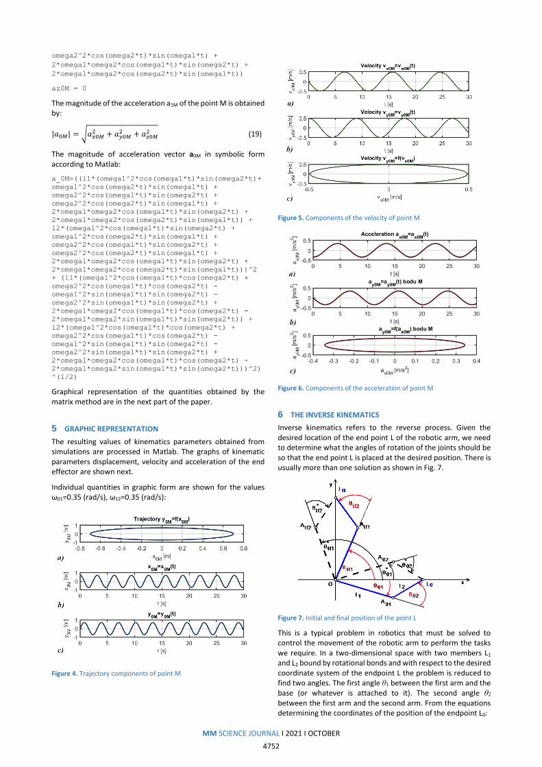
6 THE INVERSE KINEMATICS

Inverse kinematics refers to the reverse process. Given the desired location of the end point L of the robotic arm, we need to determine what the angles of rotation of the joints should be so that the end point L is placed at the desired position. There is usually more than one solution as shown in Fig. 7.

Figure 7. Initial and final position of the point L

This is a typical problem in robotics that must be solved to control the movement of the robotic arm to perform the tasks we require. In a two-dimensional space with two members L1 and L2 bound by rotational bonds and with respect to the desired coordinate system of the endpoint L the problem is reduced to find two angles. The first angle θ1 between the first arm and the base (or whatever is attached to it). The second angle θ2 between the first arm and the second arm. From the equations determining the coordinates of the position of the endpoint L0:


4753

𝑥𝐿 = 𝐿1cosθ1 + 𝐿2cos(𝜃1 + 𝜃2) (20)

𝑦𝐿 = 𝐿1sinθ1 + 𝐿2sin(𝜃1 + 𝜃2) (21)

we calculate the angles in the initial position xL0 and yL0. This represents two equations with two unknowns θ1 and θ2. We proceed in the same way for the end position of the point Ltf xLtf and yLtf.

7 THE FORWARD KINEMATICS

The two-arm robot model shown in the Fig. 3 consists of two

members of length L1 and L2 which are connected by one

rotational kinematic pair to the frame and are connected to each

other by a second rotational kinematic pair. The drives are

mounted in rotational kinematic pairs. The angle of rotation in

kinematic pairs is denoted by angles θ1 and θ2. When solving the

forward kinematics problem we determine the position of the

endpoint L described by equations (20) and (21):

Knowing the values of both angles we determine the position of the endpoint. During the motion of the manipulator with arms with lengths L1 = 0.4 meters and L2 = 0.3 meters, with the values θ10=-19°, θ1fin=43°, θ20=44°, θ2fin=151° in Fig. 7 is the position of the trajectory during the movement shown in Fig. 8.

Figure 8. Trajectory of the point M

Illustration of the position of the endpoint at different combinations of the angles θ1 and θ2 are shown in Fig.9.

Figure 9. Coordinates x-y for different combinations of θ1 and θ2

The angles θ1 and θ2 with known trajectory (Fig. 8) of the end point L is shown in Fig. 10.

Figure 10. Rotations θ1 and θ2, angular velocities ω1 and ω2 and angular accelerations α1 and α2

During the motion of the manipulator with arms with lengths L1=0.4 meters and L2=0.3 meters with the values θ10=0°, θ1fin=180°, θ 20=-90°, θ 2fin=270° the position of point L is shown in Fig. 11.

Figure 11. Trajectory of the point L

Illustration of the position of the endpoint at different combinations of the angles θ1 and θ2 are shown in Fig.12.

Figure 12. Coordinates x-y for different combinations of θ1 and θ2

The angles θ1 and θ2 with known trajectory (Fig. 11) of the end point L is shown in Fig. 13.

Using SimMechanics in the Matlab/Simulink with the inverse dynamic problem we obtain driving torques τ1 a τ2 (Fig.14) in respective joints of the manipulator (Fig.3). Maximum torque magnitudes are τ1 = 2,7784Nm and τ2 = 0,6901Nm.


4754

Figure 13. Rotations θ1 and θ2, angular velocities ω1 and ω2 and angular accelerations α1 and α2

Figure 14. Torques τ1 and τ2 in joints of member 1 and 2

The block diagram in SimMechanics for calculation of these torques is in (Fig.15).

Figure 15. SimMechanics block diagram for determining torques τ1 and τ2 in joints of member 1 and 2

Verification of the accuracy of the calculation is possible by substituting the obtained results into the forward problem. The respective block diagram in SimMechanics is shown in Fig. 16.

Figure 16. SimMechanics block diagram for determining the angular motion produced by torques τ1 and τ2 in joints of member 1 and 2

The IC (Initial Conditions) blocks define the values of the angles at the beginning of the motion.

8 SOFTWARE SIMULATION

MSC Adams uses an object-oriented programming environment with animated simulation. It simulates complex mechanical systems with more degrees of freedom. Models are defined directly by the geometry of individual bodies and their kinematic bonds, driving forces and motion generators. The analyzed robot model (Fig. 1) is next simulated in the MSC Adams / View software.

Our goal is to describe the movement of the end effector. The previous parts of the paper were also devoted to solving the forward problem of kinematics [Hunady 2019].

Figure 17. MSC Adams/View model and the trajectory of the basket during the simulation

We write the dynamic equations of motion in the form:

𝑀(𝛳)�̈� + 𝑉(𝛳, �̇�) + 𝐺(𝛳) = 𝜏 (22)

where

τ – the vector of actuator torques, M(θ) – the inertia matrix,

𝑉(𝜃, �̇�) – the Coriolis centripetal vector and G(θ) – the gravity

vector.

Equation (22) in our case represents a system of two 2nd order differential equations.

A reliable computation of the respective mechanical quantities is essential in design of mechanisms. These quantities then allow for further scaling of the individual parts of the mechanism. Graphs of kinematic quantities shown in Fig. 18 to Fig. 21.

a)

b)

c)

Figure 18. Position of the gripper's center of gravity a)xM , b) yM , c) |rM|


4755

a)

b)

c)

Figure 19. Velocity of the gripper's center of gravity a)vxM , b) vyM , c) |vM|

a)

b)

c)

Figure 20. Acceleration of the gripper's center of gravity a)axM , b) ayM , c) |aM|

a)

b)

c)

Figure 21. The torques τ1, τ2 and τ3 in bonds

The postprocessing is an integral part of computer modeling. It serves for creating, processing, modifying and presenting simulation results in the form of graphs. In the postprocessor we can display the model at any instant of the simulation, we can export the simulation process in a video format. The simulation results can be viewed also as numerical values in a tabular form or displayed in graphs.

9 CONCLUSIONS

We presented the procedure for analysis of the kinematic problem of the mechanism in Matlab using the matrix method and in MSC Adams/View software. MSC Adams/View is used for the simulation of motion of complex mechanical systems. A significant advantage of computer simulation is the possibility of immediate visualization of various variants of the model and analysis of the impact of any changes on the function of the model. Simulation verifies and reports possible collisions of model elements and displays the information about the chosen indicators on the screen. This gives a better understanding of the function of the model and verifies its functionality. Interactive simulation and visualization make this process even more comfortable and more effective. Immediate visualization gives feedback of the effect of potential changes of the model. The model is solved numerically. The results are obtained in the form of diagrams. This methodology provides a suitable tool for solving problems of teaching and practice.

ACKNOWLEDGMENTS

The authors would like to thank to Slovak Grant Agency project VEGA 1/0389/18, project VEGA 1/0201/21, grant project KEGA 030 TUKE-4/2020 supported by the Ministry of education of Slovak Republic. Authors also specially thank to supporting of project IVG-21-01 supported by the Faculty of Mechanical Engineering of Technical University of Kosice.

REFERENCES

[Abramov 2014] Abramov, I.V., et al. Control and Diagnostic Model of Brushless DC Motor, Journal of Electrical Engineering. 2014, Vol. 65, No. 5, pp. 277–282. [Bozek 2014] Bozek, P., Turygin, Y. Measurement of the operating parameters and numerical analysis of the mechanical subsystem, Measurement Science Review, 2014, Vol. 14, No. 4, pp. 198-203. [Brat 1981] Brat, V. Matrix methods in analysis and synthesis of bound spatial mechanical systems. Prague: Academia Praha, 1981. (in Czech) [Delyova 2014] Delyova, I., et al. Kinematic analysis of crank rocker mechanism using MSC Adams/View. Applied Mechanics and Materials, 2014, pp. 90-97. [Frankovsky 2013] Frankovsky, P., et al. Modeling of Dynamic Systems in Simulation Environment MATLAB/Simulink SimMechanics. American Journal of Mechanical Engineering. 2013, Vol. 1, No. 7, pp. 282-288. [Garcia 2015] Garcia, F.J.A., et al.: Simulators based on physical modeling tools to support the teaching of automatic control (2): rotating pendulum. In: Proceedings of the 36 Conference on Automation, 2015, Bilbao, pp. 667-673. [Gmiterko 2010] Gmiterko, et al. Theory of dynamical systems. Kosice, TU Kosice, 2010. [Hroncova 2012] Hroncova, D., et al. Kinematical analysis of crank slider mechanism using MSC Adams/View. Procedia Engineering, 2012, Vol. 48, pp. 213-222.


4756

[Hroncova 2014] Hroncova, D., et al. Kinematic Analysis of the Press Mechanism Using MSC Adams. American Journal of Mechanical Engineering, 2014, Vol. 2, No. 7, pp. 312-315. [Hroncova 2019] Hroncova, D., et al. Simulation in Matlab/Simulink. Kosice, TU Kosice, 2019. ISBN 978-80-553-3470-7. [Hunady 2019] Hunady, R., et al. Modeling of mechanical systems in the MSC Adams. Kosice, TU Kosice, 2019. ISBN 978-80-553-3471-4. [Karban 2006] Karban, P. Calculations and simulations in Matlab and Simulink. Brno, Computer Press, 2006. (in Czech) [Kelemenova 2016] Kelemenova, T., et. al. Machines for inspection of pipes. Acta Mechatronica, 2016, Vol. 1, No. 1, pp. 1-7.

[Kurylo 2018] Kurylo, P. Experimental Stand for Actuator Testing. Acta Mechatronica, 2018, Vol. 3, No. 2, pp. 7-10. [Papacz 2018] Papacz, W. Didactic models of manipulators. Acta Mechatronica, 2018, Vol. 3, No. 3, pp. 7-11. [Serrano 2015] Serrano, J., et al. Simulators Based on Physical Modeling Tools to Support the Teaching of Automatic Control (I): Mobile Robot with Flexible Arm. In: XXXVI Conference on Automation, Minutes Book, 2015, Bilbao, pp. 659-666. [Stejskal 1996] Stejskal, V., Valasek, M. Kinematics and dynamics of Machinery. New York, Marcel Dekker, Inc., 1996. [Xiong 2018] Xiong, W., et al. Solution to the motion of a delta manipulator with three degrees of freedom. Ferroelectrics, 2018, Vol. 529, No. 1, pp. 159-167.

CONTACTS:

Ing. Darina Hroncova, PhD. Technical University of Kosice, Faculty of Mechanical Engineering Letna 9, 040 01 Kosice, Slovak Republic [email protected]

kinematics of two link manipulator in matlab/simulink and msc ...

Documents

Transcript of kinematics of two link manipulator in matlab/simulink and msc ...