Mind the Gap!

Bridging the Reality Gap in Visual Perception and Robotic Grasping with

Domain Randomisation

João Henrique Pechirra de Carvalho Borrego

Thesis to obtain the Master of Science Degree in

Electrical Engineering

Supervisors: Dr. Plinio Moreno LopezProf. José Alberto Rosado dos Santos Vitor

Examination Committee

Chairperson: Prof. João Fernando Cardoso Silva SequeiraSupervisor: Dr. Plinio Moreno Lopez

Members of the Committee: Prof. Luís Manuel Marques Custódio

November 2018

Declaration

I declare that this document is an original work of my own authorship and that it fulfills all the require-

ments of the Code of Conduct and Good Practices of the Universidade de Lisboa.

ii

Acknowledgments

First and foremost, I would like to thank my mom, dad, stepmom and all three of my brothers, whom

I love dearly. Your continuous support and care over the years was invaluable to the materialisation of

this project. To my grandmothers, uncles, aunts, cousins, and the like, for the unmoved trust you put on

me.

To my colleagues and friends Atabak and Rui, without whom this work could not have been carried

out. To my dissertation supervisor Prof. José Santos-Victor, and co-supervisor Plinio for their guidance,

encouragement and precious insight into which direction I should pursue with my research. To the whole

of Vislab, which has naturally become a second home for me over the last year. Never have I felt so

welcome and surrounded by bright, interesting individuals, yet also kind, unassuming and approachable.

To all my friends, from different stages of my life, who have led me to grow into the person I am

today. For all the compelling debates, nonsensical banter, entertaining distractions and camaraderie

that helped me through countless working late nights and tough moments.

If this achievement bears any meaning, it is undoubtedly because of each and every one of you.

Thank you.

iii

Abstract

In this work, we focus on Domain Randomisation (DR), which has rapidly gained popularity among the

research community when the task at hand involves knowledge transfer from simulated to the real-world

domain. This is common in the field of robotics, where the cost of performing experiments with real

robots is too unwieldy for acquiring the massive amount of data required for deep learning methods. We

propose to study the impact of introducing random variations in both visual and physical properties in a

virtual robotics environment. This is done by tackling two different problems namely, 1) object detection

and 2) autonomous grasping. Concerning 1), to the best of our knowledge, our research was the first

to extend the application of DR to a multi-class shape detection scenario. We introduce a novel DR

framework for generating synthetic data in a widely popular open-source robotics simulator (Gazebo).

We then train a state–of–the–art object detector with several simulated-image datasets and conclude

that DR can lead to as much as 26% improvement in mAP (mean Average Precision) over a fine-tuning

baseline, which is pre-trained on a huge, domain-generic dataset. Regarding 2) we created a pipeline for

simulating grasp trials, with support for both simple grippers and complex multi-fingered robotic hands.

We extend the aforementioned framework to perform randomisation of physical properties and ultimately

analyse the effect of applying DR to a virtual grasping scenario.

Keywords

Domain Randomisation; Reality Gap; Simulation; Object Detection; Grasping; Robotics; Synthetic Data

v

Resumo

Neste trabalho focamo-nos em Domain Randomisation (DR), que tem ganho popularidade junto da

comunidade investigadora quando a tarefa em estudo envolve transferir conhecimento de um domínio

simulado para o mundo real. Isto é comum na área de robótica, na qual o custo da realização de exper-

iências com um robô real é demasiado elevado para se adquirir a quantidade necessária de dados para

o uso de métodos de deep learning (aprendizagem profunda). Propomos o estudo do impacto de intro-

duzir variações aleatórias em propriedades tanto visuais como físicas, num ambiente robótico virtual.

Isto é feito ao abordar dois problemas distintos, nomeadamente 1) detecção de objectos e 2) grasping

autónomo. No que diz respeito a 1), tanto quanto sabemos, o nosso trabalho foi o primeiro a aplicar

DR à detecção de objectos multi-classe. Introduzimos uma nova ferramenta de DR para a geração de

dados sintéticos num estabelecido simulador de robótica open-source. Posteriormente, treinámos um

detector de objectos estado–de–arte com múltiplos datasets de imagens simuladas e concluímos que

DR pode levar a um aumento de até 26% em mAP (mean Average Precision) relativamente ao uso da

técnica de fine-tuning, que envolve o pré-treino num dataset enorme e genérico. Relativamente a 2),

criámos um procedimento para a simulação de tentativas de grasp, com suporte tanto para grippers

como para mãos robóticas complexas com múltiplos dedos. Estendemos a ferramenta anteriormente

mencionada para possibilitar a variação de propriedades físicas e finalmente analisámos o impacto de

aplicar DR a um cenário de grasping virtual.

Palavras Chave

Domain Randomisation; Reality Gap; Simulação; Detecção de Objectos; Grasping; Robótica; Dados

Sintéticos

vii

Contents

1 Introduction 1

1.1 Motivation . . . . . . . . . . . . . . . . . . . . . . . . . . . . . . . . . . . . . . . . . . . . . 3

1.1.1 Reality gap and domain randomisation . . . . . . . . . . . . . . . . . . . . . . . . . 4

1.1.2 Problem statement . . . . . . . . . . . . . . . . . . . . . . . . . . . . . . . . . . . . 5

1.2 Background . . . . . . . . . . . . . . . . . . . . . . . . . . . . . . . . . . . . . . . . . . . . 6

1.2.1 Object detection and Convolutional Neural Networks . . . . . . . . . . . . . . . . . 6

1.2.2 Grasping . . . . . . . . . . . . . . . . . . . . . . . . . . . . . . . . . . . . . . . . . 9

1.2.2.A Coulomb friction model . . . . . . . . . . . . . . . . . . . . . . . . . . . . 9

1.2.2.B Force-closure . . . . . . . . . . . . . . . . . . . . . . . . . . . . . . . . . 10

1.3 Contributions . . . . . . . . . . . . . . . . . . . . . . . . . . . . . . . . . . . . . . . . . . . 11

1.4 Outline . . . . . . . . . . . . . . . . . . . . . . . . . . . . . . . . . . . . . . . . . . . . . . . 12

2 Related Work 13

2.1 Convolutional neural networks . . . . . . . . . . . . . . . . . . . . . . . . . . . . . . . . . 15

2.1.1 Classification . . . . . . . . . . . . . . . . . . . . . . . . . . . . . . . . . . . . . . . 15

2.1.2 Detection . . . . . . . . . . . . . . . . . . . . . . . . . . . . . . . . . . . . . . . . . 16

2.1.3 Segmentation . . . . . . . . . . . . . . . . . . . . . . . . . . . . . . . . . . . . . . . 17

2.2 Robotic grasping . . . . . . . . . . . . . . . . . . . . . . . . . . . . . . . . . . . . . . . . . 18

2.2.1 Analytic and data-driven grasp synthesis . . . . . . . . . . . . . . . . . . . . . . . 18

2.2.2 Vision-based grasping . . . . . . . . . . . . . . . . . . . . . . . . . . . . . . . . . . 20

2.2.2.A Grasp detection . . . . . . . . . . . . . . . . . . . . . . . . . . . . . . . . 20

2.2.2.B Grasp quality estimation . . . . . . . . . . . . . . . . . . . . . . . . . . . 21

2.2.2.C End-to-end reinforcement learning . . . . . . . . . . . . . . . . . . . . . . 23

2.2.2.D Dexterous grasping . . . . . . . . . . . . . . . . . . . . . . . . . . . . . . 24

2.3 Domain Randomisation . . . . . . . . . . . . . . . . . . . . . . . . . . . . . . . . . . . . . 25

2.3.1 Visual domain randomisation . . . . . . . . . . . . . . . . . . . . . . . . . . . . . . 25

2.3.2 Physics domain randomisation . . . . . . . . . . . . . . . . . . . . . . . . . . . . . 28

ix

3 Domain Randomisation for Detection 33

3.1 Parametric object detection . . . . . . . . . . . . . . . . . . . . . . . . . . . . . . . . . . . 35

3.1.1 GAP: A domain randomisation framework for Gazebo . . . . . . . . . . . . . . . . 35

3.1.1.A Gazebo simulator . . . . . . . . . . . . . . . . . . . . . . . . . . . . . . . 35

3.1.1.B Desired domain randomisation features . . . . . . . . . . . . . . . . . . . 37

3.1.1.C Offline pattern generation library . . . . . . . . . . . . . . . . . . . . . . . 38

3.1.1.D GAP: A collection of Gazebo plugins for domain randomisation . . . . . . 39

3.2 Proof–of–concept trials . . . . . . . . . . . . . . . . . . . . . . . . . . . . . . . . . . . . . 41

3.2.1 Scene generation . . . . . . . . . . . . . . . . . . . . . . . . . . . . . . . . . . . . 41

3.2.2 Preliminary results for Faster R-CNN and SSD . . . . . . . . . . . . . . . . . . . . 42

3.3 Domain randomisation vs fine-tuning . . . . . . . . . . . . . . . . . . . . . . . . . . . . . . 44

3.3.1 Single Shot Detector . . . . . . . . . . . . . . . . . . . . . . . . . . . . . . . . . . . 44

3.3.2 Improved scene generation . . . . . . . . . . . . . . . . . . . . . . . . . . . . . . . 45

3.3.3 Real images dataset . . . . . . . . . . . . . . . . . . . . . . . . . . . . . . . . . . . 46

3.3.4 Experiment: domain randomisation vs fine-tuning . . . . . . . . . . . . . . . . . . . 47

3.3.5 Ablation study: individual contribution of texture types . . . . . . . . . . . . . . . . 50

4 Domain Randomisation for Grasping 55

4.1 Grasping in simulation . . . . . . . . . . . . . . . . . . . . . . . . . . . . . . . . . . . . . . 57

4.1.1 Overview and assumptions . . . . . . . . . . . . . . . . . . . . . . . . . . . . . . . 57

4.1.2 Dex-Net pipeline for grasp quality estimation . . . . . . . . . . . . . . . . . . . . . 58

4.1.3 Offline grasp sampling . . . . . . . . . . . . . . . . . . . . . . . . . . . . . . . . . . 59

4.1.3.A Antipodal grasp sampling . . . . . . . . . . . . . . . . . . . . . . . . . . . 60

4.1.3.B Reference Frames . . . . . . . . . . . . . . . . . . . . . . . . . . . . . . . 63

4.2 GRASP: Dynamic grasping simulation within Gazebo . . . . . . . . . . . . . . . . . . . . . 64

4.2.1 DART physics engine . . . . . . . . . . . . . . . . . . . . . . . . . . . . . . . . . . 64

4.2.2 Disembodied robotic manipulator . . . . . . . . . . . . . . . . . . . . . . . . . . . . 65

4.2.3 Hand plugin and interface . . . . . . . . . . . . . . . . . . . . . . . . . . . . . . . . 66

4.3 Extending GAP with physics-based domain randomisation . . . . . . . . . . . . . . . . . . 67

4.3.1 Physics randomiser class . . . . . . . . . . . . . . . . . . . . . . . . . . . . . . . . 67

4.4 DexNet: Domain randomisation vs geometry-based metrics . . . . . . . . . . . . . . . . . 68

4.4.1 Novel grasping dataset . . . . . . . . . . . . . . . . . . . . . . . . . . . . . . . . . 68

4.4.2 Experiment: grasp quality estimation . . . . . . . . . . . . . . . . . . . . . . . . . . 70

4.4.2.A Trials without domain randomisation . . . . . . . . . . . . . . . . . . . . . 71

4.4.2.B Trials with domain randomisation . . . . . . . . . . . . . . . . . . . . . . . 72

x

5 Discussion and Conclusions 75

5.1 Discussion . . . . . . . . . . . . . . . . . . . . . . . . . . . . . . . . . . . . . . . . . . . . 77

5.2 Conclusions . . . . . . . . . . . . . . . . . . . . . . . . . . . . . . . . . . . . . . . . . . . . 78

5.3 Future Work . . . . . . . . . . . . . . . . . . . . . . . . . . . . . . . . . . . . . . . . . . . . 80

A Appendix 89

A.1 Metrics . . . . . . . . . . . . . . . . . . . . . . . . . . . . . . . . . . . . . . . . . . . . . . 90

A.1.1 Precision and Recall . . . . . . . . . . . . . . . . . . . . . . . . . . . . . . . . . . . 90

A.1.2 Intersection over Union (IoU) . . . . . . . . . . . . . . . . . . . . . . . . . . . . . . 90

A.1.3 Average Precision . . . . . . . . . . . . . . . . . . . . . . . . . . . . . . . . . . . . 90

A.1.3.A PASCAL VOC Challenge . . . . . . . . . . . . . . . . . . . . . . . . . . . 91

A.1.4 F1 score . . . . . . . . . . . . . . . . . . . . . . . . . . . . . . . . . . . . . . . . . . 91

A.1.5 Loss functions . . . . . . . . . . . . . . . . . . . . . . . . . . . . . . . . . . . . . . 92

A.1.5.A L1-norm and L2-norm . . . . . . . . . . . . . . . . . . . . . . . . . . . . . 92

A.2 Implementation . . . . . . . . . . . . . . . . . . . . . . . . . . . . . . . . . . . . . . . . . . 93

A.2.1 GAP Implementation details . . . . . . . . . . . . . . . . . . . . . . . . . . . . . . . 93

A.2.1.A Simultaneous multi-object texture update . . . . . . . . . . . . . . . . . . 93

A.2.1.B Creating a custom synthetic dataset . . . . . . . . . . . . . . . . . . . . . 94

A.2.1.C Randomising robot visual appearance . . . . . . . . . . . . . . . . . . . . 94

A.2.1.D Known issues . . . . . . . . . . . . . . . . . . . . . . . . . . . . . . . . . 95

A.2.2 GRASP Implementation details . . . . . . . . . . . . . . . . . . . . . . . . . . . . . 95

A.2.2.A Simulation of underactuated manipulators . . . . . . . . . . . . . . . . . . 95

A.2.2.B Efficient contact retrieval . . . . . . . . . . . . . . . . . . . . . . . . . . . 96

A.2.2.C Adding a custom manipulator . . . . . . . . . . . . . . . . . . . . . . . . . 96

A.2.2.D Adjusting randomiser configuration . . . . . . . . . . . . . . . . . . . . . 97

A.2.2.E Reference frame: Pose and Homogenous Transform matrix . . . . . . . . 97

A.2.2.F Known issues . . . . . . . . . . . . . . . . . . . . . . . . . . . . . . . . . 98

A.3 Additional Material . . . . . . . . . . . . . . . . . . . . . . . . . . . . . . . . . . . . . . . . 98

xi

xii

List of Figures

1.1 Real and simulated robotic grasp trials . . . . . . . . . . . . . . . . . . . . . . . . . . . . . 4

1.2 Domain Randomisation of visuyayal properties . . . . . . . . . . . . . . . . . . . . . . . . 5

1.3 Computer Vision problems . . . . . . . . . . . . . . . . . . . . . . . . . . . . . . . . . . . 6

1.4 Convolutional neural net topology comparison . . . . . . . . . . . . . . . . . . . . . . . . . 7

1.5 Friction cone and pyramid approximation representations . . . . . . . . . . . . . . . . . . 10

2.1 Cornell grasping dataset examples . . . . . . . . . . . . . . . . . . . . . . . . . . . . . . . 21

2.2 Synthetic scenes employing domain randomisation . . . . . . . . . . . . . . . . . . . . . . 27

2.3 Examples from car detection dataset employing domain randomisation . . . . . . . . . . . 28

2.4 Randomly generated object meshes . . . . . . . . . . . . . . . . . . . . . . . . . . . . . . 30

2.5 OpenAI synthetic scenes with Shadow Dexterous Hand . . . . . . . . . . . . . . . . . . . 31

3.1 Gazebo architecture . . . . . . . . . . . . . . . . . . . . . . . . . . . . . . . . . . . . . . . 37

3.2 Pattern generation library example output . . . . . . . . . . . . . . . . . . . . . . . . . . . 38

3.3 Example scene created with GAP . . . . . . . . . . . . . . . . . . . . . . . . . . . . . . . 40

3.4 Synthetic scenes generated using GAP . . . . . . . . . . . . . . . . . . . . . . . . . . . . 42

3.5 Preliminary results on real image test set . . . . . . . . . . . . . . . . . . . . . . . . . . . 43

3.6 Real image training set examples . . . . . . . . . . . . . . . . . . . . . . . . . . . . . . . . 47

3.7 Viewpoint candidates . . . . . . . . . . . . . . . . . . . . . . . . . . . . . . . . . . . . . . 48

3.8 Per class AP and mAP for different training sets . . . . . . . . . . . . . . . . . . . . . . . . 49

3.9 SSD output on test set for FV + Real . . . . . . . . . . . . . . . . . . . . . . . . . . . . . . 50

3.10 PR curves for SSD trained with sets of 30k images . . . . . . . . . . . . . . . . . . . . . . 51

3.11 SSD performance on validation set, trained with sets of 6k images . . . . . . . . . . . . . 52

3.12 SSD performance on the test set, trained with sets of 6k images . . . . . . . . . . . . . . 52

3.13 PR curves for SSD trained with sets of 6k images and fine-tuned on real dataset . . . . . 53

4.1 Antipodal grasp candidates . . . . . . . . . . . . . . . . . . . . . . . . . . . . . . . . . . . 62

4.2 Reference frames for Baxter gripper . . . . . . . . . . . . . . . . . . . . . . . . . . . . . . 63

xiii

4.3 Time-lapse of successful grasp trial . . . . . . . . . . . . . . . . . . . . . . . . . . . . . . 72

4.4 Proposed metric comparison with baseline . . . . . . . . . . . . . . . . . . . . . . . . . . 73

A.1 Shadow Dexterous Hand with randomised individual link textures . . . . . . . . . . . . . . 94

xiv

List of Tables

2.1 Randomisation of dynamic properties . . . . . . . . . . . . . . . . . . . . . . . . . . . . . 31

3.1 Availability of robotic platforms . . . . . . . . . . . . . . . . . . . . . . . . . . . . . . . . . 36

3.2 SSD and Faster R-CNN preliminary results . . . . . . . . . . . . . . . . . . . . . . . . . . 43

3.3 Number of real images in train, validation and test partitions. . . . . . . . . . . . . . . . . 46

3.4 Number of instances and percentage of different classes in the real dataset. . . . . . . . . 46

3.5 SSD performance on the test set, trained with sets of 30k images . . . . . . . . . . . . . . 49

3.6 SSD performance on the test set (6k training sets) . . . . . . . . . . . . . . . . . . . . . . 51

4.1 Grasp trials preliminary results . . . . . . . . . . . . . . . . . . . . . . . . . . . . . . . . . 71

4.2 Randomised physical properties for grasp trials . . . . . . . . . . . . . . . . . . . . . . . . 72

A.1 Grasp trials preliminary per-object results . . . . . . . . . . . . . . . . . . . . . . . . . . . 100

xv

xvi

List of Algorithms

4.1 Grasp generator . . . . . . . . . . . . . . . . . . . . . . . . . . . . . . . . . . . . . . . . . . 61

4.2 Antipodal grasp sampler . . . . . . . . . . . . . . . . . . . . . . . . . . . . . . . . . . . . . 62

4.3 Dynamic trial run . . . . . . . . . . . . . . . . . . . . . . . . . . . . . . . . . . . . . . . . . . 70

A.1 Perlin noise generator . . . . . . . . . . . . . . . . . . . . . . . . . . . . . . . . . . . . . . . 99

xvii

xviii

Listings

A.1 Randomiser configuration . . . . . . . . . . . . . . . . . . . . . . . . . . . . . . . . . . . . 97

xix

xx

Acronyms

AP Average Precision

API Application Programming Interface

COCO Common Objects In Context

CNN Convolutional Neural Network

CVAE Conditional Variational Auto-Encoder

DART Dynamic Animation and Robotics Toolkit

DOF degrees of freedom

DR Domain Randomisation

fps frames per second

FoV Field of View

GAN Generative Adversarial Network

GPU Graphical Processing Unit

GWS Grasp Wrench Space

IK Inverse Kinematics

ILSVRC Imagenet’s Large Scale Visual

Recognition Challenge

IoU Intersection over Union

mAP mean Average Precision

MDP Markov decision process

ODE Open Dynamic Engine

RL Reinforcement Learning

RoI Region of Interest

RPN Region Proposal Network

sdf signed distance function

SDF Simulation Description Format

SSD Single Shot Detector

SVM Support Vector Machine

VAE Variational Auto-Encoder

URDF Unified Robot Description Format

YOLO You Only Look Once

xxi

xxii

1Introduction

Contents

1.1 Motivation . . . . . . . . . . . . . . . . . . . . . . . . . . . . . . . . . . . . . . . . . . . 3

1.1.1 Reality gap and domain randomisation . . . . . . . . . . . . . . . . . . . . . . . . 4

1.1.2 Problem statement . . . . . . . . . . . . . . . . . . . . . . . . . . . . . . . . . . . 5

1.2 Background . . . . . . . . . . . . . . . . . . . . . . . . . . . . . . . . . . . . . . . . . . 6

1.2.1 Object detection and Convolutional Neural Networks . . . . . . . . . . . . . . . . 6

1.2.2 Grasping . . . . . . . . . . . . . . . . . . . . . . . . . . . . . . . . . . . . . . . . . 9

1.3 Contributions . . . . . . . . . . . . . . . . . . . . . . . . . . . . . . . . . . . . . . . . . 11

1.4 Outline . . . . . . . . . . . . . . . . . . . . . . . . . . . . . . . . . . . . . . . . . . . . . 12

1

Almost in the beginning was curiosity.

Isaac Asimov, 1988

2

1.1 Motivation

Currently, robots thrive in rigidly constrained environments, such as factory plants, where human-

robot interaction is kept to a bare minimum. Our long-term goal as researchers on robotic systems is

to aid in the transition of this field into our daily lives, namely to our households. Ultimately, we strive to

achieve cooperative, effective and meaningful interactions. For this to occur we are met with numerous

challenges and unsolved research problems. In this work, we focus on tackling robotic visual percep-

tion and autonomous grasping, which are crucial skills for achieving any kind of significant synergistic

relationship with humans.

Regarding computer vision, the emergence of deep neural networks, and specifically Convolutional

Neural Networks has led to outstanding results in many challenging tasks. These frameworks are par-

ticularly appealing in that they automate feature extraction from raw image data, thus allowing one to

forego feature engineering, a popular approach that falls into the category of what we now designate as

classical machine learning.

An important drawback of employing deep learning is its requirement of substantial amounts of data.

This is, in turn, due to the typically enormous number of parameters that have to be estimated. In

computer vision, manual data annotation is a slow and tedious process, particularly for large image

datasets such as ImageNet [12]. In robotics, acquiring massive datasets of physical experiments is

generally impracticable, since physical trials are greatly both resource and time-consuming as well as

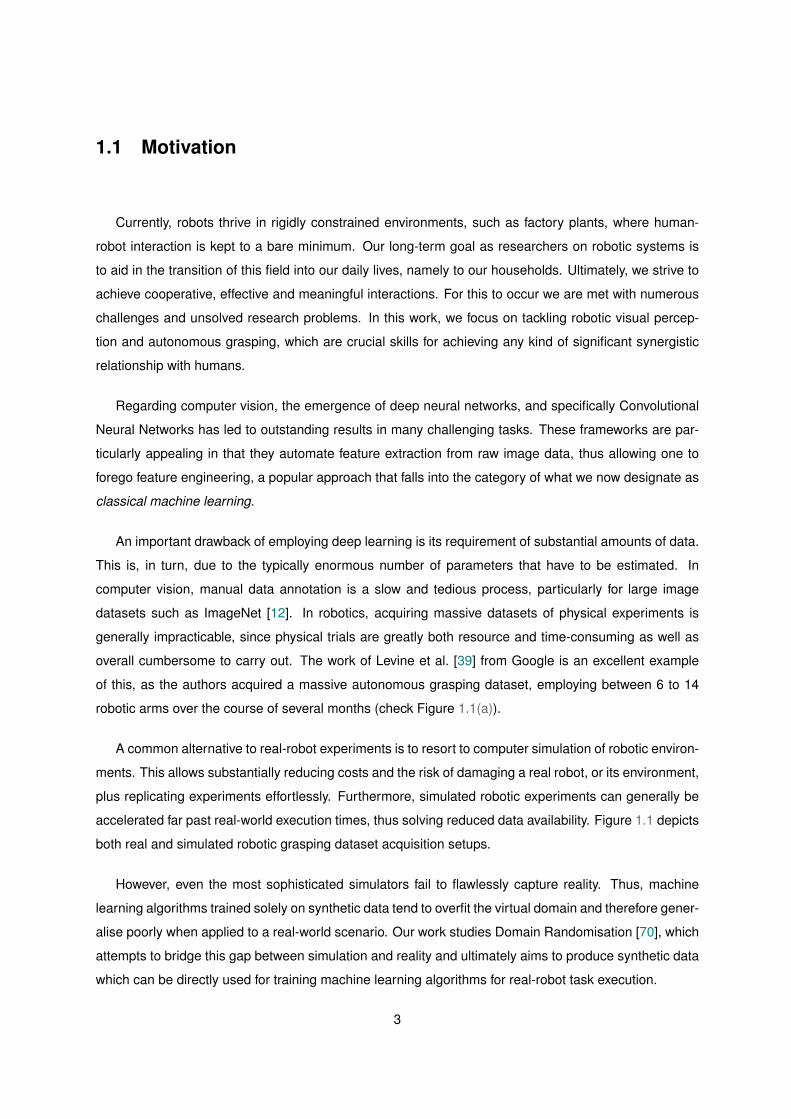
overall cumbersome to carry out. The work of Levine et al. [39] from Google is an excellent example

of this, as the authors acquired a massive autonomous grasping dataset, employing between 6 to 14

robotic arms over the course of several months (check Figure 1.1(a)).

A common alternative to real-robot experiments is to resort to computer simulation of robotic environ-

ments. This allows substantially reducing costs and the risk of damaging a real robot, or its environment,

plus replicating experiments effortlessly. Furthermore, simulated robotic experiments can generally be

accelerated far past real-world execution times, thus solving reduced data availability. Figure 1.1 depicts

both real and simulated robotic grasping dataset acquisition setups.

However, even the most sophisticated simulators fail to flawlessly capture reality. Thus, machine

learning algorithms trained solely on synthetic data tend to overfit the virtual domain and therefore gener-

alise poorly when applied to a real-world scenario. Our work studies Domain Randomisation [70], which

attempts to bridge this gap between simulation and reality and ultimately aims to produce synthetic data

which can be directly used for training machine learning algorithms for real-robot task execution.

3

(a) Google arm farm [39] (b) Simulated KUKA arm [56]

Figure 1.1: Real and simulated robotic grasp trials, left and right respectively.

1.1.1 Reality gap and domain randomisation

The discrepancy between the real world and the simulated environment is often referred to as the

reality gap. There are two common approaches to bridging this disparity, either (i) reducing the gap

by attempting to increase the resemblance between these two domains or (ii) exploring methods that

are trained in a more generic domain, representative of simulation and reality domains simultaneously.

To achieve the former, we can increase the accuracy of the simulators, in an attempt to obtain high-

fidelity results. This method has a major limitation: it requires great effort in the creation of systems

which model complex physical phenomena to attain realistic simulation. Our work focuses mainly on

the second approach. Instead of diminishing the reality gap in order to use traditional machine-learning

procedures, we analyse methods that are aware of this disparity.

Rather than attempting to perfectly emulate reality, we can create models that strive to achieve ro-

bustness to high variability in the environment. Domain Randomisation (DR) is a simple yet powerful

technique for generating training data for machine-learning algorithms. At its core, it consists in synthet-

ically generating or enhancing data by introducing random variance in the environment properties that

are not essential to the learning task. This idea dates back to at least 1997 [28], with Jakobi’s observa-

tion that evolved controllers exploit the unrealistic details of flawed simulators. His work on evolutionary

robotics studies the hypothesis that controllers can evolve to become more robust by introducing random

noise in all the aspects of simulation which do not have a basis in reality, and only slightly randomising the

remaining which do. It is expected that given enough variability in the simulation, the transition between

simulated and real domains is perceived by the model as a mere disturbance, to which it has become

robust. This is the main argument for this method. Recent literature has established that DR enables

achieving valuable generalisation capabilities [29, 70, 71, 78, 51, 73]. The term came into prominence

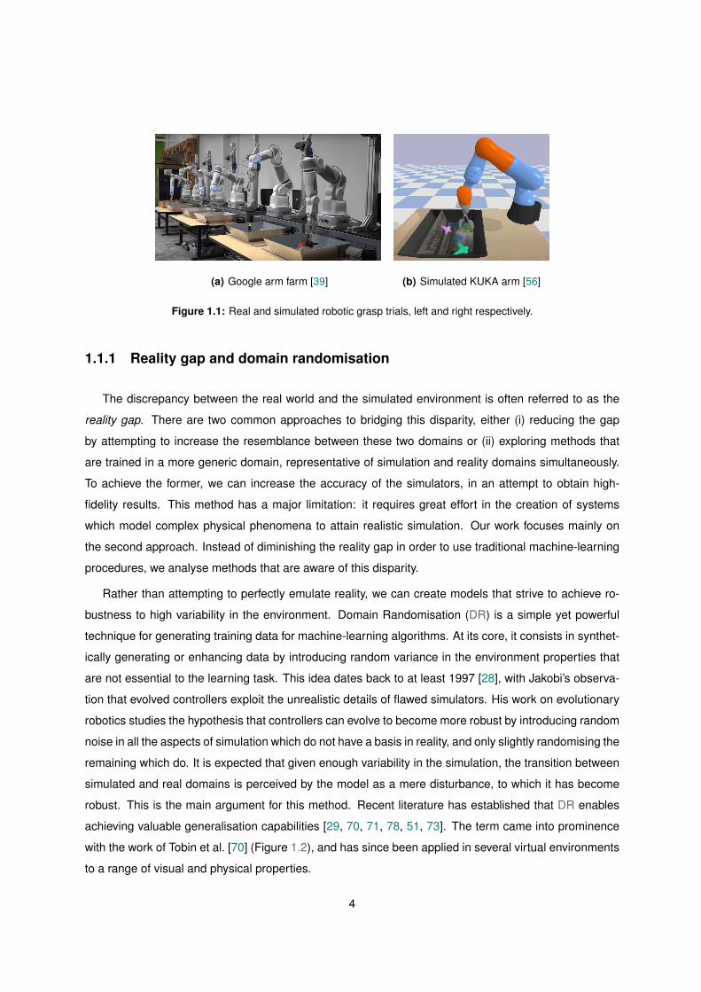
with the work of Tobin et al. [70] (Figure 1.2), and has since been applied in several virtual environments

to a range of visual and physical properties.

4

Source: Adapted from Tobin et al. [70]Figure 1.2: Example of Domain Randomisation (DR) applied to visuals of synthetic tabletop grasping scenario.

Three synthetic images are depicted on the left, the real robot setup is shown on the right.

1.1.2 Problem statement

This work focuses on exploring several DR methods employed in recent research which led to promis-

ing results with regard to overcoming the reality gap. Concretely, we study two different scenarios.

We start by addressing the task of object detection using deep neural networks trained on synthetic

data. We create tools for generating datasets employing DR to visual properties of a tabletop scene,

integrated into a well-known open-source robotics simulator. We claim that we can use such datasets to

train detectors that can overcome the reality gap by fine-tuning on a limited amount of real-world domain-

specific images. What is more, we find that this approach can outperform simple, yet widespread domain

adaptation method involving pre-training detectors on huge domain-generic image datasets.

Subsequently, we move to a robotic grasp setting and aim to understand the impact of applying the

principles of DR to the physical properties of the simulated environment. Specifically, we wish to modify

an existing state–of–the–art grasp quality estimation pipeline to incorporate full dynamic simulation of

grasp trials in a widespread open-source robotics simulator. We conjecture that by applying randomness

to physical properties such as friction coefficients, and grasp targets mass, will ultimately lead to more

robust systems.

The research questions we propose to examine were split in two subjects, namely (i) object detection,

and (ii) simulated grasping, and can be summarised as follows:

(i) RQ1: Can we successfully train state–of–the–art object detectors with synthetic datasets created

exploiting Domain Randomisation in a multi-class scenario?

(i) RQ2: Can small domain-specific synthetic datasets generated employing DR be preferable to

pre-training object detectors on huge generic datasets, such as COCO [40]?

(i) RQ3: Which is the impact of each of the texture patterns most commonly employed for visual

Domain Randomisation, in an object detection task?

5

(ii) RQ4: How can we integrate dynamic simulation of robotic grasping trials into a state–of–the–art

framework for grasp quality estimation?

(ii) RQ5: Can DR improve synthetic grasping dataset generation, employing a physics-based grasp

metric in simulation?

1.2 Background

Now that we have presented the challenge at hand and its relevance, we establishconcepts required for fully understanding the context in which our work is inserted.

1.2.1 Object detection and Convolutional Neural Networks

Being capable of performing object classification, localisation, detection and segmentation is closely

related to the ability to reason about and interact with dynamic environments.

Object classification consists of assigning a single label to a given image. Localisation includes not

only classifying the subject of an image but also identifying its position, usually by means of a rectangular

bounding box. Object detection assumes the possibility that more than a single instance can exist in a

single image, namely of different classes. Thus the desired output consists of every instance’s class

label and respective bounding box. Finally, segmentation includes all of the aforementioned problems,

but each instance is defined by its contour. Its objective is to obtain the label and outline of each instance

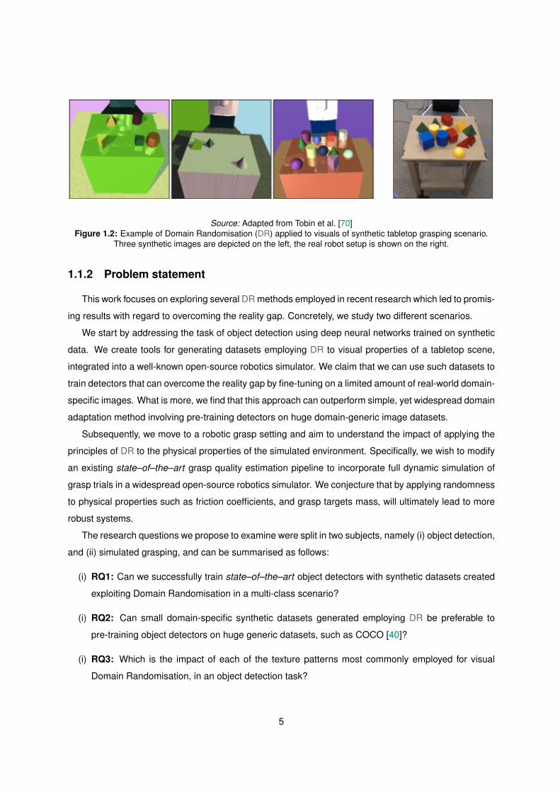
on the input image. Figure 1.3 provides an example of each of these tasks.

Source: Original images from ImageNet dataset [12]Figure 1.3: Computer Vision problems. Classification, localisation, detection and segmentation respectively from

left to right.

Neural networks can be thought of as generic function approximators, in the sense that their task

consists of learning a mapping between input and output variables. A traditional neural network receives

an input feature vector and processes it along its hidden layers in order to produce the desired output.

The process of training the network is essentially learning the parameters of these hidden layers, which

can be done in a supervised manner, by optimising a carefully designed loss function.

6

Each layer is composed of neurons, which are the primitive building blocks of neural networks. Neu-

rons perform a dot product with an input and the internal weight parameters, add a bias term, and apply

some non-linear activation function, e.g. threshold operation. The output of a neuron is in turn connected

to the input of another neuron of the following layer. For this reason these architectures can effectively

learn highly nonlinear functions.

In a traditional neural network all layers are fully connected, i.e. each neuron is connected to every

neuron of the previous layer. Therefore, these architectures display poor scalability in visual processing

tasks where the network input is a raw image, as far as computational resources are concerned. This is

due to the huge amount of parameters that need to be estimated, as each connection in the network is

associated with a given weight.

Convolutional Neural Networks (CNNs) are similar to regular neural networks in the sense that they

consist of neurons for which we wish to estimate weight and bias parameters. However, they assume

the input is an image with a given width and height and some number of channels (depth). CNNs have

a much more efficient structure as each neuron is only connected to a specific region of the previous

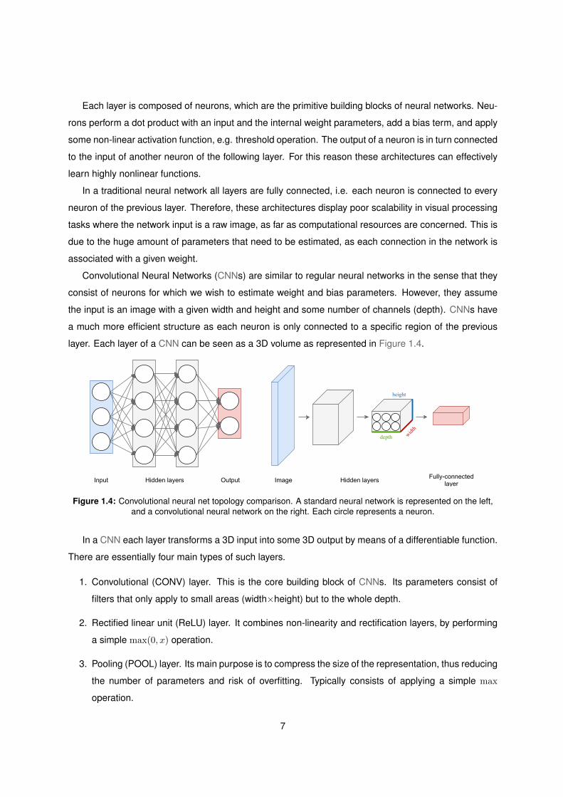
layer. Each layer of a CNN can be seen as a 3D volume as represented in Figure 1.4.

Figure 1.4: Convolutional neural net topology comparison. A standard neural network is represented on the left,and a convolutional neural network on the right. Each circle represents a neuron.

In a CNN each layer transforms a 3D input into some 3D output by means of a differentiable function.

There are essentially four main types of such layers.

1. Convolutional (CONV) layer. This is the core building block of CNNs. Its parameters consist of

filters that only apply to small areas (width×height) but to the whole depth.

2. Rectified linear unit (ReLU) layer. It combines non-linearity and rectification layers, by performing

a simple max(0, x) operation.

3. Pooling (POOL) layer. Its main purpose is to compress the size of the representation, thus reducing

the number of parameters and risk of overfitting. Typically consists of applying a simple max

operation.

7

4. Fully-connected (FC) layer.

When training a neural network each iteration consists of two steps. The first, known as forward

pass consists of computing the output of the network for a given input, with fixed weight parameters. The

second, named backward pass involves recursively computing the error between the network output and

the desired output value (for instance class label), and propagating the results all the way back to the

inputs of the network, adjusting its weights in the process. The latter step is much more computationally

expensive than the former.

In order to streamline CNN training, we often resort to using a batch of training examples per training

iteration, rather than providing a single image. However, this comes at the expense of memory require-

ments. Performing a full pass (both forward and backward passes) with each training example in a

dataset corresponds to an epoch.

The computer vision problems highlighted earlier involve estimating labels Y , given input image X,

and thus require discriminative models. Whereas typical discriminative models, also known as con-

ditional models, aim to estimate the conditional distribution of unobserved variables Y depending on

observed X, denoted by P (Y |X), generative models aim to estimate the joint probability distribution on

X × Y , P (X,Y ). Once trained, the latter models can be used for generating data that is congruent with

the learned joint distribution. In this fashion, we can produce new synthetic data for a target domain

when large amounts of data are available in a similar, yet distinct source domain. This is a promising

solution for the scarcity of labelled training data.

We provide several concrete examples of discriminative models in Section 2.1. Regarding generative

models, we briefly highlight two types of architectures: Generative Adversarial Networks (GANs) and

Variational Auto-Encoders (VAEs).

Generative Adversarial Networks [15] split the training process as a competition between two net-

works. The first is known as the generator, whereas the second is named the discriminator. Their

objective functions are opposite: the generator is optimised to produce synthetic images from real data

in such a way that the discriminator cannot reliably classify whether these images are real or synthetic.

Similarly, Variational Auto-Encoders [33] also employ two separate networks. First, the input is com-

pressed into a compact and efficient representation which exists in a lower-dimensional latent-space by

an encoder network. A second network known as decoder is trained to reconstruct the original input

when given the corresponding compressed representation in the latent space.

8

1.2.2 Grasping

Even though grasping and in–hand manipulation are essential skills for humans to interact with their

surroundings, they remain largely unsolved problems in robotics, specifically when the target object’s

geometry is unknown, or accurate dynamic models of the robot are unavailable. In this section, we

provide a brief overview of some key theoretical concepts for understanding grasping. Friction plays a

crucial role in grasping, as it allows objects to be safely held without slipping.

1.2.2.A Coulomb friction model

Friction is defined as the force resisting motion between two contacting surfaces. Specifically, we

focus on dry friction, which occurs when two solid surfaces are in direct contact with one another.

Experiments carried out from the 15th to 18th centuries have led to establishment of three empirical

laws [54]:

1. Amontons’ 1st Law – The force of friction is independent of the contact surface area;

2. Amontons’ 2nd Law – The frictional force is proportional to the normal force, or load;

3. Coulomb’s Law of Friction – The magnitude of the kinetic friction force is independent of the mag-

nitude of the relative velocity of the sliding surfaces.

Dry friction can be fairly accurately modelled by the Coulomb model, otherwise known as Amonton-

Coulomb friction model. It roughly outlines the properties of dry friction, by considering two separate

interactions (i) static friction, between non-moving surfaces, (ii) kinetic fiction, between sliding surfaces.

The law establishes that the frictional force FT for two contacting surfaces which are pressed together

with a normal force FN is sufficient to prevent motion between the bodies as long as

|FT| 6 µ|FN|, (1.1)

where µ is the coefficient of static friction, an empirical property of the pair of contacting materials.

Equation (1.1) defines a friction cone, where the contact point is the vertex, and the normal force its

axis. If the resulting friction vector is within this cone, then the force should be enough to prevent the

contacting surfaces from sliding. If it is not contained in the friction cone, then it generally cannot prevent

sliding.

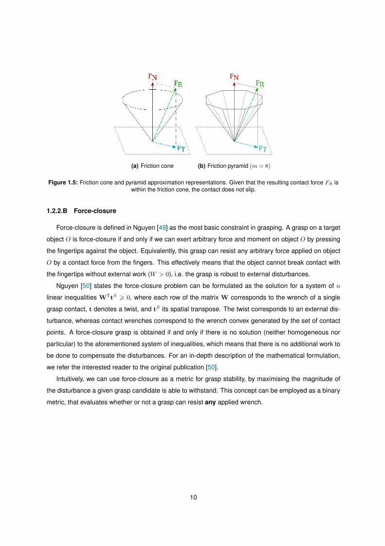
For reasons of computational efficiency, the continuous surface of the friction cone tends to be ap-

proximated by an m-sided pyramid.

Grasp stability implies that the object is secured in the manipulator in such a way that contacts do not

slip. A simple evaluation metric involves verifying whether or not the force-closure condition is achieved.

9

FN

FT

FR

(a) Friction cone

FN

FT

FR

(b) Friction pyramid (m = 8)

Figure 1.5: Friction cone and pyramid approximation representations. Given that the resulting contact force FR iswithin the friction cone, the contact does not slip.

1.2.2.B Force-closure

Force-closure is defined in Nguyen [49] as the most basic constraint in grasping. A grasp on a target

object O is force-closure if and only if we can exert arbitrary force and moment on object O by pressing

the fingertips against the object. Equivalently, this grasp can resist any arbitrary force applied on object

O by a contact force from the fingers. This effectively means that the object cannot break contact with

the fingertips without external work (W > 0), i.e. the grasp is robust to external disturbances.

Nguyen [50] states the force-closure problem can be formulated as the solution for a system of n

linear inequalities WTtS > 0, where each row of the matrix W corresponds to the wrench of a single

grasp contact, t denotes a twist, and tS its spatial transpose. The twist corresponds to an external dis-

turbance, whereas contact wrenches correspond to the wrench convex generated by the set of contact

points. A force-closure grasp is obtained if and only if there is no solution (neither homogeneous nor

particular) to the aforementioned system of inequalities, which means that there is no additional work to

be done to compensate the disturbances. For an in-depth description of the mathematical formulation,

we refer the interested reader to the original publication [50].

Intuitively, we can use force-closure as a metric for grasp stability, by maximising the magnitude of

the disturbance a given grasp candidate is able to withstand. This concept can be employed as a binary

metric, that evaluates whether or not a grasp can resist any applied wrench.

10

1.3 Contributions

In the previous sections, we motivated our work and introduced relevant concepts,which will be used throughout the thesis. In this section, we summarise our work’smajor contributions.

Our main goal is to show the application of the concept of Domain Randomisation (DR). This ob-

jective is achieved by (i) validating its use in an object recognition task, by changing objects’ visual

properties, and (ii) by employing it in a grasping scenario, where it is directly applied to the dynamic

properties of a physics simulation.

Our contributions regarding (i) can be summarised as follows.

1. We developed GAP1, an open-source tool for employing DR integrated with a prevalent open

robotics simulation environment (Gazebo2) for generating synthetic tabletop scenarios populated

by parametric objects with random visual properties;

2. Using GAP as the main tool for data generation, we demonstrate the efficiency of DR in a shape

detection task from visual perception. This is achieved by training a state–of–the–art deep neural

network with a fully synthetic dataset and a real one and comparing the performance on a real-

world image test set, with previously unseen objects;

3. We performed a novel ablation study regarding the impact of the degree of randomisation of ob-

ject visual properties, specifically by varying the complexity of the object textures. The code for

replicating our experiments is also available as tf-shape-detection3.

Our contributions regarding (ii) are outlined thusly.

1. We develop a framework for full dynamic simulation of grasp trials within Gazebo, which can be

used to autonomously evaluate grasp candidates for any robotic manipulator or target object. This

tool is open-source and available as grasp4.

2. We extend our proposed DR tool to include randomisation of physical properties of entities in a

grasping scenario. We provide an easy-to-use interface for automating physics DR, by sampling

desired random variables from customisable probability distributions.

3. We create a pipeline for evaluating externally provided grasp candidates [43] with a parallel-plate

gripper in a simulated environment, integrated with our physics DR tool, for generating synthetic

grasping datasets, and perform trials with and without employing DR.1� jsbruglie/gap Gazebo plugins for applying domain randomisation, on GitHub as of December 17, 20182Gazebo simulator http://gazebosim.org/, as of December 17, 20183� jsbruglie/tf-shape-detection Gazebo plugins for applying domain randomisation, on GitHub as of December 17, 20184� jsbruglie/grasp Gazebo plugins for running grasp trials, on GitHub as of December 17, 2018

11

1.4 Outline

The remainder of the document is structured as follows.

Chapter 2 presents an overview of relevant literature. Firstly we provide a brief introduction to Con-

volutional Neural Network in Section 2.1, focusing on increasingly difficult visual tasks, from object clas-

sification to detection and segmentation. Then, we present an analysis of methods for robotic grasping

in Section 2.2. Finally, in Section 2.3 we analyse work that specifically focuses on employing Domain

Randomisation predominantly in grasping-related scenarios, usually resorting to physics simulation en-

vironments.

In Chapter 3 we investigate how we can apply Domain Randomisation to visual properties of a scene.

In order to achieve this, we perform multi-class parametric object detection with state–of–the–art neural

networks, while resorting to synthetic images as training data. We introduce a novel framework for

generating random virtual scenarios integrated with an established robotics simulation environment in

Section 3.1. We perform preliminary trials in Section 3.2 to validate our approach and data generation

pipeline. In Section 3.3 we pursue a much more thorough performance analysis, employing different

schemes for training a state–of–the–art Convolutional Neural Network, and conclude with an ablation

study that focuses on the impact of applying object textures with varying degrees of complexity.

Chapter 4 transitions into a grasping scenario, and instead aims to determine the benefits of applying

DR to the physical properties in a robotic manipulation scenario. In Section 4.1 we address the main

assumptions in our research, with respective motivation. Additionally, we describe the work of Mahler

et al. [43], which we adapted to integrate our data generation pipeline. This research also constitutes

a baseline for offline grasp proposal sampling and grasp quality evaluation via geometric metrics. In

Section 4.2 we propose a novel open-source tool for grasping trials in simulation, with support for simple

manipulators such as parallel-plate grippers but also multi-fingered robotic hands. We describe how

we extended our previous set of DR tools to incorporate the randomisation of physical properties of a

grasping scene in Section 4.3. Finally, in Section 4.4 we acquire a grasping dataset in a simulated envi-

ronment, using Dex-Net [43] for offline grasp candidate generation, and baseline grasp quality estimation

via robust geometric metrics. We compare the latter with the outcome of our full dynamic simulation of

grasp trials within Gazebo, both with and without physics-based DR.

The main body of the thesis is closed in Chapter 5, where we analyse our contributions and conclude

the discussion of our findings. Finally, we present the outline for possible future work.

12

2Related Work

Contents

2.1 Convolutional neural networks . . . . . . . . . . . . . . . . . . . . . . . . . . . . . . . 15

2.1.1 Classification . . . . . . . . . . . . . . . . . . . . . . . . . . . . . . . . . . . . . . 15

2.1.2 Detection . . . . . . . . . . . . . . . . . . . . . . . . . . . . . . . . . . . . . . . . 16

2.1.3 Segmentation . . . . . . . . . . . . . . . . . . . . . . . . . . . . . . . . . . . . . . 17

2.2 Robotic grasping . . . . . . . . . . . . . . . . . . . . . . . . . . . . . . . . . . . . . . . 18

2.2.1 Analytic and data-driven grasp synthesis . . . . . . . . . . . . . . . . . . . . . . . 18

2.2.2 Vision-based grasping . . . . . . . . . . . . . . . . . . . . . . . . . . . . . . . . . 20

2.3 Domain Randomisation . . . . . . . . . . . . . . . . . . . . . . . . . . . . . . . . . . . . 25

2.3.1 Visual domain randomisation . . . . . . . . . . . . . . . . . . . . . . . . . . . . . 25

2.3.2 Physics domain randomisation . . . . . . . . . . . . . . . . . . . . . . . . . . . . . 28

13

If I have seen further it is by standing on the shoulders of Giants.

Sir Isaac Newton, 1675

14

This chapter provides the literature review partitioned in three sections. First, we provide a

chronologically-driven overview of CNNs, opening with the relatively simple problem of classification,

and gradually working our way into complex challenges, namely pixel-level segmentation. Secondly,

we analyse current research on robotic grasping, with an emphasis on data-driven grasp synthesis,

specifically resorting to visual information. Finally, we present methods that employ Domain Randomi-

sation in a robotics scenario, most of which specifically tackle grasping, the remaining focusing only on

perception.

2.1 Convolutional neural networks

Having introduced the main properties of Convolutional Neural Networks (CNNs)which allow them to outperform traditional neural networks in computer vision, inthis section we discuss a few concrete approaches for classification, detection andsegmentation tasks. Additionally, we provide the historical context which led to thesustained improvement of the state–of–the–art witnessed in the past few years.

As of today, CNNs are state–of–the–art in visual recognition. Several architectures for CNNs

have been proposed recently in part due to Imagenet’s Large Scale Visual Recognition Challenge

(ILSVRC) [62]. The latter consists of a yearly competition with the goal to evaluate the performance

of algorithms in object classification and detection tasks at a large scale. Analogously, the PASCAL

VOC challenge [13] initially focused on the same problems, later extending the set of challenges to

include object segmentation and action detection.

2.1.1 Classification

AlexNet [35] is considered to have first popularised CNNs. This network was submitted to ILSVRC

2012 and significantly outperformed its runner-up, achieving 15.3% top-5 test error in object classification

while the second-best entry attained 26.2%. It has a similar architecture to LeNet [37], which had been

developed in 1998 by Yann LeCun. AlexNet had over 60 million parameters and 650,000 neurons. As

previously stated. data availability is a major concern when training networks of such dimension, as well

as the computational effort it requires. ILSVRC used a subset of the ImageNet dataset with roughly

1000 images per each of the 1000 categories, resulting in 1.2 million training images, 50,000 validation

images, and 150,000 testing images.

GoogLeNet [66] won ILSVRC 2014. This work’s main contribution was the drastic improvement in

the use of computing resources, managing to reduce the number of estimated parameters to 4 million,

through what the authors call an inception module. The latter applies multiple convolutional filters to

a given input in parallel and concatenates the resulting feature maps. This allows the model to take

15

advantage of multi-level feature extraction from each input.

This architecture has since been improved, its most recent variant being Inception-v4 [67], which

achieved 3.08% top-5 error on the test set of the ImageNet classification challenge.

The runner-up in ILSVRC 2014 became known as VGGNet [65]. This work shows that the depth of

the network is a critical component, by achieving state–of–the–art performance using very small (3× 3)

convolutional filters and 2× 2 pooling layers. However, these configurations require much more memory

due to the massive amount of parameters (approximately 140 million). Most of these parameters consist

of weights in the first fully connected layer, concretely around 100M.

ResNet [22] was victorious in ILSVRC 2015. Its name stands for Residual Network, as the authors’

approach consists of modelling the layers as learning residual functions with reference to the layers’

inputs. Their main contribution is showing that these residual networks are easier to optimise, thus

allowing for deeper networks to be trained and achieving considerably better performance (around 3.57%

test error on ImageNet), whilst maintaining a lower complexity.

2.1.2 Detection

The aforementioned network architectures show the progress in object classification for image input.

However, we have not yet addressed the intuitively more challenging problems such as object detection

and segmentation. In 2013 a three-step pipeline was proposed [17] in an attempt to improve the state

of the art results in PASCAL VOC 2012, achieving a performance gain of over 30% in mean Average

Precision (mAP)1. when compared to the previous best result. Their proposed method entitled R-CNN

(Regional CNN) first extracts region proposals from the image, and then feeds each region to a CNN

with a similar architecture to that of AlexNet [35]. The output of the CNN is then evaluated by a Support

Vector Machine (SVM) classifier. Finally, the bounding boxes are tightened by resorting to a linear

regression model. This network produces the set of bounding boxes surrounding the objects of interest

and the respective classification. The region proposals are obtained through selective search [74]. This

method has a major pitfall – it is very slow. This is due to requiring the training of three different models

simultaneously, namely the CNN to generate image features, the SVM classifier and the regression

model to tighten the bounding boxes. Moreover, each region proposal requires a forward pass of the

neural network.

In 2015, the original author proposed Fast R-CNN [16] to address the above-mentioned issues. This

network has drastically faster performance and achieves higher detection quality. This is mainly due

to two improvements. The first leverages the fact that there is generally an overlap between proposed

interest regions, for a given input image. Thus, during the forward pass of the CNN it is possible to reduce

1For completeness sake, the definition of the mAP metric is provided in Appendix A.1.3, along with that of other requiredconcepts such as precision and recall, that are introduced earlier in Appendix A.1.1.

16

the computational effort substantially by using Region of Interest (RoI) Pooling (RoIPool). The high-level

idea is to have several regions of interest sharing a single forward pass of the network. Specifically,

for each region proposal, we keep a section of the corresponding feature map and scale it to a pre-

defined size, with a max pool operation. Essentially this allows us to obtain fixed-size feature maps for

variable-size input rectangular sections. Thus, if an image section includes several region proposals we

can execute the forward pass of the network using a single feature map, which dramatically speeds up

training times. The second major improvement consists of integrating the three previously separated

models into a single network. A Softmax layer replaces the SVM classifier altogether and the bounding

box coordinates are calculated in parallel by a dedicated linear regression layer.

The progress of Fast R-CNN exposed the region proposal procedure as the bottleneck of the object

detection pipeline. Ren et al. [59] introduces a Region Proposal Network (RPN) which is a fully convo-

lutional neural network (i.e. every layer is convolutional) that simultaneously predicts objects’ bounding

boxes as well as objectness score. The latter term refers to a metric for evaluating the likelihood of the

presence of an object of any class in a given image window. Since the calculation of region proposals

depends on features of the image calculated during the forward pass of the CNN, the authors merge

RPN with Fast R-CNN into a single network, which was named Faster R-CNN. This further optimises

runtime while achieving state of the art performance in the PASCAL VOC 2007, 2012 and Microsoft’s

COCO (Common Objects In Context) [40] datasets. However, the method is still too computationally

intensive to be used in real-time applications, running at roughly 7 frames per second (fps) in a high-end

graphics card (Nvidia® GTX Titan X).

An alternative approach is that of Liu et al. [41], which eliminates the need for interest region proposal

entirely. Their fully convolutional network known as Single Shot Detector (SSD) predicts category scores

and bounding box offsets for a fixed set of default output bounding boxes. SSD outperformed Faster R-

CNN and previous state of the art single shot detector YOLO (You Only Look Once) [58], with 74.3% mAP

on PASCAL VOC07. Furthermore, it achieved real-time performance2, processing images of 512 × 512

resolution at 59 fps on an Nvidia® GTX Titan X Graphical Processing Unit (GPU).

2.1.3 Segmentation

Recent research has made promising advances in pixel-level object segmentation. The work of He

et al. [23] extends Faster R-CNN with a parallel branch for predicting an object high-quality segmentation

mask. The authors claim to outperform every single-model state–of–the–art methods in all of the three

challenges of the COCO dataset, including instance segmentation, bounding box object detection and

person keypoint detection. However, even though this architecture provides a much richer understanding

of a scene from images it cannot be run in real-time, unlike state–of–the–art object detection networks.

2Note that the term real-time is respective to usual image capture rates.

17

The authors report their implementation ran at 5 fps.

In robotics, it is generally preferable to obtain real-time input with sufficient information for the desired

interaction than slower high-quality input streams, which are rendered unusable due to high latency in

communication or processing. During our review, we found this claim to be substantiated by the promi-

nence of grasping research that employs detection rather than object segmentation as an intermediate

step.

2.2 Robotic grasping

The previous section introduced several deep architectures for solving computervision problems with increasing level of difficulty, opening with image classifica-tion task and culminating in pixel-level segmentation and synthetic data creationvia generative models. In this section, we will briefly discuss recent work done onrobotic grasping by employing visual perception. We start by motivating the choiceof data-driven methods and then present several lines of research that were invalu-able to our own work.

2.2.1 Analytic and data-driven grasp synthesis

Grasp synthesis refers to the problem of finding a grasp configuration for a given target object that

fulfils a set of requirements. Depending on the degrees of freedom in the manipulator, a grasp configu-

ration can simply define its position and orientation with respect to the target object. When working with

complex multi-fingered hands, a grasp configuration may be given by the position of each joint, or by the

contact points and respective forces exerted on the target object.

Autonomous grasping is a challenging task, especially when trying to generalise to novel objects.

The main reasons for this include sensor noise and occlusions, which prevent an accurate estimation of

object physical properties such as shape, pose, surface friction and mass; and simplifying assumptions

of the physical models.

The classical approach to grasp planning consists of using analytic methods that assume some

prior knowledge about the object, the robot hand model and the relative pose between them. Analytic

methods, also referred to as geometric, usually involve a formal description of the grasping action,

and solving the task as a constrained optimisation problem over analytic grasp metrics, such as force-

closure [2], Ferrari-Canny [14] or caging [61]. Even though this formal approach ensures desirable grasp

properties, the latter often come at the expense of restrictive assumptions which tend not to hold in a

real-world practical application.

Shimoga [64] states that analytic grasp synthesis aims at achieving four essential properties, namely

dexterity, equilibrium, stability and some dynamic behaviour. Each of them is mathematically formulated

18

and provided with a set of relevant metrics to optimise. Finally, their work focuses on dexterous multi-

fingered grasping, as it claims that parallel-plate or two-fingered grippers are inefficient at grasping

objects of arbitrary shapes and uneven surface, and cannot perform small reorientations independently.

Bicchi and Kumar [2] present a comprehensive review on grasping focused on two separate tasks,

restraining objects, also known as fixturing and object manipulation using fingers, named dexterous

manipulation. The authors study existing analytic grasp formulations, distinguishing between fingertip

grasps for fine manipulation, and enveloping grasps, which are more suitable for the restraining task,

and sometimes called power grasps. The review identifies the need for finding an accurate yet tractable

contact compliance model, which is particularly relevant when not all internal forces can be controlled.

This is the case using underactuated hands, which have fewer number of actuated degrees of freedom

(DOF) than contact forces.

Contrastingly, empirical or data-driven methods try to overcome the challenges of incomplete and

noisy information concerning the object and surrounding environment by directly estimating the quality of

a grasp from a convenient representation obtained from perceptual data [3]. The latter include monocular

3-colour channel (RGB) frames [39, 29, 77, 63], 2.5D RGB-Depth images [43, 10, 47], 3D point cloud

scene reconstructions [68, 69] and even contact sensor input [20, 8].

Data-driven approaches differ from analytic formulations in that they rely on sampling grasp candi-

dates for target objects and rank them according to a grasp quality metric. Typically, this requires some

previous grasping experience, that can either originate from heuristics, simulated data or real robot grasp

trials. Although some data-driven methods measure grasp quality based on analytic formulations [3],

most encode multi-modal data, namely perceptual information, semantics or demonstrations.

Bohg et al. [3] reviewed existing work on data-driven grasp synthesis, as well as methods for ranking

grasp proposals. Their study divides each approach based on whether the target objects are fully known,

familiar or unknown. In the case of known objects, the problem becomes that of object recognition and

pose estimation. For familiar objects, typically the targets are matched with known examples via some

similarity metric. Lastly, for unknown objects, the main challenge is the extraction of object properties

that are indicative of good grasp candidate regions. Methods for novel objects typically rely on local

low-level 2-D or 3-D visual features, or try to estimate the global object shape, either by assuming some

type of symmetry or simply fitting what is observed to approximate volumes.

In this work, the authors observed that most analytic approaches towards grasp synthesis are only

applicable to simulated environments, under the assumption of full knowledge regarding the hand’s

kinematics model, the object’s properties and their exact poses. In a real-world scenario, analytic ap-

proaches are limited, as robotic systems have inherent systematic and random error, which can originate

from inaccurate kinematic or dynamic models, as well as from noisy sensor data. This, in turn, implies

that the relative pose between the robot and the target object can only be approximated, which further

19

complicates accurate fingertip placement on the object surface. In 2000, Bicchi and Kumar [2] pointed

out that few grasp synthesis methods were robust to positioning errors.

Data-driven grasping became popular in 2004, with the release of open-source tool GraspIt!3 [45].

The latter consists of an interactive simulator capable of incorporating new robotic hands and objects.

It uses Coulomb friction model4 to compute the magnitude of forces in the tangent plane to the contact

point. The friction cone is approximated by am-sided pyramid, as shown in Figure 1.5(b). The analysis of

grasp stability is performed in Grasp Wrench Space (GWS), which corresponds to the space of wrenches

that can be applied to an object by a grasp, for provided limits on the contact normal forces.

2.2.2 Vision-based grasping

In our work, we focus mostly on data-driven grasp learning using information collected from visual

and depth sensors, as opposed to tactile feedback for instance. This decision was mainly propelled by

the richness of data provided by RGB and RGB-D cameras and their low cost. These factors have led

to an ever-growing application of such sensors in robotics.

2.2.2.A Grasp detection

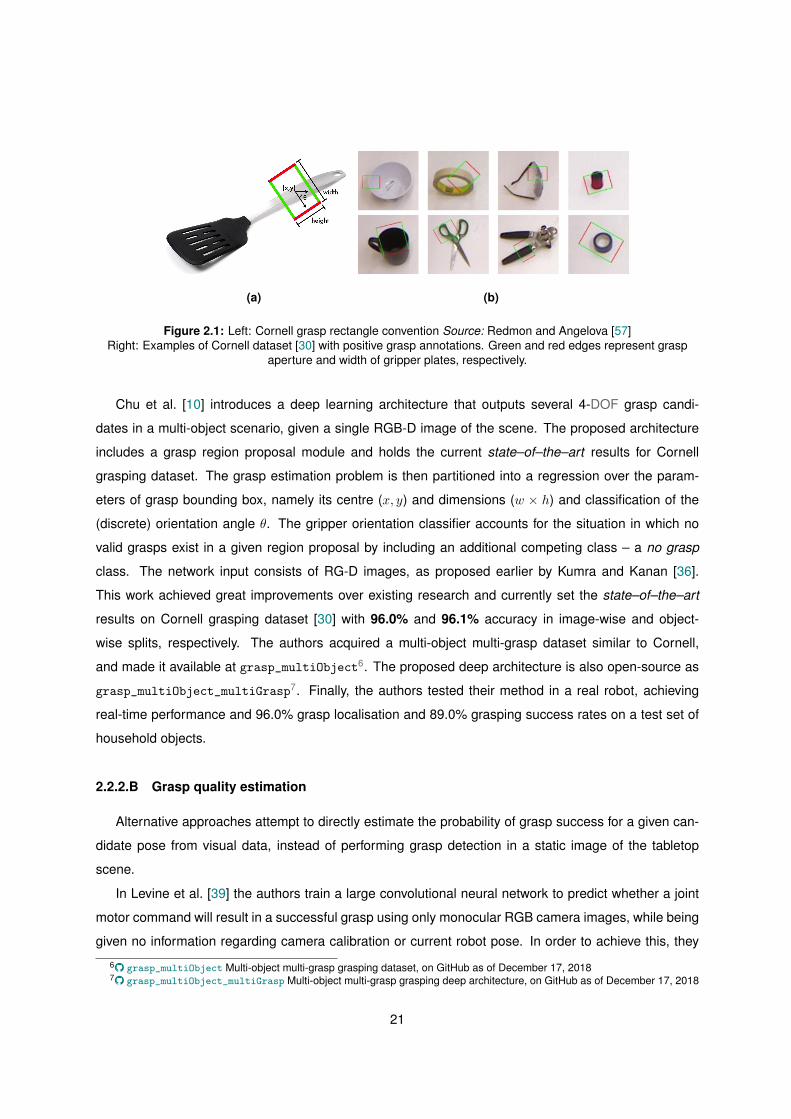
Lenz et al. [38] formulates grasping as a detection task for real RGB-D images. Specifically, grasps

are represented as oriented rectangles in the image plane, defined by rectangle centre (x, y), angle

θ and gripper aperture w (rectangle width), as well as the height of the gripper z with respect to the

image plane (check Figure 2.1(a)). Upright gripper grasps are usually referred to as 4-DOF, as only

(x, y, z, θ) can be changed (the width of the gripper is usually not considered in this convention). The

grasp detection is achieved by a two-step cascaded structure with two deep neural networks. The first

network eliminates unlikely grasp candidates quickly and provides the second with its top detections. The

second network is slower, but evaluates fewer grasp candidates. This research improved and greatly

helped establish the Cornell grasping dataset5 – initially proposed in Jiang et al. [30] – as a benchmark

for state–of–the–art grasp detection methods. The latter consists of 1035 real-life RGB-D images of 280

graspable objects, each manually annotated with several ground truth grasp candidates and respective

binary success label. Examples of this dataset are represented in Figure 2.1(b).

Additional modalities have been fused with RGB-D image data for grasping tasks. For instance,

Guo et al. [20] proposes a hybrid deep architecture that fuses visual and tactile perception. The visual

component of their method is also tested on Cornell grasping dataset [30]. To train and evaluate the

tactile module, the authors collect a novel dataset containing visual, tactile and grasp configuration

information, using a real UR5 robotic arm, a Barret hand and a Kinect 2 sensor.3GraspIt! webpage http://graspit-simulator.github.io/, as of December 17, 20184We describe Coulomb friction model in detail in Section 1.2.2.A.5Cornell grasping dataset http://pr.cs.cornell.edu/deepgrasping/, as of December 17, 2018

20

(a) (b)

Figure 2.1: Left: Cornell grasp rectangle convention Source: Redmon and Angelova [57]Right: Examples of Cornell dataset [30] with positive grasp annotations. Green and red edges represent grasp

aperture and width of gripper plates, respectively.

Chu et al. [10] introduces a deep learning architecture that outputs several 4-DOF grasp candi-

dates in a multi-object scenario, given a single RGB-D image of the scene. The proposed architecture

includes a grasp region proposal module and holds the current state–of–the–art results for Cornell

grasping dataset. The grasp estimation problem is then partitioned into a regression over the param-

eters of grasp bounding box, namely its centre (x, y) and dimensions (w × h) and classification of the

(discrete) orientation angle θ. The gripper orientation classifier accounts for the situation in which no

valid grasps exist in a given region proposal by including an additional competing class – a no grasp

class. The network input consists of RG-D images, as proposed earlier by Kumra and Kanan [36].

This work achieved great improvements over existing research and currently set the state–of–the–art

results on Cornell grasping dataset [30] with 96.0% and 96.1% accuracy in image-wise and object-

wise splits, respectively. The authors acquired a multi-object multi-grasp dataset similar to Cornell,

and made it available at grasp_multiObject6. The proposed deep architecture is also open-source as

grasp_multiObject_multiGrasp7. Finally, the authors tested their method in a real robot, achieving

real-time performance and 96.0% grasp localisation and 89.0% grasping success rates on a test set of

household objects.

2.2.2.B Grasp quality estimation

Alternative approaches attempt to directly estimate the probability of grasp success for a given can-

didate pose from visual data, instead of performing grasp detection in a static image of the tabletop

scene.

In Levine et al. [39] the authors train a large convolutional neural network to predict whether a joint

motor command will result in a successful grasp using only monocular RGB camera images, while being

given no information regarding camera calibration or current robot pose. In order to achieve this, they

6� grasp_multiObject Multi-object multi-grasp grasping dataset, on GitHub as of December 17, 20187� grasp_multiObject_multiGrasp Multi-object multi-grasp grasping deep architecture, on GitHub as of December 17, 2018

21

gathered a dataset of upwards of 800.000 grasp trials, using between 6 to 14 robotic manipulators over

the course of several months. Even though the results were favourable, this clearly illustrates how time

and overall resource consuming it is to acquire such a dataset. The authors provide a supplementary

video8 showcasing their work.

Mahler et al. [42] introduces Dex-Net 1.0, a novel grasp proposal model which relies on a large

database with over 10.000 objects autonomously labelled with grasp candidates for parallel-plate grip-

pers and respective analytic quality metrics. The emphasis is centred around a scalable retrieval system

that can be deployed in a cloud computing scenario. Mahler et al. [43] builds upon previous work and

trains a Grasp Quality CNN (GQ-CNN) to predict grasp success given a corresponding depth image.

This work was named Dex-Net 2.0 and its contributions include (i) a new dataset of over 6.7 million point

clouds and analytic grasp metrics corresponding to sampled grasp candidates, which are planned for

a subset of 1500 Dex-Net 1.0 objects; (ii) the novel GQ-CNN model that classifies a candidate grasp

as success or failure given an overhead depth image overlooking an uncluttered single-object table-

top scenario; (iii) a grasp planning method that samples 4-DOF grasp candidates and ranks them with

GQ-CNN. Later, the authors went on to extend this work in order to propose suction gripper grasps [44].

Section 4.1.2 provides additional details on the Dex-Net 2.0 pipeline.

Rather than treating grasp perception as a detection of grasp rectangles in depth images, ten Pas

et al. [69] tackles the harder problem of 3D space, 6-DOF grasping using parallel-plate grippers. The

work incorporates and extends two prior conference publications [68, 19]. The authors’ algorithmic

contributions include (i) a novel method for generating grasp proposals without precise target object

segmentation; (ii) a grasp descriptor that incorporates surface normals and multiple RGB-D camera

viewpoints; (iii) a method for incorporating prior knowledge regarding the category of the target object.

Furthermore, the authors introduce a method for detecting grasps for a specific target object by combin-

ing grasp and object detection. Their framework is tested in a dense clutter pick and place task with a real

Baxter robot. This work introduces a novel method for evaluating grasp detection performance in terms

of recall at an elevated level of precision, i.e. imposing a constraint on the number of false positives.

Their novel grasp representations are generated from a point cloud in the gripper-closing region, with

information regarded the visible and occluded geometry. A simulated dataset is created to pre-train their

proposed algorithm Grasp Pose Detector gpd9 , using object meshes from ShapeNet [9]. Grasps are

evaluated as positive or negative candidates by testing if they are frictionless antipodal, which not only

requires them to be force-closure but to also verify the latter condition for any positive friction coefficient.

Yan et al. [77] tackles the problem of evaluating grasp configurations in unconstrained 3D space

from RGB-D data, generalising to 6-DOF unlike most existing approaches, which impose upright grasp-

ing configurations. The authors introduce a deep geometry-aware grasping network (DGGN) which is

8v video Learning Hand-Eye Coordination for Robotic Grasping on YouTube, as of December 17, 20189� atenpas/gpd Grasp Pose Detector, on GitHub as of December 17, 2018

22

trained in a two-step fashion. Firstly, the network learns a compact object 3D shape representation in

the form of occupancy grid from RGB-D input. This is achieved in a weakly supervised manner in the

sense that instead of directly evaluating the voxelised representation, they instead render a depth image

which is then compared to the ground truth image. Secondly, this internal representation is used to

learn the outcome of a given grasp proposal. This works contribution includes (i) a novel method for

6-DOF grasping from RGB-D input; (ii) grasping dataset acquired in simulation resorting to virtual reality

to obtain over 150.000 human demonstrations; (iii) the model outperformed state–of–the–art baseline

CNNs in outcome prediction task; (iv) the model generalises to novel viewpoints and unseen objects.

Morrison et al. [47] proposes an object-indiscriminate grasp synthesis method which can be used for

real-time closed loop 4-DOF upright grasping for 2-fingered grippers. The authors introduce the Gener-

ative Grasping CNN (GG-CNN) which maps each pixel of an input depth image to a grasp configuration

and associated predicted quality. This 1-to-1 mapping effectively bypasses the need to sample numer-

ous grasp candidates and estimate their quality individually, which leads to long computation times. The

network is trained on a pre-processed and augmented Cornell dataset. It produces four different out-

puts, mapping a single depth frame to essentially four single-channel images, predicting respectively

pixel-wise grasp quality Q, gripper width W and cosine and sine encoding of the gripper angle Φ. The

system is evaluated on a real Kinova Mico arm10 in single object and cluttered environments in both

static and dynamic situations. Their implementation is available on GitHub as GG-CNN11.

2.2.2.C End-to-end reinforcement learning

Reinforcement Learning (RL) allows us to formulate grasp planning as an end to end motor control

problem, as an agent continually retrieves sensorial data from the scene and outputs motor commands.

Typically, in doing so we can couple the reaching and grasping into a single learning task, unlike the

previous methods which focused mainly on the latter.

Supervised learning methods typically do not take into account the sequential aspect of the grasp-

ing task, instead choosing a course of action at the outset or continuously attempting the next most

promising grasp candidate, in a greedy fashion.

Quillen et al. [56] explores RL using deep neural networks for vision-based robotic grasping. Their

work introduces a simulated benchmark for robotic grasping algorithms which favour off-policy learning

and aim to generalise to novel objects. The authors claim that off-policy learning is suitable for grasp-

ing, as it should allow for better generalisation capabilities, by allowing the agent to explore diverse

actions. It features a comparative analysis of several methods and concludes that even simple methods

achieved performance comparable to that of popular algorithms such as double Q-learning. This work’s

10Kinova Mico arm webpage https://www.kinovarobotics.com/en/products/robotic-arm-series/mico-robotic-arm, asof December 17, 2018

11� dougsm/ggcnn Generative Grasping CNN, on GitHub as of December 17, 2018

23

contributions include an open-source simulated Gym environment12 , using PyBullet13 which features a

6-DOF KUKA iiwa14 robotic arm with a 2-fingered gripper for a bin-picking task. Additionally, the authors

benchmark six different methods, namely (i) grasp success prediction proposed by Levine et al. [39],

(ii) double Q-learning [21], (iii) Path Consistency Learning (PCL) [48], (iv) Deep Deterministic Policy

Gradient (DDPG), (v) Monte Carlo Policy Evaluation, and (vi) Corrected Monte Carlo. Each algorithm

is evaluated by overall performance, data-efficiency, robustness to off-policy data and hyper-parameter

sensitivity.

Gualtieri and Platt [18] addresses 6-DOF manipulation for parallel-plate grippers, by formulating

the problem as a Markov decision process (MDP) with abstract states and actions (Sense-Move-Effect

MDP). The authors propose a set of constraints which causes the robot to learn a sequence of gazes

to focus attention on the aspects of the scene relevant to the task at hand. Additionally, they introduce

a novel system which leverages the aforementioned contributions and can learn either, picking, placing

or pick-and-place tasks. The learning model is trained in OpenRAVE15 simulated environment, but also

tested in a real UR5 robotic arm equipped with a Robotiq 85 parallel-jaw gripper and a Structure depth

camera. The authors compare their approach’s performance with GPD, proposed by ten Pas et al. [69],

and found it to beat then-state–of–the–art results for grasping success rates. This was verified for the

case where the algorithm is allowed to perform 10 separate independent runs, and choose the highest

valued state-action value. Without sampling, their method proved inferior to the baseline in some specific

tasks.

2.2.2.D Dexterous grasping

Few data-driven approaches employing deep neural networks and synthetic data focus on the harder

problem of dexterous grasp planning, i.e. finding appropriate grasp poses for multi-fingered robotic

manipulators.

Veres et al. [75] proposes the novel concept of grasp motor image (GMI), which combines object per-

ception and a learned prior over grasp configurations to produce new grasp configurations to be applied

to different and unseen objects. This work focuses on the use of motor imagery for creating internal

representations of an action, requiring some prior knowledge of the object properties. Its main contribu-

tions include showing that a unified space of generic object properties and prior experience of grasping

similar objects can be constructed to allow grasp synthesis for novel objects. Secondly, it provides a

probabilistic framework, leveraging deep generative architectures, namely Conditional Variational Auto-

Encoders (CVAEs) to learn multi-modal grasping distributions for multi-fingered robotic hands. The

12KUKA Gym environment https://goo.gl/jAESt9, as of December 17, 201813PyBullet webpage https://pybullet.org/wordpress/, as of December 17, 201814KUKA iiwa arm webpage https://www.kuka.com/en-de/products/robot-systems/industrial-robots/lbr-iiwa, as of

December 17, 201815OpenRAVE robotics simulator http://openrave.org/, as of December 17, 2018

24

authors collect a dataset of cylindrical precision robotic grasps and corresponding RGB-D images, em-

ploying the setup designed in Veres et al. [76]. The latter is built within V-REP16 simulator and generates

grasp success labels and corresponding contact points and force normals with full dynamic simulation.

This dataset generation pipeline is open-source an available as multi-contact-grasping17. The auto-

encoder network is given RGB-D images and is trained to output contact points and respective surface

normals.

2.3 Domain Randomisation

The previous sections have described how Convolutional Neural Networks (CNNs)became the state–of–the–art method for several visual perception tasks, and de-scribed several data-driven robotic grasp pipelines. Among the latter, we high-lighted many works that employ synthetic data generated in virtual robotic environ-ments, which may underperform when directly transferred to real robots, due to theso-called reality gap. In this section, we present relevant research on Domain Ran-domisation (DR), which is becoming an increasingly known technique for allowingknowledge transfer from fully simulated domains to real-world robots.

In our work, we decided to differentiate between two different types of DR depending on which

properties are randomised. Specifically, we start by verifying the effectiveness of DR applied to visual

perception tasks, and then move on to a robotics scenario, in which the technique is applied to the

physical properties of the system. The literature review follows a similar two-part approach.

2.3.1 Visual domain randomisation

Domain randomisation was employed in the creation of simulated tabletop scenarios to train real-

world object detectors with position estimation. The work of Tobin et al. [70] aims to predict the 3D

position of a single object from single low-fidelity 2D RGB images with a network trained in a simulated

environment. This prediction must be sufficiently accurate to perform a grasp action on the object in a

real-world setting. This work’s main contribution is proving that indeed a model trained solely on sim-

ulated data generated employing DR was able to generalise to the real-world setting without additional

training. Moreover, it shows that this technique can be useful for robotic tasks that require precision.

Their method estimates a specific object’s 3D position with an accuracy of 1.5 cm, succeeding in 38 out

of 40 trials, and was the first successful transfer from a fully simulated domain to reality in the context of

robotic control. Furthermore, it provides an example of properties that can be easily randomised in sim-

ulation, namely object position, colour and texture as well as lighting conditions. Moreover, the authors

introduce distractor objects with the purpose of improving robustness to clutter in the scene. Their model16V-REP simulator http://www.coppeliarobotics.com/, as of December 17, 201817� mveres01/multi-contact-grasping Dexterous grasping dataset generation pipeline, on GitHub as of December 17, 2018

25

uses CNNs trained using hundreds of thousands of 2D low resolution renders of randomly generated

scenes. Specifically, the authors employ a modified VGG-16 architecture [65] and use the MuJoCo18

[72] physics simulation environment.

Zhang et al. [78] proposes a method to transfer visuomotor policies from simulation to a real-world

robot by combining DR and domain adaptation in an object reaching task. The authors split the system

into perceptual and control modules, which are connected by a bottleneck layer. During training, this

layer is assigned the position x∗ of the target object, so the network in the perceptual module effectively

learns how to accurately predict its value, given an RGB image. The control module learns to compute

appropriate motor commands in the joint velocity space v, given the object position x∗ and current joint

angles q. The networks are trained using data acquired with V-REP in a table-top reaching in clutter

scenario for a Baxter robot equipped with a suction gripper. The authors employ DR by (i) cluttering

the scene with parametric distractor objects, with a random flat colour texture; (ii) randomising the initial

robotic arm joint configuration; (iii) altering the colours of the table, floor, robot and target cuboid (±10%

w.r.t. original colours); (iv) marginally changing camera pose and camera Field of View (FoV); (v) slightly

disturbing initial table pose. Domain adaptation is introduced by also using real-world images to fine-tune

the perception module. The control module is trained to output the velocity commands given by V-REP

simulator in order to achieve its Inverse Kinematics (IK) solution obtained via an internally implemented

method, in a supervised manner as well. By employing a suction gripper in place of a conventional

robotic fingered manipulator, the grasping physics simulation can be bypassed.

James et al. [29] explores a tabletop scenario with the objective of performing a simple pick and

place routine with an end-to-end control approach, using DR during the data generation. The authors

introduced an end-to-end (image to joint velocities) controller that is trained on purely synthetic data from

a simulator. The task at hand is a multi-stage action that involves the detection of a cube, picking it up and

dropping it in a basket. To fulfil this task, a reactive neural network controller is trained to continuously

output motor velocities given a live image feed. Figure 2.2 depicts several randomly generated synthetic

scenes.

The authors report that without using DR it was possible to fulfil the task 100% of the time in sim-

ulation. However, the performance degrades in the real-world setting if the model is directly applied.

Specifically, the gripper was only able to reach the vicinity of the cube 72% of the times, and did not

succeed even once in lifting it off the table. This work further analyses relevant research questions,

namely (1) what is the impact on the performance when varying the training data size?; (2) which prop-

erties should be randomised during simulation?; and (3) which are the additional features that may

complement the image information (e.g. joint angles) and improve the performance? To answer these

questions, the authors assessed the importance of each randomised properties in the simulated training

18MuJoCo simulation environment webpage http://www.mujoco.org/, as of December 17, 2018

26

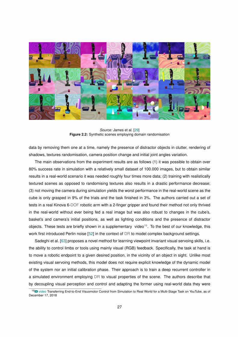
Source: James et al. [29]Figure 2.2: Synthetic scenes employing domain randomisation

data by removing them one at a time, namely the presence of distractor objects in clutter, rendering of

shadows, textures randomisation, camera position change and initial joint angles variation.

The main observations from the experiment results are as follows (1) it was possible to obtain over

80% success rate in simulation with a relatively small dataset of 100.000 images, but to obtain similar

results in a real-world scenario it was needed roughly four times more data; (2) training with realistically

textured scenes as opposed to randomising textures also results in a drastic performance decrease;

(3) not moving the camera during simulation yields the worst performance in the real-world scene as the

cube is only grasped in 9% of the trials and the task finished in 3%. The authors carried out a set of

tests in a real Kinova 6-DOF robotic arm with a 2-finger gripper and found their method not only thrived

in the real-world without ever being fed a real image but was also robust to changes in the cube’s,

basket’s and camera’s initial positions, as well as lighting conditions and the presence of distractor

objects. These tests are briefly shown in a supplementary video19. To the best of our knowledge, this

work first introduced Perlin noise [52] in the context of DR to model complex background settings.

Sadeghi et al. [63] proposes a novel method for learning viewpoint invariant visual servoing skills, i.e.

the ability to control limbs or tools using mainly visual (RGB) feedback. Specifically, the task at hand is

to move a robotic endpoint to a given desired position, in the vicinity of an object in sight. Unlike most

existing visual servoing methods, this model does not require explicit knowledge of the dynamic model

of the system nor an initial calibration phase. Their approach is to train a deep recurrent controller in

a simulated environment employing DR to visual properties of the scene. The authors describe that

by decoupling visual perception and control and adapting the former using real-world data they were19v video Transferring End-to-End Visuomotor Control from Simulation to Real World for a Multi-Stage Task on YouTube, as of

December 17, 2018

27

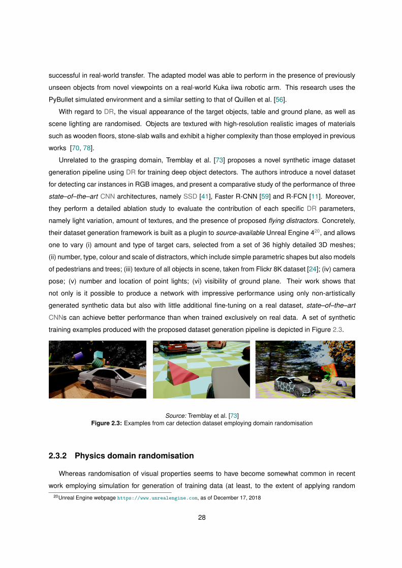
successful in real-world transfer. The adapted model was able to perform in the presence of previously

unseen objects from novel viewpoints on a real-world Kuka iiwa robotic arm. This research uses the

PyBullet simulated environment and a similar setting to that of Quillen et al. [56].

With regard to DR, the visual appearance of the target objects, table and ground plane, as well as

scene lighting are randomised. Objects are textured with high-resolution realistic images of materials

such as wooden floors, stone-slab walls and exhibit a higher complexity than those employed in previous

works [70, 78].

Unrelated to the grasping domain, Tremblay et al. [73] proposes a novel synthetic image dataset

generation pipeline using DR for training deep object detectors. The authors introduce a novel dataset

for detecting car instances in RGB images, and present a comparative study of the performance of three

state–of–the–art CNN architectures, namely SSD [41], Faster R-CNN [59] and R-FCN [11]. Moreover,

they perform a detailed ablation study to evaluate the contribution of each specific DR parameters,

namely light variation, amount of textures, and the presence of proposed flying distractors. Concretely,

their dataset generation framework is built as a plugin to source-available Unreal Engine 420, and allows

one to vary (i) amount and type of target cars, selected from a set of 36 highly detailed 3D meshes;

(ii) number, type, colour and scale of distractors, which include simple parametric shapes but also models

of pedestrians and trees; (iii) texture of all objects in scene, taken from Flickr 8K dataset [24]; (iv) camera

pose; (v) number and location of point lights; (vi) visibility of ground plane. Their work shows that

not only is it possible to produce a network with impressive performance using only non-artistically

generated synthetic data but also with little additional fine-tuning on a real dataset, state–of–the–art

CNNs can achieve better performance than when trained exclusively on real data. A set of synthetic

training examples produced with the proposed dataset generation pipeline is depicted in Figure 2.3.

Source: Tremblay et al. [73]Figure 2.3: Examples from car detection dataset employing domain randomisation

2.3.2 Physics domain randomisation

Whereas randomisation of visual properties seems to have become somewhat common in recent

work employing simulation for generation of training data (at least, to the extent of applying random20Unreal Engine webpage https://www.unrealengine.com, as of December 17, 2018

28

flat colour textures to objects), few authors explicitly mention applying it to physical properties of the

virtual scenario. Moreover, one can apply DR to the procedure of generating grasp target objects, thus

foregoing the need for accurate 3D meshes of real objects, or time-consuming artistic 3D models of

household items.

In Tobin et al. [71] the authors created a pipeline for data generation which includes creating random

3D object meshes, and a deep learning model that both proposes possible grasp configurations and

scores each of them with regard to their predicted efficiency. Their work proposes an autoregressive

architecture that maps a set of observations of an object to a distribution over grasps. Its contributions

are twofold (i) an object generation module and (ii) a grasp sampling method with corresponding grasp

quality prediction network. Regarding the former, millions of unique objects are created by the concate-

nation of small convex blocks segmented from 3D objects present in the popular ShapeNet dataset [9].

Specifically, over 40,000 3D object meshes were decomposed into more than 400,000 approximately

convex parts using V-HACD21. Then, grasps are sampled uniformly in 4 and 6-dimensional grasp space.

Each dimension is discretised into 20 buckets, with each bucket corresponding to a grasp point, within

the object’s bounding box. Grasps which do not touch the object can be discarded at the outset. For

each trial, a depth image is collected from the robot’s hand camera.

The model itself consists of two neural networks, one for grasp planning and the other for grasp

evaluation. The former is used to sample grasps which are likely to be successful whereas the latter

leverages more detailed information from the close-up depth image of the gripper’s camera. The network

is trained in simulation, using MuJoCo physics simulator. Their method was evaluated in simulation with

a set of previously unseen realistic objects achieving a high (> 90%) success rate. It demonstrates the

use of DR tools in order to generate a large dataset of random unrealistic objects and generalise to

unseen realistic objects. However, it should be mentioned that their experiments are all performed in a

simulated environment. In this case, the knowledge transfer between domains refers to the transition

from procedurally generated unrealistic object meshes to 3D models of real-life objects.

Related work has also fused visual and physics-based Domain Randomisation (DR), in order to

achieve real-world transfer in the context of visual servoing [6] and in-hand manipulation [51].

Bousmalis et al. [6] proposes an alternative to DR in order to leverage synthetic data in a real-world

4-DOF upright grasping task using images from a monocular RGB camera. The authors study a range

of domain adaptation methods and introduce GraspGAN, a generative adversarial method for pixel-level

domain adaptation. This work further tests the proposed methods in a real-world scenario, achieving

the first successful simulation-to-real-world transfer for purely monocular vision-based grasping, with a

better performance than that of Levine et al. [39]. Their deep vision-based grasping pipeline is split into

two modules. The first consists of a grasp prediction CNN that outputs the probability of a given motor

21� kmammou/v-hacd Library for near convex part decomposition, on GitHub as of December 17, 2018

29

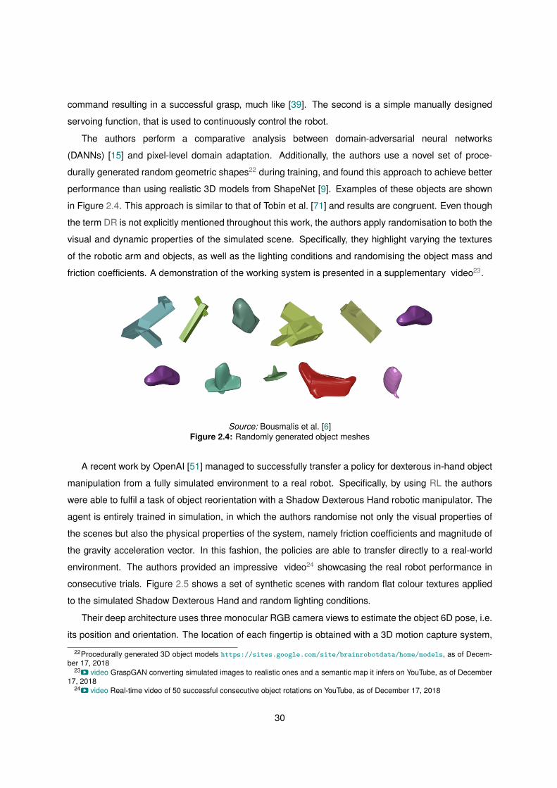
command resulting in a successful grasp, much like [39]. The second is a simple manually designed

servoing function, that is used to continuously control the robot.

The authors perform a comparative analysis between domain-adversarial neural networks

(DANNs) [15] and pixel-level domain adaptation. Additionally, the authors use a novel set of proce-

durally generated random geometric shapes22 during training, and found this approach to achieve better

performance than using realistic 3D models from ShapeNet [9]. Examples of these objects are shown

in Figure 2.4. This approach is similar to that of Tobin et al. [71] and results are congruent. Even though

the term DR is not explicitly mentioned throughout this work, the authors apply randomisation to both the

visual and dynamic properties of the simulated scene. Specifically, they highlight varying the textures

of the robotic arm and objects, as well as the lighting conditions and randomising the object mass and

friction coefficients. A demonstration of the working system is presented in a supplementary video23.

Source: Bousmalis et al. [6]Figure 2.4: Randomly generated object meshes

A recent work by OpenAI [51] managed to successfully transfer a policy for dexterous in-hand object

manipulation from a fully simulated environment to a real robot. Specifically, by using RL the authors

were able to fulfil a task of object reorientation with a Shadow Dexterous Hand robotic manipulator. The

agent is entirely trained in simulation, in which the authors randomise not only the visual properties of

the scenes but also the physical properties of the system, namely friction coefficients and magnitude of

the gravity acceleration vector. In this fashion, the policies are able to transfer directly to a real-world

environment. The authors provided an impressive video24 showcasing the real robot performance in

consecutive trials. Figure 2.5 shows a set of synthetic scenes with random flat colour textures applied

to the simulated Shadow Dexterous Hand and random lighting conditions.

Their deep architecture uses three monocular RGB camera views to estimate the object 6D pose, i.e.

its position and orientation. The location of each fingertip is obtained with a 3D motion capture system,

22Procedurally generated 3D object models https://sites.google.com/site/brainrobotdata/home/models, as of Decem-ber 17, 2018

23v video GraspGAN converting simulated images to realistic ones and a semantic map it infers on YouTube, as of December17, 2018

24v video Real-time video of 50 successful consecutive object rotations on YouTube, as of December 17, 2018

30

which requires 16 PhaseSpace tracking sensors. Finally, a deep control module is trained to output the

motor commands given the current and target object orientation, as well as the fingertip locations.

The authors specify several physical properties to which applying DR improved performance. The

latter are summarised in Table 2.1. This research uses open-source OpenAI gym25 [7] and specifically

its robotics environments [53] and MuJoCo proprietary physics simulator [72].

Source: OpenAI [51]Figure 2.5: Examples of synthetic scenes with random textures applied to the dexterous robotic manipulator.

Three camera views are concurrently fed to the neural network. Each row corresponds to a single cameraviewpoint across scenes.

Property Scaling factor Additive termTarget object size uniform([0.95, 1.05])Object and robot link masses uniform([0.5, 1.5])Surface friction coefficients uniform([0.7, 1.3])Robot joint damping coefficients loguniform([0.3, 3.0])Actuator P gain loguniform([0.75, 1.5])Joint limits N (0, 0.15) radGravity vector N (0, 0.4) ms^{-2}

Table 2.1: Parameters for randomising physical properties. The latter were either scaled by a random scalingfactor or disturbed by a random Gaussian additive term.

25� openai/gym Toolkit for developing and comparing RL algorithms, on GitHub as of December 17, 2018

31

32

3Domain Randomisation for Detection

Contents

3.1 Parametric object detection . . . . . . . . . . . . . . . . . . . . . . . . . . . . . . . . . 35

3.1.1 GAP: A domain randomisation framework for Gazebo . . . . . . . . . . . . . . . . 35

3.2 Proof–of–concept trials . . . . . . . . . . . . . . . . . . . . . . . . . . . . . . . . . . . . 41

3.2.1 Scene generation . . . . . . . . . . . . . . . . . . . . . . . . . . . . . . . . . . . . 41

3.2.2 Preliminary results for Faster R-CNN and SSD . . . . . . . . . . . . . . . . . . . . 42

3.3 Domain randomisation vs fine-tuning . . . . . . . . . . . . . . . . . . . . . . . . . . . 44

3.3.1 Single Shot Detector . . . . . . . . . . . . . . . . . . . . . . . . . . . . . . . . . . 44

3.3.2 Improved scene generation . . . . . . . . . . . . . . . . . . . . . . . . . . . . . . 45

3.3.3 Real images dataset . . . . . . . . . . . . . . . . . . . . . . . . . . . . . . . . . . 46

3.3.4 Experiment: domain randomisation vs fine-tuning . . . . . . . . . . . . . . . . . . 47

3.3.5 Ablation study: individual contribution of texture types . . . . . . . . . . . . . . . . 50

33

Goals transform a random walk into a chase.

Mihaly Csikszentmihaly, 1996

34

3.1 Parametric object detection

In the last chapter, we provided the reader with a brief review of the state–of–the–art methods, starting with the fundamental principles of Convolutional NeuralNetworks (CNNs), exploring how recent proposals explored deep architectures inrobotic grasping tasks and finally the potential of a recently popular technique formoving from simulated to the real-world domain. In this chapter, we wish to startexploring the potential of Domain Randomisation (DR) applied to visual propertiesof a scene for object detection tasks.

The main objective of this section is to explore the application of DR to visual properties of a scene.

The goal is to train a state–of–the–art neural network with synthetic data generated automatically in a

simulator and transfer performance to a real-world application.

We chose the task of vision-based object detection, which involves not only the classification of

several object instances in an image but also determining their corresponding bounding boxes. Even

though the latter is not as informative as pixel-level segmentation masks, recent methods for object

detection have shown to achieve real-time performance [58, 41]. In robotics, it is generally preferable to

produce rough estimates at a high rate than very accurate predictions with a substantial delay, depending

on the problem at hand.

3.1.1 GAP: A domain randomisation framework for Gazebo

Our research is focused on the applications of DR in the field of robotics. As established in Sec-

tion 1.1, real-world robotic trials are both time and resource-consuming. It is usually preferable to run

simulated trials in a robotics environment, due to its many advantages, namely the reproducibility of

experiments and the fact that these can typically be executed faster than real-time.

3.1.1.A Gazebo simulator

We chose Gazebo [34] as the simulation environment for generating synthetic data for our experi-

ments. It is known for its stable integration with ROS1 [55], an increasingly popular robot middleware

platform. The research conducted at our laboratory Vislab2 is heavily reliant on middlewares such as

ROS and YARP3. Ivaldi et al. [26] evaluates the then-existing robotic platforms for full dynamic simula-

tion with the purpose of electing a new environment for which to port the iCub4 robot into. The authors

carried out an online survey in 2014 and found that researchers primarily valued realism, but also using

a uniform Application Programming Interface (API) for both real and simulated robot interaction. This

1ROS Middleware webpage http://www.ros.org/, as of December 17, 20182Vislab webpage http://vislab.isr.ist.utl.pt/, as of December 17, 20183YARP webpage http://www.yarp.it, as of December 17, 20184iCub webpage http://www.icub.org/, as of December 17, 2018

35

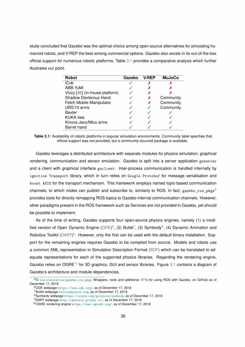
study concluded that Gazebo was the optimal choice among open-source alternatives for simulating hu-

manoid robots, and V-REP the best among commercial options. Gazebo also excels in its out-of-the-box

official support for numerous robotic platforms. Table 3.1 provides a comparative analysis which further

illustrates our point.

Robot Gazebo V-REP MuJoCoiCub 3 7 7ABB YuMi 3 7 7Vizzy [46] (in-house platform) 3 7 7Shadow Dexterous Hand 3 7 CommunityFetch Mobile Manipulator 3 7 CommunityUR5/10 arms 3 3 CommunityBaxter 3 3 3KUKA iiwa 3 3 3Kinova Jaco/Mico arms 3 3 3Barret hand 3 3 3

Table 3.1: Availability of robotic platforms in popular simulation environments. Community label specifies thatofficial support was not provided, but a community-sourced package is available.

Gazebo leverages a distributed architecture with separate modules for physics simulation, graphical

rendering, communication and sensor emulation. Gazebo is split into a server application gzserver

and a client with graphical interface gzclient. Inter-process communication is handled internally by

ignition Transport library, which in turn relies on Google Protobuf for message serialisation and

boost ASIO for the transport mechanism. This framework employs named topic-based communication

channels, to which nodes can publish and subscribe to, similarly to ROS. In fact, gazebo_ros_pkgs5

provides tools for directly remapping ROS topics to Gazebo internal communication channels. However,

other paradigms present in the ROS framework such as Services are not provided in Gazebo, yet should

be possible to implement.

As of the time of writing, Gazebo supports four open-source physics engines, namely (1) a modi-

fied version of Open Dynamic Engine (ODE)6, (2) Bullet7, (3) Symbody8, (4) Dynamic Animation and

Robotics Toolkit (DART)9. However, only the first can be used with the default binary installation. Sup-

port for the remaining engines requires Gazebo to be compiled from source. Models and robots use

a common XML representation in Simulation Description Format (SDF) which can be translated to ad-

equate representations for each of the supported physics libraries. Regarding the rendering engine,

Gazebo relies on OGRE10 for 3D graphics, GUI and sensor libraries. Figure 3.1 contains a diagram of

Gazebo’s architecture and module dependencies.

5� ros-simulation/gazebo_ros_pkgs Wrappers, tools and additional API’s for using ROS with Gazebo, on GitHub as ofDecember 17, 2018

6ODE webpage https://www.ode.org/, as of December 17, 20187Bullet webpage bulletphysics.org, as of December 17, 20188Symbody webpage https://simtk.org/projects/simbody, as of December 17, 20189DART webpage http://dartsim.github.io/, as of December 17, 2018

10OGRE rendering engine https://www.ogre3d.org/, as of December 17, 2018

36

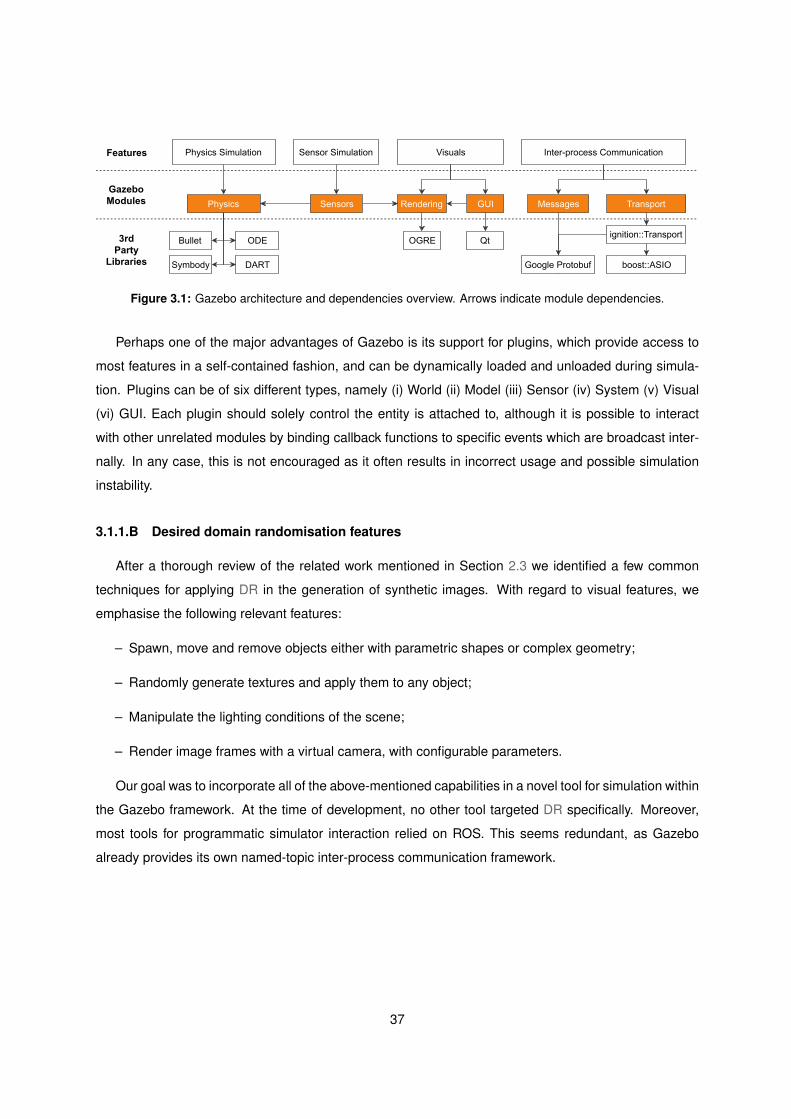
Physics

ODE

DARTSymbody

Bullet

Physics Simulation

3rdParty

Libraries

GazeboModules

Features Inter­process Communication

ignition::Transport

boost::ASIOGoogle Protobuf

Messages Transport

Visuals

GUI

Sensor Simulation

Sensors

QtOGRE

Rendering

Figure 3.1: Gazebo architecture and dependencies overview. Arrows indicate module dependencies.

Perhaps one of the major advantages of Gazebo is its support for plugins, which provide access to

most features in a self-contained fashion, and can be dynamically loaded and unloaded during simula-

tion. Plugins can be of six different types, namely (i) World (ii) Model (iii) Sensor (iv) System (v) Visual

(vi) GUI. Each plugin should solely control the entity is attached to, although it is possible to interact

with other unrelated modules by binding callback functions to specific events which are broadcast inter-

nally. In any case, this is not encouraged as it often results in incorrect usage and possible simulation

instability.

3.1.1.B Desired domain randomisation features

After a thorough review of the related work mentioned in Section 2.3 we identified a few common

techniques for applying DR in the generation of synthetic images. With regard to visual features, we

emphasise the following relevant features:

– Spawn, move and remove objects either with parametric shapes or complex geometry;

– Randomly generate textures and apply them to any object;

– Manipulate the lighting conditions of the scene;

– Render image frames with a virtual camera, with configurable parameters.

Our goal was to incorporate all of the above-mentioned capabilities in a novel tool for simulation within

the Gazebo framework. At the time of development, no other tool targeted DR specifically. Moreover,

most tools for programmatic simulator interaction relied on ROS. This seems redundant, as Gazebo

already provides its own named-topic inter-process communication framework.

37

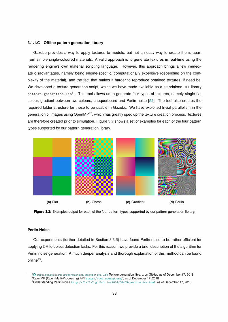
3.1.1.C Offline pattern generation library

Gazebo provides a way to apply textures to models, but not an easy way to create them, apart

from simple single-coloured materials. A valid approach is to generate textures in real-time using the

rendering engine’s own material scripting language. However, this approach brings a few immedi-

ate disadvantages, namely being engine-specific, computationally expensive (depending on the com-

plexity of the material), and the fact that makes it harder to reproduce obtained textures, if need be.

We developed a texture generation script, which we have made available as a standalone C++ library

pattern-generation-lib11. This tool allows us to generate four types of textures, namely single flat

colour, gradient between two colours, chequerboard and Perlin noise [52]. The tool also creates the

required folder structure for these to be usable in Gazebo. We have exploited trivial parallelism in the

generation of images using OpenMP12, which has greatly sped up the texture creation process. Textures

are therefore created prior to simulation. Figure 3.2 shows a set of examples for each of the four pattern

types supported by our pattern generation library.

(a) Flat (b) Chess (c) Gradient (d) Perlin

Figure 3.2: Examples output for each of the four pattern types supported by our pattern generation library.

Perlin Noise

Our experiments (further detailed in Section 3.3.5) have found Perlin noise to be rather efficient for

applying DR to object detection tasks. For this reason, we provide a brief description of the algorithm for

Perlin noise generation. A much deeper analysis and thorough explanation of this method can be found

online13.

11� ruipimentelfigueiredo/pattern-generation-lib Texture generation library, on GitHub as of December 17, 201812OpenMP (Open Multi-Processing) API https://www.openmp.org/, as of December 17, 201813Understanding Perlin Noise http://flafla2.github.io/2014/08/09/perlinnoise.html, as of December 17, 2018

38

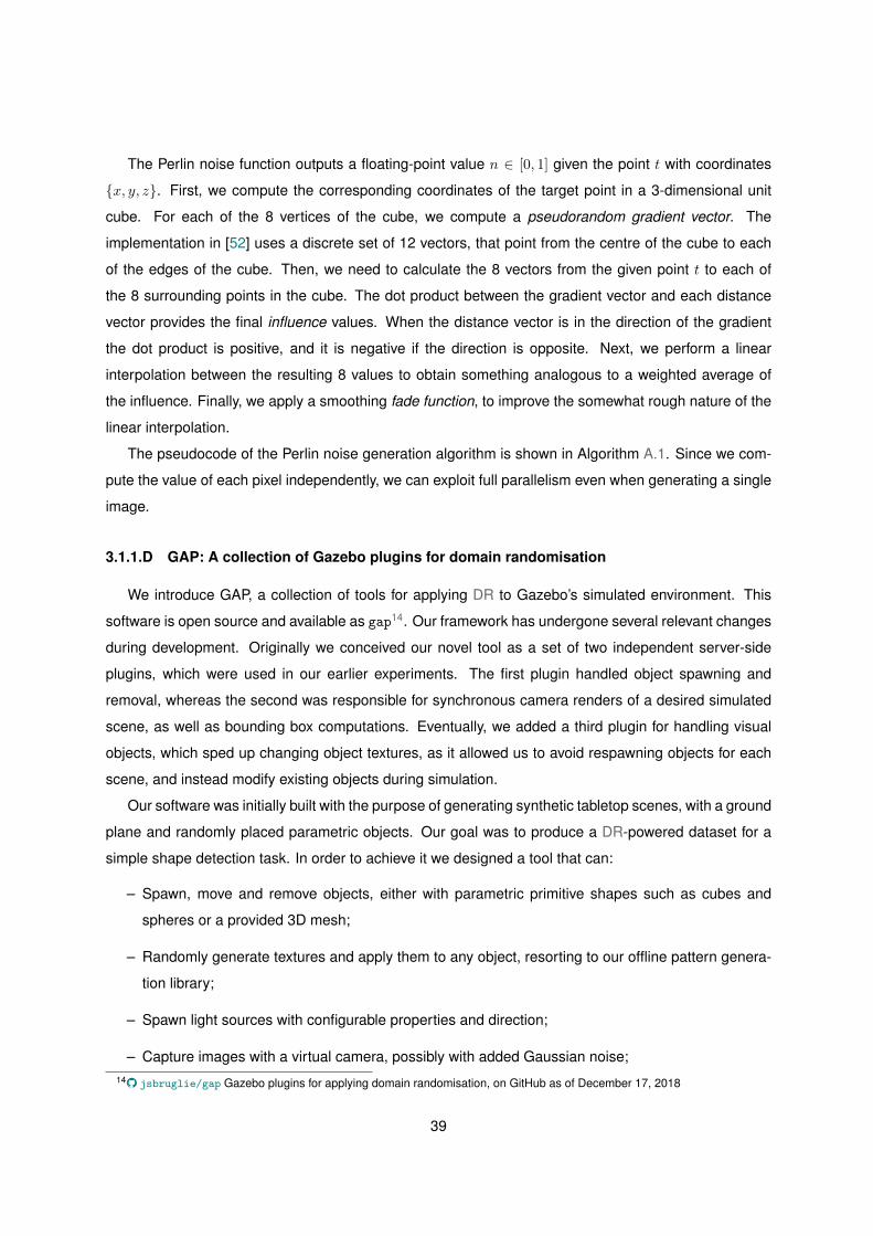
The Perlin noise function outputs a floating-point value n ∈ [0, 1] given the point t with coordinates

{x, y, z}. First, we compute the corresponding coordinates of the target point in a 3-dimensional unit

cube. For each of the 8 vertices of the cube, we compute a pseudorandom gradient vector. The

implementation in [52] uses a discrete set of 12 vectors, that point from the centre of the cube to each

of the edges of the cube. Then, we need to calculate the 8 vectors from the given point t to each of

the 8 surrounding points in the cube. The dot product between the gradient vector and each distance

vector provides the final influence values. When the distance vector is in the direction of the gradient

the dot product is positive, and it is negative if the direction is opposite. Next, we perform a linear

interpolation between the resulting 8 values to obtain something analogous to a weighted average of

the influence. Finally, we apply a smoothing fade function, to improve the somewhat rough nature of the

linear interpolation.

The pseudocode of the Perlin noise generation algorithm is shown in Algorithm A.1. Since we com-

pute the value of each pixel independently, we can exploit full parallelism even when generating a single

image.

3.1.1.D GAP: A collection of Gazebo plugins for domain randomisation

We introduce GAP, a collection of tools for applying DR to Gazebo’s simulated environment. This

software is open source and available as gap14. Our framework has undergone several relevant changes

during development. Originally we conceived our novel tool as a set of two independent server-side

plugins, which were used in our earlier experiments. The first plugin handled object spawning and

removal, whereas the second was responsible for synchronous camera renders of a desired simulated

scene, as well as bounding box computations. Eventually, we added a third plugin for handling visual

objects, which sped up changing object textures, as it allowed us to avoid respawning objects for each

scene, and instead modify existing objects during simulation.

Our software was initially built with the purpose of generating synthetic tabletop scenes, with a ground

plane and randomly placed parametric objects. Our goal was to produce a DR-powered dataset for a

simple shape detection task. In order to achieve it we designed a tool that can:

– Spawn, move and remove objects, either with parametric primitive shapes such as cubes and

spheres or a provided 3D mesh;

– Randomly generate textures and apply them to any object, resorting to our offline pattern genera-

tion library;

– Spawn light sources with configurable properties and direction;

– Capture images with a virtual camera, possibly with added Gaussian noise;14� jsbruglie/gap Gazebo plugins for applying domain randomisation, on GitHub as of December 17, 2018

39

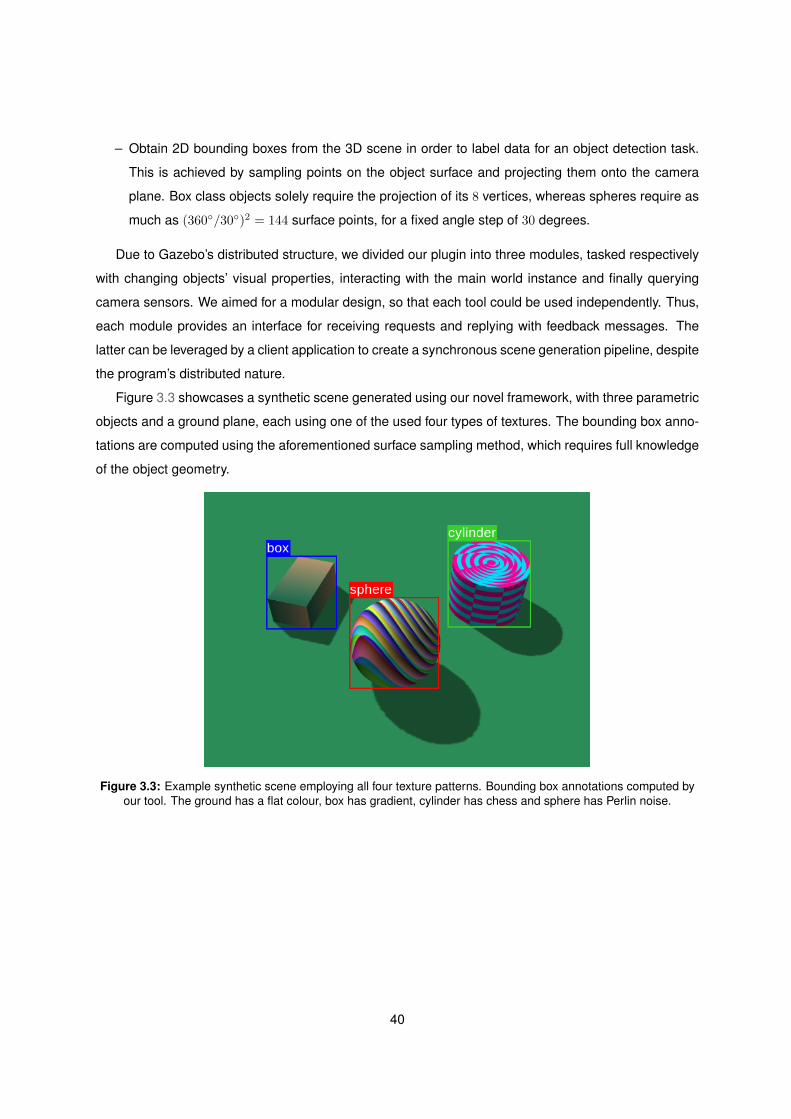
– Obtain 2D bounding boxes from the 3D scene in order to label data for an object detection task.

This is achieved by sampling points on the object surface and projecting them onto the camera

plane. Box class objects solely require the projection of its 8 vertices, whereas spheres require as

much as (360◦/30◦)2 = 144 surface points, for a fixed angle step of 30 degrees.

Due to Gazebo’s distributed structure, we divided our plugin into three modules, tasked respectively

with changing objects’ visual properties, interacting with the main world instance and finally querying

camera sensors. We aimed for a modular design, so that each tool could be used independently. Thus,

each module provides an interface for receiving requests and replying with feedback messages. The

latter can be leveraged by a client application to create a synchronous scene generation pipeline, despite

the program’s distributed nature.

Figure 3.3 showcases a synthetic scene generated using our novel framework, with three parametric

objects and a ground plane, each using one of the used four types of textures. The bounding box anno-

tations are computed using the aforementioned surface sampling method, which requires full knowledge

of the object geometry.

Figure 3.3: Example synthetic scene employing all four texture patterns. Bounding box annotations computed byour tool. The ground has a flat colour, box has gradient, cylinder has chess and sphere has Perlin noise.

40

3.2 Proof–of–concept trials

In the previous section we introduced GAP, a novel framework for applying DomainRandomisation (DR) to visual properties within the Gazebo robotics simulation en-vironment. We described its architecture and main features toward the generationof a synthetic dataset for an object detection task. In this section, we specify howthis dataset was created and elaborate on preliminary trials using state–of–the–artCNNs, namely SSD and Faster R-CNN.

3.2.1 Scene generation

With our novel DR tool integrated with the Gazebo simulated environment, we constructed a tabletop

scene generation pipeline. We started by producing 5.000 textures for each of the four supported pattern

types (flat colour, gradient, chess and Perlin noise) using our offline pattern generation tool. Then, we

wrote a client script to spawn simple parametric shapes, namely spheres, cubes and cylinders placed in

a grid, with random textures, sampled uniformly from the aforementioned set of 20k textures. For each

scene, we acquire a RGB frame and automatic annotations including object bounding boxes and class

labels.

Specifically, each synthetic tabletop-like scene incorporates a ground plane, a single light source and

the set of parametric objects. Each object is constrained to occupy a cell in a grid, although they can

rotate freely provided they are supported by the ground plane. The objects can be partially occluded in

the resulting image frame, but do not collide. Even though we deactivate physics simulation, the objects

in the scene should be in a plausible and stable pose.

The scene generation procedure consists of four steps:

1. Spawn camera and a random number N ∈ [5, 10] of parametric shapes. Each object is put in one

of 25 cells in a 5 by 5 grid.

2. Request to move camera and light source to random positions, sampled from a dome surface, with

its centre directly above the world origin, so as to ensure all objects are in the camera’s FoV.

3. Obtain object bounding boxes, by sampling 3D object surface points and project them onto the 2D

image plane.

4. Save image of the scene, as well as object bounding box and class annotations. The latter are

compatible with PASCAL VOC 2012 [13] annotation format.

We provide examples of synthetic scenes created with our novel framework in Figure 3.4.

With the first version of our pipeline setup, we managed to create a dataset of 9.000 synthetic scenes.

The texture generation process took little over 20 minutes, but is heterogeneous with regard to required

41

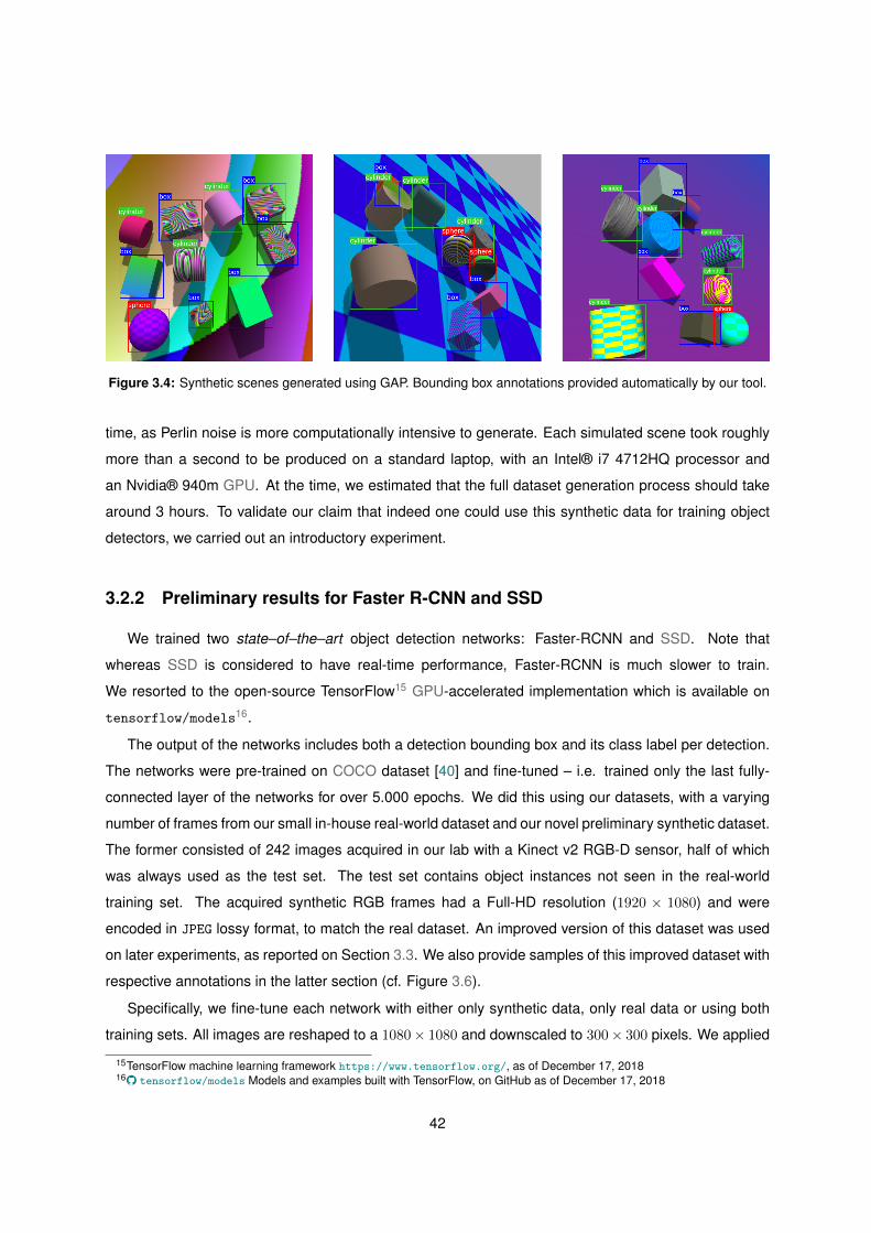
Figure 3.4: Synthetic scenes generated using GAP. Bounding box annotations provided automatically by our tool.

time, as Perlin noise is more computationally intensive to generate. Each simulated scene took roughly

more than a second to be produced on a standard laptop, with an Intel® i7 4712HQ processor and

an Nvidia® 940m GPU. At the time, we estimated that the full dataset generation process should take

around 3 hours. To validate our claim that indeed one could use this synthetic data for training object

detectors, we carried out an introductory experiment.

3.2.2 Preliminary results for Faster R-CNN and SSD

We trained two state–of–the–art object detection networks: Faster-RCNN and SSD. Note that

whereas SSD is considered to have real-time performance, Faster-RCNN is much slower to train.

We resorted to the open-source TensorFlow15 GPU-accelerated implementation which is available on

tensorflow/models16.

The output of the networks includes both a detection bounding box and its class label per detection.

The networks were pre-trained on COCO dataset [40] and fine-tuned – i.e. trained only the last fully-

connected layer of the networks for over 5.000 epochs. We did this using our datasets, with a varying

number of frames from our small in-house real-world dataset and our novel preliminary synthetic dataset.

The former consisted of 242 images acquired in our lab with a Kinect v2 RGB-D sensor, half of which

was always used as the test set. The test set contains object instances not seen in the real-world

training set. The acquired synthetic RGB frames had a Full-HD resolution (1920 × 1080) and were

encoded in JPEG lossy format, to match the real dataset. An improved version of this dataset was used

on later experiments, as reported on Section 3.3. We also provide samples of this improved dataset with

respective annotations in the latter section (cf. Figure 3.6).

Specifically, we fine-tune each network with either only synthetic data, only real data or using both

training sets. All images are reshaped to a 1080× 1080 and downscaled to 300× 300 pixels. We applied

15TensorFlow machine learning framework https://www.tensorflow.org/, as of December 17, 201816� tensorflow/models Models and examples built with TensorFlow, on GitHub as of December 17, 2018

42

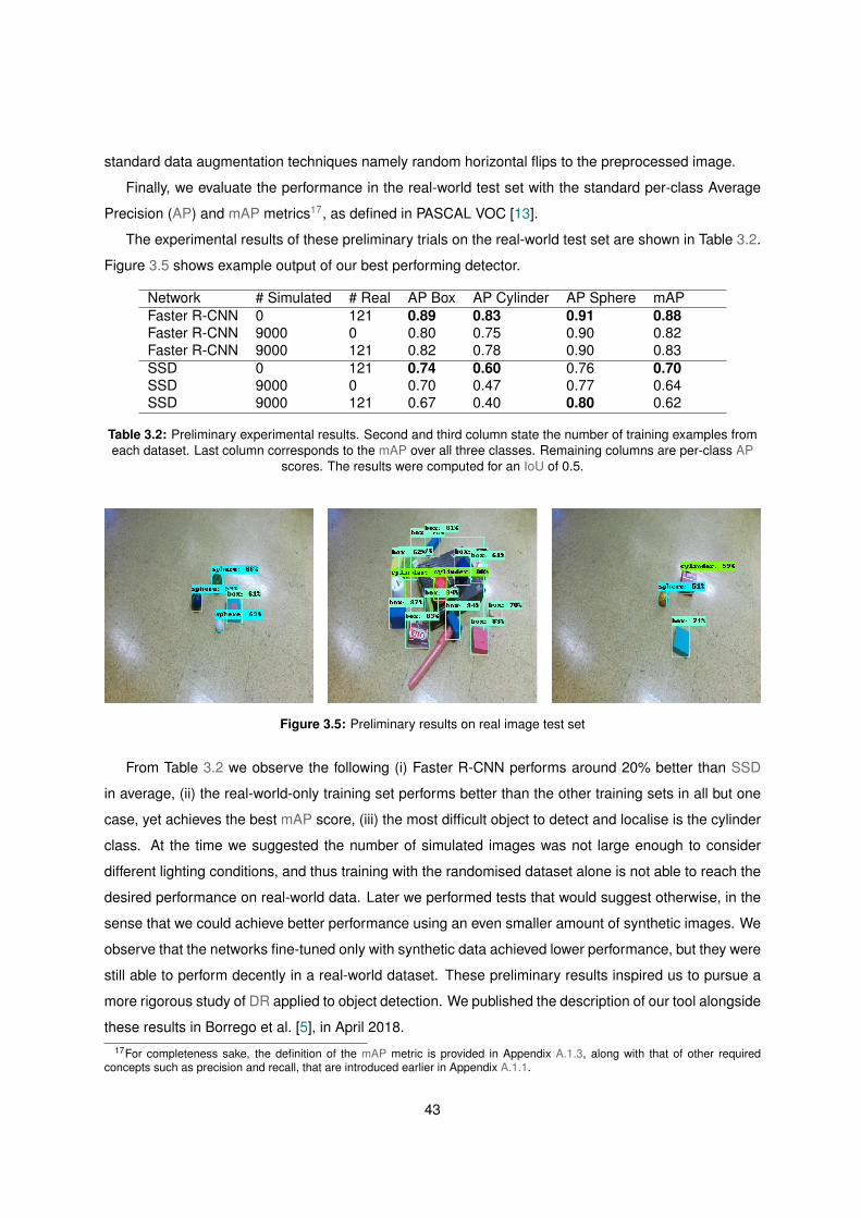
standard data augmentation techniques namely random horizontal flips to the preprocessed image.

Finally, we evaluate the performance in the real-world test set with the standard per-class Average

Precision (AP) and mAP metrics17, as defined in PASCAL VOC [13].

The experimental results of these preliminary trials on the real-world test set are shown in Table 3.2.

Figure 3.5 shows example output of our best performing detector.

Network # Simulated # Real AP Box AP Cylinder AP Sphere mAPFaster R-CNN 0 121 0.89 0.83 0.91 0.88Faster R-CNN 9000 0 0.80 0.75 0.90 0.82Faster R-CNN 9000 121 0.82 0.78 0.90 0.83SSD 0 121 0.74 0.60 0.76 0.70SSD 9000 0 0.70 0.47 0.77 0.64SSD 9000 121 0.67 0.40 0.80 0.62

Table 3.2: Preliminary experimental results. Second and third column state the number of training examples fromeach dataset. Last column corresponds to the mAP over all three classes. Remaining columns are per-class AP

scores. The results were computed for an IoU of 0.5.

Figure 3.5: Preliminary results on real image test set

From Table 3.2 we observe the following (i) Faster R-CNN performs around 20% better than SSD

in average, (ii) the real-world-only training set performs better than the other training sets in all but one

case, yet achieves the best mAP score, (iii) the most difficult object to detect and localise is the cylinder

class. At the time we suggested the number of simulated images was not large enough to consider

different lighting conditions, and thus training with the randomised dataset alone is not able to reach the

desired performance on real-world data. Later we performed tests that would suggest otherwise, in the

sense that we could achieve better performance using an even smaller amount of synthetic images. We

observe that the networks fine-tuned only with synthetic data achieved lower performance, but they were

still able to perform decently in a real-world dataset. These preliminary results inspired us to pursue a

more rigorous study of DR applied to object detection. We published the description of our tool alongside

these results in Borrego et al. [5], in April 2018.17For completeness sake, the definition of the mAP metric is provided in Appendix A.1.3, along with that of other required

concepts such as precision and recall, that are introduced earlier in Appendix A.1.1.

43

3.3 Domain randomisation vs fine-tuning

In the last section, we described a synthetic scene generation pipeline for detectingobjects with parametric shapes using state–of–the–art Convolutional Neural Net-works (CNNs). In this section, we will provide an in-depth study on how to improvethe preliminary results. We start by presenting an overview of Single Shot Detec-tor (SSD), which we chose as the object detector used from this point on. Then weperform a comparative study on training SSD on synthetic data employing the prin-ciples of Domain Randomisation (DR), as opposed to fine-tuning an existing modelpre-trained on large domain-generic datasets.

In order to apply an object detector in a new domain, it is often required to collect some training

samples from the domain at hand. Labelling data for object detection is harder than labelling it for

object classification, as bounding box coordinates are needed in addition to target object’s identity, which

increases to the importance of optimally benefiting from the available data.

After data collection, a detector is selected, commonly based on a trade-off between speed and

accuracy, and is fine-tuned using the available target domain data. Our proposal is to use a synthetic

dataset, with algorithmic variations in irrelevant aspects of simulation, instead of relying on networks

pre-trained with datasets which share little resemblance to the task at hand. This approach is further

detailed in this section.

3.3.1 Single Shot Detector

Even though our preliminary results established that Faster R-CNN obtained better performance in

the object detection task, we elected SSD as the base detector. The main reason for this is that SSD

is one of the few detectors that can be applied in real-time while showing a decent accuracy. Once

more, we emphasise that in the field of robotics real-time performance often comes as a necessity for

closed-loop control systems. Furthermore, since SSD is considerably faster to train, we were allowed

to perform a thorough ablation study with respect to the individual contribution of texture types for DR,

which is further detailed in Section 3.3.5.

In any case, we believe that SSD has no property which makes it more or less susceptible to benefit

from DR. Thus, we expect our results to directly generalise to other deep learning based detectors.

We provide a brief description of the inner workings of SSD in this report. However, readers should

refer to the original publication [41] for a comprehensive study of the detector.

At the root of all deep learning based object detectors, there exists a base CNN which is used as a

feature extractor for further down-stream tasks, i.e. bounding box generation and foreground/background

recognition. Similar to YOLO architecture [58], SSD takes advantage of the concept of priors or default

boxes18 where each cell identifies itself as including an object or not, and where this object exists in a18Called anchor box in YOLO.

44

position relative to a default location. However, unlike YOLO, SSD does this at different layers of the

base CNN. Since neurons in different layers of CNNs have different receptive fields in terms of size and

aspect ratios, effectively, objects of various shapes can be detected.

During training, if a ground truth bounding box matches a default box, i.e. they have an IoU of more

than 0.5, the parameters of how to move this box to perfectly match the ground truth are learned by

minimising a smooth L1 metric19. Hard negative mining is used to create a more balanced dataset

between foreground and background boxes. This technique essentially consists of explicitly creating

negative training examples from false positive detections. Finally, Non-Maximum Suppression (NMS) is

used to determine the final location of the objects.

Unlike the original SSD architecture, we used MobileNet [25] as the base CNN for feature extraction

in all experiments. MobileNet changes the connections in a conventional CNN to drastically reduce

its number of parameters, without having a significant toll on performance, relative to a comparable

architecture.

3.3.2 Improved scene generation

In order to lower the execution time of synthetic data generation, we modified the scene creation

script. Originally, each captured image required parametric objects to be generated from a SDF (Sim-

ulation Description Files)20 formatted string, which was altered during run-time in order to allow for

different object dimensions and visuals. Furthermore, objects were created and destroyed in between

scenes. We altered our pipeline so we could instead modify their visual properties directly through the

Gazebo API, reusing existing objects in simulation. We accomplished this by creating a novel plugin that

interacts exclusively with the rendering engine and the objects visual representation21. This approach is

much more efficient than spawning and removing objects each iteration.

We start by spawning the maximum number of objects of each type in the scene, below the ground

plane, where they cannot be seen by the virtual camera sensor. Then, for each scene, the client ap-

plication performs requests to change the objects’ visuals poses, scale and materials. This method

has been widely used to reduce load times in the video game industry, where performance constraints

are ever present. Specifically, objects are created out of bounds and placed in view of the player once

they become relevant. We found this optimisation to be quite effective and obtained almost doubled

performance, generating 9.000 synthetic images in little over 1h30min, albeit resorting to a larger set of

available random textures (a total of 60.000 textures, compared to the reported 20.000), which should

have increased run-time. We believe this contribution to be significant, particularly considering we did

not have to write rendering-specific code to optimise the pipeline.

19For completeness sake, the definition of the L1-norm loss function is provided in Appendix A.1.5.A.20SDF Specification http://sdformat.org/, as of December 17, 201821Check Appendix A.2.1.A for additional implementation details.

45

Additionally, we made several improvements regarding the modularity of each component in the

framework. Other enhancements concern making our tool straightforward to use and to integrate with

other projects, namely the addition of automatic Doxygen22 documentation, which can be found online23

and the ability to use our software kit as a proper CMake24 package, with support for installation and

version system. This essentially translates to providing a shared library to interact with our plugins.

Finally, we provided example clients that showcase how to use each of the developed tools. Among

these is the script used to create the dataset of images of synthetic tabletop scenes.

3.3.3 Real images dataset

It is our goal to apply our object detector to real-world images. We created an improved dataset of

images acquired in our lab with a Kinect v2 RGB-D sensor, part of which were used in our preliminary

trials with both SSD and Faster R-CNN. These scenes include household objects (such as cups, mugs,

balls and cardboard boxes) placed arbitrarily on the ground, or stacked on top of each other, with varying

degrees of occlusion. Each image was manually annotated with object class labels and bounding boxes.

The refined dataset consists of 250 real images, 49 of which contain objects unseen in training, for the

sole purpose of reporting final performance. The train, validation and test partitions of our real image

dataset are specified in Table 3.3.

Training Validation Test Total175 26 49 250

Table 3.3: Number of real images in train, validation and test partitions.

In this dataset, there was no consideration to explicitly keep the percentage of different classes

balanced (Table 3.4). Thus, we have also reported precision-recall curves for each class.

Partition # Box # Cylinder # Sphere TotalTrain set 502 (63%) 209 (26%) 86 (11%) 797Test set 106 (40%) 104 (40%) 53 (20%) 263

Table 3.4: Number of instances and percentage of different classes in the real dataset.

A set of training images from our small in-house dataset is shown in Figure 3.6. Finally, the dataset

has been made available online25.

22Doxygen: Generate documentation from source code http://www.doxygen.nl/, as of December 17, 201823GAP Documentation http://web.tecnico.ulisboa.pt/~joao.borrego/gap/, as of December 17, 201824CMake: tools designed to build, test and package software https://cmake.org/, as of December 17, 201825Real dataset http://vislab.isr.ist.utl.pt/datasets/#shapes2018, as of December 17, 2018

46

Figure 3.6: Real image training set examples

3.3.4 Experiment: domain randomisation vs fine-tuning

We have conducted various experiments and tests to quantify the results of different scenarios.

Initially, two sets of 30k synthetic images were generated. The software modifications we mentioned

in Section 3.3.2 have greatly facilitated this process. These two sets differed from one another by the

degree to which the virtual camera in the scene has changed its location. In the first set, the viewpoint

was fixed, whereas in the other set, its location varied largely across the scene. All synthetic images

have Full-HD (1920 × 1080) resolution and are encoded in JPEG lossy format, to match the training

images from the real images dataset. For training and testing, images are down-scaled to half these

dimensions (960 × 540) which is the resolution employed for all test scenarios in our pipeline.

For baseline calculations, we have used SSD, trained on COCO, and fine-tuned it on the train set

until the performance on the real-image validation set failed to improve. In other experiments, we have

used MobileNet which was trained on ImageNet as the CNN classifier of SSD and first fine-tuned it

on synthetic datasets with bigger learning rates and later, in some experiments, fine-tuned again with

smaller learning rates on the real dataset.

Finally, smaller synthetic datasets of 6k images were generated, each with a type of texture missing,

and an additional baseline for comparison which includes every pattern type. These datasets allowed

us to study the contribution of each individual texture in the final performance, as well as evaluate the

effectiveness of smaller synthetic datasets.

Networks were trained with mini-batches of size 8, on a machine with two Nvidia Titan Xp GPUs, for

a duration depending on the performance in a real image validation set. We have only used horizontal

47

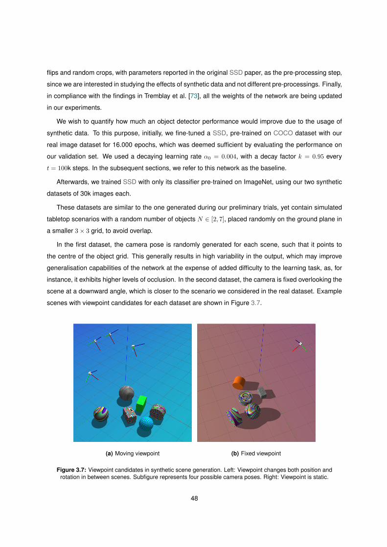
flips and random crops, with parameters reported in the original SSD paper, as the pre-processing step,

since we are interested in studying the effects of synthetic data and not different pre-processings. Finally,

in compliance with the findings in Tremblay et al. [73], all the weights of the network are being updated

in our experiments.

We wish to quantify how much an object detector performance would improve due to the usage of

synthetic data. To this purpose, initially, we fine-tuned a SSD, pre-trained on COCO dataset with our

real image dataset for 16.000 epochs, which was deemed sufficient by evaluating the performance on

our validation set. We used a decaying learning rate α0 = 0.004, with a decay factor k = 0.95 every

t = 100k steps. In the subsequent sections, we refer to this network as the baseline.

Afterwards, we trained SSD with only its classifier pre-trained on ImageNet, using our two synthetic

datasets of 30k images each.

These datasets are similar to the one generated during our preliminary trials, yet contain simulated

tabletop scenarios with a random number of objects N ∈ [2, 7], placed randomly on the ground plane in

a smaller 3× 3 grid, to avoid overlap.

In the first dataset, the camera pose is randomly generated for each scene, such that it points to

the centre of the object grid. This generally results in high variability in the output, which may improve

generalisation capabilities of the network at the expense of added difficulty to the learning task, as, for

instance, it exhibits higher levels of occlusion. In the second dataset, the camera is fixed overlooking the

scene at a downward angle, which is closer to the scenario we considered in the real dataset. Example

scenes with viewpoint candidates for each dataset are shown in Figure 3.7.

(a) Moving viewpoint (b) Fixed viewpoint

Figure 3.7: Viewpoint candidates in synthetic scene generation. Left: Viewpoint changes both position androtation in between scenes. Subfigure represents four possible camera poses. Right: Viewpoint is static.

48

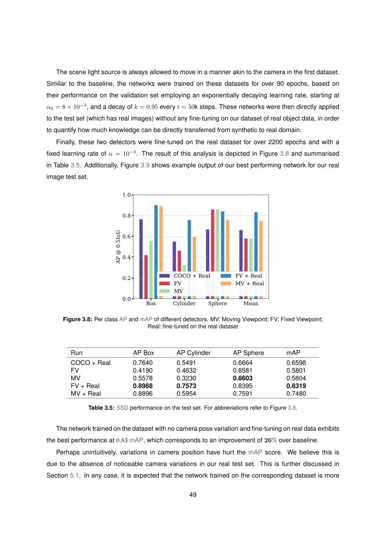
The scene light source is always allowed to move in a manner akin to the camera in the first dataset.

Similar to the baseline, the networks were trained on these datasets for over 90 epochs, based on

their performance on the validation set employing an exponentially decaying learning rate, starting at

α0 = 8× 10−3, and a decay of k = 0.95 every t = 50k steps. These networks were then directly applied

to the test set (which has real images) without any fine-tuning on our dataset of real object data, in order

to quantify how much knowledge can be directly transferred from synthetic to real domain.

Finally, these two detectors were fine-tuned on the real dataset for over 2200 epochs and with a

fixed learning rate of α = 10−3. The result of this analysis is depicted in Figure 3.8 and summarised

in Table 3.5. Additionally, Figure 3.9 shows example output of our best performing network for our real

image test set.

Box Cylinder Sphere Mean0.0

0.2

0.4

0.6

0.8

1.0

AP @

0.5

IoU

COCO + RealFVMV

FV + RealMV + Real

Figure 3.8: Per class AP and mAP of different detectors. MV: Moving Viewpoint; FV: Fixed Viewpoint;Real: fine-tuned on the real dataset

Run AP Box AP Cylinder AP Sphere mAPCOCO + Real 0.7640 0.5491 0.6664 0.6598FV 0.4190 0.4632 0.8581 0.5801MV 0.5578 0.3230 0.8603 0.5804FV + Real 0.8988 0.7573 0.8395 0.8319MV + Real 0.8896 0.5954 0.7591 0.7480

Table 3.5: SSD performance on the test set. For abbreviations refer to Figure 3.8.

The network trained on the dataset with no camera pose variation and fine-tuning on real data exhibits

the best performance at 0.83 mAP, which corresponds to an improvement of 26% over baseline.

Perhaps unintuitively, variations in camera position have hurt the mAP score. We believe this is

due to the absence of noticeable camera variations in our real test set. This is further discussed in

Section 5.1. In any case, it is expected that the network trained on the corresponding dataset is more

49

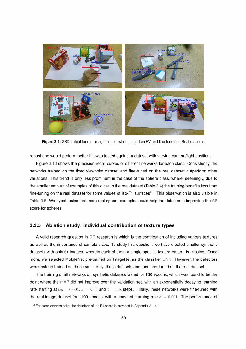
Figure 3.9: SSD output for real image test set when trained on FV and fine-tuned on Real datasets.

robust and would perform better if it was tested against a dataset with varying camera/light positions.

Figure 3.10 shows the precision-recall curves of different networks for each class. Consistently, the

networks trained on the fixed viewpoint dataset and fine-tuned on the real dataset outperform other

variations. This trend is only less prominent in the case of the sphere class, where, seemingly, due to

the smaller amount of examples of this class in the real dataset (Table 3.4) the training benefits less from

fine-tuning on the real dataset for some values of iso-F1 surfaces26. This observation is also visible in

Table 3.5. We hypothesise that more real sphere examples could help the detector in improving the AP

score for spheres.

3.3.5 Ablation study: individual contribution of texture types

A valid research question in DR research is which is the contribution of including various textures

as well as the importance of sample sizes. To study this question, we have created smaller synthetic

datasets with only 6k images, wherein each of them a single specific texture pattern is missing. Once

more, we selected MobileNet pre-trained on ImageNet as the classifier CNN. However, the detectors

were instead trained on these smaller synthetic datasets and then fine-tuned on the real dataset.

The training of all networks on synthetic datasets lasted for 130 epochs, which was found to be the

point where the mAP did not improve over the validation set, with an exponentially decaying learning

rate starting at α0 = 0.004, k = 0.95 and t = 50k steps. Finally, these networks were fine-tuned with

the real-image dataset for 1100 epochs, with a constant learning rate α = 0.001. The performance of

26For completeness sake, the definition of the F1-score is provided in Appendix A.1.4.

50

0.0 0.2 0.4 0.6 0.8 1.0Recall

0.0

0.2

0.4

0.6

0.8

1.0

Prec

isio

n

COCO + RealFVMVFV + RealMV + Real

(a) Box

0.0 0.2 0.4 0.6 0.8 1.0Recall

0.0

0.2

0.4

0.6

0.8

1.0

Prec

isio

n

COCO + RealFVMVFV + RealMV + Real

(b) Cylinder

0.0 0.2 0.4 0.6 0.8 1.0Recall

0.0

0.2

0.4

0.6

0.8

1.0

Prec

isio

n

COCO + RealFVMVFV + RealMV + Real

(c) Sphere

Figure 3.10: Precision-recall curves of different variants of the detectors. For abbreviations refer to Figure 3.8.

SSD on the validation set during training is shown in Figure 3.11. The results of these experiments are

reported in Figure 3.12 and Table 3.6.

Training dataset AP Box AP Cylinder AP Sphere mAPAll 0.8344 0.6616 0.8694 0.7885No Flat 0.8775 0.7546 0.8910 0.8410No Chess 0.8332 0.6958 0.8485 0.7925No Gradient 0.8296 0.6172 0.8536 0.7668No Perlin 0.7764 0.5058 0.7880 0.6901

Table 3.6: SSD performance on the test set after train on each of the 6k sub–datasets and fine-tuned on realimages.

By comparing figures Figures 3.12(a) and 3.12(b) it is clear that all variations have benefited from

fine-tuning with the real dataset.

Regarding individual texture patterns, generally speaking, by removing more and more complex

51

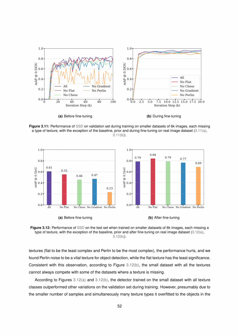
0 20 40 60 80 100Iteration Step (k)

0.0

0.2

0.4

0.6

0.8

1.0

mAP

@ 0

.5IO

U

AllNo FlatNo Chess

No GradientNo Perlin

(a) Before fine-tuning

0.0 2.5 5.0 7.5 10.0 12.5 15.0 17.5 20.0Iteration Step (k)

0.0

0.2

0.4

0.6

0.8

1.0

mAP

@ 0

.5IO

U

AllNo FlatNo ChessNo GradientNo Perlin

(b) During fine-tuning

Figure 3.11: Performance of SSD on validation set during training on smaller datasets of 6k images, each missinga type of texture, with the exception of the baseline, prior and during fine-tuning on real image dataset (3.11(a),

3.11(b)).

All No Flat No Chess No Gradient No Perlin0.0

0.2

0.4

0.6

0.8

1.0

mAP

@ 0

.5Io

U 0.610.55

0.46 0.47

0.23

(a) Before fine-tuning

All No Flat No Chess No Gradient No Perlin0.0

0.2

0.4

0.6

0.8

1.0

mAP

@ 0

.5Io

U

0.790.84

0.79 0.770.69

(b) After fine-tuning

Figure 3.12: Performance of SSD on the test set when trained on smaller datasets of 6k images, each missing atype of texture, with the exception of the baseline, prior and after fine-tuning on real image dataset (3.12(a),

3.12(b)).

textures (flat to be the least complex and Perlin to be the most complex), the performance hurts, and we

found Perlin noise to be a vital texture for object detection, while the flat texture has the least significance.

Consistent with this observation, according to Figure 3.12(b), the small dataset with all the textures

cannot always compete with some of the datasets where a texture is missing.

According to Figures 3.12(a) and 3.12(b), the detector trained on the small dataset with all texture

classes outperformed other variations on the validation set during training. However, presumably due to

the smaller number of samples and simultaneously many texture types it overfitted to the objects in the

52

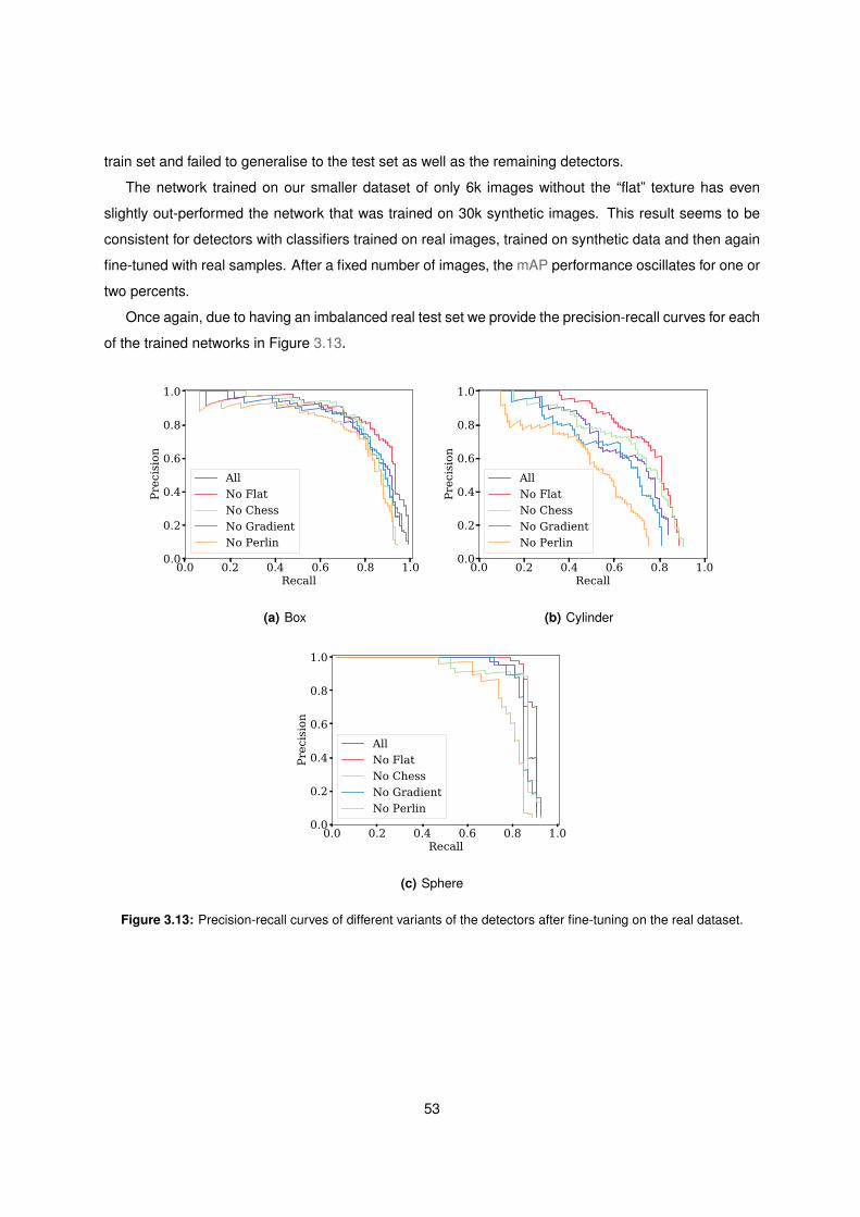
train set and failed to generalise to the test set as well as the remaining detectors.

The network trained on our smaller dataset of only 6k images without the “flat” texture has even

slightly out-performed the network that was trained on 30k synthetic images. This result seems to be

consistent for detectors with classifiers trained on real images, trained on synthetic data and then again

fine-tuned with real samples. After a fixed number of images, the mAP performance oscillates for one or

two percents.

Once again, due to having an imbalanced real test set we provide the precision-recall curves for each

of the trained networks in Figure 3.13.

0.0 0.2 0.4 0.6 0.8 1.0Recall

0.0

0.2

0.4

0.6

0.8

1.0

Prec

isio

n

AllNo FlatNo ChessNo GradientNo Perlin

(a) Box

0.0 0.2 0.4 0.6 0.8 1.0Recall

0.0

0.2

0.4

0.6

0.8

1.0

Prec

isio

n

AllNo FlatNo ChessNo GradientNo Perlin

(b) Cylinder

0.0 0.2 0.4 0.6 0.8 1.0Recall

0.0

0.2

0.4

0.6

0.8

1.0

Prec

isio

n

AllNo FlatNo ChessNo GradientNo Perlin

(c) Sphere

Figure 3.13: Precision-recall curves of different variants of the detectors after fine-tuning on the real dataset.

53

The code for replicating our experiments is also available as tf-shape-detection27. This repository

includes an interactive Jupyter notebook28 with a step-by-step walkthrough which explains how to

1. Download the real image dataset publicly hosted in our server;

2. Preprocess an image dataset and create binary TF records for usage in TensorFlow;

3. Train SSD with configurable starting checkpoints, learning parameters, etc.;

4. Compute mAP curves on the validation set during training and visualising them with TensorBoard

web application;

5. Export the resulting inference graphs and infer detections on new images;

6. Obtain precision metrics and precision-recall curves on a test set.

Furthermore, it provides a list that summarises all the tests we performed, in tests.md29, and the associ-

ated configuration files for each run, which specify learning parameters and number of training iterations.

Our pipeline is based on TF_ObjectDetection_API30, and uses the open-source implementation of SSD

available in tensorflow/models31.

The results presented in the current section were made available as an early preprint article, in

Borrego et al. [4], in July 2018.

27� jsbruglie/tf-shape-detection Object detection pipeline, on GitHub as of December 17, 201828Jupyter project webpage http://jupyter.org/, as of December 17, 201829Trial description https://github.com/jsbruglie/tf-shape-detection/blob/master/tests.md, as of December 17, 201830� wagonhelm/TF_ObjectDetection_API TensorFlow Object Detection API Tutorial, on GitHub as of December 17, 201831� tensorflow/models TensorFlow Models, on GitHub as of December 17, 2018

54

4Domain Randomisation for Grasping

Contents

4.1 Grasping in simulation . . . . . . . . . . . . . . . . . . . . . . . . . . . . . . . . . . . . 57

4.1.1 Overview and assumptions . . . . . . . . . . . . . . . . . . . . . . . . . . . . . . . 57

4.1.2 Dex-Net pipeline for grasp quality estimation . . . . . . . . . . . . . . . . . . . . . 58

4.1.3 Offline grasp sampling . . . . . . . . . . . . . . . . . . . . . . . . . . . . . . . . . 59

4.2 GRASP: Dynamic grasping simulation within Gazebo . . . . . . . . . . . . . . . . . . 64

4.2.1 DART physics engine . . . . . . . . . . . . . . . . . . . . . . . . . . . . . . . . . . 64

4.2.2 Disembodied robotic manipulator . . . . . . . . . . . . . . . . . . . . . . . . . . . 65

4.2.3 Hand plugin and interface . . . . . . . . . . . . . . . . . . . . . . . . . . . . . . . 66

4.3 Extending GAP with physics-based domain randomisation . . . . . . . . . . . . . . . 67

4.3.1 Physics randomiser class . . . . . . . . . . . . . . . . . . . . . . . . . . . . . . . 67

4.4 DexNet: Domain randomisation vs geometry-based metrics . . . . . . . . . . . . . . 68

4.4.1 Novel grasping dataset . . . . . . . . . . . . . . . . . . . . . . . . . . . . . . . . . 68

4.4.2 Experiment: grasp quality estimation . . . . . . . . . . . . . . . . . . . . . . . . . 70

55

It is far better to grasp the universe as it really is than to persist in delusion, however

satisfying and reassuring.

Carl Sagan, 1995

56

4.1 Grasping in simulation

In the previous chapter, we studied the application of Domain Randomisation (DR)to visual features in an object detection task. We proposed a novel frameworkintegrated with a widely used robotics simulator for synthetic scene generation. Thissimulated data was then used for training state–of–the–art Convolutional NeuralNetworks (CNNs), which we then tested on a small real image in-house dataset. Inthis chapter, we will focus on the problem of robotic grasping, and how to extendDR to physical properties in the context of simulated dynamic grasp trials. We startby stating our problem and assumptions in order to simplify it.

In this section, we aim to explore how to apply DR in a simulated grasping environment. Particularly,

we wish to apply randomisation to the physical properties of the entities at play, such as mass, friction

coefficients, robotic joint dynamic behaviour and controller parameters. Ultimately, we hope to create

synthetic datasets which can be used for real robotic grasping. For this, we require a tool that incorpo-

rates a grasp proposal module and pairs each of the grasp candidates with a quality metric. Additionally,

in order to achieve a robust grasp quality estimation, we wish to obtain some metric through full dynamic

simulation of grasp trials, preferably in an open and established robotics simulator. This approach differs

from that of Mahler et al. [43], which computes metrics from the geometry of the object, such as force-

closure and Ferrary-Canny [14]; or GraspIt! [45], which relies on building the GWS from each individual

contact between the robotic manipulator and the target object. Instead, we propose to obtain a grasp

quality estimation by replicating real robotic trials in a simulated environment, and evaluate whether

they are successful or not. In this fashion, by applying DR to the physical properties between different

attempts of a given grasp configuration we aim to achieve a robust metric.

4.1.1 Overview and assumptions

We are aware that robotic grasping is a hard task, even more so when the target object geometry is

unknown. For this reason, we must first simplify the problem at hand, imposing reasonable constraints,

which may eventually be relaxed, so as to streamline our research.

Firstly, in our work we chose not to include the reaching motion as part of the grasping problem.

Essentially, this task corresponds to positioning the robotic manipulator in a pre-grasp pose and should

be made possible by a 6-DOF arm to which the hand is attached. For an adequately calibrated robot, with

known kinematic model, this effectively corresponds to solving an IK problem, i.e. computing the angles

of each arm joint required for the endpoint to perform the desired trajectory, while avoiding collisions with

other objects in the world. Currently existing frameworks such as MoveIt!1 already provide a satisfactory

solution to the reaching problem. The latter software can produce collision-free trajectories in simple

scenarios and supports a great number of robot platforms.1Robotic motion planning software https://moveit.ros.org/, as of December 17, 2018

57

By eliminating the reaching action from our concerns we are able to focus solely on the grasp quality

estimation, and avoid computationally expensive IK calculations or learning policies for closed-loop arm

control. Thus, we assume a disembodied manipulator with full 3D-space mobility. Evidently, this or

similar approaches have been proposed in relevant recent literature [31, 60, 75, 77, 18].

In order to perform full dynamic simulation of grasp trials we require an adequate physics engine,

preferably integrated with Gazebo, so our experiments on grasping come as a natural extension of our

previous work on DR, reported in Chapter 3. This, in turn, restricts us to rigid body simulation, as none

of the supported engines can effectively simulate soft or compliant objects2. To our knowledge, only

proprietary physics engine MuJoCo fully supports this feature, while integrated with a robotic simulation

framework. The contact forces present in a grasping action play a crucial role in whether it will be

successful or not. For rigid, dry contacting surfaces, most physics engines use the Coulomb friction

model, which we further elaborate on, in Section 1.2.2.A.

Finally, for now we chose to focus on parallel-plate grippers, as opposed to dexterous manipula-

tors. We intend to extend our work to multi-fingered autonomous grasping. For this reason, our novel

framework provides out-of-the-box support for some desired features, namely coupled joints, which are

typically found in underactuated hands.

Summarising, our principal assumptions involve using:

1. A disembodied robotic manipulator with unconstrained movement in 3-D space;

2. Simplified rigid body contact and Coulomb friction models;

3. A parallel-plate gripper as opposed to dexterous multi-fingered robot hands.

In the next section, we provide a brief description of Dex-Net 2.0 [43], which was later used in our

work.

4.1.2 Dex-Net pipeline for grasp quality estimation

Rather than designing our end-to-end pipeline for grasping candidate generation and evaluation, we

decided to employ that of Mahler et al. [43]. This allows us to focus on studying the impact of employing

DR and prevents additional biases stemming from novel self-proposed methods, which would ultimately

confuse a comparative analysis.

Recalling Section 2.2.2.B, the authors tackle grasping unknown objects with parallel-plate grippers

given visual input from an RGB-D camera mounted on the gripper. The problem of grasping is split into

two steps, namely (i) grasp candidate proposal and (ii) grasp quality evaluation.

2 In fact, DART physics engine can simulate soft contacts using the model of Jain and Liu [27]. However, currently, Gazeboonly supports this feature for box-shaped objects.

58

Specifically, [43] states the second step as approximating a grasp robustness function, given by

Q(u,y) = E[S(u,x)|u,y], where

• S(u,x) ∈ {0, 1} is a binary success metric;

• u = (p, φ) ∈ R3 × S1 4-DOF upright grasp candidate, with grasp centre p (x, y, z) and angle φ;

• x = (O, TO, TC , γ), respectively object geometry, object and camera poses and friction coefficient;

• y ∈ RW×H+ a 2.5D point cloud (depth image with width W and height H) acquired using a camera

with known parameters.

The depth camera is aligned with each grasp proposal before capture, generating a 32 × 32 pixel

frame. Each grasp is sampled provided no collision is detected, and then a relaxed force-closure metric

is computed analytically with the geometric information of each object. Uncertainty is introduced in the

problem to model sensor errors using Monte-Carlo sampling. Specifically, object and gripper poses, as

well as the static friction coefficient are disturbed by Gaussian noise, during metric computation for grasp

candidates. Regarding data augmentation, each frame can be flipped vertically and horizontally due to

the gripper symmetry.

In our work, we wish to use Dex-Net as the main building block. Our goal is to generate a novel

grasping dataset, using 3D models scanned from real-world household objects found in KIT object

dataset [32]. Grasp candidates for these objects should be computed using the method of [43] so

we can establish an adequate baseline. Analogously, we should use this framework to provide baseline

grasp quality estimates, computed resorting to geometric metrics. At this stage, we introduce Domain

Randomisation in the metric used to evaluate a grasp candidate. Instead of relying on geometric-driven

metrics, we perform full dynamic simulation of grasping trials, while randomising physical properties

of the environment. We expect our method to provide a more robust estimate of grasp success, and

ultimately improve the grasps selected in a real-world robotic scenario.

4.1.3 Offline grasp sampling

Sampling grasp candidates in continuous 3D space (6-DOF) is no trivial undertaking, even for simple

robotic grippers with a single actuated joint. In this section, we describe the method of Mahler et al. [43],

which we employed in our own work, with minor modifications so as to fit our scenario.

Each object’s shape is defined by a signed distance function (sdf) f : R3 → R, which is 0 on the object

surface, positive outside the object, and negative within. The object surface for a given sdf f is denoted

by S = {y ∈ R3|f(y = 0)}. All points are specified with respect to an object-centric reference frame

centred at the object centre of mass z and oriented along the principal axes of S. This representation is

59

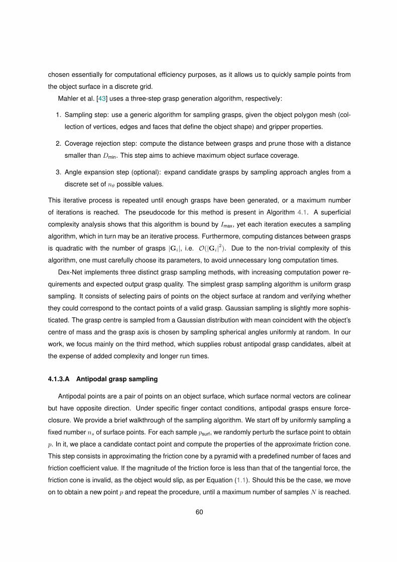
chosen essentially for computational efficiency purposes, as it allows us to quickly sample points from

the object surface in a discrete grid.

Mahler et al. [43] uses a three-step grasp generation algorithm, respectively:

1. Sampling step: use a generic algorithm for sampling grasps, given the object polygon mesh (col-

lection of vertices, edges and faces that define the object shape) and gripper properties.

2. Coverage rejection step: compute the distance between grasps and prune those with a distance

smaller than Dmin. This step aims to achieve maximum object surface coverage.

3. Angle expansion step (optional): expand candidate grasps by sampling approach angles from a

discrete set of nθ possible values.

This iterative process is repeated until enough grasps have been generated, or a maximum number

of iterations is reached. The pseudocode for this method is present in Algorithm 4.1. A superficial

complexity analysis shows that this algorithm is bound by Imax, yet each iteration executes a sampling

algorithm, which in turn may be an iterative process. Furthermore, computing distances between grasps

is quadratic with the number of grasps |Gi|, i.e. O(|Gi|2). Due to the non-trivial complexity of this

algorithm, one must carefully choose its parameters, to avoid unnecessary long computation times.

Dex-Net implements three distinct grasp sampling methods, with increasing computation power re-

quirements and expected output grasp quality. The simplest grasp sampling algorithm is uniform grasp

sampling. It consists of selecting pairs of points on the object surface at random and verifying whether

they could correspond to the contact points of a valid grasp. Gaussian sampling is slightly more sophis-

ticated. The grasp centre is sampled from a Gaussian distribution with mean coincident with the object’s

centre of mass and the grasp axis is chosen by sampling spherical angles uniformly at random. In our

work, we focus mainly on the third method, which supplies robust antipodal grasp candidates, albeit at

the expense of added complexity and longer run times.

4.1.3.A Antipodal grasp sampling

Antipodal points are a pair of points on an object surface, which surface normal vectors are colinear

but have opposite direction. Under specific finger contact conditions, antipodal grasps ensure force-

closure. We provide a brief walkthrough of the sampling algorithm. We start off by uniformly sampling a

fixed number ns of surface points. For each sample psurf, we randomly perturb the surface point to obtain

p. In it, we place a candidate contact point and compute the properties of the approximate friction cone.

This step consists in approximating the friction cone by a pyramid with a predefined number of faces and

friction coefficient value. If the magnitude of the friction force is less than that of the tangential force, the

friction cone is invalid, as the object would slip, as per Equation (1.1). Should this be the case, we move

on to obtain a new point p and repeat the procedure, until a maximum number of samples N is reached.

60

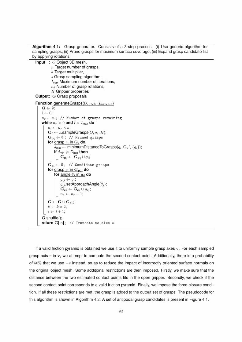
Algorithm 4.1: Grasp generator. Consists of a 3-step process. (i) Use generic algorithm forsampling grasps; (ii) Prune grasps for maximum surface coverage; (iii) Expand grasp candidate listby applying rotations.

Input : O Object 3D mesh,n Target number of grasps,k Target multiplier,s Grasp sampling algorithm,Imax Maximum number of iterations,nθ Number of grasp rotations,H Gripper properties

Output: G Grasp proposals

Function generateGrasps(O, n, k, Imax, nθ)G← ∅;i← 0;nr ← n ; // Number of grasps remainingwhile nr > 0 and i < Imax do

ni ← nr × k;Gi ← s.sampleGrasps(O,ni, H);Gpi ← ∅ ; // Pruned graspsfor grasp gi in Gi do

dmin ← minimumDistanceToGrasps(gi,Gi \ {gi});if dmin > Dmin then

Gpi ← Gpi ∪ gi;

Gci ← ∅ ; // Candidate graspsfor grasp gi in Gpi do

for angle θj in nθ dogij ← gi;gij .setApproachAngle(θj);Gci ← Gci ∪ gij ;nr ← nr − 1;

G← G ∪Gci;k ← k × 2;i← i+ 1;

G.shuffle();return G[:n] ; // Truncate to size n

If a valid friction pyramid is obtained we use it to uniformly sample grasp axes v. For each sampled

grasp axis v in v, we attempt to compute the second contact point. Additionally, there is a probability

of 50% that we use −v instead, so as to reduce the impact of incorrectly oriented surface normals on

the original object mesh. Some additional restrictions are then imposed. Firstly, we make sure that the

distance between the two estimated contact points fits in the open gripper. Secondly, we check if the

second contact point corresponds to a valid friction pyramid. Finally, we impose the force-closure condi-

tion. If all these restrictions are met, the grasp is added to the output set of grasps. The pseudocode for

this algorithm is shown in Algorithm 4.2. A set of antipodal grasp candidates is present in Figure 4.1.

61

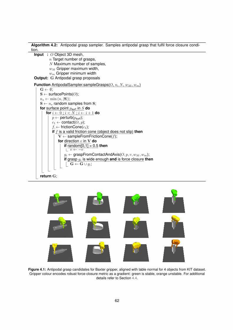
Algorithm 4.2: Antipodal grasp sampler. Samples antipodal grasp that fulfil force closure condi-tion.

Input : O Object 3D mesh,n Target number of grasps,N Maximum number of samples,wM Gripper maximum width,wm Gripper minimum width

Output: G Antipodal grasp proposals

Function AntipodalSampler.sampleGrasps(O, n, N , wM , wm)G← ∅;S← surfacePoints(O);ns ← min (n, |S|);S← ns random samples from S;for surface point psurf in S do

for i← 0 ; i < N ; i← i+ 1 dop← perturb(psurf);c1 ← contact(O, p);f,← frictionCone(c1);if f is a valid friction cone (object does not slip) then

V← sampleFromFrictionCone(f );for direction v in V do

if random[0,1] > 0.5 thenv ← −v

gi ← graspFromContactAndAxis(O, p, v, wM , wm);if grasp gi is wide enough and is force closure then

G← G ∪ gi;

return G;

Figure 4.1: Antipodal grasp candidates for Baxter gripper, aligned with table normal for 4 objects from KIT dataset.Gripper colour encodes robust force-closure metric as a gradient: green is stable, orange unstable. For additional

details refer to Section 4.4.

62

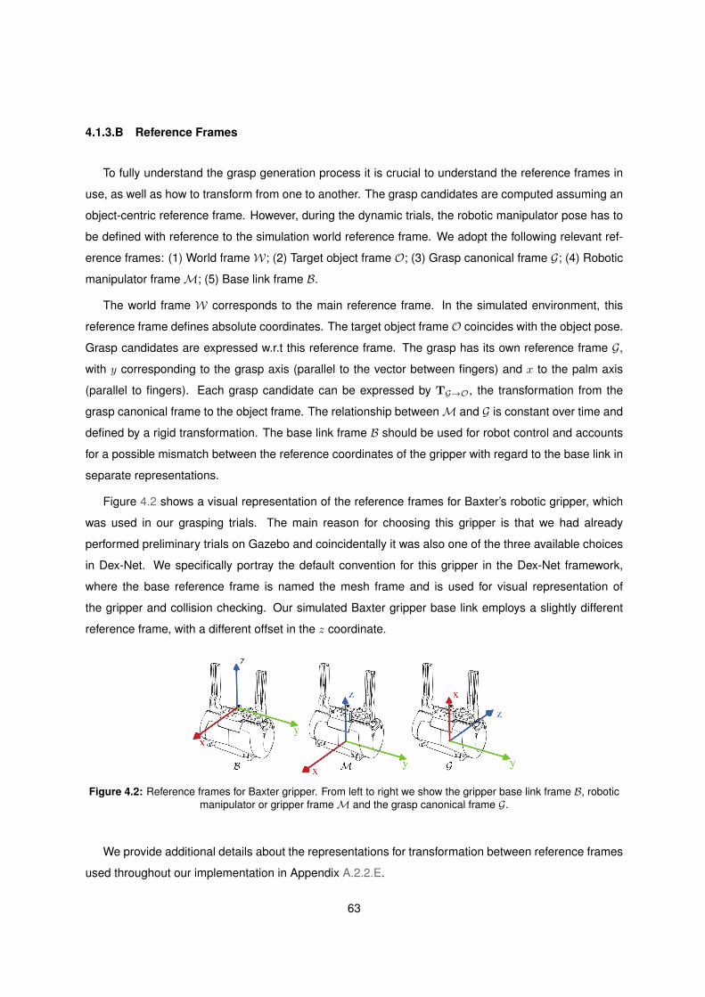
4.1.3.B Reference Frames

To fully understand the grasp generation process it is crucial to understand the reference frames in

use, as well as how to transform from one to another. The grasp candidates are computed assuming an

object-centric reference frame. However, during the dynamic trials, the robotic manipulator pose has to

be defined with reference to the simulation world reference frame. We adopt the following relevant ref-

erence frames: (1) World frameW; (2) Target object frame O; (3) Grasp canonical frame G; (4) Robotic

manipulator frameM; (5) Base link frame B.

The world frame W corresponds to the main reference frame. In the simulated environment, this

reference frame defines absolute coordinates. The target object frame O coincides with the object pose.

Grasp candidates are expressed w.r.t this reference frame. The grasp has its own reference frame G,

with y corresponding to the grasp axis (parallel to the vector between fingers) and x to the palm axis

(parallel to fingers). Each grasp candidate can be expressed by TG→O, the transformation from the

grasp canonical frame to the object frame. The relationship betweenM and G is constant over time and

defined by a rigid transformation. The base link frame B should be used for robot control and accounts

for a possible mismatch between the reference coordinates of the gripper with regard to the base link in

separate representations.

Figure 4.2 shows a visual representation of the reference frames for Baxter’s robotic gripper, which

was used in our grasping trials. The main reason for choosing this gripper is that we had already

performed preliminary trials on Gazebo and coincidentally it was also one of the three available choices

in Dex-Net. We specifically portray the default convention for this gripper in the Dex-Net framework,

where the base reference frame is named the mesh frame and is used for visual representation of

the gripper and collision checking. Our simulated Baxter gripper base link employs a slightly different

reference frame, with a different offset in the z coordinate.

Figure 4.2: Reference frames for Baxter gripper. From left to right we show the gripper base link frame B, roboticmanipulator or gripper frame M and the grasp canonical frame G.

We provide additional details about the representations for transformation between reference frames

used throughout our implementation in Appendix A.2.2.E.

63

4.2 GRASP: Dynamic grasping simulation within Gazebo

In the former section, we have stated our objective and main assumptions. More-over, we motivated resorting to an existing pipeline for grasp proposal and qualityestimation [43], and provided a brief analysis of the proposed offline grasp samplingalgorithm. In this section, we introduce a novel framework for dynamic simulationof grasp trials in Gazebo.

We propose a novel framework for Gazebo, for performing dynamic simulation of grasp trial outcome,

which we named GRASP, and is open source as grasp3. One of our greatest concerns was flexibility

and accessibility, to allow for straightforward integration with any existing robotic manipulator and object

dataset. So far, the development of this platform has produced

– A model plugin for programmatic control of a floating robotic manipulator, either a single DOF

gripper or multi-fingered hand, with support for coupled (underactuated) joints 4;

– An interface class for simplifying interaction with the former from a client application, which sup-

ports a uniform configuration across distinct manipulators;

– A server-side service that allows for efficiently checking whether two objects are colliding and, if

so, obtain the contacts at play at a given instant;

– A tool for creating Gazebo model datasets from object mesh files;

– A script for obtaining object stable poses via dynamic simulation, which leverages a novel model

plugin, attached to grasp target objects;

– A pipeline to compute grasp trial outcomes using full dynamic simulation, given a dataset of objects

and a set of grasp candidates per object computed externally for the desired robotic manipulator.

In the coming subsection, we motivate our choice of an adequate physics engine.

4.2.1 DART physics engine

By default, Gazebo uses a modified version ODE physics engine, which can be quite effective for

simulating mobile robots navigating in environments, possibly with uneven terrain. It can also be used

for more complex operations and testing inverse kinematic solvers, or even simple manipulation tasks,

as shown by in an online pick-and-place routine for Baxter5. However, attempting finer-grain manip-

ulation such as grasping complex objects typically results in physically unrealistic behaviour, such as

3� jsbruglie/grasp Gazebo plugins for running grasp trials, on GitHub as of December 17, 20184For more details on coupled joint emulation, check Appendix A.2.2.A.5Baxter MoveIt! Pick and Place Demo https://www.youtube.com/watch?v=BPOLWBsOnOQ, as of December 17, 2018

64

manipulator instability or links clipping through each other. One available solution is to compute grasp

metrics analytically, in order to determine whether or not a grasp would be successful, and then bypass

the grasp trial altogether and just attach the object to the manipulator, ceasing to compute further inter-

actions between the manipulator and the target. An implementation of this is available in gazebo-pkgs6.

In our preliminary trials, we were able to confirm that indeed the default setup would not allow us to

perform full dynamic simulation of grasping on complex objects. Furthermore, simple scenarios employ-

ing a gripper or complex hand would be highly unstable and typically result in a server crash, especially

if self-collision is partially enabled i.e. some links of the manipulator can collide with others. This be-

haviour is desired for instance when using Shadow Dexterous Hand, where the high number of degrees

of freedom would otherwise allow for a great number of impossible configurations, with links clipping

through each other.

Our initial assumption was that merely altering the underlying physics engine would allow for a faith-

ful simulation of complex grasping trials. Motivated by Johns et al. [31], we decided to perform our

experiments using DART. The authors perform dynamic simulation of parallel-plate grasping trials and

report that even though DART was slower than physics engines more suitable for computer graphics

applications, such as Bullet, it showed greater accuracy in modelling precise, real-world behaviour. One

of the few downsides of this decision includes resulting in a more involved setup process, as Gazebo

has to be compiled from source. In fact, due to a dependency issue with official software repositories,

we found ourselves forced to install DART and fcl7 from source as well.

4.2.2 Disembodied robotic manipulator

We do not aim to solve the problem of servoing, i.e. planning a valid trajectory so the hand can reach

the grasp candidate pose. Thus, as previously mentioned we employ a disembodied manipulator with full

mobility in 3D-space. To achieve this we propose a set of six virtual joints, each controlling respectively

x,y,z position and roll, pitch and yaw rotation. The former three are prismatic joints, whereas the latter

are rotational, with no lower or upper limits (also known as continuous). This particular solution was

suggested by one of Gazebo’s developers on the official community forums 8 even though we found this

approach to cause great instability when using ODE physics engine. Notice however that we did not

write any part of the framework to be physics-engine specific, and it is possible that in the future our

tools can be successfully employed in other engines. By default, we disable gravity for the manipulator

alone, which is equivalent to robust robot arm controllers maintaining the manipulator’s pose.

6� JenniferBuehler/gazebo-pkgs A collection of tools and plugins for Gazebo, on GitHub as of December 17, 20187� flexible-collision-library/fcl Flexible collision library, on GitHub as of December 17, 20188Check http://answers.gazebosim.org/question/18109/movement-of-smaller-links-affecting-the-whole-body/

?answer=18111#post-id-18111, as of December 17, 2018.

65

4.2.3 Hand plugin and interface

The main component of our novel grasp pipeline consists of a Gazebo Model plugin for robotic

hands. The latter can be interacted with directly or via a custom client interface, that provides high-level

commands such as moving fingers to a set of configurable positions, with coupled dynamic movement

(somewhat analogous to synergies [1]) and support for underactuated manipulators9. One of our main

concerns when developing this tool was to provide a uniform, yet highly customisable procedure for

sampling grasp trials for grippers and multi-fingered manipulators alike.

In our specific case, we desire to obtain the outcome of pre-computed grasp candidates, as ac-

curately and efficiently as possible. For this, we designed a client script which requires actions to be

performed sequentially, such as moving to a pre-grasp pose, then closing fingers, and so on. To enforce

the order in which these smaller tasks are carried out, we implemented a server-side timer, that can be

set up to trigger and notify a client with a configurable delay. The key concept here is that it actually

uses the simulation time, as real-world time cannot be used reliably. The reason for this is that each

simulation step corresponds to a constant simulated time step ∆t, which, in reality, may take a variable

amount of time to compute. Concretely, during grasp trials, when a higher number of contacts is present,

simulation performance can drop to 20%.

Since grasp candidates are provided externally, and, in our case, do not take into account collisions of

the gripper with either the object or the ground plane, some are bound to be invalid, for certain object rest

poses. In simulation, if objects clip through one another, the physics engine tries to solve the interaction,

and ultimately ends up creating a large number of contacts between the colliding surfaces. This will have

a tremendous performance impact. For this reason, we developed a fast plugin for checking whether

two objects are colliding and if so, obtaining the contact points10.

9Check Appendix A.2.2.A for implementation details on how this is achieved despite not being available out-of-the-box inGazebo.

10Check Appendix A.2.2.B for implementation details of our efficient strategy for querying the simulator for contacts.

66

4.3 Extending GAP with physics-based domain randomisation

In the preceding section, we described the main features of our novel frameworkfor dynamic simulation of grasp trials in Gazebo. In the present section, we explainhow we extended our set of tools for Domain Randomisation (DR) to incorporaterandomisation of physical properties of objects in a scene.

In Section 3.1 we introduced a set of Gazebo plugins for employing DR to the visual appearance

of synthetic scenes. Since our present goal is to randomise physical properties, we decided to en-

hance our proposed framework GAP and develop a brand-new module for physics-based DR. The main

implemented features allow us to:

– Change gravity vector components;

– Alter the scale of existing models;

– Modify individual link properties, namely mass and inertia tensor;

– Change individual joint properties, such as angle lower and upper limits, as well as maximum effort

and velocity constraints;

– Adjust individual PID controller parameters and target values;

– Vary individual collision surface properties, including µ Coulomb friction coefficients. Some param-

eters are physics-engine specific, but our tool uses Gazebo’s own message types, and as such

should be fully compatible with the supported libraries.

Our tool includes yet another Gazebo World plugin, that has full access to the physics engine. We

also provide a client interface that can easily be imported into third-party applications and used as an

API. It provides a set of methods to easily access each of the aforementioned functions and automati-

cally packages the command in messages that are sent and parsed by the DR plugin instance, running

on the Gazebo server application. We designed the interface to be as flexible as possible, providing a

layer of abstraction to developers for simpler interaction with our tool. Since synchronisation tends to

be of utmost importance for automating robotic trials, and coordinating a sequence of events between

client and service execution, we provide a blocking request service, that halts the client until an explicit

acknowledgement response is sent back.

4.3.1 Physics randomiser class

To integrate our novel physics DR tools in the dynamic grasp trial simulation pipeline we envisioned

a method for attaching generic properties with specific random variations. For instance, we desired the

67

ability to tether the target object mass to a random scaling factor, itself behaving according to a uniform

distribution defined in a configurable interval [a, b]. Moreover, we wanted to be able to specify all of

the physical properties, affected models, links and joints, and the respective random distributions in a

simple, user-readable format.

For this, we designed the physics randomiser class, as part of our grasping pipeline toolkit. It maps

random distributions to physical properties specified in a yaml configuration file11, samples values from

these distributions, and communicates with the Gazebo server via our custom API in GAP to update the

physical properties of the scene. This class allows the automation of the whole scene randomisation

process, through a clean interface, and swift testing, as all of the parameters are read from an external

file, upon launching the client application.

This tool showcases the potential of our DR interface. Moreover, for improved maintainability we use

GAP as an external dependency and enforce version checks, to ensure third-party software is compatible

with installed binaries of our framework.

4.4 DexNet: Domain randomisation vs geometry-based metrics

In the former sections, we introduced a set of tools we designed for employing Do-main Randomisation (DR) to the physical properties of a simulated grasp scenario.In this section, we describe in detail how we integrated parts of Dex-Net [43] in ourgrasp framework for Gazebo. Specifically, we outline the proposed experiment forvalidating the claim that indeed DR can lead to more robust grasp quality estima-tion.

4.4.1 Novel grasping dataset

Our current process for generating a grasping dataset can be summarised as follows:

1. Create and pre-process object dataset in Dex-Net;

2. Import objects into Gazebo compatible models;

3. Compute antipodal grasp candidates in Dex-Net and respective baseline quality metrics, from

object geometry;

4. Compute realistic object rest poses in Gazebo via physics simulation;

5. Import object rest poses into Dex-Net in order to obtain aligned grasp candidates;

6. Import resulting grasp candidates into Gazebo and perform grasp trials in order to ascertain

whether grasp is robust or not, introducing DR by randomising properties between trial repetitions.11An example configuration is provided in Appendix A.2.2.D.

68

We start by creating a novel object dataset, using the models from KIT dataset [32]. It contains 3D

models of 129 different household items, including not only boxes and cups but also more complexly

shaped objects, such as small sculptures of dogs or horses. The latter evidently present a harder

challenge to parallel-plate grippers. The main reason for picking this dataset is twofold: (i) KIT had

previously been used for training Dex-Net grasp quality estimator network, which reduces the risk of

dataset-specific issues that could arise; (ii) the triangular meshes for each 3D object were simplified to

have roughly 800 faces, which is desirable, as it conveys a high level of detail, but is not enough that

dynamic simulation in Gazebo is painfully slow. Preliminary experiments with our pipeline showed that

very high detail 3D meshes, such as those provided in ShapeNet [9] (which in turn was also used in

Mahler et al. [43]), resulted in very poor performance, due to the high number of contacts in simulation.

We could, however, have generated lower fidelity models using a 3D mesh edition tool such as open-

source MeshLab12.

Our dataset is pre-processed in Dex-Net, which applies a scaling factor that ensures that the mini-

mum dimension of the object fits in the open gripper. In our simulated experiments, we used a Baxter

electric gripper with narrow aperture and basic solid fingertips. The main reason for this was that it was

already integrated with Dex-Net, and required minimal changes for functioning correctly. Moreover, we

had already worked previously with Baxter in Gazebo.

Then, we need to convert the processed meshes into Gazebo models, so they can be effortlessly

spawned in simulation. We provide a script that performs this task, which involves converting meshes to

a Gazebo-compatible format13.

We compute antipodal grasp candidates for each of these objects, as described in Section 4.1.3.A.

These grasp candidates essentially define the gripper contact points with the object that should result

in a successful grasp. However, the approach angle must be computed in such a way that the gripper

does not collide with the planar surface the object is resting on, henceforth referred to generically as the

table. Dex-Net uses an analytic method for obtaining stable poses with the associated probability, yet

early evaluation has shown that they are not very reliable. This can be particularly undesirable when

running the dynamic simulation in Gazebo, as the object may start moving and intersect with the gripper.

Instead, we compute object rest poses in Gazebo, using our set of tools. A rest pose is obtained by

dropping the object from an initial height and ensuring that both positional and angular velocities drop

below a threshold ε.

We can then import these reliable rest poses into Dex-Net in order to align the grasp with the normal

of the table. This minimises the amount of grasp poses that immediately result in a collision with the

planar surface. These aligned grasps candidates are then exported and read in our pipeline. Finally, we

can proceed to perform grasp trials, within Gazebo’s simulated environment.

12MeshLab website http://www.meshlab.net/, as of December 17, 201813Dex-Net generates .obj files by default, and Gazebo can only process Collada (.dae) or .stl files

69

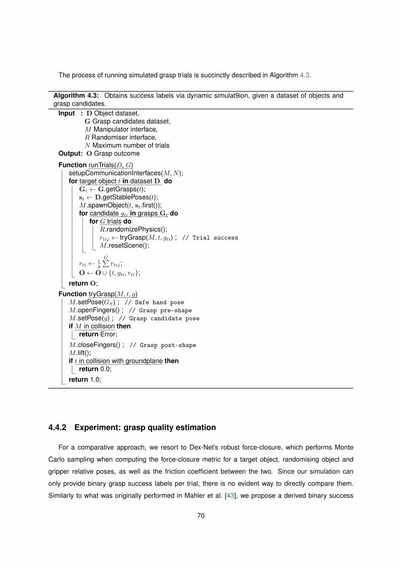
The process of running simulated grasp trials is succinctly described in Algorithm 4.3.

Algorithm 4.3: Obtains success labels via dynamic simulat9ion, given a dataset of objects andgrasp candidates.

Input : D Object dataset,G Grasp candidates dataset,M Manipulator interface,R Randomiser interface,N Maximum number of trials

Output: O Grasp outcome

Function runTrials(D, G)setupCommunicationInterfaces(M,N );for target object t in dataset D do

Gt ← G.getGrasps(t);st ← D.getStablePoses(t);M .spawnObject(t, st.first());for candidate gti in grasps Gt do

for G trials doR.randomizePhysics();rtij ← tryGrasp(M, t, gti) ; // Trial successM .resetScene();

rti ← 1g

G∑rtij ;

O← O ∪ {t, gti, rti};return O;

Function tryGrasp(M, t, g)M .setPose(GS) ; // Safe hand poseM .openFingers() ; // Grasp pre-shapeM .setPose(g) ; // Grasp candidate poseif M in collision then

return Error;

M .closeFingers() ; // Grasp post-shapeM .lift();if t in collision with groundplane then

return 0.0;

return 1.0;

4.4.2 Experiment: grasp quality estimation

For a comparative approach, we resort to Dex-Net’s robust force-closure, which performs Monte

Carlo sampling when computing the force-closure metric for a target object, randomising object and

gripper relative poses, as well as the friction coefficient between the two. Since our simulation can

only provide binary grasp success labels per trial, there is no evident way to directly compare them.

Similarly to what was originally performed in Mahler et al. [43], we propose a derived binary success

70

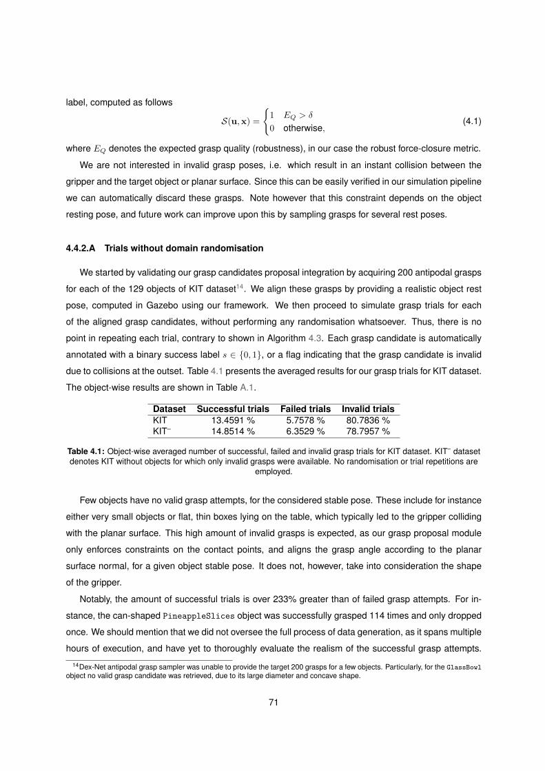
label, computed as follows

S(u,x) =

{1 EQ > δ

0 otherwise,(4.1)

where EQ denotes the expected grasp quality (robustness), in our case the robust force-closure metric.

We are not interested in invalid grasp poses, i.e. which result in an instant collision between the

gripper and the target object or planar surface. Since this can be easily verified in our simulation pipeline

we can automatically discard these grasps. Note however that this constraint depends on the object

resting pose, and future work can improve upon this by sampling grasps for several rest poses.

4.4.2.A Trials without domain randomisation

We started by validating our grasp candidates proposal integration by acquiring 200 antipodal grasps

for each of the 129 objects of KIT dataset14. We align these grasps by providing a realistic object rest

pose, computed in Gazebo using our framework. We then proceed to simulate grasp trials for each

of the aligned grasp candidates, without performing any randomisation whatsoever. Thus, there is no

point in repeating each trial, contrary to shown in Algorithm 4.3. Each grasp candidate is automatically

annotated with a binary success label s ∈ {0, 1}, or a flag indicating that the grasp candidate is invalid

due to collisions at the outset. Table 4.1 presents the averaged results for our grasp trials for KIT dataset.

The object-wise results are shown in Table A.1.

Dataset Successful trials Failed trials Invalid trialsKIT 13.4591 % 5.7578 % 80.7836 %KIT– 14.8514 % 6.3529 % 78.7957 %

Table 4.1: Object-wise averaged number of successful, failed and invalid grasp trials for KIT dataset. KIT– datasetdenotes KIT without objects for which only invalid grasps were available. No randomisation or trial repetitions are

employed.

Few objects have no valid grasp attempts, for the considered stable pose. These include for instance

either very small objects or flat, thin boxes lying on the table, which typically led to the gripper colliding

with the planar surface. This high amount of invalid grasps is expected, as our grasp proposal module

only enforces constraints on the contact points, and aligns the grasp angle according to the planar

surface normal, for a given object stable pose. It does not, however, take into consideration the shape

of the gripper.

Notably, the amount of successful trials is over 233% greater than of failed grasp attempts. For in-

stance, the can-shaped PineappleSlices object was successfully grasped 114 times and only dropped

once. We should mention that we did not oversee the full process of data generation, as it spans multiple

hours of execution, and have yet to thoroughly evaluate the realism of the successful grasp attempts.

14Dex-Net antipodal grasp sampler was unable to provide the target 200 grasps for a few objects. Particularly, for the GlassBowlobject no valid grasp candidate was retrieved, due to its large diameter and concave shape.

71

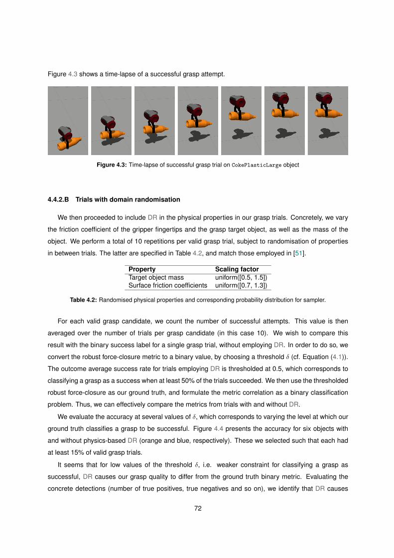
Figure 4.3 shows a time-lapse of a successful grasp attempt.

Figure 4.3: Time-lapse of successful grasp trial on CokePlasticLarge object

4.4.2.B Trials with domain randomisation

We then proceeded to include DR in the physical properties in our grasp trials. Concretely, we vary

the friction coefficient of the gripper fingertips and the grasp target object, as well as the mass of the

object. We perform a total of 10 repetitions per valid grasp trial, subject to randomisation of properties

in between trials. The latter are specified in Table 4.2, and match those employed in [51].

Property Scaling factorTarget object mass uniform([0.5, 1.5])Surface friction coefficients uniform([0.7, 1.3])

Table 4.2: Randomised physical properties and corresponding probability distribution for sampler.

For each valid grasp candidate, we count the number of successful attempts. This value is then

averaged over the number of trials per grasp candidate (in this case 10). We wish to compare this

result with the binary success label for a single grasp trial, without employing DR. In order to do so, we

convert the robust force-closure metric to a binary value, by choosing a threshold δ (cf. Equation (4.1)).

The outcome average success rate for trials employing DR is thresholded at 0.5, which corresponds to

classifying a grasp as a success when at least 50% of the trials succeeded. We then use the thresholded

robust force-closure as our ground truth, and formulate the metric correlation as a binary classification

problem. Thus, we can effectively compare the metrics from trials with and without DR.

We evaluate the accuracy at several values of δ, which corresponds to varying the level at which our

ground truth classifies a grasp to be successful. Figure 4.4 presents the accuracy for six objects with

and without physics-based DR (orange and blue, respectively). These we selected such that each had

at least 15% of valid grasp trials.

It seems that for low values of the threshold δ, i.e. weaker constraint for classifying a grasp as

successful, DR causes our grasp quality to differ from the ground truth binary metric. Evaluating the

concrete detections (number of true positives, true negatives and so on), we identify that DR causes

72

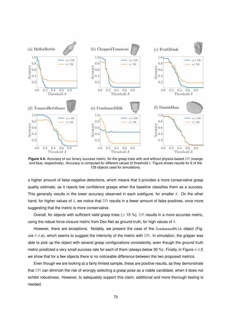
(a) MelforBottle

(d) TomatoHerbSauce

(b) ChoppedTomatoes

(e) CondensedMilk

(c) FruitDrink

(f) DanishHam

Figure 4.4: Accuracy of our binary success metric, for the grasp trials with and without physics-based DR (orangeand blue, respectively). Accuracy is computed for different values of threshold δ. Figure shows results for 6 of the

129 objects used for simulations.

a higher amount of false negative detections, which means that it provides a more conservative grasp

quality estimate, as it rejects low confidence grasps when the baseline classifies them as a success.

This generally results in the lower accuracy observed in each subfigure, for smaller δ. On the other

hand, for higher values of δ, we notice that DR results in a fewer amount of false positives, once more

suggesting that the metric is more conservative.

Overall, for objects with sufficient valid grasp trials (> 15 %), DR results in a more accurate metric,

using the robust force-closure metric from Dex-Net as ground truth, for high values of δ.

However, there are exceptions. Notably, we present the case of the CondensedMilk object (Fig-

ure 4.4.e), which seems to suggest the inferiority of the metric with DR. In simulation, the gripper was

able to pick up the object with several grasp configurations consistently, even though the ground truth

metric predicted a very small success rate for each of them (always below 30 %). Finally, in Figure 4.4.f)

we show that for a few objects there is no noticeable difference between the two proposed metrics.

Even though we are looking at a fairly limited sample, these are positive results, as they demonstrate

that DR can diminish the risk of wrongly selecting a grasp pose as a viable candidate, when it does not

exhibit robustness. However, to adequately support this claim, additional and more thorough testing is

needed.

73

74

5Discussion and Conclusions

Contents

5.1 Discussion . . . . . . . . . . . . . . . . . . . . . . . . . . . . . . . . . . . . . . . . . . . 77

5.2 Conclusions . . . . . . . . . . . . . . . . . . . . . . . . . . . . . . . . . . . . . . . . . . 78

5.3 Future Work . . . . . . . . . . . . . . . . . . . . . . . . . . . . . . . . . . . . . . . . . . 80

75

Life is one long struggle between conclusions based on abstract ways of conceiving cases,

and opposite conclusions prompted by our instinctive perception of them.

William James, 1890

76

5.1 Discussion

The previous sections described our approach, experimental trials and their out-come. In this section, we reiterate our major findings and attempt to unveil thecauses for unexpected results.

Regarding our object detection trials, our work was the first to demonstrate the application of DR in a

multi-class scenario. Our preliminary trials suggested that even with small synthetic datasets and even

smaller number of domain-specific real images it was possible to train state–of–the–art object detectors

and achieve acceptable performance. However, at that point it was unclear which was the impact of

having pre-trained the networks on the massive COCO [40] dataset. Furthermore, we believed that

performance was bottlenecked by the size of our synthetic dataset.

Our subsequent experiments with SSD showed that we could successfully train our object detec-

tion network from scratch employing only synthetic images. Initially, one could argue that knowledge

from the generic classes of the COCO dataset may fail to generalise to our parametric shape classes.

Yet, pre-training networks on COCO was shown to be useful, as it outperformed both networks trained

solely on synthetic data. However, the synthetic datasets employing DR allowed SSD to substantially

outperform the COCO baseline when fine-tuned on a limited dataset of domain-specific real images, for

a much smaller number of iterations. This development proves that domain-specific synthetic datasets

employing DR can lead to substantial improvements over pre-training on huge generic datasets, which

is currently a common approach.

We concluded that it is possible to achieve great results with small synthetic datasets. In an unre-

ported exploratory trial, we generated a dataset of 200.000 simulated scenes only to attain a negligible

improvement in detection performance. This result is in line with the findings in Tremblay et al. [73],

suggesting that more is not always better. Additionally, we verified it was possible to achieve better

performance with the smaller dataset of 6.000 images with no flat texture, than employing 30.000 with

all possible texture variations.

We found that even though only the work of James et al. [29] employs Perlin noise for DR, this texture

proved to be the most useful among the patterns mentioned in the literature.

Contrary to our expectations, we found that adding camera variations to our synthetic datasets low-

ered performance on the real test set. We presume this is a direct consequence of our test set showing

no noticeable differences in camera pose between scenes. Thus, unnecessary variations merely in-

crease the difficulty of the learning task. We re-emphasise that the goal of this work was to generalise

detections across unseen instances of the categories, given only a small real dataset and inevitably,

data artefacts always leak in such limited datasets. However, for DR to optimally work, one should only

randomise aspects of the environment that are expected to vary in the real scenario. For instance, con-

sidering a moving viewpoint may be useful for a robot with moving eyes but detrimental for fixed-installed

77

cameras. This result holds, even though we did not put any effort in aligning the simulated camera with

the real one.

In our experiments, we did not model the impact of using distractor shapes, although it has become

a common DR technique. In our particular case, these could correspond to shapes such as pyramids, or

cones or even with arbitrarily complex geometry. Nevertheless, our test set contains spurious irrelevant

objects, and our detectors were able to correctly classify them as background.

With respect to our novel pipeline for the generation of synthetic grasping datasets, we faced two

major challenges. The first is that a very high fraction of proposed grasps had to be discarded at the

outset, as these led to the robotic manipulator colliding with either the object or planar surface. The

employed grasp proposal from Dex-Net [43] has to be adapted to incorporate knowledge of the gripper

geometry, so as to maximise the amount of collision-free grasp candidates. The second concerns the

tuning of both simulation parameters and the randomisation of physics properties, in order to strike an

adequate balance between realistic simulation and a dataset for robust grasp estimation.

We have performed trials with and without the application of DR and argue that the latter leads to a

better grasp quality estimation w.r.t robustness, as evidenced by the results described in Sections 4.4.2.A

and 4.4.2.B.

5.2 Conclusions

In the previous section, we presented the discussion of our findings, relating them toour own initial expectations and the results of relevant related work. In this section,we wrap up the main body of the document, stating our major conclusions andsummarising our contributions.

Recalling the research questions presented in Section 1.1.2, we hereby compile this work’s major

findings.

(i) RQ1: Can we successfully train state–of–the–art object detectors with synthetic datasets

created exploiting Domain Randomisation in a multi-class scenario? The experiments presented

in Section 3.2 have shown that indeed one can transfer the benefits of applying DR to synthetic dataset

generation into a multi-class object detection scenario. Moreover, we propose an open-source dataset

generation framework integrated with established robotic simulator Gazebo. We successfully trained two

state–of–the–art deep CNNs with non-photo-realistic simulated images dataset and obtained decent, yet

not overwhelming preliminary results. However, this was unsurprising, as some of the main aspects of

the object’s appearance, namely their scale and the possibility of having distinct textures per object face

were not thoroughly considered in the synthetic data generation. Because of this, networks fully trained

on synthetic data were unable to fully transfer performance to real images.

78

(i) RQ2: Can small domain-specific synthetic datasets generated employing DR be preferable to

pre-training object detectors on huge generic datasets, such as COCO? The analysis described

in Section 3.3.4 allows us to conclude that DR can be used to train networks that outperform widespread

domain adaptation method involving fine-tuning on large and available datasets, by as much as 26% in

mAP metric. This effectively demonstrates that DR is a viable option when dealing with small amounts

of annotated real images for a multi-class object detection task.

(i) RQ3: Which is the impact of each of the texture patterns most commonly employed for visual

Domain Randomisation, in an object detection task? The ablation study described in Section 3.3.5

established the importance of each of the four texture patterns found in recent relevant textures. We

found that by removing more complex textures performance of state–of–the–art object detector SSD

on real image test set would drop considerably, despite having comparable results on the validation set

during the fine-tuning stages. This suggests that patterns of higher complexity are more relevant for the

generalisation capability of object detectors, which although intuitive, had not been clearly demonstrated

prior to our work.

(ii) RQ4: How can we integrate dynamic simulation of robotic grasping trials into a state–of–

the–art framework for grasp quality estimation? In Section 4.3 we describe how we extend GAP in

order to allow for the randomisation of physical properties such as object mass and friction coefficients,

in Gazebo. We present a novel framework for dynamic grasp trial in Gazebo (Section 4.2), which can

be used for generating grasp success labels, under physical property randomisation. We use Dex-

Net [43], an existing state–of–the–art grasping framework for the generation of grasp candidates and

providing respective geometric grasp metrics. We propose replacing the latter with our own grasp quality

estimation metric obtained from dynamic trials in a simulated environment. Furthermore, this study

establishes that, contrary to numerous reports, Gazebo simulator can indeed be used for simulating

complex grasp trials and produce realistic outcomes.

(ii) RQ5: Can DR improve synthetic grasping dataset generation, employing a physics-based

grasp metric in simulation? In Section 4.4 we describe how we use our novel framework for dynamic

simulation of grasp trials and acquire a dataset pairing grasp candidates with respective expected quality

metrics. We then perform a comparative study, reported in Sections 4.4.2.A and 4.4.2.B, analysing the

impact of applying DR to physical properties of objects, and conclude that DR leads to a more robust

grasp quality estimation. Our claim is substantiated by using Dex-Net [43] robust grasp quality metric to

provide ground truth success labels, and compare them with the outcome of our trials with and without

DR.

79

5.3 Future Work

Regarding visual perception, in this work we have studied the simplest form of domain adaptation,

namely fine-tuning, as it is by far the most popular approach due to its simplicity. We could also employ

more sophisticated forms of domain adaptation, as GANs become an increasingly viable option, even

when only limited amounts of labelled training data is available. In real scenarios where final perfor-

mance metric is usually the most pertinent consideration, various data augmentation techniques such

as colour or brightness distortions, random crops, should be added to the training pipeline of DR to

improve the generalisation capabilities of the detector at test time.

Moreover, in order to further validate our findings, we should deploy our detector in an adversarial test

set, which exhibits heavy lighting condition variations, different camera poses and other disturbances.

This should demonstrate the robustness of our detectors in comparison with the baseline.

Regarding grasp quality estimation pipeline, the roadmap is clear. First of all, to indeed verify that we

can train deep neural networks for evaluating grasp candidates with our physics DR enriched dataset we

should train the CNN of Dex-Net 2.0 [43]. We should then proceed to compare the performance of the

baseline network, trained with geometric grasp quality measures with those produced with our pipeline.

Furthermore, we barely scratched the surface regarding the properties we can randomise in simu-

lation, and future work could leverage the implemented features, employing a large object dataset with

several trial repetitions, in order to achieve a considerable grasping dataset exploiting DR for robustness

and generalisation capabilities.

We provide a framework for multi-fingered robotic manipulators but have yet to perform any mean-

ingful simulated experiments employing such robots. Future work could extend our work to dexterous

grasping, even employing discrete grasp synergies, which are already supported in our framework. Ul-

timately, by providing a wrapper for a grasp quality estimation pipeline employing such a dataset, one

could move on to perform validation trials in a real dexterous robot. Currently, we already support our

in-house Vizzy platform for performing full dynamic grasp trial simulation.

80

Bibliography

[1] A. Bernardino, M. Henriques, N. Hendrich, and J. Zhang, “Precision grasp synergies for dexterous

robotic hands,” in 2013 IEEE International Conference on Robotics and Biomimetics (ROBIO), Dec.

2013, pp. 62–67.

[2] A. Bicchi and V. Kumar, “Robotic grasping and contact: A review,” in Proceedings 2000 ICRA.

Millennium Conference. IEEE International Conference on Robotics and Automation. Symposia

Proceedings (Cat. No.00CH37065), vol. 1, Apr. 2000, pp. 348–353 vol.1.

[3] J. Bohg, A. Morales, T. Asfour, and D. Kragic, “Data-Driven Grasp Synthesis-A Survey,” IEEE Trans-

actions on Robotics, vol. 30, no. 2, pp. 289–309, Apr. 2014.

[4] J. Borrego, A. Dehban, R. Figueiredo, P. Moreno, A. Bernardino, and J. Santos-Victor, “Applying

Domain Randomization to Synthetic Data for Object Category Detection,” ArXiv e-prints, Jul. 2018.

[5] J. Borrego, R. Figueiredo, A. Dehban, P. Moreno, A. Bernardino, and J. Santos-Victor, “A Generic

Visual Perception Domain Randomisation Framework for Gazebo,” in 2018 IEEE International Con-

ference on Autonomous Robot Systems and Competitions (ICARSC), Apr. 2018, pp. 237–242.

[6] K. Bousmalis, A. Irpan, P. Wohlhart, Y. Bai, M. Kelcey, M. Kalakrishnan, L. Downs, J. Ibarz, P. Pastor,

K. Konolige, S. Levine, and V. Vanhoucke, “Using Simulation and Domain Adaptation to Improve

Efficiency of Deep Robotic Grasping,” CoRR, vol. abs/1709.07857, 2017.

[7] G. Brockman, V. Cheung, L. Pettersson, J. Schneider, J. Schulman, J. Tang, and W. Zaremba,

“OpenAI Gym,” CoRR, vol. abs/1606.01540, 2016.

[8] R. Calandra, A. Owens, M. Upadhyaya, W. Yuan, J. Lin, E. H. Adelson, and S. Levine, “The Feeling

of Success: Does Touch Sensing Help Predict Grasp Outcomes?” CoRR, vol. abs/1710.05512,

2017.

[9] A. X. Chang, T. A. Funkhouser, L. J. Guibas, P. Hanrahan, Q.-X. Huang, Z. Li, S. Savarese,

M. Savva, S. Song, H. Su, J. Xiao, L. Yi, and F. Yu, “ShapeNet: An Information-Rich 3D Model

Repository,” CoRR, vol. abs/1512.03012, 2015.

81

[10] F.-J. Chu, R. Xu, and P. A. Vela, “Deep Grasp: Detection and Localization of Grasps with Deep

Neural Networks,” CoRR, vol. abs/1802.00520, 2018.

[11] J. Dai, Y. Li, K. He, and J. Sun, “R-FCN: Object Detection via Region-based Fully Convolutional

Networks,” in Advances in Neural Information Processing Systems 29, D. D. Lee, M. Sugiyama,

U. V. Luxburg, I. Guyon, and R. Garnett, Eds. Curran Associates, Inc., 2016, pp. 379–387.

[12] J. Deng, W. Dong, R. Socher, L. J. Li, K. Li, and L. Fei-Fei, “ImageNet: A large-scale hierarchical

image database,” in 2009 IEEE Conference on Computer Vision and Pattern Recognition (CVPR),

Jun. 2009, pp. 248–255.

[13] M. Everingham, L. Van Gool, C. K. I. Williams, J. Winn, and A. Zisserman, “The Pascal Visual

Object Classes (VOC) Challenge,” International Journal of Computer Vision, vol. 88, no. 2, pp.

303–338, Jun. 2010.

[14] C. Ferrari and J. Canny, “Planning optimal grasps,” in Proceedings 1992 IEEE International Confer-

ence on Robotics and Automation, May 1992, pp. 2290–2295 vol.3.

[15] Y. Ganin, E. Ustinova, H. Ajakan, P. Germain, H. Larochelle, F. Laviolette, M. Marchand, and V. Lem-

pitsky, “Domain-adversarial Training of Neural Networks,” J. Mach. Learn. Res., vol. 17, no. 1, pp.

2096–2030, Jan. 2016.

[16] R. Girshick, “Fast R-CNN,” in 2015 IEEE International Conference on Computer Vision (ICCV), Dec.

2015, pp. 1440–1448.

[17] R. Girshick, J. Donahue, T. Darrell, and J. Malik, “Rich Feature Hierarchies for Accurate Object

Detection and Semantic Segmentation,” in 2014 IEEE Conference on Computer Vision and Pattern

Recognition (CVPR), Jun. 2014, pp. 580–587.

[18] M. Gualtieri and R. Platt, “Learning 6-DoF Grasping and Pick-Place Using Attention Focus,” ArXiv

e-prints, Jun. 2018.

[19] M. Gualtieri, A. ten Pas, K. Saenko, and R. P. Jr., “High precision grasp pose detection in dense

clutter,” CoRR, vol. abs/1603.01564, 2016.

[20] D. Guo, F. Sun, H. Liu, T. Kong, B. Fang, and N. Xi, “A hybrid deep architecture for robotic grasp

detection,” in 2017 IEEE International Conference on Robotics and Automation (ICRA), May 2017,

pp. 1609–1614.

[21] H. V. Hasselt, “Double Q-learning,” in Advances in Neural Information Processing Systems 23, J. D.

Lafferty, C. K. I. Williams, J. Shawe-Taylor, R. S. Zemel, and A. Culotta, Eds. Curran Associates,

Inc., 2010, pp. 2613–2621.

82

[22] K. He, X. Zhang, S. Ren, and J. Sun, “Deep Residual Learning for Image Recognition,” in 2016

IEEE Conference on Computer Vision and Pattern Recognition (CVPR), Jun. 2016, pp. 770–778.

[23] K. He, G. Gkioxari, P. Dollár, and R. Girshick, “Mask R-CNN,” in Computer Vision (ICCV), 2017

IEEE International Conference On, 2017, pp. 2980–2988.

[24] M. Hodosh, P. Young, and J. Hockenmaier, “Framing Image Description As a Ranking Task: Data,

Models and Evaluation Metrics,” J. Artif. Int. Res., vol. 47, no. 1, pp. 853–899, May 2013.

[25] A. G. Howard, M. Zhu, B. Chen, D. Kalenichenko, W. Wang, T. Weyand, M. Andreetto, and H. Adam,

“MobileNets: Efficient Convolutional Neural Networks for Mobile Vision Applications,” CoRR, vol.

abs/1704.04861, 2017.

[26] S. Ivaldi, J. Peters, V. Padois, and F. Nori, “Tools for simulating humanoid robot dynamics: A survey

based on user feedback,” in 2014 IEEE-RAS International Conference on Humanoid Robots, Nov.

2014, pp. 842–849.

[27] S. Jain and C. K. Liu, “Controlling Physics-based Characters Using Soft Contacts,” in Proceedings

of the 2011 SIGGRAPH Asia Conference, ser. SA ’11. Hong Kong, China: ACM, 2011, pp. 163:1–

163:10.

[28] N. Jakobi, “Evolutionary Robotics and the Radical Envelope-of-Noise Hypothesis,” Adaptive Behav-

ior, vol. 6, no. 2, pp. 325–368, 1997.

[29] S. James, A. J. Davison, and E. Johns, “Transferring End-to-End Visuomotor Control from Simula-

tion to Real World for a Multi-Stage Task,” in Proceedings of the 1st Annual Conference on Robot

Learning, ser. Proceedings of Machine Learning Research, S. Levine, V. Vanhoucke, and K. Gold-

berg, Eds., vol. 78. PMLR, Nov. 2017, pp. 334–343.

[30] Y. Jiang, S. Moseson, and A. Saxena, “Efficient grasping from RGBD images: Learning using a new

rectangle representation,” in 2011 IEEE International Conference on Robotics and Automation, May

2011, pp. 3304–3311.

[31] E. Johns, S. Leutenegger, and A. J. Davison, “Deep learning a grasp function for grasping under

gripper pose uncertainty,” in Intelligent Robots and Systems (IROS), 2017 IEEE/RSJ. IEEE, Oct.

2016, pp. 4461–4468.

[32] A. Kasper, Z. Xue, and R. Dillmann, “The KIT object models database: An object model database

for object recognition, localization and manipulation in service robotics,” The International Journal

of Robotics Research, vol. 31, no. 8, pp. 927–934, 2012.

[33] D. P. Kingma and M. Welling, “Auto-Encoding Variational Bayes,” ArXiv e-prints, Dec. 2013.

83

[34] N. Koenig and A. Howard, “Design and use paradigms for Gazebo, an open-source multi-robot

simulator,” in 2004 IEEE/RSJ International Conference on Intelligent Robots and Systems (IROS)

(IEEE Cat. No.04CH37566), vol. 3, Sep. 2004, pp. 2149–2154 vol.3.

[35] A. Krizhevsky, I. Sutskever, and G. E. Hinton, “ImageNet Classification with Deep Convolutional

Neural Networks,” in Advances in Neural Information Processing Systems 25, F. Pereira, C. J. C.

Burges, L. Bottou, and K. Q. Weinberger, Eds. Curran Associates, Inc., 2012, pp. 1097–1105.

[36] S. Kumra and C. Kanan, “Robotic grasp detection using deep convolutional neural networks,” in

2017 IEEE/RSJ International Conference on Intelligent Robots and Systems (IROS), Sep. 2017,

pp. 769–776.

[37] Y. LeCun, L. Bottou, Y. Bengio, and P. Haffner, “Gradient-based learning applied to document recog-

nition,” Proceedings of the IEEE, vol. 86, no. 11, pp. 2278–2324, 1998.

[38] I. Lenz, H. Lee, and A. Saxena, “Deep learning for detecting robotic grasps,” The International

Journal of Robotics Research, vol. 34, no. 4-5, pp. 705–724, 2015.

[39] S. Levine, P. Pastor, A. Krizhevsky, and D. Quillen, “Learning Hand-Eye Coordination for Robotic

Grasping with Deep Learning and Large-Scale Data Collection,” CoRR, vol. abs/1603.02199, 2016.

[40] T.-Y. Lin, M. Maire, S. Belongie, J. Hays, P. Perona, D. Ramanan, P. Dollár, and C. L. Zitnick, “Mi-

crosoft COCO: Common Objects in Context,” in Computer Vision – ECCV 2014, D. Fleet, T. Pajdla,

B. Schiele, and T. Tuytelaars, Eds. Cham: Springer International Publishing, 2014, pp. 740–755.

[41] W. Liu, D. Anguelov, D. Erhan, C. Szegedy, S. Reed, C.-Y. Fu, and A. C. Berg, “SSD: Single Shot

MultiBox Detector,” in Computer Vision – ECCV 2016, B. Leibe, J. Matas, N. Sebe, and M. Welling,

Eds. Cham: Springer International Publishing, 2016, pp. 21–37.

[42] J. Mahler, F. T. Pokorny, B. Hou, M. Roderick, M. Laskey, M. Aubry, K. Kohlhoff, T. Kröger, J. Kuffner,

and K. Goldberg, “Dex-net 1.0: A cloud-based network of 3d objects for robust grasp planning using

a multi-armed bandit model with correlated rewards,” in IEEE International Conference on Robotics

and Automation (ICRA), 2016, pp. 1957–1964.

[43] J. Mahler, J. Liang, S. Niyaz, M. Laskey, R. Doan, X. Liu, J. A. Ojea, and K. Goldberg, “Dex-Net 2.0:

Deep Learning to Plan Robust Grasps with Synthetic Point Clouds and Analytic Grasp Metrics,”

CoRR, vol. abs/1703.09312, 2017.

[44] J. Mahler, M. Matl, X. Liu, A. Li, D. V. Gealy, and K. Goldberg, “Dex-Net 3.0: Computing Robust

Robot Suction Grasp Targets in Point Clouds using a New Analytic Model and Deep Learning,”

CoRR, vol. abs/1709.06670, 2017.

84

[45] A. T. Miller and P. K. Allen, “Graspit! A versatile simulator for robotic grasping,” IEEE Robotics

Automation Magazine, vol. 11, no. 4, pp. 110–122, Dec. 2004.

[46] P. Moreno, R. Nunes, R. Figueiredo, R. Ferreira, A. Bernardino, J. Santos-Victor, R. Beira, L. Var-

gas, D. Aragão, and M. Aragão, “Vizzy: A Humanoid on Wheels for Assistive Robotics,” in Robot

2015: Second Iberian Robotics Conference, L. P. Reis, A. P. Moreira, P. U. Lima, L. Montano, and

V. Muñoz-Martinez, Eds. Cham: Springer International Publishing, 2016, pp. 17–28.

[47] D. Morrison, P. Corke, and J. Leitner, “Closing the Loop for Robotic Grasping: A Real-time, Gener-

ative Grasp Synthesis Approach,” CoRR, vol. abs/1804.05172, 2018.

[48] O. Nachum, M. Norouzi, K. Xu, and D. Schuurmans, “Bridging the Gap Between Value and Policy

Based Reinforcement Learning,” CoRR, vol. abs/1702.08892, 2017.

[49] V. Nguyen, “Constructing force-closure grasps,” in Proceedings. 1986 IEEE International Confer-

ence on Robotics and Automation, vol. 3, Apr. 1986, pp. 1368–1373.

[50] ——, “Constructing force-closure grasps in 3D,” in Proceedings. 1987 IEEE International Confer-

ence on Robotics and Automation, vol. 4, Mar. 1987, pp. 240–245.

[51] OpenAI, “Learning Dexterous In-Hand Manipulation,” ArXiv e-prints, Aug. 2018.

[52] K. Perlin, “Improving Noise,” in Proceedings of the 29th Annual Conference on Computer Graphics

and Interactive Techniques, ser. SIGGRAPH ’02. San Antonio, Texas: ACM, 2002, pp. 681–682.

[53] M. Plappert, M. Andrychowicz, A. Ray, B. McGrew, B. Baker, G. Powell, J. Schneider, J. Tobin,

M. Chociej, P. Welinder, V. Kumar, and W. Zaremba, “Multi-Goal Reinforcement Learning: Chal-

lenging Robotics Environments and Request for Research,” CoRR, vol. abs/1802.09464, 2018.

[54] V. L. Popov, “Coulomb’s Law of Friction,” in Contact Mechanics and Friction: Physical Principles

and Applications. Berlin, Heidelberg: Springer Berlin Heidelberg, 2010, pp. 133–154.

[55] M. Quigley, K. Conley, B. P. Gerkey, J. Faust, T. Foote, J. Leibs, R. Wheeler, and A. Y. Ng, “ROS:

An open-source Robot Operating System,” in ICRA Workshop on Open Source Software, 2009.

[56] D. Quillen, E. Jang, O. Nachum, C. Finn, J. Ibarz, and S. Levine, “Deep Reinforcement Learning

for Vision-Based Robotic Grasping: A Simulated Comparative Evaluation of Off-Policy Methods,”

CoRR, vol. abs/1802.10264, 2018.

[57] J. Redmon and A. Angelova, “Real-time grasp detection using convolutional neural networks,” in

2015 IEEE International Conference on Robotics and Automation (ICRA), May 2015, pp. 1316–

1322.

85

[58] J. Redmon, S. Divvala, R. Girshick, and A. Farhadi, “You Only Look Once: Unified, Real-Time

Object Detection,” in 2016 IEEE Conference on Computer Vision and Pattern Recognition (CVPR),

Jun. 2016, pp. 779–788.

[59] S. Ren, K. He, R. Girshick, and J. Sun, “Faster R-CNN: Towards Real-Time Object Detection

with Region Proposal Networks,” IEEE Transactions on Pattern Analysis and Machine Intelligence,

vol. 39, no. 6, pp. 1137–1149, Jun. 2017.

[60] A. Rocchi, B. Ames, Z. Li, and K. Hauser, “Stable simulation of underactuated compliant hands,”

in 2016 IEEE International Conference on Robotics and Automation (ICRA), May 2016, pp. 4938–

4944.

[61] A. Rodriguez, M. T. Mason, and S. Ferry, “From Caging to Grasping,” Int. J. Rob. Res., vol. 31,

no. 7, pp. 886–900, Jun. 2012.

[62] O. Russakovsky, J. Deng, H. Su, J. Krause, S. Satheesh, S. Ma, Z. Huang, A. Karpathy, A. Khosla,

M. Bernstein, A. C. Berg, and L. Fei-Fei, “ImageNet Large Scale Visual Recognition Challenge,”

International Journal of Computer Vision, vol. 115, no. 3, pp. 211–252, Dec. 2015.

[63] F. Sadeghi, A. Toshev, E. Jang, and S. Levine, “Sim2Real Viewpoint Invariant Visual Servoing by

Recurrent Control,” in The IEEE Conference on Computer Vision and Pattern Recognition (CVPR),

Jun. 2018.

[64] K. Shimoga, “Robot Grasp Synthesis Algorithms: A Survey,” The International Journal of Robotics

Research, vol. 15, no. 3, pp. 230–266, 1996.

[65] K. Simonyan and A. Zisserman, “Very Deep Convolutional Networks for Large-Scale Image Recog-

nition,” CoRR, vol. abs/1409.1556, 2014.

[66] C. Szegedy, W. Liu, Y. Jia, P. Sermanet, S. Reed, D. Anguelov, D. Erhan, V. Vanhoucke, and

A. Rabinovich, “Going deeper with convolutions,” in 2015 IEEE Conference on Computer Vision

and Pattern Recognition (CVPR), Jun. 2015, pp. 1–9.

[67] C. Szegedy, S. Ioffe, and V. Vanhoucke, “Inception-v4, Inception-ResNet and the Impact of Residual

Connections on Learning,” AAAI Conference on Artificial Intelligence, Feb. 2016.

[68] A. ten Pas and R. Platt, “Using Geometry to Detect Grasps in 3D Point Clouds,” CoRR, vol.

abs/1501.03100, 2015.

[69] A. ten Pas, M. Gualtieri, K. Saenko, and R. Platt, “Grasp Pose Detection in Point Clouds,” The

International Journal of Robotics Research, vol. 36, no. 13-14, pp. 1455–1473, 2017.

86

[70] J. Tobin, R. Fong, A. Ray, J. Schneider, W. Zaremba, and P. Abbeel, “Domain randomization for

transferring deep neural networks from simulation to the real world,” in IROS. IEEE, Sep. 2017,

pp. 23–30.

[71] J. Tobin, W. Zaremba, and P. Abbeel, “Domain Randomization and Generative Models for Robotic

Grasping,” CoRR, vol. abs/1710.06425, 2017.

[72] E. Todorov, T. Erez, and Y. Tassa, “MuJoCo: A physics engine for model-based control,” in 2012

IEEE/RSJ International Conference on Intelligent Robots and Systems, Oct. 2012, pp. 5026–5033.

[73] J. Tremblay, A. Prakash, D. Acuna, M. Brophy, V. Jampani, C. Anil, T. To, E. Cameracci, S. Boo-

choon, and S. Birchfield, “Training Deep Networks with Synthetic Data: Bridging the Reality Gap by

Domain Randomization,” CoRR, vol. abs/1804.06516, 2018.

[74] J. R. R. Uijlings, K. E. A. van de Sande, T. Gevers, and A. W. M. Smeulders, “Selective Search for

Object Recognition,” International Journal of Computer Vision, vol. 104, no. 2, pp. 154–171, Sep.

2013.

[75] M. Veres, M. Moussa, and G. W. Taylor, “Modeling Grasp Motor Imagery Through Deep Conditional

Generative Models,” IEEE Robotics and Automation Letters, vol. 2, no. 2, pp. 757–764, Apr. 2017.

[76] M. Veres, M. A. Moussa, and G. W. Taylor, “An Integrated Simulator and Dataset that Combines

Grasping and Vision for Deep Learning,” CoRR, vol. abs/1702.02103, 2017.

[77] X. Yan, M. Khansari, Y. Bai, J. Hsu, A. Pathak, A. Gupta, J. Davidson, and H. Lee, “Learning Grasp-

ing Interaction with Geometry-aware 3D Representations,” CoRR, vol. abs/1708.07303, 2017.

[78] F. Zhang, J. Leitner, M. Milford, and P. Corke, “Sim-to-real Transfer of Visuo-motor Policies for

Reaching in Clutter: Domain Randomization and Adaptation with Modular Networks,” CoRR, vol.

abs/1709.05746, 2017.

87

88

AAppendix

Contents

A.1 Metrics . . . . . . . . . . . . . . . . . . . . . . . . . . . . . . . . . . . . . . . . . . . . . 90

A.1.1 Precision and Recall . . . . . . . . . . . . . . . . . . . . . . . . . . . . . . . . . . 90

A.1.2 Intersection over Union (IoU) . . . . . . . . . . . . . . . . . . . . . . . . . . . . . . 90

A.1.3 Average Precision . . . . . . . . . . . . . . . . . . . . . . . . . . . . . . . . . . . . 90

A.1.4 F1 score . . . . . . . . . . . . . . . . . . . . . . . . . . . . . . . . . . . . . . . . . 91

A.1.5 Loss functions . . . . . . . . . . . . . . . . . . . . . . . . . . . . . . . . . . . . . . 92

A.2 Implementation . . . . . . . . . . . . . . . . . . . . . . . . . . . . . . . . . . . . . . . . 93

A.2.1 GAP Implementation details . . . . . . . . . . . . . . . . . . . . . . . . . . . . . . 93

A.2.2 GRASP Implementation details . . . . . . . . . . . . . . . . . . . . . . . . . . . . 95

A.3 Additional Material . . . . . . . . . . . . . . . . . . . . . . . . . . . . . . . . . . . . . . 98

89

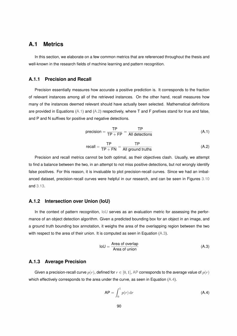
A.1 Metrics

In this section, we elaborate on a few common metrics that are referenced throughout the thesis and

well-known in the research fields of machine learning and pattern recognition.

A.1.1 Precision and Recall

Precision essentially measures how accurate a positive prediction is. It corresponds to the fraction

of relevant instances among all of the retrieved instances. On the other hand, recall measures how

many of the instances deemed relevant should have actually been selected. Mathematical definitions

are provided in Equations (A.1) and (A.2) respectively, where T and F prefixes stand for true and false,

and P and N suffixes for positive and negative detections.

precision =TP

TP + FP=

TPAll detections

(A.1)

recall =TP

TP + FN=

TPAll ground truths

(A.2)

Precision and recall metrics cannot be both optimal, as their objectives clash. Usually, we attempt

to find a balance between the two, in an attempt to not miss positive detections, but not wrongly identify

false positives. For this reason, it is invaluable to plot precision-recall curves. Since we had an imbal-

anced dataset, precision-recall curves were helpful in our research, and can be seen in Figures 3.10

and 3.13.

A.1.2 Intersection over Union (IoU)

In the context of pattern recognition, IoU serves as an evaluation metric for assessing the perfor-

mance of an object detection algorithm. Given a predicted bounding box for an object in an image, and

a ground truth bounding box annotation, it weighs the area of the overlapping region between the two

with respect to the area of their union. It is computed as seen in Equation (A.3).

IoU =Area of overlapArea of union

(A.3)

A.1.3 Average Precision

Given a precision-recall curve p(r), defined for r ∈ [0, 1], AP corresponds to the average value of p(r)

which effectively corresponds to the area under the curve, as seen in Equation (A.4).

AP =

∫ 1

0

p(r) dr (A.4)

90

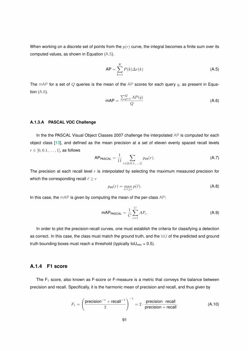
When working on a discrete set of points from the p(r) curve, the integral becomes a finite sum over its

computed values, as shown in Equation (A.5).

AP =

K∑k=1

P (k)∆r(k) (A.5)

The mAP for a set of Q queries is the mean of the AP scores for each query q, as present in Equa-

tion (A.6).

mAP =

∑Qq=1AP (q)

Q(A.6)

A.1.3.A PASCAL VOC Challenge

In the the PASCAL Visual Object Classes 2007 challenge the interpolated AP is computed for each

object class [13], and defined as the mean precision at a set of eleven evenly spaced recall levels

r ∈ [0, 0.1, . . . , 1], as follows

APPASCAL =1

11

∑r∈[0,0.1,...,1]

pint(r). (A.7)

The precision at each recall level r is interpolated by selecting the maximum measured precision for

which the corresponding recall r ≥ r

pint(r) = maxr:r≥r

p(r). (A.8)

In this case, the mAP is given by computing the mean of the per-class AP:

mAPPASCAL =1

C

C∑c=1

APc. (A.9)

In order to plot the precision-recall curves, one must establish the criteria for classifying a detection

as correct. In this case, the class must match the ground truth, and the IoU of the predicted and ground

truth bounding boxes must reach a threshold (typically IoUmin = 0.5).

A.1.4 F1 score

The F1 score, also known as F-score or F-measure is a metric that conveys the balance between

precision and recall. Specifically, it is the harmonic mean of precision and recall, and thus given by

F1 =

(precision−1 + recall−1

2

)−1= 2 · precision · recall

precision + recall. (A.10)

91

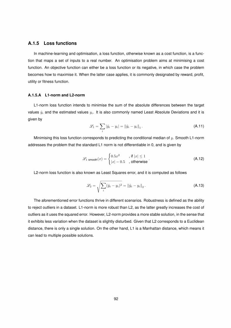
A.1.5 Loss functions

In machine-learning and optimisation, a loss function, otherwise known as a cost function, is a func-

tion that maps a set of inputs to a real number. An optimisation problem aims at minimising a cost

function. An objective function can either be a loss function or its negative, in which case the problem

becomes how to maximise it. When the latter case applies, it is commonly designated by reward, profit,

utility or fitness function.

A.1.5.A L1-norm and L2-norm

L1-norm loss function intends to minimise the sum of the absolute differences between the target

values yi and the estimated values yi. It is also commonly named Least Absolute Deviations and it is

given by

L1 =∑i

|yi − yi| = ‖yi − yi‖1 . (A.11)

Minimising this loss function corresponds to predicting the conditional median of y. Smooth L1-norm

addresses the problem that the standard L1 norm is not differentiable in 0, and is given by

L1 smooth(x) =

{0.5x2 , if |x| ≤ 1

|x| − 0.5 , otherwise. (A.12)

L2-norm loss function is also known as Least Squares error, and it is computed as follows

L2 =

√∑i

(yi − yi)2 = ‖yi − yi‖2 . (A.13)

The aforementioned error functions thrive in different scenarios. Robustness is defined as the ability

to reject outliers in a dataset. L1-norm is more robust than L2, as the latter greatly increases the cost of

outliers as it uses the squared error. However, L2-norm provides a more stable solution, in the sense that

it exhibits less variation when the dataset is slightly disturbed. Given that L2 corresponds to a Euclidean

distance, there is only a single solution. On the other hand, L1 is a Manhattan distance, which means it

can lead to multiple possible solutions.

92

A.2 Implementation

In this section, we provide relevant implementation details for the two developed frameworks. These

provide additional information to the official automatically generated documentation, that is hosted on-

line. Throughout development, we encountered several issues derived from the usual constraints of

building on top of existing code, and some of the solutions we found to be effective are neither intuitive

nor very straightforward. Whereas understanding these design choices might not be crucial for using

our tools from an end-user standpoint, these additional reports might be helpful for developers that may

one day decide to extend our platform.

A.2.1 GAP Implementation details

The official documentation of gap1 is hosted online2 and was generated automatically using Doxy-

gen3. It provides full coverage of plugin classes and interfaces, as well as additional utilities and ex-

amples. This section describes relevant implementation details of some features of our framework,

motivating design choices and clarifying seemingly convoluted procedures.

A.2.1.A Simultaneous multi-object texture update

Our first version of the dataset generation pipeline spawned and removed objects each scene. We

then proposed an enhanced approach that reuses object instances already in simulation. This led us to

the creation of a Gazebo plugin that handles an object visual appearance during simulation.

Gazebo’s modular design results in a barrier between physics and rendering classes, from the API

standpoint. Furthermore, the provided conventional Visual plugins are tied to a single model’s visual

appearance. These conditions persuaded us to create a Visual plugin, which is instanced once per

object in the scene, to which it is linked. Each object is able to specify which textures it should load and

supports loading a group of materials that match a given prefix. The latter feature was particularly useful

in our texture ablation study (Section 3.3.5).

These plugin instances share communication request and response topics. Because of this, we

are able to broadcast a single request to every connected peer simultaneously. Each object visual is

either modified or reset depending on whether its name is mentioned in the target field of the request

message. Thus, by specifying which objects should be updated, we implicitly state that the remaining

should perform some default behaviour (in this case resetting to its initial state). Each object has its

own instance of the plugin and is responsible for providing feedback to the client once texture has been

1� jsbruglie/gap Gazebo plugins for applying domain randomisation, on GitHub as of December 17, 20182Official GAP documentation http://web.tecnico.ulisboa.pt/joao.borrego/gap/, as of December 17, 20183Doxygen: Generate documentation from source code http://www.doxygen.nl/, as of December 17, 2018

93

updated. The client application (in our case the scene generation script) is tasked with keeping track of

which plugin instances have already replied.

A.2.1.B Creating a custom synthetic dataset

We provide a brief tutorial on how to create a custom synthetic dataset using our framework, which

is available online4 In order to do so, one must first launch Gazebo server and open a world file that in

turn loads our WorldUtils plugin. Then, in a separate terminal, we launch our scene_example client,

specifying the number of scenes to generate and dataset output directories for images and annotations.

This script assumes that the custom models for the ground plane, box, cylinder, sphere and camera

are located in a valid Gazebo resource directory and can be loaded in simulation. Parameters such as

which textures should be loaded and camera properties should be specified in these models respective

SDF files. Finally, we developed a Python script to debug resulting datasets, which displays images and

annotation overlays, specifying both class and bounding box, per object.

A.2.1.C Randomising robot visual appearance

Gazebo provides built-in features for programmatically altering objects during simulation, by listening

to named topics for particular requests. The latter include for instance messages for Visuals which

define the visual appearance of some model. Although in most of our proposed tools we handle parsing

requests ourselves, our DR interface uses these features directly. This is mostly because the physics

and rendering engines are decoupled and, as such, the plugin handling altering physical properties has

no control whatsoever regarding object visuals. We chose to use the default /visual topic, rather

than implementing custom visual plugins, as we had previously done for our object detection synthetic

dataset generation.

The randomisation of the visual appearance of each of the links in a robotic hand was performed in

OpenAI [51]. Figure A.1 shows Shadow Dexterous Hand robotic manipulator undergoing randomisation

of individual link colours.

Figure A.1: Shadow Dexterous Hand with randomised individual link textures

4Custom synthetic dataset tutorial https://github.com/jsbruglie/gap/tree/dev/examples/scene_example, as of Decem-ber 17, 2018

94

A.2.1.D Known issues

During our synthetic dataset generation, we noticed that Gazebo resources are automatically loaded

into memory. However, when replaced by other textures, we noticed memory usage did not decrease.

This suggests there exists a memory leak concerning the texture images. However, we believe this to

be a bug in Gazebo itself, specifically Rendering::Visual.setMaterial() but have made no further

efforts to identify the cause.

A.2.2 GRASP Implementation details

The official documentation of grasp5 is hosted online6 and was generated automatically using Doxy-

gen.

A.2.2.A Simulation of underactuated manipulators

Underactuated manipulators correspond to robotic hands which have fewer actuated DOF than over-

all number of moving joints. This allows for increased dexterity and compliant designs, while reducing

the number of required actuators and the overall complexity of the manipulator.

By default, Gazebo does not provide support for such joints, although a community-made Mimic Joint

plugin7. Previous experience with an older version of this plugin while working with Vizzy [46] had led

to underwhelming results, as the plugin commands collided with already existing PID instances. This

would typically result in unrealistic and buggy behaviour, sometimes even allowing fingers to clip through

objects.

For this reason, we provide our own implementation of this feature as part of our manipulator plugin

(HandPlugin), which reuses existing PID controllers and can control several joints at once. We have

found our solution to produce realistic behaviour and improved stability.

We need only specify a joint group, which consists of an actuated joint, and pairs of mimic joints

and respective multipliers. We model the coupling between actuated and mimic joints with a linear

relationship. Given the target value for an actuated joint ta, the target for the i-th mimic joint ti, associated

with multiplier mi is given by ti = mi · ta. The joint groups, initial target values and type of PID control

should be specified in the hand model SDF description.

5� jsbruglie/grasp Gazebo plugins for grasping in Gazebo, on GitHub as of December 17, 20186Official GRASP documentation http://web.tecnico.ulisboa.pt/joao.borrego/grasp/, as of December 17, 20187Set of Gazebo plugins by the Robotics Group University Of Patras. https://github.com/roboticsgroup/roboticsgroup_

gazebo_plugins, as of December 17, 2018

95

A.2.2.B Efficient contact retrieval

In Gazebo, contact information is broadcast using a named topic, to which a contact manager pub-

lishes. The latter creates filters for deciding which contacts should be published, for minimal performance

impact. However, we found that using the provided sensor plugin class and monitoring the communi-

cation channel caused a severe simulation speed downgrade (by as much as 30%). Since our specific

case does not require permanent monitoring of contacts, but rather evaluation at certain key instants,

we decided on an alternate approach.

Essentially, we developed a plugin that accepts requests with names of links for which to test for

contacts. When a request is received, the plugin briefly subscribes to the communication topic. As soon

as the first message is received it immediately leaves the channel.

If no other subscribers exist, this resumes regular simulation performance. Even though this may

seem convoluted, it was actually inspired by an official solution to a similar problem, involving Gazebo’s

graphical client’s feature to toggle the visualisation of contacts in simulation.

A.2.2.C Adding a custom manipulator

Currently, our framework has out-of-the-box support for two variants of Baxter grippers (short+narrow,

long+wide fingers), Shadow Dexterous Hand and Vizzy’s [46] right hand. Vizzy is our in-house robotic

platform, mostly used for human-robot interaction related research. Creating a custom manipulator

involves the following steps: (i) Obtain the robot manipulator’s Unified Robot Description Format (URDF)

file (typically generated using xacro), and simplify collision model; (ii) Add virtual joints and Hand plugin

instance to URDF file; (iii) Create an entry in the robot configuration file for the interface class.

In order to achieve efficient and reliable simulation, the manipulator’s collision model should be sim-

ple, and consist of convex components, or even parametric volumes, such as cylinders and boxes. We

performed this job manually for Vizzy’s right hand but could have resorted to open-source 3D model

editor software MeshLab8, to programmatically generate convex and low-polygon counterparts of each

link mesh.

The remaining steps of the process are further detailed in the repository’s official webpage. Finally,

we started creating a tool with a graphical interface for streamlining this process, which worked decently

for the pipeline we had then. Currently, the tool is not operational and requires fixing simple parsing

issues.

8MeshLab website http://www.meshlab.net/, as of December 17, 2018

96

A.2.2.D Adjusting randomiser configuration

Our randomiser class can be fully configured with a single YAML file, which essentially allows one to

specify

– Which properties to randomise, e.g. link masses, model scale vector components, joint damping

or friction coefficients, etc.;

– The associated probability distribution tied to each property, currently supporting uniform, log-

uniform and Gaussian distributions, with customisable parameters;

– The target joint, links or models of the property randomisation, supporting generic grasp target

objects by employing a pre-defined keyword that is later replaced by the appropriate model name;

– Whether the random sample is addictive or a coefficient given each property’s initial value.

The randomiser configuration used in the trials described in section 4.3 is presented in Listing A.1.

properties:link_mass:

dist:uniform: {a: 0.5, b: 1.5}

additive: Falsetarget:

0: {model: TARGET_OBJECT, link: base_link, mass: 0.250}friction_coefficient:

dist:uniform: {a: 0.7, b: 1.3}

additive: Falsetarget:

0: {model: TARGET_OBJECT, link: base_link,mu1: 10000, mu2: 10000}1: {model: baxter, link: gripper_l_finger_tip, mu1: 1000, mu2: 1000}2: {model: baxter, link: gripper_r_finger_tip, mu1: 1000, mu2: 1000}

Listing A.1: Example randomiser configuration

A.2.2.E Reference frame: Pose and Homogenous Transform matrix

In our work, we use 6D poses (x, y, x, roll, pitch, yaw) and 4 × 4 homogeneous transformation ma-

trices interchangeably when working with transforms between reference frames. Ignition’s math library

provides mathematical operators for chaining transform operations, which correspond to multiplying the

respective transform matrices.

97

A.2.2.F Known issues

Currently, our grasp simulation pipeline still exhibits some software stability issues, likely stemming

from our yet limited understanding of Gazebo’s internal physics API and lower-level interactions with

DART engine. This seems only natural, as the open-source simulator has grown to become a complex

tool, with its own share of issues and subtle intricate procedures which are hard to fully understand in

such a short time period. During earlier stages of testing our framework, we noticed sometimes the

Gazebo server would crash when running for several hours at once. When attempting to diagnose the

issue we arrived a the conclusion that it was related to some low-level computation in FCL (Flexible

collision library), yet made no further effort to fix it. Instead, we merely added protection mechanisms to

ensure minimal stress on the physics engine.

Currently, our pipeline can sample hundreds of grasps for multiple objects, without any significant

problems, although some physics-related bugs may occur under extreme cases where the forces exerted

on the object are tremendous.

A.3 Additional Material

In this section, we present supplementary material, which was not included in the main body of the

document as it may be important, yet not crucial to understanding our work.

Algorithm A.1 presents the pseudocode description of the algorithm for Perlin noise generation, out-

lined in Section 3.1.1.C.

Table A.1 presents the extensive results of our dynamic simulation trials described in Section 4.4.2.A,

including the outcome label for each of the up to 200 grasp trials performed per object in the KIT object

dataset [32].

98

Algorithm A.1: Perlin noise generator. In our 2D image case, only x and y coordinates areprovided. For z, a uniformly random zi coordinate is provided per each image channel.

Input : x x coordinate of target point t,y y coordinate of target point t,z z coordinate of target point t,p permutation table

Output: n Perlin noise value

Function generatePerlinNoise(x, y, z)/* Compute coordinates in unit cube */{xf , yf , zf} ← computeCoordinatesUnitCube(x, y, z);/* Compute fade curves */{u, v, w} ← { fade(xf ), fade(yf ), fade(zf ) };/* Hash coordinates of the 8 cube corners from permutation table p */{aaa, aba, aab, abb, baa, bab, bbb} ← getHash(p);x1 ← lerp ( gradient (aaa, xf , yf , zf ), gradient (baa, xf − 1, yf , zf ), u);x2 ← lerp ( gradient (aba, xf , yf − 1, zf ), gradient (bba, xf − 1, yf − 1, zf ), u);x3 ← lerp ( gradient (aab, xf , yf , zf − 1), gradient (bab, xf − 1, yf , zf − 1), u);x4 ← lerp ( gradient (abb, xf , yf − 1, zf − 1), gradient (bbb, xf − 1, yf − 1, zf − 1), u);y1 ← lerp (x1, x2, v);y2 ← lerp (x3, x4, v);n← 1

2 ( lerp(y1, y2, w) + 1)return n;

Function fade(t)/* For smoother transition between gradients */return 6t5 − 15t4 + 10t3;

Function lerp(a, b, t)/* Linear interpolation given inputs a, b for parameter t */return a+ t(b− a);

Function gradient(hash, x, y, z)/* Convert lower 4 bits of hash into one of 12 gradient directions */h← hash & 0b1111 ; // Obtain first 4 bits of hash/* If the MSB of the hash is 0 then u = x, else u = y */u← (h� 0b1000) ? x else y;if h� 0b0100 then

v ← y ; // If the 1st and 2nd MSBs are 0, v = yelse if h = 0b1100 or h = 0b1110 then

v ← x ; // If the 1st and 2nd MSBs are 1, v = xelse

v ← z/* Use the last 2 bits to decide if u and v are positive or negative */u← (h� 0b0001) ? u else −u;v ← (h� 0b0010) ? v else −v;return u+ v;

99

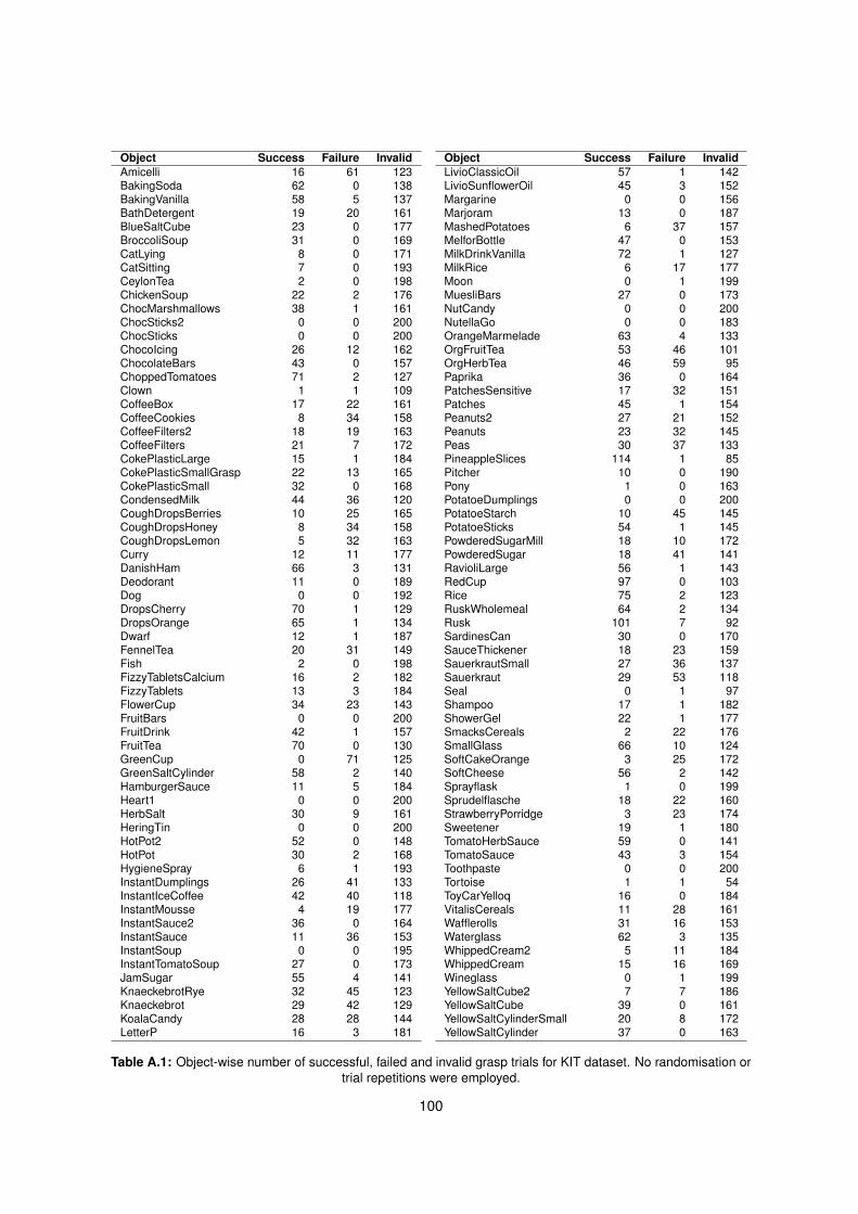
Object Success Failure InvalidAmicelli 16 61 123BakingSoda 62 0 138BakingVanilla 58 5 137BathDetergent 19 20 161BlueSaltCube 23 0 177BroccoliSoup 31 0 169CatLying 8 0 171CatSitting 7 0 193CeylonTea 2 0 198ChickenSoup 22 2 176ChocMarshmallows 38 1 161ChocSticks2 0 0 200ChocSticks 0 0 200ChocoIcing 26 12 162ChocolateBars 43 0 157ChoppedTomatoes 71 2 127Clown 1 1 109CoffeeBox 17 22 161CoffeeCookies 8 34 158CoffeeFilters2 18 19 163CoffeeFilters 21 7 172CokePlasticLarge 15 1 184CokePlasticSmallGrasp 22 13 165CokePlasticSmall 32 0 168CondensedMilk 44 36 120CoughDropsBerries 10 25 165CoughDropsHoney 8 34 158CoughDropsLemon 5 32 163Curry 12 11 177DanishHam 66 3 131Deodorant 11 0 189Dog 0 0 192DropsCherry 70 1 129DropsOrange 65 1 134Dwarf 12 1 187FennelTea 20 31 149Fish 2 0 198FizzyTabletsCalcium 16 2 182FizzyTablets 13 3 184FlowerCup 34 23 143FruitBars 0 0 200FruitDrink 42 1 157FruitTea 70 0 130GreenCup 0 71 125GreenSaltCylinder 58 2 140HamburgerSauce 11 5 184Heart1 0 0 200HerbSalt 30 9 161HeringTin 0 0 200HotPot2 52 0 148HotPot 30 2 168HygieneSpray 6 1 193InstantDumplings 26 41 133InstantIceCoffee 42 40 118InstantMousse 4 19 177InstantSauce2 36 0 164InstantSauce 11 36 153InstantSoup 0 0 195InstantTomatoSoup 27 0 173JamSugar 55 4 141KnaeckebrotRye 32 45 123Knaeckebrot 29 42 129KoalaCandy 28 28 144LetterP 16 3 181

Object Success Failure InvalidLivioClassicOil 57 1 142LivioSunflowerOil 45 3 152Margarine 0 0 156Marjoram 13 0 187MashedPotatoes 6 37 157MelforBottle 47 0 153MilkDrinkVanilla 72 1 127MilkRice 6 17 177Moon 0 1 199MuesliBars 27 0 173NutCandy 0 0 200NutellaGo 0 0 183OrangeMarmelade 63 4 133OrgFruitTea 53 46 101OrgHerbTea 46 59 95Paprika 36 0 164PatchesSensitive 17 32 151Patches 45 1 154Peanuts2 27 21 152Peanuts 23 32 145Peas 30 37 133PineappleSlices 114 1 85Pitcher 10 0 190Pony 1 0 163PotatoeDumplings 0 0 200PotatoeStarch 10 45 145PotatoeSticks 54 1 145PowderedSugarMill 18 10 172PowderedSugar 18 41 141RavioliLarge 56 1 143RedCup 97 0 103Rice 75 2 123RuskWholemeal 64 2 134Rusk 101 7 92SardinesCan 30 0 170SauceThickener 18 23 159SauerkrautSmall 27 36 137Sauerkraut 29 53 118Seal 0 1 97Shampoo 17 1 182ShowerGel 22 1 177SmacksCereals 2 22 176SmallGlass 66 10 124SoftCakeOrange 3 25 172SoftCheese 56 2 142Sprayflask 1 0 199Sprudelflasche 18 22 160StrawberryPorridge 3 23 174Sweetener 19 1 180TomatoHerbSauce 59 0 141TomatoSauce 43 3 154Toothpaste 0 0 200Tortoise 1 1 54ToyCarYelloq 16 0 184VitalisCereals 11 28 161Wafflerolls 31 16 153Waterglass 62 3 135WhippedCream2 5 11 184WhippedCream 15 16 169Wineglass 0 1 199YellowSaltCube2 7 7 186YellowSaltCube 39 0 161YellowSaltCylinderSmall 20 8 172YellowSaltCylinder 37 0 163

Table A.1: Object-wise number of successful, failed and invalid grasp trials for KIT dataset. No randomisation ortrial repetitions were employed.

100