Kinematic modeling of cross-sectional deformation sequences by computer simulation: coding and...

JOURNAL OF GEOPHYSICAL RESEARCH, VOL. 95, NO. B13, PAGES 21,913-21,929, DECEMBER 10, 1990

Kinematic Modeling of Cross-Sectional Deformation Sequences by Computer Simulation

JUAN CONTRERAS AND MAX SUTER

Institute of Geology, National University of Mexico, Mexico City

We derive a kinematic algorithm which permits simulation of postulated cross-sectional deformation sequences in sedimentary rocks affected by faulting, fault-related folding, and simple shear. The transformations are to a more deformed state and are formulated analytically in terms of the less deformed configuration (forward modeling, Lagrangian description). The medium is subdivided into domains of constant dip and homogeneous displacement vector fields which are delimited by the axial planes of the fault inflections. The displacement trajectory is of constant length for all the displaced particles throughout the medium and parallel to the underlying active fault segment. As a consequence, the deformation path is continuous but not smooth and causes an angular style of parallel folding, except at the deformation front where the layer thickness is not conserved. The inhomogeneity of the displacement vector field across axial planes introduces longitudinal and angular shear strains, whereas the area of the medium remains constant. These strains, which are superposed on the externally applied simple shear, make the mapping transformation unconformal. We define the stratigraphic layering of the undeformed medium by an approximating body of finite quadrilateral elements, evaluate the defined displacement functions for the grid nodes, and graph the deformed mesh. Eventually, we create with the algorithm synthetic deformation sequences for simple boundary conditions and try in a specific case study to match the resulting synthetics with the available observational and experimental data.

INTRODUCTION

The subsurface geometry of geological structures is not only the subject of intellectual curiosity but also a key in the search for natural resources such as hydrocarbons. A structural model of the subsurface geometry can be based on patterns of surface geological maps, experimental data such as seismics and gravimetry, and well data from cores, geophysical wireline measurements, and borehole seismics. These data acquisition techniques have different sampling rates which may range over 5-6 orders of magnitude. The highest one-dimensional resolution is provided by borehole logs, such as the dipmeter tool with a vertical definition of 5x10 '3 m [Serra, 1984], whereas the smallest sampling rate may correspond to a geological reconnaissance map with a horizontal definition of 103 m.

This wide range in sampling rates normally causes the three- dimensional data distribution to be inhomogeneous, which requires the use of conventional projection methods [De Paor, 1988a], as well as numerical interpolation and extrapolation techniques [Press et al., 1986] which are gradually finding acceptance in structural geology [Evans et al., 1985; McCoss, 1987; Stowe, 1988]. The application of these numerical analysis techniques in defining the subsurface geometry is hindered by the existence of discontinuities in form of faults, and singular surfaces in form of axial planes. Axial planes correspond to singular surfaces where the material lines remain continuous, but not their derivatives with respect to position and time [Cobbold et al., 1984]. This also has implications if we wish to determine in the medium the distributions of physical parameters which are governed by dif- ferential equations, as in the case of the numerical integration of strain.

Copyright 1990 by the American Geophysical Union.

Paper number 90JB01246. 0148-0227/90/90JB-01246505.00

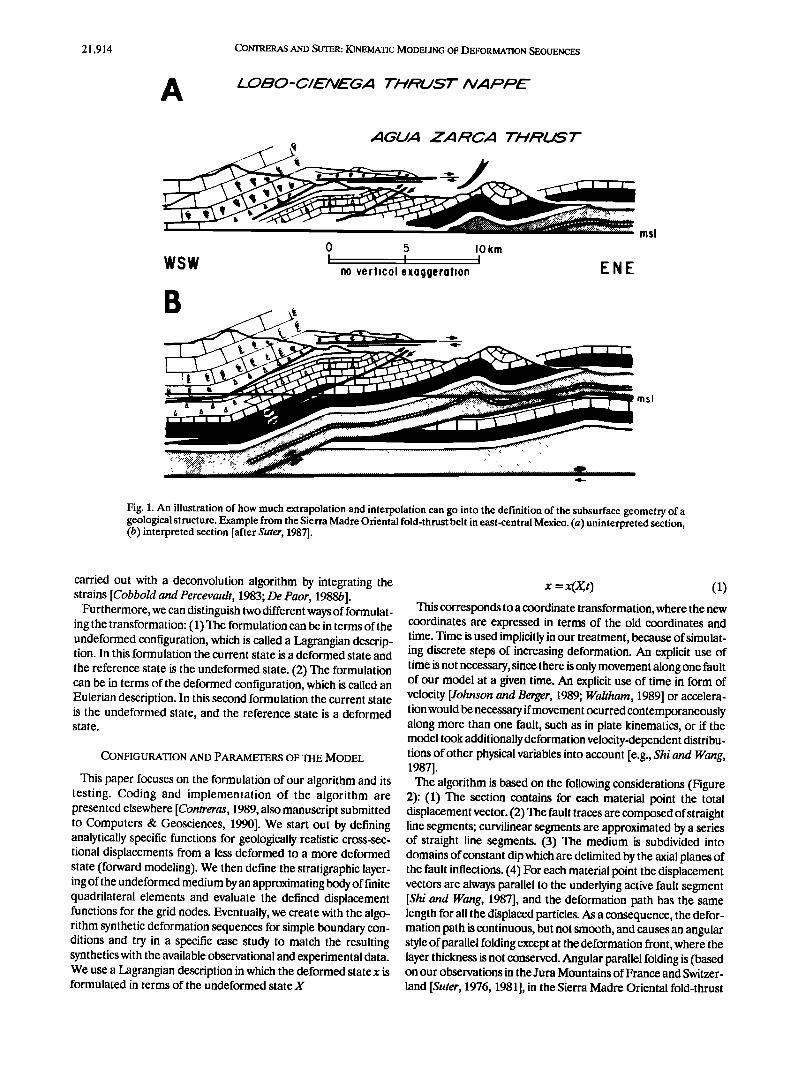
An illustration of how much interpolation and extrapolation may go into a structural subsurface interpretation is given in Figure 1. The extrapolation is based on surface geology (Figure la) and data from two nearby wells [Suter, 1987]. Extrapo- lated data are the thickness and dip of the stratigraphic layering and dips of axial planes and faults, as well as the angles contained between the stratigraphic layering and the faults. Additionally, in the interpreted section (Figure lb), a basal detachment fault is defined, the calculation of the depth of which is based on the general principle in continuum mechanics of the conservation of mass [Truesdell and Toupin, 1960; Malvern, 1969] by defining a closed system. The resulting subsurface geometry is, as is the case with most geophysical problems, a consistent but nonunique solution. Besides, the uncertainty of the result basically increases with depth.

A different approach, undertaken in this paper, to defining the structural subsurface geometry, is to carry out a deterministic simulation of a deformation sequence that leads to a final synthetic geometry in agreement with the available data [Contreras and Suter, 1988]. We define for that purpose analytically geologically realistic transformation functions.

We have two options cocerning the direction of the transformation: (1) Fov0•ard modeling, which is the transformation from a less deformed to a more deformed state, or as a special case the transformation from the uncleformed to a deformed state. The

linear vector operator relating the two states is known as Cauchy's finite deformation tensor [Means, 1976], the transformation matrix as Jacobian matrix. The determinant of the Jacobian is the

local volume ratio at each point in the transformation between the deformed and uncleformed regions [Barr, 1984]. (2) Inverse modeling, which is the transformation from a deformed to a less deformed state, or as a special case to the uncleformed state. The transformation matrix relating the two states is known as Green's finite deformation tensor [Means, 1976]. The inversion transformation consists in inverting the transformation matrix, which is easiest for an orthogonal matrix because the inverse A t coincides with the transpose A; 1 . The inverse transformation can also be

21,913

21,914 CONTRERAS AND SUTER: KINEMATIC MODELING OF DEFORMATION SEQUENCES

A LOBO-C/E/VEGA THRUST NAPPE

AGUA ZA RCA THRlI9 T

0 5 IOkm

WSW : no vertical exaggeration E N E

B •

A A 6

ms1

Fig. 1. An illustration of how much extrapolation and interpolation can go into the definition of the subsurface geometry of a geological structure. Example from the Sierra Madre Oriental fold-thrust belt in east-central Mexico. (a) uninterpreted section, (b) interpreted section [after Suter, 1987].

carried out with a deconvolution algorithm by integrating the strains [Cobbold and Percevault, 1983; De Paor, 1988b].

Furthermore, we can distinguish two different ways of formulat- ing the transformation: (1) The formulation can be in terms of the undeformed configuration,-which is called a Lagrangian description. In this formulation the current state is a deformed state and

the reference state is the undeformed state. (2) The formulation can be in terms of the deformed configuration, which is called an Eulerian description. In this second formulation the current state is the undeformed state, and the reference state is a deformed state.

CONFIGURATION AND PARAMETERS OF THE MODEL

This paper focuses on the formulation of our algorithm and its testing. Coding and implementation of the algorithm are presented elsewhere [Contreras, 1989, also manuscript submitted to Computers & Geosciences, 1990]. We start out by defining analytically specific functions for geologically realistic cross-sectional displacements from a less deformed to a more deformed state (forward modeling). We then define the stratigraphic layering of the u ncleformed medium by an approximating body of finite quadrilateral elements and evaluate the defined displacement functions for the grid nodes. Eventually, we create -with the algorithm synthetic deformation sequences for simple boundary conditions and try in a specific case study to match the resulting synthetics with the available observational and experimental data. We use a Lagrangian description in which the deformed state x is formulated in terms of the uncleformed state X

x = x(X,,t) (1)

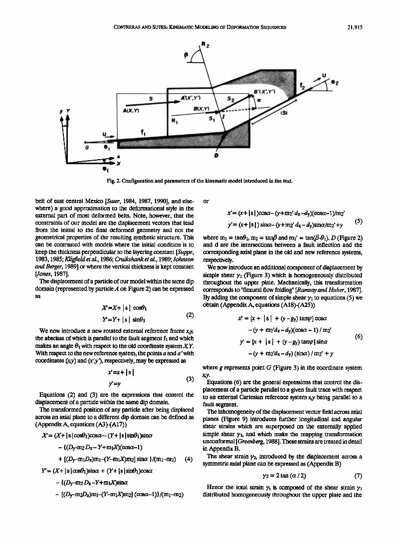
This corresponds to a coordinate transformation,-where the new coordinates are expressed in terms of the old coordinates and time. Time is used implicitly in our treatment, because of simulating discrete steps of increasing deformation. An explicit use of time is not necessary, since there is only movement along one fault of our model at a given time. An explicit use of time in form of velocity [Johnson and Berger, 1989; Waltham, 1989] or accelera- tion would be necessary ifmovement ocurred contemporaneously along more than one fault, such as in plate kinematics, or if the model took additionally deformation velocity-dependent distributions of other physical variables into account [e.g., Shi and Wang, 1987]. The algorithm is based on the following considerations (Figure

2): (1) The section contains for each material point the total displacement vector. (2) The fault traces are composed of straight line segments; curvilinear segments are approximated by a series of straight line segments. (3) The medium is subdivided into domains of constant dip which are delimited by the axial planes of the fault inflections. (4) For each material point the displacement vectors are always parallel to the underlying active fault segment [Shi and Wang, 1987], and the deformation path has the same length for all the displaced particles. As a consequence, the deformation path is continuous, but not smooth, and causes an angular style of parallel folding except at the deformation front, where the layer thickness is not conserved. Angular parallel folding is (based on our observations in the Jura Mountains of France and Switzer-

land [Suter, 1976, 1981], in the Sierra Madre Oriental fold-thrust

CONTRERAS AND SLATER: KINEMATIC MODELING OF DEFORMATION SEQUENCES 21,915

R 2

8'(X'.

S A'tX'.¾'}

y Y A(X.Y•

ß t

fl

R! $1 ISI

Fig. 2. Configuration and parameters of the kinematic model introduced in the text.

u

e2

belt of east central Mexico [Suter, 1984, 1987, 1990], and elsewhere) a good approximation to the deformational style in the external part of most deformed belts. Note, however, that the constraints of our model are the displacement vectors that lead from the initial to the final deformed geometry and not the geometrical properties of the resulting synthetic structure. This can be contrasted with models where the initial condition is to

keep the thickness perpendicular to the layering constant [Suppe, 1983, 1985; Kligfield et al., 1986; Cmikshank et aL, 1989; Johnson and Berger, 1989] or where the vertical thickness is kept constant [Jones, 1987].

The displacement of a particle of our model within the same dip domain (represented by particle ,4 on Figure 2) can be expressed as

;c=x+ Is I

Is I sin01 (2) We now introduce a new rotated external reference frame •;y,

the abscissa of which is parallel to the fault segment f2 and which makes an angle 0• with respect to the old ccx)rdinate system X,, Y. With respect to the new reference system, the points a and a'with coordinates (x,y) and (x',y'), respectively, may be expressed as

Y' =Y (3) Equations (2) and (3) are the expressions that control the

displacement of a particle within the same dip domain. The transformed position of any particle after being displaced

across an axial plane to a different dip domain can be defined as (Appendix A, equations (A3)-(A17))

X' = (X+ I s I cos01)cosat-- (Y+ Is I sin01)sina

- {(Dy-m2 Dx- Y+mlX)(cosa-1)

+ [(Dy-mlDx)m•-(Y-m•X)m2] sina }/(m•-m2) (4)

r' = (x+ Is I cos0•)sina + (Y+ I s I sin0•)cosa

- { (Dy-m2 Dx -Y+ mlX)sina

- [(Dy-m2Dx)m•-(Y-mlX)m2] (cosa-1)}/(m•-m2)

or

x'= (x+ I s I)cosa- 0,+m2' dx-dy)(cosa-1)/m2'

y' = (x+ Is I ) sina- (y + m2' dx - dy)sina/m2' +y (5) where m• = tan0•, m2 = tanf and m2' = tan05• 0. D (Figure 2) and d are the intersections between a fault inflection and the

corresponding axial plane in the old and new reference systems, respectively.

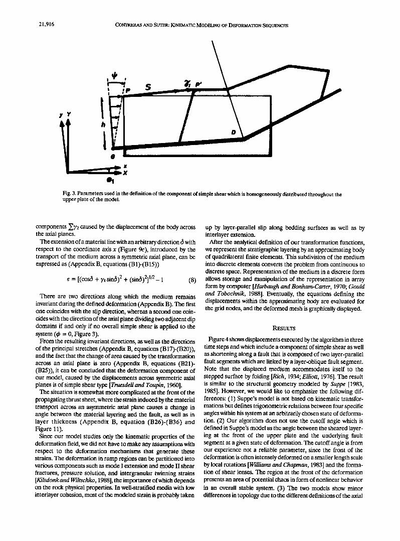
We now introduce an additional component of displacement by simple shear 72 (Figure 3) which is homogeneously distributed throughout the upper plate. Mechanically, this transformation corresponds to "flexural flow folding" [Ramsay and Huber, 1987]. By adding the component of simple shear 72 to equations (5) we obtain (Appendix A, equations (A18)-(A25))

x' = [x + I sl + Cv-gy) tang,] cosat

-(y + m2'dx-dy)(coscr- 1)/m2' (6)

y' = [x + I sl + (y-gy) tang,] sina

- C v + m2'dx-dy) (sine 0 / m2' + y

where g represents point G (Figure 3) in the ccx)rdinate system x;y.

Equations (6) are the general expressions that control the displacement of a particle parallel to a given fault trace with respect to an external Cartesian reference system x,y being parallel to a fault segment.

The inhomogeneity of the displacement vector field across axial planes (Figure 9) introduces further longitudinal and angular shear strains which are superposed on the externally applied simple shear 72, and which make the mapping transformation unconformal [Greenberg, 1988]. These strains are treated in detail in Appendix B.

The shear strain y2, introduced by the displacement across a symmetric axial plane can be expressed as (Appendix B)

72 = 2 tan (a / 2) (7)

Hence the total strain •'t is composed of the shear strain distributed homogeneously throughout the upper plate and the


! IP !

Fig. 3. Parameters used in the definition of the component of simple shear which is homogeneously distributed throughout the upper plate of the model.

components •y2 caused by the displacement of the body across the axial planes.

The extension of a material line with an arbitrary direction (5 with respect to the coordinate axis x (Figure 9c), introduced by the transport of the medium across a symmetric axial plane, can be expressed as (Appendix B, equations (B 1)-(B 15))

e = [(co• + 7t sin6) 2 + (sin6)2] 1/2- 1 (8)

There are two directions along which the medium remains invariant during the defined deformation (Appendix B). The first one coincides with the slip direction, whereas a second one coincides with the direction of the axial plane dividing two adjacent dip domains if and only if no overall simple shear is applied to the system ((p = 0, Figure 3).

From the resulting invariant directions, as well as the directions of the principal stretches (Appendix B, equations (B 17)-(B20)), and the fact that the change of area caused by the transformation across an axial plane is zero (Appendix B, equations (B21)- (B25)), it can be concluded that the deformation component of our model, caused by the displacements across symmetric axial planes is of simple shear type [Truesdell and Toupin, 1960].

The situation is somewhat more complicated at the front of the propagating thrust sheet, where the strain induced by the material transport across an asymmetric axial plane causes a change in angle between the material layering and the fault, as well as in layer thickness (Appendix B, equation (B26)-(B36) and Figure 11).

Since our model studies only the kinematic properties of the deformation field, we did not have to make any assumptions with respect to the deformation mechanisms that generate these strains. The deformation in ramp regions can be partitioned into various components such as mode I extension and mode II shear fractures, pressure solution, and intergranular twinning strains [Kilsdonk and Wiltschko, 1988], the importance ofwhich depends on the rock physical properties. In well-stratified media with low interlayer cohesion, most of the modeled strain is probably taken

up by layer-parallel slip along bedding surfaces as well as by interlayer extension.

After the analytical definition of our transformation functions, we represent the stratigraphic layering by an approximating body of quadrilateral finite elements. This subdivision of the medium into discrete elements converts the problem from continuous to discrete space. Representation of the medium in a discrete form allows storage and manipulation of the representation in array form by computer [Harbaugh and Bonham-Carter, 1970; Gould and Tobochnik, 1988]. Eventually, the equations defining the displacements within the approximating body are evaluated for the grid nodes, and the deformed mesh is graphically displayed.

RESULTS

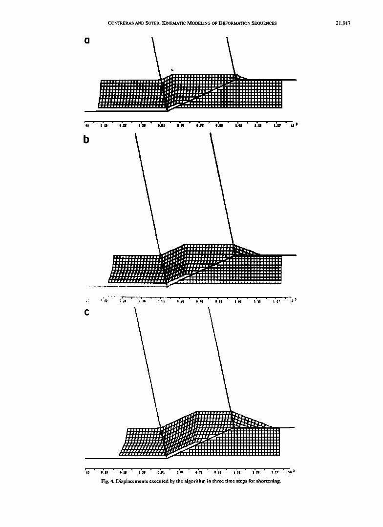
Figure 4 shows displacements executed by the algorithm in three time steps and which include a component of simple shear as well as shortening along a fault that is composed of two layer-parallel fault segments which are linked by a layer-oblique fault segment. Note that the displaced medium accommodates itself to the stepped surface by folding [Rich, 1934; Elliott, 1976]. The result is similar to the structural geometry modeled by Suppe [1983, 1985]. However, we would like to emphasize the following differences: (1) Suppe's model is not based on kinematic transformations but defines trigonometric relations between four specific angles within his system at an arbitrarily chosen state of deformation. (2) Our algorithm does not use the cutoff angle which is defined in Suppe's model as the angle between the sheared layering at the front of the upper plate and the underlying fault segment at a given state of deformation. The cutoff angle is from our experience not a reliable parameter, since the front of the deformation is often intensely deformed on a smaller length scale by local rotations [Williams and Chapman, 1983] and the formation of shear lenses. The region at the front of the deformation presents an area of potential chaos in form of nonlinear behavior

in an overall stable system. (3) The two models show minor differences in topology due to the different definitions of the axial

CONTRERAS AND SUTER: KINEMATIC MODELING OF DEFORMATION SEQUENCES 21,917

cI

i i111 !!i !i ii111 ! ß .a i il!!l!!llll!!!llil li

•11 If!! !!!Ill !!!! !111 I I Jll!lJiJ!lll!111111lll Id JlllJii!!!!!!!!111llll

!_

i I I i ! I• r

•/I iI IIII •,-

ii

.•W•l i ! ! i i ! !!11

b

lll[!!lll[! !__

dlllrl'f f _.drTe ![i[l ],•/!!!!111II '--=,LpP'r!--! ! I ! I ! ! I I I ....

c

rillifil/Ill 111111iiL .,.-

Ifillib r

•'"'T, IIi i i i! i !111 iii i !111

Fig. 4. Displacements executed by the algorithm in three time steps for shortening.

21,918 COt•rRERAS AND SLITER: KINEMATIC MODELING OF DEFORMATION SEQUENCES

planes. In our model the axial planes located at the inflections of the fault trace are stationary with respect to the lower plate (Figure 4a) and bisect the angles between neighboring fault segments, which satisfies our constraint that the slip vectors be parallel to the underlying fault segment. This is entirely not the case in Suppe's model, where the axial plane between the ramp and the upper flat bisects the upper plate dip domains which satisfies his constraint of constant layer thiclmess. Both configurations have been observed in experimental analog models [Morse, 1978].

Beside the a•ve mentioned stationary axial planes we can also observe in Figure 4 the formation of a nonstationary axial plane which is propagating through the material layering of the upper plate.

Figure 5 is an example of extension along a series of listfie normal faults executed by the algorithm. As in the case of shortening, the displacement vectors of the hanging wall are parallel to the underlying fault segment, and the lengths of the displacement trajectories within the hanging wall are constant. The resulting structure is similar to the graphical slip line construction by 145Iliams and Vann [1987], the only difference being that in our model the axial planes bisect the angle between adjacent fault segments, whereas in the model by Williams and Vann the hanging wall deformation is considered in terms of fault-perpendicular displacement segments. The activation of the faults was sequen- tially from right to left, opposite to the general direction of material displacement. An external component of 10 ø of simple shear was counterclockwise applied to the system during the activation of the third fault. This causes the displacement along

the fault to increase with increasing depth, as can be seen at the right grid margin and from the separations of the shaded reference horizon in the folded left part of the section. Improve- ments of our model could account for syntectonic sedimentation [Waltham, 1989], and subsidence due to sediment loading [Gibbs, 1983; Wendeville and Cobbold, 1988]. It is possible with our algorithm to simulate duplexes [Boyer and

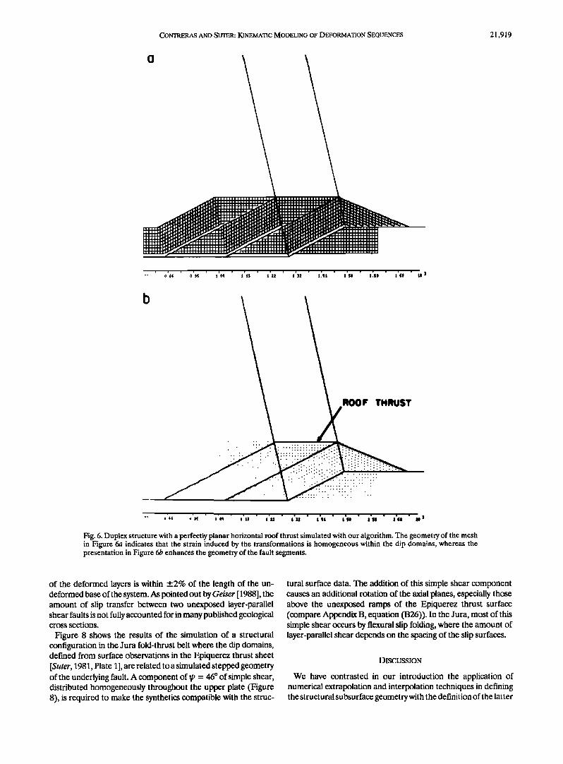
Elliott, 1982] with a perfectly planar horizontal roof thrust (Figure 6), whereas the simulation of duplexes with the Suppean fault- bend fold model, which keeps the layer thickness constant, leads to roof thrusts with a rugose geometry [Groshong and Usdansky, 1988; Cruikshank et al., 1989]. Natural examples of roof duplexes are often planar [Groshong and Usdansky, 1988], especially if there is a strong contrast in mechanical competence across the roof thrust (R. Groshong, verbal communication, 1990). Further- more, it seems to us intuitively that transport along a flat roof thrust should consume less energy than transport along a fault with an irregular surface, which suggests that our model is more realistic. It can also be noted from the geometry of the mesh in Figure 6a that the strain induced by the transformations is homogeneous within the dip domains.

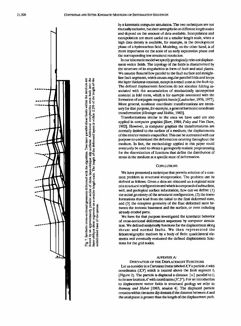
Figure 7 shows a more complicated cross-sectional geometry deformed with the same algorithm. Two layer-parallel shear faults within the medium are linked by an approximately parallel series of three layer-oblique slip surfaces. A component of simple shear was applied at the left end of the system. Additional complexities were built into the layer-oblique shear segments on a smaller length scale in analogy to fault configurations observed in fold- thrust terrane (Boyer and Elliott [1982] and Figure 1). The length

......... :. :..:.. . ::::::::::::::::::::::::::::::::::::::: : ..... .................................

......

--

Fig. 5. Synthetic cross-sectional geometry deformed with the algorithm, simulating deformation in an extensional terrain. A simple shear component of 10 ø was applied counterclockwise to the system during the activation of the third fault from the right. (a) mesh representing the final deformed geometry. The graphed axial planes correspond to the inflections of the outermost fault on the left. (b) Final deformed geometry with the faults being enhanced.


o

•ll !I ! I!!!

ROOF THRUST

Fig. 6. Duplex structure with a perfectly planar horizontal roof thrust simulated with our algorithm. The geometry of the mesh in Figure 6a indicates that the strain induced by the transformations is homogeneous within the dip domains, whereas the presentation in Figure 6/9 enhances the geometry of the fault segments.

of the deformed layers is within _+2% of the length of the uncleformed base of the system. As pointed out by Geiser [1988], the amount of slip transfer between two unexposed layer-parallel shear faults is not fully accounted for in many published geological cross sections.

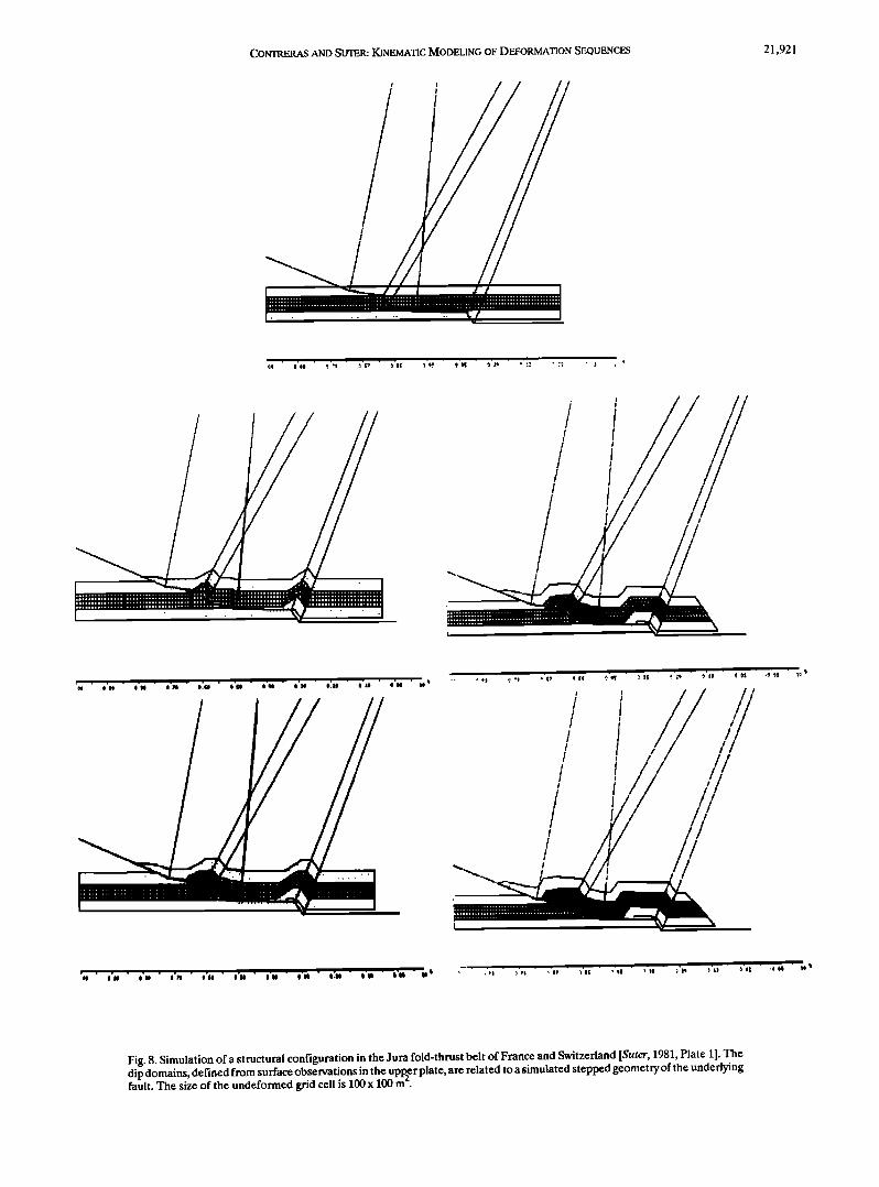
Figure $ shows the results of the simulation of a structural configuration in the Jura fold-thrust belt where the dip domains, defined from surface observations in the Epiquerez thrust sheet [Suter, 1981, Plate 1], are related to a simulated stepped geometry of the underlying fault. A component of •, = 46 ø of simple shear, distributed homogeneously throughout the upper plate (Figure $), is required to make the synthetics compatible with the struc-

tural surface data. The addition of this simple shear component causes an additional rotation of the axial planes, especially those above the unexposed ramps of the Epiquerez thrust surface (compare Appendix B, equation (B26)). In the Jura, most of this simple shear occurs by flexural slip folding, where the amount of layer-parallel shear depends on the spacing of the slip surfaces.

DISCUSSION

We have contrasted in our introduction the application of numerical extrapolation and interpolation techniques in defining the structural subsurface geomet.,T with the definition of the latter


by a kinematic computer simulation. The two techniques are not mutually exclusive, but their strengths lie on different length scales and depend on the amount of data available. Interpolation and extrapolation are more useful on a smaller length scale, when a high data density is available, for example, in the development phase of a hydrocarbon field. Modeling, on the other hand, is of more importance on the scale of an early exploration phase and the corresponding low structural resolution.

In our kinematic model we specify geologically relevant displacement vector fields. The topology of the fields is characterized by the structure of its singularities in form of fault and axial planes. We assume flexural flow parallel to the fault surface and straight- line fault segments, which causes angular parallel folds and keeps the layer thickness constant, except in a small zone at the fault tip. The defined displacement functions do not simulate folding associated with the accumulation of mechanically incompetent material in fold cores, which is for example associated with the formation of conjugate megakink bands [Laubscher, 1976, 1977]. More general, nonlinear coordinate transformations are necessary for that purpose, for example, a general harmonic coordinate transformation [Hirsinger and Hobbs, 1983].

Transformations similar to the ones we have used are also

applied in computer graphics [Barr, 1984; Foley and Van Dam, 1982]. However, in computer graphics the transformations are normally limited to the surface of a medium; the displacements of the interior remain unspecified. This can be contrasted with our purpose to understand the deformation ocurring throughout the medium. In fact, the methodology applied in this paper could eventually be used to obtain a geologically realistic preprocessing for the discretization of functions that define the distribution of

stress in the medium at a specific state of deformation.

CONCLUSIONS

We have presented a technique that permits solution of a com- mon problem in structural interpretation. The problem can be defined as follows: Given a data set obtained on a regional scale of a structural configuration and which is composed of subsurface, well, and geological surface information, how can we define: (1) the initial geometry of the structural configuration, (2) the transformations that lead from the initial to the final deformed state, and (3) the complete geometry of the final deformed state between the tectonic basement and the surface, or even including already eroded parts.

We have for that purpose investigated the kinematic behavior of cross-sectional deformation sequences by computer simulation. We defined analytically functions for the displacement along thrust and normal faults. We then represented the lithostratigraphic medium by a body of finite quadrilateral elements and eventually evaluated the defined displacement functions for the grid nodes.

APPENDIX A:

DERIVATION OF THE DISPLACEMENT FUNCTIONS

Let us consider in a Cartesian frame labeledX, Ya particleA with coordinates (X,Y) which is located above the fault segment f• (Figure 2). The particle is displaced a distance I s I parallel to f• to its new locationA' with coordinates (X', Y'). For an introduction to displacement vector fields in structural geology we refer to Ramsay and Huber [1983, session 4]. The displaced particle remains within the same dip domain if the distance betweenA and the axial plane is greater than the length of the displacement path.


/

i • /

/ / t

/ t

ß e:ee ß

, ,/ // / ! / i / i I

i

' to I•

Fig. 8. Simulation of a structural configuration in the Jura fold-thrust belt of France and Switzerland [Suter, 1981, Plate 1]. The dip domains, defined from surface observations in the uppffr plate, are related to a simulated stepped geometry of the underlying fault. The size of the undeformed grid cell is I00 x 100 m.

21,922 CONTRE• AND SUTER: KINEMATIC MODELING OF DEFORMATION SEQUENCES

.4 and .4' are connected by the equations

x'=x+ Is (^•)

Y'= Y + Is I sin0• We now introduce a new rotated external reference frame x,y,

the abscissa of which is parallel to the fault segment f• and which makes an angle 0• with respect to the old coordinate system X;Y. Both reference systems have the same scale and origin. With respect to the new reference system, the points a and a' with coordinates (x,y) and (x;y'), respectively, may be expressed as

Y'= Y (A2) Equations (A1) and (A2) are the expressions that control the

displacement of a particle within the same dip domain. By introducing the displacement unit vector

u = cos01i + sin01j

where i and j are base vectors, equations (A1) can be written as:

x,=x + Islux

Y'=Y + I s luy (A•)

which gives the equations (A1) a kinematic meaning. Consider now a different particle B which, after being displaced

a distance s • parallel to f•, crosses an axial plane, as shown in Figure 2. The displacement path of particle B is made up of two components s• and s2 which are parallel to the fault segments h and f2, respectively, such that

s = sl + s2 (A4)

However, this decomposition is complicated by the dependence of s• and s2 on the specific position of each particle.

The second component of the transformation from B to B' can also be carried out by a rotation around I with an angle a =02-0•, as shown in Figure 2. Counterclockwise rotations are considered positive. IfI coincides with the origin of the reference system, the rotation can be expressed in matrix form as

Additional transformations are necessary if I does not coincide

IX' v'] :(x+ Is I cos0• - cos• sina 1 y+ I s I sin0t I .sin• cosa_ ] (AS) with the origin of the reference system. The origin of the reference system is in that case translated to the center of rotation and, after executing the rotation, back to its original location. In matrix form, this may be written as

x+ Is I I

[X'Y'I]= Y+lslsin0• / 1 1IIx_Iy • lms•S• sina i i Ii X 0 il O1 acosa 1

o Iy

(A6) An additional row and an additional column have been introduced

to make the matrices conformable for multiplication. We now expand equation (A6) in both the old and new

reference systems:

z--Cx + Is I cos01)cos•- (Y + I s I sin00sina

-Ix(cosa- 1) + Iy sina

Y'=(x + I s I cos0•)sina + (Y + I s I sin0•)cosa (A7)

-Ixsina + Iy(cosa- 1)

and

x'= (x + I s I )cosa - y sina - ix (cosa - 1) + iy sina (A8)

y'= (x + I s I )sina + ycosa - ixsina - iy (sina -1) As mentioned above, the coordinates of I vary in accordance to

the location of B(X;Y):

Ix = Ix(X,,Y)

Iy =/y(X;Y) (A9) Geometrically, I can be considered as the intercept of the lines

R• and R2 (Figure 2), where R• represents a family of parallel lines of the displacement vector field, and R2 is the axial plane bisecting adjacent dip domains. R• and R2 can be expressed as

Ri=mlX+C1 (AlO)

R2=m2X+C2

where m• =tan0•, and mz=tanfl; C•, C2 are constants:

Ci = Y+ mlX (All)

C2 =Dy- m2Dx

where D is the intersection between a fault inflection and the

corresponding axial plane (Figure 2). We can now substitute (A11) in (A10) and obtain in matrix form

1 - m I Y- mix

ll-m21 I)l =•Dy-m2D,• i (A12) We now substitute I for (XY) and solve the system (A12) using

Cramefts rule:

Ix= (Dy- m2Dx- Y + miX) / (ml - m2) (A13)

Iy = [(Dy- m2Dx)ml - (Y- miX) m2] / (ml - m2)

Equations (A13) define the locus formed by the intercept of the parallel field lines R• with the axial plane R2. With respect to the new coordinate system, equations (A13) can be written as

where

ix = (y + m2'dx-dy) / m2' (A14)

m2' = tan(f1-01) whereas m•' = 0.

We now substitute equations (A13) and (A14) in equations (A7) and (A8), respectively:

X' - (X+ Is I cos01)cosa-- (Y+ Is [ sin01)sina

- {(Dy-m2 Dx- Y+mlX)(cosa-1)

+ [(Dy-mlDx)ml-(Y-mlX)m2] sina }/(ml-m2) (A16)

Y' = (X+ I s I cos01)sina + (Y+ I s I sin01)cosa

- { (Dy-m2 Dx -Y+ mlX)sina

- [(Dy-m2Dx)ml-(Y-mlX)m2] (cosa-1)}/(ml-m2) or

(A15)

x'= (x+ Is I)•os•- 0,+m2' dx--dy)(cosa-1)/m2'

y' = (x q- Is l) sina- 0' + m2' dx - dy)sina/m2' +y (A17)

CONTRERAS AND SLr'rER: KINEMATIC MODELING OF DEFORMATION SEQUENCES 21,923

which corresponds to equations (4) and (5) in the main body of this article.

Equations (A16) and (A17) are the expressions for the transformed position of any particle of our model after having been displaced across an axial plane to a new dip domain (Figure 2).

We now introduce an additional component of displacement by simple shear 7• (Figure 3) which is homogeneously distributed throughout the upper plate. Mechanically, this transformation corresponds to "flexural flow folding" [Ramsay and Huber, 1987]. The displacement 7• is a function of the angle •p (clockwise increases of•p are considered positive) and of the distance h of the displaced particle P from the fault trace such that

yl=h tamp (A18)

where h is the projection of G'P on the y axis

h = (X- Gx)sin 01 + (Y- Gy)cos 0• (A19)

or with respect to the reference systemx, y, where 0• =O,h becomes

h=y-gy (A20)

The magnitudes of the components of y• are

lyl• I -- I yll cos {91 (A21)

171yl = l y• I sin 01 and

l ylx I = (Y - qy) tang,

lylyl--0 (A22)

APPENDIX B: ANALYSIS OF STRAIN INDUCED BY MATERIAL

TRANSPORT ACROSS AXIAL PLANES

In our model the bisectrices between adjacent fault segments coincide with symmetrical axial planes separating dip domains of the upper plate, except at the front of the propagating thrust sheet where the axial plane is not symmetric (Figure 4). In what follows we determine first the strain induced by material transport across symmetrical axial planes, and then the strain induced by material transport across the asymmetrical axial plane at the front of the system.

Strain Induced by Material Transport Across Sy•nmetrical Axial Planes

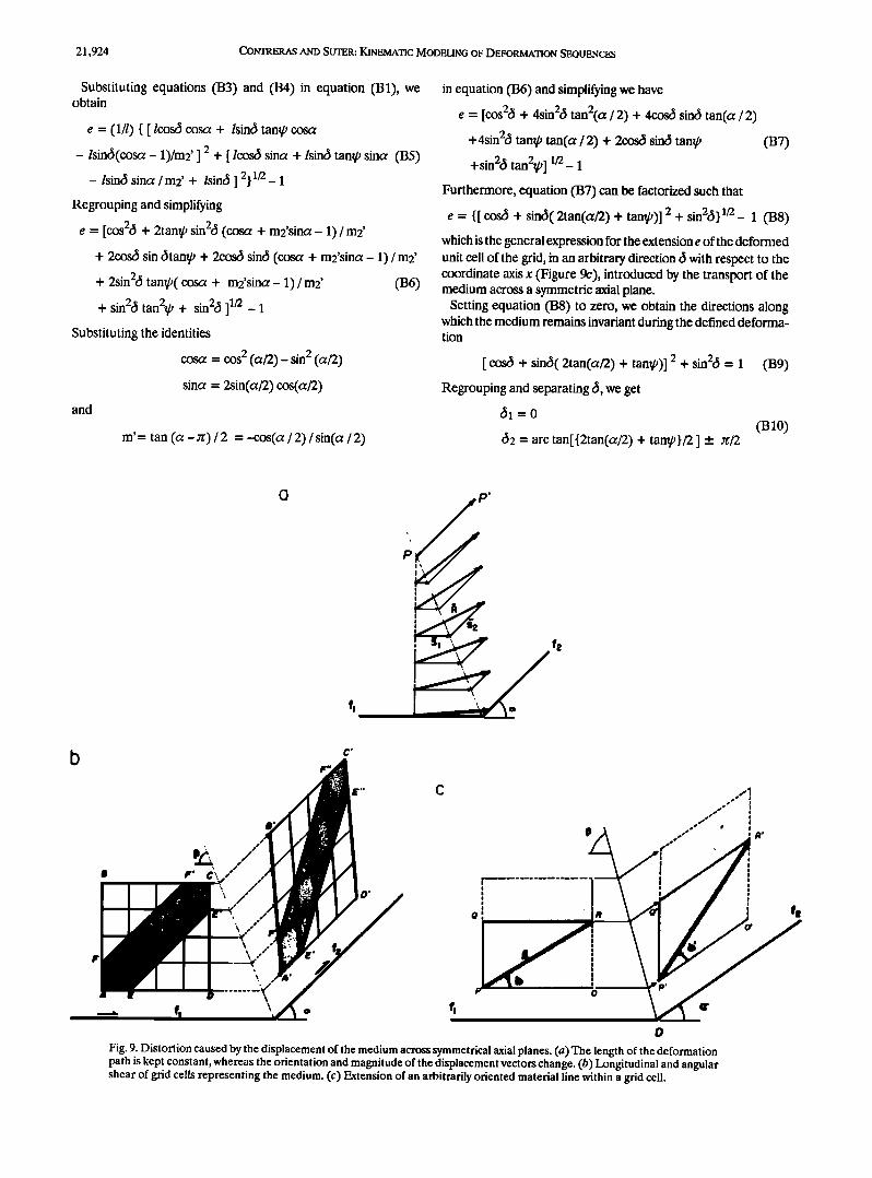
The length of the deformation path is kept constant across symmetrical axial planes of our model, whereas the orientation and magnitude of the displacement vectors change (Figure 9a), which simulates a noncoaxial progressive deformation. The inhomogeneity of the displacement vector field across axial planes introduces longitudinal and angular shear strains (Figure 9b) that make the mapping transformation unconformal [Greenberg, 1988]. This distortion is evident on Figure 4 and present in our simulations even without the introduction of an external simple shear component y•. Hence the simulated displacements cause an internal deformation of the stratigraphic layering, which would not be recognizable without vertical grid lines.

In Figure 9b, we show the part of the grid that corresponds to the displacement vectors of Figure 9a. The extension e of an arbitrary material line of the model (Figure 9c) can be defined as

We now substitute equations (A18) and (A19) in equations (A21) and add them to equations (A1)

X' = X + { I s I + [(X- Gx)sin01

+ (Y- Gy)cos01]tamp } cosat

r= Y + {Isl + [(x-Gx)sin01

+ (Y- Gy)cos01] tamp}sina

(A23)

or with respect to the reference frame x,y

x'= x + Is I + Cv-gy) tang, (A24)

y'=y

Similarly, by adding the component of simple shear y• to the equations (A17) we obtain

x' =Ix+ Isl + Cv-gy)tang']cosa

- (y + m2'dx - dy)(CO• - 1) / m2'

y' = Ix + I sl + Cy-gy) tamp] sina (A25)

- (y + m2'dx-dy) (sina) / m2' + y

which corresponds to equations (6) in the main body of the text. Equations (A24) and (A25) are the general expressions that

control the displacement of a particle parallel to a given fault trace with respect to an external Cartesian reference system x,y being parallel to a fault segment.

e= (B1)

The coordinates of the points P and R (Figure 9c) can be expressed as follows:

R x = Px + l cosc5

Ry =Py + lsin(5 (B2)

where (5 is the angle, measured counterclockwise, between the x axis and an arbitrary material line (Figure 9c).

We now map the nodes P and R according to equations (4):

px'= (Vx + Is I)cosa

-(iVy + l + dy - m2'dx)(cosa-O/m2'

py'= (p• + I sl)sina

- (py + l + dy - m2'dx) sina / m2' + py

(B3)

and

rx' = (px + lcos• + I s I + lsin(5 tamp) cosa

- (py + lsin(5 + dy- m2'dx)(COSa - 1) / m2'

ry' = (px + lcos• + I sl +/sin(5 tamp)sina

- (py +/sinc$ + dym2'dx) sina / m2' + py +/sin(5

(B4)


Substituting equations (B3) and (B4) in equation (B1), we obtain

e = (l/l) { [ 1cos6 cosa + /sin6 tang, cosa

-/sin6(cosa- 1)/m2' ] 2 + [ lco• sina +/sin6 tang, sina (B5) -/sin6 sina /m2' + /sin6 ] 2} 1/2_ 1

Regrouping and simplifying

e = [cos26 + 2tang, sin26 (cosa + m2'sin0: - 1) / m2' + 2c0s6 sin 6tang, + 2c0s6 sin6 (cosa + m2'sin0: - 1) / m2'

+ 2sin26 tang,( cos0: + m2'sin0:- 1)/m2' (B6) + sin26 tan2½, + sin26 ]1/2 _ 1

Substituting the identities

cos0: = cos 2 (0:/2)- sin 2 (0:/2) sin0: = 2sin(0:/2) cos(0:/2)

and

m' = tan (0: - Jr) / 2 = --cos(o: / 2) / sin(o: / 2)

in equation (B6) and simplifying we have

e = [cos26 + 4sin26 tan2(0: /2) + 4cos6 sin6 tan(o: /2) +4sin26 tang, tan(o: /2) + 2cos6 sin6 tang, (B7) +sin26 tan2½,] 1/2- 1

Furthermore, equation (B7) can be factorized such that

e = {[ cos6 + sin6(2tan(a/2) + tang,)] 2 + sin26}•/2_ 1 (B8) which is the general expression for the extension e of the deformed unit cell of the grid, in an arbitrary direction di with respect to the coordinate axis x (Figure 9c), introduced by the transport of the medium across a symmetric axial plane.

Setting equation (B8) to zero, we obtain the directions along which the medium remains invariant during the defined deformation

[ cos3 + sin6(2tan(o:/2) + tang,)] 2 + sin26 = 1 (B9) Regrouping and separating 6, we get

6• =0 030)

62 = arc tan[ {2tan(o:/2) + tang,}/2 ] +_

f2

Fig. 9. Distortion caused bythe displacement of the medium across symmetrical axial planes. (a) The length of the deformation path is kept constant, whereas the orientation and magnitude of the displacement vectors change. (b) Longitudinal and angular shear of grid cells representing the medium. (c) Extension of an arbitrarily oriented material line within a grid cell.

CONTRERAS AND SU'I•R: KINEMATIC MODELING OF DEFORMATION SEQUENCES 21,925

The first invariant direction coincides with the slip direction. For the special case of •, = 0, where no overall simple shear is

applied to the displaced body, we obtain

c5=a/2ñ n:/2 (Bll) in which case the second invariant direction coincides with the

direction of the axial plane dividing two adjacent dip domains (Figure 9).

In order to determine the extension in the direction of the y coordinate we substitute • =yr/2 in equation (B8)

ey= { [2tan(a/2) + tan•,] 2 + 1• 1;2- 1 (B12) The discriminant of equation (B12) is the expression for the

hypotenuse of a rectangular triangle with sides [2tan(¾,/2)+tang,] and 1, where [2tan(•,/2)+tang,] is the total shear strain yt caused by the simulated deformation and the remaining side is the unit length in direction y.

For the special case of•, = 0, equation (B12) becomes

ey = { [2tan(a / 2)] 2 + 1 } 1/2 _ 1 (B13) Applying the same interpretation as for equation (B12), the

shear strain y2, introduced by the displacement of the body across an axial plane, can be expresed as

Y2 = 2 tan(a / 2) (B14)

Hence the total strain yt is composed of the shear strain 7• distributed homogeneously througout the upper plate and the components •'.Y2 caused by the displacement of the body across the axial planes.

Equation (B14) is equivalent to the shear strain caused by layer-parallel slip during angular parallel folding [Rainsay, 1967; Suppe, 1983, 1985].

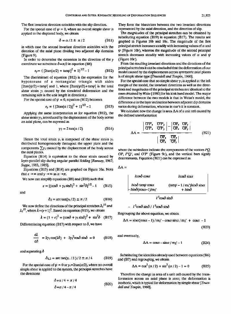
Equations (B13) and (B14) are graphed on Figure 10a. Note that e • oo and y • oo as a •r.

We now can simplify equations (B8) and (B 10) such that

e = [(costS + yt sin6) 2 + sin26] 1/2- 1 (B15) and

62 = arc tan(yt / 2) +_ •r / 2 (B 16)

We now define the directions of the principal stretches 2•/2 and 2ff2, where 2 =(e+ 1) 2. Based on equation (B15), we obtain

•. = (1 + e) 2 = (co• + yt sin(5) 2 + sin26 (B17) Differentiating equation (B17) with respect to 6, we have

They form the bisectrices between the two invariant directions represented by the axial direction, and the direction of slip.

The magnitudes of the principal stretches can be obtained by substituting equation (B19) in equation (B17). The results are graphed in Figures 10b and 10c. The magnitude of the first principal stretch increases steadily with increasing values of a and •, (Figure 10b), whereas the magnitude of the second principal stretch decreases steadily with increasing values of a and •, (Figure 10c).

From the resulting invariant directions and the directions of the principal stretches it can be concluded that the deformation of our model caused by the displacements across symmetric axial planes is of simple shear type [Truesdell and Toupin, 1960].

For the special case that no simple shear yl is applied at the left margin of the model, the invariant directions as well as the directions and magnitudes of the principal stretches are identical to the ones obtained by Weiss [1980] for his kink band model. The major difference between the two models is that in Weiss's model, the

difference a in the layer inclination between adjacent dip domains varies during deformation, whereas in our's it is constant.

We calculate now the change in area AA of a unit cell caused by the defined transformation

•[•'x •[•'y U'x

O'Px O'Py

AA = (B21)

where the subindices indicate the components of the vectors PQ, OP, P'Q', and O'P' (Figure 9c), and the vertical bars signify determinants. Equation (B21) can be expressed as

AA =

/cos(5 cora /co• sina

/sin3 tan• cora (tan•- 1 /m2')/sin3 sina /sin3(cora-1)/m2' +/sin3

l 2coS• sin6

- l 2cos• sin6 / l 2cosc$ sin6

Regrouping the above equation, we obtain

AA = sina(cora - 1) / m2' - cora sina / m2' + cora - 1

(B23)

= 2yt cos(2c!J) + 2yt2cosc$ sin6 = 0 (B18) and eventually,

AA = cora- sina /m2'- 1 (B24)

and separating cS

61,2 = arc tan(yt / 2 ) / 2 +_ yr / 4 (B19)

For the special case of• = 0 or yt=2tan(a/2), where no overall simple shear is applied to the system, the principal stretches have the directions

c5=a/4 + ;r / 4 (B20)

(5=a / 4- yr / 4

Substituting the identities already used between equations (B6) and (B7) and regrouping, we obtain

AA = cos 2 (a / 2) + sin 2 (a / 2) - 1 = 0 (B25)

Therefore the change in area of a unit cell caused by the transformation across an axial plane is zero; the deformation is isochoric, which is typical for deformation by simple shear [Trues- dell and Toupin, 1960].


3.0

2.0

1.0

0.5

O* •0- 40' 60' 80'

•0 ß

•o- IO-

:o* io-

-ZO* 30'

40'

SO*

-$0 ß

lO'

30 ø

40'

-80' -•0' -40' -•0' O* •0' 40' GO"' eC• •

3.0

2O

1.0

-80- -.eO* -40- -20' O* •0- 40- CO- 80- OL

Fig. 10. Distortion of the layered medium caused by the transport across symmetrical axial planes. (a) Graph of the equations • 1/2 (B13) and (B14) that define the longitudinal and an•,ular shear strains. (b) Magnitude of the principal stretch )•l within the

medium as a function of the difference c• in the fault inclination between adjacent di• domains and the simple shear • applied to the overall upper plate of the system. (c) Magnitude of the principal stretch •2 I72 within the medium as a function of the difference c• in the fault inclination between adjacent dip domains and the simple shear • applied to the overall upper plate of the system.

CONTRERAS AND SLrIER: KINEMATIC MODELING OF DEFORMATION SEQUENCES 21,927

Strain Induced by Material Transport Across the Asymmetrical Axial Plane at the Front of the Propagating Thrust Sheet

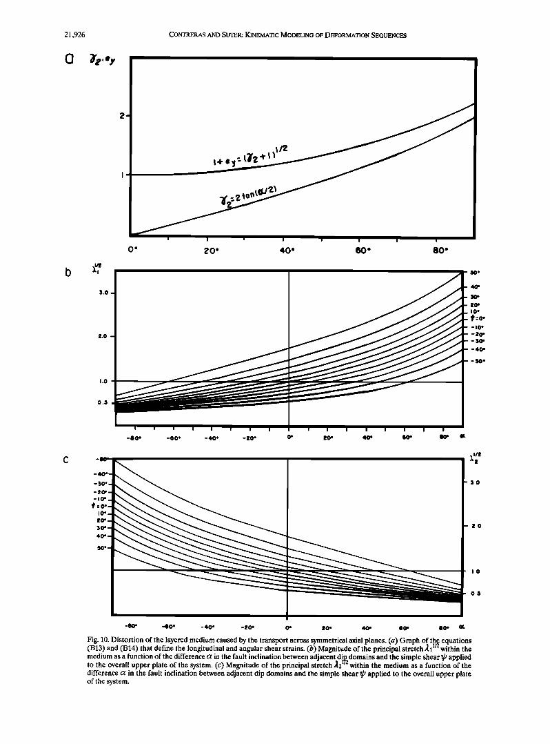
The orientation • of an arbitrary material line, measured counterclockwise with respect to the x axis in the undeformed state, becomes in the deformed state (Figure 11a)

3'= arc tan[sin 3 / (cos (5 + yt sin (5 ]+ a (B26)

Similarly, the angle fi•' between the stratification and the fault, after the transport of the material across the frontal axial plane (Figure 1 lb) can be expressed as

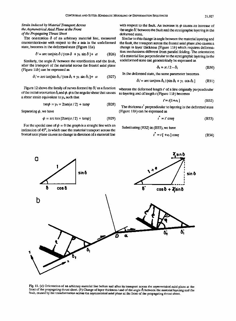
arc tan[sin 3i/(coS 3i + yt sin 3i ]+ a (B27)

Figure 12 shows the family of curves formed by •' as a function ofthe initial orientation di• and •p. •p is the angular shear that causes a shear strain equivalent to yt, such that

tamp = Yt = 2tan(a / 2) + tang, (B28)

Separating •p, we have

•p = arc tan [2tan(a / 2) + tang,] (B29)

For the special case of •p = 0 the graph is a straight line with an inclination of 45 ø, in which case the material transport across the frontal axial plane causes no change in direction of a material line

with respect to the fault. An increase in q• causes an increase of the angle •J•' between the fault and the stratigraphic layering in the deformed state.

Similar to this change in angle between the material layering and the fault, the transport across the frontal axial plane also causes a change in layer thickness (Figure l lb)which requires deformation mechanisms different from parallel folding. The orientation of a material line perpendicular to the stratigraphic layering in the unreformed state can geometrically be expressed as

6t = n: / 2- 6i (B30) In the deformed state, the same parameter becomes

arc tan[cos 6i / (sin 6i + yt cos 3i ] (B31)

whereas the deformed length t' of a line originally perpendicular to layering and of length t (Figure 1 lb) becomes

t'= t[1 +et] (B32)

The thickness t' perpendicular to layering in the deformed state (Figure 1 lb) can be expressed as

t = t' cost/ (B33)

Substituting (B32) in (B33), we have

t =t[+et]cosr] (B34)

•sln i C3

cos 6 6' cos 6 + tsin6

õ! 61

õt

Fig. 11. (a) Orientation of an arbitrary material line before and after its transport across the asymmetrical axial plane at the front of the propagating thrust sheet. (b) Change of layer thickness t and of the angle fii between the material layering and the fault, caused by the transformation across the asymmetrical axial plane at the front of the propagating thrust sheet.


I I I I

80' - iO ß

- 20'

60' - :50'

- 40'

40 ß , - 50'

o.

o. 20' 40' 60' 80'

Fig. 12. Graph of equation (B27) which defines the angle c•i' between the stratification and the fault, after the transport of the material across the frontal axial plane, as a function of the same parameter in its undeformed state (c•i) and the total angular shear •.

0.5

0 I0' •0' $0'

•0'

$0'

-0.5 60'

o. zo. 4O' 60' 80' õt

•:0 e

- I0*

-$0'

40'

-50'

- O. 5 60'

O* 20' 40' 60' 80' õi

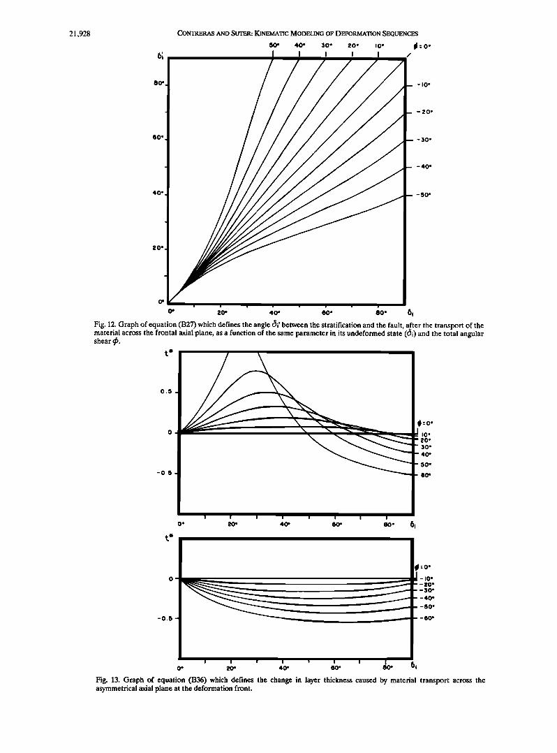
Fig. 13. Graph of equation (B36) which defines the change in layer thickness caused by material transport across the asymmetrical axial plane at the deformation front.


From Figure 1 lb it can be seen that

r/= 6i' + 6t'-• / 2 (B35)

Substituting (B35) in (B34), we get

t* = t[a +et ] sin(fif + fit') (B36) Equation (B36) is graphed in Figure 13. For positive values of

•p (clockwise shear) the forelimb layer-thickness t is thinned, whereas for negative values of •p (counterclockwise shear) thin- ning as well as thickening of the forelimb is possible.

Acknowledgments. This article has benefitted from several peer reviews and discussion with Rick Groshong and John Suppe at the 7th annual meeting of the Swiss Tectonic Studies Group. We also would like to thank Peter Jordan for inviting the second author to that meeting and providing a travel grant. We also have benefitted from Juan Manuel L6pez's expertise in desk top publishing. Financial and logistic support by the National University of Mexico and a grant from the Mexican Secretariat of Education (SNI 881161) are acknowledged.

REFERENCES

Bart, A. H., Global and local deformations of solid primitives, Cornput. Graphics 18(3), 21-30, 1984.

Boyer, S. E., and D. Elliott, Thrust systems, AAPG Bull., 66, 1196-1230, 1982.

Cobbold, P. R., and M. N. Percevault, Spatial integration of strain using finite elements, J. Struck Geol., 5, 299-305, 1983.

Cobbold, P. R., W. D. Means, and M. B. Bayly, Jumping deformation gradients and particle velocities across propagating coherent boun- daries, Tectonophysics, 80, 283-298, 1984.

Contreras, J., Modelado de secuencias de deformaci6n geo!6gica por microcomputadora, Univ. Nac. Auto. Mex, lnsk Geol. Bol. in press, 1989.

Contreras, J., and M. Suter, Numerical simulation of cross-sectional deformation sequences (abstract),Eos Trans. AGU, 69, 1435, 1988.

Cruikshank, K. M., K. E. Neavel, and G. Zho Zhao, Computer simulation of growth of duplex structures, Tectonophysics. 164, 1-12, 1989.

De Paor, J. G., Balanced sections in thrust belts, 1, Construction, AAPG Bull., 72, 73-90, 1988a.

De Paor, J. G., Non-linear analysis of displacement and strain in structural cross-sections using a grid composed of quadrilateral finite elements (abstract), Eos Trans. AGU, 69, 493, 1988b.

Elliott, D., The energy balance and deformation mechanisms of thrust sheets, Philos. Trans. I• Soc. London Ser. A, 283, 289-312, 1976.

Evans, D. G., P. N. Schweitzer, and M. S. Hanna, Parametric cubic splines and geologic shape descriptions, J. Math. Geol., 17, 611-624, 1985.

Foley, J.D., and A. van Dam, Fundamentals of Interactive Computer Graphics, 664 pp., Addison-Wesley, Reading, Mass., 1982.

Geiser, P., The role of kinematics in the construction and analysis of geological cross sections in deformed terranes, Spec. Pap. GeoL Soc. Am, 222, 47-76, 1988.

Gibbs, A.D., Balanced cross-section construction from seismic sections in areas of extensional tectonics, J. Struck GeoL, 5, 153-160, 1983.

Gould, H., and J. Tobochnik, An Introduction to Computer Simulation Methods, Applications to Physical Systems, vol 1,318 pp., Addison-Wes- ley, Reading, Mass., 1988.

Greenberg, M. D.,AdvancedEngineeringMathemadcs, 946 pp., Prentice- Hall, Englewood Cliffs, N.J., 1988.

Groshong, R. H., and S. I. Usdansky, Kinematic models of plane-roofed duplex styles, Spec. Pap. GeoL Soc. Am, 222, 197-206, 1988.

Harbaugh, J.W., and G. Bonham-Carter, Computer Simulation in Geol- ogy, 575 pp., John Wiley, New York, 1970.

Hirsinger, V., and B.E. Hobbs, A general harmonic coordinate transformation to simulate the states of strain in inhomogeneously deformed rocks, J. Struck Geol., 5, 307-320, 1983.

Johnson, A.M., and P. Berger, Kinematics of fault-bend folding, En- gineering Geology, 27, 181-200, 1989.

Jones, P., Quantitative geometry of thrust and fold belts, 26 pp. Methods Explor. Ser. vol 6, American Association of Petroleum Geologist., Tulsa, Okla., 1987.

Kilsdonk, B., and D. V. Wiltschko, Deformation mechanisms in the southeastern ramp region of the Pine Mountain block, Geol. Soc. Am. Bull., 100, 653-664, 1988.

Kligfield, R. P., P. Geiser, and J. Geiser, Construction of geologic cross sections using microcomputer systems, Geobyte, 1, 60.66, 1986.

Laubscher, H. P., Geometrical adjustments during rotation of a Jura fold limb, Tectonophysics, 36, 347-365, 1976.

Laubscher, H. P., Fold development in the Jura, Tectonophysics, 37, 337-362, 1977.

Malvern, L. E., Introduction to the Mechanics of a Continuous Medium, 713 pp., Prentice-Hall, Englewood Cliffs, N.J., 1969.

Means, W. D., Stress and Strain, Basic Concepts of Continuum Mechanics for Geologists, 339 pp., Springer-Verlag, New York, 1976.

McCoss, A.M., Practical section drawing through folded layers using sequentally rotated cubic interpolators,J. Struck Geol., 9, 365-370,1987.

Morse, J. D., Deformation in ramp regions of thrust faults, M. Sc. thesis, 138 pp., Tex. A & M Univ., College Station, 1978.

Press, W. H., B. P. Flannery, S. A. Teukolsky, and W. T. Vetterling, NutnericalRecipes, 818 pp., Cambridge University Press, New Rochelle, N.Y., 1986.

Ramsay, J.G., Folding and Fracturing of Rocks, 568 pp., McGraw-Hill, New York, 1967.

Ramsay, J.G., and M. I. Huber, The Techniques of Modern Structural Geology, vol. 1, Strain Analysis, 307 pp., Academic, San Diego, Calif., 1983.

Ramsay, J.G., and M. I. Huber, The Techniques of Modern Structural Geology, vol. 2, Folds and Fractures, 700 pp., Academic, San Diego, Calif., 1987.

Rich, J. L., Mechanics of low-angle overthrust faulting as illustrated by Cumberland thrust block, Virginia, Kentucky and Tennessee, AAPG Bull. 18, 1584-1596, 1934.

Serra, 0., Fundamentals of Well-Log Interpretation, 423 pp., Elsevier Science, New York, 1984.

Shi, Y., and C. Y. Wang, Two-dimensional modeling of the P-T-t paths of regional metamorphism in simple overthrust terrains, Geology, 15, 1048-1051, 1987.

Stowe, C. W., Application of Fourier analysis for computer representation of fold profiles, Tectonophysics, 156, 303-311, 1988.

Suppe, J., Geometry and kinematics of fault-bend folding, Am. J. $ci., 283, 684-721, 1983.

Suppe, J., Principles of Structural Geology, 537 pp., Prentice-Hall, Englewood Cliffs, N.J., 1985.

Suter, M., 1976, Tektonik des Doubstals und der Freiberge in der Um- gebung yon Saigneldgier, Eclogae Geol. Helv., 69, 41-670, 1976.

Suter, M., Strukturelles Querprofil durch den nordwestlichen Faltenjura, Mt-Terri-Randiiberschiebung-Freiberge, Eclogae Geol. Helv., 74, 255- 275, 1981.

Suter, M., Cordilleran deformation along the eastern edge of the Vailes- San Luis Potosf carbonate platform, GeoL $oc. Am Bull., 95, 1387- 1397, 1984.

Suter, M., Structural traverse across the Sierra Madre Oriental fold- thrust belt in east-central Mexico, GeoL $oc. Am Bull., 98, 249-264, 1987.

Suter, M., Hoja Tamazunchale 14Q-e(5) con Geologœa de la Hoja Tamazunchale, Estados de Hidalgo, Quer6taro y San Luis Potosi', serie de 1:100,000 (geological map, structural sections, and explanations), Univ. Nac. Aut6n. de M6x., Inst. Geol., Carta geol. de M6x., 1989.

Truesdell, C., and R. Toupin, The classical field theories, in En- cyclopaedia of Physics, vol. 3(1), edited by S. Flugge, pp. 226-793, Springer-Verlag, New York, 1960.

Waltham, D., Finite difference modelling of hangingwall deformation, J. Struck Geo,, 11,433-437, 1989.

Vendeville, B., and P. R. Cobbold, How normal faulting and sedimentation interact to produce listtic fault profiles and stratigraphic wedges, J. Struck Geo,, 10,649-659, 1988.

Weiss, L. E., Nucleation and growth of kink bands, Tectonophysics, 65, 1-38, 1980.

Williams, G. D., and T. J. Chapman, Strains developed in the han- gingwails of thrusts due to their slip/propagation rate: a dislocation model, J. Struck Geo,, 5, 563-571, 1983.

Williams, G., and I. Vann, The geometry of listric normal faults and deformation in their hangingwalls, J. Struct. Geol., 9, 789-795, 1987.

J. Contreras and M. Suter, Institute of Geology, National University of Mexico, Apartado Postal 70-296, M6xico DF 04510, Mexico.

(Recived July 10, 1989; revised March 27, 1990; accepted April 6, 1990.)

Kinematic modeling of cross-sectional deformation sequences by computer simulation: coding and...

Documents

Transcript of Kinematic modeling of cross-sectional deformation sequences by computer simulation: coding and...