MEHDI TALE MASOULEH

KINEMATIC ANALYSIS OF FIVE-DOF (3T2R) PARALLEL MECHANISMS WITH

IDENTICAL LIMB STRUCTURES

Thèse présentée à la Faculté des études supérieures de l'Université Laval

dans le cadre du programme de doctorat en génie mécanique pour l'obtention du grade de Philosophise Doctor (Ph.D.)

FACULTÉ DES SCIENCES ET DE GÉNIE UNIVERSITÉ LAVAL

QUÉBEC

2010

© Mehdi Taie Masouleh, 2010

Abstract

This dissertation is presented specifically to an audience composed of two separate groups working on the kinematics of parallel mechanisms: mechanical engineers and geometricians.

Originally, this work was based solely on engineering concepts. However, during the course of this work, a theoretical and practical algebraic geometry approach has been proposed, and now, this thesis is a (hopefully judicious) mixture of these two approaches. The work presented in this thesis does not favour one method over an­other but rather uses the synergies between the methods of engineering mechanics and algebraic geometry.

By keeping the kinematic analysis of symmetrical parallel mechanisms with five-degree-of-freedom—three translations and two rotations—as a case study, this thesis can be regarded as a guideline of the application of algebraic geometry in the kinematic analysis of parallel mechanisms. This choice, i.e., the selection of symmetric 5-degree-of-freedom parallel mechanisms, has been appreciated since the kinematic properties of this type of architecture have proven to be quite remarkable.

In this context, Chapters 2 to 4 are devoted to the adaptation of some algebraic geometry techniques to the kinematic analysis of parallel mechanisms while keeping in the background the study of symmetrical 5-degree-of-freedom parallel mechanisms. The major contribution of Chapter 2 is the development of a systematic approach for the kinematic modelling of symmetric parallel mechanisms which is applied in Chapter 3 to symmetric 5-degree-of-freedom parallel mechanisms. In Chapter 3, the applica­tion of the framework presented in Chapter 2 leads to some astonishing results for

the number of solutions for the FKP: 1680 finite solutions and for a given design 208 real solutions. All these solutions are in terms of Study parameters, i.e., in the seven-dimensional kinematic space. In Chapter 4, the mapping from the seven-dimensional to three-dimensional kinematic space is introduced which allows to obtain the Cartesian coordinates and the corresponding angles for each solution. Moreover, in this chap­ter the first-order kinematic properties are also investigated which results in a better understanding of the mechanism.

The reader will notice in Chapters 5 and 6 a kinematic investigation which is based on the three-dimensional kinematic space. The main concern of Chapter 5 is the geo­metric constructive approach for the workspace analysis in which an algorithm previ­ously proposed for the constant-orientation workspace of 6-degree-of-freedom parallel mechanisms is extended to the symmetric 5-degree-of-freedom parallel mechanisms. The CAD model of the workspace is also presented. The results of this chapter reveal that the workspace of symmetric 5-degree-of-freedom parallel mechanisms can have small isolated part. Chapter 6 completes the discussion initiated in Chapter 3 for the FKP in which the FKP is investigated for some simplified designs having either a closed-form solution or a univariate expression. For a nearly general design a uni­variate expression of degree 220 is found. In this chapter, we veer a little from the three-dimensional kinematic space to the seven-dimensional kinematic space in order to validate and refine the obtained results, a state of the art which can be applied to other cases.

The last chapter is devoted to the singularity analysis of symmetric 5-degree-of-freedom parallel mechanisms which relies on Grassmann line geometry. This chapter covers extensively the study of the singular configurations of the symmetrical 5-degree-of-freedom parallel mechanisms for the simplified design proposed in Chapter 6. The main contribution of this chapter is the application of the Grassmann line geometry to the lower-mobility parallel mechanisms in which a line at infinity is among the Plucker lines under study.

Finally, Chapter 8 concludes the thesis by summarizing the results obtained through­out Chapters 2 to 7. It provides also several ongoing works and future works which can be the subjects of some further studies for a new direction of research.

n

Résumé

Cette thèse de doctorat s'adresse tout particulièrement à deux groupes de personnes travaillant sur la cinématique des mécanismes parallèles : les ingénieurs mécaniciens et les géométriciens.

À l'origine, ce travail devait être basé uniquement sur des concepts et des outils d'ingénierie. Cependant, à mi-parcours, il a été pertinent d'utiliser un aspect pratique de l'algèbre géométrique et, désormais, cette thèse se veut un judicieux mélange de ces deux approches. En effet, contrairement à ce qu'on trouve généralement dans la littérature, le travail présenté ici ne favorise pas une méthode par rapport à l'autre, mais vise plutôt à utiliser les synergies possibles entre les méthodes de l'ingénierie mécanique et de l'algèbre géométrique.

En gardant comme étude de cas l'analyse cinématique de mécanismes parallèles symétriques à cinq degrés de liberté, trois translations et deux rotations, cette thèse peut être considérée comme une ligne directrice de l'application de l'algèbre géométrique dans l'analyse cinématique de mécanismes parallèles. Le choix de ce cas s'est avéré heureux puisque les propriétés cinématiques de ce type d'architecture se sont révélées tout à fait remarquables.

Dans cette optique, les chapitres 2 à 4 sont consacrés à l'adaptation des outils de l'algèbre géométrique à l'analyse cinématique des mécanismes parallèles. Ces chapitres gardent toujours en toile de fond l'étude des mécanismes parallèles symétriques à cinq degrés de liberté. La contribution majeure du chapitre 2 est le développement d'une approche systématique pour la modélisation cinématique des mécanismes parallèles symétriques qui est appliquée par la suite dans le chapitre 3 aux mécanismes parallèles

iii

symétriques à cinq degrés de liberté. Cette application donne des résultats étonnants en ce qui a trait au nombre de solutions du problème géométrique direct : 1680 solutions finies et 208 solutions réelles pour une architecture donnée. Toutes ces solutions sont en termes de paramètres de Study, un espace projectif à sept dimensions. Au chapitre 4, la transformation entre cet espace à sept dimensions et celui à trois dimensions est introduite afin d'obtenir les coordonnées cartésiennes et les angles correspondants pour chaque solution. En outre, les propriétés cinématiques de premier ordre sont également étudiées dans ce chapitre afin d'avoir une meilleure compréhension du mécanisme.

Le lecteur pourra ensuite suivre dans les chapitres 5 et 6 une étude cinématique basée sur l'espace à trois dimensions. La préoccupation principale du chapitre 5 est l'analyse constructive de l'espace atteignable par une approche géométrique. Un algo­rithme proposé dans la littérature pour trouver l'espace atteignable pour une orienta­tion constante d'un mécanisme parallèle à six degrés de liberté est alors étendu aux mécanismes parallèles symétriques à cinq degrés de liberté. Le modèle CAO de l'espace atteignable est également présenté. Les résultats de ce chapitre montrent que l'espace atteignable des mécanismes parallèles symétriques à cinq degrés de liberté peut pos­séder une petite partie isolée. Le chapitre 6 complète quant à lui la réflexion engagée au chapitre 3 sur le problème géométrique direct. Ce problème est ainsi étudié pour des modèles simplifiés qui ont des solutions explicites ou une expression monovariable. Pour une conception quasi-générale, une expression monovariable de degré 220 est obtenue. Dans ce chapitre, nous dévions un peu de l'espace à trois dimensions pour celui à sept dimensions afin de valider et d'affiner les résultats obtenus, une approche qui peut être appliquée à d'autres cas.

Le chapitre 7 est pour sa part consacré à l'analyse des singularités des mécanismes parallèles symétriques à cinq degrés de liberté qui repose sur la géométrie grassmanni-enne. Ce chapitre couvre largement l'étude des configurations singulières des mécan­ismes parallèles symétriques à cinq degrés de liberté pour les architectures simplifiées proposées dans le chapitre 6. La contribution principale de ce chapitre est l'application de la géométrie grassmannienne aux mécanismes parallèles à mobilité réduite pour lesquels une ligne à l'infini est parmi les lignes de Plùcker.

Enfin, le chapitre 8 conclut cette thèse en résumant les résultats obtenus dans les chapitres précédents. Il décrit également plusieurs travaux en cours et propose des sujets de travaux futurs pour une nouvelle orientation de la recherche.

iv

Foreword

Reader, I would like to say proudly that my thesis was accomplished long time ago when I had the honour to know Prof. Gosselin and Prof. Husty and this thesis, for me, is only an excuse. So, feel free to comment!

I express my gratitude to my supervisor Prof. Clément Gosselin for giving me the opportunity to be part of his research team and to entrust me with this project. I owe special thanks to him for sharing with me his comprehensive expertise in kinematics and robotics. I had the opportunity to do my undergraduate project under his supervision and I decided to get to know him better: this thesis was only an excuse.

For me, nothing has the value to replace my country Iran, but the exceptional environment which Prof. Clément Gosselin and all the members of the "Laboratoire de Robotique de L'Université Laval" have created in the laboratory made it possible for me not to have the feeling of being far from my hometown. For this reason, I can proudly say that this laboratory is my second hometown. A hometown is a place where you don't have to fill an application form to feel that you are a part of it and where the time between when you consider it as hometown and when it becomes your hometown is infinitely small.

I had the opportunity to work with Prof. Husty and I owe him a great part of this thesis. He gently shared with me his invaluable mathematical expertise and pushed me toward a new world of kinematics and mathematics.

Last, but not least, I would like to thank my parents for their unlimited support during all my studies. I did the most important part of my studies without being

beside them but I was inspired from the great success of my father in his life. I did not start from zero like him and without his encouragement and help I would never have ended up now with a Ph.D. Whenever I did not follow his advice, it led to a crisis and he gently got me out of the crisis despite having the feeling of passing through a big trouble. My loving mother, she never forgot to call me each day to ask: Are you coming back one day? The answer now is clear: I am coming back.

vi

To pieces of my heart, my parents: Manouchehr and Rouh-Afza, my two lovely sisters: Azadeh and Zahra

and all Masoulehian kids, that I hope I am still a part of

vn

vm

Contents

Abstract i

Résumé iii

Foreword v

Contents ix

List of Tables xv

List of Figures xvi

List of Symbols xxi

1 Introduction 1 1.1 Robotic Mechanical Systems 2

1.1.1 From the Motion of Robots to Two Types of Industrial Robot Architectures 3

1.2 Parallel Mechanisms 7 1.2.1 Limited-DOF Versus 6-DOF Parallel Mechanisms 10 1.2.2 Symmetrical and Asymmetrical Parallel Mechanisms 10

1.3 3 and 4-DOF Mechanisms Belonging to Multipteron Family: Origin of the Research 15 1.3.1 The Tripteron 15 1.3.2 The Quadrupteron 16 1.3.3 Toward Obtaining the Pentapteron 17

1.3.3.1 Foreshadowing 5-DOF Parallel Mechanisms 17

ix

1.3.3.2 The PRUR Limb and Pent apt eron 19 1.3.3.3 The RPUR Limb 21

1.4 Application of 5-DOF Parallel Mechanisms 21 1.5 Objectives and Contributions of the Thesis 24 1.6 Remainder ofthe Chapters and Results 25

Basics on Algebraic Geometry and Kinematic Modelling of Symmetrical Parallel Mechanisms 28 2.1 Introduction 29 2.2 Polynomials and Ideals 32

2.2.1 Formal Definition of a Polynomial 32 2.2.2 Trigonometric Functions in Polynomials 34 2.2.3 Ideals 35 2.2.4 Monomial Order 36

2.3 Toward Solving Polynomial Systems 37 2.3.1 Resultant Method 38 2.3.2 Grôbner Bases 41

2.4 Spatial Kinematic Mapping 42 2.5 Study's Kinematic Mapping 42 2.6 Kinematic Modelling of Parallel Mechanisms Using Study's Parameters 44

2.6.1 Kinematic Modelling of the Principal Limb 45 2.6.1.1 Defining the D-H Parameters ofthe Principal Limb . . 46 2.6.1.2 Kinematic Mapping from SE(3) to Study Parameters . 46 2.6.1.3 FKP Expressions and Constraint Expressions 47 2.6.1.4 Elimination of Passive Variables 48 2.6.1.5 Defining the Ideal 3 49 2.6.1.6 Selecting the Simplest Expression for the FKP . . . . 50

2.6.2 The System of Equations for the FKP: "Copy-Paste" Procedures 50 2.6.3 Solving the System of Equations $ and Some Remarks 51

2.7 Summary 53

F K P of 5-DOF Symmetrical Parallel Mechanisms Using Study's Kinematic Mapping 54 3.1 Introduction 55 3.2 FKP of 5-RPUR Parallel Mechanisms via Study's Kinematic Mapping . 58

3.2.1 Kinematic Modelling of the Principal Limb 58 3.2.1.1 Defining the D-H Parameters of the Principal Limb . . 58

3.2.1.2 Kinematic Modeling from SE(3) to Study Parameters . 59 3.2.1.3 FKP Expressions and Constraint Expressions 61 3.2.1.4 Elimination of the Passive Variables 61 3.2.1.5 Defining the Ideal I 64 3.2.1.6 Toward the Simplest Expression for the FKP 65

3.2.2 The System of Equations for the FKP: Copy-Paste Procedures . 67 3.2.3 Solving the System of Equations # 69 3.2.4 Discussion on the Simplest Expression Describing the FKP . . . 71

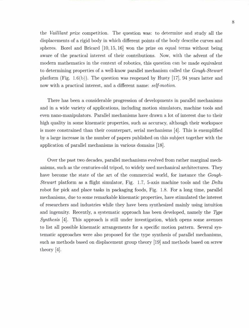
3.3 FKP of 5-PRUR Parallel Mechanisms via Study's Kinematic Mapping 73 3.4 Summary 75

4 General and First-Order Kinematic Mapping 76 4.1 Introduction 77 4.2 Mapping Between P7 and Three Dimensional Kinematic Space 78

4.2.1 Cartesian Representation of Study's Parameters 78 4.2.2 Representation of Study's Parameters in Cartesian Coordinates 80

4.3 Different Sets in P7 for Describing yj 82 4.4 First-order Kinematic Mapping for the Angular Velocity 83

4.4.1 From Three-dimensional Kinematic Space to Study Parameters 83 4.4.2 From Study Parameters to Three-dimensional Kinematic Space 84

4.5 First-order Kinematic Mapping for the Point Velocity 85 4.5.1 From Three-Dimensional Kinematic Space to Study Parameters 86 4.5.2 From Study Parameters to the Three-dimensional Kinematic Space 86

4.6 Particular Configurations 86 4.6.1 Particular Configuration for (j0 : ji : J2 : f.3) 86 4.6.2 Particular Configuration for (Xpl U Xp2)2 87

4.7 Summary 88

5 Kinematic Investigation in Three-Dimensional Kinematic Space 89 5.1 Introduction 90 5.2 Consistent Rotation Matrix, Q 95 5.3 IKP of the 5-PRUR Parallel Mechanism 97

5.3.1 Solution of the IKP for Y = 1 98 5.3.2 Solution of the IKP for Y = 0 100

5.4 Workspace Analysis of 5-PRUR Parallel Mechanisms 102 5.4.1 Topology of the Vertex Space 103

5.4.1.1 Topology ofthe Vertex Space for Y = 1 104

x i

5.4.1.2 Geometric Constructive Approach of the Vertex Space for T = 1 107

5.4.1.3 Topology of the Vertex Space for T = 0 112 5.4.1.4 Geometric Constructive Approach of the Vertex Space

for T = 0 118 5.4.2 Constant-orientation Workspace 119

5.4.2.1 CAD Model of the Constant-orientation Workspace . . 119 5.4.2.2 Geometrical Constructive Approach of the Constant-

orientation Workspace (GCACow) 120 5.4.3 Volume of the Constant-orientation Workspace 122

5.5 IKP of the 5-RPUR Parallel Mechanisms 125 5.6 Workspace Analysis of 5-RPUR Parallel Mechanisms 127

5.6.1 DGCACow for the 5-RPUR Parallel Mechanisms 132 5.7 ISA of the Symmetrical 5-DOF Parallel Mechanisms 137

5.7.1 Geometric Interpretation of the ISA 140 5.8 Summary 141

6 F K P Using Three-dimensional Euclidean Space 142 6.1 Introduction 143 6.2 Forward Kinematic Problem (FKP) of 5-RPUR Parallel Mechanisms . 145

6.2.1 Closed form Solution for the FKP of a {AJAJ} Design 149 6.2.2 Closed-form Solution for the FKP of a {AiA2} Design 153 6.2.3 Closed-form Solution for the FKP of a {A2A2} Design 155 6.2.4 Univariate Expression for Other Designs Belonging to S^ . . . . 157 6.2.5 Univariate Expression for the FKP of a {MPA2} Design 157

6.3 FKP for a Design Containing One Arrangement Belonging to Sj . . . . 159 6.3.1 Toward Obtaining the Simplest Expression for the FKP 159 6.3.2 Exploring the FKP Using Homotopy Continuation 161 6.3.3 Resorting to the Seven-dimensional Kinematic Space 162

6.4 Forward Kinematic Problem for 5-PRUR Parallel Mechanisms 166 6.4.1 Closed-form Solution for the FKP of a { A ^ A ^ } Design . . . . 166

6.5 Summary 168

7 Singularity Analysis via Grassmann Line Geometry 169 7.1 Introduction 170 7.2 Screw Theory: A Preamble to the Survey 172

7.2.1 Interpretation of 0-pitch and oo-pitch Screws 174

xi 1

7.2.2 Reciprocity of Screws 175 7.2.3 Wrench and Twist Characterizing the P and R Joints 176

7.3 Terminology Used for the Singularity Analysis 177 7.4 Singularity Classification 178 7.5 Limb Singularity 179 7.6 Actuation Singularity 182

7.6.1 Actuation Singularity for a General Design 182 7.6.2 Singular Complex 183 7.6.3 Hyperbolic Congruence 188 7.6.4 Grassmann Variety of Dimension One: Point 190 7.6.5 Some Particularities Due to the Line at Infinity 190

7.7 Singularity Analysis of {AiAi} Parallel Mechanisms 193 7.7.1 Condition 5: Linear complex 193 7.7.2 Condition 4: Congruence 194 7.7.3 Condition 3, 2 and 1 198

7.8 Singularity Analysis of the {A2A2} Design 199 7.9 Singularity Locus 200 7.10 Summary 200

8 Conclusion 202 8.1 Conclusion on the Thesis 203 8.2 Relevant Contributions of the Thesis 204 8.3 Chapters Accomplishments 204 8.4 Direction of Ongoing Works 208

8.4.1 Kinematic Modelling of Symmetric 3R2T Parallel Mechanisms . 208 8.4.2 Constant-position Workspace 209

8.5 Direction of Future Works 212 8.5.1 The Univariate Expression of Degree 1680 213 8.5.2 Coefficient-parameter Homotopy 213 8.5.3 Numerical Test Toward the Upper Bound of the real number of

Real Solutions 213 8.5.4 A Control Model from the Kinematic Mapping 214 8.5.5 Grassmann-Cay ley Algebra 214 8.5.6 Overconstraint Properties 214

Bibliography 216

A Expressions for Chapter 3 230

xiii

A.l Three Expressions T,=i.2.3 from Chapter 3 230

xiv

List of Tables

1.1 Types of legs without mechanical simplification 18

1.2 Types of legs assuming mechanical simplification 18

3.1 D-H parameters for a RPUR limb 60

5.1 Geometric properties (in mm) for a 5-PRUR parallel mechanism. . . . 120 5.2 Geometric properties (in mm) for a 5-RPUR parallel mechanisms. . . . 130 5.3 Geometric properties (in mm) for a simplified design, Fig. 6.2 130

xv

List of Figures

1.1 A schematic of the most common types of robots that may influence our daily lives, some of them perhaps in a near future 2

1.2 A genealogy of robotic mechanical systems 3 1.3 Six type of kinematic joints 4 1.4 Example of serial robots 5 1.5 A four-bar linkage 6 1.6 (a) Schematic representation of a parallel mechanism and (b) solid model

of the Gough-Stewart platform 7 1.7 A CAE flight simulator 9 1.8 Sorting and collating concept with two in-line Delta robots 9 1.9 The Agile eye : a 3-DOF 3-RRR spherical parallel manipulator 11 1.10 (a) Solid model of a Delta robot as a symmetrical parallel mechanism,

(b) Solid model of an asymmetrical 4-DOF parallel mechanism and (c) Prototype of a 5-DOF asymmetrical parallel mechanism 12

1.11 The Tripteron, developed at Laval University. 15 1.12 The Quadrupteron, developed at Laval University. 16 1.13 Schematic representation of, (a) PRUR and (b) CUR limbs 19 1.14 Solid model of Pentapteron a 5-DOF(3T2R) parallel mechanism 20 1.15 (a) Schematic representation of a RPUR limb and (b) a solid model of

a 5-RPUR parallel mechanism 21 1.16 Two 6-DOF PMTs developed by (a) Mikrolar company and (b) Toyoda 23 1.17 Asymmetrical 5-DOF PMT (a) Metrom company and (b) Tekniker . . 23

2.1 Schematic representation for the expression constituting the ideal 3. . . 49

xvi

3.1 Local reference frames based on the D-H parameters for a RPUR limb. 59 3.2 The constraint circles of the symmetrical 5-DOF mechanisms using a

2-norm for y 62 3.3 Constraint surfaces for different Euclidean norm for y 63 3.4 Schematic representation for the expressions constituting the ideal 3. . 64 3.5 Study mapping of the vertex space of a RPUR limb. 5(n) 66 3.6 One solution amongst the 208 solutions 70 3.7 Local systems for the D-H parameters of a PRUR limb 73 3.8 Interpretation of — 2b6,. — 2b7i and —2b5, for the j thlimb of Pentapteron. 74

4.1 Schematic model for the mapping of the rotational parameters 87

5.1 Flowchart of the design of devices based on parallel mechanisms 90 5.2 Schematic representation of. (a) CUR (Y = 1) and (b) PRUR (r = 0). . 97 5.3 Configuration for which results in two solutions for the IKP of Y = 1. . 99 5.4 Configuration for which results in four solutions, only two are shown for

clarity, for the IKP of Y = 0 with prismatic actuator along the x-axis. . 101 5.5 The lower half of a Bohemian dome 103 5.6 Vertex space for Y = 1 having both holes H\ and H.\ 104 5.7 CAD model of the vertex space for G ta, i = 1 4 106 5.8 Boundary generated by the first moving link for Y = 1 108 5.9 Boundary generated by the second moving link for Y = 1 due to the

motion generated by the first moving link 109 5.10 The GCAV for Y = 1 and the seven boundary conditions I l l 5.11 The three steps for obtaining the main body of Y = 0 115 5.12 First and second steps for obtaining the H\ (a) eBju (SB\U), (b) eBu and

sB l together and (c) their intersection e sB l u 116 5.13 Third step for H\ (a) assembling eB\u, SB[U and e sB , u and (b) the final

result for Ti? 116 5.14 Steps for obtaining 7Y2 (a) intersection of eB\ and SBU. (b) adding the

two cylindrical shape and (c) the final results for Ti® 117 5.15 Steps for obtaining 71% (a) Putting together SBU and eBu (b) subtracting

with eB t and (c) the final results for H% 117 5.16 CAD model of the vertex space of Y = 0 for 9 = § 118 5.17 Boundary generated by the first moving link for Y = 0 119 5.18 Boundary generated by the second moving link for Y = 0 due to the first

moving link 120

xvi 1

5.19 Vertex space for F = 0. prismatic actuator along 2-axis and 8 = | , obtained by GCAV 121

5.20 Constant-orientation workspace for 0 = | and <j> = | for the design presented in Table 5.1 123

5.21 Constant-orientation workspace for 6 = | and 0 = \ for the design presented in Table 5.1 123

5.22 Volume of the constant-orientation workspace with respect of (0, 6) for the design presented in Table 5.1 124

5.23 (a) The Schematic representation of a RPUR limb, (b) solid model of a 5-RPUR parallel mechanism and (c) two working modes for a RPUR limb. 125

5.24 Two working modes for a RPUR limb 126 5.25 The Hi hole 128 5.26 The H2 hole 128 5.27 The H3 hole 129 5.28 The main body. 129 5.29 The most general vertex space of a RPUR limb, B™, having the three

holes 129 5.30 Constant-orientation workspace for 0 = 0 and 9 = 0 with design param­

eters as presented in Table 5.2 131 5.31 Constant-orientation workspace for 0 = 0 and 9 = 0 with design param­

eters as presented in Table 5.3 131 5.32 A schematic representation of a B™ including the parameters used. . . 133 5.33 Constant-orientation workspace for the design presented in (a) Table 5.2

and (b) Table 5.3 for 0 = 9 = 0 135 5.34 Volume of the constant orientation with respect of (0, 9) 136 5.35 Feasible values of 9 as a function of the angular velocity components, uix

and uz, Eq. 5.88. ofthe mobile platform 139

6.1 Simplified kinematic arrangements 146 6.2 Solid model of a {AiAi} parallel mechanism 147 6.3 A {MPA2} arrangement 148 6.4 Schematic representation of the base and platform for a {AiAj} parallel

mechanism 149 6.5 A 4-bar linkage generated from the two Aj arrangements 151 6.6 Schematic representation of the base and platform for a {Aj.A2} parallel

mechanism 152

xvin

6.7 Solid model of a {AiA2} parallel mechanism 153 6.8 Solid model of a {A2A2} parallel mechanism 155 6.9 Schematic representation of the base and platform for a {A2A2} parallel

mechanism 156

6.10 Solid model for {A3A3} 158 6.11 Schematic representations ofthe base and platform for a {MpA2} parallel

mechanism 159 6.12 Nearly general design for a 5-RPUR parallel mechanism containing only

one arrangement of type A] 160 6.13 Number of digits, « D , for each coefficient of t in F t . 0 < dT(F t) < 220,

with a total degree as 220 161 6.14 Inconsistent solution, the grey one, which can be found using seven-

dimensional kinematic space for the design presented in Fig. 6.12 . . . 163 6.15 Procedure to select the solutions obtained by Bertini for the FKP prob­

lem of a design having an arrangement belonging to Aj in which the first and second limbs have identical working modes 164

6.16 Schematic representation of the base and platform for a particular case with 28 solutions 165

6.17 Simplified kinematic arrangements belonging to the class As 167 6.18 Simplified kinematic arrangements belonging to the class B s 167 6.19 Solid model for a {AX IAX I} design 167

7.1 Schematic representation of a screw 172 7.2 Screw representation of the R and P joints 174 7.3 Wrench and twist systems of R and P joints 177 7.4 Limb-actuated-wrench, $;, for a RPUR limb 180 7.5 Limb singularity. 181 7.6 A5 singularity where five planes V* are intersecting one common line, Cv. 185 7.7 A n 4 A 4 singularity configuration 189 7.8 Condition 1 of Grassmann line geometry, for the sake of better represen­

tation other limbs are not shown 190 7.9 Particular configurations due to the line at infinity 192 7.10 Plane V, and V, for a { A i A j design 194 7.11 A n 4 A 4 singularity for a {AiAj.} design 196 7.12 Solid model of a {A2A2} parallel mechanism with constituting plane Vi

and V; 200

xix

7.13 Singularity locus of a { A J A J } design for 9 = § and 0 = § 201

8.1 Constant-position workspace for a 5-RPUR parallel mechanism. The grey zones are not permitted 209

8.2 The constraint circle, Eq. (3.17) and geometric interpretation of angle î. 210 8.3 Spherical parameters for representing the rotational capabilities 211 8.4 Constant-translation workspace for a general 5-RPUR parallel mechanism. 212

xx

List of Symbols

A major issue, regrettably very often overlooked, is the unification of notation. Due to the particularity of this thesis in which both three and seven-dimensional kinematic spaces are used, we adopted two different notations to help distinguish them through­out the thesis. Moreover, we unified the notation for calling geometrical objects or geometrical properties and dummy variables. These can be summarized as follows for the non-matrix expressions:

1. Expressions in 3-dimensional space are expressed using the italic Times font: F ;

2. Uppercase "blackboard bold" is used to represent sets and groups, for instance R;

3. Lowercase "blackboard bold" represents dummy variables, for instance z;

4. Expressions in 7-dimensional space are written using Euler Fraktur literals, 5";

5. Calligraphic literals are used to represent geometrical objects, such as planes, and geometrical properties such as area and volume and Screw components, C.

The boldf.ace font is used to indicate matrices, arrays and vectors, with uppercase reserved for matrices and lowercase for arrays and vectors. This convention is valid for both three and seven-dimensional expressions. For instance, for a matrix containing components respectively from three and seven-dimensional spaces one has: M and SDÎ. It should be noted that the lowercase of "blackboard bold" literals, for instance x, plus i and j for indices, are dummy variables and they are subject to be changed at each time they are used.

xxi

7-Dimensional Kinematic Space Notation Description

Dz(ff) Degree of a polynomial, ff, with respect to one of its variable, *z

Or(i) Total degree of a polynomial ff

3 g General ideal (used only for definition)

©e Study quadric

s 8 components of Study's parameters

?i=o,...,3 First set of Study's parameters

t)i=o,...,3 Second set of Study's parameters

y Array representation of the first set of Study's parameters

rj Array representation of the second set of Study's parameters

& Seven-dimensional transformation matrix

$j Homogeneous condition and first component of the first row of &

p First component of the second row of &

q First component of the third row of S

r First component of the forth row of &

(£x Exceptional or absolute generator

<$j:'=o,...,3 Expressions for the kinematic mapping from SE(3) to the first set of Study parameters

^m=o,...,3 Expressions for the kinematic mapping from SE(3) to the second set of Study parameters

0 System of equations representing the kinematic mapping from Eu­clidean displacement to the Study parameters

3 Ideal containing the kinematic modelling expressions

xxn

r^i=i,...,nc+nf Expressions of kinematic modeling

X Ideal for the expressions of the kinematic modeling

5c Ideal for the expressions of the F K P expressions

<tc Ideal for the constraint expressions

2) Expressions obtained from the Grôbner basis of J

2) Ideal for the expressions obtained from the Grôbner basis of 3

5 P F K P expression of the principal limb

bj Geometric parameters of the fixed base

mj Geometric parameters of the mobile platform

*Bj Matrix for the fixed frame transformation

2lj Diagonal sub-matrix of 93 j

Cj Lower triangular sub-matrix of *Bj

?Rlj Matrix for the mobile frame transformation

S)j Diagonal sub-matrix of SPÎj

(Bj Lower triangular sub-matrix of ffllj

Sj Study's parameters transformation for fixed based and mobile plat­form

# Ideal of the system of expressions for the FKP analysis

ms Mapping from the seven to three-dimensional space

nifc Mapping from the three t o seven-dimensional space

fx = {0, 1} Two solution modes for the mapping from the three-dimensional space to f3

f2 = {0, 1} Two solution modes for the mapping from the three-dimensional space to jo

xxin

3-Dimensional Kinematic Space Notation Description

n Number of degree-of-freedom

T = 0, 1 Cosine of the angle between the prismatic actuator and the

axis of the first R joint in a PRUR limb

p = [x, y, z]T Position vector of a reference point on the mobile platform

(9, 0) Rotational parameters of the platform

A General matrix for the Euclidean displacement

nk Number of kinematic joints in the principal limb

( X J , y i , Zi) Local reference frame defined according to the D-H conven­

tion

Ui Joint coordinate for the principal limb

Qj Angles between axes Z{ and z;+iaccording to the D-H con­

vention

Vi Tan-half-angle substitution of joint coordinate Ui

Ej Rotation matrix about two successive z\ axes based on the D-H convention

Ti Transformation matrix for the local system defined by the D-H convention

F Matrix representing the kinematic model based on the D-H convention

a. Distance between two successive zt axes based on the D-H convention

di Offset distance for Xj with respect to Zi based on the D-H convention

np Number of passive joints in the principal limb

xxiv

nc Number of constraint expressions

nj Number of FKP expressions

nc Number of constraint expressions

pp Elongation of the prismatic actuator of the principal limb (RPUR)

lp Leg length of the second moving link of the principal limb

(RPUR)

p = [x, y, z]T Velocity of a reference point on the mobile platform

ui = [9, 0]T Angular velocity of the mobile platform

ei Unit vector along the axis of the first R joint

e'2 Unit vector along the axis of the first R joint of the U joint expressed in the mobile frame

e2 Unit vector along the axis of the first R joint of the U joint

expressed in the fixed frame

e3 Unit vector along the axis perpendicular to ei and e2.

Qa Rotation matrix around the y-axis by angle 9

Q^ Rotation matrix around the x-axis by angle 0

Q Rotation matrix of the mobile platform

0(x, y, z) Coordinate of the fixed frame attached to the base

i Unit vector along the x-axis of the fixed frame

j Unit vector along the y-axis of the fixed frame

k Unit vector along the z-axis of the fixed frame

0'(x', y1', z') Coordinate of the mobile frame attached to the mobile plat­form

ePl Unit vector along the prismatic actuator

xxv

Pi Elongation of the direction of the prismatic ac tua tor in

R P U R

Pi Vector representing the elongation prismatic ac tuator

yPi Elongation of the prismatic actuator in CUR

xPi Elongation of the prismatic actuator along the x-axis in P R U R

z Pi Elongation of the prismatic actuator along the z-axis in P R U R

Ti Vector defined along the geometry of the fixed base

Vij Vector defined along the first moving link in P R U R

v2 j Vector representing the second moving link in P R U R

s- Vector representing the geometry of the mobile platform

hi Leg length of the first moving link in P R U R

l2i Leg length of the second moving link in P R U R

Api Stroke of the prismatic actuator

Pmin i Minimum elongation of the prismatic actuator

Pmaxi Maximum elongation of the prismatic actuator

Wj = [Wix, Wiy, WiZY Vector representation of a vertex space in the fixed frame

w " = [w"x, w"y, w"z]T Vector representation of a vertex space in a frame with re­spect of X1

[x"H, y"H, z'ff]T Coordinates of the cross-sectional plane X

B\{ Interval for the vertex space for Y = 1

liirimin x Lower bound on the x-axis for the vertex space limit

hmmax x Upper bound on the x-axis for the vertex space limit

Components expressed in this frame are distinguished by the " "" superscript.

xxvi

^4P A test point for boundary verification

BY Interval for the vertex space for Y = 0

(z[, z'u) z' Components of the lower and upper line constituting the boundary of the workspace

(y'h Vu) v' Components of the lower and upper line const i tut ing the

boundary of t h e workspace

li Leg length of the second moving link of a R P U R

V; Vector defined along the second moving link of a R P U R

a* Vector connecting Ai t o C; for a R P U R limb

Upi Angular velocity of the prismatic ac tua tor

Hj Normal to the plane Vi

Aj Normal t o the plane V*

u Tan-half-angle-substi tution of 0

t Tan-half-angle-substi tution of 9

F t Univariate polynomial of degree 220 for t he F K P of a nearly general design wi th respect to t

F y Univariate polynomial of degree 28 for the F K P of a simpli­fied design wi th respect of y

xxvn

Geometrical Objects, Screw and Singularity Repre­sentation

Notation Description

Ui Surface generated by the first moving link of a PRUR limb for Y = 1

H\ Side hole for the vertex space of a PRUR for Y = 1

Hi Central hole for the vertex space of a PRUR for Y = 1

Goi First type of vertex space for a PRUR with T = 1

Ç/02 Second type of vertex space for a PRUR with T = 1

Ç/03 Third type of vertex space for a PRUR with T = 1

£04 Fourth type of vertex space for a PRUR with T = 1

X Particular cross-sectional plane for the constant-orientation workspace analysis

lCi Circles obtained by applying X for a PRUR limb with T = 1

1C i Lines obtained by applying X for a PRUR limb with Y = 1

H° Central hole for the vertex space of a PRUR for Y = 0

Tï® Side hole for the vertex space of a PRUR for Y = 0

H° Isolate hole for the vertex space of a PRUR for Y = 0

B General Bohemian dome generated by a limb for a fixed prismatic actuator

SB Bohemian dome generated by fixing the prismatic actuator to pmin

B Bohemian dome generated by fixing the prismatic actuator to pmax

Bu Upper part of a Bohemian dome

Bi Lower part of a Bohemian dome

Br Right side of a Bohemian dome

e

XXV111

Bi Left side of a Bohemian dome

°Ci Circles obtained by applying X for a PRUR limb with Y = 0

° d Lines obtained by applying X for a PRUR limb with T = 0

C Set of circles obtained by applying X for a PRUR limb for both r = {o, i}

C Set of Lines obtained by applying X for a PRUR limb for both Y =

{0,1}

S Circular sketch for obtaining the main body of the vertex space of

PRUR limb with Y = 0

3 i Plane limiting the main body of the vertex space

y2 Plane limiting the main body of the vertex space

Vr A reference point in right side of S

V1 A reference point in left side of S

S\ Circular sketch for obtaining the main body of the vertex space of PRUR limb with Y = 0

Aax Area generated by arcs of the constant-orientation workspace for a

given cross-section

Alx Area created lines an arc of the constant-orientation workspace for a

given cross-section

Ax Area of the constant-orientation workspace for a given cross-section

Vu, Volume of the constant-orientation workspace

H.\ Side hole for the vertex space of R P U R

TL2 Central hole for the vertex space of RPUR

H3 Isolate hole for the vertex space of RPUR

<S3 A sketch for obtaining the 7i2

Si A sketch for obtaining the main body of the RPUR vertex space

xxix

Qi A plane for keeping desired objects for H2

Q2 A plane for keeping desired objects for obtaining the main body of RPUR

$* A general screw

$ Axis of a general screw

Vi Plane formed by the first and second R joints

Vj Plane formed by the third and fourth R joints

s Vector along the screw axis

rs Vector connecting a point on a screw axis to the origin

h Pitch of a screw

Vi A general Plucker line

(£ , A4, Af) The first set of a screw

(V, Q, TV) The second set of a screw

$oo A screw with pitch at infinity

$o A screw with zero-pitch

£0 A 0-pitch wrench

£00 A oo-pitch wrench

Co A 0-pitch twist

Coo A oo-pitch twist

Sj Kinematic screw system

$c Constraint wrench

$ l c and $ic Equivalent set for the constraint wrench

$* Limb actuated wrench

J Actuated constraint system (Jacobian matrix)

xxx

S% Set of n screws whose cor responding Vi intersect in a c o m m o n line C p

S% Set of n screws whose cor responding Vi intersect in a c o m m o n line C v

C p Transversa l line of two or more Vi planes

C v Transversa l line of two or more V planes

n 5 A singularity

A5 A singularity

Ti A transversal line for singularity determination purpose

Jj Intersection point of % with the $*

n4A4 A singularity

Afp Number of limbs whose axis of the first moving link is aligned with the third R joint axis

(YlA)'Np A singularity

C^ A general singularity having line at infinity

Cj° A general singularity having line at infinity

C\°° A general singularity having line at infinity

C|°° A general singularity having line at infinity

xxx i

Sets and Groups Notation Description

Ai Simplified kinematic arrangement combining two limbs of RPUR type

A2 Simplified kinematic arrangement combining two limbs of RPUR type

A3 Simplified kinematic arrangement combining two limbs of RPUR type

§d Set representing Ai, A2 and A3

S^ Set representing the second order subsets of §<*

Mp A combination of three kinematic arrangements of type RPUR

AZI Simplified kinematic arrangements combining two limbs of PRUR types along the x-axis

Azz Simplified kinematic arrangements combining two limbs of PRUR types along the z-axis

Axz Simplified kinematic arrangements combining two limbs of PRUR

types along the x and z-axes

As Set representing A x x , A z z and AX2

B x x Simplified kinematic arrangements combining two limbs of P R U R types along the x-axis

B 2 2 Simplified kinematic arrangements combining two limbs of P R U R types along the z-axis

Mxz Simplified kinematic arrangements combining two limbs of P R U R

types along the x and z-axes

B s Set representing Mxx, Mzz and Mxz

H)s Set representing the second order of {As U B J

xxxn

Chapter 1

Introduction

In defining the scope of the subject of this thesis, and to avoid submerging the reader with theory before presenting applications and fundamentals, in this chapter some insight is given on robotic mechanical systems with an emphasis on parallel mechanisms. The aim of this chapter is to bring the attention of the reader gradually to a new family of parallel mech­anisms called multipteron parallel mechanisms—arising from the systematic type synthesis of symmetrical parallel mechanisms—by making an exhaustive overview of different classifi­cations of parallel mechanisms. The recent results of the type synthesis performed for the symmetrical 5-DOF parallel mechanisms are broadly examined and the ones which succeed to pass the preliminary verifications will be the subject of comprehensive investigations for the rest of the thesis. This chapter does not claim to lay down the theoretical concepts of this thesis, which it is postponed to the next chapter, but intends to clarify the origin and the line of though of this thesis.

f- C 3

airtomated guided vehicle» unmanned aerial

vehicles

w^ded robot* S b S ? "a r

'1 r a C k e d

/ C j £ 4-legged V^e-legged

' Humanoid robots %■ Z-legged robots robots

Figure 1.1: A schematic of the most common types of robots that may influence our daily lives, some of them perhaps in a near future. Taken from [1].

1.1 Robotic Mechanical Systems

It hats long been known that robotic1 mechanical systems, born of the needs of the industrial revolution, are playing an important role in the life of human­beings. Figure 1.1 shows schematically some applications that robotic mechanical systems may have nowadays and the two that are perhaps closest in spirit to the purpose of this thesis are circled. In the context of the industrial world, the last two decades have witnessed an important spread in the use of robotic mechanical systems, Fig. 1.2. The robot devel­

opments are not limited to mechanical discoveries and they are ranging from the most intangible, such as interpreting images collected by a space probe and face recognition, to the most concrete, such as cutting tissue in a surgical operation or the humanoid two­

legged robots [2]. More precisely, researchers in the Human Robot Interaction (HRI) and spoken dialogue systems communities have addressed challenges at the intersection of robotics and cognitive psychology, human factor and artificial intelligence.

To summarize, from a more general standpoint, motion is not an inherent property of a robotic system. However, it is usual to identify robots with motion and manipulation, since they have evolved from an industrial context which required to displace human manipulation activities. The scope of this thesis coincides perfectly with this classical perspective of robots and to the end of clarifying this scope it important to define

'In 1921 the word "Robot" (meaning "labor") was introduced by Czech writer Karel Capek.

NATURAL

UNCONTROHXD

PROGRAMMABLE ROBOTS

■ Yonlpiilotors

■ Automatic G u k M V o t t k l n

TELEUANIPULATORS

* Su' fac i Manipulators a Spac* Manipulators

• Undsrwotor Manipulators

INTELLIGENT MACHINES

• Manipulator»

■ Rolling Robots

• Dtmfrout Hands

• Walking Machines

Figure 1.2: A genealogy of robotic mechanical system. The blue line illustrates the path to be followed in order to find the correspondence of the mechanisms under study in this thesis. The schematic is adapted from [2].

motion accordingly.

1.1.1 From the Motion of Robots to Two Types of Industrial Robot Architectures

From the Merriam­ Webster's Dictionary, motion is defined as: An act or instance of moving the body or its parts. The independent motion generated by a robotic mechanical system is referred to as its Degree­Of­Freedom (DOF). Generally, the DOF of a robotic mechanical system is associated to motion performed by its end­effector, namely the member the most remote from the base frame, and is partly a tool that may take many forms, for instance that of a griper, a welding devices, a routing cutter or a machine tool [3]. In fact, the end­effector, or sometimes called mobile platform, is identified as a rigid body2 that carriers the tool where the output of the robot is measured with respect to a point lying on it. The first law of thermodynamics, an expression of the principle of conservation of energy, states that energy can be

2Without any exception, here and throughout this thesis, all the bodies are considered to be rigid.

(a) R joint (b) P joint

(c) H joint (d) U joint

(e) C joint (f) S joint

Figure 1.3: Six type of kinematic joints. Taken from [4].

transformed (changed from one form to another), but cannot be created or destroyed. This implies that the output of the robot should be the result of the set of some inputs, either acting in series or in parallel, to perform the desired output motion. Both input and output are obviously a kind of motion and from Chasles' theorem [5,6] a general displacement of a rigid body from one location to another can be achieved by a rotation about a unique axis and independently, a translation parallel to that axis. Thus any input can be a pure rotation, a pure translation or a combination of both. In [2,4,7,8], six different types of kinematic joints are presented. They are shown in Fig. 1.3. The motions of the joints, based on the above theory, can be produced from two basic types, namely the rotating pair, denoted by R and also called revolute, and the sliding pair, represented by P and also called prismatic. To distinguish the actuated joint from a non-actuated one, which is referred to as passive joint, the actuated one is underlined,

(a) A 6-DOF orthogonal decoupled manipulator. Taken from [2].

(b) ABB, IRB 4600. Taken from [9],

Figure 1.4: Example of serial robots.

for instance P. The P, R, U, C and S kinematic joints are the ones which have more practical interest. It should be noted that in a C joint usually the translation DOF is actuated.

Having defined the possibilities to perform an input by different kinematic joints, it remains to discuss about the alternatives of producing an output from a robotic mechanical system by different sets of actuated and passive joints. The most straight­forward approach consists in joining several kinematic joints successively to obtain a serial kinematic chain, Fig. 1.4(a), which has an anthropomorphic character, resem­bling a human arm. This kind of robotic mechanical system is usually practical in the context of manipulation, such as pick and place or welding tasks. They are called serial manipulators. This kind of manipulators is extensively studied in the literature and they are not the subject of this thesis. However a broad review is given. As it can be observed from Fig. 1.4, each actuator in a serial arm is linked to the preced­ing and the following actuator. Thus each actuator should support the weight of the segments following it in addition to the load. This implies that all the segments are subject to considerably large bending moments, and to make them stiff, the segments are generally heavy. The latter inherent property of serial manipulators propounds

Figure 1.5: A four-bar linkage, one ofthe simplest closed-loop kinematic chain, parallel mechanism. Taken from [11].

several other drawbacks. Obviously, the position accuracy— absolute accuracy and repeatability [10], the ratio pay load/mass and acceleration performance then may be questioned. In what concerns the accuracy, being installed in series results in magni­fying the errors from the base to the end-effector which may lead to the need for extra sensors. In [10], it is claimed that for a one meter long arm made up of just one R joint, a measurement of 0.06 degrees leads to an error of 1 mm in the position of the end-effector. However, actuators being installed in series also have their own advan­tages, such as a large workspace which in many industrial applications is an asset. The volume occupied by a serial manipulator, when installed in a factory, with respect of the volume of its workspace is also interesting. This can be observed also from Fig. 1.4(b).

Now, as hinted from the beginning of this section, there is another alternative for robotic mechanical systems to produce an output by considering the set of six kinematic joints as inputs. As mentioned, the input of the robotic mechanical systems can be provided either in series or, by resorting to the electrical analogy, in parallel. This moves us toward a vast range of possible robotic mechanical systems that embody parallel actuation which are called parallel manipulators. On the theoretical side, the serial and parallel mechanisms are denoted respectively as open and closed-loop kinematic chain. From [12], a closed-loop kinematic chain is defined as a set of rigid bodies connected to each other with joints where at least one closed loop exists. This can be readily observed in one of the simplest parallel mechanisms depicted schematically in Fig. 1.5 where one could readily trace a closed loop from the actuator associated with joint angle a to pass through the second ground joint associated to angle 3 and to close finally the loop in a. Here only a simple parallel mechanism, the 4-bar linkage, is introduced and there still remains an unending list of potential structural designs for such robots. In what follows a comprehensive description is provided.

Moving platform

(a) (b)

Figure 1.6: (a) Schematic representation of a parallel mechanism, taken from [4] and (b) solid model of the Gough-Stewart platform. Taken from [13].

1.2 Parallel Mechanisms

A parallel mechanism, Fig. 1.6(a), is a multi-DOF mechanism composed of one moving platform and one base connected by at least two serial kinematic chains in parallel [4]. This definition is consistent with the one given above: parallel mechanisms are a closed-loop kinematic chain. Parallel mechanisms, often erroneously said to be recent developments, have a pedigree far more ancient than that of the serial robot-arms which are usually called anthropomorphic [3]3. A simple contradictory example to the latter believe is the so-called Tripod. The tripod, used by photographers, can be regarded as a precursor to the development of the parallel mechanisms: it comprises a small triangular platform with three supporting adjustable legs. A comprehensive survey about the true origins of parallel mechanisms is provided in [14]. The origin of the theoretical study of parallel mechanisms dates back to the beginning of the 20thcentury, in a completely different context. In 1904 "l'Académie des Sciences (Paris)" posed a "question" for

3From [3]: Serial manipulators are often called anthropomorphic because they outwardly resemble a human arm. But the joints of a human arm nowhere have rotary actuators; rather, they are moved by an elaborated system of muscles and tendons. Many muscles span not just one joint but two or more, so there is a substantial element of in-parallel actuation in the limbs of living organisms.

6

the Vailllant prize competition. The question was: to determine and study all the displacements of a rigid body in which different points of the body describe curves and spheres. Borel and Bricard [10,15,16] won the prize on equal terms without being aware of the practical interest of their contributions. Now, with the advent of the modern mathematics in the context of robotics, this question can be made equivalent to determining properties of a well-know parallel mechanism called the Gough-Stewart platform (Fig. 1.6(b)). The question was reopened by Husty [17], 94 years latter and now with a practical interest, and a different name: self-motion.

There has been a considerable progression of developments in parallel mechanisms and in a wide variety of applications, including motion simulators, machine tools and even nanc-manipulators. Parallel mechanisms have drawn a lot of interest due to their high quality in some kinematic properties, such as accuracy, although their workspace is more constrained than their counterpart, serial mechanisms [4]. This is exemplified by a large increase in the number of papers published on this subject together with the application of parallel mechanisms in various domains [18].

Over the past two decades, parallel mechanisms evolved from rather marginal mech­anisms, such as the centuries-old tripod, to widely used mechanical architectures. They have become the state of the art of the commercial world, for instance the Gough-Stewart platform as a flight simulator, Fig. 1.7, 5-axis machine tools and the Delta robot for pick and place tasks in packaging foods, Fig. 1.8. For a long time, parallel mechanisms, due to some remarkable kinematic properties, have stimulated the interest of researchers and industries while they have been synthesized mainly using intuition and ingenuity. Recently, a systematic approach has been developed, namely the Type Synthesis [4]. This approach is still under investigation, which opens some avenues to list all possible kinematic arrangements for a specific motion pattern. Several sys­tematic approaches were also proposed for the type synthesis of parallel mechanisms, such as methods based on displacement group theory [19] and methods based on screw theory [4].

Figure 1.7: A CAE flight simulator based on the concept of Gough-Stewart platform "Courtesy of CAE Electronics".

Figure 1.8: Sorting and collating concept with two in-line Delta robots for carrying out pick and place operations on two parallel conveyors. Taken from [20].

10

As it will be seen later on, parallel mechanisms have their own drawbacks and even a simple parallel mechanism can lead to complicated kinematics. In general, when a parallel mechanism tends towards structural generality, its geometry and analysis get more complicated. What should be retained from the above is that parallel mechanisms are not an ultimate remedy to the drawbacks of serial manipulators.

From the above we touch upon some hints, such as symmetry and lower-mobility, aiming to set up gradually the perspective of this thesis. More precisely, it is worth noticing that the novelty of this project comes from the kinematic investigation of the combination of two categories of parallel mechanisms, limited-DOF and symmetrical. For the sake of clarity, each of them is introduced separately in what follows. This review aims at clarifying the origin of this research and its ultimate goal.

1.2.1 Limited-DOF Versus 6-DOF Parallel Mechanisms

A limited-DOF parallel mechanism, also referred to as lower mobility mechanism, is a mechanism that produces a motion pattern with fewer than 6-DOF. Although 6-DOF parallel manipulators, such as Gough-Stewart platforms, can be used as versatile robots and machine tools, their complexity remains a major obstacle to their industrial applications. This enables parallel mechanisms with lower-mobility to displace their 6-DOF counterparts in some particular applications. A representative example for a limited-DOF parallel mechanism is the well-known Agile eye [21], a spherical 3-DOF parallel mechanism, Fig. 1.9. On the other hand, it may be argued that 6-DOF parallel mechanisms could be used in all applications and the need to develop parallel mechanisms with fewer than 6-DOFs may be questioned. This question can be answered by introducing the symmetrical and asymmetrical parallel mechanisms.

1.2.2 Symmetrical and Asymmetrical Parallel Mechanisms

A parallel mechanism is called symmetrical4 when all the limbs follow the same im­posed kinematic arrangement to realize the desired motion pattern. The kinematic

4In the context of this thesis, the term symmetric refers to the limb type and not to the geometry, unless otherwise specified.

11

Figure 1.9: The Agile eye [21]: a 3-DOF 3-RRR spherical parallel manipulator devel­oped at Laval University for the rapid orientation of a camera.

arrangement, limb structure or kinematic chain, consists of the placement order and type of the joints. As introduced earlier, a well-known symmetrical parallel mechanism is obviously the Gough-Stewart platform, Fig. 1.6, in which all the limbs are following the same kinematic arrangement, namely UPS. By the same reasoning, the Delta robot, Fig. 1.10(a), designed by the research group at the École Polythechnique Fédérale de Lausanne (EPFL) in Switzerland [22,23], can be categorized as a symmetrical parallel mechanism. Moreover, the agile eye, Fig. 1.9, belongs also to this category of parallel mechanisms with RRR kinematic arrangement such that all the axes (9 axis in total) of the three limbs pass through a common point, the reason for which the mechanism performs spherical motion.

In an asymmetrical parallel mechanism at least one limb, often a passive limb, does not obey the common rules imposed by the identical kinematic arrangement of other limbs. In general, the kinematic arrangement of the passive limb should provide the same DOF as the desired motion pattern of the mobile platform which constrains the mobility of the remaining limbs that generate more DOFs than the passive limb. Generally, the desired lower-mobility parallel mechanism should be symmetrical with identical limbs structure to meet the requirements of kinematic isotropy [24].

12

(a) (b)

(c)

Figure 1.10: (a) Solid model of a Delta robot as a symmetrical parallel mechanism, (b) Solid model of an asymmetrical 4-DOF parallel mechanism (from [25]) and (c) Prototype of a 5-DOF asymmetrical parallel mechanism developed at RWTH/ Aachen University [26].

13

As it can be observed from Fig. 1.10(b), the passive limb with a RRU kinematic arrangement constrains the motion of four 6-DOF actuated limbs with a UPS kinematic arrangement where finally the mechanism has the same DOF as the passive limb, i.e., 4-DOF. Figure 1.10(c) illustrates a prototype developed at the RWTH/ Aachen Univer­sity. This design is the fruit of exhaustive investigations conducted by the research team of the Institut fur Getriebetechnik und Maschinendynamik der RWTH Aachen [26-28].

Based on the characteristics of the constraining limb, the asymmetrical parallel mechanisms fall into two categories: actuated-asymmetrical and unactuated asymmet­rical parallel mechanisms. The asymmetrical parallel mechanism shown in Fig. 1.10(b) is unactuated while the asymmetrical mechanism shown in Fig. 1.10(c) is actuated. Indeed, in the latter mechanism, the constraining leg is actuated. Another example of actuated -asymmetrical parallel mechanism is proposed in [29].

In asymmetrical parallel mechanisms, the passive limb is generally supporting the constraint loads and it should be designed accordingly. Hence, the passive limb becomes heavier than other regular limbs and this will increase the inertia of the mechanism, thereby degrading the acceleration performance of the mechanism. However, in another perspective, the passive limb, reduces remarkably the workspace of the manipulator and being actuated may mend this drawback. Moreover, by being actuated it may also help to avoid some singularities. This is a question of compromising between performing high acceleration or having a better conditioned workspace.

In this context, the following arguments taken from [30] which is extensively cited in the literature can be stated in favour of limited-DOF parallel mechanisms:

"It is generally believed that in comparison with a general-purpose manipulator a limited-DOF parallel manipulator has the advantages of simple mechanical structure, low manufacturing cost, simple control algorithm, and, therefore, high-speed capabil-ity."

Despite the advances in the development of limited-DOF parallel mechanisms— especially by the means of systematical type synthesis [4]— from a quick glimpse at the proposed architectures—see examples of architectures developed in [4]—one could readily realize that we are far from deducing such a general statement for many kine­matic aspects of symmetrical parallel mechanisms. Due to the long history of the

14

Gough-Stewart platform in industrial and academical context, a large number of 4 and specially 5-DOF parallel mechanisms fail in this comparison. In fact, there is no simple answer to this question of superiority. The main idea behind such a conclusion is the simple reasoning that in a limited-DOF parallel mechanism the cost is directly related to the number of actuators! But one should be aware that whether this reduction of number of actuators, by one or two depending on the desired lower DOF, leads to more benefits or more drawbacks in terms of kinematic properties. A consistent compromise can be achieved by conducting comprehensive studies on the different kinematic prop­erties of interest for such parallel mechanisms and then to put in contrast those of the 6-DOF Gough-Stewart platform.

One should be aware that this comparison should be consistent with respect to the topology of the mechanisms under study. A 6-DOF Gough-Stewart platform is classified as a symmetrical parallel mechanism. Thus a 6-DOF parallel mechanism accomplishing a 4-DOF motion as a redundant parallel mechanism, should be compared with a symmetrical 4-DOF parallel mechanism. Emerging here is the issue of the redundancy which is beyond the scope of this thesis but we close the discussion within some lines. In contrast to limited-DOF parallel mechanisms, a redundant parallel mechanism can exhibit more DOFs than the desired task requires, such as a 6-DOF parallel mechanisms for machining purposes where only an axis-symmetric tool must be positioned and oriented regardless the orientation around the tool axis. Redundant parallel manipulators have been introduced to alleviate some of the shortcomings of parallel manipulators, such as limited workspace and extensive singularities [31].

To return to our subject, the development of type synthesis channels researchers to synthesize lower-mobility parallel mechanisms, since it was believed that parallel mechanisms with identical limb structures, topologically symmetrical, with 4 and 5-DOF cannot be built. The principal goal of this thesis is the kinematic investigation of symmetrical 5-DOF parallel mechanisms which are the fruit ofthe recent type synthesis performed for this kind of parallel mechanisms. To the end of a better understanding of the objective of this thesis, a brief overview of 3 and 4-DOF parallel mechanisms is given which channels us finally to a family of symmetrical parallel mechanisms called multipteron family. One of the mechanisms under study in this thesis belongs to this family.

15

(a) Schematic model (b) The Prototype

Figure 1.11: The Tripteron, developed at Laval University [32].

1.3 3 and 4-DOF Mechanisms Belonging to Multipteron Family: Origin of the Research

This thesis is arises from the great success of the development of the orthogonal sym­metrical 3-DOF parallel mechanism, called Tripteron [32], Fig. 1.11, followed by the orthogonal symmetrical 4-DOF parallel mechanism, Quadrupteron [33], Fig. 1.12. Both mechanisms belong to the family of multipteron parallel mechanisms [34] and arose from the type synthesis performed for the symmetrical 3 and 4-DOF parallel mechanisms, re­spectively. The latter symmetrical parallel mechanisms, Tripteron and Quadrupteron, have demonstrated high performances in several kinematic properties, such as straight­forward IKP and FKP and well-conditioned workspace. This encouraged us to put forward the study and to built the third member, Pentapteron, which will be intro­duced later on. In summary, the multipteron parallel mechanisms, which belong to the symmetrical parallel mechanisms, are characterized by their fixed orthogonal actuators. In what follows, we recall the Tripteron and Quadrupteron in order to introduce the Pentapteron.

1.3.1 The Tripteron

The first member of the multipteron family, the Tripteron [32,35], is a fully decoupled and singularity-free 3-DOF translational parallel mechanism [36]. It is represented

16

0 patte x 0 V

(a) Schematic model (b) The Prototype

Figure 1.12: The Quadrupteron, developed at Laval University [33].

schematically in Fig. 1.11(a). It consists of three legs of the PRRR type attached orthogonally to a common platform. In each leg, the direction of the P joint and the axes of the R joints are all parallel. Each of the linear actuators thereby controls one of the translations and the mechanism is fully decoupled. The kinematics and workspace of the Tripteron were presented in [35], its design was discussed in [32].

1.3.2 The Quadrupteron

The Quadrupteron [33], represented schematically in Fig. 1.12(a), is a 4-DOF parallel mechanism capable of producing the Schonflies motions, namely all translations plus one rotation about a given fixed direction. The Quadrupteron is composed of 4 legs of the PRRU type attached to a common platform. The four fixed linear actuators are mounted along three orthogonal directions. In one of the legs, the last U joint degenerates into an R joint because of the kinematic arrangement chosen. Thus, there are three legs each having four R joints and one leg having three R joints. In each leg, the axes of the first three R joints (starting from the base) are parallel to the direction of the P joint (linear actuator) within the same leg. The axes of the R joints on the moving platform are all parallel. The mechanism is partially decoupled since the translation along the direction of allowed rotation is controlled independently by one of the actuators. Additionally, for a constant orientation of the platform, the mechanism is fully decoupled. The kinematics, workspace and singularity analysis of the Quadrupteron were presented in [33]. Its design, Fig. 1.12(b), was proposed in [37].

17

1.3.3 Toward Obtaining the Pentapteron

1.3.3.1 Foreshadowing 5-DOF Parallel Mechanisms

Five-DOF parallel mechanisms are a class of parallel mechanisms with reduced de­grees of freedom which, according to their mobility, fall into three classes: (1) three translational and two rotational freedoms (3T2R), (2) three rotational and two planar translational freedoms (3R2TP) and (3) three rotational and two spherical transla­tional freedoms (3R2TS) [4]. Geometrically, the 3T2R motion can be made equivalent to guiding a combination of a directed line and a point on it. Accordingly, the 3T2R mechanisms can be used in a wide range of applications for a point-line combination including, among others, 5-axis machine tools [14,18], welding and conical spray-gun. In medical applications that require at the same time mobility, compactness and ac­curacy around a functional point, 5-DOF parallel mechanisms can be regarded as a very promising solution [38]. Therefore the kinematic properties of this class of 5-DOF parallel mechanisms, i.e., 3T2R, is investigated in this research.

Until rather recently, however, it was generally believed that no symmetrical 5-DOF parallel mechanism can be built [39,40]. The problem was due to some difficulty to perform the type synthesis of such a mechanism. Therefore, researchers have mainly worked on the type synthesis of such a mechanism [4,24,41-44]. There were no sym­metrical 5-DOF parallel mechanisms until Huang and Li and Jin et al. independently solved the problem and they filled this gap [45-47]. It is worth noticing that most exist­ing 5-DOF parallel mechanisms are asymmetrical, i.e., a 5-DOF passive leg constrains some actuated 6-DOF limbs [27,48].

Before presenting the results of the type synthesis performed for 5-DOF symmetrical parallel mechanisms, a set of criteria should be determined in order to ascertain which ones make the most sense from the manufacturing, assembly, workspace and stability perspectives. The following criteria can be used:

1. The guided chains must have a maximum of two links;

2. In order to obtain good dynamic capabilities and reduce the inertia of the mecha­nism, the actuators must be situated on or close to the base. Thus, it is preferable to have a base-connected active revolute joint or prismatic joint, or an interme-

18

Class No Type Class No Type 5R 1

r * * -. -.

RRRRR 5R 1 RRUR

4R1P

2 PRRRR

4R1P

2 PRUR

4R1P 3 RPRRR

4R1P 3 RPUR

4R1P 4 RRPRR

4R1P 4 RRPRR

4R1P

5 RRRPR

4R1P

5 RUPR

Table 1.1: Types of legs without mechanical sim­plification

Table 1.2: Types of legs assuming mechanical sim­plification

diate actuated prismatic joint;

3. Kinematic arrangements with inactive prismatic joints should be excluded since such joints reduce the transmission effectiveness of the mechanism.

Returning to the type synthesis performed for 3T2R parallel mechanism, in [4], Table 12.3, a complete list ofthe symmetrical 5-DOF (3T2R) parallel mechanisms is provided. According to the number of R and P joints, the kinematic arrangements for the legs of the 3T2R fall into four general categories: 5R, 4R1P, 3R2P and 2R3P. From the outset, the last two classes can be excluded from the study since they use more than one prismatic joint and consequently violate the third criterion. Table 1.1 represents the remaining five kinematic arrangements belonging to the 5R and 4R1P classes. In the notation used in Table 1.1,—taken from [4]—the axes ofthe R joints denoted by the same R or R, are parallel, while the axes of the R joints denoted by different symbols are not. The kinematic arrangements, as represented in Tables 1.1 and (1.2), require more than two links to be assembled, consequently they do not meet the first criterion. But, using some mechanical simplifications, due to the combination of successive mechanical joints, one may reduce the number of links in each limb to two. In fact, for the sake of simplicity, two non-parallel R joints in each limb can be built with intersecting and perpendicular axes and thus can be assimilated to a U joint (RR = U). Table 1.2 represents the modified kinematic arrangements by assuming the latter simplification. Finally, the second and third, PRUR and RPUR, kinematic arrangements fulfil all the criteria in having the primary conditions to be investigated in detail. For simplicity, now that we have been familiarized with both arrangements, the superscript of the joints are omitted for the rest of this thesis. The PRUR kinematic arrangement can

19

(b) PRUR s T = 0

Figure 1.13: Schematic representation of, (a) PRUR and (b) ÇUR limbs.

be used to obtain the so-called Pentapteron, since the actuators are fixed to the base and they can form a set of five orthogonal actuators. Thus, we start to introduce this kinematic arrangement in what follows.

1.3.3.2 The PRUR Limb and Pentapteron

Figures 1.13 and 1.14 provide respectively representations of two possible arrange­ments for a PRUR limb, referred to as Y = 0 and Y = 1, and a solid model for a 5-DOF parallel mechanism, called Pentapteron. Pentapteron is an orthogonal 5-DOF parallel mechanism arising from the type synthesis presented in [4,43] and consisting of 5 legs of the PRUR type linking the base to a common platform. Such a mechanism can bc used to produce all three translational DOFs, plus two independent rotational DOFs (3T2R)

20

PRUR

CUR

PRUR

PRUR

Figure 1.14: Solid model of Pentapteron a 5-DOF(3T2R) parallel mechanism.

ofthe end-effector, namely (x, y, z,<f>, 9). In the latter notation, (x, y, z) represent the translational DOFs with respect to the fixed frame O, illustrated in Fig. 1.14, and (4>, 9) stand respectively for the orientation DOFs around axes x and y.

The fixed reference frame O — xyz is attached to the base of the mechanism with i, j and k as its unit vectors and the moving reference frame or mobile frame, O' — x'y'z', is attached to the moving platform. From the type synthesis presented in [43], the geometric characteristics associated with the components of each leg are as follows: The five revolute joints attached to the platform (the last R joint in each of the legs) have parallel axes. The unit vector in the direction of these axes is noted as e2. The five revolute joints attached to the base have parallel axes and similarly a unit vector along this direction is noted as ei. The first two revolute joints of each leg have parallel axes and the last two revolute joints of each leg have parallel axes. In addition, the axes of the first R joints in all the legs are arranged to be parallel to the direction of a group of two of the linearly actuated joints. Therefore, two types of kinematic arrangements are possible, as depicted in Fig. 1.13, for the legs: a) the parallel type, T = 1, Fig. 1.13(a), and the perpendicular type, r = 0, Fig. 1.13(b). Although these two types follow the same kinematic arrangement, their IKP formulation and vertex space topology vary considerably. It is noted that Y designates the cosine of the angle between the direction of the prismatic actuator and the first R joint's axis. The definition of the notations used in Fig. 1.13 is postponed to Chapter 6, where they are applied to a more concrete kinematic analysis in chapter.

21

(a) (b)

Figure 1.15: (a) Schematic representation of a RPUR limb and (b) a solid model of a 5-RPUR parallel mechanism.

1.3.3.3 The R P U R Limb

Figures 1.15(a) and 1.15(b) provide respectively a representation of a RPUR limb and a solid model for a 5-DOF parallel mechanism providing all three translational DOFs, plus two independent rotational DOFs (3T2R) of the end-effector, namely (x, y, z, 4>, 9). This kinematic arrangement follows the same geometric characteris­tic among the axis of the R joints with the only difference that the P joint is followed by a R joint and is not fixed to the base. It should be noted that, as opposed to the PRUR arrangement, this kinematic arrangement cannot be simplified since the prismatic actuators are always orthogonal to the R joint fixed to the base.

1.4 Application of 5-DOF Parallel Mechanisms

Parallel kinematic machines (PKM), as they now appear in industry, are mainly in­spired from the traditional robotic fields (i.e. pick and place) and for high precision positioning. Their potential in maneuvering quickly and precisely heavy objects or ob­jects under large forces has led to the development of many applications, from physical motion simulation to medical (position surgical tools) [38], to machining, assembly and

22

disassembling [49].

Recently the machine tool industry has discovered the potential advantages of par­allel mechanisms and many Parallel Machine Tools (PMT) have been proposed [18]. For a comprehensive list of proposed architectures proposed for PMT in the literature see [49-65]. Upon omitting hybrid architectures— combinations of serial and paral­lel mechanisms—the development of PMT is conducted under two perspectives; they are either designed by resorting to the concept of traditional 6-DOF Gough-Stewart platform or by using asymmetrical parallel mechanisms.

In what concerns the PMT based on the Gough-Stewart platform, in [14] a compre­hensive list is provided. Figure 1.16(b) illustrates a PMT , called HexaM from Toyoda Machine Works, Ltd., which comprises six PUS limbs and which is a variation of the Gough-Stewart platform. Although, the redundancy arising when the 6-DOF parallel mechanism is accomplishing machining may have advantages, the potential use of dif­ferent parallel structures have motivated some researchers to push forward the analysis toward asymmetrical parallel mechanisms where only 5 actuators are in place. To the best knowledge of the author, only four asymmetrical PMT have been developed so far:

1. Metrom Company, Fig. 1.17(a);

2. Tekniker (Seyanka) 1.17(b);

3. In Shanghai University [18];

4. In Yanshang University [66].

23

(a) C 2000 (b) The HexaM

Figure 1.16: Two 6-DOF PMTs developed by (a) Mikrolar [67] company and (b) Toyoda [68]

(a) P 800 (b) Seyanka

Figure 1.17: Two asymmetrical 5-DOF PKMs developed by (a) Metrom company [69] and (b) Tekniker [70]

24

1.5 Objectives and Contributions of the Thesis

The principal goal of this thesis is to investigate the kinematic properties ofthe symmet­rical 5-DOF parallel mechanisms generated by the two selected kinematic arrangements, i.e., PRUR and RPUR. The kinematics investigation should be initiated by exploring the:

1. Forward Kinematic Problem (FKP)5;

2. Inverse Kinematic Problem (IKP) and workspace analysis;

3. Singularity analysis.

The above items are the central subjects of the thesis and in the literature dealing with parallel mechanisms, in both mathematical and mechanical sides, they have already de­served a special attention due to their importance in the design of parallel mechanisms. Therefore, the design objective in this thesis stems from the desire to obtain symmet­rical 5-DOF parallel mechanisms in which the above items are well-conditioned. Being well-conditioned amounts to being straightforward (IKP and FKP), readily predictable and they can be assessed geometrically (workspace and singularity analysis).

Although classical and preliminary kinematic investigations of symmetrical 5-DOF parallel mechanisms were the principal goal of this thesis, the idea of resorting to al­gebraic geometry emerged in the course of the project because problems eventually became elusive to classical approaches. The use of algebraic geometry leads to some ground-breaking results which, for the readers already familiar with the literature of parallel mechanisms, could be astonishing. The alternation of perspectives is promi­nently present in the approaches used in this thesis.

Thus, as a global objective, this thesis aims at reconciling two nearly disconnected communities, namely the geometricians and mechanical engineers. With that in mind, all the theoretical objectives mentioned above are treated by veering a little from our engineering grounding and using algebraic geometry concepts. To achieve the afore­mentioned global objective, the obtained results are also re-explored using engineering

DThe definitions of IKP and FKP are postponed to Chapter 3.

25

vision to fill some gaps that geometrical treatments fails to provide in a design context. Moreover, in some parts, the thesis attempts to revive some outstanding algorithms, such as the algorithm presented in [71], where a refreshment accompanied with some adjustments seems to be primordial.

More precisely, and considering the order of the chapters, the major contributions of this thesis can be summarized as:

1. The Gough-Stewart platform and its variations are no longer the parallel mech­anisms having the largest number of FKP solutions. They are displaced by the symmetrical 5-DOF parallel mechanisms [72-75];

2. The parallel mechanisms have their own straight-line approach for the kinematic modelling just as the serial manipulators (D-H parameters) [73];

3. The constraint of the symmetrical 5-DOF parallel mechanisms lies on a quadric [72-74];

4. The key relationship of the kinematic mapping from seven-dimensional to three-dimensional kinematic space of the constraint of the symmetrical 5-DOF parallel mechanisms is the time rate changes of the seven-dimensional parameters [76] ;

5. The workspace of symmetrical 5-DOF parallel mechanisms described using the so-called Bohemian domes [75,77-80];

6. The constant-orientation workspace of symmetrical 5-DOF parallel mechanisms may have extremely small isolated parts [77,78];

7. A univariate polynomial expression of degree 220 is obtained for the FKP of a 5-DOF parallel mechanisms of nearly general design [72,73];

8. The determination of the singular configurations of symmetrical 5-DOF parallel mechanisms amounts to identifying the intersection of a set of ten planes [81].

1.6 Remainder of the Chapters and Results

The next chapters consists of a broad overview of the major issues concerning algebraic geometry arising in the context of parallel mechanisms. A comprehensive discussion

26

of definitions and techniques used within this thesis for solving systems of polynomial expressions is presented in the first part of this chapter considering: elimination the­ory and continuation method. This overview does not claim completeness but aims at addressing the often-encountered problem arising during most common kinematic problems, i.e., the solution of a system of polynomial expressions. The second part of this chapter deals with kinematic mapping where the perspective is limited to the purpose of this thesis, i.e., the kinematic mapping of symmetrical parallel mechanisms. This kinematic mapping is carried out by means of the seven-dimensional kinematic space using Study's parameters. A systematic algorithm is presented for this kinematic mapping which will constitute the guideline of the following two chapters.

Upon laying down the framework in Chapter 2, Chapter 3 can be regarded as a case study of the state of the art presented in the latter chapter where the most compact ex­pressions defining the kinematic modelling, constraint and FKP expressions, of the two selected kinematic arrangements are obtained. This chapter features some astonishing results which may change many misconceptions concerning parallel mechanisms such as: " The parallel mechanism with the largest number of real solutions was believed to be the Gough-Stewart platform, which can have up to 40 solutions." Moreover, insight to develop a straight-line systematic approach for the kinematic modelling of symmetrical parallel mechanisms is given, an analogy to the D-H parameters in the case of serial manipulators. (This can be a new direction of research since no attempts have been made up to now and from the fruits of this thesis the debate is opened in [73].)

As a follow up of the latter two chapters, Chapter 4 makes the connection between the engineering and geometric visions by exploring the correspondence between the seven-dimensional kinematic space, i.e., Study's parameters, and the three-dimensional kinematic space, the conventional Cartesian coordinates and its corresponding angles. This mapping is also carried out for the first-order kinematic mapping, i.e., velocity, which has never been accomplished before for any other mechanisms and results in a better understanding of the essence of the constraint of symmetrical 5-DOF parallel mechanisms. The latter result provides general insight into other contexts such as calibration and control.

In Chapter 5, based on our engineering grounding, some kinematic properties, in­cluding the IKP and workspace analysis, of the two selected symmetrical 5-DOF parallel mechanisms are investigated and conducted along a classical geometrical interpretation.

27

Perhaps on of the most interesting results is the existence of extremely small isolated parts for the constant-orientation workspace, a phenomenon which has not been re­ported in the literature. Moreover, an already existing algorithm [71] for computing the workspace of the 6-DOF Gough-Stewart platform was revisited and modified. The chapter concludes by making a general investigation of the first-order kinematic proper­ties of symmetrical 5-DOF parallel mechanisms by analyzing their instantaneous screw systems.

In Chapter 6, despite the great advances made in Chapters 2 and 3 for the FKP, we pursue the FKP analysis of the mechanisms under study by having a design intention. The main objective of this chapter is to identify architectures of the two mechanisms under study whose FKP can be expressed either explicitly, i.e., closed-form solution, or by a univariate expression. Several families of architectures are proposed. The chapter concludes again with an astonishing result: a univariate expression of degree 220 for a nearly general design. The results of this chapter are compared with the ones obtained in Chapter 3 to examine whether they are consistent when explored in a seven-dimensional space.

As the kinematic investigation of parallel mechanisms leads inevitably to the study of their singularities, en exhaustive investigation of this issue is conducted in Chapter 7. Singularities are poses of the mobile platform in which parallel mechanisms lose their inherent rigidity. These configurations should be avoided either at the design stage or during the trajectory planning. As elsewhere in this thesis where the prime concern is the geometric interpretation of kinematic properties, singularities are also investigated by the same logic on the basis of Grassmann line geometry. The goal is to obtain configurations in which the mechanism exhibits singularities, rather than obtaining their loci by expanding the determinant of the Jacobian matrix.

Chapter 2

Basics on Algebraic Geometry and Kinematic Modelling of

Symmetrical Parallel Mechanisms

The kinematic analysis of parallel mechanisms requires a suitable mathematical framework in order to describe both translation and rotation in a most general way. This can be achieved by resorting to algebraic geometry. Thus the first part of this chapter is devoted to algebraic geometry where we touch upon some definitions briefly. In order to keep the discussion at the level of fundamentals, the review is given by having in mind that we are laying down the essential features of algebraic geometry for our kinematic purpose. The second part, which is the main objective of this chapter, aims at exploring the rigid-body displacement and the kinematic modelling, and consequently the forward kinematic problem, in a higher dimen­sional projective space, rather than relying on classical recipes, such as Cartesian coordinates and Euler angles. This overview is general but with regard to Study's kinematic mapping we conclude this chapter by presenting a general framework for the kinematic mapping of topologically symmetrical parallel mechanisms.

2b

29

2.1 Introduction

Algebraic geometry is the study of objects defined by polynomial equations, using al­gebraic means [82]. The origin of algebraic geometry is attributed to Decartes who had two brilliant ideas: (1) using coordinates to describe points in Euclidean space and (2) describing curves and surfaces by algebraic equations. This subject occupies a cen­tral place in modern mathematics and has multiple conceptual connections with such diverse fields as geometric design, coding theory, mechanisms and robotics. Recently, the advent of computer algebra systems made it possible to implement many theories of algebraic geometry using the algorithmic approaches [83,84]. Our interest toward applying algebraic geometry to the kinematic analysis is twofold:

1. Using the superabundance of variables which eliminates the need to resort to trigonometric expressions and produces homogeneous equations;

2. Algebraic geometry leads more naturally to a global understanding of all the solutions of a system of equations, as opposed to finding only some of the solutions.

This chapter is divided in two parts. The first introductory part provides insight into some important terminologies accompanied with their definitions in algebraic geometry, such as polynomial and ideal1. This language will be used at many points in this thesis. More precisely, in algebraic geometry the algebra stands for the ring of polynomials and the geometry is the set of zeros of polynomials referred to as an algebraic variety known also as affine variety [86]. The main object of interest in algebraic geometry is the intersection of algebraic varieties, meaning finding the zeroes of a system of polynomials. As hinted above, we can make better progress in our kinematic purpose if the polynomials are homogeneous. In this case, if the homogeneous coordinates in the projective space can be complex, then the space is denoted by PC" and when the coordinate must be real number then the space is denoted as PR" (n stands for the independent degree of the projective space). Throughout this thesis, we abbreviate the terminology to simply Pn meaning exactly the same as PC".

Several approaches are proposed for solving the system of polynomials and the literature on this topic is extensive. We touch upon three of them which are often used

1 Apart from some minor modifications, the convention proposed in [82] and [85] are adopted.

30

in the kinematics context and they are on two fronts: elimination methods, such as resultant and Grôbner basis, and continuation homotopy. More practical concerns will be elaborated upon in Chapters 3 and 6. The continuation method that we propound in this thesis has its own strengths and weaknesses and an extensive survey of this method can be found in [85]. There are a host of considerations relevant to choosing a solution method to solve a system of equations [85]:

• Does it guarantee to find all solutions?

• What happens if the system of equations admits higher-dimensional solutions?

• The efficiency of the method, in terms of implementation, accessibility in software package and computational time.

The above items are foreshadowing the obstacles that are frequently encountered during the kinematic analysis of a mechanism, especially parallel mechanisms. The study of this thesis is not exempt from the latter issues for which the above items will occupy the central subject of some chapters.

The second part of this chapter is devoted entirely to the kinematic modelling of symmetrical parallel mechanisms by the means of Study's kinematic mapping, which is a n = 7 dimensional projective space. The fundamental concept of relating me­chanical structures, including parallel mechanisms, with algebraic varieties is called Study's kinematic mapping. This mapping associates to every Euclidean displacement in SE(3), 7, a point c on a subset of a real projective space P7, called Study quadric &l C P7 [87,88]. Emerging here is an issue which occupies the central objective of the next two chapters of this thesis and perhaps leads to a new direction of research, namely systematic kinematic modelling of symmetrical parallel mechanisms via Study kinematic mapping. Unfortunately, the spread of the use of the Study parameters in mechanisms and robotics is mostly limited to geometricians and has been show to enter the engineering community. Examples of recent studies are [83,84,89-97] and the sub­jects of interest are self-motion, synthesis of planar mechanisms and workspace analysis. More concerns about the application of the Study parameters in the context of parallel mechanisms are postponed to Chapter 3 and here the main focus is with the systematic kinematic modelling of symmetrical parallel mechanisms. The word systematic should be emphasized since no prior work has been conducted on this issue.

31

One ofthe first tasks of a robotics engineer, or more generally a mechanism designer, is the kinematic modelling of a robotic manipulator [2]. To Denavit and Hartenberg is attributed the idea of unifying the nomenclature of representing a serial kinematic chain. At the time, they realized the need for a common language in order to describe unambiguously a serial robot, something that for a long time existed in electrical engi­neering for representing an electrical circuit. Returning to parallel mechanisms, their kinematic modelling is usually based on inspection and mathematical tricks, although some attempts were made to extend the D-H parameters to closed kinematic chains (cite in comment). Nevertheless, the widespread of parallel mechanisms, specially after the development of type synthesis, urges the development of a systematic kinematic modelling.

The general idea to obtain a systematic approach for the kinematic modelling of symmetrical parallel mechanisms is to regard them as a single limb, refereed to as prin­cipal limb, and then to construct the mechanism by a sort of "Copy-Paste" procedure taking into account the geometric parameters of the base and platform. In this chapter, emphasis is placed on the kinematic mapping of symmetrical parallel mechanisms and the state of the art for a general approach is presented which leads to obtaining the kinematic modelling, which includes the FKP and constraint expressions. Here, we veer a little from the study of the 5-DOF mechanisms and direct our efforts toward establishing the aforementioned general approach for the kinematic modelling of sym­metrical parallel mechanisms. Only the general approach is elaborated in this chapter, postponing case studies of more significant examples to the next chapter.

The remainder of this chapter is organized as follows. First the definition of poly­nomial and ideal are given and some manipulations are also discussed to convert a trigonometric expression into a polynomial one. Having defined the notation for the polynomials, the techniques which are used within this thesis for solving a system of polynomial expressions are then introduced which are of two types: elimination theory (resultant method and Grôbner basis) and continuation method. Then the chapter concludes with the introduction of Study's kinematic mapping and its extension to the systematic approach for the kinematic modelling of symmetrical parallel mechanisms.

32

2.2 Polynomials and Ideals

In general, expressions arising in the kinematic study of mechanisms are relations de­scribing the length, angle and velocity which usually take the form of a polynomial. A proper definition of polynomial expressions make accurate statements about the num­ber of solutions of polynomial systems, which is the main challenge of a vast type of kinematic problems, including this thesis. We start with the definition of a univariate polynomial.

2.2.1 Formal Definition of a Polynomial

A polynomial of degree d in one variable, say z, is a function of the form:

ff(-z) = «ao*zd + ai"zd-1 + . . . + ad_iz + ad, (2.1)

where the a's are the coefficients and the integer powers of z, namely 1, z, z2, . . . , zd , are monomials. Accordingly, the fundamental theorem of algebra is recalled [85]:

Theorem 2.2.1 Any polynomial ff(z) G C[z], where d is a positive integer, the coeffi­cients a* are complex numbers, and ao ^ 0, factors; that is,

ff(z) = a o n(s-x i ) d l , (2.2) 1=1

where the X; are the distinct complex numbers, otherwise there will be multiplicity of solutions, and dj are positive integers satisfying d = di -I- . . . + d^.

From the above the notation C[z] stands for the set of all polynomials over the complex numbers in the variable z which amounts to say that ff(z) maps complex numbers to complex numbers:

f : C ^ C . (2.3)

From the above, the total degree of f polynomial is dk, for a0 " 0, and one can say that ff is at most of degree dy. Having defined the single-variable case, we may generalize for a multivariate polynomial system which also covers the single variable case [85]:

33

Definition 1 (Polynomial) A function ff(z) : C" i—► C in n variables z = ( z i , . . . , zn) is a polynomial if it can be expressed as a sum of terms, where each term is the product of a coefficient and monomial, each coefficient is a complex number, and each mono­

mial is a product of variables raised to non­negative integer powers. Restating this in multi­degree notation, let g = (g i , . . ­ ,g n ) vriLh each gj a non­negative integer, and write monomials in the form zg = n"=i *zf*. Then, a polynomial ff is a function that can be written as:

ff(z) = £ agz*, (2.4) gev

where v is a finite index set and ag € C. The notation ff G C[z\ , . . . , zn] = C[z] means ff is polynomial in the variable z with coefficients in C The total degree of a monomial z s is Igl = Vi + . . . + vn and of polynomial ff(z) is max Ivl.

g € v : a g / 0

Now, with the above definitions in place, we can set up some notations for calling the degree of a polynomial. In this thesis, the notation for representing the degree of a given polynomial, ff, is based on whether it is expressed in three­dimensional space or seven­dimensional space:

1. in three­dimensional space:

• dx(î) =degree of ff with respect to z;

• dr(f) — total degree of ff;

2. in seven­dimensional space:

• Oz(ff) =degree of ff with respect to z;

• Dr(f) = total degree of ff.

In short, the three­dimensional space refers to as Cartesian coordinates and its corre­

sponding independent rotation angles, usually the Euler angles convention. The seven­

dimensional space is a projective space defined by 8 parameters, introduced above as Study's parameters which lie on a quadric, &$, and will be propounded gradually when essential background is in place.

34

2.2.2 Trigonometric Functions in Polynomials

It is rather common that problems in kinematics and geometry are formulated using trigonometric functions. The reason for which trigonometrical expressions arising in practice are so often convertible to polynomials is that they usually have to do with rotations whose main property is the preservation of length [85]. In the majority of cases arising in the kinematic analysis of mechanisms, these kinds of expressions can be converted to polynomials2. To this end, several manipulations are proposed for an expression involving sin(z) and cos(z) to convert them into rational polynomials of new variables:

1. Replacing sin(z) and cos(z) by new indeterminate, sx and cz, respectively, and keep in mind the identity:

sl + cl = l. (2.5)

The above identity stems from the fact the trigonometric functions preserve the length. Also, length relations are inherently polynomial, due to the Pythagorean theorem [85].

2. The well-known trigonometric identities, namely,

sz = z , where rz = tan ( - ) . (2.6) 1 + tf' * " 1 + T 2 ' " V2

Henceforth, the foregoing identities will be referred to as the tan-half-angle-substitution.

3. Lipking and Duffy in [98], by judiciously using a substitution, proposed a trans­formation which has the advantages to be free of representation singularity which is not the case of tan-half-angle-substitution. This issue is explained by putting in contrast both approaches in a rather simple example which often appears in kinematic problems:

Example Consider a cos z + b sin z = c. Utilizing the tan-half-angle-substitution results in:

± ( a 2 + b 2 - c 2 ) 1 / 2 ' i " z = 2 arctan \ - >. (2.7) a H - (C

2However, in other contexts, some limits exist, such as cases with nonlinear argument for the sine and cosine: cosxy + s in i 2 .

35

At the first glance, it can be deduced that when a + c vanishes then Eq. (2.7) degenerates. To circumvent this problem and to have a singularity-free repre­sentation, from [98], it is recommend to use harmonic functions which, skipping mathematical derivations, leads to:

z = arccos j ( a 2 +C

b 2 ) 1 / 2 j + atan2(b, a). (2.8)

As it can be seen, the above formulation remains valid for any combination of a, b and c.

4. Divert the usage of trigonometric functions by exploring all the kinematic mod­elling in P7 projective space with homogeneous variables. This channels us to use the Study parameters which is the subject of the second part of this chapter.

In the above, the atan2 is defined in terms of the standard arctan function as follows:

atan2(b, a) = <

arctan (~A a > 0 7T + arctan ( | ) b > 0, a < 0

-TT + arctan ( | ) b < 0, a < 0 b > 0, a = 0 2

_ £ 2

(2.9)

b < 0 , a = 0 undefined b = 0, a = 0

2.2.3 Ideals

An ideal is a basic algebraic structure defined in polynomial rings and can be defined as follow [82]:

Definition 2 (Ideal) Let? 3g C k[zi , . . . ,Zj] be a non-empty subset. 3g is said to be an ideal if:

• ff + g G 3g whenever ff G 3g and g <E 3 g ; 3A11 the ideals in this thesis are denoted by using a Euler Fraktur alphabet since throughout this

thesis all the ideals contain polynomials explored in seven-dimensional space.

36

• ffp G 3g whenever ff € 3g , and p € k[zx,... ,Zj] is an arbitrary polynomial.

As pointed out previously, in the context of this thesis the field of coefficients is con­sidered over the complex numbers which amounts to k = C for the above definition. Throughout this thesis, we use < ffi,..., ffj > to call an ideal generated by ffi,..., ff;. The reason for which ideals are presented is due to the fact that the Grôbner basis algorithm is defined on the basis of polynomial rings and ideals for a given monomial order.

2.2.4 Monomial Order

Let's start with a general definition for a monomial order [82]:

Definition 3 (Monomial order) A monomial order on lk[zi,... ,z,] is any relation > on the set monomials zg in k[z i , . . . , Zj] satisfying:

1. > is a total (linear) ordering relation;

2. > is compatible with multiplication in k[z i , . . . ,Zj], in the sense that if x s > xh

is any monomial, then x g x 7 = x g + 7 > x h x 7 = x h + 7 ;

3. > is well-ordered. That is, every non-empty collection of monomials has a small­est element under >.

Among several ways to define monomial orders, there is only one which is applied in this thesis and it is referred to as Graded Lexicographic Order [82]:

Definition 4 (Lexicographic Order) Let x g and x h be monomials in k[z i , . . . ,Zj]. We say x g >iex x h if in the difference g —Ih € Z", the leftmost nonzero entry is positive.

Lexicographic order is analogous to the ordering of words used in dictionaries.

37

2.3 Toward Solving Polynomial Systems

Since the focus of this thesis is the kinematic analysis of parallel mechanisms, inevitably the majority of the problems will be summarized as a system of polynomials. From the above, now we direct our attention to two symbolic approaches, namely the Resultant method and Grôbner bases, to solve systems of polynomials. Before that, the limit between numerical and symbolic approaches is introduced. The main question which should be addressed is how far to proceed symbolically before turning to numerical approaches. This can be answered based on the Galois theorem:

Theorem 2.3.1 (Galois) There is no symbolic formula for the roots of a general uni­variate polynomial of degree greater than four.

From the above it follows that, generally, even if the most part of a computation may rely on symbolic methods, arriving at a univariate polynomial with degree greater than four requires to proceed numerically for the rest of the analysis. Consequently, we say that a polynomial expression with one variable admits a closed-form solution if it is of degree 4 or less. In solving the system of polynomial expressions (n equations with n unknowns), the challenge is within the symbolic approach and consists in finding an efficient recipe in order to apply the symbolic approaches. In this case, the numerical approaches come up at the final stage when arriving to solve a univariate expression and they are already implemented in computer algebra systems. Combining these symbolic approaches with numerical root-finding for one variable polynomials we get a conceptually simple method that generalizes the usual techniques used to solve systems of linear equations [82]. The second numerical approach used in this thesis is the homotopy continuation and we resort to it when the symbolical approaches mentioned above fail to provide a univariate expression [85]. The solution ofthe IKP of general six-revolute serial link robots is a milestone in the development of polynomial continuation and in [99] Tsai and Morgan introduced the method of polynomial continuation to the kinematics community for the first time [85]. We shall say more about the continuation approach for the FKP purpose at the end of this chapter.

To return to the symbolic approach, the reduction of a problem to a univariate polynomial of minimal degree, the most challenge part, has two payoffs: it provides an upper bound on the root count and it leads to a numerical solution [85]. However, in

38

most cases, these approaches are far to be compatible with real-time code. For instance, obtaining a minimal degree for the IKP of the six-revolute serial link robot is very complicated and stimulated the interest of the kinematics community. It was solved by several researchers at about the same time in 1985-1988 using different approaches [99]. As mentioned above, the symbolic approaches used in this thesis are of two types: the resultant method and Grôbner bases which is the subject of what follows.

2.3.1 Resultant Method

This method is one of the most popular approaches among a wide variety of approaches developed in the field of elimination theory. It is based essentially on the following definition [85]:

Definition 5 (Eliminant) For a system of m polynomials in n unknowns, say ff(zi,..., zn) = 0, we call an éliminant any system of m < in equations in in unknowns, p ( z i , . . . , zm) = 0, such that ifz* is an isolated solution o/ff = 0, then 7r(x*) is also an isolated solution ofp = 0, where TT : ( z i , . . . ,zn) i—> (z i , . . . ,zm) is the projection onto the first mi variables.

On the basis of the above definition, the resultant can be related to the so-called Sylvester matrix as follows:

Theorem 2.3.2 (Sylvester) The polynomials pi(z) = a0zd l + . . . + ad l , ao ^ 0, and p2(z) = b0zd 2 + . . . + b d 2 , b 0 7 0, have a common root if and only if the determinant ofthe Sylvester matrix, det(Syl(px, p2)) vanishes, where the Sylvester matrix is defined as:

a0 . . . ad l 0 0 a0 . . . ad l 0

0 . . . 0 a0 . . . «ad-, b 0 . . . b 2 0 . . . 0 0 b 0 . . . b d 2 0 . . .

0 . . . 0 b 0 . . . b d l

(2.10)

39

Therefore, we call Res(pi,p2 ,z), the resultant:

Res(pi,p2 ,z) = det(5t//(p1,p2)) = 0. (2.11)

More precisely, this directs us to the approach called Hidden variables resultants [85] which is usually used to find a univariate expression of a system of m polynomials in m variables. In this technique, one variable is considered and the polynomials are rewritten with respect of this variable. Then, by applying the resultant for this variable results in a system of in — 1 polynomials with n — 1 variables which is free of the selected variable. This technique has an extensive literature on its own and further concerns can be found in [85]. In most general computer algebra systems the algorithm of computing the resultant of polynomials is already implemented.

It should be noted that, based on the definition given above for an éliminant, of which resultant is a part, p = 0 is only a necessary condition for ff = 0, and having only this necessary condition in place, certain solutions of p = 0 may not contribute in ff = 0. This can be explained by regarding the elimination procedure as a projection, which is out of the scope of this thesis. These solutions are referred to as extraneous solutions. This leads to call p = 0 an exact éliminant if it results in a sufficient condition for vanishing ff = 0 which amounts to say that p = 0 is free of any extraneous solutions. To circumvent this problem two manipulations are proposed which are often used in this thesis:

1. A linear alternation in computing the resultant for a set of variables;

2. Back-solving procedure.

The first approach which is more suitable for systems of polynomials, is based on alternating the sequence of eliminating variables. This leads to obtaining two or more polynomials whose greatest common divisor (gcd) may result in the exact eliminate, i.e., a polynomial whose roots all have pre-image onto the original expressions. The second approach can be regarded as computing the eliminate along with a numerical back-solving procedure.

It frequently occurred in the FKP analysis that a polynomial derived from the resul­tant of two polynomials factorizes into several polynomials. With the latter approaches in mind, one should detect which polynomial corresponds to the exact eliminate at all

40

steps. In the cases of a system of polynomials, this verification should be considered all along the elimination procedure in order to deal with the exact eliminate and to come up at the end stage with the simplest univariate expression and ideally of minimal-degree.

As pointed out previously, one of the drawbacks of the resultant method is that it may lead to extraneous solutions, thus should be accompanied with either a numerical verification test or a more sophisticated approach in order to avoid these undesirable solutions. The most important drawback is the weakness of this method for high degrees and many variables which tends to become unwieldy and the method is no longer useful. Even with the remarkable advances in computer algebra systems, the computation of resultants in some cases becomes an onerous task. From the study conducted by B. Strumfels it is known that the resultant for three general quadric in two variables yields to a degree 12 polynomial in the 18 coefficients with 21,894 terms [85].

To circumvent these problems, some additional algebraic tools for root-finding based on the algebraic structure of the polynomial in the same ideal are used [82]. These methods usually result in polynomials but with less complexity both in number of terms and degree which makes them suitable for other mathematical procedures and one of them which is used within this thesis is introduced in what follows: Grôbner bases.

41

2.3.2 Grôbner Bases

With the same logic as the resultant method, the Grôbner basis can be regarded as an algorithmic approach to generate new polynomials in the ideal 3g , selecting a subset that retains exactly the same solutions set as the original polynomials, and determining a valid set of monomial identities that complete the definition of an eigenvalue problem [82]. In this chapter, we present a very brief overview of this approach. Elaborated surveys can be found in [82,85]. Before defining the Grôbner bases , the basis should be introduced [85].

Definition 6 (Basis of an Ideal) Let 3g be an ideal. Any set of polynomials ffs = {ffi,... ,ffm}, ff,- € 3g , j = 1 , . . . ,in, that generates 3g , that is 3s(ffs) = 3g , is called a basis for 3 g .

which brings us to the definition of a Grôbner basis [85] :

Definition 7 (Grôbner Basis) A Grôbner basis for an ideal 3g with respect to a given monomial ordering is a basis of 3g such that the leading monomial of every polynomial in 3g is a multiple of at least one of the leading monomials of the Grôbner basis.

Routines for computing Grôbner bases are implemented in a wide class of computer algebra systems which are based on symbolic processing.

For the moment, only the mathematical framework is presented for treating poly­nomials and no indication is given for how these polynomials can be obtained in the context of kinematic analysis. More precisely, for the rest of this chapter, we confine our attention to Study's Kinematic mapping as a promising solution toward obtaining the kinematic modelling of parallel mechanisms and the study is limited to symmetrical parallel mechanisms.

42

2.4 Spatial Kinematic Mapping

The fundamental concept of relating mechanical structures, including parallel mecha­nisms, with algebraic varieties is called Study's kinematic mapping 4. This mapping associates to every Euclidean displacement, 7, a point c in real projective space P7, which leads to a quadric, called Study quadric &\ C P7. The theoretical foundations of this topic are old and date back to the 19th century and beyond [88]. This mapping was first introduced by Blaschke [100] in kinematics and was essentially inspired from the ideas of Eduard Study [87]. There exist other kinematic mappings besides Study's which are not treated in this thesis.

2.5 Study's Kinematic Mapping

The Euclidean group is the group of transformations of the vector space Rne that preserve the Euclidean metric. This group is denoted as SE(3) for ne = 3 which represents the complete rigid body motion in space. An Euclidean displacement is a mapping:

7:R 3 i—>R 3 , x i—>Ax + a, (2.12)

where A is a proper orthogonal three by three matrix and a <E M3 is a vector. The mapping of SE(3) onto the points of 65 C P7 is called the kinematic mapping. In turn, Study's kinematic mapping is a mapping of an element 7 of the Euclidean displacement group SE(3) into a 7-dimensional projective space, P7 [88]. The homogeneous coordi­nates of a point in P7 are given by s = (jo : fi : f2 : r.3 : t)0 : rji : t)2 : fy). The kinematic pre-image of s is the displacement 7 described by the transformation matrix:

e = f i

S 0 P ?8 + Ï1 - ?2 - ?3

0 2(?1?2 - ?0?3)

0 2(?ir3 + Jo?2)

q 2(yxj:2 + j0?3) ?0 - f l + ?2 - ?! 2(y2f3-fo?i) t 2(yij-3 - ?o?2) 2(?2?3+?0?l) fo ~ Â ~ À + Û

(2.13)

4This section refers mainly to the contents of the lectures of Prof. Husty, held in winter 2009, entitled "Kinematics of Manipulators Using Geometry" at Université Laval, Québec, Canada.

43

where

p = 2(­y0 t ) i+}:i>)o­?2n3+y3n2) , (2"14)

q = 2(­y0t)2 + ?it)3 + ?2rjo ­ ?3t)i),

r = 2(­y 0n 3 ­ ?it)2 + y2t)i + y3t)o)­

Note that the lower right three by three sub­matrix is a proper orthogonal matrix if:

?0»)0+fltll+?2n2+f3t)3 = 0, (2.15)

and not all jc* are zero. If these conditions are fulfilled (j­0 : . . . : t )3) r are called Study parameters of the displacement 7.

The relation (2.15) defines a quadric @| C P 7 and the range of the kinematic mapping is this quadric minus the three dimensional subspace defined by:

Cx:?o = ? i = ? 2 = ?3 = 0. (2.16)

©6 is called Study quadric and <£x is the exceptional or absolute generator. One can normalize the parameters such that f) = 1, then the coordinate *c0 represents the cosine of the half rotation angle. Note that there are other possibilities to normalize.

Reaching this step, the prime concern is with obtaining the correspondence between the Study parameters and the component of a given matrix which represents the motion of a rigid body. Let A = [a]jj=iv..4 be this general matrix, the reason for which its components are written in "Blackbord bold" literal. This mapping consists in re­

parametrization of the Euclidean displacements using algebraic parameters. It should be noted that the quadruple y = ( j 0 : Ja : "c2 : *c3) is known as the Euler parameters and the best way, i.e., free of parametrization singularity, of computing the Euler parameters was already known to Study [87]. He demonstrated that for any Euclidean transformation, in this case A, the homogeneous quadruple y = (*c0 : Ti '■ £2 : £3) can be obtained from at least one of the following proportions:

fo •" Ji : ?2 : ?3 = aoo + a n + a22 + a3 3 : a32 + a2 3 : a i 3 — a3 i : a2i — a i 2

= a 3 2 — a 2 3 : 1 + all — &22 """"* a 3 3 : a 1 2 + a 2 1 : a 3 1 + a 1 3

= a i 3 — a3i : a i 2 + a2i : 1 — a n + a22 — a33 : a23 + a32

= a2 i — a i 2 : a3i + a i 3 : a2 3 — a32 : 1 — a n — a22 + a33

It can be shown that all four proportions are valid representations [83,84]. The most important issue to retain is that each proportion is not singular­free per se. However,

44

the set as a whole is free of any parametrization singularity. The singularity for one proportion occurs when the quadruple vanishes, y = (0 : 0 : 0 : 0), i.e., j G E j . . In this case, one should use the above proportions until a non-vanishing quadruple is obtained. The reason for which this set of representation is singular-free is that it is impossible that all the proportions vanish simultaneously. In the case that the first three proportions go to zero we resort to the last proportion which yields y = (0 : 0 : 0 : 1). The four remaining Study parameters rj = (rjo : t)i : t)2 : t)3) can be computed from:

2t)o = a 2 i j ! + a31*c2 + a4ij:3,

2t)i = —a2ijo + a4i*c2 — a3i *c3, (2.18)

2t)2 = — a3ij*o — a4i"Ci + a2i*c3, 2t)3 = -a4i"c0 + a3i"Ci - a2iy2.

The above may seem to be vague, but in Chapter 4 upon applying the same reasoning to circumvent a representation singularity everything becomes clear. Up to now, with the first introductory section, we have selected specific topics in algebraic geometry, ones that will help with the better understanding of the kinematic properties of parallel mechanisms. In the next section, the state of the art of the kinematic modelling of parallel mechanisms using Study parameters is introduced.

2.6 Kinematic Modelling of Parallel Mechanisms Using Study's Parameters

The kinematic modelling of parallel mechanisms is based on the kinematic modelling of its constituting kinematic chains. According to the motion generated by the kine­matic chain, the vertex space, and its topology, the kinematic modelling of parallel mechanisms can be classified as follows:

1. The vertex space generated by the kinematic chain can be made equivalent to a conventional geometric object such as a circle or a sphere, see [101-103];

2. The vertex space is not a pre-defined geometric object and is difficult to assess geometrically (This is the case for the majority of symmetrical 4 and 5-DOF parallel mechanisms).

45

Problems arise in the kinematic modelling of parallel mechanisms when the motion generated by the kinematic chain cannot be related directly to a known geometrical object such as a circle, a line, a plane or a sphere, i.e., the second item. Consequently, at the early stage, there is no algebraic expression to model the motion generated by such a kinematic chain. To overcome this problem, a general approach is presented in this section. Since in general, the motion generated by each limb is not known, thus, as dealing with symmetrical parallel mechanisms, we first focus our attention to the kinematic modelling of one kinematic chain. This kinematic chain is referred to as the principal limb and the fixed and mobile frame are attached respectively to the first and last joints of this chain with the direction of the frames based on the Denavit-Hartenberg (D-H) convention. Then, having determined the algebraic equations for the kinematic modelling of the principal limb, the kinematic modelling of its corresponding parallel mechanism can be obtained. In summary, the proposed approach for the kinematic modelling of symmetrical parallel mechanisms falls into three major steps:

1. Kinematic modelling of the principal limb (with six sub-steps);

2. Establishing the system of equations for the FKP;

3. Solving the system of equations for the FKP.

2.6.1 Kinematic Modelling of the Principal Limb

The general approach for the kinematic modelling of the principal limb falls into 6 steps, namely:

1. Defining the D-H parameters of the principal limb;

2. Kinematic mapping from Euclidean displacement to Study parameters;

3. Eliminating the passive variables;

4. Defining the ideal 3 representing the kinematic modelling of the principal limb;

5. Distinction of the FKP expressions from the constraint equations;

6. Selecting the most appropriate expression for the FKP.

46

2.6.1.1 Defining the D-H Parameters o f t h e Principal Limb

In order to describe the architecture of a kinematic chain, i.e., the relative location and orientation of its neighbouring joint axes, the Denavit-Hartenberg notation is used as the first step for obtaining a matrix formulation for the kinematic modelling of the principal limb. Upon minor modifications the convention used in [2] is adopted here. Applying the D-H convention for the principal limb having nk kinematic joints, the two following transformation matrices are obtained:

Si =

Ti =

1 0 0 0 0 COSUj — sin Ui 0

0 sinwj cos Ui 0

0 0 0 1

1 0 0 0 Oj 1 0 0 0 0 COS Q , — sin a a\ 0 sin «j cos ai

• = 1, nk, (2.19)

i = l , . . . , n k - 1. (2.20)

where M, is the i joint coordinate, Sj stands for the rotation about the Zj-axis of the i th R joint and Tj represents the transformation between successive local coordinate frames. For the definition of a*, di and a, see [2]. Thus the kinematic model for the principal limb in matrix form with respect to joint variables and the design variables can be expressed as follows:

F= mS^W,. (2.21)

It should be noted that each limb, including the principal limb, contains n^ kinematic joints and one active joint, thus np = nk — 1 passive joints.

2.6.1.2 Kinematic Mapping from Euclidean Displacement to Study Parameters

Reaching this step, the so-called kinematic mapping should be applied to F = [fij]ij=o,...,4 which amounts to computing the Study parameters, s = (yo : ?i '• l i '• ?3 : t)o : Oi : °2 : te) from the components of F. This issue was dealt with in Eq. (2.17) and this mapping consists in re-parametrization of the Euclidean displacements using algebraic parameters. In other words, this kinematic mapping maps Euclidean displacement parametrized by the rotation angles, Eq. (2.19), to points on the Study

47

quadric. Upon re-writing Eq. (2.17) for F , one has:

?o : ?i : ?2 : ?3

= /OO + /ll + /22 + /33 : /32 + /23 : /l3 _ /îl = /32 — /23

= /l3 — /31

= /21 — /l2

/OO + /ll — /22 — /33 : /l2 + /21

/l2 + /21 /oO — /ll + /22 — /33

/21 — /l2

/31 + /l3

/23 + /32

(2.22)

/31 + /l3 /23 — /32 : /oo — /ll ~ /22 + / 33-

The four remaining Study parameters I) = (t)0 : Oi : O2 ' tfe) can be computed from Eq. (2.18):

2t>o = /21?1 + /31?2 + /«?3, 2t)l = —/21?0 + /41?2 — /31?3> 2t)2 = —/31?0 — /4lJ"l + /21?3> 2t)3 = —/4iyo + /31Ï1 — /21?2-

(2.23)

0 = (2.24)

This results in a system of 8 equations which contain np passive variables, vt = tan (^H , i = 1 , . . . , np, one active variable, pp , and 8 Study parameters, namely:

?0 - ®to(aiidi ,Vi,pp,s) = 0 ?i - ®ti(ai,di,Vi,pp ,s) = 0 l2 -®t 2 {aud i ,Vi ,pp , s ) = 0 ?3 - ®n{ a i id i ,v u pp , s ) = 0 O o - ®ito(ai,di,Vi,pp,s) = 0 t)i - ^ ^ ( a ^ d u v u p p ^ ) = 0

02 -<-V(a-,di,t>i,Pp,s) = 0 03 - <$t>3(ai>di,t;;,Pp,s) = 0

In the above system of equations, 0 ^ . . . 0 Î 3 and 0 9 o . . . 0t,3 stand respectively for each proportion presented in Eqs. (2.22) and (2.23).

2.6.1.3 F K P Expres s ions a n d C o n s t r a i n t Expre s s ions

Before proceeding to the elimination of the passive variables, in order to find the set of expressions for the kinematic modelling, two possible types of expressions are introduced. For a n-DOF parallel mechanism, the set of expressions describing the kinematic modelling of the principal limb, which later on will be from an ideal called 3, will be constituted of two distinct types of equations:

48

1. Constraint equations: expressions free of any design variables which are uniquely in terms of Study parameters;

2. FKP expressions: expressions which include both design variables and Study pa­rameters.

Depending on the DOF of the parallel mechanism, n, the ideal 3 representing the kinematic modelling of the principal limb, may contain nc constraint equations and nj independent FKP expressions. For a symmetrical non-redundant parallel mechanism, it follows that:

nc + n/ = 8 — np. (2.25)

For a symmetrical parallel mechanism each limb has the same number of kinematic constraints as the platform which implies that:

nc = 6 - n, (2.26)

and by substituting the above into Eq. (2.25), one can find the following for n f

n f = 2 - n p - \ - n . (2.27)

For instance, it can be concluded that for a 6-UPS parallel mechanism, np = 5, nc = 0 and n = 6, we can find up to nj = 3 independent FKP expressions for each limb. For a 6-SPS parallel mechanism, np = 6, nc = 0 and n = 6, the number of FKP expression reduces to nf = 2. To the end of obtaining a unique expression for the FKP, rtj = 1, of a 6-DOF parallel mechanism, one can imagine a 6-SÇS parallel mechanism—C stands for cylindrical joint whose prismatic joint is activated.

2.6.1.4 Elimination of Passive Variables

The objective now is to combine all the above expressions, Eq. (2.24), by eliminating passive variables, i.e., Vi, i = 1 , . . . , np, in order to obtain the ideal X corresponding to the kinematic modelling of the principal limb with respect to (ai,di,pp,s). The elimination procedure can be applied using elimination theory, such as the resultant method as described in the beginning of this chapter. Further details require to have a specific limb design. However, we direct our attention to two important notes:

1. One should verify whether Eq. (2.24) can be arranged in such a way that all equa­tions admit a common factor. In this case, since we are dealing with homogeneous

49

, y r u - i

.•1.3, Ï2> T]

y / ^ ^ 0 ^ / *> Principal limb j t h l i m b ^ Ç ^ ^

Figure 2.1: Schematic representation for the expression constituting the ideal 3 for the principal limb of a parallel mechanism with n—DOF having np passive joint. The schematic is adapted from [4].

parameters, this common factor can be omitted which reduces considerably the complexity of the expressions.

2. After each step of elimination, one should verify whether after eliminating a variable the obtained expression is a combination of several factors. In this case, by back substituting s, Eq. (2.24), into the factors, one should find out which factor corresponds to the kinematic modelling of the limb.

2.6.1.5 Defining the Ideal 3

The kinematic model of the principal limb can be defined using the concept of the ideal, one has:

3 = ( Z 1 , . . . < X n c + n } , e l ) . (2.28)

which is depicted schematically in Fig. 2.1.

In the above, the sub-ideal X = / X i . . . , ( I n c + n j ) stands for expressions found in the previous step by eliminating passive variables. In order to distinguish the constraint expressions from the FKP expressions, X is re-formulated as follows:

X = $ c U «Tc, (2.29)

50

where &. is the ideal containing the FKP expressions and <£c stands for the ideal rep­resenting the constraint expressions.

2.6.1.6 Selecting the Simplest Expression for the F K P

The above formulation channels us to apply a Grôbner base algorithm [82], a pow­erful algebraic geometry algorithm, to the ideal 3. Thus the Grôbner basis should be applied to the ideal 3 in order to find the simplest expression both in terms of degree and number of parameters for the FKP of the principal limb. The monomial order which should be considered to compute the Grôbner basis depends on the problem and it may happen that an inappropriate monomial order may cause problems for converg­ing to a solution. The ideal found from the Grôbner basis, which includes obviously 3, is called D:

D = 3U(5J i , . . . ) . (2.30)

where (QJi,...) is the set of new expressions found by the Grôbner basis algorithm. We denote as $ p the selected expression for the FKP of the principal limb, which can be either obtained by the Grôbner basis algorithm or simply one of the simplest expressions belonging to the ideal X constituting the ideal 3:

dp € O. (2.31)

2.6.2 The System of Equations for the FKP: "Copy-Paste" Procedures for the j t h Limb

From the preceding section, the FKP expression of the principal limb, $p, is in place. In order to find the FKP expression of other limbs, a transformation in the Study parameters s should be made in both base and moving frame and can be done by following the procedure described in [88]. One can regard this procedure as a so-called "Copy-Paste" procedure. In fact, this is called conjunction on the group in mathematics. Consider bj = (boj : . . . : fyj) and m_, = (m0j : . . . : m7j) as the Study parameters describing the j t h limb, j = 2 , . . . , n, placement in the base (fixed frame) and in the moving platform (mobile frame), respectively, which are attached to the principal limb. Thus, based on the transformation matrices presented in [88], one may

51

obtain:

where

» ; =

% =

boj - b i j - t * bij boj - h i b2j h j boj b 3 j - b 2j b„

2lj 0 4 x 4

Cj mj

- b 3 j b2 j

- b i j

boj

m j = V j o 4x4

2><

C =

S>i = « i =

m0j — mij — m2j —m3j

mij m0j m3j — m2 j

™-2j — Tl3j ™-0j Htij

m 3 j m 2 j — m i j m 0 j

Thus the transformation becomes:

and the FKP of the j t h limb, #?, can be found as follows:

Sj = S P ( S l —>*j , .P '—>J) i 3 = 2,

b 4 j - b o j - b 6 j - b 7 j

&5j b4j - b 7 j b 6 j

&6j b 7 j b4j — b*,j ?

b7j -t»6j b$j b ^

m 4 j - m 5 j -xviQj - m 7 j

m 5 j m 4 j W7j — nt6j m 6 j - m 7 j m 4 j m5:,

m 7 j m 6 j —m5j m4 j

n.

(2.32)

(2.33)

(2.34)

(2.35)

(2.36)

Finally, the system of equations representing the kinematic modelling, containing the FKP and constraint expressions, ofthe parallel mechanism with respect to homogeneous variable s can be formulated as follows:

s-=(5P,sr2,-..,-srn,6i,^)ucc,

where S) represents the homogeneous condition.

(2.37)

2.6.3 Solving the System of Equations # and Some Remarks

Solving the system of equations #, Eq. (2.37), requires more specifications about the design parameters of the mechanism and in most cases is not straightforward. As it will be elaborated in Chapter 3, the complexity of reducing such a system of equations to a univariate expression, see for instance [101], channels us to use numerical alge­braic geometry which consists of the intersection of algebraic geometry and numerical analysis. Although all the methods presented in the beginning of this chapter have

52

their own use, homotopy continuation methods are extremely helpful when simple and straightforward techniques for solving a system of equations fail, and it becomes at least as important to understand the totality of solutions of a system of equations, as to find some solutions. On the other hand, homotopy continuation is very robust in the face of multiple roots and positive dimensional solutions [85], two issues that are inherent to the mechanisms under study in this thesis.

A number of numerical algebraic algorithms have been implemented in Bertini [104]. Bertini is a software for solving polynomial systems using the Homotopy Continuation approach. Bertini tracks the solution paths of the system of equations based the Be-zout's 5 number. This upper bound for the number of solutions, i.e., the Bezout's number, corresponds to the number of paths to be tracked by the homotopy continu­ation in Bertini and a reduction of this number, which is related to the total degree of dp, decreases the computation time for Bertini. We now direct our attention to the following remark which is of paramount importance to avoid erroneous conclusions:

Remark In order to avoid instability for the upper bound of the number of the solu­tions obtained from Bertini— which has been observed when solving several systems of equations— it is recommended to use a random number generator for the parameters of the problem and make them complex of magnitude near 1. This will give coefficients of a smaller size and the result should tell the root count, complex plus real (Sug­gested by Prof. Wampler). Also, it should be stable for different random choices of the parameters.

This is due to the fact that over the complex numbers, the relationship between algebra and geometry is remarkably strong, while it is much weaker over the real numbers [85].

As mentioned above, the simpler #p is, the faster the continuation method will converge. As it will be discussed in the upcoming chapter, the proposed approach is not guaranteeing that the obtained FKP expression is the simplest one, in terms of total degree. However by an inspection procedure, which is not a proof, general insight can be obtained. This can be explained as follows: having in place the total degree of the obtained expression $p, Dr(3p), and after solving using Bertini we found ns finite

5The intersection of m homogeneous algebraic equations in n unknowns (m > n) of degree ni , n2, • • •, n m is constituted of at most nî=i" n» points.

53

solutions (real plus complex). Returning to 5P and by inspection it can be examined whether a smaller Or(30 is able to reach ns based on Bezout's theorem by also taking into account the total degree of the constraint and homogeneous expressions.

2.7 Summary

The framework of this chapter will be the guideline for our kinematic analysis using al­gebraic geometry throughout this thesis. Moreover, some techniques were propounded for solving systems of polynomial expressions, which we will resort to them frequently throughout this thesis. The advantages and weaknesses of the systematic approach presented in this chapter for the kinematic modelling of symmetrical parallel mecha­nisms can be better understood upon considering a case study, which is the subject of the next chapter.

Chapter 3

Forward Kinematic Problem of 5-DOF Symmetrical Parallel Mechanisms Using Study's

Kinematic Mapping

This chapter investigates the forward kinematic problem of the symmetrical 5-DOF parallel mechanisms generated by two kinematic arrangements of types RPUR and PRUR. More emphasis is placed on the general 5-RPUR parallel mechanisms since both of these mechanisms are kinematically equivalent for FKP analysis. Moreover, the results, such as constraint and FKP expressions of the principal limb, can be extended to other types of symmetrical 5-DOF parallel mechanisms performing 3T2R motion. For a general architecture, the kinematic modelling of the mechanism is addressed using the so-called Study parameters with the aid of the state of the art presented in Chapter 2. Then, by solving the system of equations for the FKP it is shown that the mechanism has more real solutions for the FKP than the 6-DOF Gough-Stewart platform. Moreover, this chapter commences to shed some light on the correspondence between Study's parameters and three-dimensional kinematic space, and vice versa, which will be addressed more rigorously in an upcoming chapter. We conclude this chapter by attempting to answer a quandary: Could it be possible to find an analogy of the D-H nomenclature in the context of parallel mechanism? To answer the latter question, this chapter opens an avenue to an original direction of research which is the development of a systematic straightforward program for the kinematic modelling of parallel mechanisms.

54

55

3.1 Introduction

The motion planing and control of a parallel manipulator calls for the solution of the IKP and FKP. The FKP pertains to finding the rigid-body pose(s) that the platform can reach for a given set of actuator lengths. In the context of parallel mechanisms, the analytical resolution of the FKP, due to its mathematical complexities, initiated several researches both in mathematics and mechanics. It should be noted that the FKP is solved in polynomial form when it is made equivalent to determining the roots of a univariate polynomial equation [105]. In some cases, upon considering design conditions, such as the coalescence of connection points and planar base and platform, the FKP may be expressed in a closed-form solution, i.e., an explicit solution for the FKP.

Based on the Galois theory [120]—the closed-form solution to a univariate expres­sion stops at degree 4— in the majority of cases arising in the kinematics of parallel mechanisms, obtaining a closed-form solution to FKP is impossible which limits us to expressing the FKP by a univariate expression. In the cases for which obtaining a uni­variate expression for the FKP becomes elusive to both classical and more elaborated approaches, numerical approaches are then the last resort. This challenge can be better explained by referring to the FKP analysis of one of the simplest parallel mechanisms, namely the 4-bar linkage, Fig. 1.5. The coupler curve of a 4-bar linkage [10] is of degree six and as an extension of the 4-bar linkage, the 3-RPR planar parallel mechanism has a sixth degree univariate expression for its FKP. These examples are good indicators for the complexity for the FKP of parallel mechanisms and usually by tending toward structural generality and higher DOF the analysis gets more complicated and becomes cumbersome.

The general approach toward obtaining a univariate expression for the FKP is based on elimination theory, and the use of techniques such as the resultant [105,106] and Grôbner bases [107-109]. Generally, obtaining such a univariate expression is extremely complex and during the late 1980's enjoyed the central status in the research on the FKP of the Gough-Stewart platform. In [10,85], a small indication of the level of interest that this problem has attracted is provided and can be exemplified by the number of papers published in this context. We focus on the studies which were conducted in 1990 and onward when significant advances occurred in computer algebra systems. It

56

is of historical interest to note that the number of solutions to the FKP of a general Gough-Stewart platform was found to be 40 by several different researchers at about the same time using entirely different approaches [85]. It was Raghavan [110] that revealed numerically, by means of the continuation approach, that the FKP of 6-DOF parallel mechanisms may have up to forty solutions. The latter results motivated the community to obtain analytically those forty solutions. Then, Lazard [108] turned to Grôbner basis. Mourrain [111] resorted to the resultant method to obtain the forty solutions. However, the latter efforts failed to provide a univariate expression for the FKP of the general Gough-Stewart platform until Husty [101] came up with a univariate expression of degree 40. The perspective of the formulation proposed by Husty [101], can be regarded as the introduction of the Study parameters into mechanism theory. This perspective is perhaps the closest in spirit to the one applied in thesis. Independently and at the same time, Wampler [112] used the same reasoning as Husty [101] and reached the same conclusion.

Despite the great advances reported above for the FKP of the Gough-Stewart plat­form, especially [101,112], there were and are still several issues that deserve the at­tention of researches, such as making the above approaches compatible with real-time control. Relieved by the fact that the univariate expression for the general Gough-Stewart platform is accessible, engineering researchers set aside the general case, and unfortunately also the tools leading to this great discovery, and pursued the study on architectures of practical interest.

The literature concerning the FKP of the Gough-Stewart platform is large and the most important references are [105,106,113]. In fact, the study conducted in [106] is inspired from [105] where the rotation matrix is based on the so-called Rodrigues parameters. These parameters closely resemble the rotation parameters of the Study coordinates, i.e., y, and the proposed algorithm provides all the solutions in a fairly smaller computation time compared to other existing algorithms. This is due to the fact that it directly leads to a 40thdegree univariate expression form a constructed 15 x 15 Sylvester's matrix which is relatively small in size. It is noteworthy that, some researches circumvent the problem of obtaining a real-time approach by considering some extra sensors [114-118] which is beyond the scope of this thesis.

The sequence of chapters dealing with the FKP in this thesis will be logical, rather than chronological, meaning that the trend of this thesis for investigating the FKP

57

follows the historical lead described above, with some minor modifications. Corollary, first we trust the power of algebraic geometry and the FKP study is investigated within the framework presented in chapter 2. Then, in Chapter 6, using the three-dimensional kinematic space, the FKP will be developed from a more engineering stand point, which is different from the perspective of this chapter in both objective and approach.

The fundamental basis of this chapter is treated in Chapter 2, Section 2.6, and here only a concise description is presented. With this background, this chapter can be regarded as a case study to the approach presented in Chapter 2 for obtaining the kinematic model of parallel mechanisms. The results of this chapter open an avenue to an original direction of research in the field of the FKP of parallel mechanisms which is the development of a systematic algorithm for the symbolic computation of the resultant of polynomials. In fact, the symbolic derivation of the resultant of polynomials can be an onerous task, which may result in some spurious roots, and requires a difficult and non unifiable inspection procedure for the elimination sequences and may tend to be unwieldy for complex expressions.

The remainder of this chapter is organized as follows. Having in mind the proce­dure presented in Chapter 2, the kinematic modelling of a general 5-RPUR parallel mechanism is explored by the means of Study's kinematic mapping. Then, the system of equations for the FKP in terms of Study's parameters is solved via a homotopy con­tinuation algorithm. Finally, the kinematic modelling of 5-PRUR parallel mechanisms, based on the results obtained from the study of the 5-RPUR parallel mechanism, is broadly examined and only some particularities are revealed. The chapter concludes with a discussion about the possibility of obtaining an expression simpler than the one obtained using the algorithm proposed in Chapter 2. This discussion is extended to a novel algorithm for the kinematic modelling of parallel mechanisms, which is not presented in this thesis, and can be regarded as analogy to the D-H parameters in the context of serial manipulators.

58

3.2 FKP Formulation of 5-RPUR Parallel Mechanisms via Study's Kinematic Mapping

In order to obtain the kinematic model of a 5-RPUR mechanism using Study's kinematic mapping the state of the art presented in Section 2.6 should be applied which includes three major steps:

1. Kinematic modelling of the principal limb;

2. The system of equations for the FKP: "Copy-Paste" procedures for the jthlimb;

3. Solving the system of equations #•

In what follows, each of these steps are treated in detail.

3.2.1 Kinematic Modelling of the Principal Limb

This step is the main part of the approach and it consists in describing the kinematic model of the principal limb using algebraic expressions. It includes six sub-steps de­scribed in the following subsections.

3.2.1.1 Defining the D-H Parameters ofthe Principal Limb

Referring to Fig. 3.1 one can readily obtain the D-H parameters of the principal limb. These parameters are given in Table 3.1 where pp and lp stand for the prismatic elongation (known for the FKP) and leg length of the second moving link, respectively.

Applying the D-H convention, the two following transformation matrices are ob-

59

Figure 3.1: Local reference frames attached to each R joint based on the D­H parameters for a RPUR limb.

tained:

Si =

Ti =

1 0 0 0 0 cos Ui — sin Ui 0 0 sinz/j cos Ui 0 0 0 0 1

1 0 0 0 a, 1 0 0 0 0 cos Qj — sin cti di 0 sinQj cos a*

i = l , . . . , 4, (3.1)

« = 1,2,3,

Thus the FKP for the principal limb with respect to joint variables, Vi = tan i = 1, 2, 3, 4, and the design variables can be expressed as follows:

(3.2)

( * ) •

(3.3)

3.2.1.2 Kinematic Modelling from Euclidean Displacement to Study Parameters

Reaching this step, the so­called kinematic mapping should be applied to F = [fij]i,j=i,...,4 which amounts to computing the Study parameters, s = (ïo '■ Ti '■ ?2

60

ai di CLi Ui

1 PP 0 0 U i

2 0 0 TT

2 « 2

3 h 0 0 « 3

Table 3.1: D­H parameters for a RPUR limb.

?3 : t)o : Oi : tt2 : tte), from matrix F . For that, as described in Chapter 2, Study in [87] presented a singularity­free procedure in which the homogeneous quadruple î = (?o : fi : Ï2 : ta) c a n be obtained from at least one set of four proportions which were given in Eq. (2.17). Here, among the four proportions presented in Eq. (2.17) the following proportion is adopted:

TO '■ ?1 : ?2 : ?3 — 1 + /22 + J33 + /44 : /43 — /34 : /24 ~ /42 : /32 _ /: 23- (3.4)

Then, the four remaining Study parameters t) = (t)o '­ *)i '■ t)2 '■ t)3) c a n be computed

from:

2t)o = /2I? 1 + /31?2 + /4lf3,

2t)l = —f2lto + /41J2 — /31?3i

2t)2 = —/3iyo — /4ifi + /21J3,

2t)3 = —/41?0 + /3lJl """"" /21?2­

(3.5)

Upon substituting F into Eqs. (3.4) and (3.5), it turns out that all the computed Study parameters share a common factor which is:

1 + ViV2V3V4 ­ V3V4 ­ V2VA ­ VyVA ­ ViV2 ­ ViV3 ­ v 2 v 3

(l+t*3)(l+t*2)(l+t*a)(l+1/42)

(3.6)

Using the fact that the above parameters are homogeneous allows to omit this common factor and one may obtain the following for the rotational parameters of the Study parameters:

JO = 2(1 + ViV2V3V4 ­ V3V4 ­ V2V4 ­ V1V4 ­ v i v 2 ­ v i v 3 ­ v 2 v 3 ) ,

f l = 2(1 ­I­ V\V2V3V4 + V\V3 ­ V\V2 + V1V4 + V2V3 + V2V4 ­ V3V4),

f2 = 2(t­it*2l"4 + V\V2V3 + Vl — V\V3V4 + V2 — V3 — V4 ­ V2V3V4),

•C3 = 2(vjt;2W4 ­ V\V2V3 + V \ ­ V\V3V4 + V2 + V3 + V4 ­ V2V3V4),

(3.7)

(3.8)

(3.9)

(3.10)

61

which consequently leads to the following for t) = (t)0 ' th : t)2 : t)3):

t)0 = ~lpV2V4 + p p v 2 v 3 + ppV2V4 - lpViV2 + lpV2V3 + pvV\V2 - lpViV2V3V4

(3.11) - PpVlV2V3V4 + Pp + l p - PpV\V3 - ppV3V4 - pvV\V4 + lpV\V3 - lpV\V4 + lpV3V4,

t)l = - l pV 2V4 + ppV2V3 + PpV2V4 + a3V\V2 + lpV2V3 - pvV\V2 + lpV\V2V3V4

(3.12) + PpV\V2V3V4 - P p - l p - PpV\V3 + ppV3V4 - ppV\V4 + lpVXV3 - lpV\V4 - lpV3V4,

*)2 = ~lpV2 - lpV2V3V4 + ppV\V2V4 - PpV2V3V4 + ppV\V2V3 + ppV2 — lpViV2V4

(3.13) -I- lpV\V2V3 - V\pp - IpVi + pvV3 + ppV4 + ppViV3V4 - lpV\V3V4 + lpV4 - V3lp,

03 = lpV2 + lpV2V3V4 + pvV\V2V4 + ppV2V3V4 + PpViV2V3 - ppV2 - lpV\V2V4

(3.14) + lpV\V2V3 + V\pp + IpVl + pvV3 + ppV4 - ppViV3V4 + lpV\V3V4 + l p v 4 - v 3 a 3 .

From the above one can obtain the system of equations presented in Eq. (2.24). 3.2.1.3 F K P Expressions and Constraint Expressions

From Eq. (2.27) it follows that one should find three independent FKP expressions and one constraint expression:

nf = 3, n c = 1. (3.15)

3.2.1.4 Elimination of the Passive Variables

The objective now is to combine all the above expressions, Eqs. (3.7-3.14), by elim­inating passive variables, i.e., Vi, i = 1 , . . . ,4, in order to obtain three FKP expressions and one constraint expression for the kinematic modelling of the principal limb with respect to Study's parameters and design and input parameters, pp and lp. In fact, a rigid body is fully described by six constraint equations in space. In this case, fixing the input, P joint, results in a RUR kinematic arrangement which has four DOFs. Hence, the aim of the whole elimination procedure is to find two independent expressions for the kinematic modelling of the principal limb. This implies that from the three FKP expressions, with only one in hand, preferably the simplest one, we can construct the system of equations representing the FKP of the mechanism as a whole, since the constraint expressions is a must for the system of equations.

Before proceeding to the elimination of the passive variables, matrix F is expanded and it reveals that /44 = 0 which amounts to fi44 = 0:

^ = ?g-?f-?l + ?3 = 0. (3.16)

62

0.6 • """­"

\ 0.6 ­

/ ­­^""^v

\ 0.4 ­

\ 0.4 ­

/ 0.2 ■ \ 0.2 ­

/ n o ■ 1*2 0 ­

­0.2­ / ­0.2­\

­0.4­ / ­0.4­ \

­0.6­ / ­0.6­ \ ^

0.6 0.4 ' 1 '

0.2 1 r

K ­0.2 ­0.4 ­0.6

' 1

0.6 ' 1

0.4 1

0.2 1

u ­0.2 ­0.4 ­0.6

(a) (y0, ?3) (b) (yi,y2)

Figure 3.2: The constraint circles of the symmetrical 5­DOF mechanisms using a 2­

norm for j .

Thus, before any elimination, a quadric, which is the so­called constraint expression, is found which is free of any design parameters. This result is consistent with results found for the rotational parameters, y, in Eq. (3.7­3.10) which are all free of any design parameters, i.e., lt and pi and are all expressions in terms of the joint coordinates, V{. In other words, five RPUR limbs share a common rotational constraint as confirmed by the type synthesis performed for such a mechanism in [4] : The mechanism has a rotational constraint about the axis defined by ei x e2­ Equation (3.16) is a statement equivalent to the latter written in terms of Study's parameters and indicates that the rotational constraint of this mechanism lies on a quadric. The existence of this quadric together with the homogeneous condition, f) = 1, and the Study quadric in P7, &\, results in two independent rotational parameters for the mechanism. Here the homogeneous condition, fj = 1, is chosen such that it represents the square of the second order of the Euclidean norm of the rotational parameters, y. In this case, it can be readily concluded that the space of the two permitted rotational DOFs is divided into two circles, Fig. 3.2, which are:

(3­17) ?0 + ?3 = ï l + Û 1 2'

This kind of representation, Eq. (3.17), opens an avenue toward a new kind of rep­

resentation of the constant­position workspace which amounts to compute the feasible set of orientations of the mobile platform for a prescribed position.

As mentioned previously, the homogeneous condition can be chosen arbitrarily. Let

63

0.8

11.3

yo

-0.2

-0.7-

-1.2

to °:

(a) The 4-norm for y

y2 11

(b) The 6-norm for y

Figure 3.3: Rotational space considering different orders of the Euclidean norm for y.

us consider the Euclidean p-norm as the homogeneous condition, one has:

i=3

£?? = !• i=0

(3.18)

Upon eliminating one ofthe parameters, for instance j*3, the following can be obtained:

(t2i+Â-ïl)>+fi+f2+fo-l = 0- (3.19)

Plotting the above for p = 4 leads to Fig. 3.3(a). Similarly, Fig. 3.3(b) stands for the 6-norm of Eq. (3.18). Consider the following remark:

Remark For p = 4fc, k G N the constraint surface does not have a spike.

How this spik could be interpreted is out of the scope of the current study and only the remark is given.

Returning now to the FKP and Eqs. (3.7-3.14), skipping mathematical details, upon applying a step by step resultant method to Eqs. (3.7-3.14) and eliminating successively ^3, v2, V4 and fi, leads to three sixth degree polynomials as:

3c — (^1,^2, £3 ) , (3.20)

64

Figure 3.4: Schematic representation for the expressions constituting the ideal 3.

with respect to the Study and design parameters. This result is consistent with the conclusion reached above for the number of expressions for the FKP, i.e., nf = 3. Expressions ofthe ideal 3c are all of degree six, 0<r(Xi=i,2,3) = 6, and are rather long, see Appendix A. According to the dimension formula1 the degree and number of obtained expressions are consistent with the dimension of the set of the eliminated variables, v , i = 1 , . . . , 4, which is four. As mentioned, the degree of the expression of the ideal 3c is six which implies that the intersection of two of them, for instance Ti and T2, leads to a fifth degree space:

Dr(Ti n T2) = dim(1i n X2) = 6 + 6 - 7 = 5. (3.21)

Considering the last expression for the FKP, %3, with the expression obtained above, results in:

0T(T3 n Ti n T2) = dim(T3 n Xi D T2) = 6 + 5 - 7 = 4, (3.22)

which is consistent with the dimension of the eliminated variables, which is four.

3.2.1.5 Defining the Ideal I

In summary, the FKP of the principal limb can be defined by the following ideal:

a = < T 1 , X 2 , X 3 , £ c , 6 i > , (3.23) 1dim(C/ n V) = dim(E/) + dim(V) - dim(f/ + V) where, in this case, dim(«iV U V) = 7 corresponds

to the 7-dimensional projective space P7.

65

i.e., three sixth degree polynomials, Xi=i,2>3, Fig- 3.4, and two quadrics <£c and &\, the constraint and Study quadric, respectively.

3.2.1.6 Toward the Simplest Expression for the F K P

The above formulation channels us to apply a Grôbner base algorithm [82] to the ideal 3. The Grôbner basis of the ideal 3 is computed with respect to the monomial graded lexicographic order:

To -< Fi -< ?2 -< ?3 -< Oo -< Oi -< 02 -< Os, (3.24)

which in Section 2.6.1.6 wets referred to as D. After several mathematical manipula­tions, among a set of several expressions, the following expression is selected which is of degree four instead of six for Xj=i,2,3:

3p(s) = ( - 8 pp2 + 8 lp2) t}i r-2 03 J o + (8 Pp2 - 8 lp

2) rj2 ? i Os ?o + ( - 2 /p2pp

2 + V* + ft,4) ?i4

- {Spp2 + 8lp2) 0i2?i2 - (4/P

2pP2 - 2/P

4 - 2/9p4) y 2 V - ( l6a! 2 + 16Zp

2) Iji 02f2yi

+ ( - 8 pp2 + 8 lp2) t)2 Ooysyi + 16 032022 + 1 6 O o V + 16 0o20i2 + 16 0s20i2

+ (8 pp2 - 8 lp2) y3 Oo Oi ?2 + ( - 8 pp2 - 8 lp

2) y22022 + ( - 2 /p V + lp

A + P p4 ) y2

4 = 0. (3.25)

In order to obtain a more compact representation for $p(s) some substitutions should be applied. Upon considering that:

a p = pp - lp , b p = p p + l p , (3.26)

then substituting the above into Eq. (3.25) leads to:

3p(5) = - 8 a p 0 i f 2 03fo + 8apt)2?i03fo + a p ? i 4 - 8 6 2 0 i 2 f i 2 + a 2 y2 2 yi 2 -16 620i02f2j:i

-8a2 t)20o?3fi + 16032022 + 160o2022 + 160o20i2 + 160320i2 + 8apy30o0i?2 -86 p y 2

2 02 2 + ap?24 = 0.

(3.27)

By collecting the terms of the above with respect of rj = {l)o, 0i, 02, O3}, o n e has:

3P(s) =(-8a p y 2 030i + 8aP02fi03) x0 - 8 6p t)32yi2 - (16 fep 0302^2 + 8apt)2y30o)2"i -86 p y 2

2 02 2

+8apy30o03?2 + 16 (022 + 0i2) (oo2 + 032) + a2p (y2 + y|) = 0.

(3.28)

66

Figure 3.5: Study mapping of the vertex space of a RPUR limb, 3(0), for a given orientation, (p0 : fi : y2 : y3) = (1 : 1 : 4 : 4), and design parameters pp = lp = 1.

Finally, by collecting and re-grouping the coefficients for ap and bp then substituting their corresponding expressions, Eq. (3.26), we obtain:

$p(s) = -8(p2p + l2p) (Oi ?i + 02 ?2)2 + 8(p2 - l2p) (tji y2 - ifeyi) (-ïo Os + 0o?3)

+ 16 (t)22 + Ol2) (OO2 + 032) + (P2 - l2pf (?22 + t ! 2 ) ' = 0.

(3.29)

As mentioned, the above polynomial is of degree four, instead of six for the ideal expressions of 3c, and could be conjectured to be the simplest expression describing the FKP of a RPUR limb in terms of the Study parameters, s. The latter conjecture will be confirmed later when the system of equations for the FKP is solved and the upper bound on the number of finite solutions is in place. Thus, reaching this step two expressions are in place, Eqs. (3.16) and (3.29), standing for the constraint and FKP expressions, which fully constrain the mechanism in space. In order to ensure the validity of Eq. (3.29), the Study parameters found in Eqs. (3.7-3.14) can be back substituted into $p(s) which will then vanish.

The geometric meaning of Eq. (3.29) is difficult to assess. However, from the results which will be shown in Chapter 5, it can be confirmed that in the three-dimensional kinematic space the vertex space for a given orientation and input of a RPUR limb generates a Bohemian dome. Thus for a given (y, pp, lp), 3P(0) c a n De interpreted geometrically as the Study mapping of a Bohemian dome, Fig. 3.5 [119]. In this mapping one should take into account £c, for the feasible orientation, and 65, the

67

Study quadric. It should be noted that if Eq. (3.29) for the IKP is prescribed, it takes a general form as ap* + hp2 + c = 0, from which it can be inferred that only two real positive solutions are possible for pp, meaning that a RPUR limb has two real working modes. This statement may be vague for the moment, but, in Chapter 5, upon a geometric inspection of the IKP, the latter issue will be more clear.

3.2.2 The System of Equations for the FKP: Copy­Paste Procedures for the j t h Limb

In order to find the FKP corresponding to the four other limbs, j = 2 , . . . , 5, a transfor­

mation in the Study parameters s should be made in both base and moving frames and can be done by following the procedure described in [88] and section 2.6.2. Consider bj = (boj : ■ ■ ■ : bij) and ntj = (m0j : . . . : m7j) as the Study parameters describing the j>'th limb placement in the base (fixed frame) and in the moving platform (mobile frame), respectively. Since the axes of the R joints fixed to the base, ei, are all parallel thus bj consists of a pure translation. In order to obtain the general conditions to per­

form a pure translation in the 7­dimensional projective space, we return to Eq. (2.13) and considering only the lower three by three sub matrix which is the equivalent to the rotational matrix:

?o + À ~ À ~ Â 2(?i?2 ­ Ton) 2(yxy3 + r.0j:2) 2(?i?2 + m s ) ? o ­ ? i + f 2 ­ ? 3 2(f2?3­?ofi) • (3­30) 2(?ij3 ­ ?o?a) 2(p2?3 + ? of i ) ? o ­ ? ï ­ Â + Û

Thus for a pure translation in the space the above should be the identity matrix. This requires that all the diagonal components become equal to one:

?o "■*" ?i — ?2 — ?3 = U

ï l ­ ï î + ï 22 ­ û = l, (3.31)

?0 — ?1 — ? 2 + ?3 = 1 •

Considering x0 = 1 as the homogeneous condition results in the following for the Study parameters of a pure translation:

b0j = 1, bij = b2j = b 3 j = b 4 j = 0. (3.32)

The same reasoning can be applied to the axes of the R joints attached to the platform, e2, and leads to:

rrioj = 1, my = m2j = m3j = m4j = 0. (3.33)

68

These particularities for the axes attached to the base and platform should not be interpreted as mechanical simplifications. They are inherent to the mechanisms and originate from the type synthesis performed for such mechanisms [4]. Thus based on the transformation matrices presented in [88] and recalled in Section 2.6.2, one obtains:

(3.34)

where I 4 x 4 stands for a four­by­four identity matrix. In the above, Cj and Cj are the following skew­symmetric matrices:

Llx4 0 4 x 4 I 4 x 4 0 4 x 4 ® j = , Wlj =

J V7 ■'•4x4 J

t j * ­Mx4,

C j =

0 — &5j — b6j — bi j bhj 0 — by b§j b6 j b7j 0 — b5j

bij ­ b 6 j b5j 0

« i =

0 ­ m 5 j ­ m 6 j ­ m 7 j

m5j 0 m7j ­niej

"Vy ­ m 7 j 0 m5j

m7j m6j ­ m 5 j 0

(3.35)

Thus the transformation becomes:

Bj = (tXfijVL\j)­ ls, (3.36)

which once expanded leads to:

S j =

(b5j + m5j) yi + (b6j + m6j) j 2 + (&7j + m7j) ?3 + Oo

(—boj ­ nisj) jo + (b7j ­ m7 j) 3:2 + (­boj + tn6j) p3 + i 3

(­boj ­ nx6j) yo + (—byj + m7j) y 1 + (b5j ­ m5 j) j : 3 + t)2

( ­b 7 j ­ m7 j)y0 + (bej ­ m6 j) j i + {­b5j + m5 j)y2 + 03

Thus the FKP of the jfth limb, $j(s ) , can be found as follows:

3 j { s ) = 3 P (*) 1—> S j , lp 1—> I j , p p 1—> P j ) .

(3.37)

(3.38)

From Eq. (3.37) it follows that the Study rotational parameters, (y0 : fi : f2 : £3), remain the same for all limbs. This is consistent with the rotational constraint of the mech­

anisms where all the limbs should share the same rotational constraint, an algebraic reason for which the symmetrical 5­DOF parallel mechanisms are overconstrained.

In summary, the FKP for the mechanism is equivalent to 8 equations and 8 un­

knowns:

3 = ( 3 P , 3 j 5 6 2 , £, £ ­ l ) , j = 2 , . . . , 5 . (3.39)

69

3.2.3 Solving the System of Equations £

For the FKP, the above system of equations should be solved for s with design values of: {bj, xtij, Ij, pj, lp, pp}. Although the degree of the FKP expressions is reduced from 6 to 4, X{i=i)2,3} versus 3P , the degree is still too high to apply the resultant method to 3 in order to find a univariate expression for the FKP. This channels us to use numerical algebraic geometry which can be regarded as the intersection of algebraic geometry and numerical analysis.

A number of numerical algebraic algorithms have been implemented in Bertini [104]. Using Bertini, it follows that the FKP of a general 5-RPUR admits 1680 finite solutions, real and complex. Numerous random examples in solving the set of Eqs. (3.39) reveal that the FKP of this 5-DOF parallel mechanism may admit up to 208 real solutions among the 1680 finite solutions. However, this is not necessarily the upper bound for the number of real solutions because this result was merely obtained through numerical trials. Providing an upper bound for the number of real solutions requires first the development of a univariate expression for the FKP which is an extremely complicated task. As a matter of fact, the determination of an upper bound of real solutions cannot be guaranteed by a univariate expression. This can be better understood by referring to the FKP of the well-known 3-RPR planar parallel mechanism. For a simplified design of a 3-RPR planar parallel mechanism the univariate expression is of degree 6 where only four real solutions is possible.

The number of solutions obtained for the 5-RPUR parallel mechanism is remarkably high since it was generally believed that the 6-DOF Gough-Stewart platform— with up to 40 solutions for the FKP— was the parallel mechanism which possesses the largest number of real solutions for its FKP. Obtaining 1680 finite solutions and also 208 real solutions leads to conclude that arriving at a univariate expression for the FKP of this parallel mechanism should be extremely difficult especially considering the complexity of deriving a univariate expression for the forty solutions of the FKP of the Gough-Stewart platform [101].

In order to ensure the validity of the solutions obtained by Bertini, all the real solutions are back substituted into the IKP expression found in Chapter 5, which is expressed in terms of the three-dimensional kinematic space. This test reveals that for all solutions converted to Cartesian coordinates and their corresponding angles,

70

>C? ' -KK)

-50 entbrml

0 X

hm

Xoo

TX'"*

Figure 3.6: One solution amongst the 208 solutions.

the same set of prismatic actuator elongations can be found. This test requires that solutions obtained in terms of Study parameters be converted to three-dimensional kinematic space. The transformation of Study parameters into Cartesian coordinates and its corresponding angles is elaborated in the upcoming chapter and here only an example is shown, Fig. 3.6. It should be noted that all attempts to reach 208 real solutions or even close for a design of practical interest failed2, i.e., the designs leading to large numbers of solution are typically not practical.

Applying the so-called witness set method, Bertini has the ability to detect positive dimensional solution sets. Using this feature of Bertini, it can be confirmed that regard­less of the inputs and geometric parameters of the mechanism, the following complex sets are always a solution of Eq. (3.39):

fo = 0 ?3 = 0 ?i = -iy2 Oi = -i«j2, fo = 0 p3 = 0 yi = i?2 Oi = % , fi = 0 y2 = 0 y0 = -*?3 Oo = - % , ?i = 0 r2 = 0 y0 = i n Oo = ^03-

(3.40)

As the equations are linear, the dimension formula shows directly that they represent a three dimensional complex space. The above solutions lie in a three-dimensional space

2The numerical data for some examples are available at: http://robot.gmc.ulaval.ca/ metaml/FKPsolutions/ Click here to have access

71

and the solution set itself is then the intersection of this three-dimensional linear space with the Study quadric. Because this set is always complex, it can never contribute to the real solutions of the FKP regardless of the chosen design parameters. However, algebraically any point in the above set of solutions is a valid solution for the FKP. These solutions can be regarded as the so-called imaginary circular points for the intersection of two circles [10].

In summary, using the Study kinematic mapping, the FKP of the general 5-RPUR mechanism is reduced to a system of equations 3 of degree 4 whose compactness and simplicity make it suitable for Bertini. It should be noted that due to the fact that 3p is of degree 4 then this system of equations, on the basis of Bezout's theorem [120,121], has an upper bound for the number of solutions of 45 x 2 x 2 = 4096 (four times 3p, <tc

and &1) while using the three sixth degree expressions of the ideal 3c, instead of 3p, leads to 65 x 2 x 2 = 31104. This upper bound corresponds to the number of paths to be tracked by the homotopy continuation in Bertini and a reduction of this number decreases the computation time for Bertini. Once more, a remark made at the end of Chapter 2 is recalled, since it is extremely important to retain it in order to avoid erroneous conclusions:

Remark In order to avoid instability for the upper bound of the number of solutions obtained from Bertini, it is recommended to use a random number generator for the parameters of the problem and make them complex of magnitude near 1.

3.2.4 Discussion on the Simplest Expression Describing the FKP

The main question which should be answered at this stage is whether 3p is the simplest and smallest expression, in terms of total degree, describing the FKP of a RPUR limb. From an algebraic geometry stand point, the above question can be rephrased as follows:

Is there any other expression with a degree lower than four which can pass through the two quadrics &$ and €c and contain all points which can be generated by the para­metric expressions in Eqs. (3.7-3.14).

72

Back to our procedure, the opportunities for obtaining a minimal-degree for the FKP expression of the principal limb were taken care of by the Grôbner basis of the ideal 3, called O. Besides 3P , which is of degree four, other expressions are of degree six or even higher and there were no expressions with a degree lower than four, except Cc and 6g. However, the above is not guaranteeing that the obtained expression, 3 P

is of minimal-degree for the FKP. To circumvent this problem, by having in place the upper bound for the number of solutions, which is known to be 1680, a trial and error verification could direct us toward a proof the obtained expression of being of minimal degree. By a trial and error procedure the possibility of a lower-degree expression can be examined as follows: assume that instead of a fourth degree expression one could find a second degree expression which does not belong to the expressions obtained by the Grôbner basis. From Bezout's theorem [120] it follows that, in this case, the upper bound for the number of solutions would be 27 = 128 which is smaller than 1680. However, this number could not cover all the solutions and therefore the possibility of having a second degree expression beside Cc and &l is excluded. By the same token, a third degree expression results in 35 x 2 x 2 = 972 as an upper bound for the number of solutions and is excluded. Consequently, we are one step close to conclude that 3 P

is of minimal-degree for describing the FKP of a RPUR limb.

The above can be regarded as just the tip of the iceberg in obtaining the minimal-degree expression for $p. The latter is now the subject of a joint work with Prof. Husty and Dominic Walter at Innsbruck University. The main idea is to develop a systematic algorithm in order to obtain the simplest expressions, i.e., for the FKP and constraint expressions, describing the kinematic modelling which guarantees that the obtained expressions, for constraint and FKP, are of minimal-degree. The interest toward introducing this algorithm for obtaining the FKP expression is twofold:

1. From the above analysis it cannot be guaranteed that no other expression with a degree lower than four can pass through the two quadrics &l and <£c and contain all points which can be generated by the parametric expressions in Eqs. (3.7-3.14).

2. Refine the elimination approach in order to establish a more systematic procedure which deals with linear expressions and does not result in extraneous roots for the FKP.

73

m m

Figure 3.7: Local systems attached to each R joint for the D-H parameters of a PRUR limb.

It should be noted the above algorithm aims higher by attempting answer to the following question: Could it be possible to find an analogy of the D-H nomenclature in the context of parallel mechanisms?

This makes this algorithm a new direction of research in the field of the FKP of parallel mechanisms. The detail concerning this algorithm, called linear implicitization algorithm, is not elaborated in this thesis and published in [73] accompanied with a case study, the FKP of 5-RPUR parallel mechanisms.

3.3 FKP Formulation of 5-PRUR Parallel Mechanisms via Study's Kinematic Mapping

As mentioned previously, in the context of the FKP, a 5-PRUR is kinematically equiv­alent to a 5-RPUR parallel mechanism. In short, we need not start afresh, but rather we can use the principles presented in Chapter 2 and adapt what has been done in this chapter to suit a slightly different mechanism, the 5-PRUR parallel mechanism. Hence, almost all the conclusions reached above for a 5-RPUR parallel mechanism remain valid for the 5-PRUR. However, some particularities arise which upon considering Fig. 3.7 can be summarized as follows:

74

Figure 3.8: Interpretation of — 2bei, —2b7i and —2bsj for the j thlimb of Pentapteron.

1. The FKP expression for the principal limb becomes:

3p(s) = -8(/2p + 1%) ( t ) ^ +1)2?2)2 + 8(l2

p ~ lip) (Oi ?2 - 02?i) (-?o 03 + 0o?3)

+ 16 (022 + Oi2) (Oo2 + 032) + (l2lp - l\p)2 (?22 + fi2)2 = 0. (3-41)

Considering that both moving links have equal lengths, / lp = l2p = lp, which could be regarded as a design with great practical interest, leads to:

3p(s) = (t)2 + t)2)(t)2 + t)2) - /2(t)ij:i + o2f2)2 = 0. (3.42)

where /ip and l2p are respectively the lengths of the first and second moving links, Fig. 3.7. For a 5-RPUR parallel mechanism this situation, pp = lp, may happen instantaneously.

2. As it can be observed from Fig. 3.7, the inputs of the mechanism are given with respect to the coordinates of the prismatic actuator of the principal limb, i.e., bj. From Eq. (4.9), it follows that —2b6,, —2b7i and —2b5i stand respectively for the elongation of the prismatic actuators along the x, y and z-axes, Fig. 3.8.

3. The IKP for a PRUR with prismatic actuator along x-axis, by prescribing s, takes the form of abgj + bb^ -I- cb^ + db\j + ebej + ff = 0. This implies that up to four real solutions are possible for the IKP, instead of two for the RPUR one.

75

3.4 Summary

The results of this chapter, especially Eq. (3.42), reveal the power and effectiveness of the seven-dimensional projective space in expressing the kinematic model and FKP expression of parallel mechanisms. However, without a mapping formulation from seven-dimensional kinematic space to three-dimensional Euclidean space, an expression such as Eq. (3.29) for the FKP of a parallel mechanism may not be appreciated. On many occasions in this chapter, section 3.2.3, the mapping from the Study parameters to Cartesian coordinates and vice versa, was mentioned without providing any details.

Chapter 4

General and First-Order Kinematic Mapping

This chapter aims at laying down the fundamentals of a largely unexplored issue: the kine­matic mapping from seven-dimensional projective space, i.e., the Study parameters, to the classical three-dimensional kinematic space and vice versa. The main objective of this chap­ter is to view the constraint expression of the symmetrical 5-DOF parallel mechanisms in a different light. This kinematic mapping allows to convert the results obtained from solving the FKP explored in the projective space to the three-dimensional kinematic space in order to obtain more meaningful results. Moreover, applying such a kinematic mapping for the first-order kinematics provides a better understanding of the kinematic essence of the mecha­nism especially for the parallel mechanisms with constrained DOF. The chapter concludes by remarking that the time derivative of Study parameters are another possible parametrization of the proposed 5-DOF parallel mechanisms, since they uniquely represent the end-effector pose.

70

77

4.1 Introduction

The complexity in the analysis of spatial motion is mainly due to the nature of ro­tation in space which not only requires some more parameters, but is coupled and non-Euclidean [122]. In the literature, the representation of the orientation of a body in space is investigated under different perspectives and an elaborated survey for this issue can be found in [2,122]. Most of these representations rely on the basic idea presented by Leonard Euler which is referred to as Euler angles. As a follow up of the previous chapter, this chapter is devoted entirely to the kinematic mapping of the 7-dimensional projective space to three-dimensional kinematic space, and vice versa, of the symmetrical 5-DOF parallel mechanisms.

Two general terminologies are often used within this chapter: The general kine­matic mapping and first-order kinematic mapping. The general kinematic mapping is the direct mapping which provides correspondence between the Study parameters and Cartesian coordinates plus the corresponding rotation angles. The first-order kinematic mapping, i.e., the velocity, stands for relations which map the time derivative of the Study parameters into the linear and angular velocity in conventional three-dimensional kinematic space, and vice versa. The general kinematic mapping helps to convert the solutions obtained by solving the system of equations of the FKP expressed in terms of Study parameters into Cartesian coordinates and corresponding angles in order to ob­tain a better visualization of the position and orientation of the mobile platform. The first-order kinematic mapping provides a better understanding of the behaviour of the mechanism in some particular configurations. It should be noted that exploring these mappings provides some information regarding the orientation and angular velocity ca­pabilities which cannot be obtained by entailing ourselves to only one representation. Moreover, it opens some avenues to have a model which will be of great importance in the context of control.

The remainder of this chapter is organized as follows. First, the general kinematic mapping is elaborated. Different sets in P7 are introduced which allow to fully determine the Study parameters and their corresponding time derivatives. Then, the first-order kinematic mapping for the angular velocity is given. Thereafter the first-order kinematic mapping is studied for the point velocity. Finally, some particular configurations are outlined and their physical interpretations are fully described. Care is taken along the

78

mathematical derivations to ensure that all the mappings are singularity­free.

4.2 Mapping Between Study Parameters and Three­Dimensional Kinematic Space

In this section, we attempt to set up correspondences between the Study parameters and the three­dimensional kinematic space— Cartesian coordinates and corresponding angles— and vice versa. These transformations can be used to convert the solutions obtained for the FKP which are explored in projective space, i.e. Study parameters, in order to ensure their validity. It should be noted that the concept of this chapter is general and could be applied to any kind of symmetrical 5­DOF parallel mechanism. However, the RPUR kinematic arrangement is referred to often as an example.

4.2.1 Cartesian Representation of Study's Parameters

Mathematically, the mapping from an element of P7, s G P7, into a three­dimensional real vector space, called Euclidean three space, SE(3), is defined as:

ms : P7 i—■ SE(3), s i—> ms(s), ms(s) G R5, (4.1)

where R5, stands for the five­dimensional real array space representing the three trans­

lations and two permitted orientational DOFs. The first step to obtain ms, which is a set of relations, is to compute the rotational DOFs ((f), 9). To this end, the lower three by three sub matrix of &, noted as <&t, should be made equivalent to Q1, i.e., a one to one component correspondence. As it can be observed from Fig. 1.15(a), the base frame used for describing Study's parameters is different from the one used for Carte­

sian coordinates. It should be noted that the frame used for describing the Study's parameters is based on the definition for the D­H parameters. Thus & t and Q are not expressed in the same base. It can be shown that the fixed frame used for representing Study's parameters can be converted to the frame used for Cartesian coordinates by

1The representation of this rotation matrix is postponed to chapter 5.

79

applying the following transformation:

i Â

2(?1?3 + ?0?2)

JO - Ï Ï - Ï2 + ?3 (4.2) 2(?i?2-r0?3) -(?o + F ? - f 2 - ? l )

2(?2?3 + ?o?i) -2(y i?3 - yofcO -2(j2?3-?ofi) — (?8 — ?? + ?! — ?§) 2(yij2 + f0?3)

where Q^=2. is the rotation matrix around the z-axis by an angle of | . Now, the inspection of the components of Q and those of &'t leads to a unique solution for 9 and (j>, namely:

9 = arctan2(yij-3 + y0r-2, fctfs - M i ) ,

cj) = arctan2(y2j3 + y0?i, ?i?3 - Wh)-

(4.3)

(4.4)

To compute the position of the platform, p = [x, y, z]T, for a given set of j: = (j:0 : ?i : y2 : j;3) obtained above, one should use the following [84]:

(4.5)

2n 0 = iix + t2y + nz ,

20i = - n x + n z - ny ,

202 = - t o y - t i z + nx ,

203 = -Toz + Viy - W -

One could consider any three equations in order to obtain a unique set of solutions for (x, y, z) for a given s. By considering the first three equations it results that the determinant of this system of equations is:

n b ï + fi + Â + iD- (4.6)

For the considered system of equations, once £3 = 0 the system of equations degenerates. Using the fact that this system of equations is overdetermined, one can establish another system of equations which avoids this singular condition. For instance in the previous case when y3 = 0 one could consider a system of equations in which the first equation is replaced by the fourth one and the determinant becomes:

MÏI + ÏÎ + Â + ÏD- (4.7)

It follows that when y3 = 0 then "c0 = ± ^ and the system of equations is of full rank.

Once the latter system of equations is solved for (x, y, z) the position of the plat­form, p, with respect to the base frame presented in Fig. 1.15(a) becomes:

p = [y, z, x ] T . (4.8)

80

Following the same procedure, one can transform the vectors describing the geome­

try of the base and platform, written in terms of Study's parameters, bj = (bi ; , . . . , b&) and mj = (mn,. . . ,m6t), respectively, into the vectors describing them in the Carte­

sian coordinates, r* and s't (see Fig. 1.15). Skipping the mathematical derivations one obtains:

^ = [­2b6i, ­2b7 i , ­2b5 if , s| = [­2m7i, 2m5î, ­2m 6 i ]r . (4.9)

It is recalled that due to the parallelism of the axes attached to the base and platform, one has respectively boi = 1, bu = b2i = b3i = b4i = 0 and m0i = 1, m^ = m2i = m3j = m4j = 0. It should be noted that these are not mechanical simplifications and come directly from the kinematic arrangement of 3T2R symmetrical parallel mechanisms.

4.2.2 Representation of Study's Parameters in Terms of Cartesian Coordinates

Mathematically, the mapping from an element of SE(3), K G R5, into seven­dimensional space, P7, is defined as:

mfc:SE(3)i—► P7, KI—► (mfc(«;) = s). (4.10)

The mapping from Cartesian space to Study's parameters requires further mathematical manipulations. Without loss of generality, assume the homogeneous condition to be:

£ > ? = 1. (4.11) t=0

From Eq. (4.3) and (4.4) it follows that:

4?i"C3 = cos# + sin0, (4­12)

4? 2?3 = sin 9 + cos <j). (4­13)

Squaring both sides of the above expressions and adding them results in:

16r32(r2 + y 2 ) = 2 + 2sin(0 + 4>). (4.14)

Combining the homogeneous and constraint equation, Eq. (3.17), one has:

tî + tl = \ , fo + Â = \, (4­15)

81

where one can obtain the following for y3:

, J l + sin(0 + <f>) ?3 = ( - l ) h ^ ry - , (4-16)

which yields the following for y0'

, J \ - sin(0 + tp) fo = ( - l ) f 2 ^ ^ - • (4.17)

In the above fi = {0,1} and f2 = {0,1} stand for the two distinct solutions. As it can be observed from the above, this mapping admits two distinct solutions for y0 and £3 for a given pose of the platform in the Cartesian space. These two distinct solutions can be classified as follows:

1. When 9<p > 0 then fi = f2;

2. When 9<p < 0 then U ^ fa-

Handling the values for jo and J3 and substituting into Eq. (4.3) leads to: cos0 = yij:3 + j:oy2, . .

• a ( 4 1 8 )

sm6' = j:2j:3-po?i, which, once solved for ji and y2 yield:

11 = (?3 cos 9 - io sin ff), (4.19)

j - 2 = (y3sin0 + j:ocos0). (4.20)

One could also find a more compact formulation for yi and y2 as follows:

fi = ±^1+8111(0-0) , P2 = ±y/l - sin(0 - 0). (4.21)

In practice, it would be more advantageous to use Eq. (4.19) and (4.20) since the corresponding solutions for tt)i and fo2 can be directly related to yi and p2.

The transformation for the fixed parameters r and s-, vectors representing respec­tively the geometry of the base and platform, can be readily obtained using Eq. (4.9). Finally, t) can be found by back substitution into Eq. (4.5).

Thus from the above it follows that the mapping from the Study parameters to the Cartesian space is one to one and the converse, i.e., from Cartesian space to Study's parameters is two to one. This is called double covering of the Euclidean displacement group, SE(3). In other words, the dual quaternions are a double covering of SE(3).

82

4.3 Different Sets in P7 for Describing yj

We now direct our attention to a formulation based on the projective space which leads to define different sets in order to fully determine the Study parameters and their corresponding time rate of change. Differentiating Eq. (3.17) with respect to time results in:

Jo?o + n h = 0, ?iji + n h = 0. (4.22)

Then, combining the above with Eqs. (3.17) leads to the following system of equations:

(

nh + nh = o ?o + fi = è

Fiji + n h = o ?? + ?! = i

(4.23)

The above allows to conclude that prescribing i = (h '■ h '■ h '■ h ) results in four solutions to y:

n = ±

n = ±

V2 n 2 JÏÏ+1

V2 h

â

y/W+ï Û

Ti = ±

n = ±

V2 n 2 y/iî + i

V­ h

Û (4.24)

V î 2 + ?2

From Eq. (4.23), one can define different sets to fully determine yy = [y : y]. In order to obtain these sets, we define Xpl and Xp2 respectively as the set of parameters which allow to solve the first and second system of equations presented in Eq. (4.23) as follows:

Xpi = {(y0 : yo), (fo : h ) , (?3 : jo), (n ■ h ) } , (4.25)

Xp2 = {(yi : yi), (yi : y2), (y2 : yi), (y2 : h ) } ■ (4.26)

Consequently, a set, called Xp, which is the two­by­two combination of components of Xpi and Xp2 allows to fully determine i i and is formulated as follows:

[Pi U Xp2)2 U (y0 : yi : y2 : h)­ (4.27)

Thus it can be inferred that 21 different sets exist in order to fully determine y and y. It follows that the rotation and angular velocity of the mobile platform can be fully prescribed either by prescribing all the time derivatives of the Study parameters, (yo '■ h '■ h '■ h ) , or by a combination of some Study parameters and their time derivatives, (Xpi UXp2)2.

83

4.4 First­order Kinematic Mapping for the Angular Velocity

The mapping of the first­order kinematic from the time derivative of the Study param­

eters, y and r) = (Oo '■ Oi : O2 : O3), t o the translational velocity and angular velocity p = [x, y, z]T and a; is addressed in this section. The mathematical definitions for these mappings is the same as that provided before, Eq. (4.1) and (4.10), and are not recalled here.

4.4.1 Mapping of the Time Derivative of Three­dimensional Kinematic Space to Study Parameters

Referring to Eq. (4.16) and upon differentiating with respect to time, and skipping mathematical derivations, one has:

f3 = ( ­ l ) f l ^ c o s ( 0 + 0). (4.28) 8y3

As it can be observed, the above fails to result in a solution for y3 when l+sin(#+0) = 0 which in the projective space corresponds to a configuration for which y3 = 0. In order to avoid such a configuration the corresponding value for cos(# + 4>) should be found by referring to Eq. (4.14):

cos(0 + 0) = ±2v /2y3V/ l­2fï­ (4­29)

Upon substituting the above into Eq. (4.28) and replacing the corresponding expression found for y3 in Eq. (4.16) leads to:

ft = ( ­ l ) h ^ > / l ­ s i n ( f l + 0), (4.30)

which is obviously singularity­fee. Following the same reasoning it follows that:

y0 = ( ­ l ) f 2 ^ v / l + s i n ( 0 + 0). (4.31)

Upon differentiating Eq. (4.19) and (4.20) with respect of time one could obtain the relations which map the three­dimensional kinematic space to yi and y2. The following

84

can be obtained:

fi = h cos 0 ­ 0y3 sin 9 ­ y0 sin 9 ­ 0yo cos 9, (4.32)

y2 = h sin 9 + 0y3 cos 9 + y0 cos 0 ­ 0yo sin 0. (4.33)

To avoid confusion with the correspondences among the solutions, due to the ± signs coming from fi and f2, one should use respectively Eq. (4.16) and (4.17) for y3 and y0, then Eq. (4.30) and (4.31) for the mapping of y3 and y0 to end up finally with Eq. (4.32) and (4.33) to obtain yi and y2 coherently. One could find a more compact representation for Eq. (4.32) and (4.33) by differentiating Eq. (4.21). As mentioned for Eq. (4.21) in practice this formulation would not be helpful since an extra effort would be required in order to relate the correspondence of different solutions obtained for h and y3.

From the above it can be concluded that the mapping for the first order kinematics from the three­dimensional kinematic space to the Study parameters are all singularity­

free. Moreover, it follows that this mapping is a four to one, meaning that for a set of (4>, 9) and (</», 9) four solutions are possible for y.

4.4.2 M a p p i n g of t h e T i m e d e r i v a t i v e of t h e S t u d y

P a r a m e t e r s t o t h e T h r e e ­ d i m e n s i o n a l K i n e m a t i c Space

From Eq. (4.3) it follows that:

­0sin0 =(hn + ï i h + h n + nh) , (4.34) 9 cos 9 = (hn + n h ­ h n + n h ) ­ (4.35)

Squaring both sides and then adding leads to:

92 = 4 ((yiy3 + yiy3 + h n + n h ) 2 + (hn + n h ­ h n + Jofi)2) • (4.36)

A similar approach yields to the following for 0:

02 = 4 [(hn + n h + h n + n h ) 2 + (hn + n h ­ h n ­ nh) 2 ) ■ (4.37)

The above can be used for the first­order kinematic mapping from the Study kine­

matic space to three­dimensional kinematic space. In order to obtain a more compact representation we write the above as follows:

ê2 ­ ft = i6(nh ­ h n ) ( n h ­ nh)­ (4.38)

85

Squaring both sides of Eq. (4.30) and (4.31) and adding them results in:

(0 + 0)2 = 8(y2+y2). (4.39)

Solving the latter two expressions for 9 and (f> then leads to the following for 9:

6 = ±V2 ( 2 ^ 2 ~ frfrXyoft - n h ) - (il + i l ) \ ( 4 4 0 )

From Eq. (4.24) substituting expressions for yx and yo into the above, upon skipping the mathematical derivations, yields to:

9 = ±V2 (2 (y2 + y2) ^ f 3 - yfW+ti] - (4.41)

From Eq. (4.23) it can be confirmed that:

n i n 1 (4.42)

fr Vyi + yl' ° ^ 0 + ?!'

where, finally, upon introducing into Eq. (4.41), one has:

6 = ±V2 (y/j*T$ ± y / U + n ) ■ (4-43)

A similar approach leads to the following for 0:

4> = ± V 2 ^ i 2 + f2±y/i20 + g y (4.44)

It should be noted that the ± sign should be considered such that Eq. (4.39) is satisfied. It is straightforward to conclude that the above mappings are all singularity-free and is a four to one mapping.

4.5 First-order Kinematic Mapping for the Point Velocity

The relations allowing the mapping of angular velocity from the projective space into the three-dimensional kinematic space, and vice versa, can be readily extended to obtain the mapping for the velocity of a point. This can be done by differentiating Eq. (4.5) with respect of time.

NO

4.5.1 From Three­Dimensional Kinematic Space to Study Parameters

In this case the pose of the platform, (x, y, z, <f>, 9) and the time rate of change of its coordinates, (x, y, z, 4>, 9) are given. Upon differentiating Eq. (4.5) with respect to time one could readily find the rate of change of the translational components of the Study parameters, r).

4.5.2 From Study Parameters to the Three­dimensional Kinematic Space

In this case, the time derivative of Eq. (4.5) with respect to time should be solved for (x, y, z) by having in hand s, y and i). Finally, based on Eq. (4.8), it follows that:

p = [y, z, x ) T . (4.45)

It should be noted that if Eq. (4.5) is rank deficient then one should proceed as explained in section 4.2.1. As a consequence the above mappings are both singularity­

free.

4.6 Particular Configurations

As stated before, the sets belonging to Xp may fail to fully determine ip. These config­

urations are treated hereafter for (y0 : h '­ h '• h ) and the set belonging to (XpJ UXp2)2.

It should be noted that these configurations should not be interpreted as singular con­

figurations and there are configurations which admit infinitely many solutions.

4.6.1 Particular Configuration for (jo '■ h '• Ï2 '■ h)

In general for a given y, which stands for the angular velocity of the platform, one can readily determine its corresponding y from Eq. (4.24). In fact, if y is prescribed then

(M) 1

è , i

1

è , i

! 1 .

y ô.<t> ^ y ô.<t>

87

Figure 4.1: Schematic model for the mapping of the rotational parameters.

one could readily find y from the above and also 9 and 0 respectively from Eq. (4.43) and (4.44). Then having y by using Eq. (4.3) and (4.4) leads to obtain 9 and 0. This means that y can be used as the central information for the mapping is the central of the mapping. This issue is depicted in Fig. 4.1. As it can be observed from the latter tree­model, having in place y allows to find y, (0, 9) and (0, 9). This is not happening for the inverse in which having (0, 9) requires to have also (0, 9) in order to obtain y and y. As mentioned above there are some configurations for which the mapping would have infinitely many solutions. Inspecting Eq. (4.24), it follows that in the following case the mechanism would have infinitely many solutions for the rotational DOF:

(?o,:ft) = ( 0 : 0 ) ­

(yi, y2) = ( 0 : 0 ) ­

(h, h ■ h ■ ft) = (0 : 0 : 0 : 0) ­

These configurations can be interpreted as follows: the angular velocity as given above can be produced for any orientation of the mechanism.

0 + 0 = 0, (4.46) 0 ­ 0 = 0, (4.47) ,9 = 0 = 0. (4.48)

4.6.2 Particular Configuration for (Xpi U Xp2)'

In this case, for a configuration in which one of the Study parameters becomes zero, then it would be impossible to fully determine y. Let's consider respectively the first and third component of Xpi and Xp2 which results in (y0 : y2 : yo : h)­ In the case that Xo = 0 then yo, and as a consequence y, may have infinitely many solutions. These configurations and their influences in both projective space and three­dimensional kinematic space

"S*

can be summarized as follows:

y0 = 0 ^ y 3 = 0, 0 + 0 = ^ , (4.49)

y i = 0 ^ y 2 = 0, 0 - 0 = - ^ , (4.50)

y2 = 0 ^ y i = 0, 0 - 0 = | , (4.51)

y3 = 0 ^ y o = 0, 0 + 0 = - | . (4.52)

The above configurations can be interpreted as follows: the mechanism is able to per­form any angular velocity for 0 and 0.

4.7 Summary

In this chapter we studied the correspondences between the seven and three-dimensional kinematic space in order to make the results obtained in Chapter 3 for the FKP more practical. Although this chapter does not claim completeness and generality, it can be regarded as a general concept aiming at making the results useful in an engi­neering context. Pursuing this objective, the next chapter is based entirely on the three-dimensional kinematic space and we do pause on the seven-dimensional concept temporarily.

Chapter 5

Kinematic Investigation in Three-Dimensional Kinematic

Space

This chapter begins by shedding light on some kinematic properties, including the inverse kinematic problem, workspace and velocity expression, of the symmetrical 5-DOF parallel mechanisms. Despite the preceding two chapters, which clarify the concept of the seven-dimensional projective space and its application to parallel mechanisms, the analysis of this chapter is performed using the three-dimensional kinematic space, i.e., Cartesian coordinates, which is more convenient for engineering purposes having a design intention. Both inverse kinematic problem and workspace analysis are carried out from a three-dimensional geomet­rical stand point which yields the most compact description and interpretation of the results. More precisely, from the workspace investigation the Bohemian dome comes up which reveals some interesting results. One of the subjects of this chapter can be regarded as the revival to an already existing algorithm for the workspace analysis of 6-DOF parallel mechanisms and its extension to the symmetrical 5-DOF parallel mechanisms.

89

90

Application requirements

Type synthesis

Kinematics

Detailed design

Rigid body dynamics

Drive system t

Elastic body dynamics

1 Control system design

Feasible PMs

Figure 5.1: Flowchart of the design of devices based on parallel mechanisms, taken from [4].

5.1 Introduction

Although recent studies conducted on the type synthesis for the symmetrical 5-DOF parallel mechanisms [4, 24,41-44] have provided a complete list for the possible kine­matic arrangements performing such a motion pattern, their kinematic properties have been the subject of very few investigations. In [4], a flowchart is presented for the design of parallel mechanisms which can be regarded as a guideline for the development of a parallel mechanism. Based on the latter flowchart, Fig. 5.1, as the type synthesis for 5-DOF symmetrical parallel mechanisms is fully investigated, the next step consists in the kinematic investigation.

To the best of the knowledge of the author, up to now, very few kinematic studies have been conducted on symmetrical 5-DOF parallel mechanisms. This is probably due to their short history. Recently, in [123-125] some kinematic properties, such as singular configurations, of certain symmetrical 5-DOF parallel mechanisms performing 3R2T motion have been studied. However, the kinematic properties of symmetrical

91

5-DOF performing 3T2R motion pattern are still not well understood and there are many issues which should inevitably be addressed.

The kinematic analysis of the parallel mechanisms leads inevitably to IKP, FKP, workspace and singularity analysis. These are topics have already deserved the atten­tion of many research initiatives in the field of kinematic analysis of parallel mechanisms as can be exemplified with the extensive literature on them. In this chapter, the prime concerns are with the IKP, workspace analysis and velocity-vector-loop-closure and in what follows they are broadly explained with an emphasis on a particular type of workspace, the constant-orientation workspace.

Inverse Kinematic Problem (IKP)

The IKP pertains to finding the set of actuated joint variables for a given pose (po­sition and orientation) of the platform and plays a crucial role in the position control of a parallel mechanism. Contrary to serial manipulators, the IKP of parallel mech­anisms is usually straightforward and in most of the cases the actuated variable can be expressed explicitly, in a closed-form solution, in terms of the pose of the platform. The IKP of the symmetrical 5-DOF parallel mechanisms is no exception. However, as it will be elaborated in this chapter, since the motion generated by a limb of a sym­metrical 5-DOF parallel mechanism, called the vertex space, cannot directly be made equivalent to a known geometric object— as it is the case for the 3-RPR and 6-UPS parallel mechanisms having respectively a circle and sphere as vertex space—thus its IKP formulation requires some extra mathematical manipulations.

The IKP has been investigated under different perspectives in the literature. The classical approach is based on the vector algebra and the use of linear algebra concepts. The latter approach consists in developing the vector-loop-closure of the limb and to derive an explicit formulation for the IKP either in a vector or in a scalar form. This approach becomes more challenging when the limb includes intermediate passive joints, which is the case ofthe two kinematic arrangements under study here. It is usually more advantageous to express the IKP in a vector form since in some cases this facilitates the procedure of computing the first-order expression, i.e., velocity, of the mechanism which will be the subject of the last section of this chapter. The second approach is based on exploring the kinematic modelling of the parallel mechanism using Study's kinematic mapping which was fully described in Chapter 3, Eq. (3.29).

92

Workspace Analysis

Parallel mechanisms are well-known to have a restricted workspace compared to their counterpart serial manipulators. Thus a thorough analysis of the workspace of a parallel mechanism is primordial before entering into its design stage. Most frequently, however, the user and the designer of a parallel mechanism will be interested in the set of feasible output variables which we will refer to as the complete workspace [122]. In the majority of cases, the complete workspace of spatial parallel mechanisms is embedded into a six-dimensional space for which no visualization exists or which is extremely difficult to assess geometrically. To circumvent this problem, sections—with fixed translation or rotation—of the complete workspace are proposed. The focus of this chapter is on a commonly used such section: the constant-orientation workspace. The constant-orientation workspace consists of the set of feasible positions of the mobile platform, that can be used, while the orientation of the platform is prescribed. Also, there is another section, namely the constant-position workspace which consists of the set of permitted orientations for the mobile platform when a point on the mobile platform is fixed.

There is a vast literature on various approaches to obtain the workspace of parallel mechanisms which ranges from discretization algorithms to geometrical approaches [10]. Generally, classical recipes, such as discretization algorithms and node search approach, are used by most researchers which can be applied to any kind of parallel mechanisms. The main drawback of such approaches is that they are computationally intensive and consequently time consuming. To overcome this problem, instead of treating numerically the constant-orientation workspace, the problem is investigated geometrically, i.e., using a geometric constructive approach which also provides insight into the optimal design of the mechanism. The central concept of the latter approach is based on the identification of the curves, surfaces and volumes that are obtained by successively releasing the joints from the base to the platform and formulating their connections mathematically. These concepts are either implemented in a computer algebra system or in a CAD system. The majority of these approaches rely on the idea of intersecting the motion generated by each limb or expressions arising from the kinematic constraints by respectively modelling in a CAD software and by implementing into a computer algebra system. Both approaches have their own places and advantages. An elaborated survey about the advantages and drawbacks of the latter two approaches can be found in [122].

93

As the unique aspect of this thesis is geometric investigation, the constant-orient­ation workspace is investigated by the geometric constructive approach which is inspired from the method proposed in [71,119] for the computation of the constant-orientation workspace of 6-DOF Gough-Stewart platforms.

The prime concern in this chapter is to reveal the importance of the study conducted in [71] for the workspace analysis of parallel mechanisms. While most of the literature propounded on this topic is based either on purely numerical methods, including the continuation method and interval analysis, or using CAD systems, we realized that the need for a revival of the approach proposed in [71] is essential. Two important features of the method are its low computational time1 and the possibility to readily find the volume of the workspace. To the best of the author's knowledge, besides the study presented in [119], the approach proposed in [71] for the 6-DOF parallel mechanisms has not been applied yet to other types of parallel mechanisms with fewer than 6-DOF, which encourages us to push forward the workspace analysis for the mechanisms under study in this thesis by restoring to the latter approach. The main obstacle to the widespread of the approach proposed in [71] to other type of parallel mechanisms is the fact that the motion generated by one limb of the most recent parallel mechanisms for a given orientation, called vertex space, does not correspond to a simple pre-defined geometry object and is difficult to assess geometrically. Emerging here is the notion of the vertex space which is the motion generated by one limb constituting the parallel mechanism for a prescribed orientation of the mobile platform.

Generally, in the workspace analysis, a horizontal or vertical cross-sectional plane is used to reduce the problem to a two-dimensional one. For a large number of par­allel mechanisms generating a motion pattern with fewer than 6-DOFs, the latter two cross-sectional planes will not result in homogeneous sections to which algebraic equa­tions can be associated, such as lines, circles ans spheres. Based on the above discus­sion, the cross-sectional plane proposed for the computation of the constant-orientation workspace of the symmetrical 5-DOF parallel mechanisms differs from the classical one mentioned above. The proposed cross-sectional plane in this study, results in a homo­geneous section and known geometric objects, such as set of lines and circles and lay

JFor example, this approach was implemented in KADMOS, a Software developed at Laval Uni­versity for visual interactive analysis that allows the geometric parameters to be varied at will and allow the workspace, the singularity loci and other properties such as the stiffness and the dexterity to be obtained interactively [126].

94

down the first step toward applying the algorithm presented in [71].

In this chapter, we extend the algorithm presented in [71] in such a way that it will be applicable to find the constant-orientation workspace of the 5-RPUR and 5-PRUR parallel mechanisms. To do so, the geometric constructive approach is divided into two steps:

1. Geometric Constructive Approach of the Vertex space (GCAV);

2. Geometric Constructive Approach of the Constant-orientation workspace (GCA-Cow).

In this investigation, the study of the geometric constructive approach is not lim­ited to an algorithm implemented in a computer algebra system. To the best of our knowledge, representing the CAD model of the parallel mechanisms workspace is only limited to the 6-UPS, 3-RPR and Tripteron [32,126 128] parallel mechanisms, since a majority of parallel mechanisms recently developed, do not have geometrically pre­defined vertex space. The mechanisms under study in this thesis are mechanisms whose limbs are multi-link which increases the difficulty of the kinematic analysis, especially for the workspace and FKP analysis.

In this chapter, an in-depth geometric inspection of the vertex space of the mecha­nisms under study is performed in order to provide a kind of state of the art for other parallel mechanisms.

The study conducted in this chapter reveals that the topology of the vertex space of the symmetrical 5-DOF parallel mechanisms can be made equivalent to a quadric surface called Bohemian dome. Having in place the topology of the vertex space leads to its implementation in a CAD software. There are advantages and drawbacks associated with this approach which are well discussed in [122]. As it will be elaborated here, the main challenge in obtaining the topology of the vertex space, in this case, is the extension of Bohemian domes to the final vertex space, which should be performed by considering particular cases and the stroke of the actuators. Generally, the topology of the vertex space is not related to the DOF of the platform. If the latter situation occurs, then the complexity of modelling the topology of the vertex space in a CAD system increases, since, in such a case, it leads to a non-homogeneous vertex space.

95

The mechanisms under study in this thesis are exhibiting such a situation which makes them more difficult to investigate. It is noteworthy that, to the best of the knowledge of the author, never before such a vertex space has been reported and investigated.

The remainder of this chapter is organized as follows. First the consistent rotation matrix is obtained which considers the rotational capabilities of the symmetrical 5-DOF parallel mechanisms with one rotational constraint. Then, the kinematic properties, including the IKP and workspace, of the 5-PRUR parallel mechanisms are investigated. More emphasis is placed on the geometric constructive approach of the workspace carried out by computer algebra systems, GCAV and GCACow, and the CAD model of the workspace. Finally, the first-order kinematic properties of both mechanisms are investigated in order to obtain the Instantaneous Screw Axis (ISA).

5.2 Consistent Rotation Matrix, Q, for the Symmetrical 5-DOF Parallel Mechanisms

Referring to Fig. 1.13, the position of the platform is represented by vector p connecting point O to point O' and the orientation of the moving frame with respect to the fixed frame is given by a rotation matrix Q. It should be noted that Q cannot be prescribed arbitrarily since the mechanism has only two degrees of rotational freedom. Therefore, a rotation matrix consistent with the orientation capabilities of the mechanism must be chosen. Thus the motion capabilities of the mobile platform should be limited to the position and orientation of a line attached to the mobile platform. To this end and for simplicity, the reference frames attached respectively to the base and to the platform are chosen such that e'2 = [1,0, 0] r and ex = [0,1,0]T. In this thesis the superscript ' for a vector stands for a representation in the mobile frame. From Fig. 1.13, it is clear that vector ei is fixed and that vector e2 is constrained to a plane orthogonal to vector ei. Vector e2 expressed in the fixed frame can then be written as:

Qé»e'2 = e2 = [cos9, 0 , —sin9} , (5.1)

where

Qe =

cos 9 0 sin 9 0 1 0

— sin 9 0 cos 9 (5.2)

96

Since e2 is attached to the mobile platform it can be used as an intermediate step to represent the orientation of the mobile platform. Indeed, when the orientation of vector e2 is given, the frame attached to the platform can be oriented by performing a rotation of angle 0 around vector e2 which can be formulated as follows [2]:

1 0 0 Q^ = e2e% + cos 0(I3X3 - e2e2) + s^n <$> (cPm(e2)) = 0 cos 0 - sin 0 , (5.3)

0 sin 0 cos 0

where I3 x 3 is the three by three identity matrix and cpm(-) stands for the cross-product matrix of its unite vector argument:

<9(e2 x x) cpm = ftx x € (5.4)

(5.5)

Hence, for a given line on the mobile platform, lp, it can be written that:

lp = V ^ J I J / J

ly = Qeh,

where \y and 1/j stand respectively for a representation of 1 in the same frame as e2 and in the fixed frame. Combining the above relations, one has:

16 = Q*CMP, (5.6)

where it can be deduced that upon expanding QeQ^ the following can be obtained for the platform orientation matrix:

cos 9 sin 0 sin 9 cos 0 sin 9 0 cos 0 — sin 0

- sin 9 sin 0 cos 9 cos 0 cos 9 Q = Q0Q* = (5.7)

From the above it can be concluded that the rotation from the fixed frame Oxyz to the moving frame 0'x,y,z, is defined as follows: a first rotation of angle 0 is performed around the x-axis followed by the second rotation about the y-axis by angle 9. In a 5-PRUR parallel mechanism, the axes of all the R joints are always parallel to a plane defined by its normal vector e3 = ei x e2 where ei and e2 are unit vectors defining the direction of R joints. From screw theory, it follows that the mechanism has no possibility to perform a rotation about an axis which is orthogonal to a plane spanned by [ei,e2]. The foregoing remark concerning the constraint of the mechanism is consistent with the matters that we dealt with in Chapter 3 where it was shown that the constraint of the symmetrical 5-DOF parallel mechanisms lies on a quadric. Evidently, for the 5-RPUR parallel mechanisms one could find the same rotation matrix as in Eq. (5.7).

97

Ot

(a) CUR = T = 1 (b) PRUR = T = 0

Figure 5.2: Schematic representation of, (a) CUR (r = 1) and (b) PRUR (Y = 0).

5.3 IKP of the 5-PRUR Parallel Mechanism

With reference to Fig. 5.2, in the ith leg, the motion of the actuated prismatic joint is measured with respect to a reference point Ai, located on the direction associated with the prismatic actuator. Vector e^ is in turn defined as a unit vector in the direction of the prismatic joint and therefore the vector connecting point Oi to point Ai can be written as p i = Pie^. It is noted that pi stands for the prismatic elongation which is followed by a superscript indicating its direction along one of the principal axes of the fixed frame. Vector rj is defined as the position vector of point Oi, the starting point of the prismatic actuator, in the fixed reference frame. Similarly, vector S; is the vector connecting point O' of the platform to a reference point Di on the axis of the last revolute joint of the i th leg. Point Ci is defined as the intersection of the axes of the second and third revolute joints of the i th leg. Vectors Vu and v2i are respectively the vector connecting point Bi to point Cj and point Ci to Di. Since in the proposed architecture vectors ei and e2 are orthogonal, one has

ei • e2 = 0. (5.8)

Finally, the position of the platform is represented by vector p = [x, y, z]T connecting point O to point O' and the orientation of the moving frame with respect to the fixed frame is given by a rotation matrix Q. For a given value of the angles 0 and 6, matrix Q is readily computed and vectors s* can obtained as:

s, = C&. (5.9)

With reference to Fig. 5.2, the following equations, arising from the kinematic

98

constraint of the ith limb, can be written:

(xCi - x m ) 2 + (zCi - zBi)2 = l2i,

(xDi - x a ) 2 + (ym ~ ya ) 2 + (zDi - z a ) 2 = lh,

(xDi - xCi) cos 9 - (zDi - zCi) sin 9 = 0,

(5.10)

(5.11)

(5.12)

such that the first two equations represent, respectively, the magnitude of vi, and v2j and the last one corresponds to the kinematic constraints between e2 and v2i, i.e., e2 _L v2j. The solution of the IKP is different for each case, i.e., T = 1 and T = 0, and requires to be investigated separately.

5.3.1 Solution of the IKP for T = 1

In this case, Eqs. (5.10-5.12) should be solved for y a = yp% for a given pose of the platform. Having in mind that for Y = 1 one has y a = yBi = yPi, then the coordinate of point Ci is unknown for the IKP. Thus by eliminating passive variables, and skipping mathematical details, it follows that the IKP formulation can be divided into two expressions for two different sets of working modes:

yPi = yDi + ( - l t ^ l 22 i - ( l K > i ) \

yPi = yDl + (-l)ô»yJl22i-(2K>)->,

(5.13)

(5.14)

where

and

K = Vi-e3 - y j l l - f a . e t ) * , 2 K [ = v, • e3 + y/Pu - (a, • e2)2, (5.15)

aj = Sj + p - rj . (5.16)

In the above, Su = {0, 1} stands for the two working modes. From the above expres­sions it can be deduced that the IKP admits up to four solutions. From a geometric stand point, as depicted in Fig. 5.3, the IKP resolution for a Y = 1 limb can be made equivalent to the intersection of a cylindrical surface and a circle whose axes are orthog­onal. From Fig. 5.3, the schematic approach for the IKP solution, it follows that these two orthogonal objects may have up to four intersection points which stand for the co­ordinates of Cj. From each obtained point for Cj one line perpendicular to the direction of the prismatic actuator can be passed which represents the corresponding solution

99

Figure 5.3: Configuration for which results in two solutions for the IKP of Y = 1.

of the IKP. Thus up to four real intersections points can be found which is consistent with Eqs. (5.13) and (5.14). The cylindrical surface, with its axis along the direction of the prismatic actuator and lu as radius, is generated by the first moving link and the circle lies in a plane with e2 as normal, centred at the known point O' = p and with l2i as radius. From the compact and rigorous formulation found for the IKP we gain insight into the boundary curves of the limb which prepares the essentials for the first step toward the constant-orientation workspace analysis of the 5-PRUR parallel mechanisms. Boundary curves of a limb can be identified mathematically by inspecting the conditions for which the IKP looses its capability to produce real solutions. To lay down the essential tools for the workspace analysis, we start to formulate the conditions for which the IKP solutions for a given limb are on the verge of having real solutions and to satisfy the corresponding stroke of the actuator. These conditions are based on the inequality constraints of the IKP, plus the inequalities expressing the stroke of the actuator which can be written as:

K u > 0 Kii = y[qi - (v , • e2)2

K2l = g, - CKtf > 0, Ku = 1% - (2K'i)2 > 0,

Ks = A » lppi - y Ai >o.

(5.17)

(5.18)

(5.19)

(5.20)

100

The first one, KXi, should hold in order to have the primary condition for having a real solution for the IKP and a pose which fails to satisfy this condition will be definitely out of the reachable region of the limb, regardless the stroke of the actuator. The next two ones, K2i and K3i, are governing the number of the solutions to be either two or four where upon each satisfaction two solutions are generated. The fourth one, KSi, has the role to determine whether the prismatic actuator is within the range of the motion defined by its stroke, Ap, = pmaxj — prmni- The above analysis is a foretaste to the constant-orientation workspace analysis but we do pause here and pursue the kinematic analysis by exploring the IKP for T = 0.

5.3.2 Solution of the IKP for T = 0

Let us consider the case for which the prismatic actuator is along the x-axis, in which case its elongation is denoted as xpi, based on the defined convention. As it can be observed, Eqs. (5.10-5.12) contain passive variables, Ci(xa, ya , z a ) and Di(xoi, yoi, Zoi), which are respectively the coordinates of the passive U and the last R joints. Using the fact that the last R joint is attached to the platform, the coordinate of point Di can be related to the pose of the platform. One has:

[XZH, Vm, z D i ] T = p + Qs-. (5.21)

Upon eliminating the above passive variables from the system of equations presented in Eqs. (5.10-5.12) and by skipping mathematical details, leads to the following for the IKP:

xpi = xDi + (-1)*" sindy/Ki + i - ^ s J l l i - (zDi + (-îyoi cœdy/Ki - zm) 2 , (5.22)

where 8Qi = {0, 1} and v0i = {0, 1} stand for the two different working modes and:

Ki = l l - (yDi - y a ) 2 - (5.23)

An analogous approach leads to obtaining the IKP when the prismatic actuator is along z-axis, denoted as zpf.

2A = zm + (-1)*01 cos9yfKl + ( - l ) V 0 ' ) l ï h - (xDi + (-!)*« sm9yfKi - xB if. (5.24)

From Soi = {0,1} and vox = {0,1}, which stand for representing different working modes, it follows that the IKP admits up to four real solutions and 45 = 1024 for the

101

Figure 5.4: Configuration for which results in four solutions, only two are shown for clarity, for the IKP of Y = 0 with prismatic actuator along the x-axis.

mechanisms as a whole. Figure 5.4 shows a configuration for which the IKP admits four solutions and in order to avoid overloading the figure only two of them are represented (They are distinguished by different colours where the red C) stands for the two omitted solutions). From the above figure, the IKP can be interpreted as follows: The first moving link generates a circle with lu as radius and by considering the stroke of the actuator, Api, this circle leads to a surface, called Ui, the grey surface in Fig. 5.4. For a given pose of the end effector, D t is fixed and the second moving link generates a circle with l2i as radius which lies on a plane with e2 as normal. Intersecting Hi and the circle generated by the second moving link results in two solutions which are the coordinates of point Ci, the green and red one, as indicated in Fig. 5.4. Having in place the two obtained solutions for Cj, for each of them, a circle centred at Cj with lu as radius intersects the direction of prismatic actuator in two distinct points which are the solutions to the IKP. It is worth noticing that for a given Q the second moving link is superimposed for both working modes. In summary, up to four intersection points can arise, which is consistent with the conclusion reached above inspection of the IKP, Eqs. (5.22) and (5.24). In a desire to set down gradually the essentials for the workspace analysis, which is the matter of the next section, the boundary curves for Y = 0 are obtained. By the same reasoning as for Y = 1, the boundary curves of Y = 0 are:

102

1. For-Vj:

2. For zp{:

Ku = Ki>0, (5.25)

K2i = l2u - (zDi - cos9y/Ki - zBi)2 > 0, (5.26)

K3i = l2u - (zm + cos9yfÏÏi - z B l ) 2 > 0 , (5.27)

K« = ^T-\ 'PI-XM\>0. (5.28)

Ku = Ki>0, (5.29)

K2i = l2u - (xDi - sin 9y/ÏCi - xB i)2 > 0, (5.30)

K3l = l l - (xDi + sin OyfKi - xBi)2 > 0, (5.31)

KSi = ^ - \ z P i - z A i \ > 0 . (5.32)

5.4 Workspace Analysis of 5-PRUR Parallel Mechanisms

The complete workspace of a 5-RPUR manipulator can be regarded as a five-dimensi­onal space for which no visualization exists. In the context of parallel mechanism workspace, one representation that is often used is the constant-orientation workspace, which is the set of locations of the moving platform that can be reached with a given prescribed orientation [10]. Here and throughout this thesis, the passive joints are con­sidered to have an unrestricted excursion range. Moreover, the mechanical interferences are not considered in the workspace analysis. Geometrically, the problem of determin­ing the constant-orientation workspace for a limb of the 5-PRUR parallel mechanism can be regarded as follows: For a fixed elongation of the prismatic actuator, the first revolute joint provides a circular trajectory centred at Aj with lu as radius. The second link generates a surface by sweeping a second circle, with e2 as axis and l2i as radius, along the first circle. Since the direction of e2 is prescribed and must remain constant, the surface obtained is quadratic and is called a Bohemian dome.

This quadratic surface can be obtained by moving a circle that remains parallel to a plane along a curve that is perpendicular to the same plane, as shown in Fig. 5.5.

103

Figure 5.5: The lower half of a Bohemian dome. The representation is adapted from [119].

Once this surface is obtained, it should be extended in such a way that it represents the vertex space of the limb for different elongations of the prismatic actuators with respect to its stroke Apj. The main challenge in obtaining the topology of the vertex space of a PRUR limb is to find a general and complete model to extend the Bohemian dome to the vertex space. As mentioned above, T = 0 and Y = 1 have different IKP formulations and vertex space topologies. Moreover, the vertex space of each case falls into different classes depending on the values of lu, l2i and Apj. In what concerns the rotational parameters, (0, 9), only 9 influences the vertex space topology, since the axis e2 which defines the angle 9 is located intermediately in the limb, in contrast of 0 which is remote to the platform. The influence of lu, hu Ap* and 9 on the vertex space is the main reason that makes difficult to assess geometrically the vertex space of a PRUR limb and for which it requires a thorough and comprehensive analysis. In the following section, first, the topology of the vertex space, for both cases Y = {0,1}, is elaborated and then the constant-orientation workspace is investigated. It is worth noticing that the study of both vertex spaces and constant-orientation workspace are conducted by using a CAD model and also a constructive geometric approach inspired from the one proposed in [71].

5.4.1 Topology of the Vertex Space

Prior to finding the constant-orientation workspace, the topology of the vertex space generated by both types of a PRUR limb, i.e., Y = {0,1}, is presented. As mentioned above, among the DOFs of the platform only 9 influences the shape of the vertex space. Before presenting the details related to the construction of the CAD model of the vertex

104

(a) Schematic model (b) CAD model

Figure 5.6: Vertex space for Y = 1 having both holes H\ and H\.

space, the complexity of the model is discussed briefly. In fact, 9 is the rotation angle around axis ei, which is in the direction of the y-axis. Thus in the case for which the prismatic actuator is along the i/-axis, i.e., Y = 1, the vertex space for different angles 9 can be obtained by applying a rotation around the prismatic actuators direction by 9. It is apparent that the latter rotation preserves the direction of the prismatic actuator. Thus for T = 1 once the vertex space for 9 = 0 is in hand then it can be readily extended to different 9. By contrast, the vertex space of Y = 0 cannot be modelled readily in such a way that covers different 9 since rotating the vertex space obtained for 9 = 0 for Y = 0 around ei does not preserve the direction of the prismatic actuator. In what concerns the second alternative toward obtaining the boundary of the vertex space, a geometrical constructive approach is used, called the Geometric Constructive Approach of the vertex space (GCAV).

5.4.1.1 Topology of the Vertex Space for T = 1 in a CAD System

Having determined that for a fixed prismatic actuator and fixed 9 both T = {0,1} generate a Bohemian dome, the next step consists in extending this surface in such a way that results in a general model of the vertex space which considers the stroke of the actuator plus 9. For T = 1, one should first consider the motion generated by the second moving link for which the Apj is considered. This surface is represented in Fig. 5.6(a) as a grey surface. Directly from Fig. 5.6, it follows that two distinct types of

105

holes can appear in the extension from Bohemian dome to the vertex space of Y = 1:

1. A throughout hole called 7i\: when Apj < hi',

2. A side hole called H\: when /2i < lu-

Remark: In the CAD system, it is preferable to model the upper and lower part separately and then assemble them, as indicated in Fig. 5.6(b).

106

(a) 0oi

(b) S02

(c) 003

(d) 004

Figure 5.7: CAD model of the vertex space for Gou ï = 1 , . . . , 4.

107

Thus from the above, the topology of the vertex space for Y = 1 falls into four cases:

1. £oi" Apj > /2i and /2i > lu, none of the holes appear;

2. Go2: Apj > Z2j and hi < hi, only Hi appears;

3. Ç/03' Apj < hi and l2i > lu, only H\ appears;

4. G04: Api < hi and /2j < lu, both H\ and Hi appear.

Figure 5.7 demonstrates the four different vertex spaces belonging to Y = 1. From the latter figure it can observed how H\ and Hi may influence the vertex space. It can be readily deduced that an optimal design for a Y = 1 corresponds to Goi- All the vertex spaces depicted in Fig. 5.7 correspond to a configuration for which 9 = 0. As mentioned previously, vertex spaces for different values of 9 for Y = 1 can be obtained by applying a rotation about the direction of the prismatic actuator by 9.

5.4.1.2 Geometric Constructive Approach o f t h e Vertex Space (GCAV) for T = 1

For the remaining of this subsection we attempt to obtain the vertex space by exploring the IKP and the geometric characteristics of a limb , which is called Geometric Constructive Approach of the Vertex space (GCAV), which will be helpful later on for setting up the Geometric Constructive Approach of Constant-orientation workspace (GCACow). In what follows, the GCAV for Y = 1 is investigated. For the sake of better understanding, first a general overview of the approach with certain details is given and finally a step-by-step procedure is given.

Since in this case we are dealing with a three-dimensional space, a cross-sectional plane should be considered in order to reduce the problem to a two-dimensional one. The main obstacle to extend the algorithm presented in [71] to other parallel mecha­nisms, besides the complexity involved in the classification of a huge amount of results, is related to the fact that a conventional cross-sectional plane is not resulting in some know geometric objects, such as line and circles.

From a geometric inspection, it follows that a cross-sectional plane, called X, which is rotated around the y-axis of the fixed frame by angle 9 results in a homogeneous

108

c-x

Figure 5.8: Boundary generated by the first moving link for Y = 1.

section for the vertex space and leads to conventional geometric objects such as circles and lines. This helps to reduce the complexity of the computation and, to be precise, leads to an algorithm which consists in finding the intersections of some known geo­metric objects such as intersections of circles and lines. In the fixed frame, the vertex space, Wj, can be formulated mathematically as follows:

Wj = Tj - Qs^. (5.33)

The particular cross section X defined above, implies that the above expression should be multiplied by Q^1, Eq. (5.2):

w i = Qe l w i = Qe l r i ~ Q<t>s'i, (5.34)

where Q^ was represented in Eq. (5.3). In the above, one should be aware that Q = Q0Q0 which is coming from the rotation sequence order. Each limb is constituted of two moving links and their corresponding motions are shown respectively in Figs. 5.8 and 5.9. From Fig. 5.8 it follows that:

(*"-«£)2+ (**-«£)* «ft. (5.35)

where w" = [w"x, w"y, w"z]. It should be noted that components in the coordinate frame attached to the cross-sectional plane X with principal axes along ei and e2 are distinguished by the """ superscript. The cross section is followed along the x"-axis.

109

> ! /

Figure 5.9: Boundary generated by the second moving link for Y = 1 due to the motion generated by the first moving link.

The intervals of the vertex space are as follows:

limminjx: w'(x

B l = w w / 2i

- hi < x"H < w"x + lu : limmaxj x ^<t / i t<w i y + l2i + ^f (5.36)

WiX - lu < z " H < wiz + hi

for which the cross section should be repeated with respect to Eq. (5.36). In the above, [x"H, y"H, zB] stands for the coordinates of the cross section. It is worth noting that Eq. (5.36) can be regarded as a box in which the vertex space of its corresponding limb is contained. The intersections of these boxes could be of great interest for the workspace determination using a node search method or interval analysis [10] which will decrease the computational complexity.

Thus, for a given x" = x"H, two solutions are in hand for z", called z'Lx, j = {1,2}, which are the z" coordinates of the two sets of circles in Fig. 5.9. The equation representing the four circles in Fig. 5.9 can be expressed as follows:

l d - ( z " - z ^ i ) 2 + ( y " - w ' > y ± ^ ) 2 = l22i, 7 = 1,2. (5.37)

Referring to Fig. 5.9, the expression of the four lines, called £j, tangent to the above circles having zero slopes is:

(5.38) Ci : zbj ± t2j.

As it can be deduced from Fig. 5.9, the problem of obtaining the vertex space for T = 1 is made equivalent to finding the intersections of the four circles connected

110

by four lines, respectively Eqs. (5.37) and (5.38), for a given cross-sectional plane X, with respect of the interval given in Eqs. (5.36) and, finally, identifying which intersection is constituting the boundary of the vertex space. To do so, we resort to the algorithm presented in [71] for obtaining the constant-orientation workspace of general 6-DOF parallel mechanisms. The foregoing algorithm is not fully developed here and an adapted version, which makes it applicable for our purpose, is introduced.

Thus the last step consists in obtaining all the circular arcs and lines defined by the intersection points found above and ordering these points. This should be accompanied by a checking procedure to identify the arcs and lines that constitute the boundary of the workspace. To do so, for a given curve, belonging to a given arc or line, a point lying on the curve is chosen, preferably not one of the end points. Then, using the IKP, it is verified whether this point has boundary condition, as indicated in Fig. 5.10, meaning that a little variation on this point leads to violate either the constraint inequalities of the IKP or the strokes of the prismatic actuator. In summary, the following steps should be taken to determine the GCAV:

1. Formulating the vertex space, Eq. (5.33);

2. Applying the cross-sectional plane X to the vertex space, Eq. (5.34);

3. Obtaining the interval for which the cross-sectional plane X should be repeated, Eqs. (5.36);

4. Identifying circles, 1 d and lines, lL\, which are obtained by applying the cross-sectional plane X to the vertex space, Eq. (5.37) and (5.38);

5. Finding all the intersection points among 1Ci and 1Ci which results in up to 32 intersection points as a whole.

6. Identifying all the arcs and lines from the intersection points obtained above;

7. Considering an arbitrary point, called Ap , preferably the mid-point, for each arc and line obtained above;

8. Verifying whether that Ap has boundary condition which, based on Eq. (5.17-5.20), can be classified as follows:

• K u = 0;

I l l

W j

w^

« ■ '

*&

i { ^ii ^ i s

i%n lCi} "

it"2i = 0andA'3,<0 Ka = OandA'2, <0

AT2i = 0andA'3i = 0

A",, = 0

' A'a =0andA"3, > ObutA"^ < 0

K3i = 0 and A"2, > 0 but KSl < 0

Arcs and lines it"2i = 0andA'3,<0 Ka = OandA'2, <0

AT2i = 0andA'3i = 0

A",, = 0

' A'a =0andA"3, > ObutA"^ < 0

K3i = 0 and A"2, > 0 but KSl < 0

u

it"2i = 0andA'3,<0 Ka = OandA'2, <0

AT2i = 0andA'3i = 0

A",, = 0

' A'a =0andA"3, > ObutA"^ < 0

K3i = 0 and A"2, > 0 but KSl < 0

j 4 p

it"2i = 0andA'3,<0 Ka = OandA'2, <0

AT2i = 0andA'3i = 0

A",, = 0

' A'a =0andA"3, > ObutA"^ < 0

K3i = 0 and A"2, > 0 but KSl < 0

"

it"2i = 0andA'3,<0 Ka = OandA'2, <0

AT2i = 0andA'3i = 0

A",, = 0

' A'a =0andA"3, > ObutA"^ < 0

K3i = 0 and A"2, > 0 but KSl < 0

Boundary Conditions

it"2i = 0andA'3,<0 Ka = OandA'2, <0

AT2i = 0andA'3i = 0

A",, = 0

' A'a =0andA"3, > ObutA"^ < 0

K3i = 0 and A"2, > 0 but KSl < 0 II

it"2i = 0andA'3,<0 Ka = OandA'2, <0

AT2i = 0andA'3i = 0

A",, = 0

' A'a =0andA"3, > ObutA"^ < 0

K3i = 0 and A"2, > 0 but KSl < 0 Boundary Curves

it"2i = 0andA'3,<0 Ka = OandA'2, <0

AT2i = 0andA'3i = 0

A",, = 0

' A'a =0andA"3, > ObutA"^ < 0

K3i = 0 and A"2, > 0 but KSl < 0 Boundary Curves

Figure 5.10: The GCAV for Y = 1 and the seven boundary conditions.

• K2i = 0 and jftT3j < 0;

• K3i = 0 and K2i < 0;

• K2i = 0 and K3i = 0;

• Ks = 0;

• K2i = 0 and K3i > 0 but Ks < 0 for the two solutions obtained from K3i > 0;

• K3i = 0 and K2i > 0 but Ks < 0 for the two solutions obtained from K2i > 0.

Since a CAD model is presented for the vertex space of Y = 1 thus the vertex space obtained by using the above procedure is omitted. However, the above formulation given for GCAV will be used for obtaining the geometric constructive approach for the constant­orientation workspace, the so­called GCACow. It should be noted that the GCAV introduced here can be regarded as a general approach for obtaining the

112

vertex space of other parallel mechanisms whose vertex space are difficult to assess geometrically.

5.4.1.3 Topology of the Vertex Space for T = 0 in a CAD System

The vertex space generated by a PRUR limb having a prismatic actuator along x-axis is equivalent to the vertex space generated by the same leg having the prismatic actuators along z-axis but rotated by | around the direction of the prismatic actuator. Thus, only the vertex space for the limb with prismatic actuator in the direction of z-axis is elaborated.

In the case of Y = 0, the topology of the vertex space is highly related to 9 in such a way that the vertex space for 9 = 0 could not be extended to other 9 by a simple rotation. Moreover, for different 9 the shape and characteristic of the holes vary. In contrast of Y = 1, in the case of Y = 0, there are three types of holes:

1. H®: Always exists, except for 9 = {0, n}. This hole is overall with respect of the following conditions:

• if (lu cos9 — ApjSin#) > 0 the condition becomes: hi > Jlfi — (xf1) ~ ^ cos 9;

• otherwise, the condition is: hi > -I1**. ' ** s i n «9

2. H% and H% exist when Apj < 2hï-

. H\ is overall when: ' " " S " ^ < hi where 8 = arcsin ( à ^ È ) \

• H3 is not overall but it would be larger when Apj decreases.

Since in this case extruding a Bohemian dome in a CAD software is nearly impossible and the angle 9 changes the topology of the vertex space, thus the CAD model of the vertex space of Y = 0 cannot be obtained directly. Therefore, a step-by-step procedure should be applied in order to construct different parts of the vertex space and finally assemble them to obtain the CAD model. Before entering into detail, we direct our attention to Fig. 5.11(a). As it is illustrated in the latter figure, the vertex space is embodied of two Bohemian domes called eB and SB which are respectively the Bohemian domes generated by assuming the prismatic actuator positioned at pmaxi and pmint- The

113

procedure which should be followed in order to obtain the CAD model of the vertex space of T = 0 is not straightforward and falls into three major steps:

1. Obtaining the main body: First, the sketch presented in Fig. 5.11(a), called <S, should be considered where the centre of the circles with radius as hi are the end and the start points of the prismatic actuator. In this step, we use this sketch in order to define two vertical planes, ^i and y2. These two planes pass through two points, namely, V1 and VT, as illustrated in Fig. 5.11(a). Having obtained ^i and point V1 then the green sketch called Si, presented in Fig. 5.11(b), should be swept by Apj along the axis called Ax which is the axis connecting the two circles of S. It should be noted that the radius of the semi-circle in «Si is equal to Z2j and the rectangular should be as large as possible to cover the space between SB and eB. The same logic should be applied for y 3 and point VT. Finally, the main body is the common intersection of the latter two objects with SB and eB, as it is depicted in Fig. 5.11(c).

2. Modeling the holes H?, H\ and H%\

Reaching this step, we need to divide the eB and SB into two parts. Each of the latter Bohemian domes, for instance eB, can be divided into two parts namely, the upper, eBu , and the lower, eB\, with respect of the symmetrical vertical plane. Similarly, the right and left side of eB and SB are respectively referred to as eB l

and eB r with respect of the symmetrical horizontal plane (The subscript u and / stand respectively for the upper and lower parts of a Bohemian dome and the superscript / and r represent respectively the left and right sides of a Bohemian dome).

. Modeling W?:

The procedure to find the H° falls into three steps:

First the hole appearing in the extreme sides of the vertex space should be obtained. To this end, we direct our attention to the one which is due to eB. To this end, the common intersection of eBJ and eBT

u should be first considered, called eB\u, Fig. 5.12(a). Similarly, one could find SB\U.

The second step consists in obtaining the common intersection of eBu and sB l , called e sB l u , Fig. 5.12(c). In the case that the vertex space does not have an overall hole there will not be a common intersection for this step.

114

The last step consists in assembling the objects found in the latter two steps and to apply nearly the same logic explained for the first step. As it can be seen from Fig. 5.13(a), a semi-circle with l2i as radius tangent to the corresponding circular surface in 3 i accompanied with a large enough rectangular should be extruded along axis Ax by Apj and should be removed from the objects obtained in the previous steps. The same reasoning should be repeated for y2. The final results for the CAD model of H® is presented in Fig. 5.13(b).

• Modeling H\:

The second hole, H% is due to the space between eBi and SBU. In order to obtain H%, one should first intersect two circles with radius lu where the centre is the start and the end points of the slider of the prismatic actuator. Then extruding by 2l2u the common intersection surface of the latter two circles results in a volume which can be regarded as the intersection of two cylinders. Then by intersecting the latter shape with the lower part of eB, eBi, and the upper part of SB, SBU, leads to the H\ hole which is presented in Fig. 5.14(c).

• Modeling H%:

The third hole, H3, can be obtained as follows: First, the intersection of SBU, the upper part of SB, and the eBu , the upper part of eB, should be found which are presented respectively in Figs. 5.15(a) and 5.15(b). The obtained objects should be subtracted from eBi, the lower part of eB, which leads to H i Fig. 5.15(c).

3. Removing the above holes from the main body

Finally, the vertex space can be obtained by removing the three holes obtained above from the main body. Figure 5.16 represents the CAD model of the vertex space for a limb with lu = 100, hi = 160 and Apj = 140 for 9 = | .

115

(a) Step 1 (b) Step 2

(c) Step 3

Figure 5.11: The three steps for obtaining the main body of Y = 0.

116

\ the ol

aftre this p^Tit should be eliirii-nated

(a) (b) (c)

Figure 5.12: First and second steps for obtaining the H® (a) eB\u (sBrlu), (b) eBu and

sB l together and (c) their intersection e sB l u .

(a) (b)

Figure 5.13: Third step for H\ (a) assembling eB\u, SB\U and e sB l u and (b) the final result for H\.

117

(a)

The cylindrical surface

(b) (c)

Figure 5.14: Steps for obtaining H2 (a) intersection of eB\ and SBU, (b) adding the two cylindrical shape and (c) the final results for H2.

(a) (b) (c)

Figure 5.15: Steps for obtaining H3 (a) Putting together SBU and eBu (b) subtracting with eBi and (c) the final results for H%.

118

n'-'

(a) (b)

Figure 5.16: CAD model of the vertex space of Y = 0 for 9 = | .

5.4.1.4 Geometric Constructive Approach o f t h e Vertex Space (GCAV) for T = 0

The GCACow requires the GCAV, thus in what follows the vertex space for Y = 0 is obtained using the GCAV. As each limb is constituted of two moving links, thus their corresponding motions are shown respectively in Figs. 5.17 and 5.18. Skipping mathematical details, the equations for the circles and lines in Fig. 5.17 are:

(*" - < ± ^ sinfl)2 + (x" - < ± * £ cos9)2 = l l

z" sin 9 + x" cos 9 = wix ± lu.

(5.39)

(5.40)

For a given x", solving z" from above, called z^0 , j > 0 provides the number of intersections which may vary for different X, leading to the following circles and lines which are depicted in Fig. (5.18):

°C{ : (z" - zlj)2 + (y" - < ) 2 = l l , 0 C t :y" = w' i v±hi.

(5.41)

(5.42)

The intervals which include the vertex space are:

limminj x : w"x - hi ~ ^-"1 sin0| < x"H < w"x + l u + ^ | sin6»| : limmaXj x B l = i

w'

w ' l y - h i < y " H < < y + hi In - ^ t \ z o % 9 \ < z " H < w'(x + lu + ^ f | cos#|

(5.43)

119

Figure 5.17: Boundary generated by the first moving link for T = 0.

Thus the problem of obtaining the vertex space for Y = 0 is made equivalent to finding the intersections of circles and lines, Eq. (5.41) and (5.42), for a given cross-sectional plane X and identifying which arc or line is constituting the boundary of the vertex space. This can be done by resorting to the GCAV for Y = 1 which, in summary, consists of using the algorithm presented in Fig. 5.10. Figure 5.19 illustrates the vertex space for T = 0 for a configuration for which 9 = | and design parameters as hi = 100, /2i = 90 and Apj = 140.

5.4.2 Constant-orientation Workspace

Reaching this step, having the topology of the vertex space and the GCAV, we pursue the study respectively on two fronts: CAD model and GCACow.

5.4.2.1 CAD Model ofthe Constant-orientation Workspace

Up to this point, the analysis of the vertex space in the preceding sections was arranged in such a way that allows to conduct the analysis of the constant-orientation workspace using both approaches mentioned above. Having in place the CAD model of the vertex space we are one step away from the CAD model of the constant-orientation

120

Figure 5.18: Boundary generated by the second moving link for Y = 0 due to the first moving link.

i (Ti)x ( t i )v ('<). « ) . «)» « ) . 1 140 0 70 0 -30 30 2 140 70 0 30 0 0 3 70 140 0 0 30 0 4 0 70 0 -30 0 0 5 0 140 70 0 30 30

Table 5.1: Geometric properties (in mm) assumed for the 5-PRUR parallel mechanism.

workspace. The final step is to apply an offset vector to all the five vertex spaces which is in opposite direction of the vector connecting the last joint of the limb to the mobile frame attached to the platform, Sj. Finally, the workspace will be the intersection of the five offset vertex spaces. Figures 5.20(a) and 5.21(a) illustrate the CAD model of the constant-orientation workspace for two different sets of orientations of the mobile platform for a given mechanism with geometric properties presented in Table 5.1.

5.4.2.2 Geometrical Constructive Approach of the Constant-orientation Workspace (GCACow)

Emphasis in this section is placed on GCACow which can be regarded as the exten­sion of GCAV for 5 limbs. Based on the reasoning given for the GCAV, the following steps should be considered for the GCACow:

121

Figure 5.19: Vertex space for T = 0, prismatic actuator along z­axis and 9 obtained by GCAV.

1. Reduce the three­dimensional problem to a two­dimensional one by using the cross­sectional plane X defined in Eq. (5.34) for the five vertex spaces.

2. Consider a 5­PRUR comprising ng < 5 limbs having T = 0 and 5 — ng limbs with T = 1. The set of all the circles and lines segments obtained by applying the cross­sectional plane X for the five vertex spaces is defined respectively as C and C:

n _ (On On I n I n \ ■" — I ' - ' l i • • • i *-"ng, W» • • • , ^r ig—5),

r — f°r °r l

r l

r \ *" 1 *­*!, • ■ • , ' " T i g , *—l, • • ■ , '­'Tig — 5 f ­

(5.44)

(5.45)

3. The cross­sectional plane X is repeated along the x" axis, x"H, over the following interval:

max < lim x > < x"H < min < lim x >, i — 1 , . . . , 5. (5.46)

In the above, limminj and limmaxj were defined in Eqs. (5.36) and (5.43) for Y = 1 and T = 0, respectively.

4. Having in place all the information concerning the circles (centre and radius) and lines (expression) from Eqs. (5.44) and (5.45), then upon considering the required interval for applying the cross­sectional plane X, the following steps should be followed:

(a) Finding the intersection points of all the circles in C;

122

(b) Finding the intersection points of circles, C, with lines, C;

(c) Finding the intersection points between line segments, £.

(d) Ordering the intersection points found above. (Hint: The intersection points of circles are ordered using "atan2" function and intersection point of lines in ascending order) ;

5. Determining each arc or line constituting the boundary of the constant-orientation workspace by using the seven boundary conditions. This item is the most chal­lenging part and it should be elaborated with care. To do so, one should verify whether a given point belonging to the arc or line is inside of all the vertex spaces. To do so, the mid-point of the arc or line, called Ap, is considered and substituted into the IKP of all the limbs. Obviously, the arc or line will be a boundary of the workspace if the mid-point satisfies the seven boundary conditions, presented in Fig. 5.10.

Figures 5.20(b) and 5.21(b) represent the constant-orientation workspace for two given orientations of the platform. The constant-orientation workspace obtained by the CAD software, Figs. 5.20(a) and 5.21(a), are compared with the ones obtained by implementing the GCACow, Figs. 5.20(b) and 5.21(b), and as it can be observed they are consistent. As it can be observed form the latter two figures, the constant-orientation workspace is highly irregular and also from Fig. 5.20 it can be inferred that the constant-orientation workspace may have an extremely small isolated part which is usually unexpected.

5.4.3 Volume of the Constant-orientation Workspace

As elaborated in [71], reaching this step the volume of the constant-orientation works­pace can be obtained. The technique is based on the Gauss Divergence Theorem which can be applied to planar regions. As mentioned previously, the constant-orientation workspace for a given cross-section consists of the intersection of circles, resulting in some arcs, and lines.

123

Isolated part

(a) CAD model

0 ^ r - - ^ ^ ^ - = - ^ 120 X»50 100 8 0 1 0 V

(b) GCACow

Figure 5.20: Constant-orientation workspace for 6 = | and 0 = | for the design presented in Table 5.1.

(a) CAD model (b) GCACow

Figure 5.21: Constant-orientation workspace for 9 = | and <fi = f for the design presented in Table 5.1.

124

«Mrad)

Figure 5.22: Volume of the constant-orientation workspace with respect of (tj), 9) for the design presented in Table 5.1.

Thus, in order to compute the area, Ax, for a given section obtained from the cross-sectional plane X, the area generated by both arcs and lines should be consid­ered, namely A x and Al

x. Based on results obtained in [71], apart from some minor modifications, the area created by an outer-arc— with centre of curvature as [ax, ay]T, its radius of curvature ra and the angle corresponding to the end points 9i and 92, (not to be confused with 9 for DOF)— can be written as:

A% = arxra[sin92 - sinflj] + ar

yra[cos9i - cos02] + r2a[92 - 6i). (5.47)

In what concerns the area created by the lines based on the formulation given in [71] for the Gauss Divergence Theorem, upon performing the integration, for the outer lines, it follows that :

Alx = <

- y ï « - z'{)

- z ' M - y'l) <W - <)

vertical line located in the left side oivff,, vertical line located in the right side of w"

(5.48) horizontal line located in the lower side of w'(z

horizontal line located in the upper side of w"

where (z", z„) and (y", y") stand respectively for the z" (lower and upper) and y" (right and left) components of the line constituting the boundary ofthe constant-orientation workspace found by the GCACow. For the inner arcs and lines the negative values of Aa

x and Alx should be respectively considered. Finally, the area of the cross section is:

Aax + A x \

Finally, the volume of the workspace, V^ is obtained as follows:

(5.49)

Vw = ^ A x . (5.50)

125

(a) Schematic model (b) CAD model

Figure 5.23: (a) The Schematic representation of a RPUR limb, (b) solid model of a 5-RPUR parallel mechanism and (c) two working modes for a RPUR limb.

The above formulation for computing the volume of the constant-orientation workspace is integrated inside the GCACow. Figure 5.22 represents the volume of the constant orientation workspace with respect of two permitted orientations, ((/>, 9), for the designs presented in Table 5.1.

5.5 IKP of the 5-RPUR Parallel Mechanisms

Compared to the 5-PRUR parallel mechanism, some kinematic properties of the 5-RPUR mechanism remain unchanged, including the rotation matrix Eq. (5.7) and the rotation capabilities of the platform. However, for other kinematic properties, such as the IKP, this kinematic arrangement results in different formulations and requires further investigation. However, the state of the art applied for the kinematic analysis of the previous case remains the same for the kinematic study of 5-RPUR parallel mechanisms.

With some minor modifications from the previous case, the notation used for for­mulating the kinematics of a limb is first introduced. Refering to Fig. 5.5, in the ith

limb, the extension of the actuated prismatic joint is measured with respect to a ref­erence point Ai, located on the axis of the first revolute joint, by the joint coordinate

126

Figure 5.24: Two working modes for a RPUR limb.

Pi which is the signed distance between point Aj and a reference point Bi on the U joint (AiBi l e i ) . Vector epi is in turn defined as a unit vector in the direction of the prismatic joint and therefore the vector connecting point Aj to point Bi can be written as Pi = PiGpi. Point Bi is defined as the intersection of the axes of the second and third revolute joints of the i th limb. Finally, v, is the vector connecting point Bj to Cj, Cj being the coordinate of the last R joint attached to the platform.

From a geometric stand point, the IKP can be regarded as finding the intersection of a circle centred at Cj with /j as radius with a plane whose normal is ei and that passes through At. Obviously, this intersection results in two real solutions. Skipping mathematical derivations, the IKP can be formulated in a vector form as follows:

Pi =

with

a t - i - r ( - l ) S i s i n 9 ^ K l 0

a j -k+( - l ) < 5 - cos^ v/ ï ^ î

iKt = - % - { * - e r f

aj = Sj + p (5.51)

(5.52)

Consistent with the conclusion reached above, as Eq. (5.51) indicates, two different working modes, Si = {0, 1}, can be predicted for the IKP for a given pose yielding 25 = 32 different working modes for the mechanism as a whole. The two possible solutions can be regarded, in fact, as the so-called elbow-up and elbow-down arm postures [2] as depicted in Fig 5.24.

127

5.6 Workspace Analysis of 5 -RPUR Parallel Mechanisms

Having in mind the geometric reasoning used for the 5-PRUR parallel mechanisms, the problem of determining the vertex space of a RPUR limb can be made equivalent to a Bohemian dome for a given elongation of the prismatic actuator. Again the challenge is with the extension of the Bohemian dome to the vertex space where the stroke of the actuator is taken into account. The CAD model of the vertex space of a RPUR limb is resembling in many aspects the case ofthe preceding mechanism with T = 1. Moreover, one of the most common issues for all the vertex spaces of symmetric 5-DOF parallel mechanisms is the fact that the topology of the vertex space is influenced by the value of 9. The RPUR and Y = \ arrangements have the advantage to readily interpret the influence of 9 into their vertex space topology— a simple rotation around the axis of the first R joint by angles 9—which was not the case for T = 0. For obtaining the vertex space of a RPUR limb we need not to start afresh, but rather we can invoke the framework presented for Y = 1 and adapt it to suit to the vertex space of a RPUR arrangement. The vertex space of a RPUR parallel mechanism have up to three holes:

1. Hi'. Always exists and it can be obtained by considering the upper and lower parts of the Bohemian dome generated by pmax , Fig. 5.25;

2. H2: Sweeping S3 around the fixed circle, by having the Bohemian dome concept, Pmin with Aj as centre and then cut all the objects located after the plane Q\, Fig. 5.26;

3. H3: Exists when ^ < l{ and comes from the intersection of the upper parts of the Bohemian domes generated by pmaxi and pmini, Fig. 5.27.

These are the holes which should be removed from the main body presented in Fig. 5.28 in order to obtain the vertex space, Fig. 5.29, called simply B™. For the main body, in Fig. 5.28, one should sweep «S4 around the fixed circle centred at Aj with pmax

as radius. Then only objects located in upper side of Q2 are kept.

128

•

fioni' M o n * 4 ^ ^

(a) The upper and lower parts of the Bohemian dome generated by pm a x j

(b) Their intersections

Figure 5.25: The Hi hole.

(a) Sketch to obtain H2 (b) Final result

Figure 5.26: The H2 hole.

129

(a) The upper parts of the Bohemian (b) Their intersection domes generated by pm a x i and p m i n i

Figure 5.27: The H3 hole.

(a) Sketch to obtain the main body (b) Intersecting with the grey plane

Figure 5.28: The main body.

(a) The whole (b) The cross-section

Figure 5.29: The most general vertex space of a RPUR limb, B™, having the three holes.

130

i {*i)x (r-)y (r*)2 (<)* (*i)y M). 1 -55 30 50 -50 0 0 2 245 30 50 50 0 0 3 20 205 0 0 50 0 4 200 180 0 0 50 -50 5 0 0 0 0 -50 -50

Table 5.2: Geometric properties (in mm) assumed for a general 5-RPUR parallel mech­

anisms.

i (r«)x ( r i ) y (r*)2 të)x M), M). 1 0 0 0 0 -50 0 2 245 0 0 0 -50 0 3 -50.8 127 -50.8 0 50 0 4 203.2 127 -50.8 0 50 0 5 -101.6 50.8 0 -50 0 0

Table 5.3: Geometric properties (in mm) assumed for a simplified design, Fig. 6.2.

Finally, the workspace of the mechanism is found by intersecting five B™ which are offset by their corresponding —Sj. Figure 5.30, obtained with a CAD system, represents an example for the constant-orientation workspace of a 5-RPUR parallel mechanism, which consists ofthe intersection of five offset B™, whose design parameters are presented in Table 5.2. In this section, for all RPUR limbs, it is assumed that li = 150mm, Pmini = 90mm and pmajri = 400mm. Similarly, Fig. 5.31 represents the constant-orientation workspace of a simplified architecture, with design parameters presented in Table 5.3, which will be introduced in an upcoming section.

131

Figure 5.30: Constant-orientation workspace for <f> = 0 and 9 = 0 with design parame­ters as presented in Table 5.2.

Figure 5.31: Constant-orientation workspace for 0 = 0 and 9 = 0 with design parame­ters as presented in Table 5.3.

132

Handling the topology of the constant-orientation workspace of each limb, the so-called vertex space, B™, makes it easy to model in a CAD system but there are some drawbacks to this approach [122] as it was explained in the beginning of this chapter.

In what follows, resorting to the GCAV and GCACow, proposed previously for 5-PRUR, we pursue the workspace analysis for the 5-RPUR parallel mechanism.

5.6.1 Direct Geometric Constructive Approach for the Constant-orientation Workspace (DGCACow) for 5-RPUR Parallel Mechanisms

The analysis of GCAV and GCACow for 5-RPUR parallel mechanisms can be readily extended to 5-PRUR parallel mechanisms upon some modifications. For the forthcom­ing, we narrow down our investigation of the constant-orientation workspace of the 5-RPUR parallel mechanisms by only considering vertex spaces that do not have a H3 hole, which makes sense for having an optimum design for the constant-orientation workspace. Moreover, this assumption allows to merge both GCAV and GCACow in or­der to find directly the constant-orientation workspace and this without resorting to the IKP since explicit formulations can be obtained to determine whether the intersection points among circles and lines are a part of boundary curves. This approach is referred to as Direct Geometric Constructive Approach for Constant-orientation workspace (DG­CACow).

Being aware that each vertex space Bi should be offset by —Sj, then, mathematically, this offset can be expressed as follows:

Wj = rj - C&. (5.53)

In order to reduce the problem to a two-dimensional one, the cross-sectional plane defined previously as A" is used in order to deal with homogeneous sections for the B™ and to conventional geometric objects such as circles and lines. The advantages of using such a cross sectional plane were previously stated. It can be shown that the equation of each line leads to \Ki > 0 which is the inequality constraint of the IKP, Eq. (5.51) and (5.52). This particular cross section implies that Eq. (5.53) should be multiplied

133

Figure 5.32: A schematic representation of a B^1 including the parameters used.

by OJ1: w? = Q.- 'WJ = Q^Fj - Q0S;. (5.54)

The next step consists in obtaining the interval for which the cross-sectional plane should be applied in order to avoid non-essential cross sections. This can be done by considering Fig. 5.32 which represents schematically a B™ for a x" — z" view. From Fig. 5.32, it can be seen that two different Bohemian domes are constituting the Bf1: (1) Bmaxi coming from pmaxi and (2) Bm\ni coming from pminj- From the latter figure it follows that X crosses all the Bms,Xi iff it lies inside of this interval:

max(u4 - Pmax •) < x"H < min(u4 + pm a x i), i = 1, 2 , . . . 5 (5.55)

where w^ = [w'ix, w'iy, w'iz]T. Similarly, it can be confirmed that each, and not all, #minj crosses X iff:

w"x - Pmint < X"H < w"ix + p m i n j . (5.56)

From Eqs. (5.55) and (5.56), it can be concluded that for a given X passing through x"H it is possible that certain circles of Bm\ni are crossed while all the circles of Bm a x i

are crossed. As mentioned previously, the defined cross-sectional plane, X, results in a homogeneous section for which the circles obtained in each section have the same radius. However, the centre of the circles changes for different X. These centres sho­uld be obtained separately for the circles obtained by crossing jBminj and Bmaxi by X. Skipping mathematical derivations, these centres can be obtained as follow:

1. ForR,

134

The lower circle:

c, = **- <, < - y/pLn-W- Af

• The upper circle:

c„ = X"H, W"y, W-z + ^Pmini - (W"x ~ A ) 2

2. For Bm a x i :

• The lower circle:

c; = X H, Wiy, W"iz ~ \JPlnxi ~ (w'L ~ X H Y

• The upper circle:

c:.= X'^, W^, W iz + \ J p 2m a x i ~ (W'(x ~ X"H)2 .

(5.57)

(5.58)

(5.59)

(5.60)

Reaching this step, the steps which should be followed for the DGCACow for 5-RPUR parallel mechanisms can be summarized as follows:

1. Determine the centre of all circles, Eq. (5.57-5.60), and the position of the lines, iKf,

2. Obtain the intersections of:

(a) circles due to Bmini

(b) circles due to BmaXi

(c) circles due to Bmini and Bmaxi

(d) circles due to .Bminj and the lines i/C = 0

(e) circles due to BmaLXi and the lines iKj = 0

3. Obtaining all the circular arcs and lines defined by the intersection points found above by ordering these points.

4. Applying a checking procedure to identify the arcs and lines that constitute the boundary of the workspace. To do so, for a given curve (line or circle portion), belonging to a given B™, a point lying on the curve is chosen, preferably not

135

(a) CUR = r = 1 (b) PRUR

Figure 5.33: Constant-orientation workspace for the design presented in (a) Table 5.2 and (b) Table 5.3 for 0 = 9 = 0

one of the end points. Then, it is verified if this point is located inside all the other Bmax- and outside all the other Bmini. This can be regarded as the most challenging part of the workspace determination which should be elaborated with care. Consider Ap = (xp, yp, zp) to be a mid-point lying on a given arc found in the previous step which could be a candidate for the boundary of the workspace. Skipping mathematical derivations, one has:

aCl = z t - (C£ - vAi - (th ~ Q;)2) ,

aC2 = z t - ( C l + ft - (yp - q y i ) ,

(5.61)

(5.62)

and the criterion for which Ap, and consequently its corresponding arc, is inside of the all the jBmaxj is:

{aCl,aC2} e ac, > 0, aC2 < 0. (5.63)

Referring to Eqs. (5.59) and (5.60) , C'{(C'{X, C'ly, Cg) and C'^C'^ <%,, C£) stand respectively for the centres of the circles obtained from Bmaxi. Similarly, the same can be obtained for being outside of a Bm i n i and it follows that:

aCl = z t - ( 4 + y/l2 - (yp - J(yY) ,

aC2 = zt - (d'uz - yjl2i - (yp - dly)2) ,

(5.64)

(5.65)

136

x l l f

Figure 5.34: Volume of the constant orientation with respect of (0, 9).

and the criterion for which Ap, and consequently the corresponding arc, is outside of a Bmin i is that one of the following conditions is not satisfied:

{aCl,aC2} e R, aCl > 0, oC2 < 0. (5.66)

In the above, c"(c'lx, d(y, d(z) and d'u(d'ux, d'uy, d'uz) stand respectively for the centre of the circles presented in Eqs. (5.57) and (5.58). It is noted that when two circles originating from Bmini are intersecting then the curve connecting the two intersection points is excluded and should not be considered as a boundary of the constant-orientation workspace.

Finally, applying the above procedure for different x"H leads to obtaining the constant orientation workspace in three dimensional space. Figure 5.33(a) represents the con­stant orientation workspace for a design presented in Table 5.2 for 0 = 9 = 0 and it can be seen that the same result is found with the CAD system in Fig. 5.30. Figure 5.33(b) shows also the constant orientation workspace for the design presented in Table 5.3 which corresponds to a simplified design which is presented in an upcoming chapter.

The volume of the workspace can be obtained using the same reasoning applied for 5-PRUR parallel mechanisms. Figure 5.34 represents the volume of the constant-orientation workspace with respect of two permitted orientations, (0, 9), for the design presented in Table 5.2.

137

5.7 Instantaneous Screw Axis (ISA) of Symmetric 5-DOF Parallel Mechanisms

The aim of this section is to investigate the first-order kinematic properties, i.e., the velocity, of the 3T2R symmetric parallel mechanisms and to relate it to the so-called Instantaneous Screw Axis (ISA) [2]. For 5-DOF parallel mechanisms, differentiating directly the IKP results in a 5-dimensional array which does not have a clear geometric meaning. In what follows, it is shown that, without resorting to the screw theory concept, one can express the velocity formulation of a 5-RPUR kinematic arrangement using its corresponding ISA, a result can be readily extended to the 5-PRUR parallel mechanism.

The loop closure equation of the i t h limb can be written as:

Pi = a j - V j , aj = Sj + p - r j , (5.67)

Differentiating Eq. (5.67) with respect to time leads to the general form of velocity equation:

Pi = àj - v u (5.68)

where once expanded leads to:

pj = s, + p - Vj. (5.69)

From Eq. (5.9) it follows that:

Si = Qs'j = QQTSj = W X S J , (5.70)

where UJ represents the angular velocity of the mobile platform.

Upon substituting the above into Eq. (5.69) and after taking the dot product with vector Vj the following is obtained:

Vj • Pi = v, • p + (VJ x Sj) • w. (5.71)

Since the actuated joint is placed after a revolute joint, thus it gains two velocity components, one along e^ and one due to the angular velocity with respect to ei noted épi. Thus, upon differentiating p{ = p^pi and using the fact that èp i = u i ^ e i x e^) , one has:

Pi = Pi*pi + Pi^pifa x epi). (5.72)

138

The above equation should be substituted into Eq. (5.71) but the angular velocity of the prismatic actuator, uipi, should be expressed in terms of the pose of the mechanism and known terms where it can be found by multiplying both sides of Eq. (5.67) by e2

and differentiating with respect to time. One has:

Pi ■ e2 = àj • e2 + UJ ■ (e2 x Vj). (5.73)

Once Eq. (5.72) is introduced into the above equation and the equation is solved for Upi, skipping mathematical details, the following is obtained:

àj • e2 + w ■ (e2 x Vj) ­ pj(ePj • e2) U * = ÎJ­pi ' ( 5 ' 7 4 )

where

Ui = (epi x e 2 ) ­ e i . (5.75)

Substituting Eqs. (5.72­5.74) into Eq. (5.71) leads to an expression ofthe rate of change of the input, pi, as a function of the rate of change of the mechanism pose, p and UJ:

pi (Ui(vi ■ epi) ­ Vi(e2 ■ epi)) = p • (t/jVj ­ Uje2) + UJ ■ (st x (f/jVj ­ Uje2) ­ Vri(e2 x Vj)).

(5.76) where

Vi = (e^ x Vj)­e i . (5.77)

In order to obtain a more compact representation, consider IIj = ei x e^j and Aj = e2 x Vj and applying Lagrange's identity 2 for repeated products leads to the velocity equation as follows:

Pi ■ ( n { x Aj) = p • (IT x A , ) + w (SJ x (IT x Aj) + Aj (Iii ■ Vj)). (5.78)

Then, by assuming $j = IIj x Aj, one has:

P i ■ $j = p • $j + UJ ■ (SJ x $j + Aj {Ui ■ Vj)). (5.79)

Using Lagrange's identity for repeated vectors, one may write:

$j = IT x Aj = (ei x P l ) x (e2 x V i ) = A°e2 ­ B?V i , (5.80)

where AS i=Tli Vj, BI = Ui ■ e2 . (5.81)

2(a x b) • (c x d) = (a • c)(b ■ d) ­ (a • d)(b • c) (a x b) x (c x d) = (a ■ (b x d))c ­ (a • (b x c))d

139

.T

-K

3* " T

Figure 5.35: Feasible values of 9 as a function of the angular velocity components, ux

and u>z, Eq. 5.88, of the mobile platform.

Taking the cross product of both sides of Eq. (5.80) by Vj leads to:

$i x Vj = A*e2 x Vj.

Noting that Aj = e2 x Vj leads to the following expression from Eq. (5.82):

$ j X V j $ j X V j A j =

A I I j Vj

(5.82)

(5.83)

Introducing the above result for Aj into Eq. (5.79), and skipping some mathematical manipulations, the following can be obtained for the velocity expression:

P j - $ j = $ - p + ( ( s j - V j ) x $ j ) - u ; . (5.84)

In order to be consistent with the DOF of the mobile platform, one should also consider a second expression which describes the linear dependency among the DOFs. This constraint expression should be among the components of UJ = [u>x,uiy,u>z]T since we are dealing with a 3T2R parallel mechanism. This can be achieved by considering the kinematic constraint between axes ei and e2:

ei • e2 = 0. (5.85)

Differentiating the above with respect to time, and having in mind the reasoning

140

applied in Eq. (5.70), leads to:

e iQQ r e 2 = UJ ■ (ei x e2) = sin^u^ + cos9uz = 0. (5.86)

Combining the above with Eq. (5.84) allows to write the velocity formulation in a matrix form as follows:

P i * i 0

$ f ((Sj - Vj) X $ j f

0T (e, x e3)

T P U)

(5.87)

Referring to Eq. (7.2), it can be confirmed that the ISA is a Plucker line, i.e., a 0­pitch screw, and the constraint expression in terms of the first­order kinematic properties is a line at infinity. These issues will be of paramount importance for exam­

ining the regularity of the Jacobian matrix formed by the five ISA plus the common constraint expression which is a foretaste to the singularity analysis in Chapter 7.

Figure 5.35 represents the rotational capabilities with respect to the angular velocity, Eq. (5.86). Explicitly, for a given angular velocity of the mobile platform the angle 9 is :

9 = atan2 u. UJ,

(5.88)

5.7.1 Geometric Interpretation of the ISA

From Eq. (5.80) it can be deduced that $j lies on a plane spanned by [e2, Vj]. There is a duality in defining an axis: The line connecting two points or the intersection of two planes. Therefore, $j cannot be determined by having in place only one plane defined by [e2,Vj]. To this end, using some linear algebra formulations, it can be shown that, besides Eq. (5.80), $j can also be expressed as follows:

\i = C8iPi­Daiei, (5.89)

where C/ = e i ­A t , D s

t =Pi ­A i . (5.90)

Considering Eqs. (5.80) and (5.90), a new geometric interpretation can be found for the ISA, $j. In fact, from Eq. (5.80) it can be deduced that $j lies on a plane defined by e2 and Vj which contains Bi, called Vj, while Eq. (5.89) shows that $j should lie on

141

a plane formed by ei and Pj, called Vi. Therefore, it can be concluded that $j lies on the axis generated by the intersection of planes Vi and Vj. The same conclusion can be drawn for a PRUR limb for which the ISA axis lies in both planes formed by [vij,ei] and [v2i,e2].

In summary, the following conclusions can be stated for the geometric interpretation of the velocity formulation:

1. The ISA takes the form of a Plucker line;

2. From a geometric stand point, the constraint of the mechanism is a line at infinity and from a mechanical stand point it can be regarded as a pure couple;

3. The ISA is the intersection of two planes spanned by ei and the first moving link, called Vi, and e2 and the second moving link, namely V,;

4. The ISA passes through the centre of the U joint, Bi and intersects the axis of the first and last R joints.

5.8 Summary

This chapter sheds some light on the state of the art which should be applied for the constant-orientation workspace analysis of parallel mechanisms whose limb vertex space are not pre-defined geometrical objects, such as circle and sphere. The study conducted in lays down the essentials for the study of the FKP in the three-dimensional kinematic space, the subject of the next chapter. Moreover, the investigation of ISA of the kinematic arrangements under study provides a foretaste for the subject of Chapter 7.

Chapter 6

Forward Kinematic Problem Using the Three-dimensional Euclidean

Space

As a follow up of Chapter 3, this chapter is devoted to the analysis of the forward kinematic problem of the two selected symmetric 5-DOF parallel mechanisms by the means of the three-dimensional kinematic space. More specifically, the motivation of this chapter is twofold. On the one hand, special attention is paid to providing different classes of simplified designs whose forward kinematic problem can be either expressed by a univariate expression or by a closed-form solution. On the other hand, by removing gradually the simplifications that leads to a closed-form solution for the forward kinematic problem, it is examined how far we can pursue the elimination of simplifications in such a way that a univariate expression can be found for the forward kinematic problem. To ensure the validity of the conclusions reached in this chapter, especially for the 220thdegree univariate expression, the results obtained in the three-dimensional kinematic space for a given mechanism are put into contrast with the ones obtained by resorting to the framework presented in Chapters 2 and 3. This simple maneuver could be regarded as a conceptual way to verify the minimal-degree ofthe univariate expression for the forward kinematic problem of other parallel mechanisms.

142

143

6.1 Introduction

Our journey into the FKP analysis of symmetrical 5-DOF parallel mechanisms started in Chapter 3 by exploring the kinematic modelling of such mechanisms in the seven-dimensional projective space following the framework presented in Chapter 2. Pursuing the study of the FKP, in this chapter the FKP is investigated upon the conventional approach which is used widely in the literature, i.e., the three-dimensional kinematic space, to the end of obtaining either a univariate expression or ideally a closed-form solution for the FKP. In fact, most of the robotics books that touch upon the kinematic investigation of mechanisms treat these problems using classical recipes by exploring the motion of rigid bodies in the three-dimensional kinematic space. The books [85,129,130] are amongst exceptions. The relevance of this issue, i.e., obtaining an analytical solution for the FKP of a parallel mechanism, cannot be overlooked and is a definite asset at the design stage: The former is of paramount importance for the real-time feedback control of the systems and may open insight into the optimal synthesis of mechanisms.

Up to this point, in this thesis, the FKP addressed using algebraic geometry and less attention was paid to more classical methods. In this chapter, the FKP of the mechanisms under study is approached using the same vision that was used for a long time for the FKP of the 6-DOF Gough-Stewart platforms. Naturally, after the 40thdegree univariate expression was revealed [101], the kinematic community returned to the three-dimensional kinematic space to investigate the opportunities to reduce the complexity to find a univariate expression by proposing design conditions, such as coalescence of joints. The use of extra sensors is also reported which is beyond the scope of this study.

The principal objective of this Chapter, as it was not reached in Chapter 3, is to in­vestigate opportunities to find possible architectures ofthe two mechanisms under study in this thesis, 5-PRUR and 5-RPUR parallel mechanisms, whose FKP admits either a univariate expression or, in an ideal case, a closed-form solution. The reduction of the FKP analysis to a univariate polynomial of minimal-degree has two payoffs: it proves an upper bound on the root count and it leads to numerical solutions [85]. Moreover, once such simplified designs are obtained, we will examine how close we can approach to the most general design by reducing mechanical simplifications while maintaining again a univariate expression for the FKP. As elsewhere in this thesis, a prime concern

144

is with obtaining analytical expressions without resorting to numerical approaches. In this chapter, occasionally, we will veer a little from the three-dimensional space and an­alytical treatments and direct our efforts to solving the system of equations for the FKP of a nearly general design by exploring the expression for the FKP using the framework presented in Chapter 2 and solve the system of equations using Bertini. In this case, the state of the art presented in chapter 2, i.e., using Study parameters, provides a better understanding of the results obtained in this chapter which are based on the three-dimensional kinematic space. However, as it will be elaborated, one should blend the results obtained from both approaches which can be regarded as a general concept to refine the solutions obtained for the FKP of other kinds of parallel mechanisms.

Moreover, to illustrate the compactness of the FKP expression of the principal limb obtained in Chapter 3 in terms of Study parameters, Eq. (3.29), we have put it into contrast with the one obtained by the conventional approach used in this chapter, i.e., the three-dimensional kinematic space. However the results in the three-dimensional kinematic space are far from being acceptable in this comparison, but as it will be seen later on in this chapter, since the equation resulting form the three-dimensional kine­matic space is directly related to the mechanical architecture of the mechanism, thus mechanical simplifications can be extracted from the equations representing the kine­matic modelling of the mechanism. This feature of three-dimensional kinematic space facilities the achievement of the principal objectives outlined above for this chapter, namely the identification of architectures having a simplified FKP.

The remainder of this chapter is organized as follows. First the FKP of 5-RPUR parallel mechanisms is investigated and simplified designs having either a closed-form or a univariate solution for the FKP are introduced with great emphasis on the ones with closed-form solutions. Some solid models are proposed for the simplified designs. Then the FKP of a nearly general design is elaborated and the results obtained are compared with the ones of completely general design obtained in Chapter 3 by resorting to seven-dimensional kinematic space. Finally, the FKP of 5-PRUR parallel mechanisms is investigated on the basis of the reasoning applied for 5-RPUR parallel mechanisms.

145

6.2 Forward Kinematic Problem (FKP) of 5-RPUR Parallel Mechanisms

With reference to Fig. 1.15(a), the following equations, arising from the kinematic constraint of the i thlimb, can be written:

(xBi - xAi)2 + (zBi - zAi)2 = p2, (6.1)

(xa - xB i)2 + (ya - yBi)2 + (za - zBi)2 = I2, (6.2)

(xCi - xBi) cos 9 - (za - zBi) sin9 = 0, (6.3)

such that the first two equations represent, respectively, the magnitude of pf and Vj and the last one corresponds to the kinematic constraints between e2 and Vj, i.e., e2 J. Vj.

For the FKP, the above system of equations for i = 1 , . . . , 5 should be solved for (x, y, z, 0, 9) with respect to the input data which are the lengths of the prismatic actuators, pj. The set of Eqs. (6.1-6.3) contains intermediate variables, or passive variables, which are the coordinates of the two passive joints, namely Bi and Cj. Since Cj is attached to the platform, its coordinates can be written directly in terms of the platform pose. One has:

[xa, ya , z a ] T = P + Qs-. (6.4)

Upon eliminating the passive variables Bi(xBi, yBi, zBi) from Eqs. (6.1-6.3) leads to an expression which is a function of design parameters and (x, y, z, u, t) where u and t stand respectively for the tan-half-angle-substitution of 0 and 9. The degrees of the obtained equation, free of passive variables, are respectively (4, 4, 4, 4, 4) for (x, y, z, u, t). Thus it follows that the univariate expression in the three-dimensional kinematic space for a RPUR limb is of degree 12, e.g. x4u4y4. The counterpart of this expression in seven-dimensional space is of degree 4, Eq. (3.29), instead of 12.

As the complete solution of this kind of problem is quite challenging, numerous approaches were proposed in the literature and practice including the use of numerical procedures, simplifying the mechanism by the coalescence of some of the connection points on the platform or the base and, finally, to use some extra sensors. Similarly, in this project, simplifying the mechanism by the coalescence of some of the connection-points is considered for solving the FKP with the aim of obtaining a simpler design, reducing the mechanical interferences and increasing the workspace volume.

146

(a) (RP)cUR = Ai (b) (R)2PUR = A2 (c) (RPUR)2 = A3

Figure 6.1: Simplified kinematic arrangements.

Various special families of Gough-Stewart platforms are proposed in the literature requiring some joint centres attached to the base and platform to be coincident. Inspired by the simplified designs proposed for the 6-DOF Gough-Stewart platform, such as the so-called MSSM [10], and the results obtained from the IKP, Eq. (5.51), the following conclusion can be drawn:

Any mechanical simplification which provides the coordinates of two pairs of U joints explicitly or a relation among them leads to a univariate solution for the FKP.

The above issue remains central to the development of the simplified designs having either a univariate or a closed-form solution to the FKP. With the above conclusion in mind, consider two limbs, i and j , for which:

1. The connection points at the base, Aj and Aj, are in a plane with ei as normal or coincide;

2. Both second moving links have the same length, /j = Ij, or coincide;

3. The connection points on the platform, Cj and Cj, are aligned with e2, or coincide.

From the solution to the IKP presented in Eq. (5.51), it follows that the above condi­tions result in a simplified arrangement for which both second moving links are parallel, Vj || Vj, or coincide, and the line connecting Bi to Bj is aligned with e2 or coincide. Consequently, in such a design there is a relation between two of the U joints, i.e., the

147

Figure 6.2: Solid model of a {A1A1} parallel mechanism.

line connecting them is aligned with e2 which implies that:

x B j - x B i = (SJ - Si)cos9,

zBj - zBi = (si - Sj) sin9,

(6.5)

(6.6)

where st is a geometric parameter of the platform representing the x component of s-, the vector connecting the limb to the mobile frame, i.e., Cj to O'. It can be confirmed that Eqs. (6.5) and (6.6) lead to \Ki = \Kj. Therefore, in a design for which two pairs of limbs fulfil the latter triplet conditions, on the basis of the above conclusion, its FKP admits a univariate solution. There are three distinct situations, §<* = {Ai, A2, A3}, in which the latter triplet conditions described above can occur as depicted in Fig. 6.1. Therefore, all second order subsets of §d adopt a polynomial form for their FKP, namely:

S2 = {{AiAi}, {AiA,}, {AiAs}, {A2A3}, {A2A2}, {A3A3}}. (6.7)

For instance, a {AiA2} design is a 5-DOF parallel mechanism which consists of two simplified arrangements of type Ai and A2 plus a regular RPUR limb free of design constraints. Figure 6.2 presents a solid model of a {AiAi} design. As it can be observed, the U joints in I?i2 and B34 are designed in such a way that there is an offset between the axes, which leads to a reduction in the mechanical interferences and hence a large travel for the joints. In such a situation, although the joint is no longer a U joint per se, the kinematic model given above remains valid. From Eq. (6.7) it follows that a

148

Figure 6.3: A {MPA2} arrangement.

{A3A3} design, Fig. 1.15, is free of any coalescence of connection points and comparing with other designs presented above could be regarded as the most general design having a univariate solution for the FKP.

There is a second class of 5-RPUR parallel mechanisms whose FKP has a closed-form solution and can be formulated as follows:

{{MpAi}, {MPA2}, {MPA3}}, (6.8)

where Mp is a limb which, together with its accompanying simplified arrangement satisfies the latter triplet conditions. Figure 6.3 depicts schematically a {MPA2} design and it can be observed that Vj || Vj \\ vp. Although the two remaining limbs could be placed arbitrarily, they should not belong to §>d, i-e., {MpAjAj}, because it would result in an architecturally singular mechanism. The complete set of architecturally singular mechanisms requires the study of the regularity of the inverse Jacobian matrix accompanied by the study of the so-called self-motion [17] which is beyond the scope of this study.

It is worth mentioning that regarding the number of limbs free of design conditions, designs corresponding to Eq. (6.8) are more advantageous than the ones belonging to Eq. (6.7). In the following section, the FKP of three simplified designs, {AiAi}, {A,;A2} and {A2A2}, which correspond to Eq. (6.7) are investigated. They are the only ones resulting in a closed-form solution. Other simplified designs result in a univariate expression and are broadly elaborated. Moreover, the FKP for a nearly general design having one simplified arrangement belonging to §d is investigated.

149

Base Platform

Figure 6.4: Schematic representation of the base and platform for a {A1A1} parallel mechanism.

6.2.1 Closed-form Solution for the FKP of a {AiAi} Design

Figure 6.4 and 6.2 represent respectively the schematic model of the base and the platform connection points and a solid model for a {AiAi} design. Referring to the latter figure, the coordinates of the U joints belonging to the simplified arrangements belonging to Ai, BX2 and B34, can be readily computed and consist of the intersection of two circles centred at Ax and A2 (A3 and A4) with radius pi and p2 (p3 and p4). Four solutions can be found as a whole for the coordinates of the latter U joints. Having in place the coordinates of these two joints and upon subtracting Eq. (6.3) for i = 1, 2 from i = 3, 4 leads to:

( x B 3 i - xB 1 2) cos9 - (zB 3 4 - zB 1 2) sinfl = (s34 - s1 2). (6.9)

Then applying the approach proposed in [98] for solving an equation having the general form of acos# + bsin# = c, results in the following for 9:

9 = arccos , + atan2 ( z m 2 - zB 3 4 , x B 3 4 - x B 1 2 ) . \ \J(XB 34 ~ X B U ) 2 + (ZB34 - ZB 1 2 ) 2J

(6.10) From the above it can be deduced that 9 have up to 2 x 4 = 8 solutions (2 and 4 stand respectively for the above quadratic expression and for the number of solutions for the coordinates of the U joints of the two Ai arrangements).

Moreover, by inspecting Eq. (6.9), it is clear that when xB34 — xB\2 = zB34 — ZBVI = («34 — si2) = 0 then the FKP admits infinitely many solutions for 9 and the mechanism exhibits a singularity which can be classified as a self-motion [17]. In such a configuration the first axes, ei, of both U joints belonging to the simplified arrangement

150

are aligned. Based on the Grassmann line geometry, this singularity is a hyperbolic congruence. The details concerning the determination of singular configurations by the means of the so-called Grassmann line geometry will be elaborated in the next chapter.

As mentioned previously and as observed from Fig. 6.2, the axes of the U joint in a Ai arrangement are offset. As mentioned above, this offset does not affect the solution for 9 and still a closed-form solution can be found. However, this offset means that two solutions exist for the placement of the second axes of the U joint, e2, and as an immediate consequence, the number of solutions for the FKP increases. Here, without loss of generality, it has been assumed that both prismatic actuators pass through the second axis which amounts to say that there is one solution for the placement of this axis.

Having determined the value of 9 and the coordinates of both U joints, the next step consists in computing the coordinates of the U joint belonging to the regular limb, B5. Skipping mathematical derivations, Eq. (6.1) for i = 5 can be re-written with respect to the values obtained and solved for xB5 as follows:

xB5 = XAssin29 + L5cos9 ± sin9y pi — (XASCOS9 — L5)2, (6.11)

where L$ = x m c o s 9 — zBi sin# + (s5 — si). (6.12)

From the above it can be concluded that two sets of solutions can be found for (XBS, ZBS). Moreover, it can be confirmed that the FKP may have a set of solutions for which some variables, here 9, may be real while the others are complex. Reaching this step, all the passive variables, Bi, and 9 are known. Combining Eqs. (6.2) and (6.3) for the limbs i = 1(2), 3(4), 5 leads to:

R12 = 1K12 cos2 9 + (zCi2 - zB12)2 = 0 R34 =iK 3 4 cos 2 9 + (zC 34-zB 34)2 = 0 (6.13)

^ R5 = i # 5 cos2 9 + (zC5 - z m ) 2 = 0 In the above iKi was introduced in Eq. (5.52) where \Kij stands for the case of a Ai arrangement in which the second moving links are merged. As it can be seen from the above system of equations the unknowns are now (y, z, 0) and are contained in \Ki and the point coordinate Ci(ya,za)- Subtracting R34 and R5 from R\2 leads to two polynomials of first degree, namely R\3 and Ri5. Taking the resultant of R\2 and R\3

151

Figure 6.5: A 4-bar linkage generated from the two Ai arrangements.

with respect of y leads to R\3z. A similar approach results in R\5Z. Finally, by applying the last resultant of R\3z and Ri5z with respect to z a univariate expression, R^, with respect of u = tan ( | J can be found which is of degree 16. It turns out that Ru is the factor of four expressions:

Ru = C r(l + U )RulRu2 = 0, (6.14)

where Cr is a numerical constant value. It should be noted that Ru\ and R^ are respectively sixth and eighth degree polynomial expressions. Now, the main concern is to verify which expression, Rui or Ru2, corresponds to the FKP and which one contains spurious roots. This can be done by inverting the order of elimination of the variables for computing the resultant, as explained in Chapter 2. Thus the first resultant is computed for i?i and R13 with respect to z, in spite of y, yielding Ri3y. Similarly one can obtain R\*,y. Then by applying the last resultant to Ri3y and Ri$y, in order to eliminate y, the univariate expression can be expressed as:

R'u = C'r(l + u2)RulR'u2 = 0. (6.15)

Both expressions Ru and R'u reflect the FKP of this mechanism thus the solution for the FKP is their greatest common divisor (gcd) which is:

gcd(Ru,R'u) = ( l - r u 2 ) R u l = 0 . (6.16)

This implies that the univariate expression for u = tan ( | ) , Rul, is of degree six. Then, a back-solving procedure for Eq. (6.13) leads to construct the corresponding position of

152

B a s e Pla?form ° 3 ' 4

Figure 6.6: Schematic representation of the base and platform for a {AiA2} parallel mechanism.

the mechanism (x, y, z) for a given (0, 9). Consequently, the FKP of this mechanism admits up to 6 x 8 x 2 = 96 real solutions where (6, 8, 2) are coming respectively from the upper bound of solutions for (Rui, 9, B5).

One could arrive at the same result for the upper bound of the FKP solutions upon considering a geometric approach. Starting from Eq. (6.10), it follows that 9 admits up to 8 solutions for the FKP. From Fig. 6.5, it can be seen that in a {AiAi} design the loop Bi2C\2C34B34 can be made equivalent to a planar 4-bar linkage. This result is valid for all designs belonging to §^. As it is well-known, the motion of a 4-bar linkage generates a sextic, i.e., a sixth order curve [40]. Thus, in such a design, the FKP corresponds to the intersection of the sextic and a circle centred at B5 which is generated by the regular limb. From Bezout's theorem, it follows that this intersection results in 2 x 6 = 12 intersection points including two circular imaginary points as triple points [121]. Thus the intersection of the sextic and the circle results in up to 2 x 6 — 2 x 3 = 6 real intersection points (2 stands for the degree of the circle, 6 for the sextic and 3 for the imaginary points). From the IKP, it is known that there are two possibilities (two working modes) for the position of B5. Taking account all the above factors, for one given value of 9 the FKP of this mechanism results in 6 x 2 = 12 solutions. Since the 4-bar linkages can be constructed upon 8 ways then the upper bound for the number of postures of the FKP is 12 x 8 = 96 which is consistent with the conclusion reached above by direct manipulation of the equations.

153

Figure 6.7: Solid model of a {AiA2} parallel mechanism.

6.2.2 Closed-form Solution for the FKP of a {AiA2} Design

Figure 6.6 and 6.7 show respectively the schematic representation of the base and moving platform and the solid model of a {AiA2} design. As it can be observed from Fig. 6.6, two moving frames 0'(x, y, z) and 0[(x\, y\, Z\), are considered in such a way that the line connecting them is perpendicular to e2, i.e., 0 '0 [ • e2 = 0:

(x — :ri)cos0 — (z — zi)sin# = 0. (6.17)

The choice of a second orthogonal mobile frame, 0[ , aims at avoiding the presence of 0 in the expressions and the components expressed in this mobile frame are expressed by a superscript '"" and subscript "1". Re-writing Eqs. (6.2) and (6.3) for the limbs belonging to A2, i = 1, 2, one has:

(6.18)

(6.19)

(xi - x m ) 2 + (yi - y m ) 2 + (zi - zB l)2 = s\ + l\,

(xi - xB2)2 + (?/i - yB2)2 + (zi - zB2)2 = s\ +1 2 .

Subtracting Eq. (6.18) from (6.19) leads to:

2x l(xB2 - xB1) + 2zi(zB2 - z m ) = s2 - s2 + x2B2 + z%2 - (x2

m + z | 2) . (6.20)

It should be noted that due to the A2 arrangement, we have y m = 2/B2 which leads to the y component vanishing as a whole for the rest of the analysis. Subtracting Eq. (6.1)

154

for the second limb, i = 2, from the first one, i = 1, results in:

*B2 + ZB2 ~ ( X B I + z2B2) = p\ - p\- (6.21)

For this design, Eqs. (6.5) and (6.6) hold for i — 1, 2, and one has:

xB2 - xm = (s2 - sx) cos9, (6.22)

ZB2 - zm = (si - s2) sin#. (6.23)

Substituting Eqs. (6.21-6.23) into Eq. (6.20) leads to:

Xlcos9 - zisinfl = (%-fi+ 8*- s2. (6.24) 2 ( s 2 - s i )

For the third and fourth limbs, i = 3, 4, belonging to the Ai arrangement, one could write Eq. (6.3) as follows:

x cos 9 — z sin 9 = xB34 cos 9 — zB34 sin 9. (6.25)

It should be noted that B34(xB34, zB34) is a known point for the FKP. Having in mind that Eq. (6.17) holds, subtracting Eq. (6.24) from Eq. (6.25) leads to:

9 9 Q O

xB34cos9 - zB34sin9 = P 2 - P i ^ s i ~ s 2 ( 6 2 6 ) 2(s2 - si)

Then applying the approach proposed in [98] for solving an equation having the general form of a cos 9 + b sin 9 = c results in the following for 9:

( rp' fp- _i_ g2 <j2 \ ——— F 1 1 2 = - atan2 (zB34, xB 3 4) . (6.27)

2(s2-s1)y/x2B34 + z2

m4J

Moreover, for a configuration for which xB34 = zB34 = 0, which implies that both prismatic actuators corresponding to Ai are aligned, then the FKP admits in­finitely many solutions for 9 and consequently the mechanism exhibits the so-called self-motion.

Since two solutions can be found for the coordinates of Bu, then, in general, four solutions are possible for 9. It can be shown that for a given 9 and B34 one solution can be found for B\ and B2 corresponding to the A2 arrangement. Reaching this step, similarly to what was done for the previous mechanism, the FKP can be solved for the remaining variables (x, y, z, 0).

155

Figure 6.8: Solid model of a {A2A2} parallel mechanism.

As mentioned previously, {AiA2} can be regarded as a 4-bar linkage. Thus, upon considering the circle generated by the last limb, for a given 9, 6 solutions can be found for 0. In summary, since up to 4 solutions are in hand for 9, upon considering the two solutions for B5, the FKP has up to 48 real solutions.

6.2.3 Closed-form Solution for the F K P of a {A2A2} Design

Figure 6.8 represents a solid model for this simplified 5-RPUR parallel mechanism and Fig. 6.9 illustrates a schematic model for the distribution of connection points on the base and platform for a {A2A2} parallel mechanism. As it can be observed from Fig. 6.9, for this case, two distinct mobile frames are considered for the first A2, i = 1, 2, and for the second one, i = 3, 4, respectively O' (x, y, z) and 0[ (x\, y\, z\), such that 0 '0 [ and e2 are orthogonal. Re-writing Eq. (6.2) and (6.3) for i = 1, 2, one has:

(x - x m ) 2 + ( y - ym)2 + (z - z m ) 2 = s2 + ij,

(x - xB2)2 + ( y - yB2)2 + (z - zB2)2 = s22-r I2.

Subtracting the above equations leads to :

2x(xB2 - x B 1 ) + 2z(zB2 - z m ) = s2 - s\ + x2B2 + z%2 - (xB1 + z2

Bl).

(6.28)

(6.29)

(6.30)

156

o -= Axa C l °^ °2

Base Platform

Figure 6.9: Schematic representation of the base and platform for a {A2A2} parallel mechanism.

Subtracting Eq. (6.1) for the second limb, i = 2, from the first one, i — 1, results in:

x BI + z2B 2-(x2

m + z2m) = p 2 - p 2 . (6.31)

xcos9 - zsinfl = p 2 P l + 8 \ *2. (6.34)

For this design, Eq. (6.5) and (6.6) hold for i = 1, 2, one has:

xB2 - xm = (s2 - Si) cos 9, (6.32)

ZB2 - zm = (si - s2) sm.9. (6.33)

Back substituting Eqs. (6.31-6.33) into Eq. (6.30) leads to:

-2 - p2 + s\ - -2

2(s2 - si)

Similar mathematical developments lead to the analogous relation for the second A2, i = 3, 4, with respect to the mobile frame 0[ :

a - a P 4 - P Î + 2XA34(XB4 - xB3) + sj - s\ xi cos 9 — z\ sin 9 = — ; r -. (6.35)

2 ( s 4 - s 3 ) v ' Being aware that Eq. (6.5) holds for i = 3, 4 and substituting into the above equation, one has:

a - a P4-P3 + 2^ 3 4 ( s 4 ~ S3) cos 9 + s2 - s\ xi cosy — zi sin9 = — 2 ; r -. (6.36)

2 ( s 4 - s 3 ) v ;

As pointed out previously, the two mobile frames are considered in such a way that O'O'i is perpendicular to e2, i.e.,:

( x - x i ) c o s 9 - ( z - z i ) s i i \ 9 = 0. (6.37)

Therefore, subtracting Eq. (6.34) from Eq. (6.36) then solving for cos# leads to

À - p\ + s\ - 4 P\ - Pi + 4 ~ 4 2xA34(s2 - Si) 2xA34(s4 - S3)

C O S 0 = p2-p\+4-4_Pi-pl + 4~4 ( 6 3 8 )

157

Thus one variable of the FKP, 9, is found explicitly. The above expression reveals that 9 admits up to two solutions for the FKP. It should be noted that when x,434 = 0 then the axes of the R joints attached to the base at Ai2 and A34 are aligned and the resulting mechanism is architecturally singular. (A hyperbolic congruence where two skew transversal lines pass through five wrenches, four limb wrenches plus one constraint wrench).

In this design, the value of 9 is directly related to the input of the mechanism and not to the coordinates of the U joints which may have a multitude of solutions. This implies that only two solutions are possible for 9. Having in place 9, following the same reasoning described for other designs, it can be deduced that the upper bound for the number of real solutions for a {A2A2} design is 48.

6.2.4 Univariate Expression for Other Designs Belonging to

§3

Up to this point, all the simplified designs introduced had a closed-form solution for their FKP for 9. The are three others belonging to S2, which are not enjoying this property. For instance, the {A3A3}, Fig. 6.10, admits a univariate expression of degree eight for 9. This expression can be obtained on the basis of what has been presented up to now for the latter three simplified designs. In fact, upon following the reasoning explained for Eqs. (6.28) and (6.29), by using two orthogonal mobile frames, one can readily find a system of three second degree polynomial expressions and three unknowns which are (xBi, zm, t) where t = t a n ( | J . As it is known from [131] this system of equations, can be expressed as a univariate expression of degree eight. Thus up to eight solutions are possible for 9, implying that it is impossible to obtain a closed-form solution for this variable.

6.2.5 Univariate Expression for the FKP of a {MPA2} Design

The FKP of this simplified design, Fig. 6.11, for 9 can be made equivalent to the FKP of the 3-RPR planar parallel mechanism [132]. Having in place 9, the rest of the analysis is similar to what has been done up to now for other simplified designs. From Fig. 6.3, the

158

Figure 6.10: Solid model for {A3A3}.

lower loop constituted by AijBiBjBpApAij can be made equivalent to a 3-RPR planar parallel mechanism. It is well-known that a general planar 3-RPR parallel mechanism has up to 6 real solutions for the FKP. However, considering some design conditions may reduce this upper bound for the number of real solutions. Such design conditions are presented in [132] which reveals that the equivalent 3-RPR parallel mechanism, due to the linear base and platform, which is our case, has up to four real solutions. This implies that four solutions can be found for 9. As mentioned previously, there exist two limbs which are free of any design conditions. By considering one of these two limbs together with the three limbs constituting the {MPA2} design, one may imagine again a 4-bar linkage. Hence, the sextic coming from the FKP of the 4-bar linkage intersects the circle generated by the last limb in 6 points. Thus the upper bound for the number of real solutions becomes: 6 x 2 x 2 x 4 = 96 solutions (6 for the 4-bar linkage, 2 for B4, 2 for B5 and 4 for 9).

159

Figure 6.11: Schematic representations of the base and platform for a {MPA2} parallel mechanism.

6.3 FKP for a Design Containing One Arrangement Belonging to S

6.3.1 Toward Obtaining the Simplest Univariate Expression for the FKP in a New Coordinate Frame

In such a design only one simplified arrangement belonging to §<f is considered. No matter which one is chosen the approach toward obtaining a univariate expression for the FKP remains similar. Let us consider Ai in order to describe the approach and Fig. 6.12 depicts, notationally, such a design. As it can be observed from the latter figure, the fixed frame is attached to 0(x, y, x) = Bi2, whose coordinates are known for the FKP, and the direction of the principal axes are such that the x-axis is in the direction of e2, the y-axis in the direction of ei and obviously the z-axis becomes in the direction of ei x e2. The origin of the mobile frame coincides with Ci2. For this case, Eqs. (6.1-6.3) are re-formulated with respect to the new frames. The latter equations for Ai can be expressed as:

Fi = y2 + z2 - l\2 = 0, (6.39)

xBi2 = zBX2 = x = 0. (6.40)

For the three regular limbs, i = 3, 4, 5, which are free of mechanical simplifications, one has:

(ya - yBi)2 + (za - zBi)2 ~ If = 0, (6.41)

(xBi - xAi)2 - (zBi - zAi)2 - P2 = 0, (6.42)

x a - xBi = 0. (6.43)

160

Figure 6.12: Nearly general design for a 5-RPUR parallel mechanism containing only one arrangement of type Ai.

The coordinates of the passive variables Cj can be computed as follows:

= p + CLs-, x a y a z a

(6.44)

with: 1 0 0

0,4,= 0 cos 0 — sin 0 . (6.45) 0 sin 0 cos 0

Due to the special particularity for the fixed frame, i.e., O = B i 2 , the coordinates of the fixed R joints, Aj, for the three regular limbs are no longer known parameters and depend on the orientation of the fixed frame around the y-axis, namely 9. This implies that:

Pai =

X Ai

VAi

ZAi

= OjrB i , « = 3 ,4 ,5 , (6.46)

where cos 9 0 sin 9

Q e = 0 1 0 . (6.47) - sin 9 0 cos 9

In the above, rBi stands for the vector connecting B i 2 to Ai expressed in a frame similar to the one used in Fig. 1.15(a) but originating from 5 i 2 .

The first step is to find the FKP of each limb. For the arrangement Ai the FKP is already known, Eq. (6.39). Moreover, form Eq. (6.40) it follows that x = 0. Thus,

161

100 dt(Ft)

Figure 6.13: Number of digits, nD, for each coefficient of t in F t, 0 < dT(Ft) < 220, with a total degree «as 220.

one unknown for the FKP is readily in place. For the sake of obtaining the simplest expression describing the FKP of the three other limbs, i = 3, 4, 5, one should sub­tract Eq. (6.39) from Eq. (6.41). Then, taking the resultant of the latter expression with Eq. (6.42), by substituting Eq. (6.43), with respect to zBi yields a second degree expression, called Fi, i = 3, 4, 5, for y and z, instead of 4 for the general case. This expression is of degree 4 with respect to t = tan ( | ) and u = tan ( | J and as a whole the final expression is of degree 10, instead of 12 for the general case. Although it seems that the degree of the expressions is too high to proceed to the resultant method, upon considering an appropriate sequence of elimination together with some simplifications and factoring in each step of elimination, it is possible to obtain a univariate expression for t, namely F t:

F34 = Res(F3,F4,u) = 0, F45 = Res(F4,F5,w) = 0, F34i = Res(F34,Fi,y) = 0, (6.48) F45i = Res(F45,F1,y) = 0, F t = Res(F45i,F341,z) = 0.

Thus, F t is the univariate expression with respect to t which consists of 5 polynomial factors. Only one of these factors corresponds to the FKP and this can be found using Bertini which is described in the following subsection.

6.3.2 Exploring the FKP Using Homotopy Continuation

We saw in Chapter 3, by using Bertini, that the homotopy continuation method can be effective to find all the solutions for a system of polynomial equations. To do so, the system of equations constituted by Eq. (6.39) and Eqs. (6.41-6.43) with respect to variables (y, z, t, u, zB3, zB4, zB$) is given to Bertini, which reveals that all the so-

162

lutions found by Bertini for (y, z, t, u) correspond to the solution of only one of the seven factors of F t. This expression is of degree 220 which allows us to conclude that the FKP for this design can be expressed by a univariate expression of degree 220 with respect to t. The best way to demonstrate how this expression could be complex, is to determine the number of digits, np, for the coefficients of the latter univariate expres­sion from the constant term to the highest one, t220. This is illustrated in Fig. 6.13. Reaching this step, the solution of the FKP is made equivalent to solving the univariate expression F t which now with the advances in computer algebra software is no longer a serious hindrance. However in order to avoid erroneous solutions, one should fix ac­cordingly the number of digits that the algebra software uses when calculating with floating-point numbers. By numerous random numerical examples it is revealed that fixing the floating-point numbers to 50 results in reasonable appropriate solutions close to the expected solution. The expected solution stands for a given pose of the platform which is substituted into the IKP formulation, Eq. (5.51), and the corresponding pris­matic elongations set, p = [pi,. . . ,p5], are obtained. Now, upon applying the reverse procedure, the foregoing prismatic elongations set is considered for the FKP resolution and one should absolutely find the expected solution among the solutions of the FKP at the final stage. In our case, this happens and the expected solution appears among the 220 finite solutions of F t.

Handling the value of t, finding other unknowns is just a question of back substitu­tion which is fully explained for the previous cases.

6.3.3 Resorting to the Seven-dimensional Kinematic Space

Although the prime concern in this chapter is with the three-dimensional kinematic sp.ace, we examine the FKP of this nearly general design by using the FKP expression written in terms of Study parameters, Eq. (3.29). The latter reveals a contradiction between the results obtained from the three-dimensional kinematic space, 220 finite solutions, and the seven-dimensional kinematic space, 1680 finite solutions. From Eq. (4.9) it follows that the Study parameters defining an Ai arrangement for limbs 2 = 1,2 are such that:

&7i = b72, b5i = b52, m5i = m52, m6i = m62, m7i = m72. (6.49)

163

Figure 6.14: Inconsistent solution, the grey one, which can be found using seven-dimensional kinematic space for the design presented in Fig. 6.12

Upon applying the framework presented in Chapter 3 for a general 5-RPUR par­allel mechanism whose first and second limbs satisfy the above conditions, it results, obviously, in 1680 finite solutions which is absolutely not consistent with the conclusion reached above, i.e., the univariate 220thdegree polynomial expression.

This inconsistent number of solutions is due to the fact that Eq. (3.29) does not take into account the Ai arrangement, i.e., a coalescence for two U joints in BX2 even by considering Eq. (6.49) and in some of the 1680 solutions can lead to a solution which is depicted in Fig. 6.14. This reveals, in fact, a drawback of using Study parameters in the analysis of the FKP:

When design conditions are considered for the mechanism, then an extra effort should be applied to refine solutions satisfying the latter design conditions.

To circumvent this problem all the 1680 solutions, complex and real, should be verified in such a way that the two limbs belonging to the Ai arrangement, here i = 1,2, have the same working modes. This can be regarded as the simplest way to verify the coalescence for the two U joints. To this end, all the solutions obtained by Bertini are

164

( x , y , z , 6 , <j>)

t>\ - (th)d P2 = (Pi)d

s, h, h

S\ = 82 = {0,1}

Figure 6.15: Procedure to select the solutions obtained by Bertini for the FKP problem of a design having an arrangement belonging to Ai in which the first and second limbs have identical working modes.

mapped into the three-dimensional space, using the formulations provided in Chapter 4, and only the solutions for which the limbs 2 = 1,2 have the same working modes are considered. As described in Fig. 6.15, the working mode verification is based on the IKP formulation, Eq. (5.51), for which we examine the IKP for all the solutions converted into the three-dimensional kinematic space by considering equal working modes for both limbs forming an Ai arrangement and verify whether or not a similar working mode yields to the imposed actuator elongation, noted as (pi)d and (p2)d in Fig. 6.15. Upon applying the latter verification, the number of solutions falls to 220 from 1680 solutions which all correspond to the roots of the univariate polynomial of degree 220 found in this chapter. It should be noted that the majority of these solutions are complex. From the above it is now known that the univariate expression for FKP of this nearly general design is of degree 220. The main question arising at this stage is: what do the other four factors of F t stand for and how can one interpret their existence? Along applying the resultant in Eq. (6.48), at each step, the obtained expression is examined to see whether it contains some factors and the correct factor is chosen in order to end up with the exact éliminant at the final stage for F t. The first idea which might come to mind is to obtain the total degree of F t upon adding

165

Figure 6.16: Schematic representation of the base and platform for a particular case with 28 solutions.

the power of all these factors, one has:

DT(F t) = 220 + 592 + 556 + 296 + 16 = 1680. (6.50)

Surprisingly, the total degree of F t is 1680 which corresponds to the upper bound for the number of finite solutions for the FKP of a general design. Therefore, the mathematical effect of considering an arrangement belonging to §d is:

It splits the possible polynomial expression of degree 1680 for the general design into five distinct factors among which the factor of degree 220 corresponds to the FKP of the mechanism.

It is important to note that the other factors have also real solutions, but they are not contributing in the FKP solution. Just to provide some insight into how this nearly general design could be simplified without forming any other § design, consider a design, Fig. 6.16, for which the axes of two R joints attached to the platform in C3 and C4 and the axis of the R joint of an Ai arrangement, Ci2, are aligned with e2. It should be noted that there are no restrictions on the base and the last regular limb (for the last limb the axis of the R joint attached to platform should not be aligned with the others). This results in a system of equations as {F i2, F3, F4} with three unknowns {y, z, t} for the FKP of three limbs. This implies that in such a design three limbs decouple the FKP into, (y, z, t), and the last one, i = 5, controls the remaining rotational DOF, i.e., u = tan ( | j . The elimination in this case can be formulated as follows:

F34 = Res(F3,F4,u) = 0, Fy = Res(F34,Fi,z) = 0.

The univariate expression found above, Fy, is of degree 28 with respect to y.

166

6.4 Forward Kinematic Problem for 5-PRUR Parallel Mechanisms

The reasoning applied for the 5-RPUR parallel mechanisms can be extended to the 5-PRUR parallel mechanisms in order to obtain simplified designs which admit a uni­variate expression or a closed-form solution for their FKP. Therefore, the FKP of this kind of parallel mechanism is broadly investigated here and in what follows the list of simplified designs are introduced including one example for the FKP resolution.

Figures 6.17 and 6.18 depict respectively the simplified arrangements which belong to As and Bs. A combination of them on the basis of the conclusion reached for obtaining the simplified design for the 5-RPUR parallel mechanisms results in a FKP formulation which can be either expressed by a univariate expression or by a closed-form solution. Therefore, all second order subsets of {ASUBS} adopt a polynomial form for their FKP which is called H)s = {As U B s}2 . For instance, {AI2BX2} consists in a parallel mechanism with A I2 and Mxz as simplified limb arrangements and one regular limb. Consequently, from the above analysis one could find 18 different designs whose FKP can be expressed as a univariate expression. In fact, the most general designs which have a univariate expression without any coalescence of connection points are designs which belong to the second order subsets of class Ms, for instance {B22B22}. In the following section the FKP of one ofthe simplified design, { A ^ A ^ } , is investigated.

6.4.1 Closed-form Solution for the FKP of a {A^ Axx} Design

Figure 6.19 represents the solid model of a {Aia:AIX} design where limbs i = {1, 2}, {3, 4} both belong to Axx. For the FKP, the coordinates of the U joints belonging to the simplified arrangements, Ci2 and C34, can be readily computed and they have in total up to 4 sets of real solutions. Upon subtracting Eq. (6.3) for i = 1, 2 from those obtained with i = 3, 4 results in the following for 9:

9 = arccos 12 = + atan2 (zCi2 - zc34, zC34 - x c U ) . \\J(XC34 ~ X c U) 2 + (ZC34 - Zci2)2)

(6.52) From the above it can be deduced that the FKP admits up to 2 x 4 = 8 solutions for 9.

167

(a) Ax (b) A* (c) Ax

Figure 6.17: Simplified kinematic arrangements belonging to the class

J­^XXt ™ZZl ■ru­X2J

■TP t n 3

(a) B2 ( b ) B , (c) B3

Figure 6.18: Simplified kinematic arrangements belonging to the class

"XX, ^ z z , ^ x z \

Figure 6.19: Solid model for a {AxxAxx\ design.

168

Then, it follows that in such a design when (xc34 — xci2) = (zc34 — zCi2) = (s34 — si2) = 0 then the FKP admits an infinite number of solutions for 9 and the mechanism exhibits a singularity. In such a configuration the first axis, ei, of both U joints belonging to the simplified arrangement are aligned and point to each other. Based on the Grassmann line geometry this singularity is a hyperbolic congruence [10] and will be elaborated in detail in the next section.

Reaching this step one can use the reasoning described for solving Eq. (6.13) to obtain the remaining unknowns of the FKP, i.e., (x, y, z, 0).

Again it can be shown that once 9 is in place the FKP analysis of this mechanism can be made equivalent to the FKP of a 3-RPR parallel mechanisms for obtaining 0. Consequently, having determined 9 and coordinate of Cj the mechanism can be oriented around the x-axis by angle 0 up to six different values. In summary, the FKP of a {Axx Axx} admits up to 6 x 8 x 2 = 96 real solutions.

It is noteworthy that all the simplified designs introduced in this chapter are also investigated using the framework presented in Chapter 2 and are put in contrast with the results obtained from chapter 3. Upon converting the obtained solutions in terms of Study parameters into the three-dimensional kinematic space, it reveals that the set of solutions have common solutions for 9 and 0 which is consistent with the conclusions reached in this chapter. It is of paramount importance to verify the working modes of the limbs belonging to a simplified kinematic arrangement. Joined legs must have the same working mode, otherwise it may lead to erroneous conclusions.

6.5 Summary

By exploring the FKP of symmetric 5-DOF parallel mechanism in the three-dimensional kinematic space, we conclude our study on the FKP analysis. The subjects treated in this chapter gain value when they are accompanied with those of Chapters 2-4. We have been close to the univariate expression of degree 1680 by obtaining a 220thdegree polynomial expression. The simplified designs proposed in this chapter are not only enjoying the properties of having simpler FKP, but their singular configurations could be easier to predict which is the subject of the following chapter.

Chapter 7

Singularity Analysis via Grassmann Line Geometry

This chapter deals in an exhaustive manner with the singular configurations of the symmetric 5-DOF parallel mechanisms. In these particular configurations the mechanism loses its inher­ent rigidity and, as a consequence, leads to the gain or the loss of some DOFs. Mathematically, these configurations can be related to the regularity of certain Jacobian matrices defining the input-output velocity equation. Thus the comprehensive study of singular configurations re­quires a relevant representation of the former Jacobian matrices which is elaborated under different perspectives in the literature. Generally, it is more enlightening and advantageous to perform such a analysis by resorting to screw theory which is adopted for the purpose of this chapter. The second step consists in examining the regularity of the Jacobian matrices which can be accomplished either by using linear algebra concepts or by using line geometry, i.e., Grassmann line geometry. In this chapter, emphasis is placed on the geometric investigation of singular configurations by the means of Grassmann line geometry. Finally, singular config­urations of the simplified designs proposed in the preceding chapter are presented, which, in some cases yield to algebraic expressions.

169

170

7.1 Introduction

The kinematic investigation of parallel mechanisms leads inevitably to the study of the singular configurations—critical poses in which parallel robots lose their inherent stiffness—and it has been a central issue in the robotics community due to its major effect on the performance of robots [10, 133]. From a mathematical stand point, a non-redundant parallel mechanism can be regarded as a system of equations—number of variables as the number of output and number of equations as the number of limbs comprising the fixed base to the mobile platform—where, as any kind of system of equa­tions, it may happen that for some particular configurations this system of equations becomes rank-deficient. The former system of equations is the first-order kinematic relation, which is referred to as input-output velocity equation and is linear with re­spect of time-rate changes of input-output variables. In [12], the first-order kinematic relation of the parallel mechanisms is explored using two Jacobian matrices and based on their regularities it is revealed that the singularities of parallel mechanisms falls into three types, namely Type 1, 2 and 3.

As opposed to serial manipulators, parallel mechanisms present a number of sub­tleties for establishing a general classification for their singular configurations. There­fore, the classification of singularities of parallel mechanisms has stimulated the interest of many researchers [12,41,134-137] and these singularities have been investigated un­der different perspectives which are essentially based on the regularity of the above Jacobian matrices. For instance, in [136] a more detailed classification which results in six types of singularities is proposed for parallel mechanisms which can be extended to redundant parallel mechanisms. Moreover, it takes into account the singularity caused by the passive joints, called the Redundant Passive Motion (RPM).

The comprehensive discussion for different classifications of singularities is beyond the scope of this thesis and the classification proposed by Fang and Tsai in [41] is used, whose prospective is perhaps the closest in spirit the one proposed in [12]. Based on the latter classification, the singularities of lower-mobility parallel mechanisms fall into three types: limb singularity, platform singularity and actuation singularity. Each of them can be related to a system of screws, or more precisely a Plucker line, expressed in a matrix form, called Jacobian matrix, whose rank-deficiency leads to a singularity.

171

Thus the singularity analysis of parallel mechanisms pertains to finding either the poses, yielding the singularity loci, or the conditions, yielding the configurations, for which the latter Jacobian matrices become rank-deficient. It should be noted that different approaches can be employed to define the Jacobian matrices such as velocity analysis, analysis of mechanical equilibrium and screw theory. In the majority of cases, it is advantageous and enlightening to perform such an analysis via screw theory. Thus in this chapter the singularity analysis are carried out by resorting to screw theory.

The next step is to explore the regularity of the Jacobian matrix which can be clas­sified into two general approaches: linear algebra and Grassmann geometry [10,28,133, 138-144]. Linear algebra consists in a direct analysis ofthe Jacobian matrix by expand­ing its determinant and examining the conditions under which it vanishes. Generally, the determinant of such a matrix is highly non linear and tends to be unwieldy and difficult to assess, even with a computer algebra system. Nevertheless, in some cases it provides expressions that can be used to obtain singularity loci, which can be very useful in a context of design. For more complex mechanisms though, the use of Grass­mann geometry can be regarded as a promising solution for exploring the degeneration of the Jacobian matrix. Two approaches are reported in the literature in order to study the singularity of parallel mechanisms using Grassmann geometry: (1) Grassmann line geometry [10,28,139,140,144] and (2) Grassmann-Cay ley algebra [133,138,141-143]. Grassmann line geometry is a geometric approach which provides a classification for the conditions in which m Plûcker lines span a variety of less than in while Grassmann-Cayley is a systematic approach to obtain a bracket representation of the Jacobian matrix determinant to which a geometrical signification can be associated. It should be noted that both require a Jacobian matrix which consists of Plucker lines .From Eq. (5.87), it is evident that the instantaneous screw axis of the limbs constituting a symmetric 5-DOF parallel mechanism can be made equivalent to a Plucker line. In this research, the Grassmann line geometry accompanied with screw theory is applied since the Plucker lines are not associated directly to the mechanism links which would make the application of Grassmann-Cayley algebra difficult.

Recently, in [123-125,145] the singularity properties of some 5-DOF symmetric 3R2T parallel mechanisms have been studied. The results obtained in the latter refer­ences are based on some inspections and intuitions and a great deal of attention is paid to the limb singularity which is usually straightforward to obtain.

172

Figure 7.1: Schematic representation of a screw taken from [4] .

The remainder of this chapter is organized as follows. First, in order to lay down the essential tools for the singularity analysis, we shed light upon the principle of screw theory. The singularity analysis is treated for a general design and the classification proposed in [41] is adopted (Limb singularity, actuation singularity and platform singu­larity). Limb singularity is studied by considering the degeneracy of the screw system of each limb. In turn, actuation singularity is investigated by the means of Grassmann line geometry due to the presence of Plucker lines in the actuated wrench system. Finally for some simplified designs proposed in the preceding chapter— which besides having a simpler FKP expression also have the advantage of simpler singular configurations—a more comprehensive study is conducted for the singularity analysis. It should be noted that the 5-RPUR parallel mechanisms are considered for the case study and the results can be readily extended to the 5-PRUR parallel mechanisms.

7.2 Screw Theory: A Preamble to the Survey

A screw, as depicted notationally, in Fig. 7.1 is defined by1:

$* = $ s x rs -f fo$

(7.1)

where $ is a unit vector along the axis of the screw $*. Conventionally rs is directed from any point lying on the screw axis to the origin of the reference frame Oxyz which is consistent with the convention adopted in instantaneous kinematics: The velocity vector

1 Apart from some modifications most notations and terminologies are adopted from [4] and [40].

173

Vi = (7.2)

of a point is expressed in the form o f u j x r s (UJ standing for the angular velocity). To switch now to the analogous statics, one could consider rs in the opposite direction which is consistent with the static convention: The vector product for a couple, or a moment, is given by r s x F. Since, in this thesis, we lay considerable stress on the kinematics, thus the corresponding convention is used for representing a screw. The latter duality arises from a well established concept known as the duality between instantaneous kinematics and statics which is referred to as the reciprocity principle. We shall say more about this important concept once all essential notations are well defined.

In the above, h stands for the pitch of the screw which is helpful in order to represent a line in six-dimensional space which amounts to the definition of 6-dimensional Plucker coordinates. A line is fully determined by its 6-dimensional Plucker homogeneous coordinates which require only four independent components. Starting from a general screw coordinates, then a Plucker line, noted as Vu can readily be extracted as those screws having a 0-pitch:

$ $ x rs

Emerging here is the notation of a line at infinity which frequently arises in the kine­matic context of mechanisms. A line at infinity consists of a screw of infinitely large pitch. To derive the general form of the Plucker coordinate of a line, and consequently the line at infinity, a more general representation of a screw as defined in [3] is consid­ered. According to the latter reference, a screw can be written as:

$* = (£, M , Af : V \ Q*, 71*}. (7.3)

In the above, to be consistent with the notation used in [3], the asterisks in the su­perscript stand for a screw having a finite pitch different from zero. Skipping the derivations, it follows that the pitch of a screw is given by:

CV* + MQ* + Mil* C2 + M 2 + Af2 ' [ '

The above relation removes one dimension from the six-dimensional space of a screw which amounts to say that five independent conditions are sufficient to specify a screw. From the above, having in mind that a line is a 0-pitch screw, it immediately follows that the coordinates of every line must satisfy a quadratic identity which is:

CV + MQ+AfTZ = 0. (7.5)

174

:

(a) P joint (b) R joint

Figure 7.2: Screw representation of the R and P joints [4].

Moreover, the pitch of a screw tends to infinity if and only if the denominator of Eq. (7.4) vanishes. This occurs when:

C = M = A f = 0. (7.6)

Thus a screw with oo—pitch, from a geometric stand point, is a line at infinity which can be expressed as follows:

(0, 0, 0 ;V, Q,K) . (7.7)

7.2.1 Interpretation of 0-pitch and oo-pitch Screws

Both of these screws are constituting the first-order system [3]. Based on the kinematic joints presented in Fig. 7.2, a 0-pitch screw is a line which can be associated to the movement of a R joint. From a static stand point, it corresponds to a wrench, combi­nation of force and moment, with a force F = (C, M , Af) accompanied by a moment T = (V, Q, VS). The oo-pitch screw is a special case of the first-order screw system and displays a special quality both in kinematics and statics. By virtue of kinematic concepts, a oo-pitch screw is a line at infinity which describes a direction. All lines at infinity belong to a plane, the plane at infinity. From a static point of view, a oo-pitch screw can be regarded as a pure couple and, as a consequence, it can be associated to the movement of a P joint. It it noteworthy that a couple is presented by two forces of equal magnitude and of opposite direction whose lines of action are set apart form one another in any plane to which the couple is normal [3]. Hence a line at infinity can be

175

made equivalent to two parallel 0-pitch screws lying in a plane normal to the axis of the line at infinity.

Among the kinematic joints presented in Fig. 1.3 , the R and P joints are the most commonly used where other types of kinematic joints can be regarded as a composition of them, on the basis of Chasles's theorem. The study of the kinematic properties of a limb, comprising some R and P joints, requires to define some important concepts in screw theory which are the subject of the following section.

7.2.2 Reciprocity of Screws

The notion of reciprocity between two screws can be regarded as the fundamental issue in the theory of the screw systems [146]. This concept is based on the principle of virtual work and leads to extend the analogy between instantaneous kinematics and statics for a screw to find the rate of working of a wrench. Screw theory is relevant to the properties of first-order kinematic properties and, in the general motion of a rigid body, cannot carry on it the representation of the acceleration [3].

In fact, two reciprocal screws enjoy the property that the contribution of their corresponding screw system into the instantaneous rate of working (power) is zero. In the literature, the principle of reciprocal screw is generally carried out by the means of virtual work concept. Skipping the reasoning, by converting the expression found for the rate change of working (power) into screw coordinates, Lipking and Duffy in [147] formulated the reciprocity condition for two screws, $i = (Ci, M i , Afi ; V*, Q\, 7c*} and $2 = (C2, M 2 ,Af 2 ; V*2, Q*2, U*2} as follows:

$ i o $ 2 = [$1]T[A][$2]=0, (7.8)

where [A] is an interchange operator defined as follows:

[A] s 03x3 13x3 13x3 0 3 x 3

(7.9)

In the above I3 x 3 and 03 x 3 stand respectively for a three-by-three identity and zero ma­trix. Upon expanding Eq. (7.9), the reciprocity condition in terms of screw coordinates becomes:

c v ; + MQ*2 +Afn*2 + c2v* + M 2 Q * +N 2 n* = o. (7.10)

176

Since in the kinematic analysis of mechanisms screws having zero and infinite pitch are of particular interest—which correspond respectively to R and P joints—their reciprocal conditions are more elaborated in the literature. The reciprocal conditions for a set of two screws containing a combination of {0, oo}—pitch fall into three classes:

1. Two $oo are always reciprocal to each other;

2. A $oo is reciprocal to a $0 if and only if their axes are orthogonal;

3. Two $o are reciprocal to each other if and only if their axes are coplanar.

Having defined the reciprocal concept, the reciprocal screw system is defined as follows:

Definition 8 Given an n—system, there is a unique reciprocal screw system of order 6 — n which comprises all the screws reciprocal to the original screw system.

The triplet conditions given above together with Definition 8 can be regarded as the central concept of analyzing parallel mechanisms via screw theory which as a case study will be elaborated for the symmetric 5-DOF parallel mechanisms.

In the above, we used the term wrench, which was first introduced by Sir Robert Ball [146] as the canonical form of F. Reaching this step, having defined all essential concepts, the wrench systems and their reciprocal, twist systems, will be presented by their kinematic analogy for R and P joints. It is noteworthy that there is an indis­pensable analogy between instantaneous kinematics and statics and their reciprocity conditions which is beyond the scope of this thesis and more details can be found in [3,40].

7.2.3 Wrench and Twist Characterizing the P and R Joints

In order to summarize all the above issues and making them more practical for the kinematic analysis of parallel mechanisms, the following geometric conditions, arising from the concept of reciprocity of wrench-twist, £-£, can be obtained [4]:

177

(a) R joint (b) P joint

Figure 7.3: Wrench and twist systems of R and P joints [4].

1. The axis of a £0 is coplanar with the axis of any £0;

2. The direction of a ^ is orthogonal to the axis of any £0;

3. The axis of a £0 is orthogonal to the direction of any ^oc.

Figure 7.3 depicts the wrench and twist systems corresponding to the most com­monly used kinematic joints, namely R and P joints. Referring to Fig. (7.3), the above conditions can be readily verified for the wrench-twist system of R and P joints. Reaching this step, we initiate our investigation for the singularity analysis of symmetric 5-DOF parallel mechanisms by establishing some primordial terminologies.

7.3 Terminology Used for the Singularity Analysis

Apart from some minor modifications, the convention introduced in [148] is adopted for our singularity analysis. For the i th limb, the kinematic screw system, Sj, is a system of screws, in a matrix form, containing all joint screws including the actuator screw. The reciprocal screw to the kinematic screw system, called the constraint wrench, consists of the platform wrenches that the leg can resist (transmit to the base) when all its joints are free to move including the actuated ones. The wrench resisted by the ith limb for a locked actuator is called the limb-actuated wrench. The structural constraints

178

system and actuated constraints system, which is the same as inverse Jacobian matrix, represent the wrenches that the parallel mechanism can resist, when the actuated joints are free and blocked, respectively.

7.4 Singularity Classification

In this chapter, the classification proposed in [41] is adopted which falls into three types:

1. Limb singularity;

2. Actuation singularity;

3. Platform singularity.

Briefly, a limb singularity is studied by considering the degeneracy of the kinematic screw system, Sj, for each limb, while an actuation singularity is related to the de­generation of the actuated constraints system and a platform singularity, which only limited-DOF parallel mechanisms may exhibit, is due to the rank-deficiency of struc­tural constraints system.

The platform singularity which, based on the classification proposed in [136] is a IIM (increased instantaneous mobility), referred to also as constraint singularity in [149] and as an uncertainty configuration by Hunt in [40], is first examined for this mecha­nism since it can be readily identified and it has been revealed while performing the type synthesis of such a mechanism. This type of singularity occurs when the structural constraints system becomes rank-deficient and the platform can gain instantaneously some DOFs. As reported in [43], the order of such a system for a 5-DOF parallel mech­anism, with identical limb structures, will never be less than 1, since all the limbs share the same constraint wrench, implying that the symmetric 5-DOF parallel mechanisms are highly overconstrained, which lets to set aside the platform singularity (constraint singularity) from the rest of the analysis.

179

7.5 Limb Singularity

A limb singularity is similar to the singularity of a serial manipulator. It occurs when the limb kinematic screw system degenerates, i.e., becomes rank-deficient [124], and consequently the platform loses one or more DOFs. The rank of the kinematic screw system is independent from the reference frame. Thus, for convenience, the reference frame 0(x, y, z) is placed at the first R joint, i.e., Aj, and the directions are the same as illustrated in Fig. 1.15(a). Upon using screw theory, one can find the kinematical screw system, Sj, for a RPUR limb as:

S , =

e{ 0 T

0T PÏ ef (Pi x ei)T

*I (Pi x e2)T

e2 ((Pi + Vi) x e 2 ) T

(7-11)

5x6

Consistent with the conclusion reached in [4,43], using the reciprocal screw concepts, the constraint wrench, $c, is:

$c = [0T : e[], e3 = ei x e2. (7.12)

From a static standpoint, the constraint wrench, $c, can be regarded as a unique pure couple applied by all limbs, the reason for which the order of the structural constraints system is 1 and will never decrease. It is noticed that $c is a line at infinity. Throughout this chapter, {$ci, $c2} is called an equivalent set for the constraint wrench, $c, where $cl and $c2 are parallel and lie in a plan orthogonal to the axis of $c, e3.

In a non-singular limb posture, for a fixed input, each limb has an independent limb-actuated wrench, $*, and using the reciprocity concepts one could find:

$* = [$f : ((* - Vi) x S,)7]. (7.13)

The above results is consistent with the instantaneous screw axis found in Eq. (5.84) by resorting to the velocity vector-loop-closure expression. As depicted in Fig. 7.4, the screw axis, $j, lies on the intersection of planes Vi = (ei x pf) and Vj = (e2 x Vj). In fact, in this case, , in order to find the limb-actuated wrench one should find a screw which passes through all the four R joints. Since we have two pairs of parallel screws thus the line which intersects all these four screws is the intersection of the two planes formed by each pair of parallel parallel screws, namely Vi and Vj.

180

Figure 7.4: Limb­actuated­wrench, $», for a RPUR limb.

The limb­actuated wrench of all limbs together with $c form the actuated constraints system which will be elaborated in details in the upcoming section for analyzing the actuation singularity.

To return to the limb singularity, Zhu et al. in [124] stated that the necessary and sufficient condition for the limb singularity is that the kinematic limb screw system becomes rank­deficient, i.e., the determinant of the system falls to zero. As it can be observed from Eq. (7.11), for a RPUR limb this screw system is a non­square 5 x 6 matrix. It can be verified that all screw systems obtained by eliminating a column become rank­deficient except the first and third columns, namely iSj and 3Sj. Skipping mathematical derivation, expanding the determinant of the latter two screw systems, one has:

detdSi) = p2sin(0)(Vj • (e, x e2)). (7.14)

det(3Sj) = p2 cos(9)(vi ■ (ej x e2)), (7.15)

where det(­) stands for the determinant of its square matrix argument. Thus the kinematic screw system becomes rank­deficient once both determinants vanish and the two following cases represent this situation:

A = 0, (7.16)

v, || ei. (7.17)

181

(a) Pi || e2 (b) $i || e2 and v* || ei

Figure 7.5: Limb singularity.

The first case, pt = 0, corresponds to the redundant passive motion (RPM) [135] and corresponds to a configuration of the mechanism in which there exists a non­zero passive-joint-velocity vector which satisfies the velocity equation for a zero input and zero output, i.e., the actuators are locked and the platform is immobile. In such a configuration, i.e, pi = 0, the centre of rotation of the U joint coincides with the axis of the first R joint. In other words points Ai and Bi coincide. As an immediate consequence, the R joint is free to rotate without affecting the elongation of the ac­tuator and the pose of the platform. One could consider this singularity to be trivial and unlikely to occur. In fact, for the proposed RPUR limb, it is assumed that the direction of the prismatic actuator passes through the axis of the corresponding first R joint. Therefore, due to mechanical interferences, this singularity can be neglected for the proposed RPUR limb. However, in a limb design for which the direction of the prismatic actuator is not passing through the axis of the first R joint, for instance shifted along ei, this singularity can happen without mechanical interferences among the joints.

Regarding the second case, Vj || ei, it can be shown that in such a configuration the limb-actuated wrench, $j, is along ei, Fig. 7.5(a), and consequently is orthogonal to the direction of the prismatic actuator which makes $j reciprocal to the input. This implies that the input can exhibit an infinitesimal motion when the platform is held immobile.

182

Finally, for a particular configuration for which simultaneously p{ || e2 and Vj || ei, Fig. 7.5(b), then there are infinitely many possibilities for the limb­actuated wrench since Vi and Vj become coplanar. In fact, the limb­actuated wrench is all screws lying on Vi = Vj. This limb singularity is, in fact, also an actuation singularity which is the subject of the next section.

7.6 Actuation Singularity

This type of singularity, referred to as type II singularity in [12], occurs when the movable platform possesses certain DOFs after locking all actuators [123]. As stated in [41], the rank of the actuated constraints system of a parallel mechanism should be equal to six. Once the rank of such a system decreases, the platform exhibits an actuation singularity which results in the actuators losing control of the platform. Referring to Eq. (7.13) the actuated constraints system of a 5­RPUR mechanism can be written as:

$[ ((■! ­ VX) X $i)T

3 = $r ((s5 ­ v5) x $ 5 ) T

0T e ï

(7.18)

6x6

From a static standpoint, each of the first five rows of the above matrix, $*, i = 1,...,5, can be interpreted as a wrench with a force $j accompanied by a moment (s, — Vj) x $j. The last row is the common constraint wrench applied by all legs and is a pure moment.

In what follows for this section, the analysis of actuation singularities is considered in sequence for a general design and then for some simplified designs.

183

7.6.1 Actuation Singularity for a General Design: Singular Complex and Hyperbolic Congruence

For the sake of a better representation, here and throughout this chapter, two sets of screws are defined as follows:

1. S% is a set of n screws whose corresponding Vi intersect in a common line Cp.

2. S% is a set of n screws whose corresponding Vj intersect in a common line Cv.

As an evident geometric observation, Cp is parallel to ei and Cv is parallel to e2. From Eq. (7.18), it follows that the rows ofthe actuated constraints system have a Plucker line structure [10]. Thus based on the so-called Grassmann line geometry, one can find the possible configurations for which the variety spanned by these Plucker lines degenerates. In fact, a set of Plucker coordinates, (pi, p2 , p3 , P4, p5 , p6) ^ (0,0,0,0,0,0) is a special case of Grassmann coordinates of linear spaces which obey the relation

3

J 2 = PfP<*+3 = 0. (7.19)

Therefore, from the latter expression it follows that the constraint wrench, $c, is also a Plucker line.

Here and throughout this chapter the classification proposed in [10] for the Grass­mann line geometry is considered. The latter classification consists of 5 conditions for which a set of n Pluker lines span a variety of m— 1. Covering all possible configurations for a general design of a 5-RPUR parallel mechanism is an extremely complex task. For instance, for the well-studied 6-DOF Stewart platform, the singular configurations are obtained by means of Grassmann line geometry for some simplified designs in which one should absolutely assume the coalescence of some connection points together with planar base and mobile platform [10,139].

In what follows for this section two singular configurations, Singular complex and Hyperbolic congruence, are studied in detail for a completely general design. The results of the latter investigation provide some insight into a more complete investigation for a class of simplified designs which is then presented.

184

7.6.2 Singular Complex

The singular complex, referred as to condition 5b in [10], corresponds to a case for which a transversal line, %, passes through six Plucker lines. In a 5-RPUR parallel mechanism, this occurs when a line crosses all limb-actuated wrenches plus the constraint wrench. From screw theory it follows that two lines, [Li : Mi], [L2 : M2], intersect if their reciprocal product vanishes:

Li • M2 + L2 ■ Mj = 0. (7.20)

Using the above fact, it can be confirmed that T\ = [Ti : T2] is transversal for the constraint wrench, $c, a line at infinity, if and only if % lies on a plane with a normal in the direction e3. In other words:

T, • e3 = 0. (7.21)

As explained previously, the axis of the limb-actuated wrench, $j, is coming from the intersection of two planes Vi and Vj. Having in mind the classifications proposed above for S% and S%, it can be concluded that in a configuration for which five Vi have a common intersection line, Cp, the mechanism exhibits a singularity corresponding to condition 5b which is called a n 5 singularity. One has:

6? = n5 . (7.22)

In other words, Cp passes through all the six Plucker lines constituting the actuated constraints system. From Eq. (7.21) it follows that since Cp is parallel to ei it is also transversal for $c. Consequently, in a n 5 singularity the actuated constraints system spans a variety of dimension 5 which means that the rank of actuated constraints system drops to five. The same observation follows for planes Vj and the corresponding singularity is called a A5 singularity:

SI = A5. (7.23)

A n 5 singularity can occur for a case in which all Vi intersect a line at infinity which corresponds to the case in which all p{ are parallel. In the actuated constraints system the latter configuration yields a linear dependency among the columns corresponding to the rate changes of x and z. It is instructive, in this case, to show what would be the first and third columns, J c l and J^ , of the actuated constraints system:

Jci = (VJ • e3) pxi, Jc3 = (VJ • e3) pzi, (7.24)

185

Figure 7.6: A5 singularity where five planes V are intersecting one common line, Cv.

where pxi and pzi are the x and z components of the ithprismatic actuator. It can be readily concluded that having all prismatic actuators parallel results in two linearly dependent columns.

The A5 singularity can be justified using a similar interpretation: a configuration in which all Vj are parallel makes all Vj parallel and the intersection is a line at infinity. A particular case for a A5 singularity is the case in which:

i = !,-•• ,5, (7.25)

where Sj is the vector connecting Cj to O as depicted in Fig. 1.15(a). It can be shown that this singularity appears in actuated constraints system as a zero column for the rate of change of 0. For the singular configurations described above the platform is unable to resist any external torque around Cp (Yl5 singularity) and Cv (A5 singularity) [28]. Figure 7.6 depicts a A5 singularity in which five Vj planes have a common intersection line, Cv.

From the above reasoning, one cannot reach the conclusion that n 5 and A5 cover all possible singular configurations corresponding to condition 56 of Grassmann line geometry. To do so, the kinematic conditions for condition 5b should be explored.

186

Let's assume a configuration in which a transversal line, %, intersects the five limb­

actuated wrenches at Jj, i = 1 , . . . , 5, plus the constraint wrench. Reaching this step, two possibilities can be considered for point XJ:

{Vi, Tx = Bi], (7.26)

{3i, J, ■£ Bi}. (7.27)

Since the limb­actuated wrench, $», is coming from the intersection of planes Vi and Vj, if one applies some modifications in the mechanisms, for instance the elongation of the prismatic actuators, pi, without affecting the latter planes then the singularity properties remain the same. Having in mind the latter observation, it can be concluded that Jj à Bi can be made equivalent to 2j = Bj in such a way that the singularity property remains the same. Thus, point Jj satisfies the kinematic expressions of a RPUR limb described in Eqs. (6.1­6.3). Hence, the first case, i.e., Eq. (7.26) covers all possible situations corresponding to condition 5b. The kinematic model expressing Eq. (7.26) for limbs i and j can be written as follows:

(xBi ­ xBj) cos9 ­ (zBi ­ zBj) sin9 = (SJ ­ Sj), (7.28)

(xBi ­ XBJ) sin0 + (zBi ­ zBj) cos0 = 0, (7.29)

where the first expression is the subtraction of Eq. (6.3) for limbs i and j and the second expression stands for the condition for which % should be perpendicular to e3. In the above, Sj stands for the magnitude of vector Sj along the x­axis. Skipping mathematical derivations, once the above system of equations is solved for (xBi — xBj) and (zBi — zBj) it follows that:

(xBi ­ XBJ) = (si ­ Sj) cos 9, (7.30)

(ZBi ­ zBj) = (SJ ­ Si) sine». (7.31)

Up to now we have not taken into account the fact that the line connecting all points Bi constitutes a single line which is T\. Considering a third limb, A;, it follows that the cross product of the line connecting Bi to Bj, BiBj, with the line connecting Bi to Bk, BiBk, should be a zero vector:

BiBj x BiBk = 0. (7.32)

Expanding the above expression and substituting Eqs. (7.30) and (7.31) leads to:

VBij{si ­ sk) ­ yBik(si ­ Sj) = 0, (7.33)

yBik(si ­ S j ) ­ yBij(si ­ sk) = 0, (7.34)

187

which implies that VBij = 0, y B i k = 0. (7.35)

Taking into account Eqs. (7.30) and (7.31) with the above expressions allows to conclude that the transversal line, %, should be in the direction of e2 which is equivalent to having a A5 singularity. In the case for which Sj — Sj = 0 then from Eq. (7.28) it follows that % is in the direction of ei and as a consequence a n 5 singularity.

The above analysis confirms that the transversal line, %, for condition 5b should be either in the direction of ei or e2. From the beginning of this section it is known that the condition for which all the limb-actuated wrenches are passing through a transversal line in the direction of either ei or e2 corresponds to having respectively S\ and S\. This is shown for two cases for which all the limb-actuated wrenches are intersecting £p

or Cv at a finite point or all at an infinity point, i.e., when all Vi or Vj are parallel. The case for which a mix of finite and infinity intersections exists is not elaborated upon. As it was demonstrated above, the transversal line should be in the direction of either ei or e2, thus it can be deduced that a limb-actuated wrench, $j, intersects this line at infinity if it is parallel to the transversal line, except in the case for which all of them are parallel. It was shown, while analyzing the limb singularity, that when $j || ei, the mechanism exhibits a limb singularity, thus this case is excluded. From Eq. (5.84), it follows that the condition for which $j is parallel to e2 is:

Pi II e2, (7.36)

which implies that the prismatic actuator should be aligned with the second axis of the U joint. This implies that all the prismatic actuators should be parallel which was obtained previously.

Let's assume Afp to be the number of limb-actuated wrenches which satisfy Eq. (7.36). When Afp = 1 then the condition for having a condition 5b singularity without forming a »Sf is to have a S4 for the other four limb-actuated wrenches and it can be generalized as follows: When Afp limb-actuated wrenches satisfy Eq. (7.36) then the mechanism exhibits a singularity of type 5b if other remaining limb-actuated wrenches form a S?5_tf ) and this without forming a S%. This singularity is called a A'^ singular­ity. It should be noted that Afp = 5 results in a five parallel Vi and consequently a n 5

singularity. For the case of Ap = 4 the mechanism exhibits a singularity which belongs also to condition 4b, called hyperbolic congruence, which will be elaborated upon in the next subsection.

188

Condition 5a, general complex or non singular complex, is spanned by six or more Plucker screws whose associated lines can be characterized as follows: all coplanar lines of the non singular complex generate a planar pencil of lines [10]. This condition is extremely difficult to represent and is omitted for the general design.

7.6.3 Hyperbolic Congruence

Condition 4b, called the hyperbolic congruence which is the intersection of two linear complexes, can be analyzed on the basis of the above reasoning applied to planes Vi and Vj. Condition 4b corresponds to a configuration in which five Plucker lines intersect two given skew lines and as a consequence the five screws span a variety of four rather than five. It can occur if four limb-actuated wrenches form a set as:

Sp4 = SI = n4A4, (7.37)

which amounts to say that the four Vi have a common intersection line, Cp, as well as the four corresponding Vj with Cv as common intersection line which are skew. Therefore, two skew lines, Cp \\ ei and Cv || e2, exist which intersect four limb-actuated wrenches plus the constraint wrench since Cp and Cv are orthogonal to $c. As a whole, this causes the rank of the actuated constraints system to drop to five. In such a configuration a torque exerted on the platform along the line Cp and Cv cannot be countered by the actuators [28]. This singularity in Eq. (7.37) is called a Yl4A4 singularity. Figure 7.7 represents a n4A4 singularity for which two skew lines, Cp and Cv, cross five wrenches: {$i, $2, $3, $4, $c}. Similarly to the condition 5b, condition 4b can occur even if S4 = S% is not satisfied and corresponds to a general configuration for which:

1. Two given skew lines intersect all five limb-actuated wrenches;

2. Two skew lines perpendicular to e3 intersect four limb-actuated wrenches.

From the reasoning given for condition 5b, it can be confirmed that in the first case both skew lines should be in the direction of ei and e2. The A - singularity is extended to (YIA)' singularity for which:

$1 = {«Sf4-jvp)- *i II e2L i = l,--.,Afp, (7.38)

189

C

Figure 7.7: A n4A4 singularity configuration.

where 1 < Afp < 3. For instance, for Afp = 2 there are two $j which are in the direction of e2, pi || e2, which form a S2, any two limb-actuated wrenches form a S2, and all the four involved limb-actuated wrenches are forming a S4, i.e., their corresponding Vi have a common intersection line, Cp.

Covering all possible configurations for the second case is extremely complex and it will be elaborated upon in detail for some simplified designs.

190

end-effector

Figure 7.8: Condition 1 of Grassmann line geometry, for the sake of better representa­tion other limbs are not shown.

7.6.4 Grassmann Variety of Dimension One: Point

In the Grassmann variety of dimension 1, called a point, there is just one Plucker screw and one line. For a 5-RPUR parallel mechanism a set of more than one limb-actuated wrench spans a variety of one when they coincide. This occurs when for two limbs, or more, the corresponding Vi and Vj coincide. This can be summarized mathematically as follows:

' A i A 2 - (p 1 x e i ) = 0 AiA2 • (p2 x ei) = 0 CiC2 • (vi x e2) = 0

_ C3C4 - (v2 x e2) = 0 The above amounts to say that the line connecting the centre of both R joints at­tached to the base, AiA2, is in plane Vi = V2. Likewise, the line connecting the R joints attached to the mobile platform lies in plane Vi = V2. Figure 7.8 illustrates a configuration for which two limb-actuated wrenches are coincident.

(7.39)

7.6.5 Some Particularities Due to the Line at Infinity

For a 5-RPUR parallel mechanism, the last row of the actuated constraints system, the constraint wrench, $c, is a line at infinity. For a parallel mechanism whose actuated constraints system is wholly constituted by Plucker lines, Grassmann line geometry provides all the configurations for which the mechanism may exhibit a singularity. The classification proposed in [10] covers all possible line geometries for which a set

191

of Plùcker lines span a variety with dimension n < 6. However, there will be some special conditions when a line at infinity is among the Plucker line set. To address this situation, the following cases are enumerated as possible cases for which a set of n > 1 Plùcker lines plus a line at infinity span a variety of n and are depicted, notationally in Fig. 7.9:

1. For n = 2, Cf0: two lines are parallel and lie in a plane orthogonal to the axis of the line at infinity;

2. For n = 3, Cf°: three lines are constituting a single plane, i.e., they are coplanar, and the plane is orthogonal to the axis of the line at infinity;

3. For n = 4, C4°°: Three lines meet in a common point which, together with the fourth line lie on a plane orthogonal to axis of the line at infinity; C|°°: Two pairs of lines define two distinct planes where the projection of these two planes into the plane perpendicular to the line at infinity are parallel;

4. For n = 5, all possible configurations correspond to condition 5b of Grassmann line geometry or involve the above conditions.

All the above cases can be related to Grassmann line geometry but for the sake of better understanding they are presented separately. It should be noted that the configurations which cause a degeneracy among the n Plucker screws of the above cases are not considered since they are already covered by the classification proposed in [10] for Grassmann line geometry. Conditions C%° and Cf require that some limb-actuated wrenches be orthogonal to e3. Based on the results presented for Eq. (5.84), the screw axis of the limb-actuated wrench for a RPUR limb can be expressed as:

$j = A*e2 - Bfvi, (7.40)

so that Al = (ej x e^) ■ v u B\ = (ex x epi) • e2. (7.41)

From the above it follows that a limb-actuated wrench is orthogonal to e3, $j • e3 = 0, if and only if:

Pi || e2 or Vj || ei. (7.42)

Thus, condition Cf may occur upon two cases:

192

(a) CT

(c) C\ loc

(b)C; 3

(d) C\ 2oc

Figure 7.9: Particular configurations due to the line at infinity. The schematic and concepts of the arrows are adapted from [4].

193

1. Two planes Vi coincide and the corresponding directions of both prismatic actu­ators become parallel to e2, i.e., p t || e2;

2. Two planes Vj coincide and Vj is aligned to ei and this induces also a limb singu­larity as discussed in the previous section.

The above reasoning leads to the conclusion that C3 is equivalent to C2. Condition C\°° and C|°° will be investigated for some simplified designs.

7.7 Singularity Analysis of {AiAi} Parallel Mechanisms

The two combined arrangements lead to two pairs of limb-actuated wrenches, namely $12 = {$i, $2} and $34 = {$3, $4}, intersecting in B i 2 and B34, respectively. As depicted in Fig. 7.10, this leads to a triplet of planes Vj as Vi2, V34 and V5 containing $12, $34 and $5, respectively. Five planes Vi exist in which Vi2 = {Vi, V2} and V34 = {^3, ^4} intersect distinctively in a common line forming two distinct sets of S2 where V5 and V5 are general since they belong to the regular limb.

7.7.1 Condition 5: Linear complex

Based on the singular configurations belonging to condition 5b obtained for a general design in the previous section, it can be confirmed that once the triplet planes Vi2, V34

and V5 have a common line of intersection, Cv, a A5 singularity occurs which belongs to condition 5b of Grassmann line geometry. For a particular case once V5 becomes coplanar with either Vi2 or V34, a common transversal line passes through all the screws of the actuated constraints system which leads to A5 singularity. As a corollary, the mechanism exhibits a singularity which can be classified as n 5 singularity when V5 has a common intersection with \Vi,V2} and {V3,V4}. This implies that Bx2 and B M become aligned along ex and it will be shown that this results in a hyperbolic congruence, condition 4b. In this design since {Vi,V2} and{V3, V4} always form a S%

194

{Vz,Vf)

{Vx,V2}

Figure 7.10: Plane Vi and Vj for a {AiAi} design.

thus Afp = 1 is only of interest for the A'^ singularity which is associated to the regular limb, i = 5, and corresponds to a case that p5 || e2, implying that $5 || e2.

While elaborating the Grassmann variety of dimension five for a general design, condition 5a, the so-called general complex, was omitted because of its complexity. In fact, screws belonging to a general complex have the following characteristic: all coplanar lines of a general complex generate a planar pencil of lines. Since $c belongs to a plane at infinity thus the only way to have condition 5a is to have a planar pencil of lines at infinity, i.e., all the lines are parallel. Having that in mind, it can be concluded that plane Vi2 and V34 should be projected into a plane with e3 as normal, called E. The projection of Vi2 and V34 into £ results in parallel lines if the line Bi2B34 is perpendicular to e3. In what follows for condition 4 it will be shown that this condition is equivalent to condition 4bl which will be explained in the following section.

7.7.2 Condition 4: Congruence

Let us consider condition 4a for this mechanism which, due to complexity, was omitted for the general design. In condition 4a the variety is spanned by 4 skew lines such that

195

none of these lines intersects the regulus that is generated by the other three. Thereby this condition involves five skew lines. The lines of the reguli possess an interesting characteristic: all the lines of a regulus intersect all the lines of the other reguli and none if its own regulus [10]. Since the screws of the two combined arrangements of type Ai intersect thus a maximum of two skew lines can be selected among four and together with the fifth limb-actuated wrench and the constraint wrench $c leads to have up to four skew lines. Consequently, condition 4a is excluded.

Upon revising the two cases presented for condition 4b in a general design it can be confirmed that the second case can be made equivalent to condition 5b. The latter observation is coming from the fact that in a {AiAi} design the S4 is always in place due to Vi2 and V34 as depicted in Fig. 7.10. This implies that there is always a transversal line passing through {$i, $2, $3, $4}, Cv. Evidently the second transversal line should pass through Bi2 and B34, the centre of the U joints of two Ai arrangements. Regardless the second transversal line, upon considering the first transversal line it follows that the unique way to have a transversal line passing through the last limb-actuated wrench is that the five limb-actuated wrench form a Sg. Thus the first case for condition 4b is made equivalent to a A5 singularity (condition 5).

Thus the hyperbolic congruence for the second case can occur upon two distinct situations:

1. 4bl: the four limb-actuated wrenches of both combined kinematic arrangements plus the constraint wrench, $c, are involved

2. 4b2: three limb-actuated wrenches from the two combined kinematic arrange­ments, the limb-actuated wrench of the regular kinematic arrangement plus the constraint wrench, $c, are involved.

The first situation can be analyzed as follows: Since plane VJ2 and V34 have always a common transversal as Cv then once Vi2 and V34 intersect in a common line, Cp, then the mechanism undergoes a singularity where the five involved screws, {$i2, $34, $c}, generate a hyperbolic congruence and we have S4 = S4, see Fig. 7.11. This occurs when the first axes, ei, of the U joints for the two Ai arrangements are aligned, i.e., XBU = ££34 and zBi2 = zB34, which is defined previously in Eq. (7.37) as a n4A4

singularity. As mentioned previously a n4A4 singularity is a particular case for condition

196

Figure 7.11: AII4A4 singularity for a {AiAi} design.

4b where Cp \\ ei and Cv || e2 are evidently skew. In this design, a general case for the condition 4bl can be regarded as a configuration for which the line connecting both U joints is coplanar with the plane with e3 as normal, i.e, Bi2B34 - e3 = 0, and once expanded leads to:

(xB U - xB34) sin 9 + (z m 2 - zB34) cos9 = 0. (7.43)

Upon subtracting Eq. (6.3) for i = 1,2 from i = 3,4, one has:

(XBU - xB34) cos 9 - (zB U - zB34) sin 9 = s i 2 - s34, (7A4)

solving the latter two expressions for (xBi2 — xB34) and (ZBI2 — zB34) results in:

( x m 2 - xB34) = (s i 2 - s34) cos9,

(ZBI2 - zB34) = - ( s i 2 - s34)sin0.

(7.45)

(7.46)

For a design in which (s i 2 — s34) ^ 0 the mechanism exhibits a singularity regarding the condition 4bl if the following is satisfied for 9:

(x m 2 - xB34) tan .9 =

(^Bi2 — ^534) (7.47)

and for a mechanism in which (s i2 — s34) = 0, Fig. 6.2, then condition 4bl is possible only when (xBi2—xB34) = (xBi2 — xB34) = 0 which corresponds to a n4A4 singularity. It can be shown that a n4A4 singularity induces a self motion [17] due to the degeneration of the FKP.

197

Condition 4b2, as defined, requires to consider three limb-actuated wrenches from four of the two combined kinematic arrangements, the regular kinematic arrangement and the constraint wrench. Without loss of generality, let us consider the following set: {$12, $3, $5, $c}- R is recalled that both skew lines, which should be transversal to all screws of the latter set, must lie in a plane with e3 as normal in order to intersect $c. Due to $i2, it reveals that one skew line should lie in plane Vi2 and the second one should pass through B i 2 . Consider the first case for which the skew line should lie in plane Vi2. The unique way that the desired skew line lies in the latter plane and becomes perpendicular to e3, in order to intersect $c, is to be in the direction of e2. Thus it can be concluded that in the first case the skew line is in the direction of e2 and this line can pass through all the screws of the set defined above if either their corresponding Vj intersect in a common line, a A5 singularity which corresponds to condition 5b, or p 5 || e2, which leads to a A - singularity. For the second line which should pass through B i 2 , since the first line is in direction of e2, thus it should be in the direction of ei in order to be skew and to cross $c. This amounts to say that the second skew line connects B i 2 and B34 along ei, n4A4 singularity, plus V5 should pass through Bi2

a n d as consequence B34, a n 5 singularity. Consequently, it is demonstrated that condition 4b is possible only for 4bl. From the above, it can be shown that (n4A4)^ cannot occur for the simplified design.

Condition 4c, parabolic congruence, corresponds to a configuration in which all the lines belong to the union of the three planar pencils of lines, in different planes, but which have a common line. Using the same reasoning as above, it can be confirmed that this condition, if it occurs, should amount to condition 5b except the case for which: Bx2 and B34 lie on V5 and the line Bi2B34 lies on V5 which leads to have $5 || Bi2B34. Consequently, $5 passes through the four other limb-actuated wrenches which lie on two distinct planes.

Condition 4d, degenerate congruence, corresponds to a configuration for which three lines lie on a plane and two others meet a common point that lies within this plane. Based on the three coplanar lines, this can occur upon three cases: {$5, $i2}, {$5, $34} and {$5, $1, $3}. As demonstrated previously the first two cases correspond to a A5

singularity. The last condition corresponds to a configuration for which one screw from each combined arrangement, for instance $1 and $3, plus $5 are coplanar and $2

and $4 meet at a common point lying in this plane. Since $2 and $4 intersect their corresponding screws, i.e., $1 and $3, respectively, the only possibility is that $1 and

198

$2 merge as well for $3 and $4. As demonstrated for a general design, this is equivalent to condition 1 of Grassmann line geometry for the limb-actuated wrenches of both combined arrangements.

7.7.3 Condition 3, 2 and 1

Condition 3a requires a quadruplet of skew lines to occur. It can be concluded that the regulus which passes through the three skew limb-actuated wrenches should lie on a plane orthogonal to e3 to meet condition 3a and intersects $c. Thus the regulus is a transversal in direction for e3 of all the limb-actuated wrenches and from the above analysis it can be concluded that this condition is equivalent to either a n 5 or a A5

singularity.

Condition 3b can be readily excluded from the analysis since it requires two sets of three planar pencils of lines.

Condition 3c requires four lines which have a common point of intersection. Since two sets of two limb-actuated wrenches have a common intersection point thus this con­dition should be considered for a configuration for which all the limb-actuated wrenches of the simplified arrangements Ai are not involved. Consider, {$i, $2, $3, $5}, then two configurations arise: (1) $i and $2 merge and the other two intersect them where the first condition is a singularity on the basis of condition 1 (2) $3 and $5 intersect $1 and $2 at Bi2. It reveals that the second configuration requires that the planes V3 (V4) and V5 intersect BX2 which, as an immediate consequence results in S i set for all the limb-actuated wrenches, thus a Yi$ singularity.

Condition 3d requires four coplanar lines and may happen upon four distinct cases regarding the coplanarity of the lines: (a){$i, $2, $3, $4}, (b){$l5 $2, $3, $c} and (c) {$1, $3, $5, $c}. It is straightforward to relate case (a) to condition 5b. The screws involved in cases (b) and (c) should belong to a plane at infinity since these cases contains $c. Thus it can concluded that only case (a) is possible which is a condition 5b.

Condition two of Grassmann line geometry requires at least three coplanar pencils

199

of lines. Therefore, it can be made equivalent to condition 5b and the mechanism exhibits a A5 singularity. One can also conclude that this configuration is equivalent to condition 4b in which two skew lines pass through the five limb-actuated wrenches.

The Grassmann variety of dimension one can degenerate upon two cases for this mechanism: (1) for a combined arrangement the second moving link becomes aligned with the first axis of its U joint, i.e., v i 2 || ei or v34 || ei (2) the directions of the prismatic actuators becomes aligned to each other for a combined arrangement.

Condition C2 and C3 were treated in detail for a general design and one can readily find the possible configuration for which this simplified design exhibits a singularity on the basis of such a condition. One interesting configuration for C2 is a configuration for which the line connecting B i 2 (or B34) to B5 lies on a plane with e3 as normal plus p5 || e2 which leads to $5 || e2. As pointed out previously, due to $5 || e2 this can be also classified as a singular configuration corresponding to condition 5b. Moreover, condition C\ can be made equivalent to condition 5b and Cj is equal to condition 4b of Grassmann line geometry.

7.8 Singularity Analysis of t he {A2A2} Design

Figure 7.12 represents a {A2A2} design. Following the same reasoning as above the singular configurations of this simplified design can be found. There are some partic­ularities which are worth investigating. For instance, from the condition 4b explored previously for the {AiAi} design, one can conclude that this condition for a {A2A2} design can be related to 9 and the base parameters, point A u and A34:

n ZA11 — ZA34 , - AQs. tant/ = . (7.48)

XA12 — £.434

For instance, for a design in which ZAII = ZAU, Fig- 6.8, 9 = 0 is always a singular orientation for the mechanism regardless of the position and angle cp of the mobile platform. Moreover, for a design for which z^i2 = ZAM and XAU = XA34, the R joint of both A2 arrangements are aligned and the mechanism will be architecturally singular.

200

Figure 7.12: Solid model of a {A2A2} parallel mechanism with constituting plane Vi and Vj.

7.9 Singularity Locus

So far in the introduction of this chapter we have very briefly described a few features of the singularity locus of parallel mechanisms which consists in obtaining the poses of mobile platform for which the mechanism exhibits a singularity, while in many places earlier in this chapter we lay considerable stress on the geometrical conditions of sin­gularities. It is worth spending a little time thinking throughout what the singularity locus would look like for this kind of mechanisms. To this end, the IKP expressed us­ing the three-dimensional kinematic space, Eq. (5.51), is used to express the actuated wrench system rather than using Eq. (3.29). From Fig. 7.13 it can be observed that the singularities of even a simplified design lies on some complex curves and planes.

7.10 Summary

This chapter investigated the singular configurations of 5-DOF parallel mechanisms (3T2R) with a leg kinematic arrangement of type RPUR. By the means of Grassmann line geometry, the singular configurations are described for a general design and are treated in detail for some simplified designs. It has been demonstrated that for some simplified designs, some Grassmann varieties can be made equivalent. The principles

201

350-

250 i

200-

Z 150 i

100

50 4

0

Figure 7.13: Singularity locus of a {AiA^ design for 9 = | and <fi

of this chapter can be applied equally well to the other types of symmetrical 5-DOF parallel mechanisms developed through the type synthesis, such as 5-PRUR, in order to obtain similar results for the FKP and singular configurations.

Chapter 8

Conclusion

—Three Masouleh kids looking for . . . I am not in my in hometown to help them! Guys, let me conclude this thesis and I will be there. My father did and I will do! I

dedicate this chapter to all of you. I am sure you will say dedicating for what, where you have been when — I am so sorry!! What should I do to rectify my acts!

In this chapter the results obtained in the preceding chapters are reviewed for the sake of further discussions and suggestions for improvement. Moreover, some ongoing works are introduced which open also some avenues for future works and research directions.

202

203

8.1 Conclusion on the Thesis

This thesis—which was inspired by the great success of the development of the or­thogonal symmetric 3-DOF parallel mechanism, called Tripteron then the orthogonal symmetric 4-DOF parallel mechanism, Quadrupteron—presented a rigorous and in­tuitive approach to the kinematic analysis of symmetric 5-DOF parallel mechanisms performing three translations and two independent rotations. In this process, we have veered a little from our objectives and directed our attention to some general models thereby leading to relevant contributions in a more general context, namely, the kine­matics of symmetric parallel mechanisms, and established a framework for the thesis line of thought. However, in many places, approaches and concepts can be readily extended to other types of parallel mechanisms.

In addition, this thesis, contributed to raising the awareness of researchers of the important roles and efficiency of geometric methods, in both 3 and 7-dimensional kine­matic space, in the context of kinematic analysis of parallel mechanisms by proposing a novel framework and revisiting already existing methods. Other methods, which are based on purely numerical concepts, require to follow blindly the results coming from a computer algebra system which may lead to draw erroneous conclusions. Moreover, these numerical analysis have their own limitations which should be well understood.

The geometric kinematic analysis conducted in this thesis was on two fronts: clas­sical geometric methods which are more appreciated by an engineering audience and algebraic geometry, which originated from the geometrician community and is more propounded by geometricians even in a mechanical context. This thesis, by contrast with most of the literature, did not reject one approach in favour of the other and it is attempts to use both of them as complementary rather than regard them as counter­parts. In this thesis, the objective was not to rise the question of superiority between these two approaches and in many parts an attempt has been made to link the results of both methods. From this thesis, the general conclusion that can be drawn about the state of the art applied here can be drawn is that even if algebraic geometry provides in-depth kinematic insight, it often fails to give satisfactory results when approaching the design step. In the latter case, classical geometrical approaches, and even numeri­cal approaches, which are supported by an algebraic geometrical study, will be of great help to the designers. This amounts to say that the first step toward the design of a

204

mechanism is an overall geometric investigation.

8.2 Relevant Contributions of the Thesis

As mentioned previously, this thesis aimed at providing a friendly environment for both engineering and geometrician communities and to find a compromise between them. More precisely, in designing a mechanical system, which the parallel mechanisms are a part, how for proceed geometrically before turning to engineering aspects. It is from this point of view that the whole thesis is written. If the reader, from this thesis, gains some insight about the role of an engineering and a geometric approach in designing a mechanical system, I can proudly say that my primary goal was achieved. In what follows for the rest of this chapter, first, contributions which have arisen from this thesis are reviewed to the end of a better understanding. Then some ongoing works are presented and subsequently the future works are introduced.

8.3 Chapters Accomplishments

It was Chapter 1, that upon presenting a classification of robotic mechanical systems, channelled us to our main purpose which was the symmetric parallel mechanisms and, more precisely, mechanisms performing 5-DOF. Then by an exhaustive literature re­view the multipteron parallel mechanisms, belonging to the symmetric parallel mecha­nisms, was introduced. The missing member of the multipteron family having 5-DOF, the so-called Pentapteron, was revealed by resorting to the results obtained from the type synthesis performed for symmetric 5-DOF parallel mechanisms. The objective toward obtaining promising symmetric kinematic arrangements generating 5-DOF was not limited to Pentapteron, with general kinematic arrangement as PRUR, and a sec­ond kinematic arrangement, the RPUR, was also targeted for further investigations throughout this thesis.

While in Chapter 1 our intention toward applying a different geometric approach, called algebraic geometry, was revealed, in Chapter 2, we attempted to explain the benefits of this approach by introducing the great discoveries and achievements that

205

resulted from algebraic geometry in the kinematics context. After a series of defini­tions and terminologies, Study's kinematic mapping was introduced as our main tool for the kinematic modelling of symmetric parallel mechanisms. Earlier in the chapter, we pointed out the gap that exists for a systematic kinematic modelling of parallel mechanisms. In order to fill this gap, as a first step, the kinematic modelling of sym­metric parallel mechanisms by the means of Study's kinematic mapping was introduced including some insight on solving the final system of equations for the FKP using the continuation method. The limits of this systematic approach, such as not being able to guarantee the minimal degree of the obtained expressions, were elaborated upon and more concerns were postponed to Chapter 3 for a case study.

In Chapter 3, in order to examine the power of the framework proposed in Chapter 2, the two selected kinematic arrangements, PRUR and RPUR, were considered as case studies. Following the framework presented in Chapter 2, using the continuation method, we ended up with a very surprising result: 1680 finite solutions (real plus complex) and for a given design 208 real solutions! With these results, the Gough-Stewart platform is displaced from its first place for having the largest number of solutions for to its FKP. These ground-breaking results are astonishing but at the same them raised the challenge to obtain the univariate expression which may cover all the 1680 solutions. Unfortunately, all the attempts toward obtaining such a polynomial failed, even dealing with the simplest expression describing the FKP of the principal limb, Eq. (3.29). One of the features of Eq. (3.29) is that it can be extended to all the kinematic arrangements presented in Table 1.2, and this only by modifying the input parameters accordingly. For instance, in the case of a 5-PRUR, the input is one of the components of bj representing the base of the mechanism. Moreover, it was shown that the 5-DOF symmetric parallel mechanisms admit three-dimensional complex solutions which are always solutions to the FKP, Eq. (3.40). This was also an observation that made the investigation of this kind of parallel mechanisms more credible. Finally, from the results obtained in this thesis, a novel approach for the kinematic modelling of symmetric parallel mechanisms was introduced [73] which circumvents the use of the resultant method and also guarantees the minimal-degree of the obtained expressions for the FKP. The algorithm, called linear implicitization algorithm, can be regarded as the analogy of the D-H (serial manipulators) in the context of parallel mechanisms.

Reaching Chapter 4, we put aside the FKP analysis, and in pursuing the kinematic analysis based on algebraic geometry, the general and first-order kinematic mapping

206

were addressed. The general kinematic mapping from seven-dimensional to three-dimensional kinematic space, and vice-versa, was developed to convert the solutions obtained in Chapter 3 in terms of Study parameters into the three-dimensional kine­matic space. This was, in fact, the first step toward connecting approaches used in the engineering and geometrician communities. By pushing forward the analysis, the first-order kinematic mapping was investigated. The first-order kinematic mapping of a parallel mechanism was never explored previously and from the study conducted in this thesis it was revealed that it may lead to a better understanding of the con­straint of the mechanism. In the case of the symmetrical 5-DOF parallel mechanisms, it was shown that the time derivative of the Study parameters governing the rotation of the platform, y, are the central to the mapping, meaning that having them in place all the other parameters corresponding to the orientation either expressed in seven or three-dimensional space can be obtained. It is not the case for the converse, i.e., hav­ing the angular velocity of the platform one cannot fully determined its corresponding rotational DOFs. Moreover, the latter observation may be of great importance in the context of the control which will be elaborated as a future work in an upcoming section.

In order to lay down the essentials for the analysis of the FKP in the three-dimensional kinematic space, Chapter 5 started with a preliminary investigation on the kinematic properties. However, given the results obtained, this analysis was pur­sued further. The geometric inspection of problems is prominently present in this chapter but with a different perspective than in the previous chapters. The IKP, which is usually simple and straightforward was the most complicated one compared with other parallel mechanisms. The geometric inspection of the IKP opens some avenues toward examining the opportunities to obtain the topology of the constant-orientation workspace. This investigation revealed that the vertex space for a fixed input of a limb of the symmetric 5-DOF parallel mechanisms generates a Bohemian dome. The most challenging part was to extend this vertex space in such a way that assumes the stroke of the actuators. Another unexpected result was that the topology of the vertex space of symmetric 5-DOF parallel mechanisms was related to one of the DOFs, 9, something that has not been reported yet for other parallel mechanisms. In fact, this issue was one of the items which increased considerably the complexity to model the vertex space of T = 0. The advance in the topological modelling of the vertex space allowed to im­plement it in a CAD software and led to some illustrative results. Being aware of the drawbacks of implementing the workspace analysis in a CAD system, the workspace analysis was pursued by using and adapting an algorithm which was proposed for the

207

constant-orientation workspace of 6-DOF parallel mechanisms. In this thesis, the latter algorithm was divided into two steps: the Geometrical Constructive Approach of the Vertex space (GCAV) and the Geometrical Constructive Approach of the Constant-orientation workspace (GCACow). These algorithms require a different cross-sectional plane than the two algorithms frequently used for the determination of the workspace of parallel mechanisms, i.e., the vertical or horizontal cross-sectional plane. This new cross-sectional plane made the problem of constant-orientation workspace equivalent to finding the intersections of lines and circles. One interesting phenomena that was observed was the presence of extremely small isolated part for the constant-orientation workspace. The chapter concluded with a specific approach for the 5-DOF symmetrical parallel mechanisms which resulted in the instantaneous screw axis of the limb without resorting to screw theory.

Back to the FKP and relieved by the fact that the upper bound for the number of solutions is in place, 1680 finite solutions, in Chapter 6, the opportunities for obtaining either a closed-form or a univariate expression for some simplified designs were investi­gated. A general statement was claimed which resulted in a diversity of architectures having a FKP that admits either a closed-form solution or a univariate expression. The solid model of some simplified designs arising from the latter statement are presented and their FKP were presented. A more relevant contribution of this chapter can be re­garded as obtaining a 220thdegree univariate expression for the FKP of a nearly general design which was obtained from the simplified design proposed above by gradually re­moving the design conditions. This conclusion was not reached by entailing the study to only the three-dimensional kinematic space. It required to make a return to the framework presented in Chapter 2 and the results of Chapter 3 to be able to conclude that the FKP expression of the nearly general design is of degree 220. In fact, the Study parameters and the framework presented and applied respectively in Chapters 2 and 3 are not able to handle the mechanical simplification considered for the mechanism. From this chapter our objective to show that the algebraic geometry and engineering concepts are complementary rather than counterpart, was achieved.

Despite all the advances reported in the previous chapters for the kinematic un­derstanding of symmetrical 5-DOF parallel mechanisms, the study remains incomplete without elaborating their singularities. Thus chapter 7 was devoted entirely to this issue. By means of Grassmann line geometry, the singular configurations are described progressively for a general design, and they are treated in detail for some simplified

208

designs proposed in Chapter 6. It has been demonstrated that for some simplified designs several Grassmann varieties can be made equivalent. The principles of this chapter can be applied equally well to the other types of symmetric 5-DOF parallel mechanisms developed through the type synthesis, such as 5-PRUR, in order to obtain similar results for the singular configurations.

8.4 Direction of Ongoing Works

The ongoing works presented in this section stem from the results of this thesis. Some of these works have the potential to become state of the art of the literature. To this end, for some of them we have already launched the study, in the context of Master's and undergraduate projects, and here we present broadly the general idea accompanied with some preliminary results.

8.4.1 Kinematic Modelling of Symmetric 3R2T Parallel Mechanisms

A 3R2T parallel mechanism can be used to simulate the motion of a spinal column [44]. Recently, some studies [44,123-125,145] have been conducted for this kind of mechanisms but they are still several unanswered questions. More precisely, they are not providing an in-depth insight into their kinematic behaviour.

From the type synthesis performed for symmetric parallel mechanisms exhibiting 3R2T motion a long list of kinematic arrangements is in place [4]. In this project we considered, as a case study, architecture whose singularities are investigated in [44], i.e., the 5-RRR(RR) mechanism, where the first three R joints have parallel axes and the last two joints have a common intersection point. Using the linear implicitization algorithm [73], the constraint expression of this kind of mechanism is obtained, which probably holds for all the 3R2T parallel mechanisms, and lies on a quadric defined as:

-?on3-?it)2+j:2 th+?3r)o = 0. (8.1)

The FKP expression is also in place and it is not included here. Having in mind the 1680 solutions found for the FKP of the 3T2R parallel mechanisms, the objective

209

Figure 8.1: Constant-position workspace for a 5-RPUR parallel mechanism. The grey zones are not permitted.

becomes clear: verify whether the 3R2T parallel mechanisms lead to a similar results. In fact, this is one aspect of this project, and the project aims to study all the results obtained for the mechanisms under study in this thesis for the 3R2T mechanisms. For instance, it can be confirmed that the kinematic arrangements performing 3R2T motion generate a Bohemian dome for their vertex space for a given input and the challenge, as it was for the 3T2R parallel mechanisms, is to consider the stroke of the actuator. There is obviously a connection between the Bohemian dome and the symmetric 5-DOF parallel mechanisms, either 3T2R or 3R2T, and it could be regarded as a hint for further investigation.

8.4.2 Constant-position Workspace

This subset of workspace consists of the feasible orientations of the platform for a pre­scribed position of the platform. Usually, it is very cumbersome to assess geometrically such a workspace and it is preferable to perform this analysis using numerical methods. In three-dimensional kinematic space, this can formulated as obtaining intervals for 9 and (f> for which all the actuators satisfy the stroke limits. The results are presented by considering for the moment the 5-RPUR parallel mechanisms.

210

f3

A ►fu

Figure 8.2: The constraint circle, Eq. (3.17) and geometric interpretation of angle e.

An algorithm for this purpose is proposed which results in up to eight intervals for 9 and <j> (although formal proof is not given). It should be noted that implementing this kind of algorithm is a delicate task. Figure 8.1 represents the constant­position workspace for a 5­RPUR parallel mechanism for a given position. It would be more advantageous and enlightening to explore such a problem in seven­dimensional kine­

matic space and the with the aid of the mapping presented in Chapter 4 it can be readily converted into three­dimensional kinematic space. Moreover, this approach re­

sults in a meaningful representation of the orientation workspace, which is an angular travel around a circle, Fig. 3.2, and is represented in Fig. 8.2. Usually, the results of constant­orientation workspace are plotted in a Cartesian space which is more mean­

ingful for the position purpose and few appropriate environments have been reported in the literature for the constant­position workspace, for instance the study elaborated in [122] for spatial parallel mechanisms. To follow the proposed approach, the given position of the platform should be expressed in terms of Study parameters. This can be achieved using Eq. (4.5) which is recalled here:

2n0 = flX + l2V + Ï3Z,

2tji = ­ tox+&Z­ m , 2t)2 = ­ m ­ i i z + n*, 2t)3 = ­toz + t i y ­ n x .

(8.2)

For a given position vector (x, y, z) and upon substituting the t) obtained from the above relations into 5p, one obtains an expression which is a function of only y

211

Figure 8.3: Spherical parameters for representing the rotational capabilities.

and pp. To be consistent with the number of permitted orientational DOFs, based on Eq. (3.17), the following substitution can be done into 3p(y) which results in only two unknowns, namely s and £ in trigonometric forms:

V2 V- . ?o = — c o s e , y3 = —-sine,

V2 . v/2 . e ?i = -^-cosC y2 = —sin f .

(8.3)

It should be noted that the obtained solutions for e and £ cannot be plotted along the two constraint circles presented in Fig. 3.2 since they are not decoupled. To do so, we use a spherical representation which is notationally depicted in Fig. 8.3.

Then by applying the tan-half substitution for et = tan ( |J and £t = tan ( | ) , one obtains:

°3P(et,tt,Pp) = 0. (8.4)

The above corresponds to the principal limb and applying the so-called "Copy-Paste" procedure, Eq. (3.37), one can readily find the corresponding expressions for other four limbs:

%(e t ,Ç t ,P j )=0 , j = 2 , . . . , 5. (8.5)

In what concerns the degree of the above expressions, it follows that the power of pp and pj are all even numbers. Thus by applying a simple substitution of the type

212

Figure 8.4: Constant-translation workspace for a general 5-RPUR parallel mechanism.

p2 = p'p and p2 = p'j, ° $ p can be reduced to a second degree polynomial expression. Then, one has:

M%) = M%) = M%) = 4, M % ) = M % ) = 6, op,(%)=4.

(8.6)

(8.7)

Surprisingly, it has also been observed that ° $ p and °3 j are both symmetric polyno­mials.1

Thus one should solve Eq. (8.4) and (8.5) with respect to the extension of the actuators in order to find the possible angular travels, i.e., et and £t which can be readily transformed to e and £. Figure 8.4 represents an example for the constant-position workspace where the workspace is the whole surface of the sphere except the regions which do not include the arrows. For the 5-PRUR parallel mechanisms the same reasoning should be applied but the 0 ç $ p is of degrees four in which all the degrees are present which increases the difficulty.

8.5 Direction of Future Works

Besides the accomplishments reported throughout this thesis, some loose ends remain which are outlined in what follows.

!In mathematics, a symmetric polynomial is a polynomial / ( x i , x 2 , . . . , x n ) in n variables, such that if any of the variables are interchanged, one obtains the same polynomials. For instance, xf + x | - 7.

213

8.5.1 The Univariate Expression of Degree 1680

Undoubtedly, one of the issues that is still open to be investigated is the univariate expression of degree 1680 for the FKP of a general design of symmetric 5-DOF parallel mechanism. A univariate expression of degree 220 was obtained for a nearly general design with only one design condition and it was demonstrated that it was a factor which, with several other polynomials, resulted where as a whole in a polynomial of degree 1680.

8.5.2 Coefficient-parameter Homotopy

Having in mind the complexity of the polynomial expression of degree 220 for the FKP of a nearly general design, Fig. 6.13, it can be readily deduced that the general poly­nomial of degree 1680 would be even more complicated. Obtaining such a univariate polynomial would be out of practical interest and it may be placed in a fundamen­tal research category rather than applied research. Therefore we should narrow down our investigation to making the continuation method more effective and robust. Be­ing aware that the continuation method is tracking 4096-path homotopy to find 1680 solutions, thus using an appropriate coefficient-parameter homotopy [85] it would be interesting to establish a 1680-path homotopy track. The FKP of any Stewart-Gough platform can be solved by a 128-path homotopy through the parameter space of 7 quadric or by 40-path homotopy through the space of a general Gough-Stewart plat­form [85]. This remains valid for the polynomial expression of degree 220, i.e., to find a 220-path homotopy track rather than a 4096-path homotopy.

8.5.3 Numerical Test Toward the Upper Bound of the real number of Real Solutions

The determination of an upper bound for the number of real solutions cannot be guar­anteed by a univariate expression. For instance, for a particular design of a planar 3-RPR parallel mechanism up to four solutions are possible for the FKP but the uni­variate expression covering these four real solutions is of degree 6. A numerical test

214

can provide insight into the upper bound of the number of real solutions. Dietmaier in [150], was the first to provide forty real solutions for the FKP of a Gough-Stewart platform. The idea is to start with a mechanism geometry whose solutions are all in place where some of them are real while the others are complex. Then by an itera­tive method and by perturbing the joint placements on the base and platform all the solutions are examined so that the real solutions remain real and simultaneously the imaginary part of complex solutions vanishes.

8.5.4 A Control Model from the Kinematic Mapping

Based on the results obtained in Chapter 4, there is a potential interest to use the model presented in Fig. 4.1 for control purposes. This is mainly due to the fact that y is the central of mapping, meaning that by having it in place then y, (<f), 9) and (0, 9) can be obtained. A theoretical study of the latter issue could be worth pursuing in order to assess any potential application in the control and calibration of robots.

8.5.5 Grassmann-Cay ley Algebra

Grassmann-Cayley algebra is mainly used for the singularity analysis of 6-DOF parallel mechanisms and no attempts have been made yet to account for the parallel mecha­nisms whose Plucker lines, constituting the Jacobian matrix, are not associated directly to a specific link direction. In other words, in the case of symmetrical 5-DOF parallel mechanisms the Plùcker line is the intersection of two planes which makes its bracket representation very complex. However, it is advantageous to obtain the bracket ex­pression of the Jacobian matrix which leads to an algebraic expression for the singular configurations.

8.5.6 Overconstraint Properties

As it is pointed out in [43], the mechanisms studied in this thesis are overconstrained (hyperstatic), i.e., each limb contributes redundant constraint wrenches to the platform.

215

The latter issue is the main reason for which the so-called Chebycheve-Kutzbach-Grubler criterion fails to find the mobility of the mechanism and should be revised accordingly [24,42]. From [43], it is revealed that the degree of redundancy constraints for a 5-RPUR parallel mechanism is four. By direct inspection of the static equilibrium of each limb it can be confirmed that each limb contains 5 + 4 + 5 = 14 variables (5 for the first and last R joints and 4 for the U joint). The number of equilibrium equations for each limb is 6 + 6 = 12 (6 equilibrium equations per link). Consequently, for each limb a system of 12 equations and 14 variables are in place and for the mechanism as a whole, including the six equilibrium equations of the platform, we have 12 x 5 + 6 = 66 equilibrium equations and 14x5 = 70 variables. Consistent with the conclusion reached above the degree of redundancy constraint variables is 70 — 66 = 4. The control of this mechanism requires that the static and dynamic modelling becomes fully determined, i.e, an isostatic mechanism. This can be achieved by applying some assumptions for certain passive joints connected to the platform. More precisely, assuming that some second moving links, v i ; in the case of a 5-RPUR parallel mechanism, cannot transmit torques in one direction then the mechanism may become isostatic and as a consequence non-overconstrained. This amounts to say that some R joints on the platform should be considered as U joints. The next step consists in finding the necessary number of U joints, nu, which should be considered in order to obtain an isostatic mechanism. Assuming a limb for which the last R joint is replaced by a U joint then the number of variables reduces to 4 + 4 + 5 = 13 instead of 14 for the regular limb. Thus, skipping mathematical derivations, in order to have an isostatic mechanism the following should be fulfilled for nu:

13nu + 14(5 - nu) = 66 (8.8)

which reveals that four R joints, nu = 4, on the platform should be replaced by U joints. Evidently, this replacement does not affect the mobility of the mechanism and still the mechanism performs as 5-DOF parallel mechanism.

After this exhaustive kinematic analysis, as indicated in Fig. 5.1, the static and dynamic modelling of the mechanism is the second step which needs to be investigated.

Bibliography

[1] Wikipedia. Robot — Wikipedia, The Free Encyclopedia, 2010. ht tp: / /en.wikipedia.org/wiki /Robot .

[2] J. Angeles. Fundamentals of Robotic Mechanical Systems: Theory, Methods, and Algorithms. Springer Verlag, 2003.

[3] J. K. Davidson and K. H. Hunt. Robots and Screw Theory. Oxford University Press, 2004.

[4] X. Kong and C. Gosselin. Type Synthesis of Parallel Mechanisms, volume 33. Springer, Heidelberg, 2007.

[5] M. Chasles. Aperçu Historique Sur l'Origine et le Développement des Méthodes en Géométrie. Gauthier-Villars, 1875.

[6] M. Chasles. Note Sur les Propriétés Générales du Système de Deux Corps Sem­blables Entr'eux et Placés d'une Manière Quelconque dans l'Espace; et Sur le Déplacement Fini ou Infiniment Petit d'un Corps Solide Libre. Bulletin des Sci­ences Mathématiques, Férussac, 14:321-326, 1830.

[7] R. S. Hartenberg and J. Denavit. Kinematic Synthesis of Linkages. McGraw-Hill New York, 1964.

216

217

[8] J. Denavit and R. S. Hartenberg. A Kinematic Notation for Lower-Pair Mecha­nisms Based on Matrices. ASME Journal of Applied Mechanics, 22(1):215-221, 1955.

[9] ABB. IRB 4600-The Sharp Generation, 2010. http://www.abb.com/product/seitp327/ 8c73alfa083fb25fcl2574dc0045a9af.aspx.

[10] J. P. Merlet. Parallel Robots. Springer, 2006.

[11] D. Zlatanov, I. Bonev, and C. Gosselin. Constraint Singularities as Configura­tion Space Singularities. In Advances in Robotic Kinematics, J. Lenarcic and F. Thomas (eds.), pages 24-28. Kluwer Academic Publishers, 2002.

[12] C. Gosselin and J. Angeles. Singularity Analysis of Closed-Loop Kinematic Chains. IEEE Transactions on Robotics and Automation, 6(3):281-290, 1990.

[13] C. Gosselin, J. Wang, T. Laliberté, and I. Ebert-Uphoff. On the Design of a Stat­ically Balanced 6-dof Parallel Manipulator. In IFToMM Tenth World Congress on the Theory of Machines and Mechanisms, pages 1045-1050, 1999.

[14] Parallelmic, http://www.parallemic.org/.

[15] R. Bicard. Mémoire sur la théorie de l'octaèdre articulé. Journal de L'Écolde Polythechnique, 11 (2): 1-96, 1906.

[16] É. Borel. Mémoire sur les déplacements à trajectoires sphériques. Mémoire présentés par divers savants, 33(1): 1-128, 1908.

[17] M. L. Husty and P. Zsombor-Murray. A Special Type of Singular Stewart-Gough Platform. In Advances in Robot Kinematics and Computational Geometry, J. Lenarcic and B. Ravani (eds.), pages 449-458. Kluwer Academic Publishers, 1994.

[18] F. Gao, B. Peng, H. Zhao, and W. Li. A Novel 5-DOF Fully Parallel Kinematic Machine Tool. The International Journal of Advanced Manufacturing Technology, 31(l):201-207, 2006.

[19] Q. Li, Z. Huang, and J. M. Hervé. Type Synthesis of 3R2T 5-DOF Parallel Mech­anisms Using the Lie Group of Displacements. IEEE Transactions on Robotics and Automation, 20(2):173-180, 2004.

218

[20] Hemmingson E. Robots; Packaging; Food Industry; Pharmaceutical Industry. . International Journal of Industrial Robot, 28(5):414-420, 2001.

[21] C. M. Gosselin and J. F. Hamel. The Agile Eye: A High-Performance Three-Degree-of-Freedom Camera-Orienting Device. In IEEE International Conference on Robotics and Automation, volume 1, pages 781-786, May 1994.

[22] R. Clavel. DELTA, A Fast Robot with Parallel Geometry. In 18th International Symposium on Industrial Robots, pages 91-100, Lausanne, April 1988.

[23] R. Clavel. Conception d'un robot parallèle rapide à 4 degrés de liberté. PhD thesis, EPFL, 1991.

[24] Z. Huang and Q. C. Li. General Methodology for Type Synthesis of Symmetri­cal Lower-Mobility Parallel Manipulators and Several Novel Manipulators. The International Journal of Robotics Research, 21(2):131-145, 2002.

[25] D. Zhang and C. Gosselin. Kinetostatic Modeling of N-DOF Parallel Mechanisms with a Passive Constraining Leg and Prismatic Actuators. Journal of Mechanical Design, 123(3):375-381, 2001.

[26] T. Mbarek, M. Nefzi, and B. Corves. Kinematic Analysis and Workspace Determi­nation of a Parallel Manipulator with Five Degrees of Freedom. In Computational Kinematics, CK2005, , J. P. Merlet and B. Ravani (eds.), pages 131 141. Kluwer Academic Publishers, May 4-6 2005.

[27] T. Mbarek, I. Barmann, and B. Corves. Fully Parallel Structures with Five Degree of Freedom: Systematic Classification and Determination of Workspace. In Proceedings of Mechatronics & Robotics, pages 990-996, Aachen, 2004.

[28] T. Mbarek, G. Lonij, and B. Corves. Singularity Analysis of a Fully Parallel Manipulator with Five-Degrees-of-Freedom Based on Grassmann Line Geometry. In 12th IFToMM World Congress, Besançon, France, June 18-21 2007.

[29] H. Schreiber and C. M. Gosselin. Analyse et Conception d'un Manipulateur Parallèle Spatial à Cinq Degrés de Librté. Mechanism and Machine Theory, 38(6):535-548, 2003.

[30] S. A. Joshi and L. W. Tsai. Jacobian Analysis of Limited-DOF Parallel Manip­ulators. ASME Journal of Mechanical Design, 124(2):254-258, 2002.

219

[31] I. Ebrahimi, Juan A. Carretero, and R. Boudreau. A Family of Kinematically Redundant Planar Parallel Manipulators. Journal of Mechanical Design, 130, 2008.

[32] C. Gosselin, X. Kong, S. Foucault, and I. A. Bonev. A Fully-Decoupled 3-DOF Translational Parallel Mechanism. In Parallel Kinematic Machines in Research and Practice, The 4th Chemnitz Parallel Kinematics Seminar, pages 595-610, 2004.

[33] P. L. Richard, C. Gosselin, and X. Kong. Kinematic Analysis and Prototyping of a Partially Decoupled 4-DOF 3T1R Parallel Manipulator. Journal of Mechanical Design, 129(6):611-616, 2007.

[34] C. Gosselin, M. T. Masouleh, V. Duchaine, P. L. Richard, S. Foucault, and X. Kong. Parallel Mechanisms of the Multipteron Family: Kinematic Archi­tectures and Benchmarking. In IEEE International Conference on Robotics and Automation, pages 555-560, Roma, Italy, 10-14 April 2007.

[35] X. Kong and C. Gosselin. Kinematics and Singularity Analysis of a Novel Type of 3-CRR 3-DOF Translational Parallel Manipulator. The International Journal of Robotics Research, 21(9):791, 2002.

[36] X. Kong and C. M Gosselin. Type Synthesis of Input-Output Decoupled Parallel Manipulators. Transactions of the Canadian Society for Mechanical Engineering, 28(2A):185-196, 2004.

[37] P. L. Richard. Analyse Cinématique, Synthèse et Conception Mécanique d'un Mé­canisme Parallèle à Quatre Degrés de Liberté. Master's thesis, Laval University, Quebec, QC, Canada, April 2005.

[38] O. Piccin, B. Bayle, B. Maurin, and M. de Mathelin. Kinematic Modeling of a 5-DOF Parallel Mechanism for Semi-Spherical Workspace. Mechanism and Machine Theory, 44(8): 1485-1496, 2009.

[39] J. P. Merlet. Parallel Robots- Open Problems. In 9th International Symposium of Robotics Research, pages 27-32, 9-12 Octobre 1999.

[40] K. H. Hunt. Kinematic Geometry of Mechanisms, volume 7. Oxford Engineering Science Series, 1979.

220

[41] Y. Fang and L. W. Tsai. Structure Synthesis of a Class of 4-DoF and 5-DoF Parallel Manipulators with Identical Limb Structures. The International Journal of Robotics Research, 21(9):799-810, 2002.

[42] Z. Huang and Q. C. Li. Type Synthesis of Symmetrical Lower-Mobility Parallel Mechanisms Using the Constraint-Synthesis Method. The International Journal of Robotics Research, 22(l):59-79, 2003.

[43] X. Kong and C. Gosselin. Type Synthesis of 5-DOF Parallel Manipulators Based on Screw Theory. Journal of Robotic Systems, 22(10):535-547, 2005.

[44] S. J. Zhu and Z. Huang. Eighteen Fully Symmetrical 5-DoF 3R2T Parallel Ma­nipulators with Better Actuating Modes. The International Journal of Advanced Manufacturing Technology, 34(3):406-412, 2007.

[45] Z. Huang and Q. C. Li. Two Novel Symmetrical 5-DOF Parallel Mechanisms. Journal of Yanshan University, 25(4):283-286, 2001.

[46] Z. Huang and Q. C. Li. A Decoupled 5-DoF Symmetrical Parallel Mechanism, Patent pending, China, No 01122274.3. 2001.

[47] Q. Jin, T. L. Yang, A. X. Liu, H. P. Shen, and F. H. Yao. Structure Synthesis of a Class of 5-DOF Parallel Robot Mechanisms Based on Single Opened-Chain Units. In Proceedings of the 2001 ASME Conferences DETC2001/DAC-21153, Pittsburgh, PA, 2001.

[48] J. Wang and C. Gosselin. Kinematic Analysis and Singularity Representation of Spatial Five-Degree-of-Freedom Parallel Mechanisms. Journal of Robotic Sys­tems, 14(12):851-869, 1997.

[49] I. Fassi. Analysis and Design of parallel mechanisms for manufacturing. PhD thesis, Politecnico di Milano, 2000.

[50] S. Son, T. Kim, S.E. Sarma, and A. Slocum. A Hybrid 5-axis CNC Milling Machine. Precision Engineering, 33(4):430-446, 2009.

[51] J. S. Chen and W. Y. Hsu. Design and Analysis of a Tripod Machine Tool with an Integrated Cartesian Guiding and Metrology Mechanism. Precision Engineering, 28(l):46-57, 2004.

[52] S. Seung-Kil. A Hybrid Type Small 5-axis CNC Milling Machine. PhD thesis, MIT (Massachusetts Institute of Technology), Cambridge, MA, September 2002.

221

[53] E. Ferreira. On Using Parallel Link Manipulators as Machine Tools. Transactions of NAMRI/SME, pages 305-310, 1997.

[54] L. M. Tosatti, G. Bianchi, I. Fassi, C. R. Boer, and F. Jovane. An Integrated Methodology for the Design of Parallel Kinematic Machines (PKM). CIRP Annals-Manufacturing Technology, 47(l):341-345, 1998.

[55] J. Tlusty, J. Ziegert, and S. Ridgeway. Fundamental Comparison of the Use of Serial and Parallel Kinematics for Machines Tools. CIRP Annals-Manufacturing Technology, 48(l):351-356, 1999.

[56] D. Zhang, L. Wang, and S. Y. T. Lang. Parallel Kinematic Machines: Design, Analysis and Simulation in an Integrated Virtual Environment. Journal of Me­chanical Design, 127:580, 2005.

[57] F. Rehsteiner, R. Neugebauer, S. Spiewak, and F. Wieland. Putting Parallel Kinematics Machines (PKM) to Productive Work. CIRP Annals-Manufacturing Technology, 48(l):345-350, 1999.

[58] F. Pierrot and T. Shibukawa. From Hexa to HexaM. In Proc. IPK'98: Inter­nationales Parallelkinematik-Kolloquium, Zurich, June, volume 4, pages 75-84, 1998.

[59] D. Zhang. Parallel Robotic Machine Tools. Springer Verlag, 2009.

[60] F. Pierrot, P. Dauchez, and A. Fournier. Fast Parallel Robots. Journal of Robotic Systems, 8(6):829-840, 2007.

[61] P. Wenger and D. Chablat. Kinematic Analysis of a New Parallel Machine Tool: The Orthoglide. In Advances in Robot Kinematics, J. Lenarcic and M. M. Stanisic (eds.), pages 305-314. Kluwer Academic Publishers, 2000.

[62] J. Kim, F. C. Park, and J. M. Lee. A New Parallel Mechanism Machine Tool Capable of Five-Face Machining. CIRP Annals-Manufacturing Technology, 48(l):337-340, 1999.

[63] J. Hesselbach, N. Plitea, M. Frindt, and A. Kusiek. A New Parallel Mechanism to Use for Cutting Convex Glass Panels. In Advances in Robot Kinematics, J. Lenarcic and M. L. Husty (eds.), pages 165-174. Kluwer Academic Publishers, 1998.

222

[64] Y. Zhao, Q. Li, and K. Zheng. Novel 5-axis Parallel Machine Tool Family. Chinese Journal of Mechanical Engineering (English Edition), 17:224-227, 2004.

[65] X. J. Liu, X. Tang, and J. Wang. A Novel 2-DOF Parallel Mechanism Based Design of a New 5-Axis Hybrid Machine Tool. In IEEE International Conference on Robotics and Automation, volume 3, 2003.

[66] Z. Yongsheng, L. Qinchuan, and Z. Kuijing. Novel 5-axis Parallel Machine Tool Family. In l l th World Congress in Mecchanism and Machine Science, pages 1588-1591, Tianjin, China, 2004.

[67] Mikrolar. C200, 2010. http://mikrolar.com/c2000.html.

[68] Toyoda. HexaM, 2010. http://www.toyodausa.com/.

[69] Metrom. P 800, 2010. http://www.metrom.com/index.php?id=16&L=l.

[70] Tekniker. Machine tools and capital goods , 2010. http:/ /www.tekniker.es/en/oferta-tecnologica/?subsec=10.

[71] C. Gosselin. Determination of the Workspace of 6-DOF Parallel Manipulators. ASME Journal of Mechanical Design, 112(3):331-336, 1990.

[72] M.T. Masouleh, M. Husty, and C. Gosselin. Forward Kinematic Problem of 5-PRUR Parallel Mechanisms Using Study Parameters. In Advances in Robot Kinematics: Motion in Man and Machine, pages 211-221. Springer, 2010.

[73] M. T. Masouleh, C. Gosselin, M. Husty, and D. Walter. Forward Kinematic Prob­lem of 5-RPUR Paralell Mechanisms (3T2R). Mechanism and Machine Theory, Submitted.

[74] M. T. M-asouleh, M. Husty, and C. Gosselin. A General Methodology for the For­ward Kinematic Problem of Symmetrical Parallel Mechanisms and Application to 5-PRUR parallel mechanisms (3T2R). In Proceedings of the 2010 ASME Design Engineering Technical Conferences, DETC2010-28222, Montreal, Canada, 2010. ASME.

[75] M. T. Masouleh, C. Gosselin, M. H. Saadatzi, X. Kong, and H. D Taghirad. Kinematic Analysis of 5-RPRRR (3T2R) Parallel Mechanisms. Meccanica (In process).

223

[76] M. T. Masouleh, C. Gosselin, and M. Husty. General and First-Order Kinematic Mapping for a Topologically Symmetrical 5-DOF Parallel Mechanisms(3T2R). ASME Journal of Mechanism and Robotics, Submitted.

[77] M. T. Masouleh, C. Gosselin, M. H. Saadatzi, and H. Taghirad. Geometric Constructive Approach for the 5-RPUR Paralell Mechanisms (3T2R) Workspace Analysis. Mechanism and Machine Theory, Submitted.

[78] M. T. Masouleh, M. H. Saadatzi, C. Gosselin, and H. D. Taghirad. A Geometric Constructive Approach for the Workspace Analysis of Symmetrical 5-PRUR Par­allel Mechanisms (3T2R). In Proceedings of the 2010 ASME Design Engineering Technical Conferences, DETC2010-28509.

[79] M.T. Masouleh and C. Gosselin. Kinematic Analysis of 5-DOF Parallel Mecha­nisms (3T2R) with Prismatic Actuators Based on Identical Limbs. In CCToMM Symposium on Mechanisms, Machines, and Mechatronics (SM3), volume 31, Saint-Hubert, QC, Canada, June 2007.

[80] M.T. Masouleh and C. Gosselin. Kinematic Analysis and Singularity Representa­tion of 5-RPRRR Parallel Mechanisms. In Proceedings of the 2007 ASME Design Engineering Technical Conferences, DETC2007-35281. ASME, 2007.

[81] M. T. Masouleh and C. Gosselin. Singularity Analysis of 5-RPRRR Parallel Mechanisms via Grassmann Line Geometry. In Proceedings of the 2009 ASME Design Engineering Technical Conferences, DETC2009-86261.

[82] D. A. Cox, J. B. Little, and D. O'shea. Using Algebraic Geometry. Springer Verlag, 2005.

[83] K. Brunnthaler. Synthesis of 4R Linkages Using Kinematic Mapping. PhD thesis, Institute for Basic Sciences in Engineering, Unit Geometry and CAD, Innsbruck, Austria, December 2006.

[84] M. Pfurner. Analysis of Spatial Serial Manipulators Using Kinematic Mapping. PhD thesis, Univesrity Innsbruck, Institute for Engineering Mathematics, Geom­etry and Computer Sciences, Innsbruck, Austria, October 2006.

[85] A. J. Sommese and C. W. Wampler. The Numerical Solution of Systems of Polynomials Arising in Engineering and Science. World Scientific Pub. Co. Inc., 2005.

224

[86] WolframMathWorld, The Web's Most Extensive Mathematics Resource. http://mathworld.wolfram.com/.

[87] E. Study. Von den Bewegungen und Umlegungen. Math. Ann., 39:441-566, 1891.

[88] M. L. Husty and H. P. Schrôcker. Algebraic Geometry and Kinematics, pages 85-106. Nonlinear Computational Geometry edited by Emiris, I. Z., Sottile F. and Theobald T., 2007.

[89] A. Karger. Self-motions of Stewart-Gough Platforms. Computer Aided Geometry Design, 25(9):775-783, 2008.

[90] A. Karger and M. Husty. Classification of All Self-Motions of the Original Stewart-Gough Platform. Computer-aided design, 30(3):205-215, 1998.

[91] M. L. Husty and A. Karger. Architecture Singular Parallel Manipulators and Their Self-Motions. In Advances in Robot Kinematics, , J. Lenarcic and Stanisic (eds.), pages 355-364. Kluwer Academic Publishers, 2000.

[92] M. L. Husty and A. Karger. Self Motions of Stewart-Gough Platforms, An Overview. In Proceedings of the Workshop on Fundamental Issues and Future Research Directions for Parallel Mechanisms and Manipulators, pages 131-141, 2002.

[93] M. J. D. Hayes and M. L. Husty. On the Kinematic Constraint Surfaces of General Three-legged Planar Robot Platforms. Mechanism and Machine Theory, 38(5):379-394, 2003.

[94] K. Brunnthaler, M. Pfurner, and M. Husty. Synthesis of Planar Four-Bar Mechanisms. Transactions of the Canadian Society for Mechanical Engineering, 30(2):297, 2006.

[95] M. J. D. Hayes, P. J. Zsombor-Murray, and C. Chen. Unified kinematic analysis of general planar parallel manipulators. Journal of Mechanical Design, 126(5):866-874, 2004.

[96] M. J. D. Hayes and M. L. Husty. Workspace characterization of planar three-legged platforms with holonomic higher pairs. In Advances in Robotic Kinematics, J. Lenarcic and M. M. Stanisic (eds.), 2000.

225

[97] F. Pernkopf. Worksapce Analysis of Stewart-Gough Platforms. PhD thesis, In­stitute for Basic Sciences in Engineering, Unit Geometry and CAD, Innsbruck, Austria, September 2003.

[98] H. Lipkin and J. Duffy. A Vector Analysis of Robot Manipulators. In Recent Advances in Robotics, G. Beni and S. Hackwood (eds.), pages 175-241. John Wiley & Sons, Inc., 1985.

[99] L. W. Tsai and A. P. Morgan. Solving the Kinematics of the Most General Six-and Five-Degree-of-Freedom Manipulators by Continuation Methods. ASME Journal of Mechanisms, Transmissions, and Automation in Design, 107(2): 189-200, 1985.

[100] W. Blaschke. Euklidische Kinematik und Nichteuklidische Geometric Zeitschr. Math. Phys, 60:61-91, 1911.

[101] M. L Husty. An Algorithm for Solving the Direct Kinematics of General Stewart-Gough Platforms. Mechanism and Machine Theory, 31(4):365-379, 1996.

[102] D. R. Walter, M. L. Husty, and M. Pfurner. A Complete Kinematic Analysis of the SNU 3-UPU Parallel Robot. In Interactions of Classical and Numerical Algebraic Geometry: A Conference in Honor of A. J. Sommese, May 22-24, 2008, University of Notre Dame, Notre Dame, Indiana, volume 496, page 331. American Mathematical Society, 2009.

[103] M. Husty and C. Gosselin. On the Singularity Surface of Planar 3-RPR Parallel Mechanisms. Mechanics Based Design of Structures and Machines, 36(4):411-425, 2008.

[104] D. J. Bates, J. D. Hauenstein, A. J. Sommese, and C. W. Wampler. Bertini: Software for Numerical Algebraic Geometry. Available at http://www.nd.edu/~sommese/bertini.

[105] C. Innocenti. Forward Kinematics in Polynomial Form of the General Stewart Platform. ASME Journal of Mechanical Design, 123(2):254-260, 2001.

[106] T. Y. Lee and J. K. Shim. Forward Kinematics of the General 6-6 Stewart Plat­form Using Algebraic Elimination. Mechanism and Machine Theory, 36(9): 1073-1085, 2001.

[107] D. Gan, Q. Liao, J. S. Dai, S. Wei, and L. D. Seneviratne. Forward Displacement Analysis of the General 6-6 Stewart Mechanism Using Grôbner Bases. Mechanism and Machine Theory, 44(9): 1640-1647, 2009.

226

[108] D. Lazard. On the Representation of Rigid-Body Motions and Its Application to Generalized Platform Manipulators. In Computational Kinematics, CK, vol­ume 1, pages 175-181, 1993.

[109] D. Lazard. Stewart Platform and Grôbner Basis. In Advances in Robot Kinemat­ics, pages 136-142. Kluwer Academic Publishers, 1992.

[110] M. Raghavan. The Stewart Platform of General Geometry Has 40 Configurations. Journal of Mechanical Design, 115(2):277-282, 1993.

[Ill] B. Mourrain. The 40 Generic Positions of a Parallel Robot. In Proceedings of the 1993 International Symposium on Symbolic and Algebraic Computation, page 182. ACM, 1993.

[112] C. W. Wampler. Forward Displacement Analysis of General Six-in-Parallel SPS (Stewart) Platform Manipulators Using Soma Coordinates. Mechanism and Ma­chine Theory, 31 (3).-331-338, 1996.

[113] I. D. Akçali and H. Mutlu. A Novel Approach in the Direct Kinematics of Stewart Platform Mechanisms with Planar Platforms. Journal of Mechanical Design, 128:252, 2006.

[114] V. Parenti-Castelli and R. Di Gregorio. A New Algorithm Based on Two Extra-Sensors for Real-Time Computation of the Actual Configuration of the General­ized Stewart-Gough Manipulator. Journal of Mechanical Design, 122:294, 2000.

[115] I. A. Bonev and J. Ryu. A New Method for Solving the Direct Kinematics of General 6-6 Stewart Platforms Using Three Linear Extra Sensors. Mechanism and Machine Theory, 35(3):423-436, 2000.

[116] I. A. Bonev, J. Ryu, S.G. Kim, and S.K. Lee. A Closed-Form Solution to the Di­rect Kinematics of Nearly General Parallel Manipulators with Optimally Located Three Linear Extra Sensors. IEEE Transactions on Robotics and Automation, 17(2):148-156, 2001.

[117] L. Baron and J. Angles. The Kinematic Decoupling of Parallel Manipulators Using Joint-Sensor Data. IEEE Transactions on Robotics and Automation, 16(6):644-651, 2000.

[118] K. Han, W. Chung, and Y. Youm. New Resolution Scheme of the Forward Kinematics of Parallel Manipulators Using Extra Sensors. Journal of Mechanical Design, 118(2):214-220.

227

[119] I. A. Bonev and C. M. Gosselin. Geometric Algorithms for the Computation of the Constant-Orientation Workspace and Singularity Surface of a Special 6-RUS Parallel Manipulator. In Proceedings of the 2000 ASME Design Engineer­ing Technical Conferences, DETC2002/MECH-34257, Montreal, QC, Canada, 29 September - 2 Octobre 2002.

[120] R. J. Walker. Algebraic curves, volume 2. Springer-Verlag, 1950.

[121] J. P. Merlet. Algebraic-Geometry Tools for the Study of Kinematics of Parallel Manipulators. In Computational Kinematics, J. Angeles c, G. Hommel and P. Kovacs (eds.), pages 183-194. Kluwer Academic Publishers, 1993.

[122] I. A. Bonev. Geometric Analysis of Parallel Mechanisms. PhD thesis, Laval University, Quebec, QC, Canada, October 2002.

[123] S. J. Zhu, Z. Huang, and M. Y. Zhao. Singularity Analysis for a 5-DoF Fully-Symmetrical Parallel Manipulator 5-RRR (RR). In IEEE International Confer­ence on Robotics and Automation, pages 1189-1194, 2007.

[124] S. J. Zhu, Z. Huang, and M. Y. Zhao. Singularity analysis for six practicable 5-DoF fully-symmetrical parallel manipulators. Mechanism and Machine Theory, 44(4):710-725, 2009.

[125] S. J Zhu, Z. Huang, and M. Y Zhao. Kinematics of a Partially Decoupled 3R2T Symmetrical Parallel Manipulator 3-RCRR. Proceedings of the Institution of Mechanical Engineers, Part C: Journal of Mechanical Engineering Science, 222(2):277-285, 2008.

[126] B. Mayer St-Onge and C. M. Gosselin. Logiciel d'Aide à la Conception de Plates-Formes de Mouvement d'Architecture Parallèle. In CCToMM Symposium on Mechanisms, Machines, and Mechatronics (SM3), Saint-Hubert, QC, Canada, June 2001.

[127] A. Chrisp and N. Gindy. Parallel Link Machine Tools: Simulation, Workspace Analysis and Component Positioning. In C. R. Boôer, Molinari-Tosatti L., and Smith K. S., editors, Parallel Kinematic Machines: Theoretical Aspects and In­dustrial Requirements, pages 245-256. Springer-Verlag, 1999.

[128] I. A. Bonev and J. Ryu. A Geometrical Method for Computing the Constant-Orientation Workspace of 6-PRRS Parallel Manipulators. Mechanism and Ma­chine Theory, 36(1):1-13, 2001.

228

[129] J. M. Selig. Geometrical Methods in Robotics. Springer-Verlag, 1996.

[130] M. Husty, A. Karger, H. Sachs, and W. Steinhilper. Kinematik und Robotik. Springer, 1997.

[131] B. Roth. Computations in Kinematics. In Computational Kinematics, J. Angeles c, G. Hommel and P. Kovacs (eds.), pages 3-14. Kluwer Academic Publishers, 1993.

[132] C. Gosselin and J. P. Merlet. The Direct Kinematics of Planar Parallel Manipu­lators: Special Architectures and Number of Solutions. Mechanism and Machine Theory, 29(8): 1083 - 1097, 1994.

[133] P. Ben-Horin and M. Shoham. Application of Grassmann-Cayley Algebra to Geometrical Interpretation of Parallel Robot Singularities. The International Journal of Robotics Research, 28(1):127-141, 2009.

[134] M. Conconi and M. Carricato. A New Assessment of Singularities of Parallel Kinematic Chains. In Advances in Robot Kinematics: Analysis and Design, pages 3-12, 2008.

[135] D. Zlatanov, R. G Fenton, and B. Benhabib. Singularity Analysis of Mech­anisms and Robots via a Velocity-Equation Model of the Instantaneous Kine­matics. In IEEE International Conference on Robotics and Automation, pages 986-991, 1994.

[136] D. Zlatanov, R. G. Fenton, and B. Benhabib. A Unifying Framework for Clas­sification and Interpretation of Mechanism Singularities. Journal of Mechanical Design, 117(4): 566-572, 1995.

[137] F. C. Park and J. W. Kim. Singularity Analysis of Closed Kinematic Chains. ASME Journal of Mechanical Design, 121:32-38, 1999.

[138] N. L. White. Grassmann—Cayley Algebra and Robotics. Journal of Intelligent and Robotic Systems, 11(1):91-107, 1994.

[139] J. P. Merlet. Singular Configurations of Parallel Manipulators and Grassmann Geometry. The International Journal of Robotics Research, 8(5):45-56, 1989.

[140] B. Monsarrat and C. Gosselin. Singularity Analysis of a Three-leg Six-Degree-Of-Freedom Parallel Platform Mechanism Based on Grassmann Line Geometry. The International Journal of Robotics Research, 20(4):312-328, 2001.

229

[141] P. Ben-Horin and M. Shoham. Singularity Analysis of a Class of Parallel Robots Based on Grassmann-Cayley Algebra. Mechanism and Machine Theory, 41(8):958-970, 2006.

[142] E. Staffetti and F. Thomas. Kinestatic Analysis of Serial and Parallel Robot Ma­nipulators Using Grassmann-Cayley Algebra. In Advances in Robot Kinematics, J. Lenarcic and Stanisic (eds.), pages 17-26, 2000.

[143] T. K. Tanev. Geometric Algebra Approach to Singularity of Parallel Manipulators with Limited Mobility, pages 39-8. Springer, 2008.

[144] A. Wolf and M. Shoham. Investigation of parallel manipulators using linear complex approximation. Journal of Mechanical Design, 125:564-572, 2003.

[145] S. J. Zhu, Z. Huang, and H. F. Ding. Forward/Reverse Velocity and Acceleration Analysis for a Class of Lower-Mobility Parallel Mechanisms. ASME Journal of Mechanical Design, 129:390, 2007.

[146] R. S. Ball. The Theory of Screws. 1876.

[147] H. Lipkin and J. Duffy. Hybrid Twist and Wrench Control for a Robotic Manipu­lator. Trans. ASME Journal of Mech. Transm. Automation Design, 110:138-144, 1988.

[148] D. Zlatanov, M. Zoppi, and C. Gosselin. Singularities and Mobility of a Class of 4-DOF Mechanisms. In Advances in Robot Kinematics (J. Lenarcic and C. Galletti (eds.), pages 105-112. Kluwer Academic Publishers, 2004.

[149] D. Zlatanov, I. A. Bonev, and C. M. Gosselin. Constraint Singularities of Parallel Mechanisms. In IEEE International Conference on Robotics and Automation, volume 1, 11-15 May 2002.

[150] P. Dietmaier. The Stewart-Gough Platform of General Geometry Can Have 40 Real Postures. In Advances in Robot Kinematics .-Analysis and Control, J. Lenarcic and M. L. Husty (eds.), pages 1-10. Kluwer Academic Publishers, 1998.

Appendix A

Expressions for Chapter 3

A . l Three Expressions %=\^,z from Chapte r 3

Three expressions for the FKP of a RPUR limb:

Ti =16yQ2x 2

2y i

2 + I6y 02x l

2y 12 + I6y 3

2 x 22

y i2 + I6y0

2x32y3

2 + l 6 y 32

X l2

y i2 + Wy0

2y32x0

2

+32y03yix0xi + 32y0

3y3x0x3 + 32y33x3xiyi + 32y3

3y0x0x3 + 8y02x3pp

2x2xix0 + 32y0y1y32x0x i

-8p p2 x 2

3 y 3 x 0 yi - 8y3pp2x2xi2yix0 + 32y0

2x3y3xiyi + 16y04a*o2 + 16y3

4x32 - 8pp

2xiyoy3x02x2

+p p4 x 2

4 x 32 + pp

4x24x0

2 + x02 lp

4x24 + lp

4x24x3

2 - 8y02pp

2x22x0

2 - 8pp2x2

2x32y3

2

+xi 2 p p4 x 3

2 x 22 + pp

4x22xo2xi2 + x0

2 lp4x12x2

2 + lp4xi2x2

2x32 - 8lp

2y02x0

2x22

-8 l p2 y 3

2 x 22 x 3

2 - 2 lp 2 p p2 x 2

4 x 32 - 2pp 2 x 0

2 l p2 x 2

4 + 8x23x3pp

2y1y0 + 8pp2x1

2y0x3x2yi

-8y32x3pp

2X2Xix0 - l6x22x3pp2y3x0yo + 8pp

2x\y0x32x2y3 - 8lp

2y02xQxix2x3

-8 l p2 yiy 0 xi 2 x 2 x 3 - 8lp

2yiy0x23x3 + 8lp2y3y0x0

2xix2 + 8lp2y3y lxQx2

3 +8l p2 y 3 y 1 x 0 xi 2 x 2

+8l p2y 3

2x 0x 1x 2x 3 - l6lp2y3y0xox22x3 - 8lp

2y3y0xix2x32 - 2lp p p x 2 x 2 x 3 - 2 p p

2 x 02 l P

2 x i 2 x 2

(A.l)

230

231

T2 =16y22xi2yi2 + 32y3y2y\2x2x3 + 8pp2x0

3y3xiy2 - 8yx2x3pp

2x2xxx0 + 8y22x3pp

2x2xix0

-16pp2xxx0

2x2yxy2 - 8pp2x3y2x2

2x0yi + 8pp2x3y2xi2yix0 - 8x0

3pp2y3x2yx - 8pp

2x32y3x0x2yi

+8p 2 x 32 y 2 y 3 x x x 0 + 8lp

2yx2x0xxx2x3 + I6y2

2x22yx

2 + I6yx2y3

2x02 + 16j/i2x3

2y32 + 16y2

2x32y3

2

+16y2 2 y3 2 V + x04pp

4x22 + x0

4pp4x1

2 + x 04 l p

4 xi 2 + xQ4lp

4x22 + \&y\4xx

2 + 16y24x2

2

-8l p2y 3y 2x 0

3xi - 2x 02p p

2 l p2x 2

2x 32 - 2x 0

2p p2 l p

2xi 2x 32 - 8lp

2y22x0xix2x3 - I6lp

2yiy2x02xix2

-2x 04 p p

2 l p2 x i 2 - 2x0

4pp2lp2x2

2 + 8lp2y1y2x0x2

2x3 - 8lp2yxy2x0xx

2x3 + 8lp2y3y1x0

3x2

+8lp2y3yix0x2x3

2 - 8lp2y3y2x0xix3

2 + 32yiy23xix2 + 32yx

3y2xix2 + 32yx3x3y3xi

+32y3y23x2x3 + pp

4x32x0

2Xi2 + pp4x3

2x22x0

2 - 8y x2p p

2x 02x x

2

-8y 22 p p

2 x 22 x 0

2 + x 02 l p

4xi 2x 32 + x0

2 lp4x2

2x32 - 8lp

2yx2x0

2xx2 + 32y2

2x3y3xxyx - 8x02 lp

2y22x2

2

(A.2)

T3 =16y02x3

2y32 + 16y0

2y32x0

2 + 32y03y3x0x3 + 32y3

3y0x0x3 - 8y02pp

2x02xx

2 - 8yQ2x3pp

2x2xxx0

+32y2y03x0x2 + 16yo4x0

2 + 16y34x3

2 + 8pp2xxy0y3x0

2x2 + 8lp2y2yQxxx2

2x3 + 32 y2y32y0x0x2

+32 y02x2y2x3y3 - 8x2

2y2xxx3pp2y0 - 8pp

2xx3y0y2x3 - 16pp2xi2y0x3y3x0 + 8xx

3pp2y3x0y2

+8pp2x22y3x0xxy2 + 8lp

2y2yoxx3x3 - 8lp

2y2y3x0xx3 - 16lp2y3y0x0xx

2x3 - 8lp2y2y3x0xxx2

2

- 2 l p p 2 x x4 x 3

2 - 8/p2y3

2Xi2x32 - 8y0

2 lp2x0

2xx2 - 8xx

2pp2x3

2y32 + xx

2pp4x3

2x22 + pp

4x22x0

2xx2

+x 02 l p x 2 x 2 + l p

4 x 2 x 2 x 32 -I- 8y3

2x3/9p2x2xix0 - 8pp

2xxy0x32x2y3 + 8lp

2y02x0xxx2x3

-8 l p2 y 3 y 0 x 0

2 x x x 2 - 8 lp2y3

2x0xxx2x3 + 8Zp2y3y0xix2x32 - 2l p

2 p 2 x 2 x2 x 3 - 2pp2x0

2 lp2xx

2x22

-2p p2 x 0

2 l P2 x x

4 + 32y33x2y2x3 + I6y0

2xx2y2

2 + 16y02x2

2y22 + 16y3

2xx2y2

2 + 16y32x2

2y22

+x x4p p

4x 02 + xx

4pp4x3

2 + Zp4xo2xi4 + / p

4xi 4x 32

(A.3)