arX

iv:a

stro

-ph/

0411

374v

2 1

8 Ja

n 20

05

K-shell Photoabsorption of Oxygen Ions

J. Garcıa, C. Mendoza, M. A. Bautista,

Centro de Fısica, IVIC, Caracas 1020A, Venezuela

jgarcia@ivic.ve; claudio@ivic.ve; mbautist@ivic.ve

T. W. Gorczyca,

Department of Physics, Western Michigan University, Kalamazoo, MI 49008

thomas.gorczyca@wmich.edu

T. R. Kallman,

NASA Goddard Space Flight Center, Greenbelt, MD 20771

timothy.r.kallman@nasa.gov

and P. Palmeri

Astrophysique et Spectroscopie, Universite de Mons-Hainaut, B-7000 Mons, Belgium

patrick.palmeri@umh.ac.be

ABSTRACT

Extensive calculations of the atomic data required for the spectral modelling

of the K-shell photoabsorption of oxygen ions have been carried out in a multi-

code approach. The present level energies and wavelengths for the highly ionized

species (electron occupancies 2 ≤ N ≤ 4) are accurate to within 0.5 eV and 0.02

A, respectively. For N > 4, lack of measurements, wide experimental scatter,

and discrepancies among theoretical values are handicaps in reliable accuracy

assessments. The radiative and Auger rates are expected to be accurate to 10%

and 20%, respectively, except for transitions involving strongly mixed levels. Ra-

diative and Auger dampings have been taken into account in the calculation of

photoabsorption cross sections in the K-threshold region, leading to overlapping

lorentzian shaped resonances of constant widths that cause edge smearing. The

behavior of the improved opacities in this region has been studied with the xs-

tar modelling code using simple constant density slab models, and is displayed

for a range of ionization parameters.

Subject headings: atomic processes — atomic data — line formation — X-rays:

general

– 2 –

1. Introduction

The unprecedented spectral resolution of the grating spectrographs on the Chandra

and XMM-Newton X-ray observatories have unveiled the diagnostic potential of oxygen K

absorption. O vii and O viii edges are observed in the spectra of many Seyfert 1 galaxies

which have been used by Lee et al. (2001) to reveal the existence of a dusty warm absorber

in the galaxy MCG -6-30-15. Steenbrugge et al. (2003) have detected inner-shell transitions

of O iii–O vi in the spectrum of NGC 5548 that point to a warm absorber that spans three

orders of magnitude in ionization parameter. Moreover, Behar et al. (2003) have stressed

that, in the case of both Seyfert 1 and Seyfert 2 galaxies, a broad range of oxygen charge

states are usually observed along the line of sight that must be fitted simultaneously, and

may imply strong density gradients of 2–4 orders of magnitude over short distances.

Schulz et al. (2002) have reported that the spectrum of the archetypical black hole

candidate Cyg X-1 shows a prominent oxygen K edge that when modelled suggests a deficient

O abundance approximately consistent with an abundance distribution in the interstellar

medium (ISM). Observations of the O i edge and the equivalent widths of O ii–O viii in the

spectrum of the black-hole binary LMC X-3 by Page et al. (2003) lead to upper limits of

the neutral and ionized column densities that rule out a line-driven stellar wind, and thus

suggest a black body with a multi-temperature disk. A gravitationally redshifted O viii Lyα

observed in absorption in the spectrum of the bursting neutron star EXO 0748-676 shows,

unlike Fe ions, multiple components consistent with a Zeeman splitting in a magnetic field

of around 1–2×109 G (Loeb 2003). Sako (2003) has shown that in optically thick conditions

an O viii–N vii Bowen fluorescence mechanism, caused by the wavelength coincidence of the

respective Lyα (2p–1s) and Lyζ (7p–1s) doublets, can suppress O emission while enhancing

C and N thus leading to abundance misinterpretations.

The 1s–2p resonant absorption lines from O ions with electron occupancies N ≤ 3 are

being used with comparable efficiency in the detection of the warm-hot intergalactic medium

which, according to simulations of structure formation in the Universe, contains most of the

baryons of the present epoch (Cagnoni et al. 2004). A spectral comparison of low and high

extinction sources can lead to the separation of the ISM and instrumental components of

the K edge (de Vries et al. 2003), the former closely resembling the edge structure of neutral

oxygen computed by McLaughlin & Kirby (1998) with the R-matrix method (Berrington et

al. 1987; Seaton 1987). High-resolution spectroscopy of the interstellar O K edge in X-ray

binaries has been carried out by Juett et al. (2004), discounting oxygen features from dust

and molecular components and providing the first estimates of the O ionization fractions.

Accurate laboratory wavelength measurements for K-shell resonance lines in O vii have

been reported by Engstrom & Litzen (1995) using laser pulses focused on compressed powder

– 3 –

targets and by Beiersdorfer et al. (2003) with an electron beam ion trap; the latter method

has been recently extended to O vi and O v (Schmidt et al. 2004). K-shell photoabsorp-

tion of O i has been measured by Menzel et al. (1996) and Stolte et al. (1997), and of

O ii by Kawatsura et al. (2002) where the role of theoretical data—namely level energies,

wavelengths, gf -values, and natural widths—in experimental interpretation has been em-

phasized. Laboratory energies for K-vacancy states in O i and O ii have been obtained by

Auger electron spectrometry (Caldwell & Krause 1993; Krause 1994; Caldwell et al. 1994),

but worrisome discrepancies with the photoabsorption measurements have not as yet been

settled.

Such experimental activity has certainly encouraged theoretical verifications which have

been carried out with a variety of atomic structure and close-coupling methods. Radiative

and Auger data related to the satellite lines of H-, He-, and Li-like oxygen have been com-

puted in an approach based on the 1/Z hydrogenic expansion (Vainshtein & Safronova 1971,

1978) and with the multiconfiguration Dirac–Fock method (Chen 1985, 1986). A theoretical

study of the K-shell Auger spectrum of O i has been carried out with the multiconfigura-

tion Hartree–Fock method (Saha 1994) finding good agreement with the measurements by

Caldwell & Krause (1993). Energy positions and total and partial Auger decay rates for

the [1s]2p4 4P and 2P terms of O ii have been determined by Petrini & Araujo (1994) with

the structure code superstructure (Eissner et al. 1974) and photuc (Saraph 1987), the

latter being based on an implementation of the close-coupling approximation of scattering

theory. The K-shell photoionization cross section of the ground state of neutral oxygen

has been computed with the R-matrix method by McLaughlin & Kirby (1998), giving a

detailed comparison with the experimental energy positions for the [1s]2p4(4P)np 3Po and

[1s]2p4(2P)np 3Po Rydberg series. More recently, the R-matrix method has also been used

to compute the high-energy photoionization cross section of: the ground state of O vi in an

11-state approximation (Charro et al. 2000); O i taking into account core relaxation effects

and the Auger smearing of the K edge (Gorczyca & McLaughlin 2000); and in its relativistic

Breit–Pauli mode, O i–O vi where wavelengths and f -values are listed for the n = 2 Kα

resonance complexes with f > 0.1 (Pradhan et al. 2003).

We are interested in a realistic modelling of the oxygen K edge and in formally estab-

lishing its diagnostic potential. For this purpose we have computed as accurately as possible

the required atomic data, some of which have not been previously available for the whole

oxygen isonuclear sequence, incorporating them into the xstar photoionization code (Kall-

man & Bautista 2001). Previous models have been fitted with two absorption edges and five

Gaussian absorption lines (Juett et al. 2004). The present data sets have been computed in

a systematic approach previously used for the iron isonuclear sequence (Bautista et al. 2003;

Palmeri et al. 2003a,b; Bautista et al. 2004; Mendoza et al. 2004) which has allowed the

– 4 –

determination of the efficiency of Fe K line emission and absorption in photoionized gases

(Kallman et al. 2004). Extensive comparisons are performed with several approximations

and previous data sets in order to size up contributing effects and to estimate accuracy

ratings. With the improved opacities, the edge morphology dependency on the ionization

parameter is studied for the first time.

2. Numerical methods

The numerical approach has been fully described in Bautista et al. (2003). The atomic

data, namely level energies, wavelengths, gf -values, radiative widths, total and partial Auger

widths, and total and partial photoionization cross sections are computed with a portfolio of

publicly available atomic physics codes: autostruture (Badnell 1986, 1997), hfr (Cowan

1981), and bprm (Berrington et al. 1987; Seaton 1987). Although relativistic corrections are

expected to be negligible for the lowly ionized species of the O sequence, they can be more

conspicuous for members with greater effective charge z = Z − N + 1, Z being the atomic

number and N the electron occupancy. For consistency, wavefunctions are calculated unless

otherwise stated with the relativistic Breit–Pauli Hamiltonian

Hbp = Hnr + H1b + H2b (1)

where Hnr is the usual non-relativistic Hamiltonian. The one-body relativistic operators

H1b =N∑

n=1

fn(mass) + fn(d) + fn(so) (2)

represent the spin–orbit interaction, fn(so), the non-fine-structure mass variation, fn(mass),

and the one-body Darwin correction, fn(d). The two-body Breit operators are given by

H2b =∑

n<m

gnm(so) + gnm(ss) + gnm(css) + gnm(d) + gnm(oo) (3)

where the fine-structure terms are gnm(so) (spin–other-orbit and mutual spin-orbit), gnm(ss)

(spin–spin), and the non-fine-structure counterparts gnm(css) (spin–spin contact), gnm(d)

(two-body Darwin), and gnm(oo) (orbit–orbit).

bprm is based on the close-coupling approximation whereby the wavefunctions for states

of an N -electron target and a colliding electron with total angular momentum and parity

Jπ are expanded in terms of the target eigenfunctions

ΨJπ = A∑

i

χiFi(r)

r+

∑

j

cjΦj . (4)

– 5 –

The functions χi are vector coupled products of the target eigenfunctions and the angu-

lar components of the incident-electron functions; Fi(r) are the radial part of the continuum

wavefunctions that describe the motion of the scattered electron, and A is an antisymmetriza-

tion operator. The functions Φj are bound-type functions of the total system constructed

with target orbitals. Breit–Pauli relativistic corrections have been implemented in bprm by

Scott & Burke (1980) and Scott & Taylor (1982), but the inclusion of the two-body terms

(see Eq. 3) is at present in progress. Auger and radiative dampings are taken into account

by means of an optical potential (Robicheaux et al. 1995; Gorczyca & Badnell 1996, 2000)

where the resonance energy with respect to the threshold acquires an imaginary component.

In the present work, the N -electron targets are represented with all the fine structure levels

within the n = 2 complex, and level energies are set to those obtained in approximation

AS2. Positions for states of the (N + 1)-electron system are obtained from the peaks in the

photoionization cross sections. This data set is referred to as RM1.

Core relaxation effects (CRE) are investigated with autostruture by comparing an

ion representation where all the electron configurations have a common basis of orthogonal

orbitals, to be referred to hereafter as approximation AS1, with one where each configuration

has its own set, approximation AS2. Data sets computed with hfr are labelled HF1.

3. Energy levels and wavelengths

We have looked into several interactions that can influence the accuracy of the atomic

data, namely configuration interaction (CI), relativistic corrections, and CRE. It has been

found by calculation that CI with the n = 3 complex gives rise to small contributions that

can be generally neglected. Computations are carried out in intermediate coupling that take

into account relativistic corrections even though the latter are small in particular for low

ionization stages. Some effort is then focused in characterizing CRE.

Energies calculated with approximations AS1, AS2, HF1, and RM1 for levels within the

n = 2 complex of O ions are listed in Table 1. Since the accuracy of the transition data, e.g.

wavelengths and gf -values, depends on the representations of both the lower (valence) and

upper (K-vacancy) levels, detailed comparisons are carried out for each type. For the valence

levels (see Table 2), a comparison of AS1 and AS2 reveals the importance of CRE which

lower energies by as much as 20%. Since RM1 also neglects CRE, the best accord is with

AS1: within 15% although the RM1 energies are on average lower by 4%. It may be noted

that the RM1 calculation for O i has been performed in LS coupling due to the large size

of the relativistic option. AS2 and HF1 agree to 5% and within 10% with the spectroscopic

values (Moore 1998) which we find satisfactory.

– 6 –

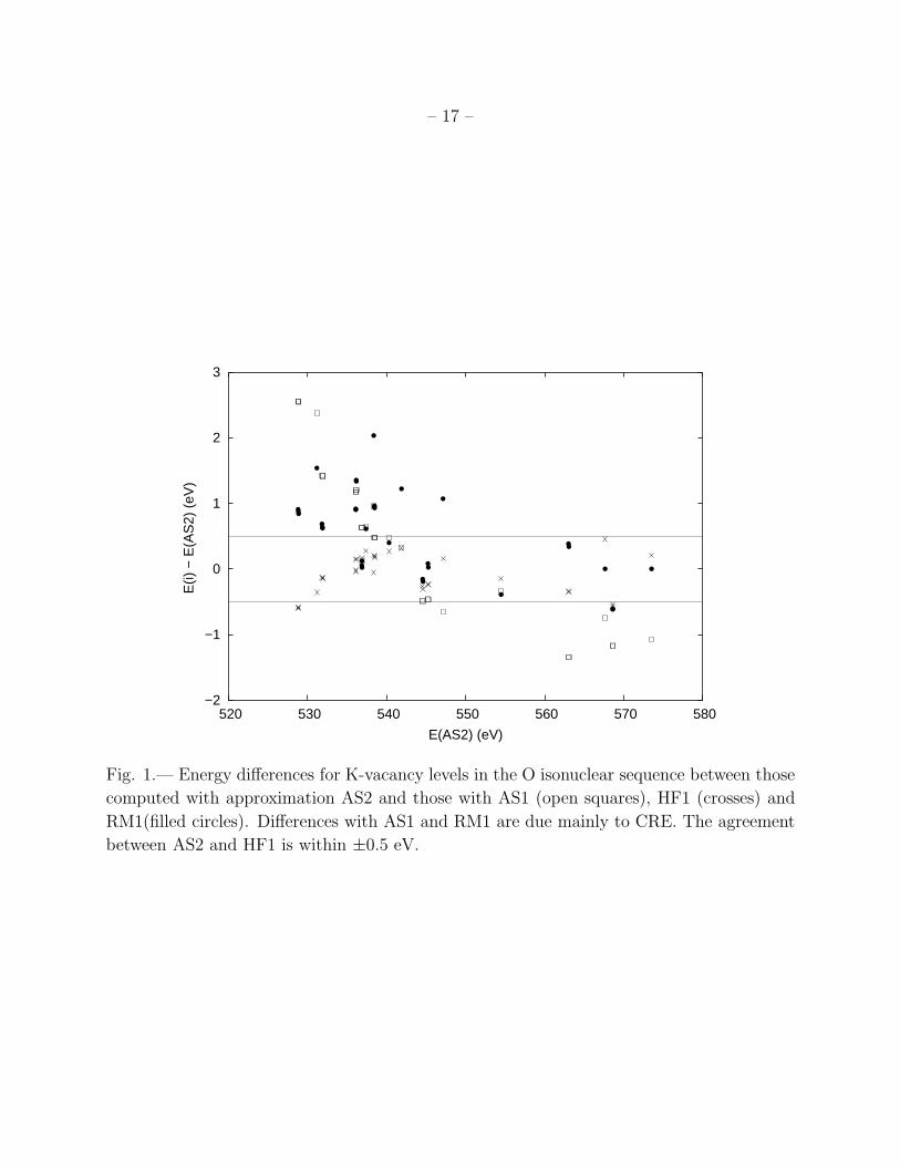
Regarding K-vacancy levels, the energy differences of the approximations considered

with respect to AS2 are plotted in Fig 1. The comparison with AS1 shows that, for species

with a half-filled L shell or with greater electron occupancies (6 ≤ N ≤ 8 and E < 544 eV),

CRE again lower energies but by amounts that increase with N : ∆E ≡ E(AS1)−E(AS2) <

0.7 eV for N = 6 to ∆E ≈ 2.5 eV for N = 8. On the other hand, for ions with a half-empty

L shell or with lower occupancies (2 ≤ N ≤ 5 and E > 544 eV), level energies are raised by

CRE particularly for N = 3 where ∆E & −1.35 eV. RM1 behaves, as expected, in a similar

fashion to AS1, but some inconsistencies (e.g. lowered rather than raised levels) occur for

N < 6 perhaps due to resolution problems in determining the position of narrow resonances

in the photoionization curves. The agreement between the AS2 and HF1 energies is a sound

±0.6 eV which sets a limit to the accuracy level that we can attain, and encourages us to

adopt AS2 and HF1 as our working approximations.

AS2 and HF1 K-vacancy level energies are compared with experiment and other theo-

retical data in Table 3. It may be noted that there are no reported measurements for species

with 4 ≤ N ≤ 6. HF1 level energies are within 0.5 eV of the spectroscopic values for N ≤ 3

and the CI values by Charro et al. (2000) for N = 2 while AS2 is undesirably higher (0.9

eV) for the [1s]2p 3Po1 level in O vii. A convincing comparison with experiment for N ≥ 7 is

impeded by the scatter displayed in measurements which is well outside the reported error

bars, and the photoionization measurements by Stolte et al. (1997) are 1 eV lower than

HF1. The energy positions computed by Pradhan et al. (2003) with bprm are noticeably

higher than present results for N > 4, in particular for the B-like system (N = 5) where

discrepancies as large as 5 eV are encountered. The values listed by McLaughlin & Kirby

(1998) for O ii (N = 7), which are also distinctively high (∼3 eV), correspond to the CI

target they prepared for the non-relativistic R-matrix calculation of the photoionization of

O i. They contrast with those quoted for an equivalent target by Gorczyca & McLaughlin

(2000) which are in good agreement with Stolte et al. (1997). However, the value obtained

by McLaughlin & Kirby (1998) for the [1s]2p5 3Po hole state in O i is in good agreement

with AS2 and HF1.

CRE also have an impact on the transition wavelengths where, as depicted in Fig. 2, the

comparison of AS1 and RM1 with AS2 indicates that in general CRE lead to increasingly

longer wavelength for N ≥ 6 (λ > 23 A) and shorter for higher charge states. It may also be

seen in Fig. 2 that wavelengths obtained with AS2 and HF1 agree to ±0.02 A setting again

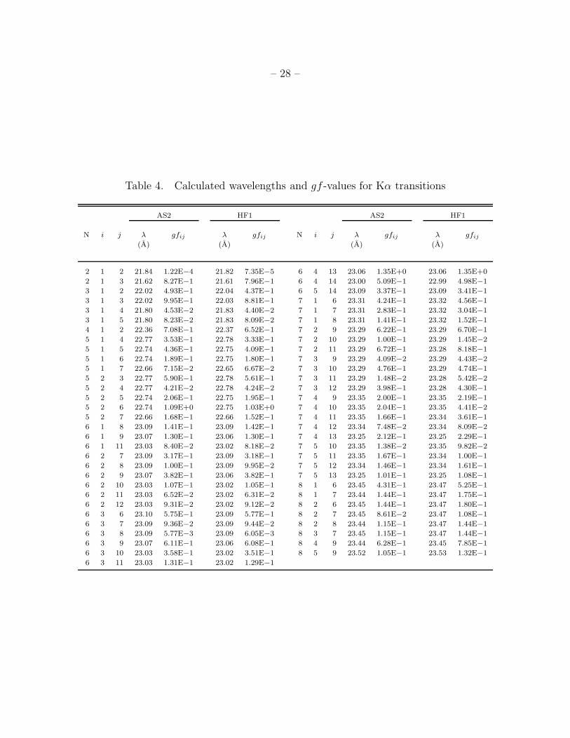
an accuracy bound. (AS2 and HF1 wavelengths are also listed in Table 4.) The present

wavelengths are compared with experiment and other theoretical predictions in Table 5. For

N ≤ 4 the present data, in particular HF1, agree with measurements and Vainshtein &

Safronova (1978) to ±0.02 A; in this respect, for 2 < N ≤ 4 the values by Chen (1985, 1986)

are somewhat long while those by Behar & Kahn (2002) are short, and for N = 3 the values

– 7 –

by Pradhan et al. (2003) are also long. For 5 ≤ N ≤ 6 the outcome is less certain due to

absence of laboratory measurements and inconsistencies in the computed values, e.g. the

order of the upper levels in N = 5. For N > 6 comparisons with measurements seem to

indicate that all theoretical results are slightly short although the agreement of HF1 is still

within ∼0.02 A except for the transition from the ground level of O ii and the measurement

by Stolte et al. (1997) in O i which are just out (less than 0.05A). It must be pointed out

again the undesirable scatter of the experimental data for O i.

4. gf-values

In the following discussion of gf -values, the transitions involving the strongly mixed

[1s]2p4 2D3/2 and 2P3/2 levels in O ii are excluded due to extensive cancellation that result

in completely unreliable data; also the 1s2 1S0 → [1s]2p 3Po1 intercombination transition in

O vii with a very small gf -value (gf < 10−3) that would require a much greater effort to

guarantee respectful accuracy.

A comparison of gf -values obtained with the AS1 and AS2 approximations shows that

CRE are relatively unimportant, leading to differences much less than 10% except for tran-

sitions involving the four [1s]2s2p 2Po relatively mixed levels of O vi where they jump up to

∼15%. In Fig. 3 we compare the AS2 and HF1 gf -values (also listed in Table 4) showing

an agreement within 10% except for O i where the latter are consistently 25% higher. In a

comparison of AS2 and HF1 f -values with other theoretical data sets in Table 6, it is found

that those by Pradhan et al. (2003) are generally 20% smaller; however, an interesting point

arises regarding the discrepancies between AS2 and HF1 where Pradhan et al. (2003) favors

AS2 for O i and HF1 for the small f -value in O vi (see Table 6).

5. Radiative and Auger widths

The radiative width of the jth level is defined as

Aj =∑

i

Aji (5)

where Aji is the rate (partial width) for a downward (j > i) transition. It is found by

calculation that CRE disturb the radiative widths of K-vacancy levels in the O isonuclear

sequence by 10% or less (5% for N > 5) except when strong admixture occurs, namely for

[1s]2p4 2D3/2 and 2P3/2 in O ii and the four [1s]2s2p 2Po levels in O vi where differences are

around 20%.

– 8 –

By contrast, as shown in Fig. 4, CRE reduce Auger rates by amounts that grow with N :

from 10% for N = 4 where log Aa < 14 up to 35% for N = 8; however, this trend is broken

for N = 3 due to strong level mixing where those for the [1s]2s2p(3Po) 2PoJ are increased by a

factor of 2 (not shown in Fig. 4) even though the [1s]2s2p(1Po) 2PoJ levels are hardly modified

(less than 5%). The Auger widths obtained with HF1 for the former levels are ∼20% higher

that AS2 while the remaining, as shown in Fig. 4, are on average lower by 10%. With this

outcome we estimate an accuracy rating for the Auger rates at just better than 20%. As

further support for this assertion, in Table 7 we compare our branching ratios for KLL Auger

transitions with other theoretical and experimental values. It may be seen that the AS1,

AS2, and HF1 data are stable to better than 10%, and the accord with other data sets is for

most cases better than 20%. Radiative and Auger widths computed in approximations AS2

and HF1 are listed in Table 8.

6. Photoionization cross sections

High-energy photoionization cross sections of O parent ions with electron occupancies

3 ≤ N ≤ 8 have been computed in approximation RM1. Intermediate coupling has been

used throughout except for O i because of computational size and negligible relativistic

corrections. Following Gorczyca & Robicheaux (1999) and Gorczyca & McLaughlin (2000),

damping is taken into account in detail in order to bring forth the correct K threshold

behavior. In Fig. 5 our cross sections are compared with those computed by Pradhan et al.

(2003) with the bprm package in the region near the n = 2 resonances and those by Reilman

& Manson (1979) in a central field potential where it may be seen that, even though the

background cross sections are in satisfactory accord, the positions and sharpness of the

edges are discrepant. In the present approach, due to the astrophysical interest of both the

n = 2 resonances and the edge region, the resonance structure is treated in a unified manner

showing that a sharp K edge occurs only in O vi due to the absence of spectator Auger

(KLL) channels of the type

[1s]2pµnp → 2pµ−2np + e− (6)

→ [2s]2pµ−1np + e− (7)

→ [2s]22pµnp + e− . (8)

For the remaining ions, these KLL processes dominate over participator Auger (KLn) decay

[1s]2pµnp → 2pµ−1 + e− (9)

→ [2s]2pµ + e− (10)

– 9 –

causing edge smearing by resonances with symmetric profiles of nearly constant width. Par-

ticipator Auger decay, on the other hand, gives rise to the familiar Feschbach resonances—

displayed by O vi in the region below the K threshold (see Fig. 5)—whose widths become

narrower with n thus maintaining sharpness over the spectral head.

In order to elucidate further the interesting properties of K resonances, we analyze the

experimental and theoretical predictions reported for the two [1s]2p4(4P)np and [1s]2p4(2P)np

Rydberg series in O i that exhibit significant discrepancies. Regarding resonance positions,

a stringent test is to compare quantum defects, µ, defined as

E = Elim −z2

(n − µ)2(11)

where Elim is the series-limit energy in Rydbergs; z ≡ Z − N + 1 is the effective charge

(z = 1 for O i); and n is the principal quantum number. In Fig. 6, the RM1 quantum

defects for these two series are plotted relative to their respective series limits and compared

with those obtained in photoionization measurements (Stolte et al. 1997) and the R-matrix

calculation of McLaughlin & Kirby (1998). Firstly, it may be seen that the experimental

error bars grow sharply with n; hence greater accuracy for high n is obtained by quantum-

defect extrapolation than actual measurement. Secondly, the agreement of experiment with

RM1 is very good while that with McLaughlin & Kirby (1998), who used practically the

same numerical method (R-matrix), is only a poor 40%. This outcome may be due to their

neglect of damping effects or their choice of a Hartree–Fock basis for the 1s, 2s, and 2p

orbitals which results in a deficient representation for the K-vacancy states. Since the R-

matrix method employs a common set of target orbitals for both valence and K-vacancy

states, we have found the most adequate orbital basis to be that optimized variationally

with an energy sum comprising all the states in the target model. The importance of K-

vacancy state representations has also been stressed by Gorczyca & McLaughlin (2000).

Thirdly, it is found that the RM1 quantum defects (n ≥ 3) are hardly modified by small

target-energy shifts prior to Hamiltonian diagonalization, a standard R-matrix procedure to

enhance accuracy by using experimental thresholds; therefore, the absolute energy positions

of these resonances mostly depend on the actual position of their series limits. Moreover,

as shown in Fig. 7, the huge and incorrect quantum-defect decline obtained for high n in

McLaughlin & Kirby (1998) when using two different sets of experimental thresholds, namely

those of Krause (1994) and Stolte et al. (1997), are not due in our opinion to the threshold-

energy shifts but to resonance misidentifications where µ(n + 1) − µ(n) ≈ −1 instead of

approximately zero (see Fig. 7). The quantum-defect changes for n ≤ 6 in McLaughlin

& Kirby (1998) as thresholds are shifted are very small in accord with our findings. By

contrast, experimental quantum defects are markedly sensitive to the series-limit positions;

for instance, if the quantum defects in the photoionization experiment of Menzel et al. (1996)

– 10 –

are computed with the series limits by Krause (1994), they display noticeable discrepancies

(see Fig. 7) while if they are computed with those by Stolte et al. (1997) (not shown),

consensus is reached.

It is inferred from the above comparison that the energy positions obtained by Auger

electron spectrometry (Krause 1994; Caldwell et al. 1994) for the [1s]2p4 4P and 2P states

of O ii and listed in Table 3 should perhaps be scaled down by 0.4 eV. If this proposition is

extended to the [1s]2p5 3Po state of O i, then the measurements by Stolte et al. (1997) and

Krause (1994) are brought to close agreement; the only remaining experimental discrepancy

for the latter state would then be the measurement by Menzel et al. (1996) still high by 1 eV.

Furthermore, contrary to the [1s]2p4(4P)np 3Po resonances of O i in our RM1 calculation,

the absolute energy position of [1s]2p5 3Po is insensitive to threshold-energy shifts. This is

a consequence of its wavefunction being mostly represented by the second term of the close-

coupling expansion (4). Therefore, a useful parameter in comparisons with experiment—in as

much as it gives an indication of both a balanced close-coupling expansion and experimental

consistency—is the energy interval between the lowest n = 2 and n = 3 resonances, ∆E(2, 3)

say. In Table 9, the RM1 ∆E(2, 3) for the whole O isonuclear sequence are tabulated and

compared with experimental and theoretical estimates. The 0.07 Ryd (1 eV) discrepancy

in the ∆E(2, 3) obtained from the measurements by Stolte et al. (1997) and Menzel et al.

(1996) in O i (N = 8) denotes irregular data: since the positions for the (4P)3p state differ

by only 0.07 eV the issue is then the [1s]2p5 3Po. The agreement of RM1 with Stolte et

al. (1997) is very good; however, if the RM1 (4P) threshold is improved by replacement

with the experimental value at Halmiltonian diagonalization, then ∆E(2, 3) is reduced to

1.00. In other words, the introduction of experimental thresholds improves the positions of

resonances with n ≥ 3 relative to the ionization threshold but not those within n = 2, as

previously mentioned. It may be appreciated in Table 9 that this finding is corroborated

by the ∆E(2, 3) resulting from the threshold-energy shifting in McLaughlin & Kirby (1998).

It is also seen in Table 9 that for the O isonuclear sequence ∆E(2, 3) ≈ z for N ≥ 2 and

∆E(2, 3) ≈ z + 1 for N = 1 if ∆E(2, 3) is expressed in Ryd.

Regarding K-resonance widths in O i, from the Auger rates listed in Table 8 widths of

159 meV (AS2) and 163 meV (HF1) are obtained for [1s]2p5 3Po. These are in good accord

(∼15%) with the measurements of 140 meV (Krause 1994; Menzel et al. 1996) and 142 eV

(Stolte et al. 1997) and the theoretical estimates of 169 meV (Saha 1994) and 139 meV

(Petrini & Araujo 1994). The value of 185.22 meV listed by McLaughlin & Kirby (1998),

on the other hand, is somewhat high. These authors also predict for the [1s]2p4(4P)np 3Po

widths a decrease with n. As previously mentioned, the utter dominance of KLL decay (see

Eqs 7–9) gives rise to constant resonance widths confirmed with AS1 for 3 ≤ n ≤ 5 to be at

103 meV and with KLn branching ratios of 5 parts in 1000 or less.

– 11 –

7. Opacities

In order to investigate the variations of the oxygen K-edge structure with plasma condi-

tions, our best atomic data for O ions have been incorporated in the xstar modelling code

(Kallman & Bautista 2001). Opacities for ionization parameters in the range 0.001 ≤ ξ ≤ 10

have then been obtained with a simple model denoted by the following specifications: gas

density of 1012 cm−3; X-ray luminosity source of 1044 erg/s; and solar abundances for H, He,

and O. Since the density is assumed constant, the well-known expression for the ionization

parameter

ξ = L/nR2 (12)

is implemented where L is the luminosity of the source, R its distance, and n the density of

the gas (Tarter et al. 1969). Therefore, the monochromatic opacities are calculated assuming

that ionization and heating are mainly due to an external source of continuum photons.

In Fig. 8 opacities for different values of log ξ are plotted in the 400–800 eV energy range

showing a rich variability mainly determined by the resonance structure and K edges of the

abundant ionic species. For a lowly ionized plasma (log ξ = −3), the opacity is dominated

by the O i edge at ∼545 eV and the Kα resonance structure belonging to O i and O ii in

the 530–540 eV energy interval. For log ξ = −2 the O ii edge is also conspicuous at ∼565

eV, but by log ξ = −1.5 is almost vanished being replaced by the O iii and O iv edges at

∼600 eV and ∼630 eV, respectively. While the latter is still distinctive for log ξ = −1, the

O v edge arises at ∼665 eV and becomes the dominant feature for log ξ = 0. At a high

degree of ionization (log ξ = 1), a three-edge structure (O v, O vi, and O vii) is observed

together with strong absorption features due to Kβ and high-n resonances that in general

enhance edge smearing, the opposite characteristics of low ionization. This behavior at the

two extremes of the ionization parameter is similar to that reported for the Fe isonuclear

sequence by Palmeri et al. (2002), an important difference being that the oxygen opacities

show important absorption features in the edge region due to the always open L shell.

8. Discussion and conclusions

Extensive computations of the atomic data required for the spectral modelling of K-

shell photoabsorption of oxygen ions have been carried out in a multi-code approach. This

method has proven to be—as in a previous systematic treatment of the Fe isonuclear sequence

(Bautista et al. 2003; Palmeri et al. 2003a,b; Bautista et al. 2004; Mendoza et al. 2004)—

effective in sizing up the relevant interactions and in obtaining accuracy rating estimates,

the latter often overlooked in theoretical work. Inter-complex CI and relativistic corrections

– 12 –

are found to be small, but CRE are shown to be conspicuous in most processes involving

K-vacancy states. The inclusion of CRE in ion representations is therefore compelling which

in practice is managed (e.g. in the hfr and autostructure codes) by considering non-

orthogonal orbital bases for K-vacancy and valence states; otherwise (e.g. bprm) orthogonal

orbital bases are optimized by minimizing energy sums that span both types of states.

By considering several approximations and comparing with reported experimental and

theoretical data, the present level energies and wavelength for O ions with electron occupan-

cies N ≤ 4 are estimated to be accurate to within 0.5 eV and 0.02 A, respectively. For ions

with N > 4, the absence of measurements in particular for 5 ≤ N ≤ 6, the wide experimental

scatter for N > 6, and discrepancies among theoretical data sets make the estimate of reli-

able accuracy ratings less certain. It is found that for N > 4 our level energies (wavelengths)

are probably somewhat high (short) by up to 1.5 eV (0.05 A) in neutral oxygen. Our best

results are from approximation HF1.

The radiative data (gf -values and total widths) computed with approximations AS2 and

HF1 are expected to be accurate to 10% except in O i where the rating is not better than

25% and in transitions involving strongly mixed levels, namely the [1s]2p4 2D3/2 and 2P3/2

levels in O ii and to a lesser extent the four [1s]2s2p 2PoJ levels in O vi, where it is unreliable.

Admixture in the latter levels also affect Auger rates which otherwise are expected to be

accurate to 20%. The complete and ranked set of radiative and Auger data for transitions

involving K-vacancy levels in O ions is one of the main achievements of the present work.

A second contribution is the high-energy photoabsorption cross sections for ions with

N > 3 that depict in detail the resonance structure of the K edge. Such structure has been

shown to be dominated by KLL damping (often neglected in previous work) which gives the

edge a blunt imprint with arguably diagnostic potential. A comparison with the experimental

K resonance positions in O i results in conclusive statements about the importance of R-

matrix computations with well balanced close-coupling expansions, i.e. where both terms

of expression (4) are separately convergent. In this respect, the accuracy of the energy

interval between the n = 2 and n = 3 components of a K resonance series gives a measure

of the close-coupling balance, and for the O isonuclear sequence, this energy interval when

expressed in Ryd has been shown to be close to the effective charge, z ≡ Z − N + 1, for

members with N ≥ 2 and near z + 1 for N = 1. This finding could be exploited in spectral

identification.

The present atomic data sets have been incorporated in the xstar modelling code in

order to generate improved opacities in the oxygen K-edge region using simple constant

density slab models. Their behavior as a function of ionization parameter, shown in detail

for the first time, is similar to that of the iron K edge with the exception of omnipresent

– 13 –

Kα resonances. Finally, as a continuation to the present work we intend to treat with

the same systematic methodology the Ne isonuclear sequence and then other sequences of

astrophysical interest (Mg, Si, S, Ar, and Ca), always bearing in mind the scanty availability

of laboratory measurements which as shown in the present work are unreplaceable requisites

in theoretical fine-tuning.

MAB acknowledges partial support from FONACIT, Venezuela, under contract No. S1-

20011000912. TWG was supported in part by the NASA Astronomy and Physics Research

and Analysis Program. PP was supported by a return grant of the Belgian Federal Scientific

Policy.

REFERENCES

Badnell, N. R. 1986, J. Phys. B, 19, 3827

Badnell, N. R. 1997, J. Phys. B, 30, 1

Bautista, M. A., Mendoza, C., Kallman, T. R., & Palmeri, P. 2003, A&A, 403, 339

Bautista, M. A., Mendoza, C., Kallman, T. R., & Palmeri, P. 2004, A&A, 418, 1171

Behar, E., et al. 2003, ApJ, 598, 232

Behar, E., & Kahn, S. M. 2002, in NASA Laboratory Astrophysics Workshop, ed. F. Salama

(NASA/CP-2002-21186), p23

Beiersdorfer, P., et al. 2003, Science, 300, 1558

Berrington, K. A., Burke, P. G., Butler, K., Seaton, M. J., Storey, P. J., Taylor, K. T., &

Yan, Y. 1987, J. Phys. B, 20, 6379

Cagnoni, I., Nicastro, F., Maraschi, L., Treves, A., & Tavecchio F. 2004, ApJ, 603, 449

Caldwell, C. D., & Krause, M. O. 1993, Phys. Rev. A, 47, R759

Caldwell, C. D., Schaphorst, S. J., Krause, M. O., & Jimenez-Mier, J. 1994, J. Electron.

Spectrosc. Relat. Phenom., 67, 243

Charro, E., Bell, K. L., Martin, I., & Hibbert, A. 2000, MNRAS, 313, 247

Chen, M. H. 1985, Phys. Rev. A, 31, 1449

– 14 –

Chen, M. H. 1986, At. Data Nucl. Data Tables, 34, 301

Cowan, R. D. 1981, The Theory of Atomic Spectra and Structure, (Berkeley, CA: University

of California Press)

de Vries, C. P., den Herder, J. W., Kaastra, J. S., Paerels, F. B., den Boggende, A. J., &

Rasmussen, A. P. 2003, A&A, 404, 959

Eissner, W., Jones, M., & Nussbaumer, H. 1974, Comput. Phys., Commun., 8, 270

Engstrom, L., & Litzen, U. 1995, J. Phys. B, 28, 2565

Gorczyca, T. W., & Badnell, N. R. 1996, J. Phys. B, 29, L283

Gorczyca, T. W., & Badnell, N. R. 2000, J. Phys. B, 33, 2511

Gorczyca, T. W., & McLaughlin, B. M. 2000, J. Phys. B, 33, L859

Gorczyca, T. W., & Robicheaux, F. 1999, Phys. Rev. A, 60, 1216

Juett, A. M., Schulz, N. S., & Chakrabarty, D. 2004, ApJ, 612, 308

Kallman, T., & Bautista, M. 2001, ApJS, 133, 221

Kallman, T. R., Palmeri, P., Bautista, M. A., Mendoza, C., & Krolik, J. H. 2004, preprint

(astro-ph/0405210)

Kawatsura, et al. 2002, J. Phys. B, 35, 4147

Krause, M. O. 1994, Nucl. Instrum. Meth. Phys. Res. B, 87, 178

Lee, J. C., Ogle, P. M., Canizares, C. R., Marshall, H. L., Schulz, N. S., Morales, R., Fabian,

A. C., & Iwasawa, K. 2001, ApJ, 554, L13

Loeb, A. 2003, Phys. Rev. Lett., 91, 071103

McLaughlin, B. M., & Kirby, K. P. 1998, J. Phys. B, 31, 4991

Mendoza, C., Kallman, T. R., Bautista, M. A., & Palmeri, P. 2004, A&A, 414, 377

Menzel, A., Benzaid, S., Krause, M. O., Caldwell, C. D., Hergenhahn, U., & Bissen, M.

1996, Phys. Rev. A, 54, R991

Moore, C. E. 1998, Tables of spectra of hydrogen, carbon, nitrogen, and oxygen atoms and

ions, ed. J. W. Gallagher (Boca Raton, FL: CRC Press)

– 15 –

Page, M. J., Soria, R., Wu, K., Mason, K. O., Cordova, F. A., & Priedhorsky, W. C. 2003,

MNRAS, 345, 639

Palmeri, P., Mendoza, C., Kallman, T. R., & Bautista, M. A. 2002, ApJ, 577, L119

Palmeri, P., Mendoza, C., Kallman, T. R., & Bautista, M. A. 2003a, A&A, 403, 1175

Palmeri, P., Mendoza, C., Kallman, T. R., Bautista, M. A. & Melendez, M. 2003b, A&A,

410, 359

Petrini, D., & Araujo, F. X. 1994, A&A, 282, 315

Pradhan, A. K., Chen, G. X., Delahaye, F., Nahar, S. N., & Oelgoetz, J. 2003, MNRAS,

341, 1268

Reilman, R. F., & Manson, S. T. 1979, ApJS, 40, 815

Robicheaux, F., Gorczyca. T. W., Pindzola, M. S., & Badnell, N. R. 1995, Phys. Rev. A, 32,

1319

Saha, H. P. 1994, Phys. Rev. A, 49, 894

Sako, M. 2003, ApJ, 594, 1108

Sako, M., et al. 2003, ApJ, 596, 114

Saraph, H. E. 1987, Comput. Phys. Commun., 46, 107

Schmidt, M., Beiersdorfer, P., Chen, H., Thorn, D. B., Trabert, E., & Behar, E. 2004, ApJ,

604, 562

Schulz, N. S., Cui, W., Canizares, C. R., Marshall, H. L., Lee, J. C., Miller, J. M., & Lewin,

W. H. G. 2002, ApJ, 565, 1141

Scott, N. S., & Burke, P. G. 1980, J. Phys. B, 13, 4299

Scott, N. S., & Taylor, K. T. 1982, Comput. Phys. Commun., 25, 347

Seaton, M. J. 1987, J. Phys. B, 20, 6363

Steenbrugge, K. C., Kaastra, J. S., de Vries, C. P., & Edelson, R. 2003, A&A, 402, 477

Stolte, W. C., et al. 1997, J. Phys. B, 30, 4489

Tarter, C. B., Tucker, W. H., & Salpeter, E. E. 1969, ApJ, 156, 943

– 16 –

Vainshtein, L. A., & Safronova, U. I. 1971, Soviet Astron., 15, 175

Vainshtein, L. A., & Safronova, U. I. 1978, At. Data Nucl. Data Tables, 21, 49

This preprint was prepared with the AAS LATEX macros v5.2.

– 17 –

−2

−1

0

1

2

3

520 530 540 550 560 570 580

E(i)

− E

(AS

2) (

eV)

E(AS2) (eV)

Fig. 1.— Energy differences for K-vacancy levels in the O isonuclear sequence between those

computed with approximation AS2 and those with AS1 (open squares), HF1 (crosses) and

RM1(filled circles). Differences with AS1 and RM1 are due mainly to CRE. The agreement

between AS2 and HF1 is within ±0.5 eV.

– 18 –

−0.14

−0.12

−0.1

−0.08

−0.06

−0.04

−0.02

0

0.02

0.04

0.06

0.08

21 22 23 24

λ(i)

− λ

(AS

2) (

Å)

λ(AS2) (Å)

Fig. 2.— Wavelength differences for Kα transitions in the O isoelectronic sequence between

those computed with approximation AS2 and those with AS1 (open squares), HF1 (crosses),

and RM1 (solid circles). The agreement between AS2 and HF1 is within ±0.02 A.

– 19 –

0.8

0.9

1

1.1

1.2

1.3

−2.5 −2 −1.5 −1 −0.5 0 0.5

gf(H

F1)

/gf(

AS

2)

Log gf(AS2)

O I

Fig. 3.— Comparison of gf -values for Kα transitions in O ions computed with approxima-

tions AS2 and HF1. It may be seen that, while the agreement for most transitions is within

10%, the HF1 gf -values for O i are consistently larger by 25%.

– 20 –

0.6

0.7

0.8

0.9

1

1.1

13.8 13.9 14 14.1 14.2 14.3 14.4 14.5

Aa(

HF

1)/A

a(A

S2)

Log Aa(AS2)

Fig. 4.— Comparison of Auger widths (s−1) for K-vacancy levels in O ions computed with

approximation AS2 and those with AS1 (filled circles) and HF1 (open circles). Differences

between AS1 and AS2 (as large as 35%) are due to CRE. It may also be seen that HF1 are

on average 10% lower than AS2.

– 21 –

520 540 560 580 600 620 640 660 680 700 7200.010.1

110

1001000

520 540 560 580 600 620 640 660 680 700 7200.010.1

110

1001000

520 540 560 580 600 620 640 660 680 700 7200.010.1

110

1001000

520 540 560 580 600 620 640 660 680 700 7200.010.1

110

1001000

520 540 560 580 600 620 640 660 680 700 7200.010.1

110

1001000

520 540 560 580 600 620 640 660 680 700 7200.010.1

110

1001000

Phot

oabs

orpt

ion

Cro

ss S

ectio

n (M

Bar

n)

Photon Energy (eV)

O I

O II

O III

O IV

O V

O VI

Fig. 5.— High-energy photoionization cross sections of O ions showing the structure of the K

edge. Solid curve — RM1; dotted curve — Pradhan et al. (2003); broken curve — Reilman

& Manson (1979).

– 22 –

0.5

0.6

0.7

0.8

0.9

1

1.1

−0.25 −0.2 −0.15 −0.1 −0.05 0

Energy (Ryd)

b

n=3 4 5 6

3

4

56

0.4

0.5

0.6

0.7

0.8

0.9

1

Qua

ntum

Def

ect

a

n=3 4 5

6

3 45 6

Fig. 6.— Quantum defects for the (a) [1s]2p4(4P)np 3Po and (b) [1s]2p4(2P)np 3Po (3 ≤ n ≤

6) resonance series of O i plotted relative to their respective threshold energies. Circles —

present RM1 results. Filled circles — experiment of Stolte et al. (1997). Filled triangles —

R-matrix data by McLaughlin & Kirby (1998).

– 23 –

−1

0

1

2

3

−0.3 −0.25 −0.2 −0.15 −0.1 −0.05 0

Energy (Ryd)

b

n=3

−3

−2

−1

0

1

2

3

Qua

ntum

Def

ect

a

n=3

Fig. 7.— Quantum defects for the (a) [1s]2p4(4P)np 3Po and (b) [1s]2p4(2P)np 3Po (3 ≤

n ≤ 10) resonance series of O i plotted relative to their respective threshold energies. Filled

squares — experiment of Krause (1994) and Menzel et al. (1996). Filled circles — experiment

of Stolte et al. (1997). Triangles — R-matrix quantum defects of McLaughlin & Kirby

(1998) relative to the experimental thresholds of Krause (1994). Filled triangles — R-matrix

quantum defects of McLaughlin & Kirby (1998) relative to the experimental threshold by

Stolte et al. (1997).

– 24 –

−12

−11.5

−11

−10.5

−10

−9.5

−9

500 550 600 650 700 750 800

log ξ=1.0

−10.5

−10

−9.5

−9

−8.5

500 550 600 650 700 750 800

log ξ=0.0

−10

−9.5

−9

−8.5

500 550 600 650 700 750 800

log ξ=−1.0

−9.5

−9

500 550 600 650 700 750 800

Photon Energy (eV)

log ξ=−1.5

−9.5

−9

−8.5

500 550 600 650 700 750 800

Log

κ (1

/cm

)

log ξ=−2.0

−9.5

−9

−8.5

−8

500 550 600 650 700 750 800

log ξ=−3.0

Fig. 8.— Opacities for a photoionized gas in the oxygen K-edge region for ionization param-

eters in the range −3 ≤ log ξ ≤ 1.

– 25 –

Table 1. Calculated energies (eV) for valence and K-vacancy levels in O ions

N i Level AS1 AS2 HF1 RM1 N i Level AS1 AS2 HF1 RM1

2 1 1s2 1S0 0.000 0.000 0.000 7 1 2p3 4So3/2

0.000 0.000 0.000 0.000

2 2 [1s]2p 3Po1 566.9 567.7 568.1 7 2 2p3 2Do

5/23.972 3.711 3.770 3.615

2 3 [1s]2p 1Po1 572.5 573.5 573.7 7 3 2p3 2Do

3/23.975 3.714 3.770 3.614

3 1 2s 2S1/2 0.000 0.000 0.000 0.000 7 4 2p3 2Po3/2

5.393 5.064 5.131 5.655

3 2 [1s]2s2p 2Po1/2

561.7 563.0 562.7 563.4 7 5 2p3 2Po1/2

5.395 5.066 5.131 5.654

3 3 [1s]2s2p 2Po3/2

561.7 563.1 562.7 563.4 7 6 [1s]2p4 4P5/2 533.2 531.8 531.7 532.5

3 4 [1s]2s2p 2Po1/2

567.4 568.6 568.0 568.0 7 7 [1s]2p4 4P3/2 533.3 531.9 531.7 532.5

3 5 [1s]2s2p 2Po3/2

567.4 568.6 568.1 568.0 7 8 [1s]2p4 4P1/2 533.3 531.9 531.7 532.5

4 1 2s2 1S0 0.000 0.000 0.000 0.000 7 9 [1s]2p4 2D5/2 537.3 536.1 536.1 537.0

4 2 [1s]2p 1Po1 554.2 554.5 554.4 554.1 7 10 [1s]2p4 2D3/2 537.3 536.1 536.1 537.0

5 1 2p 2Po1/2

0.000 0.000 0.000 0.000 7 11 [1s]2p4 2P3/2 537.4 536.2 536.3 537.5

5 2 2p 2Po3/2

0.057 0.049 0.047 0.047 7 12 [1s]2p4 2P1/2 537.4 536.2 536.3 537.5

5 3 [1s]2p2 2D5/2 544.1 544.6 544.3 544.4 7 13 [1s]2p4 2S1/2 539.3 538.4 538.3 540.4

5 4 [1s]2p2 2D3/2 544.1 544.6 544.3 544.4 8 1 2p4 3P2 0.000 0.000 0.000 0.000

5 5 [1s]2p2 2P1/2 544.8 545.2 545.0 545.3 8 2 2p4 3P1 0.023 0.020 0.018 0.000

5 6 [1s]2p2 2P3/2 544.8 545.3 545.0 545.3 8 3 2p4 3P0 0.033 0.029 0.027 0.000

5 7 [1s]2p2 2S1/2 546.5 547.1 547.3 548.2 8 4 2p4 1D2 2.353 2.181 2.200 2.149

6 1 2p2 3P0 0.000 0.000 0.000 0.000 8 5 2p4 1S0 4.244 3.975 3.979 4.833

6 2 2p2 3P1 0.016 0.014 0.014 0.014 8 6 [1s]2p5 3Po2 531.4 528.8 528.2 529.7

6 3 2p2 3P2 0.044 0.037 0.040 0.040 8 7 [1s]2p5 3Po1 531.4 528.8 528.2 529.7

6 4 2p2 1D2 2.958 2.750 2.848 2.711 8 8 [1s]2p5 3Po0 531.4 528.9 528.3 529.7

6 5 2p2 1S0 5.390 5.000 5.237 6.089 8 9 [1s]2p5 1Po1 533.5 531.2 530.8 532.7

6 6 [1s]2p3 3Do3 537.5 536.9 537.0 536.9

6 7 [1s]2p3 3Do2 537.5 536.9 537.0 536.9

6 8 [1s]2p3 3Do1 537.5 536.9 537.0 537.0

6 9 [1s]2p3 3So1 538.0 537.4 537.7 538.0

6 10 [1s]2p3 3Po2 538.9 538.4 538.6 539.4

6 11 [1s]2p3 3Po1 538.9 538.5 538.7 539.4

6 12 [1s]2p3 3Po0 538.9 538.5 538.7 539.4

6 13 [1s]2p3 1Do2 540.8 540.3 540.6 540.7

6 14 [1s]2p3 1Po1 542.2 541.9 542.2 543.1

– 26 –

Table 2. Comparison of valence level energies (eV)

N Level Expta AS1 AS2 HF1 RM1

5 2p 2Po1/2

0.000 0.000 0.000 0.000 0.000

5 2p 2Po3/2

0.048 0.057 0.049 0.047 0.047

6 2p2 3P0 0.000 0.000 0.000 0.000 0.000

6 2p2 3P1 0.014 0.016 0.014 0.014 0.014

6 2p2 3P2 0.038 0.044 0.037 0.040 0.040

6 2p2 1D2 2.514 2.958 2.750 2.848 2.711

6 2p2 1S0 5.354 5.390 5.000 5.237 6.089

7 2p3 4So3/2

0.000 0.000 0.000 0.000 0.000

7 2p3 2Do5/2

3.324 3.972 3.711 3.770 3.615

7 2p3 2Do3/2

3.327 3.975 3.714 3.770 3.614

7 2p3 2Po3/2

5.017 5.393 5.064 5.131 5.655

7 2p3 2Po1/2

5.018 5.395 5.066 5.131 5.654

8 2p4 3P2 0.000 0.000 0.000 0.000 0.000

8 2p4 3P1 0.020 0.023 0.020 0.018 0.000

8 2p4 3P0 0.028 0.033 0.029 0.027 0.000

8 2p4 1D2 1.967 2.353 2.181 2.200 2.149

8 2p4 1S0 4.190 4.244 3.975 3.979 4.833

aSpectroscopic tables (Moore 1998)

– 27 –

Table 3. Comparison of K-vacancy level energies∗ (eV)

N State AS2 HF1 Expt Theory

2 [1s]2p 3Po1 567.7 568.1 568.6a 568.2e

2 [1s]2p 1Po1 573.5 573.7 574.0a 573.6e

3 [1s]2s2p(3Po) 2Po 563.1 562.7 562.6a 562.3f

3 [1s]2s2p(1Po) 2Po 568.6 568.1 568.2a 567.0f

4 [1s]2p 1Po1 554.5 554.4 554.6f , 553.15g

5 [1s]2p2 2D3/2 544.6 544.3 545.8f

5 [1s]2p2 2P 545.3 545.0 547.0f

5 [1s]2p2 2S1/2 547.1 547.3 552.1f

6 [1s]2p3 3Do1 536.9 537.0 537.2f

6 [1s]2p3 3So1 537.4 537.7 538.6f

6 [1s]2p3 3Po1 538.5 538.7 540.7f

7 [1s]2p4 4P 531.9 531.7 530.8(3)b , 530.41(4)c 532.9f , 531.0h, 534.1i

7 [1s]2p4 2D 536.1 536.1 535.3h, 538.7i

7 [1s]2p4 2P 536.2 536.3 535.7(3)b , 535.23(4)c 535.9h, 539.2i

7 [1s]2p4 2S 538.4 538.3 538.1h, 542.9i

8 [1s]2p5 3Po 528.8 528.2 527.2(3)b , 526.79(4)c , 527.85(10)d 528.8f , 528.22i, 528.33i

∗Relative to each ion ground level

aSpectroscopic tables (Moore 1998)

bAuger electron spectrometry (Krause 1994; Caldwell et al. 1994)

cPhotoionization experiment (Stolte et al. 1997)

dPhotoabsorption measurements (Menzel et al. 1996)

eNon-relativistic CI calculation (Charro et al. 2000)

fR-matrix calculation by Pradhan et al. (2003)

gMulticonfiguration Dirac–Fock calculation by Chen (1985)

hR-matrix calculation (Gorczyca & McLaughlin 2000)

iR-matrix calculation (McLaughlin & Kirby 1998)

– 28 –

Table 4. Calculated wavelengths and gf -values for Kα transitions

AS2 HF1 AS2 HF1

N i j λ gfij λ gfij N i j λ gfij λ gfij

(A) (A) (A) (A)

2 1 2 21.84 1.22E−4 21.82 7.35E−5 6 4 13 23.06 1.35E+0 23.06 1.35E+0

2 1 3 21.62 8.27E−1 21.61 7.96E−1 6 4 14 23.00 5.09E−1 22.99 4.98E−1

3 1 2 22.02 4.93E−1 22.04 4.37E−1 6 5 14 23.09 3.37E−1 23.09 3.41E−1

3 1 3 22.02 9.95E−1 22.03 8.81E−1 7 1 6 23.31 4.24E−1 23.32 4.56E−1

3 1 4 21.80 4.53E−2 21.83 4.40E−2 7 1 7 23.31 2.83E−1 23.32 3.04E−1

3 1 5 21.80 8.23E−2 21.83 8.09E−2 7 1 8 23.31 1.41E−1 23.32 1.52E−1

4 1 2 22.36 7.08E−1 22.37 6.52E−1 7 2 9 23.29 6.22E−1 23.29 6.70E−1

5 1 4 22.77 3.53E−1 22.78 3.33E−1 7 2 10 23.29 1.00E−1 23.29 1.45E−2

5 1 5 22.74 4.36E−1 22.75 4.09E−1 7 2 11 23.29 6.72E−1 23.28 8.18E−1

5 1 6 22.74 1.89E−1 22.75 1.80E−1 7 3 9 23.29 4.09E−2 23.29 4.43E−2

5 1 7 22.66 7.15E−2 22.65 6.67E−2 7 3 10 23.29 4.76E−1 23.29 4.74E−1

5 2 3 22.77 5.90E−1 22.78 5.61E−1 7 3 11 23.29 1.48E−2 23.28 5.42E−2

5 2 4 22.77 4.21E−2 22.78 4.24E−2 7 3 12 23.29 3.98E−1 23.28 4.30E−1

5 2 5 22.74 2.06E−1 22.75 1.95E−1 7 4 9 23.35 2.00E−1 23.35 2.19E−1

5 2 6 22.74 1.09E+0 22.75 1.03E+0 7 4 10 23.35 2.04E−1 23.35 4.41E−2

5 2 7 22.66 1.68E−1 22.66 1.52E−1 7 4 11 23.35 1.66E−1 23.34 3.61E−1

6 1 8 23.09 1.41E−1 23.09 1.42E−1 7 4 12 23.34 7.48E−2 23.34 8.09E−2

6 1 9 23.07 1.30E−1 23.06 1.30E−1 7 4 13 23.25 2.12E−1 23.25 2.29E−1

6 1 11 23.03 8.40E−2 23.02 8.18E−2 7 5 10 23.35 1.38E−2 23.35 9.82E−2

6 2 7 23.09 3.17E−1 23.09 3.18E−1 7 5 11 23.35 1.67E−1 23.34 1.00E−1

6 2 8 23.09 1.00E−1 23.09 9.95E−2 7 5 12 23.34 1.46E−1 23.34 1.61E−1

6 2 9 23.07 3.82E−1 23.06 3.82E−1 7 5 13 23.25 1.01E−1 23.25 1.08E−1

6 2 10 23.03 1.07E−1 23.02 1.05E−1 8 1 6 23.45 4.31E−1 23.47 5.25E−1

6 2 11 23.03 6.52E−2 23.02 6.31E−2 8 1 7 23.44 1.44E−1 23.47 1.75E−1

6 2 12 23.03 9.31E−2 23.02 9.12E−2 8 2 6 23.45 1.44E−1 23.47 1.80E−1

6 3 6 23.10 5.75E−1 23.09 5.77E−1 8 2 7 23.45 8.61E−2 23.47 1.08E−1

6 3 7 23.09 9.36E−2 23.09 9.44E−2 8 2 8 23.44 1.15E−1 23.47 1.44E−1

6 3 8 23.09 5.77E−3 23.09 6.05E−3 8 3 7 23.45 1.15E−1 23.47 1.44E−1

6 3 9 23.07 6.11E−1 23.06 6.08E−1 8 4 9 23.44 6.28E−1 23.45 7.85E−1

6 3 10 23.03 3.58E−1 23.02 3.51E−1 8 5 9 23.52 1.05E−1 23.53 1.32E−1

6 3 11 23.03 1.31E−1 23.02 1.29E−1

– 29 –

Table 5. Wavelength (A) comparison for Kα transitions

N i j AS2 HF1 Expt Other theory

2 1s2 1S0 [1s]2p 3Po1 21.84 21.82 21.807a 21.84i, 21.84j

1s2 1S0 [1s]2p 1Po1 21.62 21.61 21.6020(3)b 21.60i

3 2s 2S [1s]2s2p(3Po) 2Po 22.02 22.03 22.038a, 22.01(1)c, 22.0194(16)d 22.02i, 22.06j, 22.05k, 22.00l

2s 2S [1s]2s2p(1Po) 2Po 21.80 21.83 21.82a 21.84j,21.87k, 21.79l

4 2s2 1S [1s]2p 1Po 22.36 22.37 22.38(1)c, 22.374(3)d 22.38i, 22.41j, 22.35k, 22.33l

5 2p 2Po1/2

[1s]2p2 2D3/2 22.77 22.78 22.74(2)c 22.73k, 22.73l

2p 2Po1/2

[1s]2p2 2P 22.74 22.75 22.67k, 22.78l

2p 2Po1/2

[1s]2p2 2S1/2 22.66 22.65 22.46k, 22.73l

6 2p2 3P0 [1s]2p3 3Do1 23.09 23.09 23.17(1)c 23.08k, 23.11l

2p2 3P0 [1s]2p3 3So1 23.07 23.06 23.00(2)c 23.02k, 23.05l

2p2 3P0 [1s]2p3 3Po1 23.03 23.02 22.93k, 22.98l

7 2p3 4So [1s]2p4 4P 23.31 23.32 23.36(1)e 23.27k, 23.30l

2p3 2Do [1s]2p4 2P 23.29 23.28 23.29(1)e

2p3 2Po [1s]2p4 2P 23.35 23.34 23.36(1)e

8 2p4 3P [1s]2p5 3Po 23.45 23.47 23.52(3)e, 23.489(5)f , 23.536(2)g 23.45k

23.508(3)h

aSpectroscopic tables (Moore 1998)

bSpectroscopic measurements (Engstrom & Litzen 1995)

cSpectroscopy of NGC 5548 (Steenbrugge et al. 2003)

dElectron beam ion trap measurements (Schmidt et al. 2004)

eAuger electron spectrometry (Krause 1994; Caldwell et al. 1994)

fPhotoabsorption measurements (Menzel et al. 1996)

gPhotoionization experiment (Stolte et al. 1997)

hISM observations (Juett et al. 2004)

i1/Z expansion method (Vainshtein & Safronova 1971, 1978)

jMulticonfiguration Dirac–Fock calculation (Chen 1985, 1986)

kR-matrix calculation (Pradhan et al. 2003)

lhullac calculation (Behar & Kahn 2002)

– 30 –

Table 6. Comparison of theoretical f -values for Kα transitions

N i j AS2 HF1 RM2a

3 2s 2S [1s]2s2p(3Po) 2Po 0.744 0.659 0.576

3 2s 2S [1s]2s2p(1Po) 2Po 0.077 0.062 0.061

4 2s2 1S [1s]2p 1Po 0.708 0.652 0.565

5 2p 2Po1/2

[1s]2p2 2D3/2 0.177 0.167 0.132

5 2p 2Po1/2

[1s]2p2 2P 0.313 0.295 0.252

5 2p 2Po1/2

[1s]2p2 2S1/2 0.036 0.033 0.027

6 2p2 3P0 [1s]2p3 3Do1 0.141 0.142 0.119

6 2p2 3P0 [1s]2p3 3So1 0.130 0.130 0.102

6 2p2 3P0 [1s]2p3 3Po1 0.084 0.082 0.067

7 2p3 4So3/2

[1s]2p4 4P 0.212 0.228 0.184

8 2p4 3P2 [1s]2p5 3P 0.115 0.140 0.113

aR-matrix data by Pradhan et al. (2003)

Table 7. Comparison of branching ratios for KLL Auger transitions

N i j AS1 AS2 HF1 Expta MCDFb CCc

7 [1s]2p4 4P 2p2 0.42 0.42 0.43 0.55(13) 0.36 0.43

[2s]2p3 0.41 0.40 0.40 0.33(3) 0.46 0.42

[2s2]2p4 0.17 0.18 0.18 0.12(2) 0.18 0.15

7 [1s]2p4 2P 2p2 0.53 0.53 0.51 0.53(9) 0.45 0.47

[2s]2p3 0.27 0.27 0.28 0.28(4) 0.31 0.28

[2s2]2p4 0.20 0.20 0.21 0.19(3) 0.24 0.25

8 [1s]2p5 3Po 2p3 0.53 0.51 0.55 0.606

[2s]2p4 0.35 0.35 0.32 0.30

[2s2]2p5 0.12 0.14 0.13 0.094

aAuger electron spectrometry (Caldwell & Krause 1993; Caldwell et al. 1994)

bMCDF calculation by M. H. Chen as quoted in Caldwell et al. (1994)

cClose-coupling calculation (Petrini & Araujo 1994)

– 31 –

Table 8. Calculated radiative and Auger widths for K-vacancy levels

AS2 HF1

N i Level Ar Aa Ar Aa

(s−1) (s−1) (s−1) (s−1)

2 2 [1s]2p 3Po1 6.60E+08 3.44E+08

2 3 [1s]2p 1Po1 3.93E+12 3.80E+12

3 2 [1s]2s2p 2Po1/2

3.39E+12 6.60E+12 3.00E+12 7.53E+12

3 3 [1s]2s2p 2Po3/2

3.42E+12 5.76E+12 3.02E+12 6.96E+12

3 4 [1s]2s2p 2Po1/2

3.19E+11 7.56E+13 3.12E+11 6.67E+13

3 5 [1s]2s2p 2Po3/2

2.90E+11 7.60E+13 2.87E+11 6.73E+13

4 2 [1s]2p 1Po1 3.40E+12 9.10E+13 3.10E+12 8.15E+13

5 3 [1s]2p2 2D5/2 1.34E+12 2.19E+14 1.22E+12 1.93E+14

5 4 [1s]2p2 2D3/2 1.35E+12 2.18E+14 1.28E+12 1.92E+14

5 5 [1s]2p2 2P1/2 4.31E+12 9.29E+13 4.05E+12 7.57E+13

5 6 [1s]2p2 2P3/2 4.31E+12 9.30E+13 4.05E+12 7.58E+13

5 7 [1s]2p2 2S1/2 1.63E+12 1.89E+14 1.50E+12 1.66E+14

6 6 [1s]2p3 3Do3 1.05E+12 2.37E+14 1.06E+12 2.11E+14

6 7 [1s]2p3 3Do2 1.05E+12 2.37E+14 1.06E+12 2.10E+14

6 8 [1s]2p3 3Do1 1.05E+12 2.37E+14 1.06E+12 2.10E+14

6 9 [1s]2p3 3So1 4.81E+12 8.87E+13 4.81E+12 7.24E+13

6 10 [1s]2p3 3Po2 1.20E+12 2.22E+14 1.18E+12 1.98E+14

6 11 [1s]2p3 3Po1 1.20E+12 2.22E+14 1.18E+12 1.98E+14

6 12 [1s]2p3 3Po0 1.20E+12 2.22E+14 1.18E+12 1.98E+14

6 13 [1s]2p3 1Do2 3.46E+12 2.05E+14 3.46E+12 1.84E+14

6 14 [1s]2p3 1Po1 3.62E+12 1.90E+14 3.60E+12 1.71E+14

7 6 [1s]2p4 4P5/2 8.67E+11 2.25E+14 9.35E+11 2.04E+14

7 7 [1s]2p4 4P3/2 8.67E+11 2.25E+14 9.35E+11 2.04E+14

7 8 [1s]2p4 4P1/2 8.68E+11 2.25E+14 9.35E+11 2.04E+14

7 9 [1s]2p4 2D5/2 1.78E+12 2.60E+14 1.93E+12 2.44E+14

7 10 [1s]2p4 2D3/2 2.46E+12 2.36E+14 1.96E+12 2.43E+14

7 11 [1s]2p4 2P3/2 3.17E+12 2.10E+14 4.17E+12 1.73E+14

7 12 [1s]2p4 2P1/2 3.85E+12 1.86E+14 4.20E+12 1.72E+14

7 13 [1s]2p4 2S1/2 1.96E+12 2.43E+14 2.10E+12 2.28E+14

8 6 [1s]2p5 3Po2 1.39E+12 2.41E+14 1.70E+12 2.48E+14

8 7 [1s]2p5 3Po1 1.39E+12 2.41E+14 1.70E+12 2.48E+14

8 8 [1s]2p5 3Po0 1.39E+12 2.41E+14 1.70E+12 2.48E+14

8 9 [1s]2p5 1Po1 2.99E+12 2.20E+14 3.66E+12 2.29E+14

– 32 –

Table 9. Comparison of ∆E(2, 3)∗ for O ions

N z Presenta Expt Other theory

8 1 1.06 1.06b, 0.99c 1.02e, 1.00f

7 2 1.93

6 3 2.90

5 4 3.73

4 5 5.03

3 6 5.64

2 7 7.00 7.02d

1 8 8.90 8.90d

∗Energy interval in Ryd between the lowest n = 2

and n = 3 resonances

aApproximation RM1 for N > 2 and AS1 for N ≤ 2

bPhotoionization experiment (Stolte et al. 1997)

cPhotoabsorption measurements (Menzel et al.

1996)

dSpectroscopic tables (Moore 1998)

eR-matrix calculation (McLaughlin & Kirby 1998)

with the experimental thresholds of Krause (1994)

fR-matrix calculation (McLaughlin & Kirby 1998)

with the experimental thresholds of Stolte et al.

(1997)