
July-September 2011 - THE INDIAN JOURNAL OF COMMERCE
111
THE INDIAN JOURNAL OF COMMERCE Quarterly Publication of the Indian Commerce Association M.S. Turan and Dimple Impact of IFRS on Firms’ Reporting: An Evidence from UK Guntur Anjana Raju and Is M&A Wealth Creation Vehicle for Business Dipa Ratnakar Gauncar Houses in India? Case of the Tata Group of Companies K.R. Jalaja Shareholder Value Creation in India- A Sectoral Analysis Dharmendra S. Mistry Role of Components of EVA in Profit Prediction: Evidence from Indian Two Wheelers Industry Pournima S. Shenvi Dhume and Performance Analysis of Indian Mutual Funds with Prof. B. Ramesh a Special Reference to Sector Funds K.Viyyanna Rao and Fundamental Factors Influencing Investment in Nirmala Daita Mutual Funds - EIC Approach - A Case Study of RCAML Deepak Jain Impact of Currency Future Trading on Base Metals Prices: An Analytical Study Ravinder Vinayek and Mapping the Reasons of Non-Adopters’ Resistance Preeti Jindal to Internet Banking Jappanjyot Kaur Kalra and Comparison of Non Performing Assets of S.K. Singla Selected Public Sector Banks General Body Meeting and Election Notice Vol. 64 No. 3 July-September 2011 Prof. Nawal Kishor – Managing Editor With Secretariat at : School of Management Studies Indira Gandhi National Open University Maidan Garhi, New Delhi - 110 068 ISSN : 0019-512X
-
Upload
khangminh22 -
Category
Documents
-
view
1 -
download
0
Transcript of July-September 2011 - THE INDIAN JOURNAL OF COMMERCE

THE INDIAN JOURNAL OFCOMMERCE
Quarterly Publication of the Indian Commerce Association
M.S. Turan and Dimple Impact of IFRS on Firms’ Reporting:An Evidence from UK
Guntur Anjana Raju and Is M&A Wealth Creation Vehicle for BusinessDipa Ratnakar Gauncar Houses in India? Case of the Tata Group of
Companies
K.R. Jalaja Shareholder Value Creation in India-A Sectoral Analysis
Dharmendra S. Mistry Role of Components of EVA in Profit Prediction:Evidence from Indian Two Wheelers Industry
Pournima S. Shenvi Dhume and Performance Analysis of Indian Mutual Funds withProf. B. Ramesh a Special Reference to Sector Funds
K.Viyyanna Rao and Fundamental Factors Influencing Investment inNirmala Daita Mutual Funds - EIC Approach - A Case Study of
RCAML
Deepak Jain Impact of Currency Future Trading on BaseMetals Prices: An Analytical Study
Ravinder Vinayek and Mapping the Reasons of Non-Adopters’ ResistancePreeti Jindal to Internet Banking
Jappanjyot Kaur Kalra and Comparison of Non Performing Assets ofS.K. Singla Selected Public Sector Banks
General Body Meeting and Election Notice
Vol. 64 No. 3 July-September 2011
Prof. Nawal Kishor – Managing Editor
With Secretariat at : School of Management Studies
Indira Gandhi National Open University
Maidan Garhi, New Delhi - 110 068
ISSN : 0019-512X

Editorial Consultants
The Indian Journal of CommerceA Quarterly Refereed Journal
Aims and Objectives : The Indian Journal of Commerce, started in 1947, is the quarterlypublication of the All India Commerce Association to disseminate knowledge and informationin the area of trade, commerce, business and management practices. The Journal focusseson theoretical, applied and interdisciplinary research in commerce, business studies andmanagement. It provides a forum for debate and deliberations of academics, industrialistsand practitioners.
Managing EditorProf. Nawal KishorDirector, School of Management StudiesIGNOU, New Delhi
Joint Managing EditorProf. N.V. NarasimhamSchool of ManagementStudiesIGNOU, New Delhi
Associate EditorProf. M.S.S. RajuSchool of ManagementStudiesIGNOU, New Delhi
Prof. R.P. Hooda, Vice ChancellorM.D. University, Rohtak
Prof. B.P. Singh, 22, VaishaliPitampura, Delhi
Prof. Bhagirath Singh, Former Vice ChancellorM.D.S. University, Ajmer, Rajasthan
Prof. Nageshwar Rao, Vice ChancellorUP Rajarshi Tandon Open UniversityAllahabad (U.P.)
Prof. V. Gangadhar, Vice ChancellorMahatma Gandhi UniversityNalgonda (AP)
Prof. L. Venugopal ReddyFormer Vice ChancellorAndhra University, Visakhapatnam
Prof. B.R. Ananthan, Former DeanFaculty of Business AdministrationUniversity of Mysore, Mysore
Prof. D. Obul Reddy, Former DeanDeptt. of CommerceOsmania University, Hyderabad
Prof. Shivshankar Mishra, ProfessorEmeritus, IHM, Aurangabad
Prof. B. Ramesh, DeanDept. of Commerce, Goa University, Goa
Joint Managing EditorProf. R.K. GroverSchool of ManagementStudiesIGNOU, New Delhi
Prof. I.V. TrivediVice ChancellorM.L. Sukhadia UniversityUdaipur, Rajasthan
Prof. M.B. Shukla, DeanDeptt. of Commerce & ManagementMG Kashi VidyapeethUniversity, Varanasi
Prof. A. ShankaraiahKakatiya University, Warangal
Dr. Subhash GargChairmanRajasthan Board of Secondary EducationAjmer
Prof. K. EresiDeptt. of Commerce, Bangalore UniversityBangalore (Karnataka)
Prof. Mahfoozur Rahman, Former DeanDeptt. of Commerce, AMU, Aligarh (U.P.)
Dr. Ramesh MangalFormer Professor & HeadDeptt. of Commerce, DAVV, Indore
Prof. A. Aziz Ansari, HeadDeptt. of Commerce and Business StudiesJamia Millia IslamiaNew Delhi
The Indian Journal of Commerce is published four times in a year i.e., March, June, Septemberand December. The Indian Journal of Commerce is freely distributed to all members.
Membership to Indian Commerce Association
Individual Institutional Foreign
Annual Members 300 600 US$100Life Members 3000 15,000Subscriptions are to be paid in the form of Demand Draft, drawn in favour of The ManagingEditor, Indian Journal of Commerce, payable at New Delhi.
Advertisements : Limited space is available for advertisement on the following rates :
Back Cover page Full Rs. 10,000Inside Cover page Full Rs. 5,000Full Page Rs. 3,000Half Page Rs. 2,000Correspondence: All correspondence regarding publications, advertisement and membershipsubscriptions should be addressed to : The Managing Editor, Indian Journal of Commerce,School of Management Studies, Indira Gandhi National Open University (IGNOU), MaidanGarhi, New Delhi 110 068.

Notes for Contributors
Papers based on application oriented research or field studies in the areas of industry,commerce, business studies and management are invited. The length of a paper includingtables, diagrams, illustrations, etc., should not exceed 20 double space pages. Shortcommunications (not more than 5 double spaced pages) relating to review articles, reportof conferences, summary/views on various governments reports, debatable issues, etc.,are also published. Book reviews and summary of Ph.D. dissertations not exceeding twodouble spaced pages, are welcome. Manuscripts sent for publication in this journal shouldnot have been published or sent for publications elsewhere. All correspondence will beheld with the senior (first) author only.
Two copies of the manuscript typed in double space on A4 size bond paper should besubmitted. Electronic version of the paper must accompany 3.5 inch high density floppydiskette in PC compatible WORD 7.0 document format. Paper without floppy/CD will berejected.
All contributions submitted will be subjected to peer review. The decision of the EditorialCommittee will be the final.
First page should consist of title of the paper, name(s), of author (s) with all details andabstract not exceeding 150 words. Second page should start with the title of the paperagain, followed by the text.
In captions for tables, figures, and column heading in tables, the first letter of the firstword should be capitalised and all other words should be in lower case (except propernouns). For example Table 5. Price ratios between edible groundnut kernel and otheredible nut kernels. Footnotes in the text should be numbered consecutively in plainArabic superscripts. All the footnotes, if any, should be typed under the heading ‘Footnotes;at the end of the paper immediately after ‘Conclusion’.
Follow the Author-date (Harvard) system in-text reference: e.g. Hooda (1997) observedthat … A study (Grover et. Al. 1998) found that …. When it is necessary to refer to aspecific page (s), cite it in the text as : Hooda (1997 P.105) observed that … A study Hooda1997a, Hooda 1997b, Hooda 1997c, so on.
Only cited works should be included in the ‘References’ which should appear alphabeticallyat the end of the paper. Follow the reference citation strictly in accordance to the followingexamples.
Book : Narasimham, N.V. 1994. A model for the commodity price system analysis. NewDelhi : Himalaya Publications.
Journal Article : Alagh, Y.K. 1997. Agriculture trade and policies. The Indian Journal of
Commerce L (192) : 1-11.
Government Publication : Government of India, Ministry of Communications, Departmentof Telecommunications 1995. Annual report 1994-95. New Delhi : Government of India,Ministry of Communications, Department of Telecommunications.
Chapter in a Book : Gilberto Mendoza, 1995, A premier on marketing channels and margins.Pages 257-276 in Prices, products and People (Gregory J. Scott, ed.) London. LynneRienner Publishers.
All copyrights are with the Indian Commerce Association and authors. The authors areresponsible for copyright clearance for any part of the content of their articles. The opinionsexpressed in the articles of this journal are those of the authors, and do not reflect theobjectives or opinion of the Association.
All manuscripts should be sent to the Managing Editor, The Indian Journal ofCommerce, School of Management Studies, IGNOU, Maidan Garhi, New Delhi 110 068.Tel: 011-29535266, E-mail [email protected]
© The Indian Commerce Association
Lasertypeset by: Nath Graphics, 1/21, Sarvapriya Vihar, New Delhi 110 016.
Printed by: Prabhat Offset, 2622, Kucha Chellan, Daryaganj, New Delhi 110 002.
Published by Prof. Nawal Kishor on behalf of the Indian Commerce Association.

64th ALL INDIA COMMERCE CONFERENCEAnnual Conference of
THE INDIAN COMMERCE ASSOCIATIONPondicherry University, Puducherry-605014
December 13–15, 2011President : Prof. B. Ramesh, Dean, Faculty of Commerce, Goa Univ., Goa.Immediate Past : Prof. Bhagirath Singh, Former Vice Chancellor, Maharishi President Dayanand Saraswati University, Ajmer, Rajasthan.Conference : Prof. Malbika Deo, Head, Deptt. of Commerce, Secretary Pondicherry University, Kalapet, Puducherry-605014
Tel.: 09442140745, 0413-2654694, 0413-2340755Executive : Prof. H. Venkateswarlu, Principal, University College of Vice President Commerce & Management, Osmania University, Hyderabad (AP)Secretary : Prof. Ravinder Vinayek, Dean, Faculty of Commerce, MD
University, Rohtak, Haryana.Joint Secretary : Dr. P.T. Choudhary, Head, Deptt. of Commerce
M.J. College, Jalgaon, Maharashtra.Managing Editor : Prof. Nawal Kishor, School of Management Studies,
IGNOU Maidan Garhi, New Delhi 110068.
Technical Sessions
I Accounting &Reporting Practices:Ethical Dimensions
II Work Life Balance:Dilemma of ModernSociety
III Regulatory Frameworkof Business: EmergingScenario
IV MGNREGA: Issues &Challenges
SeminarActivity BasedLearning inCommerceEducation
Empirical Research in the
field of Marketing
Chairpersons
Prof. Ramesh AgadiChairman, Dept. of Studiesin Mgmt. Gulbarga Univ.,Gulbarga-585106 (Karnataka)(M) [email protected]
Dr. Sachin S. VernekarDirector, BhartiyaVidyapeeth Univ., Instituteof Mgt. & Research, A-4,Paschim Vihar, New Delhi-63N.D.-63 (M) [email protected]
Dr. G.Y. ShitoleProf. & Head, Dept. ofCom, SNDT Women’sUniversity New MarineLines, Mumbai-400020(M) [email protected]
Prof. Jayant K. ParidaHead & Dean, Faculty ofCommerce Utkal Univ.,Bhubaneshwar (Orissa)(M) [email protected]
Prof. H.J. GhoshroyDirector & Dean, IMSARMaharshi DayanandUniversity, Rohtak(M) [email protected]
Dr. G.V. Bhavani PrasadChairman, Board of StudiesDept. of Com & Mgmt.Studies, Kakatiya Univ.Warangal (AP)(M) [email protected]
Co-Chairpersons
Dr. (Ms.) Anjana RajuAssociate ProfessorDept. of CommerceGoa University, Goa(M) [email protected]
Dr. Ran Singh DhaliwalAssociate ProfessorSchool of ManagementStudies, Punjabi UniversityPatiala-147002(M) [email protected]
Dr. Shiv Ram PrasadHead, Dept. of Interna-tional Business, AcharyaNagarjuna University, Guntur(AP) (M) [email protected]
Dr. (Ms) Renu JatanaAssociate Professor, Deptt.of Banking & BusinessEconomics, M.L. SukhadiaUniversity Udaipur (Raj.)(M) [email protected]
Dr. Santosh Kumar SharmaHead, Department ofCommerce, GVYT Govt. (PG)College, Durg-491001(M) [email protected]
Dr. Sanjay BaijalProfessor, Dept. ofCommerce, DDUGorakhpur UniversityGorakhpur-273009(M) [email protected]
Manubhai M Shah Memorial Research Gold Medals
Regd. No. 4973/60 Rs. 20/-

THE INDIAN JOURNAL OFCOMMERCE
Quarterly Publication of the Indian Commerce Association
Vol. 64 No. 3 July-September 2011
Contents
Impact of IFRS on Firms’ Reporting: An Evidence from UK 1M.S. Turan and Dimple
Is M&A Wealth Creation Vehicle for Business Houses 13in India? Case of the Tata Group of Companies
Guntur Anjana Raju and Dipa Ratnakar Gauncar
Shareholder Value Creation in India- A Sectoral Analysis 30K.R. Jalaja
Role of Components of EVA in Profit Prediction: 42Evidence from Indian Two Wheelers Industry
Dharmendra S. Mistry
Performance Analysis of Indian Mutual Funds with a 48Special Reference to Sector Funds
Pournima S. Shenvi Dhume and Prof. B. Ramesh
Fundamental Factors Influencing Investment in 61Mutual Funds - EIC Approach - A Case Study of RCAML
K.Viyyanna Rao and Nirmala Daita
Impact of Currency Future Trading on Base 74Metals Prices: An Analytical Study
Deepak Jain
Mapping the Reasons of Non-Adopters’ Resistance to 81Internet Banking
Ravinder Vinayek and Preeti Jindal
Comparison of Non Performing Assets of 92Selected Public Sector Banks
Jappanjyot Kaur Kalra and S.K.Singla
General Body Meeting and Election Notice 103

1M.S. Turan and Dimple
Impact of IFRS on Firms’ Reporting:An Evidence from UK
M.S. TURAN AND DIMPLE
European countries took a leap forward by making IFRS mandatory in the
year 2005, while India is bracing to take a leap with effect from 2011. This
propelled us to make a comprehensive study on UK, one of the most
developed and IFRS integrated country of Europe. This paper is an attempt
to examine the effect of transition to IFRS on selected financial statement
items of 62 sampled companies migrating from UK GAAP to IFRS. The
results reveal that on adoption of IFRS, the intangible assets, total assets
and equity have witnessed the differences across various clusters. Similarly
the prominent items of comprehensive income statement which have seen
significant effects include sales & administration expenses and gross profit/
loss explained variance in total assets, operating profit/loss and profit/loss
after tax correspondingly.
Introduction
Recent years have seen a rapid development in international reportingstandards particularly consequent to the decision of European Commissionto prepare the financial statements of listed companies under the IFRS issuedby the International Accounting Standard Board (IASB) from 2005 onwards.Currently, more than 113 countries require IFRS convergence whereas anumber of others have cleared their intention to adopt it from one or theother future date, e.g., Canada and India from the year 2011. Now no morechoices are available for Indian companies for convergence with IFRS afterits transition date from April 2011. So it is necessary for Indian corporatesto take some steps to adopt these new standards in a manner that willbenefit all those stakeholders who are associated with these companies.The journey to IFRS requires proper planning and the successfulimplementation of IFRS would involve its usage as the basis for primaryfinancial reporting on daily basis and also performance tracking.
Review of Literature
Wong and Wong (2005) examined the impact of not amortizing goodwill andidentifiable intangible assets with indefinite lives on some commonly used
Professor M.S. Turan is the Dean Academic Affairs and Director of Distance Education atGuru Jambheshwar University of Science & Technology, Hisar. and Dimple is JuniorResearch Fellow, Haryana School of Business, Guru Jambheshwar University of Scienceand Technology, Hisar, Haryana
The Indian Journal of Commerce
Vol. 64, No. 3, July-September 2011

2 Impact of IFRS on Firms’ Reporting: An Evidence from UK
valuation multiples of New Zealand listed companies. Results indicate thatnon-amortization of goodwill and identifiable intangible assets with indefinitelives have a significant downward effect on the EV/EBIT and PE multiples.Silva and Couto (2007) measured the impact of IFRS on financial informationof Portuguese public companies and noted that the PER and EPS ratiosindicate depreciation in the position of stakeholders with the new accountingstandards. Ball (2008) found that IFRS offers increased comparability andhence reduced information costs and information risk to investors. In caseof indirect benefit, IFRS lead to a reduction in firm’s cost of equity capital,the researcher observed. Callao et al. (2009) that the first application ofIFRS has different effects on the financial reporting among countries. Capkunet al. (2008) found that the transition from local GAAP to IFRS had a smallbut statistically significant impact on total assets, equity, total liabilitiesand among assets the most pronounced impact on intangible assets andproperty, plant & equipment. Christensen et al. (2008) studied howaccounting quality is affected by the adoption of IFRS for two groups of firms,those that perceive net benefits of IFRS and second is those that have noincentive to adopt and are forced to comply. The result disclosed thataccounting quality does not always improve with IFRS adoption. The resultssuggested that mandatory IFRS will not improve accounting quality for firmsthat have no incentive to adopt. Daske et al. (2008) analyzed the effect onmarket liquidity and cost of capital in 26 countries using a large sample of3100 firms that are mandated to adopt IFRS. It was found that on an average,market liquidity increase around the time of the introduction of IFRS. It wasexamined by Horton et al. (2008) whether there is market reaction to andvalue-relevance of information contained in the mandatory transitionaldocuments required by IFRS. The study revealed significant negativeabnormal returns and positive trading activity for firms reporting a negativereconciliation adjustment on UK GAAP earnings. Pickering et al. (2008)analyzed the views of preparation of financial reports on the costs and benefitsof making the transition from Australian GAAP to Australian equivalents ofIFRS. The finding of this report revealed that a major difficulty ofimplementation was the uncertainty regarding interpretation of thestandards and complexity of the standards themselves. This resulted inincrease in time and cost spent in discussion with auditors. Lantto andSahlstrom (2009) studied the impact of IFRS on continental European country(Finland) and the result of the study highlighted that the adoption of IFRSchanges the magnitude of key accounting ratios. Stent et al. (2010) assessedthe effect of New Zealand IFRS on the financial statements of first timeadoption of NZ IFRS and concluded that 87 % of firms are affected by NZIFRS.
Objectives
The major objectives are to measure the impact of transition to IFRS onfinancial statements of the selected companies and to bring out how thistransition affects the entities reported financial accounts.

3M.S. Turan and Dimple
Hypothesis
HO: There is no significant impact of transition to IFRS on the items of
financial statements.
H1: There is a significant impact of transition to IFRS on the items of financial
statements.
Research Methodology
The present study is based on secondary data on selected variables sourcedfrom the published annual reports. The annual reports were available onthe websites of companies. Only such companies are purposively selectedthat have prepared their annual reports on the basis of UK GAAP and IFRSboth. Our sample comprises of 62 companies covering important sectorslike information technology, energy, basic materials, industrials, health care,non-cyclical consumer goods, media & publishing and telecommunicationservices. For analyzing the data, statistical techniques are applied with thehelp of SPSS 13.0 software. Important among these techniques are mean,median, standard deviation, minimum, maximum, k means Cluster Analysis,correlation and regression analysis.
Results
Table 1 presents the summary of descriptive statistics such as mean, median,standard deviation, minimum and maximum for all major items of statementof financial position. The items of statement of financial position areconsidered for the fiscal year when firms converted their financial statementsfrom UK GAAP to IFRS. Table 1 presents 16 major items of statement offinancial position based on UK GAAP and IFRS. According to their UK GAAPbased annual statement of financial position, firms in our sample hasintangible assets of average £ 223.17 million and median of £ 3.20 millionranging from £ 0 to £ 3345.00 million, while the average of intangible assetsbased on IFRS is 234.36 million. This result reveals the positive change inaverage of intangible assets due to transition to IFRS. Total assets of samplefirms ranged from £ 0.92 million to £ 11618.00 million with a mean of £1032.98 million (median of £ 84.41 million), while under IFRS the same totalassets ranged from £ 0.92 million to £ 11671.00 million with a mean of1067.88 million (median of £ 88.24 million). This result also indicates positiveeffect on the average of total assets due to convergence with IFRS. The averageof total equity and the total liability for the year preceding the transition toIFRS are £ 305.88 million and £ 693.98 million (medians of £ 23.22 millionand £ 65.87 million respectively). Total current assets ranged from £ 0 to £2988.00 million and total current liabilities from £ 0.02 million to £ 5131million under UK GAAP based accounting. Similar to these, the tablepresents the descriptive statistics for others items of statement of financialposition based on both UK GAAP and IFRS standards. Further, Table 1presents the results of percentage variation in certain accounting items ofstatement of financial position. It can be seen that IFRS’s implementationsproduce some major variation in the items of statement of financial position.Average of PPE, goodwill, trade & other Receivable and retained earnings

4 Impact of IFRS on Firms’ Reporting: An Evidence from UK
Table 1: Descriptive statistics for the items of statement of financial position
Balance sheet items UK GAAP
Mean Median Std. Minimum MaximumDeviation
Intangible assets 223169 3203 695440 0 3345000
PPE 493946 12554 1645238 1.047 8152000
Total non-current assets 702858 33013.5 1837889 45 8630000
Goodwill 41197.7 1443 112817 -6420 610045
Retained Earnings 119075 3220 399066 -191600 2427000
Equity 331349 24742 934214 -1143700 4459000
Deferred tax assets 6016.9 19.5 23622.1 0 145000
Total current Assets 313904 43439 710610 0 2988000
Trade & other receivable 139642 27450 410813 0 2683000
Total assets 1032981 84413 2494883 918 11618000
Total non - current 347876 7344.5 934437 0 5672000liabilities
Provisions 53140.1 1371 215038 0 1326000
Total current liabilities 319701 29583.5 860905 18.266 5131000
Total liabilities 663466 55871 1702826 18.266 8652000
Reserves 89295.4 82 492473 -916000 2578300
Trade & other payable 209350 24854 527977 0 2385000
Balance Sheet Items IFRS
Intangible assets 234359 4953.4 853885 0 3554000
PPE 519958 12027 1576941 1.047 8329000
Total non-current assets 735353 38110.5 1913720 21 8914000
Goodwill 38635 1539 99527.3 0 508528
Retained Earnings 109547 5951 917254 -200100 2012000
Equity 305883 23220.5 1191167 -705600 4112000
Deferred tax assets 23359.6 3048 64454.4 0 342000
Total current Assets 315668 43439 825274 0 2988000
Trade & other receivable 126487 27168 337855 0 2120000
Total assets 1067876 88235 2517769 918 11671000
Total non - current 434845 15183.5 1129061 0 7021000liabilities
Provisions 101161 3144 445440 0 2670000
Total current liabilities 313977 29000.5 856807 18.266 5036000
Total liabilities 693977 65867 9.1E+07 18.266 10274000
Reserves 70229.6 257 388497 -410000 2578300
Trade & other payable 206418 25062 520939 0 2658000
percentage variation
Intangible assets 173.82 0 996.5076 -100 7694.118
PPE -2.5131 0 13006.23 -99.333 99900
Goodwill -4.96 0 23.26884 -100 14.583
Total non-current assets 12.88 4.810273 32.36294 -99.7034 131.1111
Deferred tax assets 157.81 0 536.2819 -39.8571 3333.333
contd...

5M.S. Turan and Dimple
Trade & other receivable -0.83 0 5.728171 -22.861 27.697
Total current Assets 0.3 0 11.35917 -19.9 78.858
Total assets 3.51 1.823 14.61588 -57.534 85.903
Retained Earnings -86.81 0.2405 793.1647 -5920.27 1441.71Reserves 21.2 0 128.4224 -100 710
Equity 19.2 0.138 239.9447 -1078.75 1207.752
Trade & other payable 10.98 0 104.1998 -30.2004 809.8765
Provisions 33.62 0 168.0996 -49.342 1080
Total current liabilities 1.26 0 17.95767 -26.137 129.508
Total noncurrent liabilities 67.99 6.974 272.3173 -39.549 2120
Total liabilities 11.68 2.3205 24.79231 -37.058 129.508
Table 2: Descriptive statistics for the items of comprehensive income statement
P&L Account items UK GAAP
Mean Median Std. Minimum MaximumDeviation
Revenue 1184903 163374 3041008 0 15409000
Cgs 762595.9 36775 2564946 0 14722000
Gross profit/loss 214650.1 27629 593549.4 -442 2954000
Sales & administration Exp 100574.1 5940.5 374746.3 0 2308600
Operating profit/loss 52509.46 3562 164628.2 -142000 1046000
Profit/Loss before tax 40003.23 1755 139117.1 -237000 862000
Profit/Loss after tax 41530.33 2071.5 114687.8 -23900 580000
Finance income 6010.563 150 14046.19 0 77000
Finance Cost 23314.06 1196 52889.92 0 267000
Taxation 17150.64 993.5 44720.8 0 286000
P & L Account items IFRS
Revenue 1202633 160169 3015469 0 15202000
Cgs 751232.1 36775 2538748 0 14544000
Gross profit/loss 210328.5 22131 588851.6 -528 3011700
Sales & administration Exp 99222.39 5141.699 382947.5 0 2371600
Operating profit/Loss 61032.88 4270.5 186923.2 -151000 1240000
Profit/Loss before tax 49550.13 2933.5 166008.1 -238000 1078000
Profit/Loss after tax 56553.25 4330 153426 -27900 790000
Finance income 10858.29 176 29632.78 0 180000
Finance Cost 28018.57 2287 65000.14 -56 342000
Taxation 15928.09 985.5 43574.58 -26110 288000
Revenue 1609.532 0 12687.54 -36.3752 99900
Cgs -2.36203 0 8.743262 -53.1542 6.556065
Gross profit/loss -0.39076 0 7.439258 -37.3379 25.74831
Sales & administration Exp -4.7873 0 13.17338 -71.8386 6.895659
Finance income 72.33037 0 343.5499 -14.2105 2514.286
Finance Cost 48.56173 0 331.7627 -394.737 2550
Operating profit/Loss 30.59346 2.157145 142.1769 -172.826 884.901
Profit/Loss before tax 11.9087 0 464.7964 -2603.32 2382.8
Taxation -135.25 0 984.9685 -7734.5 158.9577
Profit/Loss after tax 39.56149 3.831093 377.7942 -2146.33 1698
contd...

6 Impact of IFRS on Firms’ Reporting: An Evidence from UK
infer negative variation, while the average of remaining selected items producepositive variation due to harmonization with IFRS. Range in variation oftotal assets and equity are £ -57.53 thousand to £ 85.90 thousand and £ -1078.75 thousand to £ 1207.75 thousand respectively. Succinctly, it can bededuced from these results that total assets and equity will be improveddue to implementation of IFRS.
Table 2 reveals the summary of descriptive statistics for all major items ofcomprehensive income statement which is based on UK GAAP, IFRS andtheir percentage variations respectively. The result in Table 2 shows thatthe average of revenue is £ 1184.90 million under UK GAAP and £ 1202.63million after transition to IFRS. Concisely, it is discerned that the average ofrevenue is improved due to implementation of IFRS. The range of profit/lossafter tax have £ -23.90 million to £ 580 million under UK GAAP and having£ -27.90 million to £ 790 million under IFRS. It can be observed from Table 2,that the average of revenue, finance income, finance cost, operating profit/loss, profit/loss before tax and profit/loss after tax have registered positivechange, while the average of cost of goods sold, gross profit/loss, sales &administration expenses and taxation expenses are adversely affected bythe implementation of IFRS. All this leads us to infer that profit figure willregister an increase due to harmonization with IFRS.
Table 3 and Table 4 show the results of cluster analysis and we use k meanscluster analysis for constructing ten clusters. Here the firms are aggregatedinto various clusters according to the variations resulting from transition toIFRS. Table 3 presents the results of cluster analysis for the items ofstatement of financial position. In addition to this, the table also shows thesignificance for each of the variables used in cluster analysis and the numberof firms within each group. This table reveals that there is a significantvariation in the intangible assets, total assets and equity at 5 percent levelof significance. Table 4 reveals the results of cluster analysis for the items ofcomprehensive income statement. A reference to this table shows significantdifference at 5 percent level, in items of revenue, operating profit/loss, profit/loss after tax and sales & administration expenses. Further, both these tablesalso disclose that the firms in different cluster are asymmetric.
Table 5 presents the outcome of linear regression analysis for the independentvariables of statement of financial position such as intangible assets, PPE,goodwill, net assets, deferred tax assets, total current assets, trade &receivable, total non-current liabilities, total current liabilities and totalliabilities corresponding to four dependent variables like total assets, revenue,operating profit/loss and profit/loss after tax of statement of financial positionand comprehensive income statement. Results reported in this table indicatethat PPE explains 32.8 percent, 30.6 percent and 26.3 percent variance inthe total assets, operating profit/loss and profit/loss after tax respectively,which is highly significant at 5 percent level as indicated by Sig value of thistable. Similar to this result, goodwill and net assets also present thesignificant difference at 5 percent level for the dependent variables of totalassets, operating profit/loss and profit/loss after tax respectively, whiledeferred tax assets and total non-current liabilities reveal significant

7M.S. Turan and Dimple
Table 3: Cluster analyses for items of statement of financial position
Variables Variable’s Significance
2 3 4 5 6 7 8 9 10Cluster Cluster Cluster Cluster Cluster Cluster Cluster Cluster Cluster
Intangible 0.000 0.000 0.000 0.000 0.000 0.000 0.000 0.000 0.000assetsTotal current 0.971 0.519 0.718 0.370 0.515 0.635 0.743 0.668 0.763AssetsTotal assets 0.850 0.950 0.980 0.000 0.000 0.000 0.000 0.000 0.000Equity 0.980 0.000 0.000 0.000 0.000 0.000 0.000 0.000 0.000Total current 0.589 0.780 0.906 0.701 0.825 0.903 0.928 0.971 0.025liabilitiesTotal liabilities 0.662 0.618 0.752 0.318 0.174 0.260 0.344 0.127 0.000Cluster Number Number of cases in each cluster
Cluster 1 1 1 56 2 1 1 1 1 1Cluster 2 61 3 1 1 55 1 1 1 1Cluster 3 58 2 1 1 1 1 1 50Cluster 4 3 56 2 1 1 1 1Cluster 5 2 2 55 1 53 1Cluster 6 1 1 2 1 1Cluster 7 2 54 2 1Cluster 8 1 1 4Cluster 9 1 1Cluster 10 1
Table 4: Cluster analyses for items of comprehensive income statement
Variables Variable’s Significance
2 3 4 5 6 7 8 9 10Cluster Cluster Cluster Cluster Cluster Cluster Cluster Cluster Cluster
Revenue 0.000 0.000 0.000 0.000 0.000 0.000 0.000 0.000 0.000
Operating 0.853 0.000 0.000 0.000 0.000 0.000 0.000 0.000 0.000Profit/Loss
Profit/Loss 0.758 0.000 0.000 0.000 0.000 0.000 0.000 0.000 0.000after tax
Taxation 0.902 0.977 0.925 0.000 0.000 0.000 0.000 0.000 0.000
sales & admini-0.838 0.002 0.001 0.002 0.000 0.000 0.000 0.000 0.000stration Exp.
Cluster Number of cases in each cluster
Cluster 1 1 59 2 2 1 1 1 1 1
Cluster 2 61 2 3 1 1 1 2 9 1
Cluster 3 1 1 1 1 1 1 1 1
Cluster 4 56 55 3 50 1 1 48
Cluster 5 3 55 3 1 46 5
Cluster 6 1 5 46 1 1
Cluster 7 1 9 1 1
Cluster 8 1 1 2
Cluster 9 1 1
Cluster 10 1

8 Impact of IFRS on Firms’ Reporting: An Evidence from UK
Table 5: Results of regression models (Statement of financial position)
Dependent variables Independent variables
Total Revenue Operating Profit/LossAssets Profit/loss after Tax
Intangible assets
r2 0.002 0.001 0.001 0.002
B 2.664 -0.002 -0.261 0.142
Sig 0.765 0.862 0.773 0.704
Constant 164.622 176.662 181.771 158.869
Sig C 0.214 0.175 0.169 0.238
PPE
r2 0.328 0.001 0.306 0.263
B -0.681 0.000 -0.067 -0.026
Sig 0.000 0.894 0.000 0.000
Constant 0.037 -2.353 -0.278 0.381
Sig C 0.984 0.294 0.883 0.848
Goodwill
r2 0.227 0.001 0.138 0.112
B -0.765 0.000 -0.061 -0.023
Sig 0.000 0.098 0.003 0.008
Constant -2.321 -5.043 -3.115 -2.581
Sig C 0.392 0.832 0.275 0.383
Net assets
r2 0.170 0.000 0.201 0.145
B -7.188 0.000 -0.798 -0.279
Sig 0.001 0.970 0.000 0.002
Constant 15.725 -9.256 15.165 20.290
Sig C 0.607 0.778 0.611 0.520
Deferred Tax Assets
r2 0.000 0.001 0.013 0.004
B -0.102 -0.002 -0.432 -0.102
Sig 0.983 0.770 0.017 0.611
Constant 158.161 160.389 170.939 168.572
Sig C 0.029 0.024 0.375 0.022
Total Current Assets
r2 0.006 0.000 0.033 0.030
B -0.060 0.000 -0.015 -0.006
Sig 0.554 0.979 0.156 0.182
Constant 0.508 0.306 0.743 0.897
Sig C 0.734 0.835 0.613 0.552
Trade & other receivable
r2 0.017 0.001 0.000 0.000
B 0.050 0.000 0.000 0.000
Sig 0.331 0.884 0.925 0.898
Constant -1.004 -0.847 -0.848 -0.862
Sig C 0.185 0.257 0.263 0.266
contd...

9M.S. Turan and Dimple
Total Non-Current liabilities
r2 0.008 0.001 0.015 0.001
B 1.661 -0.001 -0.234 0.029
Sig 0.494 0.803 0.038 0.775
Constant 62.254 69.106 75.116 64.914
Sig C 0.087 0.054 0.343 0.080
Total Current liabilities
r2 0.013 0.000 0.015 0.012
B 0.143 0.000 0.015 0.006
Sig 0.371 0.896 0.351 0.401
Constant 0.763 1.219 0.794 0.662
Sig C 0.747 0.601 0.735 0.783
Total Liabilities
r2 0.027 0.004 0.002 0.008
B 0.280 0.000 0.008 0.006
Sig 0.203 0.638 0.733 0.499
Constant 10.713 11.873 11.447 11.021
Sig C 0.002 0.000 0.001 0.001
difference for the operating profit/loss as a dependent variable at 5 percentlevel of significance. In addition to these results, the table discloses thatintangible assets, total current assets, total current liabilities and totalliabilities are not showing significant difference for any dependent variables.Concisely, these results reveal that despite visible differences across allitems of the statement of financial position, the significant differences haveobtained only in case of PPE, goodwill, net assets, deferred tax assets andtotal non-current liabilities.
Table 6 divulges the regression results for the independent variables asgross profit/loss, sales & administration expenses, finance cost and taxationof comprehensive income statement corresponding to the former fourdependent variables. This table depicts that sales & administration expensesexplain 74.0 percent, 54.3 percent and 22.8 percent variance in total assets,operating profit/loss and profit/loss after tax correspondingly and thedifference is significant at 5 percent level. The table also exposes the grossprofit/loss having significant difference at 5 percent level for the samedependent variables as have been impacted by sales & administrationexpenses. However, no independent variables present significant differencefor the revenue as a dependent variable.
Table 7 presents the results of correlation between all dependent andindependent variables set out in Table 5 and Table 6. The results reportthat both intangible assets and total non-current liabilities have positivecorrelation with dependent variables total assets and profit/loss after tax,and have negative correlation with revenue and operating profit/loss. Inaddition to this, trade & other receivables, total current liabilities, totalliabilities and gross profit/loss reveal positive correlation for all the four
contd...

10 Impact of IFRS on Firms’ Reporting: An Evidence from UK
Table 6: Results of regression models (Comprehensive income statement)
Dependent variables Independent variables
Total Revenue Operating Profit/LossAssets Profit/loss after Tax
r2 0.114 0.023 0.135 0.081B 0.173 0.000 0.019 0.006Sig 0.007 0.244 0.003 0.025Constant -0.988 -0.249 -0.975 -1.037Sig C 0.288 0.794 0.286 0.282Sales & administration Exp r2 0.740 0.001 0.543 0.228B -0.246 0.000 -0.068 -0.018Sig 0.033 0.838 0.000 0.000Constant -3.936 -4.832 -2.712 -2.867Sig C 0.022 0.006 0.023 0.069Finance Cost r2 0.006 0.000 0.012 0.003B 1.802 0.000 -0.254 0.051Sig 0.543 0.884 0.400 0.680Constant 42.178 49.196 56.110 42.990Sig C 0.337 0.255 0.199 0.337Taxation r2 0.001 0.000 0.001 0.003B 0.149 0.000 0.024 -0.015Sig 0.851 0.902 0.767 0.654Constant -11.558 -11.222 -11.771 -9.467Sig C 0.328 0.332 0.316 0.429
Table 7: Correlation between variables
Dependent variables Independent variables
Total Revenue Operating Profit/LossAssets Profit/loss after Tax
PPE Negative Positive Negative Negative
Goodwill Negative Positive Negative Negative
Net assets Negative Positive Negative Negative
Deferred Tax Assets Negative Negative Negative Negative
Total Current Assets Negative Positive Negative Negative
Trade & other receivable Positive Positive Positive Positive
Total Non Current liabilities Positive Negative Negative Positive
Total Current liabilities Positive Positive Positive Positive
Total Liabilities Positive Positive Positive Positive
Gross profit/loss Positive Positive Positive Positive
Sales & administration Exp Negative Positive Negative Negative
Finance Cost Positive Positive Negative Positive
Taxation Positive Positive Positive Negative

11M.S. Turan and Dimple
dependent variables. The other remaining independent variables bear bothpositive and negative correlation with each dependent variable.
Conclusion
The study reveals that convergence with IFRS brought significant variationsin the value of total non- current assets, total current assets, total assets,equity, total liabilities, revenue, operating profit/loss and Profit/loss aftertax. The transition from UK GAAP to IFRS has had statistically significantimpact on the intangible asset, total assets, equity, revenue, operating profit/loss, profit/loss after tax and sales & administration expenses for differentclusters. Similarly, the regression results discerned significant impact ofkey financial statement items such as PPE, goodwill, net assets, gross profit/loss and sales & administration expenses on total assets, operating profit/loss and profit/loss after tax. No prominent effect of intangible assets, totalcurrent assets, total current liabilities, total liabilities, finance cost andtaxation expenses on total assets, revenue, operating profit/loss and profit/loss after tax has been revealed. The results of our study are consistentwith the study of Stent et al. (2010) which revealed that due to convergencewith IFRS in New Zealand, there was significant difference in total assets,total equity and net profit. To some extent our results are consistent withLantto and Sahlstrom (2009) that equity and net profit have significantdifference at 5 percent level. The results of our study are also consistentwith the study of Silva and Couto (2007) which noted the impact of IFRS onthe reporting of Portugal firms that reported positive variation in the averageof total assets, total equity, total liabilities, profit/loss before tax and profit/loss after tax. The results of this study indicate towards important policyimplications not only for the companies going to converge their accountswith IFRS, but also the accounting profession and the investors’ communityat large.
REFERENCES
Ball, R. 2008. What is the actual economic role of financial reporting? http://ssrn.com/abstract=1091538, Retrieved on 12 August, 2010.
Callao, S., Ferrer, C., Jarne, J.I., and Lainez, J.A. 2009. The impact of IFRS on theEuropean Union: Is it related to the accounting tradition of the countries?Journal of Applied Accounting Research, 10 (1), 33-35.
Capkun, V., Jeny, A.C., Jeanjean, T. and Weiss, L.A. 2008. “Earning managementand value relevance during the mandatory transition from local GAAP to IFRSin Europe, http://ssrn.com/abstract=1125716, Retrieved on 5 August, 2010.
Christensen, H.B., Lee, E. and Walker, M. 2008. Incentives or standards: whatdetermines accounting quality changes around IFRS adoption, financial
accounting and reporting section, http://ssrn.com/abstract=1013054, Retrievedon 20 August, 2010.
12 Impact of IFRS on Firms’ Reporting: An Evidence from UK
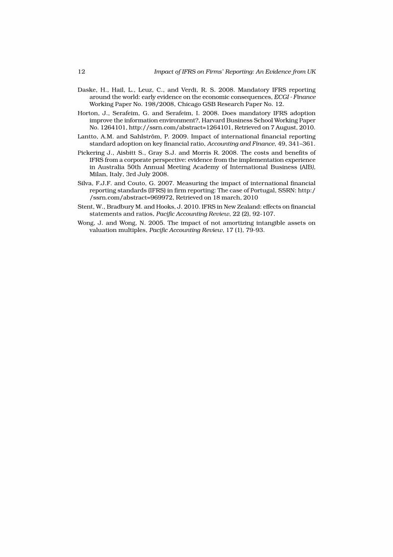
Daske, H., Hail, L., Leuz, C., and Verdi, R. S. 2008. Mandatory IFRS reportingaround the world: early evidence on the economic consequences, ECGI - Finance
Working Paper No. 198/2008, Chicago GSB Research Paper No. 12.
Horton, J., Serafeim, G. and Serafeim, I. 2008. Does mandatory IFRS adoptionimprove the information environment?, Harvard Business School Working PaperNo. 1264101, http://ssrn.com/abstract=1264101, Retrieved on 7 August, 2010.
Lantto, A.M. and Sahlström, P. 2009. Impact of international financial reportingstandard adoption on key financial ratio, Accounting and Finance, 49, 341–361.
Pickering J., Aisbitt S., Gray S.J. and Morris R. 2008. The costs and benefits ofIFRS from a corporate perspective: evidence from the implementation experiencein Australia 50th Annual Meeting Academy of International Business (AIB),
Milan, Italy, 3rd July 2008.
Silva, F.J.F. and Couto, G. 2007. Measuring the impact of international financialreporting standards (IFRS) in firm reporting: The case of Portugal, SSRN: http://ssrn.com/abstract=969972, Retrieved on 18 march, 2010
Stent, W., Bradbury M. and Hooks, J. 2010. IFRS in New Zealand: effects on financialstatements and ratios, Pacific Accounting Review, 22 (2), 92-107.
Wong, J. and Wong, N. 2005. The impact of not amortizing intangible assets onvaluation multiples, Pacific Accounting Review, 17 (1), 79-93.

13Guntur Anjana Raju and Dipa Ratnakar Gauncar
Is M&A Wealth Creation Vehicle for Business Houses inIndia? Case of the Tata Group of Companies
GUNTUR ANJANA RAJU AND DIPA RATNAKAR GAUNCAR
The Indian researchers examined corporate performance using financial ratios
to evaluate impact of M&A associated with an industry or a single company
as a case study. This article deals with empirical study in the Indian context
of M&A deals of a single Business House. It studies whether M&A have a
positive impact on the corporate performance of the acquiring companies
and on their shareholders wealth.
Introduction
The M&A activities in the world rose to unprecedented level. This reflectsthe powerful change force in the world economy. In fact this responded tothe changes, which took place due to high level of technology changes,reduction in cost of communication and transportation that createdinternational market, increased competition and emergence of newindustries. Favorable economic, financial environment and deregulation ofmost of the economies also motivated mergers and takeovers. M&A wasprevalent in India right from the post independence period, but due toGovernment regulations like Industrial Development and Regulation Act of1951, MRTP Act, FERA Act only a very few M&A took place in India prior to1990s. But policy of decontrol and liberalization coupled with globalizationof the economy after 1980s, especially after liberalization in 1991 had exposedthe corporate sector to severe domestic and global competition. In that context,Indian business houses started increasingly resorting to M&A as a meansto growth. The business group companies namely the Tata, United Breweries,Reliance, Essar, Godrej, Bharti Enterprises, Aditya Birla, ITC, Wadia andBinani had resorted to M&A as a tool for corporate restructuring whichincluded expansion, contractions, divestures, joint ventures andturnarounds.
The Tata Group had 126 M&A deals from April 1988 to March 2008 diversein seven sectors like Information Systems and Communications, Engineering,Materials, Services, Energy, Consumer products and Chemicals. They werethe first to go for cross border acquisition of Tetley in England, takeover ofprestigious car brands of the world like Jaguar and Land Rover and highestvalued deal by an Indian company of $12 billion of Corus steel. The group’s
Dr. (Ms) Guntur Anjana Raju is Associate Professor, Faculty of Commerce, Goa University,Taleigao Plateau, Goa- 403206, India and Miss Dipa. Ratnakar.Gauncar is Sales & MarketingExecutive, Angel Broking Ltd, Panaji, Goa.
The Indian Journal of Commerce
Vol. 64, No. 3, July-September 2011

14 Is M&A Wealth Creation Vehicle for Business Houses in India?
27 public listed enterprises have a combined market capitalization of around$60 billion, which is the highest among Indian business houses, and ashareholder base of 3.2 million. The group’s major companies are countedglobally. Tata Chemicals is the world’s second largest manufacturer of sodaash and Tata Communications is one of the world’s largest wholesale voicecarriers.
Literature Review
George Coontz (2004) found that merger or acquisitions in the 15 firm samplelisted on the S&P 500 Index do not on average improve shareholder wealthof the acquiring firm rather it actually decreases it. Michail Pazarskis,Manthos Vogiatzogloy, Petros Christodoulou, and George Drogalas (2006)examined empirically the impact of M&A on the operating performance ofM&A involved firms in Greece and found that there is strong evidence thatthe profitability of a firm decreased due to the M&A event. Pramod Mantravadiand A. Vidyadhar Reddy (2007) studied that type of industry, does seem tomake a difference to the post-merger operating performance of acquiringfirms. S.Vanitha and M. Selvam (2007) examined the financial performanceof merged manufacturing companies and drew conclusion that the mergingcompanies were taken over by companies with reputed and good managementand therefore, it was possible for the merged firms to turn around successfullyin due course. Carl B. McGowan and Zunaidah Sulong (2008) examinedthe effect of M&A completion announcements on the stock price behaviorfor two anchor banks in Malaysia and event study show that the M&Acompletion announcements are treated as positive information by the market.
Trends of Mergers and Acquisitions in India
Prior to 1991 there were only cases of Merging another companies and Beingmerged into another companies. Takeover cases started only in the year1996 and then onwards this mode of M&A has gained importance. In theyear 1997, Securities and Exchange Board of India (SEBI) introduced the“Substantial Acquisition of Shares and Takeovers, Regulations, 1997” withdisclosure norms on takeovers. This made companies to disclose taking overownership stake in the target company. The number of deals really pickedup in the year 1999 with total of 1453 deals as compared to only 172 dealsin 1998. There was a percentage change of almost 966% in 1999. The internetbubble had a negative impact which resulted in a decline of 22% in thenumber of deals in 2001. The years 2007 and 2008 saw decline in the dealsby 2% and 24% respectively due to the global credit crises. The transactionsof Being taken over recorded more than any other type of transactions with736 deals in 2007. The acquiring and selling assets deals over the time hasshown a decreasing trend from the year 2000 to 2008. The industry giantstook over smaller companies in their operating industries. Few largecompanies took over smaller companies.
Starting with the year 1996, the sale of asset dominated the scene of M&Ain India with value of Rs. 148030 million. Sale of asset generally is carriedout to sell off businesses which becomes unprofitable for the company or if

15Guntur Anjana Raju and Dipa Ratnakar Gauncar
the company wants cash for expansion of existing businesses. Mostlycompanies having more than one or many business operations running indifferent industries go for sale of asset. In the year 1997, transactions ofcompanies being taken over were highest in comparison with other type oftransactions, because of the revisions made in the takeover code by SEBI.The bidders preferred taking over the whole company rather than buyingassets or part of the company. This pattern is observed throughout the periodfrom 1997 to 2008. The deal values have increased at an unprecedentedlevel from merely Rs. 206218 millions in the year 1996 to 9.41 billions at theend of year 2008. In 2006, the deal value of taking over ownership reachedat its peak. A decline of 54% is noticed in the deal value similar to thedecrease in the number of deals for 2007 and 2008. The global credit crisiswas responsible for the decline in number and value of M&A deals in Indiafor the year 2008.
Comparison of M&A Transactions of Business Groups in India
Tata is a rapidly growing Business Group based in India with significantinternational operations. Their international operations earn them around61% of their total revenue. The group employs around 350,000 peopleworldwide. The Tata Group is the most diverse group in terms of its operationsas compared to other business groups in India. They operate in seven majorsectors with 102 companies in over 80 countries producing myriad type ofproducts. There are 126 M&A deals recorded to their credit which is highestamong all the business groups of India beginning from 1988 to 2008.
There are 25 companies in Automotive sector of Tata Group of Companieswhere Tata Motors is major acquirer. It can be seen that highest number ofM&A deals are in the Consumer products sector which are 25 where TataTea and Tata Coffee are the major acquiring companies. The Automotivesector has 17 deals, followed by the Tata Power in the Energy sector with 16deals. The Indian Hotel company also has been very aggressive with 15deals which helped them expand geographical not only in India but alsooverseas. In the Communications sector the company Tata Communicationsis the major acquirer having majority of cross border acquisitions. Thishelped them expand globally and tap new emerging markets. On the otherhand Tata Consultancy Services, an IT major in India has been the companywith maximum number of acquisitions in the IT business sector area of theTata group. The dominant player in the Chemical sector is Tata Chemicalwith 5 M&A deals, and Rallis India with 3 deals. Tata Steel is also helpingthe Tata Group to expand globally and create wealth which became thesixth largest steel maker in the world after it acquired Corus.
Methodology
The study examines the impact of M&A on Corporate performance andShareholders wealth. Twelve acquiring companies of the Tata Group aretaken as sample for the period 1996 to 2008 and source of data is CMIEProwess. The‘t-Test: Paired Two Sample for Means’ and Cumulative AbnormalReturns (CAR) are used for analysis

16 Is M&A Wealth Creation Vehicle for Business Houses in India?
Hypotheses
In order to test the validity of the null hypothesis framed for the objective ofimpact on Corporate performance, i.e.
H1: There is no improvement in Profitability, Operational Efficiency
and Asset Utilization Capacity, Liquidity and Solvency of thecompanies from M&A
The Financial and Operating Performance of the 12 acquiring companies ofTata group Pre and Post of M&A event have been analyzed with the help ofnine Financial Accounting ratios. They are classified into three categories,which are Profitability, Operational Efficiency and Asset Utilization, andLiquidity and Solvency. Under Profitability, the ratios are Operating profitMargin (OPM), Net profit Margin (NPM), Return on net worth (RONW) andReturn on capital employed (ROCE). In Operational Efficiency and AssetUtilization the ratios are Asset Turnover Ratio (ATR) and Return on TotalAssets (ROTA). For Liquidity and Solvency the ratios are Quick Ratio (QR),Current Ratio (CR) and Debt-equity ratio (DE).
In order to test the validity of the null hypothesis framed for the objective ofimpact on shareholders wealth, i.e.
H2: Cumulative Abnormal Return has not been positive Post M
announcement.
The adjusted market model has been used to calculate the abnormal returns.Abnormal return (AR) is calculated as the difference between a certain stock’sreturn (R i,t) on day t, and the market return(R m,t) on day t.
Adjusted Market ModelAR
i,t=R
i,t- R
m,t(1)
The Cumulative Abnormal Returns (CAR) is the sum of the abnormal returns,that is,
CARs = ∑
=
L
Kt
AR i,t (2)
Where K to L are days surrounding the M&A announcement.
CAR is calculated for the distinct window periods for Pre announcementperiod and Post announcement period. Three Event Windows are selectedin pre-announcement period viz. t-5 (5 days before announcement date), t-10 (10 days before announcement date) and t-20 (20 days beforeannouncement date). Similarly, three Event Windows are selected for post-announcement period viz. t+5 (5 days after announcement date), t+10 (10days after announcement date) and t+20 (20 days after announcement date).The CAR calculated for Pre announcement periods are compared to therespective Post announcements periods to examine the impact of M&A onshareholders wealth of respective acquiring companies.

17Guntur Anjana Raju and Dipa Ratnakar Gauncar
Corporate Performance of Tata Group of Companies after M&A
The Table 1 discloses the Profitability ratios of sample acquiring companiesduring Pre and Post M&A period. In the test of Operating Profit Margin (OPM)
Table 1: Profitability ratios of The Tata Group Of Companies
Name of Ratios Mean % t pCompany Pre Post Change statistics value
TRF ATR 107.6602 105.0005 -2.47 0.0724 0.9489OPM 9.3867 7.2933 -22.30 1.8303 0.2085
(3.92) (4.81) (NS)NPM 4.0167 2.9900 -25.56· 0.8268 0.4953
(2.899) (3.611) (NS)TRF RONW 9.59 7.7333 -19.36 0.2913 0.7983
(5.0372) (12.7701) (NS)ROCE 34.2204 27.9717 -18.26 0.8193 0.4987
(7.6584) (20.8514) (NS)OPM 5.67674.5533 . -19.79 l.4226 0.2908
(l.4814) (0.3113) (NS)NPM 0.8233 2.5233 206.48 -4.7848** 0.0410
Voltas India (0.318) (0.297)RONW -6.9733 6.7767 -197.18 -3.3123* 0.0803
(3.8123) (10.9582)ROCE 16.7096 18.5377 10.94 -0.3913 0.7334
(5.4082) (2.7946) (NS)OPM 4.9667 1l.4133 129.80 -l.4516 0.2837
(6.375 I) (l.5237) (NS)NPM -l.94 6.2833 -423.88 -l.9540 0.1899
Rallis India (6.375) (1.527) (NS)RONW -60.1067 11.51 -119.15 -4.6935** 0.0425
(30.1592) (10.3215)ROCE 7.2098 2l.26857 195' -0.7399 0.5364
(32.5713) (0.3391) (NS)OPM 25.6567 20.53 -19.98 1.1325 0.3749
(5.0849) (2.8406) (NS)NPM 8.79 10.86 23.55 -0.9049 0.4610
Tata Chemicals (1.1930) (3.0067) (NS)RONW 8.34 23.Q433 176.30 -4.1887* 0.0525
(2.7442) (6.0351)ROCE 16.8508 18.4594 9.55 .-0.7398 0.5365
(2.1368) (2.8044) (NS)OPM 21.7133 17.5133 -19.34 1.1269 0.3768
(3.78) (2.72) (NS)NPM 11.1433 7.8933 -29.17 0.8515 0.4842
Tata Tea (2.982) (3.670) (NS)RONW 25.3333 7.67333 -69.71 3.6714* 0.0668
(5.9273) (2.4135)ROCE 29.2588 13.30~7 -54.53 4.6659** 0.0430
(4.9298) (l.4014)OPM 33.7133 29.5367 -12.40 2.9843* 0.0963
(1.0225) (1.4025)NPM 13.5933 11.0667 -18.59 2.5873 0.1225
Tata Power (1.022) ( 1.402) (NS)RONW 11.1133 11. 7333 5.58 -0.8277 0.4949
(1.2375) (0.2122) (NS)
Contd...

18 Is M&A Wealth Creation Vehicle for Business Houses in India?
ROCE 12.8343 14.5205 13.14 -9.8484** 0.0102(l.0703)(0.9708).
OPM 29.2133 27:73 -5.08 0.3784 0.7415(4.085) (3.111) (NS)
NPM -36.68 0.6068 0.6057Indian Hotels (8.496) (3.294) (NS)
RONW 8.1633 7 -14.25 0.1780 0.8751(5.9809) (5.4900) (NS)
ROCE 11.7799 10.1291 -14.01 0.5070 0.6625(2.8707) (2.8240) (NS)
OPM 31.19 20.7833 -33.37 2.2580 0.1525(1.9727) (9.7381) (NS)
Tata NPM 19.3033 6.4667 -66.50 2.8805 0.1023Communications (2.898) (9.953) (NS)
RONW 21.5433 3.7133 -82.76 5.3340** 0.0334(5.9788) (7.99[8)
ROCE 34.4007 10.6837 -68.94 3.7625* 0.0639(10.2516) (6.7302)
OPM 8.23 10.7767 30.94' -2.3447 0.1437(2.1215) (0.3512) (NS)
NPM -1.3133 6.0333 -559.39 -2.8315 0.1054Tata Motors (4.463) (0.2122) (NS)
RONW -2.98 31.48 -1156.38 -4.5371 ** 0.0453(12.5351) (0.6465),
ROCE 9.821242 28.4764 189.95 -2.9712* 0.0970(11.6664) (0.7942)
OPM 93.1167 95.8867 2.97 -1.4527 0.2835(2.8007) (0.5301) (NS)
NPM 82.4933 90.8733 10.16 -1.9054 0.1970Tata Investment (4.238) (3.7886) (NS)Corporation RONW 16.27 27.2533 67.51 -2.5961 0.1218
(4.4809) (3.0282) (NS)ROCE 16.1977 26.01571 60.61 -3.2303* 0.0839
(3.2588) (2.0124)OPM 17.03 18.3633 7.83 -0.5505 0.6373
(2.3177) (1.8794) (NS)NPM 8.4133 9.61 14.22 -0.1668 0.8829
Tata Coffee (3.182) (9.398) (NS)RONW 7.2667 10.9133 50.18 -1.6786 0.2352
(3.8279) (1.8005) (NS)ROCE 15.2717 11.21236 -26.58 1.6938 0.2324
(2.2720) (2.3547) (NS)OPM 21.54 24.8367 15.30 -0.4523 0.6954
(6.7621) (6.2689)’ (NS)NPM 8.6533 13.2033 52.58 -0.8069 0.5044
Tata Steel (5.9387) (4.0609) (NS)RONW 23.5267 46.8367 99.08 -2.8614 0.1035
(19.1236) (17.1250) (NS)ROCE 24.3366 29.9116 22.91 1.0046 0.4209
(14.6321) (13.8046) (NS)
Note: 1. Figures given in the parenthesis indicate standard deviation
2. *** Significant at the 0.01 level, ** Significant at the 0.05 level,* Significantat the 0.1 level.
3. NS-Not Significant
Contd...

19Guntur Anjana Raju and Dipa Ratnakar Gauncar
ratio, four out of the twelve companies were able to successfully achieve agrowth in their OPM after M&A. They are Rallis India, Tata Coffee, TataMotors, Tata Investment Corporation, and Tata Steel showing a percentageincrease of 129.8%, 7.8%, 30.94%, 2.97%, and 15.3% respectively. TRF, TataPower, Voltas India, Indian Hotels, Tata Communications and Tata Chemicals,showed a decline of 22.03%, 12.39%, 19.79%, 5.08%, 33.37% and 19.98%for its post period mean. Only one result was significant that of Tata Powerwith t-statistic value of 2.9843 at 1% level of significance. The ChemicalCompany Rallis India had a Pre merger mean of 4.9667 and Post mergermean of 11.4133 showing an increase of 129.8%. Major decrease came fromTata Communications of 33.37% in its mean OPM of Post M&A period. The t-test brought out the fact that Tata Power was the only one among the samplecompanies which showed a statistically significant decline in OPM afteracquisitions. Indicating that the impact of M&A on other company’s OPMwas negligible which can be noticed from the ‘t statistics’ values. Higher the‘t statistics’ value more is the impact of M&A.
In the test of Net Profit Margin (NPM), seven companies showed positiveresults for the post period. The companies being Rallis India, Voltas India,Tata Coffee, Tata Motors, Tata Investment Corporation, Tata Steel and TataChemicals which showed 423.89%, 206.48%, 14.22%, 559.39%, 10.16%,52.58% and 23.55% increase in their post mean. Only one result of NPMwas significant like that of OPM result. Voltas showed significant increaseat 5% level of significance. Whereas again the least performer was TataCommunications with a 66% decrease in its NPM in the Post period over thePre period. Largest variations in the ratio in the pre period was seen in caseof Rallis India with 6.375 and in Post period Tata Communications recordedthe highest variation of 9.953.The Rallis India was able to turn the NPMfrom negative (-1.94) to positive (6.28) by overcoming losses and earningprofits. It recorded the second highest positive percentage change in themean NPM among all the sample companies. Highest positive change camefrom Tata Motors. Voltas India improved its NPM significantly with anincrease of 206.47 % in the mean NPM(2.5233) in the post period comparedto that of pre period mean(0.8233) with a t statistic value of -4.7848, andp=0.008<0.05 and hence significance at 5% level. Largest variations in theratio in the Pre period was seen in case of Rallis India with 6.38 and in Postperiod Tata Communications recorded the highest variation of 9.95. Thehigh variation in Post period of Tata Communications indicates that majorchanges in its NPM came after the acquisition as its Pre period standarddeviation is only 2.9.
It can be noted that the eight companies showed an improvement in theirReturn on Net Worth ratio (RONW) in the Post period indicating more networth was added through M&A. Tata Power, Rallis India, Voltas India, TataCoffee, Tata Motors, Tata Investment Corporation, Tata Steel and TataChemicals showed improvement in the Post period over their Pre periodperformance recording a percentage change of 5.58%, 50.18%, 1156.38%,67.51%, 99.08% and 176.3% respectively. Whereas TRF, Tata Tea, IndianHotels and Tata Communications had recorded decline in their Post periodmean RONW ratio by 19.36%, 69.71%, 14.25%, and 82.76%. There were five

20 Is M&A Wealth Creation Vehicle for Business Houses in India?
statistical significant results of which Rallis India and Tata Motors showedsignificant increase at 5% level and Voltas India at 10% level of significance.Whereas Tata Tea and Tata Communications showed significant decreaseat 10% and 5% level of significance respectively. The major decrease wasnoticed for Tata Communications. The mean RONW of Tata Tea declinedfrom 25.33 % in the Pre period to 7.67 % in the Post period, which showed adecline by -82.76 % and the difference is significant at 10% level (tvalue=3.6714, p<0.10). Highest percentage change was noticed in the RONWvalue of Tata Motors of 1156.38% from Pre mean of mere -2.98% to 31.48 %during the Post period. Highest variation in the ratio for the Pre period isseen in the Rallis India with standard deviation of 30.16 whereas higheststandard deviation in the Post period has been being recorded by Tata Steelof 17.13.
In the test of Return on capital employed (ROCE), seven companies showedimprovement for the post period. Tata Power, Rallis India, Voltas India, TataMotors, Tata Investment Corporation, Tata Steel and Tata Chemicals showedincrease in their mean ROCE ratio in the post period by 13%, 195%, 11%,189%, 60%, 23% and 9.5% respectively. Whereas the remaining fivecompanies TRF, Tata Tea, Indian Hotels, Tata Communications and TataCoffee showed a decline of 18.26%, 54.53%, 14.01%, 68.94%, and 26.58%respectively. Tata Communications decreased its mean ROCE afteracquisition by over 68% which is also statistically significant. Significantfall is also noticed in Tata Tea ROCE with over 54% decline in the post M&Aperiod over the pre M&A period with t value of 4.6659 significant at 5 %level. It is noticed that Tata Power recorded increase in its ROCE by 13%which was significant at 5% level. The other significant increases are noticedin the ROCE of Tata Motors and Tata Investment Corporation whereas the t-values of other companies which were insignificant at the required probabilitylevels indicates that the increase or decrease in the ROCE between pre andpost M&A period is quite negligible. In other words, it can be said that theincrease or decrease in ROCE is not related to M&A.
The Table 2 shows the impact of M&A on Operational Efficiency and AssetUtilization of the Sample Companies of Tata Group of Companies. In the testof Asset Turnover Ratio (ATR), six companies have shown a decline in theratio indicating a decline in their Operating efficiency. TRF, Tata Tea, RallisIndia, Indian Hotels, Tata Communications and Tata Coffee showed a declinein their mean ratio of Post period over the mean of Pre period by 2.47%,24.67%, 0.72%, 4.21%, 29.68% and 25.77% respectively.
The highest decrease was noticed in Tata Communications of 29.67% butnot statistically significant. Both the beverage companies of the Tata group,Tata Tea and Tata Coffee noticed a statistical significant fall in their meanATR. The finance company of the Tata group, Tata Investment Corporationrecorded the highest percentage increase of 51.92% in its ATR with premean of 16.4762 and post mean of 25.0314 showing significance at 10%level. Also least variations are seen in its ratio as compared to other samplecompanies. Six companies showed an increase in the mean ratio for thepost period and they are Tata Power, Voltas India, Tata Motors, Tata

21Guntur Anjana Raju and Dipa Ratnakar Gauncar
Table 2: Operational efficiency and asset utilization ratios
Name of Ratios Mean % t statistics p valueCompany Pre Post Change
TRF ATR 107.6602 105.0005 -2.47 0.0724 0.9489(50.6431) (17.7277) (NS)
ROTA 7.7453 6.8521 -11.53 0.3821 0.7392(1.2523) (5.2876) (NS)
ATR 123.9803 140.2306 13.11 -1.4873 0.2753Voltas India (21.3638) (2.8079) (NS)
ROTA 5.3467 5.5529 3.86 -0.110 I 0.9224(2.7114) (0.5331) (NS)
ATR 129.1878 128.2569 ~0.72 0.2023 0.8584Rallis India (7.7858) (7.8826) (NS)
ROTA 3.1416 11.1035 253.43 -0.9605 0.4382(12.7097) (1.6510) (NS)
ATR 16.4762 25.0314 51.92 -3.2948* 0.0811Tata Chemicals (2.7772) (1.7208)
ROTA 15.7146 24.0059 52.76 -3.2413* 0.0834(2.6678) (1.7702)
Tata Tea ATR 96.4422 72.6507 -24.67 6.7903** 0.0210(7.2119) (10.1171)
ROTA 20.0932 10.1038 -49.72 3.0704* 0.0917(3.8294) (1.9147)
ATR 37.7053 54.3092 44.04 -2.9440* 0.0986Tata Power (2.4533) (8.4047)
ROTA 11.0971 12.1275 9.29 -3.2975* 0.0801(0.6962) (1.0511)
ATR 34.8452 .33.3794 -4.21 0.17330 0.8784Indian Hotels (6.9820) (7.9429) (NS)
ROTA 8.9500 7.3239 -18.17 0.4335 0.7069(3.6716) (2.95~3) (NS)
ATR 72.3659 50.8890 -29.68 1.2917(NS) 0.3256Tata (12.9052) (16.3517)Communications ROTA 23.1332 6.5560 -71.66 4.0566* 0.0557
(5.8661) (5.9763)ATR 112.2797 170.2773 51.65 -7.4516** 0.0175
Tata Motors (23.6152) (11.7374)ROTA 4.4167 15.5818 252.79 -5.7150** 0.0293
(5.0217) (1.6475)ATR 68.5119 50.8555 -25.77 2.4655 0.1326
Tata Investment (5.3343) (8.1047) (NS)Corporation ROTA 9.9199 8.0815 -18.53 l.1389 0.3728
(1.4612) (1.4562) (NS)ATR 53.5282 67.4825 26.07 -0.8070 0.5044
Tata Coffee (15.2101) (17.4555) (NS)ROTA 10.7797 11.2690 4.54 -1.0255 0.4130
( 1.3548) (0.9056) (NS)ATR 74.3517 . 87.3604 17.5 -0.7147 0.5490
Tata Steel (11.5783) (28.7468) (NS)ROTA 12.6793 18.9041 49.09 -0.7985 0.5083
(7.3796) (6.9170) (NS)
Note: 1. Figures given in the parenthesis indicate standard deviation2. *** Significant at the 0.01 level, ** Significant at the 0.05 level,* Significant
at the 0.1 level. 3.NS-Not Significant

22 Is M&A Wealth Creation Vehicle for Business Houses in India?
Investment Corporation, Tata Steel, and Tata Chemicals showing apercentage change of 44.04%, 13.11%, 51.65%, 51.95%, 17.5% and 26.07%respectively.
The test of Return on Total Assets (ROTA), seven companies increased theirmean ratio in the post period. Tata Power, Rallis India, Voltas India, TataMotors, Tata Investment Corporation, Tata Steel, and Tata Chemicals showedan increase in the post mean ratio by 9.29%, 253.43%, 3.86%, 253.43%,52.76%, 49.09% and 4.5% respectively. Whereas TRF, Tata Tea, Indian Hotels,Tata Communications and Tata Coffee showed decline by 11.53%, 49.72%,18.17%, 71.66 % and 18.53% respectively. And five values were statisticallysignificant which are Tata Tea, Tata Power, Tata Communications, TataInvestment Corporation showed significance at 10% level and Tata MotorsLtd at 5% level of significance. The five companies which showed a declinein their ROTA indicates under utilization of their assets. Tata Communicationsshowed the highest decrease of 71.66% with the t statistic value of 4.0566significant at 10% level. Tata Tea stood second in decrease with 49.71%showing statistical significance at 10% level.
The Table 3 shows impact of M&A on the Liquidity and Solvency Ratios ofthe acquiring Tata Group of Companies. The Quick Ratio (QR) test showedan increase for six companies in the post period and they are TRF, VoltasIndia, Indian Hotels, Tata Coffee, Tata Motors, Tata Steel, and Tata Chemicals
Table 3: Liquidity and solvency ratios
Name of Ratios Mean % t statistics p valueCompany Pre Post Change
QR 0.4467 0.6667 49.25 -2.3677 0.1415(0.1069) (0.0723) (NS)
TRF CR 1.1433 1.2233 7 -2.6186 0.1201(0.0153) (0.0493) (NS)
DE 1.3567 0.5667 -58.23 2.0962 0.1710(0.2650) (0.4665) (NS)
QR 0.43 0.6967 62.02 -4.3579*** 0.0488(0.1 044) (0.0306)
Voltas India CR 1.0J33 1.1733 15.79 -2.4400 0.1348(0.0802) (0.0451) (NS)
DE 1.29· 0.5567 -56.85 14.1715*** 0.0049(0.0624) (0.0681)
QR 0.7 0.5333 ~23.81 2.8537 0.1040(0.0954) (0.0473) (NS)
Rallis India CR J.33 1.32 -0.75 0.2847 0.8026(0.1587) (0.1015) (NS)
DE 4.9967 0.6233 -87.53 2.1486 0.1647(3.1550) (0.~278) (NS)
QR 0.3767 0.4133 9.73 -0.4308 0.7086Tata Chemicals (0.0862) (0.0874) (NS)
CR 1.34 0.83 -38.06 3.7362* 0.0648(0.1609) (0.1082)
DE 0.5267 0.9533 81.01 -1.6820 0.2346(0.1617) (0.3121) (NS)
Contd...

23Guntur Anjana Raju and Dipa Ratnakar Gauncar
QR 0.7633 0.55 -27.95 1.3806 0.3014(0.2318) (0.0985) (NS)
Tata Tea CR 1.4633 1.2967 -11.39 0.7271 0.5428(0.2335) (0.1818) (NS)
DE 0.7167 .0.7133 -0.47 0.0059 0.9958(0.1724) (0.8116) (NS)
QR 0.7667 0.5667 -26.09 1.2901 0.3261Tata Power (0.2768) (0.0757) (NS)
CR 1.35 1.1733 -13.09 1.0500 0.4039(0.3251) (0.0404) (NS)
DE 0.7133 0.5767 -19.16 2.7456 0.1110(0.0379) (0.1210) (NS)
QR 0.5733 1.2967 126.16 -2.5070 0.1290Indian Hotels (0.1193) (0.3808) (NS)
CR 1.1733 1.52 29.54 -1.5172 0.2685(0.2875) (0.3005) (NS)
DE 0.78 1.4067 80.34 -1.0258 0.4129(0.4993) (0.5658) (NS)
QR 1.63 0.57 -65.03 5.6154** 0.0303Tata (0.1706) (0.4854)Communications CR 2.1667 0.95 -56.15 2.6862 0.1151
(0.2250) (0.7454) (NS)DE 0.0567 0.29 411.76 -1.8596 0.2040
(0.0551) (0.2571) (NS)QR 0.34 ‘0.3533 3.92 -0.2097 0.8534
Tata Motors (0.0557) (0.1012) (NS)CR 0.7733 0.6633 -14.22 4.1576* 0.0532
(0.0231) (0.0681)DE 0.9267 0.6967 -24.82 0.7338 0.5394
(0.3502) (0.2230) (NS)QR 1.8167 0.2267 -87.53 1.3256 0.3161
Tata Investment (2.2902) (0.2250) (NS)Corporation CR 2.l267 0.2433 -88.56 1.2466 0.3388
(2.8253) (0.2194) (NS)DE 0.0767 0.0033 -95.65 3.3550* 0.0785
(0.0404) (0.0058)QR 0.33 0.5733 73.73 -1.8918 0.l991
Tata Coffee (0.04) (0.2290) (NS)CR 1.22 1.3833 13.388 -1.2261 0.3449
(0.0458) (0.2627) (NS)DE 0.4833 2.07 328.28 -2.3005 0.l481
(0.0814) (1.1432) (NS)QR 0.2567 0.85 231.17 -1.9518 0.l902
Tata Steel (0.0513) (0.4952) (NS)CR 0.6033 1.3667 126.52 -2.4466 0.1342
(0.0929) (0.4751) (NS)DE 1.36 0.9533 -29.90 0.6391 0.5882
(0.6065) (0.7295) (NS)
Note: 1. Figures given in the parenthesis indicate standard deviation2. *** Significant at the 0.01 level, ** Significant at the 0.05 level,* Significantat the 0.1 level.3. NS-Not Significant
Contd...

24 Is M&A Wealth Creation Vehicle for Business Houses in India?
showing a percentage change of 49.25%, 62.02%, 126.16%, 73.74%, 3.92%,231.17% and 9.73% respectively. Whereas Tata Power, Tata Tea, Rallis India,Tata Communications and Tata Investment Corporation showed a declinein their mean ratio of post period over the mean of pre period by 26.09%,23.81%, 65.03% and 87.53% respectively. In all only two results werestatistically significant, which are Voltas India and Tata Communicationsat 5% level of significance. The Indian Hotel improved its QR showing highestpercentage change among other Tata Group of companies. The declineindicates that there is more debt incurred in post M&A period and the increasein the QR is attributed to the fact that acquired companies had a betterquick ratio and being added to the acquiring sample companies.
For Current Ratio (CR) test, the five companies which improved their ratioin the post period are TRF, Voltas India, Indian Hotels, Tata Coffee and TataSteel by 7%, 15.79%, 29.55%, 13.38% and 126.52% respectively. WhereasTata Tea, Tata Power, Rallis India, Tata Communications, Tata Motors, TataInvestment Corporation and Tata Chemicals showed decrease in values inthe post period as compared to the pre period by 11.39%, 13.09%, 56.15%,14.22%, 88.565 and 38.06% respectively. Again like QR two significant valueswere obtained for Tata Motors and Tata Chemicals at 10% level of significance.The increase is attributed to the event of current assets of acquiredcompanies being added to the acquiring sample companies. The othercompanies had negligible changes in their CR.
The Debt Equity ratio (DE) test revealed that eight companies reduced theirdebt in the post M&A period. TRF, Tata Tea, Tata Power, Rallis India, VoltasIndia, Tata Motors, Tata Investment Corporation and Tata Steel reducedtheir DE by 58.23%, 0.47%, 19.16%, 87.53%, 56.85%, 24.82%, 95.65% and29.92% respectively. This indicates that the funds brought in from theacquired companies were able to meet the debt claims. Indian Hotels, TataCommunications, Tata Coffee, and Tata Chemicals increased their DE by80.34%, 411.76%, 328.28% and 81.01% respectively as these companiesadded long term debt to their balance sheets. It indicates that the acquisitionswere financed by debt and the acquiring companies already had debt intheir balance sheets. Also it is inferred that the target companies hadconsiderable debt in their balance sheets. The results for only two companies,Voltas India and Tata Investment Corporation were significant at 10% and1% level of significance respectively. Implying, that M&A had a significantimpact on their DE and thereby an impact on their overall solvency.
Table 4 summarizes the significant and non significant results. A total of108 ‘t statistics’ values were obtained of which only 28 were significant and80 were insignificant. Out of the 28 values, 13 were of profitability, 9 ofoperational efficiency and asset utilization and 6 of liquidity and solvencyparameters.
TRF, Indian Hotels, Tata Coffee and Tata Steel did not obtained any significantvariables in any of the parameter indicating that M&A did not have significantimpact on their Corporate performance. Tata Communications and TataTea obtained significant values for their decrease in their respective variablesindicating that the acquisitions made by them had a negative impact on

25Guntur Anjana Raju and Dipa Ratnakar Gauncar
their corporate performance. Tata Tea recorded significant values for RONW,ROCE, ATR and ROTA. Ironically, the four variables were significant for thedecrease in their value indicating that the acquisition negatively impactedits profitability, operating efficiency, asset utilization and liquidity. IndianHotels which is a major part of the hotel and tourism sector of operations forTata group achieved improvement only in its liquidity ratios. There was anegative impact seen on the variables of profitability, operating efficiency,asset utilization and solvency. Tata Power obtained significant values forimprovement of ROCE, ATR, and ROTA, whereas significance obtained forOPM was for its decrease. Tata Chemicals Ltd achieved significant valuesfor RONW and CR variable. The RONW showed an increase whereas CRshowed a decrease.
It can be inferred that the M&A made by the company impacted its profitabilityand liquidity. Tata Investment Corporation achieved significant growth inits one profitability ratio and two asset ratios and obtained better solvencypost acquisition. Only liquidity ratios showed a decline. TataCommunications was the worst performer as it showed decline in all theratios and debt levels also increased in the post period. Tata Steel was thecompany which benefited the most from the acquisition as all its variablesshowed an improvement in their values. This indicates a positive impact ofacquisition.
Table 4: Consolidated T-Statistics values of the ratios
Name of Company Profitability Operational Liquidity and
Efficiency and Solvency
Asset Utilization
OPM NPM RONW ROCE AT ROTA OR CR DE
TRF NS NS NS NS NS NS NS NS NS
Voltas India NS S** S* NS NS NS S** NS S***
Rallis India NS NS S** NS NS NS NS NS NS
Tata Chemicals NS NS S* NS NS NS NS S* NS
Tata Tea NS NS S* S** S** S* NS NS NS
Tata Power S* NS NS S** S* S* NS NS NS
Indian Hotels NS NS NS NS NS NS NS NS NS
Tata Communications NS NS S** S* NS S* S** NS NS
Tata Motors NS NS S** S* S** S** NS S* NS
Tata Investment NS NS NS S* S* S* NS NS S*Corporation
Tata Coffee NS NS NS NS NS NS NS NS NS
Tata Steel NS NS NS NS NS NS NS NS NS
Source: Compilation from Table 5, 6 and 7
Note: 1. *** Significant at the 0.01 level, ** Significant at. the 0.05 level, * Significantat the 0.1 level.
2. NS-Not Significant

26 Is M&A Wealth Creation Vehicle for Business Houses in India?
Impact of M&A on Shareholders Wealth
The results of Pre and Post period of CAR are analyzed in order to examinethe impact of M&A on the Shareholders wealth of the twelve acquiring Tatagroup of companies. The Table 5 depicts that Tata Motors and Tata Steelwere the only two companies which did not have any negative CAR valuesfor all the post announcement window periods signifying that the companieswere successful in adding value to their Shareholders wealth.
The 5 days window period is the shortest window period of the study. Itshows the immediate reaction of the shareholders to the announcement ofthe M&A. Out of the twelve companies’ nine companies had negative returnsin the Post period. The acquisitions made by Tata Communication, TataMotors and Tata Steel got a positive response and led to increase in thereturns for their Shareholders in the Post period. It is observed with the aidof standard deviations calculated for the respective companies that thevolatility is considerably less in the Post period as compared to the Pre period.
Table 5: CAR during Pre and Post announcement period for the window periods
Name of Company Pre Announcement period Post Announcement period
TRF 15.02 20.38 9.85 -1.89 -9.52 -11.79
(3.508) (4.368) (5.164) (2.643) (2.336) (2.059)
Tata Tea -1.97 -11.61 -6.57 -17.60 -23.10 -19.07
(5.063) (4.84) (5.209) (3.75) (3.67) (3.682)
Tata Power -8.38 -2.20 3.38 -5.71 -10.42 4.04
(1.92) ( 1.43) (0.775) (2.039) (2.06) (3.27)
Voltas India 19.09 21.83 9.09 -5.74 -2.07 -3.82
(3.09) (3.58) (3.26) (2.49) (2.32) (1.92)
Indian Hotels -7.22 -2.61 0.83 -1.17 2.02 3.03
(1.089) (1.03) (1.02) (0.89) (1.14) (1.09)
Tata Communications l3.40 9.40 -1.42 2.34 2.07 -9.58
(2.49) (3.03) (3.10) (0.90) (1.62) (2.60)
Rallis India 0.13 -0.66 -1.3 I -3.26 -10.27 -26.30
(4.61) (3.18) (3.80) (3.17) (3.08) (2.72)
Tata Motors -5.08 -1.45 1.25 2.69 1.80 0.50
(1.65) (1.97) (2.61) (1.38) (1.11) (1.60)
Tata Investment 2.19 -0.56 -4.71 -4.17 -6.19 -2.54
Corporation (2.38) (2.27) (2.91) (2.23) ( 1.57) (2.23)
Tata Coffee 24.60 22.84 -0.22 -7.32 0.86 2.28
(4.16) (4.95) (3.96) (1.64) (6.09) (4.68)
Tata Chemicals 6.68 11.07 1.66 -0.38 0.88 -7.99
(2.46) (2.52) (2.10) ( 1.36) (2.15) (2.21)
Tata Steel 8.81 4.06 -0.34 0.56 3.30 2.58
(1.63) (1.45) ( 1.19) ( 1.20) (1. 78) ( 1.58)
Figures given In the parenthesis indicate standard deviation

27Guntur Anjana Raju and Dipa Ratnakar Gauncar
For the second window period of 10 days for its Pre period Tata Coffee gave22.84% which is the highest return to its shareholders but also the highestvolatility of 4.95 was noticed in the stock. TRF which recorded a very highreturn of 20.38% during the Pre period ended up giving negative returns toits shareholders in the corresponding Post period. Six companies had negativevalue of CAR in the Post period.
For the window period of 20 days Pre and Post only four companies hadnegative CAR values in the Pre period and seven companies recordednegative CAR values in the post period. The returns of Tata Power, IndianHotels and Tata Motors improved after merger. Rallis India showed a returnof 0.13% and post merger the company recorded negative returns. Also VoltasIndia had positive CAR of 19.09% in the pre period but in post period it was-3.82% with a standard deviation of 3.09 in the pre period and 1.92 in thePost period. Indicating less volatility in the Post period compared to pre period.Returns of Tata Chemicals in the post period got highly eroded from 6.68%in the Pre period to -7.99% in that Post period. The companies which hadpositive values in the Pre period but later in the Post period it turned negative.This indicates that the Shareholders did not appreciate the M&A by thecompanies.
Consolidated Corporate Performance Impact of M&A on Tata Group
Table 6 presents the results of the Pre M&A and Post M&A Operatingperformance ratios for the entire sample set of M&A. This shows that therewas a decline in the mean OPM (25.12% to 24.10%), but the decline was notstatistically significant (t-statistic value of 0.765). However NPM (15.18% to15.38%) ratios showed increase in the Post M&A period of only 1.37% (t-statistic value of 0.11). The mean RONW (5.09% to 16.31%) and ROCE (19.07%to 19.21%) showed an increase in the Post M&A period (t- values of -1.59517
Table 6: All Ratios of the Tata Group of Companies
Ratio Mean Percentage t Statistic p-value
PRE POST Change
Profitability Ratios
OPM 25.1194 24.1014 -4.05 0.7656(NS) 0.4601
NPM 15.1755 15.3839 1.37 -0.1138(NS) 0.9115
RONW 5.0906 16.3056 220.31 -1.5952(NS) 0.1390
ROCE 19.0743 19.2076 0.70 -0.0388(NS) 0.9697
Operational Efficiency and Asset Utilization
ATR 77.2779 82.1436 6.30 -0.7604(NS) 0.4630
ROTA 11.0848 11.4552 3.34 -0.1636(NS) 0.8730
Liquidity and Solvency Ratios
QR 0.7025 0.6081 -13.44 0.4998 (NS) 0.6271
CR 1.3086 1.0953 -16.30 1.0382(NS) 0.3215
DE 1.1069 0.7842 -29.16 0.7831(NS) 0.4501
Note: NS-Not Significant

28 Is M&A Wealth Creation Vehicle for Business Houses in India?
and -0.03882 respectively). The comparison of the Pre M&A and Post M&AOperational Efficiency and Asset Utilization ratios for the entire sampleshowed that there was an increase in the ATR and ROTA by 6.30% and3.34% respectively. This depicts that the companies did achieve improvementin the Operational Efficiency and Asset Utilizations. But again the resultsare insignificant at required probability levels. Decline is observed in theliquidity and solvency ratios. The mean DE decreased from 1.1069 to 0.7842signifying a decrease in the long term debt of the companies. There was amarginal statistically insignificant decrease in leverage after the M&A (1.1069vs. 0.7842), confirmed by the low t-value of 0.7831. All the ratios showedinsignificant results. Hence it is concluded that the M&A event did not haveany major significant positive impact on the operating and financialperformance of the acquiring Tata Group of Companies. This implies thatCorporate acquisitions by Tata Group of companies did not lead to significantimproved performance for the sample companies for the period examined inthis study. The results are uniform across the nine accounting ratios whichshow insignificant results.
The Table 7 shows the Consolidated CAR (in %) of the Tata Group ofCompanies. The returns during the Pre period were positive throughout butat the end of the Pre period the returns showed a considerable decline byrecording only 0.96% CAR for the t-5 period. As evident from the results Postperiod recorded only negative CAR values. And the daily returns started todecrease more and more. Existing evidence has shown that the wealth ofbidder shareholders significantly diminishes in the period after a merger ortakeover.
Table 7: Consolidated Car of the Tata Group of Companies (in %)
t-20 t-10 t-5 t+5 t+10 t+20
5.61 5.87 0.96 –3.47 –4.22 –5.72
Conclusion
It is evident from the analysis that both hypotheses set for validation arenot fully accepted. Overall the Metal industry giant Tata Steel was thecompany that benefited most from M&A in terms of Corporate performanceand Shareholders wealth. Indicating that, their management and integrationteam were successfully able to obtain synergies from the acquisition. Worsthit was Tata Telecommunication, indicating that acquisition had a negativeimpact on corporate performance of the company. The ‘t-test’ when doneindividually, have shown significant results as compared to the consolidatedtest which showed insignificant results on Corporate performance of theTata Group of companies. Also the consolidated CAR values obtained werefound to be decreasing and negative in the post announcement period butindividually there is evidence of positive returns in the post announcementperiod.
The conclusion emerging from the point of view of Corporate performanceevaluation is that the good management of the Tata Group helped carry out

29Guntur Anjana Raju and Dipa Ratnakar Gauncar
the challenging task of integrating operations and leveraging the projectedsynergies appropriately. From the aspect of Shareholders wealth it can beconcluded that the majority of the acquiring companies were not able to addvalue to the Shareholders wealth in Post M&A announcement period. Themarket reacted to the news of the M&A in a negative manner expecting thatthe M&A would not improve the performance of the company.
REFERENCES
Alexandar Hartman, Marcus Lund. 2008. Bidder Returns & Operating Performance.Master’s thesis, Stockholm School of Economics.
Carl B. McGowan., Zunaidah Sulong. 2008. A note on the effect of M&Aannouncements on stock price behavior and financial performance changes:The case of Arab Malaysian Bank Berhad and Hong Leong Bank Berhad.International Business & Economics Research Journal, Volume 7, Number 9, pp.21-26.
Elif Akben-Selçuk. 2008. The Impact of cross-border on target company performance:evidence from Turkey. Economics Bulletin, Vol. 13, No. 5, pp. 1-9.
George Coontz. 2004. Economic impact of corporate mergers and acquisitions onacquiring firm shareholder wealth. The Park Place Economist, Volume XII, pp.62-70.
Michail Pazarskis, Manthos Vogiatzogloy, Petros Christodoulou, George Drogalas.2008. Exploring the improvement of corporate performance after mergers – thecase of Greece. International Research Journal of Finance and Economics, No. 6,pp. 184-192.
P.M. Healy, K.G. Palepu, R.S. Ruback. 1992. Does corporate performance improveafter mergers?” Journal of Financial Economics, Vol. 31, pp. 135- 175.
Pramod Mantravadi, A Vidyadhar Reddy. 2008. Post-merger performance of acquiringfirms from different industries in India. International Research Journal of Finance
and Economics, No. 22, pp. 192-204.
S. Vanitha, M. Selvam. 2007. Financial performance of Indian manufacturingcompanies during pre and post merger period. International Research Journal of
Finance and Economics, No. 12, pp. 7-35.
Stephan K.H. Gross, Hagen Lindstadt. 2006. Horizontal and vertical takeover andsell-off announcements: abnormal returns differ by industry. Corporate
Ownership Control, Vol. 3, No. 2, pp. 23-30.
Zackarias Attallah, Nassim El-Amrani. 2005. Follow the insider – an event studyon the impact of insider transactions. Master’s thesis, Stockholm University.

30 Shareholder Value Creation in India–A Sectoral Analysis
Shareholder Value Creation in India- A Sectoral Analysis
K.R. JALAJA
This paper examined the Shareholder Value Created in Indian Companies by
adopting Pablo Fernandez model, a refined model based on Market Values,
believed to be a superior model when compared to the traditional measures
(ROE, ROI, EPS) and various models developed by Consulting Firms (EP,
EVA, MVA, SVA) to analyze Value Creation. For this purpose a sample of 50
companies representing ten industrial sectors for a period of five years from
2002-2006 have been analyzed and found that Old Generation Companies (
Companies representing the Industry Sectors – Oil & Gas, Steel, Textiles,
Sugar and Cement & Cement Products) created more Shareholder Value
than New Generation Companies (Companies representing the Industry
sectors - IT, Pharmaceuticals, FMCG, Automobiles and Capital Goods)
among the sample companies.
Introduction
With the globalization of competition and capital markets and a tidal waveof privatization, Shareholder Value is rapidly capturing the attention ofexecutives worldwide. It is seen as crucial all over the world. ShareholderValue is slowly becoming the global standard for measuring businessperformance (Alfred Rappaport). The CEOs of modern firms are worried aboutShareholder Value. Satisfying the Shareholders is the best way to makesure that other stakeholders are served as well. If Shareholders believe thatthe corporation is under performing, they can try to replace the board in thenext election. If they succeed, the new board will appoint a new managementteam. The objective function of the company is to maximize the shareholdervalue. Managers in most of the firms of the world focus on building shareholdervalue. Most executives today understand that the need to create shareholdervalue is paramount and the world’s most competitive management teamsare responding to the pressure to create value by embracing new metricsand new models for managing their companies.
Literature Review
The theories on Shareholder Value Creation have a history stretching backto 1950s and 1960s and their intellectual roots are in the path breakingwork of some economists of that time and a number of them have beenhonoured with the Nobel Prize for economics. Shareholder value started totake on a life of its own as a result of the Capital Asset Pricing Model (CAPM),
Dr. K.R. Jalaja is Assistant Professor, Department of Commerce, Bangalore University(PG Center Kolar), BANGALORE - 560009
The Indian Journal of Commerce
Vol. 64, No. 3, July-September 2011

31K.R. Jalaja
which argues that the returns both received and expected by investors arerelated to the risk incurred by owning particular financial assets. As it iscommonly understood, the higher the risk the greater the return should be.The main insight of the CAPM model which is central to the shareholderview of the world is that there is a risk-weighted discount factor which allowsone to assess the value today and tomorrow’s developments, profits andcash flows. Most of the studies dealing with shareholder value creation haveinvestigated the information content of innovative performance measuresover the traditional measures.
Gordon (1985), William (1988), David Richard (1989) have advocated theimportance of managing for superior shareholder value by identifying valuedrivers and using the same to reduce the value gap by concentrating onRONA, growth, retention rate and debt equity ratio. Alfred (1980, 1981, 1992),Balachandran et al (1986) and Copeland et al (1990) have dealt with theissue of shareholder value creation. In all the papers the basic propositionis that shareholder value of alternative business strategies, including growthand expansion, can be estimated by discounting cash flows from strategicinvestments by an appropriate discount rate. Peterson and Peterson (1996)analysed traditional and value added measures of performance and foundthat traditional measures are not empirically less related to stock returnsthan return on capital. Dalborg (1999) pointed out that value is createdwhen the return to shareholders, in dividend and share price increases,exceed the risk-adjusted rate of return required in the stock market (thecost of capital). Hogan et al (1999) state that in a competitive environment,shareholder value is created when a company invests in projects that earna return in excess of the cost of capital. Knight (1997) said that higherprofitability does not guarantee value creation for shareholders in a company.Clark (2000) added that what is important is that a company adhering toshareholder value principles concentrates on cash flows rather than profits.
Petty and Martin (2001) state that value creation involves much more thanmerely monitoring firm performance. Value is created when managers areactively engaged in the process of identifying good investment opportunitiesand taking steps to capture their value potential. Olson and Knight (1997)argue that creating value for shareholders is consistent with creating valuefor the other constituents of the company. Pablo (2002) is of the opinion thataccounting based measures (including EVA, Economic Profit, Cash ValueAdded), being historic in nature does not measure value creation.
Omkar, Karthikeyan and Srivastava (1998), Gurudas (2000), Jawaharlaland Madhu (2001), Sengupta (2001), Ramana (2007), Shaveta (2007) haveattempted to study the Value creation in Indian companies by adopting EVAand MVA techniques for evaluating the performance of the companies.Bhattacharya and Phani (2004) are of the opinion that India has foundsupporters for EVA. It has already earned favour with journalists and leadersin corporate reporting. Other studies indicate that there is no strong evidenceto support Stern Stewart’s claim that EVA is superior to the traditionalperformance measures in its association with MVA, Though there is richliterature providing useful insights to earnings related issues, very few

32 Shareholder Value Creation in India–A Sectoral Analysis
researchers have made efforts to measure value creation. Hence an attempthas been made in this paper to measure the Created Shareholder Value inselect Indian companies.
Objectives of the Study
l To Measure the Shareholder Value Creation in the sample companiesby adopting Pablo Fernandez model;
l To know the shareholder value creation in old generation and newgeneration companies.
l To study the correlation between Market Capitalisation and ShareholderValue creation in the sample companies.
l To build a suggestive model for Measuring Shareholder Value Creation.
Hypotheses
The study also intended to examine the hypotheses which acted as a milestoneto reach the stated Objectives. At every stage Hypotheses provided therequired direction to steer through the research program.
The research work was based on following Hypotheses:
1 Relating to Shareholder Value Creation
H0: Old Generation Companies do not create more Shareholder Value than
New Generation companies.
H1: Old Generation Companies create more Shareholder Value than New
Generation Companies.
2 Regarding correlation between Market Capitalisation and CreatedShareholder Value.
H0: There is no Strong correlation between Market Capitalisation and
Created Shareholder Value.
H1: There is a Strong correlation between Market Capitalisation and
Shareholder Value creation.
Methodology
The study is based on the secondary data, Sampling technique used isJudgment sampling and the data is obtained from “Capitaline” databasemaintained by the Bangalore Stock Exchange. The study uses the data for aperiod of five years from 2002-2006 of 50 companies forming a part of Sensexindex of the Bombay Stock Exchange and Nifty Index of National StockExchange of India. The Sampling frame consists of companies ranked inET500 based on Market capitalization and represents five Industrial sectorsviz., InfoTech, Pharmaceuticals, FMCG, Automobiles, Oil and Gas, Steel,Textiles, Capital Goods, Sugar, Cement and Cement Products.
Shareholder Value Creation according to Pablo Fernandez: ShareholderValue Creation is the comparison between the Market Value and Book Valueper share. When the Market Value exceeds the Book value, the shareholdervalue is created; when the Book value exceeds the Market Value, the

33K.R. Jalaja
shareholder value is destroyed. To obtain the Created Shareholder Value,one must define the increase of Equity Market Value, the Shareholder ValueAdded, the Shareholder Return and the Required Return to Equity. TheEquity Market Value of a listed company is the Company’s Market Value,that is each share’s price multiplied by the number of shares. The increaseof Equity Market Value in one year is the Equity Market Value at the end ofthat year less the Equity Market Value at the end of the previous year. TheEquity Market Value is also called as Capitalization.
Difference between Increase of Equity Market Value and ShareholderValue Added: Shareholder Value Added is the term used for the differencebetween the wealth held by shareholders at the end of a given year and thewealth they held the previous year. The increase of Equity Market Value isnot the shareholder Value Added.
One talks of an increase in Equity Market Value, but not have ShareholderValue when
1. Shareholders subscribe to new shares of the company paying money.
2. A conversion of convertible debentures takes place.
One talks of a decrease of the Equity Market Value, but not of a decrease ofShareholder Value when
1. The company pays money to all of the shareholders: dividends
2. The company buys shares on the Market (Share Buybacks or Stockrepurchases)
The Shareholder Value is calculated as follows
Shareholder Value Added = Increase of Equity Market Value + Dividendspaid during the year + Other payments to shareholders (discounts on parvalue, share buybacks…) – Outlays for capital increases, exercise of optionsand warrants – Conversion of convertible debentures.
The Shareholder Return is the Shareholder value added in one year, dividedby the Equity Market Value at the beginning of the year.
Shareholder Return = Shareholder Value Added/Equity Market Value
Required Return to Equity (also called cost of Equity) is the return thatShareholders expect to obtain in order to feel sufficiently remunerated. Therequired Return to Equity depends on the interest rates of long-term treasurybonds and the company’s risk. The required return on equity is the sum ofthe interest rate of long-term Treasury bonds plus a quantity that is usuallycalled the company’s risk premium.
Required return on equity = return of long-term treasury bonds + riskpremium
Created shareholder value: A company creates value for the shareholderswhen the shareholder return exceeds the share cost (the required return toequity). In other words, company creates value in one year when itoutperforms expectations.
Created shareholder value = Equity market value x (Shareholder return – Ke)

34 Shareholder Value Creation in India–A Sectoral Analysis
OrCreated shareholder value = Shareholder value added - (Equity market value X K
e)
Measuring Shareholder Value Creation in Indian Companies: Analysis andInterpretation of data across companies
In this section, the Shareholder Value Creation across Companies andIndustry Sectors have been examined and interpreted. The Companies havebeen ranked on the basis of Value Creation and Shareholder Returns. Thedata has been analysed in the following manner:
1. Ranking of Companies on the basis of Shareholder Value Added (SVA) &Created Shareholder Value (CSV)
2. Created Shareholder Value during 2002– 2006 in Specific IndustrySectors
3. Shareholder Return during 2002 – 2006 in Specific Industry Sectors
4. Correlation Between Market Capitalisation and Created ShareholderValue (CSV) in select Indian Companies.
Table 1: Ranking of Companies on the basis of Shareholder Value Added (SVA) &Created Shareholder Value (CSV)
Currency: Rs. in Crs.
Sl. Company Total Five year Rank Total Five year RankNo. SVA Average CSV Average
2002-2006 SVA 2002-2006 CSV
1 Wipro 50182.11 10036.42 8 -25858.09 -5171.62 49
2 Infosys 57434.53 11486.91 6 -13285.33 -2657.07 47Technologies
3 HCL Info systems 2352.45 470.49 38 1020.38 204.08 32
4 Mphasis BFL 2937.94 587.59 31 5439.64 1087.93 15
5 TCS 104316.27 20863.25 2 19455.82 3891.16 6
6 Cipla 14311.09 2862.22 18 6838.13 1367.63 14
7 Dr. Reddy’s 7922.38 1584.48 21 -2790.57 -558.11 45Laboratories
8 Sun Pharma 13820.79 2764.16 19 -2704.12 -540.82 44
9 Panacea Biotech 1972.21 394.44 39 1576.27 315.25 27
10 Aventis Pharma 2376.36 475.27 36 296.71 59.34 40
11 ITC 58614.07 11722.81 5 36811.48 7362.30 2
12 Hindustan Lever 4892.30 978.46 25 -52243.32 -10448.66 50
13 Nestle India 7071.88 1414.38 23 3274.33 654.87 19
14 Marico 2875.50 575.10 32 2179.31 435.86 25
15 Glaxo Smith Kline 722.92 144.58 46 -1045.99 -209.20 43Consumers
16 Britannia 2480.35 496.07 35 1352.33 270.47 30Industries
17 Bajaj Auto 21254.43 4250.89 13 5335.87 1067.17 16
18 Tata Motors 33794.98 6759.00 10 16643.73 3328.75 7
19 Hero Honda 12632.94 2526.59 20 3079.03 615.81 21
Motors
contd...

35K.R. Jalaja
20 Punjab Tractors 430.17 86.03 49 -632.27 -126.45 42
21 Eicher Motors 804.09 160.82 45 448.54 89.71 38
22 Reliance 73977.50 14795.50 3 -23943.49 -4788.70 48Industries
23 ONGC 189641.63 37928.33 1 66500.72 13300.14 1
24 Indian Oil 64246.47 12849.29 4 19807.26 3961.45 5Corporation
25 Hindustan 7882.76 1576.55 22 -5356.04 -1071.21 46
Petroleum
26 Aban Off Shore 4074.16 814.83 28 3443.97 688.79 18
27 Tata Steel 28010.54 5602.11 12 8972.94 1794.59 13
28 Jindal Steel & 5767.89 1153.58 24 3602.60 720.52 17
Power
29 Steel Authority 34282.32 6856.46 9 10162.56 2032.51 11of India
30 Kalyani Steels 1172.90 234.58 41 792.21 158.44 33
31 Aditya Birla Nuvo 4131.23 826.25 27 3037.51 607.50 23
32 Raymond’s 2705.93 541.19 33 1516.40 303.28 28
33 Century Textiles 3909.08 781.82 29 2182.40 436.48 24
34 S Kumars 719.22 143.84 47 528.32 105.66 37Nationwide
35 Phoenix Mills 1176.43 235.29 40 1153.71 230.74 31
36 Siemens 17558.69 3511.74 16 13402.51 2680.50 8
37 BHEL 52414.15 10482.83 7 34670.44 6934.09 3
38 L & T 29142.20 5828.44 11 22985.14 4597.03 4
39 Thermax 3656.05 731.21 30 3072.26 614.45 22
40 ABB 15022.09 3004.42 17 10636.90 2127.38 10
41 Bajaj Hindustan 4550.81 910.16 26 3138.97 627.79 20
42 Balrampur 2523.98 504.80 34 1495.90 299.18 29Chini Mills
43 SHAKTI SUGAR 521.68 104.34 48 344.86 68.97 39
44 KCP Sugar 840.92 168.18 44 688.11 137.62 35
45 OUDH Sugar 214.49 42.90 50 113.16 22.63 41
46 ACC 18349.98 3670.00 15 9326.97 1865.39 12
47 Birla Corporation 2362.67 472.53 37 1676.83 335.37 26
48 Chettinada 913.73 182.75 43 681.36 136.27 36Cement Corp.
49 Dalmia Cement 914.55 182.91 42 730.21 146.04 34(Bharat) Ltd
50 Gujarat Ambuja 19544.09 3908.82 14 13324.26 2664.85 9
Interpretation
An analysis of Created Shareholder Value across Companies as exhibitedin Table 1, reveals top 10 Companies that created value for shareholdersover a period of five years from 2002-06 were ONGC (Rs.66500.72 crores),ITC (Rs.36811.48 crores), BHEL (Rs.34670.44 crores), L&T (Rs. 22985.14crores), IOC (Rs.19807.26 crores), Tata Consultancy Services (TCS-Rs.
contd...

36 Shareholder Value Creation in India–A Sectoral Analysis
19455.82 crores), Tata Motors (Rs.16643.73crores), Siemens(Rs.13402.51crores), Gujarat Ambuja (Rs . 13324.26 crores) and ABB(Rs.10636.90crores).
Comparative Analysis of Data of Industry Sectors
The data has been analysed, interpreted and ranked for each Industry sectorbased on Created Shareholder Value (CSV) and Shareholder Returns (SR)for five year period from 2002-2006.
Table 2: Created Shareholder Value during 2002– 2006 in Specific Industry Sectors
(Currency: Rs. in Crs.)
Sl. Industry Sectors Total CSV Five Year Rank
No. 2002-2006 Average CSV
I Information Technology -17213.66 -3442.73 10
II Pharmaceuticals 3216.41 643.28 8
III FMCG -9671.85 -1934.37 9
IV Automobiles 24874.91 4974.98 4
V Oil & Gas 60452.42 12090.48 2
VI Steel 23530.30 4706.06 5
VII Textiles 8418.35 1683.67 6
VIII Capital Goods 84767.26 16953.45 1
IX Sugar 5781.01 1156.20 7
X Cement & Cement Products 25739.62 5147.92 3
Table 3: Shareholder Return during 2002 – 2006 in Specific Industry Sectors
Sl. Industry Sectors Total SR (%) Five Year Rank
No. 2002-2006 Average SR (%)
I Information Technology 1326.24 265.25 8
Ii Pharmaceuticals 1198.71 239.74 9
Iii FMCG 875.45 175.09 10
Iv Automobiles 1415.13 283.03 7
V Oil & Gas 1961.27 392.25 6
Vi Steel 2161.08 432.22 4
Vii Textiles 2677.95 535.59 3
Viii Capital Goods 2796.51 559.30 2
Ix Sugar 3445.99 689.20 1
X Cement & Cement Products 2089.76 417.95 5
Interpretation
Analysis of Shareholder Value Creation in Industry Sectors for the period2002-06, reveals that, Capital Goods Sector has been ranked first with valuecreation of Rs.84767.26crores, Oil & Gas sector is ranked second with value

37K.R. Jalaja
creation of Rs.60452.42crores and third place is occupied by Cement &Cement Products sector with Rs. 84767.26crores. The Average Returns toShareholders during 2002-06 was high in Sugar Industry (689.20%), followedby Capital Goods industry (559.30%) and Textiles (535.59%). The IndustrySectors that have destroyed Shareholder Value are Information Technology(Rs.13227.58crores) and FMCG (Rs.9671.85crores) this is probably due tothe short life span of the products designed by these industries.
The Sample Companies are divided into two groups: Old GenerationCompanies and New Generation Companies. Old Generation Companiesinclude Companies representing - Oil & Gas, Steel, Textiles, Sugar andCement & Cement products Sectors. New Generation Companies includeCompanies representing - Information Technology, Pharmaceuticals, FMCG,Automobiles and Capital Goods Sectors.
The Student t-test is used for testing the hypothesis to examine and interpretthe Shareholder Value Creation among the two sets of data, i.e., OldGeneration Companies and New Generation Companies.
Hypothesis testing for High Created Shareholder Value (CSV)
N Mean Standard SEdeviation mean
Old generation Companies 25 5092.911 14985.776 2997.155
New generation Companies 25 3172.890 17565.217 3513.04
Difference 1920.020 2579.440 515.880
T - Value 3.7217
P - value 0.3447
Results and Inference
It is found that, at 5% level of significance the table value t24, 0.05
is 1.711,since calculated t-value is 3.7217 and exceeds the table value, the nullhypothesis is rejected and alternate hypothesis is accepted. Thus, there issubstantial evidence to conclude that Old Generation companies create moreShareholder value than New Generation Companies.
The Pearson Co-efficient of Correlation (r) is used to test the hypothesis todetermine the degree of correlation between Market Capitalisation andShareholder Value Creation. One very convenient and useful way ofinterpreting the Value of Co-efficient of correlation between two variables isto use square of Co-efficient called Co-efficient of determination (r2). The co-efficient of determination explains the percent of variation in the dependentvariable by the independent variable.
The Co-efficient of determination (r2) is defined as the ratio of the explainedVariance to the total variance.
Explained Variancer2 = –––––––––––––––––––
Total Variance
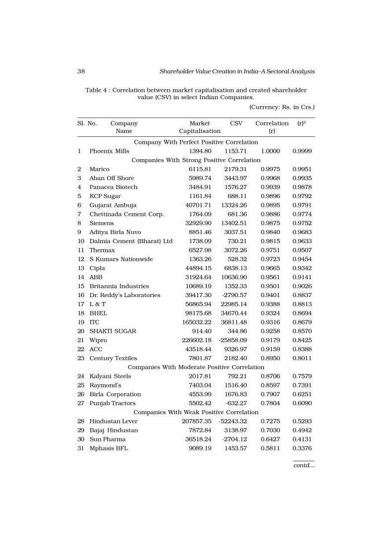
38 Shareholder Value Creation in India–A Sectoral Analysis
Table 4 : Correlation between market capitalisation and created shareholdervalue (CSV) in select Indian Companies.
(Currency: Rs. in Crs.)
Sl. No. Company Market CSV Correlation (r)2
Name Capitalisation (r)
Company With Perfect Positive Correlation
1 Phoenix Mills 1394.80 1153.71 1.0000 0.9999
Companies With Strong Positive Correlation
2 Marico 6115.81 2179.31 0.9975 0.9951
3 Aban Off Shore 5989.74 3443.97 0.9968 0.9935
4 Panacea Biotech 3484.91 1576.27 0.9939 0.9878
5 KCP Sugar 1161.84 688.11 0.9896 0.9792
6 Gujarat Ambuja 40701.71 13324.26 0.9895 0.9791
7 Chettinada Cement Corp. 1764.09 681.36 0.9886 0.9774
8 Siemens 32929.90 13402.51 0.9875 0.9752
9 Aditya Birla Nuvo 8851.46 3037.51 0.9840 0.9683
10 Dalmia Cement (Bharat) Ltd 1738.09 730.21 0.9815 0.9633
11 Thermax 6527.98 3072.26 0.9751 0.9507
12 S Kumars Nationwide 1363.26 528.32 0.9723 0.9454
13 Cipla 44894.15 6838.13 0.9665 0.9342
14 ABB 31924.64 10636.90 0.9561 0.9141
15 Britannia Industries 10689.19 1352.33 0.9501 0.9026
16 Dr. Reddy’s Laboratories 39417.30 -2790.57 0.9401 0.8837
17 L & T 56865.94 22985.14 0.9388 0.8813
18 BHEL 98175.68 34670.44 0.9324 0.8694
19 ITC 165032.22 36811.48 0.9316 0.8679
20 SHAKTI SUGAR 914.40 344.86 0.9258 0.8570
21 Wipro 226602.18 -25858.09 0.9179 0.8425
22 ACC 43518.44 9326.97 0.9159 0.8388
23 Century Textiles 7801.87 2182.40 0.8950 0.8011
Companies With Moderate Positive Correlation
24 Kalyani Steels 2017.81 792.21 0.8706 0.7579
25 Raymond’s 7403.04 1516.40 0.8597 0.7391
26 Birla Corporation 4553.99 1676.83 0.7907 0.6251
27 Punjab Tractors 5502.42 -632.27 0.7804 0.6090
Companies With Weak Positive Correlation
28 Hindustan Lever 207857.35 -52243.32 0.7275 0.5293
29 Bajaj Hindustan 7872.84 3138.97 0.7030 0.4942
30 Sun Pharma 36518.24 -2704.12 0.6427 0.4131
31 Mphasis BFL 9089.19 1453.57 0.5811 0.3376
contd...

39K.R. Jalaja
32 Tata Motors 76225.00 16643.73 0.5806 0.3371
33 Nestle India 37315.51 3274.33 0.5713 0.3263
34 Hero Honda Motors 48906.54 3079.03 0.5679 0.3225
35 Balrampur Chini Mills 5150.24 1495.90 0.4640 0.2153
36 Jindal Steel & Power 11304.59 -3633.23 0.4550 0.2070
37 Hindustan Petroleum 58412.27 -5356.04 0.4037 0.1630
38 Glaxo Smith Kline Consumers 8842.79 -1045.99 0.3868 0.1496
39 Infosys Technologies 227164.31 -13285.33 0.3712 0.1378
40 Reliance Industries 332458.63 -23943.49 0.2778 0.0772
41 OUDH Sugar 433.38 113.16 0.2664 0.0710
42 Indian Oil Corporation 211076.78 19807.26 0.1945 0.0378
43 Bajaj Auto 77355.65 5335.87 0.1333 0.0178
44 Eicher Motors 2415.06 448.54 0.0297 0.0009
Companies With Negative Correlation
45 Aventis Pharma 12250.22 296.71 -0.0378 0.0014
46 ONGC 522154.18 66500.72 -0.0473 0.0022
47 Tata Steel 74546.34 8972.94 -0.1358 0.0184
48 Steel Authority Of India 79406.94 10162.56 -0.1472 0.0217
49 HCL Infosystems 227164.31 1020.38 -0.5726 0.3278
50 TCS 337065.92 19455.82 -0.5845 0.3417
Results and Inference
For the purpose of analysis and interpretation the correlation results havebeen categorized into five groups, namely,
l Perfect positive correlation: (r) = (1.0000)
l Strong Positive correlation: (r) = (+0.9999 to +0.9000)
Õ (r2) > 80%
l Moderate positive correlation: (r) = (+0.8999 to +0.7800)
Õ (r2) > 60%
l Weak positive Correlation: (r) = (+0.7799 to +0.0001)
Õ (r2) < 60%
It can be inferred from Table 4 that among the 50 sample companies onlyone company has perfect positive correlation (r = 1.0000) and 22 companieshave strong correlation between Market Capitalization and CreatedShareholder Value (CSV) where (r) = (+0.9999 to +0.9000), representing 44%of the sample size showing a variation upto 80% (r2).
Since a large percentage of the sample companies have strong correlationbetween Market Capitalization and Created Shareholder Value (CSV), thereis substantial statistical evidence for accepting the alternate Hypothesisthat “there is strong correlation between Market Capitalisation and Created
Shareholder Value”. It can be concluded that the null hypothesis should berejected.
contd...

40 Shareholder Value Creation in India–A Sectoral Analysis
Conclusion
Old Generation Companies ( Companies representing the Industry Sectors– Oil & Gas, Steel, Textiles, Sugar and Cement & Cement Products) havecreated more Shareholder Value than New Generation Companies(Companies representing the Industry sectors - IT, Pharmaceuticals, FMCG,Automobiles and Capital Goods) among the sample companies. This bringsto light that there is huge potential for Value Creation in the Old GenerationCompanies. Hence, the management should strive to adopt new technologythrough R&D and also think about the Corporate Restructuring activities toimprove Shareholder Value. There is positive correlation between MarketCapitalisation and Shareholder Value Creation in 44 Companies out a Sampleof 50 Companies, but the degree of Correlation varies. There is strongcorrelation in 23 Companies, moderate level of correlation in 4 Companiesand weak correlation in 17 Companies and the correlation is negative in 6Companies. Empirical evidence proves that Shareholder Value Creation doesnot depend on the Size of the Company (measured in terms of MarketCapitalisation). It is also revealed that Value Creation is high in mid-capand low capitalisation companies and low in high-capitalisation companies.
REFERENCES
Alfred Rappaport. 1986. Creating shareholder value: A guide for managers andinvestors, The Free Press, New York.
Ashok Banerjee. 1998. Agency costs & free cash flows - the stakeholders stake, The
Chartered Accountant.
Beatrice Nyiramahoro and Natalie Shooshina, Creating and measuring shareholdervalue: applicability and relevance in selected Swedish companies.
Bernie Marcus. 2002. Value-building growth – a monograph on how the right kindof growth can increase shareholder value, AT Kearney research paper,.
Bhabatosh Banerjee. 2005. Financial policy and management accounting, Prentice-Hall of India Private limited, New Delhi.
David. L. Wenner and Richard W. Le Ber. 1989. Managing for shareholder value-from top to bottom, Harvard Business Review, pp 2-8.
Enrique. R. Arzac. 1986. Do your business units create shareholder value? : Harvard
Business Review, pp 120-126.
George. S. Day and Lian Fahey. 1990. Putting strategy into shareholder value analysis,Harvard Business Review, pp 156-162.
Gordon Donaldson. 1985. Financial goals and strategic consequences, Harvard
Business Review, pp 57-65.
Geraldine. E. Willigan. 1990. The value-adding CFO: an interview review, pp 85-93.
Jawahar Lal, Madhu Malik. 2001. Economic value added (EVA) and corporateperformance, The Management Accountant.
Laurence Booth. 1998. What drives shareholder value? Research paper presented atThe Federated Press, “Creating Shareholder Value” conference.

41K.R. Jalaja
Omkar Goswami and Karthikeyan.M. 1998. Are Indian companies losing shareholdervalue? CII Corporate Research Series 1/1.
Pablo Fernandez. 2002. A definition of shareholder value creation, Research Paperno. 448.
Pablo Fernandez. 2003. EVA, economic profit and cash value added do not measureshareholder value creation, ICFAI Journal of Applied Finance, Vol. VI, No 2,
pp 74-85.
Ramana D.V. 2007. Economic value added and other accounting performanceindicators: an empirical analysis of Indian Companies, The ICFAI Journal of
Accounting Research, Vol. VI, No 2, pp 7-20.
Ranjan Mukherjee. 2001. Value creation drive – a few pertinent issues, The
Management Accountant, pp 45-48.
RBI 2005-06. Handbook of Statistics on the Indian Economy.
Roger A. Morin and Serry L. Jarrell. 2004. Driving shareholder value: value-buildingtechniques for creating shareholder wealth, Tata McGraw-Hill PublishingCompany Limited, New Delhi.
Sahu R.K. 2001. Accounting profitability vs. shareholder’s value created: an empiricalstudy, The Management Accountant, pp 665-659.
Sengupta A.K. 2001. Strategic management: a tool for value management, The
Management Accountant, pp 7-15.
Shaveta Gupta. 2007. Value-based management: creating value for shareholders,The ICFAI University Press, pp 40-62.
Venkiteshwaran. N. 1996. Corporate restructuring for shareholder value, IIMAWorking Papers no.1334.
William. E. Fruhan Jr. 1984. How fast should your company grow? : Harvard Business
Review, pp. 83-93.
William. E. Fruhan Jr. 1988. Corporate raiders: Head’em off at value gap, Harvard
Business Review, pp 62-68.

42 Role of Components of EVA in Profit Prediction...
Role of Components of EVA in Profit Prediction:Evidence from Indian Two Wheelers Industry
DHARMENDRA S. MISTRY
Profit significantly affects stock market and hence prediction of profit is the
key question for any business community. The present article aims to
investigate the ability of the components of EVA in predicting the operating
profit of the subsequent period of Indian Two Wheelers Industry. The study
found that Capital Employed and Net Operating Profit After Tax have positive
impact on next period’s profit while Return on Assets has negative impact
thereon.
Introduction
In the late 1980s‚ Joel Stern and G. Bennet Stewart III of the New Yorkconsulting firm Stern Stewart and Company commenced to expand andencourage Economic Value Added (EVA) in the corporate world as a techniquethat can be associated with a firm’s share value. EVA thus, settlesconclusively whether shareholders’ wealth was formed or not. EVA is a valuebased performance measure‚ an investment decision instrument and it isfurthermore a performance measure reflecting the complete amount ofshareholder value created. It is a distinct system that gives a valid image ofshareholder wealth formation.
As profit significantly affects stock market‚ prediction of profit is the keyquestion for any business community (Hendriksen and Berda, 1992).Traditionally‚ measurement of accounting income was of central focus witha view to judging real value of the business. Shortcomings such as possibilityof manipulation and focus on the quantity of profit have given rise to theconcept of EVA (Stewart, 1991). EVA’s connection with the stock’s price forperformance evaluation and indication whether the operating profit issufficient for the cost of capital employed or not makes it simple yet significanttool for performance evaluation.
Literature Review
Traditionally‚ the gross earnings of management which a man is getting canonly be found after making up a careful account of the true profits of hisbusiness, and deducting interest on his capital (Marshall‚1920). Differencebetween net earnings and the cost of capital was treated as economic profitand operationalised as a measure of wealth creation (Solomon, 1965). EVAis the same as Residual Income (RI) that has been in existence for several
Dr. Dharmendra S. Mistry is Associate Professor, P.G. Department of Business Studies,Sardar Patel University, Vallabh Vidyanagar, Anand – 388 120 (Gujarat)
The Indian Journal of Commerce
Vol. 64, No. 3, July-September 2011

43Dharmendra S. Mistry
decades. The only significant difference between the two lies in the handlingof accounting distortions (Dodd and Chen, 1997). Solomons (1965) suggestedthat RI can be used as an internal performance measure and Anthony (1973,1982a, and 1982b) suggested that it be an external performance measure.Value added is a significant explanatory factor in market returns, and itsexplanatory power is higher than that of earnings (Bao and Bao, 1998). EVAis correct in its methodology and assumptions, and can live up to its claimsof being an alternative to traditional accounting (Stewart, 1999). It also givesintangible benefits such as improved decision making, better communicationfrom managers and improved strategic planning (Tejpavan & Kulkarni, 2005).It can also be a powerful tool for changing the company’s focus and producingtremendous financial results (Gray, 2006). It is the framework for a completefinancial management and incentive compensation system that can guideevery decision a company makes, from the boardroom to the shop floor; thatcan transform a corporate culture; that can improve the working lives ofeveryone in an organization by making them more successful; and that canhelp them produce greater wealth for shareholders, customers, andthemselves (Al Ehrbar, 1998). It is an effective measure of the quality ofmanagerial decisions as well as a reliable indicator of an enterprise’s valuegrowth in future (Geyser and Liebenberg‚2003). The EVA based performancemeasurement system is the basis on which the company should takeappropriate decisions related to the choice of strategy, capital allocation,merger & acquisitions, divesting business and goal setting (Rakshit‚ 2006).
Methodology
The major findings of above mentioned studies did not focus on use ofcomponents of EVA i.e. Return on Assets‚ Net Operating Profit After Tax andCapital Employed in forecasting subsequent year’s profit and hence anattempt has been made to analyse the predictive ability of the componentsof EVA in envisaging subsequent year’s operating profit of the Indian Twowheelers industry.
The sample of this study includes following three Indian Two Wheelers playerson the basis of their performance, position and sales during the said period:
1. Hero Honda Motors Limited
2. Kinetic Motor Company Limited and
3. TVS Motor Company Limited
The data for the accomplishment of the aforementioned research objectivesused was secondary. With a view to analyzing the predictive ability of thecomponents of EVA in forecasting subsequent year’s profit, the data wasgathered from financial statements as published in annual reports (2001-02 to 2008-09) of Indian Two Wheelers Industry. The data base of Associationof Indian Automobiles Industry has also been utilized.
Profit of the subsequent year is measured by Return on Assets‚ Net OperatingProfit After Tax and Capital Employed of the present year and thereforeprofit of the subsequent year has been taken as dependent variable for thepresent study. Return on Assets‚ Net Operating Profit After Tax and Capital

44 Role of Components of EVA in Profit Prediction...
Employed of the present year have been taken as independent variables forthe study.
Above discussed variables have been taken together as determinants ofprofit of the subsequent year and model has been developed in order toanalyse whether the components of EVA (Return on Assets‚ Net OperatingProfit After Tax and Capital Employed of the present year – independentvariables) are significant in predicting profit of the subsequent year(Operating Profit – dependent variable) or not.
In order to examine and compare the impact of independent variables onthe dependent variable, technique of regression has been applied. Thehypotheses were tested by simple linear regression.
H1 (OPt = a + bRt – 1): Return on Assets can predict next period’s Operating
Profit. Where‚ OIt = Operating Profit of subsequent period and Rt = Currentyear’s Return on Assets.
H2 (OPt = a + bCAPITALt – 1): The amount of Capital Employed can predict
next period’s Operating Profit.
(Where‚ CAPITALt = Current year’s Capital Employed)
H3 (OPt = a + bNOPATt – 1): Net Operating Profit after taxes can predict next
period’s Operating Profit.
(Where‚ NOPATt = Current year’s Net Operating Profit)
Results
In order to analyze the hypotheses, dependent and independent variableswere studied and measured. Then, the ability of each independent variablein predicting the operating profit of subsequent period was analyzed. To dothis, simple regression was used. The results are described below:
Table 1 Role of ROA in Profit Prediction of Indian two-wheelers industry
Coefficients Standard Error t Stat P-value
Constant 677.2706564 68.804076 9.843467 0.000184
Return on Assets -3.567655381 1.754898131 -2.03297 0.09774
Multiple R 0.672706
R Square 0.452533
Adjusted R Square 0.343039
Standard Error 69.06284
ANOVA
df SS MS F
Regression 1 19712.91444 19712.91 4.132967
Residual 5 23848.37932 4769.676
Total 6 43561.29375
Table 1 reveals that correlation coefficient between next period’s OperatingProfit and Return on Assets is equal to 0.672706 and the possibility of thisis 0.09774, which is more than 0.05. Therefore, with a certainty of 95%, it is

45Dharmendra S. Mistry
confirmed that there is an insignificant relation between variables. Thecalculated value of ‘F’ is 4.132967, while the table value with one degree offreedom in numerator and five degrees of freedom in denominator at fivepercent significant level is 6. 607891. As tabulated value of ‘F’ is more thancalculated value thereof, it can be concluded that Return on Assets doesnot have an impact on profit of subsequent year. Finally, considering thefirst hypothesis’ coefficient of determination which equals 0.452533, it canbe concluded that around 45.2533% of the dependent variable’s change(Subsequent Year’s Operating Profit) can be described by independent variable(Return on Assets) and the first hypothesis is rejected. Regression modelfitted to the data: OPt = 677.2706564 - 3.567655381Rt – 1. Coefficient ofReturn on Assets proposes that each 1 percent change in Return on Assetsleads to decrease of 3.567655381 percent in subsequent year’s profit.
Table 2: Role of CE in Profit Prediction of Indian two-wheelers industry
Coefficients Standard Error t Stat P-value
Coefficients Standard Error t Stat P-value
Constant 395.0330144 57.36690682 6.886078 0.000989
Capital Employed 0.159492795 0.055444429 2.876624 0.034725
Multiple R 0.789525965
R Square 0.62335125
Adjusted R Square 0.5480215
Standard Error 57.28404113
ANOVA
Df SS MS F
Regression 1 27153.98692 27153.99 8.274968
Residual 5 16407.30684 3281.461
Total 6 43561.29375
Table 2 divulges that correlation coefficient between next period’s OperatingProfit and Capital Employed is equal to 0.789525965 and the possibility ofthis is 0.034725, which is less than 0.05. Therefore, with a certainty of95%, it is confirmed that there is a significant relation between variables.The calculated value of ‘F’ is 8.274968, while the table value with one degreeof freedom in numerator and five degrees of freedom in denominator at fivepercent significant level is 6. 607891. As tabulated value of ‘F’ is less thancalculated value thereof, it can be concluded that Capital Employed has animpact on profit of subsequent year. Finally, considering the secondhypothesis’ coefficient of determination which equals 0.62335125, it can beconcluded that around 62.335125% of the dependent variable’s change(Subsequent Year’s Operating Profit) can be described by independent variable(Capital Employed) and the second hypothesis is confirmed. Regression modelfitted to the data: OPt = 395.0330144 + 0.1594927951CAPITALt – 1. Coefficientof Capital Employed proposes that each 1 percent change therein leads toincrease of 0.159492795 percent in subsequent year’s profit.

46 Role of Components of EVA in Profit Prediction...
Table 3: Role of NOPAT in Profit Prediction of Indian two-wheelers industry
Coefficients Standard Error t Stat P-value
Coefficients Standard Error t Stat P-value
Constant 284.5487789 147.0499827 1.935048 0.110771
Net Operating 0.928924012 0.50973775 1.822357 0.12802Profit After Tax
Multiple R 0.63175116
R Square 0.399109528
Adjusted R Square 0.278931434
Standard Error 72.3540826
ANOVA
Df SS MS F
Regression 1 17385.72741 17385.73 3.320984
Residual 5 26175.56634 5235.113
Total 6 43561.29375
Table 3 divulges that correlation coefficient between next period’s OperatingProfit and Net Operating Profit After Tax is equal to 0.63175116 and thepossibility of this is 0.12802, which is more than 0.05. Therefore, with acertainty of 95%, it is confirmed that there is an insignificant relation betweenvariables. The calculated value of ‘F’ is 3.320984, while the table value withone degree of freedom in numerator and five degrees of freedom in denominatorat five percent significant level is 6. 607891. As tabulated value of ‘F’ is lessthan calculated value thereof, it can be concluded that NOPAT does nothave an impact on profit of subsequent year. Finally, considering the secondhypothesis’ coefficient of determination which equals 0.399109528, it canbe concluded that around 39.91209528% of the dependent variable’s change(Subsequent Year’s Operating Profit) can be described by independent variable(Net Operating Profit After Tax) and the third hypothesis is rejected.Regression model fitted to the data: OPt = 284.5487789 + 0.928924012NOPATt– 1. Coefficient of Net Operating Profit After Tax proposes that each 1 percentchange in Net Operating Profit After Tax leads to increase of 0.928924012percent in subsequent year’s Operating Profit.
Conclusion
The study divulges that the Capital Employed has a strong connection withpredicting next period’s Operating Profit because the coefficient ofdetermination of 62% showed that Capital Employed is the most suitablechoice regarding the prediction of next period’s Operating Profit in comparisonto Net Operating Profit After Tax (40%) and Return on Assets (45%). Moreover‚Capital Employed and Net Operating Profit After Tax have positive impacton next period’s profit while Return on Assets had negative impact thereon.It can be concluded that due to the high ability of Net Operating Profit AfterTax, capital amount and Return on Assets in predicting Operating Profit ofthe next period, these variables can be the proper criteria for capital

47Dharmendra S. Mistry
allocation, designing reward system, increasing capital and evaluation ofthe companies’ performance. It can also be concluded that EVA is substantialfoundation in assessing the company’s performance by covering weaknessesinborn in accounting criteria. Looking to usefulness of the EVA and itscomponents in prediction of profit‚ it is recommended that it should be usedto determine the real value of companies i.e. through evaluation ofperformance of staff and company. At the end‚ the companies under thestudy should also take into account that EVA improves if operating profitsgrow without employing more capital, implying greater efficiencies‚ additionalcapital is invested in projects that return more than the cost of capital andcapital is curtailed in activities that do not cover its costs – minimising oreliminating unproductive capital. Therefore‚ essential steps should beinitiated to improve EVA and get benefits thereof such as improved decisionmaking, better communication from managers and improved strategicplanning.
REFERENCES
Anthony, Robert N., (1973), “Accounting for the Cost of Equity,” Harvard Business
Review 51 (No. 6, November/December), Pp.88-102.
Anthony, Robert N., (1982a), “Equity Interest — Its Time Has Come,” Journal of
Accountancy 154 (December), Pp.76-93.
Anthony, Robert N., (1982b), “Recognizing the Cost of Interest on Equity,” Harvard
Business Review 61 (No. 1, January/February), Pp.91-96.
Bao, B.H., & Bao, D.H., (1998), Usefulness of Value Added and Abnormal EconomicEarnings: An Empirical Examination, Journal of Business Finance and
Accounting, 25, 1- 2: 251-265.
Dodd, James L. and Chen, Shimin (1997) “Economic Value Added (EVA),” Arkansas
Business and Economic Review, Pp. 1-8.
Ehrbar, A. (1998). EVA: The real key to creating wealth. New York: John Wiley &Sons.
Geyser M. & Liebenberg IE (2003)‚ Creating a New Valuation Tool for South AfricanAgricultural Co-operatives‚ Agrekon‚ 42:2‚ Pp. 106-115
Gray, P. B. (2006). What’s you magic number? FSB: Fortune Small Business, 16:9,Pp.72- 78.
Hendriksen E, Berda V (1992). Accounting Theory. New York: IRWIIN.
Marshall, A., (1920), Principles of Economics, 8th Edition, 1990 Reprint, London:Macmillan.
Rakdhit D. (2006)‚ EVA based performance measurement: a case study of DaburIndia Limited‚ Vidyasagar University Journal of Commerce‚ 11:1‚ Pp. 40-59
Solomons, D., (1965), Divisional Performance: Measurement and Control,Homewood: Irwin.
Stewart GB (1991). The Quest for Value: A Guide for Senior Managers. New York:Harper Business Publisher.
Stewart, G. B., III. (1999). The quest for value. New York: HarperCollins Publisher.
Tejpavan, G. & Kulkarni, S. (2005), Stern Stewart’s clients create more wealth byoutperforming their peers. EVAluation, (January), Pp.1-7. Retrieved March 31,2011 from http://www.sternstewart.com/content/evaluation/info/ClientPerformance.pdf

48 Performance Analysis of Indian Mutual Funds with a Special Reference...
Performance Analysis of Indian Mutual Funds with aSpecial Reference to Sector Funds
POURNIMA S. SHENVI DHUME AND PROF. B. RAMESH
Mutual Fund industry in India has emerged as the most dynamic segment of
the Indian financial system. The industry grew by leaps and bounds during
the last few years. With the plethora of schemes available for the investors
to choose, it becomes essential for a retail investor to know the performance
of the mutual funds in order to make an informed decision. In this paper, we
have carried out the performance evaluation of open-ended equity sector
mutual funds using five approaches of performance measures viz, Sharpe
Ratio, Treynor Ratio, Jensen’s Measure, Information Ratio and M-squared
measure. The sectors selected for the purpose of the study are banking
sector, FMCG sector, infrastructure sector, pharma sector & technology
sector. All the schemes are selected from the respective sectors which were
existing during the period of the study. The period adopted for the study is
from 1st April 2008 to 31st March 2011.
Introduction
Mutual funds play an extremely crucial role in Indian economy. They arethe vehicles for mobilisation and channelization of savings from individualsand households towards the capital markets. Mutual funds have shown atremendous improvement in the quantum of their assets under managementover the last couple of years. The concept of mutual funds was conceived topool the resources of small and retail investors and deploy the same in thecapital markets through participation in equity and debt instruments.Mutual funds offer several benefits to the investors like diversification,professional management, tax benefits, transparency, liquidity, flexibility,choice of schemes, low cost etc. Every mutual fund is managed by a fundmanager, who is using his investment management skills and necessaryresearch works ensures much better returns than what the investors canmanage on his/her own.
The Indian mutual fund industry has come a long way from a single playermonopoly in 1964 for almost 45 years to a vibrant, competitive, fast growingsector. The industry has emerged as the most dynamic segment of the Indianfinancial system. The industry has witnessed surprising growth in terms ofproducts and services offered, returns generated, volumes generated andinternational players who have contributed to the growth of the industry.
Ms Pournima S. Shenvi Dhume is Assistant Professor, Department of Commerce, GoaUniversity, Taleigao Goa and Prof. B. Ramesh is Professor, Head & Dean, Faculty ofCommerce, Goa University, Taleigao Plateau, Goa.
The Indian Journal of Commerce
Vol. 64, No. 3, July-September 2011

49Pournima S. Shenvi Dhume and Prof. B. Ramesh
Mutual funds have time and again responded to the changing marketdynamics. They have tried to capture every pocket of the market andencourage greater investor participation. Till some years back, equitydiversified funds were the only choice available, sectoral funds were launchedas a new genre of equity funds. Today, we have Technology Funds allocatingprimarily to IT Stocks, Pharma Funds focussing on healthcare sector, BankingFunds specifically investing in Banking stocks and many more. This studyanalyses the performance of the sector mutual funds.
Literature Review
Block & French (2000) emphasised the importance to use multiple indexeswhile evaluating the performance of equity mutual funds. Saidov (2007)analysed the performance of mutual funds by using seven differentapproaches of performance measures. These seven measures were Jensen’sAlpha, Sharpe Ratio, Treynor Ratio, Sortino Ratio, Fama Ratio, InformationRatio and Fama-French Three Factor Model. His study concluded that thedifferent measures have no significant effect on the ranking results of GermanEquity Mutual Funds. Gali (1995) evaluated the past performance of themutual funds and assessed the factors that have an influence on theperformance. The factors considered were portfolio turnover, timing and stockselection skills, organisational structure, research, size and expensescharged to the fund. He found that mutual funds in general do not providerisk-adjusted returns. It was also found that mutual funds do not havemarket timing ability. Rao (2003) studied the performance evaluation of Indianmutual funds in bear market through relative performance index. He foundthat most of the mutual fund schemes were able to satisfy investor’sexpectations by giving excess returns over expected returns.
Objectives Of The Study
The major objectives of the study are:
i. To evaluate the performance of the sector mutual funds in relation withthe market performance using different approaches of performancemeasures.
ii. To study the risk-return analysis of the sector funds.
Methodology
Data sources: For the purpose of the study, we have selected 40 open-endedequity sector funds. Five Sectors viz., Banking Sector, FMCG Sector,Infrastructure Sector, Pharma Sector and Technology Sector are chosen forthe study. All funds are selected from the respective sectors which wereexisting during our period of the study. The funds launched after 1st April2008 are not been selected. Growth option and Dividend option areconsidered as separate funds in the study. 6 funds are selected from BankingSector, 5 from FMCG Sector, 34 from Infrastructure Sector, 8 funds fromPharma Sector and 7 funds from Technology Sector. The Net Asset Value(NAV) of the funds are obtained from fact sheets and websites. The data forthe study is mainly derived from AMFI Website.

50 Performance Analysis of Indian Mutual Funds with a Special Reference...
Data On Indices: Since our study includes only open-ended equity sectorfunds, the respective indices are used as benchmarks for evaluating theperformance. The benchmarks used for the analysis is obtained from BSEwebsite. The benchmark indices for the sector funds are as follows: BankingFunds – BSE BANKEX, FMCG Funds – BSE FMCG INDEX, InfrastructureFunds – BSE CAPITAL GOODS INDEX, Pharma Funds – BSE HEALTHCAREINDEX, and Technology Funds – BSE IT INDEX
Data On Risk-Free Rate Of Return: The risk-free rate is the rate of returnof the 365-days Treasury Bills obtained from Reserve Bank of India Website.
Performance Measures
Standard Deviation: is a measure if dispersion in return. A higher value ofstandard deviation means higher risk.
Beta (â): measures the relationship between index return and the fund’sreturn. It measures the systematic risk. It relates the return of the fund tothe market index. It reflects the sensitivity of the fund’s return to fluctuationsin the market index. A beta greater than 1, means that the fund is morevolatile than the benchmark index, while beta less than 1 means the fundis less volatile than the index.
R-Squared (R2): It measures how close all the points on the XY Graph are tothe best-fit line. If all points were on the line, a fund would have an R-squared of 1, indicating perfect correlation with the chosen index. A R-squared of zero would indicate no correlation. The lower the R-squared, theless reliable beta is as a measure of fund’s volatility.
Sharpe’s Ratio: It is a measure of risk-adjusted return on a portfolio developedby William Sharpe. It is a ratio of excess return to the standard deviation ofportfolio. It is relevant for performance evaluation when comparing mutuallyportfolios. It measures reward to variability. The Sharpe measure ofperformance denoted by S is give by
Rp – R
fS = ––––––– σ
p
where, Rp = portfolio rate of return during a specified period; R
f = risk-free
rate of return during the same period; σp = standard
deviation
A fund with a higher Sharpe Ratio is relation to another is preferable as itindicates that the fund has higher risk premium for every unit of standarddeviation risk.
Treynor’s Ratio: developed by Jack Treynor. It adjusts excess return forsystematic risk. This ratio of return generated by the fund over and aboverisk-free rate of return. The Treynor’s measure is denoted by T is given by
Rp – R
fT = ––––––– β
p
where, Rp = portfolio rate of return during a specified period; R
f = risk-free
rate of return during the same period; βp = beta of the fund

51Pournima S. Shenvi Dhume and Prof. B. Ramesh
While a high and positive Treynor’s measure shows a superior risk-adjustedperformance of a fund, a low and negative Treynor’s measure is an indicationof unfavourable performance.
Alpha: is the most commonly used method of determining the return thatshould have been earned by the scheme at a given level of risk.
α = (Rp – R
f ) – β
p (R
m – R
f)
where, α = The Jensen Measure (Alpha); Rp = portfolio rate of return during
a specified period; Rf = risk-free rate of return during the same period; β
p =
beta of the fund; Rm = Market Return
A positive alpha means that the return tends to be higher than expectedgiven the beta statistic. A negative alpha indicates that the fund isunderperformer. Alpha measures the value-added of the portfolio given itslevel of systematic risk. It is popularly known as Jensen’s Alpha.
M2 Measure: Franco Modigiliani and Lea Modigiliani derived another risk-
adjusted performance measure in 1997, by adjusting the risk of a particularportfolio so that it matches the risk of the market portfolio and then calculatethe appropriate return for that portfolio. It operates on the concept thatscheme’s portfolio can be levered or de-levered to reflect a standard deviationthat is identical with that of the market. The return that this adjustedportfolio earns is called M2.
M2 = ( αm / α
mf ) x ( R
mf – R
f) + R
f
Where, αm
= the standard deviation of the market; αmf
= the standarddeviation of the scheme; R
mf = return on the scheme; R
f = risk free rate of
return
A high M2 indicates that the portfolio has outperformed the market portfoliowhereas; a low M2 indicates that the portfolio has underperformed the marketportfolio.
Information Ratio: was developed by William Sharpe. It measures the excessreturn over benchmark index of an investment divided by its tracking error.It can be calculated as follows:
Rp – R
mIR = ––––––– TE
Where, IR = Information Ratio; Rp = Portfolio Return; Rm = Market return;TE = Tracking Error
Tracking error is defined as the time-series standard deviation of thedifference between a fund return and its market index return. It is expressedas follows:
TE = α (Rp – R
m)
The information ratio expresses how effectively a stock generates activereturn relative to the amount of risk taken.

52 Performance Analysis of Indian Mutual Funds with a Special Reference...
Funds Selected For The Study
Table 1: Selected funds
Sl. No. Name of the Scheme Option Launch Date
1 Jm Financial Services Sector Div Nov-06
2 Jm Financial Services Sector GR Nov-06
3 Reliance Banking DIV May-03
4 Reliance Banking GR May-03
5 Uti Banking Sector DIV Apr-04
6 Uti Banking Sector GR Apr-04
FMCG Sector
1 Franklin FMCG CDIVI Mar-99
2 Franklin FMCG CGRG Mar-99
3 Icici Prudential FMCG CDIVI Mar-99
4 Icici Prudential FMCG CGRG Mar-99
5 Sbi Msfu FMCGCG - Jul-99
Infrastructure Sector
1 Aig Infrastructure and Economic Reform DIV Jan-08
2 Aig Infrastructure and Economic Reform GR Jan-08
3 Birla Sunlife Infrastructure DIV Feb-06
4 Birla Sunlife Infrastructure GR Feb-06
5 Canara Robeco Infra DIV Nov-05
6 Canara Robeco Infra GR Nov-05
7 DSPBR T.I.G.E.R. DIV May-04
8 DSPBR T.I.G.E.R. GR May-04
9 ICICI Prudential Infra DIV Aug-05
10 ICICI Prudential Infra GR Aug-05
11 JM HI FI DIV Mar-06
12 JM HI FI GR Mar-06
13 Kotak Indo World Infra DIV Dec-07
14 Kotak Indo World Infra GR Dec-07
15 LIC Nomura Mf Infra DIV Feb-08
16 LIC Nomura Mf Infra GR Feb-08
17 Religare Infra DIV Oct-07
18 Religare Infra GR Oct-07
19 Sahara Infra Fixed Pricing DIV Mar-06
20 Sahara Infra Fixed Pricing GR Mar-06
contd...

53Pournima S. Shenvi Dhume and Prof. B. Ramesh
21 Sahara Infra Variable Pricing DIV Mar-06
22 Sahara Infra Variable Pricing GR Mar-06
23 Tata Infra DIV Dec-04
24 Tata Infra GR Dec-04
25 Taurus Infra DIV Mar-07
26 Taurus Infra GR Mar-07
27 UTI infra DIV Apr-04
28 UTI Infra GR Apr-04
Pharma Sector
1 Franklin Pharma DIV Mar-99
2 franklin Pharma GR Mar-99
3 SBI Msfu Pharma DIV Jul-99
4 SBI Msfu Pharma GR Jul-99
5 Reliance Pharma DIV May-04
6 Reliance Pharma GR May-04
7 UTI Pharma & Healthcare DIV Jun-99
8 UTI Pharma & Healthcare GR Jun-99
Technology Sector
1 Birla Sunlife New Millenium DIV Jan-00
2 Birla Sunlife New Millenium GR Jan-00
3 DSPBR Techology.com DIV Apr-00
4 DSPBR Techology.com GR Apr-00
5 Franklin Infotech DIV Aug-98
6 Franklin Infotech GR Aug-98
7 SBI MSFU IT Jul-99
Source: Mutual Fund Insight, Volume VIII, Number 8
Results Of Performance Evaluation
Standard Deviation of the market is 2.623. Sharpe ratio of the market is0.015.
The analysis of Sharpe’s measure shown in Table 2 reveals that, RelianceBanking Fund and UTI Banking Fund has outperformed the market whereasJM financial services sector fund has underperformed the market as thesharpe ratio is less than the market. Among the six funds, Reliance BankingGrowth Fund is the best performer as its value is highest (0.029).
The analysis of Treynor’s ratio reveals that, Reliance Banking Fund and UTIBanking Fund has outperformed the market as their value is greater thanthe treynor’s ratio of the market, whereas JM financial services sector fundhas underperformed the market.
contd...

54
Perfo
rma
nce A
na
lysis
of In
dia
n M
utu
al F
un
ds w
ith a
Specia
l Refe
ren
ce...
Table 2: Banking sector funds analysis
Name of the Scheme Std Dev Beta Corre- R- (Fund) (Fund) (Market) Jensen Infor- M-lation Squared Sharpe Treynor Treynor mation Squared
Jm Financial Services 2.279 0.296 0.340 0.116 -0.030 -0.229 -0.159 -0.079 9.555038817 -0.015Sector (DIV)
JM Financial Services 2.570 0.331 0.329 0.108 -0.025 -0.194 -0.142 -0.078 8.877230606 -0.003SECTOR (GR)
Reliance Banking (DIV) 2.156 0.327 0.397 0.158 0.020 0.133 -0.144 0.030 19.45701388 0.115
Reliance Banking (GR) 2.128 0.326 0.401 0.161 0.029 0.191 -0.144 0.049 24.43517174 0.139
UTI Banking Sector (DIV) 2.319 0.326 0.369 0.136 0.006 0.043 -0.144 0.001 14.15261268 0.078
UTI Banking Sector (GR) 2.241 0.329 0.385 0.148 0.022 0.151 -0.143 0.037 19.26559205 0.121

55Pournima S. Shenvi Dhume and Prof. B. Ramesh
As per Jensen’s measure, Reliance Banking Growth Fund is the bestperformer among all the six funds, with the highest Jensen’s ratio.
As per Information Ratio, Reliance Banking Growth Fund is the bestperformer whereas JM financial services sector dividend fund has worseperformance.
M2 measure shows the similar results. Overall, we can say that, RelianceBanking Growth Fund is the best performer and JM financial services sectorfund is the underperformer.
Standard deviation of the market is 1.469. Sharpe ratio of the market is0.001.
The analysis of Sharpe’s measure shown in Table 3 reveals that, FranklinFMCG Fund and SBI FMCG fund has outperformed the market whereasICICI Prudential FMCG fund has underperformed the market as the sharperatio shows a negative value. Among the five funds, SBI FMCG fund is thebest performer as its value is highest (0.033).
The analysis of Treynor’s ratio reveals that, Franklin FMCG Fund and SBIFMCG fund has outperformed the market as their value is greater than thetreynor’s ratio of the market, whereas ICICI Prudential FMCG fund hasunderperformed the market with negative Treynor’s ratio.
As per Jensen’s measure, SBI FMCG Fund is the best performer among allthe five funds, with the highest Jensen’s ratio (0.036).
As per Information Ratio, Franklin FMCG Growth Fund is the best performerwhereas SBI FMCG Fund has performance badly.
Franklin FMCG Dividend Fund is the best performer as per M2 measurewith the higher value of 0.086 among all five funds.
Standard deviation of the market is 1.313. Sharpe ratio of the market is0.005.
The analysis of Sharpe’s measure shown in Table 4 reveals that, all pharmafunds have outperformed the market. Among 8 funds, Franklin PharmaGrowth Fund has been the best performer with highest Sharpe ratio of 0.056.
The analysis of Treynor’s ratio and Jensen’s measure reveals that, all pharmafunds have outperformed the market. Franklin pharma dividend fund hasbeen the best performer.
As per Information Ratio, Franklin pharma growth fund has been the bestperformer among 8 pharma funds. M2 measure also shows the similar results.

56
Perfo
rma
nce A
na
lysis
of In
dia
n M
utu
al F
un
ds w
ith a
Specia
l Refe
ren
ce...
Table 3: FMCG analysis
Name of the Scheme Std Dev Beta Corre- R- (Fund) (Fund) (Market) Jensen Infor- M-lation Squared Sharpe Treynor Treynor Ratio mation Squared
Ratio Ratio Ratio Ratio
Franklin Fmcg (DIV) 0.981 0.227 0.340 0.116 0.016 0.069 -0.270 0.015 41.311 0.086
Franklin Fmcg (GR) 0.980 0.296 0.444 0.197 0.014 0.047 -0.207 0.013 75.910 0.083
ICICI Prudential Fmcg (DIV) 1.246 0.368 0.433 0.187 -0.038 -0.127 -0.163 -0.048 17.198 0.007
ICICI Prudential FMCG (GR) 1.181 0.365 0.452 0.205 -0.011 -0.037 -0.164 -0.015 25.931 0.046
SBI MSFU FMCG 1.121 0.383 0.499 0.249 0.033 0.097 -0.157 0.036 -10.836 0.111
Table 4: Pharma sector analysis
Name of the Scheme Std Dev Beta Corre- R- (Fund) (Fund) (Market) Jensen Infor- M-lation Squared Sharpe Treynor Treynor mation Squared
Franklin Pharma (DIV) 1.552 0.309 0.258 0.066 0.047 0.236 -0.187 0.071 17.252 0.124
Franklin Pharma (GR) 1.019 0.241 0.311 0.097 0.056 0.235 -0.240 0.055 48.383 0.135
SBI Msfu Pharma (DIV) 1.477 0.369 0.327 0.107 0.005 0.020 -0.157 0.005 22.317 0.069
SBI Msfu Pharma (GR) 1.476 0.369 0.327 0.107 0.005 0.019 -0.157 0.005 22.256 0.069
Reliance Pharma (DIV) 1.395 0.313 0.295 0.087 0.036 0.162 -0.184 0.049 27.116 0.110
Reliance Pharma (GR) 1.349 0.321 0.312 0.097 0.050 0.212 -0.180 0.066 34.767 0.128
UTI Pharma & Healthcare (DIV) 1.135 0.281 0.326 0.106 0.009 0.038 -0.205 0.009 24.499 0.075
UTI Pharma & Healthcare (GR) 1.081 0.282 0.343 0.117 0.026 0.098 -0.205 0.026 32.394 0.096

57
Pou
rnim
a S
. Sh
en
vi D
hu
me a
nd
Pro
f. B. R
am
esh
Table 5: Infrastructure sector analysis
Name of the Scheme Std Dev Beta Corre- R- (Fund) (Fund) (Market) Jensen Infor- M-lation Squared Sharpe Treynor Treynor mation Squared
AIG Infrastructure and 1.602 0.283 0.421 0.177 -0.025 -0.144 -0.284 -0.029 167.1363579 0.002Economic Reform (DIV)
AIG INfrastructure and 1.602 0.283 0.421 0.177 -0.025 -0.144 -0.284 -0.029 167.1363579 0.002Economic Reform (GR)
Birla Sunlife Infrastructure 1.174 0.030 0.049 0.002 -0.024 -0.942 -2.694 -0.027 23.2659492 0.005(DIV)
Birla Sunlife Infrastructure 1.187 0.021 0.034 0.001 -0.030 -1.685 -3.844 -0.034 20.55166098 -0.008(GR)
Canara Robeco Infra (DIV) 1.844 0.276 0.356 0.127 -0.016 -0.105 -0.291 -0.017 238.6697914 0.025
Canara Robeco Infra (GR) 1.830 0.273 0.356 0.127 -0.011 -0.072 -0.294 -0.008 -4915.616316 0.037
DSPBR T.I.G.E.R (DIV) 1.849 0.279 0.359 0.129 -0.031 -0.207 -0.288 -0.046 57.42503557 -0.012
DSPBR T.I.G.E.R. (GR) 1.782 0.339 0.453 0.205 -0.020 -0.105 -0.237 -0.021 304.4179683 0.015
ICICI Prudential Infra (DIV) 1.900 0.453 0.568 0.322 -0.035 -0.145 -0.177 -0.046 45.32595619 -0.020
ICICI Prudential Infra (GR) 1.766 0.435 0.587 0.345 -0.019 -0.076 -0.184 -0.014 -261.416002 0.018
JM HI FI (DIV) 2.157 0.349 0.385 0.149 -0.066 -0.410 -0.230 -0.128 18.48036513 -0.096
JM HI FI (GR) 2.157 0.349 0.385 0.149 -0.066 -0.410 -0.230 -0.128 18.47798919 -0.096
Kotak Indo World Infra (DIV) 1.754 0.041 0.055 0.003 -0.027 -1.150 -1.968 -0.045 41.85079368 -0.001
Kotak Indo World Infra (GR) 1.754 0.041 0.055 0.003 -0.027 -1.150 -1.968 -0.045 41.85079368 -0.001
LIC Nomura Mf Infra (DIV) 2.244 -0.031 -0.033 0.001 -0.016 1.185 2.587 -0.038 48.26788824 0.023
contd...

58
Perfo
rma
nce A
na
lysis
of In
dia
n M
utu
al F
un
ds w
ith a
Specia
l Refe
ren
ce...
LIC Nomura Mf Infra (GR) 2.244 -0.031 -0.033 0.001 -0.016 1.185 2.587 -0.038 48.26785046 0.023
Religare Infra (DIV) 1.459 0.035 0.057 0.003 -0.032 -1.341 -2.301 -0.045 64.7463308 -0.014
Religare Infra (GR) 1.456 0.036 0.058 0.003 -0.032 -1.311 -2.246 -0.045 64.90585781 -0.014
Sahara Infra Fixed Pricing 1.619 0.248 0.365 0.133 -0.027 -0.175 -0.324 -0.033 106.8678517 -0.002(DIV)
Sahara Infra Fixed Pricing 1.619 0.248 0.365 0.133 -0.027 -0.175 -0.324 -0.033 106.96844 -0.002(GR)
Sahara INFRA Variable Pricing 1.619 0.248 0.365 0.133 -0.025 -0.162 -0.324 -0.030 131.3077921 0.003(DIV)
Sahara INFRA Variable 1.619 0.248 0.365 0.133 -0.025 -0.162 -0.324 -0.030 131.3077921 0.003Pricing (GR)
Tata INFRA (DIV) 1.896 0.329 0.412 0.170 -0.026 -0.150 -0.244 -0.035 78.37103211 0.000
Tata INFRA (GR) 1.888 0.328 0.414 0.171 -0.021 -0.121 -0.245 -0.026 129.3425704 0.012
Taurus INFRA (DIV) 2.064 0.338 0.390 0.152 -0.015 -0.092 -0.238 -0.017 183.0152715 0.026
Taurus INFRA (GR) 2.053 0.338 0.392 0.154 -0.011 -0.067 -0.237 -0.008 694.6923045 0.036
UTI INFRA (DIV) 1.585 0.224 0.319 0.102 -0.031 -0.220 -0.359 -0.040 17.62251224 -0.012
UTI INFRA (GR) 1.467 0.214 0.342 0.117 -0.035 0.020 -0.375 -0.042 27.40632328 -0.021
contd...

59
Pou
rnim
a S
. Sh
en
vi D
hu
me a
nd
Pro
f. B. R
am
esh
Table 6: Technology sector analysis
Name of the Scheme Std Dev Beta Corre- R- (Fund) (Fund) (Market) Jensen Infor- M-lation Squared Sharpe Treynor Treynor mation Squared
Birla Sunlife New Millenium 1.688 0.381 0.484 0.234 -0.041 -0.179 -0.121 -0.082 9.940819462 -0.024(DIV)
Birla Sunlife New Millenium 1.614 0.227 0.302 0.091 -0.020 -0.139 -0.204 -0.039 11.82937459 0 . 0 2 1(GR)
DSPBR Techology.com (DIV) 1.527 0.366 0.514 0.264 -0.013 -0.054 -0.126 -0.032 15.11604365 0.035
DSPBR Techology.com (GR) 1.532 0.308 0.432 0.186 -0.012 -0.058 -0.150 -0.029 14.25673318 0.037
Franklin Infotech (DIV) 2.044 0.178 0.187 0.035 0.004 0.047 -0.260 0.002 12.23846714 0.071
Franklin Infotech (GR) 1.908 0.172 0.193 0.037 0.023 0.258 -0.270 0.038 13.79500651 0.112
SBI MSFU IT 1.803 0.235 0.279 0.078 -0.004 -0.029 -0.197 -0.015 12.5190963 0.054

60 Performance Analysis of Indian Mutual Funds with a Special Reference...
Standard deviation of the market is 2.283. Sharpe Ratio of the market is -0.018.
The analysis of Sharpe’s measure shown in Table 6 reveals that, allinfrastructure funds have outperformed the market. Among 28 funds, JMHi-Fi Fund has been the best performer. The analysis of Treynor’s ratio revealsthat, LIC Nomura Fund has outperformed the market as well as it has beenthe best performer among 28 infrastructure funds. As per Jensen’s measure,JM Hi-Fi Fund has been the best performer.
As per Information Ratio, Taurus Infra Growth Fund has been the bestperformer whereas Canara Robeco Infra Dividend Fund has shown worseperformance. M2 measure shows the similar results. Standard deviation ofthe market is 2.142. Sharpe Ratio of the market is -0.004.
The analysis of Sharpe’s measure shown in Table 7 reveals that, FranklinInfotech Fund with the highet Sharpe ratio i.e. 0.023. The analysis ofTreynor’s ratio reveals the same results as that of Sharpe’s ratio. As perJensen’s measure, Franklin Infotech Growth Fund has been the bestperformer among the 7 funds, with the highest Jensen’s ratio (0.038). Asper Information Ratio, DSP Black Rock Technology.com Dividend Fund hasperformed well whereas, Bila Sun Life New Millenium Dividend Fund hasshown underperformance. Franklin Infotech Growth Fund is the bestperformer as per M2 measure with the higher value of 0.112 among all 7funds. Overall, we can say that, Franklin Infotech Fund has been the bestperformer.
Conclusion
The evaluation of the performance of the open-ended equity sector mutualfunds reveal that, all the sector funds have outperformed the marketaccording to the Sharpe and Treynor’s Ratio except Infrastructure Sectorfunds. FMCG sector is the lowest volatility sector with low standard deviationand beta value having lower risk whereas Banking and Infrastructure sectorshows highest degree of volatility subject to high risk among all the sectorsconsidered together.
REFERENCES
Block & French. 2000. The effect of portfolio weighing on investment performance
evaluation: The case study of actively managed mutual funds. New Mexico StateUniversity.
Gali Kanti Kumar. 1995. Mutual funds – performance appraisal and organizational
factors: An analysis based on risk-adjusted returns. Indian Institute ofManagement. Bangalore
Mutual Fund Insight, Volume VIII, Number 8, 15th April – 14th May
Rao. 2003. Investment Styles and Performance of Equity Mutual Funds in India.
Sadhak H. 1997. Mutual funds in India, marketing strategies and investment practices.
Sage Publications.
Sahadevan & Thiripalraju. 1997. Mutual funds, data, interpretation and analysis.
New Delhi: Prentice Hall India.
Saidov. 2007. Performance evaluation of German mutual funds. University of Ulm

61K.Viyyanna Rao and Nirmala Daita
Fundamental Factors Influencing Investment in MutualFunds - EIC Approach - A Case Study of RCAML
K.VIYYANNA RAO AND NIRMALA DAITA
The present research is an attempt to analyse the influence of fundamental
factors such as economy, industry and company on the performance of
mutual funds. Effort has been made to carry out an in-depth analysis of the
economy through collection of monthly data pertaining to the key macro
economic variables covering a period of 228 months spread over 19 years.
The causal relationship between real economic variables and their impact on
the performance of mutual funds has been studied with the help of descriptive
statistics consisting of suitable test statistics, correlation matrix, Augmented
Dickey-Fuller (ADF) test, and Granger causality test. To appraise the mutual
fund industry in a lucid style, various aspects such as Assets Under
Management (AUM), investor type and product classification have been
studied with the help of percentage analysis. Finally, the fundamental
soundness of the company has been gauged against the chosen parameters
with the support of descriptive statistics, correlation matrix, simple regressionand multiple regressions.
Introduction
With the growing risk appetite, rising income, and increasing awareness,mutual funds in India are becoming a preferred investment option comparedto other investment avenues like Fixed Deposits (FDs) and postal savingsthat are considered safe but give comparatively low returns. Before investingin mutual funds, investors have to analyse the factors of the economy,industry and company within the investment environment in which theyoperate. There are several macro economic factors having influence on theinvestment choices. The investigator intends to study more particularly,the impact of quantitative economic variables on the investment of mutualfunds. The trends of the industry also have to be examined from time totime. In response to the changing circumstances, the fund houses haveintroduced a host of interesting technological innovations to grab theattention of the investors. Investors need to correctly appraise the risks andrewards of investing in schemes which seek to offer attractive returns.
Dr. K. Viyyanna Rao is Professor, Dept. of Commerce and Business Administration &Rector, Acharya Nagarjuna University, Nagarjuna Nagar, Guntur, Andhra Pradesh and Ms.Nirmala Daita is Associate Professor, MBA Dept. Nalanda Institute of P.G.Studies, Kantepudi,Guntur, Andhra Pradesh.
The Indian Journal of Commerce
Vol. 64, No. 3, July-September 2011

62 Fundamental Factors Influencing Investment in Mutual Funds...
Objectives of the Study
The study aims at concentrating on the fundamental factors influencingthe investment in mutual funds. In this direction the following objectiveshave been framed:
l To study the nature of causal relationship that exist between mutualfund market and real economic variables;
l To explore the present status and product offering of mutual fundindustry in India;
l To examine the characteristics of funds that affect the performance ofReliance Capital Asset Management company
Hypotheses
In the light of the above objectives, the study attempts to test the followinghypotheses:
Economy: The investigator has developed the following hypotheses to testempirically the impact of economy on the investment in mutual funds bytaking S&P CNX Nifty, as bench mark index (dependent variable). The keyeconomic variables included in the study are; RBI Bank Rate, DomesticSavings, Forex Reserves, Gross Domestic Capital Formation (GDCF), GrossDomestic Product (GDP), Broad Money (M3), Per-capita Gross NationalProduct (GNP) and Wholesale Price Index (WPI) (as independent variables).
H0: RBI Bank Rate does not influence S & P CNX Nifty.H1: RBI Bank Rate influence S & P CNX Nifty.
H0: Domestic Savings does not influence S & P CNX NiftyH2: Domestic Savings influence S & P CNX Nifty
H0: Forex Reserves does not influence S & P CNX NiftyH3: Forex Reserves influence S & P CNX Nifty
H0: GDCF does not influence S & P CNX NiftyH4: GDCF influence S & P CNX Nifty
H0: GDP does not influence S & P CNX NiftyH5: GDP influence S & P CNX Nifty
H0: Money Supply does not influence S & P CNX NiftyH6: Money Supply influence S & P CNX Nifty
H0: Per-capita GNP does not influence S & P CNX NiftyH7: Per-capita GNP influence S & P CNX Nifty
H0: WPI does not influence S & P CNX NiftyH8: WPI influence S & P CNX Nifty.
Company: In order to test the performance of the company, the investigatorexamined the performance of variables and developed a hypothesis by takingmutual fund return as dependent variable and the factors affecting arePopularity variables (fund size, market capitalisation, net asset value),Growth variables (P/E, P/B), Risk variables (standard deviation and beta),Cost variables (expenses) and Management variables (turnover, managementtenure, fund age) as independent variables. The test hypotheses are:

63K.Viyyanna Rao and Nirmala Daita
Ho: Fund size does not influence the performance of mutual funds.H1: Fund size influences the performance of mutual funds.
Ho: Market capitalization does not influence the return.H2: Mutual funds returns influenced with market capitalization.
Ho: Net asset value does not impact the return.H3: Net asset value does impact the return.
Ho: Growth variables (P/E, P/B) do not influence the return of the mutualfund.H4: Growth variables (P/E, P/B) influence the return of the mutual fund.
Ho: Risk variables (standard deviation and beta) do not influence the return.H5: Risk variables (standard deviation and beta) influence the return.
Ho: Expenses has no impact on the return of mutual funds.H6: Funds with high expenses generate higher returns than low expenses.
Ho: Turnover does not influence the return.H7: Funds turnover influence the return of mutual funds.
Ho: Management tenure has no impact on the return of funds.H8: Management tenure impact the return of funds.
Ho: Fund age does not influence the performance of the funds.H9: Fund age influence the performance of the funds.
Data Collection and Statistical Techniques
For the purpose of conducting a detailed study on the fundamental aspectsrelating to the economy, industry and company, the pertinent data havebeen gathered from diverse sources. The data relating to the key macroeconomic variables for a period of 228 months (covering 19 years) was gatheredfrom the Economic Survey 2009-10, Handbook of Statistics on IndianEconomy 2009-10. The data pertaining to the structure of the industry wascollected from the web sites of www.mutualfundsindia.com,www.valueresearchonline.com, www.amfiindia.com to understand thecurrent status of the players in the industry. For analyzing the companythe investigator considered Reliance mutual fund, the current market leaderof the industry with respect to AUM. In order to analyse the fundamentalsoundness of Reliance mutual funds, data have been obtained from the factsheets of reliance mutual funds covering the period 1995-2010.Efforts havealso been made to select a sample which includes all such funds that werein existence for at least 60 months as on July 6, 2010. Despite a total of 21schemes following fell under the above criterion, due to the constraint ofdata availability for the chosen parameters, a sample of 11 schemes (Table-1) has been considered out of a population of 80 schemes operated byReliance. The sample fairly represents about 14 per cent of the total schemesoffered by Reliance mutual funds.
The study pertains to analyzing the impact of several variables on theinvestment choices. The focus is mainly on the following:
Economy Analysis: For want of indepth analysis of the economy, the monthlydata of macro economic variables have been opted for the study. First, the

64
Fu
nd
am
en
tal F
acto
rs In
fluen
cin
g In
vestm
en
t in M
utu
al F
un
ds...
Table 1: Details of RCAML performance variables
Fund Name 1 Year Fund Size Market Cap NAV as P/B P/E S.D Beta Expense Tur- Tenure FundReturn (Rs. Cr) (Rs. Cr) on 6th Ratio Ratio Ratio nover (Yrs.) Age
July 2010 (%) ( %) (Mths.)
Reliance Growth 44.43 7,494,607,494.60 14,598.94 458.83 4.06 26.92 37.05 1.01 1.79 18 6 177
Reliance Vision 38.16 3,567,543,567.54 39,868.08 265.02 4.16 24.76 34.59 0.95 1.82 86 6 177
Reliance Banking 53.80 1,158,461,158.46 20,106.39 88.38 1.92 15.79 39.86 0.81 2.04 6 5 86Retail
Reliance Diversified 32.90 5,324,745,324.74 19,679.59 82.06 4.37 34.19 38.22 1.02 1.80 19 6 75Power Sector Retail
Reliance Pharma 111.32 45178451.78 5,253.43 53.86 6.44 27.40 35.95 1.08 2.36 21 5 74
Reliance Media & 53.39 12953129.53 2,629.32 28.60 2.91 15.22 40.83 0.98 2.43 25 5 70Entertainment
Reliance NRI Equity 39.02 13571135.71 23,784.10 37.67 3.53 21.49 36.70 0.99 2.43 11 2 68
Reliance Equity 69.36 2,112,972,112.97 9,792.81 33.32 3.88 25.05 37.31 1.00 1.91 46 5 64Opportunities
Reliance Regular 33.47 55391553.91 34,355.59 21.15 3.37 21.06 28.44 1.05 2.37 187 3 62Savings Balanced
Reliance Regular 40.44 2,808,182,808.18 21,439.80 29.56 3.25 29.18 41.37 1.08 1.90 40 3 62Savings Equity
Reliance Tax Saver 45.30 2,184,442,184.44 13,487.91 20.09 4.00 26.90 33.18 0.88 1.89 73 5 59
Compiled from Website of Reliance Capital Asset Management Ltd (RCAML)

65K.Viyyanna Rao and Nirmala Daita
monthly data collected have been processed through MS-Excel to conductthe descriptive statistics and correlation matrix. The descriptive statisticsexamined mean, median, maximum and minimum values; standarddeviation, skewness, kurtosis, Jarque-Bera (JB) and probability. Thecorrelation matrix helped to know the variables on which we need to applyGranger causality test. Then, unit root Augmented Dickey-Fuller (ADF) testhas been conducted on all the variables to check their stationarity, in orderto fulfill the pre condition of Granger causality. Finally, Granger causalitytest was applied to measure the causal relationship between real economicvariables and their impact on mutual funds in India.
Industry Analysis: The data relating to the various aspects of industry suchas AUM, investor type and product classification have been studied withthe help of percentage analysis.
Company Analysis: The fundamental soundness of the company has beentested with the help of chosen parameters. In the process of evaluation,descriptive statistics, Correlation matrix simple and multiple regressionshave been used. The descriptive statistics examine mean, median, minimumvalue, and maximum value. Further to analyse the degree of relationshipamong the variables, correlation matrix has been applied. Finally, by usingMS-Excel, simple and multiple regressions were conducted to know the extentof relationship and the influence of variables on the performance of thecompany.
Results and Discussion
Economy Analysis: The Economy variables were tested for their significancein influencing the investment choices of mutual funds. The macro economicvariables were represented by RBI bank rate, domestic savings, GDCF, GDP,M3, per-capita GNP, and WPI whereas influence of Mutual Funds investmentchoices of represented by S&P CNX Nifty. The testing carried on with the
Table 2: Descriptive statistics- macroeconomic variables
Particulars RBI Domestic Forex GDCF at GDP at Broad Per WPI S&PBank Savi- Reser- Current Factor Money Capita CNX
Rate ngs ves Prices Cost (M3) GNP Nifty
Mean 8.75 5.26 5.27 5.26 5.26 5.27 5.26 5.27 5.27
Median 8.00 3.90 2.40 3.90 4.60 3.90 4.90 5.30 3.50
Minimum 6.00 1.00 0.20 1.10 1.30 0.90 1.70 3.40 1.20
Maximum 12.00 14.50 18.90 15.10 12.80 15.90 11.80 7.40 16.00
Std Deviation 2.52 4.27 5.77 4.33 3.29 4.24 2.87 1.18 3.85
Kurtosis -1.69 -0.21 0.37 0.01 -0.33 0.22 -0.36 -1.12 1.39
Skewness 0.17 1.04 1.26 1.14 0.80 1.08 0.76 0.11 1.56
Jarque-Bera 185.45 38.01 34.10 32.84 50.12 36.96 52.32 126.92 92.97(JB)
Probability 0.00 0.00 0.00 0.00 0.00 0.00 0.00 0.00 0.00
Observations 228 228 228 228 228 228 228 228 228

66 Fundamental Factors Influencing Investment in Mutual Funds...
support of descriptive statistics, correlation matrix, Augmented Dickey Fuller(ADF) test and Granger test.
The descriptive statistics developed to analyse the impact of the economyrevealed that the standard deviation of forex reserves is relatively high amongother variables, indicating volatility by 5.77% around its mean value.Skewness of all the variables is found positive. Kurtosis found that forexreserves, GDCF at Current Prices, Broad Money and S & P CNX Nifty werepositively skewed and the rest negatively skewed. The calculated value ofJarque-Bera (JB) statistics is very high and compels to accept the nullhypothesis, while probability is zero (see Table 2). The test statistics followsa chi-square distribution with 2 degrees of freedom.
The correlation matrix revealed that all the variables were positivelycorrelated with each other except bank rate and WPI. Bank rate found witha high negative correlation and WPI with a low correlation (Table 3). Sincehigh or low degree of correlation certainly does not signify or rules out causalitybetween the variables under consideration, further econometric tools wereapplied.
The Augmented Dickey Fuller (ADF) test is applied on the variables to checktheir stationarity as a precondition of Granger causality and found all thevariables were stationary at 5% significance level i.e., 1.645 (Table 3). Finally,the Granger causality test revealed that no bi-directional causality existbetween macro-economic variables and mutual fund market (Table 4). Thereal economic variables considered during the study period are notsignificantly influencing the investment of mutual funds.
Industry Analysis: The Indian mutual fund industry is operating by differentfund houses and categorised into three major groups such as BankSponsored, Institutions and Private Sector. Further based on the nationalitiesof sponsoring / controlling entities, these groups can be classified into Indian,
Table 3: Correlation between macroeconomic variables
Particulars RBI Domestic Forex GDCF at GDP at Broad Per WPI S&PBank Savi- Reser- Current Factor Money Capita CNXRate ngs ves Prices Cost (M3) GNP Nifty
RBI Bank Rate 1.0000
Domestic-0.8147 1.0000Savings
Forex Reserves -0.7774 0.9924 1.0000
GDCF at -0.7909 0.9984 0.9920 1.0000Current Prices
GDP at Factor -0.8658 0.9880 0.9751 0.9842 1.0000Cost
Broad -0.8322 0.9904 0.9887 0.9887 0.9943 1.0000Money (M3)
Per Capita -0.8583 0.9841 0.9686 0.9813 0.9970 0.9881 1.0000GNP
WPI -0.2083 0.4241 0.4744 0.4278 0.3616 0.4250 0.3417 1.0000
S & P CNX -0.6548 0.9517 0.9489 0.9564 0.9122 0.9192 0.9132 0.4170 1.0000Nifty

67K.Viyyanna Rao and Nirmala Daita
Table 4: Unit Root (ADF) test for macroeconomic variables
Variables ADF Statistic
RBI Bank Rate -0.2389
Domestic Savings -0.8709
Forex Reserves -0.7411
Gross Domestic Capital Formation -0.8980
Gross Domestic Product -1.1684
Money Supply (M3) -1.1218
Per capita Gross National Product -0.8690
Wholesale Price Index 0.2124
S & P CNX Nifty -0.0871
Note: Stationarity at 5% level of significance
Table 5: Granger Causality test for macroeconomic variables
Direction of Causality (Null Hypothesis) Observations F-Statistic Probability
RBI Bank Rate does not Granger cause 228 0.0269 0.9734S&P CNX Nifty
S&P CNX Nifty does not Granger cause 0.0517 0.9496RBI Bank Rate
Domestic Savings does not Granger cause 228 0.0517 0.9496S&P CNX Nifty
S&P CNX Nifty does not Granger cause 0.2461 0.7820Domestic Savings
Forex Reserves does not Granger cause 228 0.0339 0.9667S&P CNX Nifty
S&P CNX Nifty does not Granger cause 0.1198 0.8871Forex Reserves
GDCF does not Granger cause 228 0.0453 0.9557S&P CNX Nifty
S&P CNX Nifty does not Granger 0.2066 0.8135cause GDCF
GDP does not Granger cause S&P 228 0.0601 0.9417CNX Nifty
S&P CNX Nifty does not Granger 0.3943 0.6746cause GDP
Money Supply does not Granger cause 228 0.0486 0.9526S&P CNX Nifty
S&P CNX Nifty does not Granger 0.2528 0.7768cause Money Supply
Per-capita GNP does not Granger cause 228 0.0471 0.9540S&P CNX Nifty
S&P CNX Nifty does not Granger cause 0.2416 0.7856Per-capita GNP
WPI does not Granger cause 228 0.0100 0.9900S&P CNX Nifty
S&P CNX Nifty does not Granger cause WPI 0.0006 0.9994
Note: Stationarity at 5% level of significance

68 Fundamental Factors Influencing Investment in Mutual Funds...
Foreign and Joint Ventures, the last category can be divided into -Predominantly Indian and - Predominantly Foreign (Table 6). Currently (ason 31st March 2010), 38 mutual fund players were operating in India. Amongall the players Reliance, HDFC, ICICI Prudential, UTI and Birla Sun Lifestood in the top five positions with 14.54%, 12.31%, 10.80%, 10.33% and9.04% respectively contributing 57.02% of total assets under managementof the industry; while the remaining 33 players shared the rest of the 42.98%of the industry (Table 6). Out of the top five players, Reliance is purely Indianplayer. HDFC, ICICI Prudential and Birla Sun Life are all predominantlyIndian cross-border joint ventures, while UTI, the former monopolist is anIndian financial institution. The industry is dominated by private sectorfunds with about 75% of AUM followed by bank sponsored (19 per cent) andinstitutions (6%) (Table 5).
The Industry is now offering all most all broad types of schemes that areoffered around the world. The industry is offering 92.96% of open endedschemes and 7.04% of closed ended schemes. In the open ended category offunds, 60.99% are income schemes, 21.38% are growth schemes, 11.33%are liquid/money market funds, 2.88% are ELSS, 2.18% are balancedfunds,0.46% are Gilt funds, 0.39% FOF investing overseas, 0.23% are GoldETF, and the remaining 0.17% are other EFT schemes (Table 7). In the closedended category of funds the industry is offering only few varieties of schemes- 58.09% are income schemes, 33.37% are Growth funds, 5.63% are ELSSand 2.91% are balanced funds (Table 7).
The investment contribution of different investors paved a way for a massivegrowth of mutual fund industry in the recent years. The break up of theaggregate mutual fund market by investor type for different product categoriescan be seen in the Table 7. Corporate assets account for over half of the
Table 6: Types of schemes offered by the mutual fund market as on April 30, 2010
(Rs. in Crores)
Nature Schemes
Open End Close End Total
Balanced 16127 2.18% 1630 2.91% 17757
ELSS 21328 2.88% 3157 5.63% 24485
FOF Investing Overseas 2872 0.39% - 2872
Gilt 3436 0.46% - 3436
GOLD ETF 1711 0.23% - 1711
Growth 157960 21.36% 18699 33.37% 176659
Income 451073 60.99% 32553 58.09% 483626
Liquid/Money Market 83827 11.33% - 83827
Other ETF 1271 0.17% - 1271
Total 739605 100.00% 56039 100.00% 795644
Per Cent of Total 92.96% 7.04% 100.00%
Source: AMFI Website

69
K.V
iyya
nn
a R
ao a
nd
Nirm
ala
Da
ita
Table 7: Break-up of mutual fund market by investors of different product categories as on April 30, 2010
Particulars Liquid / Gilt Debt Equity Balanced Gold ETFs Fund of Total PerMoney Oriented Oriented ETF (other Funds CentMarket than Investing
Gold) Overseas
Corporates 60527.71 2954.38 223284.90 23009.53 2084.88 594.22 303.43 628.12 313387.17 50.99%
Banks / FIs 6389.50 16.99 9285.82 2293.08 62.42 1.76 5.53 50.19 18105.29 2.95%
FIIs 2565.95 0.00 1081.80 1383.59 3.11 3.00 62.56 0.04 5100.05 0.83%
High Networth 4921.47 342.73 62530.71 39826.21 4663.24 509.16 467.17 1236.88 114497.57 18.63%Individuals*
Retail 1348.18 146.93 18146.67 133298.38 8969.41 482.49 117.90 945.91 163455.87 26.60%
Total 75752.81 3461.02 314329.93 199810.78 15783.06 1590.63 956.59 2861.16 614545.98 100.00%
Per Cent (12.33) (0.56) (51.15) (32.51) (2.57) (0.26) (0.16) (0.47) (100.00)
Source: AMFI Website
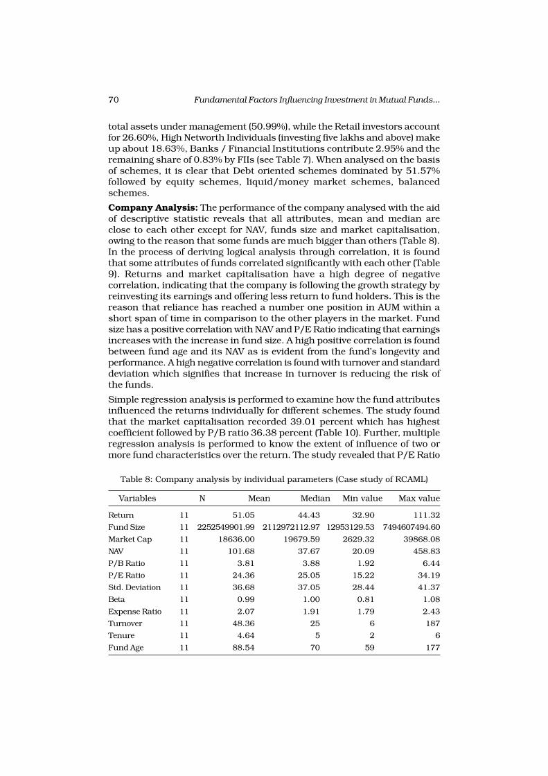
70 Fundamental Factors Influencing Investment in Mutual Funds...
total assets under management (50.99%), while the Retail investors accountfor 26.60%, High Networth Individuals (investing five lakhs and above) makeup about 18.63%, Banks / Financial Institutions contribute 2.95% and theremaining share of 0.83% by FIIs (see Table 7). When analysed on the basisof schemes, it is clear that Debt oriented schemes dominated by 51.57%followed by equity schemes, liquid/money market schemes, balancedschemes.
Company Analysis: The performance of the company analysed with the aidof descriptive statistic reveals that all attributes, mean and median areclose to each other except for NAV, funds size and market capitalisation,owing to the reason that some funds are much bigger than others (Table 8).In the process of deriving logical analysis through correlation, it is foundthat some attributes of funds correlated significantly with each other (Table9). Returns and market capitalisation have a high degree of negativecorrelation, indicating that the company is following the growth strategy byreinvesting its earnings and offering less return to fund holders. This is thereason that reliance has reached a number one position in AUM within ashort span of time in comparison to the other players in the market. Fundsize has a positive correlation with NAV and P/E Ratio indicating that earningsincreases with the increase in fund size. A high positive correlation is foundbetween fund age and its NAV as is evident from the fund’s longevity andperformance. A high negative correlation is found with turnover and standarddeviation which signifies that increase in turnover is reducing the risk ofthe funds.
Simple regression analysis is performed to examine how the fund attributesinfluenced the returns individually for different schemes. The study foundthat the market capitalisation recorded 39.01 percent which has highestcoefficient followed by P/B ratio 36.38 percent (Table 10). Further, multipleregression analysis is performed to know the extent of influence of two ormore fund characteristics over the return. The study revealed that P/E Ratio
Table 8: Company analysis by individual parameters (Case study of RCAML)
Variables N Mean Median Min value Max value
Return 11 51.05 44.43 32.90 111.32
Fund Size 11 2252549901.99 2112972112.97 12953129.53 7494607494.60
Market Cap 11 18636.00 19679.59 2629.32 39868.08
NAV 11 101.68 37.67 20.09 458.83
P/B Ratio 11 3.81 3.88 1.92 6.44
P/E Ratio 11 24.36 25.05 15.22 34.19
Std. Deviation 11 36.68 37.05 28.44 41.37
Beta 11 0.99 1.00 0.81 1.08
Expense Ratio 11 2.07 1.91 1.79 2.43
Turnover 11 48.36 25 6 187
Tenure 11 4.64 5 2 6
Fund Age 11 88.54 70 59 177

71
K.V
iyya
nn
a R
ao a
nd
Nirm
ala
Da
ita
Table 9: Correlation between variables (Case study of RCAML)
Variables Return Fund Size Market NAV P/B P/E S.D Beta Expense Turno- Te- Fund AgeCap Ratio Ratio Ratio ver nure
Return 1.0000
Fund Size -0.3453 1.0000
Market Cap -0.6246 0.1108 1.0000
NAV -0.1616 0.7733 0.1932 1.0000
P/B Ratio 0.6031 0.1110 -0.2217 0.1134 1.0000
P/E Ratio -0.0179 0.6032 0.0454 0.1635 0.6163 1.0000
S.D 0.1163 0.1497 -0.4751 0.0032 -0.2680 -0.0519 1.0000
Beta 0.1914 0.0445 -0.0573 -0.0371 0.5433 0.4753 -0.0735 1.0000
Expense Ratio 0.3019 -0.8387 -0.1854 -0.4947 0.0012 -0.5901 -0.1536 0.2024 1.0000
Turnover -0.3076 -0.2083 0.5740 -0.1460 -0.0394 -0.0632 -0.8308 0.1680 0.1226 1.0000
Tenure 0.1779 0.5889 -0.2213 0.5324 0.2630 0.2388 0.1361 -0.2727 -0.5827 -0.2384 1.0000
Fund Age -0.1684 0.6534 0.3501 0.9466 0.1085 0.0808 -0.0399 -0.1049 -0.4625 -0.0592 0.5479 1.0000

72 Fundamental Factors Influencing Investment in Mutual Funds...
Table 10: Simple regression results for RCAML
Coefficient t Stat P-value R square
Fund Size 3.191680596 -1.103615456 0.298392366 11.92 %
Market Cap -0.001243369 -2.399258270 0.039946436 39.01 %
NAV -0.026564211 -0.491358912 0.634932441 2.61 %
P/B Ratio 12.243123737 2.268403153 0.049492102 36.38 %
P/E Ratio -0.071578482 -0.053598544 0.958425904 0.03 %
Std. Deviation 0.710319911 0.351340607 0.733417652 1.35 %
Beta 52.794133550 0.584858387 0.573011153 3.66 %
Expense Ratio 25.202437214 0.950154610 0.366849568 9.12 %
Turnover -0.132500445 -0.969767593 0.357500560 9.46 %
Tenure 2.956225490 0.542432885 0.600691842 3.16 %
Fund Age -0.085834994 -0.512454265 0.620671860 2.84 %
Note: Confidence level 95 percent
Table 11: Multiple regressions results for RCAML
Coefficient t Stat P-value R square
Fund Size -5.633969096 -1.505363310 0.175948815 54.06 %
Market Cap -0.001275637 -2.449387238 0.044146915
NAV 0.071235519 1.056971056 0.325631420
P/B Ratio 20.101987606 3.525165176 0.007786851 60.85 %
P/E Ratio -2.517099779 -2.236167571 0.055757864
Std. Deviation 0.800526392 0.380125212 0.713745971 5.37 %
Beta 55.452383258 0.582800531 0.576082121
Expense Ratio 25.202437214 0.950154610 0.366849568 9.12 %
Turnover -0.109562046 -0.724735796 0.492122231 19.32 %
Tenure 5.170893855 0.743170316 0.481570583
Fund Age -0.180436658 -0.868793619 0.413753081
Note: Confidence level 95 percent
and P/B Ratio are significant in this context (Table 11). Growth variablessuch as return (P/B, P/E ratios) and popularity variables (fund size, marketcapitalisation, NAV) are found to be having significant influence on the returnof the funds.
Conclusion
It is evident from the study that the real economic variables consideredduring the period of study are not significantly influencing the investmentin mutual funds and even to predict the market movements. The study hasshown that, the state of the economy neither significant bearing on themutual fund market nor on the health of mutual funds. The study thushighlights the fact that there are certain other macro economic factors thatmight be exerting influence on the investment of mutual funds. Future

73K.Viyyanna Rao and Nirmala Daita
research could be carried out in that direction. The industry analysis hasrevealed the fact that the entire mutual fund industry is dominated by a fewplayers with big chunk of their Assets Under Management (57 percent).Further, the study reveals the fact closed-ended funds have lost their utilitywith the investing public. Company analysis has shown that P/B Ratio andP/E ratio have great impact on the returns produced by a fund followed byfund size and market capitalisation.
REFERENCES
Aggarwal, R. 1981. Exchange rates and stock prices: case study U.S capital marketsunder floating exchange rates. Akron Business and Economic Review, 12: 7-12.
Bhattacharya, B. 2002. Causal relationship stock market and exchange rates, foreignexchange reserves, values of trade balance: A case study of India. Cited from
www.igird.ac.in.
Black, A. et. Al. 2001. US Stock price and macro economics fundamentals. AberdeenWorking Papers, 1-3.
Demirgue–Kunt, A. 1995. Stock market development and financial intermediaries.Policy Research Working Paper, 14: 1-64.
Dickey, DA. and Fuller, WA. 1981. The likelihood ratio statistics for auto-regressivetime series with a unit root test. Economic, 49: 1057-1072.
Engle, R. and Granger, CW. 1987. Co-integration and error correction:Representation estimation and testing. Econometrica, 55: 251-276.
Fadhil, MH. Azizan, NA. and Shaharudin, RS. 2007. The interaction betweenmacroeconomic variable and the performance of mutual fund in Malaysia. MFA
9th conference -12th and 13th June.
Granger, CW. 1986. Some recent developments in the concept of causality. Journal
of Econometrics, 39: 194-211.
Humpe, A. Peter, M. 2009. Can macroeconomic variable explain long-term stockmarket movements? A comparison of the US and Japan. Applied Financial
Economics,19: 111-119.
Ibrahim, HM. 1999. Macroeconomics indicators and stock price in Malaysia: Anempirical analysis. Asian Economic Journal, 13 (2): 219-231.
Jha, R. 1996. Inflation targeting in India: Issues and Prospect. Reach School of
Pacific and Studies Journal, 02: 28-68.
Johansen, S. 1988. Statistical analysis of co-integration vectors. Journal of Econ.
Dyn. Control, 12: 231-254.
Kakani, R.K. Chatterjee, T. 2007. An alternate perspective on Bull Run in Indianmarkets. SPJ center IF Management Working Paper, 7: 1-13.
Kanakaraj, A. Sing, B.K. Alex, D. 2008. Stock prices, micro reasons and macroeconomy in India: What do data say between 1997-2007. Fox working paper, 3:1-17.
Nath, GC. Samanata, GP. 2000. Integration between forex and capital markets inIndia: an empirical exploration. Applied financial Economics, 7: 25-35.
Sarkar, S. Sarkar, T. 2005. Reforming financial markets in India’s strategic approach.SSRN.960532: 1-17.

74 Impact of Currency Future Trading on Base Metals Prices...The Indian Journal of Commerce
Vol. 64, No. 3, July-September 2011
Impact of Currency Future Trading on BaseMetals Prices: An Analytical Study
DEEPAK JAIN
In developed nations like US and UK, the relationship between physical
trading and volume and currency price is inverse in nature. This research
paper is an attempt to consider the investor behaviour regarding currency
future trading in India. The results were analysed with the help of statistical
tools and techniques i.e. Average method, and Karl Pearson Correlation
Coefficient Method. It is identified that there exits negative high degree of
correlation between Currency Future and four Base Metals except that of
Copper metal.
Introduction
Currency Futures can be defined as a standardised foreign exchange, wherederivatives contract traded on a recognised stock exchange to buy or sellone currency against another. Currency derivatives can be described ascontracts between sellers and buyers whose values are settled according tothe recognised exchange rate. Most of the exporters and importers use thecurrency derivatives for hedging purpose and some of the traders also usedthe currency derivatives as instruments for speculation. Currency futureor derivatives today makes the easiest way for the exporters and importersto hedge their fund. It helps them to restraint their investment and thishedging increase the volume in the currency future market. CurrencyDerivatives i.e. Currency Future is similar as Index future.
Currency Future are standardised in terms of contract sizes, settlementprocedures and traded on regulated exchanges. The contract size is fixedand is referred to as lot size. Future contract are traded through exchanges,the settlement of the contract is guaranteed by the exchange or clearingcorporation and hence there is no counter party risk. In India, the currencyfuture trading was started on 29th August 2008 in National Stock Exchange(NSE), in Multi Commodity Exchange (MCX) on 7th Oct. 2008 and in BombayStock Exchange on 1st Oct. 2008. Currency Future trading play a vital rolein developed nations and developing nations. It makes so much volatility inmetal prices in terms of online trading as well as in physical trading. Afterthe starting of currency future trading in India the volatility increased inthe MCX non precious metal. The total number of contract traded beforestarting of currency future trading in non precious metal are 84186 (lots)and after the starting of currency future trading 69358 (lots). It shows thatthere is lot of volatility in the metal market and sometimes it increases the
Dr. Deepak Jain is Assistant Professor, Shri Mata Vaishno Devi University, Katra -182320

75Deepak Jain
volume or it decreases the volume. Multi Commodity Exchange of India Ltd(MCX) is a state of the art electronic commodity future exchange.
Literature Review
Since the beginning of trading in financial futures and options in the 1970’s,the effect of financial derivatives trading on the underlying spot marketshas been of great interest to both academics and practitioners. One of theissues commonly investigated by finance researchers is whether futurestrading increases the price volatility of underlying markets and thus leadsto destabilisation of these markets. Previous studies provide mixed evidenceon this issue. Investigating the market behaviour (such as currency pricevolatility, metal market depth and trading volume) is an important aspect ofresearch on the market microstructure literature. Tauchen and Pitts (1983)argue that these three variables are closely related. However, most studiesdeal with mutual contemporaneous relationship between two of those threedimensions and reach no consistent results. Very few empirical papersinvestigate the dynamic nature of the interactions, such as the feedbackeffects between those three variables.
The relationship between currency future and trading volume has beenexamined frequently and usually is in a positive correlation between volatilityand trading volume. Copeland (1976), develop sequential arrival of informationmodels where new information flows into market to generate both tradingvolume and price movement. Karpoff (1987) identified relation between pricechanges and trading volume in financial markets. Eighteen of nineteenempircal papers support the positive correlation between volatility and tradingvolume. Bessembinder and Segun (1993) accommodate persistence in thepositive relationship on eight futures market by ARCH-GARCH empiricalmethod. There are few studies for the analysis of return volatility and tradingvolume incorporating with the market depth, which is proven to befundamentally related to trading activity and market behaviour of returnvolatility (Bessembinder and Seguin, 1992).
Some studies provide empirical results that support the opinion that tradingin futures can destabilize the spot market. For example, Figlewiski (1980)investigates the futures contracts for Treasury Bills (GNMA pass throughcertificates) and provides evidence that futures market activity increasesthe volatility of cash prices. More recent study by Bae, Kwon and Park (2004)focused on the effect of the introduction of index futures trading in the Koreanmarkets on spot price volatility. The authors concluded that introducingthe futures and options trading on the Korean stock exchange resulted inboth larger spot price volatility and greater market efficiency (allowing forquicker adjustment of market prices to information). Taylor (1998)investigates precious metals (gold, platinum and silver) reactions againstinflation. He tested the hypothesis that precious metals act as short-runand long-run hedges against inflation. He focused his analysis on the periodbefore 1939 and around the second OPEC oil shock in 1979. During noother period could precious metals be used to hedge inflation. His analysisnotices that the belief that precious metals (in particular gold) have alwaysacted as hedges against inflation until very recently is completed unfounded.

76 Impact of Currency Future Trading on Base Metals Prices...
He found that there have been particular periods during the last 80 yearswhen precious metals have been used as a short-run hedge against inflation,but they could not be used to hedge inflation around the first oil crisis in1973/74 or during the last ten years. Since he found a co integratedrelationship between metal prices and the level of CPI with the help of a VARmodel, it can be inferred that precious metals can be used as a long-runinflation hedge.
The combined average daily turnover of the currency futures contracts inall the three exchanges (NSE, BSE, MCX) increased from USD 1.1 billion inMarch 2009 to 2.5 billion in September 2009. This means a growth of morethan 125% in just six months period. The main objective of this paper is toanalyse the impact of Currency Future US$ on base metal with reference toIndia.
Research Hypothesis
H0: There is positive relationship between currency future US$ trading and
volume trading of base metals in Indian market.
H1: There is negative relationship between currency future US$ trading and
volume trading of base metals in Indian market
Research Methodology
The research design of the paper is causal in nature. Data was collectedfrom different journals, magazines, and internet sites. Data was analysedby Karl Pearson’s Correlation Coefficient Method.
Data collected was monitored on daily basis for twenty seven months. 5metals such as Aluminium, Copper, Lead, Nickel, and Zinc were taken intoconsideration and their day to day prices were collected and averaged fortwenty seven months.
Discussion
The impact of currency future i.e. US$ on base metals depend on the day today trading prices of currency as well as metals. To find out the impact ofcurrency on base metals we need the daily transaction prices, for this wecollect it from secondary resources.
Table 1: Average closing rate of five different base metals and exchange rate of US$
in Indian rupee (Yearly/Quarterly/Monthly)
Year wise Exchange Rate Alu- Copper Lead Nickel ZincMonthly details of US$ (INR) minium
2008: Quarter 4
October 49.19 102.96 230.27 71.31 567.65 62.00November 49.16 91.91 187.13 64.21 540.38 57.65December 48.80 73.38 152.75 47.27 481.86 54.44Mean 49.05 89.42 190.05 60.93 529.96 58.03Standard deviation 0.22 14.95 38.84 12.35 43.83 3.79Value of ‘R’ 0.952 0.868 0.975 0.970 0.857
contd...

77Deepak Jain
2009: Quarter 1
January 48.93 70.11 161.84 55.75 564.14 59.14
February 49.33 66.32 165.30 54.42 516.73 55.57
March 51.35 68.98 195.43 64.18 500.56 63.17
Mean 49.87 68.47 174.19 58.12 527.14 59.29
Standard deviation 1.30 1.95 18.48 5.29 33.04 3.80
Value of ‘R’ 0.074 0.998 0.961 -0.799 0.800
2009: Quarter 2
April 50.11 72.56 225.97 70.25 567.19 69.98
May 48.58 71.39 225.93 70.46 616.29 72.54
June 47.86 76.07 241.59 80.00 717.74 74.88
Mean 48.85 73.34 231.16 73.57 633.74 72.47
Standard deviation 1.15 2.44 9.03 5.57 76.78 2.45
Value of ‘R’ -0.564 -0.745 -0.759 -0.920 -0.984
2009: Quarter 3
July 48.50 81.30 254.93 81.40 715.30 76.90
August 48.38 93.25 299.62 92.52 936.68 88.20
September 48.52 89.15 302.76 106.96 844.04 91.19
Mean 48.47 87.90 285.77 93.63 832.01 85.43
Standard deviation 0.08 6.07 26.75 12.82 111.18 7.54
Value of ‘R’ -0.671 -0.326 0.206 -0.732 -0.190
2009: Quarter 4
October 46.73 88.20 298.31 104.95 868.83 97.30
November 46.58 91.38 312.38 107.43 792.86 102.66
December 46.66 102.41 330.51 109.12 808.17 111.75
Mean 46.66 94.00 313.73 107.17 823.29 103.90
Standard deviation 0.08 7.46 16.14 2.10 40.18 7.30
Value of ‘R’ -0.175 -0.401 -0.560 0.932 -0.331
2010: Quarter 1
January 46.00 103.11 339.52 108.98 852.54 111.78
February 46.37 95.74 319.70 99.36 886.78 100.50
March 45.55 101.00 341.79 99.33 1024.22 104.03
Mean 45.97 99.95 333.67 102.56 921.18 105.44
Standard deviation 0.41 3.80 12.15 5.56 90.86 5.77
Value of ‘R’ -0.651 -0.884 0.059 -0.792 -0.252
2010: Quarter 2
April 44.52 103.75 346.13 101.09 1155.72 105.93
May 45.78 94.55 317.15 87.12 1014.32 91.27
June 46.65 90.25 302.74 79.90 906.59 81.89
Mean 45.65 96.18 322.01 89.37 1025.54 93.03
Standard deviation 1.07 6.90 22.10 10.77 124.94 12.12
Value of ‘R’ -0.995 -0.996 -0.997 -1.000 -1.000
contd...
contd...

78 Impact of Currency Future Trading on Base Metals Prices...
2010: Quarter 3
July 46.92 93.77 318.31 86.95 921.26 87.13
August 46.70 98.22 341.41 97.36 1003.43 96.14
September 46.14 100.34 357.69 101.24 1054.40 99.58
Mean 46.59 97.44 339.14 95.18 993.03 94.28
Standard deviation 0.40 3.35 19.79 7.39 67.18 6.43
Value of ‘R’ -0.901 -0.941 -0.875 -0.928 -0.878
2010: Quarter 4
October 44.55 104.70 371.56 106.45 1060.99 105.98
November 45.10 105.36 382.68 107.11 1033.46 103.43
December 45.24 106.96 417.10 109.34 1092.18 103.46
Mean 44.96 105.67 390.45 107.63 1062.21 104.29
Standard deviation 0.36 1.16 23.74 1.51 29.38 1.46
Value of ‘R’ 0.844 0.815 0.805 0.227 -0.979
The quarter 2008 (4) shows, there exits high positive correlation between exchangerate of US$ and Prices of Base Metals. We can also infer there exist a direct linearrelation between two variables. The quarter 2009 (1) shows, there exits high positivecorrelation between exchange rate of US$ and Prices of three base metals i.e. Copper,Lead and Zinc, but very low positive correlation relationship with Aluminium in thequarter. Negative high correlation is with Nickel. The quarter 2009 (2) shows, thereexits high negative correlation between exchange rate of US$ and Prices of three basemetals i.e. Lead, Nickel and Zinc, but very moderate negative correlation relationshipwith Aluminium and Copper. The quarter 2009 (3) shows, there exits negative moderatecorrelation between exchange rate of US$ and Prices of three base metals i.e.Aluminium, Copper and Nickel; whereas, negative low correlation relationship withZinc but positive correlation with Lead. The quarter 2009 (4) shows, there exits negativemoderate correlation between exchange rate of US$ and Prices of three base metalsi.e. Copper, Zinc and Lead; whereas, negative low correlation relationship withAluminium. Positive high correlation relationship exits with Nickel. The quarter 2009(5) shows, there exits negative high correlation between exchange rate of US$ andPrices of two base metals i.e. Copper and Nickel; whereas, negative moderate correlationrelationship with Aluminium and Zinc. Very low but positive correlation relationshipexits with Lead. The quarter shows, there exits perfectly negative correlation betweenexchange rate of US$ and Prices of two base metals i.e. Zinc and Nickel; whereas,negative highly correlation relationship with remaining three metals. The quartershows, there exits high degree of negative correlation between exchange rate of US$and Prices of all five base metals. ACLNZ. Interpretation: The quarter shows, thereexits high degree of positive correlation between exchange rate of US$ and Prices ofthree base metals i.e. Aluminium, Copper, and Lead; where as negative high degreecorrelation with Zinc prices, but low positive correlation with Nickel prices.
Overall details for 27 months
Overall Mean 47.34 90.26 286.69 87.57 816.46 86.24
Overall Standard 1.78 13.01 72.68 19.43 209.52 18.84deviation
Value of ‘R’ -0.787 -0.267 -0.770 -0.897 -0.850
Overall, there exists high degree of negative correlation with all four metals except
that of Copper which have low but negative degree of correlation.
contd...

79Deepak Jain
Overall analysis for 27 months showed there exists negative correlationbetween Prices of Base Metals and Exchange rate of US$ It can also beinferred that when the currency future prices rise, the base metals pricesdecrease and vice-versa. This approves our alternative hypothesis.
Table 2: Pattern identified amongst prices of base metals and exchange rate of US$(compared with next quarter ‘Mean of ER of US$’ and ‘R’ Value)
Quarter Exchange Alu- Copper Lead Nickel ZincRate of minium
US$ (INR)
2008Q4 49.05 × 0.952 × 0.868 × 0.975 × 0.97 × 0.857 ×
2009Q1 49.87 × 0.074 × 0.998 × 0.961 × -0.799 × 0.8 ×
2009Q2 48.85 × -0.564 × -0.745 × -0.759 × -0.92 × -0.984 ×
2009Q3 48.47 × -0.671 × -0.326 × 0.206 × -0.732 × -0.19 ×
2009Q4 46.66 × -0.175 × -0.401 × -0.56 × 0.932 × -0.331 ×
2010Q1 45.97 × -0.651 × -0.884 × 0.059 × -0.792 × -0.252 ×
2010Q2 45.65 × -0.995 × -0.996 × -0.997 × -1 × -1 ×
2010Q3 46.59 × -0.901 × -0.941 × -0.875 × -0.928 × -0.878 ×
2010Q4 44.96 × 0.844 × 0.815 × 0.805 × 0.227 × -0.979 ×
Copper and Zinc showed strong inverse relationship with the changing pattern inExchange Rate of US$ (Table2).
Table 3: Pattern identified amongst prices of base metals and exchange rate of US$(compared with overall ‘Mean of ER of US$’ and ‘R’ Value)
Quarter Exchange Alu- Copper Lead Nickel ZincRate of minium
US$ (INR)
2008Q4 49.05 × 0.952 × 0.868 × 0.975 × 0.97 × 0.857 ×
2009Q1 49.87 × 0.074 × 0.998 × 0.961 × -0.799 × 0.8 ×
2009Q2 48.85 × -0.564 × -0.745 × -0.759 × -0.92 × -0.984 ×
2009Q3 48.47 × -0.671 × -0.326 × 0.206 × -0.732 × -0.19 ×
2009Q4 46.66 × -0.175 × -0.401 × -0.56 × 0.932 × -0.331 ×
2010Q1 45.97 × -0.651 × -0.884 × 0.059 × -0.792 × -0.252 ×
2010Q2 45.65 × -0.995 × -0.996 × -0.997 × -1 × -1 ×
2010Q3 46.59 × -0.901 × -0.941 × -0.875 × -0.928 × -0.878 ×
2010Q4 44.96 × 0.844 × 0.815 × 0.805 × 0.227 × -0.979 ×
Mean 47.34 -0.787 -0.267 -0.77 -0.897 -0.85value for27 months
There exists high level of volatility in prices of Copper metal followed byAluminium and Copper if compared with overall means of ER of US$ and ‘R’Value for twenty seven months (Table 3).
Conclusion
The data analysis proves that high degree of negative correlation in fourmetals to Currency future except that of copper. When there is volatility in

80 Impact of Currency Future Trading on Base Metals Prices...
the currency future and base metals, it impacts the relation between them.Sometimes it makes the positive relation between currency future and basemetals and sometimes it makes the negative relation between them. Whenthe prices volatility increases in base metals it creates the problem in physicalmetals trading that impact directly or indirectly to the economic condition ofour nation. The data analysis represents the inverse linear relationshipbetween currency future and base metals.
REFERENCES
Antoniou A., Holmes P. 1995. Futures trading, information and spot price volatility:evidence for the FTSE-100 Stock Index Futures contract using GARCH. Journal
of Banking and Finance 19, pp. 117-129.
Bae S.C., Kwon T.H., Park J.W. 2004. Futures trading, spot market volatility, andmarket efficiency: the case of the Korean index futures markets. The Journal of
Futures Markets, Vol. 24, No. 12, pp. 1195–1228.
Bessembinder H., Seguin P.J. 1993. Price volatility, trading volume, and marketdepth: evidence from futures markets. The Journal of Financial and Quantitative
Analysis, Vol. 28, No. 1, pp. 21-39.
Bessembinder H., Seguin P.J. 1992. Futures-trading activity and stock price volatility.The Journal of Finance, Vol. XLVII, No. 5, pp. 2015-2034
Copeland, T. 1976. A model of asset trading under the assumption of sequentialinformation arrival. Journal of Finance 31, 1149–1168.
Figlewski S. 1980. Futures trading and volatility in the GNMA market. The Journal
of Finance, Vol. 36, No. 2, pp. 445-456.
Karpoff, J.M. 1987. The relationship between price changes and trading volume: asurvey.” Journal of Financial and Quantitative Analysis 22, 109–126.
Malliaris A.G. 1997. Futures markets: Why are they different? The InternationalLibrary of Critical Writings in Financial Economics. An Elgar ReferenceCollection, pp. xi-xxix.
Tauchen, G. and M. Pitts. 1983. The Price variability – volume relationship onspeculative markets.” Econometrica 51, 485–505.
Taylor, N. 1998. Precious metals and inflation, Applied Financial Economics, 1998,vol. 8, pages 201-210.
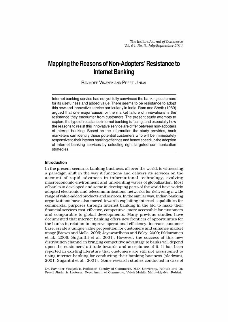
81Ravinder Vinayek and Preeti Jindal
Mapping the Reasons of Non-Adopters’ Resistance toInternet Banking
RAVINDER VINAYEK AND PREETI JINDAL
Internet banking service has not yet fully convinced the banking customers
for its usefulness and added value. There seems to be resistance to adopt
this new and innovative service particularly in India. Ram and Sheth (1989)
argued that one major cause for the market failure of innovations is the
resistance they encounter from customers. The present study attempts to
explore the type of resistance internet banking is facing, and especially how
the reasons to resist this innovative service are differ between non-adopters
of internet banking. Based on the information the study provides, bank
marketers can identify those potential customers who will be immediately
responsive to their internet banking offerings and hence speed up the adoption
of internet banking services by selecting right targeted communication
strategies.
Introduction
In the present scenario, banking business, all over the world, is witnessinga paradigm shift in the way it functions and delivers its services on theaccount of rapid advances in informational technology, evolvingmacroeconomic environment and unrelenting waves of globalization. Mostof banks in developed and some in developing parts of the world have widelyadopted electronic and telecommunications networks for delivering a widerange of value-added products and services. In the similar way, Indian bankingorganizations have also moved towards exploiting internet capabilities forcommercial purposes through internet banking in the bid to make theirfinancial services cost-effective, competitive, more accessible for customersand comparable to global developments. Many previous studies havedocumented that internet banking offers new frontiers of opportunities forthe banks in relation to improve operational efficiency, increase customerbase, create a unique value proposition for customers and enhance marketimage (Brown and Molla, 2005; Jayawardhena and Foley, 2000; Pikkarainenet al., 2006; Suganthi et al. 2001). However, the success of this newdistribution channel in bringing competitive advantage to banks will dependupon the customers’ attitude towards and acceptance of it. It has beenreported in existing literature that customers are still not accustomed tousing internet banking for conducting their banking business (Aladwani,2001; Suganthi et al., 2001). Some research studies conducted in case of
Dr. Ravinder Vinayek is Professor, Faculty of Commerce, M.D. University, Rohtak and Dr.Preeti Jindal is Lecturer, Department of Commerce, Vaish Mahila Mahavidyalya, Rohtak
The Indian Journal of Commerce
Vol. 64, No. 3, July-September 2011

82 Mapping the Reasons of Non-Adopters’ Resistance to Internet Banking
India are also in the agreement that a large portion of customers hesitate touse internet banking to manage their financial affairs and it is not beingpopularly adopted in India (IAMAI, 2006; Ravi et al., 2007).
Review of Existing Literature
A thorough review of existing research studies undertaken to identify factorsresisting customers to bank upon internet reveals that although manystudies (Al-Sabbagh and Molla, 2004; Chung and Paynter, 2002; Geetika etal., 2008; Laukkanen et al., 2008; ; Lee et al., 2005; Mattila et al. 2001;Mattila et al., 2003; Mittal and Gandhi, 2008; Nor and Pearson, 2007;Padachi, et al., 2008; Ramayah et al., 2006; Sathye, 1999; Sudha et al.,2007; Suganthi et al., 2001) have been geared to address this issuethroughout the world, but except very few (such as Laukkanen et al., 2008;Lee et al., 2005) most of these studies seem to have dichotomous view ofadopters versus non-adopters in regard of investigating the reasons for theresistance to internet banking. It will be more revealing if the differences inresistance among non-adopters who have varying degree of behavioralintention to adopt internet banking are studied.
Table 1: Summary of studies dealing with factors resisting customers toadopt internet banking
Study Research Tools of FindingsSettings and DataSample Size Analysis
Studied
Sathye(1999)
Mattila et al.(2001)
Suganthi etal. (2001)
Chung andPaynter(2002)
Australia612
Finland350
Malaysia300
New-Zealand109
FactorAnalysis
FactorAnalysis
FactorAnalysisfollowedby T-test
FrequencyAnalysisfollowed byCorrelationAnalysis
The study identified concern aboutsecurity of transactions, concern aboutease of use, lack of awareness of internetbanking services and benefits, ambiguityabout cost of services, resistance tochange and lack of accessibility of theinternet to be major inhibitors ofcustomers’ adoption of internet banking.
The study found lack of personal service,time consuming and security concern tobe major barriers to internet bankingadoption.
The study found that lack of trust,security of internet transaction,reluctance to change and preference forhuman interface had an adverse impacton the decision to adopt internetbanking.
The study identified security concern,likings of personal contacts, has not triedit before, perceived complexity and don’tneed instant 24 hours access to accountto be factors resisting customers to useinternet banking.
contd...

83Ravinder Vinayek and Preeti Jindal
Mattila et al.(2003)
Al-Sabbaghand Molla(2004)
Lee et al.(2005)
Ramayah etal. (2006)
Nor andPearson(2007)
Geetika et al.(2008)Mittal andGandhi(2008)
Laukkanenet al. (2008)
Padachi etal. (2008)
Finland1167
Oman205
USA1349
NorthernMalaysia180
Malaysia1164
India200India140
Finland302
Island188
FactorAnalysis
DescriptiveAnalysis
MultinomialLogitModeling
DiscriminantAnalysis
SEM(StructuralEquationModeling)
T-test
T-test
ANOVA
Cross-Tabulation
The study identified perceived difficultyin using computers, concern aboutsecurity and lack of personal service tobe significant barriers in the adoptionof e-banking.
The study found concern about security,preference for face to face personalbanking as major deterrents to internetbanking adoption.
The study found non-adopters to be moreconcerned about the security and privacyof transactions conducted over internetas compared to adopters.
The study found internet banking usersto be more aware about the benefits ofinternet banking services, having priorinternet experience, having positive viewsabout the ease of use and security incontrast to non-users of internet banking
The results showed that trust intechnology, relative advantage andtrialability had significant influence onthe customers’ attitude towards thelikelihood of adopting internet banking.
The study found non-users far more con-scious for the security than that of users.
The study found that internet bankingusers were mid-aged male, moretechnology-oriented, well-awaked aboutthe benefits of internet banking andconvenience-mined consumers on onehand. And on the other hand, it foundnon-users to be younger or older, moretraditional-oriented, less familiar aboutthe benefits of internet banking andhaving lack of confidence of using thisinnovative service.
The findings of the study revealed thatresistance to internet banking of theRejecters was much more intense anddiverse than that of the Opponents,while the Postponers showed only slightresistance. And Security and privacyconcern tend to resist all three identifiednon-adopter categories uniformly.
The study found awareness, access tointernet facility, length of bankingrelationship, people working in theinternet banking/finance sector,education level and income to besignificantly correlated with the adoptionof internet banking.
contd...

84 Mapping the Reasons of Non-Adopters’ Resistance to Internet Banking
Variables Known to Resist Adoption of Internet Banking
The Variables are: Prior Knowledge, Awareness, Amount of Information,Scarcity and Privacy Concern, Fear of Committing Error, PerceivedComplexity, Lack of Interest, Lack of Accessibility to Internet.
Research Methodology
Sample Design: The present study is exploratory in nature. The populationof the interest for the present study has been retail customers of four Indianscheduled commercial banks consisting of two public sector banks, namely,State Bank of India (SBI) and Punjab National Bank (PNB) and two privatesector banks, namely, ICICI bank and HDFC bank. The study carried out aquestionnaire survey to gather data from the targeted population withinRohtak, Panipat, Gurgaon located in North India during July-December 2009.Respondents have been chosen by Judgmental sampling method. A total of600 questionnaires have been administered to those adult individualcustomers who have bank account in the CBS branches either in publicsector banks or in private sector banks under reference for a period ofapproximately one year or more.
Survey Instrument: A five-point Likert scale ranging from strongly disagree(1) to strongly agree (5) has been used to measure the level of agreementwith each of the 8 variables. The possible range of scores is 1 to 5 with highscores reflecting high degree of resistance. Mean score more than 3 attestexistence of resistance. Second part of this section designed to evince non-adopters’ intention to use/reject internet banking in future so as to categorizethem into three different segments based on their intention about adoptinginternet banking. First segment belongs to the customers intending to adoptinternet banking within next 12 months. Second segment comprisescustomers intending to adopt internet banking but have not yet decidedwhen to adopt. Third segment relates to those who do not intend to adoptinternet banking at all.
Procedure: Before conducting a full-fledged survey, the questionnairedeveloped for the study has been subjected to pilot study among 50 bankcustomers via personal interview method to confirm the face validity andreliability of the questionnaire after pre-testing by the experts, academicand professional. Based on feedback received, necessary revisions concerningrewording, clarity and consistency of the items were made. The finalizedquestionnaire has then been issued to a total of 600 targeted subjects.
Data Collection and Sample Description: Out of the total 600questionnaires issued, 512 usable questionnaires were collected, resultingin 85.3% valid response rate. Of the 512 respondents 316 respondents havebeen found not having experience of using internet banking and 196respondents have been found availing internet banking service. Since theinterest of the study in those respondents who are not having experience ofusing internet banking service, users of internet banking do not constitutethe part of the present study. Furthermore, from the 316 non-adopters, we

85Ravinder Vinayek and Preeti Jindal
analyzed inputs from those non-adopters who have heard about internetbanking (n=264). Those non-adopters who answered that they have not heardabout the internet banking service (n=52) have been removed from the furtheranalysis. The justification lies in the fact that it will make the results morerevealing to study the responses of those customers who are still not inclinedto use internet banking in spite of being aware about the prevalence of thisservice. As to the intention to start using internet banking service in future,of the 264 non-adopters, 74 (28.03 per cent) are those intending to adoptinternet banking within next 12 months, 129 (48.9 per cent) are thoseintending to adopt this service but have not decided when, and finally, 61(23.1 per cent) are those reporting that they would not go to adopt internetbanking at all. In the line of the Laukkanen et al.’s (2008) research thepresent study named these three non-adopters segments as Postponers,Opponents and Rejecters respectively.
Reliability Analysis: Collected data on perception of barriers deterring toadopt internet banking have been first analyzed for reliability analysis usingCronbach’ Alpha Model. As alpha value of all eight variables underconsideration has been found to be .615 which is above the commonlyaccepted threshold of .60 (Hair et al., 1998), all variables are deemed reliablefor subsequent analysis.
Statistical Analysis: To investigate the reasons for the resistance of internetbanking, the data so collected has been first subjected to descriptivestatistical analysis to measure the intensity of different causes of resistanceto internet banking on aggregate level by computing mean score for each ofthe variable. Thereafter, One-way ANOVA (Analysis of Variance) has beenperformed using intention to adopt internet banking as group variable(independent variable) and factors causing resistance to internet bankingas dependent variables. The ultimate goal of this analysis is to ascertainwhether the average perceptions (of the issues under investigation) havebeen identical for all non-adopter groups i.e. Posponers, Opponents andRejecters (formed based on their intention to adopt/reject internet bankingin future) involved in this survey. These statistical techniques have beenconducted through SPSS (Statistical Package for Social Science) version 17for windows.
Analysis and Discussion
Descriptive Statistical Analysis: Table 2 displays the results of descriptivestatistical analysis based on mean responses measured in 5-point Likert-Scale.
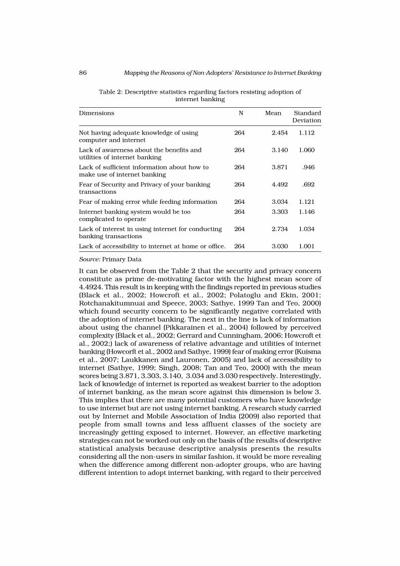
86 Mapping the Reasons of Non-Adopters’ Resistance to Internet Banking
Table 2: Descriptive statistics regarding factors resisting adoption ofinternet banking
Dimensions N Mean StandardDeviation
Not having adequate knowledge of using 264 2.454 1.112computer and internet
Lack of awareness about the benefits and 264 3.140 1.060utilities of internet banking
Lack of sufficient information about how to 264 3.871 .946make use of internet banking
Fear of Security and Privacy of your banking 264 4.492 .692transactions
Fear of making error while feeding information 264 3.034 1.121
Internet banking system would be too 264 3.303 1.146complicated to operate
Lack of interest in using internet for conducting 264 2.734 1.034banking transactions
Lack of accessibility to internet at home or office. 264 3.030 1.001
Source: Primary Data
It can be observed from the Table 2 that the security and privacy concernconstitute as prime de-motivating factor with the highest mean score of4.4924. This result is in keeping with the findings reported in previous studies(Black et al., 2002; Howcroft et al., 2002; Polatoglu and Ekin, 2001;Rotchanakitumnuai and Speece, 2003; Sathye, 1999 Tan and Teo, 2000)which found security concern to be significantly negative correlated withthe adoption of internet banking. The next in the line is lack of informationabout using the channel (Pikkarainen et al., 2004) followed by perceivedcomplexity (Black et al., 2002; Gerrard and Cunningham, 2006; Howcroft etal., 2002;) lack of awareness of relative advantage and utilities of internetbanking (Howcorft et al., 2002 and Sathye, 1999) fear of making error (Kuismaet al., 2007; Laukkanen and Lauronen, 2005) and lack of accessibility tointernet (Sathye, 1999; Singh, 2008; Tan and Teo, 2000) with the meanscores being 3.871, 3.303, 3.140, 3.034 and 3.030 respectively. Interestingly,lack of knowledge of internet is reported as weakest barrier to the adoptionof internet banking, as the mean score against this dimension is below 3.This implies that there are many potential customers who have knowledgeto use internet but are not using internet banking. A research study carriedout by Internet and Mobile Association of India (2009) also reported thatpeople from small towns and less affluent classes of the society areincreasingly getting exposed to internet. However, an effective marketingstrategies can not be worked out only on the basis of the results of descriptivestatistical analysis because descriptive analysis presents the resultsconsidering all the non-users in similar fashion, it would be more revealingwhen the difference among different non-adopter groups, who are havingdifferent intention to adopt internet banking, with regard to their perceived

87Ravinder Vinayek and Preeti Jindal
factors of resistance is studied. Since all non-users do not carry equalprobability of adoption it would be inappropriate to approach all non-usersas a homogeneous population (Lee et al., 2005). As already discussed, it is ofparamount importance to understand the diversity of resistance betweendifferent non-adopters because it can better help the banking organizationin identifying profitable segment of non-users, thereby employing rightpromotional strategies. To address this issue, inferential statistical analysisis undertaken.
Inferential Statistical Analysis: One-way ANOVA (Analysis of Variance) isnext used to analyze statistical differences in resistance to internet bankingamong three groups of non-adopters i.e. Posponers, Opponents and Rejecters.
It is observed from the Table 3 that except security and privacy concern,there are significant differences among different non-adopters categories,
Not having adequateknowledge of usingcomputer and internet
Lack of awarenessabout the benefits andutilities of internetbanking
Lack of sufficientinformation abouthow to make use ofinternet banking
Fear of Security andPrivacy of yourbanking transactions
Fear of making errorwhile feedinginformation
Internet bankingsystem would be toocomplicated to operate
Lack of interest inusing internet forconducting bankingtransactions
Lack of accessibility tointernet at home oroffice.
Table 3: ANOVA result examining the differences among Postponers, Opponentsand Rejecters regarding factors resisting them to adopt internet banking
Dimensions Postponers Opponents Rejecters F- Sig.(N=74) (N=129) (N=61) Value
Mean SD Mean SD Mean SD
1.473 .502 2.751 1.000 3.016 1.131 59.538 .000*
2.851 1.130 3.178 .987 3.409 1.054 4.943 .008*
3.635 1.105 3.961 .860 3.967 .874 3.254 .040*
4.459 .601 4.511 .740 4.491 .698 .133 .876
2.837 1.034 2.891 1.201 3.573 .865 9.865 .000*
2.378 1.094 3.612 .912 3.770 1.022 45.198 .000*
2.283 .672 2.403 .667 3.983 1.056 103.342 .000*
2.729 .969 3.007 1.003 3.442 .904 9.059 .000*
Source: Primary DataNote: * Denotes significant at 5% level of significance

88 Mapping the Reasons of Non-Adopters’ Resistance to Internet Banking
namely, Postponers, Opponents and Rejecters with respect to all the factorsdeterring them to adopt internet banking. Security and privacy concern isthe most intense and uniformly perceived barrier to the adoption of internetbanking among all three groups. This result supports the findings ofLaukkanen et al. (2008) and Lee et al. (2005). A closer look at the resultsreveals that resistance to internet banking on the part of Postponers is notintense and diverse in contrast to Opponents and Rejecters. Security andprivacy concerns followed by lack of information about using internet bankingseem to prevent Postponers to adopt internet banking. An examination ofOpponents’ results reveals that in addition to sharing Postponers’ causes ofresistance to internet banking with greater intensity, they perceive internetbanking as more complex to use. They seem to think that internet bankingwould be complicated to operate. They are also having doubts about thepotential benefits and utilities of internet banking. However, lack ofaccessibility to internet does not appear causing resistance amongOpponents, as the mean score against this variable is almost equal to 3. Asfar as Rejecters are concerned, their resistance to internet banking is moreintense and diverse than that of other two groups. They not only report highresistance of internet banking on the ground of all those barriers what twoother groups report, but also they have negative interest of using internetbanking and concern to the fear of feeding wrong information. Lack ofaccessibility to internet can also be noticed as barrier to adoption of internetbanking among Rejecters. They are having relatively less knowledge of usinginternet in comparison other two groups, but this seems not a great causeof resistance, as the mean score against this variable is slightly above 3. Inthe order of intensity, the most intense barrier among Rejecters is clearlylack of interest that differentiates most this group from other two groups.These findings are in corroboration with the results reported by Gerrard etal. (2006) and Mattila et al. (2003) that lack of interest in using internet aschannel to conduct banking transactions adversely affects intention to useinternet banking. All in all, findings of present study reflects heterogeneityof non-adopter population of internet banking in the line of Lee et al. (2005)and Laukkanen et al. (2008).
Conclusion
The present study furthers the understanding of how the reasons to resistthe internet banking differ between non-adopters of internet banking. Anexamination of ANOVA results reveal that security and privacy concern isthe major and identical barrier that tend to hamper the willingness to adoptinternet banking of all three non-adopter segments of internet bankinguniformly. With the exception of security and privacy concern, there existssignificant difference among the identified three non-adopter segments i.e.Postponers (those who intend to use internet banking within 12 nextmonths), Opponents (those who intend to use internet banking but notdecided when) and Rejecters (those who do not intend to use internet bankingat all) in respect of their reasons for the resistance to internet banking.Postponers seem to register resistance to internet banking because of Securityand privacy concern and lack of adequate information of how to use internet

89Ravinder Vinayek and Preeti Jindal
banking. Opponents demonstrate resistance not only on the ground of thosebarriers reported by Postponers but also they tend to perceive internetbanking complex to use and having doubts about the utilities and benefitsof internet banking. However, lack of accessibility to internet does not appearcausing resistance among Opponents, as the mean score against thisvariable is almost equal to 3. As far as Rejecters are concerned, they seemto be more challenging ones, as they report résistance to internet bankingon the various grounds than that of Postponers and Opponents. In additionto sharing concerns reported by other two groups regarding internet bankingrisks with greater intensity, they seem to have negative interest towardsusing internet banking and concern to the fear of feeding wrong information.They also seem to attach resistance due to lack of accessibility to internet.The findings of the present study are consistent with the results of Lee et al.(2005) and Laukkenen et al. (2008) studies which reported security andprivacy to be most intense barrier to the adoption of internet banking.Furthermore, in the line of these studies, the present study reinforces thatnon-adopters do not constitute homogeneous population but are ratherheterogeneous population, as they differ from each other in their resistanceto internet banking. Hence, the study emphasizes the need to devise distinctpromotional strategies as per the attitudinal feature of targeted non-adoptersegment.
REFERENCES
Aladwani, A. 2001. Online banking a field study of drivers, development, challengesand expectations. International Journal of Information Management, 21 (3): 213-225.
Al-Sabbagh, Imtiyaz and Molla, Alemayehu 2004. Adoption and use of internetbanking in sultanate of Oman: an exploratory study. Journal of Internet Banking
and Commerce, http://www.arraydev.com/commerce/jibc/0406-07.asp,accessed on 28-01-2008.
Alter, S. 2002. Information system: the foundation of e-business. New Jersey: PrenticeHall.
Black, Nancy Jo, Lockett, Andy, Ennew, Christine, Winklhofer, Heidi and McKechnie,Sally 2002. Modeling consumer choice of distribution channels: an illustrationfrom financial services. International Journal of Bank Marketing, 20 (4): 161-173.
Brown, I. and Molla, A. 2005. Determinants of internet and cell phone banking inSouth Africa, Journal of Internet Banking and Commerce,http://www.arraydev.com/commerce/jibc/2005-02/brown.HTM, accessed on 24-03-2009.
Chung, Winnie and Paynter, John 2002. An evaluation of internet banking in New-Zealand. in Proceedings of the 35th Hawaii International Conference on System
Sciences (HICSS), http://www2.computer.org/portal/web/csdl/doi/10.1109/HICSS.2002.994178, accessed on 30-06-2007.
Daniel, E. 1999. Provision of electronic banking in the UK and the republic ofIreland. International Journal of Bank Marketing, 17 (2): 72-82.

90 Mapping the Reasons of Non-Adopters’ Resistance to Internet Banking
Geetika, Nandan, Tanuj and Upadhyay, Ashwani Kr. 2008. Issues and prospects ofinternet banking in India: a customer perspective. The ICFAI Journal of Bank
Management, 7 (2): 1-16.
Gerrard, P., Cunningham, J. B. and Devlin, J. F. 2006. Why consumers are notusing internet banking: a qualitative study. Journal of Service Marketing, 20(3):160-168.
Hair, J.F., Anderson, R.E., Tatham, R.L. and Black, W.C. 1998. Multivariate data
analysis. New Jersey: Prentice-Hall.
Howcroft, B., Hamilton, R. and Heder, P. 2002. Consumer attitude and the usageand adoption of home-based banking in United-Kingdom. International Journal
of Bank Marketing, 20 (3): 111-121.
IAMAI 2006. IAMAI’s report online banking ‘2006’. http://www.iamai.in/pdf/IAMAI_Report_on_Online_Banking_2006.pdf, accessed on 23-02-2008.
Jayawardhena, C. and Foley, P. 2000. Changes in banking sector – the case ofinternet banking in UK. Journal of Internet Research: Networking and Policy, 10(1): 19-30.
Karjaluoto, Heikke, Mattila, Minna and Pento, Tapio 2002. Factors underlyingattitude formation towards online banking in Finland. International Journal of
Bank Marketing, 20 (6): 261-272.
Kuisma, T., Laukkanen, T. and Hiltunen, M. 2007. Mapping the reasons for theresistance to internet banking: a means-end approach. International Journal of
Information Management, 27 (2): 75-85.
Laukkanen, T. and Lauronen, J. 2005. Consumer value creation in mobile bankingservices. International Journal of Mobile Communications, 3 (4): 325-338.
Laukkanen, Pekka, Sinkkonen, Suvi and Laukkanen, Tommi 2008. Consumerresistance to internet banking: postponers, opponents and rejectors. The
International Journal of Bank Marketing, 26 (6): 440-455.
Lee, E. J. and Lee, J. 2000. Consumer adoption of internet banking: need basedand/or skill based. Marketing Management Journal, 11 (1): 101-113.
Lee, Eun-Ju, Kwon, Kyoung-Nan and Schumann, David W. 2005. Segmenting thenon-adopter category in the diffusion of internet banking. International Journal
of Bank Marketing, 23 (5): 414-437.
Mattila, Minna, Karjaluoto, Heikki and Pento, Tapio 2001. Internet banking adoptionfactors in Finland. Journal of Internet Banking and Commerce, http://www.arraydev.com/commerce/JIBC/MATTILA.HTM, accessed on 26-05-2008.
Mattila, Minna, Karjaluoto, Heikki and Pento, Tapio 2003. Internet banking adoptionamong mature customers: early majority or laggards?. Journal of Service
Marketing, 17 (5): 514-528.
Mittal, R.K. and Gandhi, Meenakshi 2008. E-banking and its adoption by customers:an exploratory study. in Mittal, R.K., Saini, A.K. and Dingra, Sanjay (eds):Emerging trends in the banking sector, Ist Edition, Macmillan India Ltd., NewDelhi, 30-39.
Nor, Khail Md. and Pearson, J. M. 2007. The influence of trust on internet bankingacceptance. Journal of Internet Banking and Commerce, http://www.arraydev.com/commerce/jibc/2007-08/Md_Nor_Final_PDFReady.pdf,accessed on 22-03-2009.
Padachi, K., Rojid, S. and Seetanah, B. 2008. Investigating into the factors thatinfluence the adoption of internet banking in Mauritius. Journal of Internet
Business, 5: 90-120.

91Ravinder Vinayek and Preeti Jindal
Polatoglu, V. and Ekin S. 2001. An empirical investigation of the Turkish consumers’acceptance of internet banking services. International Journal of Bank Marketing,19 (4): 156-165.
Pikkarainen, T., Pikkarainen, K., Karjaluoto, H. and Pahnila, S. 2004. Consumeracceptance on online banking: an extension of the technology acceptance model.Internet Research, 14 (3): 224-235.
Pikkarainen, K., Pikkarainen, T., Karjaluoto, H. and Pahnila, S. 2006. Themeasurement of end-user computing satisfaction of online banking services:an empirical evidence from Finland. International Journal of Bank Marketing, 24(3): 158-172.
Ram, S. and Sheth, J.N. 1989. Consumer resistance to innovations: the marketingproblem and its solutions. The Journal of Consumer Marketing, 6 (2): 5-14.
Ramayah, T., Taib, Fauziah Md. and Ling, Koay Pei 2006. classifying users andnon-users of internet banking in northern Malaysia. Journal of Internet Banking
and Commerce, http://www.arraydev.com/commerce/jibc/2006-08/Thurasamy.asp/htm, accessed on 20- 02-2007.
Ravi, V., Carr, Mahil and Sagar, N. V. 2007. Profiling of internet banking users inIndia using intelligence technique. Journal of Service Research, 6 (2): 61-73.
Rotchanakitumnuai, Siriluck and Speece, Mark 2003. Barriers to internet bankingadoption: a qualitative study among corporate customers in Thailand.International Journal of Bank Marketing, 21 (6): 312-323.
Sathye, Milind 1999. Adoption of internet banking by Australian consumers: anempirical investigation. International Journal of Bank Marketing, 17 (7): 324-334.
Singh, Balwinder and Malhotra, Pooja 2004. Adoption of internet banking: anempirical investigation of Indian banking sector. Journal of Internet Banking
and Commerce, http://www.arraydev.com/commerce/jibc/0406-08.asp,accessed on 6-02-2007.
Singh, Dharmendra 2008. Consumers’ perspectives on factors affecting internetbanking in India: an empirical study. Abhigyan, 26 (2): 34-43.
Suganthi, Balachandher and Balachandran 2001. Internet banking patronage: anempirical investigation of Malaysia. Journal of Internet Banking and Commerce,http://www.arraydev.com/commerce/JIBC/0103_01.htm, accessed on 2-06-2007.
Tan, M. and Teo, T. S. H. 2000. Factors influencing the adoption of internet banking.Journal of Association for Information Systems, 1 (5): 1-42.

92 Comparison of Non Performing Assets of Selected Public Sector Banks
Comparison of Non Performing Assets of SelectedPublic Sector Banks
JAPPANJYOT KAUR KALRA AND S.K.SINGLA
The study included loan follow up procedure and causes and suggestions of
NPAs of Punjab and Sind bank and Central Bank of India, in Ludhiana. The
major causes for the occurrence of NPAs were lack of proper planning, wrong
selection of the customer by the banks and the recessionary trend. This
paper compares the non performing assets of selected public sector banks.
Introduction
Commercial banks act as a vehicle through which demand deposits act as amedium of exchange and circulate among the public. In general there areseveral challenges confronting the commercial banks in its day to dayoperations. The main challenge facing the commercial banks is thedisbursement of funds in quality assets (Loans and Advances) or otherwiseit leads to non-performing assets. An asset, including a leased asset, becomesnon-performing when it ceases to generate income for the bank. A non-performing asset (NPA) was defined as a credit facility in respect of whichthe interest and/ or installment of principal has remained past due for aspecified period of time. Non performing asset means an asset or account ofborrower ,which has been classified by bank or financial institution as sub–standard , doubtful or loss asset, in accordance with the direction orguidelines relating to assets classification issued by RBI. Standard asset isone which does not disclose any problems and which does not carry morethan normal risk attached to the business. Such an asset is not a ‘non-performing asset’ (NPA). Sub-standard asset is one which has been classifiedas NPA for a period not exceeding two years. With effect from 31st March2001, a sub-standard asset is one, which has remained NPA for a periodless than or equal to 18 months. A doubtful asset is one, which has remainedNPA for a period exceeding two years. With effect from 31 March 2001, anasset is to be classified as doubtful, if it has remained NPA for a periodexceeding 18 months. A loss asset is one where loss has been identified bythe bank or internal or external auditors or the RBI inspection but the amounthas not been written off, wholly or partly. According to the RBI guidelinesthe banks are required to make provision for NPAs limit between 0.25%- 2%of the total assets. In order to regulate and control the NPAs and quickenrecovery, the Goverment of India set up Debt Recovery Tribunals and Debt
Jappanjyot Kaur Kalra is Lecturer GNAIMT Phagwara and Dr. S.K.Singla is Director cumProfessor GNAIMT Phagwara.
The Indian Journal of Commerce
Vol. 64, No. 3, July-September 2011

93Jappanjyot Kaur Kalra and S.K.Singla
Appellate Tribunals under the “Recovery of Debts Due to Banks and FinancialInstitutions Act, 1993”. As a corollary to this and to speed up the process ofrecovery from NPAs, the Securitization and Reconstruction of Financial Assetsand Enforcement of Security Interest Act, 2002, was enacted by theGoverment of India for regulation of securitization and reconstruction offinancial assets and enforcement of security interest by secured creditors,including Securitization or Reconstruction Companies (SC/RC).
Review of Literature
Reddy (2002) stresses the importance of a sound understanding of themacroeconomic variables and systemic issues pertaining to banks and theeconomy for solving the NPA problem along with the criticality of a stronglegal framework and legislative framework. Gupta (2004) found that amongstthe seven parameters, NPAs are the most important variable that affectsthe performance of any financial corporation. Naik (2006) concluded thatthe government of India has to set the asset reconstruction companies tomanage NPAs to face the challenges before the banking sector and givevarious management techniques like analysis of NPAs by sector , preventionof slippage, early warning signals and legal remedies etc to cure NPAsproblem.
Antony and M (2007) has made an attempt to design a model for pricingloans in the backdrop of Basel 2nd guidelines. Accordingly interest rate for aloan is to be fixed as a sum of percentage costs, percentage risk premiumand percentage economic value added. The risk premium is the computationof the expected loss premium and unexpected loss premium depends on thevalue of probability of default and loss given default and their values have tobe arrived at based on past data. Expected loss is completed as the productof probability of default and loss given default. Un expected loss is computedas the product of weighted average cost of capital and economic capitalrequired for the loan. To compute economic capital the IRB risk weight modelsof Basel 2nd are used.
Bhatia (2007) found that the amount of NPAs has been on a continuousincrease and had reached an alarming 6% in 2006 which was much higherthan the 4% benchmark of Citi Financial. Rajender and Suresh (2007) anassessment on the cause and consequences of NPAs of the commercial bankswas done. Rajaraman and Vasishtha (2008) applied a panel regression onthe definitionally uniform data available for a five-year period ending in1999-2000, on non-performing loans of commercial banks. Ahmed (2009)concluded that Indian banking has huge quantum of NPAs and the effectivemanagement of NPAs is essential to speed up the growth of profitability ofpublic sector banks. Bishnoi and Pal (2009) seeks to explain the productivitygrowth of the Indian banking sector using panel data of 63 commercial banksfrom 1996-2005. Rehman (2009) found that the volume of idle fund is inincreasing trend that leads to increase the NPA level.
Research Methodology
Present study has been conducted on the two leading public sector banks of

94 Comparison of Non Performing Assets of Selected Public Sector Banks
Ludhiana zone- Punjab & Sind bank and Central Bank of India. The studywas conducted for all the 50 branches of Punjab and Sind bank and 44branches of Central Bank of India in Ludhiana zone. To study the NPAsboth primary and secondary data were collected. Secondary data wasobtained from the records of the banks. The secondary data was related tothe numbers of sanctions, disbursements, recovery, NPAs etc. This datahelped in understanding the trend of NPAs in the banks and its impact onthe performance of the banks. The time period chosen for the study of NPAsof 2005-2009 as this period is considered sufficient to study the trend ofNPAs in all the branches. To study the causes and remedies of NPAs, primarydata was collected from the employees as well as NPA account holders ofCentral bank of India and Punjab and Sind bank using pre tested andmodified two structured non- disguised questionnaires. The questionnairewas personally administered and got filled up through personal interviewfrom the employees and account holders of the two banks. For this 30accounts of both Central bank of India and Punjab and Sind bankrespectively, which have turned NPA, were contacted. This helped us infinding whether the causes of NPAs as perceived by the bank and the actualreasons for not returning the loan amount by NPAs are same or there is adifference in both.
Dicussions
Let us set up the null hypothesis that there is no significance difference inthe assets and year wise recovery of mounting NPAs of Punjab and Sindbank and Central Bank of India over the study period, for which ANOVA testis employed and the results are presented in the table 4. The quality of theloan asset is most important factor for the basic viability of the Bankingsystem. The level of Non Performing loans is recognized as a critical indicatorfor assessing banks credit risk, asset quality and efficiency in allocation ofresources to productive sectors. The avoidance of loan losses is one of theimportant functions to be performed by the management of banks.
Asset-wise Classification of NPAs of the banks
NPAs are categorized into three groups viz. Sub-Standard, Doubtful andLoss assets. It is clear from table 2 that in P&S bank, there has been decreasein quantum of doubtful assets over the periods. Doubtful assets in absoluteterms decreased from Rs.21.13 cr in 2005 to Rs.0 .49 cr in 2009. In relativeterms there has been significant decrease in doubtful assets since percentageof doubtful assets to total advances came down to 0.05% at the end of march2009 from 6.6% at the end of march 2005. The increase in share of standardassets to total advances from 90.76% in 2005 to 99.73% in 2009 wassignificant enough. The sub-standard assets has decreased from 7.03 cr in2005 to 1.72 crores in 2009 in absolute terms and from 2.2% in 2005 to0.2% in 2009 in relative terms shows the increased efficiency of the bank.Also the loss assets has decreased from 1.45 cr in2005 to 0.01 cr in 2009and the percentage decrease was from 0.005% in 2005 to 0.001% in 2009.This shows that the management of the bank is effective in recovering

95Jappanjyot Kaur Kalra and S.K.Singla
mounting NPAs over the study period. From table -3, we can see that in CBI,there has been a decrease in the quantum of doubtful assets over the periods.Doubtful assets in absolute terms decreased from Rs.33.78 cr in 2005 toRs.15.73 cr in 2009. In relative terms there has been significant decrease indoubtful assets since percentage of doubtful assets to total advances camedown to 1.49 % at the end of march 2009 from 12.59% at the end of march2005. The standard assets increased from 209.46 cr in 2005 to 1041.32crores in 2009 and rose to 98.33% to total advances in 2009 in percentageterms. The increase in standard assets both in absolute and relative termsshows the efficiency of the bank.
The study found that there is no significance difference in the means ofsub-standard assets, doubtful assets and loss assets in recovery of mountingNPAs and significant difference in the year wise recovery of NPAs. In thecase of CBI the calculated value of F is greater than the table value in boththe cases the year of recovery and the asset wise recovery, thus the hypothesisis rejected. Hence there is significance difference in the asset wise recoveryand year wise recovery.
Factors evaluated before giving loan
Many factors have to be evaluated before giving loan to someone. Afterreceiving the application, the manager looks into various factors like industrygrowth, financial statements, plant and machinery, etc.
In table 5 factors like industry prospects (mean score=4.04 in P&S bankand 3.94 in CBI), operational Efficiency of the client (mean score=3.6 in P&Sbank and 3.68 in CBI) and financial efficiency (mean score=4.00 in P&Sbank and 4.04in CBI) are the most important factors looked up by themanagers of both the banks before lending loans. Managerial efficiency (meanscore=2.98 in P&S bank and 2.78 in CBI) and government proposals (meanscore=2.34 in P&S bank and 2.4 in CBI) came out to be low. The z-valueshave been checked at 5% level of significance. The results have been foundto be significant for all the factors and insignificant for the responses of themanagers.
Causes of NPAs
To restrain the problems of NPAs the causes of their occurrence were asked.They rated responses as per the importance on a five point scale rangingfrom most important(5) to least important(1). The mean scores and standarddeviation were found out and z- test was applied to check whether there isany difference between the replies of the managers of these two banks. Table6 shows that in the opinion of the managers of the P&S bank and CBI aresame. The major cause are lack of proper planning and wrong selection ofthe customer with mean(4.18 and 4.16) and the next important factor islack of owners stake and heavy outside borrowings . The recessionary trendand the lack of experience and exposure along with the mismanagement ofthe funds becomes other such reasons for account turning to NPAs(meanscore ranges between (3.7-4.10). The least important factors as marked bythe managers are high competition and political interference. Sometimes

96
Com
pa
rison
of N
on
Perfo
rmin
g A
ssets
of S
ele
cte
d P
ublic
Secto
r Ba
nks
Table 2: Asset classification of P&S Bank from year 2005-09
Year Standard assets Sub standard assets Doubtful assets Loss assets Total advances
Rs. % of total Rs. % of total Rs. % of total Rs. % of total Rs. Totalcrores advances Crores advances crores advances crores advances crores %
2005 290.62 90.76 7.03 2.2 21.13 6.6 1.45 0.005 320.23 100
2006 403.25 94.16 3.99 0.93 19.33 4.51 1.69 0.39 428.26 100
2007 544.66 98.88 1.53 0.28 4.37 0.79 0.29 0.05 550.85 100
2008 840.59 99.6 2.77 0.33 0.61 0.07 0.04 0.005 844.01 100
2009 848.05 99.73 1.72 0.2 0.49 0.05 0.01 0.001 850.29 100
Table 3: Asset classification of CBI from year 2005-09
Year Standard assets Sub standard assets Doubtful assets Loss assets Total advances
Rs. % of total Rs. % of total Rs. % of total Rs. % of total Rs. Totalcrores advances Crores advances crores advances crores advances crores %
2005 209.46 78.04 24.28 9.04 33.78 12.59 0.89 0.33 268.41 100
2006 227.18 81.63 9.75 3.5 40.78 14.65 0.59 0.21 278.3 100
2007 492.51 92.9 3.73 0.7 33.45 6.31 0.44 0.08 530.13 100
2008 771.75 96.5 1.51 0.19 25.73 3.22 0.7 0.09 799.69 100
2009 1041.32 98.33 1.18 0.11 15.73 1.49 0.18 0.02 1059 100

97
Ja
pp
an
jyot K
au
r Ka
lra a
nd
S.K
.Sin
gla
Table 4: ANOVA test
Year S.S. (Sum of squares) v (Degress of freedom) M.S.S. (Mean sum of squares) F Significance
P&S CBI P&S CBI P&S CBI P&S CBI P&S CBIBank Bank Bank Bank Bank
Years 188.034 2320.998 4 4 28.3942 62.5763 3.02 4.86 N.S 6.758
Assets 224.690 382.711 2 2 42.9895 213.587 4.58 16.59 4.47 5.235
Error 510.468 2832.778 8 8 9.3917 12.8768
Total 923.193 5536.488 14 14
Table 5: Factors evaluated before giving Loan
Consideration Mean Score Standard Deviation Z-value Z-value with two means
P&S CBI P&S CBI P&S CBI P&S and CBI
Industry Prospects 4.04 3.94 0.807 0.651 9.111* 10.197* 0.682
operational Efficiency of 3.66 3.68 1.222 1.077 3.818* 4.463* -0.088the client
Financial Efficiency 4.00 4.04 1.385 0.832 5.105* 8.838* -0.175
Managerial Efficiency 2.98 2.78 1.203 1.183 -0.118* -1.315* 0.838
Government proposals 2.34 2.4 1.272 0.990 -3.670* -4.287* -0.263
* Significant at 5% level of significance µ= 3 z (table) at 5% ( d.f. = 49) = 1.96
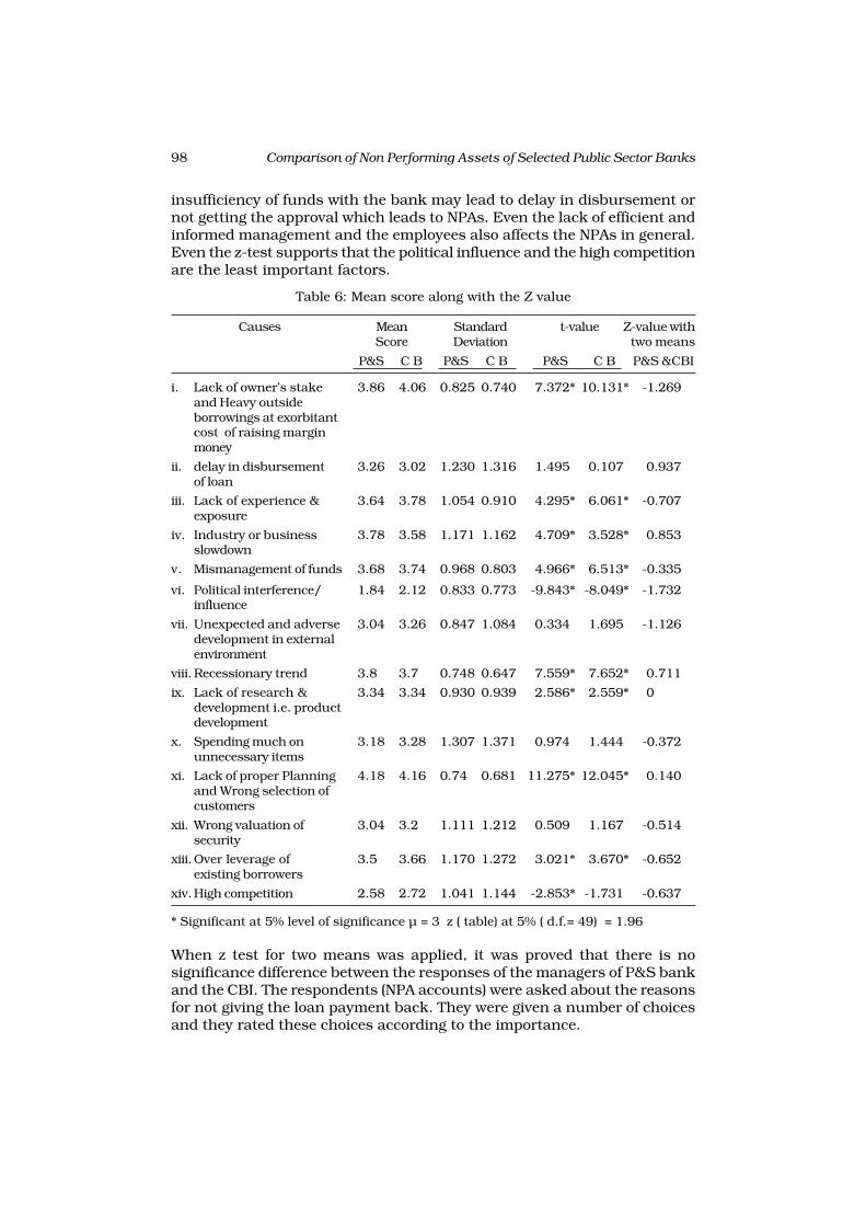
98 Comparison of Non Performing Assets of Selected Public Sector Banks
insufficiency of funds with the bank may lead to delay in disbursement ornot getting the approval which leads to NPAs. Even the lack of efficient andinformed management and the employees also affects the NPAs in general.Even the z-test supports that the political influence and the high competitionare the least important factors.
Table 6: Mean score along with the Z value
Causes Mean Standard t-value Z-value withScore Deviation two means
P&S C B P&S C B P&S C B P&S &CBI
i. Lack of owner’s stake 3.86 4.06 0.825 0.740 7.372* 10.131* -1.269and Heavy outsideborrowings at exorbitantcost of raising marginmoney
ii. delay in disbursement 3.26 3.02 1.230 1.316 1.495 0.107 0.937of loan
iii. Lack of experience & 3.64 3.78 1.054 0.910 4.295* 6.061* -0.707exposure
iv. Industry or business 3.78 3.58 1.171 1.162 4.709* 3.528* 0.853slowdown
v. Mismanagement of funds 3.68 3.74 0.968 0.803 4.966* 6.513* -0.335
vi. Political interference/ 1.84 2.12 0.833 0.773 -9.843* -8.049* -1.732influence
vii. Unexpected and adverse 3.04 3.26 0.847 1.084 0.334 1.695 -1.126development in externalenvironment
viii.Recessionary trend 3.8 3.7 0.748 0.647 7.559* 7.652* 0.711
ix. Lack of research & 3.34 3.34 0.930 0.939 2.586* 2.559* 0development i.e. productdevelopment
x. Spending much on 3.18 3.28 1.307 1.371 0.974 1.444 -0.372unnecessary items
xi. Lack of proper Planning 4.18 4.16 0.74 0.681 11.275* 12.045* 0.140and Wrong selection ofcustomers
xii. Wrong valuation of 3.04 3.2 1.111 1.212 0.509 1.167 -0.514security
xiii.Over leverage of 3.5 3.66 1.170 1.272 3.021* 3.670* -0.652existing borrowers
xiv.High competition 2.58 2.72 1.041 1.144 -2.853* -1.731 -0.637
* Significant at 5% level of significance µ = 3 z ( table) at 5% ( d.f.= 49) = 1.96
When z test for two means was applied, it was proved that there is nosignificance difference between the responses of the managers of P&S bankand the CBI. The respondents (NPA accounts) were asked about the reasonsfor not giving the loan payment back. They were given a number of choicesand they rated these choices according to the importance.

99Jappanjyot Kaur Kalra and S.K.Singla
Table 7 shows that the most important reasons according to the NPAaccounts were the outside borrowing increases and business slowdownoccurs, delay in the disbursement of the loan , lack of experience and thevery important fact was the recessionary trend in the economy. Factorswere political influence, over leverage of existing borrowers or certainunexpected changes in the external environment. The t value has beenchecked at 5% level of significance. The t values have been found insignificantin case of factors like political influence and mismanagement of the borrowedfunds. The results have been found to be significant for factors like, businessslowdown, outside borrowing increases and delay in the disbursement ofthe loan, recessionary trend, lack of experience, unable to pay due toinsufficiency of funds and lack of experience and technical knowledge of themanagement. Then t-test for checking the responses of the managers whowsthat there is no significance difference between their responses.
Table 7: Causes for not making the payments
Causes Mean Standard Z-value Z-value withScore Deviation two means
P&S C B P&S C B P&S C B
i. Lack of owner’s stake 3.833 4.167 1.053 0.379 4.334* 16.858* -1.631and Heavy outsideborrowings atexorbitant cost ofraising margin money
ii. delay in disbursement 4.167 4.5 0.874 0.900 7.309* 7.443* .466of loan
iii. Lack of experience & 3.6 3.7 1.221 0.466 2.693* 8.226* -.419exposure
iv. Industry or business 4.3 4.3 0.702 0.466 10.140* 15.227* 0slowdown
v. Mismanagement 3.233 3.367 0.935 1.033 1.366 1.943 -.524of funds
vi. Political interference/ 2 2.7 0.743 0.988 -7.374* -4.877* -.284influence
vii. Unexpected and 2.667 3.1 1.269 1.185 -1.439 -0.162 -.968adverse developmentin externalenvironment
viii. Recessionary trend 4 4.567 1.438 0.817 3.808* 9.256* -1.217
ix. Lack of research & 4.067 3.033 1.230 0.928 4.750* 4.646* 2.115development i.e.product development
x. Spending much on 3.633 2.9 1.245 1.125 2.786* 1.361 1.601unnecessary items
xi. Lack of proper 2.6 3.3 1.003 1.055 -2.183* -.150 -1.273Planning and Wrongselection of customers contd...

100 Comparison of Non Performing Assets of Selected Public Sector Banks
xii. Wrong valuation of 2.467 2.5 1.224 1.225 -2.386* -2.236* -.105security
xiii. Over leverage of 2.7 3.1 1.291 1.269 -1.273 0.432 -1.210existing borrowers
xiv. High competition 2.933 2.63 0.740 1.377 -0.494 -1.459 1.051
* Significant at 5% level of significance µ = 3 t (table) at 5% ( d.f. = 29) = 2.045
Remedies of NPAs
Today the major chunks of the profits of these banks are suffering becauseof the non performing loans. The earning capacity of banks is limited by itsquantum and thus inversely related to NPAs. Thus, if the banks want toincrease their profitability than the reduction of NPAs is significant.
Table 8: Remedies of NPAs
Causes Mean Standard Z-value Z-value withScore Deviation two means
P&S C B P&S C B P&S C B
I. Bank should prevent 4.08 3.94 0.752 0.712 10.16* 9.339* 0.956diversion of funds bythe promoters
II. Operating staff should 4.2 4.3 0.535 0.707 15.87* 13* -0.798scrutinize the level ofinventories/receivablesat the time of assessmentof working capital
III. The Credit section 4 3.84 0.606 0.710 11.67* 8.363* 1.212should carefully watchthe warning signals viz.non-payment of quarterlyinterest, dishonor ofcheck etc
IV. Effective inspection 3.96 4.14 0.570 0.351 11.91* 22.99* -1.902system should beimplemented
V. More frequent inspections 3.64 3.84 0.663 0.584 6.829* 10.168* -1.601
VI. Increase in provision 4.38 4.54 0.490 0.503 19.90* 21.629* -1.61of NPAs
VII.Re phasing un paid 3.26 3.38 1.209 1.123 1.520 2.393* -0.514loan installments
VIII. Efficient reminder 4.2 4.02 0.670 0.622 12.66* 11.589* 1.392system
IX. Providing assistance 2.6 2.92 1.069 0.986 -2.646* -0.573 -1.556
X. Checking financial 3.84 4.02 0.997 0.769 5.957* 9.379* -1.011projections likeprofitability ratios, cashbooks, bank statements.
* Significant at 5% level of significance µ = 3 z ( table) at 5% ( d.f.= 49) = 1.96
contd...

101Jappanjyot Kaur Kalra and S.K.Singla
Table 8 shows that the most important factor to cure NPAs is increase in theprovision of NPAs(mean score=4.38,4.45), before and after sanctioning theloans the effective inspection system should be implemented so that bankcan prevent diversion of funds by the borrower (mean score=3.96,4.14). Theother important tools are of valuation of inventories and the receivables andefficient reminder systems are very necessary. The bank managers gaveleast importance to the rephrasing of unpaid loan installments and toproviding assistance to the borrower.
Conclusion
Majority of the managers are of the opinion that if the due care and cautionare taken at the time of sanctioning a loan, an asset will not turn into nonperforming asset. The effective monitoring, follow-up and the efficientreminder system is also considered as vital necessity by a large section ofthe study group. According to the managers by developing propermanagement information system and improving the coordination betweenthe banks and providing the list of the defaulters, the NPAs level can bereduced to great extent.
REFERENCES
Ahmed J (2009) Management of non-performing assets of commercial banks inIndia. Mgmt Acct 43: 470-78.
Antony PV and M R (2007) A model for pricing bank loans. Mgmt Acct 42: 261-65.
Banga G, Bhatia S and Kumar B (2007) Menace of non performingassets (NPAS) innon banking finance companies (NBFCS). Indian J Acct 38: 42-50.
Bishnoi N.K. and Pal V (2009) Productivity analysis of commercial banks in India.
Decision 36: 131-55.
Bloem A M and Goerter C N (2001) The macroeconomic statistical treatment ofnon-performing loans. Discussion Paper, Statistics Department of theIMF,December1, 2001.
Eur J Oper Res 148: 662-71.
Gupta R (2004) A comparative study of performance of punjab financial corporationand haryana financial corporation with special reference to non performingassets( NPAs). Research project. Punjab Agricultural University, Ludhiana, India.
Gupta R, Kumar B and Kapur S (2004) Rising NPAs in PFC and HFC- Reasons andremedies. Indian J Acct 34: 10-17.
Maugham W.S. quotation. Retrived on Feburary 19,2009 www.quotationspage.com/quotes/ W._Somerset_Maugham.
Muniappan G (2002) The NPA Overhang Magnitude,Solution and Legal Reforms.Reserve Bank of India Bulletin.
Naik J G (2006) NPAs Management Challengs Before Banking Sector. Mgmt Acct41: 355-60.

102 Comparison of Non Performing Assets of Selected Public Sector Banks
Rajender K and Suresh S (2007) Management of NPAs in Indain banking- A case ofstate bank of Hyderabad. Mgmt Acct 42: 740-49.
Reddy P (2002) Comparative study of non-performing assets in India in the globalcontext-similarities and dissimilarities, remedial measures. Retrived onSeptember 23,2009 from www. crisil.com/ youngthoughtleader /winners/2002/topic3-Pr2ashanth-Reddy-IIM-AHM.PDF
Rehman Mudasir (2009) A study on the non performing assets of J&K bank ltd.Project report Annamali university, Tamilnadu
Sathye Milind (2003) Efficiency of banks in a developing economy: The case ofIndia.

GENERAL BODY MEETING AND ELECTION NOTICE FOR 64th ALLINDIA COMMERCE CONFERENCE AT PONDICHERRY UNIVERSITY(DECEMBER 13-15, 2011).
Dear friends,
It gives me great pleasure to inform you that as per the wishes of theLife Members of the Indian Commerce Association expressed at the time ofthe Annual General Body Meeting held at Goa in 63rd All India CommerceConference, the General Body Meeting of the Indian Commerce Associationshall be held on the second day of the 64th All India Commerce Conferenceat Pondicherry University on 14 December 2011 at 4.00 p m (The agenda forthe General Body Meeting shall be circulated in Puducherry at the time ofthe Conference). This shall be followed by the Elections of the Office Bearersand the Executive Committee Members of the ICA. To finalise the mode andschedule of the Elections a Committee was constituted.
The Committee comprising of the Office Bearers and Past Presidentsof the ICA finalized the election mode for 2011 ICA elections which shall beconducted at the time of 64th Annual Conference of the ICA scheduled to beheld on December 13-15, 2011 at Pondicherry University, Pondicherry. Thedetails of the election mode are as follows:
i) There shall be direct elections for the four office bearer positions, i.e.Executive Vice-President, Secretary, Joint Secretary, and ManagingEditor-cum-Treasurer.
ii) There shall be direct elections for eight positions of the EC members inthe following manner.
Various States and Union Territories of India shall be grouped intofour zones and two EC members shall be elected from each zone. Each voterwill have only one vote for electing an EC member. Voter belonging to aparticular zone will be entitled to elect EC member from their respectivezone only. The distribution of States and Union Territories in four zonesshall be as given below:
East Zone Assam, Meghalaya, Mizoram, Manipur, Nagaland, ArunachalPradesh, Sikkim, Tripura, West Bengal, Orissa, Bihar, Jharkhand,Chhattisgarh.
West Zone Maharashtra, Gujarat, Rajasthan, Goa, Daman, Diu & NagarHaveli.
North Zone Jammu & Kashmir, Himachal Pradesh, Punjab, Haryana,Chandigarh, Delhi, Uttar Pradesh, Uttrakhand, Madhya Pradesh.
South Zone Tamil Nadu, Kerala, Pondicherry, Andhra Pradesh, Karnataka,Lakshadweep, Andeman & Nicobar.
iii) Individual Life Members registered upto 31st October 2011 shall be eligibleto vote in election 2011.
iv) Each voter shall have to bring his/her photo ID card at the time of voting,failing which, he/she shall not be entitled to vote.

v) Prof. P Purushatham Rao, (Past President, ICA), Department of Commerce,Osmania University, Hyderabad shall be the Returning Officer. He isauthorized to appoint his own team of Assistant Returning Officer(s)/Polling Officer(s).
vi) The Conference Secretary shall make all the arrangements for the smoothconduct of elections at the time of 64th All India Commerce Conferenceincluding making arrangement of 12 empty boxes for casting votes andother logistics.
vii) The schedule of the election shall be as follows:
a) Time & Date for filing : 13th December 2011 betweennomination papers 12.00 noon to 5.00 pm
b) Withdrawal of nomination : 14th December 2011 betweenpapers 9.00 a.m. to 11.00 a.m.
c) Scrutiny of nomination : 14th December 2011 at 11.15 a.m.papers
d) Printing of ballot papers : 14th December 2011 upto 3.00 p.m.
e) Election, if required : 14th December 20115.30 p.m. to 8.00 p.m.
f) Counting of votes : Immediately after the completionof polling
g.) The Returning Officer shall declare the results of the Election 2011
RAVINDER VINAYEK
Secretary, ICA

The Indian Commerce Association
Membership Form
To
The Managing EditorThe Indian Journal of CommerceSchool of Management StudiesIndira Gandhi National Open UniversityMaidangarhiNew Delhi 110068
Dear Sir,
You are requested to enroll me as (put a 3 mark):
Individual Life Member (Rs. 3,000)
Institutional Annual Member (Rs. 600)
Patron – Institutional Life Member (Rs. 15,000)
I am sending an amount of Rs. ........................... (in words)....................................
by DD No...................................................... Dated............................................
drawn on (bank and branch)...............................................................................
payable at New Delhi towards the membership of the Indian Commerce Association.
Personal Details (In Capital letters)
Name ...............................................................................................................
Designation................................. Qualification.................................................
Office Address: ...............................................................................................
...............................................................................................
......................................................... Pincode.............................
Mailing Address: ...............................................................................................
...............................................................................................
........................................................ Pin Code............................
Tel. No. ............................................... Mobile No............................................
E-mail..................................................
Yours Sincerely
Date: Signature of Applicant
Mode of Payment: Subscriptions are to be paid in the form of Demand Draft, drawn infavour of ‘The Managing Editor, The Indian Journal of Commerce’, payable at New Delhi.
Correspondence: All correspondence should be addressed to: The Managing Editor, TheIndian Journal of Commerce, School of Management Studies, Indira Gandhi National OpenUniversity (IGNOU), Maidan Garhi, New Delhi 110 068.
The Indian Journal of Commerce is published four times in a year i.e. March, June,September and December. The Journal is freely distributed to all members of the IndianCommerce Association.

Statement about Ownership and Other Particulars of the Journal –THE INDIAN JOURNAL OF COMMERCE
Form – 5(Rule 8)
1. Printer’s Name :Nationality :Address :
2. Place of Publication :
3. Periodicity of Publication :
4. Publisher’s Name :Nationality
Address
5. Chief Editor’s Name :Nationality
Address
6. Name and address of the :individuals who own the
newspaper and Partners or
share-holders holding more
than one percent of
the total capital
7. Printed at :
I, Nawal Kishor, hereby declare that the particulars given are true to the best ofmy knowledge and belief.
(Sd/-)Prof. Nawal Kishor
(Signature of the Publisher)
The Indian Commerce AssociationIndianSOMS, IGNOU, Maidan GarhiNew Delhi-110 068
New Delhi
Quarterly
The Indian Commerce AssociationIndianSOMS, IGNOU, Maidan GarhiNew Delhi-110 068
Prof. Nawal KishorIndianSOMS, IGNOU, Maidan GarhiNew Delhi-110 068
The Indian Commerce Association
Prabhat Offset Press2622, Kucha Chellan, DaryaganjNew Delhi-110 002