Journal of Multimedia - CiteSeerX

Journal of Multimedia

ISSN 1796-2048

Volume 9, Number 2, February 2014

Contents

REGULAR PAPERS

Beef Marbling Image Segmentation Based on Homomorphic Filtering

Bin Pang, Xiao Sun, Deying Liu, and Kunjie Chen

Semantic Ontology Method of Learning Resource based on the Approximate Subgraph Isomorphism

Zhang Lili and Jinghua Ding

Trains Trouble Shooting Based on Wavelet Analysis and Joint Selection Feature Classifier

Yu Bo, Jia Limin, Ji Changxu, Lin Shuai, and Yun Lifen

Massive Medical Images Retrieval System Based on Hadoop

YAO Qing-An, ZHENG Hong, XU Zhong-Yu, WU Qiong, LI Zi-Wei, and Yun Lifen

Kinetic Model for a Spherical Rolling Robot with Soft Shell in a Beeline Motion Zhang Sheng, Fang Xiang, Zhou Shouqiang, and Du Kai

Coherence Research of Audio-Visual Cross-Modal Based on HHT

Xiaojun Zhu, Jingxian Hu, and Xiao Ma

Object Recognition Algorithm Utilizing Graph Cuts Based Image Segmentation

Zhaofeng Li and Xiaoyan Feng

Semi-Supervised Learning Based Social Image Semantic Mining Algorithm

AO Guangwu and SHEN Minggang

Research on License Plate Recognition Algorithm based on Support Vector Machine Dong ZhengHao and FengXin

Adaptive Super-Resolution Image Reconstruction Algorithm of Neighborhood Embedding Based on

Nonlocal Similarity

Junfang Tang and Xiandan Xu

An Image Classification Algorithm Based on Bag of Visual Words and Multi-kernel Learning

LOU Xiong-wei, HUANG De-cai, FAN Lu-ming, and XU Ai-jun

Clustering Files with Extended File Attributes in Metadata

Lin Han, Hao Huang, Changsheng Xie, and Wei Wang

Method of Batik Simulation Based on Interpolation Subdivisions

Jian Lv, Weijie Pan, and Zhenghong Liu

Research on Saliency Prior Based Image Processing Algorithm

Yin Zhouping and Zhang Hongmei

A Novel Target-Objected Visual Saliency Detection Model in Optical Satellite Images

Xiaoguang Cui, Yanqing Wang, and Yuan Tian

A Unified and Flexible Framework of Imperfect Debugging Dependent SRGMs with Testing-Effort

Ce Zhang, Gang Cui, Hongwei Liu, Fanchao Meng, and Shixiong Wu

A Web-based Virtual Reality Simulation of Mounting Machine

Lan Li

189

196

207

216

223

230

238

245

253

261

269

278

286

294

302

310

318

Improved Extraction Algorithm of Outside Dividing Lines in Watershed Segmentation Based on PSO

Algorithm for Froth Image of Coal Flotation Mu-ling TIAN and Jie-ming Yang

325

Beef Marbling Image Segmentation Based on

Homomorphic Filtering

Bin Pang, Xiao Sun, Deying Liu, and Kunjie Chen* College of Engineering, Nanjing Agricultural University, Nanjing 210031, China

*Corresponding author, Email: [email protected]

Abstract—In order to reduce the influence of uneven

illumination and reflect light for beef accurate segmentation,

a beef marbling segmentation method based on

homomorphic filtering was introduced. Aiming at the beef

rib-eye region images in the frequency domain,

homomorphic filter was used for enhancing gray, R, G and

B 4 chroma images. Then the impact of high frequency /low

frequency gain factors on the accuracy of beef marbling

segmentation was investigated. Appropriate values of gain

factors were determined by the error rate of beef marbling

segmentation, and the results of error rate were analyzed

comparing to the results without homomorphic filtering.

The experimental results show that the error rates of beef

marbling segmentation was remarkably reduced with low

frequency gain factor of 0.6 and high frequency gain factor

of 1.425; Compared with other chroma images, the average

error rate (5.38%) of marbling segmentation in G chroma

image was lowest; Compared to the result without

homomorphic filtering, the average error rate in G chroma

image has decreased by 3.73%.

Index Terms—Beef; Marbling; Homomorphic Filter; Image

Segmentation

I. INTRODUCTION

Beef color, marbling and surface texture are key

factors used by trained expert graders to classify beef

quality [1]. Of all factors, the beef marbling score is

regarded as the most important indicator [2]. The

Ministry of Agriculture of the People's Republic of China

has defined four grades of beef marbling and correspondingly published standard marbling score

photographs. Referring to the standard photographs,

graders determine the abundance of intramuscular fat in

rib-eye muscle and then label the marbling score [3].

Since the classification of beef marbling score largely

depends on the subjective visual sensory of graders, the

estimation on the same beef region may differ. Therefore,

developing an objective system of beef marbling grading independent on subjective estimation is imperative in

beef industry.

Beef marbling, which is an important evaluation

indicator in the existing beef quality classification criteria,

is usually determined by the abundance of intramuscular

fat in beef rib-eye region. Machine vision and image

processing technology are considered as the most

effective methods in automatic identification of beef marbling grades [4]. In automatic identification, the first

thing is to precisely segment beef marbling. Numerous

methods for beef marbling image segmentation have been

reported in the past 20 years. For the first time, Ref. [5]

segments the image of beef rib-eye section into fat and

muscle areas by image processing, and then calculates the

total area of fat, and obtains the relationship between fat area and the sensory evaluation results of beef quality.

Ref. [3] proposes a beef marbling image segmentation

method based on grader's vision thresholds and automatic

thresholding to correctly separate the fat flecks from the

muscle in the rib-eye region and then compares the

proposed segmentation method to prior algorithms. Ref.

[6] proposes an algorithm for automatic beef marbling

segmentation according to the marbling features and color characteristics, which uses simple thresholding to

remove background and then uses clustering and

thresholding with contrast enhancement via a customized

grayscale to remove marbling. And the algorithm is

adapted to different environments of image acquisition.

Due to complex and changeable beef marbling, no clear

boundary can be discerned between muscle and fat areas.

Therefore, marbling can hardly be precisely segmented. The results of Ref. [7] show that fuzzy c-mean (FCM)

algorithm functioned well in the segmentation of beef

marbling image with high robustness. On this basis, Ref.

[8] uses a sequence of image processing algorithm to

estimate the content of intramuscular fat in beef

longissimus dorsi and then uses a kernel fuzzy c-means

clustering (KFCM) method to segment the beef image

into lean, fat, and background. Ref. [9] presents a fast modified FCM algorithm for beef marbling segmentation,

suggesting that FCM is highly effective. Ref. [10, 11]

introduces a kind of method to segment the area of

longissimus dorsi and marbling from rib-eye image by

using morphology filter, dilation, erosion and logical

operation. Ref. [12] uses computer image processing

technologies to segment the lean tissue region from beef

rib-eye cross-section image and to extract color features of each image, and then uses BP neural network to

predict the color grade of beef lean tissue. Ref. [13, 16]

establish a kind of predicting models for beef marbling

grading, indicating that beef marbling grades could be

determined by using fractal dimension and image

processing method. Ref. [14] developed a beef image

online acquisition system according to the requirements

of beef automatic grading industry. In order to reduce the calculating time of the system, only Cr chroma image are

JOURNAL OF MULTIMEDIA, VOL. 9, NO. 2, FEBRUARY 2014 189

© 2014 ACADEMY PUBLISHERdoi:10.4304/jmm.9.2.189-195

considered to extract the effective rib-eye region by using

image processing methods. Ref. [15] uses machine vision

and support vector machine (SVM) to determine color

scores of beef fat. And the fat is separated from the rib-

eye by using a sequence of image processing algorithms,

boundary tracking, thresholding and morphological

operation, etc. Then twelve features of fat color are used as inputs to train SVM classifiers. As machine vision

technology aims to objectively assess marbling grades, a

machine vision system will first collect the entire rib-eye

muscle image of a beef sample. Then the sample image

can be segmented into exclusively marbling region and

rib-eye region images with the image processing

algorithm. As a result, marbling features can be computed

according to the processed images, which are more prone to objectively and consistently determine beef marbling

grading compared with visual sensory. However, in

collection of beef rib-eye images, the unfavorable light

and acquisition conditions will unavoidably cause

problems, such as overall darkness, local shadow, and

local reflection, which increase the difficulty in

subsequent marbling segmentation and reduce the

segmentation precision. Homomorphic filtering is a special method that is often

used to remove multiplicative noise. Illumination and

reflectance are not separable, but their approximate

locations in the frequency domain may be located. Since

illumination and reflectance combine multiplicatively, the

components are made additive by taking the logarithm of

the image intensity, so that these multiplicative

components of the image can be separated linearly in the frequency domain. Illumination variations can be thought

of as a multiplicative noise, and can be reduced by

filtering in the log domain. To make the illumination of

an image more even, the high-frequency components are

increased and low-frequency components are decreased,

because the high-frequency components are assumed to

represent mostly the reflectance in the scene (the amount

of light reflected off the object in the scene), whereas the low-frequency components are assumed to represent

mostly the illumination in the scene. That is, high-pass

filtering is used to suppress low frequencies and amplify

high frequencies, in the log-intensity domain. As a result,

the uneven illumination of color images can be

effectively corrected [17-25]. In this paper, homomorphic

filtering is used to correct the non-uniform illumination in

the beef rib-eye region, and thereby the effects of filtering gain factors and 4 chroma images on marbling

segmentation precision are analyzed. Based on this, a

beef marbling segmentation method based on

homomorphic filtering with G chroma image was

introduced.

This paper proposes an accurate beef marbling

segmentation method based on homomorphic filtering

theory, and the specific work is as follows: (a) Homomorphic filtering is a generalized technique

for signal and image processing, involving a nonlinear

mapping to a different domain in which linear filter

techniques are applied, followed by mapping back to the

original domain. Homomorphic filter is sometimes used

for image enhancement. It simultaneously normalizes the

brightness across an image and increases contrast. In

order to find out the optimal chroma image to extract beef

marbling area accurately, homomorphic filtering in this

paper is used respectively to enhance gray, R, G and B 4

chroma images in beef rib-eye region in the frequency

domain and then the beef marbling areas are extracted by Otsu method.

(b) Homomorphic filtering is used to correct the

illumination and reflection variations of beef rib-eye

images, which will affect the beef marbling extraction to

some extent. In order to select appropriate high/low gain

factor values of homomorphic filter to enhance the

contrast ratio in the beef rib-eye region, the impact of

high /low frequency gain factors on the accuracy of beef marbling segmentation is investigated. Corresponding to

different high/low frequency gain factor values of

homomorphic filter, the error rate curves of marbling

segmentation in gray, R, G and B chroma images are

plotted. Then the minimum error rate curves of the 4

chroma images are plotted and the trends of the minimum

error rates corresponding to high/low frequency gain

factors are discussed. (c) In order to achieve the optimal beef marbling

segmentation effect, the segmentation error rates with

different chroma images are analyzed and compared. The

average values of high/low frequency gain factors are

selected to segment marbling. Then the error rate results

with homomorphic filtering are compared to those

without homomorphic filtering.

The rest of paper is organized as follows. The materials and proposed methods are presented in Section

2. Then the impact of homomorphic filter gain factors

and different chroma images on the accuracy of beef

marbling segmentation is discussed in Section 3. Finally,

the conclusions are given in Section 4.

II. PROPOSED METHOD

Under natural illumination, 10 beef rib-eye images

(640×480 pixels) were collected by using a Minolta Z1 digital camera and stored as JPG format in PC. The PC

has a Pentium(R) Daul-Core CPU (basic frequency 2.6

GHz), a memory of 2.0 GB, and an operating system of

Windows XP. Image processing and data analysis are

performed on Matlab software.

Before segmentation, preprocessing is needed to

separate the rib-eye region for subsequent marbling

segmentation. The separation includes threshold setting, regional growth, and morphological processing (details in

Ref. [11]).

Homomorphic filtering is used to correct the uneven

illumination in beef images and thus reduce the effects of

darkness and reflection on subsequent image processing.

This provides a favorable foundation for accurate

segmentation of beef marbling. The principle is as

follows.

In the illumination-reflection model, image ( , )f x y

can be expressed as the product of the illumination

component ( , )i x y and the reflection component ( , )r x y :

190 JOURNAL OF MULTIMEDIA, VOL. 9, NO. 2, FEBRUARY 2014

© 2014 ACADEMY PUBLISHER

http://en.wikipedia.org/wiki/Multiplicative_noise

http://en.wikipedia.org/wiki/Logarithm

http://en.wikipedia.org/wiki/High-pass_filter

http://en.wikipedia.org/wiki/High-pass_filter

http://en.wikipedia.org/wiki/Image_enhancement

( , ) ( , ) ( , )f x y i x y r x y (1)

where 0 ( , )i x y , and 0 ( , ) 1r x y .

First, the logarithm of ( , )f x y is obtained:

( , ) ln ( , )

ln ( , ) ln ( , )

z x y f x y

i x y r x y

(2)

By using Fourier transform, then

[ ( , )] [ln ( , )] [ln ( , )]F z x y F i x y F r x y (3)

or

( , ) ( , ) ( , )Z u v I u v R u v (4)

The filter's transfer function ( , )H u v is designed as:

( , ) ( , ) ( , )

( , ) ( , ) ( , ) ( , )

S u v H u v Z u v

H u v I u v H u v R u v

(5)

By using inverse Fourier transform on ( , )S u v , then:

1

1 1

( , ) [ ( , )]

[ ( , ) ( , )] [ ( , ) ( , )]

s x y F S u v

F H u v I u v F H u v R u v

(6)

Let

1( , ) [ ( , ) ( , )]i x y F H u v I u v (7)

and

1( , ) [ ( , ) ( , )]r x y F H u v R u v (8)

Then equation (6) can be expressed as:

( , ) ( , ) ( , )s x y i x y r x y (9)

Finally, because ( , )z x y is the logarithm of the original

image ( , )f x y , the inverse operation (exponential) can be

used to generate a satisfactory enhanced image, which

can be expressed by ( , )g x y as:

( , )

( , ) ( , )

0 0

( , )

( , ) ( , )

s x y

i x y r x y

g x y e

e e

i x y r x y

(10)

where

( , )

0 ( , ) i x yi x y e

(11)

( , )

0 ( , ) r x yr x y e

(12)

are the illumination component and reflection component

of the output image respectively.

A Gaussian high-pass filter ( , )H u v is selected as the

homomorphic filter's function:

2 2

0( ( , ))/( , ) ( )[1 ]

c D u v D

H L LH u v r r e r

(13)

where 0 ( , )D u v is cut-off frequency, ( , )D u v is the

frequency at point ( , )u v ; c is a constant; (0, )Hr is

high frequency gain factor; (0,1]Lr is low frequency

gain factor. Appropriate values of high/low gain factors

should selected, so as to enhance the contrast ratio of the

image in the beef rib-eye region, sharpen the image edges

and details, and make marbling segmentation more effectively.

The processed beef rib-eye images undergo gray-scale

transformation; then the gray and R, G and B 4 chroma

images undergo the above homomorphic filtering. Otsu

automatic threshold method is used for dividing the rib-

eye region into the target (muscle) and the background

(fat). With the optimal threshold, image ( , )g x y is

binaryzed:

0 ( ( , ) )

( , )255 ( ( , ) )

g x y Tg x y

g x y T

(14)

In order to evaluate the effects of beef marbling

segmentation, the precision of segmentation should be

analyzed. Marbling segmentation error rate Q is defined

as the error ratio of pixel counts between the extracted marbling region after processing and the marbling region

manually segmented from the original image [14]. The

pixel count in the manually segmented marbling region is

expressed as ( , )q x y ; the pixel count in the extracted

marbling region after processing is expressed as ( , )q x y ;

then the beef marbling extraction error rate is calculated

as:

| ( , ) ( , ) |

100%( , )

q x y q x yQ

q x y

(15)

Manual segmentation is performed on Photoshop. The

pixel count in the marbling region is summarized. In

order to reduce manual extraction error, each image is

repeated 3 times to obtain the average value, which is

used as the marbling pixel count by deleting decimal part.

III. RESULTS AND DISCUSSION

A. Beef Marbling Extraction Based on Homomorphic filtering

One image (Fig. 1) is randomly selected from the

collected beef images. After preprocessing as described

in Section 2, the rib-eye image is obtained (Fig. 2). Then the rib-eye image undergoes gray-scale transformation

(Fig. 3) for homomorphic filtering with different

frequency gain factors, and the rib-eye image is showed

in Fig. 4.

Figure 1. Original beef sample image



Figure 2. Beef rib-eye image

Figure 3. Rib-eye gray image

As showed in Fig. 2 and Fig. 3, because of light

insufficiency, the rib-eye image lacks brightness, so the

contrast between marbling and muscle is small and some

tiny marbling is unclear. After homomorphic filtering, the

brightness is improved (Fig. 4a), especially the edges are

sharpened, so the tiny marbling fragments are enhanced.

However, when different values of Lr and Hr are used,

the filtering effects are different. When a small gain

factor is used, the image brightness is too large, while the

contrast between marbling and muscle is significantly

reduced (Fig. 4b), which is unfavorable for subsequent

segmentation. When a large gain factor is used, the high frequency part will be excessively enhanced, so the

brightness decreases (Fig. 4c), which is also unfavorable

for subsequent segmentation. Therefore, appropriate

values of gain factors should be selected to improve beef

marbling segmentation precision.

(a) rL=0.8, rH=1.2

(b) rL=0.2, rH=0.2

(c) rL=0.9, rH=1.8


(a) R chroma image

(b) G chroma image

(c) B chroma image

(d) Gray chroma image




B. Selection of Homomorphic Filtering Gain Factors and

Their Effects on Beef Marbling Segmentation Precision

Homomorphic filtering is used to correct the

illumination and reflection components of rib-eye images, which will affect the beef marbling segmentation to some

extent. Appropriate values of homomorphic filtering gain

factors Lr and

Hr are selected, so as to enhance the

contrast ratio in the beef rib-eye region. One image is selected from the 10 images, then the rib-

eye region is segmented as described in Section 2;

different values of Lr and

Hr are selected to construct

different filters. Then the gray, R, G and B 4 chroma

images undergo homomorphic filtering separately. Finally, the marbling is extracted as described in Section

2 and the error rates are calculated as described in Section

2. The results are listed in Fig. 5.

Fig. 5 shows that when Lr is constant, the beef

marbling extraction error rates in the 4 chroma images all slowly decrease firstly and then sharply increase with the

increasing Hr . Each beef marbling segmentation error

rate curve corresponding to each value of Lr shows a

minimum error rate. For instance, in gray chroma image,

when Lr =0.4 and

Hr =0.8, the beef marbling error rate is

minimized to 0.08%.

Then the minimum error rates of the 4 chroma images

under both Lr and Hr are used for obtaining the changing

curves (Fig. 6 and Fig. 7).

Figure 6. Effects of low frequency gain factor on minimum error rate

in beef marbling segmentation

Figure 7. Effects of high frequency gain factor on minimum error rate

in beef marbling segmentation

Fig. 6 shows that with the increase of Lr , the minimum

error rate firstly decreases and then increases, and

concentrates within Lr =0.4-0.8. Fig. 7 shows that with

the increase of Hr , the minimum error rate also firstly

decreases and then increases, and concentrates within

Hr =0.8-1.8. Specifically, for gray chroma image, the

minimum error rate is 0.08% when Lr =0.4 and

Hr =0.8;

for R chroma image, the minimum error rate is 0.05%

when Lr =0.6 and

Hr =1.7; for G throma image, the

minimum error rate is 0.27% when Lr =0.7 and

Hr =1.4;

for B chroma image, the minimum error rate is 0.64%

when Lr =0.7 and

Hr =1.8.

C. Analysis and Comparison of Marbling Segmentation

Error Rates Based on Homomorphic Filtering

The above analysis shows that within Lr =0.4-0.8, and

Hr =0.8-1.8, the gray, R, G and B chroma images after

homomorphic filtering show the minimum error rates,

and therefore, Lr and

Hr are arithmetically averaged to

Lr =0.6 and rH=1.425. The 10 images are preprocessed as

described in Section 2 to segment the beef rib-eye regions;

then a homomorphic filter with Lr of 0.6 and Hr of 1.425

is used for filtering the gray, R, G and B 4 chroma image

and thereby for segmenting marbling area. Finally

equation (15) is used to calculate the error rates of the 4

chroma images for each beef image, and the results are

listed in Table 1.

TABLE I. ERROR RATE IN BEEF MARBLING SEGMENTATION WITH

HOMOMORPHIC FILTERING

Image

No.

Chroma Image

Gray R G B

1 10.97 16.62 6.91 15.59

2 10.24 21.05 0.40 14.41

3 3.38 13.86 7.44 2.97

4 6.56 17.82 4.46 10.91

5 1.41 13.29 10.27 5.99

6 15.02 25.26 4.95 18.97

7 6.85 22.38 5.82 12.57

8 12.77 17.42 9.25 9.86

9 4.45 16.12 1.71 10.36

10 8.48 18.69 2.56 20.03

Mean 8.01 18.25 5.38 12.17

TABLE II. ERROR RATE IN BEEF MARBLING SEGMENTATION

WITHOUT HOMOMORPHIC FILTERING

Image

No.

Chroma Image

Gray R G B

1 11.71 19.87 8.82 15.29

2 20.53 23.29 7.12 15.13

3 13.30 10.83 5.65 14.27

4 22.47 27.82 14.46 20.91

5 12.39 16.48 12.72 10.63

6 14.11 16.37 9.53 22.12

7 17.41 22.56 6.98 16.94

8 12.99 14.78 14.32 13.57

9 9.67 15.96 6.61 18.59

10 14.82 20.16 4.84 23.79

Mean 14.94 18.81 9.11 17.12

Table 1 shows that after homomorphic filtering, the

error rates of all the 4 chroma images are different. The



minimum error rate is from G chroma images, which is

5.38%, significantly lower than gray chroma image

(8.01%), R chroma image (18.25%) and B chroma image

(12.17%), indicating that G image can be used to obtain

the optimal segmentation effect.

Table 2 shows the error rates of beef marbling

extraction without homomorphic filtering (only with Otsu method).

Table 2 shows that without homomorphic filtering, the

minimum error rate is also from G chroma image (9.11%),

significantly lower than the average error rate of gray, R,

or B images. However, the error rates without

homomorphic filtering are all higher than those with

homomorphic filtering. The average error rate in G

chroma images is 3.73% higher than that after filtering, indicating that the beef marbling error rate decreases

significantly after homomorphic filtering.

IV. CONCLUSIONS

(1) After homomorphic filtering, beef rib-eye images

are improved and much tiny marbling is enhanced.

Appropriate values of frequency gain factors should be

selected, which is favorable for precise segmentation of

beef marbling. (2) High/low frequency gain factors both significantly

affect the error rate of beef marbling segmentation. With

the increase of either factor, the minimum error rate

firstly decreases and then increases. When high frequency

gain factor Hr is within 0.8-1.8, and when low frequency

gain factor Lr is within 0.4-0.8, the beef marbling error

rate could get the minimum value.

(3) Lr =0.6 and Hr =1.425 are selected to build a

homomorphic filter to process the beef rib-eye images;

the minimum error rate is from G chroma images, which

is 5.38%, about 3.73% lower than that without

homomorphic filtering. This indicates that with this gain

factor, G images after homomorphic filtering can achieve

the optimal beef marbling segmentation effect.

ACKNOWLEDGMENT

This work was supported by the National Science

Foundation of China under Grant No.31071565 and the

Funding of the Research Program of China Public

Industry under Grant No.201303083.

REFERENCES

[1] P. Jackman, D. W. Sun, et al, “Prediction of beef eating quality from colour, marbling and wavelet texture features,” Meat Science, vol. 80, no. 4, pp. 1273-1281, 2008.

[2] Y. N. Shen, S. H. Kim, et al, “Proteome analysis of bovine longissimus dorsi muscle associated with the marbling score,” Asian-Australasian Journal of Animal Sciences, vol. 25, no. 8, pp. 1083-1088, 2012.

[3] K. Chen, C. Qin, “Segmentation of beef marbling based on vision threshold,” Computers and Electronics in Agriculture, vol. 62, no. 2, pp. 223-230, 2008.

[4] K. Chen, C. Ji, “Research on Techniques for Automated Beef Steak Grading,” Transactions of the Chinese Society

of Agricultural Machinery, vol. 37, no. 3, pp. 153-156, 159, 2006.

[5] T. P. Mcdonald, Y. R. Chen, “Separating connected muscle tissues in images of beef carcass ribeyes,” Transactions of the Asae, vol. 33, no. 6, pp. 2059-2065, 1990.

[6] P. Jackma, D. W. Sun, P. Allen, “Automatic segmentation of beef longissimus dorsi muscle and marbling by an adaptable algorithm,” Meat Science, vol. 83, no. 2, pp. 187-194, 2009.

[7] J. Subbiah, N. Ray, G. A. Kranzler, S. T. Acton, “Computer vision segmentation of the longissimus dorsi for beef quality grading,” Transactions of the ASAE, vol. 47, no. 4, pp. 1261-1268, 2004.

[8] C. J. Du, D. W. Sun, et al, “Development of a hybrid image processing algorithm for automatic evaluation of intramuscular fat content in beef M-longissimus dorsi,” Meat Science, vol. 80, no. 4, pp. 1231-1237, 2004.

[9] J. Qiu, M. Shen, et al. “Beef marbling extraction based on modified fuzzy C-means clustering algorithm,” Transactions of the Chinese Society of Agricultural Machinery, vol. 41, no. 8, pp. 184-188, 2010.

[10] J. Zhao, M. Liu and H. Zhang, “Segmentation of longissimus dorsi and marbling in ribeye imaging based on mathematical morphology,” Transactions of the Chinese Society of Agricultural Engineering, vol. 20, no. 1, pp.

143-146, 2004. [11] K. Chen, C. Qin and C. Ji, “Segmentation Methods Used in

Rib-eye Image of Beef Carcass,” Transactions of the Chinese Society of Agricultural Machinery, vol. 37, no. 6, pp. 155-158, 2006.

[12] K. Chen, X. Sun and Q. Lu, “Automatic color grading of beef lean tissue based on BP neural network and computer vision,” Transactions of the Chinese Society for Agricultural Machinery, vol. 40, no. 4, pp. 173-178, 2009.

[13] K. Chen, G. Wu, M. Yu and D. Liu, “Prediction model of beef marbling grades based on fractal dimension and image

features,” Transactions of the Chinese Society for Agricultural Machinery, vol. 43, no. 5, pp. 147-151, 2012.

[14] B. Pang, X. Sun and D. Liu, “On-line Acquisition and Real-time Segmentation System of Beef Rib-eye Image,” Transactions of the Chinese Society of Agricultural Machinery, vol. 44, no. 6, pp. 190-193, 2013.

[15] K. Chen, X. Sun, C. Qin, X. Ting, “Color grading of beef fat by using computer vision and support vector machine,” Computers and Electronics in Agriculture, vol. 70, no. 1, pp. 27-32, 2010.

[16] K. Chen, “Determination of the box-counting fractal

dimension and information fractal dimension of beef marbling, ” Transactions of the Chinese Society of Agricultural Engineering, vol. 23, no. 7, pp. 145-149, 2007.

[17] X. Zhang, S. Hu, “Video segmentation algorithm based on homomorphic filtering inhibiting illumination changes,” Pattern Recognition and Artificial Intelligence, vol. 26, no. 1, pp. 99-105, 2013.

[18] Z. Jiao, B. Xu, “Color image illumination compensation based on homomorphic filtering,” Journal of Optoelectronics Laser, vol. 21, no. 4, pp. 602-605, 2010.

[19] X. Wang, F. Hu and Y. Zhao, “Corner extraction based on homomorphic filter,” Computer Engineering, vol. 32, no.

11, pp. 211-212, 264, 2006. [20] J. Xiao, S. Song, and L. Ding, “Research on the fast

algorithm of spatial homomorphic filtering, ” Journal of Image and Graphics, vol. 13, no. 12, pp. 2302-2306, 2008.

[21] Z. Jiao, B. Xu, “Color image illumination compensation based on HSV transform and homomorphic filtering,” Computer Engineering and Applications, vol. 46, no. 30, pp. 142-144, 2010.



[22] J. Xiong , X. Zou, H. Wang, H. Peng, M. Zhu and G. Lin, “Recognition of ripe litchi in different illumination

conditions based on Retinex image enhancement,” Transactions of the Chinese Society of Agricultural Engineering, vol. 29, no. 12, pp. 170-178, 2013.

[23] J. Li, X. Rao and Y. Ying, “Detection of navel surface defects based on illumination—reflectance model,” Transactions of the Chinese Society of Agricultural Engineering, vol. 27, no. 7, pp. 338-342, 2011.

[24] J. Qian, X. Yang, X. Wu, Chen Meixiang and Wu Baoguo, “Mature apple recognition based on hybird color space in

natural scene,” Transactions of the Chinese Society of Agricultural Engineering, vol. 28, no. 17, pp. 137-142, 2012.

[25] J. Tu, C. Liu, Y. Li, J. Zhou and J. Yuan, “Apple recognition method based on illumination invariant graph,” Transactions of the Chinese Society of Agricultural Engineering, vol. 26, no. 2, pp. 26-31, 2010.



Semantic Ontology Method of Learning Resource

based on the Approximate Subgraph

Isomorphism

Zhang Lili College English Teaching & Researching Department, Qiqihar University Qiqihar Heilongjiang 161006 China

Jinghua Ding

College of Information and Communication Engineering, Sungkyunkwan University, Suwon, Korea

Email: [email protected]

Abstract—Digital learning resource ontology is often based

on different specification building. It is hard to find

resources by linguistic ontology matching method. The

existing structural matching method fails to solve the

problem of calculation of structural similarity well. For the

heterogeneity problem among learning resource ontology,

an algorithm is presented based on subgraph approximate

isomorphism. First of all, we can preprocess the resource of

clustering algorithm through the semantic analysis, then

describe the ontology by the directed graph and calculate

the similarity, and finally judge the semantic relations

through calculating and analyzing different resource

between the ontology of different learning resource to

achieve semantic compatibility or mapping of ontology. This

method is an extension of existing methods in ontology

matching. Under the comprehensive application of features

such as edit distance and hierarchical relations, the

similarity of graph structures between two ontologies is

calculated. And, the ontology matching is determined on the

condition of subgraph approximate isomorphism based on

the alternately mapping of nodes and arcs in the describing

graphs of ontologies. An example is used to demonstrate this

ontology matching process and the time complexity is

analyzed to explain its effectiveness.

Index Terms—Digital Learning; Ontology Matching; Digital

Resource Ontology; Graph Similarity

I. INTRODUCTION

In the 1990s, the development of computer network

and multimedia technology provides the education

development with new energy. education mode, method,

scope experience astonishing change and global excellent

education resources sharing and communication is

realized. The mode of education supported by the

computer network technology is often referred to as

digital learning [1]. However, because the Internet is a

highly open, heterogeneous and distributed information

space, and the real meaning is hard to be understood when we use URL technology to search the learning

resources, target learning resources are often submerged

in a large number of useless redundancy information, so

the digital learning resources cannot be found efficiently.

To strengthen information semantic characteristics, the

inventor of the URL technology Tim Berners-lee

proposed to represent mutual recognized commonly and

shared knowledge through Ontology and give strict

definition of the concept and the relations between

concepts to determine the meaning of the concept [2].The digital learning supported by ontology technique

describes the learning resources according to the learning

resource metadata standards, establishing a learning

resource ontology, apply similarity calculation and

matching of ontology to support digital learning resource

discovery, which can prevent the learners from losing

direction in network learning environment and improve

the learning efficiency and accuracy.

Similarity is two the basic condition of digital learning

resources ontology matching, however, in the present

digital learning environment, learning resource ontology

often consists of different creators who apply different data specification, modeling method and the technology

to create, learning resource ontology of the same topic in

a field of often differ greatly, which has a direct impact

on the efficiency of digital learning resources discovery.

how to effectively solve the matching problem of

heterogeneous ontology learning resources, or the

ontology matching in the semantic Web, is a challenge

the digital learning is facing. At present, the domestic and

foreign scholars have proposed many ontology matching

methods, mainly based on linguistics, the structure, the

instance, and so on, and developed all kinds of ontology matching tools, such as the ONION created by American

Stanford university, GLUE [4] created by American

Washington University, FAOM created by German

Karlsruhe University and so on. Among them, the

PROMPT is based on the linguistics, GLUE and QOM is

based on machine learning methods. However, when we

apply the existing ontology matching methods to learning

resource ontology matching, it still have problems as

follows: (1) It is difficult for the method based on

linguistic to solve the problem of learning resource

ontology matching. The reason: the current learning

resource ontology metadata standards and specifications



are different, such as LOM proposed by the Learning

Technology Standards Committee (LTSC) subordinate to

IEEE, Dublin core metadata set (DCMS) proposed by

Online Computer Library Center (OCLC), LRM released

by IMS Global Learning Consortium, etc. Different

metadata specification determines different learning

resource ontology description language. It is hard to

define scientific semantic distance and can't solve the

problem of learning resource ontology matching. (2) The

existing structural matching method can't meet the

demand of learning resource ontology matching. The existing ontology matching methods based on the

structure mostly focus only on the hierarchical structure

of the ontology itself, and pay little attention to other

relations’ influence on ontology matching. Digital

learning resources ontology matching should consider the

similarity of the overall structure made up of all kinds of

relationships, so we cannot use the tree structure

similarity matching methods. (3) The matching methods

based on the example are limited by the complexity,

computing performance, correctness, optimization

problems of the machine learning technology and the effectiveness in the practical ontology matching

application need to be tested, so it is not a learning

resource ontology matching scheme that can be used as

the optimization technology. (4) The extracted sentences

of multi-document summarization usually come from

different documents. It is necessary to sort the extracted

sentences to improve the readability of the summarization.

The available ways to sort the extracted sentences are

most methods [2] [3], [12] time sorting method [2] [3],

probability sorting method [4], machine learning method

[6] [7] [9], and their improved algorithm, etc. Most sorting method gets the order of the theme according to

the successive relationship, so it is easy to interrupt

sentence topic; The time information extracted by using

the time sorting method is not necessarily accurate;

Probability sorting method is likely to lead to imbalance

of the subject; Machine learning method is comparatively

complex to realize in the process of sorting and rely

heavily on training corpus; Subsequent improved

algorithm makes some difference in improving the

abstract readability.

In this type of ontology matching technology, the

extract of structure similar characteristic set extraction and similarity calculation is one of the key elements. To

extract the information of different structure feature, we

use different similarity measure and calculation methods.

For example, SF (Similarity Flooding) [8] structure

matching method does not consider the pattern

information and judge the ontology matching based on

the transitivity of graph nodes’ similarity, namely: if two

elements’ adjacency nodes in different mode are similar,

so does the two similar elements’ node. The structure of

the matching period of Cupid [9], the leaf nodes

similarities depend on similarity of linguistics, data types and neighboring nodes, the non-leaf nodes similarities are

got by calculating similarity with the similarity of the

subtree of its root. In the Anchor - PROMPT [10], the

ontology is seen as a directed labeled graph, with fixed

length of anchors path as structural characteristics of

extraction and subgraph path limited by anchors through

traverse. Semantic similarity was represented by tagging

node similar values in the same location. In the ASCO,

nodes’ adjacent relations and concept hierarchy paths are

extracted as ontology structural characteristic. Structural

similarity is similar proportion in adjacent structure and

path in measurement and calculation and get the weighted

sum then. In the above ontology matching methods based

on structure, the similarity propagation of ontology

structural characteristic is an important factor to judge matching, but the present methods rely on the similarity

of adjacent nodes too much in the calculation of structural

similarity. Similarity propagation usually requires

traversing the total graph, with large amounts of

calculation and blindness. It needs further study in depth.

Research on Ontology Matching: now, many

universities and research institutions at home and abroad

have studied in this area and invented a lot of tools. The

ontology mapping based on semantic Web is the key

technology of ontology study. It is the basis of

completing ontology finding, aligning, learning and capturing. Ontology mapping and merging tools has been

developed abroad, such as PROMPT, Cupid, Similarity

Flooding, GLUE, etc.. They measure the similarity of

terminology of concepts from different angles. There are

element level, structural level and instance level, etc., but

the following problems are still existed: (1) versatility is

not high: These tools are mostly of the more obvious

effects for ontology of specific area or different versions,

and if it replaced with ontology of other areas, the effect

is not very obvious; (2) It is difficult to ensure the

effectiveness and efficiency of mapping: In order to obtain a more accurate similarity, calculation method will

be more. In this way, the efficiency is bound to be

affected, so a balance point between the effectiveness and

efficiency in mapping need to be found; (3) calculation

method is not comprehensive enough : While the existing

calculation methods can reflect the similarity of physical

layer, semantic network layer, description logical layer

and etc., there are no similarity calculation standards for

the presentation layer and the rule layer at present

because that the restriction and rule of ontology still don't

have mature theory; (4) automatic level is not high : now,

most methods still in semi-automatic mode. After the mapping is calculated, the same ontology may be

involved in a number of physical mapping. Due to the

deficiencies of the existing calculation method, the

mapping with the highest similarity is not necessarily

accurate, which requires users to manually select the

choice and decide the result.

The innovation points of this paper:

(1) Digital learning resource ontology is often based on

different specification building. It is hard to find

resources by linguistic ontology matching method. The

existing structural matching method fails to solve the problem of calculation of structural similarity well. After

studying and analyzing of existing ontology matching

methods, this paper puts forward a method of digital

learning resources ontology matching. The method in



Ontology matching methods

Element level Structure level

Sring-based

name

similarity

Description

Similarity

Comment

Synonyms

Language-

based

Tokenization

Lemmatisation

Morphology

elimination

Linguistic

Resources

Lexicons

thesaurus

Constrain

t

-based

Type

Similarity

Key

properties

Alignment

Reuse

Entire

Schema or

Ontology

fragment

Upper level

Domain

Specific

Ontologies

SUMO

DOLCE

UMLS

FMA

Data analysis

and

statistics

Frequency

distribution

Griph-based

Graph

Homomorphi

Sm

Path

Children

leaves

Taxonomy

-based

Taxonomy

structure

Repository

of

structures

Structure

metadata

Model-

based

SAT

Solvers

DL

reasoners

Particle size

The basic technology

The term structure epitaxial The semantic

Input type

Figure 1. Method for classification of ontology matching

comprehensive concept of edit distance and similarity

based hierarchical architecture and other relations,

alternates point of ontology of directed graph, edge

matching, thus to determine approximate subgraph

isomorphism ontology matching. As the judgment

standard, the method to structure the overall similarity

helps strengthen the efficiency of digital learning

resources ontology matching, improve the ability of

resource discovery, found efficient similarity subgraph,

improve the precision and efficiency of ontology matching.

(2) In view of the two difficulties that the subject is

interrupted and the extracted sentences are incoherent,

this paper analyses the application of clustering algorithm

of the latent semantic analysis in sentence sorting in order

to improve the quality of the generation of

summarizations. We use the clustering algorithm of latent

semantic analysis to cluster the extracted sentence to a

topic set, achieving the goal of solving the topic interrupt.

Through calculating the ability of exhibition of the

document, we will pick out the best document as a template, and then make a twice sorting of the extracted

sentence according to the template.

II. ONTOLOGY MATCHING METHOD AND FRAME

Digital learning resources ontology matching is the key

technology to find the mapping relationship between

different learning resources, which plays an important

supportive role in the retrieval, integration and reuse and

so on of digital learning resource ontology. Foreign

scholars began to research on ontology matching since

the 90 s and have formed many famous ontology

matching systems. On ontology matching method,

document [6] summarizes the classification map of ontology matching methods as shown in the figure 1

according to the information granularity and type of input

at matching. Among them, element level refers to the

information of the single entity based on the ontology

without considering the correlation between entities while

structure level refers to take the information of each

entity of the ontology as a whole structure.

On the matching technology, there are:

(1) Based on the matching technology of character

string, the writing style of the ontology is handled as the

character string. We use the string matching method to

calculate the similarity between ontology texts, use edit

distance to measure similarity between strings S1 and

S2.The formula is:

1 2

1 2

1 2

(| , )

( , )(| , )

i

i

Edit

Max S S oper

Sim S SMax S S

(1)

Among them, 1S and 2S are separately is the

length of the character string S1 and S2, iiper means

insert, delete, replace, and character exchange operation,

etc.

(2) The matching technology based on the upper

ontology or field ontology. The upper ontology has

nothing to do with field. It can be used as the external

knowledge with a common recognition and to discover

the semantic relations among await matching ontology.

There are common upper ontology such as ycC ontology,

SUMO, DOLCE, etc. Field ontology includes common

background knowledge. It can be used to eliminate the

phenomenon of polysemy, such as FMA, UMLS, OBO,

in the field of biomedical, etc.

(3) The matching technology based on the structure.

Usually, the ontology is represented as a tree hierarchy

structure or directed labeled graph structure. Similarity

measure is calculated with the help of Tversky model or

the structural relations of objects. In general, ontology

matching system architecture based on the similarity can be summarized as the following figure 2.



app:ds:frame

Interactive interface

Match the controller

Pretreatment of ontology and

parsing

Similarity calculation method 1 Matches the

stored

Similarity calculation method 2

Similarity calculation method n

Similar seats combination

Matching extraction Match the tuning

Ontology B

Matching results

Ontology A

Figure 2. Similarity based on ontology matching system architecture diagram

III. PROPOSED SCHEME

A. The Semantic Analysis of Clustering Algorithm

According to the size of the corpus, the vector of

document clustering is often high-dimensional. It is a

sparse matrix and just estimate the frequency of words.

Sometimes, it can't depict the semantic association

between the words. The synonyms are liable to reduce the

clustering accuracy. YuHui [13] put forward a kind of

document clustering algorithm based on improving latent semantic analysis. This paper use the document clustering

as a source of reference, try to reduce the size of the

clustering granularity, regarding the extracted sentences

as miniature document and using clustering algorithm of

latent semantic analysis to make a topic cluster of

selected extracted sentence collection.

This article make a word segmentation processing

firstly to remove related stop words, trying to reduce the

space dimension and reduce the complexity of calculation.

Multiplying the contribution factor of word distribution

when characteristics are extracted in order to describe words characteristics better. If P is the probability

distribution of the extracted sentences including

characteristic words in each document collection, then the

entropy ( )iI p of the words’ distribution can be

calculated by the following formula:

1

( ) ( )*log ( )k

i i

i

I X P x P x

The weight of characteristic words can be calculated

according to the following formula:

,

1( , ) (1 log( ))*log( / 5)*log( 5)

( ) 0.8i j i

i

weight i j tf N dfI p

In this paper, constructed word – matrix of the

extracted sentence: A = ij m na

, ija means the thi

word’s appearance weight in the thj document. The

word corresponds to the matrix while the extracted

sentence corresponds to the matrix column. Turning ija

into log( ija +1), then divided by its entropy, so we can

take consideration to context, getting a new word –

matrix of the extracted sentence: '' ij m nA a

, among the

formula, 'log( 1)

log

ij

ij

ij ij

l j ij ij

l j l j

aa

a a

a a

Making the latent semantic analysis to the new word -

matrix of the extracted sentence 'A , this paper uses the

singular value decomposition algorithm for dimension

reduction and exchange the characteristic space

transformation, so that we can get k rank approximate

matrix kA .Specific means is: as for the equivalent

formula ' '

* * * ** *n m n n n m m mA U D V , we’d get k rank at

beginning after making a descending sort k rank to

singular value, replacing 'A with kA approximately

and converting the characteristic space to strengthen the

semantic relations between word and the extracted sentence. For the set of the extracted sentence

1 2{ , , }nD d d d , set of word 1 2{ , , }mW w w w and

the k rank approximation matrix after singular value

decomposition, ija represent the weight value of

different words in the extracted sentence id ; Behind the

probability ( , ) ( )* ( | )i j i j ip d w p d p w d lies the latent

semantic space 1 2{ , , }kZ z z z . Assuming that the

word – the extracted sentence is of conditional

independence and the distribution of the latent semantic

on extracted sentence or words is of conditional

independence, then conditional probability formula of the

word – the extracted sentence is as follows:

1

( | ) ( | ) ( | )k

j i j k k i

k

p w d p w z p z d

Than ( , ) ( )* ( | )* ( | )i j i j k k ip d w p d p w z p z d

In the formula, |j kp w z is the distribution

probability of latent semantic on word, the latent

semantic can get visual representation through sorting

|j kp w z . |k ip z d is the distribution probability of

the latent semantic in the extracted sentence.



Then the maximum expected EM algorithm is adopted

to make latent semantic model fitting, implementing step

E and step M alternately to make iterative calculation.

Calculate the conditional probability in the step E:

1

( | ) ( | )( | , )

( | ) ( | )

j k k i

k i j k

j l l i

l

P w z P z dP z d w

P w z P z d

In step M, the calculation formula is as follows:

1

1 1

( , ) ( | , )

( | )

( , ) ( | , )

n

i j k i j

i

j k m n

i j k i j

j i

a d w P z d w

P w z

a d w P z d w

1

( , ) ( | , )

( | )( )

m

i j k i j

j

k i

i

a d w P z d w

P z da d

Making iterative calculation of step E and step M, and

stop it until raising range of expectation of likelihood

function L is less than the threshold, so we can get a

optimal solution as follows:

1 1 1

( ) ( , ) ( | , ) log[ ( | ) ( | )]n m k

i j l i j j k k i

i j l

E L a d w P z d w P w z P z d

After clustering the extracted sentence, we will get the

topic collection. In each topic, there are all closely

connected extracted sentence in semantic.

B. Graph Representation and Similarity of the Ontology

1) The Representation of the Directed Graph of

Ontology There are a lot of formalized definition of ontology.

We’d like to adopt the definition of document [12] in this

paper.

Definition 1: Ontology can be defined as five-element

group, among them, C is the concept set, I is the instance

set, P is the concept set of attribute, cH is the set of

hierarchical relationships among concepts, R is the set of

the other relations among concepts, 0A is ontology

axiom set.

For r R , the domain of definition and range are

separately recorded as .r dom , .r ran :

. { | }r

i i ir dom c c C c ,

. { | }r

j j jr dom c c C c c .

Definition 2: If the directed labeled graph of ontology 0( , , , , , )O C I P Hc R A is represented as

( ) ( , , , , , )V EG O V E L L , among them:

1) The node set V C , the edge set E V V ;

2) : VV L is the mapping function from node set

to node tag set;

3) : EE L is the mapping from edge set to edge

marking set.

For example, when : VV L is assigned to the

concept of ontology for the node, : EE L is

assigned to the hierarchical relationships among concepts

for solid arc, and the R relations among concepts for the

dotted line arc, the following figure 3 can be regarded as

a description of the ontology.

Figure 3. The directed graph representation of ontology

2) Similarity Ontology semantic similarity is an important index of

similarity, such as the edit distance of concept, the

distance of node base, the similarity of probability and

structure of examples. Field scholars have proposed many

semantic similarity calculation method, such as edit

distance calculation as it shows in the above formula (1),

so no more explanation. The calculation formula base

distance among nodes is as follows:

1 2

2( , ) 1

mDist A B

n n

(2)

Among them, 1n , 2n are separately the number of

node A in ontology 1O , and node B in ontology

2O , m

is the number of overlapping word.

Probability similarity of instance can be represented as:

( ) ( , )( , )

( ) ( , ) ( , ) ( , )

P A B P A BSim A B

P A B P A B P A B P A B

(3)

Among them, ( , )P A B is the probability of the

instance that belongs to concept A and B at the same time,

( , )P A B is the probability of instance that belongs to

concept B but not concept A, and ( , )P A B is the

probability of the instance of concept A but not concept

B.

Based on the structure of ontology matching, map matching is a NP complete problem It is difficult to

directly use the application of graph structure matching to

solve ontology matching, so this kind of method is often

achieved through calculate and match the similarity of

ontology structure. The general guiding ideology is: to

speculate the elements’ similarity through the similarity

of the adjacent elements in the graph. In the other word, if

the adjacent nodes of a node are similar, then the nodes

are similar. The core is the similarity spread. The two

most typical ontology matching algorithm based on

structure, SF and GMO, its core idea is: the concepts with similar concept of parent/child may be similar and

concepts with similar attribute. Among them, the

similarity propagation of the Similarity of Flooding

algorithm Similarity just considers the spread to adjacent

nodes of matched concept while GMO is the similarity

spread to overall situation.



Ontology PDF

diagram

Step 1Anchor point selection and graph extraction

Step 2Similarity computation

and communication

1.1 the candidate anchors

1.2 the anchor filtering

1.3 based on the anchor subgraph extraction

2.1 structure similarity propagation graph

2.2 structural similarity calculation

2.3 structure similarity

2.4 to extract candidate approximate isomorphism subgraph

4.1 based on the approximate isomorphism subgraph integrated ontology similarity calculation

3.1 subgraph isomorphism approximation is calculated

3.2 approximate subgraph isomorphism

4.2 based on the approximate isomorphism subgraph of ontology matching

Based on the ontology matching of approximate subgraph isomorphism

Ontology B

Ontology A

Ontology B

Ontology A

Step 3Approximate

subgraph isomorphism

Step 4Based on the approximate

isomorphism subgraph ontology matching

Figure 4. Ontology matching based on the approximate subgraph isomorphism

B. Learning Resource Ontology Matching Problem

Ontology matching is an effective way to solve

ontology heterogeneity of digital learning resources. It

judges the semantic relations through calculating and

analyzing the similarity among different learning

resource ontology to achieve semantic compatibility or mapping of ontology. In matching granularity there are

matching of concept - concept, attribute- attribute,

concept-attribute, and so on. To two ontology A and B, as

for the concept in A, we can find a corresponding concept

that share the same or similar semantic in B. As for the

concept in B, we can do it, too. So A and B is the

concept-concept matching. In this paper, the matching of

digital learning resource ontology refers to the process of

discovering of the whole semantic corresponding among

different entities (concept, attribute, relation and so on).

Making a description as: Definition 3: The Ontology Matching of digital

learning resource is a semantic correspondence,

represented as four-element groups:

Among them, 1e , 2e are separately entities(concept,

attribute, instance, axiom and so on) of ontology A and B,

{ , , , }rel is the collection of semantic relations

among entities, ( , , , respectively refers to

inclusion, non-inclusion, independence and equivalent of

semantic, [0,1]sim is a semantic equivalent degree

measurement in the entities.

1) Ontology Matching Method based on Approximate

Subgraph Isomorphism The overall framework of e - Learning resource

Ontology Matching method (SIOM) based on

approximate Subgraph Isomorphism is shown in figure 4.

The figure shows that SIOM is a sequential adapter,

mainly including four steps: anchor selection and graph

extraction, similarity calculation of graph structure,

judgment of approximate subgraph isomorphism and

ontology matching based on similar isomorphism

subgraph.

2) Anchor Selection and Graph Extraction The anchor, in this article, refers to match the first pair

of similar concepts that can be sure between candidate

ontology A, B, presenting in the directed labeled graph of

ontology as the first pair of determined matching node.

The definition is as follows:

Defining 4: (Anchor) provides two candidate matching

ontology A and B, and the corresponding graph structure

are respectively is ( )G A , ( )G B , If there is a node

By C for the node Ax C in ( )G A , then:

( , )OM x y , namely: concept x can match concept y

(1) 0 0( ) , ( ) , ( ) , ( ) , ( )A A A A A AI x I P x P Hc x Hc R x R A x A ,

(2) 0 0( ) , ( ) , ( ) , ( ) , ( )B B B B B BI y I P y P Hc y Hc R y R A y A ,

there is

0 0

( ( ), ( )) ( ( ), ( )) ( ( ), ( ))

( ( ), ( )) ( ( ), ( ))A B

OM I x I y OM P x P y OM R x R y

OM Hc x Hc y OM A x A y

(4)

So we call ,x y is a pair of anchor of A,B, while

x and y is the anchor concept.

According to the different location of anchors in

hierarchical structure of ontology, there are 9 situations as follows:

x and y were the root node ( )G A , ( )G B ;

x as the intermediate node ( )G A , y as the root

node in the ( )G B ;

x is the root node in the ( )G A , y as the

intermediate node ( )G B ;

x as the intermediate node ( )G A , y as the root


x as the intermediate node ( )G A , y is the root


x as the intermediate node ( )G A , y as the leaf

nodes of ( )G B ;

x as the leaf nodes of ( )G A , y as the intermediate

node ( )G B ;

x as the leaf nodes of ( )G A , y as the root node in

the ( )G B ;

x as the leaf nodes of ( )G A , y as the leaf nodes of

( )G B .



Defining 5: Provide an ontology O and x is the anchor

concept of O, then the ontology derive from anchor can

be represented as five-element group 0( , , , , , )x x X x x x

xO C I P Hc R A , in which:

(1) { | ( ) ( ) ( ) ( )}xC c C c Hc x x Hcc c R x x Rc

is concept set.

(2) { { }}x xP P C , { { }}x xI I C is Attribute

set and instance set.

(3) { { }}x xHc Hc C is the set of hierarchy

relationship between Concept.

(4) { { }}x xR R C is the set of other relationship

between concept.

Reference 1: provide the ontology O and ontology xO

derived from its anchor concept x . If the directed graph

( )G O , ( )xG O is represented respectively as their

corresponding graph structure representation, so there is:

( ) ( )xG O G O (5)

Proof: We can learn that the inference 1 is right from

definition1, 2, 7.

Reference 2: To the ontology O and ontology xO

derived from its anchor concept x , as for its directed

graph representation ( )G O , ( )xG O , there is:

(1) If x is the root node of ( )G A , then

( ) ( )xG O G O

(2) X is not the root node of ( )G A , then

( ) ( )xG O G O

In particular, when x is the leaf node of ( )G A ,

( )xG O degenerates to be a node in ( )G O .

Proof: According to the analysis of anchor concept’s

location in hierarchical structure of ontology and

reference 1,reference 2 is right.

3) The Calculation of Structural Similarity of the

Directed Graph of Ontology For candidate ontology matching A,B and their

directed graph representation ( )G A , ( )G B , the

similarity calculation of ( )G A and ( )G B consist of

four parts: (1) the similarity of node edit distance; (2)

similarity of hierarchical relationships between nodes; (3)

the similarity of other relationships between nodes; (4)

the similarity of graph structure.

Details are as follows:

(1) The similarity calculation of edit distance: it is get

through comprehensive calculation of concept similarity and attribute similarity represented by node. The specific

method is as follows: provided that x and y respectively

is the node in ( )G A , ( )G B , ( , )c

eS x y is the edit

distance of concept of x and y, and

2 | |( , ) ( ( ), ( ))

| | | |

A Bp P Pp

e A Bp

pS x y S p x p x

P P

is edit distance

of the common attribute of x and y. We use the formula

(1) to calculate, so the formula of similarity calculation

between node x and y is as follows:

( , ) ( , ) ( , )c p

e e eS x y S x y S x y (6)

, is the weight adjustment coefficient, and

0 , 1 1

(2) The similarity of hierarchy relationship between

nodes: provided that the in-degree set of hierarchy

relationship of x in ( )G A , the out-degree set of

hierarchy relationship is { ( ) | }out j jx x V A x Hc x ,

and the in-degree set and the out-degree set of hierarchy

relationship in ( )G B of the similar y separately is

iny , outy , then the calculation formula of the similarity

of hierarchy relationship is as follows:

( , )in in out out

Hc

in out in out in out in out

x y x yS x y

x x y y x x y y

(7)

{ | , : ( , ) ( , )}in in in in ex y x x x y y S x y OM x y

is the node set that can be matched in the father node

which has hierarchy relationship with x, y.

{ | , : ( , ) ( , )}out out out out ex y x x x y y S x y OM x y

is the node set that can be matched in the son node which has hierarchy relationship with x, y.

(3) The similarity of the other relations between nodes:

we record the node sets that have relations with ,x y as

respectively : ' ' '{ ( ) | : ( ) ( )}R Ax x V A r R x r x x r x

' ' '{ ( ) | : ( ) ( )}R By y V B r R y r y y r y

If 1 2,A Br R r R , then

' ' ' '

1 2

' ' ' '

1 2

(( ) ( ) ( , ))

(( ) ( ) ( , ))

x r x y r y OM x y

x r x y r y OM x y

(8)

We record the node set satisfying the formula 10 as R Rx y , with the help of weight adjustment coefficient,

then the formula of the similarity of other relations

between nodes can be shown as:

The weight adjustment parameter i , i satisfy

0 , 1 1 1i i i i

i i

r

( , )

( )

A B

A B

r r r r

R i ir r r rr R r R

r r

i i r rr R R

x y x yS x y

x y x y

x y

x y

(9)

The similarity of graph structure: the candidate

ontology A, B and its directed graph is a pair of anchor of

A, B, then the formula of similarity between the directed

graph ( )G x , ( )G y of ontology derived from x and y

can be shown as :

( ( ), ( )) ( , ) ( , ) ( , )e Hc RS G x G y S x y S x y S x y (10)

1 is weight adjustment coefficient



Ontology matching algorithm based on approximate

subgraph isomorphism

Definition 6: if there is one-to-one correspondence

between the point and point, the edge and the edge of the

directed graph G and 'G , and the correspondent point

and the correspondent edge keep the same relation, then

we call G and 'G is isomorphism, recorded as 'G G .

Because it’s difficult to achieve strict one-to-one

correspondence in the ontology matching in general, we

can judge the match as long as the similarity in ontology

satisfy the threshold. It’s why the paper propose the

concept of approximate isomorphism of the ontology

graph structure

Definition 7: we provide the tag ontology A and

candidate matching ontology B. Its directed graph

representation is ( )G A , ( )G B . If

(1) For the root node a of ( )G A , there is a node b

in and ,a b is a pair of anchor of A,B

(2) For ( )G A and the directed graph ( )bG B derived

from ontology b , there is

( ) ( ), ( ) ( )b bV A V B E A E B ;

( ) : ( ) : ( , )bx V A y V B OM x y ;

' '( ) : ( ) : ( , )be E A e E B OM e e

To the setting matching threshold , there is

( ( ), ( ))bS G A G B

Then we call A and B is approximate graph

isomorphism, recorded as ( ) ( )G A G B

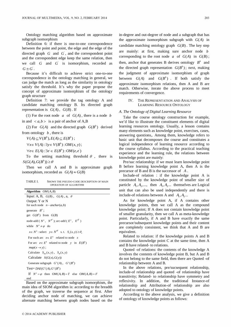
TABLE I. SHOWS THE PSEUDO-CODE DESCRIPTION OF MAIN

OPERATION OF ALGORITHM

Algorithm ( , )OM A B

Input: A, B, ( )G B , ( )G A , a,

Output: Y or N for each node ( , )n anchor a b

generate bB ;

get ( )bG B from ( )G B

node-add ( aN , bBN ); arc-add (

aE , bBE )

while aN do

ax N : select bBy N s. t. ( , )e eS x y

For each arc ae E related to node x

For arc be E related to node y in ( )bE B

( )map x y ;

Calculate ( , )HcS x y , ( , )RS x y

Calculate ( ( ), ( ))S G x G y

Generate subgraph ( )xG A , ( )y bG B

Test= ( ( ), ( )x y bDAI G A G B

If aN then ( , )OM A B T else ( , )OM A B F

end

Based on the approximate subgraph isomorphism, the main idea of SIOM algorithm is: according to the breadth

of the graph, we traverse the sequence at first. After

deciding anchor node of matching, we can achieve

alternate matching between graph nodes based on the

in-degree and out-degree of node and a subgraph that has

the approximate isomorphism subgraph with ( )G A in

candidate matching ontology graph ( )G B . The key step

are mainly: at first, making sure anchor node b

corresponding to the root node a of ( )G A in ( )G B ;

then, anchor that generates B derives ontology bB and

the directed graph representation ( )bG B ; next, making

the judgment of approximate isomorphism of graph

between ( )G A and ( )bG B . If both satisfy the

approximate isomorphism relations, then A and B are

match. Otherwise, iterate the above process to meet

requirements of convergence.

IV. THE REPRESENTATION AND ANALYSIS OF

LEARNING RESOURCE ONTOLOGY

A. The Ontology of Digital Learning Resource

Take the course ontology construction for example,

we’d like to illustrate the constituent elements of digital

learning resources ontology. Usually, a lesson contains

many elements such as knowledge point, exercises, cases,

answering questions,. Among them, knowledge refers to

basic unit that decomposes the course and constitutes a

logical independence of learning resource according to

the course syllabus. According to the practical teaching

experience and the learning rule, the relations between

knowledge point are mainly: Pre/suc relationship: if we must learn knowledge point

B before learning knowledge point A, then A is the

precursor of B and B is the successor of A .

Include-of relation : if the knowledge point A is

constituted by the knowledge point of smaller size of

particle 1 2, ,...,A A then 1 2, ...A A themselves are Logical

unit that can also be used independently and there is

include-of relations between A and 1 2, ...A A

As for knowledge point A, if A contains other

knowledge points, then we call A as the compound

knowledge point; If A does not contain knowledge point

of smaller granularity, then we call A as meta-knowledge

point. Particularly, if A and B have exactly the same

precursor/subsequent knowledge points and their content are completely consistent, we think that A and B are

equivalent.

Related to relation: if the knowledge points A and B

contains the knowledge point C at the same time, then A

and B have related- to relations.

Quoted -of relations: the contents of the knowledge A

involves the contents of knowledge point B, but A and B

do not belong to the same field, then there are Quoted -of

relationship between A and B.

In the above relations, pre/sucsequent relationship,

include-of relationship and quoted -of relationship have transitivity; Related- to relationship have symmetry and

reflexivity. In addition, the traditional Instance-of

relationship and Attribution-of relationship are also

adopted to ontology of knowledge points.

According to the above analysis, we give a definition

of ontology of knowledge points as follows:



The DNS server configuration

DNS common terms

DNS domain name resolution

DNS resource allocation

DNS lookups configuration

Private DNS configuration experiment

DNS backup and restore test

DNS assigned experimental

DNS is applied to network management

experiment

The DNS configuration

example

Distributed DNS

Centralized DNS

A forward lookup zone configuration A reverse

lookup zone configuration

DNS resource records format

functiondefine

Contains the relationship

The property relationship

Precursor relationship

The subsequent relationship

Correlation between the

Instance relationship

Reference relationship

Knowledge point ID

Algorithm number

The algorithm name

The theme

Property list

The content description

Subordinate to the subject

The difficulty coefficient

The importance of

The instance

Precursor knowledge

The subsequent knowledge

Contains the knowledge

The relevant knowledge

Reference points

Number

string

String

String

Txt

Txt

String

Float

Float

Object

Ontology

Ontology

Ontology

Ontology

ontology

Figure 5. The ontology of knowledge point of DNS sever configuration

Contains the relationship

Correlation between the

Chapter five commonly used configuration server

The certificate server

configuration

Video server configuration

The FTP server configuration knowledge

E - mail server configuration

WWW server configuration

The DHCP server configuration

The DNS server configuration

Figure 6. The configuration of the ontology model of learning resource of common server

Definition 8: a knowledge ontology (KO) can be

represented as a 7-element group:

( ) , , , , , , KOKO name id name define function content includedKO R (11)

And id , name , define , function , content ,

includedKO , KOR are respectively the number, name,

definition, function, content description, relation set of

KO of knowledge point. According to definition 8, we take the lesson “network

management” for an example, we build correspondent

ontology of knowledge point as it shows in figure 5. It is

the knowledge point “DNS server configuration” in

chapter5 from “network management from entry to

master” written by Cui Beiliang and so on.

Provided that the ontology of the knowledge point

contained in the chapter is build on sound base, then

figure 6 shows the framework of correspondent learning

resource ontology.

B. The Representation of Ontology Matching Process of

Knowledge Point:

To represent conveniently, we simplify the ontology of

knowledge point as it shows in figure 5, and then abstract

to be the directed graph as it shows in 7, recording as tag

ontology Q . The mark number in node represent

attribute. The mark number on the directed are represent

the requirement of other relations in node. We give a

candidate ontology 'Q as it shows in figure 7.

The first step of algorithm: selecting and matching a

pair of node of anchor concept ,c B , as it shows in

following figure 8.



d

e

c

f

a b

1315

22

16

18

20

17

6 4

12

9

9 7

A

B C

F

D E

H

J

30 40

30

60

60

50

50

5060

4050

4040

60

30

20

25

40 3

0

25

50

55

Figure 7. 1) the representation of tag ontology Q 2) the

correspondent representation of tag ontology B

d

e

c

f

a b

1315

22

16

18

20

17

6 4

12

9

9 7

A

B C

F

D E

H

J

30 40

30

60

60

50

50

5060

4050

4040

60

30

20

25

40 3

0

25

50

55

(ⅰ)

d

e

c

f

a b

1315

22

16

18

20

17

6 4

12

9

9 7

A

B C

F

DE

H

J

30 40

60

60

50

50

5060

4050

40

40

60

30

20

25

40 3

0

25

50

55

15

13

18

22

(ⅱ)

d

e

c

f

a b

1315

22

16

18

20

17

6 4

12

9

9 7

A

B C

F

DE

H

J

30 40

30

60

60

50

50

50

60

4050

40

40

60

30

2025

4030

25

50

55

15

13

18

22

16

20

17

(ⅲ)

Figure 8. (i) The matching of the first pair of anchor concept (ii) Based

on the ,c B anchor Q and 'Q spanning graph (iii) The

complete matching of Q and 'Q

To begin with anchor concept node, we can generate

the first subgraph of Q and 'Q in order, showing in

figure. We can calculate and judge the matching of node,

edge and structure of subgraph and achieve the first

matching of Q and 'Q .

In matched ontology subgraph, we’d like to match a

pair of node of anchor concept. Repeating the above

process until overall graph matching or no matching, the

algorithm stops, as it shows in figure 8

In the above process, the graph representation of

ontology Q achieved approximate isomorphism in the

graph representation of ontology 'Q , so we think that

ontology 'Q can match ontology Q .

C. The Analysis of Algorithm Time Complexity

In the description of the pseudo code given in the table

1, the scale of operation amount of approximate subgraph isomorphism of 3 layers of nested loop decides the time

complexity of the algorithm.

Provided that in the graph representation ( )G Q of

ontology Q , ( )V Q n , ( )E Q m and in the graph

representation '( )G Q of ontology 'Q , '( )V Q N ,

'( )E Q M , so in order to finish the matching of

ontology 'Q and Q , the unit time needed for the main

calculation is respectively: (1) The amount of time needed for the matching of the

first pair of anchor node is n N

(2) For the node ,x y , the amount of time needed

for the matching of the edge is ( ) ( )E x E y

(3) For the isomorphism judgment of subgraph ( )G x

and ( )G y and enjoys, the amount of time needed is

2 2

( ( )) ( ( ))( ) ( )

V G x V G YC C E x E y

When the number of node and edge is respectively n ,

N , m , M , the scale of the amount of time of the main

operation is

( 1) ( 1)

2 2

n n N Nm M

As a result, the complexity of the algorithm time is 6( )O n level. It is an effective algorithm.

V. CONCLUSION

Digital learning resource ontology is often based on

different specification building. It is hard to find

resources by linguistic ontology matching method. The existing structural matching method fails to solve the

problem of calculation of structural similarity well So the

paper propose a kind of ontology matching method based

on the subgraph isomorphism. It makes a alternate

matching of the point and the edge in the directed graph

of ontology representation based on calculating the

overall similarity of graph structure to achieve ontology

matching by the judgment of subgraph isomorphism. The

method aims to find efficient approximate subgraph,

improving the accuracy and efficiency of the ontology

matching.

ACKNOWLEDGEMENTS

Thanks for the support of fund, which is the Study and

Practice of the Targeted Public English Educational

Pattern under the Concept of Outstanding Talents

Education (G2012010681).



REFERENCES

[1] Rifaieh R, Benharkat N A. Query-based data warehousing tool, 2002. Proc of the 5th ACM International Workshop

on Data Warehousing and OLAP. New York: ACM, 2002 pp. 35-42.

[2] S. ALIREZA HASHEMI GOLPAYEGANI, BAHARM EMAMIZADEH. "Designing work breakdown structures using modular neural networks". Decision Support Systems. 2007, 44(11) pp. 202-222.

[3] A. K. M ZAHIDUL QUAIUM AHMED LATIFSHAHRIAR, M. ROKONUZZAMAN, "Process

Centric Work Breakdown Structure of Software Coding for Improving Accuracy of Estimation, Resource Loading and Progress Monitoring of Code Development", Proceedings of 2009 12th International Conference on Computer and Information Technology (ICCIT 2009)21-23 December, Dhaka, Bangladesh, 2009

[4] NÚÑEZ S M, DE ANDRÉS SUÁREZ J, GAYO J E L, et al. A semantic based collaborative system for the interoperability of XBRL accounting information//

Emerging technologies and information systems for the knowledge society. Springer Berlin Heidelberg, 2008 pp. 593-599.

[5] GARCÍA R, GIL R. Publishing xbrl as linked open data// CEUR Workshop Proceedings. 2009, 538.

[6] SPIES M. An ontology modelling perspective on business reporting. Information Systems, 2010, 35(4) pp. 404-416.

[7] O'RIAIN S, CURRY E, HARTH A. XBRL and open data

for global financial ecosystems: A linked data approach. International Journal of Accounting Information Systems, 2012, 13(2) pp. 141-162.

[8] HODGE F D, KENNEDY J J, MAINES L A. Does search-facilitating technology improve the transparency of financial reporting. The Accounting Review, 2004, 79(3) pp. 687-703.

[9] BARTLEY J, CHEN A Y S, TAYLOR E Z. A comparison

of XBRL filings to corporate 10-Ks-Evidence from the voluntary filing program. Accounting Horizons, 2011, 25(2) pp. 227-245.

[10] Barzily, R N. Elhadad, K. McKeown. Sentence Ordering in Multidocument Summarization. Human Language Technology Conference, Proceedings of the first international conference on Human language technology research. San Diego. 2001, pp. 79-82.

[11] Barzily, R N. Elhadad, K. McKeown. Inferring strategies for sentence ordering in multidocument news summarization. Journal of Artificial Intelligence Research, 2002, 17(2) pp. 35-55.

[12] Lapata, M. Probabilistic text structuring: experiments with sentence ordering. In proceedings of the annual meeting of ACL2003, 2003, pp. 545-552.

[13] Naoaki Okazaki, Yutaka Matsuo, Mitsuru Ishizuka. Improving Chronological Sentence Ordering by

Precedence Relation. In Proc. 20th Internaional Conference on Computational Linguistics (COLING 04),

Geneva, Swiss, August 2004, pp. 750-756. [14] Danushka Bollegala, Naoaki Okazaki, Mitsuru Ishizuka. A

bottom-up approach to sentence ordering for multi-document summarization. In Proceedings of ACL-COLING 2006. 2006, pp. 134-137.

[15] Danushka Bollegala, Naoaki Okazaki, Mitsuru Ishizuka. A Machine Learning Approach to Sentence Ordering for Multi Document. Proceedings of the Annual Meeting of the

Association for Natural Language Processing. 2005, pp. 1381-1384.

[16] Zhuli Xie, Xin Li, Barbara Di Eugenio, Weimin Xiao, Thomas M. Tirpak and Peter C. Nelson Using Gene Expression Programming to Construct Sentence Ranking Functions for Text Summarization. In 20th International Conference on Computational Linguistics. 2004, pp. 1381-1384.

[17] ZHANG J, ACKERMAN M S, ADAMIC L. Expertise networks in online communities: Structure and algorithms// Proceedings of the 1 6th International World-wide Web Conference. 2007.

[18] ABDUL-RAHMAN A, HAILES S. Supporting trust in virtual communities// Proceedings of the Hawai’i International Conference on System Sciences. 2000.

[19] Bongwon Suh, Peter L. Pirolli, Finding Credible

Information Sources in Social Networks Based on Content and Social Structure// Kevin R. Canini, 2011 IEEE International Conference on Privacy, Security, Risk, and Trust, and IEEE International Conference on Social Computing, 2011 pp. 978-985.

[20] A. Ritter, C. Cherry, and B. Dolan. Unsupervised Modeling of Twitter Conversations. // NAACL, 2010.

[21] Alonso, Omar, Carson, Chad, Gerster, David, Ji, Xiang,

and Nabar, Shubha. Detecting Uninteresting Content in Text Streams// SIGIR Crowdsourcing for Search Evaluation Workshop, 2010

[22] GIRVAN M, NEWMAN M. Community structure in social and biological networks// National Academic Science. Vol. 99. 2002 pp. 7821-7826.

Zhang Lili was born in Sichuan province of China at 2th May, 1976. He received his bachelor degree from Southwest Petroleum University, China in 2000, received his master degree in University of Electronic Science and Technology of China in 2008.

Jinghua Ding is a graduating doctoral students in Sungkyunkwan University. He regularly reviews papers for

some well-known journals and conferences. His research interests are in M2M communications, cloud computing, machine learning and wireless networks.



Trains Trouble Shooting Based on Wavelet

Analysis and Joint Selection Feature Classifier

Yu Bo Beijing Jiaotong University, School of Traffic and Transportation, Beijing China


Jia Limin*, Ji Changxu, and Lin Shuai

Beijing Jiaotong University, State Key Laboratory of Rail Traffic Control and Safety Beijing, China

*Corresponding author, Email: [email protected], [email protected], [email protected]

Yun Lifen Mississippi State University, Civil and Environmental Engineering, Mississippi State, USA


Abstract—According to urban train running status, this

paper adjusts constraints, air spring and lateral damper

components running status and vibration signals of vertical

acceleration of the vehicle body, combined with

characteristics of urban train operation, we build an

optimized train operation adjustment model and put

forward corresponding estimation method-- wavelet packet

energy moment, for the train state. First, we analyze

characteristics of the body vertical vibration, conduct

wavelet packet decomposition of signals according to

different conditions and different speeds, and reconstruct

the band signal which with larger energy; we introduce the

hybrid ideas of particle swarm algorithm, establish fault

diagnosis model and use improved particle swarm algorithm

to solve this model; the algorithm also gives specific steps

for solution; then calculate features of each band wavelet

packet energy moment. Changes of wavelet packet energy

moment with different frequency bands reflect changes of

the train operation state; finally, wavelet packet energy

moments with different frequency band are composed as

feature vector to support vector machines for fault

identification.

Index Terms—Wavelet Packet Energy Moments;

Supporting Vector Machine; Train Operation Adjustment;

Monitoring Data; Urban Trains

I. INTRODUCTION

With increased speed, the train running stability and

comfort needs to be improved. When trains are running at

high speed, the impact of track irregularities input will

make train body produces sliding, rolling and shaking his

head and will laterally accelerate through the body

synthesis, affecting the lateral stability and reducing the

comfort of the train. Lateral active and semi-active

suspension transverse are often used to reduce lateral

vibration. Therefore, the study of the relation between the

train track irregularity and lateral vibration has important theoretical and practical value for improving lateral

stability train and suspension damping effect and

estimating transform law of lateral vibration [1]. Train

Operation Adjustment issues are non-linear

multi-objective combinatorial optimization problem,

which has been known as NP-hard [2] (Nondeterministic

Polynomial Problem).

As the urban rail transit train speeds increase, driving

density increases, the train operation adjustment is also

more complicated. Therefore, the study of adjustment method which fits the characteristics of urban rail transit

train operation has significance for optimal operation in

order to improve the quality of train operator. Domestic

and foreign experts and scholars had done a lot of

research on train operation adjustment, simulation,

operations research, fuzzy decision making, expert

systems and other methods have been applied in the

solution process [3], and achieved certain results. Urban

rail transit train operation adjustment as the core of the

work vehicle dispatching, determines the merits of the

train running order [4]. For vehicle acceleration track

irregularity relationship between inputs, many researchers have been studied and achieved certain results. For

example, the literature [5] studies of vehicle-orbit

coupling system random vibration characteristics of the

train based on the establishment of the vehicle-track

vertical cross-coupling model, proving that lateral

vibration signal energy is concentrated in 1 ~ 2Hz.

Literature [6] uses the power spectral density to study the

effects of the track level and direction of the irregularity

to the vehicle random vibration, the results show that the

train is mainly influenced by rail vehicle direction and the

level of irregularity and the performance is low-frequency vibration. In order to extract the low-frequency signal

track irregularity, the literature [7-9] use wavelet

transform to analyze the track irregularity signal.

Literature [10] uses wavelet transform method to process

the signal of track irregularity and vertical acceleration

collected by the comprehensive test car, and analyze a

certain band to determine relationship between the track

irregularity and the vertical acceleration. But there are



sliding lateral vibration, shaking head and rolling, while

relative track irregularities inputs include level and

direction, so we need to further explore relationship

between the vibration components and input irregularity

[11]. Meanwhile, the cross-correlation function reflects

the relationship between signals, so we can combine the

wavelet transformation and the cross-correlation function

method. Thus, firstly use Simulink software to build 17

degrees of freedom transverse suspension model to

produce vibration signals of sliding, rolling and shaking

head, and then use wavelet transformation and cross-correlation function to analyze the relationship

between this three kinds of vibration components and

orbital level, direction and unsmooth inputs[12].

Sensors can monitor a large number of vibration data

when the high-speed train is running, different train

running status will show different characteristics of the

data, the way based on characteristics of the monitoring

data has important significance to characterize high-speed

train security state and state estimation [13]. In recent

years, many scholars have proposed some optimization

algorithm to solve with train operation adjustment problems. Mainly using genetic optimization algorithm

and particle swarm algorithm (PSO) [14]. Although the

applicability of genetic algorithms is great, shortcomings

exist in solving the optimal solution, such as complex

coding process ,time-consuming, slow convergence and

poor local search capability; because constraints of train

running are many, the search space is great, standard

particle groups convergence algorithm are susceptible to

premature, it is difficult to obtain the optimal solution

[15]. Based on the PSO algorithm, Angeline proposed

hybrid particle swarm algorithm, an improved algorithm, which introduce the idea of hybrid of genetic algorithm to

PSO algorithm, making the searching capacity of

algorithm enhance and it is not easy to fall into local

optimum. Therefore, it is urgent to propose a fast

optimization method based on a hybrid particle swarm

algorithm to solve the problem of urban rail transit train

operation adjustment. Therefore, train fault diagnosis

simulation, includes two key elements-feature selection

and classifier design. Besides useful features, there are

redundant features and useless features during extraction

of train status feature set, which increase the learning

time of classifiers and adversely affect the diagnostic results [16]. To this end, a number of trains

troubleshooting feature selection algorithms are put

forwarded, such as association rule selection algorithm,

genetic algorithm, simulated annealing algorithm, particle

swarm optimization and rough sets algorithm [17]. In

addition to feature selection, the simulation results of

train fault diagnosis are also associated with fault

classifier. The current analog fault diagnosis model trains

are mainly Bayesian network, K-nearest neighbor method,

neural networks and support vector machines [18]. The

neural network nonlinear approximation ability is superior, but the complexity of network structure is great,

so it has defects such as it is easy to fall into local

minimum value [19]. Least squares support vector

machine classifier, LSSVM, better overcomes defects

such as the over-fitting of neural network, the slow

standard SVM training and it is used broadly in simulated

fault diagnosis. So we need to choose LSSVM as the

classifier of train fault diagnosis, however the

classification performance of LSSVM is closely related

with the parameters, there are mainly genetic algorithms,

simulated annealing algorithm, particle swarm

optimization algorithm to select LSSVM parameters [20].

When the train is running, its key components [21]

may be faulty, the vibration signal [22] of the sensor

monitors as an information factor directly whether the operating state is normal or not. While the vibration

signal is majorly nonlinear and non-stationary signals,

and wavelet analysis has strong local analysis capabilities,

and it have more significant advantages [23] compared to

short time Fourier analysis and Fourier transform.

Through expansion and translation of the wavelet

function, time-frequency window can be adjusted

according to the signal frequency, and continuation on

wavelet packet decomposition has no further

decomposition of the high-frequency band, improving

frequency resolution [24]. The main innovations are the following:

(a) Compared to the normal state, when critical

components of train fails , the main frequency is changed,

and the performance is that some bands energy increases,

while some bands’ energy decreases, mapping

relationship exists between the energy band and fault

condition. Based on the monitoring data, evaluate the

running status of high-speed train’s air springs and shock

absorbers and other key components, aim at the body

vertical acceleration vibration signal, this paper propose

wavelet packet energy moments method which estimates the train state. Use the feature of the wavelet packet

energy moments to extract the method, and use support

vector machines for state estimation. Experimental results

show that this method can extract the train key

components of the initial fault characteristics and the

fault recognition rate is high.

(b) First, analyzes characteristics of the body vertical

vibration, conduct wavelet packet decomposition for

signals under the different conditions and different speeds

and reconstruct the band signal with larger energy, and

then calculate each band’s features of wavelet packet

energy moment. Changes of wavelet packet energy moment of different frequency bands reflect changes of

the train running. Compose wavelet packet energy

moments of different band as feature vectors, and

simulation analysis of experimental data shows that the

loss of gas train air springs and fault identification lateral

damper failure’s recognition rate is high ,which shows

that this method can well estimate the fault condition of

high-speed train .

(c) Considered that train operation adjustment

constraints are a lot and difficulty of solving problems is

great and other such problems, this paper combine with the characteristics of urban rail transit train operation to

establish of an optimized train operation adjustment

model. In order to improve the accuracy of fault

diagnosis, this paper takes feature selection and the



intrinsic link method of LSSVM parameters into

consideration and proposes a model with joint selection

feature and LSSVM parameters fault diagnosis. The

simulation results show that the proposed model

improves the accuracy of fault diagnosis and efficiency, It

can meet the requirements of simulative train fault

diagnosis.

II. PROPOSE METHOD

A. Adjustment Model for Train Running Status

1) Wavelet Packet Energy Moment The actual operation of the vehicle is mainly affected

by the incentive track irregularity, which is a major

source of various generated vibration. And with increased

speed, vertical acceleration increases and affects the

vehicle body through frame, excite elastic vibration of the

vehicle body with a higher frequency. And in turn, the

body train affects the frame through the spring, affecting

the dynamic performance of the train. Air spring and

horizontal absorber as the second line and the first line

suspension are the key components of train system,

abnormal vibration generated when failure occurs. It can be known by the actual knowledge the that body vibration

frequency is mainly concentrated in the low frequency

range, the main vertical vibration is generally less than

4Hz.In order to extract the subtle characteristics under

different faults, wavelet packet decomposition has a great

advantage, and this paper also proposes that wavelet

packet energy moment algorithm can reflect energy

changes of different faults in different bands. The

so-called wavelet packet is a family of functions which

construct their orthonormal base library 2( )L R , after the

wavelet packet decomposition, the signal can be

decomposed to the neighbour frequency band without

leakage, overlapping, and the frequency range of each

band is 1 1[( 1)2 , 2 ], 1,2, 8j j

s sn f n f n ,

where in, sf is sampling frequency. Most vertical

vibration generated when high-speed train runs are

nodding and rolling and pendulum and other complex

vibration of typical vibration combination. The

acceleration sensor mounted on the bogie train can

monitor different frequency band energy distribution

characteristics when signals are under different conditions. The traditional wavelet energy methods do

not consider energy distribution of each band

decomposition on the timeline, so that the extracted

feature parameters can not accurately reflect the nature of

fault, so this paper introduces the energy [8,9] parameters

sf , the energy moment ijM of each band signal ijS is:

2

1

( ) | ( ) |n

ij ij

k

M k t S k t

where in, t is the sampling interval n is the total

number of samples, k is the sampling point, and the

energy matrix algorithm steps are:

(1) Conduct wavelet packet decomposition for the

body vertical vibration signal, let S represent the original

signal, jkX be the wavelet packet decomposition

coefficients of signal of j scale in k time.

(2) Reconstruct coefficients of the wavelet packet

decomposition to obtain the frequency range jkS of the

signal.

(3) Find wavelet packet energy moment jM of each

band signal jkS .

(4) Structure feature vector to obtain a normalized

feature vector T :

2

1 2

1

[ , , ] /n

n j

j

T M M M M

2) Fault Diagnosis Model According to changes of the proportion of each

frequency band energy moment, train running status can

be monitored. Train operation adjustment is that when the running train is disturbed, actual operation of the train

deviates from the scheduled chart. Through re-adjustment

of train operation plan, so far the actual train running

route is as possible close to the scheduled chart [5]. Train

operation adjustment is a multi-constrained combinatorial

optimization problem, this kind of problem is usually

expressed by using the following abstract form [6]:

Equation of state:

( 1) ( ) ( )G j G j T G j (1)

Optimization objectives set:

(1)Object and (2)Object ...and ( )Object n

Set of constraints:

(1)Restraint and (2)Restraint ...and ( )Restraint n

Among them, ( )G j is the train running status of time

j , T is the state transition operator decided by the

adjust strategy of the running train.

For the given set of features of analog train state

1 2, , ,

nS s s s , 0,1

is , 1, 2, ,i n , where in n

is the size of the feature set , 1 and 0 denote whether the

corresponding feature is selected or not. Ultimate goal of feature selection is to improve the simulation train fault

diagnostic accuracy (G), therefore, simulate the

mathematical model of feature selection:

1 2

max ( )

. .

, , ,

0,1

1,2, ,

S

n

i

G S

s t

S s s s

s

i n

(2)

Using particle swarm optimization algorithm to

simulate the solving problem of train multi-feature

combinatorial selection optimization, particle bit string

representing the selected feature subset (S), PSO fitness

function is the analog train fault diagnostic accuracy. In

calculating the fitness value of each particle, first learn

the training set according to the selection feature S,

calculate the accuracy (G) of fault diagnosis of the



classifier of analog train, but the classifier (LSSVM)

parameters needs to be given before calculating G.

In the designing of train fault classifier based on

LSSVM, we shall determine the kernel function and its

parameters. Currently there are several LSSVM kernel

function, a large number of studies have shown that when

there is absence of a prior knowledge of the process, in

the general case, LSSVM based on radial basis function

(RBF) outperforms other kernel function, so we choose

RBF kernel, which is defined as follows:

22( , )

u v

RBFK u v e

(3)

In the formula, u , v represents the two vectors of

input space, is the width of the kernel function.

Besides RBF kernel function parameters σ, LSSVM

classification performance is also related to the

regularization parameter γ. Combined kernel function and

related parameters, classifier parameter selection model

based on LSSVM is:

,M (4)

Take analog train fault diagnostic accuracy (G) as the

classification parameters electing target, classifier

parameters mathematical model based on LSSVM is:

max min

min max

max ( )

. .

,

( , )

( , )

MG M

s t

M

(5)

Like Train simulator troubleshooting features with

combinatorial optimization, formula (4) uses PSO to seek

solution. Particle bit string represents parameter (M) of

LSSVM, the fitness function is the analog train fault

diagnostic accuracy. In calculating the particle fitness

value, LSSVM demands to study the training set

according to the parameter (M), then calculate the

simulated train fault diagnosis accuracy of classifier

(LSSVM), but the feature subset (S) needs to be given

before calculating G .

In the current modeling process of train simulator fault diagnosis, the feature selection and LSSVM parameters

intrinsic link between the two has not been considered,

the two are independent to choose, so there are some

drawbacks: firstly, it can not be determined should

feature selection or LSSVM parameters [11] selection

goes first. Secondly, if one process be carried out, then

the other will be randomly determined, so even taking

turns we can not guarantee that both are optimal.

B. Model Solving Process

1) Particle Swarm Optimization Diagnostic Model Particle swarm optimization (PSO) finds the optimal

solution by following their historic P best and throughout

the history of particle swarm optimal solution g best. PSO

algorithm has the advantage of fast convergence, without

regulation of many parameters, change impacts of the

dimension is minor, and so on, so it is easy to implement

[12]. In each iteration, the particle’s velocity and position

updating equation is:

1

2

( 1) ( ) () (

( ) () ( ( ))

id id best

id best id

v i v i c rand P

x i c rand g x i

(6)

( 1) ( ) ( 1)id id idx i x i v i (7)

where in, ( )idv i and ( 1)idv i respectively represents

the current particle velocity and the updated particle

velocity; ( )idx i and ( 1)idx i respectively represents

the current position of the particle and the updated

position of particles; w is the inertia weight; c1, c2 represents the acceleration factor; rand () indicates the

number of random function. Location of individual

particles is composed of three parts. The first part

characterize the analog train status information, using the

binary coding, in which each bit is respectively

corresponding to a given feature, "1" indicates that the

corresponding feature selection subset, and when this bit

is "0", it indicates that the corresponding feature is not in

the selected subset of features; second and third parts

respectively represent and , the code length can be

adjusted according to the required accuracy (8).

max min

min2 1

p p

p lp d

(8)

In this formula, p represents the converted value of the

parameter; l represents the length of the bit string of

corresponding parameters; max p and min p denote the

minimum and maximum of parameter; d represent

representative accuracy of binary.

Train fault feature and classification parameters selection goal is to improve train fault diagnostic

accuracy while ensuring fault feature as little as possible,

so the fitness function is defined as:

1

1

fN

a f i

i

f Acc f

(9)

where in, if denotes the feature selection status; f

N

indicates total number of features; a indicates feature

weights, f means the weights of the number of

features with respect to the accuracy of the validation set ;

Acc validates set diagnostic accuracy.

LSSVM is for two classification problems, however,

train simulator includes a variety of fault types of fault,

thus train simulator troubleshooting essentially is a

multi-classification problem, currently there are "1 to 1"

and "1 to many" which construct multiple classifiers. In

this paper, we use the "1 to 1" way to build a

multi-intended classifier for stimulating train fault.

2) Analog Troubleshooting Steps (1) Collect information of train simulator status and

use wavelet packet to extract candidate feature.



(2) To prevent that too large a difference of

characteristic values will adversely affect the training

process, the characteristic values needs to be normalized.

(3) Initialize PSO. Randomly generate m particles to

compose the initial particle swarm, each particle is

composed by a subset of features, LSSVM parameters (γ,

σ).

(4) According to the coding scheme of the particle, the

binary representation of each particle is changed into the

selected subset of features, LSSVM parameters γ and σ,

then calculate the fitness value of the particle according to formula (8).

(5) For each particle, it should compare the fitness

function value with of its own optimal value, and if the

fitness function value is better than the optimal value,

then the fitness value replace the historic optimal value,

and uses the position best of the current particle.

(6) For each particle, it should compare the fitness

function value with of its group optimal value, and if the

fitness function value is better than the group optimal

value, then the fitness value replace the historic optimal

value, and uses the position best of the current particle. (7) Update the particle velocity and position according

to equation (6) and (7), and adjust the inertia weight.

(8) When the maximum number of iterations is

reached, then output corresponding feature subset of

optimal particles, LSSVM parameters; otherwise go to

step (4) and continue the iteration.

(9) Simplify the training set and test set according to

the optimal feature subset, and then use the optimal

parameters of LSSVM to learn the training set to build a

simulation model train fault diagnosis and diagnose test

set, then output the diagnosis.

III. EXPERIMENTS AND ANALYSIS

A. Effectiveness of Experimental Wavelet Analysis

In order to verify the effectiveness of the method,

install a sensor, which monitors the vertical acceleration,

on the motor car test rig floor-mounted pillow beam of

front body, collecting working conditions signals of EMU

original car (normal condition), EMU front spring loses

gas (air spring fails), EMU yaw full demolition (yaw

damper failure conditions) and transverse damper motor

car full demolition (lateral damper failure conditions).The sampling frequency is 243Hz, the sampling time is1

minute. Figure 1 and 2 are the time domain and frequency

domain of the four conditions at 200Km / h.

Many of the train vibration is low frequency vibration,

so we first chose the Butterworth filter filters out signals

above 15Hz and zero mean processing, so that we can

eliminate the low-frequency-high-peak interference

signals in the frequency domain. It is conducive to feature

extraction. Figure 3 and 4 is a time-frequency domain

after pretreatment. The figure shows that the vertical

acceleration of EMU front springs is the biggest, and vibration energy at the fault characteristic frequency

reaches maximum. It contains a lot of pulse-pounding

ingredients, EMU yaw full demolition fault performance

is not obvious, EMU lateral damper fully demolished has

sensitive vibration frequency around 1Hz. In order to

further analyze the characteristics of all conditions for

fault identification, we select db14 wavelet according to

the main characteristics of the signal frequency range,

taking into account that because we analyze the signal

within 15Hz , we only reconstruct the preceding 8-band

wavelet packet coefficients decomposed by the layer

6.The corresponding frequency range is: 0-1.875Hz,

1.875-3.75 Hz, 3.75-5.625 Hz, 5.625-7.5 Hz, 7.5-9.375

Hz, 9.375-11.25 Hz, 11.25-13.125 Hz, 13.125-15 Hz.

Corresponding figure of frequency band and energy

moment can be obtained under different speeds ,as shown from figure 3 to figure 6.

0 50

-0.1

0

0.1

time/s

The

ver

tica

l ac

cele

rati

on

of

m/s

2

Train the original car

0 10 200

20

40

60

80am

pli

tud

e

0 50

-0.1

0

0.1

Move the front overhead spring loss of air pressure

0 10 200

20

40

60

80

time/s

Frequency/Hz

amp

litu

de

Frequency/Hz

The

ver

tica

l ac

cele

rati

on

of

m/s

2

Figure 1. Frequency motor vehicle and air spring air

0 50

-0.1

0

0.1

Train all resist sinusoidal

0 10 200

20

40

60

80

0 50

-0.1

0

0.1

Train all transverse shock absorber

0 10 200

20

40

60

80

time/s

Th

e v

erti

cal

acce

lera

tio

n o

f m

/s 2

amp

litu

de

time/s

Frequency/Hz

amp

litu

de

Frequency/Hz

Th

e v

erti

cal

acce

lera

tio

n o

f m

/s 2

Figure 2. Frequency domain anti hunting around buildings and lateral

damper fully

In the figure, the letters A-D respectively denotes the

original car EMU, EMU loss of gas spring before

overhead, yaw full EMU demolition and EMU lateral

damper demolition. Brackets after the letters indicates

failure state when the train runs at certain speed.

Instability occurs when EMU is at yaw full demolition

220Km / h , so 250Km / h without the condition, it is

know from the figure that the same conditions has the

same trend at different speeds, front overhead spring loss of gas failure, energy is concentrated in a second band, i.e.

There is sensitive vibration sequency within the 2-4Hz

and there are many responsive impulse .Known from the

train model, the air spring is mounted and supported on



the bogie of the rubber base body, the compressed air

inside the rubber balloon is took as the elastic restoring

force of the reaction force, this can reduce the vibration

and shock. The air spring failure just relies on the rubber

buffer alone to reduce damping and this will make the

acceleration vibration of the vehicle increase. Energy of

the other two faults and normal condition is concentrated

in the first and second bands, as the speed increases, the

torque difference between the energy band increases.

When lateral damper fully removed excite instability, the

energy is mainly in the first frequency band. Above analysis indicates that under different conditions and

different speeds, energy changes according to the

respective conditions of frequency and time distribution.

0 2 4 6 80

0.2

0.4

0.6

0.8

1

Eight before 6 layer decomposition of

wavelet packet frequency band

En

erg

y m

om

ent

160Km/h

A

BC(micro sway)

D

Figure 3. 160 Km/h wavelet packet energy moment

0 2 4 6 8

200Km/h

A

BC(shakes, HuanShou)

D

0

0.2

0.4

0.6

0.8

1



Ener

gy m

om

ent


0 2 4 6 80

0.2

0.4

0.6

0.8

1220Km/h

A

BC (buckling)D (vibration, shaking, HuanShou)



Ener

gy m

om

ent


B. Fault Diagnosis Test

SVM is advantageous for the small sampling,

nonlinear and high dimensional pattern recognition

[10-12], so we use support vector machines for fault

identification. We extract 30 sample groups for each

group of these four kinds of working conditions, there are

120 groups of samples in total, wherein 60 groups are for

training and 60 groups for testing. Each group is a dimensional feature vector which is composed of the

energy moment of the 8 preceding frequency band of the

last layer wavelet packet. The experiment has four

conditions of the vibration signal, so it needs to establish

three second-class SVM. The fault identification topology

structure is shown in Figure 7, four kinds of conditions of

the correct recognition rate results are shown in Table 1.

0 2 4 6 80

0.2

0.4

0.6

0.8

1250Km/h



En

erg

y m

om

ent

A

BD(turbulence instability )


From table 1, we know, as the speed increases in each

case, the correct recognition rate is 100% when EMU gas

spring failure speed is 200Km / h; when the motor car full

demolition fault yaw rate reached 220Km / h, meandering

instability occurs and when the speed is 200Km / h, the

recognition rate is the highest; excitation instability

occurs when EMU lateral damper fully dismantle is at 250Km / h , then the vibration frequency is very small

and the correct identification rate is 100 %.

C. Fault Identification

In order to verify the effectiveness of high-speed train

bogie mechanical fault signal extract wavelet entropy

features, we use support vector machine to classify and recognize characteristic data. The data used is the

simulation data under single fault condition, select the

responding data collected by the 58 sensors as a group

when the speed is 200km / h, under four kinds of fault

state. In order to achieve classification, take each group’s

data under the same conditions and the same position into

a 3 seconds of data segments, each segment as a sample,

then a single failure has 70 samples an the four faults

have 280 samples. As previous description, these samples

needs to do de-noising preprocessing and feature

extraction wavelet entropy, wherein we abandon the distance rounding wavelet entropy, each sample has a

feature vector with five of five-dimensional wavelet

entropy .Put these five-dimensional feature vectors which

are extracted by 280 samples into the input support vector

machine to recognise. Wherein, 60% of the samples were

randomly selected as the training samples, and the

remaining 40% as test samples.

Figure 8 is a three-dimensional features figure of

lateral acceleration signal of the central frame and

acceleration signal plot of longitudinal axis gearbox. It

can be seen from the figure that there is a little overlap phenomenon of two-dimensional wavelet entropy under

four kinds of conditions, the same conditions feature is

not very concentrated, but some characteristics of the

particular condition has a good degree of differentiation,

so when we select five-dimensional wavelet entropy

features to form a high-dimensional feature, we are able

to get a satisfactory recognition effect.



SVM 1

F ( x )= 1 ?

SVM 2

F ( x )= 1 ?

Train normal signal

The input

The feature vectors

SVM 3

F ( x )= 1 ?

No

Yes

Move the front overhead spring loss

of air pressure

Train of serpentine complete

Train all transverse shock absorber

Yes

Yes

No

No

Figure 7. The fault identification topology structure is shown

TABLE I. DIFFERENT SPEEDS UNDER FOUR CONDITIONS OF THE RATE OF CORRECT RECOGNITION

speed(Km/h) Motor

car

Before starting the overhead

spring loss of gas

Train anti hunting around

buildings

Vehicle lateral damper around

buildings

160 20% 93.3% 40% 60%

200 60% 100% 73.3% 66.7%

220 80% 100% 53.3%(unstability) 46.7%

250 66.7% 100% - 100%(Excitation instability)

280 93.3% 100% - -

300 93.3% 100% - -

330 100% 100% - -

The average recognition rate 73.3% 99% 55.5% 68.4%

TABLE II. THE RECOGNITION SENSOR CHANNEL RATE

Wavelet entropy feature discrimination %

1—10 66.9 66.9 67.8 30.3 58.0 66.0 91.9 51.7 83.9 59.8

11—20 94.6 79.4 92.8 44.6 90.1 47.3 70.5 54.4 74.1 96.4

21—30 48.2 93.6 76.7 29.4 97.3 98.2 24.1 91.9 61.6 33.9

31—40 91.0 84.8 90.2 83.0 93.7 85.7 62.5 64.3 67.8 58.9

41—50 70.5 59.8 71.4 56.2 66.9 75.9 75.0 71.4 59.8 60.7

51—58 71.4 65.1 95.5 92.8 75.0 69.6 62.5 61.6

TABLE III. THE EXPERIMENTAL RESULTS ARE SHOWN

discrimination % 40 km/h 80 km/h 120 km/h 140 km/h 160 km/h 200 km/h

wavelet energy feature 34.4 41.3 70.1 79.6 81.0 84.9

Wavelet entropy feature 26.7 38.3 69.6 81.2 85.7 96.4

Data signal recognition results of each channel

(different sensor) are shown in Table 2. Experimental

data were collected from 58 channels, distributed in

various parts of the bogie. But the theory is not clear about which parts of the vibration signal acquisition is

more conducive to the identification of a fault condition,

the experimental results show that the recognition

performance is uneven between different sensors. As can

be seen from table 2, a high recognition rate of the

channel is the channel 11, 20, 25, 26 and 53. They are

respectively corresponding to the mounting position of

the sensor lateral acceleration of the central frame, one

axle lateral acceleration, longitudinal axis gear box

accelerometer, three-axis gearbox lateral acceleration and

a series a relative displacement.

In order to verify the validity of feature extraction, this paper compares the proposed method with the traditional

wavelet energy feature extraction methods, and

respectively calculate the fault recognition rate when the

train is running at 40km / h, 80 km / h, 120 km / h, 160

km / h and 200 km / h , the experimental results are

shown in table 3.

It can be concluded from table 3 that compared to

traditional wavelet energy feature, the wavelet entropy features can get higher fault recognition rates, especially

in the high state. As the train speeds increase gradually

the recognition rate increases and when the speed is 200

km / h the wavelet entropy feature recognition rate can

reach 90% or a more satisfactory result. It is believed that

the higher the speed, the greater the difference between

the law of the vibration signal bogie caused by different

failure. The more obvious the fault feature are the greater

the impact on train mechanical systems and this

conclusion is consistent with the kinetic theory.

IV. CONCLUSION

According to high-speed train running status, this paper adjusts constraints, air spring and the running status

of lateral damper components and vibration signals of

vertical acceleration of the vehicle body. Combined with

operation characteristics of urban train, the paper



establishes an optimized train operation adjustment

model, and proposes the train state estimation method of

corresponding wavelet packet energy moment. Besides,

as for the problem that the features of the current analog

fault diagnosis does not match the classification

parameter selection, this paper also proposes an analog

train fault diagnosis model with joint selection

characteristics and classifier parameters. As for the

vertical acceleration vibration signals based on

monitoring front beam floor, we propose using the feature

extraction method of wavelet packet energy moments, and use SVM to estimate the running state. Experimental

results show that the is the signal is most sensitive to air

spring failure and has sensitive vibration frequency

within 2-4Hz; lateral damper fully removed is relatively

more sensitive when excitation instability occurs around

1Hz, and the accurate recognition rate is 100%.It

indicates that vertical acceleration monitoring data is

effective for air spring losing of gas and lateral damper

excitation instability. The next step needs to be done is:

the train running from normal to abnormal is a gradual

process, the shown signs are fuzzy and random in many cases. This article just makes a preliminary discussion,

further study of the high-speed train safety warning and

health maintenance needs to be carried out.

00.2

0.40.6

0.8

0

0.2

0.40.2

0.3

0.4

0.5

0.6

0.7

WEEWTFE

WS

E

The original car

Air spring loss of air pressure

Coil resistance failure

Lateral damper failure

a) 11 channel architecture the central lateral acceleration signal

0.10.2

0.30.4

0.50.6

0

0.2

0.40.45

0.5

0.55

0.6

0.65

0.7

WEEWTFE

WS

E

The original car

Air spring loss of air pressure

Coil resistance failure

Lateral damper failure

b) 25 channel three axle gear box longitudinal acceleration signal

Figure 8. Three dimensional feature pictures of different position

signal

ACKNOWLEDGMENT

This work was supported in part by The National High

Technology Research and Development Program of

China (Grant No. 2011AA110506).

REFERENCES

[1] Kuihe Yang, Ganlin Shan, Lingling Zhao. Application of Wavelet Packet Analysis and Probabilistic Neural Networks in Fault Diagnosis, Proceedings of the 6th World

Congress on Intelligent Control and Automation. 2006 pp. 4378-4381.

[2] Jiang Zhao, Feng Sun, Huapeng Wang. Pipeline leak fault feature extraction based on wavelet packet analysis and application, IEEE 2011 International Conference on Electrical and Control Engineering, 2011 pp. 1148-1151.

[3] Alexios. D. Spyronasios, Michael. G. Dimopoulos. Wavelet Analysis for the Detection of Parametric and Catastrophic Faults in Mixed-Signal Circuits. IEEE Transactions on Instrumentation and Measurement, 2011,

60(6) pp. 2025-2038 [4] Shengchun Wang, Qing Zhang, Study on The Fault

Diagnosis Based on Wavelet Packet and Support Vector Machine, International Congress on Image and Signal Processing. 2010, (3) pp. 3457-3461.

[5] Urmil. B. Parikh, Biswarup. Das, Combined Wavelet-SVM Technique for Fault Zone Detection in a Series Compensated Transmission Line. IEEE Transactions on

Power Delivery, 2008, 23(4) pp. 1789-1794. [6] CHO Chan-Ho, CHOI Dong-Hyuk, QUAN Zhong-Hua, et

al. Modeling of CBTC Carborne ATO Functions using SCADE. //Proc of 11th International Conference on Control, Automation and Systems. Korea: IEEE Press, 2011 pp. 1089-1093.

[7] CHENG Yun, LI Xiao-hui, XUE Song, et al. The position and speed detection sensors based on electro-magnetic

induction for maglev train. //Proc of the 29th Chinese Control Conference Beijing: IEEE Press, 2010 pp. 5463-5468.

[8] HOU Ming-xin, NI Feng-lei, JIN Ming-he. The application of real-time operating system QNX in the computer modeling and simulation. //Proc of 2nd International Conference on Artificial Intelligence, Management Science and Electronic Commerce. Deng Leng: IEEE Press, 2011

pp. 6808–6811. [9] ESTEREL Technologies. SCADE Suite. (2012-11-1)

[2013-03-07]. http: //www. esterel-technologies. com/ products/ scade-suite/.

[10] WANG Hai-feng, LIU Shuo, GAO Chun-hai. Study On Model-based Safety Verification of Automatic Train Protection System. //Proc of 2nd Asia-Pacific Conference on Computational Intelligence and Industrial Applications. Wuhan : IEEE Press, 2009 pp. 467-470.

[11] DH Wang, WH Liao. Semi-Active Suspension Systems for Railway Vehicles Using Magnetorheological Dampers. Vehicle System Dynamics, 2009, 47(11): pp, 1130-1135

[12] Guangjun Li, Weidong Jin, Cunjun Chen. Fuzzy Control Strategy for Train Lateral Semi-active Suspension Based on Particle Swarm Optimization//System Simulation and Scientific Computing Communications in Computer and Information Science 2012, pp. 8-16

[13] Camacho J, Picó J. Online monitoring of batch processes using multi-phase principal component analysis. Journal of Process Control, 2006, 16(10) pp. 1021-1035.

[14] Hua Kun-lun, Yuan Jing-qi. Multivariate statistical process control based on multiway locality preserving projectio- ns. Journal of Process Control, 2008, 18(7-8) pp. 797-807.

[15] Yu Jie, Qin S J. Multiway Gaussian mixture model based multiphase batch process monitoring. Industrial &

Engineering Chemistry Research, 2009, 48 (18) pp. 8585-8594.

[16] Guo Jin-yu, Li Yuan, Wang Guo-zhu, Zeng Jing. Batch Process monitoring based on multilinear principal component analysis//Proc of the 2010 International Conference on intelligent systems and Design and Engineering Applications, 2010, 1 pp. 413-416.



[17] Chang Yu-qing, Lu Yun-song, Wang Fu-Li, et al. Sub-stage PCA modelling and monitoring method for

uneven-length batch processes. The Canadian Journal of Chemical Engineering, 2012, 90(1) pp. 144-152.

[18] Kassidas A, MacGregor J F, Taylor P A. Synchronization of batch trajectories using dynamic time warping. AIChE Journal, 1998, 44(4) pp. 864-875.

[19] Rothwell S G, Martin E B, Morris A J. Comparison of methods for dealing with uneven length batches//Proc of the 7th International Conference on Computer Application

in Biotechnology (CAB7), 1998 pp. 387-392. [20] Lu Ning-yun, Gao Fu-rong, Yang Yi, et al. PCA-Based

modeling and on-line monitoring strategy for uneven-length batch processes. Industrial & Engineering Chemistry Research. 2004, 43(13) pp. 3343-3352.

[21] Yao Yuan, Dong Wei-wei, Zhao Lu-ping, Gao Fu-rong. Multivar -iate statistical monitoring of multiphase batch processes with uneven operation durations. The Canadian

Journal of Chemical Engineering, 2012, 90(6) pp. 1383-1392.

[22] Zhao Chunhui, Mo Shengyong, Gao Furong, et al. Statistical analysis and online monitoring for handling multiphase batch processes with varying durations. Journal of Process Control, 2011, 21(6) pp. 817-829.

[23] Wang Jin, Peter He Q. Multivariate statistical process monitoring based on statistics pattern analysis. Industrial

& Engineering Chemistry Research, 2010, 49 (17) pp. 7858-7869.

[24] Garcia-Alvarez D, Fuente M J, Sainz G. I. Fault detection and isolation in transient states using principal component analysis. Journal of Process Control, 2012, 22(3) pp. 551-563.

[25] Wise B M, Gallagher N B, Butler S W, et al. A comparison of principal component analysis, multiway principal

component analysis, trilinear decomposition and parallel factor analysis for fault detection in a semiconductor etch process. Chemomotrics, 1999, 13(3-4) pp. 379-396.

Yu Bo (1985-), he is currently pursuing the Ph.D. degree in traffic and transportation at Beijing Jiaotong

University. He is currently working on real-time monitoring and safety warning technology of urban rail trains. His main research directions are train safety, train fault diagnoses, train networks and etc.

Jia Limin (1963-), received Ph.D. degree from China Academy of Railway

Sciences 1991 and EMBA from Peking University 2004. He is now a chair Professor at the State Key Lab of Rail Traffic Control and Safety, Beijing Jiaotong University. His research interests include Intelligent Control, System Safety, Fault Diagnosis and their applications in a variety of fields such as

Rail Traffic Control and Safety, Transportation and etc.

Ji Changxu (1960-), received Ph.D. degree from Jilin university of technology. He is now a Professor at school of traffic and transportation, Beijing Jiaotong Univesity. His research interests include train safety, train fault

diagnoses, traffic planning and management, network optimization of the comprehensive passenger transport

hub service and etc.

Lin Shuai (1987-), she is currently pursuing the Ph.D. degree in traffic and transportation at Beijing Jiaotong

University. She is currently working on reliability assessment of urban rail trains. Her main research directions are train safety, train reliability and etc.

Yun Lifen (1984-), she is pursuing the Ph.D. degree in traffic and transportation at Beijing Jiaotong University and

currently as exchange students in Mississippi State University. Her main research directions are traffic planning and management, network optimization of the comprehensive passenger transport hub service and etc.



Massive Medical Images Retrieval System Based

on Hadoop

YAO Qing-An 1, ZHENG Hong

1, XU Zhong-Yu

1, WU Qiong

2, LI Zi-Wei

2, and Yun Lifen

3

1. College of Computer Science and Engineering, Changchun University of Technology, Changchun, China

2. College of Humanities and Information, Changchun University of Technology, Changchun, China

3. Mississippi State University, Civil and Environmental Engineering, Mississippi State, USA

Abstract—In order to improve the efficiency of massive

medical images retrieval, against the defects of the

single-node medical image retrieval system, a massive

medical images retrieval system based on Hadoop is put

forward. Brushlet transform and Local binary patterns

algorithm are introduced firstly to extract characteristics of

the medical example image, and store the image feature

library in the HDFS. Then using the Map to match the

example image features with the features in the feature

library, while the Reduce to receive the calculation results of

each Map task and ranking the results according to the size

of the similarity. At the end, find the optimal retrieval

results of the medical images according to the ranking

results. The experimental results show that compared with

other medical image retrieval systems, the Hadoop based

medical image retrieval system can reduce the time of image

storage and retrieval, and improve the image retrieval

speed.

Index Terms—Medical Image Retrieval; Feature Library;

Brushlet Transform; Local Binary Patterns; Distributed

System

I. INTRODUCTION

The development of digital sensor technology and

storage device leads to the rapid expansion of the digital

image library, and all kinds of digital equipment produce

vast amounts of images every day. So how to effectively

organize the management and access of these images

becomes a hot research direction in recent years. The

traditional text-based image retrieval system uses the key

words to retrieve the marked images. But owing to the

limitations that artificial marking causes large workload,

the content of the images cannot be completely described

by words, and the understanding of images is different

from person to person and so on, the text-based image

retrieval system cannot meet the requirements for

massive images retrieval. And how to carry on the

effective management and organization of these medical

images to provide services to clinical diagnosis becomes

a problem faced by medical workers [1]. The

content-based medical image retrieval (CBMIR) has the

advantages of high retrieval speed and high precision and

so on, and has been widely applied in the fields such as

medical teaching, aided medical diagnosing, medical

information management, etc [2].

The content-based image retrieval [3] is a kind of

technology which makes use of the visual features of the

images to carry on the image retrieval. Under the premise

of a given query image, and according to the information

of the image content or the query standard, it searches

and finds out the images that meet the query requirements

in the image library. There are mainly three key steps:

first, selecting the appropriate image characteristics;

second, adopting the effective feature extraction method;

third, using the effective feature matching algorithm.

Features that can be extracted from an image include

color, texture, shape, flat space corresponding relation,

etc. Color can be presented by color moment, histogram,

etc. Texture can extract the Tamura feature, Gabor and

wavelet transform of image. Shape can be divided into

area-based method and edge-based method. Flat space

corresponding relation can be described through

two-dimensional string [4].

At present, many institutions have further studied

CBMIR, and developed systems that went into practice.

Such as the earliest commercial QBIC system [5]

developed by IBM, WebSeek system [6] by Columbia

University, Photobook system [7] by Massachusetts

Institute of Technology and so on. There are also many

outstanding works in the content-based image retrieval

direction in recent years, for example, literature [8], based

on the clustering of unsupervised learning, are the typical

examples of CBMIR technology, literature [8][9] use the

semi-supervised learning method, literature [9] carry on

image retrieval with the method of relevance feedback,

and a lot of works also improve the quality of image

retrieval by improving the method of feature extraction,

such as literature [11, 12]. The CBMIR algorithm needs

to calculate the similarity between the features of sample

medical images and the features in the feature library. It

is a typical data-intensive computing process [13]. When

the number of the features in the library is large, the

efficiency of the single-node retrieval in the traditional

browser/server mode (B/S) is difficult to meet the

real-time requirements of the images, and the system has

a poor stability and extensibility [14]. Cloud computing

can assign the tasks to each work node to complete the

tasks together, and with a distributed and parallel

processing ability, it provides a new research idea for

medical image retrieval [15].



Hadoop is an open-source project under the Apache

Software Foundation organization, which provides the

reliable and scalable software under distributed

computing environment. It is a framework that allows

users easily using and distributing computing platform,

and it can support thousands of computing with PB-level

nodes data [11, 12]. Hadoop distributed computing

platform is suitable for all kinds of resources, data and

other deployed on inexpensive machines for distributed

storage and distributed management. It is with high

reliability, scalability, efficiency and high fault tolerance,

etc., and it can effectively improve the image the speed of

retrieval. The text on the basis of reaching open-source

framework Hadoop, analyzing the traditional image

retrieval system and combining the content-based image

retrieval technology and MapReduce computing

framework [13] stores the image feature in database

HDFS and developers the realized Hadoop-based mass

image Retrieval System.

Hadoop Distributed File System (HDFS) is a scalable

distributed file system. For it can be run on a cheap and

ordinary hardware, it is supported by many companies,

such as Google, Amazon, Yahoo! and so on. Under the

circumstance that the underlying details is unknown,

using the Map/Reduce functions to realize the parallel

computing easily has been widely applied in the field of

mass data processing [16]. Making use of the advantages

of Hadoop, the problem that the retrieval efficiency is

low in the process of medical image retrieval can be

better solved, and there is no related research in the

domestic presently [17]. Content-based image retrieval

CBIR is the underlying objective retrieval by using global

and local features of the image. Global features include

color, shape, texture and so on; local features include

SIFT, PCA-SIFT, SURF and so on [14]. As an automatic

objective reflection image content-based retrieval method,

CBIR is suitable for mass image retrieval. Semantic

retrieval is the direction of development of CBIR image,

but the image semantic has the characteristics of

complexity, subjectivity, etc., and it is difficult in the

extraction, expression and application of technical exist

[15]. There are two main aspects of development of

parallel image processing system; one is for some

algorithms. It is searching the efficient parallel algorithm

and development of high-performance parallel computer

to achieve specific purposes, but such system is limited to

the scope of application. The other is developed for

general-purpose parallel image processing system, which

is the mainstream of the parallel image processing system

[16]. Image parallel computing generally are divided into

two kinds: pipelined parallel and data parallel. Pipelined

parallel is with the handling unit sequentially connected

in series, that is, the output of a processing unit and the

input of the next processing unit is connected. Data

parallelism is composed of a plurality of processing units

in parallel arrays, and each processing unit can perform

its tasks independently [17]. With the increasing of the

image data, the mass of the image retrieval process has

become a very time consuming process.

To improve the efficiency of medical image retrieval,

aiming at the shortage of the B/S single-node system, a

medical image retrieval system based on the distributed

Hadoop is put forward. And the experimental results

show that the Hadoop-based medical image retrieval

system not only reduces the time of image retrieval,

improves the efficiency of image retrieval, but also

presents a more apparent advantage for massive medical

images retrieval.

Main innovations of this paper:

(a) With the continuous development of digital

technology, there is a sharp increase in the amount of

image data for the image data. For the mass interested in

image retrieval problem of low efficiency, as well as the

deficiencies of B / S single-node system, the efficiency of

medical image retrieval is further improved and Medical

Image Retrieval system based on Hadoop Distributed is

proposed. It is based on Hadoop cloud computing

platform, adopts the parallel retrieval technology and uses

the SIFT Scale Invariant Feature Transform algorithm to

solve the problem of massive image retrieval.

(b) Medical Image Retrieval system based on the

Hadoop Distributed improves the efficiency of image

storage and retrieval, which get better search results.

They are mainly showing in the following aspects:

medical image retrieval can meet real-time requirements

of medical image retrieval, especially when dealing with

large-scale medical image. It has the unparalleled

advantages compared to traditional B / S single-node, and

at the same time it reduces the image retrieval time and

improves the efficiency of image retrieval, especially for

massive medical image retrieval.

II. HADOOP DISTRIBUTED MEDICAL IMAGE

RETRIEVAL

A. Hadoop Platform

Hadoop platform is the most widely used open source

cloud computing programming platform nowadays. It is

an open source framework which runs large database to

deal with application programs on the cluster, and it

supports the use of MapReduce distributed scheduling

model to implement the virtualization management,

scheduling and sharing of resources [10].

The structure of HDFS is that a HDFS cluster consists

of a master server (NameNode) and multiple chunk

servers (DataNode), and accessed by multiple clients. The

NameNode is responsible for managing the namespace of

the file system and the access of the clients to the files,

while DataNode manages the storage of the data of its

node, handles the client’s reading and writing requests of

the file system, as well as carries on the creation, deletion

and copy of the data block under the unified scheduling

of NameNode [11]. HDFS cuts the files into pieces, then

stores them in different DataNode dispersedly, and each

piece can be copied and stored in different DataNode.

Therefore, HDFS has high fault tolerance and high

throughout of data reading and writing.

MapReduce is a programming model, which is used

for the calculation of large amount of data. For the

calculation of large amount of data, the usually adopted



processing technique is parallel computing. First of all,

breaking a logically complete larger task into subtasks,

then according to the information of the tasks, using

appropriate strategies, the system assigns the different

tasks to different resource nodes for their running. When

all the subtasks have been finished, the processing of the

whole large task is finished. Finally, the processing result

is sent to the user [12]. In the Map phase, each Map task

calculates the data assigned, and then maps the result data

to the corresponding Reduce task, according to the key

value output by Map.

In the Reduce phase, each Reduce task carries on the

further gathering processing of the data received and

obtains the output results. To make the data processing

cycle of MapReduce more visual, the calculation process

of the MapReduce model is shown in Figure 1. Map

Map

…

Map

Map

Reduce

Service Get Results

User1

StartJob1

Tasks

User2

StartJob2

Stop Job1

Store status

and results

Combine

Map

Map

…

Map

Map

Reduce

Tasks

Stop Job2

Combine

Figure 1. Data processing cycle of map reduce

1

2

3

4

567891011121314

15

16

1718

19

20

21

22

23 24 25 26 27 28 29 30 31 32

33

34

35

36

Figure 2. Level three decomposition direction of brushlet

B. Feature Extraction of Brushlet Domain

Brushlet transform is the image multi-scale geometric

analysis tool which aims at solving the problem of

angular resolution. The two-dimensional Brushlets has

certain direction structure and vibration frequency range,

and can be reconstructed perfectly. The structure size of

its basic function is inversely proportional to the size of

the analysis window. The two-dimensional Brushlet with

phase parameters shows its direction, thus better reflects

the direction information of the image, and can conduct

the decomposition of the Fourier domain [13]. Level one

of Brushlet transform will divide the Fourier plane into

four quadrants, and the coefficient is divided into four

sub-bands, the corresponding direction is / 4 / 2k ,

0,1,2,3k . Level two further divides each quadrant into

four parts on the basis of level one, and the whole twelve

directions respectively are /12 / 6k , 0,1, 11k .

There are sixteen coefficients after the decomposition,

among which the four sub-bands around the center are

with low frequency component, and the rest are with high

frequency component. And so on in a similar fashion.

Figure 2 is the decomposition direction graph of level

three.

Given an image f , and conducts level l

decomposition of Brushlet to it, there are will be two

parts after the decomposition, which are the real part ˆrf

and the imaginary part ˆif . Each part has 4l sub-bands,

and each sub-band reflects the direction information of its

corresponding decomposition direction. The place where

the energy focused is exactly the parts where the texture

image mutations. For each sub-band, its energy

information can choose to be shown by the mean value

and the standard deviation of the module value. Because

Brushlet is a complex function, the corresponding

sub-band coefficient of the real part and the imaginary

part after the decomposition is used to calculate the

module value at the same time. After the decomposition,

the n sub-bands of the real part and the imaginary part

respectively are marked to be ˆnrf and ˆ

nif

1,2, 4ln . The mean value n and the standard

deviation n of the n sub-band’s module value

respectively are:

1 1

2 2

1 1

1| ( , ) |

1 [ ( , )] [ ( , )]

M N

n n

i j

M N

nr ni

i j

f i jMN

f i j f i jMN

(1)

^

2

1 1

1(| ( , ) | )

M N

n n n

i j

f i jMN

(2)

In the above equation, 1,2, ,i M , 1,2, ,j N .

M and N respectively represents the line number and the

column number of each sub-band. The feature vector of

image f is:

1 1 2 2[ , , , , ]F (3)

C. Feature Extraction of LBP

LBP can depict the changes relative to the center of the

pixel’s gray level within the territory. It pays attention to

the changes of the pixel’s gray level, which is in

accordance with human’s visual perception features of

the image, and the histogram is treated as the airspace

characteristics of the image.

7

3203

( )2 , ( ) 2

256,

i

i cui

s g g U LBPLBP

otherwise

(4)

Among which:



1, 0

( )0, 0

i c

i c

i c

g gs g g

g g

(5)

3 7 0

7

1

1

( ) ( ) ( )

| ( ) ( ) |

c c

i c i c

i

U LBP s g g s g g

s g g s g g

(6)

In the above equation, cg is the pixel’s gray value of

a neighborhood center, and ig means each pixel’s gray

value of the neighborhood in clockwise, which is within

the range of 3×3, and cg as the center.

D. The Similarity Matching

To measure the feature similarity of Brushlet domain,

the average distance is used:

6

Brushlet

1

, Pi Qi

i

Sim P Q E E

(7)

Among which, P is the medical image waiting to be

retrieved, and Q is the image of the medical image

library.

For the LBP features of the image, firstly the

characteristics are being unanimously processed, and then

the Euclidean distance is used to calculate the similarity.

32 2

LBP

1

, Pi Qi

i

Sim P Q

W W (8)

In the above equation, W represents the

characteristic vector after the normalization.

Because the value range of '

BrushletSim and LBPSim is

different, the external normalization is being processed to

them. The specific process is as follows:

Brushlet Brushlet'

Brushlet

Brushlet

,1,

2 6

Sim P QSim P Q

(9)

'

,1,

2 6

LBP LBP

LBP

LBP

Sim P QSim P Q

(10)

In the above equation, Brushlet , Brushlet

, LBP and

LBP respectively represents the standard deviation and

the mean value of '

BrushletSim and '

LBPSim .

The distance between the two medical images is as

follows:

' '

1 Brushlet 2, , ,LBPSim P Q w Sim P Q w Sim P Q (11)

In the equation, 1w and

2w are for the weight, and

meet the formula that 1w +

2w =1.

E. The Algorithm of Medical Image Retrieval

1) The Medical Image Storage of MapReduce

Image storage is the foundation of the automatic

medical image retrieval, and it is a data-intensive

computing process. The using of the traditional method to

put the image into HDFS is very time-consuming, thus

the distributed processing method of MapReduce is

applied to upload the image to HDFS. The specific

situation is as follows:

(1) In the Map phase, using the Map function to read a

medical image every time, and extract the color and

texture feature of the image.

(2) In the Reduce phase, the extracted feature data of

medical image is stored in HDFS. HBase is a

column-oriented distributed database, thus the table form

of it is used for the medical image of HDFS. The specific

process is shown in Figure 3.

HDFS took a picture of a medical image as

the Map input

Extract the image feature

The image and characteristics

into HBase

Finish the HDFS image processing

Collect the output of each Map

Medical images uploaded to the HDFS

N

Y

Figure 3. Storage process of medical image

Upload the medical images to HDFS→Take a medical

image from HDFS and input it as Map→Extract the

image features→Write the image and features in HBase

→Complete the image processing in HDFS→Collect the

output of Map

2) Medical Image Retrieval of MapReduce

The medical image and its features are all stored in

HBase, when the data set of HBase is very large, the scan

and search of the entire table will take a relatively long

time. To reduce the time of image retrieval and improve

the retrieval efficiency, the MapReduce calculation model

is used to conduct the parallel computing of medical

image retrieval. The specific framework is shown in

Figure 4.

Reduce

Map

HDFS (and features to retrieve image)

Map

Medical image retrieval

Map

Medi

cal

imag

e ID

Medi

cal

imag

e up

load

Medical image ID set

HDFS (images)

feature

Figure 4. Work diagram of image retrieval

The steps of MapReduce based medical image retrieval

are as follows:



(1) Collect the medical images, extract the

corresponding features and store the features into HDFS.

(2) With the user’s submission of search requests,

extract the Brushlet features and LBP features of the

medical images waiting for retrieval.

(3) In the Map phase, conduct the similarity matching

between the features of the medical images waiting for

retrieval and the features of images in HBase. The output

of the map is the key value of <similarity, image ID>.

(4) Conduct the ranking and redistricting of the whole

key value of <similarity, image ID > output by map,

according to the size of the similarity, and then input

them into the reducer.

(5) In the Reduce phase, collect all the key-value pairs

of <similarity, image ID >, then conduct the similarity

sorting of these key values, and write the first N keys into

the HDFS.

(6) Output the ID of those images that are the most

similar to the medical images waiting for retrieval, and

the user gets the final result of the medical retrieval.

The function of Map and Reduce is as follows:

,Map key value

Begin

//read the features of the medical images waiting for

retrieval

ReCsearch ad SearchCharact ;

// read the data in the feature library

Cdatabase value ;

// read the image path in the image library

Path Get Figure Path value ;

// calculate the similarity between the features of

Brushlet domain and the features of LBP

,

SimByBrushlet Compare By Brushlet

Csearch Cdatabase

;

,SimByLBP CompareByLBP Csearch Cdatabase ;

// calculate the similarity of matching, among which

1w and 2w respectively represents the similarity weight

of the Brushlet domain features and LBP features.

1 2* *Sim w SimByBrushlet w SimByLBP ;

,Commit Sim Path ;

End

Re ,duce key value

Begin

// conduct the ranking of the medical images

,Sort key value ;

// key refers to the similarity value, value refers to the

path of the similar medical images

,Commit key value ;

End

III. THE SIMULATION TEST

A. Experimental Environment

Under the Linux environment, one master node (Name

Node) and three work nodes (Data Node) form a Hadoop

distributed system. The specific configuration is shown in

table 1.In the Hadoop distributed system, by conducting

the test of medical image retrieval with different number

of nodes, compare its test results with the test results of

the traditional image retrieval system in literature [15]

and the image retrieval system under the B/S structure.

The system performance evaluation criteria use the

storage efficiency, retrieval speed, precision ratio (%) and

recall ratio (%), and analysis the performance of the

Hadoop distributed image retrieval system.

TABLE I. CONFIGURATION OF EACH NODE IN THE DISTRIBUTED

SYSTEM

Node CPU RAM IP

NameNode Intel Core i7-3770K 4.5GHz 8G 192.168.0.1

DataNode1 AMD Athlon II X4 631 2.8GHz 2G 192.168.0.21 DataNode2 AMD Athlon II X4 631 2.8GHz 2G 192.168.0.22

DataNode3 AMD Athlon II X4 631 2.8GHz 2G 192.168.0.23

B. Load Performance Testing of the System

For Hadoop medical image retrieval system, the CPU

usage rate of each node in 400000 medical images is

shown in Figure 5. From Figure 5 it is known that due to

there are only two Map tasks, the tasks are respectively

assigned to DataNode1 and DataNode3. In the t1 and t2

moment, the Map tasks of the two nodes are in the

execution; in t3 moment, the Map task in DataNode3 has

been completed and the Reduce task is started in this

node, while the Map task in DataNode1 is still in the

complementation; in t4 moment, the Map task in

DataNode1 is completed, and DataNode1 transfers the

intermediate result generated from the Map task to

DataNode3 to conduct the processing of Reduce; in t5

moment, only DataNode3 is processing the Reduce task,

while DataNode1 and DataNode2 are idle; in t6 moment,

the whole retrieval task is finished, each node is in the

idle state. For 800000 and one million medical images,

the CPU usage rate of each node is shown in Figure 6 and

Figure 7. From Figure 6 and 7 it is known that the

loading condition of each node is similar to that of

400000 medical images.

C. Result of the Medical Image Retrieval

After uploading a medical image, and using the

Hadoop medical image system to retrieve, the results are

shown in Figure 8. From Figure 8 it is known that the

retrieval results are relatively better. The results show that

the Hadoop distributed medical image system is based on

Hadoop, and uses the Map/Reduce method to decompose

the tasks, which transforms the traditional single-node

working mode into the teamwork between all the nodes in

the cluster, and splits the parallel tasks to the spare nodes

for processing, improves the retrieval efficiency of the

medical image.

D. Performance Comparison with the Traditional Method

1) Contrast of Storage Performance

With different number of medical images, and under

the situation of different nodes, the storage time of the

images is shown in Figure 9. From Figure 9 it is known

that, when the number of the medical image is less than

200000, the difference of the storage performance

between the two systems is little. But with the increasing



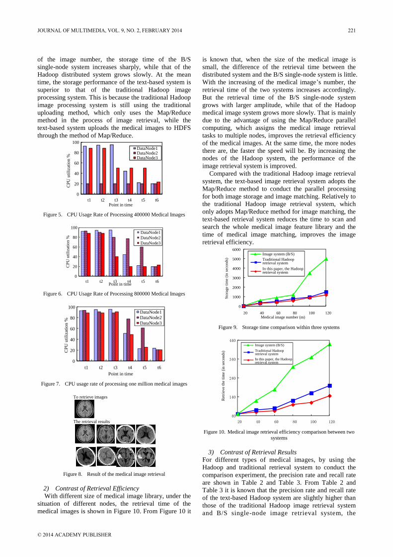
of the image number, the storage time of the B/S

single-node system increases sharply, while that of the

Hadoop distributed system grows slowly. At the mean

time, the storage performance of the text-based system is

superior to that of the traditional Hadoop image

processing system. This is because the traditional Hadoop

image processing system is still using the traditional

uploading method, which only uses the Map/Reduce

method in the process of image retrieval, while the

text-based system uploads the medical images to HDFS

through the method of Map/Reduce.

0

20

40

60

80

100

t1 t2 t3 t4 t5 t6Point in time

DataNode1DataNode2DataNode3

CP

U u

tili

zati

on %

Figure 5. CPU Usage Rate of Processing 400000 Medical Images

0

20

40

60

80

100

t1 t2 t3 t4 t5 t6

DataNode1

DataNode2

DataNode3

Point in time

CP

U u

tili

zati

on

%

Figure 6. CPU Usage Rate of Processing 800000 Medical Images

0

20

40

60

80

100

t1 t2 t3 t4 t5 t6

DataNode1

DataNode2

DataNode3

Point in time

CP

U u

tili

zati

on

%

Figure 7. CPU usage rate of processing one million medical images

To retrieve images

The retrieval results

Figure 8. Result of the medical image retrieval

2) Contrast of Retrieval Efficiency

With different size of medical image library, under the

situation of different nodes, the retrieval time of the

medical images is shown in Figure 10. From Figure 10 it

is known that, when the size of the medical image is

small, the difference of the retrieval time between the

distributed system and the B/S single-node system is little.

With the increasing of the medical image’s number, the

retrieval time of the two systems increases accordingly.

But the retrieval time of the B/S single-node system

grows with larger amplitude, while that of the Hadoop

medical image system grows more slowly. That is mainly

due to the advantage of using the Map/Reduce parallel

computing, which assigns the medical image retrieval

tasks to multiple nodes, improves the retrieval efficiency

of the medical images. At the same time, the more nodes

there are, the faster the speed will be. By increasing the

nodes of the Hadoop system, the performance of the

image retrieval system is improved.

Compared with the traditional Hadoop image retrieval

system, the text-based image retrieval system adopts the

Map/Reduce method to conduct the parallel processing

for both image storage and image matching. Relatively to

the traditional Hadoop image retrieval system, which

only adopts Map/Reduce method for image matching, the

text-based retrieval system reduces the time to scan and

search the whole medical image feature library and the

time of medical image matching, improves the image

retrieval efficiency.

0

1000

2000

3000

4000

5000

6000

20 40 60 80 100 120

Sto

rag

e ti

me

(in

sec

on

ds)

Image system (B/S)

Traditional Hadoop retrieval system

In this paper, the Hadoop retrieval system

Medical image number (m)

Figure 9. Storage time comparison within three systems

40

140

240

340

440

20 40 60 80 100 120

Ret

riev

e th

e ti

me

(in

sec

on

ds)

Image system (B/S)

Traditional Hadoop retrieval system

In this paper, the Hadoop retrieval system

Figure 10. Medical image retrieval efficiency comparison between two systems

3) Contrast of Retrieval Results

For different types of medical images, by using the

Hadoop and traditional retrieval system to conduct the

comparison experiment, the precision rate and recall rate

are shown in Table 2 and Table 3. From Table 2 and

Table 3 it is known that the precision rate and recall rate

of the text-based Hadoop system are slightly higher than

those of the traditional Hadoop image retrieval system

and B/S single-node image retrieval system, the



TABLE II. PRECISION RATE (%) COMPARISON WITHIN MULTIPLE TYPES OF MEDICAL IMAGES

Different Types of Medical Images Text-based Retrieval System Traditional Retrieval System B/S Single-node Retrieval System

Images of Brain CT 95.04 94.98 94.63 Images of Brain MRI 91.61 91.58 91.28

Images of Skin-micro 93.67 92.93 92.26

Images of X-ray Breast 91.46 91.09 90.67 HRCT of Lung 93.52 92.93 92.53

TABLE III. RECALL RATE (%) COMPARISON WITHIN MULTIPLE TYPES OF MEDICAL IMAGES

Different Types of Medical Images Text-based Retrieval System Traditional Retrieval System B/S Single-node Retrieval System

Images of Brain CT 92.21 91.26 91.59

Images of Brain MRI 90.32 89.84 90.94

Images of Skin-micro 90.38 90.32 90.33 Images of X-ray Breast 90.82 90.04 89.60

HRCT of Lung 91.10 90.57 89.31

advantages over the precision rate and recall rate is not

obvious. But for the large-scale medical image retrieval

system, the merits of the system performance are mainly

measured by the image retrieval efficiency. Through

Figure 10 it is known that the text-based Hadoop

distributed system effectively reduces the retrieval time

of the medical image, improves the retrieval efficiency of

the medical image, which better solves the problem that

the massive medical images retrieval has a low efficiency,

obtains a relatively satisfactory retrieval results.

IV. CONCLUSION

CBMIR medical image retrieval is a data-intensive

computing process, the traditional B/S single-node

retrieval system has the defects of low efficiency and

poor reliability and so on. Thus, a kind of Hadoop

medical image retrieval system is put forward. The results

of the simulation test show that the Hadoop medical

image retrieval system improves the efficiency of the

image storage and image retrieval, obtains a better

retrieval result, and can satisfy the real-time requirements

of the medical image retrieval. Especially when deals

with the massive medical images, it has the advantages

the traditional B/S single-node system cannot compared

with. Therefore, the working focuses in the future are

improving the transmission speed of data between the

Map task and the Reduce task, reducing more time

consumption which is due to the transfer of information,

to further improve the execution efficiency of the existing

image retrieval system.

REFERENCES

[1] Song ZHen, Yan Yongfeng. Interest points in images

integrated retrieval features of the. 2012 based on

computer applications, 32 (10) pp. 2840-2842.

[2] Zhang Quan, Tai Xiaoying. Relevance feedback Bayesian

in medical image retrieval based on. Computer

Engineering, 2008, 44 (17) pp. 158-161.

[3] Yu Sheng, Xie Li, CHeng Yun. Image color and primitive

features of computer application based on. 2013, 33 (6) pp.

1674-1708.

[4] FAY C, JEFFREY D, SANYJAY G, et al. Bigtable: A

distributed storage system for structured data// Proceedings

of the 7th Symposium on Operating Systems Design and

Implementat. Seattle: WA, 2006, 276-290.

[5] KEKRE H B, THEPADE S, SANAS S. Improving

performance of multileveled BTC based CBIR using

sundry color spaces. International Journal of Image

Processing, 2010, 4(6) pp. 620-630.

[6] Liye Da, Lin Weiwei. A Hadoop data replication method

of computer engineering and applications, 2012, 48 (21) pp.

58-61.

[7] Wang Xianwei, Dai Qingyun, Jiang Wenchao, Cao

Jiangzhong. Design patent image retrieval methods for

MapReduce. Mini micro system based on 2012, 33 (3,

626-232.).

[8] SANJAY G, HOWARD G, SHUNTAK L. The Google

File System// Proceedings of the 19th ACM Symposium on

Operating Systems Principles. Bolton Landing: ACM,

2003 pp. 29-43.

[9] Liang Qiushi, Wu Yilei, Feng Lei. MapReduce micro-blog

user search ranking algorithm of computer application

based on. 2012, 32 (11) pp. 2989-2993.

[10] JEFFREY D, SANJAY G. Mapreduce: a flexible data

processing tool. Communications of the ACM 2010, 53(1)

pp. 72-77.

[11] KONSTANTIN S, HAIRONG K, SANJAY R, et al.

Hadoop distributed file system for the Grid// Proceedings

of the Nuclear science Symposium Conference Record

(NSS/MIC). IEEE: Orlando, 2009 pp. 1056-1061.

[12] JEFFREY D, SANJAY G. Mapreduce: simplified data

processing on large clusters // Proceedings of the 6th

Symposium on Operating Systems Design and Implementat.

IEEE: San Francisco, 2004 pp. 107-113.

[13] Lian Qiusheng, Li Qin, Kong Lingfu. The texture image

retrieval combining statistical features of the circular

symmetric contourlet and LBP. Chinese Journal of

computers, 2007, 30 (12) pp. 2198-2204.

[14] Wang Zhongye, Yang Xiaohui, Niu Hongjuan. Brushlet

domain retrieval algorithm based on complex computer

simulation of. image texture characteristics, 2011, 28 (5)

pp. 263-266, 282

[15] ZHANG J, LIU X L, LUO J W, BO L T N. DIRS:

Distributed image retrieval system based on MapReduce//

The Network Security and Soft Computing Technologies.

IEEE: Maribor, 2010 pp. 93-98.



Kinetic Model for a Spherical Rolling Robot with

Soft Shell in a Beeline Motion

Zhang Sheng, Fang Xiang, Zhou Shouqiang, and Du Kai PLA Uni. of Sci & Tech/Engineering Institute of Battle Engineering, Nanjing, China

Email: [email protected], [email protected]

Abstract—A simplified kinetic model called Spring

Pendulum is developed for a spherical rolling robot with soft

shell in order to meet the needs of attitude stabilization and

controlling for the robot. The elasticity and plasticity of soft

shell is represented by some uniform springs connected to

the bracket in this model. The expression of the kinetic

model is deduced from Newtonian mechanics principles.

Testing data of the driving angle acquired from a prototype

built by authors indicate that testing data curve accords to

the theoretic kinetic characteristic curve, so the kinetic

model is validated.

Index Terms—Soft Shell; Spherical Rolling Robot; Kinetic

Model

I. INTRODUCTION

Spherical robot is a kind of robots which can roll by

themselves. More and more researchers are focusing on

spherical robot due to their many advantages on moving

and their hermetical structure. More than 10 species

spherical robots and their accessories are advanced as

well [1-4]. These robots are preliminarily applied in many

domains. All these robots are mainly constructed by hard

shell. Soft-shell spherical robot has many advantages like

good cross ability, changeable bulk and good impact

resistance comparing to the hard-shell robots. Li Tuanjie

and his group researched the light soft-shell spherical

robot driven by wind power and founded the equation to

describe the ability of the robot to cross the obstacle

without deeply research about how much would the soft-

shell influence the spherical robot [5]. Sugiyama Y, Irai S

and other people researched the transformation-driven

spherical robot. It uses several shape memory alloys to

support and control the reduction by change the amount

of the voltage to make the robot roll like crawling. It

moves slowly and now still stays at the stage of checking

the principle [6]. Fang Xiang and Zhou Shouqiang have

gained the patent of automatically aerating and

discharging soft-shell spherical robot [7].

On the modeling of spherical robot, Ref. [8, 9] began

with the principle of kinematics, found the dynamic

model of the hard-shell spherical robot walking along a

straight line driven by pendulum. Since they ignored the

quadratic items, there would be some errors in the

dynamic model when the robot moves in high speed. In

order to make the robot start and stop steady and speed

controllable, Ref. [10] researched the kinematic model of

a kind of spherical robot driven by two masses deflected

from the centre of the sphere moving straight in order to

control the robot starting and stopping smoothly.

According to the description of Euler angles, Ref. [11]

found a kinematic model of the spherical robot. Ref. [12,

13] found the dynamic model of a hard-shell spherical

robot from the angle of Newton mechanics. They

simplified the model of a straight moving spherical robot

to a single pendulum hung on the centre of the ball

connected to the shell through the drive motor. They all

had a simulation experiment on the dynamic model of

their spherical robot respectively, but didn’t check the

data from the experiment to prove the correctness of the

model. So this paper will deeply analyze the

characteristics of the soft-shell spherical robot on

kinematics and dynamics to establish its mechanic model

and use the experimental sample to check the correctness

of the model.

In this paper we consider a class of spherical rolling

robots actuated by internal rotors. Under a proper

placement of the rotors the center of mass of the

composite system is at the geometric center of the sphere

and, as a result, the gravity does not enter the motion

equations. This facilitates the dynamic analysis and the

design of the control system.

The idea of such a rolling robot and its design was first

proposed in [14], and later on studied in [15]. Also

relevant to our research is the study [16] in which the

controllability and motion planning of the rolling robots

with the rotor actuation were analyzed.

A spherical robot is a new type of mobile robot that

has a ball-shaped outer shell to include all its mechanisms,

control devices and energy sources inside it.

Thisstructural characteristic of a spherical robot helps

protect the internal mechanisms and the control system

from damage. At the same time, the appearance of a

spherical robot brings a couple of challenging problems

in modeling, stabilization and position tracking (path

following). Two difficulties hinder the progress of the

control of a spherical robot. One is the highly coupled

dynamics between the shell and inner mechanism, and

another is that although different spherical robots have

different inner mechanism including rotor type, car type,

slider type, etc (Joshi, Banavar and Hippalgaonka, 2010),

most of them have the underactuation property, which

means they can control more degrees of freedom (DOFs)

than drive inputs. There are still no proven general useful

control methodologies for spherical robots, although



researchers attempted to develop such methodologies. Li

and Canny (Li and Canny, 1990) proposed a three‐step

algorithm to solve the motion planning problems of a

sphere, the position coordinates of the sphere can

converge to the desired values in three steps. That method

is complete in theory, but it can only be applied to

spherical robots capable of turning a zero radius as the

configurations are constrained. Mukherjee and Das et al.

(Das and Mukherjee, 2004), (Das and Mukherjee, 2006)

proposed a feedback stabilization algorithm for four

dimensional reconfiguration of a sphere. By considering a

spherical robot as a chained system Javadi et al. (Javadi

and Mojabi, 2002) established its dynamic model with the

Newton method and discussed its motion planning with

experimental validations. As compared to other existing

motion planners, this method requires no intensive

numerical computation, whereas it is only applicable for

their specific spherical robot. Bhattacharya and Agrawal

(Bhattacharya and Agrawal, 2000) deduced the first‐order mathematical model of a spherical robot from the

non‐slip constraint and angular momentum conservation

and discussed the trajectory planning with minimum

energy and minimum time. Halme and Suomela et al.

(Halme, Schonberg and Wang, 1996) analyzed the rolling

ahead motion of a spherical robot with dynamic equation,

but they did not consider the steering motion. Bicchi, et al.

(Antonio B. et. al., 1997), (Antonio and Alessia, 2002)

established a simplified dynamic model for a spherical

robot and discussed its motion planning on a plane with

obstacles. Joshi and Banavar et al. (Joshi, Banavar and

Hippalgaonka, 2009) proposed a path planning algorithm

for a spherical mobile robot. Liu and Sun et al. (Liu, Sun

and Jia, 2008) deduced a simplified dynamic model for

the driving ahead motion of a spherical robot through

input ‐ state linearization and derived the angular

velocity controller and angle controller respectively with

full feedback linearized form [17].

It should be noted the even though the gravitational

term is not presented; the motion planning for the system

under consideration is still a very difficult research

problem.

In fact, no exact motion planning algorithm has yet

been reported for the case of the actuation by two rotors.

In [18], the motion planning problem was posed in the

optimal control settings using an approximation by the

Phillip Hall system [19]. However, since the robot

dynamics are not nilpotent, this is not an exact

representation of the system and it results to inaccuracies.

An approximate solution to the motion planning problem

using Bullo’s series expansion was constructed in [19],

but that has been done for the case of three rotors. An

exact motion planning algorithm is reported only in [6],

but as we will see it later it is not dynamically realizable.

Thus, the motion planning in dynamic formulation for the

robot under consideration is still an open problem and a

detailed analysis of the underlying difficulties is

necessary.

This constitute the main goal of our paper. The paper is

organized as follows. First, in Section II we provide a

geometric description and a kinematic model of the

system under consideration and then, in Sections III

derive its dynamic models. A reduced dynamic model is

then furnished in Section IV, and conditions of dynamic

realizability of kinematically feasible trajectories of the

rolling sphere are established in Section V. A case study,

dealing with the dynamic realizability of tracing circles

on the surface of the sphere, is undertaken in Section VI.

Finally, conclusions are drawn in Section VII.

II. DYNAMICS MODEL OF SOFT-SHELLED SPHERICAL

ROBOT

A. Constitution

The soft-shelled spherical robot developed by PLA Uni.

of Sci & Tech is shown in fig. 1. There are 3

electromotors inside the spherical shell to provide

moment of force input. One steering motor is connected

to a bevel gear rolling in a gear circle. The battery and

load are connected to the bevel gear as well in order to

control the rotation direction. The other two drive motors

in-phase and their shells are fixed on the bracket, while

the armatures of them are on the shell of the spherical

robot to provide drive moment of force.

Fig. 1 illustrates the overview of the internal

drivingmechanism. The internal driving mechanism is

composed of two rotors with their axes perpendicular to

each other. Each axis is called Yaw axis and Pitch axis,

respectively. An actuator is put at the bottom of each axis

and a rotor is put at the both ends of Pitch axis. The

spherical shell is driven by the reaction torque generated

by actuators. The internal driving device is fixed to the

spherical shell at a point P. The point P is at the

geometric center of the sphere. The gravity point of the

internal driving device does not lie at the center of the

sphere.Due to this asymmetry, the robot tends to be stable

when the weights are beneath the center, while it tends to

be unstable when they are above the center. This is

important to realize both the stand-still stability and quick

dynamic behavior by a single mechanism.

Figure 1. Planform for inner machines of the spherical soft shell robot

Figure 2. Appearance & planform for inner machines of the spherical soft shell robot

B. Exterior Structure

Fig. 2 illustrates the overview of the exterior structure.

The exterior part is composed of two hemispheres and



circular board that divides the sphere in half. All

electronic components such as sensors, motor drivers, and

a microcomputer are put on the circular board. Weight of

electronic components are large enough that we can not

neglect them when we construct the dynamic model.

Moreover, distribution of weight on the circular board is

inequable. Therefore, the gravity point of exterior

structure does not lie at the center of sphere. By

considering this asymmetry property in the dynamic

model, we can construct more accurate model and

simulate the effects of distribution of weight on motions

of the robot.

C. System Models in a Beeline Motion

Without considering the viscous friction on robot

produced by air resistance, the robot can be decomposed

into two subsystems: one is the bracket and spherical

shell, another is the single pendulum, then we make the

following assumptions:

a. The spherical shell is equivalent to a rigid and thin

spherical shell which quality is mb and radius is R. There

is no deformation of the spherical shell when it is contact

with the ground, the soft and elastic properties of the

spherical shell is reflected by the relative displacement of

different directions between spherical shell and bracket.

b. The component inside the ball equivalent to a solid

ball which quality is M and radius is r beside the storage

battery and load; They are equivalent to the connection

through the radial light spring, known as the model called

spring pendulum (Fig. 3).In Figure 3, the distance offset

centre affected by the spring force is △R which becomes

△X and △Y when it decomposed into horizontal and

vertical displacement.(Fig. 4).

Figure 3. The model called spring pendulum

c. The battery and load equivalent to a particle which

quality is m and hinged with solid ball in center by

massless connecting rod which length is L.

Figure 4. Mechanics analysis for the bracket & shell and the pendulum

Establishing the inertial coordinate system XOY on the

ground and decomposing the spherical shell robot into

two subsystems: spherical shell and “frame + pendulum”.

The two subsystems connected by the bearing force and

the bearing countermoment associated with each other.

The positive direction of every parameter shows in Fig. 4.

When the system is pure rolling in the horizontal plane

in a straight line, the displacement of spherical and

pendulum on the direction of X and Y is Xb, Yb, Xp, Yp

respectively according to kinematic law:

0

sin

cos

b

b

p bx

p

X R

Y

X X L X

Y L L Y

(1)

Taking the above equation second derivative with

time,then we can get the acceleration of spherical and

pendulum on the direction of X and Y is abx, aby, apx, apy :

2

2

0

cos sin

sin cos

bx

by

px

py

a R

a

a R L L X

a L L Y

(2)

The force and moment balace of vector mechanics and

moment of momentum theorem for spherical shell and

pendulum can be presented as two equations: (3) and (4)

=

2 22 20 3 5

0 0

0

+

=

0 X b bx

Y b N

X Y b

N

F F m M a

F m M g F

T F R F Y F X m R Mr

F F

(3)

2cos sin

X px

Y py

F ma

F mg ma

T m RL mgL mL

(4)

where the static friction is F0 caused by the ground. The

orthogonal component force is FX, FY when the bracket

forces on shell in the plane; The supportive force is FN,

the angle that rotated relative to the ground by the shell is

φ and the angle that relative to the vertical direction by

the pendulum is θ; The friction of static coefficient is μ0.

When considering about the constraint when the ball is

pure rolling and assuming that the motor is rotating in

constant angular velocity as ωi, we can get the equation

(5):

it (5)

Dates of manuscript submission, revision and

acceptance should be included in the first page footnote.

Remove the first page footnote if you don’t have any

information there. Taking equations (1), (2) and (5) into

equations (3) and (4) and sorting, then omitting the

quadratic term of △X and △Y as small high-end quantity,

where sinθ≈θ, cosθ≈1.



2 2 2 2 25 7

3 5

2 2 2 22 20 0 0 03 5

0

0

b

b b

mLR mL m R Mr mR mgL mR X

m LR mL mLR m R Mr m LR mgL m M g R m R Y

(6)

III. CALCULATION AND ANALYSIS OF DYNAMIC

MODEL OF SOFT SHELL SPHERICAL ROBOT

Equation (4) is composed of two order nonlinear

differential equation. Generally it is hard to get the

analytical solution. So this paper used the method of

difference approximation for the numerical solution. The

values of X and Y are relevant to θ. First of all,

omitting the related items of X and Y , it can get the

dynamic equation of hard spherical robot. Substituting

relative parameters: the mass of spherical mb=0.62kg,

radius R=0.39m, the mass of internal mechanism and

support M=3.12㎏, equivalent radius r=0.07m; the mass

of battery and load m=6.29kg, L=0.28m, μ0 =0.5.

Defining the initial conditions: the 0 time, θ(0)= (0)=0.

Substituting relative parameters, difference discretization

of the two differential equations, taking 0.05 as steps,it

can get the numerical solutions of hard shell spherical

robot driving angle θ, which was shown by solid line in

figure 4. By determination, the values of X and Y

were less than 10-2

, it may be assumed as constants,

X = Y =0.02m/s2. Substituting equation (6), it can get

dynamic equation on soft spherical robot; the numerical

solution of the equations was shown in dotted line in

figure 4.

0 0.5 1 1.5 2 2.5 3 3.5 4-1

0

1

2

3

4

5

6

t/s

θ/rad

Hard Shell

Soft Shell

Figure 5. Driving angle curve from theoretic kinetic model for the robot with hard shell & soft shell

As can be seen from Fig. 5, in the case of a constant

speed of drive motor, The change of horizontal line pure

rolling soft shell spherical robot driven angle has

consistent trend with hard shell spherical robot of the

same parameters: firstly, the maximum swing angle

appeared in a relatively short time, and then decreased

rapidly, finally, kept in a certain angle oscillation. Soft

shell spherical robot driven angular oscillation amplitude

was bigger than the hard shell spherical robot, but the

maximum swing angle was smaller, the impact was

relatively small.

IV. PROTOTYPE TEST

A. Test Conditions

To demonstrate the feasibility of the new driving

mechanism shown in Sec. II, we make the spherical

rolling robot move with a desired translational velocity

by a simple feedback controller. Based on the observed

state shown in the above subsection, the driving torque τ

in (5) is given by a state feedback law. It should be noted

that the counter torque -τ is applied to the inner

subsystem composed of the gyro case and the gyro as

shown in (3). Since the gyro has a large angular

momentum, nutation of the subsystem may be caused by

the angular momentum. However, the nutation was not

seen in the results of preliminary experiments. It seems

that the nutation is quickly damped by the frictional

torque between the outer shell and the gyro case.

In this paper, we adopt Strategy A and use the

feedback law (6) in the experiments. In Strategy A, the

rotational motion of the outer shell around the vertical

axis would not be controlled by (6). However, the

rotation around horizontal axes would approach the

desired horizontal rotation, and the experimental results

in the next section will show that the spherical rolling

robot can achieve a translational motion by the feedback

law (6).

The experimental prototype quality, size and other

parameters are the same to the last chapter, the filled

pressure of spherical shell is 1.8×105Pa and the battery

voltage is 12V. Using photoelectric encoder to control the

speed of driving motor should be maintained in the π

rad/s and the robot starts from rest. PID is used to control

the steering angle of steering motor so that to keep the

robot lateral stability and the robot can keep a horizontal

linear to move. What’s more, it also makes use of the

three axis accelerometer and a three axis gyro sensors to

measure the three axis acceleration and angular velocity

at the same time. The sampling frequency is 20Hz.

Through data processing, we can get the change trend of

driven angle θ, which is shown in dotted line in Fig. 6.

0 0.5 1 1.5 2 2.5 3 3.5 4-1

0

1

2

3

4

5

6

t/s

θ/rad

Hard Shell

Soft Shell

Figure 6. Driving angle curve from testing result & theoretical result

V. CASE STUDY

Spherical rolling robots have a unique place within the

pantheon of mobile robots in that they blend the

efficiency over smooth and level substrates of a

traditional wheeled vehicle with the maneuverability in

the holonomic sense of a legged one. This combination of

normally exclusive abilities is the greatest potential



benefit of this kind of robot propulsion. An arbitrary path

that contains discontinuities can be followed (unlike in

the case of most wheeled vehicles) without the need for

the complex balancing methods required of legged robots.

However, spherical rolling robots have their own set of

challenges, not the least of which is the fact that all of the

propulsive force must somehow be generated by

components all of whom are confined within a spherical

shape.

This general class of robots has of late earned some

notoriety as a promising platform for exploratory

missions and as an exoskeleton. However, the history of

this type of device reveals that they are most common as

a toy or novelty. Indeed, the first documented device of

this class appears to be a mechanical toy dating to 1909

with many other toy applications following in later years.

Many efforts have been made to design and construct

spherical rolling robots and have produced many methods

of actuation to induce self-locomotion. With a few

exceptions, most of these efforts can be categorized into

two classes.

The first class consists of robots that encapsulate some

other wheeled robot or vehicle within a spherical shell.

The shell is then rolled by causing the inner device to

exert force on the shell. Friction between the shell and its

substrate propels the assembly in the same direction in

which the inner device is driven. Early examples of this

class of spherical robot had a captured assembly whose

length was equal to the inner diameter of the spherical

shell, such as Halme et al. and Martin, while later

iterations included what amounts to a small car that

dwells at the bottom of the shell, such as Bicchi et al.

The second major class of spherical robots includes

those in which the motion of the sphere is an effect of the

motion of an inner pendulum. The center of mass of the

sphere is separated from its centroid by rotating the arm

of the pendulum. This eccentricity of the center of mass

induces a gravitational moment on the sphere, resulting in

rolling locomotion. Examples of these efforts are those of

Michaud and Caron, Jia et al. Javadi and Mojabi [16] as

well as Mukherjee et al. have devised systems that work

using an eccentric center of mass, but each moves four

masses on fixed slides within the spherical shell to

achieve mass eccentricity instead of tilting an inner mass.

Little work has been done outside these two classes.

Jearanaisilawong and Laksanacharoen and Phipps and

Minor each devised a rendition of a spherical robot.

These robots can achieve some rolling motions when

spherical but are capable of opening to become a wheeled

robot and a legged walking robot respectively. Sugiyama

et al. created a deformable spherical rolling robot using

SMA actuators that achieves an eccentric center of mass

by altering the shape of the shell. Finally, Bart and

Wilkinson and Bhattacharya and Agrawal each developed

spherical robots where the outer shell is split into two

hemispheres, each of which may rotate relative to each

other in order to effect locomotion.

The condition of dynamic realizability (4) imposes a

constraint on the components of the vector of the angular

velocity ω0, and this constraint needs to be embedded

into the motion planning algorithms. If the motion

planning is based on the direct specification of curves on

the sphere or on the plane, as is the case in many

conventional algorithms [10], [12], the embedding can be

done as follows.

Assume that the path of the rolling carrier is specified

by spherical curves, and the structure of the functions u0(t)

and v0(t) up to some certain constant parameters is known.

The kinematic equations (3) can now be casted as

0 0sin cos cosav Ru Rv (7)

0 0cos cos sinau Ru Rv (8)

In [6] the rotors are mounted on the axes n1 and n3, so

the condition of dynamic realizability becomes n2·Jcω 0 =

0. However, the motion planning algorithm in [6] is

designed under the setting n2·ω0 = 0, which is not

equivalent to the condition of dynamic realizability.

To guarantee the dynamic realizability, express ω z in

the last formula through ω x and ω y. In doing so, we first

need to express ω x, ω y as well as n3x, n3y, n3z in terms of

the contact coordinates. From the definition of the

angular velocity T

0 = RR , one obtains

0 0 0cos sin cosx u v v (9)

0 0 0cos cos siny u v v (10)

while n3 is simply the last column of the orientation

matrix R. Therefore,

3 0 0 0sin cos cos sin sinxn u u v (11)

3 0 0 0sin sin cos sin cosyn u u v (12)

3 0 0cos coszn u v (13)

Having expressed everything in terms of the contact

coordinates, one can finally replace in (13) by

0

0 0 0

0

tan1 sin

cos

uk u v kv

v

If we, formally, set here k = 0 the variable will be

defined as in the pure rolling model. However, in our

case k > 1.

Consider a maneuver when one traces a circle of radius

a on the spherical surface. This maneuver is a component

part of many conventional algorithms (see, for instance

[6], [10], [13], [14]). Tracing the circle results to the non-

holonomic shift Δ h(a) of the contact point on the plane

and to the change of the holonomy (also called as the

geometric phase), Δ φ(a). By concatenating two circles of

radii a and b, one defines a spherical figure eight. By

using the motion planning strategy [13], based on tracing

an asymmetric figure eight n times, one can, in principle,

fabricate an exact and dynamically realizable motion

planning algorithm.

A detailed description of the circle-based motion

planning algorithm is not presented in this paper due to



the page limitation. However, in the remaining part of his

section we illustrate under simulation an important

feature of this algorithm—the dependance of the non-

holonomic shift on the inertia distribution specified by

the parameters k.

B. Results Analysis

The most apparent behavior that the spherical robot

prototype displayed was a tendency to wobble or rock

back and forth with little damping. For example, when

the sphere was at rest with the pendulum fixed inside,

bumping the sphere would cause it to oscillate back and

forth about a spot on the ground. The sphere also

wobbled if a constant pendulum drive torque was

suddenly applied to the sphere starting from rest. In this

case, it would accelerate forward while the angle between

the pendulum and the ground would oscillate. Since the

pendulum was oscillating, the forward linear velocity of

the sphere also appeared to oscillate as it accelerated.

When traveling forward and then tilting the pendulum a

fixed angle to the side to steer, the radius of the turn

would oscillate as well.

Another behavior that was observed but not found to

be discussed in the literature was the tendency of the

primary drive axis to nutate when the sphere was

traveling at a reasonable forward velocity. Specifically,

the primary drive axis (the axis of the main drive shaft

attached to the spherical shell) would incur some angular

misalignment from the axis about which the sphere was

actually rolling. When traveling slowly (estimated to be

less than 0.5 m/s) this nutating shaft behavior, which

could be initiated by a bump on the ground, would damp

out quickly. When traveling at a moderate speed, the

nutation would persist causing the direction of the sphere

to oscillate back and forth.

When attempting to travel at high speed (estimated to

be above 3 m/s) the angular misalignment between the

axes would go unstable until the primary drive axis was

flipping end over end. Even during a carefully controlled

test on a level, smooth surface

The angle of inclination of the gyro increased rapidly

from 0 [deg] to about 10 [deg] by t = 0.25 [s], and kept

increasing slowly to about 20 [deg] for 0.25 ≤ t ≤ 3 [s]. It

seems that the increase after t = 0.25 [s] was caused by

the rolling friction at the contact point between the outer

shell and the floor surface that was covered with carpet

tiles. The rolling friction may change the total angular

momentum of the robot.

The friction torque about the vertical may also

decrease the total angular momentum, when ω(0) 10z is

not zero. We will examine the behavior of the inclination

angle for other types of floor surfaces and for Strategy B

in future works.

Moreover, due to the limited power of the DC motors,

the maximum angular speed of the outer shell that was

achieved in the experiments was about 1.5πrad/s.

Comparing with the driven angle measured curve

(dashed line) and the results of theoretical calculations

(solid line) of the soft shell spherical robot in Fig. 5, we

can see that the measured curve is basically agree with

the theoretical calculation results, which can prove the

correctness of the dynamics model of “spring pendulum”

of soft shell spherical robot in this paper. The theoretical

and experimental curves calculated difference: (1) the

final angular oscillation amplitude is smaller than the

theoretical analysis, probably because the theoretical

model does not consider the energy loss of internal

movement; (2) the measured maximum pendulum angle

is bigger than the theoretical results, which is probably

caused by the modeling error. For example, the

parameters of support quality equivalent radius r is

difficult to be precise enough, and the other reason to

result in modeling errors is that the support eccentric

displacement acceleration X and Y are

approximately regarded as constant.

VI. CONCLUSIONS

A dynamic model named spring pendulum of the soft-

shell spherical robot is advanced in this paper. The

theoretic curve of drive angle for time is educed in the

condition of invariable drive motor rev from this dynamic

model. The test result on a soft-shell prototype is

identical to the theoretic result which proves the validity

of the spring pendulum model. The rules of drive angle

fluctuation and the influence characteristics will be

proposed by means of numerical research on the spring

pendulum model in order to stabilize and control the

attitude of soft-shell spherical robot.

ACKNOWLEDGMENT

This work was supported in part by a grant from

Chinese postdoctoral fund.

REFERENCES

[1] Jiang Jie, Wang Hai-sheng, Su Yan-ping. Structural design

of the internal and external driven spherical Robots.

Machinery, 2012, 03 pp. 42-44. G. Eason, B. Noble, and I.

N. Sneddon, “On certain integrals of Lipschitz-Hankel type

involving products of Bessel functions,” Phil. Trans. Roy.

Soc. London, vol. A247, pp. 529–551, April 1955.

[2] Sang Shengju, Zhao Jichao, Wu Hao, Chen Shoujun, and

An Qi. Modeling and Simulation of a Spherical Mobile

Robot. ComSIS, 2010, 7(1), Special Issue: 51-61J. Clerk

Maxwell, A Treatise on Electricity and Magnetism, 3rd ed.,

vol. 2. Oxford: Clarendon, 1892, pp. 68–73.

[3] Mattias Seeman, Mathias Broxvall, Alessandro Saffiotti,

Peter Wide. An Autonomous Spherical Robot for Security

Tasks IEEE International Conference on Computational

Intelligence for Homeland Security and Personal Safety,

Alexandria, USA, 2007 pp. 51 - 55 I. S. Jacobs and C. P.

Bean, “Fine particles, thin films and exchange anisotropy,”

in Magnetism, vol. III, G. T. Rado and H. Suhl, Eds. New

York: Academic, 1963, pp. 271–350.

[4] S. Chaplygin, “On rolling of a ball on a horizontal plane,”

Mathematical Collection, St. Petersburg University, vol. 24,

pp. 139–168, 1903, (In Russian; English transl. : Regular

& Chaotic Dynamics, Vol. 7, No. 2, 2002, pp. 131–148).

[5] Li Tuanjie, Liu Weigang. Dynamics of the Wind-driven

Spherical Robot. Acta Aeronautica Et Astronautica Sinica,

2010, 31(2) pp. 426-430. R. Nicole, “Title of paper with

only first word capitalized”, J. Name Stand. Abbrev, in

press.



[6] Sugiyama Y. Circular / Spherical Robots for Crawling and

Jumping. Proceedings of the 2005 IEEE lntemational

Conference on Robotics and Automation, Barcelona, Spain,

2005 pp. 3595-3600. Y. Yorozu, M. Hirano, K. Oka, and Y.

Tagawa, “Electron spectroscopy studies on magneto-

optical media and plastic substrate interface, “IEEE Transl.

J. Magn. Japan, vol. 2, pp. 740–741, August 1987 [Digests

9th Annual Conf. Magnetics Japan, p. 301, 1982].

[7] China Patent, CN202243763U. 2012-05-30M.

[8] Zhao Kai-liang, Sun Han-xu, Jia Qing-xuan, et al. Analysis

on acceleration characteristics of spherical robot based on

ADAMS. Journal of Machine Design, 2009, 26(7) pp. 24-

25.

[9] ZHENG Yi-li1, SUN Han-xu. Dynamic modeling and

kinematics characteristic analysis of spherical robot.

Journal of Machine Design, 2012, 02 pp. 25-29.

[10] ZHAO Bo, WANG Pengfei, SUN Lining, et al. Linear

Motion Control of Two-pendulums-driven Spherical Robot.

Journal of Mechanical Engineering, 2011, 11 pp. 1-6.

[11] FENG Jian-Chuang, ZHAN Qiang, LIU Zeng-Bo. The

Motion Control of Spherical Robot Based on Sinusoidal

Input. Development & Innovation of Machinery &

Electrical Products, 2012, 04 pp. 7-9.

[12] YUE Ming, LIU Rong-qiang, DENG Zong-quan. Research

on the effecting of coulomb friction constraint to the

Spherical robot. Journal of Harbin Institute of Technology,

2007, 39(7) pp. 51.

[13] YUE Ming, DENG Zong-quan, LIU Rong-qiang.

Quasistatic Analysis and Trajectory Design of Spherical

Robot. Journal of Nanjing University of Science and

Technology (Natural Science), 2007, 31(5) pp. 590-594.

[14] V. A. Joshi, R. N. Banavar, and R. Hippalgaonkar, “Design

and analysisof a spherical mobile robot, “ Mech. Mach.

Theory, vol. 45, no. 2, pp. 130–136, Feb. 2010.

[15] E. Kayacan, Z. Y. Bayraktaroglu, and W. Saeys,

“Modeling and controlof a spherical rolling robot: A

decoupled dynamics approach,” Robotica, vol. 30, pp.

671–680, 2011.

[16] M. Ahmadieh Khanesar, E. Kayacan, M. Teshnehlab, and

O. Kaynak, “Extended Kalman filter based learning

algorithm for type-2 fuzzy logic systems and its

experimental evaluation, “IEEE Trans. Ind. Electron. vol.

59, no. 11, pp. 4443–4455, Nov. 2012. [17] Haiyan Hu, Pengfei Wang, Lining Sun. Simulation

Platform of Monitoring and Tracking Micro System for

Dangerous Chemicals Transportation. Journal of Networks,

Vol 8, No 2 (2013), 477-484, Feb 2013.

[18] J. -C. Yoon, S. -S. Ahn and Y. -J. Lee, “Spherical Robot

with NewType of Two-Pendulum Driving Mechanism,

“ Proc. 15th Int. Conf. on Intelligent Engineering Systems,

pp. 275-279, 2011.

[19] Q. Zhan, Y. Cai and C. Yan, “Design, Analysis and

Experiments of an Omni-Directional Spherical Robot,

“Proc. IEEE Int. Conf. on Robotics and Automation, pp.

4921-4926, 2011.

Zhang Sheng was born in Jiangsu Province, China on Nov. 13,

1979. He was in PLA Ordnance College, Shi Jiazhuang, Hebei

Province, China from 1998 to 2005 and earned his bachelor

degree and master degree in ammunition engineering and

weapon system application engineering respectively. The

author’s major field of study is cannon, autoweapon &

amunnition engineering.

He was a Lecturer from 2005 to 2013 in PLA International

Relationships University. His current and research interests are

smart ammunitions.



Coherence Research of Audio-Visual Cross-

Modal Based on HHT

Xiaojun Zhu*, Jingxian Hu, and Xiao Ma College of Computer Science and Technology, Taiyuan University of Technology, Taiyuan, China

*Corresponding author, Email: [email protected],{hjxocean, tyut2010cstc}@163.com

Abstract—Visual and aural modes are two main manners

that human utilize to senses the world. Their relationship is

investigated in this work. EEG experiments involving mixed

aural and visual modes are designed, utilizing Hilbert-

Huang Transform (HHT) and electroencephalogram (EEG)

signal processing techniques. During EEG data processing,

I-EEMD method of similar weighted average waveform

extension is proposed to decompose the EEG signals,

specifically accounting for the problem of end effects and

mode mixing existing in the traditional HHT. The main

components of are obtained after decomposing the signals

including mixed modes with I-EEMD respectively. The

correlation coefficient of consistent and inconsistent mixed

signal is calculated, and the comparison is made.

Investigation on the comparison condition of the correlation

coefficient indicates that there is coherence in both the

visual and aural modes.

Index Terms—EEG; Audio-visual; Coherence; HHT;

EEMD

I. INTRODUCTION

Human obtain information from the outside world with

different sensory channels such as vision, hearing, touch,

smell and taste. However, the role of different sensory

modalities for human memory and learning are not independent of each other. The encouraging research

results” Cross modal learning interaction of Drosophila”

of Academician Aizeng Guo and Dr. Jianzeng Guo of

Chinese Academy of Sciences proves that there are

mutually reinforcing effects between modal of visual and

olfactory in drosophila’s learning and memory [1]. Then,

whether the human’ visual and auditory are able to

produce a similar cross-modal collaborative learning effect? Can we take advantage of this learning effect to

strengthen the information convey efforts, and then

produce the effect of synergistic win - win and mutual

transfer on memory? Human beings obtain and

understand the information of the outside world by

multiple sensory modals [2] [3]. However, the

information from multiple modals sometimes may be

consistent, and sometimes may be inconsistent. So that it requires the brain to treat and integrate the information

and form a unified one. Since vision and hearing are the

primary ways to percept the outside world for human [4],

the coherence research for the information in the visual

and audio channels is particularly important, and it also

has the extraordinary significance for discovering the

functional mechanism of the brain. Therefore, the

coherence research of audio-visual information and its

function in knowing the world and perceiving the

environment will contribute to improving the lives of the

handicapped whose visual or audio channel is defective,

and make the reconstruction of some functions in their cognitive system come true [5].

Meanwhile, it will also give the active boost to

improve the visual and audio effect of the machine and

further develop the technology of human-computer

interaction. Human brains’ integration to the visual and

auditory stimuli of the outside world is a very short but

complicated non-linear process [6] [7]. In recent years,

EEG is widely used in the visual and audio cognitive domain. EEG is the direct reflection of the brain electrical

physiological activity, of which the transient cerebral

physiological activities are included [8] [9] [10].

Accordingly, some researchers consider the transient

process of the brain integrating the visual information and

audio information mutually can cause the electric

potential on the scalp surface to change [11]. Event-

Related Potential (ERP) is the brain potential extracted from EEG and related to the stimulation activities. It can

establish the relations between the brain responses and

the events (visual or auditory stimulus), and capture the

real-time brain information processing and treating

process. Thus, in recent years, when the researchers in the

brain science field and artificial intelligence field are

studying the interaction in multiple sensory and crossing

modals, the technology for analyzing ERP has be paid attention to unprecedentedly.

In this article, we will discuss the coherence between

the visual EEG signal and the audio EEG signal from the

perspective of signal processing based on Hilbert-Huang

Transform (HHT) [12], and then investigate the mutual

relations between the visual and audio modals. Firstly,

this paper designs a visual and auditory correlation test

experiment; evoked potential data under the single visual stimulus, the single audio stimulus, and the stimulus of

audio-visual consistence and the stimulus of audiovisual

inconsistence were collected respectively. Then, he main

IMF components of single visual signal and single audio

signal are decomposed by HHT, and analysis the

coherence of visual and audio modals by calculating the

correlation coefficient between these components and

ERP signal under the stimulus of visual & audio modals. Our paper is organized as follows. Section II describes



Experiment and Records of Audio-visual Evoked. Section

III describes Data Treatment Method in detail. We

analyze the I-EEMD Processing and Analysis of

Experimental Data, and provide the simulation results in

Section IV. In Section V, We conclude this paper.

II. EXPERIMENT AND RECORDS OF AUDIO-VISUAL

EVOKED EEG

A. Design of Experiment

The experiment contents include single visual

experiment (experiment A), single audio experiment

(experiment B) and stimulus experiment of audio-visual modals (experiment C). The stimulation experiment of

audio-visual modals is also divided into experiment of

consistent audio-visual modals (experiment C1) and

experiment of inconsistent audio-visual modals

(experiment C2). The materials for visual stimulus

include seven elements in total, namely Chinese

characters “ba”, “ga”, “a”, the letters “ba”, “ga”, “a” and

a red solid circle. The size and lightness of presented Chinese characters or the letters are consistent, and

appeared by pseudorandom fashion; the materials for

audio stimulus include four sound elements, namely the

sound “ba”, “ga”, “a” and a short pure sound “dong”. The

sound file is edited by use of Adobe audition with the

unified attribute of two-channel stereo, sampling rate of

44100 and resolution ratio of 16-bit. In the experiment of

visual evoked potentials, the red solid cycle is the target stimulus, the pictures of other Chinese characters or

letters are the non-target stimuli; In the experiment of

audio evoked potentials, the short pure sound “tong” is

the target stimulus, the other sounds are the non-target

stimuli; In the audio-visual dual channels experiment, the

visual pictures and the audio sounds combine randomly.

When the picture is red solid cycle and the sound is short

pure sound “dong”, it is target stimulus, and other combinations are non-target stimuli. The experiment

requires the subject to pushing a button to indicate their

reactions for the tested target stimuli. This experiment

model investigates the ERP data under the non-note

model. Three groups of experiment stimulus are all OB

(Oddball Paradigm) with the target stimulus rate of 20%.

The lasting time for every stimulus is 350ms with the

interval of 700ms. Three groups of experiments all include 250 single stimuli, of which 50 are target

stimulus (trials). The software E-prime is used to

implement this experiment.

B. Conditions to be Tested

20 healthy enrolled postgraduates with no history of

mental illness (including 10 males and 10 females, right-

handed, and their age from 22 to 27 years old) were

selected as the subjects. All of them have normal

binocular vision or corrected vision and normal hearing.

Before the experiment, all of them have signed the

informed consent form of the experiment to be tested

voluntarily. Before the experiment, scalp of the subjects was kept clean. After the experiment, certain reward was

given. Every subject participated in the experience for

about one hour, including the experiment preparation and

formal experiment process. In the process of the

experiment, it was arranged that every subject had three

minutes for resting, to prevent the data waveform of ERP

being affected because of the subjects’ overfatigue.

C. Requirements of Experiment and Electrode Selection

This EEG experiment was arranged to be completed in

an independent sound insulation room. The subject faces

toward the computer monitor and pronunciation speaker.

The subject was 80cm away from the screen, the

background color was black. In the process of experiment,

the subjects were required to be relax, not nervous, keep the sitting posture well, concentrate, not to twist the head,

stare at the computer screen with eyes, press the key

“space” when the target stimulus appeared, and not to

react to the non-target stimulus. EEG data was recorded

by NEUROSCAN EEG system with 64-lead. The

electrode caps with the suitable size were worn by the

subjects. The electrode caps were equipped with Ag-

AgCl electrodes. 10-20 system which is used internationally was employed for the electrode placement.

Its schematic diagram is shown as figure 1. The

conductive paste is placed between electrode and

subject’s scalp. It is required that the impedances of all

leads should be lower than 5K .

F3F7 Fz F4 F8

C3T3 Cz C4 T4

Pz P4 T6P3T5 A2A1

O1 O2

Fp2Fp1

Figure 1. 10-20 Electrode Lead System

In this experiment, 64-lead EEG acquisition system of

NEUROSCAN is adopted. However, according to the

needs of the experiment, we only use 12 leads among

them for analysis. According to the human brain scalp

structure partitions and their functions, the visual

activities mainly occur in occipital region, and the leads

O1, O2 are chosen for analysis; The audio region is located at temporal lobe, and the leads T3, T4, F7, F8

related to the audio activities are chosen for analysis; In

addition, the leads F3, F4, Fp1, Fp2 related to the

stimulation classification at frontal lobe and the leads C3,

C4 related to the whole brain information treatment

process are chosen for analysis.

D. Records and Pre-treatment of EEG Signal

The process of EEG experiment is safe and harmless to

human body, the time resolution ratio is also extremely

high. Therefore, it plays a more and more important role

in the field of cognitive science. The parts contained in

EEG experiment designed by this paper include lead, electrode cap, signal amplifier, stimulation presentation

computer, data recording computer and ERP



synchronization software. The details are shown in figure

2:

Figure 2. Experimental system equipment

In the experiment, 64-lead EEG equipment of

NEUROSCAN is used and the storing data is collected.

Quik-Cap of NEUROSCAN is employed for the

electrode cap, and the caps of all electrodes are marked.

The location of electrodes is simple and fast. The data

collection is realized by AC. The reference electrodes are

placed at the nose tip. Bilateral mastoid is the recorded

electrode. The data sampling rate is set as 1000Hz. Before performing HTT analysis treatment to EEG, it is

necessary to pre-treat the recorded and stored EEG data.

The general methods include several procedures, namely,

eliminating electro-oculogram (EOG), digital filtering,

dividing EEG into epochs, baseline correction,

superposition average and group average [13].

III. DATA TREATMENT METHOD

In the process of the EEG signal processing with traditional HHT, the problems such as end effect [14] and

mode mixing [15] may be caused, so very great affect

will be brought to the experiment results. Therefore,

based on a great number of researches which are

implemented for the existing solutions, this paper puts

forth an end extension algorithm of similar waveform

weighted average to restrain the end effect. Meanwhile,

EEMD is used to replace EMD to eliminate the mode mixing. The combination of these two methods is named

as I-EEMD (Improved-EEMD). The relevant methods are

described in details below.

A. Extension Algorithm of Similar Waveform Weighted

Average

So far, EMD method has been widely applied in

several fields of signal analysis. Although this method

has the advantage which is not possessed by other

methods, the problem of end effect will bring great

obstacles to the application in practical uses. For the

problem of end effect, the researchers have brought

forward some solutions, such as mirror extension method [16], envelope extension method [17], cycle extension

method [18] and even continuation [19] etc. These

methods can reduce the influence of end effect in some

extent. However, EEG signal is a typical nonlinear and

non-stationary signal and it has high requirements for the

detail feature of the signal [20] during analysis and

treatment. Therefore, these methods still need to be

improved. For the end extension, the continued signal must be maintained with the variation trend inside the

original signal. After analyzing all kinds of end extension

methods, this paper puts forth a method of similar

waveform weighted matching to extend the ends.

Definitions 1( )S t ,

2 ( )S t are set as two signals on the

same time axis, 1 1 1 1( , ( ))P t S t and

2 2 2 2( , ( ))P t S t are two

points on 1( )S t and

2 ( )S t respectively. The condition of

1 2t t is satisfied but 1 1 2 2( ) ( )S t S t . Here the condition

of 1 2t t is set. The signal

1( )S t is moved right with the

length of (2 1t t ) horizontally along the time axis t, to

make the points 1P and

2P coincide. Along the

coincident point 1P takes the wave form section with the

length of L on the left (or right), and the waveform

matching degree m of the signals 1( )S t and

2 ( )S t for the

point 1P (or

2P ) can be defined as:

2

2 1

1

[ ( ) ( )]L

i

S i S i

mL

. (1)

Apparently, the more 1( )S t

and

2 ( )S t are matching,

the less the m value will be.

According to the signal analysis theory we know that,

the similar waveform will appear in the same signal

repeatedly, so that we can choose a number of matching

waves similar to the waveform at the end. Moreover,

weighted averaging is performed to them, then, the obtained average wave is used to extend the signal ends.

The extension for the signal ends generally includes two

ends on the left and right. In the following, the left end of

the signal is taken as the example. The original signal is

set as ( )x t , the leftmost end of ( )x t is 0( )x t , the

rightmost end is '( )x t , and the signal contains n

samplings points.

Starting from the left end 0( )x t of the signal, part of

the curved section of ( )x t is taken from the right, and

this curved section is set as ( )w t , which needs to only

contain an extreme point (either the maximum value or

the minimum value) and a zero crossing point. The length

of ( )w t is l .The right end of the curved section ( )w t

can be set as one zero crossing point, and it is recorded as

1( )x t . The intermediate point 1( )mx t in the horizontal

axis of ( )w t is taken, of which 1 0 1( ) / 2mt t t . Taking

1( )

mx t as the reference point, the sub-wave ( )w t is moved

to the right horizontally along the time axis t. When some

point ( )x t on the signal ( )x t coincides with 1( )mx t , the

sub-wave with the same length of ( )w t and the point

( )ix t as the central point is taken and recorded as ( )iw t .

The wave form matching degree im of ( )iw t and ( )w t is

calculated, and the wave form matching degree im as

well as a small section of data wave (the wave form

length of this section is set as 0.1 l ) in the front of ( )iw t

are stored. Move it to the right horizontally with the same

process, and successively record these adjacent data



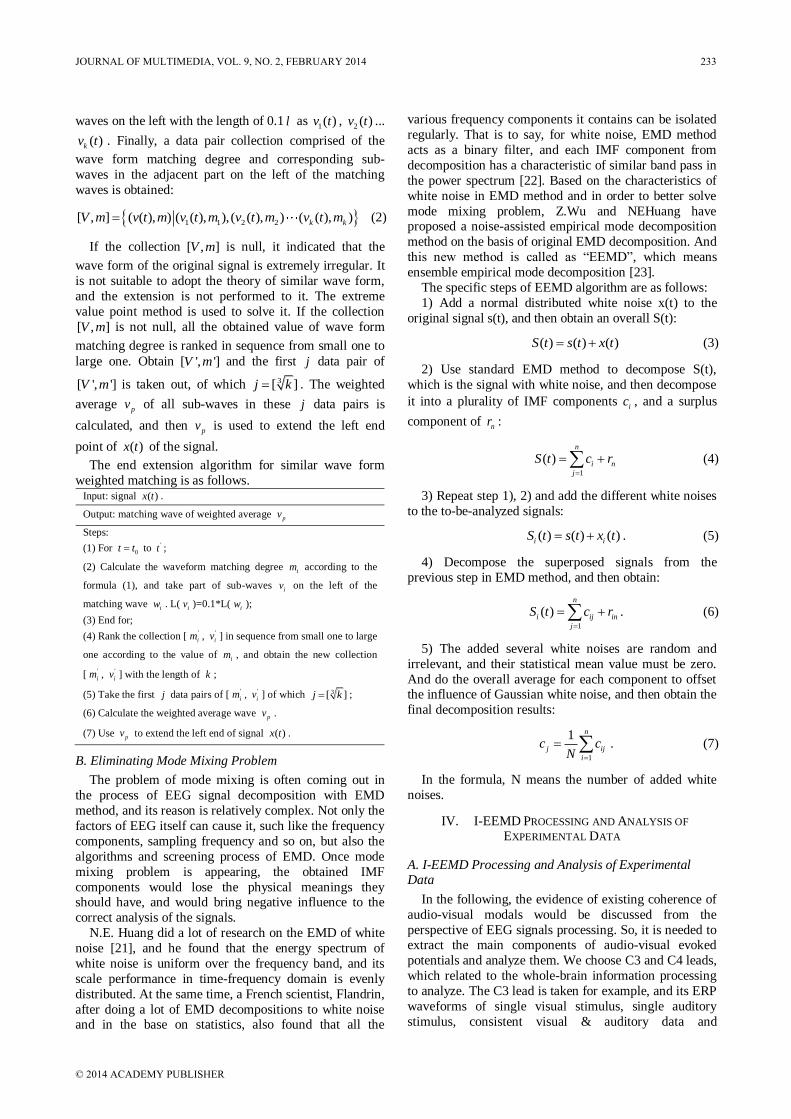
waves on the left with the length of 0.1 l as 1( )v t ,

2 ( )v t ...

( )kv t . Finally, a data pair collection comprised of the

wave form matching degree and corresponding sub-

waves in the adjacent part on the left of the matching

waves is obtained:

1 1 2 2[ , ] ( ( ), ) ( ( ), ),( ( ), ) ( ( ), )k kV m v t m v t m v t m v t m (2)

If the collection [ , ]V m is null, it indicated that the

wave form of the original signal is extremely irregular. It

is not suitable to adopt the theory of similar wave form,

and the extension is not performed to it. The extreme

value point method is used to solve it. If the collection

[ , ]V m is not null, all the obtained value of wave form

matching degree is ranked in sequence from small one to

large one. Obtain [ ', ']V m and the first j data pair of

[ ', ']V m is taken out, of which 3[ ]j k . The weighted

average pv of all sub-waves in these j data pairs is

calculated, and then pv is used to extend the left end

point of ( )x t of the signal.

The end extension algorithm for similar wave form

weighted matching is as follows. Input: signal ( )x t .

Output: matching wave of weighted average pv

Steps:

(1) For 0t t to 't ;

(2) Calculate the waveform matching degree im according to the

formula (1), and take part of sub-waves iv on the left of the

matching wave iw . L(

iv )=0.1*L(iw );

(3) End for;

(4) Rank the collection ['

im , '

iv ] in sequence from small one to large

one according to the value of im , and obtain the new collection

['

im , '

iv ] with the length of k ;

(5) Take the first j data pairs of ['

im , '

iv ] of which 3[ ]j k ;

(6) Calculate the weighted average wave pv .

(7) Use pv to extend the left end of signal ( )x t .

B. Eliminating Mode Mixing Problem

The problem of mode mixing is often coming out in

the process of EEG signal decomposition with EMD

method, and its reason is relatively complex. Not only the

factors of EEG itself can cause it, such like the frequency

components, sampling frequency and so on, but also the

algorithms and screening process of EMD. Once mode

mixing problem is appearing, the obtained IMF

components would lose the physical meanings they should have, and would bring negative influence to the

correct analysis of the signals.

N.E. Huang did a lot of research on the EMD of white

noise [21], and he found that the energy spectrum of

white noise is uniform over the frequency band, and its

scale performance in time-frequency domain is evenly

distributed. At the same time, a French scientist, Flandrin,

after doing a lot of EMD decompositions to white noise and in the base on statistics, also found that all the

various frequency components it contains can be isolated

regularly. That is to say, for white noise, EMD method

acts as a binary filter, and each IMF component from

decomposition has a characteristic of similar band pass in

the power spectrum [22]. Based on the characteristics of

white noise in EMD method and in order to better solve

mode mixing problem, Z.Wu and NEHuang have proposed a noise-assisted empirical mode decomposition

method on the basis of original EMD decomposition. And

this new method is called as “EEMD”, which means

ensemble empirical mode decomposition [23].

The specific steps of EEMD algorithm are as follows:

1) Add a normal distributed white noise x(t) to the

original signal s(t), and then obtain an overall S(t):

( ) ( ) ( )S t s t x t (3)

2) Use standard EMD method to decompose S(t),

which is the signal with white noise, and then decompose

it into a plurality of IMF components ic , and a surplus

component of nr :

1

( )n

i n

j

S t c r

(4)

3) Repeat step 1), 2) and add the different white noises

to the to-be-analyzed signals:

( ) ( ) ( )i iS t s t x t . (5)

4) Decompose the superposed signals from the

previous step in EMD method, and then obtain:

1

( )n

i ij in

j

S t c r

. (6)

5) The added several white noises are random and

irrelevant, and their statistical mean value must be zero.

And do the overall average for each component to offset the influence of Gaussian white noise, and then obtain the

final decomposition results:

1

1 n

j ij

i

c cN

. (7)

In the formula, N means the number of added white

noises.

IV. I-EEMD PROCESSING AND ANALYSIS OF

EXPERIMENTAL DATA

A. I-EEMD Processing and Analysis of Experimental Data

In the following, the evidence of existing coherence of

audio-visual modals would be discussed from the

perspective of EEG signals processing. So, it is needed to extract the main components of audio-visual evoked

potentials and analyze them. We choose C3 and C4 leads,

which related to the whole-brain information processing

to analyze. The C3 lead is taken for example, and its ERP

waveforms of single visual stimulus, single auditory

stimulus, consistent visual & auditory data and



inconsistent visual & auditory data are obtained shown as

Fig. 3:

Figure 3. C3 Lead ERP Waveform

In Fig. 3 it shows four kinds of ERP data waveforms on the length of one epoch. Among them the selected

stimulating text for the visual stimulation is the screen

text letter "ba"; the selected stimulating material for the

auditory stimulus is the sound "ba" from the audio; the

stimulating material for the audio-visual consistent is the

letter "ba" and sound "ba"; and the selected stimulating

material for audio-visual inconsistent is the letter "ba"

and sound "ga". After decomposing the above four kinds of ERP data

in the I-EEMD method, all the IMF components are

obtained as Fig. 4 shown. Every component is distributed

according to the frequency from high to low. For the

point of decomposition effect, each component is

relatively stable at the end, and there was also no flying

wing phenomenon, and producing no significant mode

mixing problem. Each component has a complete physical meaning, and through these components it could

examine the advantages and disadvantages of

decomposition effects. And the fact that Res, the surplus

component is close to zero, once again proves the validity

of the proposed method in this paper.And from that figure

it can be seen, through the I-EEMD decomposition the

VEP data of C3 lead decomposed into 7 IMF components

and a surplus component. Among these seven IMF components, there may be some pseudo-components,

which could be screened out by the method of correlation

coefficients calculation. Through the I-EEMD

decomposition the AEP data of the C3 leads turned into

seven IMF components and a surlpus component. The

audio-visual consistent data of C3 leads through I-EEMD

decomposition turned into seven IMF components and a

surplus component. The audio-visual inconsistent data of C3 lead through I-EEMD decomposition turned in six

IMF components and a surplus component.

Among the seven IMF components of the VEP data

through I-EEMD decomposition, there usually are some

pseudo-components, which should be screened out and

not taked into consideration. Through the relavent theory

of signals, the varity of IMF components could be judged.

The dicision threhold value of the pseudo-component is

one-tenth of the biggest correlation coefficient [24].

Caculate the correlation coefficients between these seven

IMF componnets and original signal, and they are shown

in Table 1.

(a) visual modal

(b) auditory modal

(c) audio-visual consistent modal

(d) audio-visual inconsistent modal

Figure 4. I-EEMD Decomposition of ERP Data



TABLE I. THE CORRELATION COEFFICIENT BETWEEN IMF COMPONENTS AND ORIGINAL SIGNAL

IMF1 IMF2 IMF3 IMF4 IMF5 IMF6 IMF7 Res

0.0153 0.9435 0.5221 0.0275 0.7433 0.7028 0.0649 0.0032

TABLE II. THE CORRELATION COEFFICIENT BETWEEN IMF COMPONENTS AND ORIGINAL SIGNAL

IMF1 IMF2 IMF3 IMF4 IMF5 IMF6 IMF7 Res

0.0211 0.6541 0.9022 0.5728 0.0325 0.0411 0.0353 0.0049

As Table 1 shown, the correlation coefficients of IMF1,

IMF4, IMF7 with the original signal are relatively low,

which are 0.0153, 0.0275 and 0.0649. From that we could

say that these three components are pseudo-components

obtained from the decomposition. And the correlation

coefficient between surplus component and the original

signal is 0.0032. So these four decomposition components don’t have real physical meanings and don’t

deserve deeper analysis. The correlation coefficents of

IMF2, IMF3, IMF5, IMF6 with the original signal are

relatively high, so they are the effective components from

decomposition.

Similarly, do the same process to the IMF components

from AEP data and obtain Table 2

It could be seen from Table 2 that the correlation coefficients of IMF1, IMF5, IMF6 and IMF7 with

original signal are relatively low, which are 0.0211,

0.0325, 0.0411 and 0.0353. From that we could say that

these four components are pseudo-components coming

from decomposition and don’t have real physical

meanings. The correlation coefficients of IMF2, IMF3,

IMF4 with orignal signal are relatively high, which

means they are the effecitve components from decomposition.

B. Analysis of Experiment Result

It could analyze the coherence of audio-visual modals

by comparing the correlation coefficients of ERP signal in single visual or auditory modal with the ERP signal in

audio-visual modals. Due to the sound is “ga” when

audio-visual are inconsistent, it should choose the sound

as “ga” when considering compare the ERP data in single

auditory modal and audio-visual inconsistent modal. The

other situations should take the sound “ba”. The

comparison situation of correlation coefficient calculating

from the above experiment data is shown in Table 3:

TABLE III. COMPARISON OF THE CORRELATION COEFFICIENT

Correlation coefficient value Single visual

ERP data

Single auditory

ERP data

Audio-visual consistent ERP data 0.5331 0.4519

Audio-visual inconsistent ERP data 0.2379 0.2022

It could be seen from Table 3 that the signal

correlation coefficient of ERP data between single visual

modal and audio-visual consistent modal is 0.5331, while

the signal correlation coefficient of ERP data between it

and audio-visual inconsistent is 0.2379; the signal

correlation coefficient between the ERP data of single

auditory stimuli and that of audio-visual consistent is 0.4519, while the signal correlation coefficient of ERP

data between it and audio-visual inconsistent is 0.2022.

So from that we could say, when the information in

audio-visual modal is consistent, it could improve the

information in single modal; while, when the information

in audio-visual modal is not consistent, it could have

inhibitory effect on single-modal state information.

In addition, could also find some evidence to support

the above points when considering the main compositions

of ERP signal in single audio or visual stimulus and the correlation of ERP signal in audio-visual modals mixing

stimuli.

From the principle of EMD decomposition, we could

know that the IMF components got from decomposition

have complete physical meaning. So it could inspect the

coherence of audio-visual modals through the main

compositions of single visual stimulus, single auditory

stimulus and the correlation coefficient of the ERP data of audio-visual consistent and inconsistent.

To compare the valid components of single visual

evoked potentials and single auditory evoked potentials,

and compare the correlation coefficients of ERP data of

audio-visual consistent and inconsistent, we could get the

data in Table 4:

TABLE IV. VISUAL COMPOSITION'S COMPARISON OF THE

CORRELATION COEFFICIENT

Correlation coefficient IMF2 IMF3 IMF5 IMF6

Audio-visual consistent data 0.5111 0.3853 0.5037 0.4202

Audio-visual consistent data 0.2195 0.1528 0.3001 0.2673

From Table 4 we could see that the correlation

coefficients between the main compositions of single visual stimulus evoked potentials and the ERP signal in

audio-visual consistent are obviously greater than the

correlation coefficients between it and ERP signal in

audio-visual inconsistent. And that also shows that when

the audio-visual information is consistent, it could help

people to prompt information-controlling power of

outside world. Then let’s look at the corresponding data

in audio modal. Because in experiment under the situation of audio-visual inconsistent, we select sound

“ga” and letter “ba” as the to-be-analyzed data. In order

to get a better comparability of the experiment results,

here we choose the sound “ga” in the auditory modal to

compare with the data in audio-visual cross-modal data,

and get the results shown as Table 5:

TABLE V. AUDIO COMPOSITION'S COMPARISON OF THE

CORRELATION COEFFICIENT

Valid auditory components IMF2 IMF3 IMF4

Correlation coefficient of audio-

visual consistent

0.6232 0.7869 0.5466

Correlation coefficient of audio-

visual inconsistent

0.2752 0.3456 0.0387

From Table 5 it could be seen that the comparison is

similar to what in the visual modal, which is to say that,



the correlation coefficients between the main

compositions of single auditory evoked potentials and the

ERP signal in audio-visual consistent modal are

apparently greater than what of ERP signal in audio-

visual inconsistent modal. And what could also show that

when the information in audio-visual is consistent, the

EEG signal will be stronger than single modal auditory information in the brain.

V. CONCLUSIONS

This paper discusses the theory evidence of audio-

visual modals’ coherence from the perspective of EEG

signal processing. And the experiment is designed based

on the EEG in audio-visual cross-modal and then collect,

process and analyze the experiment data. During the

process of EEG signal, it uses EEMD, which combined the similar waveform average end continuation

algorithms, which is called in paper as I-EEMD,

considering the need to restrain the effects of mode

mixing and end point effect. And try to describe the

collected ERP data through two perspectives based on the

theory of signal coherence. First, investigated the

correlation of the data in single visual modal, single

auditory modal and the data in audio-visual cross-modal. From the calculated correlation coefficient it could be

found that, when audio-visual is consistent, the

correlation coefficient of it with any single modal is

relatively great. Second, form the main valid

compositions in single visual or audio modal, the

comparison situation of the calculated correlation

coefficient is similar. From these two points we could

find that, when the informations in audio & visual modals are consistent, it could help the brain promptly handle

outside environment, and that is to say, it could improve

each other’s information under the condition of audio-

visual consistent; when the informations in these two

modals are not consistent, it could restrain each other’s

information and the brain could get a combined result

after integrated, which is consistent with the famous

McGulk effect.

ACKNOWLEDGMENT


Foundation for Young Scientists of Shanxi Province,

China (GrantNo.2013021016-3).

REFERENCES

[1] Guo, Jianzeng and Guo, Aike. Cross modal interactions between olfactory and visual learning in Drosophila, Science, vol. 309, no. 5732, pp. 307–310, 2005.

[2] Suminski, Aaron J and Tkach, Dennis C and Hatsopoulos, Nicholas G. Exploiting multiple sensory modalities in brainmachine interfaces, Neural Networks, vol. 22, no. 9, pp. 1224–1234, 2009.

[3] Ohshiro, Tomokazu and Angelaki, Dora E and DeAngelis,

Gregory C. A normalization model of multisensory integration. Nature Neuroscience, vol. 14, no. 5, pp. 775–782, 2011.

[4] Nishibori, Kento and Takeuchi, Yoshinori and Matsumoto, Tetsuya and Kudo, Hiroaki and Ohnishi, Noboru. ”Finding the correspondence of audio-visual events by object

manipulation. in IEEJ Transactions on Electronics, Information and Systems, 2008, pp. 242–252.

[5] Mitchell, T. AI and the Impending Revolution in Brain Sciences. in Eighteenth National Conference on Artificial Intelligence, July 28-August 1, 2002, Menlo Park, United States.

[6] Ethofer, Thomas and Pourtois, Gilles and Wildgruber, Dirk. Investigating audiovisual integration of emotional signals in the human brain” in Progress in Brain Research, vol. 156, pp. 345–361, 2006.

[7] Gonzalo-Fonrodona, Isabel. Functional gradients through the cortex. multisensory integration and scaling laws in brain dynamics. in Neurocomputing, vol. 72, no. 4C6, pp.

831-838, 2009. [8] Liu, Baolin and Meng, Xianyao and Wang, Zhongning and

Wu, Guangning. An ERP study on whether semantic integration exists in processing ecologically unrelated audio-visual information. in Neuroscience Letters, vol. 505, no. 2, pp. 119-123, 2011.

[9] Lee, TienWen and Wu, YuTe and Yu, Younger WY and Chen, Ming-Chao and Chen, Tai-Jui. The implication of functional connectivity strength in predicting treatment response of major depressive disorder: A resting EEG study. In Psychiatry Research-Neuroimaging, vol. 194, no. 3, pp. 372-377, 2011.

[10] Blankertz, Benjamin and Tomioka, Ryota and Lemm, Steven and Kawanabe, Motoaki and Muller, K-R. Optimizing spatial filters for robust EEG single-trial analysis. in IEEE Signal Processing Magazine, vol. 25, no. 1, pp. 41-56, 2008.

[11] Molholm, Sophie and Ritter, Walter and Murray, Micah M and Javitt, Daniel C and Schroeder, Charles E and Foxe, John J. Multisensory auditory-visual interactions during early sensory processing in humans: a high-density electrical mapping study. Cognitive brain research, vol. 14, no. 1, pp. 115-128, 2002.

[12] Yuan, Ling and Yang, Banghua and Ma, Shiwei. Discrimination of movement imagery EEG based on HHT and SVM. ”Chinese Journal of Science Instrument, vol. 31, no. 3, pp. 649-654, 2010.

[13] Coyle, Damien and McGinnity, T Martin and Prasad, Girijesh. Improving the separability of multiple EEG features for a BCI by neural-time-series-prediction preprocessing. Biomedical Signal Processing and Control, vol. 5, no. 3, pp. 649-654, 2010.

[14] He, Zhi and Shen, Yi and Wang, Qiang. Boundary extension for Hilbert-Huang transform inspired by gray

prediction model.” Signal Processing, vol. 92, no. 3, pp. 685-697, 2012.

[15] Lee, Ray F and Xue, Rong. A transmit/receive volume strip array and its mode mixing theory in MRI. Magnetic Resonance Imaging, vol. 25, no. 9, pp. 1312-1332, 2007.

[16] Jin Ping, ZHAO and Da ji, Huang. Mirror extending and circular spline function for empirical mode decomposition method. Journal of Zhejiang University, vol. 2, no. 3, pp. 247-252, 2001.

[17] Gai, Q. Research and Application to the Theory of Local Wave Time-Frequency Analysis Method. PHD, Dalian University of Technology, Dalian, 2001.

[18] Hamilton, James Douglas. Time Series Analysis; Cambridge Univ Press, vol. 2, 2001.

[19] Qiao Shijie. The Symmetric Extension Method for Wavelet Transform Image Coding.” Journal of Image and Graphics, vol. 5, no. 9, pp. 725-729, 2005.

[20] Pigorini, Andrea and Casali, Adenauer G and Casarotto, Silvia and Ferrarelli, Fabio and Baselli, Giuseppe and Mariotti, Maurizio and Massimini, Marcello and Rosanova,



Mario. Time-frequency spectral analysis of TMS-evoked EEG oscillations by means of Hilbert-Huang transform.

Journal of Neuroscience Methods, vol. 192, no. 2, pp. 236-245, 2011.

[21] Huang, Norden E. Review of empirical mode decomposition. In Proceedings of SPIE - The International Society for Optical Engineering, Orlando, FL, United

States, March 26; SPIE: Bellingham WA, United States, 2001.

[22] Bao, Fei and Wang, Xinlong and Tao, Zhiyong and Wang, Qingfu and Du, Shuanping. “EMD-based extraction of modulated cavitation noise.” Mechanical Systems and Signal Processing, vol. 24, no. 7, pp. 2124-2136, 2010.

[23] Wu, Zhaohua and Huang, Norden E. Ensemble empirical mode decomposition: a noise assisted data analysis method.

Advances in Adaptive Data Analysis, vol. 1, no. 1, pp. 1-41,

2009. [24] Yu, Dejie and Cheng, Junsheng and Yang, Yu. Application

of Improved Hilbert-Huang Transform Method in Gear Fault Diagnosis.” Journal of Aerospace Power, vol. 41, no. 6, pp. 1899-1903, 2009.

Xiaojun Zhu was born in Jiangsu, China, in 1977. He received the Master degree in Computer Science in 2001, from Taiyuan

University of Technology, Taiyuan, China. He received the Doctor’s degree in 2012, from Taiyuan University of Technology, Taiyuan, China. His research interests include Intelligent Information processing, cloud computing, and audio-visual computing.

Jingxian Hu is currently a Graduate student and working towards his M.S. degree at Taiyuan University of Technology, China. Her current research interest includes wireless sensor network and Intelligent Information processing.

Xiao Ma is currently a Graduate student and working towards his M.S. degree at Taiyuan University of Technology, China. Hercurrent research interest includes cloud computing, and audiovisual computing.



Object Recognition Algorithm Utilizing Graph

Cuts Based Image Segmentation

Zhaofeng Li and Xiaoyan Feng College of Information Engineering Henan Institute of Science and Technology, Henan Xinxiang, China


Abstract—This paper concentrates on designing an object

recognition algorithm utilizing image segmentation. The

main innovations of this paper lie in that we convert the

image segmentation problem into graph cut problem, and

then the graph cut results can be obtained by calculating the

probability of intensity for a given pixel which is belonged to

the object and the background intensity. After the graph cut

process, the pixels in a same component are similar, and the

pixels in different components are dissimilar. To detect the

objects in the test image, the visual similarity between the

segments of the testing images and the object types deduced

from the training images is estimated. Finally, a series of

experiments are conducted to make performance evaluation.

Experimental results illustrate that compared with existing

methods, the proposed scheme can effectively detect the

salient objects. Particularly, we testify that, in our scheme,

the precision of object recognition is proportional to image

segmentation accuracy.

Index Terms—Object Recognition; Graph Cut; Image

Segmentation; SIFT; Energy Function

I. INTRODUCTION

In the computer vision research field, image

segmentation refers to the process of partitioning a digital

image into multiple segments, which are made up of a set

of pixels. The aim of image segmentation is to simplify

and change the representation of an image into something that is more meaningful and easier for users to analyze.

That is, image segmentation is typically utilized to locate

objects and curves in images [1] [2]. Particularly, image

segmentation is the process of allocating a tag to each

pixel of an image such that pixels with the same tag

sharing specific visual features. The results of image

segmentation process can be represented as a set of

segments which totally cover the whole image [3]. The pixels belonged to the same region are similar either in

some characteristics or in some computed properties,

which refer to the color, intensity, or texture. On the other

hand, adjacent regions are significantly different with

respect to the same characteristics.

The problems of image segmentation are great

challenges for computer vision research field. As the time

of the Gestalt movement in psychology, it has been known that perceptual grouping plays a powerful role in

human visual perception. A wide range of computational

vision problems could in principle make good use of

segmented images, were such segmentations reliably and

efficiently computable. For instance intermediate-level

vision problems such as stereo and motion estimation

require an appropriate region of support for

correspondence operations. Spatially non-uniform regions

of support can be identified using segmentation

techniques. Higher-level problems such as recognition and image indexing can also utilize segmentation results

in matching, to address problems such as figure-ground

separation and recognition by parts [4-6].

As salient objects are important parts in images, hence,

if they can be effectively detected, the performance of

image segmentation can be promoted. Object recognition

refers to locate collections of salient line segments in an

image [7]. The object recognition systems are designed to correctly identify an object in a scene of objects, in the

presence of clutter and occlusion and to estimate its

position and orientation. Those systems can be exploited

in robotic applications where robots are required to

navigate in crowded environments and use their

equipment to recognize and manipulate objects [8].

In this paper, the image segmentation is regarded as a

graph cut problem, which is a basic problem in computer algorithm and theory. In computer theory, the graph cut

problem is defined on data represented in the form of a

graph ( , )G V E , where V and E represent the vertices

and edges of the graph respectively, such that it is

possible to cut G into several components with some

given constrains. Graph cut method is widely used in

many application fields, such as scientific computing,

partitioning various stages of a VLSI design circuit and

task scheduling in multi-processor systems [9] [10]. The main innovations of this paper lie in the following

aspects:

(1) The proposed algorithm converts the image

segmentation problem into graph cut problem, and the

graph cut results can be obtained by an optimization

process using energy function.

(2) In the proposed, the objects can be detected by

computing the visual similarity between the segments of the testing images and the object types from the training

images.

(3) A testing image is segmented into several segments,

and each image segment is tested to find if there is a kind

of object can match it.

The rest of the paper is organized as the following

sections. Section 2 introduces the related works. Section

3 illustrates the proposed scheme for recognizing objects



from images utilizing graph cut policy. In section 4,

experiments are implemented to make performance

evaluation. Finally, we conclude the whole paper in

section 5.

II. RELATED WORKS

In this section, we will survey related works about this

paper in two aspects, including 1) image segmentation and 2) graph cut based image segmentation.

Dawoud et al. proposed an algorithm that fuses visual

cues of intensity and texture in Markov random fields

region growing texture image segmentation. The main

idea is to segment the image in a way that takes

EdgeFlow edges into consideration, which provides a

single framework for identifying objects boundaries

based on texture and intensity descriptors [11]. Park proposed a novel segmentation method based on

a hierarchical Markov random field. The proposed

algorithm is composed of local-level MRFs based on

adaptive local priors which model local variations of

shape and appearance and a global-level MRF enforcing

consistency of the local-level MRFs. The proposed

method can successfully model large object variations

and weak boundaries and is readily combined with well-established MRF optimization techniques [12].

Gonzalez-Diaz et al. proposed a novel region-centered

latent topic model that introduces two main contributions:

first, an improved spatial context model that allows for

considering inter-topic inter-region influences; and

second, an advanced region-based appearance

distribution built on the Kernel Logistic Regressor.

Furthermore, the proposed model has been extended to work in both unsupervised and supervised modes [13].

Nie et al. proposed a novel two-dimensional variance

thresholding scheme to improve image segmentation

performance is proposed. The two-dimensional histogram

of the original and local average image is projected to

one-dimensional space in the proposed scheme firstly,

and then the variance-based criterion is constructed for

threshold selection. The experimental results on bi-level and multilevel thresholding for synthetic and real-world

images demonstrate the success of the proposed image

thresholding scheme, as compared with the Otsu method,

the two-dimensional Otsu method and the minimum class

variance thresholding method [14].

Chen et al. proposes a new multispectral image texture

segmentation algorithm using a multi-resolution fuzzy

Markov random field model for a variable scale in the wavelet domain. The algorithm considers multi-scalar

information in both vertical and lateral directions. The

feature field of the scalable wavelet coefficients is

modelled, combining with the fuzzy label field describing

the spatially constrained correlations between

neighbourhood features to achieve more accurate

parameter estimation [15].

Han et al. presented a novel variational segmentation method within the fuzzy framework, which solves the

problem of segmenting multi-region color-scale images

of natural scenes. The advantages of the proposed

segmentation method are: 1) by introducing the PCA

descriptors, our segmentation model can partition color-

texture images better than classical variational-based

segmentation models, 2) to preserve geometrical structure

of each fuzzy membership function, we propose a

nonconvex regularization term in our model, and 3) to

solve the segmentation model more efficiently, the

authors design a fast iteration algorithm in which the augmented Lagrange multiplier method and the iterative

reweighting are integrated [16].

Souleymane et al. designed an energy functional based

on the fuzzy c-means objective function which

incorporates the bias field that accounts for the intensity

inhomogeneity of the real-world image. Using the

gradient descent method, the authors obtained the

corresponding level set equation from which we deduce a fuzzy external force for the LBM solver based on the

model by Zhao. The method is fast, robust against noise,

independent to the position of the initial contour,

effective in the presence of intensity inhomogeneity,

highly parallelizable and can detect objects with or

without edges [17].

Liu et al. proposed a new variational framework to

solve the Gaussian mixture model (GMM) based methods for image segmentation by employing the convex

relaxation approach. After relaxing the indicator function

in GMM, flexible spatial regularization can be adopted

and efficient segmentation can be achieved. To

demonstrate the superiority of the proposed framework,

the global, local intensity information and the spatial

smoothness are integrated into a new model, and it can

work well on images with inhomogeneous intensity and noise [18].

Wang et al. presented a novel local region-based level

set model for image segmentation. In each local region,

the authors define a locally weighted least squares energy

to fit a linear classifier. With level set representation,

these local energy functions are then integrated over the

whole image domain to develop a global segmentation

model. The objective function in this model is thereafter minimized via level set evolution [19].

Wang et al. presented an online reinforcement learning

framework for medical image segmentation. A general

segmentation framework using reinforcement learning is

proposed, which can assimilate specific user intention

and behavior seamlessly in the background. The method

is able to establish an implicit model for a large state-

action space and generalizable to different image contents or segmentation requirements based on learning in situ

[20].

In recent years, several researchers utilized the Graph

Cut technology to implement the image segmentation,

and the related works are illustrated as follows.

Zhou et al. present four technical components to

improve graph cut based algorithms, which are

combining both color and texture information for graph cut, including structure tensors in the graph cut model,

incorporating active contours into the segmentation

process, and using a "softbrush" tool to impose soft

constraints to refine problematic boundaries. The

integration of these components provides an interactive



segmentation method that overcomes the difficulties of

previous segmentation algorithms in handling images

containing textures or low contrast boundaries and

producing a smooth and accurate segmentation boundary

[21].

Chen et al. proposed a novel synergistic combination

of the image based graph cut method with the model based ASM method to arrive at the graph cut -ASM

method for medical image segmentation. A multi-object

GC cost function is proposed which effectively integrates

the ASM shape information into the graph cut framework

The proposed method consists of two phases: model

building and segmentation. In the model building phase,

the ASM model is built and the parameters of the GC are

estimated. The segmentation phase consists of two main steps: initialization and delineation [22].

Wang et al. present a novel method to apply shape

priors adaptively in graph cut image segmentation. By

incorporating shape priors adaptively, the authors provide

a flexible way to impose the shape priors selectively at

pixels where image labels are difficult to determine

during the graph cut segmentation. Further, the proposed

method integrated two existing graph cut image segmentation algorithms, one with shape template and the

other with the star shape prior [23].

Yang et al. proposed an unsupervised color-texture

image segmentation method. To enhance the effects of

segmentation, a new color-texture descriptor is designed

by integrating the compact multi-scale structure tensor,

total variation flow, and the color information. To

segment the color-texture image in an unsupervised and multi-label way, the multivariate mixed student's t-

distribution is chosen for probability distribution

modeling, as MMST can describe the distribution of

color-texture features accurately. Furthermore, a

component-wise expectation-maximization for MMST

algorithm is proposed, which can effectively initialize the

valid class number. Afterwards, the authors built up the

energy functional according to the valid class number, and optimize it by multilayer graph cuts method [24].

III. THE PROPOSED SCHEME

A. Problem Statement

In this paper, the problem of image segmentation is converted into the problem of graph cut. Let an

undirected and connected graph ( , )G V E where

{1,2,..., }V n and {( , ),1 }E i j i j n are satisfied.

Let the edge weights ij jiw w be given such that 0ijw

for ( , )i j E , and in particular, let 0iiw . The graph cut

problem is to find a partition results 1 2( , , , )NV V V of V

where the condition 1 2 NV V V is satisfied.

In the problem image segmentation, the nodes in V

denotes the pixels of images and the edge weight is

estimated by computing the distance between two pixels.

Particularly, the graph cut based image segmentation

results can be obtained by a subset of the edges of the edge set E . There are several methods to calculate the

quality of image segmentation results. The main idea is

quite simple, that is, we want the pixels in a same

component to be similar, and the pixels in different

components to be dissimilar. Thai is to say that edge

between two nodes which are belonged to the same

component should have lower value of weights, and

edges which are located between nodes in different

components should have higher value of weights. Partition 1

Partition 2

Partition 3

Figure 1. Explaination of the graph cut problem

B. Graph Cut Based Image Segmentation

In the proposed, the main innovation lies in that we

regard the graph cut based image segmentation problem

as an energy minimization problem. Therefore, given a

set of pixels P and a set of labels L , the object is to seek

a label :l P L , which can minimize the following

equation.

,

( ) ( ) ( , )p

q

p p p p q

p P p P q N

E l R l C l l

(1)

where pN denotes the pixel set which is belonged to the

neighborhood of p , and ( )p pR l refers to the cost of

allocating the label pl to p . Moreover, ( , )q

p p qC l l

denotes the cost of allocate the label pl and ql to p and

q respectively. Afterwards, the proposed energy function

is defined in Eq. 2.

1 2 3

,

1 2 3

( ) ( ) ( , )

. . 1

p

p

p p p o q p q

p P p P q N

E D f S x C l l

s t

(2)

In Eq. 2, the parameters 1 , 2 and 3 denote the

weight of data stream pD , shape term pD , and the

boundary term respectively. Furthermore, the above

modules can be represented as the following forms.

( ),

( )( ),

p p

p p

p p

LogP I O l object labelD l

LogP I B l background label

(3)

2

2

( , ) ( )( , ) exp

( , ) 2

p q p qp

q p q

l l I IC l l

dis p q

(4)



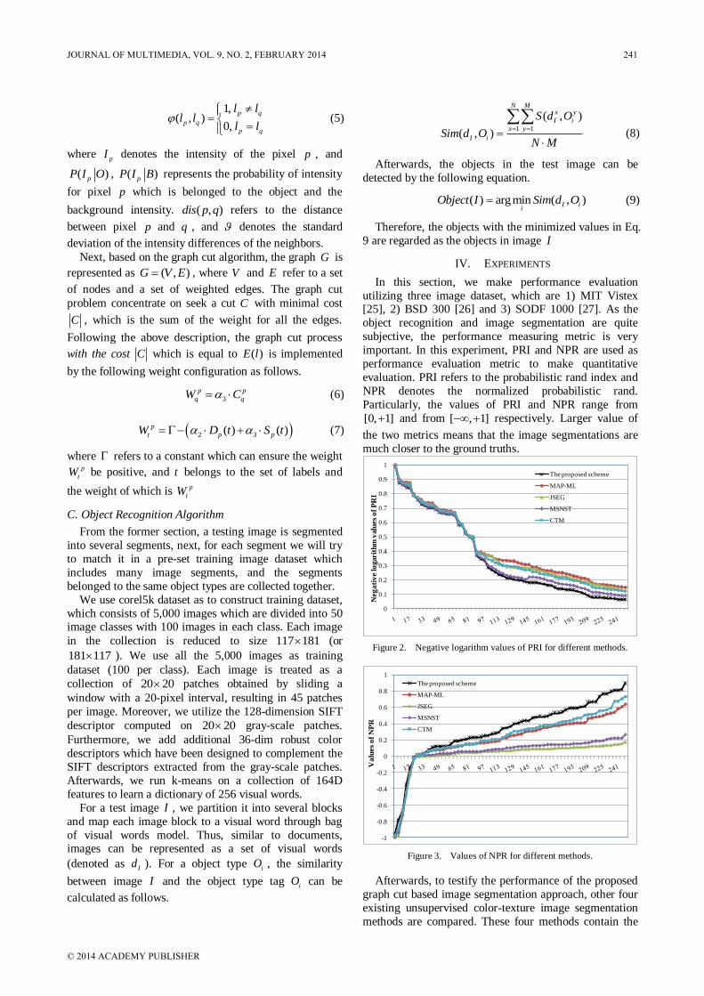
1,

( , )0,

p q

p q

p q

l ll l

l l

(5)

where pI denotes the intensity of the pixel p , and

( )pP I O , ( )pP I B represents the probability of intensity

for pixel p which is belonged to the object and the

background intensity. ( , )dis p q refers to the distance

between pixel p and q , and denotes the standard

deviation of the intensity differences of the neighbors.

Next, based on the graph cut algorithm, the graph G is

represented as ( , )G V E , where V and E refer to a set

of nodes and a set of weighted edges. The graph cut

problem concentrate on seek a cut C with minimal cost

C , which is the sum of the weight for all the edges.

Following the above description, the graph cut process

with the cost C which is equal to ( )E l is implemented

by the following weight configuration as follows.

3

p p

q qW C (6)

2 3( ) ( )p

t p pW D t S t (7)

where refers to a constant which can ensure the weight p

tW be positive, and t belongs to the set of labels and

the weight of which is p

tW

C. Object Recognition Algorithm

From the former section, a testing image is segmented

into several segments, next, for each segment we will try

to match it in a pre-set training image dataset which

includes many image segments, and the segments

belonged to the same object types are collected together.

We use corel5k dataset as to construct training dataset,

which consists of 5,000 images which are divided into 50 image classes with 100 images in each class. Each image

in the collection is reduced to size 117 181 (or

181 117 ). We use all the 5,000 images as training

dataset (100 per class). Each image is treated as a

collection of 20 20 patches obtained by sliding a

window with a 20-pixel interval, resulting in 45 patches

per image. Moreover, we utilize the 128-dimension SIFT

descriptor computed on 20 20 gray-scale patches.

Furthermore, we add additional 36-dim robust color

descriptors which have been designed to complement the

SIFT descriptors extracted from the gray-scale patches.

Afterwards, we run k-means on a collection of 164D

features to learn a dictionary of 256 visual words.

For a test image I , we partition it into several blocks

and map each image block to a visual word through bag

of visual words model. Thus, similar to documents, images can be represented as a set of visual words

(denoted as Id ). For a object type iO , the similarity

between image I and the object type tag iO can be

calculated as follows.

1 1

( , )

( , )

N Mx y

I i

x y

I i

S d O

Sim d ON M

(8)

Afterwards, the objects in the test image can be

detected by the following equation.

( ) argmin ( , )I ii

Object I Sim d O (9)

Therefore, the objects with the minimized values in Eq.

9 are regarded as the objects in image I

IV. EXPERIMENTS

In this section, we make performance evaluation

utilizing three image dataset, which are 1) MIT Vistex [25], 2) BSD 300 [26] and 3) SODF 1000 [27]. As the

object recognition and image segmentation are quite

subjective, the performance measuring metric is very

important. In this experiment, PRI and NPR are used as

performance evaluation metric to make quantitative

evaluation. PRI refers to the probabilistic rand index and

NPR denotes the normalized probabilistic rand.

Particularly, the values of PRI and NPR range from

[0, 1] and from [ , 1] respectively. Larger value of

the two metrics means that the image segmentations are

much closer to the ground truths.

0

0.1

0.2

0.3

0.4

0.5

0.6

0.7

0.8

0.9

1

The proposed scheme

MAP-ML

JSEG

MSNST

CTM

Neg

ati

ve lo

garit

hm

valu

es

of

PR

I

Figure 2. Negative logarithm values of PRI for different methods.

-1

-0.8

-0.6

-0.4

-0.2

0

0.2

0.4

0.6

0.8

1

The proposed scheme

MAP-ML

JSEG

MSNST

CTM

Va

lues

of

NP

R

Figure 3. Values of NPR for different methods.

Afterwards, to testify the performance of the proposed

graph cut based image segmentation approach, other four

existing unsupervised color-texture image segmentation

methods are compared. These four methods contain the



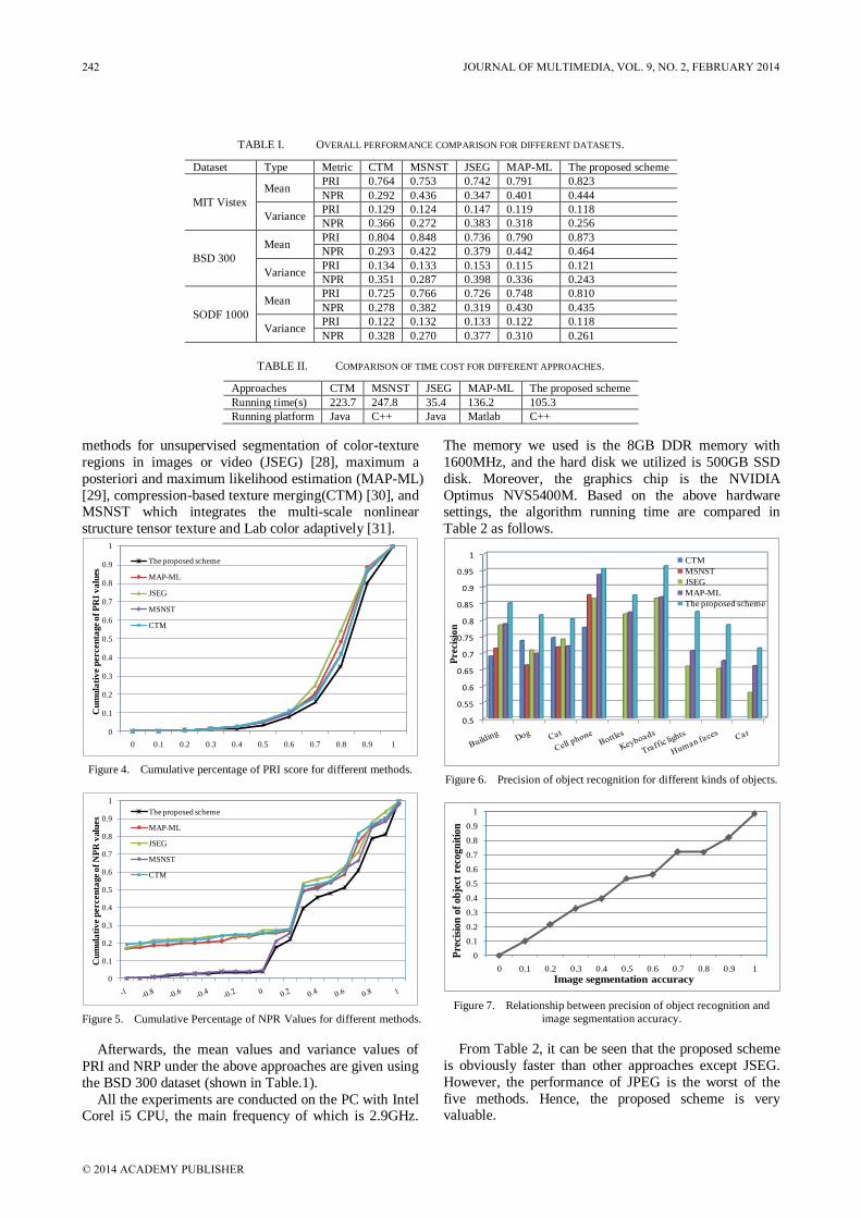
TABLE I. OVERALL PERFORMANCE COMPARISON FOR DIFFERENT DATASETS.

Dataset Type Metric CTM MSNST JSEG MAP-ML The proposed scheme

MIT Vistex

Mean PRI 0.764 0.753 0.742 0.791 0.823

NPR 0.292 0.436 0.347 0.401 0.444

Variance PRI 0.129 0.124 0.147 0.119 0.118

NPR 0.366 0.272 0.383 0.318 0.256

BSD 300

Mean PRI 0.804 0.848 0.736 0.790 0.873

NPR 0.293 0.422 0.379 0.442 0.464

Variance PRI 0.134 0.133 0.153 0.115 0.121

NPR 0.351 0.287 0.398 0.336 0.243

SODF 1000

Mean PRI 0.725 0.766 0.726 0.748 0.810

NPR 0.278 0.382 0.319 0.430 0.435

Variance PRI 0.122 0.132 0.133 0.122 0.118

NPR 0.328 0.270 0.377 0.310 0.261

TABLE II. COMPARISON OF TIME COST FOR DIFFERENT APPROACHES.

Approaches CTM MSNST JSEG MAP-ML The proposed scheme

Running time(s) 223.7 247.8 35.4 136.2 105.3

Running platform Java C++ Java Matlab C++

methods for unsupervised segmentation of color-texture

regions in images or video (JSEG) [28], maximum a

posteriori and maximum likelihood estimation (MAP-ML)

[29], compression-based texture merging(CTM) [30], and MSNST which integrates the multi-scale nonlinear

structure tensor texture and Lab color adaptively [31].

0

0.1

0.2

0.3

0.4

0.5

0.6

0.7

0.8

0.9

1

0 0.1 0.2 0.3 0.4 0.5 0.6 0.7 0.8 0.9 1

The proposed scheme

MAP-ML

JSEG

MSNST

CTM

Cu

mu

lati

ve p

ercen

tage

of

PR

I v

alu

es

Figure 4. Cumulative percentage of PRI score for different methods.

0

0.1

0.2

0.3

0.4

0.5

0.6

0.7

0.8

0.9

1

The proposed scheme

MAP-ML

JSEG

MSNST

CTM

Cu

mu

lati

ve p

ercen

tage

of

NP

R v

alu

es

Figure 5. Cumulative Percentage of NPR Values for different methods.

Afterwards, the mean values and variance values of

PRI and NRP under the above approaches are given using

the BSD 300 dataset (shown in Table.1).

All the experiments are conducted on the PC with Intel Corel i5 CPU, the main frequency of which is 2.9GHz.

The memory we used is the 8GB DDR memory with

1600MHz, and the hard disk we utilized is 500GB SSD

disk. Moreover, the graphics chip is the NVIDIA

Optimus NVS5400M. Based on the above hardware settings, the algorithm running time are compared in

Table 2 as follows.

0.5

0.55

0.6

0.65

0.7

0.75

0.8

0.85

0.9

0.95

1CTM

MSNST

JSEG

MAP-ML

The proposed scheme

Pre

cisi

on

Figure 6. Precision of object recognition for different kinds of objects.

0

0.1

0.2

0.3

0.4

0.5

0.6

0.7

0.8

0.9

1

0 0.1 0.2 0.3 0.4 0.5 0.6 0.7 0.8 0.9 1

Image segmentation accuracy

Pre

cisi

on

of

ob

ject

rec

og

nit

ion

Figure 7. Relationship between precision of object recognition and

image segmentation accuracy.

From Table 2, it can be seen that the proposed scheme

is obviously faster than other approaches except JSEG.

However, the performance of JPEG is the worst of the

five methods. Hence, the proposed scheme is very valuable.



Figure 8. Example of the object recognition results by the proposed image segmentation algorithm

In the following parts, we will test the influence of

image segmentation accuracy to object recognition.

Firstly, experiments are conducted to show the precision

of object recognition for different kinds of objects, and

the results are shown in Fig. 6.

Secondly, the relationship between precision of object recognition and image segmentation accuracy is shown in

Fig. 7.

As is shown in Fig. 7, precision of object recognition is

proportional to image segmentation accuracy. Therefore,

image segmentation module in the proposed is very

powerful in the object recognition process.

From the above experimental results, it can be seen

that the proposed scheme is superior to other two schemes. The main reasons lie in the following aspects:

(1) The proposed scheme converts the image

segmentation problem into graph cut problem, and we

obtained the graph cut results by an optimization process.

Moreover, the objects can be detected by computing the

visual similarity between the segments of the testing

images and the object types from the training images.

(2) For the JSEG algorithm, there is a major problem which is caused the varying shades due to the

illumination. However, this problem is difficult to handle

because in many cases not only the illuminant component

but also the chromatic components of a pixel change their

values due to the spatially varying illumination.

(3) The MAP-ML algorithm should be extended to

segment image with the combination of motion

information, and the utilization of the model for specific

object extraction by designing more complex features to

describe the objects.

(4) The CTM scheme should be extended to supervised scenarios. As it is of great importance to better

understand how humans segment natural images from the

lossy data compression perspective. Such an

understanding would lead to new insights into a wide

range of important problems in computer vision such as

salient object detection and segmentation, perceptual

organization, and image understanding and annotation.

(5) The performance of MSNST is not satisfied, because the proposed method is the compromise between

high segmentation accuracy and moderate computation

efficiency. Particularly, the parameter setting in this

scheme is too complex and more discriminative

segmentation process should be studied in detail.

V. CONCLUSIONS

In this paper, we proposed an effective object

recognition algorithm based on image segmentation. The image segmentation problem is converted into the graph

cut problem, and then the graph cut results can be

computed by estimating the probability of intensity for a

given pixel which is belonged to the object and the

background intensity. In order to find the salient objects



we compute the visual similarity between the segments of

the testing images and the object types deduced from the

Corel5K image dataset.

REFERENCES

[1] Peng Qiangqiang, Long Zhao, A modified segmentation approach for synthetic aperture radar images on level set, Journal of Software, 2013, 8(5) pp. 1168-1173

[2] Grady, Leo, Random walks for image segmentation, IEEE Transactions on Pattern Analysis and Machine Intelligence, 2006, 28(11) pp. 1768-1783

[3] Noble, J. Alison; Boukerroui, Djamal Ultrasound image segmentation: A survey, IEEE Transactions on Medical

Imaging, 2006, 25(8) pp. 987-1010 [4] Felzenszwalb, PF; Huttenlocher, DP, Efficient graph-based

image segmentation, International Journal of Computer Vision, 2004, 59(2) pp. 167-181

[5] Boykov, Yuri; Funka-Lea, Gareth Graph cuts and efficient N-D image segmentation, International Journal of Computer Vision, 2006, 70(2) pp. 109-131

[6] Lei Zhu, Jing Yang, Fast Multi-Object Image Segmentation Algorithm Based on C-V Model, Journal of Multimedia, 2011, 6(1) pp. 99-106

[7] Kang, Dong Joong and Ha, Jong Eun and Kweon, In So,

Fast object recognition using dynamic programming from combination of salient line groups, Pattern Recognition, 2003, 36(1) pp. 79-90

[8] Georgios Kordelas, Petros Daras, Viewpoint independent object recognition in cluttered scenes exploiting ray-triangle intersection and SIFT algorithms, Pattern Recognition, 2010, 43(11) pp. 3833-3845

[9] Andreev Konstantin, Räcke Harald, Balanced Graph Partitioning, Proceedings of the sixteenth annual ACM symposium on Parallelism in algorithms and architectures, 2004, pp. 120-124

[10] Shi, JB; Malik, J Normalized cuts and image segmentation, IEEE Transactions on Pattern Analysis and Machine Intelligence, 2000, 22(8) pp. 888-905

[11] Dawoud A., Netchaev A., Fusion of visual cues of intensity and texture in Markov random fields image segmentation, IET Computer Vision, 2013, 6(6) pp. 603-609

[12] Park Sang Hyun, Lee Soochahn, Yun Il Dong, Hierarchical MRF of globally consistent localized classifiers for 3D medical image segmentation, Pattern Recognition, 2013, 46(9) pp. 2408-2419

[13] Gonzalez-Diaz Ivan, Diaz-de-Maria Fernando, A region-

centered topic model for object discovery and category-based image segmentation, Pattern Recognition, 2013, 46(9) pp. 2437-2449

[14] Nie Fangyan, Wang Yonglin, Pan Meisen, Two-dimensional extension of variance-based thresholding for image segmentation, Multidimensional Systems and Signal Processing, 2013, 24(3) pp. 485-501

[15] Chen Mi, Strobl Josef, Multispectral textured image segmentation using a multi-resolution fuzzy Markov random field model on variable scales in the wavelet domain, International Journal of Remote Sensing, 2013,

34(13) pp. 4550-4569 [16] Han Yu, Feng Xiang-Chu, Baciu George, Variational and

PCA based natural image segmentation, Pattern Recognition, 2013, 46(7) pp. 1971-1984

[17] Balla-Arabe Souleymane, Gao Xinbo, Wang Bin, A Fast and Robust Level Set Method for Image Segmentation

Using Fuzzy Clustering and Lattice Boltzmann Method, IEEE Transactions on Cybernetics, 2013, 43(3) pp. 910-920

[18] Liu Jun, Zhang Haili, Image Segmentation Using a Local GMM in a Variational Framework, Journal of Mathematical Imaging and Vision, 2013, 46(2) pp. 161-176

[19] Wang Ying, Xiang Shiming, Pan Chunhong, Level set evolution with locally linear classification for image segmentation, Pattern Recognition, 2013, 46(6) pp. 1734-1746

[20] Wang Lichao, Lekadir Karim, Lee Su-Lin, A General Framework for Context-Specific Image Segmentation Using Reinforcement Learning, IEEE Transactions on Medical Imaging, 2013, 32(5) pp. 943-956

[21] Zhou Hailing, Zheng Jianmin, Wei Lei, Texture aware image segmentation using graph cuts and active contours, Pattern Recognition, 2013, 46(6) pp. 1719-1733

[22] Chen Xinjian, Udupa Jayaram K., Alavi Abass, GC-ASM: Synergistic integration of graph-cut and active shape model strategies for medical image segmentation, Computer Vision And Image Understanding, 2013, 117(5) pp. 513-524

[23] Wang Hui, Zhang Hong, Ray Nilanjan, Adaptive shape prior in graph cut image segmentation, Pattern Recognition, 2013, 46(5) pp. 1409-1414

[24] Yang Yong, Han Shoudong, Wang, Tianjiang, Multilayer graph cuts based unsupervised color-texture image segmentation using multivariate mixed student's t-distribution and regional credibility merging, Pattern Recognition, 2013, 46(4) pp. 1101-1124

[25] MIT VisTex texture database, http: //vismod. media. mit. edu/vismod/imagery/VisionTexture/vistex. htmls.

[26] D. Martin, C. Fowlkes, D. Tal, J. Malik, A database of

human segmented natural images and its application to evaluating segmentation algorithms and measuring ecological statistics, in: Proceedings of IEEE International Conference on Computer Vision, 2001, pp. 416-423.

[27] R. Achanta, S. Hemami, F. Estrada, S. Susstrunk, Frequency-tunedsalient region detection, in: Proceedings of IEEE Conference on Computer Vision and Pattern Recognition, 2009, pp. 1597-1604.

[28] Y. Deng, B. S Manjunath, Unsupervised segmentation of color–texture regions in images and video, IEEE Transactions on Pattern Analysis and Machine Intelligence,

2001, 23 pp. 800-810. [29] S. F. Chen, L. L. Cao, Y. M. Wang, J. Z. Liu, Image

segmentation by MAP-ML estimations, IEEE Transactions on Image Processing, 2010, 19 pp. 2254-2264.

[30] A. Y. Yang, J. Wright, Y. Ma, S. Sastry, Unsupervised segmentation of natural images via lossy data compression, Computer Vision and Image Understanding, 2008, 110 pp. 212-225.

[31] S. D. Han, W. B. Tao, X. L. Wu, Texture segmentation using independent-scale component-wise Riemannian-covariance Gaussian mixture model in KL measure based multi-scale nonlinear structure tensor space, Pattern Recog

nition, 2011, 44 pp. 503-518.



Semi-Supervised Learning Based Social Image

Semantic Mining Algorithm

AO Guangwu School of Applied Technology, University of Science and Technology Liaoning, Anshan, China

SHEN Minggang School of Materials and Metallurgy, University of Science and Technology Liaoning, Anshan, China

Abstract—As social image semantic mining is of great

importance in social image retrieval, and it can also solve

the problem of semantic gap. In this paper, a novel social

image semantic mining algorithm based on semi-supervised

learning is proposed. Firstly, labels which tagged the images

in the test image dataset are extracted, and noisy semantic

information are pruned. Secondly, the labels are propagated

to construct an extended collection. Thirdly, image visual

features are extracted from the unlabeled images by three

steps, including watershed segmentation, region feature

extraction and codebooks construction. Fourthly, vectors of

image visual feature are obtained by dimension reduction.

Fifthly, after the process of semi-supervised learning and

classifier training, the confidence score of semantic terms

for the unlabeled image are calculated by integrating

different types of social image features, and then the

heterogeneous feature spaces are divided into several

disjoint groups. Finally, experiments are conducted to make

performance evaluation. Compared with other existing

methods, it can be seen than the proposed can effectively

extract semantic information of social images.

Index Terms—Semi-Supervised Learning; Social Image;

Semantic Mining; Semantic Gap; Classification Hyperplane

I. INTRODUCTION

In recent years, low-level features of images (such as

color, texture, and shape) have been widely used in content-based image retrieval and processing. While low-

level features are effective for some specific tasks, such

as “query by example”, they are quite limited for many

multimedia applications, such as efficient browsing and

organization of large collections of digital photos and

videos, which require advanced content extraction and

image semantic mining [1]. Hence, the ability to extract

semantic information in addition to low-level features and to perform fusion of such varied types of features would

be very beneficial for image retrieval applications [2].

Unfortunately, as the famous semantic gap exists, it is

hard to effectively extract semantic information from

low-level features of images. The semantic gap is the lack

of coincidence between the information that one can

extract from the visual data and the interpretation that the

same data have for a user in a given situation [3]. The number of Web photo is increasing fastly in recent

years, and retrieving them semantically presents a

significant challenge. Many original images are constantly uploaded with few meaningful direct

annotations of semantic content, limiting their search and

discovery. Although some websites allow users to

provide terms or keywords for images, however, it is far

from universal and applies to only a small proportion of

images on the Web. The related research of image

semantic information mining has reflected the dichotomy

inherent in the semantic gap and is divided between two main classes, which are 1) concept-based image retrieval

and 2) content-based image retrieval. The first class

concentrates on retrieval by image objects and high-level

concepts, and the second one focuses on the low-level

visual features of the image [4].

To detect salient objects in images, the image is

usually divided into several segments. Segmentation by

object is widely regarded as a difficult problem, which will be able to replicate and perform the object

recognition function of the human vision system.

Particularly, semantic information of images combined

with a region-based image decomposition is used, which

aims to extract semantic properties of images based on

the spatial distribution of color and texture properties.

All in all, direct extracting high-level semantic content

in images automatically is beyond the capability of current multimedia information processing technology.

Although there have been some efforts to combine low-

level features and regions to higher level perception,

these are limited to isolated words, and this process need

substantial training samples. These approaches have

limited effectiveness in finding semantic contents in

broad image domains [4-6]. The source of image

semantic information can be classified in two types, which are 1) the associated texts and 2) visual features of

images. If this information can be integrated together

effectively, image semantic information can be mined

with high accuracy.

For the research of image semantic mining, social

image semantic information is quite important. Currently,

Social image sharing websites have made great success,

which allow users to provide personal media data and allow them to annotate media data with the user-defined

tags. With the rich tags, users can more conveniently

retrieve image visual contents on these websites [7].



Figure 1. An example of a social image photo with rich metadata

Online image sharing Websites, such as Flickr,

Facebook, Photobucket, Photosig, which are named as

social media, allow users to upload their personal photos on the web. As is shown in Fig. 1, social images usually

have rich metadata, such as “(1) photo”, “(2) other

people’s comments”, “(3) the description of the author

own”, “(4) Photo albums”, and “(5) Tags” and “(6)

Author information”. Regarding these rich tags as index

terms, user can conveniently retrieve these images. From

the above analysis, we can see that how to mine the

semantic information of social images has brought forth a lot of new research topics.

In this paper, the social image website we used is

Flickr. As is illustrated in Wikipedia, Flickr is an image

hosting and video hosting website, and web services suite

that was created by Ludicorp in 2004 and acquired by

Yahoo! in 2005. In addition to being a popular website

for users to share and embed personal photographs, and

effectively an online community, the service is widely used by photo researchers and by bloggers to host images

that they embed in blogs and social media. Yahoo

reported in June 2011 that Flickr had a total of 51 million

registered members and 80 million unique visitors. In

August 2011 the site reported that it was hosting more

than 6 billion images and this number continues to grow

steadily according to reporting sources. Photos and

videos can be accessed from Flickr without the need to register an account but an account must be made in order

to upload content onto the website. Registering an

account also allows users to create a profile page

containing photos and videos that the user has uploaded

and also grants the ability to add another Flickr user as a

contact. For mobile users, Flickr has official mobile apps

for IOS, Android, PlayStation Vita, and Windows Phone

operating systems.

The main innovations of this paper lie in the following aspects:

(1) Visual features of social images are extracted from

the unlabeled images by watershed segmentation, region

feature extraction and codebooks construction

(2) Using the semi-supervised learning algorithm, we

integrate the median distance and label changing rate

together to obtain the class central samples.

(3) The confidence score of semantic words of the unlabeled image is calculated by combining different

types of image features, and the heterogeneous feature

spaces are divided into several disjoint groups.

(4) The vector which represented the contents of

unlabeled image is embedded into Hilbert space by

several mapping functions.

The rest of the paper is organized as the following

sections. Section 2 introduces the related works. Section 3 illustrates the proposed scheme for social image

semantic information mining. In section 4, experiments

are conducted to make performance evaluation with

comparison to other existing methods. Finally, we

conclude the whole paper in section 5.

II. RELATED WORKS

Liu et al. proposed a region-level semantic mining

approach. As it is easier for users to understand image content by region, images are segmented into several

parts using an improved segmentation algorithm, each

with homogeneous spectral and textural characteristics,

and then a uniform region-based representation for each

image is built. Once the probabilistic relationship among



image, region, and hidden semantic is constructed, the

Expectation Maximization method can be applied to mine

the hidden semantic [8].

Wang et al. tackle the problem of semantic gap by

mining the decisive feature patterns. Interesting

algorithms are developed to mine the decisive feature

patterns and construct a rule base to automatically recognize semantic concepts in images. A systematic

performance study on large image databases containing

many semantic concepts shows that the proposed method

is more effective than some previously proposed methods

[9].

Zhang et al. proposed an image classification approach

in which the semantic context of images and multiple

low-level visual features are jointly exploited. The context consists of a set of semantic terms defining the

classes to be associated to unclassified images. Initially, a

multiobjective optimization technique is used to define a

multifeature fusion model for each semantic class. Then,

a Bayesian learning procedure is applied to derive a

context model representing relationships among semantic

classes. Finally, this context model is used to infer object

classes within images. Selected results from a comprehensive experimental evaluation are reported to

show the effectiveness of the proposed approaches [10].

Abu et al. utilized the Taxonomic Data Working Group

Life Sciences Identifier vocabulary to represent our data

and defined a new vocabulary which is specific for

annotating monogenean haptoral bar images to develop

the MHBI ontology and a merged MHBI-Fish ontologies.

These ontologies are successfully evaluated using five criteria which are clarity, coherence, extendibility,

ontology commitment and encoding bias [11].

Wang et al. proposed a remote sensing image retrieval

scheme by using image scene semantic matching. The

low-level image visual features are first mapped into

multilevel spatial semantics via VF extraction, object-

based classification of support vector machines, spatial

relationship inference, and SS modeling. Furthermore, a spatial SS matching model that involves the object area,

attribution, topology, and orientation features is proposed

for the implementation of the sample-scene-based image

retrieval [12].

Burdescu et al. presented a system used in the medical

domain for three distinct tasks: image annotation,

semantic based image retrieval and content based image

retrieval. An original image segmentation algorithm based on a hexagonal structure was used to perform the

segmentation of medical images. Image’s regions are

described using a vocabulary of blobs generated from

image features using the K-means clustering algorithm.

The annotation and semantic based retrieval task is

evaluated for two annotation models: Cross Media

Relevance Model and Continuous-space Relevance

Model. Semantic based image retrieval is performed using the methods provided by the annotation models.

The ontology used by the annotation process was created

in an original manner starting from the information

content provided by the Medical Subject Headings [13].

Liu et al. concentrated on the solution from the

association analysis for image content and presented a

Bidirectional- Isomorphic Manifold learning strategy to

optimize both visual feature space and textual space, in

order to achieve more accurate comprehension for image

semantics and relationships. To achieve this optimization

between two different models, Bidirectional-Isomorphic Manifold Learning utilized a novel algorithm to unify

adjustments in both models together to a topological

structure, which is called the reversed Manifold mapping.

[14].

Wang presented a remote-sensing image retrieval

scheme using image visual, object, and spatial

relationship semantic features. It includes two main

stages, namely offline multi-feature extraction and online query. In the offline stage, remote-sensing images are

decomposed into several blocks using the Quin-tree

structure. Image visual features, including textures and

colours, are extracted and stored. Further, object-oriented

support vector machine classification is carried out to

obtain the image object semantic. A spatial relationship

semantic is then obtained by a new spatial orientation

description method. The online query stage, meanwhile, is a coarse-to-fine process that includes two sub-steps,

which are a rough image retrieval based on the object

semantic and a template-based fine image retrieval

involving both visual and semantic features [15].

Peanho et al. present an efficient solution for this

problem, in which the semantic contents of fields in a

complex document are extracted from a digital image. In

order to process electronically the contents of printed documents, information must be extracted from digital

images of documents. When dealing with complex

documents, in which the contents of different regions and

fields can be highly heterogeneous with respect to layout,

printing quality and the utilization of fonts and typing

standards, the reconstruction of the contents of

documents from digital images can be a difficult problem

[16]. On the other hand, semi-supervised learning is a

powerful computing tool in the field of intelligent

computing. In the following parts, we will introduce the

applications of semi-supervised learning algorithm.

Wang et al. proposed a bivariate formulation for graph-

based SSL, where both the binary label information and a

continuous classification function are arguments of the

optimization. This bivariate formulation is shown to be equivalent to a linearly constrained Max-Cut problem.

Finally an efficient solution via greedy gradient Max-Cut

(GGMC) is derived which gradually assigns unlabeled

vertices to each class with minimum connectivity [17].

Hassanzadeh et al. proposed a combined Semi-

Supervised and Active Learning approach for Sequence

Labeling which extremely reduces manual annotation

cost in a way that only highly uncertain tokens need to be manually labeled and other sequences and subsequences

are labeled automatically. The proposed approach reduces

manual annotation cost around 90% compare with a

supervised learning and 30% in contrast with a similar

fully active learning approach [18].



Figure 2. Framework of the proposed algorithm of social image semantic information

Shang et al. proposed a novel semi-supervised learning

(SSL) approach, which is named semi-supervised

learning with nuclear norm regularization (SSL-NNR),

which can simultaneously handle both sparse labeled data

and additional pairwise constraints together with unlabeled data. Specifically, the authors first construct a

unified SSL framework to combine the manifold

assumption and the pairwise constraints assumption for

classification tasks. Then a modified fixed point

continuous algorithm to learn a low-rank kernel matrix

that takes advantage of Laplacian spectral regularization

is illustrated [19].

III. PROPOSED SCHEME

A. Framework of the Proposed Scheme

The Framework of the proposed algorithm of social

image semantic information is shown in Fig. 3. The

corpus we used is made up of a small amount of manually labeled images and a large number of unlabeled images.

For this framework, five modules are designed. In

module 1, labels which tagged the images in the given

dataset are extracted, and then to promote the accuracy of

image semantic mining, noisy terms in the label database

are deleted. In module 2, the labels obtained in the former

module are propagated to construct an extended

collection. Then, image visual features are extracted from the unlabeled images by three steps in module 3, of which

1) “Watershed segmentation”, 2) “Region feature

extraction” and 3) “Constructing codebooks” are included.

In module 4, vectors of image visual feature are obtained

by dimension reduction. Finally, after the process of

semi-supervised learning and classifier training, the

confidence score of semantic terms for the unlabeled

image can be calculated in module 5. After collecting the training images, it is of great

importance to choose a suitable learning model for social

image semantic information mining. As is well known,

the classification performance is better for supervised

learning algorithm than for unsupervised learning

algorithm. When the iteration process is initiated, there

are only a few labeled images which are available to train

the classifier for social image semantic information mining. Based on the above analysis, a semi-supervised

method is utilized to analyze the relationship between

visual feature of images and the semantic information by

considering labeled and unlabeled images.

To avoiding introduce extra manual labeling data when

utilizing class central samples, in this paper, we utilize the semi-supervised learning algorithm, we combine

median distance and label changing rate to obtain the

class central samples. For the problem of binary

classification, the unlabeled samples should be classified

to two classes, which are the positive class (denoted as P )

and the negative class (denoted as N ) as follows.

{ , ( ) 0}i i iP x x U f x (1)

{ , ( ) 0}i i iN x x U f x (2)

Afterwards, for each class the proposed semi-

supervised learning algorithm calculates the label

changing rate for all the unlabeled images, and then

chooses the centroid samples of the given class as follows. The unlabeled samples of which the label changing

rates is equal to 0 can be obtained by the following

equation.

{ , ( ) 0}P i i iU x x P x (3)

{ , ( ) 0}N i i iU x x N x (4)

where ( )ix refers to the label changing rates of the

sample ix . Then, using PU and NU , the samples which

has the median distance to the current classification

hyperplane to separate the positive class and the negative class can be obtained as follows.

( ( ) )i

P i i px

x median d x x U (5)

( ( ) )i

N i i Nx

x median d x x U (6)

However, an image cluster should not be separated if it

contains the images which have the same labels, whether

the labels are relevant or not. Furthermore, it is not

suitable to separate an image cluster which contains only



a few images. Therefore, we defined a condition to

determine if the image cluster could be separated as

follows.

1 1

2

,

( )

,

i i

i i i ik

i

i i

d dtrue if or

d d d dStop N

or d d

false otherwise

(7)

where 1 and

2 refer to two pre-defined threshold, k

iN

is the ith node in the kth image cluster. Moreover, id and

id denote the number of images which are labeled and

not labeled with the given label in k

iN respectively.

Based on the above process, we will introduce how to

calculate the confidence score of semantic terms for the

unlabeled image. As the social images have rich heterogeneous metadata, different types of image features

can be extracted from social images, and then we can

divide the heterogeneous feature spaces into several

disjoint groups ( 1 2{ , , , }Ng g g ), and 1

1

N

i

G g

is

satisfied. Hence, the feature vector of the ith social image

ix can be represented as follows.

1 2, , ,( ) ( , , , )

N

T T T T

i i g i g i gV x x x x (8)

With the grouping structure of the original image

feature vectors, ( )iV x is embedded into Hilbert space by

G mapping functions as follows.

1

2

1 1

2 2

( ) :

( ) :

( ) : G

f

f

f

G G

x

x

x

(9)

Afterwards, the G distinct kernel matrixes M can be

obtained, and 1 2( , , )GM M M M , where jM refer to

the jth kernel matrix of ix . Then the confidence score of

semantic terms for the unlabeled image x is calculated

by the following equation.

1 1

( ) ( , )na nt M

i i m m

i m

CS x k x x M d k

(10)

where is equal to 1 2[ , , , ]a tn n and ( , )ik x x

refers to a kernel function, and ( , )ik x x is obtained by the

following equation.

1

1

( , ) ( ) ( ) ( ) ( )

( , )

MT T

i i j m i m j

m

M

m i j

m

k x x x x x x

k x x

(11)

Afterwards, the semantic terms with higher confidence score are regarded as semantic information mining results.

IV. EXPERIMENTS

A. Dataset and Performance Evaluation Metric

We choose two famous social images dataset to make

performance evaluation, which are NUS-WIDE and MIR

Flickr. In the following parts, the two dataset are

illustrated as follows.

NUS-WIDE is made up of 269,648 images with 5,018

unique tags which are collected from Flickr. We

downloaded the owner information according to the image ID and obtained the owner user ID of 247,849

images. The collected images belong to 50,120 unique

users, with each user owning about 5 images. Particularly,

we choose the users with at least fifty images and keep

their images to obtain our experimental dataset, which is

named as NUSWIDE- USER15. Moreover, The NUS-

WIDE provides ground-truth for 81 tags of the images

[20]. Another dataset we used in named as MIR Flickr

which consists of 25000 high-quality photographic

images of thousands of Flickr users, made available under

the Creative Commons license. The database includes all

the original user tags and EXIF metadata. Particularly,

detailed and accurate annotations are provided for topics

corresponding to the most prominent visual concepts in

the user tag data. The rich metadata allow for a wide variety of image retrieval benchmarking scenarios [21].

In this experiment, we utilize precision and recall and

F1 as metric. For each tag t , the precision and recall are

defined as follows.

( ) c

s

Nprecision t

N (12)

( ) c

r

Nrecall t

N (13)

where sN and rN refer to the number of retrieved

images and the number of true related images in the test

set. Moreover, cN denotes as the number of correctly

annotated images. To integrate these two metric together,

F1 measure is defined as follows.

2 ( ) ( )

1( )( ) ( )

precision t recall tF t

precision t recall t

(14)

Next, we will test the proposed algorithm on NUS-

WIDE and MIR Flickr dataset respectively.

B. Experimental Results and Analysis

To testify the effectiveness of the proposed approach,

other existing methods are compared, including 1) User-

supplied tags(UT), 2) Random walk with restart (RWR)

[22], 3) Tag refinement based on visual and semantic

consistency (TRVSC) [23], 4) Multi-Edge graph (MEG)

[24], 5) Low-Rank approximation (LR) [25]. F1 values for different methods for different concepts

using NUS-WIDE and MIR Flickr dataset are shown in

Fig. 3 and Fig. 4



0.4

0.5

0.6

0.7

0.8

0.9

1

Airport Beach Birds Book Buildings Castle Cityscape Computer Cow Dog

UT RWR TRVSC MEG LR The proposed algorithm

F1

Figure 3. F1 value for different methods for different concepts using NUS_Wide dataset

0.5

0.55

0.6

0.65

0.7

0.75

0.8

0.85

0.9

0.95

1

UT RWR TRVSC MEG LR The proposed algorithm

F1

Figure 4. F1 value for different methods for different concepts using MIR Flickr dataset

Next, we will compare the performance of different

methods using precision-recall curves on several specific

concepts selected from NUS-WIDE and MIR Flickr

dataset (shown in Fig. 5-Fig. 8).

The average F1 value of different methods under

different dataset is given in Table 1, and in order to

shown the effectiveness of the proposed algorithm, some examples of semantic extraction of the MIR Flickr

dataset are illustrated in Table 2

From the above experimental results, it can be seen

that the proposed scheme is superior to other schemes.

The main reasons lie in the following aspects:

(1) Using the semi-supervised learning algorithm, we

integrate the median distance and label changing rate

together to obtain the class central samples. (2) The proposed semi-supervised learning algorithm

could compute the label changing rate for all the

unlabeled images.

(3) The confidence score of semantic words of the

unlabeled image is calculated by combining different

types of image features which are be extracted from

social images, and then the heterogeneous feature spaces

are divided into several disjoint groups. (4) The vector of the unlabeled image is embedded into

Hilbert space by several mapping functions.

(5) There are a lot of noisy information in user-

supplied tags in social images, hence, the performance of

UT is the worst among all the methods.

(6) Other methods are more suitable to mine the

semantic information for normal images. However, the

performance of social image semantic information mining using these methods is not satisfied, because these

methods can not integrate the rich heterogeneous

metadata of social images.

0.4

0.5

0.6

0.7

0.8

0.9

1

0.1 0.2 0.3 0.4 0.5 0.6 0.7 0.8 0.9 1

UT

RWR

TRVSC

MEG

LR

The proposed algorithm

Recall

Pre

cisi

on

Figure 5. Precision-recall curves on the concept “dog”

V. CONCLUSIONS

In this paper, we propose a novel social image

semantic mining algorithm utilizing semi-supervised

learning. Before the semantic information mining process,

labels which tagged the images in the test image dataset are extracted, and noisy semantic information are deleted.

Then, the labels are propagated to construct an extended

collection. Next, image visual features are extracted from

the unlabeled images and vectors of image visual feature

are obtained by dimension reduction. Finally, the process

of semi-supervised learning and classifier training are

implemented, and then the confidence score of semantic

terms for the unlabeled image are calculated. Particularly, the semantic terms with higher confidence score are

regarded as semantic information mining results.



TABLE I. AVERAGE F1 VALUE OF DIFFERENT METHODS UNDER DIFFERENT DATASET.

Method UT RWR TRVSC MEG LR The proposed algorithm

NUS-WIDE 0.576 0.661 0.676 0.657 0.666 0.747

MIR Flickr 0.667 0.728 0.758 0.738 0.788 0.858

TABLE II. EXAMPLES OF SEMANTIC EXTRACTION OF THE MIR FLICKR DATASET

Image

Semantic information Car, Corners Pad, Desk, Wire Woman, Face, Gazing City, Night, Building, Light

Image

Semantic information Camera, Girl, Olympus, Len Sky, Grass, Tree, Water Flower, White Dog, Puppy, Pet, Grass

0.3

0.35

0.4

0.45

0.5

0.55

0.6

0.65

0.7

0.75

0.8

0.1 0.2 0.3 0.4 0.5 0.6 0.7 0.8 0.9 1

UT

RWR

TRVSC

MEG

LR


Recall

Pre

cisi

on

Figure 6. Precision-recall curves on the concept “Tree”

0.4

0.45

0.5

0.55

0.6

0.65

0.7

0.75

0.8

0.85

0.9

0.1 0.2 0.3 0.4 0.5 0.6 0.7 0.8 0.9 1

UT

RWR

TRVSC

MEG

LR


Recall

Pre

cisi

on

Figure 7. Precision-recall curves on the concept “Vehicle”

0.2

0.3

0.4

0.5

0.6

0.7

0.8

0.9

0.1 0.2 0.3 0.4 0.5 0.6 0.7 0.8 0.9 1

UT

RWR

TRVSC

MEG

LR


Recall

Pre

cisi

on

Figure 8. Precision-recall curves on the concept “Rainbow”

ACKNOWLEDGEMENT

This study was financially supported by The Education

Department of Liaoning Province Key Laboratory of

China (Techniques Development of Heavy Plate by

Unidirectional Solidification with Hollow Lateral Wall

Insulation. Grant No. 2008S1222)

REFERENCES

[1] Smeulders AWM, Worring M, Santini S, “Content-based image retrieval at the end of the early years”, IEEE Transactions on Pattern Analysis and Machine Intelligence, 2000, 22(12) pp. 1349-1380.

[2] Luo JB, Savakis AE, Singhal A, “A Bayesian network-based framework for semantic image understanding”, Pattern Recognition, 2005, 38(6) pp. 919-934.

[3] Carneiro Gustavo, Chan Antoni B., Moreno, Pedro J., “Supervised learning of semantic classes for image annotation and retrieval”, IEEE Transactions on Pattern Analysis and Machine Intelligence, 2007, 29(3) pp. 394-

410. [4] Wong, R. C. F.; Leung, C. H. C. “Automatic semantic

annotation of real-world web images”, IEEE Transactions on Pattern Analysis and Machine Intelligence, 2008, 30(11) pp. 1933-1944.

[5] Djordjevic D., Izquierdo E., “An object- and user-driven system for semantic-based image annotation and retrieval”, IEEE Transactions on Circuits and Systems for Video Technology, 2007, 17(3) pp. 313-323.

[6] Tezuka Taro, Maeda Akira, “Image retrieval with generative model for typicality, Journal of Networks, 2011, 6(3) pp. 387-399.

[7] Fuming Sun, Haojie Li, Yinghai Zhao, Xueming Wang, Dongxia Wang, “Towards tags ranking for social images”, Neurocomputing, In Press.

[8] Liu Tingting, Zhang Liangpei, Li Pingxiang, “Remotely sensed image retrieval based on region-level semantic mining”, Eurasip Journal on Image and Video Processing, 2012, Article No. 4



[9] Wang W, Zhang AD, “Extracting semantic concepts from images: a decisive feature pattern mining approach”,

Multimedia Systems, 2006, 11(4) pp. 352-366 [10] Zhang Qianni, Izquierdo Ebroul, “Multifeature Analysis

and Semantic Context Learning for Image Classification”, ACM Transactions on Multimedia Computing Communications and Applications, 2013, 9(2), Article No. 12

[11] Abu Arpah, Susan Lim Lee Hong, Sidhu Amandeep Singh, “Semantic representation of monogenean haptoral Bar image annotation”, BMC Bioinformatics, 2013, 14, Article No.48

[12] Wang Min, Song Tengyi, “Remote Sensing Image

Retrieval by Scene Semantic Matching,” IEEE Transactions on Geoscience and Remote Sensing, 2013, 51(5) pp. 2874-2886

[13] Burdescu Dumitru Dan, Mihai Cristian Gabriel, Stanescu Liana, “Automatic image annotation and semantic based image retrieval for medical domain”, Neurocomputing, 2013, 109 pp. 33-48.

[14] Liu Xianming, Yao Hongxun, Ji Rongrong, “Bidirectional-isomorphic manifold learning at image semantic understanding & representation”, Multimedia Tools and Applications, 2013, 64(1) pp. 53-76

[15] Wang M., Wan Q. M., Gu L. B., “Remote-sensing image

retrieval by combining image visual and semantic features”, International Journal of Remote Sensing, 2013, 34(12) pp. 4200-4223

[16] Peanho Claudio Antonio, Stagni Henrique, Correa da Silva, Flavio Soares, “Semantic information extraction from images of complex documents, Applied Intelligence, 2012, 37(4) pp. 543-557

[17] Wang Jun, Jebara Tony, Chang Shih-Fu, “Semi-Supervised Learning Using Greedy Max-Cut”, Journal of Machine Learning Research, 2013, 14 pp. 771-800.

[18] Hassanzadeh Hamed, Keyvanpour Mohammadreza, “A two-phase hybrid of semi-supervised and active learning

approach for sequence labeling”, Intelligent Data Analysis, 2013, 17(2) pp. 251-270

[19] Shang Fanhua, Jiao L. C., Liu Yuanyuan, “Semi-supervised learning with nuclear norm regularization”, Pattern Recognition, 2013, 46(8) pp. 2323-2336

[20] Tat-Seng Chua, Jinhui Tang, Richang Hong, Haojie Li, Zhiping Luo, and Yantao Zheng. “Nus-wide: a real-world web image database from national university of singapore”, Proceedings of the ACM International Conference on Image and Video Retrieval, 2009, pp.48-55.

[21] Huiskes Mark J, Thomee Bart, Lew Michael S, “New

trends and ideas in visual concept detection: the MIR flickr retrieval evaluation initiative”, Proceedings of the international conference on Multimedia information retrieval, 2010, pp. 527-536.

[22] Changhu Wang, Feng Jing, Lei Zhang, and HongJiang Zhang. “Image annotation refinement using random walk with restarts”, Proceedings of the 14th annual ACM international conference on Multimedia, 2006, pp. 647-650

[23] Dong Liu, Xian-Sheng Hua, Meng Wang, Hong-Jiang Zhang. “Image retagging”, Proceedings of the international conference on Multimedia, 2010, pp. 491-500, 2010.

[24] Dong Liu, Shuicheng Yan, Yong Rui, and Hong-Jiang Zhang. “Unified tag analysis with multi-edge graph”, Proceedings of the international conference on Multimedia, 2010, pp. 25-34, 2010.

[25] Guangyu Zhu, Shuicheng Yan, Yi Ma. “Image tag refinement towards low-rank, content-tag prior and error sparsity”, Proceedings of the international conference on Multimedia, 2010, pp. 461-470



Research on License Plate Recognition Algorithm

based on Support Vector Machine

Dong ZhengHao 1 and FengXin 2 1. School of Economics and Management, Beijing University of Posts and Telecommunications, Beijing, P. R. China

2. Correspondence Author School of Economics and Management, Beijing University of Posts and Telecommunications, Beijing, P. R. China

Abstract—Support Vector Machine (SVM) as an important

theory of machine learning and patternrecognition has been

well applied to small sample clustering learning, nonlinear

problems, outlierdetection and so on. The license plate

automation recognition system has received

extensiveattention as an important application of machine

learning and pattern recognition in intelligent transport.The

license plate recognition system is composed of three parts,

license plate preprocessing and location, license plate

character segment, license plate character recognition. In

this paper, we mainly introduce the flow of license plate

recognition, related technology and support vector

machinetheory. Experimental results show the effectiveness

of our method.

Index Terms—Support Vector Machine; License Plate

Recognition; Intelligent Transportation; Character Segment

I. INTRODUCTION

License plate recognition, as an important research field used in computer vision, pattern recognition, image

processing and artificial intelligence, which is one of the

most important aspects of the intelligent transportation

system of human society in the 21st century. Recently,

license plate recognition can be widely used in road

traffic security monitoring, open tollbooth, road traffic

flow monitoring, the scene of the accident investigation,

vehicle mounted mobile check, stolen vehicle detection,

traffic violation vehicle-mounted mobile automatic

recording, parking lot automatic security management,

intelligent park management, access control management and etc. [1-6]. It has a very important position in the

modem traffic management and control system and has

good application value. Meanwhile, License plate

recognition can also be used in other identification field.

So it has become one of the key problems in modem

traffic engineering field [7-8].

With the rapid economic development and social

progress, number of cars in the city and urban traffic flow

are massive increases consequent on the highway and

urban traffic management difficulty increases rapidly,

however, as the world increasing levels of science and

technology, a variety of cutting-edge technology for traffic management also continue to emerge to enrich and

enhance traffic management level, so that more and more

intelligent modern traffic. License Plate Recognition is

comprised of four main sections: image preprocessing,

license plate location, character segment and character

recognition. Image processing based on pattern

recognition is one of the most important research

directions in the image recognition field. License plate

Recognition based on image is an important application

in computer vision and pattern recognition of the

intelligent transportation field. And it is also the core

technology in the intelligent transportation system. In this

paper, In 90s of the last century, a license plate

recognition system was designed by A.S. Johnson et.,

they used digital image processing technology and pattern recognition to implement license plate recognition [ 9].

This system uses the histogram method to count threshold

of plate images, and then use the template matching

license plate character recognition method. The accuracy

had made great breakthrough at time, but this system

could not meet the need of real-time. In 1994, M. Fahmy

realized the license plate recognition by BAM with neural

networks [10]. BAM neural networks are constituted by

the same neurons bidirectional associative single network,

using a matrix corresponds to a unique license plate

character template, template matching recognize license

plate characters, but this method is still a big drawback is that the system capacity can’t solve the contradiction

between recognition speed and system capacity. However,

further study of neural network development, which

gradually replaced by the template matching method led

license plate recognition, to avoid a large number of data

analysis and mathematical modeling work, after years of

technological development is increasingly concerned by

the majority of scholars [11-12].

The aim of this paper is to research license plate

recognition algorithm based on SVM. License plate

recognition system of all steps for implementing a complete system include image preprocessing, license

plate location, character segmentation and character

recognition, which are detailed in this paper. Then SVM

theory is detailed and extract license plate feature to

construct classifier by SVM. Experimental results show

the effectiveness of license plate recognition based on

SVM.

The license plate recognition system is composed of

three parts, license plate preprocessing and positioning,

licenseplate character segment, license plate character

recognition. In this paper, with vehicle imagesobtained

from the actual scene, a license plate recognition system



is designed based on SVM. This research mainly consists

of the following parts:

(1) In the part of preprocessing and position, the gray-

scale, contrast enhancement, medianfiltering, canny edge

detection, and threshold binarization method were applied

in this research. Inthe positioning stage, the line scan

mode and vertical projection means were used to

effectivelydetermine the around borders for the followed

character segment.

(2) In the part of the segment stage, the plates are

detected and corrected with Houghtransform which can detect the tilt angle of the plate. With the inherent

characteristics of thecharacter and geometry, the

character segmentation boundaries are determined by the

verticalprojection and threshold value.

(3) In the part of character recognition, the features

were extracted by normalized charactertrait. A method of

SVM combined with Sequential Minimal Optimization

algorithm was used forclassification and prediction,

optimization parameter under small samples were

obtained bycross-validation.

This rest paper is organized as follows.Section2 concisely introduces license plate location and character

segmentation. This section includes image preprocessing

technology and license plate location technology. Then

we introduce the SVM theory and license plate character

recognition method based on SVM in Section 3.

Experimental resultsare drawn in Section4 and

conclusions are described inSection5.

II. LICENSE PLATE LOCATION AND CHARACTER

SEGMENTATION

A. License Plate Preprocessing Technology

1) Image Gray Processing Color image contains a lot of image information, but in

the license plate pretreatment grayscale image using only

part of it, so you can improve on the license plate image

processing speed and efficiency without disrupting

subsequent related operations. Subsequent plates

positioning, segmentation is based on grayscale images

up operation. In the need to obtain color images, you can

get the coordinates in grayscale image back to the color

image, to obtain the corresponding part of the color

image, so that both the pretreatment reduced the amount

of information but also improves the processing efficiency.

(a) Color image (b) Gray image

Figure 1. Gray-scale image processing

The aim of gray-scale image processing is to adjust the

three components with R, G and B for color image.

Assuming gray is the gray component of the image, so

the transform equation is expressed as following:

(1)

2) Image Enhancement and Denoising Image enhancement methods can be divided into two

categories: one is the direct image enhancement method;

the other is an indirect method of image enhancement.

Histogram stretching and histogram equalization are the

two most common indirect contrast enhancement methods. Histogram Stretching is the most basic kind of

gradation conversion, using the simplest function is

piecewise linear transformation, its main idea is to

improve the image processing grayscale dynamic range,

thereby increasing the prospects for grayscale and the

difference between background intensity, in order to

achieve the purpose of contrast enhancement, this method

can be linear or non-linear way to achieve; histogram

equalization is to use the cumulative function of the gray

value is adjusted to achieve the purpose of contrast

enhancement. Histogram equalization is a use of the image histogram to adjust the contrast method. Histogram

equalization is the core of the original image histogram

from a more concentrated into a gray zone change for the

entire range of gray uniform distribution. Its purpose is to

target image linear stretching redistribute image pixel

value, a grayscale range so that approximately the same

number of pixels. In license plate recognition system can

be carried out to improve the lighting poor contrast

enhancement in case of license plate image processing,

making the subsequent part of the process to be more

efficient and faster processing.

(a)Original image

(b)Median filteredg image

Figure 2. Median filtered image denoising

As due to the light and ambient interference to licenses

plate images, there may be a lot of noise, which has



brought much high demands for the license plate location

and identification. Therefore, we need to implement

image denoising and ensure plate positioning stage not to

be effected in image processing stage. Common image

denoising methods have the following categories:

Mean filter. This filtering can also be called a linear

filter, which uses the core of the neighborhood average.

Its basic principle is to use means to replace the original

values of each pixel in the image, that is, the current pixel

to be treated select a template, and the template consists

of a number of its neighbor pixels, find the mean of all the pixels in the template, then this means assigned to the

current pixel, as the processed image on the gray value of

that point.As Fig. 2. Fig. 2 shows the results of median

filtered image denoising.

Median filtering is based on the theory of order

statistics and can effectively suppress image noise

nonlinear signal processing methods. Its basic principle is

the image with a pixel value in a neighborhood of the

point values of each point in pixel value to replace, so

that the surrounding pixel gray value changes relatively

large difference between the pixel values of the surrounding pixels taken and close to the value which can

eliminate isolated noise points.

Wavelet transform is a fixed window size, which can

change the shape of the window time-frequency

localization analysis method. Mostly due to noise, high

frequency information, so that, when the wavelet

transform, the noise information mostly concentrated in

the second low frequency sub-tuner, and high-frequency

sub-block, in particular high-frequency sub-block, based

almost the noise, then this high-frequency sub-block

when it is set to zero, and the second low frequency of sub-sub-block certain adjustments, you can achieve the

removal of noise or noise suppression effect.

3) Image Edge Detection For an image, the image edge is its most basic, is the

most obvious feature. Margin is the gray value within

certain regions discontinuity caused by a pixel if the

image pixel gray neighborhood has a step change, then to

meet this nature the composition of the set of pixels to

form the image edge, or may be the first order derivative

of the second edge detection and judgment. Changes of

the so-called step is the gray value of a point on both

sides of significantly different and changes in the larger

degree, the direction of its second derivative is zero. The main idea of image edge detection idea is to use

edge detection operator to locate the image of the local

edge position, and then define the pixels of the "edge

strength" and by setting the monitoring threshold to

locate the edge of the point of collection. Common edge

detection algorithms consist of Roberts, Sobel, Prewitt

and Canny [13-16].

Roberts is the gradient operator in the most simple

from all operators. It is mainly used to locate the position

of the edge partial differential, and it can obtain the better

detection performance for steep and low-noise image edge. This operator is expressed as following:

(2)

Sobel operator is with the size 3 × 3, to assume the

point as the center, and then the operator is

expressed as following:

(3)

There are similar detection principle between Prewitt

operator and Sobel operator. Each pixel is implemented convolution with two templates, and then what is

maximum value is as the output result. The differences

between the two operators are to select different

convolution templates. So, the template is selected as

follows:

(4)

Figure 3. Edge detection and license plate location

Canny operator is looking for an image to the local maximum gradient edge detection, and its gradient is the

first derivative of Gaussian function to calculate the

number, which is calculated as follows:

(5)

The magnitude and direction are computed as:

(6)

B. License Plate Location Technology

In order to accurately locate the license plate, license

plate recognition system generally includes coarse

location and fine location. The basic plate positioning

location process is showed as Fig. 4.

Candidate regions can be obtained after image

preprocessing, and then the real plate location is obtained

by judgment. If license plate exists skew after coarsely



location, then to use Hough transform to detection the tilt

angle of the license plate, and then to implement angle

correction. Plate image finally can be obtained by vertical

projection to fine location. The plate image is segmented

into different patch to obtain characters.

Because there may be tilt problems in coarse location,

and therefore we need to be considered for tilt correction

for precise location. There are common three methods for

correct the plate image: one is based on Hough transform;

one is based on the corner with the projector; one is based

on the corner with the projection method. In this paper, we use the corrected method based on Hough transform

to correct plate. The traditional Hough transform is a

common method for detecting. The example of the image

line detection, Hough transform the graphics from the

image space to the parameter space, image space at any

point in the parameter space corresponds to a curve. Fig.

5 shows the correction results by Hough transform. Input image

Preprocessing

Candidate regions

Adjust regions

Coarse Location

No

Yes

Fine Location

No

Output plate Image

Correct by tilted angle

Yes

Figure 4. The basic flow of plate location

Figure 5. Coarse location

These points satisfy one line that they constituted all

curves should intersect at a point in the parameter space,

and coordinates of the point in image space is the

parameters of related line. This line equation is as follows:

(7)

For the vertical direction inclined plate image, we use

Hough transform method can effectively get the angle of

tilt, and for horizontal tilt plate image, we are using the

iterative least projection method. The basic idea is to use

this approach illumination model, license plate on the

vertical tilt of the light irradiation, the use of inter-

character gap size, to get the amount of each projection

vector. Only in the case of the character without tilting

the projector is minimal, in which case it acquired the

license plate tilt angle, and the plates of each row of

pixels in the image shift. This part of the license plate of

fine positioning with some coupling, so the thin plate

portion further introduction locate relevant content.

Figure 6. License plate correction

III. LICENSE PLATE CHARACTER RECOGNITION BASED

ON SVM

A. SVM Theory

Support vector machines (Support Vector Machine,

SVM) Vapnik et al [17] first proposed in 1995, SVM

classifier is a strong generalization ability, especially in

the optimization of the small sample size problem, multi-

linear, non-linear and high dimensional pattern

recognition problems demonstrate the unique advantage.

It can be well applied to the function fitting model

predictions other machine learning problem. VC theory

SVM method is based on statistical learning theory and based on structural risk minimization principle above,

through limited training sample information to seek the

best compromise between the model complexity and

generalization of learning ability, expect most good

generalization ability. SVM is proposed mainly used for

two types of classification problems in high-dimensional

space to find a hyper-plane to achieve the classification

ensures minimal classification error rate.

SVM is a new statistical learning theory part, and it is

mainly used to solve the case of a limited number of

samples pattern recognition problem. SVM is proposed from optimal hyperplane under linearly separable

condition, the so-called optimal classification plane is

required to be classified without error, and to obtain the

biggest distance between the two classes. Fig. 5 shows

the classification process by SVM.

Assume a linear separable sample set , where and . The general form of a linear discriminant function is expressed as

following:

(8)

The classification plane equation is:

(9)



Figure 7. SVM classification

To normalize discriminant function between the two

classes of all samples to meet , and then to set

these samples that are close to the classification plane to

meet . So, classification interval is

, to

maximum interval is equivalent to minimize the . If all samples are required to classify correctly, there should

meet the following criterion:

(10)

Therefore, a classification plane that meets the above

criterion and it also can minimize , the plane will be

the best classification plane. Classification plane samples

from the two nearest point and parallel to the optimal

separating hyperplane face training samples, which is

these samples they can make the formula established, and they are called support vectors.

According to the above description, the optimal

classification surface problem can be further converted

into the following constrained optimization problem. To

minimize the following formula:

(11)

This is a quadratic programming problem, to define the

following Lagrange function:

(12)

where, and it is Lagrange coefficient. Under

constraint conditions and , to solve

the maximum of the following formula according to :

(13)

Optimal solution needs to be met:

(14)

Obviously, the coefficients of support vector are

non-zero, and only support vector will affect the final

classification result. So, can be expressed as:

(15)

where, weighted vector of optimal classification plane a

linear combination of the training sample vectors. If is

the optimal solution, after solving the above problem to

get the optimal classification function is as following:

(16)

where, represents sign function, is classification

threshold and it is obtained by any one support vector.

But for those of non-linear samples, if using SVM

classification and the minimum number of points to make

misclassification, we can add slack variable ( >0). So,

there is the following equation:

(17)

Under constrained conditions, to give the constant ,

then to solve and to minimize the following equation:

(18)

We can transform the above optimal problem.

Constraints can be expressed as:

(19)

In high-dimensional data transformation kernel

function to solve the non-linear data conversion issues, kernel function method is rewrite the decision function in

the above equation to be obtained as following:

(20)

We do not need to find a mapping function from low-dimensional to high-dimensional data mapping, only need

to know the output can be converted. For the common

linear inseparable, SVM can take advantage of the known

nuclear function mapping low-dimensional data from

low-dimensional to high-dimensional space, and can be

constructed in a high-dimensional space to be divided

into a linear hyper-plane. Since the original classic SVM

algorithm for the two types of classification and

recognition algorithm, achieved by a combination of two

types of facial expression recognition of multi-class

problems.

To briefly summarize SVM theory, its basic idea is to firstly to implement a nonlinear transformation by

converting the input space to a high dimensional space,

and the space in this new classification surface optimal

linear problem solving, and this linear transformation is

the inner product by selecting the appropriate function to

achieve. Fig. 6 shows that the optimal classification plane

is obtained by kernel function method.

Figure 8. Find the optimal classification plane by kernel function

method

Common kernel functions are described as following:

(21)

(22)



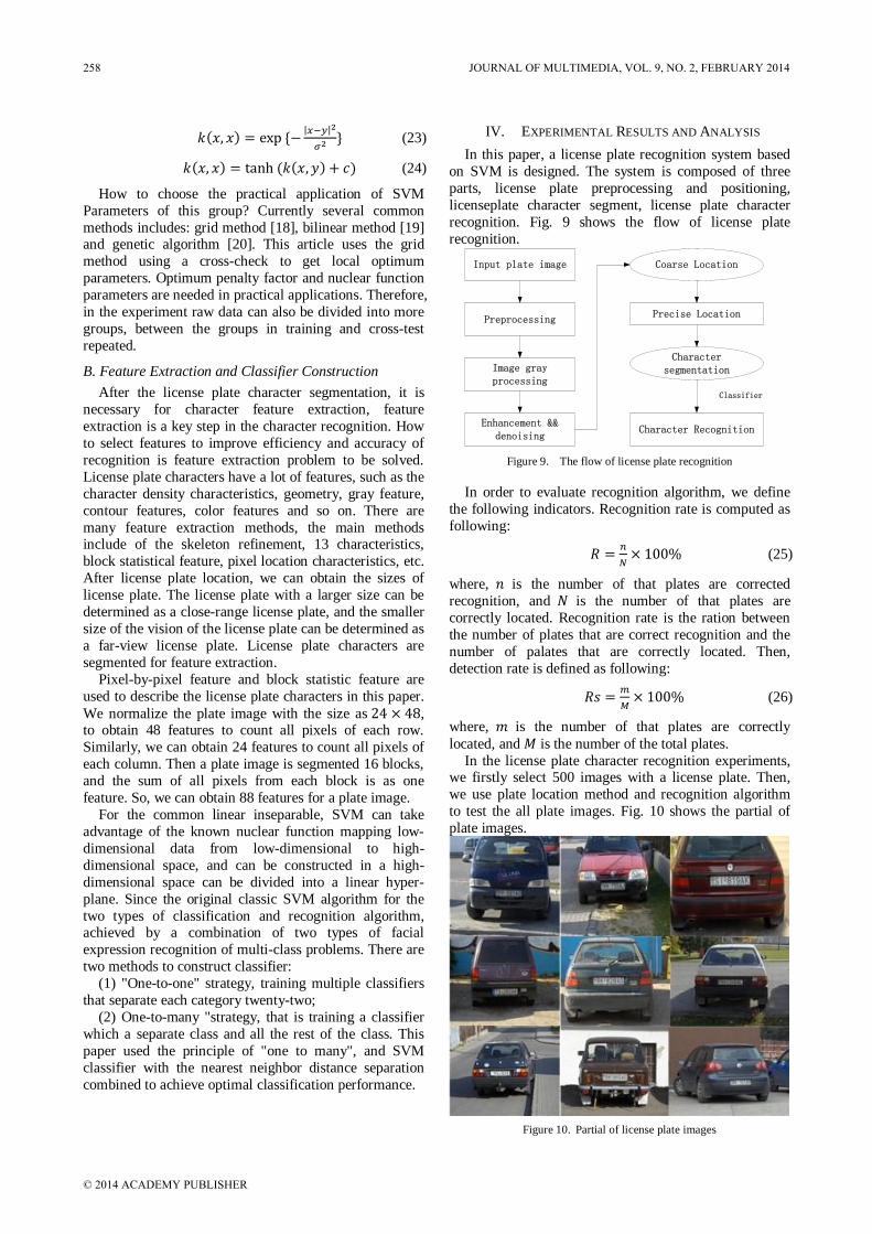
(23)

(24)

How to choose the practical application of SVM

Parameters of this group? Currently several common

methods includes: grid method [18], bilinear method [19] and genetic algorithm [20]. This article uses the grid

method using a cross-check to get local optimum

parameters. Optimum penalty factor and nuclear function

parameters are needed in practical applications. Therefore,

in the experiment raw data can also be divided into more

groups, between the groups in training and cross-test

repeated.

B. Feature Extraction and Classifier Construction

After the license plate character segmentation, it is

necessary for character feature extraction, feature

extraction is a key step in the character recognition. How

to select features to improve efficiency and accuracy of

recognition is feature extraction problem to be solved.

License plate characters have a lot of features, such as the

character density characteristics, geometry, gray feature,

contour features, color features and so on. There are

many feature extraction methods, the main methods include of the skeleton refinement, 13 characteristics,

block statistical feature, pixel location characteristics, etc.

After license plate location, we can obtain the sizes of

license plate. The license plate with a larger size can be

determined as a close-range license plate, and the smaller

size of the vision of the license plate can be determined as

a far-view license plate. License plate characters are

segmented for feature extraction.

Pixel-by-pixel feature and block statistic feature are

used to describe the license plate characters in this paper.

We normalize the plate image with the size as , to obtain 48 features to count all pixels of each row.

Similarly, we can obtain 24 features to count all pixels of

each column. Then a plate image is segmented 16 blocks,

and the sum of all pixels from each block is as one

feature. So, we can obtain 88 features for a plate image.

For the common linear inseparable, SVM can take

advantage of the known nuclear function mapping low-

dimensional data from low-dimensional to high-

dimensional space, and can be constructed in a high-

dimensional space can be divided into a linear hyper-

plane. Since the original classic SVM algorithm for the

two types of classification and recognition algorithm, achieved by a combination of two types of facial

expression recognition of multi-class problems. There are

two methods to construct classifier:

(1) "One-to-one" strategy, training multiple classifiers

that separate each category twenty-two;

(2) One-to-many "strategy, that is training a classifier

which a separate class and all the rest of the class. This

paper used the principle of "one to many", and SVM

classifier with the nearest neighbor distance separation

combined to achieve optimal classification performance.

IV. EXPERIMENTAL RESULTS AND ANALYSIS

In this paper, a license plate recognition system based

on SVM is designed. The system is composed of three

parts, license plate preprocessing and positioning,

licenseplate character segment, license plate character

recognition. Fig. 9 shows the flow of license plate

recognition.

Input plate image

Preprocessing

Image gray processing

Enhancement && denoising

Coarse Location

Precise Location

Character segmentation

Character Recognition

Classifier

Figure 9. The flow of license plate recognition

In order to evaluate recognition algorithm, we define

the following indicators. Recognition rate is computed as

following:

(25)

where, is the number of that plates are corrected

recognition, and is the number of that plates are

correctly located. Recognition rate is the ration between

the number of plates that are correct recognition and the

number of palates that are correctly located. Then,

detection rate is defined as following:

(26)

where, is the number of that plates are correctly

located, and is the number of the total plates.

In the license plate character recognition experiments, we firstly select 500 images with a license plate. Then,

we use plate location method and recognition algorithm

to test the all plate images. Fig. 10 shows the partial of

plate images.

Figure 10. Partial of license plate images



Figure 11. Results of license plate location and detection

Fig. 11 shows results of license plate location and

detection. From these experimental results, we can see

that our method can accurately locate and detect license

plate from plate images. Fig. 12 shows results of plate

detection on different angles. The plates are detected and corrected with Houghtransform which can detect the tilt

angle of the plate. From these experimental results, we

can see that our method can locate plate on different

angles. Especially, our method stilly locate plate when

big angles.

Figure 12. Plate detection results on different angles

From Table 1 and Table 2, we can see that the detection rate is 95.4% and recognition rate is 92.2%.

Correct rate reflects the effectiveness of recognition

algorithm, and detection rate reflects the effectiveness of

location algorithm. From experimental results, we can

also see that there are some errors in our experiments, as

there is 7.8% wrong rate in plate recognition. Because the

license plate image is sensitive to lighting, angle,

occlusion and other effects, the detection rate and

recognition rate will sharply reduce. Therefore, some

preprocessing for plate image is necessary to reduce these

factors, thus to improve detection rate and license plate

recognition rate in future.

TABLE I. LICENSE PLATE RECOGNITION RESULTS

Different operating The number of plates

Correctly locate license plate 477

Wrongly locate license plate 30

Correctly identify license plate 461

Wrongly identify license plate 60

TABLE II. CORRECT RATE AND WRONG RATE

Correct rate Wrong rate

Recognition rate 92.2% 7.8%

Detection rate 95.4% 4.6%

V. CONCLUSIONS

SVM as an important theory of machine learning and

pattern recognition has been well applied to small sample

clustering learning, nonlinear problems, outlier detection

and so on. The License Plate Automation Recognition

System has received extensive attention as an important

application of Machine Learning and Pattern Recognition in Intelligent Transport. Therefore, it is theoretically and

practically significant to research the license plate

character recognition technology based on SVM. The

plate recognition system is composed of three parts,

license plate preprocessing and positioning, license plate

character segment, license plate character recognition. In

this paper, we mainly introduce the flow of license plate

recognition, related technology and SVM theory.

Experimental results show the effectiveness of license

plate recognition using SVM

REFERENCES

[1] Broumandnia A, Fathy M, “Application of pattern

recognition for Farsi license plate recognition”, ICGST International Journal on Graphics, Vision and Image Processing, vol. 5, no. 2, pp. 25-31, 2005.

[2] Chang S L, Chen L S, Chung Y C, et al, “Automatic license plate recognition”, Intelligent Transportation Systems, IEEE Transactions on, vol. 5, no. 1, pp. 42-53, 2004.

[3] Yu M, Kim Y D, “An approach to Korean license plate

recognition based on vertical edge matching”, Systems, Man, and Cybernetics, IEEE International Conference on. IEEE, vol. 4, pp. 2975-2980, 2000.

[4] Hegt H A, De La Haye R J, Khan N A, “A high performance license plate recognition system”, Systems, Man, and Cybernetics, 1998 IEEE International Conference on. IEEE, pp. 4357-4362, 1998.

[5] Yan D, Hongqing M, Jilin L, et al. , “A high performance

license plate recognition system based on the web technique”, 2001 Proceedings of Intelligent Transportation Systems, pp. 325-329, 2001.

[6] Ren X, Jiang H, Wu Y, et al. , “The Internet of things in the license plate recognition technology application and design “, Business Computing and Global Informatization (BCGIN), 2012 Second International Conference on. IEEE, pp. 969-972, 2012.



[7] Chang C J, Chen L T, Kuo J W, et al. , “Applying Artificial Coordinates Auxiliary Techniques and License

Plate Recognition System for Automatic Vehicle License Plate Identification in Taiwan”, World Academy of Science, Engineering and Technology, pp. 1121-1126, 2010.

[8] Robert K, “Video-based traffic monitoring at day and night vehicle features detection tracking”, Intelligent Transportation Systems, ITSC'09. 12th International IEEE Conference on. IEEE, pp. 1-6, 2009.

[9] Comelli P, Ferragina P, Granieri M N, et al. “Optical

recognition of motor vehicle license plates”, Vehicular Technology, IEEE Transactions on, vol. 44, no. 4, pp. 790-799, 1995.

[10] Sirithinaphong T, Chamnongthai K, “The recognition of car license plate for automatic parking system”, Signal Processing and Its Applications, 1999. ISSPA'99. Proceedings of the Fifth International Symposium on. IEEE, pp. 455-457, 1999.

[11] Kim K K, Kim K I, Kim J B, et al, “Learning-based approach for license plate recognition”, Proceedings of the 2000 IEEE Signal Processing Society Workshop, pp. 614-623, 2000.

[12] Wei D, “Application of License Plate Recognition Based on Improved Neural Network”, Computer Simulation, vol. 28, no. 8, pp. 2011.

[13] Maini R, Aggarwal H, “Study and comparison of various image edge detection techniques”, International Journal of

Image Processing (IJIP), vol. 3, no. 1, pp. 1-11, 2009. [14] Vincent O R, Folorunso O, “A descriptive algorithm for

sobel image edge detection”, Proceedings of Informing Science & IT Education Conference (InSITE), pp. 97-107, 2009.

[15] Sen A. Implementation of Sobel and Prewitt Edge Detection Algorithm, 2012.

[16] Wang B, Fan S S, “An improved CANNY edge detection

algorithm”, 2009. WCSE'09. Second International Workshop on. IEEE, pp. 497-500, 2009.

[17] Vapnik V, “The Nature of 6tatistical Learning Theory”, Data Mining and Knowledge Discovery, vol. 6, pp. 1-47, 2000.

[18] Osuna E, Freund R, Girosit F, “Training support vector machines: an application to face detection”, Proceedings 1997 IEEE Computer Society Conference on, pp. 130-136,

1997. [19] Kao W C, Chung K M, Sun C L, et al. “Decomposition

methods for linear support vector machines”, Neural Computation, vol. 16, no. 8, pp. 1689-1704, 2004.

[20] Hsu C W, Lin C J, “A comparison of methods for multiclass support vector machines”, Neural Networks, IEEE Transactions on, vol. 13, no. 2, pp. 415-425, 2002.



Adaptive Super-Resolution Image Reconstruction

Algorithm of Neighborhood Embedding Based on

Nonlocal Similarity

Junfang Tang

Institute of Information Technology, Zhejiang Shuren University, Hangzhou 310015, Zhejiang, China


Xiandan Xu New Century Design& Construction (NCDC Inc.), New York 10013, USA


Abstract—Super resolution technology origins from the field

of image restoration. The increasing difficulties in the

resolution improvement by hardware prompts the super

resolution reconstruction that can solve this problem

effectively, but the general algorithms of super resolution

reconstruction model are unable to quickly complete the

image processing. Based on this problem, this paper studies

on adaptive super-resolution reconstruction algorithm of

neighbor embedding based on nonlocal similarity, in the

foundation of traditional neighborhood embedding super

resolution reconstruction method, using nonlocal similarity

clustering algorithm, classifying the image training sets,

which reduces the matching search complexity and speeds

up the algorithm; by introducing new characteristic

quantity and building a new calculation formula for solving

weights, the quality of reconstruction is enhanced. The

simulation test shows that the algorithm proposed in this

paper is superior to the traditional regularization method

and the spline interpolation algorithm no matter on the

objective index about statistic and structural features or

subjective evaluation.

Index Terms—Neighborhood Embedding; Super Resolution;

Image Restoration

I. INTRODUCTION

Super-resolution reconstruction refers to the

technology that constructs high-resolution images from

low-resolution ones [1]. It was first proposed with the

concept and method of the single frame image

reconstruction, which mainly resorts to resampling and

interpolation algorithm. However, these methods will

usually lead to some smoothing effects, and as a result,

the image edge details cannot be reconstructed very well.

And multi-frame image reconstruction can just solve this

problem [2]. This technology enhances the image

resolution by making full use of the different information

offered by low-resolution images of different frames.

Image resolution is an important index of image detail

appearance ability which describes the pixels image

contains, and put another way, is a measure of the amount

of image information [3]. In many cases, however, due to

the limit of hardware device in imaging system (such as

imaging sensor), people cannot observe image of high

resolution. It costs too much updating the hardware to

improve image resolution, and in the short term it is

difficult to overcome the technical problems of some

specific imaging system. The super resolution image

reconstruction instead utilizes the software on the premise

of existing hardware device to improve the resolution,

which is applicable in many fields [4].

Super-resolution reconstruction was first proposed in

the 1960s. In the following decades, many scholars still

haven’t got its ideal effects in the practical applications

although they studied a lot. At that time, it had been

called the “myth of super-resolution” for the super-

resolution was considered impossible with the effects of

noise. There has not been any breakthrough until the end

of 1980s with the efforts of Hunt, etc. In the 1980s,

researchers in the field of computer vision began to study

SR reconstruction technique [5]. Tsai and Huang first

proposed a multi-image SR reconstruction algorithm

based on Fourier domain [6]. Then, researchers improved

this algorithm to extend the application range. However,

this kind of SR algorithm is applicable only to the

degradation model of the global translational motion and

constant linear space. SR reconstruction gradually made

progress since 1990s. In 1995, Hunt firstly explained

from the theory the possibility of super resolution

reconstruction [7]. At the same time, researchers also

proposed some classical SR algorithms, for example,

iterative back projection method (IBP) [8], projection

onto convex sets (POCS) [9], the maximum likelihood

estimation method (ML) [10], maximum a posteriori

estimation method (MAP) and the hybrid

ML/MAP/POCS method [11]. In the late 1990s, SR

reconstruction became a hot international topic deriving a

variety of SR reconstruction algorithms. In 2004, Chang

[12] introduced the idea of Neighbor Embedding in

manifold learning into super-resolution reconstruction,

assuming that the low resolution image block and high

resolution image block have similar local manifold



structure, getting the training sets of low resolution image

and high resolution image block through the image

training, then searching the K neighbor blocks in the

training set of low resolution image blocks to be

reconstructed and solving their neighbor coefficients, and

with the linear combination of the coefficient and K

corresponding high resolution neighbor blocks of high

resolution training set to obtain the high resolution image

block after matching reconstruction. The advantage of

this method is that the number of training sets is small

and the reconstruction time is relatively short, but the

reconstruction exists the over-fitting and under-fitting

phenomenon. In 2008, the compressed sensing [13] was

introduced into the super-resolution reconstruction, and

Yang et al. [14] used the linear programming and low

resolution dictionary to solve the sparse representation of

low resolution image block to be reconstructed, using

sparse representation coefficients and the corresponding

high resolution image block to finishing image

reconstruction. This algorithm was advantageous in its no

need to set the block number of a low resolution image

for the sparse representation, but the construction of the

dictionary is random and unpopular.

Super-resolution reconstruction algorithm can be

divided into two kinds, the way based on reconstruction

and based on study. Most super-resolution reconstruction

algorithms can be classified into the way based on

reconstruction according to the existing documents. It

also can be divided into frequency domain method and

spatial domain methods according to the reconstructed

super-resolution reconstruction algorithm. Frequency

domain methods improve the quality of images by

eliminating the frequency aliasing in the frequency

domain. Tsai and Huang proposed the image

reconstruction methods based on approaching frequency

domain according to the shifting properties of Fourier

transform. Kim and others extended Tsai and Huang’s

ideas and proposed the theory based on WRLS. In

addition, Rhee and Kang adopted DCT (Discrete Cosine

Transform) instead of DFT (Discrete Fourier Transform)

in order to decrease the operand and increase the

efficiency of algorithm. Also, they overcome the lack of

frames by LR sampling and the ill-conditioned

reconstruction of unknown sub-pixel motion information

by regularization parameter. The frequency domain

methods were with comparatively easy theories and low

computation complexity. However, this kind of methods

could only handle some conditions of global motion.

What’s more, the loss of data’s dependency in the

frequency domain made the application of prior

information in regularization ill-conditioned problem

difficult. So the recent studies are most in the spatial

domain methods. This essay lucubrated the relative

problems from the aspect of super-resolution methods,

proposing an algorithm to super-resolution reconstruct

images by non-local similarity, and improved algorithm

to present the high-speed algorithm. This essay presented

that the image super-resolution reconstruction algorithm

of non-local similarity could eliminate the man-made

effects such as marginal sawtooth in reconstructed image

by studying the super-solution image reconstruction

methods and analyzing its key problems. Intensify the

real margin by bilateral filter. And it could learn from the

low-resolution image by the non-local similarity of

natural image and guide to reconstruct image with the

relationship between similar structural pixels.

This paper proposes a neighbor embedding adaptive

super-resolution reconstruction algorithm based on

nonlocal similarity, using the K-means clustering

algorithm to classify the image training sets, which

reduces the calculation of search matching, speeds up the

algorithm, and then improves reconstruction quality by

introducing new features and new formula to solve the

weight. The simulation test shows that, compared to the

traditional regularization method and the spline

interpolation algorithm, the model proposed in this paper

is better in both the objective index of the statistic and

structure features and in subjective evaluation.

The basic idea of super resolution is the combination

of fuzzy image sequences of low resolution and noise to

produce an image or image sequence of high resolution

[15]. Most of the super-resolution image reconstruction

methods have three compositions, as shown in Figure 1:

motion compensation, including motion estimation and

image registration, interpolation and blur and noise

reduction [16]. These steps can be realized separately or

simultaneously according to the reconstruction methods.

SR reconstruction method based on frequency domain

contains only two links: the motion estimation and

interpolation, during which to solve the equations of

displacement in the frequency domain is equivalent to the

interpolation process. Spatial domain SR reconstruction

method contains these three links, and most of the spatial

domain methods, such as IBP, POCS, MAP and adaptive

filtering method, integrates the interpolation and blur and

noise reduction into a process. Some other spatial domain

methods synthesize the motion estimation, interpolation

and blur and noise reduction to only one step.

Figure 1. Super-resolution scheme

II. SUPER-RESOLUTION IMAGE RECONSTRUCTION

ALGORITHM

A. Frequency Domain

Frequency domain methods utilize the aliasing existing

in each low resolution image to reconstruct a high



resolution image [17]. Tsai and Huang firstly derived a

systematic equation between a low resolution image and

a super resolution image expected by using the relative

movement between the low resolution images [18]. It is

based on three principles:

The displacement properties of Fourier transform;

The aliasing relationship between Continuous Fourier

transform (CFT) of the original high resolution image and

the discrete Fourier transform (DFT) of low resolution

observation image;

Original super resolution image is supposed to be

band-limited.

These properties make possible the formalism of

systematic equation which links the DFT coefficient of an

aliasing low resolution image with a CFT sample of

unknown image.

Suppose 1 2( , )f t t represents the continuous super

resolution image, and 1 2( , )F w w is the continuous

Fourier transform. The k th displacement image

1 2 1 1 2 2( , ) (( , )k k kf t t f t t after global translation

which is the only motion in frequency method, where 1k

and 2k are known arbitrary values, 1,2,...,k p . Then,

the CFT 1 2( , )kF w w of displacement image is noted by

these properties as:

1 2 1 1 2 2 1 2( , ) exp 2 ( ) ( , )k k kF w w j w w F w w (1)

This expression indicates the relationship between

CFT of displacement image and CFT of reference image.

Low resolution observation image 1 2( , )kg n n is

generated by taking samples to the displacement image

1 2( , )kf t t with sampling period 1T and

2T . From the

aliasing and band-limited assumption of 1 2( , )F w w ,

namely for 1 1 1( / )w L T 2 2 2( / )w L T , there

is 1 2( , )F w w , the relationship is noted between the CFT

of super resolution image and the DFT of the k th low

resolution image:

1 2

1 2

1 1

1 2

1 2 1 2

0 01 2 1 1 2 2

1 2 2( , ) ,

L L

k k

n n

G F n nTT T N T N

(2)

where 1 and

2 are the sampling points in discrete

Fourier transform domain of 1 2( , )kg n n , and

1 10 N ,

2 20 N .

Lexicographical Order is employed to the index 1 2,n n

on the right side of the equation and the k on the left side

to obtain a matrix vector form of (2):

G F (3)

Here, G is a 1p vector with elements of DFT

coefficient of 1 2( , )kg n n ; F is 1 2 1L L n vector with the

unknown samples as the elements through CFT of

1 2( , )x t t ; is 1 2p L L vector which links the DFT of

low resolution observation image with samples from

continuous super resolution image. Therefore, the

reconstruction of a super resolution image requires

definite to solve the inverse problem.

The simple theory is the main advantage of the

frequency domain method that the relationship of low

resolution image and super resolution image is explained

clear in the frequency domain. It is useful for the parallel

computing reducing the device complexity. But the

observation model is limited to the global translation

motion and the blur with constant linear space. In

addition, lack of data correlation in the frequency domain

makes difficult the application of prior knowledge about

spatial domain to regularization.

B. Regularized Super-Resolution Reconstruction Method

In the case of insufficient low resolution images and

non-ideal fuzzy operator, super resolution image

reconstruction methods usually tend to be ill-posed [19].

A method used for the stable inverse process of ill-posed

problem is known as regularization method. Following

we introduces the deterministic regularization and the

stochastic regularization method for super resolution

image reconstruction. Here highlights the constrained

least squares (CLS) and maximum a posteriori probability

(MAP) super-resolution image reconstruction method.

With the estimation of registration parameters, the

observation model in equation (2) can be determined

completely. Deterministic regularization super-resolution

method uses prior information about the solution to solve

the inverse problem in equation (2), which can make the

problem a well posed one.

CLS means choosing appropriate f to minimize the

Lagrange operator.

2 2

1

p

k k

k

g A f Cf

(4)

Here, operator C is usually a high-pass filter;

denotes the norm of 2L . In this equation, the prior

information of a reasonable solution is expressed by the

smooth constraint which means most of the images are

naturally smooth together with limited high frequency

motion. Therefore, the reconstruction image of the

minimum high-pass energy should be considered as the

solution of deterministic method. The Lagrange

multiplier , is usually called as regularization

parameter which controls the compromises of data

precision f and the smoothness of the solution 2

Cf .

More means more smooth solution. Larger is a

quite useful when there are few low resolution images or

the precision of observation data reduces because of the

registration error and noise while smaller is useful on

the opposite side. The cost function, a differential convex

function in (4) adopts a square regularized term in favor

of the global unique solution f . A basic deterministic

iteration method is to solve the following equation:

1 1

ˆp p

T T T

k k k k

k k

A A C C f A g

(5)



Method of steepest descent taken to it, the iteration to

f̂ should be,

1

1

ˆ ˆ ˆ ˆ( )p

n n T n T n

k k k

k

f f A g A f C Cf

(6)

where is the convergence parameter, and T

kA contains

the sampling operator and blur and deformation operator.

Katsaggelos et al proposed a multi-channel

regularization super-resolution method where the

regularization functional was used to calculate the

regularization parameter without any prior knowledge at

each iteration step. Kang described the generalized multi-

channel deconvolution method including multi-channel

regularization super-resolution method. Hardie et al

proposed a super-resolution reconstruction method

minimizing regularized cost functional, defining an

observation model of the optical system and detector

array (a kind of sensor point spread function). They used

an iterative registration algorithm based on gradient, and

took into consideration two optimization processes

minimizing the cost functional, the gradient descent and

conjugate gradient optimization process. Bose et al

pointed out the importance of regularization parameter,

and put forward a constrained least squares super

resolution reconstruction method which obtains optimal

parameter by using the L curve method.

C. Random Method

Random super resolution image reconstruction is a

typical Bayesian method which provides a convenient

tool for the prior knowledge model of solution.

Bayesian estimation usually makes effect when a

posterior probability density functional (PDF) of original

images can be constructed. MAP estimator of f

maximizes the PDF ( )kP f g .

1 2argmax ( , ,..., )P

f P f g g g (7)

Bayesian theorem and logarithmic function are used

for conditional probability to show the MAP optimization

problem.

1 2arg max ln ( , ,..., ) ln ( )pf P g g g f P f (8)

Prior image model ( )P f and conditional density

1 2( , ,..., )pP g g g f is determined by the prior knowledge

and noise statistic information of the high resolution

image f . Due to its prior constraints, this MAP

optimization method can effectively provide a regularized

super-resolution estimation. Bayesian estimation usually

takes Markov random field prior model, a strong method

for image prior model. ( )P f can be described by a

equivalent Gibbs prior model, with the probability

density defined as:

1 1

( ) exp ( ) exp ( )c

c S

P f U f fZ Z

(9)

Z is a regularized constant, ( )U f is the energy

function, ( )c f is a potential function depending on the

pixel in the clique, and S signifies the clique set. ( )U f

can measure the cost of the irregularity of solution

through defining ( )c f as the function of image

derivative. Usually the image is thought as global smooth

and be combined into the estimation by Gaussian prior

model.

The advantage of the Bayesian frame is that it can use

the prior model of constant edge. Potential function is

expressed in a quadric form ( ) 2( ) ( )n

c f D f with

Gaussian prior model, where ( )nD is n order difference.

Although quadric potential function can form the linear

algorithm in the process of the derivation, it severely

punishes the high-frequency components. Thus, the

solution is an over smooth solution. However, if the

potential function model is weak in the punishment on

large difference f , then an edge-preserving image will

be obtained with high resolution. If the inter-frame error

is independent, and noise is the independent and

identically distributed zero mean Gaussian noise, then the

optimization problem can be compactly represented as

1

ˆ ˆ ˆarg max ( )p

k k c

k c S

f g A f f

(10)

Here, is regularization parameter. If the Gaussian

prior model is adopted in (10), then the estimation

defined by (4) is MAP estimation.

Maximum likelihood (ML) estimation is also used for

super resolution reconstruction. ML estimation is a

special case of the MAP estimation in the absence of

prior set. However, for the ill posed condition of inverse

problem of super resolution, MAP estimation is usually

better than ML estimation.

The stability and flexibility of the model on the noise

characteristics and a priori knowledge is the main

advantage of random super resolution method. If the

noise process is white Gaussian model, MAP estimation

with a convex energy function can guarantee the

uniqueness of the solution in the prior model. Therefore,

gradient descent method is not only able to estimate high

resolution images, but also used to estimate the motion

information and high resolution image at the same time.

Generally speaking, all of three kinds of super

resolution image reconstruction algorithms listed above

are sensitive to high frequency information, which is not

conducive to the edge preserving etc.

III. NEIGHBORHOOD EMBEDDING SUPER-RESOLUTION

RECONSTRUCTION ALGORITHM BASED ON NONLOCAL

SIMILARITY

Local linear embedding is to solve the linear

expression in a higher dimensional space, and map it into

a low dimensional space while neighborhood embedding

is to solve the linear relation in low dimensional space

and then map it to a high dimensional space [20].

Therefore, neighborhood embedding can be regarded as



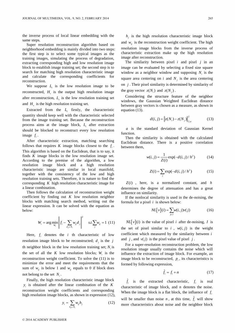
the inverse process of local linear embedding with the

same steps.

Super resolution reconstruction algorithm based on

neighborhood embedding is mainly divided into two steps:

the first step is to select some typical images as the

training images, simulating the process of degradation,

extracting corresponding high and low resolution image

block to establish image training set; the second step is to

search for matching high resolution characteristic image

and calculate the corresponding coefficients for

reconstruction.

We suppose tL is the low resolution image to be

reconstructed, tH is the output high resolution image

after reconstruction, sL is the low resolution training set

and sH is the high resolution training set.

Extracted from the tL firstly, the characteristic

quantity should keep well with the characteristic selected

from the image training set. Because the reconstruction

process aims at the image block, tL after extraction

should be blocked to reconstruct every low resolution

image if .

After characteristic extraction, matching searching

follows that requires K image blocks closest to the if .

This algorithm is based on the Euclidean, that is to say, it

finds K image blocks in the low resolution image set.

According to the premise of the algorithm, a low

resolution image block and a high resolution

characteristic image are similar in local manifold,

together with the consistency of the low and high

resolution training sets. Therefore, it is nature to find the

corresponding K high resolution characteristic image for

a linear combination.

Then follows the calculation of reconstruction weight

coefficient by finding out K low resolution neighbor

blocks with matching search method, writing out the

linear expression. It can be solved with the equation as

below:

2

arg min . . 1i

j i

i i ij j ijW

d N j

W f w d s t w

(11)

Here, if denotes the i th characteristic of low

resolution image block to be reconstructed; jd is the j

th neighbor block in the low resolution training set;iN is

the set of all the K low resolution blocks; iW is the

reconstruction weight coefficient. To solve the (11) is to

minimize the error and meet the requirements that the

sum of ijw is below 1 and ijw equals to 0 if block does

not belong to the set iN .

Finally, the high resolution characteristic image block

iy is obtained after the linear combination of the K

reconstruction weight coefficients and corresponding

high resolution image blocks, as shown in expression (12),

j i

i ij j

h N

y w h

(12)

jh is the high resolution characteristic image block

and ijw is the reconstruction weight coefficient. The high

resolution image blocks from the inverse process of

characteristic extraction make up the high resolution

image after reconstruction.

The similarity between pixel i and pixel j in an

image can be evaluated by selecting a fixed size square

window as a neighbor window and supposing iN is the

square area centering on i and jN is the area centering

on j . Their pixel similarity is determined by similarity of

the gray vector ( )iz N and ( )jz N .

Considering the structure feature of the neighbor

windows, the Gaussian Weighted Euclidean distance

between gray vectors is chosen as a measure, as shown in

equation (13).

2

2,( , ) ( ) ( )i j a

d i j z N z N (13)

a is the standard deviation of Gaussian Kernel

function.

Then the similarity is obtained with the calculated

Euclidean distance. There is a positive correlation

between them,

21( , ) exp( ( , ) / )

( )w i j d i j h

Z i (14)

2( ) exp( ( , ) / )j

Z i d i j h (15)

( )Z i , here, is a normalized constant, and h

determines the degree of attenuation and has a great

influence on similarity.

If the nonlocal similarity is used in the de-noising, the

formula for a pixel i is shown below:

( ) ( , ) ( )j I

NL v i w i j v j

(16)

( )NL v i is the value of pixel i after de-noising, I is

the set of pixel similar to i , ( , )w i j is the weight

coefficient which measured by the similarity between i

and j , and ( )v j is the pixel value of pixel j .

For a super-resolution reconstruction problem, the low

resolution image usually contains the noise which will

influence the extraction of image block. For example, an

image block to be reconstructed, ip , its characteristics is

formed by following expression,

î if f n (17)

îf is the extracted characteristic, if is real

characteristic of image block, and n denotes the noise.

When the image block is a flat block, the influence of if

will be smaller than noise n , at this time, îf will show

more characteristics about noise and the neighbor block



will be inaccurate. In order to remove the noise effect, we

refer to the de-noising method of nonlocal mean filtering,

through finding out the similar blocks and calculating

their weight, then combining them to search for K

neighbor block.

Firstly, similar block to be reconstructed should be

searched out with low resolution, as shown in figure 2.

Supposing the block as 1p with size 3×3, a 7×7 matching

block im is built centering on it with which similar

blocks are searched in a 21×21 searching window.

Nonlocal mean de-noising algorithm uses Euclidean

distance as a measure, different with the algorithm in this

paper that sets the sum of absolute deviation (SAD) value

as the measure between searching block and matching

block. Taking two 7×7 blocks with the minimum SAD,

recorded as SAD1 and SAD2, their corresponding center

place, two 3×3 small blocks 2p and

3p , then the weight

effect of the similar block can be solved by following

equation:

2

1

1

2

3

1

SAD

h

SAD

h

m

m e

m e

(18)

In this expression, parameter h controls the degree of

attenuation of the exponential function determined by the

searching window. Doing normalization to (18), we get

the weight coefficient:

1

1

1 2 3

2

2

1 2 3

3

3

1 2 3

m

m m m

m

m m m

m

m m m

(19)

where 1 ,

2 and 3 are the weight coefficients of the

similar blocks 1p 2p and

3p , respectively.

Figure 2. Non-local similarity search.

Then the characteristics 1f 2f and 3f are obtained

through the extraction of the similar block of low

resolution image block. Together with the weight

coefficients and Euclidean distance, K neighboring

blocks are searched out with the expression,

2 2 2

1 1 2 2 3 32 2 2min( )j j j

j Nf l f l f l

(20)

N is the low resolution characteristic image block

training set.

Through the introduction of nonlocal similarity

constraint, a joint search involving the search of similar

blocks and calculation of the weighted coefficient helps

find k neighborhood blocks in the low resolution training

set, effectively restraining the effect of noise on image

block.

In addition, this algorithm applying the nonlocal

similarity for image restoration in a sparse model presents

the same dictionary elements in a similar block in the

sparse decomposition, which can be used to solve the

joint sparse representation coefficients. According to this

theory, in this algorithm, the training set is similar to a

dictionary, and similar blocks benefit finding out the

exact K nearest neighbor coefficient. The weight

coefficient calculation formula is updated with the similar

block weights.

23

1

arg min . . 1j

k k j j jW

k d M j

W f w d s t w

(21)

1 , 2 and

3 is from the (19), M is the set of

K neighborhood blocks searched out by (20), w is the

reconstruction weight coefficient. The solution of (21)

makes the minimum error and meet the requirements that

the sum of jw is 1 and the jw of the block out of the set

M is zero.

Similar blocks have similar neighbor structures in the

training set. By introducing the constraint effect of

similar block, it is useful to estimate the neighbor

structure and calculate accurate weight coefficient.

IV. SIMULATION EXPERIMENT

In order to test the proposed non-local similarity

neighborhood embedded self-adaptive super-resolution

reconstruction algorithm model, the following two

experiments were carried out on it. The first experiment

tested its PSNR and image structure similarity. The

second experiment compared PSRN and run time on the

platform of Matlab. The analysis and comparison of the

two experiments tested the functionality of the non-local

similarity neighborhood embedded self-adaptive super-

resolution reconstruction algorithm model in detail

proposed in this essay.

Experiment 1: The Number image with size 256x256

and Lena image are selected as the original high-

resolution image. Then a sequence of low solution images,

totally 15, are generated after translation with the shift

range between 0-3 pixels, fuzzy with a Gauss operator in

a 3x3 window, and down sampling whose factor is 2.

Gauss noise with different noise variances are added into

low resolution image sequence to get the required data.

Compared with the spline interpolation method and the



traditional regularization methods, this algorithm adopts

the peak signal to noise ratio and structure similarity to

measure the quality of image reconstruction.

From Figure 3 and Figure 4, it is obvious that the

algorithm this paper proposed has great improvement

compared with the regularization method and the spline

interpolation algorithm PSNR, an average improvement

of 0.5dB. This is because the algorithm takes into account

the local information of image, reducing the error

introduced by the regularization. It also can be seen from

(b), (d) that the algorithm has larger improvement in

SSIM, and for Number images, along with the change of

noise variance, corresponding curve of spline

interpolation algorithm and the traditional regularization

methods declines similar to the negative exponential

curve while that of this algorithm similar to the line.

Therefore, in a certain range, this algorithm is superior

obviously.

Figure 3. Image PSNR curve

Figure 4. Image structure similarity curve

From figure 3 and 4, this algorithm proposed is

superior no matter on the objective index about statistic

and structural features or subjective evaluation.

Experiment 2: The following experiments are carried

out on the Matlab platform. The simulation experiment is

to degrade the test image (Fig. 5) to get low resolution

image, and then to reconstruct it to get the reconstructed

high resolution image. The degradation process from high

resolution to low resolution images involve the Gauss

filtering to original image with Gauss filtering window

size 5 x 5 and the variance 1, and down sampling of the

image low-pass filtered with the sampling factor 2. The

bilateral filtering includes these parameters: filtering

window size 7 x 7; the variance of spatial distance

function 10( )c domain filtering ; the variance of pixel

similarity function 30( )s range filtering . The

parameters of nonlocal similarity are matching window

size 5 x 5, the search window size 9 x 9, and the number

of similar structure pixels 7.

Table I is the objective evaluation of PSNR

experiments. From the results, the former two methods

show barely difference in PSNR, but PSNR difference of

the method in this paper is relatively large, ranging from

0.3 to 0.5dB. This is because this algorithm will lose

basic image information during the degradation of image

block data, this algorithm is to reduce the dimensionality

of high-dimensional data, which means our algorithm

transforms the high dimension data into low dimensional

data space in the loss of a small amount of information,

and thus decreases the objective measurement of PSNR.

TABLE I. PSNR (DB) RESULTS

LR image Cman Bike Foreman House

Original algorithm 26.36 26.92 32.47 24.95

Edge detection algorithm 26.36 29.86 32.45 24.88

Algorithm 25.64 26.32 31.88 24.26

TABLE II. RUN TIME (S) RESULTS

LR image Cman (128×128)

Bike (256×174)

Foreman (176×144)

House (256×256)

Original

algorithm 19.5 58.4 29.7 77.0

Edge detection

algorithm

7.2 21.1 10.9 28.2

Algorithm 1.5 7.7 2.4 9.9

Table II shows the operation time of three kinds of

methods. It can be seen that the running time of the

method of adding the pixel classification is about one

fifth of that of the original algorithm. The running time of

different images by adding different image edge detection

method is different for the edge detection is in a positive

relationship with the image content. The more textured

edges the image has, the more time the image processing

consumes. Our algorithm incorporating the degradation

and edge detection runs the fastest because it greatly

reduces the dimensions, dealing with from 49

dimensional data to 16 dimensions data.

It could be seen that the PSNR of the non-local

similarity neighborhood embedded self-adaptive super-

resolution reconstruction algorithm model proposed by

this essay had more improvement as the change of noise

variance than that of the traditional regularization method

and the spline interpolation. The corresponding curve of

interpolation algorithm and traditional regularization

method which was similar to the negative exponent

decreased. However, the algorithm corresponding curve

in this essay was similar to straight-line decline, so in a

certain range, the advantage of the algorithm in this essay

was more obvious and the run speed of dimensionality

reduction with detection processed method was the fastest.



V. CONCLUSION

Digital image is the foundation of image processing

and the spatial resolution of digital imaging sensor is an

important factor to image quality. With the progress of

information and the popularization of image processing,

scientific research and practical application demands high

on the quality of digital images, and thus poses a new

challenge to the manufacturing technology of the image

sensor. We can try a scheme of hardware to improve the

spatial resolution of the image, such as reducing the pixel

size or expanding photoreceptor chip to increase the

number of pixels of unit area, but reducing the pixel size

and increasing the size sensor chip exist technical

difficulties, and the expensive high precision sensor is not

suitable for popularization and application. Therefore,

super resolution reconstruction technique employing

signal processing method improves the image resolution

of existing low resolution imaging system, which attracts

great attention and in-depth study globally and has

important theoretical significance and application value.

REFERENCE

[1] SU Bing hua, JIN Wei qi, NIU Li hong, LIU Guang rong,

“Super resolution image restoration and progess”, Optical

Technology, vol. 27, no. 1, pp. 6-9, 2001.

[2] PARK S C, PARK M K, KANG M G, “Super-resolution

image reconstruction: a technical overv iew”, IEEE Signal

Processing Magazine, vol. 20, no. 3, pp. 21-36, 2003.

[3] WANG Liang, LIU Rong, ZHANG Li, “The

Meteorological Satellite Spectral Image Registration Based

on Fourier-Mellin Transform”, Spectroscopy and Spectral

Analysis, no. 3, pp. 855-858, 2013.

[4] GUO Tong, LAN Ju-long, HUANG Wan-wei, ZHANG

Zhen, “Analysis the self-similarity of network traffic in

fractional Fourier transform domain”, Journal on

Communications, vol. 34, no. 6, pp. 38-48, 2013.

[5] CHEN Huahua, JIANG Baolin, LIU Chao, “Image super-

resolution reconstruction based on residual error”, Journal

of Image and Graphics, vol. 16, no. 1, pp. 42-48, 2013.

[6] BAI Li ping, LI Qing hui, WANG Bing jian, ZHOU Hui

xin, “High Resolution Infraed Image Reconstruction Based

on Image Sequence”, Infrared Technology, vol. 24, no. 6,

pp. 58-61, 2002.

[7] ZENG Qiangyu, HE Xiaohai, CHEN Weilong,

“Compressed video super-resolution reconstruction based

on regularization and projection to convex set”, Computer

Engineering and Applications, vol. 48, no. 6, pp. 181-184,

2012.

[8] JIANG Yu-zhong, YING Wen-wei, LIU Yue-liang, “Fast

Maximum Likelihood Estimation of Class A Model”,

Journal of Applied Sciences, vol. 32, no. 2, pp. 165-169,

2013.

[9] XU Zhong-qiang, ZHU Xiu-chang, “Super-resolution

Reconstruction Technology for Compressed Video”,

Journal of Electronics & Information Technology, vol. 29,

no. 2, pp. 499-505, 2007.

[10] SU Heng, ZHOU Jie, ZHANG Zhi-Hao, “Survey of Super-

resolution Image Reconstruction Methods”, Acta

Automatica Sinica, vol. 39, no. 8, pp. 1202-1213, 2013.

[11] CHANGH, YEU NGDY, XIONGYM. “Super-resolution

th rough neighbor embedding”, Proceedings of the IEEE C

o mputer So ciety Conferenceon Computer Vision and

Patte rn Recognition, 2004, pp. 275-282.

[12] CANDES E J. “Compressive sampling” Proceedings of the

International Congress of Mathematicians, 2006, pp. 143-

145.

[13] CANDES E J, WAKIN M B, “An introduction to

compress ive sampling”. IEEE Signal Processing

Magazine, 2008, pp. 21-30.

[14] WRIGHT J, HUANG T, MA Y. Image super-resolution as

s parse representation of raw in IEEE Conference on

Computer Vision and Pattern Recognition, 2008, pp. 1-8.

[15] YANG J C, WRIGHT J, HUANG T, etal. Image super- re

solution via sparse representation on Image Processing,

2010, pp. 2861- 2873.

[16] XIE Kai, ZHANG Fen, “Efficient super resolution image

reconstruction parameter estimation algorithm”, Journal of

Chinese Computer Systems, 2013, pp. 2201-2204.

[17] YING Li-li, AN Bo-wen, XUE Bing-bin, “Research on

Super-resolution Reconstruction of Sub-pixel Images”,

Infrared Technology, 2013, pp. 274-278

[18] Zhang Yilun, Gan Zongliang, Zhu Xiuchang, “Video

super-resolution method based on similarity constraints”,

Journal of Image and Graphics, 2013, pp. 761-767.

[19] CAO Ming-ming, GAN Zong-liang, ZHU Xiu-chang, “An

Improved Super-resolution Reconstruction Algorithm with

Locally Linear Embedding”, Journal of Nanjing University

of Posts and Telecommunications (Natural Science), 2013,

pp. 10-15.

[20] JIANG Jing, ZHANG Xue-song, “A Review of Super-

resolution Reconstruction Algorithms”, Infrared

Technology, 2012, pp. 24-30.

Junfang Tang, born January 1977 in

Shangyu City, Zhejiang Province, China,

majored in management information

system during her undergraduate study in

Shanghai University of Finance and

Economics and got a master degree of

software engineering in Hangzhou Dianzi

University. She focuses her research

mainly on computer graphics and image

processing and has published several professional papers on the

international journals and been in charge of several projects,

from either the Zhejiang Province or Zhejiang provincial

education department.



An Image Classification Algorithm Based on Bag

of Visual Words and Multi-kernel Learning

LOU Xiong-wei 1, 3

, HUANG De-cai 2, FAN Lu-ming

3, and XU Ai-jun

3

1. College of Information Engineering, Zhejiang University of Technology, Hangzhou, Zhejiang, 310032, China 2. School of Computer Science & Technology, Zhejiang University of Technology, Hangzhou, Zhejiang, 310032,

China

3. College of Information Engineering, Zhejiang A & F University, Linan, Zhejiang, 311300, China

Abstract—In this article, we propose an image classification

algorithm based on Bag of Visual Words model and multi-

kernel learning. First of all, we extract the D-SIFT (Dense

Scale-invariant Feature Transform) features from images in

the training set. And then construct visual vocabulary via

K-means clustering. The local features of original images

are mapped to vectors of fixed length through visual

vocabulary and spatial pyramid model. At last, the final

classification results are given by generalized multiple

kernel proposed by this paper. The experiments are

performed on Caltech-101 image dataset and the results

show the accuracy and effectiveness of the algorithm.

Index Terms—BOVW; Image Classification; Spatial

Pyramid Matching; Kernel

I. INTRODUCTION

The image is always an important approach to convey

information and has penetrated into all aspects of our life.

In particular, with the development of the Internet and

multi-media technology nowadays, the digital image has

become an import media for modern information, and its

increasing rate makes traditional management method of

manual labeling more and more infeasible [1]. Thus, many researchers have started to work on automatic

image classification by computers to sort images into

different semantic classes according to people’s

comprehension. Problems in image classification,

including scene detection, object detection and so on, are

hot and difficult issues in modern computer vision and

multi-media information. Due to the wide application of

images and videos, we are in bad need of excellent and accurate image comprehension algorithms to address

problems in image classification. Computer vision aimed

at image comprehension emphasizes on the function of

computers to visually comprehend images. Vision is an

essential approach for human to observe and cognize the

world. According to statistics, a big portion of

information people obtained from the outside world stem

from the visual system. Narrowly speaking, the final target of vision is to reasonably explain and describe the

image to the observant. Generally speaking, vision even

includes action plan according to the explanation,

description, environment and the will of the observant.

Therefore, computer vision aimed at image

comprehension is the realization of human vision via

computers, and it is an important step for artificial

intelligence to accurately comprehend the world, which

can percept, cognize and comprehend the 2D scenes of

the world. For the time being, this research area mainly focuses

on object detection, object description and scene

comprehension. Therein, object detection serves for

accurate description of scene and is the basis of scene

description and comprehension. In turn, scene description

and comprehension provide priory knowledge for object

detection and guide the process by giving background

knowledge and context information. In the light of computers, image comprehension is to input the image

(mainly digital image) from vision via a series of

computational analysis and perceptive learning, which

outputs the detected objects in the scene and their

relations, while the overall description and

comprehension of the scene as well as the comprehensive

image semantic description. All in all, image content

detection and classification not only include the overall knowledge of an image, but also provide the context

under which the objects appear on it and thus lay the

foundation of further comprehension, which is widely

applicable to many aspects. When application is

considered, image classification techniques are nowadays

potentially applicable to a variety of areas, such as image

and video retrieval, computer vision and so on.

Image retrieval [2] based on content is the simplest and most direct application of object detection which can

provide effective aids and evidence for image information

retrieval and procession. With the popularization of

electronic digital cameras, the number of digital images

are increasing astonishingly and comprehension based on

objects is helpful to efficiently organize and browse

database, so the result of object detection is valuable to

image retrieval. Therefore, image classification and object detection have a promising application perspective.

Apart from the application on computer sciences such as

image engineering and artificial intelligence, its research

products can be applied to studies on human visual

system and its mechanism, the psychology and

physiology of human brain and so on. With the

development of interdisciplinary basic research and the

improvement of computer performance, image comprehension will be widely used in more complicated



application. Image classification needs different kinds of

features to describe the image contents. Such

classification methods based on bottom features have

been studied for years in the area of image and video

retrieval. These works usually perform supervised

learning via images features such as colors, textures and

boundaries, and thus sort the images into different semantic classes.

The color [3] is an important feature of images and one

of the most widely used features in image retrieval. It is

usually highly emphasized and deeply studied. Compared

to geometric feature, the color is more stable and less

sensitive to the size and the orientation. In many cases, it

is the simplest feature to describe an image. Color

histogram is a widely used color feature in many studies on image content detection. The values in color histogram,

measured via statistics, show the numerical features about

colors in the image and reflect their statistical distribution

and the basic hues. The histogram only contains the

frequency that a certain color appears, but leaves out the

spatial information of a pixel. Each image corresponds to

a unique histogram, but different images may have the

same color distribution and therefore the same histogram. So there is a one-to-many relation between histograms

and images. Traditional color histogram only depicted the

ratio of the number of pixels of a certain color to that of

all pixels, which is only a global statistical relation. On

the other hand, color correlogram describes the

distribution of colors related to distances, which reflects

the spatial relations between pairs of pixels and the

distribution relations between local and global pixels. It is easy to calculate, restricted in range and well-performed,

so some researches use it as the key feature for describing

image content. The texture is also an important visual

feature for describing the homogeneity of images [4]. It is

used to depict the smoothness, coarseness and

arrangement of images and is not uniformly defined

currently. It is essentially the description of the spatial

distribution of pixels in neighboring grey space. The methods of texture description can be divided into four

classes: statistical, structural, modelling and frequency

spectral. Textures are often shown as locally irregular and

globally regular features, such as the highly textured

region on a tree and the vertical or horizontal boundary

information of a city. The texture reflects the structural

arrangement on the surface of an object and its relation

with the surrounding environment, which is also widely applied in content based image retrieval.

In the area of object detection, sometimes global

features such as colors and textures can not effectively

detect objects of the same kind. Objects with the same

semantic may have different colors, such as cars with

various colors. It is the same with cars of different

textures. Therefore, the shape has been paid more and

more attention. It is typically local feature that depict the shapes of objects in an image and generally are extracted

from the corners in the image, which keep important

information of the objects. And the features will not be

influenced by light and have important properties such as

spatial invariance and rotational invariance.

Due to the low accuracy of image object detection

based on global features, researchers have changed the

focus of research to local features of images recently.

There are three kinds of local features based on points,

boundaries and regions but most researches today focus

on those based on points. The extraction of local features

based on points is generally divided into two steps: 1) key point detection and 2) generation of feature descriptor.

Harris Corner Detector is a widely used method of key

point detection based on the eigenvalues of a two-order

matrix. However, it is not scale invariant. Lindeberg

forwarded the concept of automatic scale selection to

detect key points on the specific scale of the image. He

used Laplacian method of the determinant and trace of

Hessian matrix to detect the spotted structure in the image. Mikolajczyk [5] etc. improved this method by proposing

key points detector with robustness and scale invariance:

Harris-Laplace and Hessian-Laplace. They used Harris

method or the trace of Hessian matrix to select locations

and Laplacian method to select scales. Lowe [6]

employed a method similar to LOG operator, i.e.

Difference of Gaussians (DOG), to improve the detection

rate. Bay etc employed fast Hessian matrix for key points detection and further improved the detection rate.

Moment invariants and phased-based local features etc.

are the early feature descriptors, whose performances are

not satisfying. In later studies of descriptors, Lowe

proposed the famous scale invariant feature

transformation description. SIFT is proved to be the best

through literature. SIFT has many variants such as PCA-

SIFT [7], GLOH and so on, but their detective performances are not as good as SIFT. Bay etc. proposed

Speeded-up Robust Features (SURF) descriptor [8],

which describes Harris-wavelet responses with the key

point region. Although the detective performance of

SURF is slightly worse than SIFT, but it’s much faster

than the latter. SIFT and SURF are the most widely used

local features in researches on image content detection.

Bag of Visual Words model [9] is the most famous image classification method, which is derived from Bag

of Words model in text retrieval. Recently, Bag of Visual

Words model is extensively applied to quantitative local

features for image description and its performance is

good. However, it has two main limitations: one is that

this model leaves out the spatial information of images,

i.e. each block in an image is related to a visual word in

the word library, but its location in this image is neglected; the other is the method of presenting an image

block by one or several approximated visual words,

which is not accurate for image classification. Lazebnik

etc. proposed Spatial Pyramid Matching (SPM) [10]

algorithm to address the spatial limitation of Bag of

Visual Words model. This method divides an image into

several regions along three scales, and intertwines Bag of

Visual Words model with the local features of each regions, which in a way adds spatial information. Soft-

weighting method searches for several nearest words and

reduces greatly the increased value on each word, which

addresses the second limitation. However, the problems



such as vocabulary generation and features coding still

confine the performance of image classification.

In the area of multi-kernel learning [11], many

researchers have applied this model to a variety of

algorithms, especially in the area of image object

detection. Bosch etc. described the shapes of objects in a

multi-kernel way under the frame of pyramid. Lampert etc. used multi-kernel method to automatically obtain a

strategy based sparse depending graph of a related object

class, which realized multi-object associative detection

and improved object detection rate. Considering the

strong distinguish ability of sparse classifier from multi-

kernel linear combination, Damoulas etc. performed fast

solution by combining multi object descriptors in feature

spaces. With the development of SVM theory, more attention

is paid to kernel method. It is an effective method to

solve problems in non-linear mode analysis. However, a

single kernel function often cannot meet complicated

application requirements for example image classification

and object recognition. It is also proved that multi-kernel

model performs better than sole-kernel models or their

combination. Multi-kernel model is a sort of kernel based on learning which is more flexible. The paper proposes a

weighed multi-kernel function, which is used in image

classification. Due to the weighted multi-kernel learning,

kernel function parameters can be better adjusted

according to images from different classes and the simple

BOVW histogram is substituted by pyramid histogram of

visual words (PHOW), which adds the ability of

distinguishing spatial distribution to the former. In this article, we research the popular algorithms in the area of

image classification and object recognition. And present

an image classification algorithm based on BOVW

models and multi-kernel. For feature extraction, we

employ D-SIFT which is robust, efficient and has more

extraction speed compared to traditional methods. For

feature coding, we using Bag of Words model and Spatial

Pyramid model, which is state-of-the-art method in the fields. For classifier, we are the first to forward the

weighed multi-kernel function. This function has

outperformed classification performance among multi-

kernel learning classifier based on Support Vector

Machine (SVM). The effectiveness of the methods in this

article is proved by experiments.

II. RELATED WORKS

A. SIFT Feature

In content based image classification, the principle

basis is the contents of the image. Results of

classification are given based on the similarity of image

contents, and image contents are described via image features. The extraction of visual features is the first step

to image classification and the basis of image content

analysis. It exists in all processing procedures in image

analysis and influences directly the ability of describing

image. Therefore, it makes a huge difference to the

quality of further analysis and the effectiveness of

application systems.

SIFT operator is an image local feature descriptor

forwarded by David G Lowe in 2004. It is one of the

most popular local features, based on scale space and

invariant to scaling, rotation and even affine

transformation. Firstly, SIFT algorithm detects features in

the scale space and confirms the location and scale of key

points. Then, it sets the direction of gradient as the direction of the point. Thus the scale and direction

invariance of the operator are realized. SIFT is a local

feature, which is invariant to rotation, scaling and change

of light and stable in a certain extent of changes in visual

angle, affine transformation and noise. It ensures

specificity and abundance, so it is applicable to fast and

accurate matching among mass feature data. Its large

quantity ensures that even a few objects can generate a number of SIFT features, high-speed satisfies the

requirement of real-time, and extensibility makes it easy

to combine with other feature vectors.

For an image, the general algorithm to calculate its

SIFT feature vector has four steps:

(1) The detection of extreme values in scale space to

tentatively determine the locations and scales of key

points. During this process, the candidate pixel need to be compared with 26 pixels, which are 8 neighboring pixels

in the same scale and 9×2 neighboring pixels around the

corresponding position of adjacent scales.

(2) Accurately determine the locations and scales of

key points via fitting three dimensional quadratic

functions, meanwhile delete the low-contrast key points

and unstable skirt response points (for DOG algorithm

will generate strong skirt responses). (3) Set the direction parameters for each key point via

the direction of gradient of its neighboring pixels to

ensure the rotation invariance of the operator. Actually,

the algorithm samples in the window centered at the key

point and calculate the direction of gradient in the

neighboring area via histogram. A key point may be

assigned to several directions (one principal and more

than one auxiliary), which can increase the robustness of matching. Up to now, the detection of key points is

completed. Each key point has three parameters: location,

scale and direction. Thus an SIFT feature region can be

determined.

(4) Generation of SIFT feature vector. First of all,

rotate the axis to the direction of key point to ensure

rotation invariance. In actual calculation, Lowe suggests

to describe each key point using 4×4 seed points to increase the stability of matching. Thus, 128 data points,

i.e. a 128-dimensional SIFT vector, are generated for one

key point. Now SIFT vector is free from the influence of

geometric transformations such as scale changes and

rotation. Normalize the length of the feature vector, and

the influence of light is eliminated.

B. Bag of Visual Words Model

With the widely application of local features in

computer vision, more attention is placed on methods of

local feature based image classification. When extracting

local features, the number of key point varies in different

images, so machine leaning is infeasible. To overcome these difficulties, researchers such as Li-feifei from



Stanford University were the first to phase Bag of Words

model into computer image process as a sort of features

[12]. Using Bag of Words model in image classification

not only solves the problem brought by the disunity of

local features, but also brings the advantages of easy

expression. Now the method is extensively used in image

classification and retrieval [13]. The main steps are as following:

(1) Detect key points though image division or random

sampling etc.

(2) Extract the local features (SIFT) of the image and

generate the descriptor.

(3) Cluster these feature related descriptor (usually via

K-means) and generate visual vocabulary, in which each

clustering center is a visual word. (4) Summarize the frequency of each visual word in a

histogram.

Images are presented only by the frequency of visual

words, which avoids complicated calculation during

matching of image local features and shows obvious

superiority in image classification with a large number of

classes and requiring a lot of training. Despite the

effectiveness of image classification based on Bag of Words model, the accuracy of visual vocabulary directly

influences the precision of classification and the size of

vocabulary (i.e. the number of clusters) can only be

adjusted empirically by experiments. In addition, Bag of

Words model leaves out spatial relations of local features

and loses some important information, which causes the

incompleteness of visual vocabulary and poor results.

C. SVM and Multi-Kernel Learning Method

Support Vector Machine (SVM) was a major

achievement in machine learning proposed by Corte and

Vapnik in 1995 [14]. It was developed from VC

dimension theory and structural risk minimization in statistical learning, rather than empirical risk

minimization in traditional statistics. The excellence of

SVM is its ability to search for the optimal tradeoff

between complicated model and learning ability to reach

the best extensibility based on limited sample information.

With the development of researches, multi-kernel

learning has become a new focus in machine learning.

The so-called kernel method is effective to solve problems in non-linear mode analysis. However, in some

complicated situations, sole-kernel machine cannot meet

various and ever-changing application requirements, such

as data isomerism and irregularity, large size of samples

and uneven sample distribution. Therefore, it is an

inevitable choice to combine multiple kernel functions for

better results. In addition, up to now there is no complete

theory about the construction and selection of kernel functions. Moreover, when facing sample isomerism,

large sample, irregular high-dimensional data or uneven

data distribution in high-dimensional feature space, it is

inappropriate to employ a simple kernel to map all

samples. To solve these problems, there are a large

number of recent researches on kernel combination, i.e.

multi-kernel learning.

Multi-kernel model is a sort of kernel based learning which is more flexible. Recently the interpretability of

substitution of sole kernel by multi-kernel has been

proved by both theories and applications. It is also proved

that multi-kernel model performs better than sole-kernel

models or their combination. When constructing multi-

kernel model, the simplest and most common method is

to consider the convex combination if basic kernel

functions, as:

1 1

0, 1M M

j j j

j j

K k

(1)

In this formula, kj is a basic kernel function, M is the

total number of basic functions, βj is the weighing factor.

Therefore, under the frame of multi-kernel function, the

problem of presenting samples in the feature space is

converted to the selection of basic kernels and their

weighs. In this combined space constructed from multiple

spaces, the selection of kernels as well as parameters and

models related kernel target alignment (KTA) is addressed successfully because the feature mapping

ability of every kernel is utilized. Multi-kernel learning

overcomes the shortcomings in sole-kernel function, and

has become a focus in machine learning.

III. IMAGE CLASSIFICATION BASED ON MULTI-KERNEL

In this article, images are presented by Dense Scale-

invariant Feature Transformation (D-SIFT) combined

with Bag of Words model. Here BOVW word library is a visual word library constructed on the basis of D-SIFT.

Related library is trained according to each image

semantic to get the proper description. Then the features

are organized via Spatial Pyramid. Next the results are

given by the classifier in this article, which is generated

from the combination of general kernel and multi-kernel

learning. This method can commendably extract from

features the spatial information contained in the semantic and optimize the parameter selection in kernel functions.

The experiments are tested on Caltech-101 image dataset

and include the comparisons on operational speed, size of

Bag of Words and kernel functions. The final results

show that this classification method based on general

kernel function is effective in image classification and

performs better than present algorithms of the same kind.

A. Feature Extraction and Organization

The algorithm uses D-SIFT feature extracted from

grids. It is similar in properties with SIFT feature, except

for the key point detection method during feature

extraction. During key point detection, in SIFT the first step is to detect key point in scale space, which is usually

Gaussian Feature Space, then the location and scale of a

key points are determined, and finally the direction of a

key point is set as the principal direction of gradient in its

neighboring region, thus the scale and direction

invariance of the operator are realized. However, a large

amount of calculation is involved in this process, and

plenty of time is spent on searching and comparison during Gaussian difference space calculation and extreme

value detection in Gaussian difference space. These

calculations are costly in situations with low scale and

direction invariance. For example, when classifying



Caltech-101 images, the images in this dataset are

preprocessed so that objects are rotated to the right

orientation. D-SIFT algorithm has two important features.

First of all, it is free from extreme detection in Gaussian

difference space because it is extracted from grids, so the

algorithm can skip a time-consuming step during

calculation. Secondary, rotational normalization is no longer needed owing to the lack of extreme detection.

Thus it is free of rotational calculation during direction

extraction, and only operations on the proper grids in the

original images are needed.

Generally, when extraction D-SIFT descriptor, features

are calculated on grids separated by M pixels (M is

typically 5 to 15) and calculations are performed on

several values respectively. For each SIFT grid, extract SIFT feature in the circle block centered on the grid with

the radius of r pixels (r is typically 4-16). Similar to

normal SIFT, a 128-dimensioanl SIFT feature is

generated. SIFT is a local feature, which is invariant to

rotation, scaling and change of light and stable in a

certain extent of changes in visual angle, affine

transformation and noise. It ensures specificity and

abundance, so it is applicable to fast and accurate matching among mass feature data. As a variant of SIFT,

D-SIFT can greatly increase the efficiency as well as

maintain the former invariance.

In traditional SIFT algorithm, massive features will be

extracted from each image after key point detection in

Gaussian feature space. In D-SIFT, although key point

detection is not needed and feature extraction is carried

out according to fixed intervals and scales, there are still a large number of SIFT features in an image, which are

even munch more than traditional SIFT algorithm. The

organization of these features is critical for the following

procedures such as machine learning and classification.

Bag of Words model at first appeared in text detection

and have achieved great success in text processing.

Probabilistic Latent Semantic Analysis model mines the

concentrated theme from the text via non-supervise methods, i.e. it can extracts semantic features from

bottom. Bag of Words model neglects the connections

and relative positions of features. Although this results in

the loss of some information, but it makes model

construction convenient and fast. Traditional

neighborhood feature extraction techniques in images and

videos mainly focus on the global distributions of colors,

textures, etc. from the bottom layer, such as color histogram and Gabor Filter. For a specific object, always

only one feature vector is generated, and Bag of Words

model is not necessary in such application. However,

recent works have showed that global features alone

cannot reflect some detailed features of images or videos.

So more and more researchers have proposed kinds of

local features, such as SIFT. This feature descriptor of

key points are effective in local region matching, but when applied to global classification, the weak coupled

features of each key points cannot effectively represent

the entire image or video. Therefore researchers have

phased Bag of Words model from text classification into

image description. The analysis of the relation between

text classification and image classification is helpful to

adapt all kinds of mature methods in the former to the

latter. Comparing text classification to image

classification, we assume that an image contains several

visual words, similar to a text containing several text

words. The values of key points in an image contain

abundant local information. A visual word is similar to a word in text detection. Clustering these features into

groups so that the difference between two groups is

obvious, and the clustering center of each group is a

visual word. In other images, group the extracted local

features according to the distance of words and a specific

feature vector of an image is generated based on a

particular group of words. Such descriptive method is

suitable to work with linear classifiers such as SVM. In this method, we at first summarize D-SIFT features

formerly extracted, and then obtain the centers of Bag of

Words via K-means, which reflect the spatial aggregation

of D-SIFT features and meanwhile serve as the Bag of

Words basis for training and test samples. According to

the algorithm in the article, the image features are shown

as the histogram vector of these Bags of Words.

B. Kernel Function and Classifier Designing

With the development of SVM theory, more attention

is paid to kernel method. It is an effective method to

solve problems in non-linear mode analysis. However, a

single kernel function often cannot meet complicated application requirements. Thus more people have started

to combine multiple kernel functions and multi-kernel

learning method has become a new focus in machine

learning. Multi-kernel model is a sort of kernel based

learning which is more flexible. Recently the

interpretability of substitution of sole kernel by multi-

kernel has been proved by both theories and applications.

It is also proved that multi-kernel model performs better than sole-kernel models or their combination. Kernel

learning can effectively solve the problems of

classification, regression and so on, and it has greatly

improved the performance of classifier. When

constructing multi-kernel model, the simplest and most

common method is to consider the convex combination if

basic kernel functions, as:

1

( , ) ( , )F

m m

m

k x y k x y

(2)

In this formula, km(x, y) is a basic kernel function, F is

the total number of basic functions, βm is the related

weighing factor and the object to be optimized. This

optimization process can be constructed via Lagrange

function.

Multi-kernel learning automatically works out the

combination of kernel function during the training stage.

It can optimize combinatory parameters of kernel function in SVM. First of all, extracting features from the

input data. Then perform spatial transformation to these

features by mapping them to the kernel function space,

which is the same as in traditional SVM kernel function.

The third step is to summarize all former features by

combinatory parameters β1, β2…βM and get the combined



kernel through linear combination. At last, classification

or regression is complete by classifier and the final result

is given. In traditional SVM, the most common kernel

function is Radial Basic Kernel function, also called

Gaussian Kernel function, which is:

2

1

( , ) exp( ( ) )n

i i

i

k x y x y

(3)

Gaussian kernel function treats each dimension of feature x and y equally and often cannot represent the

inner structure of features. Multi-kernel learning theory

can solve this problem. For Multi-kernel learning,

suppose divide a pyramid feature into m blocks, each of

the length L so that n=ML. Here each block corresponds

to a block in certain layer of grid in the pyramid. Assign

the initial values d1, d2…dm to the blocks, then the

following Gaussian Kernel function is obtained:

2

1 ( 1) 1

( , ) exp( ( ) )m iL

i k k

i k i L

k x y d x y

(4)

In Gaussian Multi-kernel learning, sum of RBF and

product of RBF are two common kernel functions, they

are shown as following:

2

1

( , ) exp( ( ) )n

i i i

i

k x y d x y

(5)

2

1

( , ) exp( ( ) )n

i i i

i

k x y d x y

(6)

Due to the introduction of multi-kernel learning, image

classification can better adjust kernel function parameters according to different semantic of images. So in many

occasions, the simple BOW histogram is substituted by

Pyramid Histogram of Visual Words (PHOW), which

added the ability of distinguishing spatial distribution to

the former spatial disorder features in the histogram.

Meanwhile, the former ordinary kernel function is

substituted by corresponding Pyramid matching kernel

function during training, and training and test are performed by multi-kernel classifier. The histogram of

visual words in this method presents images as the

histogram of a series of visual key words, which are

extracted from D-SIFT features of training images via K-

means. Then a series of key words of different resolution

are extracted via pyramid method to get the structural

features of the images. In pyramid expression, an image

is presented in several layers, each containing some feature blocks. Therein, the feature block of the 0th layer

is the image itself, and in the latter layers until the Lth

layer, each block of the previous one is divided into four

non-overlapping parts. At last, join the features of each

block together as the final descriptor. In pyramid model,

the feature of the 0th layer is presented by a v-

dimensional vector, corresponding to V blocks in the

histogram, then that of the 1th layer is presented by a 4v-dimensional vector, and so forth. For the PHOW

descriptor of the Lth layer, the dimension of feature vector

is 0

4L

i

i

V

. To better reveal the pyramid features, the

sparse blocks at the bottom are assigned with larger

weights in Pyramid matching kernel function, and the

dense blocks at the top with smaller ones. Setting Hxl and

Hyl as the histogram of x and y in the Ith layer and

presenting the number of x and y in the ith block of the

histogram by sums, then the total number of matches of the histogram orthogonal kernel in D blocks is:

1

( , ) min( ( ), ( ))D

l l l l

x y x y

i

L H H H i H i

(7)

The matches found in the Ith layer are also found in the

I+1th layer, so the number of new matches should be Ll-

Ll+1. Simplify L(Hxl, Hy

l) as Ll and assign its weight as

1/2L, which is reciprocal to the width of this layer. All in

all, the final version of pyramid kernel matching function

is:

0

11

1 1( , )

2 2

LL l

L L li

k x y L L

(8)

By now, this article has proposed a generalized

Gaussian Combinatory kernel function on the basis of

present kernel function, according to the properties of

multi-kernel functions and the distinguish ability of

pyramid features in image spatial information. This

method provides traditional pyramid kernel function with fixed weight distribution and obtains the integration

parameters of each part automatically via multi-kernel

learning. The kernel function in Formula (4) has more

parameters than traditional function, but it leaves out the

inner structure of features and is determined only via the

relations between blocks. In Formula (5) and (6), the

weight of each dimension in the feature in considered in

the kernel function, but the structure of blocks are neglected. Integrating the advantages of both kernel

functions, we have proposed a generalized Gaussian

combinatory kernel function. It comprehensively takes

block relations and inner structures into consideration,

and the integration parameters are given automatically by

multi-kernel learning classifier. In this function, n+m

parameters are taken for optimization. Therein, d1, d2…dn

are the weights among each feature block, and dn+1, dn+2…dn+m are those between different blocks. The

function is shown as:

2

1

( , ) exp( ( ) )m

n i i i i

i

k x y d x y

(9)

As shown in the above formula, this kernel function

essentially combined Gaussian Sum and Gaussian

Product. Meanwhile, it takes the inner structure of

features into consideration and distinguishes geometric

presentations of images via blocks. The function has simplified calculation as well as observes Mercer

Condition.



C. Image Classification Algorithm in This Article

In this section, we will introduce the overall

framework of image classification system. In this

framework, we extract D-SIFT feature from an image, organize it via BOW method and obtain the final blocked

histogram descriptor via Spatial Pyramid model. During

the training stage, generalized Gaussian Combinatory

Kernel function is employed and combined with Gaussian

Multi-kernel learning classifier for classification. The

procedure of the algorithm is:

1. Divide an image into grids and extract D-SIFT feature;

2. Obtain the vocabulary via K-means training;

3. Organize the statistical histogram of D-SIFT by

Spatial Pyramid model;

4. Process the former features via generalized Gaussian

Combinatory Kernel function;

5. Use GMKL as classifier, optimize kernel function

parameters and obtain the final classifier. In this method, the first step is to extract D-SIFT

feature. Compared to traditional SIFT feature, it is free

from key point detection and grids are drawn as

extraction regions, which is more efficient. During D-

SIFT extraction of our experiments, the sizes of grids are

set to 4, 8, 12 and 16 pixels, increasing 10 pixels each

time. Then, Bag of Words method is applied. In this

method, all previous image features are clustered via K-means to get the center of every cluster. There are c=300

centers, so in the end we obtain the feature vocabulary

with the length of 300. After the generation of the

vocabulary, we organize the features via Spatial Pyramid

model mentioned previously and assign corresponding

weights so that the histograms of large blocks are

assigned with large weights and that of small blocks with

small weights. In the experiments, set L to 2 so there are 3 layers and 21 feature blocks during classification. Next,

process the spatial pyramid histograms previously

generated via generalized Gaussian Combinatory Kernel

function. The parameters are undefined, so the calculated

kernel function needs optimization, which is combined

with GMKL classifier. Optimize the selected kernel

function by gradient descent algorithm step by step, and

finally obtain the optimal solution and corresponding SVM model. Up to now, the training process is

completed. The feature extraction step is the same in

testing process, and the same vocabulary is used in BOW

feature summarization. For different semantic, use

different kernel function parameters and SVM model for

judgment and get the final results.

IV. STIMULATORY EXPERIEMNTS AND ANALYSIS

The dataset used in these experiments is Caltech-101 collected by Professor feifei Li from Princeton University

in 2003. It contains 101 groups of objects, each consists

of 31 to 800 images and the resolution of most images is

300×200 pixels. This dataset features in big intergroup

difference and is used by many researchers to test the

effectiveness their algorithms. In experiments, we

analyze the time consumption of our algorithm at first.

Then, we test on the size of vocabulary and pick out a

proper size. Next, we compare the combinatory kernel

function we have proposed with the original one. Finally,

we test our algorithm on the entire Caltech-101 dataset,

selecting respectively 15 and 30 images from each group

for training and conducting the test.

In the experiments, we extract features via the open-

source library Vlfeat [15]. It is an open-source image processing library established by Andrea Vedaldi and

Brian Fulkerson and contains some common computer

vision algorithms such as SIFT, MSER, K-means and so

on. The library is realized in C and MATLAB, C

Language is more efficient and MATLAB more

convenient. Vlfeat 0.9.9 is used in the experiment and we

mainly use SIFT algorithm realized in MATLAB and K-

means algorithm for clustering. As mentioned before, we select GMKL (Generalized

Multiple Kernel Learning) open-source library written by

Marnik Varma as the multi-kernel classifier for

classification learning. This library is realized in

MATLAB and consists of two files. The most import part

of the algorithm is obtaining the optimal kernel function

by gradient projection descent method. It is called by

another top-layer file, which contains some kernel functions, such as Sum of Gaussian Kernel function,

Product of Gaussian Kernel Function, Sum of

Recomputed Kernel function, Product of Exponential

Kernel of Recomputed Distance Matrix. We add the self-

designed kernel function for better results. The libraries

used in this experiment are coded in MATLAB and

provided with interfaces, so we conduct the entire

experiment in MATLAB Version 7.12.0.635 (R2011a).

A. Calculating Speed Analysis

We compare our kernel function with existing ones in

same conditions. In this experiment, the CPU is Intel(R)

Core(TM) i5-2410M with dual cores of 2.30-2.80GHz, the Memory is 8.00GB and the OS is Windows 7

Ultimate. First of all, we measure and compare the

training duration of every group of images, and average

them to get the following data:

TABLE I. TIME CONSUMPTIONS OF DIFFERENT ALGORITHMS

Kernel function Training time(s)

GGC 63.4

Sum of RBF 45.5

Product of RBF 43.7

This tables shows that the time consumption of Sum of

RBF and Product of RBF is nearly the same, they are

45.5s and 43.7s respectively, while that of GGC, 63.4s, is

slightly higher than the former two but still in the same

level. To improve the accuracy, the algorithm proposed in

this article includes more weighting factors. It is shown in

Formula 12 that it has more weighting factors than other

two algorithms and the exceeding parameters are those

for feature blocks. The first two algorithms are merely the

exchange of addition and multiplication and the there is

no need of additional operation when calculating kernel

functions and gradients, so it consumes more time than the former. Even though, the time consumptions of these

algorithms are at the same level and stay stable to the



introduction of more calculations. Because their

complexity is on the same level, we will compare their

effectiveness from accuracy of classification.

B. Relationship Between Size of Vocabulary and

Accuracy

Randomly select some image from the dataset and

calculate the D-SIFT feature vectors of all key points.

Cluster these vectors via k-means and get the clustering

centers as words. Each cluster center is a word, and the

size of Bag of Words is determined by the number of K-

means clusters. The number of words has a huge influence on the accuracy of final results, so in this

section we focus on the selection of proper size of

vocabulary. In this experiment, we randomly pick two

images from each of the first 10 groups in Caltech-101

for feature extraction. We test in small dataset and sum

up the D-SIFT features of these images in all scales as the

input for K-means clustering. Employing the

classification framework proposed in this article to different sizes, we test six different sizes of vocabularies

(50, 75, 150, 300, 500 and 800) and observe the influence

of size to the accuracy of results.

TABLE II. THE RELATION BETWEEN SIZE OF VOCABULARY AND

AVERAGE ACCURACY

Size of Vocabulary Average accuracy

50 84.65%

70 84.89%

150 85.77%

300 88.23%

500 87.60%

800 87.41%

The above table shows that the accuracy of

classification varies with the change in vocabulary size.

When the size is small, the accuracy increases as the size increases; when the size is large, the accuracy decrease as

the size increases. In this change that first increases then

decreases, it is shown that when the size reaches 300, we

can get the maximum accuracy of 88.23%. The data show

that generally speaking, the larger the vocabulary is, the

longer the histogram becomes, which will increase the

amount of calculation and slow down the operation.

Meanwhile, over large vocabulary will cause the over dense of clustering centers and assign the same sort of

key points into different groups, i.e. different words, thus

the images will not be well presented. In contrast, too

small vocabulary size will cause under fitting that many

features are not well separated but rather grouped in to

one BOVW block, which will influence the accuracy of

classification. Therefore, we select 300 as the size of

vocabulary to trade off efficiency and accuracy and reach the optimal classification results without too large amount

of calculation. The data show that only when the size of

vocabulary is 300, the accuracy is 88.23%, which is over

88%. The accuracies under other vocabulary sizes are all

less than 88%.

C. Comparing with the Existing Kernel Function

We compare GCC kernel proposed in this article with

Sum of Gaussian Kernel and Product of Gaussian Kernel

using the same overall framework and features. In this

experiment, we select the first 10 groups in Caltech-101

for comparison and focus on the groups on which our

kernel function has better optimization and classification

results. These 10 groups are: Background Google, Faces,

Faces Easy, Leopards, Motorbikes, Accordion, Airplanes,

Anchors, Ants and Barrels. The results are shown in

Table 3:

TABLE III. THE AVERAGE CLASSIFICATION ACCURACIES OF THREE

METHODS (%)

Kinds of classifier GGC Sum of RBF Product of RBF

Background Google 69.4 74 74.2

Faces 81.2 81.3 80.3

Faces_easy 90 86.3 86.7

Leopards 95 94.3 94.3

Motorbikes, 92.4 87.2 87.4

Accordion 99.4 98.6 98.6

Airplanes 95.8 91.7 91.7

Anchors 85 87.4 87.4

Ants 83.5 83.5 83.5

Barrels 87.6 87.6 87.6

The above table shows that the accuracies of kernel

function in proposed in this article is maintained in many groups, which proves that this method can maintain the

effectiveness of traditional methods (Sum of Gaussian

and Product of Gaussian). On the other hand, its

accuracies have been improved in many groups.

Regarding Faces Easy, Motorbikes and Airplanes,

experimental data show that our method of GGC Kernel

function has increased the accuracies greatly

from86.3%(86.7%) and87.2%(87.4%) to 92.4%, 91.7%(91.7%) to 95.8%. After observation on the three

groups of images, we can discover that the common

feature of them is that the objects in those images remain

at a certain position. In these cases, our kernel function

has certain advantages in region matching due to the

combination with pyramid model. So generalized

Gaussian Combinatory Kernel function has exceeding

advantage when deal with such problems. For other groups, the results of different kernel functions are

basically the same, except for the first group Background

Google, whose result of our method is slightly worse than

other two methods. Nevertheless, this group is typically

selected as reference and barely has classification value.

As to the overall accuracy, GGC is 87.79%, which is

higher than other two. The accuracy of Sum of Gaussian

is 86.97% and that of Product of Gaussian is 86.91%.

D. Comparing with the Existing Image Classification

Algorithm

Many researchers use Caltech-101 as the testing

dataset of their algorithms, so we can conveniently compare our algorithm to others. In [16] the author

designed an image presentation method with high

discovery rate and robustness, which integrated a number

of shape, color and texture feature. In the article, a variety

of classification models were compared, including basic

methods and some multi-kernel learning methods. This

method was aimed at searching for the combinations of

different training data features, in which Boosting reached the best result. In [12] the extraction of middle

layer features is divided in two steps, i.e. coding and



pooling. In the article, the combination of several

methods was tested regarding the two parts, for example

Hard Vector Quantization, Soft Vector Quantization,

Sparse Coding, Average Pooling and Maximum Pooling.

The best result was reached under the combination of

Sparse Coding and Maximum Pooling. In [13] a method

derived from Spatial Pyramid Matching was proposed. It combined the Spatial Pyramid of images with the Sparse

Coding presenting the SIFT vector, which can eliminate

the base limitation of vectorization. We have compared

our method to those with best results in researches and

proved the effectiveness of our method. In this

experiment, we select respectively 15 and 30 images from

each group of Caltech-101 dataset, calculate the average

accuracy and compare it with other method. The results are shown as follows:

TABLE IV. THE COMPARISON OF AVERAGE DETECTION RATES

Algorithms 15 images per class 30 images per class

LP- 71% 78%

Sparse 73.3% 75.4%

ScSPM 70.8% 73.2%

GGC 81.9% 83.6%

V. CONCLUSIONS

In this article we have propose an image classification

algorithm based on Bag of Visual Words model and

Multi-kernel learning. It is relatively efficient during

classification and can well present the spatial information

contained in Spatial Pyramid features. We use D-SIFT

feature as an example to construct image word

vocabulary and form Bag of Words to describe the

images. It has been proved by experiments that our algorithm is not only highly efficient, but also more

accurate than previous algorithm during detection.

ACKNOWLEDGEMENT

The word was supported by the Foundation of National

Natural Science of China (30972361), Zhejiang province

department of major projects (2011C12047), Zhejiang

province natural science foundation of China (Y5110145).

REFERENCES

[1] Datta R, Joshi D, Li J, et al, “Image retrieval: Ideas,

influences, and trends of the new age”, ACM Computing Surveys, vol. 40, no. 2, pp. 1-60, 2008.

[2] Rui Y, Huang T S, Chang S F, “Image retrieval: Current techniques, promising directions, and open issues”,

Journal of Visual Communication and Image Representation, vol. 10, no. 1, pp. 39-62, 1999.

[3] Van de Sande, K. E. A, Gevers, T. & Snoek, C. G. M. Evaluation of color descriptors for object and scene recognition. In Proceedings of the IEEE conference on computer vision and pattern recognition, 2008.

[4] Frances J. M., Meiri A. Z., Porat B. A., Unified texture model based on a 2D world-like decomposition. In: IEEE Trans. On Signal Processing, vol. 41, no. 8, pp. 2995-2687, 1993.

[5] Kristina Mikolajczyk, Cordelia Schmid. “A Performance Evaluation of Local Descriptors”, IEEE Trans. on Pattern Analysis and Machine Intelligence (S0162-8828), vol. 27,

no. 10, pp. 1615-1630, 2005. [6] Lowe D. G. Distinctive image features from scale-invariant

keypoints, In: Proceedings of International journal of computer vision, vol. 60, no. 2, pp. 91-110, 2004.

[7] Ke Y. Sukthankar R. PCA-SIFT. A more distinctive representation of local image descriptors. In Proceedings of IEEE Conference on Computer Vision and Pattern Recognition, Washington DC, USA, pp. 506~513, 2004.

[8] Viola P, Jones M J. Robust Real-Time Face Detection, International Journal of Computer Vision, vol. 57, no. 2, pp. 137 -154, 2004.

[9] G. Csurka, C. R. Dance, L. Fan, J. Willamowski, and C.

Bray Visual categorization with bags of keypoints, In workshop on Statistical Learning in Computer Vision, ECCV, pp, 1-22, 2004.

[10] Lazebnik, S., Schmid, C., Ponce. J. Beyond bags of features: Spatial pyramid matching for recognizing natural scene categories, Proceedings of the IEEE Computer society Conference on Computer Vision and Pattern Recognition, pp. 2169-2178, 2006.

[11] Lanckriet, G. R. G., Cristianini, N., Bartlett, P. learning the kernel matrix with semidefinite programming, In: Journal of Machine Learning Research, JMLR. Org, 2004, 5.

[12] LI. Fei-fei, FERGUS R, PERONA P. Learning generative visual models from few training examples: an incremental Bayesian approach tested on 101 object categories, In IEEE Conference on Computer Vision and Pattern Recognition, 2004.

[13] E. Nowak, F. Jurie, B. Triggs. Sampling strategies for bag-of-features image classification, In Proceedings of European Conference on Computer Vision, pp. 490-503, 2006.

[14] Vanpik, V. N., The Nature of Statistical Learning Theory. Springer Verlag, New York. 2000.

[15] Vedaldi, A., and Fulkerson, B. VLFeat: An open and portable library of computer vision algorithms. http://www. vlfeat. org/, 2010.

[16] Gehler, P., Nowozin, S. On feature combination for multiclass object classification, In: 2009 IEEE 12th International Conference on Computer Vision, pp. 221-228, 2009.



Clustering Files with Extended File Attributes in

Metadata

Lin Han 1, Hao Huang

2*, Changsheng Xie

2, and Wei Wang

1

1. School of Computer Science & Technology/Huazhong University of Science & Technology, Wuhan, P. R. China 2. Wuhan National Laboratory for Optoelectronics/Huazhong University of Science & Technology, Wuhan, P. R. China

*Corresponding Author, Email: [email protected], {thao, cs_xie}@hust.edu.cn, [email protected]

Abstract—Classification and searching play an important

role in modern file systems and file clustering is an effective

approach to do this. This paper presents a new labeling

system by making use of the Extended File Attributes [1] of

file system, and a simple file clustering algorithm based on

this labeling system is also introduced. By regarding

attributes and attribute-value pairs as labels of files,

features of a file can be represented as binary vectors of

labels. And some well-known binary vector dissimilarity

measures can be performed on this binary vector space, so

clustering based on these measures can be done also. This

approach is evaluated with several real-life datasets, and

results indicate that precise clustering of files is achieved at

an acceptable cost.

Index Terms—File Clustering; Extended File Attributes;

File System; Binary Vector; Dissimilarity Measure

I. INTRODUCTION

The cost of storage devices was decreased dramatically in recent years, and the highly extendable network

storage services, such as cloud storage services are

becoming more and more popular today. It's common to

find a PC with TBs of local storage and also TBs of

network storage attached. An individual can easily access

a massive storage space which was only available in

mainframe computers 10 years ago, and have millions of

documents, pictures, audio and video files stored in it. This leads to an increasing requirement of classification

and searching services in modern file system. Because

traditional directory based hierarchical file system was

not capable to organize more than millions of files

efficiently. People will easily forget the actual path of a

file which was saved months ago, unless the names of

files and directories which included these files are

carefully designed. So modern file systems provide classification and searching functions more or less, but

they are usually very simple, only basic functions are

built-in in these file systems, such as searching by file

name, type and modification time, etc. For example,

indexing and searching services in most modern

operating systems, such as Windows and Linux, will

index and search files by their file name, file type suffix

and last modification time, some higher version of these operating systems will even index full text of all text

based files. But for those digital media files, which

usually occupied most space of a file system, they can do

nothing more, because it is very hard to extract semantics

from digital media data.

Some sophisticated indexing and searching systems

were built to solve this problem, but they usually rely on

extended database or specified file formats. For example, some popular digital audio player software include a

media library function, which provide indexing and

searching service on all digital audio files in file system,

such as MP3, WMA and OGG files. This audio file

indexing and searching service usually rely on

information extracted from certain tags in head of

specified audio file format. These tags enhance semantics

of digital media files and make them easier to be indexed and searched. Chong-Jae Yoo and Ok-Ran Jeong

proposed a categorizing method for searching multimedia

files effectively while applying the most typical

multimedia file called podcast file [2]. Jiayi Pan and

Chimay J. Anumba presented a semantic-discovery

method of construction project by adopting semantic web

technologies, including extensible markup language

(XML), ontology, and logic rules [3]. This is proved to be helpful to manage tremendous amount of documents in a

construction project, and provide semantic based

searching interface. All these system need specified file

formats and external descriptive files to store and extract

semantics. Some recent researches are trying to improve

indexing and searching performance by implementing

semantic-aware metadata in new types of file systems. Yu

Hua and Hong Jiang proposed a semantic-aware metadata organization paradigm in next-generation file systems [4],

and performance evaluation shows that it has a promising

future. But as next-generation file systems need years to

be adopted by mainstream market, we still need a better

solution that can be applied in currently running file

systems.

This paper introduces an extended labeling system

(XLABEL) of files, and it can be applied in any modern file systems which supported Extended File Attributes

(XATTR) [1]. Classification and searching functions can

be realized in this labeling system by clustering files with

the labels in XATTR. XLABEL regards attributes and

attribute-value pairs in XATTR as labels of files, so the

presence of a certain label in the XATTR of a file is a

binary variable, and the features of a file can be

represented as a binary vector of labels. Some well-known binary vector dissimilarity measures can be



performed in this binary vector space, such as Jaccard,

Dice, Correlation, etc., and clustering based on these

measures can be done also. This approach is evaluated

with some well-known real life datasets, and proven to be

precise to cluster files, although the algorithm is

somewhat time-intensive, and future optimization is

required. The rest of the paper is structured as follows: Section 2

introduces the labeling system in extended file attributes.

Section 3 presents a simple approach to clustering file

with the labeling system introduced in section 2 and

section 4 shows the evaluation experiments did on the

approach and the evaluation results is presented. Section

5 briefly concludes the work of the paper.

II. LABELING FILES WITH EXTENDED FILE

ATTRIBUTES

Classification and searching of data need features

extracted from data previously. For files in a file system,

properties such as file name, format, length, and creating

time are all features of files, and they are usually stored in

metadata of files. In most file systems, the metadata of a

file is called an "inode". It keeps all basic properties

which the operation system and users have to maintain for a file. It's very useful for file system and operation

system, but not enough for any meaningful classification

and searching operation. Because it lacks of properties of

file contents, and when a user wants to classify files or

search for a file, it is usually content based. So we need

additional content based features to classify and search

for files. These features are highly variable, so it's

impossible to store them in strictly structured "inode". Many sophisticated indexing systems rely on external

database or special format of files to store these content

based features.

Some modern file systems support a feature called

Extended File Attributes (XATTR), which allows user

defined properties associated with files. We can create a

labeling system by using this feature. And all content

based features extracted from files or given by user and user programs can be saved as labels in XATTR.

A. Extended File Attributes

Extended File Attributes is a file system feature that

allows user to attach user defined metadata which not interpreted by the file system, whereas regular metadata

or "inodes" of computer files have a strictly defined

purpose, such as permissions and modification times, user

defined attributes can not be added in it.

Extended File Attributes had been supported in some

mainstream modern file systems of popular operation

system. Such as ext3, ext4 and ReiserFS of Linux, HFS+

of Mac OS X and NTFS of Microsoft Windows. Extended File Attributes are usually constructed by

records of attribute-value pair, each attribute name is a

null-terminated string, and associated value can be data of

variable length, but usually also a null-terminate string.

For example, an extended attribute of the author of a file

can be expressed as a pair ("author", "John Smith").

B. Labels in XATTR

Using keywords is an efficient way to indexing a large

amount of files, and offers benefits on classification and

searching in a large file system. In traditional file systems, there is no space for user defined keywords except file

name [5]. But using file name to save keywords have a

lot of limitation. First, it misappropriates the function of

file name, which is supposed to be the title of a file. And

second, most file systems limited the length of file name,

which is usually no more than 256 bytes, it is not enough

for a detailed keyword set.

TABLE I. FORMAT OF LABELS

Keywords Type Category Label(attribute-value pair)

John Smith category author ("xlabel.author", "John Smith")

romantic standalone tags ("xlabel.tags", "romantic")

XATTR in most modern file systems offers more than

4KB storage spaces out of the file content. It's enough for

a detailed keyword set which describe the file in various

aspects. We created a new simple labeling system which

is called "Extended Labels" (XLABEL) in XATTR to

keep keywords defined by user or extracted automatically

from file content. It makes use of the attribute-value pair structure of XATTR, and classified keywords into two

types. One is category keywords, which can be classified

into categories, such as keyword "John Smith" in a

category "author". The category name will be an attribute

name in XATTR, and keywords belongs to this category

will be values associated with this attribute name.

Another is standalone keywords which can not be

classified into any category. It's just one word to describe the content of a file. For example, we can describe the

movie "Roman Holiday" with an adjective "romantic".

For all keywords of this kind, we associate them with a

specified category. We call this kind of keywords "tags",

and they will be values of an attribute named "tag". A

computer file can have only one instance of each category,

but with multiple "tags", and they will be all in the

namespace of "xlabel". Each attribute-value pair in XLABEL system is called a "label". Table I shows the

representation of category keywords and standalone

keywords in the format of labels in XLABEL system.

C. Automatic File Labeling

Although labeling in metadata of files is helpful to

enhance semantic of files, and provide benefit of accurate

indexing and searching, how to get proper labels of a file

in an easy way is still a key problem in a practical file

labeling system. Because the users are usually very lazy,

and won't take much time to add labels for a file

manually. The system must have the ability to

automatically extract features and semantics of a file, and create proper labels according to it.

There are several ways to automatically extract

features and semantics from a file. First, most files that

need to be indexed and searched in a file system are

created for editing or viewing, so there must be certain

software that will edit or view these files. This software

may have the ability to automatically extract features and

semantics from the file being edited or viewed. For



example, a word processor is usually capable of

extracting titles and keywords from the text file it is

editing, and a picture viewer is usually capable of

extracting EXIF information from a digital photo. These

extracted features and semantics can be used as labels in

XLABEL system. And then, booming social network

systems in recent years provided a new aspect of automatic data semantic extraction. When content is

posted on social networks, the interactivities about this

content from social network users will provide abundant

resources about the semantics of this file, and mostly are

text based, which can be analyzed more easily and

efficiently. These extracted semantics can also be used as

labels in XLABEL system.

III. APPROACH OF CLUSTERING FILES

The labeling of files in XATTR provided the ability of

classifying files by categories and searching files by

labels or keywords. But in a file system with millions of

files, the ability of clustering files automatically and list

files which are related in content with the files that the

user is currently accessing is necessary. This will help

users to find a file from a long list of thousands files

without remembering the exact file name and deeply tracing down the hierarchical directories and sub-

directories.

Unlike the situation of most hierarchical clustering and

K-means clustering algorithm [6], clustering files in a file

system is without the complete set of vectors and

dimension of vectors known previously. Files are

continuously created, modified and deleted while the file

system is working. Clustering files in a file system is actually clustering feature vectors in a continual data

stream [7]. So the number of clusters can hardly been

determined before the clustering completed. But a

threshold distance can be designated to limit the distance

between the vectors in the same cluster, and thus

indirectly affect the total number of clusters generated.

To insert a feature vector into an existing cluster, we

expect that its distance with all other vectors in this cluster is less than the threshold diameter Dth. But directly

measure the distance between the new vector and all

other existed vectors in the cluster will cause too much

calculation. If the cluster size is n, the time complexity of

inserting a new vector to a existed cluster is O(n), not to

mention multiple cluster may be tried before the right

cluster is found, or even no existed cluster is suitable for

the vector, and a new cluster have to be created. The cost of inserting a new vector will be unacceptable if the

cluster size and file system size are very large.

To reduce the time and space complexity of clustering

operation, an alternative approximate approach was used.

We can find a suitable centroid to represent a cluster, and

a proper measure in vector space M. We will be able to

determine whether a new vector can be inserted in a

cluster by just measuring the distance between the new vector and the centroid of the cluster. The time

complexity of this operation is O(1), so a very large file

system can be handled efficiently. With this approach, we

can not ensure the distances between every two vectors

are less than Dth, but by carefully choosing the distance

measure of vectors, we can have a good enough

approximate clustering result as the strict clustering

method with Dth, while the efficiency of the algorithm

still maintained.

A. Labels of Files as Binary Vectors

Clustering files relies on features extracted from files,

and the labels in Extended File Attributes can be very

useful in file clustering. If we take every label as a feature

of the file, we can describe and represent a file with a set

of labels. And it will be a subset of the complete set of all labels. Let M be the complete set of all possible labels in

XLABEL system, each file in the file system will have a

subset of M in its Extended File Attributes. Let NA be the

subset of M for file A, we can define the features of file A

as a binary vector ZA as in (1) and (2):

1 2 3( ( ), ( ), ( ),..., ( )),A n nZ f z f z f z f z z M (1)

1,

( )0,

A

A

z Nf z

z M N

(2)

B. Centroid of Cluster

The centroid Xc of a finite set of k vectors xi

(i {1,2,3,...k}) is defined as the mean of all the points in

the set, as illustrated in (3):

1 2 ... k

c

x x xX

k

(3)

It will minimize the squared Euclidean distances

between itself and each point in the set. We can also use

this definition in a binary vector space to define the

centroid of a cluster. But the original definition of

centroid will produce decimal fraction components in the

centroid vector. So for calculation convenience of distance between the centroid and other vectors in the

cluster, we use an approximate definition of centroid Zc

as in (4), (5) and (6). Let Zi be a vector of a cluster C with

k vectors in n-dimension binary vector space , And Ij

be the unit vector of each dimension:

1

1{1,2,3,..., };

k

j i j

i

w Z I j nk

(4)

1 2 3{ ( ), ( ), ( ),..., ( )};c nZ g w g w g w g w (5)

11,

2( )

10,

2

w

g w

w

(6)

The centroid must be in vector space , and it have

not to be an actual vector in XLABEL system, it can be a

phony vector just for calculation and representing the

cluster.



C. Measures of Similarity & Dissimilarity

Measures of similarity and dissimilarity of binary

vectors have been studied for decades, and some

measures were created based on binary vector space [8]. And comprehensive researches had also been done on the

properties of these measures [9]. Here we briefly

introduced some of the most popular measures on binary

vector space.

TABLE II. MEASURES OF BINARY VECTORS

Measure S(X,Y) D(X,Y)

Jaccard 11

11 10 01

S

S S S 10 01

11 10 01

S S

S S S

Dice 11

11 10 01

2

2

S

S S S 10 01

11 10 012

S S

S S S

Correlation 11 00 10 01S S S S

11 00 10 011

2 2

S S S S

Yule 11 00 10 01

11 00 10 01

S S S S

S S S S

10 01

11 00 10 01

S S

S S S S

Russell-Rao 11S

N 11n S

N

Sokal-Michener 11 00S S

N

10 01

11 00 10 01

2 2

2 2

S S

S S S S

Rogers-Tanimoto 11 00

11 00 10 012 2

S S

S S S S

10 01

11 00 10 01

2 2

2 2

S S

S S S S

Rogers-Tanimoto-a 11 00

11 00 10 012 2

S S

S S S S

11 00

11 00

2( )

2

N S S

N S S

Kulzinsky 11

10 01

S

S S 10 01 11

10 01

S S S N

S S N

10 11 01 00 11 01 00 10(( )( )( )( ))S S S S S S S S

Let be the set of all N-dimension binary vectors,

and give two vectors X and Y , let Sij (i, j∈{0，1}) be the number of occurrences of matches with i

in X and j in Y at the corresponding position. We can

define four basic operations on vector space as in (7)

and (8):

11( , )S X Y X Y , 00 ( , )S X Y X Y (7)

10 ( , )S X Y X Y , 01( , )S X Y X Y (8)

Based on these operations, let the similarity of two

feature vectors denoted by S(X,Y) and dissimilarity

denoted by D(X,Y), some well-known measures [8] can

be defined as in Table II. Considering that there will be

new labels generated in XLABEL system at any time, and the newly generated labels will change the S00 value

and the dimension number N of all existing feature

vectors. To avoid the similarity and dissimilarity of any

two feature vectors been re-calculated every time a new

label is generated, we must use a measure that is

independent of S00 and dimension number N.

Among these measures given in Table II, only Jaccard

and Dice are independent of S00 and dimension number N. Jaccard and Dice distance measures are very similar in

form, in fact they are only different on the sum of

cardinalities, where Jaccard use the union of two vectors,

but Dice use the sum of two vectors. And unlike the

Jaccard distance, Dice distance is not a proper metric in

binary vector space [10].

Both Jaccard and Dice distance is within a normalized

range [0, 1] and with a relatively low computational

complexity. In fact, Jaccard distance and Dice distance

of the same two vectors can be transformed to each other with the following equation in (9). Let's denote Jaccard

distance by DJaccard and denote Dice distance by DDice, we

have:

2

1

Dice

Jaccard

Dice

DD

D

,

2

Jaccard

Dice

Jaccard

DD

D

(9)

By observing these two equations, we will know that

Jaccard distance is more sensitive on dissimilarities of

two vectors than Dice distance, it will always output a

greater distance value than Dice when comparing two

vectors, and the disparity get greater while the similarity of two vectors is greater. To substantiate the difference,

three example label vectors X, Y and Z with 4-dimensions

are observed in Table III:

TABLE III. EXAMPLE LABEL VECTORS X, Y AND Z

Vector Name xlabel attributes

tag:started tag:important leader:James leader:John

X project1 1 1 0 0

Y project2 1 1 1 0

Z project3 1 1 0 1

Here we can find that, the leader attribute is a

categorical attribute, vector Y and Z are different on the

attribute leader while vector X missed this attribute. All

other labels are the same in vector X, Y and Z. We can

easily have the Jaccard distance and Dice distance

calculated as DJaccard(X,Y) = 0.3333, DJaccard(Y,Z) = 0.5, DDice(X,Y) = 0.2 and DDice(Y,Z) = 0.3333. Since the

difference of attribute xlabel.leader in vector Y and Z is

determined, and X just missed this attribute, the

difference is not determined between X and Y. So we

shall have a lesser distance between X and Y than distance

between Y and Z. Obviously we have DDice(X,Y)/

DDice(Y,Z) < DJaccard(X,Y)/ DJaccard(Y,Z), so Dice distance

shall be a better measure than Jaccard in our application.

D. Clustering Files with Dice Distance

Like K-means clustering algorithm, the centroid of

clusters are not known before the clustering started when

clustering a data stream, so random centroid are designated at the initialization of clustering. And K-

means algorithms can optimize the centroid with several

iterations, and finally get an approximate optimum cluster

sets. But clustering the file system operation stream can

only have one run, so the iteration and the optimization

process have to be taken at the runtime. When clustering

the file system operation stream, the centroid of a cluster

will be re-calculated every time a vector is inserted in or removed from the cluster. And every time when a

centroid is changed, its distance with other centroid will

also be re-calculated. If the distance between two

centroids is less than a designated threshold radius Rth,

vectors of the two clusters will be re-clustered until the



distance of the two centroids is greater than Rth, or the

iteration count limitation is reached.

The detailed clustering algorithm is described with the

following pseudo codes in Fig. 1, Fig. 2 and Fig. 3:

Figure 1. Xlabel_clustering() algorithm for XLABEL system

Figure 2. Recluster() sub-algorithm for XLABEL system

IV. EVALUATION EXPERIMENTS

We evaluated the XLABEL system with three real-life

dataset, the Zoo dataset, the Mushroom dataset and the Congressional Votes dataset. They were all obtained from

the UCI Machine Learning Repository [11], and briefly

introduced here:

The Zoo dataset: It's a simple database with 101

instances of animals, and containing 18 attributes. The

first attribute is animal name. Here we use it as the file

name. And there is a "type" attribute which divided the

dataset into 7 classes. 15 out of the remaining 16 attributes are Boolean-valued, and the last one is a

numeric attribute with a set of values {0, 2, 4, 5, 6, 8},

which is the number of legs of the animal. Here we use

all the 16 attributes except the "animal name" and "type"

as the attributes of files, and labels were generated

accordingly for each file. The "type" attribute was

reserved for evaluating the result of clustering.

The Mushroom dataset: It's a database of mushroom records drawn from the Audubon Society Field Guide to

North American Mushrooms (1981). G. H. Lincoff

(Pres.), New York: Alfred A. Knopf. And it has 8124

instance of mushrooms with 22 categorical attributes. The

dataset was divided into 2 classes for the edibility of

mushroom. 4208(51.8%) out of 8124 samples are edible,

and 3916(48.2%) are poisonous. This information was

used for evaluating the result of clustering.

Figure 3. Insert_vector() sub-algorithm for XLABEL system

The Congressional Votes dataset: This dataset includes

votes for each of the U.S. House of Representatives

Congressmen on 16 key votes. It has 435 instances, and

with 16 Boolean-valued attributes for the votes of each congressmen. The dataset is divided into 2 classes for the

party affiliation of congressmen, 267 out of 435 are

democrats, and 168 are republicans. This was used for

evaluating the result of clustering.

Different from other clustering algorithm, these

datasets are not clustered separately, but mixed together

to simulate the actual usage of XLABEL in file system.

And they were mixed in sequence of the original order as in the dataset and other five pseudo random sequence.

This is intended to evaluate whether XLABEL system

will successfully cluster data from completely different

datasets into different classes, and whether the different

initial samples will affect the clustering result

dramatically.

A. Experiment Design

The samples of the datasets are fed into XLABEL

system one by one for one pass. After all the data is fed,

and the clustering completed, the clustering results are

read out, and evaluated with the class information of the



original datasets. Let's denote the number of clusters by m,

the number of all records in a dataset by n, and ai is the

number of records with the class dominates cluster i. The

accuracy V and corresponding error rate E of the

clustering result [12] is defined as in (10):

1

m

i

i

a

Vn

, 1E V (10)

Different threshold radius Rth values are designated for

each run of the experiment. And all 6 datasets, including one original order dataset and 5 different pseudo random

sequences ordered dataset will be fed into XLABEL

system for each Rth value. The range of Rth value is [0.30,

0.85] with a 0.05 step, so totally 72 runs of the

experiment will be done. Besides the accuracy of each

run will be recorded, the final number of clusters of each

run will also be evaluated. The relationship between Rth,

number of clusters, and clustering accuracy will be revealed by analyzing these data.

The number of clusters and the accuracy of clustering

at the same Rth, but with different ordered datasets will

also be evaluated to conclude whether the XLABEL

system will output a stable clustering result when initial

vectors are different.

B. Evaluation Results

The experiment results shows that Zoo dataset,

Mushroom dataset and Congressional Votes dataset in the

mixed datasets are completely clustered into different

classes successfully in all cases. The results are the same

as clustering the three datasets separately. Fig. 4, Fig. 5 and Fig. 6 shows the error rate with different Rth. Fig. 7,

Fig. 8 and Fig. 9 shows the number of clusters with

different Rth.

0.000

0.100

0.200

0.300

0.400

0.500

0.600

0.700

0.3 0.35 0.4 0.45 0.5 0.55 0.6 0.65 0.7 0.75 0.8 0.85

Error Rate

Rth

Sequential Random 1 Random 2

Random 3 Random 4 Random 5

Figure 4. Error rate of clustering Zoo dataset

0.000

0.100

0.200

0.300

0.400

0.500

0.600

0.3 0.35 0.4 0.45 0.5 0.55 0.6 0.65 0.7 0.75 0.8 0.85

Error Rate

Rth

Sequential Random 1 Random 2

Random 3 Random 4 Random 5

Figure 5. Error rate of clustering Mushroom dataset

0.000

0.050

0.100

0.150

0.200

0.250

0.300

0.350

0.400

0.450

0.3 0.35 0.4 0.45 0.5 0.55 0.6 0.65 0.7 0.75 0.8 0.85

Rth

Error Rate

Sequential Random 1 Random 2 Random 3

Random 4 Random 5

Figure 6. Error rate of clustering Congressional Votes dataset

0

2

4

6

8

10

12

14

0.3 0.35 0.4 0.45 0.5 0.55 0.6 0.65 0.7 0.75 0.8 0.85

Rth

Number of Clusters


Random 4 Random 5

Figure 7. Number of clusters of clustering Zoo dataset

0

5

10

15

20

25

30

0.3 0.35 0.4 0.45 0.5 0.55 0.6 0.65 0.7 0.75 0.8 0.85

Rth

Number of Clusters


Random 4 Random 5

Figure 8. Number of clusters of clustering Mushroom dataset

0

10

20

30

40

50

60

0.3 0.35 0.4 0.45 0.5 0.55 0.6 0.65 0.7 0.75 0.8 0.85

Rth

Number of Clusters


Random 4 Random 5

Figure 9. Number of clusters of clustering Congressional Votes

dataset

TABLE IV. DATA OF ERROR RATE AND NUMBER OF CLUSTERS ON

DIFFERENT RTH

(Error Rate, Number

of Clusters)

Rth

0.3 0.35 0.4 0.45 0.5 0.55 0.6

Datasets

Zoo (0.116,

12)

(0.142,

10)

(0.155,

9)

(0.170,

7)

(0.241,

6)

(0.295,

5)

(0.365,

4)

Mushroom (0.018,

27)

(0.044,

19)

(0.078,

15)

(0.102,

12)

(0.113,

7)

(0.124,

7)

(0.130,

4)

Congressional

Votes

(0.072,

45)

(0.078,

28)

(0.083,

19)

(0.107,

11)

(0.111,

8)

(0.132,

5)

(0.146,

4)

By observing these figures, we can conclude that the

error rate of clustering increases with the increasing of Rth, while the number of clusters decreases with the



increasing of Rth. And our approach of clustering will

have a stable output when Rth<0.6.

Table IV shows the detailed error rate and number of

clusters on different Rth. With the new labeling system,

XLABEL is capable to cluster vectors which are not

uniform in dimension. For a balanced performance of

number of clusters and error rate, 0.4<Rth<0.5 is recommended for practical use.

We found that the performance of our clustering

algorithm is similar with the Squeezer algorithm [13]

which is also based on Dice measure, as illustrated in Fig.

10, Fig. 11 and Fig. 12.

0

0.1

0.2

0.3

0.4

0.5

2 3 4 5 6 7 8 9

The number of clusters

Error rate

XLABEL Squeezer

Figure 10. Performance compare of XLABEL and Squeezer in Zoo

dataset

0

0.1

0.2

0.3

0.4

2 3 4 5 6 7 8 9


Error rate

XLABEL Squeezer

Figure 11. Performance compare of XLABEL and Squeezer in

Mushroom dataset

0

0.1

0.2

0.3

0.4

0.5

2 3 4 5 6 7 8 9


Error rate

XLABEL Squeezer

Figure 12. Performance compare of XLABEL and Squeezer in

Congressional Votes dataset

Generally, our algorithm is with slightly higher error

rate compared with Squeezer algorithm, because our

algorithm is designed to cluster a continuous feature

vector stream, not a completely prepared dataset.

XLABEL algorithm can not perform multiple clustering

iteration in whole dataset to optimize the clustering result.

But when the number of clusters is very small, we get a better result than Squeezer, especially in the datasets with

many categorical attributes. It's also because we are

clustering vector stream, so there is a better chance to get

a better centroid before it was moved by many other

vectors to a mathematical optimized but not practical

optimized position. But both our algorithm and Squeezer

have a bad performance when cluster numbers is less than

5. So this advantage is actually not practical.

0

2000

4000

6000

8000

10000

12000

14000

16000

18000

0.3 0.35 0.4 0.45 0.5 0.55 0.6 0.65 0.7 0.75 0.8 0.85

Execution Time (ms)

Rth

Execution Time

Figure 13. Execution time of clustering in different Rth

As mentioned in Subsection D of Section III, the

distance between each newly inserted label vector and

centroid of every existing cluster have to be calculated

before the label vector can be inserted in any cluster. So

the execution time of inserting a label vector will increase when the amount of existing clusters increases. As we

discussed above, the Rth can be a scaler of clustering

accuracy and the final resulting amount of clusters, the

greater value of Rth, the less amount of clusters. So the Rth

can also be a scaler of calculation complexity of

XLABEL algorithm. Fig. 13 shows that the total

execution time decreases when Rth increases. The

execution time were recorded in a platform with one Intel(R) Core(TM) i3-2100 3.1GHz dual core CPU and

2GB DDR3-1600 DRAM running CentOS-5.6 Linux.

V. CONCLUSION

We discussed the subject of clustering files in a file

system at the runtime, and proposed a labeling system

which can store features of files as labels in Extended

File Attributes. A clustering approach based on this

labeling system is also introduced and performance evaluation is done on this approach with some well-

known real life datasets. Evaluation results shows that our

approach have a stable output when a proper threshold

radius is set, and precise clustering of files is achieved at

an acceptable cost.

ACKNOWLEDGMENT

Lin Han would like to extend sincere gratitude to

corresponding author, Hao Huang, for his instructive advice and useful suggestions on this research. And we

thank the anonymous reviewers for their valuable

feedback and suggestions. This work is supported in part

by the National Basic Research Program of China under

Grant No.2011CB302303, the NSF of China under Grant

No.60933002, and National High Technology Research

and Development Program of China (863 Program) under

Grant No.2013AA013203.



REFERENCES

[1] J. Morris, "Filesystem labeling in SELinux," Linux Journal, Red Hat, Inc., 2004, pp. 3-4.

[2] C. J. Yoo, O. R. Jeong, "Category Extraction for

Multimedia File Search," Information Science and Applications (ICISA), 2013 International Conference on. IEEE, 2013, pp. 1-3.

[3] J. Pan, C. J. Anumba, "Semantic-Discovery of Construction Project Files," Tsinghua Science & Technology. 13, 2008, pp. 305-310.

[4] Y. Hua, H. Jiang, Y. Zhu, D. Feng, L. Tian, "Semantic-aware metadata organization paradigm in next-generation file systems," Parallel and Distributed Systems, IEEE Transactions on. 23(2), 2012, pp. 337-344.

[5] N. Anquetil, T. Lethbridge, "Extracting concepts from file names: a new file clustering criterion," Proc. ICSE '98.

IEEE Computer Society Washington, DC, 1998, pp. 84-93. [6] Z. Huang, "Extensions to the k-means algorithm for

clustering large data sets with categorical values," Data Mining and Knowledge. Discovery II, 1998, pp. 283-304.

[7] C. Ordonez, "Clustering Binary Data Streams with K-means," ACM DMKD03. San Diego, CA, 2003, pp. 12-19.

[8] S. S. Choi, S. H. Cha, C. C. Tappert, "A Survey of Binary Similarity and Distance Measures," Journal of Systemics, Cybernetics and Informatics. 8(1), 2010, pp. 43–48.

[9] B. Zhang, S. N. Srihari, "Properties of Binary Vector Dissimilarity Measures," Proc. JCIS Int'l Conf. Computer

Vision, Pattern Recognition, and Image Processing, 2003, pp. 26-30.

[10] AH. Lipkus, "A proof of the triangle inequality for the Tanimoto distance," Journal of Mathematical Chemistry. 26(1-3), Springer, 1999, pp. 263-265.

[11] A. Frank, A. Asuncion, "UCI Machine Learning Repository [http://archive.ics.uci.edu/ml]," University of California, School of Information and Computer Science. Irvine, CA, 2010.

[12] Z. Y. He, X. F. Xu, S. C. Deng, "A cluster ensemble method for clustering categorical data," Information Fusion. 6(2), 2005, pp. 143-151.

[13] Z. Y. He, X. F. Xu, S. C. Deng, "Squeezer: an efficient algorithm for clustering categorical data," Journal of Computer Science and Technology. 17(5), 2002, pp. 611–624.

[14] Z. Y. He, X. F. Xu, S. C. Deng, "Improving Categorical Data Clusterinq Algorithm by Weighting Uncommon Attribute Value Matches," Computer Science and Information Systems. 3(1), 2006, pp. 23-32.

[15] H. Finch, "Comparison of Distance Measures in Cluster Analysis with Dichotomous Data," Journal of Data Science. vol. 3, 2005, pp. 85-100.

[16] O. Fujita, "Metrics based on average distance between sets," Japan Journal of Industrial and Applied Mathematics. Springer, 2011.

Lin Han received the BS and MS

degrees in computer science from Huazhong University of Science and Technology (HUST), China, in 2005 and 2007, respectively. He is currently working toward the PhD degree in computer science at HUST. His research interests include computer architecture, storage system and embedded digital

media system. He is a student member of the IEEE and the IEEE Computer Society.

Hao Huang received the PhD degree in computer science from Huazhong University of Science and Technology (HUST), China, in 1999. Presently, He is an associate professor in the Wuhan National Laboratory for Optoelectronics, and School of Computer Science and Technology, HUST. He is also a member of the Technical Committee of Multimedia Technology in China

Computer Federation, and a member of the Technical Committee of Optical Storage in Chinese Institute of Electronics. His research interests include computer architecture, optical storage system, embedded digital media system and multimedia network technology.

Changsheng Xie received the BS and MS degrees in computer science from Huazhong University of Science and Technology (HUST), China, in 1982 and 1988, respectively. Presently, he is a professor and doctoral supervisor in the

Wuhan National Laboratory for Optoelectronics, and School of Computer Science and Technology at Huazhong University of Science and Technology.

He is also the director of the Data Storage Systems Laboratory of HUST and the deputy director of the Wuhan National Laboratory for Optoelectronics. His research interests include computer architecture, disk I/O system, networked data storage system, and digital media technology. He is the vice chair of the expert committee of Storage Networking Industry Association (SNIA), China.

Wei Wang received the BS and MS degrees in computer science from Huazhong University of Science and Technology (HUST), China, in 2005 and 2007, respectively. He is currently working toward the PhD degree in computer science at HUST. His research interests include computer architecture, embedded digital media system and digital copyright protection system. He

is a student member of the IEEE and the IEEE Computer Society.



Method of Batik Simulation Based on

Interpolation Subdivisions

Jian Lv, Weijie Pan, and Zhenghong Liu Guizhou University, Guiyang, China

Email: [email protected], {290008933, 328597789}@qq.com

Abstract—According to realized Batik Renderings, we

presented an algorithm for creating ice crack effects as

found in Batik wax painting and Batik techniques. This

method is based on Interpolation Subdivisions algorithm,

which can produce crackle effects similar to the natural

texture generated in the batik handcraft. In this method, the

natural distribution of ice crack is created by Random

distribution function, and then the creating of ice crack is

controlled by Interpolation Subdivisions algorithm and the

modified DLA algorithm, and the detail is associated with

those parameters: The number of growth point, noise,

direction, attenuation and so on. Then we blend Batik vector

graphics with the ice crack and Mix Color between them,

finally, such post processing realizes the visual effect. The

simulation results show that this method can create different

forms of ice crack effects, and this method can be used in

dyeing industry.

Index Terms—Ice Crack; Interpolation Subdivisions;

Segments Substitution; Batik

I. INTRODUCTION

Batik craft has a long history more than 3000 years,

and now it has been one of the world-intangible cultural

heritages. Batik craft is famous for its long history and

the civilization, which has occupies an important position

in the history of the modern textile in the world. Because

of the unique regional culture process characteristics, it

has been formed different styles of Batik which are

sought after people all over the world, such as Figure 1,

they come from these representative places: Bali and Java

in Indonesia, Guizhou in China, Japan and India.

a b c d

Figure 1. Image a. Batik in Indonesia, b. Batik in china, c. Batik in

Japan, d. Batik in India

With the speeding up of industrialization and

urbanization, the ancient Batik craft is dying. Owing to

the protection of World intangible cultural heritage, the

old craft bloom renascent vitality. The traditional Batik

creates abundant of cultural elements and symbols, which

provide vast resources for modern printing and dyeing

industry. Now, with the development of digital art and

design technology, the protection and creation for

traditional Batik has step a new way. There is a win-win

situation between traditional Batik and modern printing

and industry, and the Batik enters into modern life again.

Computer simulation of Batik involved in image

recognition, graphics vector quantization and ice crack

simulation. The most important of simulation is

expressing the esthetic of Batik. The graphics and

symbols of Batik have unique aesthetic value, which have

carried the history, culture, folk customs, myths and

legends. The ice crack is a texture which generate from

the process of naturally cracking on the wax coat. That's

exactly what people like. The ice crack is born with

abstraction, contingency and uniqueness, which is the key

feature what distinguish other printing and dyeing

technology from. So, computer simulation of Batik has a

profound impact for modern batik art creation and batik

industry. With the development of intangible cultural

heritage protection all over world, more and more people

are interested in researching this ancient art form by

computer. According to the visual characteristics and

aesthetic value of Batik, there are two research hotspots:

first, vector quantization of dermatoglyphic pattern in

Batik, that can generate a large number of basic shapes;

second, the creation of ice crack, which can simulate the

real texture of Batik. So far, some research results have

been widely used in modern printing and dyeing industry.

Currently, simulation of ice crack has been a research

hotspot in 3D animation, such as crack in ice, glass,

ceramic, and soil. Wyvill [1] first proposed an algorithm

to generate batik ice patterns which is based on Euclidean

Distance Transform Algorithm [2, 3].The method is to

get a pixel gradient image which is starting from skeleton

to edge in original pattern. Tang Ying [4] present an

improved algorithm of Voronoi [5], which is similar to

Craquelure. Besides, FEA [6, 7, 8, 9, 10] is another way

to simulate ice crack through setting up mechanics model.

The study in the field of fractal theory [11] is a hotspot,

such as are DAL [12, 13] and L - system [14, 15], and

both of them are suit for the growth model. Lightning

simulation [16] proposed a multiple subdivisions which

represents the fission model. Generally, most of those

algorithms can be used in 2D and 3D graphics, and the

crack simulation of different object has a high level sense

of reality, we present a method which is based on

Interpolation Subdivisions algorithm.



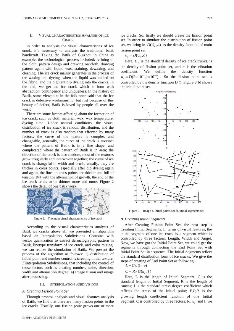
II. VISUAL CHARACTERISTICS ANALYSIS OF ICE

CRACK

In order to analysis the visual characteristics of ice

crack, it’s necessary to analysis the traditional batik

handicraft. Taking the Batik of Guizhou in China as

example, the technological process included: refining of

the cloth, pattern design and drawing on cloth, drawing

pattern again with liquid wax, staining, dewaxing, and

cleaning. The ice crack mainly generates in the process of

the waxing and dyeing, when the liquid wax cooled on

the fabric, and the pigment dip dyeing into the cracks. In

the end, we get the ice crack which is born with

abstraction, contingency and uniqueness. In the history of

Batik, some viewpoint in the folk once said that the ice

crack is defective workmanship, but just because of this

beauty of defect, Batik is loved by people all over the

world.

There are some factors affecting about the formation of

ice crack, such as cloth material, wax, wax temperature,

dyeing time. Under natural conditions, the visual

distribution of ice crack is random distribution, and the

number of crack is also random that effected by many

factors; the curve of the texture is complex and

changeable, generally, the curve of ice crack is succinct

where the pattern of Batik is in a line shape, and

complicated where the pattern of Batik is in area; the

direction of the crack is also random, most of the textures

grow irregularly and interwoven together; the curve of ice

crack is changeful in width and brush, usually, they are

thicker in cross points, especially after dip dyeing again

and again, the lines in cross points are thicker and full of

tension. But with the attenuation of growth, the end of the

ice crack tends to be thinner more and more. Figure 2

shows the detail of one batik work.

Figure 2. The main visual characteristics of ice crack

According to the visual characteristics analysis of

Batik ice cracks above all, we presented an algorithm

based on Interpolation Subdivisions. Combine with

vector quantization to extract dermatoglyphic pattern in

Batik, linetype transform of ice crack, and color mixing,

we can realize the simulation of Batik. We present the

process of the algorithm as follows: 1) distribution of

initial point and number control; 2)creating initial texture;

3)Interpolation Subdivisions, that including the control of

those factors such as creating number, noise, direction,

width and attenuation degree; 4) Image fusion and image

after processing.

III. INTERPOLATION SUBDIVISIONS

A. Creating Fission Point Set

Through process analysis and visual features analysis

of Batik, we find that there are many fission points in the

ice cracks. Usually, one fission point grows one or more

ice cracks. So, firstly we should create the fission point

set. In order to simulate the distribution of fission point

set, we bring in (U , )cD a as the density function of main

fission point set.

(U , )c cu D a

Here, cU is the standard density of ice crack trunks, is

the density of fission point set, and a is the vibration

coefficient. We define the density function 3 6(2 10 ,1 10 )cu D . So the fission point set is

controlled by the density function D (). Figure 3(b) shows

the initial point set.

a

b

Figure 3. Image a. initial points set, b. initial segments set

B. Creating Initial Segments

After Creating Fission Point Set, the next step is

Creating Initial Segments. In terms of visual features, the

initial segment of one ice crack is a segment which is

controlled by three factors: Length, Width and Angel.

Now, we have got the Initial Point Set, we could get the

segments through connecting the End Point Set with

Initial Point Set in sequence. The Initial Segments reflect

the standard distribution form of ice cracks. We give the

steps of creating of End Point Set as following.

(1 )

( , )c

L C e

C R G u f

Here, L is the length of Initial Segment; C is the

standard length of Initial Segment; R is the length of

canvas; f is the standard stress degree coefficient which

reflects the stress of the Initial point; 2 2 2P P P is the

growing length coefficient function of one Initial

Segment. C is controlled by three factors: R, cu and f. we



get L by add vibration “e” to the standard length “C”. In

this paper, we define L as the standard distribution form:

(0.5~1.5) C.

We define as the direction angle of one Initial Segment.

Usually, in a Batik, it’s a great probability for global that

the ice crack along with the normal direction of the Batik

pattern. Define E as the Initial point; define F as the end

point, so the relational expression for them is as

following: jF L e E .

Here, we will not take special considerations for width

of ice crack, and just define a basic form;

(1 )sW W b ,

sW is the standard width of one ice crack, b is the

width coefficient. This definition of width is just a

temporary effect, and we will take a method of brush

replacing to realize the final effect for width. Based on

the definition above all, we can create Initial Segments in

a canvas. Figure 3(b) shows the initial segments set.

C. Interpolation Subdivisions Algorithm

Usually, one ice crack grows abundant details

characteristics including bifurcate, cross and so on. Ice

crack usually includes these characteristics forms in

Figure 4: one-way crack, mesh crack, clusters crack and

fission crack. Among them, clusters crack and fission

crack have a higher probability than others. Especially,

the fission crack born with abstraction, contingency and

uniqueness, and has a high aesthetic value. We mainly

research the simulation of fission crack by Interpolation

Subdivisions Algorithm. Now, there are some similar

algorithms such as L-system [12], DLA [14], Finite

Element [6], Voronoi [5], lightning simulation [16], and

so on. In the following, we will compare Interpolation

Subdivisions Algorithm with these similar algorithms.

a b

c d

Figure 4. Image a. One-way crack, b. Mesh crack, c. Clusters crack, d. Fission crack

Since we got the initial vertex and the end vertex,

connect them, and we got the initial segment.

Interpolation Subdivisions Algorithm is different from

the DLA or L-system algorithm. Generally accepted,

DLA [14] or L-system [12] algorithm follows the method

of plant growth model; Interpolation Subdivisions

Algorithm follows the method of succession subdivisions,

and they are two inverse processes in graphic visual. The

main method of Interpolation Subdivisions is as

following:

Define the initial vertex and the end vertex, insert one

or two vertex by linear interpolation; and then take the

two adjacent vertexes as the new initial vertex and end

vertex, repeat the above operation until the branch details

achieve the visual aim of ice crack. Finally, connect all

the adjacent vertexes.

According to the creating of growth cracks, we present

Interpolation Subdivisions Algorithm. In Figure 5, First,

define the two initial vertex 1 1 1(a ,b ,c )E ,

2 2 2F(a ,b ,c )

and make the coordinate of the inserted point as

(x, y,z)P . Point P' is got from E and F by linear

interpolation. Establish coordinate system as Figure 6,

which is based on point E and F. In this coordinate

system, define u , v and w as the unit vector of U, V,

and W direction in turn. The expression of point P is

listed as following and all the variable definition are list

in Table 1.

(D x,D y)

(D x,D y)

A

A

VP UP

D n

VP PV PV

D n

UP PU PU

P P D v D u

D e R

D e R

Figure 5. Initial vertex defining

Figure 6. Coordinate system based on EF

In Figure 5, segment EF is the initial segment which

decided by two initial point. When we got linear

interpolation point 'P and create point P, connect EP and

PF, and we get the initial curve. In the process of creating

ice crack, it’s important to generate abundant of branches

details. So, In addition to segment EP and PF, in Figure 7,

another segment PQ is required which generated from P

to Q. The following is the solving process of point Q and

all the variable definition are list in Table 1.



(D D D )

(D x,D y)

(D x,D y)

(D x,D y)

(D x,D y)

B

B

B

B

PQ WQ VQ UQ

D m

WQ QW QW

D m

VQ QV QV

D m

UQ QU QU

D m

PQ L L

Q P D r w v u

D e R

D e R

D e R

D e R

Figure 7. The first fission of Q

Figure 8. Tagging rules

The symbols’ meanings are listed in TABLE I as

follow.

When point P and Q are created, connect PE, PF and

PQ. These segments structure the initial trunk and branch

of ice crack. In the following fission processes, we define

the trunk fission points as ijP , define the branch fission

points as ijQ , n is the number of fission process, i is the

sequence number of fission process, j is the sequence

number of fission point (1≤i≤n, 1≤j≤n). Figure 8 shows

the tagging rules of fission points. The fission process is

an iteration steps which based on the fission vertexes of

last step.

TABLE I. TABLE PARAMETERS

Symbol Meaning

, ,UP VP WPD D D P: decay degree of deviating initial segment at

U,V and W direction

, ,PU PV PWD D D P: limits of deviating initial segment at U,V

and W direction

, ,WQ VQ UQD D D Q: decay degree of deviating initial segment at

U,V and W direction

, ,QW QV QUD D D Q: limits of deviating initial segment at U,V

and W direction

PQD segment PQ after attenuation

,A BD D a basic decay degree

LD Limits of segment PQ

n, m number of subdivisions

()R a random value between two parameters

r() unit vector

When the number of fission process reaches n , define

the number of point P, Q as (P)NUM , ( )NUM Q , define

the number of total fission vertexes as (V)NUM and

define the number of segments as (Seg)NUM , the

relationship of them is as following.

1, 1 1, 1 1, 1

1, 1 1, 1

(V) (P) (Q)

3 1 3 13 1

2 2

( ) (V) 1

n n n

i j i j i j

n nn

n n

i j i j

NUM NUM NUM

NUM Seg NUM

Define the vertex density as vu , define the area of

fission process as vS , and

vu can be given by

1, 1

(V)n

i j

v

v

NUM

uS

a

b

c

Figure 9. Image a, b, c

Give the standard vertex density, and give the

constraint condition

v vu U .

End the fission process when it reaches the constraint

condition. In order to achieve abundant of details, we add

a fission probability q to vertex ijQ .

IV. SIMULATION AND ANALYSIS

A. Simulation of Ice Crack

The interpolation subdivisions algorithm is realized in

Matlab. This process mainly include: creating initial point

set, creating initial segment set, interpolation subdivisions,



and post processing. Figure 10 shows the relationship of

these processes as following.

Generate initial point E

Generate initial segment

EF

frequency

factor

Number

control

angle

control

length

control

Generate linear interpolation point P'

Generate insertion point P

Generate branch point Q

Get sequence of points

constraint

condition

Connect sequence of point

Interpolation

Subdivisions

Algorithm

F

T

Repeat fission process

Post processing

Figure 10. Simulation processes

In order to realize the real simulation effect of Batik, it

is necessary to assign these parameters which related to

the Interpolation Subdivisions Algorithm. The main

parameters include: cU , the standard density of trunk;

vU , the standard density of fission point set; q , the

fission probability of branch; n , the fission number; W ,

the width of the fission segments. The following TABLE

II is the main parameters assignment.

TABLE II. THE MAIN PARAMETERS ASSIGNMENT

Figure cU

vU q n w

a 50 5 0.4 3 (0.5,1.5)

b 50 5 0.6 5 (0.5,1) c 100 10 0.8 7 (1,1.5)

Through comparing these three results in visual feature,

we chose Figure 11 (b) whose trunks and branches

created can realize the simulation of growth crack

naturally.

B. Post Process of Batik

1) Creating Batik vector graphics

Currently, vector graphics are widely used for creating

Batik graphics in printing and dyeing industry. We can

get vector graphics by CAD software. In order to

coordinate with Post Process, we extract vector graphics

rough Adobe Illustrator, assign color

(255,255,255)RGB and (0,0,0)RGB for vector

graphics, and assign color (29,32,136)RGB for

background.

2) Graphics Blending

Taking the vector graphics boundary as the growth

boundary of ice cracks, we give the appropriate

parameters assignment for cU and

vU , and adjust other

parameters to consummate the effect of ice cracks. Since

the ice cracks are created in the Batik vector graphics, we

have got the elementary simulation effect. Figure 13(b) is

the Graphics blending effect.

3) Segments Substitution

The width is a distinct feature of ice crack segment.

Distance Transforms [1, 2, 3] uses a Multiplicative Color

Model to generate the width effect where the

intersections of ice crack. We present a method of

segments substitution to simulate the width and color of

dip dyeing. From a visual perspective, each section of the

ice crack is not a single segment; it has multiple changes

at width, linetype and color, so define a brush which has

those features. Figure 12 is a brush we defined. We take

segment MN as the trunk, point M and N are the inside

endpoint but not the outside endpoint, so the intersections

of ice crack could be coherent and thickening. Reduce the

brush opacity gradually along with the direction where is

far away from the trunk. Then assign color

(29,32,136)RGB for the brush. In order to get more

changes of brush, we add Perlin noise to the brush.

Finally, we replace the segments generated above all with

the brush.

C. Result Analysis and Comparison

Through Figure 10, we can see that there are many

steps and parameters affecting the simulation result.

Firstly, we create initial point set and create initial

segment set, and we control the distribution of the fission

trunks by density function (U ,a)c cu D . When we

creating the initial segment EF, we control parameter L to

avoid too much intersection and realize discrete effect.

Interpolation Subdivisions is the key step in the

simulation, we realize various details through modifying

those parameters in Table 1, especially with the

increasing of fission times, and the details became more

and more. In the post process, comparing with the

Multiplicative Color Model, the method of segments

substitution reduces the complexity of the algorithm, and

it completes the thickness changes and the color dyeing

effect in the same time, so it the process is simpler and

more efficient than other method.

The following is the compare of some classic

algorithms. DLA model is a stochastic and dynamic

growth model, which has the characteristics of dynamics

and growth, so it always can be able to express the

growth of plant and other growth model. Similarly, L-

System is a fractal art. L system using string rewriting

mechanism for iteration through the formation of the

continuous production string to guide Guixing draws

graphics. And the following Figure 14 is the simulation

effect comparison of these three algorithms.

Through analysis of visual characteristics, DLA is

suitable for the clusters crack simulation; L-System is

suitable for the Growth Crack simulation; Interpolation



a b c

Figure 11. Creating result for different parameters assignment inTab.2

Figure 12. Defining crack brush

a b c

Figure 13. Image a. Batik vector graphics, b. Graphics blending effect, c. Segments substitution effect

a b c d

Figure 14. Image a. Interpolation Subdivisions, b. DLA, c. Voronoi, d. L-system

TABLE III. CRACK TYPES, ALGORITHM AND PROBABILITY

Crack Form Clusters Crack Growth Crack Fission Crack One –Way Crack Mesh Crack …

Algorithms DLA L-System Interpolation Subdivisions Linear Interpolation Voronoi …

Probability 2P 2P

2P 4P

5P …



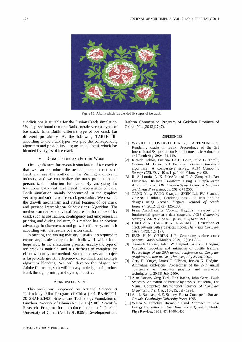
Figure 15. A batik which has blended five types of ice crack

subdivisions is suitable for the Fission Crack simulation.

Usually, we found that one Batik contain various types of

ice crack. In a Batik, different type of ice crack has

different probability. As the following TABLE Ⅲ ,

according to the crack types, we give the corresponding

algorithm and probability. Figure 15 is a batik which has

blended five types of ice crack.

V. CONCLUSIONS AND FUTURE WORK

The significance for research simulation of ice crack is

that we can reproduce the aesthetic characteristics of

Batik and use this method in the Printing and dyeing

industry, and we can realize the mass production and

personalized production for batik. By analyzing the

traditional batik craft and visual characteristics of batik,

Batik simulation mainly concentrated in the graphics

vector quantization and ice crack generation. We research

the growth mechanism and visual features of ice crack,

and present Interpolation Subdivisions Algorithm. The

method can realize the visual features performance of ice

crack such as abstraction, contingency and uniqueness. In

printing and dyeing industry, this method has an obvious

advantage in discreteness and growth efficiency, and it is

according with the feature of fission crack.

In printing and dyeing industry, usually it’s required to

create large-scale ice crack in a batik work which has a

huge area. In the simulation process, usually the type of

ice crack is multiple, and it’s difficult to complete the

effect with only one method. So the next research object

is large-scale growth efficiency of ice crack and multiple

algorithm blending. We will develop the plug-in for

Adobe Illustrator, so it will be easy to design and produce

Batik through printing and dyeing industry.

ACKNOWLEDGMENT

This work was supported by National Science &

Technology Pillar Program of China (2012BAH62F01,

2012BAH62F03); Science and Technology Foundation of

Guizhou Province of China (No. [2013]2108); Scientific

Research Program for introduce talents of Guizhou

University of China (No. [2012]009); Development and

Reform Commission Program of Guizhou Province of

China (No. [2012]2747).

REFERENCES

[1] WYVILL B, OVERVELD K V, CARPENDALE S.

Rendering cracks in Batik. Proceedings of the 3rd

International Symposium on Non-photorealistic Animation

and Rendering. 2004: 61-149.

[2] Ricardo Fabbri, Luciano Da F. Costa, Julio C. Torelli,

Odemir M. Bruno. 2D Euclidean distance transform

algorithms: A comparative survey. ACM Computing

Surveys (CSUR), v. 40 n. 1, p. 1-44, February 2008.

[3] R. A. Lotufo, A. X. FalcÃ£o and F. A. Zampirolli. Fast

Euclidean Distance Transform Using a Graph-Search

Algorithm. Proc. XIII Brazilian Symp. Computer Graphics

and Image Processing, pp. 269 -275 2000.

[4] TANG Ying, FANG Kuanjun, SHEN Lei, FU Shaohai,

ZHANG Lianbing. Rendering cracks in wax printing

designs using Voronoi diagram. Journal of Textile

Research, 2012, 33 (2): 125-130.

[5] Franz Aurenhammer, Voronoi diagrams—a survey of a

fundamental geometric data structure. ACM Computing

Surveys (CSUR), v. 23 n. 3, p. 345-405, Sept. 1991.

[6] HIROTA K, TANOUE Y, KANEKO T. Generation of

crack patterns with a physical model. The Visual Computer,

1998, 14(3): 126-137.

[7] IBEN H N, O'BRIEN J F. Generating surface crack

patterns. GraphicalModels, 2009, 12(1): 1-33.

[8] James F. O'Brien, Adam W. Bargteil, Jessica K. Hodgins,

Graphical modeling and animation of ductile fracture.

Proceedings of the 29th annual conference on Computer

graphics and interactive techniques, July 23-26, 2002.

[9] Gary D. Yngve, James F. O'Brien, Jessica K. Hodgins.

Animating explosions, Proceedings of the 27th annual

conference on Computer graphics and interactive

techniques. p. 29-36, July 2000.

[10] Alan Norton, Greg Turk, Bob Bacon, John Gerth, Paula

Sweeney. Animation of fracture by physical modeling. The

Visual Computer: International Journal of Computer

Graphics, v. 7 n. 4, p. 210-219, July 1991.

[11] A. - L. Barabási, H. E. Stanley. Fractal Concepts in Surface

Growth. Cambridge University Press. 1995.

[12] Witten S. Effective Harmonic Fluid Approach to Low

Energy Properties of One Dimensional Quantum Fluids.

Phys Rev-Let, 1981, 47: 1400-1408.



[13] ArgoalF. Self Similarity of Diffusion limited Aggregates

and Electrod eposition Clusters. Phys Rev Let, 1988, 61:

2558.

[14] G Rozenberg and A Salomaa. Visual models of plant

development. Handbook of formal languages Springer-

Verlag, 1996.

[15] Przemyslaw Prusinkiewicz. Modeling of spatial structure

and development of plants: a review. Scientia

Horticulturae. 1998, 74, 113-149.

[16] KOU Yong, LIU Zhi-fang. Method of lightning simulation

based on multiple subdivisions. Computer Engineering and

Des, 2011, (10): 3522-3525+3569.

Lv Jian, Hebei Province of China, November

28, 1983. Guizhou university, Automation

and machinery manufacturing PH. D. Major

in Advanced manufacturing mode and

manufacture information system.

He works in Guizhou university of china,

Key laboratory of Advanced Manufacturing

Technology, Ministry of Education. He has

taken up a position of Director Assistant since 2010. He

attended IEEE Conference such as 2013 International

Conference on Mechatronic Sciences, Electric Engineering and

Computer, 2013 IEEE International Conference on Big Data.

Weijie Pan, Henan Province of China. Guizhou university,

Automation and machinery manufacturing. Associate professor,

Dr. Major in Advanced manufacturing mode and manufacture

information system.

Zhenghong Liu, Hunan Province of China. Guizhou university,

Automation and machinery manufacturing. Major in Advanced

manufacturing mode and manufacture information system.



Research on Saliency Prior Based Image

Processing Algorithm

Yin Zhouping and Zhang Hongmei Anqing Normal University, Anqing 246011, Anhui, China

Abstract—According to high development of digital

technologies, image processing is more and more import in

various fields, such as robot navigator, images classifier.

Current image processing model still need large amount of

training data to tune processing model and can’t process

large images effectively. The recognition successful rate was

still not very satisfied. Therefore, this paper researched

saliency prior based image processing model, present the

Gaussian mixture process and design the feature point

based classifier, and then evaluate the model by supervised

learning process. Finally, a set of experiments were designed

to demonstrate the effectiveness of this paper designed

saliency prior based image processing model. The result

shows the model works well with a better performance in

accurate classification and lower time consumption.

Index Terms—Image Processing; Saliency Prior; Gaussian

Mixture.

I. INTRODUCTION

Recognition based on computer vision is based on the

theory of learning and discrimination classified and judge

images and video captured by cameras. The classic

computer vision is divided into three levels: Underlying

visual, Middle vision, High visual. The so-called

underlying vision refers to research about the input image

of the local metric information (Edge, Surface), such as

image SIFT descriptors, contour detection of Sober;

middle-visual including object segmentation, target

tracking and so on; senior visual tend to means that

rebuilding the underlying vision and middle visual

information gradually, integrated into the decision-

making process by ever-increasing complexity. With the

improvement of computer processing large-scale data, the

related technologies at all levels of computer vision has

been more widely used in the areas of industrial

production, security monitoring and others. Among these,

high visual closest intelligence requirements and has a

more promising practical and theoretical significance.

The perception of visual mainly in the identification of

objects and scenes. Scene mentioned here referred to a

real-world environment composition by a variety of

objects and their background in a meaningful way. Scene

recognition is to study the expression of the scene. The

definition of scenario corresponds to objects and textures.

When the observer distance concerned target from 1 to 2

meter, the image content is “object”, and when there is a

larger space between the observer and the fixed point

(Usually larger than 5 m),we began to say scenes rather

than field of view. That is to say, most of the object is a

hand distance but scenes usually means where we can

move in this space. The research on scene recognition is

similar to object classification and recognition research.

The scene is unlike objects, object is often tight and

works on it; but the scenario is extended in space and

function it.

However, visual recognition faces enormous

challenges on range of applications and processing

efficiency, illumination, covering, scale, changes within

the class and other problems all affect the visual

perception technology widely applications in practical

technology and life.

Throughout the theory and practice about the object

and scene recognition from a decade, basic framework

revolves around two core content: image expression and

classifier design. Since the essentially of image is a two-

dimensional matrix or a high-dimensional vector, the

number of original pixels is so huge that encounter

enormous difficulties in handling data even the ability of

current computer enhanced, meanwhile the original pixel

contains a large number of invalid information, so the

purpose of image expressing is obtaining low-

dimensional image vector expression with strong

judgment. The most classic image representation model is

Bag-of-features model or named codebook model, this

model is encode local descriptors of the image, quantified

the training samples, projection obtained, the principle of

this model is simple and easy to achieve, gained better

results in the scene and object recognition these years.

Commonly used classification comprises generative

model and discrimination model, LiFeiFei of Stanford

University practiced LDA technology appearing in the

text semantic into the visual field, achieving the self-

classification of objects, non-supervised learning has

been one of the most famous applications in the field of

computer vision, as discrimination model has used tag

information in the training process, so it always obtain

better classification results than the generative model, in

this chapter, we introduced the most important

background knowledge and theory in object and scene

recognition field.

As mentioned above, underlying visual information

such as edge, surface, detail and other information play

an important role in the identification, the description

based on the local structure is the underlying sub-visual

content, and it’s the most commonly used image

description method in senior visual. In this section, we



will respectively introducing classic descriptors: SIFT

and give a short brief about SURF, DAISY and others.

Before SIFT description, Gaussian distribution and

directed acyclic graph first. Figure 1 shows the diagram

of image processing Gaussian function.

Scale(next

octave)

Scale (first

ovtave)

Difference of GaussianGaussian

Figure 1. Key deduction function in image processing of Gaussian

model

A long time ago, people had made use of directed

acyclic graph (DAG) to represent causal relationships

between events. Geneticists Sewall Wright proposed a

graphical approach indicates causal path analysis which is

called path analysi; later it became a fixed causal model

representation for the economics, sociology, and

psychology. Good once used a directed acyclic graph to

represent a causal relationship which is composed by

Distributed cause binary variables. Influence diagrams

represents another application for the decision analysis

and the development of directed acyclic, they include the

event nodes and decision nodes. In these applications, the

main role of directed acyclic graph is to provide a

description of a probability function effectively. Once the

network configuration is complete, all subsequent

calculations are all completed through operating

probabilistic expression symbols. Pearl began to notice

DAG the structure can be used as a structure of method of

calculating method, and it can be used as a cognitive

behavioral model. He updated concept of distributed

program by a tree network, purpose is modeling for

reading comprehension distributed processing and

combining the reason of Top-down and bottom-up to

form a consistent explanation. This dual reasoning model

is the core of update Bayesian network model and also

the central idea of Bayesian.

SIFT which is Scale Invariant Feature Transform, was

proposed by David Lowe in1999 and further improved in

2004, to detecting and describing the algorithms of the

local feature. Descriptor SIFT looking local extreme

value among adjacent scales by DOG(Difference-of-

Gauss) in scale space determine the salient points

position and scale in the image, then extracting region

gradient histogram in the finding significant point to

obtain the final SLFT local descriptors. This method has

the following features: 1) With a strong rotation, scale, brightness, etc.

invariance and better overcome the viewpoint changes,

affine transformation, noise;

2) Good discrimination description big difference in

different local area after quantification, can be matched

quickly and accurately;

3) Producing SIFT sufficient feature vector by

adjusting the parameters;

4) Fast and optimization SIFT matching algorithm can

even achieved real-time requirements;

5) Scalability can be very convenient joint with other

forms of feature vectors.

Figure 2. The calculation of SIFT descriptor

Because of the characteristics of SIFT local features

and descriptor, it has become a typical and a standard

meaning descriptor in the session of computer vision as

showed in figure 2. It has been widely applied in the field

of object recognition, robot path planning and navigation,

behavior recognition, video target tracking and so on. In

this study, by description SIFT descriptors as the basic

contrast characterization; make the test results better

descriptive and comparative.

LiFeiFei proposed a generation model based on LDA,

and applied this model into scene classification tasks.

This model does not require labeling of image, it can

greatly improve the classification efficiency. Framework

is based codebook model, obtaining the distribution of

code word and scene theme through unsupervised

training. This method is getting from improving LDA

proposed by Dabbled. Got probability distribution of the

local area and the intermediate subjects through an

automatic learning approach, training set do not need to

label anything other than the category labels.

Training

Pattern Detection

Images input

Feature Extract

Code generate

Express images

Model Learning

Best Model

Decision

Unknow images

Feature Detection

Figure 3. Algorithms working procedure

Literature mainly introduces the basic theory of

dynamic Bayesian network classifier; literature discussed

the active Bayesian network classifier based on genetic

algorithm, literature practice dynamic Bayesian network

classifier for speech recognition and speaker recognition,

literature research on time sequence recognition, graphic

tracing and macroeconomic Modeling of dynamic

Bayesian network methods. The algorithm working

procedure is showed in figure 3.



Explain model structure in plain language, after

selected the class of the image, if known the category is

mountains, we can obtain the probability vector, this

vector pointed out each block image may have a certain

intermediate subjects. In order to obtain an image sub-

block, firstly you should define a particular subject topic

in all mixing. For example, if you choose “Rock” as your

subject, the associated code word about rock will appear

more frequencies (slanted line). So, after selected a more

inclined to the horizontal edge topics, selected a possible

code word of a horizontal partition. The process of

repeating select a theme and code words ultimately

generate an image of the scene patch which is created a

complete range of mountains. Chart is a graphical

illustration of this generation model. This model is called

the topic model as showed in figure 4.

θ

n

β

τ

C

X

Z

Figure 4. Topic model diagram

As previously mentioned, image recognition which

based on the classic machine learning theory is divided

into two parts: Feature description and Characteristic

judgment. This framework also applies to video object

recognition self-organization. However, video object has

its own unique and challenging:

Target characteristic in Video is often experienced

long-term and gradual process therefore its characteristics

go through this process of change inevitably. This

requires the analysis about the effectiveness of the

features must be a progressive process

The target in video is often appeared accompanied by

scenes, that is the target and the background has a strong

correlation. How to take advantage of this correlation,

improve recognition performance, is one of the

challenges.

As figure 5 shows, conventional saliency processing

model mainly consisted of two steps, which also can’t

handle current challenges. Step one is log the spectrum

and then smooth the logged spectrum or do spectral

residual, finally, a saliency image would showed as the

last two images shows.

Current research indicates that there is no evidence

shown human pattern recognition algorithm is

advantageous than standard machine learning algorithms,

and human beings not too dependent on the amount of

training data. Therefore the key effect of the human

cognitive accuracy may lie in the choice of characteristics.

In fact, relative to the learning methods of discrimination

characteristics, feature description plays a more important

role in the performance of the object recognition. For this

reason research focused on how to effectively description

target features in the video. On the one hand, the gradient

of target characteristics requires establish an online

evaluation mechanisms for target feature, Specific

features may only valid in a specific period of time, on

the other hand, the relevance of the objectives and the

scene, can achieved by mixing characterized of the global

scene and the local features of the target.

Log spectrum

Smoothed log spectrum Spectral residual

Figure 5. Saliency image processing model

II. SALIENCY PRIOR BASED IMAGE PROCESSING

MODEL

A. Feature Point Selection

One aim of study is to analysis the effectiveness of

different object characteristics in the course of recursive

cognitive. This study analyzes the soundness and change

in effectiveness of the target object characteristic in

spatial scale and practice in the process of people's

perception to the object, simulation the intensity changes

of the clustering characteristics in local descriptors to the

characteristic changes of target object which is perceived

by the human eye, and continue to screening on the target

object features, obtained robust through dimension

reduction and the increasing characteristics.

In the field of computer vision can achieved the analog

of statistical characteristics of the object through a

number of local descriptions. Compared to the overall

description of the image this method has a better

robustness and adaptability; the single local descriptor is

only characteristics collection in a small area around the

point of interesting, local structure can’t express the

general characteristics of the target object.

First, extracting descriptor by the samples of poly

library, secondly clustering and generates several code

word, and then, extract features description of the test

sample and the training sample in the same way and

projected onto the code word. Treat each code word as a

channel, in this way we can get the result of each channel

changes by the characterized projected in the timeline, get

distribution curve of feature projection on each channel.

Experiments under the framework of the information

entropy and mutual information criterion, two different

but related ways, reduce the dimension of the feature

channel. Finally, analyze the effects of dimensionality

reduction based on the code book and support vector



machine identification system, to achieve robustness and

effectiveness of the characterized channel. In this report,

firstly, establish the word bags express of the image, then

information entropy and mutual information from the

perspective of the characteristics of the cognitive process

of analysis is divided into recursion, then divided the

feature recursive cognitive process analysis into

robustness analysis and impact analysis on decision-

making in the perspective of information entropy and

mutual information, illustrate the dimension reduction of

the characteristics channel from the implementation of

the next two-step.

At the pre-processing stage of the target image, this

study uses the codebook to express image (Bag-of-

Features). This article was extracted features from the test

library, training library, clustering library, and clustering

generated codeword of M, getting the projection on code

word from the test library image and clustering library

sample, Bag-of-Features for object recognition and

classification are divided into the following steps:

Extracted Local feature of image, common local

features include: SIFT, SURF, DAISY, Opponent-SIFT,

texture feature and so on.

Study the visual vocabulary. The learning process

achieved mainly through the clustering algorithm, the

cluster center from classical K-means and improved

methods K-means++ is the code word, the collection of

code word is called codebook.

Quantified, projected the Local features of the training

samples onto code word obtained code word frequency

each image can be expressed by histogram which is

composed from the code word.

Image classification and identification. After the Bag-

of-Features, learning a discrimination to distinguish

different types of goals. Commonly used classification

Includes: Neighbor classifier, Neighbor K classifier,

Linear classifier, SVM, Nonlinear SVM

B. Gaussian Mixture Model

Gaussian Mixture Model, this is linear combinations of

A plurality of single-Gaussian distribution, is the

promotion of Single Gaussian probability density

function. GMM can be smoothly approximate the

probability density distribution of any shape. Therefore, it

is often used in background modeling and speech

recognition in recent years, and achieved good results.

In this research, using Gaussian mixture model

distribution fitting projection vector of a series of video

frames in the same dimension data. The resulting of

Gaussian mixture model can show the distribution of

projection vectors in the dimension of the subject more

precisely. Furthermore, by calculating the projection

vector sequences from the training and projection vector

sequences from the testing, obtaining symmetry KL

divergence from the two corresponding fitted distribution

in same dimensional data, can determine the validity of

dimensional data where the performance of the object

characteristics, and exclude a certain lower validity

dimensional, which can make no damage or even

improve the ability to correctly identify the target to

system while reducing the amount of data processing.

For the single sample 1x in the observational data sets

1, 2, nX x x x ,

The density function of Gaussian mixture distribution

is:

1

/ /k k i k

k

i

P xi w p x

In this Formula, kw is Mixing coefficient, regarded as

the weight of each Gaussian distribution component:

1, 2, k is parameter space of each Gaussian

distribution, 1i

kk

represents the component of a

Gaussian distribution mean and variance in k. Generally

use maximum likelihood estimation method to determine

the parameters of the model:

1

/ / /N

i

P X P xi L X

argmax /L X

For a Gaussian mixture model, it is not feasible to

seeking its maximum value by directly the partial

derivative. And then consult online EM for estimating

Gaussian mixture model parameter. The related formula

of the algorithm as following:

,

,

1

' / '/ '

' / '

k k i

j j j i

ik

j

w p xp k x

w p x x

,

1

/ 'N

i

i

kd p k x

1' 'k kw

N

Getting a feature vector with higher dimensional after

clustering and characterization targets. To ensure the

correctness results of the matching, we should screen out

the dimension which represents the target information

stably, and removing unstable dimension. Analysis from

the timeline seeking the probability density function

through the distribution of each dimension, choosing a

distribution is more stable dimension.

Distance K-L is a degree to measure the similarity

between distribution kp p and the known distribution

kq q in statistical, which is defined as

2// logi

i

ii

KLp

D p q pq

In this 0KLD . Only when the two distributions are

identical until the distance K-L is equal to 0.Distance K-L

is not symmetric about p and q. Generally, the

distribution from p to q is not equal to the distribution

from q to p. the value of K-L distance is lager with the

difference of the two distributions. The details are

showed in tablet 1.

We use K-L distance to calculate the similarity of the

two mixed Gaussian distribution. After description the

feature of the measured image, fit the data for each

dimension of each feature, Get mixture Gaussian model

at each dimension, and calculate the K-L distance to the

corresponding dimension of the library. Select a certain

number dimensions which is close proximity to K-L

distance, achieved the purpose of reducing the feature



dimension, improving stability of characterization,

improving matching accuracy.

TABLE I. GAUSSIAN MIXTURE MODEL FITTING RESULTS AT A

CERTAIN DIMENSION

Dimension Mean Variance Weight

1 0.007923 0.045144 1.000000

2 0.000000 12.500000 0.000000

3 0.000000 12.531255 0.000000

4 0.053632 0.2342323 1.000000

5 0.087521 0.3431683 1.000000

6 0.142327 0.5217323 1.000000

In the course of this research, we found the

characteristics for the same channel; Chart is the values

for fitted distribution of three Gaussian mixture models in

a certain dimension, wherein the 2.3 dimension is initial

value. But the eventually weight is 0. By comparing the

characteristics of all the dimensions, concluded that, the

fitting is subject to a single Gaussian distribution whether

for the test sample statistics or the training sample

statistics.

The projection value after normalizing the same

dimension, is also subject to a single Gaussian

distribution, this is also confirmed the correctness of the

conclusions from the side.

C. Evaluation Model Design

The effectiveness of characteristic in cognitive process:

the validity on object class descript as below:

Showing by the previous evidence, the effectiveness of

feature performed on the categories is the size of on the

mutual information with the category labels. As the

complexity of the conditional probability, design the

following experiment to simulate:

1. Estimated the training sample distribution between

each channel through Gaussian mixture models

2. Estimated the test sample frames image distribution

for each channel by Gaussian mixture models

3. Seeking the KL divergence according the

distribution between training and testing samples,

comparing the divergence value with a predetermined

threshold specified T, we define channel with no

performance or smaller effect to target as characteristic

channel which value is greater than the threshold.

This process can be expressed as follows flowchart.

As is shown in the flowchart, in the second process of

dimension reduction, respectively fitting the training and

test sets with Gaussian mixture model, then gather the KL

distance of each dimensions to a scatter plot. From the

figure, for the first one hundred dimensional SIFT feature,

the distance between two distributions is so small. A

greater part of distributions from the texture and color

histogram is far away the outliers. This is mainly due to

relatively large difference between the image scale in the

training and testing database, caused by lacking scale

invariance of color histogram.

Likewise, described by the former, they are

independent between the channels and features, so we can

compare the KL distances between the distributions

through threshold value T2. The channel greater than the

T2 threshold value is considered to be bad characterize

category information, and the channel smaller than the T2

threshold value is considered to be good characterize

category information, contribute to separate the different

types of objects in characteristics.

Through the feature extraction, get the most effective

feature to category determining, achieve an effective

result in dimensionality reduction, reducing the

complexity of the following model parameter estimation.

Target Video Frame

Training Video Frame

Extract Feature and

map to N dimension

Space

Calculate 2N Gaussian Mixture Model

Calculate N distribute KL divergence

Filter dimensional data according to size of divergence

Adjust character

vector

Figure 6. Schematic considering the difference between test sample and training sample

Classification decision refers to using statistical

methods classified these identified objects as a category.

Basic approach is set a judgment rules based on the

training sample, lower the identified objects error

recognition rate and loss caused by this rules, the decision

rule of Bayesian network pattern recognition model is

Bayesian network classifier, it’s obtained by learning the

structure and parameters of Bayesian networks.

Parameters usually determined by the structural and data

sets, therefore Bayesian network structure learning is the

core of Bayesian network learning.

In this research, simulate the human eye perceives

objects recursive process through targeted campaign on

the scale space, analysis the robustness of characterized

and effectiveness of objects cognition through the angle

of minimum information entropy and maximum mutual

information. Design a experiment, modeling on the

sample according Gaussian mixture model and cross-

entropy, present feature evaluation criteria to both cases.

Through the on-line self-organization recognition

experiments, we can verify dimensionality reduction

method is effective.

D. Supervised Learning Process

In order to generate high-quality code word, in the

clustering process using intersection kernel metrics K-

means method based on histogram. This is mainly

because HIK is able to effectively calculate the number of

points falling into the same collection at a given level;

and In the process of visual perception, the local

descriptors such as SIFT and DAISY are based on the

description of the histogram; in the process of comparing

the similarity of two local descriptor, using histogram

intersection is more appropriate than classical Euclidean

distance.



Set 1, 2,i

ih h h h R

histogram, ih is the frequency

of codeword in codebook model. Histogram intersection

kernel HIK is defined as:

1, 2 1 , 2

1

min( )d

HI i i

i

K h h h h

Initial center can be obtained by K-MEANS ++

method, each local feature assigned to the corresponding

center, according to the following equation: 2

2 ij

jx i x

i

hh m h

= , ,

2

2

2j j

HI j k HI x jjk j

x

ii

K h h K h hh

If xh is a arbitrary partial description, im is the current

cluster centers, using histogram intersection kernel, when

calculating the similarity between the local features and

the current cluster center, the first item at this point does

not affect the results, the second term needs to be

calculated for different feature, each time a new element

added, the amount of calculate mainly spent in the last

one.

Figure 7. Supervised learning express code image

It is critical to select the appropriate classification for

specific issues. Linear support vector machine get good

results in the visual field for its efficient and high

accuracy. In actually, Pyramid GIST description can be

seen as image histogram description at multi-scale and

multi-up and the codebook model is can be viewed as a

histogram of the frequency for local significant structure,

Euclidean distance is not the best metrics to describing

the similarity of two descriptors from this point.

As previously mentioned, histogram intersection core

is better than the Euclidean distance in histogram metrics,

it can be predicted that in the field of visual cognition

using histogram intersection kernel support vector

machines can achieve better results under this framework.

Given labeled training set

,1

N

i ii

D y x

,

ix is the training data, 1,2,iy n corresponding to

ix categories. The dual form of SVM can be reduced to

optimization problem, that is,

,

1

1

2

N

i i j i j i j

i i

W y y k x y

Define:

0 , 0i i iC y

The Commonly linear kernel is defined as

,i j i jk x x x x

The framework for this topic, as mentioned previously,

codebook model and Pyramid global are all based

essentially on the expression of the histogram. Therefore

under this case, use the histogram intersection nuclear

may better express the similarity between the two

characterizes. However, histogram intersection kernel is

non-linear kernel, requiring more memory and computing

time than the linear kernel. Maji and some others have

researched this problem, decomposing formula in a

similar manner, accelerating the calculation, ultimately

required O n time complexity and memory. In the

experiment, using a modified LIBSVM to achieve multi-

class distinguish.

III. EXPERIMENT AND VALIDATION

A. Experiment Environment

In the test, according the experiments framework set

by Quattoni, testing on a standards outdoor image

database. For each category, select eighty images used for

training, twenty pictures for testing, for the convenience

and standardize, we directly use the name of the file they

offer, so, in this experiment, we used the same

experimental data with Quattoni. In order to train one to

many classifiers, sampling N positive samples and

sampling 3N negative samples in the same. Create three-

tier expression in accordance with the previously

described pyramid image, each layer using the Gabor

filter processing at three scales and eight directions,

tandem all images to obtaining the expression vector in

the end, totally 24192 dimensional vector. In order to

obtain description of the partial salient region, we

extracted dense SIFT descriptors at the respective three

pyramid images, then projected on the 500 cluster centers,

tandem the frequency of all the blocks descriptors

similarly, so in codebook model, each image marked by a

10500 dimensional vector. Finally, as tablet 2 shows,

tandem the two described to get the latest image

compositing expression. In the determination phase,

training in the histogram intersection kernel support

vector machine.

TABLE II. COMPARISON VECTORS OF DIFFERENT METHODS

dimensionality reduction Normal dimensional

HIK SVM 100% 100%

Liner SVM 25.173% 100%

Polynomial SVM 92.053% 94.325%

RBF SVM 73.249% 92.971%

In this model, the image is modeled as a collection of a

series of local block, these regions are a part of the

“subject”, each block is expressed by the code book, and

through training can be obtained scenes themes of each

class and code word distribution. For the test samples,

identify the code word firstly, and then finding class

model which is the best matching code word distribution.



B. Test Results

Chart is the result of comparing the present method to

the other reference. Repeated experimental results of

Quattoni, include GIST of core RBF, Quattoni prototype

representation and space pyramid matching of Lazebnik.

In the experiment, take two layers of Pyramid, the size of

the dictionary is 400, primitive image is 50, matching the

two sides by histogram intersection kernel; in this paper,

support vector machine approach based on hybrid

expression and histogram intersection kernel (selected the

Number of code words are200 and 500). It is obviously

that, the proposed method achieved the best results,

reached an accuracy rate of 40%.

Figure 8. Comparison of different meyhods

Even pure pyramid GIST histogram intersection SVM

method get to 30%, this has exceeded 4% to the highest

accuracy rate of Quattoni. Finally, this method outstrips

about 4 percentage points beyond the spatial pyramid

matching of Lazebnik. From the figure, it has shown that,

using more code word can significantly improve the

accuracy.

Figure 9. Recognition result of same hybrid with different kernel of SVM

Figure 9 is using pyramid GIST express different

kernel support vector machine comparison and

verification: selected 50 pictures in each category

randomly, select another 20 images for testing, image

expressed by the GIST pyramid. It is shown in the

simplified framework, the results of histogram cross core

easily goes beyond others’. It is noteworthy that, better

performance in the usual kernel support vector machine

RBF was particularly bad in here, this may be due to this

metric is not applicable to express the characterization of

GIST based on histogram.

IV. CONCLUSION

In this part, proposed a mixing expression of images,

to test the effectiveness of hybrid expression, extend the

goal to indoor scene. In fact, the essential of general

object recognition and indoor scenes are the same, but the

interior scenes with greater within-class variance and the

similarity between classes. So much classical

identification of objects, scene understanding methods

have shown its weaknesses in processing the indoor

scenes. Inspired by the Devi Parikh study, focused the

first step of the design on the discrimination significance

of image expression, considered from the overall

expression of the image and local significant structures,

by the further excavation from the relationship between

the area of the overall expression and considering a more

suitable histogram intersection distance in the classic

codebook model, finally, got mixed image expression

after the series. After acquiring an image expression,

getting ultra-face of distinguish different types point in

high-dimensional space through the training. This

moment, compare the similarity between the image

expression has become one of the key issues, using the

histogram intersection kernel support vector machines,

through the experimental comparison, found that the

recognition rate under this framework enhance the

accuracy of Kurdish in a large extent.

ACKNOWLEDGEMENT

This research is funded by: Youth Research Fund

Anqing Normal University in 2011 Project: Domain

Decomposition Algorithm for Compact Difference

Scheme of the Heat Equation (Grant No. KJ201108).

REFERENCES

[1] Chikkerur, S., T. Serre, and T. Poggio, Attentive

processing improves object recognition. Journal of

Neuroscience, Vol. 20, No. 4, 2000.

[2] Fergus, R., P. Perona, and A. Zisserman, Object class

recognition by unsupervised scale-invariant learning, 2003

IEEE Computer Society Conference on Computer Vision

and Pattern Recognition, pp. 264-267, 2003..

[3] Jiang, Y., C. Ngo, and J. Yang. Towards optimal bag-of-

features for object categorization and semantic video

retrieval, Proceedings of the 6th ACM international

conference on Image and video retrieval, pp. 494-501,

2007.

[4] Niebles, J., H. Wang, and L. Fei-Fei, Unsupervised

learning of human action categories using spatial-temporal

words. International Journal of Computer Vision, vol. 79,

no. 3, pp. 299-316, 2008

[5] Grauman, K. and T. Darrell, The pyramid match kernel:

Efficient learning with sets of features, Journal of Machine

Learning Research, pp. 725-760, 2007.

[6] Cristianini, N. and J. Shawe-Taylor, An introduction to

support Vector Machines: and other kernel-based learning

methods, Cambridge Univ Pr, 2000.

[7] Gambetta D, Can we trust trust? In: Gambetta D, ed. Trust:

Making and Breaking Cooperative Relations. Basil

Blackwell: Oxford Press, pp. 213~ 237, 1990.

[8] Bouhafs F, Merabti M, Mokhtar H. A Semantic Clustering

Routing Protocol for Wireless Sensor Networks, IEEE



Consumer Communications and Networking Conference,

pp. 351-355, 2006

[9] Avciba, I., et al., Image steganalysis with binary similarity

measures. EURASIP Journal on Applied Signal Processing,

pp. 2749-2757, 2005.

[10] Maji, S., A. Berg, and J. Malik. Classification using

intersection kernel support vector machines is efficient,

IEEE Conference on Computer Vision and Pattern

Recognition, pp. 1-8, 2008.

[11] Lazebnik, S., C. Schmid, and J. Ponce, A sparse texture

representation using local affine regions. IEEE

Transactions on Pattern Analysis and Machine Intelligence,

pp. 1264-1276, 2005.

[12] Manjunath, B. and W. Ma, Texture features for browsing

and retrieval of image data. Pattern Analysis and Machine

Intelligence, IEEE Transactions on, vol. 18, no. 8, pp. 836-

841, 2002.

[13] Bay, H., T. Tuytelaars, and L. Van Gool, Surf: Speeded up

robust features. Computer Vision CECCV 2006, pp. 402-

415, 2006.

[14] Nowak, E., F. Jurie, and B. Triggs, Sampling strategies for

bag-of-features image classification. Computer Vision

CECCV 2006, pp. 491-502, 2006.

[15] Fischler, M. and R. Elschlager, The representation and

matching of pictorial structures. Computers, IEEE

Transactions on, vol. 100, no. 1, pp. 68-93, 2006.

[16] Joubert, O, Processing scene context: Fast categorization

and object interference. Vision Research, vol. 47, no. 26,

pp. 3285-3295, 2007.

[17] Biederman, J., J. Newcorn, and S. Sprich, Comorbidity of

attention deficit hyperactivity disorder with conduct,

depressive, anxiety, and other disorders. American Journal

of Psychiatry, vol. 145, no. 5, pp. 563-577, 1991.

[18] Oliva, A. and A. Torralba, Modeling the shape of the scene:

A holistic representation of the spatial envelope.

International Journal of Computer Vision, vol. 42, no. 3,

pp. 144-174, 2001.

[19] Odone, F., A. Barla, and A. Verri, Building kernels from

binary strings for image matching. Image Processing, IEEE

Transactions on, vol. 14, no. 2, pp. 168-180, 2005.

[20] Maji, S., A. Berg, and J. Malik. Classification using

intersection kernel support vector machines is efficient. :

Computer Vision and Pattern Recognition, 2008. CVPR

2008. IEEE Conference on, pp. 1-8, 2008.

[21] Wu, J. and J. Rehg. Beyond the Euclidean distance:

Creating effective visual codebooks using the histogram

intersection kernel.: 2009 IEEE 12th International

Conference on Computer Vision, pp. 630-637, 2009



A Novel Target-Objected Visual Saliency

Detection Model in Optical Satellite Images

Xiaoguang Cui, Yanqing Wang, and Yuan Tian Institute of Automation, Chinese Academy of Sciences, Beijing, China

Email: {xiaoguang.cui, yanqing,wang, yuan.tian}@ia.ac.cn

Abstract—A target-oriented visual saliency detection model

for optical satellite images is proposed in this paper. This

model simulates the structure of the human vision system

and provides a feasible way to integrate top-down and

bottom-up mechanism in visual saliency detection. Firstly,

low-level visual features are extracted to generate a

low-level visual saliency map. After that, an attention shift

and selection process is conducted on the low-level saliency

map to find the current attention region. Lastly, the original

version of hierarchical temporal memory (HTM) model is

optimized to calculate the target probability of the attention

region. The probability is then fed back to the low-level

saliency map in order to obtain the final target-oriented

high-level saliency map. The experiment for detecting

harbor targets was performed on the real optical satellite

images. Experimental results demonstrate that, compared

with the purely bottom-up saliency model and the VOCUS

top-down saliency model, our model significantly improves

the detection accuracy.

Index Terms—Visual Salience; Target-Oriented;

Hierarchical Temporal Memory

I. INTRODUCTION

With the development of remote sensing technology,

optical satellite images have been widely used for target

detection, such as harbors and airports. In recent years,

high spatial resolution satellite images provide more

details for shape, texture and context [1]. However, data

explosion for high resolution remote sensing images,

brings more difficulties and challenges on fast image

processing. Visual saliency detection aims at quickly

identifying the most significant region of interest in

images by means of imitating the mechanism of the

human vision system (HVS). In this way, significant

regions of interest can be processed with priority by the

limited computing resource, thus substantially improving

the efficiency of image processing [2]-[3].

There are two models for HVS information processing,

namely, bottom-up data driven model and top-down task

driven model. Bottom-up model often acts as the

unconscious visual processing in early vision and is

mainly driven by low-level cues such as color, intensity

and oriented filter responses. Currently, many bottom-up

saliency models have been proposed for computing

bottom-up saliency maps, by which we can predict

human fixations effectively. Several bottom-up models

are based on the well known biologist saliency model by

Itti et al [4]. In this model, an image is decomposed into

low-level feature maps across several spatial scales, and

then a master saliency map is formed by linearly or

non-linearly normalizing and combining these maps.

Different from the biological saliency models, some

bottom-up models are based on mathematical methods.

For instance, Graph-based Visual Saliency (GBVS) [5]

formed a bottom-up saliency map based on graph

computations; Hou and Zhang [6] proposed a Spectral

Residual Model (SRM) by extracting the spectral residual

of an image in spectral domain; Pulsed Cosine Transform

(PCT) based model [7] extended the pulsed principal

component analysis to a pulsed cosine transform to

generate spatial and motional saliency.

Although the bottom-up saliency models are shown to

be effective for highlighting the informative regions of

images, they are not reliable in target-oriented computer

vision tasks. When apply bottom-up saliency models in

optical satellite images, due to the lack of top-down prior

knowledge and highly cluttered backgrounds, these

models usually respond to numerous unrelated low-level

visual stimuli and miss the objects of interest. In contrast,

top-down saliency models learn from training samples to

generate probability maps for localizing the objects of

interest, and thus produce more meaningful results than

bottom-up saliency models. A well-known top-down

visual saliency model is Visual Object detection with a

CompUtational attention system (VOCUS) [8], which

takes the rate between an object and its background as the

weight of feature maps. The performance of VOCUS is

influenced by object background. Although it performs

well in nature images, it does not work reliably in the

complicated optical satellite images. Recently, several

top-down methods have been proposed based on learning

mappings from image features to eye fixations using

machine learning techniques. Zhao and Koch [9]-[10]

combined saliency channels by optimal weights learned

from eye-tracking dataset. Peters and Itti [11], Kienzle et

al. [12] and Judd et.al. [13] learned saliency using scene

gist, image patches, and a vector of features at each pixel,

respectively.

It is established that top-down models achieve higher

accuracy than bottom-up models. However, bottom-up

models often take much lower computational complexity

due to only taking into account of low-level visual stimuli.

In this case, an integrated method of combining



bottom-up and top-down driven mechanisms is needed to

get benefits from both types of mechanisms.

How to effectively integrate bottom-up and top down

driven mechanisms is still an unsolved problem for the

visual saliency detection. According to the mechanism of

HVS, this paper proposes a target-oriented visual saliency

detection model, which is based on the integration of both

the two driven mechanisms. The proposed model consists

of three parts, namely pre-attention phase module,

attention phase module and post-attention module. Firstly,

a low-level saliency map is quickly generated by the

pre-attention phase module to highlight the regions with

low-level visual stimuli. Then the attention phase

conducts an attention shift and selection process in the

low-level saliency map to find the current attention

region. After obtaining the attention region, a target

probability of the region evaluated by the post-attention

module is fed back to the low-level saliency map to

generate a high-level saliency map where the suspected

target regions are emphasized meanwhile the background

interference regions are suppressed. The main

contributions of this paper are:

A new method is presented for combining top-down

and bottom-up mechanisms, i.e. revising the low-level

saliency map with target probability evaluation so that the

attention regions containing suspected targets are

enhanced, meanwhile inhibiting the non-target regions.

An effective method for focus shift and attention

region selection is proposed to focus on the suspected

target regions rapidly and accurately.

The original HTM model is improved in several

respects including the input layer, the spatial module and

the temporal module, leading to a robust estimation of the

target probability.

This paper is structured as follows: Section II describes

the framework of the proposed model. The details of the

three parts i.e. pre-attention phase module, attention

phase module and post-attention module are presented in

Section III, IV and V, respectively. Experimental results

are shown in Section VI. Finally, we give the concluding

remarks in Section VII.

II. FRAMEWORK OF THE PROPOSED MODEL

A new model is presented to simulate HVS attention

mechanism, and composed of three functional modules,

namely, pre-attention phase module, attention phase

module and post-attention phase module, as shown in Fig.

1. The pre-attention phase is a bottom-up data driven

process. It is employed to extract the lower features to

form the low-level saliency map. According to principles

of winner takes all, adjacent proximity and inhibition of

return [4], the attention phase module carries out the

focus of attention shift on the low-level saliency map and

proposes a self-adaptive region growing method to

rationally select the attentions regions. The post-attention

phase is a top-down data driven process, and its major

function is to apply the HTM model [14]-[15] to evaluate

the target probability of the selected attention regions.

The probability is then multiplied with the corresponding

attention region on the low-level saliency map, thus a

high-level saliency map which is more meaningful to

locate objects of interest is generated.

III. PRE-ATTENTION PHASE

In this phase, we first extract several low-level visual

features to give rise to feature maps, and then we

compute saliency map for each feature map using the

PCT-based attention model. Finally, saliency maps are

integrated to generate the low-level saliency map. The

block diagram of the pre-attention phase is shown in Fig.

2.

A. Feature Extraction

If a region in the image is salient, it should contain at

least one distinctive feature different from its

neighborhood. Therefore, visual features of the image

should be extracted first. For this, we extract three

traditional low-level visual features, i.e. color, intensity

and orientation.

1) Color and intensity: HSI color space describes a

color from the aspect of hue, saturation and intensity,

more consistent with human visual features than RGB

color space. Hence, we transfer the original image from

RGB to HIS in order to obtain the color feature map H ,

S and the intensity feature map I :

3

),,min(1

},180;,0{

)(3

2arctan90

360

1

BGRI

I

BGRS

BGBG

BG

BGR

H

(1)

2) Orientation: Artificial targets in optical satellite

images generally possess obvious geometrical

characteristics. Therefore, orientation feature is crucial to

identify the artificial targets. Here we adopt Gabor filters

)135,90,45,0( k

oooo to extract the orientation

feature. The kernel function of a 2-D Gabor wavelet is

defined as:

kk

iv

zv

k

k

k

k

k

v

eeev

z

sin,cos

)( 22

2

22

2

22

(2)

where ),(z yx denotes the pixel position, and the

parameter determines the ration between the width

of Gaussian window and the length of wave vector. We

set 47 in the experiment. Four orientation

feature maps can be obtained by convoluting the intensity

feature map I with k

:

)()()( zzIzOkk (3)



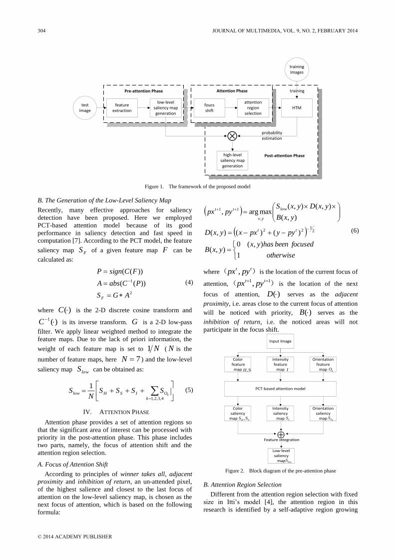
Attention Phase

featureextraction

low-level saliency mapgeneration

foucs shift

attention region

selectionHTM

trainingImages

training

high-level saliency mapgeneration

probability estimation

Pre-attention Phase

Post-attention Phase

testImage

Figure 1. The framework of the proposed model

B. The Generation of the Low-Level Saliency Map

Recently, many effective approaches for saliency

detection have been proposed. Here we employed

PCT-based attention model because of its good

performance in saliency detection and fast speed in

computation [7]. According to the PCT model, the feature

saliency map FS of a given feature map F can be

calculated as:

2

1 ))((

))((

AGS

PCabsA

FCsignP

F

(4)

where )(C is the 2-D discrete cosine transform and

)(1 C is its inverse transform. G is a 2-D low-pass

filter. We apply linear weighted method to integrate the

feature maps. Due to the lack of priori information, the

weight of each feature map is set to N1 ( N is the

number of feature maps, here 7N ) and the low-level

saliency map lowS can be obtained as:

4,3,2,1

1

k

OISHlow kSSSS

NS (5)

IV. ATTENTION PHASE

Attention phase provides a set of attention regions so

that the significant area of interest can be processed with

priority in the post-attention phase. This phase includes

two parts, namely, the focus of attention shift and the

attention region selection.

A. Focus of Attention Shift

According to principles of winner takes all, adjacent

proximity and inhibition of return, an un-attended pixel,

of the highest salience and closest to the last focus of

attention on the low-level saliency map, is chosen as the

next focus of attention, which is based on the following

formula:

otherwise

focusedbeenhasyxyxB

pyypxxyxD

yxB

yxDyxSpypx

tt

low

yx

tt

1

),(0),(

)()(),(

),(

),(),(maxarg,

21

22

,

11

(6)

where ）（ tt pypx , is the location of the current focus of

attention, ）（ 11, tt pypx is the location of the next

focus of attention, )(D serves as the adjacent

proximity, i.e. areas close to the current focus of attention

will be noticed with priority, )(B serves as the

inhibition of return, i.e. the noticed areas will not

participate in the focus shift.

Feature integration

Input Image

Color feature

map

Intensity feature

map

Orientation feature

map

PCT-based attention model

Color saliency

map

Intensity saliency

map

Orientation saliency

map

,SH I kO

,SH SS ISkOS

Low-levelsaliency

map lowS

Figure 2. Block diagram of the pre-attention phase

B. Attention Region Selection

Different from the attention region selection with fixed

size in Itti’s model [4], the attention region in this

research is identified by a self-adaptive region growing



method: taking the focus of attention as seed point, the

region growing is conducted by computing the saliency

difference between the current growing area and its

surrounding areas according to a given step-size sequence.

Once the difference tends to be decreasing, the growth

will be terminated. Finally, the minimum area-enclosing

rectangle of the growing area is deemed to the attention

region. Here we define iR as the growing area obtained

in each growth, in as the number of pixels in iR , iA

as the saliency difference between iR and its

surrounding area. Given a step-size sequence

]),0[( TiNi , where T denotes the maximum times

of growing, the algorithm for the self-adaptive region

growing is as Algorithm 1. Algorithm 1 Self-adaption region growing

Input: ( [0, ])iN i T , 0 { }R f , where f is the present focus of

attention; 0 1n ; 1i .

Iteration:

while not reach the maximum growing time do

Initialize iR and

in : 1i in n ;

1i iR R .

while do

produce a new growing point p : arg max ( )j

jp

p S p , where

jp A , A is the adjacent pixel set of iR , ( )jS p is the saliency of

jp .

update iR and : { , }i iR R p ;

1 1i in n .

end while Calulate :

1

1 1( ) ( )j i j i

i j i j i

p R p R

A S p N S p N

when 1iA

tends to

decrease, the growth is

terminated:

if then the growth is terminated.

else

1i i ; growth continues.

end if

end while

Output:

the minimum area-enclosing rectangle of .

V. POST-ATTENTION PHASE

In the post-attention phase, we optimize the original

version of the HTM model [14] to estimate the target

probability of attention regions. The probability is then

fed back to the low-level saliency map, and finally the

target-oriented high-level saliency map is generated.

A. The Optimization of HTM

HTM model is the newest layering network model that

imitates the structure of the new human neocortex [14].

HTM model takes time and space factors which depict

samples into account in order to tackle with ambiguous

rule of inference, presenting strong generalization ability.

Thus, it has been gradually highlighted in the field of

pattern recognition [16]-[19].

Different from most HTM-based applications [15]-[18]

which apply the pixel’s grayscale as the input layer of

HTM, in this research, the low-level visual features

extracted in the pre-attention phase are taken as the input

layer for the purpose of improving the precision of the

model. Fig. 3 shows the structure of our HTM model,

where the notes in the second layer conduct the learning

and reasoning of the low-level visual features, meanwhile,

the notes above the third layer conduct the learning and

reasoning of the spatial position relationships. Notes in

different layers use the same mechanism to conduct the

learning and reasoning process, and they have the same

node structure which is formed by a spatial module and a

temporal module.

1) Spatial module: The main function of spatial

module is to choose the quantization centers of the input

samples, that is, to select a few representative samples in

the sample space. These centers should be carefully

selected to ensure that the spatial module will be able to

learn a finite quantization space from an infinite sample

space. It is assumed that the learned quantization space in

the spatial module of a node is ],...,,[ 21 nqqqQ ,

where iq is quantization center and N is the number

of the existing centers. All the Euclidean distances d

between these centers are calculated and their sum S is

considered as a distance metric of the quantization space:

N

i

N

j

ji qqdS ),( (7)

when a new input sample cq appears in the node, we

first add cq to Q , and the distance increment inc

caused by cq can be calculated as follows:

N

i

ci qqdinc ),( (8)

The change rate of the distance increment Sinc is

then examined against a given threshold . If

Sinc , cq is retained in Q otherwise, cq is

removed from Q . This algorithm ensures that input

samples which contain substantial information will be

considered as new quantization centers, whereas those

which do not contain representative information will be

discarded.

The learning of the spatial module is stopped when the

added quantization centers are sufficient to describe the

sample space. In practice, the learning is completed when

the rate of adding new centers falls bellow a predefined

threshold.

2) Temporal module: The temporal module proposed

in [14] is suitable in applications where the input samples

have obvious time proximity such as video images.

However, the input images for training the HTM model

rarely share any amount of time correlation in our

research. Therefore, instead of the time adjacency matrix

proposed in [14], we exploit a correlation coefficient

matrix C to describe the time correlation between

different samples. We adopt Pearson’s coefficient as the



features extraction

1O 2O3O 4OH S I

class label

level 1

level 2

level 3

level 4

level 5 probability estimation

input space

Figure 3. The proposed HTM network structure

measure of correlation. The NN correlation matrix,

which contains the Pearson’s correlation coefficients

between all pairs of centers, is calculated as follows:

ji

ji

qq

qjqi

ji

qqEqqC

)])([(),(

(9)

where E is the expected value operator, q and q

denotes the mean and the standard deviation of the

respective quantization center, respectively. The larger

the absolute value of correlation is the stronger the

association between the two centers.

A temporal grouping procedure is then utilized to

separate the quantization space Q into highly correlated

coherent subgroups. The major advantage of replacing

the time adjacency matrix with the correlation coefficient

matrix is that it enables the grouping procedure to be

irrelevant with the temporal sequence of sample images,

so as to improve the precision of the model.

In [14], a computationally efficient greedy algorithm is

introduced to the temporal grouping procedure. The

algorithm is briefly described as follows:

Select the quantization center with the greatest

connectivity.

Find the M quantization centers with greatest

connectivity to the selected quantization center, and

create a new group for the M centers.

Repeat step 1 and step 2 until all quantization centers

have been assigned.

The greedy algorithm requires the groups to be disjoint,

i.e., no quantization center can be part of more than one

group. However, in real applications, rarely groups can be

clearly identified. Some quantization centers usually lie

near the boundaries of two of more groups. As a result,

The greedy algorithm can lead to ambiguity because the

quantization centers are forced to be member of only one

group. To overcome shortcomings of the greedy

algorithm, here we propose a fuzzy grouping algorithm

that allows quantization centers to be member of different

groups according to the correlation.

We define a gq nn matrix PQG ( qn and gn

is the numbers of quantization centers and groups,

respectively), in which element [ , ] ( | )i jPQG i j p q g

denotes the conditional probability of quantization

centers iq given the group jg . ],[ jiPQG can be

obtained as follows:

jk

jl

gq

gq l

kjk

qp

qpqqCjiPQG

)(

)(),(],[ (10)

where )(p is the prior probability of quantization

centers. ],[ jiPQG shows the relative probability of

occurrence of coincidence iq in the context of group

jg , by which we design the fuzzy grouping algorithm, as

described bellow: We first use the greedy algorithm to

generate a initial grouping solution; then the groups with

less than a given threshold tn centers are removed

because they often bring limited generalization; the

quantization centers grouped by the greedy algorithm are

expected to be the most representative for the group,

however, other centers not belonging to the group could

have high correlation to centers in the group, we allow a

center iq to be added to a group jg if ],[ jiPQG

is high. The fuzzy grouping algorithm is shown in

Algorithm 2.

B. The Generation of High-Level Saliency Map

The low-level saliency map predicts interesting

locations merely based on bottom-up mechanism. By

means of introducing top-down mechanism to obtain

more meaningful results, simultaneously inspired by [14],

we multiply the probability (estimated by the HTM

model) with the according attention region on the

low-level saliency map to generate a high-level saliency

map. By this way, the suspected target regions are

emphasized in the high-level saliency map meanwhile the

background interference regions are suppressed.

Assuming tR is the present attention region, tP is the



estimated probability of tR , Let lowhigh SS 0 , the

current high-level saliency map hightS can be obtained

as follows:

otherwise),(

),(if),(),(

1

1

yxS

RyxPyxSyxS

hight

tthigh

t

hight (11)

where hightS 1 is the corresponding high-level saliency

map of the last attention region. Algorithm 2 The fuzzy grouping algorithm

1. Create initial groups using the greedy algorithm.

2. Remove groups with less than tn (a given threshold)

quantization centers.

3. Compute the matrix PQG , each element [ , ]PQG i j is

calculated according to equation(10).

4. for each iq do

for each jg do

if [ , ]PQG i j (we set 0.8 in the experiment) then

j j ig g q

end if

end for

end for

VI. EXPERIMENT AND DISCUSSION

To verify the effectiveness of our model, the

experiment for detecting harbor targets is performed on

the real optical satellite images. There are 50 images used

in the experiment, all from Google Earth. Each image

contains 1 to 5 harbor targets. A total of 187 targets are

involved in the experiment, and 30 are chosen as the

training samples of HTM model. Related parameters in

the experiment are set as follows:

The step-size sequence is set according to the size

range of targets as:

}5050,4545,4040,3535

,3030,2525,2020,1515,1010,1{

N

The threshold value of Sinc is set to 0.08 according

to experiences, the learning of the spatial module is

completed when the rate of adding new centers falls

below 0.2, i.e. for every 10 new input vectors, when less

than 2 new centers are added, the learning procedure

should be stopped.

The focus of attention transition is stopped when the

transition times reach 20.

A. Accuracy Evaluation of the Optimized HTM

The original version of HTM [14] was implemented

for benchmarking against the optimized HTM. Both

versions used a 5-level network structure with the input

images of size 128 by 128 pixels. Firstly, the efficiency

of the original HTM and the optimized HTM were

examined. Then the input layer, spatial module and

temporal module of the original HTM was replaced

individually by the optimized version, and the resulting

efficiency was examined. The results are shown in

TABLE I.

Obviously, the optimized HTM shows much better

performances than the original HTM and both the

improvement in the input layer, spatial and temporal

module results in higher accuracy than the original

version.

The efficiency of the HTM could be further increased

with the utilization of a stronger classifier in the top layer

[15]. Therefore, we applied Support Vector Machine

(SVM) to estimate the probability in the top layer to get

higher accuracy results. To further verify the

effectiveness of the optimized HTM, a single SVM

classifier with a dimensionality reduction process via

Principal Component Analysis (PCA) was used as a

reference. TABLE II shows the detection accuracy of the

original HTM+SVM, the optimized HTM+SVM and

SVM+PCA. Obviously, by using a stronger classifier in

the top layer, both the original HTM and the optimized

HTM achieve higher accuracy than SVM+PCA.

TABLE I. DETECTION ACCURACY OF THE ORIGINAL HTM AND

THE OPTIMIZED HTM

Detection rate of

test set (%)

Detection rate of

train set (%)

Original HTM 72.51 81.63

Original HTM with feature

maps 77.42 85.17

Original HTM with the

proposed spatial module 75.12 83.42

Original HTM with the

proposed temporal module 79.74 87.94

Optimized HTM 81.34 89.28

TABLE II. DETECTION ACCURACY OF ORIGINAL HTM+SVM, THE

OPTIMIZED HTM+SVM AND SVM+PCA

Detection rate of test

set (%)

Detection rate of train

set (%)

Original

HTM+SVM 76.73 84.67

Original HTM +SVM

85.81 92.48

SVM+PCA 71.57 82.79

B. Saliency Detection Performance

Three methods are compared for accuracy evaluation,

including the low-level saliency map with the bottom-up

mechanism only, VOCUS, and the proposed model. Fig.

4 shows an experiment result and it can be seen that: 1)

the location of most harbors is significant on the

low-level saliency map. However, the most significant

regions are not harbors but other ground objects. 2) focus

of attention is shifted according to the order of the

declining intensity of significance. Moreover, the

selection of attention regions shows self-adaption (see Fig.

5 for an example), which is more consistent with the HVS

mechanism compared with the option of fixed size. 3) In

post-attention phase, the suspected target attention

regions on the low-level saliency map are enhanced while

the non-target regions are inhibited. 4) our model

performs better than VOCUS for it is more efficient to hit

target regions.

Fig. 6 shows the performance curve of the three

methods. The proposed model presents higher detection

precision than the other two methods, and can hit more

than 75% targets under 25% saliency ratio.



1O2O 3O

4O

H S I

(a) ground truth image (b) feature maps

(c) low-level saliency map with the first 5 focus shifts. Target is hit in the 2th time.

(d) VOCUS saliency map with the first 5 focus shifts.Targets are hit in the 2th, 4th and 5th time.

(e) high-level saliency map with the first 5 focus shifts.All Targets are hit in the first 4 shifts. The probability of the 5 attention regions, in sequences, is 0.77, 0.86, 0.73, 0.69, 0.21.

Figure 4. Experiment results of low-level saliency map, VOCUS and high-level saliency map.

Figure 5. The self-adaption region growing of the first focus in Fig. 4(c). The growth is terminated in the downward inflection point

(marked as a red triangle in the figure).

In order to further assess the precision of our model,

we introduce three definitions: 1) hit number: the rank of

the focus that hits the target in order of saliency; 2)

average hit number: the arithmetic mean of the hit

numbers of all targets 3) detection rate: the ratio between

the hit target number in the precious 10 focus shifts and

the total target number. The accuracy analysis of the three

approaches is expressed in TABLE III and Fig. 7.

It can be seen from the experiment results that due to

the introduction of top-down mechanism, VOCUS and

our method are better than the low-level saliency map

with bottom-up mechanism only. At the same time, our

approach is excellent to VOCUS. This is mainly because

the top-down procedure of VOCUS only takes the weight

of lower feature into consideration while that of our

approach applies HTM model comprehensively took

account of the lower features and spatial location

relationship, possessing more effective target orientation.

Figure 6. The performance curve of low-level saliency map, VOCUS and high-level saliency map. Saliency ratio is the ratio between the size

of saliency area and of the total image.

TABLE III. AVERAGE HIT NUMBER AND DETECTION RATE OF THE

THREE METHODS.

Low-level saliency map

VOCUS The proposed model

Average hit number 11.67 8.46 3.75

Detection rate (%) 18.82 37.1 73.12



the time of focus shift(a) low-level saliency map

the time of focus shift(b) VOCUS

the time of focus shift(c) the proposed model

the

num

ber o

f tar

gets

hit

in a

sin

gle

focu

s sh

ift

the

num

ber o

f tar

gets

hit

in a

sin

gle

focu

s sh

ift

the

num

ber o

f tar

gets

hit

in a

sin

gle

focu

s sh

ift

Figure 7. The number of targets hit in focus shifts. The total hit target number in the precious 10 focus shifts of the three methods is 35, 69, 136,

respectively. It is obviously that our model can hit more targets in the first few focus shifts.

VII. CONCLUSION

In this paper we propose a novel target-oriented visual

saliency detection model. Inspired by the structure of the

human vision system, we build the model with three

functional modules, i.e., pre-attention phase module,

attention phase module and post-attention phase module.

In the pre-attention phase module, a low-level bottom-up

saliency map is generated to locate attention regions with

low-level visual stimuli. In the attention phase module,

we propose an effective method for focus shift and

attention region selection to focus on the suspected target

regions rapidly and accurately. In the post-attention phase,

the original HTM is optimized in several respects

including the input layer, the spatial module and the

temporal module, leading to a robust probability

estimation. Experimental results demonstrate that our

model presents higher detection precision, compared with

models of both low-level bottom-up saliency map and

VOCUS model. It is proved that the proposed model

provides a feasible way to integrate top-down and

bottom-up mechanism in visual saliency detection.

ACKNOWLEDGMENT


Foundation of China No. 61203239, No. 61005067 and

No. 61101222.

REFERENCES

[1] M. Li, L. Xu, and M. Tang, “An extraction method for

water body of remote sensing image based on oscillatory

network,” Journal of multimedia, vol. 6, no. 3, pp.

252–260, 2011.

[2] Q. Zhang, G. Gu, and H. Xiao, “Image segmentation based

on visual attention mechanism,” Journal of multimedia, vol.

4, no. 6, pp. 363–369, 2009.

[3] B. Yang, Z. Zhang, and X. Wang, “Visual

important-driven interactive rendering of 3d geometry

model over lossy wlan,” Journal of networks, vol. 6, no. 11,

pp. 1594–1601, 2011.

[4] L. Itti, C. Koch, and E. Niebur, “A model of saliency-based

visual attention for rapid scene analysis,” IEEE

Transactions on Pattern Analysis and Machine Intelligence,

vol. 11, no. 20, pp. 1254–1259, 1998.

[5] J. Harel, C. Koch, and P. Perona, “Graph-based visual

saliency,” in Advances in Neural Information Processing

Systems, 2007, pp. 542–552.

[6] X. Hou and L. Zhang, “Saliency detection: a spectral

residual approach,” in IEEE Computer Society Conference

on Computer Vision and Pattern Recognition, 2007, pp.

1–8.

[7] Y. Yu, B.Wang, and L.Zhang, “Bottom-up attention:

Pulsed pca transform and pulsed cosine transform,”

Cognitive Neurodynamics, vol. 5, no. 4, pp. 321-332, 2011.

[8] S. Frintrop, “Vocus: A visual attention system for object

detection and goal-directed search,” Lecture Notes in

Artificial Intelligence, Berlin Heidelberg, 2006.

[9] Q. Zhao and C. Koch, “Learning a saliency map using

fixated locations in natural scenes,” Journal of Vision, vol.

11, no. 3, pp. 1–15, 2011.

[10] ——, “Learning visual saliency,” in Information Sciences

and Systems Conference, 2011, pp. 1–6.

[11] R. Peters and L. Itti, “Beyond bottom-up: Incorporating

task dependent influences into a computational model of

spatial attention,” in IEEE Computer Society Conference

on Computer Vision and Pattern Recognition, 2007,

pp.1–8.

[12] B. Scholkopf, J. Platt, and T. Hofmann, “A nonparametric

approach to bottom-up visual saliency,” in Advances in

Neural Information Processing Systems, 2007, pp.

689–696.

[13] T. Judd, K. Ehinger, F. Durand, and A. Torralba,

“Learning to predict where humans look,” in International

Conference on Computer Vision, 2009, pp. 2106–2113.

[14] J. Hawkins and D. George, “Hierarchical temporal memory:

Concepts, theory and terminology,” Whitepaper, Numenta

Inc, 2006.

[15] I. Kostavelis and A. Gasteratos, “On the optimization of

hierarchical temporal memory,” Pattern Recognition

Letters, vol. 33, no. 5, pp. 670–676, 2012.

[16] A. Csap, P. Baranyi, and D. Tikk, “Object categorization

using vfa-generated nodemaps and hierarchical temporal

memories,” in IEEE International Conference on

Computational Cybernetics, 2007, pp. 257-262.

[17] W. Melis and M. Kameyama, “A study of the different

uses of colour channels for traffic sign recognition on

hierarchical temporal memory,” in Conference on

Innovative Computing, Information and Control, 2009, pp.

111–114.

[18] T. Kapuscinski, “Using hierarchical temporal memory for

vision-based hand shape recognition under large variations

in hands rotation,” in Artificial Intelligence and Soft

Computing, 2010, pp. 272–279.

[19] D. Rozado, F. B. Rodriguez, and P. Varona, “Extending

the bioinspired hierarchical temporal memory paradigm for

language recognition,” Neurocomputing, vol. 79, pp. 75–

86, 2012.



A Unified and Flexible Framework of Imperfect

Debugging Dependent SRGMs with Testing-

Effort

Ce Zhang* School of Computer Science and Technology, Harbin Institute of Technology, Harbin, China

School of Computer Science and Technology, Harbin Institute of Technology at Weihai, Weihai, China

*Correspondence author, Email: [email protected]

Gang Cui and Hongwei Liu School of Computer Science and Technology, Harbin Institute of Technology, Harbin, China


Fanchao Meng and Shixiong Wu School of Computer Science and Technology, Harbin Institute of Technology at Weihai, Weihai, China


Abstract—In order to overcome the limitations of debugging

process, insufficient consideration of imperfect debugging

and testing-effort (TE) in software reliability modeling and

analysis, a software reliability growth model (SRGM)

explicitly incorporating imperfect debugging and TE is

developed. From the point of view of incomplete debugging

and introduction of new fault, software testing process is

described and a relatively unified SRGM framework is

presented considering TE. The proposed framework models

are fairly general models that cover a variety of the previous

works on SRGM with ID and TE. Furthermore, a special

SRGM incorporating an improved Logistic testing-effort

function (TEF) into imperfect debugging modeling is

proposed. The effectiveness and reasonableness of the

proposed model are verified by published failure data set.

The proposed model closer to real software testing has

better descriptive and predictive power than other models.

Index Terms—Software Reliability; Software Reliability

Growth Model (SRGM); Imperfect Debugging; Testing-

Effort

I. INTRODUCTION

Software reliability is important attribute and can be

measured and predicted by software reliability growth

models (SRGMs) which have already been extensively

studied and applied [1-2]. SRGM usually views software

testing as the unification of several stochastic processes.

Once a failure occurs, testing-effort (TE) can be

expended to carry out fault detection, isolation and

correction. In general, with the removal of faults in

software, software reliability continues to grow. SRGM

has become a main approach to measure, predict and

ensure software reliability during testing and operational

stage.

As software reliability is closely related to TE,

incorporating TE into software reliability model becomes

normal and imperative, especially in imperfect debugging

environment. As an important representative in sketching

the testing resource expenditure in software testing, TE

can be represented as the number of testing cases, CPU

hours and man power, etc. In software testing, when a

failure occurs, TE is used to support fault detection and

correction. A considerable amount of research on TE

applied in software reliability modeling has been done

during the last decade [3-8]. TE which has different

function expressions, can be used to describe the testing

resource expenditure [4]. The available TEFs describing

TE include constant, Weibull (further divided into

Exponential, Rayleigh and Weibull, and so on) [4], log-

logistic [5], Cobb-Douglas function (CDF) [7], etc.

Besides, against the deficiency of TEF in existence,

Huang presented Logistic TEF [3] and general Logistic

TEF [6] to describe testing-effort expenditure. Finally,

TE can also help software engineer to conduct optimal

allocation of testing resources in component-based

software [9].

In fact, software testing is very complicated stochastic

process. Compared with perfect debugging, imperfect

debugging can describe testing process in more detail. So,

in recent years, imperfect debugging draws more and

more attention [10-16]. Imperfect debugging is an

abstraction and approximation of real testing process,

considering incomplete debugging [12] and introduction

of new faults [10, 11]. It can also be studied by the

number of total faults in software [3, 4]. Reference [4]

combined Exponentiated Weibull TEF with Inflection S-

shaped SRGM to present a SRGM incorporating

imperfect debugging described by setting fault detecting



rate ( )( ) 1

m tb t b r r

a . Obviously, when r=1,

the proposed model has evolved to exponential SRGM.

Likewise, Ahmad [13] also proposed an inflection S-

shaped SRGM considering imperfect debugging and had

Log-logistic TEF employed in his SRGM. Besides, there

is also research that suggests incorporating imperfect

debugging and TE into SRGM to describe software

testing process from the view of the variation of a(t). For

example, reference [14] presented * ( )( ) W ta t ae , and [3]

employed ( ) ( )a t a m t . Considering the fact that so-

called “peak phenomenon” occurs when m>3 in EW TEF

did not conform to real software testing [15], Huang

introduced imperfect debugging environment into

analysis by combining Logistic TEF with exponential and

S-shaped SRGM to establish reliability model, finally

obtaining a better effect. Kapur [16] proposed a unified

SRGM framework considering TE and imperfect

debugging, in which real testing process was divided into

failure detection and fault correction, and convolution of

probability distribution function was employed to

represent the delay between fault detection and correction

process. The imperfect debugging above is described by

complete debugging probability p and by introducing new

faults: ( ) ( )t ta W a m W . Compared to the others, the

proposed imperfect debugging in [16] is relatively

thorough. Actually these research efforts conducted from

different views and contents, lack thorough and accurate

description.

On the above basis, in the statistical literatures, some

studies have involved imperfect debugging and TE.

However, little research has been conducted to fully

incorporate ID and TE into SRGM, failing to describe the

real software testing. Thus, we come to know how

important and imperative it is to incorporate ID and TE

into software reliability modelling.

Obviously, in testing, the more real factors SRGM

considered, the more accurate the software testing

process would be. In this paper, a SRGM framework

incorporating imperfect debugging and TE is presented

and can be used to more accurately describe software

testing process on the basis of the existing research.

Unlike the earlier techniques, the proposed SRGM covers

two types of imperfect debugging including incomplete

debugging and introduction of new faults. It unifies

contemporary approaches to describe the fault detection

and correction process. Moreover, an improved Logistic

TEF with Not Zero Initialization is presented and verified

to illustrate testing resource consumption. Finally, a

special SRGM: SRGM-GTEFID is established. The

effectiveness of SRGM-GTEFID is demonstrated through

a real failure data set. The results confirm that the

proposed framework of imperfect debugging dependent

SRGMs with TE is flexible, and enables efficient

reliability analysis, achieving a desired level of software

reliability.

The paper is structured as follows: Sec.2 presents a

unified and flexible SRGM framework considering

imperfect debugging and TE. Next, an improved Logistic

TEF is illustrated to build a special SRGM in Sec.3. Sec.4

shows experimental studies for verifying the proposed

model. Sec.5 contains some conclusions plus some ideas

for future work.

II. THE UNIFIED SRGM FRAMEWORK CONSIDERING

IMPERFECT DEBUGGING AND TE

A. Basic Assumptions

In subsequent analysis, the proposed model and study

is formulated based on the following assumptions [3, 4,

17-21].

(1) The fault removal process follows a non-

homogeneous poisson process (NHPP);

(2) Let {N(t), t≥0} denote a counting process

representing the cumulative number of software failure

detected by time t, and N(t) is a NHPP with mean value

function m(t) and failure intensity function ( )t

respectively;

( )( )

Pr ( ) , 0,1,2....!

k m tm t eN t k k

k

. (1)

0

( ) ( )t

m t d . (2)

(3) The cumulative number of faults detected is

proportional to the number of faults not yet discovered in

the time interval (t, t+ t ) by the current TE expenditures,

and the proportion function is b(t) hereinafter referred to

as FDR;

(4) The fault removal is not complete, that is fault

correction rate function is p(t);

(5) New faults can be introduced during debugging,

fault introduction probability is proportional to the

number of faults corrected, and the probability function is

r(t) (r(t)<<p(t)).

B. General Imperfect Debugging Dependent Framework

Model Considering TE

Based on the above assumptions, the following

differential equations can be derived as:

( ) 1

( ) ( ) ( )( )

( ) ( )( )

( ) ( )( )

dm tb t a t c t

dt w t

dc t dm tp t

dt dt

da t dc tr t

dt dt

. (3)

where a(t) denotes the total number of faults in software,

c(t) the cumulative number of faults corrected in [0, t]

and w(t) TE consumption rate at t, that is

0( ) ( )

t

W t w x dx . Solving the differential equations

above with the boundary condition of m(0)=0, a(0)=a,

c(0)=0 yields

0( ) ( ) ( ) 1 ( )

0( ) ( ) ( ) ( )

u

w b p r dt

c t a w u b u p u e du

(4)



0

( ) ( ) ( ) 1 ( )

0( ) 1 ( ) ( ) ( ) ( )

u

w b p r dt

a t a w u b u p u r u e du

(5)

0

0

( ) ( ) ( ) 1 ( )

0

( ) ( ) ( )

1 ( ) ( ) ( ) 1 ( )

u

t

w b p r dv

m t a w v b v

w u b u p u r u e du dv

(6)

Then the current failure intensity function ( )t can be

derived as:

0( ) ( ) ( ) 1 ( )

0

( )( ) ( ) ( )

1 ( ) ( ) ( ) 1 ( )

u

w b p r dt

dm tt aw t b t

dt

w u b u p u r u e du

(7)

Obviously, by setting the different values for b(t), p(t),

r(t) and w(t), we can obtain the several available models.

(1) If p(t)=1, r(t)=0 and regardless of TE, then the

proposed model has evolved into classical G-O model

[17];

(2) If p(t)=1, r(t)=0 and TEF is Yamada Weibull, Burr

type X, Logistic, generalized Logistic or Log-Logistic

respectively, then the proposed model has evolved into

the models in references [5,22];

(3) If p(t)=1, r(t)=0, b(t)=b [r+(1–r)m(t)/a] and TEF is

Weibull, then the proposed model has evolved into the

model in [4];

(4) In framework model, if p(t)=1, r(t)=1,

b(t)=b2t/(1+bt) and TEF is framework function, the

proposed model has evolved into the model in [3];

(5) If p(t)=1, r(t)=0, a(t) is increasing function versus

time t, and TEF is framework function, the proposed

model has evolved into the model in [14];

(6) If p(t)=1, r(t)=0 and TEF and b(t) are framework

functions, the proposed model has evolved into the

framework model in [15].

Thus, it can be seen that the proposed framework

model is a generalization over the previous works on

imperfect debugging and TEF and is more flexible

imperfect debugging framework model incorporating TE.

In a practical application, w(t), b(t), p(t) and r(t) can be

set to the proper functional forms as needed to accurately

describe real debugging environment. The proposed

model in this study incorporating imperfect debugging by

the current TE expenditures is more flexible and referred

to as SRGM-considering Generalized Testing-Effort and

Imperfect Debugging Model (SRGM-GTEFID).

III. THE IMPERFECT DEBUGGING DEPENDENT SRGM

WITH IMPROVED LOGISTIC TEF

Generally speaking, the most important factors

affecting reliability are the number of total faults: a(t),

fault detection rate (FDR): b(t) [21], and TE expenditure

rate: w(t). Hereon, we have obtained the expression of

a(t), and w(t) and b(t) will be discussed below.

Hereon, we present an improved Logistic TEF based

on Logistic TEF [6, 15, 23, 24].

1

( )1

t

t

e lW t W

e k

(8)

where W represents total TE expectation, k and l denote

the adjustment coefficient value, and is the

consumption rate of TE expenditure. At some point, TE

expenditure rate w(t) is:

2

( ) ( )( )

(1 )

t

t

dW t k l ew t W

dt ke

(9)

Obviously, 1

(0) 01

lW W

k

indicates that a

certain amount of TE needs to be expended before the

test begins. As w(t)>0, W(t) is an increasing function with

testing time t, and corresponds to the growing variation

trend of TE expenditure. When max

ln kt

, w(t) achieves

maximum: max

( )( )

4

k lw t W

k

. Obviously, w(t) first

rises then falls.

In a considerable amount of research, many research

studies suggest that b(t) is constant value [17], increasing

function or decreasing function versus time t. For

example, b(t)=btk [20], b(t)=b(0)+km(t)/a [15],

( )

1 bt

bb t

e

and b(t)=b(0) [1-m(t)/a] [15]. Actually,

these b(t) functions can only describe the varying of FDR

at some stage of software testing. Hereon, we present a

relatively flexible b(t) to comprehensively illustrate FDR.

( )1

t

t

eb t b

e

(10)

In our previous study, (10) has been verified to

describe the various changing trends of FDR.

For simplicity and tractability, let p(t)=p, and r(t)=r is

constant fault introduction rate due to r(t)<<p(t). If p≠0

and r≠0 obtained in experiment, the fault removal process

is imperfect, namely, there exist incomplete debugging

and introducing new faults phenomena. Below we

elaborate the SRGM obtained when W(t) and b(t) are set

to expressions in (8) and (10) respectively.

For convenience of exposition here, Let g(t)= w(t)b(t).

0

(1 ) ( )

0( ) ( )

u

p r g x dxv

f v g u e du

(11)

By integral transform, (11) can be converted to the

following form:

0

(1 ) ( )1( ) 1

(1 )

v

p r g x dx

f v ep r

(12)

Substitute (12) into (6), we can get:

0

(1 ) ( )

0( ) ( )

v

p r g x dxt

m t a g v e dv

(13)



app:lj:%E5%8F%98%E5%8C%96%E8%B6%8B%E5%8A%BF?ljtype=blng&ljblngcont=0&ljtran=variation%20trend


By the similar integral transform above, we can obtain:

0

(1 ) ( ) ( )

( ) 1(1 )

t

p r w x b x dxam t e

p r

(14)

where

1 21 2

0 0

20

( ) ( ) 20

( 1)

2

1 2

( ) ( ) ( ) ( )

( )

(1 ) 1

1( )

( )(1 )

( ) ( ) ( 1) 1( )

( 1)

t t

t tt

t t

t

n n tn n

G t g d w b d

k l e beW d

ke e

W b k l de e ke

k n eW b k l

n n

1 20 0n n

(15)

Substitute G(t) in (15) into (14), finally, m(t) is derived

as:

( 1)1 21 2

2

1 20 01 2

( ) ( ) ( 1) 1( )(1 )

( 1)

( )1

1

n n tn n

n n

k n ep bW k l r

n n

am t

p r

e

(16)

Accordingly, a(t) and c(t) can also be solved as follows:

( 1)1 21 2

2

1 20 01 2

( ) ( ) ( 1) 1(1 ) ( )

( 1)

( )1

1

n n tn n

n n

k n ep r bW k l

n n

ac t

r

e

(17)

( 1)1 21 22

1 20 01 2

( ) ( ) ( 1) 1(1 ) ( )

( 1)

2 1( )

1

1

n n tn n

n n

k n er p bW k l

n n

ra t a

r

e

(18)

IV. EXPERIMENTAL STUDIES AND PERFORMANCE

COMPARISONS

A. Criteria for Model Comparisons

Here, to assess the models, MSE, Variance, RMS-PE,

BMMRE and R-square are used to measure the curve

fitting effects and RE to measure the predictive abilities.

2

1

( )ki i

i

y m tMSE

k

(19)

2

1

21

1

( )1

,

k

i ki

iki

i

i

m t y

R square y yk

y y

(20)

( )qm t q

REq

(21)

2

1

( )

1

k

i i

i

y m t Bias

Variancek

(22)

1

( )k

i i

i

m t y

Biask

(23)

2 2-RMS PE Bias Variance (24)

1

( )1

min ( ),

ki i

i i i

m t yBMMRE

k m t y

(25)

where yi represents the cumulative number of faults

detected, m(ti) denotes the estimated value of faults by

time ti, and k is the sample size the real failure data set.

Obviously, the smaller the values of MSE, Variance,

RMS-PE, BMMRE, the closer to 1 of R-square, the

quickly closer to 0 of RE, which indicates better model

than the others.

TABLE I. THE SELECTED MODELS FOR COMPARISON

Model m(t)

SSRGM-

EWTEFID [4](S-shaped

SRGM-

considering the Exponentiated

Weibull TEF and Imperfect

Debugging)

( )

( )

1( )

1 (1 ) /

bW t

bW t

a em t

e

( ) (1 )tW t W e

DSSRGM-LTEFID

[3](Delay S-

shaped SRGM- considering

Logistic TEF and Imperfect

Debugging)

1 (1 ) ( )( ) 1 1 ( )1

r b r W tam t bW t e

r

( )1 1t

W WW t

Ae A

SRGM-GTEFID(the

proposed model)

0 01 2

1 21 2

( )(1 )

( 1)

2

1 2

( ) 1(1 )

( ) ( ) ( 1) 1

( 1)

n n

p bW k l r F

n n tn n

am t e

p r

Whre

k n eF

n n

B. Failure Data Set and the Selected Models for

Comparison

Hereon, in order to demonstrate the effectiveness and

validity of proposed model, we designate a failure data

set as an example which has been used and studied

extensively to illustrate the performance of SRGM [25].

In the meanwhile, three pre-eminent models considering

imperfect debugging and TE are also selected to be

compared with TEID-SRGM.



C. Experimental Results and Comparative Studies

First, in order to verify the effectiveness of improved

Logistic TEF, we compared the proposed W(t) to that of

models in Table 1, Generalized Logistic TEF [6],

Rayleigh TEF [4], and Weibull TEF [4]. The goodness of

TE has been drawn to illustrate the fitting of TEFs in

Fig.1. From Fig.1, we can see that the models fit the real

TE well except Generalized Logistic TEF and Yamada

Rayleigh TEF.

a. Logistic TEF

b. Generalized Logistic TEF

c. Yamada Rayleigh TEF

d. Yamada Weibull TEF

e. Generalized Exponential TEF

f. Improved Logistic TEF

Figure 1. Observed/estimated cumulative testing-effort of failure data

set vs time

Furthermore, here we give the criteria values of W(t) as

shown in table 2. As indicated in Table 2, the values of

MSE, Variance, RMS-PE and BMMRE for W(t) of

SRGM-GTEFID are smallest, and the value of R-square

is closest to 1. Obviously, the results provide better

goodness of fit for failure data and proposed improved

Logistic TEF is suitable for modeling the testing

resources expenditure than the others.

TABLE II. COMPARISON RESULTS FOR DIFFERENT TEFS

TEF Model MSE R-square

Variance RMS-PE

BMMRE

Logistic

TEF

1.6271

9973

0.9680

3004

1.3221

8031

1.3103

6772

0.1066

9336

Generalized

Logistic

TEF

1.3361 2585

0.9784 7165

1.1915 0482

1.1875 1480

0.0857 7016

Yamada

Rayleigh

TEF

5.1476 9334

1.1757 0817

2.7599 0107

2.3227 9389

0.6374 1841

Yamada

Weibull

TEF

0.9022 4491

1.0126 3088

0.9845 0631

0.9757 4250

0.0842 3921

Generalized

Exponential

TEF

0.8502 8680

1.0071 5706

0.9512 0432

0.9473 1067

0.0720 7974

Improved

Logistic

TEF

.805117071 0.9945 2474

0.9479 3279

0.9478 6913

0.0496 6124

By calculating, n1=5 and n2=2 in (15) can satisfy the

requirements. The parameters of the models are estimated

based upon the failure data set and estimation results are

shown in Table 3.



TABLE III. M(T) PARAMETER ESTIMATION RESULTS OF THE

MODELS

Model Estimation of model parameters

SSRGM-

EWTEFI

D

ˆ 392.41819765a , ˆ 0.05845694b , ˆ 0.39793805

, ˆ 67.3168W , ˆ 0.00000017 , ˆ 4.8380 ,

ˆ 0.231527

DSSRGM

-LTEFID

ˆ 181.415525a , ˆ 0.1393933b , ˆ 0.5076305r ,

ˆ 120.4042W , ˆ 3.1658A , ˆ 0.090

SRGM-

GTEFID

ˆ 265.81098261a , ˆ 0.00002672b , ˆ 0.8304480p ,

ˆ 0.03087796r , ˆ -0.00000895 , ˆ 0.5364128 ,

ˆ -0.57446398 , ˆ 67.2513W , ˆ 0.1425 ,

ˆ 5.0814u , ˆ 0.8969v

As can be seen from Table 3, the estimated value p and

r of SRGM-GTEFID are not equal to zero (p=0.8304480,

r=0.03087796, and r<<p). Therefore we can conclude

that the fault removal process is imperfect.

Next, the fitting curve of the estimated cumulative

number m(t) of failures is graphically illustrated in Fig. 2.

a. SSRGM-EWTEFID

b. DSSRGM-LTEFID

c. SRGM-GTEFID

Figure 2. Observed/estimated cumulative number of failures vs time

As seen from Fig. 2, it can be found that the proposed

model (SRGM-GTEFID) is very close to the real failure

data and fits the data excellently well. Furthermore, we

calculate comparison criteria results of all the models as

presented in Table 4. It is clear from the Table 4 that the

values of MSE, Variance, RMS-PE and BMMRE in

SRGM-GTEFID are the lowest in comparison with

models, and SRGM-GTEFID is followed by SSRGM-

EWTEFID, and DSSRGM-LTEFID. On the other hand,

in the R-square comparison, SRGM-GTEFID and

SSRGM-EWTEFID are the best, slightly differing in the

fourth decimal points of R-square value and closely

approximate to 1. Thus, R-square value of SRGM-

GTEFID is excellent. Moreover, the values of MSE,

Variance and BMMRE for SSRGM-EWTEFID are not

very close to the proposed model. Therefore, SRGM-

GTEFID provides better goodness of fit for failure data

set than the other three models, and can almost be

considered the best. The result can be explained in the

following. DSSRGM-LTEFID not only ignores

incomplete debugging but also sets FDR to b(t)=b2t/(1+bt)

form which are hard to describe different situations.

Likewise, SSRGM-EWTEFID also thinks debugging is

complete and sets ( ) [ (1 ) ( ) ]b t b m t a form which

cannot show accurately the variation trend of FDR. In

describing TE function W(t), SSRGM-EWTEFID

employs complicated Exponentiated Weibull distribution

TEF, but DSSRGM-LTEFID employ Logistic TEF.

These TEFs diverge from the real testing resources

expenditures. Due to all these insufficiencies, descriptive

powers of these two models are inferior to that of the

proposed one.

TABLE IV. COMPARISON CRITERIA RESULTS OF THE MODELS

Model MSE R-square Variance RMS-PE BMMRE

SSRGM-EWTEFID

85.963 38226

1.0177 8405

9.6015 4938

9.5243 7274

0.0642 1603

DSSRGM-

LTEFID

477.39

889056

1.2337

8026

25.569

67952

26.479

07462

0.5938

2104

SRGM-GTEFID

70.018 93565

1.0181 1856

8.6727 8321

8.5956 92178

0.0640 4033

In predictive capability, the relative error (RE) in

prediction is calculated and the results are shown

graphically in Fig. 3 respectively. It is noted that the RE

of the models approximate fast to zero. Furthermore, we

can see that SRGM-GTEFID is not close to zero most

quickly in all the models in the beginning. And for this,

we compute the REs in prediction for the models in Table

1 at the end of testing and the results are shown in Table

5. As indicated in Table 5, the minimums of RE in the

final four testing time (0.0625893076791,

0.02181151519274, 0.00866202271253 and

0.00502853969464, respectively) indicate the better

prediction ability than the others. Thus, predictive

capability of SRGM-GTEFID presents a gradually rising

tendency. The reason for this is that, due to involving

more parameters, predictive performance of SRGM-

GTEFID is modest when the failure data set is small, and

predictive performance is increasing and superior to the

other models when larger failure data set is employed.




app:ds:exponentiated%20Weibull%20distribution

Figure 3. RE curve of the models

TABLE V. COMPARISON OF PREDICTIVE POWER (RE) OF THE

MODELS AT THE END OF TEST

Model 16th week 17th week 18th week 19th week

SSRGM-

EWTEFID

0.108543

8509796

0.071069

10995250

0.044780

78433134

0.027102

83884195

DSSRGM-LTEFID

-0.08418 3653131

-0.061996 76798341

-0.049032 80103292

-0.036132 5818587

SRGM-

GTEFID

0.062589

3076791

0.021811

51519274

0.008662

02271253

0.005028

53969464

Altogether, from Fig. 1-3 and Table 2, 4 and 5, we

conclude that the proposed model (SRGM-GTEFID) fits

well the observed failure data than the others and gives a

reasonable prediction capability in estimating the number

of software failures. Moreover, from Table 2, it can be

concluded that incorporating improved Logistic TEF into

SRGM-GTEFID yields a better fitting and can be used to

describe the real testing-effort expenditure.

V. CONCLUSIONS

A relatively unified and flexible SRGM framework

considering TE and ID is presented in this paper. By

incorporating the improved Logistic TEF into software

reliability models, the modified SRGM become more

powerful and more informative in the software reliability

engineering process. By the experimentation, we can

conclude that the proposed model is more flexible and fits

the observed failure data better and predicts the future

behavior better. Obviously, developing SRGM tailored to

diverse testing environment is main research direction in

view of imperfections in the real testing. Thus, change

point (CP) problem, the delay between fault detection

process (FDP) and fault correction process (FCP), and

dependence of faults should be incorporated to enlarge

the researching range of imperfect debugging. Further

research on these topics would be worthwhile.

ACKNOWLEDGMENT

This research was supported in part by the National

Key R&D Program of China (No.2013BA17F02), the

National Nature Science Foundation of China

(No.60503015), and the Shandong province Science and

Technology Program of China (No.2011GGX10108,

2010GGX10104).

REFERENCES

[1] E. A. Elsayed, “Ovewview of reliability testing,” IEEE

Trans on Reliability, vol. 61(2), pp. 282-291, 2012.

[2] Y. J. Long, J. Q, Ouyang, “Research on Multicast

Reliability in Distributed Virtual Environment,” Journal of

networks, vol. 8(5), 2013.

[3] C. Y. Huang, S. Y. Kuo, & M. R. Lyu, “An assessment of

testing-effort dependent software reliability growth

models,” IEEE Trans on Reliability, vol. 56, pp. 198-211,

2007.

[4] N. Ahmad, M. G. Khan, & L. S. Rafi, “A study of testing-

effort dependent inflection S-shaped software reliability

growth models with imperfect debugging,” International

Journal of Quality & Reliability Management, vol. 27, pp.

89-110, 2010.

[5] M. U. Bokhari, N. Ahmad, “Analysis of a software

reliability growth models: the case of log-logistic test-

effort function,” the 17th IASTED international conference

on Modelling and simulation. Montreal, Canada, pp. 540-

545, 2006.

[6] C. Y. Huang, & M. R. Lyu, “Optimal release time for

software systems considering cost, testing-effort, and test

efficiency,” IEEE Trans on Reliability, vol. 54, pp. 583-

591, 2005.

[7] S. N. Umar, “Software testing effort estimation with Cobb-

Douglas function: a practical application,” International

Journal of Research Engineering and Technology (IJRET),

vol. 2(5), pp. 750-754, 2013.

[8] H. F. Li, S. Q. Wang, C. Liu, J. Zheng, Z. Li, “Software

reliability model considering both testing effort and testing

coverage,” Ruanjian Xuebao/Journal of Software, 2013,vol.

24(4), pp. 749-760, 2013.

[9] Fiondella L, Gokhale SS. Optimal allocation of testing

effort considering software architecture. IEEE Trans on

Reliability, vol, 61(2), pp. 580-589, 2012.

[10] P. K. Kapur, H. Pham, S. Anand, & K. Yadav, “A unified

approach for developing software reliability growth models

in the presence of imperfect debugging and error

generation,” IEEE Trans on Reliability, vol. 60(1), pp.

331-340, 2011.

[11] O. Singh, R. Kapur, & J. Singh, “Considering the effect of

learning with two types of imperfect debugging in software

reliability growth modeling,” Communications in

Dependability and Quality Management., vol. 13, pp. 29-

39, 2010.

[12] P. K. Kapur, O. Shatnawi, A. G. Aggarwal, & R. Kumar,

“Unified framework for development testing effort

dependent software reliability growth models,” WSEAS

TRANSACTIONS on SYSTEMS, vol. 8, pp. 521-531, 2009.

[13] N. Ahmad, M. G. Khan, & L. S. Rafi, “Analysis of an

inflection S-shaped software reliability model considering

log-logistic testing-effort and imperfect debugging,”

International Journal of Computer Science and Network

Security, vol. 11, pp. 161-171, 2011.

[14] R. Peng, Q. P. Hu, S. H. Ng, & M. Xie, “Testing effort

dependent software FDP and FCP models with

consideration of imperfect debugging,” 4th International

Conference on Secure Software Integration and Reliability

Improvement, IEEE, pp. 141-146, 2010.

[15] S. Y. Kuo, C. Y. Huang, & M. R. Lyu, “Framework for

modeling software reliability, using various testing-efforts

and fault-detection rates,” IEEE Trans on Reliability, vol.

50, pp. 310-320, 2001.

[16] P. K. Kapur, O. Shatnawi, A. G. Aggarwal, & R. Kumar,

“Unified framework for developing testing effort

dependent software reliability growth models,” Wseas

Transactions on Systems, vol. 4, pp. 521-531, 2009.

[17] A. L. Goel, K. Okumoto, “Time-dependent error-detection

rate model for software reliability and other performance



measures,” IEEE Trans on Reliability, vol. R-28, pp. 206-

211, 1979.

[18] M. Xie, B. Yang, “A study of the effect of imperfect

debugging on software development cost,” IEEE Trans on

Software Engineering, vol. 29, pp. 471-473, 2003.

[19] C. T. Lin, C. Y. Huang, “Enhancing and measuring the

predictive capabilities of testing-effort dependent software

reliability models,” The Journal of Systems and Software,

vol. 81, pp. 1025-1038, 2008.

[20] P. K. Kapur, V. B. Singh, S. Anand, & V. S. S. Yadavalli,

“Software reliability growth model with change-point and

effort control using a power function of the testing time,”

International Journal of Product Research, vol. 46, pp.

771-787, 2008.

[21] C. Y. Huang, “Performance analysis of software reliability

growth models with testing-effort and change-point,” The

Journal of Systems and Software, vol. 76, pp. 181-194,

2005.

[22] N. Ahmad, M. U. Bokhari, S. M. K. Quadri, & M. G. Khan,

“The exponentiated Weibull software reliability growth

model with various testing-efforts and optimal release

policy,” International Journal of Quality & Reliability

Management, vol. 25, pp. 211-235, 2008.

[23] H. F. Li, Q. Y. Li, M. Y. Lu, “A software reliability growth

model considering an S-shaped testing effort function

under imperfect debugging,” Journal of Harbin

Engineering University, vol. 32, pp. 1460-1467, 2011.

[24] Q. Y. Li, H. F. Li, M. Y. Lu, X. C. Wang, “Software

reliability growth model with S-shaped testing effort

function,” Journal of Beijing University of Aeronautics and

Astronautics, vol. 37(2), pp. 149-154, 2011.

[25] M. Ohbha, “Software reliability analysis models,” IBM

Journal of Research and Development, vol, 28, pp. 428-

443, 1984.

Ce Zhang, born in 1978, received Bachelor and Master degrees

of computer science and technology from Harbin Institute of

Technology (HIT) and Northeast University (NEU), China in

2002 and 2005, respectively. He has been a Ph.D. candidate of

HIT major in computer system structure since 2010. His

research interests include software reliability modeling, Fault-

Tolerant Computing (FTC) and Trusted Computing (TC).

Gang Cui was born in 1949 in China. He earned his M.S.

degree in 1989 and B.S. degree in 1976, both in

ComputerbScience and Technology from Harbin Institute of

Technology at Harbin. He is currently a professor and Ph.D.

supervisor in School of Computer Science and Technology at

Harbin Institute of Technology. He is a member of technical

committee of fault tolerant computing of the computer society

of China. His main research interests include fault tolerance

computing, wearable computing, software testing, and software

reliability evaluation. Prof. Cui has implemented several

projects from the National 863 High-Tech Project and has won

1 First Prize, 2 Second Prizes and 3 Third Prizes of the Ministry

Science and Technology Progress. He has published over 50

papers and one book.

HongWei Liu was born in1971 in China, is doctor, processor

and doctoral supervisor of HIT. His research interests include

software reliability modeling, FTC and mobile computing.

FanChao Meng was born in 1974 in China, is doctor and

associate processor of HIT. His research interests include

software architecture derived by model, software reliability

modeling software reconstruction and reuse, and Enterprise

Resource Planning (ERP).



app:ds:NEU

A Web-based Virtual Reality Simulation of

Mounting Machine

Lan Li* School of Mathematics and Computer Science, ShanXi Normal University, Linfen, China

*Corresponding author, Email: [email protected]

Abstract—Mounting machine is the most critical equipment

in the SMT (Surface Mounted Technology), the production

efficiency of which affects the entire assembly line's

productivity dramatically, and can be the bottleneck of the

assembly line if poorly designed. In order to enhance the

VM(Virtual Manufacturing) of mounting simulation for

PCB(Printed Circuit Board) circuit modular, the virtual

reality simulation of web-based mounting machine is

written in Java Applet as controlling core and

VRML(Virtual Reality Modeling Language) scenes as 3D

displaying platform. This system is data driven and

manufacturing oriented. System can dynamically generate

3D static mounting scene and interactively observe the

dynamic process from all angles. Simulation results prove

that the system has a high fidelity which brings good

practical significance to manufacturing analysis and

optimization for process design. It offers a new thought for

establishing a practical PCB circuit modular VM system in

unit production.

Index Terms—Virtual Reality; Virtual Manufacturing;

Vrml; Mounting; Simulation

I. INTRODUCTION

To accommodate the requirement for electronic

product with more varieties, variable batch, short cycle

and fast renewal, SMT assembly line has been widely

used. VM is the application of virtual reality technology

in the manufacturing field. The combination of SMT and

VM is ideal for promoting the design level of PCB board

circuit modular, guiding products to assemble correctly

for rapid manufacturing; thereby it is a hot topic for

research [1].

PCB virtual manufacturing technology has just begun

in both China and abroad. At present, researches on it

mainly focus on developing the VM system of the

Electronic Design and Manufacturing Integrated (EDMI)

established in Beijing by the Military Electronic Research

Institute of the former Electronic Division, which has led

to great research findings: it has established the

architecture of EDMI’s VM system from a point on

developing data-driven animation simulation technology;

and it has developed a virtual manufacturing system

orienting to the bottlenecks and efficiencies of the

production line. Huazhong University of Science and

Technology, and Wuhan Research Institute of Posts and

Telecommunications mainly engage in the research and

development of Computer Aided Process Planning

(CAPP) system for PCB Assembly in Computer

Integrated Manufacturing System (CIMS) [2]. Researches

on optimization problems were conducted in relevant

literatures and various resolution algorithms were given.

For instance, Guo et al proposed the optimization on

component allocation between placement machines in

surface mount technology assembly line [3]. Meanwhile,

Peng et al proposed an optimization based on scatter

search specific to the placement sequence for mounting

machine [4]. However, the researches mentioned above

mainly concentrate on the simulation in the production

line and the optimum allocation of manufacturing

technology. In addition, in spite of being quick and

effective, it is difficult for the development environment

to change the existing simulation software, which brings

some disadvantages. The virtual manufacturing

technology of PCB fails to reach some of its objectives

due to the limitations of the existing simulation software.

For instance, when taking SIMAN/CINEMA as the

virtual manufacturing development environment of

EDMI, it cannot simulate the manufacturing process of

some specific manufacturing units, such as mounting

machine and reflow machine.

Mounting machine is the most essential equipment in

the SMT, the production efficiency of which affects the

entire assembly line's productivity dramatically, and

could be the bottleneck of the entire assembly line if

poorly designed. However, there is little simulation on

the working process of the mounting machine. Hu et al

proposed five categories of mounting machines based on

their specification and operational methods [5]. By

combining software with programming, 3D simulation

system for SMT production line was designed and

implemented in [6]. Ma et al [7-9] proposed the way for

transferring model from the platform by OpenGL to

create scenes, designs an interface program to directly

transfer 3DS model documents, thus achieved the scene

simulation of mounting. The simulation environment

mentioned above uses high-level language (such as VC

++6.0) combined with 3D graphics library (such as

OpenGL), but programming is complex and it is difficult

for the system to satisfy the requirements of virtual reality

simulation.

Virtual reality simulation is the highest level of

simulation, which has the "dynamic, interactive,

immersive" characteristics. VRML is a standard

modeling language, which is easier than other high-level



app:ds:architecture

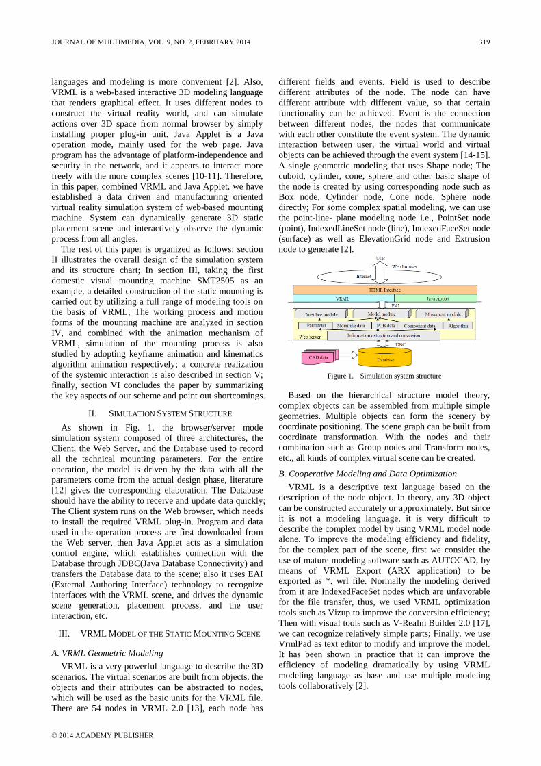
languages and modeling is more convenient [2]. Also,

VRML is a web-based interactive 3D modeling language

that renders graphical effect. It uses different nodes to

construct the virtual reality world, and can simulate

actions over 3D space from normal browser by simply

installing proper plug-in unit. Java Applet is a Java

operation mode, mainly used for the web page. Java

program has the advantage of platform-independence and

security in the network, and it appears to interact more

freely with the more complex scenes [10-11]. Therefore,

in this paper, combined VRML and Java Applet, we have

established a data driven and manufacturing oriented

virtual reality simulation system of web-based mounting

machine. System can dynamically generate 3D static

placement scene and interactively observe the dynamic

process from all angles.

The rest of this paper is organized as follows: section

II illustrates the overall design of the simulation system

and its structure chart; In section III, taking the first

domestic visual mounting machine SMT2505 as an

example, a detailed construction of the static mounting is

carried out by utilizing a full range of modeling tools on

the basis of VRML; The working process and motion

forms of the mounting machine are analyzed in section

IV, and combined with the animation mechanism of

VRML, simulation of the mounting process is also

studied by adopting keyframe animation and kinematics

algorithm animation respectively; a concrete realization

of the systemic interaction is also described in section V;

finally, section VI concludes the paper by summarizing

the key aspects of our scheme and point out shortcomings.

II. SIMULATION SYSTEM STRUCTURE

As shown in Fig. 1, the browser/server mode

simulation system composed of three architectures, the

Client, the Web Server, and the Database used to record

all the technical mounting parameters. For the entire

operation, the model is driven by the data with all the

parameters come from the actual design phase, literature

[12] gives the corresponding elaboration. The Database

should have the ability to receive and update data quickly;

The Client system runs on the Web browser, which needs

to install the required VRML plug-in. Program and data

used in the operation process are first downloaded from

the Web server, then Java Applet acts as a simulation

control engine, which establishes connection with the

Database through JDBC(Java Database Connectivity) and

transfers the Database data to the scene; also it uses EAI

(External Authoring Interface) technology to recognize

interfaces with the VRML scene, and drives the dynamic

scene generation, placement process, and the user

interaction, etc.

III. VRML MODEL OF THE STATIC MOUNTING SCENE

A. VRML Geometric Modeling

VRML is a very powerful language to describe the 3D

scenarios. The virtual scenarios are built from objects, the

objects and their attributes can be abstracted to nodes,

which will be used as the basic units for the VRML file.

There are 54 nodes in VRML 2.0 [13], each node has

different fields and events. Field is used to describe

different attributes of the node. The node can have

different attribute with different value, so that certain

functionality can be achieved. Event is the connection

between different nodes, the nodes that communicate

with each other constitute the event system. The dynamic

interaction between user, the virtual world and virtual

objects can be achieved through the event system [14-15].

A single geometric modeling that uses Shape node; The

cuboid, cylinder, cone, sphere and other basic shape of

the node is created by using corresponding node such as

Box node, Cylinder node, Cone node, Sphere node

directly; For some complex spatial modeling, we can use

the point-line- plane modeling node i.e., PointSet node

(point), IndexedLineSet node (line), IndexedFaceSet node

(surface) as well as ElevationGrid node and Extrusion

node to generate [2].

Figure 1. Simulation system structure

Based on the hierarchical structure model theory,

complex objects can be assembled from multiple simple

geometries. Multiple objects can form the scenery by

coordinate positioning. The scene graph can be built from

coordinate transformation. With the nodes and their

combination such as Group nodes and Transform nodes,

etc., all kinds of complex virtual scene can be created.

B. Cooperative Modeling and Data Optimization

VRML is a descriptive text language based on the

description of the node object. In theory, any 3D object

can be constructed accurately or approximately. But since

it is not a modeling language, it is very difficult to

describe the complex model by using VRML model node

alone. To improve the modeling efficiency and fidelity,

for the complex part of the scene, first we consider the

use of mature modeling software such as AUTOCAD, by

means of VRML Export (ARX application) to be

exported as *. wrl file. Normally the modeling derived

from it are IndexedFaceSet nodes which are unfavorable

for the file transfer, thus, we used VRML optimization

tools such as Vizup to improve the conversion efficiency;

Then with visual tools such as V-Realm Builder 2.0 [17],

we can recognize relatively simple parts; Finally, we use

VrmlPad as text editor to modify and improve the model.

It has been shown in practice that it can improve the

efficiency of modeling dramatically by using VRML

modeling language as base and use multiple modeling

tools collaboratively [2].



Figure 2. Internal hierarchical structure

C. Model Establishment

Currently mounting machine can be divided into four

types: boom, composite, turret and large parallel system.

Boom machine works on medium speed with high

precision that can support many different types of feeders

and its price is cheap, so it is especially suitable for multi-

variety, small batch production, thus this paper uses

boom for simulation research. Take the domestic first full

visual mounting machine SMT2505 [16] as an example,

it can identify different component by its visual system

and place Chip, IC, SOIC rapidly and accurately. The

placement accuracy, placement velocity and identify

capability have reached the international level.

1) Internal Model

Without loss of generality, we analyze and abstract the

internal hierarchical structure of the machine by

referencing the relevant documents for simplicity, as Fig.

2 shows. The basic elements of mounting machine can be

divided into three parts: robot parts, the X/Z positioning

system and other ancillary parts. Through gripper

attached on the robot head, the boom mounting conducts

a series of actions such as suction- shift-positioning-

placing, mounting the components quickly and accurately

to the PCB position.

The modeling of all different parts is mainly based on

the basic modeling nodes and stretch solid modeling

under AUTOCAD. Next we are going to discuss the

generation of main parts in detail.

(1) Robot parts: As the key component of mounting

machine, it includes base, robot head and other parts.

Through gripper attached on the robot head, the boom

mounting conducts a series of actions such as suction-

shift-positioning-placing, mounting the components

quickly and accurately to the PCB position. Base's

modeling uses two cuboids doing minus operation to

generate under AutoCAD [2], the rest parts use Box node,

Cylinder node assembly, the resulting model is shown in

Fig. 3 below.

Figure 3. Robot parts model

(2) Gripper: It is used for grapping components and

uses the Cylinder node assembly for regulation shape as

shown in Fig. 4.

Figure 4. Gripper: (a) physical, (b) model

(3) Gripper location: It is used for storage of gripper

and has no corresponding node and may be carried on

with rectangular and circular to do the boolean

calculation under AutoCAD to reform the stretch solid

modeling as shown in Fig. 5.

(4) Feeder: Components to be assembled are kept in

various component feeders around the PCB. The shape is

relatively complex and usually contains tape, waffle and

bulk etc. Material modeling mainly uses the Box node,

Cylinder node assembly completed is shown in Fig. 6.

Figure 5. Gripper location model

Figure 6. Feeder model

X and Z positioning system models use the elliptic

region stretching to convert under AutoCAD. PCB

transmission mechanism can be modeling with Cylinder

node, PCB board and the rack can be simplify modeling

with the Box node [18].

The whole scene generation depends on each

component space position relationship. Impose a

Cartesian coordinate system on the work area, with the

center of z positioning system z-track 1 representing the

origin, and other parts by translation, rotation, scaling and

other geometric transformations with Transform node

assembly together, the resulting model is shown in Fig. 7

(b) below.

Figure 7. SMT2505:(a) interior,(b) internal model



2) External Model

As shown in Fig. 8(a), the case of the mounting

machine can be grouped into three parts: operational

control, the shell itself and the display monitor based on

the structural features. Each of these three parts is made

up by corresponding components based on the structure

modeling principles. The geometric model of the

operational control part can be implemented by shifting,

rotating, shrinking and expanding the models of the

keyboard and electrical switch. The same can be applied

to the shell body and the display monitor geometric

models. The whole model of the outside part of mounting

machine is shown in Fig. 8(b) below.

Figure 8. SMT2505: (a) exterior,(b) external model

IV. DYNAMIC SIMULATION OF MOUNTING PROCESS

There are many methods for realization of the dynamic

simulation, such as key frame technology and kinematics

algorithm, etc. Key frame technology utilizes the

continuous play of the object movement for some key

frames specified path (a constant and orderly images) to

achieve animation effects. In VRML, a time sensor node

such as Time Sensor output clock drives various

interpolation and route changing some domain of

Transform node; Kinematics algorithm is determined by

kinematic equation of the object trajectory and rate,

without knowing its physical properties, that can be done

efficiently, In VRML, by means of the Script node

embedded JavaScript scripts, it can complete more

complex animation. Thus, according to mounting

machines work process definition, key frames or

derivation of kinematics equations is the basis and the

essential part of dynamic simulation [19]. The following

example analyzes the key steps.

A. Assembly Operation

The sequence of operations performed by such a pick-

and-place robot can be described as follows: the robot

head starts from its designated home location, moves to a

pickup slot location, then grabs a component, and moves

to the desired placement location, where the PCB is

assembled, and places it there. After placement, the robot

head moves to another pickup slot location to grab

another component and repeats the prior sequence of

operations. In case the components are not the same size,

robot also changes its gripper by moving to the gripper

location during the assembly operation. Also, finepitch

components are tested for proper pin alignment against an

upward-looking camera during their assembly. After

completing the assembly operation, the robot returns to

its home location, and waits for the next raw PCB to

arrive [20].

B. Key Frame Technology

Assumption: we need to mount three components

defined as 1, 2, 3 on PCB, which has been stored in

feeders respectively i.e., each feeder can contain one type

of components, two gripper defined as 1,2 placed in

gripper location, so, gripper1 mounts components 1,3,

gripper2 mounts components 2 in the order of 1-3-2, the

robot head starts from the home location, the movement

path is shown as in Fig. 9:

Figure 9. Movement path

Path 1: robot head moves to the gripper location, grabs

gripper 1;

Path 2: robot head moves to the feeder, gets

component 1;

Path 3: robot head moves to the desired placement

location where the PCB is assembled, and places it there;

Path 4: robot head moves to the gripper location, gets

component 3;



Path 6: robot head moves to the gripper location,

unloads gripper 1;

Path 7: robot head moves to the gripper location, grabs

gripper 2;

Path 8: robot head moves to the feeder, gets

component 2;



Path 10: robot head moves to the gripper location,

unloads gripper 2;

Path 11: robot returns to its home location.

Therefore, the action of robot head during the pick-

and-place operation can be described as follows:

Grabing gripper: in Y-direction moves down close to

the gripper then moves up to grab the gripper;

Unloading gripper: in Y-direction moves down to put

down the gripper then moves up;

Getting component: in Y-direction moves down close

to the component then moves up to get component;

Placing component: rotation around Y-axis and in Y-

direction moves down to place the component on the

PCB then moves up.

Based on the path described above and robot head

movements, the key frames (for simplicity, take the

simple model as the example) as shown in Fig. 10 can be

set to determine the coordinates of the location

throughout.



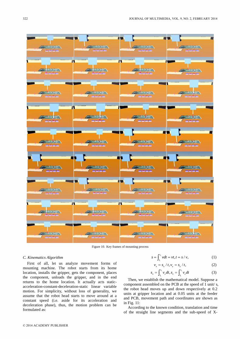
Figure 10. Key frames of mounting process

C. Kinematics Algorithm

First of all, let us analyze movement forms of

mounting machine. The robot starts from its home

location, installs the gripper, gets the component, places

the component, unloads the gripper, and in the end

returns to the home location. It actually acts static-

acceleration-constant-deceleration-static linear variable

motion. For simplicity, without loss of generality, we

assume that the robot head starts to move around at a

constant speed (i.e. aside for its acceleration and

deceleration phase), thus, the motion problem can be

formulated as:

2

1

, / ,t

ts vdt vt t s v (1)

/ , / ,x x z zv s t v s t (2)

2 2

1 1

,t t

x x z zt t

s v dt s v dt (3)

Then, we establish the mathematical model. Suppose a

component assembled on the PCB at the speed of 1 unit/ s,

the robot head moves up and down respectively at 0.2

units at gripper location and at 0.05 units at the feeder

and PCB, movement path and coordinates are shown as

in Fig. 11:

According to the known condition, translation and time

of the straight line segments and the sub-speed of X-



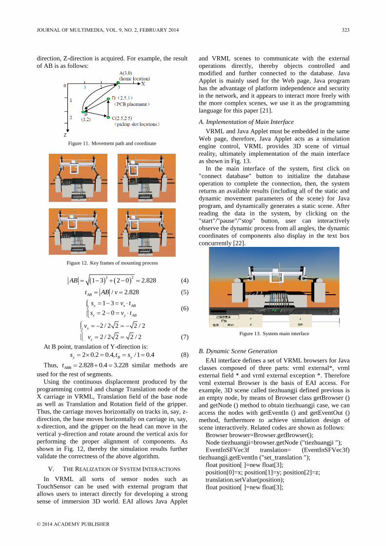
direction, Z-direction is acquired. For example, the result

of AB is as follows:

Figure 11. Movement path and coordinate

Figure 12. Key frames of mounting process

2 2

1 3 2 0 2.828AB (4)

/ 2.828ABt AB v (5)

1 3

2 0

x x AB

z y AB

s v t

s v t

(6)

2 / 2 2 2 / 2

2 / 2 2 2 / 2

x

z

v

v

(7)

At B point, translation of Y-direction is:

2 0.2 0.4, /1 0.4y B ys t s (8)

Thus, 2.828 0.4 3.228ABBt similar methods are

used for the rest of segments.

Using the continuous displacement produced by the

programming control and change Translation node of the

X carriage in VRML, Translation field of the base node

as well as Translation and Rotation field of the gripper.

Thus, the carriage moves horizontally on tracks in, say, z-

direction, the base moves horizontally on carriage in, say,

x-direction, and the gripper on the head can move in the

vertical y-direction and rotate around the vertical axis for

performing the proper alignment of components. As

shown in Fig. 12, thereby the simulation results further

validate the correctness of the above algorithm.

V. THE REALIZATION OF SYSTEM INTERACTIONS

In VRML all sorts of sensor nodes such as

TouchSensor can be used with external program that

allows users to interact directly for developing a strong

sense of immersion 3D world. EAI allows Java Applet

and VRML scenes to communicate with the external

operations directly, thereby objects controlled and

modified and further connected to the database. Java

Applet is mainly used for the Web page, Java program

has the advantage of platform independence and security

in the network, and it appears to interact more freely with

the more complex scenes, we use it as the programming

language for this paper [21].

A. Implementation of Main Interface

VRML and Java Applet must be embedded in the same

Web page, therefore, Java Applet acts as a simulation

engine control, VRML provides 3D scene of virtual

reality, ultimately implementation of the main interface

as shown in Fig. 13.

In the main interface of the system, first click on

"connect database" button to initialize the database

operation to complete the connection, then, the system

returns an available results (including all of the static and

dynamic movement parameters of the scene) for Java

program, and dynamically generates a static scene. After

reading the data in the system, by clicking on the

"start"/"pause"/"stop" button, user can interactively

observe the dynamic process from all angles, the dynamic

coordinates of components also display in the text box

concurrently [22].

Figure 13. System main interface

B. Dynamic Scene Generation

EAI interface defines a set of VRML browsers for Java

classes composed of three parts: vrml external*, vrml

external field * and vrml external exception *. Therefore

vrml external Browser is the basis of EAI access. For

example, 3D scene called tiezhuangji defined previous is

an empty node, by means of Browser class getBrowser ()

and getNode () method to obtain tiezhuangji case, we can

access the nodes with getEventIn () and getEventOut ()

method, furthermore to achieve simulation design of

scene interactively. Related codes are shown as follows:

Browser browser=Browser.getBrowser();

Node tiezhuangji=browser.getNode ("tiezhuangji ");

EventInSFVec3f translation= (EventInSFVec3f)

tiezhuangji.getEventIn ("set_translation ");

float position[ ]=new float[3];

position[0]=x; position[1]=y; position[2]=z;

translation.setValue(position);

float position[ ]=new float[3];



position=((EventOutSFVec3f)

(tiezhuanji.getEventOut("translation_changed"))).getValu

e();

…

VI. CONCLUSION

In this paper after the research of structure

characteristics and working principle of mounting

machine, we establish the network application with data

driven, manufacturing–oriented visualization simulation

system that can interactively, represent the whole mount

process. Detailed product design information added

would achieve manufacturability analysis and process

optimization to provide reference for the practical

production in further research.

ACKNOWLEDGMENT

This paper is supported in part by the technical support

of military electronic pre-research project, No.

415011005.

REFERENCES

[1] H. Koriyama and Y. Yazaki, "Virtual manufacturing system", International Symposium on Semiconductor Manufacturing, 2010, pp. 5-8.

[2] Lan Li, "Modeling and simulation of mounting machine based on VRML ", 2012 Fourth International Conference on Computational and Information Sciences, Chongqing.

[3] Shujuan Guo, "Optimization on component allocation between placement machines in surface mount technology assembly line", Computer Integrated Manufacturing Systems, 2009. 15(4), pp. 817-821.

[4] Peng Yuan, "Scatter searching algorithm for multi- headed surface mounter", Electronics Process Technology, 2007. 28(6), pp. 316-320.

[5] Yijing Hu, "Mounting optimization approaches of high-speed and high-precision surface mounting machines", Eiectronics Process Technoiogy, 2006. 27(4), pp. 191-194.

[6] Nanni Zhang, "3D simulation system for key devices in surface mounting technology production line", Computer Applications and Software, 2009. 26(2), pp. 55-57.

[7] Min Ma, "Visible simulation of the key equipment in PCB fabrication", Master's degree thesis, 2007.

[8] Xiao Guo, "Visual modeling and simulation of electronic circuit manufacturing equipment of PCB board level", Master's degree thesis, 2007.

[9] Bingheng Lai, "Study of paste to pack manchine simulation based on OpenGL", Master's degree thesis, 2007.

[10] Kotak, D. B. Fleetwood, M. Tamoto, H. Gruver, W. A. "Operational scheduling for rough mills using a virtual manufacturing environment", Systems, Man, and Cybernetics, 2011 IEEE International Conference.

[11] Zhe Xu, "VRML modeling and simulation of 6DOF AUV based on MATLAB", Journal of System Simulation, 2007. 19(10), pp. 2241-2243.

[12] Hong Chang, Qusheng Li, Xinzhi Zhu; Liang Chen, "Study of PCB recovered for the SMT module of electronic product VM", computer simulation. 2009, 20(1), pp. 109-111.

[13] Haifan Zhang, "According to the Simulink imitate with realistic and dynamic system of VR Toolbox conjecture really", Control & Automation, 2007. 23(28), pp. 212-214.

[14] Xiangping Liu, "Visual running simulation of railway vehicles based on Simulink and VRML", Railway Computer Application, 2009. 18(11), pp. 1-3.

[15] Kurmicz, W. "Internet-based virtual manufacturing: a verification tool for IC designs, Quality Electronic Design, 2000. ISQED 2000". Proceedings. IEEE 2000 First International Symposium, March 2000.

[16] Ames A L, Ndaeau D R, Moreland J L. VRML 2. 0 Sourcebook. [S.1.]: John Wiley & Sons, Inc., 1997.

[17] M. sadiq, T. L. Landers, and G. D. Taylor, "A heuristic algorithm for minimizing total production time for a sequence of jobs on a suferace mount placement machine", Int. J. Productions Res, vol. 31, 1998. pp. 1327-1341

[18] Swee M. Mok, Chi-haur Wu, and D. T. Lee, "Modeling automatic assembly and disassembly operations for virtual manufacturing", IEEE Transactions on System, 2004.

[19] Sihai Zheng, Layuan Li, Yong Li, "A qoS routing protocol for mobile Ad Hoc networks based on multipath", Journal of Networks, 2012. 7(4), pp. 691-698.

[20] Ratnesh Kumar and Haomin Li, "Assembly Time Optimization for PCB Assembly", Proceedings of the American Control Conference altmore, 1994, pp. 306-310

[21] Xiaobo Wang, Xianwei Zhou, Junde Song, "Hypergraph based model and architecture for planet surface Networks and Orbit Access", Journal of Networks, 2012. 7(4), pp. 723-729.

[22] F. Larue, M. D. Benedetto, M. Dellepiane, and R. Scopigno, "From the digitization of cultural artifacts to the Web publishing of digital 3D collections: an Automatic Pipeline for Knowledge Sharing", Journal of multimedia, 2012. 7(2), pp. 132-144.

Lan Li, is a lecturer of ShanXi Normal University, China. She

received her B.S. degree in Computer Science from Southwest

Jiaotong University and her M.S. degree in Computer Science

from Xidian University in 2003. Her current research interests

include virtual reality and multimedia technology.



Improved Extraction Algorithm of Outside

Dividing Lines in Watershed Segmentation Based

on PSO Algorithm for Froth Image of Coal

Flotation

Mu-ling TIAN Institute of Mechatronics Engineering, College of Electrical and Power Engineering, Taiyuan University of Technology,

Taiyuan, China


Jie-ming Yang Institute of Mechatronics Engineering Taiyuan University of Technology, Taiyuan, China


Abstract—It is difficult to exact accurate bubble size and to

make image recognition more reliable for forth image of

coal floatation because of low contrast and blurry edges in

froth image. An improved method of getting outside

dividing lines in watershed segmentation was proposed. In

binarization image processing, threshold was optimized

applying particle swarm optimization

algorithm(PSO)combining with 2-D maximum entropy

based gray level co-occurrence matrix. After distance

transform, outside dividing lines have been exacted by

watershed segmentation. By comparison with Otsu method,

the segmentation results have shown that the gotten external

watershed markers are relatively accurate, reasonable.

More importantly, under segmentation and over

segmentation were avoided using the improved method. So

it can be proved that extraction algorithm of outside

dividing lines based on PSO is effective in image

segmentation.

Index Terms—Froth Image in Coal Floatation; Threshold

Optimization; Particle Swarm Optimization Algorithm; On-

Class Variance Maximum Otsu Method; Distance

Transform; Image Segmentation

I. INTRODUCTION

Because flotation indexes have the extremely strong

correlation, accurate extraction of bubble in flotation

image becomes the key. In general, size characteristic of

the bubble will be obtained by watershed segmentation

for froth image. Watershed segmentation is a method of

image segmentation based on region .With fast, efficient,

accurate segmentation results, watershed segmentation

way has be pay attention to by more and more people.

Because the traditional watershed segmentation is easily

affected by the noise and the image texture details, small

basin formed by noise and small details are segmented by

error [1], This can lead to over-segmentation. On the

contrary, for the low contrast images, under-segmentation

can form because image edge is not clear [2]. In order to

solve this problem, people use the two methods mainly.

The first kind is to preprocess the image by filter; the

second kind is to use watershed segmentation algorithm

based on marker extraction. In addition, the fuzzy C-

means clustering algorithm is applied to solve over-

segmentation by merging segmentation results [3] [4].

Considering that froth images of coal flotation are

collected in floatation factory, gray distribution is

concentrated, there is low contrast in background and

foreground and bubble edges in images are blurry [5]. As

a consequence, it is difficult to segment bubbles. To solve

this problem, the marked watershed is often adopted. In

addition to the internal identifier, outside segmentation

lines should be extracted. There are several kinds of

extraction algorithm of outside segmentation lines. The

extraction way of outside dividing lines is based on

binary image processing in this paper. When gray level

image was converted into binary image, traditional

threshold selection method by one-dimensional histogram

is often used in binary image segmentation. This kind of

methods is simple and effective to implement. Its

concrete step is to make a one-dimensional histogram for

a gray image, namely, gray statistic information of the

image, and then to find the lowest valley in double peak,

which is often considered the image segmentation

threshold. The principle of this method is based on the

two gray mountains are composed from foreground and

background gray values of a image and target and

background could be separated if separating the image at

the low point of the two peaks. However, due to the

impact of lighting and other reasons, sometimes obvious

wave crests and troughs don’t appear in the one-

dimensional histogram. So it is unable to realize only to

use the gray distribution to obtain the threshold. In

addition, there are many methods for threshold selection

in binary image segmentation, such as on-class variance



maximum Otsu, the method of minimum error, the

method of maximum entropy and so on. The method of

Otsu threshold segmentation is a kind of segmentation

methods based on maximum on-class variance of

histogram, in which a threshold will be gotten to make

the on-class variance maximum. In the method of

maximum entropy, a threshold will be gotten to make the

information entropy of the two kinds of distribution of

target and background maximum. The method of

maximum entropy includes one-dimensional and two-

dimensional maximum entropy method. One-dimensional

maximum entropy method depends only on the gray level

histogram of image; only considers the statistical

information of the gray of image itself, ignoring the other

pertinent information. So it is not accurate to segment

image with much noise by the gotten threshold. Two-

dimensional maximum entropy method, which not only

uses the gray information of image pixels, and fully

considers the pixel and its spatial correlation information

within the neighborhood, is suitable for all of SNR image,

and can produce better image segmentation effect. So it is

a kind of threshold selection methods with very high

practical value. It will produce good effect to segment an

image by the gotten threshold using the maximum

entropy method of 2-D gray histogram as the objective

function [6] [7] [8] [9].

Different from the commonly used method of

extracting outside dividing lines in watershed

segmentation, an improved algorithm has been proposed

in this paper.

1) Using optimized threshold by particle swarm

optimization algorithm, transform a gray image into a

binary image. Multi-threshold segmentation can make

froth image undistorted and satisfied segmentation effect.

Considering that particle swarm optimization algorithm

not only has strong searching ability and ideal

convergence but also code by real, it is more efficient to

find threshold ( , )s t which make the two-dimensional

entropy maximum. The linearly decreasing weight (LDW)

strategy more is adopted in PSO algorithm.

2) Use two dimensional-maximum entropy based on

the gray level co-occurrence matrix as the fitness function

of optimize algorithm. In binary image process, threshold

selection is one of the most a key problem. In fact, it

plays a decisive role in image segmentation in keeping

quality of image segmentation and integrity. Because

there is low contrast in froth image and bubble edges are

blur, no matter threshold method based on the histogram

or OTSU method are not suitable for threshold selection.

The double-threshold way based on two dimensional-

maximum entropy can keep bubble original appearance

and make character extraction more accurate. Gray level

co-occurrence matrix contains obvious physical meaning

and is simpler and timesaving compared with two-

dimensional histogram matrix based on gray mean. So

two dimensional-maximum entropy based on the gray

level co-occurrence matrix has been proposed as the

fitness function of optimize algorithm in this paper.

3) Segment distance image transformed by binary

image using watershed segmentation algorithm and

obtain outside segment lines. In common, there are

several kinds of extraction algorithm for outside

segmentation line. But in view of froth image

particularity that under segmentation is caused easily

because of bubble adhesion, the method to segment

distance image formed by binary image was applied in

extracting outside segment lines. Combining internal

marker, the gradient image can be segmented by

watershed accurately.

II. PROPOSED ALGORITHM OF EXTRACTING OUTSIDE

SEGMENTATION LINES

A. The Segmentation Method of Image Based on 2-D

Maximum Entropy

1. Two-dimensional histogram

The definition of two-dimensional histogram: Two-

dimensional histogram 1 2( , )Num G G refers a frequency

that level of a pixel is 1G , and mean value of gray of its

neighborhood or the gray of its adjacent points in

different direction is 2G .

Suppose that ( , )f x y is an image with the 256 gray

levels, and ( , )g x y is the average image of adjacent gray

of ( , )x y or the neighborhood image of left (right) of

( , )x y . So two-dimensional histogram 1 2( , )Num G G

can be expressed as

1 2 1 2

1 2

( , , {{ ( , )

} { ( , ) }

Num G G G G Num f x y

G g x y G

(1)

2. Two-dimensional histogram based on gray level co-

occurrence matrix

Two-dimensional histogram usually means as the

following two kinds, the gray of current point of image as

the abscissa, gray mean value of the neighborhood or the

gray of adjacent point in different directions as ordinate,

such as the adjacent points on left or right or up or down.

In general, the included information of adjacent point on

the left and up direction is less clear and important than

one of adjacent point on the right and down direction [10]

[11].

The combined frequency of gray of image and gray of

the corresponding right neighborhood point was selected

as the two-dimensional histogram. Suppose that

[ ( , )]M NF f x y is original image matrix, ( , )f x y is

gray value of coordinate ( , )x y , M N refers the size of

the image. Define that transfer matrix [ ]ij M NW n of

L L dimension is used to represent two-dimensional

histogram. Among these, ijn means the number that the

gray of current pixel is i and the gray of its right

neighborhood point is j . It can be expressed as the

following representation [12].

1 1

( , )M N

ij

l k

n l k

1, ( , ) ( , 1)

( , )0,

f l k i and f l k jl k

otherwise

(2)



http://www.iciba.com/frequency

The combined frequency ijp is expressed as the

following representation.

/ij ijp n M N (3)

From the above significance, two-dimensional

histogram based on the pixel in the right neighborhood

means the same as gray level co-occurrence matrix. So it

can be directly calculated using the gray level co-

occurrence matrix. In contrast, it is more troublesome,

time-consuming to compute two-dimensional histogram

based on gray mean value of the neighborhood in the

right neighborhood. For example, for a froth image with

size of 512x512, time to calculate two-dimensional

histogram matrix based on gray mean is 201s; but time to

calculate two-dimensional histogram matrix based on

gray level co-occurrence matrix is 0.172s.

Besides these, because of the application in adjacent

point, two-dimensional histogram based on the pixel in

the right neighborhood contains obvious physical

meaning and represents the gray transfer of image and

change. It is obvious that two-dimensional histogram

matrix based on gray level co-occurrence matrix is

simpler and timesaving.

Figure 1. The two-dimensional histogram matrix of image

3. The physical significance of two-dimensional

histogram

The graph of definition and constraint domain of two-

dimensional histogram is shown as the followings. The

abscissa ( , )f x y is gray value at ( , )x y scale, and the

ordinate ( , )g x y gray value at the right neighborhood of

( , )x y , vector ( , )s t is segmentation threshold of image,

by which the graph is divided into four districts, namely

A, B, C and D respectively, shown below. From the

shown components of histogram matrix, compared with

elements in quadrant B and D, elements in quadrant A

and C mean that the pixel gray value in the original image

is less different than and gray value of its right

neighborhood. The characteristic is close to the properties

of internal elements in target or background. If the object

is dark, A is the object area and C is the background. The

bright object, and vice versa. For general images, most

pixels fall within the object region and background region

and are concentrated on diagonal in two areas because

gray level changes are relatively flat [13]. It is to say that

the numbers of two-dimensional histogram matrix of

image along the diagonal are large obviously, result as

figure 2.Compared with elements in quadrant A and C,

the elements in quadrant B and D mean that the pixel

gray value in original image is different from gray value

of its right neighborhood. The characteristic is close to

formation characteristics of the edge and noise, and so C

and D can be taken as the edge and noise area.

Figure 2. The sketch map of two-dimensional histogram

3. 2-D entropy function

In the image histogram matrix, supposing that the

threshold vector is ( , )s t , region entropies of A, B, C, D

were obtained by the definition of two-dimensional

entropy as the followings.

0 0

( ) ( / ) log( / ) log /s t

ij A ij A A A A

i j

H A p P p P P H P

(4)

1

1 0

( ) ( / ) log( / ) log /L t

ij B ij B B B B

i s j

H B p P p P P H P

(5)

1 1

1 1

( ) ( / ) log( / ) log /L L

ij C ij C C C C

i s j t

H C p P p P P H P

(6)

1

0 1

( ) ( / ) log( / ) log /s L

ij D ij D D D D

i j t

H D p P p P P H P

(7)

Among them:

0 0

s t

A ij

i j

P p

1

1 0

L t

B ij

i s j

P p

1 1

1 1

L L

C ij

i s j t

P p

1

0 1

s L

D ij

i j t

P p

0 0

logs t

A ij ij

i j

H p p

1

1 0

logL t

B ij ij

i s j

H p p

1 1

1 1

logL L

C ij ij

i s j t

H p p

1

0 1

logs L

D ij ij

i j t

H p p

Determination functions of entropy include local

entropy, joint entropy and the global entropy, and then

determinations are shown respectively.

Local entropy:

( ) ( )LEH H A H C (8)

Joint entropy:

( ) ( )JEH H B H D (9)

Global entropy:



GE LE JEH H H (10)

B. Particle Swarm Algorithm

Particle swarm optimization (Particle Swarm

Optimization, PSO) is an evolutionary computation

technique [14] [15], which was put forward by Dr.

Eberhart and Dr. Kennedy in 1995. PSO algorithm came

from the study of prey behavior of birds and is an

optimization tool based on iteration. The basic purpose of

PSO algorithm is to find the optimal solution through

group collaboration between individual and social

information sharing.

In PSO algorithm, a bird is abstracted as particle

without mass and volume (point), whose position vector

is 1 2( , , , )i nX x x x , whose flight velocity vector I

1 2( , , )i nV v v v . Expressed as 1 2( , , , )i i i iDx x x x ,

each particle's search space is D dimension.

Correspondingly, the particle velocity vector is

1 2( , , , )i i i iDv v v v , which is used to determine the

direction and distance of particles flying. Each particle

has a fitness decided by objective function. Fitness value

is standard which is used to measure pros and cons of

each particle in the whole group of. In addition, each

particle don’t know itself best position (pbest) so far and

all the particles group experienced the best location

(gbest). gbest is the optimal value in pbest. Whether it is

pbest or gbest, evaluation is based on the fitness value.

PSO algorithm is a process in which the particles follow

the two extreme value pbest and gbest to update itself

constantly in order to find the optimal solution of the

problem. This algorithm has been widely used in the

domain of function optimization, image processing,

mechanical design, communication, robot path planning

and has achieved good results.

1

1

2

() ( )

() ( )

k k k

i i i

k

i

v v c rand pbest x

c rand gbest x

(11)

1 1K k k

i i ix x v (12)

Among them, 1, 2, ,i M , M is the total number

of particles in the group; iv is the speed of the particle;

pbest and gbest are as defined earlier; is called inertia

factor; k

ix is the current position of the particle; 1c and

2c is the learning factor; rand() is a random number

between 0 and1.

From a sociological perspective, in (11), the first part

is called inertia, which refers the ability to maintain their

original velocity and direction; second part is called

cognitive particle, which is about his "learning" for own

experiences and means that the particle movement is

originated from their own experience component; the

third part is called social cognition, which is the vector

from current a pointer to the best point of population and

reflects the collaboration and knowledge sharing between

particles. The particle is to decide the next step of

movement just through the own experience and best

experience of peers.

1. The advantages of particle swarm algorithm in

threshold optimization of image segmentation

From the original segmentation process of image by

two dimensional threshold, its essence is to search a set of

optimal solutions ( , )s t to make two dimensional entropy

maximum in two dimensional reference space of attribute

formed by the gray values of pixels and the gray values in

their neighborhood. As the dimensions increase, the

amount of calculation of this threshold algorithm will

become larger, time-consuming. It not only reduces the

complexity of the algorithm, not only meets the real-time

requirements applying particle swarm algorithm in

searching the optimal threshold by two dimensional

threshold algorithm [16]. In image processing, including

image segmentation, many people use the genetic,

immune and other stochastic optimization algorithm to

find the target value, and get good effect in [17] [18].

Considering that there are many parameters to be set in

these algorithms and set is quite different for different

image parameters, this will lead to considerable

differences in treatment effect. Compared with the

genetic, immune optimization algorithm, particle swarm

algorithm can code applying real directly with less

parameters and fast convergence speed. Accordingly, this

algorithm is not only simple and easy but also can reduce

the dimension of population. With respect to genetic,

immune algorithm, there are no crossover and mutation

operations in PSO algorithm and the particle is updated

through the internal velocity. Especially in threshold

selection of image segmentation, PSO algorithm can

realize threshold optimization effectively while

combining with 2-D maximum entropy algorithm

because is real not binary code. With fast convergence

speed, PSO algorithm has the incomparable advantages

with other algorithm and makes threshold selection

simpler, more efficient.

2. Threshold optimization process of image

segmentation based particle swarm algorithm

1) Initializing population. Set the population size N,

the dimension of each particle D . Form randomly N

particles, the position (0, 1)L , velocity ( 1,2, )iv i N ,

and interval max max[ , ]v v . Among them, L is the gray

level of image.

2) According to 2D entropy formula (8), calculate the

fitness value of each particle.

3) For each particle, determine its best location the

pbest and the current global best position gbest; the initial

pbest of each particle is initial value of each particle, the

initial gbest value is maximum value of pbest for all

particles.

4) According to (11) and (12), adjust particle velocity

and position.

5) Calculate new fitness for each particle and update

fitness.

6) For each particle, compare current fitness with that

of the best position pbest, if better, the best pbest's is

current position; find the fitness maximum of all pbest,

and update gbest;



7) Whether the end condition (enough good fitness

values or reaching maxiter ) has been realized. If the end

condition hasn’t been reached, turn 4). If reached, gbest is

the optimal solution.

3. Fitness function selection in particle swarm

algorithm

Because PSO algorithm is a process to obtain the

optimal solutions to the problems by searching the best

fitness value using continuous iteration, the selection of

the fitness function is the soul of PSO algorithm.

According to the maximum entropy principle, the

threshold ( , )s t is the value which will make two-

dimensional entropy maximum. Here, the local entropy

( ) ( )LEH H A H C will be adopted as criterion of

threshold selection of image segmentation, namely,

( , ) max( )LEs t Arg H . The binary image which was

segmented using two-dimensional vector ( , )s t is

, ( , )s tf x y , and it was expressed as the formula (13).

,

0, ( , ) ( , )( , )

1, ( , ) ( , )s t

when f x y s and g x y tf x y

when f x y s or g x y t

(13)

4. The parameter selection of particle swarm algorithm

1) Population size M: The larger population scale is,

the higher searching capability of the algorithm is. But

this is at a cost of large amount of calculation. For the

specific issues, a suitable size should be found, generally

from 20 to 40. If problem is more complex and specific,

population size may be increased appropriately, here,

20M .

2) Particle dimension D : In binary image process,

threshold optimization means to find threshold ( , )s t

which make the two-dimensional entropy maximum

threshold, so, 2D .

3) Maximum speed: Maximum limit speed in each

particle reflects the particle search accuracy, namely

resolution between the current position and the best

position. If too fast, particle may be over the extreme

point; if too slow, particle can’t search outside the local

extreme point so as to fall into the local extreme area. If

velocity in some dimension exceeds the set value, it is

defined as maxv (

max 0v ). Here the maximum speed

maxv is 4, namely, speed range [ 4,4] .

4) Inertia factor : can keep the particle motion

inertia, it has the trend of searching space, and has the

ability to explore new areas. If is larger, it will has

strong global searching, but its local search ability is

weak; If is smaller, its local search ability is strong. At

present, the linearly decreasing weight (LDW) strategy

more is adopted mostly. That is

max max min max[( ) / ]iter iter (14)

Among them, max and min is the maximum and

minimum value of ; iter and maxiter are the current

iteration number and the maximum iteration number.

Typical values: max 0.9 ,

min 0.4 . Here,

max 0.95 , min 0.4 .

5) Acceleration coefficient 1c and

2c : 1c and

2c are

weights which adjust each particle moving to the Pbest

and gbest [19]. Lower values allow particles wandering

outside the target region before they are drawn back.

Higher values will make particle suddenly rush or cross

the target area. Learning factors is to adjust role and

weight of own experience and social (Group) experience

of particle in its movement. If 1 0c , it means that

particle had it experience, but had only the social

experience (social-only). As a consequence, its speed of

convergence may be faster and but it can fall local optima

in dealing with complex problems. If 2 0c , it means

that particle had itself group information, but had own

experience because there is no interaction between

individuals. In general, set 1 22, 2c c . When

1c and

2c are constants, a better solution can be gotten, but not

necessarily equal to 2. Here choose 1 22, 2c c .

6) The iteration termination condition: According to

the specific problems, set the conditions for the

termination that the maximum number of iterations

maxiter is has reached or particle swarm optimal position

has meet predetermined expectations. Here choose

max 50iter . The iteration termination condition: the

maximum number of iterations has reached maxiter or

average fitness groups of two successive generations is

less than or equal to 0.0001.

C. Distance Transformation of Binary Image

Distance transformation is a kind of operations to

transform a binary image into a grayscale image.

Distance transformation refers to each pixel into distance

between it and the nearest nonzero pixel in the image.

Finally transformed target image is grayscale using

distance representation.

For a binary image with a size of M N , a set of the

target pixels in image [ ]ijA f is expressed as

{( , ) | 1}xyM x y f , and a set of background pixels

regions is expressed as {( , ) | 0}xyB x y f . Distance

transform is to get the shortest distance between pixels in

background region pixel and target points. The gotten

image is [ ]ijD a after distance transformation, its

expression is

( , )min [( , ), ( , )]ijx y M

d D i j x y

(15)

1. Euclidean Distance

Distance transformation includes many kinds of

transformation methods, such as Euclidean distance, a

chessboard distance transform, and block distance

transform and so on. Euclidean distance transform is one

of the used most commonly. Euclidean distance

transform is a kind of accurate two norm nonlinear

distance transform, which has been applied different



fields in image processing. It can be expressed as

[( , ),( , )]D i j x y .

2 2[( , ), ( , )] i- ( )D i j x y x j y （） (16)

III. EXPERIMENTAL RESULTS AND ANALYSIS

A. The Simulation Results of External Segmentation Lines

Based on Watershed Wegmentation

In this paper, the experimental platform was Microsoft

Windows XP Professional system, CPU of Intel Core,

main frequency of 1.86GHz, RAM of 1GB. Matlab

R2007 was used as processing software. For the image

acquired by CCD industrial camera in coal flotation

factory whose size is 512×512. In order to make the

image more clear and real it was processed by

morphological de-noising and enhancement processing,

and processed image was shown as figure 3.The image

was segmented by two kinds of threshold selection,

namely Otsu and PSO respectively.

1. Otsu method

After gray image was segmented by automatic single

threshold segmentation of on-class variance maximum

method (Otsu), the gotten threshold is 119. Firstly,

binaryzation image was obtained through threshold

segmentation and the binary image was shown as figure 4.

Secondly, the binary image was transformed by

Euclidean distance transform. Finally, external tag can be

gotten using watershed segmentation, as shown in figure

5, the image superimposed by outside dividing lines as

shown in figure 6.

2. PSO method

The gray image was segmented by double threshold

particle using swarm optimization algorithm which took

2-D maximum local entropy segmentation method of

local entropy ( ) ( )LEH H A H C as the fitness function.

After 20 times running, the algorithm converged at 35th

generation averagely, functional relation between average

fitness value and the iteration as shown in figure 7. The

obtained average optimal threshold of 20 times is

(113,112). Firstly, binaryzation image was obtained

through threshold segmentation and the binary image was

shown as figure 8. Secondly, the binary image was

transformed by Euclidean distance transform. Finally,

external tag can be gotten using watershed segmentation,

as shown in figure 9, the image superimposed by outside

dividing lines as shown in figure 10. 原图像

Figure 3. Original froth image of coal flotation

OSTU二值图像

Figure 4. The binary image by Otsu

OSTU外部分割线

Figure 5. External tag gotten by Otsu using watershed segmentation

OSTU分割边界与原图叠加图

Figure 6. The image superimposed by outside dividing lines of Otsu

PSO二值图像

Figure 7. The binary image by PSO



PSO外部分割线

Figure 8. External tag gotten by PSO using watershed segmentation

PSO分割边界与原图叠加图

Figure 9. The image superimposed by outside dividing lines of PSO

0 5 10 15 20 25 30 3514

14.2

14.4

14.6

14.8

15

15.2

15.4

15.6

15.8

16

Figure 10. Functional relation between average fitness value and the iteration

B. Analysis and Conclusion

The experiment indicated that watershed ridge lines

seriously deviated from the bubble edge lines when the

binary image which was obtained using automatic single

threshold segmentation based on on-class variance

maximum Otsu was segmented by watershed after

distance transform. By comparison, when the binary

image which was obtained by optimal double thresholds

using the particle swarm algorithm was segmented by

watershed after distance transform, image segmentation is

not only has the most ideal effect, but also greatly reduce

the computational time. More important, the gotten

external watershed ridge markers are relatively accurate,

reasonable, and can accurately distinguish each bubble in

the forth image. As a result this avoids under

segmentation and over segmentation; in the meanwhile,

this created favorable conditions for the feature extraction

in bubble size of flotation image. Especially, the feature

extraction based on binary image by PSO can greatly

improve accuracy in image recognition. So it can be

proved that PSO algorithm for threshold selection of

image binaryzation is a kind of effective method.

ACKNOWLEDGEMENTS

Thanks for the support of Special Research Fund of

Doctoral Tutor Categories of Doctoral Program in higher

education (20111402110010) and Shanxi Science and

Technology Program (20120321004-03) Shanxi Science

and Technology Program (20110321005-07).

REFERENCES

[1] Zhang Guoying, Zhu Hong, XuNing, “Flotation bubble

image segmentation based on seed region boundary

growing”, Mining Science and Technology, 21(12) pp.

239–242, 2011.

[2] Shao Jianbin, Chen Gang, “bubble segmentation of image

based on watershed algorithm”, Journal of Xi'an University

of technology, 27 (2) pp. 185 – 189, 2011.

[3] Gong may, YaoYumin, “improved fuzzy clustering image

segmentation based on watershed”, Application Research

of Computers, Vol. 28, No. 12, pp. 4773–4775, Dec. 2011.

[4] Gao Jinyong, Tang Hongmei, “an image segmentation

algorithm based on improved PSO and FCM”, Journal Of

Hebei University Of Technology, Vol. 40, No. 6, pp. 6– 10,

December 2011.

[5] Yang Jieming, Yang Dandan, “a segmentation method of

flotation froth image based improved watershed algorithm”,

Coal Preparation Technology, No. 5, pp. 82–85, Oct. 2012.

[6] Chen Guo, Zuo Hongfu, “Genetic algorithm image

segmentation of the two-dimensional maximum entropy”,

Journal of computer aided design and graphics, 16(4), pp.

530–534, 2002.

[7] Pun T. A, “new method for gray level picture threshold

using the entropy of histogram”, Signal Processing, 2(3),

pp. 223–237. 1980.

[8] Kapur J N, Sahoo P K, Wong A K C, “A new method for

gray level picture threshold using the entropy of the

histogram”, ComputerVision, Graphics and Image

Processing, 29(3), pp. 273–285. 1985.

[9] Yang Haifeng, Hou Zhaozhen, Image, “segmentation using

ant colony based on 2D gray histogram” Laser and Infra.,

35(8), pp. 614-617, 2005.

[10] Nikhil R. Pal, Sankar K. Pal, “Entropic thresholding”,

Signal Processing, 16, pp. 97–108, 1989.

[11] Li Na, Li Yuanxiang, “image segmentation by two-

dimensional threshold based on adaptive particle swarm

algorithm and data field”, Journal of Computer Aided

Design Computer Graphics, Vol. 24, No. 5, pp. 628–635,

May 2012.

[12] Gu Peng, Zhang Yu, “improved segmentation algorithm

for infrared image by two dimensional Otsu”, Journal of

Image and Graphics, Vol. 16, No. 8, pp. 1425–1428, Aug.

2011.

[13] Wang Dong, Zhu Ming, “The improved threshold

segmentation method based on 2D entropy in low contrast

image”, Chinese Journal of scientific instrument, vol. 25,

No. 4 Suppl., pp. 356–357, 2004.



[14] Kennedy J, Eberhant R, “Particle Swarm Optimization”,

Proceedings of the IEEE International Conference on

Neural Networks, 1942–1948, 1995.

[15] Eberhant R, Kennedy J, “A New Optimizer Using Particle

Swarm Theory”, Proceedings of the 6th International

Symposium on MicroMachine and Human Science, pp. 39–

43. 1995.

[16] Huang Hong, Li Jun, Pan Jingui, “The two dimensional

Otsu fast image segmentation algorithm based on particle

swarm optimization method”, Journal of Image and

Graphics, Vo. l 16, No. 3, pp. 377–381, 2011.

[17] Yue Zhenjun, Qiu Wangcheng, Liu Chunlin, “An adaptive

image segmentation method for targets”, Chinese Journal

of image and graphics, 9 (6), pp. 674–678, 2004.

[18] Yin Chunfang, Li Zhengming, “Application of a hybrid

genetic algorithm in image segmentation”, Computer

Simulation, 21 (8), pp. 158–160, 2004.

[19] Peiyi Zhu, Weili Xiong, et al., “D-S Theory Based on an

Improved PSO for Data Fusion”, Journal Of Networks,

VOL. 7, NO. 2, pp. 370–376, February 2012.

Muling Tian, female, born in 1969, in

Taiyuan, Shanxi Province, China. A Ph.D

candidate in Institute of Mechatronics

Engineering, Taiyuan University of

Technology. Received the bachelor's

degree in Electronic and master's degree

in mechatronic engineering from Taiyuan

University of Technology.

She is a teacher in College of

Electrical and Power Engineering, Taiyuan University of

Technology. Her main interest is focus on the image processing

and automatic control.

Jieming Yang, female, born in 1956 in Taiyuan, Shanxi

Province, China. Received the PhD degree in Mechatronics

Engineering from Taiyuan University of Technology.

She is a Professor in Taiyuan University of Technology .Her

research interest covers image processing, automatic monitoring

and control and fault diagnosis. She has hosted several

provincial projects. More than 30 academic articles are

published and there are more than ten papers cited by EI.



http://www.iciba.com/bachelor's_degree

http://www.iciba.com/bachelor's_degree

Instructions for Authors

Manuscript Submission All paper submissions will be handled electronically in EDAS via the JMM Submission Page (URL: http://edas.info/newPaper.php?c=7325). After

login EDAS, you will first register the paper. Afterwards, you will be able to add authors and submit the manuscript (file). If you do not have an EDAS account, you can obtain one. Along with the submission, Authors should select up to 3 topics from the EDICS (URL: http://www.academypublisher.com/jmm/jmmedics.html

JMM invites original, previously unpublished, research papers, review, survey and tutorial papers, application papers, plus case studies, short research notes and letters, on both applied and theoretical aspects. Submission implies that the manuscript has not been published previously, and is not currently submitted for publication elsewhere. Submission also implies that the corresponding author has consent of all authors. Upon acceptance for publication transfer of copyright will be made to Academy Publisher, article submission implies author agreement with this policy. Manuscripts should be written in English. Paper submissions are accepted only in PDF. Other formats will not be accepted. Papers should be formatted into A4-size (8.27" x 11.69") pages, with main text of 10-point Times New Roman, in single-spaced two-column format. Authors are advised to follow the format of the final version at this stage. All the papers, except survey, should ideally not exceed 12,000 words (14 pages) in length. Whenever applicable, submissions must include the following elements: title, authors, affiliations, contacts, abstract, index terms, introduction, main text, conclusions, appendixes, acknowledgement, references, and biographies.

), and clearly state them during the registration of the submission.

Conference Version

Submissions previously published in conference proceedings are eligible for consideration provided that the author informs the Editors at the time of submission and that the submission has undergone substantial revision. In the new submission, authors are required to cite the previous publication and very clearly indicate how the new submission offers substantively novel or different contributions beyond those of the previously published work. The appropriate way to indicate that your paper has been revised substantially is for the new paper to have a new title. Author should supply a copy of the previous version to the Editor, and provide a brief description of the differences between the submitted manuscript and the previous version.

If the authors provide a previously published conference submission, Editors will check the submission to determine whether there has been sufficient new material added to warrant publication in the Journal. The Academy Publisher’s guidelines are that the submission should contain a significant amount of new material, that is, material that has not been published elsewhere. New results are not required; however, the submission should contain expansions of key ideas, examples, elaborations, and so on, of the conference submission. The paper submitting to the journal should differ from the previously published material by at least 30 percent.

Review Process

Submissions are accepted for review with the understanding that the same work has been neither submitted to, nor published in, another publication. Concurrent submission to other publications will result in immediate rejection of the submission.

All manuscripts will be subject to a well established, fair, unbiased peer review and refereeing procedure, and are considered on the basis of their significance, novelty and usefulness to the Journals readership. The reviewing structure will always ensure the anonymity of the referees. The review output will be one of the following decisions: Accept, Accept with minor changes, Accept with major changes, or Reject.

The review process may take approximately three months to be completed. Should authors be requested by the editor to revise the text, the revised version should be submitted within three months for a major revision or one month for a minor revision. Authors who need more time are kindly requested to contact the Editor. The Editor reserves the right to reject a paper if it does not meet the aims and scope of the journal, it is not technically sound, it is not revised satisfactorily, or if it is inadequate in presentation. Revised and Final Version Submission

Revised version should follow the same requirements as for the final version to format the paper, plus a short summary about the modifications authors have made and author's response to reviewer's comments.

Authors are requested to use the Academy Publisher Journal Style for preparing the final camera-ready version. A template in PDF and an MS word template can be downloaded from the web site. Authors are requested to strictly follow the guidelines specified in the templates. Only PDF format is acceptable. The PDF document should be sent as an open file, i.e. without any data protection. Authors should submit their paper electronically through email to the Journal's submission address. Please always refer to the paper ID in the submissions and any further enquiries.

Please do not use the Adobe Acrobat PDFWriter to generate the PDF file. Use the Adobe Acrobat Distiller instead, which is contained in the same package as the Acrobat PDFWriter. Make sure that you have used Type 1 or True Type Fonts (check with the Acrobat Reader or Acrobat Writer by clicking on File>Document Properties>Fonts to see the list of fonts and their type used in the PDF document). Copyright

Submission of your paper to this journal implies that the paper is not under submission for publication elsewhere. Material which has been previously copyrighted, published, or accepted for publication will not be considered for publication in this journal. Submission of a manuscript is interpreted as a statement of certification that no part of the manuscript is copyrighted by any other publisher nor is under review by any other formal publication.

Submitted papers are assumed to contain no proprietary material unprotected by patent or patent application; responsibility for technical content and for protection of proprietary material rests solely with the author(s) and their organizations and is not the responsibility of the Academy Publisher or its editorial staff. The main author is responsible for ensuring that the article has been seen and approved by all the other authors. It is the responsibility of the author to obtain all necessary copyright release permissions for the use of any copyrighted materials in the manuscript prior to the submission. More information about permission request can be found at the web site.

Authors are asked to sign a warranty and copyright agreement upon acceptance of their manuscript, before the manuscript can be published. The Copyright Transfer Agreement can be downloaded from the web site. Publication Charges and Re-print

The author's company or institution will be requested to pay a flat publication fee of EUR 360 for an accepted manuscript regardless of the length of the paper. The page charges are mandatory. Authors are entitled to a 30% discount on the journal, which is EUR 100 per copy. Reprints of the paper can be ordered with a price of EUR 100 per 20 copies. An allowance of 50% discount may be granted for individuals without a host institution and from less developed countries, upon application. Such application however will be handled case by case.

More information is available on the web site at http://www.academypublisher.com/jmm/authorguide.html.

http://edas.info/newPaper.php?c=7325�

http://www.academypublisher.com/jmm/authorguide.html�

(Contents Continued from Back Cover)

Method of Batik Simulation Based on Interpolation Subdivisions

Jian Lv, Weijie Pan, and Zhenghong Liu

Research on Saliency Prior Based Image Processing Algorithm

Yin Zhouping and Zhang Hongmei

A Novel Target-Objected Visual Saliency Detection Model in Optical Satellite Images

Xiaoguang Cui, Yanqing Wang, and Yuan Tian

A Unified and Flexible Framework of Imperfect Debugging Dependent SRGMs with Testing-Effort

Ce Zhang, Gang Cui, Hongwei Liu, Fanchao Meng, and Shixiong Wu

A Web-based Virtual Reality Simulation of Mounting Machine

Lan Li

Improved Extraction Algorithm of Outside Dividing Lines in Watershed Segmentation Based on PSO

Algorithm for Froth Image of Coal Flotation

Mu-ling TIAN and Jie-ming Yang

286

294

302

310

318

325

Journal of Multimedia - CiteSeerX

Documents

Transcript of Journal of Multimedia - CiteSeerX