
journal of multimedia, vol. 5, no. 3, june 2010 1 ... - CiteSeerX
106
Journal of Multimedia ISSN 1796-2048 Volume 5, Number 3, June 2010 Contents Special Issue: Recent Advances in Information Processing & Intelligent Information Systems and Applications - Track on Multimedia Guest Editors: Fei Yu, Chin-Chen Chang, Jian Shu, Guangxue Yue, and Jun Zhang Guest Editorial Fei Yu, Chin-Chen Chang, Jian Shu, Guangxue Yue, and Jun Zhang 197 SPECIAL ISSUE PAPERS A Blind Steganalytic Scheme Based on DCT and Spatial Domain for JPEG Images Zhuo Li, Kuijun Lu, Xianting Zeng, and Xuezeng Pan Gray Cerebrovascular Image Skeleton Extraction Algorithm Using Level Set Model Jian Wu, Guang-ming Zhang, Jie Xia, and Zhi-ming Cui Delay Prediction for Real-Time Video Adaptive Transmisson over TCP Yonghua Xiong, Min Wu, and Weijia Jia Virtual Conference Audio Reconstruction Based on Spatial Object Bo Hang, Rui-Min Hu, and Ye Ma A Robust Oblivious Watermark System base on Hybrid Error Correct Code C. M. Kung Multi-criterion Optimization Approach to Illposed Inverse Problem with Visual Feature’s Recovery Weihui Dai 200 208 216 224 232 240 REGULAR PAPERS Saturation Adjustment Scheme of Blind Color Watermarking for Secret Text Hiding Chih-Chien Wu, Yu Su, Te-Ming Tu, Chien-Ping Chang, and Sheng-Yi Li Incoherent Ray Tracing on GPU Xin Yang, Duan-qing Xu, and Lei Zhao A Novel Image Correlation Matching Approach Baoming Shan A Practical Subspace Approach To Landmarking G. M. Beumer and R.N.J. Veldhuis Research on Image Self-recovery Algorithm based on DCT Shengbing Che, Zuguo Che, and Xu Shu 248 259 268 276 290
-
Upload
khangminh22 -
Category
Documents
-
view
3 -
download
0
Transcript of journal of multimedia, vol. 5, no. 3, june 2010 1 ... - CiteSeerX
Journal of Multimedia ISSN 1796-2048 Volume 5, Number 3, June 2010 Contents Special Issue: Recent Advances in Information Processing & Intelligent Information Systems and Applications - Track on Multimedia
Guest Editors: Fei Yu, Chin-Chen Chang, Jian Shu, Guangxue Yue, and Jun Zhang
Guest Editorial Fei Yu, Chin-Chen Chang, Jian Shu, Guangxue Yue, and Jun Zhang
197
SPECIAL ISSUE PAPERS A Blind Steganalytic Scheme Based on DCT and Spatial Domain for JPEG Images Zhuo Li, Kuijun Lu, Xianting Zeng, and Xuezeng Pan Gray Cerebrovascular Image Skeleton Extraction Algorithm Using Level Set Model Jian Wu, Guang-ming Zhang, Jie Xia, and Zhi-ming Cui Delay Prediction for Real-Time Video Adaptive Transmisson over TCP Yonghua Xiong, Min Wu, and Weijia Jia Virtual Conference Audio Reconstruction Based on Spatial Object Bo Hang, Rui-Min Hu, and Ye Ma A Robust Oblivious Watermark System base on Hybrid Error Correct Code C. M. Kung Multi-criterion Optimization Approach to Illposed Inverse Problem with Visual Feature’s Recovery Weihui Dai
200
208
216
224
232
240
REGULAR PAPERS Saturation Adjustment Scheme of Blind Color Watermarking for Secret Text Hiding Chih-Chien Wu, Yu Su, Te-Ming Tu, Chien-Ping Chang, and Sheng-Yi Li Incoherent Ray Tracing on GPU Xin Yang, Duan-qing Xu, and Lei Zhao A Novel Image Correlation Matching Approach Baoming Shan A Practical Subspace Approach To Landmarking G. M. Beumer and R.N.J. Veldhuis Research on Image Self-recovery Algorithm based on DCT Shengbing Che, Zuguo Che, and Xu Shu
248
259
268
276
290

Special Issue on Recent Advances in Information Processing & Intelligent Information Systems and Applications
Track on Multimedia
Guest Editorial
This special issue comprises of six selected papers from the International Symposium on Information Processing 2009 (ISIP 2009), Huangshan, China, 21-23 August 2009 and International Symposium on Intelligent Information Systems and Applications 2009 (IISA 2009), Qingdao, China, 28-30 October 2009. The conference received 623 papers submissions from 11 countries and regions, of which 320 papers were selected for presentation after a rigorous review process. From these 320 research papers, through two rounds of reviewing, the guest editors selected six as the best papers on the Multimedia track of the Conference. The candidates of the Special Issue are all the authors, whose papers have been accepted and presented at the ISIP 2009 and IISA 2009, with the contents not been published elsewhere before.
The ISIP 2009 are Co-sponsored by Jiaxing University, China, Peoples' Friendship University of Russia, Russia, Nanchang HangKong University, China, Sichuan University, China, Hunan Agricultural University, China, National Chung Hsing University, Taiwan, Guangdong University of Business Studies, China, Academy Publisher of Finland, Finland.
The IISA 2009 are Co-sponsored by Qingdao University of Science & Technology, China; Peoples’ Friendship University of Russia, Russia; Nanchang HangKong University, China; National Chung Hsing University, Taiwan; Hunan Agricultural University , China; Guangdong University of Business Studies, China; Jiaxing University, China. Technical Co-Sponsors of the conference are IEEE, IEEE Shandong Section, IEEE Shanghai Section.
“A Blind Steganalytic Scheme Based on DCT and Spatial Domain for JPEG Images”, by Zhuo Li, Kuijun Lu, Xianting Zeng and Xuezeng Pan, proposes a novel blind steganalytic scheme able to detect JPEG stego images embedded with several known steganographic programs.
“Gray Cerebrovascular Image Skeleton Extraction Algorithm Using Level Set Model”, by Jian Wu, Guang-ming Zhang, Jie Xia and Zhi-ming Cui, proposes a cerebrovascular image skeleton extraction algorithm based on Level Set model, using Euclidean distance field and improved gradient vector flow to obtain two different energy functions.
“Delay Prediction for Real-Time Video Adaptive Transmisson over TCP”, by Yonghua Xiong, Min Wu and Weijia Jia, proposes a real-time video adaptive transmission scheme which can dynamically adjust video frame rate and playout buffer size according to available network bandwidth.
“Virtual Conference Audio Reconstruction Based on Spatial Object”, by Bo Hang, Rui-Min Hu and Ye Ma, proposes a virtual conference audio reconstruction model based on spatial audio object. The aim of the model is to enhance the realistic experience of virtual conference.
“A Robust Oblivious Watermark System base on Hybrid Error Correct Code”, by C. M. Kung, proposes the method for robust watermarking. The proposed algorithms and approaches have been implemented and verified, and the experimental results have demonstrated the superiority of the proposed digital signal processing techniques in terms of performance and innovations.
“Multi-criterion Optimization Approach to Ill-posed Inverse Problem with Visual Feature’s Recovery”, by Weihui Dai, analyzes ill-posed inverse problem with the case of image reconstruction from projections and discusses its fidelity based on various visual features in the estimated solution.
We are particularly grateful to IEEE Fellow Prof. Gary G. Yen, President-Elect of IEEE Computational Intelligence Society and Editor-in-Chief of IEEE Computational Intelligence Magazine, Oklahoma State University, USA; IEEE Fellow Prof. Jun Wang from Chinese University of Hong Kong, Hong Kong; IEEE Fellow Prof. Derong Liu, Associate Editor of IEEE Trans. on Neural Networks, University of Illinois at Chicago, USA; IEEE & IET Fellow Prof. Chin-Chen Chang from National Chung Hsing University, Taiwan, and Chair of IEEE Shanghai Section; and Prof. Junfa Mao at Shanghai Jiaotong University, China. for accepting our invitation to deliver invited talks at this year’s conference.
We wish to thank the Jiaxing University,China and Qingdao University of Science & Technology, China for providing the venue to host the conference.We would like to take this opportunity to thank the authors for the efforts they put in the preparation of the manuscripts and for their valuable contributions. We wish to express our deepest gratitude to the program committee members for their help in selecting papers for this issue and especially the referees of the extended versions of the selected papers for their thorough reviews under a tight time schedule. Last, but not least, our thanks go to the Editorial Board of the Journal of Multimedia for the exceptional effort they did throughout this process.
The ISIP 2010 will be held in Guangdong University of Business Studies, China, we are looking forward to seeing you in Guangdong University of Business Studies, China.
JOURNAL OF MULTIMEDIA, VOL. 5, NO. 3, JUNE 2010 197
© 2010 ACADEMY PUBLISHERdoi:10.4304/jmm.5.3.197-199
In closing, we sincerely hope that you will enjoy reading this special issue. Guest Editors: Fei Yu, Peoples’ Friendship University of Russia, Russia. Email:[email protected] Chin-Chen Chang, National Chung Hsing University, Taiwan. Email:[email protected] Jian Shu, Nanchang HangKong University, China, Email:[email protected] Guangxue Yue, Jiaxing University, China. Email:[email protected] Jun Zhang, Guangdong University of Business Studies, China. Email: [email protected]
Fei Yu was born in Ningxiang, China, on February 06, 1973. Before Studying in Peoples’ Friendship University of Russia, Russia, He joined and worked in Hunan University, Zhejiang University, Hunan Agricultural University, China. He has wide research interests, mainly information technology. In these areas he has published above 50 papers in journals or conference proceedings and a book has published by Science Press, China (Fei Yu, Miaoliang Zhu, Cheng Xu, et al. Computer Network Security, 2003). Above 30 papers are indexed by SCI, EI. He has won various awards in the past. He served as many workshop chair, advisory committee or program committee member of various international ACM/IEEE conferences, and chaired a number of international conferences such as IITA’07, ISIP’08, ISECS’08 ISIP’09,ISECS’09 and ISISE’08. He
have taken as a guest researcher in State Key Laboratory of Information Security, Graduate School of Chinese Academy of Sciences, Guangdong Province Key Lab of Electronic Commerce Market Application Technology, Jiangsu Provincial Key Lab of Image Processing and Jiangsu Provincial Key Laboratory of Computer Information Processing Technology.
Chin-Chen Chang was born in Taichung, Taiwan on Nov. 12th, 1954. He obtained his Ph.D. degree in computer engineering from National Chiao Tung University. He's first degree is Bachelor of Science in Applied Mathematics and master degree is Master of Science in computer and decision sciences. Both were awarded in National Tsing Hua University. Dr. Chang served in National Chung Cheng University from 1989 to 2005. His current title is Chair Professor in Department of Information Engineering and Computer Science, Feng Chia University, from Feb. 2005.
Prior to joining Feng Chia University, Professor Chang was an associate professor in Chiao Tung University, professor in National Chung Hsing University, chair professor in National Chung Cheng University. He had also been Visiting Researcher and Visiting Scientist to Tokyo University and Kyoto University, Japan. During his service in Chung Cheng, Professor Chang served as Chairman of the Institute of Computer Science and Information Engineering, Dean of College of Engineering, Provost and then Acting President of Chung Cheng University and Director of Advisory Office in Ministry of Education, Taiwan.
Professor Chang has won many research awards and honorary positions by and in prestigious organizations both nationally and internationally. He is currently a Fellow of IEEE and a Fellow of IEE, UK.
Jian Shu was born in Jiangxi, China, on May 25,1964, received his B.S. degree in computer science from North-western Polythenical University, Xian, China, in 1985, M.S. degree in computer networks from North-western Polythenical University , in 1990.
He was a lecture from 1992 to 1997, and was an associate professor from 1998 to 2002 in school of computing, Nanchang Hangkong University, Nanchang, China. He was a Visiting Researcher, Department of physics and computing, Wilfrid Laurier University, Ontario, Canada, from August,2001 to August,2002. He is currently a professor in School of Computing, Nanchang Hangkong University. His research interests include Wireless Sensor Networks and Load Balancing. He was the recipient of Jiangxi Science & Technology Award, Jiangxi Province (2007).
198 JOURNAL OF MULTIMEDIA, VOL. 5, NO. 3, JUNE 2010
© 2010 ACADEMY PUBLISHER
Guangxue Yue was born in 1963, Guizhou, China. He obtained his master in Hunan University. Professor, the College of Mathematics & Information Engineering, Jiaxing University, China. His main research interests include Distributed Computing & Network, Network Security, and Hybird & Embedded Systems. In these areas he has published above 30 papers in leading journals or conference proceedings, above 20 papers are indexed by SCIE, EI. He served as many workshop chairs, advisory committee or program committee member of various international IEEE conferences, and chaired a number of international conferences such as ISECS’08, ISIP’09, ISECS’09 and ISISE’08. He have taken as a guest researcher in Jiangxi University of Science and
Technology, Jiangsu Polytechnic University, State Key Laboratory for Novel Software Technology at Nanjing University, Graduate School of Chinese Academy of Sciences, Guangdong Province Key Lab of Electronic Commerce Market Application Technology.
Jun Zhang was born in Sichuan, China in 1966. He received his Ph.D degree in computer science from Huazhong University of Science & Technology, China in 2003 and his M.Sc. degree in Mathematics from Lanzhou University in 1993. He had been a visiting postdoctoral Researcher in University College London, UK under Prof. Ingemar Cox’supervision. Now, he is the rector of Information Science School, Guangdong University of Business Studies. His research interest is information security such as data hiding, watermarking and privacy protection. In this field, He has published more than 30 papers. Moreover he had been in charge of some projects sponsored by National Natural Science Foundation of China and Guangdong Natural Science Foundation. He served as many workshop chairs, advisory committee or program committee member of various international IEEE conferences, and chaired a number of international conferences such as
ISECS’08, ISECS’09 and ISIP’09.
JOURNAL OF MULTIMEDIA, VOL. 5, NO. 3, JUNE 2010 199
© 2010 ACADEMY PUBLISHER
A Blind Steganalytic Scheme Based on DCT and Spatial Domain for JPEG Images
Zhuo Li, Kuijun Lu, Xianting Zeng, Xuezeng Pan
College of Computer Science, Zhejiang University, Hangzhou, China [email protected]
Abstract—In this paper, we propose a novel blind steganalytic scheme able to detect JPEG stego images embedded with several known steganographic programs. By estimating the original image of the given image, thirteen types of statistics are collected in the DCT domain and the decompressed spatial domain. Then we calculate the histogram characteristic function (HCF) and the center of mass (COM) for each statistic, and obtain a 77-dimensional feature vector for each image. Support vector machine (SVM) is utilized to construct the blind classifiers. Experimental results demonstrate that the proposed scheme provides better performance in terms of detection accuracy and false positive compare with several known blind approaches. In addition, we construct a multi-classifier capable of recognizing the steganography used for embedding in a stego image. At last, a universal steganalyzer is built, and the experimental results show that it is possible to recognize a new or yet not to be developed embedding algorithm by the steganalyzer. Index Terms—Steganalysis, Blind detection, Feature vector, Multi-classifier, Steganalyzer
I. INTRODUCTION
Steganography, which is sometimes referred to as information hiding, is used to conceal secret messages into the cover medium such as digital images imperceptibly. Opposite to the steganography, steganalysis focuses on discovering the presence of the hidden data, recognizing what the embedding algorithm is, and estimating the ratio of hidden data eventually. In general, steganalytic techniques can be divided into two categories — targeted approaches and blind steganalysis. The former can also be called as specific steganalysis, which is designed to attack a known specific embedding algorithm [1-3]. While the latter, blind steganalysis, is designed independent of specific hiding schemes. It is likely that for a specific steganography the targeted approaches would provide more accurate and reliable results than blind steganalysis, while in practice, blind steganalysis is very important. The biggest advantage of blind steganalysis is that there is no need to develop a new specific targeted approach each time a new steganography appears. In comparison with the targeted approaches, blind steganalysis has much better
extensibility. For blind steganalysis, machine learning techniques are
often used to train a classifier capable of classifying cover and stego feature sets in the feature space. It has been proved that natural images can be characterized using some numerical features, and the distributions of the features for cover images are likely different from those for their corresponding stego images. Therefore, by using methods of artificial intelligence or pattern recognition, a classifier can be built to discriminate between images with and without hidden data in the feature space.
The idea using the trained classifier to detect steganographies was first proposed by Avcibas et al. [4]. The authors used image quality metrics as the features and tested their scheme on several watermarking algorithms. Later in their work [5], they proposed a different set of features base on binary similarity measures between the lowest bit planes to classify the cover and stego images.
Lyu et al. [6] proposed a universal steganalyzer based on first-and high-order wavelet statistics for gray scale images. The first four statistical moments of wavelet coefficients and their local linear prediction errors of several high frequency subbands were used to form a 72-dimensional (72-D) feature vector for steganalysis. In their late work [7], the authors extended the features to contend with color images. Statistics were collected by construct a four-level, three-orientation QMF pyramid for each color channel, and then a 216-D feature vector (72 per color channel) of coefficient and error statistics was then computed for each image.
Harmsen et al. [8] proposed a novel method to detect additive noise steganography in the spatial domain by using the center of mass (COM) of the histogram characteristic function (HCF). It exploited the COM changes of HCF between cover and stego images. However, only a small number of features were extracted and the performance was not satisfying. Later, in [9], they considered the histograms between pairs of channels in RGB images and reduced the computational requirements. But the detection rate is still not high since the rather limited number of features could not achieve good classification accuracy.
Fridrich [10] proposed an effective blind steganalytic technique to detect JPEG images. It collected a 23-D feature vector directly from the DCT coefficients and achieved a good performance in terms of detection accuracy on some popular steganographies, such as F5
Project supported by the Science and Technology Project ofZhejiang Province, China (No. 2008C21077), the Key Science andTechnology Special Project of Zhejiang Province, China (No.2007C11088), National Support Schemes (No. 2008BA21B03)
200 JOURNAL OF MULTIMEDIA, VOL. 5, NO. 3, JUNE 2010
© 2010 ACADEMY PUBLISHERdoi:10.4304/jmm.5.3.200-207

[15] and Outguess [18]. Later in the work [11-13], the authors used the 23 DCT features to construct several blind steganalyzers capable of recognizing the steganography used for embedding in a stego image.
Another blind steganalytic scheme was proposed in [14] to detect color JPEG images specifically. The authors extended the 23 DCT features [10] and presented some novel statistics between the color channels of the given JPEG image. As a result, Ping et al.’s method provides better detection accuracy on color JPEG images in comparison with Fridrich’s scheme.
In our work, we combine the concepts of image calibration [10-13] and COM of HCF [8-9] with the feature-based classification to construct a new blind steganalyzer capable of detecting the JPEG steganographies effectively. All statistics are extracted in both the DCT domain and the decompressed spatial domain, and then the COMs of HCFs are calculated for each statistic. At last, we obtain 77 features in total for an image. In addition, we utilize the support vector machine (SVM) to construct classifiers in our experiments. To evaluate the proposed scheme, we detect stego images embedded with six popular steganographies — F5, Jsteg [16], Jphide [17], Outguess, Steghide [19] and MB1 [20]. And in comparison with several previous known blind approaches, our scheme provides better performance in terms of detection accuracy and false positive.
The rest of this paper is organized as follows. In the next section, we describe the details that how the features are extracted and calculated. Section 3 gives some preparation details of SVMs used in our work and describes the image database used for experiments. In Section 4, we illustrate the experimental details to evaluate our proposed scheme. At last, the paper is concluded in Section 5.
II. FEATURES
Fridrich has proposed the concept of image calibration to obtain statistics of the DCT coefficients accurately. He chose 23 features directly from the DCT domain, and demonstrated these features to be positive to the detection rate for some popular steganographies. However, the feature set collected only from the DCT domain is not enough. As shown in following experiments, the detection accuracy is not satisfying to the stego images embedded with some steganographies such as Jphide and Steghide. In this section, we extract several statistics from the decompressed spatial domain. And furthermore, we extend to collect some more statistics from the DCT domain in order to improve the classification accuracy. Finally, there are thirteen types of statistics extracted in total. To denote the histograms and co-occurrence matrixes later in this section, we firstly introduce a function ( , )x yϕ as below.
1, if x y
A. Image Calibration Image calibration is used to accurate the obtained
statistics. We can get the calibrated JPEG image from the given one by cropping and recompressing as following.
1. Decompress the given JPEG image J1 into the spatial domain to get B1.
2. Crop B1 by 4 pixels in each of horizontal and vertical direction to obtain B2.
3. Recompress B2 with the same quantization table as J1 and generate the calibrated JPEG image J2.
One can think that the cropped stego image is perceptually similar to the cover image.
B. DCT Domain Statistics
( , )0,
x yelsewise
ϕ ==⎧
= ⎨ ⎩
( , )i j( , )i j i
. (1)
Suppose the processed file is a JPEG image with size M×N. Let dct denote the DCT coefficient at location in an 8×8 DCT block, where 1 8≤ ≤
1 8j
and ≤ ≤ (1,1)
( , ),dct i jr c ( , )r c
[1, / 8]∈ [1, / 8]N
. In each block, dct is called the DC coefficient, which contains a significant fraction of the image energy and generally little changes occur to it during the embedding procedure. So, we only consider the remaining 63 AC coefficients in each DCT block.
Histogram of Global AC Coefficients The first statistic is the histogram of all AC
coefficients. Suppose the JPEG image is represented with a DCT block matrix , where denotes the
index of the DCT block, and r M , c ∈ . Then the histogram of all AC coefficients can be computed as following.
/8 /8 8 8
1 ,1 1 1 1
( ) ( ( , ( , )))M N
r cr c i j
H d d dct i jϕ= = = =
= ∑∑ ∑∑
( , ) (1,1)i j
(2)
[ , ]d L Rwhere ≠ , ∈ ,
and . ,min( ( , ))r cL dct i j=
,max( ( , ))r cR dct i j=
( )
Histograms of AC coefficients in specific locations Some steganographic schemes may preserve the global
histogram H d
( , )i j
/8 /8
2 ,1 1
( ) ( , ( , ))M N
r cr c
H d d dct i jϕ= =
= ∑∑
12,13, 21, 22,23,31,32,33
. So we add individual histograms for low-frequency AC coefficients to our set of functional. Equation (3) describes the histograms at the special location .
(3)
where ij ∈ . Histograms of AC coefficients with specific values For a fixed coefficient value d, we calculate the
distribution of all AC coefficients in the 63 locations separately among all DCT blocks. In fact, H i is an 8×8 matrix.
( , )d j
/8 /8
3 ,1 1
( , ) ( , ( , ))M N
r cr c
H i j d dct i jϕ= =
= ∑∑
) (1,1)i j
(4)
5, 4,...4,5d≠ and − − . where ( , ∈
JOURNAL OF MULTIMEDIA, VOL. 5, NO. 3, JUNE 2010 201
© 2010 ACADEMY PUBLISHER
Histogram of AC coefficient differences between adjacent DCT blocks
Many steganographies may preserve the statistics between adjacent DCT coefficients, but the dependency of the DCT coefficients in the same location between adjacent DCT blocks may hardly be preserved. So we can describe this dependency as (5). All DC coefficients are still not considered.
/8 /8 1 8
4 ,1 1 , 1
/8 1 /8 8
, _1,1 1 , 1
( ) ( ( , ( , )) ( , ))
( ( , ( , )) ( , ))
M N
r c r cr c i j
M N
r c r cr c i j
, 1H v v dct i j dct
v dct i j dct i j
ϕ
ϕ
−
+= = =
−
= = =
= −
−
∑ ∑ ∑
∑ ∑ ∑
i j +
]
, 1
, 1,1 1 , 1
r c r cr c i j
+
= = =
+
, 2] [ 2,2]− × −
2
/ 8 / 8
1 21 1
( 1, (1,1)) ( 2, (1,1))M N
r c
d dct d dctϕ ϕ= =
−
∑∑ i
( , )2dct i j
1 2( , )C d d 1R L− +
/8 /8
7 1 21 1
( 1, 2) ( 1, ( , )) ( 2, ( , ))M N
r cC d d d dct i j d dct i jϕ ϕ
= =
= ∑∑ i
1 2 12,13, 21,22,23,31,32,33d ∈
( , )j( , )i j
81 1
( ) ( , ( , ))M N
i jH d d b i jϕ
= =
= ∑∑
55d
(5)
where . [ ,v L R R L∈ − −Co-occurrence matrix is a very important second order
statistic to describe the alteration of luminance for an image. It can not only inspect the distributional characteristics of luminance, but also reflect the positional distribution of pixels with the same or similar luminance. Therefore, we utilize co-occurrence matrix to calculate more features in both DCT domain and spatial domain.
Co-occurrence Matrix of coefficients in adjacent DCT block
Co-occurrence matrix of DCT coefficients in the same location between adjacent blocks is calculated as following.
(6)
/ 8 / 8 1 8
5 ,1 1 , 1
/ 8 1 / 8 8
( 1, 2) ( ( 1, ( , )) ( 2, ( , ))
( ( 1, ( , )) ( 2, ( , ))
M N
r c r cr c i j
M N
C d d d dct i j d dct i j
d dct i j d dct i j
ϕ ϕ
ϕ ϕ
−
+
= = =
−
=
∑ ∑ ∑
∑ ∑∑
i
i
To preserve more information and obtain better results of classification, we use the central elements in the range of [ 2 and yield another 25 scalar features.
Co-occurrence Matrix of coefficients in the same location between J1 and J2
J2 is the calibrated image of the processed image J1. In order to find more differences between J1 and J2, we can also introduce co-occurrence matrix. Equation (7) calculates the distributional characteristic in the same location between J1 and J2.
(7)
/ 8 / 8 8
6 11 1 , 1
( 1, 2) ( 1, ( , )) ( 2, ( , ))M N
r c i j
C d d d dct i j d dct i jϕ ϕ= = =
= ∑∑∑ i
1( , )dct i jwhere denotes the DCT coefficients of J1, and denotes that of J2. And we can find that
has a dimension of . Co-occurrence Matrix of coefficients in the specific
locations between J1 and J2 Similar to (3), we can calculate the individual co-
occurrence matrixes of AC coefficients in the special locations between J1 and J2. It is calculated using (8).
(8)
where d .
C. Spatial Domain Statistics Although steganographies for JPEG images usually
embed messages into the DCT domain, the embedding operation would also cause some alterations to the decompressed spatial domain. Hence, we would collect some significant features from the spatial domain in this section.
Histogram of Global Intensity Bitmap B1(B2) is the image decompressed by J1(J2).
And let b i denote the pixel luminance at location . Histogram of all pixel values in the whole image is the simplest statistic in spatial domain, and can be calculated below.
(9)
where 0 2≤
1
91 1
1
1 1
( ) ( ( , ( , ) ( , 1)))
( ( , ( , ) ( 1, )))
M N
i j
M N
i j
H e e b i j b i j
e b i j b i j
ϕ
ϕ
−
= =
−
= =
. ≤Histogram of Adjacent pixel Differences The distribution of adjacent pixel differences can also
reveal some information when embedding happens. And many steganographic schemes do not preserve its distributional characteristics, so we can utilize the histogram of pixel differences as a feature.
= − + +
− +
∑∑
∑∑
/8 /8 8
10 , ,1 1 1
8
, ,1
( ) ( ( , (1, ) (2, ))
( , ( ,1) ( ,2)))
M N
r c r cr c j
r c r ci
H e e b j b j
e b i b i
ϕ
ϕ
= = =
=
(10)
Obviously we can find that e is in range [-255,255]. Histogram of adjacent pixel differences along the
DCT block boundaries Embedding operations on modifying the DCT
coefficients would make the boundaries of DCT blocks in the decompressed spatial domain more discontinuous. So, distributional characteristic of pixel differences at the side locations in the DCT blocks would help to capture the discontinuous property. We calculate it by (11) as following.
= − +
−
∑∑ ∑
∑
( , ),b i jr c( , )dct i j
(11)
where is the pixel value in the decompressed
spatial domain corresponding to . ,r cCo-occurrence Matrix of adjacent pixel differences Similar to the feature extraction in DCT domain, we
introduce co-occurrence matrix in the spatial domain.
202 JOURNAL OF MULTIMEDIA, VOL. 5, NO. 3, JUNE 2010
© 2010 ACADEMY PUBLISHER
Adjacent pixel differences would enlarge the discontinuous property in stego images, so we can calculate the co-occurrence matrix of adjacent pixel differences to depict this characteristic.
(12)
11
2
1 1
2
1 1
( 1, 2)
( 1, ( , ) ( , 1)) ( 2, ( , 1) ( , 2))
( 1, ( , ) ( 1, )) ( 2, ( 1, ) ( 2, ))
M N
i j
M N
i j
C e e
e b i j b i j e b i j b i j
e b i j b i j e b i j b i j
ϕ ϕ
ϕ ϕ
−
= =
−
= =
=
− + + − +
− + + − +
∑∑
∑∑
i
i
+
1
1 11 1 2 2( 1, ( , ) ( 1, )) ( 2, ( , ) ( 1, ))
M N
i j
e b i j b i j e b i j b i jϕ ϕ−
= =
+
− + − +∑∑ i
Co-occurrence Matrixes of pixel value and adjacent pixel difference in the same location between B1 and B2
The matrixes are also utilized to describe the characteristics between processed image and its calibrated image. The former statistic can be calculated using (13) while the latter one can be calculated by (14).
(13) 12 1 2
1 1i j= =
13
1
1 11 1 2 2
( 1, 2)
( 1, ( , ) ( , 1)) ( 2, ( , ) ( , 1))M N
i j
C e e
e b i j b i j e b i j b i jϕ ϕ−
= =
=
− + − +∑∑ i
( 1, 2) ( 1, ( , ) ( 2, ( , ))M N
C d d d b i j d b i jϕ ϕ= ∑∑ i
(14)
As mentioned above, thirteen types of statistics in total are collected in both DCT domain and spatial domain.
D. Calculating Features The histogram characteristic function (HCF) is a
representation of the image histogram in the frequency domain [8-9]. And the center of mass (COM) can be introduced as a measure of the energy distribution in an HCF. For each histogram, we can take its 1-dimensional Discrete Fourier Transform as its HCF. Then the COM can be calculated using (15). For each co-occurrence matrix, the 2-dimensional Discrete Fourier Transform can be considered as the HCF, and the COM in each dimension can be calculated by (16). DFT is central symmetric, so for a DFT sequence with length N, we only need to compute COM in range [1,N/2]. Finally, a 77-dimensional feature vector can be collected for a JPEG image.
/ 2N
11
1 1 / 2
11
[ ]( [ ])
[ ]
kN
k
k HCF kCOM HCF k
HCF k
=
=
=∑
∑
i (15)
1 2
1 2
1 2
1 2
/ 2 / 2
1 2 2 1 21 1
2 2 1 2 / 2 / 2
2 1 21 1
( , ) [ , ]
( [ , ])
[ , ]
N N
k k
N N
k k
k k HCF k k
COM HCF k k
HCF k k
= =
= =
=
∑∑
∑∑
i
( 1) / 2n n
(16)
III. CLASSIFIER AND IMAGE DATABASE
A. SVM Classifier In our work, we use LibSVM [21] to construct the
classifiers. LibSVM is a publicly available library for SVM, and it provides some automatic model selection tools for classification. For convenience, we use the provided tools, such as svm-scale, svm-train and svm-predict, to construct classifiers in the following experiments.
B. Multi-class SVM In our work, we construct a multi-class classifier by
combining several binary classifiers using the "one-against-one" approach, which is first introduced by [22] and first used on SVM by [23]. It is also referred to as "Max-Wins" in some literature [11-13]. This method constructs − binary classifiers for every pair of classes, where n is the number of classes we wish to classify.
C. Image Database We create a database containing about 4,500 natural
color images which are downloaded from Greenspun [24], and these images span decades of digital and traditional photography and consist of a broad range of indoor and outdoor scenes. For each image, we crop it to a central 640×480 pixel area and compress it with a quality factor of 75 to generate the cover image.
Then we embed hidden messages using six popular steganographies: F5, Jsteg, Jphide, Outguess, Steghide and MB1. For MB1, we embed into each cover image with a random binary stream of different lengths — 10%, 20%, 40%, 60%, 80% of the maximal capacity for a given image. For the other five algorithms, as introduced in [6], the embedded messages consist of a n n× pixel ( 16,32,64)n ∈ central portion of a random image chosen from the same image database.
IV. EXPERIMENTAL RESULTS AND DISCUSSIONS
In this section, experimental results are presented to evaluate the performance of our method. Firstly, by comparison, our scheme presents good detection accuracy on stego images which are embedded with six popular steganographic algorithms. And then, we show the ability of our scheme in constructing a multi-classifier capable of recognizing the steganography used in a stego image. At last, our scheme presents good ability to construct a universal steganalyzer to detect an “unknown” steganography. The universal steganalyzer is trained on four steganographic algorithms and used to detect stego images embedded with another two steganographies. To make the experimental results more reasonable, every experiment is repeated 50 times and the average testing accuracy is taken.
A. Binary Classifiers In the first experiment, we construct a set of binary
SVM classifiers to distinguish cover images from stego
JOURNAL OF MULTIMEDIA, VOL. 5, NO. 3, JUNE 2010 203
© 2010 ACADEMY PUBLISHER
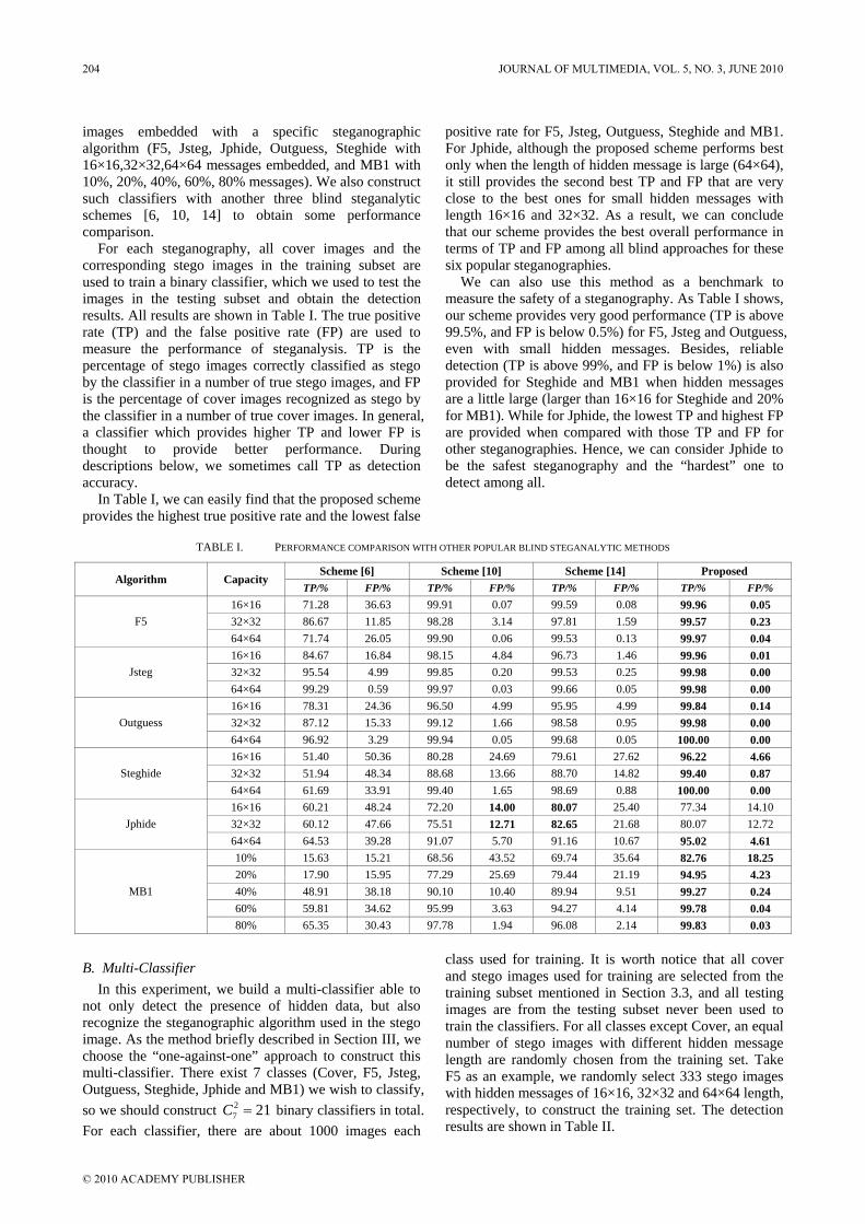
images embedded with a specific steganographic algorithm (F5, Jsteg, Jphide, Outguess, Steghide with 16×16,32×32,64×64 messages embedded, and MB1 with 10%, 20%, 40%, 60%, 80% messages). We also construct such classifiers with another three blind steganalytic schemes [6, 10, 14] to obtain some performance comparison.
For each steganography, all cover images and the corresponding stego images in the training subset are used to train a binary classifier, which we used to test the images in the testing subset and obtain the detection results. All results are shown in Table I. The true positive rate (TP) and the false positive rate (FP) are used to measure the performance of steganalysis. TP is the percentage of stego images correctly classified as stego by the classifier in a number of true stego images, and FP is the percentage of cover images recognized as stego by the classifier in a number of true cover images. In general, a classifier which provides higher TP and lower FP is thought to provide better performance. During descriptions below, we sometimes call TP as detection accuracy.
In Table I, we can easily find that the proposed scheme provides the highest true positive rate and the lowest false
positive rate for F5, Jsteg, Outguess, Steghide and MB1. For Jphide, although the proposed scheme performs best only when the length of hidden message is large (64×64), it still provides the second best TP and FP that are very close to the best ones for small hidden messages with length 16×16 and 32×32. As a result, we can conclude that our scheme provides the best overall performance in terms of TP and FP among all blind approaches for these six popular steganographies.
We can also use this method as a benchmark to measure the safety of a steganography. As Table I shows, our scheme provides very good performance (TP is above 99.5%, and FP is below 0.5%) for F5, Jsteg and Outguess, even with small hidden messages. Besides, reliable detection (TP is above 99%, and FP is below 1%) is also provided for Steghide and MB1 when hidden messages are a little large (larger than 16×16 for Steghide and 20% for MB1). While for Jphide, the lowest TP and highest FP are provided when compared with those TP and FP for other steganographies. Hence, we can consider Jphide to be the safest steganography and the “hardest” one to detect among all.
TABLE I. PERFORMANCE COMPARISON WITH OTHER POPULAR BLIND STEGANALYTIC METHODS
Scheme [6] Scheme [10] Scheme [14] Proposed Algorithm Capacity
TP/% FP/% TP/% FP/% TP/% FP/% TP/% FP/% 16×16 71.28 36.63 99.91 0.07 99.59 0.08 99.96 0.05 32×32 86.67 11.85 98.28 3.14 97.81 1.59 99.57 0.23 F5 64×64 71.74 26.05 99.90 0.06 99.53 0.13 99.97 0.04 16×16 84.67 16.84 98.15 4.84 96.73 1.46 99.96 0.01 32×32 95.54 4.99 99.85 0.20 99.53 0.25 99.98 0.00 Jsteg 64×64 99.29 0.59 99.97 0.03 99.66 0.05 99.98 0.00 16×16 78.31 24.36 96.50 4.99 95.95 4.99 99.84 0.14 32×32 87.12 15.33 99.12 1.66 98.58 0.95 99.98 0.00 Outguess 64×64 96.92 3.29 99.94 0.05 99.68 0.05 100.00 0.00 16×16 51.40 50.36 80.28 24.69 79.61 27.62 96.22 4.66 32×32 51.94 48.34 88.68 13.66 88.70 14.82 99.40 0.87 Steghide 64×64 61.69 33.91 99.40 1.65 98.69 0.88 100.00 0.00 16×16 60.21 48.24 72.20 14.00 80.07 25.40 77.34 14.10 32×32 60.12 47.66 75.51 12.71 82.65 21.68 80.07 12.72 Jphide 64×64 64.53 39.28 91.07 5.70 91.16 10.67 95.02 4.61 10% 15.63 15.21 68.56 43.52 69.74 35.64 82.76 18.25 20% 17.90 15.95 77.29 25.69 79.44 21.19 94.95 4.23 40% 48.91 38.18 90.10 10.40 89.94 9.51 99.27 0.24 60% 59.81 34.62 95.99 3.63 94.27 4.14 99.78 0.04
MB1
80% 65.35 30.43 97.78 1.94 96.08 2.14 99.83 0.03
B. Multi-Classifier In this experiment, we build a multi-classifier able to
not only detect the presence of hidden data, but also recognize the steganographic algorithm used in the stego image. As the method briefly described in Section III, we choose the “one-against-one” approach to construct this multi-classifier. There exist 7 classes (Cover, F5, Jsteg, Outguess, Steghide, Jphide and MB1) we wish to classify, so we should construct C binary classifiers in total. For each classifier, there are about 1000 images each
class used for training. It is worth notice that all cover and stego images used for training are selected from the training subset mentioned in Section 3.3, and all testing images are from the testing subset never been used to train the classifiers. For all classes except Cover, an equal number of stego images with different hidden message length are randomly chosen from the training set. Take F5 as an example, we randomly select 333 stego images with hidden messages of 16×16, 32×32 and 64×64 length, respectively, to construct the training set. The detection results are shown in Table II.
27 21=
204 JOURNAL OF MULTIMEDIA, VOL. 5, NO. 3, JUNE 2010
© 2010 ACADEMY PUBLISHER

In Table II, we can find that about 95.58% of cover images are classified accurately by the multi-classifier. In other words, the FP is 4.42%. In practice, FP plays a very important role in the ability of a classifier. Only when the FP is low, the detection accuracy can be deemed to be significative. If the FP is high, such as above 50%, the detection accuracy will make no sense even thought it is 100%. Since the FP is only 4.42%, we can think the TP of our multi-classifier to be believable.
As shown in Table II, the multi-classifier provides a good detection accuracy (over 97%) to identify F5 and Outguess among all steganographies even when the stego images are embedded with a small size of hidden
messages (16×16). Jsteg seems to be the second easiest steganography to detect since it can be reliably recognized (detection accuracy over 96%) when the size of hidden messages is larger than 16×16. For Steghide and Jphide, acceptable detection accuracy (about 95%) is provided when the hidden data is large (64×64). Among all, MB1 looks like the hardest steganography to identify. It can be hardly recognized when small messages (below 20% of the maximum capacity) are embedded, and the detection accuracy is still below 80% even with larger hidden data. Training sets of binary classifiers for the multi-classifier
TABLE II. DETECTION RESULTS OF IDENTIFYING DIFFERENT CLASSES BY THE MULTI-CLASSIFIER
Algorithm Cover F5 Jsteg Outguess Steghide Jphide MB1 F5 16×16 0.00 99.13 0.03 0.00 0.03 0.81 0.00 F5 32×32 0.02 99.36 0.00 0.00 0.00 0.62 0.00 F5 64×64 0.03 99.42 0.00 0.00 0.03 0.52 0.00
Jsteg 16×16 0.73 0.00 80.59 18.68 0.00 0.00 0.00 Jsteg 32×32 0.00 0.03 96.60 3.37 0.00 0.00 0.00 Jsteg 64×64 0.00 0.03 99.97 0.00 0.00 0.00 0.00
Outguess 16×16 0.42 0.09 1.13 97.96 0.34 0.00 0.06 Outguess 32×32 0.00 0.03 0.79 99.18 0.00 0.00 0.00 Outguess 64×64 0.00 0.04 0.30 99.66 0.00 0.00 0.00 Steghide 16×16 15.50 0.15 0.00 0.03 60.88 2.79 20.65 Steghide 32×32 0.79 0.09 0.00 0.03 79.87 0.23 18.99 Steghide 64×64 0.00 0.04 0.00 0.00 94.74 0.00 5.22 Jphide 16×16 34.28 0.09 0.00 0.06 0.59 64.81 0.17 Jphide 32×32 26.60 0.12 0.00 0.06 0.82 72.29 0.11 Jphide 64×64 3.26 0.32 0.00 0.00 0.53 95.81 0.08
MB1 10% 70.04 0.09 0.00 0.06 12.90 7.78 9.13 MB1 20% 26.13 0.09 0.00 0.06 28.74 1.82 43.16 MB1 40% 0.93 0.23 0.00 0.03 30.92 0.06 67.83 MB1 60% 0.17 0.29 0.03 0.00 26.53 0.00 72.98 MB1 80% 0.12 0.32 0.03 0.00 21.73 0.00 77.80
Cover 95.58 0.03 0.03 0.03 2.08 2.08 0.17
C. Universal Steganalyzer The goal of a universal steganalyzer is to classify
images into two classes — cover and stego images — independent of the steganographies used for embedding. In this experiment, we construct a SVM multi-classifier as the universal steganalyzer capable of detecting different steganographies no matter whether they were used for training or not. In this way, we evaluate the universality of the collected features.
The methods to construct the multi-classifier are the same as that described in Section III, while the difference is that only four steganographies (Jsteg, Outguess, Jphide and MB1) are selected for training the multi-classifier, and the others (F5 and Steghide) are used for testing. The reasons for such selection are simple: Steghide has a similar embedding mechanism as MB1; while F5, as shown in Table II, can be classified accurately the best. This suggests that it has the most different embedding mechanism with others. As a result, we select F5 and Steghide as the steganographies never used for training in
order to inspect some relationships between the classification accuracy and the embedding mechanism.
There are C 25 10= binary classifiers constructed in
this experiment. In the steganalyzer, the images classified as Jsteg, Outguess, Jphide and MB1 are all thought to be the stego images. The rightmost column in Table III consists of the detection rate as stego images for each category. We can find that the false positive rate is only 4.72%, hence the detection accuracy of this classifier is deemed to be significative.
At first, we take account of the steganographies used for training. As shown in Table III, very good detection accuracy (over 98.5%) is provided for Jsteg and Outguess even with a small size of hidden data embedded (16×16). For MB1, if the embedded messages are larger than or equal to 40% of the maximum embedding capacity of a image, the detection accuracy is also very good (over 98.5%). Just as the conclusion in Section 4.1, Jphide seems to be the hardest steganographic algorithm to detect. Only with larger messages (64×64) embedded,
JOURNAL OF MULTIMEDIA, VOL. 5, NO. 3, JUNE 2010 205
© 2010 ACADEMY PUBLISHER
stego images embedded with Jphide can be reliably detected (over 96%).
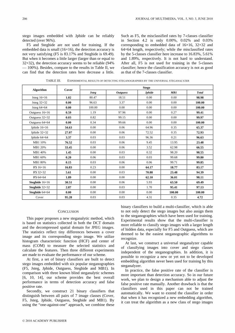
F5 and Steghide are not used for training. If the embedded data is small (16×16), the detection accuracy is not very satisfying (F5 is 83.17% and Steghide is 69.49). But when it becomes a little larger (larger than or equal to 32×32), the detection accuracy seems to be reliable (94% — 100%). Besides, compare to the results in Table II, we can find that the detection rates here decrease a little.
Such as F5, the misclassified rates by 7-classes classifier in Section 4.2 is only 0.00%, 0.02% and 0.03% corresponding to embedded data of 16×16, 32×32 and 64×64 length, respectively; while the misclassified rates by the 5-classes classifier here increase to 16.83%, 5.61% and 1.89%, respectively. It is not hard to understand. After all, F5 is not used for training in the 5-classes classifier; hence the classification accuracy is not as good as that of the 7-classes classifier.
TABLE III. EXPERIMENTAL RESULTS OF DETECTING STEGANOGRAPHIES BY THE UNIVERSAL STEGANALYZER
Stego Algorithm Cover
Jsteg Outguess Jphide MB1 Total
Jsteg 16×16 1.02 80.47 18.51 0.00 0.00 98.98 Jsteg 32×32 0.00 96.63 3.37 0.00 0.00 100.00 Jsteg 64×64 0.00 100.00 0.00 0.00 0.00 100.00
Outguess 16×16 0.59 1.19 97.96 0.00 0.27 99.41 Outguess 32×32 0.03 0.82 99.15 0.00 0.00 99.97 Outguess 64×64 0.00 0.34 99.66 0.00 0.00 100.00
Jphide 16×16 34.63 0.00 0.06 64.96 0.35 65.37 Jphide 32×32 27.07 0.00 0.06 72.52 0.35 72.93 Jphide 64×64 3.37 0.03 0.03 96.36 0.21 96.63
MB1 10% 76.52 0.03 0.06 9.45 13.95 23.48 MB1 20% 33.45 0.00 0.06 3.52 62.98 66.55 MB1 40% 1.45 0.00 0.03 0.32 98.20 98.55 MB1 60% 0.20 0.06 0.03 0.03 99.68 99.80 MB1 80% 0.15 0.03 0.06 0.06 99.71 99.85 F5 16×16 16.83 0.23 0.00 64.17 18.77 83.17 F5 32×32 5.61 0.00 0.03 70.88 23.48 94.39 F5 64×64 1.89 0.00 0.00 62.10 36.01 98.11
Steghide 16×16 30.51 0.00 0.06 5.93 63.50 69.49 Steghide 32×32 2.87 0.00 0.03 1.70 95.41 97.13 Steghide 64×64 0.00 0.00 0.00 0.00 100.00 100.00
Cover 95.28 0.03 0.03 4.31 0.35 4.72
CONCLUSION
This paper proposes a new steganalytic method, which is based on statistics collected in both the DCT domain and the decompressed spatial domain for JPEG images. The statistics reflect tiny differences between a cover image and its corresponding stego image. We utilize histogram characteristic function (HCF) and center of mass (COM) to measure the selected statistics and calculate the features. Then three different experiments are made to evaluate the performance of our scheme.
At first, a set of binary classifiers are built to detect stego images embedded with six popular steganographies (F5, Jsteg, Jphide, Outguess, Steghide and MB1). In comparison with three known blind steganalytic schemes [6, 10, 14], our scheme provides the best overall performance in terms of detection accuracy and false positive rate.
Secondly, we construct 21 binary classifiers that distinguish between all pairs of 7 image classes (Cover, F5, Jsteg, Jphide, Outguess, Steghide and MB1). By using the “one-against-one” approach, we combine these
binary classifiers to build a multi-classifier, which is able to not only detect the stego images but also assign them to the steganographies which have been used for training. Experimental results show that the multi-classifier is more reliable to classify stego images with a larger length of hidden data, especially for F5 and Outguess, which are deemed to be the easiest steganographic algorithms to recognize.
At last, we construct a universal steganalyzer capable of classifying images into cover and stego classes independent of the steganographies. In addition, it is possible to recognize a new or yet not to be developed embedding algorithm never been used for training by this steganalyzer.
In practice, the false positive rate of the classifier is more important than detection accuracy. So in our future work, we plan to design a mechanism able to adjust the false positive rate manually. Another drawback is that the classifiers used in this paper can not be trained automatically. We want to extend the classifier in order that when it has recognized a new embedding algorithm, it can treat the algorithm as a new class of stego images
206 JOURNAL OF MULTIMEDIA, VOL. 5, NO. 3, JUNE 2010
© 2010 ACADEMY PUBLISHER

and be trained automatically. However, it is not easy work to do, and need more efforts in future.
REFERENCES [1] J. Fridrich, M. Goljan, and D. Hogea, “Steganalysis of
JPEG Images: Breaking the F5 Algorithm”, Proceedings of the 5th Information Hiding Workshop, Lecture Notes in Computer Science, 2002, pp.310-323.
[2] J. Fridrich, M. Goljan, and D. Hogea, “Attacking the Outguess”, ACM Multimedia 2002 Workshop W2 - Workshop on Multimedia and Security: Authentication, Secrecy, and Steganalysis, 2002, pp.3-6.
[3] T. Zhang and X. J. Ping, “A new approach to reliable detection of LSB steganography in natural images”, Signal Process, 83:2085–93, 2003.
[4] I. Avcibas, N. Memon, and B. Sankur, “Steganalysis Based on Image Quality Metrics”, IEEE Fourth Workshop on Multimedia Signal Processing, 2001, pp.517-522.
[5] I. Avcibas, M. Khrrazi, N. Memon, and B. Sankur, “Image steganalysis with binary similarity measures”, EURASIP Journal on Applied Signal Processing, 2005, 17, pp.2749-2757.
[6] S. Lyu and H. Farid, “Detecting Hidden Messages Using Higher-Order Statistics and Support Vector Machines”, Proc. of 5th International Workshop on Information Hiding, 2002, pp.340-354.
[7] S. Lyu and H. Farid, “Steganalysis Using Color Wavelet Statistics and One-Class Support Vector Machines”, Proceedings of SPIE - The International Society for Optical Engineering, v.5306, pp.35-45, 2004.
[8] J. J. Harmsen and W. A. Pearlman, “Steganalysis of Additive Noise Modelable Information Hiding”, Proceedings of SPIE - The International Society for Optical Engineering, v.5020, pp.131-142, 2003.
[9] J. J. Harmsen, K. D. Bowers, and W. A. Pearlman, “Fast Additive Noise Steganalysis”, Proceedings of SPIE - The International Society for Optical Engineering, v.5306, pp.489-495, 2004.
[10] J. Fridrich, “Feature-based Steganalysis for JPEG Images and Its Implications for Future Design of Steganographic Schemes”, In Proc. 6th Int. Information Hiding Workshop, 2004, pp.67-81.
[11] T. Pevny and J. Fridrich, “Towards Multi-class Blind Steganalyzer for JPEG Images”, In Proc. IWDW, 2005, pp.39-53.
[12] T. Pevny and J. Fridrich, “Multi-class Blind Steganalysis for JPEG Images”, Proceedings of SPIE - The International Society for Optical Engineering, 2006, v.6072, pp.607200.
[13] T. Pevny and J. Fridrich, “Determining the Stego Algorithm for JPEG Images”, Information Security, IEE Proceedings, 2006, 153(3) pp.77–86.
[14] L. D. Ping, Z. G. Liu, L. Shi and K. Sun, “Variable Characteristics Based Blind Detection of Hidden Information”, Journal of Zhejiang University (Engineering Science), 2007, 41(3) pp.374-379 (in Chinese).
[15] A. Westfeld, F5. Available from: http://wwwrn.inf.tu-dresden.de/~westfeld/f5.html, 2001.
[16] D. Upham, Jsteg. Available from: ftp://ftp.funet.fi/pub/crypt/steganography/, 2002.
[17] A. Latham, Jphide&Seek. Available from: http://linux01.gwdg.de/~alatham/stego.html, 1999.
[18] N. Provos, Outguess. Available from: http://www.Outguess.org, 2001.
[19] S. Hetzl, Steghide. Available from: http://Steghide.sourceforge.net, 2003
[20] P. Sallee, “Model Based Steganography”, International Workshop on Digital Watermarking, LNCS 2939, pp.154-167, 2004.
[21] C. C. Chang and C. J. Lin, “LIBSVM: A Library for Support Vector Machines”, Software Available from: http://www.csie.ntu.edu.tw/~cjlin/libsvm, 2001
[22] S. Knerr, L. Personnaz and G. Dreyfus, “Single-layer Learning Revisited: A Stepwise Procedure for Building and Training a Neural Network”. Neurocomputing: Algorithms, Architectures and Applications, 1990.
[23] J. H. Friedman, “Another Approach to Polychotomous Classification”, Technical report, Department of Statistics, Stanford Univeristy, 1996.
[24] Greenspun Image Library, Available from: http://philip.greenspun.com
Zhuo Li was born in 1984. He is currently a Ph.D. candidate in college of computer science and technology, Zhejiang University, Hangzhou, China. He received his B.S degree from Zhejiang University, in 2005. His research interests include information security, signal processing and data hiding.
Kuijun Lu is currently an associate professor of computer
science, Zhejiang University, Hangzhou, China. His research interests include information security, signal and image processing.
Xianting Zeng is a Ph.D. candidate in college of computer
science and technology, Zhejiang University. He received his B.S degree in computer science from Sichuan University, Chengdu, China, in 1986, and the M.S degree in computer engineering from South China University of Technology, Guangzhou, China, in 1989. His research interests include image processing, data hiding.
Xuezeng Pan received her B.S degree from Zhejiang
University, Hangzhou, China, in 1965. He is currently a professor of computer science, Zhejiang University. His research interests include information security, digital watermarking, signal and image processing.
JOURNAL OF MULTIMEDIA, VOL. 5, NO. 3, JUNE 2010 207
© 2010 ACADEMY PUBLISHER

Gray Cerebrovascular Image Skeleton Extraction Algorithm Using Level Set Model
Jian Wu1,2
1.Provincial Key Laboratory for Computer Information Processing Technology; 2.The Institute of Intelligent Information Processing and Application, Soochow University, Suzhou 215006, China
Email: [email protected]
Guang-ming Zhang1,2, Jie Xia1,2, Zhi-ming Cui1,2 1.Provincial Key Laboratory for Computer Information Processing Technology; 2.The Institute of Intelligent
Information Processing and Application, Soochow University, Suzhou 215006, China
Abstract—The ambiguity and complexity of medical cerebrovascular image makes the skeleton gained by conventional skeleton algorithm discontinuous, which is sensitive at the weak edges, with poor robustness and too many burrs. This paper proposes a cerebrovascular image skeleton extraction algorithm based on Level Set model, using Euclidean distance field and improved gradient vector flow to obtain two different energy functions. The first energy function controls the obtain of topological nodes for the beginning of skeleton curve. The second energy function controls the extraction of skeleton surface. This algorithm avoids the locating and classifying of the skeleton connection points which guide the skeleton extraction. Because all its parameters are gotten by the analysis and reasoning, no artificial interference is needed. Index Terms—gray cerebrovascular image, Level Set model, energy function, skeleton extraction
I. INTRODUCTION
The analysis and understanding of shape is of great significance in the field of machine intelligence and pattern recognition field. Medial axial and skeleton are considered the presentation of compressed shape in the case of maintaining the topology information, the goal of skeletonization is to reduce the dimension of shape, that is, to express original image with less information. Zhou and Toga [1] proposed a pixel decoding technology, discrete wavefront spread over the entire object beginning with a hand-selected control point. Bitter [2] proposed a punishment distance algorithm to extract the skeleton line. Extraction of the medial axis uses the Dijkstra shortest path algorithm [3]. Bouix [4] extract medial axis using the Euclidean distance gradient vector field of the average outward flux across the Jordan curve to the border, and use calculation of the gradient of the distance map and a threshold to calculate the skeleton. Deschamps and Cohen [5] associate skeleton extraction with finding the shortest path. First slove short-term equation with fast marching method, and then follow the sudden drawdown between the two user-selected points, and finally find the shortest path.
The existing methods of skeleton extraction more or less have the following deficiencies: (1) the need of
binarization of the target image, and results of skeleton extraction depends on the threshold segmentation to a large extent; (2) the usage of different pruning techniques to extract skeleton from the mesial surface; (3) high computational complexity; (4) the need of manually select starting point of each skeleton; (5) the usage of search method when deal with a branch node; (6) unable to deal with the target objects with holes; (7) lack of robustness; (8) noise-sensitive of the edges.
This paper proposes a skeleton extraction algorithm using Level Set model, which can avoid the above shortcomings. The main idea is to capture the topological information of objects by spreading a wavefront with a medium velocity to with skeleton point (source point), and second spread high-velocity wavefront to start with these topology nodes, in which the skeleton point is the points with greatest curvature value on spreading peak surface. Through the solution of ordinary differential equations, the skeleton points can be identified.
II. FORMULA EXPRESSIONS OF LEVEL SET
Fast Marching Method (FMM) is a technology using fully binary tree method to find the point of the least arrival time by sorting all the arrival time in narrow-band region, assuming that the pixel number of narrow band is N . Every step must be to do this, so the time complexity
is )log( 2 NNO . In order to reduce the computational cost, Kim
proposed an effective )(NO Group Marching Method (GMM) [6]. Eikonal type equations are:
)(1),( 2
2
xvxxT =∇ ζτ (1)
Where ),( xxT ζτ denotes the time from ζx to x on
curve, )(2 xv denotes the velocity at the peak x . GMM is to fine a group of points to move forward at
the same time, rather than finding the point of least arrival time by sorting points of all solutions.
208 JOURNAL OF MULTIMEDIA, VOL. 5, NO. 3, JUNE 2010
© 2010 ACADEMY PUBLISHERdoi:10.4304/jmm.5.3.208-215
To the m th pixel ),( yjxiPm ∆∆= of narrow-band,
assuming its velocity is mV , the velocity components on
x axis and y axis are mxV , myV respectively. In order to
simplify the problem, supposing hyx =∆=∆ , so we
can see the distance s from mP to y axis can be obtained by the following formula.
)/(my
mx
m vvvhS += (2)
The time from mP to y axis can be calculated by the following formula:
ym
xm
m
m
m
vvh
vsT
+==∆
φφm
(3) Supposing that the value of interpolation nodes has
already been known, so calculate the mT by equation (3)
should satisfy the following inequality.
mjijim TTTT ∆+≥ ++ ),min( 1,,1 (4) Choose G as follows.
:p minNNmm TTTNG ∆+≤∈= (5)
Where, mNPNmNPN TTTTmm
∆=∆=∈∈
min,minmin
. If final time is prescribed, also should satisfy
finalm TT ≤.
III. GMM HIGH SPEED MODEL
Consider the least-cost path problem, suppose the
pathnRsL →∞),0[:)( , minimize the cumulative cost
from starting point A to destination B. If the cost W is the only function of node x in object domain, the cost function W is called isotropic, the minimum cumulative cost at x is defined as follows.
dxxLWxTS
LAx∫=0
))((min)( (6)
AxL is set of all the path connect A to x , S is the length of path, the starting point and end point are
AL =)0( and xSL =)( respectively. The path with minimum integral is the lowest cost path [7]. The solution of formula(6) satisfy Eikonal equation:
)(1)( xWxF = . This paper uses a new cost function, that is, the lowest
cost path between two central points is a skeleton line, which is defined as follows.
0)( )( >= − λλµ xnexW (7) Parameter λ is the control coefficient of peak surface
crown on skeleton points, )(xnµ is a function
proportional to the normalized minimum distance domain to the edge of the target. In order to make algorithm realize automation without artificial interference, the following the analysis of λ and selection of intermediate
function )(xµ is shown as follows.
A. Value Selection of λ Consider the following figure.
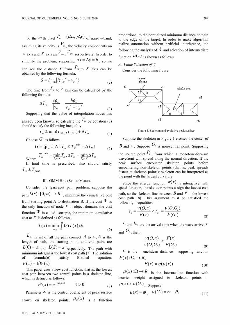
Figure 1. Skeleton and evolutive peak surface
Suppose the skeleton in Figure 1 crosses the center of
B and x . Suppose iG is non-central point. Supposing
the source point sP , from which a monotone-forward wavefront will spread along the normal direction. If the peak surface encounter skeleton points before encountering non-skeleton points (that is, peak spreads fastest at skeleton points); skeleton can be interpreted as the point with the largest curvature.
Since the energy function )(xw is interactive with speed function, the skeleton points assign the lowest cost path, so the skeleton line between B and x is the lowest cost path [8]. This argument must be satisfied the following inequalities.
)(),(
)(),(
i
iGx GF
GOtxFxOt
i
νν=<=
(8)
xt and iGt are the arrival time when the wave arrive x
and iG , then,
)()(
),(),(
ii GFxF
GOxO
<νν
(9) ν is the euclidean distance, supposing function
+→Ω RxF :)( ))(()( xxF µη= (10)
+→Ω Rx :)(µ is the intermediate function with heavier weight assigned to skeleton points ,
)()( iGx µµ > 。Suppose
ϖµ =)(x , iiG θϖµ −=)( (11)
JOURNAL OF MULTIMEDIA, VOL. 5, NO. 3, JUNE 2010 209
© 2010 ACADEMY PUBLISHER
h and iθ are positive real number, iθ donotes the absolute difference between two nearhood points. When
bax 22),0( ∆+∆=ν (12)
),min(),0( baGi ∆∆=ν (13)
Proportion ),0(/),0( iGx νν is largest, function F must satisfy:
),min()()( 22
baba
GFxF
i ∆∆∆+∆
> (14)
That is,
)()(
),min(
22
ibabad
θϖηϖη−
<∆∆∆+∆
= (15)
0)()( <−− ϖηθϖη id (16)
Expend )( iθϖη − and substitute into equation (16) as follows.
0)())()()(( <−+− ϖηθνϖϖηθϖη ii d
dd (17)
Where,
∑∞
=
−=2 !
)1()(k
k
kkik
i dkdϖηνθν
(18)
Supposing 0)( →iθν is a very small value which can be negligible , so the condition can satisfy the supposition.
The higher order can be negligible, as follows.
ϖθϖη
ϖη dddd
i
1)()( −>
(19)
iθ of each point is different, so without loss of generality,the minimal positive value of on Ω satisfy the equation (19).
)()(,)()(min babai µµµµθθ ≠−== (20) Suppose
0)),min(1(11221 >
∆+∆
∆∆−=
−=
baba
dd
θθλ
(21) Substitute a given a into the both sides of equation
(19) , as follows.
∫∫ >)(
1
)(
minmin )()( aa
dd µ
µ
µ
µϖλ
ϖηϖη
(22) ))(()(ln))((ln min1min µµλµηµη −>− aa
(23) )ln()()(ln minmin11 FaaF −−> µλµλ (24)
Where, )( minmin µη=F is the minimal velocity. Suppose
minmin1 ln F−= µλζ (25) so
)()( 11)( aa eeeaF µλζζµλ −− => (26) Many velocity functions all satisfy equation (26),but
only function with negligible )(θν doesn’t change
equation can be chose. If 02 >λ ,one function )(xF can be expressed as follows.
)()( 12)( aa eeaF µλµλ= (27) Require
ζµλ −> ee a)(2 (28)
min1min2 ln)( µλµλ −> Fa (29) Any wavefront which can spread such a function can
be called λ -surface. At present, we search conditions
satisfied 0)( →θν . Substitute velocity function of (29) into (19),(30) can be concluded.
0)1( <−−λϖλϖ dee (30) Therefore,
)),min(
ln(1)ln(1 22
babad
∆∆∆+∆
=>θθ
λ (31)
is the necessary condition to satisfy equation (19).
B. Selection of Intermediate Function )(xµ
The Selection of intermediate function )(xµ is as follows.
Minimize the following function:
dxfZfZZE 222)( ∇−∇+∇= ∫∫∫υ (32)
Obtain gradient vector flow (GVF) of the vector
domain )(xZ . Where, ),( bax = , υ is a
regularization parameter. )(xg is from the edge image of )(xI . To a binary image, )()( xIxg −= . In the
Euclidean distance )(xD , an interesting character of
)(xZ is that it does not produce three-dimensional surface of non-tubular objects, because there is only one
border voxel has an impact calculation on the )(xD , but more than one linked the border voxels have influence
on the calculation of )(xD . Because boundary
movement of GVF is very slow, Z points to the center
of objects, value of Z is very small, therefore, the
impact of Z to distinguish between focal point and non-focal point is insufficient, as shown in Figure 2(b). Therefore, the intensity of the following middle function is controlled by the domain intensity r .
210 JOURNAL OF MULTIMEDIA, VOL. 5, NO. 3, JUNE 2010
© 2010 ACADEMY PUBLISHER
r
ZZZxZ
x )minmax
min)((1)(
−−
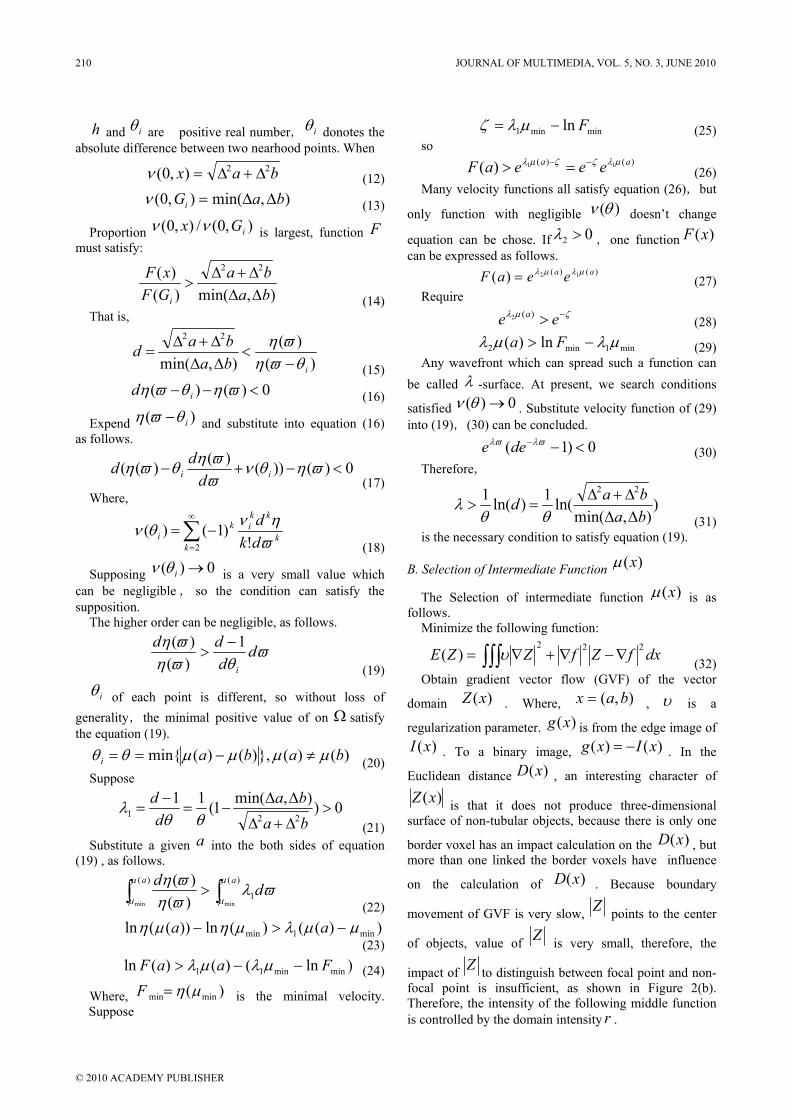
−=µ 10 << r (33)
(a) a connected n-shaped graph
(b) function )(xZ
(c) intermediate function )(xµ
Figure 2. Intermediate function of n-shaped graph
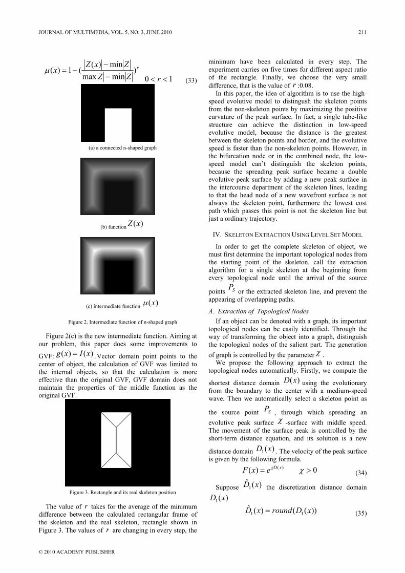
Figure 2(c) is the new intermediate function. Aiming at our problem, this paper does some improvements to
GVF: )()( xIxg = .Vector domain point points to the center of object, the calculation of GVF was limited to the internal objects, so that the calculation is more effective than the original GVF, GVF domain does not maintain the properties of the middle function as the original GVF.
Figure 3. Rectangle and its real skeleton position
The value of r takes for the average of the minimum difference between the calculated rectangular frame of the skeleton and the real skeleton, rectangle shown in Figure 3. The values of r are changing in every step, the
minimum have been calculated in every step. The experiment carries on five times for different aspect ratio of the rectangle. Finally, we choose the very small difference, that is the value of r :0.08.
In this paper, the idea of algorithm is to use the high-speed evolutive model to distingush the skeleton points from the non-skeleton points by maximizing the positive curvature of the peak surface. In fact, a single tube-like structure can achieve the distinction in low-speed evolutive model, because the distance is the greatest between the skeleton points and border, and the evolutive speed is faster than the non-skeleton points. However, in the bifurcation node or in the combined node, the low-speed model can’t distinguish the skeleton points, because the spreading peak surface became a double evolutive peak surface by adding a new peak surface in the intercourse department of the skeleton lines, leading to that the head node of a new wavefront surface is not always the skeleton point, furthermore the lowest cost path which passes this point is not the skeleton line but just a ordinary trajectory.
IV. SKELETON EXTRACTION USING LEVEL SET MODEL
In order to get the complete skeleton of object, we must first determine the important topological nodes from the starting point of the skeleton, call the extraction algorithm for a single skeleton at the beginning from every topological node until the arrival of the source
points SP or the extracted skeleton line, and prevent the appearing of overlapping paths.
A. Extraction of Topological Nodes If an object can be denoted with a graph, its important
topological nodes can be easily identified. Through the way of transforming the object into a graph, distinguish the topological nodes of the salient part. The generation of graph is controlled by the parameter χ .
We propose the following approach to extract the topological nodes automatically. Firstly, we compute the
shortest distance domain )(xD using the evolutionary from the boundary to the center with a medium-speed wave. Then we automatically select a skeleton point as
the source point SP , through which spreading an evolutive peak surface χ -surface with middle speed. The movement of the surface peak is controlled by the short-term distance equation, and its solution is a new
distance domain )(1 xD . The velocity of the peak surface is given by the following formula.
0)( )( >= χχ xDexF (34)
Suppose )(ˆ1 xD the discretization distance domain
)(1 xD ))(()(ˆ
11 xDroundxD = (35)
JOURNAL OF MULTIMEDIA, VOL. 5, NO. 3, JUNE 2010 211
© 2010 ACADEMY PUBLISHER

Do discretization by the method of calculating integer
value of the distance domain )(xD . Therefore, the basic elements of objects become the cluster from the point. Each cluster is composed of the connection points with the same discreet distance value. If the two clusters have a common point, the two clusters are adjacent. Build a level set graph (LSG), whose root node is cluster
containing SP , and supposing its cluster value is zero. Cluster graph contains two main types of the cluster. Xcluster consist in the end of the cluster graph, and Mcluster contain at least two adjacent clusters (Successors). The target contains cluster only when it has internal hole. The middle point of cluster is achieved by
searching the points with the largest value of )(xD in clusters. End-point and the cluster nodes are the mid-point of the associated cluster.
Figure 4 shows the effect of extracted topological nodes from a star graph.
(a) the LSG denoted by Nodes and line connecting
(b) the topological nodes of star graph
Figure 4. Schematic diagram of the extraction of topological nodes
B. Extraction of Single Skeleton Line In order to extract skeleton line between the two
skeleton points A and B , initialize the spreading time of A to zero, and then select the high-speed evolutive function of GMM to reach the B point. Finally, we backtrack from B to A along the T∇ . The extraction process is the solving the following ordinary differential equation:
BLTT
dtdL
=∇∇
−= )0(, (36)
Solving the equation (36) can depict the skeleton line
with )(tL , the error is )( 2hO , h is the integration step. T
iii baG ],[= , and
)(,)()()( 1 i
i
ii Ghfk
GTGTGf =
∇∇
−= (37)
))2
( 11
kGhfGG iii ++=+ (38)
In order to ensure the connectivity of skeleton points, we choose 1.0=h . Figure 5 is the extraction effect of single skeleton when 1.0=h .
Figure 5. Single skeleton extraction schematic
C. Circular Extraction of Skeleton Line In this paper, use an effective way to deal with the
cycles of any quantity in the object. The method is as follows. Each cycle is associated with a clustering clusters M . Supposing that M has only two adjacent
clusters 1S and 2S , the following work is divided into
three steps: (1) calculating the middle point 1s of 1S ,
regarding all points including M and 2S as a part of the background (including the holes), so there is only one
skeleton line from 1s to SP . Evolute a rapid GMM
wavefront from SP to 1s , and then extract a skeleton line between them; (2) using the same method as the first step
to extract skeleton line between 2s and SP , regard all
points including M and 1S as a part of the background;
(3)evoluting a rapid GMM wavefront from 1s to 2s , and then extract the skeleton line between them. This method is also applicable to a number of clustering clusters.
V. EXPERIMENTAL RESULT AND ANALYSIS
212 JOURNAL OF MULTIMEDIA, VOL. 5, NO. 3, JUNE 2010
© 2010 ACADEMY PUBLISHER

A. Experimental Effect Figure Use the algorithm proposed in this paper to extract
skeleton from a number of cerebrovascular images, and the extraction effect is shown as follows.
(1)Figure 6 and Figure 7 are the skeleton extraction of two-dimensional cerebrovascular images.
(a) the original two-dimensional cerebrovascular image
(b) intermediate function )(xµ
(c) the skeleton of two-dimensional cerebrovascular image
Figure 6. The 1th skeleton extraction example of two-dimensional cerebrovascular image
(a) the original two-dimensional cerebrovascular image
(b) intermediate function )(xµ
(c) the skeleton of two-dimensional cerebrovascular image
Figure 7. The 2th skeleton extraction example of two-dimensional cerebrovascular image
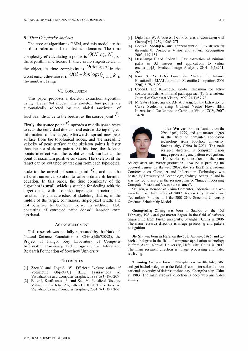
(2)Figure 8, Figure 9 and Figure 10 are the skeleton extraction of three-dimensional cerebrovascular images.
(a) the original three-dimensional cerebrovascular image
(b) intermediate function )(xµ
JOURNAL OF MULTIMEDIA, VOL. 5, NO. 3, JUNE 2010 213
© 2010 ACADEMY PUBLISHER
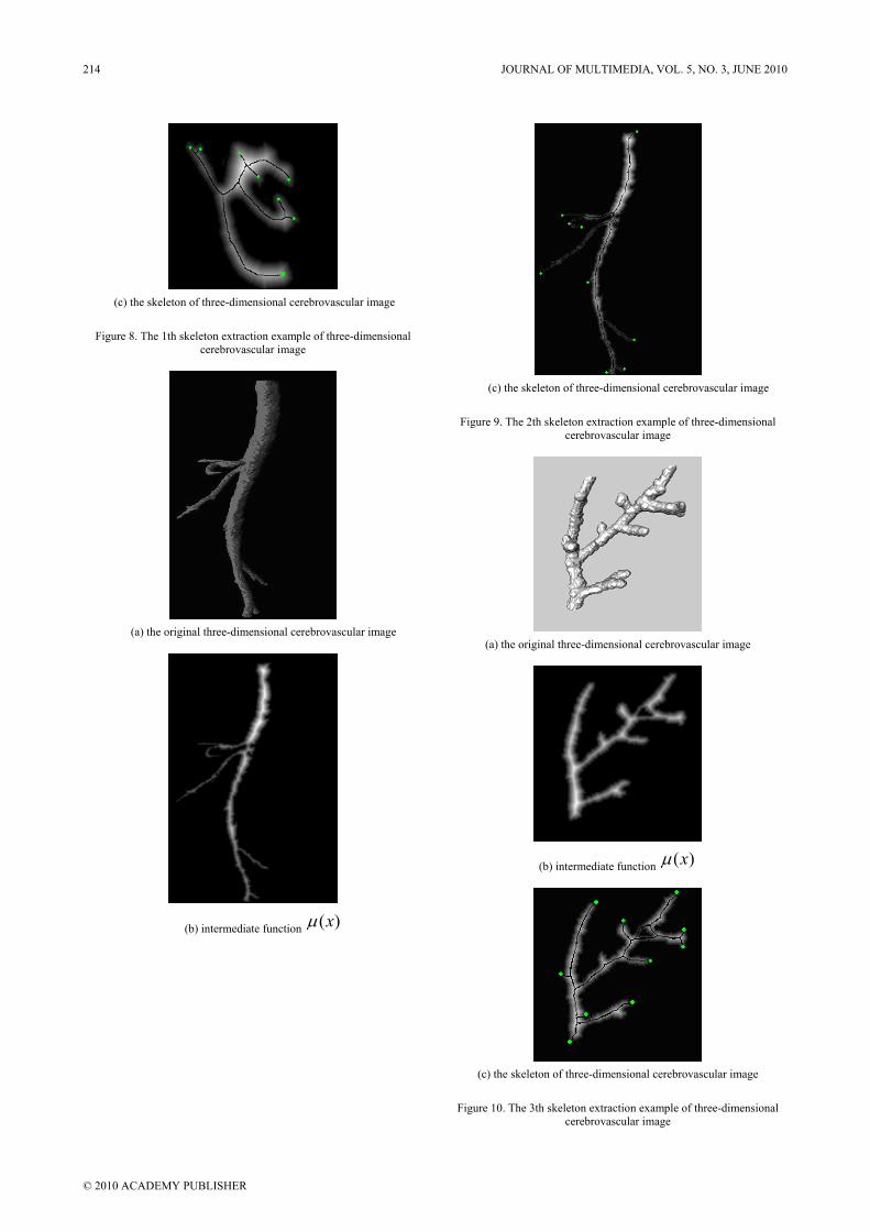
(c) the skeleton of three-dimensional cerebrovascular image
Figure 8. The 1th skeleton extraction example of three-dimensional cerebrovascular image
(a) the original three-dimensional cerebrovascular image
(b) intermediate function )(xµ
(c) the skeleton of three-dimensional cerebrovascular image
Figure 9. The 2th skeleton extraction example of three-dimensional cerebrovascular image
(a) the original three-dimensional cerebrovascular image
(b) intermediate function )(xµ
(c) the skeleton of three-dimensional cerebrovascular image
Figure 10. The 3th skeleton extraction example of three-dimensional cerebrovascular image
214 JOURNAL OF MULTIMEDIA, VOL. 5, NO. 3, JUNE 2010
© 2010 ACADEMY PUBLISHER
B. Time Complexity Analysis The core of algorithm is GMM, and this model can be
used to calculate all the distance domains. The time
complexity of calculating n points is )log( 2 NNO , so the algorithm is efficient. If there is no ring-structure in
the object, its time complexity is )log3( nnO in the
worst case, otherwise it is )log)3(( nnkO + , and k is the number of rings.
VI. CONCLUSION
This paper proposes a skeleton extraction algorithm using Level Set model. The skeleton line points are automatically selected by the global maximum of
Euclidean distance to the border, as the source point sP .
Firstly, the source point sP spreads a middle-speed wave to scan the individual domain, and extract the topological information of the target. Afterwards, spread new peak surface from the topological nodes, and the spreading velocity of peak surface at the skeleton points is faster than the non-skeleton points. At this time, the skeleton points intersect with the evolutive peak surface at the point of maximum positive curvature. The skeleton of the target can be obtained by tracking from each topological
node to the arrival of source point sP , and use the efficient numerical solution to solve ordinary differential equation. In this paper, the time complexity of the algorithm is small, which is suitable for dealing with the target object with complex topological structure, and satisfies the characteristics of skeleton, that is, in the middle of the target, continuous, single-pixel width, and not sensitive to boundary noise. In addition, LSG consisting of extracted paths doesn’t increase extra overhead.
ACKNOWLEDGMENT
This research was partially supported by the National Natural Science Foundation of China(60673092), the Project of Jiangsu Key Laboratory of Computer Information Processing Technology and the Beforehand Research Foundation of Soochow University.
REFERENCES
[1] Zhou.Y and Toga.A. W. Efficient Skeletonization of Volumetric Objects[C]. IEEE Transactions on Visualization and Computer Graphics, 1999, 5(3):196-209
[2] Bitter.I, Kaufman.A. E, and Sato.M. Penalized-Distance Volumetric Skeleton Algorithm[C]. IEEE Transactions on Visualization and Computer Graphics, 2001, 7(3):195-206
[3] Dijkstra.E.W. A Note on Two Problems in Connexion with Graphs[M], 1959, 1:269-271
[4] Bouix.S, Siddiqi.K, and Tannenbaum.A. Flux driven fly throughs[J]. Computer Vision and Pattern Recognition, 2003, 449-454
[5] Deschamps.T and Cohen.L. Fast extraction of minimal paths in 3d images and applications to virtual endoscopy[J]. Medical Image Analysis, 2001, 5(4):261-265
[6] Kim. S. An O(N) Level Set Method for Eikonal Equation[J]. SIAM Journal on Scientific Computing, 200l, 22(6):2178-2193
[7] Cohen.L and Kimmel.R. Global minimum for active contour models: A minimal path approach[J]. International Journal of Computer Vision, 1997, 24(1):57-78
[8] M. Sabry Hassouna and Aly A. Farag. On the Extraction of Curve Skeletons using Gradient Vector Flow. IEEE International Conference on Computer Vision ICCV, 2007, 14-20
Jian Wu was born in Nantong on the 29th April, 1979, and got master degree in the field of computer application technology from Soochow university, Suzhou city, China in 2004. The main research direction is computer vision, image processing and pattern recognition.
He works as a teacher in the same college after his master graduation. Now he is pursuing the doctoral degree. In the year 2008, the 8th IEEE International Conference on Computer and Information Technology was hosted by University of Technology, Sydney, Australia, and he was invited to serve as the session chair of “Image Processing, Computer Vision and Video surveillance”.
Mr. Wu, a member of China Computer Federation. He was awarded the Third Prize of 2007 Suzhou City Science and Technology Progress and the 2008-2009 Soochow University Graduate Scholarship Model.
Guang-ming Zhang was born in Suzhou on the 10th February, 1981, and got master degree in the field of software engineering from Fudan university, Shanghai, China in 2006. The main research direction is image processing and pattern recognition.
Jie Xia was born in Hefei on the 20th January, 1986, and got bachelor degree in the field of computer application technology in from Anhui Normal University, Hefei city, China in 2007. The main research direction is image processing and video retrieving.
Zhi-ming Cui was born in Shanghai on the 4th July, 1961 and got bachelor degree in the field of computer software from national university of defense technology, Changsha city, China in 1983. The main research direction is deep web and video mining.
JOURNAL OF MULTIMEDIA, VOL. 5, NO. 3, JUNE 2010 215
© 2010 ACADEMY PUBLISHER
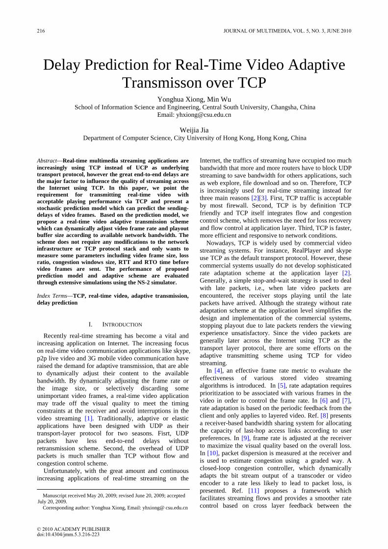
Delay Prediction for Real-Time Video Adaptive Transmisson over TCP
Yonghua Xiong, Min Wu School of Information Science and Engineering, Central South University, Changsha, China
Email: [email protected]
Weijia Jia
Department of Computer Science, City University of Hong Kong, Hong Kong, China
Abstract—Real-time multimedia streaming applications are increasingly using TCP instead of UCP as underlying transport protocol, however the great end-to-end delays are the major factor to influence the quality of streaming across the Internet using TCP. In this paper, we point the requirement for transmitting real-time video with acceptable playing performance via TCP and present a stochastic prediction model which can predict the sending-delays of video frames. Based on the prediction model, we propose a real-time video adaptive transmission scheme which can dynamically adjust video frame rate and playout buffer size according to available network bandwidth. The scheme does not require any modifications to the network infrastructure or TCP protocol stack and only wants to measure some parameters including video frame size, loss ratio, congestion windows size, RTT and RTO time before video frames are sent. The performance of proposed prediction model and adaptive scheme are evaluated through extensive simulations using the NS-2 simulator. Index Terms—TCP, real-time video, adaptive transmission, delay prediction
I. INTRODUCTION
Recently real-time streaming has become a vital and increasing application on Internet. The increasing focus on real-time video communication applications like skype, p2p live video and 3G mobile video communication have raised the demand for adaptive transmission, that are able to dynamically adjust their content to the available bandwidth. By dynamically adjusting the frame rate or the image size, or selectively discarding some unimportant video frames, a real-time video application may trade off the visual quality to meet the timing constraints at the receiver and avoid interruptions in the video streaming [1]. Traditionally, adaptive or elastic applications have been designed with UDP as their transport-layer protocol for two seasons. Fisrt, UDP packets have less end-to-end delays without retransmission scheme. Second, the overhead of UDP packets is much smaller than TCP without flow and congestion control scheme.
Unfortunately, with the great amount and continuous increasing applications of real-time streaming on the
Internet, the traffics of streaming have occupied too much bandwidth that more and more routers have to block UDP streaming to save bandwidth for others applications, such as web explore, file download and so on. Therefore, TCP is increasingly used for real-time streaming instead for three main reasons [2][3]. First, TCP traffic is acceptable by most firewall. Second, TCP is by definition TCP friendly and TCP itself integrates flow and congestion control scheme, which removes the need for loss recovery and flow control at application layer. Third, TCP is faster, more efficient and responsive to network conditions.
Nowadays, TCP is widely used by commercial video streaming systems. For instance, RealPlayer and skype use TCP as the default transport protocol. However, these commercial systems usually do not develop sophisticated rate adaptation scheme at the application layer [2]. Generally, a simple stop-and-wait strategy is used to deal with late packets, i.e., when late video packets are encountered, the receiver stops playing until the late packets have arrived. Although the strategy without rate adaptation scheme at the application level simplifies the design and implementation of the commercial systems, stopping playout due to late packets renders the viewing experience unsatisfactory. Since the video packets are generally later across the Internet using TCP as the transport layer protocol, there are some efforts on the adaptive transmitting scheme using TCP for video streaming.
In [4], an effective frame rate metric to evaluate the effectiveness of various stored video streaming algorithms is introduced. In [5], rate adaptation requires prioritization to be associated with various frames in the video in order to control the frame rate. In [6] and [7], rate adaptation is based on the periodic feedback from the client and only applies to layered video. Ref. [8] presents a receiver-based bandwidth sharing system for allocating the capacity of last-hop access links according to user preferences. In [9], frame rate is adjusted at the receiver to maximize the visual quality based on the overall loss. In [10], packet dispersion is measured at the receiver and is used to estimate congestion using a graded way. A closed-loop congestion controller, which dynamically adapts the bit stream output of a transcoder or video encoder to a rate less likely to lead to packet loss, is presented. Ref. [11] proposes a framework which facilitates streaming flows and provides a smoother rate control based on cross layer feedback between the
Manuscript received May 20, 2009; revised June 20, 2009; accepted
July 20, 2009. Corresponding author: Yonghua Xiong, Email: yhxiong@ csu.edu.cn
216 JOURNAL OF MULTIMEDIA, VOL. 5, NO. 3, JUNE 2010
© 2010 ACADEMY PUBLISHERdoi:10.4304/jmm.5.3.216-223
Figure 1. Fragment and retransmission of real-time video via TCP
transport protocol and streaming server. Ref. [12] presents a distortion optimized streaming algorithm for on-demand streaming of multimedia which minimized the overall client distortion. Ref. [1] proposes a bandwidth prediction methodology based on TCP events, including the information gathering, time series creation and prediction parameter selection.
All of the above adaptive schemes can be classified into the following some types: definition the prioritization and weight of video frames, grading the congestion level, using the period feedback information of network parameter, utilizing the dynamic switch model of buffer, hypothesizing packet loss at the sender size, setting the TCP advertise window, predicting the available network bandwidth and so on.
In this paper, we present a novel adaptive methodology for real-time video transmission across the Internet over TCP based on a delay prediction model. There are three main contributions of our work. First, we study the performance when using TCP directly for streaming (i.e., without rate adaptation at the application level) and then point the requirement of transmitting real-time video with acceptable playing performance via TCP. The second contribution is a stochastic prediction model to predict the sending-delays of video frames. The third one is a rate adaptive real-time video transmission scheme based on the model which can dynamically adjust video frame rate and playout buffer size according to available network bandwidth. The proposed scheme does not require any modification to TCP protocol stack and only wants to measure some parameters before video frames being delivered into network including video frame size, loss ratio, congestion windows size, RTT(Round Trip Time), RTO (Retransmission Timeout) time, so it is easily deployable.
This paper is organized as follows. Section 2 analyses the performance of real-time video transmission via TCP and explores the relationship between end-to-end delays and sending-delays. Section 3 designs the stochastic prediction model to predict sending-delays. Section 4 gives the proposed rate adaptive scheme. In Section 5, we present the simulation results and the comparison with different schemes. Conclusions are given in Section 6.
II. PERFORMANCE OF REAL-TIME VIDEO TRANSMISSION VIA TCP
A. Requirement of Transmitting Real-Time Video with Acceptable Playing Performance
Real-time video applications usually use a playout buffer to insulate the playout from jitter arising from the variable delay through the Internet. A receiver application normally delays processing to operate with a playout delay of Dplayout milliseconds later than the source so that a packet is only late in its processing if it is delayed by more than Dplayout milliseconds. Namely, the playout buffer of receiver is set up to eliminate the jitter posed by the irregular arrivals of video frames. All the arrived video frames would be kept in the playout-buffer for no more than Dplayout. Ref. [13] presents equation (1)
playout3 32
D RTT period delta≥ + + (1)
where RTT is the TCP round-trip time and period is the typical interval between transmissions of data on the stream and delta is some modest extra time. The equation shows that if TCP has lost packets but it has finished the retransmission during Dplayout, application would be oblivious to the packet loss, then the playing performance of real-time streaming using TCP and the Dplayout is acceptable. In other words, if TCP has lost part of segments but it could finish the retransmission during Dplayout, the playing quality would be immune to the loss. However, [13] considers only the ideal condition, namely, it supposes that a video frame be packaged into a TCP segment. Practically, the size of an encoded video frame is usually much larger than TCP MSS (Maximum Segment Size, typically it is 1460 bytes), wherefore a video frame should be fragmented and packaged into multiple TCP segments each of which is equal to the MSS. Meanwhile, when the number of segments exceeds the sum of current TCP congestion window, delivering all the segments of the video frame into network would have to expense multiple RTT period, as shown in Fig.1.
We assume that a video frame could be fragmented into n ( 1>n ) segments from S1 to Sn and let Wi denote the size of TCP congestion window at the beginning time of the ith (1 )i n≤ ≤ RTT period. We obtain that the number of segments that could be sent by sender on the ith RTT period is at most Wi, so the video frame that is larger than Wi would expense more than one RTT period to be sent. When there exists segment loss, e.g. S2 in Figure1, according to the RFC standard of TCP Reno and TCP SACK protocol, after the sender receives more than 3 duplicated ACK, it will retransmit all the loss segments and simultaneously send some new segments whose number is equal to the half of current TCP congestion window. Therefore, we derive that the segments lost on the ith RTT period could be sent together with new segments on the i+1 th RTT period. Suppose that the aftermost segments of the video frame are sent at the beginning time of the ith RTT period (the size of TCP congestion window is Wk, now), we have
∑=
≥k
ii nW
1 (2)
Let sendD denote the interval from the time that the first segment of the video frame is delivered into network to the time that the last segment is sent into network. Note that the last segment maybe the aftermost one or the
JOURNAL OF MULTIMEDIA, VOL. 5, NO. 3, JUNE 2010 217
© 2010 ACADEMY PUBLISHER

retransmitted one of the video frame. If there is not segment loss in the last TCP congestion window, we have send ( 1)D k RTT= − ⋅ , and otherwise since retransmission needs one extra RTT period, we obtain sendD k RTT= ⋅ . Based on above analyzing, in a similar way with equation (1), we have the requirement of transmitting real-time video with acceptable playing performance as
playout send 0.5D D RTT≥ + (3) and then we get
send playout 0.5D D RTT≤ − (4) Namely, when Dplayout is a constant, the sendD of a video frame should confirm with equation (4), if not the video frame would not be played on normal time, which could pose serious jitter and then cut down the visual quality. In other words, TCP can provide satisfactory viewing experience just under the condition of equation (4).
B. Sending-Delays of Video Frame Denote Dframe(i) as the ith video frame delays from the
time of being sampled in the sender to the time of being played in the receiver, Dwait(i) as the ith video frame delays from the time being pushed into TCP’s sender buffer to the time being delivied into network, and Dnetwork(i) as the propagation delay from sender to receiver. Namely, Dframe(i), Dwait(i), Dsend(i) and Dnetwork(i) indicate respectively the end-to-end delays, waiting delays, sending delays and network delays of the ith video frame. For easy to research, we set Dnetwork(i)=0.5RTT. According to our earlier works [14] and [15], we obtain
frame wait send( ) ( ) ( ) 0.5RTTD i D i D i C= + + + (5) where C is a constant. Denotes P as the time period of video sampling, and
wait send( 1) ( 1) ( 1)A i D i D i P− = − + − − (6) as the accumulative factor. If A(i-1)>0, it means that parts or all of the (i-1)th video frame is still in the TCP send-buffer while the ith video frame has been generated and put into the buffer, therefore we get Dwait(i)=A(i-1)>0, namely, under the circumstances, Dwait has the accumulative effect. In a similar way, if A(i-1) ≤ 0, then
wait ( ) 0D i = . Namely,
wait
0, ( 1) 0( )
( 1), ( 1) 0A i
D iA i A i
− ≤⎧= ⎨ − − >⎩
. (7)
Supposed that the first video frame could be sent into network without waiting, we have
wait (1) 0D = . (8) Combining (3), (4) , and (5), we can derive Dwait as
1
wait send1
( ) max0, ( ) ( 1) i
jD i D j i P
−
=
≥ − −∑ . (9)
Combining (5) and (9), we can get 1
frame send send1
( ) max0, ( ) ( 1) ( ) 0.5RTTi
j
D i D j i P D i C−
=
≥ − − ⋅ + + +∑
(10) It can be seen from equation (6) and (7) that it is
exactly the Dsend of previous video frames that poses the accumulation of Dwait, and then causes the continuously
increasing of Dframe. In order to decrease Dframe, we could either reduce Dwait or cut down Dsend. Moreover, since Dsend is the most essential reason for accumulation of Dwait and rising of Dframe, it seems that decreasing Dsend is more reasonable. However, Dsend is determined directly by TCP’s sliding window and congestion control method, which make application programs unable to control Dsend. Therefore, for decreasing Dframe, in [14] and [15], we just cut down Dwait using a multi-buffer schduling model, while in this paper, we will use an adaptive scheme based on a novel delay prediction model which can predict the Dsend of video frames. In the next section, we will describe the delay prediction model.
III. TCP STOCHASTIC PREDICTION MODEL
A. Assumptions The model is based on the TCP Reno release and its
SACK complementation, which are the default version of all the windows operation system and meanwhile used most widespreadly in the Internet nowadays.
The model we develop here has exactly the same assumptions about the endpoints and network as the steady state model presented in [16] and [17]. The following section describes a few assumptions not stated explicitly in[16] and [17], since these details can have a large impact on the model.
1) Assumptions about TCP sender and receiver buffer We assume that TCP sender buffer can contain many
continuous video frames, and TCP receiver buffer can forward all data to application layer on time preventing from the data overflowing. Since the capacity of TCP sender and receiver buffer is decided by the performance of endpoints, these assumptions can attain easily.
2) Assumptions about packet loss We assume that a packet is lost in a round (i.e. a RTT
period) independently of any packets lost in other rounds, and suppose that if a packet is lost in a round, all remaining packets transmitted until the end of the round are also lost. Since the TCP SACK complementation is able to retransmit all the loss segments of the same congestion window in a round, our assumptions do not influence the delays of transmission and retransmission.
3) Assumptions about TCP window According to the TCP protocol standards, since the size
of TCP sender window is the least between TCP congestion window and TCP advertise window, we assume that the TCP advertise window is large enough and then we can obtain that the size of sender window is equal to size of congestion window. The sizes of TCP advertise window is also decided by the performance of endpoints, therefore the assumptions is reasonable.
4) Assumptions about TCP ACK (Acknowledgement) We consider only the steady phase in which the TCP
connection has been set up and the video has streamed for a period of time. We suppose that the Nagel algorithm has been forbidden. Since the real-time video communication is mutual, we use piggyback ACK instead of delay ACK.
Based on the assumptions described above, we ignore
218 JOURNAL OF MULTIMEDIA, VOL. 5, NO. 3, JUNE 2010
© 2010 ACADEMY PUBLISHER
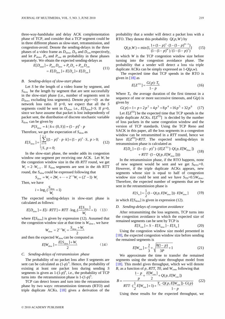
three-way-handshake and delay ACK complementation phase of TCP, and consider that a TCP segment could be in three different phases as slow-start, retransmission, and congestion-avoid. Denote the sending-delays in the three phases of a video frame as Dslow, Dre and Dcon respectively, and let Pslow, Pre and Pcon as probability in these phases separately. We obtain the expected sending-delays as
send slow slow re re con con
slow re con
[ ] [ ] [ ] [ ]E D P D P D P D
E D E D E D= + += + +
(11)
B. Sending-delays of slow-start phase Let S be the length of a video frame by segment, and
Sslow be the length by segment that are sent successfully in the slow-start phase (i.e., number of segments sent in Dslow, excluding loss segments). Denote p(p>=0) as the network loss ratio. If p=0, we expect that all the S segments could be sent in Dslow, i.e., E[Sslow]=S. If p>0, since we have assume that packet is lost independently of packet sent, the distribution of discrete stochastic variable Sslow can be given by
slow | (0, ) (1 )kP S k k S p p= ∈ = − ⋅ Therefore, we get the expectation of Sslow as
1
0slow
[(1 ) ] (1 ) , 0;[ ]
, 0;
Sk S
kp p k p S p
E SS p
−
=
⎧ − ⋅ ⋅ + − ⋅ >⎪= ⎨⎪ =⎩
∑ (12)
In the slow-start phase, the sender adds its congestion window one segment per receiving one ACK. Let Wi be the congestion window size in the ith RTT round, we get
12 −⋅= ii WW . If Sslow segments are sent in the ith RTT round, the Sslow could be expressed following that
1slow 1 1 1 12 2 (2 1)i iS W W W W−= + + ⋅⋅⋅ + = − ⋅
Then, we have slow
21
log ( 1)S
iW
= +
The expected sending-delays in slow-start phase is calculated as follows:
slowslow 2
1
[ ][ ] [ ] log ( 1)
E SE D E i RTT RTT
W= ⋅ = ⋅ + (13)
where E[Sslow] is given by expression (12). Assumed that the congestion window size at that time is Wslow , we have
1 slow 1slow 12
2i S W
W W− += =
and then the expected Wslow can be computed as
slow 1slow
[ ][ ]
2E S W
E W+
= (14)
C. Sending-delays of retransmission phase The probability of no packet loss after S segments are
sent can be calculated as (1-p) S. Hence, the probability of existing at least one packet loss during sending S segments is given as 1-(1-p)S, i.e., the probability of TCP turns into the retransmission phase is 1-(1-p)S.
TCP can detect losses and turn into the retransmission phase by two ways: retransmission timeouts (RTO) and triple duplicate ACKs. [18] gives a derivation of the
probability that a sender will detect a packet loss with a RTO. They denote this probability ),( WpQ by
3 3
3
1 (1 ) (1 (1 ) )( , ) min1, (1 (1 ) ) (1 (1 ) )
W
W
p pQ p Wp p
−+ − ⋅ − −=
− − − − (15)
in which W is the TCP congestion window size before turning into the congestion avoidance phase. The probability that a sender will detect a loss via triple duplicate ACKs can be simply expressed as 1-Q(p,w).
The expected time that TCP spends in the RTO is given in [18] as
TO 0( )[ ]
1G p T
E Zp⋅
=−
(16)
Where T0 is the average duration of the first timeout in a sequence of one or more successive timeouts, and G(p) is given by
65432 32168421)( pppppppG ++++++= (17) Let E[ZTD] be the expected time that TCP spends in the
triple duplicate ACKs. E[ZTD] is decided by the number of loss packets in the same congestion window and the version of TCP standards. Using the TCP Reno and SACK in this paper, all the loss segments in a congestion window can be retransmitted in a RTT round, hence we have E[ZTD]=RTT. The expected sending-delays in retransmission phase is calculated as
TOre Slow
slow
[ ] (1 (1 ) ) ( [ ] ( , [ ]) (1 ( , [ ])))
SE D p E Z Q p E WRTT Q p E W
= − − ⋅ ⋅
+ ⋅ − (18)
In the retransmission phase, if the RTO happens, none of new segment would be sent and we get SRTO=0. However, if the triple duplicate ACKs appears, new segments whose size is equal to half of congestion window size could be sent and we have STD=0.5Wslow. Therefore, the expected number of segments that are be sent in the retransmission phase is
re slow slow1[ ] (1 ( , [ ])) [ ]2
E S Q p E W E W= − ⋅ (19)
in which E[Sslow] is given in expression (12).
D. Sending-delays of congestion avoidance After retransmitting the loss segments, TCP turns into
the congestion avoidance in which the expected size of remained segments can be sent by TCP is
con slow re[ ] [ ] [ ]E S S E S E S= − − (20) Using the congestion window size model presented in
[18], the expected congestion window size before sending the remained segments is
con2 8(1 )[ ] 13 3
pE WP−
= + + (21)
We approximate the time to transfer the remained segments using the steady-state throughput model from [18]. This model gives throughput, which we will denote B), as a function of pp, RTT, T0, and Wcon, following that
concon
0 concon
[ ]1 ( , [ ])2
( , [ ]) ( )1( [ ] 1)2 1
E Wp Q p E WpB
T Q p E W G pRTT E Wp
−+ +
=⋅ ⋅
⋅ + +−
(22)
Using these results for the expected throughput, we
JOURNAL OF MULTIMEDIA, VOL. 5, NO. 3, JUNE 2010 219
© 2010 ACADEMY PUBLISHER
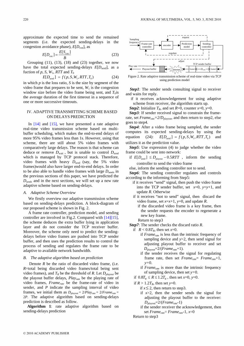
Internet
Frame-rate controller encoder Prediction
modelSending
controller
Playout buffer Dwait
Sampling frequency
TCP sender buffer
frame1 frame2
request
regulate
adjust
Play rate
Figure 2. Rate adaptive transmission scheme of real-time video via TCP using prediction model
approximate the expected time to send the remained segments (i.e. the expected sending-delays in the congestion avoidance phase), E[Dcon], as
concon
[ ][ ]
E SE D
B= (23)
Grouping (11), (13), (18) and (23) together, we now have the total expected sending-delays E[Dsend], as a fuction of p, S, W1, RTT and T0
send 1 0[ ] ( , , , , )E D f p S W RTT T= (24) in which p is the loss ratio, S is the size by segment of the video frame that prepares to be sent, W1 is the congestion window size before the video frame being sent, and T0 is the average duration of the first timeout in a sequence of one or more successive timeouts.
IV. ADAPTIVE TRANSMITTING SCHEME BASED ON DELAYS PREDICTION
In [14] and [15], we have presented a rate adaptive real-time video transmission scheme based on multi-buffer scheduling, which makes the end-to-end delays of more 95% video frames less than 1s. However, using that scheme, there are still about 5% video frames with comparatively large delays. The reason is that scheme can deduce or remove Dwait , but is unable to control Dsend which is managed by TCP protocol stack. Therefore, video frames with heavy Dsend (say, the 5% video frames)would also have larger end-to-end delays. In order to be also able to handle video frames with large Dsend, in the previous sections of this paper, we have predicted the Dsend, and in the next sections, we will set up a new rate adaptive scheme based on sending-delays.
A. Adaptive Scheme Overview We firstly overview our adaptive transmission scheme
based on sending-delays prediction. A block-diagram of our proposed scheme is shown in Fig. 2.
A frame rate controller, prediction model, and sending controller are involved in Fig.2. Compared with [14][15], the scheme deduces the extra buffer lying in application layer and do not consider the TCP receiver buffer. Moreover, the scheme only need to predict the sending-delays before video frames are pushed into TCP sender buffer, and then uses the prediction results to control the process of sending and regulates the frame rate to be adaptive to available network bandwidth.
B. The adaptive algorithm based on prediction Denote R be the ratio of discarded video frame, (i.e.
R=total being discarded video frames/total being sent video frames), and TR be the threshold of R. Let Dplayout be the playout buffer delays, Playrate be the playing rate of video frames, Framerate be the frame-rate of video in sender, and P indicate the sampling interval of video frames, we initial them as Dplayout = 2/Playrate = 2/Framerate = 2P. The adaptive algorithm based on sending-delays prediction is described as follow.
Algorithm 1: rate adaptive algorithm based on sending-delays prediction
Step1: The sender sends consulting signal to receiver and waits for reply.
if it receives acknowledgement for using adaptive scheme from receiver, the algorithm starts up.
Step2: Initialize TR, and set R=0, counter x=0, y=0. Step3: If sender received signal to constrain the frame-
rate, set Framerate=2/Dplayout, and then return to step2, else goes to step4.
Step4: After a video frame being sampled, the sender computes its expected sending-delays by using the equation (24): send 1 0[ ] ( , , , , )E D f p S W RTT T= and utilizes it as the prediction value.
Step5: Use expression (4) to judge whether the video frame could be sent into network:
if send playout[ ] 0.5E D D RTT≤ − , inform the sending controller to send the video frame
else, inform the sending controller not to send. Step6: The sending controller regulates and controls
according to the informing from Step5: if it receives “send” signal, then push the video frame
into the TCP sender buffer, set x=0, y=y+1, and update R. Otherwise
if it receives “not to send” signal, then discard the video frame, set x=x+1, y=0, and update R. if the discarded video frame is a key frame, then
the sender requests the encoder to regenerate a new key frame.
Return to step3 Step7: The sender checks the discard ratio R.
if R < 0.8TR, then set x=0. if Framerate is less than the intrinsic frequency of
sampling device and y>2, then send signal for adjusting playout buffer to receiver and set Dplayout=2/(Framerate+1).
if the sender receives the signal for regulating frame rate, then set Framerate= Framerate+1, y=0.
if Framerate is more than the intrinsic frequency of sampling device, then set y=0.
if 0.8 1.2R RT R T≤ ≤ , then set x=0, y=0. if R > 1.2TR, then set y=0.
if x≤ 2, then return to step3. if x>2, then the sender sends the signal for
adjusting the playout buffer to the receiver: Dplayout=2/(Framerate-1)
if the sender receiver the acknowledgement, then set Framerate= Framerate-1, x=0
Return to step3
220 JOURNAL OF MULTIMEDIA, VOL. 5, NO. 3, JUNE 2010
© 2010 ACADEMY PUBLISHER
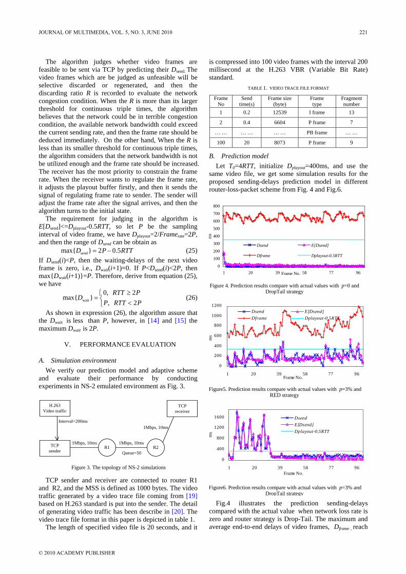
R1TCP sender
TCPreceiver
H.263Video traffic
1Mbps, 10ms
Queue=50
1Mbps, 10ms
1Mbps, 10ms
R2
Interval=200ms
Figure 3. The topology of NS-2 simulations
0
100
200
300
400
500
600
700
800
1 20 39 58 77 96Frame No.
ms
Dsend E[Dsend]
Dframe Dplayout-0.5RTT
Figure 4. Prediction results compare with actual values with p=0 and DropTail strategy
0
200
400
600
800
1000
1200
1 20 39 58 77 96Frame No.
ms
Dsend E[Dsend]Dframe Dplayout-0.5RTT
Figure5. Prediction results compare with actual values with p=3% and RED strategy
0
400
800
1200
1600
1 20 39 58 77 96Frame No.
ms
DsendE[Dsend]Dplayout-0.5RTT
Figure6. Prediction results compare with actual values with p=3% and DropTail strategy
The algorithm judges whether video frames are feasible to be sent via TCP by predicting their Dsend. The video frames which are be judged as unfeasible will be selective discarded or regenerated, and then the discarding ratio R is recorded to evaluate the network congestion condition. When the R is more than its larger threshold for continuous triple times, the algorithm believes that the network could be in terrible congestion condition, the available network bandwidth could exceed the current sending rate, and then the frame rate should be deduced immediately. On the other hand, When the R is less than its smaller threshold for continuous triple times, the algorithm considers that the network bandwidth is not be utilized enough and the frame rate should be increased. The receiver has the most priority to constrain the frame rate. When the receiver wants to regulate the frame rate, it adjusts the playout buffer firstly, and then it sends the signal of regulating frame rate to sender. The sender will adjust the frame rate after the signal arrives, and then the algorithm turns to the initial state.
The requirement for judging in the algorithm is E[Dsend]<=Dplayout-0.5RTT, so let P be the sampling interval of video frame, we have Dplayout=2/Framerate=2P, and then the range of Dsend can be obtain as
sendmax 2 0.5D P RTT= − (25) If Dsend(i)<P, then the waiting-delays of the next video frame is zero, i.e., Dwait(i+1)=0. If P<Dsend(i)<2P, then maxDwait(i+1)=P. Therefore, derive from equation (25), we have
wait
0, 2max
, 2RTT P
DP RTT P
≥⎧= ⎨ <⎩
(26)
As shown in expression (26), the algorithm assure that the Dwait is less than P, however, in [14] and [15] the maximum Dwait is 2P.
V. PERFORMANCE EVALUATION
A. Simulation environment We verify our prediction model and adaptive scheme
and evaluate their performance by conducting experiments in NS-2 emulated environment as Fig. 3.
TCP sender and receiver are connected to router R1 and R2, and the MSS is defined as 1000 bytes. The video traffic generated by a video trace file coming from [19] based on H.263 standard is put into the sender. The detail of generating video traffic has been describe in [20]. The video trace file format in this paper is depicted in table 1.
The length of specified video file is 20 seconds, and it
is compressed into 100 video frames with the interval 200 millisecond at the H.263 VBR (Variable Bit Rate) standard.
TABLE 1. VIDEO TRACE FILE FORMAT
FrameNo
Send time(s)
Frame size (byte)
Frame type
Fragmentnumber
1 0.2 12539 I frame 13
2 0.4 6604 P frame 7
… … … … … … PB frame … …
100 20 8073 P frame 9
B. Prediction model Let T0=4RTT, initialize Dplayout=400ms, and use the
same video file, we get some simulation results for the proposed sending-delays prediction model in different router-loss-packet scheme from Fig. 4 and Fig.6.
Fig.4 illustrates the prediction sending-delays compared with the actual value when network loss rate is zero and router strategy is Drop-Tail. The maximum and average end-to-end delays of video frames, Dframe , reach
JOURNAL OF MULTIMEDIA, VOL. 5, NO. 3, JUNE 2010 221
© 2010 ACADEMY PUBLISHER

200
400
600
800
1000
1200
1400
1600
1 20 39 58 77 96Frame No.
end-
to-e
nd d
elay
s(m
s)
multi-buffer schedulingUDPprediction model
Figure 7. Comparison of end-to-end delay using different schemes with p=3% and DropTail strategy
300
400
500
600
700
800
1 20 39 58 77 96Frame No.
end-
to-e
nd d
elay
s (m
s)
multi-buffer schedulingUDPprediction model
Figure 8. Comparison of end-to-end delay using different schemes with
p=3% and RED strategy
726ms and 652ms separately, i.e., all the sent video frames have achieved the requirement for transmitting real-time video across the Internet, which shown that using expression (4) to judge whether video frames could be played on time via TCP is reasonable. Then, using expression (4), we judge all the video frame is feasible to be sent via TCP according to the actual sending-delays. Moreover, according to the prediction sending-delays, we can also judge that, so the judging error rate is zero and the precision is 100%. Fig.5 shows the results with p=3% and RED router strategy. The Dsend fluctuated synchronously with the Dframe, and video frames which are judged as unfeasible to be sent via TCP using Dsend are also of larger Dframe. Ultilizing the actual sending-delays, 5 of 100 video frames are judged as unfeasible via TCP whose number are indicated as the assembly, Actual(40,42,73,75,91), while using the prediction sending-delays the corresponding assembly is Prediction ( 13, 40, 42,73,91,96,97)where child assembly(40,42,73,91), is included in Actual. Hence, one unfeasible video frame is ignored and three feasible video frames are judge as unfeasible by mistake when using prediction value to judge, and then the precision can be computed as (100-(1+3))/100=96%.The results with p=3% and DropTail strategy is shown in Fig.6. The assembly Actual involves 19 video frames, and the assembly Prediction contains 26 video frames where 18 are included in Actual, therefore the precision is 92% by the same reason.
The simulation results overall from Fig.4 to Fig.6 show the precision of prediction model for judging whether video frames are feasible to be sent via TCP is in 92%~100%, and the model is more suitable for the RED.
C. Adaptive scheme Fig. 7 and Fig.8 shows the differences of video frame
end-to-end delays using distinct scheme when network loss rate is about 3% while router strategy is drop-tail and RED separately.
As shown in Fig.7, using the scheme based on multi-buffer scheduling in [14][15], the fluctuation of end-to-end delays is larger than using the scheme based on prediction model in this paper. The former’s maximum and average delays reach 1426 and 816 ms separately, and there are 5 video frames with the delays more than 1 second. However, that of the later are only 902 and 600 ms respectively. Although average delays using UDP is below our scheme, UDP can not selectively discard video frames which will pose some key frames to be discarded and cut down the visual quality.
Fig.8 shows that the delay fluctuation range of the scheme based on prediction model is in 150ms from 453 to 555 ms while the range of scheme based on multi-buffer scheduling scheme in [14 ][15] is in 250ms from 488 to 766, so the scheme presented in this paper is also better than than [14][15].
VI. CONCLUSIONS
Larger end-to-end delays posed by TCP retransmission is major factor of influence playing quality using TCP to transmit real-time video across the Internet. The playout-buffer of receiver is set up to eliminate the jitter posed by the irregular arrivals of video frames. If TCP has lost packets but it has finished the retransmission during the playout buffer delays, Dplayout, application would be oblivious to the packet loss, then using TCP and setting the Dplayout is available. We explore how to set fit Dplayout to assure the playing quality be immune to the loss and TCP retransmission and point the relationship between Dplayout, Dsend, and RTT: Dsend<=Dplayout-0.5RTT as the requirement of transmitting real-time video with acceptable playing performance via TCP.
We set up a stochastic prediction model to predict the Dsend (sending-delays of video frames), and the prediction values can be used to judge whether real-time video frames are feasible to be sent using TCP. The input of our prediction model include TCP congestion window size, video frame size, loss ratio, RTT and RTO time, and the output is the expected Dsend. Based on the model, we propose a novel rate adaptive scheme, which selectively discards some video frames which are judged as unfeasible to be sent vip TCP before they are sent by predicting sending-delays. The scheme considers integratedly the selective discard rate, frame rate constraining from receiver, and the intrinsic frequency of sampling device, and then can dynamically adjust video frame rate and playout buffer size which makes the sending rate adaptive to the available network bandwidth.
The scheme does not require any modifications to the network infrastructure or TCP protocol stack and only wants to measure some parameters before video frames are sent. By using the scheme, the average video frame end-to-end delays are significantly cut down. Compared
222 JOURNAL OF MULTIMEDIA, VOL. 5, NO. 3, JUNE 2010
© 2010 ACADEMY PUBLISHER
with our earlier works in [14][15], the delays are reduced about 25%. Compared with those schemes in [4~12], the presented scheme can also archieve the requirement of transmitting real-time video on Internet but it only needs fewer data and feedback informations, and the argrithm and architecture is more simple, so it is also easier deployable and maitainalbe. Compared with UDP, the scheme can assure not to discard key frames, and then it can provides better visual quality.
ACKNOWLEDGMENT
This work was supported by City University of Hong Kong Strategic Research Grant, under No. 7002214 and the National Science Fund for Distinguished Youth Scholars of China, under Grant No. 60425310.
REFERENCES
[1] R.P. Karrer, “TCP Prediction for Adaptive Applications”, in Proc. of 32nd IEEE Conf. on Local Computer Networks, pp. 989-996,2007.
[2] B. Wang, J. Kurose, P. Shenoy. , D. Towsley, “Multimedia Streaming via TCP: An Analytic Performance Study”, ACM Trans. on Multimedia Computing, Communications, and Applications, vol. 4, Issue 2, pp. 1-8, 2008.
[3] C. Krasic, K. Li, J. Walpole, “The Case for Streaming Multimedia with TCP”, in 8th International Workshop on Interactive Distributed Multimedia Systems, Lancaster, UK, Sep., 2001.
[4] N. Seelam, P. Sethi, W.C. Feng, “A Hysteresis Based Approach for Quality, Frame Rate, and Buffer Management for Video Streaming Using TCP”, in Proc. of the Management of Multimedia Networks and Services, Heidelberg, Germany, pp. 1-15, 2001.
[5] C. Krasic, J. Walpole, “Priority-Progress Streaming for Quality-Adaptive Multimedia”, in Proc. of ACM Multimedia, Ottawa, pp. 463-464, 2001.
[6] P. de Cuetos and K.W. Ross, “Adaptive Rate Control for Streaming Stored Fine-Grained Scalable Video”, in Proc. of IEEE NOSSDAV, 2002.
[7] P. de Cuetos, P. Guillotel, K. W. Ross, and D. Thoreau, “Implementation of Adaptive Streaming of Stored MPEG-4 FGS Video over TCP”, in Proc. of IEEE Inter. Conf. on Multimedia and Expo (ICME02), 2002.
[8] P. Mehra, De Vleesc, “Receiver-Driven Bandwidth Sharing for TCP and its Application to Video Streaming”, IEEE Trans. on Multimedia, No.7, pp. 740-752, 2005.
[9] I.V. Bajic, O. Tickoo, A. Balan, S. Kalyanaraman, and J.W. Woods, “Integrated End-to-End Buffer Management and Congestion Control for Scalable Video Communications”, in Proc. of IEEE Inter. Conf. on Image Processing, Barcelona, Spain, vol. 3, pp. 257-260, 2003.
[10] E.A. Jammeh, M. Fleury, M. Ghanbari, “Rate-adaptive Video Streaming Through Packet Dispersion Feedback”. IEEE Trans. on Communications, vol. 3, No.1, pp. 25-37, 2009.
[11] S. Hasan, L. Lefevre, P. Huang, P. Werstein, “Cross Layer Protocol Support for Live Streaming Media”. in Proc. of IEEE Inter. Conf. on Advanced Information Networking and Applications, pp. 319-326, 2008.
[12] A. Sehgul, O. Verscheure, P. Frossurd, “Distortion-Buffer Optimized TCP Video Streaming”, in Proc. of IEEE Inter. Conf. on Image Processing, pp. 2083-2086, 2004.
[13] S. Liang, D. Cheriton, “TCP-RTM: Using TCP for Real Time Multimedia Applications”. in Proc. of Inter. Conf. on Network Protocols, Paris, France, pp. 1-20, 2002.
[14] Y.H. XIONG, M. WU, W.J. JIA, “Rate Adaptive Real-Time Video Transmission Scheme over TCP Using Multi-Buffer Scheduling”, in Proc. of IEEE ICYCS’08, Zhangjiajie, pp. 354-361, 2008.
[15] Y.H. Xiong, M. Wu, W.J. Jia, “Efficient Frame Schedule Scheme for Real-time Video Transmission Across the Internet Using TCP”, Journal of Networks, vol.4, No.3, May 2009.
[16] N. Cardwell, S. Savage, T. Anderson, “Modeling TCP Latency”, in Proc. of IEEE INFOCOM, pp. 1742-1751,2000.
[17] D. Zheng, G.Y. Lazarou, R. Hu, “A stochastic model for short-lived TCP flows”, in Proc. of IEEE Inter. Conf. on Communications, pp. 76-81, 2003.
[18] J. Padhye, V. Firoiu, D. Towsley, Jim Kurose, “Modeling TCP Throughput: A Simple Model and its Empirical Validation”, in Proc. of ACM SIGCOMM Computer Communication Review, vol. 28, No. 4, pp. 303-314, 1998.
[19] http://www.tkn.tu-berlin.de/research/trace/ltvt.html. [20] FHP. Fitzek, M. Reisslein, “MPEG-4 and H.263 Video
Traces for Network Performance Evaluation”, IEEE Network, vol. 15, pp. 40-54, 2001.
Yonghua Xiong was born in 1979. He received his MSc and PhD degree in engineering from Central South University, Changsha, China in 2004 and 2009. He was a visiting scholar with the Department of Computer Science, City University of Hong Kong, Hong Kong, from 2006 to 2008.
He joined the staff of Central South University in 2005, where he is currently a lecturer of School of Information
Science and Engineering. His research interests include multimedia communication and wireless network.
Min Wu was born in 1963. He received his BSc and MSc degrees from the Central South University, China in 1983 and 1986. He received his PhD degree in engineering from Tokyo Institute of Technology, Japan in 1999. He is currently a professor of automatic control engineering in the Central South University.
His research interests include robust control and its application, process
control, and intelligent control. Prof. Wu received the best paper award at IFAC 1999. He is the Senior Member of IEEE.
Weijia Jia received the MSc and PhD degrees in 1984 and 1993 from Center South University, China and Polytechnic Faculty of Mons, Belgium. In 1995, He joined the Department of Computer Science, City University of Hong Kong (CityU) and, currently, he is a professor of CityU.
His research interests include wireless communication, protocols and heterogeneous networks, distributed
systems. Prof. Jia has been the Principal-Investigator of 18 research projects supported by RGC Research Grants, Hong Kong and Strategic Research Grants, CityU. He is the Senior Member of IEEE and the Member of ACM.
JOURNAL OF MULTIMEDIA, VOL. 5, NO. 3, JUNE 2010 223
© 2010 ACADEMY PUBLISHER
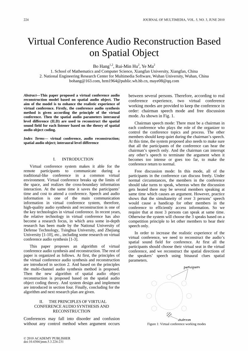
Virtual Conference Audio Reconstruction Based on Spatial Object
Bo Hang1,2, Rui-Min Hu2, Ye Ma2
1. School of Mathematics and Computer Science, Xiangfan University, Xiangfan, China 2. National Engineering Research Center for Multimedia Software, Wuhan University, Wuhan, China
[email protected], [email protected], [email protected]
Abstract—This paper proposed a virtual conference audio reconstruction model based on spatial audio object. The aim of the model is to enhance the realistic experience of virtual conference. Firstly, the conference audio synthesis method is given according the principle of the virtual conference. Then the spatial audio parameters interaural level difference (ILD) are used to reconstruct the spatial sound field for each listener based on the theory of spatial audio object coding. Index Terms— virtual conference, audio reconstruction; spatial audio object; interaural level difference
I. INTRODUCTION
Virtual conference system makes it able for the remote participants to communicate during a traditional-like conference in a common virtual environment. Virtual conference breaks up the limits of the space, and realizes the cross-boundary information interaction. At the same time it saves the participants’ time and cost to attend a conference. Speech and audio information is one of the main communication information in virtual conference system, therefore, high-quality audio synthesis and reconstruction is one of the key technologies in virtual conference. In recent years, the relative technology in virtual conference has also become a research focus, in which area some in-depth research has been made by the National University of Defense Technology, Tsinghua University, and Zhejiang University [1-10], etc., including some research on virtual conference audio synthesis [1-3].
This paper proposes an algorithm of virtual conference audio synthesis and reconstruction. The rest of paper is organized as follows. At first, the principles of the virtual conference audio synthesis and reconstruction are introduced in section 2. And based on the principles the multi-channel audio synthesis method is proposed. Then the new algorithm of spatial audio object reconstruction is proposed based on the spatial audio object coding theory. And system design and implement are introduced in section four. Finally, concluding for the algorithm and next research plan are given.
II. THE PRINCIPLES OF VIRTUAL CONFERENCE AUDIO SYNTHESIS AND
RECONSTRUCTION
Conferences may fall into disorder and confusion without any control method when argument occurs
between several persons. Therefore, according to real conference experience, two virtual conference working modes are provided to keep the conference in order: chairman speech mode and free discussion mode. As shown in Fig. 1.
Chairman speech mode: There must be a chairman in each conference who plays the role of the organizer to control the conference topics and process. The other members should keep quiet during the chairman’s speech. At this time, the system proposed also needs to make sure that all the participants of the conference can hear the chairman’s speech only. And the chairman can interrupt any other’s speech to terminate the argument when it becomes too intense or goes too far, to make the conference return to normal.
Free discussion mode: In this mode, all of the participants in the conference can discuss freely. Under normal circumstances, the members in the conference should take turns to speak, whereas when the discussion gets heated there may be several members speaking at same time which causes an argument. However, practice shows that the simultaneity of over 3 persons’ speech would cause a handicap for other members in the conference to efficiently access information. So we require that at most 3 persons can speak at same time. Otherwise the system will choose the 3 speaks based on a competition principle to let other members to hear their speech only.
In order to increase the realistic experience of the virtual conference, we need to reconstruct the audio’s spatial sound field for conference. At first all the participants should choose their virtual seat in the virtual conference, and we reconstruct the spatial directions of the speakers’ speech using binaural clues spatial parameters.
Figure 1: Virtual conference working modes
224 JOURNAL OF MULTIMEDIA, VOL. 5, NO. 3, JUNE 2010
© 2010 ACADEMY PUBLISHERdoi:10.4304/jmm.5.3.224-231
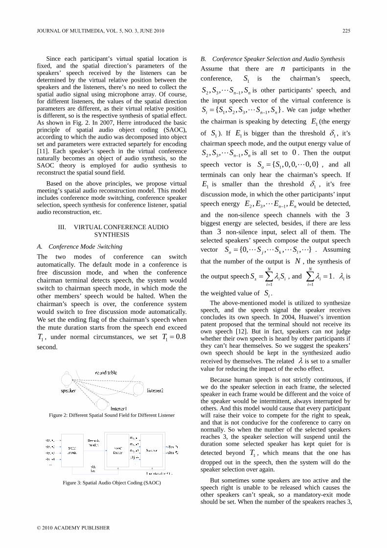
Since each participant’s virtual spatial location is fixed, and the spatial direction’s parameters of the speakers’ speech received by the listeners can be determined by the virtual relative position between the speakers and the listeners, there’s no need to collect the spatial audio signal using microphone array. Of course, for different listeners, the values of the spatial direction parameters are different, as their virtual relative position is different, so is the respective synthesis of spatial effect. As shown in Fig. 2. In 2007, Herre introduced the basic principle of spatial audio object coding (SAOC), according to which the audio was decomposed into object set and parameters were extracted separtely for encoding [11]. Each speaker’s speech in the virtual conference naturally becomes an object of audio synthesis, so the SAOC theory is employed for audio synthesis to reconstruct the spatial sound field.
Based on the above principles, we propose virtual meeting’s spatial audio reconstruction model. This model includes conference mode switching, conference speaker selection, speech synthesis for conference listener, spatial audio reconstruction, etc.
III. VIRTUAL CONFERENCE AUDIO SYNTHESIS
A. Conference Mode Switching The two modes of conference can switch automatically. The default mode in a conference is free discussion mode, and when the conference chairman terminal detects speech, the system would switch to chairman speech mode, in which mode the other members’ speech would be halted. When the chairman’s speech is over, the conference system would switch to free discussion mode automatically. We set the ending flag of the chairman’s speech when the mute duration starts from the speech end exceed
, under normal circumstances, we set 1T 1 0.8T = second.
Figure 2: Different Spatial Sound Field for Different Listener
Figure 3: Spatial Audio Object Coding (SAOC)
B. Conference Speaker Selection and Audio Synthesis Assume that there are n participants in the conference, is the chairman’s speech,
is other participants’ speech, and the input speech vector of the virtual conference is
1S
2 3 1, , ,nS S S S− n
i nS S S S S −1 2 3 1 , , , , n S= . We can judge whether
the chairman is speaking by detecting (the energy
of ). If is bigger than the threshold 1E
1S 1E 1δ , it’s chairman speech mode, and the output energy value of
is all set to . Then the output
speech vector is 2 3 1, , ,nS S S S− n 0
1 ,0,0, 0,0oS S= , and all terminals can only hear the chairman’s speech. If
is smaller than the threshold 1E 1δ , it’s free discussion mode, in which the other participants’ input speech energy would be detected,
and the non-silence speech channels with the 3 biggest energy are selected, besides, if there are less than non-silence input, select all of them. The selected speakers’ speech compose the output speech vector
2 3 1, , ,nE E E E− n
3
0, , , , o j k lS S S S= . Assuming
that the number of the output is , the synthesis of
the output speech
N
1
N
s i ii
S Sλ=
=∑ , and 1
1N
ii
λ=
=∑ . iλ is
the weighted value of . iSThe above-mentioned model is utilized to synthesize
speech, and the speech signal the speaker receives concludes its own speech. In 2004, Huawei’s invention patent proposed that the terminal should not receive its own speech [12]. But in fact, speakers can not judge whether their own speech is heard by other participants if they can’t hear themselves. So we suggest the speakers’ own speech should be kept in the synthesized audio received by themselves. The related λ is set to a smaller value for reducing the impact of the echo effect.
Because human speech is not strictly continuous, if we do the speaker selection in each frame, the selected speaker in each frame would be different and the voice of the speaker would be intermittent, always interrupted by others. And this model would cause that every participant will raise their voice to compete for the right to speak, and that is not conducive for the conference to carry on normally. So when the number of the selected speakers reaches 3, the speaker selection will suspend until the duration some selected speaker has kept quiet for is detected beyond , which means that the one has dropped out in the speech, then the system will do the speaker selection over again.
1T
But sometimes some speakers are too active and the speech right is unable to be released which causes the other speakers can’t speak, so a mandatory-exit mode should be set. When the number of the speakers reaches 3,
JOURNAL OF MULTIMEDIA, VOL. 5, NO. 3, JUNE 2010 225
© 2010 ACADEMY PUBLISHER
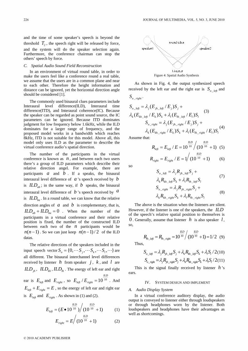
and the time of some speaker’s speech is beyond the threshold , the speech right will be released by force, and the system will do the speaker selection again. Furthermore, the conference chairman can stop the others’ speech by force.
2T
C. Spatial Audio Sound Field Reconstruction In an environment of virtual round table, in order to
make the users feel like a conference round a real table, we assume that the users are in a common plane and near to each other. Therefore the height information and distance can be ignored, yet the horizontal direction angle should be considered [1].
The commonly used binaural clues parameters include Interaural level difference(ILD), Interaural time difference(ITD), and Interaural coherence(IC). Because the speaker can be regarded as point sound source, the IC parameters can be ignored. Because ITD dominates judgment for low frequency below 1.6kHz, while the ILD dominates for a larger range of frequency, and the proposed model works in a bandwidth which reaches 8kHz, ITD is not suitable for this model. Above all, this model only uses ILD as the parameter to describe the virtual conference audio’s spatial direction.
The number of the participants in the virtual conference is known as , and between each two users there’s a group of ILD parameters which describe their relative direction angel. For example, there are participants and . If a speaks, the binaural interaural level difference of ’s speech received by is
n
a ba b
abILD ; in the same way, if speaks, the binaural
interaural level difference of ’s speech received by is
bb a
baILD . In a round table, we can know that the relative
direction angles of and is complementary, that is, . When the number of the
participants in a virtual conference and their relative position is fixed, the number of the constructed ILD between each two of the participants would be
. So we can just keep of the ILD datas.
a b0ab baILD ILD+ =
n( 1n n − ) ( 1) / 2n n −
The relative directions of the speakers included in the input speech vector are all different. The binaural interchannel level differences received by listener from speaker
0, , , , o j k lS S S S=
h j , , and are k ljhILD , khILD , lhILD . The energy of left ear and right
ear is leftE and rightE , so 10/ 10ILD
left rightE E = . And
left rightE E+ = E , so the energy of left ear and right ear
is leftE and rightE . As shown in (1) and (2).
10 10( 10 ) (10 1ILD ILD
leftE E= • + ) (1)
10(10 1)ILD
rightE E=
Figure 4: Spatial Audio Synthesis
As shown in Fig. 4, the output synthesized speech
received by the left ear and the right ear is and
. _o leftS
_o rightS
_ _
_ _
( / )
( / ) ( /o left j jh left j j
k kh left k k l lh left l l
S E E S
)E E S E E S
λ
λ λ
= +
+ (3)
_ _
_ _
( / )
( / ) ( /o right j jh right j j
k kh right k k l lh right l l
S E E S
)E E S E E S
λ
λ λ
= +
+(4)
Assume that:
10 10/ 10 (10ILD ILD
left leftR E E 1)= = + (5)
10/ 1 (10 1ILD
right rightR E E )= = + (6) so
_ _
_ _
o left j jh left j
k kh left k l lh left l
S R S
R S R S
λ
λ λ
= +
+ (7)
_ _
_ _
o right j jh right j
k kh right k l lh right l
S R S
R S R S
λ
λ λ
= +
+ (8)
The above is the situation when the listeners are silent. However, if the listener is one of the speakers, the ILD of the speech’s relative spatial position to themselves is
. Generally, assume that listener is also speaker , so, 0 h l
10 10_ _ 10 (10 1) 1/ 2
ILD ILD
lh left lh rightR R= = + = (9) Thus,
_ _ _ / 2o left j jh left j k kh left k l lS R S R S Sλ λ λ= + + (10)
_ _ _ /2o right j jh right j k kh right k l lS R S R S Sλ λ λ= + + (11)
This is the signal finally received by listener ’s ears.
h
IV. SYSTEM DESIGN AND IMPLEMENT
A. Audio Display System In a virtual conference auditory display, the audio
output is conveyed to listener either through loudspeakers or through headphones worn by the listener. Both loudspeakers and headphones have their advantages as well as shortcomings.
+ (2)
226 JOURNAL OF MULTIMEDIA, VOL. 5, NO. 3, JUNE 2010
© 2010 ACADEMY PUBLISHER

Loudspeakers cause some problems. The signals from the speakers interfere with each other. It is possible to create the signals for each speaker in such a way that the resulting signal at each ear is still correct, but it has a quite high computational complexity. And, the listener has to be sitting in the right spot, or the sound effect will be different.
If headphones are used, it is not difficult to generate a specific signal for each ear, since there is no interference of the two signals. And the computational complexity is also lower than loudspeakers. So we use headphones in this virtual conference audio reconstruction system.
B. Audio Coding Algorithm If the audio signal in virtual conference is transmitted
without compression, a lot of network bandwidth will be used and the audio signal delay will increase, that will impact the communication effect in virtual conference. So we need to compress the audio signal to audio stream in the proposed system with some encoding algorithm.
As different participants in virtual conference would be in different environment and their network condition may be different, too, the network bandwidth of the proposed system should be restricted. Therefore, we use mid range or low bit-rate wideband audio encoding algorithm to get better sound quality in low bit-rate. The currently used main wideband audio encoding algorithm for mid range or low bit-rate includes HE-AACv2 standardized by MPEG [13], G.729.1 standardized by ITU [14], and AMR-WB+ standardized by 3GPP [15]. The comparison of the three audio codec is shown in Table I.
China AVS (Audio Video coding Standard) organization has drafted AVS-P10 (Part 10), with China’s own independent intellectual property [16]. We were actively involved in the work for AVS audio coding standards, and made important contributions [17-24]. Compared with AMR-WB+, AVS-P10 achieves almost equivalent sound quality at same bitrate, so we use the audio compression algorithm in AVS-P10 to compress the virtual conference audio in the proposed system.
C. Client/Server System Design In this virtual conference audio reconstruction system,
a conference server, which is used to receive the audio from speakers and send out the synthesized audio to listener, is needed. Each virtual conference participant has a client terminal. The client terminal is used to send the audio signal if the participant is a speaker, and receive the audio from server and synthesize the audio to be displayed to listener.
We designed two optional systems for the audio reconstruction: centralized computing system, and distributed computing system. The physical structures of the two systems are same, as shown in Fig. 5. The server and the clients access to the same network or Internet. The difference between the two systems is where the spatial audio signals are synthesized? The server or clients.
TABLE I. COMPARISON OF THREE CODEC
Codec Bit Rate [kbit/s] Bandwidth [Hz]
HE-AAC V2 16~128 0~16900
G.729.1 8~32 50~7000
AMR-WB+ 6~48 50~19200
Figure 5: Physical structure of the proposed system
(1) Centralized computing system
In the centralized computing system, the server receives the speakers' audio signal, computes the synthesized audio signal for each participant respectively, according to the relative positions of the participants. Client terminals receive audio signals from the server, decode and output the signals.
In detail, the processing of the server in centralized is shown in Fig. 6.
Figure 6: Server processing flow in centralized computing
system
JOURNAL OF MULTIMEDIA, VOL. 5, NO. 3, JUNE 2010 227
© 2010 ACADEMY PUBLISHER
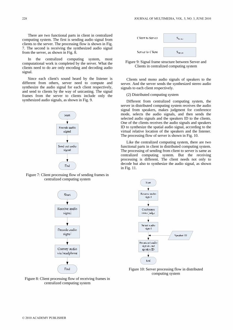
There are two functional parts in client in centralized computing system. The first is sending audio signal from clients to the server. The processing flow is shown in Fig. 7. The second is receiving the synthesized audio signal from the server, as shown in Fig. 8.
In the centralized computing system, most computational work is completed by the server. What the clients need to do are only encoding and decoding audio signal.
Since each client's sound heard by the listener is different from others, server need to compute and synthesize the audio signal for each client respectively, and send to clients by the way of unicasting. The signal frames from the server to clients include only the synthesized audio signals, as shown in Fig. 9.
Figure 7: Client processing flow of sending frames in
centralized computing system
Figure 8: Client processing flow of receiving frames in
centralized computing system
Figure 9: Signal frame structure between Server and
Clients in centralized computing system
Clients send mono audio signals of speakers to the server. And the server sends the synthesized stereo audio signals to each client respectively.
(2) Distributed computing system
Different from centralized computing system, the server in distributed computing system receives the audio signal from speakers, makes judgment for conference mode, selects the audio signals, and then sends the selected audio signals and the speakers ID to the clients. One of the clients receives the audio signals and speakers ID to synthesize the spatial audio signal, according to the virtual relative location of the speakers and the listener. The processing flow of server is shown in Fig. 10.
Like the centralized computing system, there are two functional parts in client in distributed computing system. The processing of sending from client to server is same as centralized computing system. But the receiving processing is different. The client needs not only to decode but also to synthesize the audio signal, as shown in Fig. 11.
Figure 10: Server processing flow in distributed
computing system
228 JOURNAL OF MULTIMEDIA, VOL. 5, NO. 3, JUNE 2010
© 2010 ACADEMY PUBLISHER
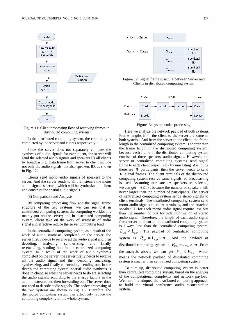
Figure 11: Client processing flow of receiving frames in
distributed computing system
In the distributed computing system, the computing is completed by the server and clients respectively.
Since the server does not separately compute the synthesis of audio signals for each client, the server will send the selected audio signals and speakers ID all clients by broadcasting. Data frame from server to client include not only the audio signals, but also speakers ID, as shown in Fig. 12.
Clients send mono audio signals of speakers to the server. And the server sends to all the listeners the mono audio signals selected, which will be synthesized in client and construct the spatial audio signals.
(3) Comparison and Analysis
By comparing processing flow and the signal frame structure of the two systems, we can see that in centralized computing system, the computing workload is mainly put on the server; and in distributed computing system, client take on the work of synthesis of audio signal and effective reduce the server computing load.
In the centralized computing system, as a result of the work of audio synthesis completed on the server, the server firstly needs to receive all the audio signal and then decoding, analyzing, synthesizing, and finally re-encoding, sending out. In the centralized computing system, as a result of the work of audio synthesis completed on the server, the server firstly needs to receive all the audio signal and then decoding, analyzing, synthesizing, and finally re-encoding, sending out. In the distributed computing system, spatial audio synthesis is done in client, so what the server needs to do are selecting the audio signals according to the energy factors in the audio bitstream, and then forwarding out. The server does not need to decode audio signals. The codec processing of the two systems are shown in Fig. 13. Therefore, the distributed computing system can effectively reduce the computing complexity of the whole system.
Figure 12: Signal frame structure between Server and
Clients in distributed computing system
Figure13: system codec processing
Here we analyze the network payload of both systems. Frame lengths from the client to the server are same in both systems. And from the server to the client, the frame length in the centralized computing system is shorter than the frame length in the distributed computing system, because each frame in the distributed computing system consists of three speakers' audio signals. However, the server in centralized computing systems send signal frame to each client respectively by unicasting. Assuming there are participants, then the server needs to send
signal frames. The client terminals of the distributed computing system receive same signals, so broadcasting is used. Assuming there are m speakers are selected, we can get
nn
m n≤ , because the number of speakers will never larger than the number of participants. The server of centralized computing system sends stereo signals to client terminals. The distributed computing system send mono audio signals to client terminals, and the attached speaker ID for each mono audio signal require less bits than the number of bits for side information of stereo audio signal. Therefore, the length of each audio signal from server to client in the distributed computing system is always less than the centralized computing system,
Dis CenL L< . The payload of centralized computing
system is Cen CenP L n= ×m
. And the payload of
distributed computing system is . From
the analysis above, we can get Dis DisP L= ×
Dis CenP P< , which means the network payload of distributed computing system is smaller than centralized computing system.
To sum up, distributed computing system is better than centralized computing system, based on the analysis of the computational complexity and network payload. We therefore adopted the distributed computing approach to build the virtual conference audio reconstruction system.
JOURNAL OF MULTIMEDIA, VOL. 5, NO. 3, JUNE 2010 229
© 2010 ACADEMY PUBLISHER
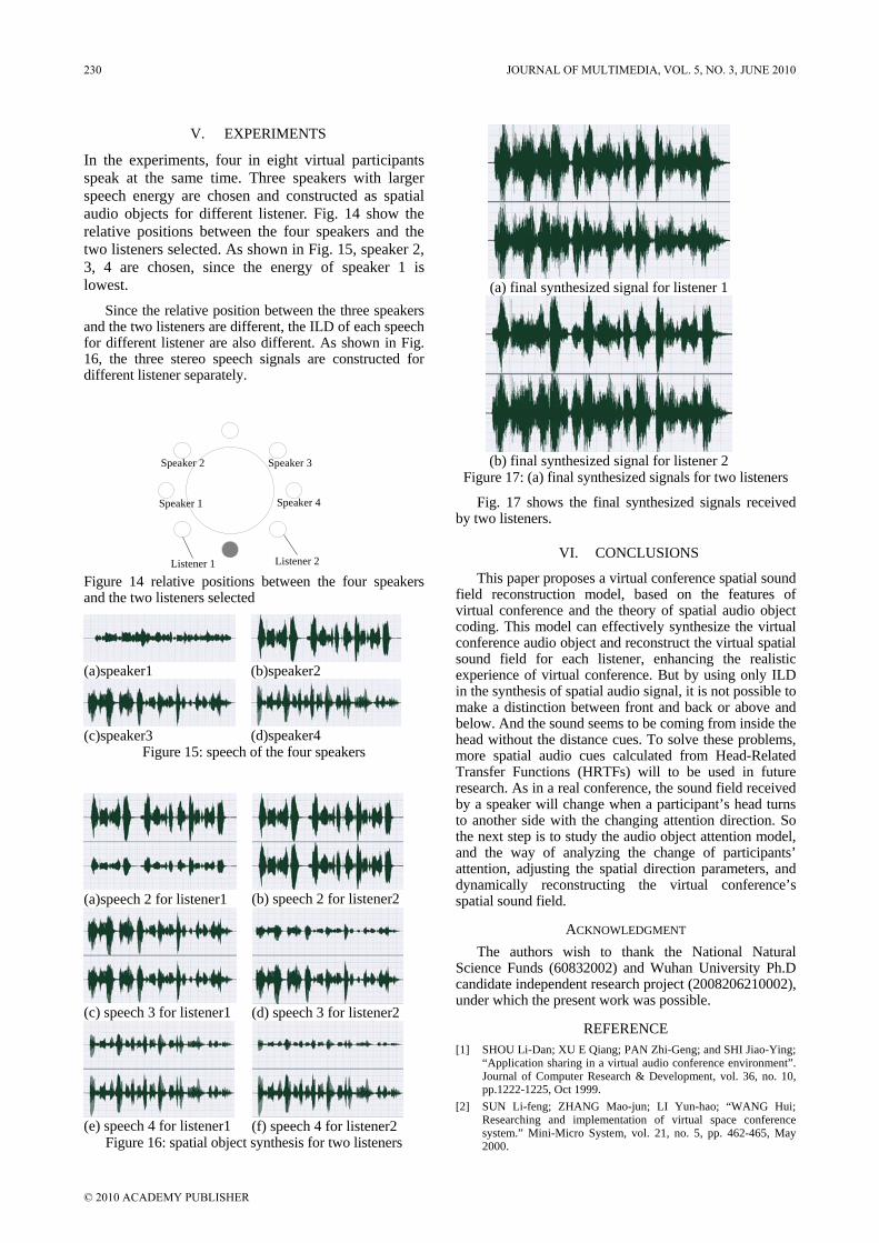
V. EXPERIMENTS
In the experiments, four in eight virtual participants speak at the same time. Three speakers with larger speech energy are chosen and constructed as spatial audio objects for different listener. Fig. 14 show the relative positions between the four speakers and the two listeners selected. As shown in Fig. 15, speaker 2, 3, 4 are chosen, since the energy of speaker 1 is lowest.
Since the relative position between the three speakers and the two listeners are different, the ILD of each speech for different listener are also different. As shown in Fig. 16, the three stereo speech signals are constructed for different listener separately.
Listener 1
Speaker 1
Listener 2
Speaker 2 Speaker 3
Speaker 4
Figure 14 relative positions between the four speakers and the two listeners selected
(a)speaker1 (b)speaker2
(c)speaker3 (d)speaker4
Figure 15: speech of the four speakers
(a)speech 2 for listener1
(b) speech 2 for listener2
(c) speech 3 for listener1
(d) speech 3 for listener2
(e) speech 4 for listener1
(f) speech 4 for listener2
Figure 16: spatial object synthesis for two listeners
(a) final synthesized signal for listener 1
(b) final synthesized signal for listener 2
Figure 17: (a) final synthesized signals for two listeners
Fig. 17 shows the final synthesized signals received by two listeners.
VI. CONCLUSIONS
This paper proposes a virtual conference spatial sound field reconstruction model, based on the features of virtual conference and the theory of spatial audio object coding. This model can effectively synthesize the virtual conference audio object and reconstruct the virtual spatial sound field for each listener, enhancing the realistic experience of virtual conference. But by using only ILD in the synthesis of spatial audio signal, it is not possible to make a distinction between front and back or above and below. And the sound seems to be coming from inside the head without the distance cues. To solve these problems, more spatial audio cues calculated from Head-Related Transfer Functions (HRTFs) will to be used in future research. As in a real conference, the sound field received by a speaker will change when a participant’s head turns to another side with the changing attention direction. So the next step is to study the audio object attention model, and the way of analyzing the change of participants’ attention, adjusting the spatial direction parameters, and dynamically reconstructing the virtual conference’s spatial sound field.
ACKNOWLEDGMENT The authors wish to thank the National Natural
Science Funds (60832002) and Wuhan University Ph.D candidate independent research project (2008206210002), under which the present work was possible.
REFERENCE [1] SHOU Li-Dan; XU E Qiang; PAN Zhi-Geng; and SHI Jiao-Ying;
“Application sharing in a virtual audio conference environment”. Journal of Computer Research & Development, vol. 36, no. 10, pp.1222-1225, Oct 1999.
[2] SUN Li-feng; ZHANG Mao-jun; LI Yun-hao; “WANG Hui; Researching and implementation of virtual space conference system.” Mini-Micro System, vol. 21, no. 5, pp. 462-465, May 2000.
230 JOURNAL OF MULTIMEDIA, VOL. 5, NO. 3, JUNE 2010
© 2010 ACADEMY PUBLISHER
[3] HE Bao-quan; SUN Li-feng; ZHANG Mao-jun; SUN Lei; “Research and implementation of audio synthesize technique in the virtual space conference system.” Mini-Micro System, vol. 21, no. 6, pp. 574-576, June 2000.
[4] ZHANG Maojun; SUN Lifeng; LI Yunhao; YANG Bing; SUN Lei; HE Baoquan; “Research and implementation of virtual conferencing space.” Computer Engineering, vol. 27, no. 1, pp. 1-2, January 2001.
[5] Wu Lingda; Zhang Maojun; Sun Lifeng; Yang Bing; Li Yunhao; Wang Hui; “The development of virtual space teleconferencing system.” High-tech Communications, pp. 41-44, May 2001.
[6] YANG Bing; LI Meng-jun; ZHANG Mao-jun; LI Yun-hao; WU Ling-da; “Research and implementation of video composition in the virtual conferencing space.” Mini-Micro System, vol. 22, no. 6, pp. 683-686, June 2001.
[7] CHEN Jin-hua; LI Fen; “Research on video segmentation and synthesis in video conferencing.” Computer Engineering and Design, vol. 25, no. 8, pp. 1293-1295, Aug 2004.
[8] LI Ling; TIAN Shu-zhen; SUN Li-feng; ZHONG Yu-zhuo; “The video transmission scenario based on awareness in the virtual space teleconference.” Computer Application Research, pp. 209-211, Apr. 2004.
[9] Lv Xiaoxing; Sun Lifeng; Li Ling; Li Fang; “Research of video synthesize and transmission technique in the virtual space conference system.” Journal of Beijing Radio & TV University, pp. 40-44, March 2004.
[10] SUN Li-feng; LI Fang; ZHONG Yu-zhuo; YANG Shi-qiang; “Multiview video based virtual teleconferencing synthesizing.” ACTA ELECTRONICA SINICA, vol. 33, no. 2, pp. 193-196, Feb. 2004.
[11] Jürgen Herre; Sascha Disch; “New Concepts in Parametric Coding of Spatial Audio From SAC to SAOC.” ICME 2007, IEEE International Conference on Multimedia & Expo, July 2007.
[12] Yu Shui-an; “Speech switching method and device.” Chinese patent: CN 1697472A, 2005-11-16.
[13] Herre, J.; Dietz, M; “MPEG-4 high-efficiency AAC coding.” Signal Processing Magazine, IEEE, Vol 25, Issue3, pp:137-142, May 2008
[14] Ragot, S.; Kovesi, B.; Trilling, R.; Virette, D.; Duc, N.; Massaloux, D.; Proust, S.; Geiser, B.; Gartner, M.; Schandl, S.; Taddei, H.; Yang Gao; Shlomot, E.; Ehara, H.; Yoshida, K.; Vaillancourt, T.; Salami, R.; Mi Suk Lee; Do Young Kim; “ITU-T G.729.1: AN 8-32 Kbit/S Scalable Coder Interoperable with G.729 for Wideband Telephony and Voice Over IP.” IEEE International Conference on Acoustics, Speech and Signal Processing, 2007. ICASSP 2007., Vol 4, pp:IV529 - IV532, 15-20 April 2007
[15] Makinen, J.; Bessette, B.; Bruhn, S.; Ojala, P.; Salami, R.; Taleb, A.; “AMR-WB+: a new audio coding standard for 3rd generation mobile audio services.” IEEE International Conference on Acoustics, Speech and Signal Processing, 2005, ICASSP 2005, Vol 2, pp:ii/1109 - ii/1112, 18-23 March 2005
[16] AVS-M2421, “AVS P10: Mobile Speech and Audio Codec Committee Draft v1.0,” AVS Beijing Ad-hoc Meeting, Beijing, China, July 2008.
[17] Hu Ruimin; Chen Shuixian; Ai Haojun; Xiong Naixue; “AVS Generic Audio Coding” Sixth International Conference on Parallel and Distributed Computing, Applications and Technologies, 2005. PDCAT 2005. Page(s):679 – 683, 05-08 Dec. 2005
[18] RuiMin Hu; Yong Zhang; Haojun Ai; “Digital audio compression technology and AVS audio standard research” International Symposium on Intelligent Signal Processing and Communication Systems, 2005. ISPACS 2005. Page(s):757 – 759, 13-16 Dec. 2005
[19] Cong Zhang; RuiMin Hu; HaoJun Ai; “AVS Digital Audio Processing Technology.” International Conference on Innovative Computing, Information and Control, 2006. ICICIC '06. Vol 2, pp:342 – 345, Aug. 30 - Sept. 1 2006
[20] Chen Shuixian; Ai Haojun; Hu Ruimin; Yang Yuhong; “Optimization of an AVS Audio Decoder on DSP” International Conference on Wireless Communications, Networking and
Mobile Computing, 2006. WiCOM 2006. Page(s):1 – 4, 22-24 Sept. 2006
[21] Chen Shuixian; Ai Haojun; Hu Ruimin; Deng Guiping; “A Window Switching Algorithm for AVS Audio Coding” International Conference on Wireless Communications, Networking and Mobile Computing, 2007. WiCom 2007. Page(s):2889 – 2892, 21-25 Sept. 2007
[22] Yang Yuhong; Hu Ruimin; Zhang Yong; Zhang Wei; “Analysis and Application of Perceptual Weighting for AVS-M Audio Coder” International Conference on Wireless Communications, Networking and Mobile Computing, 2007. WiCom 2007. Page(s):2923 – 2926, 21-25 Sept. 2007
[23] Hang, Bo; Hu, RuiMin; “The Research and Implement of Mean-Quantization-Based Fragile Watermarking in AVS-S Audio Coding” Congress on Image and Signal Processing, 2008. CISP '08. Volume 5, Page(s):208 – 211, 27-30 May 2008
[24] Bo Hang, Rui-Min Hu, Xing Li, Yuan Fang and An-Chao Tsai; “A Low Bit Rate Audio Bandwidth Extension Method for Mobile Communication” Lecture Notes in Computer Science, Advances in Multimedia Information Processing - PCM 2008, Volume 5353/2008 778-781, Dec. 2008
Bo Hang received the M.S. degree in computer science from Harbin Engineering University, Harbin, P.R.China, in 2003. He is currently a Ph.D. candidate in communication and information system at Wuhan University, Wuhan, P.R.China. He came into National Engineering Research Center for Multimedia Software, Wuhan University, in 2007,
and has been a student member of IEEE since 2008. His current research interests include audio signal compression and proccessing for mobile communication and surveillance. Rui-Min Hu received the Ph.D degree in communication and electronic system at Huazhong University of Science and Technology, Wuhan, P.R.China in 1994. Prof.Hu is the dean of the National Engineering Research Center for Multimedia Software, Wuhan University, and the vice-dean of Computer School of Wuhan University. His current research interests include multimedia signal compression and proccessing, multimedia communication Ye Ma received the B.S. degree in computer science from Wuhan University, Wuhan, P.R.China. She is currently pursuing the M.S. degree in National Engineering Research Center for Multimedia Software, Wuhan University.
JOURNAL OF MULTIMEDIA, VOL. 5, NO. 3, JUNE 2010 231
© 2010 ACADEMY PUBLISHER
A Robust Oblivious Watermark System base on
Hybrid Error Correct Code
C. M. Kung
Department of Information Technology and Communication
Shin-Chien University
Kaohsiung, Taiwan, R.O.C.
Email:[email protected]
Abstract - Due to the rapid development of computer
networks and data communication technologies,
communication using digital media (text, picture, sound,
video, etc.) has become more and more frequent. Digital
media can be readily duplicated, modified, and transmitted,
making them easy for people to create, manipulate, and
enjoy. Thus the protection of the intellectual property rights
of digital images becomes an important issue. Watermark is
an effective and popular technique for discouraging illegal
copying and distribution of copyrighted digital image
information. In this paper, we proposed the method for
robust watermarking. First, the robust watermarking
scheme performed in the frequency domain. It can be used
to prove the ownership. Second, we can provide a high
degree of robustness against JPEG compression attacks by
the source coding, and protect the transmit information by
channel coding. We adopt the data distribution idea to
avoid the continue information attack, because it will
destroy the entire error correction scheme. Experimental
results are also presented to demonstrate the validity and
robustness of the approach.
Index Terms - Watermark, Robust, ECC, RS code, Golay
code
I. INTRODUCTION
The digital data can be easily reproduced, such that
copyright protection becomes an imperative requirement
to prevent piracy. To prevent data piracy and plagiarism,
digital watermarking has been proposed. There is an
urgent need for copyright protection against unauthorized
data reproduction. The conventional copyright protection
technologies such as enciphering, authentication, and
pulse marking mechanisms that are employed for digital
content applications are handicapped by a common
drawback. That is, as long as the protection mechanism
has been deciphered, the illegal reproduction of the
copyrighted material can no longer be prevented such that
using single enciphering mechanism for the copyright
protection is not sufficient.
Digital watermarking is a set of information which is
embedded in the data robustly and imperceptibly, and it
could be applied on copyright protection and
authentication. A number of methods have been proposed
in recent years to embed watermarks in images for various
applications. The watermark is an owner–designed logo or
trademark, which can be hidden in the owner’s image
products and makes claiming legitimate usage,
authentication of authorized users, and providing extra
information for digital contents become possible. [1, 2].
When the watermarked images are distributed via
public channels such as the internet, it can discourage
unauthorized copying. This is because the owner can
prove his ownership by extracting the watermark using
open methods and some security keys. Recently, A variety
of digital watermarking schemes have been reported as a
means to provide copyright protection of multimedia data
against unauthorized uses [3, 4]. In most cases the
research was focused on un-oblivious watermarking [5, 6,
7]. And most of them are based on ideas known from
spread spectrum communication. In practice, spread
spectrum watermarks in their most simple form are
vulnerable to a variety of attacks and modifications. To
improve the robustness of the spread spectrum
watermarking, several methods have been proposed,
exploiting results and concepts from digital
communication theory. For instance, in [8-16], the authors
adopt an error control coding (ECC) technique to generate
the watermark, which in turn makes it possible to
correct and detect the changes from the extracted
watermarks. In [10], ECC techniques, such as binary
BCH and convolution codes, are used advantageously for
watermarking. The Reed Solomon code and Hamming
code are the most convincing error correction code. In
[13], the authors show that the (15, 7)-RS code is the most
convincing error correction code. Most of the research is
based on the grayscale raw image.
II. LOGISTIC MAP FUNCTION
Before the binary watermark is embedded, it is first
scrambled such that the amount of 0 and 1 is nearly the
same. This scrambling is performed through an 1-dim
map given in [17], which is the logistic map from the unit
interval ]1,0[ into ]1,0[ defined by
)1()( xxxf −= µµ (1)
232 JOURNAL OF MULTIMEDIA, VOL. 5, NO. 3, JUNE 2010
© 2010 ACADEMY PUBLISHERdoi:10.4304/jmm.5.3.232-239
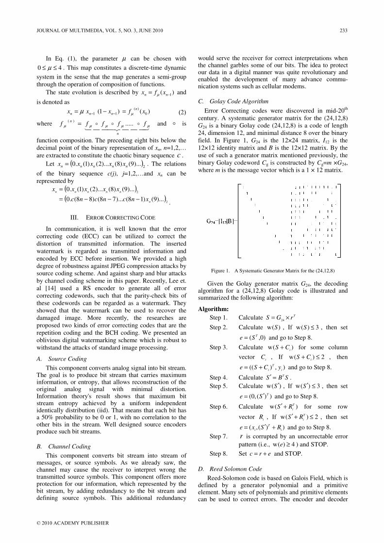
In Eq. (1), the parameter µ can be chosen with
40 ≤≤ µ . This map constitutes a discrete-time dynamic
system in the sense that the map generates a semi-group
through the operation of composition of functions.
The state evolution is described by )( 1−= nn xfx µ and
is denoted as
)1( 11 −− −= nnn xxx µ )( 0
)(xf
n
µ= (2)
where 444 3444 21ooo
n
nfffff µµµµµ .....
)(= and o is
function composition. The preceding eight bits below the
decimal point of the binary representation of xn, n=1,2,…
are extracted to constitute the chaotic binary sequence c .
Let ( )2
)...9()8()...2()1(.0 nnnnn xxxxx = . The relations
of the binary sequence c(j), j=1,2,…and xn can be
represented by
( )( )
2
2
)...9()18()...78()88(.0
)...9()8()...2()1(.0
n
nnnnn
xncncnc
xxxxx
−−−=
=
.
III. ERROR CORRECTING CODE
In communication, it is well known that the error
correcting code (ECC) can be utilized to correct the
distortion of transmitted information. The inserted
watermark is regarded as transmitted information and
encoded by ECC before insertion. We provided a high
degree of robustness against JPEG compression attacks by
source coding scheme. And against sharp and blur attacks
by channel coding scheme in this paper. Recently, Lee et.
al [14] used a RS encoder to generate all of error
correcting codewords, such that the parity-check bits of
these codewords can be regarded as a watermark. They
showed that the watermark can be used to recover the
damaged image. More recently, the researches are
proposed two kinds of error correcting codes that are the
repetition coding and the BCH coding. We presented an
oblivious digital watermarking scheme which is robust to
withstand the attacks of standard image processing.
A. Source Coding
This component converts analog signal into bit stream. The goal is to produce bit stream that carries maximum information, or entropy, that allows reconstruction of the original analog signal with minimal distortion. Information theory's result shows that maximum bit stream entropy achieved by a uniform independent identically distribution (iid). That means that each bit has a 50% probability to be 0 or 1, with no correlation to the other bits in the stream. Well designed source encoders produce such bit streams.
B. Channel Coding
This component converts bit stream into stream of messages, or source symbols. As we already saw, the channel may cause the receiver to interpret wrong the transmitted source symbols. This component offers more protection for our information, which represented by the bit stream, by adding redundancy to the bit stream and defining source symbols. This additional redundancy
would serve the receiver for correct interpretations when the channel garbles some of our bits. The idea to protect our data in a digital manner was quite revolutionary and enabled the development of many advance commu-nication systems such as cellular modems.
C. Golay Code Algorithm
Error Correcting codes were discovered in mid-20th
century. A systematic generator matrix for the (24,12,8)
G24 is a binary Golay code (24,12,8) is a code of length
24, dimension 12, and minimal distance 8 over the binary
field. In Figure 1, G24 is the 12×24 matrix, I12 is the
12×12 identity matrix and B is the 12×12 matrix. By the
use of such a generator matrix mentioned previously, the
binary Golay codeword Cg is constructed by Cg=m ×G24,
where m is the message vector which is a 1 × 12 matrix.
Figure 1. A Systematic Generator Matrix for the (24,12,8)
Given the Golay generator matrix G24, the decoding algorithm for a (24,12,8) Golay code is illustrated and summarized the following algorithm:
Algorithm:
Step 1. Calculate TrGS ×=24
Step 2. Calculate )(w S , If 3)(w ≤S , then set
)0,( TSe = and go to Step 8.
Step 3. Calculate )(wi
CS + for some column
vector i
C , If 2)(w ≤+i
CS , then
),)((i
T
iyCSe += and go to Step 8.
Step 4. Calculate SBST=′ .
Step 5. Calculate )(w S′ , If 3)(w ≤′S , then set
))(,0( TSe ′= and go to Step 8.
Step 6. Calculate )(w T
iRS +′ for some row
vector i
R , If 2)(w ≤+′ T
iRS , then set
))(,(i
T
iRSxe +′= and go to Step 8.
Step 7. r is corrupted by an uncorrectable error
pattern (i.e., 4)(w ≥e ) and STOP.
Step 8. Set erc += and STOP.
D. Reed Solomon Code
Reed-Solomon code is based on Galois Field, which is defined by a generator polynomial and a primitive element. Many sets of polynomials and primitive elements can be used to correct errors. The encoder and decoder
JOURNAL OF MULTIMEDIA, VOL. 5, NO. 3, JUNE 2010 233
© 2010 ACADEMY PUBLISHER
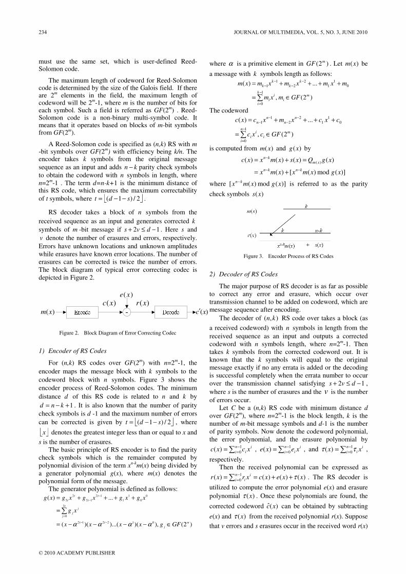
must use the same set, which is user-defined Reed-Solomon code.
The maximum length of codeword for Reed-Solomon code is determined by the size of the Galois field. If there are 2
m elements in the field, the maximum length of
codeword will be 2m-1, where m is the number of bits for
each symbol. Such a field is referred as GF(2m) . Reed-
Solomon code is a non-binary multi-symbol code. It means that it operates based on blocks of m-bit symbols from GF(2
m).
A Reed-Solomon code is specified as (n,k) RS with m -bit symbols over GF(2
m) with efficiency being k/n. The
encoder takes k symbols from the original message
sequence as an input and adds kn − parity check symbols
to obtain the codeword with n symbols in length, where
n=2m-1 . The term d=n-k+1 is the minimum distance of
this RS code, which ensures the maximum correctability
of t symbols, where 2/)1( sdt −−= .
RS decoder takes a block of n symbols from the
received sequence as an input and generates corrected k
symbols of m -bit message if 12 −≤+ dvs . Here s and
v denote the number of erasures and errors, respectively.
Errors have unknown locations and unknown amplitudes
while erasures have known error locations. The number of
erasures can be corrected is twice the number of errors.
The block diagram of typical error correcting codec is
depicted in Figure 2.
)(xm
)(xc)(xe
)(xr)(xc′
Figure 2. Block Diagram of Error Correcting Codec
1) Encoder of RS Codes
For (n,k) RS codes over GF(2m) with n=2
m-1, the
encoder maps the message block with k symbols to the
codeword block with n symbols. Figure 3 shows the
encoder process of Reed-Solomon codes. The minimum
distance d of this RS code is related to n and k by
1+−= knd . It is also known that the number of parity
check symbols is d -1 and the maximum number of errors
can be corrected is given by 2/)1( sdt −−= , where
x denotes the greatest integer less than or equal to x and
s is the number of erasures.
The basic principle of RS encoder is to find the parity
check symbols which is the remainder computed by
polynomial division of the term xn-k
m(x) being divided by
a generator polynomial g(x), where m(x) denotes the
polynomial form of the message.
The generator polynomial is defined as follows:
)2( ),)()...()((
...)(
012212
2
0
0
0
1
1
12
12
2
2
m
j
tt
t
j
j
j
t
t
t
t
GFgxxxx
xg
xgxgxgxgxg
∈−−−−=
=
++++=
−−
=
−
−
∑
αααα
where α is a primitive element in )2( mGF . Let )(xm be
a message with k symbols length as follows:
)2( ,
...)(
1
0
0
1
1
2
2
1
1
m
i
k
i
i
i
k
k
k
k
GFmxm
mxmxmxmxm
∈=
++++=
∑−
=
−−
−−
The codeword
)2( ,
...)(
1
0
0
1
1
2
2
1
1
m
i
n
i
i
i
n
n
n
n
GFcxc
cxcxmxcxc
∈=
++++=
∑−
=
−−
−−
is computed from )(xm and )(xg by
)]( mod )([)(
)()()()( )(
xgxmxxmx
xgQxsxmxxc
knkn
xm
kn
−−
−
+=
=+=
where )]( mod )([ xgxmx kn− is referred to as the parity
check symbols )(xs
Figure 3. Encoder Process of RS Codes
2) Decoder of RS Codes
The major purpose of RS decoder is as far as possible
to correct any error and erasure, which occur over
transmission channel to be added on codeword, which are
message sequence after encoding.
The decoder of ),( kn RS code over takes a block (as
a received codeword) with n symbols in length from the
received sequence as an input and outputs a corrected
codeword with n symbols length, where n=2m-1. Then
takes k symbols from the corrected codeword out. It is
known that the k symbols will equal to the original
message exactly if no any errata is added or the decoding
is successful completely when the errata number to occur
over the transmission channel satisfying 12 −≤+ dvs ,
where s is the number of erasures and the v is the number
of errors occur.
Let C be a (n,k) RS code with minimum distance d
over GF(2m), where n=2
m-1 is the block length, k is the
number of m-bit message symbols and d-1 is the number
of parity symbols. Now denote the codeword polynomial,
the error polynomial, and the erasure polynomial by
∑−
==
1
0)(
n
i
i
i xcxc , ∑−
==
1
0)(
n
i
i
i xexe , and ∑−
==
1
0)(
n
i
i
i xx ττ ,
respectively.
Then the received polynomial can be expressed as
)()()()(1
0xxexcxrxr
n
i
i
i τ++== ∑−
=. The RS decoder is
utilized to compute the error polynomial e(x) and erasure
polynomial )(xτ . Once these polynomials are found, the
corrected codeword )(ˆ xc can be obtained by subtracting
e(x) and )(xτ from the received polynomial r(x). Suppose
that v errors and s erasures occur in the received word r(x)
234 JOURNAL OF MULTIMEDIA, VOL. 5, NO. 3, JUNE 2010
© 2010 ACADEMY PUBLISHER
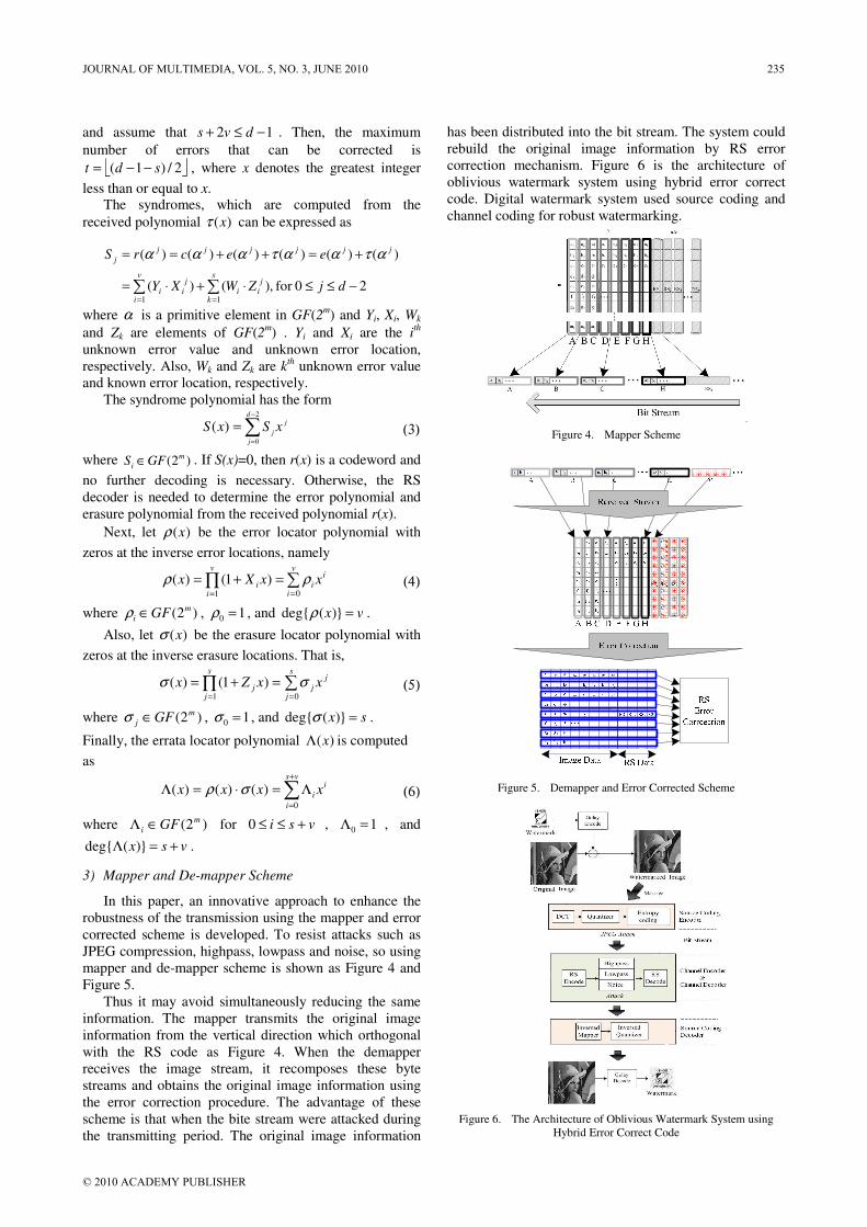
and assume that 12 −≤+ dvs . Then, the maximum
number of errors that can be corrected is
2/)1( sdt −−= , where x denotes the greatest integer
less than or equal to x. The syndromes, which are computed from the
received polynomial )(xτ can be expressed as
20for ,)()(
)()()()()()(
11
−≤≤⋅+⋅=
+=++==
∑∑==
djZWXY
eecrS
s
k
j
ii
v
i
j
ii
jjjjjj
j αταατααα
where α is a primitive element in GF(2m) and Yi, Xi, Wk
and Zk are elements of GF(2m) . Yi and Xi are the i
th
unknown error value and unknown error location,
respectively. Also, Wk and Zk are kth unknown error value
and known error location, respectively.
The syndrome polynomial has the form
∑−
=
=2
0
)(d
j
j
jxSxS (3)
where )2( m
i GFS ∈ . If S(x)=0, then r(x) is a codeword and
no further decoding is necessary. Otherwise, the RS
decoder is needed to determine the error polynomial and
erasure polynomial from the received polynomial r(x).
Next, let )(xρ be the error locator polynomial with
zeros at the inverse error locations, namely
∏ ∑= =
=+=v
i
v
i
i
ii xxXx1 0
)1()( ρρ (4)
where )2( m
i GF∈ρ , 10 =ρ , and vx =)(degρ .
Also, let )(xσ be the erasure locator polynomial with
zeros at the inverse erasure locations. That is,
∏ ∑= =
=+=s
j
s
j
j
jj xxZx1 0
)1()( σσ (5)
where )2( m
j GF∈σ , 10 =σ , and sx =)(degσ .
Finally, the errata locator polynomial )(xΛ is computed
as
∑+
=
Λ=⋅=Λvs
i
i
i xxxx0
)()()( σρ (6)
where )2( m
i GF∈Λ for vsi +≤≤0 , 10 =Λ , and
vsx +=Λ )(deg .
3) Mapper and De-mapper Scheme
In this paper, an innovative approach to enhance the
robustness of the transmission using the mapper and error
corrected scheme is developed. To resist attacks such as
JPEG compression, highpass, lowpass and noise, so using
mapper and de-mapper scheme is shown as Figure 4 and
Figure 5.
Thus it may avoid simultaneously reducing the same
information. The mapper transmits the original image
information from the vertical direction which orthogonal
with the RS code as Figure 4. When the demapper
receives the image stream, it recomposes these byte
streams and obtains the original image information using
the error correction procedure. The advantage of these
scheme is that when the bite stream were attacked during
the transmitting period. The original image information
has been distributed into the bit stream. The system could
rebuild the original image information by RS error
correction mechanism. Figure 6 is the architecture of
oblivious watermark system using hybrid error correct
code. Digital watermark system used source coding and
channel coding for robust watermarking.
Figure 4. Mapper Scheme
Figure 5. Demapper and Error Corrected Scheme
Figure 6. The Architecture of Oblivious Watermark System using
Hybrid Error Correct Code
JOURNAL OF MULTIMEDIA, VOL. 5, NO. 3, JUNE 2010 235
© 2010 ACADEMY PUBLISHER
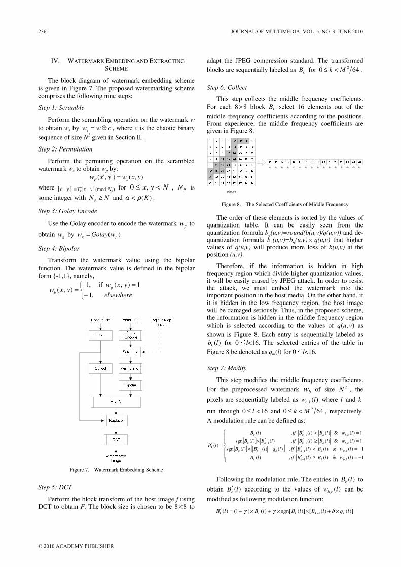
IV. WATERMARK EMBEDING AND EXTRACTING
SCHEME
The block diagram of watermark embedding scheme
is given in Figure 7. The proposed watermarking scheme
comprises the following nine steps:
Step 1: Scramble
Perform the scrambling operation on the watermark w
to obtain ws by cwws ⊕= , where c is the chaotic binary
sequence of size N2 given in Section II.
Step 2: Permutation
Perform the permuting operation on the scrambled
watermark ws to obtain wp by:
),()','( yxwyxw sP =
where [ ] [ ] ) (mod'' P
T
K
TNyxTyx
α= for Nyx <≤ ,0 , PN is
some integer with NNP
≥ and )(Kρα < .
Step 3: Golay Encode
Use the Golay encoder to encode the watermark pw to
obtain gw by )( pg wGolayw =
Step 4: Bipolar
Transform the watermark value using the bipolar
function. The watermark value is defined in the bipolar
form -1,1, namely,
=
−=
elsewhere
yxwyxw
g
b
1),(if
,1
,1),(
Figure 7. Watermark Embedding Scheme
Step 5: DCT
Perform the block transform of the host image f using DCT to obtain F. The block size is chosen to be 88 × to
adapt the JPEG compression standard. The transformed
blocks are sequentially labeled as kB for 640 2Mk <≤ .
Step 6: Collect
This step collects the middle frequency coefficients.
For each 88 × block kB select 16 elements out of the
middle frequency coefficients according to the positions. From experience, the middle frequency coefficients are given in Figure 8.
),( vuq
0q 1q 15q2q 3q 4q 5q 6q 7q 8q 9q 10q 11q 12q 13q 14q
Figure 8. The Selected Coefficients of Middle Frequency
The order of these elements is sorted by the values of quantization table. It can be easily seen from the quantization formula bq(u,v)=round(b(u,v)/q(u,v)) and de-quantization formula b’(u,v)=bq(u,v) × q(u,v) that higher values of q(u,v) will produce more loss of b(u,v) at the position (u,v).
Therefore, if the information is hidden in high frequency region which divide higher quantization values, it will be easily erased by JPEG attack. In order to resist the attack, we must embed the watermark into the important position in the host media. On the other hand, if it is hidden in the low frequency region, the host image will be damaged seriously. Thus, in the proposed scheme, the information is hidden in the middle frequency region
which is selected according to the values of ),( vuq as
shown is Figure 8. Each entry is sequentially labeled as
)(lbk for 0≦l<16. The selected entries of the table in
Figure 8 be denoted as qm(l) for 0≦l<16.
Step 7: Modify
This step modifies the middle frequency coefficients.
For the preprocessed watermark bw of size 2N , the
pixels are sequentially labeled as )(, lw kb where l and k
run through 160 <≤ l and 640 2Mk <≤ , respectively.
A modulation rule can be defined as:
[ ][ ]
−=≥′
−=<′−′×
=≥′′×
=<′
=′
−
−−
−−
−
1)(&)()(,)(
1)(&)()(,)()()(sgn
1)(&)()(,)()(sgn
1)(&)()(,)(
)(
,1
,11
,11
,1
lwlBlBiflB
lwlBlBiflqlBlB
lwlBlBiflBlB
lwlBlBiflB
lB
kbkkk
kbkkkkk
kbkkkk
kbkkk
k
Following the modulation rule, The entries in )(lBk to
obtain )(lBk′ according to the values of )(, lw kb can be
modified as following modulation function:
)]()([)](sgn[)()1()( 1 lqlBlBlBlB kkkkk ×+××+×−=′− δγγ
236 JOURNAL OF MULTIMEDIA, VOL. 5, NO. 3, JUNE 2010
© 2010 ACADEMY PUBLISHER
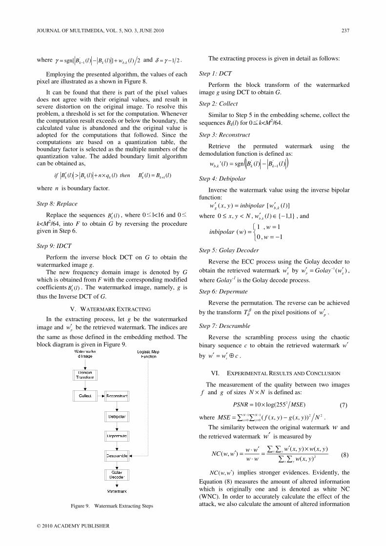
where 2)(])()(sgn[ ,
'
1 lwlBlB kbkk +−= −γ and 21−= γδ .
Employing the presented algorithm, the values of each pixel are illustrated as a shown in Figure 8.
It can be found that there is part of the pixel values does not agree with their original values, and result in severe distortion on the original image. To resolve this problem, a threshold is set for the computation. Whenever the computation result exceeds or below the boundary, the calculated value is abandoned and the original value is adopted for the computations that followed. Since the computations are based on a quantization table, the boundary factor is selected as the multiple numbers of the quantization value. The added boundary limit algorithm can be obtained as,
)()()()()( 1 lBlBthenlqnlBlBif kkkkk +=′×+>′
where n is boundary factor.
Step 8: Replace
Replace the sequences )(lBk′ , where 0≦l<16 and 0≦
k<M2/64, into F to obtain G by reversing the procedure
given in Step 6.
Step 9: IDCT
Perform the inverse block DCT on G to obtain the
watermarked image g.
The new frequency domain image is denoted by G
which is obtained from F with the corresponding modified
coefficients )(lBk′ . The watermarked image, namely, g is
thus the Inverse DCT of G.
V. WATERMARK EXTRACTING
In the extracting process, let g be the watermarked
image and p
w′ be the retrieved watermark. The indices are
the same as those defined in the embedding method. The
block diagram is given in Figure 9.
Figure 9. Watermark Extracting Steps
The extracting process is given in detail as follows:
Step 1: DCT
Perform the block transform of the watermarked
image g using DCT to obtain G.
Step 2: Collect
Similar to Step 5 in the embedding scheme, collect the
sequences Bk(l) for 0≦k<M2/64.
Step 3: Reconstruct
Retrieve the permuted watermark using the
demodulation function is defined as:
( ))()(sgn)(' '
1
'
, lBlBlw kkkb −−=
Step 4: Debipolar
Inverse the watermark value using the inverse bipolar
function:
)]([),( , lwinbipolaryxw kbg′=′
where 1,1)( ,,0,
−∈′<≤ lwNyxkb
, and
1,
1,
0
1)(
−=
=
=w
wwinbipolar
Step 5: Golay Decoder
Reverse the ECC process using the Golay decoder to
obtain the retrieved watermark g
w′ by )(1
gpwGolayw ′=′ −
,
where Golay-1
is the Golay decode process.
Step 6: Depermute
Reverse the permutation. The reverse can be achieved
by the transform βδT on the pixel positions of pw′ .
Step 7: Descramble
Reverse the scrambling process using the chaotic
binary sequence c to obtain the retrieved watermark w′
by cwws
⊕′=′ .
VI. EXPERIMENTAL RESULTS AND CONCLUSION
The measurement of the quality between two images
f and g of sizes NN × is defined as:
)255log(102
MSEPSNR ×= (7)
where 21
0
1
0
2)),(),(( NyxgyxfMSEN
x
N
y∑ ∑−
=
−
=−= .
The similarity between the original watermark w and
the retrieved watermark w′ is measured by
∑ ∑∑ ∑ ×′
=⋅
′⋅=′
x y
x y
yxw
yxwyxw
ww
wwwwNC
2),(
),(),(),( (8)
),( wwNC ′ implies stronger evidences. Evidently, the
Equation (8) measures the amount of altered information
which is originally one and is denoted as white NC
(WNC). In order to accurately calculate the effect of the
attack, we also calculate the amount of altered information
JOURNAL OF MULTIMEDIA, VOL. 5, NO. 3, JUNE 2010 237
© 2010 ACADEMY PUBLISHER

which is originally zero and denoted as black NC (BNC).
The formula of BNC is the same as (8) with all 1’s
changed to 0’s and vice versa.
The proposed method has been simulated using the
C++ program on Windows XP platform. In the simulation,
all the watermarks are binary images of size 9090 × and
the host images are 8-bit gray level images of size
512512× . The watermark information bits are encoded
with different Reed-Solomon codes (15,7) RS code and
(31,19) RS code.
The first test uses 1 watermark and 6 host images
(Lena, F16, Baboon, Boy & Girl, Pepper, and Girl) as
Table I.
TABLE I. THE EFFECTS OF THE WATERMARK AND IMAGE QUALITY.
Watermarked
Image
PSNR (db) 37.65 36.61 35.1 39.56 36.76 40.09
Logo
BNC 0.898 0.894 0.874 0.915 0.895 0.916
WNC 0.970 0.959 0.939 0.985 0.965 0.988
Total Loss 5.88% 6.70% 8.68% 4.30% 6.31% 4.12%
It is observed that the qualities (PSNR) of embedded
image with respect to the host image are more than 36 dB
in average. We found that the image quality of “Baboon”
(PSNR=35.1) is worst and the image quality of “Girl”
(PSNR = 40.09) is best. Nevertheless, all watermarks are
visible. Also, the NC values of the retrieved watermarks
are all above 93%. This demonstrated that the proposed
scheme provides a good mechanism for watermarking
applications. This demonstrates that the proposed scheme
provides a good mechanism for watermarking
applications.
Table II show the compare result of extracted
watermark with a golay code and without a golay code.
That shows the comparison results of extracted watermark
with the (24,12,8) Golay code, the (23,12,7) Golay code
and without ECC. Among all of these schemes, the
detection response of the processed image introduced by
the (24,12,8) Golay code is much higher than those of
other schemes. For example, when the BPP of
watermarked image is 1.55, the NC of logo without using
ECC is down to 0.89, However, the NC of logo with the
(24,12,8) Golay code can be kept in 0.98.
The results achieved are that the proposed embedding
mechanism for watermarking is robust for JPEG
compression, cropping, blur, sharpen, and noise. Of
course, both the watermark and host image are not
required in the extracting process and the watermark can
therefore be corrected using the (24,12,8) Golay code
TABLE II. THE COMPARE RESULT OF EXTRACTED WATERMARK WITH A GOLAY
CODE AND WITHOUT A GOLAY CODE
Image
BPP 8.0 2.28 1.55 0.81 0.62 0.54
Logo NC
Normal
(%)
0.93 0.91 0.89 0.82 0.75 0.67
Logo NC
Golay
(23,12,7)
(%)
0.99 0.97 0.94 0.82 0.72 0.65
Logo NC
Golay
(24,12,8)
(%)
1 0.99 0.98 0.82 0.76 0.67
.
Table III shown the improvement of presented
algorithm on the attacked images. The test uses 1
watermark and 1 host images, and the comparison results
of attacked image. The result shows our oblivious
watermark system used hybrid error correct code can
subject to attacks by various image operations such as
JPEG compression, highpass, lowpass, noise and cropping,
and error correct can obtain excellent result.
TABLE III. THE IMPROVEMENT OF PRESENTED ALGORITHM ON THE ATTACKED
IMAGES.
Attack Crop 75% Gaussian
Blur Sharp
Gaussian
noise 5%
Watermarked
Image
PSNR(db) 5.1 28.01 25.51 28.47
(15,7)
RS
Code
+
Golay
(24,12,8)
Logo
BNC 0.407 0.864 0.906 0.802
WNC 0.921 0.703 0734 0.737
Total Loss 33.6% 21.65% 18.00% 23.05%
Identified
Watermark Yes Yes Yes Yes
(31,19)
RS
Code
+
Golay
(24,12,8)
Logo
BNC 0.422 0.882 0.912 0.852
WNC 0.935 0.884 0.872 0.787
Total Loss 32.15% 11.70% 10.80% 18.05%
Identified
Watermark Yes Yes Yes Yes
238 JOURNAL OF MULTIMEDIA, VOL. 5, NO. 3, JUNE 2010
© 2010 ACADEMY PUBLISHER
That shows the comparison results of extracted
watermark with the (15,7) RS code, and (31,19) RS code.
Among all of these schemes, the detection response of the
processed image introduced by the (31,19) RS code is
higher than those of other schemes.
In summary, the major contributions of this paper to
the robust watermarking scheme. We can provide a high
degree of robustness against JPEG compression attacks by
the source coding, and protect the transmit information by
channel coding. We adopt the data distribution idea to
avoid the continue information attack, because it will
destroy all of the error correction mechanism. The
proposed algorithms and approaches have been
implemented and verified, and the experimental results
have demonstrated the superiority of the proposed digital
signal processing techniques in terms of performance and
innovations.
REFERENCES
[1] C. Y. Lin and S. F. Chang, “A robust image authentication method
distinguishing JPEG compression from malicious manipulation,”
IEEE Transaction on circuits and systems of video technology, vol.
11 (2), pp. 153-168 , 2001.
[2] C. M. Kung, J. H. Jeng, and C. H. Kung, "Watermarking Base on
Block Property," 16th IPPR Conference on Computer Vision,
Graphics and Image Processing , pp. 540-546, 2003.
[3] B. M. Macq and J. J. Quisquater, “Cryptology for digital TV
broad-casting,” Proc. IEEE, pp. 944-957, 1995.
[4] M. D. Swanson, M. Kobayashi and A. H. Tewfik, “Multimedia
data-embedding and watermarking technologies,” Proc. IEEE, pp.
1064-1087, 1998.
[5] I. J. Cox, J. Kilian, F. T. Leighton and T. Shamoon, “Secure
spread spectrum watermarking for multimedia,” Image Processing,
IEEE Transactions on, pp. 1673-1687, 1997.
[6] E. Koch, J. Rindfrey and J. Zhao, “Copyright protection for
multimedia data, ” in Proc. Int. Conf. Digital Media and
Electronic Publishing, 1994.
[7] C. T. Hsu and J. L. Wu, “Hidden digital watermarks in images,”
IEEE Trans. on Images Processing, pp. 58-68, 1998.
[8] J. Lee and C. S. Won, “A Watermarking sequence using parities
of error control coding for image authentication and correction,”
IEEE Transactions on Consumer Electronics, vol. 46, no. 2, pp.
313-317, 2000.
[9] Y. Wu, “Tamper-Localization Watermarking with Systematic
Error Correcting Code,” ICIP 2006, pp.1965-1968, 2006.
[10] F. Alturki and R. Mersereau, “An oblivious robust digital
watermark technique for still images using DCT phase
modulation,” Acoustics, Speech, and Signal Processing, 2000.
ICASSP '00. Proceedings. 2000 IEEE International Conference on,
vol. 4 (14), pp. 1975-1978, 2000.
[11] A. Sinha, A. Das, and S. Pandith, “Pattern based robust digital
watermarking scheme for images,” Acoustics, Speech, and Signal
Processing, 2002 IEEE International Conference on, vol. 4,
pp.3481-3484 ,2002.
[12] H. Zhu, W. A. Clarke and H. C. Ferreira, “Watermarking for
JPEG Image Using Error Correction Coding” IEEE AFRICON
2004, pp. 191-196, 2004.
[13] N. Tsnijia. M. Repgcs, K. Luck, W. Crisrlhard!, "Impact of
different Recd-Solomon codes on drgrlal walemrkr based on
DWT", Mulfimcdia and Sccunty Workshop at ACM Multimedia
2002.
[14] J. Lee and C. S. Won, "Authentication and Correction of Digital
Watermarking Images," Electronics Letters, vol. 35, pp. 886-887,
1999.
[15] C. M. Kung, T. K. Troung, “Visual Robust Oblivious
Watermarking Technique Using Error Correcting Code,”
Communication Technology, 2006. ICCT '06. International
Conference on, pp1-4, 2006
[16] C. M. Kung, K. Y. Juan, Y. C. Tu, C. H. Kung, “A Robust
Watermarking and Image Authentication Technique on Block
Property,” Information Science and Engieering, 2008. ISISE '08.
International Symposium on, Vol. 1, (20-22 ), pp.173 - 177 , Dec.
2008.
[17] C. W. Wu and N. F. Rul'kov, “Studying chaos via 1-D maps-a
tutorial,” Circuits and Systems I: Fundamental Theory and
Applications, IEEE Transactions, pp.707-721, 1993.
C. M. Kung was born in Tainan, Taiwan, R. O.
C. He received the B.S. degree in Eelectronic
Engineering from Fu Jen Catholic University,
Taiwan, R. O. C., in 1991, the M.S. degree in
Business and Operations Management from
Chang Jung Christian University, Taiwan, R. O.
C., in 1999, and the Ph.D. degree in Electrical Engineering from
the I-Shou University, Taiwan, R. O. C., in 2006. He is the
Assistant Professor at Department of Information Technology
and Communication, Shih Chien University Kaohsiung Campus,
Kaohsiung County, Taiwan, R.O.C. His research interests
include watermarking, soft-computing, image compression, and
error-correcting code.
JOURNAL OF MULTIMEDIA, VOL. 5, NO. 3, JUNE 2010 239
© 2010 ACADEMY PUBLISHER

Multi-criterion Optimization Approach to Ill-posed Inverse Problem with Visual Feature’s
Recovery
Weihui Dai School of Management, Fudan University, Shanghai 200433, P.R.China
Email: [email protected]
Abstract—Ill-posed inverse problem is commonly existed in signal processing such as image reconstruction from projection, parameter estimation on electromagnetic field, and path optimization in IP network. Usually, the solution of an inverse problem is unstable, not unique or does not exit. Traditional approach to solve this problem is to estimate the solution by optimizing a regularized objective function. In some cases, recovery of visual features is most emphasized in that solution; thereof the distribution of residual errors has distinct influence on the quality of solution.
This paper analyzes ill-posed inverse problem with the case of image reconstruction from projections and discusses its fidelity based on various visual features in the estimated solution. Multi-criterion Optimization Approach, a new approach to solve the ill-posed inverse problems with good recovery of visual features, is presented with its theory basis and the experiment results. The solution stability and accuracy are analyzed using singular value decomposition (SVD), and main factors affecting the reconstruction quality are also discussed.
Index Terms—inverse problem, ill-posed problem, multi-criterion optimization, visual feature
I. INTRODUCTION
Forward problem and inverse problem are two kinds of common questions in signal processing.
Figure 1. Basic Model of Signal Processing System
Fig.1 is the basic model of a signal processing system. Here, X(t) is input signal, Y(t) is output signal, T(t) is transfer function, and N(t) is noise. The forward problem can be described as how to estimate the output of Y(t) while X(t) and T(t) are given. Contrarily, the inverse problem can be described as one of the two questions:
1. How to estimate the input of X(t), while Y(t) and
T(t) are obtained ? 2. How to estimate the T(X), while X(t) and Y(t) are
obtained ? Image reconstruction from projections in X-CT is the
situation as question 2. In most cases, ill-posedness exists inherently in the estimate process of inverse problem, and affects seriously the existence, stability and accuracy of the solution with susceptibility to the errors in measurement data and errors in the numerical discretization [1][2]. In 1923, Hadamard postulated that in order to be well-posed a problem should have three properties [3]: (1) Existence of a solution; (2) Uniqueness of the solution; and (3) Continuous dependence of the solution on the data. Correspondingly, ill-posed inverse problem refers to this situation that its solution does not exist or it is not unique or not stable under perturbations on data. The ill-posed inverse problem of image reconstruction mainly reflects in the following three aspects:
(a) The non-uniqueness of the solution to the image reconstruction on finite observational data;
(b) The non-continuous and unbounded characteristics of the reconstruction inverse operators;
(c) The existence of the solution influenced by the errors and the noises in observation data.
Traditional approach to solve this problem is to estimate the solution by optimizing a regularized objective function [4]. In some cases, recovery of visual features is very important in that process [5]. For example, the requirement which image reconstruction differs from other inverse problems is that the former emphasizes not only the solution accuracy, but also its fidelity based on various visual features. Commonly used regularized approaches, such as the famous Tikhonov regularized approach [6], adopt only different single summed error function as the objective function. Those approaches do not consider the quality in visual cognition and its psychological effects due to specific distribution of those errors. The effects of error distribution on image are illustrated in Fig.2.
In Fig.2, the image (a) is a Shepp-Logan test phantom [7], image (b) and image (c) are reconstructed images by Tikhonov regularized approach and with the same sum of squared error.
This research was supported by National High-tech R & D Program(863 Program) of China (No.2008AA04Z127), National NaturalScience Foundation of China (No.70401010),and Shanghai LeadingAcademic Discipline Project (No.B210)
240 JOURNAL OF MULTIMEDIA, VOL. 5, NO. 3, JUNE 2010
© 2010 ACADEMY PUBLISHERdoi:10.4304/jmm.5.3.240-247
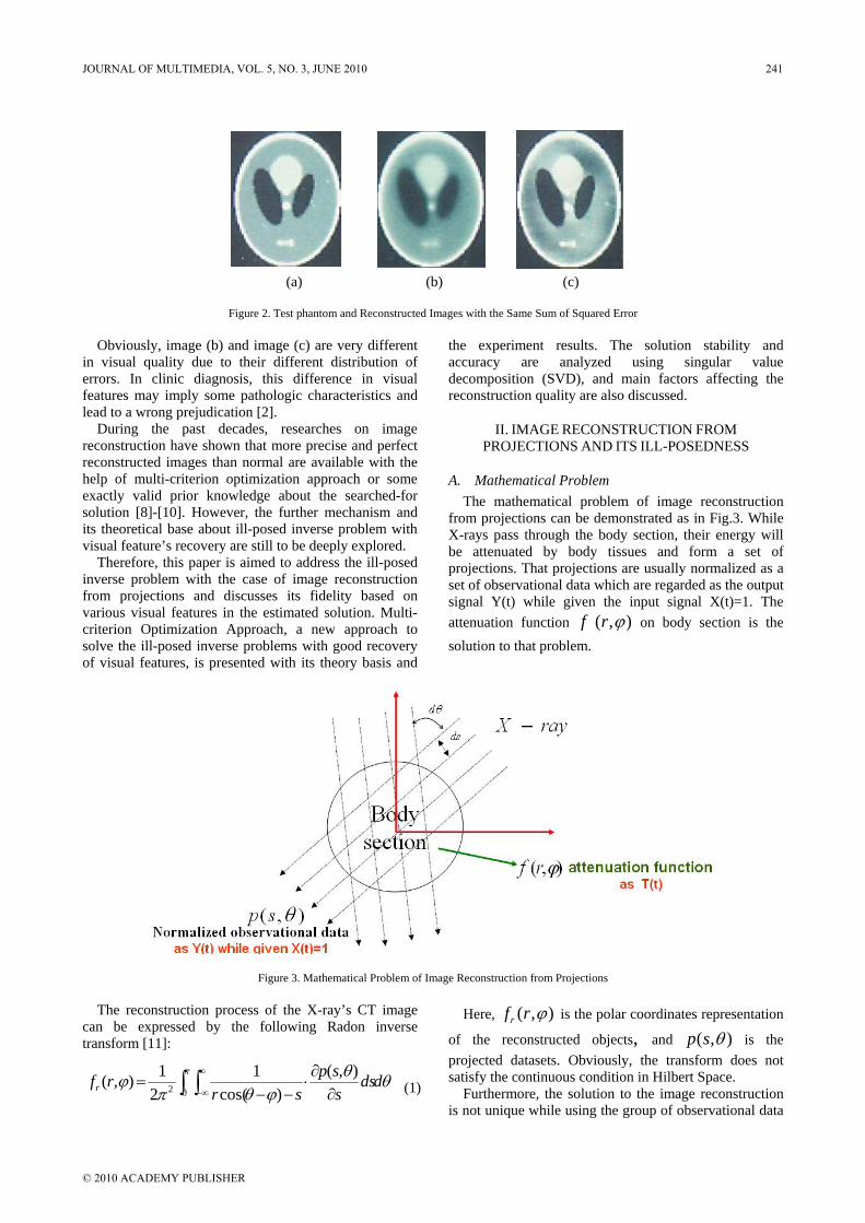
(a) (b) (c)
Figure 2. Test phantom and Reconstructed Images with the Same Sum of Squared Error
Obviously, image (b) and image (c) are very different in visual quality due to their different distribution of errors. In clinic diagnosis, this difference in visual features may imply some pathologic characteristics and lead to a wrong prejudication [2].
During the past decades, researches on image reconstruction have shown that more precise and perfect reconstructed images than normal are available with the help of multi-criterion optimization approach or some exactly valid prior knowledge about the searched-for solution [8]-[10]. However, the further mechanism and its theoretical base about ill-posed inverse problem with visual feature’s recovery are still to be deeply explored.
Therefore, this paper is aimed to address the ill-posed inverse problem with the case of image reconstruction from projections and discusses its fidelity based on various visual features in the estimated solution. Multi-criterion Optimization Approach, a new approach to solve the ill-posed inverse problems with good recovery of visual features, is presented with its theory basis and
the experiment results. The solution stability and accuracy are analyzed using singular value decomposition (SVD), and main factors affecting the reconstruction quality are also discussed.
II. IMAGE RECONSTRUCTION FROM PROJECTIONS AND ITS ILL-POSEDNESS
A. Mathematical Problem The mathematical problem of image reconstruction
from projections can be demonstrated as in Fig.3. While X-rays pass through the body section, their energy will be attenuated by body tissues and form a set of projections. That projections are usually normalized as a set of observational data which are regarded as the output signal Y(t) while given the input signal X(t)=1. The attenuation function ),( ϕrf on body section is the solution to that problem.
Figure 3. Mathematical Problem of Image Reconstruction from Projections
The reconstruction process of the X-ray’s CT image can be expressed by the following Radon inverse transform [11]:
∫ ∫∞
∞− ∂∂⋅
−−=
πθθ
ϕθπϕ
02),(
)cos(1
21),( dds
ssp
srrfr
(1)
Here, ),( ϕrfr is the polar coordinates representation
of the reconstructed objects, and ),( θsp is the projected datasets. Obviously, the transform does not satisfy the continuous condition in Hilbert Space.
Furthermore, the solution to the image reconstruction is not unique while using the group of observational data
JOURNAL OF MULTIMEDIA, VOL. 5, NO. 3, JUNE 2010 241
© 2010 ACADEMY PUBLISHER
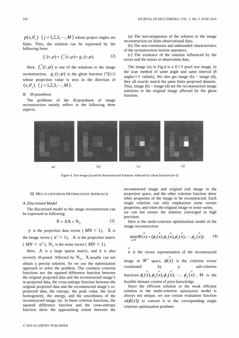
),( jsp θ ( )Mj ,,3,2,1 L= whose project angles are finite. Then, the solution can be expressed by the following form:
),(),(),( * ϕϕϕ rgrfrf rrr += (2)
Here, ),(* ϕrfr is one of the solutions to the image
reconstruction, ),( ϕrgr is the ghost function [7][11] whose projection value is zero in the direction of
),( js θ ( )Mj ,,3,2,1 L= .
B. Ill-posedness The problems of the ill-posedness of image
reconstruction mainly reflect in the following three aspects:
(a) The non-uniqueness of the solution to the image reconstruction on finite observational data;
(b) The non-continuous and unbounded characteristics of the reconstruction inverse operators;
(c) The existence of the solution influenced by the errors and the noises in observation data.
The image (a) in Fig.4 is a 8×8 pixel test image, in the scan method of same angle and same interval (8 angles×8 radials). We also get image (b) ~ image (d), they all exactly match the same finite projected datasets. Thus, image (b) ~ image (d) are the reconstruction image solutions to the original image affected by the ghost function.
Figure 4. Test Image (a) and Its Reconstructed Solutions Affected by Ghost Function (b~d)
III. MULTI-CRITERION OPTIMIZATION APPROACH
A..Discretized Model The discretized model to the image reconstruction can
be expressed as following:
SNAXP += (3)
P is the projection data vector ( MN × 1), X is
the image vector ( 2n × 1), A is the projection matrix
( MN × 2n ), SN is the noise vector ( MN × 1). Here, A is a large sparse matrix, and it is also
severely ill-posed. Affected by SN , X usually can not obtain a precise solution. So we use the optimization approach to solve the problem. The common criterion functions are: the squared difference function between the original projected data and the reconstructed image’s re-projected data, the cross-entropy function between the original projected data and the reconstructed image’s re-projected data, the entropy, the peak value, the local homogeneity, the energy, and the smoothness of the reconstructed image, etc. In these criterion functions, the squared difference function and the cross-entropy function show the approaching extent between the
reconstructed image and original real image in the projection space, and the other criterion function show other properties of the image to be reconstructed. Each single criterion can only emphasizes some certain properties, and when the original image or noise varies, we can not ensure the solution converged in high precision.
Here is the multi-criterion optimization model of the image reconstruction:
))(,),(),(),(()(min 321
p
p
pppp
xxxxxx φφφφ L=Φ
Θ∈ (4)
ρx is the vector representation of the reconstructed
image in nℜ space, )(ρ
φ x is the criterion vector constituted by p sub-criterion
functions ,),(),(),( 321 Lρρρ
φφφ xxx )(ρ
φ xp , Θ is the feasible domain consist of prior knowledge. Since the efficient solution or the weak efficient solution to the multi-criterion optimization model is always not unique, we use certain evaluation function
))(( xu φ to convert it to the corresponding single criterion optimization problem:
242 JOURNAL OF MULTIMEDIA, VOL. 5, NO. 3, JUNE 2010
© 2010 ACADEMY PUBLISHER

))((min xux
φΘ∈
(5)
The most common and simple evaluation function is the weighted linear sum function:
10,)())((11
=≥= ∑∑==
p
iii
p
iii wandwxwxu φφ (6)
Thus, the multi-criterion optimization model to the image reconstruction can be converted to the single criterion optimization problem:
⎪⎩
⎪⎨⎧
Θ∈
==ΦΦ ∑=
xts
xwxuxxp
iii
..
)())(()(),(min1
φφ(7)
Here, )(xΦ is a real number in 1ℜ space, not same
to the )(pxΦ in formula (4).
Many researches and experiences show that choosing a proper multi-criterion optimization model and solution method, we can obtain much better reconstruction image than the normal single criterion approach. Furthermore, the reconstruction process has better stability. In most cases, we can get the stable result only through three to five iterations, and then we can obtain the satisfying accuracy.
B. Stability and Accuracy For the sake of convenience, we use the optimization
model in formula (7), we choose the following function as the criterion function and the feasible domain:
⎭⎬⎫
⎩⎨⎧ =−ℜ∈=Θ
=
−=
021,:
)()(
2
22
21
2
EXXX
XQxAXPx
n
Dφφ
DQ is the second-order difference operator. Then the formula (7) can be converted to the unconstrained extremum problem:
⎟⎠⎞
⎜⎝⎛ −+=Φ ∑
=
EXXwXp
iii
2
1 21)(),(min λφλ (8)
λ is the Lagrange multiplier. There exists the unique global optimal solution:
0),(=
∂Φ∂
XX λ .
λ is the number satisfying the constrained condition Θ∈X .
Suppose λ and iw have been adjusted, then the solution to the multi-criterion optimization problem can be expressed as:
( )
PAIw
QQww
AA
PAwIQQwAAwX
TD
TD
T
TD
TD
T
1
1
*
1
2
1
1*
21
2
21ˆ
−
−
⎥⎦
⎤⎢⎣
⎡++=
⎥⎦⎤
⎢⎣⎡ ++=
λ
λ (9)
*λ is the number shows that λ has been adjusted to
the value which X satisfying the constrained condition
EX =2ˆ
21
, and *λ can be obtained by the following
formula:
EPAIw
QQwwAA T
DTD
T =⎥⎦
⎤⎢⎣
⎡++
− 21
1
*
1
2
221 λ
(10)
Here *λ indicates the prior knowledge “The energy of the image is E.”.
Now, let’s analyze the stability and the accuracy of the reconstruction solution through formula (9).
The stability of the solution is decided by the following matrix’s singular value spectra:
Iw
QQwwAAT D
TD
T
1
*
1
2
2λ
++= (11)
AAT in T is the Gram matrix corresponding to the estimating solution obtained by the minimum square error approach. We use singular value decomposition (SVD) on AAT :
( )0,211
2
=≤<
== ∑∑==
i
n
i
Tiii
r
i
Tiii
T
nir
VVVVAA
λ
λλ (12)
Here, TiiVV is AAT ’s characteristic sub-graph of
dimension 2n . iV is A ’s singular value column vector.
( )2,2,1 nii L=λ are the 2n characteristic values of
A . r is the rank of AAT . Since AAT is a nonnegative Hermite Matrix, then 0≥iλ . Fig.5 is the singular value spectra distribution of 8×8 pixel test phantom, in the scan method of same angle and same interval (8 angles×8 radials).
JOURNAL OF MULTIMEDIA, VOL. 5, NO. 3, JUNE 2010 243
© 2010 ACADEMY PUBLISHER

Figure 5. Singular Value Spectra of AAT
In Fig.5, we see that the singular value distribution of AAT descend rapidly, and the zero characteristic value
appears. NC (the number of the nonzero characteristic value) is as high as 7.7513×10¹⁷ . In theory, when the projection is complete and accurate, we can obtain the unique accurate original image through the minimum square estimating. But due to the severe ill-posedness of
AAT , the noises in the projection data and the inevitable data processing bias in computing, the
accuracy we can get from the experiment is far from the ideal accuracy. In order to solve the problem, we should adjust the singular value distribution of AAT , reduce the condition number of the matrix properly.
In formula (11), after maximum rank matrix T is revised by D
TDQQ and I , the ill-posedness of AAT
has been restrained and improved, and can get the unique solution. The singular value spectra of T varies with the
factor 1
2
ww
and1
*
2wλ
. For the sake of convenience, we
rewrite T as:
IQQAAT DTD
T21 γγ ++= (13)
1
*
21
21 2
,ww
w λγγ == .
Here is figure of the singular value spectra distribution of D
TDQQ and I .
Figure 6. Singular Value Spectra of DTDQQ and I
We see from Fig.6 that the singular value spectra
distribution of DTDQQ and I has many difference: The
former has larger amplitude ( maxλ = 226.49) than AAT in the low side, and also descend more slowly than
AAT ; The latter is identically 1 in the whole range of the spectra distribution. So the revising effects of
DTDQQ and I to AAT are not the same: D
TDQQ
makes the revised singular value spectra get larger in the range, the revised effect of the spectra distribution in the low side is more obvious than that in the high side; on
the other side, I makes the singular value get the same raise in all the range (here we suppose the singular value vector remain the same after the revision) . The variable ratio in the high side is much large than that in the low side.
In order to do the further research on the relation between the singular value spectra of T and the coefficient 1γ and 2γ , we let 1γ = 0, 0.5, 1, 1.5, 2
( 2γ =0) and 2γ = 0, 0.5, 1, 1.5, 2 ( 1γ =0), then we can get the altering of singular value spectra of T in Fig.7.
244 JOURNAL OF MULTIMEDIA, VOL. 5, NO. 3, JUNE 2010
© 2010 ACADEMY PUBLISHER
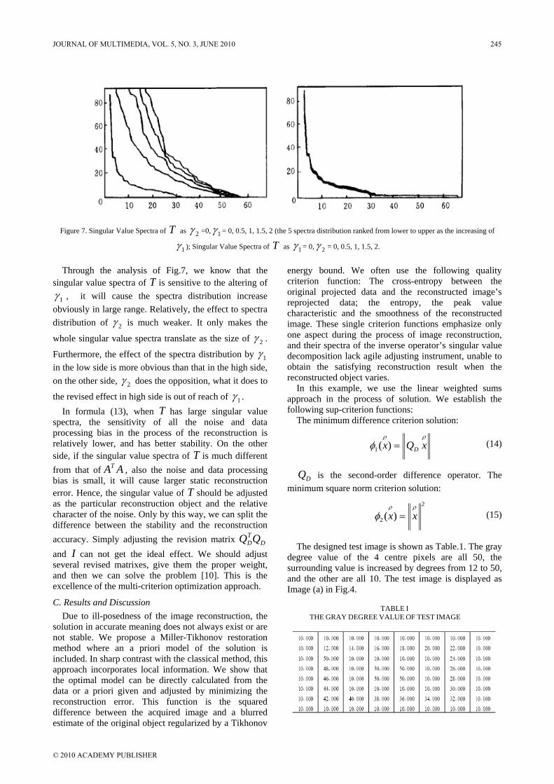
Figure 7. Singular Value Spectra of T as 2γ =0, 1γ = 0, 0.5, 1, 1.5, 2 (the 5 spectra distribution ranked from lower to upper as the increasing of
1γ ); Singular Value Spectra of T as 1γ = 0, 2γ = 0, 0.5, 1, 1.5, 2.
Through the analysis of Fig.7, we know that the singular value spectra of T is sensitive to the altering of
1γ , it will cause the spectra distribution increase obviously in large range. Relatively, the effect to spectra distribution of 2γ is much weaker. It only makes the
whole singular value spectra translate as the size of 2γ .
Furthermore, the effect of the spectra distribution by 1γ in the low side is more obvious than that in the high side, on the other side, 2γ does the opposition, what it does to
the revised effect in high side is out of reach of 1γ . In formula (13), when T has large singular value
spectra, the sensitivity of all the noise and data processing bias in the process of the reconstruction is relatively lower, and has better stability. On the other side, if the singular value spectra of T is much different from that of AAT , also the noise and data processing bias is small, it will cause larger static reconstruction error. Hence, the singular value of T should be adjusted as the particular reconstruction object and the relative character of the noise. Only by this way, we can split the difference between the stability and the reconstruction accuracy. Simply adjusting the revision matrix D
TDQQ
and I can not get the ideal effect. We should adjust several revised matrixes, give them the proper weight, and then we can solve the problem [10]. This is the excellence of the multi-criterion optimization approach.
C. Results and Discussion Due to ill-posedness of the image reconstruction, the
solution in accurate meaning does not always exist or are not stable. We propose a Miller-Tikhonov restoration method where an a priori model of the solution is included. In sharp contrast with the classical method, this approach incorporates local information. We show that the optimal model can be directly calculated from the data or a priori given and adjusted by minimizing the reconstruction error. This function is the squared difference between the acquired image and a blurred estimate of the original object regularized by a Tikhonov
energy bound. We often use the following quality criterion function: The cross-entropy between the original projected data and the reconstructed image’s reprojected data; the entropy, the peak value characteristic and the smoothness of the reconstructed image. These single criterion functions emphasize only one aspect during the process of image reconstruction, and their spectra of the inverse operator’s singular value decomposition lack agile adjusting instrument, unable to obtain the satisfying reconstruction result when the reconstructed object varies. In this example, we use the linear weighted sums approach in the process of solution. We establish the following sup-criterion functions: The minimum difference criterion solution:
ρρφ xQx D=)(1 (14)
DQ is the second-order difference operator. The minimum square norm criterion solution:
2
2 )(ρρ
φ xx = (15)
The designed test image is shown as Table.1. The gray degree value of the 4 centre pixels are all 50, the surrounding value is increased by degrees from 12 to 50, and the other are all 10. The test image is displayed as Image (a) in Fig.4.
TABLE I
THE GRAY DEGREE VALUE OF TEST IMAGE
JOURNAL OF MULTIMEDIA, VOL. 5, NO. 3, JUNE 2010 245
© 2010 ACADEMY PUBLISHER

Figure 8. Minimum Difference Criterion Solution (a), Minimum Square Norm Criterion Solution (b) and Multi-criterion Optimization Solution (c)
Image (a) ~ image (c) in Fig.8 is the reconstruction
images of the test image in Fig.4, which use the minimal second derivative criterion, the minimal square norm criterion and the multi-criterion optimization approach consists of the above single criterion functions.
Each single criterion can only emphasizes some certain properties, and when the original image or noise varies, we can not ensure the solution converged in high precision. The reconstructed image obtained by multi-criterion optimization approach has the best recovery with visual features. The square errors between the images in Fig.8 and the test image in Fig.4 are 64.590, 336.514 and 51.607. In many practical applications, the accuracy of multi-criterion regularization approach is much higher than that of the normal single criterion approach, and the reconstruction process has better stability, through two or three iterations we can obtain the satisfying accuracy. This approach has been successfully applied in CT, NMR, ECG and atmospheric turbulence image reconstruction.
IV. CONCLUSION
Due to the severe ill-posedness in the solution process of inverse image reconstruction problem, we must use certain additional criterion and constraint to obtain the stable and credible estimating solution of the reconstruction image. We can use several criterion functions which have different singular value spectra to obtain the solution, and then give the matrices the proper weight according to the character of noise, and then we can make the adjusted singular value spectra the ideal status. Thus, we get the reconstruction image in high accuracy.
The reasonable application of previous knowledge has significant meaning for avoiding multiform solution and obtaining reconstruction image which has high accuracy and recovery with visual features. From the various solutions for reconstruction image in Fig.2, we see that if we have no previous knowledge, we can not confirm correct reconstruction image. The exhibiting form of experiment knowledge is various, besides entropy, Bayesian prior distribution and boundary gray scale, the novel prior knowledge such as reconstruction object’s geometry figure, model restrict and gauss cross-zero point is fetched in gradually [12].
Multi-criterion optimization approach provide flexible
adjusting mechanism for seeking the optimal reconstruction image in the feasible fields (different criterion functions have different adjusting mechanism). In the process of multi-criterion optimization, the choice of criterion function and the constraint modality, the confirming of the weighted coefficients and the utilization of the prior knowledge all have the key effects in the control of the reconstruction quality. The way to select weighted coefficients is not ideal at present, so the self-adaptive multi-criterion optimization approach will be a valuable direction for further research.
ACKNOWLEDGMENT
This research was supported by National High-tech R & D Program (863 Program) of China (No.2008AA04Z127), National Natural Science Foundation of China (No.70401010) and Shanghai Leading Academic Discipline Project (No.B210).
REFERENCES
[1] Berteo M., De Mol C., and Viano G. A., “The stability of inverse problems,” in Inverse Scattering Problems, Baltes H. P., Eds., Berlin: Springer, 1980.
[2] Louis A. and Natterer F., “Mathematical problems of computerized tomography,” Proceedings of the IEEE, vol. 71(3): pp.379-389, 1983.
[3] Hardamard J., Lectures on the Cauchy Problem in Linear Partial Differential Equations, New Haven: Yale University Press, 1923.
[4] Franklin J. N., “Well posed extension of ill posed linear problems,” J. Math Analysis & Application, vol. 31: pp.682-716, 1970.
[5] Weihui Dai and Yuou Sun, “Quality analysis of image reconstruction from projections based on visual cognition psychological properties,” Journal of Electron Devices, vol. 20(1): pp.317-322, 1997.
[6] Demoment G., “Image reconstruction and restoration: Overview of common estimation structure and problems,” IEEE Trans. ASSP, vol. 37(12): pp.2024-2036, 1989.
[7] Logan B. G., “The uncertainty principle in reconstructing functions from projections”, Duke math J, vol. 42(4), pp.661-706, 1975.
[8] Yuanmei Wang and Weixue Lu, “Multicrierion image reconstruction and implementation,” CVGIP, vol. 46 (2): pp.131-135, 1989.
[9] Yuanmei Wang and Weixue Lu, “Multicriterion maximum entropy image reconstruction from projections,” IEEE trans On MI, vol. 11(1): pp.70-75, 1992.
246 JOURNAL OF MULTIMEDIA, VOL. 5, NO. 3, JUNE 2010
© 2010 ACADEMY PUBLISHER
[10] Weihui Dai, “Researches of the solution accuracy of the multicriterion optimization approach in image reconstruction,” Chinese Journal of Biomedical Engineering, vol. 18(3): pp.310-316, 1999.
[11] Herman G T, Image Reconstruction from Projections: The Fundamental of Computerized Tomography, Academic Press, New York, 1980.
[12] Llacer J, “A review of current method of tomographic image reconstruction from projections,” Lawrenece Berkeley Laboratory, University of California, 1992.
Weihui Dai received his B.S. degree in Automation Engineering in 1987, his Msc. degree in Automobile Electronics in 1992, and his Ph.D. in Biomedical Engineering in1996, all from Zhejiang University, China. Dr. Dai worked as
the CTO at Hangzhou New Century Science and Technology Development Co.Ltd from 1996 to 1997, a post-doctor at School of Management, Fudan University from 1997 to 1999, a visiting scholar at Sloan School of Management, M.I.T from 2000 to 2001, and a visiting professor at Chonnam National University, Korea from 2001 to 2002. He is currently an Associate Professor at the Department of Information Management and Information Systems, School of Management, Fudan University, China. He has published more than 100 papers in Software Engineering, Information Management and Information Systems, Complex Adaptive System and Socioeconomic Ecology, Digital Arts and Creative Industry, etc. Dr. Dai became a member of IEEE in 2003, a senior member of China Computer Society in 2004, and a senior member of China Society of Technology Economics in 2004.
JOURNAL OF MULTIMEDIA, VOL. 5, NO. 3, JUNE 2010 247
© 2010 ACADEMY PUBLISHER

Saturation Adjustment Scheme of Blind Color
Watermarking for Secret Text Hiding
Chih-Chien Wua, Yu Sub, Te-Ming Tuc, Chien-Ping Changa, Sheng-Yi Lia
aDepartment of Electrical and Electronic Engineering, Chung Cheng Institute of Technology,
National Defense University, Taoyuan, Taiwan 33509, R. O. C. bDepartment of Computer Science & Information Engineering,
Yuanpei University. , Hsinchu, Taiwan 33307, R. O. C. cDepartment of Computer and Communications Engineering,
Ta Hwa Institute of Technology, Hsinchu, Taiwan 33307, R. O. C.
Email: [email protected]
Abstract—This paper presents a novel secret text hiding
technique, where the secret text is embedded into the low
frequency sub-band of the saturation component of a color
image via redundant discrete wavelet transform (RDWT),
while the intensity and hue components are preserved with
direct saturation adjustment. The hidden secret text can be
extracted from the watermarked image based on
independent component analysis (ICA) without referring to
the original cover image. Experimental results demonstrate
that our scheme successfully fulfills the requirement of
imperceptibility and provides sufficient robustness to
against the most prominent attacks, such as JPEG2000,
JPEG-loss compression, low-pass filtering, scaling, and
cropping.
Index Terms—RDWT, ICA, Digital Watermark, Saturation
Adjustment, JPEG2000 Compression, JPEG-loss
Compression
I. INTRODUCTION
The goal of this paper aims to transmit secret
information by hiding it into a color image via watermark
techniques. First, the secret text information is edited as a
document and then converted to a binary image. This
binary image is embedded into a color host image and
then transmitted it over a public networks (e.g., Internet)
without raising suspicion from any unauthorized third
parties. To keep the goal of confidentiality, the color host
image and text image should be unavailable beforehand
for the receiver, and therefore only a blind watermarking
approach can fulfill this requirement. In this paper, we
propose a blind watermarking technique for concealing a
secret text into a color host image, which can be applied
in the frequency domain and utilizes the saturation
component to embed a secret text image.
For color watermarking, many previous systems
adopted algorithms originally for gray-scale images to the
color space by utilizing the luminance of cover image [1].
With similar idea, Kutter et al. [2] embedded watermark
in the blue channel of RGB color space. Recently, more
approaches used the essential properties of color and
characteristics of human visual system. Ahmidi et al. [3]
represented a non-blind scheme based on discrete cosine
transform (DCT), which inserts adapted color watermarks
in the middle-frequency coefficients of cover images.
Chang et al. [4] proposed a multiple watermark system by
exploiting the properties of hue, intensity, and saturation
(HIS) color space and DCT. However, most of these
methods focus on the copyright protection (especially for
logo embedding) and the capacity of the embedded
information is relatively smaller than those of the cover
images.
The traditional RGB color model is inappropriate for
direct watermarking because the components of red,
green and blue are highly correlated. In contrast, hue,
intensity, and saturation components are less correlated in
the perceptual color space. The saturation component
refers to the relative purity of white light and its mixtures
with hue. With controlling a weighting factor, hiding a
watermark in the saturation components only changes the
amount of white light mixed with the hues, and makes the
watermarked image just slightly different than the
original image. For the human visual system, this is less
obvious than a change in hue and intensity. We make use
of this property to embed the secret text image in the
saturation component of a color image. Before
embedding the secret text image into the Redundant
Discrete Wavelet Transform (RDWT) coefficients of the
achromatic component, the secret text image is scrambled
first by a pre-defined pseudo-random sequence, and then
applied with the pixel-wised adaptive shuffle to enhance
the perceptual invisibility. For the purpose of secret
message transmission, it is the best to use up all the
capacity as much as possible. The size of the hidden
information is a quarter of the host image in Yu et al. [5]
while it is equal to the size of the host image in our
approach.
Regarding to watermark extraction, several
Independent Component Analysis (ICA) [6] schemes
based on the linear combinations of the host image, the
key image and the watermark are utilized to accomplish
the watermark extraction [5][7-9]. Yu et al. [5]
introduced a watermarking approach to embed
248 JOURNAL OF MULTIMEDIA, VOL. 5, NO. 3, JUNE 2010
© 2010 ACADEMY PUBLISHERdoi:10.4304/jmm.5.3.248-258

information into the spatial domain of a cover image and
detect it during the Principal Component Analysis (PCA)
whiting stage, and ICA technique is adopted for
information extraction. Kefeng et al. [7] proposed a
scheme where the watermark is embedded in the DCT
domain and each watermark value with different strength
is inserted into the chosen DC coefficients based on
human visual masking. For the watermark extraction
procedure, ICA is used to extract the watermark from
three designed mixtures, including the DC coefficients of
the watermarked image, the private key and the host
image. Hien et al. [8-9] proposed a RDWT watermarking
scheme and a similar extraction method. Both of the
approaches proposed by Yu, Kefeng and Hien need
additional mixtures of the host image, the key, and the
watermarked image for message extraction. However,
these processes are easy to drag attention from malicious
listeners on open networks while the host images (or its
combination) are transmitting.
To solve this problem, an innovative scheme is
proposed here with a set of new mixtures, where only the
watermarked image and the keys are required. For the
extraction phase, ICA is employed for the secret text
extraction form three designed mixtures, which are
created from the linear combination of the watermarked
color image and the private key-pair. The presented
technique has been evaluated and compared with other
RDWT-ICA based watermarking techniques in our
experiments. The experimental results illustrate that our
method provides sufficient robustness against the most
prominent attacks, such as JPEG2000 and JPEG-loss
compressions, small angle rotation, random noise, low-
pass filtering, self-similarity, scaling, and cropping
operations.
This paper is organized as follows. In Section II,
shortly gives overview knowledge of RDWT and
saturation adjustment for watermark insertion, and ICA
for watermark extraction. The algorithm of watermark
embedding is explained in Section III and the extraction
procedure is stated in Section IV. Section V reports the
experimental results of the proposed approach, and
finally, we conclude and draw perspectives in Section VI.
II. PRELIMINARIES
In this section, we briefly describe the techniques of
redundant frame expansion by RDWT. Then, for color
image watermarking, saturation adjustment method is
applied and expressed. Furthermore, to separate unknown
sources of signals from their mixtures, the ICA technique
is also represented.
A. Redundant Discrete Wavelet Transform (RDWT)
In this paper, we utilize a specific redundant frame
expansion known as the redundant discrete wavelet
transform (RDWT), which removes the decimation
operators from the discrete wavelet transform (DWT)
filter banks. The RDWT had been independently
discovered by a number of researchers and have been
given several names, such as the undecimated DWT
(UDWT) and the overcomplete DWT (ODWT) [10]. To
retain the multi-resolution characteristics, the wavelet
filters need to be adjusted at each scale. Given a low-pass
filter and a high-pass filter[ ]h k [ ]g k , the start scale
equals , where is a normal DWT scaling filter.
Filters at latter scales are up-sampled version from the
filter coefficients at the previous stage and defined
recursively as
0[ ]h k
[h k ] [ ]h k
, (1) 1[ ] [ ] 2
j jh k h k
where 2 denotes up-sampling, and similar definitions
are applied to [ ]j
g k . The RDWT multi-resolution
analysis of the signal x can be implemented through
scales with the filter-bank operations by
and (2) 1[ ] [ ] [ ]
j j jc k h k c k
, (3) 1[ ] [ ] [ ]
j j jd k g k d k
where and are the input signal 0
c0
d x ; denotes
convolution and [0, .., 1]j J . Note that [ k ]h and
[ ]g k are the analysis filters; and are the low-
band and high-band coefficients at scale . The
jc
jd
j J -scale
RDWT is( )J
1[
J J]X c d d , which satisfies
2 22( )
1
JJ
J j jX c d . (4)
Given( )J
X , the original signal x can be recursively
reconstructed by the following synthesis operation:
1 1
1[ ] [ ] [ ] [ ] [ ]
2j j j j j
c k h k c k g k d k . (5)
Similar analysis and synthesis of 2D RDWT operations
are applied for 2D images, which are implemented with
separable operations at rows and columns, respectively.
The RDWT removes the down-sampling operation
from the traditional DWT. This property of redundancy
provides an over-complete representation of the input
signal and introduces an over-complete frame expansion.
It has been proved that frame expansions add more
numerical robustness in case of adding white noise [11-
12]. Figure 1 shows spatially coherent illustration of a
two-level 2D RDWT, where the sub-band coefficients
preserve their original location and with the same size as
the cover image.
For RDWT, the LL sub-band contains most energy of
the original image, and watermark embedded in the low
frequency components can resist attack operations of
general image processing [13-14]. Furthermore, the
watermark strength is adjustable to reduce the
degradation of image quality, and therefore, the sub-
band is selected for watermark embedding in this work.
In Section III, we will describe the detailed watermark
embedding procedures, including the achromatic
2LL
JOURNAL OF MULTIMEDIA, VOL. 5, NO. 3, JUNE 2010 249
© 2010 ACADEMY PUBLISHER
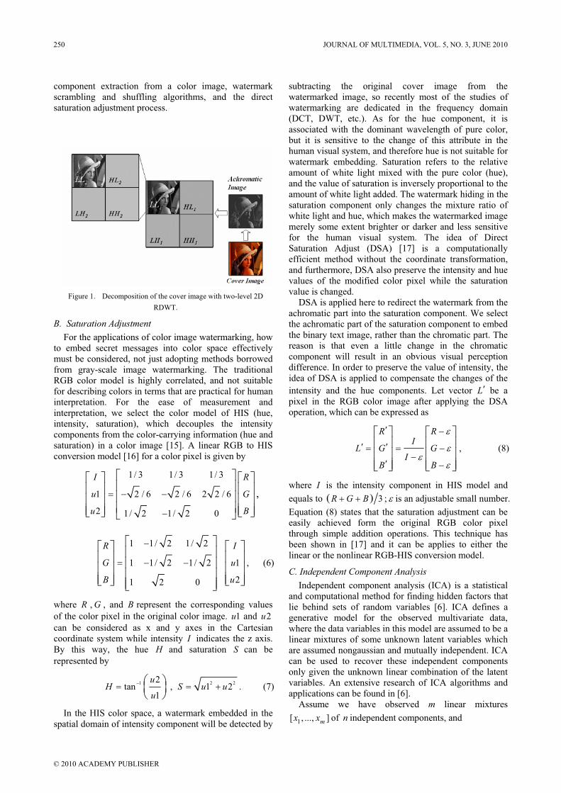
component extraction from a color image, watermark
scrambling and shuffling algorithms, and the direct
saturation adjustment process.
Figure 1. Decomposition of the cover image with two-level 2D
RDWT.
B. Saturation Adjustment
For the applications of color image watermarking, how
to embed secret messages into color space effectively
must be considered, not just adopting methods borrowed
from gray-scale image watermarking. The traditional
RGB color model is highly correlated, and not suitable
for describing colors in terms that are practical for human
interpretation. For the ease of measurement and
interpretation, we select the color model of HIS (hue,
intensity, saturation), which decouples the intensity
components from the color-carrying information (hue and
saturation) in a color image [15]. A linear RGB to HIS
conversion model [16] for a color pixel is given by
1/ 3 1/ 3 1/ 3
1 2 / 6 2 / 6 2 2 / 6
2 1/ 2 1/ 2 0
,
I R
u G
u B
1 1/ 2 1/ 2
1 1/ 2 1/ 2 1
21 2 0
R I
G u
B u
, (6)
where , , and B represent the corresponding values
of the color pixel in the original color image. and
can be considered as x and y axes in the Cartesian
coordinate system while intensity
R G
1u 2u
I indicates the z axis.
By this way, the hue H and saturation S can be
represented by
1 2tan , 1 2
1
u 2 2H S u u
u. (7)
In the HIS color space, a watermark embedded in the
spatial domain of intensity component will be detected by
subtracting the original cover image from the
watermarked image, so recently most of the studies of
watermarking are dedicated in the frequency domain
(DCT, DWT, etc.). As for the hue component, it is
associated with the dominant wavelength of pure color,
but it is sensitive to the change of this attribute in the
human visual system, and therefore hue is not suitable for
watermark embedding. Saturation refers to the relative
amount of white light mixed with the pure color (hue),
and the value of saturation is inversely proportional to the
amount of white light added. The watermark hiding in the
saturation component only changes the mixture ratio of
white light and hue, which makes the watermarked image
merely some extent brighter or darker and less sensitive
for the human visual system. The idea of Direct
Saturation Adjust (DSA) [17] is a computationally
efficient method without the coordinate transformation,
and furthermore, DSA also preserve the intensity and hue
values of the modified color pixel while the saturation
value is changed.
DSA is applied here to redirect the watermark from the
achromatic part into the saturation component. We select
the achromatic part of the saturation component to embed
the binary text image, rather than the chromatic part. The
reason is that even a little change in the chromatic
component will result in an obvious visual perception
difference. In order to preserve the value of intensity, the
idea of DSA is applied to compensate the changes of the
intensity and the hue components. Let vector L be a
pixel in the RGB color image after applying the DSA
operation, which can be expressed as
R RI
L G GI
B B
, (8)
where I is the intensity component in HIS model and
equals to 3R G B ; is an adjustable small number.
Equation (8) states that the saturation adjustment can be
easily achieved form the original RGB color pixel
through simple addition operations. This technique has
been shown in [17] and it can be applies to either the
linear or the nonlinear RGB-HIS conversion model.
C. Independent Component Analysis
Independent component analysis (ICA) is a statistical
and computational method for finding hidden factors that
lie behind sets of random variables [6]. ICA defines a
generative model for the observed multivariate data,
where the data variables in this model are assumed to be a
linear mixtures of some unknown latent variables which
are assumed nongaussian and mutually independent. ICA
can be used to recover these independent components
only given the unknown linear combination of the latent
variables. An extensive research of ICA algorithms and
applications can be found in [6].
Assume we have observed m linear mixtures
1[ , ..., ]mx x of n independent components, and
250 JOURNAL OF MULTIMEDIA, VOL. 5, NO. 3, JUNE 2010
© 2010 ACADEMY PUBLISHER

1 1 2 21
...n
j ji i j j jn ni
x a s a s a s a s , (9)
(a) (b)
Figure 2. (a) Original and (b) scrambled binary text image.
where x denoted as a random vector and whose elements
are the mixtures of 1[ , ..., ]mx x , and s is the random
vector of unobserved independent sources, whose
elements are 1[ , ..., n ]s s . Then the basic ICA model can be
defined as x As ; A is an unknown linear mixing m n
matrix for . The object of ICA is to find out a
matrix and obtains the independent component
by
m n
B
y Bx , where is the estimated
component of
1[ , ...,y y ]ny
s . In this work, the watermarked color
image is treated as the linear mixtures of the cover image
and the watermark image (i.e., independent sources), and
FastICA [18], a simple form of generalized fixed point
algorithm, is applied in spatial domain to direct extract
the secret text image from the watermarked color image.
III. SECRET TEXT IMAGE EMBEDDING
The achromatic component of the original color image
is used for secret text hiding, followed by the saturation
adjustment technique defined in Section II.B to redirect
the secret message into the saturation component. The
procedure to embed secret text image into the achromatic
component is explained in the following subsections.
A. Achromatic Separation and Watermark Encryption
The achromatic component A with the size of M N
is firstly separated from the original cover image for the
secret text image embedding. Let vector L r be
an original RGB color pixel and L L
[ , , ]T
g b
a cL ,
where is the achromatic component
with
[ , , ]T
aL X X X
min( , , )X r g b and cL L aL
L
a
is the chromatic
component. Even a little change in the component
will result in an obvious visual perception difference. To
overcome this drawback, we select and utilize the
idea of DSA for embedding the secret text message. The
set of achromatic component , denoted by
cL
a
L A , is
decomposed into two-level RDWT, and the sub-
band of
2LL
A , denoted as 2LL
A , is the candidate for
watermark embedding as described in Section II.A. The
watermark W is a binary text image with the same size
as A . W exists in a binary pattern and is represented by
(10) ( , ), 0 , 0 ,
( , ) 1, 1.
W W i j i M j N
W i j
(11)( ) ( , ) ( , ),
0 , , 0 , .
sc sc scW K W W i j W i j
i i M j j N
The pseudorandom scrambling key scK will be used to
create one mixture signal for watermark extraction in
Section IV. scW is a 1-D sequence pseudorandom
number of length M N , and needs to be transformed
into a 2-D sequence before applying it for the scramble of
the watermark image. Figure 2 shows the binary text
image and the scrambled result.
B. LL2 sub-band Computation and Watermark Shuffling
In [9], and2
LH2
HL sub-bands of RDWT are chosen
to embed watermark rather than the sub-band. The
authors of [9] stated that the quality of image will be
seriously degraded, if the approximation component
of sub-band is chosen to embed watermark. However,
we have different view for this issue. Our consideration is
all the sub-bands (including and ) contain most
energy of the host image, and embedding the watermark
into these low frequency components can resist the attack
operations of general image processing [13-14]. In
addition, the strength of embedded watermark is
adjustable in the step of DSA operation to reduce the
degradation of image quality. Therefore, sub-band is
selected for watermark embedding in this paper.
2LL
2LL
2LL
LL1
LL
2LL
In order to improve the perceptual invisibility, Hsu et
al.[19] suggested that the watermark should be permuted
to disperse the spatial relationship based on the
characteristics of the host image. This permutation result
is shW , which is a shuffled scW according to the
permutation sequence of and represented as 2
LL
( ) ( , ) ( , )
0 , , 0 , ,
sh sh sc sh scW K W W i j W i j
i i M j j N
, (12)
Notice that all the pixels in the watermark W are
scrambled by a pseudorandom order to produce a
permuted watermark scW , which is defined as where each pixel ( , )i j of the scrambled watermark
shW is shuffled to the new position ( , according to the )i j
JOURNAL OF MULTIMEDIA, VOL. 5, NO. 3, JUNE 2010 251
© 2010 ACADEMY PUBLISHER
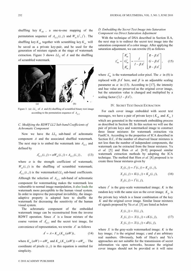
D. Embedding the Secret Text Image into Saturation Component via Direct Saturation Adjustment
(
2
a) (b)
Figure 3. (a) LL of A and (b) shuffling of scrambled binary text i
2
mage
according to the permutation sequence ofLL
A
shuffling key shK , a e ma f the
permutation s ence of 2( , )
LL
one-to-on pping o
equ A i j and ( ,scW i )j . The
shuffling key shK together with scrambling key scK will
be saved as a private key-pair, and be used for the
generation of mixture signal the tage of watermark
extraction. Figure 3 show
s at
s 2LL of
With the technique of DSA described in Section II.A,
the next step is to redirect the secret text image into the
saturation component of a color image. After applying the
saturation adjustment, we can rewrite (8) as follows s
A
d Co
and the shuffling
efficients o
of scrambled ark.
Ac
waterm
C. Modifying the RDWT LL2 Sub-ban f
hromatic Component
Now we have the 2LL sub-band of achromatic
component A and the associated shuffled watermark.
The next step is to embed the watermark into 2LL
A and
efined by d
2 2( , ) ( , ) ( , )
LL sh LLA i j W i j A i j , (13)
where is the strength coefficient of watermark;
is the shuffling of scrambled watermark;
2( , )
LL
( ,sh
W i )j
A i j is the watermarke 2L sub-band coefficients.
Although the selection of 2
d L
LLA sub-band of achromatic
component for watermarking makes the watermark less
vulnerable to normal image manipulation, it also leads the
watermark more perceptible to the human visual system.
In order to improve the perceptual invisibility, the image-
adaptive property is adopted here to shuffle the
watermark for decreasing the sensitivity of the human
visual system.
The achromatic comp nent of the embedded
watermark image can be reconstructed from the inverse
RDWT operation. Si e
o
nc A is a linear mixture of the
coarse version of 2LL
A and the secret te t image, forx
onvenience c of representation, we rewrite A as follows
( (sh sc ))A A K (14)
where ( )
K W ,
m
m m
m
R R AI
L G G AI A
B AB
, (15)
where mL is the watermarked color pixel. The in (8) is
replaced with A here, and is an adjustable scaling
parameter as in (13). According to [17], the intensity
and hue value are preserved as the original cover image,
but the saturation value is changed and multiplied by a
scaling factor ( )I I A .
IV. SECRET TEXT IMAGE EXTRACTION
For each cover image embedded with secret text
messages, we have a pair of private keys ( shK and scK )
which are generated in the watermark embedding process
as described in Section III. In this section we will use the
pair of private keys and watermarked image to construct
three linear mixtures for watermark extraction via
FastICA. According to the properties of ICA described in
Section II.C, if the number of observed linear mixtures is
not less than the number of independent components, the
watermark can be extracted from the linear mixtures. Yu
et al. [5] and Hien et al. [8-9] proposed similar
watermark extraction methods by adopting the ICA
technique. The method that Hien et al. [8] proposed is to
create three linear mixtures given by
1
2
3
( , ) ( , ) ( , ),
( , ) ( , ) ( , ),
( , ) ( , ),
p
p
X i j I i j K i j
X i j K i j K i j
X i j I i j
(16)
where I is the gray-scale watermarked image; K is the
random key with the same size as the cover image; pK is
the private key which is a linear combination of the key
K and the original cover image. Similar linear mixtures
of signals proposed by Yu et al. [5] are listed as below
1
2
3
( , ) ( , ),
( , ) ( , ) ( , ),
( , ) ( , ) ( , ),
X i j X i j
X i j X i j cK i j
X i j X i j dI i j
(17)
sc scK W W nd ( ( ))ash shscK K W W . The
coordinate o
where X is the gray-scale watermarked image; is the
key image;
K
I is the original image; c and are arbitrary
real numbers. Obviously, both of Hien’s and Yu’s
approaches are not suitable for the transmission of secret
information via open networks, because the original
cover images should not be provided or it will raise
d
( ,i jf pixels ) in this equation is omitted for
simplicity.
252 JOURNAL OF MULTIMEDIA, VOL. 5, NO. 3, JUNE 2010
© 2010 ACADEMY PUBLISHER
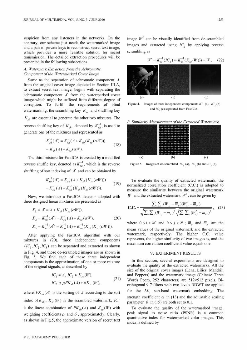
suspicion from any listeners in the networks. On the
contrary, our scheme just needs the watermarked image
and a pair of private keys to reconstruct secret text image,
which provides a more feasible solution for secret
transmission. The detailed extraction procedures will be
presented in the following subsections.
(a) (b) (c)
Figure 4. Images of three independent components1
IC (a), 2
IC (b)
and3
IC (c) separated from FastICA.
(a) (b) (c)
Figure 5. Images of de-scrambled 1
IC (a), 2
IC (b) and3
IC (c).
A. Watermark Extraction from the Achromatic
Component of the Watermarked Cover Image
Same as the separation of achromatic component A
from the original cover image depicted in Section III.A,
to extract secret text image, begins with separating the
achromatic component A from the watermarked cover
image which might be suffered from different degree of
corruption. To fulfill the requirements of blind
watermarking, the scrambling key scK and shuffling key
shK are essential to generate the other two mixtures. The
reverse shuffling key of shK , denoted by 1
shK , is used to
generate one of the mixtures and represented as
(18)
1 1
1
( ) ( ( ( )))
( ) ( ).
sh sh sh sc
sh sc
K A K A K K W
K A K W
The third mixture for FastICA is created by a modified
reverse shuffle key, denoted as1
saK , which is the reverse
shuffling of sort indexing of A and can be obtained by
(19)
1 1
1 1
( ) ( ( ( )))
( ) ( ( ( ))).
sa sa sh sc
sa sa sh sc
K A K A K K W
K A K K K W
Now, we introduce a FastICA detector adopted with
three designed linear mixtures are presented as
1
1 1
2
1 1 1
3
( ( )),
( ) ( ) ( ),
( ) ( ) ( ( ( ))).
sh sc
sh sh sc
sa sa sa sh sc
X A A K K W
X K A K A K W
X K A K A K K K W
(20)
After applying the FastICA algorithm with our
mixtures in (20), three independent components
1 2 3( , , )IC IC IC can be separated and extracted as shown
in Fig. 4, and those de-scrambled images are as shown in
Fig. 5. We find each of these three independent
components is the approximation of one or more mixture
of the original signals, as described by
1 2
3
, ( ),
( ) ( ),
sc
sh sc
IC A IC K W
IC PK A K W (21)
where is the sorting of ( )shPK A A according to the sort
index of shK ; ( )scK W is the scrambled watermark, 3IC
)is the linear combination of PK and (sh A) (scK W with
weighting coefficients and , approximately. Clearly,
as shown in Fig.5, the approximate version of secret text
image W can be visually identified from de-scrambled
images and extracted using 2IC
1 1
scK
by applying reverse
scrambling as
2( ) ( ( )))sc scW K IC K W W . (22)
B. Similarity Measurement of the Extracted Watermark
To evaluate the quality of extracted watermark, the
ormalized correlation coefficient (C.C.) is adopted to
measure the similarity between the original watermark
and the extracted watermark W , can be given by
n
W
, ,( )
i
W i
2 2
, , '
( )
( ) ( )
i j
i j j
i j j W
i j W i j W
W m W m
W m W m
C.C. , (23)
i M and 0 j Nwhere 0 ;W
m and W
m are the
mean values of the original watermark and the extracted
watermark, respectively. The higher C.C. value
represents, the higher similarity of two images is, and the
maximum correlation coefficient value equals one.
V. EXPERIMENT RESULTS
In this section, several experiments are designed to
evaluate the quality of the extracted watermarks. All the
size of the original cover images (Lena, Lilies, Mandrill
and Peppers) and the watermark image (Chinese Three
Words Poem, 252 characters) are 512 512 pixels. Bi-
orthogonal 9-7 filters with two levels RDWT are applied
for the LL sub-band watermark embedding. The
strength coefficient
2
in (13) and the adjustable scaling
parameter in (15) are both set to 0.1.
To evaluate the quality of the watermarked image,
peak signal to noise ratio (PSNR) is a common
quantitative index for watermarked color images. This
index is defined by
JOURNAL OF MULTIMEDIA, VOL. 5, NO. 3, JUNE 2010 253
© 2010 ACADEMY PUBLISHER

2
10
255PSNR 10 log
MSE, (24)
(a) (b) (c)
(d) (e) (f)
Figure 6. The original “Lena”, “Mandrill” and “Peppers” images (a-
c), and the corresponding watermarked images (d-f) with PSNR values
of 45.3289, 41.9150 and 40.3032 respectively.
1 1
2
0 0
2 2
1M SE [(( ( , ) ( , ))
3
(( ( , ) ( , )) (( ( , ) ( , )) ],
M N
i j
m
m m
r i j i jM N
g i j i j b i j i j
r
g b
(25)
where represents a color pixel in
location of the original cover image;
depicts a color pixel in the
watermarked image;
T[ ( , ), ( , ), ( , )]r i j g i j b i j
( , )i j
T, ), ( , ), ( , )]
m m mj g i j b i j[ (r i
M and denote the row and
column sizes of color image. In this paper
N
M and are
both 512 pixels.
N
Several experiments are conducted to evaluate the
robustness of our proposed scheme against various kinds
of attack. For the verification of robustness, general
image operations (JPEG-2000 and JPEG-loss
compression, low pass filtering, and medium filtering),
geometrical distortions (cropping, rescaling and rotating)
and self-similarities attacks (in three different color
spaces) are applied to the watermarked images in these
experiments. Two different processes of attacks are
classified by:
(1) StirMark attacks [20]: Several image alterations
were applied using StirMark benchmark 4.0, including
Gaussian low-pass filtering, 5 medium filtering,
JPEG-loss compression, image cropping, resizing,
rotation-scaling, and self-similarities attacks in different
color models.
3 3 5
(2) JPEG2000 attacks: Based on JASPER [21], the
XnView software is adopted to perform the JPEG2000
attacking operations.
For the invisibility requirement, we can control the
PSNR of watermarked image by setting the value of ,
where , as presented in (13) and (15). The PSNR
of the watermarked images respecting to the original
cover images fall in a range of (40.3032, 45.3289), as
showed in Fig. 6, so the perceptual qualities of
watermarked images are retained. Also the intensity and
hue of watermarked images are preserved as described in
Section III.D.
For the operations of JPEG2000 and JPEG-loss
compression, the setting of quality level is varied from
15% to 95%. JPEG-loss and JPEG2000 compression
attacks are implemented with StirMark and XnView,
respectively. The correlation coefficients of these
extracted watermarks are collected in Table I and II,
which show the C.C. values of the extracted watermarks
are still acceptable (>0.66) for low quality of JPEG-loss
and JPEG2000 compression, and demonstrate that our
scheme is robust enough to against these attacks.
To verify the robustness of our scheme compared with
Hien’s method [8], the same attacking operations are
conducted to “Lena” image. Table III and IV show the
TABLE ITHE PSNR OF WATERMARKED IMAGES WITH JPEG-LOSS COMPRESSION AND CORRELATION COEFFICIENTS OF THE EXTRACTED WATERMARKS.
JPEG Quality 15% 25% 35% 45% 55% 65% 75% 85% 95%
PSNR 32.0763 33.7043 34.7675 35.4047 36.0057 36.6428 37.547 38.9699 43.3145 Lena
C.C. 0.9699 0.9768 0.9874 0.9845 0.9852 0.9919 0.9963 0.9993 0.9999
PSNR 24.2786 25.6495 26.3543 27.3785 27.9209 29.1134 30.3441 32.8674 40.3998 Mandrill
C.C. 0.7101 0.7567 0.7860 0.8032 0.8146 0.8303 0.8484 0.8801 0.9172
PSNR 30.2772 31.3099 31.9660 32.3743 32.7177 33.1456 33.7450 35.3447 41.4158 Peppers
C.C. 0.9615 0.9801 0.9835 0.9855 0.9867 0.9868 0.9925 0.9980 0.9995
TABLE IITHE PSNR OF WATERMARKED IMAGES WITH JPEG200 COMPRESSION AND CORRELATION COEFFICIENTS OF THE EXTRACTED WATERMARKS.
JPEG2000 Quality 15% 25% 35% 45% 55% 65% 75% 85% 95%
PSNR 31.0248 31.7621 32.5559 33.5688 34.7665 36.1186 37.9310 39.9054 43.7266 Lena
C.C. 0.9907 0.9937 0.9968 0.9987 0.9997 0.9993 0.9996 0.9998 1.0
PSNR 21.0825 21.4430 21.8961 22.4825 23.2771 24.2694 25.5830 27.6214 32.3011 Mandrill
C.C. 0.6662 0.6852 0.7091 0.7267 0.7551 0.8357 0.8709 0.9237 0.9835
PSNR 27.6724 28.1585 28.6966 29.2697 29.8989 30.6837 31.7822 33.5007 36.8875 Peppers
C.C. 0.9141 0.9434 0.9477 0.9598 0.9802 0.9916 0.9981 0.9996 1.0
254 JOURNAL OF MULTIMEDIA, VOL. 5, NO. 3, JUNE 2010
© 2010 ACADEMY PUBLISHER

(a) SS1 (b) SS2 (c) SS3
(d) Low-pass filter (e) High-pass filter (f) Median filter
(g) Rotate 1 (h) Rotate 2 (i) Center crop 15%
(j) Surrounding crop. (k) Random noise (l) Pepper&salt noise
Figure 7. Various kinds of attack applied to watermarked “Lena”
images.
comparison results based on different JPEG-loss and
JPEG2000 compression ratios with similar PSNR values,
where all of the C.C. values of our proposed scheme are
higher than Hien’s. Table V shows the comparison results
based on several other attacking operations, including add
random noise, low-pass filtering, median filtering, center
cropping and surround cropping, where most of the C.C.
value of these extracted watermarks with our method are
better than Hien’s, except for the center cropping and
surround cropping. These unsatisfactory results is caused
by our approach doesn’t need the original cover image,
but only use the watermarked cover image to extract the
watermark, and nevertheless the C.C. values of these two
extracted watermarks are still comparable with Hien’s
experiment results.
TABLE VITHE PSNR OF WATERMARKED IMAGES AND CORRELATION
COEFFICIENTS OF THE EXTRACTED WATERMARKS, AFTER APPLYING
SELF-SIMILARITIES ATTACKS IN DIFFERENT COLOR MODELS.
Self Similarities
Test
Lena (PSNR=45.3289)
Mandrill(PSNR=41.9150)
Peppers (PSNR=40.
3020)
PSNR 25.6328 23.7944 25.1552 SS1
C.C. 0.9995 0.8360 0.9935
PSNR 25.7709 23.1262 25.1875 SS2
C.C. 0.9975 0.8819 0.9888
PSNR 25.1693 23.4813 24.6181 SS3
C.C. 0.9999 0.9168 0.9994
TABLE III COMPARISONS OF CORRELATION COEFFICIENTS OF EXTRACTED
WATERMARKS, COMPUTED FROM DIFFERENT WATERMARKING
METHODS AND JPEG-LOSS COMPRESSIONS APPLIED TO
WATERMARKED “LENA” IMAGES.
JPEG Quality 15% 25% 45% 65% 85%
PSNR of Hien's 32.4353 34.2840 36.1640 37.5554 43.3334
C.C. of Hien's 0.5770 0.6270 0.6698 0.8162 0.9979
PSNR of ours 32.0763 33.7043 35.4047 36.6428 38.9699
C.C. of ours 0.9699 0.9768 0.9845 0.9919 0.9999
TABLE IVCOMPARISONS OF CORRELATION COEFFICIENTS OF EXTRACTED
WATERMARKS, COMPUTED FROM DIFFERENT WATERMARKING
METHODS AFTER JPEG2000 COMPRESSIONS APPLIED TO
WATERMARKED “LENA” IMAGES.
JPEG2000 compression
bit rates 0.4
With the help of StirMark, the self-similarity attacks
are applied on the watermarked images in HSV, RGB and
YUV color models. In HSV, the S channel is selected to
be attacked and the result is presented as SS1. In RGB,
we choose the B channel to be attacked and the result is
denoted as SS2. For YUV, the attack is applied to U and
V channels and the result is symbolized as SS3. Note that
the channels selected in HSV and YUV color models are
used to verify the robustness of our proposed approach
under saturation attacks. For these three self-similarity
tests, the percentages of swaps are all set to 60. Figure 7
0.8 1.2 1.6 2.0 2.4
PSNR of Hien's
36.2844 39.3927 40.9852 43.3334 43.3334 44.3645
C.C. of Hien’s
0.6859 0.7578 0.8342 0.8873 0.9155 0.9330
PSNR of ours
37.7258 41.0654 42.8726 43.8071 44.3217 44.6518
C.C. of ours 0.9709 0.9937 0.9950 0.9956 0.9973 0.9987
TABLE VCOMPARISONS BASED ON SEVERAL ATTACKING OPERATIONS APPLIED
TO WATERMARKED “LENA” IMAGES.
Attacking operations PSNR of Hien’s
C.C of Hien’s
PSNR of ours
C.C. of ours
Adding random noise 25.13 0.90 25.6986 0.9839
5 5 Low-pass filter 29.15 0.64 29.3959 0.9792
5 5 Median filter 32.1 0.81 31.95 0.9643
Center crop 15% and replace with other image
21.14 0.91 21.1425 0.8718
Surrounding crop 15% and replaced with “peppers” image
17.93 0.72 16.4290 0.6966
JOURNAL OF MULTIMEDIA, VOL. 5, NO. 3, JUNE 2010 255
© 2010 ACADEMY PUBLISHER
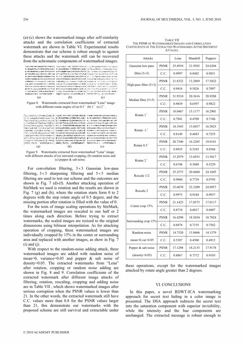
(a) (b) (c)
Figure 8. Watermarks extracted from watermarked “Lena” image
with different rotate angles of (a) 0.5 (b) 1 (c) 2
(a) (b) (c)
Figure 9. Watermarks extracted from watermarked “Lena” image
with different attacks of (a) surround cropping, (b) random noise and
(c) pepper & salt noise.
(a)-(c) shows the watermarked image after self-similarity
attacks and the correlation coefficients of extracted
watermark are shown in Table VI. Experimental results
demonstrate that our scheme is robust enough to against
these attacks and the watermark still can be recovered
from the achromatic components of watermarked images.
For convolution filtering, 3 Gaussian low-pass
filtering, sharpening filtering and median
filtering are used to test our scheme and the outcomes are
shown in Fig. 7 (d)-(f). Another attacking operation of
StirMark we used is rotation and the results are shown in
Fig. 7 (g) and (h), where the rotation starts form 0 to 2
degrees with the step rotate angle of 0.5 degree, and the
missing portion after rotation is filled with the value of 0.
3
3 3 5 5
For the tests of image scaling operations by StirMark,
the watermarked images are rescaled to one half or 2
times along each direction. Before trying to extract
watermarks, the scaled images are resized to the original
dimensions using bilinear interpolation. As for attacking
operation of cropping, these watermarked images are
individually cropped by 15% in the center or surrounding
area and replaced with another images, as show in Fig. 7
(i) and (j).
With respect to the random-noise adding attack, these
watermarked images are added with random noise of
mean=0, variance=0.05 and pepper & salt noise of
density=0.05. The extracted watermarks from “Lena”
after rotation, cropping or random noise adding are
shown in Fig. 8 and 9. Correlation coefficients of the
extracted watermark after different image attacks of
filtering, rotation, rescaling, cropping and adding noise
are in Table VII , which shows watermarked images after
serious corruption when the PSNR values is lower than
21. In the other words, the extracted watermark still have
C.C. values more than 0.8 for the PSNR values larger
than 21, this demonstrate our watermarks with the
proposed scheme are still survival and extractable under
these operations, except for the watermarked images
attacked by rotate angle greater than 2 degrees.
TABLE VIITHE PSNR OF WATERMARKED IMAGES AND CORRELATION
COEFFICIENTS OF THE EXTRACTED WATERMARKS AFTER DIFFERENT
ATTACKS.
Attacks Lena Mandrill Peppers
PSNR 25.4934 21.9583 24.6204Gaussian low-pass
filter (3 3) C.C. 0.9997 0.8482 0.9831
PSNR 21.8332 13.2869 17.5822High-pass filter (3 3)
C.C. 0.9416 0.5826 0.7097
PSNR 31.9510 20.3616 28.9288Median filter (5 5)
C.C. 0.9839 0.6597 0.9822
PSNR 18.0467 15.1177 16.2901Rotate 1
C.C. 0.7941 0.4709 0.7186
PSNR 18.1943 15.0457 16.5025Rotate -1
C.C. 0.8149 0.4683 0.7253
PSNR 20.7340 16.2285 19.0141Rotate 0.5
C.C. 0.8935 0.5245 0.8566
PSNR 15.2979 13.6933 13.5017Rotate 2
C.C. 0.6748 0.3880 0.5229
PSNR 25.2575 20.8404 24.1045Rescale 1/2
C.C. 0.9960 0.7739 0.9793
PSNR 25.6070 23.3209 24.9957Rescale 2
C.C. 0.9975 0.9184 0.9937
PSNR 21.1425 17.0573 17.0117Center crop 15%
C.C. 0.8718 0.6017 0.6807
PSNR 16.4290 18.5654 18.7024Surrounding crop 15%
C.C. 0.6974 0.7155 0.7562
PSNR 14.7520 13.8606 14.1579Random noise
mean=0,var=0.05 C.C. 0.5387 0.4500 0.4912
VI. CONCLUSIONS
In this paper, a novel RDWT-ICA watermarking
approach for secret text hiding in a color image is
presented. The DSA approach redirects the secret text
into the saturation component with superior invisibility,
while the intensity and the hue components are
unchanged. The extracted message is robust enough to
PSNR 17.1298 18.2135 17.9178Pepper & salt noise
(density=0.05) C.C. 0.8867 0.7372 0.9103
256 JOURNAL OF MULTIMEDIA, VOL. 5, NO. 3, JUNE 2010
© 2010 ACADEMY PUBLISHER
sustain the general spatial and frequency domain
degradations, which including JPEG-loss and JPEG2000
compression, filtering, adding noise, self-similarities,
image cropping and scaling. In our experiment the
traditional Chinese characters are processed as a secret
message, but our watermarking approach can be also
applied for message hiding of binary patterns, binary
images, and characters of any languages.
REFERENCES
[1] M. D. Swanson, M. Kobayashi and A. H. Tewfik,
“Multimedia Data-Embedding and Watermarking
Technologies,” Proceedings of the IEEE, vol. 86, no 6, pp.
1064-1087, June 1998.
[2] M. Kutter, S. K. Bhattacharjee and T. Ebrahimi, “Towards
Second Generation Watermarking Schemes”, 6th
International Conference on Image Processing (ICIP’99),
Kobe, Japan, vol. 1, pp. 320-323, Oct. 1999.
[3] N. Ahmidi and R. Safabakhsh, “A Novel DCT-based
Approach for Secure Color Image Watermarking”,
Proceedings of the International Conference on
Information Technology: Coding and Computing
(ITCC’04), Vol. 2, pp.709-713, Apr. 2004.
[4] C. P. Chang, Y. C. Lee, A. C. Chang, P. S. Huang and T.
M. Tu, “StarMarker – A Fast and Robust RGB-based
Saturation Watermarking System for Pan-sharpened
IKONOS and Quickbird Imagery”, Optical Engineering,
Vol.45, Issue 5, May 2006.
[5] D. Yu and F. Sattar, “A New Blind Watermarking
Technique based on Independent Component Analysis,”
Spinger-Verlag Computer Science Lecture Series, Vol.
2613, pp.51-63, May 2003.
[6] A. Hyvärinen and E. Oja, “Independent Component
Analysis: Algorithms and Applications,” Neural Networks,
13(4-5), pp. 411-430, 2000.
[7] F. Kefeng, W. Meihua, M. Wei and Z. Xinhua, “Novel
Copyright Protection Scheme for Digital Content,” Journal
of Systems Engineering and Electronics, Vol.17, No.2, pp.
423-429, 2006.
[8] T. D. Hien, Z. Nakao, and Y. W. Chen, “Robust RDWT-
ICA based information hiding,” Soft Comput, Vol. 10, pp.
1135-1144, 2006.
[9] T. D. Hien, Zensho Nakao, Y. W. Chen, “RDWT/ICA for
Image Authentication,” Proceedings of the Fifth IEEE
International Symposium on Signal Processing and
Information Technology, pp. 805-810, 2005.
[10] J. E. Fowler, “The Redundant Discrete Wavelet Transform
and Additive Noise”, IEEE Signal Processing Letters, Vol.
12, pp. 629-632, Sep., 2005.
[11] L. Hua and J. E. Fowler, “RDWT and image
Watermarking,” Technical Report MSSU-COE-ERC-01-18,
Engineering Research Center, Mississippi State University,
Dec., 2001.
[12] V. K. Goyal, M. Vetterli, and N. T. Thao, “Quantized
Overcomplete Expansions in RN: Analysis, Synthesis, and
Algorithms,” IEEE Transactions on Information Theory,
Vol. 44, No. 1, pp. 16-31, Jan., 1998.
[13] I. J. Cox, J. Kilian., F. T. Leighton, and T. Shamoon,
“Secure Spread Spectrum Watermarking for Multimedia,”
IEEE Transactions on Image Processing, Vol. 6, No. 12,
pp. 1673-1687, Dec., 1997.
[14] J. Huang, Y. Q. Shi, and Y. Shi, “Embedding Image
Watermarks in DC Components,” IEEE Transactions on
Circuits and Systems for Video Technology, Vol. 10, No. 6,
pp. 974-979, Sep., 2000.
[15] Rafael C. Gonzalez, Richard E. Woods, Digital Image
Processing, 2nd Ed., Prentice Hall, pp. 282-295, 2002.
[16] R. S. Ledley, M. Buas, and T. J. Golab, “Fundamentals of
True-Color Image Processing,” Proceedings of
International Conference on Pattern Recognition, Vol. 1,
pp. 791-795, 1990.
[17] P. S. Huang, C. S. Chiang, C. P Chang and T. M. Tu,
“Robust Spatial Watermarking Technique for Colour
Images via Direct Saturation Adjustment” IEE Proc.-Vis.
Image Signal Process., Vol.152, No. 5, Oct., 2005.
[18] A. Hyvärinen, “Fast and Robust Fixed-point Algorithm for
Independent Component Analysis,” IEEE Transactions on
Neural Networks, 10(3), pp. 626-634, 1999.
[19] C. T. Hsu and J. L. Wu, “Hidden Digital Watermarks in
Images,” IEEE Transactions on Image Processing, Vol. 8,
No. 1, pp. 58-68, Jan., 1999.
[20] F. A. P. Petitcolas, R. J. Anderson, and M. G. Kuhn,
“Attacks on Copyright Marking Systems,” Proceedings of
Information Hiding, Second International Workshop,
Portland, Oregon, U.S.A., April 15-17, 1998, LNCS 1525,
Springer-Verlag, ISBN 3-540-65386-4, pp. 219-239.
[21] M. D. Adams and F. Kossentini, “JasPer: A Software-
Based JPEG-2000 Codec Implementation”, Proceedings of
International Conference on Image Processing, Vol. 2, pp.
53-56, Sep., 2000.
Chih-Chien Wu received the M.S. degrees from Department
of Electrical and Electronic Engineering, Chung Cheng Institute
of Technology, National Defense University, Taiwan, in 2000,
and is currently pursuing the Ph.D. degree in the Department of
Electrical and Electronic Engineering, National Defense
University, Taiwan. His research interests include image and
signal processing, data hiding, and web GIS system. His recent
research has focused on blind color image steganography.
Dr. Yu Su received his BS degree from Chung Cheng
Institute of Technology in 1987, the MS degree from
Chinese Culture University in 1999, and the PhD degree
in computer science & engineering from Yuan Ze
University, in 2005. Currently he is an assistant professor
in the Department of Computer Science & Information
Engineering, Yuanpei University. His current research
interests include multispectral remote sensing, statistical
pattern recognition, and digital image processing.
Prof. Te-Ming Tu received the BS degree from Chung
Cheng Institute of Technology in 1986, the MS degree from
National Sun Yat-Sen University in 1991, and the PhD degree
in electrical engineering from the National Cheng Kung
University, in 1996. Since 1981, he has served in the R.O.C.
Army. He was a professor 2001 to 2009, and is currently a
professor in the Department of Computer and Communications,
Ta Hwa Institute of Technology. His current research interests
include multispectral/hyperspectral remote sensing, medical
imaging, independent component analysis, and statistical pattern
recognition.
Prof. Chien-Ping Chang received the BS degree in
Electrical Engineering from Chung Cheng Institute of
Technology in 1986, and the PhD degree in Computer and
Information Science from National Chiao Tung University,
Taiwan, Republic of China, in 1998. He is currently a professor
in the Department of Electrical and Electronic, Chung Cheng
Institute of Technology, Taiwan, Republic of China. His
research interests include parallel computing, interconnection
networks, graph theory, image processing, and data hiding.
JOURNAL OF MULTIMEDIA, VOL. 5, NO. 3, JUNE 2010 257
© 2010 ACADEMY PUBLISHER

Dr. Sheng-Yi Li received the BS, MS, and PhD degrees in
electrical engineering from Chung Cheng Institute of
Technology in 1990, National Sun Yat-Sen University in 1994,
and National Central University in 2004, respectively. He is
currently an associate professor in the Department of Electrical
and Electronic Engineering, Chung Cheng Institute of
Technology, R.O.C. His research interests include satellite
communications, ionospheric radio propagation, and electric
circuit design for wireless communications.
258 JOURNAL OF MULTIMEDIA, VOL. 5, NO. 3, JUNE 2010
© 2010 ACADEMY PUBLISHER
Incoherent Ray Tracing on GPU
Xin Yang College of Computer Science, Zhejiang University, Hangzhou, China
Email: [email protected]
Duan-qing Xu and Lei Zhao College of Computer Science, Zhejiang University, Hangzhou, China
Email: xdqzju, [email protected]
Abstract—Tracing secondary rays, such as reflection, refraction and shadow rays, can often be the most costly step in a modern real-time ray tracer. In this paper, we propose a new approach to ray tracing on GPU. Our approach is especially efficient for incoherent rays. Combined with the common packets ray tracing, we propose a different data-parallel approach to ray tracing on GPU, in which individual ray intersect with k different nodes/triangles in the same operation. Besides, we add some additional information in the construction of acceleration structure, and propose a new approach to travel the acceleration structure. Our acceleration structure needn’t collapse, so it could be built very efficiently, which is promising for dynamic scenes. Despite this approach is slower for primary rays, but demonstrate that it performs better than those techniques as soon as incoherent rays are considered. Index Terms—Ray tracing, GPU, BVH.
I. INTRODUCTION
In the two decades since the introduction of ray tracing in its classic form [1], exponential growth in the available compute power and a variety of algorithmic developments have combined to realize real-time ray tracing on commodity processors. Current research on real-time ray tracing has been very biased toward optimizing primary and shadow rays. The results are impressive, approaching frame rates of rasterization-based techniques. However, one major motivation of using ray tracing instead of a GPU renderer is the natural extension to secondary rays, giving true reflections, refraction and global illumination effects.
Secondary rays here means those rays with multiple bounces of reflections and refractions, multiple shadow rays per area light source, in contrast to primary rays that have a common origin (the camera/eye) and want to traverse the same nodes and intersect the same primitives. Current interactive ray tracers rely on SIMD instructions and packets to achieve high performance. The primary rays are coherent rays, and it is straightforward to group these rays into packets, which usually achieves both very high SIMD utilization and bandwidth reductions – both of which are crucial to exploiting the hardware’s full potential.
However, these techniques explicitly rely on high coherence, either SIMD or packet, to provide any benefit over traditional ray tracers using single rays. The
performance issue for tracing incoherent packets of rays has received almost no attention in the interactive ray tracing community. Worse yet, the focus on primary rays ignores a simple fact: primary rays are the minority of rays in high quality renderings. For renderings that send multiple shadow rays per light source or compute multiple bounces of reflections, the first level of rays does not account for a large percentage of the rendering time. While the secondary rays are not necessarily completely random, it is well understood that they do not behave in the same manner as coherent primary rays: two secondary rays generated from neighbouring points can intersect with objects that are far away in the scene. As a consequence, efficient computation of secondary rays is a harder problem than for primary rays.
Current interactive ray tracers rely on SIMD instructions and packets to achieve high performance. Packets benefit these systems by reducing the amount of computation and bandwidth required to trace a set of rays. Computation is reduced either by amortizing computations over an entire packet for packets larger than the SIMD width (e.g. 64 rays miss a bounding box) or by using the SIMD instructions available on modern processors to perform SIMD-width computations for approximately the cost of a single computation. Similarly, bandwidth is reduced because geometry or acceleration structure data is only fetched once for a traversal step; fewer traversal steps yields less geometry bandwidth requirements. These techniques explicitly rely on high coherence, either SIMD or packet, to provide any benefit over traditional ray tracers using single rays.
Additionally, the requirement of carefully built secondary packets makes the software implementation of a packet based renderer unattractive. One reason behind this is that shaders are no longer independent of the traversal algorithm since secondary rays must be grouped coherently for performance benefit. This can get complicated when a packet hits different objects with different materials since either: the shaders must generate a coherent group of secondary rays independently; secondary rays from multiple shaders must be grouped together; or both.
On the other hand, given current architectural trends, only highly parallel algorithms can be expected to leverage throughput-oriented architectures such as GPUs and to scale well into the future as processors become
JOURNAL OF MULTIMEDIA, VOL. 5, NO. 3, JUNE 2010 259
© 2010 ACADEMY PUBLISHERdoi:10.4304/jmm.5.3.259-267
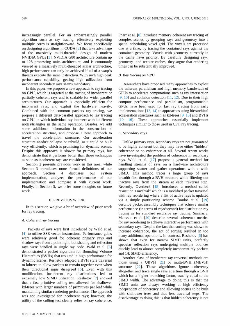
increasingly parallel. For an embarrassingly parallel algorithm such as ray tracing, effectively exploiting multiple cores is straightforward. We focus specifically on designing algorithms in CUDA [2] that take advantage of the massively multi-threaded design of modern NVIDIA GPUs [3]. NVIDIA G80 architecture contain up to 128 processing units architecture, and is commonly viewed as a massively multi-threaded scalar architecture, high performance can only be achieved if all of a warp’s threads execute the same instruction. With such high peak performance capability, getting high utilization from incoherent secondary rays seems mandatory.
In this paper, we propose a new approach to ray tracing on GPU, which is targeted at the tracing of incoherent or partially coherent rays and is scalable for wider parallel architectures. Our approach is especially efficient for incoherent rays, and exploit the hardware heavily. Combined with the common packets ray tracing, we propose a different data-parallel approach to ray tracing on GPU, in which individual ray intersect with k different nodes/triangles in the same operation. Besides, we add some additional information in the construction of acceleration structure, and propose a new approach to travel the acceleration structure. Our acceleration structure needn’t collapse or rebuild, so it could be built very efficiently, which is promising for dynamic scenes. Despite this approach is slower for primary rays, but demonstrate that it performs better than those techniques as soon as incoherent rays are considered.
Section 2 presents previous work in this area, while Section 3 introduces more formal definitions of our approach. Section 4 discusses our system implementation, analyzes the performance of our implementation and compare it with current work. Finally, in Section 5, we offer some thoughts on future work.
II. PREVIOUS WORK
In this section we give a brief overview of prior work for ray tracing. A. Coherent ray tracing
Packets of rays were first introduced by Wald et al. [4] to utilize SSE vector instructions. Performance gains were relatively good for coherent primary rays and shadow rays from a point light, but shading and reflection rays were handled in single ray code. Wald et al. [5] demonstrated a packet algorithm for Bounding Volume Hierarchies (BVHs) that resulted in high performance for dynamic scenes. Reshetov adapted a BVH style traversal to kdtrees to allow packets to remain together even when their directional signs disagreed [6]. Even with this modification, incoherent ray distributions led to extremely low SIMD utilization. Reshetov [7] showed that a fast primitive culling test allowed for shallower kd-trees with larger numbers of primitives per leaf while maintaining similar rendering performance. The approach was not investigated for incoherent rays; however, the utility of the culling test clearly relies on ray coherence.
Pharr et al. [8] introduce memory coherent ray tracing of complex scenes by grouping rays and geometry into a spatial scheduling voxel grid. The voxels are processed one at a time, by tracing the contained rays against the contained geometry. Voxels with geometry currently in the cache have priority. By carefully designing ray-, geometry- and texture caches, they argue that rendering times can be substantially improved. B. Ray tracing on GPU
Researchers have proposed many approaches to exploit the inherent parallelism and high memory bandwidth of GPUs to accelerate computations such as ray intersection [9, 10] and collision detection [11, 12]. Due to their high compute performance and parallelism, programmable GPUs have been used for fast ray tracing from early implementations [13, 14] to approaches using hierarchical acceleration structures such as kd-trees [9, 15] and BVHs [10, 16]. These approaches essentially implement techniques similar to those used in CPU ray tracing. C. Secondary rays
Unlike primary rays, secondary rays are not guaranteed to be highly coherent but they may have either “hidden” coherence or no coherence at all. Several recent works have investigated the problem of coherence in secondary rays. Wald et al. [17] propose a general method for handling streams of rays on a hardware architecture supporting scatter and gather operations with a wide SIMD. This method traces a large group of rays breadth-first through a BVH structure while filtering out inactive rays from the stream at each traversal step. Recently, Overbeck [18] introduced a method called “Partition Traversal” which is a modified packet traversal with ray reordering where a list of active rays is updated via a simple partitioning scheme. Boulos et al. [19] describe packet assembly techniques that achieve similar performance (in terms of rays/second) for distribution ray tracing as for standard recursive ray tracing. Similarly, Mansson et al. [20] describe several coherence metrics for ray reordering to achieve interactive performance with secondary rays. Despite the fact that sorting was shown to increase coherence, the act of sorting resulted in too many additional operations. In contrast, Reshetov [6] has shown that even for narrow SIMD units, perfectly specular reflection rays undergoing multiple bounces quickly lead to almost completely incoherent ray packets and 1/k SIMD efficiency.
Another class of incoherent ray traversal methods are those using a QBVH [21] or multi-BVH (MBVH) structure [22]. These algorithms ignore coherency altogether and trace single rays at a time through a BVH which has a higher branching factor, usually equal to the SIMD width. The advantage to doing this is that the SIMD units are always working at high efficiency independent of coherency and allowing scenes to be built with shallower trees and thus less traversal steps. The disadvantage to doing this is that hidden coherency is not
260 JOURNAL OF MULTIMEDIA, VOL. 5, NO. 3, JUNE 2010
© 2010 ACADEMY PUBLISHER
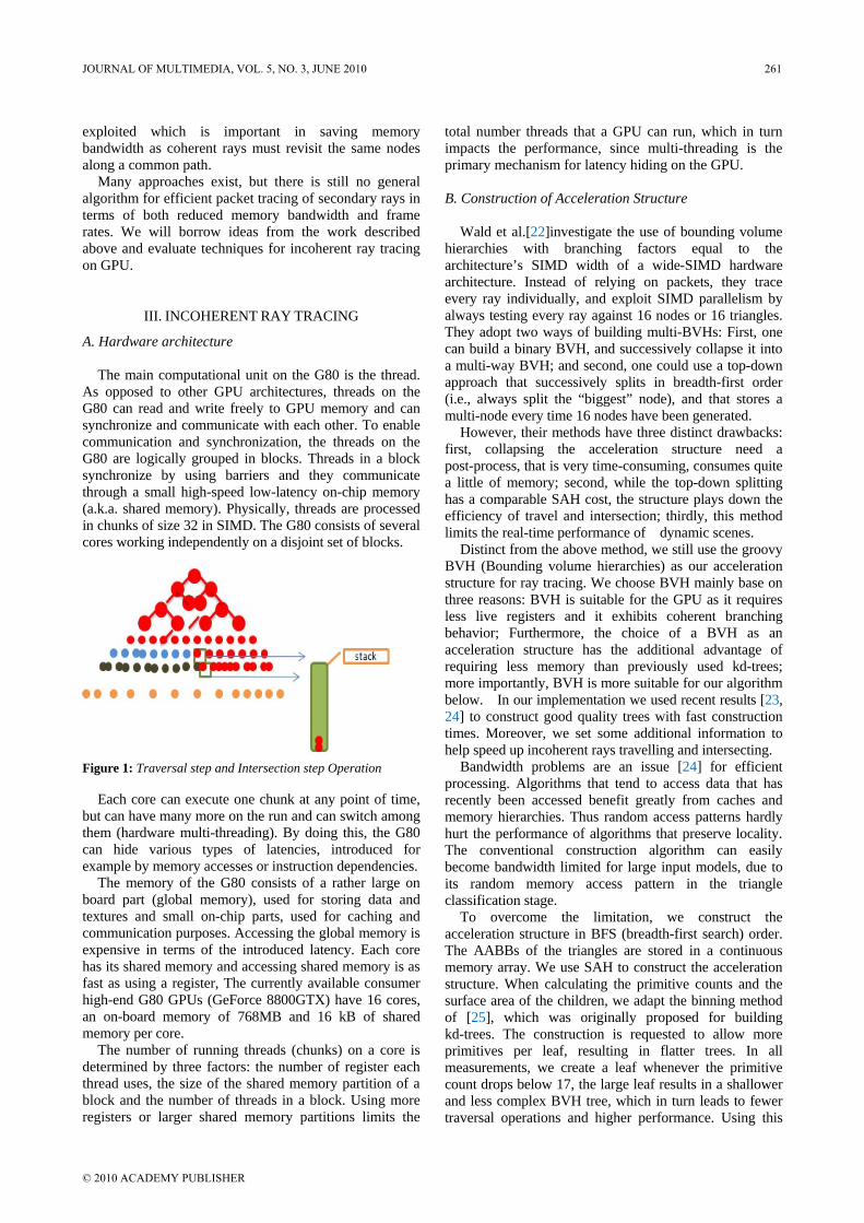
exploited which is important in saving memory bandwidth as coherent rays must revisit the same nodes along a common path.
Many approaches exist, but there is still no general algorithm for efficient packet tracing of secondary rays in terms of both reduced memory bandwidth and frame rates. We will borrow ideas from the work described above and evaluate techniques for incoherent ray tracing on GPU.
III. INCOHERENT RAY TRACING
A. Hardware architecture
The main computational unit on the G80 is the thread. As opposed to other GPU architectures, threads on the G80 can read and write freely to GPU memory and can synchronize and communicate with each other. To enable communication and synchronization, the threads on the G80 are logically grouped in blocks. Threads in a block synchronize by using barriers and they communicate through a small high-speed low-latency on-chip memory (a.k.a. shared memory). Physically, threads are processed in chunks of size 32 in SIMD. The G80 consists of several cores working independently on a disjoint set of blocks.
Figure 1: Traversal step and Intersection step Operation
Each core can execute one chunk at any point of time, but can have many more on the run and can switch among them (hardware multi-threading). By doing this, the G80 can hide various types of latencies, introduced for example by memory accesses or instruction dependencies.
The memory of the G80 consists of a rather large on board part (global memory), used for storing data and textures and small on-chip parts, used for caching and communication purposes. Accessing the global memory is expensive in terms of the introduced latency. Each core has its shared memory and accessing shared memory is as fast as using a register, The currently available consumer high-end G80 GPUs (GeForce 8800GTX) have 16 cores, an on-board memory of 768MB and 16 kB of shared memory per core.
The number of running threads (chunks) on a core is determined by three factors: the number of register each thread uses, the size of the shared memory partition of a block and the number of threads in a block. Using more registers or larger shared memory partitions limits the
total number threads that a GPU can run, which in turn impacts the performance, since multi-threading is the primary mechanism for latency hiding on the GPU. B. Construction of Acceleration Structure
Wald et al.[22]investigate the use of bounding volume hierarchies with branching factors equal to the architecture’s SIMD width of a wide-SIMD hardware architecture. Instead of relying on packets, they trace every ray individually, and exploit SIMD parallelism by always testing every ray against 16 nodes or 16 triangles. They adopt two ways of building multi-BVHs: First, one can build a binary BVH, and successively collapse it into a multi-way BVH; and second, one could use a top-down approach that successively splits in breadth-first order (i.e., always split the “biggest” node), and that stores a multi-node every time 16 nodes have been generated.
However, their methods have three distinct drawbacks: first, collapsing the acceleration structure need a post-process, that is very time-consuming, consumes quite a little of memory; second, while the top-down splitting has a comparable SAH cost, the structure plays down the efficiency of travel and intersection; thirdly, this method limits the real-time performance of dynamic scenes.
Distinct from the above method, we still use the groovy BVH (Bounding volume hierarchies) as our acceleration structure for ray tracing. We choose BVH mainly base on three reasons: BVH is suitable for the GPU as it requires less live registers and it exhibits coherent branching behavior; Furthermore, the choice of a BVH as an acceleration structure has the additional advantage of requiring less memory than previously used kd-trees; more importantly, BVH is more suitable for our algorithm below. In our implementation we used recent results [23, 24] to construct good quality trees with fast construction times. Moreover, we set some additional information to help speed up incoherent rays travelling and intersecting.
Bandwidth problems are an issue [24] for efficient processing. Algorithms that tend to access data that has recently been accessed benefit greatly from caches and memory hierarchies. Thus random access patterns hardly hurt the performance of algorithms that preserve locality. The conventional construction algorithm can easily become bandwidth limited for large input models, due to its random memory access pattern in the triangle classification stage.
To overcome the limitation, we construct the acceleration structure in BFS (breadth-first search) order. The AABBs of the triangles are stored in a continuous memory array. We use SAH to construct the acceleration structure. When calculating the primitive counts and the surface area of the children, we adapt the binning method of [25], which was originally proposed for building kd-trees. The construction is requested to allow more primitives per leaf, resulting in flatter trees. In all measurements, we create a leaf whenever the primitive count drops below 17, the large leaf results in a shallower and less complex BVH tree, which in turn leads to fewer traversal operations and higher performance. Using this
JOURNAL OF MULTIMEDIA, VOL. 5, NO. 3, JUNE 2010 261
© 2010 ACADEMY PUBLISHER
implementation, it is possible to get very fast tree construction times that are even comparable to the BIH [26].
We make every inner-node take the same size, and use a bit to encode whether a node is a leaf or an inner-node. Because our acceleration structure is construct in BFS, the nodes of the same level are placed in succession. We use a bit to depict whether adjacent nodes is the same level or not, in other word, we distinguish different levels only through alternant 0 and 1. Besides, we record the location of child in its father node. C. Travel
While packet tracing significantly increase the efficiency of ray tracing, for the complex scene or mostly incoherent secondary rays, there eventually isn’t enough parallelism for the input rays to exploit. However, many experiences have indicated that ray packet are indeed useful with coherent rays, e.g. primary, shadow, specular reflection, or spatially localized rays such as short ambient occlusion rays, so for these rays, we still adopt the packet tracing to process them quickly and efficiently.
After these rays encounter some bounce, some ray packets become inefficient due to the incoherent rays in a packet. Then, we adopt a different data-parallel approach to ray tracing on GPU. In contrast to the common packets ray tracing, we make individual ray intersect with k different nodes/triangles in the same operation. In fact, the first approaches towards SIMD ray tracing that did exactly that, by building kd-trees whose cost function was skewed to favor large leaves with triangles close to the architecture’s SIMD width, and then intersecting k triangles at once. Wald et al.[22]pointed that this idea had three drawbacks in favor of packet techniques: first, kd-trees (the favorite data structure at that time) favor small leaves, and perform badly for large leaves; second, because kd-trees are intrinsically binary the same idea cannot be used for traversal; and third, the approach would not have given any benefit for shading and ray generation; and third, the approach would not have given any benefit for shading and ray generation. For these reasons, Wald et al. [4] then argued that a more efficient way of using SIMD in a (kd-tree based) ray tracer is to trace, intersect, and shade packets of rays.
However, commodity hardware architectures continue to offer more compute performance every year, increasingly rely on thread parallelism and ever wider SIMD units to deliver that performance. Especially, recent GPUs, as highly parallel processors, is viewed as a massively multi-threaded scalar architecture, each warp of 32 threads is essentially run in a SIMD fashion, high performance can be achieved when all the threads of a warp execute same instructions or programs.
The currently available consumer high-end G80 GPUs (GeForce 8800GTX) have 16 cores, each core execute its algorithm and data independently, so we may process a ray packet per core, and trace 16 ray packets in parallel at the same time. We use the existing shading framework, but traverse each ray packets individually, one after
another. On each core, we make individual rays intersect with 16 different nodes/triangles through 16 threads in the SIMD fashion. These operations are in parallel and fast. With the list built at the step of construction, we don’t need to load the whole acceleration structure into the shared memory of the core on-chip every time.
We define packet utilization to be: P/Q, where P is the number of coherent rays in the packet and Q is the total number of rays in the packet. When the packet utilization drops below a threshold, we will travel and intersect in a new way, i.e. individual rays intersect with different nodes/triangles through parallel threads in the SIMD fashion, rather than ray packets. In our implementation, we switch the kernel whenever the packet utilization drops below 50%. Intuitively, this balances between the cost of individual ray procession for each step and the overhead of low SIMD utilization. Empirically, our threshold of 50% works rather well.
Given an input ray packet, we simply loop over all rays in that packet and traverse them individually, where there is no difference in cost between doing a test between a ray and a triangle versus many triangles since they are done simultaneously using same instructions. We continuously dispatch a ray packet to SM core on GPU, each such ray gets pulled out of the packet, and is immediately replicated into a 16-ray SoA (structure of arrays) packet format similar to that used by packet techniques (this allows the compiler to keep the ray data in registers), so we can get ray data in a clock circle. This ray is then sent to the traversal loop, which starts at the root node.
While we construct the acceleration structure in BFS, we travel it in a hybrid mode. We set a work pool in the shared memory, whose size is equal to the wide of threads in parallel on GPU. Each thread in a warp takes corresponding node data in the work pool. A ray travel these nodes in parallel, test these nodes’ AABB (axis-aligned bounding box). The test returns a mask indicating which of these children are hit by the ray.
We first travel the nodes in BFS, fetch the nodes from the global memory, place them in work pool, until the pool is filled. Because these nodes are placed one by one, reading these data is very efficient. It should be pointed out that the nodes in the wok pool are of the same level in acceleration structure. Then, a ray intersects all the nodes in the work pool through a same operation at the same time. After such a operation finishes, if a ray hits some nodes, the ray continue to travel the acceleration structure in DFS, that is, we flush the work pool, and fetch the children nodes in the next level, whose father nodes are flushed just now.
On the other hand, we set a stack in the shared memory, if some nodes of last level haven’t been travelled, that may be judged through the bit in the node, the first node of whose noses haven’t been travelled in current level will be pushed into the stack (other nodes may be fetched by offside); if a ray doesn’t hit any nodes in the current work pool, it will flush the work pool, get a node from the stack, fetch enough nodes, and fill the work pool. Those nodes haven’t been travel, and are in the same level with the node in the stack. In order to make all the
262 JOURNAL OF MULTIMEDIA, VOL. 5, NO. 3, JUNE 2010
© 2010 ACADEMY PUBLISHER
threads busy efficiently, if the child node is an empty node, it won’t be put into the work pool. One point needs to be emphasized, the nodes in the current work pool are of the same level. C. Intersection
So far, we have only considered inner node traversal steps. When a node in the work pool is a leaf node, the kernel will be switched to a triangle-intersection kernel. Similarly, we iterate over the leaf’s item list in chunks of k, assuming that k is the width of thread parallel, fetch 16 triangle IDs, gather the resulting triangles and vertices, and perform 16 parallel triangle tests. The resulting code again is nearly identical to the 16-rays-one-triangle code, except that after all triangle tests have been performed, an additional reduction has to be performed (since the ray may have hit several of the triangles and we have to determine the closest one). This reduction however is rather simple. One drawback of the 16-wide SIMD triangle test is that the intersection code has to gather triangles from up to 16 different memory locations. We adopt a small technology to avoid it. When the acceleration structure is built, we store all the triangles of a leaf one by one in the memory space. This is trivial to implement and greatly simplifies memory access patterns.
After a leaf is processed, if any triangle is hit by the ray, yet we cannot stop the intersection kernel, due to the characteristic of BVH, that is, BVH tree is not a ordered traversal, so early traversal stop is not applicable because surfaces closer to the ray origin can be found during the following traversal steps. Thus, we still need to process another child node. In order to avoid the waiting time caused by node data loaded from the global memory to the shared memory, we load the child nodes from global memory in pair, unless one of the child nodes is empty. So when a leaf is hit, we can continue to process its brother node which is also in the current work pool. The complete algorithm is depicted in Algorithm 1.
D. Memory validity
Packet tracing reduces memory bandwidth by
amortizing each memory access over all rays in the packet. MBVH traversal ignores hidden coherency and provides high SIMD utilization during box tests for incoherent rays but incurs high memory bandwidth costs due to node fetching as the fetch is not amortized over multiple rays. Our approach solves the problem by combine the two method. At the begin of the travel, we still adopt the coherent ray packet, which amortize each memory access over all rays in the packet; when the packet utilization drop below a threshold, we use single ray to travel, but because our acceleration structure is built as breath-first manner, it makes that accessing memory more efficient, on the other hand, we could hide the memory latency by launching large threads, so when some threads append due to wait for the data from global memory, other threads can continue to process.
Algorithm 1: Pseudo-code for the travel and intersection Node = root; work pool = NULL; IF packet utilization isn’t less than the threshold Then Perform ray packet travel and intersection Else
While true do Load the nodes at the current level into the work pool; Execute the ray-boxes for k AABBs at one time (k is
the width of threads in parallel); IF hit exist Then Push the first node not travelled at the current
level into the stack; Load the child nodes of next level into the
work pool; Else IF stack is empty Then Return;
End if Pop the stack;
End if End while
End if
E. Parallelism
To achieve full performance on the G80, algorithms should be able to exploit fully its parallelism. Thus an algorithm should be able to benefit from running with tens of thousands of threads. Furthermore, each thread should use as few resources as possible in order to not limit the parallelism of the GPU. One challenge of CUDA is analyzing their algorithms and data to find the optimal numbers of threads and blocks that will keep the GPU fully utilized. Factors include the size of the global data set, the maximum amount of local data that blocks of threads can share, the number of thread processors in the GPU, and the sizes of the on-chip local memories. One important limit on the number of concurrent threads—besides the obvious limit of the number of thread processors—is the number of registers each thread requires. The CUDA compiler automatically determines the optimal number of registers for each thread. To reach the maximum possible number of 12,288 threads in a 128-processor GeForce 8, the compiler can’t assign more than about 10 registers per thread. Thus, we assign 20 registers per thread, which limits the practical degree of concurrency to about 6000 threads—still, a stupendous number.
IV. EXPERIMENTS AND RESULTS
To evaluate the impact of our method, we compare it against single ray, packet traversal, and measure the efficiency of these methods in a variety of experiments. To demonstrate the feasibility of our approach, we extended the Manta Interactive Ray Tracer [27] with our acceleration structure and traversal method. The described algorithm has been tested on an Intel Xeon 3.7GHz CPU with an NVIDIA GeForce 8800 ULTRA
JOURNAL OF MULTIMEDIA, VOL. 5, NO. 3, JUNE 2010 263
© 2010 ACADEMY PUBLISHER
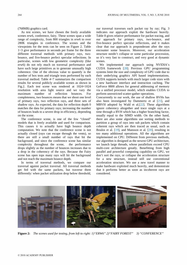
(768MB) graphics card. As test scenes, we have chosen the freely available
scenes erw6, conference, fairy. These scenes span a wide range of complexity, from 800 triangles in erw6 to over 280K triangles in conference. The scenes and the viewpoints for the tests can be seen on Figure 2. Table 1~3 give performance in seconds per frame for the three different traversal methods with primary rays, two- bounce, and five-bounce perfect specular reflections. In particular, scenes with low geometric complexity (like erw6) do not rely much on traversal performance and have such large primitives as to generate unusually high coherence. One of the obvious value to quantify is the number of box tests and triangle tests performed by each traversal method. Table 4~7 summarizes the comparison results for several publicly available scenes as shown in Fig.2. Each test scene was rendered at 1024×1024 resolution with area light source and we vary the maximum number of reflection bounces. For completeness, two bounces means that we shoot one level of primary rays, two reflection rays, and three sets of shadow rays. As expected, the data for reflection depth 0 matches the data for primary rays; increasing the number of bounces leads to a severe drop in efficiency, depending on the scene.
The conference scene, is one of the few “closed” models that is freely available and used for comparison. This causes it to actually have high bounce depth computation. We note that the conference scene is not actually closed (rays can escape through the vents), so there are still a small number of rays that hit the background, and since the conference scene has similar complexity throughout the scene, the performance drops slightly as the number of bounces increases due to a drop in the coherency of the rays. Because the Fairy scene has open tops many rays will hit the background and not reach the maximum bounce depth.
In terms of traversal methods, we compare our traversal against packet traversal. All traversal methods get fed with the same packets, but traverse them differently: when packet utilization drop below threshold,
our traversal traverses each packet ray by ray; Fig. 3 indicates our approach exploit the hardware heavily. Table 8 gives relative performance for packet tracing, and our approach for primary rays, two-bounce, and five-bounce perfect specular reflections, and it makes clear that our approach is preponderant after the rays encounter some bounces. Moreover, our acceleration structure needn’t collapse or some particular procession, so it’s very fast to construct, and very good at dynamic scenes.
We implemented our approach using NVIDIA’s CUDA framework [28]. Previous GPU programming systems limit the size and complexity of GPU code due to their underlying graphics API based implementations. CUDA supports kernels with much larger code sizes with a new hardware interface and instruction caching. The GeForce 8800 allows for general addressing of memory via a unified processor model, which enables CUDA to perform unrestricted scatter-gather operations. Concurrently to our work, the use of shallow BVHs has also been investigated by Dammertz et al [21], and MBVH adopted by Wald et al.[22]. These algorithms ignore coherency altogether and trace single rays at a time through a BVH which has a higher branching factor, usually equal to the SIMD width. On the other hand, there are also some algorithms use sorting methods to partition a group of rays into sub packets which contain coherent rays which are then traced as usual, such as Boulos et al. [19], and Mansson et al. [20], resulting in too many additional operations. All the algorithms are implemented on CPU. Different from previous methods, our algorithm is designed as the newest GPU architecture, we launch large threads, whose parallelism exceed CPU multi-core architecture greatly. Benefitting from high parallel and powerful computing capability on GPU, we don’t sort the rays, or collapse the acceleration structure for a new structure, instead still use conventional acceleration structure. We use a new travel manner to make hardware exploited much heavily, and demonstrate that it performs better as soon as incoherent rays are considered.
Figure 2: The scenes used for testing, from left to right: 1)“ERW6” 2)“FAIRY FOREST” 3) “CONFERENCE”
264 JOURNAL OF MULTIMEDIA, VOL. 5, NO. 3, JUNE 2010
© 2010 ACADEMY PUBLISHER
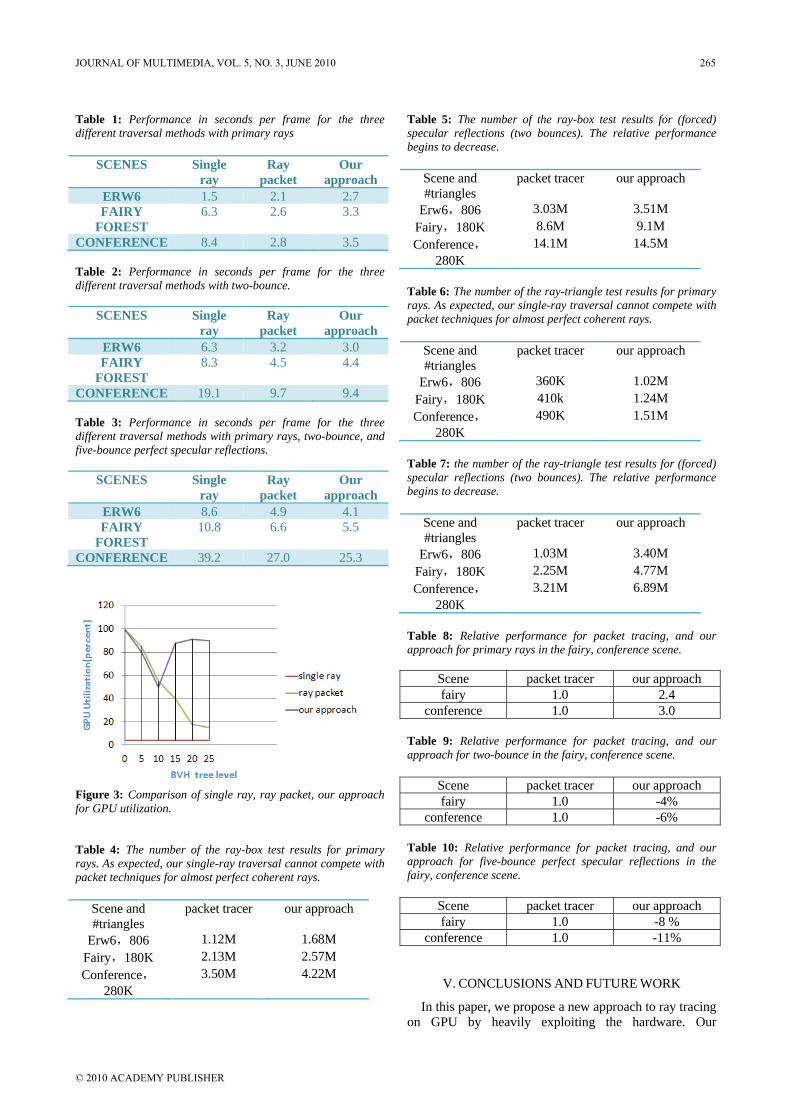
Table 1: Performance in seconds per frame for the three different traversal methods with primary rays
SCENES Single ray
Ray packet
Our approach
ERW6 1.5 2.1 2.7 FAIRY
FOREST 6.3 2.6 3.3
CONFERENCE 8.4 2.8 3.5 Table 2: Performance in seconds per frame for the three different traversal methods with two-bounce.
SCENES Single ray
Ray packet
Our approach
ERW6 6.3 3.2 3.0 FAIRY
FOREST 8.3 4.5 4.4
CONFERENCE 19.1 9.7 9.4 Table 3: Performance in seconds per frame for the three different traversal methods with primary rays, two-bounce, and five-bounce perfect specular reflections.
SCENES Single ray
Ray packet
Our approach
ERW6 8.6 4.9 4.1 FAIRY
FOREST 10.8 6.6 5.5
CONFERENCE 39.2 27.0 25.3
Figure 3: Comparison of single ray, ray packet, our approach for GPU utilization. Table 4: The number of the ray-box test results for primary rays. As expected, our single-ray traversal cannot compete with packet techniques for almost perfect coherent rays.
Scene and #triangles
packet tracer our approach
Erw6,806 1.12M 1.68M Fairy,180K 2.13M 2.57M Conference,
280K 3.50M 4.22M
Table 5: The number of the ray-box test results for (forced) specular reflections (two bounces). The relative performance begins to decrease.
Scene and #triangles
packet tracer our approach
Erw6,806 3.03M 3.51M Fairy,180K 8.6M 9.1M Conference,
280K 14.1M 14.5M
Table 6: The number of the ray-triangle test results for primary rays. As expected, our single-ray traversal cannot compete with packet techniques for almost perfect coherent rays.
Scene and #triangles
packet tracer our approach
Erw6,806 360K 1.02M Fairy,180K 410k 1.24M Conference,
280K 490K 1.51M
Table 7: the number of the ray-triangle test results for (forced) specular reflections (two bounces). The relative performance begins to decrease.
Scene and #triangles
packet tracer our approach
Erw6,806 1.03M 3.40M Fairy,180K 2.25M 4.77M Conference,
280K 3.21M 6.89M
Table 8: Relative performance for packet tracing, and our approach for primary rays in the fairy, conference scene.
Scene packet tracer our approach fairy 1.0 2.4
conference 1.0 3.0 Table 9: Relative performance for packet tracing, and our approach for two-bounce in the fairy, conference scene.
Scene packet tracer our approach fairy 1.0 -4%
conference 1.0 -6% Table 10: Relative performance for packet tracing, and our approach for five-bounce perfect specular reflections in the fairy, conference scene.
Scene packet tracer our approach fairy 1.0 -8 %
conference 1.0 -11%
V. CONCLUSIONS AND FUTURE WORK
In this paper, we propose a new approach to ray tracing on GPU by heavily exploiting the hardware. Our
JOURNAL OF MULTIMEDIA, VOL. 5, NO. 3, JUNE 2010 265
© 2010 ACADEMY PUBLISHER

approach is especially efficient for incoherent rays. In contrast to the common packets ray tracing, we propose a different data-parallel approach to ray tracing on GPU, in which individual ray intersect with k different nodes/triangles in the same operation. Besides, we add some additional information in the construction of acceleration structure, and propose a new approach to travel the acceleration structure. Despite this approach is slower for primary rays, but demonstrate that it performs better than those techniques as soon as incoherent rays are considered. Our acceleration structure needn’t collapse or some particular procession, and with significantly shallower trees, less nodes, and more triangles per leaf, our acceleration structure could be built very efficiently, which is promising for dynamic scenes.
Our approach is the newest and least optimized, leaving some room for improvement. It give an instructive try to design incoherent ray tracing on GPU, and opens a new design space that offers many interesting implementation alternatives. We believe that our work provides a compelling design for future ray-based graphics hardware. Though the existing numbers are promising, a lot still remains to be done. We also plan to explore our algorithm with increasing support for SIMD parallelism expected in new generations of commodity. We also believe the same techniques we have presented could be useful in adapting some aspects of general purpose programming on GPU.
ACKNOWLEDGEMENTS
The first author would like to thank T. David for his insightful discussion during the early stage of this work. Ren C. has provided help in implementation, and experimentation. Fairy scene provided by DAZ Productions via the Utah 3D Anim. Repo.. This research work has been partially supported by National Key Technology R&D Program in the 11th Five year Plan of China (2007BAH11B05).
REFERENCES [1] T. Whitted. 1980. An improved illumination model for
shaded display. Communications of the ACM, 23(6):343–349.
[2] NICKOLLS, J., BUCK, I., GARLAND, M., AND SKADRON, K. 2008. Scalable parallel programming with cuda.. ACM SIGGRAPH 2008 classes,, Queue 6, 2, 40–53.
[3] LINDHOLM, E., NICKOLLS, J., OBERMAN, S., AND MONTRYM, J. 2008. Nvidia tesla: A unified graphics and computing architecture. IEEE Micro 28, 2, 39–55.
[4] I.Wald, C. Benthin, M.Wagner, and P. Slusallek. 2001. Interactive rendering with coherent ray tracing. Computer Graphics Forum, 20(3):153–164.
[5] I. Wald, S. Boulos, and P. Shirley. 2007. Ray Tracing Deformable Scenes using Dynamic Bounding Volume Hierarchies. ACM Transactions on Graphics, 26(1):6:1–6:18.
[6] A. Reshetov. 2006. Omnidirectional ray tracing traversal algorithm for kdtrees. In Proceedings of the IEEE Symposium on Interactive Ray Tracing, pages 57–60.
[7] A.Reshetov. 2007. Faster Ray Packets-Triangle Intersection through Vertex Culling. Proceedings of the IEEE Symposium on Interactive Ray Tracing, pages 105–112.
[8] M. Pharr, C. Kolb, R. Gershbein, and P. Hanrahan. 1997. Rendering complex scenes with memory-coherent ray tracing. In Proceedings of SIGGRAPH, pages 101–108.
[9] HORN, D. R., SUGERMAN, J., HOUSTON, M., AND HANRAHAN, P. 2007. Interactive k-d tree GPU raytracing. In I3D ’07: Proceedings of the 2007 symposium on Interactive 3D graphics and games, 167–174.
[10] GÜNTHER, J., POPOV, S., SEIDEL, H.-P., AND SLUSALLEK, P. 2007. Realtime Ray Tracing on GPU with BVH-based Packet Traversal. In Proceedings of the IEEE/Eurographics Symposium on Interactive Ray Tracing 2007, 113˝U–118.
[11] ERICSON, C. 2004. Real-Time Collision Detection. Morgan Kaufmann. (book)
[12] GOVINDARAJU, N., KNOTT, D., JAIN, N., KABAL, I., TAMSTORF, R., GAYLE, R., LIN, M., AND MANOCHA, D. 2005. Collision detection between deformable models using chromatic decomposition. ACM Trans. on Graphics (Proc. of ACM SIGGRAPH) 24, 3, 991–999.
[13] CARR, N. A., HALL, J. D., AND HART, J. C. 2002. The Ray Engine. In HWWS ’02: Proceedings of the ACM SIGGRAPH/EUROGRAPHICS conference on Graphics hardware, Switzerland, 37–46.
[14] PURCELL, T. J., BUCK, I., MARK, W. R., AND HANRAHAN, P. 2002. Ray tracing on programmable graphics hardware. In SIGGRAPH ’02: Proceedings of the 29th annual conference on Computer graphics and interactive techniques, ACM Press, 703–712.
[15] FOLEY, T., AND SUGERMAN, J. 2005. KD-tree acceleration structures for a GPU raytracer. In HWWS ’05: Proceedings of the ACM SIGGRAPH/EUROGRAPHICS conference on Graphics hardware, ACM, 15–22.
[16] THRANE, N., AND SIMONSEN, L.-O. 2005. A comparison of acceleration struc-tures for GPU assisted ray tracing. Master’s thesis, University of Aarhus, Aarhus, Denmark.
[17] WALD, I., GRIBBLE, C. P., BOULOS, S., AND KENSLER, A. 2007. SIMD Ray Stream Tracing - SIMD Ray Traversal with Generalized Ray Packets and On-the-fly Re-Ordering. Tech. Rep. UUSCI-2007-012.
[18] OVERBECK, R., RAMAMOORTHI, R., AND MARK, W. R. 2008. Large Ray Packets for Real-time Whitted Ray Tracing. In IEEE/Eurographics Symposium on Interactive Ray Tracing 2008.
[19] S. Boulos, D. Edwards, J. D. Lacewell, J. Kniss, J. Kautz, I. Wald, and P. Shirley. 2007. Packet-based Whitted and distribution ray tracing. In Graphics Interface 2007, pages 177–184.
[20] E. Mansson, J. Munkberg, and T. Akenine-Moller. 2007. Deep coherent ray tracing. In 2007 IEEE Symposium on Interactive Ray Tracing, pages 79–85
[21] DAMMERTZ, H., HANIKA, J., AND KELLER, A. 2008. Shallow Bounding Volume Hierarchies for Fast SIMD Ray Tracing of Incoherent Rays. Rendering Techniques 2008, Proceedings of the Eurographics Symposium on Rendering, 2008.
[22] WALD, I., BENTHIN, C., AND BOULOS, S. 2008. Getting Rid of Packets: Efficient SIMD Single-Ray Traversal using Multibranching BVHs. IEEE/Eurographics Symposium on Interactive Ray Tracing 08.
[23] Shevtsov M., Soupikov A., Kapustin A. 2007.: Highly
266 JOURNAL OF MULTIMEDIA, VOL. 5, NO. 3, JUNE 2010
© 2010 ACADEMY PUBLISHER

Xin Yang, a PhD student in theComputer Science Department ofZhejiang University, in China. Hisresearch concentrates on real-timecomputer graphics and parallelcomputing.
parallel fast kd-tree construction for interactive ray tracing of dynamic scenes. In Computer Graphics Forum (Proc. Eurographics 2007), pp. 395–404.
[24] Wald I. 2007.: On fast construction of SAH based bounding volume hierarchies. In Proc. 2007 IEEE/EG Symposium on Interactive Ray Tracing , pp. 33–40.
[25] POPOV S., GÜNTHER J., SEIDEL H.-P., SLUSALLEK P. 2006.: Experiences with Streaming Construction of SAH KD-Trees. In Proceedings of the 2006 IEEE Symposium on Interactive Ray Tracing , pp. 89–94. 1, 3, 4, 6
[26] Wächter C., Keller A. 2006. : Instant ray tracing: The bounding interval hierarchy. In Rendering Techniques 2006 (Proc.17th Eurographics Symposium on Rendering) , pp. 139–149.
[27] J. Bigler, A. Stephens, and S. G. Parker. 2006. Design for parallel interactive ray tracing systems. In Proceedings of the IEEE Symposium on Interactive Ray Tracing, pages 187–195.
[28] NVIDIA: The CUDA Homepage. http://developer.nvidia.com/cuda. 1, 2, 3
JOURNAL OF MULTIMEDIA, VOL. 5, NO. 3, JUNE 2010 267
© 2010 ACADEMY PUBLISHER
A Novel Image Correlation Matching Approach
Baoming Shan College of Automation and Electronic Engineering
Qingdao University of Science and Technology Qingdao, 266042, shandong Province, China
Email:[email protected]
Abstract—In this paper we present a novel approach which is combined local invariant feature descriptor named ARPIH (Angular Radial Partitioning Intensity Histogram) with histogram-based similar distance (HSD). The approach succeeds the ARPIH descriptor’s distinctive advantage and provides higher robustness in deformation image matching, such as rotation image, illumination changing image and perspective image, etc. Based on the MCD algorithm, we present the HSD algorithm. This algorithm transforms the image matching into the histogram matching by calculating the number of the similar points between template histogram and target histogram in order to decrease the calculation complicacy and improve the matching efficiency. A large amount groups of images are used in testing the approach presented in this paper. The matching results presented here indicate that the presented algorithm is efficient to figure out both the geometric deformation image matching and the illumination changing image matching. Contrast with the traditional matching algorithm, the approach presented in this paper has the obvious advantage of high matching precision, robustness and performance efficiency. Index Terms—image matching; local invariant feature; ARPIH; HSD
I. INTRODUCTION
Image matching defines the process of finding out the same or similar image modes from the target image according to the known image template [1]. With the development of technology, image matching technique is very important in many applications including modern spaceflight, military affairs, medicine and industry in latter-day information processing. Because of variant imaging conditions such as illumination, visual angle, rotation and sensors, more requirements of image matching are raised. It is the emphasis of research that how to find out a quick matching method with higher robustness for image deformations.
The recent researches indicate that the local information of image is enough to describe the image and can be used for image matching to avoid more errors in image segmentation [2]. Lowe [3] takes local DOG extremum as interest point and presents a particular local invariant descriptor- SIFT (scale invariant feature transform) descriptor through calculating local image grads histogram. The descriptor has the characters of image scaling, rotation and affine invariant which makes it figure out the deformations matching, such as local
shelter, rotation and view point changing. It is proved to be distinctiveness and robustness. Reference [4] applies the SIFT descriptor to shaped fibers inspection, and built an automatic fiber recognition system. Schmid and Mohr [5] prove the local information is enough for image recognition. They take Harris corner as interest point and distill the rotation-invariant descriptor from its neighborhood area. This descriptor can ensure the correct matching of rotary image. Tuytelaars and Van Goal [6] construct a small affine invariant region at the corner and grayscale extremum. All the ways are common in searching for a specific structure of parallelogram, [3] and [5] are circumvolving and grayscale invariant, [6] is affine invariant. Lei Qin and Wen Gao [7] put forward a novel local invariant descriptor named angular radial partitioning intensity histogram (ARPIH), which describes images by a series of feature descriptors of grayscale and rotation-invariant. This method can solve the matching problems of geometric deformations and illumination changing, but it has some shortcomings of complex operation and long matching time. Xu Xiao-Ming and Yang Dan [8] presented a novel algorithm to design the descriptor of image feature points based on locality preserving projections (LPP). The proposed algorithm can preserve invariability on the geometric structure: the eigenvectors which are neighboring each other in the original space will maintain the same attribute in low-dimensional space; on the contrary, the dissimilar eigenvectors become apart farther each other. Therefore, the description generated by their algorithm can show the interrelationship between features and has strong robustness. But it has disadvantage of complexity in calculation.
Similarity measure which indicates using some measurement to confirm the similarity among the features to match normally takes use of some kind of cost functions or distance functions. The classical similarity measure includes correlation function and Minkowski Distance [9]. Recently people take Hausdorff Distance [10], mutual information [11] as matching measurement. Hausdorff Distance has the advantage of high sensitive to noise. And fractional Hausdorff Distance can process covered target and outliers, but it costs long time in computing. The mutual information-based method has been widely used in matching medical images because of its insensitive to illumination changing, but it also has the shortcoming of complex computation and the images must have wide overlap region. The performance of the traditional matching
268 JOURNAL OF MULTIMEDIA, VOL. 5, NO. 3, JUNE 2010
© 2010 ACADEMY PUBLISHERdoi:10.4304/jmm.5.3.268-275
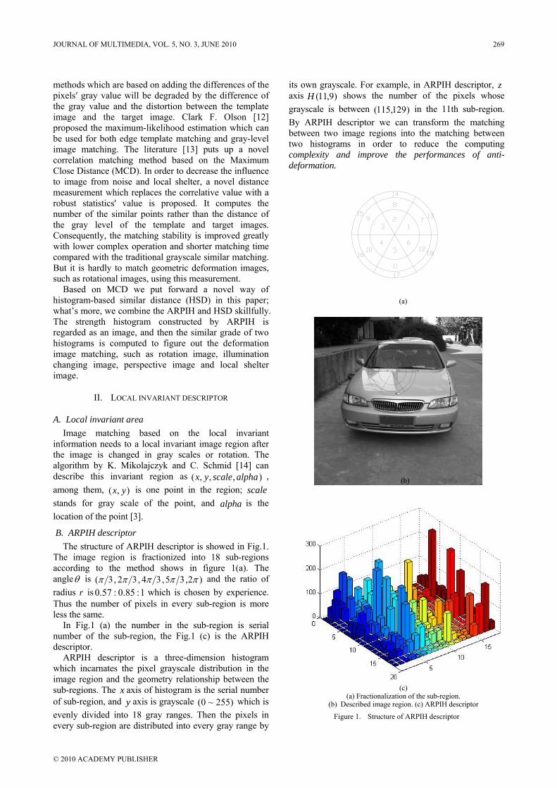
methods which are based on adding the differences of the pixels′ gray value will be degraded by the difference of the gray value and the distortion between the template image and the target image. Clark F. Olson [12] proposed the maximum-likelihood estimation which can be used for both edge template matching and gray-level image matching. The literature [13] puts up a novel correlation matching method based on the Maximum Close Distance (MCD). In order to decrease the influence to image from noise and local shelter, a novel distance measurement which replaces the correlative value with a robust statistics' value is proposed. It computes the number of the similar points rather than the distance of the gray level of the template and target images. Consequently, the matching stability is improved greatly with lower complex operation and shorter matching time compared with the traditional grayscale similar matching. But it is hardly to match geometric deformation images, such as rotational images, using this measurement.
Based on MCD we put forward a novel way of histogram-based similar distance (HSD) in this paper; what’s more, we combine the ARPIH and HSD skillfully. The strength histogram constructed by ARPIH is regarded as an image, and then the similar grade of two histograms is computed to figure out the deformation image matching, such as rotation image, illumination changing image, perspective image and local shelter image.
II. LOCAL INVARIANT DESCRIPTOR
A. Local invariant area Image matching based on the local invariant
information needs to a local invariant image region after the image is changed in gray scales or rotation. The algorithm by K. Mikolajczyk and C. Schmid [14] can describe this invariant region as , among them, is one point in the region; scale stands for gray scale of the point, and alpha is the location of the point [3].
),,,( alphascaleyx),( yx
B. ARPIH descriptor The structure of ARPIH descriptor is showed in Fig.1.
The image region is fractionized into 18 sub-regions according to the method shows in figure 1(a). The angleθ is )2,35,34,32,3( πππππ and the ratio of radius r is which is chosen by experience. Thus the number of pixels in every sub-region is more less the same.
1:85.0:57.0
In Fig.1 (a) the number in the sub-region is serial number of the sub-region, the Fig.1 (c) is the ARPIH descriptor.
ARPIH descriptor is a three-dimension histogram which incarnates the pixel grayscale distribution in the image region and the geometry relationship between the sub-regions. The x axis of histogram is the serial number of sub-region, and axis is grayscale which is evenly divided into 18 gray ranges. Then the pixels in every sub-region are distributed into every gray range by
its own grayscale. For example, in ARPIH descriptor, z axis shows the number of the pixels whose grayscale is between in the 11th sub-region. By ARPIH descriptor we can transform the matching between two image regions into the matching between two histograms in order to reduce the computing complexity and improve the performances of anti-deformation.
y )255~0(
)9,11(H)129,115(
(a)
(b)
(c)
(a) Fractionalization of the sub-region. (b) Described image region. (c) ARPIH descriptor
Figure 1. Structure of ARPIH descriptor
JOURNAL OF MULTIMEDIA, VOL. 5, NO. 3, JUNE 2010 269
© 2010 ACADEMY PUBLISHER
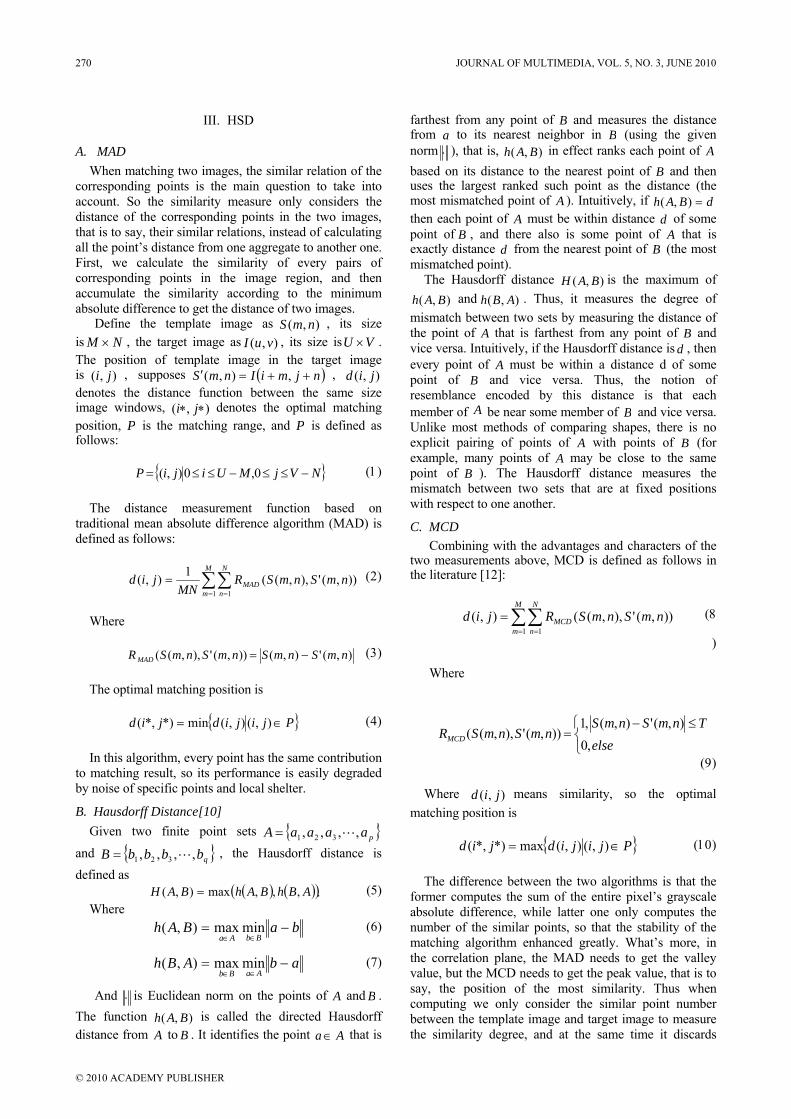
III. HSD
A. MAD When matching two images, the similar relation of the
corresponding points is the main question to take into account. So the similarity measure only considers the distance of the corresponding points in the two images, that is to say, their similar relations, instead of calculating all the point’s distance from one aggregate to another one. First, we calculate the similarity of every pairs of corresponding points in the image region, and then accumulate the similarity according to the minimum absolute difference to get the distance of two images.
Define the template image as , its size is , the target image as , its size is
),( nmSNM × ),( vuI VU × .
The position of template image in the target image is , supposes),( ji ( )njmiInmS ++=′ ,),( ),( jid, denotes the distance function between the same size image windows, denotes the optimal matching position,
),( ∗∗ jiP is the matching range, and P is defined as
follows:
NVjMUijiP −≤≤−≤≤= 0,0),( (1)
The distance measurement function based on traditional mean absolute difference algorithm (MAD) is defined as follows:
∑∑= =
=M
m
N
nMAD nmSnmSR
MNjid
1 1)),('),,((1),( (2)
Where
),('),()),('),,(( nmSnmSnmSnmSR MAD −= (3)
The optimal matching position is
Pjijidjid ∈= ),(),(min*)*,( (4)
In this algorithm, every point has the same contribution to matching result, so its performance is easily degraded by noise of specific points and local shelter.
B. Hausdorff Distance[10] Given two finite point sets paaaaA ,,,, 321 L=
and qbbbbB ,,,, 321 L= , the Hausdorff distance is defined as
( ) ( )( )ABhBAhBAH ,,,max),( = (5) Where
baBAhBbAa
−=∈∈
minmax),( (6)
abABhAaBb
−=∈∈
minmax),( (7)
And ⋅ is Euclidean norm on the points of A and B . The function is called the directed Hausdorff distance from A to
),( BAhB . It identifies the point a that is
farthest from any point of
A∈
B and measures the distance from to its nearest neighbor in a B (using the given norm ⋅ ), that is, in effect ranks each point of based on its distance to the nearest point of
),( BAh AB and then
uses the largest ranked such point as the distance (the most mismatched point of ). Intuitively, if A dBAh =),( then each point of A must be within distance d of some point of B , and there also is some point of A that is exactly distance d from the nearest point of B (the most mismatched point).
The Hausdorff distance is the maximum of and . Thus, it measures the degree of
mismatch between two sets by measuring the distance of the point of A that is farthest from any point of
),( BAH),( BAh ),( ABh
B and vice versa. Intuitively, if the Hausdorff distance is d , then every point of A must be within a distance d of some point of B and vice versa. Thus, the notion of resemblance encoded by this distance is that each member of be near some member of A B and vice versa. Unlike most methods of comparing shapes, there is no explicit pairing of points of A with points of B (for example, many points of A may be close to the same point of B ). The Hausdorff distance measures the mismatch between two sets that are at fixed positions with respect to one another.
C. MCD Combining with the advantages and characters of the
two measurements above, MCD is defined as follows in the literature [12]:
(8
)
∑∑= =
=M
m
N
nMCD nmSnmSRjid
1 1,('),,((),( ))
Where
⎩⎨⎧ ≤−
=else
TnmSnmSnmSnmSRMCD ,0
),('),(,1)),('),,((
(9)
Where means similarity, so the optimal matching position is
),( jid
Pjijidjid ∈= ),(),(max*)*,( (10)
The difference between the two algorithms is that the former computes the sum of the entire pixel’s grayscale absolute difference, while latter one only computes the number of the similar points, so that the stability of the matching algorithm enhanced greatly. What’s more, in the correlation plane, the MAD needs to get the valley value, but the MCD needs to get the peak value, that is to say, the position of the most similarity. Thus when computing we only consider the similar point number between the template image and target image to measure the similarity degree, and at the same time it discards
270 JOURNAL OF MULTIMEDIA, VOL. 5, NO. 3, JUNE 2010
© 2010 ACADEMY PUBLISHER
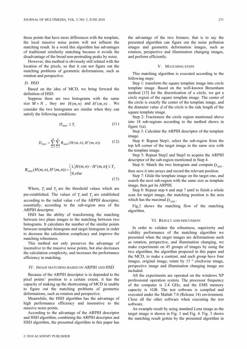
those points that have more differences with the template, the local massive noise points will not influent the matching result. In a word this algorithm has advantages of traditional similarity matching because it avoids the disadvantage of the broad non-protruding peaks by noise.
However, this method is obviously still related with the location of the pixels, so that it can not figure out the matching problems of geometric deformations, such as rotation and perspective.
D. HSD Based on the idea of MCD, we bring forward the
definition of HSD. Suppose there are two histograms with the same
size , they are and . We consider the two histograms are similar when they can satisfy the following conditions:
NM × ),( nmH ),( nmH ′
(11) 1TDHSD ≥
(12) ∑∑= =
=M
m
N
nHSDHSD nmHnmHRD
1 1
)),('),,((
⎩⎨⎧ ≤−
=else
TnmHnmHnmHnmHRHSD ,0
),('),(,1)),('),,(( 2
(13)
Where, and are the threshold values which are pre-established. The values of and are established according to the radial value
1T 2T
1T 2Tr of the ARPIH descriptor,
essentially, according to the sub-region area of the ARPIH descriptor.
HSD has the ability of transforming the matching between two plane images to the matching between two histograms. It calculates the number of the similar points between template histogram and target histogram in order to decrease the calculation complicacy and improve the matching robustness.
This method not only preserves the advantage of insensitive to the massive noise points, but also decreases the calculation complexity, and increases the performance efficiency in matching.
IV. IMAGE MATCHING BASED ON ARPIH AND HSD
Because of the ARPIH descriptor is in depended to the pixel points’ position to a certain extent, it has the capacity of making up the shortcoming of MCD in unable to figure out the matching problems of geometric deformations, such as rotation and perspective.
Meanwhile, the HSD algorithm has the advantage of high performance efficiency and insensitive to the massive noise points.
According to the advantage of the ARPIH descriptor and HSD algorithm, combining the ARPIH descriptor and HSD algorithm, the presented algorithm in this paper has
the advantage of the two formers, that is to say the presented algorithm can figure out the noise pollution images and geometric deformation images, such as rotation, perspective and illumination changing images, and perform efficiently.
V. MATCHING STEPS
This matching algorithm is executed according to the following steps:
Step 1: transform the square template image into circle template image. Based on the well-known Bresenham method [15] for the discretization of a circle, we get a circle region of the square template image. The center of the circle is exactly the center of the template image, and the diameter value of the circle is the side length of the square template image.
d
Step 2: Fractionize the circle region mentioned above into 18 sub-regions according to the method shows in figure 1(a).
Step 3: Calculate the ARPIH descriptor of the template image.
Step 4: Repeat Step1, select the sub-region from the top left corner of the target image in the same size with the template image.
Step 5: Repeat Step2 and Step3 to acquire the ARPIH descriptor of the sub-region mentioned in Step 4.
Step 6: Match the two histogram and compute HSDD , then save it into arrays and record the relevant position.
Step 7: Glide the template image on the target one, and search the next sub-region with the same size as template image, then get its ARPIH.
Step 8: Repeat step 6 and step 7 until to finish a whole scan for target image, the matching position is the area which has the maximal . HSDD
Fig.2 shows the matching flow of the matching algorithm.
VI. RESULT AND DISCUSSION
In order to validate the robustness, superiority and validity performance of the matching algorithm we presented when the target images are deformations such as rotation, perspective, and illumination changing, we make experiments on 45 groups of images by using the two algorithm, the algorithm proposed in this paper and the MCD, to make a contrast, and each group have four images, original image, rotate by 15 º clockwise image, perspective image and illumination changing image are included.
All the experiments are operated on the windows XP professional operation system. The processor frequency of the computer is 2.4 GHz, and the EMS memory capacity is 1GB. The test software is compiled and executed under the Matlab 7.0 (Release 14) environment. Close all the other software when executing the test software.
An example result by using standard Lena image as the target image is shown in Fig. 3 and Fig. 4. Fig. 3 shows the matching result gotten by the presented algorithm in
JOURNAL OF MULTIMEDIA, VOL. 5, NO. 3, JUNE 2010 271
© 2010 ACADEMY PUBLISHER
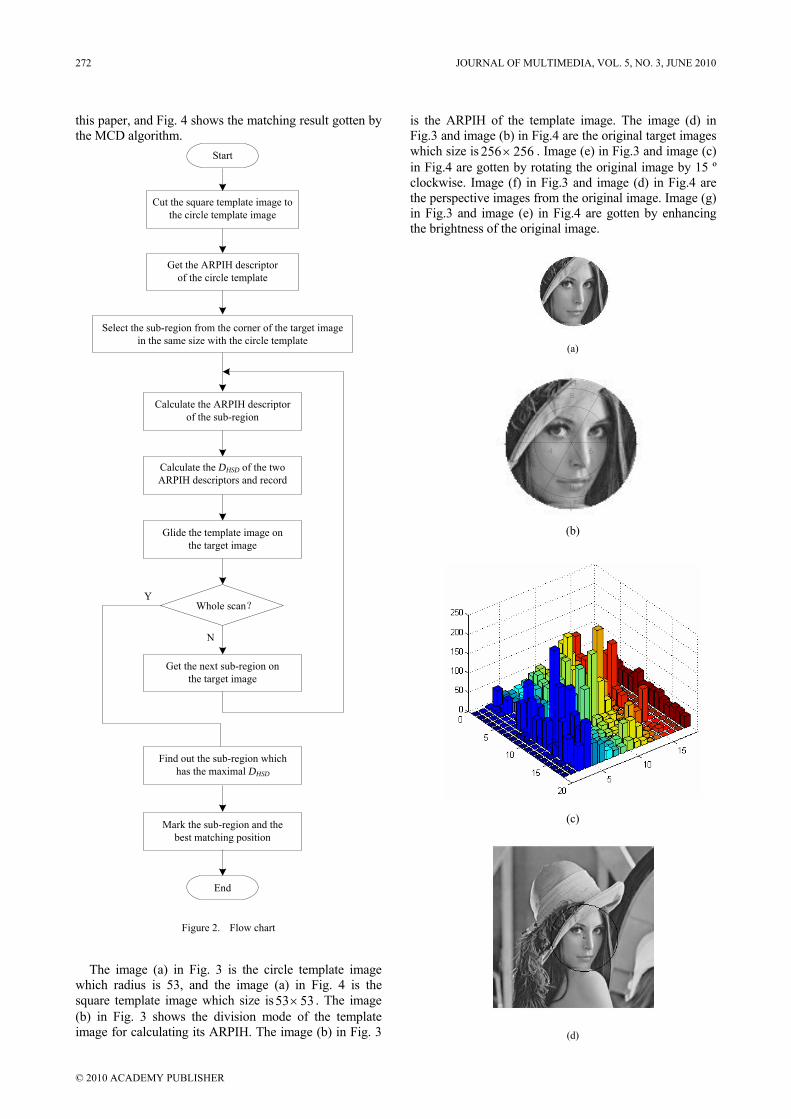
this paper, and Fig. 4 shows the matching result gotten by the MCD algorithm.
Cut the square template image to the circle template image
Get the ARPIH descriptor of the circle template
Calculate the ARPIH descriptor of the sub-region
Calculate the DHSD of the two ARPIH descriptors and record
Glide the template image on the target image
Mark the sub-region and the best matching position
Whole scan?
Find out the sub-region which has the maximal DHSD
End
Select the sub-region from the corner of the target image in the same size with the circle template
Get the next sub-region on the target image
Start
N
Y
Figure 2. Flow chart
The image (a) in Fig. 3 is the circle template image
which radius is 53, and the image (a) in Fig. 4 is the square template image which size is . The image (b) in Fig. 3 shows the division mode of the template image for calculating its ARPIH. The image (b) in Fig. 3
is the ARPIH of the template image. The image (d) in Fig.3 and image (b) in Fig.4 are the original target images which size is
5353×
256256 × . Image (e) in Fig.3 and image (c) in Fig.4 are gotten by rotating the original image by 15 º clockwise. Image (f) in Fig.3 and image (d) in Fig.4 are the perspective images from the original image. Image (g) in Fig.3 and image (e) in Fig.4 are gotten by enhancing the brightness of the original image.
(a)
(b)
(c)
(d)
272 JOURNAL OF MULTIMEDIA, VOL. 5, NO. 3, JUNE 2010
© 2010 ACADEMY PUBLISHER
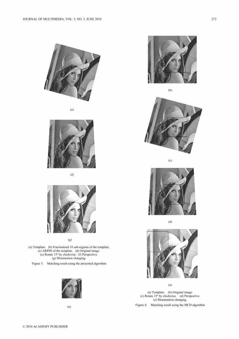
(e)
(f)
(g)
(a) Template. (b) Fractionized 18 sub-regions of the template. (c) ARPIH of the template. (d) Original image.
(e) Rotate 15º by clockwise. (f) Perspective. (g) Illumination changing.
Figure 3. Matching result using the presented algorithm
(a)
(b)
(c)
(d)
(e)
(a) Template. (b) Original image. (c) Rotate 15º by clockwise. (d) Perspective.
(e) Illumination changing.
Figure 4. Matching result using the MCD algorithm
JOURNAL OF MULTIMEDIA, VOL. 5, NO. 3, JUNE 2010 273
© 2010 ACADEMY PUBLISHER
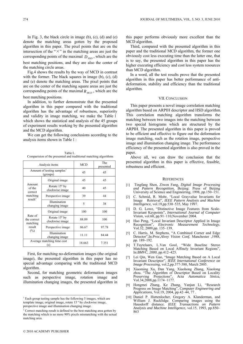
In Fig. 3, the black circle in image (b), (c), (d) and (e) denote the matching areas gotten by the proposed algorithm in this paper. The pixel points that are on the intersection of the “×” in the matching areas are just the corresponding points of the maximal , which are the best matching positions, and they are also the center of the matching circle areas.
HSDD
Fig.4 shows the results by the way of MCD in contrast with the former. The black squares in image (b), (c), (d) and (e) denote the matching areas. The pixel points that are on the center of the matching square areas are just the corresponding points of the maximal , which are the best matching positions.
MCDR
In addition, to further demonstrate that the presented algorithm in this paper compared with the traditional algorithm has the advantage of robustness, superiority and validity in image matching, we make the TableⅠ which shows the statistical and analysis of the 45 groups of experiment results working by the presented algorithm and the MCD algorithm.
We can get the following conclusions according to the analysis items shown in TableⅠ:
Table I. Comparision of the presented and traditional matching algorithms
Analysis items MCD The presented
Amount of testing samples1
(groups) 45 45
Original image 45 45
Rotate 15º by clockwise image 40 45
Perspective image 39 44
Amount of the correct
matching result2
Illumination changing image 5 38
Original image 100 100
Rotate 15º by clockwise image 88.89 100
Perspective image 86.67 97.78
Rate of the correct matching
result (%)
Illumination changing image 11.11 84.44
Average matching time cost (s) 18.663 7.351
First, for matching no-deformation images (the original
image), the presented algorithm in this paper has no special advantage comparing with the traditional MCD algorithm.
Second, for matching geometric deformation images such as perspective image, rotation image and illumination changing images, the presented algorithm in
1 Each group testing sample has the following 5 images, which are template image, original image, rotate 15 º by clockwise image, perspective image and illumination changing image. 2 Correct matching result is defined to the best matching area gotten by the matching which is no more 90% pixels mismatching with the actual matching area.
this paper performs obviously more excellent than the MCD algorithm.
Third, compared with the presented algorithm in this paper and the traditional MCD algorithm, the former one obviously cost less executing time than the latter one, that is to say, the presented algorithm in this paper has the higher executing efficiency and cost less system resources than MCD algorithm.
In a word, all the test results prove that the presented algorithm in this paper has better performance of anti-deformation, stability and efficiency than the traditional algorithm.
VII. CONCLUSION
This paper presents a novel image correlation matching algorithm based on ARPIH descriptor and HSD algorithm. This correlation matching algorithm transforms the matching between two images into the matching between two special histograms which are structured by the ARPIH. The presented algorithm in this paper is proved to be efficient and effective to figure out the deformation image matching, such as the rotation image, perspective image and illumination changing image. The performance efficiency of the presented algorithm is also proved in the paper.
Above all, we can draw the conclusion that the presented algorithm in this paper is effective, feasible, robustness and efficient.
REFERENCES [1] Tingfang Shen, Ziwen Fang, Digital Image Processing
and Pattern Recognition, Beijing: Press of Beijing University of Science and Engineering, 1998, pp.150–151.
[2] C. Schmid, R. Mohr, “Local Grayvalue Invariants for Image Retrieval”, IEEE Pattern Analysis and Machine Intelligence, vol.19,pp.530–535, May 1997.
[3] D. G. Lowe, “Distinctive Image Features from Scale-Invariant Keypoints”, International Journal of Computer Vision, vol.60, pp.91–110,November 2004.
[4] Hao Peng, “Local Invariant Descriptor Applied in Image Recognition”, Electronic Measurement Technolegy, Vol.32, 2009,pp. 135–139.
[5] C. Harris, M. Stephens, “A Combined Corner and Edge Detector”,In:Proc,Alvey Vision Conf, Manchester ,1988, pp. 189–192.
[6] T.Tuytelaars, L.Van Gool, “Wide Baseline Stereo Matching Based on Local Affinely Invariant Regions”, In:BMVC, 2000, pp.412–425.
[7] Lei Qin, Wen Gao, “Image Matching Based on A Local Invariant Descriptor”, IEEE International Conference on Image Processing, vol.2,pp.377-380, March 2005.
[8] Xiaoming Xu, Dan Yang, Xiaohong Zhang, Xiaolong zhou. “The Algorithm of Descriptor Based on Locality Preserving Projections”, Acta Automatica Sinica, Vol.34,2008,pp.1174–1177.
[9] Hongmei Zhang, Ke Zhang, Yanjun Li, “Research Progress on Image Matching”, Computer Engineering and Applications, Vol.19, 2004, pp.42–44, 77 .
[10] Daniel P. Huttenlocher, Gregory A. Klanderman, and William J. Rucklidge. Comparing images using the Hausdorff distance. IEEE Transactions on Pattern Analysis and Machine Intelligence, vol.15, 1993, pp.850–863
274 JOURNAL OF MULTIMEDIA, VOL. 5, NO. 3, JUNE 2010
© 2010 ACADEMY PUBLISHER
[11] Fookes C, Bennamoun M, The Use of Mutual Information for Rigid Medical Image Registration: A review, IEEE International Conference on Systems, Man and Cybemetics, 2002.
[12] Clark F. Olson, “Maximum-Likelihood Image Matching”, IEEE Transactions on Pattern Analysis and Machine Intelligence, vol.24, 2002, pp.853-857
[13] Guilin Zhang, Xianyi Ren Tianxu Zhang, Yuntao Liao, “Correlation tracking using a novel distance measurement as feedback”. Infrared and Laser Engineerin, vol.32, 2003,pp.624–629.
[14] K. Mikolajczyk, C. Schmid, Indexing Based on Scale Invariant Interest Points, In: ICCV,2001, pp.525–531.
[15] Andrew S. Glassner, Graphics Gems Academic Press Inc, 1995, pp.327–329.
Baoming Shan was born in 1974 in Dongying,China. He received the B.S. degree and M.S. degrees from Qingdao University of Science & Technology in 1996 and 1999,respectively. His research interest covers digital image processing and computer vision, adaptive control,intelligent control of industrial process.
JOURNAL OF MULTIMEDIA, VOL. 5, NO. 3, JUNE 2010 275
© 2010 ACADEMY PUBLISHER
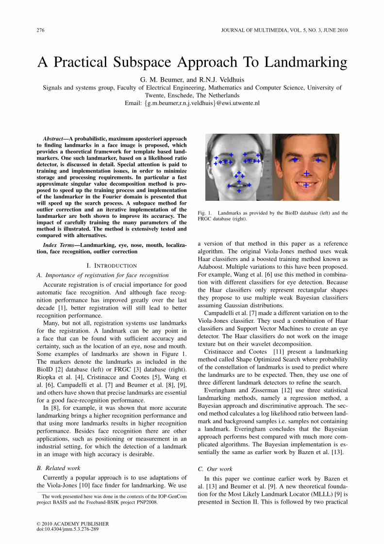
A Practical Subspace Approach To LandmarkingG. M. Beumer, and R.N.J. Veldhuis
Signals and systems group, Faculty of Electrical Engineering, Mathematics and Computer Science, University ofTwente, Enschede, The Netherlands
Email: g.m.beumer,[email protected]
Abstract—A probabilistic, maximum aposteriori approachto finding landmarks in a face image is proposed, whichprovides a theoretical framework for template based land-markers. One such landmarker, based on a likelihood ratiodetector, is discussed in detail. Special attention is paid totraining and implementation issues, in order to minimizestorage and processing requirements. In particular a fastapproximate singular value decomposition method is pro-posed to speed up the training process and implementationof the landmarker in the Fourier domain is presented thatwill speed up the search process. A subspace method foroutlier correction and an iterative implementation of thelandmarker are both shown to improve its accuracy. Theimpact of carefully training the many parameters of themethod is illustrated. The method is extensively tested andcompared with alternatives.
Index Terms—Landmarking, eye, nose, mouth, localiza-tion, face recognition, outlier correction
I. INTRODUCTION
A. Importance of registration for face recognitionAccurate registration is of crucial importance for good
automatic face recognition. And although face recog-nition performance has improved greatly over the lastdecade [1], better registration will still lead to betterrecognition performance.
Many, but not all, registration systems use landmarksfor the registration. A landmark can be any point ina face that can be found with sufficient accuracy andcertainty, such as the location of an eye, nose and mouth.Some examples of landmarks are shown in Figure 1.The markers denote the landmarks as included in theBioID [2] database (left) or FRGC [3] database (right).Riopka et al. [4], Cristinacce and Cootes [5], Wang etal. [6], Campadelli et al. [7] and Beumer et al. [8], [9],and others have shown that precise landmarks are essentialfor a good face-recognition performance.
In [8], for example, it was shown that more accuratelandmarking brings a higher recognition performance andthat using more landmarks results in higher recognitionperformance. Besides face recognition there are otherapplications, such as positioning or measurement in anindustrial setting, for which the detection of a landmarkin an image with high accuracy is desirable.
B. Related workCurrently a popular approach is to use adaptations of
the Viola-Jones [10] face finder for landmarking. We use
The work presented here was done in the contexts of the IOP-GenComproject BASIS and the Freeband-BSIK project PNP2008.
Fig. 1. Landmarks as provided by the BioID database (left) and theFRGC database (right).
a version of that method in this paper as a referencealgorithm. The original Viola-Jones method uses weakHaar classifiers and a boosted training method known asAdaboost. Multiple variations to this have been proposed.For example, Wang et al. [6] use this method in combina-tion with different classifiers for eye detection. Becausethe Haar classifiers only represent rectangular shapesthey propose to use multiple weak Bayesian classifiersassuming Gaussian distributions.
Campadelli et al. [7] made a different variation on to theViola-Jones classifier. They used a combination of Haarclassifiers and Support Vector Machines to create an eyedetector. The Haar classifiers do not work on the imagetexture but on their wavelet decomposition.
Cristinacce and Cootes [11] present a landmarkingmethod called Shape Optimized Search where probabilityof the constellation of landmarks is used to predict wherethe landmarks are to be expected. Then, they use one ofthree different landmark detectors to refine the search.
Everingham and Zisserman [12] use three statisticallandmarking methods, namely a regression method, aBayesian approach and discriminative approach. The sec-ond method calculates a log likelihood ratio between land-mark and background samples i.e. samples not containinga landmark. Everingham concludes that the Bayesianapproach performs best compared with much more com-plicated algorithms. The Bayesian implementation is es-sentially the same as earlier work by Bazen et al. [13].
C. Our work
In this paper we continue earlier work by Bazen etal. [13] and Beumer et al. [9]. A new theoretical founda-tion for the Most Likely Landmark Locator (MLLL) [9] ispresented in Section II. This is followed by two practical
276 JOURNAL OF MULTIMEDIA, VOL. 5, NO. 3, JUNE 2010
© 2010 ACADEMY PUBLISHERdoi:10.4304/jmm.5.3.276-289
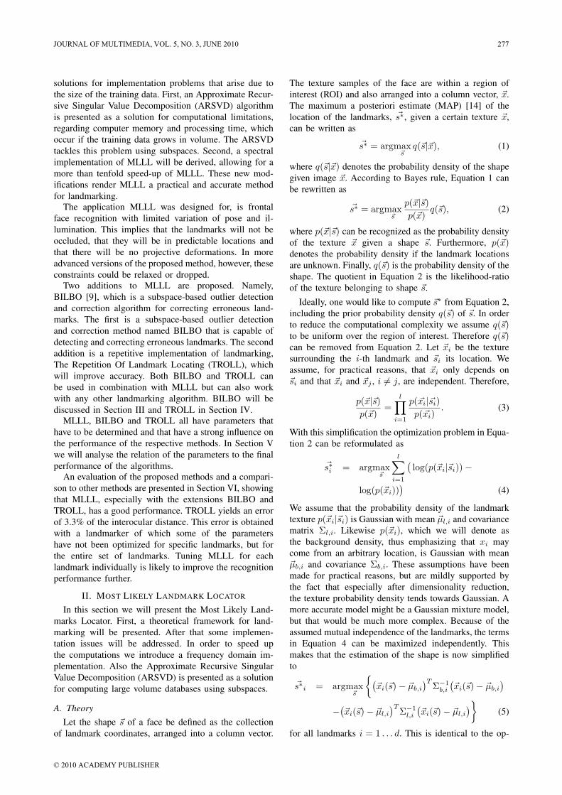
solutions for implementation problems that arise due tothe size of the training data. First, an Approximate Recur-sive Singular Value Decomposition (ARSVD) algorithmis presented as a solution for computational limitations,regarding computer memory and processing time, whichoccur if the training data grows in volume. The ARSVDtackles this problem using subspaces. Second, a spectralimplementation of MLLL will be derived, allowing for amore than tenfold speed-up of MLLL. These new mod-ifications render MLLL a practical and accurate methodfor landmarking.
The application MLLL was designed for, is frontalface recognition with limited variation of pose and il-lumination. This implies that the landmarks will not beoccluded, that they will be in predictable locations andthat there will be no projective deformations. In moreadvanced versions of the proposed method, however, theseconstraints could be relaxed or dropped.
Two additions to MLLL are proposed. Namely,BILBO [9], which is a subspace-based outlier detectionand correction algorithm for correcting erroneous land-marks. The first is a subspace-based outlier detectionand correction method named BILBO that is capable ofdetecting and correcting erroneous landmarks. The secondaddition is a repetitive implementation of landmarking,The Repetition Of Landmark Locating (TROLL), whichwill improve accuracy. Both BILBO and TROLL canbe used in combination with MLLL but can also workwith any other landmarking algorithm. BILBO will bediscussed in Section III and TROLL in Section IV.
MLLL, BILBO and TROLL all have parameters thathave to be determined and that have a strong influence onthe performance of the respective methods. In Section Vwe will analyse the relation of the parameters to the finalperformance of the algorithms.
An evaluation of the proposed methods and a compari-son to other methods are presented in Section VI, showingthat MLLL, especially with the extensions BILBO andTROLL, has a good performance. TROLL yields an errorof 3.3% of the interocular distance. This error is obtainedwith a landmarker of which some of the parametershave not been optimized for specific landmarks, but forthe entire set of landmarks. Tuning MLLL for eachlandmark individually is likely to improve the recognitionperformance further.
II. MOST LIKELY LANDMARK LOCATOR
In this section we will present the Most Likely Land-marks Locator. First, a theoretical framework for land-marking will be presented. After that some implemen-tation issues will be addressed. In order to speed upthe computations we introduce a frequency domain im-plementation. Also the Approximate Recursive SingularValue Decomposition (ARSVD) is presented as a solutionfor computing large volume databases using subspaces.
A. TheoryLet the shape ~s of a face be defined as the collection
of landmark coordinates, arranged into a column vector.
The texture samples of the face are within a region ofinterest (ROI) and also arranged into a column vector, ~x.The maximum a posteriori estimate (MAP) [14] of thelocation of the landmarks, ~s∗, given a certain texture ~x,can be written as
~s∗ = argmax~s
q(~s|~x), (1)
where q(~s|~x) denotes the probability density of the shapegiven image ~x. According to Bayes rule, Equation 1 canbe rewritten as
~s∗ = argmax~s
p(~x|~s)p(~x)
q(~s), (2)
where p(~x|~s) can be recognized as the probability densityof the texture ~x given a shape ~s. Furthermore, p(~x)denotes the probability density if the landmark locationsare unknown. Finally, q(~s) is the probability density of theshape. The quotient in Equation 2 is the likelihood-ratioof the texture belonging to shape ~s.
Ideally, one would like to compute ~s∗ from Equation 2,including the prior probability density q(~s) of ~s. In orderto reduce the computational complexity we assume q(~s)to be uniform over the region of interest. Therefore q(~s)can be removed from Equation 2. Let ~xi be the texturesurrounding the i-th landmark and ~si its location. Weassume, for practical reasons, that ~xi only depends on~si and that ~xi and ~xj , i 6= j, are independent. Therefore,
p(~x|~s)p(~x)
=l∏
i=1
p(~xi|~si)p(~xi)
. (3)
With this simplification the optimization problem in Equa-tion 2 can be reformulated as
~s∗i = argmax~s
l∑i=1
(log(p(~xi|~si))−
log(p(~xi)))
(4)
We assume that the probability density of the landmarktexture p(~xi|~si) is Gaussian with mean ~µl,i and covariancematrix Σl,i. Likewise p(~xi), which we will denote asthe background density, thus emphasizing that xi maycome from an arbitrary location, is Gaussian with mean~µb,i and covariance Σb,i. These assumptions have beenmade for practical reasons, but are mildly supported bythe fact that especially after dimensionality reduction,the texture probability density tends towards Gaussian. Amore accurate model might be a Gaussian mixture model,but that would be much more complex. Because of theassumed mutual independence of the landmarks, the termsin Equation 4 can be maximized independently. Thismakes that the estimation of the shape is now simplifiedto
~s∗i = argmax~s
(~xi(~s)− ~µb,i
)T Σ−1b,i
(~xi(~s)− ~µb,i
)−(~xi(~s)− ~µl,i
)T Σ−1l,i
(~xi(~s)− ~µl,i
)(5)
for all landmarks i = 1 . . . d. This is identical to the op-
JOURNAL OF MULTIMEDIA, VOL. 5, NO. 3, JUNE 2010 277
© 2010 ACADEMY PUBLISHER

timization criterion used in MLLL presented in previouswork [9]. Equation 5 is intuitively pleasing as each termof the summation benefits the similarity to a landmarkand penalizes the similarity to the background.
1) Dimensionality reduction: The covariance matrices,Σl and Σb in Equation 5, need to be estimated fromtraining data. Because landmark templates can be as largeas 96×64 = 6144 pixels, direct evaluation of Equation 5would be a too high a computational burden. Due to thelimited number of training samples available in practice,the estimates of the covariance matrices could be rank-deficient. Even if not, they would be too inaccurate toobtain a reliable inverse, which is needed in Equation 5.
Therefore, prior to the evaluation of Equation 5, thevector ~x will be projected onto a lower dimensionalsubspace. This subspace should have several properties.First of all, its basis should contain the significant modesof variation of the landmark data. Secondly, it should con-tain the significant modes of variation of the backgrounddata. Finally, it should contain the difference vectorbetween the landmark and the background means, for agood discrimination between landmark and backgrounddata. The modes of variation are found by principalcomponent analysis (PCA) on landmark and backgroundtraining data. After this first dimensionality reduction thelandmark and background densities are simultaneouslywhitened [15], such that the landmark covariance matrixbecomes a diagonal and the background covariance matrixan identity matrix in the reduced feature space. Thelatter whitening step is done for computational reasons.See Appendix A1 for details of the procedure of thedimensionality reduction.
The previous feature dimensionality reduction stepsaimed at creating a good representation of the landmarkand background data. In the next feature reduction stepwe want to select the features that have the highestdiscriminative power. In this feature selection step, afixed number of features are kept. The standard LinearDiscriminant Approach as proposed by Fisher [16] isnot applicable because the covariance matrices Σb,i andΣl,i are different. Instead, our approach is to keep thosefeatures for which the mean divided by their standarddeviation is maximal. Informal experiments in which thismethod was compared with alternatives have shown thatthis method gave the best results.
2) Feature extraction and classification: The total pro-cess of feature reduction and simultaneous whiteningcan be combined into one linear transformation by amatrix T ∈ Rm×n, with n the dimensionality of thetraining samples and m the final number of featuresafter reduction. The detailed calculation of the featurereduction transformation T is given in Appendix A withthe final result in Equation 32.
With T we project the means, covariance matrices andfeature vectors onto the subspace, ideally:
~µ′ldef= T~µl, ~µ′b
def= T~µb. (6)
Λldef= TΣlT
T , Ibdef= TΣbT
T . (7)
~y(~s) def= T~x(~s). (8)
where Λl is diagonal, Ib is identity, ~y(~s) is the featurevector and ~x(~s) denotes sample values from the ROI atlocation ~s. Please note that Σ and T are estimates obtainedfrom data and, therefore, not exact. Consequently, theresulting covariance matrices after the transformation areonly approximately diagonal. After this transformationEquation 5 becomes
~s∗ = argmax~s
(~y(~s)− ~µ′b
)T (~y(~s)− ~µ′b
)−(~y(~s)− ~µ′l
)T Λ−1l
(~y(~s)− ~µ′l
). (9)
Note that although Equation 9 resembles Equation 5, theresult will be different due to the dimensionality reduc-tion. Solving Equation 9 is, however, computationally farmore efficient than solving Equation 5.
1
1
T
~y(1,1)
ROI
s2
s1~x(1, 1)
~x(~s)
~y(~s)
Fig. 2. Feature extraction in the spatial domain. The pixel valuessurrounding the location of interest, ~x(~s) ∈ Rm are multiplied withT ∈ Rm×n. The resulting feature vector ~y(~s) ∈ Rn is of lowerdimensionality than ~x(~s).
B. Approximate Recursive Singular Value Decomposition
Training on large data sets should make MLLL ac-curate and robust. However, as the amount of train-ing data grows, the calculation of T quickly becomescomputationally prohibitive, either because of time or,more likely, memory constraints. Especially the SingularValue Decompositions (SVDs) in Equations 21 and 29in Appendix A1 are troublesome. In order to overcomethese problems an Approximate Recursive SVD (AR-SVD) algorithm is introduced. Proper application relieson two conditions. The first is that the estimates of thecovariance matrix improve when more data is processed.Second, the amount of explained variance kept in eachrecursion step must be sufficient. As the SVD is partof the feature reduction process, finally only a certainamount of the explained variance is to be kept andthe amount of variance kept by the ARSVD should behigher than that. If these two conditions are met, thereshould be no significant loss of information. ARSVD isfairly straightforward. Let X be a matrix with all featurevectors as columns, split up into a number of submatrices,called blocks, with a fixed number of columns, called theblocksize b:
X = [X1, X2 . . . Xo] (10)
Let Uj , Wj and Vj represent the ARSVD after j blocks,i.e.
[X1 . . . Xj ] ≈ UjWjVTj (11)
278 JOURNAL OF MULTIMEDIA, VOL. 5, NO. 3, JUNE 2010
© 2010 ACADEMY PUBLISHER
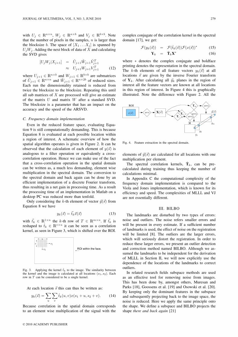
with Uj ∈ Rn×n, Wj ∈ Rn×b and Vj ∈ Rb×b. Notethat the number of pixels in the samples, n is larger thanthe blocksize b. The space of [X1 . . . Xj ] is spanned byUjWj . Adding the next block of data of X and calculatingthe SVD gives
[UjWj |Xj+1] = Uj+1Wj+1VTj+1
≈ Uj+1Wj+1VTj+1 (12)
where Uj+1 ∈ Rn×b and Wj+1 ∈ Rb×b are submatricesof Uj+1 ∈ Rn×n and Wj+1 ∈ Rn×2b of reduced sizes.Each run the dimensionality retained is reduced fromtwice the blocksize to the blocksize. Repeating this untilall sub matrices of X are processed will give an estimateof the matrix U and matrix W after a standard SVD.The blocksize is a parameter that has an impact on theaccuracy and the speed of the ARSVD.
C. Frequency domain implementationEven in the reduced feature space, evaluating Equa-
tion 9 is still computationally demanding. This is becauseEquation 8 is evaluated at each possible location withina region of interest. A schematic overview of how thespatial algorithm operates is given in Figure 2. It can beobserved that the calculation of each element of y(~s) isanalogous to a filter operation or equivalently a cross-correlation operation. Hence we can make use of the factthat a cross-correlation operation in the spatial domaincan be written as, a much less demanding, element wisemultiplication in the spectral domain. The conversion tothe spectral domain and back again can be done by anefficient implementation of a discrete Fourier transform,thus resulting in a net gain in processing time. As a resultthe processing time of an implementation in Matlab on adesktop PC was reduced more than tenfold.
Only considering the k-th element of vector ~y(~s) fromEquation 8 we have
yk(~s) = ~tk~x(~s) (13)
with ~tk ∈ R1×n the k-th row of T ∈ Rm×n. If ~tk isreshaped to tk ∈ Rv×u it can be seen as a correlationkernel, as seen in Figure 3, which is shifted over the ROI.
ROI within the face.
u
v s1
s2
Fig. 3. Applying the kernel tk to the image. The similarity betweenthe kernel and the image is calculated at all locations (s1, s2). Eachrow in T can be considered to be a single kernel.
At each location ~s this can thus be written as:
yk(~s) =∑
u
∑v
tk(u, v)x(s1 + u, s2 + v). (14)
Because correlation in the spatial domain correspondsto an element wise multiplication of the signal with the
complex conjugate of the correlation kernel in the spectraldomain [17], we get:
F(yk(~s)) = F(tk(~s))F(x(~s))∗ (15)Yk = TkX∗ (16)
where ∗ denotes the complex conjugate and boldfaceprinting denotes the representation in the spectral domain.The k-th elements of all feature vectors yk(~s) at alllocations ~s are given by the inverse Fourier transformof Yk. After calculating all ~yk planes in the region ofinterest all the feature vectors are known at all locationsin this region of interest. In Figure 4 this is graphicallyillustrated. Note the difference with Figure 2. All the
IDFFT2
ROI IDFFT2
DFFT2
IDFFT2
X(~s)
y1
x(~s) ~y(~s)
T1
ym
Tm
yk
Tk
Fig. 4. Feature extraction in the spectral domain.
elements of ~y(~s) are calculated for all locations with onemultiplication per element.
The spectral correlation kernels, Tk, can be pre-calculated during training thus keeping the number ofcalculations minimal.
In Appendix C the computational complexity of thefrequency domain implementation is compared to theViola and Jones implementation, which is known for itsefficiency and speed. The complexities of MLLL and VJare not essentially different.
III. BILBO
The landmarks are disturbed by two types of errors:noise and outliers. The noise refers smaller errors andwill be present in every estimate. If a sufficient numberof landmarks is used, the effect of noise on the registrationwill be limited [8]. The outliers are the larger errors,which will seriously distort the registration. In order toreduce these larger errors, we present an outlier detectionand correction method named BILBO. Although we as-sumed the landmarks to be independent for the derivationof MLLL in Section II, we will now explicitly use thedependence of the locations of the landmarks to correctoutliers.
In related research fields subspace methods are usedas an effective tool for removing noise from images.This has been done by, amongst others, Muresan andParks [18], Goossens et al. [19] and Osowski et al. [20].By keeping only the dominant features in the subspaceand subsequently projecting back to the image space, thenoise is reduced. Here we apply the same principle ontothe shape. We define a subspace and BILBO projects theshape there and back again [21]
JOURNAL OF MULTIMEDIA, VOL. 5, NO. 3, JUNE 2010 279
© 2010 ACADEMY PUBLISHER

A. Theory
Correct shapes are assumed to lie in a subspace ofR2d with d the number of landmarks. Incorrect shapes,containing one or more erroneous landmarks, are assumedto be outside this subspace. Consider a measured shape~s ′ that consists of a part ~s which fits the subspace Rn
with n < 2d and an error ~ε which cannot be representedin this subspace.
~s ′ = ~s+ ~ε (17)
Erroneous landmarks correspond to a pair of large ele-ments, εi, of ~ε. BILBO aims to find those landmarks andcorrect them. We can estimate the error on the measuredshape ~s ′ by
~ε = ~s ′ −(BBT (~s ′ − ~µs) + ~µs
)(18)
Large elements of ~ε indicates an outlier. If for a certainlandmark the error is above a threshold, τ , its location isreplaced with the location after projection.
~s ′i = ~si ∀i∣∣|~εi| > τ (19)
This procedure is repeated until convergence has beenreached, which is usually already after 1 iteration.
Training BILBO is done by finding the largest vari-ations for all normalized training shapes. Normalisedmeans that the shapes are aligned to a reference shape.The reference shape, which is the average shape when thefound face coordinates have been scaled between 0 and1. Our implementation is explained in Appendix B1.
Applying BILBO is schematically shown in Figure 5. Itshows how the error, ~ε, is calculated. The error is used todetermine which landmarks seem to be wrong and needto be corrected. This is done repetitively until all |~εi| arebelow the adaptive threshold τ . In Appendix B2 this willbe discussed in more detail.
Though simpler, BILBO shows a resemblance to theRansac algorithm [22] where also a distinction between”inliers” and ”outliers” is made.
update ~i~s = BBT~s ′ τ = rc1
d
∑di=1 |~εi|
~si′ = ~si ∀i
∣∣ |~εi| > τ
τ
reset ~i
Yes
No
r = r + 1
~s ′new
~s−µs +µs
δ
~ε~ε = ~s− ~s ′
~s ′new
~s ′new
~s ′
~s ′new
=~s ′?
~s ′new
Fig. 5. A schematic overview of BILBO. The vector ~i keeps trackof the landmarks to be updated. A detailed description can be found inAppendix B2.
IV. THE REPETITION OF LANDMARK LOCATING
The training images have been registered to a stan-dard scale and pose before extracting the transformationmatrix T and the parameters of Equation 9. Therefore,these do not fully model the orientation variations thatoccur in the images when landmarking. Because of this,
MLLL would perform best on registered faces. This is,of course, normally impossible as landmarking is one ofthe steps of registration. We therefore propose to iteratethe landmarking procedure. This procedure will be called:The Repetition Of Landmark Locating (TROLL). Oncelandmark candidates have been found, the image is reg-istered and the landmarking is repeated on the registeredimage. We use MLLL, in combination with BILBO asthe landmarking method, but other landmarking methodscould also be used iteratively in the same manner. Theprocessing time is linear with the number of iterations.We will choose the number of iteration such that furtheriterations yield no significant improvement.
V. TRAINING AND TUNING
In this section we will discuss the training and tuningof the parameters of MLLL, BILBO and TROLL. Theperformance of these algorithms has a strong relation tothe choice of the parameters.
First, we discuss the databases used in Section V-A.Second, this section will focus on tuning of the variousparameters and their influence on the algorithms. Anoverview of these parameters and their final values isgiven in Table I. Repeatedly one parameter was optimizedwhile all others were kept fixed until a stable solution wasreached. We present only the results of the final parametersettings.
In order to evaluate the performance of the meth-ods used we used the same error measure as Cristi-nacce [23]. The error measure, me is the mean euclideandistance between the landmarks and the manually labelledgroundtruth coordinates as a percentage of the interoculardistance ∆ocl.
me =1
n∆ocl
n∑i=1
√δ2i,x + δ2i,y (20)
All results in this section are obtained by landmarkingimages in the training set. The final results obtained withthe fully tuned algorithm on the testing sets are given inSection VI.
Sometimes the full parameter space was not exploredbut only the part where an optimum could be expectedbecause exploration of the full parameter space is notfeasible due to time constraints. Although the authorsmade an effort in finding a good solution it may, therefore,be a local optimum.
A. Databases usedWe used two databases from which we drew several
datasets for the experiments. Both the FRGC 2.0 [3]and the BioID [2] are publicly available. For testingwe only used images in which the face was found byan unsupervised face finder, in this case the Viola andJones [24] classifier from the OpenCV library with the”frontalface alt2” cascade [25].
The BioID database consists of 1521 images, takenfrom 22 persons, which vary in pose, scale and illumina-tion conditions, but which are mainly frontal. All images
280 JOURNAL OF MULTIMEDIA, VOL. 5, NO. 3, JUNE 2010
© 2010 ACADEMY PUBLISHER

TABLE IOVERVIEW OF THE TUNING PARAMETERS AND CHOSEN VALUES.
Parameter final valueMLLL
Face size 384 [px]Template size Nose (n = v × u) 48x64 [px]Template size Eye (n = v × u) 64x96 [px]Template size Mouth (n = v × u) 64x96 [px]Relative distance to the landmark 25 [%]ARSVD blocksize (b) 500Number of features (m) 219Explained variance Landmark 81 [%]Explained variance Background 100 [%]Explained variance Total 98 [%]
BILBOMaximum number of iterations (r) 3Minimal threshold (τmin) 0.055Error weight (c) 1.15Number of features in subspace 1
TROLLNumber of repetitions 3
have been landmarked manually. The Viola-Jones facedetector found a face in 1459 of the images (95.9%).
In total, the FRGC 2.0 database contains 39328 images,roughly one third of which are low quality images (LQ)and two third are high quality images (HQ). The FRGC2.0 comes with hand labelled ground truth locations forfour landmarks: the eyes, nose and mouth. We split theFRGC into a training set and a testing set: a training setcontaining 19674 images with subject ID number 4519 orlower and a testing set containing 19427 (98.8%) foundfaces in the 19654 images with subject ID numbers 4520or higher. Both sets contain images from HQ and LQ.
B. Tuning MLLL
The MLLL has many parameters to tune. In Table I anoverview of these parameters is given. For all parameterswe started with an educated guess. Repetitively oneparameter was optimized while the others were kept fixed.This was done until for all parameters a final setting wasfound, based on the landmarking performance in terms ofeither speed of accuracy.
It was possible, by reusing intermediate results, to keepthe training of the algorithm sufficiently fast. Testing thealgorithm was however slow because it had to be redonefor each new parameter choice. In order to limit the tuningtime, the parameters were tuned by landmarking the first2000 images of the FRGC training set. This limitationimplies the risk of overtraining on the first 2000 images ofthe training set. Verification on the larger dataset showedthat this did not happen. Finally, after all parameters havebeen optimized the error measure, me calculated over thefirst 2000 images of the FRGC training set is 4.06 andover the full set it is 3.89. The fact that over the full set theerror is lower suggests that there has been no significantovertraining in the tuning of the parameters.
1) Image size and landmark region of interest size:Since larger images imply larger areas to scan, the pre-determined upper bound was an image size of 384× 384
pixels. Experiments showed that smaller images resultedin larger errors. Therefore, the image size was set to384× 384. Note that for computational reasons we chosenot to use images larger than 384 × 384. Improvementmight be possible here.
Experiments with the template sizes showed that land-scape shaped templates yielded lower errors than squareor portrait shaped templates. For the eyes a template sizeof 64× 96 gave best results. For the nose and the mouththe maximum performance was reached with templates of48× 64.
2) Selection of landmark and background trainingsamples: In order to create a good separation betweenthe landmark samples and the background samples, thebackground training samples should not include landmarktemplates. In Figure 6 we illustrate how the centre ofthe background training sample must have a minimaldistance to the centre of the landmark. The minimaldistance is relative to the width and height of the image,resulting in elliptical regions from which the centres ofthe background samples are taken. Experiments showedthat a distance larger than 0.2 gave significantly betterresults than smaller distances. To be on the safe sidethis parameter was set to 0.25. The ellipse denotingthe maximum distance had the same radius as half thetemplate size, resulting in an elliptical doughnut wherethe centres of the background training samples are takenfrom.
Fig. 6. Training sample selection. The landmark training sampleis a rectangular region around the landmark, denoted with the solidrectangle and cross. Within this region a subregion is defined. Thiselliptic doughnut shaped area is the region where the centres of thebackground training samples, denoted by the pluses, are chosen from.Three examples are given as rectangles with a dashed border.
3) Block size: The block size in the ARSVD algorithmmust be large enough to capture all the variation. It turnedout that it is not a parameter with a very large influenceon the final result as long as it is larger than 300. To be onthe safe side we chose 500, as illustrated in Figure 7. Forthe HQ smaller block sizes would be allowed than for theLQ. In Table II the amount of kept variance for a blocksize is given for both Landmark and Background samples.In Figure 8 the amount of kept variance is illustrated for ablocksize of 500. It shows clearly that each time a block isadded the variance within the blocks is modelled better.Finally near 100% of the variance in the new block isalready modelled by the data.
4) Dimensionality reduction: MLLL has four param-eters that determine the dimensionality reduction of the
JOURNAL OF MULTIMEDIA, VOL. 5, NO. 3, JUNE 2010 281
© 2010 ACADEMY PUBLISHER
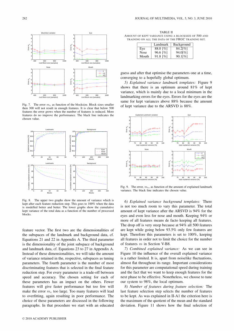
400 600 800 10002
3
4
5
6
7
8
9BlockSize variation
Err
or m
e
rsvd Block size [samples]400 600 800 1000
2
3
4
5
6
7
8
9Eye
Err
or m
e
rsvd Block size [samples]
400 600 800 10002
3
4
5
6
7
8
9Nose
Err
or m
e
rsvd Block size [samples]400 600 800 1000
2
3
4
5
6
7
8
9Mouth
Err
or m
e
rsvd Block size [samples]
CLQHQ
Fig. 7. The error me as function of the blocksize. Block sizes smallerthen 300 will not result in enough features. It is clear that below 500features the error grows when the number of features is reduced. Morefeatures do no improve the performance. The black line indicates thechosen value.
0 20 40 60 8099
99.2
99.4
99.6
99.8
100Landmarks
Exp
lain
ed v
aria
nce
[%]
Blocks0 100 200 300 400
99
99.2
99.4
99.6
99.8
100Background
Exp
lain
ed v
aria
nce
[%]
Blocks
EyesNoseMouth
0 20 40 60 8080
85
90
95
100Landmarks
Cum
ulat
ive
expl
aine
d va
rianc
e [%
]
Blocks0 100 200 300 400
80
85
90
95
100Background
Cum
ulat
ive
expl
aine
d va
rianc
e [%
]
Blocks
Fig. 8. The upper two graphs show the amount of variance which iskept after each feature reduction step. This goes to 100% when the datais modelled better and better. The lower graphs show the cumulativekept variance of the total data as a function of the number of processedblocks.
feature vector. The first two are the dimensionalities ofthe subspaces of the landmark and background data, cf.Equations 21 and 22 in Appendix A. The third parameteris the dimensionality of the joint subspace of backgroundand landmark data, cf. Equations 23 to 27 in Appendix A.Instead of these dimensionalities, we will take the amountof variance retained in the, respective, subspaces as tuningparameters. The fourth parameter is the number of mostdiscriminating features that is selected in the final featurereduction step. For every parameter is a trade-off betweenspeed and accuracy. The chosen setting for each ofthese parameters has an impact on the others. Fewerfeatures will give faster performance but too few willmake the error me too large. Too many features will leadto overfitting, again resulting in poor performance. Thechoice of these parameters are discussed in the followingparagraphs. In that procedure we start with an educated
TABLE IIAMOUNT OF KEPT VARIANCE USING A BLOCKSIZE OF 500 AND
TRAINING ON ALL THE DATA OF THE FRGC TRAINING SET.
Landmark BackgroundEye 88.0 [%] 84.2[%]Nose 96.6 [%] 94.0[%]Mouth 91.8 [%] 90.1[%]
guess and after that optimise the parameters one at a time,converging to a hopefully global optimum.
5) Explained variance landmark templates: Figure 9shows that there is an optimum around 81% of keptvariance, which is mainly due to a local minimum in thelandmarking errors for the eyes. Errors for the eyes are thesame for kept variances above 88% because the amountof kept variance due to the ARSVD is 88%.
75 80 85 90 95 1002
3
4
5
6
7
8
9Explained Landmark variation
Err
or m
e
kept explained variance [%]75 80 85 90 95 100
2
3
4
5
6
7
8
9Eye
Err
or m
e
kept explained variance [%]
75 80 85 90 95 1002
3
4
5
6
7
8
9Nose
Err
or m
e
kept explained variance [%]75 80 85 90 95 100
2
3
4
5
6
7
8
9Mouth
Err
or m
e
kept explained variance [%]
CLQHQ
Fig. 9. The error, me, as function of the amount of explained landmarkvariance. The black line indicates the chosen value.
6) Explained variance background templates: Thereis not too much room to vary this parameter. The totalamount of kept variance after the ARSVD is 94% for theeyes and even less for nose and mouth. Keeping 94% ormore of all features means de facto keeping all features.The drop off is very steep because at 94% all 500 featuresare kept while going below 93.5% only few features arekept. Therefore this parameters is set to 100%, keepingall features in order not to limit the choice for the numberof features m in Section V-B8.
7) Combined explained variance: As we can see inFigure 10 the influence of the overall explained varianceis a rather limited. It is, apart from noiselike fluctuations,almost flat throughout its range. Important considerationsfor this parameter are computational speed during trainingand the fact that we want to keep enough features for thenext phase to be effective. Nonetheless, we choose to tuneour system to 98%, the local optimum.
8) Number of features during feature selection: Thelast feature selection step selects the number of featuresto be kept. As was explained in II-A1 the criterion here isthe maximum of the quotient of the mean and the standarddeviation. Figure 11 shows how the final selection of
282 JOURNAL OF MULTIMEDIA, VOL. 5, NO. 3, JUNE 2010
© 2010 ACADEMY PUBLISHER
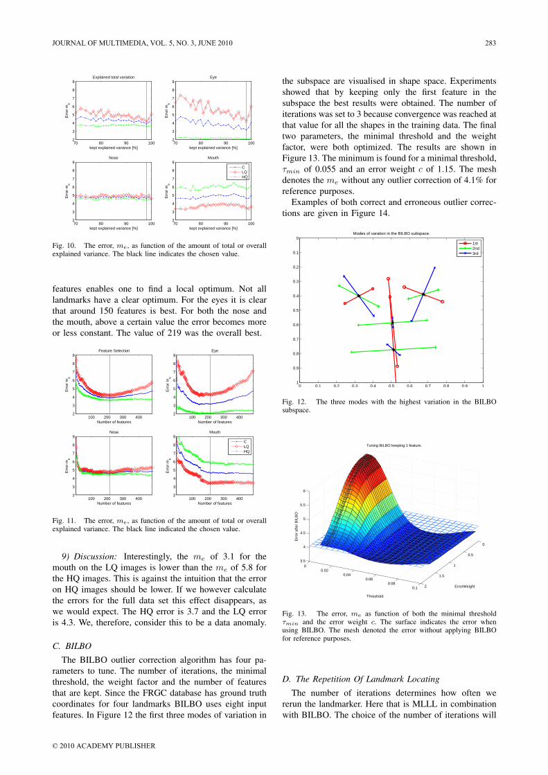
70 80 90 1002
3
4
5
6
7
8
9Explained total variation
Err
or m
e
kept explained variance [%]70 80 90 100
2
3
4
5
6
7
8
9Eye
Err
or m
e
kept explained variance [%]
70 80 90 1002
3
4
5
6
7
8
9Nose
Err
or m
e
kept explained variance [%]70 80 90 100
2
3
4
5
6
7
8
9Mouth
Err
or m
e
kept explained variance [%]
CLQHQ
Fig. 10. The error, me, as function of the amount of total or overallexplained variance. The black line indicates the chosen value.
features enables one to find a local optimum. Not alllandmarks have a clear optimum. For the eyes it is clearthat around 150 features is best. For both the nose andthe mouth, above a certain value the error becomes moreor less constant. The value of 219 was the overall best.
100 200 300 4002
3
4
5
6
7
8
9Feature Selection
Err
or m
e
Number of features100 200 300 400
2
3
4
5
6
7
8
9Eye
Err
or m
e
Number of features
100 200 300 4002
3
4
5
6
7
8
9Nose
Err
or m
e
Number of features100 200 300 400
2
3
4
5
6
7
8
9Mouth
Err
or m
e
Number of features
CLQHQ
Fig. 11. The error, me, as function of the amount of total or overallexplained variance. The black line indicated the chosen value.
9) Discussion: Interestingly, the me of 3.1 for themouth on the LQ images is lower than the me of 5.8 forthe HQ images. This is against the intuition that the erroron HQ images should be lower. If we however calculatethe errors for the full data set this effect disappears, aswe would expect. The HQ error is 3.7 and the LQ erroris 4.3. We, therefore, consider this to be a data anomaly.
C. BILBO
The BILBO outlier correction algorithm has four pa-rameters to tune. The number of iterations, the minimalthreshold, the weight factor and the number of featuresthat are kept. Since the FRGC database has ground truthcoordinates for four landmarks BILBO uses eight inputfeatures. In Figure 12 the first three modes of variation in
the subspace are visualised in shape space. Experimentsshowed that by keeping only the first feature in thesubspace the best results were obtained. The number ofiterations was set to 3 because convergence was reached atthat value for all the shapes in the training data. The finaltwo parameters, the minimal threshold and the weightfactor, were both optimized. The results are shown inFigure 13. The minimum is found for a minimal threshold,τmin of 0.055 and an error weight c of 1.15. The meshdenotes the me without any outlier correction of 4.1% forreference purposes.
Examples of both correct and erroneous outlier correc-tions are given in Figure 14.
0 0.1 0.2 0.3 0.4 0.5 0.6 0.7 0.8 0.9 1
0
0.1
0.2
0.3
0.4
0.5
0.6
0.7
0.8
0.9
1
Modes of varation in the BILBO subspace.
1st2nd3rd
Fig. 12. The three modes with the highest variation in the BILBOsubspace.
0
0.5
1
1.5
2
00.02
0.040.06
0.080.1
3.5
4
4.5
5
5.5
6
ErrorWeight
Tuning BILBO keeping 1 feature.
Threshold
Err
or a
fter
BIL
BO
Fig. 13. The error, me as function of both the minimal thresholdτmin and the error weight c. The surface indicates the error whenusing BILBO. The mesh denoted the error without applying BILBOfor reference purposes.
D. The Repetition Of Landmark Locating
The number of iterations determines how often wererun the landmarker. Here that is MLLL in combinationwith BILBO. The choice of the number of iterations will
JOURNAL OF MULTIMEDIA, VOL. 5, NO. 3, JUNE 2010 283
© 2010 ACADEMY PUBLISHER
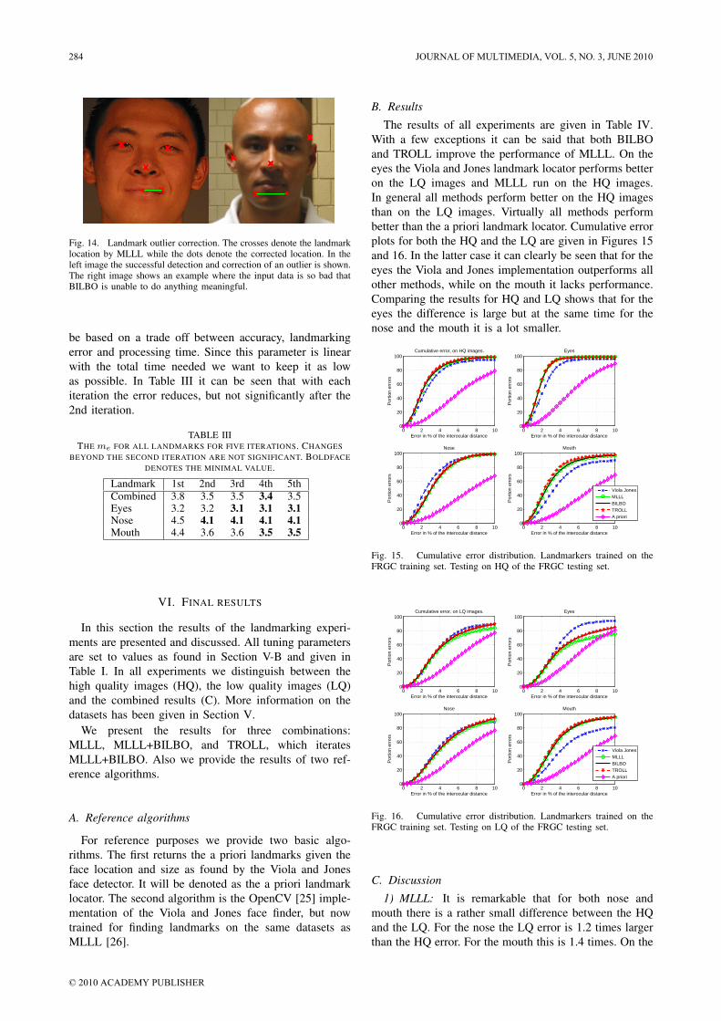
Fig. 14. Landmark outlier correction. The crosses denote the landmarklocation by MLLL while the dots denote the corrected location. In theleft image the successful detection and correction of an outlier is shown.The right image shows an example where the input data is so bad thatBILBO is unable to do anything meaningful.
be based on a trade off between accuracy, landmarkingerror and processing time. Since this parameter is linearwith the total time needed we want to keep it as lowas possible. In Table III it can be seen that with eachiteration the error reduces, but not significantly after the2nd iteration.
TABLE IIITHE me FOR ALL LANDMARKS FOR FIVE ITERATIONS. CHANGES
BEYOND THE SECOND ITERATION ARE NOT SIGNIFICANT. BOLDFACEDENOTES THE MINIMAL VALUE.
Landmark 1st 2nd 3rd 4th 5thCombined 3.8 3.5 3.5 3.4 3.5Eyes 3.2 3.2 3.1 3.1 3.1Nose 4.5 4.1 4.1 4.1 4.1Mouth 4.4 3.6 3.6 3.5 3.5
VI. FINAL RESULTS
In this section the results of the landmarking experi-ments are presented and discussed. All tuning parametersare set to values as found in Section V-B and given inTable I. In all experiments we distinguish between thehigh quality images (HQ), the low quality images (LQ)and the combined results (C). More information on thedatasets has been given in Section V.
We present the results for three combinations:MLLL, MLLL+BILBO, and TROLL, which iteratesMLLL+BILBO. Also we provide the results of two ref-erence algorithms.
A. Reference algorithms
For reference purposes we provide two basic algo-rithms. The first returns the a priori landmarks given theface location and size as found by the Viola and Jonesface detector. It will be denoted as the a priori landmarklocator. The second algorithm is the OpenCV [25] imple-mentation of the Viola and Jones face finder, but nowtrained for finding landmarks on the same datasets asMLLL [26].
B. Results
The results of all experiments are given in Table IV.With a few exceptions it can be said that both BILBOand TROLL improve the performance of MLLL. On theeyes the Viola and Jones landmark locator performs betteron the LQ images and MLLL run on the HQ images.In general all methods perform better on the HQ imagesthan on the LQ images. Virtually all methods performbetter than the a priori landmark locator. Cumulative errorplots for both the HQ and the LQ are given in Figures 15and 16. In the latter case it can clearly be seen that for theeyes the Viola and Jones implementation outperforms allother methods, while on the mouth it lacks performance.Comparing the results for HQ and LQ shows that for theeyes the difference is large but at the same time for thenose and the mouth it is a lot smaller.
0 2 4 6 8 100
20
40
60
80
100
Por
tion
erro
rs
Error in % of the interocular distance
Cumulative error, on HQ images.
0 2 4 6 8 100
20
40
60
80
100
Por
tion
erro
rs
Error in % of the interocular distance
Eyes
0 2 4 6 8 100
20
40
60
80
100
Por
tion
erro
rs
Error in % of the interocular distance
Nose
0 2 4 6 8 100
20
40
60
80
100
Por
tion
erro
rs
Error in % of the interocular distance
Mouth
Viola JonesMLLLBILBOTROLLA priori
Fig. 15. Cumulative error distribution. Landmarkers trained on theFRGC training set. Testing on HQ of the FRGC testing set.
0 2 4 6 8 100
20
40
60
80
100
Por
tion
erro
rs
Error in % of the interocular distance
Cumulative error, on LQ images.
0 2 4 6 8 100
20
40
60
80
100
Por
tion
erro
rs
Error in % of the interocular distance
Eyes
0 2 4 6 8 100
20
40
60
80
100
Por
tion
erro
rs
Error in % of the interocular distance
Nose
0 2 4 6 8 100
20
40
60
80
100
Por
tion
erro
rs
Error in % of the interocular distance
Mouth
Viola JonesMLLLBILBOTROLLA priori
Fig. 16. Cumulative error distribution. Landmarkers trained on theFRGC training set. Testing on LQ of the FRGC testing set.
C. Discussion
1) MLLL: It is remarkable that for both nose andmouth there is a rather small difference between the HQand the LQ. For the nose the LQ error is 1.2 times largerthan the HQ error. For the mouth this is 1.4 times. On the
284 JOURNAL OF MULTIMEDIA, VOL. 5, NO. 3, JUNE 2010
© 2010 ACADEMY PUBLISHER
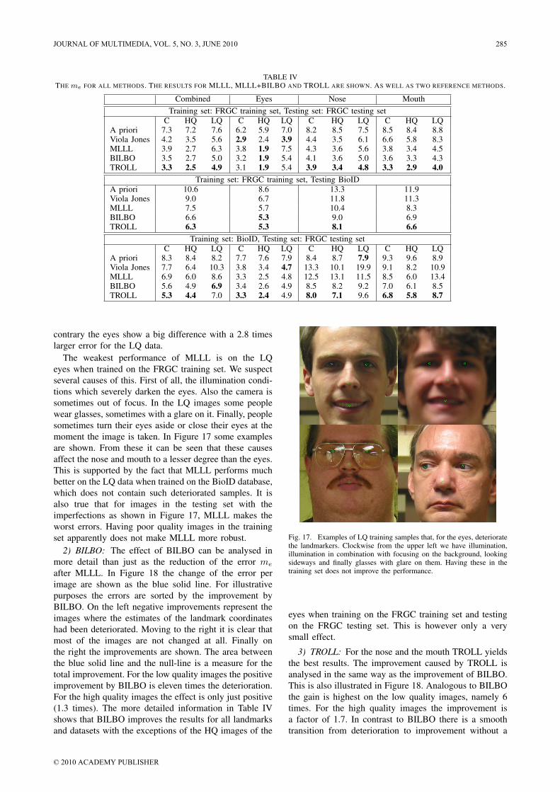
TABLE IVTHE me FOR ALL METHODS. THE RESULTS FOR MLLL, MLLL+BILBO AND TROLL ARE SHOWN. AS WELL AS TWO REFERENCE METHODS.
Combined Eyes Nose MouthTraining set: FRGC training set, Testing set: FRGC testing set
C HQ LQ C HQ LQ C HQ LQ C HQ LQA priori 7.3 7.2 7.6 6.2 5.9 7.0 8.2 8.5 7.5 8.5 8.4 8.8Viola Jones 4.2 3.5 5.6 2.9 2.4 3.9 4.4 3.5 6.1 6.6 5.8 8.3MLLL 3.9 2.7 6.3 3.8 1.9 7.5 4.3 3.6 5.6 3.8 3.4 4.5BILBO 3.5 2.7 5.0 3.2 1.9 5.4 4.1 3.6 5.0 3.6 3.3 4.3TROLL 3.3 2.5 4.9 3.1 1.9 5.4 3.9 3.4 4.8 3.3 2.9 4.0
Training set: FRGC training set, Testing BioIDA priori 10.6 8.6 13.3 11.9Viola Jones 9.0 6.7 11.8 11.3MLLL 7.5 5.7 10.4 8.3BILBO 6.6 5.3 9.0 6.9TROLL 6.3 5.3 8.1 6.6
Training set: BioID, Testing set: FRGC testing setC HQ LQ C HQ LQ C HQ LQ C HQ LQ
A priori 8.3 8.4 8.2 7.7 7.6 7.9 8.4 8.7 7.9 9.3 9.6 8.9Viola Jones 7.7 6.4 10.3 3.8 3.4 4.7 13.3 10.1 19.9 9.1 8.2 10.9MLLL 6.9 6.0 8.6 3.3 2.5 4.8 12.5 13.1 11.5 8.5 6.0 13.4BILBO 5.6 4.9 6.9 3.4 2.6 4.9 8.5 8.2 9.2 7.0 6.1 8.5TROLL 5.3 4.4 7.0 3.3 2.4 4.9 8.0 7.1 9.6 6.8 5.8 8.7
contrary the eyes show a big difference with a 2.8 timeslarger error for the LQ data.
The weakest performance of MLLL is on the LQeyes when trained on the FRGC training set. We suspectseveral causes of this. First of all, the illumination condi-tions which severely darken the eyes. Also the camera issometimes out of focus. In the LQ images some peoplewear glasses, sometimes with a glare on it. Finally, peoplesometimes turn their eyes aside or close their eyes at themoment the image is taken. In Figure 17 some examplesare shown. From these it can be seen that these causesaffect the nose and mouth to a lesser degree than the eyes.This is supported by the fact that MLLL performs muchbetter on the LQ data when trained on the BioID database,which does not contain such deteriorated samples. It isalso true that for images in the testing set with theimperfections as shown in Figure 17, MLLL makes theworst errors. Having poor quality images in the trainingset apparently does not make MLLL more robust.
2) BILBO: The effect of BILBO can be analysed inmore detail than just as the reduction of the error me
after MLLL. In Figure 18 the change of the error perimage are shown as the blue solid line. For illustrativepurposes the errors are sorted by the improvement byBILBO. On the left negative improvements represent theimages where the estimates of the landmark coordinateshad been deteriorated. Moving to the right it is clear thatmost of the images are not changed at all. Finally onthe right the improvements are shown. The area betweenthe blue solid line and the null-line is a measure for thetotal improvement. For the low quality images the positiveimprovement by BILBO is eleven times the deterioration.For the high quality images the effect is only just positive(1.3 times). The more detailed information in Table IVshows that BILBO improves the results for all landmarksand datasets with the exceptions of the HQ images of the
Fig. 17. Examples of LQ training samples that, for the eyes, deterioratethe landmarkers. Clockwise from the upper left we have illumination,illumination in combination with focusing on the background, lookingsideways and finally glasses with glare on them. Having these in thetraining set does not improve the performance.
eyes when training on the FRGC training set and testingon the FRGC testing set. This is however only a verysmall effect.
3) TROLL: For the nose and the mouth TROLL yieldsthe best results. The improvement caused by TROLL isanalysed in the same way as the improvement of BILBO.This is also illustrated in Figure 18. Analogous to BILBOthe gain is highest on the low quality images, namely 6times. For the high quality images the improvement isa factor of 1.7. In contrast to BILBO there is a smoothtransition from deterioration to improvement without a
JOURNAL OF MULTIMEDIA, VOL. 5, NO. 3, JUNE 2010 285
© 2010 ACADEMY PUBLISHER

0 2000 4000 6000−40
−20
0
20
40
60
80
100
Images
Err
or r
educ
tion,
me
Low quality images
BILBOTROLL
0 5000 10000−40
−20
0
20
40
60
80
100
Images
Err
or r
educ
tion,
me
High quality images
BILBOTROLL
Fig. 18. The error reduction by BILBO and TROLL, sorted by theimprovement. The blue line denotes the error reduction by BILBO. Thegreen dashed line denotes TROLL. Negative values show a deteriorationof the results and positive values an improvement.
dead zone where the coordinates are not adjusted.It proved that TROLL was not able to get any intelligi-
ble results if the initial face bounding box had dimensionsso that some landmarks fall outside the search areas. Thiswould cause MLLL in the first run to give just any randomposition, and thus TROLL can drift away. An example isgiven in Figure 19. Because the face finder found the faceon the wrong scale, the nose and mouth are not within thesearch regions, denoted by the red rectangles. The resultsof MLLL, BILBO and TROLL are thus not meaningful.In the FRGC testing set there are 810 images for whichone of the landmarks is not in the search area. The impacton the overall performance is limited: it increases the errormeasure roughly 0.1%.
MLLLBILBOTROLLGroundTruth
Fig. 19. Poor performance of all algorithms because the face finderfound the face on the wrong scale. The landmarks lie outside the searchareas denoted by the red rectangles.
TABLE VCOMPARING OTHER WORK ON THE EYES. BOLDFACE DENOTES THEMINIMUM. ITALICS DENOTES AN ESTIMATE NOT PROVIDED BY THE
AUTHORS.
Combined HQ LQWang et al. [6] 2.67Campadelli et al. [7] 2.7 2.65 2.88Viola and Jones [10] 2.9 2.4 3.9Troll 3.1 1.9 5.4
4) Comparison to other work: Several papers reportresults on eye-finders. Unfortunately the authors were notable to find any work for nose and mouth localization thatcould be compared on the FRGC database. Here we onlyfocus on the ones that report results on the eyes and theFRGC for ease of comparison.
There is a difference between the shape Shape Opti-mised Search (SOS) by Cristinacce et al. and our proposedmethods BILBO: SOS is an integral part of the approachand BILBO is performed as an outlier correction methodafter landmarking.
Wang et al. [6] used Adaboost in combination withmultiple weak probabilistic classifiers. Using non FRGCtraining data from multiple sources they report a meanEuclidian distance error on the eyes of 2.67% of theinterocular distance on the FRGC 1.0 database, whichis a subset of the FRGC 2.0 database. Their results canbe compared to ours because they tested on the FRGC1.0. The FRGC 2.0 database is larger but includes theFRGC 1.0 database. Wang et al. seem to have a similar,but slightly better result on the eyes than the Viola andJones algorithm which has an me of 2.9 for the Viola andJones method and a 3.1 for TROLL.
Campadelli et al, [7] used a combination of Haarclassifiers and Support Vector Machines. They report a2.65% error on the HQ data and a 3.88% error on the LQdata of the FRGC 1.0 database. These results are alsosimilar to the ones we obtained with a Viola and Jonesdetector. The MLLL performs significantly better on theHQ data while on the LQ data it is worse. These resultsare summarised in Table V.
In previous work by the authors [27] results for earlierversions of MLLL, which were not tuned nor optimized,and BILBO were given. See Table VI. These versionswere trained on the BioID database and tested on theFRGC 1.0 database. The new results are significantlybetter for MLLL. For newly trained BILBO the resultson the mouth and the nose yield slightly higher errors.This can be explained by the fact that BILBO used 4landmarks while the ‘old BILBO’ in [27] used 17 andtherefore could make better use of the dependency of thelandmarks. Note that MLLL and BILBO were tuned usingthe FRGC 2.0 database. The tuned parameters were notchanged when training on the BioID database. Thereforewe do not have optimal performance when training on theBioID database. The numbers are given in Table VI. Thisshows that tuning can lead to significantly better result forMLLL. Also it shows that BILBO using more landmarksis useful for BILBO.
286 JOURNAL OF MULTIMEDIA, VOL. 5, NO. 3, JUNE 2010
© 2010 ACADEMY PUBLISHER
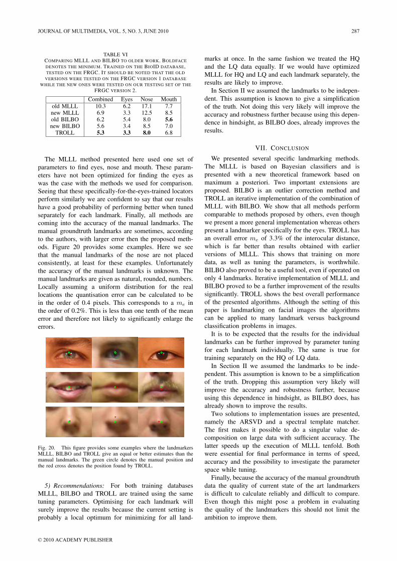
TABLE VICOMPARING MLLL AND BILBO TO OLDER WORK. BOLDFACEDENOTES THE MINIMUM. TRAINED ON THE BIOID DATABASE,TESTED ON THE FRGC. IT SHOULD BE NOTED THAT THE OLD
VERSIONS WERE TESTED ON THE FRGC VERSION 1 DATABASEWHILE THE NEW ONES WERE TESTED ON OUR TESTING SET OF THE
FRGC VERSION 2.
Combined Eyes Nose Mouthold MLLL 10.3 6.2 17.1 7.7new MLLL 6.9 3.3 12.5 8.5old BILBO 6.2 5.4 8.0 5.6new BILBO 5.6 3.4 8.5 7.0
TROLL 5.3 3.3 8.0 6.8
The MLLL method presented here used one set ofparameters to find eyes, nose and mouth. These param-eters have not been optimized for finding the eyes aswas the case with the methods we used for comparison.Seeing that these specifically-for-the-eyes-trained locatorsperform similarly we are confident to say that our resultshave a good probability of performing better when tunedseparately for each landmark. Finally, all methods arecoming into the accuracy of the manual landmarks. Themanual groundtruth landmarks are sometimes, accordingto the authors, with larger error then the proposed meth-ods. Figure 20 provides some examples. Here we seethat the manual landmarks of the nose are not placedconsistently, at least for these examples. Unfortunatelythe accuracy of the manual landmarks is unknown. Themanual landmarks are given as natural, rounded, numbers.Locally assuming a uniform distribution for the reallocations the quantisation error can be calculated to bein the order of 0.4 pixels. This corresponds to a me inthe order of 0.2%. This is less than one tenth of the meanerror and therefore not likely to significantly enlarge theerrors.
Fig. 20. This figure provides some examples where the landmarkersMLLL, BILBO and TROLL give an equal or better estimates than themanual landmarks. The green circle denotes the manual position andthe red cross denotes the position found by TROLL.
5) Recommendations: For both training databasesMLLL, BILBO and TROLL are trained using the sametuning parameters. Optimising for each landmark willsurely improve the results because the current setting isprobably a local optimum for minimizing for all land-
marks at once. In the same fashion we treated the HQand the LQ data equally. If we would have optimizedMLLL for HQ and LQ and each landmark separately, theresults are likely to improve.
In Section II we assumed the landmarks to be indepen-dent. This assumption is known to give a simplificationof the truth. Not doing this very likely will improve theaccuracy and robustness further because using this depen-dence in hindsight, as BILBO does, already improves theresults.
VII. CONCLUSION
We presented several specific landmarking methods.The MLLL is based on Bayesian classifiers and ispresented with a new theoretical framework based onmaximum a posteriori. Two important extensions areproposed. BILBO is an outlier correction method andTROLL an iterative implementation of the combination ofMLLL with BILBO. We show that all methods performcomparable to methods proposed by others, even thoughwe present a more general implementation whereas otherspresent a landmarker specifically for the eyes. TROLL hasan overall error me of 3.3% of the interocular distance,which is far better than results obtained with earlierversions of MLLL. This shows that training on moredata, as well as tuning the parameters, is worthwhile.BILBO also proved to be a useful tool, even if operated ononly 4 landmarks. Iterative implementation of MLLL andBILBO proved to be a further improvement of the resultssignificantly. TROLL shows the best overall performanceof the presented algorithms. Although the setting of thispaper is landmarking on facial images the algorithmscan be applied to many landmark versus backgroundclassification problems in images.
It is to be expected that the results for the individuallandmarks can be further improved by parameter tuningfor each landmark individually. The same is true fortraining separately on the HQ of LQ data.
In Section II we assumed the landmarks to be inde-pendent. This assumption is known to be a simplificationof the truth. Dropping this assumption very likely willimprove the accuracy and robustness further, becauseusing this dependence in hindsight, as BILBO does, hasalready shown to improve the results.
Two solutions to implementation issues are presented,namely the ARSVD and a spectral template matcher.The first makes it possible to do a singular value de-composition on large data with sufficient accuracy. Thelatter speeds up the execution of MLLL tenfold. Bothwere essential for final performance in terms of speed,accuracy and the possibility to investigate the parameterspace while tuning.
Finally, because the accuracy of the manual groundtruthdata the quality of current state of the art landmarkersis difficult to calculate reliably and difficult to compare.Even though this might pose a problem in evaluatingthe quality of the landmarkers this should not limit theambition to improve them.
JOURNAL OF MULTIMEDIA, VOL. 5, NO. 3, JUNE 2010 287
© 2010 ACADEMY PUBLISHER
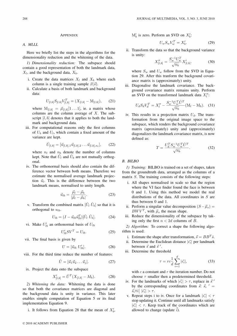
APPENDIX
A. MLLL
Here we briefly list the steps in the algorithms for thedimensionality reduction and the whitening of the data.
1) Dimensionality reduction: The subspace shouldcontain a good representation of both the landmark data,Xl, and the background data, Xb.
i. Create the data matrices Xl and Xb where eachcolumn is a single training sample ~x(~s).
ii. Calculate a basis of both landmark and backgrounddata:
U[l,b]S[l,b]VT[l,b] = (X[l,b] −M[l,b]), (21)
where M[l,b] = ~µ[l,b][1 . . . 1], ie. a matrix whosecolumns are the column average of X . The sub-script [l, b] denotes that it applies to both the land-mark and background data.
iii. For computational reasons only the first columnsof Ub and Ul, which contain a fixed amount of thevariance are kept.
U[l,b] = [~u[l,b],1~u[l,b],2 . . . ~u[l,b],nl], (22)
where nl and nb denote the number of columnskept. Note that Ul and Ub are not mutually orthog-onal.
iv. The orthonormal basis should also contain the dif-ference vector between both means. Therefore weestimate the normalised average landmark projec-tion ~ul. This is the difference between the twolandmark means, normalised to unity length.
~ulb =~µl − ~µb
|~µl − ~µb|. (23)
v. Transform the combined matrix [Ul Ub] so that it isorthogonal to ulb.
Ulb = (I − ~ulb~uTlb)[Ul Ub]. (24)
vi. Make U ′lb an orthonormal basis of Ulb
U ′lbSVT = Ulb. (25)
vii. The final basis is given by
U = [~ulb U′lb]. (26)
viii. For the third time reduce the number of features:
U = [~u1~u2 . . . ~uj ]. (27)
ix. Project the data onto the subspace
X ′[l,b] = UT (X[l,b] −Mb). (28)
2) Whitening the data: Whitening the data is doneso that both the covariance matrices are diagonal andthe background data is unity in variance. This laterenables simple computation of Equation 5 or its finalimplementation Equation 9.
i. It follows from Equation 28 that the mean of X ′b,
M′b is zero. Perform an SVD on X ′b:
UwSwVTw = X ′b. (29)
ii. Transform the data so that the background varianceis unity:
X ′′[l,b] =S−1
w UTw√
nbX ′[l,b]. (30)
where Sw and Uw follow from the SVD in Equa-tion 29. After this tranform the backgound covari-ance matrix is (approximately) unity.
iii. Diagonalise the landmark covariance. The back-ground covariance matrix remains unity. Performan SVD on the transformed landmark data X ′′l :
UdSdVTd = X ′′l −
S−1w UT
w UT
√nb
(Ml −Mb). (31)
iv. This results in a projection matrix Ud. The trans-formation from the original image space to thesubspace, which renders the background covariancematrix (aproximately) unity and (approximately)diagonalizes the landmark covariance matrix, is nowdefined as:
T =UT
d S−1w UT
w UT
√nb
. (32)
B. BILBO
1) Training: BILBO is trained on a set of shapes, takenfrom the groundtruth data, arranged as the columns of amatrix S. The training consists of the following steps:
i. All shapes normalised in scale so that the regionwhere the VJ face finder found the face is between0 and 1. Using this method we model the realdistributions of the data. All coordinates in S arethus between 0 and 1.
ii. Perform a singular value decomposition (S−~µs) =BWV T , with ~µs the mean shape.
iii. Reduce the dimensionality of the subspace by tak-ing only the first n < 2d columns of B.
2) Algorithm: To correct a shape the following algo-rithm is used:
i. Estimate the shape after transformation, ~s = BBT s.ii. Determine the Euclidean distance |~εi| per landmark
between ~s and ~s ′.iii. Determine the threshold
τ = rc1d
d∑i=1
|~εi|, (33)
with c a constant and r the iteration number. Do notchoose τ smaller then a predetermined threshold.
iv. For the landmarks of which |~εi| > τ , replace in ~s ′
by the corresponding coordinates from ~s: ~si′ =
~si∀i∣∣ |~εi| > τ .
v. Repeat steps i to iv. Once for a landmark |~εi| < τstop updating it. Continue until all landmarks satisfy|~εi| < τ . Keep track of the coordinates which areallowed to change (update ~i).
288 JOURNAL OF MULTIMEDIA, VOL. 5, NO. 3, JUNE 2010
© 2010 ACADEMY PUBLISHER
vi. Repeat step i to v changing all coordinates untilstable or r = 5. Allow all landmark coordinates toupdate (reset ~i).
vii. Transform the coordinates back to the original scale.In Figure 5 a schematic overview of the shape correctionalgorithm is shown.
C. Complexity
1) MLLL: Consider a ROI containing n pixels. Thenumber of operations per DFFT2 is then O(n log2(n)).After feature reduction the number of features is m. Thenumber of DFFT2s to be computed is m + 1, as can beseen in Figure 4. Computing the likelihood ratio afterfeature computation, Equation 9, at every pixel locationhas a complexity of O(5mn). Number of operations perROI for finding the maximum value is O(n). This makesthe total number of operations per ROI:
(m+ 1)O(n log2(n)) + nO(5m) +O(n) (34)
Dividing by n gives the number of operations per pixelin ROI
O(m(log2(n) + 6)) (35)
The large ROIs used are 256× 256 pixels, which meansthat n = 25088. We used m = 219 features. Equation 35results in a complexity of O(5000) operations per pixelin the ROI.
2) Viola and Jones: The complexity of the Viola andJones algortihm depends on the numbers of scales S,cascades C, and features K. Estimates for these numbersare taken from [26]; S = 11, C = 15, K = 30, onaverage. The total number of operations per pixel in theROI are upperbounded by O(S × C ×K) ≈ O(5000).
REFERENCES
[1] NIST, “Face recognition vendor test, 2006,” http://www.frvt.org/.[2] O. Jesorsky, K. J. Kirchberg, and R. W. Frischholz, “Robust
Face Detection Using the Hausdorff Distance,” in Audio- andVideo-Based Person Authentication - AVBPA 2001, ser. LectureNotes in Computer Science, J. Bigun and F. Smeraldi, Eds., vol.2091. Halmstad, Sweden: Springer, 2001, pp. 90–95. [Online].Available: citeseer.ist.psu.edu/article/jesorsky01robust.html
[3] P. J. Phillips, P. J. Flynn, T. Scruggs, K. W. Bowyer, J. Chang,K. Hoffman, J. Marques, J. Min, and W. Worek, “Overview ofthe face recognition grand challenge,” in In Proceedings of IEEEConference on Computer Vision and Pattern Recognition, 2005.
[4] T. Riopka and T. Boult, “The eyes have it,” in Proceedings ofACM SIGMM Multimedia Biometrics Methods and ApplicationsWorkshop., Berkeley, CA, 2003, pp. 9–16.
[5] D. Cristinacce, T. Cootes, and I. Scott, “A multi-stage approach tofacial feature detection,” in 15th British Machine Vision Confer-ence, London, England, 2004, pp. 277–286.
[6] P. Wang, M. B. Green, Q. Ji, and J. Wayman, “Automatic eyedetection and its validation,” in CVPR ’05: Proceedings of the2005 IEEE Computer Society Conference on Computer Vision andPattern Recognition (CVPR’05) - Workshops. Washington, DC,USA: IEEE Computer Society, 2005, p. 164.
[7] P. Campadelli, R. Lanzarotti, and G. Lipori, “Precise eyelocalization through a general-to-specific model definition,”in British Machine Vision Conference (BMVC), Edinburgh,UK, 2006. BMVA, 2006, pp. 187–196. [Online]. Available:http://hdl.handle.net/2434/24373
[8] G. M. Beumer, A. M.Bazen, and R. N. J. Veldhuis, “On theaccuracy of EERs in face recognition and the importance ofreliable registration.” in SPS 2005. IEEE Benelux/DSP Valley,April 2005. [Online]. Available: http://acivs.org/sps2005/
[9] G. M. Beumer, Q. Tao, A. M. Bazen, and R. N. J. Veldhuis, “Alandmark paper in face recognition,” in Automatic Face and Ges-ture Recognition, 2006. FGR 2006. 7th International Conferenceon, Southampton, UK. Los Alamitos: IEEE Computer SocietyPress, April 2006.
[10] P. Viola and M. Jones, “Robust real-time object detection,”International Journal of Computer Vision, 2002. [Online].Available: citeseer.ist.psu.edu/viola01robust.html
[11] D. Cristinacce and T. Cootes, “A comparison of shape constrainedfacial feature detectors,” in 6th International Conference on Au-tomatic Face and Gesture Recognition 2004, Seoul, Korea, 2004,pp. 375–380.
[12] M. Everingham and A. Zisserman, “Regression and classificationapproaches to eye localization in face images,” in FGR ’06:Proceedings of the 7th International Conference on AutomaticFace and Gesture Recognition (FGR06). Washington, DC, USA:IEEE Computer Society, 2006, pp. 441–448.
[13] A. M. Bazen, R. N. J. Veldhuis, and G. H. Croonen, “Likelihoodratio-based detection of facial features,” in Proc. ProRISC 2003,14th Annual Workshop on Circuits, Systems and Signal Processing,Veldhoven, The Netherlands, nov 2003, pp. 323–329.
[14] H. van Trees, Detection, Estimation and Modulation Theory, PartI. New York: John Wiley and Sons, 1968.
[15] K. Fukunaga, Introduction to statistical pattern recognition (2nded.). San Diego, CA, USA: Academic Press Professional, Inc.,1990.
[16] R. A. Fisher, “The use of multiple measurements in taxonomicproblems,” Annals of Eugenics, vol. 7, no. 2, pp. 179–188, 1936.
[17] R. C. Gonzales and P. Wintz, Digital Image Processing. Reading,MA: Addison-Wesley, 1977.
[18] D. D. Muresan and T. W. Parks, “Adaptive principal componentsand image denoising,” in ICIP (1), 2003, pp. 101–104.
[19] B. Goossens, A. Pizurica, and W. Philips, “Noise removal fromimages by projecting onto bases of principal components.” inACIVS, ser. Lecture Notes in Computer Science, J. Blanc-Talon,W. Philips, D. Popescu, and P. Scheunders, Eds., vol. 4678.Springer, 2007, pp. 190–199.
[20] S. Osowski, A. Majkowski, and A. Cichocki, “Robust PCA neuralnetworks for random noise reduction of the data,” in ICASSP’97: Proceedings of the 1997 IEEE International Conference onAcoustics, Speech, and Signal Processing (ICASSP ’97) -Volume 4.Washington, DC, USA: IEEE Computer Society, 1997, p. 3397.
[21] J. Tolkien, The Hobbit – There and back again. London: GeorgeAllen and Unwin, 1937.
[22] M. A. Fischler and R. C. Bolles, “Random sample consensus: aparadigm for model fitting with applications to image analysis andautomated cartography,” Commun. ACM, vol. 24, no. 6, pp. 381–395, 1981.
[23] D. Cristinacce and T. F. Cootes, “Facial feature detection and track-ing with automatic template selection,” in FGR ’06: Proceedings ofthe 7th International Conference on Automatic Face and GestureRecognition (FGR06). Washington, DC, USA: IEEE ComputerSociety, 2006, pp. 429–434.
[24] P. A. Viola and M. J. Jones, “Rapid object detection using aboosted cascade of simple features.” in CVPR (1), 2001, pp. 511–518.
[25] Intel, “Open computer vision library,”http://sourceforge.net/projects/opencvlibrary/.
[26] Q. Tao, “Face verification for mobile personal devices,” Ph.D.dissertation, Univ. of Twente, February 2009.
[27] G. M. Beumer and R. N. J. Veldhuis, “A map approach to land-marking,” in Proceedings of the 28th Symposium on InformationTheory in the Benelux, Enschede, The Netherlands, May 24/252007, pp. 183–187.
JOURNAL OF MULTIMEDIA, VOL. 5, NO. 3, JUNE 2010 289
© 2010 ACADEMY PUBLISHER

Research on Image Self-recovery Algorithm
based on DCT
Che Shengbing College of computer and information engineering
Central South University of Forestry & Technology
Hunan Changsha 410004, China
Che Zuguo, Shu Xu College of computer and information engineering
Central South University of Forestry & Technology
Hunan Changsha 410004, China
Abstract—Image compression operator based on discrete cosine
transform was brought up. A securer scrambling locational
operator was put forward based on the concept of anti-tamper
radius. The basic idea of the algorithm is that it first combined
image block compressed data with eigenvalue of image block and
its offset block, then scrambled or encrypted and embeded them
into least significant bit of corresponding offset block. This
algorithm could pinpoint tampered image block and tampering
type accurately. It could recover tampered block with good image
quality when tamper occured within the limits of the anti-tamper
radius. It could effectively resist vector quantization and
synchronous counterfeiting attacks on self-embedding
watermarking schemes.
Index Terms—-self-embedding authentication, discrete cosine
transform, anti-tamper radius, scrambling location
I. INTRODUCTION
Owing to the popularization of Internet, especially extensive application of multimedia technology, security problem of multimedia information has become more and more important. As a effective protection means of multimedia data, digital watermarking technology, especially the self-embedding watermarking technology which possesses the self-recovery function, has become researchful hot spot in the international academia[1-4]
.
In 1999, self-embedding watermaking algorithm based on DCT (discrete cosine transform) was brought up by Fridrich first. It divided image into 8 × 8 blocks and made DCT, quantization, coding, then embedded the code of 11 important coefficients into LSB(least significant bit) of corresponding offset block[4]. It stored 11 important coefficients got by zigzag scanning with the largest number of bits, but it didn’t analyze the probability of these coefficients, so it couldn’t enhance the image recovery quality as far as possible. And the fixity of offset block selection led the poor anti-tamper characteristic.
In 2004, a new self-embedding algorithm was put forward by Zhang etc. According to a large number of statistical experimental data of DCT quantization coefficients, the new algorithm decided on the position of 14 stored major coefficients and their storage bits by zigzag scanning. It improved locational function of embedding code, and enhanced
the quality of the recovery image and the capacity of algorithmic testing and locating[5]. It detailedly analyzed the rule of 14 coefficients, and assigned the bits of 14 important coefficients more rational. It did not experimentalize in the image databases, so it did not get the true distribution rule of 14 coefficients, then it did not get the true rational bit distribution scheme of the 14 coefficients. The quality of recovery image needs to be raised. Further more, the locational function which chose offset block to embed watermarking information was a big fixed circle, so the security was poor.
In 2006, based on the work of Zhang, Qian and the others brought up a new method based on JPEG compression. It used digital information embedding and extraction method based on the digital-position information, and adopted revolving method to calculate corresponding offset block in accordance with the diagonal direction. When modifying 31 bits of offset block LSB at most, it could embed 62 bits authentication and recovery information. The algorithm improved the quality of carrier and recovery image, enhanced the security of the algorithm, and could recovery half of the tamper sub-block in the extreme cases[6]. But the JPEG compression information of
a 8 8 image offset block must at least include the size of sub-
block, brightness component quantitative information form and Huffman form of DCT’s DC and AC components. It could not primely recover image sub-block content by only saving interceptive 50 bits data after JPEG compression when all the sub-block were using these same information. Although it could recover half of the tamper sub-block when the image was cut out half symmetrically, the average anti-tamper radius is only a quarter of image size according to the offset block calculation function. In other words, any recoverable size of the cut block is only a quarter of the image size averagely.
Since the birth of self-embedding technology, people are greatly concerned about its safety. Self-embedding watermarking information are usually embedded into LSB of image pixel value. When the attacker tampered the image high seven bits information and the watermarking embedding information at the same time, the tampered carrier image may pass through authentication. Vector quantization (VQ) attack is one of the ordinary attack means[7-8]. The main reasons of security vulnerabilities about self-embedding watermarking algorithm are as follows. First, the key space of location
290 JOURNAL OF MULTIMEDIA, VOL. 5, NO. 3, JUNE 2010
© 2010 ACADEMY PUBLISHERdoi:10.4304/jmm.5.3.290-297
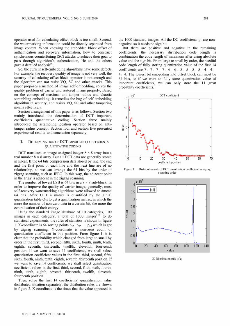
operator used for calculating offset block is too small. Second, the watermarking information could be directly separated from image content. When knowing the embedded block offset of authentication and recovery information, how to construct synchronous counterfeiting (SC) attacks to achieve their goal to pass through algorithm’s authentication, He and the others gave a detailed analysis[9]
.
So, the current self-embedding algorithms have some defects. For example, the recovery quality of image is not very well, the security of calculating offset block operator is not enough and the algorithm can not resist VQ, SC and other attacks. This paper proposes a method of image self-embedding, solves the quality problem of carrier and restored image properly. Based on the concept of maximal anti-tamper radius and chaotic scrambling embedding, it remedies the bug of self-embedding algorithm in security, and resists VQ, SC and other tampering means effectively.
Section arrangement of this paper is as follows. Section two mainly introduced the determination of DCT important coefficients quantitative coding. Section three mainly introduced the scrambling location operator based on anti-tamper radius concept. Section four and section five presented experimental results and conclusion separately.
II. DETERMINATION OF DCT IMPORTANT COEFFICIENTS
QUANTITATIVE CODING
DCT translates an image unsigned integer 8 × 8 array into a real number 8 × 8 array. But all DCT data are generally stored in linear. If the 64 bits compression data stored by line, the end and the first point of each line and the next line are of no relationship, so we can arrange the 64 bits by the order of zigzag scanning, such as JPEG. In this way, the adjacent point in the array is adjacent in the zigzag scanning.
The number of lowest LSB is 64 bits in a 8 × 8 sub-block. In order to improve the quality of carrier image, generally, most self-recovery watermarking algorithms were allowed to amend 64 bits. After DCT a matrix is quantified by the JPEG quantization table Q38 to get a quantization matrix, in which the more the number of non-zero data in a certain bit, the more the centralization of their energy.
Using the standard image database of 10 categories, 100 images in each category, a total of 1000 images[10] to do statistical experiments, the rules of statistics is shown in figure
1. X-coordinate is 64 sorting points p1 p2 ... p64 which is got
by zigzag scanning. Y-coordinate is non-zero count of quantization coefficient in this position. From figure 1, it is clear that the probability which changed from large to small by order in the first, third, second, fifth, sixth, fourth, ninth, tenth, eighth, seventh, thirteenth, twelfth, eleventh, fourteenth position. If we want to save 11 coefficients, we shall select quantization coefficient values in the first, third, second, fifth, sixth, fourth, ninth, tenth, eighth, seventh, thirteenth position. If we want to save 14 coefficients, we shall select quantization coefficient values in the first, third, second, fifth, sixth, fourth, ninth, tenth, eighth, seventh, thirteenth, twelfth, eleventh, fourteenth position.
Then, solve the first 14 coefficients’ quantification value distributed situation separately, the ditribution rules are shown in figure 2. X-coordinate is the times that the value appeared in
the 1000 standard images. All the DC coefficients p1 are non-negative, so it needs no sign bit.
But there are positive and negative in the remaining coefficients, the necessary distribution code length is combination the code length of maximum after using absolute value and the sign bit. From large to small by order, the needful code length of fully storing quantization value of the first 14
coefficients are 7 7 7 7 6 6 5 5 5 5 4 4
4 4. The lowest bit embedding into offset block can most be
64 bits, so if we want to fully store quantization value of important coefficients, we can only store the 11 great probablity coefficients.
Figure 1. Distribution rule of DCT quantization coefficient in zigzag scanning order
Distribution rule of q1
JOURNAL OF MULTIMEDIA, VOL. 5, NO. 3, JUNE 2010 291
© 2010 ACADEMY PUBLISHER
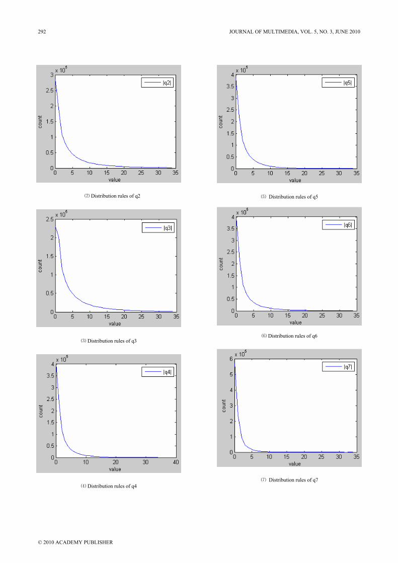
Distribution rules of q2
Distribution rules of q3
Distribution rules of q4
Distribution rules of q5
Distribution rules of q6
Distribution rules of q7
292 JOURNAL OF MULTIMEDIA, VOL. 5, NO. 3, JUNE 2010
© 2010 ACADEMY PUBLISHER
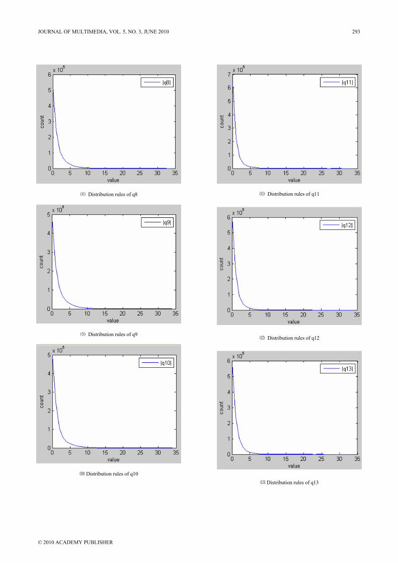
Distribution rules of q8
Distribution rules of q9
Distribution rules of q10
Distribution rules of q11
Distribution rules of q12
Distribution rules of q13
JOURNAL OF MULTIMEDIA, VOL. 5, NO. 3, JUNE 2010 293
© 2010 ACADEMY PUBLISHER

Distribution rules of q14
Figure 2. Distribution rules of 14 coefficients
Except the sign bit, the use factor of the highest bit is too low. So we reduce a bit in each coefficient’s code and store some new coefficients using the remainning bits. As shown in table 1, setting threshold value of preserve the bits which contain more than 96% of the coefficient quantization value, it can obtain the greatest degree of recovery quality by re-encoding. In this paper, the final code form of 11 or 14 coefficients shown as paper1 or paper2 in table 1. Among them, q1 does not need to retain sign bit, so it’s only to retain 7 bits coefficient value
DC coefficient q1 is gotten by DCT coefficients of image sub-block through Q38 matrix after quantization. We can prove that q1 is half of the average value of sub-block pixel value and q1 is distributing in the interval [0,127.5]. Comparing the distribution rule of DCT quantization coefficients between this paper and reference[5], their maximum value of q1 is only about 65 and the rest of the coefficients can not be 0. Their conclusion and common sense existence obvious violation.
III. SCRAMBLING LOCATION OPERATOR BASED ON ANTI-
TAMPER RADIUS CONCEPT
This paper brings up the concept of scrambling anti-tamper radius to resist the conventional attack methods. A point lies in
position ),( ji in matrix A whose size is N×N. When it moves
to position ),( sr after scrambling, define anti-tamper radius R
as follows
max( ( ), ( ))R abs i r abs j s
It shows that after scrambling the original matrix point lies in the square vertex whose square length of side is R. Perfect anti-tamper radius is N/2. The bigger the anti-tamper radius, the smaller the relativity of sub-block and offset block. But when anti-tamper radius is N/2, the corresponding offset block calculation will be simple and changeless. This will make against to the algorithm’s resisting attack characteristic.
The bigger the anti-tamper radius, the bigger the recovery probability after sub-block being attacked, but the more similar
the distribution rule of offset block. In order to achieve a better balance, in this paper the selection way of offset sub-block are as follows.
Divide entire image into 16 small block, k1 k2 ...k16.
As shown in Figure 3.
Take four small block as a large block, then offset by
diagonal direction. In figure 3, take the first, second, fifth and sixth small block as the first large block; take the third, fourth, seventh and eighth small block as the second large block etc. These four large blocks exchange by diagonal direction, for example, changing the small block in the first large block into the fourth large block.
Divide each small piece k1 k2 ... k16 into 8 × 8 sub-
blocks, take each block as a unit, create scrambling sequence using composite chaotic[11], confirm the final position of offset block in the small block ranges by this sequence. In this way, it randomly confirms the corresponding offset block of a sub-block to embed authentication and recovery information.
The average radius of anti-tamper is N/3 and it can recover half of the damaged region when symmetrical cutting attack happened.
Figure 3. The choice of offset sub-block
IV. SELF-EMBEDDING AND SELF-RECOVERY ALGORITHM
A. Self-embedding algorithm
After DCT, we obtain a coefficient matrix through quantization matrix Q38. Only by storing entire coefficient matrix, multiplying the quantization matrix Q38 and doing inverse DCT, can we get recovery image of the best quality. An image can not be fully embedded into its own data, so the coefficient matrix must be compressed. It is necessary to ensure large compression ratio, so that the image compression information can be fully saved into itself. At the same time, the image can not be compressed too much, because the proper quality need to be ensured when the image is to be recovered.
The self-embedding algorithm of this paper is as follows.
Divide image I0 into 8 8 sub-block a1 a2 ...,ar, where
r is the count of sub-block.
Do DCT respectively to the sub-block ai i=1,2,...,r
then get the coefficient matrix divided by quantization table Q38.
According to the experimental data in table 1, we select
the first 14 coefficients by zigzag scanning order in figure 4.
294 JOURNAL OF MULTIMEDIA, VOL. 5, NO. 3, JUNE 2010
© 2010 ACADEMY PUBLISHER
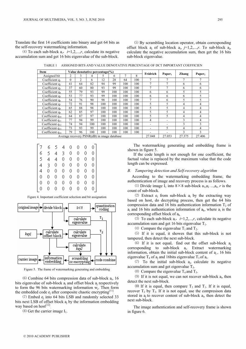
Translate the first 14 coefficients into binary and get 64 bits as the self-recovery watermarking information.
To each sub-block ai i=1,2,...,r, calculate its negative
accumulation sum and get 16 bits eigenvalue of the sub-block.
By scrambling location operator, obtain corresponding
offset block aj of sub-block ai, j=1,2,...,r. To sub-block aj,calculate the negative accumulation sum, then get the 16 bits sub-block eigenvalue.
TABLE 1 ASSIGNED BITS AND VALUE DENOTATIVE PERCENTAGE OF DCT IMPORTANT COEFFICIEN
Item Value denotative percentage(%)
Assigned bit 2 3 4 5 6 7 8 Fridrich Paper1 Zhang Paper2
Coefficient q1 0 2 6 12 28 64 100 7 7 7 7
Coefficient q2 41 64 82 94 99 100 100 7 7 6 6
Coefficient q3 37 60 80 93 99 100 100 7 7 6 6
Coefficient q4 55 79 93 99 100 100 100 6 6 5 5
Coefficient q5 53 77 93 99 100 100 100 6 6 6 5
Coefficient q6 54 76 90 98 100 100 100 7 6 5 5
Coefficient q7 72 91 98 100 100 100 100 5 5 4 4
Coefficient q8 65 88 98 100 100 100 100 5 5 4 4
Coefficient q9 62 85 97 100 100 100 100 5 5 4 4
Coefficient q10 64 87 97 100 100 100 100 5 5 4 4
Coefficient q11 77 94 99 100 100 100 100 4 - 3 4
Coefficient q12 74 94 100 100 100 100 100 - - 3 3
Coefficient q13 73 93 99 100 100 100 100 - 5 4 4
Coefficient q14 79 96 100 100 100 100 100 - - 3 3
Average recovery PSNR(dB) in image database 27.048 27.053 27.375 27.406
Figure 4. Important coefficient selection and bit assignation
Figure 5. The frame of watermarking generating and embedding
Combine 64 bits compression data of sub-block ai, 16
bits eigenvalue of sub-block ai and offset block aj respectively to form the 96 bits watermarking information wj. Then form the embedded code ej after composite chaotic encrypting[11]
.
Embed ej into 64 bits LSB and randomly selected 33
bits next LSB of offset block aj by the information embedding way based on host[12]
.
Get the carrier image I1.
The watermarking generating and embedding frame is shown in figure 5.
If the code length is not enough for one coefficient, the factual value is replaced by the maximum value that the code length can be expressed.
B. Tampering detection and Self-recovery algorithm
According to the watermarking embedding frame, the authemtication of image and recovery process is as follows.
Divide image I1 into 8 8 sub-block a1,a2 ...,ar, r is the
count of sub-block.
Extract ei from sub-block ai by the extracting way
based on host, do decrypting process, then get the 64 bits compression data and 16 bits authentication information T2 of ai and 16 bits authentication information of ak, where ai is the corresponding offset block of ak.
To each sub-block ai i=1,2,...,r, calculate its negative
accumulation sum and get 16 bits eigenvalue T1.
Compare the eigenvalue T1 and T2.
If it is equal, it showes that this sub-block is not
tampered, then detect the next sub-block.
If it is not equal find out the offset sub-block aj
corresponding to sub-block ai. Extract watermarking information, obtain the initial sub-block content of aj , 16 bits eigenvalue T4 of aj and 16bits eigenvalue T3 of ai.
To the initial sub-block aj, calculate its negative
accumulation sum and get eigenvalue T5.
Compare the eigenvalue T4 and T5.
If it is not equal, we can not recover sub-block ai, then
detect the next sub-block.
If it is equal, then compare T3 and T1. If it is equal,
recover T2 by T3. If it is not equal, use the compresison data stored in aj to recover content of sub-block ai, then detect the next sub-block.
The image authentication and self-recovery frame is shown in figure 6.
JOURNAL OF MULTIMEDIA, VOL. 5, NO. 3, JUNE 2010 295
© 2010 ACADEMY PUBLISHER
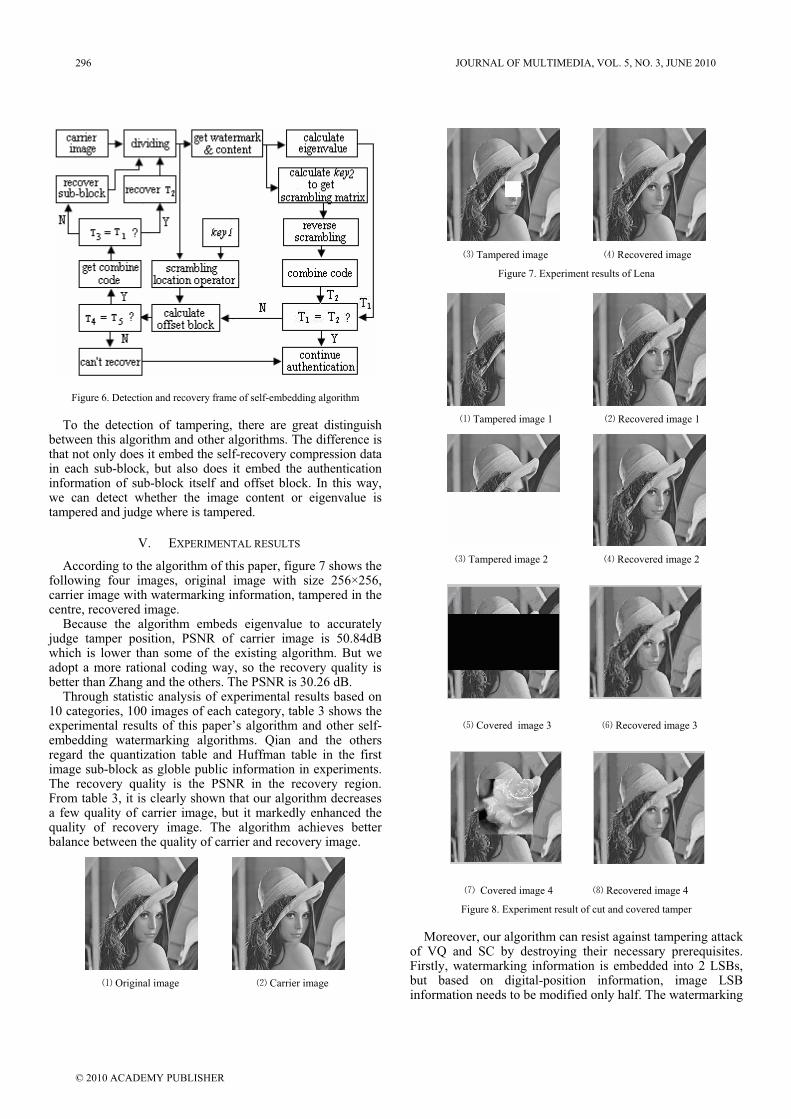
Figure 6. Detection and recovery frame of self-embedding algorithm
To the detection of tampering, there are great distinguish between this algorithm and other algorithms. The difference is that not only does it embed the self-recovery compression data in each sub-block, but also does it embed the authentication information of sub-block itself and offset block. In this way, we can detect whether the image content or eigenvalue is tampered and judge where is tampered.
V. EXPERIMENTAL RESULTS
According to the algorithm of this paper, figure 7 shows the following four images, original image with size 256×256, carrier image with watermarking information, tampered in the centre, recovered image.
Because the algorithm embeds eigenvalue to accurately judge tamper position, PSNR of carrier image is 50.84dB which is lower than some of the existing algorithm. But we adopt a more rational coding way, so the recovery quality is better than Zhang and the others. The PSNR is 30.26 dB.
Through statistic analysis of experimental results based on 10 categories, 100 images of each category, table 3 shows the experimental results of this paper’s algorithm and other self-embedding watermarking algorithms. Qian and the others regard the quantization table and Huffman table in the first image sub-block as globle public information in experiments. The recovery quality is the PSNR in the recovery region. From table 3, it is clearly shown that our algorithm decreases a few quality of carrier image, but it markedly enhanced the quality of recovery image. The algorithm achieves better balance between the quality of carrier and recovery image.
Original image Carrier image
Tampered image Recovered image
Figure 7. Experiment results of Lena
Tampered image 1 Recovered image 1
Tampered image 2 Recovered image 2
Covered image 3 Recovered image 3
Covered image 4 Recovered image 4
Figure 8. Experiment result of cut and covered tamper
Moreover, our algorithm can resist against tampering attack of VQ and SC by destroying their necessary prerequisites. Firstly, watermarking information is embedded into 2 LSBs, but based on digital-position information, image LSB information needs to be modified only half. The watermarking
296 JOURNAL OF MULTIMEDIA, VOL. 5, NO. 3, JUNE 2010
© 2010 ACADEMY PUBLISHER
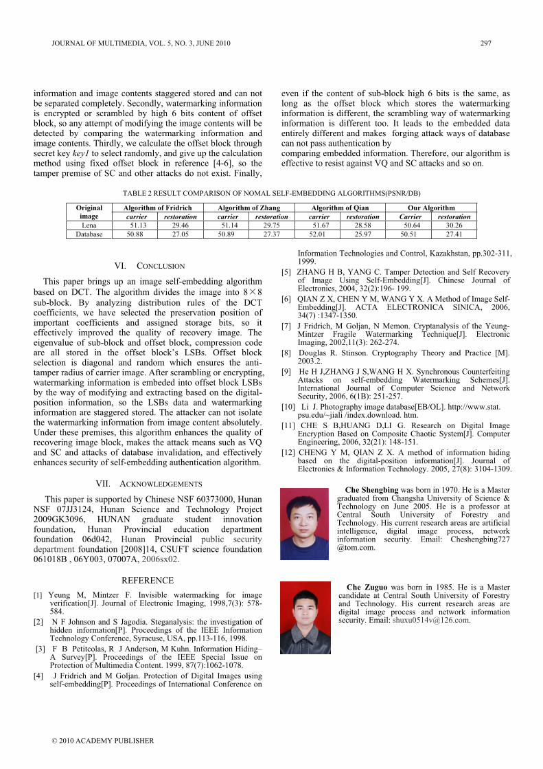
information and image contents staggered stored and can not be separated completely. Secondly, watermarking information is encrypted or scrambled by high 6 bits content of offset block, so any attempt of modifying the image contents will be detected by comparing the watermarking information and image contents. Thirdly, we calculate the offset block through secret key key1 to select randomly, and give up the calculation method using fixed offset block in reference [4-6], so the tamper premise of SC and other attacks do not exist. Finally,
even if the content of sub-block high 6 bits is the same, as long as the offset block which stores the watermarking information is different, the scrambling way of watermarking information is different too. It leads to the embedded data entirely different and makes forging attack ways of database can not pass authentication by comparing embedded information. Therefore, our algorithm is effective to resist against VQ and SC attacks and so on.
TABLE 2 RESULT COMPARISON OF NOMAL SELF-EMBEDDING ALGORITHMS(PSNR/DB)
Algorithm of Fridrich Algorithm of Zhang Algorithm of Qian Our Algorithm Original
image carrier restoration carrier restoration carrier restoration Carrier restoration
Lena 51.13 29.46 51.14 29.75 51.67 28.58 50.64 30.26
Database 50.88 27.05 50.89 27.37 52.01 25.97 50.51 27.41
VI. CONCLUSION
This paper brings up an image self-embedding algorithm
based on DCT. The algorithm divides the image into 8 8
sub-block. By analyzing distribution rules of the DCT coefficients, we have selected the preservation position of important coefficients and assigned storage bits, so it effectively improved the quality of recovery image. The eigenvalue of sub-block and offset block, compression code are all stored in the offset block’s LSBs. Offset block selection is diagonal and random which ensures the anti-tamper radius of carrier image. After scrambling or encrypting, watermarking information is embeded into offset block LSBs by the way of modifying and extracting based on the digital-position information, so the LSBs data and watermarking information are staggered stored. The attacker can not isolate the watermarking information from image content absolutely. Under these premises, this algorithm enhances the quality of recovering image block, makes the attack means such as VQ and SC and attacks of database invalidation, and effectively enhances security of self-embedding authentication algorithm.
VII. ACKNOWLEDGEMENTS
This paper is supported by Chinese NSF 60373000, Hunan NSF 07JJ3124, Hunan Science and Technology Project 2009GK3096, HUNAN graduate student innovation foundation, Hunan Provincial education department foundation 06d042, Hunan Provincial public security department foundation [2008]14, CSUFT science foundation 061018B , 06Y003, 07007A, 2006sx02.
REFERENCE
[1] Yeung M, Mintzer F. Invisible watermarking for image verification[J]. Journal of Electronic Imaging, 1998,7(3): 578- 584.
[2] N F Johnson and S Jagodia. Steganalysis: the investigation of hidden information[P]. Proceedings of the IEEE Information Technology Conference, Syracuse, USA, pp.113-116, 1998.
[3] F B Petitcolas, R J Anderson, M Kuhn. Information Hiding–A Survey[P]. Proceedings of the IEEE Special Issue on Protection of Multimedia Content. 1999, 87(7):1062-1078.
[4] J Fridrich and M Goljan. Protection of Digital Images using self-embedding[P]. Proceedings of International Conference on
Information Technologies and Control, Kazakhstan, pp.302-311, 1999.
[5] ZHANG H B, YANG C. Tamper Detection and Self Recovery of Image Using Self-Embedding[J]. Chinese Journal of Electronics, 2004, 32(2):196- 199.
[6] QIAN Z X, CHEN Y M, WANG Y X. A Method of Image Self-Embedding[J]. ACTA ELECTRONICA SINICA, 2006, 34(7) :1347-1350.
[7] J Fridrich, M Goljan, N Memon. Cryptanalysis of the Yeung-Mintzer Fragile Watermarking Technique[J]. Electronic Imaging, 2002,11(3): 262-274.
[8] Douglas R. Stinson. Cryptography Theory and Practice [M]. 2003.2.
[9] He H J,ZHANG J S,WANG H X. Synchronous Counterfeiting Attacks on self-embedding Watermarking Schemes[J]. International Journal of Computer Science and Network Security, 2006, 6(1B): 251-257.
[10] Li J. Photography image database[EB/OL]. http://www.stat. psu.edu/~jiali /index.download. htm.
[11] CHE S B,HUANG D,LI G. Research on Digital Image Encryption Based on Composite Chaotic System[J]. Computer Engineering, 2006, 32(21): 148-151.
[12] CHENG Y M, QIAN Z X. A method of information hiding based on the digital-position information[J]. Journal of Electronics & Information Technology. 2005, 27(8): 3104-1309.
Che Shengbing was born in 1970. He is a Master graduated from Changsha University of Science & Technology on June 2005. He is a professor at Central South University of Forestry and Technology. His current research areas are artificial intelligence, digital image process, network information security. Email: Cheshengbing727 @tom.com.
Che Zuguo was born in 1985. He is a Master candidate at Central South University of Forestry and Technology. His current research areas are digital image process and network information security. Email: [email protected].
JOURNAL OF MULTIMEDIA, VOL. 5, NO. 3, JUNE 2010 297
© 2010 ACADEMY PUBLISHER


Call for Papers and Special Issues
Aims and Scope.
Journal of Multimedia (JMM, ISSN 1796-2048) is a scholarly peer-reviewed international scientific journal published bimonthly, focusing on
theories, methods, algorithms, and applications in multimedia. It provides a high profile, leading edge forum for academic researchers, industrial professionals, engineers, consultants, managers, educators and policy makers working in the field to contribute and disseminate innovative new work on multimedia.
The Journal of Multimedia covers the breadth of research in multimedia technology and applications. JMM invites original, previously
unpublished, research, survey and tutorial papers, plus case studies and short research notes, on both applied and theoretical aspects of multimedia. These areas include, but are not limited to, the following topics:
• Multimedia Signal Processing • Multimedia Content Understanding • Multimedia Interface and Interaction • Multimedia Databases and File Systems • Multimedia Communication and Networking • Multimedia Systems and Devices • Multimedia Applications JMM EDICS (Editors Information Classification Scheme) can be found at http://www.academypublisher.com/jmm/jmmedics.html.
Special Issue Guidelines Special issues feature specifically aimed and targeted topics of interest contributed by authors responding to a particular Call for Papers or by
invitation, edited by guest editor(s). We encourage you to submit proposals for creating special issues in areas that are of interest to the Journal. Preference will be given to proposals that cover some unique aspect of the technology and ones that include subjects that are timely and useful to the readers of the Journal. A Special Issue is typically made of 10 to 15 papers, with each paper 8 to 12 pages of length.
The following information should be included as part of the proposal: • Proposed title for the Special Issue • Description of the topic area to be focused upon and justification • Review process for the selection and rejection of papers. • Name, contact, position, affiliation, and biography of the Guest Editor(s) • List of potential reviewers • Potential authors to the issue • Tentative time-table for the call for papers and reviews If a proposal is accepted, the guest editor will be responsible for: • Preparing the “Call for Papers” to be included on the Journal’s Web site. • Distribution of the Call for Papers broadly to various mailing lists and sites. • Getting submissions, arranging review process, making decisions, and carrying out all correspondence with the authors. Authors should be
informed the Instructions for Authors. • Providing us the completed and approved final versions of the papers formatted in the Journal’s style, together with all authors’ contact
information. • Writing a one- or two-page introductory editorial to be published in the Special Issue.
Special Issue for a Conference/Workshop A special issue for a Conference/Workshop is usually released in association with the committee members of the Conference/Workshop like
general chairs and/or program chairs who are appointed as the Guest Editors of the Special Issue. Special Issue for a Conference/Workshop is typically made of 10 to 15 papers, with each paper 8 to 12 pages of length.
Guest Editors are involved in the following steps in guest-editing a Special Issue based on a Conference/Workshop: • Selecting a Title for the Special Issue, e.g. “Special Issue: Selected Best Papers of XYZ Conference”. • Sending us a formal “Letter of Intent” for the Special Issue. • Creating a “Call for Papers” for the Special Issue, posting it on the conference web site, and publicizing it to the conference attendees.
Information about the Journal and Academy Publisher can be included in the Call for Papers. • Establishing criteria for paper selection/rejections. The papers can be nominated based on multiple criteria, e.g. rank in review process plus
the evaluation from the Session Chairs and the feedback from the Conference attendees. • Selecting and inviting submissions, arranging review process, making decisions, and carrying out all correspondence with the authors.
Authors should be informed the Author Instructions. Usually, the Proceedings manuscripts should be expanded and enhanced. • Providing us the completed and approved final versions of the papers formatted in the Journal’s style, together with all authors’ contact
information. • Writing a one- or two-page introductory editorial to be published in the Special Issue. More information is available on the web site at http://www.academypublisher.com/jmm/.

(Contents Continued from Back Cover)
A Novel Image Correlation Matching Approach Baoming Shan A Practical Subspace Approach To Landmarking G. M. Beumer and R.N.J. Veldhuis Research on Image Self-recovery Algorithm based on DCT Shengbing Che, Zuguo Che, and Xu Shu
268
276
290