
Journal of Mathematics and System Science - David Publishing ...
73
Journal of Mathematics and System Science Volume 4, Number 2, February 2014 (Serial Number 24) David David Publishing Company www.davidpublishing.com Publishing David
-
Upload
khangminh22 -
Category
Documents
-
view
5 -
download
0
Transcript of Journal of Mathematics and System Science - David Publishing ...

Journal of Mathematics
and System Science
Volume 4, Number 2, February 2014 (Serial Number 24)
David
David Publishing Company
www.davidpublishing.com
PublishingDavid

Publication Information: Journal of Mathematics and System Science is published monthly in hard copy and online (Print: ISSN 2159-5291; Online: ISSN 2159-5305) by David Publishing Company located at 16710 East Johnson Drive, City of Industry, CA 91745, USA.
Aims and Scope: Journal of Mathematics and System Science, a monthly professional academic and peer-reviewed journal, particularly emphasizes new research results in theory and methodology, in realm of pure mathematics, applied mathematics, computational mathematics, system theory, system control, system engineering, system biology, operations research and management, probability theory, statistics, information processing, etc.. Articles interpreting practical application of up-to-date technology are also welcome.
Editorial Board Members: William P. Fox (USA) Wattanavadee Sriwattanapongse (Thailand) Zoubir Dahmani (Algeria) Claudio Cuevas (Brazil) Elisa Francomano (Italy) Baha ŞEN (Turkey) Assia Guezane-Lakoud (Algeria) Alexander Nikolaevich Raikov (Russia) Shelly SHEN (China)
Manuscripts and correspondence are invited for publication. You can submit your papers via web submission, or E-mail to [email protected], [email protected], [email protected]. Submission guidelines and web submission system are available at http://www.davidpublishing.org or http://www.davidpublishing.com.
Editorial Office: 16710 East Johnson Drive, City of Industry, CA 91745, USA Tel: 1-323-984-7526, 323-410-1082 Fax: 1-323-984-7374, 323-908-0457 E-mail: [email protected], [email protected], [email protected]
Copyright©2013 by David Publishing Company and individual contributors. All rights reserved. David Publishing Company holds the exclusive copyright of all the contents of this journal. In accordance with the international convention, no part of this journal may be reproduced or transmitted by any media or publishing organs (including various websites) without the written permission of the copyright holder. Otherwise, any conduct would be considered as the violation of the copyright. The contents of this journal are available for any citation. However, all the citations should be clearly indicated with the title of this journal, serial number and the name of the author.
Abstracted / Indexed in: Database of EBSCO, Massachusetts, USA Index Copernicus, Poland Google Scholar Ulrich’s Periodicals Directory CSA Technology Research Database Norwegian Social Science Data Services (NSD), Database for Statistics on Higher Education (DBH), Norway Universe Digital Library S/B, Proquest Summon Serials Solutions Chinese Database of CEPS, Airiti Inc. & OCLC Chinese Scientific Journals Database, VIP Corporation, Chongqing, P. R. China
Subscription Information: Price (per year): Print $520; Online $300; Print and Online $560
David Publishing Company 16710 East Johnson Drive, City of Industry, CA 91745, USA Tel: 1-323-984-7526, 323-410-1082; Fax: 1-323-984-7374, 323-908-0457 E-mail: [email protected] Digital Cooperative Company: www.bookan.com.cn
David Publishing Company www.davidpublishing.com
DAVID PUBLISHING
D

Journal of Mathematics and System Science
Volume 4, Number 2, February 2014 (Serial Number 24)
Contents 69 Game Modeling and Strategic Behavior Analysis in Public Goods Provision: Evidence From Water
Resources Management
Guocheng Wang, Ye Tian and Ping Li
83 Diagrams Produced by Secondary Students in Multiplicative Comparison Word Problems
Fany M. González Barrios and Enrique Castro Martínez
93 From Digital Analogs Through Recursive Machines to Quantum Computer
M.B. Ignatyev, Yu.E. Sheynin, A.A. Litovkin
99 Interpolated Tensor Products of Exponential Type Vectors of Unbounded Operators
Marian Dmytryshyn
105 Measurement of Surplus Labor in Viet Nam Agriculture Quyet Dang Pham and Hoa Huu Vo
111 Estimation of Demographic Statistics in the Cambodia Socio-Economic Survey (CSES) 2004-2012
Pen Socheat and Anders Holmberg
116 Regulating Neuronal Hyper-Excitability and Hyper-Synchrony in Epileptic Patients by Using PUFA, Calcium and ATP Buffering
Kodwo Annan, Bryan Banfill, and Stephanie Brock
127 Development and Application of Statistical Business Register Guidelines in African Countries
Michael J. Colledge and Besa Muwele
133 Effect of Heteroscedastic Variance Covariance Matrices on Two Groups Linear Classification Techniques
Friday Zinzendoff Okwonu and Abdul Rahman Othman

Journal of Mathematics and System Science 4 (2014) 69-82
Game Modeling and Strategic Behavior Analysis in
Public Goods Provision: Evidence From Water
Resources Management
Guocheng Wang1, Ye Tian2 and Ping Li1
1. Institute of Quantitative & Technical Economics, Chinese Academy of Social Sciences (CASS), Beijing 100732, China
2. Department of Industrial Economics, Graduate School of Chinese Academy of Social Sciences, Beijing 102488, China Received: November 04, 2013 / Accepted: December 12, 2013 / Published: February 25, 2014. Abstract: The utility of public goods vary with the behaviors of stakeholders (players), and it is appropriate to study effective supply and management of public goods with game modeling and analysis. The comparison effect is the key issue of public good provision both in theoretical analysis and in practice. One major contribution of the paper is the extension of Clarke-Groves mechanism, to achieve which strategic behavior analysis is applied through the analysis and the comparison effect among various stakeholders in different stages is created and highly emphasized. In the first section of this paper, the definition of integrated water resources management (IWRM), the importance of stakeholder participation as well as some models and methods that have been applied are illustrated. Following this, the framework of analysis is elaborated, in which the scenario and aims are shown, and it is claimed that game theory is the main approach, which includes both cooperative games and non-cooperative games. To achieve the aims of the public project, five approaches from game theory are able to cover the entire process of the project, and the fourth approach on interest compensation mechanism is the highlight of the research. After this, the interest compensation mechanism is demonstrated in the model section, and is proved to be an incentive compatible mechanism that makes each stakeholder choose to behave in accordance with the interest of the entire project. The Clarke-Groves mechanism is applied and extended in establishing the model, and the utility change by the comparison among stakeholders (defined as the comparison effect) is involved. In the application section, a water project is analyzed in consideration of various stakeholders, and other possible applications are also indicated. Keywords: Game modeling, strategic behavior analysis, integrated water resources management (IWRM), interest compensation mechanism, the Clarke-Groves mechanism.
1. Introduction
It is an arising and active area to study public goods provision with game modeling and experimental game methods in game theory and public management. Water management that depends on interacting or strategic behavior of stakeholders (players) is a type of public goods as well, and it is more appropriate to analyze them with game modeling and analysis. Issues related to water resources have attracted increasingly more attention as the problems of water shortage and
Corresponding author: Ye Tian, Ph.D., research field:
industrial economics, technical economics. E-mail: [email protected].
water pollution hinder economic growth and affect social progress. As a result, voices calling for integrated water resources management (IWRM) have been heard in different places all over the world. In the process of integrated water resources management, stakeholder involvement, public participation and multi-stakeholder analysis are usually emphasized in many management domains.
As for the content of integrated water resources management, it is defined in different ways after its emergence. A most commonly cited definition was given by Global Water Partnership, which can often be read in literature related to IWRM. It was defined that “IWRM is a process which promotes the co-ordinated
D DAVID PUBLISHING

Game Modeling and Strategic Behavior Analysis in Public Goods Provision: Evidence From Water Resources Management
70
development and management of water, land and related resources, in order to maximize the resultant economic and social welfare in an equitable manner without compromising the sustainability of vital ecosystems.” [1] This definition was well elaborated by Biswas [2], and another relatively comprehensive definition was cited in Jaspers’s article (cf. Van Hofwegen & Jaspers, 1999) [3]. Being a widely used tool for multi-stakeholder analysis, the concept of multi-stakeholder platform is often seen in literature, and Warner unpacked and analyzed that. Meanwhile, Warner supposed that multi-stakeholder processes, multi-stakeholder partnerships, multi-stakeholder dialogues, multi-stakeholder fora and multi-stakeholder roundtables can also be used as multi-stakeholder platforms if the focus is wide enough [4].
1.1 The Importance of Stakeholder Participation
Stakeholder analysis is widely used in many fields, and stakeholder participation can help to build a better relationship among stakeholders as well as a more harmonious relationship between human beings and nature. Ostrom considered the role of different people in natural resources in solving the problem of “the tragedy of the commons” which was firstly proposed by Hardin [5, 6]. Later, Ostrom demonstrated that strong temptations of short-run self-interest can be overcome with the help of reciprocity, reputation, and trust [7]. With regard to water, Moss, Downing and Rouchier argued that inevitably where water is concerned, concerns of stakeholders reflect or engender social conflict [8]. Therefore, solving conflicts in water resources management has always been a heated topic for research.
For a long time, technological fixes have been an efficient way in solving urgent environmental problems, but dissatisfaction and much expenditure requires public opinion which is also aroused by environmental awareness [9]. In Jaspers’s article, it was stated that stakeholder participation has become a
crucial issue and water resources planning without stakeholder participation is highly ineffective [3]. In addition, Mostert et al. found that participatory processes can lead to changes in river-basin management and benefit all stakeholders as well as the environment. These processes increased the understanding of key issues in management, helped to build trust and improve relations, established and developed new organizations [8]. Hemmati concluded the benefits of Multi-Stakeholder Processes (the similar concept to multi-stakeholder platforms, MSPs): (1) The quality of opinion-forming and decision-making is improved. (2) Credibility and moral authority can be gained if done in an equitable, transparent and democratic way. (3) People’s commitment to the outcomes and implementation can be enhanced. (4) Mutual respect and tolerance in society are increased, and conflict on contentious issues can be solved more easily [10].
1.2 Models and Methods Applied in Literature
After many became aware of the significance of stakeholder participation, various models and methods were applied in stakeholder participation and multi-stakeholder analysis. As early as 1985, Henderson and Schilling used decision support systems (DSS) in the public sector for a community mental health system as an experience, and this DSS can also support other decision process in the public sector [11]. The DSS encompasses a multiple objective allocation model as well as a multiple party decision process. Moss, Downing and Rouchier applied simulation modeling for water demand policy and response in consideration of stakeholder participation [12]. In addition, by using The Integrated Systems for Knowledge Management (ISKM) as framework, collaborative learning and information sharing process was conducted [13].
In the research conducted by Borsuk et al., many means were applied, such as literature searches, phone interviews, personal interviews, public meetings,

Game Modeling and Strategic Behavior Analysis in Public Goods Provision: Evidence From Water Resources Management
71
written surveys or questionnaires [14]. They relied on a probabilistic model which is called probability network, and this depicts probabilistic relationships among uncertain variables. Hamalainen et al. used modeling approaches to group decision support based on Multiple Criteria Decision Making (MCDM), and value tree analysis, Pareto-optimality and consensus seeking were applied and role playing experiments were conducted to evaluate and improve the models [15]. Besides, Turcotte and Pasquero introduced the method of Multi-stakeholder Collaborative Roundtable (MCR), and considered the outcomes in three aspects: consensus, learning and problem solving capacities [16].
Pahl-Wostl mentioned that the focus group, an important and novel method in integrated environmental assessment, is widely used in public opinion research and in marketing [17]. Pahl-Wostl also introduced agent-based models (ABMs) [17]. Wang et al. utilized a cooperative game approach in water allocation, and achieved efficient use of water through water transfers by reallocation of water [18]. In the case of South Africa, Simpungwe examined the central issues of Catchment Management Forums (CMFs) which are one of the new institutional forms being referred to as MSPs. Desktop research (secondary data collection), informal survey, interviews, participant observation, stakeholder analysis and workshops were used as major methods and techniques [19].
These methods provide remarkable insights for the application of stakeholder participation in various situations, especially for water resources management. Some means can be adopted in the research, but at the same time, application highly relies on the specific scenario, which requires modification and adaptation in utilizing them and innovation for further development.
2. The Framework of Analysis
The main scenario in this paper is a water project, for
example, a water diversion project or a desalination project, which is one major domain in water resources management, and is especially important for China in many areas of which water shortage has become a severe problem. The entire project discussed here can be divided into three parts: preparation for the project, construction of the project and operation, maintenance and renovation after completion.
In the water project, aims in two aspects are to be fulfilled. One is people’s harmonious relationship with the environment, a basic principle in making the project more sustainable in the future. After longtime development, it is commonly accepted that nature is an indispensable foundation for human development, and any kind of large project should consider the impact imposed on the environment. If the project can not get along well with the surroundings, it can not be sustainable in the long run. Another is the economic and social aspect. Public participation is increasingly important in decision making, and the simple but difficult target is to let all stakeholders join the decision process and finally gain from the project (at least not worse off). One reason for this is that more participants may generate more ideas and potentially enriches process substance [20]. In addition, willingness as well as acceptance of the stakeholders heavily influences the construction and maintenance of the project from the micro perspective, and the social welfare and social stability in a much wider range. In a more comprehensive way, Global Water Partnership illustrated principles for effective water governance which require approaches to be open and transparent, inclusive and communicative, coherent and integrative, equitable and ethical; performance and operation should be accountable, efficient, responsive and sustainable [21]. These should be well taken into account in water projects. In this paper, the emphasis is mainly put on the economic aspect.
The analysis of stakeholders in water resources management for this paper highly emphasizes on the strategic behaviors of stakeholders. Although

Game Modeling and Strategic Behavior Analysis in Public Goods Provision: Evidence From Water Resources Management
72
commonly used methods in MSPs are necessary to be adopted, such as written surveys or questionnaires, interviews, collaborative learning, public meetings, formal or informal visits and information sharing, the most important technique in the analysis is the use of both cooperative games and non-cooperative games.
First of all, water resources management involves many stakeholders from different sectors, which makes it more difficult to find equilibrium for multi-stakeholder analysis in considering comprehensively the interests of various stakeholders. Just within the first level of stakeholders in this specific scenario, there are stakeholders from the government, residents, industries and other possible stakeholders, not to mention the secondary level or even the tertiary level. In this sense, it is clearer and more convenient to use game theory approaches to analyze strategic behaviors of stakeholders. Besides, cooperative games and non-cooperative games are both applied. The overall project is a complicated and long-lasting task, the analysis of which is diversified for various aspects during the process. Hence, both cooperative games and non-cooperative games are to be considered. In addition, water resources management often lasts for a long time, and situations often change after more information is disclosed and participants get to know each other better. Therefore, multi-stage analysis is needed so as to reflect the dynamic changes as time goes on. On the whole, the framework of the analysis is a multi-stage, multi-stakeholder, multi-domain, multi-factor and multi-target game analysis process. Within the entire process, five major approaches are of great significance, thus needing explanation. Before
explaining the five major approaches in detail, some general definitions are to be illustrated:
(1) The set of players is illustrated by N ,
and : 1, 2, ,N i i n= = ⋅⋅⋅ , where individual i N∈ . This
shows that there are n stakeholders in the model. They represent different stakeholders from the government sector, residents, different industries and other possible entities. It is to be noted that government agencies are involved as stakeholders in this model to represent the administrative factors. Although some of them still help to coordinate various stakeholders in this project, their own benefits and losses are taken into account in the model.
(2) For each stakeholder i , the set of strategic behaviors is iS , and one strategic behavior is i is S∈ . The entire space of strategic behaviors is
1 2 nS S S S= × ×⋅⋅⋅× . (3) The space of information is 1 2, , , nθ θ θΘ = ⋅⋅⋅ .
iθ is specifically known by individual i , for 1, 2, ,i n= ⋅⋅⋅ , and cannot be directly revealed to other
stakeholders. In the following, five major stages within the
strategic analysis are given, and a brief illustration of the five stages as well as mechanisms and possible models that may be applied can be found in Table 1.
(1) Disclosure of information. Without knowing the actual information of the stakeholders, it is hard to determine how much each stakeholder should pay for the project. Hence, understanding how to reveal the private information of each stakeholder is necessary. In this process, the objective is to make each stakeholder tell the truth and reveal his or her real revenue and loss.
Table 1 Five Stages of Stakeholder Analysis. Stage Mechanism applied Possible model Disclosure of information Mechanism for telling the truth The revelation principle Negotiation mechanism Negotiation mechanism Nash negotiation model Incentive mechanism and regulatory mechanism Incentive/penalty/regulatory mechanism Principal-Agent model, incentive
mechanism design, optimal contract
Interest compensation mechanism Clarke-Groves mechanism Free-riding model in public goods, interest compensation
Trust and sustainable development Sustainable and cooperation mechanism Trust games, dynamic/repeated games, evolutionary games, reputation model

Game Modeling and Strategic Behavior Analysis in Public Goods Provision: Evidence From Water Resources Management
73
By doing so, it becomes possible to let stakeholders bear their costs in a relatively fair way and finally gain benefits from the operation of the project. This belongs to non-cooperative games, and can be realized mainly by the revelation principle.
(2) Negotiation mechanism. During the preparation period of the project, general consensus should be made before construction. In the construction period and maintenance stage, when problems arise, negotiation mechanism can also be effective. In practice, meetings and workshops can be held to get stakeholders together and discuss problems that appear in the project. During this process, information and ideas are exchanged through communication, and people will adjust their expectations in order to reach agreement. Several rounds of negotiations may be involved as progress is made step by step. As was concluded by Ravnborg and Westermann, joint learning provides a crucial and often essential basis for solving or ameliorating problems, and third party facilitation plays an important role in stakeholder identification, bringing conflicts and interdependencies into open and facilitating negotiations [22]. Moreover, the understanding of the governance and cultural systems and the way they are structured and managed is also one point to be conscious of [23]. In negotiation mechanism, collaboration is underlined, and the negotiation model can be applied as the basis.
(3) Incentive mechanism and regulatory mechanism. The incentive mechanism can help to realize that what the stakeholder wants to behave is just what the project or the society wishes to see. By designing a proper mechanism, the goal of the project can be achieved automatically by the individual optimization of each stakeholder, although it is often a second best solution as a whole. In the analysis, individual rationality and incentive compatibility should be taken into consideration. Individual rationality ensures that the participants are better off, and each one is willing to join the project. Incentive compatibility is the one that makes the individual voluntarily chooses what the
society wants to see. But when reaching this outcome, individuals can get extra revenue due to their private information. This is why the best solution for the public is almost impossible to be obtained within the incentive mechanism. On the other side, regulatory mechanism will force stakeholders to keep their promises and make the negotiation process more effective. By supervision, constraints and punishment set by the public are good supplement to incentive mechanism. They limit the behaviors of stakeholders, and is conducive to reaching the point where social benefits are attained at the highest possible level.
(4) Interest compensation mechanism. Interest compensation mechanism is the creative point and the essential topic in this paper, which is the key to the success of a project. It will be elaborated in a model in the following section. Based on the approaches shown above and under certain assumptions, it is to be proved that as long as the total revenue of the project is more than the total cost, it is possible to find a solution which is accepted by all stakeholders. In this way, Pareto improvement can be achieved with one round or several rounds of interest compensation. All stakeholders will either be better off or still hold their reservation utility.
(5) Trust and sustainable development. In the operation, maintenance and renovation stages after the completion of the project, trust among stakeholders is the most important factor for a sustainable development. With no trust, things often get worse than they can be when people truly trust each other. An example that is usually mentioned is the monetary policy [24]. When the authority betrays the public and chooses high inflation, it loses its authority in keeping inflation at a low rate and is less believed by the public. At this time, one monetary policy that aims to stimulate the economy may be ineffective and triggers high inflation, making the situation even worse. Reputation model can be used in solving the problem and dynamic game is introduced. The process involves adjustment of faith, which is determined by previous behaviors

Game Modeling and Strategic Behavior Analysis in Public Goods Provision: Evidence From Water Resources Management
74
conducted by each stakeholder. In addition to rewards, punishment is also necessary to enhance trust and make the project more sustainable after completion. A mechanism ought to be designed in the way that stakeholders are aware that keeping promises is better than violating what is agreed on, thus reaching a better solution and building trust among people.
These five approaches are closely connected to each other, and cover the entire process of the project from the preparation stage to the operation and maintenance stage after completion. From the technique perspective, both cooperative games and non-cooperative games are utilized, and one approach may provide proper technique for another. For instance, the interest compensation mechanism is the core element in the analysis, which has to be based on the first three approaches, especially the disclosure of information, the incentive mechanism and the regulatory mechanism. Trust and sustainable development is formed upon the results of preparation and construction stages of the project, and is assisted by rewards and punishment methods derived from the regulatory mechanism.
3. Model for Compensation Mechanism
The model corresponds to the fourth approach in the last section and mainly applies and extends the Clarke-Groves mechanism, which provides a mechanism that makes stakeholders tell the truth in making decisions for public goods [25-28].
In establishing the model, some differences are to be considered. In China, both administrative factors and economic mechanisms have significant influence on the strategic behaviors of the stakeholders, and pure economic model without considering the specific situations of China may not be feasible sometimes. The mechanism of information disclosure, incentive mechanism and negotiation mechanism mentioned in the previous section can be applied in solving problems of independent individuals, whereas stakeholders from China have particular characteristics resulted by the
two factors, thereby needing further discussion in a new scenario. Hence, interest compensation mechanism with comparison effect of strategic behavior among stakeholders is the key method in the analysis of stakeholders, and the behaviors of government sectors are involved when both administrative factors and economic mechanisms are taken into account. And the other mechanisms can play a role on the basis of the interest compensation mechanism.
In addition, previous theories often analyze stakeholders in a relatively independent way, and do not consider the effects imposed by the amount of transfer given to the other stakeholders. When one individual knows the amount of transfer received by the others, this individual may compare that amount to his or her own. Although sometimes the transfer is large enough, after one knowing that what he or she receives is less than what another person gets, this person will be dissatisfied. In this sense, the utility function is not only determined by the utility of the project and the absolute amount of the transfer, but it is also affected by the comparison among different individuals. This kind of effect is defined as comparison effect in the paper, and will be added in the model involving comparison effects.
3.1 Definitions
In the model for compensation mechanism, besides those definitions illustrated above that can be used in all five stages, a few definitions are to be given for this model:
(1) The final plan of the public project is x , which have many alternatives, and is determined by the strategic behaviors of each stakeholder is , for
1, 2, ,i n= ⋅⋅⋅ . (2) The utility of stakeholder i is iU , and it is
assumed to take a quasi-linear form. The utility function is expressed as
( , , , ) ( , ) ( )i i i i i i i iU x e t v x e tθ θ= + + (3.1) for 1, 2, ,i n= ⋅⋅⋅ , where iθ is the type of stakeholder i ;

Game Modeling and Strategic Behavior Analysis in Public Goods Provision: Evidence From Water Resources Management
75
iv is the utility gained from the project, and is determined by the final plan x and the type of the stakeholder iθ ; ie is the initial endowment of individual i or the reservation utility, which can be thought as the utility of holding a certain amount of currency or the utility gained from private goods bought by the same amount of currency, and ie can be seen as a constant which will not have any influence on the maximization process; it is the transfer from the project to stakeholder i , and the transfer can be positive, negative or just equal to zero, but the total transfer cannot be positive since banks are also considered as stakeholders and it is assumed that there is no external source to raise funds, and is denoted as
10
n
ii
t=
≤∑ . In the analysis, it is assumed that 1
0n
ii
t=
=∑ .
3.2 Model analysis
For the entire project, the total revenue is the sum of the benefits gained by each individual who is better off from the project. As for the total cost, besides the construction and operation costs of the project, losses caused by the project to those who are worse off should also be considered. Stakeholders’ benefits and losses are represented by iv , for 1, 2, ,i n= ⋅⋅⋅ as was mentioned in the definition part above. The goal of the project is to make everyone involved or affected become better off or at least do not get worse off (maintain their reservation utility), namely a Pareto improvement situation. In this sense, a basic condition is that the total revenue of the project must exceed the total cost of it, but this condition is not sufficient since those who enjoy the benefits and those who burden the costs are not the same stakeholders. Therefore, monetary transfer is needed among stakeholders. However, the question is how much the transfer should be for each stakeholder. Hence, a mechanism for interest compensation is required as a way to answering the question. It is supposed that if the type of each stakeholder were known, it would be much easier to solve the problem according to iv . Whereas, in reality,
the type of stakeholders iθ , for 1, 2, ,i n= ⋅⋅⋅ or the information is kept by each individual and it is likely for them to speak out an untrue type to the public in order to gain more from the project, and this is denoted as i is v≠ . In the following analysis, it is to be proved that there exists a mechanism that drives stakeholders to behave the same way as required for achieving social maximization.
For the entire project, the total revenue minus the total cost can be expressed as
1( , ) ( )
n
i ii
v x C xθ=
−∑ (3.2)
where 1
( , )n
i ii
v x θ=∑ contains both revenues and losses
caused by the project to various stakeholders, and ( )C x is the construction and operation costs of the
project. Equation 3.2 is the payoff function of the entire project, the maximization of which indicates the social optimization. However, as the public does not know
( , )i iv x θ and only knows ( , )i is x θ , the maximization has to be done with
1( , ) ( )
n
i ii
s x C xθ=
−∑ (3.3)
The key to the mechanism is the establishment of the transfer function:
1( ) ( ) ( )
n
i j i ijj i
t s x C x r s−=≠
= − +∑ (3.4)
for 1, 2, ,i n= ⋅⋅⋅ , where ( )i ir s− is a function that can be found in a specific circumstance to make the transfer function suitable for the mechanism, and the requirement is that its changes have no relevance with
iv or is , only depending on the strategies of stakeholders except individual i .
Therefore, the utility function of stakeholder i becomes (derived from Equation 3.1 and 3.4)
1( , , , ) ( , ) ( ) ( , ) ( )
n
i i i i i i i i i i i jjj i
U x e t v x e t v x e s xθ θ θ=≠
= + + = + + ∑
( ) ( )i iC x r s−− + (3.5) In the right side of the equation, ie and ( )C x are
constant, 1
( )n
jjj i
s x=≠
∑ and ( )i ir s− are decided by other
individuals rather than stakeholder i . Hence, the only

Game Modeling and Strategic Behavior Analysis in Public Goods Provision: Evidence From Water Resources Management
76
element that depends on individual i ’s choice is ( , )i iv x θ . Looking back at Equation 3.3 (the
maximization process that is conducted by the public), if the individual wants to maximize its own utility function, the proper strategy should be telling the truth, that is ( ) ( )i is x v x= . The utility function can be changed to
1( , , , ) ( ) ( ) ( )
n
i i i i i i i ii
U x e t e s x C x r sθ −=
= + − +∑ (3.6)
In this equation, ie and ( )i ir s− do not depend on
stakeholder i ’s decision, and 1
( , ) ( )n
i ii
s x C xθ=
−∑ is
maximized by the public. As a result, telling the truth is chosen by stakeholder i to maximize its utility function. In this way, each stakeholder i , for
1, 2, ,i n= ⋅⋅⋅ , chooses the strategy “telling the truth”, and Equation 3.2 is achieved, proving that this mechanism is able to solve the problem.
3.3 Model Involving Comparison Effects
Based on the model above, a small change exists after the comparison effects of stakeholders are introduced, which can show the utility change due to the comparison of transfer with the other stakeholders, especially those individuals who are alike. The new utility function is expressed as
( , , , , ) ( , ) ( ) ( , )i i i i i i i i i i i iU x e t t v x e t comp t tθ θ− −= + + + (3.7) Where ( , )i i icomp t t− represents the comparison
effects and varies from person to person. In general, if stakeholder i finds the transfer it is smaller than the transfer of the other stakeholders who have similar characteristics, and finds the transfer is not sufficient after comparison, this individual will get negative utility in comparison effects, that is ( , ) 0i i icomp t t− < ; vice versa, ( , ) 0i i icomp t t− > .
Next, consider the entire project. Since the comparison effects change the utility of individuals, the total revenue minus the total cost becomes
1 1( , ) ( , ) ( )
n n
i i i i ii i
v x comp t t C xθ −= =
+ −∑ ∑ (3.8)
The situation is similar in that the public does not know ( , )i iv x θ and ( , )i i icomp t t− . The public only
knows the strategies chosen by each stakeholder. The strategy does not only include consideration of
( , )i iv x θ , but it also reflects ( , )i i icomp t t− . The strategy chosen by individual i is now named as ' ( , )i is x θ , then the maximization of the public has to be done with
'
1( , ) ( )
n
i ii
s x C xθ=
−∑ (3.9)
The transfer function is chosen as ' ' '
1( ) ( ) ( )
n
i j i ijj i
t s x C x r s−=≠
= − +∑ (3.10)
for 1, 2, ,i n= ⋅⋅⋅ , where ' '( )i ir s− is a function that can be found in a specific circumstance to make the transfer function suitable for the mechanism, and the requirement is that its changes have no relevance with
iv , ( , )i i icomp t t− and 'is , only depending on the
strategies of other stakeholders. Therefore, the utility function of stakeholder i
becomes (derived from Equation 3.7 and 3.10) '
1( , , , , ) ( , ) ( , ) ( )
n
i i i i i i i i i i i jjj i
U x e t t v x e comp t t s xθ θ− −=≠
= + + + ∑
' '( ) ( )i iC x r s−− + (3.11)
In the right side of the equation, ie and ( )C x are
constant, '
1( )
n
jjj i
s x=≠
∑ and ' '( )i ir s− are decided by other
individuals rather than stakeholder i . The elements that depend on individual i ’s choice are ( , )i iv x θ and
( , )i i icomp t t− . Looking back at Equation 3.9 (the maximization process conducted by the public), if the individual wants to maximize its own utility function, the proper strategy should be telling the truth, that is
' ( ) ( ) ( , )i i i i is x v x comp t t−= + . The utility function can be changed to
' ' '
1( , , , ) ( ) ( ) ( )
n
i i i i i i i ii
U x e t e s x C x r sθ −=
= + − +∑ (3.12)
In this equation, ie and ' '( )i ir s− do not depend on
stakeholder i ’s decision, and '
1( ) ( )
n
ii
s x C x=
−∑ is
maximized by the public. It is proved that this mechanism is also incentive compatible when comparison effects are involved.

Game Modeling and Strategic Behavior Analysis in Public Goods Provision: Evidence From Water Resources Management
77
3.4 Policy Recommendation from the Comparison Effects
From the psychological side, when experiencing the same amount of changes in different directions, a person’s utility change is often larger in the circumstance of losses than gains. For example, the degree of sadness caused by a loss of 100 units of currency is usually larger than the degree of happiness with a gain of 100 units of currency. As for comparison effects, it may be natural to reach the same conclusion. In the scenario of two people who are exactly the same in characteristics, person A receives more transfer than person B. After comparison, the increase of person A’s utility by the comparison effect is smaller than the decrease of person B’s utility by the comparison effect, and the total utility change caused by comparison effects is negative. This can be extended when more people are considered. In consequence,
1( , ) 0
n
i i ii
comp t t−=
<∑ (considered in Equation 3.8) if
inequality exists. As the degree of inequality increases,
the value of 1
( , )n
i i ii
comp t t−=∑ becomes smaller, thus
decreasing the total utility of the entire project. In conclusion, when comparison effects are considered, inequality in interest compensation among different stakeholders reduces the total welfare of the project, and inequality should be avoided as much as possible. In practice, comparison effects are more obvious among residents than the other stakeholders, and this will be analyzed in the application later.
3.5 Conclusion of the Models
From the analysis above, it is proved that the interest compensation mechanism proposed is an incentive compatible mechanism that makes each stakeholder voluntarily choose to behave in accordance with the interest of the entire project when they are actually maximizing their own utility function. It should be noted that without knowing the type of each stakeholder, the public project is finally chosen as if the
preferences of all stakeholders were uncovered and the project were determined for social maximization as a whole. In addition, during the entire process, the most important technique is the establishment of the transfer function, which is required not to be dependent on the strategy of stakeholder i . Meanwhile, the utility function and the social maximization target are somewhat overlapping, which partly results in an incentive compatible situation of the individuals. Within the models, the administrative factors can be analyzed by the involvement of government sectors, and the comparison effects are considered in the second model.
4. Applications
4.1 In a Water Project
Now consider a water project, for example, a water diversion project. Stakeholders can be divided into four categories: the government sector, residents, industries and other possible stakeholders. In each category, there are different stakeholders in the secondary level. Classification and behavioral characteristics will be discussed briefly, and a rough illustration of classification of stakeholders is shown in Table 2.
4.1.1 Governments The first primary category of stakeholders is
governments. For the government sector, it is classified into nine stakeholders in the secondary level: central government, municipal government, relevant district and county governments, river basin management agency, Municipal Bureau of Water Resources, Municipal Bureau of Environmental Protection, legal entities of water resources projects, entities for project routine management and water supply companies.
The central government is responsible for making policies, laws and regulations for macro level water resources management, and the municipal government has the similar duties in a more micro level. Also, relevant district and county governments have even more micro responsibilities. Their utility functions are alike in aspects of financial income and expenditure,

Game Modeling and Strategic Behavior Analysis in Public Goods Provision: Evidence From Water Resources Management
78
Table 2 Classification of Stakeholders. Primary stakeholders Secondary stakeholders
Governments
Central government, municipal government, relevant district and county governments, river basin management agency, Municipal Bureau of Water Resources, Municipal Bureau of Environmental Protection, legal entities of water resources projects, entities for project routine management and water supply companies
Residents Urban residents, rural residents as water users and immigrants caused by building the project Industries The first industry, the second industry and the third industry
Other possible stakeholders Banks, meteorological departments, meteorological departments, research institutes and non government organizations (NGOs)
shares in power, satisfaction of residents and enterprises as well as social harmony and social stability. The municipal government and relevant district and county governments are also influenced by approval or critic from the upper level governments. The utility functions of other government agencies that are to be analyzed are also dependent on the evaluation from the upper level government sectors in different degrees, and this point will not be repeated in the following analysis. The river basin management agency is the representative agency of the Ministry of Water Resources. It implements water management for major water basins, but has no right to enact laws. Its target is to coordinate different stakeholders and follow the instructions of the central government. Municipal Bureau of Water Resources integrates three major sectors (water irrigation, water supply and drainage), allocates water resources and achieves unified management of the city’s water affairs. Besides, Municipal Bureau of Environmental Protection is responsible for planning, implementation, management and control of environmental pollution and natural resources conservation. These two agencies pay more attention on the harmonious relationship between humans and nature. Legal entities of water resources projects are set up for the construction period, and are responsible for project quality, safety, schedule, funding and the use of funds. Entities for project routine management is responsible for management, surveying (including surveying and mapping), design, supervision and construction, etc. The last considered agency is water supply companies. They are responsible for construction, operation and management
of water supporting projects and provide water supply to users. At the same time, they can cover the costs by charging water users and may receive transfer from the local governments. Here the water companies are supposed to be government controlled companies for the convenience of analysis, but more and more water companies are becoming private-owned enterprises.
For government sectors, ( , )i iv x θ is the main concern, and is determined by their preferences to the outcomes of the water project. For instance, the central government may give the satisfaction of people and social stability high weights. it may be government transfers between different government sectors, or may be transfers to residents or industries. it can also be gains from specific taxes or penalties on some stakeholders.
4.1.2 Residents Residents are roughly divided into urban residents,
rural residents as water users and immigrants caused by building the project according to their different behaviors in general. Although water users are different even within the urban area or the rural area, they are not further divided for the convenience of analysis. If it is analyzed in a more specific way, more types of residents can be formed, which will make the analysis more like the reality. Urban residents may actually pay more taxes due to the construction of the water project, since large infrastructure projects often get subsidies from the government, and this is essentially paid by tax payers. Urban residents might also have to pay more for higher water price, but they can benefit from better water transport, more stable water supply, higher water quality and flood control,

Game Modeling and Strategic Behavior Analysis in Public Goods Provision: Evidence From Water Resources Management
79
etc. All of these considerations can be put into the utility function, affecting ( , )i iv x θ and it . Rural residents may suffer from taxes and increased costs from higher water price, but benefit from the improvement of rural water supply, which will add to their utilities. Immigrants that are forced to leave their home lose utility for both economic and mental reasons, but they should be compensated with monetary transfer and other compensations which can be calculated in currency form, such as new houses or apartments, a better place for living, new working opportunities, etc.
Comparison effects are especially obvious in residents, and ought to be focused upon in empirical studies. First of all, various residents may have different function types for ( , )i i icomp t t− . Some may feel extremely annoyed by inequality when their transfer is less than that of the others, and ( , )i i icomp t t− takes an important role in the utility function; whereas some may not be affected severely by the comparison effects. Therefore, in empirical analysis, methods from experiments and surveys may be utilized in finding different types of stakeholders and their proportion in a certain area. In consideration of the three types of residents, immigrants caused by building the project need the most concern. They are more sensitive to inequality, and may require higher interest compensation if the problem of inequality is serious. On one hand, higher interest compensation makes the project harder to realize and operate. On the other hand, some social problems and conflicts often arise when the problem of inequality is not treated in a right way.
4.1.3 Industries Industries can be roughly classified into the first
industry, the second industry and the third industry in a less detailed way. Without sufficient water, farmlands may suffer from droughts when rainfall is small or unevenly distributed in different time of the year or areas. But when a reliable water supply system is established, it will help the agricultural industry in times of droughts. Although production costs may rise due to higher water price as well as some construction
costs for water facilities if it is necessary, stakeholders within the first industry benefit from eased water pressure, and the overall economic benefits are often improved. As for the second industry and the third industry, they also gain from eased water pressure, and are able to produce products and services in a more reliable way despite possible rise in water price.
For industries, the comparison effect may not be as significant as that of the residents. They pay more attention on the production process and profit maximization, and ( , )i i icomp t t− does not take up a high percentage in their utility function. For different industries and different sectors within an industry, various prices should be charged according to their amount of water consumption, and externality as well as the concept of water saving are to be emphasized.
4.1.4 Other possible stakeholders Other possible stakeholders may include banks that
offer loans and other financial services for the water project, meteorological departments, geographical departments, research institutes and non government organizations (NGOs) concerning different domains, for example, pollution prevention, environmental changes, animal protection or social equity. Banks get revenues from interests of loans and consulting fees for services, but also take risks for lending money to the water project. Meteorological departments, geographical departments and research institutes provide help in the appraisal of the water project and set rigid constraints with the help of relevant technology, and their advice is good for risk control, and may reduce costs and alleviate possible conflicts for the project. Non government organizations (NGOs) are becoming an indispensible part for problem solving in social life. They can be seen as third parties that often supervise the process, uphold the interests of a certain group and find problems in a more independent perspective.
In the entire process of the water project, five approaches introduced above can be used for different stages of the project, from the preparation period of the

Game Modeling and Strategic Behavior Analysis in Public Goods Provision: Evidence From Water Resources Management
80
project, the construction process, to the operation, maintenance and renovation stages after the completion of the water project. In the interest compensation aspect, the most critical concern is the transfer function of each stakeholder which ought to be set in the way demonstrated in the model section, and is independent from the stakeholder’s own strategies. For some stakeholders, comparison effects have a relatively high weight, and should be paid much attention on.
4.2 Other Possible Applications
Apart from the water project like the water diversion project or a desalination project, the five approaches discussed in the paper, especially the interest compensation mechanism, can be taken into practice in many areas related to public or quasi-public goods and services. For instance, infrastructure projects are similar to the water project analyzed in the paper, and this can be used in the same way, such as electricity or energy plants and networks, communication facilities, highways and railways, city public transportation systems, etc. Besides, environmental protection and natural resources protection can also get hints from the mechanisms. Within a certain range, stakeholders need to pay for costs of protection and confine their own behaviors, but will benefit from better environment and the use of the improved environment and natural resources. In this process, the interest compensation mechanism is put into practice and gets everyone better off or at least not harmed from the program. In addition, other possible applications are basic cultural and educational services, scientific and technological development, the governance of market disorders, protection of intellectual properties, anti-corruption [29] as well as other domains related to externalities and information asymmetry.
Although the range of application is vast, it should be noted that due to time, costs and effort constraints, the application of the proposed five approaches hasn’t been put into practice for the time being and may
encounter difficulties in practice, thereby needing further empirical research and analysis in the future.
5. Conclusion
As is illustrated in the introduction section, the role of integrated water resources management and stakeholder participation is of great importance. After getting insights from some literature on this issue, some methods can be applied in strategic behavior analysis of stakeholders in water resources management. Besides, the application of game theory can be seen as an alternative or a supplement. In the scenario of a water project, two aims are to be accomplished. One is people’s harmonious relationship with the environment, which is a basic principle in making the project more sustainable in the future. The other aim is considered in the economic and social aspect, which emphasizes public participation and wants to make all stakeholders join the decision process and finally gain from the project or are at least not worse off. In order to achieve these two aims, five approaches from game theory are presented, and the fourth approach which is on interest compensation mechanism is elaborated in a model.
There are two categories with the provision of public goods: one is the specific items or projects such as street lights and parks; and another is the “open” public goods which can be unspecific things or materials like environment and institutions, the border issues of which such as the beneficiaries, utilities, construction costs and evaluation criteria are vague. Meanwhile, these may also vary with changes of participants or stakeholders as well as their organizational forms, and the marginal utility may increase as more participants are involved. In this paper, the issues of IWRM are more inclined to have features of the latter type, and the compensated mechanisms designed for IWRM can better solve the effective supply problem of public goods by attracting more participants and arousing the enthusiasm of various stakeholders to the maximum extent.
Game Modeling and Strategic Behavior Analysis in Public Goods Provision: Evidence From Water Resources Management
81
By applying the Clarke-Groves mechanism, one interest compensation mechanism for public project is found that makes each stakeholder tell the truth and finally realizes social optimization. The key element is the establishment of the transfer function, which motivates the stakeholders to behave in accordance with the interest of the entire project or the society. Since the administrative factors are important especially in China, these can be analyzed by the involvement of government sectors within the models. Meanwhile, a model including the comparison effects are considered, which highlights the utility change caused by stakeholders’ comparison in the amount of interest compensation. Thus, the framework of the analysis is a multi-stage, multi-stakeholder, multi-domain, multi-factor and multi-target game analysis process, and is extended in the comparison between stakeholders.
As for the application of the mechanisms, a water project is analyzed and the classification as well as strategic characteristics is stated. Meanwhile, the five approaches especially the interest compensation mechanism can be used in other domains relevant to public or quasi-public goods and services. But it should be noted that the application hasn’t been put into practice for the time being and may encounter difficulties in practice, thereby needing further empirical research and analysis in the future.
Acknowledgments
We thank the National Basic Research Program of China (973 Program) (Serial No. 2012CB955802) and China-Netherlands Joint Scientific Thematic Research Programme (JSTP) (Analysis of Water Resource Management Mechanisms on Social-Economic and Environmental Regional Development-- Comparative Case Study Research of Tianjin City (China) and Rotterdam City (The Netherlands)).
References [1] Global Water Partnership, Integrated water resources
management, Global Water Partnership (GWP) Technical
Advisory Committee Background Paper No.4 (2000). [2] A. K. Biswas, Integrated water resources management: a
reassessment, Water International 29(2) (2004) 248-256. [3] F. G. W. Jaspers, Institutional arrangements for integrated
river basin management, Water Policy 5 (2003) 77–90. [4] J. F. Warner, Multi-stakeholder platforms: integrating
society in water resource management?, Ambiente & Sociedade 8(2) (2005) 4-28.
[5] E. Ostrom, Governing the commons: the evolution of institutions for collective action, Cambridge University Press, 1990.
[6] G. Hardin, The tragedy of the commons, Science 162 (1968) 1243-1248.
[7] E. Ostrom, A behavioral approach to the rational choice theory of collective action: presidential address, American Political Science Association, 1997, American Political Science Review 92(1) (1998) 1-22.
[8] E. Mostert, C. Pahl-Wostl, Y. Rees, B. Searle, D. Tàbara, J. Tippett, Social learning in European river-basin management: barriers and fostering mechanisms from 10 river basins, Ecology and Society 12(1) (2007), 19.
[9] C, Pahl-Wostl, Towards sustainability in the water sector--the importance of human actors and processes of social learning, Aquatic Sciences, 64 (2002a) 394-411.
[10] M. Hemmati, The world commission on dams as a multi-stakeholder process: some future challenges, Politics and the Life Sciences 21(1) (2002) 63-66.
[11] J. C. Henderson, D. A. Schilling, Design and implementation of decision support systems in the public sector, MIS Quarterly 9(2) (1985) 157-169.
[12] S. Moss, T. E. Downing, J. Rouchier, Demonstrating the role of stakeholder participation: an agent based social simulation model of water demand policy and response, Centre for Policy Modelling Discussion Papers (CPM) Report No. 00-76 (2000).
[13] W. J. Allen, O. J. H. Bosch, M. J. Kilvington, D. Harley, I. Brown, Monitoring and adaptive management: addressing social and organisational issues to improve information sharing, Natural Resources Forum 25(3) (2001) 225-233.
[14] M. Borsuk, R. Clemen, L. Maguire, K. Reckhow, Stakeholder values and scientific modeling in the Neuse River watershed, Group Decision and Negotiation 10 (2001) 355–373.
[15] R. Hamalainen, E. Kettunen, M. Marttunen, H. Ehtamo, Evaluating a framework for multi-stakeholder decision support in water resources management, Group Decision and Negotiation 10 (2001) 331-353.
[16] M.-F. Turcotte, J. Pasquero, The paradox of multistakeholder collaborative roundtables, The Journal of Applied Behavioral Science 37(4) (2001) 447-464.
[17] C. Pahl-Wostl, Participative and stakeholder-based policy design, evaluation and modeling processes, Integrated

Game Modeling and Strategic Behavior Analysis in Public Goods Provision: Evidence From Water Resources Management
82
Assessment 3(1) (2002b) 3-14. [18] L. Z. Wang, L. Fang, K. W. Hipel, Water resources
allocation: a cooperative game theoretic approach, Journal of Environmental Informatics 2(2) (2003) 11-22.
[19] E. Simpungwe, Water, stakeholders and common ground: challenges for multi-stakeholder platforms in water resource management in South Africa, Dissertation at Wageningen University, Wageningen, The Netherlands, 2006.
[20] J. Edelenbos, E. H. Klijn, Managing stakeholder involvement in decision making: a comparative analysis of six interactive processes in the Netherlands, Journal of Public Administration Research and Theory 16(3) (2006) 417-446.
[21] Global Water Partnership, Effective water governance, Global Water Partnership (GWP) Technical Committee (TEC) Background Paper No.7 (2003).
[22] H. M. Ravnborg, O. Westermann, Understanding interdependencies: stakeholder identification and negotiation for collective natural resource management,
Agricultural Systems 73 (2002) 41-56. [23] C. Pahl-Wostl, E. Mostert, D. Tàbara, The growing
importance of social learning in water resources management and sustainability science, Ecology and Society 13(1) (2008) 24.
[24] R. Barro, Reputation in a model of monetary policy with incomplete information, Journal of Monetary Economics 17 (1986) 3-20.
[25] E. G. Clarke, Multipart pricing of public goods, Public Choice 11(Fall) (1971) 17-33.
[26] T. Groves, Incentives in teams, Econometrica, 41(4) (1973) 617-631.
[27] A. Mas-Colell, M. D. Whinston, J. R. Green, Microeconomic theory, Oxford University Press, 1995.
[28] G. D. Myles, Public economics, Cambridge University Press, 1995.
[29] G. Wang, On the game mechanism in management & supply of public goods, Conference paper at WCC&CMGTA 2004, Qingdao, China, Aug 8-11, 2004.

Journal of Mathematics and System Science 4 (2014) 83-92
Diagrams Produced by Secondary Students in
Multiplicative Comparison Word Problems
Fany M. González Barrios and Enrique Castro Martínez Department Didactic of Mathematics, University of Granada, 18071, Spain Received: November 08, 2013 / Accepted: December 16, 2013 / Published: February 25, 2014. Abstract: We investigated the use of diagrams in multiplicative comparison word problems. The diagrams have been considered as one of the effective heuristic strategies or solving math problems. However, how students use during their school and the degree development that shows in their performance when applied to specific fields of knowledge is a task to be elucidated. We place our study in the school stage in which it makes the transition from arithmetic to algebra and arithmetic problems we focus on in the underlying multiplicative comparison scheme. In this paper, we analyzed the responses of high school students to the translation of multiplicative comparison word problems to representation graphs. We have used the responses of 12 -14 year old students (freshman year of secondary school) to represent multiplicative comparison word problems to identify and categorize the students responses, which allowed us identify categories for each type of representation and hypothesize priority order and subordination between the categories. Results show that students are not familiar with building diagrams that integrate existing relations in word problems. Most of the students do not use all the quantitative information contained in the word problem, therefore draw diagrams referring to the subject or context of the problem without relating to the data in it. We describe in detail the quantitative diagram types produced by these students. We have identified four kinds of quantitative diagrams that the students used to represent the multiplicative comparison problems with inconsistent statements, and these diagrams correspond to the four strategies for tackling the construction of the diagram. Key words: Representations, diagrams, multiplicative comparison, word problems.
1. Introduction
The research community in the field of teaching and learning mathematics recognizes the usefulness of using different kinds of representations for mathematical thinking and problem solving. Several researchers propose that simultaneous work with different types of representations allows better conceptual construction of the mathematical objects and improved problem solving [1]. This leaves many open questions concerning the role and relationship of the different representations in the mind of the problem solver. Diagrams are used in various activities of cognitive character, such as learning, comprehension, problem solving, and decision making.
Our study focuses on diagrams as a way of
Corresponding author: Fany M. González Barrios, researcher, field research: Numerical Thinking. E-mail: [email protected].
representing the mathematical relationships and the way in which the students conceive them when they solve word problems verbally.
A diagram is a visual representation that presents the information spatially [2]. Diagrams are considered to be structural representations in which the superficial details are not important. In problem solving, a diagram may serve to represent the structure of a problem, and it can thus be a useful tool for understanding that problem.
We have stressed the importance of diagrams in the phase of comprehending or representing arithmetic word problems, since diagrams can be used to help unpack the structure of a problem and thus establish.
The basis for solving it. Without diagrams, problems can be more difficult to solve [3-5].
The use of diagrams has been identified as one of the problem solving strategies that has been
D DAVID PUBLISHING

Diagrams Produced by Secondary Students in Multiplicative Comparison Word Problems
84
incorporated as a methodological element in proposals for improving the efficiency of solving mathematics problems [6]. Diagrams have also been used as facilitators in the problem-solving process. The presence of diagrams does not increase students’ general performance in the solving of nonroutine problems [7]. As an implication of the conclusions obtained, their study suggests that teachers can give students opportunities not only to use diagrams but also to invent or find their own strategy for a solution, including the active construction and use of diagrams as tools in solving problems. Various studies have shown that diagrams are more useful when the participants invent them than when the diagrams are provided. Students in the first year of secondary school use a wide variety of graphic strategies spontaneously in solving mathematics problems [8, 9]. There is not unanimous agreement on the use of diagrams, however, since some study results conclude that spontaneous diagrams generated by students are not always effective [10], while other studies indicate that the diagrams constructed by the students themselves are heuristics with great possibilities for helping in situations that involve problem solving [11].
Prior studies have paid considerable attention to the impact of providing students with diagrams as an aid prior to the process of solving mathematics problems. Studies have also shown that diagrams are more useful when the problem solvers use them spontaneously than when the diagrams are provided for them. However, little research has probed what kinds of diagrams the students themselves construct, when they use them, how they use them, and why they decide to use a diagram.
We believe that the use or not of diagrams in problem solving is conditioned by the kind of problem tackled. We analyze this idea using word problems involving multiplicative comparison with inconsistent statements [12]. Multiplicative comparisons word problems describe static relationships between
quantities that are announced using terms such as “times as many as” and involve three quantities: referent quantity, compared quantity, and scalar. Any one of the three quantities may be the unknown in the problem. For problems in which the referent is the unknown, we say that the word problem is inconsistent, whereas problems in which the compared is unknown are called consistent [12]. Comparison problems are considered to be one of the most difficult problems for students [13], a kind in which the solvers tend to commit persistent errors [14]. Because in Spain these problems are not usually treated explicitly as school tasks, they are not influenced by the instruction received, making them useful for detecting actions of the students that are unconnected to prior instruction.
1.1 Schematic and Pictorial Representations
Use a drawing or a graph to solve a problem sometimes help and other difficult to get your solution [10, 15]. The usefulness of the representation depends on the nature of the problem and the competence and skills of the solvers to graph problems. Graphical representations of a problem are not the same and depend on the individual who performs it. The literature identifies two distinct ways of representing a problem schematic and pictorial representation [15-17].
Schematic representations are those that include relevant information problem contributing to the solution of the same [16]. They contain a schematic drawing of the relations between the amounts represented. You can include details, but the details represent a component of the problem, such as the quantities. Note that the schematic drawings are not necessarily simplistic drawings. Rather, the schematic drawings are a type of graphical representation showing the amounts many as the relationships established between them on the issue. On the other hand, pictorial drawings (not schematic representations) are those that include elements or

Diagrams Produced by Secondary Students in Multiplicative Comparison Word Problems
85
surface without reflecting problem anecdotal internal structure implicit relationships therein. The pictorial drawing focuses on qualitative and quantitative aspects visually reflects that are necessary to solve the problem. The details that focus on drawing are necessary for solving the math problem [15, 16].
Pictorial representations may direct attention to problem insignificant details later diverted student consideration of the key elements of the problem [18]. There are students who are skilled in the schematic representations, representations that show the spatial relationships between the objects mentioned in the problem. As for the investigation of the relationship between the type of visual representation (schematic against pictorial) and successful problem solving, found that use of schematic visual representations associated with the successful resolution of problems [15]. Also they studied the use of schematic and pictorial representations in a sample of students with and without learning disabilities. They found success in the task is positively correlated with the use of schematic representations and a negative correlation with the use of pictorial representations [17].
Prior research has examined the way elementary students graphically represent mathematical information in order to solve a problem. The study sought to determine if students spontaneously generated visual, diagrammatic or pictorial mainly when asked “use a drawing to help solve the problem”. Students using spontaneously schematic visual representations were able to solve problems more successfully than those who represent pictorially the elements present in the problem statement verbally. The results indicated students using schematic visual representations were able to solve problems more successfully than pictorially representing the elements of the problem. They found a significant relationship between the use of schematic visual representations and problem solving [16]. The results of this investigation are in agreement with the results obtained in previous research [15-17] in which the
schematic representations are positively related to solving the problem.
1. 2 Strip Diagrams and Word Problems
An arithmetic word problem can be classified according of the time-dimension in static or dynamic. Research pointed out that dynamic problems turn out to be easier for children than static ones [19]. Linear models shaped band are a particular case of schematic diagrams and are being used in curriculum development in different countries [3]. The static nature occurs in arithmetic word problem that containing the part-whole relationship (part-whole scheme) or comparison relationship (comparison scheme). These two categories of problems are modeled with strip diagrams that own distinctive characteristics, which reflect this distinction from the diagrams that illustrate the texts of Singapore [3].
Static problems of part-whole type are modeled by a rectangle diagram representing the whole, which in turn is divided into parts. For example, the problem
Mary made 686 biscuits. She sold some of them. If 298 were left over, how many biscuits did she sell? [3].
It is associated with the diagram in Fig. 1.
In Fig. 1, the number 686 is the whole and the part number is 298. This type of representation respects the dimensions associated with each quantity.
Comparison problems are represented by two parallel rectangular linear bands, one represents the group compared to the other the reference group, both for problems as for discrete continuous. As they appear in various documents [3, 20, 21]. For example, the following problem:
Fig. 1 Associated diagrams to part-whole relationship in a word problem.

Diagrams Produced by Secondary Students in Multiplicative Comparison Word Problems
86
Fig. 2 Associated diagrams to comparison relationships in a word problem.
A farmer has 7 ducks. He has 5 times as many chickens as ducks….How many more chickens than ducks does he have?
The problem is represented together with a diagram similar to Fig. 2.
We note that in this type of representation of the two compared quantities are placed in parallel, the first part of the diagram show the reference quantity and the second, the unknown quantity, that is to say the compared quantity.
The goal of this study is to analyze the models or type of diagrams employing students in solving word problems involving multiplicative comparison with inconsistent statements. We will focus on the following questions: a) Do students use some kind of diagrammatic representation to solve comparison problems? b) What kinds of diagram do they construct? c) What different kinds of quantitative diagrams do the problem solvers use?
2. Experimental Section
2.1 Methods
A total of 89 students from the first year of the secondary school in two public high schools in the city of Granada participated in the study. The students were 12-14 years old. They had received no specific prior instruction on either the construction of diagrams or solving comparison problems. We posed two written questions to the students, a) and b), for two multiplicative comparison problems with inconsistent statements (see Table 1).
The students were given no instructions on what kind of diagram to make. The problems were applied and solved individually in a test using paper and
Table 1 Problems and questions used in this study.
pencil during the usual mathematics class time. The test was administered by the researcher, with the teacher of the corresponding class also present.
As for the type of tasks presented in this study, we found connections with works related to the topic of fractions as those of Ref. [22], in which they use word problems similar to ours, and they can be related to the idea of partition, since these authors use two problem-solving processes, integrating the unit (fed from the drive to all) and the decomposition of unity in parts (moving from whole to parts).
3. Results and Discussion
3.1 Results
The 178 answers (74 % correct and 26 % incorrect) given by the students for section a, of problems 1 and 2, were produced symbolically. That is, they used no diagram or other kind of figure to solve the comparison problems. Students have not used explicitly graphic strategies to solve problems, but we are interested in knowing if they can graph the multiplicative comparison and what level of structural complexity achieved in their representations. Thus, in the following, we present in detail the results obtained for the second question posed in each problem, that is, in section b.
In section b of problems 1 and 2, the students were asked to draw a diagram of a problem stated in words. To analyze the subjects’ productions in response to this translation between verbal and graphic representation, we established prior criteria, based on which we categorized the answers. Specifically, the criteria for analyzing the diagrams produced by the students were: a) whether the response included a

Diagrams Produced by Secondary Students in Multiplicative Comparison Word Problems
87
drawing or not; b) the degree to which the student productions reflect the data of the problem and the relationships between the quantities. According to these criteria, we have observed in student productions responses of the following kinds:
(1) Without drawing Left blank. Verbal reformulation of the problem statement. In the form of a schematic expression. (2) With drawing Qualitative drawing. Quantitative drawing: and, within this level,
whether the drawings: - Represent only the quantities compared, or - Represent the relationship between the quantities.
Based on these types of responses, we have established a classification of responses into five categories.
3.1.1 Description of the Categories We will now describe the categories established
beforehand according to the students’ productions in this study and provide examples for each of them, except for the categories without drawings. The description of the categories we have made since less elaborate responses to those that reflect a greater mathematical competence in the use of diagrams.
Category C1: without answer. We have included in it which contain no information, drawings not appear or left blank.
Category C2: reformulation of the statement. In them the student does not draw, but make notes or rewrite the problem statement.
Category C3: schematic expression. The student writes in synthetic, telegraphic, summary form, sketches the information, that is, writes phrases that give an idea of schematic representations. Some of these are similar to schematic representations for proportionality. They are visual and simple, capturing part or all of the information in the problem statement.
Category C4: qualitative drawing. In this category we have included responses of the students in which
we see drawings of people or objects that refer to the topic or context of the statement. Por ejemplo, en la Fig. 3, se observa que el estudiante representa en forma paralela los dos vehículos mencionados en las cantidades de la comparación intentando mostrar en la imagen el tamaño relativo de las cantidades, pero no establece la relación multiplicativa entre ellas.
Category C5: quantitative drawing. These are more completed or developed diagrams. They show a drawing that represents the two quantities included in the comparison scheme (referent and compared quantity), as well as the multiplicative relation between them. These quantitative drawings give a coherent representation of the structure of the problem. According to the phases of word problem solving [23], the problem solvers have performed a process of translation and integration of the problem, we therefore call these quantitative diagrams.
For example, the response shown in Fig. 4, shows how to use a circle to represent the compared, the circle is divided into as many parts as indicated by the scalar and parallel comparison shows the referent.
In this case the student representation adapts to own characteristics of part-whole scheme, then identifies as compared quantity to a whole (the circle) and the reference quantity to a part of that circle.
Fig. 3 Qualitative diagram produced by a student for Problem 1.
Fig. 4 Quantitative diagram produced by a student for Problem 2.

Diagrams Produced by Secondary Students in Multiplicative Comparison Word Problems
88
A diagrame more consistent with comparison scheme shown in figure 5. Here, neither the reference nor compared are associated with an whole or a defined unit, and shows the qualitative relationship between the compared and reference quantities. Therefore, this response contains all the features or requirements of the comparative scheme.
3.1.2 Frequencies of Categories The first three categories do not contain illustrations,
and their frequency is lower than the other two categories, therefore, we have grouped the frequencies in a single block we denominate without drawing.
Table 2 shows that the subjects used quantitative drawings less frequently than qualitative ones and that the quantitative drawings occurred even less frequently than responses without a drawing.
3.1.3 Relation Between Such Processes and Diagrams
We study two types of relationships. In principle we analyze the ability of students in the construction of a diagram from a multiplicative comparison problem statement verbally, in relation to success or failure in its resolution. In the second part we analyzed the association between the efficiency in solving multiplicative comparison word problems and the type of diagram produced.
Table 3 shows together the frequencies of the success rate in solving multiplicative comparison word problems and building diagrams to them.
We have obtained that no significant association between the variables that make up the rows and columns of table 3, that is to say, between the success rate for solving the multiplicative comparison word problems and the ability of students to draw diagrams (= 9,178, p= 0.05) although the degree of association between variables is not very high (Phi = 0.227). Not being the two independent variables, and shows the individual effect of each variable, it is necessary to stress the joint effects of the two variables
In total values (see Table 3) shows that only 31 of students construct quantitative diagrams, while 132
Table 2 Frequencies for each category.
Table 3 Problem solving versus draw a diagrams
stated problems solved correctly, that is to say, students are more successful in solving problems identified verbally in the construction of a suitable diagram.
The partial associations (see Table 3) allow a more detailed analysis, which we note that there are only 31 of students successfully solve problems and make a diagram set right. Furthermore, we observed that 101 of students are successful in solving the problems mentioned and do diagrams. Finally, 46 of students fail both to construct a diagram as to solve the word problem.
3.1.4 Types of Quantitative Diagrams We analyzed the quantitative diagrams produced by
the students to determine the theoretical models to which the students’ drawings belonged, as well as the strategies employed in their construction. The students used rectangles and circles as basic figures (see Table 4) in visual representations, some of which contain an aspect of statistical diagrams, bar and pie charts, and other associated with fractional quantities (part and whole). Table 4 includes the different theoretical models that synthesize the diagrams drawn by the students in the first year of secondary education in response to the request that they draw a diagram for the multiplicative comparison problems.
We will now describe synthetically the strategies used in constructing diagrams D1, D2, D3, and D4,

Diagrams Produced by Secondary Students in Multiplicative Comparison Word Problems
89
Table 4 Quantitative diagrams produced by the students
which were found in the participants’ answers. D1-diagram: The starting point that the problem
solvers used to make this model is the reference. These diagrams include two drawings. The first represents the referent quantity as the starting point, and the second arises from the first, representing the compared quantity, where we can observe in the compared quantity a division into parts that reflects the scalar.
D2-diagram: The students constructed this diagram model by taking the compared quantity as their starting point and representing it. In another parallel drawing, they then made a representation that is the equivalent of the drawing of the compared quantity, but using the reference as many times as the scalar indicates.
D3: This kind of diagram produced by the study participants highlights the help of an auxiliary external measurement instrument (in this case, an axis similar to the axis of Cartesian coordinates), which serves to establish the vertical measurements of the drawings of both the referent and the compared quantity.
D4-diagram: In this diagram, the students represent the referent quantity and the compared quantity in a single figure as parts of a whole, whether as a part-whole or a part-part relationship.
Table 5 shows the frequencies of the types of quantitative diagram in tasks 1b and 2b. According to the results obtained in the table, we see that the students used linear representation more frequently
Fig. 5 diagram D1 produced by the students.
Fig. 6 diagram D2 produced by the students.
Fig. 7 diagram D3 produced by the students.
Fig. 8 diagram D4 produced by the students.
Table 5 Frequencies of types of diagrams.

Diagrams Produced by Secondary Students in Multiplicative Comparison Word Problems
90
than circular and that the diagrams that we labeled D1 and D3 occur with greater frequency than D2 and D4.
3.2 Discussion
Our first goal in this paper is to study whether secondary school students that have difficulties understanding the multiplicative comparison problems turn to used a diagram. This is the purpose of the question that appears in section a, solving word problems involving multiplicative comparison. We expected that some students used diagrams or models that will facilitate the understanding, especially those students with incorrect answers. Thus try to evaluate their competence regarding the possibility of building some kind of graphics. Since students have not built any illustration to help them solve the multiplicative comparison problems that we have proposed, we believe that such problems do not elicit the construction of diagrams. Students solve them directly from verbal representation, writing directly the mathematical operation. It became clear to students of similar age [8], when these students have presented other problems that do elicit the use of graphics; students spontaneously have built a variety of graphic strategies in problem solving. Another explication is that students have a lack in the construction of graphical models.
The second issue that we proposed to the subjects of the study was intended to elucidate this dichotomy and to demonstrate their level of competence in developing multiplicative diagrams for comparison. To do this, we have asked in paragraph b of the questionnaire a diagram representing the comparison problems previously proposed. As a Result, a third of the students have not drawn anything, so they do not appear to be competent to associate a visual model to the multiplicative comparison. The remaining two thirds if they make a drawing but the answers are not homogeneous. The quality of the responses and its adaptation to a schema comparison are very different. The classification of the diagrams produced by subjects
led us to distinguish between them reflecting on qualitative aspects of the statement against which include comparative relationship on your diagram. The distinction we have made between qualitative and quantitative diagrams, other authors call pictorial and schematic, and has proven adequate for categorizing the representations made by the subjects [15-17]. Highlight schematic representations produced are two types of models: the part-whole in which the reference is made to coincide with a part of a greater whole (see Fig. 1) and the comparison model in which the reference and the comparison are drawn in parallel and independent of each other (see Fig. 2). Despite not having received formal instruction, students seem to fit the models or rectangular band diagrams that are used in other countries [3].
4. Conclusions
One purpose of this study is to detect whether or not students use diagrams in solving arithmetic problems multiplicative comparison and what kind of representations or diagrams associated with multiplicative comparison. In response to the first question, we have obtained that the students did not use diagrams in response to the request that they solve the comparison problems. This result leads us to conclude that multiplicative comparison does not elicit the use of visual representation from the students. More interesting is what we have obtained for the second question. The responses obtained to the request to draw a diagram show the students’ lack of visual interpretation of the multiplicative comparison. Approximately 33% of the responses do not contain drawings, 39% are qualitative drawings, and only 28% are quantitative diagrams that show the relationships between the data in the problem. The latter are the most interesting, since they reflect a representation of the relationship compared with schematic diagrams or quantitative. Within the 28% of responses that included a quantitative o schematic diagram, the students only use rectangular and circular forms, and

Diagrams Produced by Secondary Students in Multiplicative Comparison Word Problems
91
they use rectangular forms more often than circular. These diagrams represent the comparison models that students have adapted spontaneously without having received training about. We believe that this result is due to the fact that the students use the knowledge acquired previously in mathematics class about fractions and statistical graphs to make the diagrams. This would conclude that students are not familiar with the construction of diagrams that integrate the relationships in the statement and that they therefore extrapolate their knowledge to another area of mathematics to represent the comparison problems we posed.
The analysis of the quantitative diagrams has led us to detect four possible strategies for constructing diagrams: Some students begin the construction of the diagram by taking the drawing of the reference as their starting point and then, in a parallel figure, draw the compared quantity, in which the value of the scalar is reflected; some students follow a second strategy, in which they first draw the compared quantity and then, in another parallel figure, draw the referent quantity as many times as the scalar indicates; a third strategy consists of using an auxiliary numerical scale for the construction of the compared quantity and the referent; finally, the fourth strategy followed by students is to draw the compared quantity and the referent quantity in a single figure. These strategies are reflected in the four quantitative diagrams, which we call D1, D2, D3, and D4, respectively.
References [1] A. Cuoco, F. R. Curcio, The Roles of Representation in
School Mathematics, Yearbook 2001, NCTM, Reston, VA, 2001.
[2] C. M. Diezmann, L. D. English, Promoting the use of diagrams as tools for thinking, in: The Roles of Representation in School Mathematics, NCTM, Reston, VA, 2001, pp. 77-89.
[3] S. Beckmann, Solving Algebra and Other Story Problems with Simple Diagrams: a Method Demonstrated in Grade 4-6 Texts Used in Singapore, The Mathematics Educator 14 (2004) 42-46.
[4] A. B. Lewis, Training students to represent arithmetic
word problems, Journal of Educational Psychology 81 (1989) 521-531.
[5] Y. Uesaka, E. Manalo, S. Ichikawa, What kinds of perceptions and daily learning behaviours promote students’ use of diagrams in mathematics problem solving? Learning and Instruction 17 (2007) 322-335.
[6] D. Van Garderen, Teaching Students with LD to Use Diagrams to solve Mathematical Word Problems, Journal of Learning Disabilities 40 (2007) 540-553.
[7] M. Pantziara, A. Gagatsis, I. Elia, Using diagrams as tool for the solution of non-routine mathematical problems, Educational Studies in Mathematics 72 (2009) 39-60.
[8] E. Castro, N. Morcillo, E. Castro, Representations Produced by Secondary Education Pupils in Mathematical Problem Solving, in: Proceedings of the Twenty First Annual Meeting of the North American Chapter of the International Group for the Psychology of Mathematics Education. ERIC Clearinghouse for Science Mathematics, and Environmental Education, Columbus, OH, Vol. 2 (1999) pp. 547-558.,
[9] D. De Bock, L. Verschaffel, D. Janssens, W. Van Dooren, K. Claes, Do realistic contexts and graphical representations always have a beneficial impact on students’ performance? Negative evidence from a study on modelling non-linear geometry problems, Learning and Instruction 13 (2003) 441-463.
[10] G. Van Essen, C. Hamaker, Using self-generated drawings to solve arithmetic word problems, Journal of Educational Research 83 (1990) 301-312.
[11] K. R. Koedinger, A. A. Terao, Cognitive task analysis of using pictures to support pre-algebraic reasoning, in: Proceedings of the Twenty-Fourth Annual Conference of the Cognitive Science Society, Lawrence Erlbaum Associates Mahwah, NJ, 2002, pp. 542-547.
[12] A. B. Lewis, R. E. Mayer, Students' miscomprehension of relational statements in arithmetic word problems, Journal of Educational Psychology 79 (1987) 363-371.
[13] E. Stern, What makes certain arithmetic word problems involving the comparison of sets so difficult for children? Journal of Educational Psychology 85 (1993)7-23.
[14] E. Castro, L. Rico, E. Castro, Choice of structure and interpretation of relation in multiplicative compare problems, in: Proceedings of the sixteenth PME Conference. University of New Hampshire. Durham, NH, Vol. 1 (1992) pp. 113- 120.
[15] M. Hegarty, M. Kozhevnikov, Types of visual-spatial representations and mathematical problem solving, Journal of Educational Psychology 91 (1999) 684-689.
[16] K. Edens, E. Potter, How students "unpack" the structure of a word problem: Graphic representations and problem solving, School Science and Mathematics 108 (2008) 184-196.

Diagrams Produced by Secondary Students in Multiplicative Comparison Word Problems
92
[17] D. Van Garderen, M. Montague, Visual-spatial representation, mathematical problem solving and students of varying abilities, Learning Disabilities Research and Practice 18 (2003) 246-254.
[18] N. C. Presmeg, Visualization in high school mathematics, For the Learning of Mathematics 6 (1986) 42-46.
[19] P. Nesher, The Stereotyped Nature of Word Problems, For the Learning of Mathematics 1 (1980) 41-48.
[20] Ch. Forsten, Step-by-step model drawing: solving word problems. The Singapore Way, Crystal Springs Books,
Peterborough, NH, 2010. [21] L. Walker, Model drawing for challenging word
problems. Finding Solutions the Singapore Way, Crystal Springs Books, Peterborough, NH, 2010.
[22] J. Wilkins, A. Norton, S. Boyce, Validating a written instrument for assessing students’ fractions schemes and operations, The Mathematics Educator 22 (2013) 31-54.
[23] R. E. Mayer, Mathematical ability, in: Human abilities: An information processing approach. Freeman, New York, 1985, pp. 127-150.

Journal of Mathematics and System Science 4 (2014) 93-98
From Digital Analogs Through Recursive Machines to
Quantum Computer
M.B. Ignatyev, Yu.E. Sheynin, A.A. Litovkin Saint -Petersburg State University of Aerospace Instrumentation Received: November 10, 2013 / Accepted: December 16, 2013 / Published: February 25, 2014. Abstract: The report examines the evolution of computers from digital analogs through non-von Neumann machines to quantum computers , which are also digital analogs. In the 60 years of digital analogs successfully developed at the Institute of Electromechanics of the USSR in Leningrad. An important stage in the development of non-classical multiprocessor machine performance and reliability has been the development of recursive machines, which was carried out at the Institute of Cybernetics led V.M.Glushkov and the Leningrad Institute of Aviation Instrumentation. The general approach to the synthesis is carried out through linguo- combinatorial modeling with structured uncertainty. Keywords: Exaflops computation, digital analog, recursive machines, linguo-combinatorial simulation of atoms, structural uncertainty
1. Introduction
After the organization of the Department of Computer Systems and Networks at the Leningrad Institute of Aviation Instrumentation ( LIAP - now it's St. Petersburg State University of Aerospace Instrumentation, GUAP) in 1972, except for robotics important aspect of its activities was enabled developing non-traditional computing systems architecture. To understand the logic of this decision, you need to tell the world about the state of computer technology in the early seventies .
At this time the company was dominated by IBM, in flagrant violation of the laws of the monopolies and conducting litigation in many states in the U.S. and other countries. This monopoly was manifested in a computer literature - it described the IBM machine, and almost nothing was said about the machines of other companies such as Control Data Corporation, Burroughs and others, who were rivals IBM. The computers of the company IBM implemented a classical von Neumann architecture, which could not Corresponding author: M.B. Ignatyev, Saint-Petersburg State University of Aerospace Instrumentation. E-mail: [email protected].
satisfy the consumers. In the Soviet Union there was a struggle between two tendencies - between the tendency to develop their own design, such as BESM, the Urals and others, and the tendency to copy foreign experience, especially IBM copy machine. In this situation, our young department released from the Department of Engineering Cybernetics LIAP in February 1972, decided to develop non-conventional multi-processor systems, which in the long term for high performance and reliability. For Dr. M.B.Ignatev, the head of this department, the decision was a continuation of his work in the field of digital differential analyzers, which were specialized multiprocessor recursive structures with feedback, high performance and reliability by introducing redundancy redundant variables method that was previously developed by them [1, 2, 4-9]. An important step was taken by our lecturer V.A. Torgashev [35], who proposed to extend and develop these principles into mainframe computers. In the end, was born the concept of recursive machines, which received the support of the State Committee for Science and Technology in Moscow and the Institute of Cybernetics, headed by Academician V.M. Glushkov in Kiev. There was the
D DAVID PUBLISHING

From Digital Analogs Through Recursive Machines to Quantum Computer
94
group of muscovites, who represented the V.A. Myasnikov, the group of Kiev, which was represented by V.M. Glushkov and Leningrad with a common center in LIAP. In the most vibrant form, this concept was presented at the International Congress of IFIP in Stockholm in 1974 in our report [10]. First Soviet computer development was announced on the international scene that has drawn attention from all sides. The result of this action was, firstly , the inclusion in the program of work and the allocation of the SCS & T finance to create experimental prototype machine recursive , second, an agreement with the firm Control Data to create a recursive machine on the basis of our architectural decisions, and thirdly, to provide the best for the time element base and debugging tools. M.B. Ignatev became the head of the working group on cooperation with the firm Control Data Corporation and as a project developed by the recursive machine and other projects, among which was the purchase of the supercomputer Cyber for Leningrad Scientific Center of the USSR, on the basis of this machine first organizing the Leningrad Research Scientific Computing center, and then the Leningrad Institute for Informatics and Automation, Academy of Sciences of the USSR. It should be noted, it was a time of a warming of US-Soviet relations, it is the time the project was implemented Soyuz- Apollo. Thus, as a result of a confluence of favorable circumstances, we were able to initiate work on the actual establishment of the recursive machine. Work started, which was attended by many members of our department - V.A. Torgashev, V.I. Shkirtil, S.V. Gorbachev, VB Smirnov, V.M. Kiselnikov, A.M. Lupal, Yu.E. Sheynin and many others. As a result, by 1979, many units were manufactured machines and autumn 1979, an experimental model of recursive machine was presented to the state commission, headed by academician in A.A. Dorodnitsyn. In the special Decree of the USSR and the SCST of the Presidential Committee of the Council of Ministers on 14.09.1979g for number 472/276 noted that the launch of the world's
first experimental model of a multi- recursive machine performance and reliability is the achievement of a world level. Plans have been made for further development of this work, but in December 1979, Soviet troops invaded Afghanistan and the U.S. government severed all scientific and technical ties with the Soviet Union, including on -line firm Control Data, which caused us a lot of damage. But the work went on, even though our team was divided - some staff in January 1980, led by V.A. Torgashev moved to Leningrad Research Scientific Computing Center, Academy of Sciences of the USSR, while others continued to work in our department to create different versions of multiprocessor systems. At the Institute of Cybernetics in Kiev was to create Department of recursive machines. These are the external contours of this pioneering work .
2. The Principles of Organization Recursive Machines and Systems
In mathematics there is a large section - a recursive function [3]. For a long time the term "recursion" was used by mathematicians , not being clearly defined . His rough intuitive sense can be described as follows. The value of the desired function F at a point x (a point means a set of arguments) is defined, in general, through the values of the same function in other parts of H, which in some sense precede H. The word "recursion" means the return [17]. Recursive functions - is computable functions. Essentially all computable functions on computers - is a recursive function, but different on different computer architectures are computational processes. The better the structure corresponding to the structure of the computer problems, the lower the cost of memory and time. So when we talk about recursive machines, we are talking about machines and structures according to the tasks, as well as the tasks are different, the structure of the machine should be flexible to adapt to the structure of the problem. Math being immersed in programming and distributed programming recursive

From Digital Analogs Through Recursive Machines to Quantum Computer
95
operations. Computer acts as a means of materializing the
logical- mathematical transformations. Computer is an illustration of the concept of potential feasibility, as in the absence of restrictions on the time and memory capacity of computers in any condition to any calculation. The specific flow is shown only computing processes at the enterprise level change information (specific registers are utilized, switches, processors, data lines in a specific order and combination, etc.). From this point of view, "computer architecture" - that is , its structure in the (process) of the algorithm, it is like an animated texture. The philosophical basis of this representation is the theory of reflection, revealing a map of categories and phenomena of the same nature (numbers, algorithms) to the objects of a different nature (physical elements , signals). Moreover, this mapping is ambiguous - aj algorithm can match many architectures A and back - Aj architecture does not directly correspond to any algorithm aj. The specificity of interaction a and A reveals the underlying properties of the dialectical process of development of mathematics and computer science as a particular case of the interaction of abstract and concrete. As the SA Yanovska, "face mechanized mathematics is becoming increasingly dependent on the development of philosophical and logical foundations of mathematics" [23]. It is not possible to display a consistent formalization of a A because of its ambiguity. Therefore, to construct the corresponding axiomatic theory of computer design is not feasible [24].
When we formulated the principles of recursive machines, we started from the needs of the development of computers and systems, have received many certificates of authorship [13-15, etc.], it was a fun and creative process from the point of view of reliability made back in 1974-1979 years. Our report on the IFIP Congress in Stockholm [ 10] (the text of the report is reproduced in full in Ref. [34]) contained an analysis of the shortcomings of traditional architecture machines, inspection principles von Neumann
architecture principles recursive machines, the main features of the language of recursive machines, fragmentary description of the recursive machine. As an illustration of a recursive structure of the system can cause 3M - modular microprocessor system [18]. 3M system is built from modules of three types - operational, communication and interface. Operating modules perform most of the work on data processing , mathematical objects of the memory processes determine the availability and implementation of the program operators in the internal language. The communication module is designed to implement the communication system - establishing a logical connection between the modules, the exchange of information between modules, search the resource system of the type requested. The interface modules are connected to external devices for its input-output unit . Questions to exchange information with the outside world are essential to significantly multiprocessor systems have a significant impact on their actual performance. Different classes of problems require different intensities of exchange with external devices. The computer system should provide the construction of its configurations for each particular application, which would have the optimum for this application specifications for input-output. 3M system provides an incremental build-up of computing power to any desired value by adding additional blocks without making changes to the existing system and its software as a system development phase , and in the course of its operation. Methodology for the design and implementation of a system based on a review of 3M's computer system as a hierarchy of virtual machines. 3M system is recursively organized a multi-level structure. Recursive structure is that the structure of any modification of set recursive definition. Dynamically changing in the course of virtual computing processes require constant dynamic reconfiguration of links between modules. Now implemented systems containing thousands or millions of processors.

From Digital Analogs Through Recursive Machines to Quantum Computer
96
3. Prospects for the Development of Computing Systems.
In connection with the above, would consider the problems of computing. Computing machines are designed to solve problems. The general scheme of solving the problems of the form
L manl -> L math -> L pr -> L machine -> L result (1) where L man - formulation of the problem in natural language, L math - formulation of the problem in the language of the basic relations, L pr - formulation of the problem in a programming language, L machine - formulation of the problem in machine language, L result - formulation of the problem in the language of the result in the form of graphs, tables, images, texts, sounds, etc. Each of these formulations has its own meaning. Unfortunately for most purposes there is only the wording in natural language, most of the tasks poorly formalized. So is the actual transition from the description in natural language to the language of the basic relations, linguistic- mixture modeling is a way of formalizing [22]. As a result of the formalization of recursive structures generated with structured uncertainty. Thus the recursive structure of the machines should include three components – the words, the phenomenon of meanings and structured uncertainties, which are present in any task.
An interesting direction in the development of hardware components - a quantum computer – a hypothetical computing device that by performing quantum algorithms essentially uses when working quantum mechanical effects, such as quantum parallelism and quantum entanglement. Quantum parallelism can be realized by using the redundant variables and quantum entanglement structure realized by arbitrary coefficients. Linguo-combimatorial modeling allows you to build such a system, based on the use of key words, key concepts prevailing in the subject field. The model consists of three groups of variables - characteristics of the basic concepts, meaning of these characteristics and structured uncertainty in equivalent equations, which can be used
to adapt, control and calculation. You can build a linguistic-combinatorial model of atoms, which can be used as a quantum computer. Consider as an example a hydrogen atom and as keywords take the word "atom", "proton", "electron", then the initial phrase is of the form
Atom + Proton + Electron (2) In natural language, we denote the word , and the
meaning is implied. There is a need to introduce the notation constructive sense , such as
A1*E1 + A2*E2 + A3*E3 = 0 (3) this equation A1 - characteristics of the hydrogen atom, E1 - the meaning of the hydrogen atom, A2 -characteristics of the proton, E2 - the meaning of the proton of the hydrogen atom, A3 - characteristics of the electron, E3 - the meaning of the electron of a hydrogen atom. This is the algebraic semantic computing model of hydrogen, it can be used as a calculator.
In order to solve the equation (3), or the variables Ai, or the variables Ei, are conducting a third group of variables - the arbitrary coefficients Us, then the structure of equivalent equations will have the form
A1 = U1 * E2 + U2 * E3 A2 = - U1 * E1 + U3 * E3 (4)
A3 = - U2*E1 – U3*E2 or
E1 = U1*A2 + U2*A3 E2 = - U1 * A1 + U3 * A3 (5)
E3 = - U2 * A1 - U3 * A2 where U1, U2, U3 - the arbitrary coefficients.
Substituting equation (4) or (5) in equation (3) it is identically zero for all U. All calculations are made by us in the algebraic rings, it's linguo- combinatorial algebraic models.
For simulation of deuterium using the key word "atom", "proton", "electron", "neutron"
Atom + proton + electron + neutron (6) After the operation, the polarization A11*E1 + A12*E2 + A13*E3 + A14*E4 = 0 (7)
and the equivalent equations are

From Digital Analogs Through Recursive Machines to Quantum Computer
97
E1 = U1 * A12 + U2 * A13 + U3 * A14 E2 = - U1 * A11 + U4 * A13 + U5 * A14 E3 = - U2 * A11 - U4 * A12 + U6 * A14 (8) E4 = - U3 * A11 - U5 * A12 - U6 * A13
where U1, U2, U3, U4, U5, U6 - the arbitrary coefficients, which may be the wave functions; A11 -characteristics of the deuterium atom, E1 - the meaning of the deuterium atom; A12 - characteristics of the proton deuterium atom; E2 - the meaning of the proton deuterium atom; A13 - characteristic of an electron of an atom of deuterium, E3 - the sense of an electron of an atom of deuterium; A14 - characteristics of the neutron of the deuterium atom; E4 - meaning a neutron of the deuterium atom. In imposing a further restriction on the variables of the system
A21 * E1 +A22 * E2 + A23*E3 + A24 * E4 = 0 (9) Equivalent equations have the form ( 10) E1 = U1 * D123 + U2 * D124 + U3 * D134 E2 = - U1 * D213 - U2 * D214 + U4 * D234 (10) E3 = U1 * D312 - U3 * D314 - U4 * D324 E4 = U2 * D412 + U3 * D413 + U4 * D423
where U1, U2, U3, U4 - arbitrary coefficients, D123 = A12 * A23 - A13 * A22 , etc.
Similarly, the possible construction of linguo-combinatorial models of all the elements of the periodic table and various molecules. From the structure of these models implies the existence of a control unit, which can handle arbitrary coefficients , ie, our model of the atom - a model of the atom with the control unit [12] , the development of which opens up the possibility to carry out informational influence on the atoms, which is important for their use as calculators. This is another way for computer modeling of physical and chemical reactions. This verification is necessary to solve the problem of such models for specific systems.
Baseline characteristics of quantum computers in theory allow them to overcome some of the limitations that arise when working with classical computers. A quantum computer - a kind of digital analog, digital device analog nature[1]. Model of Fluorum atom can be the model of city, model of Carboneum atom can be he model of
organism[30,31,34]. The S. Lloid book [37] the quantum computers, and
this consideration applies to the entire universe, while it uses the Shannon's definition of information, the classical laws of thermodynamics and the concept of entropy, in which the meaning is not defined. This means that the S. Lloid building not be used for the construction of calculators, they can be used only for the analysis of meaningless physical systems. We considered approach can be used to construct meaningful (intelligent, sensible) computing structures based on atomic and molecular systems.
4. Conclusion
Baseline characteristics of quantum computers in theory allow them to overcome some of the limitations that arise when working with classical computers. A quantum computer - a kind of digital analog, digital device analog nature. Linguo-combinaorial approach permit o create both the model of atoms and moleculs and the model of complex systems – city, organism etc., which can simulate each other. Today quantum computers are the copy of the digital universal computer, but the digital analogs of quantum computers have he interesting possibilities.
Reference [1] A.A. Voronov, A.R. Garbuzov, B.L. Ermilov, M.B.
Ignatyev, G.N. Sokolov, Yang Xi Zhen "Digital analogues for automatic control systems" izd. USSR Academy of Sciences, 1960, translated into Chinese, 1963.
[2] M.B. Ignatyev "Holonomic automatic systems" izd. AN USSR, L - M, 1963 .
[3] A.I. Mal'tsev "Algorithms and recursive functions", Moscow, 1965.
[4] M.B. Ignatyev "On the joint use of the principles of redundancy and feedback to build ultrastability systems" Proceedings of the III All-Union Conference on Automatic Control, Volume 1, izd. Academy of Sciences of the USSR, 1968.
[5] M.B. Ignatyev "The method of redundant variables for the function of coding digital machines” Sb." Automata Theory” 4, Kiev, 1969
[6] M.B.Ignatyev "On the linguistic approach to the analysis and synthesis of complex systems," Proceedings Interuniversity Scientific Conference "Technical

From Digital Analogs Through Recursive Machines to Quantum Computer
98
Cybernetics" M., 1969. [7] M.B. Ignatyev "Redundancy in the multi-purpose
systems" Proceedings of the IV Symposium on the problem of redundancy, L., 1970.
[8] M.B. Ignatyev, F.M. Kulakov, A.M. Pokrovsky "Control algorithms robotic manipulators" izd. Mashinostroenie, 1972, in the U.S. edition of Virginia Press, 1973, third edition 1977.
[9] G.S. Britov, M.B. Ignatyev, L.A. Mironovsky, Yu.M. Smirnov "Control of computer processes” izd. LGU, 1973 .
[10] V. Glushkov, M. Ignatyev, V. Miasnikov, V. Torgashev "Recursive machines and computing technology" Proceedings IFIP- 74, computer hardware and architecture, p. 65-70, Stockholm, August 5-10, 1974 .
[11] M.B. Ignatyev, V.A. Myasnikov, A.M.Pokrovsky " Program control of equipments" izd. Mashinostroenie, 1974, second edition 1984 .
[12] M.B. Ignatyev, V.A. Myasnikov, V.A. Torgashev "Recursive computers" Preprint number 12, ITM and CM, Academy of Sciences of the USSR, 1977.
[13] M.B. Ignateyv, V.M. Kiselnikov, V.A. Torgashev, V.B. Smirnov " Associative memory" Certificate number 4844562, Invention Bulletin number 34, 1975 .
[14] A.A. Bekasova, S.V. Gorbachev, M.B. Ignatyev, V.A. Myasnikov, V.A.Torgashev "CPU with firmware control" certificate number 814118 with priority from 18.10. 1979.
[15] S.V. Gorbachev, M.B. Ignatyev, V.M. Kiselnikov, V.A. Myasnikov, V.A. Torgashev “Multiprocessor system" Certificate number 962965 with a priority date of 27 August 1974, the Inventions Bulletin number 36, 1982.
[16] M.B. Ignatyev , V.A. Myasnikov, V.V. Filchakov "The organization of the computational process for solving applied problems on a multiprocessor system with a recursive organization," Journal of Cybernetics, Academy of Sciences of the USSR, 3, 1984, p.30 -37.
[17] "Recursion " article in the Mathematical Encyclopedia, Vol. 4, pages 962-966, M, 1984 .
[18] M.B. Ignatyev, A.A. Kochkin, V.A. Myasnikov, Yu.E. Sheynin" Microprocessors - system programming and debugging" Atomenergoizdat, M., 1985.
[19] S.V. Gorbachev, M.B. Ignatyev, Yu.E. Sheynin "Recursive machines for wide application" Theses of 11 All-Union conference on Computer Science, izd. Armenian SSR, Yerevan, 1987
[20] M.B. Ignatyev, Ya. Komora" A generalized parametric model of the locally - recursive structures in three-dimensional integrated circuits" Reports of the USSR, 1991, tom.320, 5, str.1058 - 1062.
[21] M.B. Ignatyev, V.V. Filchakov, L.G. Osovetsky "Active methods to ensure the reliability of algorithms and
programs" izd.Politehnika, 1992. [22] M.B. Ignatyev "Linguo-combinatorial modeling badly
formalized systems", Information and Control Systems, 6 , 2003, p.34 -37.
[23] S.A. Yanovskaya "Methodological problems of science" M, 1972 .
[24] P.G. Suvorova "Dialectics of the abstract and the concrete in the concept of computer architecture" Sb "New ideas in the philosophy of science and technical knowledge ."M., 2002.
[25] M.B. Ignatyev, Yu.E. Sheynin "25 years since the creation of recursive computer performance and reliability, and the problem of parallel computing," Report to the plenary session of the 23rd International Conference on the computer science and sustainable development, St. Petersburg, house of Scientists, Russian Academy of Sciences, April 16, 2004 .
[26] M.B. Ignatyev, Yu.E. Sheynin "Recursive Computing", Informatization and Communication 2, 2005, p.33 -40.
[27] www.computer-museum.ru [28] R. Penrouz "The path to reality or the laws that govern the
Universe", Moscow, 2007 [29] Ignatiev M.B. "Simulation of Adaptational Maximim
Phenomenon in Developing Systems" Proceedings of The SIMTEC'93 - 1993 International Simulation Technology Conference, San Francisco, USA, 1993, p.41- 42.
[30] Ignatyev M.B., D.M. Makina, N.N. Petrischev, I.V. Poliakov, E.V. Ulrich, A.V. Gubin "Global model of organism for decision making support" Proceedings of the High Performance Computing Symposium - HPC 2000, Ed. A. Tentner, 2000 Advanced Simulation Technologies Conference, Washington DC USA, 2000, p.66- 71.
[31] Ignatyev M.B. "Linguo-combinatorial method for complex systems simulation" Proceedings of the 6th World Multiconference on Systemics, Cybernetics and Informatics, vol. XI, Computer science II, Orlando, USA, 2002, p.224- 227.
[32] R. Bader "Atoms in Molecules" M, izd. Mir, 2001. [33] Ignatyev M.B."Information technology and micro -, nano-
and optoelectronics " izd. GUAP, St. Petersburg, 2008 . [34] Ignatyev M.B. "Cybernetic world picture. The theory of
complex systems" St. Petersburg, 2011 [35] Torgashev VA" Automaton networks and computers:
history and current state of development" / History of computer science and computer science at St. Petersburg (Leningrad ). Issue 3. Under the general editorship of R.M.Yusupov, St. Petersburg, 2012.
[36] M.Ignatyev “The linguo-combinatorial simulation in modern physics” American Journal of Modern Physics, USA, 2012, vol.1, No 1, pp. 7-11.
[37] S.Lloid “Programming Universe” USA, 2006
Journal of Mathematics and System Science 4 (2014) 99-104
Interpolated Tensor Products of Exponential Type
Vectors of Unbounded Operators
Marian Dmytryshyn Department of Mathematics and Informatics, Precarpathian National University, 57 Shevchenko str., 76-025 Ivano-Frankivsk,
Ukraine Received: November 27, 2013 / Accepted: December 28, 2013 / Published: February 25, 2014. Abstract: In this paper we define the tensor products of spaces of exponential type vectors of closed unbounded operators in Banach spaces. Using the real method of interpolation (K-functional) we prove the interpolation theorems that permit to characterize of tensor products of spaces of exponential type vectors. We show an application of abstract results to the theory of regular elliptic operators on bounded domains. For such operators the exponential type vectors are root vectors. Thus we describe the tensor products of root vectors of regular elliptic operators on bounded domains. Key words: Exponential type vector, tensor product, interpolation space, regular elliptic operator
1. Introduction
The concept of entire exponential type vector of unbounded operator in Banach space is defined in Ref. [1]. The spaces of such vectors are used in connection with the problems of operator calculus, theory of differential equations, approximation theory.
In Ref. [2] is constructed the operator calculus on the exponential type vectors of the operator with discrete spectrum. Notice that for such operator the subspace of exponential type vectors coincides with the linear span of all its spectral subspaces.
The problem of approximation with different classes of smooth vectors of closed operator has been studied in Ref. [3]. A characterization of some classes of infinitely differentiable vectors of a normal operator in Hilbert space is given in terms of the rate with which the best approximation of the vectors by entire exponential type vectors tend to zero. Using the K-functional instead of module of continuity the direct and inverse theorems in problems on the approximation
Corresponding author: Marian Dmytryshyn, Ph.D., professor, research field: functional analysis, operator theory, interpolation theory, approximation theory. E-mail: [email protected].
of finite degree vectors are studied in Ref. [4]. The analogues of classical Bernstein and Jackson
theorems in the nonclassical context of the stratified groups are established in Ref. [5]. In stratified group is defined the class of functions that plays a role analogous to entire exponential type functions.
The conditions on a closed operator A in Banach space which are necessary and sufficient for the existence of solutions of a differential equation
)()( tAyty =′ , );0[ ∞∈t , in the classes of entire vector-functions with given order of growth and type are established in Ref. [6].
The spaces of ultrasmooth vectors of some elliptic differential operators are described in Ref. [7]. Some interpolation properties of spaces of exponential type vectors of the unbounded operators in Banach spaces are presented in Ref. [8].
The motivation of this paper is to establish new interpolation properties of tensor products of exponential type vectors of unbounded operators in Banach spaces (Theorems 1, 2). The application of the obtained abstract results for the regular elliptic operators on bounded domains is also shown (Theorem 3). In Theorem 4 we show that the tensor product of
D DAVID PUBLISHING

Interpolated Tensor Products of Exponential Type Vectors of Unbounded Operators
100
the spaces of all exponential type vectors for the regular elliptic operators with constant coefficients in
)Ω(pL is isomorphic to the tensor product of the subspaces of entire exponential type functions, that their restrictions on Ω belong to )Ω(pL .
2. Main Results
Let J
jXj j
X1
.,=
be a finite collection of Banach
complex spaces. In the space jX we consider a closed unbounded linear operator jA with a dense domain
)( jAD . For any numbers ∞<< jν0 , ∞≤≤ jp1 we define
the space of exponential type vectors of jA
∞<∈= )(:)(:)(j
jνjp
jj AEjj
νp xADxAE ,
jj
j
j
jjνjp
p
k
p
Xkj
kpjAE xAνx
/1
0)( :
= ∑
∞
=
− , ∞<≤ jp1 ,
jjjν
Xkj
kj
kAE xAνx −
>=
∞ 0)( sup: , ∞=jp .
Proposition 1. The space )( jνp AE j
j is complete.
Proof. Let us use the inequality
( )jj
jνjp X
kjjAE xνAx /)( ≥ with )( j
νp AEx j
j∈ . It follows
that if ( )∞=1nnx is a Cauchy sequence in the space
)( jνp AE j
j then ( )∞=1nnx and ( )( )∞=1
/nn
kjj xνA are Cauchy
sequences in the space jX for all +∈ Zk . The
completeness of jX implies that there exist jXyx ∈,
such that xxn → and ( ) yxνA nk
jj →/ by norm of
jX . The graph of kjA is closed in jj XX × , therefore
( ) xνAy kjj /= . It is true for all +∈ Zk , so
( ) ( ) xνAxνA kjjn
kjj // → by norm of jX for all
+∈ Zk .
For any 0>ε there exists Nnε ∈ such that εxx
jjνjp AEmn <− )(
for all εnmn ≥, . It follows that
( ) ( ) εxxνAjXmn
kjj <−/ for all εnmn ≥, and +∈ Zk .
So, for all +∈ Zk there exists εkε nm ≥, such that
( ) ( ) kXnm
kjj εxxνA
j2// <− and ( ) ( )
Xmk
jj xxνAj
/ <−
kε 2/ for kεmm ,≥ . Hence, from the inequality
( ) ( )
( ) ( ) ( ) ( )jj
ε
jε
j
Xmk
jjXnmk
jj
Xnk
jjX
kjj
xxνAxxνA
xνAxνA
−+−+
≤
//
//
it follows
( ) ( ) kXn
kjjX
kjj εxνAxνA
jε
j2/2// +≤
for all +∈ Zk . We may use that the scalar sequences
( )∞
=
=
1
/k
Xnk
jjj
εxνAξ and ( )∞=
−= 12 kkζ belong to the
Banach space jpl . From the previous inequality, we obtain
.4)()( εxζξζξx
jjνjp
εjpjpjpjjνjp AEnlllAE +=+≤+≤
Hence, )( jνp AEx j
j∈ . Moreover,
( ) ( ) ( ) ( )( ) ( ) ,/
//
,
,
jkε
jkε
j
Xmnk
jj
Xmk
jjXnk
jj
xxνA
xxνAxxνA
−+
−≤−
where in this inequality all sequences by k belong to
jpl . We obtain εxxj
jνjp AEn 4)( <− , εnn ≥ . So, )( j
νp AE j
j
is complete.
Let )()(:)( 111 J
νp
νpj
νp
Jj AEAEAE J
Jjj
⊗⊗=⊗ be a tensor
product with the projective norm
∑=
⋅⋅⊗=⋅⊗⋅⋅
∑=
N
nE
JnEn
xwE JνJp
νpn
jn
Jj
jνjp
Jj
xxw1
)()(1
)( 11
inf: ,
where inf takes on all representation of
)( jνp
Jj AEw j
j⊗∈ as the sum ∑
=⊗=
N
n
jn
Jj xw
1 with finite
N , )( jνp
jn AEx j
j∈ and J
nnj
nJj xxx ⊗⊗=⊗
1: .
Completeness of )( jνp
Jj AE j
j⊗ on this norm we
denote by )(~j
νp
Jj AE j
j⊗ .
Let ∞<< jj γν ,0 , ∞≤≤ jjj rpq ,,1 , 10 << θ and ∞<< t0 . Using the real method of interpolation
(K-functional) in the notation of [9], we define the

Interpolated Tensor Products of Exponential Type Vectors of Unbounded Operators
101
interpolation space ( )j
jj
jj qθj
γrj
νp AEAE
,)(),( with the norm
( ) [ ]j
jjj
jjjqθ
jγrj
νp
θtdtAEAExtKtx
/1
0, )(),(;,(:
,
= ∫
∞−
⋅⋅,
where
+=⋅⋅
+= )(1)(010
inf:),;,(j
jγjrj
jνjp AEAExxx
xtxxtK ,
)(0 jνp AEx j
j∈ , )(1 j
γr AEx j
j∈ .
For ∞≤≤ q1 we also consider the interpolation
space ( )qθj
γr
Jjj
νp
Jj AEAE j
jjj ,
)(~),(~⊗⊗ with the norm
( ) ( )[ ]q
qj
γr
Jjj
νp
Jj
θtdtAEAEwtKtw j
jjjqθ
/1
0, )(~),(~;,:
,
⊗⊗= ∫
∞−
⋅⋅ ,
where
+=⋅⋅
⊗⊗+= )(~)(~inf:),;,(j
jγjr
Jjj
jνjp
Jj AEAEvuw
vtuwtK ,
)(~j
νp
Jj AEu j
j⊗∈ , )(~
jγr
Jj AEv j
j⊗∈ .
Theorem 1. Let ∞≤≤ jj pqq ,,1 , ∞<≤< jj γν0 ,
10 << θ and ∑=
−=−
J
j jqq 11111 . Then the following
equality holds
( ) ( ) ,)(),(~)(~),(~,, j
jj
jj
jj
jj qθ
γp
νp
Jjqθ
γp
Jj
νp
Jj EEEE ⋅⋅⊗=⋅⊗⋅⊗ (1)
with equivalent norms. Proof. Notice that the inequality
)()( jjνjpj
jγjp AEAE xx ≤ is valid for ∞<≤< jj γν0 and
)( jνp AEx j
j∈ . Then for ∞<< τ0 and tτ J = we obtain
( )
∑∑∑≤
⋅⋅
∑+
⋅⋅
∑=
⊗⊗
∑
∑
∑
=⊗+⊗=⊗
=⊗=
=⊗=+=
N
nAEn
vux
N
nAE
JnAEn
vv
N
nAE
JnAEn
uuvuw
jγp
Jjj
νp
Jj
νpn
jn
Jjn
jn
Jjn
jn
Jj
JJγJp
γpn
jn
Jj
JJνJp
νpn
jn
Jj
jj
jj
u
vvt
uu
AEAEwtK
1)(
1
1)()(
1
1)()(
1
111
111
111
inf
inf
infinf
)(~),(~;,
1)()(
1)( 11
1
N
nAE
JnAEnAE
Jn vvtu
JJγJp
γpJJν
Jp
⋅⋅+⋅ ∑
=
( )( ).)(),(;,
)(),(;,
inf
inf
111
1
)()(
)(1
)(1
1
11
11
11111
1111
JγpJ
νp
Jn
N
n
γp
νpn
AEJnAE
Jn
vux
AEnAEn
N
n vux
AEAExτK
AEAExτK
vτu
vτu
JJ
JJ
JJγJpJJν
JpJn
Jn
Jn
γp
νpnnn
⋅
=
+⋅
+≤
∑
∑
=
+=
= +=
Using the Young’s inequality, we have
( )[ ]
( )[
( )]
( )[ ]
( )[ ] .)(),(;,
)(),(;,
)(),(;,
)(),(;,
)(~),(~;,
0
1 011
1
1 011
1
0
1111
11
11
11
JJJJ
JJ
JJ
JJ
jj
jj
qJ
γpJ
νp
Jn
θ
N
n
qγp
νpn
θ
qJ
γpJ
νp
Jn
N
n
γp
νpn
Jθ
qj
γp
Jjj
νp
Jj
θ
ττdAEAExτKτ
ττdAEAExτKτJ
ττdAEAExτK
AEAExτKτJ
tdtAEAEwtKt
⋅
≤
⋅
≤
⊗⊗
∫
∑ ∫
∑∫
∫
∞−
=
∞−
=
∞−
∞−
Thus, we have the inequality
∑=
⋅⊗⋅⊗
⋅⋅≤N
nqθ
Jnqθn
qEE Jqθ
jγjp
Jj
jνjp
Jj
xxJw1
,,1
1
)(~),(~1
,
,
where jqθ
jjγjpj
jνjpj AEAE
jnqθ
jn xx
,)(),(,
:
= .
Takes inf on all representation of element
( )j
jj
jj qθj
γpj
νp
Jj AEAEw
,)(),(~
⊗∈ as the finite sum
∑=
⊗=N
n
jn
Jj xw
1
, ( )j
jj
jj qθj
γpj
νp
jn AEAEx
,)(),(∈ , we obtain
jqθj
jγjpj
jνjp
Jj
qθj
jγjp
Jjj
jνjp
Jj AEAE
qAEAE wJw
,,)(),(~
1
)(~),(~
⊗
⊗⊗
≤ ,
which shows the embedding
( ) ( ) .)(~),(~)(),(~,, qθ
γp
Jj
νp
Jjqθ
γp
νp
Jj
jj
jjj
jj
jj
EEEE ⋅⊗⋅⊗⊂⋅⋅⊗ (2)
Using the interpolation inequality θ
AEθ
AEqθqθ jjγjpj
jνjpjj
xxcx )(1
)(,,−≤ , )( j
νp AEx j
j∈ ,
we obtain

Interpolated Tensor Products of Exponential Type Vectors of Unbounded Operators
102
( )qθ
jjγjp
Jjj
jνjp
Jj
jj
jj
JγJp
γp
JνJp
νpn
jn
Jj
JγJp
JνJp
γp
νpn
jn
JjJ
njn
Jjjqθ
jjγjpj
jνjp
Jj
AEAEqθ
jγp
Jjj
νp
Jj
θ
EJn
N
nEn
JθE
Jn
N
nEn
Jθ
xw
θ
EJn
θ
EJn
N
n
θ
Enθ
Enxwqθ
Jn
N
nqθn
xwAEAE
wc
AEAEwtKtc
xxτx
xτcxx
xxcx
xw
,
11
11
11
11
1,
)(~),(~,
)(1
)(1)1(
)(
1)(
1)(
1
)(
1)(
11
)(1
,
1,
1)(),(~
)(~),(~;,
inf
inf
inf
⊗⊗
−
⋅=
⋅−
⋅
=⋅
−
⊗=⋅
−
⋅
=⋅
−
⋅⊗=
=⊗=
⊗
≤
⊗⊗′′=
⋅⋅+⋅
∑′′≤
⋅
∑′≤⋅
∑=
∑
∑
∑
∑
for all ( )qθj
γp
Jjj
νp
Jj
N
n
jn
Jj AEAExw j
jjj ,1
)(~),(~⊗⊗∈⊗= ∑
=
, such
that )( jνp
jn AEx j
j∈ . Since the space )( j
νp AE j
j is dense
in ( )j
jj
jj qθj
γpj
νp AEAE
,)(),( , then the inequality
qθj
jγjp
Jjj
jνjp
Jj
jqθj
jγjpj
jνjp
Jj AEAEqθAEAE wcw
,,)(~),(~,)(),(~
⊗⊗
⊗
≤
is valid for all ( )qθj
γp
Jjj
νp
Jj AEAEw j
jjj ,
)(~),(~⊗⊗∈ . From
this inequality we have
( ) ( ) .)(),(~)(~),(~,, j
jj
jj
jj
jj qθ
γp
νp
Jjqθ
γp
Jj
νp
Jj EEEE ⋅⋅⊗⊂⋅⊗⋅⊗ (3)
The desired result follows from (2) and (3). Theorem 2. Let ∞≤≤ jj pqq ,,1 , ∞<<< jj γν0 ,
θj
θjj γνη −= 1 , 10 << θ and ∑
=
−=−
J
j jqq1
1111 . Then
the following equality holds
( ) ),(~)(~),(~, j
ηq
Jjqθj
γp
Jjj
νp
Jj AEAEAE j
jjj
jj
⊗=⊗⊗ (4)
with equivalent norms.
Proof. The space )( jνp AE j
j is isometric to the
space of sequences ( ) )(::0 j
νpk
kj
νp AExxAxl j
jjj
∈==∞
=
with the norm )( jjνjp
jνjp AEl xx = . Let us replace
jjj σj
σj
σj γνη 10 2,2,2 −−− === in which the condition
θj
θjj γνη −= 1 turns into equality jjj θσσθσ 10)1( +−= .
Moreover, the following equivalences are valid,
( ) ( )j
jjjjX
kj
σkσk
k
γν xAtllxtK 10 2,2minsup,;, ≈∞∞ ,
( ) ( )∑∞
=
≈1
1110 2,2min,;,
kX
kj
σkσkγν
j
jjjj xAtllxtK .
We use reasoning with Theorem 1.18.2 [9]. For
( )j
jjqθ
γν llx ,, ∞∞∈ and jj σσ 10 > we have
( ),2
2,2minsup
2
))1((
)(
)(
,
10
1100
10
,
jjηjq
j
j
jjj
j
j
jjjj
jjjj
jqθ
jγjν
q
li
q
Xij
θσθσiq
q
Xkj
σkσσiσk
k
i
σσiqθq
ll
xcxA
xA
x
=≥
×
≈
∑
∑
∞
−∞=
+−
+−
∞
−∞=
−−
∞∞
which shows the embedding
( ) jjj
jj ηqqθ
γν lll ⊂∞∞ ,, . (5)
Using the Holder’s inequality, for jj
ηqlx ∈ we have
( ) j
j
jjjj
jjjj
jqθ
jγjν
q
kX
kj
σkσσiσk
i
σσiqθq
ll
xA
x
×
≈
∑
∑
∞
−∞=
+−
∞
−∞=
−−
1100
10
,11
)(
)(
,
2,2min
2
,2 jjηjq
j
j
jj q
lk
q
Xkj
qηk xcxA =≤ ∑∞
−∞=
which shows the embedding
( )j
jjjj qθ
γνηq lll ,11 ,⊂ . (6)
From (5) and (6) we have
( ) ( ) ( ) jjj
jj
j
jj
jjj
jjjj
ηqqθ
γν
qθ
γp
νpqθ
γνηq llllllll ⊂⊂⊂⊂ ∞∞ ,,,11 ,,, .
Thus we proved the equality
( ) )()(),(, j
ηqqθj
γpj
νp AEAEAE j
jj
jj
jj
= . (7)
The desired result follows from (1) and (7). 3. Regular Elliptic Operators Let nR⊂Ω be an open bounded domain with the
infinitely smooth boundary ∞C and the system of operators
)Ω()(,)()())(( ,2
,∞
≤∈= ∑ CxaxuDxaxuA αj
mα
ααjj ,

Interpolated Tensor Products of Exponential Type Vectors of Unbounded Operators
103
)Ω()(,)()())(( ,, ∂∈= ∞
≤∑ CxbxuDxbxuB αji
mα
ααjiji
i
,
miJj ,,1,,,1 == , is regular elliptic (see e.g. [9], Section 5.2.1).
In the complex space )Ω(jrL , ∞<< jr1 we
consider the closed operator jA with domain
miuBWuW jim
rmBr jjij
,,1,0:)Ω()Ω(Ω
22, ==∈=
∂
where )Ω(2mrj
W is the Sobolev space. Suppose that the
resolvent set of jA is nonempty, i.e. ∅≠)( jAρ . As is
known [9] (Section 5.4.4), jA has a discrete spectrum
∞=
=1
)(kjkj λAσ and ∞=
∞→jkk
λlim . Denote by )( jk AR a
root subspace of jA , that corresponds to the eigenvalue jkλ . Theorem 3. Let ∞≤≤ jpq,1 , ∞<<< jj γν0 ,
θj
θjj γνη −= 1 , 10 << θ . Then the following equality
holds
( ) ,:)(span~)(~),(~, jjkjk
Jjqθ
γp
Jj
νp
Jj ηλAREE j
jjj
<⊗=⋅⊗⋅⊗
with equivalent norms. Proof. In [2, Theorem 2.2] it is proven that for
∞≤≤ jq1 , ∞<< jν0 the following equality holds,
jjkjkjνq νλARAE j
j<= :)(span)( . (8)
From the equalities (7) and (8) we obtain
( ) jjkjkqθjγpj
νp ηλARAEAE
j
jj
jj
<= :)(span)(),(,
.
It remains to use the equality (4). Suppose that the coefficients )(, xa αj of jA are
constants. Denote by [ ])Ω(jrLExp the space of entire
exponential type functions, that their restrictions on Ω belong to )Ω(
jrL and
[ ] [ ].,,,1,0
:)Ω(:)Ω(
Ω
,
+∂∈==
∈=
ZkmiuAB
LExpuLExp
kjji
rrBA jjjij
For any ∞<≤< jj γν0 the embedding
)()( jγpj
νp AEAE j
jjj
⊂ holds. Then we can define the
space )(indlim:)(:)(0
jνrν
jνr
νjr AEAEAE j
jj
jj
jj ∞→>
== and
tensor product )()(:)( 11 JrrjrJj AEAEAE
Jj⊗⊗=⊗
with projective locally convex topology (see e.g. [10], Chapter III, 6). Completeness of )( jr
Jj AE
j⊗ on this
topology we denote by )(~jr
Jj AE
j⊗ .
Theorem 4. The following topological isomorphism holds
[ ])Ω(~)(~, jjijj rBA
Jjjr
Jj LExpAE ⊗=⊗ .
Proof. Consider the space
+∞ ∈=∈∈= ZkαLuDCuDE
jj
j rαν
r ),Ω(:)Ω(:)( ,
endowed with the norm j
j
jr
jjνjr
r
k kα
r
Lαkr
jDE uDνu/1
0)Ω()( :
= ∑ ∑
∞
= =
− .
Show that the space )(:)(0
DEDE jj
jj
νr
νr
>= coincides
with the space [ ])Ω(jrLE xp . For simplicity we put
Ω0 ∈ . If rnl /> and )(DEu jj
νr∈ then Sobolev’s
embedding theorem yields
kjDE
kj
ljj
α
xνcuνννcxuD jν
jr1)(0
Ω,,,1max)(sup ≤≤
∈
,
where a constants 10,cc are independent of k . It follows that
( ) yν
k kα
kα jeck
yxuDiyxu ≤≤+ ∑ ∑
∞
= =0!)( (9)
for all Ω∈x and nRy ∈ , where a constant c is independent of k . Hence, u has entire extension onto
nC of an exponential type. Conversely, let an entire function u satisfies (9).
Then the inequality ( ) xνkj
α jeνncxuD 2)( 2≤ holds for
all nRx ∈ and +∈= Zkα . Via boundedness of Ω
we have ( )kjkα
Lα νnсuD
jr
23)Ω(
2≤∑=
. It follows that
)(24 DEu j
j
νnr∈ , because
( ) ( ) krj
kα
r
Lα
kq
q
k kαkr
j
r
Lα
j
j
jr
j
j
jr
νn
uD
νn
uD
2
)Ω(
0 2
)Ω(
2sup
122
4
∑∑ ∑ =∞
= = −≤ .
Thus, )(DEujr∈ and we have
[ ])Ω()(jj rr LExpDE = . (10)
Now we prove the equality

Interpolated Tensor Products of Exponential Type Vectors of Unbounded Operators
104
.,,,1
,0:)()(Ω
+
∂
∈=
==
Zkmi
uABDEAE kjjirjr jj
(11)
From Theorem 5.4.3 [9], for any Nk ∈ there exist positive numbers 21,cc such that
)Ω(2)Ω()Ω(1 22 mjrjr
mjr W
kL
kjW
k ucuAuc ≤≤ , )( kjADu ∈ .
It follows the inequalities
( )
.
)(
0 )()Ω(
2
0)Ω(
22
∑ ∑
∑∞
= =
−
∞
=
−
≤≤k kα
r
DE
r
Lαmkr
j
k
r
Lkj
krmj
jjνjr
j
jr
j
j
jr
j
ucuDνc
uAνnc
Thus, the embedding
)(,,,1,0:)(Ω j
τr
kjji
νr AEZkmiuABDE j
jj
j⊂∈== +∂
with mjj νncτ 2
2 )(= holds.
Conversely, let )( jνr AEu j
j∈ . Then
( )∑ ∑∞
= =
−−≥0
)Ω(1
1)( k kα
r
Lαkr
jr
AE
j
jr
jj
jjνjr
uDνcu .
It follows that
+∂∈==⊂ ZkmiuABDEAE k
jjiσrj
νr
jj
jj
,,,1,0:)()(Ω
with jj νcσ 1
1−= .
The desired result follows from (10) and (11).
References [1] Ya. V. Radyno, Vectors of exponential type in operators
calculus and differential equations. Differential Eq. 21(9) (1985) 1559-1569.
[2] M.I. Dmytryshyn, O.V. Lopushansky, Operator calculus on the exponential type vectors of the operator with point spectrum. Chapter 12 in book "General Topology in Banach Spaces", Nova Sci. Publ., Huntington, New York, (2001), pp. 137-145.
[3] M.L. Gorbachuk, V.I. Gorbachuk, On approximation of smooth vectors of a closed operator by entire vectors of exponential type, Ukr. Math. J. 47(5) (1995) 713-726.
[4] G.V. Radzievskii, Direct and inverse theorems in problems on the approximation of finite degree vectors, Mat. Sb. 189(4) (1998) 83-124.
[5] S. Giulini, Approximation and Besov spaces on stratifiled groups, Proc. Amer. Math. Soc. 96(4) (1986) 1741-1764.
[6] M.L. Gorbachuk, On analytic solutions of differential-operator equations, Ukr. Math. J. 52(5) (2000) 596-607.
[7] M.I. Dmytryshyn, Ultrasmooth vectors of singular differential operators, Journal of Mathematical Sciences. 107(1) (2001) 3558-3561.
[8] M.I. Dmytryshyn, O.V. Lopushansky, Interpolated subspaces of exponential type vectors of the unbounded operators in Banach spaces, Demonstratio Mathematica. 37(1) (2004) 149-158.
[9] H. Triebel, Interpolation theory. Function spaces. Differential operators, Springer, Berlin-Heidelberg-New York-Tokyo, 1995.
[10] H. Schaefer, Topological vector spaces, The Macmillan Company, New York, 1966.

Journal of Mathematics and System Science 4 (2014) 105-110
Measurement of Surplus Labor in Viet Nam Agriculture
Quyet Dang Pham1 and Hoa Huu Vo2 1. Institute of Statistical Science, General Statistics Office, Viet Nam
2. Duy Tan University, Da Nang, Viet Nam Received: July 07, 2013 / Accepted: August 21, 2013 / Published: February 25, 2014. Abstract: The large shift of surplus labor from agriculture to industry and services is seen in many countries around the world as well as in Vietnam in the process of industrialization and modernization of the country that has set questions about the sustainability of rural surplus labor: is there still a source of surplus labor in rural areas? If so, how large is the source of surplus labor and how long it can be lasting? These questions were hotly debated in the literature abroad. But in Vietnam there is very little or hardly exchanged opinions about the concepts and methods of measurement of surplus labor in general and surplus labor in agriculture in particular. This article refers to the measurement approach of surplus labor in agriculture in Vietnam. Key words: Labor force, agricultural labor, surplus labor, surplus labor in agriculture.
1. Introduction
It is no coincidence that the theme of the World Development Report 2008 is related to agriculture: "Strengthening Agriculture for Development". "In the 21st century, agriculture continues to be a fundamental tool for sustainable development and poverty reduction. Three quarters of the poor in the developing countries live in rural areas, where 2.1 billion people live on less than $2 per day and 880 million people live on less than $1 per day and most take agriculture as their livelihood"1.
For Vietnam, a country with nearly 70% of the population living in rural areas and agriculture continues to be the main livelihood of millions of rural labor, the development of this sector plays an important role in strategy for socio-economic development of the country. In rural areas, agriculture remains the main occupation, but the ability to actually create new jobs of the agricultural sector is quite low. Agricultural production methods still basically heavy traditional and
Corresponding author: Quyet Dang Pham, Ph.D., research field: statistics and labor research. E-mail: [email protected]. 1 Preface cover of World Development Report 2008 of the World Bank, Strengthening Agriculture for Development, published 10/2007
fragmentation while the agriculture is also risk sector. Besides, the economic value of the agricultural products always belong to the low group compared with many other commodities that make social labor productivity of the agricultural sector is far distant from other industries. This fact makes more rural labor surplus and laborers which want to stick with agriculture are declining, especially among young workers.
The large shift of surplus labor from agriculture to industry and services is seen in many countries around the world as well as in Vietnam in the process of industrialization and modernization of the country that has set questions about the sustainability of rural surplus labor: is there still a source of surplus labor in rural areas? If so, how large is the source of surplus labor and how long it can be lasting? These questions were hotly debated in the literature abroad. But in Vietnam there is very little or hardly exchanged opinions about the concepts and methods of measurement of surplus labor in general and surplus labor in agriculture in particular. This article refers to the measurement approach of surplus labor in agriculture in Vietnam.
Surplus labor, as defined by most economists, is the
D DAVID PUBLISHING
Measurement of Surplus Labor in Viet Nam Agriculture
106
condition exists when a portion of the labor force can be removed without causing a reduction in output. Surplus labor, technically speaking, is that there is too much labor compared to the demand to produce the same output as it is in the current one. The assumption of zero marginal productivity, which suggests that the marginal productivity of labor in agriculture in relevant developing countries is very low, is most useful as a device to facilitate clarity in analysis. This assumption offers a convenient measure of how the marginal product of labor is increasing in developing countries by comparing the trend of the marginal product over time [4].
Surplus labor is a concept of low using labor that was discussed in economic development but rarely measured. Aside from the question of whether there is an excess supply of labor in the market, in the form of unemployed or underemployed people who are ready to respond to new employment opportunities as they emerge, there is the question of whether some sectors simply have surplus labor in the sense of having too many workers in relation to the number technically required to produce current levels of output. The policy implication here is that, if there is surplus labor of this kind, it represents a hidden saving potential: surplus people could be removed from their present activity without affecting output and put to work on developmental projects of various kinds
Consideration amount of literature published on measuring surplus labor shows three broad approaches have been used to measure the size of the surplus labor in agriculture in the pre-1990s [4]. They are: Experience method; Estimation method, and Labor norm method.
(1) The experience method is the most traditional approach to estimate the average labor-hour requirements for agricultural production in rural areas. The amount of surplus is calculated by comparing these estimates with actual labor hours. It's quite simple method to apply. Surplus agricultural labor can be
understood as the difference between the total agricultural labor supply compared to the actual demand for agricultural labor by adopting more advanced agricultural production and management technologies. In the study by Wang and Ding (2006), the agricultural production function is described as:
( , , , )Y F T K D A= (1) Where T, K, D, and A indicate the working days,
capital investment, the land areas, and technology respectively. Then the demand for workdays in production of a maximum amount output Y' is calculated as follows:
1( ', , , )T F Y K D A−= (2) Assuming that there are L agricultural labor, the
number of workdays provided by one worker in one year is calculated as follows:
/t T L= (3) This reflects the actual workload of one farmer.
Then, a rational workload for one farmer must be set, i.e., a farmer’s rational number of working days in one year. Scholars generally agree that a farmer’s number of working days per year should be 270 days (Chen, 1992). Therefore, the actual demand for agricultural labor can be calculated as follows:
' / 270L T= (4) From equation (3) and (4), the ratio of agricultural
labor demand to the supply is calculated as follows: '/ / 270d L L t= = (5)
Thus, the ratio of agricultural surplus labor to the total agricultural labor is calculated as follows:
1 / 270r t= − (6)
Thus, there is no need to know the information on agricultural output, land areas, number of livestock raised, total working days, etc. ..., but only a farmer’s work load t.
2. The estimation method seeks to determine the labor requirements based on the land-labor ratio designed for a particular year. Then a comparison can be made between the actual labor and labor norms associated with the benchmark year in order to derive the amount of surplus labor. An example of this method was found in Chen (2004). Chen argued that

Measurement of Surplus Labor in Viet Nam Agriculture
107
under current natural, social, economic, and technological circumstance, agricultural resources, production methodologies, and government policies regarding agriculture have important effects on the demand of agricultural labor. Among these factors, the agricultural resources, especially arable land, are decisive factors. Chen considered 1952 a year with no surplus labor, and thus fixed the ratio of arable land to labor at the level of that in 1952. Chen estimated agricultural surplus labor using the following formula:
( / )t t t tSL L S M= − (7)
Where SLt is surplus labor to be estimated, Lt is the real labor force (agricultural labor supply), St is the actual area of arable land, and Mt is the cultivated area per capita . Furthermore, Mt is expressed as follows:
( 1952)0.4966 (1 ) ttM β −= × + (8)
Where 0.4966 represents the average area under cultivation per capita from 1949 to 1957 (unit: hectares), and β is the rate of change in agricultural management (due to advances in agricultural production technology). Chen (2004), set β = 0.0018 through computation.
3. The labor norm method. Instead of selecting a base year for efficient labor use, this technique calculates the total labor required and derives the surplus by subtracting the required labor from actual labor used. Total labor requirements can be calculated in four different ways (Wang, 1994)
300 /L La Z Q LaD
X a L D= = = = (9)
Where, DL: demand for agricultural labor, La: total arable land, X: per laborer arable land, Z: sum of arable land; Q: value of agricultural output, a: per capita agricultural output, L: annual work days for each laborer, D: number of working days required per hectare and A: rural labor force.
One material of the ILO [6] has introduced two approaches of measurement of surplus labor in agriculture according to the mentioned above methods.
The usual approach to measurement of such surplus labor, in the case of agriculture, generally as follows:
The removable agricultural surplus labor (in labor-hours) is defined as the difference between the labor available and labor required, where the labor available consists of the total economically active population in the agriculture multiplied by the number of full working days available for agriculture in the period (allowing for days off on weekends and holidays!), multiplied again by the number of hours per day normally worked, and labor required to produce a given agricultural output is calculated by applying the labor coefficients to output or acreage figures. The main problem with an exercise of this kind concerns the norms on which it is based. However, a typical hectare that is selected as the basis for calculating labor coefficients, variations from it in crop mix, land quality, farm size, agro-climatic zone, technology system etc will greatly affect demand for labor per hectare farm on individual farms and thus in the aggregate.
An alternative approach - approach (based on Mehra 1966), which avoids the need to set technical norms, essentially compares the use of labor on farms which employ wage labor with its use on farms which do not. The basis of the method is the assumption that farms which employ wage workers do not have any surplus family workers available (otherwise they would not need to employ wage labor). So if family farms are using more workers per hectare than labor farms (similar in every other respect) they are using more than they need. The assumption (as with Sen) is that surplus labor in agriculture takes the form not of the expenditure of more labor-hours or labor-days than necessary but of the spreading of the necessary number of labor-hours or days more thinly than necessary over the number of family workers that is available.
In formal terms, the amount of surplus labor in a family farm of a given type (i.e. given size, crop mix, agro-climatic zone, fertilizer use, irrigation type etc.) will be calculated as follows.
Since employing wage farms have no surplus labor, where
w w= NR (10)

Measurement of Surplus Labor in Viet Nam Agriculture
108
Rw is the required number of workers per hectare in farms employing wage labor; Nw is the number of workers actually employed in farms employing wage labor.
The number of workers required on a family farm is the number that they would use if their workers worked the same number of hours per day as workers on wage employing farms of a similar type. i.e. if, where
f
f
w
w
LR
= LN
(11)
Lf is total number of labor-hours of labor expended per hectare per year on family farms; Rf is the required number of workers per hectare on family farms; Lw is total number of labor-hours of labor expended per hectare per year on farms employing wage labor; then
f wf
wR = N .L
L (12)
and
f f f f wf
wS = N - R = N - N .L
L (13)
where Sf is the number of surplus labor per hectare in family farms.
So far in the country does not have any research on comprehensive and systematic measurement of surplus labor to be able to monitor surplus labor in the country. The Institute of Statistical Science (ISS) has made the research topic " Study and test measurement method of surplus labor in Viet Nam agriculture" to identify and propose methods measuring surplus labor in agriculture to answer the question, whether or no amount of surplus labor in rural areas? If so, how large is this workforce and for how long it can survive? From there we will make the right decision to resolve the challenge and development trend of the labor market in general and labor markets in agriculture and industry in particular.
2. Experimental Section
The research topic receives the concept of surplus labor in the sense that if a number of agricultural labor can be removed without causing a reduction in output, this part of the labor force is called surplus labor. The
amount of removable agricultural surplus labor (in labor-hours) is defined as the difference between the labor available and labor required to produce a certain output of agriculture.
The research topic noticed measurement approach of surplus labor given by the ILO, the method of comparing the use of labor on farm with employ wage labor with its use on farms seems more comprehensive, systematic and feasible alternative method. So the topic proposed use ILO methodology to test the measurement of surplus labor in agriculture in Vietnam.
In order to gather the information needed to calculate the agricultural surplus labor under the ILO methodology described above, the topic has designed a survey on surplus labor in rural agricultural areas in Hai Duong province with the sample size of 900 rural households, 20 farms in six communes of Hai Duong province in 2011. The questionnaire was designed to collect information on excess farm labor supply. Household questionnaire is divided into 5 sections:
Section I. Demographics of households/farms. Section II. Labor and working time involved in the
past 12 months. Section III. Land use and farming of
households/farms. Section IV. Results of farm production. Section V. Employing wage labor and capital of
investment of households/farms for agricultural production.
The key question in this survey is to collect exactly the number of self-employed and employing wage labor by households as well as work hours, work days in the households and number of work hours, work days of employing wage labor in samples. The questionnaire was designed more detail for this question.
The topic concentrated on processing and analysis of data from household questionnaire. Here are the results of calculation of surplus labor in agriculture in Hai Duong.

Measurement of Surplus Labor in Viet Nam Agriculture
109
In total 920 households/farms surveyed there are 692 farm households (75.2%), 228 non-agricultural households (24.8%), with 422 households employing wage labor (45.9%) and 498 households not employing wage labor (54.1%)
The total surveyed household demographics is 2,794 people, of which total number of persons 15 years of age or older is 2,128 people. In total 2,128 persons 15 years of age or older there are 988 people work in agriculture (cultivation - 866 people, livestock - 122 people) accounting for 46.4%, 797 of non-agricultural employment accounting for 37.5% and 343 people not working accounting for 16.1%.
The survey results show that the average land area per household is 1961 m2 ≈ 0.2 ha, of which per employing wage labor household is 2010 m2 ≈ 0.2 ha, per household not employing wage labor is 1905 m2 ≈ 0.19 ha.
In general, the average number of working months per laborer is 11 months of which per cultivation labor is 10.3 months, per livestock labor is 11.2 months, per non-agricultural worker is 11, 6 months.
Average number of working days in the year per labor is 215 day, of which per cultivation laborer is 166 days, per livestock workers is 238 days and per off-farm labor is 264 days.
Average number of working hours per laborer per day for a year is 6.2 hours, of which per cultivation laborer is 5.1 hours, per livestock workers is 4.8 hours, and per off-farm labor is 7.6 hours
Table 1 shows how calculate the total number of labor-hours of labor used per hectare for a year of employing wage labor households.
Where Nw is the number of laborers actually employed in the households employing wage labor Nw = 496; Lw is the total number of labor-hours of labor expended per hectare per year on households Lw = 2777223 labor-hours.
Table 2 shows how calculate the number of agricultural surplus labor in the sample households,
Where Nf is the number of laborers actually employed in households Nf = 987;
Lf is total number of labor-hours of labor expended per hectare per year on households Lf = 4,491,255
Rf is the required number of laborers per hectare on households calculated using the formula (12):
LL
N=Rw
fwf . = 802 persons
Sf is the number of surplus labor per hectare in households calculated using the formula (13):
=R-N=S fff 987 – 496 = 185 persons Calculation results showed that there are 185 surplus
labor of total 987 agricultural laborers in the sample survey in Hai Duong province.
Surplus labor ratio 100.f
fsurplus N
Sr = = 18,7%.
This result is useful evidence for the study of agricultural surplus labor in Hai Duong province, where arable land is shrinking and declining due to urbanization rate rapidly increased.
Table 1 Calculation of labor-hours of labor used per hectare for a year of employing wage labor households.
No. Indicators Numbers 1 Number of laborers in past 12 months of wage employing households (Nw) 496 2 Average number of work months per labor in past 12 months of wage employing households 11.4 3 Average number of work days per labor in past 12 months of wage employing households 173 4 Average number of work per labor in past 12 months of wage employing households 5.2 5 = 1x3x4 Total labor-hours of wage employing households 445400 6 Total labor-hours per hectare of wage employing households 221601 7 Total work hours of employing wage labor 112800 8 = 5+7 Total number of work hours of household labor plus employing wage labor 558200 9 Total number of work hours of household labor plus employing wage labor per hectare (Lw) 2777223

Measurement of Surplus Labor in Viet Nam Agriculture
110
Table 2 Calculation of surplus agricultural labor
No. Indicators Numbers 1 Number of laborers in past 12 months of households (Nf) 987 2 Average number of work months per laborer in past 12 months of households 10.4 3 Average number of work days per laborer in past 12 months of households 175 4 Average number of work hours per laborer in past 12 months of households 5.1 5 = 1x3x4 Total labor-hours of households 880812 6 Total labor-hours per hectare of households (Lf) 4491255 7 The coefficient of labor demand per hectare 1.6 8 Total labor demand (Rf) 802 9 Number of redundant laborers (Sf) 185 10=9:1 Surplus labor ratio 18.7
3. Results and Discussion
The results of the research topic are just the result of experimental research, the size of survey is stopped only of one province. The research topic has not questioned on expansion and generalization sample to estimate the overall scale of surplus labor in rural agriculture at national level. This limitation should be addressed in further studies. In the future time a module of survey on surplus labor would be proceeded to install in the labor force survey or sample survey of agriculture and rural annually. Results of this sample survey and estimation of surplus labor will answer questions about the sustainability of the labor market: whether or not the amount of surplus labor in rural areas? If so, how large is this workforce and how long it can be lasting. From there the right decisions will be made and solve challenging development trend of the general labor market, the labor market in the industry and agriculture sectors in particular.
In order to expand the research results, we suggest to set up a project involving research collaboration not only of the researcher in the Institute of Statistical Sciences, statistician of General Statistics Office in Viet Nam but all experts, scientists abroad. It is possible through this initial study, we introduce to international organizations such as the International Labour Organization (ILO), Statistical Institute for
Asia - Pacific (SIAP), International Statistical Institute (ISI) ... such a project on measuring labor surplus in Viet Nam.
References [1] Amaresh Dubey, Richard Palmer Jones and Kuna Sen.
(2004): Surplus Labor, Social Structure and Rural to Urban Migration: Evidence from Indian Data, School of Development Studies, University of East Anglia, Norwich.
[2] Chen, Xianyun (2004), The methodological research of measuring rural residual labor forces, Statistical Research 21 (2): 50-53 (in Chinese).
[3] Chen, Xi-kang (1992), Analysis of Input-Occupation-Output of Urban and Town Economics in China. Beijing: Science Press (in Chinese).
[4] Fung Kwan (2008): Agricultural labour and the incidence of surplus labour: experience from China during reform, University of Nottingham Jubilee Campus Wollaton Road, Nottingham.
[5] Furong Jin and Keun Lee (2009): Surplus Labor, Openness and the Urban-Rural Inequality in China, Department of Economics, Seoul National University.
[6] ILO/EASMAT (1998): Manual on labour market analysis and policy, Bangkok.
[7] Lewis, W. A. (1954), Economic Development with Unlimited Supply of Labour, The Manchester School 22 (2): 139-191.
[8] Mehra, S., (1966), Surplus Labour in Indian Agriculture, Indian Economic Review, 1.
[9] Wang, Jiangui and Shouhai Ding (2006), A re-estimation of China’s agricultural surplus labor – The demonstration and modification of three prevalent methods, Frontiers of Economics in China 1 (2): 171-181.

Journal of Mathematics and System Science 4 (2014) 111-115
Estimation of Demographic Statistics in the Cambodia
Socio-Economic Survey (CSES) 2004-2012
Pen Socheat1 and Anders Holmberg2
1. National Institute of Statistics, Demographic Statistics Census and Survey Department, #386 Preah Monivong Blvd, Boeung Keng
Kong 1, Chamkarmor, Phnom Penh,Cambodia
2. Statistics Sweden, Department of Research and Development, 701 89 Örebro, Sweden Received: September 12, 2013 / Accepted: Octorber 23, 2013 / Published: February 25, 2014. Abstract: Since 2007 the CSES is the only source that every year has provided estimates of Cambodian demographic statistics such as population and household sizes by geographical region, sex, marital status and ethnicity. This “work” describes the methodology used to make the estimates consistent with Census projections taking into account change in household sizes. The methods are based on assumptions and they will adjust the weights of the survey. The assumptions need to be evaluated continuously and this presentation is the first documentation and evaluation. Using time series of some key statistics, the work also presents and discusses the demographic development in Cambodia. A future decision if the methodology in the CSES has to be completely changed or just updated must be made when the Inter-censual result from 2013 are available. Key words: Consistency, census projections, weighting method.
Nomenclature
t Time indicator in years k Exponential index counter k 0, for 2008
The total population (POP)of Cambodia in year t
The number of Households (HHs) in Cambodia in year t
′ The Census estimate of the Cambodia population adjusted for undercount for normal households (HHs)
The estimated population of Cambodia from CSES adjusted with calibrated weights
The estimated average HH Size of year t, where, X Y′ M⁄
′, The population change since 2008 according to Census projections.
, The change in average household size since 2008 according to census projection
δ Constant based on the assumption of the same annual change in the average household during a ten year period.
Greek Letters
[ ] Delta
Corresponding author: Pen Socheat, National Institute of
Statistics, Cambodia. E-mail: pen.socheat@ Hotmail.com.
1. Introduction
Since Cambodia’s 2008 Census, the official demographic statistics are based on yearly projections of the Census results. The statistics and the underlying methodology of the projections are described in Refs. [1] and [2]. The National Institute of Statistics in Cambodia has, with the assistance of Statistics Sweden and the financial support of the Swedish International Development cooperation Agency, conducted the Cambodian Socio-Economic Survey (CSES) every year since 2007. An important part of the CSES is its estimates of demography and migration. They are used as background information and for statistical comparisons of all the other subject matter content in the CSES. The CSES contain modules of country wide sample of households and household members about housing conditions, education, economic activities, household production and income, household level and structure of consumption, health, victimization, etc. There are also questions related to people in the labour force, e.g. labour force participation.
D DAVID PUBLISHING

Estimation of Demographic Statistics in the Cambodia Socio-Economic Survey (CSES) 2004-2012
112
CSES was conducted intermittently in the period 1993 to 2004 but since 2007 the survey is annual. The 2004 and 2009 were large sample surveys (12,000 households), whereas the years between have small samples (about 3,600 households).
The data from the CSES provide important information about living conditions in Cambodia and have a wide range of use. Results from CSES are used for monitoring the National Strategic Development Plan (NSDP) and progress towards the Millennium Development Goals.
It is important that the demographic estimates of the CSES and other Cambodian surveys to a certain degree are consistent with the official Census statistics. Not primarily because the projections from the Census are particularly accurate in a given domain of study, but rather to keep Cambodian official statistics harmonized. This paper describes the method used up to now, and discusses its properties and future developments. The outline is the following. After initially defining necessary notation and parameters, I will describe the methods that are used to estimate the population growth and the changes in household compositions. Thereafter I will present demographic estimates and comment.
2. Background of the Cambodia Socio- Economic Survey
The CSES is a multistage sample survey of Cambodian normal 1 households (and persons). Presently, the sampling design consists of three stages. The primary sampling units come from nationwide frame of villages. These are divided into a rural and an urban stratum and ordered by geographical location. From each stratum a systematic sample with probabilities proportional to size (number of households per village) is selected. The secondary sampling units are enumeration areas in the villages selected by simple random sampling and in the final
1 Normal households are all household except homeless, Institutional household, boat population, transient population
stage ten households are selected by systematic sampling. Data are collected every month in face to face interviews. The two main parameter of interest considered in this paper are,
:
:
Estimates of is given by, ′: The Census estimate of the Cambodia population adjusted for undercount for normal households (HHs) and : The estimated population of Cambodia from CSES adjusted with Calibrated weights. Furthermore, define : as the estimated average HH Size of year t, where,
′ ⁄ . When we estimate demographic characteristics of
Cambodia, we need to take into account two different trends over time. First the growth number of persons and second the change in HHs composition. The household sizes are decreasing. I will begin by describing method used for the population growth. The method has been used since CSES 2010 and it uses the census projection and the census estimate from 2008,
′ , as a base.
3. Methods and Assumptions to Estimate Demographic Change in the CSES Population Growth
Let ′, be the population change since 2008 according to Census projections. Then, the yearly estimate of change from March 2008 to March 2009 for the whole Cambodia is given by ′
′′
1.021 according to Population Census of
Cambodia 2008. Since the CSES is stratified by Urban/Rural, similar estimates are computed for Urban/Rural separately. This will give us a series of estimates of change from 2008- 2012. Table 1 Estimate of demographic change since 2008 in CSES. 2009 2010 2011 2012 2.1% 3.7% 5.3% 6.9%

Estimation of Demographic Statistics in the Cambodia Socio-Economic Survey (CSES) 2004-2012
113
From the census projections some adjustments must be made for the number of persons living in normal HHs or not and adjustment also needs to be made for administrative changes happening in the provinces since the census.
4. Change in HHs Size
The other trend that is necessary to estimate, is the change in HHs composition. Define , : as the change in average household size since 2008 according to census projection. For the change in household size the CSES estimate have been based on a crude model using the observed change between 1998 census and 2008 census. In 1998, the average household size was 5.18 persons per household and in 2008 the household size had decreased to 4.66, according to census data. This means an annual decrease in household size by approximately 1% . This is used for a projection model of the annual change in average household size based on the assumption of the same annual change every year in the period 1998 to 2008, that is
δ =X2008
X1998
0.1
=4.665.14
0.1
=0.9902
Hence, a decrease by approximately 1 percent every year is assumed, however household size cannot continue to decrease linearly, so the yearly projection formula applied to the change in the average household size is
, 1 0.9 1 where 0 for
2008, 1 for 2009, and so on. Therefore, , = 0.99118 gives the projection
4.73 for normal household size in 2009. The projected number of normal households are then given by the following computation. E.g for 2009 we get
′, / , 2,902,389 Taking into account the administrative changes and
the two trends, (i) increasing population and (ii) decreasing household sizes we can compute a series of estimated total number of households per year using the above formula.
5. Estimation in the CSES and Calibration Estimate of the Population Size.
The CSES estimate of the population size is calibrated with weights to satisfy the equation ′. Theory about calibration can be found in Ref. [3]. The information used in the estimation is the projections
′ from the Census. Since the CSES has practically no nonresponse the estimator is of the form
∑ with , being a general notation of a study variable which when counting the population here is equal to one for each unit. However it can also be a domain indicator counting the population in a e.g. a province. The weight consists of two parts, is the design weight from the sampling design, and is the calibrating factor determined as to satisfy ∑ ′. In our case it gives us a simple
expansion estimator with ′
∑.
The calibration technique guarantees that the CSES estimates of the population size will be equal to the forecasts from the 2008 Census and this assures consistent results in the Cambodian population statistics. The weights that are computed will also influence other CSES estimates. A possible problem is that the accuracy of the census population forecasts are decreasing as time passes. Comparative studies of Cambodian population forecasts and results from later censuses and an Inter-Censal survey show quite disturbing inconsistencies (See Refs. [2] and [4]). It is important that the CSES is calibrated against information that is as reliable as possible; otherwise the calibrated weights may introduce an unnecessary source of error to the survey results. Continuing to use the above method based on the projections from the 2008 census is not a good alternative. The Cambodian 2013 inter-censal survey will provide new information that can be used for the 2013 CSES results and onwards until the next planned Census in 2018.
6. Demographic Estimates
In this section we illustrate the demographics
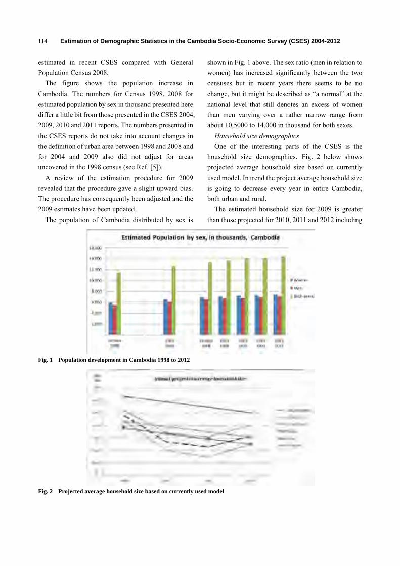
Estimation of Demographic Statistics in the Cambodia Socio-Economic Survey (CSES) 2004-2012
114
estimated in recent CSES compared with General Population Census 2008.
The figure shows the population increase in Cambodia. The numbers for Census 1998, 2008 for estimated population by sex in thousand presented here differ a little bit from those presented in the CSES 2004, 2009, 2010 and 2011 reports. The numbers presented in the CSES reports do not take into account changes in the definition of urban area between 1998 and 2008 and for 2004 and 2009 also did not adjust for areas uncovered in the 1998 census (see Ref. [5]).
A review of the estimation procedure for 2009 revealed that the procedure gave a slight upward bias. The procedure has consequently been adjusted and the 2009 estimates have been updated.
The population of Cambodia distributed by sex is
shown in Fig. 1 above. The sex ratio (men in relation to women) has increased significantly between the two censuses but in recent years there seems to be no change, but it might be described as “a normal” at the national level that still denotes an excess of women than men varying over a rather narrow range from about 10,5000 to 14,000 in thousand for both sexes.
Household size demographics One of the interesting parts of the CSES is the
household size demographics. Fig. 2 below shows projected average household size based on currently used model. In trend the project average household size is going to decrease every year in entire Cambodia, both urban and rural.
The estimated household size for 2009 is greater than those projected for 2010, 2011 and 2012 including
Fig. 1 Population development in Cambodia 1998 to 2012
Fig. 2 Projected average household size based on currently used model

Estimation of Demographic Statistics in the Cambodia Socio-Economic Survey (CSES) 2004-2012
115
Fig,3 Average household size in six CSES and Census 2008
urban and rural (see Fig 2). However, Fig. 3 below shows a different picture,
with estimates from the 2010 and 2011 CSES illustrating a steeper decrease in average household size than the modelled assumptions suggest. We also have indications from the migration statistics in CSES 2010 that the population in Cambodia was moving to Phnom Penh and other abroad. Most for job opportunity and in some cases (Marries, Repatriation or return after displacement, Insecurity, Transfer of work place. Etc.). In these cases the household size is decreasing.
Fig. 3 shows the estimated mean household size in the CSES surveys and the mean household size in normal households according to census 2008, see Ref. [6]. The census figure, is recorded after adjusting for the undercount.
Since we believe that systematic measurements bias is small in recording the CSES household sizes, we suspect from comparing Figs. 2-3 that the assumptions about the change in household sizes needs to be revised. There are signs that the decrease is faster than previously assumed. The CSES 2012 and the Inter-Censal survey 2013 will spread new light on this.
7. Final Comments and Conclusion
For a country, it is of outmost importance that the population statistics are reliable. Another requirement that sometimes appears is consistency in the numbers and estimates, hence that many sources provide if not the same but at least a similar picture of reality. The Cambodian 2008 census and its population projections have up till today been the baseline for improving the estimates of the CSES. This paper describes this estimation methodology and it also raises some questions and doubts, which are the key findings of this paper.
For example, the census results are getting older and there are signs that the accuracy is decreasing. Moreover, the methodology used to project the household sizes does also show signs of being off the mark. The future plans are to compare these findings with the results from the ongoing Cambodian Inter-Censal survey. It will be used to assess the quality of the census projections and to draw conclusions of how to improve future demographic estimates of the CSES.
References [1] Arriaga, E. (1994). Population Analysis with
Microcomputers, US Bureau of the Census, New York [2] National Institute of Statistics Cambodia. (2011) General
Population Census of Cambodia 2008, Analysis of the Census Result Report 12 Population Projection of Cambodia. (January 2011).
[3] Särndal, C-E. and Lundström, S. (2005) Estimation in Surveys with Nonresponse. New York, Wiley.
[4] National Institute of Statistics Cambodia (2004) First revisions of Population Projections for Cambodia 1998-2020. (June 2004).
[5] National Institute of Statistics Cambodia. (2010). Analysis of the Census Results Report 11, Family and Households. NIS June 2010.
[6] Pettersson, H. (2010). Average household sizes in the CSES-surveys, internal report, National Institute of Statistics Cambodia.

Journal of Mathematics and System Science 4 (2014) 116-126
Regulating Neuronal Hyper-Excitability and
Hyper-Synchrony in Epileptic Patients by Using PUFA,
Calcium and ATP Buffering
Kodwo Annan1, Bryan Banfill1, and Stephanie Brock2 1. Department of Mathematics & Computer Science, Minot State University, Minot, ND 58707
2. Department of Science, Minot State University, Minot, ND 58707 Received: December 18, 2013 / Accepted: January 23, 2013 / Published: February 25, 2014. Abstract: Epilepsy is a severe neurological disorder clinically identified by hyper-excitability and/or hyper-synchrony in the cortex and other subcortical regions of the brain. To regulate such excitability and synchrony, Hodgkin and Huxley model has been deployed with either PUFA or calcium buffering coupled with ATP modulate neurotransmitter release. We formulate and analyze a system of differential equations that describe the effects of PUFA, ATP, and calcium buffering in regulating neuronal hyper-excitability and hyper-synchrony in epileptic patients. We observed that PUFA had diverse effects on the gating variables. Specifically, there was a significant reduction in the inhibitory potency of PUFA on the -gatesm which may cause a direct inhibition of the voltage-gated Na+ channels and thus reduce neuronal excitability in epileptic patients. Also, the activation of the potassium channels by PUFA directly limited the neuronal hyper-excitability, while a small change in voltage potential coupled with PUFA restraint activated the voltage dependent ion channels which aided in lowering epileptic excitability in patients. In addition, higher ATP buffer levels in the presence of PUFA caused a significant hyperpolarization which may decrease neuronal excitability while lower ATP level initiated neuron depolarization. These results clearly suggest that PUFA coupled with calcium and ATP buffering could be used to modulate neuronal excitability excessive synchrony in epileptic patients. Keywords: PUFA, Calcium & ATP buffering, mathematical model, neuronal excitability.
1. Introduction
Epilepsy is a severe neurological disorder characterized by episodes of spontaneous recurrent seizures. The clinical manifestations of the seizures are identified by hyperexcitability and/or hypersynchrony in the cortex and other subcortical regions of the brain. Even though there are many factors linked to the etiology, the ion channels concept rooted in the seminal work of Hodgkin and Huxley [1] have become a central paradigm to describe and regulate such excitability and synchrony of neurons [2-8]. The underlying idea behind the Hodgkin and Huxley model is that the opening of voltage-gated sodium ( Na ) channels
Corresponding author: Kodwo Annan, Ph.D., assistant professor, research fields: epidemiological modeling, biomedical. E-mail: [email protected].
increases excitability while opening of voltage-gated potassium (K +) channels reduces excitability. Thus, several gain-of-function mutations in Na+ channels [2] as well as loss-of-function mutations in both delayed rectifier ( 1VK ) and A-type K (
3VK ) channels [7-8] are linked with epilepsy.
Studies have shown that highly synchronized neuronal activity during epileptogenesis is suppressed by the 3VK channel in dendrites, which therefore may function as a protective mechanism against hyperexcitability [9-12]. In epilepsy, since the 3VK current may not be strong enough to compensate for the excitability changes, antiepileptic substances such as the polyunsaturated fatty acids (PUFA) have been used in suppressing cellular responses to synchronicity during ketogenic diet to help prevent epileptic seizures
D DAVID PUBLISHING

Regulating Neuronal Hyper-Excitability and Hyper-Synchrony in Epileptic Patients by Using PUFA, Calcium and ATP Buffering
117
[13-15]. It is believed that PUFA targets and interacts with a wide range of ion channels, including Na+ and
K + channels, which lead to modified voltage dependence of the channels’ activation and inactivation [16-17].
In addition, earlier classic work of Hodgkin and Huxley included calcium ions ( 2Ca +) which studies have shown to regulates neurotransmitter release and ionic channel permeability [18-21]. At the neuronal level, 2Ca + depolarizes (as the sodium current), but also acts on the slower timescale of the potassium current. For example, research has shown that the concentration of calretinin acting as a fast calcium buffer controls the excitability of cerebellar granule cells and through the activation of high-conductance voltage- and 2Ca +activated K + [20-21]. Furthermore, Roussel et al. (2006) have indicated that changes in the buffer concentration can dramatically affect the electrical discharge pattern of cerebellar granule cells, hence allowing transitions between regular neuronal firing and different types of bursting [22].
Therefore, the basic concept of neuronal 2Ca + is that the influx of 2Ca + through voltage-operated channels causes transmitter release. Among them are the After-Hyperpolarization (AHPs) and the depolarizing After-Potentials (DAPs) which modify neuronal activity by suppressing or promoting hyperexcitability, respectively. Thus, to control the
2Ca + -dependent ion channels responsible for the variations in the membrane potential, 2Ca + entering through the voltage-operated channels or 2Ca + released from the internal stores needs to be regulated. To modulate neuronal excitability specifically, calcium homeostasis modulator 1 (CALHM1) have been shown to induce cation currents and elevate cytoplasmic
2Ca + concentration [20-22]. Adenosine-5-triphosphate (ATP) dependent
potassium channel ( ATPK ) is another substance shown to be potent regulators of neuronal excitability. Closing and opening of ATPK depends on the intracellular concentration of ATP. When the intracellular
ATP/adenosine diphosphate ratio increases, ATPK closes and vice versa. So, closing of ATPK leads to membrane depolarization and thus, increases the excitability while opening of ATPK hyperpolarizes the membrane and is inhibitory. Hence, activation/ opening of ATPK potentially protects against excitotoxicity.
The aim of this paper is to use conductance-based computational model to investigate the extent to which PUFA, calcium buffering and ATPK regulate neuronal excitability and synchronism in epileptic patients. The model allows us to investigate the effect of variations in the concentration of PUFA, calcium and ATPK in neuronal activity during epileptogenesis.
The model formulation is presented in section 2 followed by results and discussion in section 3. We finally make our conclusion in section 4.
2. Model Formulation
We adapt the conductance-based model proposed by Bischop et al. (2012) for neuronal excitability and calcium binding proteins [23]. The modification of the model includes calcium homeostasis modulator 1 and Adenosine-5-triphosphate channels. In addition, we modify the model to include PUFA modulated cellular responsible for altering the activity of the voltage gated ion channels. We focus on the ion channels,
1 3, ,
V VNa K KI I I and ATPI . The current conservation equation governing the membrane potential dynamics is given by
1 3V Vm Na K K CadVC I I I Idt
= − − − − −
CaK ATP leak inputI I I I− − − + (1) where mC and V are the membrane capacitance and potential of the neuron respectively, NaI is a fast transient Na+ current, 3vKI is a fast delayed rectifier potassium current, 1vKI a slow delayed rectifier potassium current, CaKI the 2Ca + activated K + current, CaI the calcium current, leakI the passive leak current, ATPI the ATP-dependent potassium ion current and inputI an external applied current. The ionic currents are given by

Regulating Neuronal Hyper-Excitability and Hyper-Synchrony in Epileptic Patients by Using PUFA, Calcium and ATP Buffering
118
1 1
3 3
3
41
23
2
2
( ),
( ),
( ),
( ),
( ),( ),
( ).
v v
v v
Na Na Na
K K K
K K K
CaK CaK K
Ca Ca Ca
ATP ATP ATP
l l l
I g m h V VI g n V V
I g n V V
I g k V VI g a V VI g V VI g V V
∞
∞
= −
= −
= −
= −
= −= −
= −
(2)
In Eq. (2), h and m are the activation and inactivation gating variables of the NaI current respectively, 1 3, , ,a k n n are respectively the activation variables of 1 3
, , ,v vCa KCa K KI I I I currents. Based on the
a clinical membrane capacitance values between 25 30 pF− , with membrane resistance 400 M Ω and resting membrane potential of 70mV− , the parameter values for (2) is presented in Table 1.
2.1 Modulation of PUFA
PUFA modulation of the Na+ channel ( NaI ) is implemented as a hyperpolarizing shift of the steady state inactivation curve given as 19 [ ]NamV PUFA× , where [ ]NaPUFA is altered in the interval between zero and one [24, 25]. This leads to the reduction of the sodium channel [24]. The implementation of PUFA modulation on the slow delayed rectifier potassium current, 1VKI , is a hyperpolarizing shift of the steady state activation curve by
18 [ ]
VKmV PUFA× that lead to an increase in the potassium current [26]. Similarly, we assume that the fast delayed rectifier potassium ion current, 3VKI , is also affected by PUFA with the same
value 3
8 [ ]VKmV PUFA× . Furthermore, we implement
PUFA modulation of ATP – dependent potassium channel, ATPI , as a shift from the resting membrane potential by 5 [ ]ATPmV PUFA− × . In our model, PUFA shifted activation and inactivation will be denoted by aPUFA and iPUFA respectively, while shifting both activation and inactivation is represented by aiPUFA .
2.2 Modeling gating Variables
To model gated voltage channels, each gate can be open or closed with transition probability from open to close ( )Vα and from close to open ( )Vβ . Thus, the fraction of open channels dynamics of the gating variables, 1 3, ,y h n n= follow [27]
( )(1 ) ( ) .y ydy V y V ydt
α β= − − (3)
Initially, the resting values of y is (0)
(0) .(0) (0)
y
y y
yα
α β∞ =+
(4)
However, as the voltage is clamped to a different voltage, V , the steady state values become
( )( ) .
( ) ( )y
y y
Vy V
V Vα
α β∞ =+
(5)
Solution to (3) is an exponential function of the form
( ) ( ) [ ( ) (0)]exp ,ty t y V y V yτ∞ ∞ ∞
= − − −
(6)
Where the time constant τ given by ( )y Vτ = 1
( ) ( )y yV Vα β+ and the steady-state gating variables
y∞ depend on the membrane potential V . In particular,
Table 1 The model parameters used to simulate equation (2). Parameter Value Reference Membrane capacitance, mC 30 pF [23] Calcium conductance, Cag 30 nS [23]
2Ca + activated K + conductance, CaKg 2 nS [28]
1VK potassium conductance, 1VKg 2 nS [23]
3VK potassium conductance, 3VKg 300 nS [23] Leak conductance, leakg 2.5 nS [23] Sodium conductance, Nag 700 nS [23] Calcium reversal potential, CaV 80 mV [22] Potassium reversal potential, KV 90 mV− [29] Leak reversal potential, leakV 68 mV− [23] Sodium reversal potential, NaV 74 mV [29]

Regulating Neuronal Hyper-Excitability and Hyper-Synchrony in Epileptic Patients by Using PUFA, Calcium and ATP Buffering
119
since the activations variables a and m in (2) are considered fast as compared to the other gating variables, we set their steady state values as
( )a a V∞= and ( )m m V∞= respectively with a∞ and m∞ defined as
61 exp , .7.775
m
m m
Va m αα β∞ ∞
− − = + = + (7)
With the kinetics of the a variable defined by Roussel et al. (2006) as Ref. [22]
18.0 0.1( 8.9)
1 exp[ 0.072( 5)] exp[0.2( 8.9)] 1aV
V Vτ
− +
= + + − − + − (8)
The K variable for the 2Ca + activated K + channels do not depend on voltage and can be modeled, according to Goldberg et al. (2009), as Ref. [28]
2
2
2 2
( ([ ] ) ) ,
[ ] 1, ,[ ] [ ]
i
k
ik
CaK i CaK i
k Ca kdkdt
CakK Ca K Ca
τ
τ
+∞
+
∞ + +
−=
= =+ +
(9)
where ,
,
off CaKCaK
on CaK
kK
k= with 1
, 0.2off CaKk ms−= and
the 2Ca + binding rate 1 1, 0.4on CaKk M msµ − −= .
2.3 Calcium Ion Current
Currents through voltage-activated 2Ca + channels play a critical double role. First, inward 2Ca + flux ( CaI ) depolarizes the cell, and thus contributes to action potential formation. Once reaching the intracellular compartment, however, 2Ca + is also a key second messenger, controlling a broad range of neuronal functions responsible for neurotransmitter release, which includes opening of 2Ca + -activated K + channels ( CaKI ). The basic concept of neuronal 2Ca + is the 2Ca + concentration change and calcium binding proteins. Changes of 2Ca + concentration, 2[ ]Ca + , have been observed to modulate neuronal excitability. For example, CALHM1 expression has been shown to induce cation currents in neuron cell and elevate cytoplasmic 2Ca + concentration ( 2[ ]Ca + ) in response
to removal of extracellular 2Ca + . Calcium binding proteins such as the Parvalbumin (PV) is a member of the calcium binding proteins group that has two mixed
2 2Ca Mg+ + binding sites. Since the binding of 2Ca + is determined by the slow 2Mg + off- rate, the dynamic mechanism of calcium in the presence of PV is modeled as
2[ ]id Cadt
+
=
2 2 [ ]([ ] [ ] ) ,2
Ca ii rest
I d PVCaCa CadFA dt
γ + +− − − −
(10)
2, ,
[ ] [ ] [ ] [ ] ,ion Ca i i off Ca i
d PVCa k Ca PV k PVCadt
+= −
(11) 2
, ,[ ] [ ] [ ] [ ] ,i
on Mg i i off Mg id PVMg k Mg PV k PVMg
dt+= −
(12) where 2[ ]Ca + and [ ]iPV represent the free intracellular 2Ca + and free (PV) concentrations respectively, [ ]iPVCa and [ ]iPVMg are the concentration of PV bound to 2Ca + and 2Mg + with the total concentration of PV [ ] [ ]T iPV PV= +[ ] [ ]i iPVCa PVMg+ The inward flux term is
2CaI
dFA− where F is the Faraday constant and A is
the cell surface area of a shell with thickness
0.2d mµ= . The term ( )2 2[ ] [ ]i restCa Caγ + +− is the
clearance mechanism associated with 2Ca + fluxes across the membrane where 11msγ −= and 2[ ]restCa + .
0.07 Mµ= In addition, PV might also act as a fast buffer [34]
and so we consider both fast and slow buffers by denoting [ ]iB and [ ]iBCa , respectively, as the concentration of free and bound buffer for slow or fast buffer with total buffer [ ] [ ] [ ]T i iB B BCa= + . Therefore, we can couple the calcium dynamics as
2[ ]id Cadt
+
=
2 2 [ ]([ ] [ ] ) ,2
Ca ii rest
I d BCaCa CadFA dt
γ + +− − − − (13)

Regulating Neuronal Hyper-Excitability and Hyper-Synchrony in Epileptic Patients by Using PUFA, Calcium and ATP Buffering
120
2[ ] [ ] [ ] [ ] .ion i i off i
d BCa k Ca B k BCadt
+= − (14)
3. Numerical Results and Discussions
We numerically simulate the Eqs. (1)-(14) with model parameter values stated in Tables 1 and 2 by using a fourth-order Runge-Kutta method and MATLAB software tool. Given a differential equation
( ) ( , ( ))y t f t y t′ = with initial condition, the method determines the next point on the curve by using the previous point and the weighted averages of the four increments (i.e. 1 ( , )n nk hf t y= ,
2 11( , )
2 2n nhk hf t y k= + + ,
3 21( , )
2 2n nhk hf t y k= + + ,
4 3( , )n nk hf t h y k= + + ).
The first increment, 1k , is simply Euler increment. It takes into consideration the slope of the tangent of the previous point with the step size h . The second increment is based on the slope of the tangent at the center of the step. While the third and fourth increments are the slope in the middle with respect to the second increment and at the end of the step, respectively.
3.1 PUFA Effects on Gating Variables
Fig. 1 characterizes the potency of PUFA on voltage
-gated sodium channels. The activation -gatesm and the inactivation -gateh curves and PUFA effects on both gated variables are plotted against time.
There is a significant reduction in the inhibitory potency of PUFA on the -gatesm while the -gateh became almost completely resistant to PUFA. The strong but transient inhibition of the -gatesm may directly decrease the sodium current and thus reduce neuronal membrane excitability. In addition, since PUFA also shift the inactivation of the sodium channel [25], it may have a direct inhibition on voltage-gated sodium ion channel and thus act to limit hyperexcitability activity.
The activation of potassium channels such as the slow and fast delayed rectifier potassium currents, 1VK and 3VK with their PUFA effects are illustrated in Fig. 2.
The 1VK shows strong but persistent potassium currents with delayed onset and slow inactivation with PUFA while 3VK depicts weak but fast onset and fast inactivation of potassium current with PUFA. Therefore, a highly synchronized neuronal activity may be suppressed by the 3VK channel and may function as a protective mechanism against hyperexcitability. Hence, PUFA may act directly to limit hyperexcitability and seizure activity by activating the potassium channels.
Table 2 The model parameters used to simulate equations (10)-(14). Parameter Value Reference Cell surface area, A 23000 mµ [23] Shell thickness, d 0.2 mµ [23]
2Ca + extrusion rate, γ 11ms− [23] Resting 2Ca + concentration, 2[ ]restCa + 0.07 Mµ [23]
2Mg + concentration, 2[ ]iMg +
500 Mµ [30] 2Ca + binding rate to PV, ,on CaK 1 10.1 M msµ − − [31]
PV affinity for 2Ca +, ,D CaK 0.01 Mµ [32] Fast 2Ca + buffer binding rate, onk 1 10.1 M msµ − − [31] Slow 2Ca + buffer binding rate, onk 1 10.1 M msµ − − [33] Fast buffer affinity for 2Ca +, DK 0.01 Mµ [32] Slow buffer affinity for 2Ca +, DK 0.1 Mµ [33] PV affinity for 2Mg +, ,D Mgk 31 Mµ [32]
2Mg + unbinding rate from PV, ,off MgK 10.025 ms− [31] 2Mg + binding rate from PV, ,on MgK 1 10.0008 M msµ − − [31]

Regulating Neuronal Hyper-Excitability and Hyper-Synchrony in Epileptic Patients by Using PUFA, Calcium and ATP Buffering
121
Fig. 1 The sensitivity of the activation and inactivation gating variables h and m to PUFAs with respect to time is illustrated. PUFAs caused a significant reduction in the activation -gatesm while there is nearly no effects on the inactivation -gateh . This may cause a direct inhibition of the voltage-gated Na+
channels and thus reduce neuronal excitability.
Fig. 2 The delayed rectifiers of the potassium currents are displayed. While there is strong potassium current of the slow delayed rectifier there exist a weak fast delayed rectifier with or without PUFA. However in both cases, there is a significant activation increase of potassium currents with PUFA which may suppress hyperexcitability and/or hypersynchrony of neurons.
Fig. 3 shows the effect of PUFA on the activation of calcium and the calcium-activated potassium channels. As can be seen, there is an increase in steepness as well
as the shift of the calcium activation when PUFA is added. The rapid initial activation of the -gatinga variable may affects calcium inward current which
0 0.5 1 1.5 2 2.5 3 3.5 4 4.5 50
0.1
0.2
0.3
0.4
0.5
0.6
0.7
0.8
0.9
1
Time (ms)
Gat
ing
Var
iabl
es
The Effects of PUFA on m and h Gating Variables
m Without PUFAm With PUFAh without PUFAh with PUFA
0 0.5 1 1.5 2 2.5 3 3.5 4 4.5 50
0.1
0.2
0.3
0.4
0.5
0.6
0.7
0.8
0.9
1
Time (ms)
Gat
ing
Var
iabl
es
The Effects of PUFA on Kv1 and Kv3 Gating Variables
Kv1 Without PUFAKv1 With PUFAKv3 without PUFAKv3 with PUFA

Regulating Neuronal Hyper-Excitability and Hyper-Synchrony in Epileptic Patients by Using PUFA, Calcium and ATP Buffering
122
Fig. 3 PUFA rapidly activates and shifts the -gatinga variable curve along the gating axis initially, then slow down afterwards while no change is encountered in the 2Ca + -activated K + channels. The slow and fast activation of the
-gatinga variable leads to calcium buffering which may result in bursting.
may cause fast calcium buffering in the system. The slowdown in the activation of -gatinga later on indicates a slower 2Ca + dynamics. Indeed, the transition to bursting arising with an increased calcium buffering capacity may be the direct consequence of the no-PUFA effects in the activation of -gatinga-activated K + channels due to the slower -gatinga dynamics. The coexistence of the fast and slow gating variables which lead to bursting is caused by the presence of PUFA concentration. In addition, the presence of PUFAs cause negligible conductance of
2Ca + -dependent K + channels that are known to couple voltage-gated 2Ca + channels.
3.2 PUFA Effects on Voltage Potential
PUFA also has a potential of altering the activity of voltage dependence channel. Without PUFA,
Studies have shown that all neurons are electrically excitable, maintaining voltage gradients across their membranes. From Fig. 4, a small change in the voltage potential results in a large effect on neurons excitability
in the absence of PUFA. The steep voltage change alters the functions of the voltage-dependent potassium channel which is in the region that matters for epileptic repetitive firing. However, applying PUFA significantly changes the steep curvature and shape of the voltage potential curve. PUFA induced a shift of early and final voltage dependence and linearized transition which may strongly supports the hypothesis that PUFA acts directly on the voltage dependence. Hence, may suggest that PUFA has major effects on early and final voltage dependence transitions that lower epileptic excitability in patients.
3.3 Effects of ATP Level Coupled with PUFA
To evaluate the role ATP plays in the presence of PUFA, we assume the notion that PUFA generally increases ATP level and varied the ATP levels above and below the standard ATP (i.e. 2 mM). Higher ATP level (5 mM) causes a small transient outward current in voltage mode and opens the ATP-sensitive potassium ( ATPK ) channel, see Fig. 5. Since the ATPK
0 0.5 1 1.5 2 2.5 3 3.5 4 4.5 50
0.1
0.2
0.3
0.4
0.5
0.6
0.7
0.8
0.9
1
Time (ms)
Gat
ing
Var
iabl
es
The Effects of PUFA on a- and k- Gating Variables
a Without PUFAa With PUFAk without PUFAk with PUFA

Regulating Neuronal Hyper-Excitability and Hyper-Synchrony in Epileptic Patients by Using PUFA, Calcium and ATP Buffering
123
Fig. 4 The effect of PUFA on a small change in voltage potential is plotted against time. A small voltage change coupled with PUFA moderates the voltage-gated ion channels by shifting the steady-state activation curve in negative direction along the voltage axis.
Fig. 5 PUFA coupled with significant or high ATP concentration level causes small transient outward current and may decrease neuronal excitability in epileptic patients. The ATP amount used was 5 mM which is significantly higher than the standard ATP of 2 mM.
channel is noted to be an excellent mediator for excitability, we suggest that PUFA coupled with sufficient or high ATP concentration level will cause
neurons to significantly hyperpolarize themselves via direct ATP release. This hyperpolarization may decrease neuronal excitability and subsequently
0 0.1 0.2 0.3 0.4 0.5 0.6 0.7 0.8 0.9 1-80
-60
-40
-20
0
20
40
60
80
100
Time (ms)
Vol
tage
(mV
)
Voltage Change per Time with and without PUFA
Without PUFAWith PUFA
0 0.1 0.2 0.3 0.4 0.5 0.6 0.7 0.8 0.9 1-80
-60
-40
-20
0
20
40
60
80
100
Time (ms)
Vol
tage
(mV
)
Voltage Change per Time for Higher ATP Value
Without PUFAWith PUFA

Regulating Neuronal Hyper-Excitability and Hyper-Synchrony in Epileptic Patients by Using PUFA, Calcium and ATP Buffering
124
Fig. 6 PUFA coupled with significantly low ATP value of 0.5 mM causes a large transient inward current and therefore resulting in neuron depolarization.
reduces epileptic activity, see Fig 5. Contrary, Fig. 6 shows that reducing ATP
concentration level to 0.5 mM causes a large but transient inward current in voltage mode. Therefore, the ATPK channel which represents a type of inward rectifying potassium channel is activated when ATP concentration level is low and thus depolarizes the neurons.
4. Conclusion
In conclusion, we have generated a system of differential equations that describe the role PUFA plays in regulating neuronal hyper-excitability and hyper-synchrony in epileptic patients by moderating calcium and ATP Buffering. First, we observed that PUFA has diverse effects (increasing and decreasing) on the gating variables. There is a significant reduction in the inhibitory potency of PUFA on the -gatesmwhile the -gateh became almost completely resistant to PUFA. This observation may cause a direct inhibition of the voltage-gated Na+ channels and thus reduce neuronal excitability in epileptic patients. In addition, the activation of potassium channels (the slow
and fast delayed rectifier potassium currents, 1VK and
3VK ) by PUFA directly limited the neuronal hyper-excitability. Furthermore, a small change in voltage potential coupled with PUFA moderation activated the voltage dependent ion channels which aided in lowering epileptic excitability in patients. We then altered the ATP buffering below and above the standard value of 2 mM and observed that PUFA coupled with higher ATP level caused a significant hyperpolarization which may decrease neuronal excitability while low ATP level caused neuron depolarization. These results clearly suggest that PUFA coupled with calcium and ATP buffering could modulate neuronal excitability in epileptic patients.
Reference [1] Hodgkin A, Huxley A (1952), A quantitative description
of membrane current and its application to conduction and excitation in nerve. J. Physiol. 117: 500-544.
[2] Meisler MH, Kearney JA (2005) Sodium channel mutations in epilepsy and other neurological disorders. J Clin Invest 115: 2010–2017.
[3] Hahn A, Neubauer BA (2009) Sodium and potassium channel dysfunctions in rare and common idiopathic epilepsy syndromes. Brain Dev 31: 515–520.
0 0.1 0.2 0.3 0.4 0.5 0.6 0.7 0.8 0.9 1-80
-60
-40
-20
0
20
40
60
80
100
Time (ms)
Vol
tage
(mV
)
Voltage Change per Time for lower ATP Value
Without PUFAWith PUFA
Regulating Neuronal Hyper-Excitability and Hyper-Synchrony in Epileptic Patients by Using PUFA, Calcium and ATP Buffering
125
[4] Singh NA, Charlier C, Stauffer D, DuPont BR, Leach RJ, et al. (1998) A novel potassium channel gene, KCNQ2, is mutated in an inherited epilepsy of newborns. Nat Genet 18: 25–29.
[5] Charlier C, Singh NA, Ryan SG, Lewis TB, Reus BE, et al. (1998) A pore mutation in a novel KQT-like potassium channel gene in an idiopathic epilepsy family. Nat Genet 18: 53–55.
[6] Biervert C, Schroeder BC, Kubisch C, Berkovic SF, Propping P, et al. (1998) A potassium channel mutation in neonatal human epilepsy. Science 279: 403–406.
[7] Browne DL, Gancher ST, Nutt JG, Brunt ER, Smith EA, et al. (1994) Episodic ataxia/myokymia syndrome is associated with point mutations in the human potassium channel gene, KCNA1. Nat Genet 8: 136–140.
[8] Singh B, Ogiwara I, Kaneda M, Tokonami N, Mazaki E, et al. (2006) A Kv4.2 truncation mutation in a patient with temporal lobe epilepsy. Neurobiol Dis 24: 245–253.
[9] Bragin A, Mody I, Wilson CL, Engel J (2002) Local generation of fast ripples in epileptic brain. J Neurosci 22: 2012–2021.
[10] Lasztoczi B, Antal K, Nyikos L, Emri Z, Kardos J (2004) High-frequency synaptic input contributes to seizure initiation in the low-[Mg2+] model of epilepsy. Eur J Neurosci 19: 1361–1372.
[11] Fransén E, Tigerholm J (2010) Role of A-type potassium currents in excitability, network synchronicity, and epilepsy. Hippocampus 20: 877–887.
[12] Gasparini S, Migliore M, Magee JC (2004) On the initiation and propagation of dendritic spikes in CA1 pyramidal neurons. J Neurosci 24: 11046–11056.
[13] Leaf A, Xiao YF, Kang JX, Billman GE (2005) Membrane effects of the n-3 fish oil fatty acids, which prevent fatal ventricular arrhythmias. J Membr Biol 206: 129–139.
[14] Taha AY, Burnham WM, Auvin S (2010) Polyunsaturated fatty acids and epilepsy. Epilepsia 51: 1348–1358.
[15] Xu XP, Erichsen D, Börjesson SI, Dahlin M, Åmark P, et al. (2008) Polyunsaturated fatty acids and cerebrospinal fluid from children on the ketogenic diet open a voltage-gated K channel: A putative mechanism of antiseizure action. Epilepsy Res 80: 57–66.
[16] Börjesson SI, Parkkari T, Hammarström S, Elinder F (2010) Electrostatic Tuning of Cellular Excitability. Biophys J 98: 396–403.
[17] Börjesson SI, Elinder F (2011) An electrostatic potassium channel opener targeting the final voltage sensor transition. J Gen Physiol 137: 563–577.
[18] Schwaller, B. (2009). The continuing disappearance of “pure” Ca2+ buffers. Cell. Mol. Life Sci. 66, 275–300.
[19] Lambers, T. T., Mahieu, F., Oancea, E., Hoofd, L., de Lange, F., Mensenkamp, A. R., Voets, T., Nilius, B., Clapham, D. E., Hoenderop, J. G., and Bindels, R. J.
(2006). Calbindin-d28k dynamically controls trpv5-mediated Ca2+ transport. EMBO J. 25, 2978–2988.
[20] Gall, D., Roussel, C., Nieus, T., Cheron, G., Servais, L., D’Angelo, E., and Schiffmann, S. N. (2005). Role of calcium binding proteins in the control of cerebellar granule cell neuronal excitability: experimental and modeling studies. Prog. Brain Res. 148, 321–328.
[21] Bearzatto, B., Servais, L., Roussel, C., Gall, D., Baba-Aïssa, F., Schurmans, S., de Kerchove d’Exaerde, A., Cheron, G., and Schiffmann, S. N. (2006). Targeted calretinin expression in granule cells of calretinin-null mice restores normal cerebellar functions. FASEB J. 20, 380–382.
[22] Roussel, C., Erneux, T., Schiffmann, S. N., andGall, D. (2006). Modulation of neuronal excitability by intracellular calcium buffering: from spiking to bursting. Cell Calcium 39, 455–466.
[23] Bischop DP, Orduz D, Lambot L, Schiffmann SN., Gall D. (2012) Control of neuronal excitability by calcium binding proteins : a new mathematical model for striatal fast-spiking interneurons, Frontiers in Molecular Neuroscience, Vol 5:78, DOI=10.3389/fnmol.2012.00078
[24] Vreugdenhil M, bruehl C, Voskuyl RA, Kang JX, Leaf A, et al. (1996) Polyunsaturated fatty acids modulate sodium and calcium currents in CA1 neurons. Proc Natl Acad Sci USA 93: 12559-12563.
[25] Leaf A, Xiao YF, Kang JX, Billman GE, (2003) Prevention of sudden cardiac death by n-3 polyunsaturated fatty acids. Pharmacology & Therapeutics, 98: 355-377
[26] Xu XP, Erichsen D, Börjesson SI, Dahlin M, Åmark P, et al. (2008) Polyunsaturated fatty acids and cerebrospinal fluid from children on the ketogenic diet open a voltage-gated K channel: A putative mechanism of antiseizure action. Epilepsy Res 80: 57–66
[27] Mancilla, J. G., Lewis, T. J., Pinto, D. J., Rinzel, J., and Connors, B. W. (2007). Synchronization of electrically coupled pairs of inhibitory interneurons in neocortex. J. Neurosci. 27, 2058–2073.
[28] Goldberg, J. A., Teagarden, M. A., Foehring, R. C., and Wilson, C. J. (2009). Nonequilibrium calcium dynamics regulate the autonomous firing pattern of rat striatal cholinergic interneurons. J. Neurosci. 29, 8396– 8407.
[29] Jolivet, R., Lewis, T. J., and Gerstner, W. (2004). Generalized integrate-and-fire models of neuronal activity approximate spike trains of a detailed model to a high degree of accuracy. J. Neurophysiol. 92, 959–976.
[30] Li-Smerin, Y., Levitan, E. S., and Johnson, J. W. (2001). Free intracellular Mg(2+) concentration and inhibition of NMDA responses in cultured rat neurons. J. Physiol. (Lond.) 533(Pt 3), 729–743.
[31] Lee, S. H., Schwaller, B., and Neher, E. (2000). Kinetics

Regulating Neuronal Hyper-Excitability and Hyper-Synchrony in Epileptic Patients by Using PUFA, Calcium and ATP Buffering
126
of Ca2+ binding to parvalbumin in bovine chromaffin cells: implications for [Ca2+] transients of neuronal dendrites. J. Physiol. (Lond.) 525(Pt 2), 419–432.
[32] Eberhard, M., and Erne, P. (1994). Calcium and magnesium binding to rat parvalbumin. Eur. J. Biochem. 222, 21–26.
[33] Schwaller, B., Meyer, M., and Schiffmann, S. (2002).
‘New’ functions for ‘old’ proteins: the role of the calcium-binding proteins calbindin d-28k, calretinin and parvalbumin, in cerebellar physiology studies with knockout mice. Cerebellum 1, 241–258.
[34] Eggermann, E., and Jonas, P. (2012). How the ‘slow’ Ca(2+) buffer parvalbumin affects transmitter release in nanodomain-coupling regimes. Nat. Neurosci. 15, 20–22.

Journal of Mathematics and System Science 4 (2014) 127-132
Development and Application of Statistical Business
Register Guidelines in African Countries
Michael J. Colledge1 and Besa Muwele2 1. Michael Colledge Statistical Consulting, Canberra, Australia
2. African Development Bank, Pretoria, South Africa Received: September 06, 2013 / Accepted: Octorber 18, 2013 / Published: February 25, 2014. Abstract: Within the framework of its Statistical Capacity Building Program the African Development Bank (AfDB) is supporting development and improvement of statistical business registers (SBRs) in African countries. As a first step, the AfDB prepared a document entitled Guidelines for Building Statistical Business Registers in Africa, which describes SBR design, construction, introduction, use and maintenance. To support dissemination, interpretation and effective use of the Guidelines, the AfDB is now sponsoring a programme of review and recommendations for enhancements to SBRs in selected African national statistical offices. The paper outlines the content of the Guidelines and experiences in their application. The views expressed are those of the authors and do not necessarily reflect an official position of the AfDB. Keywords: Administrative data, economic statistics, profiling, statistical capacity building, statistical integration
1. Introduction
1.1 Motivation for Guidelines
Coordination of the individual surveys and administrative collections that constitute the economic statistics program of a national statistical office (NSO) is vital. It depends upon the use of a common conceptual framework, including, in particular, the System of National Accounts (SNA) and the International Standard Industrial Classification of All Economic Activities (ISIC). A crucial requirement in making this framework operational is to ensure that the frames for the individual surveys are properly harmonized.
An up-to-date survey frame (meaning a list of units and information about those units needed for the survey) is required for each repetition of a regularly conducted survey. It is more effective and efficient to maintain a frame so that it can support the sequence of repetitions of a survey than it is to create the frame afresh with
Corresponding author: Michael J. Colledge, Michael
Colledge Statistical Consulting Pty Ltd, e-mail: [email protected].
each repetition. Survey frame maintenance is best achieved through the development of a single statistical business register (SBR) and its use as the source of frames for all economic surveys. (The adjective statistical is added to the usual term business register to emphasize that the register is developed by an NSO for statistical purposes.)
The design, development, and introduction or enhancement of an SBR is considered so important that it appears as a core goal in the five-year national strategies of most, if not all, African NSOs. In response to requests from NSOs, the African Development Bank (AfDB) established a project to prepare and promote the document entitled Guidelines for Building Statistical Business Registers in Africa (abbreviated SBR Guidelines).
1.2 Objectives of SBR Guidelines
The objectives of the Guidelines are to provide: a general background on the need for a SBR and
the concepts on which it is based; a detailed description of the functions of an SBR
and its inputs and outputs; detailed information on the development and
D DAVID PUBLISHING

Development and Application of Statistical Business Register Guidelines in African Countries
128
implementation of an SBR; and a starting point for harmonization of SBRs across
African NSOs. The Guidelines are expected to be useful to: SBR managers and staff – by detailing SBR
concepts, SBR creation and maintenance procedures, and SBR quality and performance measures; economic survey managers and staff – by
providing the basic concepts on which an SBR is based, by describing the generation of survey frames from the SBR, and by discussing the possibility of publishing SBR data; staff responsible for respondent relations – by
defining and enabling calculation of individual and cumulative respondent burden imposed by economic surveys; staff responsible for liaison with other
organizations in the national statistical system and with international organizations – by providing the basic concepts; and senior managers – in outlining the basic concepts,
and providing quality and performance measures and suggestions for quality improvements.
1.3 Existing Documentation on Business Registers
The starting point for development of the SBR Guidelines was existing international documentation on SBRs. This includes: papers from 23 meetings of the Wiesbaden Group
on Business Registers (formerly International Round Table on Business Survey Frames), which provides a forum for the exchange of views on development, maintenance and use of business registers; papers from joint UNECE/EUROSTAT/OECD
meetings of the Expert Group on Business Registers; the Business Registers Recommendation Manual
for European Union (EU) countries; discussions of the Euro Groups Register Project –
a network of SBRs in EU countries, focusing on multinational enterprise groups; EU regulations - Regulation 177/2008
establishing a common framework for business registers for statistical purposes, and Regulation
696/93 on the statistical units for the observation and analysis of production systems.
By and large this documentation is too sophisticated to provide the basic guidance required by developing African NSOs, some of whom do not have a working SBR, or have one with only a very limited functionality.
The Wiesbaden Group recognized the need for international SBR guidelines and a guidelines development project was subsequently set up by the Bureau of the European Conference of Statisticians. However, the resulting document will go through several iterations, which will take time. Also, it will be aimed at all countries, in particular NSOs with well developed SBRs, and thus will likely address with the sort of complex issues that the Group members are currently tackling.
1.4 Development of SBR Guidelines
Taking into account relevant international standards, existing SBR documentation, and current status of SBRs in Southern African countries, the AfDB prepared a preliminary draft of the SBR Guidelines in January 2012.The draft was discussed at an Expert Group Meeting (EGM) held in Pretoria in May 2012 and attended by SBR unit heads from 12 NSOs belonging to Southern African Development Community (SADC) and Common Market for Eastern and Southern Africa (COMESA) countries. Comments and examples from EGM were used in preparation of the first version of the Guidelines in October 2012.
1.5 Application of SBR Guidelines
To promulgate and promote the SBR Guidelines, the AfDB set up a program of missions to selected SADC and COMESA countries. The program aims are: to review the existing register(s), if any, at each
NSO visited and to prepare a comprehensive suite of recommendations for register improvement, incorporating ideas from SBR Guidelines but tailoring them to each particular country’s specific requirements; to identify additions and changes to the SBR

Development and Application of Statistical Business Register Guidelines in African Countries
129
Guidelines to make them more useful.
2. Content of SBR Guidelines
2.1 SBR Guidelines Part I: Underlying Concepts and Methods
The aims of Part I are, first, to describe the environment within which an SBR operates and to indicate the role of the SBR, second, to detail the underlying concepts and methods, including broadly accepted principles and practices, on the basis of which an SBR should be designed, developed, and implemented.
Chapter 2 summarizes the conceptual framework for economic statistics provided by the System of National Accounts 2008 (SNA2008) in so far as it is relevant to the SBR. It defines what is meant by economic production and by enterprise. It explains the need to profile (divide) large complex enterprises into smaller units such as establishments for data collection purposes and it introduces the International Standard Industrial Classification of All Economic Activities (ISIC) Rev 4.
Chapter 3 describes the types of units – legal, administrative, and statistical units – that are important in the context of survey frames, and how they relate to one another.
Chapter 4 discusses the elements of an economic statistics program and the need for and use of a frame for each survey, and it details the contents of a survey frame.
Chapter 5 explains the reasons for an SBR, its primary function in providing survey frames, its other possible functions in measuring business respondent burden, in linking business statistics databases, and as a stand-alone source of business statistics.
2.2 SBR Guidelines Part II: SBR Design
Part IIA focuses on design of SBR coverage (units) and content (data items) and the input sources and functions by which coverage and content are created and maintained.
Chapter 6 presents a framework for specification of an economic units model and the coverage and content of the SBR.
Chapter 7 provides details of the administrative sources of SBR data and how they are used in combination to construct and maintain the SBR.
Chapter 8 describes additional sources of SBR data involving direct data collection, including profiling of large businesses, SBR improvement surveys, and use of survey feedback.
Chapter 9 indicates how the various sources are used in combination to update the SBR as businesses are created, transformed, and disappear over time.
Chapter 10 sets out an SBR maintenance strategy and outlines update procedures.
Part IIB focuses on design of the outputs and output functions of the SBR.
Chapter 11 discusses the primary output function of the SBR, namely the production of survey frames, also the coordination of sample selection across surveys and the creation of survey control files.
Chapter 12 deals with the other output functions relating to respondent management, business statistics, and linkage of data across sources. It describes how the reporting commitments of individual business respondents can be identified and overall respondent burden can be compiled. It discusses the production of business statistics directly from the SBR and the role of the SBR in bringing together data from surveys and administrative sources.
Part IIC focuses on the organization of the SBR and the system that supports it.
Chapter 13 discusses SBR organization and operations.
Chapter 14 deals with SBR systems, i.e., application programs and database.
Chapter 15 focuses on SBR quality and performance management and evaluation.
2.3 SBR Guidelines Part III: SBR Implementation
Part III details the steps in the implementing or enhancing an SBR.
Chapter 16 presents a broad level plan for first-time design, development, and introduction of an SBR.

Development and Application of Statistical Business Register Guidelines in African Countries
130
Chapter 17 presents a broad level plan for review of an existing SBR, for determination of the extent of the changes required – reengineering, major enhancement, or continuous improvement – and for implementation of these changes.
2.4 Summary Diagrams
Figures 1 and 2 summarise the SBR functions, inputs, outputs and data model.
3. Experiences in Application of the SBR Guidelines
3.1 NSOs and Countries Visited
SBRs have been reviewed and recommendations for improvements made in five countries to date: Statistics Botswana, the Central Statistical Office (CSO) Zambia, the National Bureau of Statistics (NBS) Tanzania,
Figure 1: Summary of SBR Functions, Inputs and Outputs.
Figure 2: Summary model of organizational, administrative and statistical units.

Development and Application of Statistical Business Register Guidelines in African Countries
131
Statistics Mauritius (SM) and the Instituto Nacional de Estistica (INE) Mozambique.
3.2 Principal Findings
There are both striking similarities and significant differences in SBRs across the NSOs.
In theory, the SBR is a high priority in all NSOs. In practice it is sometimes poorly staffed and not always used. It is administered by separate organisational unit in four of the five countries. (The advantage of SBR administration by a separate unit is that it is likely to receive more priority.)
In only one country is the SBR based on and maintained from an administrative source. In this one case it is based on business licences, which is not a particularly good source for two reasons. First, a single enterprise may have several licenses and hence there is potential duplication of enterprises. Second, licences may be administered by local authorities as well as by national agencies, so many organisations may be involved and data collection correspondingly difficult.
In all cases the SBR contains too many enterprises to be sustainable in the absence of automated updating from an administrative source, and in no case is updating automated. The result is that, in all but one case, the SBR is not sufficiently comprehensive or up to date to be used as the source of the frame for the annual enterprise survey and thus the survey has to maintain and use its own frame.
In the past there were few large complex enterprises but, as countries grow, they become more numerous. This, coupled with an increasing demand for regional statistics, means there is a need to divide large complex enterprises into establishments for data collection purposes. However, in no case does the SBR contain enterprises and establishments. Thus, there is general lack of capacity to deal effectively with large complex enterprises.
In three countries the SBR System comprises a set of Excel files on personal computers. This means there is no effective version control and little capacity to
increase functionality or to automate. In the two countries with databases, the latter have limited functionality.
3.3 Principal Recommendations
Use international standard concepts and best practices. It is both efficient and effective to make full use of international standards such as SNA2008 and ISIC Rev 3. It is efficient because it saves development effort. It is effective because it results in use of well tried and tested concepts, systems and procedures
Define an enterprise to be in one to one correspondence with a legal entity. As most administrative processes register and deal with legal and natural persons, this makes lists of enterprises easy to obtain directly from administrative sources.
Use the simplest possible statistical units model. The SNA2008 describes three possible types of smaller standard statistical units into which an enterprise can be divided. One unit – the establishment - is sufficient. Provision should also be made for associating enterprises linked by ownership and/or control into enterprise groups.
A good quality well defined small SBR is better than a larger poorly defined SBR of inferior quality. It is simply not possible for the SBR to provide coverage of every enterprise within the SNA2008 production boundary. Many small enterprises are too difficult to identify and locate and then too volatile to track over time. Thus, there has to be a type/size related threshold below which the SBR does not provide coverage. In defining this threshold it is better to aim for well defined coverage of a smaller number of clearly visible and trackable enterprises than for less certain coverage of a larger number of enterprises that are more difficult to identify and to track. The temptation to add enterprises that have been found during the course of field operations should be resisted.
Use administrative data to provide SBR coverage. Administrative registers list and track specific groups of enterprises according to the particular legislation

Development and Application of Statistical Business Register Guidelines in African Countries
132
being enacted. The most efficient and effective way of identifying and tracking enterprises is to make use of administrative registers. They should be the only source of coverage.
Define the coverage provided by the SBR to be the formal sector. This definition is very practical and easily understood. Also, given that the SBR coverage is based on administrative sources, the definition is perfectly in line with the informal sector framework given in the International Conference of Labor Statisticians 1993 Resolution.
Undertake SBR design in broader context of economic survey program redesign. The introduction of a comprehensive SBR is a catalyst for review and re-engineering the economic statistics program as a whole. Maximum use should be made of data from administrative sources. Formal sector surveys should be driven by the SBR. Informal sector production should be covered on an occasional basis by introduction of a household based informal sector survey.
Incorporate sample selection and sample control file creation procedures in the SBR. In order to ensure that sample selection and sample control file creation procedures are standardised and follow smoothly from survey frame creation, these functions should be included within the SBR framework.
Automate as much as possible. The key to efficiency is to standardise and to automate, in particular to avoid the need for repetitive clerical activities. In the context of the SBR, processing of data from administrative sources must be automated, as must be the production of survey frames and samples
Ensure SBR database and applications are maintainable. It is essential to use a database not
spreadsheets as the repository of SBR data. Spreadsheets are well known to be error-prone, processing can be automated only in a clumsy way, and maintenance is difficult especially if the development staff leave.
4. Conclusions
Future developments include SBR review and recommendations in more countries, revision of the SBR Guidelines in light of experiences, and establishment of a project for development of generic SBR System and its installation in NSOs who want to use it.
Without a reasonably well developed SBR System (meaning database and accompanying programmes) only very marginal improvements to an existing SBR are possible. At a minimum, the SBR System has to be able to support automated processing of incoming administrative data and to produce survey frames on demand. A universal problem is that NSOs do not have on site IT capacity to build even a minimal SBR System.
The SBR used by INE Mozambique, actually called the Fichier Unidadas Estistica (FUE), provides an excellent example of how this problem is best addressed. The FUE was developedand promoted by Instituto Nacional de Estistica Portugal and Instituto Nacional de Estistica Cape Verde (INECV) for the five Portuguese speaking African countries. A private consulting company working on contract actually built and installed the system in the countries. Whilst the FUE system does not have functionality needed to enable automated update, it shows the direction to go. It is envisaged that the generic SBR System will be based on Statistics Mauritius’ New SBR System or will be an enhancement of the FUE System.

Journal of Mathematics and System Science 4 (2014) 133-138
Effect of Heteroscedastic Variance Covariance Matrices
on Two Groups Linear Classification Techniques
Friday Zinzendoff Okwonu1,2 and Abdul Rahman Othman2 1. Department of Mathematics and Computer Science, Delta State University, P.M.B.1, Abraka, Nigeria.
2. Center for Mathematical Sciences, PPJJJ, Universiti Sains Malaysia, 11800, Penang, Malaysia. Received: Octorber 23, 2013 / Accepted: November 28, 2013 / Published: February 25, 2014. Abstract: The authors investigate the comparative classification performance of the two groups linear classification techniques. They compared the Fisher linear classification analysis, its robust version based on the minimum covariance determinant with the Filter linear classification rule and the linear combination linear classification technique. These procedures are investigated using laboratory reared aedes albopictus mosquito data set and simulated data set generated based on heteroscedastic covariance matrices with various proportion of contamination. The evaluation procedure is based on the effect of contamination on the mean probabilities of correct classification obtain for each technique. The comparative analysis revealed that the robust Fisher linear classification rule and the linear combination linear classification rule are robust and comparable than the other procedures. Keywords: Classification, Heteroscedastic, mean probability, robust.
1. Introduction
The Fisher linear classification analysis (FLCA) [1] is a dimension reduction technique which encompass separation and classification. The FLCA procedure was proposed based on two basic assumptions: the data set come from a multivariate normal distribution with equal variance covariance matrices [2]. The sample mean vectors and covariance matrices are influenced by influential observations and when these parameters are applied to develop the FLCA, the misclassification error tends to increase, hence various approach to robustfiy these parameters have been suggested. Among these robust estimation techniques are; the maximum likelihood estimator (M estimator) [3], generalized maximum likelihood estimator (GM estimators) [4], Smoot estimator (S estimator) [5], minimum volume ellipsoid (MVE) [6] and the minimum covariance estimator (MCD) [7]. The robustified sample mean vectors and covariance
Corresponding author: Friday Zinzendoff Okwonu, Ph.D., research fields: robust statistics, classification, discrimination and modeling. Email: [email protected].
matrices are plug-in into the conventional FLCA technique to transform it to robust Fisher’s method. Hubert and Van Driessen (2004) applied the MCD procedure to robustify the linear discriminant analysis and the quadratic discriminant analysis [8]. This technique strictly depends on the half set. The MCD procedure is a data cleaning technique that is used as a preprocessing step before being applied to the FLCA or other technique of interest. A general description of the minimum covariance determinant estimation procedure and its application to linear and quadratic classification techniques is given by Rousseeuw and Van Driessen [9].
Krzanowski (1977) reviewed the performance of the Fisher’s procedure when the assumptions are violated[10]. Wahl and Kronmal (1977) studied the comparative performance of the dicriminant function based on the work of Marks and Dunn (1974) for unequal covariance matrices for the quadratic, best linear and Fisher’s linear discriminant function and they concluded that sample size be used as a factor to chose between quadratic and linear discriminant
D DAVID PUBLISHING

Effect of Heteroscedastic Variance Covariance Matrices on Two Groups Linear Classification Techniques
134
functions. Wahl and Kronmal (1977) deduced that when the covariance matrices for each group differ significantly, the quadratic discriminant function is the method of choice [11]. Several authors have suggested the use of quadratic discriminant analysis for heteroscedastic covariance matrices. Hubert and Van Driessen (2004) investigated the classification performance of the classical quadratic and robust quadratic discriminant analysis based on the MCD estimator for heteroscedastic covariance matrices. Leung (1996) studied the unequal variances using location linear discriminant function to perform classification for two groups problem [12, 13]. Leung (2003) investigated heteroscedastic variance covariance matrices across location using location linear discriminan function and quadratic location discriminant function[14]. Lachenbruch (1975) also investigated the quadratic discriminant function for unequal covariance matrices. Flury (1992) investigated the quadratic discriminant function by constraining the unequal variance covariance matrices [15]. Gilbert (1969) study the unequal variance covariance matrices for the quadratic discriminant function when the sample means and covariance matrices are known and concluded that this technique is optimal but on the other hand, if the variance covariance matrices are not too different, the Fisher’s procedure perform almost the same as the quadratic discriminant function. Marks and Dunn (1974) considered the heterogenous variance covariance matrices when the mean vectors and covariance matrices are estimated from initial samples. Kronmal and Wahl (1975) observed that the quadratic procedure should be used when the variance covariance matrices are not equal. Mira (1980) investigated the effect of unequal covariance matrices on the linear discriminant function by citing the case of natural hybridation between organisms. Kumar and Andreou (1998) developed a heteroscedastic discriminant analysis as a theoretical framework for the generalization of the linear discriminant analysis using the maximum likelihood to handle the unequal
variance covariance matrices. Kumar and Andreou (1998) observed that the Fisher’s technique is not a technique of choice when the covariance matrices are heterogenous. Kumar and Andreou (1996) [16, 17] proposed the heteroscedastic procedure by dropping the homogeneity assumption of the covariance matrix.
Having given prelude to the various propositions and justification of using the quadratic discriminant analysis instead of the FLCA when the homogenous assumption is violated. This paper considers comparable linear classification procedures based on filter linear classification rule (FLCR) and the linear combination linear classification rule (LCMLCR). These procedures are investigated based on real and simulated data set using heteroscedastic variance covariance matrices. Contamination model, sample size, dimension and proportion of contamination are applied to investigate classification performance. The mean of the optimal probability is used as the performance benchmark to determine robustness.
This paper is outline as follows. Section Two contains the methods. Section Three contains results and discussion. Conclusion is contain in Section Four.
2. Methods
This section describes the different linear classification procedures.
2.1 Fisher Linear Classification Analysis (FLCA)
The Fisher’s procedure is a linear combination of measured variables that best describe the allocation of individual or observation to known or well define groups. The coefficient of this procedure is obtained by post-multiplying the inverse of the pooled covariance matrix by the within group mean vector difference. In mathematical form, denote q to be the classification score, v is the coefficient vector and is non-zero p dimensional vector, v denote the transpose of the coefficient vector, x be a vector of observations, iN is the sample size with respect to the groups and q denote the comparative cutoff point, a scalar. The

Effect of Heteroscedastic Variance Covariance Matrices on Two Groups Linear Classification Techniques
135
Fisher linear classification rule assigns an observation 1x to group one if
,q q v x (1) otherwise to group two if
.q q v x (2) The parameters in Eq. (1-2) are defined as follows;
2 2
1 1
22
1
,
( 1) / 2,
( ) / ( 1), 1, 2, 1,2,.... ,
(( ) / 2) .
pooled
pooled i i ii i
i ij i i ii
N N
N i j N
q
1 2
1 2
v = (x - x ) / S
S S
S x x
x + x v
2.2 Fisher Linear Classification Analysis Based on the Minimum Covariance Determinant (FMCD)
The minimum covariance determinant procedure search for the subset ih (out of iN ) of the data set whose covariance matrix has the minimum determinant [8]. The sample observations based on the half set ih are chosen from the multivariate data set to obtain the MCD estimates of mean vectors and covariance matrices. These robust estimates are computed based on the clean data set selected by the half set. The robust MCD estimates of mean vectors and covariance matrices are plug-in into the Fisher’s Eq. (1-2) to obtain the robust Fisher linear classification rule [8]. This procedure can be expressed mathematically as follows,
11 2
1 2
( ) , ,
( ) / 2 .mcd mcd mcdpooled mcd
mcd mcd mcd
w
w
x x S x u x
x x u
(3)
22
1 1
2
1 1
2
/ ,
/ ,
/ ,
1 if ( ( , )) 0.975.
0 otherwise
i i
i i
p
N N
mcdi i ij ij j
N N
mcdi i ij mcdi ij j
p
mcdi mcdi pi
c c
K c c
K F
Dc
+
=
,χ
2,
x x
S (x - x )
x S ,
From the mathematical notations above, the following parameters are defined, K is the correction
factor required to obtain unbiased and consistent estimates if the data set comes from a multivariate normal distribution [18-24]. Where mcdix and mcdiS are the MCD estimates, mcdpooledS denote the pooled covariance matrix based on the MCD estimates and D is the squared Mahalanobis distance. The correction factor is used in the FAST-MCD algorithm to compute the MCD estimates. Detail description and theorem to compute the concentration steps based on the half set of the MCD technique is contained in Refs. [23] and [21], respectively.
The robust Fisher linear classification score is denoted as ,w mcdu is the robust linear classification coefficient and w is the robust cutoff point. The classification procedure is described as follows; an observation 1x in group one is classified to group one if the following condition is satisfied, ,w w otherwise the observation 1x is assigned to group two if the following condition holds, .w w
2.3 Filter Linear Classification Rule (FLCR).
This section describes an affine equivariant linear classification procedure with respect to the weighted mean and covariance matrix. This technique applies the weighted sample mean vectors and covariance matrices to develop the linear classification rule. The weighted sample observation is given as:
ˆ , 1, 2, 1, , ,ij i ij iw i j N t x
where ˆ iw is the weight function obtained by assigning one to inliers and zero to outliers. The weighted mean is defined as
1
/ ,ik
fi ij i
jk
x t
where ik is the sample size of the filtered sample observations ,ijt
2
1
( ) / ( 1),ik
f fi ij i i
jk
S t x
2 2
1 1( 1) / 2.f f
pooled i i ii i
k k
S S
Relying on the above definitions, the linear classification score is described mathematically as,

Effect of Heteroscedastic Variance Covariance Matrices on Two Groups Linear Classification Techniques
136
12 2
1 21 1
( ) ( 1) / 2 .f f fi i i
i ie k k
x x S x
The comparative cutoff point is defined as
2
1 211 2
2
1
( ) ( 1)( ) .
2 2
f f fi if f
i
ii
ke
k
x x Sx x
The classification rule for this procedure is
formulated as follows; ,e e (4) .e e (5)
An observation 1x is assign to group one if Eq. (4) is satisfied otherwise the observation 1x is assign to group two if Eq. (5) hold.
2.4 Linear Combination Linear Classification Rule (LCMLCR)
This technique is based on the linear combination of the separation parameter. The separation parameter
LCMix
is a linear combination of the group medians, group means and a constant. This linear combination is substituted for the group means and consequently applied to compute the sample covariance matrices and pooled sample covariance matrix, respectively. The model is described mathematically as follows,
11 2( ) ,LCM LCM LCM pooledLCM LCM x x S x u x
(6)
1
2
1
1 2
( ) ( ) ,
2 ,
.
LCMi ij i
ii
LCM LCM
med
N p
x x x
x x
2
1
( ) / ( 1),iN
LCMi ij LCMi ij
N
S x x
2 2
1 1( 1) / 2.pooledLCM i LCMi i
i iN N
S S
The parameter LCMu denotes 1p linear
classification coefficient vector and LCM is the
linear classification score. Based on Eq. (6) the comparative average point is computed as follows,
1 2 1 2( ) ( ) .2
LCM LCM LCM LCMLCM
pooledLCM
x x x xS
(7)
An observation 1x is classify to group one if the following condition hold,
11 2( ) ,LCM LCM pooledLCM LCM LCM x x S x u x
otherwise the observation is classify to group two if the following condition is satisfy,
11 2( ) .LCM LCM pooledLCM LCM LCM x x S x u x
3. Results and Discussion
The simulations discussed in this paper are based on real and simulated data set. The sample size for the simulated data is categorized as small, medium and large with respect to their corresponding dimensions. The data set was divided into two; say training set (60%) and validation set (40%). The training sample is used to develop the model while the validation sample is used to validate the model. In each case, the data set is randomly reshuffled.
The detail description of this data set has appeared in Ref. [25]. In this analysis, this data set is used to investigate the classification performance of the various classification techniques to classify aedes albopictus mosquito as male or female. The data set is obtained via body size (wing length) measurement. The simulation results show that the FLCR and the FLCA performed comparable followed by FMCD technique. This result suggested that body size based on wing length can be used to classify aedes albopictus mosquitoes as male or female. Table 1 below shows the mean probabilities and standard deviations of the different procedures considered.
The Monte Carlo simulation is designed to investigate the effect of contamination on the mean Table 1 Mean probability and standard deviation (in bracket) of correct classification for the aedes albopictus mosquito data.
FLCA FMCD FLCR LCMLCR 0.9998 (0.0005)
0.9415 (0.0106)
1.0000 (0.0000)
0.8373 (0.0172)

Effect of Heteroscedastic Variance Covariance Matrices on Two Groups Linear Classification Techniques
137
probability of correct classification based on heteroscedastic covariance matrices, sample size, dimension and proportion of contamination. The contamination model is given as
2(1 ) (0,1) ( , )p p pN N I (8)
Eq. (8) requires that majority of the data sets come from the uncontaminated data set while the rest come from the contaminated data set. The robustness of these procedures is adjudged based on the above conditions. To determine the performance of each procedure, the mean of the optimal probability (Optimal) is used as the performance benchmark. The comparative analyses are based on the comparison of the mean of the optimal probability and the mean probabilities of correct classification obtain from each technique. The mean probabilities of correct classification reported are based on 1000 replications. Fig.1 below reveals the performance of the different techniques for small sample size 1 2(N =N =30).
Fig.2 shows the performance of the different classification techniques for medium sample size
1 2(N =N =60). Fig. 3 shows the performance of the above methods
for large sample size 1 2(N =N =100). The comparative performance analysis based on
the mean of the optimal probability and the mean probabilities of correct classification for each method revealed that the FMCD method is the best for small
10 15 20 25 30 35 400.64
0.66
0.68
0.7
0.72
0.74
0.76
0.78
0.8
0.82
(Proportion of contamination)
(Mea
n pr
obab
ilitie
s of
cor
rect
cla
ssifi
catio
n)
Mean of the optimal probabilityFLCAFMCDFLCRLCMLCR
Fig. 1 Effect of contamination on the mean probability of classification.
10 15 20 25 30 35 400.86
0.88
0.9
0.92
0.94
0.96
0.98
1
(Proportion of contamination)
(Mea
n pr
obab
ilitie
s of
cor
rect
cla
ssifi
catio
n)
Mean of the optimal probabilityFLCAFMCDFLCRLCMLCR
Fig. 2 Effect of contamination on the mean probability of classification.
10 15 20 25 30 35 400.8
0.82
0.84
0.86
0.88
0.9
0.92
0.94
0.96
0.98
1
(Proportion of contamination)
(Mea
n pr
obab
ilitie
s of
cor
rect
cla
ssifi
catio
n)
Mean of the optimal probabilityFLCAFMCDFLCRLCMLCR
Fig 3 Effect of contamination on the mean probability of classification.
sample size. For medium sample size, both LCMLCR and FMCD techniques performed comparable. The LCMLCR method was the best for large sample size. Generally, as the proportion of contamination increases the rate of misclassification increases especially for the classical method. Though, the FLCR and the FLCA methods outperformed the FMCD method for large sample size.
4. Conclusions
The performance analysis using the mean of the optimal probability as the performance benchmark indicate that the FLCA and FMCD methods can be applied to perform classification when the covariance
Effect of Heteroscedastic Variance Covariance Matrices on Two Groups Linear Classification Techniques
138
matrices are not equal. Thus, the FLCR and the LCMCLR procedures are better alternative for the quadratic discriminant function when the assumption of equal variance covariance matrices is violated. This study has revealed that linear classification procedures can be used to perform classification when the variance covariance matrices are not equal provided their exist well established evaluation criteria. Generally, the Monte Carlo simulation revealed that contamination affect the mean probability of correct classification thereby increasing the rate of misclassification.
Acknowledgment
The authors thank Universiti Sains Malaysia for providing the short term grant.
References [1] R.A. Fisher, The use of multiple measurements in
taxonomic problems, Ann. of Eug., 7, 179-188, 1936. [2] R.A. Johnson, W. D. Wichen, Applied multivariate
statistical analysis, 5th (ed): Prentice Hall:New York, 2002.
[3] P.J. Huber, Robust estimation of a location parameter, Ann. Math. Statist., 35, 73-101, 1964.
[4] C.L. Mallows, On some topics in robustness:Technical memorandum, Murray Hill, New Jersey: Bell Telephone Laboratories., 1975.
[5] H.P. Lopuhaa, On the relation between S estimators and M estimators of multivariate location and covariance, The Ann. of Statistics, 17, 1662-1683, 1989.
[6] P.J. Rousseeuw, Least median of square regression, J. of the Amer. Stat. Assoc., 79, 871-880, 1984.
[7] P.J. Rousseeuw, Multivariate estimators with high breakdown point, Math. Stat. and its Appl., B, 283-297, 1985.
[8] M. Hubert, K. Van Driessen, Fast and robust discriminant analysis," Comp. Stat. and Data Anal., 45, 301-320, 2004.
[9] P.J. Rousseeuw, K. Van Driessen, A fast algorithm for the minimum covariance determinant estimator, Techn.s, 41, 212-223, 1999. W. J. Krzanowski, The performance of Fisher's linear discriminant function under non-optimal conditions, Techn., 19, 191-200, 1977.
[10] P. W. Wahl, R.A. Kronmal, Discriminant function when
covariance matrices are unequal and sample size are moderate, Biomet., 33, 479-484, 1977.
[11] C.-Y. Leung, The covariance adjusted location linear discriminant function for classifying data with unequal dispersion matrices in different locations Ann. of Inst. of Stat. and Math., 50, 417-431, 1998.
[12] C.-Y. Leung, The location linear discriminant for classifying observations with unequal variances, Stat. and Prob. Letters, 31, 23-29, 1996.
[13] C.-Y. Leung, The effect of across-location heteroscedasticity on the classification of mixed categorical and continuous data, J. of Mult. Anal., 84, 369-386, 2003.
[14] B.W. Flury, Quadratic discriminant functions with constraints on the covariance matrices: Some asymptotic results*, J. of the Mult. Anal., 4., 244-261, 1992.
[15] N. Kumar, A.G. Andreou, On the generalizations of linear discriminant analysis, Electrical and Computer Engineering Technical Report 96-97, 1996, 1-41.
[16] N. Kumar, A.G. Andreou, Generalization of linear discriminant analysis in maximum likelihood framework, In Proceedings Joint Meeting of Amer. Stat. Assoc. (Chicago, IL), 1996.
[17] C. Croux, G. Haesbroeck, Influence function and efficiency of the minimum covariance determinant scatter matrix estimator, J. of Mult. Anal., 71, 161-190, 1999.
[18] G. Fauconnier, G. Haesbroeck, Outliers detection with minimum covariance determinant estimator in practice, Stat. Meth., 6, 363-379, 2009.
[19] M. Hubert, P.J. Rousseeuw, T. Verdonck, A deterministic algorithm for the MCD, 2011.
[20] M. Hubert, P.J. Rousseeuw, S. Van Aelst, High breakdown robust multivariate methods, Stat. Sci., 23, 92-119, 2008.
[21] G. Pison, S. Van Aelst, G. Willems, Small sample corrections fot LTS and MCD, Metrika, 55, 111-123, 2002.
[22] P.J. Rousseeuw, K. Van Driessen, A fast algorithm for the minimum covariance determinant estimator," Techn. , 41, 212-223, 1999.
[23] R. Maronna, R. D. Martin, V. J. Yohai, Robust statistics: Theory and Methods," John Wiley, New York, 2006.
[24] F.Z. Okwonu, H. Dieng, A.R. Othman, O.S. Hui, Classification of aedes adults mosquitoes in Two distinct groups based on Fisher linear discriminant analysis and FZOARO techniques," Math. Theo. and Mod., 2, 22-30, 2012.