Journal of Development and

Agricultural Economics

ISSN 2006-9774

Volume 6 Number 11 November 2014

ABOUT JDAE

The Journal of Development and Agricultural Economics (JDAE) (ISSN:2006-9774) is an open access journal that provides rapid publication (monthly) of articles in all areas of the subject such as The determinants of cassava productivity and price under the farmers’ collaboration with the emerging cassava processors, Economics of wetland rice production technology in the savannah region, Programming, efficiency and management of tobacco farms, review of the declining role of agriculture for economic diversity etc. The Journal welcomes the submission of manuscripts that meet the general criteria of significance and scientific excellence. Papers will be published shortly after acceptance. All articles published in JDAE are peer- reviewed.

Contact Us

Editorial Office: jdae@academicjournals.org

Help Desk: helpdesk@academicjournals.org

Website: http://www.academicjournals.org/journal/JDAE

Submit manuscript online http://ms.academicjournals.me/

Editors

Prof. Diego Begalli Prof. Mammo Muchie University of Verona Tshwane University of Technology, Via della Pieve, 70 - 37029 Pretoria, South Africa and San Pietro in Cariano (Verona) Aalborg University,

Italy. Denmark.

Prof. S. Mohan Dr. Morolong Bantu

Indian Institute of Technology Madras University of Botswana, Centre for Continuing Dept. of Civil Engineering, Education

IIT Madras, Chennai - 600 036, Department of Extra Mural and Public Education

India. Private Bag UB 00707 Gaborone, Botswana.

Dr. Munir Ahmad Dr. Siddhartha Sarkar

Pakistan Agricultural Research Council (HQ) Faculty, Dinhata College,

Sector G-5/1, Islamabad, 250 Pandapara Colony, Jalpaiguri 735101,West Pakistan. Bengal,

India.

Dr. Wirat Krasachat Dr. Bamire Adebayo Simeon

King Mongkut’s Institute of Technology Ladkrabang Department of Agricultural Economics, Faculty of 3 Moo 2, Chalongkrung Rd, Agriculture Ladkrabang, Bangkok 10520, Obafemi Awolowo University

Thailand. Nigeria.

Editorial Board

Dr. Edson Talamini Federal University of Grande Dourados - UFGD Rodovia Dourados-Itahum, Km 12 Cidade Universitária - Dourados, MS - Brazil.

Dr. Okoye, Benjamin Chukwuemeka National Root Crops Research Institute, Umudike. P.M.B.7006, Umuahia, Abia State. Nigeria.

Dr. Obayelu Abiodun Elijah Quo Vadis Chamber No.1 Lajorin Road, Sabo - Oke P.O. Box 4824, Ilorin Nigeria.

Dr. Murat Yercan Associate professor at the Department of Agricultural Economics, Ege University in Izmir/ Turkey.

Dr. Jesiah Selvam Indian Academy School of Management Studies(IASMS) (Affiliated to Bangalore University and Approved By AICTE) Hennur Cross, Hennur Main Raod, Kalyan Nagar PO Bangalore-560 043

India.

Dr Ilhan Ozturk Cag University, Faculty of Economics and Admistrative Sciences, Adana - Mersin karayolu uzeri, Mersin, 33800, TURKEY. Dr. Gbadebo Olusegun Abidemi Odularu Regional Policies and Markets Analyst, Forum for Agricultural Research in Africa (FARA), 2 Gowa Close, Roman Ridge, PMB CT 173, Cantonments, Accra - Ghana.

Dr. Vo Quang Minh Cantho University 3/2 Street, Ninh kieu district, Cantho City, Vietnam.

Dr. Hasan A. Faruq Department of Economics Williams College of Business Xavier University Cincinnati, OH 45207 USA. Dr. T. S. Devaraja Department of Commerce and Management, Post Graduate Centre, University of Mysore, Hemagangothri Campus, Hassan- 573220, Karnataka State, India.

Journal of Development and Agricultural Economics

Table of Contents: Volume 6 Number 11 November 2014

ARTICLES

Research Articles

Assessment of farmers’ perceptions and the economic impact of climate change in Namibia: Case study on small-scale irrigation farmers (SSIFs) of Ndonga Linena irrigation project 443 Montle, B. P. and Teweldemedhin, M. Y.

Profit efficiency of dairy farmers in Kenya: An application to smallholder farmers in Rift Valley and Central Province 455 Leone Iga Mawa, Mutuku Muendo Kavoi, Isabelle Baltenweck and Jane Poole

Comparative economic analysis of tomato (Lycopersicon esculenta) under irrigation and rainfed systems in selected local government areas of Kogi and Benue States, Nigeria 466 Josephine Bosede Ayoola

Vol. 6(11), pp. 443-454, November, 2014

DOI: 10.5897/JDAE2014.0596

Article Number: 6E9BF6948134

ISSN 2006-9774

Copyright ©2014

Author(s) retain the copyright of this article http://www.academicjournals.org/JDAE

Journal of Development and Agricultural Economics

Full Length Research Paper

Assessment of farmers’ perceptions and the economic impact of climate change in Namibia: Case study on

small-scale irrigation farmers (SSIFs) of Ndonga Linena irrigation project

Montle, B. P. and Teweldemedhin, M. Y.

Polytechnic of Namibia, Windhoek, Namibia.

Received 5 August, 2014; Accepted 20 August, 2014

This paper examines perceptions of small-scale irrigation farmers (SSIFs) with regard to climate change and their adaptation strategies in terms of its effects. The Multinomial Logit (MNL) and the Trade-Off Analysis models were applied. Farm-level data was collected from the entire population of 30 SSIFs at the Ndonga Linena Irrigation Project in February 2014. Results from the MNL reveal that the gender, age and farming experience and extension services, yield and mean rainfall shift, are significant and positively related to the level of the farmers’ diversification strategies. Trade-off analysis for multi-dimensional impact assessment (TOA-MD) model results project that climate change will have a negative economic effect on farmers, with 17.5, 25.95, 41.15 and 3.76% of farmers set to gain from climate change across 20, 30, 40 and 50% physical yield reduction scenarios respectively. Farm net return and per capita income are also expected to decline across all scenarios in future, while the poverty level is expected to rise. This study will have certain policy implications in terms of safeguarding the farmers’ limited productive assets. Policy should target diversification. Key words: Climate change, perceptions, small-scale irrigation farmers, multinomial model, trade-off analysis for multi-dimensional (TOA-MD), policy implications.

INTRODUCTION Empirical evidence of climate change impact studies (Schulze et al., 1993; Du Toit al., 2002; Kiker, 2002; Kiker et al., 2002; Poonyth et al., 2002; Deressa et al., 2005; Gbetibouo and Hassan, 2005; Benhin, 2008) on the agricultural sector in Southern Africa show that climate change will adversely affect agricultural production, induce (or require) major shifts in farming practices and

patterns, and will have significant effects on crop yields. Available evidence indicates that Southern Africa is

already experiencing climate change, with increases in surface temperature evident over both South and Southern part of the region (Kruger and Shongwe, 2004; New et al., 2006). In addition, the projected increases in temperatures and changes in precipitation timing, amount

*Corresponding author. E-mail: tmogos@polytechnic.edu.na, Tel: +264 61 207 2304. Fax: +264 61 207 2143.

Author(s) agree that this article remain permanently open access under the terms of the Creative Commons Attribution License 4.0 International License

444 J. Dev. Agric. Econ. and frequency have critical implications of the agricultural sector.

The recent completed project on ‘Impact of Climate Change in Southern Africa regional study, which involved five countries, that projected that Southern Africa will exceed 2°C of mean annual temperature and projected rainfall in the mid and late 21 century is variable and uncertain in terms of timing. Rainfall decreases are also projected during austral spring months, implying a delay in the onset of seasonal rains over a large part of the summer rainfall.

Future rainfall projections show changes in the scale of the rainfall probability distribution, indicating that extremes of both signs may become more frequent in the future. The changing climate is exacerbating existing vulnerabilities of the poorest people who depend on semi-subsistence agriculture for their survival; in particular is predicted to experience considerable negative impacts of climate change (SAAMIP, 2014). The latest report from the Intergovernmental Panel on Climate Change (IPCC, 2014) indicates that the effects of global warming are already occurring on all continents, however, few sectors are prepared for the risks that this change brings.

Namibia is among the countries that are most vulnerable to climate change in Sub-Saharan Africa. The climate is characterised by semi-arid to hyper-arid conditions and highly variable rainfall, although small stretches of the country (about 8% in total) are classified as semi-humid or sub-tropical (MAWF, 2010). Rainfall distribution across the country varies from an average of <25 mm per year in parts of the Namibian Desert to 700 mm in some parts of the Caprivi Strip, to the northeast.

Although the agricultural sector in Namibia contributes only about 4.1% to the GDP, it is regarded as an important part of the economy, as it employs 37% of the workforce and sustains 70% of Namibia’s population as being fully or largely dependent on agriculture for their livelihoods (CBS, 2012). In comparison, for the year 2010, the fishing and fish-processing industry contributed 3.6% towards the GDP, while the mining and quarrying industry remained the highest contributor at 12.4% (CBS, 2012). Identifying new methods that can improve food security in Namibia with view towards developing an adoptive management strategy to mitigate the impact of climate induced risks that threaten to agriculturesector constitute among the most important government policy priority; due to the fact that as majority of the populations are sustenance farmers depend on the limited farming sources, further being climatic condition is characterized by semi-arid to hyper-arid conditions and highly variable rainfall. This nature of study may promote economic growth

and poverty reduction, furthermore, can provide a policy formulation base that may benefit the agricultural sector.

This study form part of the broader Southern Africa Agricultural Model Inter-comparison and Improvement Project (SAAMIIP), focusing on the impact of climate

change on maize farmers in Southern Africa (constituting Namibia, South Africa, Lesotho, Swaziland, Zimbabwe, Mozambique, Botswana and Malawi). Therefore, this study focuses mainly on the Kavango region of Namibia, which is the location of some significant crop irrigation incentive projects. In this area, small-scale irrigation farming is promoted through high-level government support in the form of “Green Scheme”, as part of government’s efforts to promote crop production for export in support of the economy (FAO, 2005). This irrigation project extract water from the perennial river, Kavango river hence the pressure on renewable water resources. This pressure is largely influenced due the demand for food and attempts to increase agricultural production (Valipour, 2014).

However, efforts are being explored for future water usage in benefit of this projects as agricultural water management is one of the most important parameters to achieve the sustainable development worldwide (Valipour, 2012). Pearl millet, maize, sorghum and cassava are among the dominant crops in the region, with approximately 95% of cultivated land being planted with millet and only small patches of mostly clay soils being used for maize and sorghum production (Mendelsohn, 2006).

The Okavango region is characterised by semi-arid conditions with an average rainfall of 550 mm per annum (October to April). The natural vegetation consists of fairly tall woodlands and tree savannahs. The dominant soil types are Kalahari sands, which are nutrient-poor aerosols with low water retention (NNF, 2010). The region is one of the most densely populated in Namibia, with the population of approximately 202,694 (Mendelsohn, 2006). DATA ANALYSIS Study area

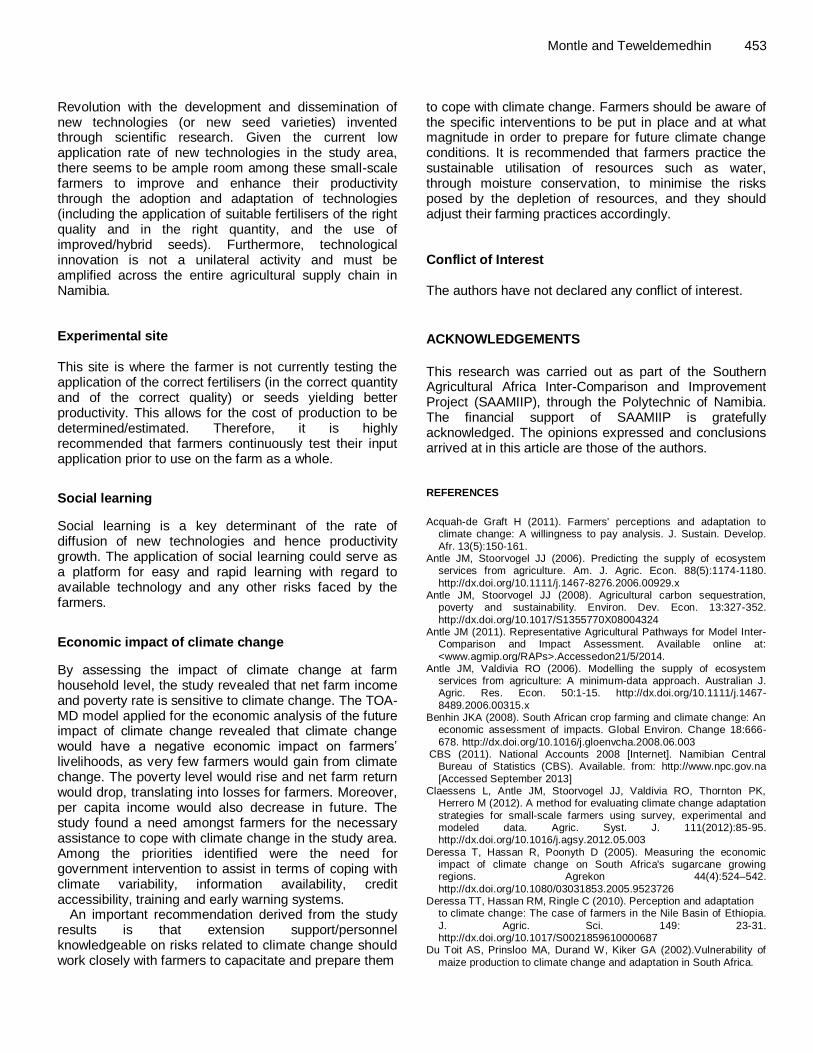
The main study area, namely the Ndonga Linena Green Scheme Project, is located 80 km along the Rundu Katima Mulilo highway, at coordinates 17°57′20.41 S and 20°31’41.56 E, and at an elevation of 3,543 ft. All 30 small-scale irrigation farmers (SSIFs) involved in the project were included in the study (Figure A4). The soil type is mainly sandy soils with excellent drainage, while the average temperature is 22.4°C and the average rainfall is 577 mm annually. Most rainfall occurs during the month of February, with an average of 147 mm (Mendelsohn, 2006).

Data collection

Farm-level data was collected during February 2014 from the entire population of 30 SSIFs participating in the Ndonga Linena Irrigation Project in the Kavango region of Namibia. As a continuation of the broader research project, the study was based on interviews with the SSIFs through the use of a semi-structured and self-

administered survey questionnaire, consisting of both closed- and open-ended questions.

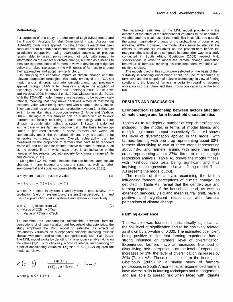
Methodology For purposes of this study, the Multinomial Logit (MNL) model and the Trade-Off Analysis for Multi-Dimensional Impact Assessment (TOA-MD) model were applied. To date, limited research has been conducted from a combined econometric, mathematical and simple calculation perspective, using quantitative analysis, to produce results able to assist policymakers, not only with regard to information on the impact of climate change, but also as a means to measure the perceptions of farmers in view of developing mitigation policy that takes into account the willingness of farmers to change their approaches and adopt new technology.

In analysing the economic impact of climate change and the

relevant adaptation strategies, this study employed the TOA-MD model under different scenario considerations, as previously applied through SAAMIIP to intensively analyse the adoption of technology (Antle, 2011; Antle and Stoorvogel, 2006, 2008; Antle and Valdivia, 2006; Immerzeel et al., 2008, Claessens et al., 2012). With the TOA-MD model, farmers are assumed to be economically rational, meaning that they make decisions aimed at maximising expected value while being presented with a simple binary choice: They can continue to operate with production system 1, or they can

switch to an alternative production system 2 (Antle and Valdivia, 2006). The logic of this analysis can be summarised as follows: Farmers are initially operating a base technology with a base climate – a combination defined as system 1. System 2 is defined as the case where farmers continue using the base technology under a perturbed climate. If some farmers are worse off economically under the perturbed climate, they are said to be vulnerable to climate change. Overall, vulnerability can be measured by the proportion of farmers that have been rendered

worse off, and can also be defined relative to some threshold, such as the poverty line, in which case there is an indication of the number of households put into poverty by climate change (Antle and Valdivia, 2011).

Using the TOA-MD model, impacts that can be simulated include changes in farm income and poverty rates, as well as other environmental and social outcomes (Antle and Valdivia, 2011).

ω = system 1 value – system 2 value (1) Where: P = price in system 1 and system 2 respectively; Y = production (yield) in system 1 and system 2 respectively; a = land use; C = production cost in system 1 and system 2 respectively.

losses from CC (2)

Value of CClim + XTech

Value of FClim + XTech To examine the econometric relationship between farmers’ perceptions of climate variation and household characteristics, the study employed the MNL model to estimate the effects of explanatory variables on a dependent variable involving multiple choices with unordered response categories (Legesse et al., 2012). The MNL model works by denoting “y” a random variable taking on the values {1,2….j} for choices j, a positive integer, and denoting “x” a set of conditioning variables. Legesse et al. (2012) equated the model as follows:

Where βj is K × 1, j = 1……., J.

Montle and Teweldemedhin 445 The parameter estimates of the MNL model provide only the direction of the effect of the independent variables to the dependent variable, and the weakness of the model lies in its failure to quantify the actual magnitude of change or the probabilities of occurrences (Greene, 2000). However, the model does serve to interpret the effects of explanatory variables on the probabilities; hence the marginal effects need to be computed in some other way. In a study conducted in South Africa, Gbetibouo (2009) applied MNL specifications in order to model the climate change adaptation behaviour of farmers, involving discrete dependent variables with multiple choices.

The models used in this study were selected on the basis of their suitability in reaching conclusions about the use of resources at

farm level and the adoption of suitable technology, in view of finding solutions to the issue of farmers’ uncertainty regarding resource allocation into the future and their production capacity in the long run.

RESULTS AND DISCUSSION

Econometrical relationship between factors affecting climate change and farm household characteristics

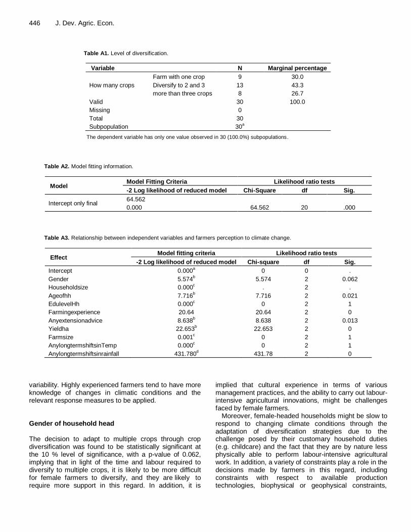
Tables A1 to A3 depict a number of crop diversifications included in the model, in terms of model fitness and multiple logic model output respectively. Table A1 shows the level of diversification applied in the model, with farmers farming with one crop representing about 30%, farmers diversifying to two or three crops representing about 43%, and farmers farming with more than three crops representing about 27%, fitted to multiple logic regression analysis. Table A2 shows the model fitness, with likelihood ratio tests being significant and thus implying linear regression and a well-fitting model. Table A3 presents the model output.

The results of the analysis examining the factors influencing farmers’ perceptions of climate change, as depicted in Table A3, reveal that the gender, age and farming experience of the household head, as well as extension services, yield and mean rainfall shift, have a positive and significant relationship with farmers’ perceptions of climate change.

Farming experience

This variable was found to be statistically significant at the 5% level of significance and to be positively related, as shown by a p-value of 0.000. The estimated coefficient being positive implies that farming experience has a strong influence on farmers’ level of diversification. Experienced farmers have an increased likelihood of diversifying their enterprises – as the level of experience increases by 1%, the level of diversification increases by 20% (Table A3). These results confirm the findings of Gbetibouo (2009) in a similar study of farmers’ perceptions in South Africa – that is, experienced farmers have diverse skills in farming techniques and management, and are able to spread risk when faced with climate

𝑦 =𝑗

𝑥 =

exp (𝑥𝛽𝑗 )

1+ exp (𝑥𝛽𝑘)𝑗𝑥=1

𝑗 = 1,… , 𝑗

446 J. Dev. Agric. Econ.

Table A1. Level of diversification.

Variable N Marginal percentage

How many crops

Farm with one crop 9 30.0

Diversify to 2 and 3 13 43.3

more than three crops 8 26.7

Valid 30 100.0

Missing 0

Total 30

Subpopulation 30a

The dependent variable has only one value observed in 30 (100.0%) subpopulations.

Table A2. Model fitting information.

Model Model Fitting Criteria Likelihood ratio tests

-2 Log likelihood of reduced model Chi-Square df Sig.

Intercept only final 64.562

0.000 64.562 20 .000

Table A3. Relationship between independent variables and farmers perception to climate change.

Effect Model fitting criteria Likelihood ratio tests

-2 Log likelihood of reduced model Chi-square df Sig.

Intercept 0.000a 0 0 .

Gender 5.574b 5.574 2 0.062

Householdsize 0.000c . 2 .

Ageofhh 7.716b 7.716 2 0.021

EdulevelHh 0.000c 0 2 1

Farmingexperience 20.64 20.64 2 0

Anyextensionadvice 8.638b 8.638 2 0.013

Yieldha 22.653b 22.653 2 0

Farmsize 0.001c 0 2 1

AnylongtermshiftsinTemp 0.000c 0 2 1

Anylongtermshiftsinrainfall 431.780d 431.78 2 0

variability. Highly experienced farmers tend to have more knowledge of changes in climatic conditions and the relevant response measures to be applied. Gender of household head The decision to adapt to multiple crops through crop diversification was found to be statistically significant at the 10 % level of significance, with a p-value of 0.062, implying that in light of the time and labour required to diversify to multiple crops, it is likely to be more difficult for female farmers to diversify, and they are likely to require more support in this regard. In addition, it is

implied that cultural experience in terms of various management practices, and the ability to carry out labour-intensive agricultural innovations, might be challenges faced by female farmers.

Moreover, female-headed households might be slow to respond to changing climate conditions through the adaptation of diversification strategies due to the challenge posed by their customary household duties (e.g. childcare) and the fact that they are by nature less physically able to perform labour-intensive agricultural work. In addition, a variety of constraints play a role in the decisions made by farmers in this regard, including constraints with respect to available production technologies, biophysical or geophysical constraints,

labour and input market constraints, financial and credit constraints, social norms, inter-temporal trade-offs, policy constraints, and constraints in terms of knowledge and skills (Teweldemedhin and Van Schalkwyk, 2010). Age of household head This variable was found to be significant at the 5% level of significance, with a p-value of 0.021 and a positive coefficient, implying that the age of the household head has a strong influence on the level of diversification. The older the farmer, the more experienced he/she is in farming and the more exposure he/she has had to past and present climatic conditions over longer periods of time. Mature farmers are better able to access the characteristics of modern technology than younger farmers, who might be more concerned about profit than the long-term sustainability of their operations. Similarly, Deressa et al. (2009) found that the age of the household head represents experience in farming, and that age is an indication of specialisation, because as the farmer matures he/she is more likely to grow more commercialised. The negative estimate coefficient for age implies the decision on diversification. It appears, therefore, that older and more experienced farmers are less willing to diversify their enterprise. Farmers with such characteristics might have acquired enough knowledge over time to deal with income and risk without diversification. However, the findings of Jarvie and Nieuwoudt (1988) and Vandeveer (2001, cited in Teweldemedhin and Kafidi, 2009) indicate that younger farmers, or those with less experience, are less likely to diversify their enterprise. Extension advice This variable was found to be statistically significant at the 5% level of significance, as shown by a p-value of 0.013, with a positive sign. This implies that extension advice has a strong influence on the ability of farmers to diversify their crops. Access to extension services increases the likelihood of perceiving changes in climate, as well as the likelihood of adapting to such changes through the creation of opportunities for the farmer to adopt suitable strategies that better suit the changed climatic conditions. This suggests that extension services assist farmers to take climate changes and weather patterns into consideration, through advice on how to deal with climatic variability and change. These results are in line with the findings Nhemachena and Hassan (2007), namely that access to information on climate change forecasting, adaptation options and other agricultural activities is an important factor in determining the farmers’ use of various adaptation strategies.

Montle and Teweldemedhin 447 Yield per hectare This parameter was found to be statistically significant at the 1% level of significance and positively linked (p-value of 0.000). The magnitude and weight of this parameter of the estimated coefficient were found to be greater than the other parameters, implying that yield/ha has a strong influence on the level of crop diversification in effect. Where diversified crops are proven to have a greater yield per hectare than a single crop, with an associated advantage in terms of market opportunities, farmers are likely to have the ability to provide a unique product giving them a competitive advantage, which would be a good incentive for farmers to continue diversifying into even more crops, thus spreading the risk of vulnerability to the changing climate. Mean rainfall shifts This variable was found to be statistically significant at the 5% level of significance (p-value of 0.000). With the level of significance at 1% and a positive coefficient, it implies that rainfall has a strong influence on the level of crop diversification within the study area. An increase in the mean annual precipitation is associated with an increased probability of farmers changing their management practices, in particular by diversifying to crop varieties best suited to the prevailing and forecasted precipitation. Equally, a decrease in the mean precipitation would cultivate the farmers’ technical knowledge in view of responding with sustainable measures in order to withstand the changing climate. Through this study, the farmers’ priority solution areas were found to be moisture conservation and crop diversification. Climate change impact The farmers involved in this study were all found to be aware of the negative effect of climate variability on their production levels (Table A4). With regard to the farmers’ long-term observations/perceptions of changing rainfall patterns, 78% of respondents perceived an increase in air temperature and 80% a reduction in rainfall (Table A5). With regard to direction and tendency, 78% claimed to have noticed an increase, while 13% had noticed a decrease and only 9% responded as not understanding the question about shift in temperature. Similarly, with regard to shift in rainfall patterns, 83% responded that they had noticed a decrease and 17% responded that they had noticed an increase in rainfall (Table A5). The farmers reported that they had been experiencing high temperatures, with negative effects on their crops (wilting, stunted growth and subsequent poor yields).

448 J. Dev. Agric. Econ.

Table A4. Perceived impact of climate change.

Variable YES NO

Do you notice long-term impact of climate change? 30 (100%) 0

Do you notice shift in temp? 23 (77%) 7 (23%)

Do you notice rainfall shift over time? 24 (80%) 4 (20%)

Table A5. Direction and magnitude of perceived temperature and rainfall shifts.

Consistent (%) Decrease (%) Increase (%) Do not understand (%)

Perception of mean temperature shifts 0 13 78 9

Perception of mean rainfall shifts 0 83 17 0

Table A6. Perceived adaptation strategies to climatic variation ranking (1 – top priority and 7 – bottom priority options).

Variable 1 (%) 2 (%) 3 (%) 4 (%) 5 (%) 6 (%) 7 (%) Total

Early planting 7 0 3 17 7 7 60 100

Use of hybrid seeds 0 10 3 3 27 43 13 100

Mixed farming 43 10 7 7 3 20 10 100

Conservational tillage/moisture conservation 3 23 30 17 20 0 7 100

Switching farming system (crop to livestock) 63 20 7 0 7 3 0 100

Information on meteorological service 33 7 17 27 10 3 3 100

Crop diversification 3 0 7 30 30 23 7 100

Furthermore, the farmers mentioned that the average annual rainfall had dropped dramatically in recent times, posing a threat to their operations due to their reliance on the Okavango River as a source of irrigation water. Adaptation strategies to climatic variations Table A6 presents the perceived adaptation strategy options identified by the farmers in the study area. Switching the farm system (for example to livestock) and adopting a mixed farming system was identified by 63 and 43% of farmers respectively as their future vision for coping with climate change variability, while the remaining options were selected by less than 7% of respondents. Conservation was identified as second on the list of priorities by 23% of respondents, while 60% of respondents selected early planting as the last option. These results imply that the level of understanding and awareness amongst farmers is lacking.

In a study by Lorenzoni and Langford (2005) using group discussions, respondents were asked to express their level of concern about climate change and their belief in human influence on climate. The findings of that study revealed that most of the participants possessed

detailed knowledge of the issue, which they invariably related to their personal perceptions and interpretation. Through much discussion of the influence of human activities on the climate and the consequent need for behavioural and lifestyle changes, the aforementioned participants differentiated among various institutions, organisations and governmental levels with regard to the responsibility of reducing the impact of climate change, as well as those who should be entrusted with this responsibility.

As a solution, changing the crop planting date would be cost effective, but would require good technical knowledge and up-to-date information on the best time to plant. Furthermore, the use of improved crop species and crop diversification in response to climate change would require some measure of scientific input, technical knowledge and access to information by the farmers. The implication of this finding is that for climate change adaptation strategies to be effectively adopted by small-scale farmers, they should not have to face any heavy financial burden. Awareness and capacity building in terms of climate change adaptation options, as well as the provision of the necessary farm inputs, should also be incorporated into the adaptation options for small-scale farmers.

Montle and Teweldemedhin 449

Figure A1. Major constraints in adapting to climate change and variability (7 – most constraining and 1 – least

constraining).

Constraints to climate adaptation Figure A1 depicts the constraints involved in making the necessary adjustments to climatic variations between seasons. The most significant constraint identified by respondents was poor extension services (50%), followed by lack of access to credit (40%), and inadequate meteorological services and lack of climate change knowledge (26%). Market access was also identified as a major constraint (Figure A1). Economic analysis of the impact of climate change Assumptions adopted by the study Table A7 depicts the crop and climate model simulation for SAAMIIP (including South Africa, Botswana and Namibia) in respect of the percentage of the mean net return impact for the maize production summary, calibrated to the climate and crop model. On average, the five climate scenarios presented are predicted to experience a future rise in temperature (+2.0 to +3.5°C), accompanied by greater variability in rainfall. Future rainfall/precipitation projections are less consistent, with

different climate models revealing different projections in the Southern African region.

In achieving these results, different crop management practices (planting date, soil depth, fertiliser application and harvesting date) were identified for use as inputs into crop modelling. Sequential climate modelling, followed by crop modelling, yielded a projection of a negative economic impact across five different climate scenarios, with an average net impact of 12.73, 34.07 and 48.16% for South Africa, Botswana and Namibia respectively. However, it is important to note that the case study in South Africa was focused on commercial farmers, while the studies in Botswana and Namibia were focused on small-scale farmers and thus yielded results that are more applicable to the small-scale irrigation farmers involved in the study at hand.

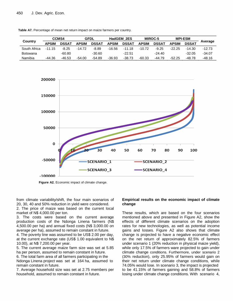
The key findings mentioned above were used to develop four different scenarios for the farmers of Ndonga Linena, in terms of modelling the economic impact within the study area. In summary, the following assumptions were considered in the application of the TOA-MD model: 1. In the absence of a climate and crop model simulation based on the above key findings of SAAMIIP resulting

450 J. Dev. Agric. Econ. Table A7. Percentage of mean net return impact on maize farmers per country.

Country CCMS4 GFDL HadGEM_2ES MIROC-5 MPI-ESM

Average APSIM DSSAT APSIM DSSAT APSIM DSSAT APSIM DSSAT APSIM DSSAT

South Africa -11.15 -8.25 -14.72 -8.89 -16.56 -11.18 -10.72 -9.25 -22.25 -14.30 -12.73

Botswana

-60.80

-30.60

-22.51

-24.40

-32.05 -34.07

Namibia -44.36 -46.53 -54.00 -54.89 -36.93 -38.73 -60.33 -44.79 -52.25 -48.78 -48.16

Figure A2. Economic impact of climate change.

from climate variability/shift, the four main scenarios of 20, 30, 40 and 50% reduction in yield were considered. 2. The price of maize was based on the current local market of N$ 4,000.00 per ton. 3. The costs were based on the current average production costs of the Ndonga Linena farmers (N$ 4,500.00 per ha) and annual fixed costs (N$ 3,000.00 on average per ha), assumed to remain constant in future. 4. The poverty line was assumed to be US$ 2.00 per day, at the current exchange rate (US$ 1.00 equivalent to N$ 10.00), at N$ 7,200.00 per year. 5. The current average maize farm size was set at 5.85 ha per person, assumed to remain constant in future. 6. The total farm area of all farmers participating in the Ndonga Linena project was set at 164 ha, assumed to remain constant in future. 7. Average household size was set at 2.75 members per household, assumed to remain constant in future.

Empirical results on the economic impact of climate change These results, which are based on the four scenarios mentioned above and presented in Figure A2, show the effects of different climate scenarios on the adoption rates for new technologies, as well as potential income gains and losses. Figure A2 also shows that climate change is projected to have a negative economic effect on the net return of approximately 82.5% of farmers under scenario 1 (20% reduction in physical maize yield), while only 17.5% of farmers ware projected to gain under climate change conditions. Furthermore, under scenario 2

(30% reduction), only 25.95% of farmers would gain on their net return under climate change conditions, while 74.05% would lose. In scenario 3, the impact is projected to be 41.15% of farmers gaining and 58.8% of farmers losing under climate change conditions. With scenario 4,

Montle and Teweldemedhin 451

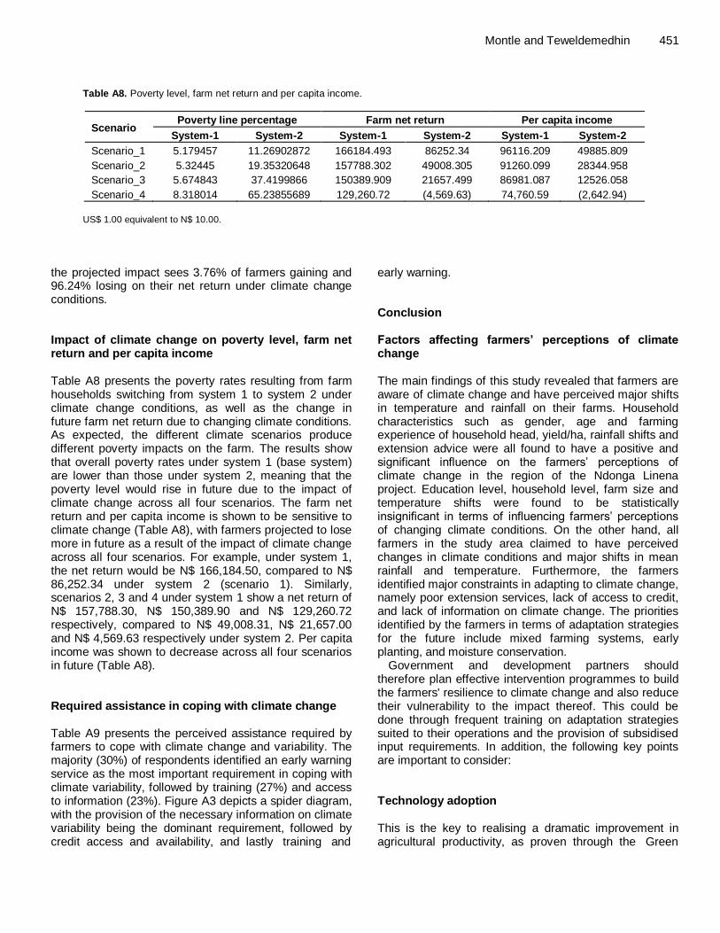
Table A8. Poverty level, farm net return and per capita income.

Scenario Poverty line percentage Farm net return Per capita income

System-1 System-2 System-1 System-2 System-1 System-2

Scenario_1 5.179457 11.26902872 166184.493 86252.34 96116.209 49885.809

Scenario_2 5.32445 19.35320648 157788.302 49008.305 91260.099 28344.958

Scenario_3 5.674843 37.4199866 150389.909 21657.499 86981.087 12526.058

Scenario_4 8.318014 65.23855689 129,260.72 (4,569.63) 74,760.59 (2,642.94)

US$ 1.00 equivalent to N$ 10.00.

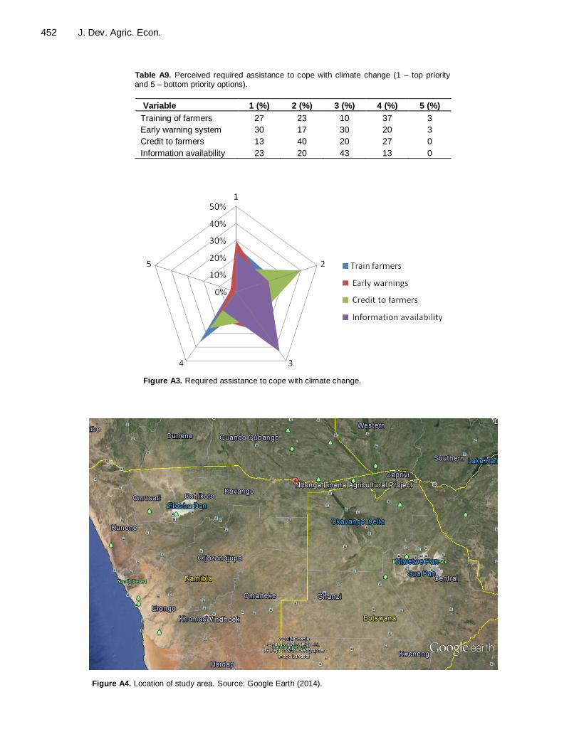
the projected impact sees 3.76% of farmers gaining and 96.24% losing on their net return under climate change conditions. Impact of climate change on poverty level, farm net return and per capita income Table A8 presents the poverty rates resulting from farm households switching from system 1 to system 2 under climate change conditions, as well as the change in future farm net return due to changing climate conditions. As expected, the different climate scenarios produce different poverty impacts on the farm. The results show that overall poverty rates under system 1 (base system) are lower than those under system 2, meaning that the poverty level would rise in future due to the impact of climate change across all four scenarios. The farm net return and per capita income is shown to be sensitive to climate change (Table A8), with farmers projected to lose more in future as a result of the impact of climate change across all four scenarios. For example, under system 1, the net return would be N$ 166,184.50, compared to N$ 86,252.34 under system 2 (scenario 1). Similarly, scenarios 2, 3 and 4 under system 1 show a net return of N$ 157,788.30, N$ 150,389.90 and N$ 129,260.72 respectively, compared to N$ 49,008.31, N$ 21,657.00 and N$ 4,569.63 respectively under system 2. Per capita income was shown to decrease across all four scenarios in future (Table A8). Required assistance in coping with climate change Table A9 presents the perceived assistance required by farmers to cope with climate change and variability. The majority (30%) of respondents identified an early warning service as the most important requirement in coping with climate variability, followed by training (27%) and access to information (23%). Figure A3 depicts a spider diagram, with the provision of the necessary information on climate variability being the dominant requirement, followed by credit access and availability, and lastly training and

early warning. Conclusion Factors affecting farmers’ perceptions of climate change The main findings of this study revealed that farmers are aware of climate change and have perceived major shifts in temperature and rainfall on their farms. Household characteristics such as gender, age and farming experience of household head, yield/ha, rainfall shifts and extension advice were all found to have a positive and significant influence on the farmers’ perceptions of climate change in the region of the Ndonga Linena project. Education level, household level, farm size and temperature shifts were found to be statistically insignificant in terms of influencing farmers’ perceptions of changing climate conditions. On the other hand, all farmers in the study area claimed to have perceived changes in climate conditions and major shifts in mean rainfall and temperature. Furthermore, the farmers identified major constraints in adapting to climate change, namely poor extension services, lack of access to credit, and lack of information on climate change. The priorities identified by the farmers in terms of adaptation strategies for the future include mixed farming systems, early planting, and moisture conservation.

Government and development partners should therefore plan effective intervention programmes to build the farmers' resilience to climate change and also reduce their vulnerability to the impact thereof. This could be done through frequent training on adaptation strategies suited to their operations and the provision of subsidised input requirements. In addition, the following key points are important to consider: Technology adoption This is the key to realising a dramatic improvement in agricultural productivity, as proven through the Green

452 J. Dev. Agric. Econ.

Table A9. Perceived required assistance to cope with climate change (1 – top priority and 5 – bottom priority options).

Variable 1 (%) 2 (%) 3 (%) 4 (%) 5 (%)

Training of farmers 27 23 10 37 3

Early warning system 30 17 30 20 3

Credit to farmers 13 40 20 27 0

Information availability 23 20 43 13 0

Figure A3. Required assistance to cope with climate change.

Figure A4. Location of study area. Source: Google Earth (2014).

Revolution with the development and dissemination of new technologies (or new seed varieties) invented through scientific research. Given the current low application rate of new technologies in the study area, there seems to be ample room among these small-scale farmers to improve and enhance their productivity through the adoption and adaptation of technologies (including the application of suitable fertilisers of the right quality and in the right quantity, and the use of improved/hybrid seeds). Furthermore, technological innovation is not a unilateral activity and must be amplified across the entire agricultural supply chain in Namibia. Experimental site This site is where the farmer is not currently testing the application of the correct fertilisers (in the correct quantity and of the correct quality) or seeds yielding better productivity. This allows for the cost of production to be determined/estimated. Therefore, it is highly recommended that farmers continuously test their input application prior to use on the farm as a whole.

Social learning

Social learning is a key determinant of the rate of diffusion of new technologies and hence productivity growth. The application of social learning could serve as a platform for easy and rapid learning with regard to available technology and any other risks faced by the farmers.

Economic impact of climate change

By assessing the impact of climate change at farm household level, the study revealed that net farm income and poverty rate is sensitive to climate change. The TOA-MD model applied for the economic analysis of the future impact of climate change revealed that climate change would have a negative economic impact on farmers’ livelihoods, as very few farmers would gain from climate change. The poverty level would rise and net farm return would drop, translating into losses for farmers. Moreover, per capita income would also decrease in future. The study found a need amongst farmers for the necessary assistance to cope with climate change in the study area. Among the priorities identified were the need for government intervention to assist in terms of coping with climate variability, information availability, credit accessibility, training and early warning systems.

An important recommendation derived from the study results is that extension support/personnel knowledgeable on risks related to climate change should work closely with farmers to capacitate and prepare them

Montle and Teweldemedhin 453 to cope with climate change. Farmers should be aware of the specific interventions to be put in place and at what magnitude in order to prepare for future climate change conditions. It is recommended that farmers practice the sustainable utilisation of resources such as water, through moisture conservation, to minimise the risks posed by the depletion of resources, and they should adjust their farming practices accordingly. Conflict of Interest The authors have not declared any conflict of interest.

ACKNOWLEDGEMENTS

This research was carried out as part of the Southern Agricultural Africa Inter-Comparison and Improvement Project (SAAMIIP), through the Polytechnic of Namibia. The financial support of SAAMIIP is gratefully acknowledged. The opinions expressed and conclusions arrived at in this article are those of the authors. REFERENCES

Acquah-de Graft H (2011). Farmers' perceptions and adaptation to

climate change: A willingness to pay analysis. J. Sustain. Develop.

Afr. 13(5):150-161. Antle JM, Stoorvogel JJ (2006). Predicting the supply of ecosystem

services from agriculture. Am. J. Agric. Econ. 88(5):1174-1180.

http://dx.doi.org/10.1111/j.1467-8276.2006.00929.x Antle JM, Stoorvogel JJ (2008). Agricultural carbon sequestration,

poverty and sustainability. Environ. Dev. Econ. 13:327-352.

http://dx.doi.org/10.1017/S1355770X08004324 Antle JM (2011). Representative Agricultural Pathways for Model Inter-

Comparison and Impact Assessment. Available online at:

<www.agmip.org/RAPs>.Accessedon21/5/2014. Antle JM, Valdivia RO (2006). Modelling the supply of ecosystem

services from agriculture: A minimum-data approach. Australian J. Agric. Res. Econ. 50:1-15. http://dx.doi.org/10.1111/j.1467-

8489.2006.00315.x Benhin JKA (2008). South African crop farming and climate change: An

economic assessment of impacts. Global Environ. Change 18:666-

678. http://dx.doi.org/10.1016/j.gloenvcha.2008.06.003 CBS (2011). National Accounts 2008 [Internet]. Namibian Central

Bureau of Statistics (CBS). Available. from: http://www.npc.gov.na

[Accessed September 2013] Claessens L, Antle JM, Stoorvogel JJ, Valdivia RO, Thornton PK,

Herrero M (2012). A method for evaluating climate change adaptation

strategies for small-scale farmers using survey, experimental and modeled data. Agric. Syst. J. 111(2012):85-95. http://dx.doi.org/10.1016/j.agsy.2012.05.003

Deressa T, Hassan R, Poonyth D (2005). Measuring the economic impact of climate change on South Africa's sugarcane growing regions. Agrekon 44(4):524–542.

http://dx.doi.org/10.1080/03031853.2005.9523726 Deressa TT, Hassan RM, Ringle C (2010). Perception and adaptation

to climate change: The case of farmers in the Nile Basin of Ethiopia.

J. Agric. Sci. 149: 23-31. http://dx.doi.org/10.1017/S0021859610000687

Du Toit AS, Prinsloo MA, Durand W, Kiker GA (2002).Vulnerability of

maize production to climate change and adaptation in South Africa.

454 J. Dev. Agric. Econ.

Combined Congress: South African Society of Crop Protection and South African Society of Horticultural Science, Pietermaritzburg, South Africa.

FAO (Food and Agricultural Organisation) (2005). National Medium Term Investment Programme. Support To Nepad–Caadp Implementation. Windhoek: FAO.

Gbetibouo G (2009). Understanding farmers' perceptions and adaptations to climate change and variability: The case of the Limpopo Basin, South Africa. Washington, DC: IFPRI Discussion P.

00849. Gbetibouo GA, Hassan RM (2005). Measuring the economic impact of

climate change on major South African field crops: A Ricardian

approach. Global. Planet. Change 47:143–152. http://dx.doi.org/10.1016/j.gloplacha.2004.10.009

Greene WH (2000). Econometric analysis. 4th Ed. New Jersey:

Prentice-Hall. Immerzeel W, Stoorvogel JJ, Antle JM (2008). Can payments for

ecosystem services secure the water tower of Tibet. Agric. Syst.

96(1-3):52-63. http://dx.doi.org/10.1016/j.agsy.2007.05.005 IPCC (Intergovernmental Panel on Climate Change) (2014) Climate

change 2014: Impacts, adaptation, and vulnerability. IPCC WGII AR5

Summary for Policymakers. Jarvie EM, Nieuwoudt WL (1988). Factors influencing crop insurance

participation in maize farming. Agrekon. 28(2):11-16.

http://dx.doi.org/10.1080/03031853.1989.9525097 Kiker GA, Bamber IN, Hoogenboom G, Mcgelinchey M (2002). Further

Progress in the validation of the CANEGRO-DSSAT

model.Proceedings of International CANGRO Workshop, Mount Edgecombe, South Africa. PMid:12184583

Kiker GA (2002). CANEGRO-DSSAT linkages with geographic

information systems: applications in climate change research for South Africa. Proceedings of International CANGRO Workshop, Mount Edgecombe, South Africa.PMid:12184583

Kruger AC, Shongwe S (2004). Temperature trends in South Africa: 1960-2003. Int. J. Climatol. 24:1929-1945. http://dx.doi.org/10.1002/joc.1096

Legesse B, Ayele Y, Bewket W (2012). Smallholder Farmers' Perceptions and Adaptation to Climate Variability and Climate Change in Doba District, West Hararghe, Ethiopia. Asian J. Empir.

Res. 3(3):251-265. Lorenzoni I, Langford I (2005). Climate Change Now and in the Future:

A Mixed Methodological Study of Public Perceptions in Norwich (UK).

CSERGE Working Paper ECM 01-05. University of East Anglia, Norwich.

MAWF (Ministry of Agriculture, Water and Forestry) (2010). Extension

Staff Handbook: Crop Production. Windhoek: Directorate of Crop Production.

Mendelsohn J (2006). Farming systems in Namibia. Windhoek: Research and Information Services of Namibia.

New M, Hewitson B, Stephenson DB, Tsiga A, Kruger A, Manhique A, Gomez B, Coelho CAS, Masisi DN, Kululanga E, Mbambalala E, Adesina F, Saleh H, Kanyanga J, Adosi J, Bulane L, Fortunata L,

Mdoka ML, Lajoie R (2006). Evidence of trends in daily climate extremes over southern and west. Afr. J. Geophys. Res. P. 111. D14102, doi:10.1029/2005JD006289.

http://dx.doi.org/10.1029/2005JD006289 Newsham AJ, Thomas DSG (2011). Knowing, farming and climate

change adaptation in North-Central Namibia. Global Environ.

Change. 21(2):761-770. http://dx.doi.org/10.1016/j.gloenvcha.2010.12.003

Nhemachena C, Hassan R (2007). Micro-level Analysis of Farmers'

Adaptations to Climate Change in Southern Africa. IFPRI, Environment and Production Technology Division. Washington, DC: International Food Policy Research Institute.

NNF (Namibia Nature Foundation) (2010). Land Use Planning

Framework for the Kavango Region of Namibia within the Okavango River Basin. Windhoek: NNF.

Poonyth D, Hassan RM, Gbetibouo GA, Ramaila JM, Letsoalo MA (2002). Measuring the impact of climate change on South African agriculture: A Ricardian approach. A paper presented at the 40th

Annual Agricultural Economics Association of South Africa Conference, Bloemfontein, 18–20 September.

Southern Africa Agricultural Model Intercomparison and Improvement

Project (SAAMIIP) (2014). Impacts of Projected Climate Change Scenarios on the Production of nutritionally important crops in Southern Africa: South Africa, Botswana, Namibia, Swaziland and

Lesotho. A Final Report Submitted to ICRISAT/Agricultural Model Intercomparison and Improvement Project (AgMIP), Project P. 120.

Schulze RE, Kiker GA, Kunz RP (1993). Global climate change and

agricultural productivity in Southern Africa. Global Environ. Change 3(4):330–349. http://dx.doi.org/10.1016/0959-3780(93)90022-D

Teweldemedhin MY, Van Schalkwyk HD (2010). The impact of trade

liberalisation on South African agricultural productivity. Afr. J. Agric. Res, 5(12):1380-1387.

Valipour M (2014). Land use policy and agricultural water management

of the previous half of century in Africa. Applied Water Science: Springer Berlin Heidelberg. 4:1-29.

Valipour M (2014). Pressure on renewable water resources by irrigation

to 2060. Acta Advan. Agric. Sci. 2(8):32-42. Valipour M, Montazar AA (2012). An evaluation of SWDC and

WinSRFR Models to Optimize of infiltration Parameters in Furrow

Irrigation. Am. J. Scient. Res. 69:128-142.

Vol. 6(11), pp. 455-465, November, 2014

DOI: 10.5897/JDAE2014.0561

ISSN 2006-9774 ©2014.

Article Number: 73E8B2848136

Copyright © 2014

Author(s) retain the copyright of this article

http://www.academicjournals.org/JDAE

Journal of Development and Agricultural

Economics

Full Length Research Paper

Profit efficiency of dairy farmers in Kenya: An application to smallholder farmers in Rift Valley and

Central Province

Leone Iga Mawa1*, Mutuku Muendo Kavoi2, Isabelle Baltenweck1 and Jane Poole3

1Department of Markets, Gender and Livelihoods, International Livestock Research Institute (ILRI),

P. O. Box 30709-00100, Nairobi, Kenya. 2Faculty of Agriculture, Jomo Kenyatta University of Agriculture and Technology, P. O. Box 62000-00200,

Nairobi, Kenya. 3Research Methods Group, International Livestock Research Institute, P. O. Box 30709-00100, Nairobi, Kenya.

Received 21 January, 2014; Accepted 20 August, 2014

The dairy industry in Kenya is an important source of livelihood among the smallholder farmers who supply over 70% of the total milk. However, there is a growing concern on rising costs of milk production among farmers. The study assessed profit efficiency of smallholder dairying in the Rift Valley and Central Provinces of Kenya using stochastic frontier analysis for estimating farm level profit efficiency and identifying the specific determinants of efficiency. The results showed that the farmers are fairly profit efficient with an average of about 68%. Cost of fodder produced on farm significantly improved profit efficiency among farmers. However dairy profit efficiency can be enhanced if fodder production is embraced, as well as other supplemental feed technologies that are commensurate with local conditions. Institutional policy reforms on smallholder dairying will help protect the industry and its sustainability for smallholders. Key words: Dairy, profit efficiency, stochastic frontier, smallholder farmer.

INTRODUCTION Kenya is the second largest dairy producer and consumer in sub-Sahara Africa and is relatively self-reliant (USAID, 2010). About 60% of the total milk production in Kenya is produced by farmers in the Rift Valley and Central Province who own about 80% of the exotic and cross-breed cattle (Omore et al., 1999). Previous studies have identified that smallholder farmers supply over 70% of the total milk, mainly from cattle, but some little quantities from camels and goats (USAID,

2008; Muriuki, 2003). Smallholder dairying is a potential contributor of income and employment generation both on-farm and off-farm, as well as improved nutrition of households (Staal et al., 2008; USAID, 2010). At the macro level, the dairy industry contributes an estimated 14% of agricultural gross domestic product (GDP) and approximately 4% of overall Kenya’s national GDP (USAID, 2010). It is anticipated that the demand for milk is likely to double due to the growing world population

*Corresponding author E-mail: leonemawa@gmail.com, Tel: +254 726 205601.

Author(s) agree that this article remain permanently open access under the terms of the Creative Commons

Attribution License 4.0 International License

456 J. Dev. Agric. Econ. (FAO, 2011, 2003). Despite the demand prospects, farmers and stakeholders have increasingly expressed concern over the growing costs of milk production which ultimately result in diminishing milk profits in Kenya. FAO (2003) reported that there is competition for land, water and other environmental resources due to the increasing population. It is apparently plausible that these constraints are shifting farmers’ practices from traditional pasture grazed systems to intensive production technologies which are often more expensive than extensive systems. This study proposed to assess profit efficiency of smallholder dairy production and identify its determinants among farmers in the Rift Valley and Central Provinces using Stochastic Frontier approach (SFA). Profit efficiency is a wider concept than cost efficiency since it takes into account the effects of the choice of a certain vector of production both on costs and on revenues, thus offering complementary information useful for the analysis of dairy farm efficiency. METHODOLOGY Theoretical framework

Stochastic production frontier models were introduced by Aigner et al. (1977) and Meensen and van den Broeck (1977). Battese and

Coelli (1995) and Coelli (1996), extended the stochastic production frontier model, suggesting that the inefficiency effects can be expressed as a linear function of explanatory variables, reflecting farm-specific characteristics. Farm level inefficiency measurements are common among researchers (Kumbhakar et al., 1989; Wang et al., 1996; Abdulai and Huffman, 2000; Rahman, 2003). The advantage of the stochastic frontier model is that it allows estimation of farm specific efficiency scores and the factors explaining efficiency differentials among farms in a single stage estimation procedure. Three common efficiency measures include Technical efficiency, Allocative efficiency and Economic efficiency. However, the profit efficiency measure combines the concepts of Technical and Allocative efficiencies into the profit relationship and as such any errors in the production decision are assumed to be translated into lower profits or revenue for the producer (Ali et al., 1994). Kumbhakar and Lovell (2000) provided a detailed account of stochastic frontier models. Accordingly, the stochastic frontier

function is defined by Equation 1 as follows:

∏ = f ( , ) exp(ε) (1)

The error term, - , is assumed to behave in a manner consistent with the stochastic frontier concept (Ali and Flinn, 1989) Where:

∏ = normalized profit of the firm;

= price of variable input faced by the farm divided by

output price;

= level of the fixed factor on the firm.

is assumed to be identically and normally distributed with mean zero and constant variance as:

N (0, ).

is the one-sided disturbance form representing profit inefficiency

and it is independent of ; and i = 1,2 ….., n, representing the individual firms.

Profit efficiency of the firm can be presented as:

EFF = E[exp(- / ] = E[exp(- - )/ ] (2)

Where: E = expectation operator, which is achieved by obtaining the

expressions for the conditional expectation upon the observed

value of ;

= dth explanatory variable associated with inefficiencies on firm i.

and = unknown parameters jointly estimated using the maximum likelihood method with the stochastic frontier and the

inefficiency effects functions simultaneously. The likelihood function is expressed in terms of the variance parameters: sigma squared;

( ) = - and; gamma (γ) = (Battese and Coelli 1995). The parameter γ represents the share of inefficiency in the overall residual variance with values in the interval of 0 and 1. A value of 1 suggests the existence of a deterministic frontier, whereas a value of 0 can be seen as evidence in the favor of ordinary least square

(OLS) estimation. Specification of the empirical model

Profit efficiency is defined as the gain from operating on the profit frontier, while taking into account farm-specific prices faced and factor endowments. Assuming a farm that maximizes profit is

operating in a perfectly competitive input and output markets and uses a singular output technology, the actual normalized profit function is derived as:

GM(∏) = TR – TVC = PQ - W (3) Where: GM = Gross margin; TR = total revenue; TVC = total variable cost - (as opposed to fixed costs as they remain fixed whether or not production has taken place, and to what scale

production has been). Normalizing the profit function is achieved by dividing both sides of Equation 3 by the output market price, that is:

= ∑ = = f( ,Z)∑Pi (4)

Where: - f ( , Z) is the production function. The profit function in implicit form which specifies efficiency is

expressed as:

∏ = f (Pij,Zik ) exp ( - ) (5)

I = 1,2,3…………..n represent the individual firms. The profit efficiency is expressed as the ratio of predicted profit to

the predicted maximum profit for a best firm and is expressed as:

Profit efficiency (E∏) = = (6)

Firm specific profit efficiency is again the mean of the conditional

distribution of given by E∏ and is defined as:

E∏ (7)

E∏ takes the value between 0 and 1.

If is = 0, that is, on the frontier, the firm is obtaining potential

maximum profit given the price it faces and the level of fixed factors.

If > 0, the firm is inefficient and losses profit as a result of inefficiency. The inefficiency effect model can only be estimated if

the efficiency effects are present. Given that is present in the

model it implies that it is justifiable to employ the SFA as similarly argued by Aneani et al. (2011). In this study, Battesse and Coelli (1995) and Coelli (1996) models were used to specify the stochastic frontier function with behavior inefficiency components and used to estimate all parameters together in one step maximum likelihood estimation.

Different functional forms have been used by scholars for measuring firm level efficiency, namely the Cobb-Douglas function, normalized quadratic, normalized translog and generalized Leontif, but the commonly used forms are the Cobb-Douglas and Translog forms. A detailed literature is presented by Abdulai and Huffman (2000) on the weaknesses of the two functional forms. It is argued that the Cobb-Douglas form is restrictive compared to the more flexible functional forms such as the translog and quadratic forms. Upton (1979) also added that the Cobb-Douglas function cannot show both increasing and diminishing marginal productivity in a single response curve. As a result it does not give a technical optimum and may lead to the over estimation of the economic

optimum. An ideal option would be the translog. However, the drawbacks of the translog model are that it has potential problems of insufficient degrees of freedom due to the presence of interaction terms; even though such interaction terms do have important economic implications and meaning (Abdulai and Huffman, 2000). Scholars such as Ọlayide and Heady (1982) used the quadratic function to measure the direct effects of inputs on output. However, the transcendental function and the quadratic functional models

seem unpopular among researchers due to limited application. Despite the restrictive nature of the Cobb-Douglas function, many

scholars and researchers have found it relevant, especially when there are many variables in the model (Taru et al., 2011; Ojo et al., 2006; Rahman, 2003; Ekpebu, 2002; Abdulai and Huffman, 2000; Saleem, 1988; Kalirajan and Obwona, 1994; Dawson and Lingard, 1991; Yilma, 1996; Nsanzugwanko et al., 1996; Battese and Hassan, 1999). Ekpebu (2002) on the other hand argued that the Cobb-Douglas functional form is useful in analysis of surveys where many variable inputs are involved and it is necessary to measure returns to scale, intensity of factors of production and overall efficiency of production. It is also argued that it provides a means of obtaining coefficients for testing hypotheses (Cobb and Douglas, 1928; Erhabor, 1982). Akighir and Shabu (2011) cited Ellebu, Koku and Ogidi (2004) that the evidence of the superiority of Cobb-Douglas functional form is supported by its satisfaction of the economic, statistical and econometric criteria required unlike the

other functional forms. In view of the above arguments, the Cobb-Douglas functional

form was applied for estimating dairy profit efficiency of the smallholder farmers in the study area, whose empirical model is specified below. However, for comparison purposes, the translog, quadratic and transcendental forms were equally applied (though their empirical models have not been specified here).

The explicit Cobb-Douglas functional model for this study is specified as follows:

)(lnlnln12

1

110 ii

k

kikii uvPZ

(8)

Where π is the normalized profit computed as total milk revenue per litre less variable cost per litre divided by farm specific milk price per litre; α and β represent the individual variable coefficients in the stochastic frontier model; Z is the total number of cows on the farm; Ps represent the cost of production inputs per unit of each respective input (that is, P1i = artificial insemination price per cow, P2i = price of veterinary services per administration, P3i= price of

Mawa et al 457 extension services per visit, P4i = monthly labor wage, P5i = purchase fodder price per kilogram (kg), P6i = imputed price of produced fodder per kg, P7i = price of dairy concentrates per kg, P8

i= price of conserved feeds per kg, P9i = grazing price per cow, P10i = price of water per litre, P11i = price of milk transport (per litre), P12i = price of milk (per litre) for feeding calves. (vi-ui ) is the composed error term.

The inefficiency model ( ) is defined by the equation as follows:

12

1

0

z

zzi Tu (9)

Where δ represent the respective regressor coefficients; Ts

represent farm, household and institutional socioeconomic characteristics (that is, T1 = age of farm owner, T2 = size of fodder land, T3 = size of grazing land, T4 = hourly wage rate, T5 = production system(dummy), T6 = production scale(dummy), T7 = gender of farm owner (dummy), T8 = hired labor(dummy), T9 = extension service access (dummy), T10 = paid extension service (dummy), T11 = paid water (dummy), T12 = rented land (dummy).

Data and variables measurement

The study was conducted in Kenya’s Rift Valley and Central Provinces where the East Africa Dairy Development (EADD) project has earmarked interventions, excluding the pastorally dominant cattle keeping communities. Data was collected from smallholder dairy farmers using structured household questionnaires. Details of production costs and revenues generated from milk in the past 3 months from the date of interview (August, 2012) were identified. This was to ensure accurate recall of production situations by the farmer, which is highly unlikely for an entire annual period due to lack of record keeping as argued by Staal et al. (2008). Detailed data was collected on feeds and their sources, other inputs used in production, the costs involved in acquiring these inputs and related services accessed by the farmer. Additionally, the amount of milk obtained from lactating cows and the revenues generated were obtained. Milk that was consumed by the farm families, milk fed to

calves and milk given to family friends/neighbors were valued at the cost price, while that sold was valued at the going market price of the respective channels. The gross profit of milk was used as the main outcome variable. The cost determinants and inefficiency factors in the frontier model were then examined against the outcome variable as earlier specified. Multistage sampling procedure was used to select a representative number of farmers into the study. Farmers were stratified according to the main

production system that is, mainly extensive or intensive system. A further stratification was based on the production scale that is, small-scale and medium-scale, assigned according to the number of cows managed under the respective production systems. These were arrived at based on the EADD precept for categorizing production scales of the smallholder farmers based on the baseline data for Rwanda, Uganda and Kenya (Table 1).

The study sample size was computed using the formula (Equation 10) for obtaining sample sizes of each group for

comparison in the study (if the outcome variable is a continuous univariate data). An assumption of this study was that unit profits among the farmers is a continuous variation and follows a normal distribution pattern, varied unit costs, herd sizes, production systems, parity differences of lactating cows, and management efficiency differences across farms, to mention but a few.

)10.(..............................................................................................................2 2

2

2

2

dn

(10)

458 J. Dev. Agric. Econ. Where: n = approximate sample size; d = margin of error (mean unit

profit difference between the 2 groups, mean d = confidence

interval) (assumed at 0.1); 2 = assumed std deviation of 0.2 for unit

Table 1. Production scales per production system.

Production scale Production system

Intensive Extensive

Small-scale ≤ 3 Cows ≤ 15 Cows

Medium-scale ≥ 4 Cows ≥ 16 Cows

Source: EADD Field Survey (2009). profit; Zα/2 = 1.96 signifying a 2-sided sample size at 95%

confidence level; Z = power of the test in identifying a significant difference (that is, ‘chance’ of this happening - 80%)

A total of 122 farmers (half for intensive and half for extensive production systems) were therefore approximated to be an adequate representative sample for the study. However, there were relatively fewer numbers of intensive farms identified during the field data collection process. Hence, only a total of 85 farmers were therefore ultimately surveyed.

EMPIRICAL RESULTS AND DISCUSSION Descriptive summaries Table 2 shows the descriptive summaries of the variables that were structured in the study questionnaire. The study found that the average number of cows owned per farm is 3 with a standard deviation of 2.0. The average land size under fodder production was found to be 2.3 acres with a standard deviation of 2.2, while that of grazing land was 6.0 acres with a high standard deviation of 52.4.

The proportion of farmers practicing extensive system was only 27% of the total farmers. This is mainly attributed to the competitive use of land resources influenced by the rising population (FAO, 2003). It was found that the intensive farms incurred higher production costs than the extensive farms on average. This difference was mainly attributed to feed costs and labour expenses incurred in intensive systems than extensive systems. The average total cost of milk production incurred per household in the past 3 months was Kshs 41,070, while total revenue amounted to Kshs 42,210. The average household milk produced in 3 months amounted to 1617 L, while the average total milk sold was 1100 L. Households also consumed about 520 L at home on average. Feed costs constituted the greater proportion of farmers’ cost of milk production. Among the cost components, fodder produced on farm constituted the greater proportion of variable costs with an average of Kshs 23,000. The average amount of milk produced by households was 1,617 L though with a high standard

deviation. This variation was mainly attributed to the number of cows in lactation, varying lactation lengths and parity effects, among others.

In terms of marketing of milk outputs, majority of farmers sold a greater portion of milk to the Chilling Plants (CPs) (local fresh milk buying centers) in the past 3 months amounting to 930 L on average. The least quantity was sold to private traders (35 L). Although the study did not prioritize producer choice for market channels, the preference for CPs by farmers would be largely attributed to a couple of factors, despite the lower prices offered by this channel. These could range from: a) the capability and the reliability of CPs to buy and pay for every quantity supplied compared to small scale traders and individual consumers; b) the relatively stable prices offered by CPs; c) the input incentives and extension services by some CPs to farmers on contractual terms; d) the belonging of some of the farmers’ to the cooperatives owning these CPs. Overall, the average household revenue earned in a quarter of a year from milk amounted to Kshs 42,000. The revenue from direct milk sales approximated to Kshs 29,000 and that of unsold milk amounted to KShs13,000 (Table 2).

Table 3 presents a summary statistics of the normalized unit variable costs and gross margin per liter of milk in the stochastic frontier model. Generally, the cost of feeds constituted the greater proportion of cost of milk production. The average cost of fodder production amounted to Kshs 0.74. This was followed by cost of labour and conserved feeds (Kshs 0.20, respectively). Among the feed costs, the cost of grazing was the cheapest (Kshs 0.10). Overall, the average cost of milk transport was the least of all the variable costs (Kshs 0.03). The normalized average gross margin per litre of milk amounted to Kshs 0.62. Smallholder dairy profit efficiency in Kenya Table 4 shows the stochastic model estimation results for the four functional forms: Cobb-Douglas, translog, quadratic and transcendental forms. The results showed that the average profit efficiency estimated by the Cobb-Douglas functional model was 68%. Compared to the other functional forms, the quadratic function estimated a similar mean efficiency (68%). The translog form estimated an average efficiency of 67%, while the transcendental form estimated an average of 71% (Table 4).

The likelihood ratio test was used to compare between the functional forms. The translog form was taken as the unrestricted log likelihood function (ULLF) and the rest as the restricted log likelihood functions (RLLF) since the coefficient estimates of some variables were hypothesized to be 0. The test statistic used to determine whether there was any difference between the translog function and any one of the other forms was:

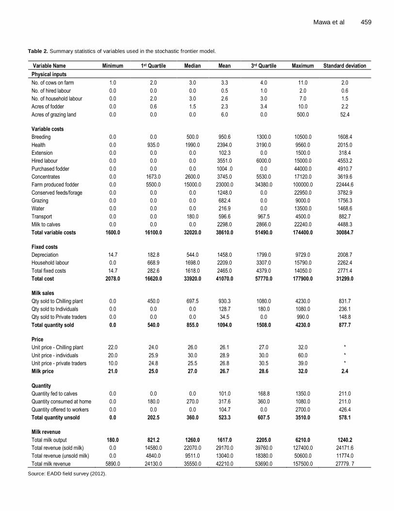
Mawa et al 459 Table 2. Summary statistics of variables used in the stochastic frontier model.

Variable Name Minimum 1st Quartile Median Mean 3rd Quartile Maximum Standard deviation

Physical inputs

No. of cows on farm 1.0 2.0 3.0 3.3 4.0 11.0 2.0

No. of hired labour 0.0 0.0 0.0 0.5 1.0 2.0 0.6

No. of household labour 0.0 2.0 3.0 2.6 3.0 7.0 1.5

Acres of fodder 0.0 0.6 1.5 2.3 3.4 10.0 2.2

Acres of grazing land 0.0 0.0 0.0 6.0 0.0 500.0 52.4

Variable costs

Breeding 0.0 0.0 500.0 950.6 1300.0 10500.0 1608.4

Health 0.0 935.0 1990.0 2394.0 3190.0 9560.0 2015.0

Extension 0.0 0.0 0.0 102.3 0.0 1500.0 318.4

Hired labour 0.0 0.0 0.0 3551.0 6000.0 15000.0 4553.2

Purchased fodder 0.0 0.0 0.0 1004 .0 0.0 44000.0 4910.7

Concentrates 0.0 1673.0 2600.0 3745.0 5530.0 17120.0 3619.6

Farm produced fodder 0.0 5500.0 15000.0 23000.0 34380.0 100000.0 22444.6

Conserved feeds/forage 0.0 0.0 0.0 1248.0 0.0 22950.0 3782.9

Grazing 0.0 0.0 0.0 682.4 0.0 9000.0 1756.3

Water 0.0 0.0 0.0 216.9 0.0 13500.0 1468.6

Transport 0.0 0.0 180.0 596.6 967.5 4500.0 882.7

Milk to calves 0.0 0.0 0.0 2298.0 2866.0 22240.0 4488.3

Total variable costs 1600.0 16100.0 32020.0 38610.0 51490.0 174400.0 30084.7

Fixed costs

Depreciation 14.7 182.8 544.0 1458.0 1799.0 9729.0 2008.7

Household labour 0.0 668.9 1698.0 2209.0 3307.0 15790.0 2262.4

Total fixed costs 14.7 282.6 1618.0 2465.0 4379.0 14050.0 2771.4

Total cost 2078.0 16620.0 33920.0 41070.0 57770.0 177900.0 31299.0

Milk sales

Qty sold to Chilling plant 0.0 450.0 697.5 930.3 1080.0 4230.0 831.7

Qty sold to Individuals 0.0 0.0 0.0 128.7 180.0 1080.0 236.1

Qty sold to Private traders 0.0 0.0 0.0 34.5 0.0 990.0 148.8

Total quantity sold 0.0 540.0 855.0 1094.0 1508.0 4230.0 877.7

Price

Unit price - Chilling plant 22.0 24.0 26.0 26.1 27.0 32.0 *

Unit price - individuals 20.0 25.9 30.0 28.9 30.0 60.0 *

Unit price - private traders 10.0 24.8 25.5 26.8 30.5 39.0 *

Milk price 21.0 25.0 27.0 26.7 28.6 32.0 2.4

Quantity

Quantity fed to calves 0.0 0.0 0.0 101.0 168.8 1350.0 211.0

Quantity consumed at home 0.0 180.0 270.0 317.6 360.0 1080.0 211.0

Quantity offered to workers 0.0 0.0 0.0 104.7 0.0 2700.0 426.4

Total quantity unsold 0.0 202.5 360.0 523.3 607.5 3510.0 578.1

Milk revenue

Total milk output 180.0 821.2 1260.0 1617.0 2205.0 6210.0 1240.2

Total revenue (sold milk) 0.0 14580.0 22070.0 29170.0 39760.0 127400.0 24171.6

Total revenue (unsold milk) 0.0 4840.0 9511.0 13040.0 18380.0 50600.0 11774.0

Total milk revenue 5890.0 24130.0 35550.0 42210.0 53690.0 157500.0 27779. 7

Source: EADD field survey (2012).

460 J. Dev. Agric. Econ.

Table 3. Descriptive statistics of variable costs (Kshs) in the stochastic frontier model.

Variable Frequency Minimum 1st

Quartile Median Mean 3rd

Quartile Maximum

Breeding 45 0.01 0.03 0.04 0.05 0.06 0.19

Health 78 0.00 0.04 0.06 0.08 0.10 0.37

Extension 8 0.01 0.02 0.03 0.04 0.07 0.11

Labour 41 0.03 0.08 0.13 0.20 0.28 0.83

Purchased fodder 12 0.01 0.03 0.08 0.12 0.15 0.56

Produced fodder 69 0.04 0.26 0.60 0.74 1.15 3.70

Concentrate 74 0.00 0.05 0.11 0.13 0.16 0.60

Conserved feeds 20 0.00 0.03 0.07 0.20 0.31 0.90

Grazing 17 0.00 0.05 0.07 0.10 0.12 0.28

Water 7 0.01 0.01 0.02 0.06 0.04 0.31

Transport 48 0.00 0.01 0.02 0.03 0.04 0.07

Calf milk 25 0.05 0.10 0.12 0.13 0.15 0.33

Gross margin 85 -0.10 0.45 0.62 0.62 0.75 1.86

Source: EADD field survey, August (2012). = 2(ULLF - RLLF) (11)

The test statistic follows the Chi-square (χ2) distribution

with degrees of freedom (df) equal to the number of restrictions imposed by the null hypothesis on the RLLF.

Equation 11 was used to compute from the log likelihood values of the estimated functional forms in Table 4. If the apriori restrictions are valid, the restricted and the unrestricted (log) LF should not be different, in

which case will be 0. But if that is not the case, the two LFs will diverge. The hypothesis tested was that the translog function was not different from the Cobb-

Douglas function (where = 72.6598 and df = 32), the

quadratic function (where = 18.3322 and df = 8), the

transcendental function (where = 16.0474 and df = 21). The statistics calculator was then used to compute the p-values for the Chi-square test of the given Chi-square values and the df. The respective computed p-values were 0.0000, 0.0189 and 0.7156. The results showed that the translog function was statistically significant from the Cobb-Douglas function (p-value = 0.000) and the quadratic function (p-value = 0.0189); leading to the conclusion that the restrictions should not have been imposed. However, there was no difference between the translog and the transcendental functions (p-value = 0.7156).

As alluded to the earlier discussion, each of the functional forms has strengths and weaknesses. Nevertheless, scholars and researchers have found the Cobb-Douglas functional form useful in analysis of surveys where many variable inputs are involved like in this study. In spite of restrictions, the superiority of the Cobb-Douglas functional form in the results is supported by its satisfaction of the economic, statistical and econometric criteria required unlike the other functional forms. A panoramic view over the results of the models gives the impression that the Cobb-Douglas functional

form resonates with and underscores the significance of the socioeconomic and institutional factors better than the other functional forms. Hence, the Cobb-Douglas functional model output was adopted for further discussion of the study findings.

The study found that the specified stochastic frontier model was adequate in estimating profit efficiency, in that the variance parameter, sigma-squared (0.86), was statistically significant (p-value < 0.001). This implied that the composed error term (ε = vi - ui) strongly dominated the measurement error. The gamma value of 0.91 was also found to be significant. A value of 1 would suggest a deterministic approach for the efficiency estimates since there is no random noise, while a value of 0 would mean OLS model is a best estimator because there is no inefficiency. A variance ratio (γ*)

1 of 0.79 was computed,

implying that 79% of the differences in actual and the observed frontier efficiency is attributable to the farmers inefficient practices. Additionally the null hypothesis (H0: γ = 0); specifying that the inefficiency effects in the stochastic frontier are not stochastic was rejected because the value of gamma is significantly different from 0 (p-value < 0.001). Further evidence of “goodness of fit” of the stochastic frontier model was proven by the likelihood ratio test (Table 4) with a significant p-value (<0.001), signifying that the stochastic frontier model was a better estimator of profit efficiency in this study than the traditional OLS model.

The estimated coefficients of the Cobb-Douglas function can best be explained as the elasticity of the respective variables. As argued by Abdulai and Eberlin (2001) the first-order coefficients of the functional forms are of less significance in interpreting the outputs of the model because they are not very informative, but rather

1 γ* = (Coelli et al., 1998)

Mawa et al 461 Table 4. Profit efficiency estimates of the respective functional forms.

Variable name Parameter Cobb-Douglas Translog Quadratic Transcendental

Stochastic frontier model

Intercept β0 -1.6511*** -2.9966*** -0.6766 0.6755

ln Cows (size on farm) β1 0.0021 0.5325* -0.2048 -0.2780

ln Breeding β2 -0.0175 0.0164 0.0033 -0.0068

ln Health β3 -0.0005 -0.1733 -0.0417 -0.0233

ln Extension β4 -0.0043 -0.2497** -0.0715. 0.0009

ln labour β5 -0.0057 -0.0291 0.0084 -0.0106

ln Fodder purchased β6 -0.0521*** 0.0712 -0.0474* 0.0134

ln Produced fodder β7 0.0902*** 1.3983*** 0.1035*** 0.0743***

ln Concentrates β8 -0.0056 -0.1756* 0.0410 0.0171

ln Conserved feeds β9 -0.0390*** 0.0694 0.0454 0.0299

ln Grazing β10 -0.0144 -0.0249 -0.0021 -0.0283

ln Water β11 -0.0385* 0.1380 0.0875 0.0204

ln Transport β12 -0.0280*** -0.0232 -0.0798* -0.0494*

ln Calf milk β13 -0.0121 -0.1612*** -0.0973* -0.0070

ln Cows (size on farm) squared β14 -0.5474** -0.0244

ln Breeding squared β15 0.1056* -0.0191

ln Health squared β16 -0.0339 -0.0302

ln Extension squared β17 -0.4671** -0.1885

ln Labour squared β18 -0.0444 0.0292

ln Fodder purchased squared β19 0.3257*** 0.0194

ln Produced fodder squared β20 0.0979* 0.0352*

ln Concentrates squared β21 0.0507*** 0.0308 *

ln Conserved feeds squared β22 0.1529* 0.0882

ln Grazing squared β23 0.0041 0.0081

ln Water squared β24 0.5899*** 0.2915

ln Transport squared β25 0.0828 -0.1473*

ln Calf milk squared β26 -0.2425* -0.1230.

ln Breeding * ln Extension β27 -0.0069***

ln Breeding * ln Health β28 0.0091

ln Fodder purchase * ln fodder Produced β29 -0.1255***

ln Fodder Produced *ln Concentrates β30 -0.0141.

ln Cows* ln Labour β31 0.0215*

ln Health * ln Concentrates β32 0.0080

ln Cows * ln Health β33 0.0504*

ln Cows* ln fodder produced β34 0.1230

Cows (total number on farm) β35 0.0030

Breeding β36 -0.0570

Health β37 0.1705

Extension β38 -0.0582

Labour β39 0.0774

Fodder purchased β40 -5.5331***

Fodder produced β41 0.0215

Concentrates β42 -0.2885

Conserved feeds β43 -0.2920

Grazing β44 -0.0025

Water β45 -1.9768*

Transport β46 0.8178

Calf milk β47 -0.1616

Breeding * extension β48 0.1281

Breeding * health β49 -0.0157

462 J. Dev. Agric. Econ. Table 4. Contd.

Fodder purchased* produced fodder β50 0.7646***

Produced fodder * concentrates β51 10.1260

Cows * Labour β52 -0.0006

Health * concentrates β53 0.0001

Cows * health β54 -0.0044

Cows * produced fodder β 55 0.0570

Inefficiency frontier model

Intercept δ0 -4.94633** -0.9067 -1.7096* -0.4652

Age of household head δ1 0.00802* -0.0576*** -0.0348. -0.0291

Acres of fodder land δ2 -0.44717*** -0.4073*** -0.3249** -0.2713.

Acres of grazing land δ3 -0.02519*** -0.0510*** -0.0572*** -0.0516*

Hourly wage rate δ4 0.20042 0.2463 0.3882 0.0530**

System (dummy:1 = Int., 0 = Ext.) δ5 0.99896* -0.2764 -2.0451** -1.5180*

Scale (dummy:1 = Sml., 0 = Med.) δ6 0.54996 0.1873 1.3588. 0.8707

Gender (dummy:1 = Male, 0 = Fem.) δ7 0.04999 0.8587 1.0500 0.9295

Hired labor (dummy:1 = Yes,0 = No) δ8 1.38063** -1.5717*** 0.1484 -0.2401

Access extn.(dummy:1 = Yes, 0 = No) δ9 1.41616*** 0.6302 -0.1252 -0.4361

Paid extn.(dummy:1 = Yes, 0=No) δ10 0.48777 -0.8412 -0.7587 -0.4195

Paid water (dummy:1 = Yes, 0 = No) δ11 -0.06407 0.0700 0.7039 -0.4242

Hired land (dummy:1 = Yes, 0 = No) δ12 1.03041*** 0.3016 0.8440. 0.7041

Age * Size fodder land δ13 -0.0394*** -0.0162. -0.0104

Age * Size grazing land δ14 -0.0026*** -0.0025*** -0.0022***

Age * wage rates δ15 0.0472* -0.0086 0.0089

System * Scale δ16 0.1928 0.5424 0.6655

Gender * hired labour δ17 0.0400 -0.1351 0.1376

Extension access * paid extension δ18 0.9995 -0.7587** -0.4195

System * access to extension δ19 0.9634 2.2072 1.6131*

Scale * Gender δ20 -0.2463 -1.0247 -1.0294

Gender * access to extension δ21 -0.0536 -1.1522 -0.6770

System * gender δ22 -1.1091 1.0000** 1.0000

Hired labour * paid extension δ23 4.2317*** 2.8884*** 2.6968**

Model diagnostics

Sigma-squared (σ2 = + ) σ

2 0. 8593*** 0.2095*** 0.3232*** 0.1690***

Gamma (γ = /( + )) γ 0. 9099*** 0.9455*** 0.9610*** 0.9382***

Total number of observations 85 85 85 85

Log likelihood value -24.4045 11.9254 2.7593 3.9017

Mean efficiency 0.6768 0.6727 0.6796 0.7122

Source: EADD field survey (August 2012). Extn.= Extension the output elasticity for each of the inputs calculated at the variable means. The principle underlying elasticity is the measure of responsiveness of an output to unit increase in input. From the Cobb-Douglas model the elasticity with respect to normalized unit cost of purchased fodder, conserved feeds and milk transport were significant (p-value <0.001). The elasticity with respect to water was significant at 5% (p-value <0.05). The negative coefficient signs of these variables imply that they are significant at reducing profits among

smallholder dairy farmers. The absolute values of these coefficients suggest that a unit increase in the price of purchased fodder, conserved feeds, milk transport and purchased water have the ability to decrease efficiency by 5, 4, 3 and 4%, respectively. Despite the fact that the parameter coefficients for cost of breeding, health, extension, labour, concentrates, grazing and milk to calves were negative, implying that a unit increase in the price of these inputs decreases profit efficiency, their effects were found not to be significant (p-value >0.05).

The elasticity with respect to cost of farm produced fodder was significant (p-value <0.001) and with a positive coefficient. A unit increase in the cost of on-farm fodder led to 9% increase in profit efficiency. This indicates that investments in on-farm fodder production are a better feed choice in current dairy production in Kenya since it enhances profitability of the smallholder farmers. It was also observed that a unit increase in the number of cows of a household positively increased frontier function for milk gross margin, though not significant (p-value >0.05). Determinants of profit efficiency among smallholder dairy farmers This study considered several socio-economic characteristics that have the potential of influencing profit efficiency of the farmers (Table 4). The classical interpretation of inefficiency variables in the stochastic frontier function is based on the signs of the parameter estimates which are interpreted in the opposite manner to those of the general stochastic frontier model. A negative sign implies that there is an increase in profit efficiency associated with the inefficiency factor, while a positive sign means a decrease in efficiency. The socio-economic variables that significantly increased profit efficiency among the smallholder farmers were size of fodder land and size of grazing land. Efficiency increments associated with size of land for fodder and for grazing are in line with theoretical expectations. This is attributed to the lower unit feed costs in milk production of farmers with fair land sizes under fodder production and for grazing.

The study found that profit efficiency significantly decreased with age of the farm owner (p-value <0.05). This was mainly attributed to the high production costs associated with the elderly farmers especially due to hired labor services used on farm as a result of reduced mobility in farming, limited application of new technologies that are more efficient than the traditionally inefficient technologies, among others. The positive and the significant (p-value <0.05) impact of the production system variable indicated that farmers engaged in intensive system of dairy keeping tend to exhibit higher levels of inefficiency. This difference could arise due to the higher costs incurred in intensive systems, as well as inefficiencies in resource allocation that renders them less profitable as argued by Kumbhakar and Lovell (2000). Farmers’ access to extension services was significant (p-value <0.0001) and decreased profit efficiency. In theory, the access to extension services paid for by the farmer can result into increased cost of milk production hence a decrease in milk gross margins. Hired labor and hired land were significant (p-value <0.01 and p-value <0.001, respectively) inefficiency factors at reducing profit efficiency among smallholder farmers. These findings tally with theoretical expectations, in that a

Mawa et al 463 farmer who relied entirely on household labor incurred no costs on labor and therefore their unit gross margins remained high and hence were more profit efficient. It is also true that paying for land for dairy activities increased the cost of milk production among farmers and hence caused such farmers to be less profit efficient. The study identified that factors such as gender, scale of production, wage rates, paid water and paid extension services were insignificant at influencing dairy profit efficiency among the smallholder farmers. Efficiency distribution among dairy farmers The mean profit efficiency of the smallholder dairy farmers approximated to 68% as earlier presented. It was also found that 54% of the farmers were distributed to a profit efficiency of greater than 70% (Table 5). The least farmer was 6.5% profit efficient, while the best farmer was 99% efficient. A general distribution of efficiency among other socio-economic characteristics is summarized in Table 6. Most of the observed differences are attributed to the costs incurred in production by the respective groups, and are in line with theoretical expectations. CONCLUSION AND RECOMMENDATIONS There has steadily been an increasing concern on feed resources for smallholder dairying in Kenya especially in the past decade. Stakeholders often cite high costs in milk production as farm technology is changing so fast to intensive systems. The study explored profit efficiency of smallholder dairy farmers in the Rift Valley and Central Provinces in Kenya. It was found that the farmers were 68% profit efficient. Despite this mean efficiency, there was a wide variation among the farmers, with 54% of them achieving a profit efficiency of more than 70%. The best farmer attained a maximum profit efficiency of 99%, while the least had 6.5%. Fodder produced on farm significantly improved profit efficiency among the dairy farmers. On the other hand, costs such as fodder purchased, conserved feeds, milk transport and water for cattle significantly reduced profit efficiency among the farmers.

The socio-economic variables that significantly influenced profit efficiency among the dairy farmers were size of fodder land, size of grazing land, age of farm owner, production system, extension service, hired labour and hired land. With an average profit efficiency of only 68%, the smallholders can further improve their profit efficiency if farmers’ inefficient practices are improved. With the increasing competition for land resources, an average profit efficiency of only 68% among the farmers is an indication that the farmers are not very efficient in dairy production currently. Hence, efficient feed

464 J. Dev. Agric. Econ.

Table 5. Profit efficiency indices of dairy farmers in Kenya.

Efficiency Class Index Frequency Percentage (%) Cumulative Percentage

0.00 - 0.10 2 2.4 2.4

0.11 - 0.20 3 3.5 5.9

0.21 - 0.30 3 3.5 9.4

0.31 - 0.40 6 7.1 16.5

0.41 - 0.50 6 7.1 23.5

0.51 - 0.60 8 9.4 32.9

0.61 - 0.70 11 12.9 45.9

0.71 - 0.80 14 16.5 62.4

0.81 - 0.90 14 16.5 78.8

0.91 - 1.00 18 21.2 100.0

Total 85 100.0

Source: EADD field survey (August 2012).

Table 6. Efficiency distribution among socio-economic groups.

Socio-economic characteristic Dummy Frequency Efficiency

Gender Female 29 0.67

Male 56 0.68

Age below 51 years No 26 0.64

Yes 59 0.69

Extension services No 24 0.71

Yes 61 0.66

Paid extension services No 75 0.67

Yes 10 0.72

Employed labor No 45 0.72

Yes 40 0.63

Paid water services No 77 0.67

Yes 8 0.71

Paid land services No 64 0.68

Yes 21 0.66

Source: EADD field survey (August 2012).

technologies commensurate with farm local conditions are required. Institutional policy reforms targeting competitive dairy sector performance are needed so as to expand the productivity and profitability of the smallholder dairy farmers. Conflict of Interest The author(s) have not declared any conflict of interests

REFERENCES

Abdulai A, Eberlin R (2001). Technical efficiency during economic

reform in Nicaragua: Evidence from farm household survey data.

Econ. Syst. 25(2):113-125. Abdulai A, Huffman W (2000). Structural adjustment and economic

efficiency of rice farmers in Northern Ghana. Econ. Dev. Cult.

Change 48(3):503-520. Aigner DJ, Lovell CAK, Schmidt P (1977). Formulation and estimation of stochastic frontier production function models. J. Econ. 6:21-37.

Akighir DT, Shabu T (2011). Efficiency of resource use in rice farming enterprise in Kwande Local Government Area of Benue State,

Nigeria. Int. J. Hum. Soc. Sci. 1(3):215-220. Ali F, Parikh A, Shah M (1994). Measurement of profit efficiency using

behavioural and stochastic frontier approaches. Appl. Econ.

26(2):181-188. Ali M, Flinn JC (1989). profit efficiency among basmati rice producers in

Pakistan Punjab. Am. J. Agric. Econ. 71(2):303.

Aneani F, Anchirinah VM, Asamoah M, Owusu-Ansah F (2011). Analysis of economic efficiency in cocoa production in Ghana. Afri. J. Food Agric. Nutri. Dev. 11(1):4507-4526.

Battese GE, Coelli TJ (1995). A model for technical inefficiency effects in a stochastic frontier production function for panel data. Emp. Econ. 20(2):325-332.

Battese GE, Hassan S (1999). Technical efficiency of cotton farmers in the Vehari District of Punjab, Pakistan. Pakistan J. Appl. Econ. 15(1&2):41–53.

Cobb C, Douglas P (1928). A theory of production. Am. Rev. 18(1):139-165.

Coelli TJ (1996). A guide to Frontier 4.1: A Computer program for

stochastic frontier production and cost Function Estimation, CEPA Working Paper 96/07, University of New England, Armidale, NSW, 2351, Australia. P. 33. Available at:

https://files.itslearning.com/data/ku/103018/publications/coelli96.pdf? Dawson PJ, Lingard J (1991). Approaches to measuring technical

efficiency on Philippine rice farms. J. Int. Dev. 3(3):211-228. Available

at: http://doi.wiley.com/10.1002/jid.4010030303 [Accessed January 13, 2014]

Ekpebu I (2002). “Resources Productivity in Cassava Yam based Farm

Enterprises in Benue Nigeria” Ph.D Thesis. Department of Agriculture Economics, University of Nigeria, Nsukka.

Erhabor P (1982). Efficiency of resource use under small-scale irrigation

technology in Nigeria. Purdue University, Water Resources Research Center. “June 1982,” Available at: https://openlibrary.org/books/OL3002834M/Efficiency_of_resource_u

se_under_smallscale_irrigation_technology_in_Nigeria FAO (2003). World agriculture: towards 2015/2030. FAO, Rome.

Available at: http://www.fao.org/docrep/005/y4252e/y4252e00.htm

FAO (2011). Dairy development in Kenya, by H.G. Muriuki. Rome, Available at: http://www.fao.org/docrep/013/al745e/al745e00.pdf

Kalirajan KP, Obwona MB (1994). A measurement of firm- and input-

specific technical and allocative efficiencies. Appl. Econ. 26(4):393-398. Available at: http://dx.doi.org/10.1080/00036849400000085 [Accessed January 13, 2014]

Kumbhakar SC, Biswas B, Bailey DV (1989). “A study of economic efficiency of Utah Dairy Farmers: A system approach”. Rev. Econ. Stat. 71:595-604.

Kumbhakar SC, Lovell CAK (2000). Stochastic frontier analysis. Cambridge: Cambridge University Press.

Meensen W, Van den Broeck J (1977). “Efficiency estimation from Cobb-Douglas production functions with composed error”. Int. Econ.

Rev. 9:43-64. Muriuki H (2003). Milk and dairy products, post-harvest losses and food

safety in sub-Saharan Africa and the Near East: A review of the

small-scale dairy sector - Kenya. Rome, Italy: Food Agric. Organ. Prevention of Food Losses Programme. Rome, Italy, p.60. Available at:

http://www.fao.org/fileadmin/templates/ags/docs/dairy/P1assessmentkenya.pdf [Accessed January 13, 2014].

Nsanzugwanko MD, Battese GE, Fleming EM (1996). The technical

efficiency of small agricultural producers in Central Ethiopia. Working Paper No. 5/96, Centre for efficiency and productivity analysis, University of New England, Australia.

Mawa et al 465 Ojo SO, Afolabi JA, Fagbenro OA (2006). Profitability and technical

efficiency of Artisanal fisheries production in Nigeria. Mar. Res. Econ. 19:23-30.

Ọlayide SỌ, Heady EO (1982). Introduction to agricultural production economics, Ibadan University Press, University of Ibadan. Available at:

http://books.google.co.ke/books/about/Introduction_to_Agricultural_Production.html?id=RKVHAAAAYAAJ&pgis=1 [Accessed January 9, 2014]

Omore A, Muriuki H, Kenyanjui M, Owango M, Staal SJ (1999). The Kenya dairy sub-sector; A rapid appraisal. Smallholder Dairy (Research and Development) Project Report. Nairobi, Kenya,

Available at: http://ilri.org/infoserv/Webpub/fulldocs/InvestingInDairy/DOX/Omore et al-1999-Kenya dairy sector rapid appraisal.pdf

Rahman S (2003). Profit efficiency among Bangladeshi rice farmers. Food Policy 28(5):487-503.

Saleem ST (1988). Relative efficiency of cotton farms in Sudanese

irrigated agriculture. World Dev. 16(8):975-984. Staal SJ, Nin Pratt A, Jabbar M (2008). Dairy development for the

resource poor. Part 3: Pakistan and India dairy development case

studies. Available at: http://cgspace.cgiar.org/handle/10568/1582 [Accessed January 9, 2014]

Taru VB, Lawal H, Tizhe I (2011). Technical efficiency of sole cowpea

production in Adamawa State, Nigeria: A Cobb-Douglas stochastic frontier function. J. Econ. Int. Fin. 3(8):504-507.

Upton M (1979). Farm Management in Africa: The principles of

production and planning, English Language Book Society. USAID (2008). Kenya Dairy Sector Competitive Program: Annual report

June 2008-September 2008, Available at:

http://pdf.usaid.gov/pdf_docs/Pdacm614.pdf USAID (2010). Consumer milk quality perception/preferences and an

assessment of willingness to pay for quality. USAID dairy sector

competitiveness program, Available at: http://pdf.usaid.gov/pdf_docs/PDACS668.pdf

Wang JC, Wailes EJ, Cramer GL (1996). A shadow-price frontier

measurement of profit efficiency in Chinese agriculture. Am. J. Agric. Econ. 78:146-156.

Yilma M (1996). Measuring Smallholder efficiency: Uganda coffee and

food crop production. Unpublished dissertation, Goteborgs. Universitet: Ekonomiska Studier Utgivnaav Nationalekonomiska Institutionen Handelsh, Kompendiet-Goteborg. Sweden.

Vol. 6(11), pp. 466-471, November, 2014

DOI: 10.5897/JDAE2013.0572

Article Number: AEFB40748138

ISSN 2006-9774

Copyright ©2014

Author(s) retain the copyright of this article http://www.academicjournals.org/JDAE

Journal of Development and Agricultural Economics

Full Length Research Paper

Comparative economic analysis of tomato (Lycopersicon esculenta) under irrigation and rainfed

systems in selected local government areas of Kogi and Benue States, Nigeria

Josephine Bosede Ayoola

Institute of Food Security, University of Agriculture, Makurdi, P. M. B. 2373, Makurdi, Benue State, Nigeria.

Received 31 March, 2014; Accepted 19 August, 2014

The study compared the economic performance of tomato (Lycopersicon esculenta) under irrigation and rain fed systems in Bassa and Makurdi Local Government Areas of Kogi and Benue States of Nigeria, with the aim of assessing the determinants of its profitability. Primary data obtained from a sample of 120 farmers by stratified and multi-staged random sampling from four villages were analyzed using percentages, means, gross margin, net profit, Shepherd-future coefficient and exponential regression model of combined profit function. Results revealed gender inequality; all respondents under irrigation system were male, compared to 71.7% female participation under rain fed system. Average net profits were N128,750 and N57,050; and economic efficiencies were 1.380 and 0.986 for irrigated and rain-fed systems respectively. Results also showed that farm size, planting material and herbicide were significant at one and five percent levels, and positively correlated with farmers’ profit; while age and costs of fertilizer and labor were negative. The study concludes that tomato is more profitable and economically efficient under irrigation; and that increased access to land, herbicides, and improved seeds will promote profitability of the crop in the study area. Key words: Irrigation, rain-fed, tomato (Lycopersicon esculenta), profitability, economic efficiency.

INTRODUCTION Tomato (Lycopersicon esculenta) is an important vegetable crop grown in many parts of the world, contributing significantly to income security and the nutritive diets of many households. According to Mofeke et al. (2003) vegetable crops constitute 30 to 50% of iron and vitamin A in resource poor diet. Vegetable crops including tomatoes are widely cultivated in most parts of Sub Sahara Africa, particularly by small scale farmers in

most states of Nigeria (Adeolu and Taiwo 2009; Giroh et al., 2010). Global production of fruits and vegetables tripled from 396 million MT in 1961 to 1.34 billion MT in 2003 (International Institute of Tropical Agriculture, 2005) and Nigeria ranked 16

th on the global tomato production

scale, accounting for 10.79% of Africa’s and 1.2% of total world production of tomatoes (Weinberger and Lumpkin, 2007).

*Corresponding author. E-mail: jboseayoola@gmail.com; gbayoola@yahoo.com

Author(s) agree that this article remain permanently open access under the terms of the Creative Commons Attribution

License 4.0 International License

Denton and Swarup (1983) observed that tomato production in the Northern States as in other parts of the country is done during the dry season, while its production is scarce during the rainy season because of high disease incidence associated with growing tomatoes and preference of tomato producers for grain food crops during rainy season. Nigeria is unable to meet its growing domestic requirements for vegetables, fruits, floriculture, herbs and spices, dried nuts and pulses. Between 2009 and 2010, Nigeria imported a total of 105,000 metric tons of tomato paste valued at over 16 billion Naira to bridge the deficit gap between supply and demand in the country (Food and Agriculture Organization, 2006). Kalu (2013) attributed this situation to socio-economic constraints surrounding the key actors in the tomato value chain, institutional weaknesses and declining agricultural research.

Irrigation farming relatively low in Nigeria and Africa as a whole, with irrigated area estimated at only 6% of total cultivated area, compared with 37% for Asia and 14% for Latin America (FAOSTAT, 2009). Svendsen and Sangi (2009) observed that more than two-third of existing irrigated area is concentrated in five countries namely Egypt, Madagascar, Morocco, Aouth Africa and Sudan. Given that irrigated crop yields are more than double of rainfed yields in Africa (Liangzhi et al., 2010), it is important to invest on irrigation development with particular focus on locations and technologies with greatest potential for irrigation. The efforts of the Federal Government of Nigeria, with the support of the World Bank and the African Development Fund to develop irrigation systems in the country started with the approval of the implementation of the National Fadama Development Project in 1992 (World Bank, 1992), followed by second National Fadama Development Project between 2004 and 2010, and the on-going third National Fadama Development Project (2008-2016). Small scale irrigation systems have gone a long way to support dry season farming of crops all over the country. Dry season production of vegetables is common along the banks of the rivers Niger and Benue that cut across cities and towns in Kogi and Benue States, respectively.

Tomato crop is cultivated in traditional small holdings in Nigeria and specifically in the study area. Denton and Swarup (1983), observed that tomato had ceased to be the main crop during rainy season in Northern Nigeria. In cognizance of the characteristic competition among major food crops for the limited resources of the farmers, one then wonders if the capital investment on irrigation for dry season farming of tomato is worthwhile relative to rainy season production; and what factors could further promote the profitability of tomato under irrigation or rain-fed system? Within this context, the general objective of the study was to assess the relative performance of tomato crop under irrigation and rain-fed systems in Bassa and Makurdi Local Government Areas of Kogi and Benue States of Nigeria respectively. Specifically, the study assessed the

Ayoola 467 relative profitability and economic efficiency of tomato crop under irrigation and rain-fed systems, and identified the determinants of its profitability in the study area. It was thus, hypothesized that production of tomato crop under irrigation was not more economically efficient and profitable than those grown under rain-fed system; and that the socio-economic characteristics of the farmers did not affect profitable production in the area. It is expected that the results of the study would contribute to agricultural transformation policies and promote food security in Nigeria.

CONCEPTUAL AND ANALYTICAL FRAMEWORK

The conceptual framework is within the context of relative efficiency and profitability of investments in the production of tomato under irrigation and rain-fed systems. Thus, the concepts of gross margin and net profit were employed to compare the profitability, while Shepherd-future model was used to compare the economic efficiency of tomato crop under irrigation and rain-fed systems. Gross margin was measured in terms of the amount in Naira that is contributed to the enterprise after paying for direct variable unit costs, while the net profit accounts for the direct fixed costs in addition. The total variable costs comprised the expenses incurred on variable inputs such as fertilizers, seeds, and labor; while fixed costs comprised expenses on rent on land, depreciation of capital assets such as irrigation pumps, hoes, cutlasses, and wheel barrow. Shepherd-future coefficient was used as a measure of how well each naira return on the enterprise is utilized to cover the operational and overhead expenses. Shepherd-future model was expressed as the ratio of gross margin obtained from the production of tomato crop to the total cost of production (Shepherd, 1962). Greater positive net profit and Sheperd-futre coefficient would indicate higher profitability and efficiency of tomato crop production. METHODOLOGY Study area

The study was carried out in North Central Nigeria, covering Sharia and Gboloko villages in Bassa LGA of Kogi State, and Ugondo and Mbayong villages in Makurdi LGA of Benue State, where Fadama land is very prominent. The area is located in Southern Guinea Savanna zone within latitude 14°N and 16°N and longitude 12°E

and 13°E, respectively for Kogi and Benue States; with annual rainfall of between 1100 and 1600 mm and an average temperature of 35°C (National Population Commission, NPC 2006). Both states are bound on the North and West by Rivers Niger and Benue.

Data sampling and collection methods

A total sample of 120 farmers used for the study was selected using stratified and six-staged random techniques. The sample was

468 J. Dev. Agric. Econ. stratified into two; 60 farmers under one rrigation system and 60 farmers under rain-fed system. The six-stage random sampling firstly comprised, of the two States (Kogi and Benue) randomly selected from among six States in the Southern Guinea agro-ecological zone (Kwara, Niger, Benue, Kogi, Nasarawa and Taraba States). Secondly, one Local Government Area (LGA) was selected from each State (Bassa LGA from Kogi state and Makurdi LGA from Benue state). Thirdly, two villages were selected in each LGA (including Sharia and Gboloko in Bassa LGA of Kogi State, and Udongo and Mbayong in Makurdi LGA of Benue State). Fourthly, 3 Fadama Associations (FAs) were selected in each of the four villages making 12 FAs; and fifthly, 5 farmers were randomly selected from each of the FAs making a total of 60 farmers (15

farmers per village) under irrigation system. Lastly, 15 farmers that cultivated tomato crop under rain-fed system were purposively selected from each of the four villages to make a total of 60 farmers under rain-fed system.

Structured questionnaire was used to obtain primary data about farmers’ socio-economic characteristics; such as sex (male or female), family size (number of persons in the household), age (years), and educational level (number of years in school). Also, data were obtained on production variables such as farm size (ha),

farm output (N); variable costs (N) such as costs of fertilizer, labour, planting materials, pesticide and herbicide; and fixed costs (N) such as rent on land, as well as depreciation of capital assets such as irrigation pumps, hoes, cutlasses, and wheel barrow. Analytical methods

Descriptive and inferential statistics including frequency, percentage, gross margin and net profit analyses were used to describe the socio-economic characteristics of farmers and level of profitability of tomato crop production. Multiple regression was also used to analyze the socio-economic determinants and coefficients of profitability, while Shepherd-future coefficient was used to determine the economic efficiency of tomato crop under irrigation and rain-fed systems.

Models specification

(1) The functional form of the multiple regression function is: Y = βo + β1X1 + β2X2 + β3X3 + β4X4 + β5X5 + β6X6 + е1

Where: Y = Profit (N); Βo = Intercept (N); β = Marginal effect of Xs on Y; X1 = Farm size (ha); X2 = Educational level (number of years

in school); X3 = Age of the farmer (years); X4 = Cost of fertilizer (N); X5 = Cost of labour (N); X6 = Cost of planting materials (N); X7 = Cost of herbicide (N); е1 = Error term, (2) Gross Margin: GM = TR – TVC; where GM = Gross Margin (N); TR = Total Revenue (N); TVC = Total Variable Cost (N), (3) Net Profit: NP = TR – TC; where: NP = Net Profit (N); TR = Total Revenue (N); TC = Total Cost (N) = Total Variable Cost (TVC) + Total Fixed Cost (TFC), (4) Shepherd-future: S.F = (GMTC) x 100; Where: S.F. = Shepherd-future.

RESULTS AND DISCUSSION

Socio-economic characteristics of tomato farmers The results revealed that all the farmers under irrigation s ystem were male while about 72% of farmers under rain-

fed system were female farmers (Table 1); indicating gender inequality in access of farmers to irrigation facilities, and insensitivity of the irrigation programme to the Millennium Development Goal of gender equality and women empowerment (United Nations Development Programme, 2002, and International Food Policy Research Institute, 2006). About 62% of farmers under irrigation system and 22% of farmers under rain-fed system were above 50 years of age; indicating that majority of the farmers were getting advanced in age and may lack sufficient vigor for large scale and efficient production of vegetable crops. About 73% of farmers under irrigation system and 68% of farmers under rain-fed system have no formal education; indicating that low literacy rate among the farmers might hinder adoption of innovations since education has been reported to influence the level of technology adoption (Chinaka et al., 1995).

Despite the family size that was above six for about 94% of the farmers, more than 80% of farmers under irrigation system employed hired labor for farm operations; indicating that family labor was not a preferred option for reducing the cost of labor. About 98% of farmers under irrigation system have more than 10 years of farming experience; suggesting the possession of necessary farming and irrigation skills for increased productivity and efficiency. About 53% of farmers under irrigation system were land owners while about 47% obtained their farm land on lease from government; land ownership structure might be a decision factor with respect to investment on irrigation facilities as farmers that owned land could guarantee continuous access to the use of irrigated land. Majority of the farmers (58% under irrigation system and 98.4% under rain-fed system) cultivated less than 2 ha of farm size; indicating that tomato crop farming is generally small scale and corroborating Kalu (2013) that tomato is produced on small holdings in Northern Nigeria.

Relative profitability and economic efficiency of tomato crop

Table 2, results showed that gross margins obtained per hectare of tomato crop under irrigation and rain-fed systems were N153,500 and N68,000, respectively; and average net profits per hectare were N128,750 and N57,050. Shepherd-future coefficients were 1.380 and 0.986t, indicating that tomato crop was economically efficient under both irrigation and rain-fed systems. The results indicated that investment on tomato crop production under irrigation system was worthwhile, as it yielded greater revenue in excess of operational and overhead expenses in comparison with that of rain-fed system. These results corroborate Hussain and Wijerathna (2004) linking irrigation and poverty alleviation in developing countries. Adewumi et al. (2005) that

Ayoola 469

Table 1. Socio-economic characteristics of farmers under irrigation and rain-fed systems.

Socio-economic variables Irrigation system Rain-fed system Total

Frequency % Frequency % Frequency %

Sex: Male 60 100 17 28.3 77 64.17

Female - - 43 71.7 43 35.83

Age (years): <40 9 15 21 35 30 25

41-50 14 23.33 26 43.3 40 33.33

>50 37 61.67 13 21.7 50 41.67

Educational status: No formal 44 73.3 37 61.7 81 67.5

Primary (1-6 years) 16 26.7 22 36.7 38 31.67

Secondary (7-12 years) - - 1 1.6 1 0.83

Family size: <6 2 3.3 5 8.3 7 5.83

6-10 32 53.3 34 56.7 66 55

>10 26 43.4 21 35 47 39.17

Farming experience (years): <10 1 1.7 30 50.0 31 25.83

10-20 28 46.6 26 43.33 54 45.00

>20 31 51.7 4 6.67 35 29.17

Land status: Bought 3 5.0 26 43.0 29 24.17

Inheritance 29 48.3 24 40.0 53 44.17

Rent / Leased 28 46.7 10 16.7 38 31.66

Farm size (Ha): <1 2 3.1 34 56.7 36 30

1<X<2 33 55.0 25 41.7 58 48.33

2-3 23 38.4 1 1.6 24 20

>3 2 3.3 - - 2 1.67

Type of labor: Family 6 10.0 41 68.3 47 39.17

Hired 48 80.0 19 31.7 67 55.83

Both 6 10.0 - - 6 5

tomato farming under small scale irrigation systems was profitable in Sokoto State; where an average gross margin of N87,543.00/ha and average net income of N77,559.80/ha, with a rate of return to investment greater than 1 were obtained. Denton and Swarup (1983) had earlier observed that tomato crop has ceased to be the main crop during the raining season in Northern States, because farmers sustained greater loss during the rainy season due to diseases, nematodes, insect pests and high flower drops; resulting in lower yield and poor quality fruits (Sabo and Dia, 2009). Kalu (2013) later observed that farmers in Northern Nigeria engaged in the production of other crops during raining seasons, while they planted tomatoes in the dry season using the irrigation system, as a strategy for reducing losses incurred on tomato farming. Gani and Omonona (2009) also confirmed greater profitability and economic efficiency for maize production under irrigation system relative to rain-fed system. These results indicated that investments in irrigation facilities for tomato crop production would promote higher income among small scale farmers, and thus contribute to poverty alleviation in the study areas. Similarly, irrigation agriculture has been linked to poverty reduction in six Asian Countries

(Hussain, 2007). Determinants of profitability of tomato production The exponential regression model of combined profit function gave the coefficient of multiple determination (R

2) value of 0.91 (Table 3), implying that 91% of the

variation in farmers’ profit is explained by the independent variables while the remaining 9% could be accounted for by the error term. The parameter estimates of combined profit function for tomato crop showed that age and planting material as well as farm size and herbicide were significant at one percent and five percent respectively. Farm size, level of education, cost of herbicide and planting material have positive correlation with farmers’ profit; while age and costs of fertilizer and labor were negatively correlated to farmers’ profit. These results implied that an increase in farm size, level of education, planting material and cost of herbicide would lead to an increase in income from tomato. Formal education could aid managerial ability of farmers and enable them achieve greater efficiency in tomato crop production. Age of farmers was significantly negative;

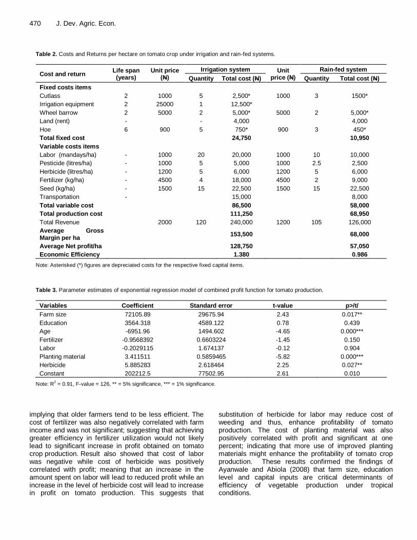
470 J. Dev. Agric. Econ.

Table 2. Costs and Returns per hectare on tomato crop under irrigation and rain-fed systems.

Cost and return Life span (years)

Unit price (N)

Irrigation system Unit price (N)

Rain-fed system

Quantity Total cost (N) Quantity Total cost (N)

Fixed costs items

Cutlass 2 1000 5 2,500* 1000 3 1500*

Irrigation equipment 2 25000 1 12,500*

Wheel barrow 2 5000 2 5,000* 5000 2 5,000*

Land (rent) -

- 4,000

4,000

Hoe 6 900 5 750* 900 3 450*

Total fixed cost

24,750

10,950

Variable costs items

Labor (mandays/ha) - 1000 20 20,000 1000 10 10,000

Pesticide (litres/ha) - 1000 5 5,000 1000 2.5 2,500

Herbicide (litres/ha) - 1200 5 6,000 1200 5 6,000

Fertilizer (kg/ha) - 4500 4 18,000 4500 2 9,000

Seed (kg/ha) - 1500 15 22,500 1500 15 22,500

Transportation -

15,000

8,000

Total variable cost

86,500

58,000

Total production cost

111,250

68,950

Total Revenue

2000 120 240,000 1200 105 126,000

Average Gross Margin per ha

153,500

68,000

Average Net profit/ha

128,750

57,050

Economic Efficiency

1.380

0.986

Note: Asterisked (*) figures are depreciated costs for the respective fixed capital items.

Table 3. Parameter estimates of exponential regression model of combined profit function for tomato production.

Variables Coefficient Standard error t-value p>/t/

Farm size 72105.89 29675.94 2.43 0.017**

Education 3564.318 4589.122 0.78 0.439

Age -6951.96 1494.602 -4.65 0.000***

Fertilizer -0.9568392 0.6603224 -1.45 0.150

Labor -0.2029115 1.674137 -0.12 0.904

Planting material 3.411511 0.5859465 -5.82 0.000***

Herbicide 5.885283 2.618464 2.25 0.027**

Constant 202212.5 77502.95 2.61 0.010

Note: R2 = 0.91, F-value = 126, ** = 5% significance, *** = 1% significance.

implying that older farmers tend to be less efficient. The cost of fertilizer was also negatively correlated with farm income and was not significant; suggesting that achieving greater efficiency in fertilizer utilization would not likely lead to significant increase in profit obtained on tomato crop production. Result also showed that cost of labor was negative while cost of herbicide was positively correlated with profit; meaning that an increase in the amount spent on labor will lead to reduced profit while an increase in the level of herbicide cost will lead to increase in profit on tomato production. This suggests that

substitution of herbicide for labor may reduce cost of weeding and thus, enhance profitability of tomato production. The cost of planting material was also positively correlated with profit and significant at one percent; indicating that more use of improved planting materials might enhance the profitability of tomato crop production. These results confirmed the findings of Ayanwale and Abiola (2008) that farm size, education level and capital inputs are critical determinants of efficiency of vegetable production under tropical conditions.

SUMMARY AND CONCLUSIONS The study aimed at assessing the extent to which investment in small scale irrigation have contributed to profitability of tomato crop farming in the North Central Southern Guinea Savanna agro-ecology of Nigeria. Specifically, the study estimated the relative profitability and efficiency of tomato crop production under irrigation and rain-fed systems, and identified the socio-economic determinants of profitability of tomato crop. Primary data obtained from a sample of 120 farmers were analyzed using descriptive statistics, gross margin, net profit, as well as Shepherd-future and multiple regression models.

Results showed that all the respondents under irrigation system were male farmers, indicating gender inequality in farmers’ access to irrigation facilities. Majority of the farmers were above 50 years of age, with low literacy and average family size of 8 per household. Results also showed that the gross margins per hectare under irrigation and rain-fed systems were N153,500 and N68,000 respectively; and that average net profits per hectare were N128,750 and N57,050; indicating profitability of tomato crop under both systems. Shepherd-future coefficients were 137.98 and 98.62% respectively for irrigation and rain-fed systems; indicating that tomato crop was more economically efficient under irrigation system than rain-fed system. Parameter estimates from the combined profit function also revealed that farm size, level of education, cost of herbicide and planting material have positive correlation; while age of farmers, costs of fertilizer and labor were negatively related to farmers’ profit. Age of farmers and planting materials were significant at one percent, while farm size and costs of herbicide were significant at five percent.

Thus, it was concluded that tomato crop was more profitable and economically efficient under irrigation; and that increased access to land, herbicides, and improved seeds would promote profitability of the crop in Bassa and Makurdi Local Government Areas of Kogi and Benue States, Nigeria. Land policies that increase access of farmers (with special consideration for women farmers) to adequate land, irrigation facilities, herbicides and good quality improved planting material would promote gender equality in irrigation farming and profitability of tomato production; thus contributing to food security in Nigeria and enhancing the income potential of farmers. Conflict of interest The authors have not declared any conflict of interest. REFERENCES

Adewumi MO, Omotesho OA, Tsoho B (2005). Economics of irrigation

farming in Nigeria: a case study of tomato based farming in Sokoto

State, Nigeria. Int. J. Agric. Rural Dev. 6:103-110.

Ayoola 471 Adeolu BA, Taiwo A (2009). Potential and Opportunities for Sustainable

Production and Utilization of Horticultural Crops in Nigeria. Horticultural EOS magazine, September 2009. P. 9.

Ayanwale AB, Abiola MO (2008). Efficiency of Fluted Pumpkin Production under Tropical Conditions. Int. J. Veget. Sci. 13(3):35-49. http://dx.doi.org/10.1300/J512v13n03_04

Chinaka CC, Chikwendu DO, Asumugha GN (1995). A Socio-economic Study of the Adoption and Sustainability of Improved Cassava Varieties Among Resource Poor Farmers in South-East Zone of Nigeria. In Root crops and poverty alleviation. International Society

for Tropical Crops African Branch, Malawi. pp. 333-336. Denton T, Swarup V (1983). Tomato Cultivation and its Potential in

Nigeria. Acta Hort. (ISHS) 123:257-272. http://www.actahort.org/books/123/123_23.htm)

Food and Agriculture Organization (2006). State of Food Insecurity in

the World. Food and Agricultural Organization, FAO. Rome. FAOSTAT (2009). Food and Agriculture Organization, FAO

AQUASTAT: http://www.fao.org/nr/water/aquastat/dbase/index.sfm>

Accessed May 2009. Gani BS, Omonona BT (2009). Resource Use Efficiency Among Small

Scale Irrigated Maize Producers in Northern Taraba State of Nigeria.

J. Hum. Ecol. 28(2):113-119. Giroh DY, Waizah Y, Umar HY (2010). Technical Efficiency and Cost of

Production Among Gum Arabic Farmers in Jigawa State. Report

Opin. 2(1):52-57. Hussain I (2007). Irrigation and Poverty Alleviation: Pro-poor

Intervention Strategies in Irrigated Agriculture in Asia. Paper

presented in the 4th Asian Regional conference and 10

th International

Seminar on Participatory irrigation Management. 2-5 May, 2007, Tehran, Iran. http://fadama.org/taraba.html

Hussain I, Wijerathna D (2004). Irrigation and Income-poverty Alleviation: A comparative analysis of irrigation systems in developing Asia. International Water Management Institute (IWMI) February

2004. International Food Policy research Institute (2006). Agriculture and

Achieving the Millenium Development Goals. Agriculture and Rural development Department. Report No. 32729 GLB. Pp. 10

International Institute of Tropical Agriculture, IITA (2005). Annual Report 2005, IITA, Ibadan, Nigeria. pp. 29-30.

Kalu S (2013). The great tomato waste in Nigeria. http://kalusam.wordpress.com/2013/09/11

Liangzhi Y, Claudia R, Gerald N, Ulrike W-S, Richard R, Stanley W, Zhe

G, Tingju Z, Yau S (2010). What is the Irrigation Potential for Africa? A combined Biophysical and Socio-economic Approach. IFPPRI Discussio Paper 00993. Environment and Production Technology

Division. June 2010. Mofeke ALE, Ahmada A, Mudiane OJ (2003). Relationship Between

Yield and Seasonal Water Use for Tomatoes, Onions, and Potatoes Grown under Fadama Irrigation. Asset Series A. 3:35-46.

Sabo E, Dia YZ (2009). Awareness and Effectiveness of Vegetable Technology Information Packages by Vegetable Farmers in Adamawa State, Nigeria. Afr. J. Agric. Res. 4(2):065-070, February,

2009 Shepherd GS (1962). Marketing Farm Products Economic Analysis. 4

th

Edition. Ames Iowa, Iowa State University Press.

Svendsen E, Sangi M (2009). Measuring Irrigation Performance in Africa: IFFPRI Discussion Paper 894, Washington D.C., IFFPRI

United Nations Development Programme (UNDP) (2002). Human

Development Report 2002. Available at: www.undp.org/hdr2002/ Weinberger K, Lumpkin TA (2007). Diversification into Horticulture and

poverty Reduction: A research agenda. World Dev. 35(8):1464-1480.

http://dx.doi.org/10.1016/j.worlddev.2007.05.002 World Bank (1992). National Fadama Development Project (NFDP),

Staff Appraisal Report (SAR). Washington D.C. World Bank, pp. 55-

72.

Journal of Development

and Agricultural

Economics

Related Journals Published by Academic Journals

Journal of Plant Breeding and Crop Science

African Journal of Agricultural Research

Journal of Horticulture and Forestry

International Journal of Livestock Production

International Journal of Fisheries and Aquaculture

Journal of Cereals and Oilseeds

Journal of Soil Science and Environmental Management

Journal of Stored Products and Postharvest Research